absorption of low-frequency sound energy by vegetation
TRANSCRIPT

Approved for public release; distribution is unlimited.
ERD
C/C
ERL
CR
-06-
1
Absorption of Low-frequency Sound Energy by Vegetation A Laboratory Investigation Ryan Joseph Lee February 2006
Con
stru
ctio
n E
ngin
eeri
ng
Res
earc
h La
bora
tory

ERDC/CERL CR-06-1February 2006
Absorption of Low-frequency Sound Energy by Vegetation A Laboratory Investigation Ryan Joseph Lee Construction Engineering Research Laboratory PO Box 9005 Champaign, IL 61826-9005 through Department of Electrical and Computer Engineering University of Illinois Urbana, IL 61801
Final Report Approved for public release; distribution is unlimited.
Prepared for U.S. Army Corps of Engineers Washington, DC 20314-1000
Under Work Unit #3JD946

ABSTRACT: Many field research projects have been conducted to study the effects of natural foliage on the propagation and attenuation of sound. This research takes natural foliage into a controlled laboratory setting to test its low-frequency acoustic characteristics. Absorption of low-frequency components of unwanted noise is of interest to the Army, but has been an unsolved problem due in part to the cumbersome and expensive testing facilities needed to study long wavelengths.
In this research, low-frequency absorption and reflection coefficients were found reliably and consistently. Due to study of the steady state conditions, the methods presented here could constitute a more consistent method than ever before. The procedures described in this paper can serve as a handbook for future research; recommendations are included.
DISCLAIMER: The contents of this report are not to be used for advertising, publication, or promotional purposes. Citation of trade names does not constitute an official endorsement or approval of the use of such commercial products. All product names and trademarks cited are the property of their respective owners. The findings of this report are not to be construed as an official Department of the Army position unless so designated by other authorized documents.
DESTROY THIS REPORT WHEN IT IS NO LONGER NEEDED. DO NOT RETURN IT TO THE ORIGINATOR.

ERDC/CERL CR-06-1 iii
Contents
List of Figures and Tables ............................................................................................................... v
Preface.............................................................................................................................................. vii
Acknowledgements....................................................................................................................... viii
List of Symbols ................................................................................................................................ xi
1 Introduction ................................................................................................................................ 1
2 Testing Facility and Operation................................................................................................. 3
2.1 Impedance Chamber ................................................................................................... 3 2.2 Yokogawa ScopeCorder .............................................................................................. 5 2.3 Theoretical Operational Rationale. .............................................................................. 6
3 (Quality Factor)..................................................................................................................... 9 Q
3.1 Methods of Computing Q ........................................................................................... 9
3.1.1 Method 1: the 3 dB-down method ............................................................................ 9 3.1.2 Method 2: the energy method................................................................................. 10 3.1.3 Method 3: the logarithmic decrement method ........................................................ 11 3.2 Choosing a Method.................................................................................................... 13
3.3 and Q α , Absorption Coefficient ............................................................................ .16
3.4 Laboratory Techniques .............................................................................................. 16
4 Quality Factor Results.............................................................................................................19
4.1 Empty Chamber......................................................................................................... 19 4.2 Vegetation in Chamber .............................................................................................. 20 4.2.1 Apple tree branches................................................................................................ 21 4.2.2 Bales of straw ......................................................................................................... 21 4.2.3 Northern white pine tree ......................................................................................... 23 4.3 Testing Limestone Crushed Rock.............................................................................. 26
5 Load Impedance and Reflection Coefficient........................................................................31

ERDC/CERL CR-06-1 iv
6 Standing Wave Results ...........................................................................................................38
6.1 Vegetation Tests......................................................................................................... 38 6.2 Gamma Results. ........................................................................................................ 40
7 Chamber Handbook ................................................................................................................42
7.1 White Noise Q .......................................................................................................... 42
7.2 Computation and Standing Wave Fitter................................................................ 47 Γ
8 Conclusion................................................................................................................................55
Appendix A: Theoretical Standing Wave Viewer........................................................................57
Appendix B: Code to Find of the Chamber ...........................................................................59 Q
Appendix C: Code to Find Best Fit Standing Wave ...................................................................65
References.......................................................................................................................................69
Report Documentation Page.........................................................................................................71

ERDC/CERL CR-06-1 v
List of Figures and Tables
Figures
2.1 Reinforced concrete impedance chamber with steel door. ............................................... 3
2.2 Loudspeaker installed in the center of the back of the chamber...................................... .4
2.3 The microphone port on the left has a cable running out of it, whereas the other microphone ports are plugged. ................................................................................... 5
2.4 A single frame of the output of RUNCHAMBER................................................................ 8
3.1 A parallel resonant circuit ................................................................................................. .9
3.2 The bandwidth of a parallel RLC circuit whose resonant frequency is 20 Hz and where Q = 1 ............................................................................................................. 10
3.3 This theoretical device has a steady response to a 20 Hz pure tone signal until the input is completely cut off at time t = 0 s.. ................................................................. 12
3.4 The power spectrum of the input white noise is flat in the frequency range of interest, i.e., 15-100 Hz. ............................................................................................ 15
3.5 The magnitude of the DFT of a microphone in the chamber when white noise is the chamber’s input................................................................................................... 15
3.6 Standing current and pressure waves shown on a hypothetical transmission line with characteristic impedance Z0(a). The placement of even an infinitely large impedance at a current null does not affect the standing waves (b)......................... 17
3.7 Standing pressure waves in an empty chamber for the first four modes........................ 18
4.1 The transmission line equivalent of the empty chamber (a) and the chamber with some vegetation placed at some location along its axis (b)...................................... 19
4.2 The microphones in the chamber measure pressure (Vmic in our analogy) at different locations.. .................................................................................................... 20
4.3 For each resonant mode, the of the chamber decreases with increasing vegetation amounts placed inside............................................................................. 22
Q
4.4 Two branches (a) cut from another tree were used for extra vegetation mass and the top 130 lb. of the tree (b) at the chamber door.................................................... 24
4.5 Indeed, the is a function of the mass of the vegetation in the chamber.. .................. 25 Q
4.6 A 2 m x 2 m two-level box. ............................................................................................. .26
4.7 The lower level of the box placed at the door side of the chamber................................ .27
4.8 The full box placed at the door side of the chamber. ...................................................... 27
4.9 The lower half of the box filled with gravel. ..................................................................... 29
4.10 The full box, fully loaded. .............................................................................................. 29

ERDC/CERL CR-06-1 vi
4.11 Eight bales of straw on top of the full box filled with limestone. ................................... .29
4.12 The empty chamber compared to the five other tests with varying amounts of rock and the box........................................................................................................ 30
5.1 The terminating load impedance is most likely complex................................................ .31
6.1 The chamber terminated with (a) 10-bale straw wall and (b) pine tree branches hung on the inside of the chamber door.................................................................... 38
6.2 Best fit standing wave patterns for a pure tone input at 70 Hz in a chamber terminated with different amounts of vegetation... .................................................... 39
6.3 rΓ as a function of frequency for three chamber terminations: empty, pine tree
sections, and bales of straw. ..................................................................................... 41
7.1 Ten bales of straw placed to terminate the empty chamber............................................ 47
7.2 The code outputs the best fit standing pressure wave as well as the data given at the top of the graphic: tone frequency, reflection coefficient, standing wave ratio (SWR), and load impedance............................................................................. 48
Tables
2.1 The acoustic/electric/mechanical analogy ........................................................................ 7
4.1 Empty chamber .......................................................................................................... 20 Q
4.2 Chamber values with varying amounts of straw bales .............................................. 23 Q
4.3 Chamber values with varying amounts of pine tree................................................... 26 Q
4.4 Limestone properties....................................................................................................... 28
4.5 Limestone gradation........................................................................................................ 28
4.6 Chamber values from rock experiments .................................................................... 30 Q
6.1 Reflection coefficients ..................................................................................................... 39
ERDC/CERL CR-06-1 vii
Preface
The work was monitored by the Ecological Processes Branch (CN-N) of the Installa-tions Division (CN), Construction Engineering Research Laboratory (CERL). The CERL Principal Investigator overseeing the work was Michael White. This work was done by Ryan J. Lee. Alan B. Anderson is Branch Chief, CN-N, and John T. Bandy is Chief, CN. The associated Technical Director was William D. Severing-haus. The Acting Director of CERL is Dr. Ilker R. Adiguzel.
CERL is an element of the U.S. Army Engineer Research and Development Center (ERDC), U.S. Army Corps of Engineers. The Commander and Executive Director of ERDC is COL James R. Rowan, and the Director of ERDC is Dr. James R. Houston.

viii
ACKNOWLEDGMENTS
This work would not have been possible without the support, guidance, and faith
of Dr. George W. Swenson, Jr., and the acoustics team at the U.S. Army CERL.
Specifically, Dr. Swenson assisted in my coursework, believed in my adaptability as a
civil engineer transitioning into an electrical engineering curriculum, and came up with
the idea for many experiments. His extensive knowledge is unsurpassed in our field and
has challenged me to dig as deeply as possible.
Of the CERL acoustics team, Dr. Larry Pater provided funding as well as a wide
variety of projects to give my research breadth. Dr. Michael White and Dr. Michelle
Swearingen offered countless suggestions and brainstorming to help me achieve a more
extensive level of understanding in acoustics. Jeff Mifflin assisted in technical expertise,
equipment procurement, operations, and helped bridge the gap between theory and
empirical results. Dr. Steven J. Franke offered his time, patience, and possible solutions
at an important time in completing the thesis. My most sincere gratitude goes out to
these friends and colleagues without whom this work would not have been executed.

ix
LIST OF SYMBOLS
A amplitude
α absorption coefficient
β cω
c speed of sound
C capacitance
f frequency
γ specific weight
Γ reflection coefficient
γ attenuation constant
k specific heat ratio
I current
l length
L inductance
ω radian frequency
,p P instantaneous sound pressure
P+ positive-traveling pressure wave
P− negative-traveling pressure wave
q charge
Q quality factor
R gas constant
ρ instantaneous density
0ρ static density
S cross-sectional area
T temperature
t time
θ phase angle
U volume velocity
V voltage
Z impedance
1
1 INTRODUCTION
A multitude of research projects have been conducted to study the effects of
natural foliage on the propagation and attenuation of sound. Scores of species have
been tested and compared.1 Other variables such as wind, temperature, humidity, and
elevation have, for the most part, been out of the control of the researcher. This paper
takes natural foliage into a controlled laboratory setting to test its low-frequency acoustic
characteristics.
Three mechanisms that have commonly been studied and quantified are ground
reflection, scattering, and absorption of sound. Absorption of low-frequency components
of unwanted noise is of interest to the U.S. Army Corps of Engineers, but is an unsolved
problem due to the cumbersome and expensive testing facilities needed for long
wavelengths and parameters that are out of the control of the researcher.
Until now, low frequencies of sound ( 20 80− Hz) have not been studied in
controlled laboratory conditions with testing apparatuses the size of a half wavelength or
more. Until Burns2 brought pine tree components into the laboratory, experiments were
done in the field under nonideal conditions. However, his testing apparatus was a box
much smaller than the half-wavelengths of low frequency sound. Also, of the papers I
researched, only a few address low frequencies. Still, even those papers take into
account only 1 3 -octave bands as low as band number 18 (centered at 63 Hz) while the
focus of study tends to be on much higher bands.
The proceeding research describes the main testing apparatus, a concrete
waveguide herein called “the chamber,” in Chapter 2. MATLAB code written for using
the chamber serves as an operator’s manual for future researchers. All of the code is
included and well documented in Chapter 7.

2
This thesis takes an electrical approach; a pressure-voltage analogy is used to
compare the acoustic setting with an electrical one. The waveguide is analogous to an
electromagnetic cavity resonator (or electrical transmission line in one dimension), and
analogous parameters are laid out in a table in order to make solutions of the wave
equation in either analogy straightforward.
The quality factor Q of the chamber is studied extensively in Chapter 3. Varying
amounts of vegetation are placed inside the chamber to affect the Q . One goal of such
tests is to find a relationship between Q and the absorption coefficient α of vegetative
material. This relationship is still under investigation and could be a subject of future
research.
Results for experiments with bales of straw and a full White Pine tree are
included in Chapter 4. Gravel, at one time outside of the scope of this paper, is tested in
order to compare foliage results with a nonvegetative absorber.
In Chapter 5, the electrical analogy is used to find the impedance and reflection
characteristics of anything placed in the chamber. Once again, straw bales and tree
branches are used as test foliage. MATLAB code is supplied in an appendix and can be
used by future researchers.
Chapter 6 shows results of how a standing wave inside our testing chamber is
affected by adding increasing amounts of vegetation to dampen the system.
The chamber handbook is presented in Chapter 7. MATLAB code along with
extensive commenting is included so that future researchers can copy and comprehend
the routines used herein.
Finally, conclusions are given and a discussion of the limitations of the results
obtained is presented. This work does make use of other researchers’ testing methods,
however it does not attempt recreate their work.
3
2 TESTING FACILITY AND OPERATION
The testing facility is the main component that makes this research original and
unique. The concrete chamber described in Section 2.1 could not be recreated without
a sizeable budget, an abundance of space, and long-term planning. MATLAB code was
written to work with and process the signals taken on the recording device. This
recorder is described in detail in Section 2.2. Section 2.3 describes the approach taken
in reconciling transmission theory and operating the facilities.
2.1 Impedance Chamber
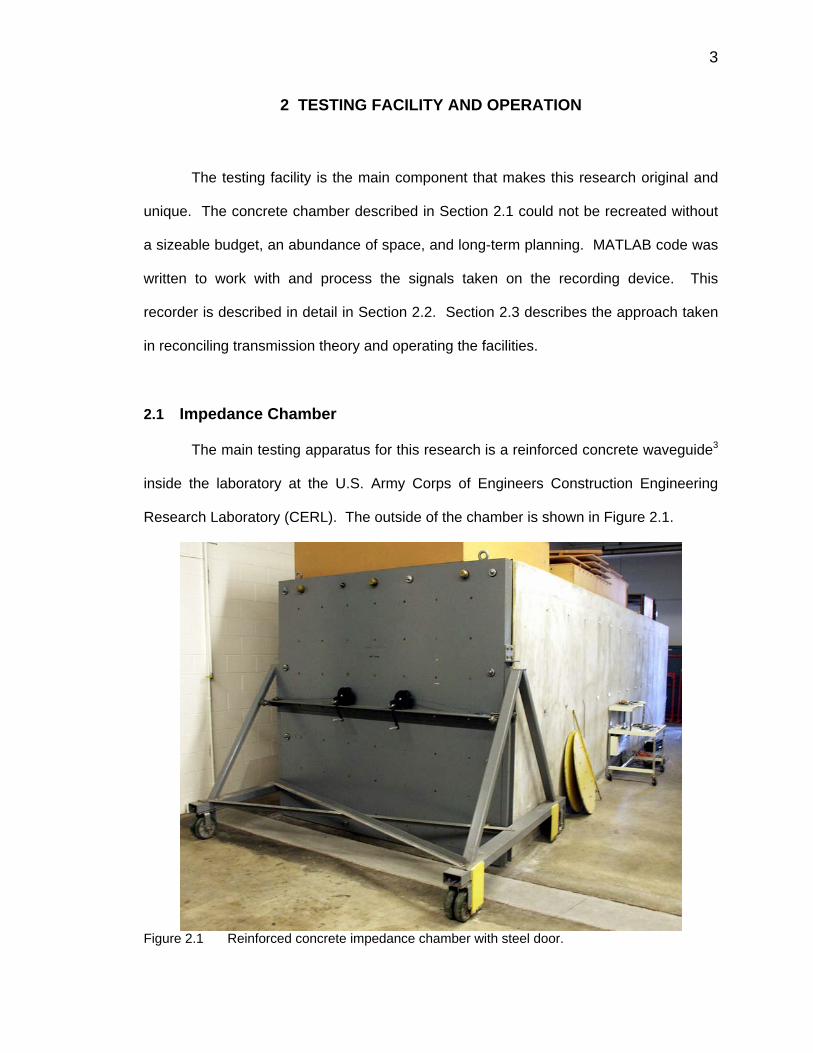
The main testing apparatus for this research is a reinforced concrete waveguide3
inside the laboratory at the U.S. Army Corps of Engineers Construction Engineering
Research Laboratory (CERL). The outside of the chamber is shown in Figure 2.1.
Figure 2.1 Reinforced concrete impedance chamber with steel door.

4
The chamber’s design is such that its 2 m × 2 m cross-sectional dimensions are
much smaller than its length of m. Thus, the first four modes of oscillation of an
acoustic field inside the chamber are the modes (1, ), ( ), ( ), and ( )
corresponding to roughly , , , and 80 Hz, respectively. The current research
deals with one-dimensional uniform time-harmonic plane waves.
8.8
0,0 2,0,0 3,0,0 4,0,0
20 40 60
Minimal displacement occurs in the reinforced concrete walls during internal
acoustic reflection so coefficients of internal reflection Γ (the overbar denotes that Γ is
complex) approach an ideal value of 1.0 with no phase shift. A door closes at the front
of the chamber, allowing items to be placed inside for experiments. A loudspeaker
shown in Figure 2.2 is sealed in a small cutout in the center of the wall opposing the
door, herein called the back of the chamber. This loudspeaker is the noise source for
normal-incidence plane waves and can input a pulse, white noise, pink noise, a pure
tone, or any other signal into the chamber.
Figure 2.2 Loudspeaker installed in the center of the back of the chamber.

5
Microphone ports shown in Figure 2.3 are cut out of the chamber wall at different
heights and locations along its length. This research makes use of the ports that are 1
m above the chamber floor (halfway up the 2 m wall). When a steady state pure tone is
input to the chamber, these microphones record the pressure fluctuations of a standing
pressure wave.
Figure 2.3 The microphone port on the left has a cable running out of it, whereas the other
microphone ports are plugged. 2.2 Yokogawa ScopeCorder
Although almost any data recorder could be used in these experiments, the
Yokogawa ScopeCorder DL750, which is available at the testing facility, is important for
four main reasons. First, the DL750 can record at sampling rates up to
samples per second. Although such high sampling rates and frequencies are not
necessarily needed for the low-frequency scope of this paper, they are beneficial for
testing code over a large range of conditions. Using such a versatile machine allows
future researchers to make use of the code contained in this paper even if their research
is targeted at higher frequency bands.
62 10×

6
Second, 16 channels are available at one time, making time sync between all
microphones in the chamber simple and reliable. Third, the ScopeCorder is flexible in its
methods of downloading data digitally for use and processing by computer programs.
Specifically, the ScopeCorder has an internal hard drive, an IBM microdrive that holds a
1 GB PC card, and an Ethernet port for input and output of data via a category-5 cable.
Fourth, this data-recording device has a large full-color LCD screen on which to view the
channels’ inputs before, during, and after the data are taken. This is incredibly useful to
pinpoint a bad microphone, preamp, power supply, or channel setting thus saving time
when debugging faulty systems.
2.3 Theoretical Operational Rationale
Taking an electrical approach to an acoustical problem simply means using
electromagnetic theory and parameters in the following wave equation,4, 5, 6, 7 shown here
for acoustic plane waves propagating in the z -direction where is pressure, is the
speed of the wave, and is time:
p c
t
2 2
2 2 2
1p pz c t
∂ ∂=
∂ ∂ (2.1)
Table 2.1 shows the parameters of the “pressure-voltage” analogy and their units
used throughout the rest of this paper. There are other valid analogies such as the
“pressure-current” analogy that will not be covered here.
In order to understand plane wave propagation in the empty chamber, MATLAB
code based on transmission line theory was written and is included in Appendix A. The
MATLAB function RUNCHAMBER.m allows the user to input a frequency of pure tone at
which they would like to excite the chamber, initially at rest. It makes use of concepts
such as impedance, reflection, Ohm’s law, and superposition all while outputting three

7
graphs: a positive-going digital pressure wave, a negative-going digital pressure wave,
and a superimposed total digital pressure wave.
Table 2.1 The acoustic/electric/mechanical analogy Acoustic Electrical Mechanical
Parameter Units Paramter Units Parameter Units Compliance 3m m
Pa N=
5
Capacitance 2q
N m⋅
Compliance (stiffness -1)
2skg
Pressure NPam
= Voltage N mV
q⋅
= Force
2
kg mNs⋅
=
Volume Velocity
3ms
Current qA
s=
Particle Velocity
ms
Volume Displacement
3m Charge q Distance m
Inertance5 or Acoustic Mass4
2
5 4
N s kgm m⋅
= Inductance V s
A⋅
Mass kg
Impedance 3
Pa sm⋅
Impedance Ω Mechanical Impedance m
s
N
Resistance 3
Pa sm⋅
Resistance Ω Viscous Friction m
s
N
Figure 2.4 shows a single frame of the moving picture output of RUNCHAMBER
after the loudspeaker has been turned on at a constant pure tone of Hz for s
(these numbers were chosen arbitrarily). The top graph is the positive-going wave
moving to the right, the middle graph is the negative-going wave
21.5 0.5
pP
nP moving to the left,
and the bottom graph is the total pressure in the chamber. A distinct jump in
pressure in can be seen at a distance of 2 m down the chamber axis due to the onset
of a reflected wave with the source-produced . This jump travels back and forth with
the traveling waves.
totP
nP
pP
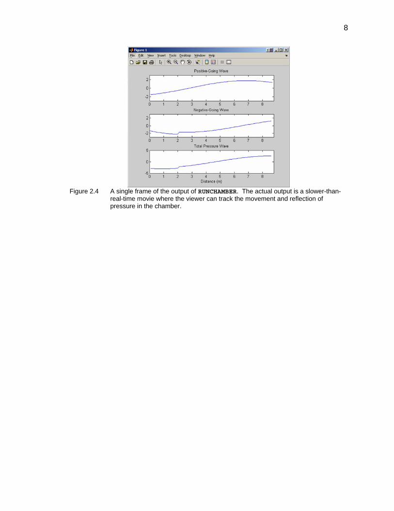
8
Figure 2.4 A single frame of the output of RUNCHAMBER. The actual output is a slower-than-
real-time movie where the viewer can track the movement and reflection of pressure in the chamber.

9
3 (QUALITY FACTOR) Q
3.1 Methods of Computing Q
In this section, we investigate several methods of computing the Q of the
chamber. Historically, Q designated the ratio of reactance to resistance of a series
circuit element.8 It applies to mechanical, electrical, and acoustic systems. The letter
“Q” was arbitrarily chosen and eventually took on the name “quality factor.”
3.1.1 Method 1: the 3 dB-down method
The definition of Q that describes a system’s frequency selectivity is
1 2Bandwidth
r rf fQf f
= =−
(3.1)
where is the resonant frequency of the system and and are the points
(determined by half power) on each side of . Maximum power delivered by a source
to a system occurs at .
rf 1f 2f 3 dB−
rf
rf
For example, the magnitude of impedance Z of the resonant circuit shown in
Figure 3.1 is shown in Figure 3.2 as a function of frequency. At low frequencies, voltage
across the resistor goes to zero because an inductor is a short at DC.
Figure 3.1 A parallel resonant circuit.9

10
At high frequencies, voltage also goes to zero because a capacitor is a short as
. Maximum power is transferred (dissipated) to the resistor when the inductor
and capacitor resonate each other at . Bandwidth, determined by the frequencies
where half peak power is delivered to the resistor, is determined by points where
f →∞
rf
Z is
1 2 times the peak value of Z on the frequency versus impedance curve shown in
Figure 3.2.
Figure 3.2 shows an example of a graphical representation of finding the Q from
the bandwidth of a system.
Figure 3.2 The bandwidth of a parallel RLC circuit whose resonant frequency is Hz and
where . 20
1Q = Section 3.2 explains in detail how the of an acoustic system can be found using
pressure and volume velocity (to obtain impedance as a function of frequency) just as
easily as the Q of an electrical circuit can be found using voltage and current (to obtain
impedance as a function of frequency).
Q
3.1.2 Method 2: the energy method
Another way Q can be defined for drivers, driver/box combinations,
electromagnetic resonators, acoustic cavities, and other analogous systems is

11
(energy stored at resonance)2(energy dissipated at resonance)
Q π= × , (3.2)10, 11
( )
( )overall reactive energy in the enclosure
dissipated powerQ ω= , (3.3)
time average of the energy stored in the system2
rate of energy dissipationQ fπ= , (3.4)11
( )
( )oscillating energy
2energy loss per cycle of oscillation
Q π= , (3.5)
peak value of energy stored in 1 cycle
dissipated powerQ ω= . (3.6)12
These definitions are mathematically equal and directly related to the other two methods
presented here.
3.1.3 Method 3: the logarithmic decrement method
A third way can be defined is via the logarithmic decrement method. The
decrement
Q
δ is defined as the ratio of the amplitude of any damped oscillating peak to
the amplitude of the next one.13 The logarithmic decrement Λ then is defined as
( )ln δΛ = (3.7)
and
Q π=Λ
. (3.8)
When the input of a steady state system (such as the one shown in Figure 3.1) is
shut off, its response decays logarithmically corresponding to te γ− , where γ is an
attenuation constant and is time. An example of this is shown in Figure 3.3. t
The relationship between Q and γ can be found from the following procedure.
Let A0 and A1 be the amplitudes of successive larger and smaller oscillations,
respectively. The decrement is defined as

12
Figure 3.3 This theoretical device has a steady response to a Hz pure tone signal until the
input is completely cut off at time 20
0t = s. The device’s energy decays logarithmically.
0
1
AA
δ = . (3.9)
Let the period of the system be T ,
1Tf
= (3.10)
where f is the frequency of the oscillation. The logarithmically decaying envelope
defines the amplitudes of oscillations as follows5
0tA A e γ−= (3.11)
where A is the amplitude of the decaying sinusoid at some time t . For two successive
oscillations, occurring one period T apart, Equation (3.11) can be rewritten as
0
1
T AeA
γ = .
Substituting Equation (3.9),
Teγ δ= ,
feγ
δ= . (3.12)
Plugging Equation (3.12) into Equation (3.7), we get

13
ln feγ⎛ ⎞Λ = ⎜
⎝ ⎠⎟ ,
fγ
Λ = . (3.13)
Finally, plugging Equation (3.13) into Equation (3.8), we get
fQ πγ
= . (3.14)
Mathematically, one implication of this result is that the Q equals the number of cycles
undergone until the amplitude reaches e π− (~ ) of the initial value. 0.04
Another equivalent perspective is to measure the amplitude of two consecutive
cycles of the decay. The second cycle’s amplitude will have a value that is Qe π− times
the amplitude of the previous cycle. If the of the chamber is high, however, this
method is difficult with empirical data because the ratio of amplitudes of successive
cycles of the decay will be extremely close to 1.
Q
In such instances, it is best to count multiple oscillations of the system. If the
decay of amplitude in one cycle of oscillation were too small to measure, one could
measure the decay of some number cycles of decay. In this case, the cycle’s
amplitude will have a value that is
N thN
N Qe π− times the amplitude of the original cycle.
3.2 Choosing a Method
The first attempt to measure Q consisted of sending a sweepable pure tone into
the empty chamber. A microphone was placed inside the chamber, and its output was
displayed on the screen of an oscilloscope. This test did not work well because a high
implies a very narrow bandwidth (see Figure 3.2). The analog signal generator was
not precise enough to dial in changes of frequency
Q
f∆ small enough to find such a

14
bandwidth. The values of the three frequencies needed for Equation (3.1), namely, rf ,
, and 1f 2f , were determined by counting divisions on the screen of the oscilloscope.
Although this constitutes a crude method, for mode (1,0,0) was found to be (a
value very close to later, more precise tests).
Q 73
After this initial testing, data was no longer analyzed in real time. Rather, it was
recorded and processed in MATLAB using signal processing routines to precisely
analyze the signals.
The second experiment to measure Q attempted to make good use of the
aforementioned logarithmic decrement method. Once again, a signal generator with a
pure tone at a user-defined frequency was connected to the chamber’s loudspeaker. A
microphone was placed inside the chamber and this time its output was recorded on a
Sony TCD-D8 DAT recorder. The pure tone was played long enough for a steady state
standing pressure wave to be set up inside the chamber. The input to the chamber was
then abruptly cut off, and the decay of the standing pressure wave was recorded and
analyzed. Q for mode (1,0,0) was 85 .
The third type of test came about in order to measure more than one frequency at
a time. For this third group of tests, an impulse (or spark) was put into the chamber. An
impulse has equal energy across all frequencies. The decay of the pressure wave due
to the impulse was too difficult and erratic to analyze with logarithmically decaying
envelopes.
The fourth and final way to analyze the chamber was to use white noise as the
input source, once again at steady state. White noise is made up of impulses with
random amplitude in succession, so it too has equal energy across all frequencies.
Since we are only interested in the first four resonant modes of the chamber

15
(frequencies below 10 Hz), the white noise was lowpass filtered with a cutoff of 11
Hz. Figure 3.4 shows the power spectrum of the filtered white noise.
0 0
Figure 3.4 The power spectrum of the input white noise is flat in the frequency range of
interest, i.e., 15-100 Hz. Microphones along the chamber wall sent pressure signals due to the white noise
inside the chamber to the aforementioned ScopeCorder. Data were sampled at 500 Hz,
well above Nyquist frequency for signals in the range of 15-100 Hz. The discrete Fourier
transforms (DFTs) of the signals were analyzed. Figure 3.5 shows the result from a
single microphone after smoothing algorithms detailed in Appendix B.
Figure 3.5 The magnitude of the DFT of a microphone in the chamber when white noise is the
chamber’s input. The 3 d down method was used on the peaks in Figure 3.5 to obtain the Q at
each resonance. As long as there are enough points in the DFT shown in Figure 3.5,
B−

16
the bandwidth of system resonant peaks can easily be found. With enough points so
that the frequency resolution 180f∆ = Hz, this proved to be a reliable and useful
method of analysis and is the method used throughout the rest of this paper.
3.3 and Q α , Absorption Coefficient
The absorption coefficient α , defined14 as the ratio of the energy absorbed by a
surface to the energy incident upon a surface, of an absorbing material placed against
the door so as to terminate the chamber is a dimensionless constant related to Q .
Beranek14 equates α to a measure of the absorbing power of unit area.
In the past, measurement of α has been a detailed process often performed by
laboratories created specifically for such experimental determination. The method most
often used consisted of measuring reverberation times in a reverberation chamber. The
research in this thesis improves upon their limitations because it deals with steady state
signals, thus minimizing error. The particular relationship between α and is currently
under investigation and may be a topic of future research.
Q
3.4 Laboratory Techniques
Vegetation placed inside will lower the from that of an empty chamber,
however the change is dependent upon the location of the vegetation. This problem can
best be studied via the electric analogy.
Q
In transmission line theory dealing with lossless lines varying sinusoidally at
steady state, the location of maximum voltage occurs at a location of minimum current
(and vice versa).11 A transmission line terminated by an open circuit at one end and a
short circuit at the other end is shown in Figure 3.6 to illustrate one mode of standing

17
waves and depict boundary conditions that go along with such line terminations. Using
Ohm’s law ( V IZ = ), an added impedance (no matter how large) placed at a location
where current is zero does not affect the standing wave pattern. One could open circuit
the line at current nulls and short the line at voltage nulls without changing these natural
oscillations.11
Figure 3.6 Standing current and pressure waves shown on a hypothetical transmission line
with characteristic impedance 0Z (a). The placement of even an infinitely large
impedance at a current null does not affect the standing waves (b).
In the acoustic analogy, maximum volume velocity in a transmission medium
occurs where the pressure is minimum. An impedance of any magnitude (but
infinitesimal thickness) added where the volume velocity is zero (maximum pressure) will
not affect the acoustic standing waves. Therefore, to study the effect of added
impedance on the standing wave patterns, it is necessary to add such impedances (i.e.,
vegetation mass) where the pressure wave has a null. Due to pressure doubling, the
standing pressure waves of the empty chamber at any frequency will have a maximum
at the chamber door. The shapes of the first four fundamental modes of the empty
chamber are shown in Figure 3.7.
To best study the effect of vegetation on the for mode (1,0,0), the brush would
be placed at location
Q
2l , where is the length of the chamber. In the same way, brush l

18
would be placed at 4l , 2l , and 8l (or any other nulls in the pressure waves shown in
Figure 3.7), for modes (2,0,0), (3,0,0), and (4,0,0) respectively.
Figure 3.7 Standing pressure waves in an empty chamber for the first four modes. The hard
chamber ends are almost perfectly reflecting and can be modeled as an open circuit.
19
4 QUALITY FACTOR RESULTS
4.1 Empty Chamber
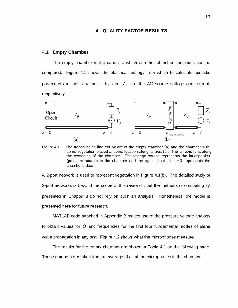
The empty chamber is the canon to which all other chamber conditions can be
compared. Figure 4.1 shows the electrical analogy from which to calculate acoustic
parameters in two situations. sV and sZ are the AC source voltage and current,
respectively.
Figure 4.1 The transmission line equivalent of the empty chamber (a) and the chamber with
some vegetation placed at some location along its axis (b). The -axis runs along the centerline of the chamber. The voltage source represents the loudspeaker (pressure source) in the chamber and the open circuit at represents the chamber’s door.
z
0z =
A 2-port network is used to represent vegetation in Figure 4.1(b). The detailed study of
2-port networks is beyond the scope of this research, but the methods of computing Q
presented in Chapter 3 do not rely on such an analysis. Nonetheless, the model is
presented here for future research.
MATLAB code attached in Appendix B makes use of the pressure-voltage analogy
to obtain values for and frequencies for the first four fundamental modes of plane
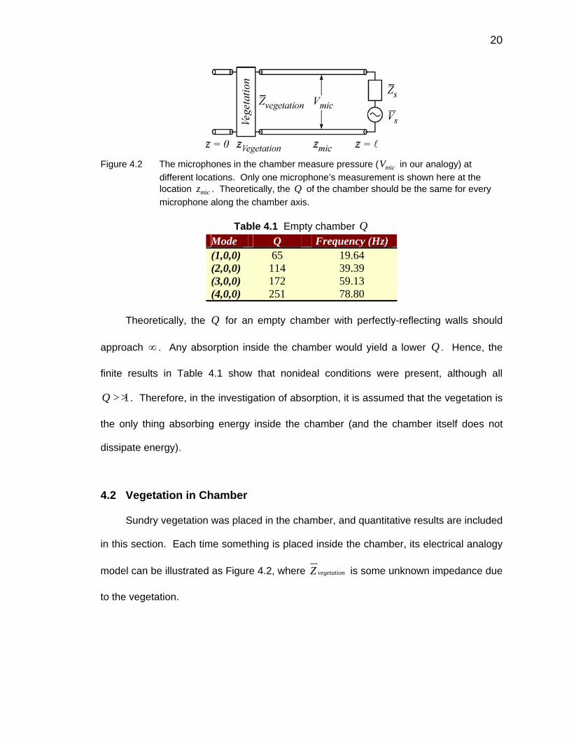
wave propagation in any test. Figure 4.2 shows what the microphones measure.
Q
The results for the empty chamber are shown in Table 4.1 on the following page.
These numbers are taken from an average of all of the microphones in the chamber.
20
Figure 4.2 The microphones in the chamber measure pressure ( in our analogy) at
different locations. Only one microphone’s measurement is shown here at the location . Theoretically, the of the chamber should be the same for every microphone along the chamber axis.
micV
micz Q
Table 4.1 Empty chamber Q
Mode Q Frequency (Hz) (1,0,0) 65 19.64 (2,0,0) 114 39.39 (3,0,0) 172 59.13 (4,0,0) 251 78.80
Theoretically, the Q for an empty chamber with perfectly-reflecting walls should
approach . Any absorption inside the chamber would yield a lower Q . Hence, the
finite results in Table 4.1 show that nonideal conditions were present, although all
. Therefore, in the investigation of absorption, it is assumed that the vegetation is
the only thing absorbing energy inside the chamber (and the chamber itself does not
dissipate energy).
∞
1Q >>
4.2 Vegetation in Chamber
Sundry vegetation was placed in the chamber, and quantitative results are included
in this section. Each time something is placed inside the chamber, its electrical analogy
model can be illustrated as Figure 4.2, where vegetationZ is some unknown impedance due
to the vegetation.

21
4.2.1 Apple tree branches
A -kg dry leafless branch of an apple tree was placed in the center of the
chamber in an attempt to affect the Q of the chamber. The branches had no effect
(probably due to the low mass and lack of leaves) and the results will not be included
here.
29
4.2.2 Bales of straw
Dense brush more robust than the apple tree branches was needed to affect the
, so bales of straw were used. Each bale of straw had a mass of 39 kg and
measured
Q .7
0.375 m tall 0.5 m wide× 1 m long× . Twenty bales were procured in order
to create vegetation walls of different sizes in various locations along the chamber’s axis.
The resultant for each resonant mode is a function of two variables, namely the
location and the amount of added vegetation. For this reason, tests with equally sized
straw-bale walls were repeated with the wall in different locations along the chamber
axis.
Q
Each bale was situated so that the 0.5 width was aligned with the -axis; thus
the area facing the loudspeaker was . The results for straw-
bale tests are shown in Figure 4.3.
m z
2 0.375 m 1 m = 0.375 m×
As predicted by the transmission line analogy, vegetation placed at 2l affects the
for resonant modes (1, ) and ( ) more than at any other location (see Figure
4.2(a) and (c)). Likewise, the mode ( 2, ) is affected most substantially by
vegetation placed at
Q 0,0 3,0,0
0,0 Q
4l (Figure 4.1(b)). Figure 4.2(d) equally supports that mode
( ) is most substantially affected by vegetation placed at 4,0,0 Q 8l , a standing wave
pressure minimum for that mode.
22
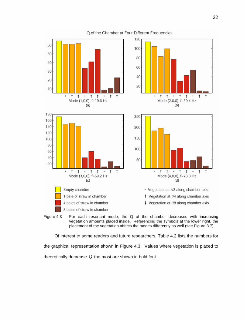
Figure 4.3 For each resonant mode, the Q of the chamber decreases with increasing
vegetation amounts placed inside. Referencing the symbols at the lower right, the placement of the vegetation affects the modes differently as well (see Figure 3.7).
Of interest to some readers and future researchers, Table 4.2 lists the numbers for
the graphical representation shown in Figure 4.3. Values where vegetation is placed to
theoretically decrease Q the most are shown in bold font.

23
Table 4.2 Chamber values with varying amounts of straw bales QVegetation Location Vegetation
Amount l/2 l/4 l/8 Mode (1,0,0), f ≈19.6 Hz
None 64.90 64.90 64.90 1 bale 61.09 61.09 62.09 4 bales 33.35 41.00 55.16 8 bales 8.60 10.45 22.78
Mode (2,0,0), f ≈39.4 Hz None 114.37 114.37 114.37 1 bale 104.52 82.95 99.54 4 bales 76.69 30.43 42.55 8 bales 53.84 10.03 8.40
Mode (3,0,0), f ≈59.2 Hz None 172.15 172.15 172.15 1 bale 148.03 151.31 141.81 4 bales 39.65 59.83 35.65 8 bales 10.24 27.12 11.64
Mode (4,0,0), f ≈78.8 Hz None 251.49 251.49 251.49 1 bale 183.88 195.99 167.50 4 bales 94.62 103.55 41.72 8 bales 46.99 64.05 21.49
4.2.3 Northern white pine tree
A freshly-cut Pinus strobes (White Pine) was brought into the laboratory for
testing. The specimen came from the west side of a 15 -m thick stand of White Pine at
the Vermillion River Observatory in Danville, IL. It was tested in the chamber within two
days of being cut.
The -m tall tree was cut down and driven to CERL on the back of a trailer in
two smaller sections totaling less than 9. m. The longest section consisted of the top 6
m and 13 lb of the tree. It was bushy with branches full of needles. For this top piece,
the trunk measured 5.7 in in diameter at the bottom cut and tapered to a single bunch
9.2
2
0
5

24
of needles at the top. The east-facing side of the tree had significantly fewer branches
and needles because it faced the inside of the stand of trees and received less sunlight
than the west-facing side.
The second section consisted of the next 1 m; the 11 lb section of trunk had a
medium amount of branches with needles. The branches on the east side were barren
and void of needles. The trunk measured 7 in at the bottom cut.
.5 5
Two bushy branches were cut from the base of a larger White Pine and piled on
the trailer. The branches, shown in Figure 4.4 (a), weighed 89 lb and 70 lb,
respectively. They were added simply for additional vegetation mass in the chamber. In
addition to the aforementioned 13 lb and 11 lb pieces of the tree, 10 lb of branches
that had broken off during tree removal were gathered from the tree and piled on the
trailer.
0 5 0
(a) (b)
Figure 4.4 Two branches (a) cut from another tree were used for extra vegetation mass and the top 130 lb of the tree (b) at the chamber door.
Thus, the total mass from the main tree was (13 lb 0 + lb 100 lb) lb,
with an additional ( lb lb) 15 lb of the two branches from another tree. The
lowest 1.5 m of the main tree had few branches and needles and was left in the forest.
115 + 345
89 + 70 9

25
The main 13 lb section of the tree was loaded into the chamber first, propped
on two sawhorses, and is shown in Figure 4.4 (b) on the previous page. The 115 lb
section of the trunk was placed in the rear of the chamber (near the speaker).
0
Unlike the bales of straw in Section 4.2.2, it was impossible to place the tree in
discreet locations of standing wave pressure minima. Results for four different amounts
of tree are shown in Figure 4.5.
Figure 4.5 Indeed, the is a function of the mass of the vegetation in the chamber. Q For each of the first four modes, the higher amounts of tree in the chamber
resulted in lower Q , as expected. It is difficult to determine which parts of the tree were

26
absorbing energy because the tree did not reside at a finite z -location. The only way to
load the tree into the chamber was along the chamber axis where the tree took up the
entire length of the chamber.
Once again, for convenience, the values for Q are listed in Table 4.3.
Table 4.3 Chamber Q values with varying amounts of pine tree
Mode Vegetation Amount (1,0,0) (2,0,0) (3,0,0) (4,0,0) None 64.90 114.37 172.15 251.49 143 kg 53.62 94.90 133.46 163.69 163 kg 49.66 87.68 124.82 160.58 188 kg 46.68 70.78 119.33 156.26 229 kg 44.99 64.81 114.93 150.72
4.3 Testing Limestone Crushed Rock
Absorption of low-frequency energy is not limited to vegetation. The testing facility
and methods detailed here are useful for testing other materials, such as earth or gravel,
as well. Three tons of crushed limestone rock were procured and the container called
“the box” shown in Figure 4.6 was built.
Figure 4.6 A 2 m 2 m two-level box. ×

27
The lower level of the square box was built using 2 10s× ; hence it measures
deep. The upper level of the box was built using 9.25" 2 8s× and measures 7.25
deep. Each side of the box measures m, equal to the width of the chamber.
"
2
To continue with the method of incrementally adding mass in the chamber, the first
step was to place the lower level of the box inside the chamber as shown in Figure 4.7.
Figure 4.7 The lower level of the box placed at the door side of the chamber.
A test for Q was also performed on the empty half-box. Ideally, it would have
absorbed no energy so that when the box was filled with material to be tested, the
decrease in could be attributed solely to that material. Q
A test for Q was performed on the empty complete box, shown in Figure 4.8.
Figure 4.8 The full box placed at the door side of the chamber.

28
Limestone mined in Kankakee, IL, from the Vulcan Materials Company
headquartered in Lombard, IL, was delivered to our laboratory. Properties of the CA-7
gravel are shown in Table 4.4.
Table 4.4 Limestone properties Property Value Soundness 37% LA Abrasion 28% Deleterious Chert 0 Soft & Unsound 0.4 Clay 0 Shale 0 Total Deleterious 0.4 Bulk SPG 2.658 SSD SPG 2.702 Absorption 1.6
The rock, shipped from the Urbana transfer yard in 2004 meets all State of Illinois
gradation and quality specifications. Gradation information is provided in Table 4.5.
Table 4.5 Limestone gradation Sieve Average σ(standard deviation) Specification1.5” (37.5) 100 0.0 100-100 1” (25) 100 0.1 90-100 0.75” (19) 89.2 2.7 - 0.625” (16) 72.4 4.4 - 0.5” (12.5) 48.8 4.2 40-56 0.375” (9.5) 23.8 4.2 - 0.25” (6.3) 7.5 2.4 - #4 (4.75) 4.7 1.1 0-10 #16 (1.18) 2.2 0.4 - #200 (0.075) 1.76 0.38 0-2.5 Pan (0) 0.00 0.00 -
The lower box, loaded with limestone as shown in Figure 4.9 was tested.

29
Figure 4.9 The lower half of the box filled with gravel.
Next the full box, loaded with the crushed rock as shown in Figure 4.10 was tested.
Figure 4.10 The full box, fully loaded.
Finally, eight bales of straw were placed on top of the box full of rock in order to
further reduce the . The setup is shown in Figure 4.11. Q
Figure 4.11 Eight bales of straw on top of the full box filled with limestone.

30
Results for the five box/rock tests are given in Table 4.6. Empty chamber Q
values are given for comparison.
Table 4.6 Chamber Q values from rock experiments
Mode Chamber Condition (1,0,0) (2,0,0) (3,0,0) (4,0,0)
Empty 64.90 114.37 172.15 251.49 Empty lower box 59.18 102.84 169.12 251.58 Empty full box 58.21 99.93 167.42 238.44 Lower box (w/gravel) 57.20 89.29 145.02 171.81 Full box (w/gravel) 49.39 74.39 90.10 127.10 Full box, gravel, and 8 straw bales
32.58 17.83 27.28 19.42
Figure 4.12 shows the graphical representation of the data in Table 4.6 for the
sake of consistency.
Figure 4.12 The empty chamber compared to the five other tests with varying amounts of rock
and the box.

31
5 LOAD IMPEDANCE AND REFLECTION COEFFICIENT
Transmission line theory allows us to find the load impedance LZ and reflection
coefficient RΓ of any substance placed against the chamber door. Unlike Figure 4.2,
Figure 5.1 below shows the electrical model with the vegetation terminating the
transmission line.
Figure 5.1 The terminating load impedance is most likely complex.
The reflection coefficient may be complex (and introduce phase shift in the
reflected wave) when any surface/substance takes the place of the chamber door. The
amplitudes of the oscillating pressure waves at each microphone can be used to
determine standing wave ratio (SWR), RΓ , and LZ . The theory and methodology is
described below and the explanation of the MATLAB code as a “handbook” to use the
chamber is given in Section 7.2.
The speed of sound is found from the temperature , the specific heat ratio
( ), and the gas constant ( J/kg/K at the temperature of the
laboratory) at that temperature.
airT
1.40k = 22.869 10airR = ×
6 A controlled temperature of K was maintained
throughout the experiments in the laboratory.
297
345 air air airc kR T m= = s
The pressure stated in height of mercury Hgmm can be found in the local weather
forecast or on the internet. The specific weight of mercury Hgγ is 133 kN/m3.

32
atm Hg Hgp mmγ= ⋅
The static density of air can be found from the following equation:6
0 atm
airair air
pR T
ρ =⋅
The characteristic acoustic impedance inside the chamber can be found and is defined
by:4, 7, 11
0 0
air air
chamber
cZSρ ⋅
=
where m4chamberS = 2 is the cross-sectional area of the chamber.
In setting up the signal generator, the user may choose a frequency f at which
to excite the chamber with a pure tone. The expression 2 airf cπ is frequently
encountered when using the wave equation. It is convenient to substitute the variable
β for said expression:
2
air
fcπβ = .
Ohm’s law5, 11 says
0i r
i r
P PPZU U U
= = = −
where is pressure and U is volume velocity. The subscripts i and represent the
incident and reflected waves respectively. A simple, general solution
P r
5, 7, 11 to Equation
(2.1) is the superposition of a negative-going (incident) and a positive-going (reflected)
pressure wave in the coordinate system presented in the previous chapter:
i rP P P= +
Letting the -direction be the direction of wave propagation, z

33
( ), i rair air
zP z t P t P tc c
⎛ ⎞ ⎛= + + −⎜ ⎟ ⎜
⎝ ⎠ ⎝
z ⎞⎟⎠
. (5.1)
0
1 ( )i r i rU U U P PZ
= + = −
The expression corresponding to Equation (5.1) for the phasor chamber pressure15 is
( ) j z j zi rP z P e P eβ β+ −= +
where Pji iP P e θ= , r rP = Γ iP , and j
r r e θΓΓ = Γ .
( )( ) j z j zriP z P e eβ β−= + Γ
( ) Pj jj z j zi rP e e e eθ θβ Γ −= + Γ β (5.2)
Note that the complex values used in the previous equations are not necessarily equal to
their similarly named counterparts. For example, rP is not the same as . rP
The real and imaginary parts of Equation (5.2) are
( ) ( ) (Re ( ) cos cosi i rP PP z P z P z)θ β θ θΓ= + + Γ + − β (5.3)
( ) ( ) ( )Im ( ) sin sini i rP PP z P z P zθ β θ θΓ= + + Γ + − β . (5.4)
Because we are interested in steady state conditions, we may choose to let 0t =
when 0Pθ = . All phase angles then will be relative to Pθ . Setting 0Pθ = , Equations
(5.3) and (5.4) become
( ) ( ) (Re ( ) cos cosi i rP z P z P z)β θ βΓ= + Γ − (5.5)
( ) ( ) (Im ( ) sin sini i rP z P z P z)β θ βΓ= + Γ − . (5.6)
Squaring Equations (5.5) and (5.6):
( ) ( ) ( )
( ) ( )
2 2 22 2 2
2
Re ( ) cos cos
2 cos cos
i i r
i r
P z P z P z
P z z
β θ β
β θ β
Γ
Γ
= + Γ
+ Γ −
− (5.7)

34
( ) ( ) ( )
( ) ( )
2 2 22 2 2
2
Im ( ) sin sin
2 sin sin
i i r
i r
P z P z P z
P z z
β θ β
β θ β
Γ
Γ
= + Γ
+ Γ −
− (5.8)
The magnitude of ( )P z can be found by plugging Equations (5.7) and (5.8) into the
following:
( ) ( )2 2( ) Re ( ) Im ( )P z P z P z= +
( ) ( )( ) ( ) ( ) ( )( )
2 2
2 2 2 2
Re ( ) Im ( )
2 cos cos sin sini i r i r
P z P z
P P P z z z zβ θ β β θ βΓ Γ
+ =
+ Γ + Γ − + −
( ) ( ) ( ) (( )( )2 21 2 cos cos sin sini r rP z z zβ θ β β θ βΓ= + Γ + Γ − + − )zΓ (5.9)
An aside:
( ) ( ) ( ) ( )( ) ( ) ( ) ( ) ( )( )( ) ( ) ( ) ( ) ( )( )
( ) ( ) ( ) ( ) ( ) ( ) ( )2 2
cos cos sin sin
cos cos cos sin sin
sin sin cos cos sin
cos cos 2cos sin sin sin cos
z z z z
z z z
z z z
z z z z
β θ β β θ β
β θ β θ β
β θ β θ β
β θ β θ β β
Γ Γ
Γ Γ
Γ Γ
Γ Γ
− + − =
+
+ −
= + − θΓ
u
z
(5.10)
and using the identity
2 2cos sin cos 2u u− =
where u β= , we simplify Equation (5.10) to
( ) ( ) ( ) ( )cos cos sin sinz z zβ θ β β θ βΓ Γ z− + − =
( ) ( ) ( ) ( ) ( )cos 2 cos 2cos sin sinz z zβ θ β θΓ Γ+ β . (5.11)
Making use of the identity
( ) ( ) ( )2cos sin sin 2u u = u
z
where u β= , we further simplify Equation (5.11) to
( ) ( ) ( ) ( ) ( )cos 2 cos 2cos sin sinz z zβ θ β θΓ Γ+ β
( ) ( ) ( ) ( )cos 2 cos sin 2 sinz zβ θ β θΓ Γ= + . (5.12)

35
Using the identity
( )cos cos sin sin cosu v u v u v+ = −
where 2u zβ= and v θΓ= , we simplify Equation (5.12) to
( ) ( ) ( ) ( ) ( )cos 2 cos sin 2 sin cos 2z z zβ θ β θ θΓ Γ+ = βΓ − . (5.13)
Substituting Equation (5.13) into Equation (5.9), we get
( ) ( )( )( )
2 2
2 2
Re ( ) Im ( )
1 2 cos 2i r r
P z P z
P zβ θΓ
+
= + Γ + Γ −
( )2
( ) 1 2 cos 2i r rP z P zβ θΓ∴ = + Γ + Γ − . (5.14)
Equation (5.14) is the crux of the MATLAB code titled SW_FITTER included in
Appendix C and explained in Section 7.2. The unknown variables iP , rΓ , and θΓ are
determined by minimizing the error between recorded and estimated pressure levels.16
To simplify the math, they can also be determined by minimizing the error E between
the square of recorded levels p and the square of estimated pressure levels defined by
( )22
22
11 2 cos 2
N
i r rj jj
E p P zβ θΓ=
⎛ ⎞⎧ ⎫= − + Γ + Γ −⎜ ⎟⎨ ⎬⎜ ⎟⎩ ⎭⎝ ⎠∑
(2
2 22
11 2 cos 2
N
i r rjj
E p P zβ θΓ=
⎛ ⎞)j⎡ ⎤= − + Γ + Γ −⎜ ⎟⎢ ⎥⎣ ⎦⎝ ⎠∑ (5.15)
where jp is the measured sound pressure level at the microphone port with
coordinates , and is the number of microphones (and thus channels on the
recorder) used.
z
jz N
To minimize E , let the partial derivatives of E with respect to iP , rΓ , and θΓ
be zero:

36
( )( )
( )( )
2 22
1
2
4 1 2 cos 2
1 2 cos 2 0
N
i r rj jji
r r j
E p P zP
z
β θ
β θ
Γ=
Γ
∂ ⎡ ⎤⎛ ⎞= − − + Γ + Γ −⎜ ⎟⎢ ⎥⎝ ⎠⎣ ⎦∂
× + Γ + Γ − =
∑ (5.16)
( )( )
( )( )
2 22
1
2
4 1 2 cos 2
cos 2 0
N
i r rj jjr
i r j
E p P z
P z
β θ
β θ
Γ=
Γ
∂ ⎡ ⎤⎛ ⎞= − − + Γ + Γ −⎜ ⎟⎢ ⎥⎝ ⎠⎣ ⎦∂ Γ
× Γ + − =
∑ (5.17)
( )( )
( )
2 22
1
2
4 1 2 cos 2
sin 2 0
N
i r rj jj
i r j
E p P z
P z
β θθ
β θ
Γ=Γ
Γ
∂ ⎡ ⎤⎛ ⎞= − + Γ + Γ −⎜ ⎟⎢ ⎥∂ ⎝ ⎠⎣ ⎦
× Γ − =
∑ (5.18)
Simplifying Equations (5.16)-(5.18),
( )( ) ( )( )2 2 22
11 2 cos 2 1 2 cos 2
N
i r r r rj jj
p P z zβ θ β θΓ Γ=
⎡ ⎤⎛ ⎞− + Γ + Γ − + Γ + Γ −⎜ ⎟⎢ ⎥⎝ ⎠⎣ ⎦∑ 0j =
( )( ) ( )( )2 2 22
11 2 cos 2 cos 2 0
N
i r r i rj jj
p P z P zβ θ β θΓ Γ=
⎡ ⎤⎛ ⎞− + Γ + Γ − Γ + −⎜ ⎟⎢ ⎥⎝ ⎠⎣ ⎦∑ j =
( )( ) ( )2 2 22
11 2 cos 2 sin 2
N
i r r i rj jj
p P z P zβ θ β θΓ Γ=
⎡ ⎤⎛ ⎞− + Γ + Γ − Γ −⎜ ⎟⎢ ⎥⎝ ⎠⎣ ⎦∑ 0j =
This set of nonlinear simultaneous equations can be solved using the Newton-Raphson
method. Code used for this research included in Appendix C uses a least-mean squares
(LMS) algorithm.
Once values for rΓ , θΓ , and iP are found, ( )P z can be calculated with
Equation (5.14). Next, SWR can be calculated with Equation (5.19). 4
maximum value of ( )
minimum value of ( )
P zSWR
P z= (5.19)

37
The variable rΓ can be found by definition as jr r e θΓΓ = Γ , and rZ can be found by the
following equation:4, 11
011
rr
rZ Z +Γ
=−Γ
. (5.20)

38
6 STANDING WAVE RESULTS
6.1 Vegetation Tests
The chamber was tested in a variety of situations in order to better understand
the effect of vegetation. First, the chamber was tested while empty. Next, the chamber
was tested with a 3 -bale wall of straw (bales stacked on top of each other), a -bale
wall, and a 10 -bale wall termination shown in Figure 6.1 to test the effect of gradually
increasing vegetation. Finally, the chamber was tested with lbs. of pine branches
and needles hung from the chamber door. This setup is shown in Figure 6.1 below.
6
68
(a) (b)
Figure 6.1 The chamber terminated with (a) 10-bale straw wall and (b) pine tree branches hung on the inside of the chamber door.
Tests in this section were done at four different pure tone frequencies. The
frequencies were chosen at random within the band of interest, namely 20 80− Hz.
Both tabular and graphical results are possible, with an example of the latter shown on
the following page in Figure 6.2 for the frequency 4 70f = Hz. The curves are taken
from the output of four different runs of SW_FITTER.m mentioned in the previous
chapter, explained in detail in Section 7.2, and included in Appendix C.

39
Figure 6.2 Best fit standing wave patterns for a pure tone input at 70 Hz in a chamber
terminated with different amounts of vegetation. Resultant values for terminating reflection coefficient and standing wave ratio are also given.
Table 6.1 Reflection coefficients Frequency Terminating Condition |Γr| SWR f1 = 25 Hz Empty chamber 0.992 249 3-bale straw wall 0.990 199 6-bale straw wall 0.906 20.3 10-bale straw wall 0.914 22.3 f2 = 30 Hz Empty chamber 1.00 11 200 3-bale straw wall 0.934 29.3 6-bale straw wall 0.932 28.4 10-bale straw wall 0.848 12.2 f3 = 50 Hz Empty chamber 0.97 65.7 3-bale straw wall 0.888 16.9 6-bale straw wall 0.740 6.69 10-bale straw wall 0.524 3.2 f4 = 70 Hz Empty chamber 1.00 6 720 3-bale straw wall 0.860 13.3 6-bale straw wall 0.470 2.77 10-bale straw wall 0.164 1.39

40
Indeed, adding vegetation decreases both the SWR and rΓ as expected. It can
also be seen in Figure 6.2 that θΓ changes slightly for each case by looking at the
change in locations of the peaks of the standing wave.
The case for 68 lbs of pine tree branches (Figure 6.1) is not included in the
following results because it did not differ from the results of that of the empty chamber.
From Table 6.1, it appears as though straw absorbs more energy near the higher
frequencies (relative to our frequencies of interest, 20 80− Hz).
6.2 Gamma Results
Another useful test is to terminate the chamber with some material of interest and
plot the rΓ output of SW_FITTER.m as a function of frequency. Figure 6.3 shows the
results of such a test for three chamber conditions.
The variance in the top line (representing empty chamber conditions) from
1.0rΓ = in Figure 6.3 shows the margin of error due to noise in the system, imperfect
chamber construction, and the plane wave approximation. The line representing testing
of the pine tree-branch wall shown in Figure 6.1 varies with frequency in an
unpredictable manner. The wall of branches is so nonhomogeneous that resonances and
reflections are unpredictable. The smoothest line gives rΓ for the homogeneous 10-
bale straw wall shown in Figure 6.1. It is shown that the bales of straw absorb the most
energy in the frequency range of 70-85 Hz.

41
Figure 6.3 rΓ as a function of frequency for three chamber terminations: empty, pine tree
sections, and bales of straw.

42
7 CHAMBER HANDBOOK
7.1 White Noise Q
The code explained in this section, titled white_noise_Q.m is used to find the Q
of the closed chamber with any vegetation placed inside. It is explained in a piecewise
fashion here to act as a handbook for future researchers and is included in its
uninterrupted entirety in Appendix B.
The header provides a help menu for the program and explains its limitations.
There is only one input parameter, and that must be a character string with the location
of a folder from which the user wants to process data.
function [frequencies,Qs] = white_noise_Q(folder) %WHITE_NOISE_Q Calculates Qs of microphones in the chamber at CERL. % % [frequencies,Qs]=WHITE_NOISE_Q(FOLDER) makes use of data % taken on the Yokogawa ScopeCorder and prepared by code % written by Tim Eggerding at CERL. The folders that hold % the shots must be renamed "01", "02", etc. Said folders % must be in a main folder identified in the character % string FOLDER. Valid for 99 shots or less only. % % There can be between 1 and 16 channels of data taken for % any number of shots (or events). WHITE_NOISE_Q goes through % FOLDER and averages the DFT of all shots. % % The averaged DFT is then smoothed by bin averaging and the % Q is taken using the "3 dB down" bandwidth method. % % The frequencies at which resonant peaks are found are also % saved in FREQUENCIES. % % See also YOKOGAWADATAGUI. % R. Lee, 2004 % 10/01/04
The program loads pertinent information and has a variable called bin_size that is
hard-coded here:
load shotTimes %get the time of all of the shots num_shots = length(shotTimeArray);%total number of shots to process H_tot = 0; %initialize memory bin_size = 22; %choose a bin size for bin averaging %this parameter can be changed by the user %at a later point in time based on the %sampling rate and length of time of a %single recorded shot

43
A subroutine included in Appendix B titled bin_average.m makes use of bin_size to
smooth out unwanted jagged edges in a waveform.
If data were taken at a different sampling rate or for a different length of time, the
user would most likely change this number to something that gives clear, smooth
graphical results. While choosing the right number takes some thought, it is best
determined by trial and error and is based on the user’s preferences.
Generating noise that is perfectly white is difficult. For short recordings, the
spectrum of the output of the random noise generator does not look flat at all. In order to
get noise that approaches true random white noise, recordings were excessively long,
increasing file size beyond what many computers could process. Taking a larger
number of shorter recordings was the solution, and the following for loop processes all
of those recordings at once:
for k = 1:num_shots %find out the name of the next folder if k < 10 %if it's a single-digit number, like "1", make %the folder name a 2-digit number like "01". fol_name = sprintf('%s%s','0',num2str(k)); else %else if it's between 10-99, just name the folder %the name of that number. fol_name = num2str(k); end; cd(fol_name); %get into that individual folder %get sampling rate; it's the same for all channels on the Yokogawa cd CH1;load eventHeader;cd ..;clear traceName; clear date;clear time %clear from memory parameters that aren't going to be used num_channels = num_folders(cd);%the # of channels we're dealing %with = the # of folders in the working directory %put together data matrix by going into each channel's folder %and getting the shot data = build_data(num_channels); H = abs(fft(data)); %take an DFT of the data matrix d_f = samplingRate/size(H,1); %delta F, or the smallest change %in frequency between points freq_axis = 0:d_f:samplingRate-d_f; %freq_axis is not used in future %computation, but it is helpful %to have it here for plotting %purposes, should you want to %view the DFT. H_av = bin_average(H,bin_size);

44
save H H %save variable for later use
Here the discrete Fourier transform (DFT) of the shorter recording is stored:
save H_av H_av H_tot = H_tot + H_av; %add up the spectra cd .. %return to parent directory end;
The DFT, stored in H_tot ends up with units that are multiple times too large from all of
the smaller shots’ DFTs being compounded on top of one another. The following line of
code averages out H_tot and gives it proper units:
H_tot = H_tot/num_shots; %average 'em out %make a window l_window = round(2*samplingRate); %length in # of samples
The variable l_window is a moving set of samples that will parse through the total DFT,
H_tot to find peaks. Ultimately, these peaks tell us the frequency of the tone being
played in the chamber.
cutoff_freq = 100; %cutoff, in Hz, above which we %don't care about peaks
A 10 Hz cutoff is instated so that the code does not have to iterate through frequencies
in which the user is not interested.
0
num_iterate = round(cutoff_freq/d_f)-l_window+1; %# of times our %window will have to be run through maxx = max(H_tot(1:l_window,:));%a list of maxima from each window
As the window parses the DFT, it stores maximum values out of those samples in the
window’s range.
indicator = ones(1,num_channels); %initialize memory %has range of [1:l_window] locator = ones(1,num_channels); %locates a point for k = 2:l_window maxx(k,:) = max(H_tot(k:k+l_window-1,:)); %the maximum value amongst the %nearest samples for i_mic = 1:num_channels if maxx(k,i_mic) == maxx(k-1,i_mic) %if the maximum in this %set of samples is the same as the maximum of %the last set of samples (one window before) indicator(i_mic) = indicator(i_mic) + 1;
%increment indicator else indicator(i_mic) = 1; %if there's a new maximum, end; %reset the indicator to 1.

45
end; end;
%at this point through (one run through with the window), the only %possible local max could be at zero Hz (D.C.) for i_mic = 1:num_channels if indicator(i_mic) == l_window %if so, |H(1,i_column)|
If a maximum value in a window stays the same as the window incrementally moves
across the DFT's samples, it must be a local peak. If, however, new maxima occur as
the window moves, the code is not finding any peaks. When that occurs, the variable
indicator is reset. The indicator is also reset if a local peak has been determined
so that another peak could be found:
local_max(i_mic) = H_tot(1,i_mic); %is a local max frequencies(i_mic) = 0; %zero for D.C. locator(i_mic) = locator(i_mic) + 1;%increment it
Each time a peak is found, locator stores the index so that the frequency of that peak
can be determined:
indicator(i_mic) = 1; %reset indicator end; end;
for i_mic = 1:num_channels %for each microphone for k = l_window+1:num_iterate %iterate through the DFT maxx(k,i_mic) = max(H_tot(k:k+l_window-1,i_mic)); %max value in that window if maxx(k,i_mic) == maxx(k-1,i_mic)%if this window's maxx %is the same as the last window's, increment the indicator indicator(i_mic) = indicator(i_mic) + 1; else %else reset the indicator indicator(i_mic) = 1; end; if indicator(i_mic) == l_window; %if so, then |H(1,i_column)| is a local max
When a peak is found, it is stored:
local_max(locator(i_mic),i_mic) = H_tot(k,i_mic); frequencies(locator(i_mic),i_mic) = freq_axis(k); %mark the frequency (Hz) locator(i_mic) = locator(i_mic) + 1; %increment it indicator(i_mic) = 1; %reset indicator indices(locator(i_mic)-1,i_mic) = k; %index in the FFT end; end; end;
When peaks are known, then points determining bandwidth are found:
%bandwidth points are at 1/sqrt(2) times original peak BW_point = local_max/sqrt(2); value = local_max; %a copy of local_max so we can augment it

46
With the bandwidth points found, the frequencies at those points can be found. In this
program they are called f_low and f_high to represent 2f and 1f , respectively, of
Equation (3.1):
%get f_low for the "3 dB down" method for i_mode = 1:size(frequencies,1)%do this for each mode found for i_mic = 1:num_channels %do it for each channel offset = 0; %an offset (in samples) from f_0 while value(i_mode,i_mic) > BW_point(i_mode,i_mic) value(i_mode,i_mic) = H_tot(indices(i_mode,i_mic)-
(offset+1),i_mic); offset = offset + 1;
%increment the offset as long as you're still above the 3 dB down point end; if indices(i_mode,i_mic)-offset >= 1 %if the index were ever recorded, %do some interpolation to calculate a low frequency to mark %the bandwidth point for the "3 dB down" method"
slope = H_tot(indices(i_mode,i_mic)-offset+1,i_mic) - H_tot(indices(i_mode,i_mic)-offset,i_mic);
rise = BW_point(i_mode,i_mic)-H_tot(indices(i_mode,i_mic)-offset,i_mic);
f_low(i_mode,i_mic) = (rise/slope+indices(i_mode,i_mic)-offset)*d_f;
end; end; end;
%get f_high for the "3 dB down" method value = local_max; for i_mode = 1:size(frequencies,1)%do this for each mode found for i_mic = 1:num_channels %do it for each channel offset = 0; %an offset (in samples) from f_0 while value(i_mode,i_mic) > BW_point(i_mode,i_mic)
value(i_mode,i_mic) = H_tot(indices(i_mode,i_mic)+(offset+1),i_mic);
offset = offset + 1; %increment the offset as long as you're still above the 3 dB down point
end; if indices(i_mode,i_mic)+offset-1 >= 1 %if the index were ever recorded, %do some interpolation to calculate a high frequency to mark %the bandwidth point for the "3 dB down" method"
slope = H_tot(indices(i_mode,i_mic)+offset,i_mic) - H_tot(indices(i_mode,i_mic)+offset-1,i_mic);
rise = BW_point(i_mode,i_mic)-H_tot(indices(i_mode,i_mic)+offset-1,i_mic);
f_high(i_mode,i_mic) = (rise/slope+indices(i_mode,i_mic)+offset-1)*d_f;
end; end; end;
Equation (3.1) is used to calculate : Q
Qs = frequencies./(f_high-f_low);%the definition of the 3 dB down Q Return

47
7.2 Computation and Standing Wave Fitter Γ
The code explained in this section is used to find information about material placed
so as to terminate the chamber. The terms channel and microphone are often used
interchangeably since each microphone’s output is recorded on its own separate
channel of the recorder. Figure 7.1 page shows an example of bales of straw that
were used to test and develop this code.
Acoustic properties of interest are rΓ , SWR, and LZ . The code makes use of a
pure tone put into the chamber with a signal generator and the microphones in the
chamber receiving oscillating standing pressure waves.
The frequency of the pure tone is determined, the amplitude of the standing wave
at each microphone is calculated, and a standing pressure wave is “best fit” to the data.
Figure 7.2 illustrates one example of the output of the code.
Figure 7.1 Ten bales of straw placed to terminate the empty chamber.

48
Figure 7.2 The code outputs the best fit standing pressure wave as well as the data given at
the top of the graphic: tone frequency, reflection coefficient, standing wave ratio (SWR), and load impedance.
The code sw_fitter is explained in a piecewise fashion. It is included in its
uninterrupted entirety in Appendix C for neatness. The program begins by defining
some constants:
%%% DEFINE CONSTANTS location_rate = 1000; %samples per meter l_chamber = 8.798; %length of chamber in meters chamber_axis = 0:1/location_rate:l_chamber;
This axis is an x-axis with which to plot the output shown in Figure 7.2:
T_air = 297; %air temp in Kelvin R_air = 2.869E2; %Gas constant, (J/kg/K) k_air = 1.40; %specific heat ratio mm_HG = 762; %mm of HG for barometric pressure; 762 mm = 30 in. gamma_HG = 133; %specific weight of mercury (kN/m^3)
The constants shown above are true for laboratory conditions at CERL in Champaign,
IL. The following equation6 is for measuring pressure relative to atmospheric pressure
(gage pressure):
p_atm = gamma_HG*mm_HG; %atmospheric pressure The following equation9 is known as the ideal gas law and is used to find the density of
air:
rho_air = p_atm/(R_air*T_air); %kg/m^3

49
The following equation6 makes use of the ideal gas law to find the speed of sound in air,
, at the temperature : airc airT
c_air = sqrt(k_air*R_air*T_air);%Eq. 1.20 in Munson
The characteristic acoustic impedance is defined here:
Z_0 = rho_air*c_air/4; %Z = rho*c/A where A = 4 m^2
Loading the variable eventHeader from one of the microphone’s folders
retrieves the sampling rate of all data taken for this event. The Yokogawa DL750
ScopeCorder can only record its channels with one sampling rate; therefore, retrieving
the sampling rate for any single channel suffices for all channels. In the code below, the
data taken on channel 1 in the folder “CH1” is used to retrieve the sampling rate for all
channels. If, for some reason, channel 1 were not used on the DL750, this code would
have to be modified to retrieve the sampling rate from a different channel’s folder.
%get sampling rate cd CH1;load eventHeader;cd ..;clear traceName;clear date;clear time
The variables traceName, date, and time are not needed for the rest of the program
and can be cleared to save memory.
loc=[0.744 1.354 1.964 2.574 3.184 3.794 4.404 5.014 5.624 6.234]'; %locations of microphones
The variable loc lists the -coordinate of the first 10 microphones. It should be
modified if a different number of microphones are used or some microphones are
omitted:
z
%%% OPEN THE FILES AND READ 'EM IN num_channels = num_folders(cd); %the # of channels we're dealing with = % # of folders in the working directory
The chamber has 13 microphone ports along its length that measure
pressure, however Figure 7.2 shows only 10. When all 13 channels were used,
sw_fitter gave an output where the red circles in Figure 7.2 did not necessarily lie on
50
the blue “best fit” standing wave. The error was unacceptable and can be explained by
higher-order evanescent modes near the loudspeaker.
Three-dimensional modes decay with distance from the speaker as opposed
to the ( ) modes (where is the number of half wavelengths shown in Figure 3.7)
that set up standing waves. The math presented in Chapter 5 is based on Equation
(2.1), which describes a plane wave propagating in only one direction. Since no
loudspeaker can create a perfectly plane wave, however, microphones closest to the
speaker pick up decaying higher-order modes. Trial and error found that data from
these microphones introduced the unacceptable error in sw_fitter. Data taken with
only the first 10 microphones yielded results that were acceptable, predictable, and
agreed with one-dimensional wave theory:
, 0,0n n
%put together data matrix by going into each %channel's folder and getting the shot data = build_data(num_channels); %outputs an array of peak-peak amplitudes and frequencies
The subroutine build_data is included in Appendix B and puts together a
matrix that contains all of the microphones’ data in units of pascals. Each channel’s data
is placed in columns lined up in numerical order.
%%% FIND THE FREQUENCY OF THE EXCITATION [amplitude,freq]=freq_finder(data,samplingRate);
The subroutine freq_finder takes the data matrix and outputs a list of amplitudes
(one for each microphone) and a single frequency. The frequency is that of the pure
tone being put into the chamber. The amplitudes are the peak values, in pascals, of the
sinusoidal oscillating pressure from the standing pressure wave at each microphone.
These amplitudes can be seen as red circles in Figure 7.2:
beta = 2*pi*freq/c_air; %in radians
%%% MAKE SOME INITIAL GUESSES amp = sort(amplitude(:),'descend'); %tabulate all of the various amplitudes %make the largest mic's amplitude your initial guess abs_Pi = amp(1);clear amp;

51
The variable abs_Pi is a good initial guess for iP and is taken from the largest value
in the array amplitude. The variable d_pi represents iP∆ , a small increment
between guesses of iP .
%an incremental amount to differentiate guesses for the magnitude %of the incident pressure wave d_Pi = abs_Pi/50; %initial array of a bunch of guesses for |Pi| Pi = 0.2*abs_Pi:d_Pi:1.2*abs_Pi-d_Pi;
There is also a variable for θΓ∆ , the increment between guesses of θΓ , and r∆ Γ , the
increment between guesses of rΓ .
%an incremental amount to differentiate guesses of theta, %the phase angle of gamma d_theta = pi/50; %initial array of a bunch of guesses for theta theta = d_theta:d_theta:2*pi; %an incremental amount to differentiate guesses of magnitude of %gamma, the reflection coefficient d_gamma = 0.002;
The user can replace the very first d_gamma in the following line with a larger number by
the user to make the following for loops run more quickly. Doing so would yield the
correct result only if the resultant rΓ were between the new number and 1:
%initial array of a bunch of guesses for |gamma| gamma = d_gamma:d_gamma:1;
The next three for loops create a matrix, p, representing ( )P z given in Equation
(5.14). The values in p come from combinations of guesses for rΓ , θΓ , and iP at
each mic location micz given in the code by the variable loc:
%the following 3 for loops generate a 4-dimensional matrix %consisting of all of the combinations of gamma, theta, %mic location, and Pi amplitude you can get for i_gamma = 1:length(gamma) for i_Pi = 1:length(Pi) for i_theta = 1:length(theta) p(i_theta,:,i_gamma,i_Pi) = Pi(i_Pi)*
sqrt(1+gamma(i_gamma)^2+2*gamma(i_gamma) *cos(2*beta*loc-theta(i_theta)))';
end; end;

52
end;
A matrix e is created to measure the error between p and the actual measured pressure
amplitudes at each mic location:
%create an error matrix for i_gamma = 1:length(gamma) for i_Pi = 1:length(Pi) for i_theta = 1:length(theta)
e(i_theta,:,i_gamma,i_Pi) = amplitude -p(i_theta,:,i_gamma,i_Pi);
end; end; end;
The error, e is squared to make all values positive:
e_2 = e.^2; %error squared clear e;
A matrix, error is created after summing values of e_2 over all microphones (values of
micz ). In other words, each entry in error contains the sum of all of the microphone’s
errors for that particular guess of rΓ , θΓ , and iP . It will be one dimension less than e
or e_2 since those matrices have entries for each individual microphone:
error = sum(e_2,2); %create an error matrix that's 1 dimension %less than p summing 10 individual errors clear e_2; clear p
The minimum value of error occurs at some particular guess of rΓ , θΓ , and iP .
Since error does not hold the actual value of rΓ , θΓ , or iP , the following code finds
the index (the location in the matrix error) of the minimum value:
[throw_away,theta_index] = min(min(min(error,[],4),[],3)); %throw away the actual value, but keep the index [throw_away,Pi_index] = min(min(min(error),[],3)); %throw away the actual value, but keep the index [throw_away,gamma_index] = min(min(min(error),[],4));
Once the index for each of those variables is found, the actual value for the variable can
be found by locating the index in the variable array theta, Pi, or gamma, the list of
guesses for θΓ , iP , and rΓ , respectively:
theta = theta(theta_index); %LMS result for theta

53
Pi = Pi(Pi_index); %LMS result for |Pi| amplitude gamma = gamma(gamma_index); %LMS result for |gamma|
Once the values are found for the variables that will give the best fit curve for ( )P z , p is
recalculated, this time as a single waveform rather than a matrix of guesses:
p = Pi*sqrt(1+gamma^2+2*gamma*cos(2*beta*chamber_axis-theta));
The maximum and minimum values of the curve p yield the SWR in the following line of
code:
SWR = max(p)/min(p); %standing wave ratio clear i;
The following line of code gives a single complex number to represent rΓ from rΓ and
θΓ :
gamma_i = gamma*exp(i*theta);%define complex reflection coefficient
The variable for rΓ can, in turn, be used to find the terminating load impedance, rZ
from Equation (5.20):
Z_R = Z_0*(1+gamma_i)/(1-gamma_i); %kg/m^2/s
The final step is to be able to create a graphical output similar to Figure 7.2:
plot(chamber_axis,p) hold;plot(loc,amplitude,'ro'); xlabel('Chamber axis (m)'); ylabel('Pressure (Pa)'); title(sprintf('%s%0.3g%s%0.3g%s%0.3g%s%0.3g%s%0.3g%s', 'f = ',freq,' Hz, Gamma = ',gamma,', SWR = ',SWR, ', Z_L = ',real(Z_R),' + ',imag(Z_R),'i.'))
Each time the code is run, the results are saved as MATLAB .mat files as well as a
graphical Adobe Illustrator .ai file:
save p_wave p; save chamber_axis chamber_axis; print -dill standing_wave; return

55
8 CONCLUSION
A new method of testing vegetation in a controlled laboratory environment has
been developed at the U.S. Army Corps of Engineers CERL. Low frequency absorption
and reflection coefficients have been found reliably and consistently. Due to study of the
steady state conditions, the methods presented here could constitute a more consistent
method than ever before. While there are innumerable species that were not tested, the
procedures described in this paper serve as a handbook of sorts for other CERL
employees.
One suggested area of improvement would be regarding the third attempt to
measure in Section 3.2. Instead of analyzing a decaying signal with all decaying
modes together, the signal should be filtered for a single mode and then studied.
Although the author believes this method would work, it defeats the benefit of using an
impulse as input to the chamber because each resonant Q would be studied separately.
Q
Another area of improvement would be to incorporate the two-port network
presented the electrical model in Figure 4.1 into theoretical calculations. This paper had
extremely reliable results when based off of theory, and the acoustic properties of
vegetation could be more closely modeled if the parameters of a two-port network were
known.
The largest leap of improvement would be to find a definitive relationship between
the of the chamber and the absorption coefficient α of some material. Through many
attempts at derivations, discussions with other professors and professionals, and a
number of different mathematical representations of the chamber, I believe that such a
relationship is not far away.
Q

56
A suggestion for improvement would be to study the impedance characteristics of
the loudspeaker and incorporate them into the electrical model. Once again, theoretical
calculations would improve and make the entire setup more reliable and easily
understood.

57
APPENDIX A
THEORETICAL STANDING WAVE VIEWER
The following MATLAB code was written to obtain the graphical results shown in
Figure 2.4. It is well-commented and uses the most basic transmission equations. The
biggest benefit of this program is to be able to watch in slower-than-real-time traveling
waves interfere to create a standing wave. One can see the system go from the onset of
an input signal all the way to a steady state condition.
function [p]=runchamber(f_sound,R_door,R_src,T_air) %[p] = RUNCHAMBER(f_sound,R_door,R_src,T_air) % % RUNCHAMBER simulates a loudspeaker with a pure tone as the % source driving the impedance chamber we have at CERL. % % f_sound is the frequency of the sound source, in Hz. % R_door is the reflection coefficient at the door (load) end % R_src is the reclection coefficient at the source wall % T_air is air temperature (use 297 if none given) in Kelvin. % if nargin > 4 error('Too many inputs.') end; if nargin <= 3 T_air = 297; %degrees Kelvin end; if nargin <= 2 R_src = 0.95; %reflection coefficient at source wall end; if nargin ==1 R_door = 0.99; %reflection coefficient at the door end; if nargin <1 error('No input arguments! Can''t compute.') end; %definition of variables R_air = 2.869E2; %Gas constant, (J/kg/K) k_air = 1.40; %specific heat ratio c_air = sqrt(k_air*R_air*T_air); %Eq. 1.20 in Munson omega = 2*pi*f_sound; %omega = 2*pi*f beta = omega/c_air; %page 415 in Rao l_chamber = 8.79; %8.79 m is the actual measurement dist_rate = 0.1; %the number of meters per sample z = 0:dist_rate:l_chamber; %an array in .1 m steps for distance L = length(z); %L = # of samples along chamber t_run = .5; %length of time (in seconds) to run the simulation sampling_rate = c_air/dist_rate; %number of samples per second t = 1/sampling_rate:1/sampling_rate:t_run; %0.25 seconds is the length %of time you'd like to simulate the chamber P_src = cos(omega.*t); %driving function (source pressure) Pp = zeros(length(t),length(z)); %allocate memory for positive-

58
%going pressure wave Pn = zeros(length(t),length(z)); %allocate memory for negative- %going pressure wave %load the first sample Pp(1) = P_src(1); n = 1; %clock pulse while n <= t_run*sampling_rate-1 %for each increment in time endpoint = Pp(n,L); %save endpoint begpoint = Pn(n,1); %save beginning point Pn(n,L) = endpoint*R_door; %load Pn(L) Pp(n,1) = begpoint*R_src+P_src(n); %load Pp(1) Pp(n+1,2:L)=Pp(n,1:L-1); %shift Pp(x) right Pn(n+1,1:L-1)=Pn(n,2:L); %shift Pm(x) left n = n + 1; %increment clock if mod(n,10) == 0 %every 10 steps, make a plot subplot(3,1,1),plot(z,Pp(n,:)) axis([0 l_chamber -3 3]) subplot(3,1,2),plot(z,Pn(n,:)) axis([0 l_chamber -3 3]) subplot(3,1,3),plot(z,Pp(n,:) + Pn(n,:)) axis([0 l_chamber -5 5]) xlabel('Distance (m)') drawnow M(n-1) = getframe; end; end; P_tot = Pp + Pn; %Total pressure standing wave is %the superposition of the positive- %going wave and the negative- %going wave. p = max(P_tot(:,1)); %maximum pressure achieved return

59
APPENDIX B
CODE TO FIND Q OF THE CHAMBER
The following MATLAB code was written to obtain results shown in Chapter 4.
Subroutines are also presented after the main program.
B.1 White Noise Q
function [frequencies,Qs] = white_noise_Q(folder) %WHITE_NOISE_Q Calculates Qs of microphones in the chamber at CERL. % % [frequencies,Qs]=WHITE_NOISE_Q(FOLDER) makes use of data % taken on the Yokogawa ScopeCorder and prepared by code % written by Tim Eggerding at CERL. The folders that hold % the shots must be renamed "01", "02", etc. Said folders % must be in a main folder identified in the character % string FOLDER. Valid for 99 shots or less only. % % There can be between 1 and 16 channels of data taken for % any number of shots (or events). WHITE_NOISE_Q goes through % FOLDER and averages the FFT of all shots. % % The averaged FFT is then smoothed by bin averaging and the % Q is taken using the "3 dB down" bandwidth method. % % The frequencies at which resonant peaks are found are also % saved in FREQUENCIES. % % See also YOKOGAWADATAGUI. % R. Lee, 2004 % 10/01/04 load shotTimes %get the time of all of the shots num_shots = length(shotTimeArray); %total number of shots to process H_tot = 0; %initialize memory bin_size = 22; %choose a bin size for bin averaging %this parameter can be changed by the user %at a later point in time based on the %sampling rate and length of time of a %single recorded shot for k = 1:num_shots %find out the name of the next folder if k < 10 %if it's a single-digit number, like "1", make %the folder name a 2-digit number like "01". fol_name = sprintf('%s%s','0',num2str(k)); else %else if it's between 10-99, just name the folder %the name of that number. fol_name = num2str(k); end; cd(fol_name); %get into that individual folder %get sampling rate; it's the same for all channels on the Yokogawa cd CH1;load eventHeader;cd ..;clear traceName;clear date;clear time %clear from memory parameters that aren't going to be used

60
num_channels = num_folders(cd); %the # of channels we're dealing %with = the # of folders in the working directory %put together data matrix by going into each channel's folder %and getting the shot data = build_data(num_channels); H = abs(fft(data)); %take an FFT of the data matrix d_f = samplingRate/size(H,1); %delta F, or the smallest change %in frequency between points freq_axis = 0:d_f:samplingRate-d_f; %freq_axis is not used in future %computation, but it is helpful %to have it here for plotting %purposes, should you want to %view the FFT. H_av = bin_average(H,bin_size); save H H %save variable for later use save H_av H_av H_tot = H_tot + H_av; %add up the spectra cd .. %return to parent directory end; H_tot = H_tot/num_shots; %average 'em out %make a window l_window = round(2*samplingRate); %length in # of samples cutoff_freq = 100; %cutoff, in Hz, above which we %don't care about peaks num_iterate = round(cutoff_freq/d_f)-l_window+1; %# of times our %window will have to be run through maxx = max(H_tot(1:l_window,:)); %a list of maxima from each window indicator = ones(1,num_channels); %initialize memory %has range of [1:l_window] locator = ones(1,num_channels); %locates a point for k = 2:l_window maxx(k,:) = max(H_tot(k:k+l_window-1,:)); %the maximum value amongst the %nearest samples for i_mic = 1:num_channels if maxx(k,i_mic) == maxx(k-1,i_mic) %if the maximum in this %set of samples is the same as the maximum of %the last set of samples (one window before) indicator(i_mic) = indicator(i_mic) + 1;%increment indicator else indicator(i_mic) = 1; %if there's a new maximum, end; %reset the indicator to 1. end; end; %at this point through (one run through with the window), the only %possible local max could be at zero Hz (D.C.) for i_mic = 1:num_channels if indicator(i_mic) == l_window %if so, |H(1,i_column)| local_max(i_mic) = H_tot(1,i_mic); %is a local max frequencies(i_mic) = 0; %zero for D.C. locator(i_mic) = locator(i_mic) + 1;%increment it indicator(i_mic) = 1; %reset indicator end; end; for i_mic = 1:num_channels %for each microphone for k = l_window+1:num_iterate %iterate through the FFT maxx(k,i_mic) = max(H_tot(k:k+l_window-1,i_mic));

61
%max value in that window if maxx(k,i_mic) == maxx(k-1,i_mic) %if this window's maxx is %the same as the last window's then increment the indicator indicator(i_mic) = indicator(i_mic) + 1; else %else reset the indicator indicator(i_mic) = 1; end; if indicator(i_mic) == l_window; %if so, then |H(1,i_column)| is a local max local_max(locator(i_mic),i_mic) = H_tot(k,i_mic); frequencies(locator(i_mic),i_mic) = freq_axis(k); %mark the frequency (Hz) locator(i_mic) = locator(i_mic) + 1; %increment it indicator(i_mic) = 1; %reset indicator indices(locator(i_mic)-1,i_mic) = k; %index in the FFT end; end; end; %bandwidth points are at 1/sqrt(2) times original peak BW_point = local_max/sqrt(2); value = local_max; %a copy of local_max so we can augment it %get f_low for the "3 dB down" method for i_mode = 1:size(frequencies,1)%do this for each resonant mode found for i_mic = 1:num_channels %do it for each channel offset = 0; %an offset (in samples) from f_0 while value(i_mode,i_mic) > BW_point(i_mode,i_mic) value(i_mode,i_mic) = H_tot(indices(i_mode,i_mic)-(offset+1),i_mic); offset = offset + 1; %increment the offset as long as you're still above the 3 dB down point end; if indices(i_mode,i_mic)-offset >= 1 %if the index were ever recorded, %do some interpolation to calculate a low frequency to mark %the bandwidth point for the "3 dB down" method" slope = H_tot(indices(i_mode,i_mic)-offset+1,i_mic) -
H_tot(indices(i_mode,i_mic)-offset,i_mic); rise = BW_point(i_mode,i_mic)-H_tot(indices(i_mode,i_mic)-offset,i_mic); f_low(i_mode,i_mic) = (rise/slope+indices(i_mode,i_mic)-offset)*d_f; end; end; end; %get f_high for the "3 dB down" method value = local_max; for i_mode = 1:size(frequencies,1)%do this for each resonant mode found for i_mic = 1:num_channels %do it for each channel offset = 0; %an offset (in samples) from f_0 while value(i_mode,i_mic) > BW_point(i_mode,i_mic) value(i_mode,i_mic) = H_tot(indices(i_mode,i_mic)+(offset+1),i_mic); offset = offset + 1; %increment the offset as long as you're still above the 3 dB down point end; if indices(i_mode,i_mic)+offset-1 >= 1 %if the index were ever recorded, %do some interpolation to calculate a high frequency to mark %the bandwidth point for the "3 dB down" method" slope = H_tot(indices(i_mode,i_mic)+offset,i_mic) -
H_tot(indices(i_mode,i_mic)+offset-1,i_mic); rise = BW_point(i_mode,i_mic)-H_tot(indices(i_mode,i_mic)+offset-
1,i_mic); f_high(i_mode,i_mic) = (rise/slope+indices(i_mode,i_mic)+offset-1)*d_f; end;

62
end; end; Qs = frequencies./(f_high - f_low); %the definition of the 3 dB down Q return B.2 Number of Folders Subroutine function [num_channels] = num_folders(folder) %NUM_CHANNELS = NUM_FOLDERS(FOLDER) % Num_folders finds the number of folders within a % folder. % % 'folder' is any string that contains the location % of the main folder % % Ryan Lee, 2004 return_path = cd; %save the current path %so that you can return to it later. cd(folder); %make 'folder' your current directory d = dir; num_channels = 0; %initialize # of channels to zero for i = 3:size(d,1) %start at i = 3 because i = 1 is not for a folder, %but rather the "." in DOS commands, and the i = 2 %is for the ".." DOS folder, which is definitely %not of interest here. if d(i).isdir == 1 %if, out of all of the files and folders in %our folder, we come across a directory (folder) num_channels = num_channels + 1; %add 1 to num_channels for end; %every folder encountered end; cd(return_path); %return to the original directory return
B.3 Build Data Subroutine function [data] = build_data(num_channels) %[DATA] = BUILD_DATA(NUM_CHANNELS) % Puts together a matrix with data from various channels % of the Yokagawa ScopeCorder in columns. % %Written for handling data from the Yokagawa ScopeCorder %Version 1.0 completed 13 JUL 2004 by: %Ryan Lee parent_dir = cd; %get the sensitivities of all the mics sensitivities = build_sensitivities(num_channels); d = dir;column = 1; for i = 1:num_channels %for each of the channels cd(sprintf('%s\\%s%s',parent_dir,'CH',num2str(i)));%get into folder load eventWaveform.mat; %this waveform is in volts! data(:,column) = waveform*sensitivities(column); %this column of 'data' gets this folder's waveform %units will be in pascals if length(waveform) ~= size(data,1) error('Channel data is of different lengths!') end; clear waveform %save memory by clearing variable

63
column = column + 1; cd(parent_dir); end; return B.4 Bin Average Subroutine function [H_out]= bin_average(H,bin_size) %[H_OUT]= BIN_AVERAGE(H,BIN_SIZE) % Bin_average takes any data vector or matrix and smoothes out the % curve by bin averaging. The program takes the nearest number of % points (dictated by bin_size input variable) and averages them % to get a value for that particular point. % % Hence, size(H_out) will equal size(H). % % If H is 2-dimensional, data should be in the columns of H, not the % rows. % % @Ryan Lee % 08/13/04 bin_size = 2*round(bin_size/2); %make it an even number H_out = zeros(size(H)); %initialize memory H_out(1:bin_size/2,:) = H(1:bin_size/2,:); for i_column = 1:size(H,2) %for each signal in H for i = bin_size/2+1:size(H,1)-bin_size/2 %RMS bin average H_out(i,i_column) =
sqrt(mean(H(i-bin_size/2:i+bin_size/2,i_column).^2)); end; end; return

65
APPENDIX C
CODE TO FIND BEST FIT STANDING WAVE The following MATLAB code was written to obtain results shown in Chapter 6.
C.1 Standing Wave Fitter Routine
function [Pi,gamma,theta,SWR] = sw_fitter(filename,locations) %SW_FITTER Calculates parameters of a transmission line terminated % by a resistive load as an analogy to a standing wave in the % chamber at US Army CERL. 13 microphone ports on the side of % the chamber must be used unless the user manually changes % the variable "loc" on line __. % % The chamber can be empty, which results in a line terminated % by a short circuit, or may have a material placed inside % the chamber door. For current thesis research, the material % of choice is vegetation mass. % % Parameters output are Pi, the magnitude of an incident % pressure wave, gamma, the magnitude of the reflection % coefficient at the chamber door due to the added impedance; % theta, the phase angle of the reflection coefficient (gamma % will be complex); and SWR, the standing wave ratio. % % [Pi,gamma,theta,SWR]=SW_FITTER(FILENAME,LOCATIONS) % %%% DEFINE CONSTANTS location_rate = 1000; %samples per meter l_chamber = 8.798; %length of chamber in meters chamber_axis = 0:1/location_rate:l_chamber; T_air = 297; %air temp in Kelvin R_air = 2.869E2; %Gas constant, (J/kg/K) k_air = 1.40; %specific heat ratio mm_HG = 762; %mm of HG for barometric pressure; 762 mm = 30 in. gamma_HG = 133; %specific weight of mercury (kN/m^3) p_atm = gamma_HG*mm_HG; %atmospheric pressure rho_air = p_atm/(R_air*T_air); %kg/m^3 c_air = sqrt(k_air*R_air*T_air);%Eq. 1.20 in Munson Z_0 = rho_air*c_air/4; %Z = rho*c/A where A = 4 m^2 gamma_R = 0.99; %reflection coefficient at door of chamber %get sampling rate cd CH1;load eventHeader;cd ..;clear traceName;clear date;clear time loc=[0.744 1.354 1.964 2.574 3.184 3.794 4.404
5.014 5.624 6.234 6.844 7.454 8.064]'; %locations of microphones %%% OPEN THE FILES AND READ THEM IN num_channels = num_folders(cd); %the # of channels we're dealing with = % # of folders in the working directory %put together data matrix by going into each %channel's folder and getting the shot data = build_data(num_channels); %%% FIND THE FREQUENCY OF THE EXCITATION [amplitude,freq]=freq_finder(data,samplingRate);

66
%outputs an array of peak-peak amplitudes and frequencies time_axis = 1/samplingRate:1/samplingRate:size(data,1)/samplingRate; beta = 2*pi*freq/c_air; %in radians %%% MAKE SOME INITIAL GUESSES
%tabulate all of the various amplitudes amp = sort(amplitude(:),'descend');
%make the largest mic's amplitude your initial guess abs_Pi = amp(1);clear amp;
%an incremental amount to differentiate guesses of theta d_theta = pi/50;
%initial array of a bunch of guesses for theta theta = d_theta:d_theta:2*pi;
%an incremental amount to differentiate guesses of Pi d_Pi = abs_Pi/50;
%initial array of a bunch of guesses for Pi Pi = 0.5*abs_Pi:d_Pi:(3/2)*abs_Pi-d_Pi;
%an incremental amount to differentiate guesses of gamma d_gamma = 0.02;
%initial array of a bunch of guesses for magnitude of gamma gamma = d_gamma:d_gamma:1; %the following 3 for loops generate a 4-dimensional matrix %consisting of all of the combinations of gamma, theta, %mic location, and Pi amplitude you can get for i_gamma = 1:length(gamma) for i_Pi = 1:length(Pi) for i_theta = 1:length(theta)
p(i_theta,:,i_gamma,i_Pi) = Pi(i_Pi)*sqrt(1+gamma(i_gamma)^2+2*gamma(i_gamma)*cos(2*beta*loc+theta(i_theta)))';
end; end; end; %Create an error matrix that's 1 dimension less than the dimension of p for i_gamma = 1:length(gamma) for i_Pi = 1:length(Pi) for i_theta = 1:length(theta) for i_loc = 1:length(loc)
e(i_theta,i_loc,i_gamma,i_Pi) = (amplitude(i_loc)-p(i_theta,i_loc,i_gamma,i_Pi))^2;
end; end; end; end; error = sum(e,2);clear e; clear p %summing 13 individual errors %throw away the actual value, but keep the index [throw_away,theta_index] = min(min(min(error,[],4),[],3)); %throw away the actual value, but keep the index [throw_away,Pi_index] = min(min(min(error),[],3)); %throw away the actual value, but keep the index [throw_away,gamma_index] = min(min(min(error),[],4)); theta = theta(theta_index); %LMS result for theta Pi = Pi(Pi_index); %LMS result for |Pi| amplitude gamma = gamma(gamma_index); %LMS result for |gamma| p = Pi*sqrt(1+gamma^2+2*gamma*cos(2*beta*chamber_axis+theta)); SWR = max(p)/min(p); %standing wave ratio %define complex reflection coefficient clear i;gamma_i = gamma*exp(i*theta); Z_R = rho_air*c_air*(1+gamma_i)/(1-gamma_i); %kg/m^2/s plot(chamber_axis,Pi*sqrt(1+gamma^2+2*gamma*

67
cos(2*beta*chamber_axis+theta))) hold;plot(loc,amplitude,'ro');xlabel('Chamber axis (m)') title(sprintf('%s%0.3g%s%0.3g%s%0.3g%s%0.3g%s%0.3g%s','f = ',
freq,' Hz, Gamma = ',gamma,', SWR = ',SWR, ', Z_L = ',real(Z_R),' + ',imag(Z_R),'i.'))
return C.2 Frequency Finder Subroutine function [amplitude,frequency]=freq_finder(data,sampling_rate) %FREQ_FINDER finds the main frequencies of waveforms % and also the amplitudes of those signals for % that particular frequency. The signal can be a cal % signal or any other signal with a main resonance that % can clearly be seen in the form of a spike % in the FFT of the data that is in 'data'. % That main resonance must be above 16 Hz. % % The data must be set up in columns (as opposed % to rows) in the data input matrix, and there % can be more than 1 waveform. % % [amplitude,omega]=freq_finder(data,sampling_rate) % for i_column = 1:size(data,2) %for each waveform remove DC offset data(:,i_column) = data(:,i_column)-mean(data(:,i_column)); end; fft_length = 2^(nextpow2(size(data,1))-1); %this will be the length %of the FFT and the "-1" insures that our data will be %truncated (rather than zero padded) in the FFT algorithm freq_res = sampling_rate/fft_length; %frequency resolution (Hz) % FIND THE FREQUENCY OF THE SIGNALS num_sigs = size(data,2); %the # of signals we're dealing with H = fft(data,fft_length); %takes the FFT of the columns % IMPORTANT NOTE: H(1) is really the element of the % FFT that is at a frequency of 0. Matlab does not % index any matricies beginning with 0, it always % begins with an index of 1. Therefore H(0) is % improper in Matlab. % freq_axis = 0:freq_res:sampling_rate-freq_res; %the location (an index) of 16 Hz on the frequency axis pointer = (round(16/freq_res)+1)*ones(1,num_sigs); if pointer(1) < fft_length H(1:pointer(1),:) = 0; %zero out everything below 16 Hz %zero out everything above -16 Hz H(fft_length+1-pointer(1):fft_length,:) = 0; else error('FFT is not long enough or Sampling rate too small.'); error('...Or actually maybe your
data was in rows instead of columns.'); end; for i_sig = 1:num_sigs %for each waveform %keep going as long as max hasn't been reached while abs(H(pointer(i_sig),i_sig)) < max(abs(H(:,i_sig))) %increment pointer along the freq. axis of the FFT(data) pointer(i_sig) = pointer(i_sig) + 1; end; %in Hz, get frequency of that point that's max in the FFT freq(i_sig) = pointer(i_sig)*freq_res-freq_res;
68
end; frequency = mode(freq); %finds the mode of these frequencies %and eliminates outliers %some cutoff frequencies %signal freq - a semitone cutoff_1 = round(frequency*2^(-1/12)/freq_res)+1; %signal freq + a semitone cutoff_2 = round(frequency*2^(1/12)/freq_res)+1; cutoff_3 = size(H,1)+2 - cutoff_2; %the negative frequency of freq_2 cutoff_4 = size(H,1)+2 - cutoff_1; %the negative frequency of freq_1 block_size = round(sampling_rate/frequency);%in units of samples/cycle %an easy way to zero out all unwanted low and high frequencies from %zero to one semitone below our calibration frequency H(1:cutoff_1,:) = 0; %from one semitone above our calibration freq. to one semitone below H(cutoff_2:cutoff_3,:) = 0; %the negative cal signal frequency %from one semitone above the negative cal signal frequency to H(cutoff_4:length(H),:) = 0; %the end of the FFT zero it out. idata = real(ifft(H,size(H,1))); %a new time-based signal. This %should be similar to the original signal minus any unwanted noise. %Its mean should be zero for i_sig = 1:num_sigs %for each waveform % FIND AMPLITUDES OF THE SIGNALS n=1; %block data up and find max and mins for num_block = 1:floor(fft_length/block_size) %for each block
pos_pt(num_block) = max(idata((num_block-1)*block_size+1:num_block*block_size,i_sig));
neg_pt(num_block) = min(idata((num_block-1)*block_size+1:num_block*block_size,i_sig));
end; amplitude(i_sig) = (mean(pos_pt)-mean(neg_pt))/2; end; return

69
REFERENCES
1D. I. Cook and D. F. Van Haverbeke, “Trees and shrubs for noise abatement,” University of Nebraska, U.S. Department of Agriculture Research Bulletin 246, 1971.
2S. H. Burns, “The absorption of sound by pine trees,” in The Journal of the Acoustical Society of America 65 (3), 658-661 (1979). 3G. W. Swenson, Jr., “A standing-wave facility for low-frequency impedance/absorption measurement,” Applied Acoustics 40, 355-362 (1993). 4G. W. Swenson, Jr., Principles of Modern Acoustics (D. Van Nostrand Company, Inc, New York, 1953), pp. 49, 90, 153-157, 172. 5L. E. Kinsler, A. R. Frey, A. B. Coopers, and J. V. Sanders, Fundamentals of Acoustics, 3rd ed. (John Wiley & Sons, Inc., New York, 1982), pp. 32-33, 107, 208, 231, 233. 6B. R. Munson, D. F. Young, and T. H. Okiishi, Fundamentals of Fluid Mechanics, 2nd ed. (John Wiley & Sons, Inc., New York, 1994), pp. 15, 27, 46. 7B. Gold and N. Morgan, Speech and Audio Signal Processing (John Wiley & Sons, Inc., New York, 2000), pp. 141-143, 176. 8D. R. Glover, NASA’s Glenn Research Center, “Dictionary of technical terms for aerospace use,” 1965, http://roland.lerc.nasa.gov/~dglover/dictionary/q.html. 9R. C. Dorf and J. A. Svoboda, Introduction to Electric Circuits, 5th ed. (John Wiley & Sons, Inc., New York, 2001), pp. 602-605. 10V. Dickason, The Loudspeaker Design Cookbook, 6th ed. (Audio Amateur Press Publishers, Peterborough, New Hampshire, 2000), p. 111. 11N. N. Rao, Elements of Engineering Electromagnetics, 5th ed. (Prentice Hall, Upper Saddle River, New Jersey, 2000), pp. 250-251, 414, 419, 420, 430, 611. 12F. V. Hunt, Electroacoustics, The Analysis of Transduction, and Its Historical Background (American Institute of Physics for the Acoustical Society of America, Melville, NY, 1982), p. 99. 13J. L. Herring, “Developments in transmission-line modeling method for electromagnetic compatibility studies,” Ph.D. dissertation, University of Nottingham, United Kingdom, 1993, pp. 127-132. 14L. L. Beranek, Acoustics (Acoustical Society of America through the American Institute of Physics, Inc., New York, 1996), p. 24, 299, 301. 15J. A. Kong, Electromagnetic Wave Theory (EMW Publishing, Cambridge, Massachusetts, 2000), pp. 183, 191, 206, 208-209.

70
16J. Lee and G. W. Swenson, Jr., “Operation manual for the low-frequency acoustic impedance measurement facilities,” USA CERL, Champaign, IL, (1993).

REPORT DOCUMENTATION PAGE Form Approved OMB No. 0704-0188
Public reporting burden for this collection of information is estimated to average 1 hour per response, including the time for reviewing instructions, searching existing data sources, gathering and maintaining the data needed, and completing and reviewing this collection of information. Send comments regarding this burden estimate or any other aspect of this collection of information, including suggestions for reducing this burden to Department of Defense, Washington Headquarters Services, Directorate for Information Operations and Reports (0704-0188), 1215 Jefferson Davis Highway, Suite 1204, Arlington, VA 22202-4302. Respondents should be aware that notwithstanding any other provision of law, no person shall be subject to any penalty for failing to comply with a collection of information if it does not display a currently valid OMB control number. PLEASE DO NOT RETURN YOUR FORM TO THE ABOVE ADDRESS. 1. REPORT DATE (DD-MM-YYYY)
02-2006 2. REPORT TYPE
Final3. DATES COVERED (From - To)
5a. CONTRACT NUMBER 5b. GRANT NUMBER
4. TITLE AND SUBTITLE Absorption of Low-frequency Sound Energy by Vegetation: A Laboratory Investigation
5c. PROGRAM ELEMENT NUMBER 5d. PROJECT NUMBER 622720D048 5e. TASK NUMBER
6. AUTHOR(S) Ryan Joseph Lee
5f. WORK UNIT NUMBER 3JD946 8. PERFORMING ORGANIZATION REPORT
NUMBER 7. PERFORMING ORGANIZATION NAME(S) AND ADDRESS(ES) U.S. Army Engineer Research and Development Center (ERDC) Construction Engineering Research Laboratory (CERL) PO Box 9005 Champaign, IL 61826-9005
ERDC/ CR-06-1
9. SPONSORING / MONITORING AGENCY NAME(S) AND ADDRESS(ES) 10. SPONSOR/MONITOR’S ACRONYM(S) Headquarters, U.S. Army Corps of Engineers
441 G Street NW Washington, DC 20002
11. SPONSOR/MONITOR’S REPORT NUMBER(S)
12. DISTRIBUTION / AVAILABILITY STATEMENT Approved for public release; distribution is unlimited.
13. SUPPLEMENTARY NOTES Copies are available from the National Technical Information Service, 5285 Port Royal Road, Springfield, VA 22161.
14. ABSTRACT
Many field research projects have been conducted to study the effects of natural foliage on the propagation and attenuation of sound. This research takes natural foliage into a controlled laboratory setting to test its low-frequency acoustic characteristics. Absorption of low-frequency components of unwanted noise is of interest to the Army, but has been an unsolved problem due in part to the cumber-some and expensive testing facilities needed to study long wavelengths.
In this research, low-frequency absorption and reflection coefficients were found reliably and consistently. Due to study of the steady state conditions, the methods presented here could constitute a more consistent method than ever before. The procedures described in this paper can serve as a handbook for future research; recommendations are included.
15. SUBJECT TERMS low-frequency sound sound absorption sound propagation sound attentuation sound characteristics 16. SECURITY CLASSIFICATION OF: 17. LIMITATION
OF ABSTRACT 18. NUMBER
OF PAGES 19a. NAME OF RESPONSIBLE PERSON
Michael White a. REPORT
Unclassified b. ABSTRACT
Unclassified c. THIS PAGE
Unclassified
SAR
81 19b. TELEPHONE NUMBER (in-
clude area code) (217) 352-6511 ext 4522
NSN 7540-01-280-5500 Standard Form 298 (Rev. 8-98) Prescribed by ANSI Std. 239.18