abstract a comprehensive study of the outskirts of galaxy …

ABSTRACT

Title of dissertation: A COMPREHENSIVE STUDY OF THEOUTSKIRTS OF GALAXY CLUSTERSUSING SUZAKU

Jithin Varghese GeorgeDoctor of Philosophy, 2014

Dissertation directed by: Professor Richard MushotzkyDepartment of Astronomy

Galaxy clusters, which contain up to tens of thousands of galaxies and which

are the largest virialized structures in the universe, serve as unique probes of cos-

mology. Most of their baryonic mass is in the form of hot gas that emits X-rays

via thermal bremsstrahlung radiation. The study of this emission from the outer,

least-relaxed portions of clusters yields valuable information about the hierarchical

assembly of large scale structure. In this thesis, we report on our X-ray analysis of

the outskirts of four clusters.

For this purpose, we Suzaku data, which is well-suited to the study of the

outsides of clusters. Accurate parameter estimates require reliable data and proper

analysis, so we focus on the 0.7–7.0 keV range because other studies have shown

that energies below or above this range are less reliable.

A key component of our analysis is our careful modeling of the background

emission as a thermal component plus a power law contribution. Our power law

model uses a fixed slope of 1.4, which is consistent with other clusters. We constrain

our thermal background component by fitting it to ROSAT data over the energy

range 0.3–2.0 keV.

Using this method, we extract the temperature, density, and surface brightness

from the Suzaku data. These parameters are somewhat different from the values

obtained using XMM-Newton data but are consistent with other measurements using

Suzaku. We then deprojected these quantities to estimate the total mass, entropy,

pressure, and baryonic fraction. We find an entropy that is consistent with the

previously suggested ‘universal’ entropy profile, but our pressure deviates from the

‘universal’ profile. We discuss some possible reasons for this discrepancy.

Consistent with previous observations but in contrast to what is expected

from simulations, we infer that the outer parts of the clusters we study have baryon

fractions in excess of the cosmic fraction. We suggest some explanations for this,

focusing on clumping as a possibility. We then finish by discussing the role of

our observations in cluster physics studies and by enumerating other avenues of

exploration to attain a more complete picture of galaxy clusters.

A COMPREHENSIVE STUDY OF THE OUTSKIRTS OFGALAXY CLUSTERS USING SUZAKU

by

Jithin Varghese George

Dissertation submitted to the Faculty of the Graduate School of theUniversity of Maryland, College Park in partial fulfillment

of the requirements for the degree ofDoctor of Philosophy

2014

Advisory Committee:Professor Richard Mushotzky, Chair/AdvisorProfessor Chris ReynoldsProfessor Coleman MillerDr. Eric MillerProfessor Robert Hudson (Dean’s Representative)

c© Copyright byJithin Varghese George

2014

Preface

The Suzaku data was obtained as part of the Suzaku Project titled “The Outer

Limits of Rich Clusters: Suzaku Observations to r200”. The work presented here was

done in close collaboration with the PI of this project, Dr. Eric Miller.

ii

To science, to my family and to my friends.

iii

Acknowledgments

It has been a wonderful ride these past few years, and there are countless

people who have made it both fruitful and enjoyable.

First and foremost, I would like to thank my advisor Dr. Richard Mushotzky.

He took a chance bringing me into his group and the experience for me has been

life-altering. His constant prodding on ways to improve myself and my science have

made me a better scientist and has made me produce fruit in the form of this thesis.

He also helped provide opportunities to travel for the sake of science which were

wonderful adventures.

Next I would like to thank Dr. Eric Miller, who has been my personal sounding

board for all my science ideas and whose input has been invaluable in extracting

the proper science. Dr. Mark Bautz is another person who has been critical to my

research by providing timely comments and the all-important funding to continue

research. I would also like to specifically mention Dr. Coleman Miller (or Lord

Miller as he likes to be called). Thank you for the wonderful conversations over

the years and the sharp elbows during basketball. To Dr. Alberto Bolatto and Dr.

Derek Richardson: your timely chats about science, coding, ‘mojo’ and video games

were very entertaining. Special thanks to my committee for taking the time out of

their busy schedules.

The department of Astronomy has been a great place to work and I have

made some lifelong friendships here. First I would like to thank all the faculty and

administrative staff here. As an international student, I am sure I have been the

iv

cause for many a headache for MaryAnn and Adrienne, but they have always helped

me out with a smile. I have had a plethora of office mates: Alan, Anne, Ashlee,

Che-yu, Gabriele, Hannah, Kari, Ron, Taro, and they have all made ‘work’ so much

more enjoyable, with our chats ranging from sports to politics.

Next in line, are my friends and my housemates. This is a long list which has

some overlaps and never truly complete. Hannah, Anne, Volkan, Mark H., Camille,

Shantanu and Mark A., have all had to tolerate my strange hours while sharing liv-

ing space. Thanks for the great times together. Special thanks to Jonathan Fraine,

Patrick Gillespie, Katie Jameson, Kory Kreimeyer, Alec McCormick, Mike McDon-

ald, Alice Olmstead, Maxime Rizzo, Stacy Teng, Lisa Wei and Tracey Wells who

have been such great friends during my time here and for the wonderful adventures

we have had.

In all of this my family has been my true rock. My parents have always

believed in me and have sacrificed a lot so that I could achieve my dreams. Special

thanks to my sister for some very cheery conversations which renewed my zeal every

time. Thanks also to my cousins, Sabu ‘chetan’, Kochu ‘chechi’ and the kids who

have welcomed me into their own little family which served as my home away from

home to cure my little bouts of home sickness.

Finally, the person who has helped to keep me sane, especially through the

final stretch, Kim-Yen Nguyen. She has been able to keep my head above the

water through the countless hours of error analysis and simulations, corrections and

proof-reading.

Thank you everyone!

v

Table of Contents

List of Tables viii

List of Figures ix

1 Introduction 11.1 Cluster Outskirts . . . . . . . . . . . . . . . . . . . . . . . . . . . . . 21.2 Entropy Deficit at Large Radii . . . . . . . . . . . . . . . . . . . . . . 31.3 Baryonic Gas Fraction . . . . . . . . . . . . . . . . . . . . . . . . . . 71.4 Previous Cluster Outskirts Work . . . . . . . . . . . . . . . . . . . . 81.5 Previous Suzaku Observations of Cluster Outskirts . . . . . . . . . . 10

2 Data 142.1 Suzaku and XIS detectors . . . . . . . . . . . . . . . . . . . . . . . . 142.2 Sample Selection . . . . . . . . . . . . . . . . . . . . . . . . . . . . . 152.3 Observations . . . . . . . . . . . . . . . . . . . . . . . . . . . . . . . . 19

3 Analysis 213.1 Spatial Analysis . . . . . . . . . . . . . . . . . . . . . . . . . . . . . . 21

3.1.1 Attitude Corrections with Suzaku . . . . . . . . . . . . . . . . 213.1.2 Image Analysis . . . . . . . . . . . . . . . . . . . . . . . . . . 223.1.3 Attitude Corrections & Spurious Sources . . . . . . . . . . . . 23

3.2 Spectral Analysis . . . . . . . . . . . . . . . . . . . . . . . . . . . . . 253.3 Background Analysis . . . . . . . . . . . . . . . . . . . . . . . . . . . 30

3.3.1 Background Model . . . . . . . . . . . . . . . . . . . . . . . . 343.3.1.1 Soft X-Ray Background . . . . . . . . . . . . . . . . 353.3.1.2 Non X-Ray Background . . . . . . . . . . . . . . . . 373.3.1.3 Cosmic X-Ray Background . . . . . . . . . . . . . . 37

3.4 Energy Range Considerations . . . . . . . . . . . . . . . . . . . . . . 37

4 Results 494.1 Primary Attributes . . . . . . . . . . . . . . . . . . . . . . . . . . . . 494.2 Deprojection . . . . . . . . . . . . . . . . . . . . . . . . . . . . . . . . 534.3 Secondary Attributes . . . . . . . . . . . . . . . . . . . . . . . . . . . 64

vi

4.3.1 Total Mass . . . . . . . . . . . . . . . . . . . . . . . . . . . . 644.3.1.1 Calculation of scaling parameters . . . . . . . . . . . 66

4.3.2 Pressure . . . . . . . . . . . . . . . . . . . . . . . . . . . . . . 704.3.3 Entropy . . . . . . . . . . . . . . . . . . . . . . . . . . . . . . 754.3.4 Baryonic Gas Fraction . . . . . . . . . . . . . . . . . . . . . . 78

4.4 Clumping . . . . . . . . . . . . . . . . . . . . . . . . . . . . . . . . . 78

5 Conclusions 825.1 Summary of Results . . . . . . . . . . . . . . . . . . . . . . . . . . . 825.2 Future Science . . . . . . . . . . . . . . . . . . . . . . . . . . . . . . . 85

A Spectral Fits of the Cluster Data 88A.1 Abell 1413 . . . . . . . . . . . . . . . . . . . . . . . . . . . . . . . . . 89A.2 Abell 2204 . . . . . . . . . . . . . . . . . . . . . . . . . . . . . . . . . 106A.3 Abell 773 . . . . . . . . . . . . . . . . . . . . . . . . . . . . . . . . . 130A.4 Abell 383 . . . . . . . . . . . . . . . . . . . . . . . . . . . . . . . . . 151

vii

List of Tables

2.1 The Suzaku Cluster Outskirts Project subsample: List of clusters,their redshifts z (from Snowden et al. [2008]), r200 (taken from liter-ature) and the exposure time texp . . . . . . . . . . . . . . . . . . . . 18

3.1 The inner and outer radii of annuli used for the cluster analysis . . . 26

4.1 Detailed description of the cluster details: Temperature, Abundance,Surface Brightness. These quantities are directly fitted during anal-ysis. Also shown are the 1 σ errors for each of the parameters. . . . . 51

4.2 The values of r500 and r200: and the corresponding values of M500

and M200 calculated using the thermal model (equation 4.5), whichassumes hydrostatic equilibrium. . . . . . . . . . . . . . . . . . . . . . 69

4.3 The values of r200 and M200 as calculated using the thermal and NFWmethods described in section 4.3.1. . . . . . . . . . . . . . . . . . . . 70

A.1 The Suzaku data on Abell 1413 used for this analysis . . . . . . . . . 89A.2 The Suzaku data on Abell 2204 used for this analysis . . . . . . . . . 106A.3 The Suzaku data on Abell 773 used for this analysis . . . . . . . . . . 130A.4 The Suzaku data on Abell 383 used for this analysis . . . . . . . . . . 151

viii

List of Figures

1.1 Entropy profiles of clusters explored with Suzaku, XMM-Newton andChandra in the outskirts from Walker et al. [2012a] . . . . . . . . . . 5

1.2 The integrated, enclosed gas mass fraction prole for the NW arm ofthe Perseus cluster from Simionescu et al. [2012] . . . . . . . . . . . . 9

2.1 XMM-Newton temperature profiles from Snowden et al. [2008] . . . . 172.2 Sample Suzaku image of Abell 1413 . . . . . . . . . . . . . . . . . . . 20

3.1 Attitude Errors . . . . . . . . . . . . . . . . . . . . . . . . . . . . . . 243.2 Spurious Sources: These two images were taken 1 kilo-second apart.

The image in the left shows no source while the image in the rightshows the sudden occurrence of a bright point source. . . . . . . . . . 25

3.3 Suzaku images of the clusters with Annuli . . . . . . . . . . . . . . . 273.4 Images of Abell 773 produced by the ray tracing program xissimarfgen

for the two kinds of ARFs. . . . . . . . . . . . . . . . . . . . . . . . . 293.5 The relative fractions of the various components as one moves from

the center of the cluster Abell 383 to the outermost annuli . . . . . . 313.6 Effect of the addition of Chandra data in the analysis . . . . . . . . . 323.7 Effect of the Variation in Soft X-Ray Background in Cluster Analysis 363.8 Simulation of cluster Abell 383 over the innermost Annulus . . . . . . 403.9 Simulation of cluster Abell 383 over the intermediate Annulus . . . . 413.10 Simulation of cluster Abell 383 over the outermost Annulus . . . . . . 423.11 Simulation of cluster Abell 773 over the innermost Annulus . . . . . . 433.12 Simulation of cluster Abell 773 over the intermediate Annulus . . . . 443.13 Simulation of cluster Abell 773 over the outermost Annulus . . . . . . 453.14 Comparison of the temperature and normalization for the simulation

of cluster Abell 773 over the innermost Annulus . . . . . . . . . . . . 463.15 Comparison of the temperature and normalization for the simulation

of cluster Abell 773 over the intermediate Annulus . . . . . . . . . . . 473.16 Comparison of the temperature and normalization for the simulation

of cluster Abell 773 over the outermost Annulus . . . . . . . . . . . . 48

4.1 Comparison of Suzaku and XMM-Newton parameters for Abell 2204 . 50

ix

4.2 The Temperature profiles for the clusters (Part 1) . . . . . . . . . . . 564.3 The Temperature profiles for the clusters (Part 2) . . . . . . . . . . . 574.4 The Abundance profiles for the clusters (Part 1) . . . . . . . . . . . . 584.5 The Abundance profiles for the clusters (Part 2) . . . . . . . . . . . . 594.6 The Surface Brightness profiles for the clusters (Part 1) . . . . . . . . 604.7 The Surface Brightness profiles for the clusters (Part 2) . . . . . . . . 614.8 The Density profiles for the clusters (Part 1) . . . . . . . . . . . . . . 624.9 The Density profiles for the clusters (Part 2) . . . . . . . . . . . . . . 634.10 The Total Mass profiles for the clusters (Part 1) . . . . . . . . . . . . 674.11 The Total Mass profiles for the clusters (Part 2) . . . . . . . . . . . . 684.12 Comparison to the Universal Planck Pressure Profile . . . . . . . . . 724.13 Comparison to the Universal Arnaud Pressure Profile . . . . . . . . . 744.14 Comparison to the Universal Entropy Profile 1 . . . . . . . . . . . . . 764.15 Comparison to the Universal Entropy Profile 2 . . . . . . . . . . . . . 774.16 The Baryonic Gas Fraction Profiles for the clusters (Part 1) . . . . . 794.17 The Baryonic Gas Fraction Profiles for the clusters (Part 2) . . . . . 80

x

Chapter 1: Introduction

Galaxy clusters are very important cosmological probes [Allen et al., 2011]

because their size and total mass are very sensitive to cosmological parameters.

These objects also present a unique opportunity of study as they are small enough

to be mostly relaxed and in hydrostatic equilibrium [Sarazin, 1988] while also being

massive. Thus clusters help to place constraints on structure formation since they

can be observed out to high redshifts.

Clusters are the largest and most massive gravitationally bound systems and

represent the location of peaks in the large scale matter density [Allen et al., 2011].

They consist of thousands of galaxies in a region of radius ∼2 Mpc, and total cluster

masses range from 1014 to 1015 M⊙. A cluster’s mass is comprised of dark matter,

the galaxies it contains as well as very hot intracluster gas (T > 106 K). The domi-

nant component of galaxy clusters is dark matter: baryonic matter represents only

about 15–25% of the total mass of the cluster [Vikhlinin et al., 2006]; however, the

intracluster gas constitutes more of the cluster’s baryonic mass than all of the clus-

ter’s galaxies combined and therefore radiation from the gas is a galaxy cluster’s

primary observable. The free electrons in the hot plasma are accelerated by encoun-

ters with heavier ions, resulting in thermal bremsstrahlung radiation. Because the

1

gas is so hot, this radiation emits primarily at very high energies and necessitates

observations with X-ray satellites.

Previous studies of galaxy clusters have focused on the interior of galaxy clus-

ters [Sarazin, 1986, Snowden et al., 2008], but in order to use clusters to probe larger

cosmological questions, it is also necessary to understand the outskirts of clusters.

The physics in cluster outskirts is governed primarily by cosmological processes

and conditions. This thesis begins to characterize the heretofore poorly understood

outskirts of galaxy clusters.

1.1 Cluster Outskirts

Observations of the outskirts of galaxy clusters offer insight into a more com-

plete understanding of clusters and also provide the best view of the accretion pro-

cesses onto the cluster and of large-scale structure formation in the early universe.

These studies can help answer vital questions of how clusters grow and what the

properties of accreting material are. Observations of these regions also probe areas

where hydrostatic equilibrium begins to break down in the hot gas, thus enabling

the study of accreting matter as it becomes virialized [Allen et al., 2011]. These clus-

ter outskirts also contain plasma in exotic conditions: some of the lowest densities,

highest entropies and longest electron-ion equilibration timescales ever measured.

Typically these are regions beyond the virialization radius of the cluster. The viri-

alization radius corresponds to ∼ r200, the radius at which the average density of

the cluster enclosed is 200 times the critical density of the universe. To date, most

2

cluster studies have been limited to observations well within r200, usually only ex-

tending to r500 (the radius at which the average density of the cluster enclosed is

500 times the critical density of the universe).

1.2 Entropy Deficit at Large Radii

The entropy profile of clusters has generated much interest because it deter-

mines the structure of the intra-cluster medium (hereafter ICM) and provides a

record of the ICM’s thermodynamic history. When the heated gas expands in a

gravitational potential, its thermal energy can be converted into gravitational po-

tential energy [Walker et al., 2012a]. This introduction of heat will cause the entropy

to increase, while radiative cooling will cause the entropy to decrease.

Assuming a polytropic equation of state: P (r) = K(r) ·ne(r)5/3 for the cluster,

the ideal gas equation yields a functional form for the entropy, K(r). By defintion,

the pressure in a cluster is calculated as:

P (r) = ne(r)kT (r)

K(r) · n5/3e = ne(r)kT (r)

K(r) = kT (r)ne(r)−2/3

(1.1)

A simple yet realistic model for the density is the beta model with a value of

β = 2/3 [Sarazin, 1988]:

ne = n0 ·

(

1 +r

rc

)−3β

2

(if β = 2/3) =⇒ ne =n0

1 +(

rrc

)2 (1.2)

Combining equations 1.1 and 1.2, the entropy profile for the simplest isother-

mal case reduces to a simple power law of the form K(r) ∝ r4/3.

3

Tozzi and Norman [2001] analytically modeled the entropy assuming a Navarro-

Frenk White model for the density and temperature profiles. They presented the-

oretical studies of clusters of galaxies for the shock-dominated regime assuming a

constant and homogeneous initial entropy in the external galactic medium. They

find that for the shock-dominated regime, the slope of the derived entropy profile is

independent of the initial value and follows:

d ln(K)

d ln r≃ 1.1 =⇒ K ∝ r1.1 (1.3)

which is similar to the isothermal case presented in equation 1.1

This work was followed up by simulations in Voit et al. [2005] using two differ-

ently simulated clusters. They were able to empirically fit these simulated clusters

to the above power law and extracted the relationship:

K

K200

= 1.32 ·

(

r

r200

)1.1

(1.4)

for the regime r > 0.2r200. For r < 0.2r200, both simulations and observations

find an excess of entropy when compared to the r1.1 behavior. This central excess

has been attributed to central heating caused by non-gravitational sources like AGN

feedback. The few studies of well measured systems which have included cluster out-

skirts have also shown similar deviations from this baseline entropy profile [Walker

et al., 2012a] (Figure 1.1).

Walker et al. [2012a] also observed another deviation from the baseline model:

a flattening in the entropy profile at large radii. This flattening entropy profile can

be attributed to several possible processes. Hoshino et al. [2010] cites the difference

between the electron and ion temperatures inside the accretion shock as a possible

4

Figure 1.1: Entropy profiles of clusters outskirts explored with Suzaku, XMM-

Newton and Chandra. The scaled radius r/r200 plotted over the scaled entropy

K/K500(refer Section 4.3.1.1). The solid green line shows the baseline entropy pro-

file from Voit et al. [2005] The black line shows the median entropy profile from the

REXCESS cluster sample in Pratt et al. [2010]. (From Walker et al. [2012a])

reason for this deviation. The temperature differential could arise because the heav-

ier ions get thermalized immediately after the accretion shock whereas the much

lighter electrons take longer to thermalize [Rudd and Nagai, 2009]. However, the

inefficient transfer of energy to electrons through electron-ion collisions could also

cause a similar separation in temperatures.

Another possible explanation for the flattening entropy profile is that the prop-

agating accretion shock strength weakened as the cluster became older and more

relaxed [Cavaliere et al., 2011]. As cosmological structure growth slows down at later

5

cosmic times, the accreting gas encounters a smaller potential drop as the accretion

shock expands outwards. This weakening reduces the gain in entropy at the shock

with the added effect of increasing the amount of energy passing across the shock

[Lapi et al., 2010].

There is also the possibility of some of the accretion energy going into tur-

bulence or cosmic ray acceleration as opposed to purely gravitational mechanisms,

thus causing the entropy deficit. As an after effect of the increased energy pass-

ing through the shock, there will be an increase in the turbulence and non-thermal

pressure support in the outskirts, causing deviations from hydrostatic equilibrium

[Lau et al., 2009].

Finally, clumping in the outskirts of these clusters could also explain the ob-

served deviation in the entropy profile. Assuming hierarchical formation, we expect

to find structures like groups or galaxies at the very outer edges of clusters. These

structures are sufficiently large that they have enough gravitational binding energy

to be held together while being accreted onto the larger cluster. Such structures

would not be immediately visible because of the surrounding cluster material, but

would cause the gas density to be overestimated, thus causing the entropy to be

underestimated [Nagai and Lau, 2011]. This phenomenon is expected to be most

significant around r200, beyond which we expect to see unvirialized cluster matter.

6

1.3 Baryonic Gas Fraction

In the study of cluster outskirts, another important goal is to ascertain the

boundary between the virialized cluster and infalling material, beyond which any as-

sumptions of hydrostatic equilibrium break down. Beyond this boundary, we should

detect inhomogeneities in the ICM, specifically clumps or other such signatures of

accretion.

The baryonic fraction – the ratio of the gas mass enclosed to the total mass

enclosed within a particular radius – is a valuable cosmological probe to determine

this boundary. Assuming hierarchical structure formation and the large size of

clusters, the matter contained in clusters must have been accreted from regions

which are now 8–40 co-moving Mpc [Takizawa and Mineshige, 1998]. Because it

is so large, this region of accretion matter is a good sample of the mean matter

content of the universe. The large masses of clusters ensure that clusters have

enough gravitational binding energy to retain their gas over time. Additionally,

there is no observed separation of the baryons and the dark matter over such large

scales of several megaparsecs for relaxed clusters [Takizawa and Mineshige, 1998].

Thus, it is expected that clusters will have the same baryonic fraction as the one

they began with: the cosmic baryonic fraction.

However, Simionescu et al. [2012] finds that for the Perseus cluster, the bary-

onic fraction increases to a much larger value than the cosmic baryonic fraction in

the very outskirts of the cluster (Figure 1.2). This adds further evidence to the

possibility of clumping in the outskirts, as clumping would bias the results of the

7

density observed, causing the cluster’s gas mass calculation to be biased towards

larger values.

1.4 Previous Cluster Outskirts Work

In spite of the scintillating science on cluster outskirts awaiting study, these

regions have not been studied extensively. Until very recently, only up to the inner

∼ 10% of a cluster’s volume has been well studied [Reiprich et al., 2013] because

obtaining robust observations and simulations is challenging in this regime. But

advances in observation methods and theoretical techniques are quickly opening

opportunities for deeper outskirts observations.

The surface brightness is the easiest quantity to characterize for clusters and,

because it is directly related to density, is rich in physical information. The ROSAT

Position Sensitive Proportional Counters (PSPC) has been heavily utilized for an-

alyzing cluster surface brightness profiles due to its large field of view and low

instrumental background [Vikhlinin et al., 1999]. A simple β-model was found to fit

the surface brightness profile out to r180 with β =0.65–0.85 [Vikhlinin et al., 1999,

Neumann, 2005]. The Chandra instrument has also been utilized to extract surface

brightness profiles for regions r > r500 yielding results similar to the ROSAT results

[Roncarelli et al., 2006, Nagai and Lau, 2011]. The possible existence of density

inhomogeneities in the outskirts of a large cluster sample was recently studied using

the ROSAT instrument. Eckert et al. [2012] observes a steepening of the density

profiles beyond ∼ r500, which can be modeled by accounting for gas clumping.

8

Figure 1.2: The integrated, enclosed gas mass fraction profile for the NW arm of

the Perseus cluster. The cosmic baryonic fraction from WMAP values is indicated

by the horizontal solid black line; accounting for 12% of the baryons being in stars

gives the expected fraction of baryons in the hot gas phase, shown as a dashed black

line. Predictions from numerical simulations are shown in blue.(From Simionescu

et al. [2012])

9

Temperature measurements of the cluster outskirts are much harder to obtain

because of large PSFs and high instrumental backgrounds. There have been tem-

perature measurements of the outskirts using the ASCA instrument [Markevitch

et al., 1998] and the BeppoSAX instrument [Irwin and Bregman, 2000] in spite of

the poor, energy dependent point spread function. But for both XMM-Newton and

Chandra which have much sharper PSFs, their high particle backgrounds prevent

robust measurements of the temperature at the outskirts [Snowden et al., 2008,

Allen et al., 2001].

XMM-Newton observations of the REXCESS sample, which is a representative

sample of nearby clusters, suggest that the scaled pressure distribution follows a

universal form [Pratt et al., 2009] suggested by simulations [Nagai et al., 2007a].

The Planck satellite has also made a similar observation [Planck Collaboration et al.,

2013a] using the Sunyaev-Zeldovich effect. These studies combined suggest that such

a profile exists up to r > 3r500.

The baryonic gas fraction has been studied using the ROSAT PSPC as it

was suitable for measuring gas density profiles out to the outskirts [Eckert et al.,

2012]. Reiprich [2001] performed a study of about 58 ROSAT clusters and observed

baryonic fraction values larger than expected in ∼ 10% of the clusters.

1.5 Previous Suzaku Observations of Cluster Outskirts

Several of the observational issues mentioned in section 1.4 can be improved

upon by using the Suzaku instrument. There have already been several studies of

10

galaxy clusters using the Suzaku instrument. Cluster PKS0745-191 [George et al.,

2009, Walker et al., 2012b] exhibits a decrease in temperature by roughly 70% out

to r200. This cluster also exhibits a flattening of the entropy profile at large radii.

Reiprich et al. [2009] was able to determine the temperature profile from the center

out to r200 for Abell 2204 in high detail.

In the case of Abell 1795, Bautz et al. [2009] was able to use high resolution

Suzaku data to extract temperature, density, entropy and pressure profiles. They

observed a rapidly declining temperature profile and evidence for a deviation from

hydrostatic equilibrium at radii as small as r500. Hoshino et al. [2010] extends

the previous measurements with Chandra and XMM-Newton for Abell 1413 using

Suzaku data. They notice an entropy flattening at around 0.5 r200 and a temperature

drop to about 3 keV around the virial radius.

Abell 1689 shows anistropic gas temperature and entropy distributions in the

cluster outskirts. In the north-eastern outskirts, Kawaharada et al. [2010] find an

excess of temperature and entropy which is attributed to an overdense filamentary

structure. Deviations from hydrostatic equilibrium are only seen in the outskirts

regions with low density voids. Abell 2142 [Akamatsu et al., 2011] also has a tem-

perature drop in the profile and entropy flattening beyond 0.4 r200.

The entropy flattening at the outskirts is confirmed for the cluster Hydra A

[Sato et al., 2012] beyond r500. They also notice that the ratio of the gas mass

to hydrostatic mass (baryonic fraction) exceed the WMAP results by a large value

and attribute this to a breakdown in hydrostatic equilibrium. Walker et al. [2012c]

suggest that the assumptions for spherical symmetry and hydrostatic equilibrium are

11

responsible for the discrepant flattening in the entropy profile and the temperature

anisotropies observed in Abell 2029.

Using high quality Suzaku data, Simionescu et al. [2012] discovered that the

baryonic fraction exceeds the cosmic mean at large radii for the Perseus cluster,

suggesting a clumpy distribution of gas. Entropy flattening is observed for the

Centaurus cluster and an excess in the pressure in the outskirts which could be the

result of an excess in the measured gas density possibly due to clumping [Walker

et al., 2013]. Walker et al. [2013] find that the gas mass fraction does not exceed

the mean cosmic baryonic fraction and that there is increased entropy in the central

regions.

Simionescu et al. [2013] used a large mosaic of Suzaku observations of the

Coma cluster to study cluster properties. The azimuthally averaged temperature

profiles, the deprojected density, and the pressure profile all show the sharp drop

in the values expected due to an outward propagating shock. There is no entropy

flattening seen at high radii but the central excess is still observed here as well.

The pressure profile observed is also consistent with the ‘universal’ pressure profile

obtained using the Planck satellite. Finally, Suzaku data was used to study the fossil

group RXJ 1159+5531 [Humphrey et al., 2012]. They find no evidence of flattening

of the entropy profile or an excess of baryonic fraction in the outskirts, which is in

sharp contrast to previous results.

There are currently several studies of other clusters trying to map out the

baryonic gas fraction profiles to study whether Perseus is a unique cluster or whether

there are other such anomalies [Gonzalez et al., 2013, Dai et al., 2010].

12

In this work, we will study the existing conditions of the ICM around r200

by extracting a variety of parameters from the Suzaku data beginning with the

primary parameters of temperature, abundance, surface brightness and density; and

then further on to secondary parameters like pressure, entropy, total mass and

the baryonic fraction. We will compare these secondary parameter profiles to the

theoretical ‘universal’ profiles for these parameters. This will give us clues about

the viability of clumping as a possible explanation for the entropy flattening seen in

the other clusters.

13

Chapter 2: Data

2.1 Suzaku and XIS detectors

Suzaku is a Japanese satellite that conducts various observational studies for a

wide variety of X-ray sources with higher energy resolution and a higher sensitivity

over a wider energy range (from 0.3 to 600 keV) than other currently available

X-ray satellites. The satellite carries five soft X-ray instruments and one hard X-

ray instrument [Koyama et al., 2007]. For our purposes, we used the on-board

X-Ray Imaging Spectrometer (XIS) instrument which is utilized for imaging and

spectroscopy. The XIS instrument covers an energy range of 0.4-10 keV with a

typical energy resolution of 60 eV to 200 eV; the exact resolution is dependent on

the observation date (due to variation in contamination) and the energy regime.

It consists of four X-Ray CCD cameras (XIS0-3), three of them front-illuminated

and one back-illuminated. One of the front illuminated CCDs, XIS2 has seen heavy

micro-meteorite damage and has become unusable since November 9, 2009 . For

this reason, in two of the clusters only the other three CCD cameras were used for

this thesis.

14

2.2 Sample Selection

For the study of cluster outskirts, the Suzaku satellite is the optimal choice.

Suzaku has a low and stable background which, coupled with the large effective

area, enables the observation of clusters out to the far outskirts. For a complete

picture of the outskirts, we undertook a comprehensive program to observe a sample

of twelve clusters in 2010 using Suzaku. These clusters are a subset of the sample

of clusters observed in Snowden et al. [2008] which exhibit a variety of temperature

profiles in the outer regions of the cluster (falling, flat, rising) and which also have

high quality XMM-Newton data. The sample was also restricted to ensure that

the clusters appeared relaxed in the XMM-Newton images. The Snowden et al.

[2008] sample was selected empirically, by comparing ROSAT images for available

XMM-Newton archival data. Clusters with ‘reasonable’ extent and brightness were

included in the sample.

To maximize the efficiency of the observation, the sample was further confined

to clusters with r200 . 16′ where r200 = 2.77(1 + z)−3/2(kTx/10 keV )1/2h−170 Mpc

assuming kT , the average temperature of the cluster. This ensures that the chosen

cluster can be observed to a sufficient area beyond r200 for accurate background es-

timation. This analytic formulation of r200 was derived using the mass-temperature

relationship explored in Henry et al. [2009], defined as:

0.7 E(z) h70 M500 = AMT (kT )αMT (2.1)

where h70 is the present value of the Hubble parameter in units of 70 km s−1 Mpc−1,

15

E(z) =√

ΩM(1 + z)3 + ΩΛ for a redshift z, M500 is the total mass enclosed within

r500, and AMT and αMT refer to the normalization and the index of the power law

used to characterize this mass-temperature relation. Starting from the definition of

M200 (the total mass enclosed within a radius of r200 from the center of the cluster)

and ρcrit(z) =3H0E(z)2

8πG, the critical density of the universe at the redshift z:

M200 =4

3πr3200 · 200ρcrit

r3200 =

(

15

8π

)

·M200 ·

(

1

500 · ρcrit

)

=

(

15

8π

)(

M200

M500

)(

AMT (kT )αMT

500 · ρcrit · 0.7E(z)h70

)

(2.2)

For the typical values of the parameters, M200/M500=1.479 (assuming a NFW

profile for density), αMT = 3/2 and AMT = 10−3/2 · 1015, equation 2.2 reduces to:

r200 = 2.77(1 + z)−3/2(kTx/10 keV)1/2h−170 Mpc (2.3)

The large Suzaku point spread function (PSF) can cause X-rays from bright

sources to scatter to large radii. Because of this, a few clusters had to be removed

from the sample as they were either too compact or too centrally bright, causing

scattered light to dominate cluster emission in the r500–r200 region. Some of the

remaining clusters already have archival data with sufficient exposure and the proper

pointing to accurately determine the temperature and density profiles at the largest

radii. Abell 1413 and Abell 2204 already had single offset pointings, which are

supplemented with three additional pointings to provide the full azimuthal coverage.

As unresolved point sources in Suzaku data are the main source of background

uncertainty, it is necessary to identify as many point sources as possible. For that

reason, we also proposed for side-by-side snapshot Chandra observations for the same

16

(a) Abell 1413 (b) Abell 2204

(c) Abell 773 (d) Abell 383

Figure 2.1: XMM-Newton temperature profiles for Abell 1413, Abell 2204, Abell

773 and Abell 383 [Snowden et al., 2008]. Abell 1413 shows a rise in temperature

beyond r500 while Abell 2204 shows a flat temperature profile out to r500. Abell 773

and Abell 383 show the expected falling temperature profile at high radii.

17

Suzaku clusters to isolate the point sources for removal during analysis. Together,

these data will help provide an accurate and comprehensive picture of these clusters.

The clusters analyzed in this work are shown in Table 2.1, which is a subset of the

larger sample of twelve clusters observed for the Suzaku outskirts project. These

clusters were chosen to be a representative subset of the entire sample.

Cluster z r200 texp

(arcmin) (ksec)

A1413 0.1427 14.8 170

A383 0.187 9.3 110

A2204 0.1523 11.8 140

A773 0.217 9.5 200

Table 2.1: The Suzaku Cluster Outskirts Project subsample: List of clusters, their

redshifts z (from Snowden et al. [2008]), r200 (taken from literature) and the exposure

time texp

While a major motivation for this sample is to study the non-axisymmetric

nature of the cluster, the first step in the project is to verify the accuracy of our

analysis method. And the best way to do so is to extract average profiles by as-

suming axisymmetry. By combining the multiple pointings, we are able to achieve

greater signal-to-noise, enabling better comparisons to theoretical expectations and

observed trends. This thesis focuses on this averaging step of the analysis. Once this

has been achieved, the next step would be to study any non-axisymmetric effects.

18

2.3 Observations

Three of the clusters were observed in 2010: Abell 383 was observed in July

2010, Abell 1413 (Figure 2.2) was observed in May 2010 and Abell 2204 was observed

in August 2010. The last one, Abell 773 was observed in May 2011. For Abell 1413,

Abell 2204 and Abell 773, we had four overlapping pointings which together give a

full view of the cluster. For Abell 1413 and Abell 2204, one of the pointings came

from archival Suzaku data. For Abell 1413, we used an archival pointing of the

northern region of the cluster observed in November 2005. The observation ID for

the pointing is 800001010 and the analysis on this data set was published by Hoshino

et al. [2010]. Similarily, for Abell 2204 we also utilized an archival pointing of the

north-eastern region of the cluster observed in September 2006. The observation

ID for the pointing is 801091010 and the analysis was published in Reiprich et al.

[2009]. In the case of Abell 383, we only had three overlapping pointings but this is

sufficient to cover the azimuthal range of the cluster.

We used the three detectors XIS 0, XIS 1 and XIS 3 for the analysis of all four

clusters. For the case of Abell 1413 and Abell 2204, we include XIS 2 data for the two

archival pointings. The XIS data was cleaned using the complete cleaning routine of

aepipeline version 1.1.0. Both the 3× 3 and 5× 5 editing modes were merged for

each pointing and the standard Suzaku filters were applied. The calibration source

regions and regions of low effective area near the chip edges were masked out.

19

Figure 2.2: Sample Suzaku image of Abell 1413 showing the four different pointings

mosaiced together. Each square represents a pointing which combined together gives

azimuthal coverage of the cluster.

20

Chapter 3: Analysis

3.1 Spatial Analysis

3.1.1 Attitude Corrections with Suzaku

The Suzaku data was initially checked for overall attitude errors in the expected

orientation of the satellite with respect to the source. We created preliminary images

for each pointing individually by extracting images in the 0.5–7 keV band (to mini-

mize background and maximize point source signal) for each XIS and summing the

images together. Each image was then compared with overlapping XMM-Newton

data, which identified typically two to four comon point sources. From these point

sources, we determined the average pointing offset. This pointing correction was

then applied using a single correction for all XIS observations in a single field. The

correction was typically less than the published 20” pointing accuracy of Suzaku,

with a few deviations of 1′ or more. From the uncertainty in the point source posi-

tions, we estimate that the residual astrometric accuracy of the Suzaku data is 5”,

registered to the XMM-Newton frame of reference.

21

3.1.2 Image Analysis

To produce exposure-corrected, mosaicked images of the clusters, we followed

a similar procedure to Bautz et al. [2009]. Images from each detector and pointing

were extracted in two bands (0.5-2 keV or ”soft” and 2-8 keV or ”hard”) in sky

coordinates. Normalized instrument maps were created for each image in detector

coordinates, including the effects of bad pixels and the unusable region in post-2009

XIS 0 data. Vignetting maps were created in the same coordinate system, using as

input two field-filling uniform spectral models in xissim to weight the maps: an

absorbed thermal+power law model similar to the cosmic X-ray background model

described in Section 3.3.1, and an absorbed 5 keV APEC (refer to section 3.2) model

to represent cluster emission. These maps were created for both the soft and hard

energy bands, thus resulting in four vignetting maps for each detector/pointing

combination, representing the response of the telescope to two different spectral

sources within two different energy bands. Each vignetting map was combined with

the appropriate instrument map.

Using the Suzaku attitude table for each observation, the combined instru-

ment+vignetting maps were projected onto the sky coordinate plane for each atti-

tude time stamp, and finally combined and scaled by the exposure time to create

exposure maps for each detector-pointing combination. For a typical cluster, this

resulted in 48 individual exposure maps (4 fields times 3 detectors times 2 spectral

model times 2 energy bands). Finally, the counts images and individual exposure

maps were mosaicked onto a common re-gridded map, resulting in two mosaicked

22

counts images (one in each of 2 energy bands) and four mosaicked exposure maps

(one in each of 2 energy bands, corresponding to each of 2 input source spectra).

Maps of the non-X-ray background (NXB) were produced for each pointing-

detector combination using xisnxbgen, and were combined and mosaicked in the

same way as the counts image, yielding two such maps in the soft and hard energy

bands.

3.1.3 Attitude Corrections & Spurious Sources

We broke down each of the pointings into one kilo-second intervals and re-

generated the images. We also checked for attitude errors and the existence of

spurious and variable sources during the observation of each individual cluster. To

illustrate these possible complications, we present here images from a similar cluster

RXCJ0605.

• Errors in attitude: If there are attitude variations that happened during the

course of the observations which are not accounted for, we run the risk of

inaccurate region analysis and inaccurate point source removal. The problem

is compounded when performing azimuthally averaged cluster analysis. This

is shown in Figure 3.1

23

(a) (b)

Figure 3.1: Attitude Errors in Suzaku. Left (Before Correction): The cluster source

in the left corner of the image shows several point-like sources within the same area,

all of which are technically the cluster center. Right (After Correction): The cluster

source in the right corner of the image is confined to a single collated source after

attitude correction.

• Spurious sources: We also identified a few spurious sources which initially ap-

pear as bright sources and then slowly dissipate away. Such occurrences can

usually be attributed to cosmic rays or high-powered Fe ions hitting the de-

tector. However, the time scales and spatial scales for this phenomenon in our

samples are not consistent with what is observed. It is more likely these are

an unknown transient source. In either scenario, the random nature of these

sources will cause invalid fits to the cluster variables. This feature is shown in

Figure 3.2

24

(a) (b)

Figure 3.2: Spurious Sources: These two images were taken 1 kilo-second apart.

The image in the left shows no source while the image in the right shows the sudden

occurrence of a bright point source.

3.2 Spectral Analysis

Spectra were extracted from each of the clusters as a series of annuli specified

in Table 3.1. These particular annuli definitions were chosen due to the relatively

large Suzaku point spread function. These annuli have a minimum separation of

2.5′ to account for the Suzaku half-power diameter (HPD) of 2′. The annuli were

extracted using the FTOOL xselect v2.4b directly from the cleaned event lists.

In the case of Abell 773, we had to use a larger annulus for the outermost cluster

annulus as we were unable to achieve enough signal to noise for accurate analysis.

The annulus definitions are shown on the Suzaku image in Figure 3.3.

25

Annulus Inner Outer

Radius Radius

1 0′ 2.5′

2 2.5′ 5′

3 5′ 7.5′

4 7.5′ 10′

5 10′ 12.5′

6a 12.5’ 15′

6b 12.5’ 17.5′

Table 3.1: The inner and outer radii of annuli used for the cluster analysis

26

(a) Abell 1413: r200 = 11.101837′ (b) Abell 2204: r200 = 10.706187′

(c) Abell 773: r200 = 9.7031247′ (d) Abell 383: r200 = 6.9362954′

Figure 3.3: Suzaku images of the clusters with annuli. The green concentric annuli

represent the different annuli that were used to extract the parameter profiles. The

magenta circles mark the point sources that were removed from the data. The

white circle marks r200 to show the spatial scale of the images, the values of which

are included below each cluster image.

27

For each of the annuli, the appropriate redistribution matrix files (RMF files)

were created using the FTOOL xisrmfgen v2012-04-21. These files account for the

time variation in the energy response for the particular XIS instrument being used.

The ancillary response files (ARF files) for these annuli were generated using the

FTOOL xissimarfgen v2010-11-05. This is a ray-tracing algorithm which accounts

for the telescope vignetting, telescope structure blocking and scattering, filter trans-

mission, molecular contamination absorption, and the point spread function for the

source. The program generates tables which relate the energy of the incident photon

to the spectral response of the instrument. We utilize two different ARFs for our

analysis. The first kind was created using a 20′ radius source of uniform brightness.

This ARF is used in the analysis of the uniform background emission. The second

ARF is created using a β model. The β model is an analytic approximation of

the observed surface density for many clusters [Cavaliere and Fusco-Femiano, 1978].

Integrating this density distribution yields an Abel integral which has an analytic

solution, in the bremsstrahlung limit, of the form:

S(R) = S0(1 + (R/rc)2)−3β+0.5 (3.1)

where S is the surface brightness and rc is the core radius. The flux distribution used

as input for these ARFs was produced by fitting the surface brightness profiles of

Snowden et al. [2008] out to a radius of 6′. This was used to construct an input image

for xissimarfgen, with arbitrary normalization, representing the flux distribution

of the cluster. Note that this means the beta model was extrapolated beyond 6′.

This ARF is used for fitting the cluster emission in each of the annuli (Figure 3.4).

28

(a) Ray-traced image for the uni-

form source

(b) Ray-traced image for the beta

model

Figure 3.4: Images of Abell 773 produced by the ray tracing program xissimarfgen

for the two kinds of ARFs.

The data from all the annuli and the three working XIS detectors were fit

in XSPEC v12.8.0 using the C-statistic. The C-statistsic is a maximum likelihood

function ideally suited for model fitting poisson distributed data. The spectral

fitting was restricted to the 0.7–7.0 keV range as the response calibration is the best

in this region. Restricting the energy range also helps constrain values better. The

detailed effects of using this energy range is described in section 3.4.

A combination of an absorbed thermal plasma model (APEC) and a background

model (described in section 3.3.1), is used to fit the emission from the annuli. In

addition to this, a background region was chosen outside the cluster annuli to which

just the background model was fit. A ROSAT data spectrum was also fit simul-

taneously to help constrain the background. The redshift for each of the clusters

was fixed to the value obtained from Snowden et al. [2008]. For each of the cluster

29

fits, the cluster’s heavy element abundance relative to cosmic values [Grevesse and

Anders, 1989] was allowed to vary.

The ROSAT data spectrum was obtained using the HEASARC X-Ray back-

ground tool. The tool generates a FITS spectrum file for the specific region requested

(typically an annulus between 0.4 and 1 degree). This helps to accurately calculate

the X-ray background fluxes using the ROSAT data.

For our analysis, we assume a standard ΛCDM cosmology withH0 = 70 km/s/Mpc,

ΩM = 0.27 and ΩΛ = 0.73. All errors unless specifically stated are at the 1 σ level.

3.3 Background Analysis

Extracting information from annuli becomes increasingly difficult as one moves

away from the center of the cluster to the outskirts. At the outskirts of galaxy clus-

ters, the expected cluster flux (acquired from extrapolating the surface brightness

profile) is less than 30% of the X-ray background [Bautz et al., 2009], making under-

standing and constraining the background a vital aspect of studying cluster outskirts

accurately (Figure 3.5).

One source of background uncertainty is cosmic background variations. This

comes from point sources just below the detection limit of the instrument that can

still cause variations in the background as large as 40%. To address this issue, we ex-

cised point sources from the field using the already available data from XMM-Newton

and Chandra, which are better at detecting point sources than Suzaku (Figure 3.6).

For typical Suzaku exposures (about 40 kilo-seconds), we can resolve and re-

30

(a) Spectrum from 0’ to 2.5’ (b) Spectrum from 5’ to 7.5’

(c) Spectrum from 10’ to 12.5’

Figure 3.5: The relative fractions of the various components as one moves from the

center of the cluster Abell 383 to the outermost annuli. The red line depicts the

contribution from the cluster emission, blue the galactic thermal background and

green the extragalactic background. In the inner regions of the cluster (Figure 3.5a),

emission from the cluster dominates. However, moving further out, the background

components start to dominate over the cluster emission (Figure 3.5c). The relative

fractions of the different components shown here are true for all other clusters in

our sample as well.

31

(a) Chandra data for Abell 773 (b) Suzaku data for Abell 773

Figure 3.6: Using the Chandra data, more of the point sources can be extracted

than using Suzaku data alone, which will help to constrain the background better.

In these images, the Chandra point sources are the smaller circles (with a size of

approximately 10”), and the Suzaku annuli are in magenta circles (with a size of

approximately 30”). Removal ensures that point sources are no longer a dominant

component of the error in the background subtraction.

32

move point sources down to a threshold detection limit of Sexcl = 10−13 erg cm−2 s−1

for both the soft (0.5–2.0 keV) and the hard (2.0–10.0 keV) X-ray ranges [Bautz

et al., 2009]. Using the point source distribution described in Moretti et al. [2003],

one can calculate the expected surface brightness fluctuations of the background in

the outskirts within a given solid angle (Ω) as described in the following equation

from Walker et al. [2013]:

σ2CXB = (1/Ω)

Sexcl∫

0

(

dN

dS

)

× S2dS (3.2)

Here dNdS

refers to the differential distribution of point sources at each flux as

calculated in Moretti et al. [2003]; S refers to the flux and σCXB to the surface

brightness fluctuations of the X-ray background expected after removing all point

sources which have a flux above Sexcl. For the Suzaku data, one can then expect

surface brightness variations to be σSuzakuCXB = 3.3×10−12Ω

−1/20.01 erg cm−2 s−1 deg−2 in

the soft band and σSuzakuCXB = 4.9× 10−12Ω

−1/20.01 erg cm−2 s−1 deg−2 in the hard band.

Here Ω−1/20.01 is the solid angle of the measurement region in units of 10−2 deg−2 which

is the size of a typical annular extraction region in the outskirts used for spectral

analysis.

Using the 5 kilo-second Chandra data, we are able to detect 95% of all sources

above a detection limit of S = 5×10−15 erg cm−2 s−1 in the 0.5–2.0 keV range across

most the of the field of view (Miller et al., in prep.). This immediately allows the

background to be resolved to a threshold flux ∼ 20 times lower than that achieved

with just the Suzaku data. It also reduces the variations in the background flux by

about a factor of 5.5 (σChandraCXB = 6× 10−13Ω

−1/20.01 erg cm−2 s−1 deg−2). Additionally,

33

these values can be improved by increasing the solid angle of the extraction region

– increasing the value of Ω−1/20.01 . This, however would limit our ability to trace

azimuthal variations.

3.3.1 Background Model

When studying clusters, background modeling is of prime importance and is

known to have the following components [Kuntz and Snowden, 2001, Snowden et al.,

2008, Bautz et al., 2009]:

• Instrumental Background: simulated as part of the data pipeline.

• A cool (∼0.1 keV) unabsorbed thermal component which represents emission

from the Local Hot Bubble.

• A cool (∼0.1 keV) absorbed thermal component which represents emission

from the cooler halo.

• A warmer (∼0.25–0.7 keV) absorbed thermal component which represents

emission from the hotter halo or the inter-galactic medium.

• An absorbed power law (α ∼ 1.46) for the sum of cosmological sources in the

unresolved background.

Typically X-Ray data for clusters is modeled over the entire range of 0.5–

10 keV, but due to calibration and signal-to-noise concerns, we model the data over

the energy range of 0.7–7.0 keV. This choice is described in detail in Section 3.4.

34

We use Suzaku data beyond the extent of the cluster as regions with only

background emission to constrain the background model. In addition to this, we

also fit ROSAT data to help anchor the background. These backgound components

are then simultaneously fit along with the cluster model.

3.3.1.1 Soft X-Ray Background

The soft X-Ray background for the cluster was modeled as a single temper-

ature APEC model [Smith et al., 2001], which creates an emission spectrum from

collisionally-ionized diffuse gas. The model uses atomic data to calculate spectral

models for hot plasmas. The norms and the temperature for all the annuli and the

ROSAT spectra for this background APEC model are linked together, ensuring that

it is a uniform source across the field. We included an additional unabsorbed APEC

model for just the ROSAT data to account for the fact that the ROSAT is modeled

over the range of 0.3–2.0 keV. This additional range of the model will account for

other thermal components that contribute to the emission within this energy range.

To study the effect of this particular component, we ran two iterations of

the model fitting, one using a variable temperature value and the other using a

fixed value of 0.18 keV, which is an expected median value (Yoshino et al. [2009]).

This was to test the effect of variation in the thermal background on the cluster

parameters. We do not see any significant variation in the parameters primarily

because at this energy range (0.7–7.0 keV) lower energy components’ contribution

is minimal (Figure 3.7).

35

(a) Temperature profile modeled with fixed thermal back-

ground (red) and with free thermal background (blue)

(b) Surface Brightness profile modeled with fixed thermal

background (red) and with free thermal background (blue)

Figure 3.7: Analysis of the cluster Abell 383 using a variable temperature model and

fixed temperature model for the Soft X-Ray Background. The variation between the

two models in temperature and surface brightness is insignificant primarily due to

the choice of energy range in modeling.

36

3.3.1.2 Non X-Ray Background

The non X-Ray Background is the sum total of all the non X-Ray components

that are part of the data. To this end, the FTOOL xisnxbgen v2010-08-22 was

used to generate the particle-induced non X-ray background spectra. This utilizes

the night earth data: a database of spectra taken by pointing the satellite at the

night earth; in addition to the latest contamination correction models to generate

background spectra which are subtracted from each of the source spectra before

cluster analysis.

3.3.1.3 Cosmic X-Ray Background

This is the most significant component of the background model and represents

the sum of all cosmological sources in the unresolved background. This phenomenon

is well studied by several surveys of the X-Ray sky [Jahoda et al., 1992, Gendreau

et al., 1995], and between 1–10 keV, the background shape can be approximated by a

power-law with an index of 1.4. This was further validated in Vasudevan et al. [2013]

which deduced the same spectrum using a sample of local active galactic nuclei to

calculate the background. We employ the same model with a single normalization

for all the annuli due to the isotropic nature of this component.

3.4 Energy Range Considerations

In order to understand the effects of modeling the data between 0.5–10.0 keV

and 0.7–7.0 keV, we simulate cluster data using the clusters Abell 383 and Abell 773

37

as a template for the other clusters in our sample. These particular clusters were

used because their temperature and surface brightness values fall in the average value

range for clusters [Snowden et al., 2008]. Since Abell 383 only has three pointings

versus Abell 773 which has four, it will also help reveal any differences which stem

from the number of pointings.

For both clusters, we simulate three separate cluster annuli: an inner annulus,

an outer annulus, and an intermediate annulus in between the two. This translates

to annuli 2, 4 and 6b for Abell 773 and annuli 1, 3 and 5 for Abell 383 (refer to

Table 3.1). The cluster is simulated over the entire Suzaku energy range. In addition

to this, we also simulate a ROSAT spectrum and a spectrum from a background

Suzaku region which lies just beyond the cluster. We then model both sets of cluster

data for two separate energy ranges 0.5–10.0 keV and 0.7–7.0 keV. We choose an

upper limit of 7.0 keV because the cluster signal is not significant at lower ener-

gies, resulting in a low signal-to-noise ratio. Below 0.7 keV, there is uncertainty in

the response matrices due to time variable contamination, and the contaminating

contribution from the soft X-ray background is very large. Analyzing the data in

this energy range (0.7-7.0 keV) is becoming more commonplace, as seen in Schellen-

berger et al. [2014]; however, the true test of the validity of these energy cutoffs lies

in whether the physical parameters become better constrained within this range.

We initially fit the cluster over the entire range of 0.5–10.0 keV using all the

different components of the model. These values are then used to simulate data

using the fakeit command in XSPEC. This command creates spectrum files, where

the model we supplied is multiplied by the Suzaku response curves. This product is

38

then added to a realization of the background to which statistical fluctuations are

then injected to get the final output spectra. This fake data was fit over both the

ranges of 0.5–10.0 keV and 0.7–7.0 keV and then the simulation and fitting were

repeated 25 times. In one or two instances of these simulations, the fit obtained

is very different from the expected values in either or both energy ranges. For the

purposes of this study, these iterations were eliminated from analysis shown in the

plots below (figures 3.8–3.13).

From these simulations, it is clear that there is no significant loss of information

by restricting the analysis to between 0.7-7.0 keV. In all cases, it is seen that the

values for the temperature and normalization are similarly or better constrained over

this smaller range. This is manifested as smaller error bars on these parameters.

In some cases, we see larger deviations from the expected value of the tem-

perature. This can be attributed to the random nature of the spectrum creation,

especially of the background regions. This manifests as much larger deviations at

higher radii where the fractional contribution of the background component is much

larger than the inner regions. Such deviations could also arise because the fitting

routine falsely finds a local minimum instead of global minimum because the nor-

malization and the temperature of the cluster model are not independent parameters

(Figures 3.14–3.16).

39

(a) Top: The results of simulations for the 0.5–10.0 keV regime.

Bottom: The results of simulations for the 0.7–7.0 keV regime. The

line represents the value used to simulate the data. The temperature

is plotted on a linear scale.

(b) Ratio of the values obtained in the two different energy

ranges.

Figure 3.8: Simulation of cluster Abell 383 over the innermost Annulus (0’ – 2.5’).

40






ranges.

Figure 3.9: Simulation of cluster Abell 383 over the intermediate Annulus (5.0’ –

7.5’).

41




is plotted on a log scale.


ranges.

Figure 3.10: Simulation of cluster Abell 383 over the outermost Annulus (10.0’ –

12.5’).

42


Bottom: The results of simulations for the 0.7-7.0 keV regime. The




ranges.

Figure 3.11: Simulation of cluster Abell 773 over the innermost Annulus (2.5’ –

5.0’).

43






ranges.

Figure 3.12: Simulation of cluster Abell 773 over the intermediate Annulus (7.5’ –

10.0’).

44




is plotted on a log scale.


ranges.

Figure 3.13: Simulation of cluster Abell 773 over the outermost Annulus (12.5’ –

17.5’).

45

(a) The results of simulations for the 0.5–10.0 keV regime

(b) The results of simulations for the 0.7–7.0 keV regime.

Figure 3.14: Comparison of the temperature and normalization for the simulation

of cluster Abell 773 over the innermost Annulus (2.5’–5.0’). Both parameters are

plotted on a linear scale.

46




of cluster Abell 773 over the intermediate Annulus (7.5’ – 10.0’). Both parameters

are plotted on a linear scale.

47




of cluster Abell 773 over the outermost Annulus (12.5’–17.5’). Both parameters are

plotted on a log scale.

48

Chapter 4: Results

The method outlined in Chapter 3 was used to analyze the four clusters from

our sample, namely Abell 1413 (z = 0.135), Abell 2204 (z = 0.151), Abell 773 (z =

0.216) and Abell 383 (z = 0.187). We obtained the primary attributes temperature,

metal abundance, surface brightness, and density as well as the secondary attributes

pressure, entropy, total mass and baryonic fraction.

4.1 Primary Attributes

The temperature, abundance, surface brightness and density profiles for the

afore-mentioned clusters are shown below in Figures 4.2 through 4.9 and in Table 4.1.

As our sample enables a direct comparison with the results from Snowden et al.

[2008], those values are also plotted in these figures.

For Abell 1413, we compared our results to Hoshino et al. [2010], which pub-

lished values for the temperature, abundance, normalization and the surface bright-

ness for the northern region of Abell 1413 using Suzaku. We extend and improve

their results by incorporating four distinct pointings that cover the entire cluster,

facilitating a better understanding of the cluster as a whole. Due to the fact that

we are using four different pointings and are azimuthally averaging the data, we are

49

able to reduce our errors significantly more than in Hoshino et al. [2010]. Within

errors, our results are still similar to the values produced in Hoshino et al. [2010].

For Abell 2204, we obtained newer XMM-Newton results for the cluster from

Dave Davis’ work [Davis, 2013]. These results account for changes in the XMM-

Newton analysis due to improved extended emission analysis routines. The compar-

ison of the older data and the newer are shown in Figure 4.1. We notice that our

values disagree at high radii.

Figure 4.1: Comparison of Suzaku and XMM-Newton parameters for Abell 2204.

The plot shows the older Snowden analysis and the newer Dave Davis analysis of

XMM-Newton data for this cluster. The large disparity between the values shows

unreliability of this instrument at large radii.

We have also compared our results to the Suzaku values in Reiprich et al.

[2009], which provides temperature and abundance values for the north eastern

region of Abell 2204 (Figure 4.2b). Our results are in agreement with their published

50

values.

For Abell 773, we see a discrepancy in temperature provided by Snowden et al.

[2008] when compared to our results. For the two outermost XMM-Newton bins, the

temperature is underestimated in their analysis. This suggests that XMM-Newton

data fails to accurately describe the outskirts of the cluster. For Abell 383, like

Abell 773, there is a temperature discrepancy in the XMM-Newton values in the

outermost bins shown in Snowden et al. [2008].

Table 4.1: Detailed description of the cluster details: Temperature, Abundance,

Surface Brightness. These quantities are directly fitted during analysis. Also shown

are the 1 σ errors for each of the parameters.

Cluster Annulus kT Abund1 S (0.3–10.0 keV)

[keV] [10−14 ergs s−1 cm−2 arcmin−2]

Abell 1413

3 6.631+0.535−0.368 0.301+0.097

−0.090 1.808+0.031−0.039

4 4.254+0.361−0.273 0.445+0.127

−0.114 0.575+0.011−0.014

5 4.445+0.561−0.556 0.314+0.156

−0.143 0.364+0.001−0.012

6a 3.723+0.517−0.714 0.768+0.383

−0.326 0.191+0.008−0.001

Abell 2204

1 6.965+0.067−0.067 0.391+0.011

−0.011 182.209+0.590−0.586

2 8.039+0.138−0.137 0.316+0.023

−0.022 9.816+0.059−0.074

continued on next page

51

continued from previous page

Cluster Annulus kT Abund1 S (0.3–10.0 keV)

[keV] [10−14 ergs s−1 cm−2 arcmin−2]

3 6.655+0.297−0.218 0.286+0.046

−0.044 2.094+0.023−0.027

4 4.625+0.312−0.301 0.238+0.075

−0.070 0.689+0.015−0.016

5 3.262+0.488−0.214 0.441+0.127

−0.113 0.426+0.014−0.015

6a 1.817+0.218−0.238 0.682+0.480

−0.327 0.169+0.007−0.027

Abell 773

2 6.512+0.255−0.244 0.173+0.045

−0.043 3.348+0.051−0.051

3 7.537+0.909−0.825 0.222+0.118

−0.112 0.738+0.025−0.029

4 5.415+0.991−0.650 0.200+0.120

−0.200 0.312+0.015−0.020

5 3.633+1.203−0.649 - 0.136+0.015

−0.018

6b 1.719+0.319−0.612 - 0.021+0.014

−0.014

Abell 383

1 4.219+0.076−0.069 0.408+0.036

−0.035 34.112+0.351−0.418

2 3.262+0.141−0.139 0.264+0.067

−0.061 0.902+0.019−0.023

3 2.080+0.244−0.101 0.178+0.094

−0.081 0.144+0.007−0.008

4 2.276+0.560−0.318 - 0.042+0.003

−0.004

5 1.721+0.523−0.199 - 0.021+0.004

−0.004

1Abundances are with respect to Anders and Grevesse [1989]

52

4.2 Deprojection

The parameters in Table 4.1 were obtained by projecting the three dimensional

cluster as a two dimensional object onto the plane of the sky. To accurately un-

derstand cluster physics, one needs to deproject these parameters before calculating

physical quantities such as entropy and pressure. We deprojected the temperature

and density values using the three-dimensional models used in Vikhlinin et al. [2006].

These equations were proven to accurately represent the three-dimensional

temperature and gas density of clusters generated from high resolution numerical

simulations [Nagai et al., 2007b, Vikhlinin et al., 2006]. The large number of vari-

ables ensures that this model works over multiple radii regimes. However, the Suzaku

data is not adequate to derive all 14 parameters in these models. For this reason,

we must either eliminate some terms or fix the values of some of these parameters.

The equations are shown below:

nenp = n20 · n1 · n2 + n3

nenp = n20

(r/rc)−α

(1 + (r/rc)2)3β−α/2

1

(1 + (r/rs)γ)ǫ/γ+

n20,2

(1 + (r/rc,2)2)3β2

(4.1)

T3D = T0 · T1 · T2

T3D = T0(r/rcool)

acool + (Tmin/T0)

(r/rcool)acool + 1

(r/rt)−a

(1 + (r/rt)b)c/b

(4.2)

In equation 4.1, n1 and n2 are dimensionless fractions, while n0 and n3 have units

of density [cm−3]. In equation 4.2, T1 and T2 are dimensionless fractions, while T0

have units of temperature [keV ].

53

In equation 4.1, n1 describes the central density of relaxed clusters which are

typically modeled as a power-law-type cusp similar to Pointecouteau et al. [2004].

Here, rc refers to the radius of the central core while α and β refer to the slope

variation in this region. n2 models the steepening in the slope of the density profile

beyond r > 0.3r200 relative to the slope at smaller radii [Neumann, 2005]. In n2,

ǫ refers to the change in slope which occurs around the radius rs. The parameter

γ sets the width of the transition range over which the slope steepens. For the

sample of the ten relaxed clusters fit in Vikhlinin et al. [2006] a fixed value of γ = 3

provided acceptable fits. We therefore use the same value. The final term n3 is

an additional β-model component with a smaller core radius r < rc to increase the

models capability to accurately constrain cluster centers. However, considering the

quality of our data at cluster centers this term is unnecessary for our modeling as

it probes regions much smaller than the Suzaku PSF, so we set n3 = 0. These

considerations reduce equation 4.1 to:

nenp = n20

(r/rc)−α

(1 + (r/rc)2)3β−α/2

1

(1 + (r/rs)3)ǫ/3(4.3)

Similarly for the three dimensional temperature model (equation 4.2), T1 mod-

els the temperature decline seen moving from the temperature peak at around 0.1–

0.2 r200 towards the center of the cluster [Allen et al., 2001]. rcool constrains the

radius of this cooling region while αcool determines the slope of the temperature

decline moving towards the center. Tmin is defined as the temperature at the very

center of the cluster and T0 scales the power-law dependence. For our analysis, we

set the ratio of Tmin/T0 as a variable and the slope value as αcool = 2. Since our

54

Suzaku clusters are not well sampled at these small radii, fixing this slope does not

bias our results significantly. Beyond this central cooling region, the temperature

profile is well-modeled by a broken power-law with a transition region from the

cooling region represented by the term T2. This term is parametrized by rt, the

scaling radius beyond which the transition from the cooling region occurs, and by

the power-law indices a, b and c which determine the slopes for this region. While

testing the effect of these variables, we noticed that the temperature profile in this

regime can be effectively modeled by assuming a single slope without a transition

region. This reduces the T2 term to a beta model where a = 0 and b = c = 2. The

final equation for the deprojected temperature then becomes:

T3D = T0(r/rcool)

2 + (Tmin/T0)

(r/rcool)2 + 1

1

(1 + (r/rt)2)(4.4)

We project these three-dimensional models described by equations 4.3 and 4.4

onto the observational plane in order to fit the projected models to the temperature

and density profiles previously determined. This fit then allows us to generate

deprojected profiles for the temperature and density. Errors for these deprojected

values are determined by performing a Monte Carlo search of the parameter space.

55

(a) Abell 1413: Our values agree with the Snowden et al. [2008] XMM-

Newton values except at the outer bins, where we see a continuation of

the falling temperature profile. Our profile agrees with the Hoshino et al.

[2010] Suzaku values.

(b) Abell 2204: Our values agree with the Snowden et al. [2008] XMM-

Newton values and with the Suzaku values of Reiprich et al. [2009]. We

observe a continuation of the falling temperature profile to the outskirts.

Figure 4.2: The Temperature profiles for the clusters (Part 1)

56

(a) Abell 773: Our values do not agree with the Snowden et al. [2008]

XMM-Newton values, which have underestimated temperature values.

(b) Abell 383: Our values agree with the Snowden et al. [2008] XMM-

Newton values within errors. While the individual values are overesti-

mated for XMM-Newton, these values have very large errors

Figure 4.3: The Temperature profiles for the clusters (Part 2)

57

(a) Abell 1413: Our values disagree with the Snowden et al. [2008] XMM-Newton

values but agree with the Hoshino et al. [2010] Suzaku values. Our profile suggests

a flat metal abundance out to the outskirts.

(b) Abell 2204: Our values disagree with the Snowden et al. [2008] XMM-Newton

values but agree with the Reiprich et al. [2009] Suzaku values. Once again we observe

a flat metal abundance out to the outskirts.

Figure 4.4: The Abundance profiles for the clusters (Part 1)

58

(a) Abell 773: Our values agree with the Snowden et al. [2008] XMM-Newton

values. Once again, we observe a flat metal abundance out to the outskirts.

(b) Abell 383: Our values agree with the Snowden et al. [2008] XMM-Newton

values. Here we notice a slightly falling metal abundance profile.

Figure 4.5: The Abundance profiles for the clusters (Part 2)

59


values and the Hoshino et al. [2010] Suzaku values.


values.

Figure 4.6: The Surface Brightness profiles for the clusters (Part 1)

60

(a) Abell 773: Our values agree with the Snowden et al. [2008]

XMM-Newton values.


values.

Figure 4.7: The Surface Brightness profiles for the clusters (Part 2)

61


values and the Hoshino et al. [2010] Suzaku values.


values.

Figure 4.8: The Density profiles for the clusters (Part 1)

62


values.


values.

Figure 4.9: The Density profiles for the clusters (Part 2)

63

4.3 Secondary Attributes

4.3.1 Total Mass

The total mass profiles for these clusters were calculated using two different

methods. Both of our chosen methods were chosen for their ability to account for

dark matter as well.

• Method 1 (Thermal Model): This is the simplest and most common method

for determining the total mass which includes both baryonic and dark matter.

We use the analytic profiles of the deprojected temperature and density to

calculate the mass using the hydrostatic equilibrium formula for the total

mass enclosed at that radius [Vikhlinin et al., 2006].

M(< r) = −3.68× 1013M⊙

[

T (r)

1 keV

](

r

1 Mpc

)(

d log ρgd log r

+d log T

d log r

)

(4.5)

Here, T (r) refers to the average temperature of the annulus in keV , r is the

distance of the annulus from the center of the cluster and ρg is the mass density

of the ICM. We assume the mean molecular weight of the ICM to be µ = 0.62

[Vikhlinin et al., 2006].

• Method 2 (NFW Model): We choose to use a second model in part to eval-

uate the validity of the commonly assumed thermal model. We choose the

following model because it does not assume hydrostatic equilibrium and be-

cause it accurately accounts for dark matter [Navarro et al., 1997]. We use

the deprojected temperature and density values to collectively fit a generalized

64

Navarro-Frenk White [Navarro et al., 1997] model (henceforth referred to as

the NFW model; shown below) to the cluster density. We then use this NFW

model for density to evaluate the total mass using the NFW model for density.

ρ(r) =ρ0

rRs

(

1 + rRs

)2

M =

∫ Rmax

0

ρrdV

(4.6)

Here, ρ0 is a normalization parameter and Rs refers to a scaling radius.

This analysis was done using a script written by Helen Russell and Stephen

Walker which fits the deprojected temperature to the following equation [Et-

tori et al., 2010].

T (r) = T0ngas,0

ngas(r)−

µmaG

kBngas(r)

∫ r

r0

ngasMtotdr

r2(4.7)

where ngas is the gas density, ngas,0 and T0 are the density and temperature

at the ’reference’ radius r0, kB is Boltzmanns constant and Mtot is the total

mass enclosed within the radius r.

Both the thermal and NFW methods give us similar results (Figures 4.10 and

4.11) except in the case of Abell 2204. In Abell 2204 (Figure 4.10b), the thermal

model predicts that the total mass enclosed decreases within increasing radii, which

is unphysical. This points directly to a breakdown in hydrostatic equilibrium at

these radii possibly due to clumping, which would completely bias the results for

the total mass. Sanders et al. [2009] also finds the existence of large cavities in the

northern and southern regions of the clusters which could also bias our results. We

65

are confident in our Abell 2004 results since the XMM-Newton and Suzaku results

are consistent.

4.3.1.1 Calculation of scaling parameters

There are two different size scales which are used to characterize any given

cluster: r500 and r200. These spatial scales refer to regions that compare the density

at that radius to the critical density of the universe at that particular redshift. r500

is the radius from the center of the cluster at which the average density of the cluster

enclosed is 500 times the critical density of the universe; r200 is the radius from the

center of the cluster at which the average density of the cluster enclosed is 200 times

the critical density of the universe. Similarly, M500 and M200 correspond to the total

mass enclosed within r500 and r200 respectively.

The values of r500 and r200 are solved for iteratively using equation 4.5 and the

total mass at these radii which is calculated as:

Mδ =4

3πr3δδρcrit (4.8)

where ρcrit is the critical density of the universe at a particular redshift and δ is 200

or 500 depending on the variable being calculated.

The results of this calculation are shown in Table 4.2. These values are biased

by assuming hydrostatic equilibrium, which may not be accurate. This is especially

important in the calculation of r200 and M200, where a breakdown in equilibrium

is expected, as evidenced in Abell 2204 where we see a lower value for M200 than

M500. This bias is also highlighted in Table 4.3 which compares the values of r200

66

(a) Abell 1413: Both the thermal and the NFW models agree with each other. We

see a slight discrepancy at large radii for the thermal model, suggesting a breakdown

in the assumption of hydrostatic equilibrium.

(b) Abell 2204: The calculation of the total mass using the thermal model gives

very biased and unphysical results in the cluster outskirts, namely a lower total mass

at large radii. This points to a breakdown in hydrostatic equilibrium.

Figure 4.10: The Total Mass profiles for the clusters (Part 1)

67

(a) Abell 773: Both the thermal and the NFW models agree with each other. We

see a slight discrepancy at high radii for the thermal model, suggesting a breakdown

in the assumption of hydrostatic equilibrium.

(b) Abell 383: Both the thermal and the NFW models agree with each other.

Figure 4.11: The Total Mass profiles for the clusters (Part 2)

68

and M200 for the two different mass calculation methods mentioned in section 4.3.1.

Cluster r500 M500 r200 M200

(arcmin) 1014 M⊙ (arcmin) 1014 M⊙

A1413 8.24± 0.06 6.2± 0.15 11.8± 0.21 7.3± 0.37

A2204 8.7± 0.41 8.7± 0.98 10.7± 0.54 6.0± 1.4

A773 6.4± 0.56 8.0± 2.6 9.7± 0.63 12.0± 2.6

A383 4.9± 0.25 2.7± 0.36 6.9± 0.31 3.0± 0.44

Table 4.2: The values of r500 and r200: and the corresponding values of M500 and

M200 calculated using the thermal model (equation 4.5), which assumes hydrostatic

equilibrium.

These scaling parameters are also extremely sensitive to the type of data be-

ing used. The Planck Collaboration et al. [2013b] studied instrumental effects on

the observed values of the Sunyaev-Zeldovich (SZ) flux which is then used for de-

termining the scaling parameters. They note the systematic differences in SZ flux

values obtained using the two different satellites Chandra and XMM-Newton, and

investigate the possible causes of the difference between the two data sets. They

suggest that the uncertainties in the X-Ray measurements are dominated by errors

in the temperature uncertainties caused by calibration issues. The Chandra values

for the SZ flux were systematically larger than the XMM-Newton values. They also

study a discrepancy in values obtained from different analysis methods which stems

from different treatments of background estimation and the effect of point sources in

69

Cluster rThermal200 MThermal

200 rNFW200 MNFW

200

(arcmin) 1014 M⊙ (arcmin) 1014 M⊙

A1413 11.8± 0.21 7.3± 0.37 12.7+0.60−0.45 7.0+1.01

−0.69

A2204 10.7± 0.54 6.0± 1.4 14.1+0.42−0.84 15.0+1.3

−2.5

A773 9.7± 0.63 12.0± 2.6 9.3+0.39−0.55 11.0+1.4

−1.8

A383 6.9± 0.31 3.0± 0.44 7.1+0.17−0.22 3.2+0.24

−0.29

Table 4.3: The values of r200 and M200 as calculated using the thermal and NFW

methods described in section 4.3.1.

the analysis. A similar bias is expected between the values we calculated using the

Suzaku data when compared to other satellites. We, however, do not have enough

data values to completely quantify this bias.

4.3.2 Pressure

The pressure profiles for each of these clusters were calculated as P = nekT

where P is pressure, ne is electron density, and kT is temperature. The characteristic

scale for cluster pressure, P500 is calculated as:

P500 = 1.65× 10−3h(z)8/3 ×

[

M500

3× 1014h−170 M⊙

]2/3

h270 keV cm−3 (4.9)

where h(z) is the ratio of the Hubble constant at redshift z to its present value.

As the normalization P500 is directly proportional to M500 and thus r500, these

values heavily influence the cluster pressure profile.

70

The scaled pressure profile is typically characterized using the analytical for-

mulation for the generalized Navarro-Frenk White profile [Navarro et al., 1997, Nagai

et al., 2007a]:

P(x) =P0

(c500x)γ [1 + (c500x)α](β−γ)/α

(4.10)

where P(x) = PP500

and x = rr500

and where P0, c500, α, β and γ are respectively

the pressure normalization, the concentration parameter defined at r500, the slope

defined in the intermediate region (x ∼ 1/c500), the slope defined in the outer

regions (x >> 1/c500) and the slope defined in the central region (x << 1/c500).

However, observations of real pressure profiles systematically deviate from this NFW

model. The systematic deviation can be expressed as a function of the total mass.

Adding this mass dependence to the pressure model can generate a model that now

accurately describes all clusters which we shall henceforth dub a ‘universal’ pressure

profile.

Currently there are two possible models that take into account this mass de-

pendence: the Planck Pressure Profile and the Arnaud Pressure Profile.

Planck Collaboration et al. [2013a] defines a ‘universal’ pressure profile as:

P (r)

P500

= P(x)

[

M500

3× 1014h−170 M⊙

]0.12

(4.11)

with the parameters for equation 4.10 [P0, c500, γ, α, β] set as [6.41, 1.81, 0.31, 1.33,

4.13]. This is plotted against our pressure profiles in Figure 4.12.

We notice that our values do not agree with this version of the pressure profile.

There is mismatch in the shape of the profile versus our values causing our values

to deviate to larger values at low radii, but not see quite a large deviation at large

71

Figure 4.12: Comparison of Suzaku data to the Universal Planck Pressure Profile:

The colored points refer to the individual clusters studied in this paper. The line

refers to the Planck Pressure Profile (equation 4.11).

72

radii. This can be attributed to the fact that Planck PSF is quite large causing

the points to be not well sampled at low radii. There is also a large dispersion seen

in the XMM-Newton pressure values at low radii, which have also been included in

Planck Collaboration et al. [2013a].

Arnaud et al. [2010] defines a slightly different ‘universal’ pressure profile which

includes an additional radial dependence for the mass dependence in the pressure

profiles as shown below:

P (r)

P500

= P(x)

[

M500

3× 1014h−170 M⊙

]αp+α′

p(x)

(4.12)

with the parameters for equation 4.10 [P0, c500, γ, α, β] set as [8.403, 1.177, 0.3081,

1.0510, 5.4905]. The additional parameters αp and α′

p(x) are defined as:

αp = 0.12

α′

p(x) = 0.10− (αp + 0.10(x/0.5)3

1 + (x/0.5)3

(4.13)

This is compared to our scaled pressure profiles in Figure 4.13.

Here too, we see that our values are not in good agreement with Arnaud et al.

[2010] profile. But unlike previously, we see a problem in the normalization of the

profile versus our values. This bias too can be explained by the sample utilized in

Arnaud et al. [2010]: large deviations at low radii from the XMM-Newton values

and their extrapolation to high radii by using simulated data.

The values we observed in our clusters are also systematically higher than

both the Planck and Arnaud ‘universal’ profiles. This is likely due to the bias in

the values of r500 and M500 introduced by clumping. Such a bias would create a

normalization error and not an error in the overall shape of the profile. While our

73

Figure 4.13: Comparison of Suzaku data to the Universal Arnaud Pressure Profile:

The colored points refer to the individual clusters studied in this paper. The line

refers to the Arnaud Pressure Profile (equation 4.12).

74

data show an offset to both the Planck and Arnaud profiles, the Arnaud pressure

profile gives a better fit to the data, suggesting the existence of radial dependence

in pressure profiles as seen in the Arnaud profile.

4.3.3 Entropy

We also calculated the entropy profile for these clusters using S = kTn−2/3e ,

where kT and ne refer to the temperature and the electron density respectively. As

derived in section 1.2, Voit et al. [2005], Walker et al. [2012a] both present a picture

of the entropy profile which can be described as a power law that obeys r1.1.

Voit et al. [2005] describes a universal entropy profile given by:

S

S200

= 1.32

(

r

r200

)1.1

(4.14)

The entropy normalization S200 is defined as S200 ≡ T200ne−2/3, where ne is

the mean electron density of the universe inside r200 and T200 is the characteristic

temperature scale defined as T200 ≡GM200µmp

2r200. This has been plotted in Figure 4.14.

In Figure 4.14 we see an excess in the entropy values at smaller radii. This

excess has been observed and well studied as an extra mass dependence [Voit et al.,

2005] not included in numerical simulations that include only gravity. This mass

dependence disappears at larger radii. This central excess has also been seen as a

possible signature of AGN feedback at the cores of clusters. There is also a slight

flattening of the entropy profile at larger radii in our analysis.

These deviations are corrected when we apply the universal entropy profile

75

Figure 4.14: Comparison of Suzaku data to the Universal Entropy Profile [Voit et al.,

2005]: The scaled entropy of each of the clusters plotted as a function of r/r200. The

solid line represents the Universal Entropy Profile as described in Voit et al. [2005].

defined in Walker et al. [2012a]:

S

S(0.3r200)= 4.4

(

r

r200

)1.1

e−(r/r200)2 (4.15)

Unlike the Voit profile, the entropy values in the Walker profile are scaled to

S(0.3 r200), which is the entropy calculated at 0.3r200. This profile models a turnover

of the entropy profile at high radii as shown in Figure 4.15.

While we do not see as strong a turnover in the entropy profile in our data

as expected from the Walker profile, the flattening seen is indicative of additional

phenomena occurring at these outer regions of the clusters. This flattening could

occur as a result of a weakening of accretion shock for older clusters. A similar

situation can arise due to clumps of gas in the outskirts of clusters, which would

76

Figure 4.15: Comparison to the Universal Entropy Profile [Walker et al., 2012a]:

The scaled entropy of each of the clusters plotted as a function of r/r200. The solid

line represents the Universal Entropy Profile as described in Walker et al. [2012a].

cause a bias towards higher density measurements. A third alternative is that the

entropy deficit in the outskirts is caused by low electron temperatures. Shock fronts

heat the ions instantaneously, while electrons gain equilibrium on a much larger

equilibrium timescale [Simionescu et al., 2012]. Determining the exact cause of this

observed flattening requires additional studies in the future with larger data sets or

high resolution studies of nearby clusters (refer to section 5.2).

While the precise mechanism causing deviations in the profile is not obvious

from our study, it is clear that the central excess indicates non-thermal heating and

that the flattening at large radii indicates additional non-gravitational processes

occurring in cluster outskirts.

77

4.3.4 Baryonic Gas Fraction

We also calculate the baryonic gas fraction, the ratio of the gas mass to the

total mass enclosed within a particular radius. These values were calculated sepa-

rately for the two different methods of measuring the total mass and are shown in

Figures 4.16 and 4.17. In all cases, it is observed that the baryonic fraction does

increase beyond the cosmic fraction value. This suggests the existence of clumps in

these outer regions of clusters [Eckert et al., 2013] because our models will overesti-

mate the density if they do not account for clumping.

The case of Abell 2204 is particularly unique in this data group. As seen

in Figure 4.10, there is a breakdown in the hydrostatic equilibrium manifested as

a decreasing total mass at larger radii. This causes the anomalous profile seen in

Figure 4.16b. While Abell 2204 is the most extreme example, all our clusters defy

expectation by exhibiting baryonic fractions that exceed the cosmic value in the

outskirts.

4.4 Clumping

Clumping in the outskirts has been predicted by numerical simulations [Ron-

carelli et al., 2006] and may explain the anomalous behavior exhibited by these

clusters in the outskirts. It is the most convincing explanation for all of the ob-

served discrepancies between our data and the universal profiles.

Our overestimated density values is rooted in the way we observed the intensity

of the bremsstrahlung radiation. This intensity is related to the average of the

78

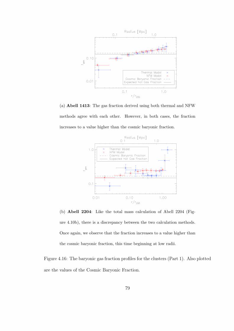
(a) Abell 1413: The gas fraction derived using both thermal and NFW

methods agree with each other. However, in both cases, the fraction

increases to a value higher than the cosmic baryonic fraction.

(b) Abell 2204: Like the total mass calculation of Abell 2204 (Fig-

ure 4.10b), there is a discrepancy between the two calculation methods.

Once again, we observe that the fraction increases to a value higher than

the cosmic baryonic fraction, this time beginning at low radii.

Figure 4.16: The baryonic gas fraction profiles for the clusters (Part 1). Also plotted

are the values of the Cosmic Baryonic Fraction.

79

(a) Abell 773: The gas fraction derived using both methods agree with each other.

Similar to Abell 2204 (Figure 4.16b), this profile shows an anomalous behavior with

the fraction increasing beyond the cosmic baryon fraction at very low radii.

(b) Abell 383: The gas fraction derived using both methods agree with each other.

However, in both cases, the fraction increases to a value higher than the cosmic

baryonic fraction.

Figure 4.17: The baryonic gas fraction profiles for the clusters (Part 2). Also plotted

are the values of the Cosmic Baryonic Fraction.

80

density squared < n2e > rather than the average density, < ne >.

Iν ∝

∫

n2eT

−1/2dl (4.16)

So if the gas is clumpy, the average density estimated by this method will

be over-estimated. This would in turn cause an underestimation of the entropy

calculated (∝ n−2/3e ) as well as an over-estimation of the pressure (∝ ne) and the

baryonic gas fraction calculated.

Clumping in the outskirts could also introduce another bias in our corrections.

Urban et al. [2011] has discovered that if gas clumping is present and if these clumps

are in pressure equilibrium with their surroundings, they would be at a lower tem-

perature than their surroundings. This would could cause the average temperature

to be biased to lower values. However, Walker et al. [2013] notices no such biases

in the analysis of the Centaurus cluster. We have not compared our data to tem-

perature models, so we cannot definitively say whether our data also show these

biases.

In the case of Abell 2204, there have been observed cavities in the northern

and southern regions of the clusters. This would also cause a bias in the density

and temperature calculations for this cluster. The unphysical values calculated for

this cluster can be attributed to these cavities which we have not modeled for.

81

Chapter 5: Conclusions

This thesis examines the very outer regions, or the outskirts, of galaxy clusters

using X-ray spectroscopy. We have been able to achieve unique insights into the

physics governing these regions as well identify some of the key issues involved in

the processing of these low signal to noise data.

5.1 Summary of Results

We utilized Suzaku data for four clusters (Abell 1413, Abell 2204, Abell 773

and Abell 383) to draw generalized profiles for temperature, density, entropy, pres-

sure and baryonic fraction.

In Chapter 3, we outlined the various data effects one must consider while

analyzing cluster data. Of particular importance was the proper analysis of the

background and the various issues involved in the spectral and image analysis of

the data. In order to get a better handle on the background diagnostics, we uti-

lize Chandra data to remove point sources, which helps constrain the cosmological

background.

We chose to model the data between 0.7–7.0 keV to account for data limitations

and to eliminate regions where contamination is poorly modeled. To further under-

82

stand the effect this has on the analysis, we ran simulations of the clusters Abell

773 and Abell 383 over the ranges of 0.5–10.0 keV and 0.7–7.0 keV. We notice no

significant deviations between the two energy ranges. We modeled the background

using an APEC model for the thermal components and a power law to account for the

unresolved point sources in the cosmic background. We notice that the exact value

of the thermal background has little effect on the parameters. The proper modeling

of the cosmic background is very significant as it becomes the dominant source of

error.

Using this analysis, we were able to directly obtain temperature, surface bright-

ness, abundance, and density for the clusters. All of the values agree with latest

available literature within errors. However, we do see deviations from the older

XMM-Newton results, highlighting the effects of erroneous extended emission anal-

ysis.

These primary parameters were then deprojected using three dimensional mod-

els for temperature and density [Vikhlinin et al., 2006]. Using these deprojected val-

ues, we compared our calculated values of entropy and pressure to their respective

universal profiles.

The pressure profiles we compiled for the clusters yield higher values than the

expected universal pressure profile [Arnaud et al., 2010, Planck Collaboration et al.,

2013a]. We believe that this deviation can be attributed to the bias we observed

with the calculations of the scaling parameters, r500, M500, r200 and M200. This bias

occurs due to the variation in the parameters obtained using different methods of

analysis and different instruments [Planck Collaboration et al., 2013b]. Similarly,

83

we calculated the entropy profile for each of the clusters, and compared the same to

the universal profile. Here, we see agreement with previously observed deviations

from the universal profile. We also observe an excess in entropy values at smaller

radii when compared to the universal entropy profile according to Voit et al. [2005].

While the Walker et al. [2012a] profile accounts for the observed turnover at large

radii, our results do not see as strong a turnover at larger radii as seen in this Walker

et al. [2012a] profile.

Finally, we calculated the baryonic fraction profiles for each of the clusters.

For all the clusters, we observe values that significantly exceed the expected cosmic

baryonic fraction at r200. This seems to suggest the existence of clumps in the

outskirts of clusters. Of particular interest is the cluster Abell 2204, where we

observe an obvious breakdown in hydrostatic equilibrium in the very outskirts, which

could be due to clumping. Our unphysical observation that M200 < M500 is likely

due to the breakdown in the assumption of hydrostatic equilibrium in the calculation

of these scaling parameters.

We have shown that, in spite of the variety of the temperature profiles cho-

sen (falling, rising, constant) seen in the XMM-Newton [Snowden et al., 2008], all

of our clusters actually having a fall ling temperature profile out to the outskirts

which matches up to the theoretical expectations. It also highlights the inaccuracies

seen in modeling cluster outskirts using XMM-Newton data. For the first time, we

also carried out side-by-side calculations of the total mass using two different meth-

ods: the assumption of hydrostatic equilibrium and the modeling using the NFW

model. Comparing these, we notice that the assumption of hydrostatic equilibrium

84

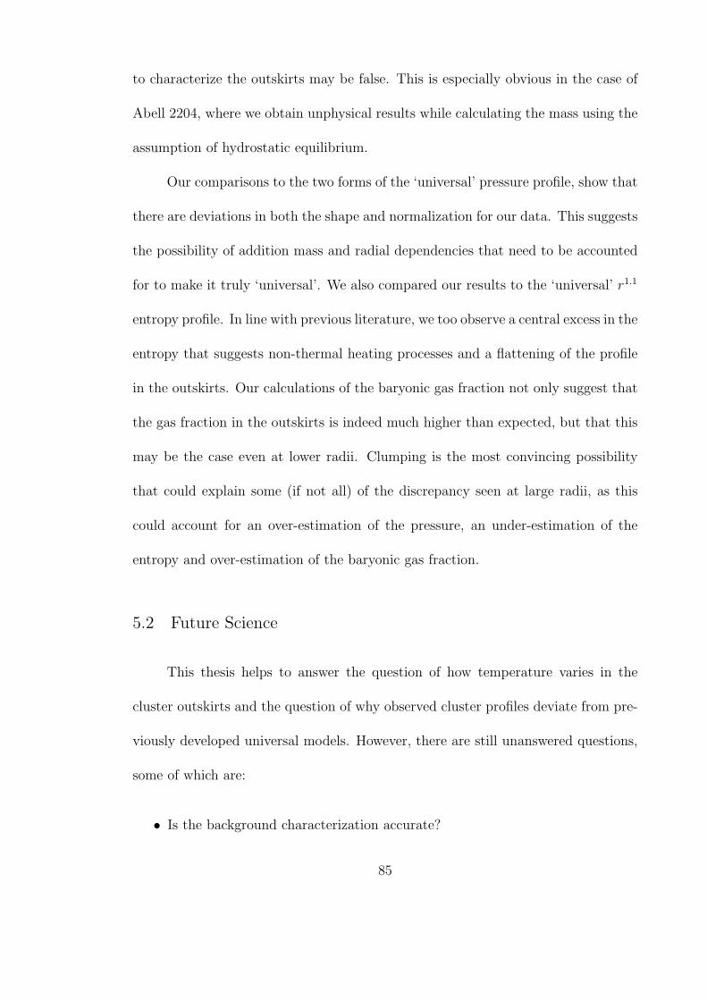
to characterize the outskirts may be false. This is especially obvious in the case of

Abell 2204, where we obtain unphysical results while calculating the mass using the

assumption of hydrostatic equilibrium.

Our comparisons to the two forms of the ‘universal’ pressure profile, show that

there are deviations in both the shape and normalization for our data. This suggests

the possibility of addition mass and radial dependencies that need to be accounted

for to make it truly ‘universal’. We also compared our results to the ‘universal’ r1.1

entropy profile. In line with previous literature, we too observe a central excess in the

entropy that suggests non-thermal heating processes and a flattening of the profile

in the outskirts. Our calculations of the baryonic gas fraction not only suggest that

the gas fraction in the outskirts is indeed much higher than expected, but that this

may be the case even at lower radii. Clumping is the most convincing possibility

that could explain some (if not all) of the discrepancy seen at large radii, as this

could account for an over-estimation of the pressure, an under-estimation of the

entropy and over-estimation of the baryonic gas fraction.

5.2 Future Science

This thesis helps to answer the question of how temperature varies in the

cluster outskirts and the question of why observed cluster profiles deviate from pre-

viously developed universal models. However, there are still unanswered questions,

some of which are:

• Is the background characterization accurate?

85

• Are the universal profiles for entropy and pressure truly universal?

• Is clumping the true solution to the increased baryonic fraction in the very

outskirts?

• What role do the metallic abundances of the clusters in the outskirts play?

To answer these questions and more requires a two-pronged approach: detailed

observations of nearby clusters to maximize resolution of the clusters and larger

surveys of multiple clusters.

For this purpose, we have already obtained Suzaku data for several more clus-

ters. We hope to extend our analysis to complete the entire sample. This will help

us to improve our statistics when studying the validity of the universal profiles for

entropy and pressure. This will also help to pick out anomalous behavior of individ-

ual galaxy clusters. In addition to extending this axisymmetric study of clusters, we

can also study the non-axisymmetry found in some clusters. The aforementioned

sample, however, only includes relaxed clusters. Similar surveys should be done

which includes unrelaxed clusters to complete a universal sample.

Another topic which has been untouched in this thesis is the role of chemical

abundance in the evolution of clusters. There has been indication of early metal

enrichment in the outskirts of clusters, and the implications of such a scenario are

manifold:

• All massive clusters would have a level of enrichment similar to the cosmic

value at 13of the solar metallicity.

86

• The warm-hot intergalactic medium in large-scale structure filaments connect-

ing to massive clusters would be metal-rich, which will be detectable using

high-spectral resolution instruments.

• If the material currently falling into massive clusters is iron-rich, this indicates

that the accreting material is being accelerated by the accretion shocks. This

makes cluster accretion an important source of high energy cosmic rays.

Looking further out into the future, theAstro-H mission, which will be launched

in 2015, promises great results in this area. The satellite houses two soft X-ray sys-

tems: the Soft X-ray Spectroscopy System and the Soft X-ray Imager (SXI). The

satellite will have a similar low background orbit as the Suzaku satellite. The spec-

troscopy system will have a X-ray Calorimeter Spectrometer (XCS) which will have a

much better energy resolution than XIS. The big advantage will be the X-ray Imag-

ing system which provides a better field of view, that can be exploited to provide

views of more clusters out to r200. The better angular resolution is also helpful as

it helps minimize the area lost to bright point sources and to maximize the depth

of the observations which will help to minimize cosmic variance.

This thesis is the first important step in creating a fiducial data set for more

detailed comparisons to high resolution simulations to further our understanding

cluster outskirts. More in-depth studies of the full Suzaku sample will shed more

light on the ‘universality’ of parameter profiles and on the physical processes occur-

ring in outskirts.

87

Appendix A: Spectral Fits of the Cluster Data

This section shows the fits achieved for each of the clusters using the method

outlined in 3.2. We present the spectra extracted from each annulus, for each point-

ing and for each XIS detector used and the corresponding model fit. In each case,

the red line depicts the contribution from the cluster emission, blue the galactic

thermal background and green the extragalactic background. The black solid line

represents the total model i.e. the sum of all the individual components. The spec-

tra are shown over the modeled range of 0.7–7.0 keV. In some cases, the spectra are

cut-off at 5.5 keV. This was done to excise the two 55Fe calibration sources (Mn I

Kα and Kβ) that appear at 5.9 keV and 6.5 keV.

88

A.1 Abell 1413

Presented below are the Suzaku pointings for Abell 1413 we utilized for this

analysis. The observation details are shown below in Table A.1.

Pointing # Observation ID Comments

1 805059010 Proposed Data


3 800001010 Archival Data [Hoshino et al., 2010]


Table A.1: The Suzaku data on Abell 1413 used for this analysis

For pointings 1, 2 and 4, we use only detectors XIS 0, XIS 1 and XIS 3 for the

analysis. For pointing 3, we used the XIS 2 detector in addition to XIS 0, 1 and 3

as it was observed before the detector was damaged.

89

1 2 510−

410

−3

0.01

0.1

1

norm

aliz

ed c

ount

s s

−1

keV

−1

Energy (keV)

data and folded model

(a) XIS 0

1 2 510−

410

−3

0.01

0.1

1

norm

aliz

ed c

ount

s s

−1

keV

−1

Energy (keV)


(b) XIS 1

1 2 510−

410

−3

0.01

0.1

1

norm

aliz

ed c

ount

s s

−1

keV

−1

Energy (keV)


(c) XIS 3

Figure A.1: The spectral fits for Annulus 3 (refer Table 3.1) of Abell 1413 for the

first pointing

90

1 2 510−

410

−3

0.01

0.1

1

norm

aliz

ed c

ount

s s

−1

keV

−1

Energy (keV)


(a) XIS 0

1 2 510−

410

−3

0.01

0.1

1

norm

aliz

ed c

ount

s s

−1

keV

−1

Energy (keV)


(b) XIS 1

1 2 510−

410

−3

0.01

0.1

1

norm

aliz

ed c

ount

s s

−1

keV

−1

Energy (keV)


(c) XIS 3


second pointing

91

1 2 510−

410

−3

0.01

0.1

1

norm

aliz

ed c

ount

s s

−1

keV

−1

Energy (keV)


(a) XIS 0

1 2 510−

410

−3

0.01

0.1

1

norm

aliz

ed c

ount

s s

−1

keV

−1

Energy (keV)


(b) XIS 1

1 2 510−

410

−3

0.01

0.1

1

norm

aliz

ed c

ount

s s

−1

keV

−1

Energy (keV)


(c) XIS 2

1 2 510−

410

−3

0.01

0.1

1

norm

aliz

ed c

ount

s s

−1

keV

−1

Energy (keV)


(d) XIS 3


third pointing

92

1 2 510−

410

−3

0.01

0.1

1

norm

aliz

ed c

ount

s s

−1

keV

−1

Energy (keV)


(a) XIS 0

1 2 510−

410

−3

0.01

0.1

1

norm

aliz

ed c

ount

s s

−1

keV

−1

Energy (keV)


(b) XIS 1

1 2 510−

410

−3

0.01

0.1

1

norm

aliz

ed c

ount

s s

−1

keV

−1

Energy (keV)


(c) XIS 3


fourth pointing

93

1 2 510−

410

−3

0.01

0.1

1

norm

aliz

ed c

ount

s s

−1

keV

−1

Energy (keV)


(a) XIS 0

1 2 510−

410

−3

0.01

0.1

1

norm

aliz

ed c

ount

s s

−1

keV

−1

Energy (keV)


(b) XIS 1

1 2 510−

410

−3

0.01

0.1

1

norm

aliz

ed c

ount

s s

−1

keV

−1

Energy (keV)


(c) XIS 3


first pointing

94

1 2 510−

410

−3

0.01

0.1

1

norm

aliz

ed c

ount

s s

−1

keV

−1

Energy (keV)


(a) XIS 0

1 2 510−

410

−3

0.01

0.1

1

norm

aliz

ed c

ount

s s

−1

keV

−1

Energy (keV)


(b) XIS 1

1 2 510−

410

−3

0.01

0.1

1

norm

aliz

ed c

ount

s s

−1

keV

−1

Energy (keV)


(c) XIS 3


second pointing

95

1 2 510−

410

−3

0.01

0.1

1

norm

aliz

ed c

ount

s s

−1

keV

−1

Energy (keV)


(a) XIS 0

1 2 510−

410

−3

0.01

0.1

1

norm

aliz

ed c

ount

s s

−1

keV

−1

Energy (keV)


(b) XIS 1

1 2 510−

410

−3

0.01

0.1

1

norm

aliz

ed c

ount

s s

−1

keV

−1

Energy (keV)


(c) XIS 2

1 2 510−

410

−3

0.01

0.1

1

norm

aliz

ed c

ount

s s

−1

keV

−1

Energy (keV)


(d) XIS 3


third pointing

96

1 2 510−

410

−3

0.01

0.1

1

norm

aliz

ed c

ount

s s

−1

keV

−1

Energy (keV)


(a) XIS 0

1 2 510−

410

−3

0.01

0.1

1

norm

aliz

ed c

ount

s s

−1

keV

−1

Energy (keV)


(b) XIS 1

1 2 510−

410

−3

0.01

0.1

1

norm

aliz

ed c

ount

s s

−1

keV

−1

Energy (keV)


(c) XIS 3


fourth pointing

97

1 2 510−

410

−3

0.01

0.1

1

norm

aliz

ed c

ount

s s

−1

keV

−1

Energy (keV)


(a) XIS 0

1 2 510−

410

−3

0.01

0.1

1

norm

aliz

ed c

ount

s s

−1

keV

−1

Energy (keV)


(b) XIS 1

1 2 510−

410

−3

0.01

0.1

1

norm

aliz

ed c

ount

s s

−1

keV

−1

Energy (keV)


(c) XIS 3


first pointing

98

1 2 510−

410

−3

0.01

0.1

1

norm

aliz

ed c

ount

s s

−1

keV

−1

Energy (keV)


(a) XIS 0

1 2 510−

410

−3

0.01

0.1

1

norm

aliz

ed c

ount

s s

−1

keV

−1

Energy (keV)


(b) XIS 1

1 2 510−

410

−3

0.01

0.1

1

norm

aliz

ed c

ount

s s

−1

keV

−1

Energy (keV)


(c) XIS 3


second pointing

99

1 2 510−

410

−3

0.01

0.1

1

norm

aliz

ed c

ount

s s

−1

keV

−1

Energy (keV)


(a) XIS 0

1 2 510−

410

−3

0.01

0.1

1

norm

aliz

ed c

ount

s s

−1

keV

−1

Energy (keV)


(b) XIS 1

1 2 510−

410

−3

0.01

0.1

1

norm

aliz

ed c

ount

s s

−1

keV

−1

Energy (keV)


(c) XIS 2

1 2 510−

410

−3

0.01

0.1

1

norm

aliz

ed c

ount

s s

−1

keV

−1

Energy (keV)


(d) XIS 3


third pointing

100

1 2 510−

410

−3

0.01

0.1

1

norm

aliz

ed c

ount

s s

−1

keV

−1

Energy (keV)


(a) XIS 0

1 2 510−

410

−3

0.01

0.1

1

norm

aliz

ed c

ount

s s

−1

keV

−1

Energy (keV)


(b) XIS 1

1 2 510−

410

−3

0.01

0.1

1

norm

aliz

ed c

ount

s s

−1

keV

−1

Energy (keV)


(c) XIS 3


fourth pointing

101

1 2 510−

410

−3

0.01

0.1

1

norm

aliz

ed c

ount

s s

−1

keV

−1

Energy (keV)


(a) XIS 0

1 2 510−

410

−3

0.01

0.1

1

norm

aliz

ed c

ount

s s

−1

keV

−1

Energy (keV)


(b) XIS 1

1 2 510−

410

−3

0.01

0.1

1

norm

aliz

ed c

ount

s s

−1

keV

−1

Energy (keV)


(c) XIS 3

Figure A.13: The spectral fits for Annulus 6a (refer Table 3.1) of Abell 1413 for the

first pointing

102

1 2 510−

410

−3

0.01

0.1

1

norm

aliz

ed c

ount

s s

−1

keV

−1

Energy (keV)


(a) XIS 0

1 2 510−

410

−3

0.01

0.1

1

norm

aliz

ed c

ount

s s

−1

keV

−1

Energy (keV)


(b) XIS 1

1 2 510−

410

−3

0.01

0.1

1

norm

aliz

ed c

ount

s s

−1

keV

−1

Energy (keV)


(c) XIS 3


second pointing

103

1 2 510−

410

−3

0.01

0.1

1

norm

aliz

ed c

ount

s s

−1

keV

−1

Energy (keV)


(a) XIS 0

1 2 510−

410

−3

0.01

0.1

1

norm

aliz

ed c

ount

s s

−1

keV

−1

Energy (keV)


(b) XIS 1

1 2 510−

410

−3

0.01

0.1

1

norm

aliz

ed c

ount

s s

−1

keV

−1

Energy (keV)


(c) XIS 2

1 2 510−

410

−3

0.01

0.1

1

norm

aliz

ed c

ount

s s

−1

keV

−1

Energy (keV)


(d) XIS 3


third pointing

104

1 2 510−

410

−3

0.01

0.1

1

norm

aliz

ed c

ount

s s

−1

keV

−1

Energy (keV)


(a) XIS 0

1 2 510−

410

−3

0.01

0.1

1

norm

aliz

ed c

ount

s s

−1

keV

−1

Energy (keV)


(b) XIS 1

1 2 510−

410

−3

0.01

0.1

1

norm

aliz

ed c

ount

s s

−1

keV

−1

Energy (keV)


(c) XIS 3


fourth pointing

105

A.2 Abell 2204




1 801091010 Archival Data [Reiprich et al., 2009]





For pointings 2, 3 and 4, we use only detectors XIS 0, XIS 1 and XIS 3 for the

analysis. For pointing 1, we used the XIS 2 detector in addition to XIS 0, 1 and 3

as it was observed before the detector was damaged. For the first annulus, we did

not use the data from the third pointing and the data from the XIS 0 and XIS 3

detectors, as these regions directly overlapped with the calibrator regions.

106

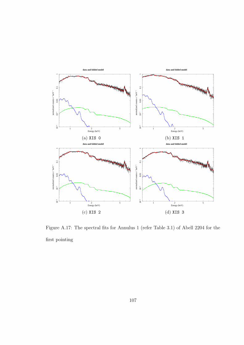
1 2 510−

410

−3

0.01

0.1

1

norm

aliz

ed c

ount

s s

−1

keV

−1

Energy (keV)


(a) XIS 0

1 2 510−

410

−3

0.01

0.1

1

norm

aliz

ed c

ount

s s

−1

keV

−1

Energy (keV)


(b) XIS 1

1 2 510−

410

−3

0.01

0.1

1

norm

aliz

ed c

ount

s s

−1

keV

−1

Energy (keV)


(c) XIS 2

1 2 510−

410

−3

0.01

0.1

1

norm

aliz

ed c

ount

s s

−1

keV

−1

Energy (keV)


(d) XIS 3


first pointing

107

1 2 510−

410

−3

0.01

0.1

1

norm

aliz

ed c

ount

s s

−1

keV

−1

Energy (keV)


(a) XIS 0

1 2 510−

410

−3

0.01

0.1

1

norm

aliz

ed c

ount

s s

−1

keV

−1

Energy (keV)


(b) XIS 1

1 2 510−

410

−3

0.01

0.1

1

norm

aliz

ed c

ount

s s

−1

keV

−1

Energy (keV)


(c) XIS 3


second pointing

108

1 2 510−

410

−3

0.01

0.1

1

norm

aliz

ed c

ount

s s

−1

keV

−1

Energy (keV)



fourth pointing in XIS1

109

1 2 510−

410

−3

0.01

0.1

1

norm

aliz

ed c

ount

s s

−1

keV

−1

Energy (keV)


(a) XIS 0

1 2 510−

410

−3

0.01

0.1

1

norm

aliz

ed c

ount

s s

−1

keV

−1

Energy (keV)


(b) XIS 1

1 2 510−

410

−3

0.01

0.1

1

norm

aliz

ed c

ount

s s

−1

keV

−1

Energy (keV)


(c) XIS 2

1 2 510−

410

−3

0.01

0.1

1

norm

aliz

ed c

ount

s s

−1

keV

−1

Energy (keV)


(d) XIS 3


first pointing

110

1 2 510−

410

−3

0.01

0.1

1

norm

aliz

ed c

ount

s s

−1

keV

−1

Energy (keV)


(a) XIS 0

1 2 510−

410

−3

0.01

0.1

1

norm

aliz

ed c

ount

s s

−1

keV

−1

Energy (keV)


(b) XIS 1

1 2 510−

410

−3

0.01

0.1

1

norm

aliz

ed c

ount

s s

−1

keV

−1

Energy (keV)


(c) XIS 3


second pointing

111

1 2 510−

410

−3

0.01

0.1

1

norm

aliz

ed c

ount

s s

−1

keV

−1

Energy (keV)


(a) XIS 0

1 2 510−

410

−3

0.01

0.1

1

norm

aliz

ed c

ount

s s

−1

keV

−1

Energy (keV)


(b) XIS 1

1 2 510−

410

−3

0.01

0.1

1

norm

aliz

ed c

ount

s s

−1

keV

−1

Energy (keV)


(c) XIS 3


third pointing

112

1 2 510−

410

−3

0.01

0.1

1

norm

aliz

ed c

ount

s s

−1

keV

−1

Energy (keV)


(a) XIS 0

1 2 510−

410

−3

0.01

0.1

1

norm

aliz

ed c

ount

s s

−1

keV

−1

Energy (keV)


(b) XIS 1

1 2 510−

410

−3

0.01

0.1

1

norm

aliz

ed c

ount

s s

−1

keV

−1

Energy (keV)


(c) XIS 3


fourth pointing

113

1 2 510−

410

−3

0.01

0.1

1

norm

aliz

ed c

ount

s s

−1

keV

−1

Energy (keV)


(a) XIS 0

1 2 510−

410

−3

0.01

0.1

1

norm

aliz

ed c

ount

s s

−1

keV

−1

Energy (keV)


(b) XIS 1

1 2 510−

410

−3

0.01

0.1

1

norm

aliz

ed c

ount

s s

−1

keV

−1

Energy (keV)


(c) XIS 2

1 2 510−

410

−3

0.01

0.1

1

norm

aliz

ed c

ount

s s

−1

keV

−1

Energy (keV)


(d) XIS 3


first pointing

114

1 2 510−

410

−3

0.01

0.1

1

norm

aliz

ed c

ount

s s

−1

keV

−1

Energy (keV)


(a) XIS 0

1 2 510−

410

−3

0.01

0.1

1

norm

aliz

ed c

ount

s s

−1

keV

−1

Energy (keV)


(b) XIS 1

1 2 510−

410

−3

0.01

0.1

1

norm

aliz

ed c

ount

s s

−1

keV

−1

Energy (keV)


(c) XIS 3


second pointing

115

1 2 510−

410

−3

0.01

0.1

1

norm

aliz

ed c

ount

s s

−1

keV

−1

Energy (keV)


(a) XIS 0

1 2 510−

410

−3

0.01

0.1

1

norm

aliz

ed c

ount

s s

−1

keV

−1

Energy (keV)


(b) XIS 1

1 2 510−

410

−3

0.01

0.1

1

norm

aliz

ed c

ount

s s

−1

keV

−1

Energy (keV)


(c) XIS 3


third pointing

116

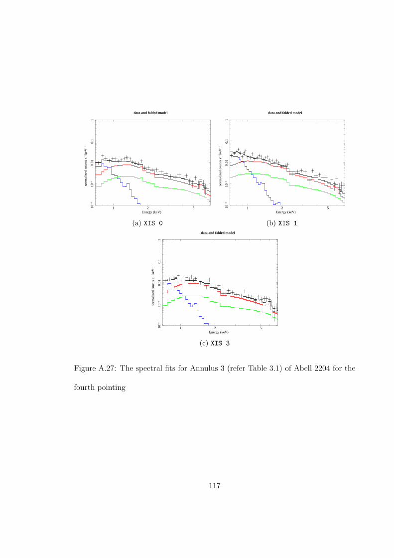
1 2 510−

410

−3

0.01

0.1

1

norm

aliz

ed c

ount

s s

−1

keV

−1

Energy (keV)


(a) XIS 0

1 2 510−

410

−3

0.01

0.1

1

norm

aliz

ed c

ount

s s

−1

keV

−1

Energy (keV)


(b) XIS 1

1 2 510−

410

−3

0.01

0.1

1

norm

aliz

ed c

ount

s s

−1

keV

−1

Energy (keV)


(c) XIS 3


fourth pointing

117

1 2 510−

410

−3

0.01

0.1

1

norm

aliz

ed c

ount

s s

−1

keV

−1

Energy (keV)


(a) XIS 0

1 2 510−

410

−3

0.01

0.1

1

norm

aliz

ed c

ount

s s

−1

keV

−1

Energy (keV)


(b) XIS 1

1 2 510−

410

−3

0.01

0.1

1

norm

aliz

ed c

ount

s s

−1

keV

−1

Energy (keV)


(c) XIS 2

1 2 510−

410

−3

0.01

0.1

1

norm

aliz

ed c

ount

s s

−1

keV

−1

Energy (keV)


(d) XIS 3


first pointing

118

1 2 510−

410

−3

0.01

0.1

1

norm

aliz

ed c

ount

s s

−1

keV

−1

Energy (keV)


(a) XIS 0

1 2 510−

410

−3

0.01

0.1

1

norm

aliz

ed c

ount

s s

−1

keV

−1

Energy (keV)


(b) XIS 1

1 2 510−

410

−3

0.01

0.1

1

norm

aliz

ed c

ount

s s

−1

keV

−1

Energy (keV)


(c) XIS 3


second pointing

119

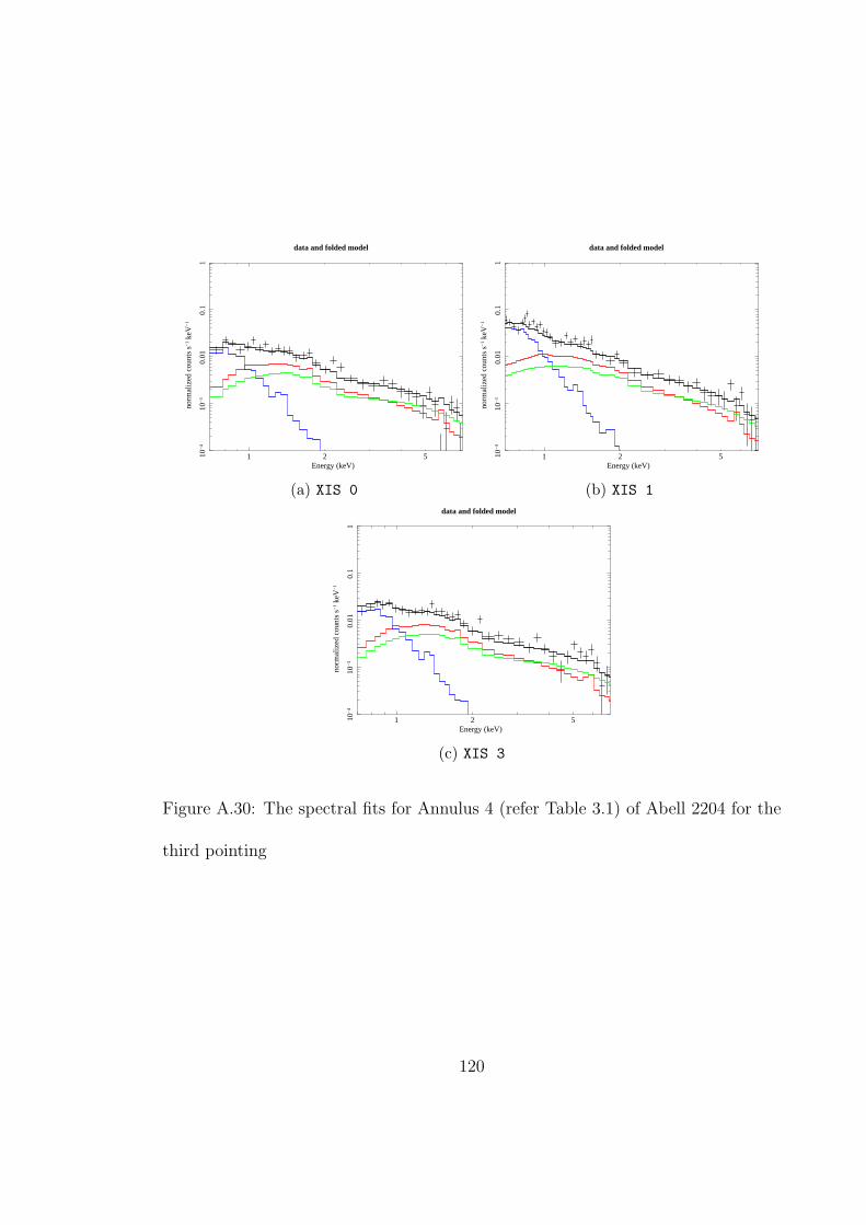
1 2 510−

410

−3

0.01

0.1

1

norm

aliz

ed c

ount

s s

−1

keV

−1

Energy (keV)


(a) XIS 0

1 2 510−

410

−3

0.01

0.1

1

norm

aliz

ed c

ount

s s

−1

keV

−1

Energy (keV)


(b) XIS 1

1 2 510−

410

−3

0.01

0.1

1

norm

aliz

ed c

ount

s s

−1

keV

−1

Energy (keV)


(c) XIS 3


third pointing

120

1 2 510−

410

−3

0.01

0.1

1

norm

aliz

ed c

ount

s s

−1

keV

−1

Energy (keV)


(a) XIS 0

1 2 510−

410

−3

0.01

0.1

1

norm

aliz

ed c

ount

s s

−1

keV

−1

Energy (keV)


(b) XIS 1

1 2 510−

410

−3

0.01

0.1

1

norm

aliz

ed c

ount

s s

−1

keV

−1

Energy (keV)


(c) XIS 3


fourth pointing

121

1 2 510−

410

−3

0.01

0.1

1

norm

aliz

ed c

ount

s s

−1

keV

−1

Energy (keV)


(a) XIS 0

1 2 510−

410

−3

0.01

0.1

1

norm

aliz

ed c

ount

s s

−1

keV

−1

Energy (keV)


(b) XIS 1

1 2 510−

410

−3

0.01

0.1

1

norm

aliz

ed c

ount

s s

−1

keV

−1

Energy (keV)


(c) XIS 2

1 2 510−

410

−3

0.01

0.1

1

norm

aliz

ed c

ount

s s

−1

keV

−1

Energy (keV)


(d) XIS 3


first pointing

122

1 2 510−

410

−3

0.01

0.1

1

norm

aliz

ed c

ount

s s

−1

keV

−1

Energy (keV)


(a) XIS 0

1 2 510−

410

−3

0.01

0.1

1

norm

aliz

ed c

ount

s s

−1

keV

−1

Energy (keV)


(b) XIS 1

1 2 510−

410

−3

0.01

0.1

1

norm

aliz

ed c

ount

s s

−1

keV

−1

Energy (keV)


(c) XIS 3


second pointing

123

1 2 510−

410

−3

0.01

0.1

1

norm

aliz

ed c

ount

s s

−1

keV

−1

Energy (keV)


(a) XIS 0

1 2 510−

410

−3

0.01

0.1

1

norm

aliz

ed c

ount

s s

−1

keV

−1

Energy (keV)


(b) XIS 1

1 2 510−

410

−3

0.01

0.1

1

norm

aliz

ed c

ount

s s

−1

keV

−1

Energy (keV)


(c) XIS 3


third pointing

124

1 2 510−

410

−3

0.01

0.1

1

norm

aliz

ed c

ount

s s

−1

keV

−1

Energy (keV)


(a) XIS 0

1 2 510−

410

−3

0.01

0.1

1

norm

aliz

ed c

ount

s s

−1

keV

−1

Energy (keV)


(b) XIS 1

1 2 510−

410

−3

0.01

0.1

1

norm

aliz

ed c

ount

s s

−1

keV

−1

Energy (keV)


(c) XIS 3


fourth pointing

125

1 2 510−

410

−3

0.01

0.1

1

norm

aliz

ed c

ount

s s

−1

keV

−1

Energy (keV)


(a) XIS 0

1 2 510−

410

−3

0.01

0.1

1

norm

aliz

ed c

ount

s s

−1

keV

−1

Energy (keV)


(b) XIS 1

1 2 510−

410

−3

0.01

0.1

1

norm

aliz

ed c

ount

s s

−1

keV

−1

Energy (keV)


(c) XIS 2

1 2 510−

410

−3

0.01

0.1

1

norm

aliz

ed c

ount

s s

−1

keV

−1

Energy (keV)


(d) XIS 3


first pointing

126

1 2 510−

410

−3

0.01

0.1

1

norm

aliz

ed c

ount

s s

−1

keV

−1

Energy (keV)


(a) XIS 0

1 2 510−

410

−3

0.01

0.1

1

norm

aliz

ed c

ount

s s

−1

keV

−1

Energy (keV)


(b) XIS 1

1 2 510−

410

−3

0.01

0.1

1

norm

aliz

ed c

ount

s s

−1

keV

−1

Energy (keV)


(c) XIS 3


second pointing

127

1 2 510−

410

−3

0.01

0.1

1

norm

aliz

ed c

ount

s s

−1

keV

−1

Energy (keV)


(a) XIS 0

1 2 510−

410

−3

0.01

0.1

1

norm

aliz

ed c

ount

s s

−1

keV

−1

Energy (keV)


(b) XIS 1

1 2 510−

410

−3

0.01

0.1

1

norm

aliz

ed c

ount

s s

−1

keV

−1

Energy (keV)


(c) XIS 3


third pointing

128

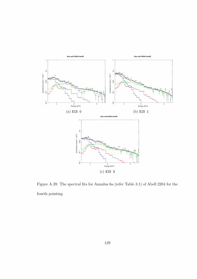
1 2 510−

410

−3

0.01

0.1

1

norm

aliz

ed c

ount

s s

−1

keV

−1

Energy (keV)


(a) XIS 0

1 2 510−

410

−3

0.01

0.1

1

norm

aliz

ed c

ount

s s

−1

keV

−1

Energy (keV)


(b) XIS 1

1 2 510−

410

−3

0.01

0.1

1

norm

aliz

ed c

ount

s s

−1

keV

−1

Energy (keV)


(c) XIS 3


fourth pointing

129

A.3 Abell 773









For all pointings, we use only detectors XIS 0, XIS 1 and XIS 3 for our analysis.

130

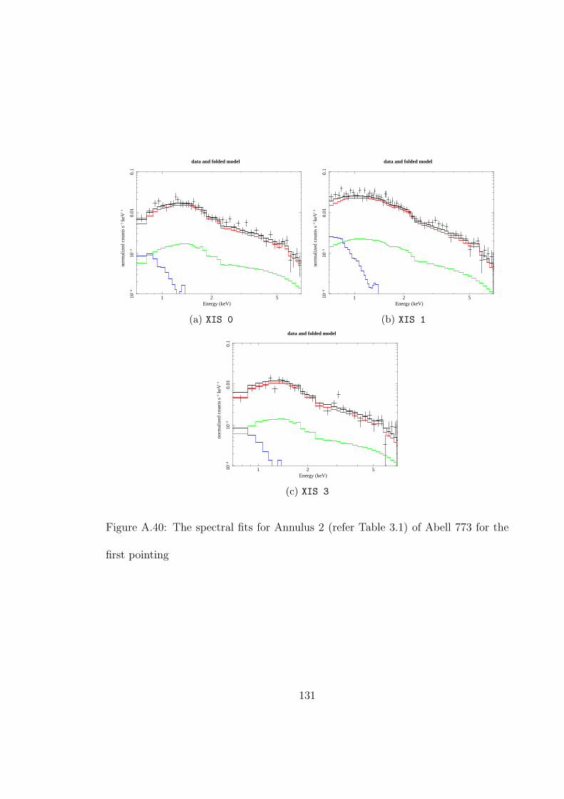
1 2 510−

410

−3

0.01

0.1

norm

aliz

ed c

ount

s s

−1

keV

−1

Energy (keV)


(a) XIS 0

1 2 510−

410

−3

0.01

0.1

norm

aliz

ed c

ount

s s

−1

keV

−1

Energy (keV)


(b) XIS 1

1 2 510−

410

−3

0.01

0.1

norm

aliz

ed c

ount

s s

−1

keV

−1

Energy (keV)


(c) XIS 3


first pointing

131

1 2 510−

410

−3

0.01

0.1

norm

aliz

ed c

ount

s s

−1

keV

−1

Energy (keV)


(a) XIS 0

1 2 510−

410

−3

0.01

0.1

norm

aliz

ed c

ount

s s

−1

keV

−1

Energy (keV)


(b) XIS 1

1 2 510−

410

−3

0.01

0.1

norm

aliz

ed c

ount

s s

−1

keV

−1

Energy (keV)


(c) XIS 3


second pointing

132

1 2 510−

410

−3

0.01

0.1

norm

aliz

ed c

ount

s s

−1

keV

−1

Energy (keV)


(a) XIS 0

1 2 510−

410

−3

0.01

0.1

norm

aliz

ed c

ount

s s

−1

keV

−1

Energy (keV)


(b) XIS 1

1 2 510−

410

−3

0.01

0.1

norm

aliz

ed c

ount

s s

−1

keV

−1

Energy (keV)


(c) XIS 3


third pointing

133

1 2 510−

410

−3

0.01

0.1

norm

aliz

ed c

ount

s s

−1

keV

−1

Energy (keV)


(a) XIS 0

1 2 510−

410

−3

0.01

0.1

norm

aliz

ed c

ount

s s

−1

keV

−1

Energy (keV)


(b) XIS 1

1 2 510−

410

−3

0.01

0.1

norm

aliz

ed c

ount

s s

−1

keV

−1

Energy (keV)


(c) XIS 3


fourth pointing

134

1 2 510−

410

−3

0.01

0.1

norm

aliz

ed c

ount

s s

−1

keV

−1

Energy (keV)


(a) XIS 0

1 2 510−

410

−3

0.01

0.1

norm

aliz

ed c

ount

s s

−1

keV

−1

Energy (keV)


(b) XIS 1

1 2 510−

410

−3

0.01

0.1

norm

aliz

ed c

ount

s s

−1

keV

−1

Energy (keV)


(c) XIS 3


first pointing

135

1 2 510−

410

−3

0.01

0.1

norm

aliz

ed c

ount

s s

−1

keV

−1

Energy (keV)


(a) XIS 0

1 2 510−

410

−3

0.01

0.1

norm

aliz

ed c

ount

s s

−1

keV

−1

Energy (keV)


(b) XIS 1

1 2 510−

410

−3

0.01

0.1

norm

aliz

ed c

ount

s s

−1

keV

−1

Energy (keV)


(c) XIS 3


second pointing

136

1 2 510−

410

−3

0.01

0.1

norm

aliz

ed c

ount

s s

−1

keV

−1

Energy (keV)


(a) XIS 0

1 2 510−

410

−3

0.01

0.1

norm

aliz

ed c

ount

s s

−1

keV

−1

Energy (keV)


(b) XIS 1

1 2 510−

410

−3

0.01

0.1

norm

aliz

ed c

ount

s s

−1

keV

−1

Energy (keV)


(c) XIS 3


third pointing

137

1 2 510−

410

−3

0.01

0.1

norm

aliz

ed c

ount

s s

−1

keV

−1

Energy (keV)


(a) XIS 0

1 2 510−

410

−3

0.01

0.1

norm

aliz

ed c

ount

s s

−1

keV

−1

Energy (keV)


(b) XIS 1

1 2 510−

410

−3

0.01

0.1

norm

aliz

ed c

ount

s s

−1

keV

−1

Energy (keV)


(c) XIS 3


fourth pointing

138

1 2 510−

410

−3

0.01

0.1

norm

aliz

ed c

ount

s s

−1

keV

−1

Energy (keV)


(a) XIS 0

1 2 510−

410

−3

0.01

0.1

norm

aliz

ed c

ount

s s

−1

keV

−1

Energy (keV)


(b) XIS 1

1 2 510−

410

−3

0.01

0.1

norm

aliz

ed c

ount

s s

−1

keV

−1

Energy (keV)


(c) XIS 3


first pointing

139

1 2 510−

410

−3

0.01

0.1

norm

aliz

ed c

ount

s s

−1

keV

−1

Energy (keV)


(a) XIS 0

1 2 510−

410

−3

0.01

0.1

norm

aliz

ed c

ount

s s

−1

keV

−1

Energy (keV)


(b) XIS 1

1 2 510−

410

−3

0.01

0.1

norm

aliz

ed c

ount

s s

−1

keV

−1

Energy (keV)


(c) XIS 3


second pointing

140

1 2 510−

410

−3

0.01

0.1

norm

aliz

ed c

ount

s s

−1

keV

−1

Energy (keV)


(a) XIS 0

1 2 510−

410

−3

0.01

0.1

norm

aliz

ed c

ount

s s

−1

keV

−1

Energy (keV)


(b) XIS 1

1 2 510−

410

−3

0.01

0.1

norm

aliz

ed c

ount

s s

−1

keV

−1

Energy (keV)


(c) XIS 3


third pointing

141

1 2 510−

410

−3

0.01

0.1

norm

aliz

ed c

ount

s s

−1

keV

−1

Energy (keV)


(a) XIS 0

1 2 510−

410

−3

0.01

0.1

norm

aliz

ed c

ount

s s

−1

keV

−1

Energy (keV)


(b) XIS 1

1 2 510−

410

−3

0.01

0.1

norm

aliz

ed c

ount

s s

−1

keV

−1

Energy (keV)


(c) XIS 3


fourth pointing

142

1 2 510−

410

−3

0.01

0.1

norm

aliz

ed c

ount

s s

−1

keV

−1

Energy (keV)


(a) XIS 0

1 2 510−

410

−3

0.01

0.1

norm

aliz

ed c

ount

s s

−1

keV

−1

Energy (keV)


(b) XIS 1

1 2 510−

410

−3

0.01

0.1

norm

aliz

ed c

ount

s s

−1

keV

−1

Energy (keV)


(c) XIS 3


first pointing

143

1 2 510−

410

−3

0.01

0.1

norm

aliz

ed c

ount

s s

−1

keV

−1

Energy (keV)


(a) XIS 0

1 2 510−

410

−3

0.01

0.1

norm

aliz

ed c

ount

s s

−1

keV

−1

Energy (keV)


(b) XIS 1

1 2 510−

410

−3

0.01

0.1

norm

aliz

ed c

ount

s s

−1

keV

−1

Energy (keV)


(c) XIS 3


second pointing

144

1 2 510−

410

−3

0.01

0.1

norm

aliz

ed c

ount

s s

−1

keV

−1

Energy (keV)


(a) XIS 0

1 2 510−

410

−3

0.01

0.1

norm

aliz

ed c

ount

s s

−1

keV

−1

Energy (keV)


(b) XIS 1

1 2 510−

410

−3

0.01

0.1

norm

aliz

ed c

ount

s s

−1

keV

−1

Energy (keV)


(c) XIS 3


third pointing

145

1 2 510−

410

−3

0.01

0.1

norm

aliz

ed c

ount

s s

−1

keV

−1

Energy (keV)


(a) XIS 0

1 2 510−

410

−3

0.01

0.1

norm

aliz

ed c

ount

s s

−1

keV

−1

Energy (keV)


(b) XIS 1

1 2 510−

410

−3

0.01

0.1

norm

aliz

ed c

ount

s s

−1

keV

−1

Energy (keV)


(c) XIS 3


fourth pointing

146

1 2 510−

410

−3

0.01

0.1

norm

aliz

ed c

ount

s s

−1

keV

−1

Energy (keV)


(a) XIS 0

1 2 510−

410

−3

0.01

0.1

norm

aliz

ed c

ount

s s

−1

keV

−1

Energy (keV)


(b) XIS 1

1 2 510−

410

−3

0.01

0.1

norm

aliz

ed c

ount

s s

−1

keV

−1

Energy (keV)


(c) XIS 3

Figure A.56: The spectral fits for Annulus 6b (refer Table 3.1) of Abell 773 for the

first pointing

147

1 2 510−

410

−3

0.01

0.1

norm

aliz

ed c

ount

s s

−1

keV

−1

Energy (keV)


(a) XIS 0

1 2 510−

410

−3

0.01

0.1

norm

aliz

ed c

ount

s s

−1

keV

−1

Energy (keV)


(b) XIS 1

1 2 510−

410

−3

0.01

0.1

norm

aliz

ed c

ount

s s

−1

keV

−1

Energy (keV)


(c) XIS 3


second pointing

148

1 2 510−

410

−3

0.01

0.1

norm

aliz

ed c

ount

s s

−1

keV

−1

Energy (keV)


(a) XIS 0

1 2 510−

410

−3

0.01

0.1

norm

aliz

ed c

ount

s s

−1

keV

−1

Energy (keV)


(b) XIS 1

1 2 510−

410

−3

0.01

0.1

norm

aliz

ed c

ount

s s

−1

keV

−1

Energy (keV)


(c) XIS 3


third pointing

149

1 2 510−

410

−3

0.01

0.1

norm

aliz

ed c

ount

s s

−1

keV

−1

Energy (keV)


(a) XIS 0

1 2 510−

410

−3

0.01

0.1

norm

aliz

ed c

ount

s s

−1

keV

−1

Energy (keV)


(b) XIS 1

1 2 510−

410

−3

0.01

0.1

norm

aliz

ed c

ount

s s

−1

keV

−1

Energy (keV)


(c) XIS 3


fourth pointing

150

A.4 Abell 383








For all pointings, we use only detectors XIS 0, XIS 1 and XIS 3 for our analysis.

This cluster only required three pointings for full azimuthal coverage out r200.

151

1 2 510−

410

−3

0.01

0.1

1

norm

aliz

ed c

ount

s s

−1

keV

−1

Energy (keV)


(a) XIS 0

1 2 510−

410

−3

0.01

0.1

1

norm

aliz

ed c

ount

s s

−1

keV

−1

Energy (keV)


(b) XIS 1

1 2 510−

410

−3

0.01

0.1

1

norm

aliz

ed c

ount

s s

−1

keV

−1

Energy (keV)


(c) XIS 3


first pointing

152

1 2 510−

410

−3

0.01

0.1

1

norm

aliz

ed c

ount

s s

−1

keV

−1

Energy (keV)


(a) XIS 0

1 2 510−

410

−3

0.01

0.1

1

norm

aliz

ed c

ount

s s

−1

keV

−1

Energy (keV)


(b) XIS 1

1 2 510−

410

−3

0.01

0.1

1

norm

aliz

ed c

ount

s s

−1

keV

−1

Energy (keV)


(c) XIS 3


second pointing

153

1 2 510−

410

−3

0.01

0.1

1

norm

aliz

ed c

ount

s s

−1

keV

−1

Energy (keV)


(a) XIS 0

1 2 510−

410

−3

0.01

0.1

1

norm

aliz

ed c

ount

s s

−1

keV

−1

Energy (keV)


(b) XIS 1

1 2 510−

410

−3

0.01

0.1

1

norm

aliz

ed c

ount

s s

−1

keV

−1

Energy (keV)


(c) XIS 3


third pointing

154

1 2 510−

410

−3

0.01

0.1

1

norm

aliz

ed c

ount

s s

−1

keV

−1

Energy (keV)


(a) XIS 0

1 2 510−

410

−3

0.01

0.1

1

norm

aliz

ed c

ount

s s

−1

keV

−1

Energy (keV)


(b) XIS 1

1 2 510−

410

−3

0.01

0.1

1

norm

aliz

ed c

ount

s s

−1

keV

−1

Energy (keV)


(c) XIS 3


first pointing

155

1 2 510−

410

−3

0.01

0.1

1

norm

aliz

ed c

ount

s s

−1

keV

−1

Energy (keV)


(a) XIS 0

1 2 510−

410

−3

0.01

0.1

1

norm

aliz

ed c

ount

s s

−1

keV

−1

Energy (keV)


(b) XIS 1

1 2 510−

410

−3

0.01

0.1

1

norm

aliz

ed c

ount

s s

−1

keV

−1

Energy (keV)


(c) XIS 3


second pointing

156

1 2 510−

410

−3

0.01

0.1

1

norm

aliz

ed c

ount

s s

−1

keV

−1

Energy (keV)


(a) XIS 0

1 2 510−

410

−3

0.01

0.1

1

norm

aliz

ed c

ount

s s

−1

keV

−1

Energy (keV)


(b) XIS 1

1 2 510−

410

−3

0.01

0.1

1

norm

aliz

ed c

ount

s s

−1

keV

−1

Energy (keV)


(c) XIS 3


third pointing

157

1 2 510−

410

−3

0.01

0.1

1

norm

aliz

ed c

ount

s s

−1

keV

−1

Energy (keV)


(a) XIS 0

1 2 510−

410

−3

0.01

0.1

1

norm

aliz

ed c

ount

s s

−1

keV

−1

Energy (keV)


(b) XIS 1

1 2 510−

410

−3

0.01

0.1

1

norm

aliz

ed c

ount

s s

−1

keV

−1

Energy (keV)


(c) XIS 3


first pointing

158

1 2 510−

410

−3

0.01

0.1

1

norm

aliz

ed c

ount

s s

−1

keV

−1

Energy (keV)


(a) XIS 0

1 2 510−

410

−3

0.01

0.1

1

norm

aliz

ed c

ount

s s

−1

keV

−1

Energy (keV)


(b) XIS 1

1 2 510−

410

−3

0.01

0.1

1

norm

aliz

ed c

ount

s s

−1

keV

−1

Energy (keV)


(c) XIS 3


second pointing

159

1 2 510−

410

−3

0.01

0.1

1

norm

aliz

ed c

ount

s s

−1

keV

−1

Energy (keV)


(a) XIS 0

1 2 510−

410

−3

0.01

0.1

1

norm

aliz

ed c

ount

s s

−1

keV

−1

Energy (keV)


(b) XIS 1

1 2 510−

410

−3

0.01

0.1

1

norm

aliz

ed c

ount

s s

−1

keV

−1

Energy (keV)


(c) XIS 3


third pointing

160

1 2 510−

410

−3

0.01

0.1

1

norm

aliz

ed c

ount

s s

−1

keV

−1

Energy (keV)


(a) XIS 0

1 2 510−

410

−3

0.01

0.1

1

norm

aliz

ed c

ount

s s

−1

keV

−1

Energy (keV)


(b) XIS 1

1 2 510−

410

−3

0.01

0.1

1

norm

aliz

ed c

ount

s s

−1

keV

−1

Energy (keV)


(c) XIS 3


first pointing

161

1 2 510−

410

−3

0.01

0.1

1

norm

aliz

ed c

ount

s s

−1

keV

−1

Energy (keV)


(a) XIS 0

1 2 510−

410

−3

0.01

0.1

1

norm

aliz

ed c

ount

s s

−1

keV

−1

Energy (keV)


(b) XIS 1

1 2 510−

410

−3

0.01

0.1

1

norm

aliz

ed c

ount

s s

−1

keV

−1

Energy (keV)


(c) XIS 3


second pointing

162

1 2 510−

410

−3

0.01

0.1

1

norm

aliz

ed c

ount

s s

−1

keV

−1

Energy (keV)


(a) XIS 0

1 2 510−

410

−3

0.01

0.1

1

norm

aliz

ed c

ount

s s

−1

keV

−1

Energy (keV)


(b) XIS 1

1 2 510−

410

−3

0.01

0.1

1

norm

aliz

ed c

ount

s s

−1

keV

−1

Energy (keV)


(c) XIS 3


third pointing

163

1 2 510−

410

−3

0.01

0.1

1

norm

aliz

ed c

ount

s s

−1

keV

−1

Energy (keV)


(a) XIS 0

1 2 510−

410

−3

0.01

0.1

1

norm

aliz

ed c

ount

s s

−1

keV

−1

Energy (keV)


(b) XIS 1

1 2 510−

410

−3

0.01

0.1

1

norm

aliz

ed c

ount

s s

−1

keV

−1

Energy (keV)


(c) XIS 3


first pointing

164

1 2 510−

410

−3

0.01

0.1

1

norm

aliz

ed c

ount

s s

−1

keV

−1

Energy (keV)


(a) XIS 0

1 2 510−

410

−3

0.01

0.1

1

norm

aliz

ed c

ount

s s

−1

keV

−1

Energy (keV)


(b) XIS 1

1 2 510−

410

−3

0.01

0.1

1

norm

aliz

ed c

ount

s s

−1

keV

−1

Energy (keV)


(c) XIS 3


second pointing

165

1 2 510−

410

−3

0.01

0.1

1

norm

aliz

ed c

ount

s s

−1

keV

−1

Energy (keV)


(a) XIS 0

1 2 510−

410

−3

0.01

0.1

1

norm

aliz

ed c

ount

s s

−1

keV

−1

Energy (keV)


(b) XIS 1

1 2 510−

410

−3

0.01

0.1

1

norm

aliz

ed c

ount

s s

−1

keV

−1

Energy (keV)


(c) XIS 3


third pointing

166

Bibliography

S. L. Snowden, R. F. Mushotzky, K. D. Kuntz, and D. S. Davis. A catalog of galaxyclusters observed by XMM-Newton. Astronomy & Astrophysics, 478:615–658,February 2008. doi: 10.1051/0004-6361:20077930.

S. A. Walker, A. C. Fabian, J. S. Sanders, and M. R. George. Galaxy clusteroutskirts: a universal entropy profile for relaxed clusters? Monthly Notices of theRoyal Astronomical Society, 427:L45–L49, November 2012a. doi: 10.1111/j.1745-3933.2012.01342.x.

A. Simionescu, S. W. Allen, A. Mantz, N. Werner, and Y. Takei. Baryons in theoutskirts of the X-ray brightest galaxy cluster. In R. Petre, K. Mitsuda, andL. Angelini, editors, American Institute of Physics Conference Series, volume1427 of American Institute of Physics Conference Series, pages 5–12, March 2012.doi: 10.1063/1.3696143.

S. W. Allen, A. E. Evrard, and A. B. Mantz. Cosmological Parameters from Obser-vations of Galaxy Clusters. Annual Review of Astronomy and Astrophysics, 49:409–470, September 2011. doi: 10.1146/annurev-astro-081710-102514.

C. L. Sarazin. X-ray emission from clusters of galaxies. Cambridge University Press,1988.

A. Vikhlinin, A. Kravtsov, W. Forman, C. Jones, M. Markevitch, S. S. Murray,and L. Van Speybroeck. Chandra Sample of Nearby Relaxed Galaxy Clusters:Mass, Gas Fraction, and Mass-Temperature Relation. Astrophysical Journal, 640:691–709, April 2006. doi: 10.1086/500288.

C. L. Sarazin. X-ray emission from clusters of galaxies. Reviews of Modern Physics,58:1–115, January 1986. doi: 10.1103/RevModPhys.58.1.

P. Tozzi and C. Norman. The Evolution of X-Ray Clusters and the Entropy ofthe Intracluster Medium. Astrophysical Journal, 546:63–84, January 2001. doi:10.1086/318237.

167

G. M. Voit, S. T. Kay, and G. L. Bryan. The baseline intracluster entropy profilefrom gravitational structure formation. Monthly Notices of the Royal AstronomicalSociety, 364:909–916, December 2005. doi: 10.1111/j.1365-2966.2005.09621.x.

G. W. Pratt, M. Arnaud, R. Piffaretti, H. Bohringer, T. J. Ponman, J. H. Cros-ton, G. M. Voit, S. Borgani, and R. G. Bower. Gas entropy in a representativesample of nearby X-ray galaxy clusters (REXCESS): relationship to gas massfraction. Astronomy & Astrophysics, 511:A85, February 2010. doi: 10.1051/0004-6361/200913309.

A. Hoshino, J. P. Henry, K. Sato, H. Akamatsu, W. Yokota, S. Sasaki, Y. Ishisaki,T. Ohashi, M. Bautz, Y. Fukazawa, N. Kawano, A. Furuzawa, K. Hayashida,N. Tawa, J. P. Hughes, M. Kokubun, and T. Tamura. X-Ray Temperature andMass Measurements to the Virial Radius of Abell 1413 with Suzaku. Publicationsof the Astronomical Society of Japan, 62:371–389, April 2010.

D. H. Rudd and D. Nagai. Nonequilibrium Electrons and the Sunyaev-Zel’DovichEffect of Galaxy Clusters. Astrophysical Journal Letters, 701:L16–L19, August2009. doi: 10.1088/0004-637X/701/1/L16.

A. Cavaliere, A. Lapi, and R. Fusco-Femiano. A Grand Design for Galaxy Clusters:Connections and Predictions. Astrophysical Journal, 742:19, November 2011. doi:10.1088/0004-637X/742/1/19.

A. Lapi, R. Fusco-Femiano, and A. Cavaliere. Probing the astrophysics of clusteroutskirts. Astronomy & Astrophysics, 516:A34, June 2010. doi: 10.1051/0004-6361/201014218.

E. T. Lau, A. V. Kravtsov, and D. Nagai. Residual Gas Motions in the Intra-cluster Medium and Bias in Hydrostatic Measurements of Mass Profiles of Clus-ters. Astrophysical Journal, 705:1129–1138, November 2009. doi: 10.1088/0004-637X/705/2/1129.

D. Nagai and E. T. Lau. Gas Clumping in the Outskirts of ΛCDM Clusters. Astro-physical Journal Letters, 731:L10, April 2011. doi: 10.1088/2041-8205/731/1/L10.

M. Takizawa and S. Mineshige. Evolution of X-Ray Clusters of Galaxies and ShockHeating of the Intracluster Medium. Astrophysical Journal, 499:82, May 1998.doi: 10.1086/305598.

T. H. Reiprich, K. Basu, S. Ettori, H. Israel, L. Lovisari, S. Molendi, E. Pointe-couteau, and M. Roncarelli. Outskirts of Galaxy Clusters. Space Science Reviews,177:195–245, August 2013. doi: 10.1007/s11214-013-9983-8.

A. Vikhlinin, W. Forman, and C. Jones. Outer Regions of the Cluster Gaseous Atmo-spheres. Astrophysical Journal, 525:47–57, November 1999. doi: 10.1086/307876.

168

D. M. Neumann. Tracing the X-ray emitting intra-cluster medium of clusters ofgalaxies beyond r200. Astronomy & Astrophysics, 439:465–477, August 2005. doi:10.1051/0004-6361:20053015.

M. Roncarelli, S. Ettori, K. Dolag, L. Moscardini, S. Borgani, and G. Murante. Sim-ulated X-ray galaxy clusters at the virial radius: Slopes of the gas density, temper-ature and surface brightness profiles. Monthly Notices of the Royal AstronomicalSociety, 373:1339–1350, December 2006. doi: 10.1111/j.1365-2966.2006.11143.x.

D. Eckert, F. Vazza, S. Ettori, S. Molendi, D. Nagai, E. T. Lau, M. Roncarelli,M. Rossetti, S. L. Snowden, and F. Gastaldello. The gas distribution in the outerregions of galaxy clusters. Astronomy & Astrophysics, 541:A57, May 2012. doi:10.1051/0004-6361/201118281.

M. Markevitch, W. R. Forman, C. L. Sarazin, and A. Vikhlinin. The TemperatureStructure of 30 Nearby Clusters Observed with ASCA: Similarity of TemperatureProfiles. Astrophysical Journal, 503:77–96, August 1998. doi: 10.1086/305976.

J. A. Irwin and J. N. Bregman. Radial Temperature Profiles of 11 Clusters of Galax-ies Observed with BEPPOSAX. Astrophysical Journal, 538:543–554, August 2000.doi: 10.1086/309148.

S. W. Allen, R. W. Schmidt, and A. C. Fabian. The X-ray virial relations for relaxedlensing clusters observed with Chandra. Monthly Notices of the Royal Astronomi-cal Society, 328:L37–L41, December 2001. doi: 10.1046/j.1365-8711.2001.05079.x.

G. W. Pratt, J. H. Croston, M. Arnaud, and H. Bohringer. Galaxy cluster X-ray lu-minosity scaling relations from a representative local sample (REXCESS). Astron-omy & Astrophysics, 498:361–378, May 2009. doi: 10.1051/0004-6361/200810994.

D. Nagai, A. V. Kravtsov, and A. Vikhlinin. Effects of Galaxy Formation on Thermo-dynamics of the Intracluster Medium. Astrophysical Journal, 668:1–14, October2007a. doi: 10.1086/521328.

Planck Collaboration, P. A. R. Ade, N. Aghanim, M. Arnaud, M. Ashdown, F. Atrio-Barandela, J. Aumont, C. Baccigalupi, A. Balbi, A. J. Banday, and et al. Planckintermediate results. V. Pressure profiles of galaxy clusters from the Sunyaev-Zeldovich effect. Astronomy & Astrophysics, 550:A131, February 2013a. doi:10.1051/0004-6361/201220040.

T. H. Reiprich. An X-Ray Flux-Limited Sample of Galaxy Clusters: Physical Prop-erties and Cosmological Implications. PhD thesis, Max-Planck-Institut fur ex-traterrestrische Physik, P.O. Box 1312, Garching bei Munchen, Germany, July2001.

M. R. George, A. C. Fabian, J. S. Sanders, A. J. Young, and H. R. Russell. X-rayobservations of the galaxy cluster PKS0745-191: to the virial radius, and beyond.Monthly Notices of the Royal Astronomical Society, 395:657–666, May 2009. doi:10.1111/j.1365-2966.2009.14547.x.

169

S. A. Walker, A. C. Fabian, J. S. Sanders, and M. R. George. Further X-ray ob-servations of the galaxy cluster PKS 0745-191 to the virial radius and beyond.Monthly Notices of the Royal Astronomical Society, 424:1826–1840, August 2012b.doi: 10.1111/j.1365-2966.2012.21282.x.

T. H. Reiprich, D. S. Hudson, Y.-Y. Zhang, K. Sato, Y. Ishisaki, A. Hoshino,T. Ohashi, N. Ota, and Y. Fujita. Suzaku measurement of Abell 2204’s intra-cluster gas temperature profile out to 1800 kpc. Astronomy & Astrophysics, 501:899–905, July 2009. doi: 10.1051/0004-6361/200810404.

M. W. Bautz, E. D. Miller, J. S. Sanders, K. A. Arnaud, R. F. Mushotzky, F. S.Porter, K. Hayashida, J. P. Henry, J. P. Hughes, M. Kawaharada, K. Makashima,M. Sato, and T. Tamura. Suzaku Observations of Abell 1795: Cluster Emission tor200. Publications of the Astronomical Society of Japan, 61:1117–, October 2009.doi: 10.1093/pasj/61.5.1117.

M. Kawaharada, N. Okabe, K. Umetsu, M. Takizawa, K. Matsushita, Y. Fukazawa,T. Hamana, S. Miyazaki, K. Nakazawa, and T. Ohashi. Suzaku Observationof A1689: Anisotropic Temperature and Entropy Distributions Associated withthe Large-scale Structure. Astrophysical Journal, 714:423–441, May 2010. doi:10.1088/0004-637X/714/1/423.

H. Akamatsu, A. Hoshino, Y. Ishisaki, T. Ohashi, K. Sato, Y. Takei, andN. Ota. X-Ray Study of the Outer Region of Abell 2142 with Suzaku. Pub-lications of the Astronomical Society of Japan, 63:1019, November 2011. doi:10.1093/pasj/63.sp3.S1019.

T. Sato, T. Sasaki, K. Matsushita, E. Sakuma, K. Sato, Y. Fujita, N. Okabe,Y. Fukazawa, K. Ichikawa, M. Kawaharada, K. Nakazawa, T. Ohashi, N. Ota,M. Takizawa, and T. Tamura. Suzaku Observations of the Hydra A Cluster outto the Virial Radius. Publications of the Astronomical Society of Japan, 64:95,October 2012. doi: 10.1093/pasj/64.5.95.

S. A. Walker, A. C. Fabian, J. S. Sanders, M. R. George, and Y. Tawara. X-ray ob-servations of the galaxy cluster Abell 2029 to the virial radius. Monthly Notices ofthe Royal Astronomical Society, 422:3503–3515, June 2012c. doi: 10.1111/j.1365-2966.2012.20860.x.

S. A. Walker, A. C. Fabian, J. S. Sanders, A. Simionescu, and Y. Tawara. X-rayexploration of the outskirts of the nearby Centaurus cluster using Suzaku andChandra. Monthly Notices of the Royal Astronomical Society, 432:554–569, June2013. doi: 10.1093/mnras/stt497.

A. Simionescu, N. Werner, O. Urban, S. W. Allen, A. C. Fabian, A. Mantz, K. Mat-sushita, P. E. J. Nulsen, J. S. Sanders, T. Sasaki, T. Sato, Y. Takei, and S. A.Walker. Thermodynamics of the Coma Cluster Outskirts. ArXiv e-prints, Febru-ary 2013.

170

P. J. Humphrey, D. A. Buote, F. Brighenti, H. M. L. G. Flohic, F. Gastaldello, andW. G. Mathews. Tracing the Gas to the Virial Radius (R 100) in a Fossil Group.Astrophysical Journal, 748:11, March 2012. doi: 10.1088/0004-637X/748/1/11.

A. H. Gonzalez, S. Sivanandam, A. I. Zabludoff, and D. Zaritsky. Galaxy ClusterBaryon Fractions Revisited. Astrophysical Journal, 778:14, November 2013. doi:10.1088/0004-637X/778/1/14.

X. Dai, J. N. Bregman, C. S. Kochanek, and E. Rasia. On the Baryon Fractionsin Clusters and Groups of Galaxies. Astrophysical Journal, 719:119–125, August2010. doi: 10.1088/0004-637X/719/1/119.

K. Koyama, H. Tsunemi, T. Dotani, M. W. Bautz, K. Hayashida, T. G. Tsuru,H. Matsumoto, Y. Ogawara, G. R. Ricker, J. Doty, S. E. Kissel, R. Foster,H. Nakajima, H. Yamaguchi, H. Mori, M. Sakano, K. Hamaguchi, M. Nishi-uchi, E. Miyata, K. Torii, M. Namiki, S. Katsuda, D. Matsuura, T. Miyauchi,N. Anabuki, N. Tawa, M. Ozaki, H. Murakami, Y. Maeda, Y. Ichikawa, G. Y.Prigozhin, E. A. Boughan, B. Lamarr, E. D. Miller, B. E. Burke, J. A. Gre-gory, A. Pillsbury, A. Bamba, J. S. Hiraga, A. Senda, H. Katayama, S. Kitamoto,M. Tsujimoto, T. Kohmura, Y. Tsuboi, and H. Awaki. X-Ray Imaging Spectrom-eter (XIS) on Board Suzaku. Publications of the Astronomical Society of Japan,59:23–33, January 2007. doi: 10.1093/pasj/59.sp1.S23.

J. P. Henry, A. E. Evrard, H. Hoekstra, A. Babul, and A. Mahdavi. The X-RayCluster Normalization of the Matter Power Spectrum. Astrophysical Journal, 691:1307–1321, February 2009. doi: 10.1088/0004-637X/691/2/1307.

A. Cavaliere and R. Fusco-Femiano. The Distribution of Hot Gas in Clusters ofGalaxies. Astronomy & Astrophysics, 70:677, November 1978.

N. Grevesse and E. Anders. Solar-system abundances of the elements - A new table.In C. J. Waddington, editor, Cosmic Abundances of Matter, volume 183 of Ameri-can Institute of Physics Conference Series, pages 1–8, 1989. doi: 10.1063/1.38013.

A. Moretti, S. Campana, D. Lazzati, and G. Tagliaferri. The Resolved Fraction ofthe Cosmic X-Ray Background. Astrophysical Journal, 588:696–703, May 2003.doi: 10.1086/374335.

K. D. Kuntz and S. L. Snowden. On the Contribution of Unresolved Galactic Starsto the Diffuse Soft X-Ray Background. Astrophysical Journal, 554:684–693, June2001. doi: 10.1086/321421.

R. K. Smith, N. S. Brickhouse, D. A. Liedahl, and J. C. Raymond. CollisionalPlasma Models with APEC/APED: Emission-Line Diagnostics of Hydrogen-likeand Helium-like Ions. Astrophysical Journal Letters, 556:L91–L95, August 2001.doi: 10.1086/322992.

171

T. Yoshino, K. Mitsuda, N. Y. Yamasaki, Y. Takei, T. Hagihara, K. Masui,M. Bauer, D. McCammon, R. Fujimoto, Q. D. Wang, and Y. Yao. Energy Spec-tra of the Soft X-Ray Diffuse Emission in Fourteen Fields Observed with Suzaku.Publications of the Astronomical Society of Japan, 61:805–, August 2009. doi:10.1093/pasj/61.4.805.

K. Jahoda, P. J. Serlemitsos, K. A. Arnaud, E. Boldt, S. Holt, F. E. Marshall,R. F. Mushotzky, R. Petre, W. T. Sanders, A. Smale, J. Swank, A. Szymkowiak,K. Weaver, and S. Yamauchi. BBXRT Observations of DXRB - First Results. InX. Barcons and A. C. Fabian, editors, The X-ray Background, page 240, 1992.

K. C. Gendreau, R. Mushotzky, A. C. Fabian, S. S. Holt, T. Kii, P. J. Serlemitsos,Y. Ogasaka, Y. Tanaka, M. W. Bautz, Y. Fukazawa, Y. Ishisaki, Y. Kohmura,K. Makishima, M. Tashiro, Y. Tsusaka, H. Kunieda, G. R. Ricker, and R. K.Vanderspek. ASCA Observations of the Spectrum of the X-Ray Background.Publications of the Astronomical Society of Japan, 47:L5–L9, April 1995.

R. V. Vasudevan, R. F. Mushotzky, and P. Gandhi. Can We Reproduce the X-RayBackground Spectral Shape Using Local Active Galactic Nuclei? AstrophysicalJournal Letters, 770:L37, June 2013. doi: 10.1088/2041-8205/770/2/L37.

G. Schellenberger, T. H. Reiprich, L. Lovisari, J. Nevalainen, and L. David. XMM-Newton and Chandra Cross Calibration Using HIFLUGCS Galaxy Clusters.ArXiv e-prints, April 2014.

D. Davis. Abell 2204 xmm-newton analysis. Private Communication, 2013.

E. Anders and N. Grevesse. Abundances of the elements - Meteoritic and solar.Geochimica et Cosmochimica Acta, 53:197–214, January 1989. doi: 10.1016/0016-7037(89)90286-X.

D. Nagai, A. Vikhlinin, and A. V. Kravtsov. Testing X-Ray Measurements of GalaxyClusters with Cosmological Simulations. Astrophysical Journal, 655:98–108, Jan-uary 2007b. doi: 10.1086/509868.

E. Pointecouteau, M. Arnaud, J. Kaastra, and J. de Plaa. XMM-Newton observationof the relaxed cluster A478: Gas and dark matter distribution from 0.01R200 to0.5R200. Astronomy & Astrophysics, 423:33–47, August 2004. doi: 10.1051/0004-6361:20035856.

J. F. Navarro, C. S. Frenk, and S. D. M. White. A Universal Density Profile fromHierarchical Clustering. Astrophysical Journal, 490:493, December 1997. doi:10.1086/304888.

S. Ettori, F. Gastaldello, A. Leccardi, S. Molendi, M. Rossetti, D. Buote, andM. Meneghetti. Mass profiles and c-MDM relation in X-ray luminous galaxy clus-ters. Astronomy & Astrophysics, 524:A68, December 2010. doi: 10.1051/0004-6361/201015271.

172

J. S. Sanders, A. C. Fabian, and G. B. Taylor. Giant cavities, cooling and metallicitysubstructure in Abell 2204. Monthly Notices of the Royal Astronomical Society,393:71–82, February 2009. doi: 10.1111/j.1365-2966.2008.14207.x.

Planck Collaboration, P. A. R. Ade, N. Aghanim, C. Armitage-Caplan, M. Arnaud,M. Ashdown, F. Atrio-Barandela, J. Aumont, H. Aussel, C. Baccigalupi, andet al. Planck 2013 results. XXIX. Planck catalogue of Sunyaev-Zeldovich sources.ArXiv e-prints, March 2013b.

M. Arnaud, G. W. Pratt, R. Piffaretti, H. Bohringer, J. H. Croston, and E. Pointe-couteau. The universal galaxy cluster pressure profile from a representative sam-ple of nearby systems (REXCESS) and the YSZ - M500 relation. Astronomy &Astrophysics, 517:A92, July 2010. doi: 10.1051/0004-6361/200913416.

D. Eckert, S. Ettori, S. Molendi, F. Vazza, and S. Paltani. The X-ray/SZ view of thevirial region. II. Gas mass fraction. Astronomy & Astrophysics, 551:A23, March2013. doi: 10.1051/0004-6361/201220403.

O. Urban, N. Werner, A. Simionescu, S. W. Allen, and H. Bohringer. X-rayspectroscopy of the Virgo Cluster out to the virial radius. Monthly Notices ofthe Royal Astronomical Society, 414:2101–2111, July 2011. doi: 10.1111/j.1365-2966.2011.18526.x.

173

abstract a comprehensive study of the outskirts of galaxy …

Documents