Intriguing properties of neural networks

Christian SzegedyGoogle Inc.

Wojciech ZarembaNew York University

Ilya SutskeverGoogle Inc.

Joan BrunaNew York University

Dumitru ErhanGoogle Inc.

Ian GoodfellowUniversity of Montreal

Rob FergusNew York University

Facebook Inc.

Abstract

Deep neural networks are highly expressive models that have recently achievedstate of the art performance on speech and visual recognition tasks. While theirexpressiveness is the reason they succeed, it also causes them to learn uninter-pretable solutions that could have counter-intuitive properties. In this paper wereport two such properties.First, we find that there is no distinction between individual high level units andrandom linear combinations of high level units, according to various methods ofunit analysis. It suggests that it is the space, rather than the individual units, thatcontains the semantic information in the high layers of neural networks.Second, we find that deep neural networks learn input-output mappings that arefairly discontinuous to a significant extent. We can cause the network to misclas-sify an image by applying a certain hardly perceptible perturbation, which is foundby maximizing the network’s prediction error. In addition, the specific nature ofthese perturbations is not a random artifact of learning: the same perturbation cancause a different network, that was trained on a different subset of the dataset, tomisclassify the same input.

1 Introduction

Deep neural networks are powerful learning models that achieve excellent performance on visual andspeech recognition problems [9, 8]. Neural networks achieve high performance because they canexpress arbitrary computation that consists of a modest number of massively parallel nonlinear steps.But as the resulting computation is automatically discovered by backpropagation via supervisedlearning, it can be difficult to interpret and can have counter-intuitive properties. In this paper, wediscuss two counter-intuitive properties of deep neural networks.

The first property is concerned with the semantic meaning of individual units. Previous works[6, 13, 7] analyzed the semantic meaning of various units by finding the set of inputs that maximallyactivate a given unit. The inspection of individual units makes the implicit assumption that the unitsof the last feature layer form a distinguished basis which is particularly useful for extracting seman-tic information. Instead, we show in section 3 that random projections of φ(x) are semanticallyindistinguishable from the coordinates of φ(x). This puts into question the conjecture that neuralnetworks disentangle variation factors across coordinates. Generally, it seems that it is the entirespace of activations, rather than the individual units, that contains the bulk of the semantic informa-tion. A similar, but even stronger conclusion was reached recently by Mikolov et al. [12] for wordrepresentations, where the various directions in the vector space representing the words are shownto give rise to a surprisingly rich semantic encoding of relations and analogies. At the same time,

1

arX

iv:1

312.

6199

v4 [

cs.C

V]

19

Feb

2014

the vector representations are stable up to a rotation of the space, so the individual units of the vectorrepresentations are unlikely to contain semantic information.

The second property is concerned with the stability of neural networks with respect to small per-turbations to their inputs. Consider a state-of-the-art deep neural network that generalizes well onan object recognition task. We expect such network to be robust to small perturbations of its in-put, because small perturbation cannot change the object category of an image. However, we findthat applying an imperceptible non-random perturbation to a test image, it is possible to arbitrarilychange the network’s prediction (see figure 5). These perturbations are found by optimizing theinput to maximize the prediction error. We term the so perturbed examples “adversarial examples”.

It is natural to expect that the precise configuration of the minimal necessary perturbations is arandom artifact of the normal variability that arises in different runs of backpropagation learning.Yet, we found that adversarial examples are relatively robust, and are shared by neural networks withvaried number of layers, activations or trained on different subsets of the training data. That is, ifwe use one neural net to generate a set of adversarial examples, we find that these examples are stillstatistically hard for another neural network even when it was trained with different hyperparametersor, most surprisingly, when it was trained on a different set of examples.

These results suggest that the deep neural networks that are learned by backpropagation have nonin-tuitive characteristics and intrinsic blind spots, whose structure is connected to the data distributionin a non-obvious way.

2 Framework

Notation We denote by x ∈ Rm an input image, and φ(x) activation values of some layer. We firstexamine properties of the image of φ(x), and then we search for its blind spots.

We perform a number of experiments on a few different networks and three datasets :

• For the MNIST dataset, we used the following architectures [11]– A simple fully connected network with one or more hidden layers and a Softmax

classifier. We refer to this network as “FC”.– A classifier trained on top of an autoencoder. We refer to this network as “AE”.

• The ImageNet dataset [3].– Krizhevsky et. al architecture [9]. We refer to it as “AlexNet”.

• ∼ 10M image samples from Youtube (see [10])– Unsupervised trained network with ∼ 1 billion learnable parameters. We refer to it as

“QuocNet”.

For the MNIST experiments, we use regularization with a weight decay of λ. Moreover, in someexperiments we split the MNIST training dataset into two disjoint datasets P1, and P2, each with30000 training cases.

3 Units of: φ(x)

Traditional computer vision systems rely on feature extraction: often a single feature is easily inter-pretable, e.g. a histogram of colors, or quantized local derivatives. This allows one to inspect theindividual coordinates of the feature space, and link them back to meaningful variations in the inputdomain. Similar reasoning was used in previous work that attempted to analyze neural networks thatwere applied to computer vision problems. These works interpret an activation of a hidden unit as ameaningful feature. They look for input images which maximize the activation value of this singlefeature [6, 13, 7, 4].

The aforementioned technique can be formally stated as visual inspection of images x′, which satisfy(or are close to maximum attainable value):

x′ = arg maxx∈I

〈φ(x), ei〉

2

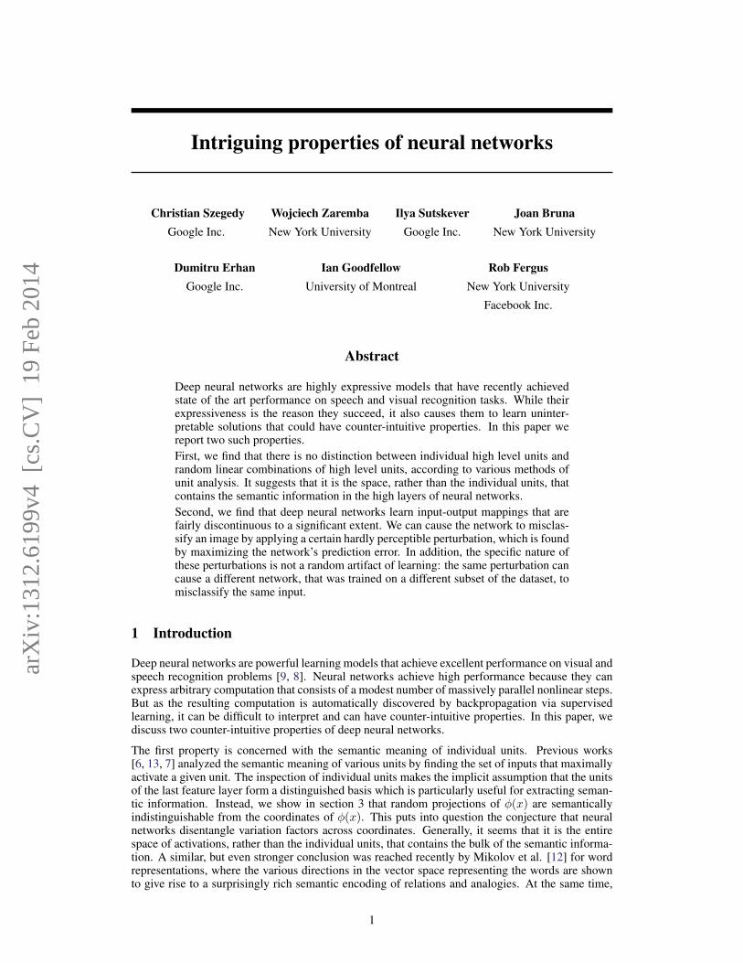
(a) Unit sensitive to lower round stroke. (b) Unit sensitive to upper round stroke, orlower straight stroke.

(c) Unit senstive to left, upper roundstroke.

(d) Unit senstive to diagonal straightstroke.

Figure 1: An MNIST experiment. The figure shows images that maximize the activation of various units(maximum stimulation in the natural basis direction). Images within each row share semantic properties.

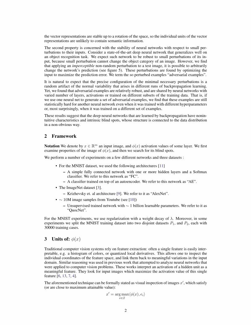
(a) Direction sensitive to upper straightstroke, or lower round stroke.

(b) Direction sensitive to lower left loop.

(c) Direction senstive to round top stroke. (d) Direction sensitive to right, upperround stroke.

Figure 2: An MNIST experiment. The figure shows images that maximize the activations in a random direction(maximum stimulation in a random basis). Images within each row share semantic properties.

where I is a held-out set of images from the data distribution that the network was not trained onand ei is the natural basis vector associated with the i-th hidden unit.

Our experiments show that any random direction v ∈ Rn gives rise to similarly interpretable se-mantic properties. More formally, we find that images x′ are semantically related to each other, formany x′ such that

x′ = arg maxx∈I

〈φ(x), v〉

This suggests that the natural basis is not better than a random basis for inspecting the propertiesof φ(x). This puts into question the notion that neural networks disentangle variation factors acrosscoordinates.

First, we evaluated the above claim using a convolutional neural network trained on MNIST. Weused the MNIST test set for I. Figure 1 shows images that maximize the activations in the naturalbasis, and Figure 2 shows images that maximize the activation in random directions. In both casesthe resulting images share many high-level similarities.

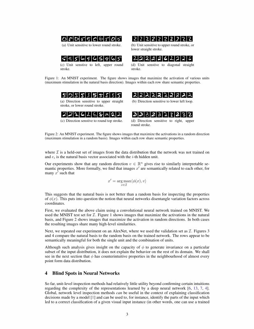
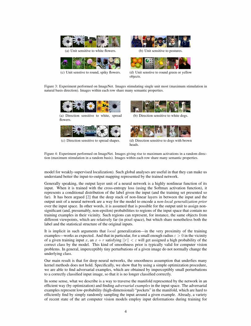
Next, we repeated our experiment on an AlexNet, where we used the validation set as I. Figures 3and 4 compare the natural basis to the random basis on the trained network. The rows appear to besemantically meaningful for both the single unit and the combination of units.

Although such analysis gives insight on the capacity of φ to generate invariance on a particularsubset of the input distribution, it does not explain the behavior on the rest of its domain. We shallsee in the next section that φ has counterintuitive properties in the neighbourhood of almost everypoint form data distribution.

4 Blind Spots in Neural Networks

So far, unit-level inspection methods had relatively little utility beyond confirming certain intuitionsregarding the complexity of the representations learned by a deep neural network [6, 13, 7, 4].Global, network level inspection methods can be useful in the context of explaining classificationdecisions made by a model [1] and can be used to, for instance, identify the parts of the input whichled to a correct classification of a given visual input instance (in other words, one can use a trained

3

(a) Unit sensitive to white flowers. (b) Unit sensitive to postures.

(c) Unit senstive to round, spiky flowers. (d) Unit senstive to round green or yellowobjects.

Figure 3: Experiment performed on ImageNet. Images stimulating single unit most (maximum stimulation innatural basis direction). Images within each row share many semantic properties.

(a) Direction sensitive to white, spreadflowers.

(b) Direction sensitive to white dogs.

(c) Direction sensitive to spread shapes. (d) Direction sensitive to dogs with brownheads.

Figure 4: Experiment performed on ImageNet. Images giving rise to maximum activations in a random direc-tion (maximum stimulation in a random basis). Images within each row share many semantic properties.

model for weakly-supervised localization). Such global analyses are useful in that they can make usunderstand better the input-to-output mapping represented by the trained network.

Generally speaking, the output layer unit of a neural network is a highly nonlinear function of itsinput. When it is trained with the cross-entropy loss (using the Softmax activation function), itrepresents a conditional distribution of the label given the input (and the training set presented sofar). It has been argued [2] that the deep stack of non-linear layers in between the input and theoutput unit of a neural network are a way for the model to encode a non-local generalization priorover the input space. In other words, it is assumed that is possible for the output unit to assign non-significant (and, presumably, non-epsilon) probabilities to regions of the input space that contain notraining examples in their vicinity. Such regions can represent, for instance, the same objects fromdifferent viewpoints, which are relatively far (in pixel space), but which share nonetheless both thelabel and the statistical structure of the original inputs.

It is implicit in such arguments that local generalization—in the very proximity of the trainingexamples—works as expected. And that in particular, for a small enough radius ε > 0 in the vicinityof a given training input x, an x + r satisfying ||r|| < ε will get assigned a high probability of thecorrect class by the model. This kind of smoothness prior is typically valid for computer visionproblems. In general, imperceptibly tiny perturbations of a given image do not normally change theunderlying class.

Our main result is that for deep neural networks, the smoothness assumption that underlies manykernel methods does not hold. Specifically, we show that by using a simple optimization procedure,we are able to find adversarial examples, which are obtained by imperceptibly small perturbationsto a correctly classified input image, so that it is no longer classified correctly.

In some sense, what we describe is a way to traverse the manifold represented by the network in anefficient way (by optimization) and finding adversarial examples in the input space. The adversarialexamples represent low-probability (high-dimensional) “pockets” in the manifold, which are hard toefficiently find by simply randomly sampling the input around a given example. Already, a varietyof recent state of the art computer vision models employ input deformations during training for

4

increasing the robustness and convergence speed of the models [9, 13]. These deformations are,however, statistically inefficient, for a given example: they are highly correlated and are drawn fromthe same distribution throughout the entire training of the model. We propose a scheme to make thisprocess adaptive in a way that exploits the model and its deficiencies in modeling the local spacearound the training data.

We make the connection with hard-negative mining explicitly, as it is close in spirit: hard-negativemining, in computer vision, consists of identifying training set examples (or portions thereof) whichare given low probabilities by the model, but which should be high probability instead, cf. [5]. Thetraining set distribution is then changed to emphasize such hard negatives and a further round ofmodel training is performed. As shall be described, the optimization problem proposed in this workcan also be used in a constructive way, similar to the hard-negative mining principle.

4.1 Formal description

We denote by f : Rm −→ {1 . . . k} a classifier mapping image pixel value vectors to a discretelabel set. We also assume that f has an associated continuous loss function denoted by lossf :Rm × {1 . . . k} −→ R+. For a given x ∈ Rm image and target label l ∈ {1 . . . k}, we aim to solvethe following box-constrained optimization problem:

• Minimize ‖r‖2 subject to:1. f(x+ r) = l

2. x+ r ∈ [0, 1]m

The minimizer r might not be unique, but we denote one such x + r for an arbitrarily chosenminimizer by D(x, l). Informally, x + r is the closest image to x classified as l by f . Obviously,D(x, f(x)) = f(x), so this task is non-trivial only if f(x) 6= l. In general, the exact computationof D(x, l) is a hard problem, so we approximate it by using a box-constrained L-BFGS. Concretely,we find an approximation ofD(x, l) by performing line-search to find the minimum c > 0 for whichthe minimizer r of the following problem satisfies f(x+ r) = l.

• Minimize c|r|+ lossf (x+ r, l) subject to x+ r ∈ [0, 1]m

This penalty function method would yield the exact solution for D(X, l) in the case of convexlosses, however neural networks are non-convex in general, so we end up with an approximation inthis case.

4.2 Experimental results

Our “minimimum distortion” function D has the following intriguing properties which we will sup-port by informal evidence and quantitative experiments in this section:

1. For all the networks we studied (MNIST, QuocNet [10], AlexNet [9]), for each sam-ple, we have always managed to generate very close, visually hard to distinguish, ad-versarial examples that are misclassified by the original network (see figure 5 andhttp://goo.gl/huaGPb for examples).

2. Cross model generalization: a relatively large fraction of examples will be misclassified bynetworks trained from scratch with different hyper-parameters (number of layers, regular-ization or initial weights).

3. Cross training-set generalization a relatively large fraction of examples will be misclassi-fied by networks trained from scratch on a disjoint training set.

The above observations suggest that adversarial examples are somewhat universal and not just theresults of overfitting to a particular model or to the specific selection of the training set. They alsosuggest that back-feeding adversarial examples to training might improve generalization of the re-sulting models. Our preliminary experiments have yielded positive evidence on MNIST to supportthis hypothesis as well: We have successfully trained a two layer 100-100-10 non-convolutional neu-ral network with a test error below 1.2% by keeping a pool of adversarial examples a random subsetof which is continuously replaced by newly generated adversarial examples and which is mixed into

5

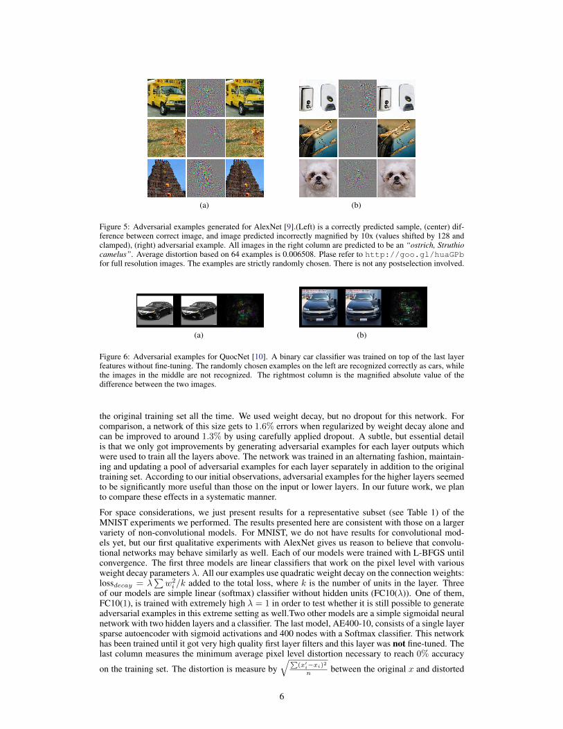
(a) (b)

Figure 5: Adversarial examples generated for AlexNet [9].(Left) is a correctly predicted sample, (center) dif-ference between correct image, and image predicted incorrectly magnified by 10x (values shifted by 128 andclamped), (right) adversarial example. All images in the right column are predicted to be an “ostrich, Struthiocamelus”. Average distortion based on 64 examples is 0.006508. Plase refer to http://goo.gl/huaGPbfor full resolution images. The examples are strictly randomly chosen. There is not any postselection involved.

(a) (b)

Figure 6: Adversarial examples for QuocNet [10]. A binary car classifier was trained on top of the last layerfeatures without fine-tuning. The randomly chosen examples on the left are recognized correctly as cars, whilethe images in the middle are not recognized. The rightmost column is the magnified absolute value of thedifference between the two images.

the original training set all the time. We used weight decay, but no dropout for this network. Forcomparison, a network of this size gets to 1.6% errors when regularized by weight decay alone andcan be improved to around 1.3% by using carefully applied dropout. A subtle, but essential detailis that we only got improvements by generating adversarial examples for each layer outputs whichwere used to train all the layers above. The network was trained in an alternating fashion, maintain-ing and updating a pool of adversarial examples for each layer separately in addition to the originaltraining set. According to our initial observations, adversarial examples for the higher layers seemedto be significantly more useful than those on the input or lower layers. In our future work, we planto compare these effects in a systematic manner.

For space considerations, we just present results for a representative subset (see Table 1) of theMNIST experiments we performed. The results presented here are consistent with those on a largervariety of non-convolutional models. For MNIST, we do not have results for convolutional mod-els yet, but our first qualitative experiments with AlexNet gives us reason to believe that convolu-tional networks may behave similarly as well. Each of our models were trained with L-BFGS untilconvergence. The first three models are linear classifiers that work on the pixel level with variousweight decay parameters λ. All our examples use quadratic weight decay on the connection weights:lossdecay = λ

∑w2i /k added to the total loss, where k is the number of units in the layer. Three

of our models are simple linear (softmax) classifier without hidden units (FC10(λ)). One of them,FC10(1), is trained with extremely high λ = 1 in order to test whether it is still possible to generateadversarial examples in this extreme setting as well.Two other models are a simple sigmoidal neuralnetwork with two hidden layers and a classifier. The last model, AE400-10, consists of a single layersparse autoencoder with sigmoid activations and 400 nodes with a Softmax classifier. This networkhas been trained until it got very high quality first layer filters and this layer was not fine-tuned. Thelast column measures the minimum average pixel level distortion necessary to reach 0% accuracy

on the training set. The distortion is measure by√∑

(x′i−xi)2

n between the original x and distorted

6

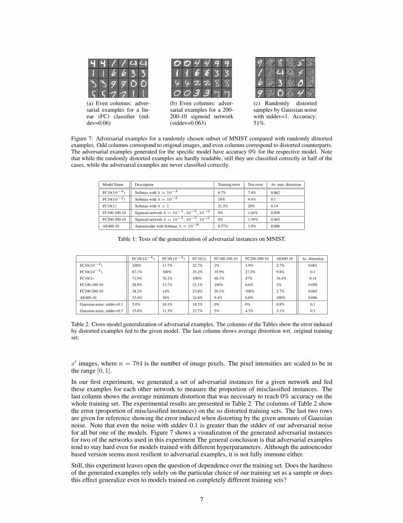
(a) Even columns: adver-sarial examples for a lin-ear (FC) classifier (std-dev=0.06)

(b) Even columns: adver-sarial examples for a 200-200-10 sigmoid network(stddev=0.063)

(c) Randomly distortedsamples by Gaussian noisewith stddev=1. Accuracy:51%.

Figure 7: Adversarial examples for a randomly chosen subset of MNIST compared with randomly distortedexamples. Odd columns correspond to original images, and even columns correspond to distorted counterparts.The adversarial examples generated for the specific model have accuracy 0% for the respective model. Notethat while the randomly distorted examples are hardly readable, still they are classified correctly in half of thecases, while the adversarial examples are never classified correctly.

Model Name Description Training error Test error Av. min. distortion

FC10(10−4) Softmax with λ = 10−4 6.7% 7.4% 0.062

FC10(10−2) Softmax with λ = 10−2 10% 9.4% 0.1

FC10(1) Softmax with λ = 1 21.2% 20% 0.14

FC100-100-10 Sigmoid network λ = 10−5, 10−5, 10−6 0% 1.64% 0.058

FC200-200-10 Sigmoid network λ = 10−5, 10−5, 10−6 0% 1.54% 0.065

AE400-10 Autoencoder with Softmax λ = 10−6 0.57% 1.9% 0.086

Table 1: Tests of the generalization of adversarial instances on MNIST.

FC10(10−4) FC10(10−2) FC10(1) FC100-100-10 FC200-200-10 AE400-10 Av. distortion

FC10(10−4) 100% 11.7% 22.7% 2% 3.9% 2.7% 0.062

FC10(10−2) 87.1% 100% 35.2% 35.9% 27.3% 9.8% 0.1

FC10(1) 71.9% 76.2% 100% 48.1% 47% 34.4% 0.14

FC100-100-10 28.9% 13.7% 21.1% 100% 6.6% 2% 0.058

FC200-200-10 38.2% 14% 23.8% 20.3% 100% 2.7% 0.065

AE400-10 23.4% 16% 24.8% 9.4% 6.6% 100% 0.086

Gaussian noise, stddev=0.1 5.0% 10.1% 18.3% 0% 0% 0.8% 0.1

Gaussian noise, stddev=0.3 15.6% 11.3% 22.7% 5% 4.3% 3.1% 0.3

Table 2: Cross-model generalization of adversarial examples. The columns of the Tables show the error inducedby distorted examples fed to the given model. The last column shows average distortion wrt. original trainingset.

x′ images, where n = 784 is the number of image pixels. The pixel intensities are scaled to be inthe range [0, 1].

In our first experiment, we generated a set of adversarial instances for a given network and fedthese examples for each other network to measure the proportion of misclassified instances. Thelast column shows the average minimum distortion that was necessary to reach 0% accuracy on thewhole training set. The experimental results are presented in Table 2. The columns of Table 2 showthe error (proportion of misclassified instances) on the so distorted training sets. The last two rowsare given for reference showing the error induced when distorting by the given amounts of Gaussiannoise. Note that even the noise with stddev 0.1 is greater than the stddev of our adversarial noisefor all but one of the models. Figure 7 shows a visualization of the generated adversarial instancesfor two of the networks used in this experiment The general conclusion is that adversarial examplestend to stay hard even for models trained with different hyperparameters. Although the autoencoderbased version seems most resilient to adversarial examples, it is not fully immune either.

Still, this experiment leaves open the question of dependence over the training set. Does the hardnessof the generated examples rely solely on the particular choice of our training set as a sample or doesthis effect generalize even to models trained on completely different training sets?

7

Model Error on P1 Error on P2 Error on Test Min Av. Distortion

FC100-100-10: 100-100-10 trained on P1 0% 2.4% 2% 0.062

FC123-456-10: 123-456-10 trained on P1 0% 2.5% 2.1% 0.059

FC100-100-10’ trained on P2 2.3% 0% 2.1% 0.058

Table 3: Models trained to study cross-training-set generalization of the generated adversarial examples. Errorspresented in Table correpond to original not-distorted data, to provide a baseline.

FC100-100-10 FC123-456-10 FC100-100-10’

Distorted for FC100-100-10 (av. stddev=0.062) 100% 26.2% 5.9%

Distorted for FC123-456-10 (av. stddev=0.059) 6.25% 100% 5.1%

Distorted for FC100-100-10’ (av. stddev=0.058) 8.2% 8.2% 100%

Gaussian noise with stddev=0.06 2.2% 2.6% 2.4%

Distorted for FC100-100-10 amplified to stddev=0.1 100% 98% 43%

Distorted for FC123-456-10 amplified to stddev=0.1 96% 100% 22%

Distorted for FC100-100-10’ amplified to stddev=0.1 27% 50% 100%

Gaussian noise with stddev=0.1 2.6% 2.8% 2.7%

Table 4: Cross-training-set generalization error rate for the set of adversarial examples generated for differentmodels. The error induced by a random distortion to the same examples is displayed in the last row.

To study cross-training-set generalization, we have partitioned the 60000 MNIST training imagesinto two parts P1 and P2 of size 30000 each and trained three non-convolutional networks withsigmoid activations on them: Two, FC100-100-10 and FC123-456-10, on P1 and FC100-100-10 onP2. The reason we trained two networks for P1 is to study the cumulative effect of changing thehypermarameters and the training sets at the same time. Models FC100-100-10 and FC100-100-10 share the same hyperparameters: both of them are 100-100-10 networks, while FC123-456-10has different number of hidden units. In this experiment, we were distorting the elements of thetest set rather than the training set. Table 3 summarizes the basic facts about these models. Afterwe generate adversarial examples with 100% error rates with minimum distortion for the test set,we feed these examples to the each of the models. The error for each model is displayed in thecorresponding column of the upper part of Table 4. In the last experiment, we magnify the effect ofour distortion by using the examples x + 0.1 x′−x

‖x′−x‖2 rather than x′. This magnifies the distortionon average by 40%, from stddev 0.06 to 0.1. The so distorted examples are fed back to each of themodels and the error rates are displayed in the lower part of Table 4. The intriguing conclusion isthat the adversarial examples remain hard for models trained even on a disjoint training set, althoughtheir effectiveness decreases considerably.

4.3 Spectral Analysis of Unstability

The previous section showed examples of deep networks resulting from purely supervised trainingwhich are unstable with respect to a peculiar form of small perturbations. Independently of theirgeneralisation properties across networks and training sets, the adversarial examples show that thereexist small additive perturbations of the input (in Euclidean sense) that produce large perturbationsat the output of the last layer. This section describes a simple procedure to measure and control theadditive stability of the network by measuring the spectrum of each rectified layer.

Mathematically, if φ(x) denotes the output of a network of K layers corresponding to input x andtrained parameters W , we write

φ(x) = φK(φK−1(. . . φ1(x;W1);W2) . . . ;WK) ,

where φk denotes the operator mapping layer k − 1 to layer k. The unstability of φ(x) can beexplained by inspecting the upper Lipschitz constant of each layer k = 1 . . .K, defined as theconstant Lk > 0 such that

∀x, r , ‖φk(x;Wk)− φk(x+ r;Wk)‖ ≤ Lk‖r‖ .

The resulting network thus satsifies ‖φ(x)− φ(x+ r)‖ ≤ L‖r‖, with L =∏Kk=1 Lk.

A half-rectified layer (both convolutional or fully connected) is defined by the mappingφk(x;Wk, bk) = max(0,Wkx+bk). Let ‖W‖ denote the operator norm ofW (i.e., its largest singu-

8

Layer Size Stride Upper bound

Conv. 1 3 × 11 × 11 × 96 4 2.75

Conv. 2 96 × 5 × 5 × 256 1 10

Conv. 3 256 × 3 × 3 × 384 1 7

Conv. 4 384 × 3 × 3 × 384 1 7.5

Conv. 5 384 × 3 × 3 × 256 1 11

FC. 1 9216 × 4096 N/A 3.12

FC. 2 4096 × 4096 N/A 4

FC. 3 4096 × 1000 N/A 4

Table 5: Frame Bounds of each rectified layer of the network from [9].

lar value). Since the non-linearity ρ(x) = max(0, x) is contractive, i.e. satisfies ‖ρ(x)−ρ(x+r)‖ ≤‖r‖ for all x, r; it follows that

‖φk(x;Wk)−φk(x+r;Wk)‖ = ‖max(0,Wkx+bk)−max(0,Wk(x+r)+bk)‖ ≤ ‖Wkr‖ ≤ ‖Wk‖‖r‖ ,and hence Lk ≤ ‖Wk‖. On the other hand, a max-pooling layer φk is contractive:

∀x , r , ‖φk(x)− φk(x+ r)‖ ≤ ‖r‖ ,since its Jacobian is a projection onto a subset of the input coordinates and hence does not expandthe gradients. Finally, if φk is a contrast-normalization layer

φk(x) =x(

ε+ ‖x‖2)γ ,

one can verify that∀x , r , ‖φk(x)− φk(x+ r)‖ ≤ ε−γ‖r‖

for γ ∈ [0.5, 1], which corresponds to most common operating regimes.

It results that a conservative measure of the unstability of the network can be obtained by simplycomputing the operator norm of each fully connected and convolutional layer. The fully connectedcase is trivial since the norm is directly given by the largest singular value of the fully connectedmatrix. Let us describe the convolutional case. If W denotes a generic 4-tensor, implementing aconvolutional layer with C input features, D output features, support N ×N and spatial stride ∆,

Wx =

{C∑c=1

xc ? wc,d(n1∆, n2∆) ; d = 1 . . . , D

},

where xc denotes the c-th input feature image, and wc,d is the spatial kernel corresponding to inputfeature c and output feature d, by applying Parseval’s formula we obtain that its operator norm isgiven by

‖W‖ = supξ∈[0,N∆−1)2

‖A(ξ)‖ , (1)

where A(ξ) is a D × (C ·∆2) matrix whose rows are

∀ d = 1 . . . D , A(ξ)d =(

∆−2wc,d(ξ + l ·N ·∆−1) ; c = 1 . . . C , l = (0 . . .∆− 1)2),

and wc,d is the 2-D Fourier transform of wc,d:

wc,d(ξ) =∑

u∈[0,N)2

wc,d(u)e−2πi(u·ξ)/N2

.

Table 5 shows the upper Lipschitz bounds computed from the ImageNet deep convolutional networkof [9], using (1). It shows that instabilities can appear as soon as in the first convolutional layer.

These results are consistent with the exsitence of blind spots constructed in the previous section,but they don’t attempt to explain why these examples generalize across different hyperparametersor training sets. We emphasize that we compute upper bounds: large bounds do not automaticallytranslate into existence of adversarial examples; however, small bounds guarantee that no such ex-amples can appear. This suggests a simple regularization of the parameters, consisting in penalizingeach upper Lipschitz bound, which might help improve the generalisation error of the networks.

9

5 Discussion

We demonstrated that deep neural networks have counter-intuitive properties both with respect tothe semantic meaning of individual units and with respect to their discontinuities. The existence ofthe adversarial negatives appears to be in contradiction with the network’s ability to achieve highgeneralization performance. Indeed, if the network can generalize well, how can it be confusedby these adversarial negatives, which are indistinguishable from the regular examples? Possibleexplanation is that the set of adversarial negatives is of extremely low probability, and thus is never(or rarely) observed in the test set, yet it is dense (much like the rational numbers), and so it is foundnear every virtually every test case. However, we don’t have a deep understanding of how oftenadversarial negatives appears, and thus this issue should be addressed in a future research.

References[1] David Baehrens, Timon Schroeter, Stefan Harmeling, Motoaki Kawanabe, Katja Hansen, and Klaus-

Robert Muller. How to explain individual classification decisions. The Journal of Machine LearningResearch, 99:1803–1831, 2010.

[2] Yoshua Bengio. Learning deep architectures for ai. Foundations and trends® in Machine Learning,2(1):1–127, 2009.

[3] Jia Deng, Wei Dong, Richard Socher, Li-Jia Li, Kai Li, and Li Fei-Fei. Imagenet: A large-scale hierarchi-cal image database. In Computer Vision and Pattern Recognition, 2009. CVPR 2009. IEEE Conferenceon, pages 248–255. IEEE, 2009.

[4] Dumitru Erhan, Yoshua Bengio, Aaron Courville, and Pascal Vincent. Visualizing higher-layer featuresof a deep network. Technical Report 1341, University of Montreal, June 2009. Also presented at theICML 2009 Workshop on Learning Feature Hierarchies, Montreal, Canada.

[5] Pedro Felzenszwalb, David McAllester, and Deva Ramanan. A discriminatively trained, multiscale, de-formable part model. In Computer Vision and Pattern Recognition, 2008. CVPR 2008. IEEE Conferenceon, pages 1–8. IEEE, 2008.

[6] Ross Girshick, Jeff Donahue, Trevor Darrell, and Jitendra Malik. Rich feature hierarchies for accurateobject detection and semantic segmentation. arXiv preprint arXiv:1311.2524, 2013.

[7] Ian Goodfellow, Quoc Le, Andrew Saxe, Honglak Lee, and Andrew Y Ng. Measuring invariances indeep networks. Advances in neural information processing systems, 22:646–654, 2009.

[8] Geoffrey E. Hinton, Li Deng, Dong Yu, George E. Dahl, Abdel rahman Mohamed, Navdeep Jaitly,Andrew Senior, Vincent Vanhoucke, Patrick Nguyen, Tara N. Sainath, and Brian Kingsbury. Deepneural networks for acoustic modeling in speech recognition: The shared views of four research groups.IEEE Signal Process. Mag., 29(6):82–97, 2012.

[9] Alex Krizhevsky, Ilya Sutskever, and Geoff Hinton. Imagenet classification with deep convolutionalneural networks. In Advances in Neural Information Processing Systems 25, pages 1106–1114, 2012.

[10] Quoc V Le, Marc’Aurelio Ranzato, Rajat Monga, Matthieu Devin, Kai Chen, Greg S Corrado, JeffDean, and Andrew Y Ng. Building high-level features using large scale unsupervised learning. arXivpreprint arXiv:1112.6209, 2011.

[11] Yann LeCun and Corinna Cortes. The mnist database of handwritten digits, 1998.

[12] Tomas Mikolov, Kai Chen, Greg Corrado, and Jeffrey Dean. Efficient estimation of word representationsin vector space. arXiv preprint arXiv:1301.3781, 2013.

[13] Matthew D Zeiler and Rob Fergus. Visualizing and understanding convolutional neural networks. arXivpreprint arXiv:1311.2901, 2013.

10