Latent Space Physics: Towards Learning theTemporal Evolution of Fluid Flow

Steffen WiewelTechnical University of Munich

wiewel@in.tum.de

Moritz BecherTechnical University of Munich

mo.becher@tum.de

Nils ThuereyTechnical University of Munich

nils.thuerey@tum.de

Abstract

We propose a method for the data-driven inference of temporal evolutions of phys-ical functions with deep learning. More specifically, we target fluid flow problems,and we propose a novel LSTM-based approach to predict the changes of the pres-sure field over time. The central challenge in this context is the high dimensional-ity of Eulerian space-time data sets. We demonstrate for the first time that dense3D+time functions of physics system can be predicted within the latent spaces ofneural networks, and we arrive at a neural-network based simulation algorithmwith significant practical speed-ups. We highlight the capabilities of our methodwith a series of complex liquid simulations, and with a set of single-phase buoy-ancy simulations. With a set of trained networks, our method is more than twoorders of magnitudes faster than a traditional pressure solver. Additionally, wepresent and discuss a series of detailed evaluations for the different componentsof our algorithm.

1 Introduction

The variables we use to describe real world physical systems often take the form of complex func-tions with high dimensionality, and we usually employ continuous models to describe how thesefunctions evolve over time. In the following work we demonstrate that it is possible to instead usedeep learning methods to infer physical functions. While such methods have been successful forsparse Lagrangian representations [2, 29, 6, 10], we will focus on high-dimensional Eulerian func-tions. More specifically, we will focus on the temporal evolution of physical functions that arisein the context of fluid flow. Fluids encompass a large and important class of materials in humanenvironments, and as such they’re particularly interesting candidates for learning models [26, 23].

The complexity of nature at human scales makes it necessary to finely discretize both space and timefor traditional numerical methods, in turn leading to a large number of degrees of freedom. Keyto our method is reducing the dimensionality of the problem using convolutional neural networks(CNNs) with respect to both time and space. Our method first learns to map the original, three-dimensional problem into a reduced latent space [17, 21, 30]. We then train a modified sequence-to-sequence network [25, 18] that learns to predict future latent space representations, which aredecoded to yield the full spatial data set for a point in time. A key advantage of CNNs in this contextis that they give us a natural way to compute accurate and highly efficient non-linear representa-tions. We will later on demonstrate that the setup for computing this reduced representation stronglyinfluences how well the prediction network can infer changes over time, and we will demonstratethe generality of our approach with several liquid and single-phase problems. The specific contribu-

Preprint. This work is supported by the ERC Starting Grant 637014.

arX

iv:1

802.

1012

3v2

[cs

.LG

] 1

5 Ju

n 20

18

tions of this work are: a hybrid LSTM-CNN architecture to predict large-scale evolutions of dense,physical 3D functions in learned latent spaces; an efficient encoder and decoder architecture, whichby means of a strong compression, yields a very fast simulation algorithm; in addition to a detailedevaluation of architectural choices and parameters.

2 Related Work and Background

While physical properties and interactions of objects have long been of interest for computer visionproblems [24, 34, 13], addressing physics problems with deep learning algorithms is an area ofparticular interest in recent years. Several works have targeted predictions of Lagrangian objects,connecting them with image data. E.g., Battaglia et al. [2] introduced a network architecture topredict two-dimensional physics, that also can be employed for predicting object motions in videos[29]. Another line of work proposed a different architecture to encode and predict two-dimensionalrigid bodies physics [6], and improved predictions for Lagrangian systems were targeted by Yuet al. [33]. Ehrhardt et al., on the other hand, use recurrent NNs to predict trajectories and theirlikelihood for balls in height-field environments [10]. While the methods above successfully predictvarious physical effects, they do not extend to the high-dimensional, Eulerian functions of materialssuch as fluids.

Fluids are ubiquitous in nature, and traditionally simulated by finding solutions to the Navier-Stokes(NS) model [11]. Its incompressible form is given by ∂u/∂t + u · ∇u = −1/ρ∇p + ν∇2u +g , ∇ · u = 0, where the most important quantities are flow velocity u and pressure p. The otherparameters ρ, ν,g denote density, kinematic viscosity and external forces, respectively. For liquids,we will assume that a signed-distance function φ is either advected with the flow, or reconstructedfrom a set of advected particles.

The sequence-to-sequence methods which we use for time prediction have so far predominantlyfound applications in the area of natural language processing, e.g., for tasks such as machine transla-tion [25]. Recurrent neural networks are popular for control tasks [18], automatic video captioning[31], or generic sequence predictions [7]. While others have studied combinations of RNNs andCNNs [8, 20], we propose a hybrid architecture to decouple the prediction task from the latent spacedimensions.

In the context of fluid simulations and machine learning for animation, a regression forest basedapproach for learning SPH interactions has been proposed by Ladicky et al. [14]. Predictions ofliquid motions for robotic control, with a particular focus on pouring motions [23] were also targeted.Other graphics works have learned flow descriptors [9], or the statistics of splash formation [28].While CNN-based methods for pressure projections were developed [26, 32], our contributions arelargely orthogonal. Instead of targeting divergence freeness for a single instance in time, our workaims for the more general task of learning the temporal evolution of physical functions, which wedemonstrate for pressure among other functions. An important difference is also that these methods,similar to other model reduction techniques [27], and POD-based methods [5] have so far has onlybeen demonstrated for single-phase simulations. For all of these methods, handling the stronglyvarying boundary conditions of liquids remains an open challenge, and we demonstrate below thatour approach works especially well for liquid dynamics.

3 Method

The central goal of our method is to predict future states of a physical function x. While previousworks often consider low dimensional Lagrangian states such as center of mass positions, x takesthe form of a dense Eulerian function in our setting. E.g., it can represent a spatio-temporal pressurefunction, or a velocity field. Thus, we consider x : R3 × R+ → Rd, with d = 1 for scalar functionssuch as pressure, and d = 3 for vectorial functions such as velocity fields. As a consequence, x hasvery high dimensionality when discretized, typically on the order of millions of spatial degrees offreedom.

Given a set of parameters θ and a functional representation ft, a trained neural network model inour case, our goal is to predict the future state x(t + h) as closely as possible given a current stateand a series of n previous states, i.e., ft

(x(t − nh), ...,x(t − h),x(t)

)≈ x(t + h). Due to the

high dimensionality of x, directly solving this formulation would be very costly. Thus, we employ

2

c5Con�3Dfe5 Con�3DT fd5

c4Con�3Dfe4 Con�3DT fd4

c3Con�3Dfe3 Con�3DT fd3

c2Con�3Dfe2 Con�3DT fd2

c1Con�3Dfe1 Con�3DT fd1

c0Con�3Dfe0 Con�3DT fd0

Input Output

1

ct

ct�1

· · ·ct�n

c LSTM d

(n+1)-iterations

fte

dn

d0

d1

· · ·do�1

Context

d LSTM Conv1D c

o-iterations

ftd (Time Convolution)

ct+1

ct+2

· · ·ct+o

Repeat (o)

1

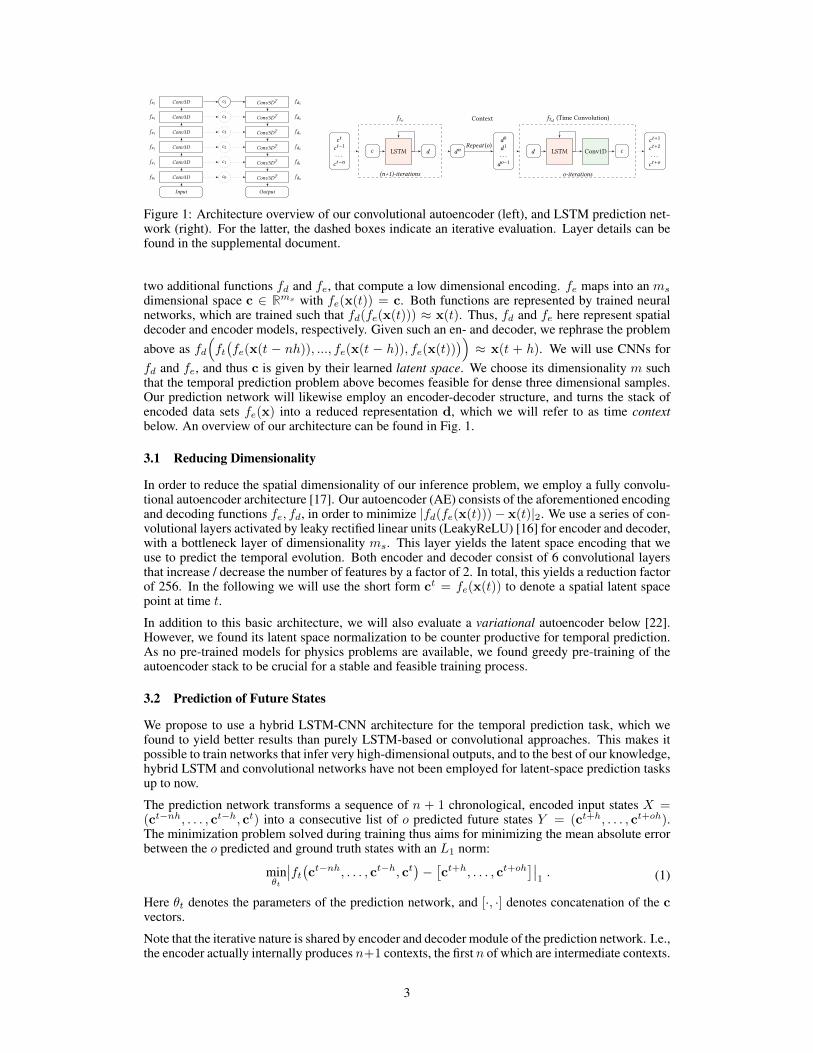
Figure 1: Architecture overview of our convolutional autoencoder (left), and LSTM prediction net-work (right). For the latter, the dashed boxes indicate an iterative evaluation. Layer details can befound in the supplemental document.

two additional functions fd and fe, that compute a low dimensional encoding. fe maps into an ms

dimensional space c ∈ Rms with fe(x(t)) = c. Both functions are represented by trained neuralnetworks, which are trained such that fd(fe(x(t))) ≈ x(t). Thus, fd and fe here represent spatialdecoder and encoder models, respectively. Given such an en- and decoder, we rephrase the problemabove as fd

(ft(fe(x(t − nh)), ..., fe(x(t − h)), fe(x(t))

))≈ x(t + h). We will use CNNs for

fd and fe, and thus c is given by their learned latent space. We choose its dimensionality m suchthat the temporal prediction problem above becomes feasible for dense three dimensional samples.Our prediction network will likewise employ an encoder-decoder structure, and turns the stack ofencoded data sets fe(x) into a reduced representation d, which we will refer to as time contextbelow. An overview of our architecture can be found in Fig. 1.

3.1 Reducing Dimensionality

In order to reduce the spatial dimensionality of our inference problem, we employ a fully convolu-tional autoencoder architecture [17]. Our autoencoder (AE) consists of the aforementioned encodingand decoding functions fe, fd, in order to minimize |fd(fe(x(t)))− x(t)|2. We use a series of con-volutional layers activated by leaky rectified linear units (LeakyReLU) [16] for encoder and decoder,with a bottleneck layer of dimensionality ms. This layer yields the latent space encoding that weuse to predict the temporal evolution. Both encoder and decoder consist of 6 convolutional layersthat increase / decrease the number of features by a factor of 2. In total, this yields a reduction factorof 256. In the following we will use the short form ct = fe(x(t)) to denote a spatial latent spacepoint at time t.

In addition to this basic architecture, we will also evaluate a variational autoencoder below [22].However, we found its latent space normalization to be counter productive for temporal prediction.As no pre-trained models for physics problems are available, we found greedy pre-training of theautoencoder stack to be crucial for a stable and feasible training process.

3.2 Prediction of Future States

We propose to use a hybrid LSTM-CNN architecture for the temporal prediction task, which wefound to yield better results than purely LSTM-based or convolutional approaches. This makes itpossible to train networks that infer very high-dimensional outputs, and to the best of our knowledge,hybrid LSTM and convolutional networks have not been employed for latent-space prediction tasksup to now.

The prediction network transforms a sequence of n + 1 chronological, encoded input states X =(ct−nh, . . . , ct−h, ct) into a consecutive list of o predicted future states Y = (ct+h, . . . , ct+oh).The minimization problem solved during training thus aims for minimizing the mean absolute errorbetween the o predicted and ground truth states with an L1 norm:

minθt

∣∣ft(ct−nh, . . . , ct−h, ct)− [ct+h, . . . , ct+oh]∣∣1 . (1)

Here θt denotes the parameters of the prediction network, and [·, ·] denotes concatenation of the cvectors.

Note that the iterative nature is shared by encoder and decoder module of the prediction network. I.e.,the encoder actually internally produces n+1 contexts, the first n of which are intermediate contexts.

3

Surface

u

pt

ps

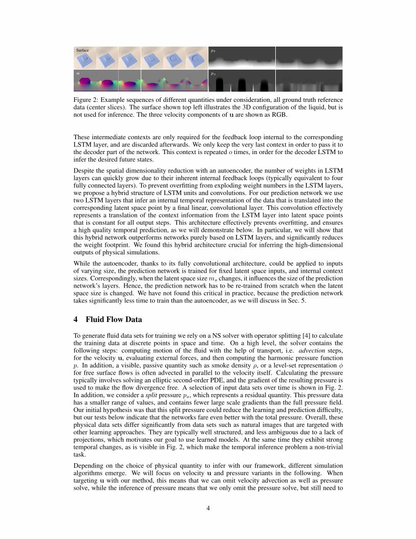
Figure 2: Example sequences of different quantities under consideration, all ground truth referencedata (center slices). The surface shown top left illustrates the 3D configuration of the liquid, but isnot used for inference. The three velocity components of u are shown as RGB.

These intermediate contexts are only required for the feedback loop internal to the correspondingLSTM layer, and are discarded afterwards. We only keep the very last context in order to pass it tothe decoder part of the network. This context is repeated o times, in order for the decoder LSTM toinfer the desired future states.

Despite the spatial dimensionality reduction with an autoencoder, the number of weights in LSTMlayers can quickly grow due to their inherent internal feedback loops (typically equivalent to fourfully connected layers). To prevent overfitting from exploding weight numbers in the LSTM layers,we propose a hybrid structure of LSTM units and convolutions. For our prediction network we usetwo LSTM layers that infer an internal temporal representation of the data that is translated into thecorresponding latent space point by a final linear, convolutional layer. This convolution effectivelyrepresents a translation of the context information from the LSTM layer into latent space pointsthat is constant for all output steps. This architecture effectively prevents overfitting, and ensuresa high quality temporal prediction, as we will demonstrate below. In particular, we will show thatthis hybrid network outperforms networks purely based on LSTM layers, and significantly reducesthe weight footprint. We found this hybrid architecture crucial for inferring the high-dimensionaloutputs of physical simulations.

While the autoencoder, thanks to its fully convolutional architecture, could be applied to inputsof varying size, the prediction network is trained for fixed latent space inputs, and internal contextsizes. Correspondingly, when the latent space sizems changes, it influences the size of the predictionnetwork’s layers. Hence, the prediction network has to be re-trained from scratch when the latentspace size is changed. We have not found this critical in practice, because the prediction networktakes significantly less time to train than the autoencoder, as we will discuss in Sec. 5.

4 Fluid Flow Data

To generate fluid data sets for training we rely on a NS solver with operator splitting [4] to calculatethe training data at discrete points in space and time. On a high level, the solver contains thefollowing steps: computing motion of the fluid with the help of transport, i.e. advection steps,for the velocity u, evaluating external forces, and then computing the harmonic pressure functionp. In addition, a visible, passive quantity such as smoke density ρ, or a level-set representation φfor free surface flows is often advected in parallel to the velocity itself. Calculating the pressuretypically involves solving an elliptic second-order PDE, and the gradient of the resulting pressure isused to make the flow divergence free. A selection of input data sets over time is shown in Fig. 2.In addition, we consider a split pressure ps, which represents a residual quantity. This pressure datahas a smaller range of values, and contains fewer large scale gradients than the full pressure field.Our initial hypothesis was that this split pressure could reduce the learning and prediction difficulty,but our tests below indicate that the networks fare even better with the total pressure. Overall, thesephysical data sets differ significantly from data sets such as natural images that are targeted withother learning approaches. They are typically well structured, and less ambiguous due to a lack ofprojections, which motivates our goal to use learned models. At the same time they exhibit strongtemporal changes, as is visible in Fig. 2, which make the temporal inference problem a non-trivialtask.

Depending on the choice of physical quantity to infer with our framework, different simulationalgorithms emerge. We will focus on velocity u and pressure variants in the following. Whentargeting u with our method, this means that we can omit velocity advection as well as pressuresolve, while the inference of pressure means that we only omit the pressure solve, but still need to

4

Reference (GT) pt ps VAE ps u

Figure 3: Different simulation fields en-/decoded with a trained AE, without the time prediction.The velocity significantly differs from the reference (i.e., ground truth data, left), while all threepressure variants fare well with average PSNRs of 64.81, 64.55, and 62.45 (f.l.t.r.).

perform advection and velocity correction with the pressure gradient. While this pressure inferencerequires more computations, the pressure solve is typically the most time consuming part with asuper-linear complexity, and as such both options have comparable runtimes. When predicting thepressure field, we also use a boundary condition alignment step for the free surface [1]. It takes theform of three Jacobi iterations in a narrow band at the liquid surface in order to align the Dirichletboundary conditions with the current position of the interface. This step is important for liquids, asit incorporates small scale dynamics, leaving the large-scale dynamics to a learned model.

A variant for both of these cases is to only rely on the network prediction for a limited time interval ofip time steps, and then perform a single full simulation step. I.e., for ip = 0 the network is not used atall, while ip =∞ is identical to the full network prediction described in the previous paragraph. Wewill investigate prediction intervals on the order of 4 to 14 steps. This simulation variant representsa joint numerical time integration and network prediction, that can have advantages to prevent driftfrom the learned predictions. We will denote such versions as interval predictions below.

4.1 Data Sets

To demonstrate that our approach is applicable to a wide range of physics phenomena, we willshow results with three different 3D data sets in the following. To ensure a sufficient amount ofvariance with respect to physical motions and dynamics, we use randomized simulation setups. Wetarget scenes with high complexity, i.e., strong visible splashes and vortices, and large CFL numbers(typically around 2-3). For each of our data sets, we generate ns scenes of different initial conditions,for which we discard the first nw time steps, as these typically contain small and regular, and henceless representative dynamics. Afterwards, we store a fixed number of nt time steps as training data,resulting in a final size of nsnt spatial data sets. Each data set content is normalized to the range of[-1,1].

Two of the three data sets contain liquids, while the additional one targets smoke simulations. Theliquid data sets with spatial resolutions of 643 and 1283 contain randomized sloshing waves andcolliding bodies of liquid. For the 1283 data set we additionally include complex geometries for theinitial liquid bodies, yielding a larger range of behavior. These data sets will be denoted as liquid64and liquid128, respectively. In addition, we consider a data set containing single-phase flows withbuoyant smoke which we will denote as smoke128. We place 4 to 10 inflow regions into an emptydomain at rest, and then simulate the resulting plumes of hot smoke. As all setups are invariant w.r.t.rotations around the axis of gravity (Y in our setups), we augment the data sets by mirroring alongXY and YZ. This leads to sizes of the data sets from 80k to 400k entries, and the 1283 data sets havea total size of 671GB. Examples from all data sets are given in the supplemental document.

5 Evaluation and Training

In the following we will evaluate the different options discussed in the previous section with respectto their prediction accuracies. In terms of evaluation metrics, we will use PSNR as a baseline metric,in addition to a surface-based Hausdorff distance1 in order to more accurately compare the position

1 More specifically, given two signed distance functions φr, φp representing reference and predicted sur-faces, we compute the surface error as eh = max(1/|Sp|

∑p1∈Sp

φr(p1), 1/|Sr|∑

p2∈Srφp(p2))/∆x.

5

(a) AE only, different phys.quantities

(b) Full alg., phys. quantities,ip =∞.

(c) Full alg., phys. quantities,ip = 14.

(d) Pred. intervals ip for pt,full alg.

(e) AE only, pressure PSNRvalues

(f) Full alg, pressure PSNR,with ip =∞.

(g) Architecture variants, ptPSNR values ip =∞, o = 5.

(h) Different output steps forpt, varied ip

Figure 4: Error graphs over time for 100 steps, averaged over ten liquid64 simulations. Note thato = 1 in Fig. 4h corresponds to Fig. 4d, and is repeated for comparison.

of the liquid interface [12, 15]. Unless otherwise noted, the error measurements start after 50 stepsof simulation, and are averaged for ten test scenes from the liquid64 setup.

Spatial Encoding We first evaluate the accuracy of only the spatial encoding, i.e., the autoencodernetwork in conjunction with a numerical time integration scheme. At the end of a fluid solving timestep, we encode the physical variable x under consideration with c = fe(x), and then restore itfrom its latent space representation x′ = fd(c). In the following, we will compare flow velocity u,total pressure pt, and split pressure ps, all with a latent space size of ms = 1024. We train a newautoencoder for each quantity, and we additionally consider a variational autoencoder for the splitpressure. Training times for the autoencoders were two days on average, including pre-training. Totrain the different autoencoders, we use 6 epochs of pretraining and 25 epochs of training using anAdam optimizer, with a learning rate of 0.001 and L2 regularization with strength 0.005. For trainingwe used 80% of the data set, 10% for validation during training, and another 10% for testing.

Fig. 4a and Fig. 4e show error measurements averaged for 10 simulations from the test data set.Given the complexity of the data, especially the total pressure variant exhibits very good represen-tational capabilities with an average PSNR value of 69.14. On the other hand, the velocity encodingintroduces significantly larger errors in Fig. 4e. It is likewise obvious that neither the latent spacenormalization of the VAE, nor the split pressure data increase the reconstruction accuracy. A visualcomparison of these results can be found in Fig. 3.

Temporal Prediction Next, we evaluate reconstruction quality when including the temporal pre-diction network. Thus, now a quantity x′ is inferred based on a series of previous latent space points.For the following tests, our prediction model uses a history of 6, and infers the next time step, thuso = 1, with a latent space size ms = 1024. For a resolution of 643 the fully recurrent networkcontains 700, and 1500 units for the first and second LSTM layer of Fig. 1, respectively. Hence, dhas a dimensionality of 700 for this setup. The two LSTM layers are followed by a convolutionallayer targeting the ms latent space dimensions for our hybrid architecture, or alternatively anotherLSTM layer of size ms for the fully recurrent version. A dropout rate of 1.32 ·10−2 with a recurrentdropout of 0.385, and a learning rate of 1.26 · 10−4 with a decay factor of 3.34 · 10−4 were used forall trainings of the prediction network. Training was run for 50 epochs with RMSProp, with 319600training samples in each epoch, taking 2 hours, on average. Hyperparameters were selected with abroad search.

6

a)

GT

AE

LSTM

b)

GT

AE

LSTM

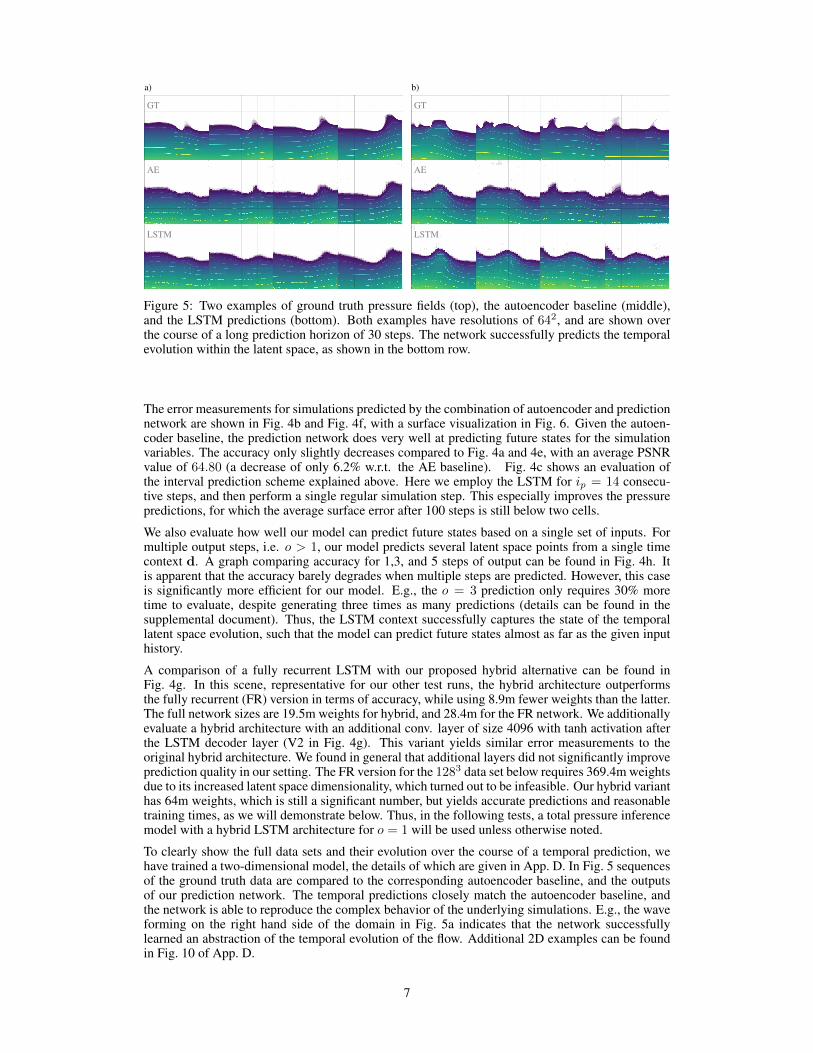
Figure 5: Two examples of ground truth pressure fields (top), the autoencoder baseline (middle),and the LSTM predictions (bottom). Both examples have resolutions of 642, and are shown overthe course of a long prediction horizon of 30 steps. The network successfully predicts the temporalevolution within the latent space, as shown in the bottom row.

The error measurements for simulations predicted by the combination of autoencoder and predictionnetwork are shown in Fig. 4b and Fig. 4f, with a surface visualization in Fig. 6. Given the autoen-coder baseline, the prediction network does very well at predicting future states for the simulationvariables. The accuracy only slightly decreases compared to Fig. 4a and 4e, with an average PSNRvalue of 64.80 (a decrease of only 6.2% w.r.t. the AE baseline). Fig. 4c shows an evaluation ofthe interval prediction scheme explained above. Here we employ the LSTM for ip = 14 consecu-tive steps, and then perform a single regular simulation step. This especially improves the pressurepredictions, for which the average surface error after 100 steps is still below two cells.

We also evaluate how well our model can predict future states based on a single set of inputs. Formultiple output steps, i.e. o > 1, our model predicts several latent space points from a single timecontext d. A graph comparing accuracy for 1,3, and 5 steps of output can be found in Fig. 4h. Itis apparent that the accuracy barely degrades when multiple steps are predicted. However, this caseis significantly more efficient for our model. E.g., the o = 3 prediction only requires 30% moretime to evaluate, despite generating three times as many predictions (details can be found in thesupplemental document). Thus, the LSTM context successfully captures the state of the temporallatent space evolution, such that the model can predict future states almost as far as the given inputhistory.

A comparison of a fully recurrent LSTM with our proposed hybrid alternative can be found inFig. 4g. In this scene, representative for our other test runs, the hybrid architecture outperformsthe fully recurrent (FR) version in terms of accuracy, while using 8.9m fewer weights than the latter.The full network sizes are 19.5m weights for hybrid, and 28.4m for the FR network. We additionallyevaluate a hybrid architecture with an additional conv. layer of size 4096 with tanh activation afterthe LSTM decoder layer (V2 in Fig. 4g). This variant yields similar error measurements to theoriginal hybrid architecture. We found in general that additional layers did not significantly improveprediction quality in our setting. The FR version for the 1283 data set below requires 369.4m weightsdue to its increased latent space dimensionality, which turned out to be infeasible. Our hybrid varianthas 64m weights, which is still a significant number, but yields accurate predictions and reasonabletraining times, as we will demonstrate below. Thus, in the following tests, a total pressure inferencemodel with a hybrid LSTM architecture for o = 1 will be used unless otherwise noted.

To clearly show the full data sets and their evolution over the course of a temporal prediction, wehave trained a two-dimensional model, the details of which are given in App. D. In Fig. 5 sequencesof the ground truth data are compared to the corresponding autoencoder baseline, and the outputsof our prediction network. The temporal predictions closely match the autoencoder baseline, andthe network is able to reproduce the complex behavior of the underlying simulations. E.g., the waveforming on the right hand side of the domain in Fig. 5a indicates that the network successfullylearned an abstraction of the temporal evolution of the flow. Additional 2D examples can be foundin Fig. 10 of App. D.

7

6 Results

We now apply our model to the additional data sets with higher spatial resolutions, and we will high-light the resulting performance in more detail. First, we demonstrate how our method performs onthe liquid128 data set, with its eight times larger number of degrees of freedom per volume. Corre-spondingly, we use a latent space size ofms = 8192, and a prediction network with LSTM layers ofsize 1000 and 1500. Despite the additional complexity of this data set, our method successfully pre-dicts the temporal evolution of the pressure fields, with an average PSNR of 44.8. The lower valuecompared to the 643 case is most likely caused by the higher intricacy of the 1283 data. Fig. 7a)shows a more realistically rendered simulation for ip = 4. This setup contains a shape that was notpart of any training data simulations. Our model successfully handles this new configuration, as wellas other situations shown in the accompanying video. This indicates that our model generalizes toa broad class of physical behavior. To evaluate long term stability, we have additionally simulateda scene for 650 time steps which successfully comes to rest. This simulation and additional scenescan be found in the supplemental video.

GT pt ps VAE ps u

Figure 6: Liquid surfaces predicted by different models for 40 steps with ip =∞. While the velocityversion (green) leads to large errors in surface position, all three pressure versions closely capturethe large scale motions. On smaller scales, both ps variants introduce artifacts.

A trained model for the smoke128 data set can be seen in Fig. 7b). Despite the significantly differentphysics, our approach successfully predicts the evolution and motion of the vortex structures. How-ever, we noticed a tendency to underestimate pressure values, and to reduce small-scale motions.Thus, while our model successfully captures a significant part of the underlying physics, there is aclear room for improvement for this data set.

Our method also leads to significant speed-ups compared to regular pressure solvers, especially forlarger volumes. Pressure inference for a 1283 volume takes 9.5ms, on average, which represents a155× speed-up compared to a parallelized state-of-the-art iterative solver [4]. While the latter yieldsa higher overall accuracy, and runs on a CPU instead of a GPU, it also represents a highly optimizednumerical method. We believe the speed up of our LSTM version indicates a huge potential for veryfast physics solvers with learned models.

Discussion and Limitations While we have shown that our approach leads to large speed-upsand robust simulations for a significant variety of fluid scenes, it also has its set of limitations, andthere are numerous interesting extensions for future work. First, our LSTM at the moment stronglyrelies on the AE, which primarily encodes large scale scale dynamics, while small scale dynamicsare integrated by the free surface treatment [1]. Thus, improving the AE network is important toimprove the quality of the temporal predictions. Our experiments show that larger data sets shoulddirectly translate into improved predictions. This is especially important for the latent space data set,which cannot be easily augmented. Interestingly, our method arrives at a simulation algorithm that

a) t = 0 t = 100 t = 200 t = 300 b) t = 20 t = 53 t = 86

Figure 7: a) A test simulation with our liquid128 model. The initial anvil shape was not part of thetraining data, but our model successfully generalizes to unseen shapes such as this one. b) A testsimulation configuration for our smoke128 model.

8

could not be formulated with traditional models: no formulation exists that allows for the calculationof a future pressure field only based on a history of previous fields.

7 Conclusion

With this work we arrive at three important conclusions: first, deep neural network architectures cansuccessfully predict the temporal evolution of dense physical functions, second, learned latent spacesin conjunction with LSTM-CNN hybrids are highly suitable for this task, and third, they can yieldvery significant increases in simulation performance. We believe that our work represents an im-portant first step towards deep-learning powered simulation algorithms. There are numerous, highlyinteresting avenues for future research, ranging from improving the accuracy of the predictions, overperformance considerations, to using such physics predictions as priors for inverse problems.

References[1] R. Ando, N. Thuerey, and C. Wojtan. A dimension-reduced pressure solver for liquid simulations. Comp.

Grap. Forum, 34(2):10, 2015.

[2] P. Battaglia, R. Pascanu, M. Lai, D. J. Rezende, et al. Interaction networks for learning about objects,relations and physics. In Advances in Neural Information Processing Systems, pages 4502–4510, 2016.

[3] Y. Bengio, P. Lamblin, D. Popovici, and H. Larochelle. Greedy layer-wise training of deep networks. InAdvances in neural information processing systems, pages 153–160, 2007.

[4] R. Bridson. Fluid Simulation for Computer Graphics. CRC Press, 2015.

[5] T. Bui-Thanh, M. Damodaran, and K. E. Willcox. Aerodynamic data reconstruction and inverse designusing proper orthogonal decomposition. AIAA journal, 42(8):1505–1516, 2004.

[6] M. B. Chang, T. Ullman, A. Torralba, and J. B. Tenenbaum. A compositional object-based approach tolearning physical dynamics. arXiv:1612.00341, 2016.

[7] Z. Che, S. Purushotham, K. Cho, D. Sontag, and Y. Liu. Recurrent neural networks for multivariate timeseries with missing values. Scientific reports, 8(1):6085, 2018.

[8] J. Chen, L. Yang, Y. Zhang, M. Alber, and D. Z. Chen. Combining fully convolutional and recurrentneural networks for 3d biomedical image segmentation. In Advances in Neural Information ProcessingSystems, pages 3036–3044, 2016.

[9] M. Chu and N. Thuerey. Data-driven synthesis of smoke flows with CNN-based feature descriptors. ACMTrans. Graph., 36(4)(69), 2017.

[10] S. Ehrhardt, A. Monszpart, N. J. Mitra, and A. Vedaldi. Learning a physical long-term predictor.arXiv:1703.00247, 2017.

[11] J. H. Ferziger and M. Peric. Computational methods for fluid dynamics. Springer Science & BusinessMedia, 2012.

[12] D. P. Huttenlocher, G. A. Klanderman, and W. J. Rucklidge. Comparing images using the hausdorffdistance. IEEE Transactions on pattern analysis and machine intelligence, 15(9):850–863, 1993.

[13] Z. Jia, A. C. Gallagher, A. Saxena, and T. Chen. 3d reasoning from blocks to stability. IEEE transactionson pattern analysis and machine intelligence, 37(5):905–918, 2015.

[14] L. Ladicky, S. Jeong, B. Solenthaler, M. Pollefeys, and M. Gross. Data-driven fluid simulations usingregression forests. ACM Trans. Graph., 34(6):199, 2015.

[15] Y. Li, A. Dai, L. Guibas, and M. Nießner. Database-assisted object retrieval for real-time 3d reconstruc-tion. In Computer Graphics Forum, volume 34(2), pages 435–446. Wiley Online Library, 2015.

[16] A. L. Maas, A. Y. Hannun, and A. Y. Ng. Rectifier nonlinearities improve neural network acoustic models.2013.

[17] J. Masci, U. Meier, D. Ciresan, and J. Schmidhuber. Stacked convolutional auto-encoders for hierarchicalfeature extraction. Artificial Neural Networks and Machine Learning–ICANN 2011, pages 52–59, 2011.

[18] V. Mnih, A. P. Badia, M. Mirza, A. Graves, T. Lillicrap, T. Harley, D. Silver, and K. Kavukcuoglu. Asyn-chronous methods for deep reinforcement learning. In International Conference on Machine Learning,pages 1928–1937, 2016.

[19] A. Odena, V. Dumoulin, and C. Olah. Deconvolution and checkerboard artifacts. Distill, 2016.

[20] D. Quang and X. Xie. Danq: a hybrid convolutional and recurrent deep neural network for quantifyingthe function of dna sequences. Nucleic acids research, 44(11):e107–e107, 2016.

9

[21] A. Radford, L. Metz, and S. Chintala. Unsupervised representation learning with deep convolutionalgenerative adversarial networks. Proc. ICLR, 2016.

[22] D. J. Rezende, S. Mohamed, and D. Wierstra. Stochastic backpropagation and approximate inference indeep generative models. In Proceedings of the 31st International Conference on International Conferenceon Machine Learning - Volume 32, ICML’14, pages II–1278–II–1286. JMLR.org, 2014.

[23] C. Schenck and D. Fox. Reasoning about liquids via closed-loop simulation. arXiv:1703.01656, 2017.

[24] J. Schulman, A. Lee, J. Ho, and P. Abbeel. Tracking deformable objects with point clouds. In Roboticsand Automation (ICRA), 2013 IEEE International Conference on, pages 1130–1137. IEEE, 2013.

[25] I. Sutskever, O. Vinyals, and Q. V. Le. Sequence to sequence learning with neural networks. In Pro-ceedings of the 27th International Conference on Neural Information Processing Systems - Volume 2,NIPS’14, pages 3104–3112, Cambridge, MA, USA, 2014. MIT Press.

[26] J. Tompson, K. Schlachter, P. Sprechmann, and K. Perlin. Accelerating eulerian fluid simulation withconvolutional networks. arXiv: 1607.03597, 2016.

[27] A. Treuille, A. Lewis, and Z. Popovic. Model reduction for real-time fluids. ACM Trans. Graph.,25(3):826–834, July 2006.

[28] K. Um, X. Hu, and N. Thuerey. Splash modeling with neural networks. arXiv:1704.04456, 2017.

[29] N. Watters, D. Zoran, T. Weber, P. Battaglia, R. Pascanu, and A. Tacchetti. Visual interaction networks.In Advances in Neural Information Processing Systems, pages 4540–4548, 2017.

[30] J. Wu, C. Zhang, T. Xue, B. Freeman, and J. Tenenbaum. Learning a probabilistic latent space of objectshapes via 3d generative-adversarial modeling. In Advances in Neural Information Processing Systems,pages 82–90, 2016.

[31] J. Xu, T. Yao, Y. Zhang, and T. Mei. Learning multimodal attention lstm networks for video captioning.In Proceedings of the 2017 ACM on Multimedia Conference, pages 537–545. ACM, 2017.

[32] C. Yang, X. Yang, and X. Xiao. Data-driven projection method in fluid simulation. Computer Animationand Virtual Worlds, 27(3-4):415–424, 2016.

[33] R. Yu, S. Zheng, A. Anandkumar, and Y. Yue. Long-term forecasting using tensor-train rnns. arXivpreprint arXiv:1711.00073, 2017.

[34] B. Zheng, Y. Zhao, C. Y. Joey, K. Ikeuchi, and S.-C. Zhu. Detecting potential falling objects by inferringhuman action and natural disturbance. In Robotics and Automation (ICRA), 2014 IEEE InternationalConference on, pages 3417–3424. IEEE, 2014.

10

Supplemental Document for Latent Space Physics:Towards Learning the Temporal Evolution of Fluid Flow

A Autoencoder Details

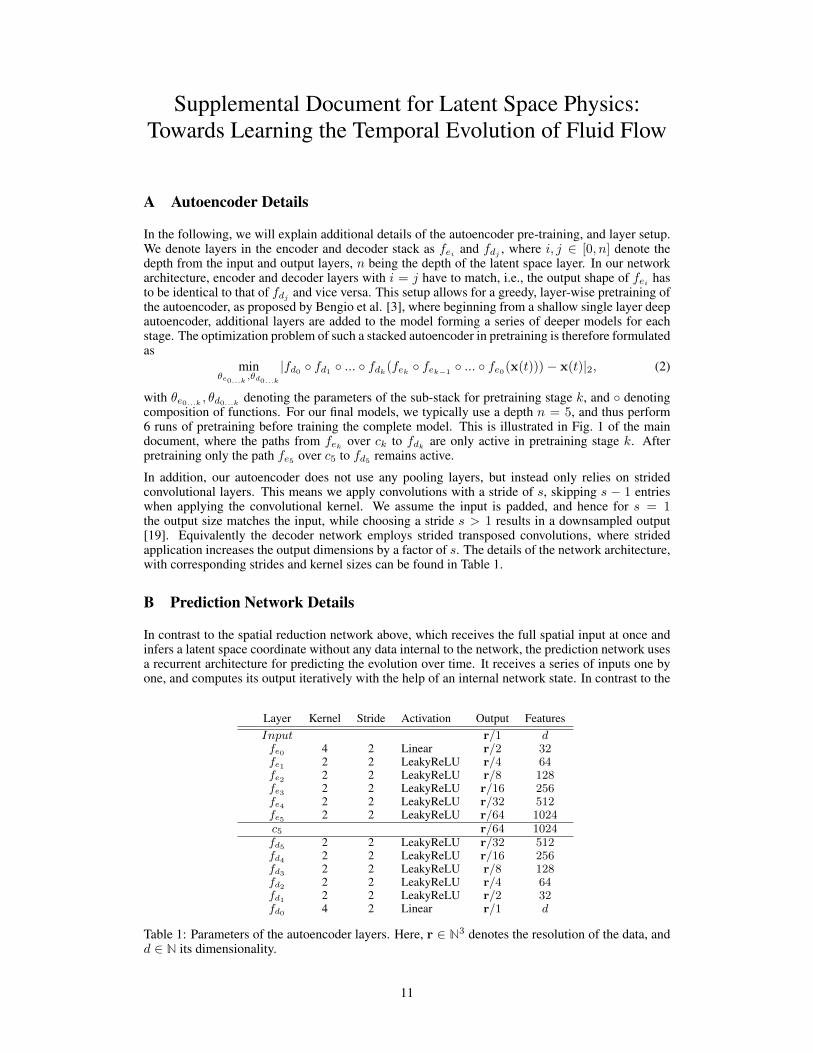
In the following, we will explain additional details of the autoencoder pre-training, and layer setup.We denote layers in the encoder and decoder stack as fei and fdj , where i, j ∈ [0, n] denote thedepth from the input and output layers, n being the depth of the latent space layer. In our networkarchitecture, encoder and decoder layers with i = j have to match, i.e., the output shape of fei hasto be identical to that of fdj and vice versa. This setup allows for a greedy, layer-wise pretraining ofthe autoencoder, as proposed by Bengio et al. [3], where beginning from a shallow single layer deepautoencoder, additional layers are added to the model forming a series of deeper models for eachstage. The optimization problem of such a stacked autoencoder in pretraining is therefore formulatedas

minθe0...k ,θd0...k

|fd0 ◦ fd1 ◦ ... ◦ fdk(fek ◦ fek−1◦ ... ◦ fe0(x(t)))− x(t)|2, (2)

with θe0...k , θd0...k denoting the parameters of the sub-stack for pretraining stage k, and ◦ denotingcomposition of functions. For our final models, we typically use a depth n = 5, and thus perform6 runs of pretraining before training the complete model. This is illustrated in Fig. 1 of the maindocument, where the paths from fek over ck to fdk are only active in pretraining stage k. Afterpretraining only the path fe5 over c5 to fd5 remains active.

In addition, our autoencoder does not use any pooling layers, but instead only relies on stridedconvolutional layers. This means we apply convolutions with a stride of s, skipping s − 1 entrieswhen applying the convolutional kernel. We assume the input is padded, and hence for s = 1the output size matches the input, while choosing a stride s > 1 results in a downsampled output[19]. Equivalently the decoder network employs strided transposed convolutions, where stridedapplication increases the output dimensions by a factor of s. The details of the network architecture,with corresponding strides and kernel sizes can be found in Table 1.

B Prediction Network Details

In contrast to the spatial reduction network above, which receives the full spatial input at once andinfers a latent space coordinate without any data internal to the network, the prediction network usesa recurrent architecture for predicting the evolution over time. It receives a series of inputs one byone, and computes its output iteratively with the help of an internal network state. In contrast to the

Layer Kernel Stride Activation Output FeaturesInput r/1 dfe0 4 2 Linear r/2 32fe1 2 2 LeakyReLU r/4 64fe2 2 2 LeakyReLU r/8 128fe3 2 2 LeakyReLU r/16 256fe4 2 2 LeakyReLU r/32 512fe5 2 2 LeakyReLU r/64 1024c5 r/64 1024fd5 2 2 LeakyReLU r/32 512fd4 2 2 LeakyReLU r/16 256fd3 2 2 LeakyReLU r/8 128fd2 2 2 LeakyReLU r/4 64fd1 2 2 LeakyReLU r/2 32fd0 4 2 Linear r/1 d

Table 1: Parameters of the autoencoder layers. Here, r ∈ N3 denotes the resolution of the data, andd ∈ N its dimensionality.

11

d0

d1

...do−1

d LSTM LSTM c

o-iterations

ftd (Fully Recurrent)

ct+1

ct+2

...ct+o

Figure 8: Alternative Sequence to Sequence Decoder (Fully Recurrent)

spatial reduction, which very heavily relies on convolutions, we cannot employ similar convolutionsfor the time data sets. While it is a valid assumption that each entry of a latent space vector c variessmoothly in time, the order of the entries is arbitrary and we cannot make any assumptions aboutlocal neighborhoods within c. As such, convolving c with a filter along the latent space entriestypically does not give meaningful results. Instead, our prediction network will use convolutions totranslate the LSTM state into the latent space, in addition to fully connected layers of LSTM units.

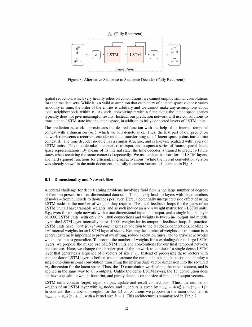
The prediction network approximates the desired function with the help of an internal temporalcontext with a dimension (mt), which we will denote as d. Thus, the first part of our predictionnetwork represents a recurrent encoder module, transforming n + 1 latent space points into a timecontext d. The time decoder module has a similar structure, and is likewise realized with layers ofLSTM units. This module takes a context d as input, and outputs a series of future, spatial latentspace representations. By means of its internal state, the time decoder is trained to predict o futurestates when receiving the same context d repeatedly. We use tanh activations for all LSTM layers,and hard sigmoid functions for efficient, internal activations. While the hybrid convolution versionwas already shown in the main document, the fully recurrent variant is illustrated in Fig. 8.

B.1 Dimensionality and Network Size

A central challenge for deep learning problems involving fluid flow is the large number of degreesof freedom present in three-dimensional data sets. This quickly leads to layers with large numbersof nodes – from hundreds to thousands per layer. Here, a potentially unexpected side effect of usingLSTM nodes is the number of weights they require. The local feedback loops for the gates of anLSTM unit all have trainable weights, and as such induce an n×n weight matrix for n LSTM units.E.g., even for a simple network with a one dimensional input and output, and a single hidden layerof 1000 LSTM units, with only 2 × 1000 connections and weights between in-, output and middlelayer, the LSTM layer internally stores 10002 weights for its temporal feedback loop. In practice,LSTM units have input, forget and output gates in addition to the feedback connections, leading to4n2 internal weights for an LSTM layer of size n. Keeping the number of weights at a minimum is ingeneral extremely important to prevent overfitting, reduce execution times, and to arrive at networkswhich are able to generalize. To prevent the number of weights from exploding due to large LSTMlayers, we propose the mixed use of LSTM units and convolutions for our final temporal networkarchitecture. Here, we change the decoder part of the network to consist of a single dense LSTMlayer that generates a sequence of o vectors of size mtd . Instead of processing these vectors withanother dense LSTM layer as before, we concatenate the outputs into a single tensor, and employ asingle one-dimensional convolution translating the intermediate vector dimension into the requiredms dimension for the latent space. Thus, the 1D convolution works along the vector content, and isapplied in the same way to all o outputs. Unlike the dense LSTM layers, the 1D convolution doesnot have a quadratic weight footprint, and purely depends on the size of input and output vectors.

LSTM units contain forget, input, output, update and result connections. Thus, the number ofweights of an LSTM layer with no nodes, and ni inputs is given by nlstm = 4(n2o + no(ni + 1)).In contrast, the number of weights for the 1D convolutions we propose in the main document isnconv-1d = nok(ni + 1), with a kernel size k = 1. This architecture is summarized in Table 2.

12

Layer (Type) Activation Output Shape

fteInput (n+ 1, ms)LSTM tanh (mt)

Context Repeat (o, mt)

ftdLSTM tanh (o, mtd )Conv1D linear (o, ms)

Table 2: Recurrent prediction network with hybrid architecture (Main doc., Fig. 1)

Layer (Type) Activation Output Shape

fteInput (n+ 1, ms)LSTM tanh (mt)

Context Repeat (o, mt)

ftdLSTM tanh (o, mtd )LSTM tanh (o, ms)

Table 3: Fully recurrent network architecture (Fig. 8)

C Pressure Splitting

Although our final models directly infer the full pressure field, we have experimented with a pressuresplitting approach, under the hypothesis that this could simplify the inference problem for the LSTM.This paragraphs explains details of our pressure splitting, as several of our tests in the main documentuse this data. Assuming a fluid at rest on a ground with height zg , a hydrostatic pressure ps for cellat height z, can be calculated as ps(z) = p(z0)+

1A

∫ z0z

∫∫Agρ(h) dxdy dh, with z0, p0,A denoting

surface height, surface pressure, and cell area, respectively. As density and gravity can be treated asconstant in our setting, this further simplifies to ps = ρg(z − z0). While this form can be evaluatedvery efficiently, it has the drawback that it is only valid for fluids in hydrostatic equilibrium, andtypically cannot be used for dynamic simulations in 3D.

Given a data-driven method to predict pressure fields, we can incorporate the hydrostatic pressureinto a 3D liquid simulation by decomposing the regular pressure field into hydrostatic and dynamiccomponents p = ps+pd, such that our autoencoder separately receives and encodes the two fields psand pd. With this split pressure, the autoencoder could potentially put more emphasis on the smallscale fluctuations pd from the hydrostatic pressure gradient. The evaluations in the main documentfocus on ps, where we have demonstrated that our approach does not benefit from this pressuresplitting. We have also experimented with only inferring ps, and using the analytically computed pdfields, which, however, likewise did not lead to improved temporal inference.

D Additional Results

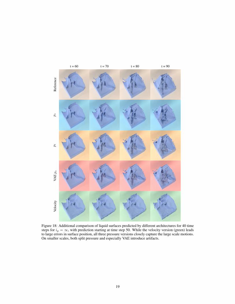
In Fig. 18 additional time-steps of the comparison from Fig. 6 are shown. Here, different inferredsimulation quantities can be compared over the course of a simulation for different models. In ad-dition, Fig. 15, 16, and 17 show more realistic renderings of our liquid64, liquid128, and smoke128models, respectively.

liquid64 liquid128 smoke128Scenes ns 4000 800 800

Time steps nt 100 100 100Size 419.43GB 671.09GB 671.09GB

Size, encoded 1.64GB 2.62GB 2.62GB

Table 4: List of the augmented data sets for the total pressure architecture. Compression by a factorof 256 is achieved by the encoder part of the autoencoder fe.

As our solve indirectly targets divergence, we also measured how well the predicted pressure fieldsenforce divergence freeness over time. As a baseline, the numerical solver led to a residual diver-

13

gence of 3.1 · 10−3 on average. In contrast, the pressure field predicted by our LSTM on averageintroduced a 2.1 · 10−4 increase of divergence per time step. Thus, the per time step error is wellbelow the accuracy of our reference solver, and especially in combination with the interval predic-tions, we did not notice any significant changes in mass conservation compared to the referencesimulations. Below we additionally evaluate the accuracy of our method with respect to the pressuregradient, as it is crucial for removing divergent motions. Fig. 9 shows additional examples of the dif-ferent physical quantities calculated with separately trained models, including boundary conditionpost processing.

Performance As outlined in the main document, our method leads to significant speed-ups com-pared to regular pressure solvers. Below, we will give additional details regarding these speed-ups.For the resolution of 1283, the encoding and decoding stages take 4.1ms and 3.3ms 2, respectively.Evaluating the trained LSTM network itself is more expensive, but still very fast with 9.5ms, onaverage. In total, this execution is ca. 155× faster than our CPU-based pressure solver3.

Interval ip Solve Mean surf. dist SpeedupReference 2.629s 0.0 1.0

4 0.600s 0.0187 4.49 0.335s 0.0300 7.814 0.244s 0.0365 10.1∞ 0.047s 0.0479 55.9

Enc/Dec Prediction SpeedupCore exec. time 4.1ms + 3.3ms 9.5ms 155.6

Table 5: Performance measurement of ten liquid128 example scenes, averaged over 150 simulationsteps each. The mean surface distance is a measure of deviation from the reference per solve.

Solve SpeedupReference 169ms 1.0

Enc/Dec PredictionCore exec., o = 1 3.8ms + 3.2ms 9.6ms 10.2Core exec., o = 3 3.9ms + 3 ∗ 3.3ms 12.5ms 19.3

Table 6: Performance measurement of ten liquid64 example scenes, averaged over 150 simulationsteps each.

It however, also leads to a degradation of accuracy compared to a regular iterative solver. Evenwhen taking into account a factor of ca. 10× for GPUs due to their better memory bandwidth, thisleaves a speedup by a factor of more than 15×, pointing to a significant gain in efficiency for ourLSTM-based prediction. In addition, we measured the speed up for our (not particularly optimized)implementation, where we include data transfer to and from the GPU for each simulation step. Thisvery simple implementation already yields practical speed-ups of 10x for an interval prediction withip = 14. Details can be found in Table 5, while Table 4 summarizes the sizes of our data sets.

Temporal Prediction in 2D To visualize the temporal prediction capabilities as depicted in Fig. 5,the spatial encoding task of the total pressure pt approach was reduced to two spatial dimensions. Forthis purpose a 2D autoencoder network was trained on a dataset of resolution 642. To increase thereconstruction quality of the input, a convolution layer with stride (1, 1) was added before each of the(2, 2) strided convolutions shown Fig. 1. Additionally, the loss was adjusted to put more emphasis onsmall values in the solution, so that the surface of the pressure field is more accurately represented.This is realized with a loss function L(x, y) = 0.9 ·MSE(tanh(x), tanh(y))+0.1 ·MSE(x, y). Thetemporal prediction network was trained as described above. Additional sequences of the ground

2Measured with the tensorflow timeline tools on Intel i7 6700k (4GHz) and Nvidia Geforce GTX970.3 We compare to a parallelized MIC-CG pressure solver [4], running with eight threads.

14

truth, the autoencoder baseline, and the temporal prediction by the LSTM network are shown inFig. 10.

a) b)

c) d)

Figure 9: Four additional example sequences of different predicted quantities (a center slice throughthe 643 domain is shown). All were calculated with ip =∞, with t = 1, 21, 42, 61, 81, 100 for eachcolumn a block. The different states over time illustrate the complexity of the temporal changesof the target functions. The rows per block are from top to bottom: ground truth pressure, totalpressure predicted, split pressure predicted, VAE split pressure predicted, ground truth velocity, andvelocity predicted. Final pressure values are shown, i.e. after applying the boundary conditionalignment. The larger errors for velocity and VAE split pressure are visible here. While all methodsdrift over time (comparing the right most column), the total pressure predictions (2nd from top) faresignificantly better than their counterparts.

15

a)

GT

AE

LSTM

b)

GT

AE

LSTM

c)

GT

AE

LSTM

d)

GT

AE

LSTM

e)

GT

AE

LSTM

f)

GT

AE

LSTM

Figure 10: Six additional example sequences of ground truth pressure fields (top), the autoencoderbaseline (middle), and the LSTM predictions (bottom). All examples have resolutions of 642, andare shown over the course of a long horizon of 30 prediction steps. The LSTM closely predicts thetemporal evolution within the latent space.

16

Figure 11: Examples of initial scene states in the liquid64 data set.

Figure 12: Examples states of the smoke128 training data set at t = 65.

Figure 13: Examples of initial scene states in the liquid128 data set. The more complex initial shapesare visible in several of these configurations.

(a) t = 0 (b) t = 200 (c) t = 400 (d) t = 600 (e) t = 800

Figure 14: Renderings of a long running prediction scene for the liquid128 data set with ip = 4.The fluid successfully comes to rest at the end of the simulation after 800 time steps.

17

t = 0 t = 50 t = 100 t = 150Figure 15: Renderings at different points in time of a 643 scene predicted with ip = 4 by ournetwork.

t = 0 t = 100 t = 200 t = 300

Figure 16: Additional examples of 1283 liquid scenes predicted with an interval of ip = 4 by ourLSTM network.

t = 0 t = 33 t = 66 t = 99

Figure 17: Several examples of 1283 smoke scenes predicted with an interval of ip = 3 by ourLSTM network.

18

t = 60 t = 70 t = 80 t = 90

Ref

eren

ceps

pt

VAEps

Vel

ocity

Figure 18: Additional comparison of liquid surfaces predicted by different architectures for 40 timesteps for ip = ∞, with prediction starting at time step 50. While the velocity version (green) leadsto large errors in surface position, all three pressure versions closely capture the large scale motions.On smaller scales, both split pressure and especially VAE introduce artifacts.

19

E Hyperparameters

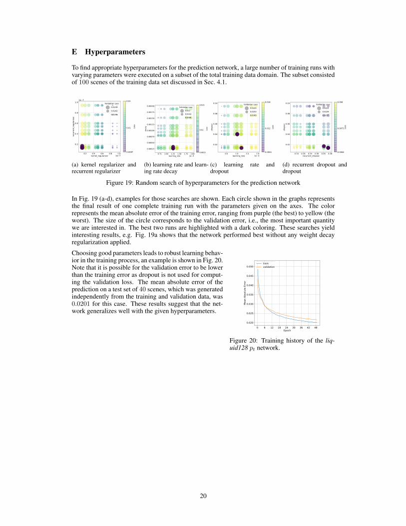
To find appropriate hyperparameters for the prediction network, a large number of training runs withvarying parameters were executed on a subset of the total training data domain. The subset consistedof 100 scenes of the training data set discussed in Sec. 4.1.

(a) kernel regularizer andrecurrent regularizer

(b) learning rate and learn-ing rate decay

(c) learning rate anddropout

(d) recurrent dropout anddropout

Figure 19: Random search of hyperparameters for the prediction network

In Fig. 19 (a-d), examples for those searches are shown. Each circle shown in the graphs representsthe final result of one complete training run with the parameters given on the axes. The colorrepresents the mean absolute error of the training error, ranging from purple (the best) to yellow (theworst). The size of the circle corresponds to the validation error, i.e., the most important quantitywe are interested in. The best two runs are highlighted with a dark coloring. These searches yieldinteresting results, e.g. Fig. 19a shows that the network performed best without any weight decayregularization applied.

Figure 20: Training history of the liq-uid128 pt network.

Choosing good parameters leads to robust learning behav-ior in the training process, an example is shown in Fig. 20.Note that it is possible for the validation error to be lowerthan the training error as dropout is not used for comput-ing the validation loss. The mean absolute error of theprediction on a test set of 40 scenes, which was generatedindependently from the training and validation data, was0.0201 for this case. These results suggest that the net-work generalizes well with the given hyperparameters.

20