abstract cooperative communication with wireless network

ABSTRACT

Title of dissertation: COOPERATIVE COMMUNICATION WITHWIRELESS NETWORK CODING

Wei Guan, Doctor of Philosophy, 2013

Dissertation directed by: Professor K. J. Ray LiuDepartment of Electrical and Computer Engineering

Cooperative communication is a new communication paradigm that allows

multiple transceivers to collaborate as a cluster for data transmission, and such

clustering could greatly improve the transmission quality due to cooperative diver-

sity. For conventional cooperation protocols, each cooperating device uses orthogo-

nal channels to relay different messages for mitigating co-channel interference and

avoiding transmission collision, but doing so would significantly reduce the band-

width efficiency. One way to tackle this issue is to use wireless network coding, in

which different messages are smartly combined at cooperating devices to save the

channel use for data relaying.

Network coding has been widely used in wireline networks, but only until very

recently was grafted onto the wireless networks. In the research community, it has

been unknown for a long time whether network-coded cooperation is able to achieve

the same diversity gain as the conventional diversity technique. On the industry

side, how to efficiently apply network coding in the current wireless systems has also

been an open design problem in the past few years. This thesis work aims to address

these important issues and challenges and provide some theoretical guidelines for

real system design.

In the first part of this work, we study the fundamental diversity performance

of uncoded cooperation systems with wireless network coding. It is demonstrated

that network-coded cooperation generally cannot achieve the same diversity gain

as the conventional diversity schemes; however, the diversity loss is usually very

limited and occurs only under particular channel conditions. For example, for digital

network coding we show that the error propagation issue would cause half of the

total available diversity gain to be lost, and we develop several link adaptive schemes

to mitigate the diversity loss. For analog network coding, we demonstrate that the

associated co-channel interference may reduce the diversity as well, but such loss

gradually diminishes as the transmitted power goes up. Finally for non-coherent

network coding, we show that when the receivers do not know the channel state

information, using blind signal detection would not hurt the dominant diversity

gain, and the diversity loss occurs only at modest signal-to-noise ratio.

The second part of this work is focused on coded cooperation systems. The

unique feature of coded systems is that the devices could somehow know the network

dynamics such as the decoding status of a transmitted packet. We explore two

transmission strategies that could efficiently exploit such information. For two-way

relay channel, we propose a network-coded retransmission strategy, where wireless

relaying is employed only when the direct link is in outage. To reduce the number of

retransmissions, network coding is performed in a static or dynamic way to combine

the to-be-retransmitted packets intended for different end terminals. We analyze

the throughput and develop power allocation scheme to maximize the throughput.

We also develop a hybrid network coding scheme that can fully exploit the network

coding gain in the multi-relay environment. Next for wireless uplink channel, we

come up with a multi-user cooperation scheme based on node clustering. We develop

inter-cluster cooperation strategy and intra-cluster transmit beamforming scheme to

exploit the cooperative diversity gain. We demonstrate that there is a basic tradeoff

between diversity gain and bandwidth efficiency, and different tradeoffs could be

achieved by changing the formation of the clusters.

COOPERATIVE COMMUNICATION WITH WIRELESSNETWORK CODING

by

Wei Guan

Dissertation submitted to the Faculty of the Graduate School of theUniversity of Maryland, College Park in partial fulfillment

of the requirements for the degree ofDoctor of Philosophy

2013

Advisory Committee:Professor K. J. Ray Liu, Chair/AdvisorProfessor Min WuProfessor Adrian PapamarcouProfessor Gang QuProfessor Lawrence C. Washington

c⃝ Copyright byWei Guan

2013

Dedication

To my parents.

ii

Acknowledgments

First of all, I would like to thank my advisor, Prof. K. J. Ray Liu, for his

continuous inspiration, guidance and support on my thesis work. In the past few

years, he constantly encouraged me to focus on those most important and challeng-

ing problems, and instructed me how to find a way toward innovative ideas and

creative solutions. He also gave me a lot of freedom to choose the favorite research

topics to strengthen my interest and enthusiasm in research. It is my great honor

and pleasure to be able to finish my thesis work with a patient, kind and responsible

advisor like Prof. Liu.

I would also like to thank all the members in Signal and Information Group.

Because of their friendship, encouragement and helpful discussions, I gain the power

to get through various hard times and no longer feel lonely along this long journey.

Special thanks to Feng, Yang, Hui and Le, with whom I have had a lot of happy

moments over the past years.

I also appreciate Prof. Min Wu, Prof. Adrian Papamarcou, Prof. Gang Qu

and Prof. Lawrence C. Washington for serving on my committee and reviewing my

thesis. Their comments and advices prove to be pretty helpful in improving the

quality of this dissertation.

Lastly, I would like to express my deepest gratitude to my parents for their

eternal love, support and comfort. Special gratitude to my grandpa, grandma and

aunt, who keep encouraging me to pursue PhD degree but unfortunately leave me

forever before the completion of my PhD study. To them I dedicate this thesis.

iii

Table of Contents

List of Tables vii

List of Figures viii

1 Introduction 11.1 Channel Fading and Diversity . . . . . . . . . . . . . . . . . . . . . . 11.2 Wireless Network Coding . . . . . . . . . . . . . . . . . . . . . . . . . 51.3 Dissertation Outline . . . . . . . . . . . . . . . . . . . . . . . . . . . 8

1.3.1 Error Performance of Two-Way Relay Channel with DigitalNetwork Coding (Chapter 2) . . . . . . . . . . . . . . . . . . . 8

1.3.2 Mitigating Error Propagation for Wireless Uplink with DigitalNetwork Coding (Chapter 3) . . . . . . . . . . . . . . . . . . . 10

1.3.3 Diversity Analysis of Wireless Uplink with Analog NetworkCoding (Chapter 4) . . . . . . . . . . . . . . . . . . . . . . . . 11

1.3.4 Diversity Analysis of Wireless Uplink with Non-Coherent Net-work Coding (Chapter 5) . . . . . . . . . . . . . . . . . . . . . 12

1.3.5 Network-Coded ARQ for Two-Way Relay Channel (Chapter 6) 141.3.6 Clustering Based Space-Time Network Coding (Chapter 7) . . 15

2 Error Performance of Two-Way Relay Channel with Digital Network Coding 162.1 System Model . . . . . . . . . . . . . . . . . . . . . . . . . . . . . . . 182.2 Performance Analysis: Single-Relay Case . . . . . . . . . . . . . . . . 23

2.2.1 Relay Detection Error . . . . . . . . . . . . . . . . . . . . . . 232.2.2 Source Detection Error . . . . . . . . . . . . . . . . . . . . . . 262.2.3 Power Allocation . . . . . . . . . . . . . . . . . . . . . . . . . 27

2.3 Performance Analysis: Multi-Relay Case . . . . . . . . . . . . . . . . 302.3.1 BER Upper Bound . . . . . . . . . . . . . . . . . . . . . . . . 312.3.2 BER Lower Bound . . . . . . . . . . . . . . . . . . . . . . . . 33

2.4 Simulations . . . . . . . . . . . . . . . . . . . . . . . . . . . . . . . . 352.5 Conclusions . . . . . . . . . . . . . . . . . . . . . . . . . . . . . . . . 41

3 Mitigating Error Propagation for Wireless Uplink with Digital Network Cod-ing 423.1 System Model . . . . . . . . . . . . . . . . . . . . . . . . . . . . . . . 433.2 Performance Analysis . . . . . . . . . . . . . . . . . . . . . . . . . . . 463.3 Relay-Side Schemes . . . . . . . . . . . . . . . . . . . . . . . . . . . . 49

3.3.1 Soft Power Scaling . . . . . . . . . . . . . . . . . . . . . . . . 493.3.2 Hard Power Scaling . . . . . . . . . . . . . . . . . . . . . . . . 54

3.4 Receiver-Side Schemes . . . . . . . . . . . . . . . . . . . . . . . . . . 573.4.1 Link Adaptive Combining . . . . . . . . . . . . . . . . . . . . 583.4.2 Maximum Likelihood Detection . . . . . . . . . . . . . . . . . 61

3.5 More Discussions . . . . . . . . . . . . . . . . . . . . . . . . . . . . . 643.5.1 Relay Power Consumption Ratio . . . . . . . . . . . . . . . . 64

iv

3.5.2 Signalling Overhead . . . . . . . . . . . . . . . . . . . . . . . 653.5.3 Extension To Higher-Order Modulations . . . . . . . . . . . . 66


4 Diversity Analysis of Wireless Uplink with Analog Network Coding 754.1 Multi-User Single-Relay Systems . . . . . . . . . . . . . . . . . . . . 77

4.1.1 System Model . . . . . . . . . . . . . . . . . . . . . . . . . . . 774.1.2 Performance Analysis . . . . . . . . . . . . . . . . . . . . . . . 804.1.3 Discussions . . . . . . . . . . . . . . . . . . . . . . . . . . . . 85

4.2 Relay Selection Strategy . . . . . . . . . . . . . . . . . . . . . . . . . 874.3 Distributed Space-Time Block Coding . . . . . . . . . . . . . . . . . 91

4.3.1 Signal Model of DSTBC . . . . . . . . . . . . . . . . . . . . . 924.3.2 Error Performance Analysis . . . . . . . . . . . . . . . . . . . 934.3.3 Selective DSTBC-VGR for Single-User Networks . . . . . . . . 96

4.4 Diagonal Distributed Space-Time Coding . . . . . . . . . . . . . . . . 984.5 Simulations . . . . . . . . . . . . . . . . . . . . . . . . . . . . . . . . 1014.6 Conclusions . . . . . . . . . . . . . . . . . . . . . . . . . . . . . . . . 106

5 Diversity Analysis of Wireless Uplink with Non-Coherent Network Coding 1085.1 System Model . . . . . . . . . . . . . . . . . . . . . . . . . . . . . . . 1105.2 Transceiver Design . . . . . . . . . . . . . . . . . . . . . . . . . . . . 112

5.2.1 Analog Network Coding . . . . . . . . . . . . . . . . . . . . . 1125.2.2 Digital Network Coding . . . . . . . . . . . . . . . . . . . . . 115

5.3 Error Performance Analysis . . . . . . . . . . . . . . . . . . . . . . . 1175.3.1 Coherent Analog Network Coding . . . . . . . . . . . . . . . . 1185.3.2 Non-Coherent Analog Network Coding . . . . . . . . . . . . . 1195.3.3 Digital Network Coding . . . . . . . . . . . . . . . . . . . . . 1235.3.4 Discussions . . . . . . . . . . . . . . . . . . . . . . . . . . . . 128


6 Network-Coded ARQ for Two-Way Relay Channel 1386.1 System Model . . . . . . . . . . . . . . . . . . . . . . . . . . . . . . . 140

6.1.1 Some Preliminaries . . . . . . . . . . . . . . . . . . . . . . . . 1436.2 Single-Relay Case . . . . . . . . . . . . . . . . . . . . . . . . . . . . . 146

6.2.1 Direct Transmission . . . . . . . . . . . . . . . . . . . . . . . . 1466.2.2 Pure Relaying . . . . . . . . . . . . . . . . . . . . . . . . . . . 1486.2.3 Static Network Coding . . . . . . . . . . . . . . . . . . . . . . 1526.2.4 Dynamic Network Coding . . . . . . . . . . . . . . . . . . . . 1556.2.5 Throughput Comparison . . . . . . . . . . . . . . . . . . . . . 1586.2.6 Power Allocation . . . . . . . . . . . . . . . . . . . . . . . . . 160

6.3 Multi-Relay Case . . . . . . . . . . . . . . . . . . . . . . . . . . . . . 1626.3.1 Successive Relaying . . . . . . . . . . . . . . . . . . . . . . . . 1626.3.2 Hybrid Network Coding . . . . . . . . . . . . . . . . . . . . . 164

v


7 Clustering Based Space-Time Network Coding 1737.1 Transmission Strategy . . . . . . . . . . . . . . . . . . . . . . . . . . 1747.2 Multiuser Detection . . . . . . . . . . . . . . . . . . . . . . . . . . . . 178

7.2.1 Source Decoding . . . . . . . . . . . . . . . . . . . . . . . . . 1787.2.2 Destination Decoding . . . . . . . . . . . . . . . . . . . . . . . 180

7.3 Performance Analysis . . . . . . . . . . . . . . . . . . . . . . . . . . . 1817.3.1 Exact SER Analysis . . . . . . . . . . . . . . . . . . . . . . . 1827.3.2 Asymptotic SER Analysis . . . . . . . . . . . . . . . . . . . . 1847.3.3 Discussions . . . . . . . . . . . . . . . . . . . . . . . . . . . . 186


8 Conclusions and Future Work 1928.1 Conclusions . . . . . . . . . . . . . . . . . . . . . . . . . . . . . . . . 1928.2 Future Work . . . . . . . . . . . . . . . . . . . . . . . . . . . . . . . . 194

8.2.1 User Scheduling . . . . . . . . . . . . . . . . . . . . . . . . . . 1948.2.2 Energy Saving . . . . . . . . . . . . . . . . . . . . . . . . . . . 195

Bibliography 196

vi

List of Tables

5.1 Four Types of PEP . . . . . . . . . . . . . . . . . . . . . . . . . . . . 1175.2 Scaling Laws of The Error Rates . . . . . . . . . . . . . . . . . . . . . 127

vii

List of Figures

2.1 System model of network-coded TWRC. . . . . . . . . . . . . . . . . 182.2 BER performances versus SNR. . . . . . . . . . . . . . . . . . . . . . 362.3 BER performances with power allocation versus SNR. . . . . . . . . . 372.4 BER performances with power allocation versus relay placement. . . . 372.5 Comparison of wireless relaying and direct transmission. Colored

areas correspond to the places where wireless relaying can achievebetter BER. . . . . . . . . . . . . . . . . . . . . . . . . . . . . . . . . 38

2.6 BER performances with multiple relays – all relays are at halfwaybetween two sources. . . . . . . . . . . . . . . . . . . . . . . . . . . . 39

2.7 BER performances with multiple relays – all relays are equispacedbetween two sources. . . . . . . . . . . . . . . . . . . . . . . . . . . . 40

3.1 System model of the network-coded uplink. . . . . . . . . . . . . . . . 443.2 Virtual channel model for the relay branch. . . . . . . . . . . . . . . . 503.3 Error performances of BPSK signal in a symmetric network. . . . . . 683.4 Error performances of BPSK signal in an asymmetric network with

strong relay-destination channel. . . . . . . . . . . . . . . . . . . . . . 693.5 Error performances of BPSK signal in an asymmetric network with

strong source-relay channel. . . . . . . . . . . . . . . . . . . . . . . . 703.6 Error performances of BPSK signal with Γ = 20dB and different relay

positions. . . . . . . . . . . . . . . . . . . . . . . . . . . . . . . . . . 713.7 Relay power consumption ratio with different relay positions. . . . . . 713.8 Error performances of QPSK signal in a symmetric network. . . . . . 733.9 Error performances of 8PSK signal in a symmetric network. . . . . . 73

4.1 System model of a multi-user multi-relay uplink channel. . . . . . . . 774.2 Error performances of a two-user network with different channel con-

ditions. . . . . . . . . . . . . . . . . . . . . . . . . . . . . . . . . . . . 1024.3 Comparison of two-user and single-user network with different data

rate. . . . . . . . . . . . . . . . . . . . . . . . . . . . . . . . . . . . . 1024.4 Error performances of a two-user network with relay selection. . . . . 1044.5 Error performances of a two-user network with DDSTC and DSTBC-

FGR. . . . . . . . . . . . . . . . . . . . . . . . . . . . . . . . . . . . . 1054.6 Error performances of a two-user network with DSTBC-VGR. . . . . 1054.7 Error performances of a single-user network with DSTBC-VGR and

selective DSTBC-VGR. . . . . . . . . . . . . . . . . . . . . . . . . . . 106

5.1 System model of the two-user network-coded uplink. . . . . . . . . . 1105.2 PEP of coherent ANC. . . . . . . . . . . . . . . . . . . . . . . . . . . 1305.3 PEP of partial coherent ANC. . . . . . . . . . . . . . . . . . . . . . . 1315.4 PEP of coherent DNC. . . . . . . . . . . . . . . . . . . . . . . . . . . 1315.5 PEP of non-coherent DNC. . . . . . . . . . . . . . . . . . . . . . . . 1325.6 Error rates of the symmetric networks. . . . . . . . . . . . . . . . . . 133

viii

5.7 Error rates of the asymmetric networks with better source-relay chan-nels. . . . . . . . . . . . . . . . . . . . . . . . . . . . . . . . . . . . . 134

5.8 Error rates of the asymmetric networks with better relay-destinationchannels. . . . . . . . . . . . . . . . . . . . . . . . . . . . . . . . . . . 135

5.9 Error rates with different relay positions. . . . . . . . . . . . . . . . . 136

6.1 System model of two-way relay channel. . . . . . . . . . . . . . . . . 1406.2 Effective throughput versus SNR for L = 4 and K = 10. The relay

node is located at (0.5, 0). . . . . . . . . . . . . . . . . . . . . . . . . 1686.3 Effective throughput versus normalized transmission constraint for

K = 10. The relay node is located at (0.5, 0). . . . . . . . . . . . . . 1686.4 Effective throughput versus relay position with power allocation for

SNR = −5dB, K = 5 and L = ∞. . . . . . . . . . . . . . . . . . . . . 1706.5 Effective throughput versus SNR with N = 3 relays for L = ∞. All

relay nodes are located at (0.5, 0). . . . . . . . . . . . . . . . . . . . . 1716.6 Effective throughput versus the number of relays for SNR = −10dB,

K = 3 and L = ∞. All relay nodes are located at (0.5, 0). . . . . . . . 171

7.1 System model of the wireless uplink with user clustering . . . . . . . 1757.2 SER performances with QPSK modulations. . . . . . . . . . . . . . . 1877.3 SER comparison in a 2x2 network. . . . . . . . . . . . . . . . . . . . 1897.4 Throughput comparison in a 4x4 network. . . . . . . . . . . . . . . . 189

ix

Chapter 1

Introduction

1.1 Channel Fading and Diversity

Nowadays, wireless applications such as Wifi, cellular phones and bluetooth

have become an important part of daily life. But compared to the conventional

wireline networks, wireless networks can only provide very limited data rate because

the underlying channel is unreliable in nature. In practice, wireless channel is subject

to fading, pathloss, shadowing and co-channel interference, and all these features

would greatly degrade the quality of transmitted signals.

Channel fading is one of the major downside to wireless communication. Chan-

nel fading is caused by multipath propagation effect, which occurs when the reflec-

tors surrounding the transmitter/receiver happen to create multiple propagation

paths for the transmitted signals to traverse. Those multipath components may

add constructively or destructively at the receiver side, thus making the amplitude

of the received signal fluctuate randomly over time [1–3]. When the channel is in

deep fading, the wireless link may totally get disconnected and no information can

be delivered reliably.

Diversity techniques have been widely used to combat channel fading. Diver-

sity is the capability to send the same signal repeatedly through independent chan-

nels. As the receiver is able to decode the source message as long as there exists at

1

least one good channel, the chance of link disconnection in cases of deep fading on

all the channels could be reduced significantly. Mathematically, the diversity gain

is defined as [1–3]

d = − limP→∞

logPelogP

, (1.1)

where Pe is the error rate and P is the signal-to-noise ratio (SNR). The diversity

gain is a measure of the decay rate of transmission error in the high SNR regions.

For conventional diversity systems, the scaling law of the error rate has a general

form of Pe = O(

1PM

), where f (x) = O (g (x)) means that a ≤ lim

x→∞f(x)g(x)

≤ b for

some positive constants a and b. The diversity gain M is equal to the number of

independent paths that the transmitted signals traverse toward the receiver.

Conventionally, there are three generic types of diversity: time diversity, fre-

quency diversity and spatial diversity [1–3]. Time diversity is to send the same

signal copy in different time slots. To guarantee independent fading, the interval

between adjacent transmissions must be greater than the channel coherence time,

which would incur large processing delay especially when the channel is in slow fad-

ing. Frequency diversity is to send the same signal copy in sufficiently separated

frequency bands that experience independent fading. However, frequency diversity

is gained at a price of lower bandwidth efficiency, which is costly since frequency

resource is pretty scarce.

Spatial diversity is a relatively new technique to address the drawbacks of time

diversity and frequency diversity. Spatial diversity is achieved by deploying multiple

antennas at the transmitter/receiver, such that there exists one independent propa-

2

gation path between each pair of transmitter antenna and receiver antenna. Multiple

antenna technique has gained a lot of attention in recent years because it also pro-

vides an efficient way to improve bandwidth efficiency. For each channel mode in

the eigen-space, it could carry one spatial stream without causing co-channel inter-

ference [4]. So The transmitters can choose to send multiple independent streams

to increase the bandwidth efficiency, or send the same stream multiple times across

different channel modes to improve the reliability, which is a fundamental trade-

off between diversity gain and multiplexing gain [5]. According to system design

goals, different tradeoffs can be achieved by employing proper space-time coding

schemes [6–8].

Theoretically, the spatial diversity gain and multiplexing gain could be arbi-

trarily high if it is possible to deploy infinitely many antennas at both the transmitter

and receiver. But in practice, since the user devices are usually of very limited size

and the adjacent antennas must be sufficiently separated to guarantee independency,

it is pretty hard to equip too many antennas on any single user device. Those hard-

ware constraints lead to a new concept of cooperative diversity. The main idea of

cooperative diversity is to use distributed antennas instead of the co-located phys-

ical antennas, where the distributed antennas could be any independent relaying

devices that may help to forward the source signals [3]. As each relay link is able

to provide one additional diversity path, the available diversity gain could be quite

remarkable in a dense wireless network where there are abundant relaying devices

between the transmitter and receiver.

Although the research on cooperative communication dates back to late 1970s

3

[9], where the capacity of single-relay channels subject to additive white Gaussian

noise (AWGN) was explored, only until recently has it gained a lot of interest in the

research community. The performance gain of cooperative diversity in a two-user

code-division multiplexing access (CDMA) system was first demonstrated in [10,11].

Since then, a bunch of cooperation protocols were developed and studied extensively.

Depending on the relay operations, all the cooperation protocols can be roughly

divided into two broad categories: analog relaying and digital relaying [12]. In analog

relaying protocols, each relay simply forwards the received signals to the receiver

after performing some linear operations in the complex domain. As the additive

noise is mixed with the signal component, it is amplified and forwarded to the in-

tended receiver too. By contrast, in digital relaying protocols each relay needs to

first decode the source message, re-encode it and then forward it to the receiver. So

the relay node always forwards a “clean” message, although the message might be

incorrect due to decoding errors. From an information theoretic view, simple digital

relaying cannot achieve cooperative diversity; however, if the relay can somehow

detect the decoding errors, then selectively forwarding the correct messages alone

could recover the diversity loss [12].

For single-relay networks, the symbol error rate (SER) is studied in [13]. Both

the exact SER and asymptotic SER are derived for analog relaying and digital re-

laying, respectively, based on which a set of optimum power allocation schemes are

obtained. The outage probability and SER for multi-node parallel analog relaying

networks are studied in [14] and [15], respectively. Parallel relaying has the disad-

vantage of low spectral efficiency, as each relay operates on orthogonal channels. To

4

address this issue, relay selection [16] and distributed space-time coding [17] could

be used to coordinate multi-relay cooperation.

In practice, it is possible to exploit spatial diversity and cooperative diversity

at the same time if all the devices are equipped with multiple antennas. For analog

relaying, the system performances could be improved via relay precoding. The

optimum precoding matrices for maximizing the achievable rate and minimizing

the mean-squared errors were developed in [18] and [19], respectively. If power

constraint is not stringent, the relay precoding matrix could also be optimized to

achieve certain quality-of-service goals [20].

1.2 Wireless Network Coding

For cooperative diversity, the relays need to first acquire the source message

before forwarding it to the receiver. However, practical devices are usually subject

to half-duplex constraint, i.e., they cannot transmit and receive signals at the same

time. As a result, the whole end-to-end data relaying is completed in two phases:

data acquiring phase and data forwarding phase. Since an independent channel is

required for each phase and only one message could be delivered across those two

phases, it incurs a pre-log factor 12on the spectral efficiency [21]. For multi-relay

systems, such rate loss is even larger if the intermediate relays operate on orthogonal

channels [14].

To save channel use for data forwarding phase, the relay can choose to combine

different source messages via network coding and forward a single mixed message

5

rather than forward the individual messages separately. Broadly speaking, network

coding refers to arbitrary coding (i.e., mapping from input to output) at intermedi-

ate nodes [22,23]. But some pioneering literatures in this area focus only on wireline

applications, where the physical channel is assumed to be error free and the con-

tents of source messages are combined beyond the physical layer [23]. With these

simplifications, it has been proved that network coding could achieve the min-cut

max-flow throughput bound for multicast networks [22–24].

For mobile networks, it is very hard to connect the transmitter/receiver to the

relay station by cable directly. So all the inter-node communications go through

wireless links, and the underlying channel features play an important role in the

design and analysis of network coding. As mentioned in Section 1.1, wireless chan-

nels suffer severe random fading that may result in serious transmission errors, and

multiple transmitters would also cause co-channel interference. Consequently, the

existing analytical results on wireline networks no longer hold for wireless applica-

tions, and new findings may rely on information theory and communication theory

from a physical-layer view.

For wireless transmissions, the transmitted signal consists of the modulated

symbols instead of the raw information bits. Depending on the way for mixing source

messages, it gives rise to two different types of wireless network coding schemes. On

one hand, the relay could choose to decode different source messages and then com-

bine the bit-streams in the finite field. This is called digital network coding (DNC)

and it is a legacy network coding scheme previously developed for wireline networks.

Alternatively, the source signals could be combined symbol-wise in the complex field

6

directly to simplify relay operations, since the decoding could be omitted. This is

a unique analog network coding (ANC) scheme dedicated for wireless applications,

as the wireless devices usually have the capability of interference cancelation and

multi-user detection [25]. In practice, DNC and ANC are suitable for digital relaying

and analog relaying, respectively.

Thanks to the additive nature of wireless medium, wireless network coding

could also save the channel use for data acquiring phase. In wireline networks,

each cable defines a distinct channel between the connected terminals. If multiple

transmitters send messages to a common intermediate node at the same time, the

relay is able to obtain a “clean” message from each transmitter because there is

no transmission collision. Those messages are then combined via network coding

locally at the intermediate node. This scheme is conventionally referred to as link-

layer network coding (LNC) [26]. For wireless applications, LNC is still applicable if

the transmitters operate on different channels to avoid co-channel interference, but

the bandwidth efficiency is low. By contrast, physical-layer network coding (PNC)

allows all the transmitters operate on the same channel to reduce channel use [27].

Because of the additive nature of wireless medium, all the transmitted signals would

be combined automatically in the air, which is a nature form of network coding.

Then the relay only needs to amplify and forward such mixed signal to the intended

receiver if ANC is employed [28], or map the mixed signal to the network-coded

symbol if DNC is employed [27,29].

7

1.3 Dissertation Outline

In this thesis, we aim to analyze and develop cooperative transmission strate-

gies with wireless network coding. The whole thesis consists of two parts. In the

first part from Chapter 2 to Chapter 5, we focus on the uncoded systems where

there are no error detection/correction codes. We resolve a bunch of problems like

transceiver design, power allocation, anti error propagation and space-time coding.

Besides, we characterize the diversity performance and show that network-coded

cooperation generally cannot achieve the same diversity gain as the conventional

diversity schemes; however, the diversity loss is very limited and only occurs under

certain channel conditions. The second part (i.e., Chapter 6 and Chapter 7) of this

thesis is devoted to transmission strategy design for coded systems, in which the

devices could somehow detect or correct the transmission errors. One key benefit

of the coded systems is that the devices may learn the network dynamics such as

the decoding status of a transmitted message and then choose the best response

accordingly. We develop some network coding strategies for coded systems and

characterize the performance in terms of error rate or throughput.

1.3.1 Error Performance of Two-Way Relay Channel with Digital

Network Coding (Chapter 2)

Two-Way Relay Channel (TWRC) is one of the most important application

scenarios of DNC. Many literatures [21, 30–32] have studied the achievable rate

and reveal the tremendous gain over the conventional orthogonal relaying. Those

8

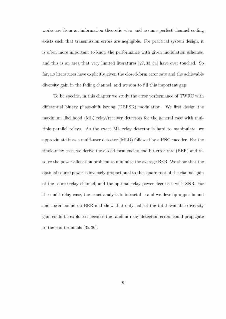
works are from an information theoretic view and assume perfect channel coding

exists such that transmission errors are negligible. For practical system design, it

is often more important to know the performance with given modulation schemes,

and this is an area that very limited literatures [27, 33, 34] have ever touched. So

far, no literatures have explicitly given the closed-form error rate and the achievable

diversity gain in the fading channel, and we aim to fill this important gap.

To be specific, in this chapter we study the error performance of TWRC with

differential binary phase-shift keying (DBPSK) modulation. We first design the

maximum likelihood (ML) relay/receiver detectors for the general case with mul-

tiple parallel relays. As the exact ML relay detector is hard to manipulate, we

approximate it as a multi-user detector (MLD) followed by a PNC encoder. For the

single-relay case, we derive the closed-form end-to-end bit error rate (BER) and re-

solve the power allocation problem to minimize the average BER. We show that the

optimal source power is inversely proportional to the square root of the channel gain

of the source-relay channel, and the optimal relay power decreases with SNR. For

the multi-relay case, the exact analysis is intractable and we develop upper bound

and lower bound on BER and show that only half of the total available diversity

gain could be exploited because the random relay detection errors could propagate

to the end terminals [35,36].

9

1.3.2 Mitigating Error Propagation for Wireless Uplink with Digital

Network Coding (Chapter 3)

Error propagation would reduce the diversity gain of any digital relaying sys-

tems. For the conventional orthogonal relaying systems, many physical-layer tech-

niques [37–42] have been developed to mitigate error propagation issue. However,

those methods work only in the scenarios where there is a single source-destination

pair, and they cannot apply to network-coded systems that deal with multiple users

at the same time. Some literatures [43–46] also develop network coding schemes

that rely on error detection/correction code, but those methods are not applicable

for uncoded systems such as some sensor networks that have very limited processing

capability. Very limited papers [47, 48] talk about anti error propagation for un-

coded systems; however, global channel state information (CSI) is required in those

methods and only receiver-side technique is considered, which largely limits their

practical use.

Because of those concerns, we develop some practical anti error propagation

methods for the uncoded two-user wireless uplink with DNC. We come up with

some power scaling schemes and advanced detection schemes that require global

CSI or only local CSI, respectively. For the soft power scaling scheme, we develop a

virtual source-relay-destination channel model and demonstrate that the relay power

should be such to balance the SNRs of the source-relay channel and relay-destination

channel. For the hard power scaling scheme, we first design a decision rule based

on total pairwise error probability (PEP), and then simplify it to the threshold-

10

based relaying strategy. At the receiver side, we show that the weighted minimum

distance detection with the weight being determined by the relative link quality of

source-relay channel and relay-destination channel can achieve full diversity if and

only if global CSI is available, otherwise the maximum likelihood detection should

be employed to achieve full diversity if the receiver only knows local CSI [49,50].

1.3.3 Diversity Analysis of Wireless Uplink with Analog Network

Coding (Chapter 4)

ANC is naturally immune to error propagation because the relay no longer

needs to decode the source messages. Since different messages are combined in the

complex field directly, they would become multi-user interference (MUI) to each

other. For TWRC, ANC is essentially interference free as the end terminals are able

to subtract the self-interference from the received signals [21,25,28,74]. By contrast,

for uplink channel the receiver has no side information about any source messages

and is unable to eliminate the co-channel interference. Many literatures [51–56] have

studied the achievable rate region and space-time code design for uplink channel with

ANC. However, the impact of MUI on the diversity gain remain unclear. In [57], the

beamforming design when only the quantized CSI is available at the relays is studied

and a generalized diversity measure is introduced to study the impact of MUI.

However, this work is focused only on the instantaneous relay power constraints

where instant CSI is available. The achievable diversity gain in the absence of

instant CSI is still unclear.

11

So in this work, we provide a study on the diversity performance of a gen-

eral K-user uplink channel with ANC. Depending on the relay power constraints,

we investigate both the variable gain relaying (VGR) and the fixed gain relaying

(FGR). We first study the single-relay networks, and show that full diversity can be

achieved regardless of MUI. However, an logarithmic term would appear in the error

rate expression and incur diversity loss at modest SNR. Several relaying schemes

to achieve distributed spatial diversity when there are multiple relays are then ex-

plored. We first propose a relay selection strategy based on the principle of min-

imizing the maximum PEP and prove that full diversity can be achieved. Next,

two distributed space-time coding (DSTC) schemes are studied. For distributed

space-time block code (DSTBC), we show that DSTBC-FGR can always achieve

full diversity, whereas the diversity of DSTBC-VGR is also bounded by the number

of users. As the diversity of single-user DSTBC-VGR is limited by 2, we develop an

adaptive relay power allocation scheme that can recover the diversity loss. Finally

for diagonal distributed space-time coding (DDSTC), we show that both VGR and

FGR can achieve full diversity, and the optimum code design criterion is to maximize

the minimum product distance [58,59].

1.3.4 Diversity Analysis of Wireless Uplink with Non-Coherent Net-

work Coding (Chapter 5)

Perfect CSI is very important for the receiver to mitigate error propagation

for DNC or suppress MUI for ANC. However, perfect CSI is not always available

12

due to various reasons such as high channel estimation overhead. To reduce the

reliance on CSI, non-coherent modulation schemes have been widely used in real

systems. Non-coherent orthogonal relaying strategies have received a lot of interest

in the community [60–65], and some literatures [26, 34, 66–68] also discuss non-

coherent transmissions for TWRC with network coding. Intuitively, using non-

coherent modulation should decrease the system performance. For the traditional

point-to-point channels, it is well known that it incurs 3dB SNR loss while the

diversity gain remains the same [1]. But for the network-coded cooperation systems,

very few literatures have ever explicitly discussed the performance loss, and this

motivates our work.

To be specific, we study the two-user uplink channel with ANC or DNC, re-

spectively. We consider FSK modulation to facilitate non-coherent detection. We

first design the coherent and non-coherent ML receivers when global CSI and sta-

tistical CSI is available at the receivers, respectively. For ANC, as the non-coherent

ML receiver has an intractable integral form, we develop two suboptimum receivers

that are near optimum depending on the relative quality of source-relay channel and

relay-destination channel. The PEP is then studied, and the scaling laws of differ-

ent PEPs are derived at high SNRs. It is demonstrated that full dominant diversity

is always achieved regardless of the CSI assumptions; however, using non-coherent

detection would incur some diversity loss at modest SNRs such that the resulting

error rates do not decrease that fast compared to coherent detection. Besides, we

show that the performance loss of ANC is more serious due to the incapability to

efficiently suppress MUI at the receiver [69, 70].

13

1.3.5 Network-Coded ARQ for Two-Way Relay Channel (Chapter 6)

In the previous chapters, we focus mainly on static relaying for uncoded sys-

tems, i.e., all the data transmission would go through the relay link regardless of the

network dynamics. For coded systems, the decoding status of each packet could be

known by performing cyclic redundancy check. If the transmission through direct

link is already successful, wireless relaying could be omitted to save the channel use

and transmitted power. Otherwise, the relay could help to retransmit the original

source packet as a part of automatic repeat-request (ARQ) mechanism. Network

coding could enhance the transmission efficiency of the conventional ARQ, since a

couple of to-be-retransmitted packets could be combined to reduce the number of

retransmissions. Network-coded ARQ has been studied for many applications, such

as broadcast channels [71], wireless multicast [72] and multiple unicast flows [73].

In this work, we study the performance of network-coded ARQ for TWRC. The

key distinction between our work and the existing literatures [31, 74–77] is that we

take into account the maximum transmission constraint, which is a very practical

concern. For single-relay networks, we derive the closed-from throughput when

the retransmission is subject to per-hop constraint or end-to-end (E2E) constraint,

respectively. We demonstrate that network coding can greatly improve the system

throughput, but the throughput gain is upper bounded. Besides, we come up with

a near-optimum power allocation scheme to maximize the throughput. For multi-

relay networks, we show that successive relaying strategy suffers great throughput

loss when the frame length is much smaller than the number of relays, and we develop

14

a hybrid network coding scheme to fully exploit the network coding gain [78,79].

1.3.6 Clustering Based Space-Time Network Coding (Chapter 7)

When there is no dedicated relay in the systems, user devices have to help

each other to enjoy the cooperative diversity gain. For a dense mobile network, how

to coordinate the large number of user devices has been an open design problem

for a long time. The existing strategies [80–82] tend to pursue the largest diversity

gain, while the bandwidth efficiency is relatively low. So in this work, we aim to

develop a new user cooperation strategy that can achieve better tradeoff between

diversity gain and bandwidth efficiency. The core idea of our method is to divide

the whole network into several small clusters, and different clusters help each other

to relay the signals. The clusters send data successively in a time-division multiple

access (TDMA) way. Each node in a certain cluster behaves as a digital relay to

other clusters, and it uses linear coding to combine the local symbol and the relayed

symbols. Linear decorrelator is used at the receivers to separate different source

signals. We obtain both the exact SER and asymptotic SER of the M-ary phase-

shift keying (PSK) signal. It is shown that different tradeoffs between diversity gain

and bandwidth efficiency can be achieved by adjusting the formation of clusters [83].

15

Chapter 2

Error Performance of Two-Way Relay Channel with Digital Network

Coding

For cellular systems, the uplink/downlink is a typical TWRC paradigm. Many

literatures have discussed how DNC could improve the achievable rate against the

conventional orthogonal relaying [21, 30–32]. However, those literatures are mainly

from an information-theoretic view, which assumes perfect channel coding and sup-

pose the transmission error could be arbitrarily small. But for real cellular systems,

there are only a limited number of modulation schemes to choose, so the data rate

usually belongs to a discrete set. On the engineering side, what is more impor-

tant is the achievable error rate associated with each modulation scheme because

it directly determines the network throughput. In the research community, very

limited literatures [27, 33, 34] have ever discussed the error performance of TWRC

with physical-layer DNC, and to the best of our knowledge, no literature has derived

the closed-form error rate expression under fading channel.

So in this chapter, we study the error performance of TWRC where both source

nodes use DBPSK modulation and physical-layer DNC is used at the relays. We

first derive the relay denoising function and source detector based on ML principles,

and then proceed to analyze the corresponding detection error at the end terminals.

As it is hard to manipulate the ML denoising function directly, we approximate it

16

as a MUD followed by a PLNC encoder and obtain the closed-form relay detection

error. For the single-relay case, we reveal the equivalence between the ML source de-

tector and the typical DBPSK detector for the relay-source channel, based on which

we obtain the exact end-to-end BER. We further investigate the power allocation

problem for minimizing the average system BER by use of asymptotic analysis, and

show that the optimal source power is inversely proportional to the square root of

the channel gain of the source-relay channel, and the optimal relay power decreases

with SNR. For the multi-relay networks with K parallel relay nodes, as the exact

analysis is intractable, we develop upper bound and lower bound on BER and show

that the diversity order is exactly equal to⌈K2

⌉.

Notations: Boldface lowercase letter a and boldface uppercase letter A rep-

resent vector in column form and matrix, respectively. ∥a∥ and |A| represent the

Euclidean norm of a vector a and the determinant of a square matrixA, respectively.

(·)∗, (·)T and (·)H stand for conjugate, transpose and conjugate transpose, respec-

tively. We shall use abbreviation i.i.d. for independent and identically distributed,

and denote Z∼CN (µ, σ2) as a circularly symmetric complex Gaussian random vari-

able Z. We define sign(x)=1 if x>0 and 0 otherwise. Finally, the probability of

an event A and the probability density function (PDF) of a random variable Z are

denoted by Pr(A) and f(Z), respectively.

17

.

.

.

.

1s

2s2

r

1r

Kr

MA Phase BC Phase

Figure 2.1: System model of network-coded TWRC.

2.1 System Model

In this chapter, we study the TWRC shown in Figure 2.1, where two sources

S1 and S2 want to exchange information with the help of K parallel relays. The

whole data transmission is completed in two phases: multiple-access (MA) phase and

broadcasting (BC) phase. At the beginning of the MA phase, the source Si first gen-

erates a sequence of i.i.d uncoded BPSK symbols bi(n) ∈ −1, 1 of length L, where

n = 1, 2, · · · , L is the symbol index. These raw symbols are then re-encoded through

differential modulation, i.e., xi(n) = xi(n− 1)× bi(n) with xi(0)=1 being the refer-

ence symbol. The two sources then send the whole block of differentially encoded

symbols simultaneously to all the relays during MA phase. To facilitate demonstra-

tion, we define a sequence of network-coded symbols b(n) = b1(n)× b2(n) ∈ −1, 1

for n = 1, 2, · · · , L to indicate whether the two source symbols of the same time

index have the same sign or not. Note that because each source knows its own sym-

bol, knowing the common information b(n) is sufficient for both sources to decode

18

the symbol sent from the other end.

During the MA phase, the nth symbol received at the kth relay is given by

yk(n) =√Ps1h

MA1,k x1(n) +

√Ps2h

MA2,k x2(n) + wMA

k (n) (2.1)

for k = 1, 2, · · · , K, where Psi = αiP is the power of Si, P is the total power and

αi ∈ [0, 1] stands for the corresponding source power ratio. hMAi,k ∼CN

(0, σ2

i,k

)is the

independent channel coefficient from Si to the kth relay during MA phase, where σ2i,k

is the channel gain. Throughout this chapter, we assume that the channels remain

unchanged within a block. Finally, wMAk (n) ∼ CN (0, N0) is the independent AWGN

at the kth relay within the nth symbol interval during MA phase.

Suppose DNC is used at the relay node, the kth relay just maps the nth

received symbol to another BPSK symbol brk(n) ∈ −1, 1 that can be used by

both sources to uniquely determine the symbol transmitted from the other end, and

this process is called denoising. Here brk(n) ∈ −1, 1 is an estimate of the network-

coded symbol b (n), so relay denoising is actually equivalent to detection for b(n).

According to [34], the single-symbol ML detector for b(n) is given by

brk(n) = arg maxb(n)∈−1,1

f (yk(n) |b(n)) , (2.2)

where yk(n) = (yk(n), yk(n− 1))T is the vector of two consecutive received symbols.

It is easy to show that given b1(n) and b2(n), yk(n)∣∣b1(n),b2(n) ∼ CN

(0,Σk

b1(n),b2(n)

),

19

where the conditional covariance matrices are given by

Σkb1(n)=1,b2(n)=1

∆= Σ1,rk = N0 (γ1,k + γ2,k + 1) I2 +N0 (γ1,k + γ2,k) I2

Σkb1(n)=−1,b2(n)=−1

∆= Σ2,rk = N0 (γ1,k + γ2,k + 1) I2 −N0 (γ1,k + γ2,k) I2

Σkb1(n)=1,b2(n)=−1

∆= Σ3,rk = N0 (γ1,k + γ2,k + 1) I2 +N0 (γ1,k − γ2,k) I2

Σkb1(n)=−1,b2(n)=1

∆= Σ4,rk = N0 (γ1,k + γ2,k + 1) I2 +N0 (γ2,k − γ1,k) I2

. (2.3)

Here γi,k =Psiσ

2i,k

N0= αiσ

2i,kγ is the received SNR, γ = P

N0is the reference system

SNR, and

I2 =

1 0

0 1

, I2 =

0 1

1 0

are two constant matrices. Based on the law of total probability, the conditional

PDF of yk(n) can be expressed as

f (yk(n) |b(n)) =1

2

∑b1(n)×b2(n)=b(n)

f (yk(n) |b1(n), b2(n)). (2.4)

After some manipulations, we can re-write the ML detector (2.2) as

brk(n) = sign (ln (lrf (yk(n) |b(n)))) , (2.5)

where

lrf (yk(n) |b(n)) =g (yk(n),Σ1,rk) + g (yk(n),Σ2,rk)

g (yk(n),Σ3,rk) + g (yk(n),Σ4,rk)(2.6)

is the likelihood ratio function (LRF) of yk(n), and

g (y,Σ) =1

π2 |Σ|exp

(−yHΣ−1y

)(2.7)

is the PDF of y ∼ CN (0,Σ). After detection, the kth relay needs to re-encodebrk(n)

Ln=1

into tk(n) = tk(n−1)×brk(n) for n = 1, 2, · · · , L through differential

20

modulation, where tk(0) = 0 is the reference symbol. Note that due to random

detection error, it is possible that brk(n) = b(n).

During BC phase, all relays broadcast their own differentially re-encoded sym-

bols together through a set of orthogonal channels. At Si, the received signal from

the kth relay is given by

rk,i(n) =√Prkh

BCk,i tk(n) + wBCk,i (n), n = 0, 1, · · · , L, (2.8)

where Prk = βkP is the transmitted power of the kth relay and βk ∈ [0, 1] stands for

the corresponding relay power ratio. hBCk,i ∼ CN(0, σ2

i,k

)is the channel coefficient

from the kth relay to the ith source during BC phase, and we assume hBCk,i and hMAi,k

are independent but have the same channel gain that is determined by the distance

between two terminals. Finally, wBCk,i (n) ∼ CN (0, N0) is the independent AWGN

on the channel from the kth relay to the ith source within the nth symbol interval

during BC phase.

As mentioned before, each source only needs to detect b(n). For example,

if the estimate of b(n) at source S1 is bs1(n) = 1, then b2(n) can be detected as

b2,s1(n) = b1(n), otherwise b2,s1(n) = −b1(n) if bs1(n) = −1. Based on the observa-

tions rk,i(n)Kk=1, the single-symbol ML detector for b(n) at Si is given by

bsi(n) = arg maxb(n)∈−1,1

f(rk,i(n)Kk=1 |b(n)

), (2.9)

where rk,i(n) = (rk,i(n), rk,i(n−1))T is the vector of two consecutive received symbols

from the kth relay, and rk,i(n)∣∣∣brk (n) ∼ CN

(0,Σk

brk (n),si

)where the conditional

21

covariance matrices are given byΣkbrk (n)=1,si

∆= Σk

1,si= N0 (γk,i + 1) I2 +N0γk,iI2

Σkbrk (n)=−1,si

∆= Σk

2,si= N0 (γk,i + 1) I2 −N0γk,iI2

, (2.10)

where γk,i =Prkσ

2i,k

N0= βkσ

2i,kγ is the received SNR of the kth relay-source channel.

As the signals from different relays are conditionally independent given b(n), we can

rewrite the joint PDF in (2.9) as

f(rk,i(n)Kk=1 |b(n)

)=

K∏k=1

∑brk (n)∈−1,1

f(rk,i(n)

∣∣∣brk(n))P (brk(n) |b(n)), (2.11)

where we use the law of total probability and the fact rk,i(n) is conditionally in-

dependent of b(n) given brk(n). From (2.11), the ML source detector (2.9) can be

simplified to

bsi(n) = sign

(K∑k=1

ln (lrf (rk,i(n) |b(n)))

), (2.12)

where

lrf (rk,i(n) |b(n)) =g(rk,i(n),Σ

k1,si

)(1− PM,rk) + g

(rk,i(n),Σ

k2,si

)PM,rk

g(rk,i(n),Σ

k1,si

)PF,rk + g

(rk,i(n),Σ

k2,si

)(1− PF,rk)

(2.13)

is the LRF of rk,i(n), and

PM,rk = Pr(brk(n) = −1 |b(n) = 1

)= Pr (lrf (yk(n) |b(n)) ≤ 1 |b(n) = 1) , (2.14)

PF,rk = Pr(brk(n) = 1 |b(n) = −1

)= Pr (lrf (yk(n) |b(n)) > 1 |b(n) = −1)(2.15)

are two kinds of conditional detection errors at the kth relay. The calculation of

those two terms is postponed to the next section.

22

2.2 Performance Analysis: Single-Relay Case

In this section, we examine the detection error rate for the single-relay case.

Without loss of generality, we assume only a single relay (i.e., the kth relay) is

activated to assist the information exchange between two sources. To optimize the

end-to-end error performance, we also investigate the power allocation problem.

2.2.1 Relay Detection Error

Using the law of total probability, we can write the relay detection error as

Pr(brk(n) = b(n)

)∆= Pe,rk =

PM,rk + PF,rk2

, (2.16)

where PM,rk and PF,rk are two kinds of conditional detection errors defined in (2.14)

and (2.15), and both of them are related to lrf (yk(n) |b(n)). After substituting (2.7)

into (2.6) and doing some manipulations, we can obtain

lrf (yk(n) |b(n)) =|Σ3,rk ||Σ1,rk |

cosh

(N0(γ1,k+γ2,k)

|Σ1,rk |yHk (n)I2yk(n)

)cosh

(N0(γ1,k−γ2,k)

|Σ3,rk |yHk (n)I2yk(n)

)× exp

(|Σ1,rk | − |Σ3,rk ||Σ1,rk | |Σ3,rk |

N0 (γ1,k + γ2,k + 1) ∥yk(n)∥2)

(2.17)

where cosh(x) = ex+e−x

2is the hyperbolic cosine function. As it is really hard

to analyze the error rate based on the above LRF directly, we use the following

approximation to simplify the analysis

cosh(x) ≈ max (ex, e−x)

2=e|x|

2, (2.18)

which is quite tight when |x| is not too small. After such approximation, only

exponential terms are left with the exponent being a quadratic form of yk(n), which

23

is analytically tractable.

After substituting (2.18) back into (2.17), we have

lrf (yk(n) |b(n)) ≈max (g (yk(n),Σ1,r1) , g (yk(n),Σ2,rk))

max (g (yk(n),Σ3,rk) , g (yk(n),Σ4,rk)). (2.19)

Now if we use (2.19) instead in (2.5), it is easy to see that this suboptimal detector

is actually a MUD

(b1,rk(n), b2,rk(n)

)= arg max

bi(n)∈−1,1,i=1,2f (yk(n) |b1(n), b2(n)) (2.20)

followed by a PLNC encoder brk(n) = b1,rk(n)×b2,rk(n). That is, the relay first jointly

detects the BPSK symbols b1(n) and b2(n), and then maps the detected symbols

to a single BPSK symbol brk(n) as an estimate of the network-coded symbol b(n).

As we shall see in simulations, this suboptimal relay detector is almost as good as

the ML detector (2.5) in all cases. The reason is that the two conditional PDFs of

yk(n) given b(n) are very well separated. As a result, the ML region on b(n) is very

close to the direct union of the individual ML regions on (b1(n), b2(n)), which leads

to the max operation in (2.20).

To characterize the error performance, let us first calculate PM,rk . After sub-

stituting (2.19) into (2.14) and making some manipulations, we have

PM,rk =1

2

∑b1(n)×b2(n)=1

Pr((ak + bk) |yk,1(n)|2 + (ak − bk) |yk,2(n)|2 ≤ ln γkth &

(ak − bk) |yk,1(n)|2 + (ak + bk) |yk,2(n)|2 ≤ ln γkth |b1(n), b2(n)), (2.21)

24

where

ak =− 4γ1,kγ2,k (γ1,k + γ2,k + 1)

N0 (2γ1,k + 2γ2,k + 1) (2γ1,k + 1) (2γ2,k + 1), (2.22)

bk =4γ1,kγ2,k (γ1,k + γ2,k) + 2min (γ1,k, γ2,k) (2γ1,k + 2γ2,k + 1)

N0 (2γ1,k + 2γ2,k + 1) (2γ1,k + 1) (2γ2,k + 1), (2.23)

γkth =(2γ1,k + 2γ2,k + 1)

(2γ1,k + 1) (2γ2,k + 1), (2.24)

and we define

yk(n) = (yk,1(n), yk,2(n))T =

1√2

1 1

1 −1

yk(n) (2.25)

as an auxiliary signal vector. Since yk(n)∣∣b1(n),b2(n) ∼ CN

(0,Σk

b1(n),b2(n)

), |yk,1(n)|2

and |yk,2(n)|2 are conditionally independent exponential random variables given

b1(n) and b2(n). Therefore, (2.21) can be easily evaluated as

PM,rk = h(u1,k, u2,k, ak, bk, γ

kth

), (2.26)

where h (t1, t2, a, b, γ) is a function with five parameters and it is given by

h (t1, t2, a, b, γ) =4abt1t2

a2 (t1 − t2)2 − b2 (t1 + t2)

2 exp

(−t1 + t2

2aln γ

), (2.27)

and the two constants are given by

u1,k =1

N0 (2γ1,k + 2γ2,k + 1), u2,k =

1

N0

. (2.28)

In a similar manner, we can show that

PF,rk = 1− h(u3,k, u4,k, ak, bk, γ

kth

), (2.29)

where

u3,k =1

N0 (2γ1,k + 1), u4,k =

1

N0 (2γ2,k + 1). (2.30)

Finally, plugging (2.26) and (2.29) back into (2.16) leads to the closed-form relay

detection error.

25

2.2.2 Source Detection Error

When there is only one active relay in the system, the source detector (2.12)

is reduced to

bsi(n) = sign (ln (lrf (rk,i(n) |b(n))))

= sign(ln(lrf(rk,i(n)

∣∣∣brk(n)))) ∆= brk,si(n), (2.31)

where

lrf(rk,i(n)

∣∣∣brk(n)) =g(rk,i(n),Σ

k1,si

)g(rk,i(n),Σ

k2,si

) . (2.32)

Note that the detector on the second line of (2.31) is actually a typical non-coherent

DBPSK detector [1, Eqn. (14-4-23)] for the point-to-point channel from the kth

relay to the ith source. Consequently, detection for the true network-coded symbol

b(n) is equivalent to detection for the transmitted symbol brk(n) at the kth relay.

Using this property, we can write the source detection error as

Pr(bsi(n) = b(n)

)= Pr

(brk,si(n) = b(n)

)∆= P k

e,si=

1

2

(P kM,si

+ P kF,si

), (2.33)

where

P kM,si

= Pr(bsi(n) = −1 |b(n) = 1

)= Pr

(brk,si(n) = −1 |b(n) = 1

), (2.34)

P kF,si

= Pr(bsi(n) = 1 |b(n) = −1

)= Pr

(brk,si(n) = 1 |b(n) = −1

)(2.35)

are two kinds of conditional detection error at the ith source, and we have used the

relation bsi(n) = brk,si(n) in (2.33)–(2.35). After expanding (2.34) by use of the law

26

of total probability, we have

P kM,si

=∑

brk (n)∈−1,1

Pr(brk,si(n) = −1

∣∣∣brk(n), b(n) = 1)P(brk(n) |b(n) = 1

)(a)=

∑brk (n)∈−1,1

Pr(brk,si(n) = −1

∣∣∣brk(n))P (brk(n) |b(n) = 1)

(b)= P k

D,si(1− PM,rk) +

(1− P k

D,si

)PM,rk (2.36)

where we use in (a) the fact that brk,si(n) is conditionally independent of b(n) given

brk(n), and in (b) we use the fact that the two kinds of conditional detection errors of

a typical non-coherent DBPSK detector are equal and given by [1, Eqn. (14-4-26)]

Pr(brk,si(n) = 1

∣∣∣brk(n) = −1)

= Pr(brk,si(n) = −1

∣∣∣brk(n) = 1)

∆= P k

D,si=

1

2 (γk,i + 1). (2.37)

In a similar way, we can obtain

P kF,si

=(1− P k

D,si

)PF,rk + P k

D,si(1− PF,rk) . (2.38)

Plugging (2.36) and (2.38) back into (2.33) we have

P ke,si

=(1− P k

D,si

)Pe,rk + P k

D,si(1− Pe,rk) , (2.39)

which is the end-to-end BER at the ith source.

2.2.3 Power Allocation

So far, we have obtained the end-to-end BER as a function of the transmitted

power. To minimize the average BER, the power could be smartly allocated among

27

the terminals. The optimum power allocation problem is formulated as

min P ke =

1

2

(P ke,s1

+ P ke,s2

)s.t. α1 + α2 + βk = 1,

0 ≤ α1, α2, βk ≤ 1. (2.40)

However, it is very hard to manipulate the exact BER expression directly, and the

optimal power level can be derived only through exhaustive search. In order to

obtain a simple closed-form solution, we choose to use the asymptotic error rate at

high SNRs (i.e., γ ≫ 1). After some approximations, we can obtain

PM,rk ≈cM,rkγ, cM,rk =

1

2min(α1σ21,k,α2σ2

2,k)

PF,rk ≈dF,rkγ

ln γdF,rk

, dF,rk =α1σ2

1,k+α2σ22,k

2α1α2σ21,kσ

22,k

P kD,si

≈qkD,siγ, qkD,si =

12βkσ

2i,k, i = 1, 2

. (2.41)

After plugging these approximations back into (2.39), we can obtain the asymptotic

end-to-end BER given by

P ke ≈ 1

2γ

(cM,rk + dF,rk ln

γ

dF,rk+ qkD,s1 + qkD,s2

), (2.42)

where we neglect the higher-order terms. There are several important observations.

Firstly, it is observed that BER is dominated by PF,rk , which scales as γ−1 ln γ at

high SNRs. Therefore, more power should be allocated to the sources in order to

reduce the relay detection error. Secondly, for point-to-point channels the BER of

non-coherent DBPSK modulation scales as γ−1 [1, Eqn. (14-4-28)], which decreases

faster than the dominant error term PF,rk . As a result, wireless relaying has no

advantage over direct transmission at high SNRs. Finally, it can be observed that

28

PF,rk>PM,rk when source power is fixed and SNR is sufficiently high. This is because

it is relatively easier to detect b(n) when the two source symbols have the same sign,

in which case the two consecutive observations yk(n) and yk(n−1) would have similar

envelopes at high SNRs.

Now let us proceed to solve (2.40) by use of the asymptotic expression (2.42).

Note that the first two terms in (2.42) depend only on source power ratio α1 and α2

while the last two terms depend only on βk. So the optimization problem (2.40) can

be resolved by two steps. In the first step, we fix βk and seek to find the optimal

source power, i.e.,

mincM,rk + dF,rk ln

γdF,rk

2γ≈ dF,rk

2γln

γ

dF,rk

s.t. α1 + α2 = 1− βk,

0 ≤ α1, α2 ≤ 1− βk. (2.43)

where we neglect the term cM,rk because it is much smaller than ln γ at high SNRs.

Note that the function ϕ (x) = x lnx is increasing when x<e−1, which is the case for

sufficiently large γ. Therefore, it is equivalent to minimizing dF,rk instead in (2.43),

and the optimizer is αopt1 = (1− βk)

σ2,kσ1,k+σ2,k

αopt2 = (1− βk)σ1,k

σ1,k+σ2,k

. (2.44)

Clearly, the optimal source power is inversely proportional to the square root of the

channel gain of the corresponding source-relay channel. That is, more power should

be allocated to the source that is far away from the relay, otherwise its signal would

be shadowed by that from the other end during MA phase, which increases the

29

relay detection error. Therefore, the above source power allocation scheme actually

provides an elegant way to resolve the near-far issue. Next, if we plug (2.44) into

(2.42), it leads to an objective function that involves the relay power coefficient βk.

After some manipulations, the second optimization problem can be formulated as

minη1,k

1− βk+η2,kβk

, s.t. 0 ≤ βk ≤ 1, (2.45)

where

η1,k =σ1,k + σ2,k

4γσ1,kσ2,kmin (σ1,k, σ2,k)+

(σ1,k + σ2,k)2

4γσ21,kσ

22,k

ln2γσ2

1,kσ22,k

(σ1,k + σ2,k)2 , (2.46)

η2,k =σ21,k + σ2

2,k

4γσ21,kσ

22,k

. (2.47)

Note that we neglect the term (1−βk) within the logarithmic function in (2.46) when

deriving the objective function in (2.45), as it is generally much smaller than γ at

high SNRs. The optimizer of (2.45) can be easily derived as

βoptk =

√η2,k

√η1,k +

√η2,k

. (2.48)

It can be shown that βoptk is a decreasing function of SNR, which coincides with

our previous analysis that more power should be allocated to the sources as SNR

increases. Another observation is that the power allocation coefficients depend only

on the channel gains and system SNR, which are static if the inter-node distances

are fixed.

2.3 Performance Analysis: Multi-Relay Case

In this section, we turn our attention to the multi-relay case. However, the

exact end-to-end BER analysis based on the ML source detector (2.9) is intractable

30

due to the non-linearity of the decision metric. Alternatively, we seek to characterize

the diversity gain at high SNRs, which reveals how the system performances improve

as the number of relays increases. Following is the main conclusion of this section.

Proposition 2.1. When there are K orthogonal relay links, the diversity gain

is

d (K) = − limγ→∞

logPe,silog γ

=

K+12, K is odd

K2, K is even

=

⌈K

2

⌉, (2.49)

where Pe,si is the detection error at the ith source.

The above result is somewhat counter-intuitive, as the diversity gain is only

about half of the number of relays. Such performance penalty is due to error propa-

gation, as the relays are assumed to forward whatever they detect without any error

correction. To prove this result, we seek to find an upper bound and a lower bound

on BER and show that they indicate the same diversity gain as (2.49).

2.3.1 BER Upper Bound

In this section, we would derive an upper bound on BER, the diversity gain of

which provides a lower bound on d (K) in (2.49). Note that the ML source detector

(2.12) is optimum in the sense of minimizing the detection error, thus any suboptimal

source detector would lead to a strictly higher BER. So we simply investigate a post-

combining detector, where the ith source first performs the single-relay detection

(2.31) on each relay-source channel and obtains a set of K estimatesbrk,si(n)

Kk=1

,

31

and then feeds these estimates into a combiner whose output is

bUsi(n) =

1 , if

∣∣DUsi

∣∣ > ∣∣DUsi

∣∣−1, if

∣∣DUsi

∣∣ ≤ ∣∣DUsi

∣∣ , (2.50)

where DUsi=m∣∣∣brm,si(n) = 1

with the complement set being DU

si.

When K is odd, the decision rule (2.50) is equivalent to bUsi(n) = 1 if∣∣DU

si

∣∣ ≥K+12

. So the detection error at the ith source can be written in a similar way as

(2.33), which is given by

PUe,si

=1

2

P(bUsi(n) = −1 |b (n) = 1

)+ P

(bUsi(n) = 1 |b (n) = −1

)=

1

2

P

(∣∣DUsi

∣∣ ≥ K + 1

2|b (n) = 1

)+ P

(∣∣DUsi

∣∣ ≥ K + 1

2|b (n) = −1

).(2.51)

Note that the detections on different relay-source channels are independent, and at

high SNRs the conditional detection errors on the kth branch can be derived from

(2.36), (2.38) and (2.41) and are given by

Pr(brk,si(n) = −1 |b (n) = 1

)≈ PM,rk + P k

D,si≈ γ−1

(cM,rk + qkD,si

), (2.52)

Pr(brk,si(n) = 1 |b (n) = −1

)≈ PF,rk+P

kD,si

≈ γ−1

(qkD,si + dF,rk ln

γ

dF,rk

). (2.53)

Therefore, we have

Pr

(∣∣DUsi

∣∣ ≥ K + 1

2|b (n) = 1

)≈ γ−

K+12

∑|DUsi|=K+1

2

∏l∈DUsi

(qlD,si + cM,rl

), (2.54)

Pr

(∣∣DUsi

∣∣ ≥ K + 1

2|b (n) = −1

)≈ γ−

K+12

∑|DUsi|=K+1

2

∏m∈DUsi

(qmD,si + dF,rm ln

γ

dF,rm

),

(2.55)

where we neglect the higher-order terms. Clearly, PUe,si

has a diversity gain of K+12

as both of the two components have the same diversity gain.

32

The case when K is even can be characterized in a similar way. Now the

decision rule (2.50) is reduced to bUsi(n) = 1 if∣∣DU

si

∣∣ ≥ K2+1, and the detection error

is given by

PUe,si

=1

2

P

(∣∣DUsi

∣∣ ≥ K

2|b (n) = 1

)+ P

(∣∣DUsi

∣∣ ≥ K

2+ 1 |b (n) = −1

).

(2.56)

From (2.52) and (2.53), we can obtain the two kinds of conditional detection errors

given by

Pr

(∣∣DUsi

∣∣ ≥ K

2|b (n) = 1

)≈ γ−

K2

∑|DUsi|=K

2

∏l∈DUsi

(qlD,si + cM,rl

)(2.57)

Pr

(∣∣DUsi

∣∣ ≥ K

2+ 1 |b (n) = −1

)≈ γ−(

K2+1)

∑|DUsi|=K

2+1

∏m∈DUsi

(qmD,si + dF,rm ln

γ

dF,rm

)(2.58)

As the aggregate detection error is dominated by (2.57), the diversity gain is equal

to K2. After combining these two cases, we observe that the diversity gain of the

BER lower bound agrees with d (K) in (2.49).

2.3.2 BER Lower Bound

In this section, we would instead derive a lower bound on BER, the diversity

gain of which provides an upper bound on d (K) in (2.49). Here we use a simi-

lar technique proposed in [84]. Specifically, we shall make the following two ideal

assumptions, i.e.,

(1) The relay-source channel is distortion free, i.e., rk,i(n) = tk(n), such that

both sources can observe the relay symbolsbrk(n)

Kk=1

directly;

33

(2) All relays have the same detection capability as the best relay, i.e.,

PM = mink∈1,2,··· ,K

PM,rk

γ≫1≈ cM

γ,

PF = mink∈1,2,··· ,K

PF,rkγ≫1≈ dF

γln

γ

dF,

where cM = mink∈1,2,··· ,K

cM,rk and dF = mink∈1,2,··· ,K

dF,rk .

Note that both assumptions would bring positive effects on system perfor-

mances, therefore helping to lower the BER. Like (2.9), the single-symbol ML de-

tector at the ith source can be written as

bLsi(n) = arg maxb(n)∈−1,1

f

(brk(n)

Kk=1

|b(n))

= sign

(∣∣DLsi

∣∣ ln 1− PMPF

+∣∣DL

si

∣∣ ln PM1− PF

)(2.59)

where DLsi=m∣∣∣brm(n) = 1

with the complement set being DL

si. At high SNRs,

both PM and PF approach 0 and lnPMlnPF

γ≫1≈ 1, so the above decision rule is reduced

to

bLsi(n) =

1 , if

∣∣DLsi

∣∣ > ∣∣DLsi

∣∣−1, if

∣∣DLsi

∣∣ ≤ ∣∣DLsi

∣∣ , (2.60)

which is similar to (2.50). So the error analysis can be done in the same way as we

did in the last sub-section, and we skip some tedious intermediate steps and give the

final results directly. In sum, when K is odd the detection error at the ith source is

given by

PUe,si

=1

2

P

(∣∣DLsi

∣∣ ≥ K + 1

2|b (n) = 1

)+ P

(∣∣DLsi

∣∣ ≥ K + 1

2|b (n) = −1

),

(2.61)

P

(∣∣DLsi

∣∣ ≥ K + 1

2|b (n) = 1

)≈ γ−

K+12

K

K+12

cK+1

2M , (2.62)

34

P

(∣∣DLsi

∣∣ ≥ K + 1

2|b (n) = −1

)≈ γ−

K+12

K

K+12

(dF lnγ

dF

)K+12

. (2.63)

When K is even, the detection error at the ith source is given by

PLe,si

=1

2

P

(∣∣DLsi

∣∣ ≥ K

2|b (n) = 1

)+ P

(∣∣DLsi

∣∣ ≥ K

2+ 1 |b (n) = −1

),

(2.64)

P

(∣∣DLsi

∣∣ ≥ K

2|b (n) = 1

)≈ γ−

K2

K

K2

cK2M , (2.65)

P

(∣∣DLsi

∣∣ ≥ K

2+ 1 |b (n) = −1

)≈ γ−(

K2+1)

K

K2+ 1

(dF lnγ

dF

)K2+1

. (2.66)

We can observe that the BER upper bound also have the same diversity gain indi-

cated by (2.49), thus completing the proof.

2.4 Simulations

In this section, we present simulation results to verify the analytical results.

Throughout simulations, we use the path loss model σ2 = d−4, where σ2 is the chan-

nel gain and d is the distance between two terminals. For simplicity, we normalize

the distance between two sources to 1, and we always place the relays on the line

connecting two sources. In all cases, BER refers to the average detection error at

both sources. Without special mention, the transmit power is always split equally

among all terminals.

We first examine the performance of the single-relay systems, where d1,r and

d2,r are the distances between the relay and two sources, respectively. In Figure 2.2,

35

0 5 10 15 20 2510

-3

10-2

10-1

100

d1r:d2r=0.5:0.5

d1r:d2r=0.2:0.8

BE

R

SNR (dB)

ML

Suboptimal

Theoretical

Approximation

Figure 2.2: BER performances versus SNR.

we compare the BER of different relay detectors with the theoretical results. The

suboptimal relay detector refers to the MUD followed by a PLNC encoder. It is

observed that there is almost no difference between the ML detector and the sub-

optimal one, and both of them coincide with the theoretical results (2.39). Besides,

the asymptotic BER (2.42) is tight when SNR is sufficiently high, e.g., when γ ≥

15dB for d1,r : d2,r = 0.2 : 0.8 and when γ ≥ 5dB for d1,r : d2,r = 0.5 : 0.5. The

tightness for the latter case is due to the high channel gains of both the source-relay

channels, which make it easier to satisfy the high SNR assumption.

Then in Figure 2.3 and Figure 2.4, we proceed to study the benefits of power

allocation. The optimal scheme is found through exhaustive search, and the sub-

optimal one refers to that given by (2.44) and (2.48) derived through asymptotic

analysis. It is observed that the suboptimal scheme performs almost as well as the

36

0 5 10 15 20 25 3010

-3

10-2

10-1

d1r:d2r=0.4:0.6

BE

R

SNR (dB)

Optimal

Suboptimal

Equal

d1r:d2r=0.1:0.9

Figure 2.3: BER performances with power allocation versus SNR.

0.1 0.2 0.3 0.4 0.50.0

0.1

0.2

0.3

0.4

SNR=5dB

SNR=10dB

BE

R

d1r

Optimal

Suboptimal

Equal

SNR=0dB

Figure 2.4: BER performances with power allocation versus relay placement.

37

−0.5 −0.4 −0.3 −0.2 −0.1 0 0.1 0.2 0.3 0.4 0.5−0.5

−0.4

−0.3

−0.2

−0.1

0

0.1

0.2

0.3

0.4

0.5

S1 S2

SNR=25dBSNR=15dBSNR=5dB

Figure 2.5: Comparison of wireless relaying and direct transmission. Colored areas

correspond to the places where wireless relaying can achieve better BER.

optimal scheme in most cases. From Figure 2.4, we can observe some slight perfor-

mance degradation when the SNR is low and the relay is far from source 2. This

is because the channel SNR from source 2 to the relay is so low that the high SNR

assumption is not fully effective on that channel. Compared with equal power alloca-

tion, about 2dB SNR gain can be observed in Figure 2.3 when d1,r : d2,r = 0.1 : 0.9.

Such performance gain is diminishing as the relay moves to the halfway between

two sources, in which case the equal power allocation is near-optimal.

We also compare wireless relaying with direct transmission using the same

modulation scheme in Figure 2.5. To this end, we place the two sources at (−0.5, 0)

and (0.5, 0), respectively. We then compare the BER of these two systems at each

grid on a square plane, and the colored areas correspond to places where wireless

38

0 5 10 15 20 2510

-6

10-5

10-4

10-3

10-2

10-1

K=4

K=3

BE

R

SNR (dB)

True BER

BER lower bound

BER upper bound

K=2

Figure 2.6: BER performances with multiple relays – all relays are at halfway be-

tween two sources.

relaying achieves better BER. To fairly compare the performance, we split the power

equally between two sources for the direct transmission; as for wireless relaying, we

use a mixed power allocation scheme that first determines the source power ratio

by (2.44) and then finds the optimal relay power through one-dimensional search in

order to reduce the time complexity. It is observed that the preferred relay locations

are always concentrated around the halfway between two sources, otherwise wireless

relaying cannot benefit from the high channel gain as a result of the shorter source-

relay distances. Another observation is that the preferred relay locations actually

shrink as SNR is increasing. This coincides with our analysis that direct transmission

is more preferable at high SNRs.

Finally in Figure 2.6 and Figure 2.7 we investigate the multi-relay scenario.

We first locate all relays at halfway between two sources, in which case they should

39

0 5 10 15 20 2510

-5

10-4

10-3

10-2

10-1

BE

R

SNR (dB)

K=1

K=2

K=3

K=4

1Tx1Rx

1Tx2Rx

Figure 2.7: BER performances with multiple relays – all relays are equispaced be-

tween two sources.

have the same detection ability. We observe in Figure 2.6 that both of the BER

bounds are tight in all cases, and they have the same slopes as we showed before. In

Figure 2.7, we further compare with the typical received diversity system using one

transmit antenna and K receive antenna (1TxKRx), which is well known to have

a diversity gain of K [1, Eqn. (14-4-28)]. It is clear that the diversity gain of the

system having 1 relay or 2 relays is 1 as 1Tx1Rx, and the system having 3 relays or

4 relays has a diversity gain of 2 as 1Tx2Rx, which validates our proposition (2.49).

It should be mentioned that as all relays operate on orthogonal channels, adding

more relays would reduce the spectral efficiency. Since the diversity gain is achieved

along with a double loss of spectral efficiency, it is better to deploy only a small

number of relays in practical systems to achieve better tradeoff between these two

performance measures.

40

2.5 Conclusions

In this work, we studied the error performance of TWRC using DBPSK mod-

ulation. For single-relay case, we obtained the closed-form BER and developed a

near-optimal power allocation scheme. We demonstrated that more power should

be allocated to the sources as SNR increases, and the source associated with the

weaker link should use more power to mitigate the near-far effect. For multi-relay

case, we showed that around half of the total diversity gain is lost due to error prop-

agation, as the relays may detect wrong symbols and forward such errors to the end

terminals unknowingly. As a result, cooperative diversity cannot always achieve the

same diversity gain as the conventional diversity schemes having the same spatial

degree of freedom.

41

Chapter 3

Mitigating Error Propagation for Wireless Uplink with Digital

Network Coding

In Chapter 2, we have demonstrated that error propagation would reduce the

diversity gain of digital relaying, and the diversity loss is very severe. In practice,

the best way to overcome error propagation is through error detection code [43–

46], which requires the devices to be able to distinguish the correct data from the

incorrect data. However, error detection mechanism requires extra overhead and is

thus not available for certain networks such as censor networks, where the devices

have very limited power and the redundant processing should be omitted as much as

possible to extend the network lifetime. Very limited papers [47,48] have discussed

the anti error propagation strategies for uncoded systems with network coding;

however, those methods require global CSI that would incur large channel estimation

overhead and is thus hard to acquire.

So in this chapter, we develop some practical anti error propagation methods

with reasonable CSI requirement. To be specific, we study a two-user single-relay

uplink channel using DNC. We first show that due to error propagation, no diversity

gain could be achieved by using the conventional transmission protocol. To address

this issue, we propose to properly scale the contribution of relay link, either through

power scaling at the relay side or through weighted combining at the receiver side.

42

Both global-CSI based methods and local-CSI based methods are explored. For soft

power scaling scheme, we first develop a virtual channel model for the relay branch

and demonstrate that the relay power should be such to balance the signal-to-noise

ratios of the source-relay channel and relay-destination channel. For hard power

scaling scheme, we first design a decision rule based on total PEP, and then simpli-

fies it to the threshold-based relaying strategy. At the receiver side, we show that

link adaptive combining with the weight being determined by the relative link qual-

ity of source-relay channel and relay-destination channel can achieve full diversity

once global CSI is available, otherwise the maximum likelihood detection should be

employed to achieve full diversity if the receiver only knows local CSI.

Notations: |·| and (·)∗ stand for absolute value and conjugate, respectively. We

shall use abbreviation i.i.d. for independent and identically distributed, and denote

Z ∼ CN (µ, σ2) as a circularly symmetric complex Gaussian random variable. The

probability of an event A and the PDF of a random variable Z are denoted by

Pr(A) and f(Z), respectively. We define Q (x) = 1√2π

∫∞xe−

t2

2 dt as the Q-function,

and denote g (z, σ2) = 1πσ2 e

− |z|2

σ2 as the PDF of Z ∼ CN (0, σ2). Finally, we say

h (x) = O (g (x)) if a ≤ limx→∞h(x)g(x)

≤ b for some positive constants a and b.

3.1 System Model

Consider a wireless uplink channel where two source nodes send data to a single

destination, as shown in Figure 3.1. The whole data transmission is completed in 3

phases. In the kth phase for k = 1, 2, the kth source broadcasts its message to the

43

1st phase 2nd phase 3rd phase

RelayDestination

Source 1

Source 2

1x

2x

,rx ⊕

Figure 3.1: System model of the network-coded uplink.

relay and destination. The received signal can be represented as

ykt = hkt√Pxk + nkt = hktxk + nkt (3.1)

for t ∈ r, d and k = 1, 2. Here ykt is the received signal at node t from source

k, nkt ∼ CN (0, N0) is the additive noise, hkt ∼ CN (0, λkt) is the Rayleigh fading

channel coefficient with λkt being the channel gain, P is the transmitted power,

and xk is the source symbol with normalized power, i.e., E|xk|2 = 1. To facilitate

the following analysis, we assume BPSK signal is used by the two sources, i.e.,

xk ∈ Ω = 1,−1. The extension to higher-order modulations shall be discussed

in later sections. The network-coded symbol as x⊕ = x1 ⊕ x2 = −x1x2. Note that

x⊕ ∈ −1, 1 is also BPSK signal. Besides, we define hkt =√Phkt as the equivalent

channel, and define γkt = |hkt|2Γ as the instantaneous channel SNR with Γ = PN0

being the reference system SNR. It is easy to show that γkt is an exponential random

variable with mean Γkt = λktΓ.

As the source symbols are randomly picked from the constellation with equal

44

probability, ML detection at the relay node is equivalent to minimum distance de-

tection given by

xr,k = arg minxk∈Ω

∣∣ykr − hkrxk∣∣2 (3.2)

for k = 1, 2. Then, the detected source messages are mixed through network coding,

and the re-encoded message is xr,⊕ = xr,1⊕xr,2 = −xr,1xr,2. Note that due to random

detection error, it is possible that xr,⊕ = x⊕. Finally in the third phase, the relay

node forwards the network-coded message xr,⊕ to the destination, and the received

signal is

yrd = hrd√αPxr,⊕ + nrd = hrd

√αxr,⊕ + nrd. (3.3)

Here nrd ∼ CN (0, N0) is the additive noise, and hrd ∼ CN (0, λrd) is the Rayleigh

fading channel coefficient with λrd being the channel gain. Besides, we define

hrd =√Phrd as the equivalent relay-destination channel, and define γrd = |hrd|2Γ

as the corresponding channel SNR that follows exponential distribution with mean

Γrd = λrdΓ. Without loss of generality, we assume the additive noises and channel

coefficients of different channels are all independent. Note that the power scaling

coefficient α (0 ≤ α ≤ 1) in (3.3) could be adaptive to channel conditions, as will

be clear later.

We consider uncoded systems throughout this chapter. As a result, neither

the relay node nor the destination knows the detection status of xr,⊕, i.e., whether

xr,⊕ = x⊕ or not. The weighted minimum distance combining can be employed at

the destination to jointly detect the two source symbols based on the observations

45

y1d, y2d and yrd, i.e.,

xd∆= (xd,1, xd,2) = arg min

x1,x2∈Ω

(2∑

k=1

∣∣ykd − hkdxk∣∣2 + w

∣∣yrd − hrd√αx⊕

∣∣2) , (3.4)

where the combining weight w can be leveraged to account for the possible relay

detection error, as will be clear later.

Depending on how much CSI is known at each node, we consider two distinct

cases. For local-CSI based methods, we assume that the receiver of each channel

knows the corresponding instantaneous channel coefficient (or equivalently, the in-

stantaneous channel SNR). Specifically, hkr (γkr) are known at the relay node for

k = 1, 2, and hkd (γkd) and hrd (γrd) are known at the destination for k = 1, 2. For

global-CSI based methods, we further assume that the relay node knows hrd (γrd)

and the destination knows hkr (γkr) for k = 1, 2 besides local CSI. As the average

channel SNRs are second-order statistics that stay stationary over a long time, we

assume that they are available to all nodes with trivial feedback overhead.

3.2 Performance Analysis

In this work, the diversity gain is defined as

d = − logΓ→∞

log Pr (xd = x)

log Γ, (3.5)

where x = (x1, x2) is the source symbol vector. Note that the maximum diversity

gain is 2 because each source symbol can reach the receiver through two indepen-

dent channels, i.e., the individual direct link and the common relay branch, as the

network-coded symbol provides information for both sources. Unfortunately, the

46

exact error analysis is intractable due to the complexity in deriving the closed-form

decision regions of (3.4). Alternatively, we study PEP which provides a tight bound

on the real error rate.

Using the law of total probability, we can express the PEP as

Pr (x → x) = Pr (x → x,Φprop,Φon) + Pr (x → x,Φfree,Φon) + Pr (x → x,Φoff ) .

(3.6)

Here Φon and Φoff are the event that the relay node does forward the message (i.e.,

α = 0) and stays idle (i.e., α = 0), respectively. In the case of α = 0, the weight w

in (3.4) should be set to 0 too as there is no information sent from the relay node

at all. On the other hand, Φfree is the event that the relay node obtains the correct

network-coded symbol (i.e., xr,⊕ = x⊕), and Φprop means xr,⊕ = x⊕. According to

the definition of network-coded symbol, we have

Pr (Φprop) = Pr (xr,1 = x1) Pr (xr,2 = x2) + Pr (xr,1 = x1) Pr (xr,2 = x2)

=1

2

(1−

√Γ1r

1 + Γ1r

√Γ2r

1 + Γ2r

)Γ→∞≈ λ1r + λ2r

4λ1rλ2rΓ−1, (3.7)

and Pr (Φfree) = 1− Pr (Φprop).

47

After some manipulations, it is also straightforward to show that1

Pr (x → −x |h) = Q

√2∑

k∈1,2

γkd

, (3.8a)

Pr (x → (−x1, x2) |Φoff , h) = Q(√

2γ1d

), (3.8b)

Pr (x → (−x1, x2) |Φfree ,Φon, h) = Q

(√2 (γ1d + αwγrd)√γ1d + αw2γrd

), (3.8c)

Pr (x → (−x1, x2) |Φprop ,Φon, h) = Q

(√2 (γ1d − αwγrd)√γ1d + αw2γrd

). (3.8d)

By using the integral representation of Q-function [85]

Q (x) =1

π

∫ π/2

0

exp

(− x2

2sin2θ

)dθ (3.9)

and averaging (3.8a) and (3.8b) over channel distributions, we can further obtainPr (x → −x) =

1

π

∫ π/2

0

∏k∈1,2

(1 +

Γkdsin2 θ

)−1

dθΓ→∞≈ 3

16λ1dλ2dΓ−2, (3.10a)

Pr (x → (−x1, x2) |Φoff ) =1

π

∫ π/2

0

(1 +

Γ1d

sin2 θ

)−1

dθΓ→∞≈ 1

4λ1dΓ−1.(3.10b)

From (3.8a), it is observed that the error event that neither of the two source symbols

is detected correctly at the receiver has the same conditional probability regardless

of the relay detection status, and the corresponding diversity gain is equal to 2.

Therefore, the dominant error event occurs when only one of the source symbols

flips at the receiver, which determines the overall diversity performance.

For conventional transmission protocol with full power relaying (i.e., α = 1)

and maximal-ratio combining (i.e., w = 1), it is easy to show that

Pr (x → (−x1, x2)) ≥ Pr (x → (−x1, x2) ,Φprop,Φon) = O(Γ−1). (3.11)

1The symbol h means the probability is conditional on the related channels. Same convention

is used throughout this work.

48

That is, the diversity gain is only 1 due to error propagation at the relay. By

contrast, for genie-aided relaying where the relay detection error could be perfectly

detected, the best response is to drop the incorrect symbol and forward only the

correct symbol with full power, i.e., α = 1 xr,⊕ = x⊕ where 1 · is the indicator

function. In this case, it is easy to show that full diversity gain of 2 could be achieved.

However, for uncoded systems it is pretty hard to perform perfect error detection.

So in the sequel, we would design some power scaling schemes and detection schemes

that can achieve full diversity without using error detection.

3.3 Relay-Side Schemes

In this section, we develop two power scaling schemes at the relay side. For

both methods, the combining weight w in (3.4) is set to 1, i.e., the regular equal-

weight minimum distance combining is employed at the receiver. We demonstrate

that full diversity can be achieved by smartly designing the power scaling coefficient

α according to channel conditions.

3.3.1 Soft Power Scaling

Soft power scaling was first proposed in [40] to mitigate error propagation for

the orthogonal relaying systems, and it is also called link adaptive relaying (LAR).

The idea is to adapt the relay power to the channel conditions so as to limit the

interference of relay detection error. However, LAR was mainly developed in the

context of single-source communication, and it cannot be employed directly in the

49

Destination

1rg

,rx Å

2rg

Source 1

Source 2

Relay

(a) Real source-relay-destination channel

1x

2x

Destination

,rx Å

Virtual

SourceRelay

(b) Virtual source-relay channel

DestinationVirtual

Source

(c) Virtual source-relay-destination channel

xÅ

xÅ

,sr ming,dx Å

,dx Å,srd vg

rdag

rdag

,dx Å

Figure 3.2: Virtual channel model for the relay branch.

network-coded uplink which accommodates multiple source nodes simultaneously.

To extend the spirit of LAR, we develop a virtual channel model for the relay

branch, as shown in Figure 3.2. For the real link in Figure 3.2(a), the relay node

simply forwards an estimate xr,⊕ of x⊕ to the destination, which is not totally reliable

but still provides some information for both sources. Suppose now the destination

just detects x⊕ as xd,⊕ based on the observation yr,d, then the end-to-end BER

Pr (xd,⊕ = x⊕) is a good measure of the reliability of this two-hop relay branch. To

50

this end, we approximate the conditional relay detection error as

Pr (xr,⊕ = x⊕|h)

= Pr (xr,1 = x1|h) Pr (xr,2 = x2|h) + Pr (xr,1 = x1|h) Pr (xr,2 = x2|h)

= Q(√

2γ1r

)+Q

(√2γ2r

)− 2Q

(√2γ1r

)Q(√

2γ2r

)≈ Q

(√2γ1r

)+Q

(√2γ2r

)≈ Q

(√2γsr,min

), (3.12)

where γsr,min = min (γ1r, γ2r) represents the SNR of the worse source-relay channel.

As γ1r and γ2r are independent exponential random variables, γsr,min is also an

exponential random variable with mean Γsr,min = λsr,minΓ, where λsr,min = λ1rλ2rλ1r+λ2r

.

Such approximation is quite tight when γ1r, γ2r and their difference are reasonably

large, as the Q-function Q (x) decays really fast with the argument x. The above

approximation shows that the multiple-input single-output source-relay channel can

be accurately characterized by a single-input single-output virtual channel with the

channel input being the true network-coded symbol x⊕ and the channel SNR being

γsr,min, as shown in Figure 3.2(b). This virtual channel model can be justified by

observing that the conditional BER Pr (xr,⊕ = x⊕|h) over the virtual source-relay

channel, which happens to be Q(√

2γsr,min), is approximately the same as that over

the real one. In a similar way, the end-to-end BER of this two-hop relay branch can

51

be approximated as

Pr (xd,⊕ = x⊕|h)

= Pr (xd,⊕ = xr,⊕|h) Pr (xr,⊕ = x⊕|h) + Pr (xd,⊕ = xr,⊕|h) Pr (xr,⊕ = x⊕|h)

≈ Q(√

2γsr,min)+Q

(√2αγrd

)− 2Q

(√2γsr,min

)Q(√

2αγrd

)≈ Q

(√2γsrd,v

), (3.13)

where γsrd,v = min (γsr,min, αγrd). Using the same arguments, we can further model

this two-hop branch as a point-to-point virtual link with the channel input being x⊕

and the equivalent channel SNR being γsrd,v, as shown in Figure 3.2(c). Note that

the link quality is uniquely characterized by this virtual SNR, which is independent

of the relay detection error patterns. Clearly, when γsr,min ≤ γrd, the source-relay

channel becomes the bottleneck, so increasing α beyondγsr,minγrd

makes no sense as

γsrd,v ≡ γsr,min. On the other hand, if γsr,min ≥ γrd, then the relay-destination

channel becomes the bottleneck and the relay node should forward the message with

full power. With the above observation, we can design the power scaling coefficient

α as

α =

min

(γsr,minγrd

, 1

), global CSI (3.14a)

min

(γsr,minΓrd

, 1

), local CSI (3.14b)

Note that γrd is unknown to the relay node when only local CSI is available, so

we have used its mean Γrd in (3.14b) as a blind estimate. In some sense, the relay

node behaves like a link coordinator that strives to balance the channel SNRs of

the two hops, as the worse hop limits the whole link quality. As for the diversity

performances, we have the following proposition.

52

Proposition 3.1. Both global-CSI and local-CSI based soft power scaling can

achieve a diversity gain of 2.

Proof. We prove the first part using our virtual channel model. As the relay branch

is modeled as a point-to-point link with the channel input being x⊕, the whole

transmitted codeword now becomes (x1, x2, x⊕), where each symbol is delivered in

different time slots. After some manipulations, it is easy to show that given any

power scaling coefficient α employed at the relay side and any combining weight w

employed at the receiver side, the PEP can be in general approximated as

Pr (x → x) ≈ E

Q

∑k∈1,2

γkd|xk − xk|2 + wαγrd|x⊕ − x⊕|2√2∑

k∈1,2γkd|xk − xk|2 + 2α2w2γ2rd|x⊕ − x⊕|2

/γsrd,v

.(3.15)

For global-CSI based soft power scaling (3.14a), the virtual channel SNR is γsrd,v =

min (γsr,min, γrd)∆= γsrd,min. Here γsrd,min follows exponential distribution with mean

Γsrd,min = λsrd,minΓ, where λsrd,min = λ1rλ2rλrdλ1rλ2r+λ1rλrd+λ2rλrd

. After applying the Cher-

noff bound [1] on the Q-function and plugging in w = 1, we can further obtain

Pr (x → x) ≤ E

12exp

−

∑k∈1,2

γkd|xk − xk|2 + γsrd,min|x⊕ − x⊕|2

4

Γ→∞≈ 1

2

(∏r

i=1Λi

)−1

Γ−r, (3.16)

where Λi and r is the ith non-zero eigenvalue and the rank of the diagonal matrixλ1d|x1−x1|2

40 0

0 λ2d|x2−x2|24

0

0 0λsrd,min|x⊕−x⊕|2

4

,

53

respectively. Because at least two diagonal elements are non-zero when an error

event happens, we have maxx=x

Pr (x → x) = O (Γ−2), which completes the proof of

the first part. For the second part, the PEP can be alternatively bounded using

(3.6) after plugging in (3.8c), (3.8d), (3.12) and Pr (Φoff ) = 0 as

Pr (x → (−x1, x2))≤ E

[(Q

(√2 (γ1d − αγrd)√γ1d + αγrd

)Q(√

2γsr,min))]

+E[(Q(√

2 (γ1d + αγrd)))]

. (3.17)

Note that the two source-relay channels have been put into one virtual channel with

the virtual channel SNR being γsr,min, which still follows exponential distribution.

As a result, we can follow the similar steps in [40] to show that both terms in (3.17)

scale as O (Γ−2) at high SNRs.

3.3.2 Hard Power Scaling

For soft power scaling, the relay node has to constantly change its power

level and let the destination know its transmitted power for performing coherent

detection. To save the extra overhead, the relay could instead apply hard power

scaling (i.e., α ∈ 0, 1). As the total PEP upper bounds the real detection error

rate at the receiver, we propose to turn on the relay node (i.e., α = 1) when

∑x=x

Pr (x → x|Φon, h1r, h2r) ≤∑x=x

Pr (x → x|Φoff ). (3.18)

That is, the relay node always chooses the action that promises smaller total PEP.

If (3.18) is otherwise false, then the relay node should stay idle by letting α = 0.

54

After some manipulations, we can show that the above decision rule is equivalent to

Pr (Φprop |h1r, h2r ) ≤

∑x=x

(Pr (x → x |Φoff )− Pr (x → x |Φfree ,Φon))∑x=x

(Pr (x → x |Φprop ,Φon)− Pr (x → x |Φfree ,Φon)),

(3.19)

where Pr (Φprop |h1r, h2r ) is given by (3.12), Pr (x → −x) and Pr (x → (−x1, x2) |Φoff )

is shown in (3.10a) and (3.10b), respectively. After plugging α = w = 1 back into

(3.8c) and (3.8d) and averaging over channel distribution, we havePr (x → (−x1, x2) |Φfree,Φon )

Γ→∞≈ 3

16λ1dλrdΓ−2, (3.20a)

Pr (x → (−x1, x2) |Φprop,Φon )Γ→∞≈ λrd

λ1d + λrd, (3.20b)

where the high-SNR approximation in (3.20b) has been proved in [38]. Note that

the exact decision rule (3.19) is somewhat intractable, as the average of Q-function

over channel distribution is hard to manipulate. Alternatively, we choose to use the

high-SNR approximations to simplify the right-hand side of (3.19), i.e.,

∑x=x

Pr (x → x |Φoff )Γ→∞≈ λ1d + λ2d

4λ1dλ2dΓ−1, (3.21a)

∑x=x

Pr (x → x |Φprop ,Φon)Γ→∞≈ λrd

λ2d + λrd+

λrdλ1d + λrd

, (3.21b)

∑x=x

Pr (x → x |Φfree ,Φon)Γ→∞≈ λ1d + λ2d + λrd

λ1dλ2dλrd

3

16Γ−2. (3.21c)

By using the virtual source-relay channel model in Figure 3.2(b) and applying the

Chernoff bound [1], we can further simplify the decision rule (3.19) as

Q(√

2γsr,min)≤ 1

2e−γsr,min ≤ 1

2λTΓ−1, (3.22)

or equivalently,

γsr,min ≥ log λTΓ, (3.23)

55

where

λT =2λ1dλ2dλrd (λ1d + λ2d + 2λrd)

(λ1d + λ2d) (λ1d + λrd) (λ2d + λrd)(3.24)

is a constant determined by the second-order statistics. Consequently, the complex

decision rule (3.19) is simplified to the threshold-based relaying strategy. We observe

that the two source-relay channels have to meet the same SNR threshold, as the relay

detection error is bounded by the worse channel as shown in (3.12). We also observe

that imposing any threshold of the form log (λT,kΓ) on γk for λT,k > 0 and k = 1, 2

would lead to the same diversity performance, since log λT,kΓΓ→∞≈ log Γ. The special

λT given in (3.24) can be justified by the following proposition.

Proposition 3.2. For all the hard power scaling strategies with

Φon = γkr ≥ log λT,kΓ, k = 1, 2 , (3.25)

where λT,k is a positive constant, a diversity gain of 2 can be achieved. Besides,

λT,1 = λT,2 = λT is optimum in the sense of minimizing the total end-to-end PEP.

Proof. From the decision rule (3.25), we can show that

Pr (Φon) =∏

k∈1,2

Pr (γkr ≥ log λT,kΓ) = exp

−∑

k∈1,2

log λT,kΓ

λkrΓ

Γ→∞≈ 1−

∑k∈1,2

log λT,kΓ

λkrΓ

Γ→∞≈ 1, (3.26)

and Pr (Φoff ) = 1 − Pr (Φon)Γ→∞≈

∑k∈1,2

log λT,kΓ

λkrΓ. The conditional PDF of γkr given

Φon is

f (γkr |Φon ) =f (γkr)

Pr (γkr ≥ log λT,kΓ)=

1

λkrΓexp

(−γkr − log λT,kΓ

λkrΓ

)(3.27)

56

for γkr ≥ log λT,kΓ and k = 1, 2. Now we can obtain

Pr (xr,k = xk |Φon ) =

∫ ∞

log λT,kΓ

Q(√

2γkr

) 1

λkrΓexp

(−γkr − log λT,kΓ

λkrΓ

)dγkr

≤ 1

2λkrΓ

∫ ∞

log λT,kΓ

exp (−γkr) dγkr =1

2λkrλT,kΓ−2, (3.28)

which leads to

Pr (Φprop |Φon ) ≤∑

k∈1,2

Pr (xr,k = xk |Φon ) ≤λ1rλT,1 + λ2rλT,22λ1rλ2rλT,1λT,2

Γ−2 = O(Γ−2),

(3.29)

and Pr (Φfree |Φon ) = 1−Pr (Φprop |Φon )Γ→∞≈ 1. After plugging (3.21) and the above

results back into (3.6), we have

∑x=x

Pr (x → x)Γ→∞≤

∑k∈1,2

log λT,kΓ

λkr

λ1d + λ2d4λ1dλ2d

Γ−2 +λ1d + λ2d + λrdλ1dλ2dλrd

3

16Γ−2

+∑

k∈1,2

λrdλkd + λrd

λ1rλT,1 + λ2rλT,22λ1rλ2rλT,1λT,2

Γ−2. (3.30)

Therefore, a diversity gain of 2 is achieved. To prove the second part, we need to

find the optimum λT,k for k = 1, 2 to minimize the above bound, i.e.,

λ∗T,k = argminλT,k

log λT,kλ1d + λ2d2λ1dλ2d

+1

λT,k

∑k∈1,2

λrdλkd + λrd

. (3.31)

It is easy to check that λ∗T,1 = λ∗T,2 = λT as given in (3.24).

3.4 Receiver-Side Schemes

So far we have shown that the error propagation issue could be efficiently

addressed at the relay side. Alternatively, we show in this section that full diversity

can also be achieved through receiver-side processing even when there is no power

scaling at the relay side. Throughout this section, we assume the relay node always

forwards message using full power (i.e., α = 1).

57

3.4.1 Link Adaptive Combining

One way to properly scale the contribution of the relay link at the receiver

side is by adopting a proper combining weight w in (3.4). Basically, the combining

weight w is a kind of confidence measure that reflects how reliable the relay branch

is. When the relay detection error is very likely to occur, the destination should

adaptively lower the combining weight to heavily discount the contribution of the

relay branch.

Before describing our choice of w, let us first revisit the virtual relay branch

shown in Figure 3.2(c) to gain more insights. As mentioned before, this virtual

channel has the BPSK input x⊕ and the channel SNR is γsrd,v. As the relay-

destination channel coefficient is hrd, we can approximate the real received signal

yrd in (3.3) as

yrd = hrd√αx⊕ + nrd, (3.32)

where nrd ∼ CN (0, γrdαγsrd,v

) is the virtual channel noise, and the noise power is such

that the SNR of this virtual signal is exactly γsrd,v. With the above signal model, it

is easy to show that the ML detection based on the observations y1d, y2d and yrd is

xd∆= (xd,1, xd,2) = arg max

x1,x2∈Ωf (y1d, y2d, yrd| x1, x2)

= arg maxx1,x2∈Ω

g

(yrd − hrd

√αx⊕,

γrdα

γsrd,v

) ∏k∈1,2

g(ykd − hkdxk, N0

), (3.33)

where we exploit the independence of the three received signals. As α = 1, we can

show that the above ML detector is actually equivalent to the weighted minimum

58

distance combiner (3.4) by letting

w =γsrd,vγrd

= min

(γsr,minγrd

, 1

). (3.34)

We remark that our design is asymptotically the same as that proposed in [47];

however, unlike [47] which directly extends the scheme in [41] in a heuristic way, we

justify such design using our virtual channel model, which clearly shows that the

adaptive weight should be such to equalize the power of virtual channel noise before

entering the combiner. To be specific, when γsr,min ≤ γrd, the virtual noise power is

γrdγsr,min

≥ 1, which reflects the fact that the delivered symbol x⊕ is unreliable as the

source-relay channel is the system bottleneck. On the other hand if γsr,min > γrd,

the relay-destination channel becomes the bottleneck, then the virtual noise has unit

power and the relay branch is given full credit as the other two source-destination

channels.

By comparing global-CSI based soft power scaling (3.14a) and global-CSI

based link adaptive combining scheme (3.34), we observe that

αwγrd = γsrd,v = min (γsr,min, γrd) (3.35)

in both schemes. This factor can be regarded as the aggregate scaling coefficient

effective on x⊕ to mitigate the impact of relay decoding error. So basically, the

two schemes are following the same principle to address the error propagation issue.

Due to such relation, one may guess that when only local CSI is available, we can

replace γsr,min by its average Γsr,min in (3.34), i.e., let

w = min

(Γsr,minγrd

, 1

)(3.36)

59

and still achieve a diversity gain of 2 as is the case of local-CSI based soft power

scaling scheme. However, this is not true as we show in the following proposition.

Proposition 3.3. For global-CSI based link adaptive combining scheme (3.34),

a diversity gain of 2 can be achieved. However, the diversity gain of local-CSI based

link adaptive combining scheme (3.36) is only 1.

Proof. The first part is easy to prove, as the PEP upper bound is the same as (3.16)

after plugging (3.35) into (3.15). So let us focus on the local-CSI based link adaptive

combining. As α = 1 and Pr (Φoff ) = 0, we derive from (3.6)

Pr (x → (−x1, x2)) ≥ Pr (x → (−x1, x2)|Φprop,Φon) Pr (Φprop) . (3.37)

After plugging α = 1 and (3.36) back into (3.8d), we have

Pr (x → (−x1, x2)|Φprop,Φon)

= E

Q √

2 (γ1d −min (Γsr,min, γrd))√γ1d +min

(Γ2sr,min, γ

2rd

)/γrd

≥ Eγ1d<Γsr,min≤γrd

Q √

2 (γ1d −min (Γsr,min, γrd))√γ1d +min

(Γ2sr,min, γ

2rd

)/γrd

≥ 1

2Pr (γrd > Γsr,min, γ1d < Γsr,min)

=1

2e−λsr,minλrd

(1− e

−λsr,minλ1d

)= O(1) , (3.38)

where in the last inequality we use the fact Q (x) ≥ 12for x ≤ 0. Recall that

Pr (Φprop) = O (Γ−1) as shown in (3.7), we conclude that Pr (x → (−x1, x2)) =

O (Γ−1).

60

3.4.2 Maximum Likelihood Detection

So far, we have focused on linear combining at the destination; however, full

diversity cannot be achieved when the receiver only knows local CSI. The problem

is that link adaptive combining is based on the virtual channel model, so the linear

detector is strictly suboptimum. So in this subsection, we study the diversity per-

formance of the exact ML detection, which is optimum in the sense of minimizing

detection errors.

The exact ML detector based on real observations y1d, y2d and yrd is given by

xd∆= (xd,1, xd,2) = arg max

x1,x2∈Ωf (yrd| x1, x2)

∏k∈1,2

g(ykd − hkdxk, N0

), (3.39)

where

f (yrd|x1, x2) = g(yrd + hrdx⊕, N0

)Pr (Φprop) + g

(yrd − hrdx⊕, N0

)Pr (Φfree)

(3.40)

is the conditional PDF of yrd given the two source symbols x1 and x2, and (3.12)

and (3.7) should be plugged in to replace the term Pr (Φprop) for global-CSI based

ML detection and local-CSI based ML detection, respectively. Our main result is

summarized below.

Proposition 3.4. Both global-CSI based ML detection and local-CSI based

ML detection can achieve a diversity gain of 2.

Proof. We only prove the case for local-CSI based ML detection, which is domi-

nated by the global-CSI based ML detection. As f (yrd|x1, x2) = f (yrd| − x1,−x2),

it is easy to show that Pr (x → −x) = O (Γ−2). Next we investigate the PEP

61

Pr (x → (−x1, x2)). After some manipulations, we have

Pr (x → (−x1, x2)) = Pr

(4Re

(y1dh

∗1dx1

)N0

≤ q

(Pr (Φprop) ,

4Re(yrdh

∗rdx1x2

)N0

)),

(3.41)

where

q (ε, t) = logε+ (1− ε) et

εet + (1− ε)≈

log 1−ε

ε, t ≥ log 1−ε

ε

t, log ε1−ε ≤ t ≤ log 1−ε

ε

log ε1−ε , t ≤ log ε

1−ε

. (3.42)

The last piece-wise linear approximation in (3.42) is proved in [84]. Define Z =

4Re(y1dh∗1dx1)N0

, which can be rewritten as the quadratic form of two independent com-

plex Gaussian random variables. According to [86], the PDF of Z is

f (z) =

aba+b

e−az, z > 0

aba+b

ebz, z ≤ 0

, (3.43)

where a =

√1 + Γ−1

1d − 1Γ→∞≈ 1

2λ1dΓ−1

b =√1 + Γ−1

1d + 1Γ→∞≈ 2

. (3.44)

With the above PDF, it is easy to show that Pr (Z ≤ − log Γ)Γ→∞≈ 1

4λ1dΓ−3 and

Pr (Z ≤ log Γ) = 12λ1d

log ΓΓ

. Likewise, we can show that the conditional PDFs of

T =4Re(yrdh∗rdx1x2)

N0are

f (t|Φprop) =

cdc+d

e−ct, t > 0

cdc+d

edt, t ≤ 0

(3.45)

and

f (t|Φfree) =

cdc+d

e−dt, t > 0

cdc+d

ect, t ≤ 0

, (3.46)

62

respectively, where c =

√1 + Γ−1

rd − 1Γ→∞≈ 1

2λrdΓ−1

d =√1 + Γ−1

rd + 1Γ→∞≈ 2

. (3.47)

Again it is easy to show that Pr (Z ≤ T |Φfree)Γ→∞≈ 3

16λ1dλrdΓ−2 = O(Γ−2). With

the above results, we can obtain

Pr (x → (−x1, x2)|Φprop) = Pr (Z ≤ q (Pr (Φprop) , T )|Φprop)

≤ Pr (Z ≤ ν)Γ→∞≈ Pr (Z ≤ log Γ) = O

(log Γ

Γ

), (3.48)

where

ν = log1− Pr (Φprop)

Pr (Φprop)

Γ→∞≈ log Γ (3.49)

according to the high-SNR approximation of Pr (Φprop) in (3.7). Besides, it is easy

to show that

Pr (x → (−x1, x2) |Φfree )

≈ Pr (Z ≤ ν ≤ T |Φfree) + Pr (Z ≤ −ν, T ≤ −ν|Φfree)

+Pr (Z ≤ T,−ν ≤ T ≤ ν|Φfree)

≤ Pr (Z ≤ T |Φfree) + Pr (Z ≤ −ν) = O(Γ−2), (3.50)

where we use the piece-wise linear approximation (3.42). After plugging (3.7), (3.48)

and (3.50) back into (3.6), we have Pr (x → (−x1, x2)) = O(log ΓΓ2

). Consequently, a

diversity gain of 2 is achieved.

63

3.5 More Discussions

In this section, we compare the aforementioned schemes in terms of relay

power consumption and signalling overhead. We also briefly discuss the extension

to higher-order modulations.

3.5.1 Relay Power Consumption Ratio

For the relay-side schemes, the relay power is adaptively scaled by the coef-

ficient α. To compare the relay power consumption of different schemes, we define

the relay power consumption ratio as α = E (α). Under this definition, the relay

power consumption ratio of the receiver-side schemes is 1 as the relay node always

sends message with full power (i.e., α = 1). After some manipulations, we can show

that

αhard ≈ Pr (γsr,min ≥ log λTΓ) = exp

(− log λTΓ

λsr,minΓ

)Γ→∞≈ 1, (3.51a)

αsoft,local =λsr,minλrd

(1− e

− λrdλsr,min

), (3.51b)

αsoft,global =λsr,minλrd

log

(λrd

λsr,min+ 1

). (3.51c)

Clearly, for hard power scaling, the relay power consumption increases as the relay

detection error probability reduces with SNR. On the contrary, the relay power

consumption ratio is independent of SNR for soft power scaling, as it is adaptive

to the relative quality of source-relay channel and relay-destination channel. When

the source-relay channel is much better than the relay-destination channel, we have

λsr,minλrd

→ ∞ and αsoft → 1. On the contrary, if the source-relay channel is the

bottleneck, we haveλsr,minλrd

→ 0 and αsoft → 0, in which case the network-coded

64

uplink reduces to the conventional TDMA without node cooperation.

3.5.2 Signalling Overhead

The CSI assumptions directly determine the signalling overhead of the whole

system. For hard power scaling, as local CSI is exploited and α ∈ 0, 1, the relay

node only needs to send 1 bit indicating ON or OFF to the destination. As for

global-CSI based soft power scaling, the destination has to feed γrd back to the

relay node, which then sends back the calculated power scaling coefficient α. So the

signalling overhead depends largely on the quantization accuracy of α and γrd. The

story is totally different for local-CSI based soft power scaling. Indeed, after the

relay node estimates the source-relay channel coefficients, it can compute the power

scaling coefficient α and effect it on the training sequence sent to the destination.

After that, the destination can obtain the equivalent channel coefficient hrd√α that

is needed for minimum distance combining. Consequently, there is no additional

signalling overhead for local-CSI based soft power scaling, which is also the case for

local-CSI based ML detection as the destination only exploits the average source-

relay channel gain. Finally for global-CSI based link adaptive combining and global-

CSI based ML detection, the relay node needs to report the source-relay channel

SNR to the destination.

65

3.5.3 Extension To Higher-Order Modulations

Although we focus primarily on BPSK signals so far, the aforementioned

schemes can also achieve full diversity for higher-order modulations. For soft power

scaling and link adaptive combining, we observe that the power scaling coefficient

α and combining weight w are independent of the underlying modulation scheme.

Through some straightforward algebra, it is easy to show that our virtual channel

model still fits for higher-order modulations, i.e., the quality of relay branch is ap-

proximately characterized by the worst channel inside. Therefore, full diversity can

be achieved by following the same proof in the binary case.

As for hard power scaling, the decision rule (3.19) depends directly on the

error probability at the relay node, which is hard to manipulate. Alternatively,

we choose to extend the spirit of the threshold-based relaying (3.23) in a heuris-

tic way. Recall that for hard power scaling, the relay node is actually striving

to prevent the error propagation by setting a stringent SNR threshold, such that

the conditional error rate when the relay node passes the threshold test scales like

Pr (Φprop |Φon ) = O (Γ−2). Intuitively, if the same scaling law is preserved for higher-

order modulations, we can expect to achieve full diversity as well. As an example,

we propose the following design for M-ary PSK signals.

Proposition 3.5. For M-ary PSK signals, if we adopt the following decision

rule for hard power scaling

Φon =γsr,min ≥ g−1

psk log Γ, (3.52)

where gpsk = sin2(πM

), then the conditional error rate is Pr (Φprop |Φon ) = O (Γ−2).

66

Proof. The conditional PDF of γkr given Φon is

f (γkr|Φon) =f (γkr)

Pr(γkr ≥ g−1

psk log Γ) =

1

λkrΓexp

(−γkr − g−1

psk log Γ

λkrΓ

)(3.53)

for γkr ≥ g−1psk log Γ and k = 1, 2. The conditional SER for M-ary PSK signal is [85]

Pe (γ) =1

π

∫ M−1M

π

0

exp(−gpskγsin2θ

)dθ. (3.54)

Averaging the above probability over the conditional PDF of γkr leads to

Pr (xr,k = xk|Φon)

=1

π

∫ M−1M

π

0

∫ ∞

g−1psk log Γ

exp(−gpskγsin2θ

) 1

λkrΓexp

(−γ − g−1

psk log Γ

λkrΓ

)dγdθ

=1

π

∫ M−1M

π

0

sin2θ

gpskλkrΓ + sin2θexp

(− log Γ

sin2θ

)dθ

≤ 1

πgpskλkrΓ

∫ M−1M

π

0

exp

(− log Γ

sin2θ

)dθ

≤ 1

πgpskλkrΓexp (− log Γ)

M − 1

Mπ =

M − 1

MgpskλkrΓ−2. (3.55)

Now we can conclude that Pr (Φprop |Φon ) ≤∑

k∈1,2Pr (xr,k = xk |Φon ) = O (Γ−2).

3.6 Simulations

In this section, we present simulation results to validate our diversity analysis.

In simulation results, SPS, HPS, LAC and MLD are short for soft power scaling, hard

power scaling, link adaptive combining and ML detection, respectively. Throughout

simulations, we use the path loss model λ = D−3, where λ is the channel gain

and D is the distance between two terminals. Pair error probability is used as the

performance metric, i.e., the probability that at least one of the source symbols is

67

0 5 10 15 20 25 3010

-7

10-6

10-5

10-4

10-3

10-2

10-1

100

Direct

Conventional

HPS, simplified

HPS

SPS, local CSI

SPS, global CSI

LAC, local CSI

LAC, global CSI

MLD, local CSI

MLD, global CSI

Genie-aided

Pai

r er

ror

pro

bab

ilit

y

SNR (dB)

Figure 3.3: Error performances of BPSK signal in a symmetric network.

detected incorrectly at the destination. We also simulate the genie-aided relaying

and the conventional transmission protocol that uses full power relaying and equal

weight combining as the baseline schemes.

Figure 3.3 shows the error performances in a symmetric network, where the

distance between any two nodes is normalized. We observe that local-CSI based link

adaptive combining only achieves a diversity gain of 1 as direct transmission and

conventional scheme, while all the other schemes achieve a diversity gain of 2. The

genie-aided relaying is the benchmark for all the practical schemes, thus having the

best error performances. It is also observed that the performance of simplified hard

power scaling (3.23) is very close to that based on the exact decision rule (3.19) at all

SNRs. Local-CSI based soft power scaling is slightly better than hard power scaling.

68

0 5 10 15 20 2510

-6

10-5

10-4

10-3

10-2

10-1

100

Direct

Conventional

HPS, simplified

HPS

SPS, local CSI

SPS, global CSI

LAC, local CSI

LAC, global CSI

MLD, local CSI

MLD, global CSI

Genie-aided

Pai

r er

ror

pro

bab

ilit

y

SNR (dB)

Figure 3.4: Error performances of BPSK signal in an asymmetric network with

strong relay-destination channel.

The performances of three global-CSI based methods are very close. Comparatively,

ML detection is the best scheme among all, but it performs nearly the same as link

adaptive combining which enjoys lower detection complexity.

Then in Figure 3.4 and Figure 3.5 we present the error performances for two

asymmetric networks. For the network with strong relay-destination channel and

with strong source-relay channel, we set Drd = 0.4 and Dsr = 0.4 respectively while

normalizing the other distances. In the former scenario, the source-relay channel is

the system bottleneck. As the relay decoding is unreliable, the conventional scheme

performs almost the same as direct transmission. Besides, the performance gap

between genie-aided relaying and all other schemes expands compared to the sym-

metric scenario, which reflects the importance of preventing error propagation. As

69

0 5 10 15 20 2510

-6

10-5

10-4

10-3

10-2

10-1

100

Direct

Conventional

HPS, simplified

HPS

SPS, local CSI

SPS, global CSI

LAC, local CSI

LAC, global CSI

MLD, local CSI

MLD, global CSI

Genie-aided

Pai

r er

ror

pro

bab

ilit

y

SNR (dB)

Figure 3.5: Error performances of BPSK signal in an asymmetric network with

strong source-relay channel.

for the network where the relay-destination channel is worse, the error propagation

issue is comparatively mitigated. We observe in Figure 3.5 that the conventional

scheme and local-CSI based link adaptive combining now have huge coding gain

against direct transmission; however, the diversity gain is still 1. For all the re-

maining schemes, the performances are almost the same, and a diversity gain of 2

is achieved.

Next we investigate the error performances with different relay positions. For

the network topology, we place the destination at (0, 0), and locate the two source

nodes at (√32,±1

2), respectively. The relay node shall move along the x-axis from

(0.2, 0) to (2, 0). The error performance is shown in Figure 3.6. It is observed

that for all the schemes, the best performance is attained when the relay node is

70

0.2 0.4 0.6 0.8 1.0 1.2 1.4 1.6 1.8 2.010

-5

10-4

10-3

10-2

Conventional Genie-aided

HPS, simplified HPS

SPS, local CSI SPS, global CSI

LAC, local CSI LAC, global CSI

MLD, local CSI MLD, global CSI

Pai

r er

ror

pro

bab

ilit

y

Drd

Figure 3.6: Error performances of BPSK signal with Γ = 20dB and different relay

positions.

0.2 0.4 0.6 0.8 1.0 1.2 1.4 1.6 1.8 2.00.0

0.2

0.4

0.6

0.8

1.0

Rel

ay p

ow

er c

on

sum

pti

on

rat

io

Drd

HPS, simplified, 20dB

HPS, 20dB

SPS, local CSI, 20dB

SPS, global CSI, 20dB

Genie-aided, 20dB

HPS, simplified, 10dB

HPS, 10dB

SPS, local CSI, 10dB

SPS, global CSI, 10dB

Genie-aided, 10dB

Figure 3.7: Relay power consumption ratio with different relay positions.

71

close to the source nodes, as the relay detection error dominates the overall system

performance. In all cases, global-CSI based schemes perform much better than their

local-CSI based counterparts at a price of higher signalling overhead.

For the same network, we also plot the relay power consumption ratio in

Figure 3.7. The simulation results are consistent with our analysis, i.e., the relay

power consumption of hard power scaling increases with SNR, while for soft power

scaling it is independent of SNR. For soft power scaling, we observe that the power

consumption is really low when the relay is close to the destination, since the source-

relay link is comparatively unreliable; as the relay node moves far away from the

destination, the relay node gradually increases its power until the relay-destination

channel becomes the bottleneck. For hard power scaling and genie-aided relaying,

the relay power consumption maximizes when the relay node is close to the source,

in which case the relay decoding is really reliable and the chance of forwarding

the message is large. We also observe that soft power scaling is much more power

efficient than hard power scaling in most cases. This is because for hard power

scaling, the relay node is always very conservative in forwarding the message so as

to keep the conditional error rate low. Note that although the relay node always

uses full power in the receiver-side schemes, better performances are also achieved

compared to the relay-side schemes.

Finally, we study the error performances using higher-order modulations in

Figure 3.8 and Figure 3.9. Clearly, a diversity gain of 2 is achieved by all the schemes

except local-CSI based link adaptive combining, which justifies our analysis.

72

0 5 10 15 20 25 3010

-5

10-4

10-3

10-2

10-1

100

Pai

r er

ror

pro

bab

ilit

y

SNR (dB)

Direct

Conventional

HPS

SPS, local CSI

SPS, global CSI

LAC, local CSI

LAC, global CSI

Genie-aided

Figure 3.8: Error performances of QPSK signal in a symmetric network.

0 5 10 15 20 25 3010

-4

10-3

10-2

10-1

100

Direct

Conventional

HPS

SPS, local CSI

SPS, global CSI

LAC, local CSI

LAC, global CSI

Genie-aided

Pai

r er

ror

pro

bab

ilit

y

SNR (dB)

Figure 3.9: Error performances of 8PSK signal in a symmetric network.

73

3.7 Conclusions

In this work, we proposed two power scaling schemes at the relay side and

two detection schemes at the receiver side, respectively, that can mitigate error

propagation and thus achieve full diversity for the wireless network-coded uplink.

We showed that the receiver-side schemes generally has better error performances,

whereas the relay-side schemes are more power efficient. We also demonstrated that

there is a basic tradeoff between the error performance and signalling overhead to

acquire CSI. We remark that the error propagation issue is addressed either at the

relay side or at the receiver side in this work to achieve full diversity. One interesting

issue for possible future consideration is how to jointly optimize the relaying scheme

and detection scheme so as to improve the coding gain.

74

Chapter 4

Diversity Analysis of Wireless Uplink with Analog Network Coding

Different from DNC that suffers error propagation issue, ANC is naturally

immune to relay detection error. So ANC is widely accepted as a good substitute

for DNC that could always achieve full diversity gain. However, there are also

disadvantages associated with ANC. On one hand, as the relay does not make a hard

decision on the source message, the noise component could not be perfectly removed

from the received signal, and such noise would be amplified and forwarded to the

intended received along with the desired messages. On the other hand, because

different source messages are directly combined in the complex field, it incurs co-

channel interference. If the receiver is unable to eliminate the interference, MUD

has to be used to separate different source messages. Many literatures [21,25,28,74]

have studied the performance of ANC for TWRC, where self-interference could

be elegantly removed and the impact of MUI is largely neglected. Very limited

literatures [57] have ever studied ANC in the presence of MUI. However, only the

special case where the relay knows the instant CSI is discussed, and the story on

the other side is still unknown.

So in this work, we provide a comprehensive study on how MUI would impact

the diversity gain of ANC. Both VGR and FGR that require instant/statistical CSI

at the relay nodes are properly discussed. We first study the error performance of

75

single-relay uplink and show that MUI would incur diversity loss at modest SNRs.

Then for multi-relay networks, we develop a Min-Max relay selection strategy and

prove that full diversity can be achieved. Next we investigate the diversity per-

formance of two DSTC schemes. For DSTBC, we show that full diversity can be

achieved by FGR but not VGR, and we propose a selective DSTBC-VGR scheme

to recover the diversity loss by adaptively allocating the relay power when there is

only one user. Finally for DDSTC, we show that both FGR and VGR can achieve

full diversity, and the optimum code design criterion is to maximize the minimum

product distance.

Notations: |·|, (·)T and (·)H stand for absolute value, transpose and conjugate

transpose, respectively. The boldface lowercase letter a and the boldface uppercase

letter A represent vector in column form and matrix, respectively. ∥a∥ and detA

denote the Euclidean norm of a vector a and the determinant of a square matrix

A, respectively. Z and C stand for the set of integers and the set of complex

numbers, respectively. We shall use the abbreviation i.i.d. for independent and

identically distributed, and denote Z ∼ CN (µ, σ2) as a circularly symmetric complex

Gaussian random variable. The probability of an event A is denoted by Pr(A).

The cumulative distribution function (CDF) and PDF of a random variable Z are

denoted by FZ(z) and fZ(z), respectively. We define the Q-function as Q (x) =

1√2π

∫∞xe−

t2

2 dt. Finally, we say h (x) = O (g (x)) if a ≤ limx→∞h(x)g(x)

≤ b for some

positive constants a and b.

76

Relay 1

Destination

User 1

User K

.

.

.

.

.

. Relay L

.

.

.

.

.

.

MUI

Figure 4.1: System model of a multi-user multi-relay uplink channel.

4.1 Multi-User Single-Relay Systems

In this section, we first study the single-relay uplink channel. The analytical

results obtained here will be used repeatedly in later sections when we consider the

multi-relay network.

4.1.1 System Model

Consider a uplink channel whereK users send data to a single destination with

the help of a single relay node, as shown in Figure 4.1 with L = 1. Let fk ∼ CN (0, 1)

be the channel coefficient from the kth user to the relay, hk ∼ CN (0, 1) be the

channel coefficient from the kth user to the destination, and g ∼ CN (0, 1) be the

channel coefficient from the relay to the destination, respectively. All the channel

coefficients are independent, and the additive noises on different channels are also

independently distributed as CN (0, 1). Without loss of generality, throughout this

work we focus only on the symmetric networks, where all the user-relay channels

77

have the same path-loss coefficient λsr, and all the user-destination channels have

the same path-loss coefficient λsd. The path-loss coefficient of the relay-destination

channel is denoted by λrd. We remark that such assumption is just to simplify the

notations, and our analysis can be easily extended to any asymmetric networks. As

will be seen later, these path-loss coefficients are only related to the coding gain but

have nothing to do with the diversity gain, which is the main concern of this work.

Due to half-duplex constraint, the whole data transmission is completed in

two phases. In the first phase, all the users broadcast their data simultaneously,

and the received signal at the relay and destination can be respectively represented

as1 ysr =

√Pλsr

K∑k=1

fksk + nsr, (4.1a)

ysd =√Pλsd

K∑k=1

hksk + nsd. (4.1b)

Here P is the transmitted power, nsd and nsr are the additive noises, and sk is

the transmitted symbol of the kth user, which is picked from some constellation Ω

with normalized power, i.e., E|sk|2 = 1. The transmitted signal of the relay node is

xr =√αPysr, where α is the amplification factor to normalize the relay power. In

this work, we consider two different ways to normalize the relay power. For VGR,

the amplification factor is chosen in such a way that the relay power is limited to P

at any time instant, i.e., E(|xr|2

∣∣ f) = P with f = (f1, f2, · · ·, fK)T . This requires

the relay node to adjust the amplification factor according to the real-time channel

1In this work, we assume all the transmitters are perfectly synchronized. The effect of synchro-

nization errors is beyond the scope of this work.

78

conditions, thus αV GR keeps changing all the time and is given by

αV GR =1

PλsrK∑k=1

|fk|2 + 1

. (4.2)

Alternatively, the relay node could also use a constant amplification factor such that

the average relay power is normalized to P in the long run, i.e., E|xr|2 = P , which

is referred to as FGR. The resulting amplification factor αFGR is given by

αFGR =1

KPλsr + 1. (4.3)

Note that in this scheme, the amplification factor αFGR is a constant depending only

on the second-order statistics of channel distributions, so the relay node needs not

to know the instantaneous channel conditions. It should also be pointed out that

the relay power of FGR may momentarily exceed the maximum load of the power

amplifier. However, such power saturation issue is not considered in this work to

simplify the analysis.

After proper power scaling, the relay node then forwards the amplified signal

to the destination in the second phase. The received signal is

yrd =√λrdgxr + nrd =

√αP 2λsrλrdg

K∑k=1

fksk + nrd, (4.4)

where nrd∆=

√αPλrdgnsr + nrd ∼ CN

(0, αPλrd |g|2 + 1

)is the equivalent additive

noise. Upon observing the signals ysd and yrd, the destination performs ML detection

to jointly detect the K user symbols as

sd = arg minsk∈Ω

∣∣∣∣∣ysd −√Pλsd

K∑k=1

hksk

∣∣∣∣∣2

+

∣∣∣∣yrd −√αP 2λsrλrdg

K∑k=1

fksk

∣∣∣∣2αPλrd |g|2 + 1

, (4.5)

79

where sd = (sd,1, sd,2, · · ·, sd,K)T is the decoded symbol vector, and different channel

noises are assumed to be independent. Note that as all the source symbols reach

the destination through 2 independent paths (i.e., one through direct link and the

other through relay branch), the maximum diversity gain is equal to 2.

4.1.2 Performance Analysis

In this subsection, we study the PEPs of the aforementioned system. PEP is

defined as the probability that a transmitted symbol x is mistaken by a different

symbol x, which provides a tight bound on the error rates. According to (4.5), the

PEP of mistaking s by s is given by

Pr (s → s) = E[Q(√

2 (Wd +Wr))]

≤ E [exp (− (Wd +Wr))] , (4.6)

where Wd = 14Pλsd

∣∣hT∆s∣∣2, Wr =

αP 2λsrλrd|g|2|fT∆s|24(αPλrd|g|2+1)

, h = (h1, h2, · · ·, hK)T , ∆s =

s− s, and we have applied Chernoff bound [1] in the inequality. As Wd follows the

exponential distribution, we have

E [exp (−Wd)] =4

Pλsd∥∆s∥2 + 4

P→∞≈ 4

λsd∥∆s∥2P−1. (4.7)

To evaluate the expectation of the second term in (4.6), we first prove the following

resutls.

Proposition 4.1. Let W1 = abXYaX+bY+cZ+1

and W2 = abXYaX+c

, where a, b and

c are constants, X and Y are independent exponential random variables with unit

mean, and Z is independent of X and Y and has the gamma distribution f (z) =

80

1Γ(N)

zN−1e−z, then for w ≥ 0 the CDF of W1 and W2 are respectively given by

FW1 (w) ≤ 1− exp

(−a+ b

abw

)2

√w + w2

abK1

(2

√w + w2

ab

)

+Ncw

abexp

(−a+ b− c

abw

)E1

(cwab

)w≪1≈ Nc+ 1

abw log

1

w, (4.8)

FW2 (w) = 1− exp(−wb

)√4wc

abK1

(√4wc

ab

)w≪1≈ c

abw log

1

w, (4.9)

where E1 (x) =∫∞x

e−t

tdt is the exponential integral function [87, 5.1.1], and K1 (x)

is the first-order modified Bessel function of the second kind [87, 9.6.1].

Proof. For W2, it is easy to show that

FW2 (w) = Pr (bY − w < 0) + Pr

(X ≤ wc

(bY − w) a, bY − w > 0

). (4.10)

The first term is given by Pr (bY − w < 0) = 1 − exp(−w

b

). For the second term,

we have

Pr

(X ≤ wc

(bY − w) a, bY − w > 0

)= exp

(−wb

)−exp

(−wb

)√4wc

abK1

(√4wc

ab

),

(4.11)

where K1 (x) is the first-order modified Bessel function of the second kind [87, 9.6.1],

and we use [88, 3.478.4] in the equality. Combining these two terms leads to the

first part of (4.9), which is consistent with a previous result derived using different

algebra [89]. Next we examine the asymptotic behaviors of FW2 (w) when w ≪ 1.

Using [87, 9.6.11], we have K1 (z)z≪1≈ z−1 + log

(12z)I1 (z), where I1 (z) is the first-

order modified Bessel function of the first kind [87, 9.6.1], which can be further

approximated as I1 (z)z≪1≈ z

2[87, 9.6.7]. Therefore we have

zK1 (z)z≪1≈ 1 +

1

2z2 log z. (4.12)

81

Using the above approximation, we can obtain

FW2 (w)w≪1≈ 1−

(1− w

b

)(1 +

2wc

ablog

(√4wc

ab

))w≪1≈ c

abw log

1

w. (4.13)

Next we study FW1 (w). Let T (w) = abXY − awX − bwY , then

FW1 (w) = Pr (T (w) ≤ w) + Pr (w ≤ T (w) ≤ cwZ + w) . (4.14)

For any t ≥ 0, we have

FT (t) = Pr (aX − w ≤ 0) + Pr

(Y ≤ t+ awX

(aX − w) b, aX − w ≥ 0

). (4.15)

The first term is given by Pr (aX − w ≤ 0) = 1 − exp(−w

a

). For the second term,

we have

Pr

(Y ≤ t+ awX

(aX − w) b, aX − w ≥ 0

)= exp

(−wa

)− exp

(−a+ b

abw

)2

√t+ w2

abK1

(2

√t+ w2

ab

), (4.16)

where we use [88, 3.478.4] again. Consequently,

FT (t) = 1− exp

(−a+ b

abw

)2

√t+ w2

abK1

(2

√t+ w2

ab

), t ≥ 0. (4.17)

Using the relation K ′ν (x) = −Kν−1 (x)− ν

xKν (x) [87, 9.6.26], we have

(xK1 (x))′ = K1 (x) + xK ′

1 (x) = K1 (x) + x

(−K0 (x)−

1

xK1 (x)

)= −xK0 (x) ,

(4.18)

where K0 (x) is the zeroth-order modified Bessel function of the second kind [87,

9.6.1]. Thus

fT (t) =2

abexp

(−a+ b

abw

)K0

(2

√t+ w2

ab

), t ≥ 0. (4.19)

82

Note that

1− FZ (z) =1

Γ (N)

∫ ∞

z

tN−1e−tdt =Γ (N, z)

Γ (N)= e−z

N−1∑k=0

zk

k!, (4.20)

where Γ (s, x) is the upper incomplete gamma function [87, 6.5.3], we can obtain

Pr (w ≤ T (w) ≤ cwZ + w)

≤ 2cw

abexp

(−a+ b

abw

)N−1∑k=0

1

k!

∫ ∞

0

tke−tK0

(2

√cw

ab

√t

)dt, (4.21)

where we use the fact that K0 (x) is a decreasing function in the inequality. To

evaluate the integral within the summation, we use [88, 6.643.3] and obtain∫ ∞

0

tke−tK0

(2

√cw

ab

√t

)dt =

Γ2 (k + 1)

2√

cwab

exp( cw2ab

)W−(k+ 1

2),0

(cwab

). (4.22)

Here Wκ,µ (z) = e−12zz

12+µU

(12+ µ− κ, 1 + 2µ, z

)is the Whittaker’s function [87,

13.1.33], and U (a, b, z) = 1Γ(a)

∫∞0e−ztta−1(1 + t)b−a−1dt is the Kummer’s function

[87, 13.2.5]. Now we have∫ ∞

0

tke−tK0

(2

√cw

ab

√t

)dt =

1

2Γ (k + 1)

∫ ∞

0

e−cwabt tk

(1 + t)k+1dt

≤ 1

2Γ (k + 1)

∫ ∞

0

exp(− cw

abt)

1 + tdt =

1

2Γ (k + 1) exp

(cwab

)E1

(cwab

), (4.23)

where E1 (x) =∫∞x

e−t

tdt is the exponential integral function [87, 5.1.1]. Finally we

have

Pr (w ≤ T (w) ≤ cwZ + w) ≤ Ncw

abexp

(−a+ b− c

abw

)E1

(cwab

). (4.24)

Plugging (4.17) and (4.24) back into (4.14) leads to the first part of (4.8). Using

(4.12), we have

FT (w)w≪1≈ 1−

(1− a+ b

abw

)(1 +

w

ablog

(4w

ab

))w≪1≈ 1

abw log

1

w. (4.25)

83

Using the inequality exE1 (x) ≤ log(1 + 1

x

)[87, 5.1.20], we have

Pr (w ≤ T (w) ≤ cwZ + w) ≤ Ncw

abexp

(−a+ b

abw

)log

(1 +

ab

cw

)w≪1≈ Nc

abw log

1

w.

(4.26)

Plugging (4.25) and (4.26) back into (4.14) leads to the second part of (4.8).

Now we proceed to study the PEPs of FGR and VGR, respectively. For FGR,

after plugging (4.3) in Wr, we have Wr,FGR =P 2λsrλrd|g|2|fT∆s|2

4(Pλrd|g|2+KPλsr+1). According to

Proposition 4.1, the CDF of Wr,FGR can be obtained by substituting a1 = Pλrd,

b1 =14Pλsr∥∆s∥2, and c1 = KPλsr + 1 in (4.9), and we have

E [exp (−Wr,FGR)](a)=

1

b1 + 1+

b1c1

a1(b1 + 1)2exp

(c1

a1 (b1 + 1)

)E1

(c1

a1 (b1 + 1)

)(b)

≤ 1

b1 + 1+

b1c1

a1(b1 + 1)2log

(1 +

a1 (b1 + 1)

c1

)P→∞≈ 4K

λrd∥∆s∥2logP

P, (4.27)

where we use [88, 6.643.3], [87, 13.1.33] and [87, 13.2.5] in (a), and the inequality

E1 (z) < e−z log(1 + 1

z

)[87, 5.1.20] in (b). Combining (4.7) with (4.27) leads to

Pr (s → s|FGR)P→∞≈ 16K

λrdλsd∥∆s∥4logP

P 2≤ 16K

λrdλsdd4min

logP

P 2, (4.28)

where dmin = mins,s∈Ω,s=s

|s− s| is the minimum distance of any two distinct points in

the set Ω.

Next we study the PEPs of VGR. After plugging (4.2) inWr, we haveWr,V GR =

P 2λsrλrd|g|2|fT∆s|2

4

(Pλrd|g|2+Pλsr

K∑k=1

|fk|2+1

) . For any error vector ∆s = 0, we can always find a K ×K

unitary matrix U with the first row being ∆sT

∥∆s∥ . Define a new vector f = Uf , then

we have Wr,V GR = ∥∆s∥24Wr,V GR with Wr,V GR =

P 2λsrλrd|g|2|f1|2

Pλrd|g|2+Pλsr|f1|2+PλsrK∑k=2

|fk|2+1

. As

84

f ∼ CN (0, I),∣∣∣f1∣∣∣2 is independent of

K∑k=2

∣∣∣fk∣∣∣2, which has the gamma distribution.

According to Lemma 1, the CDF of Wr,V GR can be obtained after plugging a2 =

Pλrd, b2 = c2 = Pλsr and N = K − 1 in (4.8), and we have

E [exp (−Wr,V GR)](a)

≤ 1− ∥∆s∥2

4exp

(− 1√

a2b2

)(∥∆s∥2

4+

(√a2 +

√b2)2

a2b2

)−1

+(K − 1) a2∥∆s∥2

4

16

∥∆s∥4a22log

(1 +

∥∆s∥2a24

)− 1

∥∆s∥2a24

(1 + ∥∆s∥2a2

4

)

P→∞≈ 4 (K − 1)

∥∆s∥2λrdlogP

P, (4.29)

where we use [88, 6.227.1] and the inequality xK1 (x) ≥ exp (−x) [57] in (a). Com-

bining (4.7) with (4.29) leads to

Pr (s → s|VGR)P→∞≈ 16 (K − 1)

λrdλsd∥∆s∥4logP

P 2≤ 16 (K − 1)

λrdλsdd4min

logP

P 2. (4.30)

4.1.3 Discussions

It is observed that the error rate of ANC-FGR and ANC-VGR has a scaling

law of O(logPP 2

)at high SNRs. According to the definition of diversity gain, we have

d = − limP→∞

log Pr (sd = s)

logP= 2− lim

P→∞

log logP

logP= 2.

Consequently, we conclude that ANC is able to achieve full dominant diversity

gain even in the presence of MUI. However, we observe that there is also another

logarithmic-term (i.e., logP ) in the numerator of the error rate expression. Al-

though its impact on the diversity gain vanishes at extremely high SNRs (i.e.,

limP→∞

log logPlogP

= 0), this logP term would introduce some diversity loss at modest

85

SNRs. For example, when P ≤ 30dB we have log logPlogP

≥ 0.28. As a result, ANC can-

not achieve the same diversity gain as the conventional diversity schemes discussed

in Section 1.1 that do not suffer such log-term loss, but the diversity loss is very

limited and only occurs at modest SNRs.

Recall that for the conventional single-user analog relaying, the error rate

scales as O(

1P 2

)[12, 13] and O

(logPP 2

)[17, 90] for VGR and FGR, respectively. So

such logarithmic-term loss could be avoided if assigning orthogonal relaying chan-

nels to different users, and the relay must normalize its instant power. To explain

this phenomenon, let us revisit the relay signal model (4.4), where the signal com-

ponent of the kth user is given by√αP 2λsrλrdgfksk. For the single-user VGR,

the amplification factor is given by αV GR =(Pλsr|fk|2 + 1

)−1 P→∞≈ 1Pλsr|fk|2

, where

the approximation holds with probability 1. Consequently, the signal component

becomes heq,ksk at high SNRs, and the equivalent channel heq,k∆=√Pλrdge

jφ(fk)

still follows Rayleigh fading, where φ (fk) is the phase of fk. On the contrary, for

ANC and single-user FGR the effective channel is proportional to fkg, which follows

double-Rayleigh fading [91] and it introduces the logarithmic-term in the error rate

expression.

From (4.28) and (4.30), we also observe that increasing the user number K

beyond 2 would not degrade the diversity gain further. However, since the dominant

PEPs are proportional to K, there is some linear loss in coding gain as the number

of users increases. Relatively speaking, VGR performs slightly better than FGR.

This is because the instantaneous output power at the relay node is always normal-

ized to P in VGR, which helps to mitigate the extent of channel fading. Finally,

86

it is also noteworthy that the dominant PEPs are inversely proportional to λrd but

is independent of λsr. This is because the received signal power of ysr is approxi-

mately proportional to λsr, so the path-loss effects of source-relay channels would

be counteracted during power normalization at the relay node. Consequently, the

quality of relay-destination channel dominates the overall error performance, and

the best relay position should be closer to the destination.

4.2 Relay Selection Strategy

From now on, we consider the more general multi-relay networks with L relays.

Given that there are totally L + 1 independent diversity paths from each user to

the destination, the design objective is to achieve full diversity gain L + 1. To this

end, we develop a relay selection strategy based on the Min-Max criterion in this

section. More sophisticated DSTC schemes will be discussed in later sections.

The system model is a natural extension of the single-relay model discussed

in the last section. Suppose there are now L parallel relays. Let fkl be the channel

coefficient from the kth user to the lth relay, and gl be the channel from the lth relay

to the destination. We still consider the symmetric networks, where all the user-

relay channels have the same path-loss coefficient λsr, and all the relay-destination

channels have the same path-loss coefficient λrd. As there are multiple parallel

relays now, the relaying strategy becomes much more flexible. An intuitive scheme

is to let each relay node forwards the uncoded data one after another during the

second phase, and the destination then performs ML detection by constructively

87

combining all the received signals. Although this scheme does achieve full diversity,

the bandwidth efficiency is really low, as L independent channels are required for

orthogonal relaying.

To address this issue, we propose to select only one good relay (i.e., the qth

relay) each time to help forward the source messages. The resulting signal model is

basically the same as that in the single-relay networks after properly modifying the

subscripts in (4.1a) and (4.4). To be specific, all the users still broadcast concurrently

in the first phase. The received signal at the qth relay is

ysrq =√Pλsr

K∑k=1

fkqsk + nsrq ,

and the received signal at the destination is still given by (4.1b). Then in the

second phase, the qth relay will amplify and forward the data using either αq,V GR =(Pλsr

K∑k=1

|fkq|2 + 1

)−1

or αq,FGR = (KPGλsr + 1)−1. Note that αq,FGR is slightly

different from (4.3) after introducing the additional factor G. This is because after

relay selection, the incoming channels are generally under very good conditions and

the channel distributions would greatly change due to order statistics. As it is very

hard to obtain the exact distribution functions, we simply assume thatK∑k=1

E|fk,q|2 =

KG, where G (>1) is a bounded constant that can be obtained through computer

simulation, and this factor would not influence the diversity performance. The

received signal at the destination during the second phase is

yrqd =√αP 2λsrλrdgq

K∑k=1

fkqsk + nrqd,

where nrqd ∼ CN(0, αPλrd|gq|2 + 1

). Finally, ML detection similar to (4.5) is

performed to detect all the user symbols based on the observations ysd and yrqd, and

88

the conditional PEP is given by

Pr (s → s|h, fsq, gq) = Q

(√2(Wd +Wrq (∆s)

))≤ exp

(−Wd −Wrq (∆s)

),

(4.31)

whereWd =14Pλsd

∣∣hT∆s∣∣2,Wrq (∆s) =

αP 2λsrλrd|gq |2|fTsq∆s|24(αPλrd|gq |2+1)

and fsq = (f1q, f2q, · · ·, fKq)T .

It is observed that the quality of the qth relay branch is uniquely characterized by

Wrq (∆s), which itself depends on the error vector ∆s. As the real error probability

is lower bounded by any PEP, we propose to select the relay branch that can mini-

mize the maximum PEP. Since the exponential function is monotonically decreasing,

the above Min-Max relay selection strategy can be equivalently formulated as

q = arg minl=1,2,···,L

maxs=s

Pr (s → s|h, fsl, gl) = arg maxl=1,2,···,L

min∆s=0

Wrl (∆s) . (4.32)

We remark that the above Min-Max criterion is also independently studied in [57]

for VGR without considering the direct link. In the sequel, we obtain the diversity

gain of VGR and FGR by using a much simpler approach.

Proposition 4.2. For the Min-Max relay selection strategy (4.32), the scaling

law of the error rate is O(

(logP )L

PL+1

)for both VGR and FGR.

Proof. Let W ∗rl= min

∆s=0Wrl (∆s) and W ∗

rq = maxl=1,2,···,L

W ∗rl, then we have

FWrq (∆s) (w) ≤ Pr(W ∗rq ≤ w

)=

L∏l=1

Pr(W ∗rl≤ w

)≤

L∏l=1

∑∆s =0

FWrl(∆s) (w). (4.33)

For VGR, we have

Wrl,FGR (∆s) =P 2λsrλrd|gl|2

∣∣fTsl∆s∣∣2

4(Pλrd|gl|2 +KPGλsr + 1

) P→∞≥

Pλsrλrd|gl|2∣∣fTsl∆s

∣∣24(λrd|gl|2 +KGλsr + 1

) .89

The CDF of Wrl,FGR (∆s) is thus given by

FWrl,FGR(∆s) (w)

P→∞≤ Pr

(λsrλrd|gl|2


4(λrd|gl|2 +KGλsr + 1

) ≤ w

P

)P→∞≈ c3

a3b3

w

Plog

(P

w

),

(4.34)

where a3 = λrd, b3 = λsr∥∆s∥24

, c3 = KGλsr + 1, and the approximation is due to

(4.9). Likewise, for VGR we have

Wrl,V GR (∆s) =P 2λsrλrd|gl|2


4

(Pλrd|gl|2 + Pλsr

K∑k=1

|fkl|2 + 1

)P→∞≥

Pλsrλrd|gl|2∣∣fTsl∆s

∣∣24

(λrd|gl|2 + λsr

K∑k=1

|fkl|2 + 1

) .The CDF of Wrl,V GR (∆s) is given by

FWrl,V GR(∆s) (w)

P→∞≤ Pr

λsrλrd|gl|2∣∣fTsl∆s

∣∣24

(λrd|gl|2 + λsr

K∑k=1

|fkl|2 + 1

) ≤ w

P

P→∞≈ (K − 1) c4 + 1

a4b4

w

Plog

(P

w

), (4.35)

where a4 = λrd, b4 = λsr∥∆s∥24

, c4 = λsr, and we use the small value approximation

in (4.8). Plugging (4.34) and (4.35) back into (4.33) leads to

FWrq (∆s) (w)P→∞≤ C

[w

Plog

(P

w

)]L,

90

where C is some constant. Therefore, for both the VGR and FGR we can obtain

E[exp

(−Wrq (∆s)

)] P→∞≤ CP (−1)L

∫ ∞

0

exp (−Pw)wL(logw)L

dw

(a)= CP (−1)L

∂L

∂wLP−wΓ (w)

∣∣∣∣w=L+1

= CP (−1)L

L∑k=0

Lk

∂kP−w

∂wk∂L−kΓ (w)

∂wL−k

∣∣∣∣∣∣∣∣w=L+1

P→∞≈ CP (−1)L∂LP−w

∂wLΓ (w)

∣∣∣∣w=L+1

= CΓ (L+ 1)(logP )L

PL, (4.36)

where we use [88, 4.358.5] in (a), and Γ (x) is the Gamma function [88, 8.310.1].

Combining the above result with (4.7) completes the proof.

From Proposition 4.2, we conclude that relay selection could achieve full dom-

inant diversity gain L + 1 at extremely high SNRs; however, the logarithmic-term

loss is also proportional to the number of relays.

4.3 Distributed Space-Time Block Coding

Although relay selection can achieve full diversity, it would induce some loss

in coding gain as each time there is only one relay node helping forward data. To

fully exploit the spatial diversity, we investigate DSTBC in this section, where all

the relay nodes participate in data relaying using some linear coding on the received

signals.

91

4.3.1 Signal Model of DSTBC

The whole data transmission is still completed in two phases. In the first

phase, all the users simultaneously broadcast a block of data sk = (sk1, sk2, · · ·, skT )T

containing T (>L) symbols. Suppose the channel is quasi-static, i.e., the channel

coefficients stay constant during a block interval, then the received signal vector at

the lth relay and at the destination can be respectively expressed asysrl =

√Pλsr

K∑k=1

fklsk + nsrl , (4.37a)

ysd =√Pλsd

K∑k=1

hksk + nsd, (4.37b)

where nsrl ,nsd ∼ CN (0, I). Then each relay node performs linear coding on the

received signal, and the transmitted signal at the lth relay node is xrl =√αlPAlysrl .

To simplify the analysis, we assume the T × T coding matrices Al are unitary,

i.e., AlAHl = I. The amplification factor αl at the lth relay node is still given by

(4.2) for VGR and by (4.3) for FGR, respectively. Then in the second phase, all the

relay nodes forward their signals simultaneously to the destination while the source

nodes stay silent. The received signal at the destination in the second phase is

yrd =√λrd

L∑l=1

glxrl + nrd = P√λrdλsr

K∑k=1

Mkvk + nrd, (4.38)

where nrd ∼ CN(0,

(L∑l=1

αlPλrd|gl|2 + 1

)I

), vk =

(√α1fk1g1, · · ·,

√αLfkLgL

)Tis

the equivalent channel vector, and Mk = (A1sk,A2sk, · · ·,ALsk) is the codeword of

the kth user. Clearly, Mk plays the role of the space-time code in the multiple an-

tenna systems. In the following, we assume that ∆Mk = (A1∆sk,A2∆sk, · · ·,AL∆sk)

always have full rank for any ∆sk = 0, which is the sufficient condition to achieve

92

full diversity for the single-user DSTBC-FGR systems [17,90].

4.3.2 Error Performance Analysis

Using the ML detection similar to (4.5), the PEPs are still given by (4.6)

after redefining Wd = Pλsd4

∥∆Sh∥2 and Wr =P 2λrdλsr

∥∥∥∥∥ K∑k=1

∆Mkvk

∥∥∥∥∥2

4

(Pλrd

L∑l=1

αl|gl|2+1

) . After some

manipulations, it is easy to show that

E [exp (−Wd)] = det−1

(I+

1

4Pλsd∆SH∆S

)P→∞≈ 4r

λrsdr∏i=1

τi

P−r ≤ 4

Pλsdτ, (4.39)

where ∆S = (∆s1,∆s2, · · ·,∆sK), and τi and r are the ith eigen-value and the

rank of the matrix ∆SH∆S, respectively. Note that the error performance is lower

bounded by the worst-case PEP, which occurs when r = 1 and leads to the last

inequality, where τ is the minimum of the eigen-values of all the matrices ∆SH∆S

for any ∆S = 0. Next we study the term E [exp (−Wr)]. For FGR, we have

Wr,FGR =P 2λrdλsr

∥∥∥∥∥ K∑k=1

∆MkD(g)fkr

∥∥∥∥∥2

4

(Pλrd

L∑l=1

|gl|2+KPλsr+1

) , where fkr = (fk1, fk2, · · ·, fkL)T and D (g) =

diag (g1, g2, · · ·, gL). It is easy to show that the expectation of exp (−Wr,FGR) is

Efkr [exp (−Wr,FGR)] = det−1

I+

P 2λrdλsrK∑k=1

∆MkD (g)DH (g)∆MHk

4

(Pλrd

L∑l=1

|gl|2 +KPλsr + 1

)

≤L∏k=1

1 +Pλrdλsrη|gk|2

4

(λrd

L∑l=1

|gl|2 +Kλsr + 1

)

−1

, (4.40)

where we use the inequality det (A+B) ≥ detA + detB for any A,B ≥ 0, and η

is the minimum of the eigen-values of all the matrices ∆MH∆M for any ∆M = 0.

When there is a large number of relay nodes, we can simplify the above expression by

93

using the approximationL∑k=1

|gl|2L≫1≈ L without affecting the diversity performances

[17,90]. Now we can obtain

E [exp (−Wr,FGR)] ≤L∏k=1

Egk

[(1 + Pδ|gk|2

)−1]=

L∏k=1

[1

Pδexp

(1

Pδ

)E1

(1

Pδ

)]

≤L∏k=1

[1

Pδlog (1 + Pδ)

]P→∞≈ 1

δL

(logP

P

)L, (4.41)

where δ = λrdλsrη4(Lλrd+Kλsr+1)

, and we use exE1 (x) ≤ log(1 + 1

x

)[87, 5.1.20] in the last

inequality. Plugging (4.39) and (4.41) back into (4.6), we have

Pr (s → s|DSTBC-FGR)P→∞≈ 4

δLλsdτ

(logP )L

PL+1. (4.42)

It is observed that the dominant diversity gain of DSTBC-FGR is L + 1 and it

is independent of the number of users; however, there is some loss in coding gain

compared to the single-user case as δ is a decreasing function of K.

Next we study DSTBC-VGR. Consider a specific error pair where ∆sk = 0

and ∆Mk = 0 for k = 2, 3, · · ·, K. Then we have Wd = Pλsd∥∆s1∥24

|h1|2. Let ρ be

the maximum eigen-value of ∆MH1 ∆M1, and without loss of generality, suppose

|g1|2 ≥ |g2|2 ≥ · · · ≥ |gL|2, then we can obtain

Wr,V GR =P 2λrdλsr∥∆Mv1∥2

4

(Pλrd

L∑l=1

αl,V GR|gl|2 + 1

) (a)

≤ρLPλrd|g1|2

(Pλsr

K∑k=1

|fk1|2 + 1

)4

(Pλrd|g1|2 + Pλsr

K∑k=1

|fk1|2 + 1

)≤ ρL

4min

(Pλrd|g1|2, Pλsr

K∑k=1

|fk1|2 + 1

), (4.43)

where we use Pλsrαl,V GR|f1l|2 ≤ 1,L∑l=1

|gl|2 ≤ L|g1|2 andL∑l=1

αl,V GR|gl|2 ≥ α1,V GR|g1|2

in (a). Now we can lower bound the PEP by

Pr (s → s|DSTBC-VGR) ≥ max (F1, F2) ,

94

where

F1 = E

[Q

(√µP(|h1|2 + |g1|2

))] P→∞≈ (2L+ 1)!

(L+ 1)!

(8

µ

)L+1

P−(L+1), (4.44)

F2 = E

Q√√√√µ

(P |h1|2 + P

K∑k=1

|fk1|2 + 1

) P→∞≈ C

(2

µ

)K+1

P−(K+1), (4.45)

and µ = 14max

(λsd∥∆s1∥2, ρLλrd, ρLλsr, ρL

), and

C =1

π

∫ π2

0

exp(− µ

2sin2θ

)(sin θ)2(K+1)dθ

is some constant. Consequently, we have

Pr (s → s|DSTBC-VGR) ≥ O(P−min(K+1,L+1)

). (4.46)

So the diversity gain of DSTBC-VGR is upper bounded by min (K + 1, L+ 1).

Comparing (4.42) and (4.46), we can observe that the diversity performances

of DSTBC-FGR and DSTBC-VGR are very distinct. To be specific, full diversity

is always achieved by DSTBC-FGR, whereas the diversity of DSTBC-VGR is also

upper bounded by the number of users. This phenomenon is caused by the noise

amplification effect of VGR, as can be seen by studying the noise power (denoted

by σ2) of the relay-destination signal (4.38). For DSTBC-FGR, we have σ2FGR =

L∑l=1

Pλrd|gl|2KPλsr+1

+1P→∞≈

L∑l=1

λrd|gl|2Kλsr

+1, which is independent of the transmitted power P

and the user-relay channels. On the contrary, for DSTBC-VGR we have σ2V GR =

L∑l=1

Pλrd|gl|2

PλsrK∑k=1

|fkl|2+1

+ 1. As a result, the noise power would be comparable to the

transmitted power P whenever PλsrK∑k=1

|fkl|2 = O(1), in which case the detection

error is likely to occur at the receiver with very high probability. It is easy to show

that the probability of such dominant error events is O(P−K), thus the overall

diversity of DSTBC-VGR is also upper bounded by K + 1.

95

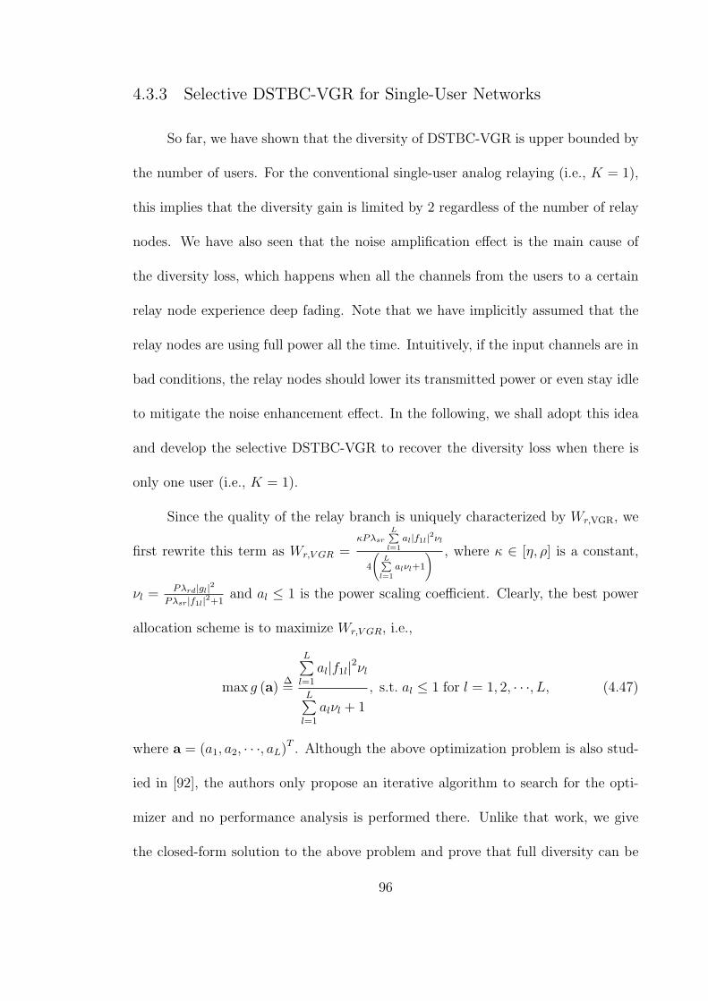
4.3.3 Selective DSTBC-VGR for Single-User Networks

So far, we have shown that the diversity of DSTBC-VGR is upper bounded by

the number of users. For the conventional single-user analog relaying (i.e., K = 1),

this implies that the diversity gain is limited by 2 regardless of the number of relay

nodes. We have also seen that the noise amplification effect is the main cause of

the diversity loss, which happens when all the channels from the users to a certain

relay node experience deep fading. Note that we have implicitly assumed that the

relay nodes are using full power all the time. Intuitively, if the input channels are in

bad conditions, the relay nodes should lower its transmitted power or even stay idle

to mitigate the noise enhancement effect. In the following, we shall adopt this idea

and develop the selective DSTBC-VGR to recover the diversity loss when there is

only one user (i.e., K = 1).

Since the quality of the relay branch is uniquely characterized by Wr,VGR, we

first rewrite this term as Wr,V GR =κPλsr

L∑l=1

al|f1l|2νl

4

(L∑l=1

alνl+1

) , where κ ∈ [η, ρ] is a constant,

νl =Pλrd|gl|2

Pλsr|f1l|2+1and al ≤ 1 is the power scaling coefficient. Clearly, the best power

allocation scheme is to maximize Wr,V GR, i.e.,

max g (a)∆=

L∑l=1

al|f1l|2νlL∑l=1

alνl + 1

, s.t. al ≤ 1 for l = 1, 2, · · ·, L, (4.47)

where a = (a1, a2, · · ·, aL)T . Although the above optimization problem is also stud-

ied in [92], the authors only propose an iterative algorithm to search for the opti-

mizer and no performance analysis is performed there. Unlike that work, we give

the closed-form solution to the above problem and prove that full diversity can be

96

achieved. Without loss of generality, we assume |f11|2 > |f12|2 > · · · > |f1L|2 and

define f1(L+1) = 0.

Proposition 4.3. The solution to the problem (4.47) is

a∗l =

1, l = 1, 2, · · ·, l0

0, o.w.

, (4.48)

where l0 ∈ 1, 2, · · ·, L is the smallest index satisfying

l0∑l=1

(|f1l|2 −

∣∣f1(l0+1)

∣∣2) νl ≥ ∣∣f1(l0+1)

∣∣2.Besides, the error rate has a scaling law of O

(1

PL+1

), and the diversity gain of

selective DSTBC-VGR is L+ 1.

Proof. In [92], it has been proved that a∗l ∈ 0, 1. We now prove by contradiction

that if a∗l1 = 1, then a∗l2 = 1 for any l2 ≤ l1. Suppose now there exists an a∗l2 = 0

with l2 < l1. Then we can always find a sufficiently small quantity δ ≪ 1 such

thatδνl1νl2

≤ 1. Consequently, there exists another feasible solution a with al1 =

a∗l1 − δ and al2 =δνl1νl2

, and the other elements of a are the same as a∗. It is

easy to check that g (a) − g (a∗) =δνl1

(|f1l2 |

2−|f1l1 |

2)

L∑l=1

a∗l νl+1

> 0, which contradicts the

optimality of a∗. Now the optimizer can be limited to the finite set a1, a2, · · ·, aL,

where al =(1l×1,0(L−l)×1

). After some manipulations, we can show that g (ak) ≥

g (ak+1) is equivalent to the conditionk∑l=1

(|f1l|2 −

∣∣f1(k+1)

∣∣2) νl ≥ ∣∣f1(k+1)

∣∣2, wherethe left-hand side is increasing with k and the right-hand side is decreasing with

k. Consequently, we have g (a1) ≤ g (a2) ≤ · · · ≤ g (al0) and g (al0) ≥ g (al0+1) ≥

· · · ≥ g (aL+1), which completes the proof of the first part. To show the diversity

97

performance, we note that the vectors e1, e2, · · ·, eL also belong to the feasible set,

where el is a L×1 vector with the kth element being 1 and the other elements being

0. Note that each el corresponds to the case when only the lth relay is selected

to forward data. Consequently, the selective DSTBC-VGR performs strictly better

than the best relay selection scheme, the error rate of which has a scaling law of

O(

1PL+1

)[16].

Basically, the above results show that each relay node either stays idle or for-

wards data with full power, and the relays with better user-relay channel conditions

have the priority to be selected. These facts indicate an easy implementation of the

proposed selective DSTBC strategy, i.e., the destination can first compute the ac-

tive relay set and then feed back a single threshold. The relays whose input channel

conditions are better than the threshold then stay active in the second phase. On

the contrary, for the iterative algorithm proposed in [92], the destination has to feed

back the whole active relay set, and the feedback overhead is prohibitive when there

is a large number of relays.

4.4 Diagonal Distributed Space-Time Coding

In this section, we study DDSTC that can achieve full diversity for both VGR

and FGR. Different from DSTBC which employs unitary coding matrices at the

relay nodes, DDSTC has a diagonal structure by letting only one relay forward data

at each time instant.

The whole data transmission is still completed in two phases. In the first

98

phase, all the users broadcast a set of L symbols. The received signals at the lth

relay node and at the destination are given by (4.37a) and by (4.37b), respectively.

Then each relay node performs linear transformation on the received signal vector,

and the transmitted signal at the lth relay node is xrl =√αlLP t

Tl ysrl . Here tl is a

L× 1 coding vector having unit norm (i.e., ∥tl∥2 = 1), the design criterion of which

will be clear later. The constant L is introduced to normalize the total transmitted

power, as each relay node only forwards data in one time slot in the second phase.

The amplification factor αl at the lth relay node is still given by (4.2) for VGR and

by (4.3) for FGR, respectively. Then in the second phase, all the relay nodes take

turns to forward data, and the received signal at the destination during the lth time

slot is

yrld =√λrdglxrl + nrld = P

√Lλsrλrdαlgl

K∑k=1

fkltTl sk + nrld, (4.49)

where nrld ∼ CN(0, LPλrdαl|gl|2 + 1

)is the equivalent additive noise. Upon ob-

serving the signals ysd and yrld, the destination performs ML detection to jointly

detect the K user symbols as

sd = arg minsk∈ΩL

∥∥∥∥∥ysd −√Pλsd

K∑k=1

hksk

∥∥∥∥∥2

+L∑l=1

∥∥∥∥yrld − P√Lλsrλrdαlgl

K∑k=1

fkltTl sk

∥∥∥∥2LPλrdαl|gl|2 + 1

,

(4.50)

and the PEP is given by

Pr (s → s) = E

Q√√√√2

(Wd +

L∑l=1

Wrl

) ≤ E

[exp

(−Wd −

L∑l=1

Wrl

)],

(4.51)

where Wd = Pλsd4

∥∆Sh∥2, Wrl =αlP

2Lλsrλrd|gl|2|fTsl∆ST tl|24(LPλrdαl|gl|2+1)

, fsl = (f1l, f2l, · · ·, fKl)T

and ∆S = (∆s1,∆s2, · · ·,∆sK). The first term E [exp (−Wd)] has been given by

99

(4.39). As for the second term, we observe that each Wrl has the similar form as

Wr in the single-relay case discussed before. By following the same steps, we can

obtain

E [exp (−Wrl)]P→∞≤ 4K

Lλrd∥∆ST tl∥2logP

P(4.52)

for both VGR and FGR. Plugging (4.39) and (4.52) back into (4.51) leads to

Pr (s → s)P→∞≤ 4L+1

λsdτ

(K

Lλrd

)L( L∏l=1

∣∣∆sTk tl∣∣2)−1

(logP )L

PL+1, (4.53)

where we useL∏l=1

∥∥∆ST tl∥∥2 ≥

L∏l=1

∣∣∆sTk tl∣∣2 in the inequality, i.e., the dominant er-

ror events occur when only one user symbol vector is decoded incorrectly. Unlike

DSTBC, we observe that both of DDSTC-VGR and DDSTC-FGR can achieve full

diversity gain L+1. This is because the diagonal structure of DDSTC can efficiently

mitigate the noise enhancement effect, as the output noises of the relay nodes would

not be combined concurrently at the destination. Besides, we conclude that the best

code design criterion is to maximize the minimum product distance, i.e.,

maxtl∈CL×1,∥tl∥2=1

min∆s=0

L∏l=1

∣∣∆sT tl∣∣2, (4.54)

which has been well studied in the literatures. For example, when L = 2s (s ≥ 1)

and the signal constellation Ω has the form Z [j] =a+ jb| a, b ∈ Z, j =

√−1, the

optimum coding matrix is given by [93] Topt = 1√LV (θ1, θ2, · · ·, θL), where T =

100

(t1, t2, · · ·, tL)T , θl = ej4l−32L

π for l = 1, 2, · · ·, L, and

V (θ1, θ2, ..., θL) =

1 θ1 · · · θL−11

1 θ2 · · · θL−12

......

. . ....

1 θL · · · θL−1L

(4.55)

is the L × L Vandermonde matrix with parameters θ1, θ2, · · ·, θL. For more code

designs, please refer to [94] and the references therein.

4.5 Simulations

In this section, we present some simulation results to validate our analysis.

We use the path loss model λ = D−3, where λ is the path-loss coefficient and D

is the distance between two terminals. Pair error probability is used as the perfor-

mance metric, i.e., the probability that at least one of the user symbols is decoded

incorrectly at the destination. To simplify the simulation settings, only symmetric

networks with one or two users are considered, and Dsd is always normalized to 1.

Figure 4.2 shows the error performances with different channel conditions,

where the two users use QPSK signals and there is only one relay node. Compared

with direct transmission (DT), a diversity gain of 2 is achieved due to node cooper-

ation. We observe that VGR has about 1dB SNR gain over FGR in all cases. It is

also observed that the error performances almost remain unchanged after improving

the qualities of user-relay channels, whereas about 3dB SNR gain is achieved when

the relay-destination channels become better, which is consistent with our analysis

101

0 5 10 15 20 25 3010

-6

10-5

10-4

10-3

10-2

10-1

100

Pai

r er

ror

pro

bab

ilit

y

SNR (dB)

VGR, Dsr=Drd=1

FGR, Dsr=Drd=1

VGR, Dsr=0.4,Drd=1

FGR, Dsr=0.4,Drd=1

VGR, Dsr=1,Drd=0.4

FGR, Dsr=1,Drd=0.4

Direct Transmission

Figure 4.2: Error performances of a two-user network with different channel condi-

tions.

0 5 10 15 20 25 3010

-7

10-6

10-5

10-4

10-3

10-2

10-1

100

VGR, K=2, BPSK FGR, K=2, BPSK

VGR, K=1, QPSK FGR, K=1, QPSK

VGR, K=2, QPSK FGR, K=2, QPSK

VGR, K=1, 16PSK FGR, K=1, 16PSK

DT, BPSK DT, QPSK

1bpcu

Pai

r er

ror

pro

bab

ilit

y

SNR (dB)

2bpcu

Figure 4.3: Comparison of two-user and single-user network with different data rate.

102

that the relay-destination channel conditions dominate the error performances.

In Figure 4.3, we compare with the conventional single-user (i.e., K = 1)

amplify-and-forward relaying [12], where all the users are served separately in a

TDMA manner. The transmitted power and the total data rate have been properly

normalized, and for network topology we let Dsr = Drd = 0.5. We observe that full

diversity is achieved in all cases. However, the single-user VGR is superior to all the

other schemes when the total data rate is only 1 bit per channel use (bpcu) because

there is no logarithmic-term loss at modest SNRs. When the data rate is 2bpcu,

although the error probability of single-user VGR still decreases faster, the spectral

efficiency dominates the overall performances and thus the two-user systems show

huge performance gain.

Next we study the error performances of relay selection in Figure 4.4, where

QPSK signal is employed. As the reference, we also simulate Ding’s scheme [54] for

VGR, where the qth relay is selected if

q = arg maxl=1,2,···,L

Pλrd|gl|2(Pλsr

K∑k=1

|fkl|2 + 1

)Pλrd|gl|2 + Pλsr

K∑k=1

|fkl|2 + 1

.

Clearly, our Min-Max scheme can achieve full diversity for both VGR and FGR,

whereas the diversity of Ding’s scheme is bounded by 2. This is because in Ding’s

scheme, the channel phases have nothing to do with relay selection. However, the

channel phases actually have tremendous effects on PEPs, since the source messages

are randomly mixed in the air and the MUI depends largely on the orthogonality of

the instant channel coefficients. Although Ding’s scheme does achieve full diversity

in terms of outage capacity [54], where successive interference cancelation is em-

103

0 5 10 15 20 25 30 3510

-8

10-7

10-6

10-5

10-4

10-3

10-2

10-1

100

Pai

r er

ror

pro

bab

ilit

y

SNR (dB)

L=1, VGR

L=1, FGR

L=3, VGR, Min-Max

L=3, FGR, Min-Max

L=5, VGR, Min-Max

L=5, FGR, Min-Max

L=3, VGR, Ding’s Scheme

L=5, VGR, Ding’s Scheme

Figure 4.4: Error performances of a two-user network with relay selection.

ployed at the destination and error-free decoding is assumed, our Min-Max strategy

is more practical for uncoded systems.

In Figure 4.5, we show the performances of DSTBC-FGR and DDSTC with

two users, where QPSK signal is employed. We observe that both coding schemes

can achieve full diversity with multiple relays. Comparatively, DSTBC-FGR per-

forms slightly better than DDSTC-FGR, since the diagonal structure of DDSTC

limits the minimum distances of the codeword. About 1dB SNR gain is achieved

by using DDSTC-VGR against DDSTC-FGR regardless of the number of relays.

Comparing Figure 4.4 and Figure 4.5, we observe that DSTC can achieve much

higher coding gain than relay selection does, as all the relay nodes are contributing

to forward data.

Finally we study the performances of DSTBC-VGR using QPSK signal. When

104

0 5 10 15 20 25 30 3510

-8

10-7

10-6

10-5

10-4

10-3

10-2

10-1

100

Pai

r er

ror

pro

bab

ilit

y

SNR (dB)

VGR, L=1

FGR, L=1

DDSTC-VGR, L=2

DDSTC-FGR, L=2

DSTBC-FGR, L=2

DDSTC-VGR, L=3

DDSTC-FGR, L=3

DSTBC-FGR, L=3

DDSTC-VGR, L=4

DDSTC-FGR, L=4

DSTBC-FGR, L=4

Figure 4.5: Error performances of a two-user network with DDSTC and DSTBC-

FGR.

0 5 10 15 20 25 30 3510

-8

10-7

10-6

10-5

10-4

10-3

10-2

10-1

100

Pai

r er

ror

pro

bab

ilit

y

SNR (dB)

VGR, L=1

DSTBC-VGR, L=2

DSTBC-VGR, L=3

DSTBC-VGR, L=4

SIMO, 1Tx3Rx

Figure 4.6: Error performances of a two-user network with DSTBC-VGR.

105

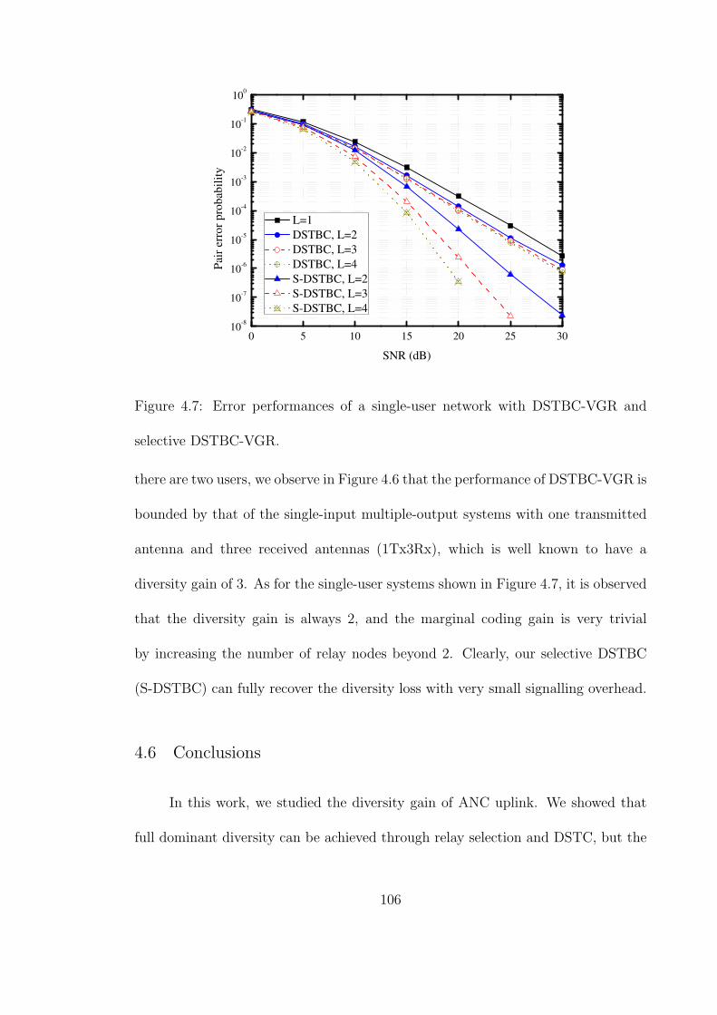
0 5 10 15 20 25 3010

-8

10-7

10-6

10-5

10-4

10-3

10-2

10-1

100

Pai

r er

ror

pro

bab

ilit

y

SNR (dB)

L=1

DSTBC, L=2

DSTBC, L=3

DSTBC, L=4

S-DSTBC, L=2

S-DSTBC, L=3

S-DSTBC, L=4

Figure 4.7: Error performances of a single-user network with DSTBC-VGR and

selective DSTBC-VGR.

there are two users, we observe in Figure 4.6 that the performance of DSTBC-VGR is

bounded by that of the single-input multiple-output systems with one transmitted

antenna and three received antennas (1Tx3Rx), which is well known to have a

diversity gain of 3. As for the single-user systems shown in Figure 4.7, it is observed

that the diversity gain is always 2, and the marginal coding gain is very trivial

by increasing the number of relay nodes beyond 2. Clearly, our selective DSTBC

(S-DSTBC) can fully recover the diversity loss with very small signalling overhead.

4.6 Conclusions

In this work, we studied the diversity gain of ANC uplink. We showed that

full dominant diversity can be achieved through relay selection and DSTC, but the

106

logarithmic term in the error rate expression would degrade the diversity perfor-

mance at modest SNRs. For DSTBC, the diversity gain would also be bounded by

the number of users due to noise amplification effect of VGR. For future work, one

may study the code design for DSTBC and extend our selective DSTBC scheme to

the multi-user networks. One may also investigate other distributed beamforming

schemes to improve the coding gain.

107

Chapter 5

Diversity Analysis of Wireless Uplink with Non-Coherent Network

Coding

In the previous chapters, we assume that instantaneous CSI is known to the

whole network, and we studied the diversity performance of ANC and DNC with

coherent transmission. Although perfect CSI is very important for the receiver to

mitigate error propagation for DNC or suppress MUI for ANC, it is not always

available in practice. This could occur when the channels experience fast fading

such that it is really hard to track the real-time channel variations at the receiver.

Channel estimation overhead is another concern. For the multi-user relay channel,

the channel estimation overhead increases linearly with the product of the number

of users and the number of relays, which may become formidable and even outweigh

the network coding gain. Besides, channel estimation requires additional wireless

resources such as power and dedicated channels that could be otherwise used to

transmit the data stream, so the bandwidth efficiency is also reduced to some extent.

Because of these concerns, non-coherent transmission that do not require perfect CSI

are of more practical interests under these circumstances.

Non-coherent transmission would reduce the performance. For the traditional

point-to-point channel, it is well known that non-coherent transmission would incur

3dB SNR loss, while the diversity gain remains the same [1]. However, as for the

108

network-coded cooperation systems very few literatures have explicitly discussed the

performance loss. So in this work, we study the non-coherent network-coded uplink

and explore the impact on diversity gain. Depending on the available CSI, we first

develop the coherent and non-coherent ML receivers. For ANC, as the non-coherent

receivers have no closed form, we develop two suboptimum receivers according to

the average link qualities. Next we study the error rates, and show that full diversity

can always be achieved at extremely high SNRs regardless of the CSI assumptions.

However, the lack of perfect CSI would incur some diversity loss at modest SNRs.

Besides, the performance loss of ANC is more serious due to the incapability to

efficiently suppress multi-user interferences at the receivers. Extensive simulations

are performed to verify our analytical results.

Notations: |·|, (·)T and (·)H stand for absolute value, transpose and conjugate

transpose, respectively. The boldface lowercase letter a and the boldface uppercase

letter A represent vector in column form and matrix, respectively. ∥a∥ and detA

denote the Euclidean norm of a vector a and the determinant of a square matrix

A, respectively. We shall use abbreviation i.i.d. for independent and identically

distributed. We denote Z ∼ CN (u,Σ) as a circularly symmetric complex Gaussian

random variable vector with mean u and covariance matrix Σ, Z ∼ exp (µ) as

an exponential random variable with mean µ, and Z ∼ χ2k as a chi-square random

variable with the degree of freedom being k. The probability of an eventA is denoted

by Pr(A). The CDF and PDF of a random variable Z are denoted by FZ(z) and

fZ(z), respectively. Finally, we say h (x) = O (g (x)) if a ≤ limx→∞h(x)g(x)

≤ b for some

positive constants a and b.

109

1st phase 2nd phase 3rd phase

RelayDestination

Source 1

Source 2

rx

1x

2x

Figure 5.1: System model of the two-user network-coded uplink.

5.1 System Model

Consider the wireless uplink channel where two source nodes send data to a

common destination with the help of a single relay node, as shown in Figure 5.1. Let

fk ∼ CN (0, 1) and hk ∼ CN (0, 1) for k = 1, 2 be the channel coefficients from the

kth source to the relay and to the destination, respectively, and g ∼ CN (0, 1) be the

channel coefficient from the relay to the destination. All the channel coefficients are

independent, and the additive noises on different channels are also i.i.d. CN (0, 1).

The channel gains are denoted by λsr, λsd and λrd for source-relay channels, source-

destination channels and relay-destination channel, respectively. The channel gains

are some constants that are determined by the distances and the path-loss exponents.

Only uncoded systems are considered throughout this work, i.e., there is no

error detection/correction code. The two source nodes are supposed to use the M-

ary FSK modulations. The symbol set is denoted by Ω = e1, e2, · · · , eM, where

el is the lth unit vector with the lth element being 1 and the other elements being

0. The whole data transmission is completed in three phases. In the kth phase

for k = 1, 2, the kth source node broadcasts its own signals while the other source

110

node keeps silent. The received signals at the relay node and at the destination are

denoted by

ykr =√Pλsrfkxk + nkr, (5.1)

ykd =√Pλsdhkxk + nkd, (5.2)

respectively. Here P is the transmitted power, xk is the kth source symbol with

xk ∈ Ω, nkr and nkd are the corresponding additive noises. As the noise power

has been normalized, the transmitted power P is also treated as the system SNR

throughout this work. The relay operation is dependent upon the network coding

schemes that would be detailed later. At this moment, we simply denote the relay

symbol by xr and assume it has unit power, i.e., E∥xr∥2 = 1. Then in the third

phase, the relay node forwards its symbol to the destination while the two source

nodes remain silent. The received signal is given by

yrd =√Pλrdgxr + nrd, (5.3)

where nrd is the additive noises. Upon observing yrd and ykd for k = 1, 2, the

destination performs ML detection to jointly detect the two source symbols as

(xd,1,xd,2) = arg maxx1,x2∈Ω

L (yrd| x1, x2,Ψ)×2∏

k=1

L (ykd| x1, x2,Ψ), (5.4)

where L(·) is the corresponding likelihood function, and Ψ is the set of instan-

taneous CSI available at the destination. For coherent detection, we have ΨF =

f1, f2, h1, h2, g, i.e., global CSI is supposed to be known at the destination. Al-

ternatively, the destination can choose to perform non-coherent detection with ΨS

being the empty set, such that channel estimation is no longer required and all the

111

real-time channel variations are blind to the whole network. To facilitate expla-

nations, we also define the partial coherent detection, where the destination only

knows the relay-destination channel, i.e., ΨP = g. As the channel gains (i.e., λ)

are only second-order statistics that remain unchanged over a long time, we assume

these coefficients are known to all the nodes in the network. According to these

definitions, we have

L (ykd| xk,Ψ) =

p(ykd −

√Pλsdhkxk, I

), Ψ = ΨF (5.5a)

p(ykd, Pλsdxkx

Hk + I

), Ψ ∈ ΨP ,ΨS (5.5b)

for k = 1, 2, where I is the identity matrix and p (y,Σ) = 1πM |Σ| exp

(−yHΣ−1y

)is

the PDF of y ∼ CN (0,Σ). The likelihood function of the relay link signal yrd is

related to the network coding schemes and would be detailed later.

5.2 Transceiver Design

In this section, we study the relay operation and the ML detection at the

destination under different network coding schemes.

5.2.1 Analog Network Coding

If ANC is used at the relay node, the two received signals ykr for k = 1, 2 are

combined in the complex field directly by xr =√α (y1r + y2r), where

α =1

2 (Pλsr +M)(5.6)

112

is the amplification factor to normalize the relay power. From (5.3), the received

signal yrd can then be rewritten as

yrd =√αPλrdg

2∑k=1

(√Pλsrfkxk + nkr

)+ nrd =

√αP 2λrdλsrg

2∑k=1

fkxk + nrd,

(5.7)

where nrd =√αPλrdg

2∑k=1

nkr+nrd is the equivalent noises. The likelihood function

of the relay link signal yrd is then given by

L (yrd| x1, x2,ΨF ) = p

(yrd −

√αP 2λrdλsrg

2∑k=1

fkxk,(2αPλrd|g|2 + 1

)I

), (5.8)

L (yrd| x1, x2,ΨP ) = p

(yrd, αP

2λrdλsr|g|22∑

k=1

xkxHk +

(2αPλrd|g|2 + 1

)I

)(5.9)

for coherent and partial coherent detection, respectively. For non-coherent detection,

the likelihood function can be obtained by averaging (5.9) over the distributions of

g, i.e.,

L (yrd| x1, x2,ΨS) = Eg [L (yrd| x1, x2,ΨP )] . (5.10)

Unfortunately, the above expression is an integral form that has no closed-

form solution, which would greatly complicate the implementation. To simplify the

receiver design, we develop two suboptimum yet efficient receivers in the sequel. To

that end, let us first revisit the signal model (5.7). The aggregate scaling coefficient

effective on the signal component from the input of the relay node to the destination

is given by √αPλrdg =

√Pλrd

2 (Pλsr +M)gP≫1≈

√λrd2λsr

g. (5.11)

When the source-relay channel is much better than the relay-destination channel

(i.e., λrd ≪ λsr), the above scaling coefficient remains small with large probability,

113

whereas the noise power of nrd is a constant. As a result, we can approximate g by

its mean and obtain

L (yrd| x1, x2,ΨS) ≈ L (yrd| x1, x2,ΨP , g = 1) , (5.12)

which is called fading elimination approximation (FEA). The error performance is

expected to remain similar because the channel fading only brings very limited effects

when the scaling coefficient is small on average. On the other hand, if the source-

relay channel is much worse than the relay-destination channel (i.e., λrd ≫ λsr), then

the noises nrd would have much lower power than the scaled noises√αPλrdgnkr.

Consequently, we can intentionally neglect nrd and obtain

yrd ≈ yrd =√αPλrdg

2∑k=1

(√Pλsrfkxk + nkr

). (5.13)

To obtain the likelihood function of yrd, we first prove the following lemma.

Proposition 5.1. Suppose v ∼ CN(0, diag

σ2vi

Mi=1

)and u ∼ CN (0, σ2

u)

are independent random variables, then the PDF of z = uv is

f (z) =

(M∏i=1

2

πσ2uσ

2vi

)q

(4

σ2u

M∑i=1

|zi|2

σ2vi

), (5.14)

where q (x) = x−M−1

2 KM−1 (√x) and KM (x) is the M th-order modified Bessel func-

tion of the second kind [87, 9.6.1].

Proof. Denote zi = riejθi for i = 1, 2, · · · ,M , then it is easy to show that the phases

θi are independent of the amplitudes ri, and θi are i.i.d. and uniformly

distributed on [0, 2π). Therefore,

f (z) =1

|J |f (r,θ) =

M∏i=1

(2πri)−1f (r) , (5.15)

114

where |J | =M∏i=1

ri is the Jacobian determinant. The CDF of r is given by

F (r) =

∫ ∞

0

1

σ2u

exp

(− x

σ2u

) M∏i=1

(1− exp

(− r2iσ2vix

))dx. (5.16)

After taking derivatives, we can obtain

f (r) =1

σ2u

M∏i=1

2riσ2vi

∫ ∞

0

x−M exp

(− x

σ2u

− 1

x

M∑i=1

r2iσ2vi

)dx

=

(M∏i=1

4riσ2uσ

2vi

)q

(4

σ2u

M∑i=1

r2iσ2vi

), (5.17)

where we use [88, 3.478.4] in the last equality. Plugging (5.17) back into (5.15)

completes the proof.

According to Proposition 5.1, the likelihood function of yrd can be obtained

after redefining the parameters in (5.14). To be specific, for x1 = x2 = el we have

σ2u = αPλrd, σ

2vl= 2 (Pλsr + 1) and σ2

vi= 2 for i = l, whereas for x1 = ek, x2 = el

with k = l we have σ2u = αPλrd, σ

2vk

= σ2vl= Pλsr + 2 and σ2

vi= 2 for i = l, k. In

later sections, this scheme is referred to as noise elimination approximation (NEA).

5.2.2 Digital Network Coding

For DNC, the two source symbols are first individually detected at the relay

node as

xr,k =

argmax

xk∈Ωp(ykr −

√Pλsrfkxk, I

),Ψ = ΨF (5.18a)

argmaxxk∈Ω

p(ykr, Pλsrxkx

Hk + I

),Ψ = ΨS (5.18b)

where the relay node is assumed to know the same type of CSI as the destination.

Next, the detected source symbols are combined in the finite field, and the relay

115

symbol is given by xr = xr,1 ⊕ xr,2. We remark that the conventional DNC is

performed bitwise through exclusive-or operations. Here to simplify the notations

we omit the mapping between the bits and symbols and express the network-coded

output in the symbol space directly. It is also noteworthy that xr belongs to the

M-ary FSK symbol set Ω as well, but it maybe different from the true network-coded

symbol x⊕ = x1 ⊕ x2 due to random detection errors.

The likelihood function of the relay link signal yrd is

L (yrd| x1, x2,Ψ) =M∑k=1

Pr ( xr = ek| x1, x2,Ψ)L (yrd| xr = ek,Ψ), (5.19)

where the second term within the summation has the same form as (5.5) after

properly modifying the subscripts, and the first term is given by

Pr ( xr = ek| x1, x2,Ψ) =∑

xr,1⊕xr,2=ek

Pr ( xr,k| x1,Ψ)Pr ( xr,2| x2,Ψ). (5.20)

Note that each term within the summation stands for the transition probability

from the trial source symbol xk to the trial relay detected symbol xr,k. For FSK

modulations, the error rates at the relay node can be obtained from [1, 5.2.19]

and [1, 5.4.42] after properly accommodating the channel fading, which are given

by

Pr,k =

1− 1√

2π

∫ ∞

−∞(1−Q (x))M−1e

− 12

(x−√

2Pλsr|fk|2)2dx, Ψ = ΨF(5.21a)

M−1∑k=1

(M − 1

k

)(−1)k+1

1 + k (1 + Pλsr), Ψ = ΨS (5.21b)

where Q (x) is Q-function. Due to symmetry, the detection errors of FSK modula-

tions are uniformly distributed in the error symbol set, so each transition probability

116

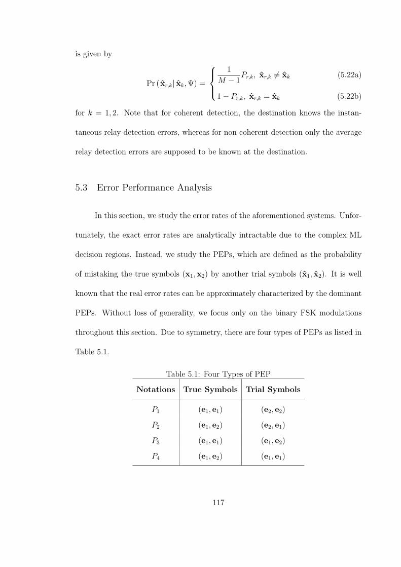
is given by

Pr ( xr,k| xk,Ψ) =

1

M − 1Pr,k, xr,k = xk (5.22a)

1− Pr,k, xr,k = xk (5.22b)

for k = 1, 2. Note that for coherent detection, the destination knows the instan-

taneous relay detection errors, whereas for non-coherent detection only the average

relay detection errors are supposed to be known at the destination.

5.3 Error Performance Analysis

In this section, we study the error rates of the aforementioned systems. Unfor-

tunately, the exact error rates are analytically intractable due to the complex ML

decision regions. Instead, we study the PEPs, which are defined as the probability

of mistaking the true symbols (x1,x2) by another trial symbols (x1, x2). It is well

known that the real error rates can be approximately characterized by the dominant

PEPs. Without loss of generality, we focus only on the binary FSK modulations

throughout this section. Due to symmetry, there are four types of PEPs as listed in

Table 5.1.

Table 5.1: Four Types of PEP

Notations True Symbols Trial Symbols

P1 (e1, e1) (e2, e2)

P2 (e1, e2) (e2, e1)

P3 (e1, e1) (e1, e2)

P4 (e1, e2) (e1, e1)

117

5.3.1 Coherent Analog Network Coding

After some manipulations, we can obtain the conditional PEPs given by

PEP|ΨF = Q

√√√√√1

2

Pλsd 2∑k=1

|hk|2∥xk − xk∥2 +αP 2λrdλsr|g|2

1 + 2αPλrd|g|2

∥∥∥∥∥2∑

k=1

fk (xk − xk)

∥∥∥∥∥2 .

(5.23)

To obtain the average PEPs, we need to average the above expression over the

channel distributions, which is analytically intractable. Instead, we seek to develop

some bounds that have the same scaling laws as the true PEPs at high SNRs.

To obtain the PEP lower bound, we use the integral representation of Q-

function given by [85]

Q (x) =1

π

∫ π2

0

exp

(− x2

2sin2θ

)dθ. (5.24)

After replacing the Q-function in (5.23) with the above expression and averaging

over the channel distributions by use of (4.9), we can obtain

PEP ≥ (2n+ 1)!!

(2n+ 2)!!

2n−1

(2 + Pλsd)n

×(

4

4 + nPλsr+

nλsr

αλrd(4 + nPλsr)2 log

(1 + 4αPλrd + αnP 2λrdλsr

)), (5.25)

where (·)!! is double factorial, n = 1x1 = x1 + 1x2 = x2 with 1· being indi-

cator function, and we use 12log(1 + 2

x

)< exE1 (x) [87, 5.1.20] in the inequality. To

obtain the PEP upper bound, we use the Chernoff bound [1] of Q-function given by

Q (x) ≤ 12exp

(−1

2x2). In a similar way, we have

PEP ≤ 2n−1

(2 + Pλsd)n

×(

4

4 + nPλsr+

2nPλsr

αPλrd(4 + nPλsr)2 log

(1 + 2αPλrd +

1

2αnP 2λrdλsr

)),(5.26)

118

where we use exE1 (x) < log(1 + 1

x

)[87, 5.1.20] in the inequality. From (5.23), it is

observed that Type-1 PEP and Type-2 PEP have the same conditional distributions,

and Type-3 PEP and Type-4 PEP also have the same conditional distributions.

That is why the PEP bounds (5.25) and (5.26) depend only on n but not the true

and trial symbol pairs. At high SNRs (i.e. P ≫ 1), we can show that both the upper

bound and lower bound scale as O(logPPn+1

). Clearly, the dominant error events occur

when only one of the two source symbols is detected incorrectly at the destination

(i.e., n = 1), and the error rates of coherent ANC scale as O(logPP 2

)at high SNRs.

5.3.2 Non-Coherent Analog Network Coding

Since the non-coherent ML receiver (5.10) has an intractable integral form,

we study the partial coherent receiver (5.9). As will be shown in simulations, the

performances of these two receivers are very close to each other.

For Type-1 PEP, we have

P1 = Pr

λsdP

1 + λsdP

(U12 + V 1

2

)+

λsrPQ

1 + λsrPQW 1

2 ≥ λsdP(U11 + V 1

1

)+ λsrPQW

11

≤ Pr

U12 + V 1

2 +W 12 ≥ PY

, (5.27)

where W 11 =

|yrd,1|21+2αPλrd|g|2+2αP 2λrdλsr|g|2

, U11 =

|y1d,1|21+λsdP

, V 11 =

|y2d,1|21+λsdP

, W 12 =

|yrd,2|21+2αPλrd|g|2

,

U12 = |y1d,2|2, V 1

2 = |y2d,2|2 are i.i.d. exponential random variables with unit mean,

and

Q =2αPλrd|g|2

1 + 2αPλrd|g|2. (5.28)

Since U12 + V 1

2 + W 12 ∼ 1

2χ26, the conditional PEP given Y

∆= λsd (U

11 + V 1

1 ) +

119

λsrQW11 = y is

P1|Y=y ≤(1 + Py +

1

2P 2y2

)exp (−Py) . (5.29)

At high SNRs, the conditional PEP decreases really fast with y. Therefore, the

average PEP is roughly determined by the behavior of the PDF of Y ≪ 1. Denoting

T∆= QW 1

1 , we can obtain

FY (y)y≪1≈∫ y

λsr

0

fT (t)(y − λsrt)

2

λ2sddt, (5.30)

Taking derivative with respect to y leads to

fY (y)y≪1≈ 2λsr

λ2sd

∫ yλsr

0

FT (t) dt = − y2

2αPλsrλrdλ2sd

(log

y

λsr− 1

2

), (5.31)

where we use FT (t)t≪1≈ − 1

2αPλrdt log t from (4.9) in the second equality. Using the

above PDF to average the conditional PEP in (5.29), we obtain

P1≤20 log (

√ePλsr)− 39 + 20γ

2αP 4λsrλrdλ2sd= O

(logP

P 3

), (5.32)

where γ is Euler constant [88, 4.352.2].

For Type-2 PEP, the likelihood function of yrd remains the same under both

hypotheses, which greatly simplifies the computations. After some manipulations,

we can obtain

P2 = Pr|y1d,2|2 + |y2d,1|2 ≥ |y1d,1|2 + |y2d,2|2

=

4 + 3λsdP

(2 + λsdP )3 = O

(1

P 2

). (5.33)

For Type-3 PEP, we have

P3 = Pr

λsdP

1 + λsdPV 32 +

λsrPQ

2 + λsrPQW 3

2

≥ λsdPV31 +

λsrPQ

2 + λsrPQW 3

1 + log(2 + λsrPQ)

2

4 (1 + λsrPQ)

≤ Pr

W 3

2 + V 32 ≥ λsdPV

31 + logZ

, (5.34)

120

where W 31 =

|yrd,1|21+2αPλrd|g|2+2αP 2λrdλsr|g|2

, V 31 =

|y2d,1|21+λsdP

, W 32 =

|yrd,2|21+2αPλrd|g|2

, and V 32 =

|y2d,2|2 are i.i.d. exponential random variables with unit mean, and Z = 2+λsrPQ4

≤

12+ Pλsr

4. The conditional PEP given Z = z is given by

P3|Z=z ≤(1 + 2λsdP ) + (1 + λsdP ) log

(12+ Pλsr

4

)(1 + λsdP )

2z. (5.35)

By defining η1 = αPλrd (2 + λsrP ), we can further obtain

E

(1

Z

)=

1

η1

(4αλrdP +

2λsrP

2 + λsrPexp

(1

η1

)E1

(1

η1

)). (5.36)

After combining (5.35) and (5.36) and using the inequality exE1 (x) ≤ log(1 + 1

x

)[87, 5.1.20], we obtain P3 ≤ O

(log2PP 2

)Finally for Type-4 PEP, we have

P4 = Pr

λsdP

1 + λsdPV 41 +

λsrPQ

2 (1 + λsrPQ)W 4

1 + log(2 + λsrPQ)

2

4 (1 + λsrPQ)

≥ λsdPV42 +

1

2λsrPQW

42

, (5.37)

where W 41 =

|yrd,1|21+2αPλrd|g|2+αP 2λrdλsr|g|2

, V 41 = |y2d,1|2, W 4

2 =|yrd,2|2

1+2αPλrd|g|2+αP 2λrdλsr|g|2,

V 42 =

|y2d,2|21+λsdP

are i.i.d. exponential random variables with unit mean. As the loga-

rithmic term is upper bounded by log (2+λsrP )2

4(1+λsrP )

∆= η2, we have

P4 ≤ Pr

W IV

1 + V IV1 ≥ max

1

2λsdPV

IV2 , η2

︸︷︷︸

∆=P

U14

+Pr

2η2 ≥ λsdPV

IV2 +

1

2λsrPQW

IV2

︸︷︷︸

∆=P

U24

. (5.38)

121

After some lengthy algebra, we have

PU14 = (1 + η2) e

−η2 −(

λsdP

2 + λsdP

)2(1 +

2 + λsdP

λsdPη2

)e− 2+λsdP

λsdPη2

= O

(log2P

P 2

), (5.39)

PU24

P≫1≈ η22

αP 3λsrλsdλrd

(1− 2 log

(4η2λsrP

))= O

(log3P

P 2

). (5.40)

Consequently, we have P4 ≤ O(

log3PP 2

), which appears to dominate all the PEPs. To

make the argument rigorous, yet we still need to show that this is the exact scaling

law of Type-4 PEP. To that end, we develop a lower bound on P4 by neglecting the

first two terms on the left-hand side of the inequality in (5.37), which leads to

P4 ≥ PL4 = Pr

log

2 + λsrPQ

4≥ λsdPV

42 +

1

2λsrPQW

42

. (5.41)

The conditional probability of PL4 given Q = q is given by

PL4

∣∣Q=q

= 1− 2λsd2λsd − qλsr

exp

(− 1

λsdPlog

2 + qλsrP

4

)+

qλsr2λsd − qλsr

exp

(− 2

qλsrPlog

2 + qλsrP

4

). (5.42)

When q ≥ P−β for any constant β ∈ (0, 1), we have qP ≥ P 1−β ≫ 1 for P ≫ 1,

thus

PL4

∣∣Q=q

P≫1≈ 1

qλsrλsdP 2

(log

2 + qλsrP

4

)2

. (5.43)

The final step is to average the above expression over the distribution of Q. The

PDF of Q is given by

fQ (q) =1

2αPλrd(1− q)2exp

(− q

2αPλrd (1− q)

), 0 ≤ q ≤ 1 (5.44)

It is easy to see that fQ (q) is a continuous function with fQ (0) = 12αPλrd

and

fQ (1) = 0, therefore it is lower bounded by some constant C on the region q ∈ [0, η3]

122

with η3 < 1 being some fixed number. Using the above facts, we can obtain

PL4 ≥

∫ η3

P−β

1

qλsrλsdP 2

(log

2 + qλsrP

4

)2

fQ (q) dq

≥Clog

(η3P

β)

λsrλsdP 2

(log

2 + λsrP1−β

4

)2

= O

(log3P

P 2

). (5.45)

As the upper bound and lower bound on P4 have exactly the same scaling laws, we

conclude that the error rates of partial coherent ANC scale as O(

log3PP 2

)at high

SNRs.

5.3.3 Digital Network Coding

For DNC, we assume x1⊕x2 = e1 for x1 = x2 and x1⊕x2 = e2 for x1 = x2. The

relay symbol xr = xr,1⊕xr,2 is a single binary FSK symbol that carries information

for both sources. Thus the likelihood function of the relay link signal yrd depends

only on the true network-coded symbol x⊕ rather than the source symbol pair

(x1,x2). From Table I, we can observe that regardless of the type of receiver, Type-

1 PEP and Type-2 PEP are always the same, and Type-3 PEP and Type-4 PEP are

the same as well. So in the sequel, we only study Type-1 PEP and Type-3 PEP, in

which cases the true source symbols are (e1, e1) and the true network-coded symbol

is x⊕ = e1 ⊕ e1 = e1.

To proceed, we first define

tkd =

2√PλsdRe h∗k (ykd,1 − ykd,2) , Ψ = ΨF (5.46a)

Pλsd1 + Pλsd

(|ykd,1|2 − |ykd,2|2

), Ψ = ΨS (5.46b)

123

for k = 1, 2 and

trd =

2√PλrdRe g∗ (yrd,1 − yrd,2) , Ψ = ΨF (5.47a)

Pλrd1 + Pλrd

(|yrd,1|2 − |yrd,2|2

), Ψ = ΨS (5.47b)

It can be shown that the above metrics can be rewritten as the quadratic forms of

some independent complex Gaussian random variables. According to [86], the PDF

of tkd is ftkd (t) = f (asd, bsd, t) for k = 1, 2, the conditional PDF of trd given xr = x⊕

is ftrd (t) |xr=x⊕ = f (ard, brd, t), and the conditional PDF of trd given xr = x⊕ is

ftrd (t) |xr =x⊕ = f (brd, ard, t), where

f (a, b, t) =ab

a+ b(exp (bt)1 t < 0+ exp (−at)1 t ≥ 0) , (5.48)

and for k ∈ s, r, bkd = akd + 1 and

akd =

1

2

(√1 +

2

Pλkd− 1

), Ψ = ΨF (5.49a)

1

Pλkd, Ψ = ΨS (5.49b)

After some algebra, we can show that Type-1 PEP is given by

P1 = Pr

(2∑

k=1

tkd ≤ 0

)=a2sd (asd + 3bsd)

(asd + bsd)3 . (5.50)

At high SNRs, Type-1 PEP can be approximated by

P1

P≫1≈

3

4P 2λ2sd, coherent (5.51a)

3

P 2λ2sd, non-coherent (5.51b)

and the scaling law is P1 = O(

1P 2

)regardless of the type of the receiver. As for

Type-3 PEP, we have

P3 = Pr

(t2d + log

(1− Pr) etrd + Pr

Pretrd + (1− Pr)≤ 0

), (5.52)

124

where Pr is the relay detection error rate of the network-coded symbol x⊕. For

coherent detection and non-coherent detection, Pr are respectively given by

Pr =2∏

k=1

Q

(√Pλsr|fk|2

)(1−Q

(√Pλsr

∣∣f1,2\k∣∣2)) ∆= Pr,F , (5.53)

Pr =2 (1 + Pλsr)

(2 + Pλsr)2

∆= Pr,S. (5.54)

As the exact analysis is intractable, we use the piecewise linear approximation [84]

given by

log(1− Pr) e

trd + PrPretrd + (1− Pr)

≈

Tr, trd ≥ Tr

trd,−Tr,S ≤ trd ≤ Tr

−Tr, trd ≤ −Tr

(5.55)

where Tr = log 1−PrPr

. After applying the above approximation in (5.52) and aver-

aging over the channel distributions of h1, h2, g, we can obtain the conditional

Type-3 PEP given f1, f2 as

P3|f1,f2 = (1− Pr)h0 (ard, brd, asd, bsd) + Prh0 (brd, ard, asd, bsd)

− asdbrd + asd

(1− Pr)h1 (brd, ard, asd, bsd, Tr)−asd

ard + asdPrh1 (ard, brd, asd, bsd, Tr)

+bsd

ard + bsd(1− Pr)h1 (ard, brd, bsd, asd, Tr)

+bsd

brd + bsdPrh1 (brd, ard, bsd, asd, Tr) , (5.56)

where

h0 (a, b, c, d) =a

a+ b

1 +

bc

(c+ d) (a+ d)− bd

(c+ d) (b+ c)

, (5.57)

h1 (a, b, c, d, t) =b

a+ b

d

c+ dexp (− (a+ c) t) . (5.58)

For non-coherent detection, (5.56) is exactly the average Type-3 PEP, because Pr,S

in (5.54) is independent of the source-relay channels f1, f2. At high SNRs, it can

125

be approximated by

P3

P≫1≈

4 + 2 log(Pλsr2

)P 2λsrλsd

+3

P 2λrdλsd= O

(logP

P 2

). (5.59)

By comparing (5.51b) and (5.59), we observe that Type-3 PEP is the dominant error

term, thus the error rates of non-coherent DNC scale as O(logPP 2

)at high SNRs.

Next we study the average Type-3 PEP of coherent DNC, which can be ob-

tained after averaging (5.56) over the channel distributions of f1 and f2. Since the

exact analysis is intractable, we shall make some approximations. As the first step,

we approximate Pr,F in (5.53) by

Pr,F ≈ Q

(√1

2Pλsr|f |2

)≈ h2

(√1

2Pλsr|f |2

), (5.60)

where |f |2 = 2min(|f1|2, |f2|2

)∼ exp (1), and

h2 (x) =1

B√2πx

(1− exp

(− A√

2x

))exp

(−1

2x2), A = 1.98, B = 1.135. (5.61)

The first approximation is quite tight from modest to high SNRs, as the relay

detection performance is roughly determined by the worse source-relay channel. The

advantage of such approximation is that the conditional PEP (5.56) now relies only

on the single variable |f |. As for the second approximation, we use Q (x) ≈ h2 (x)

[95]. Next, we observe that the average PEP depends largely on the small values of

|f |, as the conditional PEP decreases very fast with the variable |f | at high SNRs.

As a result, we can approximate Tr,F by

Tr,F = log1− Pr,FPr,F

|f |≪1≈√

4

πPλsr|f |2. (5.62)

After plugging (5.60) and (5.62) back into (5.56) and doing some lengthy algebra,

126

we can obtain

P3 ≈ h0 (ard, brd, asd, bsd) + h5

(0, 1, 0, 1,

1

2Pλsr

)h0 (brd, ard, asd, bsd)

−h5(0, 1, 0, 1,

1

2Pλsr

)h0 (ard, brd, asd, bsd)

− asdbrd + asd

(h4

(brd, ard, asd, bsd,

1

2Pλsr

)− h5

(brd, ard, asd, bsd,

1

2Pλsr

))+

bsdard + bsd

(h4

(ard, brd, bsd, asd,

1

2Pλsr

)− h5

(ard, brd, bsd, asd,

1

2Pλsr

))− asdard + asd

h5

(ard, brd, asd, bsd,

1

2Pλsr

)+

bsdbrd + bsd

h5

(brd, ard, bsd, asd,

1

2Pλsr

)(5.63)

P≫1≈ 3

4P 2λrdλsd+

2

P 2λsrλsd= O

(1

P 2

), (5.64)

where

h4 (a, b, c, d, t) =b

a+ b

d

c+ d

1−√

8(a+ c)2th3

√4(a+ c)2t

π

, (5.65)

h5 (a, b, c, d, t) =b

a+ b

d

c+ d

2

B√t (2 + t)

×

h3√8(a+ c)2t

π (2 + t)

− h3

(√t

2 (2 + t)

(4 (a+ c)√

π+ A

)) , (5.66)

and h3 (x) = exp(x2

2

)Q (x). From (5.51a) and (5.64), we conclude that the error

rates of coherent DNC scale as O(

1P 2

)at high SNRs.

Table 5.2: Scaling Laws of The Error Rates

ANC DNC

Coherent O(logPP 2

)O(

1P 2

)Partial/Non-coherent O

(log3PP 2

)O(logPP 2

)

127

5.3.4 Discussions

We summarize the scaling laws of the error rates in Table 5.2. It is observed

that the error rates can be put in a general form of Pe = O(

logd1PP d2

). The diversity

gain is defined as

d = − logPelogP

= d2 − d1log logP

logP. (5.67)

At extremely high SNRs (i.e., P → ∞), the second term vanishes and the dominant

diversity gain is d2. But at modest SNRs, the logarithmic term would incur notice-

able diversity loss and make the error curves decrease very slowly with SNRs. The

extent of such diversity loss can be measured by d1.

From Table 5.2, we can observe that the dominant diversity gain is 2 regardless

of the network coding scheme and the type of receiver. The diversity gain comes

from node cooperation, as each source symbol can reach the destination through two

independent paths, i.e., direct link and relay link. However, the logarithmic term

loss is totally different for these schemes. For coherent detection, the logarithmic

term loss of ANC has an order of 1, whereas there is no logarithmic term loss for

DNC. This is because for ANC, different source signals are randomly combined in

the complex field through linear addition, so MUI would appear at the destination

and degrade the performances of ML detection. On the contrary, for DNC the source

signals are combined in the finite field through bit operation, thus the relay symbol

is a single network-coded FSK symbol without any MUI.

For partial/non-coherent detection, the lack of perfect CSI would incur more

logarithmic term loss for both ANC and DNC. Specifically, the order of the loga-

128

rithmic term loss are 1 and 3 respectively for coherent ANC and partial coherent

ANC, while for coherent DNC and non-coherent DNC the order of the logarithmic

term loss are 0 and 1, respectively. As a result, the performance loss of ANC is more

serious, and the reasons are given in the sequel. For DNC, the relay node may detect

the wrong symbols and propagate these errors to the destination. So the relay link

signal is properly scaled through nonlinear operations in the ML combiner accord-

ing to the estimated relay detection error rates at the destination. For non-coherent

detection, the real-time relay detection states are blind to the destination, and the

scaling is based on the average relay detection error rates. Although such scaling

is accurate on average, it cannot capture the instantaneous network dynamics and

thus incurs some performance loss. The situation becomes worse for ANC, as the

formation of MUI is totally blind to the destination when perfect CSI is unknown.

Consequently, the destination cannot efficiently suppress MUI to clearly separate

the two source signals. That is why ANC suffers more serious performance loss than

DNC when perfect CSI is unavailable at the destination.

Lastly, we would like to point out that the non-coherent detection may be-

have very differently for the single-user channels and the multi-user channels. For

the single-user point-to-point channel, it is well known that non-coherent detection

only brings 3dB SNR loss compared to coherent detection, but the diversity perfor-

mances remain the same [1]. As for the multi-user network-coded uplink channel, we

have demonstrated that non-coherent detection would incur diversity loss at modest

SNRs, but the dominant diversity gains remain the same at extremely high SNRs.

129

0 5 10 15 20 25 30 3510-7

10-6

10-5

10-4

10-3

10-2

10-1

100

Type 1,2

Pairw

ise

erro

r pro

babi

lity

SNR (dB)

Simulation Upper bound, Eqn. (28) Lower bound, Eqn. (27)

Type 3,4

Figure 5.2: PEP of coherent ANC.

5.4 Simulations

In this section, we present some simulation results to validate our analysis.

The path loss model is λ = D−3, where λ is the channel gain and D is the distance

between two terminals. Pair error probability is used as the performance metric,

i.e., the probability that at least one of the source symbols is detected incorrectly at

the destination. To simplify the simulation settings, only binary FSK modulation is

studied and Dsd is always normalized to 1. In the simulations, direct transmission

means the two source nodes take turns to deliver their own information to the

destination without the help of the relay node. The transmitted power for direct

transmission is normalized in such a way that the total energy consumption of each

source node is identical to that for network coding.

130

0 5 10 15 20 25 30 3510-6

10-5

10-4

10-3

10-2

10-1

100

Pairw

ise

erro

r pro

babi

lity

SNR (dB)

Type 1, simulation Type 2, simulation Type 3, simulation Type 4, simulation Type 1, theoretical, Eqn. (34) Type 2, theoretical, Eqn. (35) Type 3, theoretical, Eqn. (37) Type 4, theoretical, Eqn. (40)

Figure 5.3: PEP of partial coherent ANC.

0 5 10 15 20 25 3010-6

10-5

10-4

10-3

10-2

10-1

100

Type 1,2

Pairw

ise

erro

r pro

babi

lity

SNR (dB)

Simulation Theoretical, Eqn. (52) & (65) Asymptotic, Eqn. (53a) & (66)

Type 3,4

Figure 5.4: PEP of coherent DNC.

131

0 5 10 15 20 25 3010-6

10-5

10-4

10-3

10-2

10-1

100

Type 1,2

Type 3,4

Simulation Theoretical, Eqn. (52) & (58) Asymptotic, Eqn. (53b) & (61)

Pairw

ise

erro

r pro

babi

lity

SNR (dB)

Figure 5.5: PEP of non-coherent DNC.

First we compare the simulated PEPs with our theoretical results in the sym-

metric networks, where all the inter-node distances are normalized to 1. For coherent

ANC, we observe in Figure 5.2 that the error curves are always between the two

bounds. Besides, the two bounds have the same slopes at high SNRs, since their

scaling laws are the same. Next in Figure 5.3, we plot the four types of PEPs of

partial coherent ANC, where for Type-4 PEP only the upper bound is given. It is

observed that all the error curves have the same scaling behaviors as our theoretical

results at high SNRs. Although Type-2, Type-3 and Type-4 PEPs have the same

dominant diversity order of 2, the PEPs with larger logarithmic term loss decrease

much more slowly at moderate SNRs. Then in Figure 5.4 and Figure 5.5, we show

the PEPs of coherent and non-coherent DNC. It is observed that the two error curves

132

0 5 10 15 20 25 30 3510-5

10-4

10-3

10-2

10-1

100

ANC, Coherent ANC, Partial coherent ANC, Non-coherent, ML ANC, Non-coherent, FEA ANC, Non-coherent, NEA DNC, Coherent DNC, Non-coherent Direct

Pair

erro

r pro

babi

lity

SNR (dB)

Figure 5.6: Error rates of the symmetric networks.

of coherent DNC have the same slopes at high SNRs, whereas for non-coherent DNC

Type-3 PEP suffers some diversity loss at modest SNRs. In all cases, our theoretical

results match perfectly well with the simulation results.

Then in Figure 5.6, we compare the real error rates in the symmetric networks.

Compared to direct transmission without user cooperation, both coherent and non-

coherent cooperation can provide a diversity order of 2. For ANC, it is observed that

the partial coherent receivers perform almost the same as non-coherent receivers.

Besides, the two suboptimum non-coherent receivers also perform reasonably well

with about 1dB SNR loss compared to the ML receivers. Compared to coherent

receivers, the partial/non-coherent receivers suffer huge performance loss due to the

logarithmic term loss. For example, the non-coherent receivers have about 6dB SNR

loss when the error rate is 10−4. For DNC, we can observe that the coherent receivers

133

0 5 10 15 20 25 30 3510-5

10-4

10-3

10-2

10-1

100


Pair

erro

r pro

babi

lity

SNR (dB)

Figure 5.7: Error rates of the asymmetric networks with better source-relay channels.

perform much better than the non-coherent receivers, but the performance gap is

not as large as that of ANC. In all cases, DNC performs better than ANC using the

same type of receivers. This is because the extent of the logarithmic term loss is

smaller for DNC, and there is no MUI within the relay branch. Finally, we observe

that the non-coherent DNC and coherent ANC have the same scaling behaviors at

high SNRs, which is consistent with our analysis.

We also compare the error rates in the asymmetric networks. In Figure 5.7, we

study the networks with better source-relay channels, where Dsr = 0.4 and all the

other distances are normalized. By comparing Figure 5.6 and Figure 5.7, we observe

that the performances of DNC have greatly improved, since better source-relay

channel conditions would lead to reduced relay detection errors. On the contrary,

the performances of ANC almost remain the same due to the power normalization

134

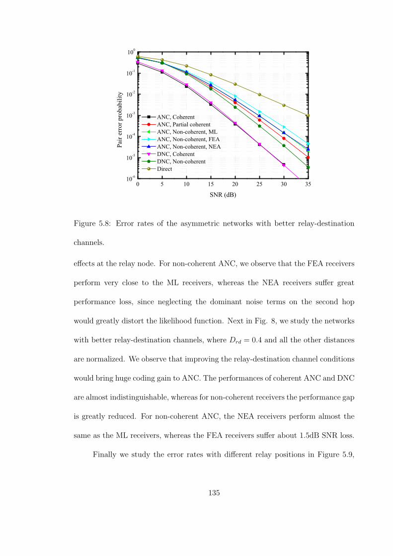
0 5 10 15 20 25 30 3510-6

10-5

10-4

10-3

10-2

10-1

100


Pair

erro

r pro

babi

lity

SNR (dB)

Figure 5.8: Error rates of the asymmetric networks with better relay-destination

channels.

effects at the relay node. For non-coherent ANC, we observe that the FEA receivers

perform very close to the ML receivers, whereas the NEA receivers suffer great

performance loss, since neglecting the dominant noise terms on the second hop

would greatly distort the likelihood function. Next in Fig. 8, we study the networks

with better relay-destination channels, where Drd = 0.4 and all the other distances

are normalized. We observe that improving the relay-destination channel conditions

would bring huge coding gain to ANC. The performances of coherent ANC and DNC

are almost indistinguishable, whereas for non-coherent receivers the performance gap

is greatly reduced. For non-coherent ANC, the NEA receivers perform almost the

same as the ML receivers, whereas the FEA receivers suffer about 1.5dB SNR loss.

Finally we study the error rates with different relay positions in Figure 5.9,

135

0.1 0.2 0.3 0.4 0.5 0.6 0.7 0.8 0.9 1.010-4

10-3

10-2

10-1

ANC, Coherent ANC, Partial coherent ANC, Non-coherent, ML ANC, Non-coherent, FEA ANC, Non-coherent, NEA DNC, Coherent DNC, Non-coherent

Pair

erro

r pro

babi

lity

Drd

Figure 5.9: Error rates with different relay positions.

where the system SNR is 20dB. For the network topology, we place the destination

at (0, 0), and locate the two source nodes at (√32,±1

2). The relay node moves along

the x-axis from (0.1, 0) to (1, 0). The simulation results clearly show that the best

performance of ANC is achieved when the relay node is close to the destination,

whereas for DNC the best performance is achieved when the relay node is close to

the sources. In all cases, non-coherent DNC performs better than the corresponding

ANC due to the smaller logarithmic term loss. For non-coherent ANC, we observe

that the NEA receivers are nearly optimum when the relay node is close to the

destination, whereas the performances of the FEA receivers get closer to the per-

formances of the ML receivers as the relay node moves to the two source nodes.

Throughout simulations, we have observed that the partial coherent ANC performs

very close to the non-coherent ANC. So we conjecture that these two schemes ac-

136

tually have the same scaling behaviors. A rigorous proof is deferred to our future

work.

5.5 Conclusions

In this chapter, we studied the diversity performance of non-coherent network

coding. We developed the optimum/sub-optimum transceivers under different CSI

conditions. It is demonstrated that non-coherent transmission would incur diversity

loss at modest SNRs, but the dominant diversity gain remains the same at extremely

high SNRs. It is also demonstrated that non-coherent ANC would incur more seri-

ous performance loss than non-coherent DNC, as the destination cannot efficiently

suppress MUI.

137

Chapter 6

Network-Coded ARQ for Two-Way Relay Channel

So far, we have studied the diversity gain of uncoded cooperation systems.

Since this chapter, we would shift attention to the coded systems. One key benefit

of the coded systems is that the network could somehow know the decoding status

of the messages by use of error detection code. Depending on the network dynamics,

the relay may choose to perform network coding when necessary or just stay idle

if the decoding fails. Note that the error propagation issue associated with DNC

discussed in Chapter 2 and Chapter 3 is no longer a big concern, which would

bring huge performance gain over the uncoded systems. How to design a sound

transmission strategy to exploit such benefit would be our main focus since this

chapter.

In this work, we focus particularly on the application of network-coded ARQ

for coded TWRC. Some related studies can be found in [31,74–77] and the references

therein. The novelty of our work is summarized below:

1) The direct link between the source nodes is neglected in the previous studies.

As a result, all data flows have to go through relay link regardless of the network

dynamics. In contrast, we incorporate the direct link in our system model, and

wireless relaying is used if and only if the direct link is in outage and the source

packets have been correctly decoded at relay nodes. Such incremental relaying

138

scheme can save the channel use and transmitted power that could be used to relay

new packets whenever possible.

2) In previous studies, it is assumed that any packet can be retransmitted in-

finitely many times until successfully received, so packet loss is neglected. However,

for most practical applications there is always some maximum transmission con-

straint to limit the transmission delay, and the packet will be dropped after several

attempts. In this work, we carefully incorporate such constraints, where the per-hop

transmission or E2E transmission of the same packet cannot exceed certain times.

We derive the closed-form throughput under these constraints after considering the

packet loss.

3) The transmitted power is supposed to be fixed in the previous work regard-

less of the network topology. In contrast, we obtain a closed-form near-optimum

power control scheme to maximize the system throughput. We show that power

control is extremely important for asymmetric networks, where the terminal of the

bottleneck link should use more power to compensate for the larger packet loss rate.

4) While the previous studies focus only on the single-relay networks, we also

study multi-relay networks in this work. We show that using localized DNC alone

may not fully leverage the network coding gain, especially when the frame length is

much smaller than the number of relays. To address this issue, we propose a hybrid

network coding schemes in which both DNC and ANC may be used within the relay

array.

Notations: The abbreviation i.i.d. stands for independent and identically dis-

tributed. The probability of an event A is denoted by Pr(A). The CDF and the

139

.

.

.

.

1S

2S

1R

2R

NR

Figure 6.1: System model of two-way relay channel.

probability mass function (PMF) of a random variable Z are denoted by FZ(z) and

fZ(z), respectively. We shall use Z ∼ CN (u,Σ) as a circularly symmetric com-

plex Gaussian random variable vector with mean u and covariance matrix Σ. Z ∼

Bin (p, n) stands for binomial distribution with parameter p and n. Z ∼ Geom (p)

stands for geometric distribution with parameter p, i.e., fZ (k) = (1− p) pk−1 for

k = 1, 2, · · · .

6.1 System Model

Consider the bidirectional relay channel shown in Figure 6.1, where the two

source nodes S1 and S2 want to exchange data with the help of a set of relay nodes Rk

for k = 1, 2, · · · , N . Suppose the source data are sent in a frame-by-frame manner,

and each frame consists of K packets. The kth packet of Si is denoted by Xi (k)

for i = 1, 2. For simplicity, we assume all the packets are of the same length, and

the data rate is fixed and is denoted by r. The time that is needed to deliver one

packet through any point-to-point channel is called one time unit.

140

The signal model for data transmission from node i to node j is given by

yij = hij√Pixi + nij. (6.1)

Here Pi is the transmitted power of node i, xi and yij are the transmitted signal and

the received signal, respectively, nij ∼ CN (0, 1) is the additive white Gaussian noise,

hij ∼ CN (0, λij) is the Rayleigh fading channel coefficient, where λij is the path

loss coefficient determined by the distance between the transmitter and receiver. All

the channel coefficients and additive noises are independent for different channels.

Due to random channel fading, the receiver may be unable to decode the

transmitted packet correctly. Usually, some parity bits are added to the raw data,

based on which the receiver can perform cyclic redundant check to tell whether the

decoding is successful. In this work, we assume such error detection is perfect. The

packet error rate is denoted by qij, and it is approximately equal to the channel

outage rate given by

qij ≈ Pr(log2

(1 + |hij|2Pi

)≤ r)= 1− exp

(−2r − 1

Piλij

). (6.2)

Depending on the decoding status of the packet, the receiver needs to feed back the

ACK/NACK signal to inform the transmitter that the decoding is successful/failed.

In this work, we assume that the feedback channels are perfect, and the channel use

of such flag bits are negligible compared to that of the information bits.

Suppose ARQ is used to guarantee the quality-of-service of data transmission.

That is, the current erroneous packet is dropped and the receiver will feed back the

NACK signal if the decoding is failed; afterwards, the transmitter may retransmit

the same packet until the decoding is successful at the receiver or the current packet

141

transmission expires when it exceeds a certain period. In this work, we investigate

two types of maximum transmission constraints, i.e., per-hop constraint and E2E

constraint. For per-hop constraint, packet transmissions on different point-to-point

channels are treated as independent sessions, and each packet transmission session

cannot exceed L times. In contrast, for E2E constraint the transmission of the same

packet from the original source to the final sink is treated as one whole session and

cannot exceed L times, regardless of the transmission routes. To give an example,

suppose there is packet transmission from S1 to S2 and the transmission route is

S1 → R1 → S2. Then for per-hop constraint, S1 can transmit the packet up to

L times and if R1 can successfully decode this packet within L times, it can also

attempt to deliver the same packet to S2 up to L times. In contrast, for E2E

constraint the total transmission of this packet cannot exceed L times, regardless it

is sent from S1 or R1.

As the performance measure, the effective throughput is defined as the average

number of successfully delivered packets per time unit within each frame, and is

given by

η =E [M ]

E [T ], (6.3)

where M and T are the total number of successively delivered packets and the

total times to exchange K packets between S1 and S2. In this work, we assume

all nodes are subject to half-duplex constraint such that they cannot transmit and

receive at the same time. As a result, the effective throughput is always bounded

by 0 ≤ η ≤ 1. The exact throughput is dependent on the transmission strategies,

142

which will be detailed in the next section.

6.1.1 Some Preliminaries

Before leaving this section, we first present some mathematical results that

appear to be pretty useful later. For notational convenience, we define the bounded

geometric distribution (BGeom) as Z = min (X,L) ∼ BGeom (p, L), where X ∼

Geom (p) for 0 ≤ p ≤ 1 and L > 0 is some integer. After some simple algebra, it is

easy to show that the PMF and CDF of Z are respectively given by

fZ (k) =

(1− p) pk−1, k = 1, 2, · · · , L− 1

pL−1, k = L

, (6.4)

and

FZ (k) =

0, k < 0

1− pk, k = 0, 1, · · · , L− 1

1, k ≥ L

. (6.5)

Besides, we can also show that

E [Z] =L∑k=1

Pr (Z ≥ k) =L∑k=1

pk−1 =

1−pL1−p , p = 1

L, p = 1

∆= gL (p) . (6.6)

With these results, we can prove the following results:

Proposition 6.1. Let X ∼ BGeom (p, L) for 0 ≤ p ≤ 1 and Y ∼ BGeom (q, L)

for 0 ≤ q ≤ 1 be independent, then

1) Z = min (X, Y ) ∼ BGeom (pq, L) and E [Z] = gL (pq).

2) Let Z = max (X,Y ), then

E [Z] = gL (p) + gL (q)− gL (pq) . (6.7)

143

3) Let Z ∼ BGeom (a, L−X) for 0 ≤ a ≤ 1. Then for 0 ≤ p < 1, we have

E [Z|X ≤ L− 1] =1

1− a

(1− 1− p

1− pL−1aL−1gL−1

(pa

))∆= h0 (a, p;L) . (6.8)

4) Let W ∼ BGeom (a, L−X) for 0 ≤ a ≤ 1 and T ∼ BGeom (b, L− Y ) for

0 ≤ b ≤ 1, and define Z = max (W,T ). Then for 0 ≤ p, q < 1, we have

E [Z|max (X, Y ) ≤ L− 1]

=1

1− pL−1

(gL−1 (a)− pL−1gL−1

(a

p

))+

1

1− qL−1

(gL−1 (b)− qL−1gL−1

(b

q

))− 1

(1− pL−1) (1− qL−1)

(gL−1 (ab) + pL−1qL−1gL−1

(ab

pq

))+

1

(1− pL−1) (1− qL−1)

(qL−1gL−1

(ab

q

)+ pL−1gL−1

(ab

p

))∆= h1 (a, b, p, q;L) . (6.9)

Proof. For property 1, we use (6.4) and (6.5) and can obtain

fZ (k) = Pr (X = k, Y > k) + Pr (X > k, Y = k) + Pr (X = Y = k)

= (1− pq) pk−1qk−1 (6.10)

for k = 1, 2, · · · , L− 1 and fZ (L) = Pr (X = Y = L) = pL−1qL−1. Comparing with

(6.4), we have Z ∼ BGeom (pq, L).

For property 2, we have

fZ (k) = Pr (X = k, Y < k) + Pr (X < k, Y = k) + Pr (X = Y = k)

= (1− p) pk−1 + (1− q) qk−1 − (1− pq) pk−1qk−1 (6.11)

for k = 1, 2, · · · , L− 1 and fZ (L) = pL−1+ qL−1− pL−1qL−1. By using (6.6), we can

obtain (6.7) immediately.

144

For property 3, we need to first derive the conditional PMF of X given by

fX (k|X ≤ L− 1) =1− p

1− pL−1pk−1 (6.12)

for k = 1, 2, · · · , L−1. Now we can calculate the conditional expectation of Z given

X from (6.6) and obtain

E [Z|X ≤ L− 1] = E

[1− aL−X

1− a

∣∣∣∣X ≤ L− 1

]=

1

1− a

(1− 1− p

1− pL−1

L−1∑k=1

pk−1aL−k

)

=1

1− a

(1− 1− p

1− pL−1aL−1gL−1

(pa

)). (6.13)

Finally for property 4, we have

fW (k|X ≤ L− 1) = Pr (W = k,X < L− k|X ≤ L− 1)

+Pr (W = k,X = L− k|X ≤ L− 1)

= (1− a) ak−11− pL−k−1

1− pL−1+ ak−1 (1− p) pL−k−1

1− pL−1

=ak−1

1− pL−1

(1− a+ (a− p) pL−k−1

)(6.14)

for k = 1, 2, · · · , L− 1. Now we can compute the conditional CDF of W given by

FW (k|X ≤ L− 1) =1− a

1− pL−1

k∑i=1

ai−1 +a− p

1− pL−1pL−2

k∑i=1

ai−1p−(i−1)

=1− ak − pL−1 + akpL−k−1

1− pL−1(6.15)

for k = 0, 1, · · · , L− 1. As W and T are independent, we have

FZ (k|max (X,Y ) ≤ L− 1) = FW (k|X ≤ L− 1)FT (k|X ≤ L− 1)

= 1− 1− pL−k−1

1− pL−1ak − 1− qL−k−1

1− qL−1bk

+1− pL−k−1 − qL−k−1 + (pq)L−k−1

(1− pL−1) (1− qL−1)akbk (6.16)

145

for k = 0, 1, · · · , L− 1. By using (6.6) and the relation

E [Z|max (X, Y ) ≤ L− 1] =L−1∑k=1

Pr (Z ≥ k|max (X, Y ) ≤ L− 1), (6.17)

we can obtain (6.9) immediately.

6.2 Single-Relay Case

In this section, we study several transmission strategies for the bidirectional

relay channel shown in Fig. 1. We focus only on the single-relay case, i.e., N = 1.

The multi-relay case will be discussed in the next section. For notational conve-

nience, we use P1, P2 and PR to represent the transmitted power of S1, S2 and

R1, respectively. The packet loss rate for the channel i → j is denoted by qi,j for

i, j ∈ 1, 2, R.

6.2.1 Direct Transmission

The simplest strategy is that the bidirectional communication goes only through

the direct link between the two source nodes, while the relay node stays idle. Due to

the half-duplex constraint, the two source nodes need to take turns to send a frame

of K packets to the other end in a time-division multiplex manner. Each time after

S1 sends out a packet, three consequences may occur:

1. S2 successfully decodes the packet and feeds back the ACK signal. Then S1

will start to deliver the next packet.

2. S2 fails to decode the packet, and the current transmission is not the Lth

146

attempt. Then S1 will initiate AQR and retransmit the same packet once

again.

3. S2 fails to decode the packet, and the current transmission is the Lth attempt.

Then the current packet is dropped, and S1 will send out a new packet in the

next time slot.

Note that for each packet of S1, it will be either successfully delivered to S2

(denoted by the event I1 = 1) or dropped after expiration (denoted by the event

I1 = 0). It is also worth noting that if the current decoding fails, S2 will drop the

erroneous packet and attempt to decode the same packet based solely on the newly

arrived signal in the future. Therefore, the total transmission times of each packet

satisfy BGeom (q1,2, L) and is denoted by T1 = min (X1, L), where X1 ∼ Geom (q1,2).

The probability of successful delivery is given by

Pr (I1 = 1) = Pr (X1 ≤ L) = 1− qL1,2, (6.18)

and the average transmission times are E [T1] = gL (q1,2). Due to symmetry, the

above metrics should be similar for any packet delivered along the reverse direction

after properly modifying the subscripts. Therefore, the effective throughput of direct

transmission is

ηDT =K × E [1 I1 = 1+ 1 I2 = 1]

K × E [T1 + T2]=

2− qL1,2 − qL2,11−qL1,21−q1,2 +

1−qL2,11−q2,1

L≫1≈ 2 (1− q1,2) (1− q2,1)

2− q1,2 − q2,1, (6.19)

where 1 · is the indicator function.

147

6.2.2 Pure Relaying

If the relay node is located at some place between the two source nodes, the

relay link would be much better than the direct link. As a result, if the relay

node happens to successfully decode the source packets, it can initiate the ARQ for

the original data source to improve the transmission quality. In this subsection, we

study the conventional pure relaying strategy [12], where the relay node forwards the

individual packets in different time slots. The whole bidirectional communication

is completed in three phases. In the first two phases, the two sources take turns to

send out a frame of K packets. Then in the third phase, the relay node will forward

all the successfully decoded packets in the buffer to the intended receivers.

We first consider the transmission phase of S1. Each time after S1 sends out

a packet, the following consequences may occur:

1. S2 successfully decodes the packet and feeds back the ACK signal. Then S1


2. S2 fails to decode the packet, but the relay R successfully decodes the packet.

For E2E constraint, the extra requirement is that the current transmission is

not the Lth attempt. Then R will store the packet in the local buffer and

continue the unfinished ARQ for S1 during the future relaying phase, and S1


3. Neither S2 nor R is able to decode the packet, and the current transmission

is not the Lth attempt. Then S1 will initiate AQR and retransmit the same

packet once again.

148

4. Neither S2 nor R is able to decode the packet, and the current transmission is

the Lth attempt. For E2E constraint, this also includes the event that S2 fails

to decode the packet, but the relay R successfully decodes the packet upon

the Lth attempt. Then the current packet is dropped, and S1 will send out a

new packet in the next time slot.

Note that in case 1), S2 and R may decode the packet simultaneously. In that

case, the transmission is successful and the relay node needs not to store that packet

any more. Also for E2E constraint, the relay node will only store the packets that

have been successfully decoded within the first L − 1 attempts. This is because

the E2E transmission session expires right after the Lth attempt, so the relay node

should drop that packet even if the Lth decoding is successful. That is why we

discriminate E2E constraint in case 2) and case 4). Eventually, each packet of S1

will be either successfully delivered to S2 (denoted by the event I1 = 1), or stored

at R but yet not decoded by S2 (denoted by the event I1 = −1), or dropped after

expiration (denoted by the event I1 = 0). As each packet transmission will terminate

right after either S2 or R is able to decode the packet, the transmission time is given

by T1 = min (T1,R, T1,2), where T1,2 = min (X1,2, L) and T1,R = min (X1,R, L), and

X1,2 ∼ Geom (q1,2) and X1,R ∼ Geom (q1,R) are independent. The probability that

S2 decodes the packet is given by

Pr (I1 = 1) =L∑n=1

Pr (X1,2 = n,X1,R ≥ n) =1− q1,2

1− q1,Rq1,2

(1− qL1,Rq

L1,2

). (6.20)

The probability that the packet is stored at R but yet not decoded by S2 is given

149

by

Pr (I1 = −1) =L∑n=1

Pr (X1,R = n,X1,2 > n) =(1− q1,R) q1,21− q1,Rq1,2

(1− qL1,Rq

L1,2

)(6.21)

for per-hop constraint, and

Pr (I1 = −1) =L−1∑n=1

Pr (X1,R = n,X1,2 > n) =(1− q1,R) q1,21− q1,Rq1,2

(1− qL−1

1,R qL−11,2

)(6.22)

for E2E constraint. By using property 1 of Proposition 6.1, we can also calculate

the average transmission times of each packet as E [T1] = gL (q1,Rq1,2).

After the two source transmission phases, the relay R will forward the packets

stored in the local buffer to the intended receiver. During this phase, both source

nodes are receivers and the relay node will continue the unfinished ARQ. Let Di be

the set of packets of Si for i = 1, 2 that are stored in the buffer, and the set size is

denoted by |Di| = Di. Besides, the relay also needs to manage a set Ri that records

the maximum residual transmission times of each packet in Di. At the beginning

of the relaying phase, the maximum residual transmission times are equal to L for

per-hop constraint and L − Ti for E2E constraint1. Note that the two sets Di and

Ri have the same size Di that satisfies binomial distribution, i.e., Di ∼ Bin (Qi, K)

where Qi∆= Pr (Ii = −1) given by (6.21) and (6.22). For pure relaying, the relay

R simply delivers all the packets in the buffer one-by-one in different time slots.

Due to symmetry, we only consider transmitting a packet from R to S2. Because

the R → S2 channel is a point-to-point channel, the transmission process mimics

the direct transmission described in the last subsection, except that each packet

1The residual transmission times could be different for packets stored at the relay R. Here we

omit the time index of packets for notational convenience.

150

may have different residual transmission times for E2E constraint. As a result, for

each packet delivered from R to S2 the total transmission times can be denoted by

TR,2 = min (XR,2, L) for per-hop constraint and TR,2 = min (XR,2, L− T1) with the

condition that T1 ≤ L−1, where XR,2 ∼ Geom (qR,2). Let IR,2 = 1 and IR,2 = 0

represent the events of successful delivery and packet loss due to transmission ex-

piration, respectively. Then for per-hop constraint, the probability of successful

delivery is

Pr (IR,2 = 1) = Pr (XR,2 ≤ L) = 1− qLR,2 (6.23)

and we have E [TR,2] = gL (qR,2). For E2E constraint, we have

Pr (IR,2 = 1) = Pr (XR,2 ≤ L− T1|T1 ≤ L− 1)

= 1− 1− q1,Rq1,2

1− qL−11,R qL−1

1,2

qL−1R,2 gL−1

(q1,Rq1,2qR,2

). (6.24)

By using property 1 and property 3 of Proposition 6.1, we have

E [TR,2] = h0 (qR,2, q1,Rq1,2;L) . (6.25)

With the above results, we can write the total number of successfully delivered

packets in three phases as

E [M ] =2∑

i=1,j=1,2\i

(KE [I Ii = 1] + E [Di]E [I IR,j = 1])

= K2∑

i=1,j=1,2\i

(Pr (Ii = 1) + Pr (Ii = −1) Pr (IR,j = 1)), (6.26)

and the total transmission times are given by

E [T ] =2∑

i=1,j=1,2\i

(KE [Ti] + E [Di]E [TR,j])

= K

2∑i=1,j=1,2\i

(E [Ti] + Pr (Ii = −1)E [TR,j]), (6.27)

151

After plugging (6.20)-(6.24) into the above two expressions, we obtain the closed-

form throughput according to (6.3). When the maximum transmission times are

sufficiently large (i.e., L ≫ 1), the two types of constraints would lead to the same

asymptotic throughput given by

ηRelay

L≫1≈ 2

2∑i=1,j=1,2\i

1− qR,j + (1− qi,R) qi,j(1− qi,Rqi,j) (1− qR,j)

−1

. (6.28)

6.2.3 Static Network Coding

Pure relaying is not bandwidth efficient as the relay node forwards all the

source packets in orthogonal time slots. However, if both buffers are non-empty, the

relay node can combine the two packets intended for different receivers to save the

channel use. For example, suppose the relay node needs to deliver X1 to S2 and also

deliver X2 to S1. Then instead of transmitting these two packets separately, the

relay can perform network coding to combine these two packets, i.e., XR = X1⊕X2,

and then send out this single network-coded packet XR. If S1 is able to successfully

decode this packet, it can also decode the message sent from S2 by X2 = X1 ⊕XR.

Likewise, S2 can also decode X1 based on XR through similar operation. In this

way, both source nodes can get the desired message while the relay node only needs

to broadcast a single packet.

For such network-coded relaying, the whole data exchange still occurs in three

phases, i.e., two source transmission phases followed by one data relaying phase.

The first two source transmission phases are exactly the same as what we studied

in the last subsection. The only difference is how the relay node shall forward

152

the packets in the local buffer during the data relaying phase. Suppose the Di

packets of Si stored in the buffer Di are Xi(1), Xi(2), · · · , Xi(Di) for i = 1, 2.

Let DNC = min (D1, D2) and DREG = |D1 −D2| be the number of network-coded

packets and the number of regular packets, respectively. If any Di is empty, the

relay node only needs to forward data to a single terminal and all the packets are

regular packets. Otherwise, without loss of generality we assume D1 ≥ D2 > 0.

Then the relay node will combine the first DNC packets in D1 and D2 through

XR(k) = X1(k) ⊕ X2(k) for k = 1, 2, · · · , DNC . Afterwards, the relay node will

forward DNC network-coded packets XR (k)DNCk=1 intended for both source nodes,

and DREG regular packets X1 (k)D2

k=DNC+1 intended for S2 alone.

The transmission of regular packets is very much like pure relaying and has

been studied in the last subsection. For the network-coded flow, it is very much like

a combination of two unicast flows where each component flow is subject to its own

maximum transmission constraint. Each time any source node is able to decode

the desired component packet, or any component packet has reached the maximum

transmission limit, that component packet will be dropped by the relay and the

following information flow will only contain a single packet. The transmission of any

network-coded flow will terminate until both component unicast flows are finished

after successful delivery or expiration. For example, suppose XR = X1 ⊕X2 where

X1 and X2 can be transmitted up to 2 and 4 times. If neither source nodes can

decode XR in the first 2 attempts, then X1 will be dropped and in the following

time slots, the relay node will forward XR = X2 to S1 alone up to 2 more times.

Next we analyze the effective throughput. The first thing to note is that the

153

packet loss rate remains the same for a network-coded packet and a regular packet.

Consequently, the average number of successfully delivered packets is still given by

(6.26). The total transmission times of all three phases are given by

E [T ] = KE [T1] +KE [T2] + E [TR]

= KgL (q1,2q1,R) +KgL (q2,1q2,R) + E [TR] , (6.29)

where Ti ∼ BGeom (qi,jqi,R, L) for i = 1, 2 and j = 1, 2 \ i is the transmission

times of a single packet sent from Si, and

E [TR] = E [(D1 −D2) I D1 > D2]E [TR,2] + E [(D2 −D1) I D2 > D1]E [TR,1]

+E [min (D1, D2)]E [TR,NC ] , (6.30)

is the total transmission times of relay R. Here Di ∼ Bin (Qi, K) with Qi∆=

Pr (Ii = −1) for i = 1, 2 is given by (6.21) and (6.22), and E [TR,i] for i = 1, 2

are the average transmission times of a regular packet sent from R to Si and have

been derived in the last subsection. As a result, we only need to compute the average

transmission times of a network-coded packet, i.e., E [TR,NC ]. Since any network-

coded flow will terminate until both component unicast flows are finished, we have

TR,NC = max (TR,1, TR,2). For per-hop constraint, TR,i ∼ BGeom (qR,i, L) for i = 1, 2

are independent. By using property 2 of Proposition 6.1, we have

E [TR,NC ] = gL (qR,1) + gL (qR,2)− gL (qR,1qR,2) . (6.31)

For E2E constraint, we have TR,i ∼ BGeom (qR,i, L− Tj) with the condition that

Tj ≤ L− 1 for i = 1, 2 and j = 1, 2 \ i. By using property 4 of Proposition 6.1,

154

we have

E [TR,NC ] = h1 (qR,1, qR,2, q1,Rq1,2, q2,Rq2,1;L) . (6.32)

6.2.4 Dynamic Network Coding

The network coding scheme studied in the last subsection is static in that

the pairing pattern is fixed after scheduling. Specifically, once the two packets are

determined to be combined by the scheduler, they cannot be paired with any other

packets later. This scheme cannot leverage the network coding gain to the full.

For example, if one unicast flow terminates earlier than the other one, the intended

receiver of that unicast flow has to stay idle and wait until the other unicast flow

terminates. So some channel use is wasted along the way. If the relay still has

more packets intended for that receiver in the buffer, a more efficient way is to send

these packets along with the remaining unicast flow and form a new network-coded

packet. In this way, both relay-source channels are in use until the relay node has

no more packets intended for any source node. We remark that a similar idea is

also studied in [75], where different network-coded packets but not the raw source

packets can be re-combined in some cases.

To realize the above idea, the pairing pattern must be determined dynamically

depending on the decoding status. If the two buffers D1 and D2 are non-empty,

the first packet in those two buffers are always combined to form a network-coded

packet. Whenever any component unicast flow terminates due to successful decoding

or transmission expiration, the related packet will be eliminated from the buffer.

155

Then the relay will pick up a new packet from that buffer and do network coding.

This process continues until one buffer becomes empty. Since then the relay will

forward the packets in the remaining buffer as regular packets successively. For

example, suppose D1 = X1(1), X1(2), X1(3) and D2 = X2(1). Then the first

network-coded packet is XR(1) = X1(1)⊕X2(1). Suppose after some transmissions,

X1(1) expires and is removed from D1 but X2(1) is still valid. Then the relay will

form a new network-coded packet given by XR(2) = X1(2) ⊕ X2(1). In contrast,

for static network coding scheme, the relay node will keep sending XR(2) = X2(1)

after removing X1(1), during which period S2 always remains idle and the channel

R → S2 is not in use at all. For dynamic network coding, all the remaining packets

are always combined whenever possible. In the above example, if X2(1) terminates

earlier than X1(2), D2 becomes empty and D1 = X1(2), X1(3). Then the relay

will send X1(2) and X1(3) to S2 successively as regular packets, which is similar to

pure relaying.

Again, dynamic network coding will not affect the probability of successful

delivery, and the total transmission times is still given by (6.29). The only difference

is the total transmission times of the relay, i.e., E [TR]. Note that given the buffer size

Di, the relay node only needs to deliverDi packetsXi(1), Xi(2), · · · , Xi(Di) to Sj for

i = 1, 2 and j = 1, 2 \ i. These packets may be organized in the form of network-

coded packets or regular packets depending on the decoding status. Nevertheless,

the packet loss rate remains the same. Therefore, if we denote the total transmission

times of all packets containing Xi(k) by TR,j(k), we have TR,j(k) ∼ BGeom (qR,j, L)

for per-hop constraint and TR,j ∼ BGeom (qR,j, L− Ti) with the condition that

156

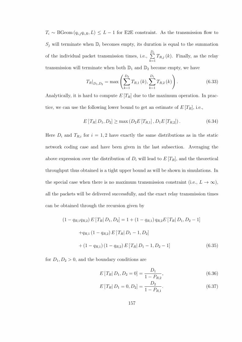
Ti ∼ BGeom (qi,jqi,R, L) ≤ L − 1 for E2E constraint. As the transmission flow to

Sj will terminate when Di becomes empty, its duration is equal to the summation

of the individual packet transmission times, i.e.,Di∑k=1

TR,j (k). Finally, as the relay

transmission will terminate when both D1 and D2 become empty, we have

TR|D1,D2= max

(D2∑k=1

TR,1 (k),

D1∑k=1

TR,2 (k)

). (6.33)

Analytically, it is hard to compute E [TR] due to the maximum operation. In prac-

tice, we can use the following lower bound to get an estimate of E [TR], i.e.,

E [TR|D1, D2] ≥ max (D2E [TR,1] , D1E [TR,2]) . (6.34)

Here Di and TR,i for i = 1, 2 have exactly the same distributions as in the static

network coding case and have been given in the last subsection. Averaging the

above expression over the distribution of Di will lead to E [TR], and the theoretical

throughput thus obtained is a tight upper bound as will be shown in simulations. In

the special case when there is no maximum transmission constraint (i.e., L → ∞),

all the packets will be delivered successfully, and the exact relay transmission times

can be obtained through the recursion given by

(1− qR,1qR,2)E [TR|D1, D2] = 1 + (1− qR,1) qR,2E [TR|D1, D2 − 1]

+qR,1 (1− qR,2)E [TR|D1 − 1, D2]

+ (1− qR,1) (1− qR,2)E [TR|D1 − 1, D2 − 1] (6.35)

for D1, D2 > 0, and the boundary conditions are

E [TR|D1, D2 = 0] =D1

1− PR,2, (6.36)

E [TR|D1 = 0, D2] =D2

1− PR,1. (6.37)

157

6.2.5 Throughput Comparison

In this subsection, we compare the throughput of different schemes obtained

above. To make the analysis tractable, we focus on the symmetric networks where

the relay node is located at the middle between S1 and S2. Besides, we assume all

nodes use the same power and transmit at the same rate. The path loss coefficient

is supposed to be dependent on the distance only. Under these assumptions, we

have q1,R = q2,R = qR,1 = qR,2∆= qR and q1,2 = q2,1

∆= qS. Besides, we assume that

the maximum transmission constraint is sufficiently large, i.e., L ≫ 1. From (6.19)

and (6.28), we have

ηDT = 1− qS, (6.38)

ηRelay =1− qRqS1 + qS

qS=1=

1− qR2

. (6.39)

For network coding schemes, the throughput also depends on the frame length K.

When K ≫ 1, we have

Di → K(1− qR) qS1− qRqS

. (6.40)

After some simple algebra, we can show that

ηS-NC =2 (1− qRqS) (1 + qR)

2 (1 + qR) + (1 + 2qR) qS

qS=1=

2 (1− q2R)

3 + 4qR, (6.41)

ηD-NC =2 (1− qRqS)

2 + qS

qS=1=

2 (1− qR)

3. (6.42)

We first consider the special case when there is no direct link, i.e., qS = 1. In

this case, ηDT ≡ 0 because no information can be delivered through the direct link

alone. Besides, we can show that 0 ≤ ηRelay ≤ 12and 0 ≤ ηS-NC, ηD-NC ≤ 2

3, and the

maximum throughput is achieved when qR = 0. Next we consider the general case

158

with direct link, i.e., 0 ≤ qS < 1. It is easy to see that 0 ≤ ηDT, ηRelay, ηS-NC, ηD-NC ≤

1, and the upper bound is achieved when qS = 0. Note that when the direct link

is in good quality (i.e., qS ≪ 1), using direct transmission alone is able to achieve

the throughput bound. In that case, the relay nodes could stay idle to save the

transmitted power and channel use. We remark again that such incremental relaying

is the key difference between the current work and previous studies [31,74–77], where

direct link is neglected and all the packet transmissions have to go through the

relay link. Actually, incorporating the direct link is pretty important in that the

throughput upper bound can increase from 23to 1.

Next we compare the relative throughput gain. By comparing direct trans-

mission and pure relaying, we have

ηRelay

ηDT

=1− qRqS1− q2S

> 1 ⇔ qS > qR. (6.43)

Therefore, wireless relaying can improve the throughput if and only if the relay link

has better quality than direct link. Next we study network coding gain, which is

given by

1 ≤ ηS-NC

ηRelay

= 1 +qS

2 + 2qR + qS + 2qRqS≤ 4

3. (6.44)

Clearly, static network coding is strictly better than pure relaying in terms of the

achievable throughput. However, the relative throughput gain is bounded by 33.3%,

which occurs when the direct link is always in outage and the relay link is in perfect

condition. Finally, we study the dynamic network coding gain, which is given by

1 ≤ ηD-NC

ηS-NC

= 1 +qRqS

2 + 2qR + qS + qRqS≤ 7

6. (6.45)

159

It is observed that dynamic network coding can further improve the throughput.

However, the relative gain is at most 16.7%. Note that the largest throughput

gain is achieved when both direct link and relay link are in bad conditions. In most

reasonable system settings, such dynamic network coding gain is not that significant,

as will be seen in simulations later.

6.2.6 Power Allocation

In the last subsection, we compared the throughput by assuming equal power

allocation. For practical wireless networks, the node distribution could be quite

random, and the transmitted power should be properly allocated to address the

near-far problem. However, the optimum transmitted power can be found only

through exhaustive search, as the closed-form throughput is hard to manipulate.

In the sequel, we seek to develop a near-optimum power allocation strategy with

closed-form solution.

For the packet loss rate, we use the channel outage model given by (6.2). To

make a step further, we intentionally neglect the maximum transmission constraint

and the direct link, i.e., let L→ ∞ and q1,2 = q2,1 = 1. From (6.28), the throughput

of pure relaying is then equal to

ηRelay ≈ 2

(exp

(α

λ1,RP1

)+ exp

(α

λ2,RP2

)+ exp

(α

λR,1PR

)+ exp

(α

λR,2PR

))−1

≤ 1

2exp

(−α4

(1

λ1,RP1

+1

λ2,RP2

+λR,1 + λR,2λR,1λR,2PR

)), (6.46)

where α = 2r − 1 and we use the arithmetic-geometric mean inequality in the last

step. To maximize the throughput, we use the upper bound instead. The power

160

allocation problem is formulated as

max ηRelay ≈ min

(1

λ1,RP1

+1

λ2,RP2

+λR,1 + λR,2λR,1λR,2PR

)s.t. P1 + P2 + PR ≤ 3P. (6.47)

By using the method of Lagrange multipliers, we can derive the optimum solution

given by

P1 =3Pλ

−1/21,R

λ−1/21,R +λ

−1/22,R +(λ−1

R,1+λ−1R,2)

1/2

P2 =3Pλ

−1/22,R

λ−1/21,R +λ

−1/22,R +(λ−1

R,1+λ−1R,2)

1/2

PR =3P(λ−1

R,1+λ−1R,2)

1/2

λ−1/21,R +λ

−1/22,R +(λ−1

R,1+λ−1R,2)

1/2

. (6.48)

For dynamic network coding, L → ∞ and q1,2 = q2,1 = 1 imply that D1 =

D2 ≡ K in (6.33), which leads to

ηD-NC ≈ 2

(exp

(α

λ1,RP1

)+ exp

(α

λ2,RP2

)+ exp

(α

min (λR,1, λR,2)PR

))−1

≤ 2

3exp

(−α3

(1

λ1,RP1

+1

λ2,RP2

+1


)). (6.49)

Likewise, the power allocation problem can be formulated as

max ηD-NC ≈ min

(1

λ1,RP1

+1

λ2,RP2

+1


)s.t. P1 + P2 + PR ≤ 3P. (6.50)

The optimizer is given by

P1 =3Pλ

−1/21,R

λ−1/21,R +λ

−1/22,R +max

(λ−1/2R,1 ,λ

−1/2R,2

)P2 =

3Pλ−1/22,R

λ−1/21,R +λ

−1/22,R +max

(λ−1/2R,1 ,λ

−1/2R,2

)PR =

3P max(λ−1/2R,1 ,λ

−1/2R,2

)λ−1/21,R +λ

−1/22,R +max

(λ−1/2R,1 ,λ

−1/2R,2

). (6.51)

161

6.3 Multi-Relay Case

In this section, we extend the above results to the multi-relay networks. The

packet loss rates of Si → Rk channel and Rk → Si channel are respectively denoted

by qi,Rk and qRk,i for i = 1, 2 and k = 1, 2, · · · , N . The buffers of Rk are denoted by

D1,Rk and D2,Rk . The power of Si is denoted by Pi and the power of Rk is denoted by

PRk . We assume the transmitted power is fixed during packet transmission and as

a result, the packet loss rate depends only on the distance between the transmitter

and the receiver. Therefore, we can rank the quality of Rk → Si channel according

to the distance, and such ranking is assumed to be known to the whole network.

6.3.1 Successive Relaying

One simple multi-relay transmission strategy is successive relaying, where all

the relays work in a time-division multiplexing manner. The whole bidirectional

communication is still completed in three phases as in the single-relay case. During

the source transmission phase, each source packet is either dropped due to exceed-

ing the maximum transmission constraint, or decoded by the intended receiver, or

decoded by some relay nodes. Note that if multiple relays happen to decode the

same packet of Si for i = 1, 2 simultaneously, we assume that only the relay with

the best Rk → Sj channel quality for j = 1, 2 \ i will store the packet and

continue the unfinished ARQ later. If several relay nodes happen to decode the

same packet and have the same channel quality, only one relay is randomly selected.

Consequently, after the two source transmission phases, all relays may store some

162

mutually exclusive packets in the local buffers. Then in the third relaying phase,

all relays take turns to send these packets to the intended receivers using either

pure relaying, static network coding or dynamic network coding studied in the last

subsection.

Next we study the throughput of such successive relaying. As the exact analy-

sis is intractable, we only consider the special case when the maximum transmission

constraint is sufficiently large, i.e., L ≫ 1. Besides, we assume symmetric settings

such that qi,Rk = qRk,i∆= qR and q1,2 = q2,1

∆= qS for i = 1, 2 and k = 1, 2, · · · , N . We

first study the scenario that N ≫ K = 1, in which case only one packet is exchanged

between source nodes. Depending on the decoding status, either both packets are

successfully delivered through direct link, or only one packet is delivered through

direct link and the other one is decoded by the relay but not the intended receiver,

or both source packets are decoded by some relay nodes. The probabilities of these

three events are (1− qS)2, 2qS (1− qS) and q

2S, respectively. As we assume N ≫ 1,

after each source transmission the packet will be either decoded by some relay node

or successfully delivered to the intended receiver. As a result, the total transmission

times of the two source transmission phases are exactly 2. For each regular packet

delivered by the relay, the average transmission times is 11−qR

. For each network-

coded packet, the average transmission times is 1+2qR1−q2R

from (6.31). Note that when

K = 1, static network coding becomes equivalent to dynamic network coding, and

network coding can only be performed when a single relay happens to decode both

163

source packets. After some simple algebra, we can obtain

ηRelay =1− qR

1− qR + qS, (6.52)

ηNC =

(1− qR + qS

1− qR− q2S

2N (1− q2R)

)−1N≫1≈ ηRelay. (6.53)

It is observed that network coding can barely boost throughput when the number

of relays is much larger than the frame length. This is because the source packets

will be decoded by different relays with large chance, in which case the network

coding gain is pretty limited. Next we study the throughput when the frame length

is sufficiently large, i.e., K ≫ N ≫ 1. On average, each relay node can decode KNqS

packets from both sources. So for dynamic network coding, the total transmission

times of each relay node is approximately KN

qS1−qR

from (6.34). Consequently, we

have

ηD-NC =2 (1− qR)

2− 2qR + qS. (6.54)

The throughput of pure relaying is independent of K and is still given by (6.52).

The relative throughput gain is

1 ≤ ηD-NC

ηRelay

= 1 +qS

2− 2qR + qS≤ 2 (6.55)

for large K. It is observed that dynamic network coding can greatly improve

throughput and the throughput gain is up to 100%.

6.3.2 Hybrid Network Coding

For successive relaying, each relay node applies DNC alone on the locally stored

packets. However, the network coding gain is quite limited in the small frame length

164

case. In this section, we develop a hybrid network coding scheme to address this

issue. Let us start with an example, where there are N = 2 relay nodes and there

is K = 1 packet per frame. Suppose in a particular frame transmission, we have

D1,R1 = X1, D2,R2 = X2 and D2,R1 = D1,R2 = ϕ. That is, each relay node is

able to decode only one source packet and for successive relaying, it is impossible

to perform network coding at both relays. However, if the two relays send X1 and

X2 simultaneously, the transmitted signal will be automatically combined in the air,

which is a nature form of ANC [25]. The received signal at Si is given by

yi = hR1,i

√PR1X1 + hR2,i

√PR2X2 + ni (6.56)

for i = 1, 2. At S1, it can fist subtract the self packet X1 from the mixed signal

and then make decoding of X2. The packet loss rate is still given by qR2,1 after the

self-interference is perfectly eliminated. Similar operations can be performed at S2

to decode X1. In this way, both packets may be delivered in a single channel use

even though they are stored at different relays.

For the general case, each relay can first perform DNC to combine as many

local packets as possible. Whenever one of the two buffers becomes empty, say D1,

it can invite another relay node with non-empty D1 to jointly perform ANC. This

process continues until it is impossible to pair any two packets within the relay

array. Afterwards, all the relays will take turns to deliver the remaining regular

packets. In some sense, the relay array behaves like a super relay node that has

distributed buffers. It can adaptively choose to perform DNC or ANC depending

on the location of the packets. However, the relay nodes do not need to know the

165

packets in other buffers, so the signaling overhead is very limited.

It is intractable to analyze the throughput of hybrid network coding for the

general case. Instead, we still consider symmetric setting, i.e., qi,Rk = qRk,i∆= qR

and q1,2 = q2,1∆= qS for i = 1, 2 and k = 1, 2, · · · , N . Under this assumption, all the

relay nodes have equal chance to decode a source packet, and the packet loss rate

is identical for all source-relay links. As a result, we can regard the relay array as

a single super relay node. The packet loss rate from any source to this super relay

node is qNR , which is the probability that none of the N relays can decode the source

packet. The packet loss rate from the relay array to any source is still given by qR,

as each packet is delivered only by one relay node, and the packet loss rate remains

the same regardless of network coding scheme. Consequently, the throughput of

network coding can be obtained from the single-relay result after replacing with

q1,R = q2,R = qNR . When L≫ 1 and N ≫ 1, we have

ηD-NC =

2 (1− qR)

2− 2qR + qS, K ≫ 1 (6.57a)

2 (1− q2R)

2 (1− q2R) + 2qS (1 + qR)− q2S, K = 1 (6.57b)

By comparing (6.54) and (6.57a), we can observe that hybrid network coding and

successive network coding achieve the same asymptotic throughput for large K. For

small K (i.e., K = 1 ≪ N), the relative throughput gain of hybrid network coding

is

1 ≤ ηHybrid

ηSuccessive= 1 +

q2S2 (1− q2R) + 2qS (1 + qR)− q2S

≤ 4

3. (6.58)

In this case, hybrid network coding can greatly improve the throughput, but the

throughput gain is up to 33.3%.

166

6.4 Simulations

In this section, we present some simulation results to validate our study.

Throughout simulations, we use the path loss model λ = d−3, where λ is the path

loss coefficient and d is the distance. The noise power is always normalized, and the

average transmitted power of all nodes is referred to as SNR. The two source nodes

are always located at (0, 0) and (1, 0), respectively.

We first compare the throughput of the four transmission schemes in the single-

relay networks in Figure 6.2. It is observed that the simulation results match

perfectly with our theoretical results regardless of the type of transmission con-

straint. Compared with direct transmission, wireless relaying can greatly boost the

throughput when the relay link is much better than the direct link. Network coding

can further improve the throughput at moderate SNRs. For example, at 0dB the

throughput goes from 0.57 to 0.68, and the relative gain is around 20%. Compara-

tively, dynamic network coding has the best performance under all situations, but

the throughput gain against static network coding is very limited over the entire

SNR range, which is consistent with the analytical results. It is also observed that

the four schemes converge to the same performance at high SNRs, in which case

most of the packets are delivered through the direct link and the relay link is active

only occasionally.

By comparing Figure 6.2(a) and Figure 6.2(b), we also observe that per-hop

constraint performs better than E2E constraint at low SNRs, while the throughput

is almost identical at medium-to-high SNRs. This is because for per-hop constraint,

167

-15 -10 -5 0 5 10 150.0

0.2

0.4

0.6

0.8

1.0

Direct - Sim Pure relaying - Sim Static NC - Sim Dynamic NC - Sim Direct - Thy Pure relaying - Thy Static NC - Thy Dynamic NC - Thy

Effe

ctiv

e th

roug

hput

SNR (dB)

(a) Per-hop maximum transmission constraint.

-15 -10 -5 0 5 10 150.0

0.2

0.4

0.6

0.8

1.0

Direct - Sim Pure relaying - Sim Static NC - Sim Dynamic NC - Sim Direct - Thy Pure relaying - Thy Static NC - Thy Dynamic NC - Thy

Effe

ctiv

e th

roug

hput

SNR (dB)

(b) E2E maximum transmission constraint.

Figure 6.2: Effective throughput versus SNR for L = 4 and K = 10. The relay node

is located at (0.5, 0).

2 4 6 8 10 12 14 16 18 200.04

0.06

0.08

0.10

0.12

0.14

0.16

0.18

0.20

Effe

ctiv

e th

roug

hput

Normalized E2E transmission constraint

Pure relaying, per-hop Pure relaying, E2E Static NC, per-hop Static NC, E2E Dynamic NC, per-hop Dynamic NC, E2E

(a) SNR = −10dB.

2 4 6 8 10 12 14 16 18 200.54

0.56

0.58

0.60

0.62

0.64

0.66

0.68

Pure relaying, per-hop Pure relaying, E2E Static NC, per-hop Static NC, E2E Dynamic NC, per-hop Dynamic NC, E2E

Ef

fect

ive

thro

ughp

ut

Normalized E2E transmission constraint

(b) SNR = 0dB.

Figure 6.3: Effective throughput versus normalized transmission constraint for K =

10. The relay node is located at (0.5, 0).

the same packet can be transmitted up to L times for each hop, whereas for E2E

constraint the total transmission times are limited by L regardless of the sender.

Therefore, the successful delivery probability is higher for per-hop constraint. To

fairly compare these two types of constraints, we normalize the aggregate E2E trans-

168

mission times and compare the throughput with different maximum transmission

constraint in Figure 6.3. For example, if L = 4 for E2E constraint, then the same

packet can only be transmitted up to 2 times for the per-hop constraint. We observe

that at low SNRs, the throughput increases quickly with the maximum transmission

times because allowing more ARQs will improve the successful delivery probability.

In contrast, at high SNRs the throughput almost remains the same when L ≥ 4,

as most packets can be delivered within 4 attempts. It is also observed that for all

relaying schemes, E2E constraint performs better when the maximum transmission

constraint is not that stringent. This is because for E2E constraint, the transmis-

sion chances are dynamically allocated between the two hops, whereas for per-hop

constraint such split is fixed. So there is some throughput loss due to early give-up

under per-hop constraint. In contrast, per-hop constraint leads to higher throughput

for very stringent maximum transmission constraint. This is because when the first

few attempts are failed, that packet should be dropped early to save the channel use

for transmitting a new packet. Otherwise, even the relay node is able to decode the

packet later, there are very limited ARQs left and the chance of successful delivery

is still pretty low. As a result, early termination appears to be a better choice for

small L.

Next we study the impact of power allocation in Figure 6.4. The relay node

is located at (Dsr, 0), and we plot the throughput with different relay locations.

It is observed that our power allocation schemes (6.48) and (6.51) perform very

close to the optimum ones that are obtained through exhaustive search. When the

network topology is highly asymmetric, i.e., when the relay node is very close to

169

0.1 0.2 0.3 0.4 0.50.1

0.2

0.3

0.4

0.5

Pure relaying - Optimum Pure relaying - Suboptimum Pure relaying - equal Dynamic NC - Optimum Dynamic NC - Suboptimum Dynamic NC - Equal

Effe

ctiv

e th

roug

hput

Dsr

Figure 6.4: Effective throughput versus relay position with power allocation for

SNR = −5dB, K = 5 and L = ∞.

one source, optimum power allocation can almost double the throughput against

equal power allocation. This is because some source-relay link will become the

system bottleneck, and that link limits the throughput of the whole system. Our

power allocation schemes try to address this issue by allocating more power to the

end terminal with larger path loss, such that the packet loss rate of that link got

improved to some extent.

Finally we study the throughput of multi-relay network in Figure 6.5 and

Figure 6.6, where all the relays are assumed to locate at (0.5, 0). In Figure 6.5, we

fix the number of relays and change the frame length. It is observed that successive

relaying performs very close to pure relaying when the frame length is only 1, as

the chance to perform network coding locally is pretty low. As the frame length

170

-15 -10 -5 0 5 10 150.0

0.2

0.4

0.6

0.8

1.0

Pure relaying Successive dynamic NC, K=1 Hybrid dynamic NC, K=1 Successive dynamic NC, K=20 Hybrid dynamic NC, K=20

Effe

ctiv

e th

roug

hput

SNR (dB)

Figure 6.5: Effective throughput versus SNR with N = 3 relays for L = ∞. All

relay nodes are located at (0.5, 0).

1 2 3 4 5 6 7 8 9 100.14

0.16

0.18

0.20

0.22

0.24

0.26

0.28

0.30

0.32

Pure relaying Successive dynamic NC Hybrid dynamic NC

Effe

ctiv

e th

roug

hput

N

Figure 6.6: Effective throughput versus the number of relays for SNR = −10dB,

K = 3 and L = ∞. All relay nodes are located at (0.5, 0).

171

becomes much larger than the number of relays, most packets can be paired together

to leverage the network coding gain. That is why the throughput is increasing with

the frame length. In that case, successive network coding performs almost as well as

hybrid network coding, which is consistent with our analysis. Then in Figure 6.6, we

investigate the throughput with fixed frame length but different number of relays.

It is observed that the gap between dynamic network coding and successive network

coding becomes wider as N increases. Besides, the throughput of successive network

coding converges to that of pure relaying when the number of relays exceeds the

frame length. In sum, the throughput of successive network coding depends largely

on the frame length and the number of relays, whereas hybrid network coding can

overcome such shortcoming by smartly switching between DNC and ANC.

6.5 Conclusions

In this work, we studied the throughput of TWRC with network-coded ARQ

and quantified the network coding gain. We showed that network coding can greatly

improve the throughput, but the gain is well bounded. We also derived the near-

optimum power allocation strategy and demonstrated that the end terminal of the

bottleneck link should use more power to improve the throughput. Finally for the

multi-relay network, we showed that successive relaying suffers significant through-

put loss for small frame length, whereas hybrid network coding scheme can leverage

the network coding gain to the full.

172

Chapter 7

Clustering Based Space-Time Network Coding

So far, we have focused on the wireless networks where there are dedicated

relays. In the cases where there is no dedicated relay in the systems, user devices

have to help each other to exploit the cooperative diversity gain. One such example

is sensor network, where all the sensor nodes form clusters for data routing. The

situation is very complicated, because users have to deliver both local data and

relayed data to the intended receiver and at the same time, they also need to share

their local data with others to achieve cooperative diversity gain. How to coordinate

data sharing and data relaying in such networks has been an open design problem

for a long time, and various user cooperation protocols [80–82] have been developed.

One common drawback of those strategies is that they tend to pursue the largest

diversity gain, while the bandwidth efficiency is relatively low. In all those methods,

the data sharing phase and data relaying phase are separated via orthogonal channel

use, therefore causing a huge loss of spectral efficiency.

So in this work, we aim to develop a new multi-user cooperation strategy that

can achieve better tradeoff between diversity gain and bandwidth efficiency. We

extend the conventional inter-user cooperation to the more general inter-cluster co-

operation. To be specific, the whole network is divided into several small clusters,

and different clusters help each other to relay the data. There is no intra-cluster co-

173

operation; however, transmit beamforming is used within each cluster to guarantee

coherent combining of the same relayed data in the air. We no longer distinguish

data relaying phase from the data sharing phase. Instead, each user would use lin-

ear network coding to combine the local data and the relayed data if the previous

decoding is successful. Linear decorrelator is used at the receiver side to separate

different source signals, and equal-gain combining (EGC) is performed to fully ex-

ploit cooperative diversity. We obtain both the exact SER and asymptotic SER of

the M-ary phase-shift keying signal. It is shown that different tradeoffs between

diversity gain and bandwidth efficiency can be achieved by adjusting the formation

of clusters.

Notations: Boldface uppercase and lowercase letter represent matrix and col-

umn vector, respectively. (·)∗, (·)T and (·)H stand for conjugate, transpose and

conjugate transpose, respectively. We shall use abbreviation i.i.d. for independent

and identically distributed, and denote Z ∼ CN (µ, σ2) as a circularly symmetric

complex Gaussian random variable. Finally, the probability of an event A and the

PDF of a random variable Z are denoted by Pr(A) and f(Z), respectively.

7.1 Transmission Strategy

Consider a wireless uplink channel where N source nodes send data to a single

destination node d via M-ary PSK signals, as shown in Figure 7.1. All source nodes

are divided into K clusters, each having Q nodes (i.e., N = KQ). The ith node in

the nth cluster is denoted by in for i = 1, 2, · · · , Q and n = 1, 2, · · · , K. Suppose

174

Cluster 1 Cluster 2

Figure 7.1: System model of the wireless uplink with user clustering

each node has a unique signature waveform sin(t), and the cross-correlation of those

signature waverforms are defined as

ρin,jm = ⟨sin(t), sjm(t)⟩ =1

Ts

∫ Ts

0

sin(t)s∗jm(t)dt =

1, if i = j and n = m

ρ, otherwise

, (7.1)

where Ts is the symbol period. As [82], we assume those waveforms are known at

each node. The cross-correlation coefficient ρ ≤ 1 is a design parameter depending

on the orthogonality of different waveforms. As will be clear later, ρ only determines

the coding gain but is independent of the diversity gain.

Without loss of generality, the AWGN at any receiver is assumed to be i.i.d.

CN (0, N0), and the channel between any two nodes u and v is modeled as hu,v ∼

CN(0, σ2

u,v

). We assume all the channels experience slow fading, and each trans-

mitter knows the phase of its own channel to the destination. When all the nodes

operate in the same frequency band and the channels are reciprocal, this can be

done by letting the destination broadcast a training sequence such that each node

can perform channel estimation and thus acquire the channel phases.

As there are K clusters, each transmission phase is divided into K time slots.

The nth time slot within the lth transmission phase is denoted by T ln. Each cluster

175

is allowed to transmit data only in its assigned time slot, and all the clusters take

turns to transmit data in a TDMA manner. Without loss of generality, we assume

that the nth time slot is assigned to the nth cluster. In each dedicated time slot, all

nodes within a certain cluster would send data simultaneously1, and all the other

clusters and the destination node would listen and attempt to decode the desired

data. The transmitted signal of each node is a linear combination of its local symbol

and the most recent symbols of other clusters. Let the symbol transmitted by node

in during time slot T ln be xlin . Then during time slot T ln, the transmitted signal of

node in consists of the local symbol xlin and the symbols sent by other clusters in the

previous K− 1 time slots T l−1n+1, · · · , T ln−1, which are given by xljm for j = 1, 2, · · · , Q

and m = 1, 2, · · · , n − 1, and xl−1jm

for j = 1, 2, · · · , Q and m = n + 1, n + 2, · · · , K.

Note that during the initial transmission phase (i.e., l = 1), the relayed symbols

xl−1jm

for m = n+ 1, n+ 2, · · · , K are equal to zero as there are no symbols received

from those clusters yet.

With the above notations, the transmitted signal of node in during time slot

T ln is given by

fin(x(n,l)

)(t) =

h∗in,d|hin,d|

√µin,inPI

lin,inx

linsin(t)

+h∗in,d|hin,d|

Q∑j=1

n−1∑m=1

√µjm,inPI

ljm,inx

ljmsjm(t)

+h∗in,d|hin,d|

Q∑j=1

K∑m=n+1

√µjm,inPI

l−1jm,in

xl−1jmsjm(t), (7.2)

where the first term corresponds to the local symbol and the last two terms corre-

1We assume the transmitters are perfectly synchronized. The effect of synchronization errors

is beyond the scope of this work.

176

spond to relayed symbols. P stands for the total transmitted power of each node,

and µjm,in is the portion of power allocated to relay node jm’s symbol. For power

normalization, we have µin,in +Q∑j=1

∑m=n

µjm,in = 1. In this work, we assume the

decoding errors could be perfectly detected, and the decoding state of symbol xljm

at node in is denoted by

I ljm,in =

1, if node in decode xljm correctly

0, otherwise

(7.3)

for m = n. For notational convenience, we further define

I ljm,in =

1, j = i

0, otherwise

(7.4)

for m = n. If node in fails to decode a specific symbol xljm of other clusters, that

symbol would be dropped instantly and would not be relayed by node in in its next

dedicated time slot. Another feature is that each node does not relay symbols of the

nodes in the same cluster, because those nodes transmit in the same time slot and

it is impossible to receive their signals due to half-duplex constraint. However, mul-

tiple nodes within the same cluster may happen to relay the same symbol for other

clusters simultaneously. To guarantee coherent combining of those replicas in the

air, transmit beamforming coefficienth∗in,d

|hin,d| is used to counter the channel phase dis-

tortion. For notational convenience, we define xlk =(xl1k , x

l2k, · · · , xlQk

)Tas the local

symbol vector of all the nodes in the kth cluster during transmission phase T lk, and

we also define the super symbol vector x(n,l) =(xl1

T, · · · ,xln

T,xl−1

n+1

T, · · · ,xl−1

K

T)T

.

177

7.2 Multiuser Detection

Because all the user signals are combined in the air, MUD should be used for

separating the source signals at the receiver side. One widely used MUD scheme

is linear decorrelator [96], which totally eliminates co-channel interference. In the

sequel, we discuss the receiver operation at other source nodes and at the receiver,

respectively.

7.2.1 Source Decoding

When a certain cluster is transmitting, all the remaining clusters would listen

and attempt to decode the local symbols of that cluster. According to the transmit-

ted signal model (7.2), the received signal during time slot T lm at the source node

in for n = m is given by

yT lmin

(t) =

Q∑j=1

hjm,infjm(x(m,l)

)(t) + w

T lmin

(t)

=

Q∑r=1

m∑k=1

b(m,l)rk,in

xlrksrk(t) +K∑

k=m+1

b(m,l−1)rk,in

xl−1rksrk(t)

+ w

T lmin

(t), (7.5)

where

b(m,l)rk,in

=

Q∑j=1

hjm,inh∗jm,d|hjm,d|

√µrk,jmPI

lrk,jm

(7.6)

is the equivalent channel coefficient from the mth cluster to node in for symbol xlrk

during time slot T lm. Although the transmitted symbols are mixed in the air, a linear

decorrelator can be used to decouple those symbols. To be specific, the received

signal yT lmin

(t) is first fed into the matched filter banksuq(t)

for u = 1, 2, · · · , Q

178

and q = 1, 2, · · · , K, the output of the uqth branch is given by

yT lmuq ,in

=⟨yT lmin

(t), suq(t)⟩

=

Q∑r=1

m∑k=1

b(m,l)rk,in

xlrkρrk,uq +K∑

k=m+1

b(m,l−1)rk,in

xl−1rkρrk,uq

+ w

T lmuq ,in

(7.7)

Those scalar outputs can be put together in a more compact matrix form as

yT lmin

=(yT lm11,in

, · · · , yTlmQK ,in

)T= RB

(m,l)in

x(m,l) +wT lmin, (7.8)

where R is the N ×N correlation matrix of the signature waveforms with 1 on the

diagonal and all the off-diagonal elements being ρ,

B(m,l)in

= diag(b(m,l)11,in

, · · · , b(m,l)Qm,in, b

(m,l−1)1m+1,in

, · · · , b(m,l−1)QK ,in

)is a diagonal matrix with the equivalent channel coefficients for the corresponding

symbols on the main diagonal, and wT lmin

∼ CN (0, N0R) is the equivalent AWGN

vector. Now the source symbols can be easily decoupled by pre-multiplying yT lmin

by

R−1, i.e.,

yT lmin

= R−1yT lmin

= B(m,l)in

x(m,l) + wT lmin. (7.9)

After the source signals are separated, the element-wise single symbol decoding can

be performed on

yT lmjm,in

= b(m,l)jm,in

xljm + wT lmjm,in

= hjm,inh∗jm,d|hjm,d|

√µjm,jmPx

ljm + w

T lmjm,in

(7.10)

to extract all the local symbolsxljmQj=1

transmitted by the mth cluster during

time slot T lm, where wT lmjm,in

∼ CN (0, N0ρN) is the equivalent AWGN and

ρN =1 + (N − 2) ρ

1 + (N − 2) ρ− (N − 1) ρ2(7.11)

179

is the noise enhancement factor due to decorrelation. The conditional SNR is given

by

γljm,in|hjm,in =µjm,jmγ

ρN|hjm,in |

2, (7.12)

where γ = PN0

is the reference system SNR.

7.2.2 Destination Decoding

When a certain cluster is transmitting, the destination node would listen and

attempt to decode both the local symbols and the relayed symbols. After decorre-

lation, the vector output during time slot T lm is given by

yT lmd = A

(m,l)d x(m,l) + w

T lmd , (7.13)

where wT lmd ∼ CN (0, N0R

−1) is the equivalent AWGN, and

A(m,l)d = diag

(a(m,l)11,d

, · · · , a(m,l)Qm,d, a

(m,l−1)1m+1,d

, · · · , a(m,l−1)QK ,d

)is a diagonal matrix with the equivalent channel coefficients

a(m,l)in,d

=

Q∑j=1

|hjm,d|√µin,jmPI

lin,jm (7.14)

from the mth cluster to the destination on the main diagonal. It is easy to see that

the signals from different nodes are combined coherently in the air due to transmit

beamforming. Besides, as the destination can obtain a set of K replicas for any

source symbol xljm in the consecutive time slots T lm, · · · , T l+1m−1, it can combine these

replicas through EGC given by

xljm,d =K∑

n=m

yT lnjm,d

+m−1∑n=1

yTl+1njm,d

= hljm,dxljm + wljm,d, (7.15)

180

where hljm,d =∑

in∈1ψljm∪jm|hin,d|

√µjm,in is the equivalent channel,

1ψljm =

in : I ljm,in = 1, n = m

is the set of source nodes that can decode xljm correctly, and wljm,d ∼ CN (0, N0ρNK)

is the equivalent AWGN. As the equivalent channel hljm,d is a function of both the

decoding states and real channel coefficients, the conditional SNR is given by

γljm|h,Iljm,in

=γ

ρNK

∣∣∣hljm,d∣∣∣2. (7.16)

It is worth noting that some soft symbols yT lnjm,d

(yTl+1njm,d

) may be pure noise.

This may occur when no nodes in the nth cluster can decode xljm correctly. So it

seems better to exclude such soft symbols during EGC to suppress the noise power.

However, this requires the destination to know the decoding states at all source

nodes, which incurs tremendous amount of feedback overhead. So in this work, we

assume the decoding states are only local information, and the destination would

combine all the soft symbols no matter they contain the source information or not.

7.3 Performance Analysis

In this section, we study the error performance of the aforementioned trans-

mission strategy. Both the exact SER and approximated SER at high SNRs are

obtained.

181

7.3.1 Exact SER Analysis

Given the channel coefficient, the conditional SER for the M-ary PSK signal

is [85]

φ(γ|h

)=

1

π

∫ M−1M

π

0

exp(−gpskγ|h

sin2θ

)dθ, (7.17)

where gpsk = sin2(πM

)is a constant determined by the constellation size M . The

unconditional SER can then be obtained after averaging the above expression over

channel distribution.

However, the SER analysis for the proposed protocol is complicated as the

SNR expression (7.16) also depends on the decoding states at other clusters. To

facilitate the analysis, we define the decoding states vector for symbol xljm as Iljm =(Iljm,1, · · · , I

ljm,m−1, I

ljm,m+1, · · · , Iljm,K

), where Iljm,n =

(I ljm,1n , I

ljm,2n , · · · , I

ljm,Qn

). Note

that Iljm is actually a random binary vector of length Q(K − 1), so it can also be

represented by the corresponding base-ten number for notational convenience, i.e.,∣∣Iljm,n∣∣2 = [Iljm,1, · · · , Iljm,m−1, Iljm,m+1, · · · , Iljm,K

]2. Besides, as the decoding states at

different nodes are independent, all the elements of the vector Iljm are independent

Bernoulli random variables with PDF

Pr(I ljm,in

)= P

1−Iljm,injm,in

(1− Pjm,in)Iljm,in . (7.18)

The PDF for the decoding states vector Iljm is then given by

Pr(Iljm)=

Q∏i=1

K∏n=1n=m

Pr(I ljm,in

)=

∏in∈0ψljm

Pjm,in∏

in∈1ψljm

(1− Pjm,in), (7.19)

where 0ψljm =

in : I ljm,in = 0, n = m

is the set of source nodes that fail to decode

182

xljm correctly, and

Pjm,in = Ehjm,inφ

(µjm,jmγ

ρN|hjm,in |

2

)=

1

π

∫ M−1M

π

0

(1 +

µjm,jmσ2jm,ingpskγ

ρN sin2 θ

)−1

dθ (7.20)

is the decoding error for symbol xljm at the source node in.

Now according to the law of total probability, the decoding error for symbol

xljm at the destination is

Pe(xljm)=

2Q(K−1)−1∑|Iljm |2=0

Pe(xljm

∣∣Iljm )Pr (Iljm), (7.21)

where Pe(xljm

∣∣Iljm ) is the conditional SER given the decoding states. If∣∣1ψ

ljm

∣∣ = 0,

i.e., no source nodes are able to decode symbol xljm , then the decoding is based

totally on the received signal from the direct link, and it is easy to show that

Pe

(xljm

∣∣∣∣∣Iljm∣∣2 = 0)=

1

π

∫ M−1M

π

0

(1 +

µjm,jmσ2jm,d

gpskγ

ρNK sin2 θ

)−1

dθ. (7.22)

On the other hand, when∣∣1ψ

ljm

∣∣ > 0 we actually have to evaluate the SER of PSK

signal using EGC with(∣∣

1ψljm

∣∣+ 1)branches. Unfortunately, no exact closed-form

expression has been found in the past decades except for the special case with two

branches. Alternatively, we apply the Gauss-Hermite quadrature approximation

developed in [97], which is given by

Pe(xljm

∣∣∣∣Iljm∣∣ > 0)≈ 1

2π2

∫ M−1M

π

0

1√ηljm (θ)

Np∑k=1

HzkFljm

zk√ηljm (θ)

, θ

dθ, (7.23)

where the integrand is given by

F ljm (ν, θ) = Re

(X (θ) + jY (ν, θ))∏

in∈1ψljm∪jm

(Ajm,in (ν) + jBjm,in (ν))

.

(7.24)

183

Here zk are the zeros of the Np-th order Hermite polynomial, andHzk are the weights

tabulated in [87, 25.10]. It has been shown that Np = 20 is enough to accurately

characterize the SER greater than 10−5. The other functions in (7.24) are defined

respectively as

ηljm (θ) =sin2 θ

2A2psk

+1

4

∑in∈1ψljm∪jm

µjm,inσ2in,d, (7.25)

X (θ) =

√π

2

sin θ

Apsk, (7.26)

Y (ν, θ) = −ν sin2 θ

A2psk

1F1

(1

2;3

2;ν2 sin2 θ

2A2psk

), (7.27)

Ajm,in (ν) = 1F1

(−1

2;1

2;ν2µjm,inσ

2in,d

4

), (7.28)

Bjm,in (ν) = Γ

(3

2

)ν√µjm,inσ

2in,d, (7.29)

where 1F1 (·; ·; ·) is the Kummer confluent hypergeometric function, Γ (·) is the

gamma function, and Apsk =√

2γgpskKρN

is a constant. Finally, plugging (7.19), (7.22)

and (7.23) back into (7.21) leads to the closed-form SER. As will be shown later,

the above results match well with the simulations.

7.3.2 Asymptotic SER Analysis

To gain more insights into the benefits of the proposed cooperation strategy,

we explore in this subsection the asymptotic SER in the high SNR regions, i.e.,

when γ ≫ 1. It is easy to check that the source decoding error Pjm,in in (7.20)

would approach zero, so we can approximate (7.19) as

Pr(Iljm)≈

∏in∈0ψljm

Pjm,in . (7.30)

184

After plugging the above expression back into (7.21), we can obtain

Pe(xljm)≈

2Q(K−1)−1∑|Iljm|2=0

Ehφ

γρNK

∣∣∣∣∣ ∑in∈1ψljm∪jm

|hin,d|√µjm,in

∣∣∣∣∣2

×∏

in∈0ψljm

Ehφ(µjm,jmγ

ρN|hjm,in|

2)

. (7.31)

A direct observation is that all terms within the summation actually have the similar

form of Ehφ(cγh2

), where c is a constant and h =

L∑i=1

|hi| is the equivalent channel

with hi ∼ CN (0, σ2i ) being independent random variables. It has been proved in [98]

that at high SNRs, this metric depends only on the behavior of the distribution of

h around the origin. Using Taylor series expansion, we can obtain

fh (x) ≈2L

Γ (2L)L∏l=1

σ2l

x2L−1 + o(x2L). (7.32)

With the above result, it is easy to show that

Ehφ(cγh2

)≈ Γ (L) 2L−1

Γ (2L) (gpskcγ)L

L∏l=1

σ2l

G(M,L), (7.33)

where

G(M,L) =1

π

∫ M−1M

π

0

sin2Lθdθ (7.34)

is a constant depending on the constellation size M and the number of combining

branches L. Finally, plugging (7.33) back into (7.31) and doing some manipulation,

we can obtain the asymptotic SER given by

Pe(xljm)≈(

ρNgpskγ

)N−Q+1

×2Q(K−1)−1∑|Iljm|2=0

K|1ψljm |+1Γ(∣∣

1ψljm

∣∣+ 1)2|1ψljm |G

(M,∣∣1ψ

ljm

∣∣+ 1)(G(M, 1))

|0ψljm|

Γ(2(∣∣

1ψljm∣∣+ 1

)) ∏in∈0ψljm

µjm,jmσ2jm,in

∏in∈1ψljm∪jm

µjm,inσ2in,d

.

(7.35)

185

7.3.3 Discussions

According to the definition (1.1), the diversity gain of the proposed method is

equal to N −Q+ 1. If M-ary PSK modulation is used throughout the network, the

symbol rate is equal to Rs = log2M . As all the clusters transmit in a TDMA way,

each node has one transmission chance every K = N/Q time slots. Consequently,

the bandwidth efficiency is equal to Rd =RsK

= QNRs. We observe that the diversity

gain is an increasing function of the cluster size Q, whereas the bandwidth efficiency

is a decreasing function of the cluster size Q. Therefore, there is a tradeoff between

diversity gain and bandwidth efficiency, and different tradeoffs can be achieved by

changing the formation of clusters. In the special case where there is a single node

in each cluster (i.e., Q = 1 and K = N), it achieves the highest diversity gain of

N at a large loss of bandwidth efficiency. However, as will be seen in simulations,

high diversity gain does not always promise better throughput, especially when

the required bandwidth efficiency is high and we are forced to use higher-order

modulations to compensate for the rate loss. In that case, a better solution is to

sacrifice some diversity gain by forming larger clusters and as a result, much smaller

constellations could be used to achieve the same bandwidth efficiency. From (7.35),

it is also observed that the diversity gain is independent of the cross correlation

factor ρ. However, as ρN is an increasing function of ρ, there would be some loss in

coding gain if the orthogonality of the signature waveforms degrades.

186

0 5 10 15 20 25 30 3510

-7

10-6

10-5

10-4

10-3

10-2

10-1

100

ρ = 0

Simulation (K=2,Q=2)

Theoretical (K=2,Q=2)

Asymptotic (K=2,Q=2)

Simulation (K=4,Q=1)

Theoretical (K=4,Q=1)

Asymptotic(K=4,Q=1)

SE

R

SNR (dB)

ρ = 0.75

Figure 7.2: SER performances with QPSK modulations.

7.4 Simulations

In this section, we present some simulation results to study the performances

of the proposed scheme. All channels are independent, and the channel gain is

modeled as σ2 = d−3, where d is the distance between the associated two nodes. In

all cases, the transmitted power at each node is equally allocated to transmit the

local symbol and relayed symbols.

The SER performances with and without clustering are given in Figure 7.2.

The four nodes are symmetrically located on a unit circle and the destination is at

the center. For the case K = 2, the two nodes on the same diameter are clustered

together, and QPSK signals are used by all nodes. Clearly, simulation results match

well with the theoretical analysis (7.21) when SER is greater than 10−5. When

SER is low, the Gauss-Hermit quadrature is not a good approximation, but the

187

asymptotic analysis (7.35) is tight since SNR is high in such cases. It is also observed

that the curve corresponding to K = 4 clusters has steeper slope than that having

K = 2 clusters in the high SNR regions. This is consistent with our analysis, as

the former has a diversity gain of 4 while the latter only has a diversity gain of

3. Somewhat surprising, at low-to-modest SNRs node clustering shows better SER

performance even though its diversity gain is lower. This is because in the case of

2 clusters, each node only needs to transmit 1 local symbol and 2 relayed symbols

and the total power is equally split into 3 portions, whereas in the other case with

4 clusters, each node has to transmit 1 local symbol and 3 relayed symbols and the

total power is equally split into 4 portions. When the channels are not in good

conditions, local symbol generally requires more transmitted power to guarantee

successful decoding at the neighboring clusters and trigger inter-cluster cooperation.

That is why having clusters shows better SER performance in the low-to-modest

SNR regions. Lastly, it is also observed that when the cross correlation factor ρ

becomes larger, the proposed scheme would suffer some loss in coding gain, though

the diversity order is still the same. This is because the noise enhancement factor

ρN in (7.11) is actually an increasing function of ρ. So the equivalent noise power

at the decorrelator output will increase accordingly.

To gain more insights into the advantage of the proposed protocol, we compare

with the conventional TDMA and STNC protocol [82] after carefully normalizing

the data rate and power. The four source nodes are now randomly generated on a

square and the destination is always at the center. We show the results in Figure

7.3 and Figure 7.4 where the square size is 2x2 and 4x4, respectively. In the case

188

-10 -5 0 5 10 15 20 25 3010

-6

10-5

10-4

10-3

10-2

10-1

100

SE

R

SNR (dB)

TDMA, QPSK

STNC, ρ=0, 16PSK

STNC, ρ=0.75, 16PSK

Proposed, K=4, ρ=0, QPSK

Proposed, K=4, ρ=0.75, QPSK

Proposed, K=2, ρ=0, BPSK

Proposed, K=2, ρ=0.75, BPSK

Figure 7.3: SER comparison in a 2x2 network.

-10 -5 0 5 10 15 20 25 300.0

0.2

0.4

0.6

0.8

1.0

1.2

1.4

1.6

1.8

2.0

STNC, ρ=0, 16PSK

STNC, ρ=0.75, 16PSK

Proposed, K=4, ρ=0, QPSK

Proposed, K=4, ρ=0.75, QPSK

Proposed, K=2, ρ=0, BPSK

Proposed, K=2, ρ=0.75, BPSK

Th

ro

ug

hp

ut

(bp

cu

)

SNR (dB)

Figure 7.4: Throughput comparison in a 4x4 network.

189

of clustering (i.e., K = 2), the two source nodes having the largest distance are

always grouped together to improve inter-cluster connectivity. It is observed that

the proposed scheme has a huge performance gain. Compared with STNC, which

also achieves a diversity gain of 4 as the proposed scheme with K = 4 clusters, the

coding gain is about 8dB in the high SNR regions in Figure 7.3. This is because

the STNC scheme is not bandwidth efficient due to the separation of data sharing

phase and data relaying phase, whereas in our scheme those two phases have been

combined through smart design of the space-time network coding. It is also observed

that both STNC and the proposed scheme with K = 4 perform worse than TDMA

in the low SNR regions in Figure 7.3. This is because for the nodes located far away

from each other, the cooperation is not effective due to higher decoding error. So

part of the transmitted power reserved to relay symbols is actually wasted in most

cases. Another interesting observation is that the proposed scheme with K = 2

actually performs best in all cases, though the diversity gain is only 3. The reason is

that the nodes having large distance are always grouped in the same cluster, so the

inter-cluster communications are really reliable. Figure 7.4 shows the throughput in

a 4x4 network, which is defined as the number of bits per channel use (bpcu) that

can be successfully delivered to the destination. Simulation results confirm again the

huge throughput gain of our scheme due to more efficient use of channel resources.

Comparatively, the throughput gain is more eminent in the low-to-modest SNR

regions, in which case the user cooperation is not fully effective and to improve the

bandwidth efficiency is more important to achieve a better overall performance.

190

7.5 Conclusions

We proposed a novel clustering based space-time network coding protocol to

achieve cooperative diversity gain for wireless uplink. Both the exact and asymp-

totic SER expressions were derived and it was shown that there is a basic tradeoff

between diversity gain and bandwidth efficiency. Depending on the channel con-

ditions, sacrificing some diversity gain could result in a large improvement on the

bandwidth efficiency and thus lead to much better performance. Future work may

concern the asynchronization problem within the cluster. One may also develop the

clustering algorithm and address the rate and power allocation issues.

191

Chapter 8

Conclusions and Future Work

8.1 Conclusions

In this thesis, we have studied the cooperative communication systems with

wireless network coding. For uncoded systems, we explored the diversity gain and

drew the important conclusion that network-coded cooperation cannot achieve the

same diversity performance as the conventional diversity schemes like multiple-

antenna diversity. The diversity loss is caused by error propagation, co-channel

interference or the use of non-coherent transmissions, which are the unique features

of wireless communication and have been neglected more or less in the existing

study of wireline network coding. However, the diversity loss is not severe and most

of the time only occurs at modest SNRs, and full dominant diversity gain is still

achievable at extremely high SNRs. In sum, network-coded cooperation is still a

good substitute for the conventional diversity schemes, especially in a dense network

where there are abundant dedicated relays.

For the networks without dedicated relays, user devices have to help each other

for data relaying. But due to half-duplex constraint, user devices cannot transmit

and receive at the same time. As a result, there is conflict between diversity gain

and bandwidth efficiency. To be specific, having more cooperating users relay data

would lead to higher diversity gain, but the chance to send the own data also got

192

reduced. Our study showed that highest diversity gain does not always lead to

best performance because of the tremendous loss in bandwidth efficiency; instead,

diversity gain and bandwidth efficiency should be compromised for different system

settings. The transmission strategy we developed is able to achieve good tradeoff

by simply changing the formation of clusters, and it is very suitable for the CDMA

cellular uplink.

For a large wireless network, the relaying channels are precious resources and

may not meet the needs of all users. Our study demonstrated that for coded systems,

network dynamics could be exploited to use cooperative diversity more flexibly.

When the channels are in good conditions, most of the time wireless relaying is

not necessary at all, and it could be a backup transmission strategy just in case

the direct link is in outage. To further enhance the relay sharing efficiency, we

developed a network-coded ARQ strategy in which the relays only retransmit the

mixed source messages when necessary. When there is error detection mechanism,

DNC is quite robust to error propagation and it is thus widely accepted as a better

scheme than ANC. However, our study revealed that using DNC alone is not able

to fully leverage the network coding gain when there are multiple relays. This is

because each relay may only decode a small portion of the source messages, so the

chance to mix different source messages locally through DNC is pretty low. In this

case, ANC is a good complement to DNC because it allows mixing messages in the

air directly. Therefore, a hybrid network coding scheme is expected to achieve better

performance for wireless applications.

193

8.2 Future Work

8.2.1 User Scheduling

In this work, we have shown that network coding is not always superior to the

conventional orthogonal relaying. This is especially true for ANC, where different

user signals may become co-channel interference to each other because of random

channel distortion. Consequently, network coding gain depends largely on the chan-

nel conditions of different users. Intuitively, proper user scheduling may help to

solve this problem by pairing users together only when they are a good match. Be-

sides user pairing, how to pair the users is yet another design issue. In the current

4G cellular systems and the Wifi networks, orthogonal frequency-division multiplex-

ing (OFDM) technique is widely used. One distinct feature of OFDM is that the

whole bandwidth is divided into small sub-carriers, and each sub-carrier is regarded

as a separate channel. So the user pairing patterns could be quite different across

the sub-carriers. In classical OFDM systems where each sub-carrier accommodates

only one user, the total transmitted power could be allocated in a water-filling way

across all sub-carriers to maximize the capacity [2]. When network coding is used,

each sub-carrier can potentially serve multiple users, how to smartly allocate the

transmitted power remains a pretty interesting topic. In sum, the user scheduling

algorithm needs to address when to pair, who to pair, and how to pair.

194

8.2.2 Energy Saving

So far, we focus only on the scenarios where the devices have limited power

but unlimited energy, and we have studied the corresponding diversity performance.

In practice, the dual problem is equally important. That is, given that a certain

quality-of-service (QoS) goal has to be achieved, how much energy could be saved by

applying network coding. In that case, power limit is no longer a big concern, and

the top priority should be placed on QoS requirements like data rate target. Network

coding reduces the channel use for data relying, so the relays could potentially use

less power to achieve the same QoS goal. At the receiver side, base-band processing

also consumes energy. As each network-coded message inherently carries information

for multiple source messages, the receiver could decode much fewer packets and thus

save energy too. From a network view, the overall benefit is much more substantial.

This is especially true for sensor networks, where the sensor nodes have very limited

energy and the whole network would break down when certain key sensor nodes

run out of battery. Consequently, how to use network coding to save energy and

extend the network lifetime is a very important practical issue and deserves more

exploration.

195

Bibliography

[1] J. Proakis, Digital Communications, 4th ed., New York: McGraw-Hill, 2001.

[2] D. N. C. Tse and P. Viswanath, Fundamentals of wireless communication, Cam-bridge University Press, 2005.

[3] K. J. Ray Liu, A. K. Sadek, W. Su, and A. Kwasinski, Cooperative Communi-cations and Networking, Cambridge University Press, 2008.

[4] E. Telatar, “Capacity of multi-antenna gaussian channels,” Eur. Trans. Tele-comn., vol. 10, pp. 585-595, Nov. 1999.

[5] L. Z. Zheng and D. N. C. Tse, “Diversity and multiplexing: A fundamentaltradeoff in multiple-antenna channels,” IEEE Trans. Inf. Theory, vol. 49, no.5, pp. 1073-1096, May 2003.

[6] V. Tarokh, N. Seshadri, and A. R. Calderbank, “Space-time codes for high datarate wireless communication: Performance criterion and code construction,”IEEE Trans. Inf. Theory, vol. 44, no. 2, pp. 744-765, Mar. 1998.

[7] S. M. Alamouti, “A simple transmit diversity technique for wireless commu-niucations,” IEEE J. Sel. Areas Commun., vol. 16, no. 8, pp. 1451-1458, Oct.1998.

[8] G. J. Foschini and M. Gans, “On the limits of wireless communication in afading environment when using multiple antennas,” Wireless Personal Com-munications, vol. 6, pp. 311-335, Mar. 1998.

[9] T. M. Cover and A. El Gamal, “Capacity theorems for the relay channel,”IEEE Trans. Info. Theory, vol. 25, no. 9, pp. 572-584, Sep. 1979.

[10] A. Sendonaris, E. Erkip, and B. Aazhang, “User cooperation diversity, part I:System description,” IEEE Trans. Commun., vol. 51, no. 11, pp. 1927-1938,Nov. 2003.

[11] A. Sendonaris, E. Erkip, and B. Aazhang, “User cooperation diversity, part II:Implementation aspects and performance analysis,” IEEE Trans. Commun.,vol. 51, no. 11, pp. 1939-1948, Nov. 2003.

[12] J. N. Laneman, D. N. C. Tse, and G. W. Wornell, “Cooperative diversity inwireless networks: Efficient protocols and outage behavior,” IEEE Trans. Inf.Theory, vol. 50, no. 12, pp. 3062-3080, Dec. 2004.

196

[13] W. F. Su, A. K. Sadek, and K. J. Ray Liu, “Cooperative communication proto-cols in wireless networks: Performance analysis and optimum power allocation,”Wireless Personal Commun., vol. 44, no. 2, pp. 181–217, Jan. 2008.

[14] K. G. Seddik, A. K. Sadek, W. F. Su, and K. J. Ray Liu, “Outage analysis andoptimal power allocation for multinode relay networks,” IEEE Signal Process.Lett., vol. 14, no. 6, pp. 377-380, Jun. 2007.

[15] A. Ribeiro, X. D. Cai, and G. B. Giannakis, “Symbol error probabilities forgeneral cooperative links,” IEEE Trans. Wireless Commun., vol. 4, no. 3, pp.1264-1273, May 2005.

[16] A. S. Ibrahim, A. K. Sadek, W. Su, and K. J. Ray Liu, “Cooperative communi-cations with relay selection: When to cooperate and whom to cooperate with?”IEEE Trans. Wireless Commun., vol. 7, no. 7, pp. 2814-2827, Jul. 2008.

[17] K. G. Seddik, A. K. Sadek, A. S. Ibrahim, and K. J. Ray Liu, “Design criteriaand performance analysis for distributed space-time coding,” IEEE Trans. Veh.Technol., vol. 57, no. 4, pp. 2280-2292, Jul. 2008.

[18] X. J. Tang and Y. B. Hua, “Optimal design ofnon-regenerative MIMO wirelessrelays,” IEEE Trans. Wireless Commun., vol. 6, no. 4, pp. 1398-1407, Apr.2007.

[19] W. Guan and H. W. Luo, “Joint MMSE transceiver design in non-regenerativeMIMO relay systems,” IEEE Commun. Lett., vol. 12, no. 7, pp. 517-519, Jul.2008.

[20] W. Guan, H. W. Luo, and W. Chen, “Linear relaying scheme for MIMO relaysystem with QoS requirements,” IEEE Signal Process. Lett., vol. 15, pp. 697-700, 2008.

[21] B. Rankov and A. Wittneben, “Spectral efficient protocols for half-duplex fad-ing relay channels,” IEEE J. Sel. Areas Commun., vol. 25, no. 2, pp. 379-389,Feb. 2007.

[22] R. Ahlswede, N. Cai, S.-Y. R. Li, and R. W. Yeung, “Network informationflow,” IEEE Trans. Inf. Theory, vol. 46, no. 4, pp. 1204-1216, Jul. 2000.

[23] T. Ho and D. S. Lun, “Network coding: An introduction,” Cambridge Univer-sity Press, 2008.

[24] S. Y. R. Li, R. W. Yeung, and N. Cai, “Linear Network Coding,” IEEE Trans.Inf. Theory, vol. 49, no. 2, pp. 371-381, Feb. 2003.

197

[25] S. Katti, S. Gollakota, and D. Katabi, “Embracing wireless interference: Analognetwork coding,” in Proc. ACM Conference of the Special Interest Group onData Communication, Aug. 2007.

[26] M. C. Valenti, D. Torrieri, and T. Ferrett, “Noncoherent physical-layer net-work coding with FSK modulation: Relay receiver design issues,” IEEE Trans.Commun., vol. 59, no. 9, pp. 2595-2604, Sep. 2011.

[27] S. Zhang, S. C. Liew, and P. P. Lam, “Physical-layer network coding,” in Proc.ACM International Conference on Mobile Computing and Networking, Sep.2006.

[28] R. H. Y. Louie, Y. H. Li, and B. Vucetic, “Practical physical layer networkcoding for two-way relay channels: Performance analysis and comparison,”IEEE Trans. Wireless Commun., vol. 9, no. 2, pp. 764-777, Feb. 2010.

[29] T. K. Akino, P. Popovski and V. Tarokh, “Optimized constellations for two-waywireless relaying with physical network coding,” IEEE J. Sel. Areas Commun.,Vol. 27, No. 5, pp. 773-787 , Jun. 2009.

[30] P. Larsson, N. Johansson, and K.-E. Sunell, “Coded bi-directional relaying,” inProc. IEEE Vehicular Technology Conference, vol. 2, pp. 851-855, May 2006.

[31] P. Popovski and H. Yomo,“The anti-packets can increase the achievablethroughput of a wireless multi-hop network,” in Proc. IEEE International Con-ference on Communication, pp. 3885-3890, Jun. 2006.

[32] P. Popovski and H. Yomo, “Physical network coding in two-way wireless relaychannels”, in Proc. IEEE International Conference on Communication, pp.707-712, Jun. 2007.

[33] E. C. Y. Peh, Y.-C. Liang, and Y. L. Guan, “Power control for physical-layernetwork coding in fading environments,” in Proc. IEEE Personal, Indoor andMobile Radio Communication, pp. 1-5, Sep. 2008.

[34] T. Cui, F. F. Gao, and C. Tellambura, “Differential modulation for two-waywireless communications: A perspective of differential network coding at thephysical layer,” IEEE Trans. Commun., vol. 57, no. 10, pp. 2977-2987, Oct.2009.

[35] W. Guan and K. J. Ray Liu, “Performance analysis of two-way relaying withnon-coherent differential modulation,” IEEE Trans. Wireless Commun., vol.10, no. 6, pp. 2004-2014, Jun. 2011.

198

[36] W. Guan and K. J. Ray Liu, “Two-way denoise-and-forward relaying with non-coherent differential modulation,” in Proc. IEEE Global TelecommunicationsConference, Dec. 2011.

[37] T. Himsoon, W. P. Siriwongpairat, W. F. Su, and K. J. Ray Liu, “Differentialmodulation with threshold-based decision combining for cooperative commu-nications,” IEEE Trans. Signal Process., vol. 55, no. 7, pp. 3905-3923, Jul.2007.

[38] F. A. Onat, A. Adinoyi, Y. Fan, H. Yanikomeroglu, J. Thompson, and I. Mars-land, “Threshold selection for SNR-based selective digital relaying in cooper-ative wireless networks,” IEEE Trans. Wireless Commun., vol. 7, no. 11, pp.4226-4237, Nov. 2008.

[39] F. A. Onat, Y. J. Fan, H. Yanikomeroglu, and J. S. Thompson, “AsymptoticBER analysis of threshold digital relaying schemes in cooperative wireless sys-tems,” IEEE Trans. Wireless Commun., vol. 7, no. 12, pp. 4938-4947, Dec.2008.

[40] T. Wang, G. B. Giannakis, and R. Q. Wang, “Smart regenerative relays forlink-adaptive cooperative communications,” IEEE Trans. Commun., vol. 56,no. 11, pp. 1950-1960, Nov. 2008.

[41] T. Wang, A. Cano, G. B. Giannakis, and J. N. Laneman, “High-performancecooperative demodulation with decode-and-forward relays,” IEEE Trans. Com-mun., vol. 55, no. 7, pp. 1427-1438, Jul. 2007.

[42] M. D. Selvaraj, R. K. Mallik, and R, Goel, “Optimum receiver performancewith binary phase-shift keying for decode-and-forward relaying,” IEEE Trans.Veh. Technol., vol. 60, no. 4, pp. 1948-1953, May 2011.

[43] Y. Chen, S. Kishore, and J. Li, “Wireless diversity through network coding,”in Proc. IEEE Wireless Communications and Networking Conference, vol. 3,pp. 1681-1686, Apr. 2006.

[44] Z. Han, X. Zhang, and H. V. Poor, “Cooperative transmission protocols withhigh spectral efficiency and high diversity order using multiuser detection andnetwork coding,” IEEE Trans. Wireless Commun., vol. 8, No. 5, pp. 2352-2361,May 2009.

[45] M. Xiao and M. Skoglund, “Multiple-user cooperative communications basedon linear network coding,” IEEE Trans. Commun., vol. 58, No. 12, pp. 3345-3351, Dec. 2010.

199

[46] G. Al-Habian, A. Ghrayeb, M. Hasna, and A. Abu-Dayya, “Threshold-basedrelaying in coded cooperative networks,” IEEE Trans. Veh. Technol., vol. 60,no. 1, pp. 123-135, Jan. 2011.

[47] A. Nasri, R. Schober, and M. Uysal, “Error rate performance of network-codedcooperative diversity systems,” in Proc. IEEE Global Telecommunications Con-ference, pp. 1-6, Dec. 2010.

[48] M. Iezzi, M. D. Renzo, and F. Graziosi, “Closed-form error probability ofnetwork-coded cooperative wireless networks with channel-aware detectors,”in Proc. IEEE Global Telecommunications Conference, Dec. 2011.

[49] W. Guan and K. J. Ray Liu, “Mitigating error propagation for wireless networkcoding,” IEEE Trans. Wireless Commun., vol. 11, no. 10, pp. 3632-3643, Oct.2012.

[50] W. Guan and K. J. Ray Liu, “Anti error propagation methods for wirelessuplink using network coding,” in Proc. IEEE Global Telecommunications Con-ference, Dec. 2012.

[51] D. Q. Chen, K. Azarian, and J. N. Laneman, “A case for amplify-forwardrelaying in the block-fading multiple-access channel,” IEEE Trans. Inf. Theory,vol. 54, no. 8, pp. 3728-3733, Aug. 2008.

[52] M. Badr and J. C. Belfiore, “Distributed space time codes for the amplify-and-forward multiple-access relay channel,” in Proc. IEEE International Symposiumon Information Theory, pp. 2543-2547, Jul. 2008.

[53] S. A. Jafar, K. S. Gomadam, and C. C. Huang, “Duality and rate optimizationfor multiple access and broadcast channels with amplify-and-forward relays,”IEEE Trans. Inf. Theory, vol. 53, no. 10, pp. 3350-3370, Oct. 2007.

[54] Z. G. Ding, T. Ratnarajah, and K. K. Leung, “On the study of network codedAF transmission protocol for wireless multiple access channels,” IEEE Trans.Wireless Commun., vol. 8, no. 1, pp. 118–123, Jan. 2009.

[55] K. S. Gomadam and S. A. Jafar, “The effect of noise correlation in amplify-and-forward relay networks,” IEEE Trans. Inf. Theory, vol. 55, no. 2, pp. 731-745,Feb. 2009.

[56] S. Berger and A. Wittneben, “Cooperative distributed multiuser MMSE re-laying in wireless ad-hoc networks,” in Proc. Asilomar Conference on Signals,Systems and Computers, pp. 1072-1076, Oct. 2005.

200

[57] E. Koyuncu and H. Jafarkhani, “Distributed beamforming in wireless multiuserrelay-interference networks with quantized feedback,” IEEE Trans. Inf. Theory,vol. 58, no. 7, pp. 4538-4576, Jul. 2012.

[58] W. Guan and K. J. Ray Liu, “Diversity analysis of analog network coding withmulti-user interferences,” IEEE Trans. Wireless Commun., vol. 12, no. 2, pp.668-679, Feb. 2013.

[59] W. Guan and K. J. Ray Liu, “Error performances of multiple access systemusing analog network coding,” in Proc. IEEE International Conference on Com-munication, Jun. 2012.

[60] D. Chen and J. N. Laneman, “Cooperative diversity for wireless fading channelswithout channel state information,” in Proc. Asilomar Conference on Signals,Systems and Computers, pp. 1307-1312, Nov. 2004.

[61] R. Annavajjala, P. C. Cosman, and L. B. Milstein, “On the performance ofoptimum noncoherent amplify-and-forward reception for cooperative diversity,”in Proc. IEEE Military Communications Conference, pp. 3280-3288, Oct. 2005.

[62] Y. Zhu, P. Y. Kam, and Y. Xin, “Non-coherent detection for amplify-and-forward relay systems in a Rayleigh fading environment,” in Proc. IEEE GlobalTelecommunications Conference, pp. 1658-1662, Nov. 2007.

[63] G. Farhadi and N. C. Beaulieu, “A low complexity receiver for noncoherentamplify-and-forward cooperative systems,” IEEE Trans. Wireless Commun.,vol. 58, no. 9, pp. 2499-2504, Sep. 2010.

[64] M. R. Souryal, “Non-coherent amplify-and-forward generalized likelihood ratiotest receiver,” IEEE Trans. Wireless Commun., vol. 9, no. 7, pp. 2320-2327,Jul. 2010.

[65] J. H. Yuan, Y. H. Li, and L. Chu, “Differential modulation and relay selectionwith detect-and-forward cooperative relaying,” IEEE Trans. Veh. Technol., vol.59, no. 1, pp. 261-268, Jan. 2010.

[66] L. Y. Song, G. Hong, B. L. Jiao, and M. Debbah, “Joint relay selection andanalog network coding using differential modulation in two-way relay channels,”IEEE Trans. Veh. Technol., vol. 59, no. 6, pp. 2932-2939, Jul. 2010.

[67] I. Krikidis, Z. G. Ding, and C. D. Charalambous, “Noncoherent energy detec-tion with orthogonal signaling for an uncoded two-way relay channel,” IEEETrans. Veh. Technol., vol. 61, no. 1, pp. 404-409, Jan. 2012.

201

[68] J. Tian, Q. Zhang, and F. Q. Yu, “Non-coherent detection for two-way AFcooperative communications in fast Rayleigh fading channels,” IEEE Trans.Commun., vol. 59, no. 10, pp. 2753-2762, Oct. 2011.

[69] W. Guan and K. J. Ray Liu, “Diversity analysis of non-coherent wireless net-work coding,” IEEE Trans. Wireless Commun., vol. 12, no. 4, pp. 1800-1811,Apr. 2013.

[70] W. Guan and K. J. Ray Liu, “On analysis of wireless uplink using analog net-work coding with non-coherent modulations,” in Proc. IEEE Global Telecom-munications Conference, Dec. 2012.

[71] D. Nguyen, T. Tran, T. Nguyen, and B. Bose, “Wireless broadcasting usingnetwork coding,” IEEE Trans. Veh. Technol., Vol. 58, pp. 914-925, Feb. 2009.

[72] P. Fan, C. Zhi, C. Wei, and K. B. Letaief, “Reliable relay assisted wirelessmulticast using network coding,” IEEE J. Sel. Areas Commun., vol. 27, no. 5,pp. 749-762, Jun. 2009.

[73] P. Larsson., B. Smida, T. Koike-Akino, and V. Tarokh, “Analysis of networkcoded HARQ for multiple unicast flows,” in Proc. IEEE International Confer-ence on Communication, May 2010.

[74] P. Popovski and H. Yomo, “Wireless network coding by amplify-and-forwardfor bi-directional traffic flows”, IEEE Commun. Lett., Vol. 11, No. 1, pp. 16-19,Jan. 2007.

[75] Q. T. Vien, L. N. Tran, and H. X. Nguyen, “Efficient ARQ retransmissionschemes for two-way relay networks,” Journal of Communication Software andSystems, vol. 7, no.1, pp. 9-15, Mar. 2011.

[76] Z. Y. Chen, Q. S. Gong, C. Zhang, and G. Wei, “ARQ protocols for two-way wireless relay systems: Design and performance analysis,” InternationalJournal of Distributed Sensor Networks, vol. 2012, 2012.

[77] F. Iannello and O. Simeone, “Throughput analysis of type-I HARQ strategiesin two-way relay channels,” in Proc. IEEE Conference on Information Sciencesand Systems, pp. 539-544, Mar. 2009.

[78] W. Guan and K. J. Ray Liu, “Network-coded ARQ for two-way relay channels,”submitted to IEEE Trans. Wireless Commun., 2013.

202

[79] W. Guan and K. J. Ray Liu, “On analysis of two-way relaying with network-coded ARQ,” submitted to Proc. IEEE Global Telecommunications Conference,2013.

[80] A. K. Sadek, W. Su, and K. J. Ray Liu, “Multinode cooperative communica-tions in wireless networks,” IEEE Trans. Signal Process., vol. 55, no. 1, pp.341-355, Jan. 2007.

[81] H. Q. Lai, A. S. Ibrahim, and K. J. Ray Liu, “Wireless network cocast:Location-aware cooperative communications using network coding,” IEEETrans. Wireless Commun., vol. 8, no. 7, pp. 3844-3854, Jul. 2009.

[82] H. Q. Lai and K. J. Ray Liu, “Space-time network coding,” IEEE Trans. SignalProcess., vol. 59, no. 4, pp. 1706-1718, Apr. 2011.

[83] W. Guan and K. J. Ray Liu, “Clustering based space-time network coding,” inProc. IEEE Global Telecommunications Conference, Dec. 2012.

[84] D. Chen and J. N. Laneman, “Modulation and demodulation for cooperativediversity in wireless systems,” IEEE Trans. Wireless Commun., vol. 5, no. 7,pp. 1785-1794, Jul. 2006.

[85] M. K. Simon and M. S. Alouini, “A unified approach to the performance anal-ysis of digital communications over generalized fading channels,” Proc. IEEE,vol. 86, no. 9, pp. 1860-1877, Sep. 1998.

[86] K. H. Biyari and W. C. Lindsey, “Statistical distributions of hermitianquadratic forms in complex gaussian variables,” IEEE Trans. Inf. Theory, vol.39, no. 3, pp. 1076-1082, May 1993.

[87] M. Abramovitz and I. A. Stegun, Handbook of Mathematical Functions withFormulas, Graphs, and Mathematical Tables, 9th ed. New York: Dover, 1972.

[88] I. S. Gradshteyn and I. M. Ryzhik, Table of Integrals, Series, and Products, 7thed. New York: Academic, 2007.

[89] M. O. Hasna and M. S. Alouini, “A performance study of dual-hop transmis-sions with fixed gain relays,” IEEE Trans. Wireless Commun., vol. 3, no. 6,pp. 1963-1968, Nov. 2004.

[90] Y. D. Jing and B. Hassibi, ”Distributed space-time coding in wireless relaynetworks,” IEEE Trans. Wireless Commun., vol. 5, no. 12, pp. 3524-3536, Dec.2006.

203

[91] J. Salo, H. M. El-Sallabi, and P. Vainikainen, “Impact of double-rayleigh fad-ing on system performance,” in Proc. International Symposium on WirelessPervasive Computing, Jan. 2006.

[92] M. Kobayashi and X. Mestre, “Impact of CSI on distributed space-time codingin wireless relay networks,” IEEE Trans. Wireless Commun., vol. 8, no. 5, pp.2580-2591, May 2009.

[93] X. Giraud, E. Boutillon, and J. C. Belfiore, “Algebraic tools to build modulationschemes for fading channels,” IEEE Trans. Inf. Theory, vol. 43, no. 3, pp. 938-952, May 1997.

[94] W. F. Su, Z. Safar, and K. J. Ray Liu, “Full-rate full-diversity space-frequencycodes with optimum coding advantage,” IEEE Trans. Inf. Theory, vol. 51, no.1, pp. 229-249, Jan. 2005.

[95] G. K. Karagiannidis and A. S. Lioumpas, “An improved approximation for theGaussian Q-function,” IEEE Commun. Lett., vol. 11, no. 8, pp. 644-646, Aug.2007.

[96] S. Verdu, Multiuser Detection. Cambridge University Press, 1998.

[97] M. S. Alouini and M. K. Simon, “Performance analysis of coherent equal gaincombiing over Nakami-m fading channels,” IEEE Trans. Veh. Technol., vol. 50,pp. 1449-1462, Dec. 2001.

[98] Z. Wang and G. B. Giannakis, “A simple and general parameterization quanti-fying performance in fading channels,” IEEE Trans. Commun., vol. 51, no. 8,pp. 1389-1398, Aug. 2003.

204

abstract cooperative communication with wireless network

Documents