abstract - department of computer science
TRANSCRIPT
Abstract
Title of dissertation User-centered Program Analysis Tools
Khoo Yit Phang, Doctor of Philosophy, 2013
Dissertation directed by Professor Jeffrey S. FosterProfessor Michael HicksDepartment of Computer Science
The research and industrial communities have made great strides in developing ad-
vanced software defect detection tools based on program analysis. Most of the work
in this area has focused on developing novel program analysis algorithms to find bugs
more efficiently or accurately, or to find more sophisticated kinds of bugs. However,
the focus on algorithms often leads to tools that are complex and difficult to actually
use to debug programs.
We believe that we can design better, more useful program analysis tools by taking a
user-centered approach. In this dissertation, we present three possible elements of such
an approach. First, we improve the user interface by designing Path Projection,
a toolkit for visualizing program paths, such as call stacks, that are commonly used
to explain errors. We evaluated Path Projection in a user study and found that
programmers were able to verify error reports more quickly with similar accuracy,
and strongly preferred Path Projection to a standard code viewer.
Second, we make it easier for programmers to combine different algorithms to
customize the precision or efficiency of a tool for their target programs. We designed

Mix, a framework that allows programmers to apply either type checking, which is
fast but imprecise, or symbolic execution, which is precise but slow, to different parts
of their programs. Mix keeps its design simple by making no modifications to the
constituent analyses. Instead, programmers use Mix annotations to mark blocks of
code that should be typed checked or symbolically executed, and Mix automatically
combines the results. We evaluated the effectiveness of Mix by implementing a
prototype called Mixy for C and using it to check for null pointer errors in vsftpd.
Finally, we integrate program analysis more directly into the debugging process.
We designed Expositor, an interactive dynamic program analysis and debugging
environment built on top of scripting and time-travel debugging. In Expositor,
programmers write program analyses as scripts that analyze entire program execu-
tions, using list-like operations such as map and filter to manipulate execution traces.
For efficiency, Expositor uses lazy data structures throughout its implementation
to compute results on-demand, enabling a more interactive user experience. We de-
veloped a prototype of Expositor using GDB and UndoDB, and used it to debug
a stack overflow and to unravel a subtle data race in Firefox.
User-centered Program Analysis Tools
by
Khoo Yit Phang
Dissertation submitted to the Faculty of the Graduate School of theUniversity of Maryland, College Park, in partial fulfillment
of the requirements for the degree ofDoctor of Philosophy
2013
Advisory Committee:
Professor Jeffrey S. Foster, Co-chair/co-advisorProfessor Michael Hicks, Co-chair/co-advisorProfessor Michel Cukier, Dean’s RepresentativeProfessor Peter J. KeleherProfessor Ben Shneiderman

© Copyright byKhoo Yit Phang
2013

Acknowledgements
My dissertation would not have been possible if it were not for the guidance and
support of numerous people during my graduate student career. First and foremost,
I am most indebted to my advisors, Mike Hicks and Jeff Foster, for indulging my
research interest and providing the advice, encouragement, as well as environment
to make this dissertation a success. I am also fortunate to have collaborated with
Martin Ma, Vibha Sazawal and Bor-Yuh Evan Chang, whose contributions form a
significant part of this dissertation. I would also like to thank members of PLUM, the
Programming Languages group at the University of Maryland, for making PLUM such
an intellectually stimulating yet greatly fun group to work in. Finally, I am grateful
to my family for instilling in me the curiosity and drive to pursue my research career,
and then patiently supporting me from half-way around the world through all these
years.
ii

This dissertation was supported in part by National Science Foundation grants
CCF-0430118, CCF-0541036, CCF-0910530, CCF-0915978, IIS-0613601, as well as
DARPA grant ODOD.HR00110810073.
iii
Table of Contents
List of Figures vi
List of Tables viii
1 Introduction 11.1 Dissertation Overview . . . . . . . . . . . . . . . . . . . . . . . . . . 3
1.1.1 Path Projection: Path-based Code Visualization for Pro-gram Analysis . . . . . . . . . . . . . . . . . . . . . . . . . . . 4
1.1.2 Mix: a Framework for Combining Program Analyses . . . . . 61.1.3 Expositor: Integrating Program Analysis into Debugging . . 9
2 Path Projection: Path-based Code Visualization for ProgramAnalysis 122.1 Motivation: Program Paths . . . . . . . . . . . . . . . . . . . . . . . 15
2.1.1 Unrealizable paths in Locksmith . . . . . . . . . . . . . . . . 162.2 Path Projection . . . . . . . . . . . . . . . . . . . . . . . . . . . . 20
2.2.1 Design Guidelines . . . . . . . . . . . . . . . . . . . . . . . . . 212.2.2 Interface Features . . . . . . . . . . . . . . . . . . . . . . . . . 222.2.3 Applying Path Projection to Other Tools . . . . . . . . . . 27
2.3 Triaging Checklist . . . . . . . . . . . . . . . . . . . . . . . . . . . . . 312.4 Preliminary Experimental Evaluation . . . . . . . . . . . . . . . . . . 34
2.4.1 Participants . . . . . . . . . . . . . . . . . . . . . . . . . . . . 352.4.2 Design . . . . . . . . . . . . . . . . . . . . . . . . . . . . . . . 352.4.3 Procedure . . . . . . . . . . . . . . . . . . . . . . . . . . . . . 362.4.4 Programs . . . . . . . . . . . . . . . . . . . . . . . . . . . . . 38
2.5 Experimental Results . . . . . . . . . . . . . . . . . . . . . . . . . . . 402.5.1 Quantitative Results . . . . . . . . . . . . . . . . . . . . . . . 402.5.2 Qualitative Results . . . . . . . . . . . . . . . . . . . . . . . . 442.5.3 Threats to Validity . . . . . . . . . . . . . . . . . . . . . . . . 47
2.6 Related Work . . . . . . . . . . . . . . . . . . . . . . . . . . . . . . . 48
3 Mix: a Framework for Combining Program Analyses 533.1 Motivating Examples . . . . . . . . . . . . . . . . . . . . . . . . . . . 563.2 The Mix System . . . . . . . . . . . . . . . . . . . . . . . . . . . . . 61
3.2.1 Type Checking and Symbolic Execution . . . . . . . . . . . . 613.2.2 Mixing . . . . . . . . . . . . . . . . . . . . . . . . . . . . . . . 713.2.3 Soundness . . . . . . . . . . . . . . . . . . . . . . . . . . . . . 75
3.3 Mixy: A Prototype of Mix for C . . . . . . . . . . . . . . . . . . . . 803.3.1 Translating Null/Non-null and Type Variables . . . . . . . . . 833.3.2 Aliasing and Mixy’s Memory Model . . . . . . . . . . . . . . 85
iv
3.3.3 Caching Blocks . . . . . . . . . . . . . . . . . . . . . . . . . . 873.3.4 Recursion between Typed and Symbolic Blocks . . . . . . . . 893.3.5 Preliminary Experience . . . . . . . . . . . . . . . . . . . . . . 903.3.6 Mixy Limitations . . . . . . . . . . . . . . . . . . . . . . . . . 94
3.4 Related Work . . . . . . . . . . . . . . . . . . . . . . . . . . . . . . . 96
4 Expositor: Integrating Program Analysis into Debugging 994.0.1 Background: Scriptable Debugging and Time-Travel Debuggers 994.0.2 Expositor: Scriptable, Time-Travel Debugging . . . . . . . . 101
4.1 The Design of Expositor . . . . . . . . . . . . . . . . . . . . . . . . 1034.1.1 API Overview . . . . . . . . . . . . . . . . . . . . . . . . . . . 1054.1.2 Warm-up Example: Examining foo Calls in Expositor . . . . 1114.1.3 Example: Reverse Engineering a Stack-Smashing Attack . . . 1144.1.4 Mini Case Study: Running Expositor on tinyhttpd . . . . . . 117
4.2 Lazy Traces in Expositor . . . . . . . . . . . . . . . . . . . . . . . 1204.2.1 Lazy Trace Operations . . . . . . . . . . . . . . . . . . . . . . 1224.2.2 Tree Scan . . . . . . . . . . . . . . . . . . . . . . . . . . . . . 124
4.3 The Edit Hash Array Mapped Trie . . . . . . . . . . . . . . . . . . . 1264.3.1 EditHAMT API . . . . . . . . . . . . . . . . . . . . . . . . . . 1274.3.2 Example: EditHAMT to Track Reads and Writes to a Variable 1294.3.3 Implementation . . . . . . . . . . . . . . . . . . . . . . . . . . 1314.3.4 Comparison with Other Data Structures . . . . . . . . . . . . 154
4.4 Micro-benchmarks . . . . . . . . . . . . . . . . . . . . . . . . . . . . 1554.4.1 Test Program . . . . . . . . . . . . . . . . . . . . . . . . . . . 1564.4.2 Experimental Setup . . . . . . . . . . . . . . . . . . . . . . . . 1564.4.3 Evaluating the Advantage of Trace Laziness . . . . . . . . . . 1574.4.4 Evaluating the Advantage of the EditHAMT . . . . . . . . . . 162
4.5 Firefox Case Study: Delayed Deallocation Bug . . . . . . . . . . . . . 1704.6 Related Work . . . . . . . . . . . . . . . . . . . . . . . . . . . . . . . 174
4.6.1 Time-Travel Debuggers . . . . . . . . . . . . . . . . . . . . . . 1754.6.2 High-Level (Non-callback Oriented) Debugging Scripts . . . . 177
5 Towards a Grand Unified Debugger 1795.1 A User Interface for Debugging . . . . . . . . . . . . . . . . . . . . . 1805.2 Program Analyses for Debugging . . . . . . . . . . . . . . . . . . . . 181
5.2.1 Static Program Analyses for Debugging . . . . . . . . . . . . . 1835.3 A Systematic Approach to Debugging . . . . . . . . . . . . . . . . . . 184
6 Conclusion 185
A Mix Soundness 188A.1 Operational Semantics . . . . . . . . . . . . . . . . . . . . . . . . . . 188A.2 Type Soundness . . . . . . . . . . . . . . . . . . . . . . . . . . . . . . 191A.3 Symbolic Execution Soundness . . . . . . . . . . . . . . . . . . . . . . 193A.4 Mix Soundness . . . . . . . . . . . . . . . . . . . . . . . . . . . . . . 210
v

List of Figures
1 Introduction 11.1 Example command-line user interface. . . . . . . . . . . . . . . . . . 51.2 Example IDE plug-in. . . . . . . . . . . . . . . . . . . . . . . . . . . 7
2 Path Projection: Path-based Code Visualization for ProgramAnalysis 122.1 Standard viewer screenshot. . . . . . . . . . . . . . . . . . . . . . . . 182.2 Path Projection screenshot. . . . . . . . . . . . . . . . . . . . . . 232.3 pathreport XML format. . . . . . . . . . . . . . . . . . . . . . . . . . . 292.4 Path Projection on BLAST. . . . . . . . . . . . . . . . . . . . . . 302.5 Checklist tabs. . . . . . . . . . . . . . . . . . . . . . . . . . . . . . . 332.6 Quantitative data. . . . . . . . . . . . . . . . . . . . . . . . . . . . . 412.7 Interaction plots. . . . . . . . . . . . . . . . . . . . . . . . . . . . . . 422.8 Qualitative data. . . . . . . . . . . . . . . . . . . . . . . . . . . . . . 45
3 Mix: a Framework for Combining Program Analyses 533.1 Program expressions, types, and symbolic expressions. . . . . . . . . . 623.2 Symbolic execution for pure expressions. . . . . . . . . . . . . . . . . 653.3 Symbolic execution for updatable references. . . . . . . . . . . . . . . 703.4 Mixing type checking and symbolic execution. . . . . . . . . . . . . . 72
4 Expositor: Integrating Program Analysis into Debugging 994.1 Expositor’s Python-based scripting API. . . . . . . . . . . . . . . . 1044.2 Expositor’s Python-based scripting API (continued). . . . . . . . . 1054.3 Illustration of complex trace operations. . . . . . . . . . . . . . . . . 1094.4 Python script to count calls to foo in GDB. . . . . . . . . . . . . . . . 1144.5 Illustration of tree-scan operations. . . . . . . . . . . . . . . . . . . . 1264.6 The EditHAMT API. . . . . . . . . . . . . . . . . . . . . . . . . . . . 1284.7 Example application of EditHAMT. . . . . . . . . . . . . . . . . . . . 1324.8 Micro-benchmark test program. . . . . . . . . . . . . . . . . . . . . . 1564.9 Trace laziness micro-benchmark time plots. . . . . . . . . . . . . . . . 1584.10 EditHAMT micro-benchmark time plots. . . . . . . . . . . . . . . . . 1634.11 EditHAMT micro-benchmark memory plots. . . . . . . . . . . . . . . 1644.12 Timeline of items in traces used to debug Firefox. . . . . . . . . . . . 171
vi

A Mix Soundness 188A.1 Standard big-step operational semantics. . . . . . . . . . . . . . . . . 189A.2 Standard type checking rules. . . . . . . . . . . . . . . . . . . . . . . 191A.3 Interpretation of symbolic expressions, symbolic memories, and sym-
bolic environments. . . . . . . . . . . . . . . . . . . . . . . . . . . . . 194
vii
List of Tables
2 Path Projection: Path-based Code Visualization for ProgramAnalysis 122.1 User interface/problem number schedules. . . . . . . . . . . . . . . . 362.2 Comparison of tool interface features. . . . . . . . . . . . . . . . . . . 49
viii

Chapter 1
Introduction
Today’s software is becoming increasingly complex as programmers strive to meet the
growing sophistication of users’ demands and expectations. Advances in programming
languages and software engineering have helped programmers to manage this com-
plexity and improve the quality of their software. There are now many automated
program analysis tools for detecting potential bugs quickly or even preventing some
kinds of bugs entirely. Several companies, such as Coverity, Inc. (a), GrammaTech,
Inc. (b), and Klocwork, Inc. (b) specialize in providing software defect detection tools
based on program analysis.
However, many advanced techniques remain inaccessible to programmers because
they are too difficult to use and understand. For example, according to Bessey et al.
(2010), Coverity “completely abandoned some analyses that might generate difficult-
to-understand reports” and “had to drop checkers or techniques that demand too much
sophistication on the part of the user” such as concurrency error checkers. One reason
for this is that most research on defect detection tools has focused on designing new
program analysis algorithms. However, we believe it is equally important to study the
other aspects of program analysis tools. Indeed, Pincus (2000) stated that “[a]ctual
1

analysis is only a small part of any program analysis tool [used at Microsoft]. In
PREfix, [it is] less than 10% of the ‘code mass’.”.
Making tools more accessible to programmers will only become more important
as program analysis tools become more sophisticated. In particular, as tools become
more effective at detecting and preventing simpler bugs, the bugs that remain are of
the more complicated variety—so called mandelbugs1—that involve code distributed
spatially across many files or machines, as well as temporally, as disparate pieces of
code interact over time. Examples of mandelbugs include concurrency errors such as
data races or deadlocks, performance bugs such as slow execution speed or excessive
memory usage, or memory corruption bugs such as buffer overflows. There are also
logic bugs, which simply compute results incorrectly, that are not easily detected by
automated tools.
Our thesis is that by taking a user-centered approach to designing program analysis
tools, we can build better tools that are more accessible and useful to programmers.
We argue that a program analysis tool is only effective if programmers can actually
use it to improve the quality of their software. Thus, we should consider how pro-
grammers would approach and use a tool, in addition to improving the efficiency or
preciseness of underlying algorithm. Not only does this mean that we should think
about how to present results of program analyses to programmers in a way that is
easy to understand and act upon, it also means that we should enable new usage
1“Mandelbug (from the Mandelbrot set): a bug whose underlying causes are so complex andobscure as to make its behavior appear chaotic or even nondeterministic.” From the New Hacker’sDictionary (3d ed.), Raymond E.S., editor, 1996.
2

scenarios or work-flows that make program analysis tools more practical to use in
real-world software development projects.
1.1 Dissertation Overview
In this dissertation, we will present three elements of our user-centered approach to
designing better program analysis tools. Each element addresses one of the following
sources of difficulty that we have identified in the use of current program analysis
tools:
• First, the user interface is often designed without considering how programmers
will use it to understand a reported error. Existing user interfaces often force
programmers to manually locate the offending lines of code and relate them to
the bug, which, for mandelbugs involving many lines of code, can be a tedious
and error-prone task.
• Second, it is often impossible to mix-and-match different program analyses to
suit the characteristics of a particular target software. For example, it would
be useful to be able to apply a slow but more precise analysis on complex parts
of the software, and a fast but less capable program analysis of other parts that
are easier to analyze.
• Finally, while program analyses play an important role in initially identifying
bugs, it is hard to take full advantage of the information computed by these
analyses in other stages of debugging. In particular, much of the intermediate
3

results is often unavailable to programmers. Without much of this information,
we find that programmers effectively have to redo the program analysis, either
mentally or using other tools, just to understand the error.
1.1.1 Path Projection: Path-based Code Visualization for Program
Analysis
Generally speaking, program analysis tools often produce false warnings due to im-
precision in the underlying algorithms. Thus, programmers must triage the list of
errors reported to deciding whether a reported error is a truly an error or false warn-
ing. However, while many tools provide support for categorizing and managing error
reports, most provide little assistance for determining whether a reported error is true
or false.
Program analysis tools commonly employ command-line interfaces or integrated
development environment (IDE) plug-ins. Command-line interfaces produce textual
error reports, typically by listing the detected errors along with the classification
of the error detected as well as information such as the lines of code implicated by
the error. For example, Figure 1.1 shows a textual error report produced by Lock-
smith (Pratikakis et al., 2006), a data race detection tool for C. The report contains
a list of variables involved in data races 1 , the lines of code that lead to the racing
accesses 2 , mutex locks acquired or otherwise 3 , as well as the threads involved
4 . Unfortunately, to triage a textual error report, programmers have to manually
relate the information from the error report to the source code, which is a tedious
and error-prone task.
4

1 Warning: Possible data race: &count2:example.c:2 is not protected! 12 references:3 dereference of count:example.c:5 at example.c:7 24 &count2:example.c:2 => atomic_inc.count:example.c:435 => count:example.c:5 at atomic_inc example.c:436 locks acquired: 37 ∗atomic_inc.lock:example.c:438 concrete lock2:example.c:169 lock2:example.c:1
10 in: FORK at example.c:21 −> example.c:43 411
12 dereference of &count2:example.c:2 at example.c:35 &count2:example.c:2 2
13 locks acquired: 314 <empty>15 in: FORK at example.c:20 416
17 Warning: Possible data race: &foo:example.c:50 is not protected! 118 ...
Figure 1.1: Example command-line user interface (error report produced by Lock-smith).
IDE plug-ins are able to report errors in a richer, interactive environment. Typ-
ically, plug-ins present a summary of all detected errors in a list box, and allow
programmers to view more details about an error by clicking on an entry in the
list box. For example, Figure 1.2 shows the FindBugs (Hovemeyer and Pugh, 2004)
for the Eclipse IDE (The Eclipse Foundation). The left panel contains the list of
bugs found by FindBugs and the bottom right panel panel contains additional details
about a particular bug, in this case, a description of the bug. The main benefit of
IDE plug-ins is that they can take full advantage of the features provided by IDEs to
manage source code. In particular, they can easily direct a programmer to the source
code implicated by the bug, e.g., as shown in the upper right panel of Figure 1.2.
5

However, for mandelbugs involving many lines of code across many files, it can still
be difficult to manage multiple windows or tabs to view all implicated lines of code
in standard IDEs.
We observe that both styles of user interfaces often present program paths, such
as call stacks or sequences of statements, to explain how an error could arise. By
following a program path, programmers can more easily reproduce an execution,
either concretely or mentally, that exhibits the error, making it easier to understand
the error or the flow in the tool’s reasoning. However, as we explained above, it is
tedious to navigate program paths in typical user interfaces. Thus, in Chapter 2,
we present a novel user interface toolkit called Path Projection that helps users
visualize, navigate, and understand program paths. We performed a controlled user
study to measure the benefit of Path Projection in triaging error reports from
Locksmith. The user study shows that Path Projection improved participants’
time to complete this task without affecting accuracy, while participants felt Path
Projection was useful and strongly preferred it to a more standard viewer.
1.1.2 Mix: a Framework for Combining Program Analyses
To encourage programmers to adopt a particular program analysis tool, the tool must
be able work effectively for any target software the programmers may have. In partic-
ular, program analysis designers must carefully balance precision and efficiency—on
one hand, a program analysis must be precise enough to prove properties of realistic
software systems, and on the other hand, it must run in a reasonable amount of time
and space. In our experience, this means that many practical program analysis tools
6
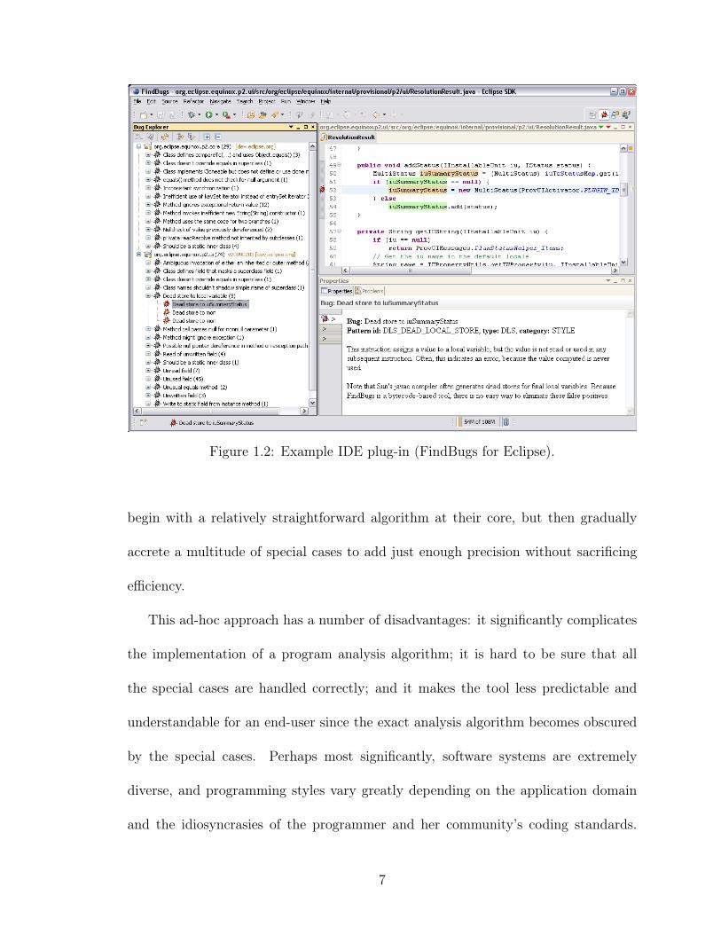
Figure 1.2: Example IDE plug-in (FindBugs for Eclipse).
begin with a relatively straightforward algorithm at their core, but then gradually
accrete a multitude of special cases to add just enough precision without sacrificing
efficiency.
This ad-hoc approach has a number of disadvantages: it significantly complicates
the implementation of a program analysis algorithm; it is hard to be sure that all
the special cases are handled correctly; and it makes the tool less predictable and
understandable for an end-user since the exact analysis algorithm becomes obscured
by the special cases. Perhaps most significantly, software systems are extremely
diverse, and programming styles vary greatly depending on the application domain
and the idiosyncrasies of the programmer and her community’s coding standards.
7

Thus an analysis that is carefully tuned to work in one domain may not be effective
in another domain.
We propose a different approach: instead of making a single algorithm suitable for
all software, we apply several algorithms of different levels of precision or efficiency
to different parts of the target software. This enables programmers to customize
the program analyses to the characteristics of their target software, for example, by
applying slower but more precise algorithms only on more complex parts of their
target software, and faster but less precise algorithms elsewhere. Another advantage
of this approach is that we can avoid making extensive tweaks to the constituent
algorithms, which potentially makes it simpler for programmers to understand the
algorithms.
In Chapter 3, we present Mix, a framework that realizes this approach by mixing
two conceptually simple program analyses—type checking and symbolic execution.
A key feature of our approach is that we use the constituent analyses as-is with no
modifications. Instead, we apply these analyses independently on disjoint parts of the
program. At the boundaries between nested type checked and symbolically executed
code regions, we use special mix rules to communicate information between the off-
the-shelf systems. The resulting mixture is a provably sound analysis that is more
precise than type checking alone and more efficient than exclusive symbolic execution.
We also describe a prototype implementation, Mixy, for C. Mixy checks for potential
null dereferences by mixing a null/non-null type qualifier inference system with a
symbolic executor.
8

1.1.3 Expositor: Integrating Program Analysis into Debugging
“...we talk a lot about finding bugs, but really, [Firefox’s] bottleneck is not find-
ing bugs but fixing [them]...”
—Robert O’Callahan (2010)
“[In debugging,] understanding how the failure came to be...requires by far
the most time and other resources”
—Andreas Zeller (2006)
We observe that using program analysis tools is just the beginning of a larger
debugging process. Debugging is a process that involves repeated application of the
scientific method: the programmer makes some observations; proposes a hypothesis
as to the cause of an error; uses this hypothesis to make predictions about the pro-
gram’s behavior, either under a program analysis or in a concrete execution; tests
those predictions using experiments; and finally either declares victory or repeats the
process with a new or refined hypothesis.
Mandelbugs in particular can truly test the mettle of programmers as they can
take hours or even days of tedious, hard-to-reuse, seemingly sisyphean effort to un-
tangle. Understanding mandelbugs often requires testing many hypotheses, with lots
of backtracking and retrials when those hypotheses fail. To make it easier to under-
stand mandelbugs, we would ideally like to take advantage of both the automation of
program analysis tools as well as quick and detailed feedback of interactive debuggers.
One way to combine program analysis with debugging is to use tools based on
dynamic program analysis, a particular kind of program analysis that detects errors
9

as they happen in a running execution of the target software. Dynamic program
analyses are typically implemented by instrumenting the target software binary with
additional code that implements the analysis logic. The programmer can then run
the instrumented executable under an interactive debugger such as GDB (The GDB
Developers), so that, when a bug is detected, the programmer can use the debugger
to examine the program states leading to the bug. For example, Valgrind (Nether-
cote and Seward, 2007), a dynamic binary program analysis framework that includes
various checkers such as memory corruption detectors, provides a mode that allows
GDB to connect to a running instance of Valgrind.
However, current dynamic program analysis tools are not well designed for this
kind of workflow. In particular, while it is possible to examine the program state of
the target software with the debugger, it is rarely possible to examine the intermediate
results produced by the dynamic analysis tools and gain some insight into the program
facts that these tools discover and use to produce an error report. In our experience,
we find that we often have to effectively redo the analysis, either mentally or using the
debugger, just to understand why a tool reports a particular error. Current interactive
debuggers do not support this workflow either: to follow the reasoning of the dynamic
program analysis requires manual effort to juggle breakpoints to stop the execution at
appropriate times to inspect the program state. As a result, it is non-trivial to apply
the information found by dynamic program analysis to debugging or vice-versa. It is
similarly difficult to run additional dynamic program analyses post-hoc on the failing
execution, e.g., to refine the original analysis or to test other hypothesis about the
bug.
10
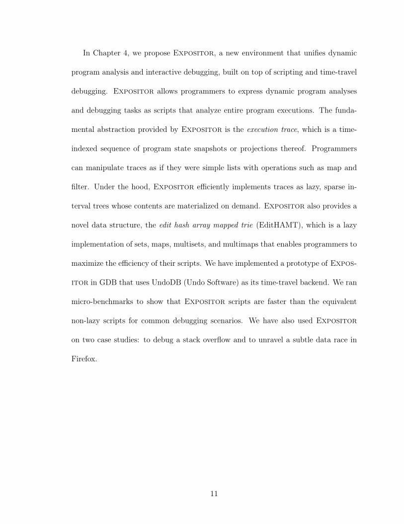
In Chapter 4, we propose Expositor, a new environment that unifies dynamic
program analysis and interactive debugging, built on top of scripting and time-travel
debugging. Expositor allows programmers to express dynamic program analyses
and debugging tasks as scripts that analyze entire program executions. The funda-
mental abstraction provided by Expositor is the execution trace, which is a time-
indexed sequence of program state snapshots or projections thereof. Programmers
can manipulate traces as if they were simple lists with operations such as map and
filter. Under the hood, Expositor efficiently implements traces as lazy, sparse in-
terval trees whose contents are materialized on demand. Expositor also provides a
novel data structure, the edit hash array mapped trie (EditHAMT), which is a lazy
implementation of sets, maps, multisets, and multimaps that enables programmers to
maximize the efficiency of their scripts. We have implemented a prototype of Expos-
itor in GDB that uses UndoDB (Undo Software) as its time-travel backend. We ran
micro-benchmarks to show that Expositor scripts are faster than the equivalent
non-lazy scripts for common debugging scenarios. We have also used Expositor
on two case studies: to debug a stack overflow and to unravel a subtle data race in
Firefox.
11

Chapter 2
Path Projection: Path-based Code Visualization for
Program Analysis†
In this chapter, we present Path Projection, a new user interface toolkit that helps
users visualize, navigate, and understand program paths (e.g., call stacks, control flow
paths, or data flow paths), a common component of many program analysis tools’
error reports. Path Projection aims to help engineers understand error reports,
improving the speed and accuracy of triage and remediation.
Path Projection accepts an XML error report containing a set of paths and
automatically generates a concise source code visualization of these paths. First,
we use function call inlining to insert the bodies of called functions just below the
corresponding call sites, rearranging the source code in path order. Second, we use
path-derived code folding to hide potentially-irrelevant statements that are not in-
volved in the path. Finally, we show multiple paths side by side for easy comparison.
By synthesizing the visualization directly from the error report, Path Projection
greatly reduces the programmer’s effort to examine the code for the error report.
†Path Projection was originally published in Khoo et al. (2008a,b) in collaboration withmy advisors Jeffrey S. Foster, Michael Hicks, and Vibha Sazawal. A prototype is available athttp://www.cs.umd.edu/projects/PL/PP/ along with screenshots and demos.
12
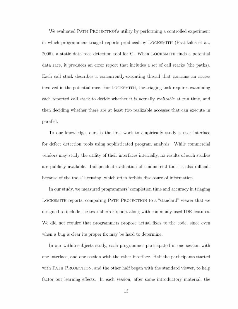
We evaluated Path Projection’s utility by performing a controlled experiment
in which programmers triaged reports produced by Locksmith (Pratikakis et al.,
2006), a static data race detection tool for C. When Locksmith finds a potential
data race, it produces an error report that includes a set of call stacks (the paths).
Each call stack describes a concurrently-executing thread that contains an access
involved in the potential race. For Locksmith, the triaging task requires examining
each reported call stack to decide whether it is actually realizable at run time, and
then deciding whether there are at least two realizable accesses that can execute in
parallel.
To our knowledge, ours is the first work to empirically study a user interface
for defect detection tools using sophisticated program analysis. While commercial
vendors may study the utility of their interfaces internally, no results of such studies
are publicly available. Independent evaluation of commercial tools is also difficult
because of the tools’ licensing, which often forbids disclosure of information.
In our study, we measured programmers’ completion time and accuracy in triaging
Locksmith reports, comparing Path Projection to a “standard” viewer that we
designed to include the textual error report along with commonly-used IDE features.
We did not require that programmers propose actual fixes to the code, since even
when a bug is clear its proper fix may be hard to determine.
In our within-subjects study, each programmer participated in one session with
one interface, and one session with the other interface. Half the participants started
with Path Projection, and the other half began with the standard viewer, to help
factor out learning effects. In each session, after some introductory material, the
13

programmer was asked to triage three error reports by filling in a triaging checklist
that enumerates the sub-tasks needed to triage the report correctly. At the end of
the experiment, we asked programmers to qualitatively evaluate the interface and
compare both.
We found that Path Projection improved the time it takes to triage a bug by
roughly 1 minute, an 18% improvement, and participants using it made about the
same number of mistakes as with the standard viewer. Moreover, in Path Projec-
tion programmers spent little time looking at the error report itself. This suggests
that Path Projection succeeds in making paths easy to see and understand in the
source code view. Also, seven of eight programmers preferred Path Projection
over the standard viewer, and generally rated all the features of Path Projection
as somewhat or very useful.
As a side result, we also observed that using triaging checklist dramatically re-
duced the overall triaging times for users of both interfaces, compared to an earlier
pilot study that did not utilize checklists. We originally created the checklist after
discovering that participants in the pilot study lack sufficient experience or knowl-
edge of Locksmith to triage its error report efficiently, and will often spend time
discerning information about the program that is not relevant to the triaging task.
So, we designed the checklist as an experimental aid to give programmers a system-
atic procedure to perform triage, but we were surprised by degree of improvement
in triaging times after introducing the checklists. Although this result is not scien-
tifically rigorous (several other features changed between the pilot and the current
14

study), we believe it suggests checklists would be a useful addition to many program
analysis interfaces, and merit further study.
In summary, this chapter makes two main contributions:
1. We present Path Projection, a novel toolkit for visualizing program paths
(Section 2.2). While mature program analysis tools can have sophisticated
graphical user interfaces (Section 2.6), these interfaces are designed for partic-
ular tools and cannot easily be used in other contexts. We show how to apply
Path Projection both to Locksmith and to BLAST (Beyer et al., 2007),
a software model checking tool. We believe Path Projection’s combination
and design of user interface features is novel.
2. We present quantitative and qualitative evidence of Path Projection’s ben-
efits in triaging Locksmith error reports (Sections 2.4 and 2.5). To our knowl-
edge, ours is the first study to consider the task of triaging defect detection tool
error reports, and the first to consider the user interface in this context. Our
study results provide some scientific understanding of which features are most
important for making programmers more effective when using program analysis
tools.
2.1 Motivation: Program Paths
The simplest way for a program analysis tool to report a potential defect is to indicate
a line in the file where the defect was detected. However, while this works reasonably
well for C or Java compiler errors, program analysis designers have long realized it
15
is insufficient for understanding the results of more sophisticated program analyses.
Accordingly, many program analysis tools provide a program path, i.e., some set of
program statements, with each error message. For example, CQual (Greenfieldboyce
and Foster, 2004) and MrSpidey (Flanagan et al., 1996) report paths corresponding to
data flow; BLAST (Beyer et al., 2007) and SDV (Ball and Rajamani, 2002) provide
counterexample traces; Code Sonar (GrammaTech, Inc., a) provides a failing path
with pre- and post-conditions; while Coverity SAVE (Coverity, Inc., b) and HP Fortify
SCA (Hewlett-Packard Development Company, L.P.) provides control-flow paths that
could induce a failure.
Because program analysis tools often make conservative assumptions, they typi-
cally produce false warnings, i.e., reports that do not correspond to actual bugs. The
programmer must therefore triage a tool’s reports by, e.g., tracing the reported paths,
to decide if a problem could actually occur at run-time.
2.1.1 Unrealizable paths in Locksmith
To understand the challenges that occur when tracing program paths, we consider
the problem of triaging error reports in Locksmith, a data race detection tool for C.
Locksmith reports paths whose execution could lead concurrent threads to access a
shared variable simultaneously. However, like many other tools, Locksmith employs
a path-insensitive analysis, meaning it assumes that any branch in the program could
be taken both ways. Thus, to triage an error report, a programmer must decide
whether a pair of reported accesses is simultaneously realizable, i.e., if there is some
execution in which both could happen at once.
16

The triaging process is conceptually simple: we must examine the control flow
logic along the paths and ensure it does not prevent both accesses from occurring at
once. However, in practice, performing this task is non-trivial, taking a surprising
amount of effort using typical code editors.
Consider Figure 2.1, a screenshot of our standard viewer, which represents the
assistance a typical editor or IDE would give programmers in understanding textual
error reports. A sample Locksmith error report is shown in the pane labeled 1 .1
This error report comes from aget, a multithreaded FTP client. The report first
identifies prev as the shared variable involved in the race. Then, it lists two call stacks
leading to conflicting accesses to prev, the first via a thread created in main, and the
second via a different thread created in resume_get. No lock is held at either access.
We need to trace through the control-flow of the program to see under what
conditions the two dereferences are reachable. The call stacks in the error report
show exactly what code to examine. In the screenshot in Figure 2.1, we begin by
tracing path 1 from the thread creation site, which can be reached by clicking on the
hyperlink 2 , and look for any branch conditions that may prevent the thread from
being created. We can continue tracing to the access by clicking on the hyperlinks
or scrolling through the code. As we navigate from function to function, we can split
windows 3 to keep various context together on the screen, and close splits when
the window becomes too crowded. After tracing path 1, we need to trace through
1Note that this format is slightly different than Locksmith’s standard output, but thedifferences are merely syntactic.
17

4
3
1
2
Figure 2.1: Standard viewer screenshot (picture in color; labels described in text).
18
path 2 in the same way, and ultimately decide whether both paths are simultaneously
realizable.
The resulting display is cluttered and hard to manage, and if we were to continue,
we would likely be forced to collapse splits, which would make it harder to refer back
to code along the path. In general, when examining program paths with standard
viewers, mundane tasks such as searching, scrolling, navigating, viewing, or combining
occur with such frequency that they add up to a significant cognitive burden on
the programmer and distract from the actual program understanding task. In our
experience, it can be quite tedious to triage error reports even for small programs
such as aget, which has only 2,000 lines of code. Since program analysis tools can
yield hundreds of defect reports on large programs, we believe it is crucial to make
triaging error reports easier.
The goal of Path Projection is to make tracing paths much easier by reducing
the cognitive load on the programmer. In our user study, we focused on the task of
triaging Locksmith error reports by looking for unrealizable paths. However, we
also believe that Path Projection is generally applicable to many other program
understanding tasks involving path tracing.
We should add that, besides unrealizable paths, there are several other reasons
Locksmith may report a false warnings, e.g., it may incorrectly decide that a variable
is shared, or it may decide a lock is not held when it is Pratikakis et al. (2006). For
many programs that we have looked at, Locksmith’s lock state analysis is accurate,
and warnings often involve only simple sharing (e.g., of global variables, or via simple
aliasing), thus, we focuses on the problem of tracing program paths.
19
2.2 Path Projection
Program paths are commonly used by program analysis tools to report errors. How-
ever, as the previous section illustrates, tracing program paths becomes difficult when
the programmer needs to examine discontinuous lines of code across many different
files.
Standard code editors provide some support for tracing program paths. For exam-
ple, they typically allow the programmer to view more than one file to be by opening
multiple windows or by splitting a window. Code folding is another commonly avail-
able feature used to hide irrelevant code.
The key issue, however, is that the programmer has to invoke and manage these
features manually. In particular, the programmer has to carefully consider the trade-
offs of these features, e.g., after opening or splitting windows, the programmer may
have to move, resize or close other windows to make them visible or simply to reduce
screen clutter.
This places a significant cognitive burden on the programmer to extract and or-
ganize relevant information from the source code and the error report, and distracts
from the actual task of understanding a program path. If paths are long or compli-
cated, as they often are, it can be hard to keep track of the context of the path while
managing windows and folded code. In our experience, it is all too easy to get lost
on a long path and have to backtrack or retrace it many times.
20
2.2.1 Design Guidelines
To develop a better interface for tracing program paths, we can look to guidelines
developed by researchers in information visualization. We found three strategies
described by Card et al. (1999) to be particularly applicable for our task:
1. Increase users’ memory and processing resources and reduce the search for in-
formation. The Locksmith error report is compact, but examining the path
in the actual source code may involve many different source code lines spread
across many different files. We would ideally like to put all the necessary infor-
mation for triaging an error report on one screen, so the programmer can see all
the information at the same time. We would also like to allow the programmer
to hide any unimportant information, to further reduce the cognitive burden.
2. Use visual representation to enhance pattern detection. We would like to visually
distinguish the source code lines appearing in the Locksmith error report from
the other lines in the program, since the lines in the error reports are presumably
very important. We would also like to bring important threading API calls, e.g.,
invocations of pthread_X functions, to the programmer’s attention.
3. Encode information in a manipulable medium. We need to give the programmer
good mechanisms for searching and comparing the information we present to
them.
Another key guideline we would like to follow is that “code should look like code”.
We want the programmer to be able to relate any visualization back to the original
21

source code. This is based on our experience as programmers: we spend a large frac-
tion of time editing source code in standard textual form, and relatively little working
with abstract visualizations. Understanding Locksmith error reports requires look-
ing at source code in great detail. A visualization that looks like source code will be
familiar, which should increase acceptance and could increase comprehension.
2.2.2 Interface Features
Figure 2.2 shows the Path Projection interface for the same program shown in
the standard viewer in Figure 2.1. The core feature of Path Projection is that it
makes multiple program paths manifest in the display of the source code. To achieve
this, Path Projection uses three main techniques:
Function call inlining. Path Projection inlines function calls along a
path. In the left path in the example, we see that the bodies of signal_waiter (called
by pthread_create), sigalrm_handler, and updateProgressBar are displayed in a series of
nested boxes immediately below the calling line 1 . We color and indent each box to
help visually group the lines from each function (Principle 2). This feature is where
our interface name comes from—we are “projecting” the source code onto the error
path. Our motivation is to reduce the need for the programmer to look at the error
report, since the path is apparent in the visualization. We also underline the racing
access (innermost boxes) to make it easy to identify.
Notice that in Path Projection, we actually visually rearrange function bodies
in the original source code to conform to the order they appear in the path. Moreover,
22

1
3
2{5
4
6
78
9
Figure 2.2: Path Projection screenshot (picture in color; labels described intext). This and additional screenshots can be found at at http://www.cs.umd.edu/projects/PL/PP.
23

we may pull in functions from multiple files (in our example, three separate files) and
display them together. Together, these regroupings help keep relevant information
close together to reduce search and free up cognitive resources (Principle 1).
In the standard viewer, the programmer could achieve a similar result by splitting
the display into several pieces to show the functions along the path. However, this
quickly becomes tedious if there are several functions to show at once, and it adds
significant mechanical overhead to viewing and navigating a path. Moreover, without
code folding, which we discuss next, it can be difficult to see all the relevant parts of
the functions simultaneously.
Path-derived code folding. To keep as much relevant information on one
screen as possible (Principle 1), we filter by default irrelevant statements, i.e., state-
ments not implicated by the error report, from the displayed source code. For exam-
ple, in the function updateProgressBar in the left path, we have folded away all lines 2
except the implicated access (line 193) and the enclosing lexical elements (the func-
tion definition and open and close curly braces). The programmer can tell code has
been folded by noticing non-consecutive line numbering.
Our code folding algorithm is a syntax-based heuristic that tags lines in the pro-
gram as either relevant or irrelevant. Irrelevant lines are hidden when the code is
folded. For each line l listed in the error report, we tag as relevant line l itself; the
opening and closing statements of any lexical blocks that enclose l; and the beginning
and end of the containing function. For lexical blocks that include a guard (i.e., if,
for, while, or do), we include the guard itself, and for an if block, we show the line
24

containing the else (though not the contents of the else block). For example, the call
to sigalrm_handler 4 is in the error path, and so we reveal it, the closing if and while
blocks, and the beginning and end of the signal_waiter function. Our code folding
heuristic resembles the degree-of-interest model proposed by Furnas (1986). A more
sound approach would be to use program slicing (Weiser, 1984) to determine relevant
lines; and in a sense, our code folding algorithm can be thought of as an extremely
simple but imprecise slicing technique.
Since our code folding algorithm is heuristic and may hide elements that the pro-
grammer actually needs to examine, we allow the programmer to click the expansion
button in the upper-left corner of a box to reveal all code in the corresponding func-
tion. When unfolded, source lines tagged as irrelevant are colored gray to ensure the
path continues to stand out. For example, we have unfolded the body of main 5 in
Figure 2.2.
While code folding is common in many IDEs, most require the programmer man-
ually perform folding on individual lexical blocks, which can be time consuming and
tricky to get exactly right. In contrast, we use the path to automatically decide
which lines of code to reveal or fold away, requiring no programmer effort. Further-
more, since we display each path in a separate column, we can apply our code folding
algorithm to each path individually.
Side-by-side paths. This error report contains two paths, each of which is
displayed side-by-side in its own column ( 3 , left side of Figure 2.2). This parallel
display makes relationships between the paths easier to see than in the standard
25
interface, which would require flipping between different views (Principle 1). Each
column is capped at a maximum width, and programmers can horizontally scroll
columns individually. This helps prevent files that are unusually wide from cluttering
the display.
Triaging Locksmith’s error report requires comparing more than one path, mak-
ing this feature a necessity. However, we believe that side-by-side paths would be
useful for other tools too. For example, a model-checker may display known-good
paths for comparison with the error path.
In our experiments, participants used a wide-screen monitor to make it easier to
see multiple paths simultaneously. Since wide-screen displays are commonly available
and popular, we think designing an interface with such displays in mind is reasonable.
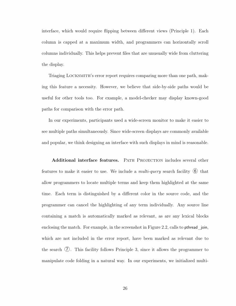
Additional interface features. Path Projection includes several other
features to make it easier to use. We include a multi-query search facility 6 that
allow programmers to locate multiple terms and keep them highlighted at the same
time. Each term is distinguished by a different color in the source code, and the
programmer can cancel the highlighting of any term individually. Any source line
containing a match is automatically marked as relevant, as are any lexical blocks
enclosing the match. For example, in the screenshot in Figure 2.2, calls to pthread_join,
which are not included in the error report, have been marked as relevant due to
the search 7 . This facility follows Principle 3, since it allows the programmer to
manipulate code folding in a natural way. In our experiments, we initialized multi-
26

query to find the four pthread functions shown in the screenshot, since in our pilot
study we found programmers almost always want to locate uses of these functions.
Our interface also includes a reveal definition facility that uses inlining to show the
definition of a function or variable. In the screenshot, the programmer has clicked on
nthreads, and its definition has been inlined below the use 8 . While this feature seems
potentially handy, we found it was rarely used by participants in our experiments.
Lastly, Path Projection still includes the original error report from which the
visualization was generated, to act as a back-up and to provide consistency with the
standard view. As with the standard view, the report is hyperlinked to the source
display.
2.2.3 Applying Path Projection to Other Tools
We intend Path Projection to be general toolkit that may be used by program
analysis tool developers to visualize their error reports. To this end, Path Projec-
tion is implemented as a standalone tool that takes as input an XML-based error
report and the source code under analysis.
pathreport XML format. Our XML format, called pathreport, describes one
or more program path using three kinds of tags. It is designed to easily convert a
textual path-based report by marking it up appropriately. Briefly, the three tags are:
<path> marks text that corresponds to a continuous block of code, such as a func-
tion. A <path> can contain any number of <detour> and <marker> tags.
27

<detour> marks text that corresponds to a reference in some code, such as a call
site. The parent <path> provides the context for this reference, e.g., the function
in which the call site appears. Each <detour> tag must in turn contain exactly
one <path> tag.
<marker> tags mark any other texts, such as function names, variable names, or
line numbers, that point to code that may be interesting.
These tags also require attributes to precisely indicate information such as the file
where a function is defined. Together, <path> and <detour> recursively describe a
program path, and <marker> can be used to mark any interesting line of code along
the path.
Figure 2.3 shows how a path-based textual report can be marked up with <path>
and <detour>. Note that on line 31, <path> marks the entire call to a. Within that,
two <detour> tags on lines 32 and 33 mark the call sites to b and e that appear in a.
Path Projection on BLAST. In addition to Locksmith, we have applied
Path Projection to counterexample traces produced by BLAST (Beyer et al.,
2007), a software model checking tool. Such traces are not call stacks, as in Lock-
smith, but rather are execution traces that include function calls and returns. We use
a short awk script to post-process a BLAST trace into our XML format. We reformat
the line annotations from the original report for brevity, but retain the indentations
as they reveal relationships between implicated lines.
Figure 2.4 shows an example of BLAST in Path Projection, generated from
a post-processed counterexample trace that describes how a failing assertion (not
28

19 Trace:20 In function a (21 On line a:5, call b (22 On line b:10, call c (23 On line c:15, call d24 )25 )26 On line a:20, call e (27 On line e:25, call f28 )29 )
(a)
30 Trace:31 In function <path name="a">a (32 On line <detour line="5" name="b">a:5, call <path name="b">b (33 On line <detour line="10" name="c">b:10, call <path name="c">c (34 On line c:15, call d35 )</path></detour>36 )</path></detour>37 On line <detour line="20" name="e">a:20, call <path name="e">e (38 On line e:25, call f39 )</path></detour>40 )</path>
(b)
Figure 2.3: A textual path-based report (a) can be converted into the pathreport XMLformat (b) using <path> and <detour> (some attributes omitted for brevity).
shown) can be reached. The counterexample trace shown is 102 lines long, much
longer than is typical with Locksmith. Note that BLAST’s counterexample trace
is not a call stack, as in Locksmith, but an execution trace that includes function
calls and returns.
We find the error report confusing in its textual form, e.g., line 4 implicates a call
to initialize in line 157 of tcas.c, and lines 5-6 are indented to indicate the function
body; but the indented lines after line 8 do not correspond to the body of atoi. As
such, it can be quite difficult to match function calls and returns in a long error report.
29

1
2
Figure 2.4: Path Projection applied to a post-processed counterexample traceproduced by BLAST (picture in color; labels described in text).
30

Occasionally, there are also missing line numbers, such as on line 5 in the error report.
Furthermore, it is not obvious from the error report that many implicated lines are
actually not interesting.
Path Projection makes the structure of the path much clearer. We can quite
easily tell that the beginning of the path contains a call to initialize 1 , and that the
subsequent 24 lines in the error report correspond to the input program’s command-
line interface. The next interesting line is a call to alt_sep_text 2 , which is impli-
cated further down the report, on the last line visible in Figure 2.4 (obscured due to
indentation). However, this is obvious at first glance in Path Projection.
We believe that this example shows how Path Projection can be quite useful to
understand complicated error reports. We think that using Path Projection can
also suggest ways to improve error reports, e.g., BLAST should not indent function
calls with no corresponding body.
2.3 Triaging Checklist
In our pilot study we found that even with extensive pre-experiment tutorials, partic-
ipants had trouble determining how to accomplish this triaging task, and would often
get distracted with irrelevant features, such as locating the definition of a global vari-
able. This inconsistent behavior confounded our attempts to measure the benefits of
the PP interface, since it varied significantly depending on the participant. To address
this issue, we developed a tabbed triaging checklist that breaks down this task into
smaller sub-tasks, one per tab, that identify conditions under which reported thread
31
states, if individually realizable, could execute in parallel and thus constitute a true
race. A single error report could identify several races, so programmers must complete
all tabs, at which point they may click Submit to complete the triage process.
A checklist is automatically generated for each Locksmith error report, and is
identical in both interfaces— 4 in Figure 2.1 and 9 in Figure 2.2. The first tab,
labeled Locks (not shown), asks programmers to document where the locks held at
the end of each path were acquired. This tab is merely an experimental device: since
programmers tend to examine the code before moving to the checklist, we insert this
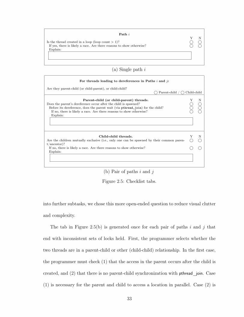
tab first to measure this initial startup period. The remaining tabs have two flavors,
both illustrated in Figure 2.5.
The tab shown in Figure 2.5(a) is generated once for each path i that ends in
an access with no locks held. The programmer is asked to check whether the access
could occur in a thread created in a loop. If it could have, then the same access
may occur in two different threads, constituting a race. For example, consider Path 2
in Figure 2.2. The write to prev (underlined in red) occurs in a thread created on
line 171 of Aget.c. Notice that that line appears in a for loop that actually creates
multiple threads. Thus, what Locksmith reports as Path 2 is actually a summary
of nthreads total paths, all of which may reach the same access. Since no lock is held
at the access, and it is a write, we have found a data race. The last part of this
tab asks the programmer to look for any logic that would prevent the data race from
occurring. For example, perhaps nthreads is always 1, so only one thread is spawned,
or perhaps the given state is not realizable due to inconsistent assumptions about the
branches taken on the path. While we could attempt to break this condition down
32
Path iY N
Is the thread created in a loop (loop count > 1)? ○ ○If yes, there is likely a race. Are there reasons to show otherwise? ○ ○Explain:
(a) Single path i
For threads leading to dereferences in Paths i and j:
Are they parent-child (or child-parent), or child-child?○ Parent-child / ○ Child-child
Parent-child (or child-parent) threads. Y NDoes the parent’s dereference occur after the child is spawned? ○ ○Before its dereference, does the parent wait (via pthread_join) for the child? ○ ○If no, there is likely a race. Are there reasons to show otherwise? ○ ○Explain:
Child-child threads. Y NAre the children mutually exclusive (i.e., only one can be spawned by their common paren-t/ancestor)?
○ ○
If no, there is likely a race. Are there reasons to show otherwise? ○ ○Explain:
(b) Pair of paths i and j
Figure 2.5: Checklist tabs.
into further subtasks, we chose this more open-ended question to reduce visual clutter
and complexity.
The tab in Figure 2.5(b) is generated once for each pair of paths i and j that
end with inconsistent sets of locks held. First, the programmer selects whether the
two threads are in a parent-child or other (child-child) relationship. In the first case,
the programmer must check (1) that the access in the parent occurs after the child is
created, and (2) that there is no parent-child synchronization with pthread_join. Case
(1) is necessary for the parent and child to access a location in parallel. Case (2) is
33
necessary because even if the parent accesses the location after creating its child, it
might wait for the child to complete before performing the access, making parallel
access impossible. If both (1) and (2) are true, then there is likely a race, and the
programmer is asked to look for other program logic that would prevent a race.
In the second case, a child-child relationship, the programmer checks whether the
two children are mutually exclusive. For example, they may be spawned in different
branches of an if statement, only one of which can execute dynamically. Again, if they
are not mutually exclusive, the programmer looks for other logic that would prevent
a race.
Though we did not carefully consider the benefits of the checklist experimen-
tally, we observed anecdotally that participants’ completion times for our current
study were reduced in both variance and magnitude (by an average of 3:46 minutes,
or 41%), compared to the pilot study. This improvement strongly suggests that a
tool-specific checklist has independent value, and that tool builders might consider
designing checklists for use with their tools. An interesting direction for future work
would be to explicitly study the benefit of checklists in performing triaging.
2.4 Preliminary Experimental Evaluation
We ran a controlled user study as a preliminary evaluation of Path Projection’s
utility. In our experiment, participants are asked to perform a series of triaging
tasks, using either Path Projection (PP), described in Section 2.2, or the standard
viewer (SV), described in Section 2.1.1. To eliminate bias due to participants’ prior
34
experience with editors, we implemented our own standard viewer instead of using
an existing editor.
For each task, the participant is presented with a Locksmith error report for a
program selected from a test corpus of open source programs. The participant’s goal
is to determine whether the error report constitutes an actual data race or whether
it is a false positive. In this task, PP provides an advantage over SV in triaging if it
is faster, easier, and/or more accurate.
2.4.1 Participants
We recruited a total of eight participants (3 undergraduate, 5 graduate) for this
experiment via e-mail and word-of-mouth advertising in the UMD Computer Science
Department. We required the participants to have prior experience with C and with
multithreaded programming (though not necessarily in C). All participants had taken
at least one college-level class that involved multithreaded programming. On a scale
of 1 (no experience) to 5 (very experienced), participants rated themselves between
3 and 4 when describing their ability to debug data races. Two participants had
previous experience in using a race detection tool (Locksmith and Eraser (Savage
et al., 1997)).
2.4.2 Design
Each participant was asked to perform the triaging task in two sessions, first with one
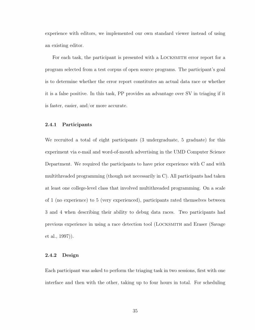
interface and then with the other, taking up to four hours in total. For scheduling
35
Session 1 Session 21 PP/1.1 PP/1.2 PP/1.3 SV/2.1 SV/2.2 SV/2.32 SV/1.1 SV/1.2 SV/1.3 PP/2.1 PP/2.2 PP/2.3
Table 2.1: User interface/problem number schedules.
flexibility, participants may opt to split up the sessions into several one- or two-hour
sections over different days.
Thus, our experiment is a within-subjects design consisting of two conditions,
using PP and using SV. Since participants experienced both interfaces, we were able
to measure comparative performance, and we could ask participants to qualitatively
compare the two interfaces.
A within-subjects design potentially suffers from order effects, since participants
may be biased towards the interface given first. To compensate, we perform coun-
terbalancing on the interface order: participants are randomly placed into one of the
two schedules shown in Table 2.1.
Participants in the first schedule use PP in the first session and SV in the second,
whereas participants in the second schedule use SV first and PP second. However, all
participants receive the same set of problems, numbered 1.1–2.3, in the same order,
which allows us to directly compare our observations of each problem without the
need to account for order effects.
2.4.3 Procedure
At the beginning of each session, we ask participants to complete several HTML-
based tutorials. First, we give a short tutorial and quiz on pthreads and data races, as
36
well as a tutorial on Locksmith with emphasis on the items in the triaging checklist
(Section 2.3); the same tutorial and quiz is repeated in second session as a review.
Then, we introduce the user interface (PP or SV) with another tutorial. We make
sure that participants are familiar with each interface by encouraging them to try
every feature and to triage a simple data race problem using the interface. We allow
participants to complete the tutorial at their own pace; all participants completed
the tutorial within 30 minutes.
Following the tutorial is a single practice trial and three actual trials, all of which
follow the same procedure. In each trial, we first ask participants to triage a real
Locksmith error report generated from Locksmith’s test corpus (Section 2.4.4).
We log participants’ mouse movements during the trial and measure the total time
to completion. Triaging ends when participants complete and submit the triaging
checklist. Immediately after, we present participants with the same problem and ask
them to explain out loud the steps they took to verify the warning. This allows us to
compare their descriptions with our expectations.
We do not tell participants whether their answers are correct, for several reasons.
Firstly, it is difficult for the experimenter to quickly judge the correctness of the
answer, since identifying a data race may involve understanding many subtle aspects
in a program. Secondly, we do not want the participants to become reliant on receiving
an answer or to guess at an answer. Finally, in a real triaging scenario, programmers
will not have the benefit of an oracle to confirm their intuitions.
We have found this two-stage procedure to be very effective in our pilot studies.
In particular, it allows us to ask about specific interesting behaviors observed without
37

interrupting the participant during the task. The participants also benefit from a lim-
ited form of feedback. By recalling their work to the experimenter, they can confirm
their initial understanding, or notice mistakes made. Furthermore, we have found
that participants gain a better understanding of the user interface by demonstrating
it to another person. This also helps mitigate the effects of what turned out to be
a long learning curve in triaging error reports. The experimenter may also ask for
clarification to certain points, which may reveal inconsistencies or mistakes.
After the experiment, participants complete a questionnaire and are interviewed
to determine their opinion of the user interface. Programmers are asked to evaluate
each tool based on ease-of-learning, ease-of-use, and effectiveness in supporting the
triaging task.
We ran the experiment on Mac OS X 10.5.2. To avoid bias due to OS competency,
all shortcuts are disabled except for cut, copy, paste, find, and find-next, and par-
ticipants are informed of these shortcuts. We also display the interface on a 24-inch
wide-screen 1920-by-1200 resolution LCD monitor.
2.4.4 Programs
Each trial’s error report was drawn from one of four open source programs, all of
which we have previously applied Locksmith to: engine, aget, pfscan, and knot. We
also chose reports in which imprecision in the sharing and lock state analysis do not
contribute to the report’s validity, so as to focus on the task of tracing program path
as discussed in Section 2.1.
38

Reports from engine and pfscan are used during the tutorial and practice trials.
Trials 1.1–1.3 use error reports from aget, and trials 2.1–2.3 use error reports from
knot. By using different programs in each trial, we prevent participants from carrying
over knowledge of the programs from the first interface to the second. The three
selected reports within each program are significantly different from each other, e.g.,
they do not follow the same paths. This helps avoid bias that could arise if participants
were given very similar triaging tasks for the same program.
Of the six reports, four contain 3 paths, and two contain 2 paths; eight paths have
a call depth of 3, and the two deepest have a call depth of 8. Overall, there were 23
(non-Locks) tabs to complete for the experiment, 8 of which are true positives and
15 of which are false positives.
We also simplify the task slightly by making four small, semantics-preserving
changes to the programs themselves. Doing so makes it simpler to ensure that our
participants have a common knowledge base to work from, and reduces measurement
variance due to individual differences. First, we made local static variables global.
Second, we converted wait/signal synchronization to equivalent pthread_join synchro-
nization when possible. We made both changes in response to confusion by some
participants in our pilot study who were unfamiliar with these constructs. Third, we
deleted lines of code disabled via #if 0 or other macros. Finally, in a few cases we
converted gotos and switch statements to equivalent if statements. These last changes
remove irrelevant complexity from the triaging task.
39
2.5 Experimental Results
2.5.1 Quantitative Results
Completion time. We measured the time it took each participant to complete
each trial, defined as the interval from loading the user interface until the participant
submitted a completed checklist. Figure 2.6(a) lists the results, and Figure 2.6(b)
shows the mean completion times for each interface and session order combination.
We found in general that PP results in 18% shorter completion times than SV.
More precisely, the mean completion time is 296 seconds (4:56 minutes) for PP, and
362 seconds (6:02 minutes) for SV. A standard way to test the significance of this result
is to run a two-way, user interface (within subjects) by presentation order (between
subjects), mixed-model ANOVA on the mean of the three completion times for each
participants in each session.2 However, this test revealed a significant interaction
effect between the interface and the presentation order (F (1, 6) = 20.157, p = 0.004;
Figure 2.7(a)).3 We believe this is a learning effect—notice that for the SV-PP order
(SV first, PP second), the mean time improved 188 seconds (3:08 minutes) from the
first session to the second, and for the PP-SV order the mean time improved 55
seconds. Since the interaction effect is significant, we cannot directly interpret the
main effect of the user interface. Instead, we use the standard approach of running
two one-way, within-subjects ANOVAs for each presentation order separately, and
2We ran all statistical tests in R. For ANOVA, we confirmed that all data sets satisfied normalityusing the Shapiro-Wilk test.
3As is standard, we consider a p-value of less than 0.05 to indicate a statistically significant result.
40

Session 1 Session 2Trial 1.1 1.2 1.3 mean 2.1 2.2 2.3 mean
Participant SV PP1 516 854 584 651 427 288* 242 3192 307* 190 350 282 256 149* 130* 1785 466 154 338* 320 313 223* 78* 2057 340 383 455 393 185 233* 152 190
411 223Participant PP SV
0 387* 369 512* 423 582 316* 191* 3633 398 438 515 450 678 381 219 4264 501 131 283 305 326* 267* 166* 2536 431 172 290** 297 273 246* 118* 212
369 314
# Tabs 3 2 6 6 3 3* one incorrectly answered tab in the checklist
(a) Completion times and accuracy for each trial
Session 1 Session 2
010
020
030
040
0
Standard ViewerPath Projection
SV−PP
PP−SV
(b) Completion time (sec)
Session 1 Session 2
020
4060
8010
012
0
Standard ViewerPath Projection
SV−PP
PP−SV
(c) Time in error report (sec)
Figure 2.6: Quantitative data (error bars are omitted as they are inappropriate forwithin-subjects design).
41
250
300
350
400
SV−PP PP−SV
SV
PP
(a) Completion time (sec)
2040
6080
100
120
SV−PP PP−SV
SV
PP
(b) Time in error report (sec)
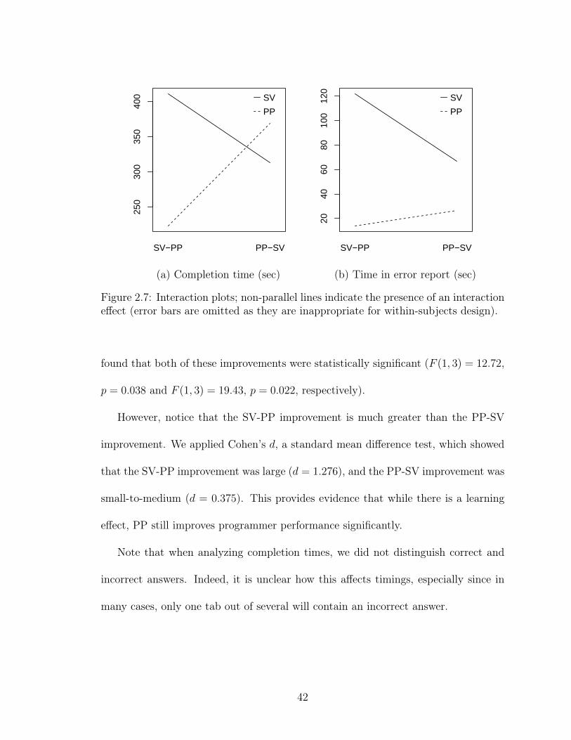
Figure 2.7: Interaction plots; non-parallel lines indicate the presence of an interactioneffect (error bars are omitted as they are inappropriate for within-subjects design).
found that both of these improvements were statistically significant (F (1, 3) = 12.72,
p = 0.038 and F (1, 3) = 19.43, p = 0.022, respectively).
However, notice that the SV-PP improvement is much greater than the PP-SV
improvement. We applied Cohen’s d, a standard mean difference test, which showed
that the SV-PP improvement was large (d = 1.276), and the PP-SV improvement was
small-to-medium (d = 0.375). This provides evidence that while there is a learning
effect, PP still improves programmer performance significantly.
Note that when analyzing completion times, we did not distinguish correct and
incorrect answers. Indeed, it is unclear how this affects timings, especially since in
many cases, only one tab out of several will contain an incorrect answer.
42

Accuracy. Figure 2.6(a) also indicates, for each trial, how many of the checklist
tabs were answered incorrectly. The total number of checklist tabs in each trial
is listed at the bottom of the chart. We did not count the Locks tab in either of
these numbers. Programmer mistakes are evenly distributed across both interfaces.
Participants made 10 mistakes (10.9%) under PP, compared to 9 mistakes (9.8%)
under SV. For each participant, we summed the number of mistakes they made in
each session, and we compared the sums for each interface using a Wilcoxon rank-sum
test. This showed that the difference is not significant (p = 0.770), suggesting the
distribution of errors is comparable for both interfaces. This shows that using PP,
participants are able to come to similarly accurate conclusions in less time.
Most of the participant mistakes occurred in trials 2.2 and 2.3, in which two
potentially-racing paths actually contain a common unrealizable sub-path, making
the data race report a false positive. In trial 1.3, one participant completed two tabs
incorrectly, but there was only one underlying mistake: misidentifying the same child
thread as a parent thread (and thus affecting the answers to two tabs).
Time in error report. We found that under PP, participants spend much less
time with the mouse hovering over the error report compared to SV. Figure 2.6(c)
shows the mean times for each session and interface. We found that on average, par-
ticipants spend 20 seconds in the error report under PP, compared to 94 seconds (1:34
minutes) under SV. As with completion time, there is a significant interaction effect
(F (1, 6) = 9.889, p = 0.020; Figure 2.7(b)) according to a two-way, user interface
(within subjects) by presentation order (between subjects), mixed-model ANOVA.
43
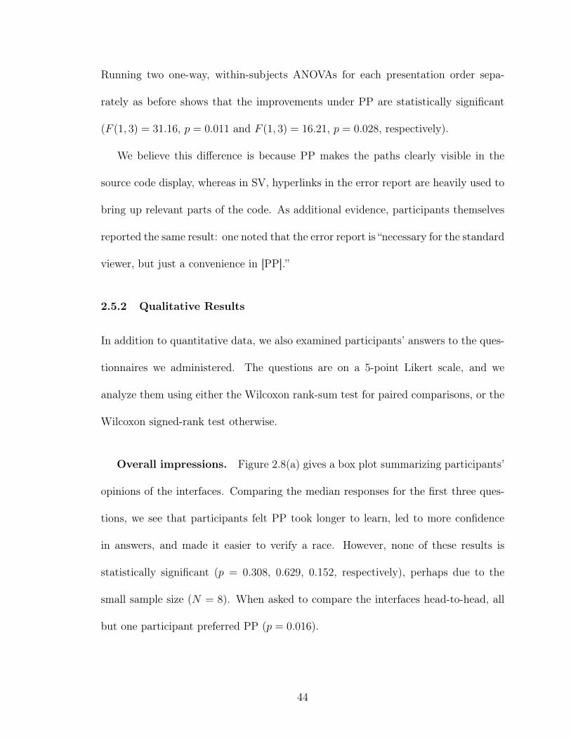
Running two one-way, within-subjects ANOVAs for each presentation order sepa-
rately as before shows that the improvements under PP are statistically significant
(F (1, 3) = 31.16, p = 0.011 and F (1, 3) = 16.21, p = 0.028, respectively).
We believe this difference is because PP makes the paths clearly visible in the
source code display, whereas in SV, hyperlinks in the error report are heavily used to
bring up relevant parts of the code. As additional evidence, participants themselves
reported the same result: one noted that the error report is “necessary for the standard
viewer, but just a convenience in [PP].”
2.5.2 Qualitative Results
In addition to quantitative data, we also examined participants’ answers to the ques-
tionnaires we administered. The questions are on a 5-point Likert scale, and we
analyze them using either the Wilcoxon rank-sum test for paired comparisons, or the
Wilcoxon signed-rank test otherwise.
Overall impressions. Figure 2.8(a) gives a box plot summarizing participants’
opinions of the interfaces. Comparing the median responses for the first three ques-
tions, we see that participants felt PP took longer to learn, led to more confidence
in answers, and made it easier to verify a race. However, none of these results is
statistically significant (p = 0.308, 0.629, 0.152, respectively), perhaps due to the
small sample size (N = 8). When asked to compare the interfaces head-to-head, all
but one participant preferred PP (p = 0.016).
44
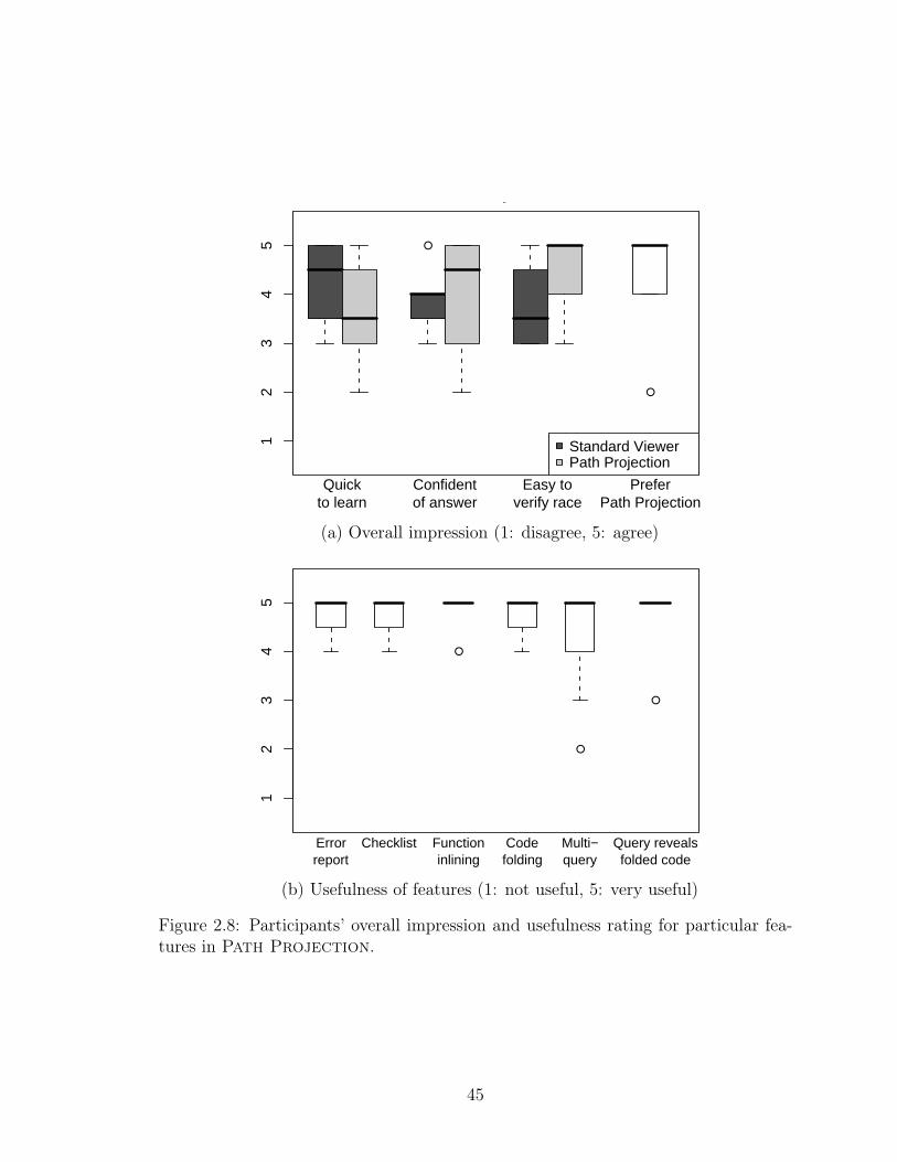
●
●
Quickto learn
Confidentof answer
Easy toverify race
PreferPath Projection
12
34
5
Overall impression
Standard ViewerPath Projection
(a) Overall impression (1: disagree, 5: agree)
●
●
●
Errorreport
Checklist Functioninlining
Codefolding
Multi−query
Query revealsfolded code
12
34
5
Usefulness of features
(b) Usefulness of features (1: not useful, 5: very useful)
Figure 2.8: Participants’ overall impression and usefulness rating for particular fea-tures in Path Projection.
45

However, we should also note that several participants felt that they were unable to
fairly assess PP due to the novelty of the interface and the limited amount of exposure
to it in the experiment. One participant rated PP worse than SV in all metrics, yet
stated he preferred PP due to its potential, saying, “once you get comfortable with
seeing [only] pieces of your code, I feel it will be more efficient.”
Usefulness of features. Finally, participants generally rated all the features
of PP as somewhat or very useful. Figure 2.8(b) shows a box plot of participants’
responses, and all answers are statistically significant in favor of PP compared to a
neutral response of 3 (p < 0.032).
While participants felt that the error report was very useful, they also commented
that it served mostly as an initial overview under PP, whereas it was critical under
SV. This matches our quantitative result indicating participants spent much less time
in the error report under PP.
The checklist was very well received overall. One participant said, “[It] saved
me from having to memorize rules.” Interestingly, two participants felt that, while
the checklist reduces mistakes, verifying the data race takes longer. This conflicts
with our own experience—as we mentioned earlier, participants in our pilot study,
which did not include the checklist, took notably longer to triage error reports than
participants in our current study.
We thought that participants would be wary about function inlining and code
folding, since the former is an unfamiliar visualization and the latter hides away
much code. However, participants rated both very highly, saying particularly that
46

code folding was “the best feature,” “my favorite feature,” and “I love using this feature
[code folding].”
Most participants found multi-query useful, but two did not. When we asked
them why, they replied that they felt that the code folding was already doing an
adequate job without it. However, they had forgotten that the multi-query was in
use by default with the four preset queries (shown in Figure 2.2). We believe that
multi-query is actually extremely useful in combination with code folding.
2.5.3 Threats to Validity
There are a number of potential threats to the validity of our results. The core threat
is whether our results generalize. The main issue is that we had a small number of
participants, all of whom were students rather than professional programmers who
had significant experience debugging data races. Due to length of our user study,
we had thought that it would be easier to recruit students who would have less
scheduling constraints than professional programmers for the preliminary user study.
Unfortunately, we found the number of students with the prerequisite experience in
C and multithreaded programming to be fewer than we expected.
We had a small set of programs (N = 2) and error reports (N = 6) in the experi-
ment due to length as well. Moreover, participants were asked to triage error reports
for unfamiliar programs, rather than code bases they had developed themselves. We
had intentionally restricted these programs to Locksmith’s test corpus to avoid any
issues in running Locksmithon other untested programs.
47

Lastly, despite long tutorials before each experiment, we were unable to eliminate
the learning effect across our trials.
However, even with these limitations, our experiment did produce statistically
significant and anecdotally useful information for our population and sample trials.
We leave carrying out a wider range of experiments to future work.
One minor threat is the small set of changes we made to the programs (Sec-
tion 2.4.4) to avoid confusion in our participants. Using more professional program-
mers as test subjects would obviate the need for this. Also, the SV interface represents
a typical IDE, but is not an actual, production-quality IDE. We chose this approach
on purpose, so that familiarity with a particular IDE would not bias our participants,
but we may have omitted features that would be useful for our task.
2.6 Related Work
Error report triaging is essentially a program comprehension task. In our study,
the particular task is to determine whether two dereferences could possibly execute
simultaneously in two different threads. There is a substantial body of tools aimed at
assisting in program comprehension tasks typically (but not exclusively) associated
with code maintenance or re-engineering (e.g., SHriMP (Storey, 1998), and Code
Surfer (Anderson et al., 2003)). As far as we are aware, none of these tools has been
specifically designed to support users of program analysis for defect detection.
Many defect detection tools that use program analysis provide custom user in-
terfaces, IDE plug-ins, or both. Since many proprietary tools have licenses that
48

Features (legend below)
Tool IDE HLR HPC PCF FCI AC AQ MQ OV
Path Projection X X X X XSDV2 X X XPREFast3 X X X n/a1 XCoverity SAVE4 X X X X XCodeSonar5 X X X X XMrSpidey6 X X X XFortify SCA7 X X XKlocwork8 X X XFluid9 X XFindBugs10 X X X n/a1
CQual11 X X
Feature legendIDE : IDE plug-in AC : annotated code with analysisHLR : hyperlinked error report AQ : analysis queriesHPC : highlighted path in code MQ : multi-queryPCF : path-derived code folding OV : other visualization (see text)FCI : function-call inlining
1 PREFast and FindBugs are intraprocedural, so FCI does not apply.2 Ball and Rajamani (2002)3 Larus et al. (2004)4 Coverity, Inc. (b)5 GrammaTech, Inc. (a)6 Flanagan et al. (1996)7 Hewlett-Packard Development Company, L.P.8 Klocwork, Inc. (a)9 Greenhouse et al. (2003)10 Hovemeyer and Pugh (2004)11 Greenfieldboyce and Foster (2004)
Table 2.2: Comparison of tool interface features.
specifically prohibit publishing the results of studies about their tools, we surveyed
a number of these tools based on publicly-available screenshots and literature and
compared their features with Path Projection in Table 2.2. Almost all tools we
surveyed provide IDE plug-ins, and all tools provide hyperlinked error reports, which
49

is unsurprising since hyperlinking is one of the most basic feature provided by IDEs
today.
Several tools provide features not present in Path Projection. For example,
SDV, PREFast, Coverity SAVE, and CodeSonar insert summaries of the internal
results of their analysis at corresponding lines in the source code. MrSpidey allows
the programmer to query possible run-time values for a given expression, based on a
value-flow analysis. Some tools provide more graphical visualizations of paths. Fortify
SCA illustrates a path as UML-style interaction diagram, and MrSpidey overlays lines
on the source code to illustrate value flows. On the other hand, Path Projection’s
path-derived code-folding and multi-query features seem to be unique among the tools
we studied.
There has been a few studies after ours that measured the impact of the user
interface on a program analysis tool’s efficacy. Ayewah and Pugh (2008) conducted a
survey to determine how programmers triage a list of errors from FindBugs and Fortify
SCA. Similarly, Guo and Engler (2009) studied how Linux developers addressed errors
found by Coverity SAVE. In contrast, our work focus on the task of determining if
an error report is true or false. Johnson et al. (2013) interviewed 20 programmers
to understand why programmers have not adopted program analysis in general, and
found that tools tend to overwhelm programmer with too many false warnings or
provide too little assistance to fix actual bugs. We believe that Path Projection
provides one part of the solution to the latter problem.
Triaging is a necessary and important first stage in identifying and fixing a soft-
ware defect. In fact, according to Ruthruff et al. (2008), Google employs a dedicated
50

team of programmers to triage errors reported by FindBugs. There has been a consid-
erable amount of research that addresses various challenges in triaging. For example,
Ruthruff et al. (2008) developed a machine learning technique to pre-screen FindBugs
error reports for false warnings before triage; similarly, Kremenek et al. (2004) pro-
posed a machine learning algorithm to prioritize error reports; Runeson et al. (2007)
used natural-language processing to detect duplicate bug reports; Anvik et al. (2006)
designed a machine learning algorithm to assign programmers to fix bugs. Path
Projection, and our study, differs from these work in exploring how triage can be
performed more accurately and efficiently.
A number of proposals aim to improve the quality of error reporting by generating
more intelligent error messages. For example, Wand (1986) proposed to modify type
inference algorithms to keep track of the reasons why a variable is assigned a particular
type, an approach that is later refined by Beaven and Stansifer (1993) to handle
parametric polymorphism, and Duggan and Bent (1996) to explain types induced
by aliasing; whereas Haack and Wells (2004) applied program slicing (Weiser, 1984)
techniques to present a minimal explanation of type errors, among others. As another
example, Findler and Felleisen (2002) developed an assertion or contract checking
system for higher-order languages that properly assigns blame to statements that are
most likely to be in error. Our work complements these techniques by visualizing
results in the context of code as much as possible.
Since our work, there has been a couple of studies that looked into using checklists
to complement program analysis tools. Ayewah and Pugh (2009) developed a checklist
to help programmers triage error reports from FindBugs. They found that program-
51

mers with little to no experience using FindBugs were able to use the checklist to
triage error reports as accurately as expert FindBugs users. Dillig et al. (2007) devel-
oped a program analysis technique based on abductive inference that automatically
generates triaging questions when the analysis is unable to reach a sound conclusion.
They found that programmers were able to triage error reports far more accurately
and quickly using their technique, up to 90% accurate and taking less than 1 minute,
compared to 33% accurate and taking 5 minutes if programmers were not given the
questions. These studies as well as ours show that there is great advantage to be
gained in using checklist to complement program analysis tools.
52

Chapter 3
Mix: a Framework for Combining Program Analyses†
In this chapter, we present Mix, a novel framework for combining different program
analysis algorithms to trade off precision and efficiency. In our implementation of
Mix, we allow programmers to choose between two conceptually simple algorithms—
type checking, a coarse but highly scalable analysis, and symbolic execution (King,
1976), which is very precise but less efficient. Programmers can add typed blocks
{t e t} or symbolic blocks {s e s} as annotations to the source code of their target
software to indicate whether expression e should be analyzed with type checking or
symbolic execution, respectively. Blocks may nest arbitrarily to achieve the desired
level of precision versus efficiency.
The distinguishing feature of Mix is that its type checking and symbolic execution
engines are completely standard, off-the-shelf implementations. Within a typed or
symbolic block, the analyses run as usual. It is only at the boundary between blocks
that we use special mix rules to translate information back-and-forth between the two
analyses. In this way, Mix gains precision at limited cost, while potentially avoiding
many of the pitfalls of more complicated approaches.
†This work was originally published as Khoo et al. (2010a,b) in collaboration with Bor-Yuh EvanChang and my advisor Jeffrey S. Foster. An implementation of Mix, Mixy, is available as part ofthe Otter project at https://bitbucket.org/khooyp/otter.
53
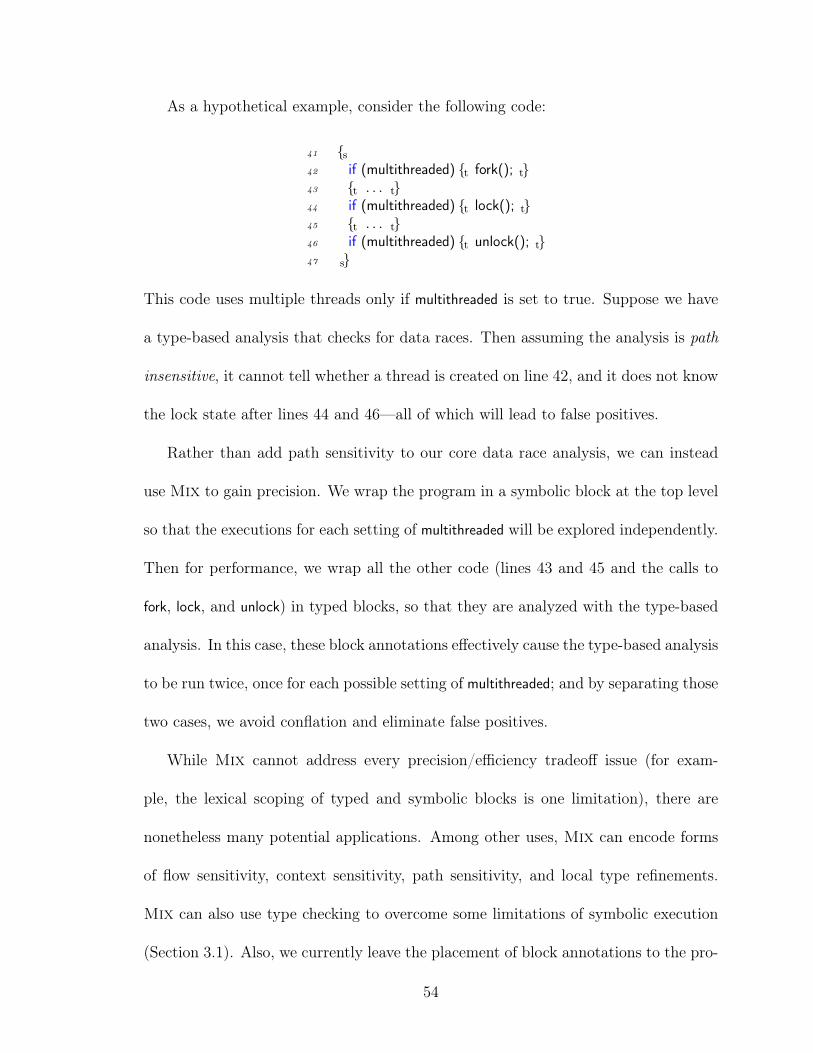
As a hypothetical example, consider the following code:
41 {s42 if (multithreaded) {t fork(); t}43 {t . . . t}44 if (multithreaded) {t lock(); t}45 {t . . . t}46 if (multithreaded) {t unlock(); t}47 s}
This code uses multiple threads only if multithreaded is set to true. Suppose we have
a type-based analysis that checks for data races. Then assuming the analysis is path
insensitive, it cannot tell whether a thread is created on line 42, and it does not know
the lock state after lines 44 and 46—all of which will lead to false positives.
Rather than add path sensitivity to our core data race analysis, we can instead
use Mix to gain precision. We wrap the program in a symbolic block at the top level
so that the executions for each setting of multithreaded will be explored independently.
Then for performance, we wrap all the other code (lines 43 and 45 and the calls to
fork, lock, and unlock) in typed blocks, so that they are analyzed with the type-based
analysis. In this case, these block annotations effectively cause the type-based analysis
to be run twice, once for each possible setting of multithreaded; and by separating those
two cases, we avoid conflation and eliminate false positives.
While Mix cannot address every precision/efficiency tradeoff issue (for exam-
ple, the lexical scoping of typed and symbolic blocks is one limitation), there are
nonetheless many potential applications. Among other uses, Mix can encode forms
of flow sensitivity, context sensitivity, path sensitivity, and local type refinements.
Mix can also use type checking to overcome some limitations of symbolic execution
(Section 3.1). Also, we currently leave the placement of block annotations to the pro-
54

grammer, but we envision that an automated refinement algorithm could heuristically
insert blocks as needed. In this scenario, Mix becomes an intermediate language for
modularly combining off-the-shelf analyzer implementations.
In this chapter, we formalize Mix for a small imperative language, mixing a stan-
dard type checking system with symbolic execution to yield a system to check for
the absence of run-time type errors. Thus, rather than checking for assertion fail-
ures, as a typical symbolic executor might do, our formal symbolic executor reports
any type mismatches it detects. To mix these two systems together, we introduce
two new rules: one rule in the type system that “type checks” blocks {s e s} using
the symbolic executor; and one rule in the symbolic executor that “executes” blocks
{t e t} using the type checker. We prove that the type system, symbolic executor,
and mix of the two systems are sound. The soundness proof of Mix uses the proofs
of type soundness and symbolic execution soundness essentially as-is, which provides
some additional evidence of a clean modularization. Additionally, two features of
our formalism for symbolic execution may be of independent interest: we discuss the
tradeoff between “forking” the symbolic executor and giving more work to the solver;
and we provide a soundness proof, which, surprisingly, we have been unable to find
for previous symbolic execution systems (Section 3.2).
Finally, we describe Mixy, a prototype implementation of Mix for C. Mixy
combines a simple, monomorphic type qualifier inference system (a reimplementation
of Foster et al. (2006)) with a C symbolic executor. There are two key challenges that
arise when mixing type inference rather than checking: we need to perform a fixed-
point computation as we switch between typed and symbolic blocks since data values
55

can pass from one to the other and back; and we need to integrate aliasing information
into our analysis so that pointer manipulations performed within symbolic blocks
correctly influence typed blocks. Additionally, we extend Mixy to support caching
block results as well as recursion between blocks. We use Mixy to look for null
pointer errors in a reasonably-sized benchmark vsftpd; we found several examples
where adding symbolic blocks can eliminate false positives compared to pure type
qualifier inference (Section 3.3).
3.1 Motivating Examples
Before describing Mix formally, we examine some coding idioms for which type infer-
ence and symbolic execution can profitably be mixed. Our examples will be written
in either an ML-like language or C-like language, depending on which one is more
natural for the particular example.
Path, Flow, and Context Sensitivity. In the introduction, we saw one
example in which symbolic execution introduced a small amount of path sensitivity
to type inference. There are several potential variations on this example where we can
locally add a little bit of path sensitivity to increase the precision of type checking.
For example, we can avoid analyzing unreachable code:
48 {t . . . {s if true then {t 5 t} else {t "foo" + 3 t} s} . . . t}
This code runs without errors, but pure type checking would complain about the
potential type error in the false branch. However, with these block annotations added
56

in Mix, the symbolic executor will only invoke the type checker for the true branch
and hence will avoid a false positive.
We can also use symbolic execution to gain some flow sensitivity. For example,
in a dynamically-typed imperative language, programmers may reuse variables as
different types, such as in the following:
49 {t . . . {s var x = 1; {t . . . t}; x = "foo"; s} . . . t}
Here the local variable x is first assigned an integer and is later reused to refer to a
string. With the annotations above, we can successfully statically check such code
using the symbolic executor to distinguish the two different assignments to x, then
type check the code in between.
Similar cases can occur if we try to apply a non-standard type system to existing
code. For example, in our case study (Section 3.3.5), we applied a nullness checker
based on type qualifiers to C. We found some examples like the following code:
50 {t . . . {s x−>obj = NULL; x−>obj = ( . . .)malloc( . . .); s} . . . t}
Here x->obj is initially assigned to NULL, immediately before being assigned a freshly
allocated location. A flow insensitive type qualifier system would think that x->obj
could be NULL after this pair of assignments, even though it cannot be.
Finally, we can also use symbolic execution to gain context sensitivity, though at
the cost of duplicate work. For example, in the following:
51 {s let id x = x in {t . . . {s id 3 s} . . . {s id 3.0 s} . . . t} s}
57
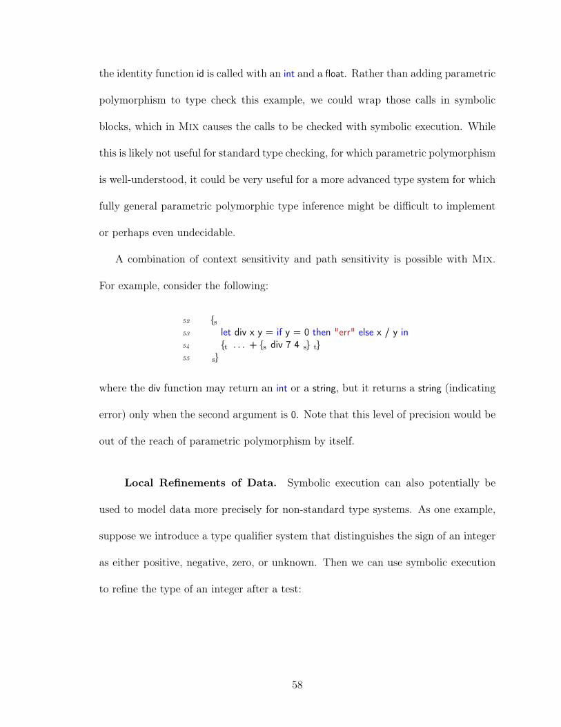
the identity function id is called with an int and a float. Rather than adding parametric
polymorphism to type check this example, we could wrap those calls in symbolic
blocks, which in Mix causes the calls to be checked with symbolic execution. While
this is likely not useful for standard type checking, for which parametric polymorphism
is well-understood, it could be very useful for a more advanced type system for which
fully general parametric polymorphic type inference might be difficult to implement
or perhaps even undecidable.
A combination of context sensitivity and path sensitivity is possible with Mix.
For example, consider the following:
52 {s53 let div x y = if y = 0 then "err" else x / y in54 {t . . . + {s div 7 4 s} t}55 s}
where the div function may return an int or a string, but it returns a string (indicating
error) only when the second argument is 0. Note that this level of precision would be
out of the reach of parametric polymorphism by itself.
Local Refinements of Data. Symbolic execution can also potentially be
used to model data more precisely for non-standard type systems. As one example,
suppose we introduce a type qualifier system that distinguishes the sign of an integer
as either positive, negative, zero, or unknown. Then we can use symbolic execution
to refine the type of an integer after a test:
58

56 {t57 let x : unknown int = . . . in58 {s59 if x > 0 then {t (∗ x : pos int ∗) . . . t}60 else if x = 0 then {t (∗ x : zero int ∗) . . . t}61 else {t (∗ x : neg int ∗) . . . t}62 s}63 t}
Here on entry to the symbolic block, x is an unknown integer, so the symbolic executor
will assign it an initial symbolic value αx ranging over all possible integers. Then
at the conditional branches, the symbolic executor will fork and explore the three
possibilities: αx > 0, αx = 0, and αx < 0. On entering the typed block in each
branch, since the value of x is constrained in the symbolic execution, the type system
will start with the appropriate type for x, either pos, zero, or neg int, respectively.
As another example, suppose we have a type system to prevent data races in C.
Then a common problem that arises is analyzing local initialization of shared data
(Pratikakis et al., 2006). Consider the following code:
64 {t65 {s66 x = (struct foo ∗) malloc(sizeof(struct foo));67 x−>bar = . . . ;68 x−>baz = . . . ;69 x−>qux = . . . ;70 s}71 insert(shared_data_structure, x);72 t}
Here we allocate a new block of memory and then initialize it in several steps before it
becomes shared. A flow-insensitive type-based analysis would report an error because
the writes through x occur without a lock held. On the other hand, if we wrap the
allocation and initialization in a symbolic block, as above, symbolic execution can
59
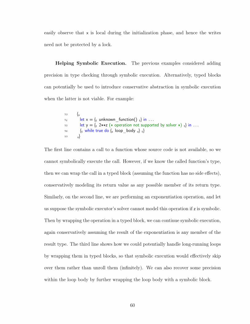
easily observe that x is local during the initialization phase, and hence the writes
need not be protected by a lock.
Helping Symbolic Execution. The previous examples considered adding
precision in type checking through symbolic execution. Alternatively, typed blocks
can potentially be used to introduce conservative abstraction in symbolic execution
when the latter is not viable. For example:
73 {s74 let x = {t unknown_function() t} in . . .75 let y = {t 2∗∗z (∗ operation not supported by solver ∗) t} in . . .76 {t while true do {s loop_body s} t}77 s}
The first line contains a call to a function whose source code is not available, so we
cannot symbolically execute the call. However, if we know the called function’s type,
then we can wrap the call in a typed block (assuming the function has no side effects),
conservatively modeling its return value as any possible member of its return type.
Similarly, on the second line, we are performing an exponentiation operation, and let
us suppose the symbolic executor’s solver cannot model this operation if z is symbolic.
Then by wrapping the operation in a typed block, we can continue symbolic execution,
again conservatively assuming the result of the exponentiation is any member of the
result type. The third line shows how we could potentially handle long-running loops
by wrapping them in typed blocks, so that symbolic execution would effectively skip
over them rather than unroll them (infinitely). We can also recover some precision
within the loop body by further wrapping the loop body with a symbolic block.
60
3.2 The Mix System
In the previous section, we considered a number of idioms that motivate the design of
Mix. Here, we consider a core language, shown in the top portion of Figure 3.1, with
which we study the essence of switching blocks for mixing analyses. Our language in-
cludes variables x; integers n; booleans true and false; selected arithmetic and boolean
operations +, =, ¬, and ∧; conditionals with if; let bindings; and ML-style updatable
references with ref (construction), ! (dereference), and := (assignment). We also
include two new block forms, typed blocks {t e t} and symbolic blocks {s e s}, which
indicate e should be analyzed with type checking or symbolic execution, respectively.
We leave unspecified whether the outermost scope of a program is treated as a typed
block or a symbolic block; Mix can handle either case.
3.2.1 Type Checking and Symbolic Execution
Type checking for our source language is entirely standard, and so we omit those
rules here. Our type checking system proves judgments of the form Γ ` e : τ , where
Γ is the type environment and τ is e’s type. Grammars for Γ and τ are given in the
bottom portion of Figure 3.1.
The remainder of this section describes a generic symbolic executor. While the
concept of symbolic execution is widely known, there does not appear to be a clear
consensus of its definition. Thus, we make explicit our definition of symbolic execution
here through a formalization similar to an operational semantics. Such a formalization
61
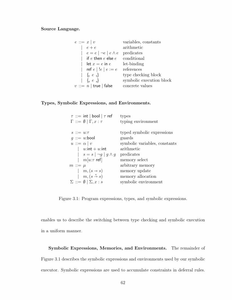
Source Language.
e ::= x | v variables, constants| e+ e arithmetic| e = e | ¬e | e ∧ e predicates| if e then e else e conditional| let x = e in e let-binding| ref e | !e | e := e references| {t e t} type checking block| {s e s} symbolic execution block
v ::= n | true | false concrete values
Types, Symbolic Expressions, and Environments.
τ ::= int | bool | τ ref typesΓ ::= ∅ | Γ, x : τ typing environment
s ::= u:τ typed symbolic expressionsg ::= u:bool guardsu ::= α | v symbolic variables, constants| u:int + u:int arithmetic| s = s | ¬g | g ∧ g predicates| m[u:τ ref] memory select
m ::= µ arbitrary memory| m, (s � s) memory update| m, (s
a� s) memory allocationΣ ::= ∅ | Σ, x : s symbolic environment
Figure 3.1: Program expressions, types, and symbolic expressions.
enables us to describe the switching between type checking and symbolic execution
in a uniform manner.
Symbolic Expressions, Memories, and Environments. The remainder of
Figure 3.1 describes the symbolic expressions and environments used by our symbolic
executor. Symbolic expressions are used to accumulate constraints in deferral rules.
62

For example, the symbolic expression (α:int+3:int):int represents a value that is three
more than the unknown integer α.
Because we are concerned with checking for run-time type errors, in our system
symbolic expressions s have the form u:τ , where u is a bare symbolic expression and
τ is its type. With these type annotations, we can immediately determine the type of
a symbolic expression, just like in a concrete evaluator with values. As a shorthand,
we use g to represent conditional guards, which are just symbolic expressions with
type bool. Bare symbolic expressions u may be symbolic variables α (e.g., α:int is a
symbolic integer, and α:bool is a symbolic boolean); known values v; or operations
+, =, ¬, ∧ applied to symbolic expressions of the appropriate type. Notice that our
syntax forbids the formation of certain ill-typed symbolic expression (e.g., α1:int +
α2:bool is not allowed).
Symbolic expressions also include symbolic memory accesses m[u:τ ref], which
represents an access through pointer u in symbolic memory m. A symbolic memory
may be µ, representing an arbitrary but well-typed memory; m, (s � s′), a memory
that is the same as m except location s is updated to contain s′; or m, (s a� s′),
which is the same as m except newly allocated location s points to s′. These are
essentially McCarthy-style sel and upd expressions that allow the symbolic executor to
accumulate a log of writes and allocations while deferring alias analysis. An allocation
always creates a new location that is distinct from the locations in the base unknown
memory, so we distinguish them from arbitrary writes.
Finally, symbolic environments Σ map local variables x to (typed) symbolic ex-
pressions s.
63
Symbolic Execution for Pure Expressions. Figure 3.2 describes our symbolic
executor on pure expressions using what are essentially big-step operational semantics
rules. These rules prove judgments of the form
Σ ` 〈S ; e〉 ⇓ 〈S ′ ; s〉
meaning with local variables bound in Σ, starting in state S, expression e evaluates
to symbolic expression s and updates the state to S ′. In our symbolic execution
judgment, a state S is a tuple 〈g ; m〉, where g is a path condition constraining the
current state and m is the current symbolic memory. The path condition begins as
true, and whenever the symbolic executor makes a choice at a conditional, we extend
the path condition to remember that choice (more on this below). We write X(S) for
the X component of S, with X ∈ {g,m}, and similarly we write S[X 7→ Y ] for the
state that is the same as S, except its X component is now Y .
Most of the rules in Figure 3.2 are straightforward and intend to summarize typical
symbolic executors. Rule SEVar evaluates a local variable by looking it up in the
current environment. Notice that, as with standard operational semantics, there is
no reduction possible if the variable is not in the current environment. Rule SEVal
reduces values to themselves, using the auxiliary function typeof(v) that examines the
value form to return its type (i.e., typeof(n) = int and typeof(true) = typeof(false) =
bool).
Rules SEPlus, SEEq, SENot, and SEAnd execute the subexpressions and then
form a new symbolic expression with +, =, ¬, or ∧, respectively. Notice that these
rules place requirements on the subexpressions—for example, SEPlus requires that
64

Symbolic Execution. Σ ` 〈S ; e〉 ⇓ 〈S ′ ; s〉 S = 〈g ;m〉
SEVar
Σ, x : s ` 〈S ; x〉 ⇓ 〈S ; s〉
SEVal
Σ ` 〈S ; v〉 ⇓ 〈S ; (v: typeof(v))〉
SEPlusΣ ` 〈S ; e1〉 ⇓ 〈S1 ; u1:int〉 Σ ` 〈S1 ; e2〉 ⇓ 〈S2 ; u2:int〉
Σ ` 〈S ; e1 + e2〉 ⇓ 〈S2 ; (u1:int + u2:int):int〉
SEEqΣ ` 〈S ; e1〉 ⇓ 〈S1 ; u1:τ〉 Σ ` 〈S1 ; e2〉 ⇓ 〈S2 ; u2:τ〉
Σ ` 〈S ; e1 = e2〉 ⇓ 〈S2 ; (u1:τ = u2:τ):bool〉
SENotΣ ` 〈S ; e1〉 ⇓ 〈S1 ; g1〉
Σ ` 〈S ; ¬e1〉 ⇓ 〈S1 ; ¬g1:bool〉
SEAndΣ ` 〈S ; e1〉 ⇓ 〈S1 ; g1〉 Σ ` 〈S1 ; e2〉 ⇓ 〈S2 ; g2〉
Σ ` 〈S ; e1 ∧ e2〉 ⇓ 〈S2 ; (g1 ∧ g2):bool〉
SELetΣ ` 〈S ; e1〉 ⇓ 〈S1 ; s1〉 Σ, x : s1 ` 〈S1 ; e2〉 ⇓ 〈S2 ; s2〉
Σ ` 〈S ; let x = e1 in e2〉 ⇓ 〈S2 ; s2〉
SEIf-TrueΣ ` 〈S ; e1〉 ⇓ 〈S1 ; g1〉 Σ ` 〈S1[g 7→ g(S1) ∧ g1] ; e2〉 ⇓ 〈S2 ; s2〉
Σ ` 〈S ; if e1 then e2 else e3〉 ⇓ 〈S2 ; s2〉
SEIf-FalseΣ ` 〈S ; e1〉 ⇓ 〈S1 ; g1〉 Σ ` 〈S[g 7→ g(S1) ∧ ¬g1] ; e3〉 ⇓ 〈S3 ; s3〉
Σ ` 〈S ; if e1 then e2 else e3〉 ⇓ 〈S3 ; s3〉
Figure 3.2: Symbolic execution for pure expressions.
65

the subexpressions reduce to symbolic integers, and SENot requires that the subex-
pression reduces to a guard (a symbolic boolean). If the subexpression does not
reduce to an expression of the right type, then symbolic execution fails. Thus, these
rules form a symbolic execution engine that does very precise dynamic type checking.
Rule SELet symbolically executes e1 and then binds e1 to x for execution of e2.
The last two rules, SEIf-True and SEIf-False, model a pure, non-deterministic
version of the kind of symbolic execution popularized by DART (Godefroid et al.,
2005), CUTE (Sen et al., 2005), EXE (Cadar et al., 2006), and KLEE (Cadar et al.,
2008). When we reach a conditional, we conceptually fork execution, extending the
path condition with g1 or ¬g1 to indicate the branch taken. EXE and KLEE would
both invoke an SMT solver at this point to decide whether one or both branches
are feasible, and then try all feasible paths. DART and CUTE, in contrast, would
continue down one path as guided by an underlying concrete run (so-called “concolic
execution”), but then would ask an SMT solver later whether the path not taken was
feasible and, if so, come back and take it eventually. All of these implementation
choices can be viewed as optimizations to prune infeasible paths or hints to focus
the exploration. Since we are not concerned with performance in our formalism, we
simply extend the path condition and continue—eventually, when symbolic execution
completes, we will check the path condition and discard the path if it is infeasible.
To get sound symbolic execution, we will compute a set of symbolic executions and
require that all feasible paths are explored (see Section 3.2.2).
Sometimes, the symbolic executor may want to throw away information (e.g.,
replace a symbolic expression for a complicated memory read with a fresh symbolic
66

variable). Such a rule is straightforward to add, but as discussed in Section 3.2.2, a
nested typed block {t e t} serves a similar purpose.
Deferral Versus Execution. Consider again the rules for symbolic execution
on pure expressions in Figure 3.2. Excluding the trivial SEVal rule, the first set
of rules (SEPlus, SEEq, SENot, and SEAnd) versus the second set (SELet,
SEVar, SEIf-True, SEIf-False) seem qualitatively different. The first set simply
get symbolic expressions for their subexpressions and form a new symbolic expression
of the corresponding operator, essentially deferring any reasoning about the operation
(e.g., to an SMT solver). In contrast, the second set does not accumulate any such
symbolic expression but rather chooses a possible concrete execution to follow. For
example, we can view SEIf-True as choosing to assume that g1 is concretely true
and proceeding to symbolically execute e2. This assumption is recorded in the path
condition. (The SELet and SEVar rules are degenerate execution rules where no
assumptions need to be made because there is only one possible concrete execution
for each.) Alternatively, we see that there are symbolic expression forms for +, =, ¬,
and ∧ but not for let, program variables, and if.
Although it is not commonly presented as such, the decision of deferral versus
execution is a design choice. For example, let us include an if-then-else symbolic ex-
pression g?s1:s2 (using a C-style conditional syntax) that evaluates to s1 if g evaluates
to true and s2 otherwise. Then, we could defer to the evaluation of the conditional
67

to the solver with the following rule:
SEIf-DeferΣ ` 〈S ; e1〉 ⇓ 〈S1 ; g1〉 Σ ` 〈S[g 7→ g(S1) ∧ g1] ; e2〉 ⇓ 〈S2 ; u2:τ〉
Σ ` 〈S[g 7→ g(S1) ∧ ¬g1] ; e3〉 ⇓ 〈S3 ; u3:τ〉S ′ = 〈(g1?g(S2):g(S3)) ; (g1?m(S2):m(S3))〉
Σ ` 〈S ; (if e1 then e2 else e3)〉 ⇓ 〈S ′ ; (g1?(u2:τ):(u3:τ)):τ〉
Here notice we also have to extend the ·? · :· relation to operate over memory as
well. With this rule, we need not “fork” symbolic execution at all. However, note
that even with conditional symbolic expressions and condition symbolic memory, this
rule is more conservative than the SEIf-True and SEIf-False execution rules, as
it requires both branches to have the same type.
Conversely, other rules may also be made non-deterministic in manner similar
to SEIf-*. For example, SEVar may instead return an arbitrary value v and add
Σ(x) = v to the path condition, a style that resembles hybrid concolic testing (Ma-
jumdar and Sen, 2007). A special case of execution rules are ones that apply only
when we have concrete values during symbolic execution and thus do not need to
“fork.” For example, we could have a SEPlus-Conc that applies to two concrete
values n1, n2 and returns the sum. This approach is reminiscent of partial evaluation.
These choices trade off the amount of work done between the symbolic executor
and the underlying SMT solver. For example, SEIf-Defer introduces many disjunc-
tions into symbolic expressions, which then may be hard to solve efficiently. To match
current practice, we stick with the forking variant for conditionals, but we believe our
system would also be sound with SEIf-Defer.
68
Symbolic References. Figure 3.3 continues our symbolic executor definition
with rules for updatable references. We use deferral rules for all aspects of references
in our formalization. Rule SERef evaluates e1 and extends m(S1) with an allocation
for fresh symbolic pointer α. Similarly, rule SEAssign extends S2 to record that
s1 now points to s2. Observe that allocations and writes are simply logged during
symbolic execution for later inspection. Also, notice that we allow any value to be
written to s1, even if it does not match the type annotation on s1. In contrast,
standard type systems require that any writes to memory must preserve types since
the type system does not track enough information about pointers to be sound if that
property is violated. Symbolic execution tracks every possible program execution
precisely, and so it can allow arbitrary memory writes.
In SEDeref, we evaluate e1 to a pointer u1:τ ref and then produce the symbolic
expression m(S1)[u1:τ ref]:τ to represent the contents of that location. However, here
we are faced with a challenge: we are not actually looking up the contents of memory;
rather, we are simply forming a symbolic expression to represent the contents. How,
then, do we determine the type of the pointed-to value? We need the type so that
we can halt symbolic execution later if that value is used in a type-incorrect manner.
That is, we do not want to defer the discovery of a potential type error.
Our solution is to use the type annotation on the pointer to get the type of the
contents—but above we just explained that SEAssign allows writes to violate those
type annotations. There are many potential ways to solve this problem. We could in-
voke an SMT solver to compute the actual set of addresses that could be dereferenced
and fork execution for each one. Or we could proceed as our implementation and use
69

Symbolic Execution for References. Σ ` 〈S ; e〉 ⇓ 〈S ′ ; s〉
SERefΣ ` 〈S ; e1〉 ⇓ 〈S1 ; u1:τ〉 α /∈ Σ, S, S1, u1
S ′ = S1[m 7→ (m(S1), (α:τ refa� u1:τ))]
Σ ` 〈S1 ; ref e1〉 ⇓ 〈S ′ ; α:τ ref〉
SEAssignΣ ` 〈S ; e1〉 ⇓ 〈S1 ; s1〉 Σ ` 〈S1 ; e2〉 ⇓ 〈S2 ; s2〉
Σ ` 〈S ; e1 := e2〉 ⇓ 〈S2[m 7→ (m(S2), (s1 � s2))] ; s2〉
SEDerefΣ ` 〈S ; e1〉 ⇓ 〈S1 ; u1:τ ref〉 ` m(S1) ok
Σ ` 〈S ; !e1〉 ⇓ 〈S1 ;m(S1)[u1:τ ref]:τ〉
Memory Type Consistency. ` m ok U ` m ok
Empty-OK
` µ ok ∅
Alloc-OK` m ok U
` m, (α:τ refa� u2:τ) ok U
Overwrite-OK` m ok U U ′ = U\ {s1 � s2 | s1 ≡ u1:τ ref ∧ s1 � s2 ∈ U}
` m, (u1:τ ref � u2:τ) ok U ′
Arbitrary-NotOK` m ok U
` m, (s1 � s2) ok (U ∪ {s1 � s2})
M-OK` m ok ∅` m ok
Figure 3.3: Symbolic execution for updatable references.
an external alias analysis to conservatively model all possible locations that could
be read to check that the values at all locations have the same type (Section 3.3).
However, to keep the formal system simple, we choose a very coarse solution: we
require that all pointers in memory are well-typed with the check ` m(S1) ok.
70
This judgment is defined in the bottom portion of Figure 3.3 in terms of the aux-
iliary judgment ` m ok U , which means memory m is consistently typed (pointers
point to values of the right type), except for mappings in U . There are four cases
for this judgment. SEEmpty-OK says that arbitrary well-typed memory µ is con-
sistently typed. Similarly, Alloc-OK says that if m is consistently typed except
for potentially inconsistent writes in U , then adding an allocation preserves consis-
tent typing up to U . Rule SEOverwrite-OK says that if ` m ok U and we extend
m with a well-typed write to u1, then any previous, inconsistent writes to locations
s1 ≡ u1:τ ref can be ignored. Here by ≡ we mean syntactic equivalence, but in
practice we could query a solver to validate such an equality given the current path
condition. Rule SEArbitrary-NotOK says that any write can be added to U and
viewed as potentially inconsistent. Finally, SEM-OK says that ` m ok if m has no
inconsistent writes that persist. Together, these rules ensure that the type assigned
to the result of a dereference is sound. We can also see how the SEDeref may be
made more precise by only requiring consistency up to a set of writes U and querying
a solver to show that u1:τ ref are disequal to all the address expressions in U .
3.2.2 Mixing
In the previous section, we considered type checking and symbolic execution sep-
arately, ignoring the blocks that indicate a switch in analysis. Figure 3.4 shows the
two mix rules that capture switching between analyses.
Rule SETSymBlock describes how to type check a symbolic block {s e s}, that
is, how to apply symbolic execution to derive a type of a subexpression for a type
71

Block Typing. Γ ` e : τ
TSymBlockΣ(x) = αx:Γ(x)
(for all x ∈ dom(Γ)) Σ ` 〈S ; e〉 ⇓ 〈Si ; ui:τ〉 S = 〈true ; µ〉 µ /∈ Σ` m(Si) ok exhaustive(g(S1), . . . , g(Sn)) (i ∈ 1..n)
Γ ` {s e s} : τ
exhaustive(g1, . . . , gn)⇐⇒ (g1 ∨ . . . ∨ gn is a tautology)
Block Symbolic Execution. Σ ` 〈S ; e〉 ⇓ 〈S ′ ; s〉
SETypBlock` Σ : Γ ` m(S) ok Γ ` e : τ µ′, α /∈ Σ, S
Σ ` 〈S ; {t e t}〉 ⇓ 〈S[m 7→ µ′] ; α:τ〉
Symbolic and Typing Environment Conformance. ` Σ : Γ
dom(Σ) = dom(Γ) Σ(x) = u:Γ(x) (for all x ∈ dom(Γ))` Σ : Γ
Figure 3.4: Mixing type checking and symbolic execution.
checker. First, we construct an environment Σ that maps each variable x in Γ to
a fresh symbolic variable αx, whose type is extracted from Γ. Then we run the
symbolic execution under Σ, starting in a state with true for the path condition and
a fresh symbolic variable µ to stand for the current memory. Recall that, because
of SEIf-True and SEIf-False, symbolic execution is actually non-deterministic—
it conceptually can branch at conditionals. If we want to soundly model the entire
possible behavior of e, we need to execute all paths. Thus, we run the symbolic
executor n times, yielding final states 〈Si ; ui:τ〉 for i ∈ 1..n, and we require that the
disjunction of the guards from all executions form a tautology. This constraint ensures
72
that we exhaustively explore every possible path (see Section 3.2.3 about soundness).
And if all those paths executed successfully without type errors and returned a value
of the same type τ , then that is the type of expression e. We also check that all paths
leave memory in a consistent state.
Symbolic execution has typically been used as an unsound analysis where there
is no exhaustiveness check like exhaustive(. . .) in the SETSymBlock. We can also
model such unsound analysis by weakening exhaustive(. . .) to a “good enough check.”
The other rule, SESETypBlock, describes how to symbolically execute a typed
block {t e t}, that is, how to apply the type checker in the middle of a symbolic
execution. We begin by deriving a type environment Γ that maps local variables
to the types of the symbols they are mapped to in Σ. This mapping is described
precisely by the judgment ` Σ : Γ, which is straightforward. We also require that the
current symbolic memory state be consistent, since the typed block relies purely on
type information (rather than tracking pointer values as symbolic execution does).
Then we type check e in Γ, yielding a type τ . The typed block itself symbolically
evaluates to a fresh symbolic variable α of type τ . Since the typed block may have
written to memory, we conservatively set the memory of the output state to a fresh
µ′, indicating we know nothing about the memory state at that point except that it
is consistent.
Note that in our formalism, we do not have typed blocks within typed blocks,
or symbolic blocks within symbolic blocks, though these would be trivial to add (by
passing-through).
73

Why Mix? The mix rules are essentially as precise as possible given the
strengths and limitations of each analysis. The nested analysis starts with the maxi-
mum amount of information that can be extracted from the other program analysis—
for symbolic blocks, the only available information for symbolic execution is types,
whereas for typed blocks, the type checker only cares about types of variables and
thus abstracts away the symbolic expressions. After the nested analysis is complete,
the result is similarly passed back to the enclosing analysis as precisely as possible.
We deliberately chose two analyses at opposite ends of the precision spectrum:
type checking is cheap, flow insensitive with a rather coarse abstraction, while sym-
bolic execution is expensive, flow and path sensitive (and context sensitive if we add
functions) with a minimal amount of abstraction. They also work in such a different
manner that it does not seem particularly natural to combine them in tighter ways
(e.g., as a reduced product of abstract interpreters (Cousot and Cousot, 1979)). We
think it is surprising just how much additional precision we can obtain and the kinds
of idioms we can analyze from such a simple mixing of an entirely standard type
system and a typical symbolic executor as-is (as we see in Section 3.1). We note
that a type system capturing all of the examples in Section 3.1 would likely be quite
advanced (involving, for example, dependent types).
However, as can be seen in Figure 3.4, the conversion between these two analyses
may be extremely lossy. For example, in SETypBlock, the memory after returning
from the type checker must be a fresh arbitrary memory µ′ because e may make
any number of writes not captured by the type system and thus not seen by the
symbolic executor. We can also imagine mixing any number of analyses in arbitrary
74

combination, yielding different precision/efficiency tradeoffs. For example, if we were
to use a type and effect system rather than just a type system, we could avoid
introducing a completely fresh memory µ′ in SESETypBlock—instead, we could
find the effect of e and limit applying this “havoc” operation only to locations that
could have been changed.
3.2.3 Soundness
In this section, we sketch the soundness of Mix, which is described in full detail
in Appendix A. The key feature of our proof is that aside from the mix rule cases,
it reuses the standalone type soundness and symbolic execution soundness proofs
essentially as-is.
We show soundness with respect to a standard big-step operational semantics
for our simple language of expressions. Our semantics is given by a judgment E `
〈M ; e〉 → r. This says that in a concrete environment E, an initial concrete memory
M and an expression e evaluate to a result r. A concrete environment maps variables
to values, while a concrete memory maps locations to values. The evaluation result
r is either a concrete memory-value pair 〈M ′; v〉 or a distinguished error token.
To prove mix soundness, we consider simultaneously type and symbolic execution
soundness. While type soundness is standard, we discuss it briefly, as it is a part of
mix soundness, and provides intuition for symbolic execution soundness.
For type soundness, we introduce a memory type environment Λ that maps loca-
tions to types, and we update the typing judgment to carry this additional environ-
ment, as Γ `Λ e : τ where Λ is constant in all rules. In many proofs, Λ is included in
75
Γ rather than being called out separately, but for mix soundness separating locations
from variables makes the proof easier. To show type soundness, we need a relation
between the concrete environment and memory 〈E;M〉 and the type environment and
memory typing 〈Γ; Λ〉. We write this relation as 〈E;M〉 ∼ 〈Γ; Λ〉, which informally
says two things: (1) the type environment Γ abstracts the concrete environment E,
that is, the concrete value v mapped by each variable x in E has type Γ(x), and (2)
the memory typing Λ abstracts the concrete memory M , that is, the concrete value
v at each location l in M has type Λ(l). We also talk about the second component
in isolation, in which case we write M ∼ Λ to mean memory typing Λ abstracts the
concrete memory M .
Type soundness is the first part of mix soundness (Statement 1 in Theorem 1).
Let us consider the pieces. Suppose we have a concrete evaluation E ` 〈M ; e〉 → r.
We further suppose that e has type τ in typing environments that are sound with
respect to the concrete state (i.e., 〈E;M〉 ∼ 〈Γ; Λ〉). Then, the result r must be
a memory-value pair 〈M ′; v〉 where the resulting concrete memory is abstracted by
Λ′, an extension of Λ, and the resulting value v has the same type τ in Γ with
the extended memory typing Λ′. Notice this captures the notions that well-typed
expressions cannot evaluate to error and that evaluation preserves typing.
For symbolic execution soundness, we need to ensure that a symbolic execution
faithfully models actual concrete executions. Let V be a valuation, which is a finite
mapping from symbolic values α to concrete values v or concrete memories M . We
write JsKV , JmKV , and JΣKV for the natural extension of V to operate on arbitrary
symbolic expressions, memories, and the symbolic environment. Symbolic execution
76
begins with symbolic values α for unknown inputs and accumulates a symbolic ex-
pression s that represents the result of the program. Then at a high-level, if symbolic
execution is sound, then a concrete run that begins with JαKV for inputs should
produce the expression JsKV .
To formalize this notion, we need a soundness relation between the concrete eval-
uation state and the symbolic execution state, just as in type soundness. The form
of our soundness relations for symbolic execution states is as follows:
〈E;M〉 ∼Λ0·V ·Λ 〈Σ;m〉
This relation captures two key properties. First, applying the valuation V to the
symbolic state should yield the concrete state (i.e., JΣKV = E and JmKV = M).
Second, the types of symbolic expressions in Σ and m must be correctly related.
Recall that an additional property of our typed symbolic execution is that it tracks the
type of symbolic expressions and halts upon encountering ill-typed expressions. The
typing of symbolic reference expressions must be with respect to some memory typing.
This memory typing is given by Λ0 and Λ. For technical reasons, we need to separate
the locations in the arbitrary memory on entry Λ0 from the locations that come from
allocations during symbolic execution Λ; to get typing for the entire memory, we write
Λ0 ∗ Λ to mean the union of submemory typings Λ0 and Λ with disjoint domains.
Analogously, we also have a symbolic soundness relation that applies to memory-value
pairs: 〈M ; v〉 ∼Λ0·V ·Λ 〈m; s〉.
As alluded to above, we first consider a notion of symbolic execution soundness
with respect to a concrete execution. This notion is what is stated in the second part
77

of mix soundness (Theorem 1). Analogous to type soundness, it says that suppose
we have a concrete evaluation E ` 〈M ; e〉 → r and a symbolic execution Σ ` 〈S ;
e〉 ⇓ 〈S ′ ; s〉 such that the symbolic state is an abstraction of the concrete state
(i.e., 〈E;M〉 ∼Λ0·V ·Λ 〈Σ;m(S)〉). There is one more premise, Jg(S ′)KV , which says
that the path condition accumulated during symbolic execution holds under this
valuation. This constrains the concrete and symbolic executions to follow the same
path. With these premises, symbolic execution soundness says that the result of
symbolic execution, that is the memory-symbolic expression pair 〈m(S ′); s〉, is an
abstraction of the concrete evaluation result, which must be a memory-value pair
〈M ′; v〉.
Theorem 1 (Mix Soundness)
1. If
E ` 〈M ; e〉 → r and
Γ `Λ e : τ such that
〈E;M〉 ∼ 〈Γ; Λ〉 ,
then ∅ `Λ′ v : τ and M ′ ∼ Λ′ for some M ′, v, Λ′ such that r = 〈M ′; v〉 and
Λ′ ⊇ Λ.
2. IfE ` 〈M ; e〉 → r and
Σ ` 〈S ; e〉 ⇓ 〈S ′ ; s〉 such that
〈E;M〉 ∼Λ0·V ·Λ 〈Σ;m(S)〉 and Jg(S ′)KV ,
then r ∼Λ′0·V ′·Λ′ 〈m(S ′); s〉 for some V ′ ⊇ V and some Λ′0,Λ
′ such that Λ′0 ∗
Λ′ ⊇ Λ0 ∗ Λ.
78
Proof
By simultaneous induction on the derivations of E ` 〈M ; e〉 → r. The proof is given
in Appendix A.
This statement of symbolic execution soundness (Statement 2 in Theorem 1) is
what we need to show Mix sound, but at first glance, it seems suspect because it does
not say anything about symbolic execution being exhaustive. However, if we look at
type checking a symbolic block (i.e., rule TSymBlock), exhaustiveness is ensured
through the exhaustive(. . .) constraint.
In particular, we can state exhaustive symbolic execution as a corollary, and the
case for TSymBlock proceeds in the same manner as this corollary.
Corollary 1.1 (Exhaustive Symbolic Execution)
Suppose E ` 〈M ; e〉 → 〈M ′; v〉 and we have n > 0 symbolic executions
Σ ` 〈〈true;m〉 ; e〉 ⇓ 〈Si ; si〉 such that
exhaustive(g(S1), . . . , g(Sn)) and
〈E;M〉 ∼Λ0·V ·Λ 〈Σ;m〉 ,
then 〈M ′; v〉 ∼Λ′0·V ′·Λ′ 〈m(Si); si〉 for some i ∈ 1..n, V ′ ⊇ V , and some Λ′0,Λ
′ such
that Λ′0 ∗ Λ′ ⊇ Λ0 ∗ Λ.
Here we say that if we have n > 0 symbolic executions that each start with a path
condition of true and where their resulting path conditions are exhaustive (i.e., g(S1)∨
. . . ∨ g(Sn) is a tautology meaning it holds under any valuation V ), then one of
79

those symbolic executions must match the concrete execution. Observe that in this
statement, there is no premise on the resulting path condition, but rather that we
start with a initial path condition of true.
3.3 Mixy: A Prototype of Mix for C
We have developed Mixy, a prototype tool for C that uses Mix to detect null pointer
errors. Mixy mixes a (flow-insensitive) type qualifier inference system with a sym-
bolic executor. Mixy is built on top of the CIL front-end for C (Necula et al.,
2002), and our type qualifier inference system, CilQual, is essentially a simplified CIL
reimplementation of the type qualifier inference algorithm described by Foster et al.
(2006). Our symbolic executor, Otter (Reisner et al., 2010), uses STP (Ganesh and
Dill, 2007) as its SMT solver and works in a manner similar to KLEE (Cadar et al.,
2008).
Type Qualifiers and Null Pointer Errors. For this application, we introduce
two qualifier annotations for pointers: nonnull indicates that a pointer must not be
null, and null indicates that a pointer may be null. Our inference system automatically
annotates uses of the NULLmacro with the null qualifier annotation. The type qualifier
inference system generates constraints among known qualifiers and unknown qualifier
variables, solves those constraints, and then reports a warning if null values may flow
to nonnull positions. Thus, our type qualifier inference system ensures pointers that
may be null cannot be used where non-null pointers are required.
For example, consider the following C code:
80
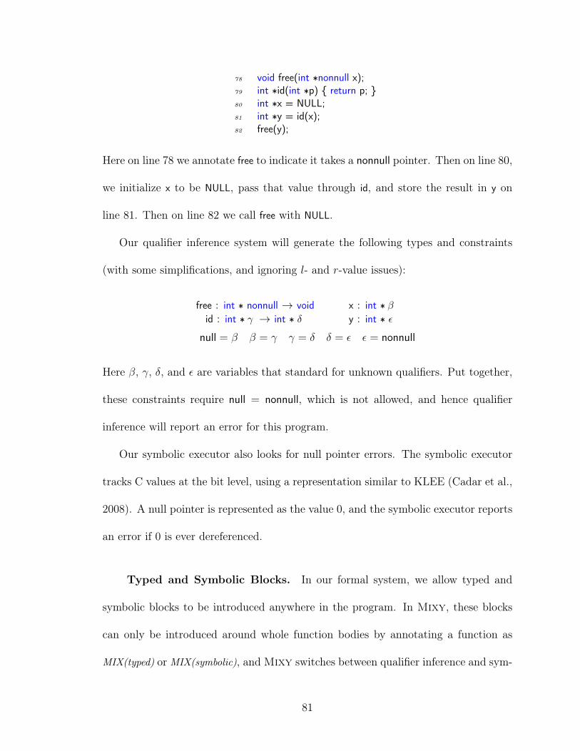
78 void free(int ∗nonnull x);79 int ∗id(int ∗p) { return p; }80 int ∗x = NULL;81 int ∗y = id(x);82 free(y);
Here on line 78 we annotate free to indicate it takes a nonnull pointer. Then on line 80,
we initialize x to be NULL, pass that value through id, and store the result in y on
line 81. Then on line 82 we call free with NULL.
Our qualifier inference system will generate the following types and constraints
(with some simplifications, and ignoring l- and r-value issues):
free : int ∗ nonnull → void x : int ∗ βid : int ∗ γ → int ∗ δ y : int ∗ ε
null = β β = γ γ = δ δ = ε ε = nonnull
Here β, γ, δ, and ε are variables that standard for unknown qualifiers. Put together,
these constraints require null = nonnull, which is not allowed, and hence qualifier
inference will report an error for this program.
Our symbolic executor also looks for null pointer errors. The symbolic executor
tracks C values at the bit level, using a representation similar to KLEE (Cadar et al.,
2008). A null pointer is represented as the value 0, and the symbolic executor reports
an error if 0 is ever dereferenced.
Typed and Symbolic Blocks. In our formal system, we allow typed and
symbolic blocks to be introduced anywhere in the program. In Mixy, these blocks
can only be introduced around whole function bodies by annotating a function as
MIX(typed) or MIX(symbolic), and Mixy switches between qualifier inference and sym-
81
bolic execution at function calls. We can simulate blocks within functions by manually
extracting the relevant code into a fresh function.
Skipping some details for the moment, this switching process works as follows.
When Mixy is invoked, the programmer specifies (as a command-line option) whether
to begin in a typed block or a symbolic block. In either case, we first initialize global
variables as appropriate for the analysis, and then analyze the program starting with
main. In symbolic execution mode, we begin simulating the program at the entry
function, and at calls to functions that are either unmarked or are marked as symbolic,
we continue symbolic execution into the function body. At calls to functions marked
with MIX(typed), we switch to type inference starting with that function.
In type inference mode, we begin analysis at the entry function f, applying qualifier
inference to f and all functions reachable from f in the call graph, up to the frontier
of any functions that are marked with MIX(symbolic). We use CIL’s built-in pointer
analysis to find the targets of calls through function pointers. Finally, we switch to
symbolic execution for each function marked MIX(symbolic) that was discovered at
the frontier.
In this section, we describe implementation details that are not captured by our
formal system from Section 3.2:
• The formal system Mix is based on a type checking system where all types are
given. Since type qualifier inference involves variables, we need to handle vari-
ables that are not yet constrained to concrete type qualifiers when transitioning
to a symbolic block (Section 3.3.1).
82

• We need to translate information about aliasing between blocks (Section 3.3.2).
• Since the same block or function may be called from multiple contexts, we need
to avoid repeating analysis of the same function (Section 3.3.3).
• Since functions can contain blocks and be recursive, we need to handle recursion
between typed and symbolic blocks (Section 3.3.4).
Finally, we present our initial experience with Mixy (Section 3.3.5), and we discuss
some limitations and future work (Section 3.3.6).
3.3.1 Translating Null/Non-null and Type Variables
At transitions between typed and symbolic blocks, we need to translate null and
nonnull annotations back and forth.
From Types to Symbolic Values. Suppose local variable x has type int ∗ nonnull.
Then in the symbolic executor, we initialize x to point to a fresh memory cell. If x
has type int ∗ null, then we initialize x to be (α:bool)?loc:0, where α is a fresh boolean
that may be either true or false, loc is a newly initialized pointer (described in Sec-
tion 3.3.2), and 0 represents null. Hence this expression means x may be either null
or non-null, and the symbolic executor will try both possibilities.
A more interesting case occurs if a variable x has a type with a qualifier variable
(e.g., int ∗ β ). In this case, we first try to solve the current set of constraints to
see whether β has a solution as either null or nonnull, and if it does, we perform
83

the translation given above. Otherwise, if β could be either, we first optimistically
assume it is nonnull.
We can safely use this assumption when returning from a typed block to a symbolic
block since such a qualifier variable can only be introduced when variables are aliased
(e.g., via pointer assignment), a case that is separately taken into account by the
Mixy memory model (Section 3.3.2).
However, if we use this assumption when entering a symbolic block from a typed
block, we may later discover our assumption was too optimistic. For example, consider
the following code:
83 {t int ∗x; {s x = NULL; s}; {s free(x); s} t}
In the type system, x has type int ∗ β , where initially β is unconstrained. Suppose
that we analyze the symbolic block on the right before the one on the left. This
scenario could happen because the analysis of the enclosing typed block does not
model control-flow order (i.e., is flow insensitive). Then initially, we would think the
call to free was safe because we optimistically treat unconstrained β as nonnull—but
this is clearly not accurate here.
The solution is, as expected, to repeat our analyses until we reach a fixed point. In
this case, after we analyze the left symbolic block, we will discover a new constraint on
x, and hence when we iterate and reanalyze the right symbolic block, we will discover
the error. We are computing a least fixed point because we start with optimistic
assumptions—nothing is null—and then monotonically discover more expressions may
be null.
84

From Symbolic Values to Types. We use the SMT solver to discover the
possible final values of variables and translate those to the appropriate types. Given
a variable x that is mapped to symbolic expression s, we ask whether g ∧ (s = 0) is
satisfiable where g is the path condition. If the condition is satisfiable, we constrain x
to be null in the type system. There are no nonnull constraints to be added since they
correspond to places in code where pointers are dereferenced, which is not reflected
in symbolic values.
Thus, null pointers from symbolic blocks will lead to errors in typed blocks if they
flow to a nonnull position; whereas null pointers from typed blocks will lead to errors
in symbolic blocks if they are dereferenced symbolically.
3.3.2 Aliasing and Mixy’s Memory Model
The formal system Mix defers all reasoning about aliasing to as late of a time as
possible. As alluded to in Section 3.2, this choice may be difficult to implement in
practice given limitations in the constraint solver. Thus in Mixy, we use a pre-pass
pointer analysis to initialize aliasing relationships.
Typed to Symbolic Block. When we switch from a typed block to a symbolic
block, we initialize a fresh symbolic memory, which may include pointers. We use a
variant of the approach described in Section 3.2 that makes use of aliasing information
to be more precise. Rather than modeling memory as one big array, Mixy models
memory as a map from locations to separate arrays. Aliasing within arrays is modeled
85

as in our formalism, and aliasing between arrays is modeled using Morris’s general
axiom of assignment (Morris, 1982; Bornat, 2000).
C also supports a richer variety of types such as arrays and structs, as well as
recursive data structures. Mixy lazily initializes memory in an incremental manner
so that we can sidestep the issue of initializing an arbitrarily recursive data structure;
Mixy only initializes as much as is required by the symbolic block. We use CIL’s
pointer analysis to determine possible points-to relationships and initialize memory
accordingly.
Symbolic to Typed Block. An issue arises from using type inference when we
switch from a symbolic block to a typed block. Consider the following code snippets,
which are identical except that y points to r on the left, and y points to x on the right:
84 {s85 // ∗y not aliased to x86 int ∗x = . . . ;87 int ∗r = . . . , ∗∗y = &r;88 {t // okay89 x = NULL;90 assert_nonnull(∗y);91 t}92 s}
93 {s94 // ∗y aliased to x95 int ∗x = . . . ;96 int ∗∗y = &x;97 {t // should fail98 x = NULL;99 assert_nonnull(∗y);
100 t}101 s}
In both cases, at entry to the typed blocks, x and ∗y are assigned types Mix’b ref and
Mix’c ref respectively, based on their current values. Notice, however, that for the
code on the right, we should also have Mix’b = ’c. Otherwise, after the assignment
x = NULL, we will not know that ∗y is also NULL.
This example illustrates an important difference between type inference and type
checking. In type checking, this problem cannot arise because every value has a
86

known type, and we only have to check that those types are consistent. However,
type inference actually has to discover richer information, such as what types must
be equal because of aliasing, in order to find a valid typing.
One solution to this problem would be to translate aliasing information from
symbolic execution to and from type constraints. In Mixy, we use an alternative
solution that is easier to implement: we use CIL’s built-in may pointer analysis to
conservatively discover points-to relationships. When we transition from a symbolic
block to a typed block, we add constraints to require that all may-aliased expressions
have the same type.
3.3.3 Caching Blocks
In C, a block or function may be called from many different call sites, so we may
need to analyze that block in the context of each call site. Since it can be quite
costly to analyze that block repeatedly, we cache the calling context and the results
of the analysis for that block, and we reuse the results when the block is called again
with a compatible calling context. Conceptually, caching is similar to compositional
symbolic execution (Godefroid, 2007); in Mixy, we implement caching as an extension
to the mix rules, using types to summarize blocks rather than symbolic constraints.
Caching Symbolic Blocks. Before we translate the types from the enclosing
typed block to symbolic values, we first check to see if we have previously analyzed
the same symbolic block with a compatible calling context. We define the calling
context to be the types for all variables that will be translated into symbolic values,
87

and we say two calling contexts are compatible if every variable has the same type in
both contexts.
If we have not analyzed the symbolic block before with a compatible calling con-
text, we translate the types into symbolic values, analyze the symbolic block, and
translate the symbolic values to types by adding type constraints as usual. At this
point, we will cache the translated types for this calling context; we cache the trans-
lated types instead of the symbolic values since the translation from symbolic values
to types is expensive. Otherwise, if we have analyzed the symbolic block before with
a compatible calling context, we use the cached results by adding null type constraints
for null cached types in a manner similar to translating symbolic values. Finally, in
both cached and uncached cases, we restore aliasing relationships and return to the
enclosing typed block as usual.
Caching Typed Blocks. Caching for typed blocks is similarly implemented,
but with one difference: unlike above, we first translate symbolic values into types,
then use the translated types as the calling context, and finally cache the final types
as the result of analyzing the typed block. We could have chosen to use symbolic
values as the calling context and the result, but since translating symbolic values to
types or comparing symbolic values both involve similar number of calls to the SMT
solver, we chose to use types to unify the implementation.
88
3.3.4 Recursion between Typed and Symbolic Blocks
A typed block and a symbolic block may recursively call each other, and we found
block recursion to be surprisingly common in our experiments. Without special han-
dling for recursion, Mixy will keep switching between them indefinitely since a block
is analyzed with a fresh initial state upon every entry. Therefore, we need to detect
when recursion occurs, either beginning with a typed block or a symbolic block, and
handle it specially.
To handle recursion, we maintain a block stack to keep track of blocks that are
currently being analyzed. Similar to a function call stack, the block stack is a stack
of blocks and their calling contexts, which are defined in terms of types as in caching
(Section 3.3.3). We push blocks onto the stack upon entry and pop them upon return.
Before entering a block, we first look for recursion by searching the block stack
for the same block with a compatible calling context. If recursion is detected, then
instead of entering the block, we mark the matching block on the stack as recursive
and return an assumption about the result. For the initial assumption, we use the
calling context of the marked block, optimistically assuming that the block has no
effect. When we eventually return to the marked block, we compare the assumption
with the actual result of analyzing the block. If the assumption is compatible with
the actual result, we return the result; otherwise, we re-analyze the block using the
actual result as the updated assumption until we reach a fixed point.
89
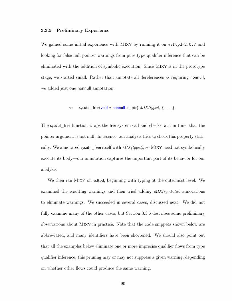
3.3.5 Preliminary Experience
We gained some initial experience with Mixy by running it on vsftpd-2.0.7 and
looking for false null pointer warnings from pure type qualifier inference that can be
eliminated with the addition of symbolic execution. Since Mixy is in the prototype
stage, we started small. Rather than annotate all dereferences as requiring nonnull,
we added just one nonnull annotation:
102 sysutil_free(void ∗ nonnull p_ptr) MIX(typed) { . . . }
The sysutil_free function wraps the free system call and checks, at run time, that the
pointer argument is not null. In essence, our analysis tries to check this property stati-
cally. We annotated sysutil_free itself with MIX(typed), so Mixy need not symbolically
execute its body—our annotation captures the important part of its behavior for our
analysis.
We then ran Mixy on vsftpd, beginning with typing at the outermost level. We
examined the resulting warnings and then tried adding MIX(symbolic) annotations
to eliminate warnings. We succeeded in several cases, discussed next. We did not
fully examine many of the other cases, but Section 3.3.6 describes some preliminary
observations about Mixy in practice. Note that the code snippets shown below are
abbreviated, and many identifiers have been shortened. We should also point out
that all the examples below eliminate one or more imprecise qualifier flows from type
qualifier inference; this pruning may or may not suppress a given warning, depending
on whether other flows could produce the same warning.
90

Case 1: Flow and path insensitivity in sockaddr_clear
103 void sockaddr_clear(struct sockaddr ∗∗p_sock) MIX(symbolic) {104 if (∗p_sock != NULL) {105 sysutil_free(∗p_sock);106 ∗p_sock = NULL;107 }108 }
This function is implicated in a false warning: due to flow insensitivity in the type sys-
tem, the null assignment on line 106 flows to the argument to sysutil_free on line 105,
even though the assignment occurs after the call. Also, the type system ignores the
null check on line 104 due to path insensitivity.
Marking sockaddr_clear with MIX(symbolic) successfully resolves this warning: the
symbolic executor determines that ∗p_sock is not null when used as an argument to
sysutil_free().
Case 2: Path and context insensitivity in str_next_dirent
109 void str_alloc_text(struct mystr∗ p_str) MIX(typed);110 const char∗ sysutil_next_dirent( . . .) MIX(typed) {111 if (p_dirent == NULL) return NULL;112 }113 void str_next_dirent( . . .) MIX(symbolic) {114 const char∗ p_filename = sysutil_next_dirent( . . .);115 if (p_filename != NULL)116 str_alloc_text(p_filename);117 }118 . . .119 str_alloc_text(str);120 . . .121 sysutil_free(str);122 . . .
In this example, the function str_next_direct calls sysutil_next_dirent on line 114, which
may return a null value. Hence p_filename may be null. The type system ignores the
91

null check on line 115 and due to context insensitivity, conflates p_filename with other
variables, such as str, that are passed to str_alloc_text (lines 116 and 119). Hence
the type system believes str may be null. However, str is used as an argument to
sysutil_free (line 121), which leads the type system to report a false warning.
Annotating function str_next_dirent as symbolic, while leaving sysutil_next_dirent
and str_alloc_text as typed, successfully eliminates this warning: the symbolic execu-
tor correctly determines that p_filename is not null when it is used as an argument
to str_alloc_text. And although the extra precision does not matter in this particular
example, notice that the call on line 116 will be analyzed in a separate invocation of
the type system than the call on line 119, thus introducing some context sensitivity.
Case 3: Flow and path insensitivity in dns_resolve and main
123 void main_BLOCK(struct sockaddr∗∗ p_sock) MIX(symbolic) {124 ∗p_sock = NULL;125 dns_resolve(p_sock, tunable_pasv_address);126 }127 int main( . . .) {128 . . .129 main_BLOCK(&p_addr);130 . . .131 sysutil_free(p_addr);132 . . .133 }134 void dns_resolve(struct sockaddr∗∗ p_sock, const char∗ p_name) {135 struct hostent∗ hent = gethostbyname(p_name);136 sockaddr_clear(p_sock);137 if (hent−>h_addrtype == AF_INET)138 sockaddr_alloc_ipv4(p_sock);139 else if (hent−>h_addrtype == AF_INET6)140 sockaddr_alloc_ipv6(p_sock);141 else142 die("gethostbyname(): neither IPv4 nor IPv6");143 }
92

There are two sources of null values in the code above: ∗p_sock is set to null on
line 124; and sockaddr_clear, which was previously marked as symbolic in Case 1
above, also sets ∗p_sock to null on line 136 in dns_resolve. Due to flow insensitivity
in the type system, both these null values eventually reach sysutil_free on line 131,
leading to false warnings.
However, we can see that these null values are actually overwritten by non-null
values on lines 138 and 140, where sockaddr_alloc_ipv4 or sockaddr_alloc_ipv6 allocates
the appropriate structure and assigns it to ∗p_sock (not shown). We can eliminate
these warnings by extracting the code in main that includes both null sources into a
symbolic block.
Also, there is a system call gethostbyname on line 135 that we need to handle. Here,
we define a well-behaved, symbolic model of gethostbyname that returns only AF_INET
and AF_INET6 as is standard (not shown). This will cause the symbolic executor to
skip the last branch on line 142, which we need to do because we cannot analyze die
symbolically as it eventually calls a function pointer, an operation that our symbolic
executor currently has limited support for. We also cannot put gethostbyname or die
in typed blocks in this case, since ∗p_sock is null and will result in false warnings.
Case 4: Helping symbolic execution with symbolic function pointers
144 void sysutil_exit_BLOCK(void) MIX(typed) {145 if (s_exit_func) (∗s_exit_func)();146 }147 void sysutil_exit(int exit_code) {148 sysutil_exit_BLOCK();149 exit(exit_code);150 }
93
In several instances, we would like to evaluate symbolic blocks that call sysutil_exit,
defined on line 147, which in turn calls exit to terminate the program. However,
before terminating the program, sysutil_exit calls the function pointer s_exit_func on
line 145. Our symbolic executor does not support calling symbolic function pointers
(i.e., which targets are unknown), so instead, we extract the call to s_exit_func into
a typed block to analyze the call conservatively.
3.3.6 Mixy Limitations
While our preliminary experience provides some real-world validation of Mix’s effi-
cacy in removing false positives, there are a number of limitations.
Most importantly, the overwhelming source of issues in Mixy is its coarse treat-
ment of aliasing, which relies on an imprecise pointer analysis. One immediate con-
sequence is that it impedes performance in the symbolic executor: if an imprecise
pointer analysis returns large points-to sets for pointers, translating symbolic point-
ers to type constraints becomes slow because we first need to check if each pointer
target is valid in the current path condition by calling the SMT solver, then deter-
mine if any valid targets may be null. This leads to a significant slowdown: our small
examples from Section 3.3.5 take less than a second to run without symbolic blocks,
but from 5 to 25 seconds to run with one symbolic block, and about 60 seconds with
two symbolic blocks. This issue is further compounded by the fixed-point computa-
tion that repeatedly analyzes symbolic blocks nested in typed blocks or for handling
recursion.
94
We also noticed several cases in vsftpd where calls to symbolic blocks would help
introduce context sensitivity to distinguish calls to malloc. However, since we rely on
a context-insensitive pointer analysis to restore aliasing relationships when switch-
ing to typed blocks, these calls will again be conflated. The issue especially affects
the analysis of typed-to-symbolic-to-typed recursive blocks because the nested typed
blocks are polluted by aliasing relationships from the entire program. A similar issue
occurs with symbolic blocks, as pointers are initialized to point to targets from the
entire program, rather than being limited to the enclosing context.
Just as in the formalism, Mixy has to consider the entire memory when switching
from typed to symbolic or vice-versa. Since this was a deliberate design decision,
we were not surprised to find out that this has an impact on performance and leads
to many limitations in practice. Any temporary violation of type invariants from
symbolic blocks would immediately be flagged when switching to typed blocks, even
if they have no effect on the code in the typed blocks. In the other direction, symbolic
blocks are forced to start with a fresh memory when switching from typed blocks even
if there were no effects.
Ultimately, we believe that these issues can be addressed with more precise in-
formation about aliasing as well as effects, perhaps extracted directly from the type
inference constraints and symbolic execution.
95
3.4 Related Work
There are several threads of related work. There have been numerous proposals
for program analyses based on type systems; see Palsberg and Millstein (2007) for
pointers. Symbolic execution was first proposed by King (1976) as an enhanced
testing strategy, but was difficult to apply for many years. Recently, SMT solvers
have become very powerful, making symbolic execution much more attractive as even
very complex path conditions can be solved surprisingly fast. There have been many
recent, impressive results using symbolic execution for bug finding (Godefroid et al.,
2005; Sen et al., 2005; Cadar et al., 2006, 2008). These systems use symbolic execution
to explore a small subset of the possible program paths, since in the presence of loops
with symbolic bounds, pure symbolic execution will not terminate in a reasonable
amount of time (unless loop invariants are assumed). In the Mix formalism, in
contrast, we use symbolic execution in a sound manner by exploring all paths, which
is possible because we can use type checking on parts of the code where symbolic
execution takes too long. Of course, it is also possible to mix unsound symbolic
execution with type checking, to gain whatever level of assurance the programmer
desires.
There are several program analyses that can operate at different levels of abstrac-
tion. Corbett et al. (2000) is a model checking system that uses abstraction-based
program specialization, in which the programmer specifies the exact abstractions to
use. System Z is an abstract interpreter generator in which the programmer can tune
the level of abstraction to trade off cost and precision (Yi and Harrison III, 1993).
96
Tuning these systems requires a deep knowledge of program analysis. In contrast, we
believe that Mix’s tradeoff is easier to understand—one selects between essentially no
abstraction (symbolic execution), or abstraction in terms of types, which are arguably
the most successful, well-understood program analyses.
Mix bears some resemblance to program analysis based on abstraction refinement,
such as SLAM (Ball and Rajamani, 2002), BLAST (Henzinger et al., 2004), and
client-driven pointer analysis (Guyer and Lin, 2005). These tools incrementally refine
their abstraction of the program as necessary for analysis. Adding symbolic blocks
to a program can be seen as introducing a very precise “refinement” of the program
abstraction.
There are a few systems that combine type checking or inference with other anal-
yses. Dependent types provide an elegant way to augment standard type with very
rich type refinements (Xi and Pfenning, 1999). Liquid types combines Hindley-Milner
style type inference with predicate abstraction (Rondon et al., 2010, 2008). Hybrid
types combines static typing, theorem proving, and dynamic typing (Flanagan, 2006).
All of these systems combine types with refinements at a deep level—the refinements
are placed “on top of” the type structure. In contrast, Mix uses a much coarser
approach in which the precise analysis is almost entirely separated from the type
system, except for a thin interface between the two systems.
Many others have considered the problem of combining program analyses. A
reduced product in abstract interpretation (Cousot and Cousot, 1979) is a theoretical
description of the most precise combination of two abstract domains. It is typically
obtained via manually defined reduction operators that depend on the domains being
97

combined. Another example of combining abstract domains is the logical product of
Gulwani and Tiwari (2006). Combining program analyses for compiler optimizations
is also well-studied (e.g., Lerner et al. (2002)). In all of these cases, the combinations
strengthen the kinds of derivable facts over the entire program. With Mix, we instead
analyze separate parts of the program with different analyses.
Finally, Mix was partially inspired by Nelson-Oppen style cooperating decision
procedures (Nelson and Oppen, 1979). One important feature of the Nelson-Oppen
framework is that it provides an automatic method for distributing the appropriate
formula fragments to each solver (if that the solvers match certain criteria). Clearly
Mix is targeted at solving a very different problem, but it would be an interesting
direction for future work to try to extend Mix into a similar framework that can
automatically integrate analyses that have appropriately structured interfaces.
98

Chapter 4
Expositor: Integrating Program Analysis into Debugging†
In this chapter, we present Expositor, a new environment that unifies dynamic
program analysis and interactive debugging. Expositor combines the advantages of
dynamic program analysis and interactive debugging: it allows programmers to auto-
mate complex dynamic program analysis by writing scripts that operate over entire
program executions, yet provides quick, interactive feedback in that programmers can
easily examine partial or intermediate results of the analysis. Expositor is designed
in particular to aid programmers in hypothesis testing, i.e., iteratively developing and
testing various hypothesis about the cause of a bug.
4.0.1 Background: Scriptable Debugging and Time-Travel Debuggers
Scriptable debugging is a powerful technique for hypothesis testing in which program-
mers write scripts to perform complex debugging tasks. For example, suppose we
observe a bug involving a cleverly implemented set data structure. We can try to
debug the problem by writing a script that maintains a shadow data structure that
implements the set more simply (e.g., as a list). We run the buggy program, and the
script tracks the program’s calls to insert and remove, stopping execution when the
†A version of this chapter was previously published as Khoo et al. (2013a,b). A prototype ofExpositor is available at https://bitbucket.org/khooyp/expositor.
99
contents of the shadow data structure fail to match those of the buggy one, helping
pinpoint the underlying fault.
While we could have employed the same debugging strategy by altering the pro-
gram itself (e.g., by inserting print statements and assertions), doing so would require
recompilation—and that can take considerable time for large programs (e.g., Firefox),
thus greatly slowing the rate of hypothesis testing. Modifying a program can also
change its behavior—we have all experienced the frustration of inserting a debugging
print statement only to make the problem disappear! Scripts also have the benefit
that they can invoke libraries not used by the program itself. And, general-purpose
scripts may be reused.
There has been considerable prior work on scriptable debugging. GDB’s Python
interface makes GDB’s interactive commands—stepping, setting breakpoints, etc.—
available in a general-purpose programming language. However, this interface em-
ploys a callback-oriented programming style which, as pointed out by Marceau et al.
(2007), reduces composability and reusability as well as complicates checking temporal
properties. Marceau et al. propose treating the program as an event generator—each
function call, memory reference, etc. can be thought of as an event—and scripts are
written in the style of functional reactive programming (FRP) (Elliott and Hudak,
1997). While FRP-style debugging solves the problems of callback-based program-
ming, it has a key limitation: time always marches forward, so we cannot ask questions
about prior states. For example, if while debugging a program we find a doubly freed
address, we cannot jump backward in time to find the corresponding malloc. Instead
we would need to rerun the program from scratch to find that call, which may be
100
problematic if there is any nondeterminism, e.g., if the addresses returned by malloc
differ from run to run. Alternatively, we could prospectively gather the addresses
returned by malloc as the program runs, but then we would need to record all such
calls up to the erroneous free.
Time-travel debuggers, like UndoDB (Undo Software), and systems for captur-
ing entire program executions, like Amber (O’Callahan, 2006), allow a single non-
deterministic execution to be examined at multiple points in time. Unfortunately,
scriptable time-travel debuggers typically use callback-style programming, with all
its problems. (Section 4.6 discusses prior work in detail.)
4.0.2 Expositor: Scriptable, Time-Travel Debugging
We developed Expositor as a new scriptable debugging system that is inspired by
FRP-style scripting but with the advantages of time-travel debugging. Expositor
scripts treat a program’s execution trace as a (potentially infinite) immutable list of
time-annotated program state snapshots or projections thereof. Scripts can create or
combine traces using common list operations: traces can be filtered, mapped, sliced,
folded, and merged to create lightweight projections of the entire program execution.
As such, Expositor is particularly well suited for checking temporal properties of
an execution, and for writing new scripts that analyze traces computed by prior
scripts. Furthermore, since Expositor extends GDB’s Python environment and
uses the UndoDB (Undo Software) time-travel backend for GDB, users can seamlessly
switch between running scripts and interacting directly with an execution via GDB.
(Section 4.1 overviews Expositor’s scripting interface.)
101

The key idea for making Expositor efficient is to employ laziness in its im-
plementation of traces—invoking the time-travel debugger is expensive, and laziness
helps minimize the number of calls to it. Expositor represents traces as sparse,
time-indexed interval trees and fills in their contents on demand. For example, sup-
pose we use Expositor’s breakpoints combinator to create a trace tr containing just
the program execution’s malloc calls. If we ask for the first element of tr before time
42 (perhaps because there is a suspicious program output then), Expositor will
direct the time-travel debugger to time 42 and run it backward until hitting the call,
capturing the resulting state in the trace data structure. The remainder of the trace,
after time 42 and before the malloc call, is not computed. (Section 4.2 discusses the
implementation of traces.)
In addition to traces, Expositor scripts typically employ various internal data
structures to record information, e.g., the set s of arguments to malloc calls. These
data structures must also be lazy so as not to compromise trace laziness—if we eagerly
computed the set s just mentioned to answer a membership query at time t, we
would have to run the time-travel debugger from the start up until t, considering
all malloc calls, even if only the most recent call is sufficient to satisfy the query.
Thus, Expositor provides script writers with a novel data structure: the edit hash
array mapped trie (EditHAMT), which provides lazy construction and queries for sets,
maps, multisets, and multimaps. As far as we are aware, the EditHAMT is the first
data structure to provide these capabilities. (Section 4.3 describes the EditHAMT.)
We have used Expositor to write a number of simple scripts, as well as to debug
two more significant problems. Section 4.1 describes how we used Expositor to
102
find an exploitable buffer overflow. Section 4.5 explains how we used Expositor to
track down a deep, subtle bug in Firefox that was never directly fixed, though it was
papered over with a subsequent bug fix (the fix resolved the symptom, but did not
remove the underlying fault). In the process, we developed several reusable analyses,
including a simple race detector.
4.1 The Design of Expositor
We designed Expositor to provide programmers with a high-level, declarative API
to write analyses over the program execution, as opposed to the low-level, imperative,
callback-based API commonly found in other scriptable debuggers.
In particular, the design of Expositor is based on two key principles. First,
the Expositor API is purely functional—all objects are immutable, and methods
manipulate objects by returning new objects. The purely functional API facilitates
composition, by reducing the risk of scripts interfering with each other via shared
mutable object, as well as reuse, since immutable objects can easily be memoized or
cached upon construction. It also enables Expositor to employ lazy programming
techniques to improve efficiency.
Second, the trace abstraction provided by Expositor is based around familiar
list-processing APIs found in many languages, such as the built-in list-manipulating
functions in Python, the Array methods in JavaScript, the List module in Ocaml, and
the Data.List module in Haskell. These APIs are also declarative—programmers ma-
nipulate lists using combinators such as filter, map, and merge that operate over entire
103

151 class execution:152 # get snapshots153 get_at(t): snapshot at time t154
155 # derive traces156 breakpoints(fn): snapshot trace of breakpoints at func fn157 syscalls(fn): snapshot trace of breakpoints at syscall fn158 watchpoints(x, rw): snapshot trace of read/write watchpoints at var x159 all_calls(): snapshot trace of all function entries160 all_returns(): snapshot trace of all function exits161
162 # interactive control163 cont(): manually continue the execution164 get_time(): latest time of the execution165
166 class trace:167 # count/get items168 __len__(): called by “ len(trace)”169 __iter__(): called by “ for item in trace”170 get_at(t): item at exactly time t171 get_after(t): next item after time t172 get_before(t): previous item before time t173
174 # create a new trace by filtering/mapping a trace175 filter(p): subtrace of items for which p returns true176 map(f): new trace with f applied to all items177 slice(t0, t1): subtrace from time t0 to time t1178
179 # create a new trace by merging two traces180 merge(f, tr): see Figure 4.3(a)181 trailing_merge(f, tr): see Figure 4.3(b)182 rev_trailing_merge(f, tr): see Figure 4.3(c)183
184 # create a new trace by computing over prefixes/suffixes185 scan(f, acc): see Figure 4.3(d)186 rev_scan(f, acc): see Figure 4.3(e)187 tscan(f, acc): see Figure 4.5(a)188 rev_tscan(f, acc): see Figure 4.5(b)
Figure 4.1: Expositor’s Python-based scripting API. The get_X and __len__methods of execution and trace are eager, and the remaining methods of those classesreturn lazy values. Lazy values include trace, snapshot, and gdb_value objects whosecontents are computed only on demand and cached.
104

189 class item:190 time: item’s execution time191 value: item’s contents192
193 class snapshot:194 read_var(x): gdb_value of variable x in current stack frame195 read_retaddrs(): gdb_values of return addresses on the stack196 backtrace(): print the stack backtrace197 . . . and other methods to access program state . . .198
199 class gdb_value:200 __getitem__(x): called by “ gdb_value[x]” to access field/index x201 deref(): dereference gdb_value (if it is a pointer)202 addrof(): address of gdb_value (if it is an l-value)203 . . . and other methods to query properties of gdb_value . . .
Figure 4.2: Expositor’s Python-based scripting API (continued).
lists, instead of manipulating individual list elements. These list combinators allow
Expositor to compute individual list elements on-demand in any order, minimizing
the number of calls to the time-travel debugger. Furthermore, they shield program-
mers from the low-level details of controlling the program execution and handling
callbacks.
4.1.1 API Overview
Figures 4.1 and 4.2 lists the key classes and methods of Expositor’s scripting in-
terface, which is provided as a library inside UndoDB/GDB’s Python environment.
The execution class and the the_execution object The entire execution of
the program being debugged is represented by the execution class, of which there is
a singleton instance named the_execution. This class provides several methods for
105

querying the execution. The get_at(t)1 method returns a snapshot object representing
the program state at time t in the execution (we will describe snapshots in more detail
later). Several methods create immutable, sparse projections of the execution, or
traces, consisting of program state snapshots at points of interest: the breakpoints(fn)
and syscalls(fn) methods return traces of snapshots at functions and system calls named
fn, respectively; the watchpoints(x, rw) method returns a trace of snapshot when the
memory location x is read or written; and the all_calls and all_returns methods return
traces of snapshots at all function entries and exits, respectively.
For debugging interactive programs, the execution class provides two useful meth-
ods: cont resumes the execution of the program from when it was last stopped (e.g.,
immediately after Expositor is started, or when the program is interrupted by press-
ing ^C), and get_time gets the latest time of the execution. If a program requires
user input to trigger a bug, we often find it helpful to first interrupt the program and
call get_time to get a reference time, before resuming the execution using cont and
providing the input trigger.
The trace class and the item class As mentioned above, the trace class
represents sparse projections of the execution at points of interest. These traces
contain snapshots or other values, indexed by the relevant time in the execution.
Initially, traces are created using the execution methods described above, and traces
may be further derived from other traces.
1We use the convention of naming time variables as t, and trace variables as tr.
106

The first five trace methods query items in traces. The tr.__len__() method is
called by the Python built-in function len(tr), and returns the total number of items
in the tr. The tr.__iter__() method is called by Python’s for x in tr loop, and returns
a sequential Python iterator over all items in tr. The get_at(t) method returns the
item at time t in the trace, or None if there is no item at that time. Since traces are
often very sparse, it can be difficult to find items using get_at, so the trace class also
provides two methods, get_before(t) and get_after(t), that return the first item found
before or after time t, respectively, or None if no item can be found. The get_at,
get_before, and get_after methods return values that are wrapped in the item class,
which associates values with a particular point in the execution.
The remaining methods create new traces from existing traces. The tr.filter(p)
method creates a new trace consisting only of items from tr that match predicate
p. The tr.map(f) method creates a new trace of items computed by calling function
f on each item from tr, and is useful for extracting particular values of interest from
snapshots. The tr.slice(t0, t1) method creates a new trace that includes only items
from tr between times t0 and t1.
The trace class also provides several more complex methods to derive new traces.
Three methods create new traces by merging traces. First, tr0.merge(f, tr1) creates a
new trace containing the items from both tr0 and tr1, calling function f to combine
any items from tr0 and tr1 that occur at the same time (Figure 4.3(a)). None can be
passed for f if tr0 and tr1 contain items that can never coincide, e.g., if tr0 contains
calls to foo and tr1 contains calls to bar, since f will never be called in this case. Next,
tr0.trailing_merge(f, tr1) creates a new trace by calling f to merge each item from tr0
107
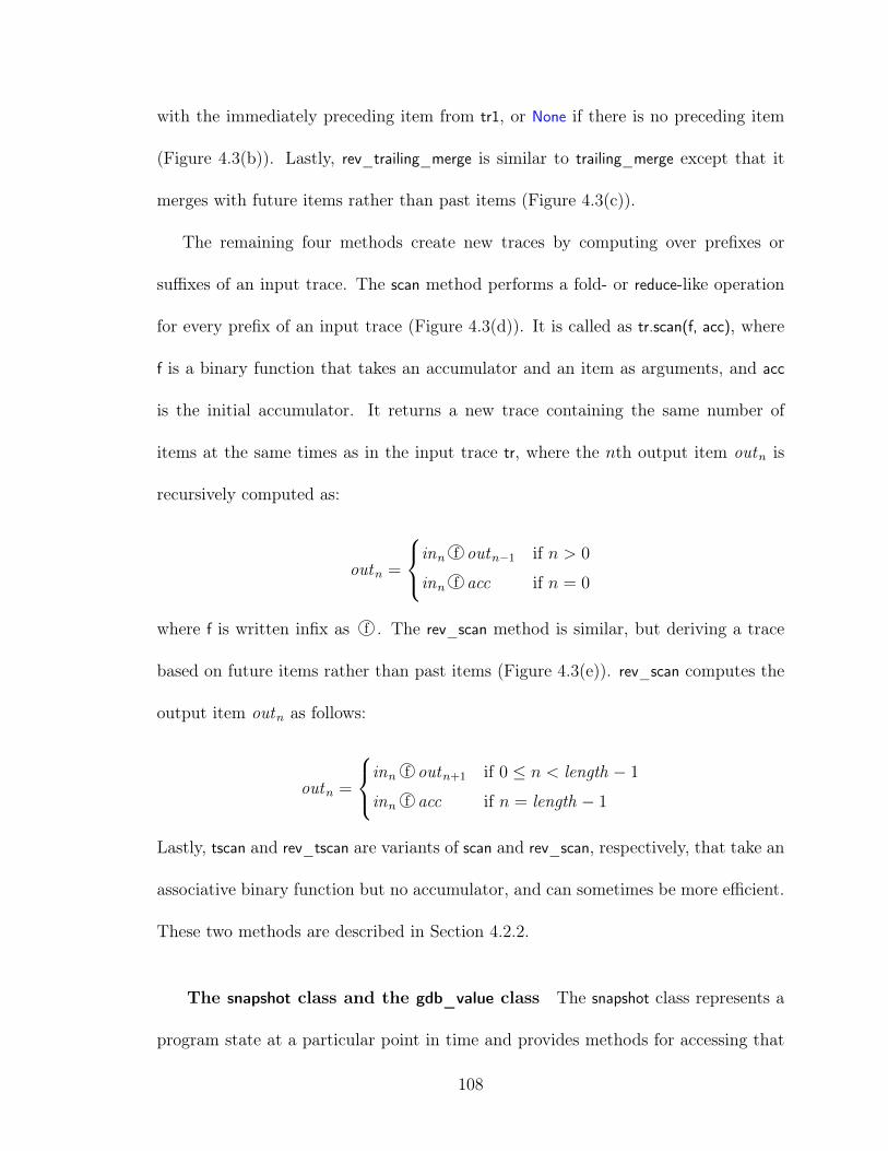
with the immediately preceding item from tr1, or None if there is no preceding item
(Figure 4.3(b)). Lastly, rev_trailing_merge is similar to trailing_merge except that it
merges with future items rather than past items (Figure 4.3(c)).
The remaining four methods create new traces by computing over prefixes or
suffixes of an input trace. The scan method performs a fold- or reduce-like operation
for every prefix of an input trace (Figure 4.3(d)). It is called as tr.scan(f, acc), where
f is a binary function that takes an accumulator and an item as arguments, and acc
is the initial accumulator. It returns a new trace containing the same number of
items at the same times as in the input trace tr, where the nth output item outn is
recursively computed as:
outn =
inn f outn−1 if n > 0
inn f acc if n = 0
where f is written infix as f . The rev_scan method is similar, but deriving a trace
based on future items rather than past items (Figure 4.3(e)). rev_scan computes the
output item outn as follows:
outn =
inn f outn+1 if 0 ≤ n < length − 1
inn f acc if n = length − 1
Lastly, tscan and rev_tscan are variants of scan and rev_scan, respectively, that take an
associative binary function but no accumulator, and can sometimes be more efficient.
These two methods are described in Section 4.2.2.
The snapshot class and the gdb_value class The snapshot class represents a
program state at a particular point in time and provides methods for accessing that
108

tr0
tr1
tr0.merge(f, tr1)
f
(a)
None
tr0
tr1
tr0.trailing_merge(f, tr1)
f f ff
(b)
None
tr0
tr1
tr0.rev_trailing_merge(f, tr1)
ffff
(c)
tr
tr.scan(f, acc)
acc f f f
(d)
tr
tr.rev_scan(f, acc)
accfff
(e)
Figure 4.3: Illustration of complex trace operations.
state, e.g., read_var(x) returns the value of a variable named x in the current stack
frame, read_retaddrs returns the list of return addresses on the stack, backtrace prints
the stack backtrace, and so on.
The gdb_value class represents values in the program being debugged at a par-
ticular point in time, and provides methods for querying those values. For example,
v.__getitem__(x) is called by the Python indexing operator v[x] to access struct fields
or array elements, deref dereferences pointer values, addrof returns the address of an
l-value, and so forth. These gdb_value objects are automatically coerced to the ap-
propriate Python types when they are compared against built-in Python values such
109

as ints, for example; it is also sometimes useful to manually coerce gdb_value objects
to specific Python types, e.g., to treat a pointer value as a Python int.
Both the snapshot and gdb_value classes are thin wrappers around GDB’s Python
API and UndoDB. When a method of a snapshot or gdb_value object is called, it
first directs UndoDB to jump to the point in time in the program execution that
is associated with the object. Then, it calls the corresponding GDB API, wrapping
the return value in snapshot and gdb_value as necessary. In general, the semantics of
snapshot and gdb_value follows GDB, e.g., the Expositor’s notion of stack frames is
based on GDB’s notion of stack frames. We also provide several methods, such as
read_retaddrs, that return the result of several GDB API calls in a more convenient
form. Additionally, all of GDB’s Python API is available and may be used from
within Expositor.
Given a debugging hypothesis, we use the Expositor interface to apply the
following recipe. First, we call methods on the_execution to derive one or more traces
that contain events relevant to the hypothesis; such events could be function calls,
breakpoints, system calls, etc. Next, we combine these traces as appropriate, applying
tracemethods such as filter, map, merge, and scan to derive traces of properties predicted
by our hypothesis. Finally, we query the traces using methods such as get_before and
get_after to find evidence of properties that would confirm or refute our hypothesis.
110

4.1.2 Warm-up Example: Examining foo Calls in Expositor
To begin with a simple example, let us consider the task of counting the number
of calls to a function foo, to test a hypothesis that an algorithm is running for an
incorrect number of iterations, for example. Counting foo calls takes just two lines
of code in Expositor. We first use the breakpoints method of the_execution to create
the foo trace:
204 foo = the_execution.breakpoints("foo")
This gives us a trace containing all calls to foo. We can then count the calls to foo
using the Python len function, and print it:
205 print len(foo)
Later, we may want to count only calls to foo(x) where x == 0, perhaps because
we suspect that only these calls are buggy. We can achieve this using the filter method
on the foo trace created above:
206 foo_0 = foo.filter(lambda snap: snap.read_var("x") == 0)
Here, we call filter with a predicate function that takes a snapshot object (at calls to
foo), reads the variable named x, and returns whether x == 0. The resulting trace
contains only calls to foo(0), which we assign to foo_0. We can then count foo_0 as
before:
111
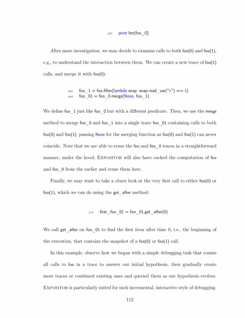
207 print len(foo_0}
After more investigation, we may decide to examine calls to both foo(0) and foo(1),
e.g., to understand the interaction between them. We can create a new trace of foo(1)
calls, and merge it with foo(0):
208 foo_1 = foo.filter(lambda snap: snap.read_var("x") == 1)209 foo_01 = foo_0.merge(None, foo_1)
We define foo_1 just like foo_0 but with a different predicate. Then, we use the merge
method to merge foo_0 and foo_1 into a single trace foo_01 containing calls to both
foo(0) and foo(1), passing None for the merging function as foo(0) and foo(1) can never
coincide. Note that we are able to reuse the foo and foo_0 traces in a straightforward
manner; under the hood, Expositor will also have cached the computation of foo
and foo_0 from the earlier and reuse them here.
Finally, we may want to take a closer look at the very first call to either foo(0) or
foo(1), which we can do using the get_after method:
210 first_foo_01 = foo_01.get_after(0)
We call get_after on foo_01 to find the first item after time 0, i.e., the beginning of
the execution, that contains the snapshot of a foo(0) or foo(1) call.
In this example, observe how we began with a simple debugging task that counts
all calls to foo in a trace to answer our initial hypothesis, then gradually create
more traces or combined existing ones and queried them as our hypothesis evolves.
Expositor is particularly suited for such incremental, interactive style of debugging.
112

Comparison to GDB’s Python API
In contrast to Expositor, it takes 16 lines of code to count foo calls using GDB’s
standard Python API, as shown in Figure 4.4. On line 211, we first initialize two
variables, count and more, that will be used to track of the number of calls to foo
and to track if the execution has ended respectively. Then, on line 212, we create a
breakpoint at the call to foo. Next, we create a callback function named stop_handler
on lines 213–216 to handle breakpoint events. In this function, we first check on
lines 214–215 to see if the breakpoint triggered is the one that we have set, and if so,
we increment count on line 216. We also create a callback function named exit_handler
on lines 217–218 to handle stop events which are fired when the program execution
ends. This function simply resets the more flag when called.
After that, we register stop_handler and exit_handler with GDB on lines 219–220,
and start the program execution on line 221. GDB will run the program until it hits
a breakpoint or the end of the execution is reached, calling stop_handler in the former
case, or exit_handler in the latter case. Then, we enter a loop on lines 222–223 that
causes GDB to continue running the program until more is False, i.e., the program has
exited. Once that happens, we deregister the event handlers from GDB and delete the
breakpoint on lines 224–226, cleaning up after ourselves to ensure that the callbacks
and breakpoint will not be unintentionally triggered by other scripts.
It also takes more work to refine this GDB script to answer other questions about
foo, compared to Expositor traces. For example, to count calls to foo(0), we would
have to modify the GDB script to add the x == 0 predicate and rerun it, instead
113
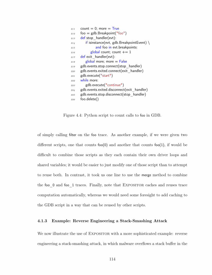
211 count = 0; more = True212 foo = gdb.Breakpoint("foo")213 def stop_handler(evt):214 if isinstance(evt, gdb.BreakpointEvent) \215 and foo in evt.breakpoints:216 global count; count += 1217 def exit_handler(evt):218 global more; more = False219 gdb.events.stop.connect(stop_handler)220 gdb.events.exited.connect(exit_handler)221 gdb.execute("start")222 while more:223 gdb.execute("continue")224 gdb.events.exited.disconnect(exit_handler)225 gdb.events.stop.disconnect(stop_handler)226 foo.delete()
Figure 4.4: Python script to count calls to foo in GDB.
of simply calling filter on the foo trace. As another example, if we were given two
different scripts, one that counts foo(0) and another that counts foo(1), if would be
difficult to combine those scripts as they each contain their own driver loops and
shared variables; it would be easier to just modify one of those script than to attempt
to reuse both. In contrast, it took us one line to use the merge method to combine
the foo_0 and foo_1 traces. Finally, note that Expositor caches and reuses trace
computation automatically, whereas we would need some foresight to add caching to
the GDB script in a way that can be reused by other scripts.
4.1.3 Example: Reverse Engineering a Stack-Smashing Attack
We now illustrate the use of Expositor with a more sophisticated example: reverse
engineering a stack-smashing attack, in which malware overflows a stack buffer in the
114

target program to overwrite a return address on the stack, thereby gaining control of
the program counter (One, 1996).
We develop a reusable script that can detect when the stack has been smashed
in any program, which will help pinpoint the attack vector. Our script maintains a
shadow stack of return addresses and uses it to check that only the top of the stack
is modified between function calls or returns; any violation of this property indicates
the stack has been smashed.
We begin by using the all_calls and all_returns methods on the_execution to create
traces of just the snapshots at function calls and returns, respectively:
227 calls = the_execution.all_calls()228 rets = the_execution.all_returns()
Next, we use merge to combine these into a single trace, passing None for the merging
function as function calls and returns can never coincide. We will use this new trace
to compare consecutive calls or returns:
229 calls_rets = calls.merge(None, rets)
Now, we map over call_returns to apply the read_retaddrs method, returning the list of
return addresses on the call stack. This creates a trace of shadow stacks at every call
and return:
230 shadow_stacks = calls_rets.map(231 lambda s: map(int, s.read_retaddrs()))
We also use map to coerce the return addresses to Python ints.
115

Then we need to check that, between function calls and returns, the actual call
stack matches the shadow stack except for the topmost frame (one return address
may be added or removed). We use the following function:
232 def find_corrupted(ss, opt_shadow):233 if opt_shadow.force() is not None:234 for x, y in zip(ss.read_retaddrs(), opt_shadow.force()):235 if int(x) != y:236 return x # l-value of return address on stack237 return None
Here, find_corrupted takes as arguments a snapshot ss and its immediately preceding
shadow stack opt_shadow; the opt_ prefix indicates that there may not be a prior
shadow stack (if ss is at the first function call), and we need to call the force method on
opt_shadow to retrieve its value (we will explain the significance of this in Section 4.2).
If there is a prior shadow stack, we compare every return address in ss against the
shadow stack and return the first location that differs, or None if there are no corrupted
addresses. (The zip function creates a list of pairs of the respective elements of the
two input lists, up to the length of the shorter list.)
Finally, we generate a trace of corrupted memory locations using the trailing_merge
method, calling find_corrupted to merge each function call and return from call_rets
with the immediately preceding shadow stack in shadow_stacks. We filter None out of
the result:
238 corrupted_addrs = calls_rets \239 .trailing_merge(find_corrupted, shadow_stacks) \240 .filter(lambda x: x is not None)
The resulting trace contains exactly the locations of corrupted return addresses at
the point they are first evident in the trace.
116

4.1.4 Mini Case Study: Running Expositor on tinyhttpd
We used the script just developed on a version of tinyhttpd (Blackstone) that we
had previously modified to include a buffer overflow bug. We created this version of
tinyhttpd as an exercise for a security class in which students develop exploits of the
vulnerability.
As malware, we deployed an exploit that uses a return-to-libc attack (Designer,
1997) against tinyhttpd. The attack causes tinyhttpd to print “Now I pwn your computer”
to the terminal and then resume normal operation. Finding buffer overflows using
standard techniques can be challenging, since there can be a delay from the exploit
overflowing the buffer to the payload taking effect, during which the exploited call
stack may be erased by normal program execution. The payload may also erase
evidence of itself from the stack before producing a symptom.
To use Expositor, we call the expositor launcher with tinyhttpd as its argument,
which will start a GDB session with Expositor’s library loaded, and then enter the
Python interactive prompt from GDB:2
241 % expositor tinyhttpd242 (expositor) python-interactive
Then, we start running tinyhttpd:
243 >>> the_execution.cont() # start running244 httpd running on port 47055
2GDB contains an existing python command that is not interactive; python-interactive is a newcommand that we have submitted to GDB, and is available as of GDB 7.6.
117

When tinyhttpd launches, it prints out the port number on which it accepts client
connections. On a different terminal, we run the exploit with this port number:
245 % ./exploit.py 47055246 Trying port 47055247 pwning...
At this point, tinyhttpd prints the exploit message, so we interrupt the debugger
and use Expositor to find the stack corruption, starting from the time when we
interrupted it:
248 Now I pwn your computer249 ^C250 Program received signal SIGINT, Interrupt251 >>> corrupted_addrs = stack_corruption()252 # function containing Section 4.1.3 code253 >>> time = the_execution.get_time()254 >>> last_corrupt = corrupted_addrs.get_before(time)
Items in a trace are indexed by time, so the get_before method call above tells
Expositor to start computing corrupted_addrs from the interrupted time backward
and find the first function call or return when the stack corruption is detected. We
can print the results:
255 >>> print time256 56686.8257 >>> print last_corrupt258 Item(56449.2, address)
This shows that the interrupt occurred at time 56686.8, and the corrupted stack
was first detected at a function call or return at time 56449.2. We can then find and
print the snapshot that corrupted the return address with:
118

259 >>> bad_writes = the_execution \260 .watchpoints(last_corrupt.value, rw=WRITE)261 >>> last_bad_write = bad_writes.get_before(last_corrupt.time)262 >>> print last_bad_write263 Item(56436.0, snapshot)
We find that the first write that corrupted the return address occurred at time
56436.0. We can then inspect the snapshot via last_bad_write.value. In this case,
the backtrace of the very first snapshot identifies the exact line of code in tinyhttpd
that causes the stack corruption—a socket recv with an out-of-bounds pointer. Notice
that to find the bug, Expositor only inspected from time 56686.8 to time 56436.0.
Moreover, had last_corrupt not explained the bug, we would then call corrupted_addrs
.get_before(last_corrupt.time) to find the prior corruption event, inspecting only as
much of the execution as needed to track down the bug.
This mini case study also demonstrates that, for some debugging tasks, it can be
much faster to search backward in time. It takes only 1 second for corrupted_addrs
.get_before(time) to return; whereas if we had instead searched forward from the be-
ginning (e.g., simulating a debugger without time-travel):
264 first_corrupted = corrupted_addrs.get_after(0)
it takes 4 seconds for the answer to be computed. Using Expositor, users can write
scripts that search forward or backward in time, as optimal for the task.
119

4.2 Lazy Traces in Expositor
As just discussed, Expositor allows users to treat traces as if they were lists of
snapshots. However, for many applications it would be impractical to eagerly record
and analyze full program snapshots at every program point. Instead, Expositor uses
the underlying time-travel debugger, UndoDB, to construct snapshots on demand and
to discard them when they are no longer used (since it is expensive to keep too many
snapshots in memory at once). Thus the major challenge is to minimize the demand
for snapshots, which Expositor accomplishes by constructing and manipulating
traces lazily.
More precisely, all of the trace generators and combinators, including execution
.all_calls, trace.map, trace.merge, etc., return immediately without invoking UndoDB.
It is only when final values are demanded, with execution.get_at, trace.get_at, trace
.get_after, or trace.get_before, that Expositor queries the actual program execution,
and it does so only as much as is needed to acquire the result. For example, the
construction of corrupted_addrs in Section 4.1.4, line 251 induces no time travel on
the underlying program—it is not until the call to corrupted_addrs.get_before(time) in
Section 4.1.4, line 254 that Expositor uses the debugger to acquire the final result.
To achieve this design, Expositor uses a lazy, interval-tree-like data structure to
implement traces. More precisely, a trace is a binary tree whose nodes are annotated
with the (closed) lower-bound and (open) upper-bound of the time intervals they
span, and leaf nodes either contain a value or are empty. The initial tree for a trace
120
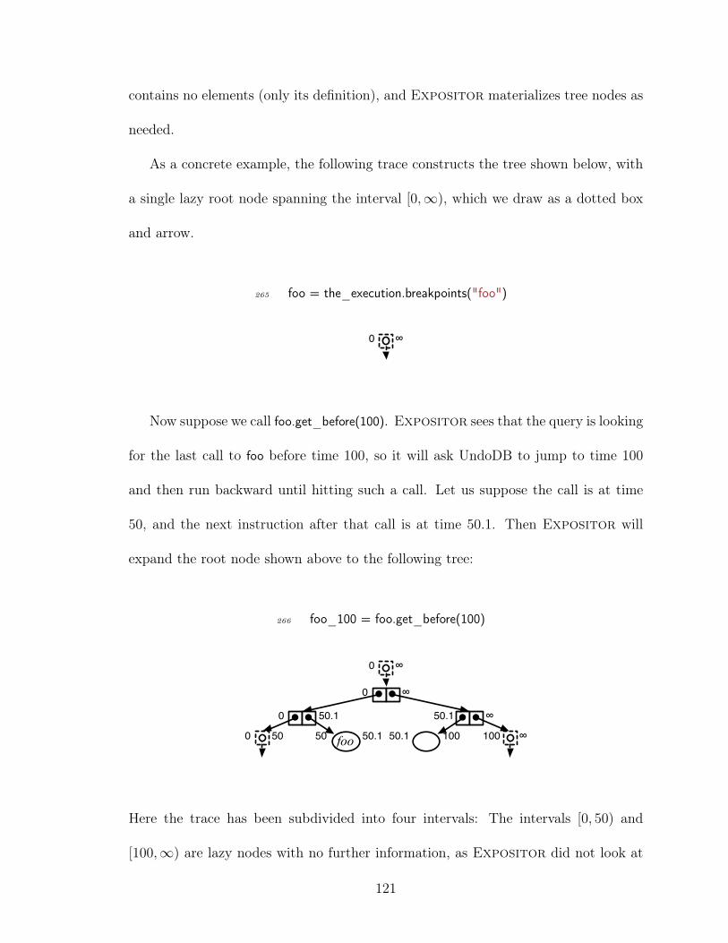
contains no elements (only its definition), and Expositor materializes tree nodes as
needed.
As a concrete example, the following trace constructs the tree shown below, with
a single lazy root node spanning the interval [0,∞), which we draw as a dotted box
and arrow.
265 foo = the_execution.breakpoints("foo")
0 ∞
Now suppose we call foo.get_before(100). Expositor sees that the query is looking
for the last call to foo before time 100, so it will ask UndoDB to jump to time 100
and then run backward until hitting such a call. Let us suppose the call is at time
50, and the next instruction after that call is at time 50.1. Then Expositor will
expand the root node shown above to the following tree:
266 foo_100 = foo.get_before(100)
0 ∞
0 ∞
50.1 ∞
100 ∞50.1 100
0 50.1
foo 50.1500 50
Here the trace has been subdivided into four intervals: The intervals [0, 50) and
[100,∞) are lazy nodes with no further information, as Expositor did not look at
121

those portions of the execution. The interval [50, 50.1) contains the discovered call,
and the interval [50.1, 100) is fully resolved and contains no calls to foo. Notice that
if we ask the same query again, Expositor can traverse the interval tree above to
respond without needing to query UndoDB.
Likewise, calling get_at(t) or get_after(t) either returns immediately (if the result
has already been computed) or causes UndoDB to jump to time t (and, for get_after(
t), to then execute forward). These methods may return None, e.g., if a call to foo did
not occur before/after/at time t.
As our micro-benchmarks in Section 4.4 will show, if we request about 10–40% of
the items in a trace, computing traces lazily takes less time than computing eagerly,
depending on the query pattern as well as the kind of computations done. This
makes lazy traces ideal for debugging tasks where we expect programmers to begin
with some clues about the location of the bug. For example, we start looking for
stack corruption from the end of the execution in Section 4.1.4, line 254, because
stack corruptions typically occur near the end of the execution.
4.2.1 Lazy Trace Operations
We implement filter and map lazily on top of the interval tree data structure. For a
call tr1 = tr0.map(f), we initially construct an empty interval tree, and when values are
demanded in tr1 (by get_X calls), Expositor conceptually calls tr0.get_X, applies f
to the result, and caches the result for future use. Calls to tr0.filter(p) are handled sim-
ilarly, constructing a lazy tree that, when demanded, repeatedly gets values from tr0
until p is satisfied. Note that for efficiency, Expositor’s does not actually call get_X
122

on the root node of tr0; instead, it directly traverses the subtree of tr0 corresponding
to the uninitialized subtree of the derived trace.
The implementation of tr0.merge(f, tr1) also calls get_X on tr1 as required. For a
call tr.slice(t0, t1) Expositor creates an interval tree that delegates get_X calls to tr,
asking for items from time t0 to time t1, and returns None for items that fall outside
that interval.
For the last four operations, [rev_]trailing_merge and [rev_]scan, Expositor em-
ploys additional laziness in the helper function argument f. To illustrate, consider a
call to tr.scan(f, acc). Here, Expositor passes the accumulator to f wrapped in an
instance of class lazy, defined as follows:
267 class lazy:268 force(): return the actual value269 is_forced():
return whether force has been called
The force method, when first called, will compute the actual value and cache it; the
cached value is returned in subsequent calls. Thus, f can force the accumulator as
needed, and if it is not forced, it will not be computed.
To see the benefit, consider the following example, which uses scan to derive a new
trace in which each item is a count of the number of consecutive calls to foo with
nonzero arguments, resetting the count when foo is called with zero:
270 foo = execution.breakpoints("foo") # void foo(int x)271 def count_nonzero_foo(lazy_acc, snapshot):272 if snapshot.read_var("x") != 0:273 return lazy_acc.force() + 1274 else:275 return 0276 nonzero_foo = foo.scan(count_nonzero_foo, 0)
123

Notice that if lazy_acc were not lazy, Expositor would have to compute its value
before calling count_nonzero_foo. By the definition of scan (Figure 4.3(d)), this means
that it must recursively call count_nonzero_foo to compute all prior output items
before computing the current item, even if it is unnecessary to do so, e.g., if we had
called nonzero_foo.get_before(t), and the call to foo just before time t had argument
x=0. Thus, a lazy accumulator avoids this unnecessary work. Expositor uses a lazy
accumulator in rev_scan for the same reason.
Likewise, observe that in tr0.trailing_merge(f, tr1), for a particular item in tr0 the
function f may not need to look in tr1 to determine its result; thus, Expositor
wraps the tr1 argument to f in an instance of class lazy. The implementation of
rev_trailing_merge similarly passes lazy items from tr1 to f. Note that there is no
such laziness in the regular merge operation. The reason is that in tr0.merge(f, tr1),
the items from tr0 and tr1 that are combined with f occur at the same time. Thus,
making f’s arguments lazy would not reduce demands on the underlying time-travel
debugger.
4.2.2 Tree Scan
Finally, Expositor provides another list combinator, tree-scan, which is a lazier
variant of scan that is sometimes more efficient. The tscan method computes an
output for every prefix of an input trace by applying an associative binary function
in a tree-like fashion (Figure 4.5(a)). It is invoked with tr.tscan(f), where f must be
an associative function that is lazy and optional in its left argument and lazy in its
right argument. The tscan method generates an output trace of the same length as
124
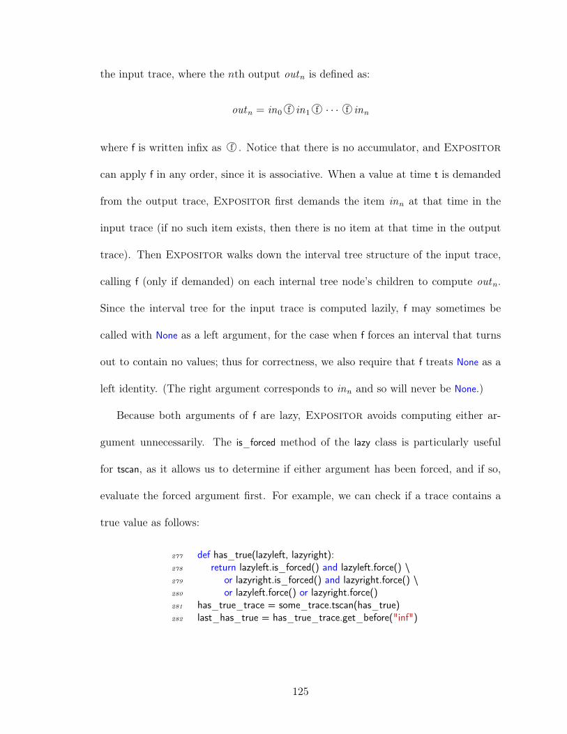
the input trace, where the nth output outn is defined as:
outn = in0 f in1 f · · · f inn
where f is written infix as f . Notice that there is no accumulator, and Expositor
can apply f in any order, since it is associative. When a value at time t is demanded
from the output trace, Expositor first demands the item inn at that time in the
input trace (if no such item exists, then there is no item at that time in the output
trace). Then Expositor walks down the interval tree structure of the input trace,
calling f (only if demanded) on each internal tree node’s children to compute outn.
Since the interval tree for the input trace is computed lazily, f may sometimes be
called with None as a left argument, for the case when f forces an interval that turns
out to contain no values; thus for correctness, we also require that f treats None as a
left identity. (The right argument corresponds to inn and so will never be None.)
Because both arguments of f are lazy, Expositor avoids computing either ar-
gument unnecessarily. The is_forced method of the lazy class is particularly useful
for tscan, as it allows us to determine if either argument has been forced, and if so,
evaluate the forced argument first. For example, we can check if a trace contains a
true value as follows:
277 def has_true(lazyleft, lazyright):278 return lazyleft.is_forced() and lazyleft.force() \279 or lazyright.is_forced() and lazyright.force() \280 or lazyleft.force() or lazyright.force()281 has_true_trace = some_trace.tscan(has_true)282 last_has_true = has_true_trace.get_before("inf")
125
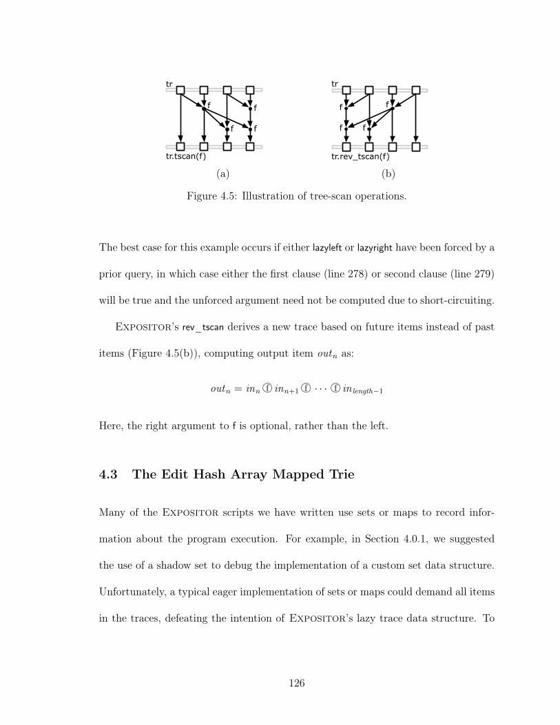
tr
tr.tscan(f)
ff
f f
(a)
tr.rev_tscan(f)
tr
f
f f
f
(b)
Figure 4.5: Illustration of tree-scan operations.
The best case for this example occurs if either lazyleft or lazyright have been forced by a
prior query, in which case either the first clause (line 278) or second clause (line 279)
will be true and the unforced argument need not be computed due to short-circuiting.
Expositor’s rev_tscan derives a new trace based on future items instead of past
items (Figure 4.5(b)), computing output item outn as:
outn = inn f inn+1 f · · · f in length−1
Here, the right argument to f is optional, rather than the left.
4.3 The Edit Hash Array Mapped Trie
Many of the Expositor scripts we have written use sets or maps to record infor-
mation about the program execution. For example, in Section 4.0.1, we suggested
the use of a shadow set to debug the implementation of a custom set data structure.
Unfortunately, a typical eager implementation of sets or maps could demand all items
in the traces, defeating the intention of Expositor’s lazy trace data structure. To
126

demonstrate this issue, consider the following code, which uses Python’s standard
(non-lazy) set class to collect all arguments in calls to a function foo:
283 foos = the_execution.breakpoints("foo") # void foo(int arg)284 def collect_foo_args(lazy_acc, snap):285 return lazy_acc.force().union( \286 set([ int(snap.read_var("arg")) ]))287 foo_args = foos.scan(collect_foo_args, set())
Notice that we must force lazy_acc to call the union method which will create a deep
copy of the updated set (lines 285–286). Unfortunately, forcing lazy_acc causes the
immediately preceding set to be computed by recursively calling collect_foo_args. As
a result, we must compute all preceding sets in the trace even if a particular query
could be answered without doing so.
To address these problems, we developed the edit hash array mapped trie (Edit-
HAMT), a new set, map, multiset, and multimap data structure that supports lazy
construction and queries. The EditHAMT complements the trace data structure; as
we will explain, and our micro-benchmark in Section 4.4.4 will show, the EditHAMT
can be used in traces without compromising trace laziness, unlike eager sets or maps.
4.3.1 EditHAMT API
From the user’s perspective, the EditHAMT is an immutable data structure that
maintains the entire history of edit operations for each EditHAMT. Figure 4.6 shows
the EditHAMT API. The edithamt class includes contains(k) to determine if key k exists,
and find(k) to look up the latest value mapped to key k. It also includes the find_multi(
k) method to look up all values mapped to key k, returned as a Python iterator that in-
crementally looks up each mapped value. EditHAMT operations are implemented as
127

288 class edithamt:289 # lookup methods290 contains(k): Return if key k exists291 find(k): Return the latest value for k or None if not found292 find_multi(k): Return an iterator of all values bound to k293
294 # static factory methods to create new EditHAMTs295 empty(): Create an empty EditHAMT296 add(lazy_eh, k): Add binding of k to itself to lazy_eh297 addkeyvalue(lazy_eh, k, v): Add binding of k to v to lazy_eh298 remove(lazy_eh, k): Remove all bindings of k from lazy_eh299 removeone(lazy_eh, k): Remove the latest binding of k to any value from lazy_eh300 removekeyvalue(lazy_eh, k, v): Remove the latest binding of k to v from lazy_eh301 concat(lazy_eh1, lazy_eh2): Concatenate lazy_eh2 edit history to lazy_eh1
Figure 4.6: The EditHAMT API.
static factory methods that create new EditHAMTs. Calling edithamt.empty() creates
a new, empty EditHAMT. Calling edithamt.add(lazy_eh, k) creates a new EditHAMT
by adding to lazy_eh, the prior EditHAMT, a binding from key k to itself (treating
the EditHAMT as a set or multiset). Similarly, edithamt.addkeyvalue(lazy_eh, k, v) cre-
ates a new EditHAMT by adding to lazy_eh a binding from key k value v (treating
the EditHAMT as a map or multimap). Conversely, calling edithamt.remove(lazy_eh, k)
creates a new EditHAMT by removing all bindings of key k from lazy_eh. Lastly, call-
ing edithamt.removeone(lazy_eh, k) or edithamt.removekeyvalue(lazy_eh, k, v) creates new
EditHAMTs by removing from lazy_eh the most recent binding of key k to any value
or to a specific value v. The lazy_eh argument to these static factory methods is lazy
so that we need not force it until a call to contains, find or find_multi demands a result.
For convenience, the lazy_eh argument can also be None, which is treated as an empty
EditHAMT.
128

The last static factory method, edithamt.concat(lazy_eh1, lazy_eh2), concatenates
the edit histories of its arguments. For example:
302 eh_rem = edithamt.remove(None, "x")303 eh_add = edithamt.addkeyvalue(None, "x", 42)304 eh = edithamt.concat(eh_add, eh_rem)
Here eh is the empty EditHAMT, since it contains the additions in eh_add followed
by the removals in eh_rem. A common Expositor script pattern is to map a trace to
a sequence of EditHAMT additions and removals, and then use edithamt.concat with
scan or tscan to concatenate those edits.
4.3.2 Example: EditHAMT to Track Reads and Writes to a Variable
As an example of using the EditHAMT, we present one piece of the race detector
used in our Firefox case study (Section 4.5). The detector compares each memory
access against prior accesses to the same location from any thread. Since UndoDB
serializes thread schedules, each read need only be compared against the immediately
preceding write, and each write against the immediately preceding write as well as
reads between the two writes.
We use the EditHAMT as a multimap in the following function to track the access
history of a given variable v:
305 def access_events(v):306 reads = the_execution.watchpoints(v, rw=READ) \307 .map(lambda s: edithamt.addkeyvalue( \308 None, v, ("read", s.get_thread_id())))309 writes = the_execution.watchpoints(v, rw=WRITE) \310 .map(lambda s: edithamt.addkeyvalue( \311 edithamt.remove(None, v), \312 v, ("write", s.get_thread_id())313 return reads.merge(None, writes)
129
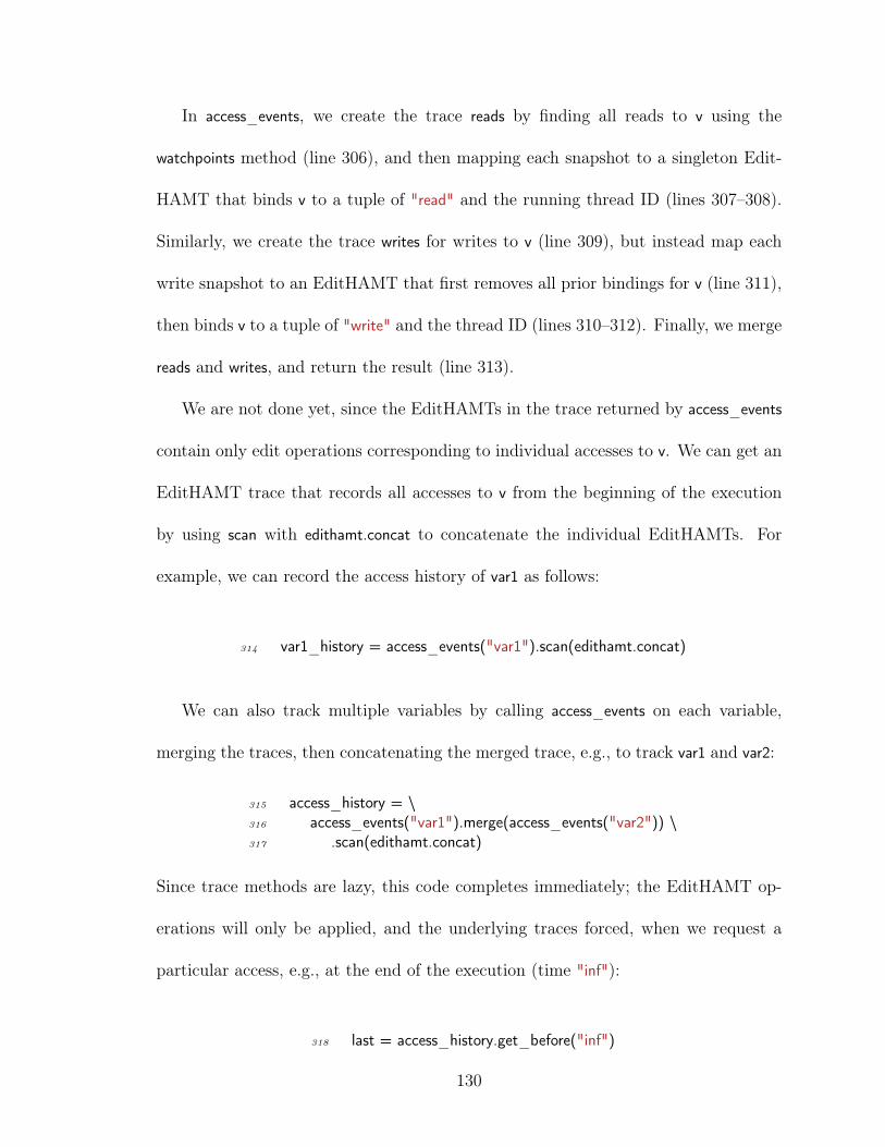
In access_events, we create the trace reads by finding all reads to v using the
watchpoints method (line 306), and then mapping each snapshot to a singleton Edit-
HAMT that binds v to a tuple of "read" and the running thread ID (lines 307–308).
Similarly, we create the trace writes for writes to v (line 309), but instead map each
write snapshot to an EditHAMT that first removes all prior bindings for v (line 311),
then binds v to a tuple of "write" and the thread ID (lines 310–312). Finally, we merge
reads and writes, and return the result (line 313).
We are not done yet, since the EditHAMTs in the trace returned by access_events
contain only edit operations corresponding to individual accesses to v. We can get an
EditHAMT trace that records all accesses to v from the beginning of the execution
by using scan with edithamt.concat to concatenate the individual EditHAMTs. For
example, we can record the access history of var1 as follows:
314 var1_history = access_events("var1").scan(edithamt.concat)
We can also track multiple variables by calling access_events on each variable,
merging the traces, then concatenating the merged trace, e.g., to track var1 and var2:
315 access_history = \316 access_events("var1").merge(access_events("var2")) \317 .scan(edithamt.concat)
Since trace methods are lazy, this code completes immediately; the EditHAMT op-
erations will only be applied, and the underlying traces forced, when we request a
particular access, e.g., at the end of the execution (time "inf"):
318 last = access_history.get_before("inf")
130

To see laziness in action, consider applying the above analysis to an execution
depicted in Figure 4.7, which shows two threads at the top and the corresponding
EditHAMT operations at the bottom. Suppose we print the latest access to var1 at
time t4 using the find method:
319 >>> print last.find("var1")320 ("read", 2)
Because "var1" was just added at time t4, answering this query will only force the
EditHAMT and query the time-travel debugger at time t4, and not before.
As another example, suppose we want to find all accesses to var1 from the last
access backward using find_multi:
321 >>> for mem_access in last.find_multi("var1"):322 print mem_access323 ("read", 2)324 ("write", 1)
Here since all "var1" bindings added prior to time t2 were removed at time t2, the
results are computed without forcing any EditHAMTs or querying the debugger before
time t2.
4.3.3 Implementation
The EditHAMT is inspired by the hash array mapped trie (HAMT) (Bagwell, 2001).
Like the HAMT, the EditHAMT is a hybrid data structure combining the fast lookup
of a hash table and the memory efficiency of a trie. The HAMT is a hash-based data
structure built in a manner analogous to a hash table. Whereas a hash table uses a
bucket array to map keys to values, the HAMT uses an array mapped trie (AMT)—a
131

Readvar1
t0
thread 1
Readvar2
t1
thread 2
Writevar1
Addvar1read,1
access_events("var1").merge(access_events("var2"))
Removevar1
Addvar1write,1
Writevar2
Readvar1
Addvar2read,2
Removevar2
Addvar2write,1
Addvar1read,2
t2 t3 t4
Figure 4.7: Example execution with two threads accessing var1 (gray) and var2, andthe corresponding EditHAMT operations returned by access_events.
trie that maps fixed-width integer keys to values—for the same purpose. When a hash
collision occurs, the HAMT resolves the collision by replacing the colliding entry with
a nested HAMT, rehashing the colliding keys, and inserting those keys in the nested
HAMT using the new hash values.
We developed the EditHAMT by making two changes to the traditional HAMT.
First, we replaced the AMT with the LazyAMT, which supports lazy, rather than
eager, updates. Second, we resolve hash collisions, as well as support remove and
multiset/multimap operations, using EditLists, which are lazy linked-lists of nodes
tallying edit operations on the EditHAMT; the tails are lazily retrieved from the prior
EditHAMT.
LazyAMT: Lazy Array Mapped Tries
The first piece of the EditHAMT is the LazyAMT, which is lazy, immutable variant
of the AMT that maps fixed-width integer keys of size k bits to values. We implement
the LazyAMT using lazy sparse arrays of size 2w as internal nodes, where w is the
132

bit-width of the array index such that w < k, and store key-value bindings as leaf
nodes. We will divide the key into w-bit words, where each w-bit word is used to
index an internal node during a lookup; the key can be padded as necessary if k is
not a multiple of w.
Lazy sparse arrays combine the properties of lazy values and sparse arrays: each
element of a lazy sparse array is computed and cached when first indexed, akin to
forcing a lazy value, and null elements are stored compactly, like sparse arrays. We
implement lazy sparse arrays using two bitmaps to track which elements are initialized
and non-null,3 respectively, and an array to store initialized, non-null elements.
To build the EditHAMT, we need to support two operations on the LazyAMT:
adding a key-value binding to a LazyAMT, and merging two LazyAMTs into a single
LazyAMT. We will explain how the LazyAMT works by example, using an internal
node index bit-width of w = 2 bits and a key size of k = 6 bits.
Adding a key-value binding When we add a binding such as 14 : b to a
LazyAMT, we first create a new lazy sparse array representing the root node:
14:bprior
LazyAMT
Initially, all elements of the root node are uninitialized, which we depict as four narrow
dotted boxes; we will use the convention of numbering the boxes from left to right,
i.e., in binary, the leftmost box is element 00, and the rightmost box is element 11.
3It is more efficient to track non-null elements as many modern processors provide a POPCNTinstruction, which counts the number of 1 bits in a word, that can be used to compute the index ofa non-null element in the storage array.
133

In addition, we also maintain a lazy reference to the prior LazyAMT; we do not yet
need to know what the prior LazyAMT contains, which we indicate with a dotted
arrow. In fact, the lazy reference allows us to further defer the construction of (the
root node of) the prior LazyAMT, i.e., the prior LazyAMT may not exist yet when
we add the binding 14 : b; we indicate this with a dotted trapezoid. For example,
in Expositor, we may query UndoDB to determine what binding should be added
only when the lazy reference to the prior LazyAMT is first forced. We also need to
store the binding 14 : b, to be added when the LazyAMT is sufficiently initialized.
The actual construction of the LazyAMT occurs only when we look up a binding.
The lookup is a standard trie lookup, however, since internal nodes are lazy sparse ar-
rays, the elements of those arrays will be initialized as necessary when we access those
elements during the lookup. We initialize an element in one of three ways, depending
on whether that element is along the lookup path of the binding we previously set
aside to be added, and whether we have reached the end of the lookup path. If the
element is along the lookup path the binding and we have not reached the end of the
lookup path, we create the next internal node and initialize the element to that node.
If the element is along the lookup path of the binding and we have reached the end
of the lookup path, we initialize the element to a leaf node containing that binding.
Otherwise, if the element is not along the lookup path of the binding, we initialize
it to point to the same subtrie as the corresponding element (at the same partial
lookup path) in the prior LazyAMT, or to be null if the corresponding element does
not exist. Note that in the last case, prior LazyAMTs will be recursively initialized
as necessary.
134
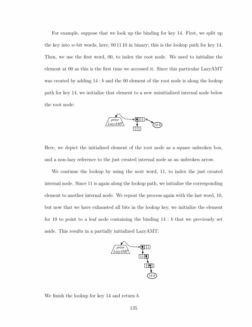
For example, suppose that we look up the binding for key 14. First, we split up
the key into w-bit words, here, 00 11 10 in binary; this is the lookup path for key 14.
Then, we use the first word, 00, to index the root node. We need to initialize the
element at 00 as this is the first time we accessed it. Since this particular LazyAMT
was created by adding 14 : b and the 00 element of the root node is along the lookup
path for key 14, we initialize that element to a new uninitialized internal node below
the root node:
14:bprior
LazyAMT
Here, we depict the initialized element of the root node as a square unbroken box,
and a non-lazy reference to the just created internal node as an unbroken arrow.
We continue the lookup by using the next word, 11, to index the just created
internal node. Since 11 is again along the lookup path, we initialize the corresponding
element to another internal node. We repeat the process again with the last word, 10,
but now that we have exhausted all bits in the lookup key, we initialize the element
for 10 to point to a leaf node containing the binding 14 : b that we previously set
aside. This results in a partially initialized LazyAMT:
prior LazyAMT
14:b
We finish the lookup for key 14 and return b.
135

The example so far illustrates how the lookup process drives the initialization
process in an interleaved manner. Also, since we are looking up a key that was just
inserted into the LazyAMT, we did not need to refer to the prior LazyAMT at all.
These properties allow LazyAMTs to be constructed lazily, by initializing only as
much as necessary to answer lookup queries.
We continue the example by considering the case of looking up a key that was not
added by the most recent LazyAMT. Suppose that the immediately prior LazyAMT,
when computed, will add binding 5 : a:
prior LazyAMT
14:b
add 5 : a
If we then look up key 5, or 00 01 01 in binary, from the rightmost LazyAMT, we
would first index 00 of the root node. We have already initialized this element from
looking up key 14 before, so we simply walk to the next internal node and index 01.
The element at 01 is uninitialized, but it is not along the lookup path of key 14, the
key added to the rightmost LazyAMT. To continue the lookup of key 5, we retrieve
the prior LazyAMT by forcing our lazy reference to it, causing it to be partially
constructed:
136

5:a
prior LazyAMT
14:b
Then, we initialize the element at 01 to point to the subtrie under the element at the
partial key 00 01 in the prior LazyAMT, initializing the middle LazyAMT a bit more
along the way:
5:a
prior LazyAMT
14:b
We finish the lookup for key 5 as before, initializing the LazyAMTs a bit more:
14:b5:a
prior LazyAMT
Note that we have simultaneously initialized parts of the rightmost LazyAMT and
the middle LazyAMT because they share a common subtrie; subsequent lookups of
key 5 on either LazyAMT will become faster as a result.
Merging two LazyAMTs The merge operation takes two LazyAMTs as input,
which we call left and right , as well as a function, mergefn(lazy-opt-leftval , rightval),
137

that is called to merge values for the same key in both LazyAMTs. As the name
of the arguments suggests, mergefn is called in an unusual, asymmetric manner in
that it is called for all keys in the right LazyAMT, but not necessarily for all keys
in the left LazyAMT. For each key in the right LazyAMT, mergefn is called with a
lazy, optional value, representing the value for that key in the left LazyAMT, as the
lazy-opt-leftval argument, and the value for the same key in the right LazyAMT as the
rightval argument. This approach maximizes laziness in that we can compute a lazy
value as soon as we determine a key exists in the one LazyAMT without immediately
looking up the value for the same key in the other LazyAMT. For example, mergefn
can be used to create a lazy linked-list by returning lazy-opt-leftval and rightval in a
tuple.
When we merge two LazyAMTs, we first create a new root node of a new LazyAMT
with two lazy references to the input LazyAMTs:
right LazyAMT
left LazyAMT
As before, the actual construction of the merged LazyAMT occurs when elements
of internal nodes are initialized during lookups. We initialize an element in one of
three ways, depending on whether the corresponding element (at the same partial
lookup path) in the right LazyAMT points to an internal node, points to a leaf node,
or is null. If the corresponding element points to an internal node, we create the next
internal node and initialize the element to that node. If the corresponding element
points to a leaf node, then we call mergefn, giving as lazy-opt-leftval a new lazy value
138

that, when forced, looks up the same key in the left LazyAMT (returning null if the
key does not exist), and as rightval the value at the leaf node. Otherwise, if the
corresponding element is null, we initialize the element to point to the same subtrie
as the corresponding element in the left LazyAMT, or to be null if the corresponding
element does not exist. Note that both the left and right LazyAMTs will be recursively
initialized as necessary.
For example, suppose the right LazyAMT contains a single binding 14 : b:
left LazyAMT
14:b
If we look up key 14, or 00 11 10 in binary, we would first index element 00 of the root
node. Since this is the first time we accessed this element, we initialize it by looking at
the corresponding element in the right LazyAMT. The corresponding element points
to an internal node, so we initialize the element to a new internal node:
left LazyAMT
14:b
We repeat this process until we exhaust all bits in the lookup key and reach the
corresponding leaf node. Because a binding exists for key 14 in the right LazyAMT,
139

we initialize a new leaf node that binds key 14 to a merged value by first creating a
new lazy value that looks up the key 14 from the left LazyAMT, and calling mergefn
on that lazy value as well as the value b from the right LazyAMT:
left LazyAMT
14:b 14:mergefn( , b)
Note that we do not have to force the left LazyAMT to be computed immediately;
the decision to force the left LazyAMT is deferred to mergefn. We finish the lookup
by returning the newly merged value.
As another example, suppose the left LazyAMT contains a single binding 5 : a:
14:b5:a 14:mergefn( , b)
If we look up key 5, or 00 01 01 in binary, we would first index element 00 of the root
note that is already initialized above. However, when we index element 01 of the next
internal node, we would find that the corresponding element in the right LazyAMT
is null. In this case, we look up the subtrie under the corresponding element in the
left LazyAMT, and initialize element 01 to it:
140

14:b5:a 14:mergefn( , b)
Note that we do not call mergefn in this case. We finish the lookup by walking into
left LazyAMT to the leaf node for key 5, and returning a.
Finally, we represent the empty LazyAMT as a special instance that simply returns
null for all key and partial key lookups, allowing us to avoid building a trie structure
with no bindings.
LazyAMT lookups are amortized O(1) time; the LazyAMT has a fixed depth
of k/w, so each lookup takes constant time to traverse the internal nodes to a leaf
node. Similarly, adding a binding to a LazyAMT or merging two LazyAMTs take
only amortized O(1) time and memory to create k/w internal nodes of size 2w each.
The amortization of lookups, adding bindings, and merging LazyAMTs is due to
laziness—most of the cost of adding a binding or merging two LazyAMTs is deferred
to subsequent lookups. Adding the same key repeatedly would take an additional
amortized O(1) memory each time (i.e., prior bindings are never removed, only shad-
owed). However, this is actually an advantage in Expositor as we are usually
interested in how bindings to the same key change over time.
141
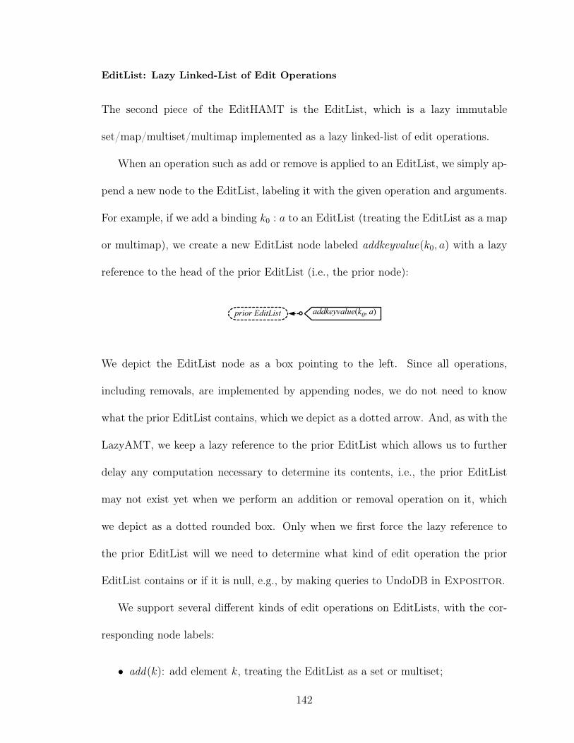
EditList: Lazy Linked-List of Edit Operations
The second piece of the EditHAMT is the EditList, which is a lazy immutable
set/map/multiset/multimap implemented as a lazy linked-list of edit operations.
When an operation such as add or remove is applied to an EditList, we simply ap-
pend a new node to the EditList, labeling it with the given operation and arguments.
For example, if we add a binding k0 : a to an EditList (treating the EditList as a map
or multimap), we create a new EditList node labeled addkeyvalue(k0, a) with a lazy
reference to the head of the prior EditList (i.e., the prior node):
prior EditList addkeyvalue(k0, a)
We depict the EditList node as a box pointing to the left. Since all operations,
including removals, are implemented by appending nodes, we do not need to know
what the prior EditList contains, which we depict as a dotted arrow. And, as with the
LazyAMT, we keep a lazy reference to the prior EditList which allows us to further
delay any computation necessary to determine its contents, i.e., the prior EditList
may not exist yet when we perform an addition or removal operation on it, which
we depict as a dotted rounded box. Only when we first force the lazy reference to
the prior EditList will we need to determine what kind of edit operation the prior
EditList contains or if it is null, e.g., by making queries to UndoDB in Expositor.
We support several different kinds of edit operations on EditLists, with the cor-
responding node labels:
• add(k): add element k, treating the EditList as a set or multiset;
142

• addkeyvalue(k, v): add a binding from key k to value v, treating the EditList
as a map or multimap;
• remove(k): remove all elements/bindings for key k;
• removeone(k): remove the latest element/binding for key k, treating the Ed-
itList as a multiset or multimap;
• removekeyvalue(k, v): remove the latest binding from key k to value v, treating
the EditList as a multimap;
• concat(lazy_el): concatenate the EditList lazy_el as a lazy reference at this
point.
These are the building blocks for the corresponding EditHAMT operations listed in
Figure 4.6.
We implement EditList lookup in two different ways: one for set membership
queries and map lookups, and another for multiset and multimap lookups.
Set Membership Queries and Map Lookups We implement set membership
queries and map lookups by traversing the EditList from head to tail (right to left),
looking for the first node that contains an edit operation for the given key. For
example, if we look up the value for key k0 in the above EditList, we would start by
looking at the head node. Since the head node adds a binding from key k0, we can
finish the lookup and return value a without having to look at the prior EditList. As
another example, suppose that the immediately prior node, when we force it to be
computed, e.g., by making calls to UndoDB in Expositor, removes key k1:
143

remove k1prior EditList addkeyvalue(k0, a)
If we look up the value for key k1, we would first look at the head node and skip it
because it does not involve key k1. Then, we would force the lazy reference to the
prior node, causing it to be initialized if necessary, and look at it:
prior EditList addkeyvalue(k0, a)remove(k1)
Here, we indicate that the tail has been forced with an unbroken arrow, and that the
prior node has been initialized by replacing the dotted rounded box with pointed box.
Since the prior node removes key k1, we know that bindings no longer exist for key
k1, so we can finish the lookup and return null. This example shows that, once we
have found a node that involves the lookup key, we no longer need to traverse the rest
of the EditList. Also, because the reference to the prior EditList is lazy, the lookup
process drives the construction of prior EditLists in an interleaved manner, just as in
the LazyAMT.
If we find a concat node during traversal, we handle that node by recursively
looking up the concatenated EditList for the given key. If we do not find any relevant
nodes in the concatenated EditList, we would then resume the lookup in the original
EditList.
Multiset and Multimap Lookups We implement multiset and multimap
lookups lazily by returning a Python iterator that allows all values for a given key to
144
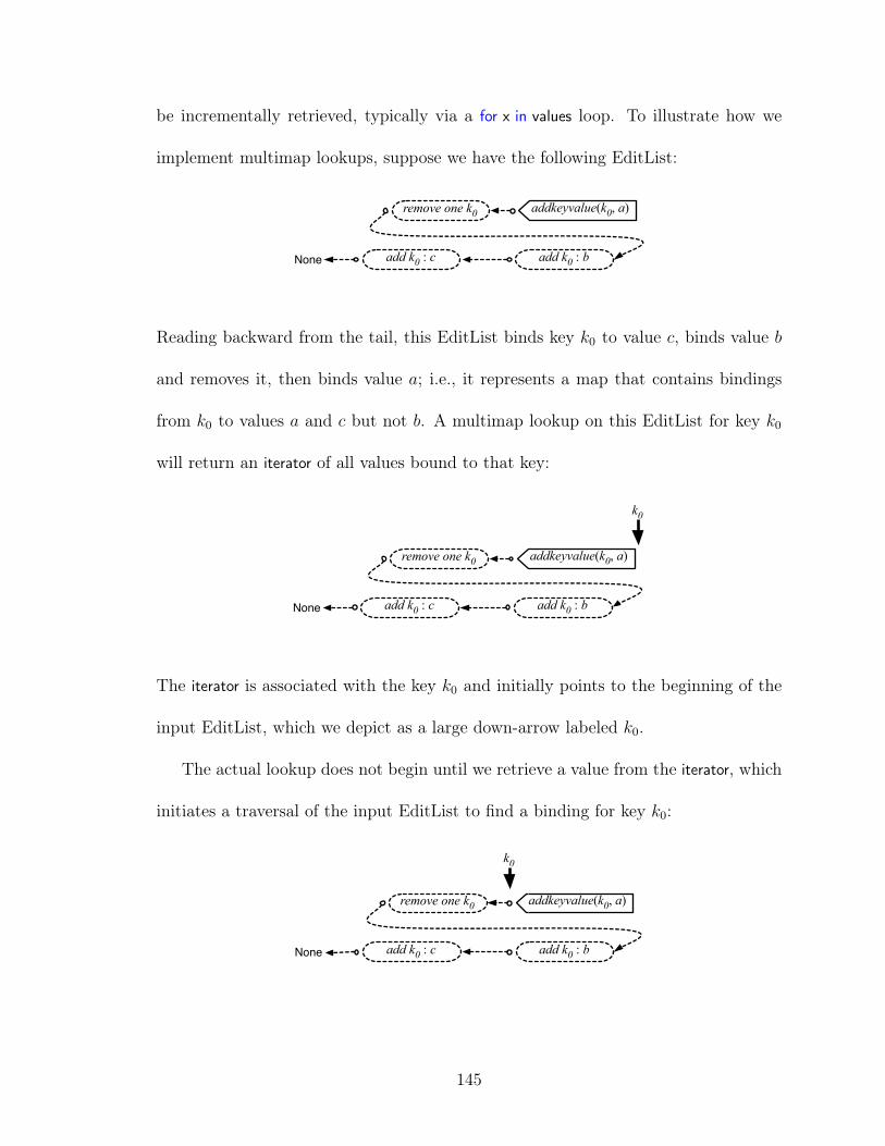
be incrementally retrieved, typically via a for x in values loop. To illustrate how we
implement multimap lookups, suppose we have the following EditList:
remove one k0
add k0 : badd k0 : cNone
addkeyvalue(k0, a)
Reading backward from the tail, this EditList binds key k0 to value c, binds value b
and removes it, then binds value a; i.e., it represents a map that contains bindings
from k0 to values a and c but not b. A multimap lookup on this EditList for key k0
will return an iterator of all values bound to that key:
k0
remove one k0
add k0 : badd k0 : cNone
addkeyvalue(k0, a)
The iterator is associated with the key k0 and initially points to the beginning of the
input EditList, which we depict as a large down-arrow labeled k0.
The actual lookup does not begin until we retrieve a value from the iterator, which
initiates a traversal of the input EditList to find a binding for key k0:
k0
remove one k0 addkeyvalue(k0, a)
add k0 : badd k0 : cNone
145

In this case, the head of the input EditList itself contains a binding to value a, so we
return the value a and update the iterator to point to the tail of the input EditList
(the head of the prior EditList), which we depict by moving the k0 down-arrow.
If we retrieve a value from the iterator again, the lookup continues from the head
of the prior EditList:
k0
None
addkeyvalue(k0, a)removeone(k0)
addkeyvalue(k0, b)addkeyvalue(k0, c)
The prior node removes the next binding for key k0; we temporarily note this as a
pending removal. The node after that adds a binding for key k0, but since we have
a pending removal, we skip over that node. Next, we reach a node that binds key k0
to value c, so we return c and update the iterator as before.
If we retrieve a value from the iterator once more, the lookup will reach the end
of the input EditList, which we depict as None, so we terminate the iterator. At this
point, all nodes in the input EditList will have been initialized:
None
addkeyvalue(k0, a)removeone(k0)
addkeyvalue(k0, b)addkeyvalue(k0, c)
We implement multiset lookups identically by treating add(k) as if key k were
bound to itself. Note in particular that, whereas a standard multiset lookup gives us
the total number of values for a given key, a lazy multiset lookup allows us to ask if
there are at least n values for a given key. As we illustrated above, both multiset and
146

multimap lookups are lazy in that the returned iterator will only initializes as many
nodes of the input EditList as retrieved.
EditList set membership and map/multiset/multimap lookups are not particularly
fast, since they take O(n), where n is the number of edit operations in the EditList
(i.e., the length of the EditList), to traverse the EditList to find a relevant binding.
However, applying an edit operation takes only O(1) time and O(1) memory to create
and append a single EditList node. Adding an element or binding to the same key
repeatedly takes an additional O(1) memory each time, but as we explained for the
LazyAMT, this is actually an advantage for Expositor as we are usually interested
in how bindings change over time.
EditList + Hash + LazyAMT = EditHAMT
As we described above, the LazyAMT provides fast amortized O(1) set/map lookups,
but supports only fixed-width integer keys as well as addition and merging operations;
it does not support removal operations or multiset/multimap lookups. Conversely,
the EditList supports arbitrary keys, removal operations as well as multiset/multimap
lookups, but lookups are a slow O(n) where n is the number of edit operations in
the EditList. Both the LazyAMT and the EditList support lazy construction, i.e.,
we can perform operations such as addition or removal without knowing what the
prior LazyAMT or EditList contains. Finally, each LazyAMT operation takes only
an additional amortized O(1) time and memory over the prior LazyAMT, and likewise
O(1) time and memory for the EditList.
147
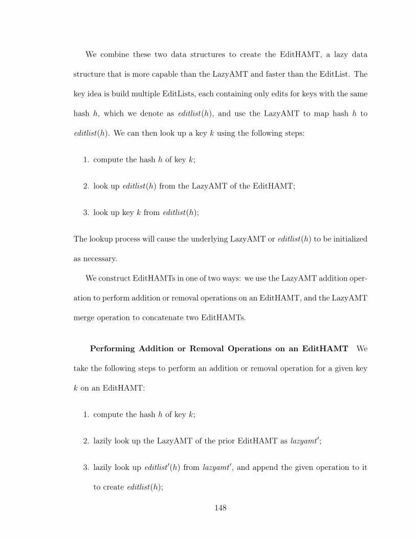
We combine these two data structures to create the EditHAMT, a lazy data
structure that is more capable than the LazyAMT and faster than the EditList. The
key idea is build multiple EditLists, each containing only edits for keys with the same
hash h, which we denote as editlist(h), and use the LazyAMT to map hash h to
editlist(h). We can then look up a key k using the following steps:
1. compute the hash h of key k;
2. look up editlist(h) from the LazyAMT of the EditHAMT;
3. look up key k from editlist(h);
The lookup process will cause the underlying LazyAMT or editlist(h) to be initialized
as necessary.
We construct EditHAMTs in one of two ways: we use the LazyAMT addition oper-
ation to perform addition or removal operations on an EditHAMT, and the LazyAMT
merge operation to concatenate two EditHAMTs.
Performing Addition or Removal Operations on an EditHAMT We
take the following steps to perform an addition or removal operation for a given key
k on an EditHAMT:
1. compute the hash h of key k;
2. lazily look up the LazyAMT of the prior EditHAMT as lazyamt ′;
3. lazily look up editlist ′(h) from lazyamt ′, and append the given operation to it
to create editlist(h);
148

4. add a new binding to lazyamt ′ from hash h to editlist(h) to create the updated
EditHAMT;
where by lazily looking up we mean to create a lazy reference that, when forced, looks
up lazyamt ′ or editlist ′(h), which allows the construction of the prior EditHAMT to
also be lazy. Because both the LazyAMT and the EditList are lazy, the EditHAMT
will be mostly uninitialized at first; (parts of) it will be initialized as necessary during
lookup.
For example, suppose we add a binding from key k0 to value b to an EditHAMT,
and key k0 has hash 14. We would create a new LazyAMT that maps hash 14 to a
new editlist(14) that appends addkeyvalue(k0, b) to the prior EditHAMT:
prior EditHAMT
editlist(14)addkeyvalue(k0, b)
At first, most of the EditHAMT—the LazyAMT as well as the tail of the editlist(14)—
is uninitialized; we indicate the uninitialized editlist(14) tail as a dotted arrow pointing
to the prior EditHAMT. When we look up key k0, we would look up hash 14 from the
LazyAMT to find editlist(14) that we just added, then look up key k0 from editlist(14).
The head of editlist(14) adds key k0, so we can return value b without looking at the
tail. At the end of the lookup, the EditHAMT will be initialized as follows:
149

prior EditHAMT
editlist(14)addkeyvalue(k0, b)
This example shows that we can apply an edit operation without knowledge of the
prior EditHAMT, and since the key k0 was just added, we can look up key k0 without
having to consult the prior EditHAMT. Both of these properties are inherited from
the underlying LazyAMT and EditList.
We continue the example by considering the case of looking up a different key
that was involved in an earlier edit operation. Suppose that the immediately prior
EditHAMT removes key k1, and key k1 has hash 5. When we look up key k1, the
EditHAMT will be initialized as follows:
prior EditHAMT
editlist(14)
editlist(5)
addkeyvalue(k0, b)
remove(k1)
Looking up the editlist(5) from the rightmost LazyAMT causes parts of the middle
LazyAMT to be initialized and shared with the rightmost LazyAMT, and since the
head of editlist(5) removes key k1, we can return null without looking at its tail.
The two examples so far do not require traversing the tail of editlist(h). We would
need to do so if there was a hash collision or if we perform a multiset or multimap
150

lookup. For example, suppose that an earlier EditHAMT added a binding from key
k0 with hash 14 to value a, and we perform a multimap lookup of key k0 to find the
second value. We have to initialize the tail of editlist(14) by looking up editlist ′(14)
from the prior EditHAMT. The immediately prior EditHAMT did not involve key
k0 or hash 14; instead, we will partially initialize the earlier EditHAMT containing
editlist ′(14) and share it. Then, we retrieve editlist ′(14) and initialize it as the tail of
editlist(14). At the end of the lookup, the EditHAMT will be initialized as depicted
below:
prior EditHAMT
editlist(14)editlist'(14)
editlist(5)
addkeyvalue(k0, b)
remove(k1)
addkeyvalue(k0, a)
Concatenating two EditHAMTs To concatenate two EditHAMTs, we call
the LazyAMT merge operation with:
• the older EditHAMT as the left LazyAMT;
• the newer EditHAMT as the right LazyAMT;
• a mergefn function that creates a new editlist(h) by appending an EditList
concat node containing editlist ′(h) from the right EditHAMT to the lazy, op-
tional value containing editlist ′′(h) from the left EditHAMT;
where the older and newer EditHAMTs are lazy_eh1 and lazy_eh2, respectively, in
Figure 4.6.
151
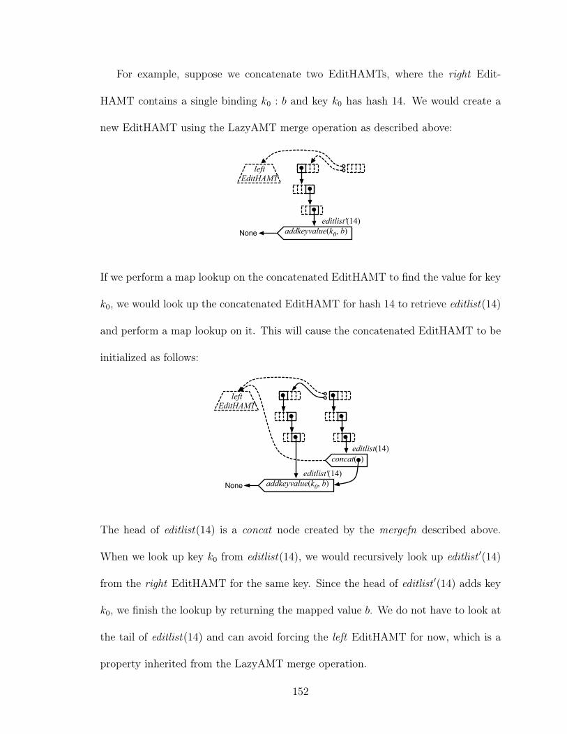
For example, suppose we concatenate two EditHAMTs, where the right Edit-
HAMT contains a single binding k0 : b and key k0 has hash 14. We would create a
new EditHAMT using the LazyAMT merge operation as described above:
left EditHAMT
editlist'(14)addkeyvalue(k0, b)None
If we perform a map lookup on the concatenated EditHAMT to find the value for key
k0, we would look up the concatenated EditHAMT for hash 14 to retrieve editlist(14)
and perform a map lookup on it. This will cause the concatenated EditHAMT to be
initialized as follows:
left EditHAMT
editlist'(14)addkeyvalue(k0, b)None
concat( )editlist(14)
The head of editlist(14) is a concat node created by the mergefn described above.
When we look up key k0 from editlist(14), we would recursively look up editlist ′(14)
from the right EditHAMT for the same key. Since the head of editlist ′(14) adds key
k0, we finish the lookup by returning the mapped value b. We do not have to look at
the tail of editlist(14) and can avoid forcing the left EditHAMT for now, which is a
property inherited from the LazyAMT merge operation.
152
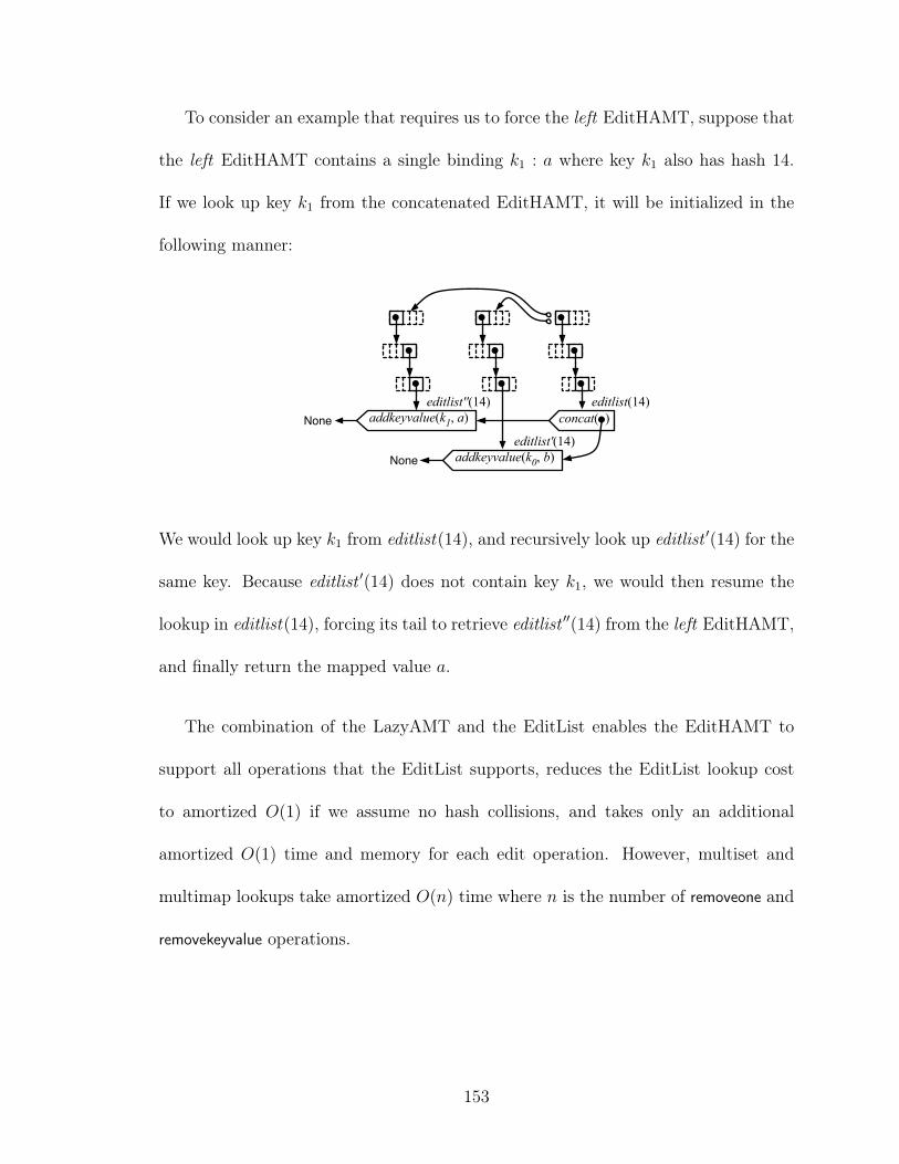
To consider an example that requires us to force the left EditHAMT, suppose that
the left EditHAMT contains a single binding k1 : a where key k1 also has hash 14.
If we look up key k1 from the concatenated EditHAMT, it will be initialized in the
following manner:
editlist'(14)addkeyvalue(k0, b)None
concat( )editlist(14)
addkeyvalue(k1, a)Noneeditlist''(14)
We would look up key k1 from editlist(14), and recursively look up editlist ′(14) for the
same key. Because editlist ′(14) does not contain key k1, we would then resume the
lookup in editlist(14), forcing its tail to retrieve editlist ′′(14) from the left EditHAMT,
and finally return the mapped value a.
The combination of the LazyAMT and the EditList enables the EditHAMT to
support all operations that the EditList supports, reduces the EditList lookup cost
to amortized O(1) if we assume no hash collisions, and takes only an additional
amortized O(1) time and memory for each edit operation. However, multiset and
multimap lookups take amortized O(n) time where n is the number of removeone and
removekeyvalue operations.
153

4.3.4 Comparison with Other Data Structures
Compared to Python sets, which are implemented as hash tables, it is more memory
efficient to make an updated copy of the EditHAMT, since only a constant number
of nodes in the underlying LazyAMT are created, than it is to make a copy of the
bucket array in the hash table underlying Python sets, which can be much larger. This
makes it viable to store every intermediate EditHAMT as it is created in a trace, as
each EditHAMT only requires an additional amortized O(1) memory over the prior
EditHAMT. In our current implementation, a trace of EditHAMTs is cheaper than
a trace of Python sets (which requires deep copying) if, on average, each EditHAMT
or set in the trace has more than eight elements.
It is also common to implement sets or maps using self-balancing trees such as
red-black trees or AVL trees. However, we observe that it is not possible to make these
tree data structures as lazy as the EditHAMT. In these data structures, a rebalancing
operation is usually performed during or after every addition or removal operation to
ensure that every path in the tree does not exceed a certain bound. In particular,
the root node may be swapped with another node in the process of rebalancing (in
fact, every node may potentially be swapped due to rebalancing). This means that
the root node of self-balancing trees is determined by the entire history of addition
and removal operations. Thus, we would be forced to compute the entire history of
addition and removal operations when we traverse the root node to look up a key,
defeating laziness.
154

We also observe a similar issue arising with hash tables. Hash tables are based on
a bucket array that is used to map hash values to keys. Typically, the bucket array
is dynamically resized to accommodate the number of keys in the hash table and to
reduce hash collisions. However, the number of keys in the hash table is determined
by the entire history of addition and removal operations. As a result, we would be
forced to compute the entire history of addition and removal operations before we
can use the bucket array to map a hash value to a key, defeating laziness.
Furthermore, the EditHAMT suffers much less from hash collisions than hash
tables. The LazyAMT in the EditHAMT is a sparse integer map, unlike the bucket
array in hash tables, and thus can be made much larger while using little memory,
which reduces the likelihood of hash collisions.
4.4 Micro-benchmarks
We ran two micro-benchmarks to evaluate the efficiency of Expositor. In the first
micro-benchmark, we evaluated the advantage of laziness by comparing a script writ-
ten in Expositor against several other equivalent scripts written using non-lazy
methods. In the second micro-benchmark, we compared the performance of scripts
using the EditHAMT against other equivalent scripts that use non-lazy data struc-
tures.
155
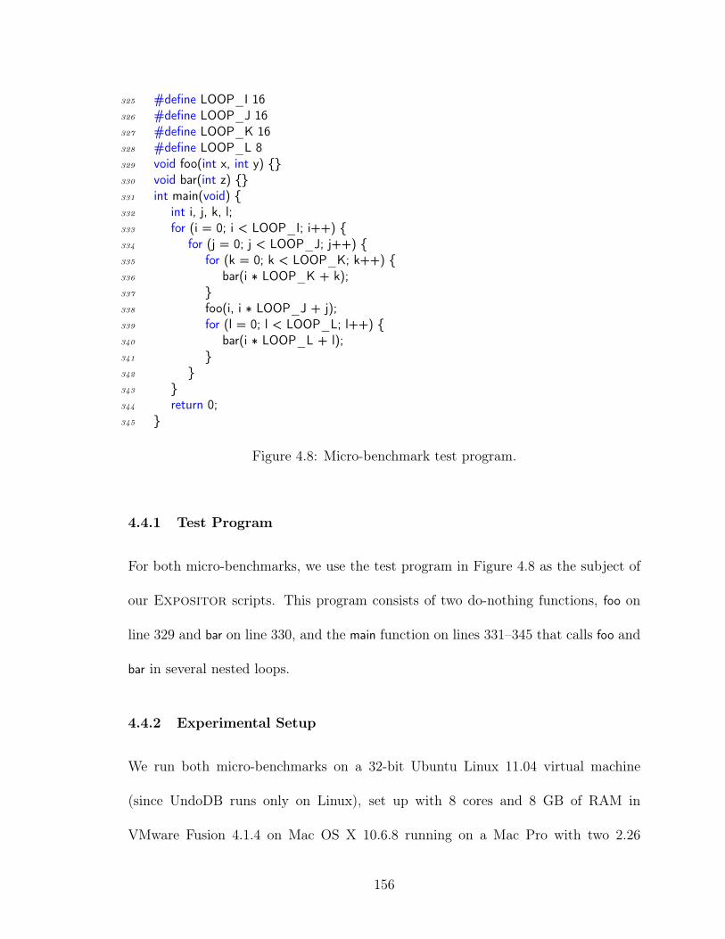
325 #define LOOP_I 16326 #define LOOP_J 16327 #define LOOP_K 16328 #define LOOP_L 8329 void foo(int x, int y) {}330 void bar(int z) {}331 int main(void) {332 int i, j, k, l;333 for (i = 0; i < LOOP_I; i++) {334 for (j = 0; j < LOOP_J; j++) {335 for (k = 0; k < LOOP_K; k++) {336 bar(i ∗ LOOP_K + k);337 }338 foo(i, i ∗ LOOP_J + j);339 for (l = 0; l < LOOP_L; l++) {340 bar(i ∗ LOOP_L + l);341 }342 }343 }344 return 0;345 }
Figure 4.8: Micro-benchmark test program.
4.4.1 Test Program
For both micro-benchmarks, we use the test program in Figure 4.8 as the subject of
our Expositor scripts. This program consists of two do-nothing functions, foo on
line 329 and bar on line 330, and the main function on lines 331–345 that calls foo and
bar in several nested loops.
4.4.2 Experimental Setup
We run both micro-benchmarks on a 32-bit Ubuntu Linux 11.04 virtual machine
(since UndoDB runs only on Linux), set up with 8 cores and 8 GB of RAM in
VMware Fusion 4.1.4 on Mac OS X 10.6.8 running on a Mac Pro with two 2.26
156

GHz quad-core Intel Xeon processors and 16 GB of RAM. We use UndoDB version
3.5.1234, a developmental version of GDB (CVS revision as of October 2012), and
Python version 2.7.5.
4.4.3 Evaluating the Advantage of Trace Laziness
In our first micro-benchmark, we benchmark the advantage of trace laziness using the
following procedure. We first start Expositor on the test program in Figure 4.8,
and run the following script:
346 foo_trace = the_execution.breakpoints("foo")347 trace1 = foo_trace.filter(348 lambda snap: int(snap.read_arg("x")) % 2 == 0)
This script creates a trace named foo_trace of calls to foo, and a trace named trace1
that keeps only calls to foo where the argument x is even. We then measure the time
it takes to call get_after to find the first item in trace1 after time 0. We repeat this
measurement to find the second item, the third item, and so forth, until there are no
more items left in trace1. Next, we create another trace named trace2:
349 trace2 = foo_trace.filter(350 lambda snap: int(snap.read_arg("x")) % 2 == 1)
This trace is similar to trace1, but keeps only calls to foo where x is odd. We then
measure again the time it takes to call get_after to find each item in trace2. Finally,
we restart Expositor and repeat the entire procedure, but use get_before to find
all items in trace1 and trace2 starting from the end of the execution, instead of using
get_after.
157

0 50 100 150 200 250
action #
0
5
10
15
20
cum
ula
tive t
ime (
seco
nds)
startup
lazy_trace
strict_trace
gdb_python
undodb_python
(a) get_after
0 50 100 150 200 250
action #
0
5
10
15
20
cum
ula
tive t
ime (
seco
nds)
startup
lazy_trace
strict_trace
gdb_python
undodb_python
(b) get_before
Figure 4.9: The time it takes to get all items in two traces using lazy or non-lazyscripts.
158
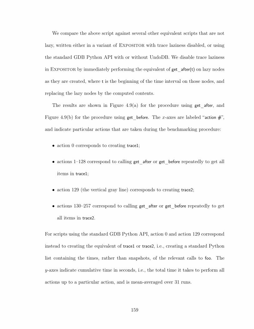
We compare the above script against several other equivalent scripts that are not
lazy, written either in a variant of Expositor with trace laziness disabled, or using
the standard GDB Python API with or without UndoDB. We disable trace laziness
in Expositor by immediately performing the equivalent of get_after(t) on lazy nodes
as they are created, where t is the beginning of the time interval on those nodes, and
replacing the lazy nodes by the computed contents.
The results are shown in Figure 4.9(a) for the procedure using get_after, and
Figure 4.9(b) for the procedure using get_before. The x-axes are labeled “action #”,
and indicate particular actions that are taken during the benchmarking procedure:
• action 0 corresponds to creating trace1;
• actions 1–128 correspond to calling get_after or get_before repeatedly to get all
items in trace1;
• action 129 (the vertical gray line) corresponds to creating trace2;
• actions 130–257 correspond to calling get_after or get_before repeatedly to get
all items in trace2.
For scripts using the standard GDB Python API, action 0 and action 129 correspond
instead to creating the equivalent of trace1 or trace2, i.e., creating a standard Python
list containing the times, rather than snapshots, of the relevant calls to foo. The
y-axes indicate cumulative time in seconds, i.e., the total time it takes to perform all
actions up to a particular action, and is mean-averaged over 31 runs.
159
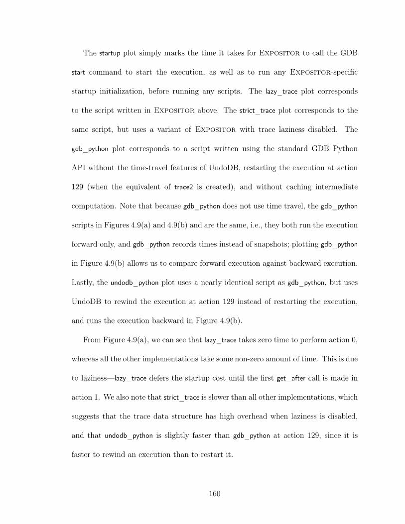
The startup plot simply marks the time it takes for Expositor to call the GDB
start command to start the execution, as well as to run any Expositor-specific
startup initialization, before running any scripts. The lazy_trace plot corresponds
to the script written in Expositor above. The strict_trace plot corresponds to the
same script, but uses a variant of Expositor with trace laziness disabled. The
gdb_python plot corresponds to a script written using the standard GDB Python
API without the time-travel features of UndoDB, restarting the execution at action
129 (when the equivalent of trace2 is created), and without caching intermediate
computation. Note that because gdb_python does not use time travel, the gdb_python
scripts in Figures 4.9(a) and 4.9(b) and are the same, i.e., they both run the execution
forward only, and gdb_python records times instead of snapshots; plotting gdb_python
in Figure 4.9(b) allows us to compare forward execution against backward execution.
Lastly, the undodb_python plot uses a nearly identical script as gdb_python, but uses
UndoDB to rewind the execution at action 129 instead of restarting the execution,
and runs the execution backward in Figure 4.9(b).
From Figure 4.9(a), we can see that lazy_trace takes zero time to perform action 0,
whereas all the other implementations take some non-zero amount of time. This is due
to laziness—lazy_trace defers the startup cost until the first get_after call is made in
action 1. We also note that strict_trace is slower than all other implementations, which
suggests that the trace data structure has high overhead when laziness is disabled,
and that undodb_python is slightly faster than gdb_python at action 129, since it is
faster to rewind an execution than to restart it.
160

As we expect from laziness, each call to get_after in lazy_trace takes a small addi-
tional amount of time, whereas the other non-lazy implementations do not take any
additional time (since all relevant calls to foo have already been found at action 0).
When we have found about 40% items from trace1, the cumulative time of lazy_trace
reaches that of gdb_python. This tells us that, as long as we do not make queries to
more than 40% of an execution, it takes us less time to construct and query a lazy
trace, compared to other non-lazy implementations. This is actually the common
scenario in debugging, where we expect programmers to begin with some clues about
when the bug occurs. For example, a stack corruption typically occurs near the end
of the execution, so we would likely only have to examine the last few function calls
in the execution.
Furthermore, we observe that the slope of lazy_trace is shallower at actions 130–
257. This is because trace2 reuses foo_trace which was fully computed and cached
during actions 1–128. Thus, Expositor does not have to perform as much work
to compute trace2. strict_trace also benefits from caching since it uses a (non-lazy)
variant of the trace data structure. In contrast, both gdb_python and undodb_python
do not reuse any computation, so action 129 takes the same amount of time as action
0.
Figure 4.9(b) shows the results of the benchmark procedure using get_before.
We can see that it is much slower to use get_before that get_after—all scripts but
gdb_python take longer than in Figure 4.9(a) (gdb_python actually runs forward as we
noted above). This is because these scripts has to run the execution in two passes:
first to get to the end of the execution, then to execute the get_before calls back to
161

the beginning of the execution. Unlike other scripts, the gdb_python script only has
to run forward once and not backward, and so is much faster. Still, lazy_trace can be
faster than gdb_python, if queries are made to fewer than about 10% of an execution.
We note that the results of this micro-benchmark actually suggest a lower bound
to the advantage of trace laziness. This micro-benchmark is based on a very simple
Expositor script that filters calls to foo using a simple predicate. Therefore, the
time used for each script is dominated by the time it takes to set a breakpoint at
foo and to run the execution, forward or backward, until the breakpoint. To a lesser
extent, the trace data structure in lazy_trace adds overhead to the time used in com-
parison to gdb_python. The filter predicate in lazy_trace and the equivalent predicate
in gdb_python takes very little time in contrast. We expect more complex Exposi-
tor scripts to spend more time in programmer-provided helper functions such as the
filter predicate or the scan operator, which will mask the overhead of the trace data
structure.
4.4.4 Evaluating the Advantage of the EditHAMT
In our second micro-benchmark, we evaluate the advantages of the EditHAMT data
structure using the following procedure. We first create a trace of EditHAMTs:
351 bar_maps = the_execution.breakpoints("bar") \352 .map(lambda snap: edithamt.addkeyvalue(353 None, int(snap.read_arg("z")), snap)) \354 .scan(edithamt.concat)
For each call to bar(z), we create a new EditHAMT that adds a binding from the
argument z to the snapshot of that call. In other words, an EditHAMT in bar_maps at
162

0 50 100 150 200 250
action #
0
100
200
300
400
500
600
700
cum
ula
tive t
ime (
seco
nds)
startup
lazy_trace_edithamt
lazy_trace_rbtree
lazy_trace_python_dict
strict_trace_edithamt
gdb_python
(a) get_after (time)
0 50 100 150 200 250
action #
0
100
200
300
400
500
600
700
cum
ula
tive t
ime (
seco
nds)
startup
lazy_trace_edithamt
lazy_trace_rbtree
lazy_trace_python_dict
strict_trace_edithamt
gdb_python
(b) get_before (time)
Figure 4.10: The time it takes to get all items in a trace computed by looking upitems from an EditHAMT or other data structures.
163

0 50 100 150 200 250
action #
0
5e+6
10e+6
15e+6
20e+6
25e+6
30e+6
35e+6
cum
ula
tive g
c_gc_
size
(byte
s) startup
lazy_trace_edithamt
lazy_trace_rbtree
lazy_trace_python_dict
strict_trace_edithamt
gdb_python
(a) get_after (memory)
0 50 100 150 200 250
action #
0
5e+6
10e+6
15e+6
20e+6
25e+6
30e+6
35e+6
cum
ula
tive g
c_gc_
size
(byte
s) startup
lazy_trace_edithamt
lazy_trace_rbtree
lazy_trace_python_dict
strict_trace_edithamt
gdb_python
(b) get_before (memory)
Figure 4.11: The memory it takes to get all items in a trace computed by looking upitems from an EditHAMT or other data structures.
164
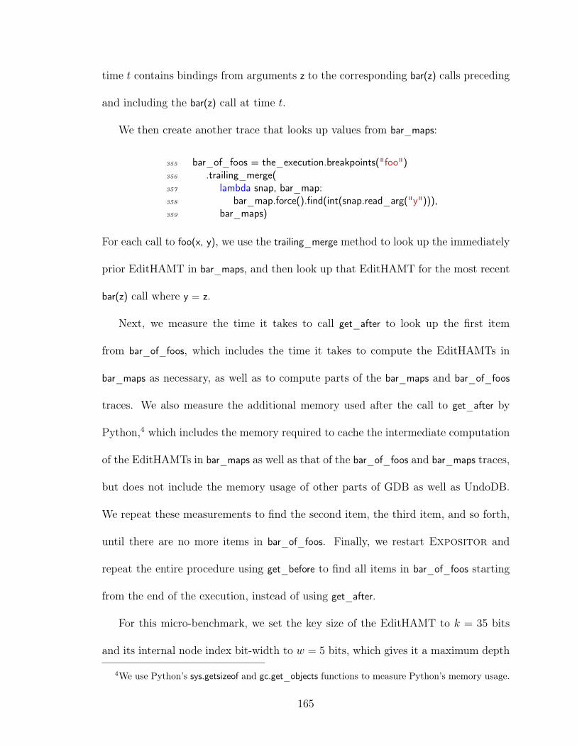
time t contains bindings from arguments z to the corresponding bar(z) calls preceding
and including the bar(z) call at time t.
We then create another trace that looks up values from bar_maps:
355 bar_of_foos = the_execution.breakpoints("foo")356 .trailing_merge(357 lambda snap, bar_map:358 bar_map.force().find(int(snap.read_arg("y"))),359 bar_maps)
For each call to foo(x, y), we use the trailing_merge method to look up the immediately
prior EditHAMT in bar_maps, and then look up that EditHAMT for the most recent
bar(z) call where y = z.
Next, we measure the time it takes to call get_after to look up the first item
from bar_of_foos, which includes the time it takes to compute the EditHAMTs in
bar_maps as necessary, as well as to compute parts of the bar_maps and bar_of_foos
traces. We also measure the additional memory used after the call to get_after by
Python,4 which includes the memory required to cache the intermediate computation
of the EditHAMTs in bar_maps as well as that of the bar_of_foos and bar_maps traces,
but does not include the memory usage of other parts of GDB as well as UndoDB.
We repeat these measurements to find the second item, the third item, and so forth,
until there are no more items in bar_of_foos. Finally, we restart Expositor and
repeat the entire procedure using get_before to find all items in bar_of_foos starting
from the end of the execution, instead of using get_after.
For this micro-benchmark, we set the key size of the EditHAMT to k = 35 bits
and its internal node index bit-width to w = 5 bits, which gives it a maximum depth
4We use Python’s sys.getsizeof and gc.get_objects functions to measure Python’s memory usage.
165

of 7. These parameters are suitable for 32-bit hash values that are padded to 35 bits.
We compare the above script against several other equivalent scripts using other data
structures, as well as a script that uses the EditHAMT in a variant of Expositor
with trace laziness disabled as described in Section 4.4.3, and a script that uses the
standard GDB Python API without the time-travel features of UndoDB and a list of
Python dicts (hash table) as the equivalent of bar_maps.
The results are shown in Figures 4.10 and 4.11: Figures 4.10(a) and 4.10(b)
show the time measurements using get_after and get_before, respectively, while Fig-
ures 4.11(a) and 4.11(b) show the memory measurements using get_after and get_before,
respectively. The x-axes are labeled “action #”, and indicate particular actions that
are taken during the benchmarking procedure:
• action 0 correspond to creating bar_maps and bar_of_foos;
• actions 1–256 corresponds to calling get_after or get_before repeatedly to get all
items in bar_of_foos.
For the script using the standard GDB Python API, action 0 correspond instead
to creating a list of Python dicts mapping the arguments z of bar to times, rather
than snapshots, of calls to bar. The y-axes indicate cumulative time in seconds or
cumulative memory usage in bytes, i.e., the total time or memory it takes to perform
all actions up to a particular action, and is mean-averaged over 31 runs.
The startup plot simply marks the time or memory it takes for Expositor to call
the GDB start command to start the execution, as well as to run any Expositor-
specific startup initialization, before running any scripts. The lazy_trace_edithamt
166

plot corresponds to the Expositor script above that creates EditHAMTs, which
are lazy, in bar_maps. The lazy_trace_rbtree plot corresponds to a similar script,
but creates maps based on immutable red-black trees, which are not lazy, instead of
EditHAMTs in bar_maps. Likewise, the lazy_trace_python_dict plot creates Python
dicts, which are also not lazy, in bar_maps. The strict_trace_edithamt plot corresponds
to a script that uses the EditHAMT in a variant of Expositor with trace laziness
disabled as described in Section 4.4.3. Lastly, the gdb_python script corresponds to
a script written using only the standard GDB Python API without the time-travel
features of UndoDB. Note that because gdb_python does not use time travel, the
gdb_python scripts in Figures 4.10(a)–4.11(b) are all the same, i.e., they all run the
execution forward only, and gdb_python records times instead of snapshots; plotting
gdb_python in Figures 4.10(b) and 4.11(b) allows us to compare forward execution
against backward execution.
From Figure 4.10(a), we can see that the scripts that use Expositor, lazy_trace_X,
take zero time to perform action 0, whereas strict_trace_edithamt and gdb_python,
which are not lazy, take some amount of time to do so, the former more than the
latter. This is the result we expect based on the results in Section 4.4.3. Also,
for lazy_trace_X, each get_after calls takes a small additional amount of time. In
particular, lazy_trace_edithamt takes less additional time than lazy_trace_rbtree and
lazy_trace_python_dict. This is due to EditHAMT laziness: lazy_trace_edithamt only
has to compute as many (parts) of the EditHAMTs in bar_maps as needed to answer
the look up in bar_of_foos. In contrast, red-black trees and Python dicts are not lazy,
so lazy_trace_rbtree and lazy_trace_python_dict have to compute all prior red-black
167

trees or Python dicts, respectively, in bar_maps, even before answering the lookup
in bar_of_foos. Also, since there are many more calls to bar than to foo in the test
program (Section 4.4.1), and the bar call that matches a foo call occurs within a few
calls to bar, lazy_trace_edithamt has to examine fewer bar calls than lazy_trace_rbtree
or lazy_trace_python_dict. Furthermore, as long as we make fewer queries than about
30% of the items in bar_of_foos, it is faster to use lazy_trace_edithamt than it is to use
gdb_python. We also note that it is far easier to compose or reuse lazy_trace_edithamt
than gdb_python. For example, if we later decide to compare the argument x of foo to
the matching bar call, we can easily create a new trace that maps foo calls to their x
argument and merge it with bar_of_foos in lazy_trace_edithamt, while we would need
to modify and rerun gdb_python to collect the x arguments.
The results are quite different for lazy_trace_rbtree and lazy_trace_python_dict in
Figure 4.10(b)—action 0 still takes zero time, but action 1, the very first call to
get_before, is very slow, contributing most of the cumulative time by the end of the
micro-benchmark. This is because that very first call to get_before retrieves the very
last item in bar_of_foos near the end of the execution, which looks up one of the
last red-black tree or Python dict in bar_maps to find the matching bar call. As we
explained above, since red-black trees and Python dicts are not lazy, lazy_trace_rbtree
and lazy_trace_python_dict has to compute all prior red-black trees or Python dicts,
respectively, and examine almost all bar calls when performing action 1. These cases
highlight the importance of using lazy data structures in Expositor scripts—non-
lazy data structures can completely defeat the advantage of trace laziness. Interest-
ingly, lazy_trace_edithamt performs similarly whether we use get_before or get_after;
168
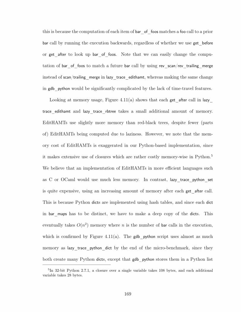
this is because the computation of each item of bar_of_foosmatches a foo call to a prior
bar call by running the execution backwards, regardless of whether we use get_before
or get_after to look up bar_of_foos. Note that we can easily change the compu-
tation of bar_of_foos to match a future bar call by using rev_scan/rev_trailing_merge
instead of scan/trailing_merge in lazy_trace_edithamt, whereas making the same change
in gdb_python would be significantly complicated by the lack of time-travel features.
Looking at memory usage, Figure 4.11(a) shows that each get_after call in lazy_
trace_edithamt and lazy_trace_rbtree takes a small additional amount of memory.
EditHAMTs use slightly more memory than red-black trees, despite fewer (parts
of) EditHAMTs being computed due to laziness. However, we note that the mem-
ory cost of EditHAMTs is exaggerated in our Python-based implementation, since
it makes extensive use of closures which are rather costly memory-wise in Python.5
We believe that an implementation of EditHAMTs in more efficient languages such
as C or OCaml would use much less memory. In contrast, lazy_trace_python_set
is quite expensive, using an increasing amount of memory after each get_after call.
This is because Python dicts are implemented using hash tables, and since each dict
in bar_maps has to be distinct, we have to make a deep copy of the dicts. This
eventually takes O(n2) memory where n is the number of bar calls in the execution,
which is confirmed by Figure 4.11(a). The gdb_python script uses almost as much
memory as lazy_trace_python_dict by the end of the micro-benchmark, since they
both create many Python dicts, except that gdb_python stores them in a Python list
5In 32-bit Python 2.7.1, a closure over a single variable takes 108 bytes, and each additionalvariable takes 28 bytes.
169
which has lower overhead than a trace. The strict_trace_edithamt script also uses a
lot memory, more than lazy_trace_edithamt by the end of the micro-benchmark, since
strict_trace_edithamt has to create every EditHAMT in bar_maps (the EditHAMTs
themselves are lazy), unlike lazy_trace_edithamt which only creates EditHAMTs in
bar_maps when they are looked up.
We see a similar pattern in Figure 4.11(b) for memory usage as in Figure 4.10(b)
for time usage: action 1 of lazy_trace_rbtree and lazy_trace_python_dict contributes
almost all of the cumulative memory usage by the end of the execution. As we
explained above for Figure 4.10(b), this is due to having to compute almost all red-
black trees or Python dicts in bar_maps.
4.5 Firefox Case Study: Delayed Deallocation Bug
To put Expositor to the test, we used it to track down a subtle bug in Firefox that
caused it to use more memory than expected (Zakai, 2011). The bug report contains a
test page that, when scrolled, creates a large number of temporary JavaScript objects
that should be immediately garbage collected. However, in a version of Firefox that
exhibits the bug (revision c5e3c81d35ba), the memory usage increases by 70MB (as
reported by top), and only decreases 20 seconds after a second scroll. As it turns out,
this bug has never been directly fixed—the actual cause is a data race, but the official
fix instead papers over the problem by adding another GC trigger.
Our initial hypothesis for this bug is that there is a problem in the JavaScript
garbage collector (GC). To test this hypothesis, we first run Firefox under Expos-
170
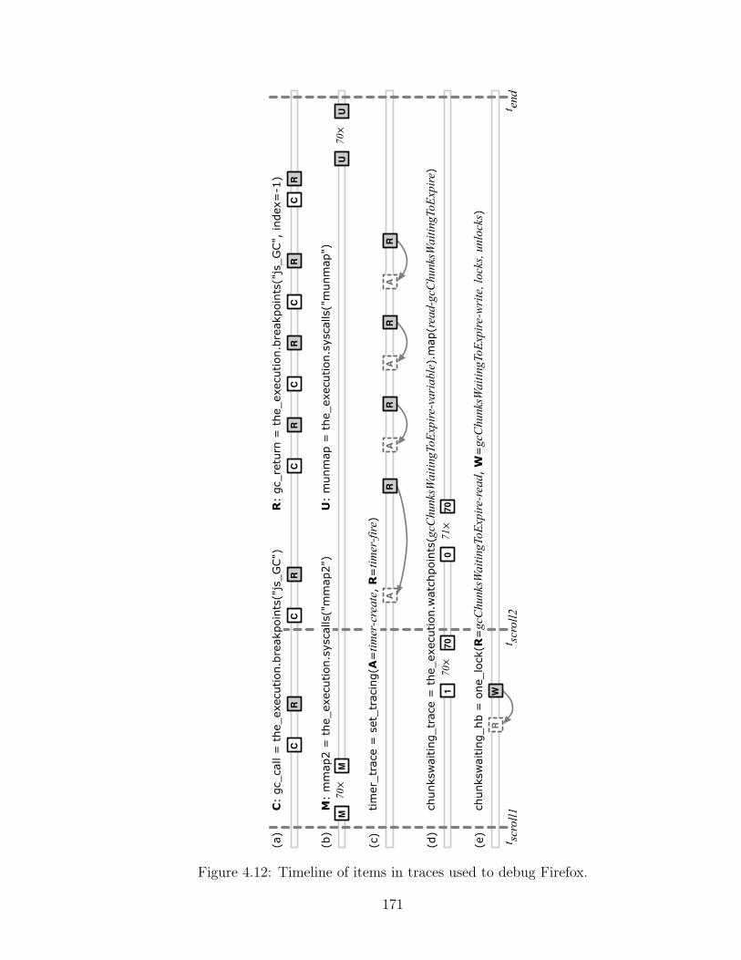
(a)
R:
gc_r
etur
n =
the
_exe
cutio
n.br
eakp
oint
s("j
s_G
C",
inde
x=-1
)
(b)
U:
mun
map
= t
he_e
xecu
tion.
sysc
alls
("m
unm
ap")
CR
70⨉
MM
CR
CR
CR
CR
70⨉
UU
CR
timer
_tra
ce =
set
_tra
cing
(A=
timer
-cre
ate,
R=
timer
-fire
)A
RA
RA
RA
R
chun
ksw
aitin
g_tr
ace
= t
he_e
xecu
tion.
wat
chpo
ints
(gcC
hunk
sWai
tingT
oExp
ire-
vari
able
).m
ap(r
ead-
gcC
hunk
sWai
tingT
oExp
ire)
70⨉
170
71⨉
070
chun
ksw
aitin
g_hb
= o
ne_l
ock(R
=gc
Chu
nksW
aitin
gToE
xpir
e-re
ad, W
=gc
Chu
nksW
aitin
gToE
xpir
e-w
rite
, loc
ks, u
nloc
ks)
RW
C:
gc_c
all =
the
_exe
cutio
n.br
eakp
oint
s("j
s_G
C")
M:
mm
ap2
= t
he_e
xecu
tion.
sysc
alls
("m
map
2")
(c)
(d)
(e)
t scr
oll1
t scr
oll2
t end
Figure 4.12: Timeline of items in traces used to debug Firefox.
171

itor, load the test page, and scroll it twice, temporarily interrupting the execution
to call the_execution.get_time() just before each scroll, time tscroll1 and time tscroll2 ,
and after the memory usage decreases, tend . Then, we create several traces to help us
understand the GC and track down the bug, as summarized in Figure 4.12.
We observe the GC behavior using a trace of the calls to (gc_call) and returns
from (gc_return) function js_GC (Figure 4.12a).6 Also, we find out when memory is
allocated or released to the operating system using mmap2 and munmap traces of the
same-named system calls (Figure 4.12b). Printing these traces reveals some oddly
inconsistent behavior: the GC is called only once after tscroll1 , but five times after
tscroll2 ; and memory is allocated after tscroll1 and deallocated just before tend . To make
sense of these inconsistencies, we inspect the call stack of each snapshot in gc_call
and discover that the first js_GC call immediately after a scroll is triggered by a scroll
event, but subsequent calls are triggered by a timer.
We now suspect that the first scroll somehow failed to trigger the creation of
subsequent GC timers. To understand how these timers are created, we write a
function called set_tracing that creates a trace for analyzing set-like behavior, using
EditHAMTs to track when values are inserted or removed, and apply set_tracing to
create timer_trace by treating timer creation as set insertion, and timer triggering as
set removal (Figure 4.12c). This trace reveals that each js_GC call creates a GC timer
(between gc_call and gc_return snapshots), except the js_GC call after the first scroll
(and the last js_GC call because GC is complete).
6The index=-1 optional argument to execution.breakpoints indicates that the breakpoint shouldbe set at the end of the function.
172

To find out why the first js_GC call does not create a GC timer, we inspect call
stacks again and learn that a GC timer is only created when the variable gcChunks-
WaitingToExpire is nonzero, and yet it is zero when the first js_GC returns (at the first
gc_return snapshot). Following this clue, we create a watchpoint trace on gcChunks-
WaitingToExpire and discover that it remained zero through the first js_GC call and
becomes nonzero only after the first js_GC returns. It stayed nonzero through the
second scroll and second js_GC call, causing the first GC timer to be created after
that (Figure 4.12d).
We posit that, for the GC to behave correctly, gcChunksWaitingToExpire should
become nonzero at some point during the first js_GC call. Inspecting call stacks
again, we find that gcChunksWaitingToExpire is changed in a separate helper thread,
and that, while the GC owns a mutex lock, it is not used consistently around gcChunks-
WaitingToExpire. This leads us to suspect that there is a data race. Thus, we develop
a simple race detection script, one_lock, that works by comparing each access to a
chosen variable against prior accesses from different threads (Section 4.3.1 explains
how we track prior accesses), and checking if a particular lock was acquired or released
prior to those accesses. For each pair of accesses, if at least one access is a write, and
the lock was not held in one or both accesses, then there is a race, which we indicate
as an item containing the snapshot of the prior access. We apply this race detector to
gcChunksWaitingToExpire and confirm our suspicion that, after tscroll1 , there is a write
that races with a prior read during the first js_GC call when the timer should have
been created (Figure 4.12e).
173

To give a sense of Expositor’s performance, it takes 2m6s to run the test page
to tscroll2 while printing the gc_call trace, with 383MB maximum resident memory
(including GDB, since Expositor extends GDB’s Python environment). The equiv-
alent task in GDB/UndoDB without Expositor takes 2m19s and uses 351MB of
memory (some difference is inevitable as the test requires user input, and Firefox
has many sources of nondeterminism). As another data point, finding the race after
tscroll1 takes 37s and another 5.4MB of memory.
The two analyses we developed, set_tracing and one_lock, take only 10 and 40
lines of code to implement, respectively, and both can be reused in other debugging
contexts.
4.6 Related Work
Expositor provides scripting for time-travel debuggers, with the central idea that
a target program’s execution can be manipulated (i.e., queried and computed over)
as a first-class object. Prior work on time-travel debugging has largely provided low-
level access to the underlying execution without consideration for scripting. Of the
prior work on scriptable debugging, Expositor is most similar to work that views
the program as an event generator—with events seeded from function calls, memory
reads/writes, etc.—and debugging scripts as database-style queries over event streams
or as dataflow-oriented stream transformers. None of this scripting work includes the
notion of time travel.
174

4.6.1 Time-Travel Debuggers
Broadly speaking, there are two classes of time-travel debuggers. Omniscient debug-
gers work by logging the state of the program being debugged after every instruc-
tion, and then reconstructing the state from the log on demand. Some examples
of omniscient debuggers include ODB (Lewis, 2003), Amber (also known as Chron-
icle) (O’Callahan, 2006), Tralfamadore (Lefebvre et al., 2012), and TOD (Pothier
et al., 2007). In contrast, replay debuggers work by logging the results of system calls
the program makes (as well as other sources of nondeterminism) and making inter-
mediate checkpoints, so that the debugger can reconstruct a requested program state
by starting at a checkpoint and replaying the program with the logged system calls.
Several recent debuggers of this style include URDB (Visan et al., 2011) and Un-
doDB (Undo Software) (which we used in our prototype) for user-level programs, and
TTVM (King et al., 2005) and VMware ReTrace (Xu et al., 2007) for entire virtual
machines. Expositor could target either style of debugger in principle, but replay
debugging scales much better (e.g., about 1.7× recording overhead for UndoDB vs.
300× for Amber). Engblom (Engblom, 2012) provides a more comprehensive survey
on time-travel debugging techniques and implementations.
The above work focuses on implementing time travel efficiently; most systems
provide very simple APIs for accessing the underlying execution, and do not consider
how time travel might best be exploited by debugging scripts.
Similarly, GDB’s Python environment simply allows a Python program to execute
GDB (and UndoDB) commands in a callback-oriented, imperative style. This is quite
175

tedious, e.g., just counting the number of calls to a particular function takes 16 lines
of code (Section 4.1.2), and cannot be composed with other scripts (e.g., to refine
the count to calls that satisfy predicate p). Expositor’s notion of traces is simpler
and more composable: function call counting can be done in one or two lines by
computing the length of a breakpoint trace; to refine the count, we simply filter the
trace with p before counting (Section 4.1.2).
Tralfamadore (Head et al., 2012) considers generalizing standard debugging com-
mands to entire executions, but does not provide a way to customize these commands
with scripts.
Whyline is a kind of omniscient debugger with which users can ask “why did ”
and “why didn’t” questions about the control- and data-flow in the execution, e.g.,
“why did this Button’s visible = true” or “why didn’t Window appear ” (Ko and Myers,
2008). Whyline records execution events (adding 1.7× to 8.5× overhead), and when
debugging begins, it uses program slicing (Xu et al., 2005) to generate questions
and the corresponding answers (imposing up to a 20× further slowdown). Whyline
is good at what it does, but its lack of scriptability limits its reach; it is hard to
see how we might have used it to debug the Firefox memory leak, for example. In
concept, Whyline can be implemented on top of Expositor, but limitations of GDB
and UndoDB (in particular, the high cost of software watchpoints, and the inability
to track data-flow through registers) makes it prohibitively expensive to track fine-
grained data-flow in an execution. We plan to overcome this limitation in future
work, e.g., using EDDI (Zhao et al., 2008) to implement fast software watchpoints.
176

4.6.2 High-Level (Non-callback Oriented) Debugging Scripts
Expositor’s design was inspired by MzTake (Marceau et al., 2007), a Scheme-based,
interactive, scriptable debugger for Java based on functional reactive programming.
In MzTake, the program being debugged is treated as a source of event streams
consisting of events such as function calls or value changes. Event streams can be
manipulated with combinators that filter, map, fold, or merge events to derive new
event streams. As such, an event stream in MzTake is like a trace in Expositor.
Computations in MzTake are implicitly over the most recent value of a stream and are
evaluated eagerly as the target program runs. To illustrate, consider our example of
maintaining a shadow stack from Section 4.1.3. In MzTake, when the target program
calls a function, a new snapshot event s becomes available on the calls stream. The
calls_rets stream’s most recent event is the most recent of calls and rets, so MzTake
updates it to s. Since shadow_stacks is derived from calls_rets, MzTake updates its
most recent event by executing map(int, s.read_retaddrs())).
This eager updating of event streams, as the program executes, can be less efficient
than using Expositor. In particular, Expositor evaluates traces lazily so that
computation can be narrowed to a few slices of time. In Section 4.1.3, we find the
latest smashed stack address without having to maintain the shadow stack for the
entire program execution, as would be required for MzTake. Also, Expositor traces
are time indexed, but MzTake event streams are not: there is no analogue to tr.get_at(
i) or tr.slice(t0, t1) in MzTake. We find time indexing to be very useful for interactivity:
we can run scripts to identify an interesting moment in the execution, then explore
177

the execution before and after that time. Similarly, we can learn something useful
from the end of the execution (e.g., the address of a memory address that is double-
freed), and then use it in a script on an earlier part of the execution (e.g., looking for
where that address was first freed). MzTake requires a rerun of the program, which
can be a problem if nondeterminism affects the relevant computation.
Dalek (Olsson et al., 1991) and Event Based Behavioral Abstraction (EBBA) (Bates,
1988) bear some resemblance to MzTake and suffer the same drawbacks, but are much
lower-level, e.g., the programmer is responsible for manually managing the firing and
suppression of events. Coca (Ducassé, 1999) is a Prolog-based query language that
allows users to write predicates over program states; program execution is driven by
Prolog backtracking, e.g., to find the next state to match the predicate. Coca provides
a retrace primitive that restarts the entire execution to match against new predicates.
This is not true time travel but re-execution, and thus suffers the same problems as
MzTake.
PTQL (Goldsmith et al., 2005), PQL (Martin et al., 2005), and UFO (Augus-
ton et al., 2002) are declarative languages for querying program executions, as a
debugging aid. Queries are implemented by instrumenting the program to gather the
relevant data. In principle, these languages are subsumed by Expositor, as it is
straightforward to compile queries to traces. Running queries in Expositor would
allow programmers to combine results from multiple queries, execute queries lazily,
and avoid having to recompile (and potentially perturb the execution of) the program
for each query. On the other hand, it remains to be seen whether Expositor traces
would be as efficient as using instrumentation.
178

Chapter 5
Towards a Grand Unified Debugger
This dissertation is part of a much larger vision to rethink the way we build high qual-
ity software. Over the course of our research, we have come to realize that program
analysis tools are part of a much larger debugging process. Therefore, we should con-
sider how the debugging process can be augmented with program analyses and bug
finding tools, rather than building tools that are then shoehorned into the debugging
process. Furthermore, we observe that debugging is a largely distinct process from
programming and requires a different skill set (albeit with some overlap). Program-
ming is a constructive engineering activity, where programmers begin with a design
goal, then incrementally write source code to achieve that goal. In contrast, debug-
ging is a deductive scientific activity, where programmers begin with a (potential)
misbehavior in a program and source code for the program,1 then derive hypotheses
to explain the misbehavior and eventually track down the root cause.
Based on the above viewpoint, we envision designing a Grand Unified Debugger
(GUD)2 that specifically addresses the needs of programmers performing debugging
1If they are lucky, it will be source code they have written; more likely, it will be source codewritten by someone else, or no source code at all.
2A more humble name would be “Integrated Debugging Environment”, but that would be tooeasily confused with “Integrated Development Environment”.
179

tasks, as a complement to integrated development environments (IDEs) that are de-
signed for programming tasks. Since debugging typically begins by examining a (po-
tential) misbehavior, we propose that the core artifacts of a GUD should be program
paths or execution traces that demonstrate or exhibit the misbehavior, in contrast
to IDEs where the central artifacts are typically source code. These program paths
or execution traces may be concretely generated from test cases or by running the
program under an interactive debugger, or they may be synthetically derived, e.g.,
from the output of program analysis tools. We believe that the GUD should provide
the following core features:
1. a user interface to generate, inspect and analyze program paths or execution
traces, and relate them back to source code;
2. a library of program analyses for debugging, as well as facilities to customize
existing analyses or write new analyses; and
3. ways for programmers to organize debugging hypotheses to be systematically
confirmed or refuted.
5.1 A User Interface for Debugging
We believe that a combination of Path Projection and Expositor would be an
excellent basis for a user interface to generate, inspect and analyze program paths or
execution traces. For example, given a program path, we imagine first using Path
Projection as a user interface for interactive debugging to generate an execution
180
trace that corresponds to that program path. Then, we can use Expositor, aug-
mented with a visual timeline-like interface resembling Figure 4.12, to examine an
execution trace at a high level overview of events. We can also use Path Projec-
tion again to examine execution trace segments at a low, binary or source-code level
of detail.
There are many interesting research questions that need to be answered to de-
velop this user interface. For example, how should Path Projection be adapted to
visualize program paths that are incrementally generated via an interactive debugger,
or to visualize partial trace segments, since a complete execution trace would result
in an excessively large visualization? As another example, how should the timeline
interface for Expositor be designed to visualize a trace of events, such as break-
points, that may simultaneously be densely packed around certain trace segments,
yet be sparsely spread throughout the entire trace?
5.2 Program Analyses for Debugging
Expositor, in a sense, is a primitive realization of the GUD vision in that it unifies
dynamic program analysis with interactive debugging. We believe that debugging
scripts written using the Expositor API are essentially as expressive as dynamic
program analyses, but are written in a more declarative style, and are more suited
for analyzing traces interactively. Nonetheless, more research is needed to determine
what sort of dynamic program analysis can be implemented effectively in Expositor,
to come up with new kinds of dynamic program analysis that can take full advantage
181
of laziness, and to determine the best way to compose dynamic program analyses from
small, reusable components such that intermediate results can be easily examined and
the analyses can be customized by programmers.
As a first step to answering these questions, we have developed a preliminary
version of a happens-before data race detector (Lamport, 1978) in Expositor. While
we were able to write the happens-before data race detector as an Expositor script,
it is currently impractical to use it due to a number of limitations in our Expositor
prototype. In particular, our Expositor prototype treats GDB and UndoDB as
black boxes, using GDB/UndoDB commands to query for breakpoint or watchpoint
events in an execution trace. This turns out to be very slow: if we had used the
happens-before race detector in place of the simple one_lock race detector in our
Firefox case study (Section 4.5), it would have taken hours instead of minutes to
verify the data race, due to processing the sheer quantity of lock/unlock events even
in a short trace segment. Furthermore, it is difficult to track data flow quickly and
accurately using GDB/UndoDB, since hardware watchpoints are limited to only four
memory addresses (on x86), GDB’s software watchpoints are prohibitively slow, and
it is non-trivial to use GDB to track data flow through registers.
We believe that solving these problems requires deeper integration between Ex-
positor and the time-travel backend. At first, this would allow us to implement
techniques such as fast watchpoints based on EDDI (Zhao et al., 2008) in Expos-
itor. Moreover, this would create many opportunities for new analysis techniques
based on time-travel debugging technology. In particular, time-travel provides de-
terministic replay, which means that we can implement dynamic program analysis
182
techniques in a far more intrusive manner without fear of perturbing the execution,
for example, to track data flow in a manner similar to Valgrind (Nethercote and
Seward, 2007). Also, deterministic replay potentially allows us to run Expositor
scripts more quickly by making parallel queries to the time-travel backend.
5.2.1 Static Program Analyses for Debugging
Static program analysis is another style of program analysis that works not by run-
ning the target software, but by analyzing the source code or binary. Static program
analyses can potentially find many more bugs than dynamic program analyses, how-
ever, static program analyses are usually less precise in that they may report more
false warnings.
One interesting research question to ask is if we can apply static program analyses
to Expositor for debugging. In other words, can we combine static program analy-
ses with time-travel based dynamic program analyses, either to optimize time-travel
queries, or to increase the precision of the static program analyses? Perhaps we can
use an approach similar to Mix to combine static program analyses and time-travel
dynamic program analyses across disjoint trace segments.
Conversely, can we use the Expositor API to write static program analyses, i.e.,
to ensure the correctness of all possible executions of the target software? We can
perhaps achieve this by substituting symbolic executors (Cadar et al., 2011) or model
checkers (Jhala and Majumdar, 2009) in place of the time-travel debugger. Unlike
time-travel debuggers which can only answer queries about particular execution trace,
symbolic executors and model checkers can generate and answer queries about all
183

possible execution traces of the target software. This approach eliminates the need to
generate a failing execution in the time-travel debugger, which is especially difficult
when the bug is nondeterministic, before the debugging process can begin.
5.3 A Systematic Approach to Debugging
When debugging, it can be more productive to keep the debugging process organized
by deriving hypotheses to explain the misbehavior and systematically confirming or
refuting each hypothesis, in a manner analogous to using specification documents to
organize programming. One possible approach is to use checklists: as a side result
of our user studies on Path Projection, we found that when checklists are used,
programmers were able to verify the results of program analysis 41% faster than
without checklists (Section 2.3). Similarly, Dillig et al. (2012) recently presented a
method to automatically derive checklists to triage program analyses, and found that
programmers improved their triaging accuracy from 33% to 90%, yet spent only 20%
of the time to do so. These checklists were designed to triage program analysis results;
we believe it would be interesting to consider how to design checklists for deriving
debugging hypotheses, or for guiding the systematic evaluation of these hypotheses.
184
Chapter 6
Conclusion
In this dissertation, we have presented three approaches to designing better program
analysis tools that are more accessible and useful to programmers.
First, to improve the user interface of program analysis tools, we introduced Path
Projection, a new program visualization toolkit that is specifically designed to
help programmers navigate and understand program paths, a common output of
many program analysis tools. Path Projection visualizes multiple paths side-by-
side, using function call inlining and code folding to show those paths in a compact
format. Our interface also includes a multi-query search facility to locate and reveal
multiple terms simultaneously. To our knowledge, Path Projection is the first
tool-independent framework for visualizing program analysis results in particular,
and program paths in general.
We measured the performance of Path Projection for triaging error reports
from Locksmith, a data race detection tool for C. For this experiment, we added
a task-specific checklist that enumerates the sub-tasks needed to triage each error
report. Our controlled user study showed that, compared to a standard viewer, Path
Projection reduced completion times for triaging data races, with no adverse effect
on accuracy, and that users felt that Path Projection was useful. We also found the
185

checklist improved performance overall compared to a pilot study. To our knowledge,
ours is the first study of the impact of the user interface on the efficiency and accuracy
of triaging program analysis error reports.
Second, to enable programmers to customize a program analysis tool for a particu-
lar target software, we presented Mix, a new program analysis framework that allows
programmers to apply either type checking or symbolic execution to different parts
of the target software, trading efficiency for precision as appropriate. The key feature
of our approach is that the mixed systems are essentially completely independent,
and they are used in an off-the-shelf manner. Only at the boundaries between typed
blocks—which the user inserts to indicate where type checking should be used—and
symbolic blocks—the symbolic checking annotation—do we invoke special mix rules to
translate information between the two systems. We proved that Mix is sound (which
implies that type checking and symbolic execution are also independently sound).
We also described a preliminary implementation, Mixy, which performs null/non-
null type qualifier inference for C. We identified several cases in which symbolic
execution could eliminate false positives from type inference. We believe that Mix
provides a promising new approach to trade off precision and efficiency in program
analysis.
Finally, to give programmers greater insight into the inner workings of program
analyses, we designed Expositor, a novel environment that unifies dynamic program
analysis and interactive debugging, based on scripting and time-travel debugging. Ex-
positor allows programmers to project a program execution onto immutable traces,
which support a range of powerful combinators including map, filter, merge, and scan.
186

The trace abstraction gives programmers a global view of the program, and is easy to
compose and reuse, providing a convenient way to correlate and understand events
across the execution timeline. For efficiency, Expositor traces are implemented us-
ing a lazy, interval-tree-like data structure. Expositor materializes the tree nodes
on demand, ultimately calling UndoDB to retrieve appropriate snapshots of the pro-
gram execution. Expositor also includes the EditHAMT, which lets script writers
create lazy sets, maps, multisets, and multimaps that integrate with traces without
compromising their laziness. We ran two micro-benchmarks that show that Expos-
itor scripts using lazy traces can be faster than the equivalent non-lazy scripts in
common debugging scenarios, and that the EditHAMT is crucial to ensure that trace
laziness is not compromised. We used Expositor to find a buffer overflow in a small
program, and to diagnose a very complex, subtle bug in Firefox. We believe that
Expositor holds promise for helping programmers better understand complex bugs
in large software systems.
As future work, we propose the Grand Unified Debugger (GUD), a conceptual en-
vironment designed specifically for debugging tasks. The core artifacts of the GUD are
program paths or execution traces, instead of source code as for IDEs, and the GUD
makes use of ideas from Path Projection, Expositor and Mix to allow program-
mers to examine these paths or traces. In addition, we suggest several new ideas for
the GUD, including a timeline-like visualization for Expositor-style traces, program
analysis techniques that combine time-travel debugging with heavyweight dynamic
analysis or static analysis, as well as checklists to support systematic debugging.
187
Appendix A
Mix Soundness
To show the soundness of Mix, we consider a standard big-step operational semantics
for our simple language of expressions (Appendix A.1). We then show the soundness
of type checking and symbolic execution separately (Appendices A.2 and A.3, respec-
tively), which will provide the basis for Mix soundness (Appendix A.4). This section
is an expansion of Section 3.2.3.
Type soundness is entirely standard. For symbolic execution soundness, we con-
sider two notions in turn: when an execution is sound with respect to a path of
exploration and when a set of executions cover all possible concrete execution paths.
One challenge for showing Mix soundness is that symbolic execution allows a tempo-
rary violation of the type invariant on memory used by the type checker, which must
be restored before entering a type checking phase.
A.1 Operational Semantics
Figure A.1 gives a big-step operational semantics for our language of expressions e. In
these rules, M is a concrete memory that maps locations l to values v. We make this
a mapping, rather than a list, to reflect the fact that the memory is actually updated
188

Big-Step Operational Semantics. E ` 〈M ; e〉 → 〈M ′; v〉
SVar
E, x : v ` 〈M ;x〉 → 〈M ; v〉
SVal
E ` 〈M ; v〉 → 〈M ; v〉
SPlusE ` 〈M ; e1〉 → 〈M1;n1〉 E ` 〈M1; e2〉 → 〈M2;n2〉
E ` 〈M ; e1 + e2〉 → 〈M2;n1 + n2〉
SEqE ` 〈M ; e1〉 → 〈M1; v1〉 E ` 〈M1; e2〉 → 〈M2; v2〉
E ` 〈M ; e1 = e2〉 → 〈M2; v1 = v2〉
SNotE ` 〈M ; e1〉 → 〈M1; b1〉
E ` 〈M ;¬e1〉 → 〈M1;¬b1〉
SAndE ` 〈M ; e1〉 → 〈M1; b1〉 E ` 〈M1; e2〉 → 〈M2; b2〉
E ` 〈M ; e1 ∧ e2〉 → 〈M2; b1 ∧ b2〉
SIf-TrueE ` 〈M ; e1〉 → 〈M1; true〉 E ` 〈M1; e2〉 → 〈M2; v〉
E ` 〈M ; if e1 then e2 else e3〉 → 〈M2; v〉
SIf-FalseE ` 〈M ; e1〉 → 〈M1; false〉 E ` 〈M1; e3〉 → 〈M3; v〉
E ` 〈M ; if e1 then e2 else e3〉 → 〈M3; v〉
SLetE ` 〈M ; e1〉 → 〈M1; v1〉 E, x : v1 ` 〈M1; e2〉 → 〈M2; v2〉
E ` 〈M ; let x = e1 in e2〉 → 〈M2; v2〉
SRefE ` 〈M ; e1〉 → 〈M1; v1〉 l 6∈ dom(M1)
E ` 〈M ; ref e1〉 → 〈M1[l 7→ v1]; l〉
SAssignE ` 〈M ; e1〉 → 〈M1; l〉 E ` 〈M1; e2〉 → 〈M2; v2〉 l ∈ dom(M2)
E ` 〈M ; e1 := e2〉 → 〈M2[l 7→ v2]; v2〉
SDerefE ` 〈M ; e1〉 → 〈M1; l1〉 l1 ∈ dom(M1)
E ` 〈M ; !e1〉 → 〈M1;M1(l1)〉
SSymBlockE ` 〈M ; e1〉 → 〈M1; v1〉
E ` 〈M ; {s e1 s}〉 → 〈M1; v1〉
STypBlockE ` 〈M ; e1〉 → 〈M1; v1〉
E ` 〈M ; {t e1 t}〉 → 〈M1; v1〉
Figure A.1: Standard big-step operational semantics.
189

on the running system. The notation M [l 7→ v] indicates an update or extension
of M so that l 7→ v (depending on whether or not l ∈ dom(M), respectively). We
consider the set of locations to be included in the set of values. The basic form of the
evaluation judgment:E ` 〈M ; e〉 → 〈M ′; v〉
says that in a concrete environment E, an initial memory M and an expression e
evaluate to a resulting memory M ′ and a value v. A concrete environment maps
variables to values (i.e., we define E ::= ∅ | E, x : v). To indicate boolean values,
we use the meta-variable b (i.e., we let b ::= false | true). To reiterate and make it
explicit, we work with following semantic domains:
v ∈ Val concrete valuesx ∈ Var program variablesl ∈ Loc ⊆ Val memory locations
E : Var⇀fin Val = Env concrete environmentsM : Loc⇀fin Val = Mem concrete memories
In addition to the rules shown in Figure A.1, there are also rules that produce
error when none of these rules apply, which is also standard. We define:
r ::= 〈M ; v〉 | error
as the result of an execution, so the general form of our execution judgment is as
follows:E ` 〈M ; e〉 → r
For example, we have the following error rule for ¬e:
SNot-ErrorE ` 〈M ; e1〉 → r1 r1 6= 〈M1; b1〉
E ` 〈M ;¬e1〉 → error
190

A.2 Type Soundness
Figure A.2 shows the type checking rules for our language. Again, these rules are
entirely standard. As usual, we introduce a memory type environment Λ that maps
locations to types, and we update the typing judgment to carry this additional envi-
ronment:Γ `Λ e : τ
Because Λ is constant in all rules, we elide it except where needed for clarity in
presentation. The memory type environment Λ is used to assign types to locations l;
specifically, we add the following typing rule:
TLoc
Γ `Λ l : Λ(l) ref
Type Checking. Γ ` e : τ
TVar
Γ, x : τ ` x : τ
TInt
Γ ` n : int
TBool
Γ ` b : bool
TPlusΓ ` e1 : int Γ ` e2 : int
Γ ` e1 + e2 : int
TEqΓ ` e1 : τ Γ ` e2 : τ
Γ ` e1 = e2 : bool
TNotΓ ` e : bool
Γ ` ¬e : bool
TAndΓ ` e1 : bool Γ ` e2 : bool
Γ ` e1 ∧ e2 : bool
TIfΓ ` e1 : bool Γ ` e2 : τ Γ ` e3 : τ
Γ ` if e1 then e2 else e3 : τ
TLetΓ ` e1 : τ1 Γ, x : τ1 ` e2 : τ2
Γ ` let x = e1 in e2 : τ2
TRefΓ ` e : τ
Γ ` ref e : τ ref
TAssignΓ ` e1 : τ ref Γ ` e2 : τ
Γ ` e1 := e2 : τ
TDerefΓ ` e : τ ref
Γ ` !e : τ
Figure A.2: Standard type checking rules.
191

We write Λ′ ⊇ Λ if Λ′ is an extension of Λ. Formally, Λ′ ⊇ Λ if:
dom(Λ′) ⊇ dom(Λ) and Λ′(l) = Λ(l) for all l ∈ dom(Λ) .
We also use the same notation for other mapping extensions.
To prove type soundness, we define a soundness relation that says that the val-
ues in the concrete environment and concrete memory are consistent with the type
environments:
Definition 2 (Type State Soundness Relation)
We define soundness relations for type environments as follows:
〈E;M〉 ∼ 〈Γ; Λ〉 if
E ∼ 〈Γ; Λ〉 and M ∼ Λ
E ∼ 〈Γ; Λ〉 if
∅ `Λ E(x) : Γ(x) for all x ∈ dom(E) = dom(Γ)
M ∼ Λ if
∅ `Λ M(l) : Λ(l) for all l ∈ dom(M) = dom(Λ)
The following theorem states type soundness and is proved only for the rules in
Figure A.2 (i.e., everything excluding the nested block rule in Figure 3.4).
Theorem 3 (Type Soundness)
If
E ` 〈M ; e〉 → r and
Γ `Λ e : τ such that
〈E;M〉 ∼ 〈Γ; Λ〉 ,
192
then ∅ `Λ′ v : τ and M ′ ∼ Λ′ for some M ′, v, and Λ′ such that r = 〈M ′; v〉 and
Λ′ ⊇ Λ.
Proof
By induction on the derivation of E ` 〈M ; e〉 → r.
Notice that above theorem says that r, the result of evaluating a well-typed ex-
pression, cannot be error.
A.3 Symbolic Execution Soundness
Intuitively, symbolic execution begins with symbolic values α for unknown inputs and
accumulates a symbolic expression s that represents the result of the program along a
path. Thus, at a high-level, a symbolic execution is sound along a path if interpreting
the symbolic result under an assignment to the symbolic values (i.e., the unknowns)
yields the same value as the concrete execution along that path.
To capture this assignment to symbolic values, or valuation, we write:
V : SymVal⇀fin Val ∪Mem
for a finite mapping from symbolic values α (drawn from set SymVal) to concrete
values v (from Val) or concrete memories M (from Mem). Recall that a concrete
environment E : Var ⇀fin Val is a finite mapping from variables to values, and a
concrete memory M : Loc⇀fin Val is a finite mapping from locations to values.
193

Concretization. JsKV = v JΣKV = E JmKV = M
Ju:τKV def= JuKV
JαKV def= V (α)
JvKV def= v
Ju1:int + u2:intKV def= Ju1KV + Ju2KV
Js1 = s2KVdef= Js1KV = Js2KV
J¬gKV def= ¬JgKV
Jg1 ∧ g2KVdef= Jg1KV ∧ Jg2KV
Jm[u:τ ref]KV def= JmKV (JuKV )
JµKV def= V (µ)
Jm, (s1 � s2)KV def= JmKV
[Js1KV 7→ Js2KV
]Jm, (s1
a� s2)KV def= JmKV
[Js1KV 7→ Js2KV
]J∅KV def
= ∅JΣ, x : sKV def
= JΣKV , x : JsKV
Figure A.3: Interpretation of symbolic expressions, symbolic memories, and symbolicenvironments.
Given a valuation V , the interpretation of symbolic expressions, symbolic memo-
ries, and symbolic environments is largely as expected, which we define in Figure A.3.
We write the following for these interpretations:
JsKV = v JmKV = M JΣKV = E
The interpretation of symbolic expressions ignores the type annotation, though would
be ill-defined if the symbolic expressions were not well-typed with respect to the
valuation V .
194

Our typed symbolic execution tracks the type of symbolic expressions (i.e., the
type of the value under any valuation that respects the types of the unknowns) and
halts upon encountering ill-typed expressions. Observe that this behavior matches
the concrete executor (i.e., the big-step operational semantics in Figure A.1). This
typing of symbolic expressions must be with respect to a memory typing Λ and thus
must be part of the soundness relation. Moreover, the symbolic executor distinguishes
between the locations in the arbitrary memory on entry and the locations that come
from allocations during execution, which must be reflected in the symbolic state
soundness relation.
Definition 4 (Symbolic State Soundness Relation)
We define soundness relations for environment-memory pairs and memory-value pairs
using the concretization defined above, which are parametrized by a valuation V , a
memory typing for the arbitrary memory on entry Λ0, and the memory typing for
locations allocated during symbolic execution Λ.
〈E;M〉 ∼Λ0·V ·Λ 〈Σ;m〉 if
JΣKV = E and E ∼ 〈Γ; Λ0 ∗ Λ〉 and` Σ : Γ for some Γ andJmKV = M and Λ0 `V m : Λ0 ∗ Λ
〈M ; v〉 ∼Λ0·V ·Λ 〈m;u:τ〉 if
JmKV = M and Λ0 `V m : Λ0 ∗ Λ andJu:τKV = v and ∅ `Λ0∗Λ v : τ
where we write Λ1 ∗ Λ2 to mean the memory typing that is the union of submemory
typings Λ1 and Λ2 with disjoint domains.
There are several pieces to these definitions:
195
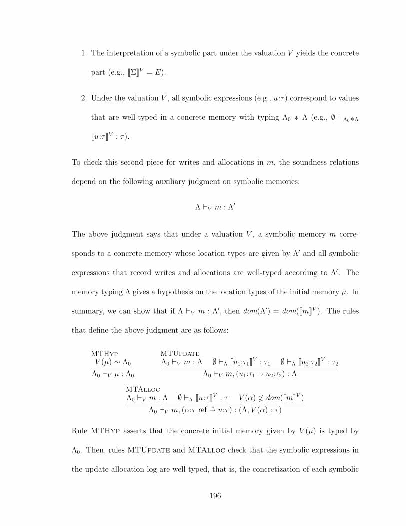
1. The interpretation of a symbolic part under the valuation V yields the concrete
part (e.g., JΣKV = E).
2. Under the valuation V , all symbolic expressions (e.g., u:τ) correspond to values
that are well-typed in a concrete memory with typing Λ0 ∗ Λ (e.g., ∅ `Λ0∗Λ
Ju:τKV : τ).
To check this second piece for writes and allocations in m, the soundness relations
depend on the following auxiliary judgment on symbolic memories:
Λ `V m : Λ′
The above judgment says that under a valuation V , a symbolic memory m corre-
sponds to a concrete memory whose location types are given by Λ′ and all symbolic
expressions that record writes and allocations are well-typed according to Λ′. The
memory typing Λ gives a hypothesis on the location types of the initial memory µ. In
summary, we can show that if Λ `V m : Λ′, then dom(Λ′) = dom(JmKV ). The rules
that define the above judgment are as follows:
MTHypV (µ) ∼ Λ0
Λ0 `V µ : Λ0
MTUpdateΛ0 `V m : Λ ∅ `Λ Ju1:τ1KV : τ1 ∅ `Λ Ju2:τ2KV : τ2
Λ0 `V m, (u1:τ1 � u2:τ2) : Λ
MTAllocΛ0 `V m : Λ ∅ `Λ Ju:τKV : τ V (α) 6∈ dom(JmKV )
Λ0 `V m, (α:τ refa� u:τ) : (Λ, V (α) : τ)
Rule MTHyp asserts that the concrete initial memory given by V (µ) is typed by
Λ0. Then, rules MTUpdate and MTAlloc check that the symbolic expressions in
the update-allocation log are well-typed, that is, the concretization of each symbolic
196

expression has the type claimed by its typing annotation (e.g., observe τ1 in the
premise ∅ `Λ Ju1:τ1KV : τ1 of MTUpdate). However, this judgment does not ensure
that writes are well-typed (i.e., in MTUpdate, types τ1 and τ2 do not need to be
compatible), as symbolic execution allows temporarily type-inconsistent memory.
Temporarily Type-Inconsistent Memory. A property of symbolic execution
is that it does not require all writes to be consistent with the memory typing (i.e.,
Λ0 ∗ Λ), as long as the consistency is restored before assigning types to expressions
that use memory. This temporary violation of the memory typing invariant allows us
to obtain, for example, flow-sensitive type checking. The memory type consistency
judgment is a validation that the memory typing invariant gets restored, and its
soundness is stated as follows:
Lemma 5 (Memory Type Consistency Soundness)
If ` m ok U and Λ0 `V m : Λ, then
∅ `Λ JmKV (l) : Λ(l) for all l ∈ dom(Λ)\L
whereL =
⋃s1�s2∈U
Js1KV .
As a corollary, if` m ok and Λ0 `V m : Λ ,
then JmKV ∼ Λ.
197
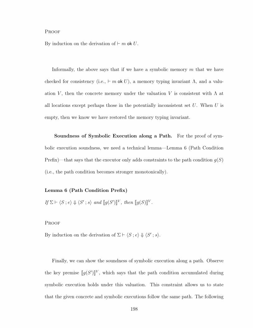
Proof
By induction on the derivation of ` m ok U .
Informally, the above says that if we have a symbolic memory m that we have
checked for consistency (i.e., ` m ok U), a memory typing invariant Λ, and a valu-
ation V , then the concrete memory under the valuation V is consistent with Λ at
all locations except perhaps those in the potentially inconsistent set U . When U is
empty, then we know we have restored the memory typing invariant.
Soundness of Symbolic Execution along a Path. For the proof of sym-
bolic execution soundness, we need a technical lemma—Lemma 6 (Path Condition
Prefix)—that says that the executor only adds constraints to the path condition g(S)
(i.e., the path condition becomes stronger monotonically).
Lemma 6 (Path Condition Prefix)
If Σ ` 〈S ; e〉 ⇓ 〈S ′ ; s〉 and Jg(S ′)KV , then Jg(S)KV .
Proof
By induction on the derivation of Σ ` 〈S ; e〉 ⇓ 〈S ′ ; s〉.
Finally, we can show the soundness of symbolic execution along a path. Observe
the key premise Jg(S ′)KV , which says that the path condition accumulated during
symbolic execution holds under this valuation. This constraint allows us to state
that the given concrete and symbolic executions follow the same path. The following
198

theorem is proven only for the rules in Figures 3.2 and 3.3 (i.e., everything excluding
the nested block rule in Figure 3.4).
Theorem 7 (Symbolic Execution Soundness)
If
E ` 〈M ; e〉 → r and
Σ ` 〈S ; e〉 ⇓ 〈S ′ ; s〉 such that
〈E;M〉 ∼Λ0·V ·Λ 〈Σ;m(S)〉 and Jg(S ′)KV ,
thenr ∼Λ′
0·V ′·Λ′ 〈m(S ′); s〉
for some V ′ ⊇ V and some Λ′0,Λ′ such that Λ′0 ∗ Λ′ ⊇ Λ0 ∗ Λ.
Proof
By induction on the derivation of E ` 〈M ; e〉 → r.
Case SVar
By assumption, we have that
SVar
E, x : v ` 〈M ;x〉 → 〈M ; v〉
The only symbolic execution rule that applies is SEVar.
SEVar
Σ, x : s ` 〈S ; x〉 ⇓ 〈S ; s〉
Since by assumption, we have that
〈E, x : v;M〉 ∼Λ0·V ·Λ 〈Σ, x : s;m(S)〉 ,
199
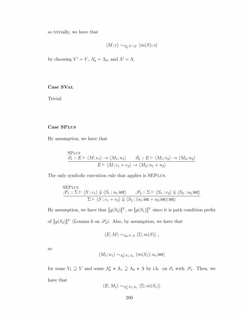
so trivially, we have that
〈M ; v〉 ∼Λ′0·V ′·Λ′ 〈m(S); s〉
by choosing V ′ = V , Λ′0 = Λ0, and Λ′ = Λ.
Case SVal
Trivial.
Case SPlus
By assumption, we have that
SPlusE1 :: E ` 〈M ; e1〉 → 〈M1;n1〉 E2 :: E ` 〈M1; e2〉 → 〈M2;n2〉
E ` 〈M ; e1 + e2〉 → 〈M2;n1 + n2〉
The only symbolic execution rule that applies is SEPlus.
SEPlusS1 :: Σ ` 〈S ; e1〉 ⇓ 〈S1 ; u1:int〉 S2 :: Σ ` 〈S1 ; e2〉 ⇓ 〈S2 ; u2:int〉
Σ ` 〈S ; e1 + e2〉 ⇓ 〈S2 ; (u1:int + u2:int):int〉
By assumption, we have that Jg(S2)KV , so Jg(S1)KV since it is path condition prefix
of Jg(S2)KV (Lemma 6 on S2). Also, by assumption, we have that
〈E;M〉 ∼Λ0·V ·Λ 〈Σ;m(S)〉 ,
so〈M1;n1〉 ∼Λ′′
0 ·V1·Λ1〈m(S1);u1:int〉
for some V1 ⊇ V and some Λ′′0 ∗ Λ1 ⊇ Λ0 ∗ Λ by i.h. on E1 with S1. Then, we
have that〈E;M1〉 ∼Λ′′
0 ·V1·Λ1〈Σ;m(S1)〉
200

and Jg(S2)KV1 because V1 ⊇ V , so
〈M2;n2〉 ∼Λ′0·V ′·Λ′ 〈m(S2);u2:int〉
for some V ′ ⊇ V1 ⊇ V and some Λ′0 ∗ Λ′ ⊇ Λ′′0 ∗ Λ1 ⊇ Λ0 ∗ Λ by i.h. on E2 with
S2. Since V ′ ⊇ V1, we have that Ju1:intKV ′= n1, so
J(u1:int + u2:int):intKV′= n1 + n2
and thus〈M2;n1 + n2〉 ∼Λ′
0·V ′·Λ′ 〈m(S2); (u1:int + u2:int):int〉 .
Case SEq, SNot, SAnd
Similar to the case for SPlus.
Case SIf-True
By assumption, we have that
SIf-TrueE1 :: E ` 〈M ; e1〉 → 〈M1; true〉 E2 :: E ` 〈M1; e2〉 → 〈M2; v〉
E ` 〈M ; if e1 then e2 else e3〉 → 〈M2; v〉
The only symbolic execution rules that could apply are SEIf-True or SEIf-False.
Sub-case SEIf-True
SEIf-TrueS1 :: Σ ` 〈S ; e1〉 ⇓ 〈S1 ; g1〉 S2 :: Σ ` 〈S1[g 7→ g(S1) ∧ g1] ; e2〉 ⇓ 〈S2 ; s2〉
Σ ` 〈S ; if e1 then e2 else e3〉 ⇓ 〈S2 ; s2〉
201
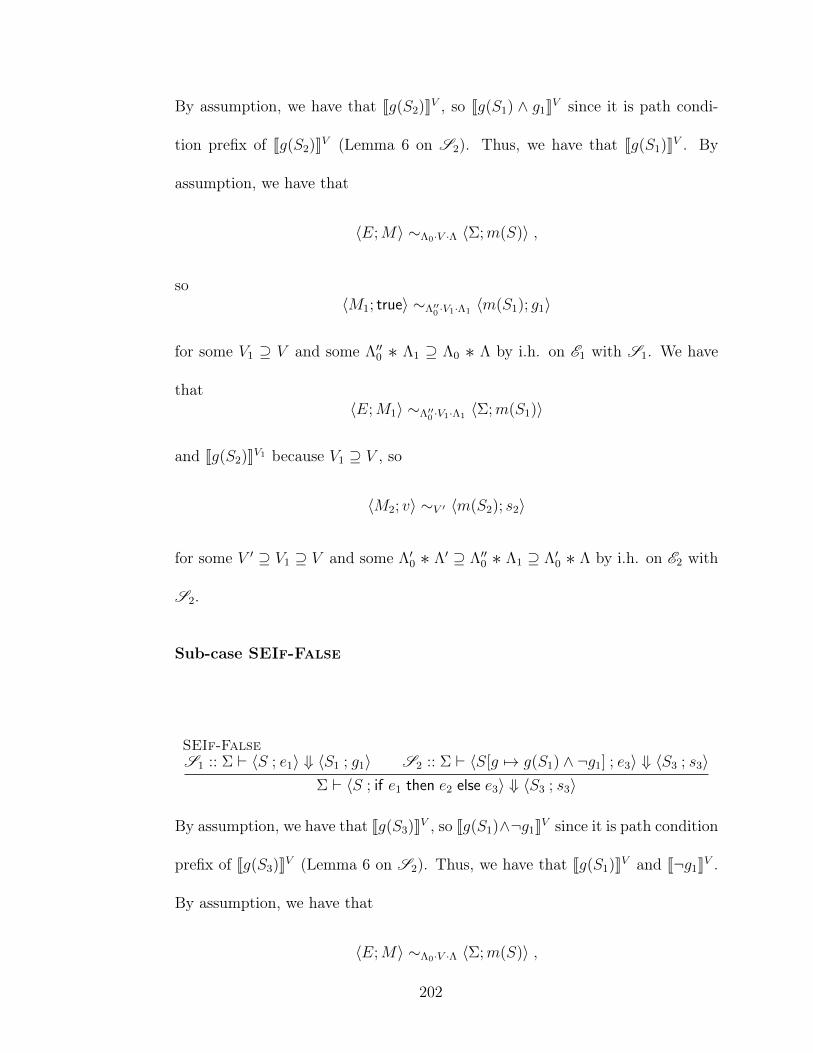
By assumption, we have that Jg(S2)KV , so Jg(S1) ∧ g1KV since it is path condi-
tion prefix of Jg(S2)KV (Lemma 6 on S2). Thus, we have that Jg(S1)KV . By
assumption, we have that
〈E;M〉 ∼Λ0·V ·Λ 〈Σ;m(S)〉 ,
so〈M1; true〉 ∼Λ′′
0 ·V1·Λ1〈m(S1); g1〉
for some V1 ⊇ V and some Λ′′0 ∗ Λ1 ⊇ Λ0 ∗ Λ by i.h. on E1 with S1. We have
that〈E;M1〉 ∼Λ′′
0 ·V1·Λ1〈Σ;m(S1)〉
and Jg(S2)KV1 because V1 ⊇ V , so
〈M2; v〉 ∼V ′ 〈m(S2); s2〉
for some V ′ ⊇ V1 ⊇ V and some Λ′0 ∗ Λ′ ⊇ Λ′′0 ∗ Λ1 ⊇ Λ′0 ∗ Λ by i.h. on E2 with
S2.
Sub-case SEIf-False
SEIf-FalseS1 :: Σ ` 〈S ; e1〉 ⇓ 〈S1 ; g1〉 S2 :: Σ ` 〈S[g 7→ g(S1) ∧ ¬g1] ; e3〉 ⇓ 〈S3 ; s3〉
Σ ` 〈S ; if e1 then e2 else e3〉 ⇓ 〈S3 ; s3〉
By assumption, we have that Jg(S3)KV , so Jg(S1)∧¬g1KV since it is path condition
prefix of Jg(S3)KV (Lemma 6 on S2). Thus, we have that Jg(S1)KV and J¬g1KV .
By assumption, we have that
〈E;M〉 ∼Λ0·V ·Λ 〈Σ;m(S)〉 ,
202

so〈M1; true〉 ∼Λ′′
0 ·V1·Λ1〈m(S1); g1〉
for some V1 ⊇ V and some Λ′′0 ∗ Λ1 ⊇ Λ0 ∗ Λ by i.h. on E1 with S1. Thus, we
have that Jg1KV1 . We also have that J¬g1KV1 because J¬g1KV and V1 ⊇ V . Con-
tradiction, both of these statements cannot hold, so this subcase is not possible.
Case SIf-False
Similar to the case for SIf-True.
Case SLet
By assumption, we have that
SLetE1 :: E ` 〈M ; e1〉 → 〈M1; v1〉 E2 :: E, x : v1 ` 〈M1; e2〉 → 〈M2; v2〉
E ` 〈M ; let x = e1 in e2〉 → 〈M2; v2〉
The only symbolic execution rule that applies SELet.
SELetS1 :: Σ ` 〈S ; e1〉 ⇓ 〈S1 ; s1〉 S2 :: Σ, x : s1 ` 〈S1 ; e2〉 ⇓ 〈S2 ; s2〉
Σ ` 〈S ; let x = e1 in e2〉 ⇓ 〈S2 ; s2〉
By assumption, we have that Jg(S2)KV , so Jg(S1)KV since it is path condition prefix
of Jg(S2)KV (Lemma 6 on S2). Also, by assumption, we have that
〈E;M〉 ∼Λ0·V ·Λ 〈Σ;m(S)〉 ,
so〈M1; v1〉 ∼Λ′′
0 ·V1·Λ1〈m(S1); s1〉
203

for some V1 ⊇ V and some Λ′′0 ∗ Λ1 ⊇ Λ0 ∗ Λ by i.h. on E1 with S1. Then, because
Js1KV1 = v1, we have that
〈E, x : v1;M1〉 ∼Λ′′0 ·V1·Λ1
〈Σ, x : s1;m(S1)〉 .
Also, Jg(S2)KV1 because V1 ⊇ V , so
〈M2; v2〉 ∼Λ′0·V ′·Λ′ 〈m(S2); s2〉
for some V ′ ⊇ V1 ⊇ V and some Λ′0 ∗ Λ′ ⊇ Λ′′0 ∗ Λ1 ⊇ Λ0 ∗ Λ by i.h. on E2 with
S2.
Case SRef
By assumption, we have that
SRefE1 :: E ` 〈M ; e1〉 → 〈M1; v1〉 l 6∈ dom(M1)
E ` 〈M ; ref e1〉 → 〈M1[l 7→ v1]; l〉
The only symbolic execution rule that applies is SERef.
SERefS1 :: Σ ` 〈S ; e1〉 ⇓ 〈S1 ; u1:τ〉 β /∈ Σ, S, S1, u1
S ′ = S1[m 7→ m(S1), (β:τ refa� u1:τ)]
Σ ` 〈S1 ; ref e1〉 ⇓ 〈S ′ ; β:τ ref〉
Also by assumption, we have that
〈E;M〉 ∼Λ0·V ·Λ 〈Σ;m(S)〉 and Jg(S1)KV
since g(S ′) = g(S1), so
〈M1; v1〉 ∼Λ′0·V1·Λ1
〈m(S1);u1:τ〉
204
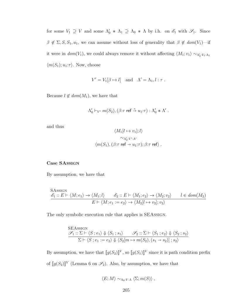
for some V1 ⊇ V and some Λ′0 ∗ Λ1 ⊇ Λ0 ∗ Λ by i.h. on E1 with S1. Since
β 6∈ Σ, S, S1, u1, we can assume without loss of generality that β 6∈ dom(V1)—if
it were in dom(V1), we could always remove it without affecting 〈M1; v1〉 ∼Λ′0·V1·Λ1
〈m(S1);u1:τ〉. Now, choose
V ′ = V1[β 7→ l] and Λ′ = Λ1, l : τ .
Because l 6∈ dom(M1), we have that
Λ′0 `V ′ m(S2), (β:τ refa� u1:τ) : Λ′0 ∗ Λ′ .
and thus〈M1[l 7→ v1]; l〉∼Λ′
0·V ′·Λ′
〈m(S1), (β:τ ref � u1:τ); β:τ ref〉 .
Case SAssign
By assumption, we have that
SAssignE1 :: E ` 〈M ; e1〉 → 〈M1; l〉 E2 :: E ` 〈M1; e2〉 → 〈M2; v2〉 l ∈ dom(M2)
E ` 〈M ; e1 := e2〉 → 〈M2[l 7→ v2]; v2〉
The only symbolic execution rule that applies is SEAssign.
SEAssignS1 :: Σ ` 〈S ; e1〉 ⇓ 〈S1 ; s1〉 S2 :: Σ ` 〈S1 ; e2〉 ⇓ 〈S2 ; s2〉
Σ ` 〈S ; e1 := e2〉 ⇓ 〈S2[m 7→ m(S2), (s1 � s2)] ; s2〉
By assumption, we have that Jg(S2)KV , so Jg(S1)KV since it is path condition prefix
of Jg(S2)KV (Lemma 6 on S2). Also, by assumption, we have that
〈E;M〉 ∼Λ0·V ·Λ 〈Σ;m(S)〉 ,
205

so〈M1; l〉 ∼Λ′′
0 ·V1·Λ1〈m(S1); s1〉
for some V1 ⊇ V and some Λ′′0 ∗ Λ1 ⊇ Λ0 ∗ Λ by i.h. on E1 with S1. Then, we
have that〈E;M1〉 ∼Λ′′
0 ·V1·Λ1〈Σ;m(S1)〉
and Jg(S2)KV1 because V1 ⊇ V , so
〈M2; v2〉 ∼Λ′0·V ′·Λ′ 〈m(S2); s2〉
for some V ′ ⊇ V1 and Λ′0 ∗ Λ′ ⊇ Λ′′0 ∗ Λ1 by i.h. on E2 with S2. Thus, we have
Λ′0 `V ′ m(S2) : Λ′0 ∗ Λ′ .
Since V ′ ⊇ V1 and Λ′0 ∗ Λ′ ⊇ Λ′′0 ∗ Λ1, we have that
Ju1:τ1KV′= l and ∅ `Λ0∗Λ′ l : τ1
where s1 = u1:τ1. Therefore, the symbolic memory relation holds for the symbolic
memory with the logged write:
Λ′0 `V ′ m(S2), (s1 � s2) : Λ′0 ∗ Λ′ .
Finally, because l ∈ dom(M2), we have that
〈M2[l 7→ v2]; v2〉 ∼Λ′0·V ′·Λ′ 〈m(S2), (s1 � s2); s2〉 .
Case SDeref
By assumption, we have that
SDerefE1 :: E ` 〈M ; e1〉 → 〈M1; l1〉 l1 ∈ dom(M1)
E ` 〈M ; !e1〉 → 〈M1;M1(l1)〉
206

The only symbolic execution rule that applies is SEDeref.
SEDerefS1 :: Σ ` 〈S ; e1〉 ⇓ 〈S1 ; u1:τ ref〉 M :: ` m(S1) ok
Σ ` 〈S ; !e1〉 ⇓ 〈S1 ;m(S1)[u1:τ ref]:τ〉
Also by assumption, we have that
〈E;M〉 ∼Λ0·V ·Λ 〈Σ;m(S)〉 and Jg(S1)KV ,
so〈M1; l1〉 ∼Λ′
0·V ′·Λ′ 〈m(S1);u1:τ ref〉
for some V ′ ⊇ V and Λ′0 ∗ Λ′ ⊇ Λ0 ∗ Λ by i.h. on E1 with S1. Thus, we have that
Λ′0 `V ′ m(S1) : Λ′0 ∗ Λ′
and∅ `Λ′
0∗Λ′ Ju1:τ refKV′: τ ref .
By memory typing soundness (Lemma 5) on M , we have that Jm(S1)KV ′ ∼ Λ′0 ∗ Λ′.
Therefore, we have that
∅ `Λ′0∗Λ′ Jm(S1)[u1:τ ref]KV
′: τ
as l1 ∈ dom(M1), which shows
〈M1;M1(l1)〉 ∼Λ′0·V ′·Λ′ 〈m(S1);m(S1)[u1:τ ref]〉 .
Case SNot-Error
By assumption, we have that
SNot-ErrorE1 :: E ` 〈M ; e1〉 → r1 r1 6= 〈M1; b1〉
E ` 〈M ;¬e1〉 → error
207

The only symbolic execution rule that applies is SENot.
SENotS1 :: Σ ` 〈S ; e1〉 ⇓ 〈S1 ; g1〉
Σ ` 〈S ; ¬e1〉 ⇓ 〈S1 ; ¬g1:bool〉
Also by assumption, we have that
〈E;M〉 ∼Λ0·V ·Λ 〈Σ;m(S)〉 and Jg(S1)KV ,
sor1 ∼Λ′
0·V ′·Λ′ 〈m(S1); g1〉
for some V ′ ⊇ V and Λ′0 ∗ Λ′ ⊇ Λ0 ∗ Λ by i.h. on E1 with S1. Thus, r1 = 〈M1; v1〉
for some M1 and v1 such that
∅ `Λ′0∗Λ′ v1 : bool
Therefore, by a standard canonical forms lemma, v1 = b1 for some b1, which con-
tradicts that r1 6= 〈M1; b1〉. Therefore, this case is not possible.
Case Other Error Cases
Similar to SNot-Error.
Exhaustive Symbolic Execution. With the soundness along a path, we can
state what it means for symbolic execution to be exhaustive. To do so, we say:
exhaustiveg(g1, . . . , gn) if g ⇒ g1 ∨ . . . ∨ gn is a tautology.
In other words, regardless of the valuation, the path conditions are exhaustive up to
an initial guard g.
208
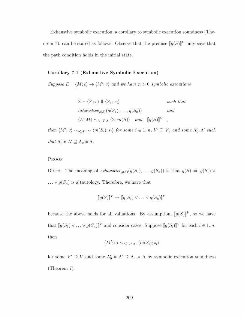
Exhaustive symbolic execution, a corollary to symbolic execution soundness (The-
orem 7), can be stated as follows. Observe that the premise Jg(S)KV only says that
the path condition holds in the initial state.
Corollary 7.1 (Exhaustive Symbolic Execution)
Suppose E ` 〈M ; e〉 → 〈M ′; v〉 and we have n > 0 symbolic executions
Σ ` 〈S ; e〉 ⇓ 〈Si ; si〉 such that
exhaustiveg(S)(g(S1), . . . , g(Sn)) and
〈E;M〉 ∼Λ0·V ·Λ 〈Σ;m(S)〉 and Jg(S)KV ,
then 〈M ′; v〉 ∼Λ′0·V ′·Λ′ 〈m(Si); si〉 for some i ∈ 1..n, V ′ ⊇ V , and some Λ′0,Λ
′ such
that Λ′0 ∗ Λ′ ⊇ Λ0 ∗ Λ.
Proof
Direct. The meaning of exhaustiveg(S)(g(S1), . . . , g(Sn)) is that g(S) ⇒ g(S1) ∨
. . . ∨ g(Sn) is a tautology. Therefore, we have that
Jg(S)KV ⇒ Jg(S1) ∨ . . . ∨ g(Sn)KV
because the above holds for all valuations. By assumption, Jg(S)KV , so we have
that Jg(S1) ∨ . . . ∨ g(Sn)KV and consider cases. Suppose Jg(Si)KV for each i ∈ 1..n,
then〈M ′; v〉 ∼Λ′
0·V ′·Λ′ 〈m(Si); si〉
for some V ′ ⊇ V and some Λ′0 ∗ Λ′ ⊇ Λ0 ∗ Λ by symbolic execution soundness
(Theorem 7).
209

As a technical point, the concerned reader might be worried that we are commingling
existentially quantified variables (i.e., the symbolic variables α) from different runs of
the symbolic executor in exhaustive (. . .); however, this commingling is permissible,
as we are combining with disjuncts and existential quantification distributes over
disjunction. At the same time, for debugging in an implementation, we would likely
want a fixed, deterministic strategy that ensures that symbolic executions of common
prefixes of paths use the same sequence of symbolic variable names.
A.4 Mix Soundness
With type soundness (Theorem 3) and symbolic execution soundness (Theorem 7),
we show soundness of Mix by additionally considering the cases for the switching
rules.
Theorem 8 (Mix Soundness)
1. If
E ` 〈M ; e〉 → r and
Γ `Λ e : τ such that
〈E;M〉 ∼ 〈Γ; Λ〉 ,
then ∅ `Λ′ v : τ and M ′ ∼ Λ′ for some M ′, v, Λ′ such that r = 〈M ′; v〉 and
Λ′ ⊇ Λ.
2. IfE ` 〈M ; e〉 → r and
Σ ` 〈S ; e〉 ⇓ 〈S ′ ; s〉 such that
〈E;M〉 ∼Λ0·V ·Λ 〈Σ;m(S)〉 and Jg(S ′)KV ,
210

thenr ∼Λ′
0·V ′·Λ′ 〈m(S ′); s〉
for some V ′ ⊇ V and some Λ′0,Λ′ such that Λ′0 ∗ Λ′ ⊇ Λ0 ∗ Λ.
Proof
By simultaneous induction on the derivations of
E ` 〈M ; e〉 → r .
We include the cases from type soundness (Theorem 3) and symbolic execution sound-
ness (Theorem 7) unchanged and consider the additional mix cases (Figure 3.4).
Case SSymBlock
By assumption, we have that
SSymBlockE1 :: E ` 〈M ; e1〉 → 〈M1; v1〉E ` 〈M ; {s e1 s}〉 → 〈M1; v1〉
The only type checking or symbolic execution rule that applies is the type checking
rule TSymBlock.
TSymBlockΣ(x) = αx:Γ(x)
(for all x ∈ dom(Γ)) Σ ` 〈S ; e〉 ⇓ 〈Si ; ui:τ〉 S = 〈true ; µ〉 µ /∈ Σ` m(Si) ok exhaustive(g1, . . . , gn) (i ∈ 1..n)
Γ ` {s e s} : τ
By assumption, we have that 〈E;M〉 ∼ 〈Γ; Λ〉. Let V be the valuation such that
V (αx) = E(x) for all x ∈ dom(Γ) andV (µ) = M
211

Now, choose Λ0 = Λ, and we have that
〈E;M〉 ∼Λ0·V ·∅ 〈Σ;m(S)〉
As we have exhaustive(g(S1), . . . , g(Sn)), we have that g(S1) ∨ . . . ∨ g(Sn) is a
tautology. Therefore, we have that
Jg(S1) ∨ . . . ∨ g(Sn)KV
because the above holds for all valuations. Now consider cases, suppose Jg(Si)KV
for each i ∈ 1..n, then
〈M1; v1〉 ∼Λ′0·Vi·Λi
〈m(Si);ui:τ〉
for some Vi ⊇ V and some Λ′0 ∗ Λi ⊇ Λ0 by the i.h. on E1. By memory typing
soundness (Lemma 5), we have that
Jm(Si)KV ∼ Λ′0 ∗ Λi and thus M1 ∼ Λ′0 ∗ Λi .
Let Λ′ = Λ′0 ∗ Λi, then we have that
∅ `Λ′ v1 : τ and M1 ∼ Λ′
where Λ′ ⊇ Λ.
Case STypBlock
By assumption, we have that
STypBlockE1 :: E ` 〈M ; e1〉 → 〈M1; v1〉E ` 〈M ; {t e1 t}〉 → 〈M1; v1〉
212

The only type checking or symbolic execution rule that applies is the symbolic
execution rule SETypBlock.
SETypBlock` Σ : Γ M :: ` m(S) ok T :: Γ ` e : τ µ′, β /∈ Σ, S
Σ ` 〈S ; {t e t}〉 ⇓ 〈S[m 7→ µ′] ; β:τ〉
Also by assumption, we have that
〈E;M〉 ∼Λ0·V ·Λ 〈Σ;m(S)〉
In particular, we have thatE ∼ 〈Γ; Λ0 ∗ Λ〉
because if ` Σ : Γ and ` Σ : Γ′ then Γ = Γ′. By memory type soundness (Lemma 5)
on M , we have that M ∼ Λ0 ∗ Λ, so
〈E;M〉 ∼ 〈Γ; Λ0 ∗ Λ〉
Then, we have that∅ `Λ′
0v1 : τ and M1 ∼ Λ′0
for some Λ′0 ⊇ Λ0 ∗ Λ by the i.h. on E1 with T . Since µ′, β 6∈ Σ, S, we can assume
without loss of generality that µ′, β 6∈ dom(V ). Now, choose
V ′ = V [β 7→ v1][µ 7→M1]
Then, we have thatΛ′0 `V ′ µ′ : Λ′0 ,
and thus, we have that〈M1; v1〉 ∼Λ′
0·V ′·∅ 〈µ′; β:τ〉 .
Note that Mix soundness (Theorem 8) as stated above considers symbolic execu-
tion along a path. To show soundness of the top-level expression, we can consider a
213

exhaustive constraint as in Corollary 7.1 or simply say that the top-level expression is
always wrapped in a type checking block {t e t}. In order words, exhaustive symbolic
execution of an expression e is type checking of {t {s e s} t}.
214

Bibliography
Paul Anderson, Thomas Reps, Tim Teitelbaum, and Mark Zarins. 2003. Tool supportfor fine-grained software inspection. IEEE Software 20, 4 (July 2003), 42–50. DOI:10.1109/MS.2003.1207453
John Anvik, Lyndon Hiew, and Gail C. Murphy. 2006. Who should fix this bug?. InProceedings of the 28th International Conference on Software Engineering (ICSE’06). ACM, New York, NY, USA, 361–370. DOI:10.1145/1134285.1134336
Mikhail Auguston, Clinton Jeffery, and Scott Underwood. 2002. A framework forautomatic debugging. In Proceedings of the 17th IEEE International Conference onAutomated Software Engineering (ASE ’02). IEEE Computer Society, Washington,DC, USA, 217–222. DOI:10.1109/ASE.2002.1115015
Nathaniel Ayewah and William Pugh. 2008. A report on a survey and study ofstatic analysis users. In Proceedings of the 2008 Workshop on Defects in LargeSoftware Systems (DEFECTS ’08). ACM, New York, NY, USA, 1–5. DOI:10.1145/1390817.1390819
Nathaniel Ayewah and William Pugh. 2009. Using checklists to review static analy-sis warnings. In Proceedings of the 2nd International Workshop on Defects in LargeSoftware Systems: Held in conjunction with the ACM SIGSOFT International Sym-posium on Software Testing and Analysis (ISSTA 2009) (DEFECTS ’09). ACM,New York, NY, USA, 11–15. DOI:10.1145/1555860.1555864
Phil Bagwell. 2001. Ideal hash trees. Technical Report. École Polytechnique Fédéralede Lausanne, Lausanne, Switzerland. http://infoscience.epfl.ch/record/64398
Thomas Ball and Sriram K. Rajamani. 2002. The SLAM project: debugging systemsoftware via static analysis. In Proceedings of the 29th ACM SIGPLAN-SIGACTSymposium on Principles of Programming Languages (POPL ’02). ACM, NewYork, NY, USA, 1–3. DOI:10.1145/503272.503274
Peter Bates. 1988. Debugging heterogeneous distributed systems using event-basedmodels of behavior. In Proceedings of the 1988 ACM SIGPLAN and SIGOPS Work-shop on Parallel and Distributed Debugging (PADD ’88). ACM, New York, NY,USA, 11–22. DOI:10.1145/68210.69217
Mike Beaven and Ryan Stansifer. 1993. Explaining type errors in polymorphic lan-guages. ACM Letters on Programming Languages and Systems 2, 1–4 (March 1993),17–30. DOI:10.1145/176454.176460
215

Al Bessey, Ken Block, Ben Chelf, Andy Chou, Bryan Fulton, Seth Hallem, CharlesHenri-Gros, Asya Kamsky, Scott McPeak, and Dawson Engler. 2010. A few billionlines of code later: using static analysis to find bugs in the real world. Communi-cations of the ACM 53, 2 (Feb. 2010), 66–75. DOI:10.1145/1646353.1646374
Dirk Beyer, Thomas A. Henzinger, Ranjit Jhala, and Rupak Majumdar. 2007. Thesoftware model checker BLAST: Applications to software engineering. InternationalJournal on Software Tools for Technology Transfer 9, 5 (Oct. 2007), 505–525. DOI:10.1007/s10009-007-0044-z
J. David Blackstone. Tiny HTTPd. Retrieved June 2013 from http://tinyhttpd.sourceforge.net
Richard Bornat. 2000. Proving pointer programs in Hoare logic. In Proceedings ofthe 5th International Conference on Mathematics of Program Construction (MPC’00). Springer-Verlag, Berlin, Heidelberg, 102–126. DOI:10.1007/10722010_8
Cristian Cadar, Daniel Dunbar, and Dawson Engler. 2008. KLEE: unassisted andautomatic generation of high-coverage tests for complex systems programs. In Pro-ceedings of the 8th USENIX Conference on Operating Systems Design and Im-plementation (OSDI ’08). USENIX Association, Berkeley, CA, USA, 209–224.http://dl.acm.org/citation.cfm?id=1855741.1855756
Cristian Cadar, Vijay Ganesh, Peter M. Pawlowski, David L. Dill, and Dawson R.Engler. 2006. EXE: automatically generating inputs of death. In Proceedings ofthe 13th ACM Conference on Computer and Communications Security (CCS ’06).ACM, New York, NY, USA, 322–335. DOI:10.1145/1180405.1180445
Cristian Cadar, Patrice Godefroid, Sarfraz Khurshid, Corina S. Păsăreanu, KoushikSen, Nikolai Tillmann, and Willem Visser. 2011. Symbolic execution for softwaretesting in practice: preliminary assessment. In Proceedings of the 33rd InternationalConference on Software Engineering (ICSE ’11). ACM, New York, NY, USA, 1066–1071. DOI:10.1145/1985793.1985995
Stuart K. Card, Jock D. Mackinlay, and Ben Shneiderman (Eds.). 1999. Readingsin information visualization: using vision to think. Morgan Kaufmann Publishers,San Francisco, CA, USA.
James C. Corbett, Matthew B. Dwyer, John Hatcliff, Shawn Laubach, Corina S.Păsăreanu, Robby, and Hongjun Zheng. 2000. Bandera: extracting finite-statemodels from Java source code. In Proceedings of the 22nd International Conferenceon Software Engineering (ICSE ’00). ACM, New York, NY, USA, 439–448. DOI:10.1145/337180.337234
Patrick Cousot and Radhia Cousot. 1979. Systematic design of program analysisframeworks. In Proceedings of the 6th ACM SIGACT-SIGPLAN Symposium onPrinciples of Programming Languages (POPL ’79). ACM, New York, NY, USA,269–282. DOI:10.1145/567752.567778
216
Coverity, Inc. a. Coverity Development Testing. Retrieved June 2013 from http://www.coverity.com/products/coverity-save.html
Coverity, Inc. b. Coverity SAVE. Retrieved June 2013 from http://www.coverity.com/products/coverity-save.html
Solar Designer. 1997. ‘return-to-libc’ attack. Bugtraq (Aug. 1997). Retrieved June2013 from http://seclists.org/bugtraq/1997/Aug/63
Isil Dillig, Thomas Dillig, and Alex Aiken. 2007. Static error detection using semanticinconsistency inference. In Proceedings of the 2007 ACM SIGPLAN Conference onProgramming Language Design and Implementation (PLDI ’07). ACM, New York,NY, USA, 435–445. DOI:10.1145/1250734.1250784
Isil Dillig, Thomas Dillig, and Alex Aiken. 2012. Automated error diagnosis usingabductive inference. In Proceedings of the 33rd ACM SIGPLAN Conference onProgramming Language Design and Implementation (PLDI ’12). ACM, New York,NY, USA, 181–192. DOI:10.1145/2254064.2254087
Mireille Ducassé. 1999. Coca: an automated debugger for C. In Proceedings of the 21stInternational Conference on Software Engineering (ICSE ’99). ACM, New York,NY, USA, 504–513. DOI:10.1145/302405.302682
Dominic Duggan and Frederick Bent. 1996. Explaining type inference. Science ofComputer Programming 27, 1 (July 1996), 37–83. DOI:10.1016/0167-6423(95)00007-0
Conal Elliott and Paul Hudak. 1997. Functional reactive animation. In Proceedings ofthe Second ACM SIGPLAN International Conference on Functional Programming(ICFP ’97). ACM, New York, NY, USA, 263–273. DOI:10.1145/258948.258973
Jakob Engblom. 2012. A review of reverse debugging. In System, Software, SoC andSilicon Debug Conference (S4D ’12). IEEE, Piscataway, NJ, USA, 1–6. http://ieeexplore.ieee.org/xpl/articleDetails.jsp?arnumber=6338149
Robert Bruce Findler and Matthias Felleisen. 2002. Contracts for higher-order func-tions. In Proceedings of the Seventh ACM SIGPLAN International Conference onFunctional Programming (ICFP ’02). ACM, New York, NY, USA, 48–59. DOI:10.1145/581478.581484
Cormac Flanagan. 2006. Hybrid type checking. In Proceedings of the 33rd ACMSIGPLAN-SIGACT Symposium on Principles of Programming Languages (POPL’06). ACM, New York, NY, USA, 245–256. DOI:10.1145/1111037.1111059
Cormac Flanagan, Matthew Flatt, Shriram Krishnamurthi, Stephanie Weirich, andMatthias Felleisen. 1996. Catching bugs in the web of program invariants. In Pro-ceedings of the 1996 ACM SIGPLAN Conference on Programming Language De-sign and Implementation (PLDI ’96). ACM, New York, NY, USA, 23–32. DOI:10.1145/231379.231387
217

Jeffrey S. Foster, Robert Johnson, John Kodumal, and Alex Aiken. 2006. Flow-insensitive type qualifiers. ACM Transactions on Programming Languages andSystems 28, 6 (Nov. 2006), 1035–1087. DOI:10.1145/1186632.1186635
George W. Furnas. 1986. Generalized fisheye views. In Proceedings of the SIGCHIConference on Human Factors in Computing Systems (CHI ’86). ACM, New York,NY, USA, 16–23. DOI:10.1145/22627.22342
Vijay Ganesh and David L. Dill. 2007. A decision procedure for bit-vectors andarrays. In Proceedings of the 19th International Conference on Computer AidedVerification (CAV ’07). Springer-Verlag, Berlin, Heidelberg, 519–531. DOI:10.1007/978-3-540-73368-3_52
Patrice Godefroid. 2007. Compositional dynamic test generation. In Proceedings ofthe 34th ACM SIGPLAN-SIGACT Symposium on Principles of Programming Lan-guages (POPL ’07). ACM, New York, NY, USA, 47–54. DOI:10.1145/1190216.1190226
Patrice Godefroid, Nils Klarlund, and Koushik Sen. 2005. DART: directed auto-mated random testing. In Proceedings of the 2005 ACM SIGPLAN Conference onProgramming Language Design and Implementation (PLDI ’05). ACM, New York,NY, USA, 213–223. DOI:10.1145/1065010.1065036
Simon F. Goldsmith, Robert O’Callahan, and Alex Aiken. 2005. Relational queriesover program traces. In Proceedings of the 20th Annual ACM SIGPLAN Conferenceon Object-oriented Programming, Systems, Languages, and Applications (OOPSLA’05). ACM, New York, NY, USA, 385–402. DOI:10.1145/1094811.1094841
GrammaTech, Inc. a. CodeSonar. Retrieved June 2013 from http://www.grammatech.com/codesonar
GrammaTech, Inc. b. GrammaTech Static Analysis. Retrieved June 2013 fromhttp://www.grammatech.com
David Greenfieldboyce and Jeffrey S. Foster. 2004. Visualizing type qualifier in-ference with Eclipse. In Proceedings of the 2004 OOPSLA Workshop on EclipseTechnology eXchange (Eclipse ’04). ACM, New York, NY, USA, 57–61. DOI:10.1145/1066129.1066141
Aaron Greenhouse, T. J. Halloran, and William L. Scherlis. 2003. Using Eclipse todemonstrate positive static assurance of Java program concurrency design intent.In Proceedings of the 2003 OOPSLA Workshop on Eclipse Technology eXchange(Eclipse ’03). ACM, New York, NY, USA, 99–103. DOI:10.1145/965660.965681
Sumit Gulwani and Ashish Tiwari. 2006. Combining abstract interpreters. In Pro-ceedings of the 2006 ACM SIGPLAN Conference on Programming Language De-sign and Implementation (PLDI ’06). ACM, New York, NY, USA, 376–386. DOI:10.1145/1133981.1134026
218

Philip J. Guo and Dawson Engler. 2009. Linux kernel developer responses to staticanalysis bug reports. In Proceedings of the 2009 conference on USENIX Annualtechnical conference (USENIX’09). USENIX Association, Berkeley, CA, USA, 22–22. http://dl.acm.org/citation.cfm?id=1855807.1855829
Samuel Z. Guyer and Calvin Lin. 2005. Error checking with client-driven pointeranalysis. Science of Computer Programming 58, 1-2 (Oct. 2005), 83–114. DOI:10.1016/j.scico.2005.02.005
Christian Haack and J. B. Wells. 2004. Type error slicing in implicitly typed higher-order languages. Science of Computer Programming 50, 1–3 (March 2004), 189–224.DOI:10.1016/j.scico.2004.01.004
Christopher C. D. Head, Geoffrey Lefebvre, Mark Spear, Nathan Taylor, and AndrewWarfield. 2012. Debugging through time with the Tralfamadore debugger. In Run-time Environments, Systems, Layering and Virtualized Environments (RESoLVE’12). http://www.dcs.gla.ac.uk/conferences/resolve12/papers/session4_paper1.pdf
Thomas A. Henzinger, Ranjit Jhala, Rupak Majumdar, and Kenneth L. McMil-lan. 2004. Abstractions from proofs. In Proceedings of the 31st ACM SIGPLAN-SIGACT Symposium on Principles of Programming Languages (POPL ’04). ACM,New York, NY, USA, 232–244. DOI:10.1145/964001.964021
Hewlett-Packard Development Company, L.P. HP Fortify Static Code Analyzer.Retrieved June 2013 from http://www8.hp.com/us/en/software-solutions/software.html?compURI=1338812
David Hovemeyer and William Pugh. 2004. Finding bugs is easy. ACM SIGPLANNotices 39, 12 (Dec. 2004), 92–106. DOI:10.1145/1052883.1052895
Ranjit Jhala and Rupak Majumdar. 2009. Software model checking. ACM ComputingSurveys 41, 4, Article 21 (Oct. 2009), 54 pages. DOI:10.1145/1592434.1592438
Brittany Johnson, Yoonki Song, Emerson Murphy-Hill, and Robert Bowdidge. 2013.Why don’t software developers use static analysis tools to find bugs?. In Proceedingsof the 2013 International Conference on Software Engineering (ICSE ’13). IEEEPress, Piscataway, NJ, USA, 672–681. http://dl.acm.org/citation.cfm?id=2486788.2486877
Yit Phang Khoo, Bor-Yuh Evan Chang, and Jeffrey S. Foster. 2010a. Mixing typechecking and symbolic execution. In Proceedings of the 2010 ACM SIGPLAN Con-ference on Programming Language Design and Implementation (PLDI ’10). ACM,New York, NY, USA, 436–447. DOI:10.1145/1806596.1806645
Yit Phang Khoo, Bor-Yuh Evan Chang, and Jeffrey S. Foster. 2010b. Mixing TypeChecking and Symbolic Execution (Extended Version). Technical Report CS-TR-4954. University of Maryland. http://hdl.handle.net/1903/10115
219

Yit Phang Khoo, Jeffrey S. Foster, and Michael Hicks. 2013a. Expositor: scriptabletime-travel debugging with first-class traces. In Proceedings of the 2013 Interna-tional Conference on Software Engineering (ICSE ’13). IEEE Press, Piscataway,NJ, USA, 352–361. http://dl.acm.org/citation.cfm?id=2486788.2486835
Yit Phang Khoo, Jeffrey S. Foster, and Michael Hicks. 2013b. Expositor: script-able time-travel debugging with first-class traces. Technical Report CS-TR-5021.University of Maryland. http://hdl.handle.net/1903/14406
Yit Phang Khoo, Jeffrey S. Foster, Michael Hicks, and Vibha Sazawal. 2008a. Pathprojection for user-centered static analysis tools. In Proceedings of the 8th ACMSIGPLAN-SIGSOFT Workshop on Program Analysis for Software Tools and Engi-neering (PASTE ’08). ACM, New York, NY, USA, 57–63. DOI:10.1145/1512475.1512488
Yit Phang Khoo, Jeffrey S. Foster, Michael Hicks, and Vibha Sazawal. 2008b. PathProjection for User-Centered Static Analysis Tools. Technical Report CS-TR-4919.University of Maryland. http://hdl.handle.net/1903/8369
James C. King. 1976. Symbolic execution and program testing. Communications ofthe ACM 19, 7 (July 1976), 385–394. DOI:10.1145/360248.360252
Samuel T. King, George W. Dunlap, and Peter M. Chen. 2005. Debugging oper-ating systems with time-traveling virtual machines. In Proceedings of the AnnualConference on USENIX Annual Technical Conference (ATC ’05). USENIX Associ-ation, Berkeley, CA, USA, 1–1. http://dl.acm.org/citation.cfm?id=1247360.1247361
Klocwork, Inc. a. Klocwork Insight. Retrieved June 2013 from http://www.klocwork.com/products/insight
Klocwork, Inc. b. Source Code Analysis Tools for Software Security & Reliability.Retrieved June 2013 from http://www.klocwork.com
Andrew J. Ko and Brad A. Myers. 2008. Debugging reinvented: asking and answeringwhy and why not questions about program behavior. In Proceedings of the 30thInternational Conference on Software Engineering (ICSE ’08). ACM, New York,NY, USA, 301–310. DOI:10.1145/1368088.1368130
Ted Kremenek, Ken Ashcraft, Junfeng Yang, and Dawson Engler. 2004. Correlationexploitation in error ranking. In Proceedings of the 12th ACM SIGSOFT Interna-tional Symposium on Foundations of Software Engineering (SIGSOFT/FSE ’04).ACM, New York, NY, USA, 83–93. DOI:10.1145/1029894.1029909
Leslie Lamport. 1978. Time, clocks, and the ordering of events in a distributed system.Communications of the ACM 21, 7 (July 1978), 558–565. DOI:10.1145/359545.359563
220

James R. Larus, Thomas Ball, Manuvir Das, Robert DeLine, Manuel Fahndrich, JonPincus, Sriram K. Rajamani, and Ramanathan Venkatapathy. 2004. Righting Soft-ware. IEEE Software 21, 3 (May 2004), 92–100. DOI:10.1109/MS.2004.1293079
Geoffrey Lefebvre, Brendan Cully, Christopher Head, Mark Spear, Norm Hutchinson,Mike Feeley, and Andrew Warfield. 2012. Execution mining. In Proceedings ofthe 8th ACM SIGPLAN/SIGOPS Conference on Virtual Execution Environments(VEE ’12). ACM, New York, NY, USA, 145–158. DOI:10.1145/2151024.2151044
Sorin Lerner, David Grove, and Craig Chambers. 2002. Composing dataflow analysesand transformations. In Proceedings of the 29th ACM SIGPLAN-SIGACT Sympo-sium on Principles of Programming Languages (POPL ’02). ACM, New York, NY,USA, 270–282. DOI:10.1145/503272.503298
Bil Lewis. 2003. Debugging backwards in time. In Proceedings of the Fifth Interna-tional Workshop on Automated Debugging (AADEBUG ’03). http://arXiv.org/abs/cs/0310016
Rupak Majumdar and Koushik Sen. 2007. Hybrid concolic testing. In Proceedingsof the 29th International Conference on Software Engineering (ICSE ’07). IEEEComputer Society, Los Alamitos, CA, USA, 416–426. DOI:10.1109/ICSE.2007.41
Guillaume Marceau, Gregory H. Cooper, Jonathan P. Spiro, Shriram Krishnamurthi,and Steven P. Reiss. 2007. The design and implementation of a dataflow languagefor scriptable debugging. Automated Software Engineering 14, 1 (March 2007),59–86. DOI:10.1007/s10515-006-0003-z
Michael Martin, Benjamin Livshits, and Monica S. Lam. 2005. Finding applicationerrors and security flaws using PQL: a program query language. In Proceedingsof the 20th Annual ACM SIGPLAN Conference on Object-oriented Programming,Systems, Languages, and Applications (OOPSLA ’05). ACM, New York, NY, USA,365–383. DOI:10.1145/1094811.1094840
Joseph M. Morris. 1982. A general axiom of assignment. In Theoretical Founda-tions of Programming Methodology, Manfred Broy and Gunther Schmidt (Eds.).NATO Advanced Study Institutes Series, Vol. 91. D. Reidel Publishing Company,Dordrecht, Holland, 25–34. DOI:10.1007/978-94-009-7893-5_3
George C. Necula, Scott McPeak, Shree Prakash Rahul, and Westley Weimer.2002. CIL: intermediate language and tools for analysis and transformationof C programs. In Proceedings of the 11th International Conference on Com-piler Construction (CC ’02). Springer-Verlag, Berlin, Heidelberg, 213–228. DOI:10.1007/3-540-45937-5_16
Greg Nelson and Derek C. Oppen. 1979. Simplification by cooperating decision pro-cedures. ACM Transactions on Programming Languages and Systems 1, 2 (Oct.1979), 245–257. DOI:10.1145/357073.357079
221
Nicholas Nethercote and Julian Seward. 2007. Valgrind: a framework for heavyweightdynamic binary instrumentation. SIGPLAN Not. 42, 6 (June 2007), 89–100. DOI:10.1145/1273442.1250746
Robert O’Callahan. 2006. Efficient collection and storage of indexed program traces.Retrieved June 2013 from http://www.ocallahan.org/Amber.pdf
Robert O’Callahan. 2010. LFX2010: a browser developer’s wish list. http://vimeo.com/groups/lfx/videos/12471856#t=27m15s at 27:15.
Ronald A. Olsson, Richard H. Crawford, and W. Wilson Ho. 1991. A dataflow ap-proach to event-based debugging. Software: Practice and Experience 21, 2 (Feb.1991), 209–229. DOI:10.1002/spe.4380210207
Aleph One. 1996. Smashing the stack for fun and profit. Phrack magazine 7, 49, 365.Retrieved June 2013 from http://www.phrack.org/issues.html?issue=49&id=14#article
Jens Palsberg and Todd Millstein. 2007. Type systems: advances and applications.In The Compiler Design Handbook: Optimizations and Machine Code Generation(2nd ed.), Y. N. Srikant and Priti Shankar (Eds.). CRC Press, Inc., Boca Raton,FL, USA, Chapter 9.
Jon Pincus. 2000. Analysis is necessary, but far from sufficient: experiences buildingand deploying successful tools for developers and testers. Keynote Address of the2000 ACM SIGSOFT International Symposium on Software Testing and Analysis(ISTTA ’00). Retrieved June 2013 from http://www.cc.gatech.edu/~harrold/issta00/cfp/slides/pincus.issta2000.ppt
Guillaume Pothier, Éric Tanter, and José Piquer. 2007. Scalable omniscient debug-ging. In Proceedings of the 22nd Annual ACM SIGPLAN Conference on Object-oriented Programming Systems and Applications (OOPSLA ’07). ACM, New York,NY, USA, 535–552. DOI:10.1145/1297027.1297067
Polyvios Pratikakis, Jeffrey S. Foster, and Michael Hicks. 2006. Locksmith: context-sensitive correlation analysis for race detection. In Proceedings of the 2006 ACMSIGPLAN Conference on Programming Language Design and Implementation(PLDI ’06). ACM, New York, NY, USA, 320–331. DOI:10.1145/1133981.1134019
Elnatan Reisner, Charles Song, Kin-Keung Ma, Jeffrey S. Foster, and Adam Porter.2010. Using symbolic evaluation to understand behavior in configurable softwaresystems. In Proceedings of the 32nd International Conference on Software Engi-neering (ICSE ’10). ACM, New York, NY, USA, 445–454. DOI:10.1145/1806799.1806864
Patrick Maxim Rondon, Ming Kawaguchi, and Ranjit Jhala. 2010. Low-level liquidtypes. In Proceedings of the 37th Annual ACM SIGPLAN-SIGACT Symposium on
222

Principles of Programming Languages (POPL ’10). ACM, New York, NY, USA,131–144. DOI:10.1145/1706299.1706316
Patrick M. Rondon, Ming Kawaguci, and Ranjit Jhala. 2008. Liquid types. In Pro-ceedings of the 2008 ACM SIGPLAN Conference on Programming Language De-sign and Implementation (PLDI ’08). ACM, New York, NY, USA, 159–169. DOI:10.1145/1375581.1375602
Per Runeson, Magnus Alexandersson, and Oskar Nyholm. 2007. Detection of dupli-cate defect reports using natural language processing. In Proceedings of the 29thInternational Conference on Software Engineering (ICSE ’07). IEEE ComputerSociety, Los Alamitos, CA, USA, 499–510. DOI:10.1109/ICSE.2007.32
Joseph R. Ruthruff, John Penix, J. David Morgenthaler, Sebastian Elbaum, andGregg Rothermel. 2008. Predicting accurate and actionable static analysis warn-ings: an experimental approach. In Proceedings of the 30th International Conferenceon Software Engineering (ICSE ’08). ACM, New York, NY, USA, 341–350. DOI:10.1145/1368088.1368135
Stefan Savage, Michael Burrows, Greg Nelson, Patrick Sobalvarro, and Thomas An-derson. 1997. Eraser: a dynamic data race detector for multi-threaded programs.In Proceedings of the Sixteenth ACM Symposium on Operating Systems Principles(SOSP ’97). ACM, New York, NY, USA, 27–37. DOI:10.1145/268998.266641
Koushik Sen, Darko Marinov, and Gul Agha. 2005. CUTE: a concolic unit testingengine for C. In Proceedings of the 10th European Software Engineering Conferenceheld jointly with 13th ACM SIGSOFT International Symposium on Foundationsof Software Engineering (ESEC/FSE ’05). ACM, New York, NY, USA, 263–272.DOI:10.1145/1081706.1081750
Margaret-Anne Darragh Storey. 1998. A cognitive framework for describing and evalu-ating software exploration tools. Ph.D. Dissertation. Simon Fraser University, Burn-aby, BC, Canada. Advisor(s) Fracchia, David and Muller, Hausi. AAINQ37756.
The Eclipse Foundation. Eclipse. Retrieved June 2013 from http://www.eclipse.org
The GDB Developers. GDB: The GNU Project Debugger. Retrieved June 2013 fromhttp://sourceware.org/gdb
Undo Software. What is UndoDB? Retrieved June 2013 from http://undo-software.com/product/undodb-overview
Ana-Maria Visan, Kapil Arya, Gene Cooperman, and Tyler Denniston. 2011.URDB: a universal reversible debugger based on decomposing debugging histo-ries. In Proceedings of the 6th Workshop on Programming Languages and Operat-ing Systems (PLOS ’11). ACM, New York, NY, USA, Article 8, 5 pages. DOI:10.1145/2039239.2039251
223

Mitchell Wand. 1986. Finding the source of type errors. In Proceedings of the 13thACM SIGACT-SIGPLAN Symposium on Principles of Programming Languages(POPL ’86). ACM, New York, NY, USA, 38–43. DOI:10.1145/512644.512648
Mark Weiser. 1984. Program Slicing. IEEE Transactions on Software Engineering10, 4 (July 1984), 352–357. DOI:10.1109/TSE.1984.5010248
Hongwei Xi and Frank Pfenning. 1999. Dependent types in practical programming.In Proceedings of the 26th ACM SIGPLAN-SIGACT Symposium on Principles ofProgramming Languages (POPL ’99). ACM, New York, NY, USA, 214–227. DOI:10.1145/292540.292560
Baowen Xu, Ju Qian, Xiaofang Zhang, Zhongqiang Wu, and Lin Chen. 2005. Abrief survey of program slicing. ACM SIGSOFT Software Engineering Notes 30, 2(March 2005), 1–36. DOI:10.1145/1050849.1050865
Min Xu, Vyacheslav Malyugin, Jeffrey Sheldon, Ganesh Venkitachalam, and BorisWeissman. 2007. ReTrace: collecting execution trace with virtual machine deter-ministic replay. In Proceedings of the Third Annual Workshop on Modeling, Bench-marking and Simulation (MoBS ’07). http://www-mount.ece.umn.edu/~jjyi/MoBS/2007/program/01C-Xu.pdf
Kwangkeun Yi and Williams Ludwell Harrison III. 1993. Automatic generation andmanagement of interprocedural program analyses. In Proceedings of the 20th ACMSIGPLAN-SIGACT Symposium on Principles of Programming Languages (POPL’93). ACM, New York, NY, USA, 246–259. DOI:10.1145/158511.158642
Alon Zakai. 2011. Bug 654028 - 70MB of collectible garbage not cleaned up. (May2011). Retrieved June 2013 from https://bugzilla.mozilla.org/show_bug.cgi?id=654028
Andreas Zeller. 2006. Why Programs Fail: A Guide to Systematic Debugging. MorganKaufmann Publishers, San Francisco, CA, USA.
Qin Zhao, Rodric Rabbah, Saman Amarasinghe, Larry Rudolph, and Weng-FaiWong. 2008. How to do a million watchpoints: efficient debugging using dy-namic instrumentation. In Proceedings of the Joint European Conferences on The-ory and Practice of Software 17th International Conference on Compiler Con-struction (CC ’08/ETAPS’08). Springer-Verlag, Berlin, Heidelberg, 147–162. DOI:10.1007/978-3-540-78791-4_10
224