abstract document: high-performance 3d image processing architectures ... · processing...
TRANSCRIPT
ABSTRACT
Title of Document: HIGH-PERFORMANCE 3D IMAGE
PROCESSING ARCHITECTURES FOR IMAGE-GUIDED INTERVENTIONS
Omkar Dandekar, Ph.D., 2008
Directed By: Professor Raj Shekhar (Chair/Advisor),
Professor Shuvra S. Bhattacharyya (Co-advisor), Department of Electrical and Computer Engineering
Minimally invasive image-guided interventions (IGIs) are time and cost
efficient, minimize unintended damage to healthy tissues, and lead to faster patient
recovery. Advanced three-dimensional (3D) image processing is a critical need for
navigation during IGIs. However, achieving on-demand performance, as required by
IGIs, for these image processing operations using software-only implementations is
challenging because of the sheer size of the 3D images, and memory and compute
intensive nature of the operations. This dissertation, therefore, is geared toward
developing high-performance 3D image processing architectures, which will enable
improved intraprocedural visualization and navigation capabilities during IGIs.
In this dissertation we present an architecture for real-time implementation of
3D filtering operations that are commonly employed for preprocessing of medical
images. This architecture is approximately two orders of magnitude faster than

corresponding software implementations and is capable of processing 3D medical
images at their acquisition speeds.
Combining complementary information through registration between pre- and
intraprocedural images is a fundamental need in the IGI workflow. Intensity-based
deformable registration, which is completely automatic and locally accurate, is a
promising approach to achieve this alignment. These algorithms, however, are
extremely compute intensive, which has prevented their clinical use. We present an
FPGA-based architecture for accelerated implementation of intensity-based
deformable image registration. This high-performance architecture achieves over an
order of magnitude speedup when compared with a corresponding software
implementation and reduces the execution time of deformable registration from hours
to minutes while offering comparable image registration accuracy.
Furthermore, we present a framework for multiobjective optimization of
finite-precision implementations of signal processing algorithms that takes into
account multiple conflicting objectives such as implementation accuracy and
hardware resource consumption. The evaluation that we have performed in the
context of FPGA-based image registration demonstrates that such an analysis can be
used to enhance automated hardware design processes, and efficiently identify a
system configuration that meets given design constraints. In addition, we also outline
two novel clinical applications that can directly benefit from these developments and
demonstrate the feasibility of our approach in the context of these applications. These
advances will ultimately enable integration of 3D image processing into clinical
workflow.

HIGH-PERFORMANCE 3D IMAGE PROCESSING ARCHITECTURES FOR IMAGE-GUIDED INTERVENTIONS
By
Omkar Dandekar
Dissertation submitted to the Faculty of the Graduate School of the University of Maryland, College Park, in partial fulfillment
of the requirements for the degree of Doctor of Philosophy
2008
Advisory Committee: Professor Raj Shekhar, Chair/Advisor Professor Shuvra S. Bhattacharyya, Co-advisor Professor Rama Chellappa Professor Manoj Franklin Professor Yang Tao

© Copyright by Omkar Dandekar
2008

ii
Dedication
To my Mother, Mangal, Himani, and the memories of my late Father,
for their love and support

iii
Publications
• W. Plishker, O. Dandekar, S. Bhattacharyya, and R. Shekhar, “Towards a
heterogeneous medical image registration acceleration platform,” IEEE
Transactions on Biomedical Circuits and Systems, (in preparation), 2008.
• R. Shekhar, O. Dandekar, V. Bhat, R. Mezrich, and A. Park, "Development of
CT-guided minimally invasive surgery," Surgical Innovation, (in
preparation), 2008.
• O. Dandekar, W. Plishker, S. S. Bhattacharyya, and R. Shekhar,
“Multiobjective optimization for reconfigurable implementation of medical
image registration,” International Journal of Reconfigurable Computing,
(under review), 2008.
• P. Lei, O. Dandekar, D. Widlus, P. Malloy, and R. Shekhar, “Incorporation of
PET into CT-guided liver radiofrequency ablation,” Radiology, (under
revision), 2008.
• O. Dandekar, W. Plishker, S. S. Bhattacharyya, and R. Shekhar,
“Multiobjective optimization of FPGA-based medical image registration,”
presented at IEEE Symposium on Field-Programmable Custom Computing
Machines, 2008.
• O. Dandekar and R. Shekhar, “FPGA-accelerated deformable image
registration for improved target-delineation during CT-guided interventions,”
IEEE Transactions on Biomedical Circuits and Systems, vol. 1 (2), 2007, pp.
116-127.

iv
• O. Dandekar, C. Castro-Pareja, and R. Shekhar, “FPGA-based real-time 3D
image preprocessing for image-guided medical interventions,” Journal of
Real-Time Image Processing, vol. 1 (4), pp. 285-301, 2007.
• W. Plishker, O. Dandekar, S. Bhattacharyya, and R. Shekhar, “Towards a
heterogeneous medical image registration acceleration platform,” presented at
IEEE Biomedical Circuits and Systems Conference, 2007, pp. 231-234.
• O. Dandekar, K. Siddiqui, V. Walimbe, and R. Shekhar, “Image registration
accuracy with low-dose CT: How low can we go?,” presented at IEEE
International Symposium on Biomedical Imaging, 2006, pp. 502-505.
• C. R. Castro-Pareja, O. Dandekar, and R. Shekhar, “FPGA-based real-time
anisotropic diffusion filtering of 3D ultrasound images,” in SPIE Real-Time
Imaging, 2005, pp. 123-131.
• S. Venugopal, C. R. Castro-Pareja, and O. Dandekar, “An FPGA-based 3D
image processor with median and convolution filters for real-time
applications,” in SPIE Real-Time Imaging, 2005, pp. 174-182.

v
Acknowledgements
I would like to express my sincere gratitude to Dr. Raj Shekhar for his
guidance and financial support throughout my graduate education at The Ohio State
University, the Cleveland Clinic, and University of Maryland. He has been the perfect
mentor for my doctoral research, and a person from whom I have learnt a lot during
the past five years. He ensured that I master not only the intricacies of medical image
processing, but also put a strong emphasis on developing the qualities necessary for
effective dissemination of scientific research and results. Beyond doubt, he has
played the most important role in shaping my technical writing and presentation
skills. All throughout my graduate career he has made himself available at any
moment when I needed his inputs and feedback for my work or anything else. The
time spent working with Dr. Shekhar has truly been the most rewarding career
experience of my life.
I would also like to thank my dissertation committee members, Prof. Shuvra
Bhattacharyya, Prof. Rama Chellappa, Prof. Manoj Franklin, and Prof Yang Tao for
their cooperation and support. I would especially like to thank Prof. Bhattacharyya for
his help and collaboration in my work that resulted in an important chapter of this
dissertation. The research work reported in this dissertation was partly supported by
U.S. Department of Defense (TATRC) under grant DAMD17-03-2-0001.
My research at the University of Maryland would not have been
possible without the support and encouragement of Drs. Rueben Mezrich, Adrian
Park, Eliot Siegel, Khan Siddiqui, Nancy Knight, Faaiza Mahmoud, Steve Kavic, and
all clinical staff at the University of Maryland and Baltimore VA. Whenever I

vi
requested, they have spared valuable time from their busy schedules for discussions
with me, and have been immensely helpful especially during the clinical validation
studies. Dr. Siddiqui, in particular, was instrumental in providing clinical perspective
on some of the research problems I have explored.
I would like to thank Prof. Jogikal Jagadeesh for allowing me to work in his
lab during my first two years at the Ohio State University, and for his crucial
guidance during early stages of my graduate education. I am also thankful to Dr.
Carlos R. Castro-Pareja, Dr Vivek Walimbe, Dr William Plishker, Dr. Jianzhou Wu,
Peng Lei, and Venkatesh Bhat from Dr. Shekhar’s research group for providing
valuable help and inputs at various times during my research.
My parents have always been the biggest source of inspiration in my life.
They have always stressed the importance of education and instilled in me the virtues
of honest and dedicated effort, for which I will forever be indebted to them. Their
love and constant encouragement has been an important driving force throughout my
life. I would like to thank my sister, Mangal, for her kind words of encouragement
from time to time during the last few years. I would like to especially mention my
long time friends Mukta, Prashant, Sandip, Siddharth, Rahul, Rakhi, and Vinayak, for
always being there with me.
Last, and most importantly, I would like to thank Himani – my wife and my
best friend. She has shown incredible patience and understanding throughout the
course of my graduate studies. I would not have been able to successfully complete
my doctoral program without the constant encouragement and motivation she
provided. My achievements are my tribute to her unconditional love and support.

vii
Table of Contents
Dedication..................................................................................................................... ii Publications.................................................................................................................. iii Acknowledgements....................................................................................................... v Table of Contents........................................................................................................ vii List of Tables ................................................................................................................ x List of Figures............................................................................................................ xiii Chapter 1: Introduction................................................................................................. 1
1.1. Overview............................................................................................................ 1 1.2. Contributions of this Dissertation ...................................................................... 3
1.2.1. Real-time 3D Image Preprocessing ............................................................ 4 1.2.2. Hardware-Accelerated Deformable Image Registration............................. 5 1.2.3. Framework for Optimization of Finite Precision Implementations............ 6
1.3. Outline of this Dissertation ................................................................................ 7 Chapter 2: Background and Related Work ................................................................... 9
2.1. Image-Guided Interventions .............................................................................. 9 2.1.1. Role of Preprocedural Imaging................................................................. 10 2.1.2. Need for Image Registration..................................................................... 12
2.2. Classification of Image Registration................................................................ 13 2.2.1. Image Registration using Extrinsic Information....................................... 14 2.2.2. Image Registration using Intrinsic Information........................................ 15
2.3. Intensity-Based Image Registration................................................................. 17 2.3.1. Transformation Models............................................................................. 18 2.3.2. Image Similarity Measures ....................................................................... 22 2.3.3. Optimization Algorithms .......................................................................... 26
2.4. Image Preprocessing ........................................................................................ 28 2.4.1. Anisotropic Diffusion Filtering................................................................. 30 2.4.2. Median Filtering........................................................................................ 31
2.5. Optimization of Finite Precision Implementations .......................................... 32 2.5.1. Optimal Wordlength Formulation............................................................. 33 2.5.2. Simulation-Based Optimal Wordlength Search........................................ 34 2.5.3. Multiobjective Optimization..................................................................... 35
2.6. Related Work ................................................................................................... 37 2.6.1. Real-Time Image Preprocessing ............................................................... 37 2.6.2. Acceleration of Image Registration .......................................................... 40 2.6.3. Optimization of Finite Precision Implementations ................................... 43
Chapter 3: Real-time 3D Image Processing................................................................ 47 3.1. Motivation........................................................................................................ 47 3.2. Filtering Algorithms......................................................................................... 50
3.2.1. Anisotropic Diffusion Filtering................................................................. 50 3.2.2. Median Filtering........................................................................................ 51
3.3. Architecture...................................................................................................... 52

viii
3.3.1. Memory Controller and Brick-caching Scheme ....................................... 54 3.3.2. 3D Anisotropic Diffusion Filtering........................................................... 58 3.3.3. Median Filtering........................................................................................ 64
3.4. Implementation and Results............................................................................. 68 3.4.1. Effects of Finite Precision Representation................................................ 69 3.4.2. Hardware Requirements............................................................................ 73 3.4.3. Filtering Performance ............................................................................... 75
3.5. Summary .......................................................................................................... 78 Chapter 4: Hardware-Accelerated Deformable Image Registration........................... 80
4.1. Motivation........................................................................................................ 80 4.2. Algorithm for Deformable Image Registration................................................ 83
4.2.1. Calculating MI for a Subvolume............................................................... 85 4.3. Acceleration Approach .................................................................................... 86 4.4. Architecture...................................................................................................... 88
4.4.1. Voxel Counter........................................................................................... 89 4.4.2. Coordinate Transformation....................................................................... 90 4.4.3. Partial Volume Interpolation..................................................................... 92 4.4.4. Image Memory Access ............................................................................. 94 4.4.5. Updating Mutual Histogram ..................................................................... 99 4.4.6. Entropy Calculation ................................................................................ 105 4.4.7. Operational Workflow ............................................................................ 108
4.5. Implementation and Results........................................................................... 111 4.5.1. Execution Speed...................................................................................... 114 4.5.2. Performance Comparison........................................................................ 117 4.5.3. Qualitative Evaluation of Deformable Image Registration .................... 122
4.6. Summary ........................................................................................................ 124 Chapter 5: Framework for Optimization of Finite Precision Implementations ........ 126
5.1. Motivation...................................................................................................... 126 5.2. Multiobjective Optimization.......................................................................... 129
5.2.1. Problem Statement .................................................................................. 129 5.2.2. Parameterized Architectural Design ....................................................... 131 5.2.3. Multiobjective Optimization Framework ............................................... 134
5.3. Experiments and Results................................................................................ 142 5.3.1. Metrics for Comparison of Pareto-optimized Solution Sets ................... 146 5.3.2. Accuracy of Image Registration ............................................................. 148 5.3.3. Post-synthesis Validation........................................................................ 150
5.4. Summary ........................................................................................................ 154 Chapter 6: Clinical Applications............................................................................... 156
6.1. Radiation Dose Reduction ............................................................................. 157 6.1.1. Motivation............................................................................................... 157 6.1.2. Dose Reduction Strategy......................................................................... 158 6.1.3. Evaluation of Registration Accuracy with Low-Dose CT...................... 159 6.1.4. Experiments ............................................................................................ 163 6.1.5. Results..................................................................................................... 164 6.1.6. Summary ................................................................................................. 167
6.2. Incorporation of PET into CT-Guided Liver Radio-Frequency Ablation ..... 168

ix
6.2.1. Motivation............................................................................................... 168 6.2.2. Registration of PET and CT.................................................................... 170 6.2.3. Experiments ............................................................................................ 171 6.2.4. Results..................................................................................................... 174 6.2.5. Summary ................................................................................................. 178
Chapter 7: Conclusions and Future Work................................................................. 180 7.1. Conclusion ..................................................................................................... 180 7.2. Future Work ................................................................................................... 185
Bibliography ............................................................................................................. 189

x
List of Tables
Table 2.1: Broad classification of image registration in the context of IGI......... 13
Table 3.1: Software execution time of 3D anisotropic diffusion filtering and 3D
median filtering of 8-bit images for common kernel sizes (N). .......... 48
Table 3.2: Average error in intensity per voxel for a Gaussian filtered image
resulting from fixed-point representation of Gaussian coefficients.... 69
Table 3.3: Average error per sample of diffusion function resulting from fixed-
point representation of diffusion coefficients employed in the
presented architecture. ........................................................................ 70
Table 3.4: Average error in intensity per voxel for anisotropic diffusion filtered
resulting from fixed-point representation of Gaussian coefficients and
the diffusion function.......................................................................... 72
Table 3.5: Hardware requirements of the architecture for real-time 3D image
preprocessing. ..................................................................................... 73
Table 3.6: Hardware requirements for the components of the linear systolic
implementation of the 3D median filtering......................................... 74
Table 3.7: Execution time of 3D anisotropic diffusion filtering and 3D median
filtering................................................................................................ 75
Table 3.8: Performance comparison of the 3D anisotropic diffusion filtering
kernel................................................................................................... 76
Table 3.9: Performance comparison of the 3D median filtering kernel............... 78
Table 4.1: Configurations of LUT-based entropy calculation module that were
considered in the presented architecture. .......................................... 106

xi
Table 4.2: Operational workflow for performing volume subdivision–based
deformable image registration using the presented architecture....... 109
Table 4.3: Comparison of mutual information calculation time for subvolumes at
various levels in volume subdivision–based deformable registration
algorithm. .......................................................................................... 115
Table 4.4: Execution time of deformable image registration............................. 116
Table 4.5: Performance comparison of the presented FPGA-based
implementation of intensity-based deformable image registration with
an equivalent software implementation and prior approaches for
acceleration of intensity-based registration. ..................................... 121
Table 5.1: Design variables for FPGA-based architecture. Integer wordlengths are
determined based on application-specific range information, and
fractional wordlengths are used as parameters in the multiobjective
optimization framework.................................................................... 136
Table 5.2: Number of solutions explored by search methods. ........................... 142
Table 5.3: Parameters used for the EA-based search......................................... 143
Table 5.4: Validation of the objective function models using post-synthesis
results. The wordlengths in a design configuration correspond to the
FWLs of the design variables identified earlier. ............................... 151
Table 6.1: Execution time for deformable image registration using low-dose CT.
........................................................................................................... 167
Table 6.2: Execution time for deformable image registration using
intraprocedural CT and preprocedural PET images.......................... 176

xii
Table 6.3: Interexpert variability in landmark identification across 20 image
pairs. PETALGO corresponds to the software implementation of the
algorithm. .......................................................................................... 177
Table 6.4: Interexpert variability in landmark identification across 20 image
pairs. PETALGO corresponds to the FPGA-based implementation of the
algorithm. .......................................................................................... 178

xiii
List of Figures
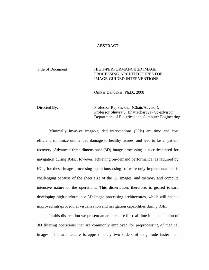
Figure 1.1: A typical IGI workflow and the scope of this dissertation work .......... 3
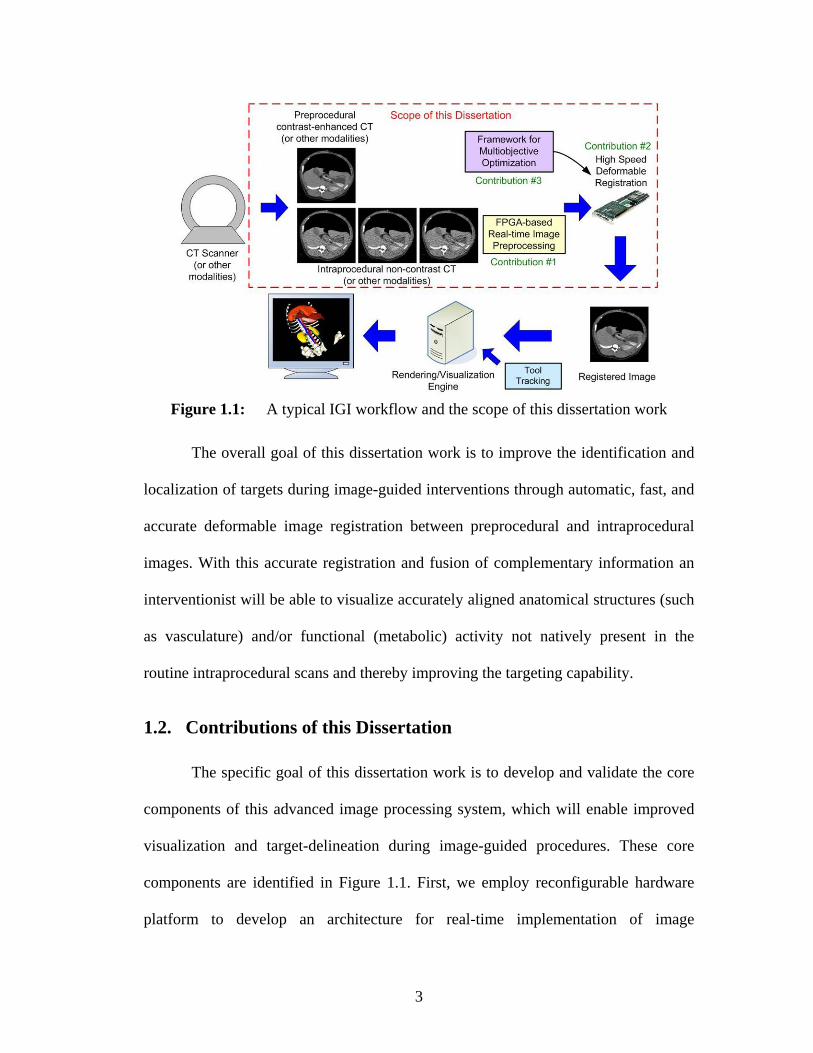
Figure 2.1: Two examples of pre- and intraprocedural image pairs. The arrows
indicate the targets that are visible in preprocedural images but not
visible in intraprocedural images. ....................................................... 11
Figure 2.2: An example of volumetric image guidance using intraprocedural
multislice CT and preprocedural MR. ................................................ 12
Figure 2.3: Flowchart of image similarity–based image registration.................... 17
Figure 2.4: Example of preprocessing techniques employed prior to intensity-
based image registration. .................................................................... 29
Figure 2.5: Pareto front in the context of multiobjective optimization. ................ 36
Figure 3.1: A median filtering example using majority voting technique. ........... 52
Figure 3.2: Block diagram of the FPGA-based real-time 3D image preprocessing
system. ................................................................................................ 53
Figure 3.3: Typical voxel access pattern for neighborhood operations–based image
processing. .......................................................................................... 54
Figure 3.4: Block diagram showing the input image memory and the input buffer
configuration. ...................................................................................... 56
Figure 3.5: Pictorial representation of the notation used in the brick-caching
scheme................................................................................................. 57
Figure 3.6: Top-level block diagram of 3D anisotropic diffusion filtering. This
diagram indicates paths that are executed in parallel.......................... 60

xiv
Figure 3.7: Block diagram of the embedded Gaussian filter bank (for N = 7,
corresponding Gaussian kernel size is 5)............................................ 61
Figure 3.8: Pipelined implementation of an individual Gaussian filter element
(Gaussian kernel size = 5)................................................................... 62
Figure 3.9: A single stage (processing element) of the linear systolic median
filtering kernel..................................................................................... 65
Figure 3.10: Linear systolic array architecture for median filter kernel using
majority voting technique. .................................................................. 68
Figure 4.1: Pictorial representation of hierarchical volume subdivision–based
deformable image registration and associated notation. ..................... 83
Figure 4.2: Pictorial representation of the acceleration approach. ........................ 86
Figure 4.3: Top-level block diagram of the architecture for accelerated
implementation of deformable image registration.............................. 88
Figure 4.4: Functional block diagram of voxel counter. ....................................... 89
Figure 4.5: Functional block diagram of coordinate transformation unit. ............ 91
Figure 4.6: Fundamentals of interpolation schemes.............................................. 92
Figure 4.7: Functional block diagram of partial volume interpolation unit. ......... 94
Figure 4.8: Voxel access patterns of the reference and floating images encountered
during image registration. ................................................................... 95
Figure 4.9: Organization of the reference image memory. ................................... 97
Figure 4.10: Organization of the floating image memory....................................... 98
Figure 4.11: Pipelined implementation of MH accumulation using dual port
memory. ............................................................................................ 100

xv
Figure 4.12: Preaccumulate buffers to eliminate RAW hazards in MH accumulation
pipeline.............................................................................................. 102
Figure 4.13: A flow diagram of steps involved in calculating MHRest. ................. 103
Figure 4.14: Error in entropy calculation corresponding to the two configurations of
the multiple LUT–based implementation. ........................................ 107
Figure 4.15: Qualitative validation of deformable registration between iCT and
preCT images performed using the presented FPGA-based solution.
........................................................................................................... 122
Figure 4.16: Qualitative validation of deformable registration between iCT and PET
images performed using the presented FPGA-based solution. ......... 123
Figure 5.1: Examples of parameterized architectural design style...................... 133
Figure 5.2: Framework for multiobjective optimization of FPGA-based image
registration. ....................................................................................... 134
Figure 5.3: Comparison of the area values predicted by the adopted area models
with those obtained after physical synthesis..................................... 141
Figure 5.4: Pareto-optimized solutions identified by various search methods.... 144
Figure 5.5: Qualitative comparison of solutions found by partial search and EA-
based search. ..................................................................................... 145
Figure 5.6: Quantitative comparison of search methods using the ratio of non-
dominated individuals (RNI). ........................................................... 147
Figure 5.7: Quantitative comparison of search methods using cover rate. ......... 148
Figure 5.8: Relationship between MI calculation error and resulting image
registration error................................................................................ 149

xvi
Figure 5.9: Results of image registration performed using the high-speed, FPGA-
based implementation for design configurations offering various
registration errors. ............................................................................. 153
Figure 6.1: Integration of deformable registration into IGI workflow................ 156
Figure 6.2: Important steps for evaluating registration accuracy with low-dose CT.
........................................................................................................... 159
Figure 6.3: Low-dose CT images generated by the dose-simulator. ................... 160
Figure 6.4: Comparison of techniques for preprocessing low-dose CT images.. 162
Figure 6.5: Qualitative comparison of registration accuracy with low-dose CT. 165
Figure 6.6: Average registration error with respect to dose using software and
FPGA-based implementations. ......................................................... 166
Figure 6.7: Graphic illustration of the quantitative validation approach used in the
context of deformable registration between intraprocedural and
preprocedural PET. ........................................................................... 173
Figure 6.8: Registration of intraprocedural CT and preprocedural PET images
using the FPGA-based implementation of deformable image
registration. ....................................................................................... 176

1
Chapter 1: Introduction
1.1. Overview
Image-guided interventions (IGIs), including surgeries, biopsies, and
therapies, have the potential to improve patient care by enabling new and faster
procedures, minimizing unintended damage to healthy tissue, improving the
effectiveness of the procedures, producing fewer complications, and allowing for
clinical intervention at a distance. As a result, IGIs has been identified by clinical
experts to have a significant impact on the future of clinical care [1]. With further
invention and development of imaging and image processing techniques, innovative
minimally invasive image-guided inventions will replace conventional open and
invasive techniques. Continuous three dimensional (3D) imaging and visualization for
intraprocedural navigation, critically important to the success of IGI, has been
technologically difficult until recently. However, the advances in medical imaging
technology and visualization capabilities, leading to improved imaging speed and
coverage, have prompted developments in imaging protocols and enabled volumetric
image-guided procedures.
The efficiency and efficacy of IGIs is critically dependant on accurate and
precise target identification and localization. Lack of clear target delineation could
lead to lengthy procedures, larger than necessary safety margins and unintended
damage to healthy tissue––factors that undermine the very motivation behind IGIs.
Intraprocedural imaging techniques provide a rich source of accurate spatial
information that is crucial for navigation but often suffer from poor signal-to-noise

2
ratio (SNR) and poor target definition from background healthy and/or benign tissue.
As in most clinical protocols, IGIs are preceded by one or more preprocedural
images, containing additional information, such as contrast-enhanced structures or
functional details such as metabolic activity, which are used for diagnosis,
treatment/navigation planning, etc. Combining this functional and/or contrast
information with intraprocedural morphological and spatial information, through co-
registration between pre- and intraprocedural images, has been shown to improve the
intraprocedural target delineation [2-6].
Achieving this registration between intraprocedural and preprocedural images
is a fundamental need during the IGI workflow. Moreover, given the on-demand
nature of IGIs, this alignment should be achieved sufficiently fast so as not to affect
the clinical workflow. Earlier approaches to meet this need primarily employed rigid
body approximation, which can be less accurate because of non-rigid tissue
misalignment between these images. Intensity-based deformable registration is a
promising option to correct for this misalignment. These algorithms are automatic,
which is an important aspect that enables their easy integration into many
applications; However, the long execution times of these algorithms have prevented
their use in clinical workflow. In addition, since this technique is based on intensity-
based alignment between images, it is sensitive to the SNR of the images to be
registered. Consequently, the images (in particular, intraprocedural images that are
characterized with poor SNR) need to be preprocessed and de-noised before they can
be registered. This workflow for providing improved visualization during IGIs is
illustrated in Figure 1.1.
3
The overall goal of this dissertation work is to improve the identification and
localization of targets during image-guided interventions through automatic, fast, and
accurate deformable image registration between preprocedural and intraprocedural
images. With this accurate registration and fusion of complementary information an
interventionist will be able to visualize accurately aligned anatomical structures (such
as vasculature) and/or functional (metabolic) activity not natively present in the
routine intraprocedural scans and thereby improving the targeting capability.
1.2. Contributions of this Dissertation
The specific goal of this dissertation work is to develop and validate the core
components of this advanced image processing system, which will enable improved
visualization and target-delineation during image-guided procedures. These core
components are identified in Figure 1.1. First, we employ reconfigurable hardware
platform to develop an architecture for real-time implementation of image
Figure 1.1: A typical IGI workflow and the scope of this dissertation work

4
preprocessing techniques commonly used in the context of IGI. Second, we develop
an field-programmable gate array (FPGA)–based architecture for accelerated
implementation of intensity-based deformable image registration. Third, we propose a
multiobjective optimization framework to analyze conflicting tradeoffs between
accuracy and hardware complexity of finite precision implementations of signal
processing application, such as presented in this work. Finally, we demonstrate the
feasibility of developing novel IGI applications leveraging the aforementioned
components.
In the following sections we elaborate further on the main contributions of this
dissertation.
1.2.1. Real-time 3D Image Preprocessing
Image preprocessing, which consists of filtering and de-noising, is a
prerequisite step in many image processing applications. Especially in the context of
IGI, where intraprocedural images are characterized by poor signal-to-noise ratio,
image preprocessing is required prior to advanced image analysis operations such as
registration, segmentation, and volume rendering. Moreover, the interactive nature of
IGIs necessitates equivalent image processing speed so that these operation can be
performed in a streamlined manner without any additional processing latency.
Most reported techniques for accelerated implementation of image processing
algorithms have primarily focused on one-dimensional (1D) or two-dimensional (2D)
cases [7-11]. These techniques do not adequately address the need for accelerating
these operations in 3D, which is required for providing volumetric image-guidance
during minimally invasive procedures. Furthermore, some of the earlier techniques

5
used for acceleration cannot be extended to 3D, whereas for some others the 3D
extension is nontrivial.
This dissertation presents an FPGA-based novel architecture for accelerated
implementation of common image preprocessing operations. This architecture is
reconfigurable and supports multiple filtering kernels such as 3D median filtering,
and 3D anisotropic diffusion filtering within the same framework. The architecture
presented in this work is faster than earlier reported techniques, supports larger kernel
dimensions, and is capable of meeting the real-time data processing need of most
IGIs. Although developed in the context of IGIs, this architecture is general-purpose
and can be applied to meet preprocessing needs of many medical as well as non-
medical applications.
1.2.2. Hardware-Accelerated Deformable Image Registration
Image registration between preprocedural images (acquired for diagnosis and
treatment planning) and intraprocedural images (acquired for up-to-date spatial
information) is an inherent need in the IGI workflow. Accurate and fast registration
between these images will enable the fusion of complementary information from
these two image categories and can enable improved treatment site identification and
localization and navigation during the procedure.
Several fiducial or point-based, mechanical alignment-based and intensity-
based rigid alignment techniques [12-16] have been proposed for this purpose. Some
of these techniques are not automatic and almost all of them employ the rigid body
approximation, which is often not valid due to tissue deformation between these two
image pairs. Deformable image registration techniques can compensate for both local

6
deformation and large-scale tissue motion and are the ideal solution for achieving the
aforementioned image registration. Some studies, in particular, have independently
underlined the importance of deformable image registration for IGIs [17-19].
However, despite their advantages, deformable image registration algorithms are
seldom used in current clinical practice due to their computational complexity and
associated long execution times (which can be up to several hours).
This dissertation presents a novel FPGA-based architecutre for accelerated
implementation of a proven automatic and deformable image registration algorithm,
specially geared toward improving target delineation during image-guided
interventions. This architecture accelerates calculation of image similarity, a
necessary and the most time consuming step in image registration, by greater than an
order of magnitude and thereby reducing the time required for deformable registration
time from hours to minutes. This design is tuned to offer registration accuracy
comparable to that achievable using software implementation. Furthermore, we
validate this high-speed design and demonstrate its feasibility in the context of
clinical applications such as computed tomography (CT)-guided interventional
applications. This accuracy, coupled with the speed and automatic nature of this
approach represents a first significant step toward assimilation of deformable
registration in the IGI workflow.
1.2.3. Framework for Optimization of Finite Precision Implementations
An emerging trend in image processing, and medical image processing, in
particular, is custom hardware implementation of computationally intensive
algorithms for achieving high-speed performance. The work presented in this

7
dissertation has a similar spirit in the context of advanced image processing required
during IGIs. For reasons of area-efficiency and performance, these implementations
often employ finite-precision datapaths. Identifying effective wordlengths for these
datapaths while accounting for tradeoffs between design complexity and accuracy is a
critical and time consuming aspect of this design process. Having access to optimized
tradeoff curves can equip designers to adapt their designs to different performance
requirements and target specific devices while reducing design time.
This dissertation proposes a multiobjective optimization framework developed
in the context of FPGA–based implementation of medical image registration. Within
this framework, we compare several search methods and demonstrate the
applicability of an evolutionary algorithm–based search for efficiently identifying
superior multiobjective tradeoff curves. In comparison with some earlier reported
techniques, this framework allows non-linear objective functions, multiple fractional
precisions, supports a variety of search methods, and thereby captures more
comprehensively the complexity of the underlying multiobjective optimization
problem. We also demonstrate the applicability of this framework for the image
registration application through synthesis and validation results using Altera Stratix II
FPGAs. This strategy can easily be adapted to a wide range of signal processing
applications, including areas of image and video processing beyond the medical
domain.
1.3. Outline of this Dissertation
The rest of the dissertation is organized as follows: Chapter 2 provides
background on image-guided interventions, image preprocessing, and image

8
registration; and presents related work in the context of the contributions of this
dissertation. In Chapter 3, FPGA-based architecture for real-time implementation of
3D image processing techniques such as median filtering and anisotropic diffusion
filtering are presented. Chapter 4 deals with deformable image registration. We
outline the intensity-based deformable image registration algorithm and present a
novel architecture for accelerated implementation of this algorithm. In Chapter 5, a
framework for multiobjective optimization of limited precision implementations of
signal processing algorithms is presented. Chapter 6 introduces some novel image-
guided procedures and demonstrates the feasibility of our approach in the context of
these applications. Finally, in Chapter 7 conclusions and future work are presented.

9
Chapter 2: Background and Related Work
2.1. Image-Guided Interventions
IGIs began to emerge in the last quarter of the 20th century, picked up pace in
the 1990s, and may become routine in the 21st century. Minimal invasiveness is the
defining characteristics of these procedures. This feature can lead to less patient
morbidity, time and cost efficient procedures, faster recovery and improve the
procedure outcomes. During these procedures, the internal anatomy is accessed
through a single or few small holes on the patient’s skin rather than though large
incisions. The interventionist introduces the appropriate tool (electrode or biopsy
needle, or/and endoscope) through this port and tries to navigate his/her way to the
target (typically a malignant spot) in order to deliver a localized treatment or take out
a sample for further investigation. Now, because the access to the internal anatomy is
through a single port, the only way to visualize the location, orientation and the path
of approach of the tool is by using external imaging techniques (that is there is no
direct visual feedback).
Any intraprocedural imaging technique used must be near real-time and thus
allow tracking underlying anatomy and flexible instruments and catheters as and
when required (“on-demand” performance) during the procedure. 2D Ultrasound
(US) and CT fluoroscopy have been conventionally used to guide placement of
biopsy needles and therapy delivery devices during IGIs [18, 20, 21]. However,
technological improvements such as multi-slice CT scanners, interventional MR, 3D
ultrasound (US), isocentric C-arms and other advanced imaging systems have enabled

10
the application of IGI to clinical domains such as interventional radiology,
neurosurgery, orthopedics, ENT surgery, cranio- and maxillofacial surgery and other
surgical specialties [22-24]. For example, Philips medical systems, one of the leading
medical imaging equipment manufacturers, has announced a 256-slice CT scanner
[25] which provides higher imaging speed (up to 8 volumes/s) and coverage (8 cm) is
ideally suited for performing CT-guided procedures. Availability of easy access MR
scanners, such as open-configuration MR scanner from GE Healthcare [26] along
with its improved imaging speed has enabled development of MR-guided procedures.
Image quality and acquisition speed of 3D ultrasound have also been enhanced
through use of latest transducer technology and digital reconstruction and it can now
be used for providing image-guidance during procedures. Moreover, real-time
volumetric visualization capabilities, that enable interactive display of images during
the procedure, are also now available [27, 28]. As a result, an emerging trend in IGI
workflow is to use volumetric imaging modalities for providing real-time
intraprocedural guidance. This dissertation, therefore, focuses on 3D image
processing and registration in the context of IGIs.
2.1.1. Role of Preprocedural Imaging
Intraprocedural imaging techniques provide (or, are a rich source of) accurate
spatial information which is crucial for navigation but offer poor target identification
from the background healthy and/or benign tissue (see Figure 2.1). Most image-
guided procedures are preceded by a preprocedural image which is used for
diagnosis, treatment/navigation planning, etc. These preprocedural images are
primarily acquired under different (often slow) imaging protocol and typically contain
11
additional information, such as contrast-enhanced structures or functional information
such as metabolic activity which is used for diagnosis and tissue differentiation prior
to the treatment. Figure 2.1(a) shows contrast-enhanced structures in a preprocedural
image which are not clearly visible in intraprocedural images. Figure 2.1(b) illustrates
the metabolic activity shown in the PET scans which can be used to identify
cancerous tumors. Availability of this functional and contrast information from the
preprocedural images can be used to augment the purely morphological and spatial
information from the intraprocedural images which will greatly improve the
intraprocedural target delineation [2-6, 29]. Therefore, there is a clear need to
combine this complementary information from the pre and intraprocedural images to
facilitate this task.
Figure 2.1: Two examples of pre- and intraprocedural image pairs. The arrows indicate the targets that are visible in preprocedural images but not visible in intraprocedural images.

12
2.1.2. Need for Image Registration
Aligning or registering the intraprocedural images with the preprocedural
image is a fundamental need in the IGI workflow. In fact, image registration has been
identified as an enabling technology for image-guided surgical and therapeutic
applications [30]. Figure 2.2 shows an example of volumetric image-guidance using
image registration between volumetric CT and magnetic resonance imaging (MRI)
scans for a neurosurgical application. There are, however, many technological and
logistic challenges in achieving this image registration. First, the intra- and
preprocedural images to be registered are acquired at different times and using
different scanners. As a result, there is invariably misalignment of anatomical
structures between these two images. This misalignment is caused because of the
Figure 2.2: An example of volumetric image guidance using intraprocedural multislice CT and preprocedural MR.

13
systemic offsets in scanner coordinate systems and due to non-rigid anatomical
changes arising from pose and diurnal variations at the time of image acquisition.
Second, the images to be combined can be of two completely different modalities
(such as PET and CT). Furthermore, given the on-demand nature of IGI applications
this registration should be achieved in a reasonably fast time. In summary, accurate,
multi-modal, and fast image registration is essential for IGIs [17, 31]. The following
section provides an overview of image registration.
2.2. Classification of Image Registration
Medical image registration is the process of aligning two images that
represent the same anatomy at different times, from different viewing angles, or using
different imaging modalities. Image registration is an active area of research and over
the last several decades there have been numerous publications outlining various
methodologies to perform image registration and its applications. Maintz and
Viergever [32] and Hill et al. [33] have presented a comprehensive summaries of the
entire gamut of the image registration domain. In general, image registration can be
classified based on image dimensionality, nature of registration basis, nature of
transformation models, type of modalities involved, etc. From the context of IGI,
Table 2.1: Broad classification of image registration in the context of IGI. Registration
Basis Method based on Retrospective Automatic Deformable Compute
Intensive Fiducial N Y N N Extrinsic
Information Stereotactic N Y N N Landmark Y N Y N
Segmentation Or Surface Y N Y N Intrinsic
Information Intensity Y Y Y Y

14
however, we broadly classify image registration into two main approaches. First,
techniques based on extrinsic information and second, techniques based on
information that is intrinsic to the image. We briefly describe these two techniques
and outline some popular image registration methods in each category. A summary of
this classification is also presented in Table 2.1.
2.2.1. Image Registration using Extrinsic Information
Methods based on extrinsic information rely on information that is not
natively a part of the medical image. This includes artificial external objects that may
be attached to the patient and are within the field of view of the image. These objects
are designed such that they are clearly visible and accurately detectable in all of the
pertinent modalities that are to be registered. As a result, the registration of the
acquired images is usually easy, fast, and can be automated with relative ease. In
addition, because the registration involves simply establishing correspondence
between external objects, it can be achieved explicitly without a need for complex
optimization techniques. One major limitation of these methods, however, is that they
are not retrospective. This means that advanced planning is required and provisions
must be made at the time of preprocedural imaging for that image to be used at a later
point. Furthermore, due to the nature of the registration these methods are mostly
limited to rigid transformation model only.
Stereotactic frame is another commonly used external object. There are many
reported image registration applications, especially in the context of neurosurgery,
that employ a stereotactic frame to establish spatial correspondence between images
[34, 35]. These methods employ a frame screwed rigidly to the patient’s skull that is

15
usually fitted with imaging markers that are visible in imaging modalities such as CT,
MRI, and X-ray. Visibility of these markers in both pre- and intraprocedural images
will then allow registration of these images using a least-square based alignment
technique. These techniques have been shown to be relatively accurate for rigid
anatomy such as the brain [36], but are relatively more invasive. Less invasive
techniques using markers attached to the skin have also been reported [37], but they
tend to offer less accurate image registration because skin can move. More recently,
there have also been efforts toward developing systems based on optical tracking
methods that will allow frameless stereotaxy [38]. Despite these advances, these
methods are fundamentally limited to providing only rigid alignment between a pair
of images.
2.2.2. Image Registration using Intrinsic Information
These methods are based on intrinsic properties and contents of patient-
generated images. Registration may be based on a limited set of identified salient
points (landmarks), on the alignment of segmented anatomical structures
(segmentation or feature based) such as organ surfaces or directly based on the image
intensity values (voxel property based).
Landmark-based registration [35, 39, 40] involves identification of the
locations of corresponding points within different images and determination of the
spatial transformation with these paired points. These landmarks are usually
identified by a user in an interactive fashion. Landmark-based methods are often used
to find rigid or affine transformations. However, if the sets of points are large enough,
they may be used for more complex non-rigid transformations as well. Registration

16
methods based on landmark identification can be retrospective, but they are not fully
automatic becasue they require user interaction.
Segmentation-based image registration methods are based on extracting
matching features and organ surfaces from the two images to be registered. These
features and organ surfaces are then used as the only input for the alignment
procedures. The alignment between the features/surfaces can be either based on rigid
transformation models or achieved using deformable mapping. The rigid model–
based approaches are more popular and a ‘head-hat’ registration method based on this
approach has been successfully applied to the registration of multimodal images such
as PET, CT, and MR [41-43]. Popular segmentation-based techniques that involve
deformable mapping of surfaces, such as the ones based on snakes or active contour
models, have been shown to be effective in intersubject and atlas registration, as well
as for registration of a template to a mathematically defined anatomical model [44,
45]. Segmentation-based techniques are retrospective, support multi-modal
registration, and are computationally efficient. However, the accuracy of registration
is dependant on the segmentation accuracy. Moreover, these methods are not fully
automatic as the segmentation step is often performed semi-automatically.
Voxel property-based methods, which are based on image intensity values, are
the most interesting methods in the current research. Theoretically, these are the most
flexible of the registration methods since they use all of the available information
throughout the registration process. In addition, these methods can be completely
retrospective, fully automatic, allow multi-modal registration and generally are more
accurate. The following section provides a detailed overview of intensity-based image

17
registration. Although these methods have existed for a long time, their extensive use
in clinical applications with 3D images has been limited because of associated
computational costs. This dissertation work addresses this aspect through the use of
hardware acceleration.
2.3. Intensity-Based Image Registration
Image registration that is based on voxel intensities is the most versatile,
powerful, and inherently automatic way of achieving the alignment between two
images. This method attempts to find the transformation T̂ that optimally aligns a
reference image RI, with coordinates x, y, and z, and a floating image FI under a
image similarity measure F . This process is summarized in the following equation
and is represented pictorially in Figure 2.3.
ˆ arg max ( ( , , ), ( ( , , )))T
T RI x y z FI T x y z= F (2.1)
Figure 2.3: Flowchart of image similarity–based image registration.

18
In the case of intensity based registration, the similarity measure F , which
provides a numerical value to indicate the degree of misalignment between the
images, is completely based on voxel intensities in the reference and the floating
images. Image transformation T maps the reference image voxels into the floating
image space. Depending on the transformation model employed, this mapping is
either rigid, affine, or deformable. The optimization algorithm, on the other hand,
searches for the best transformation parameters that optimally align the given two
images. These three components form an integral part of intensity-based image
registration and are described in the following sections.
2.3.1. Transformation Models
A transformation model provides a way to describe the misalignment between
the reference and the floating images. The ability of image registration to accurately
represent and recover this misalignment is fundamentally limited by the nature of the
transformation model employed. For example, rigid transformation model typically
offers inferior image registration accuracy as compared with computationally
intensive, non-rigid transformation models, if the underlying misalignment is non-
rigid. A comprehensive survey on image transformation models can be found in [46,
47]. The following subsections describe the transformations most commonly used in
intensity-based image registration.
2.3.1.1. Rigid and Affine Models
Affine or linear registration is a combination of rotation, translation, scaling
and shear parameters that map the reference image voxels into floating image space.

19
Voxel scaling and shearing factors are constant for rigid registration, which is a
special case of affine transformation, and as such are excluded from optimization
process. Both these transformation models can be represented using a 4 × 4
transformation matrix. For example, a rigid transformation matrix Tglobal can be
constructed as:
,
0 0 0 1
xx xy xz x
yx yy yz yglobal
zx zy zz z
r r r dr r r dT r r r d
⎡ ⎤⎢ ⎥
= ⎢ ⎥⎢ ⎥⎣ ⎦
(2.2)
where rij entries represents the components of the rotation matrix, while the di entries
represent the translation parameters. The coordinate transformation of a reference
image voxel rv into floating image space ( fv ) can then simply be achieved through
matrix multiplication:
.f global rv T v= ⋅ (2.3)
Techniques based on rigid and affine transformation models have been successfully
employed previously [47-49]. These techniques, however, offer limited degrees of
freedom in the transformation model.
2.3.1.2. Deformable Models
The strength of the deformable transformation models comes from the large
number of degrees of freedom they offer for representing the misalignment between
images. This allows modeling of not only gross misalignment between the images,
but also local deformations. As a result, image registration techniques based on
deformable transformation models are inherently capable of correcting for local
misalignments and therefore are more accurate.

20
Methods based on physical models perform image transformation by
considering a set of internal and external forces and obtaining the corresponding
deformation by applying these forces to a given model based on differential
equations. Some examples of physical models used for image transformation found in
the literature are elastic body [50], viscous fluid [51] and incompressible flow (optical
flow) [44]. Some methods based on finite element models have also been employed
for image registration, which apply predefined physical models to represent
deformation in the images [52, 53]. The key idea is to divide the image into subsets,
each with some defined physical properties. For example, a subset can be labeled as
rigid, while some others can be labeled as fluid (elastic). During the transformation
process, the shape of rigid tissues will not change, while the shape of fluid tissues will
vary according to their corresponding properties such as viscosity. Image
transformation techniques using physical models have been successfully applied to
deformable image registration. However, most of these techniques involve solving
partial differential equations and are particularly computationally complex.
Another popular method to represent deformable transformation model is to
use mathematical basis functions. These transformation techniques use basis
functions to define the correspondence between the original and the transformed
image. The basis functions may be defined in either Fourier or Wavelet domain, and
the deformation field is modeled using trigonometric or wavelet basis functions,
respectively. Ashburner and Friston [54] have reported a method based on this
approach. The deformation between the two images may also be modeled in the
spatial domain using polynomials. Polynomial-based image transformation

21
techniques use a global transformation function defined by a transformation matrix
that contains the transformation coefficients and a polynomial vector that contains the
components of the polynomial used to model the transformation. The simplest case of
polynomial-based image transformation is the affine transformation, which uses first-
degree polynomials. By increasing the degree of the polynomials, it is possible to
model complex non-rigid transformation as well. However, this method is seldom
employed due to difficulty in modeling small local transformations and that higher-
degree polynomials suffer from several artifacts [46]. These drawbacks are addressed
by spline-based representation. Splines are inherently continuous and consist of
piecewise-polynomial functions. Splines are a generalization of the polynomial-based
approach to image transformation in the sense that a polynomial representation is a
spline with just one segment. Using piecewise-polynomial functions allows modeling
of local deformations accurately without using high-order polynomials. Two different
spline families that have been used extensively in the literature to model 3D
transformations are thin-plate splines and B-splines. Kim et al. [55] and Rohr et al.
[56] have reported methods based on thin-plate splines to perform deformable image
registration. However, one major drawback of thin-plate splines is that they have
infinite support. This means that even small local changes are propagated throughout
the entire image, an effect that is undesirable in medical image registration. In
comparison, B-splines offer finite support. For this reason, B-splines are currently the
preferred basis functions for modeling deformable transformations [57, 58]. A
limitation with B-spline-based transformations is that they tend to fail at tracking
rotation of local features. Moreover, algorithms based on B-splines tend to be

22
computationally intensive due to additional complexity associated with B-spline
interpolations.
More recently, some algorithms based on hierarchical image subdivision
approaches have been reported [59, 60]. These algorithms achieve deformable
registration through registering image subvolumes using a locally linear
transformation and then applying quaternion-based interpolation to obtain the
transformation field. Algorithms based on such transformation models allow the
modeling of internal rotations better than the spline-based approaches. These
algorithms are computationally efficient and yet are capable of recovering local
deformations. The deformable registration algorithm considered in this dissertation is
also based on hierarchical volume (3D image)-subdivision. This algorithm and the
architecture for its accelerated implementation is describes in Chapter 4.
2.3.2. Image Similarity Measures
An important component of image registration is the metric that quantitatively
determines how similar two images are. This metric can then be used to judge how
well a pair of images is aligned and also to guide the optimization procedure during
image registration. In the case of intensity-based image registration this metric, or
image similarity measure, is computed using the voxel intensities of the images
involved in registration. There are many reported intensity-based similarity measures.
These can be broadly classified into measures using only image intensities (for
example, mean of square difference of intensities), measures using spatial (or
neighborhood) information (for example, pattern intensity or gradient-based
measures) and measures based on information theory (mutual information).

23
The following sections briefly describe some widely used similarity measures.
We use the following notation for this description. The images to be aligned are
reference image (RI) and the floating image (FI). A transformation T is applied to the
voxels of the reference image. An image similarity measure is calculated over the
region of overlap ( 0X ) between the RI and the FI and x represents the location of a
voxel in RI. N represents the number of RI voxel that belong to 0X . The
notations RIp , FIp , and ,RI FIp represent the individual probability distribution function
(PDF) of RI, individual PDF of FI, and the mutual PDF of RI and FI, respectively.
2.3.2.1. Sum of Squared Intensity Differences (SSD)
One of the simplest ways to achieve image alignments is to minimize the
intensity difference between the RI and FI. The sum of squared intensity differences
(SSD) measure tries to achieve that. The SSD between the two images is defined as:
0
21( , ) ( ( ) ( ( ))) .x X
SSD RI FI RI x FI T xN ∈
= −∑ (2.4)
As expected this measure will be minimized when two images are aligned well.
However, this measure is limited to work with images with same intensity patterns, or
in other words, for mono-modality image registration. Furthermore, Holden et al. [48]
have shown this similarity measure to be error-prone in the presence of noise.
2.3.2.2. Normalized Cross-Correlation (NCC)
If the assumption that registered images differ only by Gaussian noise is
replaced with a less restrictive one, namely that there is a linear relationship between
the two images, then the optimum similarity measure is the normalized cross-

24
correlation. Cross-correlation in both space and frequency domains has been used as a
voxel similarity metric. Cross-correlation in the space domain is defined by:
0
2
( ( ) )( ( ( )) )1( , ) x X
RI FI
RI x RI FI T x FINCC RI FI
N σ σ∈
− −∑=
⋅ (2.5)
where RI and FI are the mean intensities of the RI and FI respectively, whereas
RIσ and FIσ represent the standard deviations of RI and FI, respectively:
0
21 ( ( ) ) ,RIx X
RI x RIN
σ∈
= −∑ (2.6)
0
21 ( ( ) ) .FIx X
FI x FIN
σ∈
= −∑ (2.7)
Computation of this similarity measure can be time consuming as it requires
calculating the mean and the standard deviation as well as the cross-correlation
coefficient for the entire 3D images. Because of this high computational cost of
performing cross-correlation, spatial domain correlation is usually performed between
a whole image and a small portion of the other image. Cross-correlation is an
effective voxel similarity measure for images with low noise, but it high calculation
requirements make it a poor choice for real-time applications. Furthermore, it may not
yield optimal performance when applied to noisy images [46], such as ultrasound and
low-dose CT.
2.3.2.3. Mutual Information (MI)
Mutual information is a popular image similarity metric based on information theory.
The rationale behind this similarity measure is to consider image registration as the
process of maximizing the amount of information common to RI and FI, or

25
minimizing the amount of information present in the combined images. When the
images are perfectly aligned, the corresponding structures from both images will
overlap, minimizing the combined-information. The use of mutual information for
image registration was introduced by Collignon et al. [61] and Viola and Wells [62].
The MI is defined by:
( , ) ( ) ( ) ( , ) ,MI RI FI h RI h FI h RI FI= + − (2.8)
where the individual and mutual entropies are calculated as:
( ) ( ) ln( ( )) ,RI RIh RI p x p x= − ⋅∑ (2.9)
( ) ( ) ln( ( )) ,FI FIh FI p x p x= − ⋅∑ (2.10)
, ,( , ) ( ) ln( ( ))RI FI RI FIh RI FI p x p x= − ⋅ ⋅∑∑ (2.11)
A comprehensive survey of MI-based registration was presented by Pluim et al. [47].
Mutual information is a very effective similarity measure for multimodal image
registration because it can handle nonlinear information relations between data sets
[63]. Holden et al. [48] have demonstrated that mutual information-based techniques
are, in general, superior to other techniques for deformable image registration.
A broadly used variant of mutual information is called normalized mutual
information. The advantage of this similarity measure over mutual information is its
overlap-independence. It was introduced by Studholme et al. [64] as:
( ) ( )( , ) .( , )
h RI h FINMI RI FIh RI FI
+= (2.12)
There are several other intensity-based similarity measures beyond the ones
listed and described here. These include ratio of image uniformity, pattern intensity,
entropy of the difference image, etc. Mutual information, in comparison, is versatile,

26
inherently multimodal, and accurate; and hence has emerged as a popular choice for
both rigid and deformable image registration. In particular, the deformable
registration algorithm, being accelerated through custom hardware implementation in
this dissertation work, is also based on MI. See Chapter 4, for additional details.
2.3.3. Optimization Algorithms
Optimization algorithms are used to navigate the search space of
transformation parameters and to identify the optimal combination of transformation
parameters that best aligns a pair of images. It must be noted, that most often the
number of parameters to be searched for is more than one and this requires multi-
dimensional optimization algorithms. Another desired feature of an optimization
algorithm is that it requires fewer number of objective function evaluations. In the
case of intensity-based image registration, the objective function to be optimized is
the voxel similarity function. This calculation, usually, is compute intensive and
hence faster convergence is ideal. We briefly summarize common multidimensional
optimization scheme employed in the context of image registration.
The downhill simplex method, first introduced by Nelder and Mead [65] is an
unconstrained nonlinear optimization technique. A simplex is a geometrical figure
defined by N+1 points in an N-dimensional space. The simplex method starts by
placing a regular simplex in the solution space and then moves its vertices gradually
towards the optimum point through an iterative process. The downhill simplex
algorithm searches for the optimum value through a series of geometrical operations
on the simplex. Examples of these operations include reflection, reflection and
expansion, contraction, multiple contractions etc. Shekhar et al. [49, 66] and Walimbe

27
et al. [60, 67] have reported successful use of this optimization technique for voxel
similarity–based image registration.
Univariate optimization method tries to solve the multidimensional
optimization problem by breaking it into multiple one-dimensional optimization
problems. This is achieved by optimizing the variables, one variable at a time and
then repeating this step until convergence. This method is simple, but can suffer from
poor convergence in the presence of steep valleys in the search space. Powell’s
method builds upon the univariate method with an important distinction, that the
search direction does not have to be parallel with any of the variable axes. Thus, it is
possible to change multiple variables at the same time. This can achieve faster
convergence and effectively eliminate the convergence problem of the univariate
method. This algorithm has widely been used for optimizing intensity-based image
registration [47, 68, 69].
Optimization based on genetic algorithms is a technique that mimics the
genetic processes of biological organisms. Over many generations, natural
populations evolve according to the Darwinian principles of natural selection and the
“survival of the fittest”. Common operations involved in this method are crossover,
mutation and fitness evaluation. By following this process, genetic algorithms are
able to adapt starting solutions and ultimately find the optimal solution. These
techniques are capable of efficiently searching a complex optimization space.
However, representation of solutions in a genetic algorithm framework can be
challenging and limit their effectiveness especially in the context of deformable

28
registration (due to large number of parameters). Examples of genetic algorithm–
based optimization for image registration can be found in [70, 71].
Optimization using simulated annealing techniques involves minimization
methods based on the way crystals are generated when a liquid is frozen by slowly
reducing its temperature [65]. These algorithms work distinctly from the techniques
described earlier, in that they do not strictly follow the gradients of the similarity
measure. Instead, they move randomly, depending on the “temperature” parameter.
While the “temperature” is high, the algorithm allows greater variations in the
variables to be optimized. As the “temperature” decreases, the algorithm further
constrains the variation of the variables until a global optimum is reached. In general,
simulated annealing techniques are more robust than earlier described methods.
However, these techniques may require a large number of iterations to converge,
especially in the presence of local minima. Some applications of simulated annealing
techniques for image registration are described in [72, 73].
2.4. Image Preprocessing
As described in the previous section, intensity-based image registration (both
rigid and deformable) utilizes similarity measures that are based on the voxel
intensities of the images to be registered. As a consequence, these similarity measures
are sensitive to quality of the images involved. Images with poor SNR can affect the
calculation of a similarity measure and result into less-accurate image registration.
While some similarity measures such as MI and NMI are less sensitive to noise,
Holden et al. [48] have demonstrated that most intensity-based similarity measures

29
(and resulting accuracy of image registration) are adversely affected in the presence
of noise.
To address this aspect, several techniques for preprocessing images prior to
image registration have been described. While some techniques focus on identifying a
region or structures of interest in the images and exclude structures that may
negatively influence the registration results [48, 49, 74], most preprocessing
techniques rely on spatial-domain filtering operations on the images. Some reported
techniques have employed low-pass filtering to remove speckle noise in ultrasound
images, thresholding or filtering to remove noise, and blurring to correct for
differences in the intrinsic resolution of the images [49, 64, 75]. All these spatial
filtering techniques have shown to be effective in improving the image quality and
the accuracy of image registration.
In the context of IGI, which is the primary application of the work presented
in this dissertation, low-dose computed tomography (CT) and 3D ultrasound have
emerged as the preferred intraprocedural volumetric imaging modalities. These
modalities, although sufficiently fast for intraprocedural use, suffer from quantum
noise and speckle noise respectively. Furthermore, due to presence of metallic tools
Ultrasound Image Filtered US Image Low-dose CT Image Filtered CT Image
Anisotropic Diffusion Filtering Median Filtering Figure 2.4: Example of preprocessing techniques employed prior to intensity-based image registration.

30
such as needles and catheters and associated photon scattering effects, intraprocedural
CT images also suffer from metal artifacts. As a result, these images must be
preprocessed and enhanced prior to registration with preprocedural images and
subsequent visualization. Toward this end, anisotropic diffusion filtering and median
filtering have been shown to be effective. Figure 2.4 shows an example application of
these filtering operations. In particular, anisotropic diffusion filtering has been
successfully applied for preprocessing of ultrasound, CT, and low-dose CT images
[76-78]. Similarly, median filtering has been employed, both in spatial and sinogram
domains, to reduce or eliminate metal artifacts and for filtering low-dose CT images
[79, 80]. In this dissertation we, therefore, focus on these two filtering techniques.
2.4.1. Anisotropic Diffusion Filtering
Anisotropic diffusion filtering is an iterative process which progressively
smoothes an image while maintaining the significant edges. The nonlinear anisotropic
diffusion algorithm for edge-preserving image smoothing was first proposed by
Perona and Malik [81]. For a 3D image I with intensities ( , )I v t , where v is a vector
in the 3D space and t is a given point in time (for the purposes of modeling the
diffusion process), the diffusion process is described by the following equation:
( ) ( )( ), , ,I div c v t I v tt
∂∂
= ∇i (2.13)
where c is the diffusion coefficient and takes a value between zero and 1. In general,
the diffusion coefficient is defined as a function of the image gradient (i.e.,
( )c f I= ∇ ). For noisy images, Whitaker and Pizer [82] showed that gradient
estimates taken from the image itself tend to be unreliable and proposed, instead, the

31
use of a Gaussian-filtered version of the image to calculate the gradient values. Their
proposed Gaussian filter has a standard deviation ( )tσ that decreases as the time ( t )
increases, thus resulting in a multiscale approach. Dorati et al. [83] demonstrated the
usefulness of Whitaker and Pizer’s approach to 3D ultrasound image preprocessing.
The diffusion coefficient that uses the Gaussian-filtered image (indicated as ( ( ))G tσ )
is then defined as:
( )( ) ( )( ), .c f G t I v tσ= ∇ i (2.14)
Several diffusion functions have been proposed in the literature. The two most
widely used are:
( )( ) ( )
2
1
,exp ,
G t I v tc
K
σ⎛ ⎞⎛ ⎞∇⎜ ⎟⎜ ⎟= −⎜ ⎟⎜ ⎟⎜ ⎟⎝ ⎠⎝ ⎠
i (2.15)
and
( )( ) ( )
11
2
,1 .
G t I v tc
K
ασ
−+⎛ ⎞⎛ ⎞∇⎜ ⎟⎜ ⎟= +⎜ ⎟⎜ ⎟⎜ ⎟⎝ ⎠⎝ ⎠
i (2.16)
These diffusion functions depend on the gradient of the Gaussian-filtered image,
while the parameter K adjusts the levels at which edges are diffused or preserved, to
achieve the desired filtering effect.
2.4.2. Median Filtering
Median filtering is a nonlinear technique commonly used to eliminate speckle
noise from ultrasound and impulse noise from other noisy images. This technique is
called non-linear because it can not be represented as a direct convolution operation.

32
This technique is based on rank-ordering of the intensity values present in an image.
In addition, this filter is an edge-preserving filter. The advantage of this technique
when compared to most linear (convolution-based) smoothing operators is that it
smooths areas within a particular object, while preserving its edges. This feature is
important, especially in the context of medical image registration, since it generally
improves the accuracy of the image registration, segmentation, and visualization
operations by preserving anatomical boundaries, while reducing random noise in the
interiors of the structures. However, such filters, due to their nonlinear nature, tend to
be computationally more intensive as compared with linear filtering operations.
The 3D realizations of these preprocessing operations, despite their
effectiveness, can take several seconds when implemented in software. Consequently,
for seamless integration into the IGI workflow these techniques must be accelerated
so that their performance is comparable to the acquisition speed of intraprocedural
images. This dissertation addresses this need through real-time implementation of 3D
realizations of these operations as described in Chapter 3.
2.5. Optimization of Finite Precision Implementations
An emerging trend in image processing, and medical image processing, in
particular, is custom hardware implementation of computationally intensive
algorithms in the quest to achieve real-time performance. The work presented in this
dissertation has a similar spirit in the context of advanced 3D image processing
required during IGIs. For reasons of area (and power)-efficiency and performance,
these implementations often employ limited-precision datapaths. In comparison, the
original algorithms are often developed in software using the double-precision

33
representation. Identifying effective wordlengths for these datapaths while accounting
for tradeoffs between design complexity and accuracy is a critical and time
consuming aspect of this hardware design process. This problem of converting
floating-point implementations into fixed-point (or other limited precision
representations) through identification of optimum wordlengths is an important
problem in signal processing applications and has received considerable attention in
the literature. Cantin et al. [84] and Todman et al. [85] provide a comprehensive
review of techniques to identify optimal wordlengths. We briefly summarize some
important approaches here.
2.5.1. Optimal Wordlength Formulation
Consider a system with m internal variables and a wordlength iw associated
with each variable. Further, each variable can take values between the lower ( miniw )
and upper ( maxiw ) bound on the wordlength such that min max( , )
i iiw w w∈ . Each
wordlength is an integer variable, and the wordlength configuration for the entire
system can then be represented using a wordlength vector ( )mW W I∈ such as
1 2{ , , , }mw w w . Furthermore, min max( , )W W W∈ ; where 1 2min min min min{ , , , }
mW w w w=
and 1 2max max max max{ , , , }
mW w w w= . Consider a function H associated with the system
that defines the hardware implementation cost associated with a wordlength
configuration W . Also, consider that the performance of this limited-precision,
quantized system is characterized by function ( )p W and that the system must
achieve a certain performance minP . The wordlength optimization problem can then be
presented as:

34
min max
min( , )
arg min ( ), such that ( ) .W W W
H W p W P∈
≥ (2.17)
It must be noted that this formulation, for simplicity, considers only one objective
function H with respect to a predefined performance criterion minP . The more general
multi-objective formulation is briefly described below and revisited in detail later in
the context of FPGA-based implementation of deformable image registration (see
Chapter 5).
2.5.2. Simulation-Based Optimal Wordlength Search
Optimal wordlength configuration that meets a certain performance criterion
can be identified by solving analytical expressions, when the performance function
p can be represented analytically. Some earlier reported approaches have adopted
this technique [86-90]. However, if the performance function can not be represented
analytically, which is often the case for practical complex systems, simulation-based
methods can be used to search for the optimal configuration. This involves searching
the design space (defined by the wordlength vector ranges) and finding a solution that
satisfies the design criteria. Some popular methods in this category are briefly
described below. A detailed description of these methods can be found in [84, 91].
An exhaustive search attempts every possible combination of wordlengths
between the predefined lower and upper bounds and evaluates the performance of
each combination through simulation. The optimum wordlengths can then be selected
from the simulation results. An exhaustive search is guaranteed to find the global
optimal configuration, however, the number of solutions explored and the associated
execution time increase exponentially as the number of variables increases.

35
Another method, proposed by Sung and Kum [92] searches for the first
solution that satisfies a given performance requirement or an error criterion. These
method starts with an initial guess for the system configuration based on uni-variable
simulations. The wordlength of each variable, as provided by this initial guess, is then
sequentially incremented by one until a configuration that meets the error criterion is
found. Although, this method is more efficient than the exhaustive search, finding the
globally optimal configuration is not guaranteed.
A sequential search method [84, 93] that takes into account the performance
sensitivity to determine the direction of the search is another way to approach this
problem. This method starts with an initial guess based on uni-variable simulations;
however, the further search direction is determined by the sensitivity of the
performance to each variable. This sensitivity is estimated by calculating the gradient
of the system performance with respect to all the variables and the search progresses
in the direction of the variable (that is wordlength of that variable is incremented) that
offers most improvement. It is also possible to consider hardware cost sensitivity
instead of the performance sensitivity in this search method.
2.5.3. Multiobjective Optimization
One of the limitations of the optimization formulation described above is that
search methods based on this formulation are limited to finding a single solution that
satisfies a design objective. Most real-world problems (including the wordlength
optimization problem), however, can have several objectives (that generally conflict
with each other) that need to be achieved at the same time. For example, in the case
of finite-precision implementations, hardware resource requirements and the

36
implementation accuracy are two such conflicting objectives. Because of the
conflicting nature of the involved objectives, multiobjective optimization problems do
not normally have a single optimal solution and even necessitate a new definition of
optimality.
The most commonly adopted notion in multiobjective optimization problems
is that of Pareto optimality. A vector of decision variables *x ∈F is Pareto optimal if
there does not exist another solution x ∈F such that fi(x) ≤ fi(x∗), for all i, and
fj(x) < fj(x∗), for at least one j, where fi represents an objective function defined for
every x∈F . This definition of optimality almost always provides a set of solutions
called the Pareto-optimal set. The set of vectors x∗ corresponding to the solutions in
the Pareto-optimal set are called non-dominated solutions. This concept is pictorially
illustrated in Figure 2.5.
Formulating the wordlength optimization as a multiobjective problem has
merit because it allows finding a set of Pareto-optimal configurations representing
strategically-chosen tradeoffs among the various objectives. This allows a designer to
choose an efficient configuration that satisfies given design constraints and provides
ease and flexibility in modifying the design configuration as the constraints change.
Figure 2.5: Pareto front in the context of multiobjective optimization.

37
For example, Leban and Tasic [94] used error, delay, and area as objectives. Han and
Evans [91] performed optimization of area and error through linear aggregation,
while Givargis et al. [95] considered power and execution performance trade-off for
system-on-chip architecture through series of monobjective optimizations. There are
also some heuristic techniques that take into account tradeoffs between hardware cost
and implementation error and enable automatic conversion from floating-point to
fixed-point representations [96]. In this dissertation work, we develop a framework
for multiobjective optimization of finite precision implementations. This framework
has been developed for optimization of the FPGA-based image registration and has
been validated through post-synthesis evaluation.
2.6. Related Work
2.6.1. Real-Time Image Preprocessing
Image preprocessing plays a crucial role in image understanding based
systems, video processing, and in the medical imaging domain. Over last two decades
much work was done on implementing image processing components in hardware. A
detailed description of various single instruction multiple data (SIMD) and multiple
instruction multiple data (MIMD) architectures can be found in [97, 98]. With
availability of variety of computing platforms such as digital signal processors
(DSPs), graphics processing units (GPUs), and FPGAs some of the image processing
algorithms have also been mapped to these platforms for achieving superior
performance. Most reported techniques, however, focus on 1D or 2D realizations and
do not adequately address the need for accelerating these operations in 3D. Moreover,

38
because of the larger 3D neighborhoods (N3 as opposed to N or N2), data input
requirements are increased and the performance achieved for 1D or 2D realizations
may not translate to their corresponding 3D implementations. This additional
complexity, coupled with the sheer size of 3D images (typically 2–5 million voxels),
makes achieving real-time performance extremely challenging. Consequently, only a
few designs for high-speed implementation of 3D image preprocessing techniques
have been reported in the literature. We focus on implementations of anisotropic
diffusion and median filtering and summarize those efforts here.
Rumph et al. [10] implemented the 2D nonlinear diffusion process on a
graphics hardware. The primary focus of this work was to achieve acceleration
through parallelism and better memory bandwidth. Gijbels et al. [8], on the other
hand, have reported a VLSI architecture based on linear array technique for
implementation of iterative diffusion process. A similar VLSI-based approach was
also reported recently for 1D nonlinear signal processing [11]. Accelerated
implementations of 3D anisotropic diffusion filtering using computing clusters have
also been reported. Bruhn et al. [99, 100] have reported an approach using a 256-node
Myrinet cluster, whereas Tabik et al. [101] have explored multiple parallel
programming paradigms built on message passing and shared-memory architectures.
Both these techniques have yielded near-linear speedups.
Accelerated implementations of median filters based on searching, sorting,
and bit-level methods have previously been reported in the literature. We particularly
focus on bit-level methods because they are well suited to finding the median of large
3D neighborhoods in hardware. Bit-level methods for median filtering can be

39
classified into the bit-serial sorting, bit-serial searching, threshold decomposition, and
majority voting–based methods. Bit-serial sorting is performed using sorting
networks such as the odd–even exchange network and reduced bubble sort network
[102, 103]. Bit-serial searching [104], also called the radix method, involves a bit-by-
bit search to find the median. The threshold decomposition method [105] provides a
modular and parallel design, but the hardware requirements grow exponentially with
the number of bits used to represent images. Majority voting methods are based on
determining bit-wise majority starting from the most significant bits (MSBs). Lee and
Jen [9, 106] have described a novel binary majority gate that can determine the
majority of binary input signals using an inverter circuit. A compact majority voting
circuit using an adder array to count the number of 1s and a threshold comparator to
determine an individual bit of the median is described by Benkrid et al.[7]. Variations
on this approach have been described in the literature [107-109]. Systolic array
architectures for bit-level sorting networks have been shown to improve concurrency
of the bit-serial sorting designs [102, 103, 110-113]. The median filter design
presented in this work is a combination and 3D extension of bit-serial searching and
majority voting approaches.
In this dissertation work, we introduce a novel FPGA-based architecture of 3D
anisotropic diffusion filtering. In addition, this work develops an architecture for 3D
median filtering kernel, which is faster than existing solutions and is capable of
supporting higher 3D kernel sizes. Our solution is compact, easily deployable and is
capable of processing the intraprocedural images faster than their acquisition speeds.
40
2.6.2. Acceleration of Image Registration
Intensity-based automatic image registration is a key component of modern
medical imaging. Fast and accurate image registration can enhance many diagnostic
and interventional applications. However, this task is also computationally intensive
due to dimensionality of the images involved and memory-bound nature of the
operation. It is this aspect that has limited the integration of intensity-based image
registration (and that of deformable nature, in particular) in clinical applications. To
address this aspect many researches have independently attempted to accelerate
intensity-based image registration. Classification of these acceleration attempts has
been reported by Plishker et al. [114]. We briefly summarize these attempts here.
2.6.2.1. Multi-Processor and Supercomputer–Based Approaches
Image registration problem lends itself well for acceleration through parallel
implementation. Inherent data-parallel nature (same operations to be performed on
every voxel of an image) of these algorithms makes them readily amenable to
parallelization. The majority of earlier reported attempts to accelerate intensity-based
deformable registration have primarily employed a multiprocessor approach. Ourselin
et al. [115] reported a parallel implementation of affine registration using a 10-
processor cluster that provided a 6-fold speedup. Stefanescu et al. [116] implemented
Demons algorithm [44] on a similar cluster of 15 2-GHz Pentium CPUs and achieved
an 11-fold speedup for non-rigid image registration between a pair of magnetic
resonance images. Similarly, Ino et al. [117] have reported a fast implementation of
MI-based deformable registration using a 128-processor cluster. Another acceleration
approach has been to use supercomputers, which offer a high degree of parallelism.

41
Warfield et al. [118] performed deformable registration on a Sun supercomputer in 15
sec. However, interactive segmentation of the brain surface in the intraprocedural MR
images took several minutes. Moreover, this implementation was specific to brain
MR images because of high surface correspondence. Rohlfing et al. [57] have
reported a speedup of 40 for a splines-based deformable registration algorithm using a
64-processor shared-memory supercomputer (SGI Origin 3800). Although these
solutions delivered high performance by virtue of parallelization, the speedup
achieved per processor was less than unity. Moreover, these solutions may not be cost
effective, and because of their size, are unlikely to be suitable for clinical deployment.
2.6.2.2. Graphics Processor (GPU)–based Approaches
The recent emergence of powerful graphics processors (GPUs) has enabled a
new direction for accelerating computationally intensive applications. Modern GPUs
offer an array of processing elements that can offer customized data parallel
processing. Many high level languages, such as Cg, Brook, CUDA, are emerging to
aid the task of programming GPUs. This has enabled the use of GPUs for many other
applications such as image registration beyond graphics domain. Strzodka et al. [119]
reported the first implementation of image registration using the graphics hardware.
This implementation accelerated a gradient flow–based image registration using
graphics hardware. However, it was limited to registration of 2D images only and
offered only limited speedup. Kohn et al. [120] have reported another implementation
of gradient-flow based image registration that supports 3D images. Although, this
implementation offered moderate speedup for rigid registration, the performance
achieved for 3D deformable image registration was poor. Plishker et al. [121] have

42
employed GPUs for applying transformations to images during rigid registration. This
implementation achieved 3-fold improvement in execution time over a CPU-based
implementation. More recently, Vetter et al. [122] have reported acceleration of MI-
based multimodal registration using graphics hardware. Although, this
implementation achieved accuracy comparable to that achieved using a software
implementation, the speedup achieved was only about 5-fold. In summary, these
reported solutions demonstrate how this promising platform can be utilized for certain
image registration techniques. However, the architecture of GPUs along with their
lack of efficient scatter operation is not optimally suitable for operations such as
accumulation which is a prerequisite (accumulation of the mutual histogram [MH])
for calculation of MI. As a result, GPU-based solutions, despite being compact and
low-cost, may not provide substantial acceleration for calculation of MI, which is the
most versatile and robust image similarity measure.
2.6.2.3. Other Approaches
Emerging multi-core processors are able to accelerate medical imaging
applications by exploiting the parallelism available in their algorithms. Ohara et al.
[123] have implemented an MI-based 3D rigid registration algorithm on the Cell
Broadband Engine (CBE) processor, which has nine processor cores on a chip and
has a 4-way SIMD unit for each core. By exploiting the highly parallel architecture
and its high memory bandwidth, this implementation with two CBE processors can
compute MI around 11-times faster than a sequential implementation. However, this
implementation does not support deformable image registration.

43
General purpose hardware languages and compilers for transforming high-
level descriptions into hardware are becoming increasingly popular. Streams-C,
Handel-C, Mitrion-C are examples of such tools. These tools allow direct translation
of code developed using high-level languages such as C, Java, or Matlab into efficient
hardware implementations. Although, these techniques have provided considerable
speedup for applications involving matrix operations, linear algebra, and search, their
performance in complex applications requiring architectural insights has been limited.
For example, Jiang et al. [124] have reported a method for acceleration of splines-
based deformable image registration using Handel-C. The converted design, when
implemented using a Xilinx device, could achieve speedup a of only 3.2 when
compared with an equivalent software implementation.
In comparison with the techniques mentioned above, this dissertation work
presents a novel FPGA-based architecture for high-speed implementation of MI-
based deformable 3D image registration. This architecture is capable of accelerating
MI calculation by a factor of 40 using a single computing element. Consequently, the
execution time for deformable image registration is reduced from hours to a few
minutes. Furthermore, this implementation is accurate, automatic, compact, and
completely retrospective.
2.6.3. Optimization of Finite Precision Implementations
With the need for real-time performance in signal processing applications an
increasing trend is to accelerate computationally intensive algorithms using custom
hardware implementation. The architectures presented in this dissertation, for
accelerated implementation of image preprocessing and image registration, fall into

44
the same category. A critical step in going to a custom hardware implementation is
converting floating-point implementations to fixed-point realizations for performance
reasons. This conversion process is an inherently multidimensional problem, as
several conflicting objectives, such as area and error, have to be simultaneously
minimized. By systematically deriving efficient tradeoff configurations, one can not
only reduce the design time [125] but can also enable automated design synthesis [96,
126]. Furthermore, these tradeoff configurations will allow designers to identify
optimized, high quality designs for reconfigurable computing applications. The work
presented in this dissertation develops a framework for optimizing tradeoff relations
between hardware cost and implementation error in the context of FPGA-based image
registration.
Earlier approaches to optimizing wordlengths used analytical approaches for
range and error estimation [86-90]. Some of these have used the error propagation
method (e.g., see [89]), whereas others have employed models of worst-case error
[87, 90]. Although, these approaches are faster and do not require simulation,
formulating analytical models for complex objective functions, such as MI, is
difficult. Statistical approaches have also been employed for optimizing wordlengths
[127, 128]. These methods employ range and error monitoring for identifying
appropriate wordlengths. These techniques do not require range or error models.
However, they often need long execution times and are less accurate in determining
effective wordlengths.
Some published methods search for optimum wordlengths using error or cost
sensitivity information. These approaches are based on search algorithms such as

45
“Local,” “Preplanned,” and “Max-1” search [84, 93]. However, for a given design
scenario, these methods are limited to finding a single feasible solution, as opposed to
a multiobjective tradeoff curve. In contrast, the techniques we present in this
dissertation are capable of deriving efficient tradeoff curves across multiple objective
functions.
Other heuristic techniques that take into account tradeoffs between hardware
cost and implementation error and enable automatic conversion from floating-point to
fixed-point representations are limited to software implementations only [96]. Also,
some of the methods based on heuristics do not support different degrees of fractional
precision for different internal variables [87]. In contrast, the framework presented in
this dissertation allows multiple fractional precisions, supports a variety of search
methods, and thereby captures more comprehensively the complexity of the
underlying multiobjective optimization problem.
Other approaches to solve this multiobjective optimization problem have
employed weighted combinations of multiple objectives and have reduced the
problem to mono-objective optimization [91]. This approach, however, is prone to
finding suboptimal solutions when the search space is nonconvex [129]. Some
methods have also attempted to model this problem as a sequence of multiple mono-
objective optimizations [95]. The underlying assumption in this approximation,
however, is that the design parameters are completely independent, which is rarely
the case in complex systems. Modeling this problem as an integer linear
programming formulation has also been shown to be effective [86]. But this approach

46
is limited to cases in which the objective functions can be represented or
approximated as linear functions of design variables.
Evolutionary algorithms (EAs) have been shown to be effective in solving
various kinds of multiobjective optimization problems [130, 131] but have not been
extensively applied to finding optimal wordlength configurations. An exception is the
work of [94], which employs mono-objective EAs. In contrast, our work
demonstrates the applicability of EA-based search for finding superior Pareto-
optimized solutions in an efficient manner, even in the presence of a non-linear
objective function, such as MI. Moreover, our optimization framework supports
multiple search algorithms and objective function models; and can easily be extended
to a wide range of other signal processing applications. This optimization framework,
which is developed and validated in the context of FPGA-based 3D image
registration, is described in detail in Chapter 5.

47
Chapter 3: Real-time 3D Image Processing
This chapter presents an FPGA-based architecture for real-time
implementation of 3D image pre-processing techniques commonly employed in IGI.
First, we outline the filtering algorithms that are being accelerated in this work. Next,
we present the architecture for their real-time implementation. Finally, we describe
the realization of this architecture, analyze the effects of finite precision
implementation, and compare the performance of this implementation with earlier
reported efforts.
3.1. Motivation
Real-time and high-quality three-dimensional (3D) intraprocedural
visualization is a critical need for IGIs. Recent advances in computer and transducer
technology have made high-speed 3D imaging possible with high resolution and
acquisition speed. Notably, low-dose computed tomography (CT) and 3D ultrasound
have emerged as the preferred volumetric imaging modalities during many image-
guided procedures [18, 132-135]. The advent of multislice CT allows high-resolution
and high-frame-rate volumetric imaging of the operative field. In the continuous
volumetric mode, multislice CT is capable of acquiring images with 256 × 256 × 64
dimensions and resolutions of 0.625 mm, 8 times per second. Similarly, advances in
transducer technology have led to improvements in the field of 3D ultrasound
imaging, which can now acquire images with 128 × 128 × 128 dimensions and
resolution of 1 mm, 20 times per second. These intraprocedural images, acquired
during the procedure for navigation, represent the most current anatomical

48
information but often suffer from poor signal-to-noise ratio. To achieve desired
accuracy for IGIs, these intraprocedural 3D images, therefore, must be preprocessed
and enhanced before they can be used for advanced image processing operations such
as segmentation, registration, and visualization. Toward this end, anisotropic
diffusion filtering and median filtering have been shown to be effective in enhancing
and improving the visual quality of these images. It is important to note that the
interactive nature of IGIs necessitates equivalent image processing speed so that these
procedures can be performed in a streamlined manner without any additional
processing latency.
The aforementioned filtering techniques are based on neighborhood (window)
operations. For volumetric (3D) images, these neighborhoods are considerably larger
(N3), thus increasing the complexity of filtering operations. This complexity, coupled
with the sheer size of intraprocedural volumetric images, results in execution times of
several seconds for software implementations running on general-purpose
workstations (Table 3.1). This processing speed is only a fraction of the acquisition
speed of the intraprocedural images and is clearly unacceptable to meet the real-time
Table 3.1: Software execution time of 3D anisotropic diffusion filtering and 3D median filtering of 8-bit images for common kernel sizes (N).
Filter kernel Kernel size (N)
Image size (voxels)
Execution time
(seconds)
Voxel processing
rate (MHz)
128 × 128 × 128 2.28 0.92 3D anisotropic diffusion filter 7
256 × 256 × 64 4.58 0.92 128 × 128 × 128 0.85 2.46 3 256 × 256 × 64 1.59 2.63 128 × 128 × 128 3.01 0.7
3D median filter
5 256 × 256 × 64 5.67 0.74

49
requirements of IGIs. Previously reported techniques for accelerated implementation
of these filtering operations primarily focused on one-dimensional (1D) or two-
dimensional (2D) filters [7-11], with only a few implementations attempting to
accelerate these operations in 3D.
This dissertation presents an FPGA–based architecture for real-time
processing of intraprocedural 3D images. Earlier attempts to accelerate 3D
anisotropic diffusion filtering were targeted toward multiprocessor clusters [100,
101]. Despite the near-linear speedup offered by these techniques, the need to employ
up to 256 processors to achieve real-time performance makes them less suitable for
clinical deployment. In this dissertation, we introduce a novel FPGA-based
implementation of 3D anisotropic diffusion filtering. The developed solution is
compact, easily deployable, and capable of processing the intraprocedural images
faster than acquisition speeds. Some researchers have recently reported high-speed
implementations of 3D median filtering using graphics processing units [136] and
FPGAs [137]. This work presents an FPGA-based 3D median filtering module that is
faster than currently existing solutions and supports higher 3D kernel sizes (3,5,7).
The designed architecture can achieve a processing rate close to 200 Megavoxels per
second for both the 3D anisotropic diffusion and 3D median filtering, which is
equivalent to about 50 processing iterations or operations per second for images of
size 256 × 256 × 64. Consequently, this design is capable of meeting the real-time
data processing need of most IGIs.

50
3.2. Filtering Algorithms
This section briefly describes the 3D image preprocessing algorithms that are
being accelerated in the current work. The architecture for their real-time
implementation is presented in the subsequent section.
3.2.1. Anisotropic Diffusion Filtering
As described earlier, anisotropic diffusion filtering is an iterative process
which progressively smoothes an image ( ( , )I v t ) while maintaining the significant
edges. This process can be summarized by the following equation:
( ) ( )( ), , ,I div c v t I v tt
∂∂
= ∇i (3.1)
where c is the diffusion coefficient. Since the intraprocedural images typically have
poor SNR, the current implementation employs Gaussian-filtered version of the
image to estimate the gradient values, as proposed by Whitaker and Pizer [82]. The
corresponding discrete expression, which is implemented in our design, for this
filtering operation (shown for a 2D case for simplicity) is:
( )( )( )( )
( 1, , ) ( , , ) [ ( 1, , ) ( , , )]( 1, , ) ( , , ) [ ( 1, , ) ( , , )]
( , , ) ( , , )( , 1, ) ( , , ) [ ( , 1, ) ( , , )]( , 1, ) ( , , ) [ ( , 1, ) ( , ,
G G
G G
G G
G G
c I x y t I x y t I x y t I x y tc I x y t I x y t I x y t I x y t
I x y t t I x y t tc I x y t I x y t I x y t I x y tc I x y t I x y t I x y t I x y
+ − + −+ − − − −
+ Δ = +Δ+ + − + −+ − − − −
iii ii
,
)]t
⎛ ⎞⎜ ⎟⎜ ⎟⎜ ⎟⎜ ⎟⎝ ⎠
(3.2)
where GI is the Gaussian-filtered version of the image, c is the discrete realization of
the chosen diffusion function, and the time step tΔ controls the rate and stability of
the diffusion process. Gerig et al. [138] calculated maximum values for tΔ for
different neighborhood structures. For a 3D realization, diffusion is calculated in a 3D

51
space with 6-connected neighborhood, and that configuration corresponds to a
maximum tΔ value of 1/7, which is implemented by the presented design.
3.2.2. Median Filtering
The 3D median filter design presented in this dissertation is based on a
combination of bit-serial searching and majority voting approaches. This section
describes this median finding scheme by means of an example. The algorithm is
executed in b (for b-bit images) steps, where each step finds 1 bit of the resulting
median value starting from the most significant to the least significant bit.
Specifically, at the j th step, the majority bit (‘0’ or ‘1’) amongst the j th significant
bits of all the input elements in the neighborhood is calculated and represents the j th
bit of the median of the neighborhood ( 0 1j b≤ ≤ − ).
At a given step, when a bit of a input element differs from the majority bit
calculated at that step, the bit value for that element is fixed in subsequent steps and is
considered to be masked with its current bit value. Bits already masked in a previous
step are not altered in subsequent steps (i.e., if the j th bit of input value n ,
represented using b bits as: 1 2 0b bn n n− − , is masked, then the algorithm considers
, i jn n i j= ∀ < ). The process of finding the median using this approach is illustrated
in Figure 3.1. In this example, for simplicity, we consider a small input neighborhood
consisting of only five elements with four bits per voxel ( 4b = ); therefore, only four
processing steps are required. Processing starts at the MSB position of the data
elements. The bits of the data elements being considered for calculating the majority
bit at any step are indicated in gray in the figure. The masking operation that takes

52
place at the end of every step is indicated by arrows. The masked bits are shown to be
crossed out. One bit of the median is determined at every processing stage starting
from the MSB position, and the results from all the stages are combined to produce
the final median value.
3.3. Architecture
We present an FPGA-based architecture that is capable of performing 3D
anisotropic diffusion and 3D median filtering of intraprocedural images faster than
their acquisition speed. A top-level block diagram of this architecture is shown in
Figure 3.2. Input and output images are stored in two independent external memory
banks, and the memory controller, input and output image buffers, and the filtering
modules are implemented using an FPGA. The presented architecture supports two
filtering modules, one for 3D anisotropic diffusion filtering and the other for 3D
median filtering. The filtering module can be selected and reconfigured statically,
whereas the memory controller and the image buffers are designed to be common to
Figure 3.1: A median filtering example using majority voting technique.

53
all supported filtering modules. The role of input and output memory banks can be
switched at runtime, thus enabling execution of consecutive filtering operations (or
iterations) without additional data transfers between the memory banks.
In order to achieve real-time performance, it is imperative to aim at a
throughput of one processed (output) image voxel per clock cycle. Because both
anisotropic diffusion and median filtering involve neighborhood operations, meeting
this throughput requirement is challenging, given that an entire neighborhood ( 3N
voxels, where N is the filter kernel size) must be accessed in order to compute one
output voxel. Moreover, adjoining neighborhoods must be continuously fetched from
the input memory bank as next output voxels are computed sequentially. These
neighborhoods are read by the memory controller from the input image memory bank
and are stored into the input buffer in an N N N× × arrangement.
The filtering module receives the neighborhood to be processed in a pipelined
fashion: N N× new voxels every clock cycle. Once the filtering module pipeline is
full (after N clock cycles), the filtering module computes one output voxel per clock
cycle. The sequential input neighborhoods are continuously processed, and the
resulting output voxels are stored into the output buffer. The memory controller then
Figure 3.2: Block diagram of the FPGA-based real-time 3D image preprocessing system.

54
transfers these resultant voxels to the output image memory in a burst of one image
row at a time. The memory controller uses a brick-caching scheme, specifically
devised to meet the high input data rate required by this task. This brick-caching
scheme takes advantage of the fact that adjacent neighborhoods share
( 1)N N N× × − voxels and only N N× new voxels need to be supplied every clock
cycle for continuous neighborhood processing. The implementation of this scheme is
described in the following sections. For the remainder of this chapter, we use the
following notations: image dimensions are represented as x y zN N N× × . The
parameter b indicates the number of bits used to represent the voxel intensity in the
image, and N is the filter kernel size with corresponding neighborhood size of 3N .
.Input and output images are arranged in the memory banks along the z y x− − order,
with rows of the memory aligned with the z direction of the image. The output voxels
are also calculated in z y x− − order.
3.3.1. Memory Controller and Brick-caching Scheme
Memory organization and neighborhood access techniques are often the
limiting factors in 3D image processing systems [139-142]. However, most practical
filtering techniques employ standard neighborhood operations that require block-
Figure 3.3: Typical voxel access pattern for neighborhood operations–based image processing.
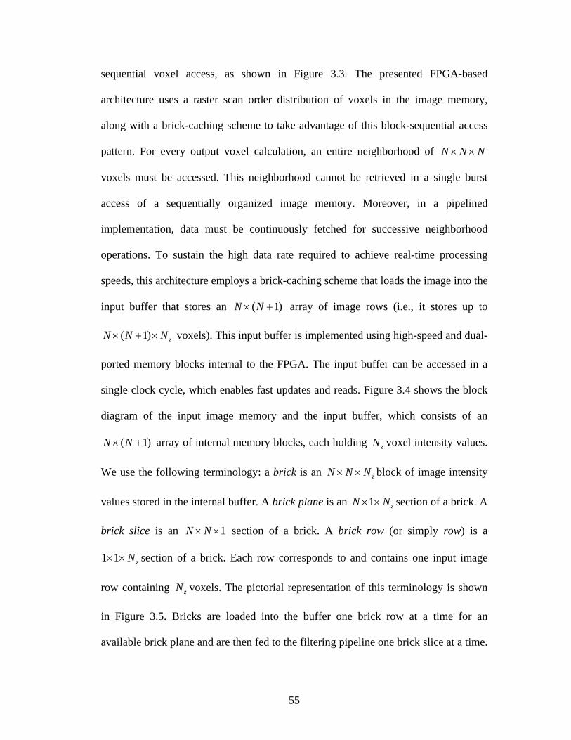
55
sequential voxel access, as shown in Figure 3.3. The presented FPGA-based
architecture uses a raster scan order distribution of voxels in the image memory,
along with a brick-caching scheme to take advantage of this block-sequential access
pattern. For every output voxel calculation, an entire neighborhood of N N N× ×
voxels must be accessed. This neighborhood cannot be retrieved in a single burst
access of a sequentially organized image memory. Moreover, in a pipelined
implementation, data must be continuously fetched for successive neighborhood
operations. To sustain the high data rate required to achieve real-time processing
speeds, this architecture employs a brick-caching scheme that loads the image into the
input buffer that stores an ( 1)N N× + array of image rows (i.e., it stores up to
( 1) zN N N× + × voxels). This input buffer is implemented using high-speed and dual-
ported memory blocks internal to the FPGA. The input buffer can be accessed in a
single clock cycle, which enables fast updates and reads. Figure 3.4 shows the block
diagram of the input image memory and the input buffer, which consists of an
( 1)N N× + array of internal memory blocks, each holding zN voxel intensity values.
We use the following terminology: a brick is an zN N N× × block of image intensity
values stored in the internal buffer. A brick plane is an 1 zN N× × section of a brick. A
brick slice is an 1N N× × section of a brick. A brick row (or simply row) is a
1 1 zN× × section of a brick. Each row corresponds to and contains one input image
row containing zN voxels. The pictorial representation of this terminology is shown
in Figure 3.5. Bricks are loaded into the buffer one brick row at a time for an
available brick plane and are then fed to the filtering pipeline one brick slice at a time.

56
The input buffer, therefore, can store a whole brick plus an extra brick plane. The
brick-caching operation is described below.
The memory controller fills up the input buffer row by row. Each row
contains Nz voxels, and thus transfer of each row takes WNtt zlatRow /+= clock cycles,
where latt is the number of clock cycles necessary to start a burst memory transfer and
W is the effective data bus width in terms of number of voxels (e.g., double-data-rate
[DDR] dynamic random access memory [DRAM] will offer twice the effective bus
width of single-data-rate DRAM with a similar configuration). After the first row is
cached in, the controller starts caching the row next to it in the x direction. A
complete brick plane ( N image rows, 1 zN N× × voxels) can be loaded in
Plane Rowt N t= ⋅ clock cycles. Associated with every brick plane is a ready flag. This
flag serves a dual purpose; when ‘1’, it indicates the availability of data for that
particular brick plane, and, when ‘0’, it indicates that the brick plane is empty and
available for caching image voxels. After one brick plane is loaded into the input
buffer, the memory controller sets the corresponding ready flag and starts loading the
Figure 3.4: Block diagram showing the input image memory and the input buffer configuration.

57
next brick plane (along the y direction). Once a complete zN N N× × brick is available
in the input buffer, it is fed into the filtering module pipeline one brick slice ( N N×
voxels) at a time.
The filtering module pipeline operates on one N N N× × neighborhood at a
time and is fed with a new brick slice every clock cycle. Loading an entire
zN N N× × brick into the filtering module pipeline thus takes Nz clock cycles. While
this operation is in progress, the memory controller loads the next brick plane (along
the y direction) into the buffer plane that is not being used for processing (indicated
by the ready flag), which requires tPlane clock cycles. After processing of all the
neighborhoods in the zN N N× × brick is complete, the processing window shifts
along the y dimension of the image, and the processing of the new neighborhoods
begins. Simultaneously, the ready flag corresponding to the brick plane that is no
longer used is set to ‘0’. This available brick plane in the input buffer is then used for
caching the next image rows (along y direction). In this fashion all brick planes in the
input buffer are cyclically used for brick caching during processing. These steps
Figure 3.5: Pictorial representation of the notation used in the brick-caching scheme.

58
continue until the processing window reaches the end of the column (i.e., until y =
Ny). At this point, the processing window moves along the x direction. To accomplish
this, data in the internal buffers are invalidated, and the complete zN N N× × brick in
the next column is cached, which requires a pipeline stall. After the initial brick in the
new x coordinates is loaded, the processing continues as described earlier. The
processing of the entire 3D image is completed accordingly. For continuous pipelined
operation with minimum stalls, the memory controller must provide the next brick
plane before the processing of the previous brick is completed. Therefore, the
relationship expressed in the following equation must be met:
( )/ ,lat z mem z procN t N W T N T⋅ + ⋅ ≤ ⋅ (3.3)
where Tmem is the clock period of the external memory clock and Tproc is the clock
period of the internal filtering pipeline. The left-hand side of Eq. (3.3) refers to the
total time required to load a new brick plane. The right-hand side refers to the total
time required to process a whole brick. Assuming that efficient burst accesses
(supported by most modern dynamic memories) are being used (which implies:
/lat zt N W ), the following relationship must be maintained to minimize pipeline
stalls:
.mem procN T W T⋅ ≤ ⋅ (3.4)
3.3.2. 3D Anisotropic Diffusion Filtering
This architecture supports 3D anisotropic diffusion filtering by pipelined
implementation of the 3D extension of the formulation shown in Eq. (3.2). As
indicated by that formulation, we use a Gaussian-filtered version of the image for

59
improved diffusion coefficient estimation. Our design implements this Gaussian
filtering at runtime using an embedded 3D Gaussian filtering module. Figure 3.6
shows a top level block diagram of the 3D anisotropic diffusion filtering module. This
filtering pipeline operates on N N N× × voxel neighborhoods. On each clock cycle,
the input data buffer feeds an N N× voxel neighborhood (brick) slice into the
pipeline. The center voxel intensity value is passed to the delay element for
accumulation at the end of the pipeline per Eq. (3.2). The 3 × 3 voxel neighborhood
located at the center of the incoming N N× neighborhood is passed to the image
gradient calculator, which calculates the image gradients with respect to each of the
6-connected neighbors of the center voxel. The embedded Gaussian filtering module
calculates, in parallel, the Gaussian-filtered values for each of the six-connected
neighbors and passes them to the diffusion coefficient calculator, which calculates the
diffusion coefficients 0..5c corresponding to each of the input gradients. Taking
advantage of the parallelism native to FPGAs, these operations are executed in
parallel, and, as a result, this filtering module can calculate the output at the rate of
one voxel per clock cycle. The resulting voxel intensity values are fed into the output
buffer, and the memory controller then stores them in the output memory bank.
3.3.2.1. Embedded Gaussian Filtering Module
Equation (3.5) shows the formula to calculate the coefficients of a 3D
Gaussian filter kernel, where σ is the standard deviation of the Gaussian function
and d is the Euclidean distance between the desired coefficient location and the kernel
center. For a chosenσ , the coefficient values depend exclusively on the Euclidean

60
distances from the kernel center; thus, the Gaussian filter kernel exhibits symmetries
with respect to its center (i.e. it is radially symmetric).
( )2
2exp2ddG σσ
⎛ ⎞= −⎜ ⎟
⎝ ⎠ (3.5)
Our architecture takes advantage of these symmetries to reduce the number of
multipliers needed for implementing the 3D Gaussian kernel to ( 1) ( 2) 6k k k× + × +
from 3( 2)N − ; where N is the size of anisotropic diffusion filtering kernel, the
corresponding size of the embedded Gaussian filtering kernel is ( 2)N − , and
( 1) 2k N= − . For example, a 5 5 5× × embedded Gaussian kernel that arises in
anisotropic diffusion filtering with 7N = can be implemented using only 10
multipliers (as opposed to 125) as we reported previously [143]. For this kernel, each
individual slice (5 5× plane of the kernel) has six isodistance regions and the whole
3D kernel has 10. During filtering operation, all voxels that are equidistant from the
kernel center are multiplied against the same Gaussian coefficient. The intensities
corresponding to these voxels in the same isodistance region can, therefore, be pre-
added before being multiplied against the Gaussian coefficients. Because a 5×5×5
Figure 3.6: Top-level block diagram of 3D anisotropic diffusion filtering. This diagram indicates paths that are executed in parallel.

61
Gaussian kernel contains 10 isodistance regions, the minimum number of multipliers
necessary to implement this filter kernel is, therefore, 10.
A block diagram of the Gaussian filter bank is shown in Figure 3.7. On each
clock cycle, the input buffer feeds an N N× voxel neighborhood into the bank. This
neighborhood is decomposed into five ( 2) ( 2)N N− × − neighborhoods by the input
demux, and these neighborhoods are then passed to five embedded 3D Gaussian
filters. Figure 3.8 shows a block diagram of an embedded 3D Gaussian filter. The
pre-adder accumulates values corresponding to the isodistance groups in the incoming
( 2) ( 2)N N− × − neighborhood, thus compressing the neighborhood based on the
intraneighborhood plane isodistance criterion (e.g., each single 5 5× slice of
a 35 Gaussian neighborhood has 6 isodistance regions). These pre-added values are
then passed to ( 2)N − pipeline buffers, which make values corresponding to the
entire 3( 2)N − neighborhood available in parallel. The sorter–accumulator
aggregates these values corresponding to the isodistance groups between the slices,
Figure 3.7: Block diagram of the embedded Gaussian filter bank (for N = 7, corresponding Gaussian kernel size is 5).

62
compressing them further using the isodistance criterion for the entire neighborhood
(e.g., 10 values that correspond to the 10 unique coefficients in a 5×5×5 Gaussian
neighborhood). These values are passed to the multiplier array, where they are
multiplied against their corresponding Gaussian coefficients. The adder tree then adds
the resulting values and outputs the result for the current 3D neighborhood. The
results for the subsequent neighborhoods are produced continuously as a result of
pipelined implementation of the operation. The Gaussian coefficients are
precomputed for a given value ofσ and are stored in internal registers using fixed-
point representation. The effect of this finite precision representation is analyzed in
the flowing section.
The results from the five individual Gaussian filters correspond to a cross-
shaped region of a neighborhood slice. In order to operate on the 3D six-connected
neighborhood, these results are passed to pipelined registers composed of two cross
buffers and the center buffer. The cross buffers store all five values in a neighborhood
slice, whereas the center buffer stores only the center value. As a result, the entire six-
connected neighborhood is available between these buffers. The buffers then send the
Gaussian-filtered, six-connected 3D voxel neighborhood to the subtractor array,
Figure 3.8: Pipelined implementation of an individual Gaussian filter element (Gaussian kernel size = 5).
63
which calculates the six corresponding gradient values and passes them to the
diffusion coefficient calculator.
3.3.2.2. Diffusion Coefficient Calculation
As noted previously, gradients calculated after Gaussian filtering are used to
estimate the diffusion coefficients. For a b -bit image, the absolute value of the
gradient is limited to the range 0 and 2 1b − . Taking advantage of this fact the desired
diffusion function is discretized in 2b steps and implemented using a lookup table
(LUT). The use of a LUT allows an efficient implementation of any diffusion
function. It must be noted that, because the dynamic range of all diffusion functions is
limited to [0,1] , there is no significant loss in precision by a using a fixed-point
representation. The effect of this finite precision representation is further analyzed in
the following section.
3.3.2.3. Image Gradient and Result Calculation
Image gradient calculation is performed by an array of six parallel subtractors.
These subtractors calculate the difference between the intensity of the voxel located
in the center of the kernel against its six-connected neighbors. These values are then
multiplied against their corresponding diffusion coefficients (supplied by the
diffusion coefficient calculator) using an array of six parallel multipliers. The
resulting filtered intensity is then obtained by adding the six results from the
multipliers to the original center voxel intensity. After rounding and truncation, this
result is then sent to the output buffer and is then further saved into output memory
bank.

64
3.3.3. Median Filtering
The 3D median filtering design presented in this work is an extension of
majority finding–based implementation proposed by Benkrid et al.[7]. That design
was reported for a 2D realization and computed only one bit of the median value per
clock cycle. All bits of the median value were obtained using a feedback loop and
hence for b -bit images, this approach required b clock cycles to compute the
resulting median value. The implementation presented in this dissertation extends that
design to 3D and unrolls the feedback loop by using multiple processing stages.
Moreover, our implementation exploits the regularity of this median finding
algorithm with a systolic array architecture that allows a pipelined implementation
and, therefore, can achieve a throughput of one median value per clock cycle. Thus,
our implementation can achieve a voxel processing speed b times higher than the
previously reported architecture [7]. Our linear systolic array employs b identical
processing stages for filtering a b-bit image. Figure 3.1 illustrates execution of this
algorithm for a small example and can be used to gain further insights into its
hardware implementation. Each processing stage of our systolic array implementation
corresponds to one step of the algorithm execution. Starting from the MSB, each
stage generates one bit of the resulting median value of the neighborhood being
processed. We first describe the operation of an individual processing element and
then explain the functioning of the entire linear systolic pipeline, which contains b-
processing elements.

65
3.3.3.1. Processing Element
The processing element is the atomic unit of the proposed linear systolic array
design. A functional block diagram of the processing element at the jth stage is shown
in Figure 3.9. The data inputs to this processing element are Data_Bitsj and
Next_Data_Bitsj, the N3 bits used considered for majority calculation and the (j+1)th
significant bits (from MSB) of the 3N neighborhood elements, respectively. It must
be noted that, although Next_Data_Bitsj are corresponding image intensity bits,
Data_Bitsj are provided by the (j–1)th processing stage and may have been masked in
the earlier stages. The accompanying input Mask_Bitsj is a binary flag that indicates
the bits in Data_Bitsj that have been masked in the prior stages. A processing element
performs two important tasks. First, it computes the majority bit within the N3 input
data bits (Data_Bitsj); second, it performs the masking operation based on the
majority bit calculated and outputs masked data bits (Data_Bitsj+1) and the
corresponding binary flag (Mask_Bitsj+1) to be used in the next processing stage. The
units that perform these two operations are described below.
Figure 3.9: A single stage (processing element) of the linear systolic median filtering kernel.

66
Majority Finding Unit (MFU)
The MFU consists of a bit-counting circuit that counts the number of 1s in the
input bits that are considered for majority calculation (Data_Bitsj). This counting is
performed using a bit adder tree customized for a chosen neighborhood size. This
count is then compared against a threshold, which is programmed to be half of the
number of elements contained in the neighborhood. The binary result of this
comparison is the jth significant (from MSB) bit of the output median value. The
highly compact, pipelined, and customized implementation of the MFU minimizes
the combinational delay within the processing element.
Mask Selection Unit (MSU)
After the median bit has been calculated, the MSU performs the masking
operation. It computes the mask bit for each bit of Data_Bitsj, based on whether it
matches with the majority bit or not. In addition, it considers and preserves the bits
that were masked in the prior stages (Mask_Bitsj). Thus, the mask calculated at the jth
stage (Mask_Bitsj+1) is a combination of the mask bits from the prior stages and the
mask calculated at the current stage. This masking operation is implemented using an
exclusive OR (XOR) operation and two multiplexing operations for each data bit. The
calculated mask (Mask_Bitsj+1) is then used to selectively generate Data_Bitsj+1 from
the input Next_Data_Bitsj, while ensuring that values corresponding to the masked
bits are preserved. Data_Bitsj+1 is then used in the next processing stage to calculate
the (j+1)th significant bit of the median value.

67
3.3.3.2. Linear Systolic Design for Median Finding
The proposed linear systolic design is realized by cascading b processing
elements for filtering b-bit images. On every clock cycle, a complete neighborhood
containing N3 voxels, b-bits each, is fed to this linear systolic array. However, the
processing stage (j+1) can not perform its operation until stage j finishes its
processing and provides Data_Bitsj+1 and Mask_Bitsj+1. Similarly, stage j produces its
output (jth significant bit of the median) one clock cycle earlier than the corresponding
output by the stage (j+1). In order to compensate for these delay and processing
latencies and to provide synchronized operation, additional line delay units and data
shift registers must be inserted at the input and output of the systolic array. Figure
3.10 shows a diagram of this configuration with b processing elements and required
delay buffers. These delays are introduced for synchronization only, and it must be
noted that as long as the input sequential neighborhoods are continuously supplied
(new N3 voxels every clock cycle), the systolic array design is capable of computing
one median result per clock cycle. This result is then sent to the output buffer and
subsequently saved into the output memory bank by the memory controller.
For correct operation, the Mask_Bits1 input of the first processing stage (stage
1, MSB) is grounded (set to “0”), indicating that no bits from the input data
(Data_Bits1) are masked. Also, in the final processing stage (stage b, LSB),
Mask_bitsb+1 and Data_Bitsb+1 do not need to be calculated, because the next stage
does not exist. Consequently, the MSU is not needed in the final stage, which
contains only an MFU to compute the last median bit. In general, for large 3D
neighborhoods, the speed of the MFU is the limiting factor of the systolic array

68
performance. In applications requiring high voxel throughput and large filtering
kernels, the operation of the MFU can be pipelined. However, in those cases the
depth of the delay elements used to synchronize the inputs and outputs of the different
processing elements must be adjusted.
3.4. Implementation and Results
The architecture described above was implemented using an Altera Stratix II
EP2S180F1508C4 FPGA (Altera Corp., San Jose, CA) with two external memory
banks to serve as input and output image memory. The memory banks used were 1-
GB DDR2 small-outline dual-inline memory DRAM modules with 64-bit data bus
(i.e., 16W = , for 8b = ) running at a 200-MHz clock speed. The architecture was
designed using VHSIC hardware description language (VHDL) and synthesized using
Altera Quartus II 6.1. The memory controller was also implemented using VHDL and
was built around the DDR2 DRAM controller megacore supplied with Altera Quartus
Figure 3.10: Linear systolic array architecture for median filter kernel using majority voting technique.

69
II. Both filtering modules were custom designed using VHDL, as per the design
description in provided earlier. Functional verification and postsynthesis timing
simulation for the entire system were performed using Modelsim SE 6.2 (Mentor
Graphics, San Jose, CA). For this purpose, DDR2 DRAM simulation models
provided by Micron (www.micron.com) were used. The presented design was then
realized to support 8-bit images (b = 8) and, consequently, all results in this section
are presented for 8-bit images. The execution speed of the presented architecture was
obtained from postsynthesis timing simulation of the design.
3.4.1. Effects of Finite Precision Representation
Real-time filtering performance offered by the presented design is critical for
the time-sensitive nature of IGIs, but of equal importance is the accuracy of the
filtering process. Most software implementations represent the arithmetic operations
involved in the filtering algorithms using a double precision floating-point format.
This format offers high dynamic range and precision, which may or may not be
required depending on the filtering technique to be implemented. Median filtering, for
example, is performed exclusively using integer data (because digital images are
represented using b-bit integer data), and, hence, there is no loss in precision by using
Table 3.2: Average error in intensity per voxel for a Gaussian filtered image resulting from fixed-point representation of Gaussian coefficients.
Average error in intensity per voxel resulting from fixed-point representation of Gaussian kernel coefficients σ of the
Gaussian kernel 8-bits 12-bits 16-bits 0.3 0.20 ± 0.47 0.07 ± 0.26 0.004 ± 0.06 0.5 0.63 ± 0.68 0.02 ± 0.11 0.004 ± 0.07 0.7 0.42 ± 0.81 0.03 ± 0.16 0.003 ± 0.06 1.0 0.21 ± 0.47 0.001 ± 0.04 0.001 ± 0.03

70
a fixed-point implementation with sufficient dynamic range (i.e., using b bits for b-bit
images). Our implementation of the 3D median filtering uses b-bit integer
representation for b-bit images, and therefore provides identical results to those
provided by a software implementation.
Anisotropic diffusion filtering, however, involves operations with the data in
real format. Our implementation, for the sake of efficiency in area and execution
speed, used fixed-point representation to implement these arithmetic operations. A
general framework for analyzing optimized tradeoff relationships between hardware
resources and implementation accuracy for finite-precision designs is presented later
(see Chapter 5). For this implementation, however, given the simplicity of the
arithmetic operations and relatively minor impact of the fixed-point datapath on the
total hardware resource requirement, we employed simulation-based wordlength
search techniques. We analyzed the effect of the number of bits used for this fixed-
point representation on the filtering accuracy, by treating a software (C++)
implementation employing double-precision floating-point representation as a
reference. This analysis was performed with an 8-bit image with dimensions
256 256 64× × . There are two sources at which error resulting from fixed-point
precision can affect the accuracy of the filtering operation: embedded Gaussian
Table 3.3: Average error per sample of diffusion function resulting from fixed-point representation of diffusion coefficients employed in the presented architecture.
Average error per sample of diffusion function resulting from fixed-point representation of diffusion coefficients K
8-bits 12-bits 16-bits 10 42 × 10-5 ± 97 × 10-5 3 × 10⁻⁵ ± 7 × 10⁻⁵ <10-5 20 78 × 10-5 ± 114 × 10-5 6 × 10⁻⁵ ± 8 × 10⁻⁵ <10-5 30 121 × 10-5 ± 125 × 10-5 9 × 10⁻⁵ ± 8 × 10⁻⁵ <10-5 50 196 × 10-5 ± 116 × 10-5 13 × 10-5 ± 7 × 10⁻⁵ <10-5

71
filtering and diffusion function calculation. To gain additional insight, we evaluated
accuracy for these individual sources and the accuracy of the anisotropic diffusion
filtering as their combined effect.
Table 3.2 presents the average error in intensity per voxel after embedded
Gaussian filtering (kernel size, N = 5) where the Gaussian kernel coefficients are
represented using the fixed-point format with the designated number of bits. Because
the Gaussian kernel was normalized, all coefficients were within the range [0,1] , and,
hence, we used one bit to represent the integer part and the rest for the fractional part.
We performed this analysis for typical choices of σ for a Gaussian kernel size of 5,
which corresponds to the anisotropic diffusion filtering kernel size of 7. The average
error for various choices of σ with 8-bit representation is less than one intensity
value, and, as expected, the average error reduces with the increasing number of bits.
It must be noted, however, that embedded Gaussian filtering is used only to estimate
the diffusion coefficients, and, hence, small errors introduced in this operation may
not have a significant impact on the final anisotropic diffusion filtered intensity value.
Because this design supported 8-bit images, a 256-entry LUT was used to implement
the diffusion function described in the background section. We implemented this
function for reasonable choices of the parameter K, which controls the level of the
gradient at which edges are diffused or preserved. The value of K depends on the
image modality and the amount of edge preservation desired. For ultrasound and low-
dose CT images, however, its value is typically less than 20% of the intensity range.
As the selected diffusion function takes values in the range [0,1] , we used one bit to
represent the integer part and the rest for the fractional part. Table 3.3 presents the

72
average error per sample of diffusion function resulting from fixed-point
representation with the designated number of bits for various choices of K. Although
the average error increases with the choice of K, its mean and standard deviations are
consistently less than 0.1% of the data range, even with representation using 8-bits.
Finally, Table 3.4 reports average error in intensity per voxel resulting from the
combined effect of finite precision implementation of both the Gaussian coefficients
and the diffusion function. For this analysis, we used the same number of bits for
fixed-point representation of both entities, with one bit for the integer part and the rest
for the fractional component. The kernel size (N) of the anisotropic diffusion filter
was chosen to be 7, with embedded Gaussian filtering with σ = 0.5, and the diffusion
function shown described earlier was implemented with K = 20. To evaluate error
accumulation over multiple iterations of anisotropic diffusion filtering, we performed
this analysis up to 5 iterations, which is typical for filtering of intraprocedural images.
The average error in intensity increases with the number of iterations, but its mean
and standard deviations are consistently less than 0.04% of the intensity range, even
with 8-bit representation.
Overall, our precision analysis indicates that even when using 8-bit fixed-
Table 3.4: Average error in intensity per voxel for anisotropic diffusion filtered resulting from fixed-point representation of Gaussian coefficients and the diffusion function
Average error in intensity per voxel resulting from fixed-point representation of the Gaussian kernel and diffusion coefficients
Number of filtering
iterations 8-bits 12-bits 16-bits 1 0.008 ± 0.092 0.001 ± 0.018 <0.001 3 0.021 ± 0.144 0.001 ± 0.031 <0.001 5 0.030 ± 0.171 0.002 ± 0.039 <0.001

73
point representation to perform Gaussian filtering and diffusion function calculation,
the average error in intensity is only a very small percentage of the intensity range.
Such small errors in intensity may not be significant for advanced operations such as
registration, segmentation, and visualization and are unlikely to affect the accuracy
and precision of IGIs. Our implementation, therefore, uses 8-bit fixed-point
representation for these operations.
3.4.2. Hardware Requirements
Table 3.5 lists the significant hardware requirements for the important
modules in the proposed architecture, parameterized on filter kernel size ( N ) and the
number of bits used to represent the voxel intensity (b ). The parameter k , introduced
in the context of 3D anisotropic diffusion filtering, represents the number of unique
isodistances in the Gaussian kernel and is related to the filter kernel size N (usually
odd) as:
( 1) .2
Nk −= (3.6)
Table 3.5: Hardware requirements of the architecture for real-time 3D image preprocessing.
Significant hardware resources Logic resources and performance (as implemented) Hardware
module Multipliers ( b b× bit)
Internal memory(bits) N Number of ALUTs
(% utilization) maxf
(MHz) Input buffer
and controller − ( ( 1) )zN N N b× + × × 7 1957 (1.5%) 233
Output buffer and controller − (2 )zN b× × 7 1743 (1.5%) 233
Anisotropic diffusion filter
( 1) ( 2)56
k k k× + × +×
(3 2 )b b× × 7 3824 (3%) 236
Median filter − − 5 11308 (8%) 224

74
The linear systolic array implementation of the 3D median filter requires logic
resources only, and the resource requirements for important components of this filter
kernel are listed separately in Table 3.6. These two tables indicate how the hardware
requirements of our architecture scale with the parameters N and b . As dictated by
the resource limitations imposed by the target device (Altera Stratix II
EP2S180F1508C4) and real-time speed requirements, our current implementation can
support filter kernel sizes ( )N from the list { }5,7 and { }3,5 for anisotropic diffusion
filtering and median filtering, respectively. The corresponding kernel sizes for the
embedded Gaussian filtering in the case of anisotropic diffusion filter supported by
our architecture are{ }3,5 . Table 3.5 also lists the absolute and percentage logic
resources consumed by the important modules in the architecture and the maximum
operating frequency ( maxf ) at which these modules can run for a specific instantiation
(choice of N ). The percentage logic resources are reported in reference to the target
device Altera Stratix II EP2S180F1508C4. The images used for this performance and
logic consumption analysis were 8-bit images ( 8b = ). The choices for the value of
N for this analysis represent common kernel size choices and are listed in the fourth
column of the table.
Table 3.6: Hardware requirements for the components of the linear systolic implementation of the 3D median filtering.
Hardware component Number required Processing elements b
Data registers 3b N× Mask select registers 3b N×
Data pipeline registers 3( 1)b N− ×
Line delay elements ( ) ( ) 32 1 ( 1) 2b b N− × − × +

75
3.4.3. Filtering Performance
The 3D median filtering module and 3D anisotropic diffusion filtering module
were synthesized for kernel sizes of {3,5} and 7 , respectively, for filtering 8-bit
images. The rest of the system, including the memory controller and input and output
buffers, was parametrically synthesized to support the desired filtering operation and
kernel size. The entire system was clocked at 200 MHz, which also corresponds to the
filtering pipeline frequency (i.e., procT = 5 ns). The image memories were also clocked
at 200 MHz ( memT = 5 ns). For this configuration, Table 3.7 reports the execution time
for 3D anisotropic diffusion filtering and 3D median filtering as obtained during
postsynthesis timing simulation of the entire system. The image sizes used for this
measurement correspond to typical dimensions of intraprocedural images.
As indicated in Table 3.7, our implementation of 3D anisotropic diffusion
filtering and 3D median filtering can easily achieve a processing rate of 46 frames per
second (fps) for images of size 256 256 64× × voxels, which is a typical size of an
intraprocedural volumetric CT scan. The corresponding processing rate for
intraprocedural 3D ultrasound scan with typical dimensions of 128 128 128× × voxels
Table 3.7: Execution time of 3D anisotropic diffusion filtering and 3D median filtering.
Filter kernel Kernel
size (N)
Image size (voxels)
Execution time (ms)
Voxel processing rate
(MHz) 128 × 128 × 128 10.90 192 3D anisotropic
diffusion filter 7 256 × 256 × 64 21.63 194 128 × 128 × 128 10.75 195 3 256 × 256 × 64 21.44 196 128 × 128 × 128 10.82 194
3D median filter
5 256 × 256 × 64 21.58 194

76
is around 92 fps. For iterative operations such as anisotropic diffusion filtering or
sequential filtering operations, this processing rate translates to 18 fps with five
iterations (or sequential operations) per frame, which is sufficient to meet the real-
time needs of most IGIs.
Table 3.8 and Table 3.9 compare the execution speed of the presented
architecture for 3D anisotropic diffusion filtering and 3D median filtering,
respectively, against a corresponding software implementation and previously
reported high-speed implementations using different computing platforms. The
execution time has been normalized by the image dimensions for all implementations,
and the performance is presented in terms of voxel processing rate to facilitate a fair
comparison independent of image dimensions. The software implementation was
developed using C++, and its performance was measured on an Intel Xeon 3.6 GHz
workstation with 2 gigabytes of DDR2 400 MHz main memory. Although this
architecture can support various kernel sizes for the filtering operations, for
consistency the performance has been compared for a kernel size (N) common to all
implementations: N=3 for the median filtering and N=7 for anisotropic diffusion
filtering.
Table 3.8: Performance comparison of the 3D anisotropic diffusion filtering kernel.
Implementation Platform Filter kernel
Voxel processing rate
(MHz) Speedup
Software (C++) Xeon workstation 3D 0.92 208 Bruhn et al.
[100] 256-processor cluster 3D 105 1.83 Tabik et al. [101] 16-processor cluster 3D 5.66 33.9
Dandekar et al. [144] FPGA 3D 192 -

77
As indicated by Table 3.8, our implementation of 3D anisotropic diffusion
filtering provides more than two orders of magnitude speedup over the software
implementation using a single workstation. Moreover, the performance of the current
architecture represents an improvement over a corresponding implementation using a
256-processor computing cluster reported previously [100]. Our work presented a
novel FPGA-based implementation of 3D anisotropic diffusion filtering. Salient
features of this filtering module are an embedded Gaussian filtering implementation
that minimizes the number of multipliers and a pipelined design that allows
throughput of one output voxel per clock cycle. This filtering module offers the
flexibility to support several anisotropic diffusion techniques previously reported in
the literature. For example, the multiscale approach proposed by Whitaker and Pizer
[82] can be implemented by changing the embedded Gaussian filter coefficients at the
end of each iteration, and a time-dependent diffusion function [145] can be
implemented by reprogramming the values in the diffusion function LUT. One
limitation of this filtering module is the limit on the size of the embedded Gaussian
filter kernel; implementing Gaussian kernels larger than 7 would result in
prohibitively high hardware requirements. Such large kernels, however, are
uncommon in most applications. Although this architecture performs some of the
arithmetic functions using fixed-point representation, the variation in the output
intensity values is only a small fraction of the intensity range, and these variations are
unlikely to affect the accuracy and precision of IGIs.
Table 3.9 compares the performance of the FPGA-based 3D median filtering
operation described in this work with previously reported high-speed

78
implementations. The present implementation provides more than an order of
magnitude speedup over software- and GPU-based 3D implementations and DSP-
based 2D implementation. Jiang and Crookes [137] recently reported an FPGA-based
3D implementation that is capable of achieving a voxel processing rate of 50 MHz.
That design, however, was based on a partial sorting technique and cannot be easily
extended to kernel sizes beyond 3. Our implementation, in contrast, achieved a
superior voxel processing rate and is sufficiently compact to allow implementation of
kernel sizes up to 7, which is sufficient for most common image processing tasks. The
logic resources required by the described systolic array–based median filter indeed
scale up as kernel sizes get larger; but as modern FPGAs become denser and offer
improved logic capacity, this requirement is still a small percentage of the total
available resources (see Table 3.5).
3.5. Summary
This chapter presented an FPGA-based architecture for real-time
preprocessing of volumetric images acquired during IGIs. The developed architecture
enables 3D anisotropic diffusion filtering and 3D median filtering of intraprocedural
Table 3.9: Performance comparison of the 3D median filtering kernel.
Implementation Platform Filter kernel
Voxel processing rate (MHz) Speedup
Software (C++) Xeon workstation 3D 2.63 74 Viola et al. [136] GPU 3D 0.76 257
Gallegos-Funes and Ponomaryov [146] DSP 2D 4.5 43
Jiang and Crookes [137] FPGA 3D 50 3.9
Dandekar et al. [144] FPGA 3D 195 -
79
images at the rate of 50 fps, which is faster than current acquisition speeds of most
imaging modalities. The solution presented offers real-time performance, is compact
and accurate, and, hence, suitable for integration into IGI workflow. As IGI
applications become increasingly popular, intraprocedural imaging modalities
continue to offer wider coverage and higher imaging speed. Thus, there is a
corresponding need for real-time processing of these images. The real-time
performance of our design along with the throughput of one voxel per cycle can cater
to these 4D (3D + time) image processing needs.

80
Chapter 4: Hardware-Accelerated Deformable Image
Registration
Intensity-based deformable image registration plays a critical role in many
diagnostic and interventional applications requiring image combination. Despite the
advantages (such as accuracy, automation, and retrospective nature) of this approach,
these algorithms find limited use in clinical applications due to their computational
complexity. This chapter presents a novel FPGA-based architecture for accelerated
implementation of MI-based deformable registration. This architecture is capable of
reducing the execution time of MI-based deformable registration from hours to a few
minutes. First, we describe the registration algorithm that is being accelerated. Next,
we present the architecture for its high-speed implementation. Finally, we
characterize the execution performance of this architecture and provide qualitative
validation results. The optimization of this architecture for accuracy and hardware
resources is presented in Chapter 5. The quantitative validation and the clinical
applicability of this architecture are presented later, in Chapter 6.
4.1. Motivation
Combining complementary information from intraprocedural and
preprocedural images is a fundamental need in IGI applications. These images,
however, are acquired at different times and using different imaging scanners and
protocols and as a result are usually misaligned. Therefore, they need to be registered
(or aligned) for a meaningful combination and fusion of the information they contain.
Deformable image registration techniques can compensate for both local deformation

81
and large-scale tissue motion and are the ideal solution for achieving the
aforementioned image registration. Some studies, in particular, have independently
underlined the importance of deformable registration and/or soft tissue modeling for
IGIs [18, 19]. However, despite their advantages, deformable registration algorithms
are seldom used in current clinical practice. The large number of degrees of freedom
that these algorithms employ makes them extremely computationally intensive. On a
modern workstation most deformable registration algorithms can take several hours,
which is clearly unacceptable for IGIs requiring on-demand performance. As a result,
most earlier reported techniques for aligning preprocedural and intraprocedural
images employ rigid body approximation, which is often not valid because of
underlying nonrigid tissue deformation. In addition, some of these techniques are not
retrospective (i.e. they require some advanced planning at the time of preprocedural
imaging), which further limits their applicability.
Mutual information (MI)–based deformable registration has been shown to be
effective in multimodality image registration because of the robustness of the
similarity measure [69]. Moreover, MI-based image registration is automatic and
completely retrospective because it uses image intensities to achieve the alignment.
Walimbe and Shekhar [60, 67] have earlier reported an MI-based deformable
registration algorithm that utilizes volume subdivision. Hierarchical volume
subdivision–based image registration techniques are inherently faster than most other
deformable registration techniques and are more amenable to hardware acceleration.
This algorithm has been used and rigorously validated in the context of PET-CT
registration [66]. This clinical validation has demonstrated the registration accuracy
82
of the aforementioned algorithm to be comparable to a group of clinical experts and
the mean registration accuracy for the abdominal region to be superior to an earlier
reported free-form deformation (FFD)–based technique [147]. This algorithm is
theoretically general and has been shown to be effective for various applications
employing multimodal deformable registration [66, 77, 148-151]. Although
computationally efficient, software implementation of this algorithm can take several
hours, which is still slow for direct integration into the IGI workflow. It is, therefore,
necessary to accelerate this algorithm and reduce the processing time to the order of
minutes and ultimately to seconds for its assimilation into clinical workflow.
Although, accelerated implementations of MI-based deformable registration
algorithms using very large multiprocessor clusters have been proposed earlier [57,
115, 117, 118], their per-node performance does not compare favorably with our
implementation. Furthermore, these solutions may not be cost effective and are
unlikely to be suitable for clinical deployment.
The chapter presents a novel field-programmable gate array (FPGA)–based
accelerated implementation of the aforementioned deformable registration algorithm,
specially geared toward improving target delineation during image-guided
interventions. The reported solution provides a speedup of about 40 for MI
calculation, thus reducing the deformable registration time from hours to minutes. In
Chapter 6, we demonstrate fast and successful registration of intraprocedural
abdominal CT scans with preprocedural CT and PET scans using the developed
architecture. We further demonstrate that the registration accuracy of the hardware
implementation is comparable with that using a software implementation and is on

83
the order of a few millimeters. This registration accuracy coupled with the execution
speed and compact implementation of the reported solution makes it suitable for
integration in the IGI workflow.
4.2. Algorithm for Deformable Image Registration
Hierarchical volume subdivision–based deformable image registration
techniques are inherently faster than most intensity-based deformable registration
techniques (e.g., FFD–based techniques) and are more amenable to acceleration
through hardware implementation. 3D image registration using volume subdivision
has been proposed earlier, but the earlier implementations were limited to a locally
translation-based model. Walimbe and Shekhar [60, 67] enhanced this model by
incorporating local rotations and reported a quaternion-based scheme for interpolating
multiple 3D rigid-body transformations for deformable registration using the volume
subdivision approach. For a pair of images, one treated as reference and the other as
floating, this algorithm performs deformable registration using a series of
hierarchical, locally rigid-body registrations. The six-parameter rigid registration at
Figure 4.1: Pictorial representation of hierarchical volume subdivision–based deformable image registration and associated notation.

84
each level is optimized by maximizing the MI between the reference and floating
images (RI and FI, respectively). This hierarchical registration scheme is shown in
Figure 4.1.
The initial optimal rigid alignment (at the root level) between RI and FI can be
represented using a transformation matrix 00T (where i
jT represents the cumulative
optimal transformation at level i for subvolume j ). Next, the algorithm uses a
hierarchical octree-based subdivision scheme. At each subdivision level i , the RI is
divided into 8i subvolumes, numbered from 0 to 8 1i − . Each of these subvolumes is
then individually registered with the FI, under transformation range constraints
derived from the transformation of its parent subvolume at the earlier level 1( )
iparent jT − .
The notation ( )parent j refers to the subvolume at the previous subdivision level
1i− , which contains the current subvolume j . For example, at the root level ( 0i = ),
there is a single subvolume (entire image) numbered 0j = . After one level of
subdivision ( 1i = ), there will be eight subvolumes numbered from 0j = to 7j = . At
level 1i = , (3)parent refers to subvolume numbered 0 at level 0i = , because it
contains subvolume 3j = at the current level ( 1i = ) of subdivision (see Figure 4.1).
The optimal alignment of the subvolume j within the FI is also determined by
maximizing MI under a six-parameter rigid-body transformation model.
Volume subdivision and subvolume registration continue until the voxel count
for an individual subvolume remains above a predefined limit (usually 316 ) to yield a
statistically significant similarity measure. Thus, this algorithm achieves hierarchical
refinement of the localized matching between RI and FI. The final cumulative non-

85
rigid alignment between the image pairs is computed by quaternion-based direct
interpolation of the individual subvolume transformations at the final subdivision
level.
4.2.1. Calculating MI for a Subvolume
Registration of a subvolume during the hierarchical refinement process is
based on maximization of the MI, which is a statistical measure. With progressive
subdivision, subvolumes at every level become increasingly smaller. The mutual
histogram (MH) corresponding to an individual subvolume becomes sparse, thus
rendering MI unreliable. The aforementioned algorithm addresses this issue by using
the MH of the entire image (all the subvolumes) to calculate MI during the
registration of a subvolume. The contribution of the current subvolume k at level i
to the MH is computed under the current candidate transformation *ikT ( *T denotes a
candidate transformation during the optimization process). The contribution to the
MH from the rest of the subvolumes remains constant during this registration process
and is derived from their parent subvolumes. Thus, MI is computed over the entire
image with local variations corresponding to the subvolume under optimization.
Equations (4.1)-(4.3) summarize this process. The function ( )j k
TAccumulate=
,
contributes to the MH using the voxels in a given subvolume k , using the mapping
provided by the given transformation T . The detailed description of this deformable
registration algorithm can be found in [60].
k k k
i i iTotal Subvolume RestMH MH MH= + (4.1)
*( )k
i iSubvolume j
j kMH TAccumulate
== (4.2)

86
1
,( )
k
i iRest parent(j)j j k
MH Accumulate T −
∀ ≠= (4.3)
4.3. Acceleration Approach
The aforementioned algorithm uses MI as a measure of image similarity. MI
is an intensity-based similarity measure and calculation of MI requires processing of
all the voxels in the RI. Registration through maximization of MI attempts to find the
transformation that best aligns an FI with an RI. This MI-based registration typically
requires thousands of iterations (MI evaluations), depending on the image complexity
and the degree of initial misalignment between the images. Repeated MI
computation, which requires accessing both the images (RI and FI), is memory access
intensive, and in particular, the memory access in the FI is completely governed by
the transformation applied. This operation, therefore, does not benefit from the cache-
based memory architectures present in most modern PCs (the caches are too small to
fit 3D images). Because memory speed has not evolved at the same rate as
microprocessor speed, introduction of faster microprocessors is not expected to
significantly speed up image registration. Thus, a factor limiting the performance of
software implementations is calculating MI for different candidate transformations.
Castro-Pareja et al. [139] have shown that, for typical medical images, accumulating
Figure 4.2: Pictorial representation of the acceleration approach.

87
the MH and calculation of MI can take up to 99% of the total image registration time
in software. Our efforts for acceleration of this algorithm, consequently, are targeted
toward optimized and pipelined implementation of MH accumulation and MI
calculation. This approach is pictorially represented in Figure 4.2.
In general, the execution time T required by a pipelined implementation (with
n-stages) of an operation is given as:
( ) ,NT t nm
= ⋅ + (4.4)
where t is the latency of each stage, N is the amount of data to be processed, and
m is the number of data units processed in parallel at each stage. In the case of MI
calculation, N represents the number of RI voxels to be processed. For typical
volumetric images (which are usually larger than 1283) it can be assumed that
N nm
, thus the main parameters that control the MI calculation time are then t and
m . Supporting 1m > requires a superscalar architecture and multiple processing
pipelines with individual image memory access, which is not practical. Therefore, to
provide maximum pipeline performance, our architecture focuses on reducing t , the
latency of each pipeline stage. The lower bound on t is the period of the system clock
and achieving this bound means that all the pipeline stages (including image memory
access) complete their operations in one clock cycle. The following section describes
an architecture geared toward meeting this goal for accelerated calculation of MI.

88
4.4. Architecture
MI-based image registration can be thought of as an optimization problem of
finding the best alignment between two images. During the execution of the
algorithm, the optimization process is executed from the host workstation. This host
provides a candidate transformation, while the presented FPGA-based solution
applies it to the images and performs corresponding MI computation. The computed
MI value is then further used by the host to update the candidate transformation and
eventually find the optimal deformable alignment between the RI and the FI. This
workflow is indicated in Figure 4.2. The top-level block diagram of the FPGA-based
architecture for accelerated implementation of volume subdivision-based image
registration is shown in Figure 4.3. The important modules in this architecture are
described below.
Figure 4.3: Top-level block diagram of the architecture for accelerated implementation of deformable image registration.

89
4.4.1. Voxel Counter
Calculation of MI requires processing every voxel in the RI. This can be
achieved by sequentially cycling though all the voxels in the RI. In addition, because
the implemented algorithm is based on volume-subdivision, RI voxels within a 3D
neighborhood corresponding to an individual subvolume must also be processed
sequentially. This is implemented as follows: the host programs the FPGA-based MI
calculator with subvolume start and end addresses. In case of the entire image (as
required for rigid registration), the start address is (0, 0, 0) whereas the end address is
equal to the dimensions of the RI. When a subvolume needs to be processed (for
example, during subvolume optimization after image subdivision), the start and end
addresses programmed by the host correspond to that of the subvolume. The voxel
counter sequentially computes the addresses corresponding to all voxels within a
given neighborhood range (a subvolume, for example) in z−y−x order. This is
implemented using three synchronized counters, one for each dimension. A functional
diagram of this module is presented in Figure 4.4. Through pipelined implementation,
this module is capable of generating address for one RI voxel per clock cycle. This
Figure 4.4: Functional block diagram of voxel counter.

90
module operates in two modes: in the reference image processing mode the address
generated is used to fetch the RI image voxels from the external image memory,
whereas in the floating image processing mode the RI address generated is
transformed to the floating image space for further processing.
4.4.2. Coordinate Transformation
The initial step in MI calculation involves applying a candidate transformation
( *ijT ), to each voxel coordinate ( rv ) in a subvolume j of the RI to find the
corresponding voxel coordinates in the FI (represented using fv ). This is
mathematically represented as shown in (4.5). Because the algorithm is linear at every
subvolume, this is implemented using the six-parameter rigid transformation model.
*if j rv T v= ⋅ (4.5)
An interesting aspect of this coordinate transformation and subsequent
operations is that they involve operations in both real (millimeter) space as well as
voxel address (image index) space. For example, the transformation (translations and
rotations) is defined in the real space, whereas the voxels to be fetched from RI and
FI are identified in voxel address space. Thus, there is a need to convert between
these address spaces during the calculation of MI. This conversion can be performed
by utilizing the voxel size information associated with each image. To circumvent the
need for performing this conversion in our FPGA-based architecture, we
appropriately scale the transformation matrix (in millimeter space) and represent it
using a mathematically equivalent matrix in voxel address space. This conversion is
performed in software by the host just prior to MI calculation. This matrix is then fed

91
to the FPGA-based MI calculator and the MI calculator performs all its operations in
voxel address space. This converted transformation can be represented as:
x x x xxx xy xz
x y z xcx cxy y y y
yx yy yz cy cyx y z ycz czz z z z
zx zy zzx y z z
vr vr vr Tr r rvf vf vf vf
i RI FIp vr vr vr Tq r r r j RI FI
vf vf vf vfr k RI FIvr vr vr Tr r rvf vf vf vf
⎡ ⎤ ⎡ ⎤⋅ ⋅ ⋅⎢ ⎥ ⎢ ⎥⎢ ⎥ ⎢ ⎥⎡ ⎤ ⎡ ⎤−⎡ ⎤ ⎢ ⎥ ⎢ ⎥⎢ ⎥ ⎢= ⋅ ⋅ ⋅ − + +⎢ ⎥ ⎢ ⎥ ⎢ ⎥⎢ ⎥ ⎢⎢ ⎥ −⎣ ⎦ ⎢ ⎥ ⎣ ⎦ ⎣ ⎦⎢ ⎥⎢ ⎥ ⎢ ⎥⋅ ⋅ ⋅⎢ ⎥ ⎢ ⎥⎣ ⎦⎣ ⎦
i .⎥⎥
(4.6)
In this equation, the tuple (i, j, k) represents the address of a voxel in RI space. This
address is calculated by the voxel counter. The ijr s represent the components of the
rotation matrix, whereas iT s represent the components of the translation vector. ivr s
and ivf s represent the voxel sizes (in millimeters) of the reference image and the
floating image, respectively. ( , , )cx cy czRI RI RI and ( , , )cx cy czFI FI FI represent the
centers of the reference image and floating image in voxel address space,
respectively.
This transformation model is represented using a 3 × 3 rotation matrix and a
Figure 4.5: Functional block diagram of coordinate transformation unit.

92
3 × 1 translation vector. The host calculates these transformation components by
appropriate scaling (as described above) of the current candidate transformation
provided by the optimization routine and sends it to the MI calculator. Fixed-point
representation is used to store the individual elements of these transformation
components. The coordinate transformation is accomplished by simple arithmetic
computations such as additions and multiplications as illustrated in Figure 4.5. The
pipelined implementation of this module allows transformation of one RI voxel
address per clock cycle.
4.4.3. Partial Volume Interpolation
The coordinates mapped in the FI space ( fv ) do not normally coincide with a
grid point (integer location), thus requiring interpolation. This scenario is illustrated
in Figure 4.6 (a). In this figure, for simplicity, we have presented a 2-dimensional
case; but similar scenario presents itself in three dimensions as well. The calculation
of interpolation weights associated with the neighborhood (again, for a 2-dimensional
case), in which the mapped coordinate lands, is illustrated in Figure 4.6 (b). In
comparison, a 3-dimensional case will have 8-interpolation weights. Nearest-
neighbor, linear, and partial volume (PV) interpolation schemes have been
Figure 4.6: Fundamentals of interpolation schemes.
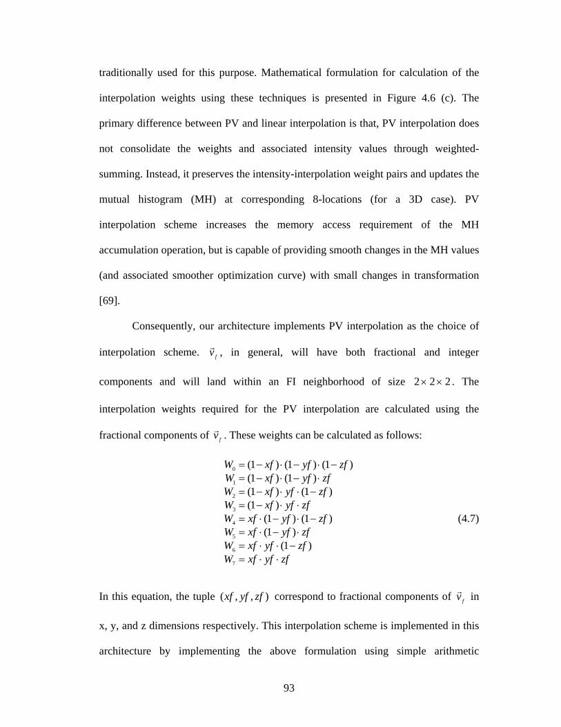
93
traditionally used for this purpose. Mathematical formulation for calculation of the
interpolation weights using these techniques is presented in Figure 4.6 (c). The
primary difference between PV and linear interpolation is that, PV interpolation does
not consolidate the weights and associated intensity values through weighted-
summing. Instead, it preserves the intensity-interpolation weight pairs and updates the
mutual histogram (MH) at corresponding 8-locations (for a 3D case). PV
interpolation scheme increases the memory access requirement of the MH
accumulation operation, but is capable of providing smooth changes in the MH values
(and associated smoother optimization curve) with small changes in transformation
[69].
Consequently, our architecture implements PV interpolation as the choice of
interpolation scheme. fv , in general, will have both fractional and integer
components and will land within an FI neighborhood of size 2 2 2× × . The
interpolation weights required for the PV interpolation are calculated using the
fractional components of fv . These weights can be calculated as follows:
0
1
2
3
4
5
6
7
(1 ) (1 ) (1 )(1 ) (1 )(1 ) (1 )(1 )
(1 ) (1 )(1 )
(1 )
W xf yf zfW xf yf zfW xf yf zfW xf yf zfW xf yf zfW xf yf zfW xf yf zfW xf yf zf
= − ⋅ − ⋅ −= − ⋅ − ⋅= − ⋅ ⋅ −= − ⋅ ⋅= ⋅ − ⋅ −= ⋅ − ⋅= ⋅ ⋅ −= ⋅ ⋅
(4.7)
In this equation, the tuple ( , , )xf yf zf correspond to fractional components of fv in
x, y, and z dimensions respectively. This interpolation scheme is implemented in this
architecture by implementing the above formulation using simple arithmetic

94
computations such as additions and multiplications as illustrated in Figure 4.7. The
pipelined implementation of these operations allows processing of one transformed
RI voxel per clock cycle. Fixed-point arithmetic is used to perform these operations.
The corresponding floating voxel intensities are fetched by the image controller in
parallel using the integer component of fv . The image controller also fetches the
voxel intensity corresponding to rv . The MH, then must to be updated for each pair of
reference and floating voxel intensities (8 in all), using the corresponding weights
computed by the PV interpolator.
4.4.4. Image Memory Access
The dimensions of typical 3D medical images are in the range of 128 × 128 ×
128 to 512 × 512 × 512 voxels. Because intensity-based image registration typically
Figure 4.7: Functional block diagram of partial volume interpolation unit.

95
operates on images with 8-bit intensity values per voxel, this corresponds to image
sizes ranging from 2 to 128 Megabytes. In comparison, the internal, high-speed
memory provided by modern FPGAs is limited to 16 Megabits (or equivalent to 2
Megabytes). Consequently, the images to be registered can not be stored using the
memory that is internal to the FPGA and external storage must be employed for this
purpose.
Because of the size of the medical images, use of static random access
memory (SRAM) modules (which are fast, but offer poor density and capacity) is not
very efficient. Dynamic random access memory (DRAM) modules, in comparison,
offer the necessary density to store the large images that are typically encountered in
medical imaging. Although, these memories do not allow random accesses
throughout the entire memory module with a uniform latency, they support burst-
mode accesses that allow efficient random accesses within a single row of the
memory module. Our architecture takes advantage of this feature and uses external
DRAM memories to store the images to be registered (in other words, the RI and FI).
Figure 4.8: Voxel access patterns of the reference and floating images encountered during image registration.

96
During calculation of MI for a given voxel location in the RI, the reference image
memory must be accessed only once, whereas a complete 2 × 2 × 2 neighborhood (as
required for PV interpolation) must be fetched from the floating image memory.
Thus, there is a disparity between the memory access needs for these two images. The
following subsections briefly describe the access requirements for both these images
and present the strategies we adopted to meet those requirements.
4.4.4.1. Reference Image
An example of memory access pattern for the RI during image registration is
illustrated in Figure 4.8. Between the two images, the RI has more relaxed access
requirements, because it is accessed in a sequential manner (in z−y−x order) and only
one voxel must be fetched from the RI for a given RI voxel address. This kind of
access benefits from burst accesses and memory caching techniques. Furthermore, the
implemented algorithm is based on volume-subdivision and requires traversing
through the RI on a subvolume basis. This means that the voxels that belong to a
subvolume need to be consecutively accessed.
An interesting feature of modern DRAMs is that they are logically partitioned
into rows and columns. As a result, these memories incur additional latency of several
clock cycles when switching between different rows of the memory. Accessing
different columns within a given row, however, is efficiently supported through burst
accesses and can be performed within one clock cycle. Our architecture takes
advantage of this feature and stores the RI in such a way that each subvolume is
aligned with a row of the DRAM memory. This memory organization is illustrated in
Figure 4.9. This allows efficient access to the voxels that belong to a subvolume.

97
For the architecture presented, both the RI and FI are stored in separate logical
partitions of the same DRAM module. However, during MI calculation both these
memories must be accessed simultaneously over a single bus. This can lead to
memory access conflicts and result into poor performance. To address this issue, our
architecture uses internal memory of the FPGA to cache a sub-block of RI voxels.
Thus, during the processing of that block of RI voxels, the image controller has
parallel access to both RI and FI voxels. The RI voxels are fetched from the internal
FPGA memory (with access time of 1 clock cycle), whereas the FI voxels are fetched
directly from the external memory.
4.4.4.2. Floating Image
An example of memory access pattern for the FI during image registration is
illustrated in Figure 4.8. The FI has much higher memory access requirements when
compared to the RI. There are two primary reasons for this:
Figure 4.9: Organization of the reference image memory.

98
1. For every RI voxel address to be processed, 8 FI voxels (corresponding to a
2 2 2× × neighborhood) must be fetched. This neighborhood is then further used
for performing PV interpolation and MH accumulation.
2. Although, the RI is accessed in a sequential manner, the corresponding access
pattern in the FI is completely governed by the transformation ( *ijT ) that is
currently being applied. For example, in Figure 4.8 the access pattern in FI is not
aligned with the natural dimensions (x, y, or z) of the image.
The first aspect of this memory access requirement is similar to that
encountered in the context of volume rendering. In the graphics domain, this problem
has been solved by developing techniques that allow parallel access to the entire
2 2 2× × voxel neighborhood. One way to provide this parallel neighborhood access
is through the use of cubic addressing [140]. Cubic addressing employs eight memory
modules that are accessed in parallel at different addresses, through arithmetic
manipulation of the corresponding single “neighborhood address”. These parallel
memory modules are thus capable of providing the entire 3D neighborhood in one
Figure 4.10: Organization of the floating image memory.

99
clock cycle. This approach, however, requires custom addressing of the memory
modules. Castro-Pareja et al. [139] have reported a method to implement cubic
addressing using standard DRAMs, by storing multiple copies of the image. This
approach does not require special addressing and take advantage of burst-mode
accesses provided by DRAMs. The presented architecture implements a similar
scheme by storing eight copies of the FI. This scheme is illustrated in Figure 4.10.
The FI voxels are arranged sequentially such that, performing a size 2 burst fetches
two adjacent 2 2× neighborhood planes, thus making the entire neighborhood
available simultaneously. Although this approach increases the image storage, it
enables accessing the entire 3D neighborhood in one clock cycle. Further, the density
of DRAM chips allows storing multiple copies of the FI.
The second aspect of the FI memory access requirement is addressed through
the following strategy: we group the neighborhoods that belong to an image block
(within the FI), and assign those neighborhoods to a single row in the DRAM module.
Thus, as long as the transformed address location ( fv ) stays within a FI subvolume,
the corresponding neighborhoods can be fetched within one clock cycle. Because, the
RI is traversed one subvolume at a time, it is highly likely that the transformed
location of that subvolume is confined to one or few FI subvolumes. Our architecture
takes advantage of this spatial locality of reference.
4.4.5. Updating Mutual Histogram
For a given RI voxel RV , there are eight intensity pairs ( 0 7, :RV FV FV ) and
corresponding interpolation weights. Because the MH must be updated (read–

100
modify–write) at these eight locations, this amounts to 16 accesses to MH memory
for each RI voxel. This means that MH memory has more stringent access
requirements when compared with the floating image memory. Moreover, the
locations that need to be accessed within the MH for a given RI voxel, may not have
any relationship with each other (such as a neighborhood-relation in the context of FI
memory) and can be completely random. Fortunately, the size of the MH memory is
typically much smaller (less than 128 128× ) than that of the images ( 256 256 256× × ).
As a result, the internal (on-chip), high-speed memory can be used for storing the
MH.
Our first strategy to meet this high memory access requirement is to use high-
speed, dual-ported memory internal to the FPGA to store the MH. Because this
memory is dual-ported, it can be read and written simultaneously (using different
ports), an operation that is integral to MH accumulation. The overview of pipelined
MH accumulation design, which takes advantage of this feature, is presented in
Figure 4.11. Furthermore, because this memory can work at high speeds, the MH
accumulation pipeline can work at twice the clock rate of the voxel processing
Figure 4.11: Pipelined implementation of MH accumulation using dual port memory.

101
pipeline. Thus, a pipelined implementation of MH accumulation can process (read–
modify–write) two voxels per every clock of the main pipeline. Our second strategy is
multiple parallel MH accumulation pipelines to support the high-memory access
requirement. We employ four copies of the MH and associated parallel pipelines that
independently and concurrently update the partial MHs. The partial MHs, stored in
each MH copy, are eventually combined when the MH is read during the entropy
calculation. Similar strategy is used for storing the individual histogram for the FI.
These two strategies, when combined together, provide sufficient memory access
speed to meet the requirement of MH accumulation.
While the MH is being computed, the individual histogram accumulator unit
computes the histograms for the RI and the FI. These individual histograms are also
stored using internal, dual-ported memories. The valid voxel counter module keeps
track of the number of valid voxels accumulated in the MH and calculates its
reciprocal value. The resulting value is then used by the entropy calculation unit for
calculating the individual and joint probabilities.
4.4.5.1. Data Hazards and Preaccumulation Buffers
The presented architecture implements the operation of updating the MH in a
pipelined fashion. This means that for each MH accumulation pipeline (there are four
such pipelines) one interpolation weight must be accumulated per clock cycle. The
MH address, which must be updated with this interpolation weight, is determined by
the RI-FI intensity pair. Furthermore, the realization of this operation using dual-
ported memories (as described above) has a latency of three clock cycles (one clock
cycle each for read, modify, and write operations). As a result, read-after-write

102
(RAW) hazards could arise if sequential MH update transactions that attempt to
access identical locations (or in other words, transactions with same RI-FI intensity
combination) are separated by fewer than three clock cycles.
To detect and eliminate these RAW hazards, the presented architecture
employs a preaccumulate buffer in each pipeline. The functional block diagram of
this buffer is shown in Figure 4.12. This buffer compares the address of the current
transaction with that of three (equal to the latency of the operation) prior transactions.
If conflicting transactions are detected, the buffer invalidates the current transaction
and adds the interpolation weight of the current transaction to that of the first
conflicting transaction. In summary, this is equivalent to aggregation of the weights
from all the conflicting transactions and all the transactions that constitute a RAW
hazard are converted into a single update to the MH. This scheme entirely eliminates
any possible RAW hazards.
Figure 4.12: Preaccumulate buffers to eliminate RAW hazards in MH accumulation pipeline.

103
4.4.5.2. Calculating RestMH
During the optimization process of finding the best alignment for a given
subvolume k at level i , kTotalMH is computed as shown in equation (4.1). For this
calculation, it is necessary to compute the contribution of the remaining subvolumes
to kTotalMH using the registration information at the previous level of subdivision
( 1( ) ,
iparent jT j k− ∀ ≠ ). This process must be repeated for every subvolume at the current
level i , and the contents of kRestMH will be different every time depending on the
subvolume under consideration. Computing kRestMH , from scratch, for every iteration
of each subvolume will not be efficient. To avoid this repeated calculation, we
introduce MH buffers ( PriorMH , RestMH , and LocalMH ), which store the previous-level
MH and partial MH during various stages of the algorithm. A flow diagram depicting
the interplay between these MH buffers during various steps of calculating RestMH is
shown in Figure 4.13, and the detailed description is provided here.
Figure 4.13: A flow diagram of steps involved in calculating MHRest.

104
At a given level i , PriorMH contains the MH for the entire image, which is
computed using all the subvolumes at the earlier level 1i − and corresponding
transformations 1ijT − . At the beginning of the registration of each subvolume k at the
current level i , LocalMH is cleared (thus, all its entries are set to 0). Next, the
transformation of its parent from the previous level, 1( )
iparent kT − , is applied to the current
subvolume k and the resultant MH is accumulated in LocalMH . LocalMH now contains
the contribution of the subvolume k to PriorMH . LocalMH is then subtracted from
PriorMH , and the resultant MH is stored in the buffer RestMH . This step is
mathematically equivalent to computing kRestMH (as in equation (4.3)) for the
subvolume k . For every subsequent optimization iteration involving this subvolume,
LocalMH is initially cleared. The candidate transformation *ikT is then applied to the
current subvolume ( k ) only, and the resultant histogram (contribution of this
subvolume) is accumulated in LocalMH . It is then added to kRestMH , to form the MH
for the entire image (kTotalMH in equation (4.1)) for the current optimization step. This
final histogram is then further used for computing the image similarity measure (MI)
corresponding to the current transformation *ikT . This process is repeated for all the
subvolumes at the current level. At the end of each level (after optimizing all the
subvolumes at that level), the MH for the entire image is computed using the updated
transformations ,ikT k∀ and is stored in PriorMH , which will then subsequently be used
at the next level of subdivision, 1i + .

105
4.4.6. Entropy Calculation
Acceleration of MH accumulation contributes to the most of the performance
improvement during calculation of MI. However, the final step in MI calculation,
which is entropy calculation, must also be implemented in the hardware to eliminate
the overhead of copy the MH back to the host. The mutual and individual entropies
are computed by using the probability distributions represented by the mutual and
individual histograms, respectively.
To calculate entropy, it is necessary to evaluate the function ( ) ln( )f p p p= ⋅
for all the probabilities. As probability p takes values between [0,1] , the
corresponding range for the function ln( )p is [ ,0]−∞ . In addition, ln( )p is undefined
for 0p = . In comparison, the corresponding range for ( )f p is 1[ ,0]e−− . Thus, ( )f p
has a finite dynamic range and is defined for all values of p . Several methods for
calculating logarithmic functions in hardware have been reported earlier [152-154],
but of particular interest is the multiple lookup table (LUT)–based approach
introduced by Castro-Pareja et al. [155]. This approach minimizes the error in
representing ( )f p for a given number and size of LUTs and, hence, is accurate and
efficient. Moreover, this approach preserves the shape of the MI curve and the
location of the extrema and thus does not significantly affect the outcome of the
optimization process. Following this approach, the presented design implements
( )f p using multiple LUT–based piecewise polynomial approximation. We provide a
brief overview of this method here and identify the multiple LUT configuration
adopted by our architecture.

106
4.4.6.1. Multiple LUT–Based Approach for Entropy Calculation
A LUT-based approach represents the target function (such as ( )f p ) using a
piecewise-polynomial approximation with n segments. In particular, approximation
using Chebyshev polynomials is employed because: 1) the Chebyshev approximation
is simple to calculate for continuous functions such as ( )f p and 2) it is very close to
the true minimax approximation, the most accurate polynomial approximation. The
polynomials used can be of arbitrarily high order. Higher degree of polynomials
typically offer better approximation, but require higher degree of arithmetic
computation (and associated hardware resources) for function evaluation. For this
reason, only 1st order polynomials are considered.
In case of a single-LUT based approach, all the segments are stored in a single
large LUT. Although this approach is simple and allows easy decoding and
addressing during function evaluation, it suffers from several drawbacks. First, the
precision of the LUT ( pΔ ) is constant throughout the entire table. As a result,
segments of the approximated function that require finer precision can not be
accurately represented. Second, the size of the LUT to achieve a desired
approximation error is usually quite large and sometimes not practical. For example,
Table 4.1: Configurations of LUT-based entropy calculation module that were considered in the presented architecture.
LUT Range Configuration #1 Configuration #2 LUT No.
minp maxp pΔ Entries pΔ Entries 1 0 2-13 2-23 1024 2-24 2048 2 2-13 2-6 2-16 1024 2-17 2048 3 2-6 2-2 2-12 1024 2-13 2048 4 2-2 1 2-10 1024 2-11 2048

107
to keep the error in entropy calculation less than 10-6, a single LUT with 16K entries
will be required.
The multiple LUT–based approach introduced by Castro-Pareja et al. [155]
attempts to address these limitations. In this approach, each segment is stored in a
different LUT. In addition, each LUT has a different precision ( pΔ ) and uses a
different polynomial coefficients to represent the individual segments of the function
( )f p . Thus, this approach allows superior approximation of the target function and
thereby keeping the approximation error below the allowable maximum.
Furthermore, this method provides a realization that is optimized for approximation
accuracy and hardware resources [155].
Using this approach the 1st-order polynomial, 4-LUT configuration was
designed. We realized two such configurations each with a different LUT precision
( pΔ ). These configurations are listed in Table 4.1. The choice of these configurations
Figure 4.14: Error in entropy calculation corresponding to the two configurations of the multiple LUT–based implementation.

108
was based on meeting the error constraints on the entropy calculation and the
availability of resources in the target FPGA device. We then evaluated the
approximation error offered by these two realizations. This was done by comparing
the entropy values calculated by using these designs against that calculated using a
double-precision software implementation. Figure 4.14 shows a plot of the error
magnitude vs. p for both these realizations. The maximum error was of the order of
10-8 for a both these configurations, which is sufficient for MI calculation in the
context of image registration [155]. For our architecture we selected realization with
8K entries, as it offers superior error performance at a relatively moderate increase in
the LUT size. As described earlier, using the lower-order polynomials has the
advantage of reducing the LUT data width and the number of required arithmetic
operations for function evaluation.
4.4.7. Operational Workflow
The sections above described the design and functional behavior of the
important modules in the architecture we developed for accelerated calculation of MI.
Our ultimate goal, however, is to accelerate deformable image registration algorithm
described earlier. This algorithm utilizes this high-speed implementation to efficiently
calculate the image similarity measure (MI), the most computationally complex step
within the algorithm. This deformable registration algorithm is based on volume
subdivision, and depending on the operational stage of the algorithm, image similarity
is calculated in a slightly different manner. For example, steps to calculate MI during
rigid registration are slightly different than those taken during optimization of a
subvolume after volume subdivision. This section identifies different operational

109
stages of the algorithm and describes how the architecture described above is utilized
to calculate MI during those stages. The summary of this description is provided in
Table 4.2.
4.4.7.1. Rigid Registration
Rigid registration is the first step in the aforementioned deformable
registration algorithm. This step attempts to recover any gross misalignment between
the RI and FI. During this step, the algorithm repeatedly calculates MI for various
candidate transformations between RI and FI. To implement this operation using the
described architecture, we first clear all the mutual histograms internal to the
architecture ( PriorMH , RestMH , and LocalMH ). Next, the host provides the current
candidate transformation along with the subvolume address range (equal to the RI
dimensions, since MI is calculated for the entire image) to the architecture. After this
operation, the MH corresponding to the given transformation is calculated and stored
Table 4.2: Operational workflow for performing volume subdivision–based deformable image registration using the presented architecture.
Operation Workflow
Rigid Registration Clear All MHs → Accumulate (entire RI) → Calculate Entropy using MHLocal
Calculating MHPrior (First subvolume) Clear All MHs → Accumulate (current subvolume)
Calculating MHPrior (Other subvolumes) Accumulate (current subvolume)
Calculating MHPrior (Copying MH) Copy MHLocal to MHPrior
Calculating MHRest Clear MHLocal → Accumulate (current subvolume) → Subtract MHLocal from MHPrior and store into MHRest
Subvolume Registration
Clear MHLocal → Accumulate ( current subvolume ) → Calculate Entropy using MHLocal + MHRest

110
in LocalMH . Later on, the individual and joint entropies are calculated using LocalMH .
4.4.7.2. Calculating PriorMH
Calculating PriorMH requires applying transformations to all the subvolumes at
a given level of subdivision and calculating the cumulative MH corresponding to all
subvolumes with their associated transformations. To implement this operation using
the described architecture, we first clear LocalMH , which is used for subvolume MH
accumulation. Next, the host provides the address range for the first subvolume and
the transformation associated with that subvolume from the previous level. The MH
corresponding to the given transformation is calculated and stored in LocalMH . This
step is repeated for all the subvolumes at a given level of subdivision, with a
difference that LocalMH is cleared only during the first subvolume. This allows the
calculation of the cumulative MH for all the subvolumes. After all the subvolumes are
processed, LocalMH is copied to PriorMH (an internal MH buffer). No entropy
calculation is required during this step. This step is repeated after each level of image
subdivision.
4.4.7.3. Calculating RestMH
Calculation of RestMH is a prerequisite for optimizing subvolumes after
volume subdivision. As described earlier, we utilize PriorMH to efficiently calculate
RestMH for a given subvolume. To implement this operation using our architecture,
we first clear LocalMH , which is used for subvolume MH accumulation. Next, the host

111
provides the address range for the current subvolume and the transformation
associated with that subvolume from the previous level. The MH corresponding to
the given transformation is calculated and stored in LocalMH . Following this operation,
we subtract LocalMH from PriorMH and store the resulting MH into RestMH (another
internal MH buffer). This step is repeated prior to registration of every subvolume at
a given level of subdivision.
4.4.7.4. Subvolume Registration
After image subdivision, the resulting subvolumes are individually registered
with the FI. However, the image registration algorithm also considers the contribution
of the rest of the image for improved statistical reliability. Our architecture supports
this operation by taking advantage of the RestMH computed in the previous step. First,
we clear LocalMH , which is used for subvolume MH accumulation. Next, the host
provides the address range for the current subvolume and the current candidate
transformation for that subvolume. The MH corresponding to the given candidate
transformation is calculated and stored in LocalMH . Later on, the individual and joint
entropies are calculated using ( )Local RestMH MH+ , thus taking into account the
contribution of the rest of the image. This step is repeated for each iteration during
the registration of a subvolume.
4.5. Implementation and Results
The architecture presented above was implemented using an Altera Stratix II
EP2S180F1508C4 FPGA (Altera Corp., San Jose, CA) in a PCI prototyping board

112
(DN7000K10PCI) manufactured by the Dini Group (La Jolla, CA). The board
featured 1 GB double-data-rate (DDR2) DRAM in a small-outline dual-inline
memory module (SoDIMM) external to the FPGA. This memory was used to store
the RI and the FI. The board provided a 64-bit bus interface between the memory and
the FPGA running at 200 MHz clock speed. The architecture was designed using
VHSIC hardware description language (VHDL) and synthesized using Altera
Quartus II 6.1. The memory controller was also implemented using VHDL and was
built around the DDR2 DRAM controller megacore supplied with Altera Quartus II.
All the modules in the architecture were custom designed using VHDL, per the
design description provided earlier. Functional verification and postsynthesis timing
simulation for the entire system were performed using Modelsim SE 6.2 (Mentor
Graphics, San Jose, CA). For this purpose, DDR2 DRAM simulation models
provided by Micron (www.micron.com) were used. The resource availability of the
target FPGA, primarily internal memory, which is used for MH accumulation, limited
the synthesis of the reported design to support 7-bit mutual histogram and,
consequently, all results in this section are presented for this configuration. In
comparison, the software implementation uses 8-bit mutual histogram. In spite of this
difference, we demonstrate that the registration accuracy for both these
implementations is comparable (see Chapter 6), which further confirms the findings
of Studholme et al. [64].
To verify the functional correctness and evaluate the performance of this
implementation we considered image registration between intraprocedural
noncontrast CT (iCT) with preprocedural contrast-enhanced CT (preCT) and positron

113
emission tomography (PET) images. The registration between these image-pair
combinations is clinically relevant and routinely encountered in the context of CT-
guided interventions. We considered five abdominal iCT-preCT and five abdominal
iCT-PET image pairs for this evaluation. The image size for iCT and preCT was 256
× 256 × 200−350 with a voxel size of 1.4−1.7 mm × 1.4−1.7 mm × 1.5 mm, whereas
the typical image size for PET was 128 × 128 × 154−202 voxels with a voxel size of
5.15 mm × 5.15 mm × 5.15 mm. The iCT, preCT, and PET images were converted to
8 bits and 7 bits, respectively, for software and FPGA-based implementations. This
conversion was performed using adaptive reduction in intensity levels [156]. The
converted iCT and preCT images were then preprocessed using 3D anisotropic
diffusion filtering. No preprocessing steps were used for the PET images. The real-
time implementation of anisotropic diffusion filtering that we presented earlier can
facilitate this preprocessing without adding any significant latency to IGI workflow
[144]. For the hardware implementation, the RI was stored in a sequential format
organized by subvolumes, while eight interleaving copies of the FI were arranged in
memory to facilitate cubic addressing. This arrangement allows simultaneous access
to an entire 3D neighborhood within the FI, as described earlier. The execution speed
of the reported architecture was obtained from postsynthesis timing measurements
using the entire system.
The design achieved a maximum internal frequency of 200 MHz, with a
theoretical maximum RI voxel processing rate of 100 MHz. The coordinate
transformation, PV interpolation, and MH accumulation operations were
implemented using fixed-point representation. Entropy calculation was implemented

114
using the 4-LUT, first-order polynomial configuration as described earlier. The
precision employed for this fixed-point datapath can affect both the implementation
accuracy and the hardware resource requirement of this architecture. An optimization
framework to systematically explore this effect is presented in the following chapter.
This framework is capable of identifying the optimized tradeoff relationship between
the hardware resources and the accuracy. The optimization of our architecture by
using this framework is presented in Chapter 5. We further evaluated the accuracy of
deformable image registration offered by that optimized architectural configuration
and those results are presented in Chapter 6. In this section, however, we focus on the
execution performance of our architecture and demonstrate its functional correctness
through qualitative validation of image registration. For this purpose we used a
designer identified architectural configuration which was not optimized for area-
implementation error tradeoff. Consequently, all the results presented in this section
are corresponding to that design configuration.
4.5.1. Execution Speed
The presented architecture is targeted toward accelerating the calculation of
MI for a hierarchical volume subdivision–based deformable registration algorithm.
During the execution of this algorithm, MI must be repeatedly calculated under a
candidate transformation for every subvolume at every level of subdivision.
Moreover, as described earlier, RestMH must be calculated once for every subvolume.
To analyze the speedup offered by the presented FPGA-based solution for calculation
of MI, we compare its calculation time with that of a software (C++) implementation
running on an Intel Xeon 3.6 GHz workstation with 2 GB of RAM. Table 4.3 details

115
this performance comparison for a iCT-preCT image pair with dimensions of 256 ×
256 × 256. The last column of the table shows the speedup offered by the reported
solution over the software implementation for a given level of subdivision. The time
to calculate MI primarily depends on the size of the subvolume and is independent of
the imaging modality and voxel size. This calculation time, however, may vary
slightly based on the actual value of the transformation used to calculate MI. These
variations are caused by differences in access patterns to the FI memory under
different transformation values. To compensate for this effect and report average MI
calculation time at a given level of subdivision, we measured the MI calculation times
for a subvolume using 100 randomly generated transformations (within the range of
±30 voxels for translations and ±20° for rotations).
The same set of transformations was used for both software and hardware
implementations. The MI calculation time reported in Table 4.3 is averaged over all
the transformations. Hardware timings reported in Table 4.3 also include the
communication time, required for writing the transformation matrix and reading back
Table 4.3: Comparison of mutual information calculation time for subvolumes at various levels in volume subdivision–based deformable registration algorithm.
Mutual information calculation time (ms) Subdivision
level Subvolume
size Software implementation
FPGA-based implementation
Speedup
0a 256 × 256 × 256 9410 225.42 41.74
1 128 × 128 × 128 1209 30.19 40.05
2 64 × 64 × 64 166 4.16 39.90 3 32 × 32 × 32 18 0.78 23.08 4 16 × 16 × 16 10 0.46 21.74
aThis corresponds to rigid registration between the reference and floating images.

116
the calculated entropy values, between the host and the MI calculator. Furthermore,
consistent with the scenario during the execution of the registration algorithm, the
time to compute RestMH (once per subvolume) is also included in the hardware and
software MI calculation time. Our acrchitecture offers a speedup of about 40 for
calculating MI up to subvolumes of size 643; whereas for smaller subvolumes the
speedup achieved is around 20. This drop in achieved speedup is explained by taking
into account overheads incurred during computation of MI. Calculating MI requires
accumulation of MH, which in turn, requires initial clearing of the MH memory.
Because the current implementation employs an MH with size 128 128× (to support
7-bit images), the process of clearing MH, which involves writing ‘0’s to all MH
entries, can consume more than 16,000 clock cycles. For smaller subvolumes, the
time required to clear MH memory becomes comparable to or larger than that
required to process a subvolume (images are processed at the rate of approximately
one voxel per clock cycle). In addition, the communication time between the host and
the MI calculator, required for exchanging the transformation matrix and the
calculated MI value, becomes comparable to the computation time. These two factors
limit the net speedup achieved for smaller subvolumes.
Table 4.4 compares the total execution time for deformable registration using
a software (C++) implementation running on an Intel Xeon 3.6 GHz workstation with
Table 4.4: Execution time of deformable image registration. Execution time (s) Image pair
used for registration
Software implementation
FPGA-based implementation
Speedup
iCT-preCT 11520 371 31.05 iCT-PET 11146 339 32.88
117
2 GB of RAM against the presented FPGA-based architecutre. This execution time
was measured for deformable registration between five iCT-preCT and five iCT-PET
image pairs, described earlier. The maximum number of global and local iterations
was set to 200 and 100 respectively. The same optimization algorithm was used for
both the software and hardware implementations, and volume subdivision continued
until the subvolume size was larger than 163. For each image modality pair, the
execution time reported is the average of execution times of the five cases. The
execution time of intensity-based image registration is directly proportional to the
size of the RI. iCT image was used as the RI for both the image modality pairs and,
hence, the execution time for deformable registration is similar for these two image
modalities, despite the fact that PET images are smaller than preCT images (128 ×
128 × 154−202 and 256 × 256 × 200−350, respectively). For both image modality
pairs, our architecture provided a speedup of about 30 over an equivalent software
implementation and achieved an execution time of around 6 minutes. This speedup is
a direct outcome of acceleration of MI calculation using the presented architecture.
4.5.2. Performance Comparison
Intensity-based image registration has been identified to be a computationally
intensive problem. Given the impact the acceleration of image registration can have
on a variety of diagnostic and interventional applications, there have been significant
efforts towards realizing high-speed implementations of image registration
algorithms. Further, given that this problem is extremely compute-extensive and
multi-faceted; researchers have applied a range of computing platforms and
acceleration strategies at different levels of this problem to improve its execution

118
performance. In Chapter 2, we provided a survey of some acceleration approaches
that are somewhat related to the work presented in this dissertation. In this section we
compare the performance improvement provided by the FPGA-based implementation
we developed in this dissertation work against that provided by the earlier reported
solutions.
For this comparison we focused on acceleration approaches involving
intensity-based image registration, since these approaches can be retrospective,
automatic and have the potential to be integrated into the clinical workflow. The
algorithms considered included FFD-based, and gradient flow-based approaches as
well as those based on the demon’s algorithm. Moreover, these implementations used
different similarity measures (MI, NMI, SSD etc.), transformation models (spline-
based, rigid, volume-subdivision based) and acceleration strategies as dictated by the
computational platform (GPUs, clusters, FPGAs etc.) used for their implementation.
Thus, there is a substantial variation in the implementation details (both, for original
and accelerated implementation) of each of these realizations, even though they try to
address the same fundamental problem of accelerating intensity-based registration. To
account for these variations and provide a fair comparison, we consider the net
speedup offered by these accelerated implementations against their corresponding un-
accelerated versions. This comparison can be used to judge the efficiency of various
strategies to accelerate intensity-based image registration. To compare the raw
computational performance these realizations, we normalize their corresponding
execution times by the dimensions of reference image used for registration and
calculate the effective voxel processing rate (throughput) offered. In some cases,

119
where sufficient implementation details (such as number of iterations, number of
voxels processed etc.) were not provided the voxel processing rate could not be
calculated.
Table 4.5 presents the results of this analysis and compares the performance
of the presented architecture for high-speed implementation of deformable image
registration, against a corresponding software implementation and previously
reported acceleration approaches. The software implementation refers to the
implementation of the volume subdivision–based algorithm. This implementation was
developed using C++, and its performance was measured on an Intel Xeon 3.6 GHz
workstation with 2 gigabytes of DDR2 400 MHz main memory. The presented
implementation of FPGA-based MI calculation provides more than an order of
magnitude speedup and superior voxel processing rate when compared to this
software implementation.
The majority of earlier reported attempts to accelerate intensity-based image
registration have primarily employed a multiprocessor or supercomputer approach
(see [57, 116, 117] , for example). Although these solutions delivered high
performance and speedup by virtue of parallelization and high-speed network
interconnects, the speedup achieved per processor was less than unity. Also, in some
cases [116] the voxel processing rate achieved was substantially less than that offered
by the presented implementation. In addition, these solutions may not be cost
effective and, because of their size, are unlikely to be suitable for clinical deployment.
Some solutions based on graphics processors [120, 122] attempt to provide
performance improvement by exploiting data parallelism native to this platform.

120
Although this platform yielded reasonable speedups for rigid registration, the
performance gain and voxel throughput for deformable registration and in particular,
for that based on MI, were poor. Ohara et al. [123] attempted to accelerate MI-based
rigid registration using a pair of cell processors, by exploiting the inherent parallelism
offered by multiple cores (8 per processor) and high memory bandwidth. Using these
16 computing cores, this implementation achieved speedup of only 11 for rigid
registration. The voxel throughput of this implementation (6 MHz), however, was
slightly better when compared with other multiprocessor implementations. This can
be attributed to the high memory bandwidth and additional designer optimizations to
take advantage of spatial locality. Jiang et al. [124] employed a high-level description
language (Handel-C) and mapped B-spline computation (a common component in
FFD-based image registration) to Xilinx FPGA devices. This implementation
leveraged elimination of nested loops and pipelined implementation to achieve
performance improvement. Despite the semi-automated nature of this approach and
high clock rate of the synthesized design, the speedup and the voxel throughput
achieved were limited to 3.2 and 4 MHz respectively.
In comparison with these acceleration approaches, the FPGA-based
implementation developed in this dissertation addresses the fundamental memory
access bottleneck in intensity-based image registration. Furthermore, voxel-level
parallelism is achieved through pipelined implementation and this implementation
can offer voxel processing rate close to one voxel per clock cycle. Thus, this solution
is not only compact, but offers high speedup (around 30) and superior voxel
throughput (> 70 MHz) using a single processing element.

121
Table 4.5: Performance comparison of the presented FPGA-based implementation of intensity-based deformable image registration with an equivalent software implementation and prior approaches for acceleration of intensity-based registration.
Implementation Algorithm Platform Speedup
Voxel processing rate (MHz)
(if available)Stefanescu et al. [116]
Demon’s algorithm
15-processor cluster 11 1.8
Rohlfing et al. [57]
FFD-based deformable,
using MI
64-processor shared-memory supercomputer
40 –
Ino et al. [117]
FFD-based deformable, using
MI
128-processor cluster, Myrinet
connectivity 90 –
Kohn et al. [120]
Gradient flow, rigid/deformable
GPU (6800) (using GLSL) 12 2.15
Vetter et al. [122]
MI-based deformable
GPU (7800) (using GLSL) 6 3.21
Ohara et al. [123]
MI-based rigid
2 cell broadband engine processors 11 5.75
Jiang et al. [124]
B-spline interpolation
FPGA (using Handel-C) 3 4.19
Software (C++)
MI-based deformable Xeon workstation – 1.75
Dandekar et al. [157]
MI-based deformable FPGA 33 74.43

122
4.5.3. Qualitative Evaluation of Deformable Image Registration
Acceleration of deformable registration, as offered by the presented
architecture, is critical for the time-sensitive nature of IGIs; however the accuracy of
the registration process is of equal importance. As described earlier, we present the
results of qualitative validation in this section, which demonstrate the functional
correctness of our architecture. The results of the quantitative validation are presented
later, in Chapter 6. The qualitative validation of deformable registration was
performed using five iCT-preCT and five iCT-PET image pairs. For all the cases
visually correct alignment was achieved after deformable image registration.
Furthermore, the results of the registration performed using our architecture was
qualitatively similar to that obtained using the software implementation.
Figure 4.15: Qualitative validation of deformable registration between iCT and preCT images performed using the presented FPGA-based solution.

123
Figure 4.15 shows an example of deformable registration between a
representative pair of iCT and preCT images. This registration was performed using
the presented FPGA-based solution. The initial seed alignment between these images
was obtained using a single-click operation to compensate for different scanner
coordinate systems and ensure reasonable overlap of common regions between two
images. Subfigures (a) and (b) show coronal slices from iCT and preCT images,
respectively. Subfigure (c) shows the overlay of these two images using the
checkerboard pattern. In this checkerboard overlay, blocks from both the images are
displayed alternately. The structural misalignment between iCT and preCT images is
evident from mismatches at the boundaries of these blocks. Subfigure (e) shows a
coronal slice from the preCT image registered to the iCT image, and subfigure (f)
shows the overlay of this image with the original iCT image. Better structural
alignment after deformable registration is evident from improved matching at the
boundaries of the blocks of the checkerboard overlay.
Similarly, Figure 4.16 shows an example of deformable registration between a
representative pair of iCT and PET images. This registration was also performed
using the reported FPGA-based solution. The initial alignment between these two
Figure 4.16: Qualitative validation of deformable registration between iCT and PET images performed using the presented FPGA-based solution.

124
images was obtained as for the previous case. Subfigures (a) and (b) show coronal
slices from iCT and PET images, respectively. Subfigure (c) shows the fusion of
these two images. Subfigure (d) shows the fusion of the registered PET image with
the original iCT image. Improved alignment after deformable registration is evident
from better matching of structures in the fusion image.
4.6. Summary
In this chapter we presented a novel FPGA-based architecture for high-speed
implementation of MI-based deformable image registration. This architecture
achieved voxel-level parallelism through pipelined implementation and employed
several strategies to address the fundamental bottleneck in the intensity-based image
registration, namely memory access management. As a result of these enhancements,
the presented architecture is capable of achieving high voxel processing rate and a
speedup of about 30 and consequently reduces the execution time of deformable
registration from hours to only a few minutes. The results of the qualitative validation
indicate that this performance improvement does not significantly compromise the
accuracy of deformable registration. As qualitatively presented in this chapter and
demonstrated quantitatively later (see Chapter 6), this implementation enables
improved target delineation during image-guided interventions through deformable
registration with preprocedural images. The robustness, speed, and accuracy offered
by this architecture, in conjunction with its compact implementation, make it ideally
suitable for integration into IGI workflow.
Accurate, robust, and real-time deformable image registration between intra-
and preprocedural images is an unmet need, critical to the success of image-guided

125
procedures. The work presented in this chapter of the dissertation represents an
important first step toward meeting this goal. With further algorithmic and hardware
improvements, geared toward enhancing its accuracy and performance, this approach
has the potential to elevate the precision of current procedures and expand the scope
of IGI to moving and deformable organs.

126
Chapter 5: Framework for Optimization of Finite Precision
Implementations
Computationally intensive algorithmic components are routinely accelerated
by mapping them to custom or reconfigurable hardware platforms. The work
presented in the earlier chapters of this dissertation has a similar flavor. An important
consideration for these implementations, which often employ finite precision
datapaths, is the tradeoff between hardware resources and implementation accuracy.
This chapter presents a methodology for systematically exploring this tradeoff and
identifying design configurations that efficiently balance these two conflicting
objectives. First, we formulate this problem as a multiobjective optimization problem.
Next, we present a multiobjective optimization framework developed in the context
of FPGA-based architecture for image registration presented in the previous chapter.
Finally, we demonstrate the applicability of the proposed approach through
simulation and post-synthesis validation results.
5.1. Motivation
An emerging trend in real-time signal processing systems is to accelerate
computationally intensive algorithmic components (for example, MI calculation as
described in the previous chapter) by mapping them to custom or reconfigurable
hardware platforms, such as ASICs and FPGAs. Most of these algorithms are initially
developed in software using floating-point representation and later migrated to
hardware using finite precision (e.g., fixed-point representation) for achieving
improved computational performance and reduced hardware cost. These

127
implementations are often parameterized, so that a wide range of finite precision
representations can be supported [158] by choosing an appropriate wordlength for
each internal variable. As a consequence, the accuracy and hardware resource
requirements of such a system are functions of the wordlengths used to represent the
internal variables. Determining an optimal wordlength configuration has been shown
to be NP-hard [159] and can take up to 50% of the design time for complex systems
[125]. Moreover, a single optimal solution may not exist, especially in the presence of
multiple conflicting objectives, as is the case in the current work. In addition, a new
configuration generally needs to be derived when the design constraints or application
requirements are altered.
An exhaustive search of the entire design space is guaranteed to find Pareto-
optimal configurations. Execution time for such exhaustive search, however,
increases exponentially with the number of design parameters, making it unfeasible
for most practical systems. Some earlier reported techniques have attempted to solve
this problem through the use of analytical modeling [86-90], gradient-based search
[93], linear programming strategies [86], or through the use of linear aggregation of
objective functions. These approaches, although successfully demonstrated, may have
limited applicability for complex designs, with non-linear objective functions and a
non-convex search space [129]. For example, in the case of FPGA-based
implementation of image registration, analytically representing the error induced in
MI-calculation will be non-trivial. In addition, MI is a non-linear objective function.
Techniques based on evolutionary methods have been shown to be effective in
searching large search spaces with complex objective functions in an efficient manner

128
[130, 131]. Furthermore, these techniques are inherently capable of performing
multipoint searches. As a result, techniques based on evolutionary algorithms (EAs)
have been employed in the context of multiobjective optimization (see SPEA2 [160],
NSGA-II [161]).
We formulate this problem of finding optimal wordlength configurations as a
multiobjective optimization, where different objectives — for example, accuracy and
area — generally conflict with one another. Although this approach increases the
complexity of the search, it can find a set of Pareto-optimized configurations
representing strategically-chosen tradeoffs among the various objectives. This novel
multiobjective optimization strategy is developed and validated in the context of
FPGA-based implementation of image registration. The tradeoff between FPGA
resources (area and memory) and implementation accuracy is systematically
explored, and Pareto-optimized solutions are identified such that a designer could use
these solutions to satisfy given design constrains or meet image registration accuracy
required by an application. This analysis is performed by treating the wordlengths of
the internal variables of the architecture presented in the previous chapter as design
variables. We also compare several search methods for finding Pareto-optimized
solutions and demonstrate in our context the applicability of search based on
evolutionary techniques for efficiently identifying superior multiobjective tradeoff
curves. This optimization strategy can easily be adapted to a wide range of signal
processing applications, including applications for image and video processing.

129
5.2. Multiobjective Optimization
The architecture presented in the previous chapter is designed to accelerate the
calculation of MI for performing intensity-based image registration. We have
demonstrated this architecture to be capable of offering execution performance
superior to that of a software implementation [157]. The accuracy of MI calculation
(and by extension, that of image registration) offered by this implementation,
however, is a function of the wordlengths chosen for the internal variables of the
design. Similarly, these wordlengths also control the hardware implementation cost of
the design. For medical imaging applications, the ability of an implementation to
achieve the desired level of accuracy is of paramount importance. It is, therefore,
necessary to understand the tradeoff between accuracy and hardware implementation
cost for a design and to identify wordlength configurations that provide effective
tradeoffs between these conflicting criteria. This multiobjective optimization allows a
designer to systematically maximize accuracy for a given hardware cost limitation
(imposed by a target device, for example) or minimize hardware resources to meet the
accuracy requirements of a medical application.
The following section provides a formal definition of this problem and the
subsequent section describes a framework developed for multiobjective optimization
of FPGA-based medical image registration.
5.2.1. Problem Statement
Consider a system Q that is parameterized by N parameters
( 1, 2, , )in i N= … , where each parameter can take on a single value from a

130
corresponding set of valid values ( iv ). Let the design configuration space
corresponding to this system be S , which is defined by a set consisting of all N-
tuples generated by the Cartesian product of the sets ,iv i∀ :
1 2 3 .NS v v v v= × × × × (5.1)
The size of this design configuration space is then equal to the cardinality of the set
S , or in other words, the product of the cardinalities of the sets iv :
1 2 3 .NS v v v v= × × × × (5.2)
For most systems, not all configurations that belong to S may be valid or practical.
We therefore define a subset ( )Sℑ ℑ⊆ , such that it contains all the feasible system
configurations. Now consider m objective functions 1 2( , , , )mf f f… defined for
system Q , such that each function associates a real value for every feasible
configuration c∈ℑ .
The problem of multiobjective optimization is then to find a set of solutions
that simultaneously optimizes the m objective functions according to an appropriate
criterion. The most commonly adopted notion of optimality in multiobjective
optimization is that of Pareto optimality. According to this notion, a solution c∗ is
Pareto optimal if there does not exist another solution c∈ℑ such that
*( ) ( )i if c f c≤ , for all i , and *( ) ( )j jf c f c< , for at least one j . The solution c∗ is also
called a non-dominated solution, because no other solution dominates (or is superior
than) solution c∗ as per the Pareto-optimality criteria. The set of Pareto optimal
solutions, therefore, comprises of all non-dominated solutions.

131
Given a multiobjective optimization problem and a heuristic technique for this
problem that attempts to derive Pareto-optimal or near-Pareto-optimal solutions, we
refer to solutions derived by the heuristic as “Pareto-optimized” solutions.
5.2.2. Parameterized Architectural Design
Implementations of signal processing algorithms using microprocessor- or
DSP-based approaches are characterized by a fixed datapath width. This width is
determined by the hard-wired datapath of the underlying processor architecture.
Reconfigurable implementation based on FPGAs, in contrast, allows the size of
datapath to be customized to achieve better tradeoffs among accuracy, area, and
power. The use of such custom data representation for optimizing designs is one of
the main strengths of reconfigurable computing [85]. To take advantage of the
described multiobjective optimization strategy, the architecture being optimized must
be able to support various design configurations as identified by the optimization
scheme. It has even been contended that the most efficient hardware implementation
of an algorithm is one that supports a variety of finite precision representations of
different sizes for its internal variables [158]. In this spirit, many commercial and
research efforts have employed parameterized design style for intellectual property
(IP) cores [162-166]. This parameterization capability not only facilitates reuse of
design cores, but also allows them to be reconfigured to meet design requirements.
During the design of the aforementioned architecture for accelerated
computation of MI, we adopted a similar design style that allows configuration of the
wordlengths of the internal variables. Hardware design languages such as VHDL and
Verilog natively support hierarchical parameterization of a design through use of

132
generics and parameters, respectively. This design style takes advantage of these
language features and is employed for the design of all the modules described earlier.
We highlight the main features of this design style using illustrative examples and
design senarios. Consider a design module with two input variables that computes an
output variable through arithmetic manipulation of the input variables. The
wordlength of the input variables (denoted by IP1_WIDTH, IP2_WIDTH) and that of
the output variable (denoted by OP_WIDTH) are the design parameters for this
module. The module can then be parameterized for these design variables as
illustrated in Figure 5.1a.
In a pipelined implementation of an operation, a module may have multiple
internal pipeline stages and corresponding intermediate variables. Wordlengths
chosen for these intermediate variables can also impact the accuracy and hardware
requirements of a design. In our implementation scheme, we do not employ any
rounding or truncation for the intermediate variables, but deduce their wordlengths
based on the wordlengths of the input operands and the arithmetic operation to be
implemented. For example, multiplication of two 8-bit variables will, at the most,
require a 16-bit wide intermediate output variable. A parameterized implementation
of this scenario is illustrated in Figure 5.1c. Sometimes, it is also necessary to
instantiate a vendor-provided or a third-party IP core, such as a FIFO module or an
arithmetic unit, within a design module. In such cases, we simply pass the wordlength
parameters down the design hierarchy to configure the IP core appropriately and
thereby maintain the parameterized design style (see Figure 5.1b for example).

133
When signals cross module boundaries, the output wordlength and format
(position of the binary point) of the source module should match the input wordlength
and format of the destination module. This is usually achieved through use of a
rounding strategy and right- or left-shifting of the signals. Adopting “rounding toward
the nearest” strategy to achieve wordlength-matching is expected to introduce the
smallest error, but requires additional logic resources. In our design, we therefore
Figure 5.1: Examples of parameterized architectural design style.

134
implement truncation (or “rounding toward zero” strategy), while the signal shifting
is achieved through zero-padding. Both these operations are parameterized and take
into account the wordlengths and the format at the module boundaries (see Figure
5.1c for example). Thus, this parameterized design style enables the architecture to
support multiple wordlength configurations for its internal variables. The parameters
of this architecture, and in particular the fractional wordlengths of the internal
variables, are being treated as design variables in this multiobjective optimization
framework. These design variables are identified in the following section.
5.2.3. Multiobjective Optimization Framework
Figure 5.2 illustrates the framework that we have developed for multiobjective
optimization of the architecture for high-speed implementation of image registration
Figure 5.2: Framework for multiobjective optimization of FPGA-based image registration.

135
described in the previous chapter. There are two basic components of this framework.
The first component is the search algorithm that explores the design space and
generates feasible candidate solutions; and the second component is the objective
function evaluation module that evaluates candidate solutions. The solutions and
associated objective values are fed back to the search algorithm so that they can be
used to refine the search. These two components are loosely coupled so that different
search algorithms can be easily incorporated into the framework. Moreover, the
objective function evaluation module is parallelized using a message passing interface
(MPI) on a 32-processor cluster. With this parallel implementation, multiple solutions
can be evaluated in parallel, thereby increasing search performance. These
components are described in detail in the following sections.
5.2.3.1. Design Parameters
As described in the earlier section, the architecture performs MI calculation
using a fixed-point datapath. As a result, the accuracy of MI calculation depends on
the precision (wordlength) offered by this datapath. The design parameters in this
datapath define the design space and are identified and listed along with the
corresponding design module (see Figure 4.3) in Table 5.1.
A fixed-point representation consists of an integer part and a fractional part.
The numbers of bits assigned to these two parts are called the integer wordlength
(IWL) and fractional wordlength (FWL), respectively. The individual numbers of bits
allocated to these parts control the range and precision of the fixed-point
representation.
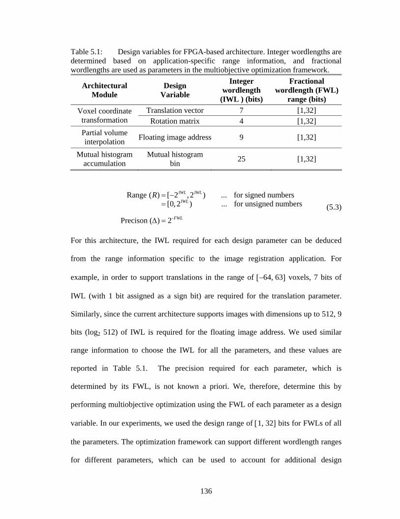
136
-
Range ( ) [ 2 ,2 ) ... for signed numbers[0,2 ) ... for unsigned numbers
Precison ( ) 2
IWL IWL
IWL
FWL
R = −=
Δ =
(5.3)
For this architecture, the IWL required for each design parameter can be deduced
from the range information specific to the image registration application. For
example, in order to support translations in the range of [–64, 63] voxels, 7 bits of
IWL (with 1 bit assigned as a sign bit) are required for the translation parameter.
Similarly, since the current architecture supports images with dimensions up to 512, 9
bits (log2 512) of IWL is required for the floating image address. We used similar
range information to choose the IWL for all the parameters, and these values are
reported in Table 5.1. The precision required for each parameter, which is
determined by its FWL, is not known a priori. We, therefore, determine this by
performing multiobjective optimization using the FWL of each parameter as a design
variable. In our experiments, we used the design range of [1, 32] bits for FWLs of all
the parameters. The optimization framework can support different wordlength ranges
for different parameters, which can be used to account for additional design
Table 5.1: Design variables for FPGA-based architecture. Integer wordlengths are determined based on application-specific range information, and fractional wordlengths are used as parameters in the multiobjective optimization framework.
Architectural Module
Design Variable
Integer wordlength
(IWL ) (bits)
Fractional wordlength (FWL)
range (bits) Translation vector 7 [1,32] Voxel coordinate
transformation Rotation matrix 4 [1,32] Partial volume interpolation Floating image address 9 [1,32]
Mutual histogram accumulation
Mutual histogram bin 25 [1,32]

137
constraints, such as, for example, certain kinds of constraints imposed by third-party
intellectual property.
The entropy calculation module is implemented using a multiple-LUT–based
approach and also employs fixed-point arithmetic. However, this module has already
been optimized for accuracy and hardware resources, as described in [155]. The
optimization strategy employed in [155] uses an analytical approach that is specific to
entropy calculation and is distinct from the strategy presented in this work. This
module, therefore, does not participate in the multiobjective optimization framework
presented in this work, and we simply use the optimized configuration identified
earlier. This further demonstrates the flexibility of our optimization framework to
accommodate arbitrary designer- or externally-optimized modules.
5.2.3.2. Search Algorithms
An exhaustive search that explores the entire design space is guaranteed to
find all Pareto-optimal solutions. However, this search can lead to unreasonable
execution time, especially when the objective function evaluation is computationally
intensive. For example, with four design variables, each taking one of 32 possible
values, the design space consists of 324 solutions. If the objective function evaluation
takes 1 minute per trial (which is quite realistic for multiple MI calculations using
large images), the exhaustive search will take 2 years. Consequently, we have
considered alternative search methods, as described below.
The first method is partial search, which explores only a portion of the entire
design space. For every design variable, the number of possible values it can take is
reduced by half by choosing every alternate value. A complete search is then

138
performed in this reduced search space. This method, although not exhaustive, can
effectively sample the breadth of the design space. The second method is random
search, which involves randomly generating a fixed number of feasible solutions. For
both of these methods, Pareto-optimized solutions are subsequently identified from
the set of solutions explored.
The third method is performing a search using evolutionary techniques. EAs
have been shown to be effective in efficiently exploring large search spaces [130,
131]. In particular, we have employed SPEA2 [160], which is very effective in
sampling from along an entire Pareto-optimal front and distributing the solutions
generated relatively evenly over the optimal tradeoff surface. Moreover, SPEA2
incorporates a fine-grained fitness assignment strategy and an enhanced archive
truncation method, which further assist in finding Pareto-optimal solutions. The flow
of operations in this search algorithm is shown in Figure 5.2.
For the EA-based search algorithm, the representation of the system
configuration is mapped onto a “chromosome” whose “genes” define the wordlength
parameters of the system. Each gene, corresponding to the wordlength of a design
variable i, is represented using an integer allele that can take values from the set vi,
described earlier. Thus, every gene is confined to wordlength values that are
predefined and feasible for a given design variable. The genetic operators for
crossover and mutation are also designed to adhere to this constraint and always
produce values from set vi, for a gene i within a chromosome. This representation
scheme is both symmetric and repair-free and, hence, is favored by the schema theory
[167], and is computationally efficient, as described in [168].

139
5.2.3.3. Objective Function Models and their Fidelity
Search for Pareto-optimized configurations requires evaluating candidate
solutions and determining Pareto-dominance relationships between them. This can be
achieved by calculating objective functions for all the candidate solutions and by
relative ordering of the solutions with respect to the values of their corresponding
objective functions. We consider the error in MI calculation and the hardware
implementation cost to be the conflicting objectives that must be minimized for our
FPGA implementation problem. We model the FPGA implementation cost using two
components: the first is the amount of logic resources (number of LUTs) required by
the design, and the second is the internal memory consumed by the design. We treat
these as independent objectives in order to explore the synergistic effects between
these complementary resources. Because of the size of the design space and
limitations due to execution time, it is not practical to synthesize and evaluate each
solution. We, therefore, employ models for calculating objective functions to evaluate
the solutions. The quality of the Pareto-optimized solutions will then depend on the
fidelity of these objective function models.
The error in MI calculation can be computed by comparing the MI value
reported by the limited-precision FPGA implementation against that calculated by a
double-precision software implementation. For this purpose, we have utilized a bit-
true emulator of the hardware. This emulator was developed in C++ and uses fixed-
point arithmetic to accurately represent the behavior of the limited-precision
hardware. It supports multiple wordlengths for internal variables and is capable of
accurately calculating the MI value corresponding to any feasible configuration. We

140
have verified its equivalence with the hardware implementation for a range of
configurations and image transformations. This emulator was used to compute the MI
calculation error. The MI calculation error was averaged for three distinct image pairs
(with different image modality combinations) and for 50 randomly generated image
transformations. The same sets of image pairs and image transformations were used
for evaluating all feasible configurations.
The memory required for a configuration is primarily needed for intermediate
FIFOs, which are used to buffer internal variables, and the MH memory. For
example, a 64-word deep FIFO used to buffer a signal with a wordlength of b will
require 64×b bits of memory. In our architecture, the depth of the FIFOs and the
dimensions of the MH are constant, whereas their corresponding widths are
determined by the wordlength of the design parameters. Using these insights, we have
developed an architecture-specific analytical expression that accurately represents the
cumulative amount of memory required for all internal FIFOs and MH. We used this
expression to calculate the memory requirement of a configuration.
For estimating the area requirements of a configuration, we adopt the area
models reported in [86, 169]. These are high-level models of common functional
units such as adders, multipliers, delays. These models are derived from the
knowledge of the internal architecture of these components. Area cost for
interconnects and routing is not taken into account in this analysis. These models
have been verified for the Xilinx Virtex series of FPGAs and are equally applicable to
alternative FPGA families and for ASIC implementations. These models have also
been previously used in the context of wordlength optimization [86, 91, 169].
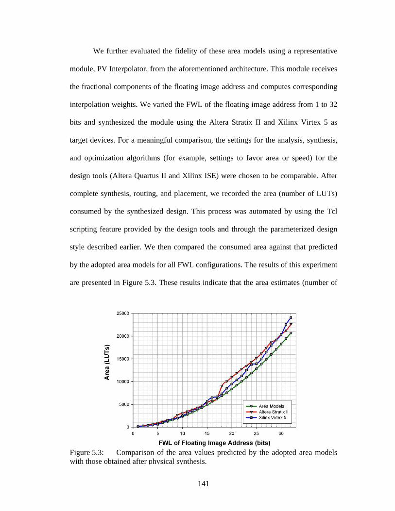
141
We further evaluated the fidelity of these area models using a representative
module, PV Interpolator, from the aforementioned architecture. This module receives
the fractional components of the floating image address and computes corresponding
interpolation weights. We varied the FWL of the floating image address from 1 to 32
bits and synthesized the module using the Altera Stratix II and Xilinx Virtex 5 as
target devices. For a meaningful comparison, the settings for the analysis, synthesis,
and optimization algorithms (for example, settings to favor area or speed) for the
design tools (Altera Quartus II and Xilinx ISE) were chosen to be comparable. After
complete synthesis, routing, and placement, we recorded the area (number of LUTs)
consumed by the synthesized design. This process was automated by using the Tcl
scripting feature provided by the design tools and through the parameterized design
style described earlier. We then compared the consumed area against that predicted
by the adopted area models for all FWL configurations. The results of this experiment
are presented in Figure 5.3. These results indicate that the area estimates (number of
Figure 5.3: Comparison of the area values predicted by the adopted area models with those obtained after physical synthesis.

142
LUTs) predicted by the model are comparable to that obtained through physical
synthesis for both the target devices. For quantitative evaluation, the fidelity of the
area models was calculated as below:
1
1 1
2 ,( 1)
N N
i j iijFidelity F
N N
−
= = +
⎛ ⎞= ⎜ ⎟− ⎝ ⎠∑∑ (5.4)
where
{1 if ( ) ( ).0 otherwisei j i j
ijsign S S sign M MF − = −= (5.5)
In this equation, the iM s represent the values predicted by the area models; and the
iS s represent the values obtained after physical synthesis. The fidelity of the area
models when evaluated with respect to the synthesis results obtained for both Altera
and Xilinx devices was 1, which corresponds to maximum (“perfect”) fidelity. This
indicates that the relative ordering of FWLs with respect to their area requirements is
consistent for the model and synthesized designs. These results further validate the
applicability of using the aforementioned area models for multiobjective
optimization.
5.3. Experiments and Results
We performed multiobjective optimization of the aforementioned architecture
using the search algorithms outlined in the previous section. To account for the
Table 5.2: Number of solutions explored by search methods.
Search Method Number of solutions explored
Partial search 65,536 Random search 6,000
EA-based search 6,000

143
effects of random number generation, the EA-based search and random search were
repeated five times each, and the average behavior from these repeated trials is
reported. The number of solutions explored by each search algorithm in a single run
is reported in Table 5.2. The execution time of each search algorithm was roughly
proportional to the number of solutions explored, and the objective function
evaluation for each solution took approximately 1 minute using a single computing
node. As expected, the partial search algorithm explored the largest number of
solutions. The parameters used for the EA-based search are listed in Table 5.3. The
crossover and mutation operators were chosen to be one-point crossover and flip
mutator, respectively. For a fair comparison, the number of solutions explored by the
random search algorithm was set to be equal to that explored by the EA-based
algorithm.
The solution sets obtained by each search method were then further reduced to
corresponding nondominated solution sets using the concept of Pareto optimality. As
described earlier, the objectives considered for this evaluation were the MI
calculation error and the memory and area requirements of the solutions. Figure 5.4
shows the Pareto-optimized solution set obtained for each search method.
Qualitatively, the Pareto front identified by the EA-based search is denser and more
widely distributed and demonstrates better diversity than other search methods.
Table 5.3: Parameters used for the EA-based search. Parameter Value
Population size 200 Number of generations 30 Crossover probability 1.0 Mutation probability 0.06

144
(a) Partial Search
(b) EA-based Search
(c) Random Search
Figure 5.4: Pareto-optimized solutions identified by various search methods.

145
Figure 5.5 compares the Pareto fronts obtained by partial search and EA-based search
by overlaying them and illustrates that the EA-based search can identify better Pareto-
optimized solutions, which indicates the superior quality of solutions obtained by this
search method. Moreover, it must be noted that the execution time required for the
EA-based search was over 10-times faster than that required for the partial search.
(a) Area vs. MI calculation error
(b) Memory vs. MI calculation error
Figure 5.5: Qualitative comparison of solutions found by partial search and EA-based search.

146
5.3.1. Metrics for Comparison of Pareto-optimized Solution Sets
Quantitative comparison of the Pareto-optimized solution sets is essential in
order to compare more precisely the effectiveness of various search methods. As with
most real-world complex problems, the Pareto-optimal solution set is unknown for
this application. We, therefore, employ the following two metrics to perform
quantitative comparison between different solution sets. We use the ratio of non-
dominated individuals (RNI) to judge the quality of a given solution set, and the
diversity of a solution set is measured using the cover rate. These performance
measures are similar to those reported in [170] and are described below.
The RNI is a metric that measures how close a solution set is to the Pareto-
optimal solution set. Consider two solution sets ( 1P and 2P ) that each contain only
non-dominated solutions. Let the union of these two sets be UP . Furthermore, let NDP
be a set of all non-dominated solutions in ( )U ND UP P P⊆ . The RNI for the solution set
iP is then calculated as:
,i NDi
ND
P PRNI
P=
∩ (5.6)
where ⋅ is the cardinality of a set. The closer this ratio is to 100%, the more superior
the solution set is and the closer it is to the Pareto-optimal front. We computed this
metric for all the search algorithms previously described, and the results are presented
in Figure 5.6. Our EA-based search offers better RNI and, hence, superior quality
solutions to those achieve7d with either the partial or random search.

147
The cover rate estimates the spread and distribution (or diversity) of a solution
set in the objective space. Consider the region between the minimum and maximum
of an objective function as being divided into an arbitrary number of partitions. The
cover rate is then calculated as the ratio of the number of partitions that is covered
(that is, there exists at least one solution with an objective value that falls within a
given partition) by a solution set to the total number of partitions. The cover rate ( kC )
of a solution set for an objective function ( kf ) can then be calculated as:
,kk
NCN
= (5.7)
where kN is the number of covered partitions and N is the total number of
partitions. If there are multiple objective functions ( m , for example), then the net
cover rate can be obtained by averaging the cover rates for each objective function as:
1
1 .m
kk
C Cm =
= ∑ (5.8)
The maximum cover rate is 1, and the minimum value is 0. The closer the cover rate
of a solution set is to 1, the better coverage and more even (more diverse) distribution
it has. Because the Pareto-optimal front is unknown for our targeted application, the
Figure 5.6: Quantitative comparison of search methods using the ratio of non-dominated individuals (RNI).

148
minimum and maximum values for each objective function were selected from the
solutions identified by all the search methods. We used 20 partitions/decade for MI
calculation error (represented using a logarithmic scale), 1 partition for every 50
LUTs for the area requirement, and 1 partition for every 50 Kbits of memory
requirement. The cover rate for all the search algorithms described earlier was
calculated using the method outlined above, and the results are illustrated in Figure
5.7. The EA-based search offers a better cover rate, which translates to better range
and diversity of solutions when compared with either partial or random searches. In
summary, our EA-based search outperforms the random search and is capable of
offering more diverse and superior quality solutions when compared with the partial
search, using only 10% of the execution time.
5.3.2. Accuracy of Image Registration
An important performance measure for any image registration algorithm,
especially in the context of medical imaging, is its accuracy. We did not choose
Figure 5.7: Quantitative comparison of search methods using cover rate.

149
registration accuracy as an objective function because of its dependence on data
(image pairs), the degree of misalignment between images, and the behavior of the
optimization algorithm that is used for image registration. These factors, along with
its execution time, in our experience, may render registration accuracy as an
unsuitable objective function, especially if there is non-monotonic behavior with
respect to the wordlength of design variables.
Instead, we evaluated the affect of error in MI calculation on the image
registration accuracy for a set of image pairs. This analysis was performed using three
computed tomography image pairs for the Pareto-optimized solutions identified by all
of the search algorithms that we experimented with. Image registration was
performed using limited-precision configurations corresponding to each solution
using the aforementioned bit-true simulator. The result of registration was then
compared with that obtained using double-precision software implementation.
Registration accuracy was calculated by comparing deformations at the vertices of a
Figure 5.8: Relationship between MI calculation error and resulting image registration error.

150
cuboid (with size equal to half the image dimensions) located at the center of the
image. The results of this analysis are illustrated in Figure 5.8. As expected, there is a
good correlation between the MI calculation error and the accuracy of image
registration. This demonstrates that optimized tradeoff curves between MI calculation
error and hardware cost, as identified by our reported analysis, can be used to
represent the relationships between registration accuracy and hardware cost with high
fidelity. This analysis also provides better insight about the sensitivity of image
registration accuracy to various design parameters.
5.3.3. Post-synthesis Validation
We performed further validation of the presented multiobjective optimization
strategy through physical design synthesis. We identified three solutions from the
Pareto-optimized set obtained using the EA-based search and synthesized the
aforementioned architecture with configurations corresponding to these solutions.
These three configurations, which offer gradual tradeoff between hardware resource
requirement and error in MI calculation, are listed in the first column of Table 5.4.
The wordlengths associated with each configuration correspond to the FWLs of the
design variables identified in Table 5.1. The design was synthesized for these
configurations and the resulting realizations were implemented using an Altera Stratix
II EP2S180F1508C4 FPGA (Altera Corporation, San Jose, CA) on a PCI prototyping
board (DN7000K10PCI) manufactured by the Dini Group (La Jolla, CA). We then
evaluated the performance of the synthesized designs and compared it with that
predicted by the objective function models. The results of this analysis are
summarized in Table 5.4 and are described below.

151
The error in MI calculation was computed by comparing the MI value
reported by the limited-precision FPGA implementation against that calculated by a
double-precision software implementation. The MI calculation error was averaged for
three distinct image pairs and for 50 randomly generated image transformations for
each pair. These image pairs and the associated transformations were identical to
those employed in the objective function calculation. In this case, the average MI
calculation error obtained by all the design configurations was identical to that
predicted by the objective function model. This is expected due to the bit-true nature
of the simulator used to predict the MI calculation error. We repeated this calculation
with a different set of three image pairs and 50 randomly generated new
transformations associated with each image pair. The MI calculation error
corresponding to this setup is reported in the second column of Table 5.4. The small
difference when compared to the error predicted by the models is explained by the
different sets of images and transformations used. The area and memory requirement
corresponding to each configuration after synthesis are reported in columns three and
Table 5.4: Validation of the objective function models using post-synthesis results. The wordlengths in a design configuration correspond to the FWLs of the design variables identified earlier.
Objective Functions Post-Synthesis Value
(Predicted Value) Design Configuration
MI Calculation Error
Area (No. of LUTs)
Memory (Mbits)
Image Registration
Error (mm)
{5, 6, 4, 9} 2.4×10⁻³ (2.1×10⁻³)
6527 (5899)
2.23 (2.23) 3.82
{8, 9, 7, 12} 5.3×10⁻⁴
(5.2×10⁻⁴) 7612
(6754) 2.45
(2.45) 1.57
{9, 12, 10, 17} 7.7×10⁻⁵ (7.8×10⁻⁵)
10356 (8073)
2.81 (2.81) 0.45

152
four of Table 5.4, respectively. For comparison, we have also included the values
predicted by the corresponding objective function models in parenthesis. It must be
noted that for all the three configurations, the relative ordering based on Pareto-
dominance relationships with respect to each objective function is identical for both
post-synthesis and model-predicted values.
We also evaluated the accuracy of image registration performed using the
implementation corresponding to each design configuration. For this analysis, we
considered five computed tomography image pairs. The image registration results for
a representative image-pair are illustrated in Figure 5.9. Subfigures (a) and (b) show
two distinct poses for the same subject; and (c) shows fusion of (a) and (b) using a
checkerboard pattern. The misalignment between images is evident at the edges of the
squares within the checkerboard pattern. Subfigures (d)-(f) show fusion images after
registration using the identified design configurations. These configurations offer
progressively reducing image registration error (3.82 mm, 1.57 mm, and 0.45 mm,
respectively), and result into correspondingly improved image alignment. The arrows
indicate representative regions with misalignment that are better-aligned after
registration. The registration error was calculated by comparing the obtained
registration results with that obtained using double-precision software
implementation. The average registration error for each configuration is reported in
the last column of Table 5.4. There is a good correlation between the MI calculation
error and the registration error, reinforcing the results presented in the previous
section.

153
This post-synthesis validation further demonstrates the efficacy of the
presented optimization approach for reconfigurable implementation of image
registration. It also further demonstrates how the approach enables a designer to
systematically choose an efficient system configuration to meet the registration
accuracy requirements for a reconfigurable implementation.
As described previously, we used error in calculation of MI as one of the
objective functions. The Pareto-optimized solutions identified by the search schemes
employed in this multiobjective optimization framework can then be used to select a
design configurations that offer best (lowest) error in calculation of MI for various
hardware resource requirements. Through additional experiments, both simulation-
based and post-synthesis validation–based, we have further demonstrated that there is
Figure 5.9: Results of image registration performed using the high-speed, FPGA-based implementation for design configurations offering various registration errors.

154
a good correlation between error in MI calculation and the image registration error. In
general, reducing the error in the calculation of MI will translate into improved image
registration accuracy. This is expected, since MI is used as a similarity measure for
performing image registration. Although, the image registration algorithm being
accelerated in the current work is of deformable nature, it achieves deformable
alignment through a series of hierarchical, locally rigid registrations that use MI as a
similarity measure. We, therefore, contend that the accuracy of the deformable
registration is directly dependant on and highly correlated with the accuracy of MI
calculation. Consequently, the design configuration offering better accuracy (lower
error) in MI calculation will lead to superior image registration accuracy. This is also
supported by the data presented in Table 5.4. As accuracy of image registration can
play a crucial rule in IGI applications (and other medical applications, in general), we
selected the system configuration that offered lowest error in MI calculation (and by
extension lowest image registration error) from Table 5.4. This system configuration
({9, 12, 10, 17}) was then used for validation of deformable registration in the
context of novel IGI applications described in the following chapter.
5.4. Summary
One of the main strengths of reconfigurable architectures over general-
purpose processor–based implementations is their ability to utilize more streamlined
representations for internal variables. This ability can often lead to superior
performance, as demonstrated by our architectures (for performing 3D image
preprocessing and deformable image registration) presented in the previous chapters
and by other researchers in the context of myriad of other applications. Furthermore,
155
this approach can result into optimized utilization of FPGA resources, by employing
just enough precision for each of its internal variables to satisfy design requirements
of a given application. Given this advantage, it is highly desirable to automate the
derivation of optimized design configurations that offer varying degree of tradeoff
between implementation accuracy and hardware resources. Toward that end, this
work has presented a framework for multiobjective optimization of finite precision,
reconfigurable implementations. This framework considers multiple conflicting
objectives, such as hardware resource consumption and implementation accuracy, and
systematically explores tradeoff relationships among the targeted objectives. This
work has also further demonstrated the applicability of EA-based techniques for
efficiently identifying Pareto-optimized tradeoff relations in the presence of complex
and non-linear objective functions. The evaluation that we have performed in the
context of the architecture for FPGA-based deformable image registration
demonstrates that such an analysis can be used to enhance automated hardware design
processes, and efficiently identify a system configuration that meets given design
constraints. This approach may also be applied in the context of reconfigurable
computing for identifying suitable design configurations that can be switched among
at runtime. Furthermore, the multiobjective optimization approach that we have
presented is quite general, and can be extended to a multitude of other signal
processing applications.
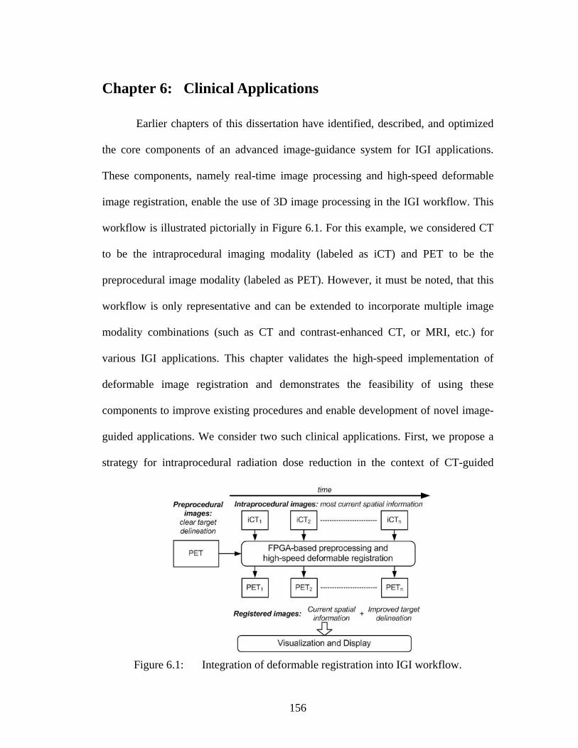
156
Chapter 6: Clinical Applications
Earlier chapters of this dissertation have identified, described, and optimized
the core components of an advanced image-guidance system for IGI applications.
These components, namely real-time image processing and high-speed deformable
image registration, enable the use of 3D image processing in the IGI workflow. This
workflow is illustrated pictorially in Figure 6.1. For this example, we considered CT
to be the intraprocedural imaging modality (labeled as iCT) and PET to be the
preprocedural image modality (labeled as PET). However, it must be noted, that this
workflow is only representative and can be extended to incorporate multiple image
modality combinations (such as CT and contrast-enhanced CT, or MRI, etc.) for
various IGI applications. This chapter validates the high-speed implementation of
deformable image registration and demonstrates the feasibility of using these
components to improve existing procedures and enable development of novel image-
guided applications. We consider two such clinical applications. First, we propose a
strategy for intraprocedural radiation dose reduction in the context of CT-guided
Figure 6.1: Integration of deformable registration into IGI workflow.

157
procedures. Second, we demonstrate the feasibility of incorporating PET into liver
radiofrequency ablations, a common procedure for treating liver tumors.
6.1. Radiation Dose Reduction
6.1.1. Motivation
3D visualization is a critical need of image guided interventions. To perform true 3D
visualization, a volumetric image of the operative field is essential, the type of data
which is native to modern CT/MRI, but not to 2D-ultrasound or fluoroscopic imaging
which are conventionally used for image-guided interventions [18, 20, 21] .
Continuous real-time 3D imaging in an interventional suite is the first step to equip
interventionists with enhanced visualization capabilities. However, continuous 3D
imaging has been technologically difficult until recently. MRI remains slow and
while real-time 3D ultrasonography was recently released, its image quality remains
suboptimal compared with that of CT and MRI. Recently introduced multi-slice CT
does not suffer from these limitations and can, in fact, image the operative field at a
high resolution and a very high frame rate (sub-seconds). As a result of this, many
interventional procedures such as liver biopsies, cryo-and radio-frequency ablations
are now being routinely carried out under volumetric CT-guidance [171-173]. With
time, its speed, image resolution and coverage will only improve, making it even
more desirable for live intraprocedural imaging. Several imaging equipment
manufacturers, Toshiba and Philips, for example, have announced availability of 256-
slice scanners [25, 174] providing sufficient coverage (8-12 cm) for most image
guided interventions. Radiation exposure to the patient and the interventionist,

158
however, continues to be a concern with use of continuous or on-demand CT. It is,
therefore, necessary to acquire the intraprocedural images at a lower dose, such that
the net radiation dose is within the safe limits. There are some previous studies which
have reported use of low-dose CT [175-177], however, these techniques were
primarily employed for diagnostic and computer-aided detection applications and did
not involve image registration.
6.1.2. Dose Reduction Strategy
Our primary radiation dose reduction strategy is to acquire a standard-dose
preprocedural CT image and scan the dynamic operative field subsequently using
low-dose CT. Using the high-speed deformable registration technique described
earlier, the preprocedural CT image can then be registered to low-dose
intraprocedural CT images. Registered preprocedural CT will then show the dynamic
intraprocedural anatomy and will substitute the low-dose CT images. These
diagnostic quality images can then be 3D rendered and used for intraprocedural
guidance and navigation. Capability of viewing hidden vasculature using
preprocedural contrast-enhanced CT together with the additional capability of
virtually inserting intraprocedural tools in the 3D renderings will add a new
dimension to CT-guided interventions.
This proposed dose reduction strategy necessitates the determination of the
threshold radiation dose for intraprocedural CT, which permits its accurate image
registration with preprocedural CT. The following sections describe a preliminary
study to evaluate the registration accuracy with low-dose CT.

159
6.1.3. Evaluation of Registration Accuracy with Low-Dose CT
Quantifying the accuracy of deformable registration, in general, is a very
difficult task due to the lack of a well known gold standard. It is, however, necessary
to judge the registration accuracy in the proposed application to determine the optimal
radiation dose that does not sacrifice the precision of an image-guided procedure.
Since our images are to be registered in the present case, our validation strategy has
been to test how well the deformable registration algorithm recovers a user-
introduced, known non-rigid misalignment. Our overall strategy can then be
described in following main steps: 1) Generate images representing the same
anatomy at varying radiation doses, 2) introduce the same known deformation in low-
dose CT images, 3) preprocess the deformed low-dose CT images to improve SNR
prior to the registration, 4) register the preprocedural standard-dose image with the
deformed intraprocedural (simulated) low-dose images using deformable image
Figure 6.2: Important steps for evaluating registration accuracy with low-dose CT.

160
registration and finally, 5) compare the transformation field obtained after image
registration with the original, user-introduced deformation field to calculate the
registration accuracy at various doses. The important steps in this workflow are
illustrated in Figure 6.2 and are described below.
6.1.3.1. Generating Low-Dose CT Images
Low dose images corresponding to a standard dose abdominal scan were
generated using syngo-based Somaris/5 simulator from Siemens. This simulator
models the noise and attenuation effects at lower radiation doses and can generate
low-dose equivalent images from tomographic projection data corresponding to an
input standard-dose image. The performance and accuracy of this simulator has been
previously reported [178]. This approach ensures that scans at all radiation doses
represent exactly the same anatomy. Example low-dose images generated using this
simulator are shown in Figure 6.3. Subfigure (a) shows a coronal slice for an input
image at a standard dose (200 mAs), and subfigures (b-d) show the corresponding
coronal slice for the low-dose images generated using the dose simulator at various
doses.
a) 200 mAs b) 50 mAs c) 20 mAs d) 10 mAs
Figure 6.3: Low-dose CT images generated by the dose-simulator.

161
6.1.3.2. Creating Anatomically Realistic Deformations
Human body, and abdominal organs and tissues in particular, undergo non-
rigid deformation during day-to-day activities, respiratory and cardiac cycles, etc.
These deformations manifest as misalignment between preprocedural and
intraprocedural scans. Further misalignments are introduced due to differences in
patient position during imaging as well as different scan parameter settings. In order
to create a realistic deformation that incorporates all these effects, it is necessary to
estimate this deformation from scans of the same anatomy taken on different days,
thus ensuring sufficient temporal separation.
We, therefore, consider CT images for the same subject acquired at different
times as a suitable image-pair. We then identify several significant anatomical
landmarks from both these images. Deformation vectors between homologous
anatomical landmarks in such two images represent the local misalignment at those
landmarks. Using these vectors, deformation field for the entire anatomy can then
approximated using thin-plate spline (TPS)-based interpolation [179]. TPS is an
interpolation scheme based on radial basis functions and is capable of providing
smooth 2D or 3D interpolation for non-uniformly spaced sample points. This
technique has been applied extensively for various medical imaging applications
[180, 181].
6.1.3.3. Image Preprocessing
Ultra low-dose CT scans acquired during the procedure show the exact same
anatomy as a standard dose scan would but are characterized by high level of
quantum noise. These scans may not be acceptable for diagnostic purposes, but

162
contain sufficient information regarding the current anatomical state. From the
perspective of MI-based deformable image registration, using these low-dose images
as is will cause the dispersion of the mutual histogram (due to noise, in an otherwise
uniform structure) leading to poor image registration. Anisotropic diffusion filtering
has been shown to be an effective processing step prior to advanced image processing
[76, 83, 182, 183]. Figure 6.4 compares the performance of anisotropic diffusion
filtering against other standard preprocessing techniques. Higher value of mutual
information between the original and the filtered image after preprocessing, which
represents increased structural similarity, indicates superior filtering performance for
a given pair of images. We, therefore, enhance the low-dose CT images through use
of anisotropic diffusion filtering prior to image registration. Anisotropic diffusion
filtering, however, is an iterative process which can take up to minutes on a modern
CPU. The FPGA-based real-time implementation of this operation, which has been
described earlier, can be employed to accelerate the execution of this step.
6.1.3.4. Applying Deformation and Image Registration
The deformation field generated using TPS-based interpolation is applied to
the low-dose images for all the simulated doses. This involves resampling of the low-
Standard Dose (200 mAs)
Ultra Low Dose (10 mAs)
Median Filtered
Gaussian Filtered
Anisotropic Diffusion Filtered
MI = 3.49 MI = 1.11 MI = 1.43 MI = 1.23 MI = 1.62 Figure 6.4: Comparison of techniques for preprocessing low-dose CT images.

163
dose image on to a regular grid using the anatomical mapping provided by the TPS-
generated deformation field. The image registration between these deformed low-
dose images and the original standard-dose image yields a registration field, which
attempts to estimate and recover the induced anatomically realistic deformation. The
mean-squared difference between the deformation vectors at every voxel
corresponding to the registration field and the induced deformation field provides a
measure of registration accuracy at a particular radiation dose.
6.1.4. Experiments
An abdominal scan acquired under clinical settings at the standard dose (200
mAs) was selected for this study. Dose correction feature of the scanner, which
automatically modulates the radiation dose based on the anatomy to be scanned, was
turned off for this scan to keep the dose consistent across all the slices. The CT image
acquired measured 256×256×300 voxels, with voxel dimensions of 1.56 mm×1.56
mm×1.5 mm and field of view restricted mostly to lower thorax and abdomen.
Four different CT scans of the same subject acquired at different times within
a span of one to sixty days were used for creating anatomically realistic deformations.
These prior scans had dimensions and resolution of 256×256×280-315 and 1.48
mm×1.48 mm×1.5 mm respectively. Based on a predetermined, well-described list of
32 anatomical landmarks, a clinical expert identified and marked a set of homologous
points in all the CT scans (one standard-dose scan and four older scans). Based on the
expert-defined landmarks, TPS-based starting deformation fields (DF1, DF2, DF3, and
DF4) corresponding to each prior scans were generated.

164
Treating the standard-dose scan as a reference, we generated eleven low-dose
scans (at 10, 15, 20, 25, 30, 40, 50, 70, 85, 100, 150 mAs) using the Somaris/5
simulator. 10mAs was the lowest setting possible for the current version of the
simulator. Each of these scans (including the standard dose scan) was deformed using
the realistic deformation fields DF1, DF2, DF3, and DF4 described above.
We registered these deformed and preprocessed low-dose images (reference
image) with the original standard-dose image (floating image) using the deformable
registration algorithm and its accelerated implementation described earlier.
Alignment between the floating and reference after deformable image registration
yields a registration field (RFi) which maps each reference image voxel into floating
image coordinate space. Comparison of this registration field (RFi) with the originally
introduced deformation field (DFj) was used to judge the registration accuracy for
each dose.
6.1.5. Results
Result of the deformable registration using the hardware implementation of
the registration algorithm for a representative image-pair generated using one of the
deformations (DF1) is shown in Figure 6.5. Columns a) and b) show the two starting
poses, and column c) the starting pose difference that the image registration must
recover. The difference images after image registration at various CT doses are
shown in columns d) to f). The top row shows coronal slices of the image and the
corresponding axial slices are shown in the bottom row. The software implementation
produced qualitatively similar registration results. Visually correct registration of the
standard-dose image with the deformed images at various low doses (evident from the

165
reduced features in the difference image) demonstrates the feasibility of deformable
registration at low CT doses.
The process of deformable registration attempts to recover any misalignment
between the reference and floating images. A perfect registration will completely
recover this misalignment and yield a non-rigid transformation field that is identical
to the deformation field representing the original misalignment. A comparison
between these two fields can be used as a performance index for the registration
accuracy.
For this experiment, the deformation field introduced (DFi) is known at every
voxel. The volume subdivision-based deformable registration algorithm generates the
transformation field (RFj), which provides the transformation at every voxel in scan
with dose j. The average of the magnitude of the vector differences between these two
fields at all doses for the software implementation is reported in Figure 6.6. This
average was calculated over the region of the image which contains sufficient part of
the subject and hence information to yield meaningful registration. The regions of the
image which contain no information (very low entropy) (e.g. black areas surrounding
d) 200 mAs e) 20 mAs f) 10 mAs a) Standard
CT Pose-1
b) Standard CT
Pose-2
c) Starting Difference Difference after registration at various doses
Figure 6.5: Qualitative comparison of registration accuracy with low-dose CT.

166
the subject) are masked out using a simple threshold operation. The results show a
maximum error of about 10% at the doses of 10 mAs and 20 mAs, respectively.
Moreover the maximum registration error at the lowest dose (10 mAs) is less than 2.5
mm, which is within acceptable limits of IGI applications. As expected, the average
error improves steadily with dose.
We repeated the experiment with the high-speed implementation of the
deformable registration algorithm described earlier, and compared the registration
field produced by the hardware implementation with the user induced deformation.
The same optimization algorithm (downhill Simplex) was used for these two
implementations and equal number of optimization iterations were used. Figure 6.6
also shows the comparison of the average registration accuracy achieved using the
software and hardware implementations. The blue curve corresponds to the average
registration accuracy using the software implementation and the red curve
corresponds to the average registration accuracy of the hardware implementation.
Figure 6.6: Average registration error with respect to dose using software and FPGA-based implementations.

167
This comparison of the registration accuracies indicates that the hardware
implementation is capable of achieving comparable registration accuracy. The
average execution time for these two implementations is reported in Table 6.1. The
hardware implementation achieved a speedup of about 30 and offers comparable
registration accuracy. Moreover, both the implementations offer acceptable
registration accuracy for most IGI applications and demonstrate the applicability of
deformable image registration to lower the radiation dose during intraprocedural
imaging.
6.1.6. Summary
In this study, we have demonstrated successful registration of standard-dose
abdominal CT images with lower-dose images of the same anatomy. Even at 10 mAs,
the smallest dose achievable using the simulator, the registration accuracy achieved
was comparable to that achieved at the standard dose. Our results demonstrate ten- to
twenty fold reduction in radiation dose with the use of low-dose CT. Reduction of
radiation dose to safe levels is highly significant in that it enables navigating
interventions using more powerful, multislice CT. Moreover, through the use of
hardware accelerated implementation, deformable image registration (which allows
this reduction in radiation dose) can be performed in a matter of minutes. This
enables assimilation of this novel dose reduction strategy in the IGI workflow. The
Table 6.1: Execution time for deformable image registration using low-dose CT. Execution Time (s)
Software Implementation
FPGA-based Implementation
Speedup
11,976 392 30.55

168
introduction of true 3D visualization possible through safe, volumetric CT imaging of
the intraprocedural anatomy may enable development of novel image-guided
interventional applications such as CT-guided minimally invasive surgery [149, 184].
6.2. Incorporation of PET into CT-Guided Liver Radio-Frequency
Ablation
I would like to thank Mr. Peng Lei from Prof. Shekhar’s research group for
his help in the quantitative validation aspect of the deformable registration presented
in this section.
6.2.1. Motivation
The liver is a common site of both primary and metastatic cancers. Performing
resection of malignant liver tumors has been shown to increase the 5-year survival
rate of patients with liver cancer [185]. However, the majority (85%–90%) of hepatic
tumors are considered unresectable at diagnosis [186], either because of their
anatomic location, size, or number or because of inadequate viable liver tissue and
morbidity. Radiofrequency ablation (RFA) as a minimally invasive procedure is often
the treatment of choice for patients who are not suitable candidates for resection
[187]. RFA is a treatment technique that uses high-frequency alternating electrical
current to destroy tissue cells by heating [188]. For small lesions (<5 cm in diameter),
RFA has been reported to achieve 4-year survival rates, comparable with those
achieved with resection [189, 190].
RFA has conventionally been performed under fluoroscopic or ultrasound
guidance. With the advent of multislie CT, many of these procedures are being

169
carried out under intraprocedural volumetric CT guidance. The volumetric CT scan
provides better 3D orientation and a detailed anatomic structural map. However,
some lesions (particularly small untreated masses or recurrent or residual tumors in a
large treated mass) are not clearly visible (see Figure 2.1) because intraprocedural CT
scanning is usually not contrast enhanced. Even in contrast-enhanced diagnostic CT
images, hepatic lesions with abnormal metabolic activity are sometimes overlooked
[191]. Consequently, local recurrence after liver RFA as a result of these missed
tumors remains one of the major factors in relapse [192], which is in the range of
3%–39% [193]. Thus, precise targeting of lesions remains a challenging task when
guided solely by volumetric CT with or without contrast enhancement.
Because malignancies are better characterized by increased metabolic activity
than CT number variations, PET (as a functional imaging modality) has higher
sensitivity and specificity than CT for tumor localization. Active lesions show up
clearly as regions of high uptake in a conventional PET scan. However, compared
with CT, PET is devoid of structural tissue details, which are also important for
intraprocedural targeting and needle placement. Moreover, PET is also challenged by
slow scanning speed, radiation exposure risks, logistic challenges, etc. Currently PET
remains primarily a preprocedural imaging modality, used to identify a treatment site
rather than provide intraprocedural guidance during an ablative procedure. To
combine the strengths and overcome disadvantages of both PET and CT as
intraprocedural imaging modalities, registration between PET and CT is essential. In
a clinical study by Veit et al. [186], PET and CT fusion images were reported to
greatly improve recognition and localization of liver masses. Our work, therefore, is

170
focused on demonstrating fast, automatic, and accurate deformable image registration
between preprocedural PET and intraprocedural CT to improve localization of liver
malignancies during RFA.
6.2.2. Registration of PET and CT
As described earlier, combining of PET and CT images is crucial during liver
RFA. PET, however, cannot be repeated intraprocedurally because of time and
logistic challenges, as well as radiation risks [194]. Consequently, the interventionist
must mentally correlate preprocedural PET data onto intraprocedural CT images to
localize the lesion into which the RFA needle will be advanced, a subjective task
dependent on operator expertise. Combined PET/CT scanners, which are based on
mechanically achieved rigid registration, have emerged in recent years. They have
provided significant improvement over separate CT and PET scanning. But in
abdominal procedures such as liver RFA (unlike thoracic or brain surgery), non-rigid
misalignment resulting from tissue deformation and respiration motion can be
significant, so rigid registration approaches such as combined PET/CT scanning and
fiducial marker–based registration may misrepresent the actual transformation of the
liver. Combined PET/CT scanners have been shown to be unable to fully compensate
for involuntary non-rigid motions, such as those from respiration [185], and the
resulting images have been found to have significant misregistration in areas close to
the diaphragm. Moreover, as mentioned previously, PET has challenges including
slow scanning speed and radiation exposure risks. A combined PET/CT scanner is not
an appropriate choice as an intraprocedural imaging modality in this application or
any other image-guided procedure.

171
Intensity-based, retrospective deformable image registration and fusion
together form the only alternative, which is also proposed here. To be clinically
practical, the registration algorithm must be automatic, which means that manual
segmentation–based registration is excluded. Moreover, as mentioned before, the
registration must be achieved sufficiently fast so as not to obstruct the clinical
workflow. The deformable registration algorithm described in the dissertation has
been previously validated for intensity based registration of whole-body PET and CT
images [66] and PET/CT images for liver RFA [78, 148]. In this work, we validate
this algorithm and its FPGA-based high-speed implementation of this algorithm in the
context of the aforementioned clinical application.
6.2.3. Experiments
This study was geared toward demonstrating the feasibility of image
registration between preprocedural PET and intraprocedural CT in the context of liver
RFA using the earlier described high-speed image registration solution. This
retrospective study involved 20 CT-PET image pairs of patients who had undergone
percutaneous abdominal RFA under CT guidance. The preprocedural PET scans had
size and resolution of 150 × 150 × 187–240 and 4.0 × 4.0 × 4.0 mm, respectively.
Noncontrast-enhanced intraprocedural abdominal CT scans were acquired for guiding
needle placement during RFA procedures. The intraprocedural CT scans had size and
resolution of 512 × 512 × 35–62 and 0.78–1.17 × 0.78–1.17 × 5 mm, respectively.

172
6.2.3.1. Image Preprocessing
The intraprocedural CT images were acquired during the RFA with the RFA
needle in the field of view. As a result, some metal artifacts were present in the CT
images. We preprocessed the CT images using 3D median filtering and 3D
anisotropic diffusion filtering in order to minimize these artifacts. To achieve a trade-
off between maintaining CT resolution and obtaining nearly isotropic voxels, we
resampled the intraprocedural CT images for all cases to have the dimensions of 256
× 256 × 128. Resampling reduced the spatial resolution of CT images in x and y
dimensions; however, the resulting images still had better spatial resolution than the
preprocedural PET images (the lower resolution image controls the accuracy of
intensity-based image registration in general). No preprocessing steps were used for
the preprocedural PET images.
6.2.3.2. Validation of Image Registration
We evaluated the accuracy of the deformable registration between PET and
CT by comparing the alignment of several anatomic landmarks (3D locations within
the images) as predicted by the algorithm (both software and FPGA-based
implementations) against a reference. Because of the lack of a gold standard for
validation of deformable registration algorithms, we assumed the ability of clinical
experts to locate landmarks in both intraprocedural CT and preprocedural PET
images as a suitable benchmark performance. We then contend that comparing the
variability in landmark matching between algorithm- and expert-defined registrations
with the variability among the three expert-defined correspondence between the

173
landmarks is a reasonable way to evaluate the registration accuracy of the algorithm
and assess whether its performance is comparable to that of the experts.
Our validation scheme is graphically represented in Figure 6.7. Three clinical
experts, experienced in interpreting CT and PET images, were involved in the
validation procedure. Each expert was asked to identify and mark anatomic
landmarks identifiable in both PET and CT images. Because the location of a specific
landmark as marked by an expert can vary slightly from expert to expert, a set of “test
landmarks” were created for each case separately. This was achieved by defining the
location of each landmark as the centroid of the expert-defined locations for that
landmark in intraprocedural CT (represented by CTTEST in Figure 6.7). The expert-
defined transformation fields were then used to determine distinct sets of homologous
preprocedural PET landmarks (PETE1, PETE2, and PETE3, respectively), each
representing the transformed locations of the test landmark (CTTEST) according to the
manual registration performed by each expert. The average expert-defined
transformed location (PETEXPERT) was calculated as the centroid of PETE1, PETE2,
and PETE3. The algorithm-determined transformation field was used to determine a
Figure 6.7: Graphic illustration of the quantitative validation approach used in the context of deformable registration between intraprocedural and preprocedural PET.

174
set of landmarks in the PET image (PETALGO) representing the transformed locations
of the test landmarks after automatic deformable registration. These locations were
calculated for both the software and FPGA-based high-speed implementation of the
algorithm.
For each case, the mean error between PETEXPERT and PETALGO was then
evaluated to quantify the registration accuracy for that case. To further evaluate the
algorithm performance in the context of inter-expert variability, we allocated the 4
sets of PET landmark points to separate groups of 3 sets each: reference group
(PETE1, PETE2, and PETE3); test group 1 (PETALGO, PETE2, and PETE3); test group 2
(PETE1, PETALGO, and PETE3); and test group 3 (PETE1, PETE2, and PETALGO). For
each group, the mean difference (Euclidean distance) in the transformed location of
corresponding landmarks was obtained for all pair wise combinations of sets of PET
points within that group. The mean difference for each group was determined by
averaging over all the cases. The variability of locations was then calculated for each
group. If the group variability of test groups 1, 2, and 3 is statistically similar to that
of the reference group, we can conclude that the algorithm and experts agree on the
PET location of a specific landmark in CT. If the group variability is statistically
different, the algorithm differs significantly from that of the experts. As mentioned
earlier, we performed this analysis for both software and the FPGA-accelerated
implementation of the deformable registration algorithm.
6.2.4. Results
All the cases were successfully registered when evaluated both qualitatively
and quantitatively. Both the software and hardware implementations yielded

175
qualitatively similar results. The average execution time for these two
implementations is reported in Table 6.2. The hardware implementation provides a
speedup of around 30 and offers comparable registration accuracy, as presented later.
Qualitative evaluation included visual assessment of improvement in image
alignment by the clinical experts. No visually apparent gross misregistration was
found in any case. Example of registration using FPGA-based high-speed
implementation of the intensity-based deformable registration is presented in Figure
6.8. For this example, axial, coronal, and sagittal views through the intraprocedural
CT and preprocedural PET, as well as fused PET-CT images before and after
deformable image registration, are shown. The first row shows the original
preprocedural CT image. The second row shows the unregistered preprocedural PET
image. The third row presents the fusion of intraprocedural CT and preprocedural
PET prior to image registration. Misalignment of anatomical structures in this fusion
image is indicated by overlaid arrows. The final row illustrates the fusion of
intraprocedural CT with registered (through FPGA-based deformable image
registration) PET image. In all three views, deformable image registration between
PET and CT images provided superior image alignment when compared with
unregistered fusion images. Deformable registration recovered the misalignment
between anatomical structures and lesions. For example, in Figure 6.8, edges of
anatomical structures in PET and CT agree quite well.

176
We performed the quantitative validation of deformable registration using the
validation strategy described earlier. Table 6.3 presents the results of this validation
for software implementation. The interexpert variability (i.e., group variability) in the
identification of each of the four landmarks was averaged for all the 20 image pairs
after software-based registration between intraprocedural CT and preprocedural PET.
Table 6.2: Execution time for deformable image registration using intraprocedural CT and preprocedural PET images.
Execution Time (s) Software
Implementation FPGA-based
Implementation Speedup
5217 164 31.81
Figure 6.8: Registration of intraprocedural CT and preprocedural PET images using the FPGA-based implementation of deformable image registration.

177
The t-tests showed no statistically significant difference between the reference group
and any test group for any of the four landmarks (the reference group value lies
within the 95% confidence intervals of all test groups), indicating that the algorithm’s
solutions were statistically similar to those of experts. For quantitative validation of
the FPGA-based implementation, we repeated the above validation procedure,
replacing the software implementation by the FPGA-based implementation. Table 6.4
presents the results of this quantitative validation. The TRE derived from the mean of
⎢PETEXPERT - PETALGO⎥ over all cases and landmarks was 6.7 mm and 7.0 mm for
software and hardware-accelerated implementations, respectively. This result is
comparable with the accuracy reported earlier for deformable registration using
whole-body 3D PET-CT images [66]. This indicates that the accuracy of the
deformable image registration algorithm is approximately independent of the
anatomy.
The TRE obtained for the FPGA-based, high speed implementation of
Table 6.3: Interexpert variability in landmark identification across 20 image pairs. PETALGO corresponds to the software implementation of the algorithm.
Mean Difference in Landmark Location (mm) ( 95% Confidence
Interval (mm) ) P Value
Group Reference group
(PET1, PET2, PET3)
Group 1 (PETALGO, PET2,
PET3)
Group 2 (PET1, PETALGO,
PET3)
Group 3 (PET1, PET2,
PETALGO) Dome
of Liver 6.7 6.8 (6.2, 7.4) P = 0.76
7.2 (6.6, 7.7) P = 0.11
7.0 (6.4, 7.6) P = 0.34
Inferior Tip of Liver 6.5 6.4 (5.9, 6.9)
P = 0.76 6.2 (5.7, 6.7)
P = 0.22 6.5 (6.0, 7.0)
P = 0.95 Right Kidney Upper Pole 6.1 6.0 (5.4, 6.6)
P = 0.74 6.2 (5.5 , 6.8)
P = 0.76 6.3 (5.7, 7.0)
P = 0.52 Right Kidney Lower Pole 5.8 5.6 (5.1, 6.1)
P = 0.43 5.7 (5.2, 6.2)
P = 0.64 6.0 (5.5, 6.5)
P = 0.39

178
deformable image registration is slightly inferior to that obtained using the software
implementation. However, the t-tests indicate no statistically significant difference
between the reference group and any test group for any of the four landmarks (the
reference group value lies within the 95% confidence intervals of all test groups).
This further indicates that the registration solutions provided by the FPGA-based
implementation were statistically similar to those of experts. Thus, the hardware
solution developed in this dissertation not only reduces the execution time of
deformable registration to a few minutes, but also offers accuracy that is statistically
similar to that of a group of clinical experts. This fast and accurate implementation
can, therefore, be used to incorporate preprocedural PET images during CT-guided
liver RFA.
6.2.5. Summary
In this study, we have demonstrated successful registration of intraprocedural
abdominal CT images acquired during liver RFA with preprocedural PET images.
Table 6.4: Interexpert variability in landmark identification across 20 image pairs. PETALGO corresponds to the FPGA-based implementation of the algorithm.
Mean Difference in Landmark Location (mm) ( 95% Confidence
Interval (mm) ) P Value
Group Reference group
(PET1, PET2, PET3)
Group 1 (PETALGO, PET2,
PET3)
Group 2 (PET1, PETALGO,
PET3)
Group 3 (PET1, PET2,
PETALGO) Dome
of Liver 6.7 7.1 (6.5, 7.8) P = 0.16
7.3 (6.6, 8.0) P = 0.08
7.2 (6.5, 7.9) P = 0.13
Inferior Tip of Liver 6.5 6.8 (6.3, 7.4)
P = 0.32 6.5 (5.9, 7.0)
P = 0.88 6.8 (6.2, 7.4)
P = 0.38 Right Kidney Upper Pole 6.1 6.3 (5.6, 7.0)
P = 0.50 6.5 (5.7 , 7.2)
P = 0.32 6.4 (5.7, 7.1)
P = 0.36 Right Kidney Lower Pole 5.8 5.7 (5.2, 6.2)
P = 0.70 5.9 (5.4, 6.4)
P = 0.67 6.2 (5.8, 6.7)
P = 0.06

179
This can enable incorporation of PET into RFA procedures through algorithmic
image registration. The hardware-accelerated implementation of image registration,
developed as part of this dissertation work, can perform this image registration task in
a matter of minutes and yet offers comparable accuracy. This represents a first
significant step toward integration deformable registration in RFA procedures. With
further technological advances, such as integration with the imaging equipment, this
approach can be made routine under clinical settings. This would lead to precise
ablation of the area of malignant activity, as indicated on PET, and avoid unnecessary
ablation of healthy tissues. For large and multiple lesions, this technique may shorten
procedure time and minimize post-procedural morbidity. Precise targeting of lesions
could allow definitive and complete treatment, potentially reducing relapse rates and
the number of repeat procedures.

180
Chapter 7: Conclusions and Future Work
7.1. Conclusion
Minimally invasive IGIs are time and cost efficient, minimize unintended
damage to healthy tissue, and lead to faster patient recovery. Consequently, these
procedures are becoming increasingly popular. With the availability of high-speed
volumetric imaging devices there is an increasing thrust on using 3D images for
navigation and target delineation during IGIs. However, processing and analysis of
these volumetric images, while meeting the on-demand performance requirements of
IGI applications remains a challenging task. To address this problem, this dissertation
has presented core components of an advanced image-guidance system that will allow
high-speed processing and analysis of these images. The execution performance
along with the accuracy and compact and reconfigurable nature of these components
enables their integration into clinical applications.
Image preprocessing and enhancement is an important prerequisite step in the
IGI workflow prior to advanced image analysis and visualization. Chapter 3 presented
a novel FPGA-based architecture for real-time preprocessing of volumetric images
acquired during IGIs. We presented a brick-caching scheme that allows efficient,
low-latency access to sequential 3D neighborhoods, a scenario common to most
filtering operations. We introduced an FPGA-based implementation of 3D anisotropic
diffusion filtering. This design takes advantage of the symmetries present in the
Gaussian kernel and implements this filtering kernel with a reduced number of
multipliers. We further presented a linear systolic array–based architecture for

181
accelerated implementation of 3D median filtering. The developed architecture
enables 3D anisotropic diffusion filtering and 3D median filtering of intraprocedural
images at the rate of 50 fps, which is faster than current acquisition speeds of most
intraprocedural imaging modalities. The solution presented offers real-time
performance, is compact and accurate, and, hence, suitable for integration into IGI
workflow. Furthermore, the additional filtering kernels that are based on
neighborhood operations (for example, general purpose convolution) can be easily
incorporated into the same framework.
As IGI applications become increasingly popular, intraprocedural imaging
modalities continue to offer wider coverage and higher imaging speed. Thus, there is
a corresponding need for real-time processing of these images. The real-time
performance of our design along with the throughput of one voxel per cycle can cater
to these 4D (3D + time) image processing needs.
Image registration between intra- and preprocedural images is a fundamental
need in the IGI workflow. To facilitate that, Chapter 4 presented a novel FPGA-based
architecture for high-speed implementation of MI-based deformable image
registration. This architecture achieved voxel-level parallelism through pipelined
implementation and employed several strategies to address the fundamental
bottleneck in the intensity-based image registration, namely memory access
management. As a result of these enhancements, the presented architecture is capable
of achieving high voxel processing rate and a speedup of about 30 and consequently
reduces the execution time of deformable registration from hours to only a few
minutes. The results of the qualitative and quantitative validation demonstrate that

182
this performance improvement does not significantly compromise the accuracy of
deformable registration. Further clinical validation performed in the context of novel
IGI applications illustrated the potential of this implementation to enable improved
target delineation during image-guided interventions through deformable registration
with preprocedural images. The robustness, speed, and accuracy offered by this
architecture, in conjunction with its compact implementation, make it ideally suitable
for integration into IGI workflow.
Accurate, robust, and real-time deformable image registration between intra-
and preprocedural images has been an unmet need, critical to the success of image-
guided procedures. The work presented in this dissertation constitutes an important
first step toward meeting this goal. With further algorithmic and hardware
improvements, geared toward enhancing its accuracy and performance, this approach
has the potential to elevate the precision of current procedures and expand the scope
of IGI to moving and deformable organs.
The work presented in this dissertation achieved superior performance
through custom design on a reconfigurable computing platform, by addressing the
fundamental bottlenecks in the considered computationally intensive applications.
One of the primary strengths of reconfigurable architectures over general purpose
processor–based implementations is their ability to utilize more streamlined
representations for internal variables. Furthermore, this approach can result into
optimized utilization of FPGA resources, by employing just enough precision for
each of its internal variables to satisfy design requirements of a given application.
Given this advantage, it is highly desirable to automate the derivation of optimized

183
design configurations that offer varying degree of tradeoff between implementation
accuracy and hardware resources. Toward that end, this dissertation has presented a
framework for multiobjective optimization of finite precision, reconfigurable
implementations. This framework considered multiple conflicting objectives, such as
hardware resource consumption and implementation accuracy, and systematically
explored tradeoff relationships among the targeted objectives. This dissertation has
also further demonstrated the applicability of EA-based techniques for efficiently
identifying Pareto-optimized tradeoff relations in the presence of complex and non-
linear objective functions. The evaluation that this work has conducted in the context
of the FPGA-based architecture for deformable image registration demonstrated that
such an analysis can be used to enhance automated hardware design processes, and to
efficiently identify a system configuration that meets given design constraints. This
approach may also be applied in the context of reconfigurable computing for
identifying suitable design configurations that can be switched among at runtime.
Furthermore, the multiobjective optimization approach presented in this dissertation
is quite general, and can be extended to a multitude of other signal processing
applications.
We have extensively validated the applicability of our approach in the context
of CT-guided interventions. In the first clinical application, we demonstrated
successful registration of standard-dose abdominal CT images with lower-dose
images of the same anatomy. Our results demonstrated ten- to twenty fold reduction
in intraprocedural radiation dose through the use of low-dose CT. Reduction of
radiation dose to safe levels is highly significant in that it enables navigating

184
interventions using more powerful, multislice CT. Moreover, through the use of
hardware accelerated implementation, deformable image registration (which allows
this reduction in radiation dose) can be performed in a matter of minutes. This
enables assimilation of this novel dose reduction strategy in the IGI workflow. In the
second IGI application, we have further demonstrated successful registration of
intraprocedural abdominal CT images acquired during liver RFA with preprocedural
PET images. This can enable incorporation of PET into RFA procedures through
algorithmic image registration. We demonstrated that the hardware-accelerated
implementation of image registration, developed in this dissertation work, can
perform this image registration task in a matter of minutes and yet offers comparable
accuracy.
Our approach represents a first significant step toward integration of 3D
image processing and deformable image registration in image-guided procedures.
This approach can not only improve target delineation and reduce radiation dose but
can also trigger the development of novel image-guided procedures. With further
technological advances, such as integration with the imaging and visualization
equipment, and additional enhancements in speed and accuracy, this approach can be
made routine under clinical settings. This approach has the potential to elevate the
precision of current IGI procedures, expand the scope of IGI to moving and
deformable organs, and thereby to provide a new level of sophistication and accuracy
during IGIs.

185
7.2. Future Work
The FPGA-based architecture for real-time implementation of image
preprocessing operations is capable of providing a high voxel throughput and a
volumetric processing rate higher than the acquisition speed of most current
generation imaging modalities. This architecture presented implementation of 3D
anisotropic diffusion filtering and 3D median filtering, the preprocessing steps most
commonly used in the context of IGI. However, the core components of this
architecture, in particular the memory controller and the brick-caching scheme, are
general enough to allow real-time realization of a range of image processing kernels
based on neighborhood operations. For example, a kernel for general-purpose 3D
convolution reported by Venugopal et al. [195] can easily be incorporated in the same
image processing framework. Similarly, certain morphological and contrast-
enhancement operations that are based on neighborhood operations can also be
supported by the same framework while providing equivalent voxel throughput. The
current implementation of this framework supports sequential image processing
operations through static reconfiguration of the filtering kernels. With the advent of
modern FPGAs that are capable of runtime reconfiguration, it is possible to support
adaptive image preprocessing by changing the preprocessing steps or tuning the
filtering kernel parameters at run-time. This will enable the preprocessing system to
adapt to the requirements of the subsequent advanced image processing applications
(for example, registration, volume rendering, or segmentation).
The architecture presented for accelerated calculation of MI, is capable of
achieving deformable registration between a pair of images with size 256 × 256 × 256

186
in about 6 minutes, while providing accuracy comparable to a software
implementation. This represents a significant first step toward enabling integration of
deformable registration in the IGI workflow. Further acceleration of the
aforementioned registration algorithm to satisfy the interactive requirement of IGIs
can be achieved through additional strategies. First, the current architecture uses the
same external memory module to store both the RI and FI. Storing these images in
two separate memory modules will allow their independent parallel access. This will
eliminate the need to prefetch the RI voxels and thus provide speedup. In addition,
using high-speed static random access memory (SRAM) modules for storing the
randomly accessed FI is likely to provide further speedup by providing faster access
to the FI with minimal latencies. Second, as showed by Studholme et al. [64], varying
MH size between 32 × 32 and 256 × 256 does not significantly affect the accuracy of
MI-based registration. Based on this observation, the size of the MH within the
FPGA-based implementation can be adaptively reduced with every level of
subdivision. This will reduce the overhead of clearing the MH for smaller
subvolumes, thereby lending additional speedup. Third, the overhead of
communication time required for exchanging the transformation matrix and the
calculated MI value between the host and the MI calculator can be minimized by
reducing the communication latency. This will provide additional speedup, especially
at finer levels of image subdivision where the computation time becomes comparable
to the communication time. Most modern FPGAs support an embedded hard- or soft-
processor core that can be utilized to implement the optimization algorithm. Thus,
both the components of the registration routine will be located on the same platform,

187
thereby reducing the communication latency. Finally, as described earlier, the
registration algorithm optimizes the individual subvolumes at a given level of
subdivision sequentially, but independently of each other. Thus, using multiple FPGA
modules in parallel it is possible to simultaneously optimize these subvolumes. This
multi-FPGA implementation will likely provide near-linear speedup. This
architecture can also be incorporated in a broader, heterogeneous computing
framework such as the one described by Plishker et al. [121]. All these strategies, in
combination, can further reduce the execution time of deformable image registration
and ultimately achieve near-real time performance for its seamless integration into
IGI applications.
The framework we presented for optimization of finite-precision
implementations considers multiple conflicting objectives, such as hardware resource
consumption and implementation accuracy, and systematically explores tradeoff
relationships among the targeted objectives. Although this framework was developed
and validated in the context of FPGA-based image registration, the presented
optimization approach is quite general and can be extended to many signal processing
applications beyond medical image processing domain. However, for demonstration
of this capability, further validation of this optimization strategy must be performed
in the context of multiple signal processing applications with known benchmarks. The
hardware area models we adopted while developing this framework, model the FPGA
area consumption using the number of look-up tables required. Modern FPGA
families, however, provide a large number of special functional units that may be
utilized for performing arithmetic operations such as multiplication, addition, etc.

188
Although we demonstrated the high fidelity of the adopted area models, enhancing
these models to take into account the utilization of specialized functional units will
better represent the area requirements of a design configuration and, in general,
provide more accurate area estimation. In addition to the approaches mentioned
above, the framework for optimization of finite precision implementations can be
enhanced in the following ways: first, the search methods could be refined further to
efficiently explore the search space. For example, the multi-objective optimization
could be preceded by univariable simulations that can help to reduce the size of the
search space. Also, the parameters used for EA-based search, such as representation
scheme, population size, crossover and mutation operators, etc. can be optimized as
well. Second, the framework could be tuned for automated selection of search
methods that are ideally suited for a given problem. For example, for small design
search spaces a technique based on exhaustive search could be utilized. Further, EA-
based search schemes could be enhanced further by exploring selection schemes
based on techniques such as NSGA-II, epsilon dominance and quality indicators.
Finally, this framework and/or the Pareto-optimized solutions identified by this
framework can be incorporated into automated design optimization flows. This will
enable selection of optimized design configurations that balance the tradeoff between
implementation accuracy and hardware cost at run-time. Further, additional objective
functions such as power requirement and operating frequency could also be
incorporated in this framework to comprehensively capture the effects of various
design configurations.

189
Bibliography
[1] W. Charboneau, "Image-guided Therapy is New Pillar in Patient Care," Radiology Society of North America, New Horizons Lecture, 2006. [2] C. Fujioka, J. Horiguchi, M. Ishifuro, H. Kakizawa, M. Kiguchi, N. Matsuura, M. Hieda, T. Tachikake, F. Alam, T. Furukawa, and K. Ito, "A feasibility study: Evaluation of radiofrequency ablation therapy to hepatocellular carcinoma using image registration of preoperative and postoperative CT," Academic Radiology, vol. 13(8), pp. 986-994, Aug 2006. [3] D. E. Heron, R. S. Andrade, and R. P. Smith, "Advances in image-guided radiation therapy--the role of PET-CT," Medical Dosimetry, vol. 31(1), p. 3, 2006. [4] P. Veit, C. Kuehle, T. Beyer, H. Kuehl, A. Bockisch, and G. Antoch, "Accuracy of combined PET/CT in image-guided interventions of liver lesions: an ex-vivo study," World journal of gastroenterology, vol. 12(15), pp. 2388-2393, 2006. [5] V. Vilgrain, "Tumour detection in the liver: role of multidetector-row CT," European radiology, p. D85, 2005. [6] J. T. Yap, J. P. J. Carney, N. C. Hall, and D. W. Townsend, "Image-guided cancer therapy using PET/CT," Cancer journal, vol. 10(4), pp. 221-233, 2004. [7] K. Benkrid, D. Crookes, and A. Benkrid, "Design and implementation of a novel algorithm for general purpose median filtering on FPGAs," Proc. of the IEEE International Symposium on Circuits and Systems, ISCAS, vol. 4(pp. 425-428, 2002. [8] T. Gijbels, P. Six, L. Van Gool, F. Catthoor, H. De Man, A. Oosterlinck, J. Rabaey, P. M. Chau, and J. Eldon, "A VLSI-architecture for parallel non-linear diffusion with applications in vision," Proc. IEEE Workshop on VLSI Signal Processing, pp. 398-407, 1994. [9] C. L. Lee and C. W. Jen, "A bit-level scalable median filter using simple majority circuit," Proc. of IEEE International Symposium on VLSI Technology, Systems and Applications, pp. 174-177, 1989. [10] M. Rumpf and R. Strzodka, "Nonlinear Diffusion in Graphics Hardware," Proceedings of IEEE TCVG Symposium on Visualization, pp. 75-84, 2001. [11] K. Wiehler, J. Heers, C. Schnorr, H. S. Stiehl, and R. R. Grigat, "A one-dimensional analog VLSI implementation for nonlinear real-time signal preprocessing," Real-Time Imaging, vol. 7(1), pp. 127-142, 2001. [12] C. Kremser, C. Plangger, R. Bosecke, A. Pallua, F. Aichner, and S. R. Felber, "Image registration of MR and CT images using a frameless fiducial marker system," Magnetic Resonance Imaging, vol. 15(5), pp. 579-585, 1997. [13] J. Weese, G. P. Penney, P. Desmedt, T. M. Buzug, D. L. G. Hill, and D. J. Hawkes, "Voxel-based 2-D/3-D registration of fluoroscopy images and CT scans for image-guided surgery," IEEE Transactions on Information Technology in Biomedicine, vol. 1(4), pp. 284-293, 1997. [14] R. C. Susil, J. H. Anderson, and R. H. Taylor, "A single image registration method for CT guided interventions," in Medical Image Computing and Computer-Assisted Intervention - MICCAI, Berlin, Germany, 1999, pp. 798 - 808.

190
[15] G. P. Penney, J. M. Blackall, M. S. Hamady, T. Sabharwal, A. Adam, and D. J. Hawkes, "Registration of freehand 3D ultrasound and magnetic resonance liver images," Medical Image Analysis, vol. 8(1), pp. 81-91, 2004. [16] B. J. Wood, H. Zhang, A. Durrani, N. Glossop, S. Ranjan, D. Lindisch, E. Levy, F. Banovac, J. Borgert, S. Krueger, J. Kruecker, A. Viswanathan, and K. Cleary, "Navigation with electromagnetic tracking for interventional radiology procedures: A feasibility study," Journal of vascular and interventional radiology, vol. 16(4), pp. 493-505, 2005. [17] G. Dorfman, J. Emond, B. Hamilton, J. Haller, T. Smith, and L. Clarke, "Report of the NIH/NSF Group on Image-Guided Interventions.," 2004. [18] D. J. Hawkes, J. McClelland, C. Chan, D. L. G. Hill, K. Rhode, G. P. Penney, D. Barratt, P. J. Edwards, and J. M. Blackall, "Tissue deformation and shape models in image-guided interventions: A discussion paper," Medical Image Analysis, vol. 9(2), p. 163, 2005. [19] J. C. Timothy, S. Maxime, M. C. David, C. B. Dean, Christine Tanner, and J. H. David, "Application of soft tissue modelling to image-guided surgery," Medical Engineering & Physics, vol. 27(10), pp. 893-909, 2005. [20] J. de Mey, W. Vincken, B. Op de Beeck, M. Osteaux, M. De Maeseneer, M. Noppen, M. Meysman, and M. Vanhoey, "Real time CT-fluoroscopy: Diagnostic and therapeutic applications," European Journal of Radiology, vol. 34(1), p. 32, 2000. [21] B. D. Fornage, H. M. Kuerer, G. V. Babiera, A. N. Mirza, F. C. Ames, N. Sneige, M. I. Ross, B. S. Edeiken, and L. A. Newman, "Small (< or = 2-cm) breast cancer treated with US-guided radiofrequency ablation: feasibility study," Radiology, vol. 231(Apr), p. 215, 2004. [22] R. L. Galloway, "The process and development of image-guided procedures," Annual Review of Biomedical Engineering, vol. 3(pp. 83-108, 2001. [23] Peters, "Image-guided surgery: From X-rays to virtual reality," Computer Methods in Biomechanics and Biomedical Engineering, vol. 4(1), p. 27, 2000. [24] T. M. Peters, "Image-guidance for surgical procedures," Physics in Medicine & Biology, vol. 51(14), p. R505, 2006. [25] Philips Medical Systems, "256-slice Brilliance iCT Scanner," http://www.medical.philips.com/main/news/content/file_1650.html. [26] GE Healthcare, "Signa OpenSpeed 0.7T " http://www.gehealthcare.com/usen/mr/open_speed/index.html. [27] Terarecon Inc., "Aquarius iNtuition," www.terarecon.com. [28] Vital Images Inc., "Vitrea® Software," www.vitalimages.com. [29] M. Das, F. Sauer, U. J. Schoepf, A. Khamene, S. K. Vogt, S. Schaller, R. Kikinis, E. vanSonnenberg, and S. G. Silverman, "Augmented reality visualization for CT-guided interventions: system description, feasibility, and initial evaluation in an abdominal phantom," Radiology, vol. 240(1), p. 230, 2006. [30] F. Sauer, "Image registration: Enabling technology for image guided surgery and therapy," in IEEE International Conference on Engineering in Medicine and Biology, 2005, pp. 7242-7245. [31] W. Hendee, "Special Report: Biomedical Imaging Research Opportunities Workshop III. A Summary of Findings and Recommendations," Medical Physics, vol. 33(2), pp. 274-277, 2006.

191
[32] J. B. A. Maintz and M. A. Viergever, "A survey of medical image registration," Medical Image Analysis, vol. 2(1), pp. 1-36, 1998. [33] D. L. G. Hill, "Medical image registration," Physics in Medicine & Biology, vol. 46(1), p. 1, 2001. [34] L. Lemieux, N. D. Kitchen, S. W. Hughes, and D. G. Thomas, "Voxel-based localization in frame-based and frameless stereotaxy and its accuracy," Medical Physics, vol. 21(8), p. 1301, 1994. [35] T. Peters, B. Davey, P. Munger, R. Comeau, A. A. Evans, and A. A. Olivier, "Three-dimensional multimodal image-guidance for neurosurgery," IEEE Transactions on Medical Imaging, vol. 15(2), pp. 121-128, 1996. [36] C. R. Maurer, Jr., J. M. Fitzpatrick, M. Y. Wang, R. L. Galloway, Jr , R. J. Maciunas, and G. S. Allen, "Registration of head volume images using implantable fiducial markers," IEEE Transactions on Medical Imaging, vol. 16(4), pp. 447-462, 1997. [37] R. D. Bucholz, K. R. Smith, J. M. Henderson, L. L. McDurmont, and D. W. Schulze, "Intraoperative localization using a three-dimensional optical digitizer," in Clinical Applications of Modern Imaging Technology, Los Angeles, CA, USA, 1993, pp. 312-322. [38] S. A. Tebo, D. A. Leopold, D. M. Long, S. J. Zinreich, and D. W. Kennedy, "An optical 3D digitizer for frameless stereotactic surgery," IEEE Computer Graphics and Applications, vol. 16(1), pp. 55-64, 1996. [39] S. Fang, R. Raghavan, and J. T. Richtsmeier, "Volume morphing methods for landmark-based 3D image deformation," in SPIE Medical Imaging 1996: Image Processing, 1996, pp. 404-415. [40] Y. Ge, J. M. Fitzpatrick, J. R. Votaw, S. Gadamsetty, R. J. Maciunas, R. M. Kessler, and R. A. Margolin, "Retrospective registration of PET and MR brain images: an algorithm and its stereotactic validation," Journal of Computer Assisted Tomography, vol. 18(5), p. 800, 1994. [41] D. N. Levin, C. A. Pelizzari, G. T. Chen, C. T. Chen, and M. D. Cooper, "Retrospective geometric correlation of MR, CT, and PET images," Radiology, vol. 169(3), p. 817, 1988. [42] H. Rusinek, W. Tsui, A. V. Levy, M. E. Noz, and M. J. de Leon, "Principal Axes and Surface Fitting Methods for Three-Dimensional Image Registration," Journal of Nuclear Medicine, vol. 34(11), pp. 2019-2024, 1993. [43] T. G. Turkington, J. M. Hoffman, R. J. Jaszczak, J. R. MacFall, C. C. Harris, C. D. Kilts, C. A. Pelizzari, and R. E. Coleman, "Accuracy of surface fit registration for PET and MR brain images using full and incomplete brain surfaces," Journal of Computer Assisted Tomography, vol. 19(1), p. 117, 1995. [44] J. P. Thirion, "Image matching as a diffusion process: an analogy with Maxwell's demons," Medical Image Analysis, vol. 2(3), p. 243, 1998. [45] P. M. Thompson, "A surface-based technique for warping 3-dimensional images of the brain," IEEE Transactions on Medical Imaging, vol. 15(4), p. 1, 1996. [46] J. V. Hajnal, D. J. Hawkes, and D. L. G. Hill, Medical image registration. Boca Raton: CRC Press, 2001.

192
[47] J. P. W. Pluim, J. B. A. Maintz, and M. A. Viergever, "Mutual-information-based registration of medical images: a survey," IEEE Transactions on Medical Imaging, vol. 22(8), pp. 986-1004, 2003. [48] M. Holden, D. L. G. Hill, E. R. E. Denton, J. M. Jarosz, T. C. Cox, T. Rohlfing, J. Goodey, and D. J. Hawkes, "Voxel similarity measures for 3-D serial MR brain image registration," IEEE Transactions on Medical Imaging, vol. 19(2), pp. 94-102, 2000. [49] R. Shekhar and V. Zagrodsky, "Mutual information-based rigid and nonrigid registration of ultrasound volumes," IEEE Transactions on Medical Imaging, vol. 21(1), pp. 9-22, 2002. [50] C. Davatzikos, "Nonlinear registration of brain images using deformable models," in Mathematical Methods in Biomedical Image Analysis, 1996., Proceedings of the Workshop on, 1996, pp. 94-103. [51] B. Morten and G. Claus, "Fast Fluid Registration of Medical Images," in Proceedings of the 4th International Conference on Visualization in Biomedical Computing: Springer-Verlag, 1996. [52] A. Hagemann, K. Rohr, H. S. Stiehl, U. Spetzger, and J. M. Gilsbach, "Biomechanical modeling of the human head for physically based, nonrigid image registration," IEEE Transactions on Medical Imaging, vol. 18(10), pp. 875-884, 1999. [53] S. K. Kyriacou, C. Davatzikos, S. J. Zinreich, and R. N. Bryan, "Nonlinear elastic registration of brain images with tumor pathology using a biomechanical model," IEEE Transactions on Medical Imaging, vol. 18(7), p. 580, 1999. [54] J. Ashburner and K. Friston, "Nonlinear spatial normalization using basis functions," Human Brain Mapping, vol. 7(4), p. 254, 1999. [55] B. Kim, J. Boes, K. A. Frey, and C. R. Meyer, "Mutual Information for Automated Multimodal Image Warping," in Proceedings of the 4th International Conference on Visualization in Biomedical Computing: Springer-Verlag, 1996. [56] K. Rohr, H. S. Stiehl, R. Sprengel, B. Wolfgang, T. Buzug, J. Weese, and M. H. Kuhn, "Point-Based Elastic Registration of Medical Image Data Using Approximating Thin-Plate Splines," in Proceedings of the 4th International Conference on Visualization in Biomedical Computing: Springer-Verlag, 1996. [57] T. Rohlfing and C. R. Maurer, Jr., "Nonrigid image registration in shared-memory multiprocessor environments with application to brains, breasts, and bees," IEEE Transactions on Information Technology in Biomedicine, vol. 7(1), pp. 16-25, 2003. [58] D. Rueckert, L. I. Sonoda, C. Hayes, D. L. G. Hill, M. O. Leach, and D. J. Hawkes, "Nonrigid registration using free-form deformations: application to breast MR images," IEEE Transactions on Medical Imaging, vol. 18(8), pp. 712-721, 1999. [59] J. F. Krucker, G. L. LeCarpentier, J. B. Fowlkes, and P. L. Carson, "Rapid elastic image registration for 3-D ultrasound," IEEE Transactions on Medical Imaging, vol. 21(11), pp. 1384-1394, 2002. [60] V. Walimbe and R. Shekhar, "Automatic elastic image registration by interpolation of 3D rotations and translations from discrete rigid-body transformations," Medical Image Analysis, vol. 10(6), p. 899, 2006.

193
[61] A. Collignon, F. Maes, D. Delaere, D. Vandermeulen, P. Suetens, and G. Marchal, "Automated multi-modality image registration based on information theory," in Information Processing in Medical Imaging, 1995, pp. 263-274. [62] W. M. Wells, P. Viola, H. Atsumi, S. Nakajima, and R. Kikinis, "Multi-modal volume registration by maximization of mutual information," Medical Image Analysis, vol. 1(1), pp. 35-51, 1996. [63] M. Capek, L. mroz, and R. Wegenkittl, "Robust and fast medical registration of 3D-multi-modality data sets," Mediterranean Conference on Medical and Biological Engineering and Computing, p. 515, 2001. [64] C. Studholme, D. L. G. Hill, and D. J. Hawkes, "An overlap invariant entropy measure of 3D medical image alignment," Pattern Recognition, vol. 32(1), pp. 71-86, 1999. [65] W. H. Press, Numerical recipes in C++ : the art of scientific computing, 2nd ed. Cambridge, UK ; New York: Cambridge University Press, 2002. [66] R. Shekhar, V. Walimbe, S. Raja, V. Zagrodsky, M. Kanvinde, G. Y. Wu, and B. Bybel, "Automated 3-dimensional elastic registration of whole-body PET and CT from separate or combined scanners," Journal of Nuclear Medicine, vol. 46(9), pp. 1488-1496, Sep 2005. [67] V. Walimbe, V. Zagrodsky, S. Raja, B. Bybel, M. Kanvinde, and R. Shekhar, "Elastic registration of three-dimensional whole body CT and PET images by quaternion-based interpolation of multiple piecewise linear rigid-body registrations," in Proceedings of SPIE Medical Imaging, 2004, pp. 119-128. [68] S. Clippe, D. Sarrut, C. Malet, S. Miguet, C. Ginestet, and C. Carrie, "Patient setup error measurement using 3D intensity-based image registration techniques," International Journal of Radiation Oncology, Biology, and Physics, vol. 56(1), pp. 259-265, 2003. [69] F. Maes, A. Collignon, D. Vandermeulen, G. Marchal, and P. Suetens, "Multimodality image registration by maximization of mutual information," IEEE Transactions on Medical Imaging,, vol. 16(2), pp. 187-198, 1997. [70] Z. Hongying, Z. Xiaozhou, S. Jizhou, and J. Zhang, "A novel medical image registration method based on mutual information and genetic algorithm," in International Conference on Computer Graphics, Imaging and Vision: New Trends, 2005, pp. 221-226. [71] J. M. Rouet, J. J. Jacq, and C. Roux, "Genetic algorithms for a robust 3-D MR-CT registration," IEEE transactions on information technology in biomedicine, vol. 4(2), p. 126, 2000. [72] C. Nikou, F. Heitz, J. Armspach, I. Namer, and D. Grucker, "Registration of MR/MR and MR/SPECT Brain Images by Fast Stochastic Optimization of Robust Voxel Similarity Measures," NeuroImage, vol. 8(1), pp. 30-43, 1998. [73] N. Ritter, R. Owens, J. Cooper, R. H. Eikelboom, and P. P. Van Saarloos, "Registration of stereo and temporal images of the retina," IEEE Transactions on Medical Imaging, vol. 18(5), pp. 404-418, 1999. [74] A. Carrillo, J. L. Duerk, J. S. Lewin, and D. L. Wilson, "Semiautomatic 3-D image registration as applied to interventional MRI liver cancer treatment," IEEE Transactions on Medical Imaging, vol. 19(3), pp. 175-185, 2000.

194
[75] H. Mark, A. S. Julia, and L. G. H. Derek, "Quantifying Small Changes in Brain Ventricular Volume Using Non-rigid Registration," in Proceedings of the 4th International Conference on Medical Image Computing and Computer-Assisted Intervention: Springer-Verlag, 2001. [76] K. Z. Abd-Elmoniem, A. M. Youssef, and Y. M. Kadah, "Real-time speckle reduction and coherence enhancement in ultrasound imaging via nonlinear anisotropic diffusion," IEEE Transactions on Biomedical Engineering, vol. 49(9), pp. 997-1014, 2002. [77] O. Dandekar, K. Siddiqui, V. Walimbe, and R. Shekhar, "Image registration accuracy with low-dose CT: How low can we go?," in IEEE International Symposium on Biomedical Imaging, 2006, pp. 502-505. [78] P. Lei, O. Dandekar, D. Widlus, P. Malloy, and R. Shekhar, "Incorporation of PET into CT-Guided Liver Radiofrequency Ablation," Radiology (under revision), 2008. [79] M. Kachelriess, O. Watzke, and W. A. Kalender, "Generalized multi-dimensional adaptive filtering for conventional and spiral single-slice, multi-slice, and cone-beam CT," Medical Physics, vol. 28(4), pp. 475-490, 2001. [80] L. Keselbrener, Y. Shimoni, and S. Akselrod, "Nonlinear filters applied on computerized axial tomography: Theory and phantom images," Medical Physics, vol. 19(4), pp. 1057-1064, 1992. [81] P. Perona and M. Jitendra, "Scale-space and edge detection using anisotropic diffusion," IEEE Transactions on Pattern Analysis and Machine Intelligence, vol. 12(7), pp. 629-639, July 1990 1990. [82] R. T. Whitaker and S. M. Pizer, "A multi-scale approach to nonuniform diffusion," CVGIP: Image Understanding, vol. 57(1), pp. 99-110, 1993. [83] A. Dorati, C. Lamberti, A. Sarti, P. Baraldi, and R. Pini, "Pre-processing for 3D echocardiography," Computers in Cardiology, pp. 565-568, 1995. [84] M. A. Cantin, Y. Savaria, and P. Lavoie, "A comparison of automatic word length optimization procedures," in IEEE International Symposium on Circuits and Systems, 2002, pp. 612-615. [85] T. J. Todman, G. A. Constantinides, S. J. E. Wilton, O. Mencer, W. Luk, and P. Y. K. Cheung, "Reconfigurable computing: architectures and design methods," IEE Proceedings - Computers and Digital Techniques, vol. 152(2), pp. 193-207, 2005. [86] G. A. Constantinides, P. Y. K. Cheung, and W. Luk, "Wordlength optimization for linear digital signal processing," IEEE Transactions on Computer-Aided Design of Integrated Circuits and Systems, vol. 22(10), pp. 1432-1442, 2003. [87] A. Nayak, M. Haldar, A. Choudhary, and P. A. B. P. Banerjee, "Precision and error analysis of MATLAB applications during automated hardware synthesis for FPGAs," in Proceedings of Design, Automation and Test in Europe, 2001, pp. 722-728. [88] A. V. Oppenheim, R. W. Schafer, and J. R. Buck, Discrete-time signal processing, 2nd ed. Upper Saddle River, N.J.: Prentice Hall, 1999. [89] M. Stephenson, J. Babb, and S. Amarasinghe, "Bidwidth analysis with application to silicon compilation," ACM SIGPLAN Conference on Programming Language Design and Implementation, vol. 35(5), pp. 108-120, 2000.

195
[90] S. A. Wadekar and A. C. Parker, "Accuracy sensitive word-length selection for algorithm optimization," in Proceedings of International Conference on Computer Design: VLSI in Computers and Processors, ICCD '98. , 1998, pp. 54-61. [91] K. Han and B. Evans, "Optimum wordlength search using sensitivity information," EURASIP Journal on Applied Signal Processing vol. 2006, Article ID 92849, pp. 1-14, 2006. [92] W. Sung and K. Kum, "Simulation-based word-length optimization method for fixed-point digital signal processing systems," IEEE Transactions on Signal Processing, vol. 43(12), pp. 3087-3090, 1995. [93] H. Choi and W. P. Burleson, "Search-based wordlength optimization for VLSI/DSP synthesis," in Proceedings of IEEE Workshop on VLSI Signal Processing, VII, 1994, pp. 198-207. [94] M. Leban and J. F. Tasic, "Word-length optimization of LMS adaptive FIR filters," in 10th Mediterranean Electrotechnical Conference 2000, pp. 774-777. [95] T. Givargis, F. Vahid, and J. Henkel, "System-level exploration for Pareto-optimal configurations in parameterized system-on-a-chip," IEEE Transactions on Very Large Scale Integration (VLSI) Systems, vol. 10(4), pp. 416-422, 2002. [96] K. Kum, J. Kang, and W. Sung, "AUTOSCALER for C: an optimizing floating-point to integer C program converter for fixed-point digital signal processors," IEEE Transactions on Circuits and Systems II: Analog and Digital Signal Processing, vol. 47(9), pp. 840-848, 2000. [97] P. M. Dew, R. A. Earnshaw, and T. R. Heywood, Parallel processing for computer vision and display. Workingham, England ; Reading, Mass.: Addison-Wesley, 1989. [98] V. K. Prasanna Kumar, Parallel architectures and algorithms for image understanding. Boston: Academic Press, 1991. [99] A. Bruhn, T. Jakob, M. Fischer, T. Kohlberger, J. Weickert, U. Bruning, and C. Schnorr, "Designing 3-D nonlinear diffusion filters for high performance cluster computing," Proc. of the 24th DAGM Symposium on Pattern Recognition, vol. 2449(pp. 290-297, 2002. [100] A. Bruhn, T. Jakob, M. Fischer, T. Kohlberger, J. Weickert, U. Bruning, and C. Schnorr, "High performance cluster computing with 3-D nonlinear diffusion filters," Real-Time Imaging, vol. 10(1), pp. 41-51, 2004. [101] S. Tabik, E. M. Garzon, I. Garcia, and J. J. Fernandez, "Evaluation of parallel paradigms on Anisotropic Nonlinear Diffusion," in 12th International Euro-Par Conference, 2006, pp. 1159-1168. [102] M. Karaman and L. Onural, "New radix-2-based algorithm for fast median filtering," Electronics Letters, vol. 25(11), pp. 723-724, 1989. [103] K. Oflazer, "Design and implementation of a single-chip 1- D median filter," IEEE Transactions on Acoustics, Speech and Signal Processing, vol. 31(5), pp. 1164-1168, 1983. [104] E. Ataman and E. Alparslan, "Applications of median filtering algorithm to images," Electronics Division, Marmara Research Institute, Gebze, Turkey 1978. [105] J. P. Fitch, E. J. Coyle, and N. C. J. Gallagher, "Median filtering by threshold decomposition," IEEE Transactions on Acoustics, Speech, and Signal Processing, vol. 32(6), pp. 1183-1188, 1984.

196
[106] C. L. Lee and C. W. Jen, "Bit-sliced median filter design based on majority gate," IEE Proceedings, Part G: Circuits, Devices and Systems, vol. 139(1), pp. 63-71, 1992. [107] I. Hatirnaz, F. K. Gurkaynak, and Y. Leblebici, "A compact modular architecture for the realization of high-speed binary sorting engines based on rank ordering," Proc. of the IEEE International Symposium on Circuits and Systems, ISCAS, vol. 4(pp. 685-688, 2000. [108] A. A. Hiasat, M. M. Al-Ibrahim, and K. M. Gharaibeh, "Design and implementation of a new efficient median filtering algorithm," IEE Proceedings on Vision, Image and Signal Processing, vol. 146(5), pp. 273-278, 1999. [109] B. K. Kar, K. M. Yusuf, and D. K. Pradhan, "Bit-serial generalized median filters," Proc. of the IEEE International Symposium on Circuits and Systems, ISCAS, vol. 3(pp. 85-88, 1994. [110] C. Chakrabarti, "High sample rate array architectures for median filters," IEEE Transactions on Signal Processing, vol. 42(3), pp. 707-712, 1994. [111] L. W. Chang and J. H. Lin, "A bit-level systolic array for median filter," IEEE Transactions on Signal Processing, vol. 40(8), pp. 2079-2083, 1992. [112] K. Chen, "An integrated bit-serial 9-point median chip," Proc. of the European Conference on Circuit Theory and Design, pp. 339-343, 1989. [113] R. Roncella, R. Saletti, and P. Terreni, "70-MHz 2-um CMOS bit-level systolic array median filter," IEEE Journal of Solid-State Circuits, vol. 28(5), pp. 530-536, 1993. [114] W. Plishker, O. Dandekar, S. Bhattacharyya, and R. Shekhar, "A taxonomy for medical image registration acceleration techniques," in IEEE Life Science Systems and Applications Workshop, 2007, pp. 160-163. [115] S. Ourselin, R. Stefanescu, and X. Pennec, "Robust registration of multi-modal images: Towards real-time clinical applications " in Medical Image Computing and Computer-Assisted Intervention — MICCAI, 2002, pp. 140-147. [116] R. Stefanescu, X. Pennec, and N. Ayache, "Parallel non-rigid registration on a cluster of workstations," Proceedings of HealthGrid, 2003. [117] F. Ino, K. Ooyama, and K. Hagihara, "A data distributed parallel algorithm for nonrigid image registration," Parallel Computing, vol. 31(1), p. 19, 2005. [118] S. K. Warfield, F. Talos, A. Tei, A. Bharatha, A. Nabavi, M. Ferrant, P. M. Black, F. Jolesz, and R. Kikinis, "Real-time registration of volumetric brain MRI by biomechanical simulation of deformation during image guided neurosurgery," Computing and Visualization in Science, vol. 5(1), pp. 3-11, 2002. [119] R. Strzodka, M. Droske, and M. Rumpf, "Fast Image Registration in DX9 graphics Hardware," Journal of Medical Informatics and Technologies, vol. 6(1), pp. 43-49, 2003. [120] A. Köhn, J. Drexl, F. Ritter, M. König, and H. Peitgen, "GPU Accelerated Image Registration in Two and Three Dimensions," in Bildverarbeitung für die Medizin, 2006, pp. 261-265. [121] W. Plishker, O. Dandekar, S. Bhattacharyya, and R. Shekhar, "Towards a heterogeneous medical image registration acceleration platform," Proceedings of the IEEE Biomedical Circuits and Systems Conference, pp. 231-234, 2007.

197
[122] C. Vetter, C. Guetter, C. Xu, and R. Westermann, "Non-rigid multi-modal registration on the GPU," in SPIE Medical Imaging 2007: Image Processing, 2007, p. 651228. [123] M. Ohara, H. Yeo, F. Savino, G. Iyengar, L. Gong, H. Inoue, H. Komatsu, V. Sheinin, and S. Daijavad, "Accelerating mutual-information-based linear registration on the cell broadband engine processor," in IEEE International Conference on Multimedia and Expo, 2007, pp. 272-275. [124] J. Jiang, W. Luk, and D. Rueckert, "FPGA-based computation of free-form deformations in medical image registration," in proceedings of IEEE International Conference on Field-Programmable Technology (FPT), 2003, pp. 234-241. [125] H. Keding, M. Willems, M. Coors, and H. A. M. H. Meyr, "FRIDGE: a fixed-point design and simulation environment," in Proceedings of Design, Automation and Test in Europe, 1998, pp. 429-435. [126] G. A. Constantinides, P. Y. K. Cheung, and W. Luk, "Optimum and heuristic synthesis of multiple word-length architectures," IEEE Transactions on Very Large Scale Integration (VLSI) Systems, vol. 13(1), pp. 39-57, 2005. [127] S. Kim, K. Kum, and W. Sung, "Fixed-point optimization utility for C and C++ based digital signal processing programs," IEEE Transactions on Circuits and Systems II: Analog and Digital Signal Processing, vol. 45(11), pp. 1455-1464, 1998. [128] K. Kum and W. Sung, "Combined word-length optimization and high-level synthesis of digital signal processing systems," IEEE Transactions on Computer-Aided Design of Integrated Circuits and Systems, vol. 20(8), pp. 921-930, 2001. [129] I. Das and J. E. Dennis, "A closer look at drawbacks of minimizing weighted sums of objectives for Pareto set generation in multicriteria optimization problems," Structural and Multidisciplinary Optimization, vol. 14(1), pp. 63-69, 1997. [130] M. S. Bright and T. Arslan, "Synthesis of low-power DSP systems using a genetic algorithm," IEEE Transactions on Evolutionary Computation, vol. 5(1), pp. 27-40, 2001. [131] C. L. Valenzuela and P. Y. Wang, "VLSI placement and area optimization using a genetic algorithm to breed normalized postfix expressions," IEEE Transactions on Evolutionary Computation, vol. 6(4), pp. 390-401, 2002. [132] G. Antoch, J. F. Debatin, J. Stattaus, H. Kuehl, and F. M. Vogt, "Value of CT volume imaging for optimal placement of radiofrequency ablation probes in liver lesions," Journal of Vascular and Interventional Radiology, vol. 13(11), p. 1155, 2002. [133] D. E. Dupuy and S. N. Goldberg, "Image-guided radiofrequency tumor ablation: challenges and opportunities--part II," Journal of vascular and interventional radiology, vol. 12(10), pp. 1135-1148, 2001. [134] N. S. Goldberg and D. E. Dupuy, "Image-guided radiofrequency tumor ablation: challenges and opportunities--part I," Journal of vascular and interventional radiology, vol. 12(9), pp. 1021-1032, 2001. [135] J. R. Haaga, "Interventional CT: 30 years' experience," European radiology, vol. 15(p. D116, 2005. [136] I. Viola, A. Kanitsar, and M. E. Groller, "Hardware-based nonlinear filtering and segmentation using high-level shading languages," IEEE Visualization, p. 309, 2003.

198
[137] M. Jiang and D. Crookes, "High-performance 3D median filter architecture for medical image despeckling," Electronics Letters, vol. 42(24), p. 1379, 2006. [138] G. Gerig, O. Kubler, R. Kikinis, and F. A. Jolesz, "Nonlinear Anisotropic Filtering of MRI Data," IEEE Transactions on Medical Imaging, vol. 11(2), pp. 221-232, 1992. [139] C. R. Castro-Pareja, J. M. Jagadeesh, and R. Shekhar, "FAIR: A Hardware Architecture for Real-Time 3-D Image Registration," IEEE Transactions on Information Technology in Biomedicine, vol. 7(4), pp. 426-434, 2003. [140] M. Doggett and M. Meissner, "A memory addressing and access design for real time volume rendering," IEEE International Symposium on Circuits and Systems, ISCAS, vol. 4(pp. 344-347, 1999. [141] H. Pfister, "Archtectures for real-time volume rendering," Future Generation Computer Systems, vol. 15(1), pp. 1-9, Feb. 1999 1999. [142] H. Pfister and A. Kaufman, "Cube-4: A scalable architecture for real-time volume rendering," Proc. of the 1996 symposium on volume visualization, pp. 47-54, 1996. [143] C. R. Castro-Pareja, O. S. Dandekar, and R. Shekhar, "FPGA-based real-time anisotropic diffusion filtering of 3D ultrasound images," in Real-Time Imaging, 2005, pp. 123-131. [144] O. Dandekar, C. Castro-Pareja, and R. Shekhar, "FPGA-based real-time 3D image preprocessing for image-guided medical interventions," Journal of Real-Time Image Processing, vol. 1(4), pp. 285-301, 2007. [145] X. Li and T. Chen, "Nonlinear diffusion with multiple edginess thresholds," Pattern Recognition, vol. 27(8), pp. 1029-1037, 1994. [146] F. J. Gallegos-Funes and V. I. Ponomaryov, "Real-time image filtering scheme based on robust estimators in presence of impulsive noise," Real-Time Imaging, vol. 10(2), p. 69, 2004. [147] D. Mattes, D. R. Haynor, H. Vesselle, T. K. Lewellen, and W. Eubank, "PET-CT image registration in the chest using free-form deformations," IEEE Transactions on Medical Imaging, vol. 22(1), pp. 120-128, 2003. [148] P. Lei, O. Dandekar, F. Mahmoud, D. Widlus, P. Malloy, and R. Shekhar, "PET guidance for liver radiofrequency ablation: an evaluation," SPIE Medical Imaging 2007: Visualization and Image-Guided Procedures, p. 650918, 2007. [149] R. Shekhar, O. Dandekar, S. Kavic, I. George, R. Mezrich, and A. Park, "Development of continuous CT-guided minimally invasive surgery," in SPIE Medical Imaging 2007: Visualization and Image-Guided Procedures, 2007, pp. 65090D-8. [150] V. Walimbe, O. Dandekar, F. Mahmoud, and R. Shekhar, "Automated 3D elastic registration for improving tumor localization in whole-body PET-CT from combined scanner," in IEEE Annual International Conference on Engineering in Medicine and Biology, 2006, pp. 2799-2802. [151] J. Wu, O. Dandekar, V. Walimbe, W. D'Souza, and R. Shekhar, "Automatic prostate localization using elastic registration of planning CT and daily 3D ultrasound images," in SPIE Medical Imaging 2007: Visualization and Image-Guided Procedures, 2007, p. 650913.

199
[152] H. Hassler and N. Takagi, "Function evaluation by table look-up and addition," in IEEE Symposium on Computer Arithmetic, IEEE, 1995, p. 10. [153] D. M. Mandelbaum and S. G. Mandelbaum, "A fast, efficient parallel-acting method of generating functions defined by power series, including logarithm, exponential, and sine, cosine," IEEE Transactions on Parallel and Distributed Systems, vol. 7(1), p. 33, 1996. [154] S. L. SanGregory, C. Brothers, D. Gallagher, and R. Siferd, "A fast, low-power logarithm approximation with CMOS VLSI implementation," in IEEE 42nd Midwest Symposium on Circuits and Systems, 2000, p. 91. [155] C. R. Castro-Pareja and R. Shekhar, "Hardware acceleration of mutual information-based 3D image registration," Journal of Imaging Science and Technology, vol. 49(2), pp. 105-113, 2005. [156] C. R. Castro-Pareja and R. Shekhar, "Adaptive reduction of intensity levels in 3D images for mutual information-based registration," in SPIE Medical Imaging 2005: Image Processing, San Diego, CA, USA, 2005, p. 1201. [157] O. Dandekar and R. Shekhar, "FPGA-Accelerated Deformable Image Registration for Improved Target-Delineation During CT-Guided Interventions," IEEE Transactions on Biomedical Circuits and Systems, vol. 1(2), pp. 116-127, 2007. [158] G. A. Constantinides, P. Y. K. Cheung, and W. Luk, "The Multiple Wordlength Paradigm," in The 9th Annual IEEE Symposium on Field-Programmable Custom Computing Machines, FCCM '01. , 2001, pp. 51-60. [159] G. A. Constantinides and G. J. Woeginger, "The complexity of multiple wordlength assignment," Applied Mathematics Letters, vol. 15(2), pp. 137-140, 2002. [160] E. Zitzler, M. Laumanns, and L. Thiele, "SPEA2: Improving the Strength Pareto Evolutionary Algorithm for Multiobjective Optimization," in EUROGEN 2001 - Evolutionary Methods for Design, Optimisation and Control with Applications to Industrial Problems, 2001, pp. 95-100. [161] K. Deb, A. Pratap, S. Agarwal, and T. A. M. T. Meyarivan, "A fast and elitist multiobjective genetic algorithm: NSGA-II," IEEE Transactions on Evolutionary Computation, vol. 6(2), pp. 182-197, 2002. [162] Altera Corp., "Altera IP Megacore Library," http://www.altera.com/literature/lit-ip.jsp. [163] W. Luk, S. Guo, N. Shirazi, and N. Zhuang, "A framework for developing parametrised FPGA libraries," in Field-Programmable Logic Smart Applications, New Paradigms and Compilers, 1996, pp. 24-33. [164] W. Luk and S. McKeever, "Pebble: A Language For Parametrised and Reconfigurable Hardware Design," in Field-Programmable Logic and Applications From FPGAs to Computing Paradigm, 1998, p. 9. [165] Xilinx Inc., "Xilinx Core Generator," http://www.xilinx.com/ise/products/coregen_overview.pdf. [166] J. Zhao, W. Chen, and S. Wei, "Parameterized IP core design," in Proceedings of 4th International Conference on ASIC, 2001, pp. 744-747. [167] T. Back, U. Hammel, and H. P. Schwefel, "Evolutionary computation: comments on the history and current state," IEEE Transactions on Evolutionary Computation, vol. 1(1), pp. 3-17, 1997.

200
[168] V. Kianzad and S. S. Bhattacharyya, "Efficient techniques for clustering and scheduling onto embedded multiprocessors," IEEE Transactions on Parallel and Distributed Systems, vol. 17(7), pp. 667-680, 2006. [169] G. A. Constantinides, P. Y. K. Cheung, and W. Luk, "Optimum wordlength allocation," in Proceedings of 10th Annual IEEE Symposium on Field-Programmable Custom Computing Machines, 2002, pp. 219-228. [170] E. Zitzler and L. Thiele, "Multiobjective evolutionary algorithms: a comparative case study and the strength Pareto approach," IEEE Transactions on Evolutionary Computation, vol. 3(4), pp. 257-271, 1999. [171] A. J. Bilchik, D. M. Rose, D. P. Allegra, P. J. Bostick, E. Hsueh, and D. L. Morton, "Radiofrequency ablation: A minimally invasive technique with multiple applications," Cancer Journal from Scientific American, vol. 5(6), p. 356, 1999. [172] J. H. Morgan, G. M. Royer, P. Hackett, T. C. Gamblin, B. L. McCampbell, A. Conforti, and P. S. Dale, "Radio-frequency ablation of large, nonresectable hepatic tumors," The American surgeon, vol. 70(12), p. 1035, 2004. [173] D. M. Rose, D. P. Allegra, P. J. Bostick, L. J. Foshag, and A. J. Bilchik, "Radiofrequency ablation: A novel primary and adjunctive ablative technique for hepatic malignancies," American Surgeon, vol. 65(11), p. 1009, 1999. [174] Toshiba, "The Next Revolution: 256-Slice CT," http://madeforlife.toshiba.com/ct256/TMS082_CT_WP_256.pdf. [175] R. Bellotti, F. De Carlo, G. Gargano, S. Tangaro, D. Cascio, E. Catanzariti, P. Cerello, S. C. Cheran, P. Delogu, I. De Mitri, C. Fulcheri, D. Grosso, A. Retico, S. Squarcia, E. Tommasi, and B. Golosio, "A CAD system for nodule detection in low-dose lung CTs based on region growing and a new active contour model," Medical Physics, vol. 34(12), pp. 4901-4910, 2007. [176] D. S. Gierada, T. K. Pilgram, M. Ford, R. M. Fagerstrom, T. R. Church, H. Nath, K. Garg, and D. C. Strollo, "Lung Cancer: Interobserver Agreement on Interpretation of Pulmonary Findings at Low-Dose CT Screening," Radiology, vol. 246(1), pp. 265-272, 2007. [177] D. Tack, P. Bohy, I. Perlot, V. De Maertelaer, O. Alkeilani, S. Sourtzis, and P. A. Gevenois, "Suspected Acute Colon Diverticulitis: Imaging with Low-Dose Unenhanced Multi-Detector Row CT," Radiology, vol. 237(1), pp. 189-196, 2005. [178] D. Sennst, M. Kachelriess, C. Leidecker, B. Schmidt, O. Watzke, and W. A. Kalender, "An Extensible Software-based Platform for Reconstruction and Evaluation of CT Images," Radiographics, vol. 24(2), pp. 601-613, 2004. [179] F. Richard, "Smooth interpolation of scattered data by local thin plate splines," Computers & Mathematics with Applications, vol. 8(4), p. 273, 1982. [180] D. G. Gobbi and T. M. Peters, "Generalized 3D nonlinear transformations for medical imaging: an object-oriented implementation in VTK," Computerized Medical Imaging and Graphics, vol. 27(4), pp. 255-265, 2003. [181] C. R. Meyer, J. L. Boes, B. Kim, P. H. Bland, K. R. Zasadny, P. V. Kison, K. Koral, K. A. Frey, and R. L. Wahl, "Demonstration of accuracy and clinical versatility of mutual information for automatic multimodality image fusion using affine and thin-plate spline warped geometric deformations," Medical Image Analysis, vol. 1(3), pp. 195-206, 1997.

201
[182] S. Balocco, O. Basset, C. Cachard, and P. Delachartre, "Spatial anisotropic diffusion and local time correlation applied to segmentation of vessels in ultrasound image sequences," Proc. of the IEEE Symposium on Ultrasonics, vol. 2(pp. 1549-1552, 2003. [183] F. Xu, Y. Yu, S. T. Acton, and J. A. Hossack, "Detection of myocardinal boundaries from ultrasound imagery using activecontours," Proc. of the IEEE Symposium on Ultrasonics, vol. 2(pp. 1537-1540, 2003. [184] R. Shekhar, O. Dandekar, S. Kavic, I. George, R. Mezrich, and A. Park, "Development of continuous CT-guided minimally invasive surgery," Multimedia Meets Virtual Reality (MMVR), 2007. [185] C. D. Knox, C. D. Anderson, L. W. Lamps, R. B. Adkins, and C. W. Pinson, "Long-term survival after resection for primary hepatic carcinoid tumor," Annals of Surgical Oncology, vol. 10(10), pp. 1171-1175, Dec 2003. [186] P. Veit, G. Antoch, H. Stergar, A. Bockisch, M. Forsting, and H. Kuehl, "Detection of residual tumor after radiofrequency ablation of liver metastasis with dual-modality PET/CT: initial results," European Radiology, vol. 16(1), pp. 80-87, Jan 2006. [187] A. R. Gillams, "Liver ablation therapy," British Journal of Radiology, vol. 77(921), pp. 713-723, Sep 2004. [188] J. P. McGhana and G. D. Dodd, 3rd, "Radiofrequency ablation of the liver: current status," American Journal of Roentgenology, vol. 176(1), pp. 3-16, 2001. [189] M. S. Chen, J. Q. Li, Y. Zheng, R. P. Guo, H. H. Liang, Y. Q. Zhang, X. J. Lin, and W. Y. Lau, "A prospective randomized trial comparing percutaneous local ablative therapy and partial hepatectomy for small hepatocellular carcinoma," Annals of Surgery, vol. 243(3), pp. 321-328, 2006. [190] L. Solbiati, T. Livraghi, S. N. Goldberg, T. Ierace, F. Meloni, M. Dellanoce, L. Cova, E. F. Halpern, and G. S. Gazelle, "Percutaneous radio-frequency ablation of hepatic metastases from colorectal cancer: long-term results in 117 patients," Radiology, vol. 221(1), pp. 159-166, 2001. [191] C. D. Roman, W. H. Martin, and D. Delbeke, "Incremental value of fusion imaging with integrated PET-CT in oncology," Clinical Nuclear Medicine, vol. 30(7), pp. 470-477, 2005. [192] K. K. Ng, C. M. Lam, R. T. Poon, V. Ai, W. K. Tso, and S. T. Fan, "Thermal ablative therapy for malignant liver tumors: a critical appraisal," Journal of Gastroenterology and Hepatology, vol. 18(6), pp. 616-629, 2003. [193] H. Higgins and D. L. Berger, "RFA for liver tumors: Does it really work?," Oncologist, vol. 11(7), pp. 801-808, 2006. [194] S. B. Solomon, "Incorporating CT, MR imaging, and positron emission tomography into minimally invasive therapies," Journal of Vascular and Interventional Radiology, vol. 16(4), pp. 445-447, 2005. [195] S. Venugopal, C. R. Castro-Pareja, and O. S. Dandekar, "An FPGA-based 3D image processor with median and convolution filters for real-time applications," in Real-Time Imaging, 2005, pp. 174-182.