ABSTRACT

Title of Document: MODELING HOUSEHOLD ENERGY

CONSUMPTION AND ADOPTION OF ENERGY-EFFICIENT TECHNOLOGY USING RECENT MICRO-DATA

Jia Li, Doctor of Philosophy, 2011 Directed By: Professor Richard E. Just

Department of Agricultural and Resource Economics

This study develops a unified technology choice and energy consumption

model (a “discrete/continuous model”) that can be applied to study household energy

use behavior. The model, stemming from consumer theory, ensures modeling of

consumer short-run energy demand and long-run capital investment decisions in a

mutually consistent manner. The model adopts a second-order translog flexible

functional form that allows considerable flexibility in the structure of consumer

preferences and in the exploration of interplays among energy uses and between

energy demand and appliance choices. This study extends the discrete/continuous

model developed by Dubin and McFadden (1984) and is the first known application

of the second-order translog flexible functional form in joint discrete/continuous

modeling of consumer energy demand and appliance choice.

Using a unique household-level dataset of 2,408 households served by the

Pacific Gas and Electric Company in California, the model is applied to examine the

roles of income, prices, household characteristics, and energy and environmental

policy in household short-run energy use and long-run technology choices. The

empirical analysis estimates a system of short-run household demand equations for

electricity and natural gas and long-run technology choices with respect to clothes

washing, water heating, space heating, and clothes drying. The results demonstrate

the modeling framework is appropriate and robust in studying household energy use

behavior.

Findings from the empirical analysis have important implications for policy

design. This study confirms two important market failures with respect to household

energy technology choice behavior: the principal/agent problem and information

imperfection. In the case of clothes washer choices, the information-based Energy

Star program emerges as the most significant factor influencing the adoption of

energy-efficient front-loading clothes washers, followed by energy efficiency

standards. Surprisingly, financial incentives, such as the popular rebate programs

used to lower the initial capital cost of energy-efficient appliances, are found to be far

less effective in influencing adoption of energy-efficient appliances.

Furthermore, the study finds at the household level that the incentive for new

technology adoption is greater under direct regulation than under market-based

instruments, such as a carbon cap-and-trade program or emission taxes.

MODELING HOUSEHOLD ENERGY CONSUMPTION AND ADOPTION OF ENERGY-EFFICIENT TECHNOLOGY USING RECENT MICRO-DATA

By

Jia Li

Dissertation submitted to the Faculty of the Graduate School of the University of Maryland, College Park, in partial fulfillment

of the requirements for the degree of Doctor of Philosophy

2011 Advisory Committee: Professor Richard E. Just, Chair Professor Kenneth McConnell Professor Marc L. Nerlove Professor Maureen Cropper Professor Howard Leathers

© Copyright by Jia Li 2011

ii

Dedication

To my parents

iii

Acknowledgements

I am deeply indebted to many people who have made this journey possible

and fulfilling. First and foremost, I am perpetually grateful to Professor Richard Just,

my dissertation advisor. Thank you for your meticulous reviews of the many versions

of the manuscripts, detailed and insightful comments, and prompt responses to my

questions. Your scholarly vision, open-mindedness and persistence have made me a

better researcher.

I also want to thank my committee members, Professors Ted McConnell,

Marc Nerlove, Howard Leathers, and Maureen Cropper for all their valuable

comments, suggestions and encouragement which have helped me overcome many

obstacles. I also thank Drs. John Horowitz and Rob Williams for their valuable inputs

on my research.

I especially acknowledge of Professor Marc Nerlove, for numerous

discussions and personal conversations on the subjects of econometrics, development,

evolution biology and science. Your wit, humor and kindness have made the

experience at AREC more enjoyable. Thank you for the opportunity to be your

research/teaching assistant, for which I was ‘forced’ to read Jared Diamond’s books,

one of the few non-research related book readings I have done in the last few years.

I am also deeply grateful to Professor Ken Leonard for his guidance and

encouragement in the early stage of dissertation topic exploration and formation. A

young scholar can always benefit from your passion for mentoring and amazing

ability to make seemingly insurmountable tasks manageable. I thank Professors Anna

iv

Alberini and Erik Litchenberg for my admission into the program and for their

continuous guidance.

I am especially grateful to Glen Sharp at the California Energy Commission

for making the RASS survey data available to me and for being continuously

supportive of my research and responsive to my numerous inquiries about the data. I

also thank Professor Kenneth Train at UC Berkeley for sharing the Matlab code for

maximum likelihood analysis and for promptly answering my questions, and to Dr.

Ravi Varadhan at Johns Hopkins University for suggestions on optimization routines

in R.

I am profoundly indebted to my colleagues in the field of clean energy and

climate change, for their friendships, encouragement and continuous support. I thank

Dr. Harvey Sachs at the American Council for Energy-efficient Economy and Dr. Jon

Koomey at Stanford University for kindly sharing insights on energy efficient

technology and markets. I thank Ernst Worrell for asking me the question “Why are

people not adopting new, energy-efficient technology which appears to make

economic sense?” Your question planted the seed for this quest. I express deep

gratitude to Skip Laitner and Neal Elliot at the American Council for Energy-efficient

Economy, Don Hanson and David Streets at Argonne National Laboratory, Michael

Shelby at U.S. EPA, Mark Heil at the U.S. Treasury, Collin Green at the U.S. Agency

for International Development, Jitu Shah, Feng Liu and Neeraj Prasad at the World

Bank, and Jonathan Sinton and Mark Levine from the Lawrence Berkeley Laboratory

for early collaboration and continuous collegial support.

v

I also want to thank Aki Maruyama and Mark Rada at the UN Environment

Programme and Doug Barnes and Anil Cabraal at the World Bank for their support in

my early exploration of research topics. I thank Susmita Dasgupta, Feng Liu and

Roger Gorham at the World Bank for collaboration, encouragement and research

opportunities.

My peers at AREC have provided a network of moral and practical support.

Special thanks go to my fellow students – Lucija Muehlenbachs, Shinsuke Uchida,

Juan Feng, Adan Martinez-Cruz, Dennis Guignet, Nitish Ranjan, Beat Hintermann,

Ryan Banerjee, Sarah Adelman, Shaikh Rahman, and John Roberts. Also I want to

thank many of my great friends – especially Mursaleena, Sudeshna, Priya, Harsh,

Sadaf, Rosana, Umar, Anna, Lilian, Sarath, and Omar – for all their support and

cheering.

I am eternally indebted to my parents for their unconditional love, generous

support and sacrifices. Mom, thanks for looking after me and the two babies over the

last three years. This dissertation simply would not have been completed without you.

Thanks dad, for your insights and guidance on research writing and organization.

Thanks uncle Mingfang, for your gentle prodding and for sharing your PhD

experience. Thanks uncle Cheng, for your continuous and generous support.

Last, but not the least, thank you dear Matt for your patience, support and

tolerance of the long process. Thanks for being my pseudo advisor to keep me on

track. You have been an inspiration to me with your intelligence and insights. Our

relationship has been as long as my PhD journey, I look forward to the time with you

beyond it.

vi

This dissertation is also for you, my 3 year old boy Leo and 5 month old baby

Leila. Thank you for the extraordinary and sweetest experience of growing with you.

What a pleasure to see my little boy growing and becoming a perfect, smart and

spirited young man. Now hopefully I can answer your question “Mama, are you a

doctor?”, even though you have a different kind of doctor in mind. Thank you, sweet

baby girl, for being my company in the late hours running regressions while you were

still in mama’s belly. I look forward to spending more time playing and growing with

you both.

vii

Table of Contents Dedication ..................................................................................................................... ii Acknowledgements ...................................................................................................... iii Table of Contents ........................................................................................................ vii List of Tables ............................................................................................................... ix List of Figures ............................................................................................................... x Chapter 1: Introduction ................................................................................................. 1 Chapter 2: Relevant Literature ...................................................................................... 5

2.1 Climate change and policy interest in energy-efficient technology adoption5 The energy paradox............................................................................................... 6 The potential of public policy ............................................................................... 8

2.2 Household energy demand and technology choice modeling..................... 10 Energy demand analysis ..................................................................................... 10 Technology Choice Modeling............................................................................. 14 Discrete/continuous modeling ............................................................................ 15

2.3 Conclusions ................................................................................................ 19 Chapter 3: Modeling Household Energy Demand and Technology Choice ............... 20

3.1 Model setup ................................................................................................ 20 3.2 Short-run fuel demand ................................................................................ 23 3.3 Long-run technology choice ....................................................................... 31 3.4 Conclusions ................................................................................................. 40

Chapter 4: California Household Data ........................................................................ 45 4.1 Data Overview ............................................................................................ 45

RASS household survey data .............................................................................. 45 Energy prices ...................................................................................................... 50 Appliance capital costs ....................................................................................... 53 Energy efficiency measures ................................................................................ 55 Consumer expenditures ....................................................................................... 58 Policy and Incentive Programs ........................................................................... 62

4.2 Household Technology Choices and Technology Characteristics .............. 62 Clothes Washer Choices ..................................................................................... 62 Water Heater Choices ......................................................................................... 66 Space Heating System Choices ........................................................................... 69 Clothes Dryer Choices ........................................................................................ 71

4.3 Conclusions ................................................................................................. 72 Chapter 5: Estimation Strategy .................................................................................. 73

5.1 Step one: Estimating the Short-run Demand System .................................. 76 5.2 Step Two: Estimating Energy Technology Choice Equations .................... 80 5.3 Conclusions ................................................................................................. 82

Chapter 6: Estimation Results .................................................................................... 84 6.1 Short-Run Energy Demand ......................................................................... 84 6.2 Energy Technology Choices ....................................................................... 93

Clothes Washer Choices ..................................................................................... 93 Water Heater Choices ....................................................................................... 100

viii

Space Heating System Choices ......................................................................... 104 Clothes Dryer Choices ...................................................................................... 108

6.3 Conclusions ............................................................................................... 110 Chapter 7: Policy Implications for Household Energy Efficiency .......................... 112

7.1 Energy-efficient Technology Adoption .................................................... 112 7.2 Short-run Household Energy Efficiency ................................................... 115

Chapter 8: Conclusions ............................................................................................ 117 8.1 Summary and Main Contributions ............................................................ 117 8.2 Future Research ........................................................................................ 119

Bibliography ............................................................................................................. 121

ix

List of Tables

Table 1. Summary statistics of selected variables used in analysis………………….48

Table 2. Assumed appliance lifetimes used in the analysis………………………….55

Table 3. Coefficient estimates of the short-run demand equations………………….87

Table 4. Estimated short-run income elasticities of demand for fuels ……………...90

Table 5. Estimated short-run price elasticities of demand for fuels…………………90

Table 6. Estimated coefficients of the clothes washer choice model………………..96

Table 7. Predicted probabilities of clothes washer choice from alternative models...98

Table 8. Estimated coefficients of the water heater choice model………………....102

Table 9. Estimated coefficients of the space heating system choice model………..105

Table 10. Estimated coefficients of the clothes dryer choice model……………….109

x

List of Figures

Figure 1. PG&E’s historic average residential energy rates…………………………53

Figure 2. Scatter plot of income and expenditure using CES data (2000 dollars)…...60

Figure 3. Historic clothes washer capital costs used in the analysis…………………64

1

Chapter 1: Introduction

Energy supply and price have been public and political concerns over the last

several decades. Increased awareness about global climate change in recent years has

rejuvenated debate about policy options to reduce energy consumption and

greenhouse gas emissions. Technological change and energy efficiency are

recognized as important factors to address multiple energy and climate change

challenges (Weyant 1993, Jaffe et al. 2003, and Pacala and Socolow, 2004).1

In the United States, various policy programs have been devised to encourage

the adoption of energy efficient technology at the federal, state and local levels. These

programs range from regulation, such as the federal appliance energy efficiency

standards, to incentive-based programs, such as federal tax incentives for fuel-

efficient vehicles and utility rebates for energy-efficient appliances (e.g., boilers, air

conditioners and refrigerators), to voluntary information and labeling programs, such

According to the International Energy Agency, in order to stabilize carbon

concentration in the atmosphere at 450 ppm by 2030 to avoid dangerous effects of

climate change, over half of the global carbon dioxide (CO2) emission reductions will

come from greater energy efficiency in the world economy (Birol 2008). The

diffusion and adoption of energy-efficient technology thus play a crucial role in

energy and climate change policy.

1 For the purpose of this study, I adopt a service-minded definition and define energy efficiency as the ratio of energy input for a given level of energy service output with the assumption that an energy service provides a consumable good (e.g., clean clothes and hot water), which provides utility to a consumer.

2

the Energy Star program. Many of these programs target the residential sector since

residential households consume about one-fifth of the total energy in the economy

and the sector has some of the most cost-effective opportunities to reduce energy

consumption.2

In California, where the empirical analysis of this study focuses, households

are found to be the most important determinants of the state’s energy consumption

(Roland-Holst 2008). In 2006, the state passed the California Global Warming

Solutions Act (“Assembly Bill 32”) to address global climate change. The Act

mandates a cap on the state’s greenhouse gas emissions at the 1990 levels by 2020

and a target to reduce the state’s emissions by 80 percent from the 1990 levels by

2050. A suite of policy instruments are under consideration to fulfill the targets,

including a cap-and-trade program, vehicle fuel efficiency standards, enhanced

appliance efficiency standards, significant increases in the share of clean, renewable

energy in power supply and end use, and energy efficiency measures such as green

buildings in new construction and utility demand-side energy management

programs.

3

Given the important policy relevance of household behavior, better

understanding is needed with respect to short-run energy consumption and long-run

energy technology adoption, as well as with respect to responsiveness to price signals

and incentive policy. However, empirical evidence to inform policymaking has been

Many of these programs would have implications for residential energy

use.

2 The share of residential energy consumption is estimated based on historic average data between 1949 and 2008 reported in the Annual Energy Review 2008 published by the Energy Information Administration (Report No. DOE/EIA-0384). 3 Source: California’s Climate Plan Fact Sheet, updated January 27, 2010 (accessed via www.climatechange.ca.gov).

3

lacking in two important areas: (i) insights on consumer behavior with respect to

adoption of energy-efficient technology, and (ii) effectiveness of alternative policy

instruments (e.g., cap-and-trade programs, energy efficiency standards, and financial

incentives) as a means of encouraging short-run and long-run household energy

efficiency.

In this study, I develop a unified discrete technology choice and continuous

energy consumption model (a “discrete/continuous model”) derived from an

underlying theoretical model of utility maximization. The approach, stemming from

consumer theory, ensures modeling of consumer short-run demand and long-run

capital investment decisions in a mutually congruent manner. The model adopts a

second-order translog flexible form of the indirect utility function which allows

considerable flexibility in the structure of consumer preferences and in the

exploration of interplays among energy end uses both across different energy forms,

and between energy demand and discrete appliance choices. This study extends the

discrete/continuous model developed by Dubin and McFadden (1984) and is the first

known application of the second-order translog flexible functional form in joint

discrete/continuous modeling of consumer energy demand and appliance choice.

Using a unique and rich micro-level household survey dataset in California,

the model is applied to examine the roles of income, prices, household characteristics,

and energy and environmental policy in short-run energy use and long-run technology

choices. I estimate a system of short-run household demand equations for electricity

and natural gas and long-run technology choices with respect to clothes washing,

water heating, space heating, and clothes drying. The results, based on observations

4

of recent energy consumption and appliance holdings among 2,408 households served

by the Pacific Gas and Electric (PG&E) Company, demonstrate the modeling

framework is appropriate and robust in studying household energy consumption and

technology choice behavior.

Another unique contribution of this study is the insights on the effectiveness

of alternative energy and environmental policy instruments (e.g., the market-based

carbon cap-and-trade program, energy technology performance standards, financial

incentives, and information programs) in encouraging the adoption of energy-efficient

technology at the household level.

The remainder of this document is organized as follows. Chapter 2 reviews

the relevant literature, discusses gaps in existing knowledge, and describes how my

study contributes to the literature. Chapter 3 establishes the theoretical model for

empirical investigation. Chapter 4 provides an overview of available data and

describes data management procedures. Chapter 5 illustrates the estimation strategy.

Chapter 6 presents the results of empirical estimation. Chapter 7 discusses the policy

implications of the study findings. Finally, Chapter 8 concludes with thoughts on

future research.

5

Chapter 2: Relevant Literature

This chapter reviews the literature related to energy efficiency policy and

modeling of consumer energy demand and energy technology adoption behavior.

Section 2.1 synthesizes the relevant policy discussions concerned with adoption of

energy-efficient technology. Section 2.2 chronicles the evolution of energy demand

modeling and the convergence to joint analysis of consumer energy demand and

technology choice decisions. Section 2.3 discusses the gaps in existing literature and

the unique contributions of this study.

2.1 Climate change and policy interest in energy-efficient technology adoption

Technological change and energy efficiency are recognized as important

factors of environmental and climate change policies (Jaffe, et al., 2003; Weyant

1993). The process of technological change is often characterized in three stages:

invention, innovation, and diffusion (Thirtle and Ruttan 1987). Diffusion refers to the

process by which a new technology is adopted by firms or individuals.

Previous research on technology adoption has consistently shown that

diffusion of new technology is a gradual process (e.g., Rogers 1957 and Mansfield

1989). Rates of adoption and diffusion of apparently cost-effective energy efficiency

investments are also noted to have been slow. Hence, this phenomenon has come to

be called the ‘energy paradox.’ This is now a subject studied extensively in the

literature (e.g., Hassett and Metcalf 1993 & 1996, Jaffe and Stavins 1994, and

DeCanio 1998).

6

The energy paradox

Using a simulation model, Jaffe and Stavins (1994) found that incomplete

information, principal/agent problems, and artificially low energy prices inhibit the

diffusion of energy-efficient technologies. Howarth and Sanstad (1995) argued that

asymmetric information, bounded rationality, and transaction costs are major

contributors to the energy paradox. Using firm level data on lighting upgrade

investment decisions, DeCanio (1998) found that a large potential for profitable

energy-saving investments has not been realized because of internal organizational

and institutional impediments in the private and public sector.

Early on, Hausman (1979) noted that individuals trade off capital costs and

expected operating costs when making energy appliance purchase decisions. He

found an implicit discount rate of about 20 percent in room air conditioner purchases.

In a stated preference study of untried, energy-saving durable goods, Houston (1983)

found that many consumers appear to calculate rationally the net worth of a

household investment, but a substantial minority appears to lack the skills or alertness

to perceive investment opportunities or initiate analysis. More recently, Hassett and

Metcalf (1993) argued that the apparently high discount rates revealed in energy

saving investment decisions were not irrational in the presence of substantial sunk

costs and uncertainty about future savings.

Train (1985) highlighted a wide range of estimates of implicit discount rates

for different types of energy technology investments. He found estimates of 4-36%

for space heating systems, 3-29% for air conditioners, 39-108% for refrigerators, and

4-67% for other appliances. He suggested that one possible explanation for the

7

differences in discount rates is consumers’ limited awareness of the true energy use

and operating costs of some of the technologies. Train’s argument is supported by

recent consumer survey studies which found that limited knowledge of energy

efficiency options inhibit adoption of energy saving measures (Hagler Bailly 1999

and Pacific Gas and Electric 2000).

In addition, energy market regulations and infrastructure constraints were

noted as factors that affect consumer choices and lock in particular patterns of energy

use (Azar and Dowlatabadi 1999).

Psychologists and market researchers have also been interested in consumers’

attitudes towards energy conservation and perceptions of new, energy-efficient

technology. Various studies have found little correlation between general energy

efficiency attitudes and reported conservation actions (e.g., Olsen 1981, Hagler Bailly

1999, KEMA-XENERGY and Quantum Consulting 2003). In their examination of

the experience during the ten years of oil crises between 1973 and 1982, Frieden and

Baker (1983) found consumers’ energy efficiency performance disappointing and

concluded that the main driver of energy efficiency activity was energy price.

Labay and Kinnear (1981) explored the consumer decision process in the

adoption of solar energy systems and found that product-related and economic factors

are of the highest concerns to adopters and informed nonadopters. High perceived

initial cost was found to remain the most pervasive barrier to the adoption of energy-

efficient measures by Customer Opinion Research (1999). Although many of the

market research studies do not put these various factors into structural models for

8

empirical analysis, they point out that the costs and benefits of conservation seem to

play significant roles in energy efficiency improvement investment decisions.

The potential of public policy

The role of public policy in promoting energy efficiency and greenhouse gas

emissions reductions has attracted great debate (e.g., Jaffe and Stavins 1994, Jaffe et

al. 1999, Anderson and Newell 2002, Goulder et al. 1999, Levine et al. 1995, and

Koomey et al. 1996). Some economists draw a distinction between ‘market failures’

(e.g., under-provision of information, principal/agent problems, subsidies, and

environmental externalities) and ‘market barriers’ (i.e., private information costs,

high discount rates, and hetereogeneity among potential adopters) that affect the

adoption of energy-efficient technologies (e.g., Jaffe and Stavins 1994, Jaffe et al.

1999, and Anderson and Newell 2002). They argue for the necessity of understanding

the sources that affect diffusion of energy-efficient technologies as a prerequisite for

government intervention. In their view, market failures provide justification for

government action whereas market barriers do not. However, others argue that if

market imperfections impair producers’ and consumers’ ability to implement cost-

effective energy savings, policy measures may be justified to improve market

performance at prevailing prices (e.g., Howarth and Sanstad 1995; Howarth et al.

2000).

The effectiveness of alternative policy instruments in encouraging the

adoption of energy-efficient technology has important implications for policy design.

Based on a number of theoretical analyses, Jaffe et al. (2003) claim that the incentive

for the adoption of new technologies is greater under market-based instruments than

9

under direct regulation. A more recent analysis by Parry et al. (2010) evaluated the

welfare impacts of energy efficiency standards for automobiles and electricity-

consuming durables. The study supports the view that pricing mechanisms (e.g.,

energy taxes and emissions taxes) are preferred to regulatory approaches in correcting

externalities associated with fossil fuel consumption.

In an analysis of market supply of air conditioners and water heaters, Newell

et al. (1999) found evidence that both changes in energy prices and government

regulations (energy efficiency labeling and energy efficiency standards) have affected

energy efficiency in the menu of appliance models offered in the market. Hassett and

Metcalf (1995) found evidence that government tax policies have significant impacts

on the probability of residential energy conservation investments. Quigley (1984)

used estimates of production and demand functions for housing services to evaluate

the social costs of government policies designed to induce energy conservation by

residential consumers (i.e., tax credits for energy efficiency improvements and

building energy performance mandates). His analysis provides support for

government intervention on the basis that residential energy prices are less than

marginal private or social costs.

Howarth et al. (2000) found strong evidence of energy efficiency

improvements among private firms in the presence of the voluntary Green Lights and

Energy Star programs sponsored by the U.S. Environmental Protection Agency.

Anderson and Newell (2002) examined the effect of government energy-efficiency

audit programs for industrial manufacturers’ decisions on energy efficient technology

adoption. Only half of the recommended energy efficiency projects were adopted by

10

firms. They argue that information or institutional barriers does not fully explain

firms’ non-adoption behavior. The underlying economic reasons (e.g., longer than

expected payback periods) ultimately affect firms’ decisions on whether to adopt a

recommended energy efficiency action.

2.2 Household energy demand and technology choice modeling

Analysis of household energy consumption and demand elasticities has long

been used to (1) assess the energy saving potential of energy efficiency programs, (2)

forecast energy demand and load profiles, and (3) plan future generation capacity

needs. Following the energy crisis in the 1970s, interest emerged in understanding

consumer investment decisions with respect to energy technology and conservation

measures. Estimation of consumer energy technology choice largely began in the

1980s in response to this policy interest. In recent years, consumer energy

consumption and technology choice behavior has received renewed interest in the

context of climate change policy. This section reviews relevant methods and studies

that model household energy demand and technology adoption, and highlights the

latest developments in joint modeling of the two aspects of consumer decisions.

Energy demand analysis

Conditional demand analysis (CDA) is a common approach for short-run

household energy demand estimation that disaggregates total household energy

consumption into appliance-specific estimates of demand functions based on

11

explanatory variables such as energy price and household demographic characteristics

given current appliance ownership.4

Estimates of appliance energy consumption typically come from metering

studies, engineering estimates, and statistical demand analyses (Wenzel et al. 1997).

Metering data provide the most accurate estimates of energy use by appliance but are

costly to collect and usually cover limited end uses in small samples. Engineering

studies estimate appliance performance based on product specifications but do not

address consumer behavior (e.g., price and income response). Statistical demand

analyses are useful when appliance-specific energy consumption is not observed.

Moreover, statistical models allow inference of changes in explanatory variables and

are particularly useful for analyzing energy consumption impacts of policy and

energy price changes.

Historically, most regression analyses of energy demand have relied on

aggregate national or state data (e.g., Balestra and Nerlove 1966, Hartman and Werth

1981, Hartman 1983). Aggregate data are prone to aggregation bias and specification

errors that pose challenges when evaluating consumer behavior. Detailed household

information is desirable because of the ability to better predict consumer demand

response to changes in energy price and income.

Parti and Parti (1980) developed one of the first conditional demand analysis

models for residential electricity consumption using household data. Their model

disaggregates a household’s electricity consumption into appliance-specific

4 Conditional demand analysis is used in the economic literature of consumer energy consumption analysis. Most studies, however, do not give a precise definition of the term nor explain the theory from which CDA stems. Pollak (1969) discusses conditional demand functions in the context of consumer behavior analysis in the short run when “fixed commitments prevent instantaneous adjustment to the long-run equilibrium” or when some good(s) are pre-allocated (e.g., rationed).

12

consumption estimates assuming linear relationships between energy consumption

and explanatory variables based on appliance ownership.

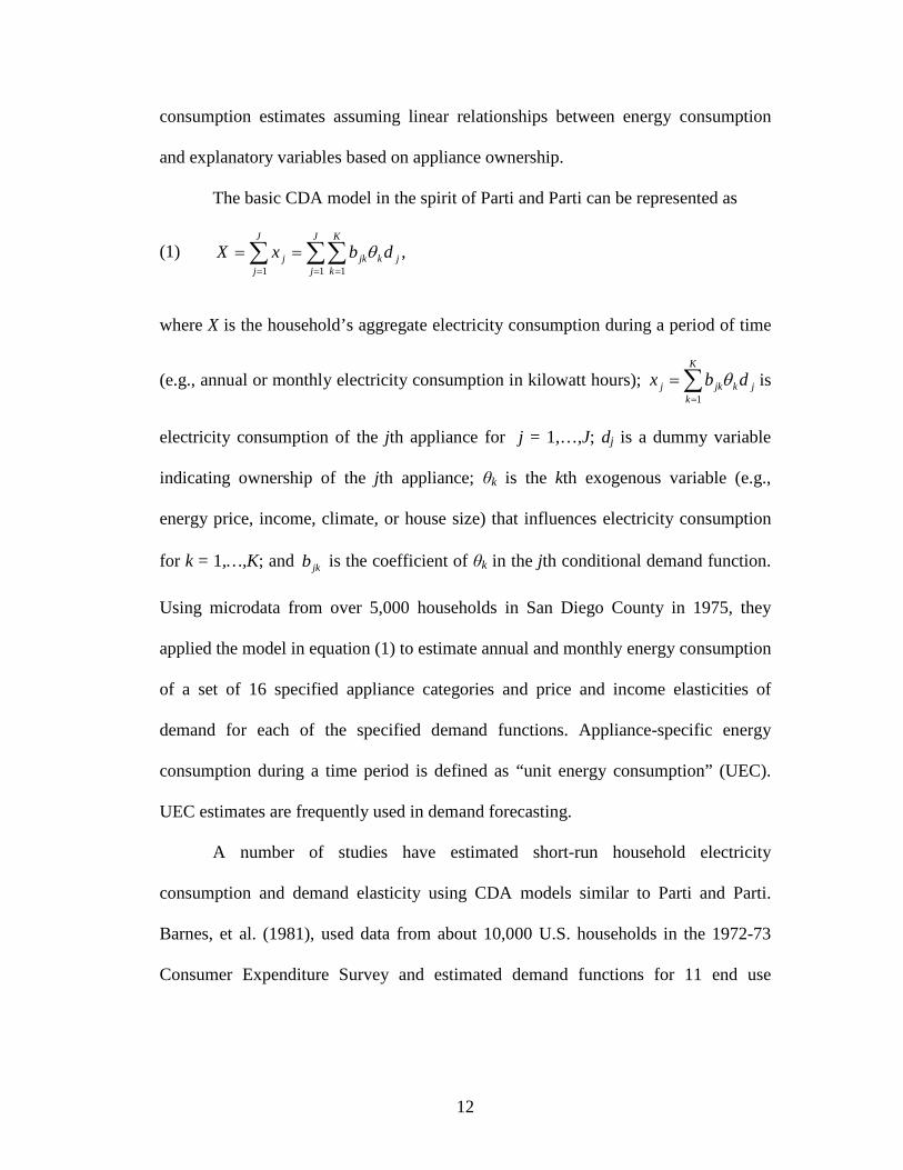
The basic CDA model in the spirit of Parti and Parti can be represented as

(1) ∑∑∑= ==

==J

j

K

kjkjk

J

jj dbxX

1 11

,θ

where X is the household’s aggregate electricity consumption during a period of time

(e.g., annual or monthly electricity consumption in kilowatt hours); ∑=

=K

kjkjkj dbx

1

θ is

electricity consumption of the jth appliance for j = 1,…,J; dj is a dummy variable

indicating ownership of the jth appliance; θk is the kth exogenous variable (e.g.,

energy price, income, climate, or house size) that influences electricity consumption

for k = 1,…,K; and jkb is the coefficient of θk in the jth conditional demand function.

Using microdata from over 5,000 households in San Diego County in 1975, they

applied the model in equation (1) to estimate annual and monthly energy consumption

of a set of 16 specified appliance categories and price and income elasticities of

demand for each of the specified demand functions. Appliance-specific energy

consumption during a time period is defined as “unit energy consumption” (UEC).

UEC estimates are frequently used in demand forecasting.

A number of studies have estimated short-run household electricity

consumption and demand elasticity using CDA models similar to Parti and Parti.

Barnes, et al. (1981), used data from about 10,000 U.S. households in the 1972-73

Consumer Expenditure Survey and estimated demand functions for 11 end use

13

categories including space heating, air conditioning and refrigeration.5

Archibald, et al. (1982), estimated monthly and seasonal electricity demand

equations for six classes of appliances using micro-data of 1,311 households in the

national survey of Lifestyles and Household Energy Use of 1975. The UEC definition

in Archibald, et al. (1982), is similar to Barnes, et al. (1981), but three types of

utilization functions are considered depending on whether each energy use is affected

by weather, housing characteristics or household demographic characteristics.

In their model,

UEC is a function of appliance ownership and utilization rate. The utilization rate is a

linear function of the logarithms of the price and income variables and a vector of

demographic variables (e.g., climate, region, and season dummy variables and

household size).

6 Using

a seemingly unrelated regression system, Aigner, Soroothian and Kerwin (1984)

estimated hourly load curves in a typical day for nine appliances. They used data for

the months of August between 1978 and 1980 from a few hundred customers of the

Los Angeles Department of Water and Power.7

5 Barnes et al. include “number of rooms” as an end-use category. It is a proxy for housing size and is not a proper energy end use category. Estimating the UEC of “number of rooms” using an OLS approach likely causes biased UEC estimates for end use categories correlated with housing size such as space heating and cooling.

6 For instance, Archibald et al. assume that UEC for common appliances (e.g., television and, microwaves) is a linear function of energy price and income only; UEC for appliances whose utilization depends on a “thermostat” (e.g., water heaters and freezers) is a linear function of energy price, income, and weather; and UEC for heaters and air conditioners is a linear function of energy price, income, weather, and housing characteristics. 7 Alternative forms of energy price representation have been used in estimation: marginal price, average price, and a declining-block rate schedule of prices. Taylor (1975) suggests that consumer demand for electricity under a multi-part rate schedule is more complex and demand equilibrium cannot be derived using conventional differential procedures. A number of CDA studies (e.g., Hartman and Werth 1981 and Barnes et al. 1981), include both a marginal price and a fixed price to reflect the block rate structure of electricity.

14

Technology Choice Modeling

Jaffe et al. (2003) reviewed two main models in the literature relevant to

energy technology adoption: the epidemic model and the rank model. The epidemic

model postulates that technology diffusion is a gradual process because a decision to

adopt a new technology is a risky undertaking requiring considerable information

both about the generic attributes of the new technology and about the details of its

use. The epidemic model captures the information externality of technology adoption

transmitted from early adopters to other potential adopters. The model yields an S-

shape curve of technology adoption for the population over time.

In contrast, the rank model posits that potential adopters are heterogeneous

and only those who face the value or return of a new technology above a threshold

choose to adopt. The rank model is analogous to the choice model. The choice model

assumes that, given a set of technology choices with different initial costs and returns

over time, a consumer makes the technology choice that minimizes discounted total

costs required to generate a level of desired energy services (Nyboer and Bataille

2000).

The epidemic model is more appropriate to describe the process of aggregate

technology adoption in a population whereas the rank, or choice, model is more

appropriate to explain technology adoption decisions faced by an individual

consumer. Because the primary interest of this study is to better understand drivers of

household choices of energy technology, the choice model is used for the purpose of

this study.

15

Most choice models implicitly or explicitly assume some form of individual

utility maximization. Empirically, logit and probit discrete choice models are used to

explain the role of factors such as purchase cost, energy prices, technology attributes

and consumer characteristics that influence consumer’s technology choice decision

(see a review of recent studies on green technology adoption in Jaffe et al. 2003).

Discrete/continuous modeling

Although the short-run decision focuses on the intensity of technology

utilization, neglecting capital stock holdings and household decisions regarding

technology choice biases estimation of the demand function because technology

choice and usage decisions are correlated.8

8 For example, a household with high demand for air conditioning is likely to purchase an energy-efficient air conditioner with higher capital cost but lower operating cost.

Balestra and Nerlove (1966) argued that

demand for energy is a dynamic problem and that “the demand function should

incorporate a stock effect and some assumptions about the adjustment of these stocks

over time” (p. 585). As Hausman (1979) put it, “energy demand may be viewed

usefully as part of a household production process in which the services of a

consumer durable good are combined with energy inputs to produce household

services” and warned that “[e]conometric models which do not differentiate the

capital-stock decision from the utilization decision cannot capture the interplay of

technological change and consumer choice in determining final energy demand” (p.

33-34). The conditional demand analyses cited above each report UEC by appliance

and some discuss it interchangeably with UEC by end use. Such treatment reflects

confusion between energy use and appliance choice.

16

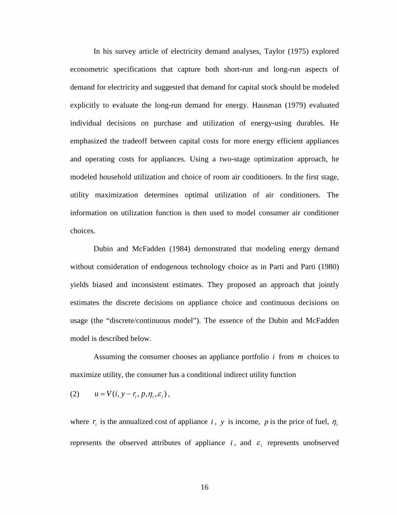
In his survey article of electricity demand analyses, Taylor (1975) explored

econometric specifications that capture both short-run and long-run aspects of

demand for electricity and suggested that demand for capital stock should be modeled

explicitly to evaluate the long-run demand for energy. Hausman (1979) evaluated

individual decisions on purchase and utilization of energy-using durables. He

emphasized the tradeoff between capital costs for more energy efficient appliances

and operating costs for appliances. Using a two-stage optimization approach, he

modeled household utilization and choice of room air conditioners. In the first stage,

utility maximization determines optimal utilization of air conditioners. The

information on utilization function is then used to model consumer air conditioner

choices.

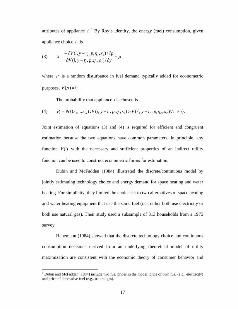
Dubin and McFadden (1984) demonstrated that modeling energy demand

without consideration of endogenous technology choice as in Parti and Parti (1980)

yields biased and inconsistent estimates. They proposed an approach that jointly

estimates the discrete decisions on appliance choice and continuous decisions on

usage (the “discrete/continuous model”). The essence of the Dubin and McFadden

model is described below.

Assuming the consumer chooses an appliance portfolio i from m choices to

maximize utility, the consumer has a conditional indirect utility function

(2) ),,,,( iii pryiVu εη−= ,

where ir is the annualized cost of appliance i , y is income, p is the price of fuel, iη

represents the observed attributes of appliance i , and iε represents unobserved

17

attributes of appliance i .9

i

By Roy’s identity, the energy (fuel) consumption, given

appliance choice , is

(3) µεηεη

+∂−∂∂−∂−

=ypryiVppryiV

xiii

iii

/),,,,(/),,,,(

where µ is a random disturbance in fuel demand typically added for econometric

purposes, ( ) 0.E µ = .

The probability that appliance i is chosen is

(4) }.),,,,(),,,,(:),..,Pr{( ''''

'1 iipryiVpryiVP iiiiiimi ≠∀−>−= εηεηεε

Joint estimation of equations (3) and (4) is required for efficient and congruent

estimation because the two equations have common parameters. In principle, any

function )(⋅V with the necessary and sufficient properties of an indirect utility

function can be used to construct econometric forms for estimation.

Dubin and McFadden (1984) illustrated the discrete/continuous model by

jointly estimating technology choice and energy demand for space heating and water

heating. For simplicity, they limited the choice set to two alternatives of space heating

and water heating equipment that use the same fuel (i.e., either both use electricity or

both use natural gas). Their study used a subsample of 313 households from a 1975

survey.

Hanemann (1984) showed that the discrete technology choice and continuous

consumption decisions derived from an underlying theoretical model of utility

maximization are consistent with the economic theory of consumer behavior and

9 Dubin and McFadden (1984) include two fuel prices in the model: price of own fuel (e.g., electricity) and price of alternative fuel (e.g., natural gas).

18

should be modeled in a mutually consistent manner. In a recent study, Davis (2008)

used the discrete/continuous model to estimate household demand for energy and

water from a field trial of energy-efficient clothes washers among 98 households in

Bern, Kansas. He found that when simultaneity of appliance choice is ignored,

estimates of price elasticities are biased away from zero.

The discrete/continuous modeling approach has been applied to analyze short-

run and long-run energy use in Europe. For instance, Dagsvik et al. (1987) used a

dynamic discrete/continuous choice model to analyze gas demand in the residential

sector of Western Europe. Vaage (2000) and Nesbakken (2001) applied

discrete/continuous models to evaluate household heating technology choice and fuel

demand in Norway. Vaage (2000) used a version of the discrete/continuous model in

Hanemann (1984) and adopted a two-step estimation approach; Nesbakken (2001)

applied the Dubin and McFadden model and used the full information maximum

likelihood estimation method. Using a two-step discrete/continuous approach,

Halvorsen and Larsen (2001) effectively estimated the short- and long-run price

elasticities of residential electricity demand in Norway.

The application of discrete/continuous modeling for energy use was sparse in

the U.S. until the recent years. With increased interests in climate change, fuel

efficiency, and clean energy, the discrete/continuous modeling approach has regained

popularity. Newell and Pizer (2008) use this approach to estimate fuel choices and

energy demand in the U.S. commercial sector in an effort to estimate a carbon

mitigation cost curve for the sector. Mansure et al. (2008) apply the method to

evaluate changes in fuel choices and energy demand among U.S. households and

19

firms in response to long-term weather change due to climate change. Both studies

largely followed the two-step estimation method of the Dubin & McFadden model

whereby a multinomial logit model of fuel choices is estimated first, followed by

fuel-specific conditional demand analysis that incorporates selection error terms from

the first stage.

2.3 Conclusions

Joint modeling of household long-run energy technology choice decisions and

short-run energy use is recognized as a holistic approach to evaluate household

energy use behavior. However, its application is still very limited. Most existing

empirical studies are based on outdated data or data of limited scope for the purpose

of robust inference. Moreover, empirical evaluation of the effectiveness of alternative

energy and environmental policy instruments for encouraging consumer adoption of

energy-efficient technology in this consistent analytical framework is even more

sparse.

This study contributes to the literature by developing a discrete/continuous

model based on a second-order translog flexible function form of the indirect utility

function, and applying the model to empirically estimate household demand for both

electricity and natural gas and technology choices for clothes washers, water heaters,

space heating systems and clothes dryers. This is the first known study to evaluate

multiple household energy uses under this comprehensive analytical framework. In

addition, the study contributes to the ongoing policy debate about the effectiveness of

alternative policy instruments for encouraging household energy efficiency and

greenhouse gas emission reductions through robust empirical analysis.

20

Chapter 3: Modeling Household Energy Demand and Technology

Choice

This chapter develops a conceptual framework for joint modeling of

household consumption and energy durable choice decisions. Section 3.1 establishes

the underlying household model. Section 3.2 derives the household short-run demand

model. Section 3.3 develops the long-run technology choice model. Section 3.4

concludes with discussions on model applications.

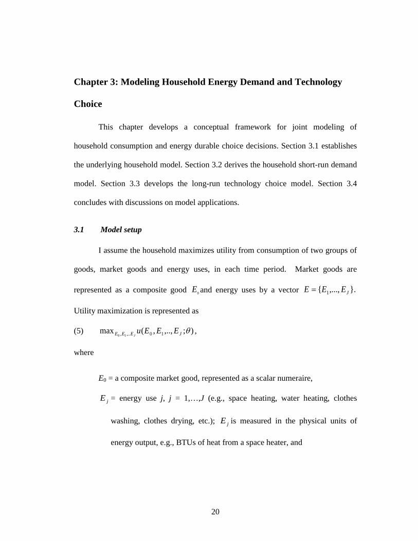
3.1 Model setup

I assume the household maximizes utility from consumption of two groups of

goods, market goods and energy uses, in each time period. Market goods are

represented as a composite good 0E and energy uses by a vector }.,...,{ 1 JEEE =

Utility maximization is represented as

(5) );,..,,(max 10,.., 10θJEEE EEEu

J,

where

E0 = a composite market good, represented as a scalar numeraire,

jE = energy use j, j = 1,…,J (e.g., space heating, water heating, clothes

washing, clothes drying, etc.); jE is measured in the physical units of

energy output, e.g., BTUs of heat from a space heater, and

21

θ = a K-dimensional column vector of household and housing characteristics

that influence household demand, e.g., household size, house square-

footage, and climate.

The utility function is assumed to be increasing and quasi-concave in E0 and E. Both

E0 and E are assumed to be essential goods. Utility maximization is constrained by

household production technologies and the budget constraint.

Demand for each energy service jE is met through utilization of a household

energy production technology (i.e., an appliance) using fuel as an input. I assume that

household energy service production does not require household labor.10 I further

assume independence of energy production technologies, i.e., no appliance produces

more than one energy service (output nonjointness) so that each energy service has a

unique production function.11

(6)

In addition, I assume input nonjointness, i.e., fuel must

be allocated among appliances that produce energy services so that fuel allocated to

one appliance (energy service) does not affect production of others. If a single

technology is used to produce a given end use j, then the energy service production

function is represented by

,),( jilijj xE ϕ= Jj ,...,1= ,

where

10 This assumption is reasonable as a majority of energy services do not involve labor. A few energy uses have time implications, such as cooking and clothes washing. However, for energy service production that requires time, the time requirement is relatively inelastic with respect to the energy price. One can argue that demand for time has an income effect. This question is worth pursuing but is beyond the scope of this study. 11 In a few cases, multiple energy services are produced using the same appliance (e.g., a heat pump is used for both space heating and cooling).

22

i = technology choice index, jIi∈ , where jI is the technology choice set for

end use j,

jilx ),( = input of fuel l(i) associated with technology i for end use j where l is

the energy source (e.g., electricity and natural gas), and

ijϕ = the average energy-efficiency coefficient (i.e., energy output per unit of

energy input) associated with technology i for energy use j.

Energy service production functions of the form in (6) are widely used in

energy engineering models to calculate the energy output for a given level of energy

input or, conversely, the energy input requirement given a level of energy service

load (e.g., Wenzel et al. 1997).12

i

The use of such functions in this model avoids

estimating certain phenomena in broad reduced form relationships for which physical

relationships are known comparatively precisely. In this setup, I assume the

technology choice determines the fuel choice as represented by l(i). That is, once

technology is chosen from the technology set jI to meet energy service demand

jE , the fuel choice l(i) is determined.

Some energy uses can be met with more than one fuel technology (e.g.,

electricity or natural gas appliances can be used for water heating, space heating, and

clothes drying); other energy use categories (e.g., lighting, refrigerators, and freezers)

have only one practical fuel possibility (electricity). Although the model I develop

here assumes that each energy service is met through a single technology, multiple

12 The exact definition of the energy-efficiency coefficient ( ijϕ ) varies by energy use. For example, the energy-efficiency level of heating equipment is typically measured by the annual fuel utilization efficiency (AFUE), whereas the energy-efficiency level of an air conditioner is measured by its energy efficiency rating (EER) or seasonal energy efficiency rating (SEER).

23

technologies are used to produce some energy services (e.g., both a central air furnace

and a portable space heater may be used simultaneously for space heating). To

capture this case, equation (6) can be represented more generally as

∑∈=

jIi jilijj xE ),(ϕ . The model generalization for the multiple technology case is

presented in Appendix 3.1 at the end of this Chapter.

In the short-run, the household capital stock (e.g., appliances and housing

stock) is likely fixed and production of the desired level of an energy service is

determined by the intensity with which the chosen technology is utilized. Therefore,

the short-run household optimization problem generates a derived demand for fuel

that treats the technology choice as given and does not depend on factors that affect

technology choice. In the long run, however, the household will “weigh the

alternatives of each appliance against expectations of future use, future energy prices,

and current financing decisions” (Dubin and McFadden 1984). In other words, the

household will consider both the capital costs and the future flow of operating costs

associated with each of the alternative technologies in the decision-making process.

The two sections below discuss household decisions on short-run fuel use and

the long-run technology choice, respectively. I demonstrate that theoretically both

decisions flow from the same underlying utility maximization problem so that a

unified framework applies to analysis of both household energy consumption and

technology choice behavior.

3.2 Short-run fuel demand

Ignoring the case of using multiple technologies for individual energy uses for

conceptual simplicity of presentation, the short-run optimization problem discussed

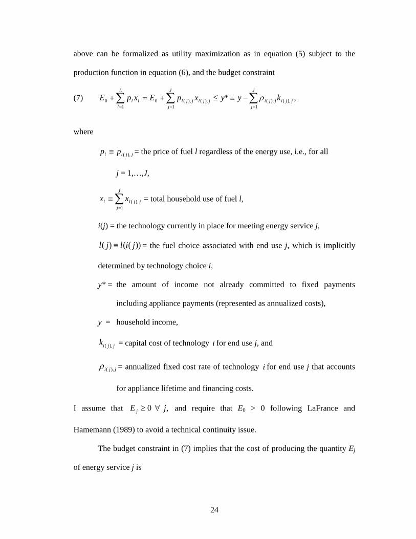
24

above can be formalized as utility maximization as in equation (5) subject to the

production function in equation (6), and the budget constraint

(7) ,*1

),(),(1

),(),(01

0 ∑∑∑===

−≡≤+=+J

jjjijji

J

jjjljjl

L

lll kyyxpExpE ρ

where

jjll pp ),(≡ = the price of fuel l regardless of the energy use, i.e., for all

j = 1,…,J,

∑=

≡J

jjjll xx

1),( = total household use of fuel l,

i(j) = the technology currently in place for meeting energy service j,

))(()( jiljl ≡ = the fuel choice associated with end use j, which is implicitly

determined by technology choice i,

y* = the amount of income not already committed to fixed payments

including appliance payments (represented as annualized costs),

y = household income,

jjik ),( = capital cost of technology i for end use j, and

jji ),(ρ = annualized fixed cost rate of technology i for end use j that accounts

for appliance lifetime and financing costs.

I assume that , 0 jE j ∀≥ and require that E0 > 0 following LaFrance and

Hamemann (1989) to avoid a technical continuity issue.

The budget constraint in (7) implies that the cost of producing the quantity Ej

of energy service j is

25

(8) ,),(),( jjljjlj xpc = .,...1 Jj =

The implicit price of energy service j, i.e., the effective cost per unit of energy output

for the jth energy use, is

(9) ,/)/()( ),(),(),(),(),(),( jjijjljjljjijjljjlj pxxpr ϕϕ =≡

.,...1 Jj =

Solving the utility maximization problem given the current appliance stock

yields the conditional indirect utility function

(10) ),*,,( θyrVV =

where r is a vector including r0, the price of the composite good, and the rj’s across

all energy end uses for j = 1,…,J, and )(⋅V is assumed to be continuous and

quasiconvex in r and y*, monotonically decreasing in r, and monotonically increasing

in y*.

I adopt a version of the second-order translog flexible functional form of the

conditional indirect utility function following Berndt et al (1977). The indirect utility

function also incorporates demographic variables by interacting them with price terms

using the “demographic translating” technique discussed in Pollak and Wales

(1992).13

13 The inclusion of household and housing characteristics in the demand functions is based on the common sense and significance of statistical test results.

In addition, I include a vector of household characteristics that may

influence energy technology choices and disturbances associated with individual

technology choices for energy service production. This functional form yields

26

(11) },*)/ln(

*)/ln(*)/ln(*)/ln(exp{),*,,(

1),(

1),(

0

0 0'''

0

∑∑∑

∑∑∑

===

= ==

+Η+Γ+

++=

J

jjji

J

jjji

J

jjj

J

j

J

jjjjj

J

jjj

yr

yryryryrV

εθθ

βααεθ

where ‘0’ denotes the composite good, α , jα , j = 0,…,J, and 'jjβ , j,j’ = 0,…,J, are

scalar parameters, and jΓ , j = 0,…,J and jji ),(Η , j = 1,…,J are row-vector parameters

of the indirect utility function, and jji ),(ε is a disturbance. Both the parameter vector

( ),i j jΗ and the disturbance jji ),(ε are associated with the specific technology i chosen

for energy use j. I assume separability in demand between the composite good and the

choice of energy technology alternatives.

Flexible functional forms have desirable properties as they do not constrain

price and income elasticities at a base point a priori (Berndt et al. 1977). Popular

functional forms include the almost ideal demand system (AIDS) (e.g., Deaton and

Muellbauer 1980), the transcendental logarithmic (Translog) system (e.g.,

Christensen, Jorgenson, and Lau 1975), the generalized Leontief (e.g., Diewert 1971),

and the generalized Cobb-Douglas (e.g., Diewert 1973). Using Bayesian procedures,

Berndt et al. (1977) compared the translog, generalized Leontief, and generalized

Cobb-Douglas using Canadian data, and concluded that the translog functional form

is preferable on theoretical and econometric grounds. Lewbel (1989) showed that the

AIDS and translog models are about equal in terms of both explanatory power and

estimated elasticities. Cameron (1985) used a translog indirect utility function to

estimate household energy conservation retrofit decisions and found that estimated

27

coefficients were robust across different specifications such as the generalized

Leontief and the quadratic form.

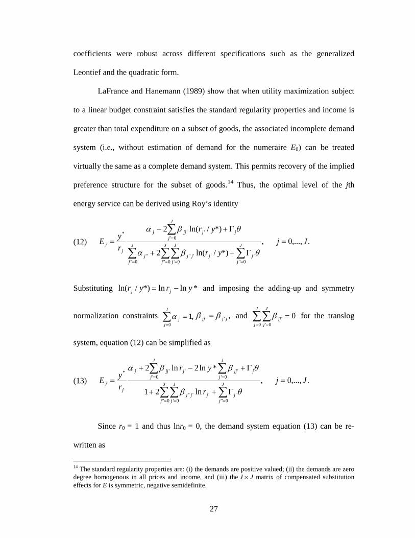
LaFrance and Hanemann (1989) show that when utility maximization subject

to a linear budget constraint satisfies the standard regularity properties and income is

greater than total expenditure on a subset of goods, the associated incomplete demand

system (i.e., without estimation of demand for the numeraire E0) can be treated

virtually the same as a complete demand system. This permits recovery of the implied

preference structure for the subset of goods.14

(12)

Thus, the optimal level of the jth

energy service can be derived using Roy’s identity

.,...,0 ,*)/ln(2

*)/ln(2

0''''

0'' 0'' 0'''''''

0'''*

Jjyr

yr

ryE J

jj

J

j

J

j

J

jjjjj

J

jjjjjj

jj =

Γ++

Γ++=

∑∑ ∑∑

∑

== = =

=

θβα

θβα

Substituting *lnln*)/ln( yryr jj −= and imposing the adding-up and symmetry

normalization constraints ,10

=∑=

J

jjα ,'' jjjj ββ =

and 0

0 0'' =∑∑

= =

J

j

J

jjjβ for the translog

system, equation (12) can be simplified as

(13) .,...,0 ,ln21

*ln2ln2

0''''

0'' 0'''''

0' 0''''*

Jjr

yr

ryE J

jj

J

j

J

jjjj

J

jj

J

jjjjjjj

jj =

Γ++

Γ+−+=

∑∑∑

∑ ∑

== =

= =

θβ

θββα

Since r0 = 1 and thus lnr0 = 0, the demand system equation (13) can be re-

written as

14 The standard regularity properties are: (i) the demands are positive valued; (ii) the demands are zero degree homogenous in all prices and income, and (iii) the JJ × matrix of compensated substitution effects for E is symmetric, negative semidefinite.

28

(14) ,ln21

*ln2ln2*

0''''

0'' 1'''''

1'0

0''0''00

0

∑∑∑

∑ ∑

== =

= =

Γ++

Γ+−+= J

jj

J

j

J

jjjj

J

j

J

jjjj

r

yryE

θβ

θββα

and

(15) .,...,1 ,ln21

*ln2ln2

0''''

0'' 1'''''

1' 0''''*

Jjr

yr

ryE J

jj

J

j

J

jjjj

J

jj

J

jjjjjjj

jj =

Γ++

Γ+−+=

∑∑∑

∑ ∑

== =

= =

θβ

θββα

Given that jE is an unobserved household quantity, equation (15) can be converted

to an estimable equation by substituting (6),

(16) ,,...,1 ,ln21

*ln2ln2

0''''

0'' 1'''''

1' 0''''*

),(),( Jjr

yr

ryxE J

jj

J

j

J

jjjj

J

jj

J

jjjjjjj

jjjljjij =

Γ++

Γ+−+==

∑∑∑

∑ ∑

== =

= =

θβ

θββαϕ

and rearranging to get

(17) .,...,1 ,ln21

*ln2ln2

0''''

0'' 1'''''

1' 0''''

),(

*

),( Jjr

yr

ryx J

jj

J

j

J

jjjj

J

jj

J

jjjjjjj

jjjijjl =

Γ++

Γ+−+=

∑∑∑

∑ ∑

== =

= =

θβ

θββα

ϕ

Further substituting (9) obtains

(18) .,...,1 ,)/ln(21

*ln2)/ln(2

0''''

0'' 1''),'('),'('''

1' 0'''),'('),'('

),(

*

),( Jjp

yp

pyx J

jj

J

j

J

jjjijjljj

J

jj

J

jjjjjijjljjj

jjljjl =

Γ++

Γ+−+=

∑∑∑

∑ ∑

== =

= =

θϕβ

θβϕβα

29

The associated budget share equations by energy end use are thus

(19) .,...,1 ,)/ln(21

*ln2)/ln(2

0''''

0'' 1''),'('),'('''

1' 0'''),'('),'('

*),(),( Jj

p

yp

ypx

J

jj

J

j

J

jjjijjljj

J

jj

J

jjjjjijjljjj

jjljjl =Γ++

Γ+−+=

∑∑∑

∑ ∑

== =

= =

θϕβ

θβϕβα

The budget constraint in (7) suggests that the amount of y* allocated to the composite

good (the numeraire) is ∑=

−=J

jjjljjl xpyE

1),(),(0 * . Thus, the budget share for the

numeraire 0ω can be expressed as

(20)

,)/ln(21

*ln2)/ln(2

*

*

0

0''''

0'' 1''),'('),'('''

1'0

0''0'),'('),'('00

1),(),(

0

µθϕβ

θβϕβα

ω

+Γ++

Γ+−+=

−=

∑∑∑

∑ ∑

∑

== =

= =

=

J

jj

J

j

J

jjjijjljj

J

j

J

jjjjijjlj

J

jjjljjl

p

yp

y

xpy

where µ0 is a disturbance.

If only aggregate household use of each fuel is observed, equation (19) can be

aggregated over end uses by fuel type to get budget shares by fuel type, lω . Here I

also introduce an error term for econometric purposes to represent errors in fuel use

decisions

30

(21)

,,...,1

,)/ln(21

*ln2

)/ln(2)0(

*)0(

*

0''''

0'' 1''),'('),'('''

0''

1''),'('),'('

1),(

1

),(),(),(

Ll

p

y

px

ypx

x

ypx

lJ

jj

J

j

J

jjjijjljj

j

J

jjj

J

jjjijjljjjJ

jjjl

J

j

jjljjljjl

lll

=

+Γ++

Γ+−

+

>Ψ

=

>Ψ=

=

∑∑∑

∑

∑∑

∑

== =

=

=

=

=

µθϕβ

θβ

ϕβα

ω

where define indicator variable, and μl is a disturbance of fuel use decisions with

respect to fuel type l. Demand for numeraire and fuels are nonrandom to households

but unobservable to researchers. I assume the disturbances μ associated with

consumption are correlated with household taste (e.g., for energy efficiency) which

also affects choices of energy technology. For the empirical analysis of household

energy demand among California households, equation (21) consists of two estimable

budget share equations, i.e., L = {electricity, natural gas}.15

Estimation of the demand system in equations (20) and (21) retrieves

parameters of the demand equations and the indirect utility function. If the appliance

The model setup

presented above only addresses situation that an energy service is met through a

single technology. The model expressions and estimation equations for multiple

technology case are presented in Appendix 3.1 at the end of this Chapter.

15 According to the 2005 Residential Energy Consumption Survey conducted by the EIA, electricity and natural gas consumption accounts for over 93 percent of an average California household’s fuel expenditure. (Source: Table US10 “Average Expenditures by Fuels Used, 2005” in the 2005 Residential Energy Consumption Survey--Detailed Tables, published by the EIA, 2008. Accessed via http://www.eia.doe.gov/emeu/recs/recs2005/c&e/detailed_tables2005c&e.html on March 2, 2008)

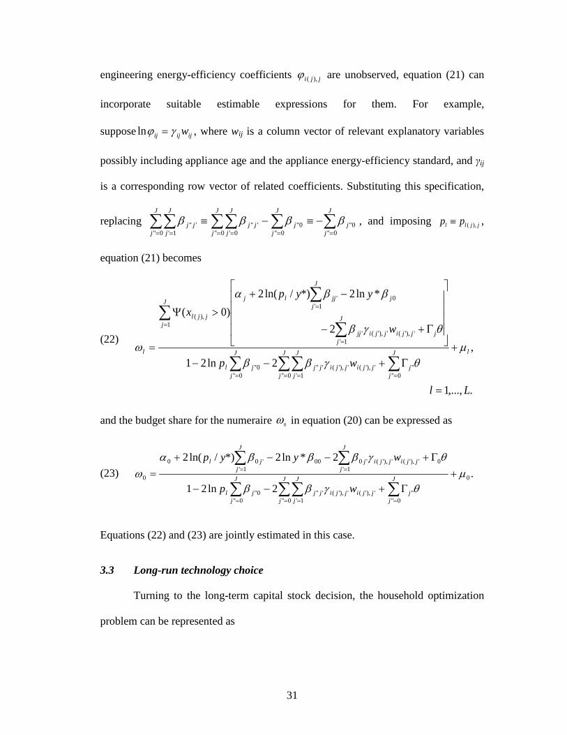
31

engineering energy-efficiency coefficients jji ),(ϕ are unobserved, equation (21) can

incorporate suitable estimable expressions for them. For example,

suppose ijijij wγϕ =ln , where wij is a column vector of relevant explanatory variables

possibly including appliance age and the appliance energy-efficiency standard, and γij

is a corresponding row vector of related coefficients. Substituting this specification,

replacing ∑∑∑∑∑∑=== == =

−≡−≡J

jj

J

jj

J

j

J

jjj

J

j

J

jjj

0''0''

0''0''

0'' 0''''

0'' 1'''' ββββ , and imposing ( ),l l j jp p≡ ,

equation (21) becomes

(22)

.,...,1

,2ln21

2

*ln2*)/ln(2)0(

0''''

0'' 0'' 1''),'('),'('''0''

'),'(1'

'),'('

01'

'

1),(

Ll

wp

w

yypx

lJ

jj

J

j

J

j

J

jjjijjijjjl

jjji

J

jjjijj

j

J

jjjljJ

jjjl

l

=

+Γ+−−

Γ+−

−+

>Ψ

=

∑∑ ∑∑

∑

∑∑

== = =

=

=

=

µθγββ

θγβ

ββα

ω

and the budget share for the numeraire 0ω in equation (20) can be expressed as

(23) .2ln21

2*ln2*)/ln(2

0

0''''

0'' 0'' 1''),'('),'('''0''

1'0'),'('),'(

1''000'00

0 µθγββ

θγβββαω +

Γ+−−

Γ+−−+=

∑∑ ∑∑

∑ ∑

== = =

= =J

jj

J

j

J

j

J

jjjijjijjjl

J

jjjijji

J

jjjl

wp

wyyp

Equations (22) and (23) are jointly estimated in this case.

3.3 Long-run technology choice

Turning to the long-term capital stock decision, the household optimization

problem can be represented as

32

(24) ,);,...,,(max1

**1

*0,...,1,)( ∑

==∈

T

tJttt

tJjIji EEEu

jθλ

subject to

,,...,1 ,1

),(),(1

*)),((),((0 TtykxpE t

J

jjtjijtji

J

jjtjiljtjilt ==++ ∑∑

==

ρ

where λ is a discount factor, t subscripts denote time, T is the planning horizon, and

‘*’ denotes optimal choice functions conditioned on technology choices according to

successive applications of the short-term decision model of the previous section.

Again, I assume only one technology is chosen to meet each energy use for

conceptual simplicity of presentation, although generalizations are easily added. I

assume that appliances have appropriate resale value consistent with remaining

lifetime when sold as part of selling a house and that T is sufficiently large to avoid

dependence of ownership costs on the planning horizon.

The modeling of household energy technology choices requires some

simplifying assumptions because the treatment of appliance usage depends on future

price expectations. Hausman (1979) modeled consumer decisions with respect to

purchase and utilization of room air conditioners. He recognized the challenge of

modeling future price expectations and used marginal electricity price in the year of

study to estimate the expected operating costs. Dubin and McFadden (1984) modeled

household technology choice as contemporaneous with utilization decisions. They

acknowledge that their assumption is realistic only if “there are perfect competitive

rental markets for consumer durables.” They used electricity price in the year of study

to calculate operating cost over the appliance lifetime, and relied on exogenous

33

estimates of ‘typical’ unit energy consumption (UEC) of appliances to derive future

usage estimates.

In a review article, Rust (1986) noted that what is needed to be accurate is “a

formal dynamic programming model of the appliance investment decision, which

models consumer expectations of future prices by specification of a parametric

stochastic process governing their law of motion.” However, no study has been able

to achieve this ideal. For example, in a much more recent study of energy

consumption and technology choice for space heating in Norway, Nesbakken (2001)

used real energy price in the year of appliance purchase as the expected energy price.

For my analysis, I assume future price and income expectations at each point

in time are given by current prices and income. Thus, the long term problem in (24)

reduces to the single time period problem,

(25) ),;,...,,(max **1

*0,...,1,)( θJJjIji EEEu

j =∈

subject to

.1

),(),(1

*)),(()),((0 ykxpE

J

jjjijji

J

jjjiljjil =++ ∑∑

==

ρ

A comparison of the budget constraints in the long- and the short-term

problems implies compatibility such that

(26) ∑=

−=J

jjjijji kyy

1),(),(* ρ ,

where y* is the available income for short-term decisions once the technology choices

in the long-term decision problem are made. To further attain compatibility of the

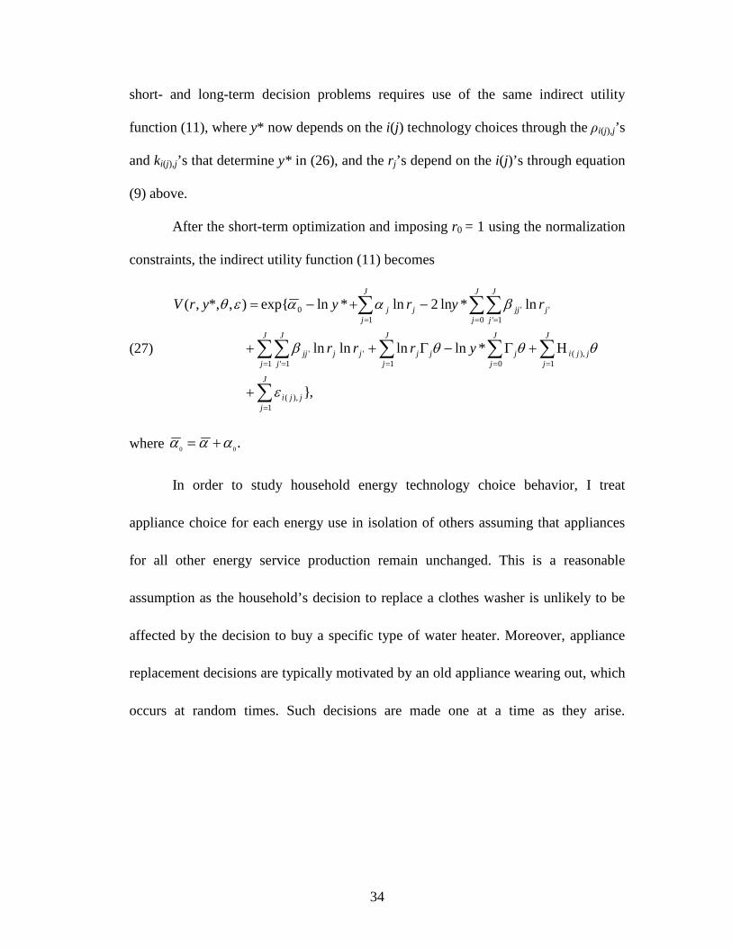
34

short- and long-term decision problems requires use of the same indirect utility

function (11), where y* now depends on the i(j) technology choices through the ρi(j),j’s

and ki(j),j’s that determine y* in (26), and the rj’s depend on the i(j)’s through equation

(9) above.

After the short-term optimization and imposing r0 = 1 using the normalization

constraints, the indirect utility function (11) becomes

(27)

,}

*lnlnlnln

ln*ln 2ln*lnexp{ ),*,,(

1),(

1),(

011 1'''

0 1'''

10

∑

∑∑∑∑∑

∑∑∑

=

==== =

= ==

+

Η+Γ−Γ++

−+−=

J

jjji

J

jjji

J

jj

J

jjj

J

j

J

jjjjj

J

j

J

jjjj

J

jjj

yrrr

ryryyrV

ε

θθθβ

βααεθ

where .00 ααα +=

In order to study household energy technology choice behavior, I treat

appliance choice for each energy use in isolation of others assuming that appliances

for all other energy service production remain unchanged. This is a reasonable

assumption as the household’s decision to replace a clothes washer is unlikely to be

affected by the decision to buy a specific type of water heater. Moreover, appliance

replacement decisions are typically motivated by an old appliance wearing out, which

occurs at random times. Such decisions are made one at a time as they arise.

35

Therefore, the unobservables that affect appliance choices are likely from different

time periods and thus likely to be independent of one another.16

Under the technology-choice-independence assumption, this model reduces to

independent minimization of the implicit cost of individual energy uses. That is,

individual appliance choice decisions can be represented by defining V as a function

of i(j) for a given energy use j assuming no other appliance choice problem arises

simultaneously, i.e., other appliances are held fixed. For this purpose, I define

(28) ,'

1'''∑

≠=

−=J

jjj

ijijj kyy ρ and

(29) .'

1''' ijij

J

jjj

ijijij kkyy ρρ −−= ∑≠=

where yj represents income available given commitments to fixed payments

associated with all energy services other than j, and yij represents income available

after choosing technology alternative i for energy service j. Analogous to rj as defined

in equation (9), I also define

jjijjilij pr ),()),(( /ϕ≡

as the effective cost per unit of energy service j where i(j) is the chosen technology.

The indirect utility function in (11) can be denoted as

(30) }';,...,1')(,)(|),,,({),,,,,( jjJj for jiijiyrVykiV ijijjijijj ≠=== εθεθρ ,

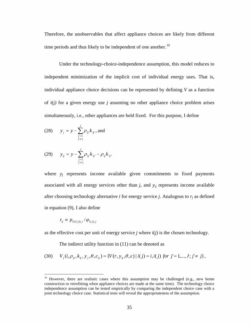
16 However, there are realistic cases where this assumption may be challenged (e.g., new home construction or retrofitting when appliance choices are made at the same time). The technology choice independence assumption can be tested empirically by comparing the independent choice case with a joint technology choice case. Statistical tests will reveal the appropriateness of the assumption.

36

where V is the same indirect utility function with the same parameters as defined in

(11). The indirect utility function Vj can be decomposed into two components: the

terms that vary with the technology choice for energy use j and the terms that are

constant regardless of this technology choice. For convenience, I introduce the

following notation for the right-hand side expression in (30):

(31) )exp(),,,( 0ijjjijijijj WBWyrV εεθ ++= ,

where

.lnlnln ln

},,,,..,,...,,,1{

},ln,ln

,lnln2,...,)(ln2,...,lnln2,lnln2,...,lnln2,ln,ln{

'1'

'),'(

'1'

'),'(

'1'

''

'1'

''1''

''''''

*1'

''00

''),(

0

''1

001

211

∑∑∑∑∑∑

∑∑∑

≠=

≠=

≠=

≠=

≠=

≠=

===

+Η+Γ+++=

ΗΓΓ≡

−

−−−≡

J

jjj

jji

J

jjj

jji

J

jjj

jj

J

jjj

J

jjj

jjjj

J

jjj

jjj

jji

J

jjjjJj

J

jjJ

J

jjjj

ijij

JijijijJijijijijij

rrrrW

B

yrrrrrrryryryW

εθθβαα

ββββα

θθθ

The probability that the household chooses technology i from the set Ij of

alternatives for energy service j can then be represented as

(32)

}',;',Pr{

}',;',Pr{

}',;'),exp()Pr{exp(

}',;'),,,'(),,,(Pr{

''

'0

'0

'0

'0

''

jjjijijijji

jjijjjiijjjij

jjijjjiijjjij

jjijijijijjij

IiiiiBWBWIiiiiWBWWBW

IiiiiWBWWBW

IiiiiyiVyiVP

∈≠∀−<−=

∈≠∀++>++=

∈≠∀++>++=

∈≠∀>=

εε

εε

εε

εθεθ

As shown in (32), the 0jW terms conveniently cancel out of this expression. Thus,

only choice-related variables and technology choice disturbances are relevant.

Assuming ,jij Ii ∈∀ε are identically and independently distributed with zero

means and follow extreme value (EV) type I distributions, the difference between two

disturbances follows the logistic distribution function,

37

(33) )exp()( ''

jiieF j

iiεε −−= ,

where .'' ijjijii εεε −= Following the well-known results developed and popularized

by McFadden (1974), the EV error term distribution leads to a logistic model of the

discrete choice probability where the probability that technology i yields the highest

indirect utility among all possible technologies is given by

(34)

,)lnlnexp(

)lnlnexp(

ln2ln

ln21ln

exp

ln2ln

ln21ln

exp

)exp()exp(

'''0'

0

'

'1'

'''

00'' 1'''''''

1'''

00'' 1''''''

''

∑

∑∑

∑∑∑

∑

∑∑∑

∑

∈

∈

=

== =

=

== =

∈

Η++−

Η++−=

Η+

Γ+++

Γ++−

Η+

Γ+++

Γ++−

=

=

j

j

j

Iijijjiji

ijjijij

Iijij

J

jjjjjji

J

jj

J

j

J

jjjjji

ijj

J

jjjjjij

J

jj

J

j

J

jjjjij

Iijji

jijij

ArAyArAy

rr

ry

rr

ry

BWBW

P

θθ

θθβα

θβ

θθβα

θβ

where

∑∑∑== =

Γ++≡J

jj

J

j

J

jjjj rA

00'' 1''''''0 ln21 θβ , and

.ln21'

'' θβα j

J

jjjjjj rA Γ++≡ ∑

=

Thus, A0 and Aj are, in effect, scalars that do not vary with the chosen technology for

a given energy service (and household). If the energy-efficiency coefficients used to

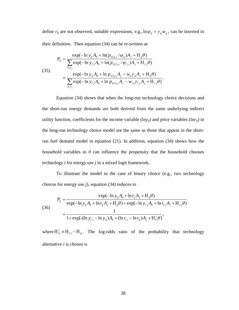
38

define rij are not observed, suitable expressions, e.g., ijijij wγϕ =ln , can be inserted in

their definition. Then equation (34) can be re-written as

(35) .

)lnlnexp()lnlnexp(

))/ln(lnexp())/ln(lnexp(

''''),'(0'

),(0

'''),'(0'

),(0

∑

∑

∈

∈

Η+−+−

Η+−+−=

Η++−

Η++−=

j

j

Iijijjijijjilji

ijjijijjjilij

Iijijjijilji

ijjijjilijij

AwApAyAwApAy

ApAyApAy

P

θγθγ

θϕθϕ

Equation (34) shows that when the long-run technology choice decisions and

the short-run energy demands are both derived from the same underlying indirect

utility function, coefficients for the income variable (lnyij) and price variables (lnrij) in

the long-run technology choice model are the same as those that appear in the short-

run fuel demand model in equation (21). In addition, equation (34) shows how the

household variables in θ can influence the propensity that the household chooses

technology i for energy use j in a mixed logit framework.

To illustrate the model in the case of binary choice (e.g., two technology

choices for energy use j), equation (34) reduces to

(36) ,

])ln(ln)lnlnexp[-(11

)lnlnexp()lnlnexp()lnlnexp(

''0'

''0'0

0

θ

θθθ

jiijijjiijji

jijjijiijjijij

ijjijijij

ArrAyy

ArAyArAyArAy

P

Η+−+−+=

Η++−+Η++−

Η++−=

where ijjijii Η−Η≡Η '' . The log-odds ratio of the probability that technology

alternative i is chosen is

39

(37)

.)ln(ln)lnln(

])ln(ln)lnlnexp[-(1])ln(ln)lnlnexp[-(

])ln(ln)lnlnexp[-(11

log

1loglog

''0'

''0'

''0'

'*'0'

'

θ

θθθ

jiijijjiijji

jiijijjiijji

jiijijjiijji

jiijijjiijji

ij

ij

ji

ij

ArrAyy

ArrAyyArrAyy

ArrAyy

PP

PP

Η−−−−=

Η+−+−+

Η+−+−

Η+−+−+=

−=

If more than two technology choice alternatives are involved, the model in

(34) is a multinomial logit model. To identify the parameters, one alternative i* is

designated as the reference choice alternative, i.e., the probability that technology i*

is chosen is

(38) ,)exp(1

1

*''

'* ∑

≠∈

+=

iiIi

jjiji

j

BWP

and the probability that technology i ( 'ii ≠ ) is chosen becomes

(39) .)exp(1

)exp(

*''

'∑≠∈

+=

iiIi

jji

jijij

j

BWBW

P

One remaining consideration in applying this appliance choice model has to

do with future price and income expectations. While the same preference parameters

from the underlying utility maximization model appear in both short-run use

equations and long-run appliance choice equations (assuming stable preferences),

consumers may have different expectations for prices and income that will prevail

over the appliance life. If consumers naively expect current prices and income to

continue, then no modification in the model is needed. However, if consumers expect

40

different prices and income to prevail during the appliance lifetime, then those

expectations may modify the prices and income used in the appliance choice model.

3.4 Conclusions

This chapter develops a consistent theoretical framework that can be used to

analyze household behavior with respect to short-run energy demand and long-run

technology choices. The model, derived from underlying utility maximization using a

second-order translog indirect utility function, provides a transparent structure with

great flexibility to empirically investigate consumer preferences and the role of

prices, income and household characteristics in energy consumption and technology

adoption decisions. This model addresses several unique features of consumer energy

use and allows analysis of demand interactions, demand aggregation, and fuel

substitution.

The empirical application of the model presented in the subsequent chapters

shows that the model predicts household energy demand and technology choice

decisions quite well given the extent of structure, validating the usefulness and

appropriateness of the model in studying household energy use behavior.

The modeling framework allows analysis of the likelihood that a technology is

chosen based on variations in its attributes (e.g., capital and operating costs, and

energy efficiency characteristics) and household characteristics (e.g., income,

education, and climate) given future expectations. Similarly, the impacts of prices,

income and household characteristics on short-run energy consumption can be

evaluated given technology choices. Analysis of these questions in this consistent

41

framework assures that the short- and long-run answers to these questions are

mutually congruent and sensible.

The effects of policy instruments designed to encourage household energy

efficiency can also be analyzed in this framework. For instance, incentive-based

policy, such as utility rebates or government tax incentives on technology purchases,

lower the capital cost of targeted technologies; energy efficiency performance

standards affect the energy efficiency performance ( ijϕ ) of targeted technologies; and

public or utility information and outreach programs that promote energy-efficient

technology potentially change the household’s perception on the attributes of the

technology.

On the other hand, climate change policies, such as a carbon cap-and-trade

program or emissions taxes, can potentially change the resource costs of fossil-based

energy supplies (natural gas, oil, and electricity) and thus related fuel prices. The

effects of these policy-induced changes on households’ technology choices and

utilization can be analyzed efficiently using this modeling framework.

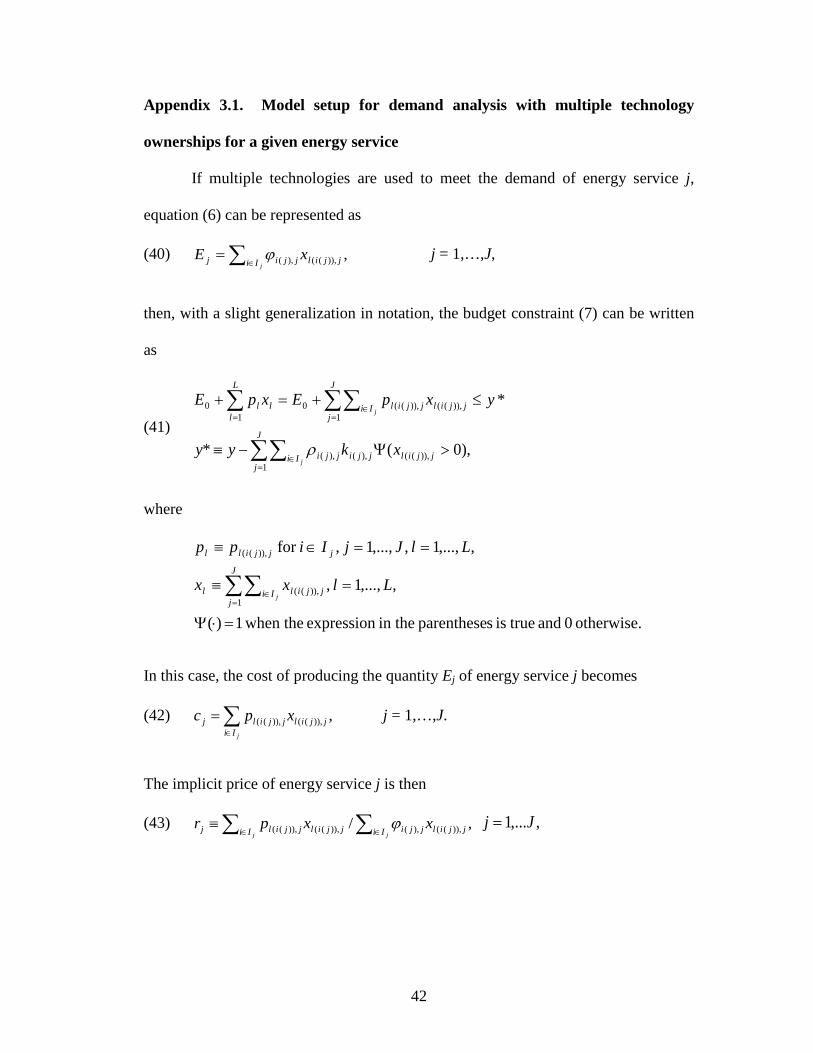
42

Appendix 3.1. Model setup for demand analysis with multiple technology

ownerships for a given energy service

If multiple technologies are used to meet the demand of energy service j,

equation (6) can be represented as

(40) ,)),((),(∑∈=

jIi jjiljjij xE ϕ j = 1,…,J,

then, with a slight generalization in notation, the budget constraint (7) can be written

as

(41) ,)0(*

*

1)),((),(),(

1)),(()),((0

10

∑∑

∑∑∑

=∈

=∈

=

>Ψ−≡

≤+=+

J

jIi jjiljjijji

J

jIi jjiljjil

L

lll

j

j

xkyy

yxpExpE

ρ

where

otherwise. 0 and trueis sparenthese in the expression when the1 )(

,,...,1 ,

,,...,1 ,,...,1,for

1)),((

)),((

=⋅Ψ

=≡

==∈≡

∑∑=

∈Llxx

LlJjIippJ

jIi jjill

jjjill

j

In this case, the cost of producing the quantity Ej of energy service j becomes

(42) ∑∈

=jIi

jjiljjilj xpc ,)),(()),(( j = 1,…,J.

The implicit price of energy service j is then

(43) ,/ )),((),()),(()),(( ∑∑ ∈∈≡

jj Ii jjiljjiIi jjiljjilj xxpr ϕ ,,...1 Jj =

43

which is the average cost to produce a unit of energy output for energy service j using

multiple technologies. If the multiple technologies use the same fuel l, equation (43)

is reduced to

(44) ,// )),((),(),()),((),(),(),( jjilIi jjiIi jjljjiljjijjljjljjj

pxxpr ϖϕϕ ∑∑ ∈∈=≡

,,...1 Jj =

where ∑∈≡

jIi jjiljjl xx )),((),( , and jjil )),((ϖ is the share of fuel input l of technology i,

,jIi∈ for energy use j. If the multiple technologies use different fuels, equation (43)

can be re-written as

(45) ,/ )),((),()),((),( jjilIi jjiIi jjiljjljjj

pr ϖϕϖ ∑∑ ∈∈≡

.,...1 Jj =

In both cases, rj is the weighted average cost to produce a unit of energy output for

energy use j with consideration of the energy efficiency and relative intensity of

utilization (thus fuel input) of each technology.

The subsequent model expressions for short-term fuel demand in equations

(12)–(18) are modified similarly for the multi-technology case. Specifically, equation

(12) becomes

(46)

.,...,1

,ln21

*ln2ln2

ln21

*ln2ln2

0''''

0'' 1'''''

1' 0''''

)),(()),((

)),((),(*

0''''

0'' 1'''''

1' 0''''*

)),((),(

Jj

r

yr

xp

xy

r

yr

ryxE

J

jj

J

j

J

jjjj

J

jj

J

jjjjjjj

Ii jjiljjil

Ii jjiljji

J

jj

J

j

J

jjjj

J

jj

J

jjjjjjj

jIi jjiljjij

j

j

j

=

Γ++

Γ+−+=

Γ++

Γ+−+==

∑∑∑

∑ ∑∑∑

∑∑∑

∑ ∑∑

== =

= =

∈

∈

== =

= =

∈

θβ

θββαϕ

θβ

θββαϕ

44

Cancelling ∑∈ jIi jjiljji x )),((),(ϕ and rearranging terms obtain

(47) ,,...,1,ln21

*ln2ln2

0''''

0'' 1'''''

1' 0''''

*

)),(()),((Jj

r

yr

y

xpJ

jj

J

j

J

jjjj

J

jj

J

jjjjjjj

Ii jjiljjilj =

Γ++

Γ+−+=

∑∑∑

∑ ∑∑

== =

= =∈

θβ

θββα

where *)),(()),(( / yxp

jIi jjiljjil∑∈is the budget share of fuel consumption for the jth

energy use.

The estimation equation of aggregate budget share for each fuel type in

equation (21) then becomes

(48)

,,...,1

,ln21

]*ln2ln2[)0(

*

)0(

*

0''''

0'' 1'''''

1' 0''''

1),(

1)),(()),(()),((

Ll

r

yrx

y

xxp

yxp

lJ

jj

J

j

J

jjjj

J

jj

J

jjjjjjj

J

jjjl

J

jjjilIi jjiljjil

lll

j

=

+Γ++

Γ+−+>Ψ=

>Ψ==

∑∑∑

∑ ∑∑

∑∑

== =

= ==

=∈

µθβ

θββα

ω

where )0( ),( >Ψ jjlx equals to one if energy service j uses fuel l and equals to zero

otherwise. The budget share equation in (48) of the multiple technology case only

differs from that of the single technology case shown in equation (21) in two terms: rj

now reflects the weighted average cost per unit of energy output for energy use j, and

y*, the amount of income available after paying for fixed costs of appliances, includes

fixed payment for multiple appliances for energy service j. The estimation procedure

for the multiple technology case is essentially the same as for the single technology

case except for modifications on variables rj and y*.

45

Chapter 4: California Household Data

This chapter describes the available data used to empirically apply the

discrete/continuous model developed in Chapter 3. Section 4.1 reviews a micro-level

survey dataset of energy use and appliance holdings among California households,

and explains additional data collection and data management procedures. Section 4.2

summarizes California households’ energy technology choices for clothes washing,

water heating, space heating, and clothes drying, the four energy uses that are

empirically analyzed later, and presents technology costs, energy performance, and

relevant policy considerations. Section 4.3 discusses the relevance of the data for

empirical estimation.

4.1 Data Overview

RASS household survey data

The empirical study uses micro-data collected for the 2003 Statewide

Residential Appliance Saturation Study (RASS) in California. The study was

conducted by the California Energy Commission (CEC) with sponsorship from the

major investor-owned utilities (IOUs) in the state (KEMA-XENERGY et al. 2004).

The utilities that participated in the survey include Pacific Gas & Electric Company

(PG&E), Southern California Edison (SCE), San Diego Gas & Electric Company

(SDG&E), Southern California Gas Company (SCG), Los Angeles Department of

Water & Power (LADWP), and a few other municipal utilities. Sample frames are the

electric customer population of the utilities. Based on a stratified random sampling of

46

the population frames, the study collected data from 21,920 households across

different utility service areas and climate zones in California.17

This analysis uses a subsample of 2,408 households served by PG&E for both

natural gas and electricity in the RASS.

18,19

In 2002, a typical California household consumed 5,914 kWh of electricity

and 536 therms (15,705 kWh equivalent) of natural gas.

The subsample only includes households

with both electricity and natural gas consumption in order to empirically estimate the

system of equations shown in equation (52) that represents tradeoffs of fuel use both

in the short run and the long run as well as between short-run and long-run decisions.

The PG&E subsample is used for analysis mainly driven by the availability and

quality of historic energy price data. PG&E provides natural gas and electric services

to approximately 15 million people, or 44 percent of the California population,

throughout northern and central California.

20 In comparison, in 2005 the

nationwide average electricity consumption per household was 11,480 kWh and the

average natural gas consumption was 689 therms.21

17 The total population was stratified based on electric utility, house age, presence of electric heat, house type (e.g., single- or multi-family), and climate zone.

Lower energy consumption by

18 The RASS has 7,295 households served by PG&E for electricity and gas. Data were cleaned by excluding households not in the clothes washer, water heater, space heater and clothes dryer choice sets (31.3 percent), households with missing values for variables (i.e., income, fuel consumption, and household variables) used in the analysis (32.4 percent), and a few outliers of households with less than one member or 20 or more members (0.08 percent) or with a budget share for fuel consumption greater than 30 percent (0.07 percent). 19 The subsample of PG&E households with both electricity and natural gas service excludes 1,500 households served with only electricity (15.5 percent of PG&E households), which have no natural gas service in their neighborhoods. 20 This average household electricity consumption comes from a conditional demand analysis based on the household energy consumption survey results of the Residential Appliance Saturation Study by KEMA-XENERGY et al. (2004); the average household natural gas consumption is based on “California Residential Natural Gas Consumption,” Energy Almanac, California Energy Commission, accessed via http://energyalmanac.ca.gov/naturalgas/residential_natural_gas_consumption.html, on November 30, 2009. 21 These estimates based on the 2005 Residential Energy Consumption Survey of the Energy Information Administration.

47

California households is due in large part to structural factors such as less floor area

per household, greater reliance on natural gas, and the significantly milder heating

season compared to the national average (Schipper and McMahon 1995). Policy

programs such as appliance energy efficiency standards, building codes, and utility

demand-side management (DSM) programs help to reduce residential energy use in

California (Schipper and McMahon 1995).

The RASS dataset contains variables including household socio-economic

characteristics (e.g., income, household size and education level), housing

characteristics (e.g., housing type, square-footage, vintage and ownership), appliance

holdings by energy use (e.g., technology, age and fuel type), and annual consumption

of electricity and natural gas.22 The dataset also assigns individual households with

climate zone and heating degree days (HDDs) and cooling degree days (CDDs) data,

which can help determine households’ heating and cooling loads.23

Technology choices (i.e. appliance type and associated fuel type) are available

for major categories of household energy services including clothes washing, water

heating, space heating, and clothes drying. Appliance efficiency and capacity are not

Historic heating

and cooling degree days between 1950 and 2003 were provided by the CEC and

merged with the RASS based on climate zone. In addition, county code was provided

by the CEC and merged with the dataset based on zip code data in the RASS.

22 The reported household annual consumption of electricity and natural gas in the RASS is estimated based on household billing data and is calendarized and normalized by climate. 23 Both heating degree days and cooling degree days are quantitative indices designed to reflect energy needed to heat or cool a structure. Heating degree days represents the number of degrees that the daily mean temperature is below the base of 65°F; cooling degree days represents the number of degrees that the daily mean temperature is above the base of 65°F. Annual heating and cooling degree days are aggregate degree days over a year.

48

reported. However, appliance ages are provided in most cases and used to construct

energy-efficiency indicators.

The PG&E subsample presents sufficient variations in household

characteristics, fuel consumption and appliance choices for meaningful analysis.

Table 1 provides the summary statistics of selected key variables of the PG&E

subsample. Overall, the characteristics of the PG&E households in the subsample are

fairly similar to the characteristics of the households in the RASS sample except for

several measures: higher mean income ($87,326 vs. $63,981), higher mean natural

gas consumption (564 vs. 472 therms), higher mean heating degree days (2,631 vs.

2,090) and lower mean cooling degree days (751 vs. 894), all with smaller standard

deviations than the whole sample. The higher mean income is mainly due to data

cleaning and higher natural gas consumption is due to higher demand for heating with

cooler climate in northern and central California.

Table 1. Summary statistics of selected variables used in analysis

Variable Mean Standard Deviation Minimum Maximum

Annual electricity use (kWh) 7023.14 3844.53 299.95 33739.49

Annual natural gas (therms) 564.24 278.62 9.02 3058.37

Average income (2000$) 87326.29 47866.74 15000 214454.7

Household size (persons) 2.79 1.46 1 13

Own dwelling dummy 0.92 0.27 0 1

House age (years) 13.73 11.97 1 37

Square footage (sqft) 1890.78 761.82 375 6000

Heating degree days 2630.76 394.53 2207 5267

Cooling degree days 751.07 627.19 0 2060 Source: Author’s estimates based on the 2,408 households in the subsample used for estimation.

49

The analysis of short-run fuel demand and long-run technology choices

explicitly models four categories of energy services: clothes washing, water heating,

space heating, and clothes drying. Together, these four energy use categories

represent 65 percent of the average household energy consumption.24,25

Despite its rich information, the RASS dataset lacks a few key variables

required for the analysis, including fuel prices (

These energy

uses are chosen for analysis mainly because of the availability and quality of

technology data for technology choice analysis. Details of these energy uses are

discussed in Section 4.2. In the short-run demand analysis, all other energy uses are

grouped in an “other” category.

lp ), appliance capital costs ( ijk ),

energy efficiency characteristics ( ijϕ ), and household fixed payments to derive the

expenditure variable ( *y ). Electricity and natural gas tariffs are collected from

PG&E and assigned to households based on definitions of service categories; annual

fuel expenditures are estimated using household annual fuel consumption and

assigned energy prices; appliance costs and energy efficiency characteristics are

compiled through a number of sources; household fixed payments are estimated

based on a regression analysis of the relationship between household income and

fixed payments using the Consumer Expenditure Survey. The data are cleaned and

merged with the RASS dataset. The subsections below describe the data collection

and management procedures.

24 This estimate is based on estimated household average energy consumption by end use in California by KEMA-XENERGY et al. (2004). 25 An initial analysis was carried out which consider joint choices of water heater and space heater given the possible correlation of fuel choices for these two energy services. However, a statistical test of the nested model of fuel choices cannot reject the null hypothesis that fuel choices for water heating and space heating are independent.

50

Energy prices

Since households’ billing data and actual charges are unobserved, the rate

schedules are used to assign energy prices to individual households. Tariff schedules

are collected from the PG&E website and through personal contacts with the utility.26

Historic average residential energy prices are used to model long-run

technology choice analysis as consumers are more likely to be concerned about the

trend of energy price changes, with or without some form of price expectations to

make trade-offs between upfront capital cost and operating cost. The appropriate

representation of energy prices in energy demand analysis is much debated in the

literature (see discussions in Taylor 1975). Alternative forms of energy price

representation have been used, i.e., marginal price (e.g., Hartman and Werth 1981,

and Hartman 1983), average price (e.g., Parti and Parti 1980), and increasing-block

On the PG&E website, historic tariffs date back to 1998 for electricity and 1986 for

natural gas. The residential electric tariff books provide various rate schedules (i.e.,

tiered energy charges, time-of-use, and seasonal) as well as estimated average

electricity prices for each residential service category (e.g., regular or discount

program) in dollars per kilo-watt hour ($/kWh). For natural gas, rate schedules are

provided in dollars per therm ($/therm) on a monthly basis, including the tiered

energy charge for baseline and excess quantities. In addition to regular charges, the

utility also implements a low-income CARE (California Alternate Rates for Energy)

program, which provides a monthly discount on energy bills for income-qualified

households and housing facilities (e.g., multi-family and mobile homes).

26 Access via http://www.pge.com/tariffs/.

51

rate schedules (e.g., Barnes et al. 1980 and Archibald et al. 1982). Recently, empirical

studies and surveys suggest that individuals may not respond to nonlinear pricing in a

way that the standard economic model predicts (see a review in Ito 2010). For

instance, using a panel data set of monthly billing records among households in

southern California, Ito (2010) found strong empirical evidence that consumers

respond to average price rather than marginal price when faced with nonlinear

electricity price schedules.

Between 2002 and 2003, a majority (95 percent) of the PG&E residential

customers was covered under a two-tier, increasing-block rate structure, a small

fraction (5.7 percent) of which was under the residential CARE discount rate. Less

than five percent of all residential customers were under time-of-use (TOU) and

seasonal rate structures.27

Between July 2001 and March 2003, the electricity charge was $0.1117/kWh

(2000$) for the baseline quantity and $0.1284/kWh (2000$) for excess quantity. In

The TOU and seasonal rate structures reflect a move to

marginal pricing. However, they were not implemented more broadly until after 2004.

Thus, this analysis focuses on the two-tier, increasing-block rate structure. The first

tier, also referred to as the “baseline” level, sets a level of price for baseline

consumption. According to the CPUC, the baseline quantities are set at about 50-60

percent of average electricity and natural gas consumption to allow a ‘reasonable

price of energy’ (CPUC code 739.4/5). The second tier, also referred to as the

“excess” level, sets a higher level of tariff for consumption above the baseline

quantity.

27 The percentages are estimated based on utility service data in the Statewide Residential Lighting and Appliance Saturation Study (RLW Analytics 2000).

52

2003, the natural gas tariff was $0.8496/therm (2000$) for baseline consumption and

$1.0563/therm (2000$) for excess quantity. In the absence of actual household billing

data to carry out specification tests, average energy prices between 2002 and 2003 are

used in the short-run energy demand analysis, corresponding to the energy

consumption data in the subsample.

Figure 1 shows the historic trend of real average PG&E residential electricity

and natural gas prices (in 2000$/kWh equivalent) between 1970 and 2008. Between

1970 and 2003, the real natural gas prices increased by 7 percent per year and real

electricity prices increased by 2 percent per year. Between 1980 and 2003, the

estimation period, changes in real energy prices were more moderate: the real

electricity and natural gas prices had increased by 1 percent per year. Figure 1 puts

the widely-cited California energy crisis that occurred in 2001 and 2002 in historical

context. Real natural gas price shows to have spiked in 2001, about 70 percent higher

than in the pre-crisis year of 1999. Electricity price in 2001 also increased sharply

from the 1999-2000 level, but was much below the peak around the early- to mid-

1990s. The energy crisis, with interrupted energy supply and higher energy prices,

likely triggered demand-side conservation response and increased adoption of energy-

efficient technologies. The short-term price response is captured in the energy price

elasticities in the short-run analysis; the long-run response to energy price changes is

captured in the technology choice analysis.

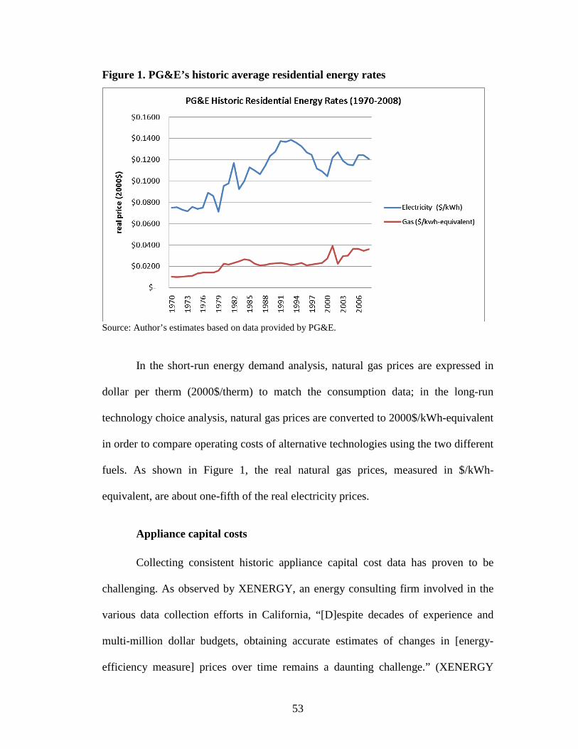
53

Figure 1. PG&E’s historic average residential energy rates

Source: Author’s estimates based on data provided by PG&E.

In the short-run energy demand analysis, natural gas prices are expressed in

dollar per therm (2000$/therm) to match the consumption data; in the long-run

technology choice analysis, natural gas prices are converted to 2000$/kWh-equivalent

in order to compare operating costs of alternative technologies using the two different

fuels. As shown in Figure 1, the real natural gas prices, measured in $/kWh-

equivalent, are about one-fifth of the real electricity prices.

Appliance capital costs

Collecting consistent historic appliance capital cost data has proven to be

challenging. As observed by XENERGY, an energy consulting firm involved in the

various data collection efforts in California, “[D]espite decades of experience and

multi-million dollar budgets, obtaining accurate estimates of changes in [energy-

efficiency measure] prices over time remains a daunting challenge.” (XENERGY

54

2001) For this analysis, historic capital cost curves are constructed for various

appliances based on a number of energy-efficient measure cost databases.28

The California Public Utility Commission (CPUC) and the California Energy

Commission maintain an online Database for Energy Efficient Resources (DEER)

with estimates on the capital, labor and installation costs of several hundreds of

residential and nonresidential energy technologies and conservation measures.

29 Two

waves of data from DEER are used in this analysis, DEER 2001 and DEER 2005.

The DEER cost estimates come from sources including manufacturers, wholesale

distributors, contractors, retail stores, websites, and utility program records

(XENERGY 2001, Itron 2005). The CPUC provided two earlier versions of the

database, Measure Cost Study 1992 and 1994 (XENERGY 1992 and XENERGY

1994). These earlier measure cost studies were conducted for similar purposes using

similar methodology. Costs are constructed for 1991, 1993, 2000 and 2003 and linear

extrapolations are used for other years.30,31

Due to the availability of technology cost data, the technology choice analysis

only includes choice decisions between 1990 and 2003 with the exception of space

heating equipment. The technology cost and efficiency estimates for space heating

and ventilation systems, obtained from two versions of the Energy Data Sourcebook

for the U.S. Residential Sector produced by the Lawrence Berkeley Laboratory

28 The analysis, which uses estimated appliance costs from the various sources, does not take into consideration potential rebates or discounts offered by retailers due to lack of data availability. 29 The latest data (2005 DEER and 2008 DEER) can be accessed via http://www.energy.ca.gov/deer/ 30 Considering the time lag between data collection and report publication, I assume a one-year lag in reported cost data. 31 Appliance ages are reported in intervals in the RASS (i.e., less than one year, one to three years, four to eight years, nine to thirteen years, fourteen to thirty years, and over 30 years), the middle year of an appliance age category is used to represent the value of technology cost. Specifically, data in years 2002, 2000, 1996, 1993, and 1991 are used.

55

(Hanford et al. 1994 and Wenzel et al. 1997), date back to 1980. The mean values of

cost estimates are used to represent the average cost of a category of appliances (e.g.,

a top-load washer and a gas tank water heater). Such a procedure matches the level of

detail of appliance holdings in the sample as only the broad category of appliance

ownership (e.g., front-load vs. top-load clothes washer, gas vs. electric tank water

heater) is reported. For water heating and space heating equipment, technology costs

are missing in some years. For these years, the appliance costs are extrapolated using

the rate of change in manufacturing costs in the Producer Price Index.

Annual appliance capital cost payments of an appliance are estimated based

on the average appliance lifetime and the interest rate at the time of purchase.

Specifically, I use the average of annual prime interest rates for time intervals by

which appliances purchases are recorded in the data. Table 2 below reports the

assumed appliance lifetimes used in the analysis.

Table 2. Assumed appliance lifetimes used in the analysis

Technology Appliance Type Average Lifetime (years)

Clothes washer 13

Clothes dryer 14

Water heater Tank 13

Water heater Tankless 20

Space heater Furnace 20

Space heater Other 18 Note: These estimates are derived from DEER 2005 and Wenzel et al. 1997.

Energy efficiency measures

The model developed in Chapter 3 assumes that the energy efficiency levels

of alternative technologies affect technology choice decisions and thus actual energy

use. Since only broad categories of appliance choices are observed, average energy

56

efficiency performance estimates for a given category of appliance stock provides the

best approximation for the specific appliance a household owns. A number of

household and market survey studies have estimated average energy efficiency levels

of existing appliance stock in California. For example, the California Statewide

Residential Lighting and Appliance Efficiency Saturation Study 2000 and 2005

(RLW Analytics 2001, RLW Analytics 2005) provide survey results of household

energy appliance ownerships, appliance capacity distributions and energy efficiency

estimates based on on-site home audits.

In addition, the Lawrence Berkeley Laboratory reports (Hanford et al. 1994

and Wenzel et al. 1997) developed energy efficiency estimates for major energy

technologies between 1972 and 1990. These studies are used to construct average

energy efficiency indicators for the various categories of appliances in the sample.

Fortunately, these studies, sponsored by the same utilities as the RASS, have similar

categories of appliances and the energy efficiency indicators are matched closely with

those in the subsample.

Average energy efficiency indicators are assigned to various space heaters

(gas or electric forced-air furnaces, floor or wall heaters, hot water radiators, electric

resistance systems, and heat pumps), water heaters (gas tank or tankless systems, and

electric tank or tankless systems), clothes washers (top-load and front-load washers)

and clothes dryers (gas and electric dryers). The energy efficiency indicators do not

distinguish potential differences in energy efficiency performance by appliance

vintage because such data were not available.

57

Given the potential measurement errors by using average energy efficiency

estimates, alternative treatments of appliance energy efficiency are tested in both the

short-run demand analysis and the long-run technology choice analysis. In the short-

run demand analysis, the model fit improves significantly when the energy efficiency

of clothes washers is modeled as a function of technology change and policy

interventions (i.e., energy efficiency standards and Energy Star Program). This is

mainly because the energy efficiency of clothes washers improved substantially over

the last two decades. To a lesser extent, statistical analysis shows that modeling the

energy efficiency levels of water heaters as a function of technology change is

preferred to using average energy efficiency estimates. In the short-run modeling, the

energy efficiency levels of clothes washers and water heaters are modeled explicitly

as a function of appliance age and policy interventions. Average energy efficiency

estimates are used for other energy appliances based on specification tests.

Similarly, the two alternative treatments of appliance energy efficiency are

tested in the long-run technology choice analysis, each representing different

perceptions of the energy efficiency performance of alternative technology choices at

the time of appliance purchase. Again, the model fits improve significantly when the

consumers’ energy efficiency perception is modeled as a function of some form of

technological change and policy variables such as energy efficiency standards and

information programs rather than using average energy efficiency estimates.

Arguably, consumers likely rely more on obvious signals about the energy

performance of appliance alternatives from energy labels such as through the Energy

Star program than estimates of the average energy efficiency of an appliance stock

58

such as provided by an energy analyst. The implications of the alternative modeling

of appliance energy efficiency are examined in Chapter 6.

In addition to the four specific energy services examined, the model also

includes a category of other energy use to represent all other energy services. Average

energy efficiency indicators are developed for these other electricity-consuming and

natural gas-consuming appliances. Natural gas, water heating, space heating and

clothes drying account for 93 percent of average natural gas consumption. The other

main gas-consuming energy service is cooking. I assign an energy factor of 0.5 for

the gas-using “other” services based on the average energy factor for gas stovetops in

Hanford et al. (1994). The main electricity-using services in the “other” category are

for lighting, refrigerators/freezers, office equipment, TVs, computers, air

conditioners, and spas. For electricity-using “other” services, I estimate a weighted

average energy efficiency factor of 0.44 based on shares of various energy uses and

estimates of energy factors in Hanford et al. (1994) and RLW Analytics (2005). I then

separately calculate the unit cost of energy output for “other” electricity-consuming

energy services (re,other) and “other” natural gas-consuming energy services (rg,other).

The unit cost of energy output for the “other” energy services category (rother) is the

weighted average of re,other and rg,other based on average household electricity and

natural gas consumption for these other energy uses.

Consumer expenditures

To derive relationships between household income and fixed payments,

regression analysis is undertaken using the Consumer Expenditure Survey (CES) of

59

the Bureau of Labor Statistics.32 A dataset of pre-tax income and expenditures is

constructed by pooling consumer units in different income groups between 1990 and

2002 reported in the CES tables.33

All income and expenditure data are converted to 2000 dollar value using the

Consumer Price Index. Figure 2 shows scatter plot of the pooled real income, total

expenditure, fixed payment variables, and expenditure of major appliances based on

the CES.

Income before taxes is used as the income

variable to match the income data in the sample. Annual fixed payments, including

for housing, vehicle purchase, and health care, are estimated. Fixed housing

expenditures distinguish between home owners and renters. Fixed payments for

owned dwelling include mortgage interest and charges, property taxes, maintenance,

repairs, insurance and other expenses; fixed payment for rented dwellings is the rent

reported. Fixed payments for vehicle purchase include net outlay of vehicle

purchases, finance charges, insurance, vehicle rental, leases, licenses, and other

charges. Health care costs include health insurance, medical services, drugs and

medical supplies.

As shown in Figure 2, expenditures and fixed payments appear to grow

relatively linearly with income for real income above $7,500 (2000$). For real

income lower than $7,500 (2000$), expenditures and income appear to have inverse

relationships.

32 Accessed via http://www.bls.gov/cex/csxstnd.htm. The average values for consumer units in each income group are treated as characteristics of a typical consumer unit (i.e., household). 33 The income groups include: less than $5,000, $5,000-$9,999, $10,000-$14,999, $15,000-$19,999, $20,000-$24,999, $25,000-$29,999, $30,000-$39,999, $40,000-$49,999, $50,000-$69,999, and $70,000 and more.

60

Figure 2. Scatter plot of income and expenditure using CES data (2000 dollars)

020

000

4000

060

000

8000

0

0 20000 40000 60000 80000 100000 120000income before tax

total expenditure fixed payments (own)fixed payments (rent) expenditure major appliances

The following quadratic linear regression model is thus hypothesized

(49) *2*2*10*_ nnnn eincomefincomeffpaymentfixed +++=

where fixed_paymentn* is the real fixed payment variables (i.e., for house owners or

renters, respectively) for consumer unit n*, incomen* is the real income before taxes

for consumer unit n*. The random variable en* is assumed to have mean zero and

variance 2eσ . Ordinary least square (OLS) of equation (49) are carried out using the

pooled data. OLS estimates of the coefficients would be unbiased and consistent if

assumption of the random variable holds.34

34 Equation (49) is also estimated using panel data methods (pooled OLS and pooled feasible generalized least square, with and without error correlation and autocorrelation). Results of estimated models are fairly consistent.

Estimated coefficients and standard errors

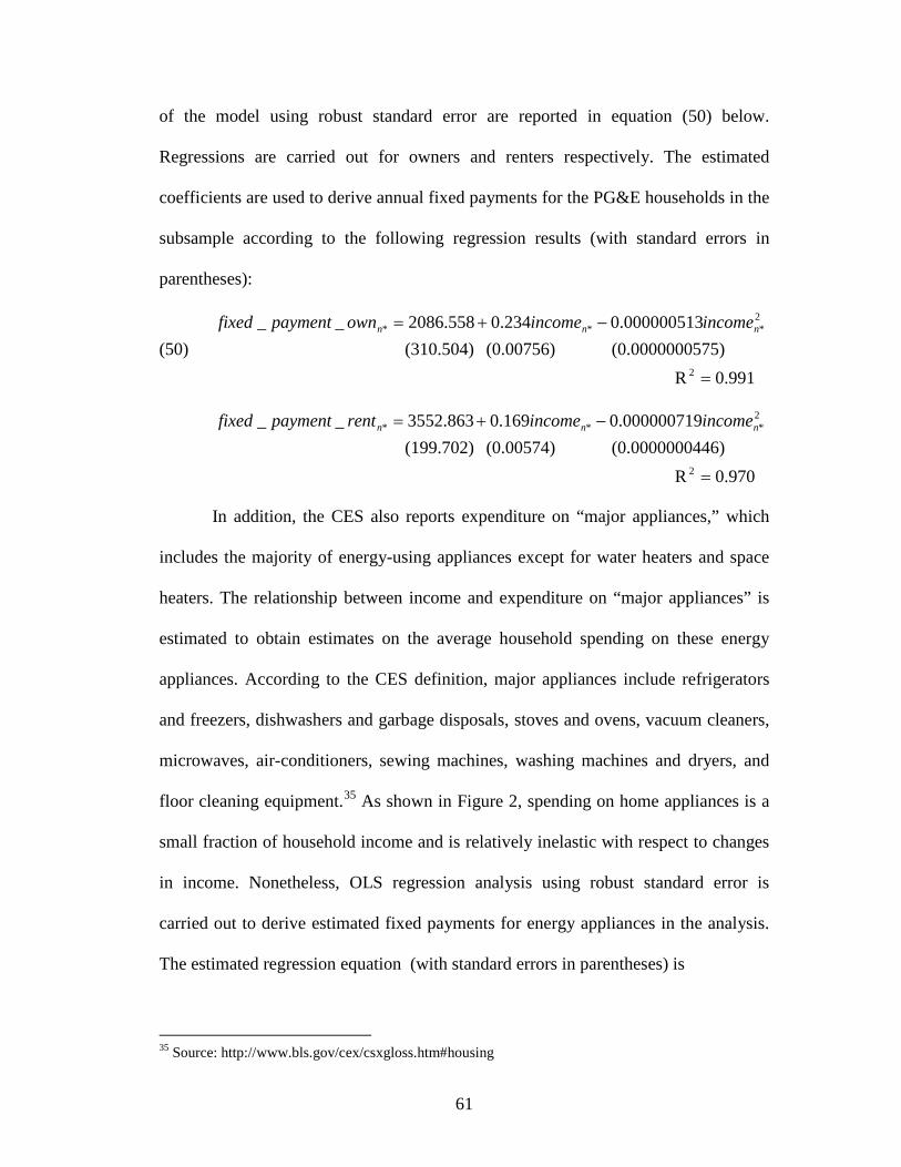
61

of the model using robust standard error are reported in equation (50) below.

Regressions are carried out for owners and renters respectively. The estimated

coefficients are used to derive annual fixed payments for the PG&E households in the

subsample according to the following regression results (with standard errors in

parentheses):

(50) 0.991R

575)(0.0000000 (0.00756) (310.504) 000000513.0234.0558.2086__

2

2***

=

−+= nnn incomeincomeownpaymentfixed

0.970R 446)(0.0000000 (0.00574) (199.702)

000000719.0169.0863.3552__

2

2***

=

−+= nnn incomeincomerentpaymentfixed

In addition, the CES also reports expenditure on “major appliances,” which

includes the majority of energy-using appliances except for water heaters and space

heaters. The relationship between income and expenditure on “major appliances” is

estimated to obtain estimates on the average household spending on these energy

appliances. According to the CES definition, major appliances include refrigerators

and freezers, dishwashers and garbage disposals, stoves and ovens, vacuum cleaners,

microwaves, air-conditioners, sewing machines, washing machines and dryers, and

floor cleaning equipment.35

35 Source: http://www.bls.gov/cex/csxgloss.htm#housing

As shown in Figure 2, spending on home appliances is a

small fraction of household income and is relatively inelastic with respect to changes

in income. Nonetheless, OLS regression analysis using robust standard error is

carried out to derive estimated fixed payments for energy appliances in the analysis.

The estimated regression equation (with standard errors in parentheses) is

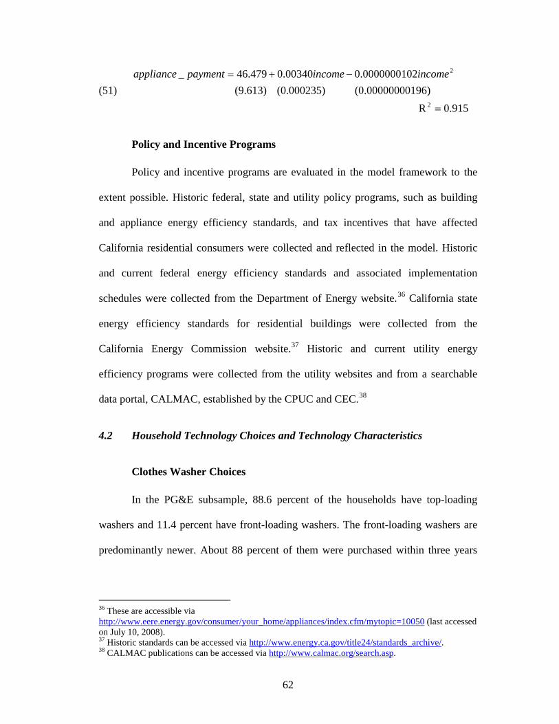
62

(51) 0.915R

0196)(0.0000000 (0.000235) (9.613) 0000000102.000340.0479.46_

2

2

=

−+= incomeincomepaymentappliance

Policy and Incentive Programs

Policy and incentive programs are evaluated in the model framework to the

extent possible. Historic federal, state and utility policy programs, such as building

and appliance energy efficiency standards, and tax incentives that have affected

California residential consumers were collected and reflected in the model. Historic

and current federal energy efficiency standards and associated implementation

schedules were collected from the Department of Energy website.36 California state

energy efficiency standards for residential buildings were collected from the

California Energy Commission website.37 Historic and current utility energy

efficiency programs were collected from the utility websites and from a searchable

data portal, CALMAC, established by the CPUC and CEC.38

4.2 Household Technology Choices and Technology Characteristics

Clothes Washer Choices

In the PG&E subsample, 88.6 percent of the households have top-loading

washers and 11.4 percent have front-loading washers. The front-loading washers are

predominantly newer. About 88 percent of them were purchased within three years

36 These are accessible via http://www.eere.energy.gov/consumer/your_home/appliances/index.cfm/mytopic=10050 (last accessed on July 10, 2008). 37 Historic standards can be accessed via http://www.energy.ca.gov/title24/standards_archive/. 38 CALMAC publications can be accessed via http://www.calmac.org/search.asp.

63

after 2000, compared to only 43 percent of top-loading washers purchased within the

same period.39

Front-loading washers are distinctively more energy efficient, consuming

about 40 percent less water per load and more than 60 percent less energy than top-

loading clothes washers (Natural Resources Canada 2005). According to a household

appliance energy efficiency survey conducted in California, in 2000 the average

energy efficiency level of existing front-loading washer stock was 3.95 measured by

energy factor (EF) whereas the average energy efficiency of existing top-loading

washer stock was 1.26 EF (RLW Analytics 2000). By 2005 the average energy

efficiency level of existing front-loading washer stock in California rose to 4.13 EF

and the average energy efficiency of existing top-loading washer stock declined to

1.22 EF (RLW Analytics 2005).

With higher efficiency performance, front-loading washers come with higher

upfront costs due to more electronics, more complicated motors, control and

suspension systems, and weight (DOE 2004).40

39 Before 1997, the energy-efficient front-loading clothes washers available were mostly European models that were considered small and expensive by American standards. Maytag and Frigidaire both introduced energy-efficient washers in 1997, which changed the market substantially. By 2001, there were 18 different manufacturers and 62 different models available on the market (Pacific Energy Associates, 2001).

Figure 3 below presents average

capital costs of the two alternatives used in the analysis. Cost difference between a

top-load washer and a front-load washer is in the range of $322 and $374 in real price

(2000$) between 1996 and 2004, consistent with industry sources that cite around

$350 of price difference.

40 Source: memo, “U.S. Department of Energy ENERGY STAR®

Criteria for Clothes Washer Meeting,” August 31, 2004.

64

Figure 3. Historic clothes washer capital costs used in the analysis

Source: Appliance cost estimates are based on several appliance and energy efficiency measure cost studies in California (XENERGY 1992, XENERGY 1994, DEER 2001, and DEER 2005).

Clothes washers are regulated under federal energy efficiency standards. The

Energy Policy and Conservation Act of 1975 directed the Department of Energy to

establish minimum energy efficiency standards for various home appliances,

including clothes washers. The first federal clothes washer standard and test

procedure were adopted in 1994, which requires a minimum energy factor of 1.18, in

terms of cubic feet per kilowatt-hour per cycle (cf3/kWh/cycle), for standard top-

loading clothes washers of 1.6 cubic feet or greater capacity.41

41 Clothes washer efficiency ratings are based on estimated annual energy use (kWh) under “typical conditions” and an average of 392 loads, or cycles, per year (source: Federal Registry, Vol. 66, No. 9, January 12, 2001, pp 3315).

The 1994 standard did

not specify a minimum energy efficiency level for front-loading washers except that it

required them to have an unheated rinse option.

65

The standard was updated on January 1, 2004 and the required minimum

energy efficiency level was revised to 1.04 modified energy factor (MEF) or higher.

The revised standard applies to both front-loading washers and top-loading washers

of 1.6 cubic feet or greater capacity. The standard was changed from “energy factor”

to “modified energy factor” to account for the amount of dryer energy used to remove

the remaining moisture content in washed items.42

Minimum energy efficiency standards change the menu of products offered in

the market (Newell et al. 1994). Voluntary, information-based labeling programs,

such as Energy Star, convey energy performance information of a product to

consumers. The Energy Policy Act of 1992 directs the U.S. Environmental Protection

Agency and the U.S. Department of Energy to establish voluntary Energy Star

programs that promote products more efficient than minimum federal or state codes.

On January 1, 2007, the standards

were revised to 1.26 MEF. The State of California has implemented the state

standards for clothes washers following the federal schedule and stringency levels.

43

42 Numerical measures of energy efficiency expressed in “energy factor” and “modified energy factor” cannot be directly compared.

In principle, the top 25 percent energy efficient products in the market are deemed

eligible for the label. The first Energy Star criteria for residential clothes washers

were established in 1997 which require a minimum energy factor of 2.5 compared to

the federal minimum standard of 1.18 EF. By 2001, the Energy Star criteria changed

to 1.26 MEF. Energy Star is moving toward more stringent criteria of a minimum

MEF of 2.0 and a maximum water factor of 6.0. If implemented, it would disqualify

every Energy Star-qualified top-loading model currently on the market and

43 Source: “ENERGY STAR Criteria for Clothes Washers: Overview of ENERGY STAR Criteria Setting Process and History of Clothes Washer Criteria.” A power point presentation by Richard H. Karney of the U.S. Department of Energy, August 31, 2004.

66

effectively force any consumer who desires an Energy Star qualified washer to

purchase a front-loading unit.44

Utilities in California have implemented incentive programs to encourage

adoption of energy-efficient clothes washers. The most popular incentive programs

are rebates. Rebates are only available for front-loading high efficiency washers

(Itron 2009). PG&E offers a $35 rebate for selected clothes washers with a minimum

MEF of 2.0 and a maximum WF of 6.0 and a $75 rebate for clothes washers with a

minimum MEF of 2.2 and maximum WF of 4.5. The San Diego County Water

Authority provides financial incentives to customers who purchase a high efficiency

washer with a maximum WF of 5.0. The program is co-funded by SDG&E and offers

a rebate of up to $185.

Water Heater Choices

Among households served by PG&E in the RASS dataset, 90.5 percent

reported to have a primary water heater. Among those households with primary water

heaters, 92.6 percent have natural gas tank (storage) systems, 4.6 percent have electric

tank (storage) systems, 1.8 percent have whole-house gas tankless systems, and 0.4

percent have solar systems with or without backup of a gas or electric tank. Other

water heater choices include propane tank systems (0.2%) and electric heat pump

(0.2%).45

44 Source: “Market Impact Analysis of Potential Changes to the ENERGY STAR

®

Criteria for Clothes Washers”, January 9, 2008.

45 In addition, 3.6 percent of the households reported to have a second water heater system of known type. The most frequently reported secondary water heaters are electric-based systems (e.g, electric tanks, heat pumps, point-of-use tankless systems, and whole house tankless systems) and the next group is solar-based systems. Since households choosing an additional water heater are a small fraction of the sample, the analysis focuses on the choices of primary water heaters.

67

The water heater technology choice analysis only considers three natural gas-

and electric-fueled technology alternatives due to the availability of historic capital

cost data: natural gas tank system, natural gas tankless system, and electric tank

system.46 The choice frequencies of these three alternatives are 95.6 percent, 1.3

percent, and 3.1 percent, respectively. These three alternatives represent over 99% of

household choices of the primary water heating system.47

According to household appliance energy efficiency surveys conducted in

2000 and 2005, majority of water heaters in California were 40 gallon tank systems

(RLW Analytics 2000 and 2005). The average energy efficiency, measured by energy

factor (EF), was 0.57-058 for gas tank systems and 0.89-0.90 for electric tank

systems. Gas tankless water heaters have significantly higher energy efficiency than

gas tank systems, with average energy factors in the range of 0.80-0.82 during the

study years. Studies show that energy efficiency for tank water heating systems had

changed modestly in the last few decades. In 1990, the shipment-weighted energy

factor was 0.55 for gas tank water heaters and 0.88 for electric tank water heaters

(Hanford et al. 1994 and Wenzel et al. 1997). Therefore, using average energy

efficiency levels from the recent surveys will unlikely introduce significant

measurement errors in the choice analysis.

With higher energy efficiency, the average purchase price of gas tankless

systems is significantly higher than that of the gas tank systems, by about $500-800

46 Analysis of household choices of solar heating systems is of interest given the energy and environmental benefits of solar energy. However, conversations with industry experts suggest that despite generous federal tax credits and various state and utility incentive programs, a mature solar hot water heater market does not yet exist in California or elsewhere in the U.S. 47 A formal test cannot reject the null hypothesis of independence of irrelevant alternatives (IIA) of the smaller set of alternatives included in the analysis, suggesting that omitting choice alternatives will unlikely alter the results significantly.

68

even though the price gap has reduced over time.48 The average installation cost of

gas tank water heaters is about $150 higher than the price for electric tank water

heaters. The average annual operating cost of tankless systems is about $100 lower

than that of gas tank systems and about $200 lower than that of electric tank

systems.49

The first federal water heater energy efficiency standards were implemented

in 1990 based on the size of water heater systems. The 1990 minimum standard was

0.54 EF for 40-gallon gas tank water heaters and 0.90 EF for 40-gallon electric water

heaters. The standards did not change till 2004 when the equivalent standards

tightened to 0.59 EF for gas tank water heaters and 0.92 EF for electric tank water

heaters. Energy Star criteria did not include water heaters until 2008.

The rates of changes in real water heating equipment manufacturing costs

in the Producer Price Index are used to calculate the equipment costs of water heater

alternatives. According to the Producer Price Index, the real value of electric water

heater manufacturing had decreased by 1 percent per year between 1990 and 2003.

The real value of natural gas water heater manufacturing had increased by 1 percent

per year between 1990 and 2003.

50

48 The higher cost of tankless products is partially offset by the federal Energy Incentives Act of 2005, which provides tax credits of up to $300 per unit for gas water heaters with EF ≥0.80.

The water

heater choice analysis covers the period from 1990 to 2003. Therefore, the effects of

water heater energy efficiency standards and Energy Star criteria cannot be identified.

49 Source: American Council for Energy-Efficient Economy (http://www.aceee.org/consumer/water-heating). 50 Press release “U.S. Department of Energy Implements Criteria for ENERGY STAR® Water Heaters”, U.S. Department of Energy, released on April 1, 2008.

69

The federal Energy Incentives Act of 2005 provides tax credits of up to $300

per unit for gas water heaters with energy factor greater than 0.80, which partially

offset the higher cost of tankless products.

Space Heating System Choices

Of the 7,295 PG&E households in the subsample, 7,053 households report a

primary space heating device. The primary space heating systems are predominantly

(90 percent) natural gas-based systems. Electricity-based systems account for about 8

percent of primary space heaters. A small percentage of primary space heaters (2

percent) are fueled by bottled gas, solar and wood. The PG&E subsample used in the

empirical estimation contains three electric- and natural gas-consuming space heating

technology choices: natural gas central forced-air systems (96.3 percent), natural-gas-

based radiator systems (0.4 percent), and electric central forced-air systems (3.3

percent).51 These three alternatives represent 74 percent of space heating system

choices among PG&E households.52

51 Nine electricity- or natural gas-based space heating technology choice alternatives are reported in the RASS data and are included in the short-run fuel demand analysis in the subsample. However, only five choice alternatives are included in the long-run technology choice analysis, of which three are natural gas-based systems (gas central forced-air furnaces, gas floor/wall heaters and natural gas radiator systems) and two are electricity-based systems (electric resistance systems and electric central forced-air furnaces). These five alternatives represent 95 percent of choices by PG&E households. The other four, of which three are electricity-based systems (central heat pumps, through-the-wall heat pumps and portable heaters) and one is a natural gas-based system (other natural gas system type), are excluded in the analysis due to the lack of reliable capital cost data. These four alternatives represent 3.3 percent of choices by PG&E households. When the observations with missing values for income, fuel consumption and household variables are removed (as explained in footnote 18), only the three choice situations described above remain. Because the excluded observations are removed for reasons unlikely to be related to space heating system choice, their exclusion likely does not cause any serious bias in the estimation results.

52 About 35 percent of the PG&E households with a primary space heating system also reported to have a secondary space heating device. The secondary heaters are predominantly wood-fired stoves or

70

The energy efficiency of space heating equipment is expressed as annual fuel

utilization efficiency (AFUE), a percentage of energy output per energy input.

Electric heating equipment is usually assumed to be 100 percent efficient (RLW

Analytics 2005). Based on appliance energy efficiency surveys conducted in

California, the average energy efficiency of gas-based central forced-air heating

equipment is 0.78 and the average energy efficiency of gas radiator systems is 0.80

(RLW Analytics 2000). In addition to the heating units, the three system choice

alternatives also involve heating distribution systems. According to Hanford et al.

(1994) and Wenzel et al. (1997), the average distribution efficiency of central forced-

air systems is estimated to be 0.7, and the hydronic radiator system is estimated to

have an average distribution efficiency of 0.9.

The average installation cost of a gas central forced-air heater is about $150-

200 (2000$) higher than an electric central forced-air heater. The average installation

cost of a radiator system is significantly higher, about $1500 (2000$) higher than a

gas central forced-air heater. In addition, the distribution system of a hydronic

radiator system costs about $1.22 more, on a per square foot basis, than the

distribution system of a central forced-air system. The rates of change in real space

heating equipment manufacturing costs in the Producer Price Index are used to

calculate the equipment costs of space heating alternatives over time. The Consumer

Price Index is used to calculate changes in installation costs.

fireplaces (45 percent) for which no data on wood consumption was available, followed by electric-based heaters (38 percent) and natural gas-based systems (12 percent). The remaining 5 percent of secondary heaters are bottled gas and solar-based systems.

71

Effective in 1990, the U.S. Department of Energy established minimum

energy performance standards for space heating furnaces and boilers. The standards

require that fossil-fueled warm-air furnaces must meet a minimum energy efficiency

of 0.78 AFUE and fossil-fueled boilers must meet a minimum energy efficiency of

0.80 AFUE.53

Energy-efficient heating furnaces and boilers are subject to financial

incentives. For example, currently, the federal government offers a tax credit of

$150for high-efficiency gas or oil-fired furnace with energy efficiency equal to or

above 0.95. The California state government offers rebates of up to $4,000 for system

upgrades including furnaces. PG&E offers $150-300 for energy-efficient central

natural gas heating units.

54

Clothes Dryer Choices

In the PG&E subsample, 40.9 percent of households have gas-fired clothes

dryers and 59.1 percent have electric-fired dryers. The energy performance of the two

types of clothes dryers is fairly similar. According to RLW Analytics (RLW

Analytics 2000), in California the average energy efficiency of gas-fired clothes

dryers is 2.67 measured by the energy factor (EF) and the average energy efficiency

of electric-fired clothes dryers is 3.01. As a result, clothes dryers are not included in

the U.S. Department of Energy’s minimum energy efficiency standards for home

appliances. The technology costs of the two clothes dryer alternatives are also fairly

similar. According to California technology cost data sources, on average, gas-fired

clothes dryers cost about $30 more than electric-fired clothes dryers. 53 Source: http://www.energysavers.gov/your_home/space_heating_cooling/index.cfm/mytopic=12530 54 Source: http://www.dsireusa.org

72

4.3 Conclusions

This chapter describes the available data and California household energy use

and technology choice characteristics. Notwithstanding a few weaknesses, this unique

dataset provides rich details for meaningful empirical investigation of household

energy use decisions pertaining to short-run energy demand and long-run technology

choices formulated in Chapter 3.

73

Chapter 5: Estimation Strategy

The discrete/continuous model developed in Chapter 3 consists of a system of

simultaneous equations with continuous demand and discrete choice endogenous

variables and a set of exogenous explanatory variables consisting of prices, income

and household characteristics. The maximum likelihood (ML) method is suitable to

obtain consistent and asymptotically efficient estimators for the set of parameters.

Estimation by ML can be implemented using two different approaches: limited

information maximum likelihood (LIML) and full information maximum likelihood

(FIML).

In principle, all the unknown parameters in the system of equations can be

estimated simultaneously using FIML. With LIML, equations are estimated

individually or in groups. One possible approach in this case is to use a two-step

procedure that first maximizes the likelihood function of the continuous demand

equations, and then maximizes the conditional log-likelihood functions of the discrete

choice equations using parametric estimates from the continuous demand model.

If the specification of all equations is correct, then LIML and FIML both yield

the same results asymptotically because both methods produce consistent estimators,

although FIML estimation is asymptotically efficient. If some part of the model is

incorrectly specified, however, then specification errors propagate through the system

with FIML estimation, possibly affecting all equations, and possibly making LIML

the more reliable of the two approaches, i.e., the adverse implications of a

74

specification error are confined to the particular equation in which specification error

is present.

Beyond the preference for estimation properties of LIML when some

specification error may exist in any particular equation, FIML is more complicated to

implement in practice in the case of discrete/continuous modeling. Greene (2008)

notes that it can be very complicated to derive the joint distribution since the

continuous and discrete variables come from different kinds of populations.55

Maximizing the joint log-likelihood can also be computationally costly or

infeasible particularly when a large number of coefficients are involved (Blanchard

1983). In addition, the normal equations may have multiple roots so that convergence

to the global maximum is not always guaranteed (Hanemann 1984). This is perhaps

why the two-step approach is more widely applied to evaluate discrete/continuous

models (e.g., Hausman 1979, Dubin and McFadden 1984, Vaage 2000, Newell and

Pizer 2005, and Mansure et al. 2005).

In some

cases, it is unclear theoretically what the joint distribution might be (Murphy and

Topel 2002).

56

The empirical estimation of the discrete/continuous model in this study also

adopts a two-step LIML approach. This system notably has a recursive structure

between the discrete and continuous components whereby energy consumption

depends on observed appliance choice but not vice versa. In this case, when

55 This is due to the fact that not all households make appliance choice decisions in every period as energy consumption. 56 Kline (1988) developed a model of household energy demand and technology choice for energy service (space heating) that jointly considers energy service production and consumption. Space heating production cost, expenditure share and demand equations are derived and estimated simultaneously using a 3SLS procedure.

75

disturbances are uncorrelated between the continuous and discrete components, the

LIML approach becomes asymptotically efficient aside from imposing common

parameter constraints. Furthermore, because the vast majority of observations on

appliance choice pertain to decisions made in a different time period, the assumption

of uncorrelated disturbances is well motivated. This yields a block recursive system

of equations in which blocks of equations can normally be estimated separately with

asymptotic efficiency.

The estimation procedure is implemented as follows. The first step estimates

the system of short-run demand equations conditioned on the current appliance stock

using the iterated feasible generalized nonlinear least squares (FGNLS) method to

produce asymptotically consistent estimators. With normally distributed disturbances,

estimates using iterated FGNLS are theoretically equivalent to ML estimates (Greene

2008). The technology choice equations are evaluated separately using the method of

ML to provide a benchmark without imposing any structural constraints. Because

choices of different appliances are made at different points in time, correlation among

the disturbances is likely minor if present at all, in which case separate estimation

does not sacrifice efficiency aside from ignoring parameter constraints among

equations.

Based on these results, estimates of the short-run demand system and the

long-run technology choices are compared to test applicability of structural parameter

constraints implied by the underlying utility maximization model. Thus, a second step

is implemented by imposing parametric constraints on technology choices implied by

76

parameters estimated in the short-run demand analysis in step one. The remaining

vector of parameters is estimated using the ML method.

The rationale for imposing the first-step estimates in the second step is as

follows. The parameters estimated in the first step (appliance use) appear only in

highly aggregated form in the second-step (appliance choice) model as is evident in

equation (34). Thus, the second-step estimation provides no information regarding the

individual parameters estimated in the first-step given aside from these aggregates.

Thus, even if a fully efficient estimation method incorporating parameter constraints

were feasible in practice, the impact of second-step information on the estimates of

parameters of the first-step model would likely be minor. Thus, I proceed by testing

applicability of the first-step estimates to the second-step model as a means of model

validation. The asymptotic covariance matrix derived in step two is corrected based

on the method developed by Murphy and Topel (2002). The following section details

the empirical procedure of the LIML estimation.

5.1 Step one: Estimating the Short-run Demand System

The system of short-run demand functions consist of three nonlinear budget

share equations for the numeraire, electricity, and natural gas. For household n,

equations (20) and (21) are rewritten as follows:

,ln21

*ln2ln2),( 05

0''''

5

0''

5

1'''''

0

5

1'

5

0''0''00

000, n

jnj

j jijjj

nj j

jijj

ndnn

r

yrβh µ

θβ

θββαµω +

Γ++

Γ+−+=+Χ=

∑∑∑

∑ ∑

== =

= =

77

(52) ,

ln21

]ln2ln2[)0(

),(

5

0''''

5

0''

5

1'''''

5

1'

5

0''

*''

5

1),(,

,

ne

jnj

j jijjj

jnj

jjjnijjjj

jjjen

nedneen

r

yrx

βh

µθβ

θββα

µω

+Γ++

Γ+−+>Ψ=

+Χ=

∑∑∑

∑ ∑∑

== =

= ==

,ln21

]ln2ln2[)0(

),(

5

0''''

5

0''

5

1'''''

5

1'

5

0''

*''

5

1),(,

,

ng

jnj

j jijjj

jnj

jjjnijjjj

jjjgn

ngdnggn

r

yrx

βh

µθβ

θββα

µω

+Γ++

Γ+−+>Ψ=

+Χ=

∑∑∑

∑ ∑∑

== =

= ==

where 0,nω is household n’s budget share for the numeraire good, en,ω is budget share

of electricity consumption, gn,ω is budget share of natural gas consumption,

),.( dn βh Χ denotes the nonstochastic, nonlinear portion of the demand functions,

nΧ is the vector of exogenous variables, dβ is the vector of coefficients of interest,

jα is constant associated with the jth energy service demand, jθ is household

variable that influences demand for the jth energy service,57

j = 0 is the numeraire good,

j = 0,..,5, where

j = 1 is clothes washing (cw),

j = 2 is water heating (wh),

j = 3 is clothes drying (cd),

j = 4 is space heating (sph), and

j = 5 is an index of all other energy services (oth).

All other notation is the same as defined in Chapter 3.

57 Inclusion of household variables is guided by the significance of specification tests.

78

The column vector of the system of short-run budget share equations for the

sample is

(53) .

),.(...

),.(

...

.

.11

N.

1.

+Χ

+Χ

=

=

NdN

d

βh

βh

µ

µ

ω

ω

ω

And the column vector of disturbances of the system is defined as

(54) , ...

N.

1.

=

µ

µ

µ

where µ has a multivariate normal distribution with mean vector zero and covariance

matrix Σ. The adding-up condition implies that Σ is singular and nondiagonal.

Therefore, one of the demand equations is dropped from the system to obtain

identification. In this case, the share equation for electricity, ωe, is dropped and the

remaining two share equations for the numeraire (ω0) and natural gas (ωg)

consumption are estimated. This specification fully utilizes constraints for the

translog system and estimates all parameters of the system directly, which provides

important identifying structure to the estimation.58

Seemingly unrelated regression (SUR) is appropriate for estimation of linear

systems when each equation includes only one endogenous variable. The underlying

58 Specification tests show that among different combinations using two of the three budget share equation specifications, the system of budget share equations for the numeraire and natural gas yields the highest log likelihood value, although all choices should yield the same asymptotic results.

79

theory for nonlinear estimation of systems of equations is similar to that for linear

systems (Greene 2008). Specifically, the generalized nonlinear least-squares system

estimator is defined as59

(55)

)}'.,X.({)},X.({minargˆ.

1

1. dnndn

N

nnβd βhβhβ

d−Σ−≡ −

=∑ ωω

An estimate of Σ is required to make the estimator feasible. The iterated procedure

first sets I=Σ̂ , which results in an inefficient but consistent estimator nlsdβ ,ˆ

of dβ .

Thus, residuals are

(56) ),ˆ,.(ˆ ,.. nlsdnnn β Xhu −= ω

and the covariance matrix is estimated by

(57) .ˆˆ1ˆ̂1

.'.∑

=

=ΣN

nnn uu

N

A new estimate dβ̂ is then obtained and the procedure is iterated until the relative

change in dβ̂ and Σ̂ is less than specified tolerance values. The variance-covariance

matrix of dβ̂ is

(58) ,)Xˆ̂X(V̂1

11'∑=

−−Σ=N

nnnd

and the robust covariance matrix estimator, rdV ,ˆ , is

(59) .Xˆ̂XXˆ̂ˆˆˆ̂XXˆ̂XV̂1

1

1'

1

1.

'.

1'1

1

1',

−

=

−

=

−−−

=

−

ΣΣΣ

Σ= ∑∑∑

N

nnn

N

nnnnn

N

nnnrd uu

59 The iterated feasible generalized nonlinear least square procedure outlined here is based on –nlsur- procedure for estimation of nonlinear systems of equations developed by Stata Corp.

80

The concentrated log-likelihood function for the two equations of N households is

(60) |}.ˆ|ln)2ln1(2{2

ln)(ln1

, Σ++−== ∑=

πNfβLN

ndnd

Iterated FGNLS yields a consistent maximum likelihood estimator dβ̂ of dβ , and the

associated robust covariance matrix ,d̂ rV .

5.2 Step Two: Estimating Energy Technology Choice Equations

Four separate energy technology choice equations are then estimated,

representing clothes washing, water heating, space heating and clothes drying.

Technology choice sets consist of two choice alternatives for clothes washing (cw)

and clothes drying (cd). Thus a binary logit choice model is appropriate. For water

heating (wh) and space heating (sph), three choice alternatives are involved in each

case so a multinomial logit choice model is appropriate. The binary choice model is a

special case of the multinomial logit choice model. The general procedure is thus

illustrated for the multinomial logit choice model.

The multinomial choice probability that alternative i is chosen by household n

from choice set Ij for energy use j is represented as

(61) ,)lnlnexp(

)lnlnexp(

' ,''0'

,0, ∑ ∈

Η++−

Η++−=

jIi njjijjiji

njijjijijnij ArAy

ArAyP

θθ

where j ={1,2,3, and 4} as defined in equation (52), and nj ,θ is the vector of

household variables included in the choice equation for energy use j. The model is

estimated using the method of maximum likelihood (ML) that maximizes the

likelihood function,

81

(62) ∏∏∏= ∈=

==N

n Ii

dnij

N

njnjc

j

nijPfβL1

,1

,, ,)(ln)( ,

where jc,β is the vector of multinomial choice parameters for energy use j, and nijd , is

an indicator variable equal to one if technology alternative i is chosen for energy use j

by household n and equal to zero otherwise. Equation (62) is transformed into a log-

likelihood function for ML estimation,

(63) .lnln)(1

,,1

,, ∑∑∑= ∈=

==N

n Iinijnij

N

njnjc

j

PdfβLL

The ML estimators of A0 and Aj from equation (63) are compared with the implied

parametric estimates derived from the short-run demand analysis in step one. With

the exception of the clothes washer choice equation, parametric estimates of A0 and Aj

are statistically equivalent between the short-run demand model and the three

equations of the long-run technology choice model for water heating, space heating

and clothes drying. This provides considerable validation of the underlying translog

indirect utility specification.

A second step of constrained estimation is then implemented by re-estimating

equation (61) by imposing parametric constraints on parameters A0 and Aj implied by

parameter estimates from the short-run demand model estimated in step one,

(64) ,)ˆlnˆlnexp(

)ˆlnˆlnexp(

' ,'.',0'

,,,0, ∑ ∈

Η++−

Η++−=

jIi njjinjjinji

njijnjijnijnij ArAy

ArAyP

θ

θ

where ∑∑∑== =

Γ++≡5

0''''

5

0''

5

1'''''',0

ˆlnˆ21ˆj

njj j

jjjn rA θβ and

njj

jjjjnj rA θβα Γ++≡ ∑=

ˆlnˆ2ˆˆ5

1''', are

the maximum likelihood estimators of common parameters A0 and Aj obtained from

82

step one. The vector of the remaining parameters, , ,c jβ is estimated, producing the

ML estimator of the parameters jc,β̂ and the associated ML estimator of the

covariance matrix of the parameters, jcV ,ˆ .

However, jcV ,ˆ

is not the appropriate estimator of the asymptotic covariance

matrix of jcβ ,ˆ without a correction that accounts for the covariance matrix estimator

d,rV̂ of dβ̂ . Following Murphy and Topel (2002), the following formula is used to

obtain the asymptotic covariance matrix of jcβ ,ˆ 60

(65)

{ }* ' ' ', , , , , , ,

1 ˆ ˆ ˆ ˆˆ ˆ ˆ ˆ ˆ ˆ ˆ ˆ ˆ- - ,c j c j c j j d r j j d r j j d r j c jV V V C V C R V C C V R VN

= +

where

,ˆln

ˆln1ˆ

1

,

,

,∑=

∂

∂

∂

∂=

N

n'd

jn

jc

jnj β

f

β

fN

C

.ˆ

lnˆ

ln1ˆ1

,

,

,∑=

∂

∂

∂

∂=

N

n'd

dn

jc

jnj β

f

β

fN

R

5.3 Conclusions

In the context of the discrete/continuous model developed in this study,

empirical application of the FIML approach has proven to be computationally

cumbersome and problematic. The main challenges stem from (i) the nonlinearity of

the system of short-run demand equations with a sizable number of coefficients, and

60 Murphy and Topel (2002) showed that a two-step approach without correcting for standard errors would vastly exaggerate the precision of the second step estimates. One of their examples also shows that standard errors from the two-step procedure are similar to those obtained from FIML estimation.

83

(ii) multicollinearity and singularities that result from demand aggregation of

individual energy services to match observed household fuel consumption data.

However, as shown in the subsequent chapter, the block recursive system approach

devised in this chapter proves to have strong statistical properties for three out of four

cases in which statistical tests do not invalidate parametric restrictions across blocks

of equations representing energy use and appliance choice.

84

Chapter 6: Estimation Results

This chapter presents the results of the empirical analysis of household energy

consumption and technology choices using the model developed in Chapter 3. Section

6.1 summarizes the results of the short-run demand analysis; Section 6.2 presents

results of technology choice analysis for clothes washing, water heating, space

heating and clothes drying, respectively; Section 6.3 synthesizes the findings.

6.1 Short-Run Energy Demand

The system of short-run budget share equations (52) is estimated by dropping

the electricity share equation. Among different combinations of budget share

equations and specifications, the system of budget share equations for the numeraire

and natural gas yields the highest log likelihood value. However, any combination of

two equations should yield the same asymptotic results because the specification fully

utilizes constraints for the translog system and estimates all parameters of the system.

Table 3 below presents the estimation results of four specifications using the

iterated feasible generalized nonlinear least squares (FGNLS) procedure. Model 1a

includes only price variables jrln , the income variable *ln y , and demand interaction

terms. Inclusion of demand interaction terms is guided by the features of energy

service demands and significance of statistical tests. Four demand interaction terms

are introduced: one between clothes washing and clothes drying, one between clothes

85

washing and water heating, one between water heating and the “other” energy use

category, and one between space heating and the “other” energy use category.61

Model 1b builds on Model 1a and adds household-demand interaction terms.

Inclusion of household and demand interaction terms is based on similar principles.

Four household and demand interaction terms are introduced, one between household

size and water heating, one between building square footage and space heating, one

between heating degree days and space heating, and one between the age of the house

and the “other” energy use category.

62

A log likelihood ratio test between Model 1a and Model 1b rejects the null

hypothesis that the household-demand interaction terms in the model are jointly zero

with a p-value less than 0.001, suggesting household variables—household size,

dwelling square footage, heating degree days and the age of dwelling in this

specification—influence household energy demand significantly.

Model 1c builds on Model 1b and instead of using average energy efficiency

indicators to derive the price variable for clothes washing, cwrln , it treats energy

efficiency of clothes washers as an estimable linear function of the energy efficiency

standards (“Standard”) and the EnergyStar information program (“EnergyStar”) aside

from an error term, i.e., ( ) 1 2 ( ) ( )ln Standard EnergyStar , ( ) 0,i cw i i i cw i cwe E eφ γ γ= + + =

where )()()()( lnln)/ln(ln cwicwlcwicwlcw ppr ϕϕ −== . Average energy efficiency indicators

61 Demand interaction between water heating the and “other” energy use category captures interactions between water heating and dishwashing; demand interaction between space heating and the “other” energy use category captures potential demand interaction between primary space heaters and secondary space heaters as 35 percent of households have a secondary space heating device. Secondary heating systems are not modeled explicitly due to the lack of technical specifics and are grouped in the “other” energy use category. 62 Inclusion of other demographic interaction terms, such as with ownership, was tested. Interacting ownership with various energy services is not statistically significant in explaining the short-run demand for fuel.

86

are used to derive the price variables for water heating, space heating, and clothes

drying.

Compared with Model 1b, the model fit of Model 1c improves significantly

with much higher log likelihood and R2 values with a p-value less than 0.001. The

results indicate potential measurement errors by using the average energy efficiency

of the clothes washer stock in the demand analysis. This is likely due to a substantial

improvement in energy efficiency performance of clothes washers over the past two

decades as a result of technology improvement and energy efficiency policy.

Changes in the energy efficiency performance of some other home appliances,

such as water heaters, has been modest during the same period. Nonetheless, a

specification test is performed to see whether use of average energy efficiency

indicators for water heaters is statistically equivalent to modeling energy efficiency of

water heaters as an estimable function of appliance age (Model 1d). In Model 1d, the

energy efficiency of water heaters is modeled a linear function of the age of water

heater (“age_wh”) and an error term, i.e., ,0)( ,age_whln )()(1)( =+= whiwhiiwhi eEeλϕ

The log likelihood ratio test between Model 1d and Model 1c suggests that modeling

energy efficiency of water heaters as a function of technology change is preferred to

using average energy efficiency indicators with a p-value of 0.021.63

Model 1d is used as the main specification for subsequent discussions and the

parametric estimates imposed in the second stage estimation of technology choice.

64

63 An additional specification test shows that using average energy efficiency indicators for space heating systems is not statistically different from explicitly modeling the energy efficiency of space heating systems with a p-value of 0.072. Thus, using average space heating energy efficiency indicators does not introduce significant measurement errors.

64 In the PG&E subsample, about 35.5 percent of households reported having a secondary heater, such as a portable electric heater, a fireplace, or a gas-fired floor or wall heater. The specifications reported

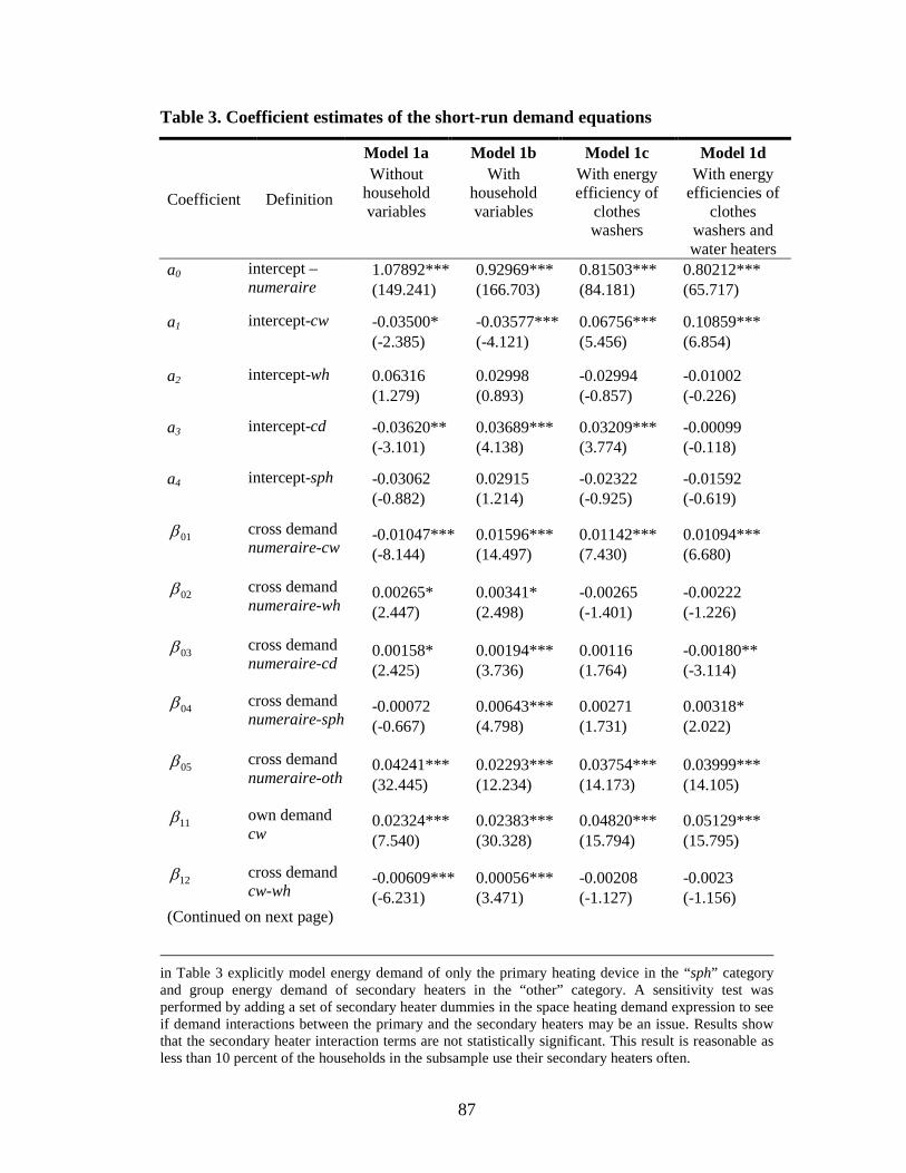
87

Table 3. Coefficient estimates of the short-run demand equations

Coefficient Definition

Model 1a Model 1b Model 1c Model 1d

Without household variables

With household variables

With energy efficiency of

clothes washers

With energy efficiencies of

clothes washers and water heaters

a0 intercept – numeraire

1.07892*** 0.92969*** 0.81503*** 0.80212***

(149.241) (166.703) (84.181) (65.717)

a1 intercept-cw -0.03500* -0.03577*** 0.06756*** 0.10859***

(-2.385) (-4.121) (5.456) (6.854)

a2 intercept-wh 0.06316 0.02998 -0.02994 -0.01002

(1.279) (0.893) (-0.857) (-0.226)

a3 intercept-cd -0.03620** 0.03689*** 0.03209*** -0.00099

(-3.101) (4.138) (3.774) (-0.118)

a4 intercept-sph -0.03062 0.02915 -0.02322 -0.01592

(-0.882) (1.214) (-0.925) (-0.619)

01β cross demand numeraire-cw

-0.01047*** 0.01596*** 0.01142*** 0.01094***

(-8.144) (14.497) (7.430) (6.680)

02β cross demand numeraire-wh

0.00265* 0.00341* -0.00265 -0.00222

(2.447) (2.498) (-1.401) (-1.226)

03β cross demand numeraire-cd

0.00158* 0.00194*** 0.00116 -0.00180**

(2.425) (3.736) (1.764) (-3.114)

04β cross demand numeraire-sph

-0.00072 0.00643*** 0.00271 0.00318*

(-0.667) (4.798) (1.731) (2.022)

05β cross demand

numeraire-oth 0.04241*** 0.02293*** 0.03754*** 0.03999***

(32.445) (12.234) (14.173) (14.105)

11β own demand

cw 0.02324*** 0.02383*** 0.04820*** 0.05129***

(7.540) (30.328) (15.794) (15.795)

12β cross demand

cw-wh -0.00609*** 0.00056*** -0.00208 -0.0023

(-6.231) (3.471) (-1.127) (-1.156)

(Continued on next page)

in Table 3 explicitly model energy demand of only the primary heating device in the “sph” category and group energy demand of secondary heaters in the “other” category. A sensitivity test was performed by adding a set of secondary heater dummies in the space heating demand expression to see if demand interactions between the primary and the secondary heaters may be an issue. Results show that the secondary heater interaction terms are not statistically significant. This result is reasonable as less than 10 percent of the households in the subsample use their secondary heaters often.

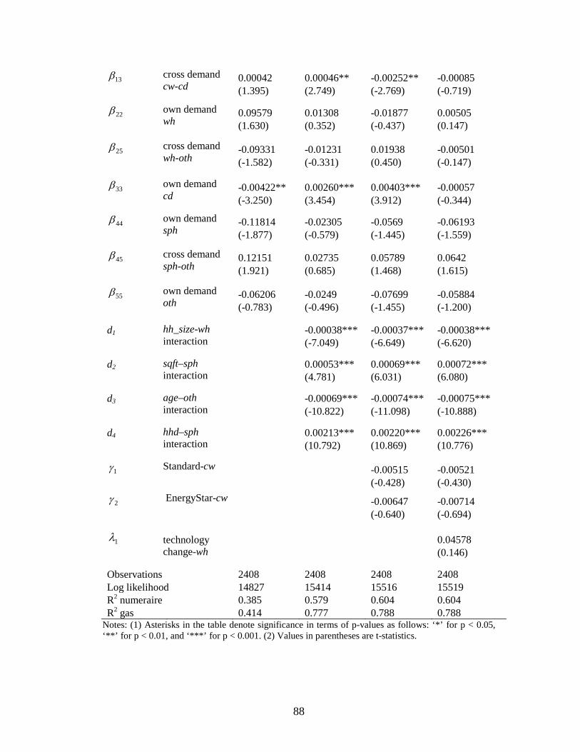
88

13β cross demand cw-cd

0.00042 0.00046** -0.00252** -0.00085

(1.395) (2.749) (-2.769) (-0.719)

22β own demand

wh 0.09579 0.01308 -0.01877 0.00505

(1.630) (0.352) (-0.437) (0.147)

25β cross demand

wh-oth -0.09331 -0.01231 0.01938 -0.00501

(-1.582) (-0.331) (0.450) (-0.147)

33β own demand

cd -0.00422** 0.00260*** 0.00403*** -0.00057

(-3.250) (3.454) (3.912) (-0.344)

44β own demand

sph -0.11814 -0.02305 -0.0569 -0.06193

(-1.877) (-0.579) (-1.445) (-1.559)

45β cross demand

sph-oth 0.12151 0.02735 0.05789 0.0642

(1.921) (0.685) (1.468) (1.615)

55β own demand

oth -0.06206 -0.0249 -0.07699 -0.05884

(-0.783) (-0.496) (-1.455) (-1.200)

d1 hh_size-wh interaction

-0.00038*** -0.00037*** -0.00038***

(-7.049) (-6.649) (-6.620)

d2 sqft–sph interaction

0.00053*** 0.00069*** 0.00072***

(4.781) (6.031) (6.080)

d3 age–oth interaction

-0.00069*** -0.00074*** -0.00075***

(-10.822) (-11.098) (-10.888)

d4 hhd–sph interaction

0.00213*** 0.00220*** 0.00226***

(10.792) (10.869) (10.776)

1γ Standard-cw

-0.00515 -0.00521

(-0.428) (-0.430)

2γ EnergyStar-cw

-0.00647 -0.00714

(-0.640) (-0.694)

1λ technology

0.04578

change-wh

(0.146)

Observations

2408 2408 2408 2408 Log likelihood 14827 15414 15516 15519 R2 numeraire 0.385 0.579 0.604 0.604 R2 gas

0.414 0.777 0.788 0.788

Notes: (1) Asterisks in the table denote significance in terms of p-values as follows: ‘*’ for p < 0.05, ‘**’ for p < 0.01, and ‘***’ for p < 0.001. (2) Values in parentheses are t-statistics.

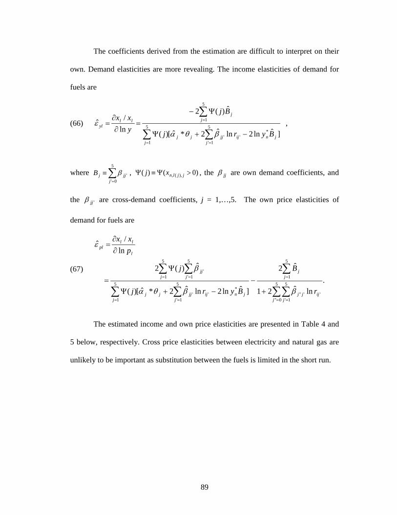
89

The coefficients derived from the estimation are difficult to interpret on their

own. Demand elasticities are more revealing. The income elasticities of demand for

fuels are

(66) ,]ˆln2lnˆ2*ˆ[)(

ˆ)(2

ln/ˆ

5

1'

*''

5

1

5

1 Byrj

Bj

yxx

jjnijjjjj

j

jj

llyl

∑∑

∑

==

=

−+Ψ

Ψ−=

∂∂

=βθα

ε

where ∑=

≡5

0''

jjjjB β , )0()( ),(, >Ψ≡Ψ jjlnxj , the jjβ are own demand coefficients, and

the 'jjβ are cross-demand coefficients, j = 1,…,5. The own price elasticities of

demand for fuels are

(67) .

lnˆ21

ˆ2

]ˆln2lnˆ2*ˆ[)(

ˆ)(2

ln/ˆ

5

0''

5

1'''''

5

15

1'

*''

5

1

5

1

5

1''

∑∑

∑

∑∑

∑ ∑

= =

=

==

= =

+−

−+Ψ

Ψ=

∂∂

=

j jijjj

jj

jjnijjjjj

j

j jjj

l

llpl

r

B

Byrj

j

pxx

ββθα

β

ε

The estimated income and own price elasticities are presented in Table 4 and

5 below, respectively. Cross price elasticities between electricity and natural gas are

unlikely to be important as substitution between the fuels is limited in the short run.

90

Table 4. Estimated short-run income elasticities of demand for fuels

Model Mean Standard Deviation Minimum Maximum

Electricity

Model 1a 0.0816 0.0843 -0.2623 2.1148

Model 1b 0.3436 0.0804 0.2560 0.8703

Model 1c 0.5032 0.0658 0.4267 1.0038

Model 1d 0.4182 0.1786 0.3189 1.6974

Natural Gas

Model 1a -0.0698 0.0358 -0.0933 0.1417

Model 1b -0.7127 0.2457 -0.9537 0.8085

Model 1c -0.3096 0.1201 -0.4029 0.4024

Model 1d -0.4201 0.1639 -0.5963 0.5113 Table 5. Estimated short-run price elasticities of demand for fuels

Model Mean Standard Deviation Minimum Maximum

Electricity

Model 1a 0.2533 0.1480 0.1538 2.8310

Model 1b -0.1313 0.0609 -0.5339 -0.0474

Model 1c -0.0641 0.0831 -0.7499 -0.0359

Model 1d -0.1343 0.1410 -1.0913 -0.0677

Natural Gas

Model 1a -0.2060 0.4769 -0.3311 2.8901

Model 1b -0.1473 0.1992 -0.2611 1.0758

Model 1c -0.1262 0.1107 -0.3432 0.6230

Model 1d -0.1188 0.1439 -0.1775 0.8373

As shown in Table 4, the mean estimates of income elasticity for electricity

are positive in all four specifications and less than unity. Model 1c yields the highest

average estimate (0.503) and Model 1a has the smallest mean estimates (0.082).

91

Model 1d, the preferred specification, has a mean estimated income elasticity of

0.418 for electricity and a range between 0.319 and 1.697. The maximum estimates of

income elasticity for electricity are greater than unity in three out of the four cases. As

expected, the results show that electricity is a superior good.

The estimated mean income elasticity for natural gas is consistently negative

in all four cases. However, in all four cases, income elasticities range widely over

both negative and positive values. For Model 1d, the mean estimate of income

elasticity for natural gas is -0.420 with a minimum value of -0.596 and a maximum

value of 0.511. These results suggest that natural gas is an inferior good for many

households, which is not surprising.

The mean estimates of own price elasticity for electricity are all negative

except for Model 1a (Table 5), the least preferred model. For Model 1d, the estimated

own price elasticity for electricity has a mean of -0.134 and a range between -1.091

and -0.068, which appears quite plausible. The mean estimates of price elasticity for

natural gas are consistently negative as they should be. Similar to estimates of income

elasticity for natural gas, however, the ranges of estimates among individual

households include both negative and positive values. In Model 1d, the estimate of

own price elasticity for natural gas has a mean of -0.119 and a range between -0.177

and 0.837, although very few households (3.3 percent) fall in the positive range.

Obtaining wrong signs for price elasticities for some households while

obtaining plausible signs as a mean is quite common with the translog specification.

In fact, being able to obtain negative own price elasticities for electricity demand for

92

all households and negative own price elasticities for natural gas demand for 96.7

percent of the households (by Model 1d) is quite exceptional.

Taylor (1975) reviewed the econometric literature on the demand for

electricity. Among the U.S. studies he reviewed, the short-run income elasticity

estimates ranged from 0.02 to 0.14. All the studies he cited used either state- or city-

level data. Using the U.S. state-level energy demand data, Maddala et al. (1997)

estimated average short-run income elasticities for electricity ranging from 0.137 to

0.429 and the short-run income elasticities for natural gas ranged from 0.048 to 0.307,

depending on the estimation approach used. Using household level expenditure data,

Branch (1993) estimated an average income elasticity of 0.23 for electricity. In an

analysis of energy demand among British households, Baker et al. (1989) estimated a

mean income elasticity of 0.131 for electricity and a mean income elasticity of 0.115

for natural gas.

Thus, the mean income elasticities for electricity demand estimated here are

not only consistent with theoretical expectations, but are also roughly in line with

previous econometric studies, although on the high end of the range of previous

estimates. The mean income elasticities for natural gas estimated here are negative

whereas the mean estimates in previous studies are positive. However, the range of

estimated income elasticities here is wide enough to include the mean estimates of the

previous studies referenced above. The difference in mean elasticities may be due to

the relatively high income status of households in the area of California served by

PG&E. For example, Baker et al. (1983) noted that the top decile of the income

distribution in their study has a small and negative median income elasticity for

93

natural gas demand. Overall, household demands for fuels are found to be fairly

inelastic with respect to income in the short run, as is expected given the fixed nature

of appliances in the short run.

Taylor (1975) reported short-run price elasticities for electricity in the range

of -0.13 and -0.90 among the studies he reviewed. Maddala et al. (1997) reported

short-run price elasticity estimates in the range of -0.158 and -0.214 for electricity

and -0.092 and -0.177 for natural gas. Examining nonlinear pricing structures, Reiss

and White (2005) estimated a mean annual electricity price elasticity of -0.39 for

California households. Aside from the Model 1a estimates for electricity demand, the

mean estimates of price elasticities for both electricity and natural gas reported here

are consistent with estimates in the literature, although the mean electricity price

elasticity is on the low end of estimates among other studies.

Reiss and White (1995) reported differences in estimated price elasticities for

different income groups among California households finding that lower income

households are more responsive to electricity price changes. In my analysis, the

estimated income and price elasticities based on Model 1d do not vary significantly

across different income groups or between home owners and renters even though the

model has the flexibility to represent such relationships.

6.2 Energy Technology Choices

Clothes Washer Choices

The binary logit model of clothes washer choices is estimated using the

method of maximum likelihood. Various specifications are tested in the first stage

analysis. Table 6 reports the estimation results of four specifications with a robust

94

covariance matrix estimator. Model cw1a and Model cw1b investigate two

specifications using average energy efficiency indicators to derive the expected

operating costs; Model cw2a and Model cw2b have the same sets of specifications

except that the perceived energy efficiency of the choice alternatives is modeled as a

function of the energy efficiency standards and the Energy Star program as in the

short-run demand analysis. The energy efficiency standards implemented during the

study period induced changes in the energy efficiency of clothes washers on the

market. The Energy Star program was launched in the middle of the study period.

These programs likely enhanced consumers’ awareness of energy performance of

clothes washers.

Model cw1a and Model cw2a evaluate the roles of the initial capital cost and

the expected operating cost of technology alternatives in clothes washer choices.

Variable ln_incCW is the negative of the logarithm of household income not already

committed to fixed payments minus the annualized capital costs between the choice

alternatives according to equation (61). In Model cw1a, the expected operating cost is

represented by the logarithm of the operating cost derived from average energy

efficiency indicators (ln_oCostCW). In Model cw2a, the expected operating cost

consists of three components: the logarithm of fuel price (ln_fuel), a dummy variable

representing the presence of clothes washer energy efficiency standards (Standard),

and a dummy variable representing the presence of clothes washer Energy Star

criteria (EnergyStar).

Model cw1b and Model cw2b add household variables to examine whether

household characteristics may have influenced clothes washer choices. Specifically,

95

three household variables are included: (1) the home ownership dummy (own), (2) the

household size (household size), and (3) a college education dummy (college). The

college education dummy is an instrument to represent consumers’ ability to

understand and interpret energy consumption and performance information pertaining

to home appliances.

A second step of constrained estimator is performed with the specification of

Model cw2b by imposing parametric constraints on the common variables (ln_incCW

and ln_fuel) based on coefficient estimates from the short-run demand model (Model

1d). Column 5 in Table 6 presents the results of the constrained estimation as Model

cw2b*.

As shown in Table 6, the coefficient of the household expenditure variable

that incorporates the initial cost of clothes washer alternatives (ln_incCW) is

significant across all specifications. The negative coefficient of ln_incCW suggests

that a reduction in the initial capital cost will increase the probability of front-loading

clothes washer adoption. (Recall that ln_incCW is the negative of household

expenditure minus the annualized capital cost of the clothes washer alternative.) The

expected operating cost, derived using average energy efficiency indicators (Model

cw1a and Model cw1b), also significantly influences clothes washer choices.

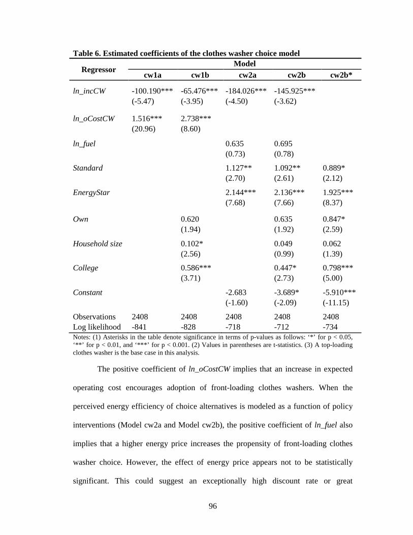
96

Table 6. Estimated coefficients of the clothes washer choice model

Regressor Model

cw1a cw1b cw2a cw2b cw2b*

ln_incCW -100.190*** -65.476*** -184.026*** -145.925*** (-5.47) (-3.95) (-4.50) (-3.62)

ln_oCostCW 1.516*** 2.738*** (20.96) (8.60)

ln_fuel 0.635 0.695 (0.73) (0.78)

Standard 1.127** 1.092** 0.889* (2.70) (2.61) (2.12)

EnergyStar 2.144*** 2.136*** 1.925*** (7.68) (7.66) (8.37)

Own 0.620 0.635 0.847* (1.94) (1.92) (2.59)

Household size 0.102* 0.049 0.062 (2.56) (0.99) (1.39)

College 0.586*** 0.447* 0.798*** (3.71) (2.73) (5.00)

Constant -2.683 -3.689* -5.910*** (-1.60) (-2.09) (-11.15)

Observations 2408 2408 2408 2408 2408 Log likelihood -841 -828 -718 -712 -734 Notes: (1) Asterisks in the table denote significance in terms of p-values as follows: ‘*’ for p < 0.05, ‘**’ for p < 0.01, and ‘***’ for p < 0.001. (2) Values in parentheses are t-statistics. (3) A top-loading clothes washer is the base case in this analysis.

The positive coefficient of ln_oCostCW implies that an increase in expected

operating cost encourages adoption of front-loading clothes washers. When the

perceived energy efficiency of choice alternatives is modeled as a function of policy

interventions (Model cw2a and Model cw2b), the positive coefficient of ln_fuel also

implies that a higher energy price increases the propensity of front-loading clothes

washer choice. However, the effect of energy price appears not to be statistically

significant. This could suggest an exceptionally high discount rate or great

97

uncertainty regarding future energy prices on the part of consumers when they make

their choices.

When the household perception of energy efficiency of alternative clothes

washer choices is modeled as a function of the energy efficiency standard and the

Energy Star program (Model cw2 in columns 3 and 4), the model fit improves

significantly compared to using average energy efficiency indicators, suggesting that

households’ formation of energy efficiency perceptions for clothes washers is more

likely influenced by information conveyed through energy efficiency standards and

Energy Star labels. The positive and significant coefficients for both the energy

efficiency standards and Energy Star program suggest that these policy interventions

have strong influences over the propensity of front-loading clothes washer adoption.65

The fitted probabilities from the various estimation specifications are

compared with the data. Table 7 below presents the predicted probabilities of Model

cw1a, Model cw1b, Model cw2a and Model cw2b. Compared with the data in the

sample, predicted probabilities also show that the specifications that model consumer

perception of energy efficiency as a function of policy variables fit the data much

better than using average energy efficiency indicators.

65 In the specifications reported in Table 6, dummy variables are used to indicate the presence of energy efficiency standards and the Energy Star program. Numerical values of the clothes washer energy efficiency standards and Energy Star criteria were also tested. A potential problem with this specification is the change of efficiency standards from using the “energy factor” to use of the “modified energy factor” during the study period. The two measures are not comparable. Regression results using the numerical values show that energy efficiency standards have a negative and significant effect in the choice of energy-efficient front-loading washers. These results were counter-intuitive and thus discarded.

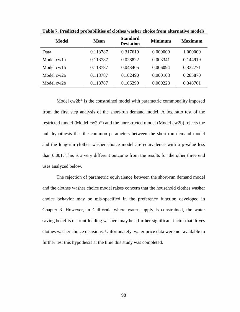
98

Table 7. Predicted probabilities of clothes washer choice from alternative models

Model Mean Standard Deviation Minimum Maximum

Data 0.113787 0.317619 0.000000 1.000000

Model cw1a 0.113787 0.028822 0.003341 0.144919

Model cw1b 0.113787 0.043405 0.006094 0.332771

Model cw2a 0.113787 0.102490 0.000108 0.285870

Model cw2b 0.113787 0.106290 0.000228 0.348701

Model cw2b* is the constrained model with parametric commonality imposed

from the first step analysis of the short-run demand model. A log ratio test of the

restricted model (Model cw2b*) and the unrestricted model (Model cw2b) rejects the

null hypothesis that the common parameters between the short-run demand model

and the long-run clothes washer choice model are equivalence with a p-value less

than 0.001. This is a very different outcome from the results for the other three end

uses analyzed below.

The rejection of parametric equivalence between the short-run demand model

and the clothes washer choice model raises concern that the household clothes washer

choice behavior may be mis-specified in the preference function developed in

Chapter 3. However, in California where water supply is constrained, the water

saving benefits of front-loading washers may be a further significant factor that drives

clothes washer choice decisions. Unfortunately, water price data were not available to

further test this hypothesis at the time this study was completed.

99

However, as shown in Table 6, estimated coefficients are fairly consistent

across specifications except for the common parameters.66

The Energy Star program emerges as the most significant factor influencing

the adoption of front-loading clothes washers, followed by energy efficiency

standards. Based on Model cw2b, the establishment of Energy Star criteria for clothes

washers increased the propensity of front-loading washer adoption by 17.4 percent. In

comparison, the establishment of energy efficiency standards for clothes washers

increased front-loading clothes washer adoption by 8.4 percent. The propensity of

front-loading washer adoption is 7.4 percent higher for a home owner than a renter. A

household with at least a college education is 6.5 percent more likely to adopt a front-

loading washer.

Household characteristics

are found to play a role in the choice decisions. Specifically, having a college

education positively and significantly influences the choice of front-loading clothes

washers. Home ownership also positively influences the choice of front-loading

washers. However, the significance of this effect varies by specification. In addition,

having a larger household size appears to favor adoption of top-loading clothes

washers, possibly due to preference for the larger capacity of top-loading washers

over the more compact front-loading washers. But the effect of household size is not

significant except for specification Model cw2b.

On the other hand, the economic factors are found to be less significant factors

influencing clothes washer choice decisions. Model cw2b provides insights on the

effects of economic factors. The estimated coefficients imply that a $100 reduction in

66 Since the parametric commonality is rejected, the coefficient interpretation focuses on Model_cw2b specification.

100

the purchase cost of front-loading washers (e.g., through appliance rebates) on

average would increase the propensity of its adoption by 0.5 percent. A $50 income

tax credit for the purchase of energy-efficient front-loading washers on average

would increase its adoption by 1 percent. Although the coefficient is statistically

significant, the estimated impacts of an income tax credit and capital cost reduction

are minimal, especially compared with the Energy Star program and energy

efficiency standards. A 20 percent increase in the electricity price would increase the

front-loading washer choice propensity by 0.5 percent. Again, the price effect is

found to be statistically insignificant.

Water Heater Choices

The multinomial logit model of water heater choices illustrated in equation

(61) is also estimated using the method of maximum likelihood. Table 8 reports three

specifications. Model wh1a evaluates the effect of a household expenditure term that

incorporates the initial capital cost of water heaters and the effect of expected

operating cost of alternative water heaters. Two variables are included in Model

wh1a: the negative of the logarithm of household income not already committed to

fixed payments minus annualized capital costs of water heater choice alternatives

(ln_incWH), and the logarithm of the expected operating costs of technology

alternatives using average energy efficiency indicators (ln_oCostWH). Since the

energy efficiency of water heaters has only changed moderately during the study

period, using average energy efficiency indicators of the alternative water heater

stock is likely a reasonable proxy for consumers’ perceptions of water heater

alternatives.

101

Model wh1b adds household variables to test the significance of household

characteristics in determining water heating technology choices. Three household

variables are included: the home ownership dummy (own), the household size

(household size), and the college education dummy (college).

A second step constrained estimation is carried out by imposing parametric

constraints from the short-run demand analysis on Model wh1b. Results of the

constrained estimation are presented in column 3 of Table 8 as Model wh1b*.

A log likelihood ratio test between the constrained model (Model wh1b*) and

the unconstrained model (Model wh1b) cannot reject the null hypothesis of

parametric equivalence between the short-run demand model and the long-run water

heater choice model with a p-value of 0.297. The parametric equivalence between the

short-run demand model and water heater choice model suggests that the theoretical

model developed in Chapter 3 is robust as common parameters explain both

consumer water heater choice behavior and short-run use behavior.

In contrast to the clothes washer choice analysis, the household expenditure

variable (ln_incWH) is not a statistically significant determinant of water heater

choices.67

The expected operating cost (ln_oCostWH) is also a statistically

insignificant predictor of water heater choices.

67 Another set of unreported specification tests shows that when the expenditure variable ln_incWH is separated into two terms (the log of income not already committed to fixed payments and the log of the capital cost of technology alternatives), the model fit does not change significantly and both the income variable and capital cost variables are statistically insignificantly.

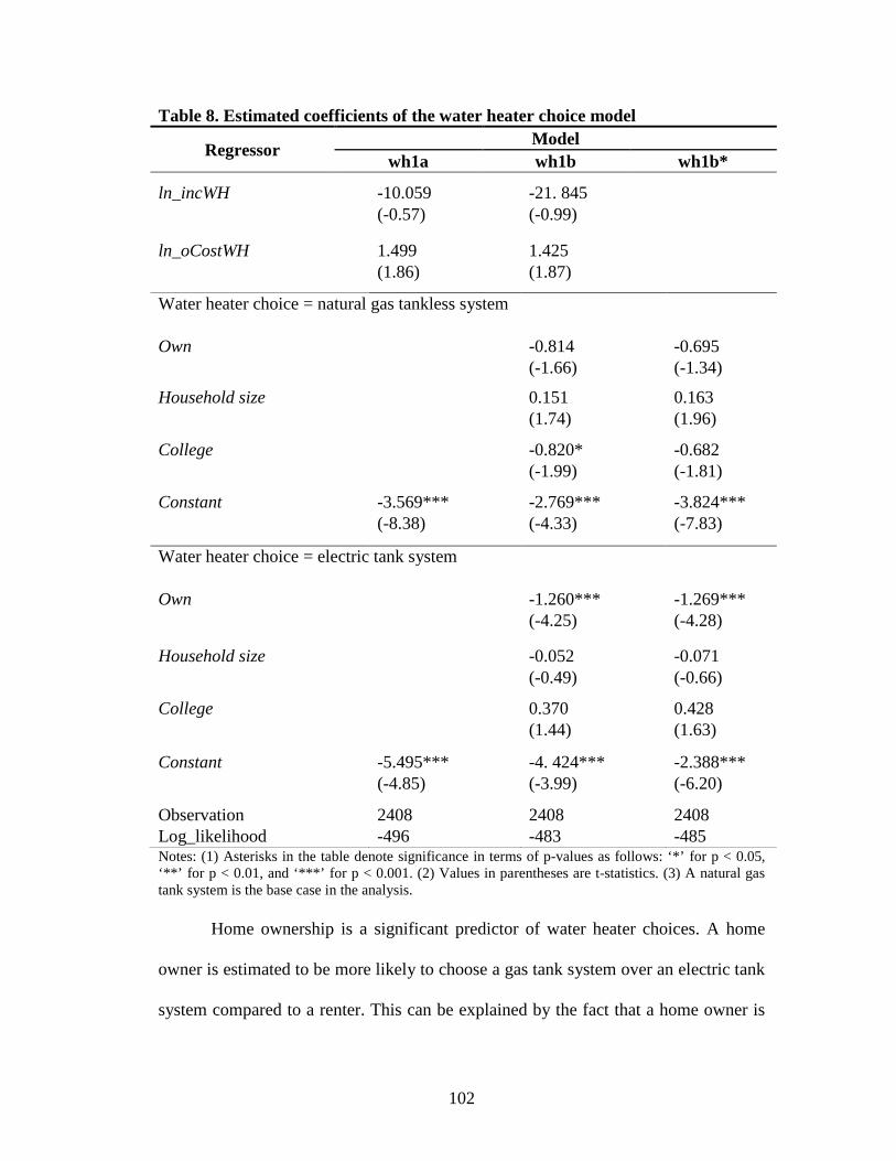
102

Table 8. Estimated coefficients of the water heater choice model

Regressor Model wh1a wh1b wh1b*

ln_incWH -10.059 -21. 845 (-0.57) (-0.99)

ln_oCostWH 1.499 1.425 (1.86) (1.87)

Water heater choice = natural gas tankless system Own -0.814 -0.695 (-1.66) (-1.34)

Household size 0.151 0.163 (1.74) (1.96)

College -0.820* -0.682 (-1.99) (-1.81)

Constant -3.569*** -2.769*** -3.824*** (-8.38) (-4.33) (-7.83)

Water heater choice = electric tank system Own -1.260*** -1.269*** (-4.25) (-4.28)

Household size -0.052 -0.071 (-0.49) (-0.66)

College 0.370 0.428 (1.44) (1.63)

Constant -5.495*** -4. 424*** -2.388*** (-4.85) (-3.99) (-6.20)

Observation 2408 2408 2408 Log_likelihood -496 -483 -485 Notes: (1) Asterisks in the table denote significance in terms of p-values as follows: ‘*’ for p < 0.05, ‘**’ for p < 0.01, and ‘***’ for p < 0.001. (2) Values in parentheses are t-statistics. (3) A natural gas tank system is the base case in the analysis. Home ownership is a significant predictor of water heater choices. A home

owner is estimated to be more likely to choose a gas tank system over an electric tank

system compared to a renter. This can be explained by the fact that a home owner is

103

more likely to pay for the operating cost of water heater usage than a renter. Along

this line of thinking, one would expect that a home owner is more likely to choose a

tankless system than a tank system, which has much lower operating cost. The

regression results show that a home owner is less likely to choose a tankless gas

system over a tank system, but the estimated coefficient is statistically insignificant.

Furthermore, the logistics as well as high cost of retrofitting an existing home with a

tankless system may be an important deterrent.

The college education dummy is also a significant explanatory variable for

water heater choices. A household with at least a college education is also more likely

to choose a natural gas tank water heater over a tankless system but more likely to

choose an electric tank system over a natural gas tank system, although only the

former relationship is statistically significant. Larger household sizes tend to choose a

tankless system over a natural gas tank system and a natural gas tank system over an

electric tank system, but neither estimated effect is statistically significant.

The results of the water heater choice analysis should be interpreted with

some caution. Due to data availability, the analysis evaluates household choices

among broad categories of water heater systems, rather than choices among different

brands and models of a technology. Thus, energy efficiency performance may vary

widely within these groups. The weak predictability of the expenditure and operating

cost variables likely reflects the fact that the decision regarding the water heating

system may not be made by consumers but rather depend heavily on an earlier stage

of building construction. Once pipes and other infrastructure are installed, households

are less likely to change, say, from a gas tank system to a tankless system than from a

104

less efficient tank system to a more efficient tank system, because such a system-wide

change involves a major renovation effort, which can be costly.68

Space Heating System Choices

The logistics as

well as the high cost of retrofitting an existing home with a tankless system may be an

important deterrent.

The multinomial logit model of space heating choices is evaluated similar to

the water heater choice model. Table 9 reports the results of three specifications.

Similar to water heater choice model, Model sph1a evaluates the logarithm of

household expenditure, which incorporates the capital costs of choice alternatives

(ln_incSPH) and the logarithm of the expected operating costs of technology

alternatives using average energy efficiency indicators (ln_oCostSPH). Using average

energy efficiency estimates is reasonable in this case as the energy efficiency of space

heating systems did not change dramatically during the study period. Model sph1b

includes household variables to detect whether housing and household characteristics

influence space heating technology choices. Four household variables are included:

(1) the home ownership dummy (own), (2) age of the house (house age), (3) historic

mean heating degree days between 1985 and the year of system installation

(hdd_mean), and (4) the college education dummy (college).

A second step constrained estimation is also carried out by imposing

parametric constraints from the short-run demand analysis on Model sph1b. The

constrained results (Model sph1b*) are reported in Column 3 of Table 9.

68 Unfortunately, data on retrofitting cost from a tank water heating system to a tankless water heating system was not available.

105

Table 9. Estimated coefficients of the space heating system choice model

Regressor Model sph1a sph1b sph1b*

ln_incSPH -3.083 -4.576 (-0.78) (-1.62)

ln_oCostSPH 0.430 0.310 (0.91) (0.65)

Space heater choice = natural gas radiator Own -1.038 -0.964 (-1.36) (-1.21) House age -0.258 -0.259 (-0.68) (-0.78)

Hdd_mean 2.881** 2.861* (2.60) (2.39)

College -0.198 -0.106 (-0.31) (-0.16)

Constant -5.244*** -11.413*** -11.726*** (-13.97) (-3.35) (-3.43)

Space heater choice = electric central forced-air system Own -0.050 -0.054 (-0.12) (-0.13)

House age 0.285** 0.291** (3.08) (3.16)

Hdd_mean -0.322 -0.368 (-0.78) (-0.84)

College -0.528* -0.517* (-2.28) (-2.24)

Constant -3.955*** -3.105* -2.566* (-6.14) (-2.38) (-2.19)

Observation 2408 2408 2408 log_likelihood -412 -400 -399 Notes: (1) Asterisks in the table denote significance in terms of p-values as follows: ‘*’ for p < 0.05, ‘**’ for p < 0.01, and ‘***’ for p < 0.001. (2) Values in parentheses are t-statistics. (3) A natural gas central forced-air system is the base case in this analysis.

106

A log likelihood ratio test between the constrained model (Model sph1b*) and

the unconstrained model (Model sh1b) cannot reject the null hypothesis of parametric

equivalence between the short-run demand model and the long-run space heater

choice model with a p-value of 0.634. Again, the parametric equivalence between the

short-run demand model and space heater choice model suggests that the theoretical

model developed in Chapter 3 is robust in as an explanation of both consumer space

heater choice behavior and short-run energy demand.

Similar to the water heater choice analysis, the household expenditure

variable, which incorporates annualized capital cost of the technology alternatives

(ln_incSPH) and the expected operating cost (ln_oCostSPH) are found not to be

significant determinants of space heating technology choices.

On the other hand, the age of dwelling and average heating degree days

significantly influence space heating system choices. Older houses are more likely to

have an electric central forced-air heating system than a natural gas central forced-air

system, and are less likely to have a natural gas-based radiator system, although only

the former relationship is statistically significant. This former effect seems plausible

given the fact that natural gas had gained popularity over time with its cost-

effectiveness as a residential fuel source. This effect represents the impact of

increasing energy consciousness with rising energy prices. In areas where the heating

load is higher (as reflected in higher heating degree days), a hydronic gas-based

radiator system is preferred over a central forced-air system, probably because of the

higher energy efficiency performance of radiator systems, and thus the lower

operating cost. Electric central force-air systems are less preferred in colder areas, as

107

one would expect, but the estimated effect is not statistically significant. In addition, a

college education is estimated to be a significant predictor of space heating system

choices whereby a natural gas forced-air system is preferred over an electric forced-

air system.

The household education level is estimated to be a significant predictor of

space heating system choices while home ownership is not. This is likely due to the

fact that the decision regarding the type of space heating system in a home is an

integral part of building design and construction. Thus, a home owner would have a

weaker role in the decision making unless involved in the original construction. In

contrast, the two types of housing that dominate the PG&E area of California are the

older homes that are beyond their first owner and the more recent large-scale

developments of builders. Thus, energy technology durables such as space heating

and water heating equipment are likely heavily determined by developers if not the

more aged housing stock.

While one might argue that a developer would tailor these choices to potential

buyers’ preferences, a home buyer likely will weigh other attributes of a house (such

as location and size) more heavily than the type of space heating system. The

significance of college education in choosing a natural gas space heating system over

an electricity-based space heating system, on the other hand, suggests that a

household with better ability to interpret energy performance information of different

energy systems is more likely to make a rational choice of the system that has lower

operating cost.

108

Clothes Dryer Choices

Similar to the clothes washer choice analysis, a binary logit model of clothes

dryer choices is evaluated using the method of maximum likelihood. Table 10 reports

the estimation results. Model cd1a evaluates the negative of the logarithm of

household expenditure which incorporates the capital costs of choice alternatives

(ln_incCD) and the logarithm of the expected operating costs of technology

alternatives assuming average energy efficiency indicators (ln_oCostCD). Again,

average energy efficiency estimates of the clothes dryer choice alternatives are seen

as reasonable to represent consumers’ perception of energy efficiency as the energy

performance of clothes dryers had not changed significantly during the study period.

Model cd1b includes household variables. Three household variables are included:

(1) the home ownership dummy (own), (2) household size (household size), and (3)

the college education dummy (college).

A second step constrained estimation is carried out by imposing parametric

constraints from the short-run demand analysis on Model cd1b. The results (Model

cw1b*) are reported in Column 3 of Table 10.

In this case, the log likelihood ratio test of parametric equivalence between the

short-run demand model and the long-run clothes dryer choice model can be mildly

rejected at the 10 percent level but cannot be rejected at more conservative levels of

1, 2, or 5 percent. The p-value is 0.051.

One possible mis-specification of the clothes dryer choice model has to do

with the electricity voltage in the laundry area of a dwelling. Most electric dryers

operate on 240-volt current, twice the strength of ordinary household current. If the

109

laundry area is not equipped with a 240-volt outlet, one either has to choose a natural

gas clothes dryer or install a 240-volt outlet in order to run an electric clothes dryer. If

natural gas service is already available, a household might choose a gas clothes dryer

over reconfiguration of the electricity outlet, especially if the home is not equipped

with a 240-volt service panel as is the case with many older homes. Unfortunately,

the electricity voltage data are not available to be included in the model for further

tests.

Table 10. Estimated coefficients of the clothes dryer choice model

Regressor Model cd1a cd1b cd1b*

ln_incCD -333. 829* -165.752 (-2.51) (-1.21)

ln_oCostCD 0.604 -0.087 (0.87) (-0.12)

Own -0.430** -0.471** (-2.65) (-2.92)

Household size -0.106*** -0.111*** (-3.51) (-3.98)

College -0.029 -0.080 (-0.32) (-0.92)

Constant -0.636 1.138 1.155 (-0.61) (1.01) (6.34)

Observations 2408 2408 2408 Log likelihood -1624 -1615 -1618 Notes: (1) Asterisks in the table denote significance in terms of p-values as follows: ‘*’ for p < 0.05, ‘**’ for p < 0.01, and ‘***’ for p < 0.001. (2) Values in parentheses are t-statistics. (3) A gas-fired clothes dryer is the base case in this analysis.

Comparing results of Model cd1b with Model cd1a shows that household

characteristics are significant predictors of clothes dryer choices. Home owners are

more likely to choose a gas-fired clothes dryer than an electric clothes dryer. A

110

household with more members is more likely to choose a gas clothes dryer than an

electric clothes dryer. Even though the operating cost variable turns out to be

statistically insignificant in the analysis, one may still reach the conclusion that the

significant coefficients of ownership and household size suggest that the operating

cost of clothes dryer usage is taken into consideration when making clothes dryer

choices.

The negative coefficient on the expected operating cost (ln_oCostCD)

suggests that when the expected operating cost increases a household is more likely to

choose a gas-fired clothes dryer over an electric-based dryer. This result is sensible.

However, similar to the analyses of water heater choices and space heating

technology choices, the household expenditure variable which incorporates

annualized capital cost of technology alternatives (ln_incCD) and the expected

operating cost (ln_oCostCD) are not significant determinants of clothes dryer choices.

In addition, in the case of clothes dryer choices, a household’s education level

does not appear to be a significant factor influencing technology choice decisions.

6.3 Conclusions

This chapter presents an empirical application of the household energy

demand and technology choice model developed in Chapter 3 by estimating the short-

run household demand for electricity and natural gas and the long-run technology

choices of clothes washers, water heaters, space heating systems, and clothes dryers

among California households.

The empirical analysis shows that the discrete/continuous model based on the

second-order translog indirect utility function is fairly robust across energy forms and

111

appliance choices in explaining household energy consumption and technology

choice behavior. With the exception of parametric estimates in the clothes washer

choice model, the parameters obtained from the short-run demand analysis are

statistically equivalent to the parameters obtained in the long-run technology choice

model, although weakly so for clothes drying. The non-equivalence of parametric

estimates in the clothes washer choice model is likely due to the omission of water

price and water efficiency in the clothes washer choice model. These are potentially

important factors influencing clothes washer choices in the water scarcity conditions

of California. For clothes dryer choices, a potentially important unobserved factor

influencing choices between a natural gas clothes dryer and an electric-based clothes

dryer is the presence of 240-volt service.

The mean short-run income and price elasticities of energy consumption

derived from the short-run demand model are all in reasonable ranges. A few of the

price elasticities of natural gas demand of individual households are implausible

ranges but no more than typically obtained with the flexibility of the translog model.

Technology choice analysis of the four energy uses shows varying effects of

technology capital cost, expected operating cost, and household characteristics. The

policy implications of the empirical findings are discussed in the following chapter.

112

Chapter 7: Policy Implications for Household Energy Efficiency

Findings from the empirical analysis using the unified modeling framework of

discrete technology choice and continuous energy consumption have important

implications for policy design aimed to reduce greenhouse gas emissions and improve

energy efficiency in the residential sector.

7.1 Energy-efficient Technology Adoption

Household-level energy durable choice decisions have long-lasting impacts on

energy consumption and greenhouse gas emissions as major home appliances

typically have lifetimes from ten to twenty years. The diffusion rates of apparently

cost-effective energy efficiency investments are often low. This phenomenon is

referred to as the “energy paradox.”

This study confirms two important market failures with respect to household

energy technology choice behavior: the principal/agent problem and information

imperfection. Home ownership appears to significantly influence household choices

of some energy durables, suggesting that policy programs targeting residential energy

efficiency should carefully distinguish the principal decision makers and

appropriately differentiate market segments. For instance, ownership is found to be a

significant factor influencing the choices of clothes washers, water heaters and

clothes dryers, but is not a significant determinant of space heating system choices,

which have longer life. Unlike home appliances such as clothes washers, decisions for

113

home-wide systems such as for space heating and cooling are more complex and are

often made as an integral part of building design and construction. Once the system is

determined, retrofitting can be expensive. In the situation of home-wide system

choices, policy intervention should thus be best designed to target developers and

contractors, such as through building codes.

In the case of clothes washer choices, the voluntary, information-based

Energy Star program emerges as the most significant factor influencing adoption of

energy-efficient front-loading clothes washers, followed by energy efficiency

standards. The establishment of Energy Star criteria for clothes washers produces an

average increase in the propensity of energy-efficient front-loading clothes washers

by 17 percent. The presence of energy efficiency standards is predicted on average to

increase the propensity of front-loading washers adoption by 8 percent. The results

suggest that policy programs aimed at providing energy technology performance

information are highly effective in promoting the adoption of energy-efficient

technology at the household level as these programs likely reduce consumers’ search

cost. In fact, they may override cost considerations that are highly uncertain at the

point of decision making in the store.

Surprisingly, the financial incentives for energy-efficient appliances, such as

through popular federal income tax credits or federal and state rebate programs, are

found to be far less effective in influencing the adoption of energy-efficient

appliances. For instance, a $100 reduction in the purchase cost of energy-efficient

front-loading washers increases the propensity of front-loading clothes washer

adoption by only 0.5 percent. Perhaps consumers who take advantage of such

114

programs have a priori preferences for energy efficiency, so that financial incentives

only provide a windfall to such consumers. In the case of water heater and space

heating system choices, the capital cost of technology alternatives appear to be an

insignificant determinant of technology choices, suggesting that changes in the

relative cost of energy-efficient technologies would have limited impacts on their

adoption.69

Furthermore, contrary to the claim that incentives for the adoption of new

technologies is greater under market-based instruments than under direct regulation

(e.g., by Jaffe et al. 2003), this empirical study finds that market-based policy

instruments, such as a carbon cap-and-trade programs or carbon taxes which induce

energy price changes, have limited impacts on energy-efficient technology adoption

decisions at the household level. For instance, a 20 percent increase in energy

(electricity) price increases the propensity of front-loading washer adoption by only

2.5 percent.

Given their popularity, these financial incentive programs and their cost-

effectiveness should be carefully examined.

The 20 percent increase in electricity price represents the estimated long-run

electricity price increase that might be due to a carbon cap-and-trade program under

the proposed HR 2454 bill (the American Clean Energy and Security Act of 2009,

also referred to as the “Waxman-Markey Bill”). This effect appears to be insignificant

69 However, it should be pointed out that the technology choice analyses for water heating and space heating examine the choices among broad categories of technology systems (e.g., a tank water heater versus a tankless system), rather than choices among different brands and models of a technology that have varying energy efficiency performance. Further, the absence of statistical significance of cost variables in these cases may be largely due to the minor differences in costs among technologies even though consumers may respond to more substantial cost variation. Inference about incentive policy based on these results should be made carefully.

115

and much smaller than the effects of energy efficiency standards or information-based

programs such as the voluntary Energy Star program.

7.2 Short-run Household Energy Efficiency

The study finds that in the short-run, energy price-induced household energy

efficiency is moderate. According to the analysis, the average price elasticity is -0.13

for electricity and -0.12 for natural gas. Therefore, a 20 percent increase in the

electricity price on average would reduce its consumption by 2.6 percent; a 20 percent

increase in the natural gas price on average would reduce its consumption by 2.4

percent. These results are reasonable given estimates and conventional wisdom that

implies household energy demand is highly inelastic in the short run.

The short-run demand analysis also highlights the importance of using

accurate estimates of appliance energy efficiency in energy demand modeling. The

energy efficiency level of household energy durables affects the amount of energy

consumed by a household to meet energy service demands. Very often, the energy

efficiency of home appliances is unknown. At best, modelers and researchers rely on

market surveys with estimates of the average energy efficiency of the appliance stock.

In this study, two alternative representations of appliance energy efficiency are tested

for clothes washers and water heaters. The first approach uses average energy

efficiency indicators of energy technology based on market surveys. The second

approach assumes household appliance energy efficiency is unobserved and explicitly

models energy efficiency as a function of technological change and possible policy

interventions such as energy efficiency standards. Compared to the survey data on

average energy efficiency, embedding this causal model of energy efficiency

116

improves model fit for clothes washers and water heaters significantly, producting

higher R2 and log likelihood values, and suggesting potential measurement errors by

using average energy efficiency data on the appliance stock.

117

Chapter 8: Conclusions

Residential consumer energy consumption is a critical aspect of energy and

climate change policy and an important application of consumer theory. This study

develops an internally consistent theoretical framework that can be used for practical

analysis of various aspects of household energy use behavior.

8.1 Summary and Main Contributions

This study develops a unified discrete technology choice and continuous

demand model (the “discrete/continuous model”) which can be used to examine

household short-run energy consumption and long-run technology choice behavior.

The model, derived from underlying utility maximization using a second-order

translog indirect utility function, provides a transparent and cohesive structure with

considerable flexibility to investigate consumer preferences and the role of economic

factors, household characteristics, and policy interventions in household energy use

and technology choice decisions.

An empirical application of the model is carried out using a rich and unique

micro-level energy consumption and appliance holdings dataset of California

households. I estimate the household short-run demand for electricity and natural gas

and long-run technology choices for four energy uses—clothes washing, water

heating, space heating, and clothes drying—using the modeling framework.

118

Results of the empirical analysis show that the discrete/continuous model

developed in this study is quite robust in explaining household energy consumption

and technology choice behavior across energy forms and appliance choices. Income

and price elasticities derived from the short-run analysis appear to be sensible and

within the range of estimates documented in the literature. With the exception of the

clothes washer choice model for which misspecification is a potential concern, the

estimated parameters from the short-run demand analysis are all statistically

equivalent to the parameters obtained in the long-run technology choice model

(weakly so for clothes drying), validating the appropriateness of the modeling

framework for both the continuous and discrete choices.70

This study is the first known application of the second-order translog flexible

functional form or of any second-order flexible form to energy demand analysis that

encompasses both discrete and continuous choices in a unified parametric structure.

This model addresses several unique features of consumer energy use and allows

analysis of demand interactions, demand aggregation, and fuel substitution.

In addition, the model extends the existing discrete/continuous models (e.g.,

Dubin and McFadden 1984) by modeling demands for multiple fuels and technology

choices for different categories of energy uses. Existing studies mostly deal with

demand for a single fuel (e.g., electricity or natural gas) and technology choices for a

single energy use. The joint modeling of demand for both electricity and natural gas

70 Parametric equivalence is rejected for the expenditure variable in the clothes washer choice model. The non-equivalence of the parameter between the short-run demand model and the long-run choice model for clothes washers is likely due to a misspecification of the clothes washer choice model by omitting the water price and water efficiency of alternative clothes washer choices, which are significant factors that potentially drive clothes washer choices in California.

119

permits the identification of tradeoffs both in the short run and the long run as well as

between short-run and long-run considerations.

Another unique contribution of this study is the empirical insights that allow

evaluation of the effectiveness of energy and environmental policy instruments (e.g.,

the market-based carbon cap-and-trade program, energy technology performance

standards, financial incentives, and information programs) in encouraging residential

short-run and long-run energy efficiency.

8.2 Future Research

Several assumptions used in the model and analysis can be relaxed and tested.

First, the analysis assumes that consumers form expectations of future operating costs

of energy technology alternatives based on the current energy prices. Preliminary

analysis suggests that households may indeed have some form of price expectations

while making energy durable choices. This assumption can be further investigated

empirically by introducing more general expectation mechanisms in the model

structure.

Second, the analysis assumes that consumers respond to average energy prices

in making both short-run energy use and long-run technology choice decisions. The

assumption is made partially due to data limitations. If actual household energy tariffs

and billing data are available, this assumption can be tested. Nonlinear pricing for

energy is an important feature of energy demand in most applications. The empirical

120

evidence of consumer response to marginal versus average energy prices is mixed and

worth further investigation.

Third, research that utilizes the full information maximum likelihood

approach to estimate discrete/continuous models remains an unconquered empirical

challenge. Like most existing studies, this study adopts a two-step limited information

maximum likelihood approach. Despite the merits of the second-order translog

flexible functional form of consumer preference functions, estimation of the system

of demand functions is computationally cumbersome and problematic due to

nonlinearity of the likelihood function. In this study, the typical problem of

nonlinearity is further complicated by multicollinearity when energy uses by

appliance type are not observed and must be aggregated for estimation. A structural

approach that estimates the entire system of equations with full information is a

challenge, but is worth further pursuit, particularly if energy uses by appliance types

can be observed.

Fourth, the clothes washer choice model rejects the parameter commonality

between the short-run demand model and the long-run choice model for clothes

washers. One possible explanation is the omission of effective water price and water

efficiency of alternative clothes washers, which is possibly a significant issue in

California. The specification could be further investigated by including representation

of water cost if appropriate data can be identified.

121

Bibliography Aigner, D.J., C. Sorooshian, and P. Kerwin. 1984. “Conditional demand analysis for estimating residential end-use load profiles.” Energy Journal 5(3), 81-97. Anderson, S.T., and R.G. Newell. 2002. Information Programs for Technology Adoption: The Case of Energy-Efficiency Audits, Resources for the Future RFF Discussion Paper 02-58. Washington DC. Archibald, R.B., D.H. Finifter and C.E. Moody Jr. 1982. “Seasonal variation in residential electricity demand: evidence from survey data.” Applied Economics 14, 167-181. Baker, P., R. Blundell, J. Michlewright. 1989. “Modelling Household Energy Expenditures Using Micro-Data,” The Economic Journal 99(397): 720-738 Balestra, P., and M. Nerlove. 1966. “Pooling gross section and time series data in the estimation of a dynamic model: the demand for natural gas.” Econometrica 34(3), 585-612. Barnes, R., R.G. Gillingham, and R. Hagemann. 1981. “The short-run residential demand for electricity.” The Review of Economics and Statistics 63(4), 541-552. Berndt, E.R., M.N. Darrough, and W.E. Diewert. 1977. “Flexible functional form and expenditure distributions: an application to Canadian consumer demand functions.” International Economic Review 18(3), 651-75. Birol, F., editor. 2008. World Energy Outlook. The International Energy Agency. Paris, France. Blanchard, L. J. 1983. “The Production and Inventory Behavior of the American Automobile Industry.” Journal of Political Economy 91(3): 365-400. Branch, E. 1993. “Short run income elasticity of demand for residential electricity using consumer expenditure.” Energy Journal 14(4): 111. Cambridge Systematics, Inc. et al. 1994. Customer Decision Study: Analysis of Commercial Customer Equipment Purchase Decisions. Final report prepared for Southern California Edison Company. 128 pp. Cameron, T.A. 1985. “A Nested Logit Model of Energy Conservation Activity by Owners of Existing Single Family.” The Review of Economics and Statistics 67(2): 205-211.

122

Dagsvik, J.K., Lorentsen, L., Olsen, Ø., Strøm, S., 1987. “Residential demand for natural gas: a dynamic discrete-continuous choice approach.” In: Golombek, R., Hoel, M., Vislie, J. (Eds.), Natural Gas Markets and Contracts. North Holland Publishing Company, Amsterdam. Davis, L.W. 2008. “Durable goods and residential demand for energy and water: evidence from a field trial.” RAND Journal of Economics 39(2), 530-546. Deaton, A. and J. Muellbauer. 1980. Economics and consumer behavior. Cambridge: Cambridge University Press. DeCanio, S.J. 1998. “The efficiency paradox: bureaucratic and organizational barriers to profitable energy-saving investments.” Energy Policy 26(5): 441-454. Diewert, W.E. 1971. “An Application of the Shephard Duality Theorem: A Generalized Leotief Production Function.” Journal of Political Economy LXXIX (May/June): 481-507. Diewert, W.E. 1973."Separability and a Generalization of the Cobb-Douglas Cost, Production, and Indirect Utility Functions," Technical Report 86, IMSSS, Stanford University, CA. Dubin, J.A., and D.L. McFadden. 1984. “An econometric analysis of residential electric appliance holding and consumption.” Econometrica 52(2): 345-362. Frieden, B.J., and K. Baker. 1983. “The Market Needs Help: The Disappointing Record of Home Energy Conservation.” Journal of Policy Analysis and Management 2(3): 432-448. Goulder, L.H., I.W Parry, R.C. Williams III, and D. Burtraw. 1999. “The Cost-Effectiveness of Alternative Instruments For Environmental Protection in a Second-Best Setting.” Journal of Public Economics 72(3): 329–360. Greene, W. H. 2008. Econometric Analysis (6th Edition). Pearson Prentice Hall. NJ. Grewal, D. and H. Marmorstein. 1994. Market Price Variation, Perceived Price Variation, and Consumers' Price Search Decisions for Durable Goods. The Journal of Consumer Research 21(3): 453-460. Griliches, Z. 1957. “Hybrid Corn: An exploration in the economics of technical change.” Econometrica 48:501-522. Halvorsen B., and B.M. Larsen. 2001. “Norwegian residential electricity demand – a microeconomic assessment of the growth from 1976 to 1993.” Energy Policy 29(3): 227-236.

123

Hanford, J.W., J.G. Koomey, L.E. Stewart, et al. 1994. Baseline Data for the Residential Sector and Development of a Residential Forecasting Database. A report of the Lawrence Berkeley Laboratory, University of California. Berkeley, CA. 179 pp. Hanemann W.M. 1984. “Discrete/continuous models of consumer demand.” Econometrica 52(3), 541-561. Hartman R.S. 1983. “The Estimation of Short-Run Household Electricity Demand Using Pooled Aggregate Data.” Journal of Business & Economic Statistics 1 (2): 127-135. Hartman, R.S., and A. Werth. 1981. “Short-run residential demand for fuels: a disaggregated approach.” Land Economics 57(2), 197-212. Hassett, K.A. and G.E. Metcalf. 1993. “Energy conservation investment: Do consumers discount the future correctly?” Energy Policy 21(6): 710-16. Hassett, K.A. and G.E. Metcalf. 1995. “Energy tax credits and residential conservation investment: Evidence from panel data.” Journal of Public Economics 57: 201-17. Howarth, R.B. and A.H. Sanstad. 1995. “Discount rates and energy efficiency.” Contemporary Economic Policy 13(3): 101-109. Howarth, R.B., B.M. Haddad, and B. Paton. 2000. “The Economics of Energy Efficiency: Insights from Voluntary Participation Programs.” Energy Policy 28: 477–86. Houston, D. 1983. “Implicit Discount Rates and the Purchase of Untried, Energy-Saving Durable Goods.” The Journal of Consumer Research 10(2): 236-246. Ito, K. 2010. Do Consumers Respond to Marginal or Average Price? Evidence from Nonlinear Electricity Pricing. Job Market Paper. University of California, Berkeley, CA. 55pp. Jaffe, A. B., and R. N. Stavins. 1994. “The Energy Paradox and the Diffusion of Conservation Technology.” Resource and Energy Economics 16(2): 91–122. Jaffe, A.B., R.G. Newell, and R.N. Stavins. 1999. Energy-Efficient Technologies and Climate Change Policies: Issues and Evidence. John F. Kennedy School of Government Faculty Research Working Papers Series, Harvard University, Cambridge, MA. Jaffe, A.B., R.G. Newell, and R.N. Stavins. 2003. “Technological Change and the Environment.” Chapter 11 in the Handbook of Environmental Economics, Volume 1, Edited by K.-G. Maler and J.R. Vincent. Elsevier Science B.V. 461-516.

124

KEMA-XENERGY, Itron, and RoperASW. 2004. California Statewide Residential Appliance Saturation Study Final Report. Consultant Report no. 400-04-009, prepared for the California Energy Commission. Kline, Y. 1988. “An Econometric Model of the Joint Production and Consumption of Residential Space Heat.” Southern Economic Journal 55(2): 351-359. Koomey, J.G. 1996. Trends in Carbon Emissions from U.S. Residential and Commercial Buildings: Implications for Policy Priorities. LBNL-39421. Lawrence Berkeley National Laboratory, Berkeley, CA. 20pp. LaFrance, J., and W.M. Hanemann. 1989. “The dual structure of incomplete demand systems.” American Journal of Agricultural Economics 71, 262-74. Levine, M.D., A.H. Sanstad, E. Hirst, J.E. McMahon, and J.G. Koomey. 1995. "Energy Efficiency Policy and Market Failures." In Annual Review of Energy and the Environment 1995. Edited by J. M. Hollander. Palo Alto, CA: Annual Reviews, Inc. Maddala, G.S., R.P. Trost, H. Li, and F. Joutz. 1997. “Estimation of Short-Run and Long-Run Elasticities of Energy Demand From Panel Data Using Shrinkage Estimators.” Journal of Business & Economic Statistics 15(1): 90-100. Mansure, E.T., R. Mendelsohn, and W. Morrison. 2008. “Climate change adaptation: A study of fuel choice and consumption in the US energy sector.” Journal of Environmental Economics and Management 55(2): 175-193. McFadden, D.L. 1974. “Conditional logit analysis of qualitative choice behavior.” In Frontiers in Econometrics. New York: Academic Press. Murphy and Topel, 2002. “Estimation and Inference in Two-Step Econometric Models.” Journal of Business & Economic Statistics 3(4), 370-379. Reprinted, 20, 2002, 88-97. Nesbakken, R. 2001. “Energy consumption for space heating: a discrete-continuous approach.” Scand. J. of Economics 103(1), 16-184. Newell, R.G., A.B. Jaffe, and R.N. Stavins. 1999. “The Induced Innovation Hypothesis and Energy-Saving Technological Change.” Quarterly Journal of Economics 114 (3): 941-975. Newell, R.G., and W.A. Pizer. 2008. “Carbon mitigation costs for the commercial sector: discrete-continuous choice analysis of multifuel energy demand.” Resource and Energy Economics 30(4): 527-539.

125

Nyboer J. and C. Bataille. 2000. Energy Equipment Purchasing Behavior: A Review of the Literature. Canadian Industrial Energy End-use Data and Analysis Centre, Simon Fraser University. 33 pp. Parry, I., D. Evans, and W.E. Oates. 2010. Are Energy Efficiency Standards Justified? Resources for the Future Discussion Paper 10-59. Washington DC. Parti, M., and C. Parti. 1980. “The total and appliance-specific conditional demand for electricity in the household sector.” The Bell Journal of Economics 11, 309-321. Pacala S. and R. Socolow, 2004. “Stabilization Wedges: Solving the Climate Problem for the Next 50 Years with Current Technologies.” Science 305 (5686): 968 – 972. Pollak, R.A. 1969. “Conditional Demand Functions and Consumption Theory.” The Quarterly Journal of Economics 83 (1), 60-78. Pollak, R.A., and T.J. Wales. 1992. Demand System Specification and Estimation. Oxford: Oxford University Press. Quigley, J.M. 1984. “The production of housing services and the derived demand for residential energy.” Rand Journal of Economics 15(4): 555-567. Reiss, P.C., and M.W. White. 2005. “Household Electricity Demand, Revisited.” Review of Economic Studies 72, 853-883. RLW Analystics. 2005. 2005 California Statewide Residential Lighting and Appliance Efficiency Saturation Study. A report prepared for California’s Investor Owned Utilities. Sonoma, CA. 124 pp. Roland-Holst, D. 2008. Energy Efficiency, Innovation, and Job Creation in California. Center for Energy, Resources, and Economic Sustainability. Department of Agricultural and Resource Economics, University of California, Berkeley. 82 pp. Rust, J. 1986. “Book Review: Consumer Durable Choice and the Demand for Electricity.” Journal of Political Economy 94(4), 900-904. Sanstad, A., and R.B. Howarth. 1994. Consumer Rationality and Energy Efficiency, paper presented to the ACEEE Summer Study on Energy Efficiency in Buildings, Carmel, California. Taylor, L. D. 1975. “The demand for electricity: a survey.” Bell Journal of Economics 6, 74-110. Thirtle, C.G., and V.W. Ruttan 1987. “The role of demand and supply in the generation and diffusion of technical change,” in Fundamentals of Pure and Applied Economics, Vol. 21. Hardwood Academic Publishers, New York.

126

Train, K. 1985. “Discount rates in consumers’ energy-related decisions: a review of the literature.” Energy 10(12), 1243-1253. Vaage K. 2000. “Heating technology and energy use: a discrete/continuous choice approach to Norwegian household energy demand.” Energy Economics 22(6), 649-666. Wenzel, W.P., J.G. Koomey, G.J. Rosenquist, M. Sanchez, and J.W. Hanford. 1997. Energy Data Sourcebook for the U.S. Residential Sector, Lawrence Berkeley National Lab LBNL-40297, Berkeley, CA. Weyant, J.P. 1993. “Costs of reducing global carbon emissions”, Journal of Economic Perspectives 7:27–46.