Inflation, Taxes, and the Durability of CapitalInflation, Taxes, and the Durability of Capital

Darrel CohenBoard of Governors of

the Federal Reserve SystemWashington, DC 20551

(202) 452 2376E-mail: dcohen@frb.gov

Kevin A. HassettAmerican Enterprise Institute

1150 17 Street, N.W.th

Washington, DC 20036(202) 862 7157

E-mail: khassett@aei.org

__________________________________________________________________________________________________________________________________We thank Alan Auerbach for helpful discussions. This paper doesnot necessarily reflect the views or opinions of the Board ofGovernors of the Federal Reserve System.

AbstractAbstract

Auerbach (1979, 1981) has demonstrated that inflation can

lead to large inter-asset distortions, with the negative effects

of higher inflation unambiguously declining with asset life. We

show that this is true only if depreciation is treated as

geometric for tax purposes. When depreciation is straightline,

higher inflation can have the opposite effect, discouraging

investment in long-lived assets. Since our current system can be

thought of as a mixture of straightline and geometric, the sign

of the inter-asset distortion is indeterminate. We show that

under current U.S. tax rules, the “straightline” and “geometric”

effects approximately cancel for equipment, causing almost no

inter-asset distortions. For structures, inflation clearly

causes substitution into long-lived assets.

1

I. IntroductionI. Introduction

With much recent discussion about the merits of achieving

price stability in the United States, it is appropriate to

consider the effects of fully anticipated price inflation on real

economic decisions, a topic of intensive study during the high

inflation period of the late 1970s and early 1980s. Recent

papers by Abel (1996) and Feldstein (1996) have returned to this

issue. They primarily examine the distortions to the

intertemporal allocation of lifetime consumption arising from the

interaction of inflation and the tax system and find that

reducing the annual inflation rate from 2 percent to zero can

generate permanent welfare gains on the order of 1 percent of GDP

per year in perpetuity. In a complementary study, Cohen,

Hassett, and Hubbard (1997) focus on the effects of inflation on

the user cost of capital and business investment; they show that,

under current tax law, an increase in inflation continues to

boost significantly the aggregate user cost even when the level

of inflation is relatively low.

Auerbach (1979, 1981) has highlighted a key additional cost

of inflation, namely that it leads to potentially large inter-

asset distortions. Indeed, he shows that the inflation

sensitivity of the user cost unambiguously declines with asset

durability. Put another way, higher inflation has a larger

adverse effect on the user cost of short-lived assets than on the

user cost of long-lived assets and, thus, encourages the

2

substitution of long-lived for short-lived capital goods. In

this paper, we show that this result, while correct, is sensitive

to the system of tax depreciation in effect; in particular, for

assets subject to straight-line depreciation on a historical cost

basis, we show that the inflation sensitivity of the user cost

can increase with asset durability. This distinction is

important because the depreciation system currently in effect in

the United States is a combination of accelerated and straight-

line depreciation schemes in the case of personal property and is

the straight-line method in the case of real property.

In the next section, we show that the present value of

depreciation allowances per dollar invested under both the

declining balance and straight-line methods of tax depreciation

varies inversely with the rate of inflation. In section III, we

establish that, under straight-line depreciation, the inflation

sensitivity of the user cost of capital may increase with asset

durability. In section IV, we calculate the inter-asset

distortions caused by inflation both within and across equipment

and structures classes under current law. Section V offers some

brief concluding thoughts.

II. Tax DepreciationII. Tax Depreciation

Auerbach (1979, 1981) assumes that the services of capital

decline exponentially, with constant rate of decay, . That is,

the service flow per dollar invested is given by S = e whicht- t

implies that -S ′/S = or that the service flow declines at the

3

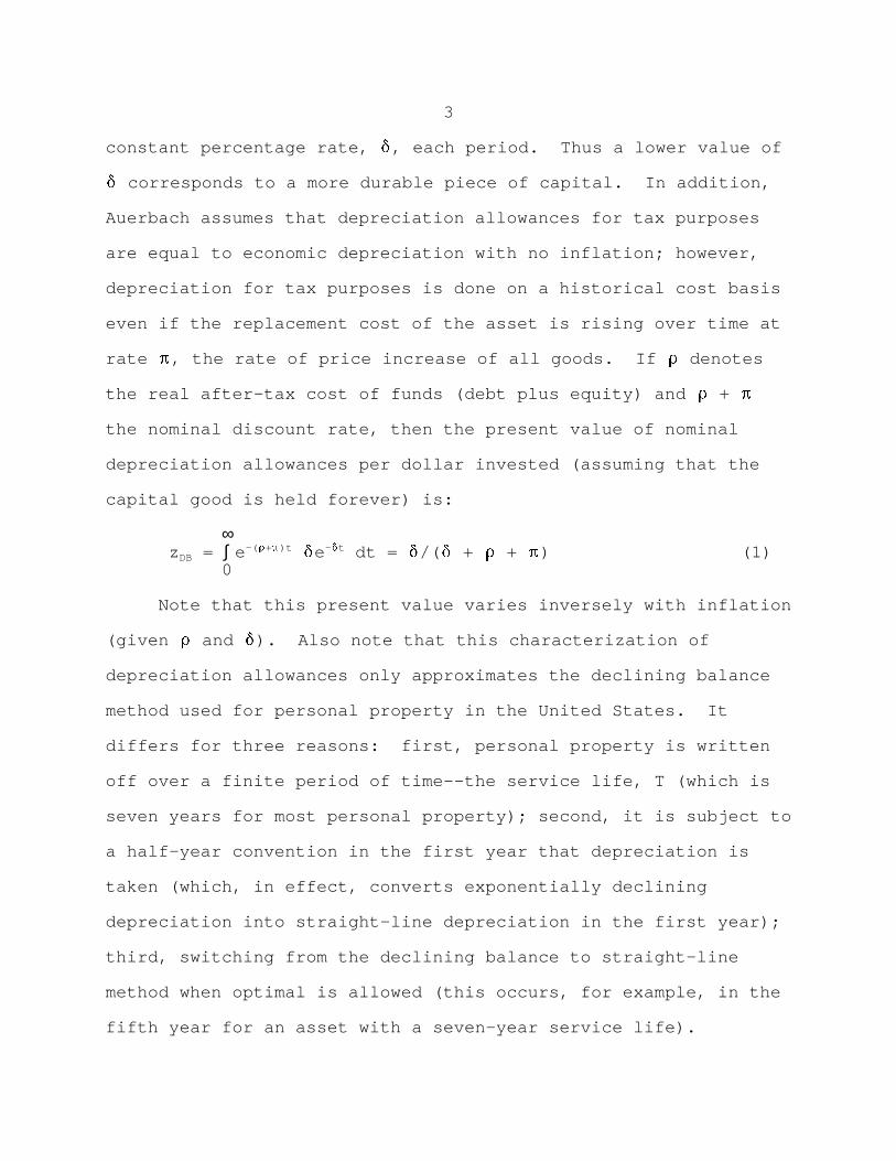
constant percentage rate, , each period. Thus a lower value of

corresponds to a more durable piece of capital. In addition,

Auerbach assumes that depreciation allowances for tax purposes

are equal to economic depreciation with no inflation; however,

depreciation for tax purposes is done on a historical cost basis

even if the replacement cost of the asset is rising over time at

rate !, the rate of price increase of all goods. If # denotes

the real after-tax cost of funds (debt plus equity) and # + !

the nominal discount rate, then the present value of nominal

depreciation allowances per dollar invested (assuming that the

capital good is held forever) is:

∞ z = ∫ e e dt = /( + # + !) (1)DB

-( #+!)t - t

0

Note that this present value varies inversely with inflation

(given # and ). Also note that this characterization of

depreciation allowances only approximates the declining balance

method used for personal property in the United States. It

differs for three reasons: first, personal property is written

off over a finite period of time--the service life, T (which is

seven years for most personal property); second, it is subject to

a half-year convention in the first year that depreciation is

taken (which, in effect, converts exponentially declining

depreciation into straight-line depreciation in the first year);

third, switching from the declining balance to straight-line

method when optimal is allowed (this occurs, for example, in the

fifth year for an asset with a seven-year service life).

4

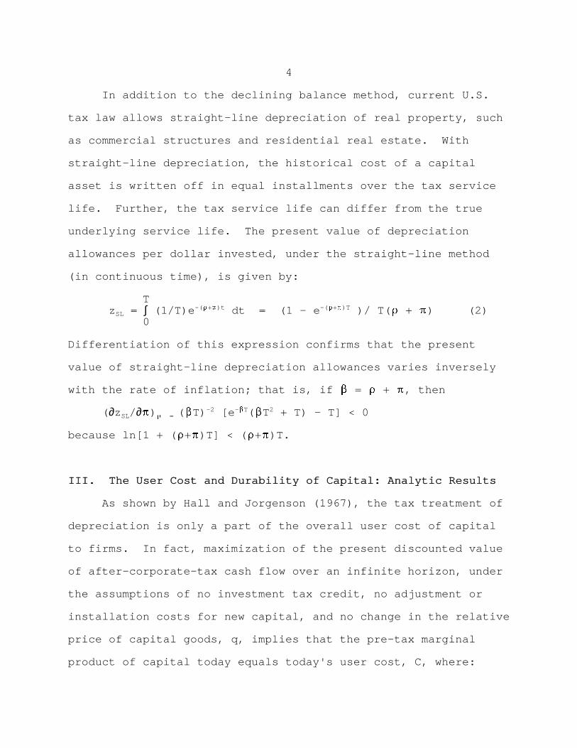
In addition to the declining balance method, current U.S.

tax law allows straight-line depreciation of real property, such

as commercial structures and residential real estate. With

straight-line depreciation, the historical cost of a capital

asset is written off in equal installments over the tax service

life. Further, the tax service life can differ from the true

underlying service life. The present value of depreciation

allowances per dollar invested, under the straight-line method

(in continuous time), is given by:

T z = ∫ (1/T)e dt = (1 - e )/ T( # + !) (2) SL

-( #+!)t -( #+!)T

0

Differentiation of this expression confirms that the present

value of straight-line depreciation allowances varies inversely

with the rate of inflation; that is, if � = # + !, then

( ∂z / ∂!) ( �T) [e ( �T + T) - T] < 0 SL # = -2 - �T 2

because ln[1 + ( #+!)T] < ( #+!)T.

III. The User Cost and Durability of Capital: Analytic ResultsIII. The User Cost and Durability of Capital: Analytic Results

As shown by Hall and Jorgenson (1967), the tax treatment of

depreciation is only a part of the overall user cost of capital

to firms. In fact, maximization of the present discounted value

of after-corporate-tax cash flow over an infinite horizon, under

the assumptions of no investment tax credit, no adjustment or

installation costs for new capital, and no change in the relative

price of capital goods, q, implies that the pre-tax marginal

product of capital today equals today's user cost, C, where:

5

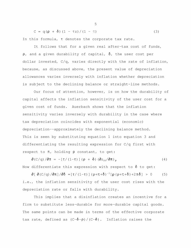
C = q( # + )(1 - )z)/(1 - )) (3)

In this formula, ) denotes the corporate tax rate.

It follows that for a given real after-tax cost of funds,

#, and a given durability of capital, , the user cost per

dollar invested, C/q, varies directly with the rate of inflation,

because, as discussed above, the present value of depreciation

allowances varies inversely with inflation whether depreciation

is subject to the declining balance or straight-line methods.

Our focus of attention, however, is on how the durability of

capital affects the inflation sensitivity of the user cost for a

given cost of funds. Auerbach shows that the inflation

sensitivity varies inversely with durability in the case where

tax depreciation coincides with exponential (economic)

depreciation--approximately the declining balance method.

This is seen by substituting equation 1 into equation 3 and

differentiating the resulting expression for C/q first with

respect to !, holding # constant, to get:

∂(C/q)/ ∂! = -[ )/(1- ))]( # + )( ∂z / ∂!) (4) DB #

Now differentiate this expression with respect to to get:

∂[ ∂(C/q)/ ∂!]/ ∂ =[ )/(1- ))]( #+!+) [ #( #+!+)+2 !] > 0 (5) -3

i.e., the inflation sensitivity of the user cost rises with the

depreciation rate or falls with durability.

This implies that a disinflation creates an incentive for a

firm to substitute less-durable for more-durable capital goods.

The same points can be made in terms of the effective corporate

tax rate, defined as (C- - #)/(C- ). Inflation raises the

6

effective rate by reducing the real value of the stream of tax

savings from depreciation deductions. Moreover, the resulting

"inflation tax" declines with asset durability, and in this

sense, inflation unambiguously weighs less heavily on long-lived

than short-lived assets.

This result does not necessarily carry over to the case of

straight-line depreciation, as seen by the following proposition.

PropositionProposition: For a given real after-tax cost of funds, #, and

an assumed inverse relationship between economic depreciation

rates and tax service lives (i.e., ∂T/ ∂ < 0), the inflation

sensitivity of the user cost under straight-line depreciation

falls with the depreciation rate [i.e., ∂[ ∂(C/q)/ ∂!]/ ∂ < 0] only

if ( # + !)T < 1.8.

To establish this result, substitute equation 2 into equation 3

and let z ′ = ( ∂z / ∂!) and � = # + !. Differentiation of theSL SL #

resulting expression yields:

∂[ ∂(C/q)/ ∂!] / ∂ = -[ )/(1- ))]{z ′ + ( #+)( ∂z ′ / ∂T) ( ∂T/ ∂)} (6)# SL SL #

Assume that capital goods with higher rates of economic

depreciation have shorter tax service lives, i.e., ∂T/ ∂ < 0.

This condition should hold under any rational tax policy even

though it is not uncommon for changes in tax law to modify the

tax service life of a depreciable capital good whose true

economic durability, as measured by , has not changed. Also,

7

differentiation of z ′ establishes that:SL

( ∂z ′ / ∂T) = (T �) {1 - e - ( �T)e - ( �T) e } (7)SL # -2 - �T - �T 2 - �T

Thus, the right hand side of expression 6 is negative--

reversing the Auerbach result--only if the right hand side of

expression 7 is negative. That is, the Auerbach result can be

reversed only when an increase in service life reduces the

inflation sensitivity of z. This condition is nonlinear in �T;

numerical approximation reveals that the condition is satisfied

for all values of #, !, and T such that ( #+!)T < 1.8. This

completes the proof of the proposition.

To illustrate the key condition of the proposition, suppose

that the inflation rate is zero and that the real after-tax cost

of funds is 5 percent per year. The condition, ( # + !)T < 1.8,

then holds for all depreciable capital goods with services lives

less than 36 years. This maximum service life declines, of

course, when higher values of the inflation rate or cost of funds

are used in the calculation. In any case, it is useful to note

that ( # + !)T < 1.8 is a necessary condition; for inflation to

encourage the substitution of short-lived for long-lived capital,

∂T/ ∂ must be sufficiently large in absolute value as well.

This result can be extended in a number of directions. For

example, the proposition assumes that the real after-tax cost of

funds, #, is constant. However, as discussed in detail in the

next section, # varies with inflation because of the tax

treatment of nominal interest payments in the case of debt

8

0 is negative in the benchmark case because a ceteris1

paribus increase in the tax service life reduces the presentvalue of depreciation allowances (i.e., ∂z/ ∂T < 0) and becausethe sensitivity of the present value of depreciation allowancesto the real discount rate declines with service life.

finance and the taxation of nominal capital gains in the case of

equity finance. When # depends on inflation, the term,

0 = -[ )/(1- ))][ ∂#/ ∂!][ ∂T/ ∂]{( ∂z/ ∂T) + ( #+)[ ∂( ∂z/ ∂#)/ ∂T]}, is

added to the right hand side of expression 6. This term is

negative when inflation raises the real cost of funds ( ∂#/ ∂! >

0); under this benchmark condition (described below), the term

reinforces the basic result of the proposition. However, this 1

need not always be the case. For example, inflation can reduce

the real cost of funds in the case of debt finance.

Further, for a hybrid depreciation system like that applying

to machinery and equipment currently in the United States, the

nature of the distortionary bias resulting from inflation is not

unambiguous a priori , because the "straight-line" and

"accelerated" portions of depreciation pull in opposite

directions. The next section examines this issue.

IV. The User cost and Durability of Capital: Empirical Results IV. The User cost and Durability of Capital: Empirical Results

In this section, we examine the inflation sensitivity of the

user cost under the depreciation rules in effect in the United

States in the mid-1990s. These rules were summarized above in

section II; a formal presentation can be found in Cohen, Hassett,

and Hubbard (1997). In addition, this section also gives a more

complete treatment of the cost of debt and equity funds, because,

9

in general, each depends on the rate of inflation. We follow the

approach in Cohen, Hassett, and Hubbard (1997), and start with a

brief discussion of the cost of debt capital.

Because corporations can deduct nominal interest expenses,

the real after-corporate-tax borrowing rate, # , is given by d

# = R(1 - )) - !, where R denotes the market rate of interest. d

Moreover, because savers are taxed on nominal interest income,

the real after-tax rate of return to savers, r, is given by:

r = R(1 - ) ) - !, where ) denotes the marginal personal incomep p

tax rate. Combining these expressions gives the real after-tax

borrowing cost from the perspective of the ultimate supplier of

debt capital: # = [r(1 - )) + !( ) - ))] (1 - ) ) , which alsod p p -1

can be written as # = (R - !)(1 - )) - )!. In our benchmark d

case, we assume that the real after-tax return to savers, r, is

invariant to changes in the rate of inflation. In this case,

(which assumes that the Fisher effect holds in tax-adjusted

terms) inflation has very little effect on the real cost of debt

capital if the marginal personal and corporate tax rates are

close to each other, as can be seen from the first expression for

# . We also discuss the case in which the real before-tax rate,d

(R - !), is invariant to inflation (or that the Fisher effect

holds in before-tax terms, i.e., that the nominal rate moves

point-for-point with inflation); in this case, higher inflation

reduces the real after-tax cost of debt, as can be seen from the

second expression for # . We now turn to a discussion of thed

cost of equity finance.

10

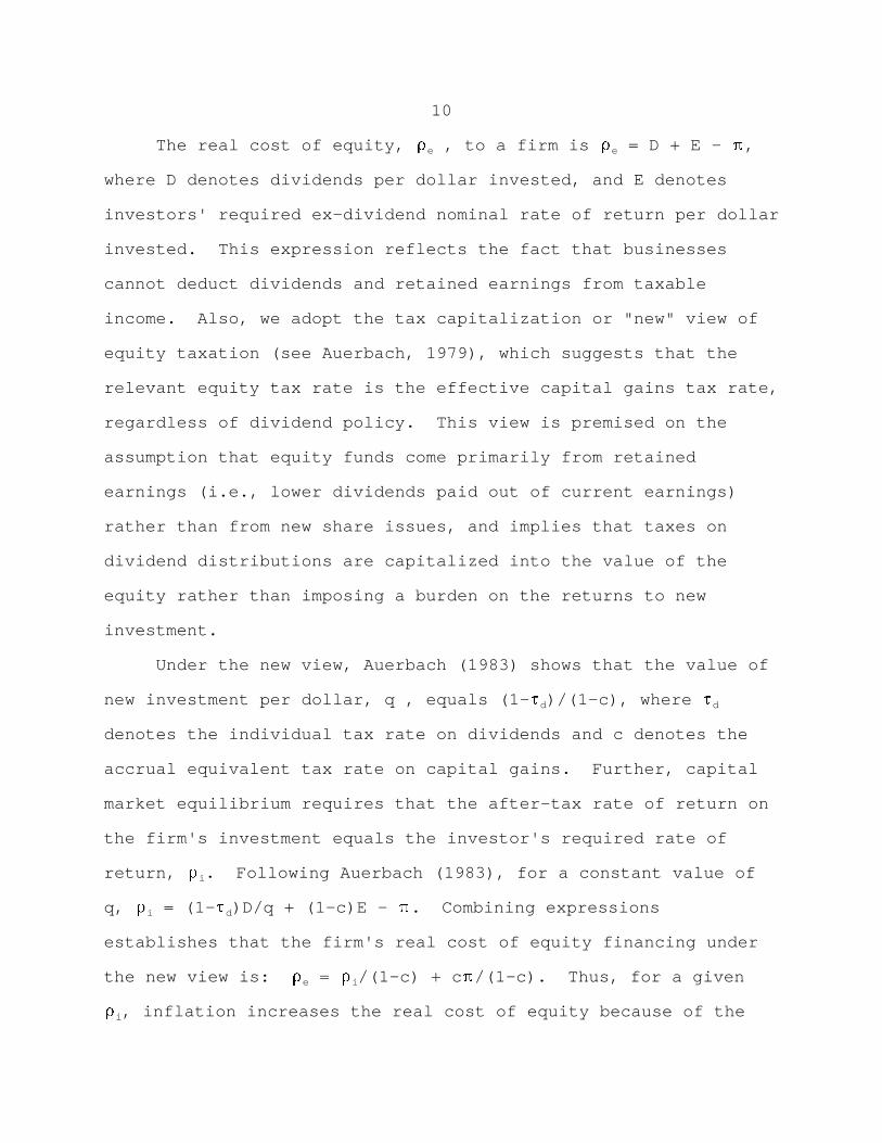
The real cost of equity, # , to a firm is # = D + E - !,e e

where D denotes dividends per dollar invested, and E denotes

investors' required ex-dividend nominal rate of return per dollar

invested. This expression reflects the fact that businesses

cannot deduct dividends and retained earnings from taxable

income. Also, we adopt the tax capitalization or "new" view of

equity taxation (see Auerbach, 1979), which suggests that the

relevant equity tax rate is the effective capital gains tax rate,

regardless of dividend policy. This view is premised on the

assumption that equity funds come primarily from retained

earnings (i.e., lower dividends paid out of current earnings)

rather than from new share issues, and implies that taxes on

dividend distributions are capitalized into the value of the

equity rather than imposing a burden on the returns to new

investment.

Under the new view, Auerbach (1983) shows that the value of

new investment per dollar, q , equals (1- ) )/(1-c), where )d d

denotes the individual tax rate on dividends and c denotes the

accrual equivalent tax rate on capital gains. Further, capital

market equilibrium requires that the after-tax rate of return on

the firm's investment equals the investor's required rate of

return, # . Following Auerbach (1983), for a constant value ofi

q, # = (1- ) )D/q + (1-c)E - !. Combining expressionsi d

establishes that the firm's real cost of equity financing under

the new view is: # = # /(1-c) + c !/(1-c). Thus, for a givene i

# , inflation increases the real cost of equity because of thei

11

We also assume that output is produced and held as2

finished goods inventories for one year; we allow for inflation'simpact on inventory profits to increase the corporate tax rate by�)!, where � is the fraction of inventories subject to FIFOaccounting. However, values of � between 0 and 30 percent havevirtually no effect on our results and, so, for simplicity,calculations in tables 1-4 are based on � = 0.

taxation of capital gains.

Combining the previous discussions of the costs of debt and

equity finance, the total real cost of funds, #, is given by:

# = w # + w # , where w and w denote the shares of debt andd d e e d e

equity in total finance, respectively. These weights will be

treated as empirical constants.

We now present the main empirical calculations of our paper.

They are summarized in tables 1-4, which show the user cost of

capital per dollar invested (see equation 3) at inflation rates

ranging from zero to 10 percent per annum and under different

assumptions about tax and economic service lives. The key

parameter values used in the benchmark calculations are: r = .02;

# = .06; ) = 0.35; ) = 0.45; w = 0.4; w = 0.6. i p d e2

The tables provide support for the basic points of this

paper. First, they implicitly reveal the possibility that

( ∂z ′/ ∂T) < 0, where z' = ∂z/ ∂! and z is the present discounted

value of depreciation allowances on one dollar invested in

personal property under current U.S. tax law. For example, the

second column of table 1 shows that the user cost of equipment

capital with a 5-year economic and tax service life rises from

26.6 percent to 31.1 percent--a 4.5 percentage point rise--as

inflation increases from zero to 10 percent. The final column

12

Algebraically, this follows by differentiation of3

equation 2, holding and # constant, i.e., ∂[ ∂(C/q)/ ∂!]/ ∂T = -[ )/(1- ))][( #+)( ∂z / ∂T)]. However, in table 1, there is a'

relatively small increase in # from roughly 5 percent to 6percent per annum as inflation varies over its entire range. Alarge # adds a bit to the value of the above expression (thatis, -[ )/(1- ))][( ∂#/ ∂!)( ∂z/ ∂T)] is added to the above expression,noting that a ceteris paribus increase in the tax service lifereduces the present value of depreciation allowances). Also notethat, in the example of table 1, ( # + !)T is less than 1.8, thecritical value derived in the previous section.

shows that over the same range of inflation rates the user cost

of equipment with the same 5-year economic life, but a 7-year tax

service life, rises 4.9 percentage points. And, an increase in

the inflation sensitivity of the user cost as the tax life rises,

for a given and #, can only occur if the inflation sensitivity

of z declines with service life. The same result also holds in3

table 2.

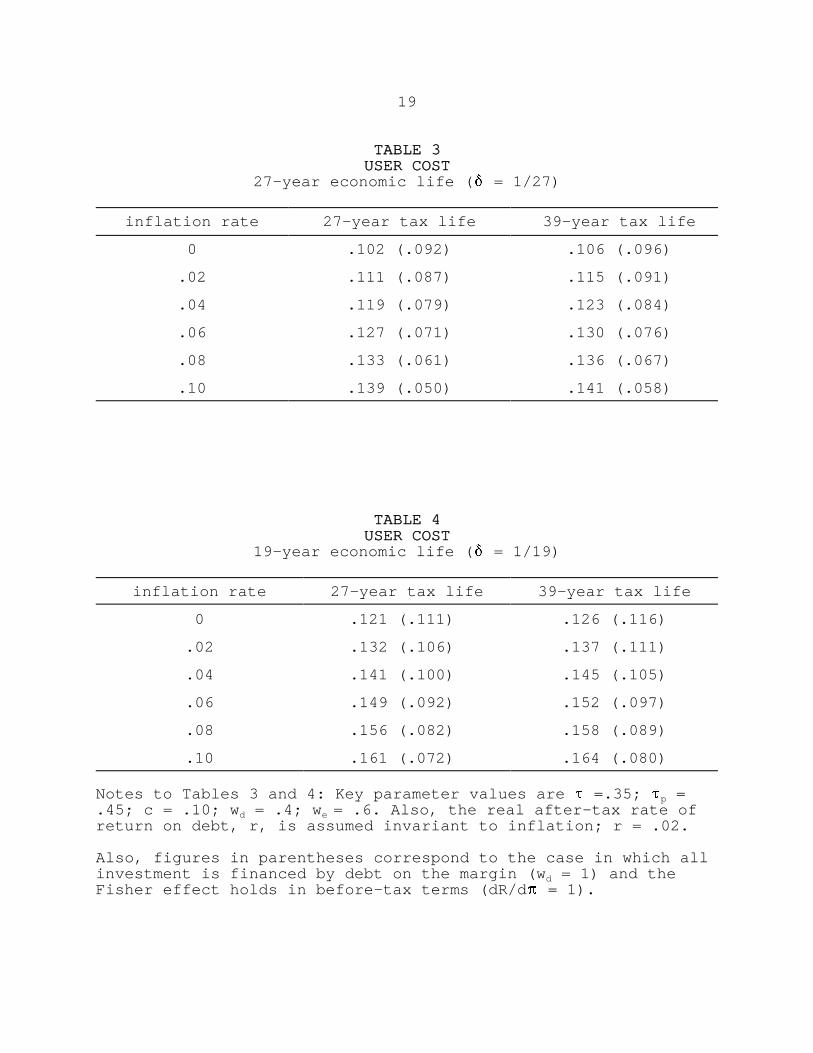
By contrast, in tables 3 and 4, the inflation sensitivity of

the user cost of structures declines as service life rises from

27 and 39 years (the two service lives currently available for

structures under U.S. tax law). This implies that the inflation

sensitivity of depreciation allowances necessarily increases with

service life (i.e., ∂z ′/ ∂T > 0) even though structures are

subject to straight-line depreciation. Evidently, for our

benchmark parameter values, there is not a small enough positive

value of inflation for which the condition, ( # + !)T < 1.8,

holds in the case of assets with 39-year tax service lives.

However, for property placed in service prior to May 1993, the

service life is 31 years; in this case (not shown in tables) the

condition does hold, but only at very low inflation rates (less

13

than 1 percent per annum).

The foregoing discussion thus strongly suggests that the

basic proposition of the last section--which, strictly speaking,

applies to assets subject to straight-line depreciation--can be

illustrated only by a comparison of tables 1 and 2, which are

applicable to producers' durable equipment. Indeed, comparison

of the benchmark values in the third column of table 1 with those

in the second column of table 2 shows that the inflation

sensitivity of the user cost of assets with a 5-year economic

life and 7-year tax life is greater (just) than the corresponding

inflation sensitivity of assets with a 3-year economic and tax

life over the full range of included inflation rates. In this

case, inflation encourages the substitution of short-lived for

long-lived equipment.

A key factor underlying this result is that the tax service

life changes by more than the economic life (both expressed in

years). This implies that the inflation sensitivity of the user

cost of capital with a 3-year economic and tax service life is

less than the corresponding sensitivity of capital with a 7-year

tax life and any economic life between 3 and 5 years (not shown

in tables).

Conversely, inflation does not encourage the substitution of

short-lived for long-lived equipment when the tax and economic

lives increase by the same amount, as seen by comparing the

benchmark figures in the third columns of tables 1 and 2. This

is true also in the special case of = 1/T. This can be seen,

14

for example, by comparing the second columns of tables 1 and 2:

inflation raises the user cost of equipment with a 3-year

economic and tax life more than it raises the user cost of

equipment with a 5-year economic and tax life.

Because economic and tax service lives can differ in our

setup, we also can explore the effects of changes in the rate of

economic depreciation ( ), holding the tax service life fixed.

Results, in the case of equipment with a 5-year tax life, can be

seen by comparing the benchmark figures in column 2 of table 1 to

those in column 3 of table 2. The inflation sensitivity of the

user cost is greater for the equipment with a 3-year economic

life than for that with a 5-year life. The user cost of less

economically durable structures also is more sensitive to

inflation, as seen by comparing the second columns of tables 3

and 4.

We also have considered the effects of different values for

the personal income tax rate, ) . Because of the difficulty inp

identifying the marginal investor in debt instruments, the value

chosen for ) is controversial. As an alternative to thep

(combined federal and state) benchmark value of 0.45, we also

consider a value of 0.21, based on an update of the average

marginal tax rate in Prakken, Varvares, and Meyer (1991). The

effects of inflation (not shown) on the user cost are uniformly

smaller than those reported in Tables 1-4. However the basic

inter-asset distortions are qualitatively the same.

Finally, we also have explored the effects of changes in the

15

composition of financing of investments. In particular, we

consider the case in which all investment is financed with debt

on the margin. In addition, we assume that the Fisher effect

holds so that the real before-tax rate of interest is invariant

to changes in the inflation rate. In this case, the real cost of

funds simplifies to # , which as shown above, is inverselyd

related to inflation when the Fisher effect holds. For example,

if the market interest rate on debt (R) is 5 percent per year

when inflation is zero, then the real cost of funds declines from

roughly 3 percent when inflation is zero to about zero when

inflation is 10 percent. Indeed, the reduction in the real cost

of funds more than offsets the reduction in the present

discounted value of nominal depreciation allowances as inflation

rises.

Thus, as shown in tables 1-4 by the figures in parentheses,

higher inflation reduces the user cost of capital. Moreover, as

revealed by tables 1 and 2, higher inflation reduces the user

cost of equipment with relatively long economic life more than it

reduces the user cost of equipment with relatively short economic

life in all the cases examined. Thus, higher inflation, in the

all debt-finance case, encourages the substitution of long-lived

for short-lived capital equipment. Similar results hold in the

case of structures, as shown in tables 3 and 4. Clearly, the

question of which Fisher effect holds, which has received

relatively little attention in public finance circles, is of

fundamental importance.

16

V. Conclusion V. Conclusion

The conventional wisdom is that inflation--in the presence

of a nominal based tax depreciation structure--biases the choice

of asset durability in favor of relatively long-lived capital

goods. We have established that the crucial assumptions

underlying this result are that depreciation allowances accorded

assets reflect actual economic depreciation in the absence of

inflation and that capital services decay exponentially. Indeed,

we show analytically that when tax depreciation is less

accelerated (relative to straight-line) than economic

depreciation, higher inflation may well, although not

necessarily, encourage the substitution of short-lived for long-

lived capital assets. Finally, under current U.S. tax law, we

demonstrate that higher inflation--in line with the conventional

wisdom--favors relatively long-lived structures. By contrast, we

also show that higher inflation favors relatively short-lived

equipment in many cases, but only minimally.

17

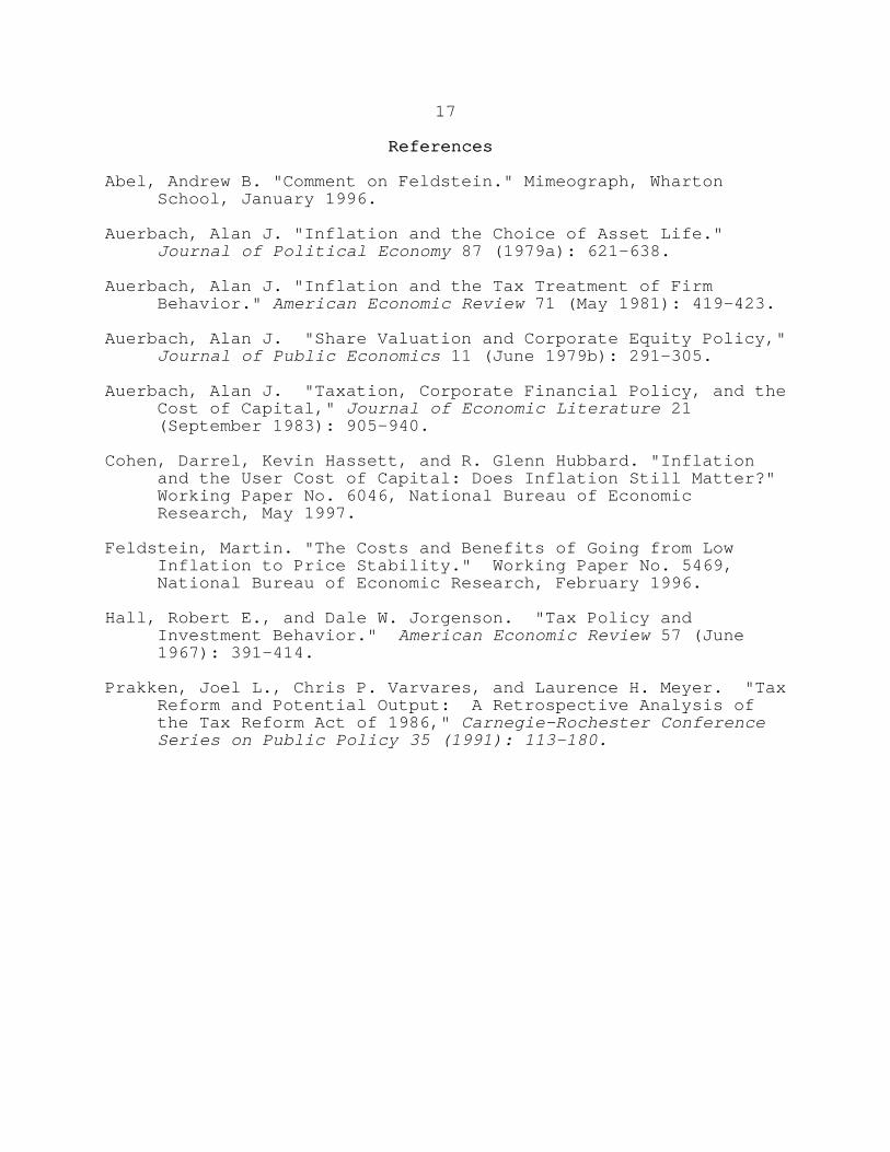
References References

Abel, Andrew B. "Comment on Feldstein." Mimeograph, Wharton School, January 1996.

Auerbach, Alan J. "Inflation and the Choice of Asset Life." Journal of Political Economy 87 (1979a): 621-638.

Auerbach, Alan J. "Inflation and the Tax Treatment of Firm Behavior." American Economic Review 71 (May 1981): 419-423.

Auerbach, Alan J. "Share Valuation and Corporate Equity Policy,"Journal of Public Economics 11 (June 1979b): 291-305.

Auerbach, Alan J. "Taxation, Corporate Financial Policy, and the Cost of Capital," Journal of Economic Literature 21 (September 1983): 905-940.

Cohen, Darrel, Kevin Hassett, and R. Glenn Hubbard. "Inflationand the User Cost of Capital: Does Inflation Still Matter?" Working Paper No. 6046, National Bureau of Economic Research, May 1997.

Feldstein, Martin. "The Costs and Benefits of Going from LowInflation to Price Stability." Working Paper No. 5469,National Bureau of Economic Research, February 1996.

Hall, Robert E., and Dale W. Jorgenson. "Tax Policy and Investment Behavior." American Economic Review 57 (June1967): 391-414.

Prakken, Joel L., Chris P. Varvares, and Laurence H. Meyer. "TaxReform and Potential Output: A Retrospective Analysis ofthe Tax Reform Act of 1986," Carnegie-Rochester ConferenceSeries on Public Policy 35 (1991): 113-180.

18

TABLE 1TABLE 1USER COSTUSER COST

5-year economic life ( = 1/5)

inflation rate 5-year tax life 7-year tax life

0 .266 (.252) .271 (.256)

.02 .276 (.248) .282 (.253)

.04 .285 (.244) .292 (.249)

.06 .294 (.240) .302 (.245)

.08 .302 (.235) .311 (.241)

.10 .311 (.230) .321 (.236)

TABLE 2TABLE 2USER COSTUSER COST

3-year economic life ( = 1/3)

inflation rate 3-year tax life 5-year tax life

0 .401 (.387) .409 (.393)

.02 .412 (.384) .422 (.391)

.04 .422 (.381) .434 (.389)

.06 .432 (.377) .446 (.387)

.08 .441 (.373) .457 (.384)

.10 .450 (.369) .468 (.380)

Notes to Tables 1 and 2: Key parameter values are ) =.35; ) = .45; c = .10; w = .4; w = .6. Also, the real after-tax p d e

rate of return on debt, r, is assumed invariant to inflation; r = .02.

Also, figures in parentheses correspond to the case in which allinvestment is financed by debt on the margin (w = 1) and the d

Fisher effect holds in before-tax terms (dR/d ! = 1).

19

TABLE 3TABLE 3USER COSTUSER COST

27-year economic life ( = 1/27)

inflation rate 27-year tax life 39-year tax life

0 .102 (.092) .106 (.096)

.02 .111 (.087) .115 (.091)

.04 .119 (.079) .123 (.084)

.06 .127 (.071) .130 (.076)

.08 .133 (.061) .136 (.067)

.10 .139 (.050) .141 (.058)

TABLE 4TABLE 4USER COSTUSER COST

19-year economic life ( = 1/19)

inflation rate 27-year tax life 39-year tax life

0 .121 (.111) .126 (.116)

.02 .132 (.106) .137 (.111)

.04 .141 (.100) .145 (.105)

.06 .149 (.092) .152 (.097)

.08 .156 (.082) .158 (.089)

.10 .161 (.072) .164 (.080)

Notes to Tables 3 and 4: Key parameter values are ) =.35; ) =p

.45; c = .10; w = .4; w = .6. Also, the real after-tax rate ofd e

return on debt, r, is assumed invariant to inflation; r = .02.

Also, figures in parentheses correspond to the case in which allinvestment is financed by debt on the margin (w = 1) and the d

Fisher effect holds in before-tax terms (dR/d ! = 1).