abstract hydrate distribution in heterogeneous marine sediment
TRANSCRIPT


ABSTRACT
Modeling Fluid Flow Effects on Shallow Pore Water Chemistry and Methane
Hydrate Distribution in Heterogeneous Marine Sediment
by
Sayantan Chatterjee
The depth of the sulfate-methane transition (SMT) above gas hydrate systems
is a direct proxy to interpret upward methane flux and hydrate saturation. However,
two competing reaction pathways can potentially form the SMT. Moreover, the pore
water profiles across the SMT in shallow sediment show broad variability leading to
different interpretations for how carbon, including CH4, cycles within gas-charged
sediment sequences over time. The amount and distribution of marine gas hydrate
impacts the chemistry of several other dissolved pore water species such as
the dissolved inorganic carbon (DIC). A one-dimensional (1-D) numerical model
is developed to account for downhole changes in pore water constituents, and
transient and steady-state profiles are generated for three distinct hydrate settings.
The model explains how an upward flux of CH4 consumes most SO2−4 at a shallow
SMT implying that anaerobic oxidation of methane (AOM) is the dominant SO2−4
reduction pathway, and how a large flux of 13C-enriched DIC enters the SMT
from depth impacting chemical changes across the SMT. Crucially, neither the

concentration nor the δ13C of DIC can be used to interpret the chemical reaction
causing the SMT.
The overall thesis objective is to develop generalized models building on this
1-D framework to understand the primary controls on gas hydrate occurrence.
Existing 1-D models can provide first-order insights on hydrate occurrence, but
do not capture the complexity and heterogeneity observed in natural gas hydrate
systems. In this study, a two-dimensional (2-D) model is developed to simulate
multiphase flow through porous media to account for heterogeneous lithologic
structures (e.g., fractures, sand layers) and to show how focused fluid flow
within these structures governs local hydrate accumulation. These simulations
emphasize the importance of local, vertical, fluid flux on local hydrate accumulation
and distribution. Through analysis of the fluid fluxes in 2-D systems, it is shown that
a local Peclet number characterizes the local hydrate and free gas saturations,
just as the Peclet number characterizes hydrate saturations in 1-D, homogeneous
systems. Effects of salinity on phase equilibrium and co-existence of hydrate and
gas phases can also be investigated using these models.
Finally, infinite slope stability analysis assesses the model to identify for
potential subsea slope failure and associated risks due to hydrate formation and
free gas accumulation. These generalized models can be adapted to specific field
examples to evaluate the amount and distribution of hydrate and free gas and to
identify conditions favorable for economic gas production.

Acknowledgments
This dissertation would not have been possible without the help and support of
several individuals who in one way or another have contributed to the preparation
and successful completion of this work. First and foremost, I offer my sincerest
gratitude to my advisor, Dr George Hirasaki, for being a great mentor. His plethora
of knowledge, diligent work ethic, patience and enthusiasm towards research
motivated me to conduct this multidisciplinary research project. I express my
deepest appreciation to him for his invaluable advice, support and guidance.
I convey my profound gratitude and indebtedness to Dr Walter Chapman
for co-advising me on this study. His continued encouragement and engaging
discussions made my graduate school a truly memorable experience. I thank Dr
Kyriacos Zygourakis, Dr Jerry Dickens and Dr Brandon Dugan for serving on my
thesis committee.
A special note of appreciation goes to Dr Jerry Dickens for his insightful
suggestions and several stimulating discussions which not only broadened my
thinking and exposed me to the field of geochemistry but also helped me tackle
some of the challenging problems from an earth science perspective. I attribute my
improved quality of scientific writing to him. I gratefully thank Dr Brandon Dugan

v
for strengthening my foundation in hydrogeology, geomechanics and providing
constructive comments and critical assessment of my research work.
A notable acknowledgement to the gas hydrate group at Rice including Dr
Gaurav Bhatnagar, Dr Glen Snyder, Dr Hugh Daigle and Guangsheng Gu for their
invaluable time, helpful discussions, and critical commentary through numerous
meetings, papers and presentations. Special thanks to Dr Jan Hewitt and Dr Tracy
Volz for greatly honing my technical writing and presentation skills.
I am truly grateful to all the faculty and staff of the Chemical and Biomolecular
Engineering department for their kind cooperation and support. I am blessed to
be surrounded by extremely helpful colleagues, especially in the Transport and
Thermodynamic Properties lab, a compassionate and cheerful group of friends,
and a considerate housemate throughout my graduate career which made my stay
at Rice not only fruitful, but also a delightful experience to remember.
I acknowledge financial support from the Department of Energy under Award
No. DE-FC26-06NT42960, the Shell Center for Sustainability and the Consortium
of Processes in Porous Media at Rice University. I thank the captains, crews and
fellow shipboard scientists of Ocean Drilling Program (ODP) Legs 112, 201, 204
and Gulf of Mexico Joint Industry Program (JIP) for successful drilling and the
collection and analyses of samples. My thesis work was supported in part by the
Shared University Grid at Rice funded by NSF under Grant EIA-0216467, and a
partnership between Rice University, Sun Microsystems, and Sigma Solutions, Inc.

vi
Lastly, I owe a heartfelt thank you to my beloved parents, sister, fiancee, and my
family in India for their endless love and continued support. My fulfilling upbringing,
education, and this advanced degree would not have been possible without their
selfless sacrifices and encouragement. I convey my deepest appreciation and
most sincere regards to them.
Sayantan Chatterjee
Contents
Abstract ii
Acknowledgments iv
List of Illustrations xiii
List of Tables xxvi
1 Introduction 1
1.1 Organization . . . . . . . . . . . . . . . . . . . . . . . . . . . . . . . 3
2 Background 7
2.1 Overview . . . . . . . . . . . . . . . . . . . . . . . . . . . . . . . . . 7
2.2 Marine Gas Hydrate Systems . . . . . . . . . . . . . . . . . . . . . . 7
2.3 Existing Methods to Quantify the Amount and Distribution of Marine
Gas Hydrate . . . . . . . . . . . . . . . . . . . . . . . . . . . . . . . 12
2.3.1 Observations . . . . . . . . . . . . . . . . . . . . . . . . . . . 12
2.3.2 One-dimensional Modeling . . . . . . . . . . . . . . . . . . . 14
2.3.3 Two-dimensional Modeling . . . . . . . . . . . . . . . . . . . 17
3 Pore Water Sulfate, Alkalinity, and Carbon Isotope Profiles

viii
in Shallow Sediment Above Marine Gas Hydrate Systems 22
3.1 Introduction . . . . . . . . . . . . . . . . . . . . . . . . . . . . . . . . 22
3.2 Pore Water Profiles Across the Sulfate-Methane Transition . . . . . . 27
3.2.1 Overview . . . . . . . . . . . . . . . . . . . . . . . . . . . . . 27
3.2.2 Site 1244: Hydrate Ridge . . . . . . . . . . . . . . . . . . . . 29
3.2.3 Site KC151-3: Keathley Canyon . . . . . . . . . . . . . . . . 32
3.3 Numerical Model . . . . . . . . . . . . . . . . . . . . . . . . . . . . . 34
3.3.1 General Framework . . . . . . . . . . . . . . . . . . . . . . . 34
3.3.2 Basic Model . . . . . . . . . . . . . . . . . . . . . . . . . . . . 36
3.3.3 Updated Model: Reactions . . . . . . . . . . . . . . . . . . . 38
3.3.4 Updated Model: Mass balances . . . . . . . . . . . . . . . . 40
3.3.5 Numerical Solution . . . . . . . . . . . . . . . . . . . . . . . . 60
3.4 Results and Discussion . . . . . . . . . . . . . . . . . . . . . . . . . 61
3.4.1 Steady State Concentration Profiles . . . . . . . . . . . . . . 61
3.4.2 Variations in AOM and Organoclastic Sulfate Reduction . . . 73
3.4.3 Concentration Crossplots of Alkalinity and Sulfate . . . . . . 76
3.4.4 Flux Crossplots . . . . . . . . . . . . . . . . . . . . . . . . . . 83
3.4.5 Relationship Between AOM and δ13C Values . . . . . . . . . 84
3.4.6 Influence of Carbonate Precipitation . . . . . . . . . . . . . . 86
3.5 Conclusions . . . . . . . . . . . . . . . . . . . . . . . . . . . . . . . . 87
4 Modeling Pore Water Profiles of Marine Gas Hydrate

ix
Systems: The Extreme Case of ODP Site 685/1230, Peru
Trench 91
4.1 Introduction . . . . . . . . . . . . . . . . . . . . . . . . . . . . . . . . 91
4.2 Site 685/1230, Peru Margin . . . . . . . . . . . . . . . . . . . . . . . 93
4.2.1 Basic Parameters and Methane . . . . . . . . . . . . . . . . . 93
4.2.2 Key Pore Water Profiles . . . . . . . . . . . . . . . . . . . . . 101
4.2.3 Additional Data . . . . . . . . . . . . . . . . . . . . . . . . . . 104
4.3 Numerical Model . . . . . . . . . . . . . . . . . . . . . . . . . . . . . 104
4.3.1 Model Framework . . . . . . . . . . . . . . . . . . . . . . . . 104
4.3.2 Modifications to Previous Modeling . . . . . . . . . . . . . . . 107
4.3.3 Initial Parameters . . . . . . . . . . . . . . . . . . . . . . . . . 107
4.3.4 General Approach for Solving . . . . . . . . . . . . . . . . . . 109
4.3.5 Steady State Solutions . . . . . . . . . . . . . . . . . . . . . 110
4.3.6 Transient Solutions . . . . . . . . . . . . . . . . . . . . . . . . 111
4.4 Results . . . . . . . . . . . . . . . . . . . . . . . . . . . . . . . . . . 112
4.4.1 Steady State Solutions . . . . . . . . . . . . . . . . . . . . . 112
4.4.2 Transient Solutions . . . . . . . . . . . . . . . . . . . . . . . . 121
4.4.3 Concentration and Flux Crossplots of Alkalinity and Sulfate . 127
4.5 Discussion . . . . . . . . . . . . . . . . . . . . . . . . . . . . . . . . 128
4.6 Conclusions . . . . . . . . . . . . . . . . . . . . . . . . . . . . . . . . 133

x
5 Two-dimensional Model for Quantification of Hydrate and
Free Gas Accumulations 136
5.1 Introduction . . . . . . . . . . . . . . . . . . . . . . . . . . . . . . . . 136
5.2 Mathematical Model . . . . . . . . . . . . . . . . . . . . . . . . . . . 138
5.2.1 General Framework . . . . . . . . . . . . . . . . . . . . . . . 138
5.2.2 Component mass balances . . . . . . . . . . . . . . . . . . . 139
5.3 Constitutive relationships . . . . . . . . . . . . . . . . . . . . . . . . 141
5.4 Normalized Variables and Key Dimensionless Groups . . . . . . . . 144
5.5 Dimensionless Mass Balance Equations, Initial Conditions and
Boundary Conditions . . . . . . . . . . . . . . . . . . . . . . . . . . . 149
5.6 Numerical Algorithm . . . . . . . . . . . . . . . . . . . . . . . . . . . 159
5.7 2-D model Development and Validation . . . . . . . . . . . . . . . . 159
6 Effects of Lithologic Heterogeneity and Salinity on Gas
Hydrate Distribution 164
6.1 Effect of Vertical Fracture Systems . . . . . . . . . . . . . . . . . . . 164
6.2 Effect of Mesh Refining . . . . . . . . . . . . . . . . . . . . . . . . . 169
6.3 Effect of Permeability Anisotropy . . . . . . . . . . . . . . . . . . . . 171
6.4 Local Flux within High Permeability Zones . . . . . . . . . . . . . . . 171
6.5 Effect of Permeability Contrast . . . . . . . . . . . . . . . . . . . . . 174
6.6 Effect of Horizontal High Permeability Layers . . . . . . . . . . . . . 174

xi
6.7 Effect of Dip Angle of High Permeability Layers . . . . . . . . . . . . 179
6.8 Effect of Free Gas Migration into the GHSZ . . . . . . . . . . . . . . 181
6.8.1 Vertical Fracture Systems . . . . . . . . . . . . . . . . . . . . 181
6.8.2 Dipping Sand Layers . . . . . . . . . . . . . . . . . . . . . . . 182
6.9 Effect of Hydrate Formation and Dissociation on Pore Water Salinity 187
6.10 Effect of Salinity on Phase Equilibrium and Methane Solubility . . . . 189
6.11 Conclusions . . . . . . . . . . . . . . . . . . . . . . . . . . . . . . . . 191
7 Effect of Gas Hydrate Distribution on Slope Failure in
Subsea Sediments 194
7.1 Introduction . . . . . . . . . . . . . . . . . . . . . . . . . . . . . . . . 194
7.2 Slope Stability Modeling . . . . . . . . . . . . . . . . . . . . . . . . . 196
7.2.1 Infinite Slope Approximation . . . . . . . . . . . . . . . . . . . 196
7.3 Results and Discussion . . . . . . . . . . . . . . . . . . . . . . . . . 199
7.4 Conclusions . . . . . . . . . . . . . . . . . . . . . . . . . . . . . . . . 203
8 Conclusions and Future Work 204
8.1 Conclusions . . . . . . . . . . . . . . . . . . . . . . . . . . . . . . . . 204
8.2 Future Research Directions . . . . . . . . . . . . . . . . . . . . . . . 208
Bibliography 213

xii
A Chemical Reactions - Methanogenesis 231
B Carbon Isotope Composition of Organic Matter at Site
1230E 233
C 1-D Mathematical Model for Pore Water Constituents in
Shallow Sediments 235
D Analytical Theory Relating Fluid Flux and the Average
Hydrate Saturation 246

Illustrations
2.1 Map showing locations with gas hydrate bearing sites drilled in thecontinental margins of north and south America. At some of thesesites, cores have been sampled and pore water chemistry hasbeen measured along with carbon isotope composition of DIC.Three sites with differing carbon chemistry have been chosenamong those where extensive datasets exist and are modeled as apart of this study. . . . . . . . . . . . . . . . . . . . . . . . . . . . . . 8
2.2 Basic schematic of static and dynamic gas hydrate systems. (a)Relationships that exist between three phases of methane,geotherm, hydrotherm and the finite zone of gas hydrate stability(GHSZ). (b) A static description of gas hydrate in marine sedimentshowing the GHSZ, SO2−
4 reduction zone, the three-phaseboundary, and generic transient and steady-state dissolved gasconcentration profiles. (c) A dynamic perspective showing relevantsediment and fluid fluxes, and the hydrate layer in the GHSZ thatcan move down with the sediment. (d) The steady-state snapshotview of these hydrate systems showing the hydrate layer overlyinga free gas zone that are in equilibrium over geologic timescales. . . 10
2.3 Average gas hydrate saturation contours within the GHSZ forsystems where all methane is supplied from in situ biogenicsources. Low values of Peclet number (Pe1), imply dominantdiffusive losses and that greater methane has to be generatedwithin the GHSZ to form any gas hydrate. Average gas hydratesaturation at different geologic settings can be obtained from asingle contour map (Taken from Bhatnagar et al., 2007). . . . . . . . 18
2.4 Gas hydrate flux Pe1〈Sh〉 contours plotted along with the curvesdistinguishing two regions of hydrate occurrence, for the case ofnon-zero, finite, sedimentation and Pe1 < |Pe2|. Average hydratesaturation 〈Sh〉 can be calculated by dividing the contour values byPe1 (Taken from Bhatnagar et al., 2007). . . . . . . . . . . . . . . . . 19

xiv
3.1 (a) Schematic representation of a gas hydrate system showingpore water sulfate (red) and methane (blue) concentrations, whichgo to near zero within the sulfate-methane transition (SMT) atshallow depths due to AOM. The dashed line represents themethane solubility curve. Fluid fluxes due to compaction-drivenflow and external flow are denoted as Uf,sed and Uf,ext respectively;Lt is the depth to the base of the gas hydrate stability zone. (b)Zoomed sulfate-methane transition (SMT) zone showing an overlapof sulfate and methane profiles and its depth below the seafloor(Ls) (Bhatnagar et al., 2008a). It should be noted, though, thataccurate, high-resolution in situ CH4 concentration gradients havenot been measured below the SMT (e.g., Dickens et al., 1997;Milkov et al., 2004). . . . . . . . . . . . . . . . . . . . . . . . . . . . . 24
3.2 Alkalinity versus δ13C of DIC at the SMT for multiple locationsknown to have gas hydrate at depth. Note the general trend fromsites with low alkalinity and low δ13C of DIC to those with highalkalinity and relatively high δ13C of DIC. Traditionally, alkalinity andδ13C of DIC at the SMT were being used to discriminate betweenAOM and POC-driven sulfate reduction to explain this trend. Thedominant cause for this trend is suggested to arise from the relativeflux of upward 13C-enriched DIC (FDICDp
). Data from ODP 994-997,Paull et al. (2000b); ODP Site 1059, Borowski et al. (2000); ODPSites 1244-1252, Claypool et al. (2006), Torres and Rugh (2006);1326, 1329, Torres and Kastner (2009); KC03-5-19, Pohlman et al.(2008); KC151-3, AT13-2 , Kastner et al. (2008b); O7GHP-1, Kimet al. (2011). The hachured line for Hole 1252A represents a rangeof values spanning the SMT. Hexagons represent the two sites(1244C and KC151-3) modeled within this chapter. . . . . . . . . . . 28
3.3 Pore water (a) SO2−4 (closed circles and squares), CH4 (open
circles and squares), (b) alkalinity (DIC), (c) Ca2+ concentrationand (d) δ13C of DIC profiles in shallow sediment at Site 1244 inHydrate Ridge and KC151-3 in Gulf of Mexico. Top panel showsthe zoomed pore water profiles for the upper 20 m of sediment andthe shaded region represents the SMT zone. The arrows indicateincreasing trend in CH4 concentration. Data from 1244, Trehu et al.(2003) and Torres and Rugh (2006); KC151-3, Kastner et al. (2008b). 31

xv
3.4 Steady state normalized pore water concentration profiles at Site1244. (a) CH4 (solid), and SO2−
4 (dashed), (b) DIC, (c) Ca2+, and(d) δ13C of DIC. The blue, green and red curves correspond toincreasing magnitude of Pe2 (fluid flux from depth) shown bydirection of arrow. Site 1244 data (black circles) (Trehu et al., 2003;Torres and Rugh, 2006). Parameters: Pe1 = 0.044, Da = 0.22,DaPOC = 2.5, DaAOM = 108, β = 2.4, cb,ext= 27 and δ13CHCO3,ext
= 20. . 65
3.5 Steady state normalized pore water concentration profiles at SiteKC151-3. (a) CH4 (solid), and SO2−
4 (dashed), (b) DIC, (c) Ca2+,and (d) δ13C of DIC. The blue, green and red curves correspond toincreasing magnitude of Pe2 (fluid flux from depth) shown bydirection of arrow. Site KC151-3 data (black circles) (Kastner et al.,2008b). Parameters: Pe1 = 0.095, Da = 0.22, DaPOC = 2.5, DaAOM
= 108, β = 0.38, cb,ext = 1.5 and δ13CHCO3,ext= 10. . . . . . . . . . . . 70
3.6 (a) Steady state pore water profiles to study the effect of DaAOM atSite 1244. Decrease in DaAOM results in a thicker SMT horizon.Parameters: Pe1 = 0.044, Pe2 = -1, Da = 0.22, DaPOC = 2.5, β =2.4, cb,ext = 27 and δ13CHCO3,ext
= 20. (b) Effect of DaPOC on porewater chemistry at Site 1244. Parameters: Pe1 = 0.044, Pe2 = -1,Da = 0.22, DaAOM = 108, β = 2.4, cb,ext = 27 and δ13CHCO3,ext
= 20.In both cases, decreasing DaAOM and increasing DaPOC result inhigher POC depletion, lesser CH4 and DIC production, greaterCa2+ concentration in pore fluids above and below the SMT and amore negative δ13C of DIC at the SMT. . . . . . . . . . . . . . . . . . 75
3.7 Concentration crossplot of ”excess alkalinity” (∆Alk∗) corrected forcarbonate precipitation versus ∆SO2−
4 (mM) relative to the seafloorfor shallow sediment at Site 1244 on Hydrate Ridge (Trehu et al.,2003) and Site KC151-3 (Kastner et al., 2008b). As emphasized byKastner et al. (2008b), there is a 2:1 relationship for pore waterconcentrations above the SMT for Site 1244 (red circles) and 1:1for Site KC151-3 (blue squares). Note, however, that excessalkalinity continues to rise below the SMT at Site 1244. This clearlyimplies an upward flux of alkalinity from depth; whereas, at SiteKC151-3, excess alkalinity decrease below the SMT. This decreaseis because DIC is consumed by Ca2+ resulting in calcite precipitation. 77

xvi
3.8 Concentration crossplots for ∆Alk∗ and ∆SO2−4 relative to
seawater. Three cases are illustrated here corresponding to a 2:1slope. Blue dashed line represents a case with organoclasticsulfate reduction, no upward fluid flux, no AOM and no deep DICsource (methanogenesis). Parameters: Pe1 = 0.044, Pe2 = 0, Da =0, DaPOC = 2.5, DaAOM = 0, β = 2.4 and cb,ext = 0. Red solid linerepresents another case with low and finite upward fluid flux, AOM,methanogenesis, and a deep DIC source, but no organoclasticsulfate reduction. Parameters: Pe1 = 0.044, Pe2 = -0.1, Da = 1,DaPOC = 0, DaAOM = 108, β = 2.4 and cb,ext = 79. The green dashedline represents a third case (combination of the first two cases). It ischaracterized by AOM, organoclastic sulfate reduction,methanogenesis, deep DIC source and low upward fluid flux.Parameters: Pe1 = 0.044, Pe2 = -0.1, Da = 1, DaPOC = 2.5, DaAOM
= 108, β = 2.4 and cb,ext = 79. A 2:1 slope not only results fromorganoclastic sulfate reduction alone, but also by a combination ofAOM, methanogenesis and a deep DIC source. The depth from theseafloor to the SMT is shown by the arrow; below the SMT, ∆Alk∗
increases with no change in ∆SO2−4 , implying a high DIC flux
entering the SMT from below. . . . . . . . . . . . . . . . . . . . . . . 79
3.9 Concentration crossplots for ∆Alk∗ and ∆SO2−4 relative to the
seafloor with AOM, organoclastic sulfate reduction,methanogenesis, deep DIC source and upward fluid flux at Site1244. The solid lines correspond to parameters same as in Figure3.4. Dashed lines correspond to a case with higher rate ofmethanogenesis rate and greater DIC flux from depth (Da = 1 andcb,ext = 50). The blue, green, and red colors indicate increasing fluidflux (corresponding to Pe2 = -1, -2 and -3). Crossplot constructedfrom Site 1244 data (black circles) (Trehu et al., 2003) matches wellwith the simulated crossplots. The slope decreases with increase influid flux from depth. Higher DIC input (due to highermethanogenesis and/or high DIC source at depth) results in agreater slope. Notably, negligence of Mg2+ in ∆Alk∗ calculationsabove, results in a slope less than 2:1 as compared to Figure 3.7. . 81

xvii
3.10 Concentration crossplots for ∆Alk∗ and ∆SO2−4 relative to the
seafloor with AOM, organoclastic sulfate reduction,methanogenesis, relatively depleted DIC source at depth andupward fluid flux at Site KC151-3. Parameters used are same as in3.5. Increasing upward fluid flux (corresponding to Pe2 = -2, -3 and-5) are represented by blue, green and red curves. Data from SiteKC151-3 data (Kastner et al., 2008b) is used to constructcrossplots shown by black circles. The slope of the crossplotdecreases as fluid flux increases (same as in Figure 3.9). Contraryto Figure 3.9, ∆Alk∗ decreases with no change in ∆SO2−
4 beyondthe SMT, implying DIC flux leaving the SMT both above and below. . 82
3.11 Flux crossplots of CH4 (circles) and DIC (stars) versus SO2−4
across the SMT corresponds to a 1:1 slope. Case 1 corresponds tosimulations shown in Figure 3.4. The simulation results that bestmatches Site 1244 data (Pe2 = -1; Figure 3.4) show 17 mol/m2kyrof SO2−
4 entering the SMT from above, 17 mol/m2kyr is thedifference between amounts of DIC entering from below andleaving toward the seafloor (including carbonate precipitation). Thisgives a net change of 17 mol/m2kyr of DIC across the SMT, whichbalances the downward flux of SO2−
4 and supports a 1:1stoichiometry and dominance of AOM at the SMT. Case 2increases the rate of organoclastic sulfate reduction by two ordersof magnitude (DaPOC = 2.5× 10²; all other parameters are same asCase 1) and the relative flux correspondence across the SMT isunaltered. Case 3 corresponds to high DIC flux entering the SMTfrom below and high methanogenesis rate also results in the same1:1 correlation between CH4 and DIC fluxes relative to SO2−
4 flux(parameters same as dashed curves in Figure 3.9). The Pe2 values(equivalent to upward fluid flux) are noted in parenthesis and thearrow indicates increase in upward fluid flux. . . . . . . . . . . . . . 85
4.1 Panels showing data and modeling results from KC151-3 (blue) and1244C (red) in a general format. The four panels show pore waterconcentrations of (a) methane and sulfate, (b) alkalinity, (c) calciumand (d) δ13C of DIC measured and modeled at two sites. Thesimulated profiles (lines) match the measured data (dots) favorablyat two sites modeled in Chapter 3 and Chatterjee et al. (2011a). . . 92

xviii
4.2 Alkalinity versus δ13C of DIC at the SMT for multiple locationsknown to have gas hydrate at depth. Note the general trend fromsites with low alkalinity and low δ13C of DIC to those with highalkalinity and relatively high δ13C of DIC. Traditionally, alkalinity andδ13C of DIC at the SMT were being used to discriminate betweenAOM and organoclastic sulfate reduction to explain this trend. Wesuggest the dominant cause for this trend arises from the relativeflux of upward 13C-enriched DIC (FDICDp
). Data from: ODP Sites994-997, Paull et al. (2000b); ODP Site 1059, Borowski et al.(2000); ODP Sites 1244-1252, Claypool et al. (2006), Torres andRugh (2006); Sites 1326 and 1329, Torres and Kastner (2009);KC03-5-19, Pohlman et al. (2008); KC151-3, AT13-2, Kastner et al.(2008b); O7GHP-1, Kim et al. (2011); Site 1230, Donohue et al.,(2006), Meister et al., (2007). The hachured line for Hole 1252Arepresents a range of values spanning the SMT. Hexagonsrepresent Sites 1244C, KC151-3, 1230 (and 685) modeled withinChatterjee et al. (2011a) and here, respectively. The relationshipbetween δ13C of DIC and alkalinity is probably more tightly coupledthan shown. . . . . . . . . . . . . . . . . . . . . . . . . . . . . . . . . 94
4.3 Map showing locations with gas hydrate bearing sites drilled in thecontinental margins of north and south America. At some of thesesites cores have been sampled and pore water chemistry has beenmeasured along with carbon isotope composition of DIC. Threesites with differing carbon chemistry have been chosen amongthose where extensive datasets exist. The two sites (Hydrate Ridge1244 in the Cascadia Margin and the Keathley Canyon KC151 inthe Gulf of Mexico) are modeled elsewhere (Chatterjee et al.,2011a) and Site 685/1230 in the Peru Margin is modeled in thischapter. Inset shows blown up drilled location in the Peru Marginshowing Sites from ODP Legs 112 and 201. . . . . . . . . . . . . . . 96
4.4 Panels showing age, lithology and physical properties at Site685/1230. (a) Lithologic units, (b) age, (c) porosity for both Sites685 and 1230, (d) Total Organic Carbon (wt %) and (e) temperatureand equilibrium curve. . . . . . . . . . . . . . . . . . . . . . . . . . . 97
xix
4.5 Pore water (a) SO2−4 (green circles) noted on upper axis, CH4
(black squares, triangles and circles) marked on lower axis, (b)alkalinity (DIC), (c) Ca2+ concentration and (d) δ13C of DIC profilesin shallow sediment at Sites 685 and 1230 in Peru Margin (Suesset al., 1988; Shipboard Scientific Party, 1988, 2003a; D’Hondt etal., 2003; Donohue et al., 2006; Meister et al., 2007). Top panelshows the zoomed pore water profiles for the upper 50 m ofsediment and the shaded region represents the SMT zone. . . . . . 99
4.6 Steady state pore water concentration profiles at Site 685/1230 inthe Peru Margin with present day parameters. (a) CH4, and SO2−
4 ,(b) DIC, (c) Ca2+, (d) δ13C of DIC, (e) gas hydrate and free gassaturations. Note that these simulations are completed for a 1430m sediment below the seafloor, however, figures (a)-(d) are shownfor the upper 400 mbsf to focus on the profiles at shallow depth.The solid curves correspond to increasing magnitude of Pe2 (fluidflux from depth) shown by direction of arrow. The dashed curvescorrespond to simulations with a temperature-dependentmethanogenesis rate constant. Field data from Sites 685 and 1230are shown (green circles; D’Hondt et al., 2003; Donohue et al.,2006; Meister et al., 2007). Parameters: Pe1 = 0.085, Da = 3,DaPOC = 25, DaAOM = 108, β = 4.5, cb,ext = 48 mM, cca,ext = 4.3 mMand δ13C = 17. . . . . . . . . . . . . . . . . . . . . . . . . . . . . . . 115
4.7 Panels show (a) pH data at Sites 685, 1230 and the best fit profileused in the model, (b) ion concentration product of Ca2+ andHCO−
3 for different pH profiles and (c) simulated Ca2+ based onthese different pH profiles. Measured pH differs at the same site,although simulations using a pH profile bracketed by the measuredprofiles at two sites can describe the measured Ca2+ profiles. . . . . 119

xx
4.8 Transient state profiles at Site 685/1230 before (a-f) and after (g-l)hiatus formation. Pre-hiatus steady state simulations (a-f) showshaded region that represents the lost sediment column formingthe hiatus corresponding to duration of 4.3 Myr. Post-hiatus timeevolved profiles: (g) organic carbon content with time evolvedhiatus, (h) dissolved CH4, and SO2−
4 , (i) gas hydrate saturation, (j)DIC, (k) Ca2+, and (l) δ13C of DIC. The solid curves correspond totemporal profiles with constant λ (methanogenesis rate constant)and dashed line shows present day profile with temperaturedependent λ. Field data at Sites 685 and 1230 are shown (greencircles; D’Hondt et al., 2003; Donohue et al., 2006; Meister et al.,2007). Common parameters: Pe2 = −9, DaPOC = 25,DaAOM = 108, cb,ext = 18 mM, cca,ext = 15 mM and δ13C = 17.Pre-hiatus parameters: Pe1 = 0.21, Da = 3, β = 6 and post-hiatusparameters: Pe1 = 0.085, Da = 6, β = 9. . . . . . . . . . . . . . . . . 123
4.9 Panels showing rate constant, organic carbon profiles in sedimentand CH4 production rates with and without geotherm effects. (a)Methanogenesis rate constant, λ, (b) organic carbon profiles and(c) rates of CH4 production for transient and steady statesimulations (Figures 4.6 and 4.8). . . . . . . . . . . . . . . . . . . . . 126
4.10 Concentration cross-plot of ”excess alkalinity” (∆Alk∗) corrected forcarbonate precipitation versus ∆SO2−
4 (mM) relative to the seafloorfor (a) steady state (Figure 4.6), and (b) transient state simulations(Figure 4.8). Crossplots constructed using field data Site 685 and1230 (green markers; Suess et al., 1988; D’Hondt et al., 2003) andsimulations match measured data. Notably, ∆Alk∗ continues to risebelow the SMT at this site. This clearly implies high flux of DIC fromdepth. . . . . . . . . . . . . . . . . . . . . . . . . . . . . . . . . . . . 129
4.11 Flux crossplots of CH4 (squares) and DIC (stars) versus SO2−4
across the SMT corresponds to a 1:1 slope implying dominant AOMreaction at the SMT. The Pe2 values (equivalent to upward fluidflux) shown in parenthesis is indirectly proportional to the SMT depth. 134

xxi
5.1 Steady-state gas hydrate and free gas saturation contours forhomogeneous sediment. The white line at unit normalized depthrepresents the base of the GHSZ. The color bars represent hydrateand free gas saturations. The fluid flux relative to the seafloor isscaled by the maximum flux and depicted by white arrows. Thefollowing parameters were used for this simulation: Pe1 = 0.1,Pe2 = 0, Da = 10, β = 6, cm,ext = 0, γ = 9, η = 6/9, kv/kh = 1,N
′
tφ = 1.485 and Nsc = 104. . . . . . . . . . . . . . . . . . . . . . . . . 161
5.2 Average hydrate flux, Pe1〈Sh〉 as a function of net fluid flux,Pe1 + Pe2 for 1-D (lines) and homogeneous 2-D sediment(squares) for a range of Da values. The assumption of negligiblevolume change due to methane dissolved in water in the 1-D modelapproximates the mass fraction of water in liquid phase, clw equal tounity (Bhatnagar et al., 2007). In the 2-D model, volume changedue to methane is not assumed to be zero and thus results in asmall change in fluid volume when methane comes out of solutionto form hydrates. Therefore, the volumetric net fluid flux,(Pe1 + Pe2) shows a slight deviation from the 1-D results withincreasing external flux. . . . . . . . . . . . . . . . . . . . . . . . . . 163
6.1 Schematic showing permeability map representing a verticalfracture system (white). The fracture system is 100 times morepermeable than the surrounding formation. The aspect ratio for thesediment formation is 1:1. . . . . . . . . . . . . . . . . . . . . . . . . 165
6.2 Steady state gas hydrate and free gas saturation contours forisotropic system (kv/kh = 1) with biogenic in situ source (Pe2 = 0)and a vertical fracture system. The location of the fracture is shownby a set of white, vertical dashed lines. A vector field plot shown bywhite arrows represents the focused fluid flow. The fluid flow withinthe sediment formation is in the downward direction because it isplotted relative to the seafloor. The effect of the fracture in focusingflow is clearly illustrated through enhanced hydrate and free gassaturations within the high permeability conduit. The followingparameters were used for this simulation: Pe1 = 0.1, Pe2 = 0,Da = 10, β = 6, cm,ext = 0, γ = 9, η = 6/9, kv/kh = 1, N
′
tφ = 1.485and Nsc = 102. . . . . . . . . . . . . . . . . . . . . . . . . . . . . . . 167

xxii
6.3 Steady state gas hydrate and free gas saturation contours with avertical fracture system, deep methane source, specified externalfluid flux at the lower boundary (Pe2 = −2), and all otherparameters same as in Figure 6.2. The following parameters wereused for this simulation: Pe1 = 0.1, Pe2 = −2, Da = 10, β = 6,cm,ext = 0.897, γ = 9, η = 6/9, kv/kh = 1, N
′
tφ = 1.485 and Nsc = 102. . 168
6.4 Steady state gas hydrate and free gas saturation contours with avertical fracture system (3 central grid columns), deep methanesource, specified external fluid flux at the lower boundary, and allother parameters same as in Figure 6.3. The grid spacing used inthe lateral dimension was refined 3 times keeping the spatialdimensions and vertical grid spacing the same as in Figure 6.3. . . . 170
6.5 Steady state gas hydrate and free gas saturation contours for ananisotropic system (kv/kh = 10−2) with a vertical fracture systemand all other parameters same as in Figure 6.3. The followingparameters were used for this simulation: Pe1 = 0.1, Pe2 = −2,Da = 10, β = 6, cm,ext = 0.897, γ = 9, η = 6/9, kv/kh = 10−2,N
′
tφ = 1.485 and Nsc = 102. . . . . . . . . . . . . . . . . . . . . . . . . 172
6.6 Steady state average gas hydrate flux, Pe1〈Sh〉 and local fluid flux,Pelocal (black squares). . . . . . . . . . . . . . . . . . . . . . . . . . . 173
6.7 Model results showing the importance of permeability contrastsand permeability anisotropy on the accumulation and saturation ofgas hydrate and free gas. As permeability contrast between afracture system (or sand) and the shale increases (kfracture orksand >> kshale) the hydrate and free gas saturations in thepermeable conduit increases. As anisotropy decreases (kv/kh) inthe shale, the saturations also increase. . . . . . . . . . . . . . . . . 175
6.8 Schematic showing initial permeability map representing highpermeability horizontal sand layer deposited between two lowpermeability sediment layers. The horizontal layer has two highpermeability vertical fluid conduits on either ends to channel thefluid flow from depth to the seafloor. The high permeability layer(white) is 100 times more permeable than the surrounding formation. 177

xxiii
6.9 Steady state gas hydrate and free gas saturation contours for asystem with high permeability horizontal sand bed flanked betweentwo vertical fracture systems on either ends. The position of thehigh permeability layer (100 times more permeable thansurrounding formation) is delineated by a set of yellow dashed lines.Parameters used for this simulation are same as used in Figure 6.3. 178
6.10 Average hydrate flux, Pe1〈Sh〉 is related to the net vertical fluid fluxfor marine hydrate systems inclined in any angle to the vertical axis.Systems with vertical fractures correspond to 0o, whereashorizontal conduits correspond to 90o. As orientation changes fromvertical to horizontal, the saturation decreases, even though highflux flows through these systems. This would imply that the verticalfluid flux relative to methane diffusion is what drives hydratesaturation and accumulation in these marine hydrate systems.Similarly, this can be extended to 2-D systems where localizedvertical fluid flux relative to methane diffusion can be correlated tolocalized average hydrate saturation in systems with complexlithology. These results are adapted for site-specific transport andgeologic parameters that resemble three classic hydrate settings. . . 180
6.11 Steady state gas hydrate and free gas saturation contours for anisotropic system with a vertical fracture system, mobile gas (Sgr =5%) and all other parameters same as in Figure 6.3. The followingparameters were used for this simulation: Pe1 = 0.1, Pe2 = −2,Da = 10, β = 6, cm,ext = 0.897, γ = 9, η = 6/9, kv/kh = 1,N
′
tφ = 1.485 and Nsc = 102. . . . . . . . . . . . . . . . . . . . . . . . . 183
6.12 Schematic showing initial permeability map representing highpermeability sand layer (lighter shade) deposited between two lowpermeability sediment layers. The sand layer is 100 times morepermeable than the surrounding formation. A 5:2 verticalexaggeration (VE) is used to plot the sediment space. . . . . . . . . 185

xxiv
6.13 Steady state gas hydrate and free gas saturation contours for asystem with high permeability dipping sand bed between twoanisotropic (kv/kh = 10−2) shale beds. The position of the sandlayer is depicted by the set of yellow dashed lines. Verticalexaggeration of 5:1 is used and the physical domain for normalizeddepth and lateral distance are [0, 2] and [0, 10], respectively. Thefollowing parameters were used for this simulation: Pe1 = 0.1,Pe2 = −2, Da = 1, β = 6, cm,ext = 0.897, γ = 9, η = 6/9,kv/kh = 10−2 (in shales), N
′
tφ = 1.485 and Nsc = 102. . . . . . . . . . 186
6.14 Steady state gas hydrate and free gas saturation coupled with achloride concentration profile at Blake Ridge Site 997. The bold linerepresents in situ chloride concentration profile before recovery anddashed lines represents concentration profiles due to hydratedissociation during core recovery. The chloride anamoly at this sitein the hydrate zone is due to hydrate dissociation as the cores weresampled. The chloride profile best matches the data with thefollowing geologic and transport parameters: Pe1 = 0.1065,Pe2 = −1, Da = 2.1, β = 4.16, cm,ext = 0.9, ccl,ext = 503 mM,ccl,o = 559 mM, γ = 9, η = 6/9, N
′
tφ = 1.485 and Nsc = 104. . . . . . . 190
6.15 Three-phase CH4 hydrate-water-gas stability boundary contours fora wide range of temperature, pressure and salinity. Thetemperature profile along a geotherm intersects this 3-phaseequilibrium curve over a zone, rather than a single point as in theconstant salinity case described in (e.g., Davie and Buffett, 2001,2003a; Bhatnagar et al., 2007). Salinity variations can be used tomodel the co-existence of hydrate and free gas phases within theGHSZ leading to enhanced saturations of hydrates and gas insystems dominated by flux from depth. . . . . . . . . . . . . . . . . . 192
7.1 Infinite slope model for slope-stability analysis where α is the slopeangle for the assumed failure plain (parallel to the sedimentsurface), z is the thickness of the sediment block, G = buoyantweight of the sediment, FN is the normal force, Fs = shearing force,and Fr is the resisting force (Taken from Loseth, 1998). . . . . . . . 197
7.2 Pore water overpressure contour plot for a 2-D marine hydrateaccumulation model with an isotropic vertical fracture systemextending through the gas hydrate stability zone. Unit normalizedlateral distance delineate the boundary of the fracture system. . . . 201
xxv
7.3 Factor of safety (FS) contour plot for a 2-D hydrate system with avertical fracture system extending through the gas hydrate stabilityzone at unit normalized lateral distance. High FS values indicatestable conditions controlled by low overpressure. Futureevaluations will look at how changes in pressure and hydratesaturation in fracture affect stability. . . . . . . . . . . . . . . . . . . . 202
D.1 Schematic of porous media inclined at angle θ to the vertical. Thediagram illustrates the lengths, depths and fluxes in geologicsystems that are described in the model. . . . . . . . . . . . . . . . . 248

Tables
3.1 Model Parameters for Sites 1244 and KC151 . . . . . . . . . . . . . 62
4.1 Model Parameters for Sites 685/1230 . . . . . . . . . . . . . . . . . 113
B.1 Carbon Isotope Composition of Organic Matter at Site 1230E . . . . 234

xxvii
Glossary
1-D: One-dimensional2-D: Two-dimensionalAGHS: Average Gas Hydrate Saturation
AOM: Anaerobic Oxidation of MethaneBHSZ: Base of Hydrate Stability Zone
BSR: Bottom Simulating Reflector
DIC: Dissolved Inorganic Carbon
DOE: Department of Energy
FS: Factor of Safety
GHOZ: Gas Hydrate Occurrence Zone
GHSZ: Gas Hydrate Stability Zone
GOM: Gulf of MexicoHS: Head Space
IODP: Integrated Ocean Drilling Program
JIP: Joint Industry Program
KC: Keathley Canyon
LWD: Logging While Drilling
MBSL: Meters Below SealevelMBSF: Meters Below SeafloorNGHP: National Gas Hydrate Program
ODP: Ocean Drilling Program
OSR: Organoclastic Sulfate Reduction
PCS: Pressure Core Sampler
PDB: Pee Dee BelemnitePOC: Particulate Organic Carbon
SMI: Sulfate Methane InterfaceSMT: Sulfate Methane TransitionSRZ: Sulfate Reduction ZoneTOC: Total Organic Carbon
VE: Vertical Exaggeration

xxviii
Notations
cji : Mass fraction of component i in phase j
cji : Normalized mass fraction of component i in phase j
cm,eqb: Equilibrium CH4 mass fraction in pore water at the base of the GHSZ
cs,o: Mass fraction of SO2−4 in seawater
cb,o: Mass fraction of dissolved inorganic carbon (DIC) in seawater
cCa,o: Mass fraction of Ca2+ in seawater
Dm: CH4 diffusivity in seawater
Ds: SO2−4 diffusivity in seawater
Db: DIC diffusivity of in seawater
DCa: Ca2+ diffusivity in seawater
DCl: Cl− diffusivity in seawater
Da: Damkohler number for methanogenesis
DaAOM : Damkohler number for anaerobic oxidation of methane (AOM)
DaPOC : Damkohler number for organoclastic sulfate reduction (OSR)
dT/dz: Geothermal gradient
g: Acceleration due to gravity
k: Absolute sediment permeability tensor
ko: Absolute sediment permeability at the seafloor
krj: Relative permeability of phase j
kor,j: End-point value of krj
Lo: Seafloor depth
Lt: Depth to the base of the GHSZ
Lz: Depth to the base of the simulation domain
Lx: Width of the simulation domain
Ls: SMT depth
Lφ: Characteristic depth of compaction
MCH4: Molecular weight of CH4
MSO4: Molecular weight of SO2−
4
MHCO3: Molecular weight of DIC

xxix
MCa: Molecular weight of Ca2+
MPOC : Molecular weight of particulate organic carbon (POC)
Morg: Molecular weight of organic matter
Nsc: Sedimentation and compaction group
Ntφ: Porosity and compaction group
n: Pore size distribution indexPo: Hydrostatic pressure at the seafloor
pj: Pressure of phase j
Pc: Capillary pressure
Pc,o: Capillary pressure at reference value
Pce,o: Capillary entry pressure at reference value
Pe1: Peclet number for compaction driven flow
Pe2: Peclet number for external fluid flow
r: Reaction rate
S: Sedimentation rate at the seafloorSj: Saturation of phase j
Sjr: Residual saturation of phase j
t: Dimensional time
t: Dimensionless timeTo: Seafloor temperature
Uf : Net fluid flux
Used: Sediment flux
Uf : Dimensionless net fluid flux
Used: Dimensionless sediment flux
Uf,sed: Fluid flux due to sedimentation and compaction
Uf,ext: Fluid flux due to external fluid flow
vj: Velocity of phase j
z: Vertical depth below seafloor
z: Normalized vertical depth below seafloor
α: Organic carbon content in sediment
α: Normalized organic carbon content in sediment

xxx
αo: Labile organic carbon content at seafloor
β: Normalized labile organic carbon content at seafloor
δ13CPOC : δ13C of POC
δ13CCH4: δ13C of CH4
δ13CHCO3: δ13C of DIC
δ13CCH4,meth: δ13C of CH4 generated by methanogenesis
δ13CHCO3,meth: δ13C of DIC generated by methanogenesis
δ13CHCO3,POC : δ13C of DIC generated by OSR
εm: Fractionation factor for methanogenesis
φ: Sediment porosity
φ: Reduced sediment porosity
φo: Sediment porosity at the seafloor
φ∞: Minimum porosity at greatest depth
γ, η: Reduced porosity parameters
λ: Reaction rate constant for methanogenesis
λAOM : Reaction rate constant for AOM
λPOC : Reaction rate constant for OSR
µj: Viscosity of phase j
ρj: Density of phase j
ρj: Normalized density of phase j
σv: Total vertical stress
σgw: Interfacial tension at gas-water contact
σφ: Characteristic stress of compaction
θ: Gas-water contact angle
Subscripts and superscripts
Components:
w: Water
s: Sulfate or SO2−4
m: Methane or CH4
b: DIC or HCO−3
Ca: Calcium or Ca2+

xxxi
Cl: Chloride or Cl−
CaCO3: Calcium carbonate or Calcite
Phases:l: Liquid or dissolved
h: Hydrate
g: Free gas
sed: SedimentReactions:
AOM : Anaerobic oxidation of methanePOC: POC-driven sulfate consumption or OSR
meth: Methanogenesis reaction
ppt: Calcite precipitation reaction

1
Chapter 1
Introduction
Solid gas hydrates form when water molecules encapsulate low molecular weight
gas molecules at relatively high pressure, low temperature, high water activity,
and high gas concentration (Sloan, 2003; Sloan and Koh, 2007). These favorable
conditions exist along many continental margins and in permafrost environments
where hydrocarbon gases, usually CH4, accumulate in sediment pore space within
a shallow depth interval commonly called the gas hydrate stability zone (GHSZ).
This thesis focuses on natural gas hydrates found in marine sediments. Primarily,
hydrates can form one of the three crystalline structures, namely: structure I,
structure II and structure H, depending on the guest gas composition. Methane
hydrates are most commonly found in nature, mostly as structure I hydrates.
Compositional studies have shown that trace amounts of higher hydrocarbons
such as ethane and propane or other gases such as carbon dioxide and hydrogen
sulfide also form hydrates (Kastner et al., 1998; Milkov and Sassen, 2000; Milkov
et al., 2005). Combinations of methane along with higher hydrocarbons result
in formation of structure II and H hydrates (Subramanian et al., 2000). While their
global abundance and distribution remain uncertain (e.g., Kvenvolden, 1988, 1993;

2
Dickens, 2001a; Milkov, 2004; Buffett and Archer, 2004; Klauda and Sandler,
2005; Archer, 2007), marine gas hydrates may constitute a future energy resource
(e.g., Collett, 2002; Walsh et al., 2009), a deep water geohazard (e.g., Borowski
and Paull, 1997; Briaud and Chaouch, 1997; Kwon et al., 2010), and an important
constituent of the global carbon cycle (e.g., Dickens, 2003, 2011; Archer et al.,
2009).
Behind much of the current interest lie two related questions: where and
how much gas hydrate is distributed with respect to sedimentary depth at a
given location? The amount and distribution of marine gas hydrates have
been investigated for more than four decades through several sediment core
analyses, logging and geophysical data and numerous numerical modeling efforts.
However, there are still some open questions, and it is of paramount importance
to understand the factors that govern the accumulation and distribution of these
hydrates in subsea sediments. Therefore, to elucidate the role of natural gas
hydrates as a potential energy resource, an agent for climate change or a
submarine geohazard, this thesis focuses on generalized numerical modeling
techniques for multiphase flow through porous media to discuss some of the
primary controls on hydrate accumulation in space and time. As a part of
this dissertation study, a basin-scale numerical model is developed to simulate
spatial and temporal distribution of hydrate and free gas over geologic timescales.
The overall thesis objective is to model these dynamic marine systems with

3
heterogeneous lithologic structures and investigate local and regional distribution
of elevated saturations of hydrates as a result of focused fluid flow. In addition to
developing these generalized numerical models, detailed pore water geochemistry
is discussed to interpret the carbon cycling processes in shallow sediment below
the seafloor. In essence, these models can be used to identify ”sweet-spots” to
detect and locate concentrated gas hydrate deposits that may be favorable for
economic gas production or to assess geohazards associated with slope failures
in submarine sediment.
These generalized models can be adapted to study field examples and explain
some of the classic hydrate settings that have been investigated in the last forty
years of ocean drilling expeditions. This thesis impacts existing gas hydrate
literature and answers some of the open-ended questions pertaining to gas hydrate
amount and distribution in heterogeneous marine sediments.
1.1 Organization
This thesis is divided into eight chapters. Chapter two briefly discusses the
background literature on natural gas hydrates and the motivation to model
the amount and distribution of these hydrates in marine sediments. Existing
state-of-the-art hydrate accumulation models and their respective drawbacks are
reviewed.
The first-order distribution of gas hydrate in marine sediment sequences has

4
been simulated previously at multiple drill sites using numerical models and
site-specific parameters. Recently, these modeling efforts have been modified to
show that the production of methane and the accumulation of gas hydrate impacts
the pore water profiles of several dissolved species, as observed. However,
this leads to two basic issues: both the concentration and the carbon isotope
composition of dissolved inorganic carbon (DIC) vary considerably across the
sulfate-methane transition (SMT) in shallow marine sediment at locations with gas
hydrate. This variability has led to different interpretations for how carbon, including
CH4, cycles within gas-charged sediment sequences over time.
Chapter three discusses development of a one-dimensional (1-D) model for
the formation of gas hydrate to account for downhole changes in dissolved CH4,
SO2−4 , DIC, and Ca2+, and the δ13C of DIC. The model includes advection, diffusion,
and two reactions that consume SO2−4 : organoclastic sulfate reduction (OSR)
and anaerobic oxidation of methane (AOM). Using this model and site-specific
parameters, steady-state pore water profiles are simulated for two sites containing
gas hydrate but different carbon chemistry across the SMT: Site 1244 (Hydrate
Ridge; DIC = 38 mM, δ13C of DIC = -22.5 0/00 PDB) and Site Keathley Canyon (KC)
151-3 (Gulf of Mexico; DIC = 16 mM, δ13C of DIC = -49.6 0/00 PDB).
In chapter four, the 1-D model is used to illustrate another unique Site 685/1230
in the Peru Margin with extreme carbon chemistry at the SMT (DIC = 55 mM, δ13C
of DIC = -13 0/00 PDB). The pore water constituents at this site, measure extreme

5
values compared to those that have been reported in the forty years history of
deep-sea research. Steady-state profiles are simulated which resemble those as
measured at this site, and carbon cycling is interpreted along with other chemical
changes across the SMT in shallow sediment. However, these steady-state results
are unable to explain the 4.3 Myr hiatus at this site. Transient results are generated
to interpret the chemical changes across the SMT. The transient profiles resemble
the field data favorably.
A series of 1-D dynamic flow hydrate models that have been published
including the one described here provide a first-order approximation of pore water
profiles, hydrate and free gas saturation at different geologic sites. However,
they are inadequate to show how focused fluid flow dictates gas hydrate
accumulation and distribution, which needs to be modeled in two or more
spatial dimensions. Therefore, chapter five develops a two-dimensional (2-D)
sedimentation-compaction fluid flow model to simulate gas hydrate and free gas
accumulation in heterogeneous marine sediment over geologic timescales. The
model includes several physical processes such as sedimentation and compaction,
biogenic methane generation, diffusion, multiphase fluid flow, and migration of
dissolved methane, water, and free gas. The system of equations is normalized
using a novel scaling scheme developed in Bhatnagar et al. (2007). This leads
to a few key dimensionless groups that are used to characterize distinct geologic
settings, as compared to a series of site-specific studies published in the literature.

6
Models of clay-dominated systems show that over thousands to millions of
years, gas hydrate can occlude the pore system, which results in pressure build-up
and hydraulic fracturing. These fractures then fill with hydrate. In chapter six,
focused fluid flow through a fracture network and/or high permeability sand layers
affecting local hydrate saturation is illustrated using the two-dimensional model.
Numerous observations of heterogeneous hydrate accumulation can be explained
and finally, the effects of salinity on phase equilibria and methane solubility are
briefly discussed.
Chapter seven evaluates seafloor stability, potential slope failure and discusses
associated risks due to hydrate formation in subsea sediments. Chapter eight
summarizes the conclusions of this thesis and proposes some significant research
directions for the future arising from this study.

7
Chapter 2
Background
2.1 Overview
Gas hydrates are solids comprised of low molecular weight gas and water that
form at relatively high pressure, low temperature, low salinity and high gas
concentrations (Sloan, 2003; Sloan and Koh, 2007). Such conditions prevail along
many continental margins (Figure 2.1) where hydrocarbon gases, principally CH4,
have accumulated in pore space of a depth horizon known as the gas hydrate
stability zone (GHSZ; Figure 2.2). Marine gas hydrates have attracted attention
because they may constitute a potential energy resource (e.g., Collett, 2002; Walsh
et al., 2009), a subsea geohazard (e.g., Borowski and Paull, 1997; Briaud and
Chaouch, 1997; Kwon et al., 2010), and a large component of the global carbon
cycle (e.g., Dickens, 2003, 2011; Archer et al., 2009).
2.2 Marine Gas Hydrate Systems
Considerable current interest is focused on how and why gas hydrate occurs at
a given concentration with sedimentary depth at a given location. For many

8
−150˚W
−150˚W
−120˚W
−120˚W
−90˚W
−90˚W
−60˚W
−60˚W
0˚ 0˚
30˚N 30˚N
533, 1059
994-997
1244-1247,
1252, 892
680,681,684,
685,688
1227-1230
1019
U1326, U1329
490-492
568, 570
565,1041
KC151
AT13
618, WR313
known/inferred
δ13C measured
497, 498
Sites with gas hydrates
Figure 2.1 : Map showing locations with gas hydrate bearing sites drilled in thecontinental margins of north and south America. At some of these sites, cores havebeen sampled and pore water chemistry has been measured along with carbonisotope composition of DIC. Three sites with differing carbon chemistry have beenchosen among those where extensive datasets exist and are modeled as a part ofthis study.

9
sites, a basic template has emerged (Dickens, 2001a; 2003; Davie and Buffett,
2001, 2003a; Bhatnagar et al., 2007; Burdige, 2011; Figure 2.2). With increasing
overburden stress due to overlying sediments and geothermal heat, both pressure
and temperature increase with depth below the seafloor. A GHSZ extends from the
seafloor to a depth where temperatures along the local geothermal gradient exceed
those on a three-phase gas hydrate-free gas-dissolved gas equilibrium curve
appropriate for local pore water chemistry. The depth at which the geothermal
gradient intersects the three-phase equilibrium curve is called the base of the
hydrate stability zone (BHSZ).
Particles, including organic carbon, settle on the seafloor to become sediment
with seawater in the pore space. As this sediment moves into and through the
GHSZ during burial, pressure and temperature increase, porosity decreases, and
various solid organic carbon and pore water constituents succumb to a series
of microbially mediated reactions. At locations with high total organic carbon
(TOC) input and within the upper few hundred meters of sediment, ”biogenic” CH4
extremely depleted in 13C is a major product. This CH4 can occur in the dissolved
phase, as free gas bubbles, or as gas hydrate, the latter precipitating when
CH4 concentrations in pore water surpass solubility conditions within the GHSZ.
Methane can also cycle within the sediment column (including below the GHSZ)
because of burial, diffusion and fluid flow. Furthermore, CH4 can escape the
system through venting into the water column (e.g., Westbrook et al., 1994; Trehu

10
Figure 2.2 : Basic schematic of static and dynamic gas hydrate systems. (a)Relationships that exist between three phases of methane, geotherm, hydrothermand the finite zone of gas hydrate stability (GHSZ). (b) A static descriptionof gas hydrate in marine sediment showing the GHSZ, SO2−
4 reduction zone,the three-phase boundary, and generic transient and steady-state dissolved gasconcentration profiles. (c) A dynamic perspective showing relevant sediment andfluid fluxes, and the hydrate layer in the GHSZ that can move down with thesediment. (d) The steady-state snapshot view of these hydrate systems showingthe hydrate layer overlying a free gas zone that are in equilibrium over geologictimescales.

11
et al., 2004), or through anaerobic oxidation of methane (AOM) in shallow sediment
(e.g., Borowski et al., 1996; Snyder et al., 2007). At all ocean locations with gas
hydrate, there exists a thin sulfate-methane transition (SMT) somewhere between
the seafloor and about 30 m below the seafloor (mbsf). This is a biogeochemical
horizon, where upward migrating CH4 reacts with downward diffusing SO2−4 via
AOM (Reeburgh, 1976; Borowski et al., 1996; Valentine and Reeburgh, 2000;
Dickens, 2001b; D’Hondt et al., 2002).
The amount and distribution of gas hydrate in a marine sediment sequence
hinge on a dynamic and somewhat complex framework (Figure 2.2). This is
because they depend on an array of parameters and processes that define the
GHSZ, describe the burial and degradation of organic carbon, and characterize
dissolved, solid and gaseous CH4 fluxes, all operating over geological timescales.
Within this context, a series of one-dimensional (1-D) models have been developed
to simulate gas hydrate occurrence (Rempel and Buffett, 1997; Egeberg and
Dickens, 1999; Xu and Ruppel, 1999; Davie and Buffett, 2001, 2003a, 2003b;
Gering, 2003; Luff and Wallman, 2003; Haeckel et al., 2004; Torres et al., 2004;
Wallman et al., 2006; Liu and Flemings, 2006, 2007; Bhatnagar et al., 2007;
Marquardt et al., 2010). The models have a similar generic framework: a series
of mathematical expressions for mass, momentum and energy transfer account
for three main factors: the dimensions of the GHSZ, the burial and degradation of
organic carbon, and the movement of dissolved, solid and gaseous CH4 fluxes.

12
The expressions are then solved simultaneously using site-specific parameters,
numerical methods and incremental steps in time to obtain CH4 profiles with
respect to depth. However, several problems remain with these 1-D models. In
general, they do not consider localized flow along sub-vertical permeable layers,
changes in salinity with gas hydrate formation and dissociation, and small-scale
heterogeneities in sediment composition and physical properties. Nonetheless,
when the simulations are run over millions of years, they give fairly accurate
amounts and distributions of gas hydrate at multiple locations, such as Blake Ridge
and Cascadia Margin. Some of these existing models used to quantify the amount
and distribution of marine hydrate abundance are reviewed.
2.3 Existing Methods to Quantify the Amount and Distribution
of Marine Gas Hydrate
2.3.1 Observations
Over the last two decades, a series of scientific expeditions have drilled boreholes
dedicated to understanding the amount and distribution of gas hydrate on
continental slopes (e.g., Paull et al., 1996, 2000c; Trehu et al., 2003, 2004).
Results of the Ocean Drilling Program (ODP), particularly Legs 146, 164, 201,
204, the Integrated Ocean Drilling Program (IODP) Leg 311 and the Joint Industry
Project (JIP) drilling expeditions in the Gulf of Mexico have investigated gas hydrate

13
distribution along active and passive margins (e.g., Westbrook et al., 1994; Paull
et al., 1996; Trehu et al., 2003; Riedel et al., 2006; Jones et al., 2008; Figure 2.1).
Unarguably, at many locations, lithology dictates gas hydrate distribution at the
local scale (Kraemer et al., 2000; Weinberger et al., 2005). Importantly, local-scale
variations in hydrate distribution across different geologic settings are observed
due to effects of focused fluid flow and lateral migration. At a given site, gas hydrate
has been quantified using several geochemical or geophysical techniques (see
above references). These include analyses of seismic data, well logs, pore fluid
geochemistry, pressurized sediment cores, and sediment properties (e.g., Paull et
al., 2000c; Trehu et al., 2004).
Natural gas hydrates are often identified by seismic data surveys in the
form of a reverse polarity in reflection that parallels the seafloor, known as the
bottom simulating reflector (BSR). This reflection is caused due to the differences
in acoustic impedance between the overlying sediment with gas hydrate and
sediment with associated free gas below the GHSZ (MacKay et al., 1994). Prior
to drilling a borehole, a logging well is drilled to carry out logging-while-drilling
(LWD) operations and to estimate the downhole characteristics. These well logs
(e.g., resistivity) are used to calculate the gas hydrate saturations using deviations
in resistivity (Archie, 1942). Scientific drilling expeditions have recently focused
on collection and sampling of sediment cores to examine the physical properties
of hydrate bearing sediment and to measure the interstitial pore water chemistry

14
(Westbrook et al., 1994; Paull et al., 1996; Trehu et al., 2003; D’Hondt et al., 2003;
Riedel et al., 2006; Jones et al., 2008). Geochemical techniques and analysis of
pore water constituents released into the pore fluids (e.g., Cl−, Sr2+, Li2+) are
used to interpret anomalies caused as a result of hydrate formation. During core
recovery, gas hydrate dissociates and pore fluid freshens thus resulting in local
deviations in concentration of pore water species. These pore water anomalies
are related to local hydrate occurrence in the recovered cores to estimate downhole
distribution of gas hydrate. Pressurized sediment coring is a more recent technique
that retains the in situ pressure during core recovery to mitigate gas hydrate
dissociation. These cores are sampled to examine the pore fluid chemistry and
to investigate in situ hydrate occurrence and distribution. Although, at many
sites these methods give similar values and show first-order versus second-order
distributions, they can only quantify the presence of gas hydrates as a snapshot in
time. However, none of these methods can explain the formation of hydrates and
the physical processes governing their accumulation and distribution.
2.3.2 One-dimensional Modeling
This limitation has led to the development of a series of numerical models
with site-specific parameters that describe the physical processes to account for
inputs and outputs of carbon, principally CH4 over geologic timescales. The
basic framework of these models remains somewhat similar with some notable

15
differences (e.g., Rempel and Buffett, 1997; Egeberg and Dickens, 1999; Xu
and Ruppel, 1999; Davie and Buffett, 2001, 2003a, 2003b; Gering, 2003; Luff
and Wallman, 2003; Haeckel et al., 2004; Torres et al., 2004; Wallman et
al., 2006; Liu and Flemings, 2006, 2007; Garg et al., 2008). These dynamic
hydrate models couple fluid, mass and energy transport with thermodynamics and
kinetics for methane formation. In particular, Davie and Buffett (2001) proposed
a 1-D numerical model for hydrate accumulation where methane was supplied
from biogenic sources. These 1-D models can be used to explain first-order
observations at many sites and provide insights into gas hydrate systems behavior.
However, its dependence on site-specific transport and geologic parameters
restricts its applicability to specific geologic locations.
The fundamental drawback of these models is that they do not incorporate
both the sources of CH4 (i.e., in situ biogenic generated CH4 and thermogenic
CH4 rising from depth) in a generalized model and therefore validates the model
only for specific hydrate settings, e.g., Blake Ridge (Egeberg and Dickens, 1999;
Davie and Buffett, 2001, 2003a; Gering, 2003; Marquardt et al., 2010) or Cascadia
Margin (Luff and Wallman, 2003; Haeckel et al., 2004; Torres et al., 2004;
Liu and Flemings, 2006). Moreover, most of these models use first-order rate
kinetics to model the formation of hydrate in porous media. In Davie and Buffett’s
model (2001), the difference between pore water methane concentration and
the local solubility has been used as the key driving force for hydrate formation.

16
By inappropriately choosing a large value for the rate constant, thermodynamic
equilibrium may not be well constrained in these models. Porosity reduction and
compaction-driven fluid flow have been modeled using empirical relationships as
opposed to using intrinsic physical and diagenetic processes common to most
sedimentary basin models. These models are consistent and accurate with data
measured during LWD and other geochemical analyses, but they often require
sensitivity analysis to understand the alterations in gas hydrate distribution due to
changes in site-specific parameters. Thus, different sites in spite of having similar
processes remain disconnected and are evaluated as isolated examples.
Recent modeling efforts have been made to develop a generalized, 1-D,
dynamic flow model in thermodynamic equilibrium to quantify the hydrate
distribution over geologically relevant timescales (Bhatnagar et al., 2007, 2011).
Their model neglects hydrate formation kinetics. In addition, this model relates
various hydrate occurrences at different isolated geologic sites in a unified model.
Furthermore, they develop a novel scaling scheme to normalize the primary
variables to characterize hydrate occurrence on the basis of a few dimensionless
groups. Thus, the model is made applicable to any generalized geologic setting
(Bhatnagar et al., 2007). Moreover, appropriate scaling of dimensionless groups
enabled collapsing numerous simulations for hydrate accumulation and saturation
over a wide range of parameters into two simple contour plots (Figures 2.3 and
2.4). One of these plots simulated gas hydrate accumulation due to biogenic

17
methane generated within the GHSZ (Figure 2.3), while the other illustrated cases
where methane was migrated with pore fluids rising from depth (Figure 2.4). In
essence, they established a correlation between the net fluid flux and the average
hydrate saturation through component balances, thermodynamic equilibrium, and
a few key dimensionless groups (Bhatnagar et al., 2007). Similar correlations are
developed in this work albeit in more complex gas hydrate systems dominated by
lithology, stratigraphy and fluid flow.
2.3.3 Two-dimensional Modeling
Most models developed over the last decade to simulate gas hydrate accumulation
have focused on first-order gas hydrate distribution. A handful of these existing
models are capable of incorporating lithologic heterogeneity and lateral fluid flow
to explain the local and regional distribution of hydrate occurrence (e.g., Bhatnagar,
2008; Malinverno, 2010; Schnurle et al., 2011). Bhatnagar (2008) acknowledged
that gas hydrate distribution in heterogeneous sediments necessitates modeling in
two or more spatial dimensions to account for lateral fluid flow and heterogeneity,
and so later extended the generalized 1-D model to two-dimensions to simulate
more complex and heterogeneous gas hydrate settings.
Malinverno (2010) studied the natural hydrate systems similar to Bhatnagar’s
2-D work and incorporated 1-D heterogeneity in the form of thin sand layers. This
study involves modeling gas hydrate formation in marine sediments by accounting

18
0 1 2 3 4 5 6 70
0.1
0.2
0.3
0.4
0.5
0.6
0.7
0.8
0.9
1
Organic carbon converted within GHSZ
Pe
cle
t n
um
be
r P
e1
1 % 2 % 3 % 4 % 5 % 6 % 7 %
Costa Rica
Margin
Site 1040
<Sh> < 1%
Blake Ridge
Site 997
<Sh> = 1.5%
Blake Ridge
Site 997
<Sh> ~ 0%
Peru Margin
Site 1230
<Sh> = 4.9%
Peru Margin
Site 1230
<Sh> = 4.2%
Figure 2.3 : Average gas hydrate saturation contours within the GHSZ for systemswhere all methane is supplied from in situ biogenic sources. Low values of Pecletnumber (Pe1), imply dominant diffusive losses and that greater methane has tobe generated within the GHSZ to form any gas hydrate. Average gas hydratesaturation at different geologic settings can be obtained from a single contour map(Taken from Bhatnagar et al., 2007).

19
0 0.2 0.4 0.6 0.8 1
−50
−45
−40
−35
−30
−25
−20
−15
−10
−5
0
Cm,ext (Normalized methane concentration in external fluid)
Net flux Pe1 + Pe2
2.08 %
1.35 %
1.59 %
1.84 %
0.40 %
0.63 %
0.87 %
1.11 %
0.17 %
No hydrate formation
~
Cascadia Margin: Site 889
Fluid flow ~ 1 mm/yr
Pe1 = 0.061
<Sh> = 3%
Figure 2.4 : Gas hydrate flux Pe1〈Sh〉 contours plotted along with the curvesdistinguishing two regions of hydrate occurrence, for the case of non-zero, finite,sedimentation and Pe1 < |Pe2|. Average hydrate saturation 〈Sh〉 can be calculatedby dividing the contour values by Pe1 (Taken from Bhatnagar et al., 2007).

20
for in-situ methane generation and diffusion. As a typical example, gas hydrate
accumulation (30-60%) is shown in the pore spaces of thin sand layers (∼5
cm thick), with no evidence of hydrates in the neighboring marine mud layers
of thickness ∼2.5 m at IODP Site U1325 along the Cascadia Margin. As a
consequence, the inhibition of hydrate formation in marine mud is evaluated
and the diffusive transport of methane into thin sands is determined to result in
concentrated deposits of hydrate (∼50%) in thin sand layers. However, natural gas
hydrates are often distributed in heterogeneous sediments in the form of nodules
and lenses over larger length scales. These observations cannot be explained
using a diffusion dominant transport model.
Recently, Schnurle et al., (2011) developed a 2-D numerical model to show gas
hydrate emplacement in marine sediment. This model is simplistic in the sense
that it excludes sedimentation, porosity reduction due to compaction and lateral
variation in temperature, salinity and solubility; however, lateral fluid migration and
mobile free gas are modeled using a finite-element model that solves for mass,
momentum and energy conservation equations in space and geologic time.
All the above models assume methane as the principal hydrate former,
neglecting the presence of higher hydrocarbons such as ethane and propane. Gu
et al. (2008) presented their work on compositional effects of gas hydrate and
free gas transition and related it to the presence of BSRs. However, CH4 has
been assumed as the only hydrate former throughout this study, and compositional

21
effects are neglected.
In this study, pore water chemistry across shallow sediment above gas hydrate
systems discusses the chemical changes across the SMT using the existing
generalized 1-D models. In the subsequent chapters, Bhatnagar’s 1-D model
(2007, 2011) extends into lateral dimensions to develop a 2-D, heterogeneous
sedimentation-fluid flow model to simulate spatial and temporal evolution of
gas hydrate accumulation over geologic timescales. Thereafter, the 2-D model
illustrates the effects of heterogeneity and lateral fluid flow on gas hydrate
distribution. To give a completeness to this research, these models are tested
and validated against field examples where sediment cores have been sampled,
pore fluid geochemistry has been analyzed, extensive datasets exist, and elevated
hydrate and free gas are observed. Finally, subsea sediment instability and
associated risks in slope failure are assessed.

22
Chapter 3
Pore Water Sulfate, Alkalinity, and Carbon IsotopeProfiles in Shallow Sediment Above Marine Gas
Hydrate Systems
3.1 Introduction
∗ The amount and distribution of gas hydrate within the GHSZ at a given location
depend on in situ concentrations of light hydrocarbons (e.g., Dickens et al., 1997;
Xu and Ruppel, 1999; Davie and Buffett, 2001; Milkov et al., 2003; Bhatnagar et
al., 2007). In most marine settings with gas hydrate, CH4 concentration dominates
total hydrocarbon concentration, and gas hydrate arises when CH4 concentrations
exceed those on a dissolved gas-gas hydrate saturation curve. Usually, however,
such excess solubility does not occur in the upper part of the GHSZ (Figure
3.1). Instead, two biogeochemical zones, separated by a thin (generally <2 m)
sulfate-methane transition (SMT), distinguish shallow sediment. From near the
seafloor to the SMT, dissolved SO2−4 decreases from seawater concentration (∼28
mM) at the seafloor to near-zero concentration at the SMT; from the SMT to
∗Chatterjee, S., G.R. Dickens, G. Bhatnagar, W.G. Chapman, B. Dugan, G.T. Snyder, and G.J.Hirasaki (2011), Pore water sulfate, alkalinity, and carbon isotope profiles in shallow sedimentabove marine gas hydrate systems: A numerical modeling perspective, J. Geophys. Res.,116, B09103, doi:10.1029/2011JB008290.

23
deeper zones, dissolved CH4 increases from near zero concentration at the SMT
to a concentration on the saturation curve (Figure 3.1). This means that the top
occurrence of gas hydrate at most locations lies below the seafloor and within
the GHSZ (e.g., Dickens et al., 1997; Xu and Ruppel, 1999; Davie and Buffett,
2001; Dickens, 2001a; Milkov et al., 2003; Bhatnagar et al., 2007; Malinverno
et al., 2008). Although a bottom simulating reflector (BSR) on seismic profiles
often marks the deepest presence of gas hydrate (Kvenvolden, 1993; Paull and
Matsumoto, 2000; Trehu et al., 2004), remote sensing methods face difficulties
detecting the shallowest gas hydrate, presumably because physical properties
of sediment do not change significantly when small amounts of gas hydrate are
present. In addition, this boundary can be hard to locate accurately in well logs and
sediment cores from drill holes (Paull and Matsumoto, 2000; Trehu et al., 2004).
Pore water SO2−4 gradients in shallow sediment may offer a geochemical
means to determine underlying CH4 gradients and the uppermost occurrence of
gas hydrate. Many papers have attributed SMTs in shallow marine sediment to
anaerobic oxidation of methane (AOM) (e.g., Borowski et al., 1996, 1999; Valentine
and Reeburgh, 2000; Dickens, 2001b; D’Hondt et al., 2002; Snyder et al., 2007).
Specifically, the SMT represents an interface where microbes utilize SO2−4 diffusing
down from the seafloor and CH4 rising up from depth according to (Reeburgh,
1976)
CH4(aq) + SO2−4 −→ HCO−
3 +HS− +H2O. (3.1)

24
0 20 400
50
100
150
200
Sulfate (mM)
De
pth
(m
bsf
)
0 100 200 Methane (mM)
(a)
0 20 400
5
10
15
20
25
30
35
Sulfate (mM)
De
pth
(m
bsf
)
0 50 100 150Methane (mM)
(b)
SMT
Base of GHSZ
Lt
Uf,sed
Uf,ext
Methane
Sulfate
Methane
solubility
curve
Methane
solubility
curve
Methane
SulfateL
s
Lt − L
h
Lh
Figure 3.1 : (a) Schematic representation of a gas hydrate system showing porewater sulfate (red) and methane (blue) concentrations, which go to near zero withinthe sulfate-methane transition (SMT) at shallow depths due to AOM. The dashedline represents the methane solubility curve. Fluid fluxes due to compaction-drivenflow and external flow are denoted as Uf,sed and Uf,ext respectively; Lt is the depthto the base of the gas hydrate stability zone. (b) Zoomed sulfate-methane transition(SMT) zone showing an overlap of sulfate and methane profiles and its depthbelow the seafloor (Ls) (Bhatnagar et al., 2008a). It should be noted, though,that accurate, high-resolution in situ CH4 concentration gradients have not beenmeasured below the SMT (e.g., Dickens et al., 1997; Milkov et al., 2004).

25
This interpretation implies a 1:1 ratio of SO2−4 and CH4 fluxes into the SMT,
and is important to gas hydrate studies. If AOM principally causes the SMT in
shallow sediment above gas hydrate, and the overall system is near steady state
conditions, the SO2−4 gradient and the SMT depth should relate to the underlying
CH4 gradient and the shallowest occurrence of gas hydrate (Figure 3.1).
Field observations, mass balance calculations, and numerical modeling results
support the assumptions and expected relationships between SO2−4 and CH4
fluxes (Borowski et al., 1996, 1999; Dickens, 2001b; Davie and Buffett, 2003b;
Paull et al., 2005; Snyder et al., 2007; Bhatnagar et al., 2008a, 2011). Nonetheless,
the use of pore water SO2−4 profiles to constrain gas hydrate distribution remains
controversial because of unresolved issues. A source of current debate concerns
the concentration and carbon isotope composition (δ13C, expressed relative to Pee
Dee Belemnite) of dissolved inorganic carbon (DIC) at the SMT (cf. Kastner et al.,
2008a; Dickens and Snyder, 2009). The CH4 in many regions with gas hydrate has
a δ13C of -50 0/00 or lower (Milkov, 2005). Moreover, given the ubiquitous 7.0-8.3
pH of pore water in these systems (e.g., Shipboard Scientific Party, 1996, 2003a,
2003b), almost all DIC consists of HCO−3 . If AOM (equation 3.1) primarily drives
the SMT, and the systems were closed, one might predict DIC at this interface
to be <28 mM with a δ13C < -50 0/00 (Kastner et al., 2008a) (the DIC being less
than the loss of SO2−4 because of authigenic carbonate precipitation). Although
this has been observed at some locations with underlying gas hydrate, often DIC

26
at the SMT is >30 mM and has a δ13C > -30 0/00 (Figure 3.2) (Paull et al., 2000b;
Borowski et al., 2000; Claypool et al., 2006; Torres and Rugh, 2006; Pohlman et
al. , 2008; Kastner et al. , 2008b; Torres and Kastner, 2009; Kim et al., 2011).
There are two basic explanations for relatively high DIC and δ13C across
the SMT in regions with gas hydrate (cf. Kastner et al., 2008a; Dickens and
Snyder, 2009). First, rather than AOM, sulfate reduction of particulate organic
carbon (POC) consumes much of the pore water SO2−4 in shallow sediment. This
bacterially mediated reaction (Berner, 1980; Boudreau and Westrich, 1984), here
and elsewhere alternatively referred to as degradation of POC or organoclastic
sulfate reduction (OSR), can be expressed as
2CH2O(s) + SO2−4 −→ 2HCO−
3 +HS− +H+. (3.2)
Notably, the reaction generates two moles of HCO−3 for each mole of SO2−
4 , in
contrast to AOM where the stoichiometry is 1:1 (equation 3.1). The δ13C of POC in
marine sediments typically lies between -26 0/00 and -16 0/00 (e.g., Conrad, 2005;
Kim et al., 2007), and there is minimal fractionation of carbon isotopes during
such sulfate reduction. Sulfate consumption via POC, therefore, should lead to
higher DIC concentrations with greater δ13C than expected from AOM (Claypool
et al., 2006; Kastner et al., 2008a; Torres and Kastner, 2009). However, this
explanation fails to explain the high DIC (>40 mM) and modest 13C depletion in
DIC (< -15 0/00) at some sites (Figure 3.2). Alternatively, along with CH4, HCO−3

27
enriched in 13C can enter the SMT from below. Such 13C-rich HCO−3 forms during
methanogenesis (e.g., Conrad, 2005), and a contribution from this source would
also lead to elevated DIC concentrations with relatively high δ13C across the SMT
(Dickens and Snyder, 2009; Kim et al., 2011).
Alternate explanations are assessed for DIC concentration and carbon isotopic
composition within the context of a numerical model for gas hydrate distribution.
First, two sites are reviewed with gas hydrate but very different carbon chemistry
across the SMT. The 1-D model for gas hydrate accumulation in marine sediment is
extended (Bhatnagar et al., 2007, 2008a, 2011) such that it more fully incorporates
carbon chemistry. Specifically, equations for both sulfate consumption reactions
are included (equations 3.1 and 3.2), to couple mass balance equations for CH4,
SO2−4 , DIC and Ca2+, and couple mass balance equations for the 12C and 13C of
CH4 and DIC. It is shown how mixtures of DIC derived from AOM and from depth
can explain the wide difference in concentrations and δ13C of DIC across the SMT
at both sites, and the implications of this result are discussed.
3.2 Pore Water Profiles Across the Sulfate-Methane Transition
3.2.1 Overview
Sediment cores have been recovered from many continental margins where
underlying strata hosts gas hydrate (e. g., Kvenvolden, 1993; Paull et al., 1996;
Shipboard Scientific Party, 1996, 2003a, 2003b; Snyder et al., 2007; Hiruta et

28
Alkalinity (mM)
δ1
3C
of D
IC (
‰)
KC151-3
1244C
1252A
994A 995B
997A
07GHP-2
1329E
1326C
1245B
1246B
1059A
1247B
KC03-5
KC03-7
KC03-19
AT13-2
KC151-3
C03-5
KC03-
KC03-
AT13-AA
121326C
1245B
1246B
1059A
1247B
1252A
??
PHigh F
DICD
Low FDICDP
AOM
POCTra
ditio
nal V
iew
Alte
rnat
ive
Vie
w
Figure 3.2 : Alkalinity versus δ13C of DIC at the SMT for multiple locationsknown to have gas hydrate at depth. Note the general trend from sites withlow alkalinity and low δ13C of DIC to those with high alkalinity and relatively highδ13C of DIC. Traditionally, alkalinity and δ13C of DIC at the SMT were being usedto discriminate between AOM and POC-driven sulfate reduction to explain thistrend. The dominant cause for this trend is suggested to arise from the relativeflux of upward 13C-enriched DIC (FDICDp
). Data from ODP 994-997, Paull et al.(2000b); ODP Site 1059, Borowski et al. (2000); ODP Sites 1244-1252, Claypoolet al. (2006), Torres and Rugh (2006); 1326, 1329, Torres and Kastner (2009);KC03-5-19, Pohlman et al. (2008); KC151-3, AT13-2 , Kastner et al. (2008b);O7GHP-1, Kim et al. (2011). The hachured line for Hole 1252A represents arange of values spanning the SMT. Hexagons represent the two sites (1244C andKC151-3) modeled within this chapter.

29
al., 2009; Kim et al., 2011). From these cores, pore water profiles have been
generated, showing how concentrations of dissolved constituents change beneath
the seafloor. Not all cores (or sets of cores in the case of drilling) penetrate
the SMT, and very few cores have been examined for a wide array of dissolved
constituents at high depth resolution. Nonetheless, two ”end-member” cases
appear to exist with regards to the concentration and δ13C of DIC across the SMT
(Figure 3.2). These can be highlighted with data from two locations, which frame
current discussions regarding carbon cycling across the SMT (e.g., Claypool et al.,
2006; Kastner et al., 2008a; Dickens and Snyder, 2009), as well as in the modeling.
3.2.2 Site 1244: Hydrate Ridge
Ocean Drilling Program (ODP) Leg 204 drilled Site 1244 at 890 m below sea
level (mbsl) on the eastern flank of Hydrate Ridge offshore the central coast of
Oregon (Trehu et al., 2003). The pressure and temperature at the seafloor are
8.72 MPa and 3.8oC. Given a measured geothermal gradient of 0.061oC/m and
the predominance of CH4 (>99 %) in gas samples (Kvenvolden, 1995), the base
of the GHSZ should be ∼133 m below seafloor (mbsf). Seismic data indicate a
BSR at ∼124 mbsf (Trehu et al., 2003). As true with many locations, however,
the amount and distribution of gas hydrates between the seafloor and the base of
the GHSZ remain uncertain. Various approaches for detecting and quantifying gas
hydrate suggest average gas hydrate saturation between 2 and 10% of pore space

30
below a depth at around 50 mbsf, which is apparently the top of the gas hydrate
zone (Trehu et al., 2003; Lee and Collett, 2006).
Headspace CH4 concentrations rise from 0.2 to 6.5 mM between 7 and 16
mbsf (Shipboard Scientific Party, 2003b). Beyond this depth, in situ methane
concentrations exceed those for gas solubility after core recovery (∼STP), so
they have little meaning (Paull et al., 2000a; Shipboard Scientific Party, 2003b).
Methane δ13C values range between -65 0/00 and -77 0/00 (Milkov et al., 2005;
Claypool et al., 2006). The amount and average isotopic composition of organic
carbon through the sequence are 1.27 wt% (Shipboard Scientific Party, 2003b)
and -24 0/00 (Yu et al., 2006), respectively.
The SO2−4 profile at Site 1244 (Figure 3.3a) (Trehu et al., 2003) is somewhat
complicated. Values decrease from 29.7 mM near the seafloor to 21.3 mM at ∼4
mbsf; below, they drop nearly linearly to <1 mM by 9.2 mbsf. This is where CH4
rises above 1.8 mM, and dissolved Ba2+ increases markedly (Trehu et al., 2003).
The latter is noteworthy because Ba2+ profiles (when measured) often show a
steep rise just below the SMT (e.g., Snyder et al., 2007).
Alkalinity increases from 2.8 mM near the seafloor to 37 mM at 8.5 mbsf;
below, it rises to ∼64 mM at 37 mbsf (Figure 3.3b) (Trehu et al., 2003). The pH
throughout the interval is between 7.1 and 8.1 (Shipboard Scientific Party, 2003b),
strongly suggesting that alkalinity, DIC and HCO−3 concentrations are nearly the
same. Thus, there is a distinct change in HCO−3 gradients across SMT, but values

31
0 10 20 30
Methane and sulfate (mM)
0 20 40 60 80
Alkalinity (mM)
0 5 10 15
Calcium (mM)
-60 -40 -20 0 20
δ13C of DIC (‰)
0
25
50
75
100
De
pth
(m
bsf)
De
pth
(m
bsf)
0
5
10
15
20
1244
KC151-3
SMT
(a) (b) (c) (d)
Figure 3.3 : Pore water (a) SO2−4 (closed circles and squares), CH4 (open circles
and squares), (b) alkalinity (DIC), (c) Ca2+ concentration and (d) δ13C of DICprofiles in shallow sediment at Site 1244 in Hydrate Ridge and KC151-3 in Gulfof Mexico. Top panel shows the zoomed pore water profiles for the upper 20 m ofsediment and the shaded region represents the SMT zone. The arrows indicateincreasing trend in CH4 concentration. Data from 1244, Trehu et al. (2003) andTorres and Rugh (2006); KC151-3, Kastner et al. (2008b).

32
continue to rise with depth.
Dissolved Ca2+ is ∼10 mM near the seafloor and decreases to ∼4 mM at the
SMT; below, it slowly decreases (Figure 3.3c) (Trehu et al., 2003). An obvious
inflection in Ca2+ concentrations, opposite to that of alkalinity, spans the SMT.
Profiles of DIC δ13C also display inflections across the SMT. The δ13C of DIC is
0 0/00 near the sediment-water interface and decreases to a minimum of -22.5 0/00 at
∼7.8 mbsf. Values then increase to +15 0/00 by ∼55 mbsf (Figure 3.3d) (Torres and
Rugh, 2006). Importantly, the δ13C profile displays concave-down curvature below
the SMT.
3.2.3 Site KC151-3: Keathley Canyon
A Department of Energy-sponsored Joint Industry Program drilled Site KC151-3 at
1322 mbsl in Keathley Canyon in the northern Gulf of Mexico (Ruppel et al., 2008).
The pressure and temperature at the seafloor are 12.95 MPa and 4oC. Given the
geothermal gradient of 0.038oC/m and the predominance of CH4 in gas samples,
the base of the GHSZ should be at ∼314 mbsf. A BSR is present between ∼380
mbsf (Kastner et al., 2008b) and 390 mbsf (Ruppel et al., 2008). Several studies
showed uneven distribution of gas hydrates in fractured silty-clayey sediments
between 220 and 300 mbsf occupying 1-12% of pore volume (e.g., Cook et al.,
2008; Lee and Collett, 2008; Kastner et al., 2008b). Cook et al. (2008) reported a
few occurrences of fracture-filled hydrates in the shallow sandy clays between 110

33
and 115 mbsf, which might be interpreted as being near the top of the gas hydrate
zone.
Headspace CH4 concentrations rise from 0 to 13.8 mM between 5 and 12 mbsf
(Lorenson et al., 2008). Again, deeper values probably represent residual CH4
after significant degassing (Paull et al., 2000a; Lorenson et al., 2008). Methane
δ13C values increase from -78.2 0/00 to -73.8 0/00 between 16 and 44 mbsf, and
remain ∼ -72 0/00 in deeper strata (Lorenson et al., 2008). The amount of organic
matter in the sediment sequence ranges from 0.44% to 0.95% (Winters et al.,
2008). The δ13C of bulk sediment organic matter ranges from -19.7 0/00 to -21.7 0/00
in this region, at least near the sediment-water interface (Goni et al., 1998).
The SO2−4 concentration profile at Site KC151-3 (Figure 3.3a) (Kastner et al.,
2008b) has a profile somewhat similar to that at Site 1244. Values decrease from
∼28 mM near the seafloor to 16.5 mM at ∼7 mbsf; below, they drop to <1 mM at
∼10.4 mbsf.
By contrast, the alkalinity profile (Figure 3.3b) (Kastner et al., 2008b) is much
different than that at Site 1244. Alkalinity gradually increases from <3 to 6.7 mM
across the upper 6 m of sediment, and reaches a maximum of 16.1 mM at 10.4
mbsf. Alkalinity then drops, such that it is <4 mM at 24 mbsf. Assuming that
alkalinity comprises mostly HCO−3 , there is an obvious bicarbonate peak at the
SMT.
Dissolved Ca2+ is ∼10 mM near the seafloor and decreases to ∼8 mM at

34
the SMT; below, it slowly increases to ∼14 mM at greater depths of ∼40 mbsf
(Figure 3.3c) (Kastner et al., 2008b). Thus, as at Site 1244, there is a minimum
in Ca2+ at the SMT. However, the Ca2+ profile is complicated at Site KC151-3
because a brine exists at depth (Kastner et al., 2008b). Extremely saline water
with high concentrations of Ca2+ (and other species) fills pore space of deep
sediment across much of the northern Gulf of Mexico (e.g., Kharaka et al., 1987;
Macpherson, 1989; Castellini et al., 2006).
As at Site 1244, the δ13C of DIC has a minimum at the depth of maximum
alkalinity (Figure 3.3d) (Kastner et al., 2008b). However, it drops from 0 0/00 near
the seafloor to -49.6 0/00 at this horizon, and increases to only +6 0/00 by 100 mbsf.
Thus, the δ13C of DIC exhibits a clear inflection across the SMT, but is generally
lower beneath the SMT compared to Site 1244.
3.3 Numerical Model
3.3.1 General Framework
Several one-dimensional (1-D) numerical models for gas hydrate accumulation in
marine sediment have been developed (e. g., Rempel and Buffett, 1997; Egeberg
and Dickens, 1999; Xu and Ruppel, 1999; Davie and Buffett, 2001, 2003a, 2003b;
Liu and Flemings, 2007; Bhatnagar et al., 2007). Although they have notable
differences, the models have similar conceptual frameworks. A series of coupled
mathematical expressions (i.e., mass, momentum and energy transport equations)

35
express the following basic processes. Particles, including organic carbon, settle
on the seafloor and become part of sediment, which has seawater within pore
space. During burial, pressure and temperature increase, porosity decreases, and
a fraction of POC converts to CH4 below the SMT. Methane can also be contributed
from depth. Dissolved CH4 can move between sediment depths during burial
because of diffusion, advection, or both. At appropriate pressure, temperature and
water activity, dissolved CH4 concentrations can surpass those for gas hydrate or
free gas saturation. Eventually, steady state conditions are reached. At this point,
as well as at transient states before, there is a distribution of CH4 with respect to
depth. The CH4 can occur dissolved in water, as gas hydrate, or within free gas.
There are problems with current 1-D models. In particular, they do not
account for changes in water activity (∼salinity) caused by gas hydrate formation
and dissociation (e.g., Egeberg and Dickens, 1999; Milkov et al., 2004), for
heterogeneities in sediment properties over depth (e.g., Trehu et al., 2003;
Malinverno et al., 2008), or for lateral variations in various parameters. As
such, resulting simulations give broad profiles for the amount of CH4 occurring
dissolved in water, in gas hydrate, and in free gas with respect to depth. The
various models also include several assumptions. For example, reaction rates
and diffusion coefficients do not change with depth and temperature in the model
by Bhatnagar et al. (2007). Nonetheless, when appropriate parameters are
incorporated, the CH4 profiles generated from numerical modeling provide good

36
first-order descriptions of CH4 profiles at sites that have been examined by direct
measurements (e.g., Davie and Buffett, 2001, 2003a; Liu and Flemings, 2007;
Bhatnagar et al., 2007, 2011).
3.3.2 Basic Model
One recent and encompassing 1-D numerical model for gas hydrate accumulation
in marine sediments has been developed and described by Bhatnagar et al.
(2007). This model differs from others in two important aspects. First, it
computes mass balances for a system in thermodynamic equilibrium over geologic
timescales, so avoids the necessity of kinetics regarding hydrate formation.
Second, it frames results in terms of dimensionless groups. This enables
identification of key factors controlling gas hydrate distribution and accumulation,
and allows results to be compiled (and compared) for a wide range of model
parameters.
Three sets of mathematical expressions underpin this model (Bhatnagar et al.,
2007). There are those that: (1) calculate appropriate CH4 phase equilibrium
and solubility curves; (2) describe sediment burial and porosity reduction; and (3)
account for mass conservation of CH4, water, and organic carbon. The latter
includes expressions for CH4 diffusion driven by concentration gradients, fluid
advection resulting from sediment burial and compaction, and external fluid flow
caused by overpressure in deeper sediments. Parameters and equations for this

37
model are presented, defined and explained by Bhatnagar et al. (2007). Some of
these are reintroduced here for clarification and expansion.
In the original model, CH4 escaped the GHSZ over time through burial (as
dissolved gas or free gas) or through the seafloor. Clearly, the latter does not
happen at most locations, because of an SMT at or near the seafloor (Figure
3.1). The model was thus extended with mathematical expressions that coupled
CH4 and SO2−4 consumption in shallow sediment (Bhatnagar et al., 2008a, 2011).
It was assumed that CH4 drove all net SO2−4 consumption, following arguments
made by numerous authors (e.g., Reeburgh, 1976; Borowski et al., 1996, 1999;
Snyder et al., 2007). Both the original and revised models give good first-order
estimates for the amount and distribution of gas hydrate at different sites (e.g.,
ODP Sites 889 and 997; IODP Sites U1325 and U1326) with appropriate input
parameters (Bhatnagar et al., 2007, 2008a, 2011). However, the models were
not evaluated with coupled mass balances for carbon. Other models for gas
hydrate accumulation likewise do not track DIC, its carbon isotope composition,
and authigenic carbonate precipitation. Without revision, they cannot be used to
assess the divergent explanations for the concentration and δ13C of pore water DIC
across the SMT.

38
3.3.3 Updated Model: Reactions
Carbon cycling within and above marine gas hydrate systems involves multiple
chemical reactions. At the most basic level, four must be considered (excluding
those relating to CH4 phase changes). These are, with their corresponding rates:
Methanogenesis (fermentation in sediment below the SMT)
2CH2O+H2O −→ CH4 +HCO−3 +H+ rmeth = −λα (3.3)
Anaerobic oxidation of methane (at the SMT)
CH4(aq) + SO2−4 −→ HCO−
3 +HS− +H2O rAOM = −λAOMclmcls (3.4)
Organoclastic sulfate consumption (between the seafloor and the SMT)
2CH2O(s) + SO2−4 −→ 2HCO−
3 +HS− +H+ rPOC = −λPOCαcls (3.5)
Authigenic carbonate (calcite) precipitation (below the seafloor)
HCO−3 + Ca2+ H+ + CaCO3 ↓ rppt =
∆cCaCO3
∆t(3.6)
where r is rate of reaction, λ is first-order methanogenesis reaction rate
constant, λAOM and λPOC refer to second-order reaction rate constants for AOM

39
and POC-driven sulfate consumption respectively; α is organic carbon content in
sediment, cji is mass fraction of component i in phase j, and t is time; and, the
subscripts m, s, CaCO3 refer to CH4, SO2−4 , and CaCO3 components respectively,
and the superscript l refers to the liquid phase (see notation section). Note that
the first three reactions (equations 3.3 - 3.5) are modeled as irreversible and
expressed with a kinetic rate, while the fourth reaction (equation 3.6) is modeled
as a reversible equilibrium reaction. Whenever pore water concentrations exceed
equilibrium, stoichiometric amounts of DIC and Ca2+ are assumed to precipitate as
calcium carbonate. The rate of this reaction in the model is the amount of calcium
carbonate formed over a unit time step. Thus, this model ignores hydrate formation
kinetics but includes CH4 formation kinetics (equation 3.3).
It is acknowledged that methanogenesis (equation 3.3) involves intermediate
reactions (Appendix A). Excess H+ produced by the above reactions is assumed
to form dissolved organic acids and ammonium ion, because pore waters in gas
hydrate systems can have a deep yellow color and very high NH+4 concentrations
(e.g., Shipboard Scientific Party, 1996, 2003a, 2003b). These species can
then advect or diffuse, although these are not modeled here. Last, carbonate
precipitation is equated to calcite precipitation throughout this work for simplicity.
Authigenic calcite certainly forms near the SMT above many gas hydrate systems
(e.g., Rodriguez et al., 2000; Snyder et al., 2007), although other carbonate
minerals (aragonite and dolomite) can also precipitate (Bohrmann et al., 1998;

40
Greinert et al., 2001).
3.3.4 Updated Model: Mass balances
Starting with the existing model framework (Bhatnagar et al., 2007, 2008a), key
mass balance equations are revised to include organoclastic sulfate consumption
(equation 3.5) and calcite precipitation (equation 3.6). Additionally, the 12C and
13C isotope compositions of CH4 and DIC, the two carbon species in the model
are tracked. The 12C and 13C compositions of CH4 and DIC are determined by
multiplying the concentration and 13C/12C ratio of the species. Isotope compositions
are then normalized to those of the Pee Dee Belemnite (PDB) standard, such that
they are computed and expressed in conventional delta notation (δ13C) over time
and depth.
Organic Carbon
During sediment burial, microbes use a portion of POC in chemical reactions. This
labile (utilizable) organic carbon is defined as αo. For this work, the reactions are
methanogenesis (equation 3.3) and organoclastic sulfate consumption (equation
3.5). The overall mass balance equation for labile organic carbon is:
∂
∂t[(1− φ)ρsedα]+
∂
∂z[(1− φ)ρsedvsα] = −ρsed(1−φ)λα−
φ(1− φ)
MSO4
λPOC(ρsedα)(ρwcls),
(3.7)

41
where ρsed is sediment density, ρw is water density, z is depth, vs is sediment
velocity, cls is dissolved SO2−4 concentration, λ is first-order rate constant of
methanogenesis (equation 3.3), φ is porosity, MSO4is molecular weight of SO2−
4 ,
and λPOC is second-order rate constant of organoclastic sulfate reduction (equation
3.5).
The two terms on the left of equation 3.7 represent the accumulation of labile
organic carbon with time, and divergence of the transport of this component with
depth. The two terms on the right correspond to the reactions that consume labile
POC (equations 3.3 and 3.5, respectively). Note three simplifications: the amount
of degradable POC at the seafloor is constant with time; organic carbon is buried
(down) with vs equivalent to the sedimentation rate (S); and the sedimentation rate
is constant over time.
Methane
Once CH4 forms in sediment, it can accumulate as dissolved gas, gas hydrate,
or free gas. In a dynamic system, CH4 also moves with respect to the seafloor
over time. It can advect down with sediment (burial) as gas hydrate, advect up or
down with fluid as dissolved or free gas, or diffuse due to concentration gradients
in the dissolved phase. It can also rise as free gas; however, free gas migration is
not modeled in this study (n.b., compelling evidence for free gas migration through
the GHSZ does not exist at the sites examined (e.g., Cook et al., 2008; Lee and

42
Collett, 2006)). Furthermore, dissolved CH4 transported toward the seafloor can
react with SO2−4 (equation 3.4). The overall mass balance equation for dissolved
CH4 is:
∂
∂t
[φρwc
lm
]+
∂
∂z
[Ufρwc
lm
]=
∂
∂z
[φρwDm
∂clm∂z
]
+MCH4
2MPOC
ρsed(1− φ)λα−φλAOM(ρwc
lm)(ρwc
ls)
MSO4
, (3.8)
where Uf is net fluid flux, clm is dissolved CH4 concentration, λAOM is AOM reaction
rate constant (equation 3.4), Dm is CH4 diffusivity, MCH4and MPOC are molecular
weights of CH4 and POC, respectively (and other parameters are defined above).
The net fluid flux Uf is the sum of the fluid flux due to sedimentation (i.e., that
carried down in pore space through burial and compaction) and the external fluid
flux (i.e., that moved relative to the sediment from deeper sources).
The two terms on the left of equation 3.8 represent the accumulation and
divergence of CH4 advection; the three terms on the right correspond to CH4
diffusion, methanogenesis (equation 3.3), and AOM (equation 3.4). Methane
production and concentration are assumed zero at and above the SMT. Hence,
methanogenesis in the model only occurs in the absence of pore water SO2−4 .
The mass balance equations in Bhatnagar et al. (2007, 2008a) include three
phases for CH4 (e.g., dissolved, hydrate, and free gas). In this study, the hydrate
and free gas phases are neglected in the calculations, and only solve for the
dissolved CH4 concentration (basically, CH4 concentrations exceeding solubility

43
do not form gas hydrate or free gas). This simplifies the model, and allows us to
focus on shallow pore water chemistry profiles, the primary concern of this work.
This simplification also does not affect the remaining pore water chemistry profiles
(e.g., SO2−4 , DIC, Ca2+) as they are all dissolved species and only relate to the
dissolved phase concentration of CH4.
Sulfate
Deep ocean SO2−4 concentrations have been a constant value, ∼28 mM, for
millions of years (Lowenstein et al., 2001), with the exception of anoxic zones. With
sediment burial, however, pore water SO2−4 concentrations can vary significantly
(Figure 3.3a) because of fluid advection, diffusion, and two consumption reactions
(equations 3.4 and 3.5). The overall SO2−4 mass balance equation that incorporates
these factors is:
∂
∂t
[φρwc
ls
]+
∂
∂z
[Ufρwc
ls
]=
∂
∂z
[φρwDs
∂cls∂z
]
−φλAOM(ρwc
lm)(ρwc
ls)
MCH4
−φ(1− φ)
2MPOC
λPOC(ρsedα)(ρwcls), (3.9)
where Ds is sulfate diffusivity (and other parameters are defined above).
The two terms on the left of equation 3.9 represent the accumulation and
divergence of SO2−4 advection; the three terms on the right correspond to SO2−
4
diffusion, AOM, and organoclastic sulfate reduction, respectively.

44
Dissolved Inorganic Carbon
The DIC of deep ocean water has also been fairly constant on long timescales
(Lowenstein et al., 2001). However, like SO2−4 , several processes can change its
concentration in pore water (Figure 3.3b). Transport by advection and diffusion
occurs, as well as production by methanogenesis (equation 3.3), AOM (equation
3.4), organoclastic sulfate reduction (equation 3.5), and removal by carbonate
precipitation (equation 3.6). The overall DIC mass balance equation is:
∂
∂t
[φρwc
lb
]+
∂
∂z
[Ufρwc
lb
]=
∂
∂z
[φρwDb
∂clb∂z
]+
MHCO3
2MPOC
ρsed(1− φ)λα
+MHCO3
φ
MCH4MSO4
λAOM(ρwclm)(ρwc
ls)+
MHCO3φ(1− φ)
MPOCMSO4
λPOC(ρsedα)(ρwcls)−φρw
∆cCaCO3
∆t,
(3.10)
where clb is dissolved DIC concentration, Db is DIC diffusivity, and MHCO3is
molecular weight of DIC, cCaCO3is concentration of CaCO3 precipitated (and other
parameters are defined above).
The two terms on the left of equation 3.10 represent the accumulation and
divergence of DIC advection; the five terms on the right correspond to diffusion,
followed by the three reactions that generate DIC (equations 3.3 - 3.5), and the
one reaction that consumes DIC (equation 3.6). The DIC mass balance equation
does not imply that all DIC will be consumed in sediment. In fact, as will be shown,
significant loss of DIC to the ocean can occur through the sediment-water interface.

45
Calcium
Dissolved Ca2+ concentrations of deep ocean water have also been relatively
constant on long timescales (Lowenstein et al., 2001), but often change
in sediment (Figure 3.3c) because of advection, diffusion, and carbonate
precipitation. The Ca2+ mass balance equation is:
∂
∂t
[φρwc
lCa
]+
∂
∂z
[Ufρwc
lCa
]=
∂
∂z
[φρwDCa
∂clCa
∂z
]− φρw
∆cCaCO3
∆t, (3.11)
where clCa is dissolved Ca2+ concentration, and DCa is Ca2+ diffusivity (and other
parameters are defined above).
The two terms on the left of equation 3.11 represent the accumulation
and divergence of Ca2+ advection; the two terms on the right correspond to
Ca2+ diffusion and carbonate precipitation (equation 3.6). As mentioned earlier,
carbonate precipitation has been modeled as an equilibrium reaction with calcite
as the mineral precipitate.
Carbon Isotope Composition
The carbon isotope composition (δ13C) of CH4 and DIC clearly change in sediment
(Figure 3.3d). Consequently, the 12C and 13C contents of these carbon-bearing
phases should be tracked, for which there are two main considerations. POC
buried with sediment has a δ13C between -260/00 and -16 0/00 (Conrad, 2005; Kim

46
et al., 2007). During methanogenesis, however, fractionation of carbon isotope
values occurs, such that the CH4 becomes depleted in 13C while the DIC becomes
enriched in 13C (e.g., Conrad, 2005).
For CH4, carbon isotopes are incorporated into equation 3.8 as follows:
∂
∂t
[φρwc
lmδ
13CCH4
]+
∂
∂z
[Ufρwc
lmδ
13CCH4
]=
∂
∂z
[φρwDm
∂(clmδ13CCH4
)
∂z
]
+MCH4
2MPOC
ρsed(1− φ)λαδ13CCH4,meth −φλAOM(ρwc
lm)(ρwc
ls)
MSO4
δ13CCH4, (3.12)
where δ13CCH4is δ13C of dissolved CH4, and δ13CCH4,meth is δ13C of CH4 produced
during methanogenesis (fixed site-specific parameter).
Likewise for DIC, we incorporate carbon isotope values into equation 3.10 as
follows:
∂
∂t
[φρwc
lbδ
13CHCO3
]+
∂
∂z
[Ufρwc
lbδ
13CHCO3
]=
∂
∂z
[φρwDb
∂(clbδ13CHCO3
)
∂z
]
+MHCO3
2MPOC
ρsed(1− φ)λαδ13CHCO3,meth +MHCO3
φλAOM(ρwclm)(ρwc
ls)
MCH4MSO4
δ13CCH4
+MHCO3
φ(1− φ)
MPOCMSO4
λPOC(ρsedα)(ρwcls)δ
13CHCO3, POC − φρw∆(cCaCO3
δ13CHCO3)
∆t,
(3.13)
where δ13CHCO3is δ13C of dissolved DIC, δ13CHCO3,meth is δ13C of DIC generated
by methanogenesis (a fixed, site-specific parameter), and δ13CHCO3,POC is δ13C of
DIC generated by sulfate reduction of POC (a fixed, site-specific parameter).

47
The two terms on the left of equation 3.13 represent the accumulation and
divergence of advection of 12C and 13C in DIC; the five terms on the right
correspond to the diffusion of 12C and 13C in DIC, followed by the three reactions
that generate DIC (equations 3.3 - 3.5), and the one that consumes DIC (equation
3.6).
Normalized Variables and Key Dimensionless Groups
The mass balance equations (equations 3.7 - 3.13) can be rewritten in
dimensionless form (Bhatnagar et al., 2007, 2008a, 2011). This reduces
the number of parameters describing a particular system, and allows for
straightforward comparisons of different systems from a mechanistic perspective.
To accomplish this, key variables need to be normalized. The scaling schemes
developed by Bhatnagar et al. (2007) are followed. All dimensionless variables
are represented with a tilde ( ˜ ) to distinguish them from their corresponding
dimensional forms.
Vertical depth is scaled to the base of the GHSZ (Lt):
z =z
Lt
. (3.14)
This means that, for all gas hydrate systems examined, various calculations are
made and results presented with the seafloor and the base of the GHSZ having
values of 0 and 1, respectively (e.g., Figures 3.4 and 3.5).
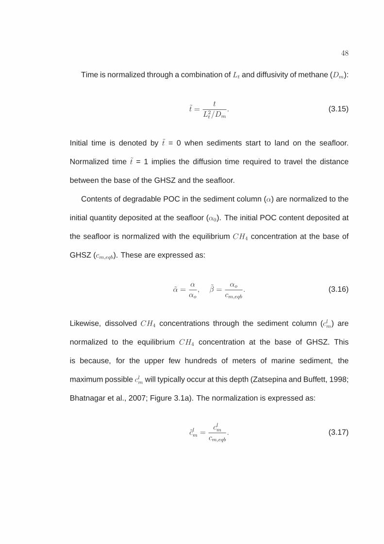
48
Time is normalized through a combination of Lt and diffusivity of methane (Dm):
t =t
L2t/Dm
. (3.15)
Initial time is denoted by t = 0 when sediments start to land on the seafloor.
Normalized time t = 1 implies the diffusion time required to travel the distance
between the base of the GHSZ and the seafloor.
Contents of degradable POC in the sediment column (α) are normalized to the
initial quantity deposited at the seafloor (α0). The initial POC content deposited at
the seafloor is normalized with the equilibrium CH4 concentration at the base of
GHSZ (cm,eqb). These are expressed as:
α =α
αo
, β =αo
cm,eqb
. (3.16)
Likewise, dissolved CH4 concentrations through the sediment column (clm) are
normalized to the equilibrium CH4 concentration at the base of GHSZ. This
is because, for the upper few hundreds of meters of marine sediment, the
maximum possible clm will typically occur at this depth (Zatsepina and Buffett, 1998;
Bhatnagar et al., 2007; Figure 3.1a). The normalization is expressed as:
clm =clm
cm,eqb
. (3.17)

49
By contrast, pore water SO2−4 , DIC, and Ca2+ concentrations are normalized to
their respective values in seawater, cs,o, cb,o, and cCa,o:
cls =clscs,o
, clb =clbcb,o
, clCa =clCa
cCa,o
. (3.18)
In general, normalized SO2−4 and Ca2+ concentrations will diminish from 1 with
depth, while normalized DIC concentrations will exceed 1 with depth (Figures 3.4
and 3.5).
Porosity at a given depth is normalized to the minimum value at great depth
(φ∞):
φ =φ− φ∞
1− φ∞
. (3.19)
However, to obtain appropriate porosity profile with depth and to simplify equations,
two additional parameters are introduced:
η =φo − φ∞
1− φ∞
, γ =1− φ∞
φ∞
, (3.20)
where φo is porosity at the seafloor and η is the normalized porosity at the seafloor.
In general, porosity decreases with depth because of compaction, so that φo >
φ > φ∞ and η > φ. At great depth, porosity approaches a minimum value and the
fluid and sediment velocities approach a common asymptotic value (Berner, 1980;
Davie and Buffett, 2001; Bhatnagar et al., 2007). Fluid gets buried (downward)
with the sediment and its velocity increases with depth. However, the fluid flux

50
(product of its velocity and porosity) at any depth remains constant at steady state
conditions.
The downward component of the net fluid flux (Uf ), defined as Uf,sed, can be
expressed as a combination of sedimentation rate (S) and porosity parameters
(Bhatnagar et al., 2007):
Uf,sed =1− φo
1− φ∞
Sφ∞. (3.21)
The sediment flux (Used) can be defined as:
Used = (1− φo)S. (3.22)
It represents the downward transport of sediment grains, and is assumed to be
constant. For convenience, it can be scaled with respect to Uf,sed, which can be
related to γ (Bhatnagar et al., 2007):
Used =Used
Uf,sed
=(1− φo)S
Uf,sed
=
(1−φ∞
φ∞
)Uf,sed
Uf,sed
=1− φ∞
φ∞
= γ. (3.23)
Other than through fluid burial, dissolved species can move through external
fluid flow and diffusion. The relative significance of these processes are
perhaps best understood by defining two dimensionless groups known as Peclet
numbers. The first Peclet number (Pe1) we define characterizes the ratio of

51
sedimentation-compaction-driven fluid flux to methane diffusion:
Pe1 =Uf,sedLt
Dm
. (3.24)
By contrast, the second Peclet number (Pe2) characterizes the ratio of external
fluid flux (generally upward from deeper sediment) to CH4 diffusion:
Pe2 =Uf,extLt
Dm
. (3.25)
These dimensionless numbers are scaled by CH4 difussion to enable quick
comparison of relative amounts of advection and diffusion of methane. Crucially,
Pe1 and Pe2 typically act in downward and upward directions respectively, and
have opposite signs.
Another set of dimensionless groups, the Damkohler numbers, are also
convenient because they characterize the ratio of reaction to diffusion. Three
Damkohler numbers are defined here:
Methanogenesis:
Da =λL2
t
Dm
, (3.26)
AOM:
DaAOM =ρwcm,eqb
MCH4
λAOML2t
Dm
, (3.27)

52
Organoclastic sulfate reduction:
DaPOC =ρwcm,eqb
MPOC
λPOCL2t
Ds
. (3.28)
All parameters and dimensionless groups are defined collectively, along with
specific values in the notation section and Table 3.1.
Dimensionless Mass Balance Equations
The dimensional mass balance equations (equations 3.7-3.13) can be rewritten
in dimensionless form using the normalized variables and dimensionless groups
defined above. The evolution of POC through depth and time can be expressed
as:
∂
∂t
[(1− φ)α
]+ Pe1
∂
∂z
[(1 + γ
γ
)Usedα
]= −Da(1− φ)α
−(1− φ)(1 + γφ)
1 + γ
DsMPOCcs,oDmMSO4
cm,eqb
DaPOCαcls. (3.29)
For CH4, the dimensionless mass balance equation is:
∂
∂t
[(1 + γφ
γ
)clm
]+
(1 + γ
γ
)(Pe1 + Pe2)
∂clm∂z
=∂
∂z
[(1 + γφ
γ
)∂clm∂z
]
+MCH4
2MPOC
ρsedDa(1− φ)αβ −
(1 + γφ
γ
)MCH4
cs,oMSO4
cm,eqb
DaAOM clmcls. (3.30)

53
For SO2−4 :
∂
∂t
[(1 + γφ
γ
)cls
]+
(1 + γ
γ
)(Pe1 + Pe2)
∂cls∂z
=∂
∂z
[(1 + γφ
γ
)Ds
Dm
∂cls∂z
]
−
((1 + γφ)
γ
)DaAOM clmc
ls −
(1 + γφ)(1− φ)
1 + γ
Ds
2Dm
ρsedDaPOCαβcls. (3.31)
For DIC:
∂
∂t
[(1 + γφ
γ
)clb
]+
(1 + γ
γ
)(Pe1 + Pe2)
∂clb∂z
=∂
∂z
[(1 + γφ
γ
)Db
Dm
∂clb∂z
]
+MHCO3
cm,eqb
2MPOCcb,oρsedDa(1− φ)αβ +
(1 + γφ
γ
)MHCO3
cs,oMSO4
cb,oDaAOM clmc
ls
MHCO3cs,o
MSO4cb,o
(1 + γφ)(1− φ)
1 + γ
Ds
Dm
ρsedDaPOCαβcls −
(1 + γφ
γ
)CCa,o
Cb,o
∆cCaCO3
∆t. (3.32)
For Ca2+:
∂
∂t
[(1 + γφ
γ
)clCa
]+
(1 + γ
γ
)(Pe1 + Pe2)
∂clCa
∂z
=∂
∂z
[(1 + γφ
γ
)DCa
Dm
∂clCa
∂z
]−
(1 + γφ
γ
)∆cCaCO3
∆t. (3.33)
For 12C and 13C of CH4:
∂
∂t
[(1 + γφ
γ
)clmδ
13CCH4
]+
(1 + γ
γ
)(Pe1 + Pe2)
∂(clmδ
13CCH4
)
∂z
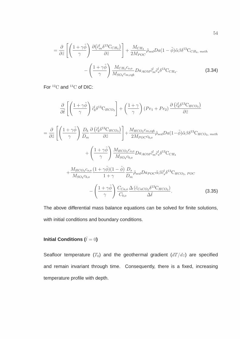
54
=∂
∂z
[(1 + γφ
γ
)∂(clmδ
13CCH4
)
∂z
]+
MCH4
2MPOC
ρsedDa(1− φ)αβδ13CCH4, meth
−
(1 + γφ
γ
)MCH4
cs,oMSO4
cm,eqb
DaAOM clmclsδ
13CCH4. (3.34)
For 12C and 13C of DIC:
∂
∂t
[(1 + γφ
γ
)clbδ
13CHCO3
]+
(1 + γ
γ
)(Pe1 + Pe2)
∂(clbδ
13CHCO3
)
∂z
=∂
∂z
[(1 + γφ
γ
)Db
Dm
∂(clbδ
13CHCO3
)
∂z
]+MHCO3
cm,eqb
2MPOCcb,oρsedDa(1−φ)αβδ13CHCO3, meth
+
(1 + γφ
γ
)MHCO3
cs,oMSO4
cb,oDaAOM clmc
lsδ
13CCH4
+MHCO3
cs,oMSO4
cb,o
(1 + γφ)(1− φ)
1 + γ
Ds
Dm
ρsedDaPOCαβclsδ
13CHCO3, POC
−
(1 + γφ
γ
)CCa,o
Cb,o
∆(cCaCO3δ13CHCO3
)
∆t. (3.35)
The above differential mass balance equations can be solved for finite solutions,
with initial conditions and boundary conditions.
Initial Conditions ( t = 0)
Seafloor temperature (T0) and the geothermal gradient (dT/dz) are specified
and remain invariant through time. Consequently, there is a fixed, increasing
temperature profile with depth.

55
Pressure is set to hydrostatic conditions throughout the sediment column. This
appears valid for z < Lt because, in several drill holes, the base of the GHSZ
lies close to a depth predicted from gas hydrate stability conditions, measured
temperatures, salinities and hydrostatic pressure (e.g., Paull et al.,1996; Trehu et
al., 2003). With this assumption, the normalized porosity profile can be computed
as an analytical expression (Bhatnagar et al., 2007):
φ =η
η + (1− η)eNtφz, (3.36)
where Ntφ is the depth to the base of the GHSZ relative to the compaction depth
(Lφ). These parameters are defined as:
Ntφ =Lt
Lφ
, Lφ =σφ
(1− φ∞)(ρsed − ρw)g, (3.37)
where σφ is characteristic constant with units of stress, and g is acceleration due
to gravity. In all the following simulations, Ntφ = 1, implying compaction depth (Lφ)
is equal to the thickness of the GHSZ (Lt). Unit compaction depth further implies
porosity at this depth is reduced by 1/e (or 36.8%) from its initial porosity at the
seafloor.
The labile organic carbon content (α) is assumed to be 0% throughout all
sediment at initial time t = 0. No CH4 is present at this time in the sediment
column, so the CH4 concentration (clm) is zero. Therefore, the normalized labile

56
organic content (α), and the CH4 concentration (clm) are zero (equation 3.38).
α(z, 0) = 0, clm(z, 0) = 0. (3.38)
The pore water SO2−4 (cls), DIC (clb), Ca2+ (clCa) concentrations, and the carbon
isotope compositions (δ13C) are assumed to be seawater values at initial time for
any depth z. The normalized pore water concentrations of SO2−4 (cls), DIC (clb),
Ca2+ (clCa) are unity at t = 0 (equation 3.39). At the same time, carbon isotope
compositions in CH4 and DIC are zero because the carbon isotope compositions
are normalized relative to a marine carbonate standard.
cls(z, 0) = 1, clb(z, 0) = 1, clCa(z, 0) = 1,
δ13CCH4(z, 0) = 0, δ13CHCO3
(z, 0) = 0. (3.39)
In essence, at t = 0, there is a sediment column with prescribed physical
conditions (i.e., temperature, pressure, and porosity). This column has no POC,
and pore space is filled with seawater. For all t > 0, POC is continuously deposited
on the seafloor. A fraction of this is labile and, upon burial, drives a sequence of
chemical reactions. These lead to changes in pore water CH4, SO2−4 , DIC, and
Ca2+ concentrations, as well as the δ13C of DIC. The amounts of CH4, DIC and
Ca2+ are restricted because of solubility.

57
Boundary Conditions
As time progresses, pore water concentrations throughout the sediment column
change from their initial values. Boundary values are specified to all variables at
the seafloor, and at the bottom of the simulation domain. Normalized labile POC
content is unity at the seafloor. By contrast, due to very low CH4 concentrations in
seawater, normalized CH4 concentration is zero at the seafloor. These boundary
values are:
α(0, t) = 1, clm(0, t) = 0. (3.40)
As discussed earlier, CH4 concentration is also zero below the seafloor until
the SMT. Importantly, however, this is not prescribed as a boundary value. Instead,
this condition arises in the model because minimal methanogenesis occurs in the
presence of SO2−4 , and because CH4 reacts with SO2−
4 via AOM.
At the seafloor, normalized pore water SO2−4 , DIC and Ca2+ concentrations are
unity, while normalized carbon isotope compositions in CH4 and DIC are zero.
These are:
cls(0, t) = 1, clb(0, t) = 1, clCa(0, t) = 1,
δ13CCH4(0, t) = 0, δ13CHCO3
(0, t) = 0. (3.41)
Upward fluid flux is modeled so as to transport dissolved CH4, DIC, Ca2+,
and other pore water species from deeper sediments. Consequently, pore water
concentrations need to be specified at the base of the simulation domain (Lz =

58
2Lt). Pore water CH4 concentration at this depth (cm,ext) equals the equilibrium
CH4 concentration cm,eqb at this depth (equation 3.42):
clm(Lz, t) = cm,ext = cm,eqb(Lz). (3.42)
where cm,ext is normalized specified CH4 concentration at depth Lz (=Lz/Lt). The
system, therefore, is charged with CH4 saturated water at the lowermost boundary.
Similarly, normalized concentrations are specified at Lz for SO2−4 (cs,ext), DIC
(cb,ext) and Ca2+ (cCa,ext). Pore water SO2−4 is consumed above or at the SMT;
hence, (cs,ext) is zero. Dissolved DIC and Ca2+ concentrations are set so they are
in equilibrium with solubility concentrations of CaCO3 at depth. Collectively,
cls(Lz, t) = cs,ext = 0, clb(Lz, t) = cb,ext, clCa(Lz, t) = cCa,ext. (3.43)
During methanogenesis, a range of solid organic molecules with a range
of carbon isotope compositions produces CH4 relatively depleted in 13C, and
DIC relatively enriched in 13C. The pathways involved are somewhat complex,
especially regarding isotope fractionation (Appendix A; Conrad, 2005). To simplify
the modeling, we assume a fixed δ13C for POC and labile POC (δ13CPOC), and
a fixed δ13C for CH4 generated during methanogenesis (δ13CCH4,meth). Both
values will be site specific. The δ13CCH4,meth values are determined by computing
the average values of δ13C of CH4 (Milkov et al., 2005; Lorenson et al., 2008)

59
measured at the two sites. This implies that the fractionation factor (εm) and the
δ13C of DIC produced during methanogenesis (δ13CHCO3,meth) will also be fixed at
a given site. For the two sites of immediate interest, the values are:
δ13CPOC = −24 0/00, δ13CCH4,meth = −70 0/00, (Site 1244), (3.44)
δ13CPOC = −22 0/00, δ13CCH4,meth = −75 0/00, (Site KC151− 3). (3.45)
Fractionation factor (εm) is defined as the ratio of δ13C of labile POC and CH4:
εm =δ13CPOC + 1000
δ13CCH4,meth + 1000. (3.46)
The δ13CHCO3,meth values and the fractionation factors at these sites are calculated
using the carbon isotope compositions δ13CPOC , and δ13CCH4,meth:
δ13CHCO3,meth = +22 0/00, εm = 1.049 (Site 1244), (3.47)
δ13CHCO3,meth = +31 0/00, εm = 1.057 (Site KC151− 3). (3.48)
The carbon isotope composition of DIC (δ13CHCO3) produced by organoclastic
sulfate reduction is equated to that of POC (δ13CPOC). For sediment at respective
sites:
δ13CHCO3,POC = δ13CPOC = −24 0/00 (Site 1244), (3.49)
60
δ13CHCO3,POC = δ13CPOC = −22 0/00 (Site KC151− 3). (3.50)
The δ13C of CH4 (δ13CCH4) and DIC (δ13CHCO3
) at the basal boundary (Lz) are
specified as observed in field data (Milkov et al., 2005; Torres and Rugh, 2006;
Lorenson et al., 2008; Kastner et al., 2008a):
For Site 1244:
δ13CCH4(Lz, t) = δ13CCH4,ext = −65 0/00,
δ13CHCO3(Lz, t) = δ13CHCO3,ext = +20 0/00. (3.51)
For Site KC151-3:
δ13CCH4(Lz, t) = δ13CCH4,ext = −70 0/00,
δ13CHCO3(Lz, t) = δ13CHCO3,ext = +10 0/00. (3.52)
3.3.5 Numerical Solution
The dimensionless mass balance equations (equations 3.29 - 3.35) were solved
in conservative form for specified initial and boundary conditions (equations 3.38
- 3.52) to obtain steady state solutions. The hyperbolic dimensionless partial
differential equation for POC (equation 3.29) was solved numerically using an
implicit, block-centered, finite difference scheme. To solve the other six equations
(equations 3.30 - 3.35), explicit numerical schemes were formulated. These six
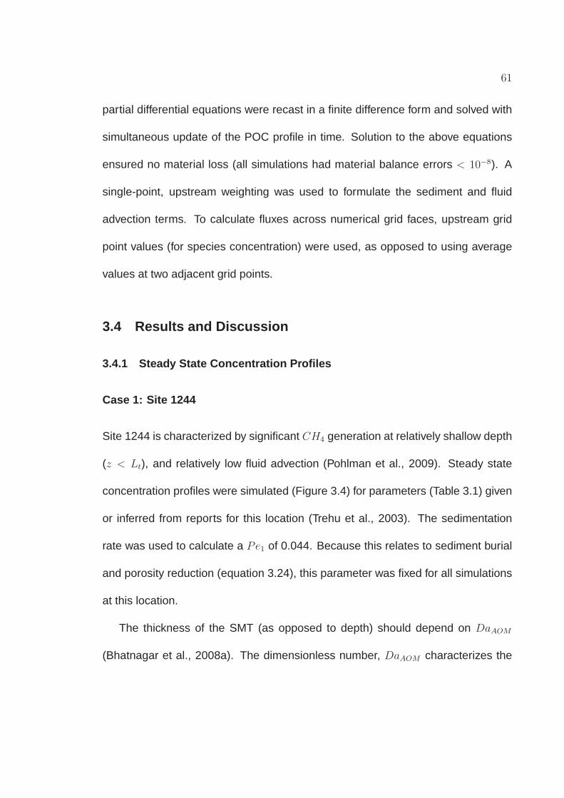
61
partial differential equations were recast in a finite difference form and solved with
simultaneous update of the POC profile in time. Solution to the above equations
ensured no material loss (all simulations had material balance errors < 10−8). A
single-point, upstream weighting was used to formulate the sediment and fluid
advection terms. To calculate fluxes across numerical grid faces, upstream grid
point values (for species concentration) were used, as opposed to using average
values at two adjacent grid points.
3.4 Results and Discussion
3.4.1 Steady State Concentration Profiles
Case 1: Site 1244
Site 1244 is characterized by significant CH4 generation at relatively shallow depth
(z < Lt), and relatively low fluid advection (Pohlman et al., 2009). Steady state
concentration profiles were simulated (Figure 3.4) for parameters (Table 3.1) given
or inferred from reports for this location (Trehu et al., 2003). The sedimentation
rate was used to calculate a Pe1 of 0.044. Because this relates to sediment burial
and porosity reduction (equation 3.24), this parameter was fixed for all simulations
at this location.
The thickness of the SMT (as opposed to depth) should depend on DaAOM
(Bhatnagar et al., 2008a). The dimensionless number, DaAOM characterizes the

62
Table 3.1 : Model Parameters for Sites 1244 and KC151
Symbol Definition (units) Hydrate Keathley
Ridge 1244 a Canyon 151 b
Lo Seafloor depth (m) 890 1322
P0 Seafloor pressure (MPa) 8.72 12.95
T0 Seafloor temperature (oC) 3.8 4
dT/dz Geothermal gradient (oC/m) 0.061 0.038
Lt Depth to GHSZ (mbsf) 133.4 314.1
Ls Depth to SMT (mbsf) 9.2 10.4
S Sedimentation rate (m/Myr) 270 250
Uf,sed Fluid flux due to sedimentation (m/s) 2.85 ×10⁻¹³ 2.64 ×10⁻¹³
Pe1 First Peclet number - sedimentation 0.044 0.095
and compaction driven fluid flow
Pe2 Second Peclet number - external fluid flow -1, -2, -3 -2, -3, -5
TOC Total organic carbon (%) 1.27 0.44
- Labile fractionc (%) 32 20
αo Labile organic carbon at seafloor (%) 0.4 0.08
β Normalized organic carbon at seafloor 2.4 0.38
cm,eqb CH4 solubility at base of the GHSZ 1.701 ×10⁻³ 2.101 ×10⁻³
cs,o Seawater SO2−4 concentration (mM) 28 28
cb,o Seawater DIC concentration (mM) 2.4 2.4
cCa,o Seawater Ca2+ concentration (mM) 10 10
Dm CH4 diffusivityd (m2/s) 0.87 ×10⁻⁹ 0.87 ×10⁻⁹
Ds SO2−4 diffusivityd (m2/s) 0.56 ×10⁻⁹ 0.56 ×10⁻⁹
aTrehu et al. (2003)bRuppel et al. (2008)cLabile fraction has been reported as a wide range in the literature. Davie and Buffett
(2001, 2003a) and Bhatnagar et al. (2007) assumed 75% of the organic carbon to belabile and available for methanogenesis. A lower estimate was chosen for this fractionbased on unconverted organic carbon data at sites 1244 and KC151-3.
dIversen and Jorgensen (1993)

63
Table 3.1 contd. Model Parameters for Sites 1244 and KC151
Symbol Definition (units) Hydrate Keathley
Ridge 1244 Canyon 151
Db DIC diffusivitya (m2/s) 0.6 ×10⁻⁹ 0.6 ×10⁻⁹
DCa Ca2+ diffusivitye (m2/s) 0.4 ×10⁻⁹ 0.4 ×10⁻⁹
Da Damkohler number (methanogenesis) 0.22 0.22
DaPOC Damkohler number (OSR) 2.5 2.5
DaAOM Damkohler numberb (AOM) 108 108
λ Rate constant for methanogenesis (s−1) c1.07 ×10−14 1.94 ×10⁻¹⁵
λPOC Rate constant for OSR (m3/(mol.s)) 5.55 ×10⁻¹⁶ 8.1 ×10⁻¹⁷
λAOM Rate constant for AOM (m3/(mol.s)) 4.60 ×10⁻⁸ 6.71 ×10⁻⁹
Ntφ Ratio of Lt to Lφ 1 1
ρsed Sediment density (kg/m3) 2650 2650
ρw Water density (kg/m3) 1000 1000
MCH4CH4 molecular weight (g/mol) 16 16
MSO4SO2−
4 molecular weight (g/mol) 96 96
MHCO3DIC molecular weight (g/mol) 61 61
MCa Ca2+molecular weight (g/mol) 40 40
MPOC POC molecular weightd (g/mol) 12 12
aLi and Gregory (1974)bBhatnagar et al. (2008a)cDavie and Buffett (2001), Bhatnagar et al. (2007)dMorg used in Davie and Buffett (2001, 2003a) and Bhatnagar et al. (2007) was interpreted
as generic organic matter (MW = 30 g/mol). After Malinverno (2010), these parameters wererededined based on organic carbon (MPOC) and mass of carbon (MW =12 g/mol) is used for thesecalculations in this work.

64
rate of AOM reaction to diffusion. The chosen value for DaAOM = 108 for all
simulations unless otherwise specified, because this results in a thin overlap of
CH4 and SO2−4 profiles at the SMT, as observed in many locations (although difficult
to prove at Site 1244 with the low sample resolution, Figure 3.3a).
The normalized dissolved CH4 concentration profile (Figure 3.4a) shows
near-zero values at the SMT (z = 0.08 or 10.6 mbsf) underlain by a rapid rise with
increasing depth (n.b., concentration profiles are plotted to the base of the GHSZ,
z = 1, although simulated to z = 2). Upon exceeding local solubility conditions,
excess CH4 would form gas hydrate. This depth occurs at z = 0.65 (or 86 mbsf),
with the chosen parameters (Table 3.1) and Pe2 = −1, which relates to an upward
fluid velocity 0.3 mm/yr at the seafloor. There should exist relationships between
pore water SO2−4 concentrations, pore water CH4 concentrations, CH4 solubility,
and the shallowest occurrence of gas hydrate (Figure 3.1). These are emphasized
elsewhere (Bhatnagar et al., 2008a, 2011). Here, the primary points are that CH4
rises from depth due to a combination of advection and diffusion, and it decreases
to near zero concentration at the SMT. The overall profile emerges because of
dissolved CH4 production below the SMT, because of internal cycling of methane
phases within the GHSZ (although not specifically modeled in this chapter), and
because of AOM at the SMT. Moreover, as discussed below, an increase in upward
fluid flux moves the methane profile and the SMT to shallower depths.
Normalized SO2−4 concentrations drop nearly linearly from unity at the seafloor

65
1 20 45
Normalized alkalinity
concentration
0 0.5 1
Normalized calcium
concentration
-30 0 250 0.5 1
0
0.2
0.4
0.6
0.8
1.0
Normalized methane and
sulfate concentration
No
rma
lize
d d
ep
th
δ13C of DIC (‰)
1244Pe
2 = -1
Pe2 = -3
Pe2 = -2
Figure 3.4 : Steady state normalized pore water concentration profiles at Site 1244.(a) CH4 (solid), and SO2−
4 (dashed), (b) DIC, (c) Ca2+, and (d) δ13C of DIC. Theblue, green and red curves correspond to increasing magnitude of Pe2 (fluid fluxfrom depth) shown by direction of arrow. Site 1244 data (black circles) (Trehu etal., 2003; Torres and Rugh, 2006). Parameters: Pe1 = 0.044, Da = 0.22, DaPOC =2.5, DaAOM = 108, β = 2.4, cb,ext= 27 and δ13CHCO3,ext
= 20.

66
to effectively zero at the SMT (Figure 3.4a). This depth lies at z = 0.08 (10.6 mbsf)
with the aforementioned initial estimates, and relatively high and low values for
dimensionless groups related to rates for AOM (DaAOM = 108) and organoclastic
sulfate reduction (DaPOC = 2.5). The combination of AOM (at the SMT) and
organoclastic sulfate reduction (between the seafloor and the SMT) removes all
SO2−4 . However, with these group values, AOM dominates net SO2−
4 consumption.
The depth of the SMT should change with upward methane flux (e.g., Borowski
et al., 1996; Davie and Buffett, 2003b; Bhatnagar et al., 2008a). This can
be simulated under conditions of finite Pe1 but varying Pe2 (Figure 3.4). For
example, with conditions stated so far, as the magnitude of Pe2 rises from 1 to
3, the SMT shoals from z = 0.08 to z = 0.03 (4 mbsf). The SO2−4 profile at Site
1244 exhibits a slight concave-up curvature above the SMT, which could reflect
a drop in sediment porosity with increasing depth over the upper few meters
(Dickens, 2001b). Physical property records at Site 1244 appear consistent with
this interpretation (Shipboard Scientific Party, 2003b), although such heterogeneity
has not been incorporated into these simulations.
The case where Pe2 is -1 is particularly interesting. This gives pore water CH4
and SO2−4 profiles similar to those at Site 1244, including an SMT at 10.6 mbsf
(z = 0.08) (Figure 3.4a). Moreover, with Pe2 = -1, the CH4 profile intersects the
solubility curve at ∼z = 0.65 (86 mbsf), (not shown here). This would mark the
shallowest occurrence of gas hydrate, which is about the depth (50 mbsf) reported

67
in field observations (Trehu et al., 2003; Lee and Collett, 2006).
With the initial estimate (Pe2 = -1), the model simultaneously simulates
normalized pore water profiles of DIC and Ca2+ concentrations, and the δ13C of
DIC. For DIC, values increase from unity at the seafloor (cb,o = 2.4 mM) to 16.6 (=
39.8 mM) at the SMT (z = 0.08); below, values increase more gradually with depth,
giving rise to a curvature similar to observations (Figure 3.4b). The overall shape
arises for three primary reasons: first, methanogenesis generates considerable
DIC at depth; second, this DIC enters the SMT through advection and diffusion to
mix with DIC generated by AOM; third, DIC decreases from the SMT to the seafloor
as it leaves the sediment through advection and diffusion. Calcite precipitation also
removes a small amount of DIC within 0.5 m around the SMT.
The previously noted simulations with different Pe2 demonstrate the effect of
increasing upward fluid flux upon the shape of the DIC profile (Figure 3.4b). As
external advection (and CH4 input from depth) increases, the SMT shallows and
the production of DIC at this horizon (by AOM) accelerates. In addition, greater
amounts of DIC generated by methanogenesis ascend with pore fluids. The total
effect is to amplify the ”kink” in the DIC profile, such that greater amounts of DIC
leave the system through the seafloor.
Normalized Ca2+ concentrations (Figure 3.4c) decrease from unity at the
sediment-water interface (cCa,o = 10 mM) to 0.37 (= 3.7 mM) at the SMT. Below
this, values continue to drop, although at a more gradual rate. The generic shape

68
of the Ca2+ profile arises for three reasons: first, seawater Ca2+ enters the SMT
from above, through diffusion; second, advection carries the fluid upward (Pe1 +
Pe2 < 0); and third, Ca2+ reacts with DIC to precipitate as carbonate. These factors
also make the Ca2+ concentration profile a ”mirror image” of the DIC profile (albeit
somewhat distorted). As such, an increase in upward fluid flux changes the shape
of the Ca2+ profile predictably: above the SMT, the gradient steepens; below the
SMT, the gradient lessens slightly (Figure 3.4c). This is because fluids depleted in
Ca2+ rise from depth and increased fluid flux causes greater CaCO3 precipitation.
Additionally, increased delivery of DIC from below promotes CaCO3 precipitation
and likewise the demand for Ca2+ from seawater, resulting in the steepened Ca2+
gradients above the SMT.
The steady state profile for the δ13C of DIC (Figure 3.4d) is especially
interesting. For the initial estimates, the δ13C of DIC drops from zero at the
seafloor to -26 0/00 at the SMT, but with ”concave-down” curvature; below the SMT, it
increases with depth to more positive values (+20 0/00), again with ”concave-down”
curvature. Importantly, the value at the SMT and the shape around the SMT are not
prescribed in the model. Instead, these occur for two reasons. First, DIC produced
during methanogenesis and having an initial δ13C of +20 0/00 rises from depth to
mix with DIC generated at the SMT and having a δ13C of -65 0/00. Second, this
”mixed source” DIC moves toward the seafloor, where DIC is fixed at 0 0/00. With an
increase in external fluid flux, the δ13C of DIC at the SMT attains a negative peak

69
(∼-25 0/00 when Pe2 = -3) at a relatively shallower depth. In summary, this pore
water δ13C profile arises in a system where AOM dominates net consumption of
SO2−4 in shallow sediment.
Case 2: Site KC151-3
Site KC151-3 differs from Site 1244 in two fundamental ways: fluids rich in CH4 and
poor in SO2−4 rise from depth but at a relatively high rate (Dugan, 2008; Daigle and
Dugan, 2010a); and concentrations of pore water DIC and Ca2+ are low (<10 mM)
and high (>20 mM), respectively, at the base of the simulated domain. Pore water
concentration profiles are modeled at Site KC151-3 (Figure 3.5) in an identical
manner to those at Site 1244, but with a different set of parameters based on
observations for Site KC151-3 (Table 3.1).
From the sedimentation rate, a Pe1 of 0.095 is calculated. An initial estimate
for Pe2 was -2, which relates to an upward fluid velocity 0.25 mm/yr at the seafloor
(comparable to Pe2 = -1 at Site 1244). The dimensionless groups related to AOM
rate (DaAOM = 108) and organoclastic sulfate reduction (DaPOC = 2.5) used to
model location KC151-3 were the same as used for Site 1244. The combined
effects of AOM (at the SMT) and organoclastic sulfate reduction (between the
seafloor and the SMT) are responsible for net SO2−4 consumption, although owing
to the relatively low value of DaPOC , AOM is dominant also at KC151-3.
The normalized dissolved CH4 profile (Figure 3.5a) is zero between the seafloor

70
0 0.5 1
0
0.2
0.4
0.6
0.8
1.0
1 5 10 0 1 2 3 -65 -25 20
KC151-3Pe
2 = -2
Pe2 = -5
Pe2 = -3
Normalized alkalinity
concentration
Normalized calcium
concentrationNormalized methane and
sulfate concentration
δ13C of DIC (‰)
No
rma
lize
d d
ep
th
Figure 3.5 : Steady state normalized pore water concentration profiles at SiteKC151-3. (a) CH4 (solid), and SO2−
4 (dashed), (b) DIC, (c) Ca2+, and (d) δ13Cof DIC. The blue, green and red curves correspond to increasing magnitude ofPe2 (fluid flux from depth) shown by direction of arrow. Site KC151-3 data (blackcircles) (Kastner et al., 2008b). Parameters: Pe1 = 0.095, Da = 0.22, DaPOC = 2.5,DaAOM = 108, β = 0.38, cb,ext = 1.5 and δ13CHCO3,ext
= 10.

71
and the SMT (z = 0.05 or 15.7 mbsf). Below 15.7 mbsf, it shows a rapid increase
with depth. Methane concentrations intersect those on the solubility curve at z =
0.45 (or 141 mbsf). This should mark the shallowest possible occurrence of gas
hydrate, but log interpretations suggest gas hydrate occurs between 110 and 115
mbsf (Cook et al., 2008).
Normalized, steady state SO2−4 concentrations (Figure 3.5a) decrease nearly
linearly from unity at the sediment-water interface to near-zero at the SMT (z
= 0.05). As at Site 1244, the SO2−4 data exhibit a slight concave-up curvature
above the SMT at Site KC151-3. The simulated SO2−4 profile does not show such
curvature, and this may again relate to a drop in porosity over the first few meters.
Upon increasing the external fluid flux (and the magnitude of Pe2), the SMT
shoals (Figure 3.5a). For one particular parameter choice (Pe2 = -3), the SO2−4
profile drops to near-zero concentration at z = 0.031. This implies that the SMT and
the top of gas hydrate occur at ∼9.8 mbsf and ∼82 mbsf (z = 0.26), respectively.
These values agree favorably with field data.
Normalized DIC profiles (Figure 3.5b) contrast markedly with those at Site
1244, irrespective of fluid flux. For the initial estimate, concentrations increase
with depth until the SMT, below which they decrease to very low values (∼4 mM).
The prominent DIC peak at the SMT arises for four primary reasons: first, and
most importantly, AOM generates DIC at the SMT; second, this DIC, through
advection and diffusion, leaves the SMT; third, methanogenesis produces DIC at

72
depth; fourth, pore fluids enriched in Ca2+ react with DIC below the SMT. Calcite
precipitation also removes relatively more DIC below the SMT at this location.
An increase in upward fluid flux changes the shape of the DIC profile above and
below the SMT (Figure 3.5b). However, the reason is somewhat different than that
for Site 1244. A higher fluid flux results in greater CH4 input to the SMT, greater
DIC generation by AOM, greater DIC input to the SMT from depth, and greater
DIC removal from the SMT toward the seafloor. It also raises the Ca2+ input from
depth, which leads to greater calcite precipitation, below the SMT. Similar to SO2−4 ,
DIC profiles also approach the field data for a value of Pe2 = -3.
Normalized pore water Ca2+ concentrations (Figure 3.5c) drop from unity at
the seafloor to a low value at the SMT and then increase to a constant value at
depth. The shape of Ca2+ profiles arises for multiple reasons: first, Ca2+ from the
ocean water enters the SMT from above due to diffusion; second, a high flux of
Ca2+ enters the SMT from deeper strata, through advection and diffusion; a third,
significant amount of calcite precipitates. The combination gives rise to the unusual
Ca2+ profile with a ”dip” below the SMT. A higher upward fluid flux compresses
this dip because of greater Ca2+ input from depth, and because of greater calcite
precipitation (Figure 3.5c). These model simulations render results approaching
those of field data when Pe2 = -3.
The modeled profiles of DIC δ13C differ significantly from those at Site 1244 in
terms of magnitude (Figure 3.5d). For the initial estimate (Pe2 = -2), normalized

73
δ13C of DIC is zero at the seafloor, drops to an extreme of -62 0/00 at the SMT,
and then increases gradually with depth, but only to 10 0/00. On increasing fluid
flux from depth, the δ13C values similarly drops from 0 0/00 to a negative peak at
a relatively shallower SMT, then increases more rapidly to more positive values at
greater depth.
Crucially, the values and the curvature of the DIC δ13C profile result from
modeling the CH4 and SO2−4 mass balances using basic parameters for the site;
they are not specified. Moreover, and importantly, the values and the curvature
arise for same general reasons as at Site 1244. The difference between the sites
mainly occurs because the flux and carbon isotopic composition of DIC entering
the SMT from below are less at KC151-3, and because the DIC produced at SMT
(by AOM) has a more 13C-depleted value (δ13C = -70 0/00). In other words, the
proportion of DIC entering the SMT from depth versus that produced by AOM
is much lower at Site KC151-3 compared to Site 1244. This gives a lower DIC
concentration at the SMT and a more negative peak in DIC δ13C at the SMT.
3.4.2 Variations in AOM and Organoclastic Sulfate Reduction
Anaerobic oxidation of methane at the SMT with minimal organoclastic sulfate
reduction at or above this horizon explains pore water profiles across the SMT
at Sites 1244 and KC151-3. The very different carbon chemistry at these sites is
predicted by the numerical simulations because of major differences in the supply

74
and isotope composition of DIC from depth. So far, an unresolved issue is how
changes in the relative proportion of AOM and organoclastic sulfate reduction
would affect the profiles. This can be assessed by changing DaAOM and DaPOC in
model simulations for Site 1244.
A decrease in DaAOM from its initial value of 108 to 105 illustrates the effect of this
dimensionless number on pore water profiles (Figure 3.6a) with same parameters
used to simulate the field data at Site 1244 (see notation section). As reported
by Bhatnagar et al. (2008a), a decrease in DaAOM slows the AOM reaction, and
leads to a thicker SMT. Because the SMT horizon is usually thin (<2 m), this small
value of DaAOM is probably unrealistic. Moreover, a smaller DaAOM lowers the
DIC generation at the SMT by AOM, and the Ca2+ removal by calcite formation.
This would render higher Ca2+ concentrations at and above the SMT, and a more
negative δ13C values for DIC. These simulated profiles (DaAOM = 105) would not
match data at the site, suggesting typical values of DaAOM are slightly on the high
side.
An increase in DaPOC should result in higher consumption of POC and SO2−4
between the seafloor and the SMT. This results in higher DIC generation above the
SMT and a non-linear SO2−4 profile with a ”concave-down” curvature. Moreover,
POC gets removed faster in shallow sediment, which means there is less POC to
form CH4 in deeper sediment. As a result, the flux and δ13C value of DIC entering
the SMT from below are lower (Figure 3.6b). A greatly increased DaPOC (= 2.5 ×

75
DaAOM
= 108
DaAOM
= 105
DaPOC
= 2.5
DaPOC
= 2.5x10⁵
No
rma
lize
d d
ep
th
(a) DaAOM
effects
1 20 45 0 0.5 1 -35 0 250 0.5 1Normalized alkalinity
concentration
Normalized calcium
concentration
Normalized methane
and sulfate concentration
δ13C of DIC (‰)
(b) DaPOC
effects
0
0.2
0.4
0.6
0.8
1.0
No
rma
lize
d d
ep
th
1 20 45 0 0.5 1 -35 0 250 0.5 1Normalized alkalinity
concentration
Normalized calcium
concentration
Normalized methane
and sulfate concentration
δ13C of DIC (‰)
0
0.2
0.4
0.6
0.8
1.0
Figure 3.6 : (a) Steady state pore water profiles to study the effect of DaAOM at Site1244. Decrease in DaAOM results in a thicker SMT horizon. Parameters: Pe1 =0.044, Pe2 = -1, Da = 0.22, DaPOC = 2.5, β = 2.4, cb,ext = 27 and δ13CHCO3,ext
= 20.(b) Effect of DaPOC on pore water chemistry at Site 1244. Parameters: Pe1 = 0.044,Pe2 = -1, Da = 0.22, DaAOM = 108, β = 2.4, cb,ext = 27 and δ13CHCO3,ext
= 20. In bothcases, decreasing DaAOM and increasing DaPOC result in higher POC depletion,lesser CH4 and DIC production, greater Ca2+ concentration in pore fluids aboveand below the SMT and a more negative δ13C of DIC at the SMT.

76
105) is not realistic because it does not give results that resemble field data.
3.4.3 Concentration Crossplots of Alkalinity and Sulfate
Excess alkalinity (∆Alk∗) represents the amount of DIC that would occur in pore
water if authigenic carbonate had not precipitated; it can be calculated by summing
the deviations in pore water alkalinity, Ca2+, and Mg2+ relative to their respective
concentrations in seawater. Plots can be constructed showing changes in excess
alkalinity (∆Alk∗) versus changes in SO2−4 (∆SO2−
4 ) (Figure 3.7). Such crossplots
have been used to interpret the relative influence of organoclastic sulfate reduction
and AOM upon SO2−4 consumption in sediment above the SMT (e.g., Claypool
et al., 2006; Kastner et al., 2008a; Torres and Kastner, 2009). Because of the
different molar quantities in the reactions (equations 3.1 and 3.2), the idea has
been that a 1:1 slope would support SO2−4 removal by AOM, a 2:1 slope would
support SO2−4 removal by POC, and a slope in between would support consumption
by both processes. Data from Site KC151-3 above the SMT lie on a 1:1 slope
(Figure 3.7). By contrast, at Site 1244, a nearly 2:1 slope in ∆Alk∗ : ∆SO2−4
characterizes pore waters above the SMT (Figure 3.7). This observation has
been argued to indicate POC driven SO2−4 consumption at Site 1244 (Kastner et
al., 2008a). However, presentation and discussion of the data in such a manner
assumes a closed system with little or no mass transfer of dissolved constituents,
and fails to account for changes in DIC below the SMT (Dickens and Snyder, 2009).

77
0 5 10 15 20 25 30-20
0
20
40
60
80
∆ [SO4
2-] (mM)
∆ [A
lk +
Ca
+ M
g] (m
M)
2:1
1:1
1244
KC151-3
SMT
Seafloor
Increasing depth
Figure 3.7 : Concentration crossplot of ”excess alkalinity” (∆Alk∗) corrected forcarbonate precipitation versus ∆SO2−
4 (mM) relative to the seafloor for shallowsediment at Site 1244 on Hydrate Ridge (Trehu et al., 2003) and Site KC151-3(Kastner et al., 2008b). As emphasized by Kastner et al. (2008b), there is a 2:1relationship for pore water concentrations above the SMT for Site 1244 (red circles)and 1:1 for Site KC151-3 (blue squares). Note, however, that excess alkalinitycontinues to rise below the SMT at Site 1244. This clearly implies an upwardflux of alkalinity from depth; whereas, at Site KC151-3, excess alkalinity decreasebelow the SMT. This decrease is because DIC is consumed by Ca2+ resulting incalcite precipitation.

78
The departure of alkalinity (DIC) and SO2−4 concentrations relative to their
respective seawater values can be obtained from the simulated steady state
pore water profiles. Because Mg2+ was not included in this modeling, ∆Alk∗ is
only computed using DIC and Ca2+ concentrations. A series of simulations is
considered.
For the first three simulations, parameters pertain to Site 1244. However,
the fluid flux and the relative proportion of SO2−4 consumption by AOM and
organoclastic sulfate reduction are adjusted by changing Pe2, DaAOM and DaPOC
(Figure 3.8). All three simulations give a 2:1 relation in ∆Alk∗ : ∆SO2−4 (Figure
3.8).
In the first case, there is zero external fluid flux, no methanogenesis, no AOM
and only organoclastic sulfate reduction. Although a 2:1 slope in ∆Alk∗ : ∆SO2−4
occurs, pore water profiles (not shown here) do not conform to observations. Pore
water SO2−4 decreases gradually with a concave-down curvature. Pore water DIC
increases with depth until the SMT, below which it attains a constant value as DIC
is carried down by advection (burial) and diffusion. The δ13C of DIC is zero at
the seafloor, and attains a constant negative value at and below the SMT. Without
methanogenesis, there is no change in the DIC and δ13C of DIC below the SMT.
In the second and the third cases, there is a low fluid flux (Pe2 = -0.1),
methanogenesis (and thus a deep source of DIC), and AOM. The third case
includes organoclastic sulfate reduction. In these cases, a 2:1 slope in ∆Alk∗:

79
0 5 10 15 20 25 30
Case 1
1:1
2:1
Increasing depth
Case 2
Case 3
SMT
∆ [SO4
2-] (mM)
0
10
20
30
40
50
60
∆ [A
lk +
Ca
] (m
M)
Seafloor
70
Figure 3.8 : Concentration crossplots for ∆Alk∗ and ∆SO2−4 relative to seawater.
Three cases are illustrated here corresponding to a 2:1 slope. Blue dashed linerepresents a case with organoclastic sulfate reduction, no upward fluid flux, noAOM and no deep DIC source (methanogenesis). Parameters: Pe1 = 0.044, Pe2 =0, Da = 0, DaPOC = 2.5, DaAOM = 0, β = 2.4 and cb,ext = 0. Red solid line representsanother case with low and finite upward fluid flux, AOM, methanogenesis, anda deep DIC source, but no organoclastic sulfate reduction. Parameters: Pe1 =0.044, Pe2 = -0.1, Da = 1, DaPOC = 0, DaAOM = 108, β = 2.4 and cb,ext = 79. Thegreen dashed line represents a third case (combination of the first two cases). Itis characterized by AOM, organoclastic sulfate reduction, methanogenesis, deepDIC source and low upward fluid flux. Parameters: Pe1 = 0.044, Pe2 = -0.1, Da= 1, DaPOC = 2.5, DaAOM = 108, β = 2.4 and cb,ext = 79. A 2:1 slope not onlyresults from organoclastic sulfate reduction alone, but also by a combination ofAOM, methanogenesis and a deep DIC source. The depth from the seafloor to theSMT is shown by the arrow; below the SMT, ∆Alk∗ increases with no change in∆SO2−
4 , implying a high DIC flux entering the SMT from below.

80
∆SO2−4 occurs and the profiles generally match the data.
Clearly, a crossplot showing 2:1 slope for in ∆Alk∗:∆SO2−4 above the SMT
concentration does not imply organoclastic consumption of SO2−4 . It can result
from multiple combinations of fluid flux with AOM and a deep source of DIC
(from methanogenesis). More interestingly, changes in the fluid flux or the rate of
methanogenesis and deep source DIC concentration can affect the slope (Figure
3.9). An increase in upward fluid flux (greater magnitude of Pe2) will generally
decrease the slope on a ∆Alk∗:∆SO2−4 crossplot. This is because the SMT shoals
(Figure 3.4) and because a high flux of DIC enters the SMT from depth. By
contrast, an increase in methanogenesis (higher Da) and a higher concentration
of DIC at depth will generally increase the slope (Figure 3.9). This is because
greater methanogenesis results in more DIC at depth, which can then enter the
SMT through advection and diffusion.
Simulated profiles for Site KC151-3 consistently render points that lie beneath
a 2:1 slope; in fact, the slope in ∆Alk∗:∆SO2−4 is less than 1:1 (Figure 3.10).
This reflects the dual facts that a portion of DIC leaves the SMT to accumulate
as carbonate beneath this horizon, and that excess Ca2+ enters shallow sediment
from below. An increase in upward fluid flux would decrease the slope of the
crossplot similar to our above result shown at Site 1244 (Figure 3.9). In any case,
the slope of the line does not indicate the reaction.

81
0 5 10 15 20 25 300
15
30
45
60
75
∆ [A
lk +
Ca
] (m
M)
SMTIncreasing external flux
Seafloor
∆ [SO4
2-] (mM)
Increasing depth
1244 data
Pe2 = -1
Pe2 = -3
Pe2 = -2
Pe2 = -1
Pe2 = -2
Pe2 = -3
2:1
1:1
Site 1244
Figure 3.9 : Concentration crossplots for ∆Alk∗ and ∆SO2−4 relative to the seafloor
with AOM, organoclastic sulfate reduction, methanogenesis, deep DIC source andupward fluid flux at Site 1244. The solid lines correspond to parameters same as inFigure 3.4. Dashed lines correspond to a case with higher rate of methanogenesisrate and greater DIC flux from depth (Da = 1 and cb,ext = 50). The blue, green,and red colors indicate increasing fluid flux (corresponding to Pe2 = -1, -2 and-3). Crossplot constructed from Site 1244 data (black circles) (Trehu et al., 2003)matches well with the simulated crossplots. The slope decreases with increase influid flux from depth. Higher DIC input (due to higher methanogenesis and/or highDIC source at depth) results in a greater slope. Notably, negligence of Mg2+ in∆Alk∗ calculations above, results in a slope less than 2:1 as compared to Figure3.7.

82
0 5 10 15 20 25 30-10
0
20
40
60
∆ [A
lk +
Ca
] (m
M)
SMT
Increasing external flux
Seafloor
∆ [SO42-] (mM)
Increasing depth
2:1
1:1
KC151-3 data
Pe2 = -2
Pe2 = -5
Pe2 = -3
Site KC151-3
Figure 3.10 : Concentration crossplots for ∆Alk∗ and ∆SO2−4 relative to the
seafloor with AOM, organoclastic sulfate reduction, methanogenesis, relativelydepleted DIC source at depth and upward fluid flux at Site KC151-3. Parametersused are same as in 3.5. Increasing upward fluid flux (corresponding to Pe2 = -2,-3 and -5) are represented by blue, green and red curves. Data from Site KC151-3data (Kastner et al., 2008b) is used to construct crossplots shown by black circles.The slope of the crossplot decreases as fluid flux increases (same as in Figure3.9). Contrary to Figure 3.9, ∆Alk∗ decreases with no change in ∆SO2−
4 beyondthe SMT, implying DIC flux leaving the SMT both above and below.

83
3.4.4 Flux Crossplots
In contrast to using ∆Alk∗: ∆ SO2−4 crossplots, concentration gradients of alkalinity
(DIC), SO2−4 and Ca2+ in and out of the SMT might be used to evaluate the role
of AOM (Luff and Wallman, 2003; Snyder et al., 2007; Dickens and Snyder, 2009;
Kim et al., 2011). The basic idea is that the gradients are proportional to fluxes, so
that the sum of changes across the SMT should balance.
Starting from the above simulated results, concentration gradients are
computed by linearly fitting the profiles above and below the SMT. Using these
gradients, and multiplying by sediment diffusion coefficients, diffusive fluxes of
CH4, SO2−4 and DIC are computed across the SMT horizon. Advective flux of
any dissolved species is a function of fluid flux and the solute concentration. In
the vicinity of the SMT, both the CH4 and SO2−4 concentrations approach zero.
Thus, in the vicinity of the SMT both the transport of CH4 and SO2−4 are diffusion
dominated. Furthermore, the net advective DIC flux across the SMT is calculated
as a difference in deeper flux from/to deeper sediment and shallow flux to/from the
seafloor. Across the SMT, this net advective DIC flux is zero as the individual deep
and shallow advective DIC fluxes are equal and opposite in sign. Hence, the total
flux (sum of advective and diffusive flux) is equal to the diffusive flux across the
SMT.
The diffusive fluxes of CH4 and DIC are now plotted relative to the SO2−4 flux
(Figure 3.11). Crucially, this cross-plot (Figure 3.11) not only represents a diffusive

84
flux cross-plot, but it is also equivalent to a net flux crossplot for a given pair of
species. Both CH4 and DIC fluxes show a unique 1:1 correspondence relative
to the SO2−4 flux. This 1:1 correspondence implies dominance of the AOM at the
SMT, due to its stoichiometric balance (equation 3.1). Increasing the reaction rate
of organoclastic sulfate reduction (DaPOC) by few orders of magnitude (∼ 2.5×10²)
does not alter the slope of the flux crossplot (Figure 3.11). Interestingly, increasing
the rate of methanogenesis (Da) and consequently, a high DIC source at depth
also correspond to a 1:1 relation between respective fluxes. In essence, the
difference between DIC flux leaving the SMT toward the seafloor and the flux
entering the SMT from below is equal to the flux added at the SMT by AOM. This
DIC flux added due to AOM at the SMT corresponds to the SO2−4 flux entering the
SMT from above by a simple 1:1 correlation, again because of the stoichiometric
relationship between CH4, DIC, and SO2−4 (equation 3.1). In all these cases, the
rate of downward SO2−4 flux via diffusion is able to keep pace with CH4 delivery
from below, allowing DIC fluxes to also balance across the SMT.
3.4.5 Relationship Between AOM and δ13C Values
Field data show a wide range in δ13C values of DIC at the SMT in shallow
sediment of gas hydrate systems (Figure 3.2). A series of papers have used this to
discriminate between potential causes for pore water SO2−4 consumption (Claypool
et al., 2006; Kastner et al., 2008a; Torres and Kastner, 2009). The basic idea

85
CH4
Case 2
0 10 20 30 40 500
∆ SO4
2- flux (mol/m2 kyr)
60
-60
(Pe2 = -1)-10
-20
-50
-30
-40
∆ C
H4 o
r D
IC flu
x (
mo
l/m
2 k
yr)
Incr
easing e
xtern
al flu
x
Case 1
Case 3
DIC
2:1 1:1
(-3)
(-2)1244(-1)
(-1)
(-2)
(-3)
(-2)(-3)
Figure 3.11 : Flux crossplots of CH4 (circles) and DIC (stars) versus SO2−4 across
the SMT corresponds to a 1:1 slope. Case 1 corresponds to simulations shownin Figure 3.4. The simulation results that best matches Site 1244 data (Pe2 = -1;Figure 3.4) show 17 mol/m2kyr of SO2−
4 entering the SMT from above, 17 mol/m2kyris the difference between amounts of DIC entering from below and leaving towardthe seafloor (including carbonate precipitation). This gives a net change of 17mol/m2kyr of DIC across the SMT, which balances the downward flux of SO2−
4
and supports a 1:1 stoichiometry and dominance of AOM at the SMT. Case 2increases the rate of organoclastic sulfate reduction by two orders of magnitude(DaPOC = 2.5× 10²; all other parameters are same as Case 1) and the relative fluxcorrespondence across the SMT is unaltered. Case 3 corresponds to high DICflux entering the SMT from below and high methanogenesis rate also results in thesame 1:1 correlation between CH4 and DIC fluxes relative to SO2−
4 flux (parameterssame as dashed curves in Figure 3.9). The Pe2 values (equivalent to upward fluidflux) are noted in parenthesis and the arrow indicates increase in upward fluid flux.

86
has been that the δ13C of DIC at the SMT relates to the relative proportion of DIC
generated through AOM and organoclastic sulfate reduction (equations 3.1 and
3.2); the first reaction would produce DIC exceptionally depleted in 13C (δ13C < -40
0/00, depending on the CH4 source) whereas the second reaction would produce
DIC moderately depleted in 13C (δ13C ∼ -23 0/00), roughly corresponding the δ13C
values of POC.
This approach, however, is fundamentally flawed because it neglects other
inputs (and outputs) of DIC to the SMT, especially DIC rising from depth. At
most locations including Sites 1244 and KC151-3, the CH4 is derived from
methanogenesis (equation 3.3 and Appendix A). As such, both 13C-depleted CH4
and 13C-enriched DIC are generated (e.g., Conrad, 2005), and the latter can enter
and leave the SMT through advection and diffusion. The δ13C of DIC at the SMT,
therefore, depends on the mixing of DIC with different carbon isotope compositions.
The simulations highlighted in this thesis clearly show that a range of DIC δ13C can
(and should) occur across the SMT, even when AOM consumes all SO2−4 in shallow
sediment.
3.4.6 Influence of Carbonate Precipitation
Methane-charged sediment deposited on modern continental margins (including
Cascadia Margin and the Gulf of Mexico) often contains authigenic carbonate
(e.g., Botz et al, 1988; Greinert et al., 2001; Formolo et al., 2004). Certainly,

87
some of this carbonate precipitates at or near an SMT (e.g., Rodriguez et al.,
2000; Snyder et al., 2007), consistent with this model (Figures 3.4 and 3.5).
Authigenic carbonate has also been found in sedimentary rocks deposited along
ancient continental margins that presumably contained high CH4 concentrations
(e.g., Campbell, 2006). Various lines of evidence (e.g., biomarkers) suggest that
some of this carbonate formed in association with AOM (Peckmann and Thiel,
2004; Allison et al., 2008).
Authigenic carbonates, both modern and ancient, exhibit a wide range in δ13C
(e.g., Greinert et al., 2001; Campbell, 2006). Various workers have generally
attributed this spread to the relative inputs of HCO−3 from AOM, the oxidation
of higher hydrocarbons, and organoclastic sulfate reduction (Botz et al., 1988;
Greinert et al., 2001; Formolo et al., 2004; Peckmann and Thiel, 2004; Campbell,
2006; Allison et al., 2008). The model results discussed above highlight a basic
problem with this approach. As discussed for pore water, carbonate precipitating at
or near the SMT should have a wide range in δ13C, even when AOM is the proximal
cause for carbonate precipitation. Vertical inputs and outputs of DIC to and from
the SMT must be considered.
3.5 Conclusions
A 1-D numerical model has been updated for the formation of gas hydrate in
marine sediment (Bhatnagar et al., 2007, 2008a, 2011) so that it has coupled

88
mass balance equations for CH4, SO2−4 , DIC, Ca2+ and the δ13C of CH4 and DIC
in pore water. This is an important progression because concentrations and carbon
isotope composition of these species must be impacted collectively if CH4 cycling
in marine gas hydrate systems includes sediment burial, CH4 production from
organic carbon, an upward flux of methane, and significant loss of CH4 by AOM.
Moreover differences in key parameters, including solute transport from deeper
sediment though advection and diffusion, should cause significant variations in the
pore water chemistry of shallow sediment.
Model simulations were conducted at two locations: Site 1244 (Hydrate Ridge)
and Site KC151-3 (Gulf of Mexico). These locations were chosen because they
have very different DIC concentrations and δ13C of DIC across the SMT. At both
sites, the simulations give good first-order descriptions for the profiles of CH4,
SO2−4 , DIC, Ca2+ and the δ13C of CH4 and DIC in shallow sediment (Figures 3.4 and
3.5). Importantly, model results are constrained by field measurements of physical
and chemical parameters, and the concentrations and shapes of model profiles.
Crucially, the concentrations and shapes of various profiles stem from coupled
mass balance equations and site-specific parameters; in other words, the inputs
and outputs of CH4 drive the profiles. Although problems with this model remain
(e.g., changing water activity, sediment heterogeneities, lateral flow), the fact that
CH4 distributions and multiple pore water profiles can be simulated simultaneously
and fairly accurately at different locations supports the approach.

89
Our numerical modeling gives a mathematically robust, process-based
explanation for SMT depth as well as the difference in carbon chemistry across
the SMT at Sites 1244 and KC151-3. At both sites, an upward flux of dissolved
CH4 reacts with dissolved SO2−4 at the SMT via AOM. Moreover, at both sites,
AOM dominates the net consumption of SO2−4 in shallow sediment. At Site 1244,
however, a high flux of 13C-enriched DIC, produced by methanogenesis at depth,
enters the SMT from below. This is not the case at Site KC151-3, where a flux
of 13C-enriched DIC leaves the SMT in both directions. As such, the SMT has
relatively high concentrations of moderately 13C-depleted DIC at Site 1244 and
relatively low concentrations of very 13C-depleted DIC at Site KC151-3. Other
factors, notably fluid flow and carbonate precipitation, secondarily affect the carbon
chemistry across the SMT at these sites. In any case, the differences in DIC
concentration and δ13C of DIC do not indicate the relative importance of AOM and
organoclastic sulfate reduction.
Crossplots showing changes in alkalinity and SO2−4 concentrations have been
used to assess the relative influence of AOM in marine sediment. The δ13C of
DIC and the δ13C of carbonate also have been used for this purpose. These
approaches are not appropriate for open systems without additional information,
especially those where large fluxes of 13C-enriched DIC enter shallow sediment
from depth. Wide deviations in ∆Alk∗:∆SO2−4 slopes and DIC δ13C are expected,
even when AOM consumes all net SO2−4 (Figure 3.2).

90
The DIC concentration and δ13C of DIC across the SMT exhibit broad ranges for
locations with underlying gas hydrate (Figure 3.2). On the basic of preliminary flux
arguments (Dickens and Snyder, 2009) and results presented here, it is suspected
that this range mostly signifies differences in fluid flux regime, and the relative
proportions of 13C-depleted CH4 and 13C-enriched DIC entering the SMT.

91
Chapter 4
Modeling Pore Water Profiles of Marine Gas HydrateSystems: The Extreme Case of ODP Site 685/1230,
Peru Trench
4.1 Introduction
∗Pore water profiles of SO2−4 , Ca2+ and alkalinity (≈DIC) have been generated at
numerous marine locations with gas hydrate. Some of these sites, as exemplified
by Site 1244 (Cascadia Margin) and KC151-3 (Gulf of Mexico), also have profiles
for the δ13C of DIC (Figure 4.1). Although various pore water profiles at different
locations exhibit certain similarities with respect to generalized depth, notably
including inflections across the SMT, they clearly exhibit wide ranges in terms
of concentration. Indeed, the alkalinity and δ13C of DIC at the SMT provides an
interesting approach to distinguish sites. Available data show an obvious trend
from locations with relatively low alkalinity and δ13C of DIC at the SMT to locations
with relatively high alkalinity and δ13C of DIC at the SMT (Figure 4.2). Possible
origins for this trend were examined using a simplified 1-D model for gas hydrate
∗Chatterjee, S., G.R. Dickens, G. Bhatnagar. W.G. Chapman, B. Dugan, G.T. Snyder, and G.J.Hirasaki (2012), Modeling pore water profiles of marine gas hydrate systems: The extremecase of ODP site 685/1230, Peru Trench, to be submitted.

92
0 50 100
Alkalinity (mM)
0 5 10 15 20 25
Calcium (mM)
-60 -40 -20 0 20
0 50 100 150
0
100
200
300
De
pth
(m
bsf)
Methane (mM)
0 10 20 30
Sulfate (mM)
δ13C of DIC (‰)
25 75
(a) (b) (c) (d)
KC151-3
1244C
Figure 4.1 : Panels showing data and modeling results from KC151-3 (blue) and1244C (red) in a general format. The four panels show pore water concentrationsof (a) methane and sulfate, (b) alkalinity, (c) calcium and (d) δ13C of DIC measuredand modeled at two sites. The simulated profiles (lines) match the measured data(dots) favorably at two sites modeled in Chapter 3 and Chatterjee et al. (2011a).
occurrence in marine sediment, one that included additional coupled mathematical
expressions for the temporal evolution of pore water alkalinity, SO2−4 and Ca2+, as
well as the δ13C of DIC (Chatterjee et al., 2011a). After simulating multiple pore
water profiles at two sites (sites 1244 and KC151-3; Figure 4.1), Chatterjee et al.
(2011a) suggested the trend represents differential mixing of HCO−3 produced by
AOM at the SMT and HCO−3 produced by methanogenesis fluxing upward into the
SMT. Crucially, the simulated profiles for alkalinity, SO2−4 , Ca2+ and δ13C of DIC
were driven by a dynamic view of gas hydrate systems (i.e., through expressions
for the production, cycling, and consumption of CH4).
The work by Chatterjee et al. (2011a) raises two open issues. First, the

93
formation and dissociation of gas hydrate were not explicitly modeled. Rather,
the distribution was fixed by steady state conditions for dissolved methane. Thus,
amounts of gas hydrate cannot be linked to pore water chemistry. Second, the
chosen sites represented the low and medium portions of the ”alkalinity vs δ13C of
DIC” trend (Figure 4.2). The modeling did not provide simulations for a location
with high alkalinity and high δ13C of DIC at the SMT. In this work, we expand on
current ideas and modeling (Chatterjee et al., 2011a), by attempting to simulate
pore water profiles at a location on the Peru Margin.
4.2 Site 685/1230, Peru Margin
4.2.1 Basic Parameters and Methane
Ocean Drilling Program (ODP) Leg 112 drilled and cored Site 685 on the lower
continental slope of the Peru Trench at 09o07’ S, 80o35’ W, and 5071 m below sea
level (mbsl) (Figure 4.3; Suess et al., 1988). The recovered sedimentary record
extends from 0 to 469 m below seafloor (mbsf). Three new holes were drilled at this
location during ODP Leg 201, although to shallower depths beneath the seafloor
(D’Hondt et al., 2003): 1230A (278 mbsf), 1230B (102 mbsf), and 1230C (14 mbsf).
The stratigraphic sequence has been divided into two lithologic units (Shipboard
Scientific Party, 1988): Unit 1 (0-203.6 mbsf), and Unit II (203.6-468.6 mbsf). Both
units consist of diatomaceous mud. However, the upper one accumulated during
the Quaternary (0-1.8 Ma) at an average rate of 100 m/Myr, while the lower one

94
Alkalinity (mM)
δ1
3C
of D
IC (
‰)
KC151-3
1244C
1252A
994A 995B
997A
07GHP-2
1329E
1326C
1245B
1246B
1059A
1247B
KC03-5
KC03-7
KC03-19
AT13-2
KC151-3
C03-5
KC0
KC0
AT13-AA
121326C
1245B
1246
1059A
1247B
1252A
??
PHigh F
DICD
Low FDICDP
AOM
POCTra
ditio
nal V
iew
Alte
rnat
ive
Vie
w
685A / 1230A
Figure 4.2 : Alkalinity versus δ13C of DIC at the SMT for multiple locations knownto have gas hydrate at depth. Note the general trend from sites with low alkalinityand low δ13C of DIC to those with high alkalinity and relatively high δ13C of DIC.Traditionally, alkalinity and δ13C of DIC at the SMT were being used to discriminatebetween AOM and organoclastic sulfate reduction to explain this trend. Wesuggest the dominant cause for this trend arises from the relative flux of upward13C-enriched DIC (FDICDp
). Data from: ODP Sites 994-997, Paull et al. (2000b);ODP Site 1059, Borowski et al. (2000); ODP Sites 1244-1252, Claypool et al.(2006), Torres and Rugh (2006); Sites 1326 and 1329, Torres and Kastner (2009);KC03-5-19, Pohlman et al. (2008); KC151-3, AT13-2, Kastner et al. (2008b);O7GHP-1, Kim et al. (2011); Site 1230, Donohue et al., (2006), Meister et al.,(2007). The hachured line for Hole 1252A represents a range of values spanningthe SMT. Hexagons represent Sites 1244C, KC151-3, 1230 (and 685) modeledwithin Chatterjee et al. (2011a) and here, respectively. The relationship betweenδ13C of DIC and alkalinity is probably more tightly coupled than shown.

95
accumulated during the late Miocene (6.1-8.5 Ma) at an average rate of 250 m/Myr.
Thus, a stratigraphic hiatus of about 4.3 Myr exists at ∼204 mbsf (Figure 4.4; Suess
et al., 1988; Shipboard Scientific Party, 1988, 2003a; D’Hondt et al., 2003). This
hiatus represents an unconformity formed due to sediment uplift and erosion (as a
result of Nazca plate subduction) where the Pleistocene slope deposits overlie the
upper Miocene accreted sediments (Shipboard Scientific Party, 1988, 2003a).
Total organic carbon (TOC) concentrations are relatively high for marine
sediment (Figure 4.4). For Unit I, they range between 1.9% and 5.2%, and
average about 3%; values are generally less for Unit II, varying between 0.2%
and 4.4%, and averaging about 2% (Shipboard Scientific Party, 1988, 2003a;
Meister et al., 2005). The high organic carbon input at Site 685/1230 leads to
production of abundant CH4 (Suess et al., 1988; Shipboard Scientific Party, 1988,
2003a). The CH4 is evidenced through gas expansion features in recovered cores
(e.g., cracks and voids), as well as gas analyses of samples collected by multiple
techniques (Dickens et al., 2003; Spivack et al., 2006). The first order distribution
of CH4 can be determined through measurements of physical properties and gas
concentration profiles.
The hydrostatic pressure and temperature at the sediment-water interface are
50.9 MPa and 1.7oC, respectively (Figure 4.4). With a measured geothermal
gradient of 0.0343oC/m and the predominance of CH4 (>99%) in gas samples
(e.g., Kvenvolden and Kastner, 1990; Shipboard Scientific Party, 2003a), the

96
−150˚W
−150˚W
−120˚W
−120˚W
−90˚W
−90˚W
−60˚W
−60˚W
0˚ 0˚
30˚N 30˚N
100 km
533, 1059
994-997
1244-1247
1252, 892
680,681,684,685,688
1227-1230
1019
U1326, U1329
490-492
568, 570
565,1041
KC151
AT13
618, WR313
685/1230
684/1227
681/1229
680/1228688
known/inferred
δ13C measured
modeled
497, 498
Sites with gas hydrates
Figure 4.3 : Map showing locations with gas hydrate bearing sites drilled in thecontinental margins of north and south America. At some of these sites coreshave been sampled and pore water chemistry has been measured along withcarbon isotope composition of DIC. Three sites with differing carbon chemistryhave been chosen among those where extensive datasets exist. The two sites(Hydrate Ridge 1244 in the Cascadia Margin and the Keathley Canyon KC151 inthe Gulf of Mexico) are modeled elsewhere (Chatterjee et al., 2011a) and Site685/1230 in the Peru Margin is modeled in this chapter. Inset shows blown updrilled location in the Peru Margin showing Sites from ODP Legs 112 and 201.
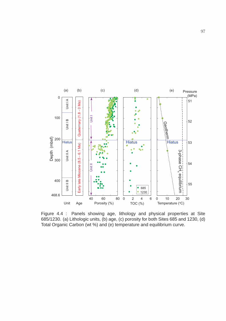
97
0 10 20 30
Temperature (oC)
0 2 4 6
TOC (%)
40 60 80
Porosity (%)
0
100
200
300
400
Age
468.6
Unit
53
54
55
52
De
pth
(m
bsf)
Pressure
(MPa)
3-p
ha
se
CH
4 eq
uilib
rium
Geoth
erm
HiatusHiatus
Qu
ate
rna
ry (
1.8
- 0
Ma
)E
arly la
te M
ioce
ne
(8
.5 -
6.1
Ma
)
Un
it I A
Un
it II A
Un
it I B
Un
it II B
Hiatus
(a) (b) (c) (d) (e)
685
1230
Un
it I
Un
it II
51
Figure 4.4 : Panels showing age, lithology and physical properties at Site685/1230. (a) Lithologic units, (b) age, (c) porosity for both Sites 685 and 1230, (d)Total Organic Carbon (wt %) and (e) temperature and equilibrium curve.

98
base of the GHSZ should be ∼715 mbsf. This thickness can be determined
by simultaneously equating pressures and temperatures along the three-phase
equilibrium curve for methane and seawater with those along the geothermal
gradient (e.g., Bhatnagar et al., 2007). Note that this depth is shallower at Site 685,
with an assumed seafloor temperature 1.5oC and geothermal gradient 0.045oC/m,
as the temperature profile was not measured at this site (Kvenvolden and Kastner,
1990). Marquardt et al. (2010) interpret this thickness as 620 mbsf consistent
with assumed values reported in Kvenvolden and Kastner (1990). Requisite high
porosity also marks the sediment sequence (Figure 4.4). In Unit I, it drops from
78% to 70% in the upper 20 mbsf; below, it decreases slightly to 68%. In Unit II,
porosity averages 55%, but ranges between 40% and 65%.
Based on organic carbon supply and physical properties, one might think that
Site 685/1230 has a thick sedimentary zone with high amounts of gas hydrate
(Marquardt et al., 2010). In fact, however, specimens of gas hydrate were only
recovered at 99 and 164 mbsf at Site 685, and at 82 and 148 mbsf at Site 1230
(Kvenvolden and Kastner, 1990; Shipboard Scientific Party, 1988, 2003a). Three
pieces of information support a distribution where relatively small amounts of gas
hydrate span a portion of the 715 m-thick GHSZ. First, seismic records do not show
a bottom-simulating reflector (BSR) at this site (e.g., Kvenvolden and Kastner,
1990; von Huene and Pecher, 1999; Pecher et al., 2001). Such a reflector is
commonly regarded as representing the case when gas hydrate directly overlies

99
Sulfate (mM)
Alkalinity (mM) Calcium (mM) δ13C of DIC (‰)
De
pth
(m
bsf)
De
pth
(m
bsf)
(a) (b) (c) (d)
SMT
0 450300
0
100
200
300
400
0 40 80 120 160 -20 -10 0 10 200 5 10 15 20
0 10 20 30
Methane (mM)
685
1230
CH4 (HS)
CH4 (PCS)
CH4 (N ratio)
CH4 solubility
0
10
20
30
40
50
HiatusHiatusHiatusHiatus
150
Sulfate (mM)
0 10 20 30
Alkalinity (mM) Calcium (mM) δ13C of DIC (‰)
0 4530 0 40 80 120 160 -20 -10 0 10 200 5 10 15 20
Methane (mM)
15
Figure 4.5 : Pore water (a) SO2−4 (green circles) noted on upper axis, CH4 (black
squares, triangles and circles) marked on lower axis, (b) alkalinity (DIC), (c) Ca2+
concentration and (d) δ13C of DIC profiles in shallow sediment at Sites 685 and1230 in Peru Margin (Suess et al., 1988; Shipboard Scientific Party, 1988, 2003a;D’Hondt et al., 2003; Donohue et al., 2006; Meister et al., 2007). Top panel showsthe zoomed pore water profiles for the upper 50 m of sediment and the shadedregion represents the SMT zone.

100
free gas (e.g., Mackay et al., 1994). Second, pore water profiles of Cl− and
other conservative species (e.g., Sr and Li) do not show numerous deviations to
lower concentrations (Shipboard Scientific Party, 2003a). These often result from
gas hydrate dissociation during core recovery (e.g., Hesse and Harrison, 1981).
Third, various approaches for quantifying CH4 concentrations suggest low values
(D’Hondt et al., 2003; Shipboard Scientific Party, 2003a).
Methane concentrations at Site 1230 were determined by several techniques.
These included measurements of samples obtained through headspace (HS), gas
void, and pressurized cores (Dickens et al., 2003; Shipboard Scientific Party,
2003a). Headspace (HS) CH4 concentrations are <0.1 mM in the upper 7 m of
sediment, where pore water SO2−4 is >5 mM. Below, where SO2−
4 drops <0.8 mM,
CH4 concentrations rise sharply from <1.8 mM at <10.2 mbsf to 7 mM at 19.7 mbsf
(Figure 4.5a). The scattered and generally low HS CH4 concentrations below this
depth undoubtedly reflect significant degassing during core recovery (Paull et al.,
2000a), because the solubility of CH4 at shipboard conditions (∼0.1 MPa; ∼20oC)
is 1.8 mM. By contrast, CH4 concentrations measured using nitrogen ratios range
between 42 mM at 28 mbsf and >200mM below 70 mbsf (Spivack et al., 2006).
These measurements are reaffirmed as the pressure core sampler (PCS) show
CH4 concentration values between 46 mM at 52 mbsf and 422 mM at 156 mbsf
(Dickens et al., 2003; Figure 4.5a).
Methane δ13C values range between -72 0/00 and -65 0/00 (e.g., Biddle et al.,

101
2006). Hydrate saturation <5% of pore space exists below a depth at around 82
mbsf, which is assumed to be shallowest occurrence of the gas hydrate. However,
these high values including the zones of hydrate occurrence are above the hiatus;
below, CH4 concentrations show scattered data below saturation.
4.2.2 Key Pore Water Profiles
Pore waters at Sites 685 and 1230 were collected using standard ODP sediment
”squeezing” procedures (Geiskes et al., 1991). However, the sheer number of
samples (112) and aliquots thereof from the three holes at Site 1230 warrant two
notes. First, the detailed pore water sampling suggests core gaps and overlaps
between holes (D’Hondt et al., 2003), a fact long recognized by paleoceanograpic
community (e.g., Lisiecki and Herbert, 2007). We have adjusted initial depths
for pore waters to a meter composite depth (mcd) scale accordingly, which has
particular importance over the upper 20 mbsf. Second, while many species
(e.g, SO2−4 , alkalinity, DIC, and Sr2+, Ba2+) were measured on board the ship,
major cations were not, in contrast to almost all other ODP Legs. Given
the very high alkalinity concentrations (discussed below) and the potential for
carbonate precipitation during storage of pore waters, we only discuss Ca2+
profiles generated from aliquots acidified (with ultrapure HNO3) immediately after
retrieval (Donohue et al., 2006).
The SO2−4 profile at Site 1230 (Figure 4.5a) exhibits characteristics similar to

102
those measured at other locations with gas hydrate. Concentrations decrease
nearly linearly from ∼28 mM near the seafloor to <1 mM by ∼8.7 mbsf. This
depth, approximately the SMT, is where dissolved CH4 and Ba2+ concentrations
begin to increase sharply. The steep rise in Ba2+ (D’Hondt et al., 2003; Shipboard
Scientific Party, 2003a) is important because it marks the SMT at numerous
locations (Dickens, 2001b; Snyder et al., 2007).
Alkalinity increases rapidly from 2.7 mM near the seafloor to 100 mM at ∼30
mbsf; below, it rises gradually to a broad maximum of 160 mM between 100
and 150 mbsf (Figure 4.5b; D’Hondt et al., 2003; Shipboard Scientific Party,
2003a). Deeper in the sediment column, alkalinity drops to ∼40 mM at 250 mbsf.
The alkalinities at the SMT (∼53 mM) and between 100-150 mbsf are extreme
(Figure 4.5b). Indeed, these alkalinities are the highest recorded in over 40
years of deep-sea drilling. The pH throughout the interval is between 6.9 and 8.3
(Shipboard Scientific Party, 2003a), suggesting that alkalinity and DIC are nearly
equal. In fact, this was confirmed at Site 1230 by measuring alkalinity and DIC
separately (Shipboard Scientific Party, 2003a).
Profiles of DIC δ13C show a wide variance in values, including a distinct peak
spanning the SMT (Figure 4.5d; Meister et al., 2007). The δ13C of DIC is 0 0/00
near the seafloor and decreases to a minimum of -13 0/00 at ∼8.7 mbsf. Values
then increase rapidly to +10 0/00 at ∼2 mbsf. Below, it steadily increases to +17
0/00 by ∼88 mbsf and remains essentially constant to greater depths. Notably, the

103
δ13C of DIC at the SMT is much greater than predicted through sulfate reduction
of particulate organic carbon (POC) (Claypool et al., 2006; Kastner et al., 2008a;
Torres and Kastner, 2009), unless solid organic carbon landing on the seafloor has
an unusual carbon isotopic composition.
Dissolved Ca2+ is 10 mM near the seafloor but decreases to 5 mM at ∼12 mbsf;
it then increases steadily to 7 mM at the bottom of the drilled section at 260 mbsf
(Figure 4.5c; Donohue et al., 2006). The significant drop in Ca2+ concentrations
across the SMT has been attributed to authigenic carbonate precipitation (Suess
et al., 1988; D’Hondt et al., 2003; Meister et al., 2007).
Pore waters collected at Site 685/1230 have three other attributes relevant to
understanding carbon cycling in gas hydrate systems. First, upon collection, many
samples from Unit I had a rich golden color. Pore water collected close to the
seafloor is nearly clear but rapidly becomes more ”yellow” with depth, approaching
a golden color (>0.50 JWBL units) by 40 mbsf. Below, at 250 mbsf, the water
becomes clear again, dropping to below 0.15 JWBL. Second, dissolved NH+4
increases from 1mM at the seafloor to a broad maximum of 35-40 mM between
100 and 200 mbsf; below, they drop to lower values (∼10 mM) at 400 mbsf.
Third, phosphate concentrations at Site 685 increase from near zero values at
the seafloor to 0.37 mM at 18 mbsf. Concentrations reach an extreme high of
0.83 mM at 107 mbsf (Suess et al., 1988). Below the hiatus, values decrease but
remain relatively high (∼0.1 mM). The distinct yellow color is unusual across pore

104
water studies of scientific boreholes, but is found at other sites with gas hydrate
(e.g., Site 1244; Trehu et al., 2003). It probably results from the presence of
dissolved organic matter (e.g., Smith, 2005). The exceptionally high ammonium
and phosphate concentrations almost assuredly reflect major decomposition of
organic carbon at depth.
4.2.3 Additional Data
We analyzed 34 samples of bulk sediment from the upper 24 m for their carbon
isotope composition of organic carbon (Appendix B). The average value is -22 0/00.
4.3 Numerical Model
4.3.1 Model Framework
Over the last 15 years, several 1-D numerical models have been developed to
understand the accumulation of gas hydrate in marine sediment (Rempel and
Buffett, 1997; Egeberg and Dickens, 1999; Xu and Ruppel, 1999; Davie and
Buffett, 2001, 2003a, 2003b; Luff and Wallman, 2003; Haeckel et al., 2004; Torres
et al., 2004; Wallman et al., 2006; Liu and Flemings, 2006, 2007; Bhatnagar et
al., 2007; Marquardt et al., 2010). Most of these models have a similar framework,
and serve to simulate methane transport for transient and steady state conditions.
These models solve coupled mass, momentum and energy transport equations
for methane, organic carbon and pore fluids over space and time. Transient and

105
steady state solutions are generated with site-specific parameters when these
models are run over geologic time scales. The simulated profiles give a broad
distribution of CH4 and pore water constituents with respect the sediment depth.
Existing 1-D models have several known problems (see above references). In
particular, they typically provide broad profiles for the amount of CH4 occurring
dissolved in water, in gas hydrate, and in free gas with respect to depth. This is
because small-scale heterogeneities in sediment composition and horizontal fluid
flow are not considered. Nonetheless, when appropriate parameters are used,
the models generate first-order CH4 profiles that approximate those constructed
using direct and indirect methods at multiple locations (e.g., Davie and Buffett,
2001, 2003a; Liu and Flemings, 2007; Bhatnagar et al., 2007, 2011; Chatterjee et
al., 2011a). Along with this work, a generalized, 1-D numerical model for gas
hydrate accumulation in marine sediments over geologic timescales has been
developed (Bhatnagar et al., 2007). Their model operates in thermodynamic
equilibrium thereby neglecting the hydrate formation kinetics. In addition, their
model summarizes the key results into two simple contour plots illustrating the
amount of gas hydrate and its distribution for a wide range of parameters applicable
to any generalized geologic location.
In their original model (Bhatnagar et al., 2007), CH4 escaped a sedimentary
column through two processes: below the GHSZ through burial, or above the
seafloor through oxidation. The latter is not correct, because CH4 is consumed

106
at the SMT via AOM, which typically lies below the seafloor (e.g., Paull et al.,
1996; Trehu et al., 2003). The model was therefore amended so that CH4
and SO2−4 consumption co-occurred across a sediment interval (Bhatnagar et al.,
2008a, 2011). This is because CH4 drives net SO2−4 consumption (e.g., Reeburgh,
1976; Borowski et al., 1996, 1999; Snyder et al., 2007). Methane production and
consumption should impact other pore water constituents. Therefore, coupling all
these pore water constituents and its carbon isotopes in a unified model would help
explain carbon cycling processes in shallow sediment. For example, production of
methane is depleted in 13C and is associated with generation of 13C-enriched DIC.
Thus, previous models were partly updated so that they included pertinent mass
balance equations and reactions for DIC, dissolved Ca2+, and the carbon isotope
composition (δ13C) of DIC (Chatterjee et al., 2011a).
The latest modeling exercise rendered reasonably good profiles for multiple
pore water species at two sites with very different carbon chemistry (Chatterjee et
al., 2011a). However, dissolved methane was the only methane phase tracked
in calculations (i.e., amounts of gas hydrate and free gas were not accounted
for). Furthermore, diffusion coefficients and reaction rates were assumed to be
independent of depth and temperature, and transient states were not considered.

107
4.3.2 Modifications to Previous Modeling
Two modifications to previous modeling exercises are made in this chapter. First,
we incorporate gas hydrate and free gas phases in our computations. When
CH4 concentrations exceed solubility, excess methane precipitates as gas hydrate
or forms free gas, depending on the thermodynamic conditions. Mathematical
formulae for this modification are presented in Appendix C. Second, we make the
reaction rate constant for methanogenesis temperature dependent.
Both theory and observations suggest that, at low temperatures (<40oC), rates
of microbial methanogenesis increase significantly with temperature (e.g., Price
and Sowers, 2004). Although a series of models published in the last decade
assumed that methanogenesis reaction rate was independent of temperature (e.g.,
Bhatnagar et al., 2007, 2008a; Chatterjee et al., 2011a). Recent studies showed
the dependence of temperature on the reaction rate constant (e.g., Gu et al., 2011;
Burdige, 2011). Following their work, we have also shown effect of temperature on
the reaction rate constant (λ).
4.3.3 Initial Parameters
The seafloor and geologic parameters measured at Site 685/1230 and recorded
in ODP reports are used as input parameters in our model. These site-specific
parameters include the seafloor depth (5086 mbsl), seafloor temperature (1.7oC),
geothermal gradient (0.0343oC/m), sedimentation rate (100 m/Myr), and an

108
average TOC (3 wt %) at the seafloor (Table 4.1).
The model has several dimensionless parameters (Equation C.3). These are:
Peclet numbers (Pe1, and Pe2), and Damkohler numbers (Da, DaAOM and DaPOC).
Peclet numbers characterizes the ratio of fluid advection to methane diffusion. Two
Peclet numbers represent the two fluid fluxes due to sedimentation-compaction
and external fluid flow. Damkohler numbers relate the reaction rates to the rate
of diffusion. The three Damkohler numbers correspond to the reactions that form
methane (methanogenesis), and consume sulfate at or above the SMT (AOM and
organoclastic sulfate reduction (OSR)).
Steady state pore water concentration profiles were simulated (Figure 6) using
the modeling approach discussed in Chatterjee et al. (2011a) for parameters (Table
4.1) obtained or inferred from reports for this location (Suess et al., 1988; D’Hondt
et al., 2003). The sedimentation rate (100 m/Myr) during the Pleistocene was used
to calculate a Pe1 of 0.085. This parameter was fixed for all simulations at this
location (unless otherwise specified) as this relates to sediment burial and porosity
reduction. Based on the upward fluid velocity values reported at this location (>200
m/Myr), our initial estimate for Pe2 is -6 at this site.
The thickness of the SMT (as opposed to the depth of the SMT) depends on
DaAOM (Bhatnagar et al., 2008a). A large value for DaAOM represents a fast rate
of AOM relative to the rate of CH4 diffusion, which results in a thin overlap of CH4
and SO2−4 profiles at the SMT. This occurs at many locations, including at Site

109
1230 (Figure 4.5a). Consequently, we initialize simulations with a relatively high
value (DaAOM = 108), the same as in previous work (Chatterjee et al., 2011a).
The dimensionless numbers Da (=3), and DaPOC (=25) were calculated based
on reaction rate values used in existing models (e.g., Davie and Buffett, 2001;
Bhatnagar et al., 2007; Chatterjee et al., 2011a).
4.3.4 General Approach for Solving
The dimensionless mass balance equations were solved conservatively with
specific initial and boundary conditions to obtain solutions (Appendix C). An
implicit, block-centered, finite-difference scheme was formulated to numerically
solve the hyperbolic, dimensionless, partial differential equation for organic carbon.
The remaining partial differential equations were expressed in a finite difference
form and solved using an explicit numerical scheme (Chatterjee et al., 2011a). The
spatial simulation domain was assumed to be 2Lt (=1430 mbsf) and the equations
were solved from initial time (t = 0) to steady state in small increments of time. A
strict material balance check ensured no loss (all simulations had errors < 10−8)
and mass conservation. The sediment and fluid advection terms were computed
using single-point, upstream weighting. Upstream grid point values (as opposed to
mean values between two neighboring grid points) were used for concentration to
calculate fluxes across each grid interface.
As emphasized in previous publications (Bhatnagar et al., 2007, 2008a;

110
Chatterjee et al., 2011a), the generation of mathematical solutions in
dimensionless units is appealing because it enables countless numerical
simulations of different gas hydrate systems to be compared systematically.
However, such presentation does not lead to obvious comparisons with field
data. Thus, we convert normalized depths and concentrations to actual depths
and concentrations at Site 1230. This can be accomplished by multiplying the
normalized depth by the depth to the base of the GHSZ (Lt = 715 mbsf), multiplying
normalized CH4 concentrations by the three-phase equilibrium value at the base
of the GHSZ (cm,eqb = 206 mM), and multiplying normalized SO2−4 , HCO−
3 and Ca2+
concentrations by their respective values in seawater values (cs,o = 28 mM; cb,o =
2.4 mM; cCa,o = 10 mM). Note that concentration profiles are therefore simulated
to 1430 mbsf, even though we generally plot them across shallower intervals (e.g.,
400 mbsf, Figure 4.6).
4.3.5 Steady State Solutions
Steady state solutions are obtained by solving the mass balance equations from
the initial time of sediment deposition through long time scales (∼20 Myr) until
pore water concentration profiles of all relevant geochemical species (CH4, SO2−4 ,
DIC, Ca2+ and δ13C of CH4 and DIC) cease to change. Site 1230 presents a
challenge to models for gas hydrate accumulation because the depth (204 mbsf),
termination age (∼1.8 Ma), and duration (∼4.3 Myr) of the hiatus strongly suggest

111
that the system has not reached steady state conditions. Consequently, to explain
complicated processes at this location, transient simulations must be considered.
Of particular importance, Site 1230 should be viewed as a system where a young
package of sediment, rich in organic carbon, lies on top of an older package of
sediment. The CH4 and DIC (as well as other products of microbial activity) in the
upper ∼200 m of sediment have mostly been generated in the last ∼2 Myr.
4.3.6 Transient Solutions
Transient solutions are obtained using time evolved simulations from a known set
of initial conditions. At the start of time (t = 0), steady state profiles are generated
over ∼10 Myr for a thick sediment column (z = 1575 mbsf). These profiles are
obtained by depositing the sediment at the rate 250 m/Myr at the seafloor. The
hiatus is modeled in our simulations as an erosion event. The upper 1075 m
of sediment is removed to model the hiatus (equivalent to duration of 4.3 Myr).
Consequently, the older sediment (1075-1575 mbsf) is retained along with its
pore water constituents at steady state. These pore water profiles act as initial
conditions for time after hiatus. At the start of this new time, organic carbon rich
sediment deposits on the seafloor and moves down with a lower sedimentation
rate (100 m/Myr). The hiatus which was at the top of the sediment column ∼2
Myr ago is tracked through time. The present day hiatus has moved 204 mbsf
into the sediment since this new time. During this time (post-hiatus) pore water

112
profiles evolve in the upper ∼200 m of sediment. However, the profiles below the
hiatus remain unaltered from pre-hiatus conditions. These time evolved pore water
profiles in the last ∼2 Myr are generated as transient solutions at this location.
4.4 Results
4.4.1 Steady State Solutions
Base Case
Our initial simulations have a set of site-specific parameters (Table 4.1), and
chosen values for key dimensionless groups. As explained above, these are: Pe1
= 0.085, Pe2 = -6, Da = 3, DaAOM = 108 and DaPOC = 25.
With these starting parameters, a set of pore water profiles arises from our
numerical model at steady state conditions (Figure 4.6). Simulated CH4 and
SO2−4 profiles provide a first-order check on model accuracy. Dissolved CH4
concentrations are nearly zero above the SMT, which occurs at 12 mbsf, and then
rapidly increase in concentration with depth. Excess dissolved CH4 forms gas
hydrate as local solubility values are surpassed. With the above set of parameters,
CH4 first exceeds solubility conditions at 122 mbsf. Gas hydrate saturations
increase with depth with a peak saturation of 30% at the base of the GHSZ. Free
gas saturations increase from 10% at the base of the GHSZ to 21% at the base of
the simulation domain (Figure 4.6e). Dissolved SO2−4 exhibits a near-linear profile

113
Table 4.1 : Model Parameters for Sites 685/1230
Symbol Definition (units) Valuea
Lo Seafloor depth (m) 5086
P0 Seafloor pressure (MPa) 50.86
T0 Seafloor temperature (oC) 1.7
dT/dz Geothermal gradient (oC/m) 0.0343
Lt Depth to GHSZ (mbsf) 715
Ls Depth to SMT (mbsf) 8.7
S Sedimentation rate (m/Myr) 100, 250
Uf,sed Fluid flux due to sedimentation (m/s) 1.05 ×10⁻¹³
Pe1 First Peclet number - sedimentation-compaction driven fluid flow 0.085, 0.21
Pe2 Second Peclet number - external fluid flow -9
TOC Total organic carbon (%) 3-6
- Labile fraction (%) 50
αo Labile organic carbon at seafloor (%) 1.5-3
β Normalized organic carbon at seafloor 4.5-9
cm,eqb CH4 solubility at base of the GHSZ (mM) 206
cs,o Seawater SO2−4 concentration (mM) 28
cb,o Seawater DIC concentration (mM) 2.4
cCa,o Seawater Ca2+ concentration (mM) 10
Dm CH4 diffusivityb (m2/s) 0.87 ×10⁻⁹
Ds SO2−4 diffusivityb (m2/s) 0.56 ×10⁻⁹
Db DIC diffusivityc (m2/s) 0.6 ×10⁻⁹
DCa Ca2+ diffusivityc (m2/s) 0.4 ×10⁻⁹
Da Damkohler number (methanogenesis) 6
DaPOC Damkohler number (OSR) 25
DaAOM Damkohler numberd (AOM) 108
λ Rate constant for methanogenesis (s−1) 1 ×10⁻¹⁴
λPOC Rate constant for OSR (m3/(mol.s)) 1 ×10⁻¹⁶
λAOM Rate constant for AOM (m3/(mol.s)) 8.4 ×10⁻⁸
aShipboard Scientific Party. (2003a)bIversen and Jorgensen (1993)cLi and Gregory (1974)dBhatnagar et al. (2008a)

114
between the seafloor and the SMT.
Pore water profiles of DIC, Ca2+ and the δ13C of DIC are simultaneously
simulated in the model (Figure 4.6), and provide an important cross check. DIC
concentrations increase from 2.4 mM at the sediment-water interface to 65 mM at
the SMT; below, values rise steadily with depth. Simulated Ca2+ concentrations
drop from 10 mM at the seafloor to 7 mM at the SMT; below, values continue to
decrease to 4.5 mM, although less rapidly with respect to depth. The steady state
profile for δ13C of DIC is intriguing. For the initial set of parameters, it decreases
with a concave-down curvature from zero at the seafloor to a minimum (-9 0/00)
at the SMT; below, it increases with a concave-down curvature to more positive
values (+17 0/00).
The simulated geochemical profiles for Site 1230, assuming steady state
conditions, render the generic shape of measured profiles at this location.
However, there are obvious discrepancies (Figure 4.6). For example, the simulated
Ca2+ values at depth are lower than measured at this site. Comparisons between
model results and field data can be improved by changing various free parameters.
Modified Dimensionless Groups
A crucial variable in our modeling is the external fluid flux, which is incorporated
in the parameter Pe2. This is because upward advection of fluids moves pore
water constituents from depth. A series of simulations with different Pe2 (from -3 to

115
0 50 100 150
0
100
200
300
400
0 80 160 240 320 -20 -10 0 10 200 5 10 15
0 10 20 30
Sulfate (mM)
Alkalinity (mM) Calcium (mM) δ13C of DIC (‰)
De
pth
(m
bsf)
Methane (mM)
Hiatus Hiatus Hiatus Hiatus
(a) (b) (c) (d)
685
1230
λ =
co
nst
λ= f(T)
Pe2 = -6
Pe2 = -9
Pe2 = -12
Pe2 = -9;
Hiatus (4.3 Ma)
(e)
Pe2 = -3
0 5025
0
500
1000
1430
De
pth
(m
bsf)
Hydrate and free gas
saturation (%)
Hiatus
Figure 4.6 : Steady state pore water concentration profiles at Site 685/1230 inthe Peru Margin with present day parameters. (a) CH4, and SO2−
4 , (b) DIC, (c)Ca2+, (d) δ13C of DIC, (e) gas hydrate and free gas saturations. Note that thesesimulations are completed for a 1430 m sediment below the seafloor, however,figures (a)-(d) are shown for the upper 400 mbsf to focus on the profiles at shallowdepth. The solid curves correspond to increasing magnitude of Pe2 (fluid flux fromdepth) shown by direction of arrow. The dashed curves correspond to simulationswith a temperature-dependent methanogenesis rate constant. Field data fromSites 685 and 1230 are shown (green circles; D’Hondt et al., 2003; Donohue etal., 2006; Meister et al., 2007). Parameters: Pe1 = 0.085, Da = 3, DaPOC = 25,DaAOM = 108, β = 4.5, cb,ext = 48 mM, cca,ext = 4.3 mM and δ13C = 17.

116
-12) and all other parameters constant illustrates the effect of fluid flux (Figure 4.6).
Changes in upward fluid advection generate different pore water chemistry profiles,
but with the same basic shape. One obvious change is the depth of the SMT,
consistent with theory and previous modeling (e.g., Borowski et al., 1996; Davie
and Buffett, 2003b; Bhatnagar et al., 2008a; Chatterjee et al., 2011a). Specifically,
for the initial model conditions at Site 1230, the SMT shoals from 14 to 7 mbsf as
the magnitude of Pe2 doubles from -3 to -12. A simulation with Pe2 = -9 produces
dissolved CH4, and SO2−4 profiles that better resemble inferred profiles at Site
1230. This includes an SMT at 9 mbsf and a shallowest occurrence of gas hydrate
(where the CH4 profile surpasses solubility conditions) at 105 mbsf.
The profiles of DIC and the δ13C of DIC also change with increasing fluid flux.
In particular, the ”kink” in the DIC profile at the SMT becomes more prominent, and
the δ13C of this DIC at the SMT becomes less with increasing flux from depth. This
is because greater advection escalates the flow of 13C-enriched DIC to shallower
sediment. Again, for Pe2 = -9, the simulated profiles of δ13C better match observed
data, at least at the SMT. The profile of dissolved Ca2+ also changes slightly at
shallow depths with differences in fluid flux.
Changing Pe1 in our simulations does not impact the pore water profiles
significantly (not shown here). The pore water profiles are affected by the net
fluid flux (Pe1 + Pe2), and Pe1 has a very small contribution in these upward fluid
flux dominated systems (|Pe2| > Pe1). Moreover, the Pe1 value is prescribed in the

117
model based on sedimentation rate at this site, so it should remain constant for a
particular geologic setting assuming constant sedimentation rate.
Simulations were performed with changes in other dimensionless groups (Da,
DaAOM and DaPOC). These are not presented and discussed here because it
has been shown that they do not significantly affect the basic shape of key pore
water profiles (Bhatnagar et al., 2008a; Chatterjee et al., 2011a). On the basis
of these sensitivity analyses, all dimensionless groups were kept the same as
the ”initial guess”, except Pe2, which was set to -9 for all remaining simulations.
Clearly, however, some problems remain. Notably, the modeling significantly
underestimates Ca2+ concentrations at depth, and generally fails to explain pore
water profiles across the hiatus (Figure 4.6).
Activity Correction
Three potential problems might explain the low Ca2+ concentrations in our initial
simulations (Figure 4.6). First, there are complications regarding the pH of pore
waters at this location. Second, the basic model does not include ion pairing and
corrections for ion activity. Third, multiple phases of carbonate could precipitate.
The simulated Ca2+ profiles are primarily governed by two factors in our model:
the simulated DIC profile and the solubility product of CaCO3 (as calcite), which
determines the extent of Ca2+ that precipitates as calcite (Equation 6 in Chatterjee
et al., 2011a). The solubility product of calcite is determined from the activity

118
product of Ca2+ and CO2−3 ions, as well as pressure, temperature and salinity
(Mucci, 1983). The pH profile is used to associate the CO2−3 and HCO−
3 ion
activities (Roy et al., 1993). Assuming constant salinity with depth (which we note is
incorrect because of extreme alkalinity, D’Hondt et al., 2003), temperature and pH
should dictate the ion activity product of Ca2+ and HCO−3 in pore fluids. However, a
problem arises in available data: although they should be the same, the measured
pore water pH profiles differ significantly between Sites 685 and 1230 (Figure 4.7a).
This leads to different ion activity products and different Ca2+ profiles (Figure 4.7b
and 4.7c).
More crucially, preliminary examinations of pore water at this location using
PHREEQC software package (Snyder, G., pers. comm.), suggests that ∼40%
of the DIC in pore water forms complex species, particularly Na(HCO3)o and
Mg(HCO3)o2. This results in limited availability of CO2−
3 for reaction with Ca2+.
These corrections were made by using 60% of the DIC to form calcite allowing
the rest to form complexes. Simulations including this correction precipitated less
Ca2+ to form calcite. Therefore, steady state simulations were matched against
observations by choosing an intermediate pH profile between measured data at
two sites and assuming correct activity coefficients for different species to model
calcite precipitation (Figure 4.6c).

119
6.5 7 7.5 8 8.5
0
100
200
300
400
500
De
pth
(m
bsf)
pH
0 500 1000 1500
0 5 10 15
Calcium, mM[Ca2+][HCO3
-], mM2
685 data
1230 data 1230 data fit
685 data fitmodel fit
Figure 4.7 : Panels show (a) pH data at Sites 685, 1230 and the best fit profileused in the model, (b) ion concentration product of Ca2+ and HCO−
3 for differentpH profiles and (c) simulated Ca2+ based on these different pH profiles. MeasuredpH differs at the same site, although simulations using a pH profile bracketed bythe measured profiles at two sites can describe the measured Ca2+ profiles.

120
Geotherm Effect
Many papers regarding microbial organic carbon degradation in marine sediment
assume that reaction rates decrease with depth below the seafloor (e.g.,
Middleburg, 1989). However, numerous studies have shown that the reaction
rate of microbial methanogenesis increases significantly with temperature below
40oC (e.g., Zeikus and Winfrey, 1976; Price and Sowers, 2004). Presumably, this
means that in rapidly accumulating sediment on the continental slope, such as at
Site 685/1230, methanogenesis may increase with depth because of the geotherm
(Figure 4.9a; Wellsbury et al., 1997; Burdige, 2011; Gu et al., 2011). The idea is
controversial, but we have included for completeness.
A ”geotherm correction” to microbial methanogenesis improves comparisons
between simulated and measured profiles. An increasing rate in microbial
methanogenesis with greater temperature and depth affects pore water profiles
considerably. Due to high methanogenic activity, the organic matter depletes
faster and completely exhausts the organic carbon in the sediment (Figure 4.9b).
Reduced organic carbon restricts generation of CH4 and associated 13C-enriched
DIC at depth. The methane generated due to this effect lessens thus reducing the
hydrate saturation at greater depths (Figure 4.6e). The resultant DIC profiles is
closer to the measured data at this site (Figure 4.6b) including this effect. Overall,
good first-order representative profiles are generated on including these geotherm
effects. However, the Ca2+ and δ13C of DIC profiles vary little with increasing

121
temperature along depth (Figure 4.6c and 4.6d).
A basic model for gas hydrate accumulation under steady state conditions
explains the generalities of pore water profiles at Site 685/1230, at least for
dissolved species of interest (Figure 4.6). Considerations of fluid flux, ion activity
and temperature improve these simulations when compared to field data (Figure
4.6). Nonetheless, a major problem remains: we cannot model pore water profiles
at depth, specifically across the hiatus. This is a fundamental problem facing
interpretations of gas hydrate systems. As indicated by Marquardt et al. (2010), a
steady state perspective necessitates that gas hydrate extends to the base of the
GHSZ (Figure 4.6e). Such a view is not supported by field data, which show no
evidence for deep gas hydrate or a BSR at this location.
4.4.2 Transient Solutions
With the general model framework, we examine possible transient systems at Site
685/1230. The modeling starts with similar initial conditions (t = 0), and runs
to steady state. However, key parameters were changed: there is now a higher
sedimentation rate (250 m/Myr), and a lower carbon input (β = 6; equivalent to
TOC = 4%) in sediment relative to present day (Table 4.1; Figure 4.8a-f). These
parameters were modified so as to simulate the observable Miocene sedimentary
record (6.7 Myr and older). The pre-hiatus Miocene sedimentation rate was used
to specify Pe1 = 0.21. Steady state profiles generated now serve as an initial

122
condition for simulations after the hiatus.
The exact cause of the hiatus remains uncertain. We assume, for simplicity,
that 1075 m of sediment (equivalent to duration of 4.3 Myr at a pre-hiatus rate of
250m/Myr) was removed from the seafloor by erosion. The depth horizon at the
hiatus (1075 mbsf) thus becomes a new seafloor with new initial conditions (set
t = 0; 2.4 Myr ago). Post hiatus time is then modeled keeping all parameters the
same except with increased amount of organic carbon (β = 9; TOC = 6%) and
higher methanogenic activity (Da = 6). Effectively, a new time zero started 2.4
Myr ago, but with inherited conditions, and pore water profiles evolve to present
day (Figure 4.8g-l). Given our modeling framework, these are non-steady state
(transient) profiles.
The temporal organic carbon profile acts a good indicator to track post-hiatus
sedimentation (Figure 4.8g). Organic carbon rich sediment rains on the seafloor
with a greater reaction activity. The depth traveled by this new sediment is
tracked over time and its present day depth below the seafloor would represent
the observed hiatus (∼200 mbsf). Furthermore, the low organic carbon values
below this horizon would represent sediment depleted in organic carbon deposited
before the hiatus formation. Overall the broad, present day profile matches the
TOC data at this location.
Considering the hiatus, the pore water SO2−4 profile remains similar to previous
steady state results (Figure 4.8h). The SMT still lies at ∼9 mbsf. This is because

123
-20 0 200 10 200 300 6
0
100
200
300
400
500
0 50 150
Seafloor 2.4 Myr ago
Seafloor 6.7 Myr ago
0 100 200
Alkalinity (mM) Calcium (mM) δ13C of DIC (‰)
De
pth
(m
bsf)
Methane (mM)
10
Saturation (%)TOC (wt %)
685
1230
Hiatus (204 mbsf)
(a) (b) (c) (d) (e) (f)
0
0.57
1.07
1.57
De
pth
(k
mb
sf) Hiatus
(4.3 Myr)
Alkalinity (mM) Calcium (mM) δ13C of DIC (‰)Methane (mM) Saturation (%)TOC (wt %)
-20 0 200 10 200 300 6 0 70 210 0 200 40010
0 10 30
Sulfate (mM)
2
42 20100
1.2 Myr ago
0.6 Myr ago
present day (0 Myr); λ = const
present day (0 Myr); λ = f(T)
10 Myr later (steady state)
0.6 Myr later
20
4 140 20
0 10 30
Sulfate (mM)
20
(g) (h) (i) (j) (k) (l)
Figure 4.8 : Transient state profiles at Site 685/1230 before (a-f) and after (g-l)hiatus formation. Pre-hiatus steady state simulations (a-f) show shaded region thatrepresents the lost sediment column forming the hiatus corresponding to durationof 4.3 Myr. Post-hiatus time evolved profiles: (g) organic carbon content with timeevolved hiatus, (h) dissolved CH4, and SO2−
4 , (i) gas hydrate saturation, (j) DIC,(k) Ca2+, and (l) δ13C of DIC. The solid curves correspond to temporal profiles withconstant λ (methanogenesis rate constant) and dashed line shows present dayprofile with temperature dependent λ. Field data at Sites 685 and 1230 are shown(green circles; D’Hondt et al., 2003; Donohue et al., 2006; Meister et al., 2007).Common parameters: Pe2 = −9, DaPOC = 25, DaAOM = 108, cb,ext = 18 mM,cca,ext = 15 mM and δ13C = 17. Pre-hiatus parameters: Pe1 = 0.21, Da = 3, β = 6and post-hiatus parameters: Pe1 = 0.085, Da = 6, β = 9.

124
it is primarily driven by upward methane flux and AOM at the SMT. The overall
CH4 profile emerges because of dissolved CH4 generation below the SMT, internal
cycling of hydrate and free gas phases within the GHSZ, and combined advection
and diffusion effects that migrates CH4 from depth which ultimately gets consumed
by AOM to near zero values at the SMT (Figure 4.8h).
The ensuing gas hydrate and free gas profiles change showing 6% peak
saturation between 72 and 175 mbsf at present day. These are consistent with
field data. As the CH4 concentration grows in pore fluids and exceeds the phase
solubility values, it forms hydrates. These hydrates can move downward with the
sediment with burial. The hydrate saturation increases with time and the peak
values appear at greater depths as sediment is buried with time (Figure 4.8i). The
transient saturation profiles show hydrates forming within the GHSZ but does not
extend till the base of the GHSZ as shown in the steady state results above. The
free gas phases are absent in these transient simulations as the hydrate front has
not exit the GHSZ which matches with observation.
The DIC concentrations increase with depth to a broad maximum due to
increased methanogenic activity above the hiatus. Below, concentrations drop to
lower values below the hiatus as observed in field data (Figure 4.8j). The generic
shape of the DIC profiles arise due to the same reasons as discussed in the steady
state modeling. First, methanogenesis generates significant amounts of DIC at
depth; second, this DIC enters the SMT to mix with DIC generated by AOM; third,

125
DIC leaves the sediment through the seafloor. Calcium also precipitates small
amounts of DIC to precipitate as calcite around the SMT.
The overall shape of the Ca2+ profile matches the field data in shallow depth.
However, at greater depths, the Ca2+ is greater than the observed profile at this
location. This aberration can be explained due to poor constraints of pH and
consequently ion activity product in the model. Nonetheless, these profiles are
driven due to three factors: first, seawater Ca2+ enters the SMT from above,
second, advection and diffusion carries the Ca2+ in the pore fluids upward; and
third, DIC reacts with Ca2+ to precipitate as carbonate (Figure 4.8k).
The δ13C of DIC profiles are simultaneously simulated with the other pore water
constituents in the model. With increasing time, DIC concentration grows and more
13C-enriched DIC enters the SMT from depth. These 13C-enriched DIC fluxing from
depth mixes with the 13C-depleted DIC formed at the SMT. This ”mixing” leads to
less negative δ13C of DIC at the SMT as more 13C-enriched DIC ascends over
time. Crucially, the shape of these profiles spanning the SMT remains the same
as the steady state modeling. Basically, these less negative δ13C values (∼-13
0/00) appear at the SMT even though AOM consumes most net SO2−4 in shallow
sediment (Figure 4.8l).
The geotherm effects discussed above show that reaction rate can vary
exponentially over depth with increasing temperature (Figure 4.9a). As a
consequence, the organic carbon profile and CH4 generation rate are affected

126
0 30 60 90
CH4 production rate
(mol/m3/Myr)
0 2 4 6
TOC (wt %)
10-16
10-14
10-12
0
100
200
300
400
500
λ (1/s)
De
pth
(m
bsf)
steady-state; const λ transient-state; const λ
steady-state; λ = f(T) transient-state; λ = f(T)
Hiatus
(4.3 Myr)
685
1230
Figure 4.9 : Panels showing rate constant, organic carbon profiles in sediment andCH4 production rates with and without geotherm effects. (a) Methanogenesis rateconstant, λ, (b) organic carbon profiles and (c) rates of CH4 production for transientand steady state simulations (Figures 4.6 and 4.8).

127
due to these effects (Figures 4.9b and 4.9c). For the transient state
simulations, the pre-hiatus simulations (Figure 4.8a-f) are assumed to have
constant methanogenesis reaction rate (λ), independent of temperature. The
fresh sediment packet that rains on the seafloor post hiatus includes temperature
(or geotherm) effects driving the reaction rates. Thus, including these geotherm
effects match the observed pore water and the gas hydrate saturation profiles at
present day (Figure 4.8g-l).
4.4.3 Concentration and Flux Crossplots of Alkalinity and Su lfate
A theoretical value known as excess alkalinity (Alk∗) can be calculated for a given
interstitial water sample given its chemical composition. Assuming closed system
behavior, it represents the amount of DIC that should exist in pore water before
precipitation of authigenic carbonate. It can be computed by adding the pore
water alkalinity, Ca2+ (and Mg2+). Plots showing deviations in excess alkalinity
(∆Alk∗) with respect to seawater versus to those of pore water SO2−4 (∆SO2−
4 )
above the SMT have been used to interpret the relative proportions of OSR and
AOM consuming SO2−4 above the SMT (e.g., Claypool et al., 2006; Kastner et al.,
2008a; Torres and Kastner, 2009; Figure 4.10). The basic idea has been that
the slope on such crossplots relates to the relative proportion of the two potential
reactions via stoichiometry (Claypool et al., 2006; Kastner et al., 2008a; Torres
and Kastner, 2009). Basically, a 1:1 slope would imply SO2−4 removal by AOM,

128
and a 2:1 slope would imply SO2−4 consumption by OSR, and a slope in between
would imply combination of both processes (Equations 1 and 2 in Chatterjee et al.,
2011a).
Field data from Site 1230 is complex. First, the Mg2+ concentration rises with
depth. Therefore, deviations in excess alkalinity with respect to its seawater values
would drop due to this elevated pore water Mg2+ values. However, the nominal 2:1
slope in ∆Alk∗: ∆ SO2−4 could indicate dominant organoclastic sulfate consumption
at this site (Figure 4.10).
Concentration gradients are computed by linear fitting steady state
concentration profiles (Figure 4.6). Fluxes entering and leaving the SMT are
evaluated by multiplying these gradients with diffusivities and these fluxes are
calculated above and below the SMT. Diffusive fluxes of CH4, SO2−4 and DIC are
cross-plotted across the SMT horizon (Figure 4.11). These fluxes also represent
the total flux across the SMT as the advective component is zero near the SMT.
4.5 Discussion
Site 685/1230 presents a real challenge in multiple regards. Pore water
concentrations measure extreme values at this location and the presence of a 4.3
Myr hiatus indicates that this sediment sequence is in transition. The key points of
discussion are extreme pore water chemistry measured at Site 685/1230 and that
the SMT at this site is primarily caused due to AOM. Although, the 2:1 slope in

129
0 5 10 15 20 25 30
0
20
40
60
80
100
120
140
160
∆ SO4
2- (mM)
∆ [A
lk +
Ca
] (m
M)
2:11:1
above SMT
between SMT and hiatus
below hiatus
Pe2 = -6; λ = constant
Pe2 = -12; λ = constant
Seafloor
2:1
1:1
Increasing depthSMT
Pe2 = -9; λ = constant
685 1230
Steady-state simulations
Increasing external flux
Pe2 = -9; λ = f(T)
Pe2 = -3; λ = constant
0 5 10 15 20 25 30
0
20
40
60
80
100
120
140
160
∆ SO4
2- (mM)
∆ [A
lk +
Ca
] (m
M)
2:11:1
above SMT
between SMT and hiatus
below hiatus
1.2 Myr ago
0.6 Myr ago
Seafloor
2:1
1:1
Increasing depth
SMT
present day (0 Myr); λ = const
685 1230
Increasing time
present day (0 Myr); λ = f(T)
10 Myr later (steady state)
0.6 Myr later
Transient-state simulations
Figure 4.10 : Concentration cross-plot of ”excess alkalinity” (∆Alk∗) corrected forcarbonate precipitation versus ∆SO2−
4 (mM) relative to the seafloor for (a) steadystate (Figure 4.6), and (b) transient state simulations (Figure 4.8). Crossplotsconstructed using field data Site 685 and 1230 (green markers; Suess et al.,1988; D’Hondt et al., 2003) and simulations match measured data. Notably, ∆Alk∗
continues to rise below the SMT at this site. This clearly implies high flux of DICfrom depth.

130
∆Alk∗: ∆ SO2−4 and δ13C of DIC at the SMT greater than that of CH4 (e.g., -13 0/00)
might indicate organoclastic sulfate reduction, our simulations show that the AOM
consumes most SO2−4 . Within this context, we will discuss some of the implications
of our simulations and how an upward flux of δ13C-enriched DIC mixes with the
13C-depleted DIC formed due to AOM at the SMT to govern the net δ13C of DIC at
the SMT in these dynamic marine gas hydrate systems.
Previous modeling has shown a similar approach to explain some of the sites
in marine environments where a low to moderate trend in ”alkalinity versus δ13C
of DIC” exists (Figure 4.2; Chatterjee et al., 2011a). This approach was used
to model two sites (Hydrate Ridge 1244 and Keathley Canyon 151-3; Figure 4.1)
containing gas hydrate but with differing carbon chemistry and showed that AOM is
the dominant sulfate reduction pathway at the SMT. They proposed that vertically
upward flux of 13C-enriched DIC from depth produced by methanogenesis mixes
with the 13C-depleted DIC formed by AOM at the SMT and results in less negative
δ13C of DIC observed at the SMT. In this chapter, we choose a site that lies on
the highest end of the ”alkalinity and δ13C of DIC” trend, expand the modeling by
Chatterjee et al., (2011a), couple the hydrate and free gas phases to the their pore
water chemistry model and explain an extreme Site 685/1230 in the Peru Trench.
There are sites where organoclastic sulfate reduction could be the dominant
sulfate reduction pathway. However, based on our current understanding, these
sites would show a curvilinear pore water sulfate profile with a deep SMT.

131
Moreover, these sites would show low or negligible methane fluxes from depth
and would not bear any gas hydrates at depth. Although data exists from these
deep drilled sites, there are very few of these sites with reasonably good pore
water chemistry and δ13C of DIC. Furthermore, these are of no interest in regard to
gas hydrate research. However, the key parameters that would characterize these
sites are low or no upward fluid flux and a low methane concentration due to a
slow methanogenic activity at depth. We have identified these characteristics as a
part of our modeling exercise to delineate conditions necessary for the two sulfate
reduction pathways. The key idea here is that the drilled sites known or inferred to
have gas hydrates invariably have AOM causing the SMT with a near-linear sulfate
profile. In addition, the upward flux of 13C-enriched DIC impacts the net δ13C of
DIC at the SMT.
The broad pore water profiles at Site 685/1230 can be simulated using a steady
state model. The steady state profiles provide good match with observations and
basic interpretations similar to other locations. However several problems remain.
Most of these problems can be understood by considering activity, the geotherm
and the hiatus. We revise our modeling to include some of the subtleties that were
not considered in previous modeling. However, we note that these modifications to
our existing model do not change the generic shape of our simulated profiles. The
simulated SO2−4 profile is near-linear between the seafloor and the SMT, suggesting
AOM dominates net SO2−4 consumption. The broad profiles for CH4 and other

132
pore water chemistry constituents still provide a first-order explanation to chemical
changes across the SMT in shallow sediment.
However, these steady state modeling exercises cannot explain the observed
data across hiatuses. A transient state modeling approach should be adapted to
explain the pore water chemistry spanning the SMT and the underlying hiatus at
this site. The transient models generate profiles similar to previous steady state
models, albeit more consistent with field data. These models explain the change
in physical properties and associated pore water chemistry across the hiatus and
help understand these dynamic systems in transition. This approach might be
extended to explain some of the evolving sites bearing gas hydrates around the
world.
Concentration crossplots cannot be used to infer processes governing the SMT.
However, deviations of alkalinity (Alk∗) and SO2−4 relative to their seawater values
are obtained from the steady state (Figure 4.6) and transient profiles (Figure 4.8)
and ∆Alk∗: ∆ SO2−4 crossplots are constructed. The simulated steady state
profiles (Pe2 = -9) favorably match the data and increasing flux shows reduction
in the slope of these crossplots as shown (Figure 4.10a; Chatterjee et al., 2011a).
Transient state profiles show that elevated DIC generation with increasing time
changes the slope of these crossplots. Constructed temporal crossplots show
that the present-day profiles match the measured data (Figure 4.10b). The key
message from these simulations is that the slopes of these crossplots do not

133
indicate stoichiometry of the sulfate reduction pathway at the SMT as emphasized
elsewhere (Dickens and Snyder, 2009; Chatterjee et al., 2011a).
Crossplots constructed using the concentration gradient of alkalinity (DIC) and
SO2−4 entering and leaving the SMT (equivalent to fluxes) as opposed to the
concentration deviation (∆Alk∗: ∆ SO2−4 ) crossplots are better candidates to
indicate the reactions causing the SMT (Luff and Wallman, 2003; Snyder et al.,
2007; Dickens and Snyder, 2009; Kim et al., 2011; Chatterjee et al., 2011a).
Both CH4 and DIC fluxes balance the SO2−4 flux along a 1:1 slope. This 1:1
correspondence implies dominant AOM at the SMT if steady state conditions
prevail. Basically, the DIC flux entering the SMT from below adds to the DIC flux
due to the AOM and the net DIC flux leaves the sediment towards the seafloor.
This additional DIC flux that is added at the SMT balance the SO2−4 flux clearly
implying AOM at the SMT as a 1:1 stoichiometric correspondence exists between
CH4, DIC, and SO2−4 .
4.6 Conclusions
One of the key points is that alkalinity and δ13C of DIC cannot be used to
discriminate between two sulfate reduction pathways. We show that the mixing
of deep flux of 13C-enriched DIC with the 13C-depleted DIC from AOM impacts the
pore water chemistry across the SMT at shallow depth. Here, we choose sites with
high alkalinity and high δ13C of DIC which cannot be explained by the traditional

134
0 105 15 20 25
0
∆ SO4
2- flux (mol/m2 kyr)
-10
-20
-5
-25
-15
∆ C
H4 o
r D
IC flu
x (
mo
l/m
2 k
yr)
Incr
easing e
xtern
al flu
x
1:12:1
(-9)
(-3)
(-6)
(-12)
685/1230
(Pe2 = -1)
CH4
DIC
Figure 4.11 : Flux crossplots of CH4 (squares) and DIC (stars) versus SO2−4 across
the SMT corresponds to a 1:1 slope implying dominant AOM reaction at the SMT.The Pe2 values (equivalent to upward fluid flux) shown in parenthesis is indirectlyproportional to the SMT depth.

135
view. This will delineate the idea that the alkalinity and the δ13C of DIC cannot be
used to distinguish between the chemical reactions at the SMT; instead, the deep
flux of 13C-enriched DIC governs the overall carbon chemistry at shallow depth.
A steady state model expands a recent pore water chemistry model and links it to
existing hydrate accumulation models to describe the broad pore water profiles and
hydrate distribution at a unique site 685/1230 in the Peru Trench. These models
also include crucial effects that are characterized by changes in ion activities due
to ion pairing and reaction rates due to geothermal gradients. A transient state
model is developed to simulate the hiatus and to explain some of these evolving
sites containing gas hydrate such as the Site 1230 on the lower Peru slope.
136
Chapter 5
Two-dimensional Model for Quantification of Hydrateand Free Gas Accumulations
5.1 Introduction
∗†A series of one-dimensional (1-D) numerical models have been built to explain
gas hydrate accumulation in the marine environment over geological time (e.g.,
Rempel and Buffett, 1997; Egeberg and Dickens, 1999; Xu and Ruppel, 1999;
Davie and Buffett, 2001, 2003a, 2003b; Gering, 2003; Luff and Wallman, 2003;
Haeckel et al., 2004; Torres et al., 2004; Wallman et al., 2006; Liu and Flemings,
2006, 2007; Bhatnagar et al., 2007, 2011; Garg et al., 2008). Although the models
differ in details and applicability, for the most part they have similar conceptual
frameworks, where coupled equations for mass, momentum and energy transport
generate, distribute and remove methane from the fluid-sediment system. These
1-D models provide first-order distribution of gas hydrate in subsea sediment
∗Chatterjee S., G. Gu, G. Bhatnagar, W.G. Chapman, B. Dugan, G.R. Dickens, G.J. Hirasaki(2011), Effects of heterogeneous lithology and focused fluid flow on gas hydrate distribution inmarine sediments, Proceedings of the 7th International Conference on Gas Hydrates (ICGH),Edinburgh, Scotland, United Kingdom, July 17-21, 2011
†Chatterjee S., G. Bhatnagar, B. Dugan, G.R. Dickens, W.G. Chapman and G.J. Hirasaki (2012),Lithologic heterogeneity and focused fluid flow governing gas hydrate distribution in marinesediments, to be submitted

137
sequences at numerous locations worldwide using site-specific parameters.
Recent modeling efforts have been made to couple the pore water chemistry
to the existing hydrate accumulation models and to interpret the carbon cycling
processes in shallow sediment (Chatterjee et al., 2011a). These revised models
can explain multiple first-order observations in pore water chemistry (e.g., Site
1244), but fail to explain some of the second-order subtleties. In essence, these
1-D models provide first-order insights on gas hydrate occurrence, but do not
capture the complexity and heterogeneity observed in natural gas hydrate systems.
Numerous studies have shown that natural gas hydrate and free gas accumulation
in marine sediments is highly heterogeneous at the m-scale (e.g., Weinberger and
Brown, 2006; Cook et al., 2008; Malinverno et al., 2008), which complicates views
on their formation.
To address this issue, we modify existing 1-D models and extend them to
two spatial dimensions. A 2-D, heterogeneous sedimentation-fluid flow model
is developed that tracks spatial and temporal gas hydrate accumulation over
geologic time scales. This 2-D model accounts for heterogeneous lithologic
features and lateral fluid migration to broaden our knowledge of primary controls
on local and regional hydrate concentration and distribution. Fracture network
systems and dipping permeable layers are common heterogeneities in natural
gas hydrate settings; these localize flow, resulting in accumulation of localized,
concentrated hydrate deposits (Weinberger and Brown, 2006). The 2-D model is

138
formulated through component mass balances and some key results are presented
to show how lithologic heterogeneity causes regions of focused fluid flux. Higher
saturations of hydrate and free gas are observed in these higher permeability
regions as a result of the increased, localized, focused fluid flux. Conditions for
generalized parameters are simulated but the generalized model can be applicable
to many heterogeneous sites.
5.2 Mathematical Model
5.2.1 General Framework
The 2-D model is a spatial extension of the 1-D model developed by Bhatnagar
et al. (2007). The mass balance equations for organic carbon, sediment, water
and methane are solved simultaneously over geologic time scales. Labile organic
carbon lands on the seafloor and moves down with sedimentation. Sedimentation
is associated with compaction and thus porosity is reduced with respect to depth.
Pore fluids are expelled from the pore space as a result of compaction and can
move down relative to the seafloor. Fluids can also migrate up due to overpressure
at depth. The organic carbon forms methane via a microbially mediated reaction.
Methane and other pore water species can diffuse in the pore space as well
as advect with the pore fluids. Thus, the 2-D model incorporates deposition
and compaction of heterogeneous sediment, in situ CH4 generation, diffusion
and migration of dissolved gas with water. Two sediment heterogeneities are

139
considered in the model: fracture networks, and high permeability layers.
5.2.2 Component mass balances
Similar to 1-D models, the current 2-D effort begins with a series of coupled
mass balance equations for various constituents. Our initial model contains water,
sediment, organic carbon, and methane. We include an additional mass balance
for chloride which will be coupled with the remaining mass balance equations and
discussed in the subsequent chapter. The appropriate mass balance equations
are (Bhatnagar, 2008; Chatterjee et al., 2011b).
For water,
∂
∂t[φSwc
lwρw + φShc
hwρh] +∇ · [φSwc
lwρwvw + φShc
hwρhvs] = 0 . (5.1)
For sediment,
∂
∂t[(1− φ)ρsed] +∇ · [(1− φ)ρsedvs] = 0 . (5.2)
For organic carbon,
∂
∂t[(1− φ)ρsedα] +∇ · [(1− φ)ρsedvsα] = −ρsedλ(1− φ)α . (5.3)
For methane,
∂
∂t[φSwc
lmρw + φShc
hmρh + φSgc
gmρg] +∇ · [φSwc
lmρwvw + φShc
hmρhvs + φSgc
gmρgvg]

140
= ∇ · [φSwρwDm∇ · clm] +MCH4
Morg
ρsedλ(1− φ)α . (5.4)
For chloride,
∂
∂t[φSwc
lclρw] +∇ · [φSwc
lclρwvw] = ∇ · [φSwρwDcl∇ · clcl] . (5.5)
The mass balance equations are the same as described in previous 1-D model,
although expressed and solved in two dimensions (Bhatnagar et al., 2007). The
parameters are: cji for mass fraction of component i in phase j, Sj for saturation
of phase j, vj for velocity vector of phase j, and ρj for density of phase j. The
kinetic rate constant for the methanogenesis reaction is represented by λ, porosity
is denoted by φ, Dm and Dcl are the diffusivities of methane and chloride in
seawater, α is the organic carbon content in the sediment. Subscript s corresponds
to sediment, w to water, m to methane, cl to chloride, h to hydrate, and g to free
gas components. Superscript l corresponds to water, h to hydrate and g to free
gas phases.
Currently 1-D models have included additional components, notably SO2−4 ,
dissolved inorganic carbon (DIC), Ca2+, and carbon isotope compositions of CH4
and DIC (Chatterjee et al., 2011a). These are not considered in this formulation.

141
5.3 Constitutive relationships
Water and free gas flux
The existing 1-D model developed by Bhatnagar et al. (2007) assumes hydrostatic
pressure. By contrast, our 2-D model simulates non-hydrostatic conditions and
tracks pore pressures as a function of space and time. Consequently, water and
gas fluxes in a compacting medium are given by Darcy’s law (Bear, 1988):
φSw(vw − vs) = −kkrwµw
(∇pw − ρwg∇z), (5.6)
φSg(vg − vs) = −kkrgµg
(∇pg − ρgg∇z), (5.7)
where vw, vg and vs denote water, gas and sediment velocities, respectively;
k is the absolute sediment permeability tensor; krw and krg are the relative
permeabilities of water and gas; µw and µg are viscosities of water and gas; and
pw and pg are the pore water and gas pressures, respectively.
Absolute sediment permeability
Absolute sediment permeability is defined by a power law function of porosity
(Smith, 1971):
k(φ) = ko
(φ
φo
)8
, (5.8)
where ko and φo are the initial sediment permeability and porosity at the seafloor.

142
Reduction in absolute sediment permeability due to formation of gas hydrates
as a pore-filling structure is modeled by (Kleinberg et al., 2003):
k(φ, Sh) = k(φ)
(1− S2
h +2(1− Sh)
2
ln(Sh)
), (5.9)
where Sh is the hydrate saturation within the pore space.
Relative permeability of water and gas
Relative permeability of water and gas in the presence of each other are modeled
as (Bear, 1988):
krw = korw(S
∗w)
4, where S∗w =
Sw − Swr
1− Swr
, (5.10)
where S∗w is normalized water saturation, ko
rw is the end-point relative permeability
of water, and Swr is the residual water saturation.
krg = korg(S
∗g )
2, where S∗g =
Sg − Sgr
1− Swr − Sgr
, (5.11)
where S∗g is normalized gas saturation, ko
rg is the end-point relative permeability of
gas, and Sgr is the residual gas saturation. The water, hydrate and gas saturations
must equal unity:
Sw + Sh + Sg = 1. (5.12)

143
Capillary pressure
Capillary pressure Pc is defined as the difference between gas and pore water
pressure:
Pc = pg − pw. (5.13)
The Leverett J-function J(Sw), is used to normalize capillary pressure profiles for
different lithologies with different porosities and permeabilities as:
J(Sw) =Pc,o(Sw)
σgw cos θ
√ko
φo
, (5.14)
where Pc,o(Sw) is the capillary pressure at reference absolute permeability ko and
porosity φo; σgw is the interfacial tension at the gas-water contact, and θ is the angle
of contact. Assuming σgw and µ as constants, capillary pressure for any φ and k is:
Pc(Sw) = J(Sw)σgw cos θ
√φ
k= Pc,o(Sw)
√koφ
φok(5.15)
The reference capillary pressure curve is defined by the Brooks-Corey model
(Bear, 1988):
Pc,o(Sw) = Pce,o(S∗w)
−1/n, (5.16)
where Pce,o is the capillary entry pressure at φo and ko, and n is the pore-size
distribution index.

144
Effective stress and porosity
Sediment porosity is assumed to be controlled by effective stress (Rubey and
Hubbert, 1959):
φ = φ∞ + (φo − φ∞)e−
(
σv−pwσφ
)
, (5.17)
where φ∞ is minimum porosity achieved at the greatest depth, σv is total vertical
stress, and σφ is a characteristic stress of compaction.
Lithostatic stress gradient
Lithostatic stress gradient is defined as a function of porosity and densities as:
∂σv
∂z= [(1− φ)ρsed + φρw]g. (5.18)
5.4 Normalized Variables and Key Dimensionless Groups
The above equations are normalized using a specific scaling scheme discussed
below (Bhatnagar et al., 2007; Bhatnagar, 2008; Chatterjee et al., 2011b).
Porosity parameters
Reduced porosities are defined as:
φ =φ− φ∞
1− φ∞
, γ =1− φ∞
φ∞
, η =φo − φ∞
1− φ∞
. (5.19)

145
Sediment parameters
Sedimentation and compaction in the model are assumed to be 1-D with no lateral
strain. This enables sediment to move and deform vertically (in the z-direction), but
not horizontally (in the x or y direction). Basically, sediment accumulates on the
seafloor and moves down with a sediment velocity (vs) with positive z being down).
Any gas hydrate within the formation and any free gas below critical saturation
move with sediment at the same velocity. However, above a critical saturation, free
gas becomes mobile, and can migrate up as well as laterally. The sedimentation
rate, S at the seafloor can be defined as:
S = vs|z=0. (5.20)
The sediment flux is given by:
Us = S(1− φo), (5.21)
Peclet numbers
Peclet numbers are defined by the ratio of advective fluid flux to methane diffusion.
Peclet number one, Pe1 is characterized by fluid flux related to sedimentation and
compaction.
Pe1 =Uf,sedLt
Dm
. (5.22)
146
Similarly, Peclet number two, Pe2 is characterized by the external fluid flux from
deeper sediment.
Pe2 =Uf,extLt
Dm
. (5.23)
Uf,sed is the fluid flux due to sedimentation and compaction at hydrostatic pore
pressure, Uf,ext is the fluid flux due to external sources from depth, and Lt is
depth to the base of the GHSZ. The vertical fluid flux due to sedimentation and
compaction Uf,sed is shown as (Bhatnagar et al., 2007).
Uf,sed =1− φo
1− φ∞
Sφ∞. (5.24)
Damkohler number
The Damkohler number is a dimensionless ratio of the methanogenesis reaction to
methane diffusion:
Da =λL2
t
Dm
, (5.25)
where λ is the reaction rate constant for methanogenesis , and Dm is the diffusivity
of methane.
Other dimensionless parameters
Overpressure often characterizes marine gas hydrate systems; that is, pore
water pressure exceeds hydrostatic expectations. However, due to the presence

147
of high permeability zones, which provide low resistance to flow, fluids focus
within high permeability conduits. Another dimensionless group is defined as the
ratio of absolute permeability to the sedimentation rate quantifying the effects of
overpressure genesis from sedimentation:
Nsc =koρwg
µwS(5.26)
Large values of Nsc imply large sediment permeability and/or low sedimentation
rate, which result in pore water pressures close to hydrostatic pressures.
Conversely, smaller Nsc values imply low permeability and/or high sedimentation
rate, thereby producing overpressure. Dimensionless groups similar to Nsc have
been defined in earlier 1-D compaction models (Yang and Fowler, 1998; Gutierrez
and Wangen, 2005). Bhatnagar et al., (2008b) explains the overpressure in hydrate
bearing sediments with the help of this dimensionless group, Nsc.
The ratio of characteristic compaction depth to the depth to the base of the GHSZ
is defined as:
N′
tφ =Lφ
Lt
=σφ/ρwg
Lt
(5.27)
Note the new dimensionless group is slightly different from the old definition
(Bhatnagar et al., 2007).
Ntφ =Lt
Lφ
=Lt
σφ/[(1− φ∞)(ρsed − ρw)g](5.28)

148
Scaled variables
The normalized CH4 phase concentrations are:
clm =clm
cm,eqb
, chm =chm
cm,eqb
, cgm =cgm
cm,eqb
. (5.29)
The pore water Cl− concentrations are scaled relative to its seawater
concentration:
clCl =clCl
cCl,o
. (5.30)
Lithostatic stress σv, water, gas and capillary pressures are normalized by the
hydrostatic pore water pressure at the base of the GHSZ:
σv =σv
ρwgLt
, pw =pw
ρwgLt
, pg =pg
ρwgLt
, Pc =Pc
ρwgLt
. (5.31)
The vertical depth and lateral distance are scaled to the depth to the base of the
GHSZ:
z =z
Lt
, x =x
Lt
(5.32)
The dimensionless time is defined as a combination of methane diffusivity Dm and
depth of the base of the GHSZ
t =t
L2t/Dm
(5.33)
149
All phase densities are scaled by the density of water as:
ρh =ρhρw
, ρg =ρgρw
, ρsed =ρsedρw
(5.34)
The sediment velocity is normalized by the sedimentation rate at the seafloor.
vs =vs
S(5.35)
Finally, organic carbon content and initial organic carbon content are scaled as:
α =α
αo
, β =αo
cm,eqb
, (5.36)
where αo is organic carbon content at the seafloor and cm,eqb is the solubility of
methane in seawater at the base of the GHSZ.
5.5 Dimensionless Mass Balance Equations, Initial Conditions
and Boundary Conditions
The five mass balance equations (Equations 5.1 - 5.5) and the constitutive
relationships are normalized using the scaling scheme discussed above and recast
in their dimensionless form with their corresponding initial condition (I.C.) and
boundary conditions (B.C.). The accumulation term is also expanded so that
porosity can be expressed as a function of changing pore water pressure and

150
lithostatic stress.
Time derivative term expansion
The accumulation terms in the mass balance equations are basically a product of
primary variables like saturation Sj, porosity φ, and mass fraction cji of component
i in phase j. The time derivative can be expanded as shown:
∆t(φSicji ) = φn+1Sn+1
i cj,n+1i − φnSn
i cj,ni (5.37)
where ∆t represents the change in time and superscripts n and n + 1 represent
different time steps. On adding and subtracting a term φn+1Sni c
j,ni :
∆t(φSicji ) = φn+1Sn+1
i cj,n+1i + φn+1Sn
i cj,ni − φn+1Sn
i cj,ni − φnSn
i cj,ni (5.38)
On rearranging:
∆t(φSicji ) = φn+1(Sn+1
i cj,n+1i − Sn
i cj,ni ) + Sn
i cj,ni (φn+1 − φn) (5.39)
which is restated as:
∆t(φSicji ) = φn+1∆t(Sic
ji ) + Sn
i cj,ni ∆t(φ) (5.40)

151
Porosity is a function of effective stress as shown (Equation 5.17) and is normalized
using the scaling scheme (Equations 5.19 - 5.36). Reduced porosity φ is related to
the dimensionless lithostatic stress σv and dimensionless pore water pressure pw:
φ = η exp
[−
(σv − pwN
′
tφ
)](5.41)
Time derivative of porosity as a function of pore pressure can be written as follows:
∆t(φSicji ) = φn+1∆t(Sic
ji ) + Sn
i cj,ni
∂φ
∂pw∆t(pw) (5.42)
From the effective stress-porosity relationship, porosity was differentiated with
respect to pore water pressure.
∆t(φSicji ) = φn+1∆t(Sic
ji ) + Sn
i cj,ni
[φ− φ∞
σφ
] [1−
σn+1v − σn
v
pn+1w − pnw
]∆t(pw) (5.43)
The time derivative expansion for accumulation terms in the following mass
balance equations can be expanded using the same technique. These time
derivative terms are now put back in the mass balance equations (Equations 5.1
- 5.5) and then normalized with the help of the scaled variables discussed above
(Equations 5.19 - 5.36).

152
Initial porosity profile
At hydrostatic pressure, the porosity profile can be calculated as an analytical
expression to serve as an initial condition:
φ =η
η + (1− η) exp
[γz(ρsed−1)
N′
tφ(1+γ)
] (5.44)
Water balance
(1 + γφ
γ
)∂
∂t
[Swc
lw + Shc
hwρh]+
φ
Ntφ
[Swclw + Shc
hwρh]
∂
∂t(pw − σv)
+Pe1
(1 + γ
1− η
)∂
∂z
[(1 + γφ
γ
)[Swc
lw + Shc
hwρh]vs
]
−Pe1
(1 + γ
1− η
)∂
∂z
Nsc
1 + γ
γ
(1 + γφ
1 + γη
)8
krw
(∂pw∂z
− 1
)clw
−Pe1
(1 + γ
1− η
)∂
∂x
Nsc
1 + γ
γ
(1 + γφ
1 + γη
)8
krw
(∂pw∂x
)clw
= 0 (5.45)
The initial condition (I.C.) is assumed to be hydrostatic. The boundary condition
(B.C.) at the seafloor is assumed hydrostatic, and the left and right extremes of the
domain are considered as no-flow boundaries. The initial condition and boundary
conditions are expressed as follows:

153
Initial condition
pw(z, x, 0) =ρwgLo + ρwgz
ρwgLt
=Lo + z
Lt
=Lo
Lt
+ z (Hydrostatic condition) (5.46)
Boundary conditions
pw(0, x, t) =Lo
Lt
(Seafloor condition) (5.47)
∂pw∂x
(z, 0, t) =∂pw∂x
(z, Lx, t) = 0 (No− flow conditions) (5.48)
The pore pressures in our 2-D model are no longer hydrostatic, so the pressure
gradient at the lowermost boundary cannot be modeled as a hydrostatic pressure
gradient ∂pw∂z
(Lz, x, t) = 1. The bottommost boundary has been modeled by
specifying the fluid flux and thereby specifying a constant non-hydrostatic pressure
gradient. The specified fluid flux is equal to Uf,sed + Uf,ext (for biogenic sources
only, Uf,ext = 0). Rewriting the Darcy water flux (Equation 5.6) for the lowermost
boundary as follows:
vwSwφ = vsSwφ−kkrwµw
(∇pw − ρwg∇z) = Uf,sed + Uf,ext, (5.49)
154
On normalizing:
vwSw1 + γφ
γ= vsSw
1 + γφ
γ− krw
(1 + γ
γ
)koρwg
Sµw
k
ko
(∇pw −∇z)
=
(1 + γ
γ
)(Uf,sed + Uf,ext)
S, (5.50)
Substituting Equations 5.24 and 5.26, normalizing the term on the right and
rearranging:
−Nsc
(1 + γ
γ
)k
ko
krw(∇pw −∇z) =(Pe1 + Pe2)
Pe1γ/(1− η)−
(1 + γφ
γ
)vsSw, (5.51)
The non-hydrostatic pressure gradient at the bottom boundary is expressed using
Equation 5.51:
∂pw∂z
(Lz, x, t) = 1−
(Pe1+Pe2)Pe1γ/(1−η)
−(
1+γφγ
)vsSw
Nsc
(1+γγ
)(1+γφ1+γη
)8krw(Lz)
(Non− hydrostatic pressure gradient)
(5.52)
where Lo is seafloor depth and Lx is the width of the domain, and Lz is the
thickness of the domain.
Notably, the relative permeability of water at this boundary is unity, krw(Lz) = 1.
Thus, a non-hydrostatic boundary condition at the lowermost boundary (Equation
5.52) is derived by specifying a finite fluid flux at the boundary. Infinite Nsc
represents infinite permeability, which implies hydrostatic conditions. For Nsc = ∞,
Equation 5.52 reduces the pressure gradient to unity which corresponds to a

155
hydrostatic pressure gradient at the lowermost boundary of our simulation domain.
Sediment balance
−φ
Ntφ
∂
∂t(pw − σv) + Pe1
(1 + γ
1− η
)∂
∂z
[(1− φ)vs
]= 0 (5.53)
The initial sediment velocity profile is evaluated assuming hydrostatic pressure,
whereas the boundary condition for velocity of sediment at the seafloor is the
normalized sedimentation rate and equal to unity.
Initial condition
vs(z, x, 0) =
(1− η
1− φ
)(Hydrostatic condition) (5.54)
Boundary condition
vs(0, x, t) = 1 (Seafloor condition) (5.55)
Organic balance
−φα
Ntφ
∂
∂t(pw−σv)+(1−φ)
∂α
∂t+Pe1
(1 + γ
1− η
)∂
∂z
[(1− φ)vsα
]= −Da(1−φ)α (5.56)

156
Initially, there is no organic carbon present within the sediment, whereas the
boundary condition of organic concentration at the seafloor is normalized to unity.
Initial condition
αs(z, x, 0) = 0 (5.57)
Boundary condition
αs(0, x, t) = 1 (Seafloor condition)
Methane balance
(1 + γφ
γ
)∂
∂t
[Swc
lm + Shc
hmρh + Sg c
gmρg]
+φ
Ntφ
[Swclm + Shc
hmρh + Sg c
gmρg]
∂
∂t(pw − σv)
+Pe1
(1 + γ
1− η
)∂
∂z
[(1 + γφ
γ
)[Swc
lm + Shc
hmρh + Sg c
gmρg]vs
]
−Pe1
(1 + γ
1− η
)∂
∂z
Nsc
(1 + γ
γ
)(1 + γφ
1 + γη
)8
krw
(∂pw∂z
− 1
)clm
−Pe1
(1 + γ
1− η
)∂
∂z
Nsc
(1 + γ
γ
)(1 + γφ
1 + γη
)8
krg
(∂pg∂z
− ρg
)(µw
µg
)ρg c
gm

157
−Pe1
(1 + γ
1− η
)∂
∂x
Nsc
(1 + γ
γ
)(1 + γφ
1 + γη
)8 [krw
∂pw∂x
clm + krg∂pg∂x
(µw
µg
)ρg c
gm
]
=∂
∂z
[1 + γφ
γSw
∂clm∂z
]+
∂
∂x
[1 + γφ
γSw
∂clm∂x
]+
MCH4ρsedDa(1− φ)αβ
Morg
(5.58)
Initially, there is no methane in the system. At the seafloor, methane
concentration is equal to zero; methane flux is set to zero at the right and
left boundaries of the domain; the bottom boundary has a choice of boundary
condition, depending on the methane source. The methane concentration gradient
is equal to zero for a system with biogenic sources only (Equation 5.62), whereas
the methane concentration is set to be a constant value for deeper methane
sources (Equation 5.63).
Initial condition
clm(z, x, 0) = 0, (5.59)
Boundary conditions
clm(0, x, t) = 0, (Seafloor condition) (5.60)
∂clm∂x
(z, 0, t) =∂clm∂x
(z, Lx, t) = 0, (No− flow conditions) (5.61)
∂clm∂z
(Lz, x, t) = 0, (Biogenic sources only) (5.62)

158
clm(Lz, x, t) = clm,ext, (Thermogenic sources only) (5.63)
Chloride balance
(1 + γφ
γ
)∂
∂t
[Swc
lcl
]+
φ
Ntφ
Swclcl
∂
∂t(pw− σv)+Pe1
(1 + γ
1− η
)∂
∂z
[(1 + γφ
γ
)Swc
lclvs
]
−Pe1
(1 + γ
1− η
)∂
∂z
Nsc
(1 + γ
γ
)(1 + γφ
1 + γη
)8
krw
(∂pw∂z
− 1
)clcl
−Pe1
(1 + γ
1− η
)∂
∂x
Nsc
(1 + γ
γ
)(1 + γφ
1 + γη
)8
krw
(∂pw∂x
)clcl
= Dcl∂
∂z
[1 + γφ
γSw
∂clcl∂z
]+
∂
∂x
[1 + γφ
γSw
∂clcl∂x
](5.64)
The initial and boundary conditions are used to solve the dimensionless
chloride mass balance equation shown above. Initially, the pore water has
seawater salinity. At the seafloor and at the bottom boundary, chloride
concentration is set to its seawater value; chloride flux is set to zero at the
right and left boundaries of the domain assuming them to be no-flow boundaries.
Initial condition
ccl(z, x, 0) = 1 (Hydrostatic condition) (5.65)

159
Boundary conditions
ccl(0, x, t) = 1 (Seafloor condition) (5.66)
ccl(Lz, x, t) = ccl, ext (Bottom boundary condition) (5.67)
∂ccl∂x
(z, 0, t) =∂ccl∂x
(z, Lx, t) = 0 (No− flow conditions) (5.68)
5.6 Numerical Algorithm
The five coupled dimensionless mass balance equations (Equations 5.45, 5.53,
5.56, 5.58 and 5.64) are solved using a fully implicit numerical scheme using
the initial condition and boundary conditions discussed above. A single-point,
upstream weighting was used to formulate the relative permeability terms. The
primary variables are pw, vs, α, (Swccl) and one of the three from the following (clm,
Sh, Sg) depending on the local thermodynamic conditions of the grid block at any
given time. All the component mass balance equations are then recast in their
residual form and the Newton-Raphson method is implemented to iterate on them
to converge to the finite solution.
5.7 2-D model Development and Validation
The 2-D model is tested, validated and benchmarked against 1-D results
(Bhatnagar et al., 2007). The seafloor parameters used are: seafloor depth =

160
2700 m below sea level, seafloor temperature = 3oC, and geothermal gradient =
0.04oC/m. The primary dimensionless transport parameters defined in the model
used for simulations are: Pe1 = 0.1, Da = 10, β = 6, η = 6/9, γ = 9, Nsc = 104 and
N′
tφ = 1.485, unless specified otherwise. Critical gas saturation, Sgr is specified as
100% and free gas is assumed to be immobile for the base cases . The 2-D code
was first tested with homogeneous sediment permeability (i.e., permeability varies
vertically due to burial and compaction but does not vary laterally), essentially a 1-D
implementation of the 2-D model. Steady-state hydrate and free gas saturations
were simulated (Figure 5.1). The hydrate saturation with only in situ methane
sources in a homogeneous sediment column increases to a peak saturation of
∼11% at the base of the GHSZ with an average hydrate saturation equal to 5.7%.
The 2-D profiles match the 1-D results. Due to lithologic homogeneity, the hydrate
and free gas saturations are uniform laterally and this case is analogous to a simple
1-D system.
There is no flow focusing or preferential accumulation of hydrate and free gas
within the sediment due to absence of heterogeneity. To assess deeper sources,
methane concentration is specified in the pore fluid migrating upwards for cases
simulated with upward fluid flux (Pe2 < 0). This enables methane charged fluids to
migrate upwards from deeper sources which results in higher hydrate and free gas
saturations. The average hydrate saturation is computed (〈Sh〉) within the hydrate
stability zone, multiplied by Pe1 and this product is related with the net fluid flux

161
Figure 5.1 : Steady-state gas hydrate and free gas saturation contours forhomogeneous sediment. The white line at unit normalized depth represents thebase of the GHSZ. The color bars represent hydrate and free gas saturations. Thefluid flux relative to the seafloor is scaled by the maximum flux and depicted bywhite arrows. The following parameters were used for this simulation: Pe1 = 0.1,Pe2 = 0, Da = 10, β = 6, cm,ext = 0, γ = 9, η = 6/9, kv/kh = 1, N
′
tφ = 1.485 andNsc = 104.

162
(Pe1+Pe2). The results identically correlate the net fluid flux to the average hydrate
saturation from the 1-D model (Figure 5.2). Therefore, such correlations can now
be used to quantify hydrate saturations using net fluid flux as the primary input.
With the validated 2-D model, heterogeneities are simulated to show how high
permeability conduits localized fluid flux, and these localized fluxes resulted in
concentrated hydrate deposits. To study heterogeneity using the 2-D model, two
sources of methane are considered: in situ biogenic and external deeper sources.
To simulate deeper sources, the model was extended to include higher pressure at
the bottom boundary to simulate higher fluid flux and methane input at depth.
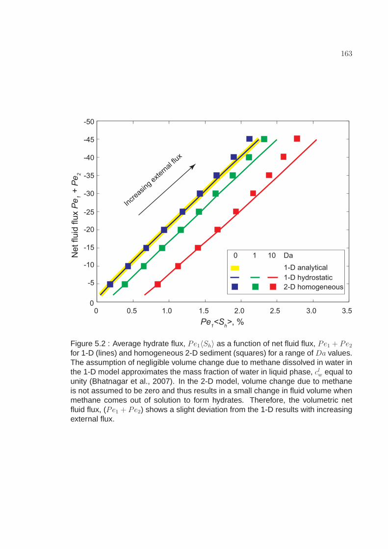
163
1-D hydrostatic
2-D homogeneous
Da1010
Incr
easing
ext
erna
l flu
x
0 0.5 1.0 1.5 2.0 2.5
Pe1<S
h>, %
3.0 3.5
-50
-45
-40
-35
-30
-25
-20
-15
-10
-5
0
Ne
t flu
id flu
x P
e1 +
Pe
2
1-D analytical
Figure 5.2 : Average hydrate flux, Pe1〈Sh〉 as a function of net fluid flux, Pe1 + Pe2for 1-D (lines) and homogeneous 2-D sediment (squares) for a range of Da values.The assumption of negligible volume change due to methane dissolved in water inthe 1-D model approximates the mass fraction of water in liquid phase, clw equal tounity (Bhatnagar et al., 2007). In the 2-D model, volume change due to methaneis not assumed to be zero and thus results in a small change in fluid volume whenmethane comes out of solution to form hydrates. Therefore, the volumetric netfluid flux, (Pe1 + Pe2) shows a slight deviation from the 1-D results with increasingexternal flux.

164
Chapter 6
Effects of Lithologic Heterogeneity and Salinity onGas Hydrate Distribution
6.1 Effect of Vertical Fracture Systems
∗†Fractures are common in geologic settings such as the Hydrate Ridge in
the Cascadia Margin varying over different length scales (Trehu et al., 2004;
Weinberger and Brown, 2006). Previous studies have hypothesized on the
significance of fracture networks in gas hydrate systems, and their impact was
quantified by implementing a vertical fracture system of higher permeability in
the gas hydrate accumulation model (Figure 6.1). Vertical fracture systems are
modeled since the time they are introduced (t = 0) in the system and gas hydrate
and free gas accumulation are tracked over time. Simulations are completed with a
vertical fracture system 100 times more permeable than the surrounding sediment
(i.e., Nsc = 102 for sediment and 104 for the vertical fracture system).
∗Chatterjee S., G. Gu, G. Bhatnagar, W.G. Chapman, B. Dugan, G.R. Dickens, G.J. Hirasaki(2011), Effects of heterogeneous lithology and focused fluid flow on gas hydrate distribution inmarine sediments, Proceedings of the 7th International Conference on Gas Hydrates (ICGH),Edinburgh, Scotland, United Kingdom, July 17-21, 2011
†Chatterjee S., G. Bhatnagar, B. Dugan, G.R. Dickens, W.G. Chapman, and G.J. Hirasaki(2012), Lithologic heterogeneity and focused fluid flow governing gas hydrate distributionin marine sediments, to be submitted

165
Figure 6.1 : Schematic showing permeability map representing a vertical fracturesystem (white). The fracture system is 100 times more permeable than thesurrounding formation. The aspect ratio for the sediment formation is 1:1.

166
Simulations with a vertical fracture network, show focused fluid flow resulting
in higher hydrate and free gas saturation within the high permeability fracture
system compared to the surrounding lower permeability sediment. First, a case
with isotropic permeability was considered. Steady state peak hydrate saturation
within the fracture system is ∼26%, while that in the surrounding low permeability
sediment matrix is ∼10% (Figure 6.2). Steady state free gas shows peak saturation
of 29% within the fracture column at the base of the domain.
A second case is simulated with a specified fluid flux from external sources at
depth representing a geologic model with thermogenic methane in deeper strata.
Higher hydrate and free gas saturation is predicted due to increased fluid flux and
greater methane input into the system from deeper sources. Simulations show
higher hydrate and free gas saturation within the high permeability fracture system
(Figure 6.3) as compared to the simulation case with biogenic in situ methane only
(Figure 6.2). Peak hydrate and free gas saturations within the fracture system are
48% and 42%, respectively.
These higher saturations were achieved by specifying external flux (Pe2 = −2),
throughout the model domain. It is shown that increased fluid flux from external
sources results in higher fluid focusing which produces higher hydrate and free
gas accumulations within the fracture system. As the fluid flux is increased, more
dissolved methane saturated water migrates into high permeability zones which
result in concentrated deposits of hydrates and free gas. Using the correlation

167
Figure 6.2 : Steady state gas hydrate and free gas saturation contours for isotropicsystem (kv/kh = 1) with biogenic in situ source (Pe2 = 0) and a vertical fracturesystem. The location of the fracture is shown by a set of white, vertical dashedlines. A vector field plot shown by white arrows represents the focused fluid flow.The fluid flow within the sediment formation is in the downward direction becauseit is plotted relative to the seafloor. The effect of the fracture in focusing flow isclearly illustrated through enhanced hydrate and free gas saturations within thehigh permeability conduit. The following parameters were used for this simulation:Pe1 = 0.1, Pe2 = 0, Da = 10, β = 6, cm,ext = 0, γ = 9, η = 6/9, kv/kh = 1,N
′
tφ = 1.485 and Nsc = 102.

168
Figure 6.3 : Steady state gas hydrate and free gas saturation contours with avertical fracture system, deep methane source, specified external fluid flux at thelower boundary (Pe2 = −2), and all other parameters same as in Figure 6.2. Thefollowing parameters were used for this simulation: Pe1 = 0.1, Pe2 = −2, Da = 10,β = 6, cm,ext = 0.897, γ = 9, η = 6/9, kv/kh = 1, N
′
tφ = 1.485 and Nsc = 102.

169
shown above (Figure 5.2), it is expected that more hydrate and free gas will
accumulate if higher flux is specified.
6.2 Effect of Mesh Refining
The general model framework was set up with coarse grid spacing (nz = 20, nx =
19) to enable faster computations. However, to test and illustrate the effect of mesh
refining, finer grid spacing was chosen for the lateral dimension for an example
simulation. The horizontal grid was refined three times while maintaining a coarse
grid spacing for the vertical domain. Although the grid spacing was refined, the
spatial dimensions were kept unchanged. Therefore, the fracture network system
was represented by three grid columns (as opposed to a single grid column in the
above simulations).
Simulations were completed using this refined grid spacing and steady state
solutions were obtained (Figure 6.4). The peak and average saturations for gas
hydrate and free gas were identical in the three grid blocks comprising the high
permeability fracture system. This result validates that our numerical model is
independent on mesh size and the saturations within the high permeability conduit
appear as broad peaks as compared to a sharp peak in our coarse grid simulations.
However, due to limitation of computational time, the subsequent simulations will
be restricted to coarser grid size to elucidate the primary controls on the amount
and distribution of hydrate accumulation within these high permeability conduits.
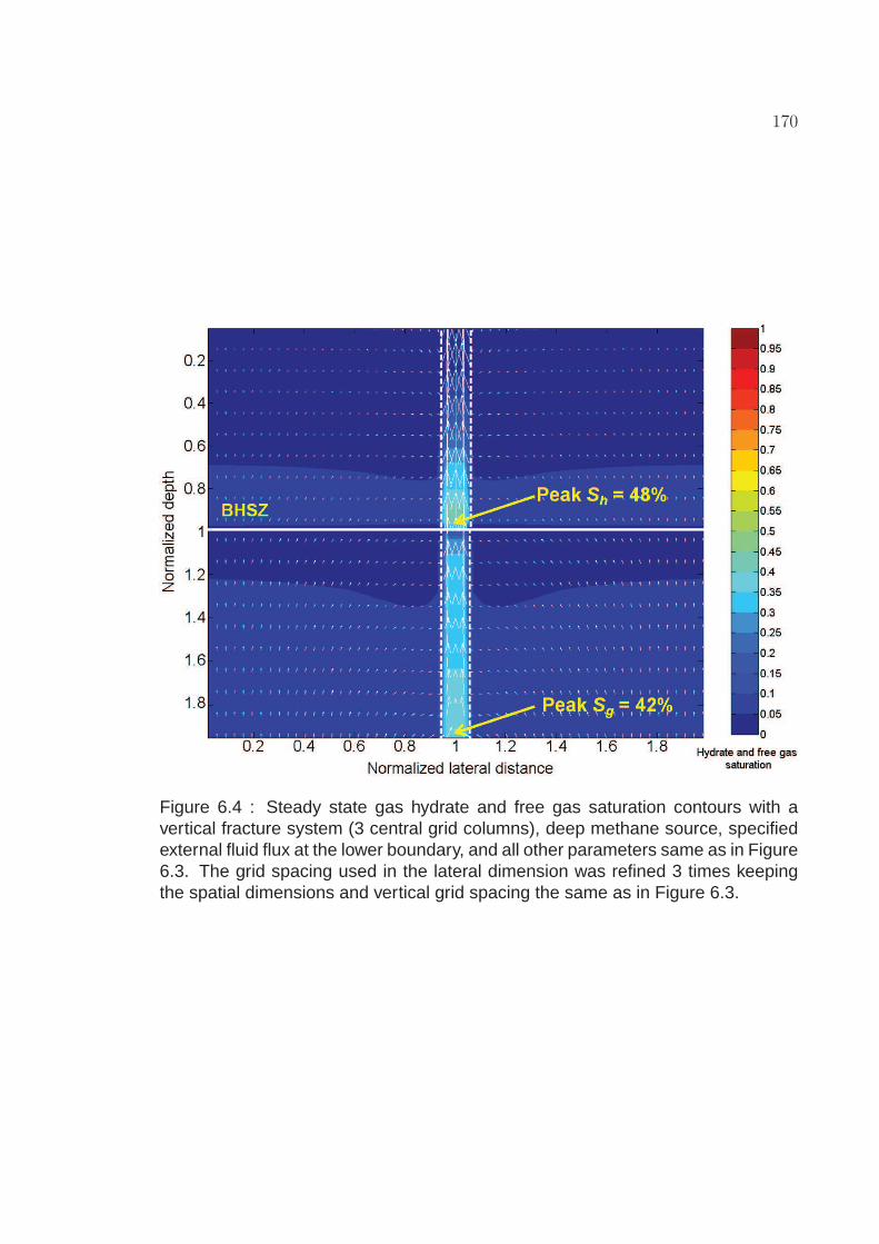
170
Figure 6.4 : Steady state gas hydrate and free gas saturation contours with avertical fracture system (3 central grid columns), deep methane source, specifiedexternal fluid flux at the lower boundary, and all other parameters same as in Figure6.3. The grid spacing used in the lateral dimension was refined 3 times keepingthe spatial dimensions and vertical grid spacing the same as in Figure 6.3.

171
6.3 Effect of Permeability Anisotropy
Natural systems are anisotropic, with the ratio of vertical to horizontal permeability
(kv/kh) less than unity. In such systems, greater horizontal permeability would
focus more fluids from neighboring regions to the high permeability conduits
by lateral migration. Anisotropic cases with a lower kv/kh ratio (order of
10−2) are expected to show relatively higher hydrate saturations within the high
permeability conduits as compared to isotropic cases (Figure 6.5). Higher
horizontal permeability would charge more fluids into these high permeability
conduits as a result of flow focusing. Simulations show peak hydrate and gas
saturations are 53% and 40% respectively (Figure 6.5). Increased horizontal
permeability results in more fluid flux towards the fracture system even from
sediment formation farther away from the fracture column.
Key findings of this thesis characterize the impact that high permeability vertical
fractures have on gas hydrate and free gas distribution by focusing fluid flow along
these fracture systems in the presence biogenic and/or thermogenic methane
sources. These models generally quantify the effects of flow focusing.
6.4 Local Flux within High Permeability Zones
The localized, focused fluid flux is computed and the local flux (Pelocal) is related to
the average hydrate saturation within the high permeability conduits in the GHSZ
(Figure 6.6). The results follow the same correlation established between net

172
Figure 6.5 : Steady state gas hydrate and free gas saturation contours for ananisotropic system (kv/kh = 10−2) with a vertical fracture system and all otherparameters same as in Figure 6.3. The following parameters were used for thissimulation: Pe1 = 0.1, Pe2 = −2, Da = 10, β = 6, cm,ext = 0.897, γ = 9, η = 6/9,kv/kh = 10−2, N
′
tφ = 1.485 and Nsc = 102.

173
Pe1<S
h> , %
0 0.5 1.0 1.5 2.0 2.5 3.0 3.5
Ne
t flu
id flu
x P
e1 +
Pe
2o
rL
oca
l flu
x P
eL
oca
l
-50
-45
-40
-35
-30
-25
-20
-15
-10
-5
0
1-D hydrostatic
2-D homogeneous
2-D heterogeneous
Bioge
nic
sour
ces
+ ext
erna
l flu
x
Biogenic
sourc
es only In
crea
sing
ext
erna
l flu
x
Figure 6.6 : Steady state average gas hydrate flux, Pe1〈Sh〉 and local fluid flux,Pelocal (black squares).
fluid flux and average hydrate saturation in 1-D systems (Figure 5.2). For lower
values of Da(< 10), methane generated in the system is not enough for hydrate
accumulation even with high local flux focused in the high permeability zones.
The gas hydrate and free gas saturations in these lithologically heterogeneous
systems can be characterized by the local Peclet number (Pelocal; localized,
focused, vertical, advective fluid flux relative to diffusion). This characterization
is consistent with the net Peclet number (Pe1 + Pe2) characterization in 1-D
homogeneous systems. This suggests that local hydrate and free gas saturations
in lithologically complex systems can be characterized by basic parameters (local
flux and diffusivity).

174
6.5 Effect of Permeability Contrast
Heterogeneous models have shown that higher permeability conduits increase
the ability to capture methane thereby enhancing saturations of gas hydrate and
free gas (Figure 6.7). The above simulations show vertical permeable conduits
which are 100 times more permeable than the surrounding matrix. Higher
permeability contrast (of the order 103 - 106) are more representative of natural
marine sediment with fractures and sand beds. Sensitivity tests are performed
by varying the permeability contrasts (kfracture/kshale) from 2 to 1000 (Figure 6.7).
Large permeability contrast (kfracture/kshale) enables greater fluid focusing and
leads to greater gas hydrate and free gas accumulation within these conduits. This
may explain elevated saturations in high flux conduits like pipes, vents, and dipping
reservoirs in advective systems.
6.6 Effect of Horizontal High Permeability Layers
Heterogeneity is now modeled as a horizontal layer parallel to the seafloor.
This horizontal layer is buried and its downward movement is tracked over long
timescales. However, it is acknowledged that fluids need a conduit to flow from
depth to the seafloor. Therefore, the formation is short-circuited with two vertical
fracture systems at the two ends of the simulation domain. This allows fluids
to flow from depth through the left vertical fracture system and then across the
simulation domain through the horizontal layer ultimately towards the seafloor

175
Hyd
rate
sa
tura
tio
n
Peak values Average values
100 101 102 103
0
10
20
30
40
50
60
70
80
Fre
e g
as s
atu
ratio
n
kfracture
/kshale
Isotropic; biogenic
Isotropic; biogenic + external flux
Anisotropic; biogenic + external flux
kfracture
/kshale
0
10
20
30
40
50
60
70
80
0
10
20
30
40
50
60
70
80
0
10
20
30
40
50
60
70
80
0
10
20
30
40
50
60
70
80
0
10
20
30
40
50
60
70
80
100 101 102 103
100 101 102 103 100 101 102 103
Figure 6.7 : Model results showing the importance of permeability contrasts andpermeability anisotropy on the accumulation and saturation of gas hydrate and freegas. As permeability contrast between a fracture system (or sand) and the shaleincreases (kfracture or ksand >> kshale) the hydrate and free gas saturations in thepermeable conduit increases. As anisotropy decreases (kv/kh) in the shale, thesaturations also increase.

176
through the right vertical fracture system (Figure 6.8). These lithologic structures
are geologically unrealistic, however, they provide a clear understanding of the
system to assess the dependence of dip angle of these permeable layers.
Steady state simulations are run with the same parameter set used in Figure
6.3, while the horizontal layer and vertical fractures are buried down through
geologic time. The steady state simulations show that high focused fluid flow
through the permeable layers from depth to the horizontal layer, then across the
simulation domain and then towards the seafloor (Figure 6.9). The fluid flow in
these horizontal conduits is mostly horizontal. However, unlike the vertical fracture
systems extending through the GHSZ, gas hydrate and free gas do not accumulate
along the horizontal layer. Even though high fluid flux gets focused and flows
through the permeable conduit, it does not result in elevated hydrate saturation.
Therefore, the localized fluid flux within these systems cannot be used to evaluate
local gas hydrate saturation and distribution. Thus, it is determined that these
horizontal fluid flux components do not influence hydrate precipitation. Therefore,
it is shown that the vertical flux in these heterogeneous relative to the methane
diffusion is what drives these elevated hydrate saturations in these lithologically
complex systems.

177
Figure 6.8 : Schematic showing initial permeability map representing highpermeability horizontal sand layer deposited between two low permeabilitysediment layers. The horizontal layer has two high permeability vertical fluidconduits on either ends to channel the fluid flow from depth to the seafloor. Thehigh permeability layer (white) is 100 times more permeable than the surroundingformation.

178
Figure 6.9 : Steady state gas hydrate and free gas saturation contours for a systemwith high permeability horizontal sand bed flanked between two vertical fracturesystems on either ends. The position of the high permeability layer (100 times morepermeable than surrounding formation) is delineated by a set of yellow dashedlines. Parameters used for this simulation are same as used in Figure 6.3.

179
6.7 Effect of Dip Angle of High Permeability Layers
A steady state, 1-D analytical theory is derived to illustrate the effect of dip angle of
the high permeability layer. The mathematical model shows that the inclination
of the permeable conduit (to the vertical axis) dictates hydrate saturation and
distribution (Appendix D). The net fluid flux (Pe1 + Pe2) is related to the average
hydrate flux (Pe1〈Sh〉) within a fluid conduit inclined in any orientation to the vertical
(not shown here). This generates a series of plots for a range of dip angle values
relating the net fluid flux and the average hydrate flux. However, this does not
generalize results as these plots are dependent on the dip angle. In order to
eliminate the dependence of dip angle, the model is further extended to collapse all
the above information over a wide range of configurations into one single contour
plot (Figure 6.10). Interestingly, there is no longer any dependence on the dip
angle, thereby reducing the parameter space. All the points collapse on a single
line for a range of configurations (θ). These plots can be used to compute the
average hydrate saturation given the fluid flux and the methane solubility gradient
is known for marine hydrate systems in any configuration. It is shown that the
vertical fluid flux is what dictates hydrate saturation and accumulation as opposed
to the net fluid flux for a case where the conduit is inclined at an angle, to the
vertical. These results can be extended to any geologic setting, by adapting the
site-specific parameters (Figure 6.10).

180
0 0.5 1 1.5 2 2.5
-50
-45
-40
-35
-30
-25
-20
-15
-10
-5
0
Pe1<S
h>, %
Ne
t ve
rtic
al flu
id flu
x, P
e1
+ P
e2
co
s θ
Parameters resembling sites
Cascadia Margin 889
Cascadia Margin U1325
Blake Ridge 997
Figure 6.10 : Average hydrate flux, Pe1〈Sh〉 is related to the net vertical fluid fluxfor marine hydrate systems inclined in any angle to the vertical axis. Systemswith vertical fractures correspond to 0o, whereas horizontal conduits correspond to90o. As orientation changes from vertical to horizontal, the saturation decreases,even though high flux flows through these systems. This would imply that thevertical fluid flux relative to methane diffusion is what drives hydrate saturation andaccumulation in these marine hydrate systems. Similarly, this can be extended to2-D systems where localized vertical fluid flux relative to methane diffusion canbe correlated to localized average hydrate saturation in systems with complexlithology. These results are adapted for site-specific transport and geologicparameters that resemble three classic hydrate settings.

181
6.8 Effect of Free Gas Migration into the GHSZ
Focusing of methane-charged liquid (water) enhances hydrate and free gas
saturations within the high permeability zones. However, free gas can also migrate
vertically and laterally if the critical gas saturation is exceeded. To simulate such
migration, critical gas saturation (Sgr) is set to 5% and free gas exceeding this
critical value is free to migrate. Free gas migrates upwards due to buoyancy
and gets sealed by the low permeability hydrate layer at the base of the GHSZ.
Hydrate formation at the base of the GHSZ causes an increase in the capillary
entry pressure and creates a hindrance for free gas to enter the GHSZ from below.
This results in accumulation of free gas beneath the GHSZ into a connected gas
column.
6.8.1 Vertical Fracture Systems
Simulations show free gas accumulation below the base of the GHSZ (Figure
6.11). A long gas column is formed before the gas pressure exceeds the capillary
entry pressure and gas migrates into the GHSZ. Free gas converts to hydrate
immediately at the base of the GHSZ giving rise to a spike in hydrate saturation.
Constant salinity is assumed hence phase equilibrium is unaffected even when
free gas migrates into the GHSZ. The high hydrate saturation in the fracture zone
causes a permeability reduction resulting in lateral fluid migration beneath the
GHSZ. High hydrate saturation also restricts further free gas invasion into the

182
GHSZ. Free gas then migrates laterally from the high permeability fracture system
to the neighboring sediment below the base of the GHSZ. Peak hydrate and free
gas saturation reach 75% and 62% right above and below the base of the GHSZ
within the fracture system. At this enhanced saturation, free gas is mobile and
migrates laterally, causing sediment near the fracture to also have relatively higher
saturations.
The length of a connected gas column has been shown to be dependent on
the dimensionless group Nsc (Bhatnagar et al., 2008b). Lower values of Nsc
(lower permeability and/or higher sedimentation rate) result in development of
higher overpressure in the system, which further results in thicker gas columns
and increased gas pressure at the base of the GHSZ close to the lithostatic stress
(e.g., Flemings et al., 2003; Hornbach et al., 2004). Fractures tend to open up at
this point (Daigle and Dugan, 2010a). This fracturing process is not modeled in any
of these simulations, and the simulations are terminated as soon as gas pressure
equals total vertical stress.
6.8.2 Dipping Sand Layers
Lithologic heterogeneity is modeled in another configuration (non-vertical), in which
dipping sand beds bounded by low permeability shale is illustrated. To model a
sand layer, a high permeability sand layer is included at a given dip angle (∼3o)
within the sediment (Figure 6.12) and buried through geologic time. The downward

183
Figure 6.11 : Steady state gas hydrate and free gas saturation contours for anisotropic system with a vertical fracture system, mobile gas (Sgr = 5%) and allother parameters same as in Figure 6.3. The following parameters were used forthis simulation: Pe1 = 0.1, Pe2 = −2, Da = 10, β = 6, cm,ext = 0.897, γ = 9,η = 6/9, kv/kh = 1, N
′
tφ = 1.485 and Nsc = 102.

184
movement of this sand layer and the corresponding transient hydrate and free gas
evolution are simulated. The sand layer is assigned an absolute permeability 100
times greater than the surrounding shale. Sediment compacts with burial (Nsc =
102 for shale and 104 for sand layers). The seafloor and transport parameters are
same as in the simulations with vertical fracture network except Da = 1. During
burial, absolute permeability of any grid block can be computed by interpolation
and therefore, interface between zones of different permeabilities are recorded
over time. The interface position is used to compute the horizontal and vertical
permeabilities and track the location of the sediment over time.
Systems with dipping sand layers show localized, enhanced concentrations
of hydrate and free gas within the high permeability sand layers (Figure 6.13).
Free gas is focused within the sand layer. Steady state peak hydrate saturation
within the sand layer is about 59%, significantly higher than the 43% peak hydrate
saturation in the low permeability sediment within the GHSZ. Peak free gas
saturation is 38% within the sand layer just below the GHSZ, and similar to fracture
network case (Figure 6.11), free gas migrates laterally into the low permeability
sediment around the sand layer. Thus, presence of higher permeability sand layer
leads to relatively higher fluid focusing and hydrate saturation within the GHSZ.
These results elucidate that lithology plays a significant role in accumulating gas
hydrate and free gas in heterogeneous sediment in most natural systems. These
generalized models can be adapted to specific field examples such as the Walker

185
Figure 6.12 : Schematic showing initial permeability map representing highpermeability sand layer (lighter shade) deposited between two low permeabilitysediment layers. The sand layer is 100 times more permeable than the surroundingformation. A 5:2 vertical exaggeration (VE) is used to plot the sediment space.

186
Figure 6.13 : Steady state gas hydrate and free gas saturation contours for asystem with high permeability dipping sand bed between two anisotropic (kv/kh =10−2) shale beds. The position of the sand layer is depicted by the set of yellowdashed lines. Vertical exaggeration of 5:1 is used and the physical domain fornormalized depth and lateral distance are [0, 2] and [0, 10], respectively. Thefollowing parameters were used for this simulation: Pe1 = 0.1, Pe2 = −2, Da = 1,β = 6, cm,ext = 0.897, γ = 9, η = 6/9, kv/kh = 10−2 (in shales), N
′
tφ = 1.485 andNsc = 102.

187
Ridge in the Gulf of Mexico to explain the enhanced saturations (60% - 80%) in the
dipping sand layers.
6.9 Effect of Hydrate Formation and Dissociation on Pore
Water Salinity
Gas hydrate formation and its dissociation to free gas alters the pore water salinity,
which in turn affects the phase equilibrium of the system (e.g., Zatsepina and
Buffett, 1998; Egeberg and Dickens, 1999; Milkov et al., 2004; Liu and Flemings,
2006). Moreover, high gas flux typical of specific sites have dominant salinity
anomalies caused due to enormous hydrate formation (Milkov et al., 2004; Liu and
Flemings, 2006, 2007). The salinity effects had been assumed to be negligible
in the previous 1-D modeling (e.g., Davie and Buffett, 2001, 2003a; Bhatnagar et
al., 2007) since salt (NaCl, or equivalently, Cl−) mass balance was not coupled
with the phase equilibrium thermodynamics. In the 2-D model developed above,
salinity changes have been neglected as well. However, if simulations with mobile
free gas discussed above in Figures 6.11 and 6.13 are investigated, it is realized
that free gas can only invade the GHSZ until the first grid block. As soon as free
gas invades the GHSZ, the CH4 phase changes from free gas to hydrate due to
thermodynamic equilibrium. This is not true in many geologic settings where free
gas is observed to independently exist near the seafloor (Trehu et al., 2003; Milkov
et al., 2004). Recently, several papers have shown coexistence of hydrate and free

188
gas phases of CH4 within the GHSZ due to salinity effects in 1-D (e.g., Liu and
Flemings, 2007; Daigle and Dugan,2010b).
A 2-D chloride mass balance is expressed in Equation 5.5 and rewritten in
its dimensionless form in Equation 5.64, normalized using the scaling scheme
discussed in Bhatnagar et al. (2007). The chloride balance is incorporated and
coupled with the benchmarked 2-D model developed in this study. During hydrate
formation, the chlorides are released by the pore fluids when fresh water forms the
cage structure during hydrate formation. This leads to local elevation of salinity
where hydrates are formed. By contrast, the pore fluids become less saline
due to local freshening during hydrate dissociation. The chloride concentrations
are tracked in the model over space and time (same as the other dissolved
constituents) as they move by advection and diffusion and the salinity is computed
from these chloride profiles. The model is tested against the field data from
Blake Ridge Site 997 where pore water chlorinity (and other geochemical datasets)
exist. The hydrate and free gas peaks at 7% and 12% respectively (Figure 6.14).
The modeled pore water chloride profile show a peak at depths corresponding
to elevations hydrate saturation. The chloride profile is also computed assuming
hydrate dissociation during core recovery and these resemble that measured at the
site (Figure 6.14). Interestingly, the observed profiles match favorably for Pe2 = −1,
which is equivalent to upward fluid velocity values of 0.085 mm/yr at the seafloor.
These upward fluid velocities resemble previously reported values of 0.08 mm/yr

189
(Egeberg and Dickens, 1999) and 0.097 mm/yr (Frederick and Buffett, 2011) near
the seafloor.
6.10 Effect of Salinity on Phase Equilibrium and Methane
Solubility
The pore water chlorinity is often related to the pore water activity and salinity.
The effect of salinity variation on CH4 hydrate stability conditions is related to the
pore water activity (Dickens and Quinby-Hunt, 1994, 1997). In this study, the
spatial Cl− profiles are used to track space- and time-dependent salinity during
hydrate formation and dissociation processes. In the above 2-D model, CH4
solubility curve is computed as a function of pressure and temperature, neglecting
salinity effects. In this section, CH4 solubility is coupled with salinity changes in
the hydrate accumulation model. This leads to recomputing the phase equilibrium
and CH4 solubility with variations in salinity (Figure 6.15). This leads to a zone of
three-phase coexistence, as opposed to a single point representing the triple-point
of CH4 in the salinity-independent model discussed above. In essence, this would
enable coexistence of free gas and hydrate phase within the GHSZ over a depth
horizon. This would allow free gas existence in the hydrate stability zone and
lead to focused free gas and enhanced hydrate saturations. A three-phase flash
calculation is required to be set up to calculate the fractions of different phases
(aqueous, hydrate, and gas) present within a specific gridblock at each timestep

190
350 400 450 500 550 600
0
100
200
300
400
500
600
700
800
900
De
pth
be
low
se
aflo
or
(mb
sf)
997 data
Model
Blake Ridge
Chloride concentration (mM)
0 5 10 15
Hydrate and free gas saturation
Figure 6.14 : Steady state gas hydrate and free gas saturation coupled with achloride concentration profile at Blake Ridge Site 997. The bold line representsin situ chloride concentration profile before recovery and dashed lines representsconcentration profiles due to hydrate dissociation during core recovery. Thechloride anamoly at this site in the hydrate zone is due to hydrate dissociationas the cores were sampled. The chloride profile best matches the data with thefollowing geologic and transport parameters: Pe1 = 0.1065, Pe2 = −1, Da = 2.1,β = 4.16, cm,ext = 0.9, ccl,ext = 503 mM, ccl,o = 559 mM, γ = 9, η = 6/9, N
′
tφ = 1.485and Nsc = 104.
191
depending on the thermodynamic conditions. The current 2-D multiphase transport
model with the three-phase flash calculation should be capable of simulating
conditions with three-phase co-existence within the GHSZ. This is not been
modeled here and has evolved as one of the future work arising from this study.
6.11 Conclusions
A generalized 2-D model was developed to simulate gas hydrate and free gas
accumulation in heterogeneous marine sediment. The model allows incorporation
of lithologic heterogeneity and lateral fluid flow in the system. Focused fluid flow
through a vertical fracture network or high permeability sand layers increases local
hydrate accumulation and saturation.
Previous one-dimensional work, showed that the accumulated hydrate
saturation was dependent on Peclet number, Pe, the ratio of advective flux to the
diffusive flux of methane. In this 2-D work, it is shown that the localized, focused,
vertical advective fluid flux relative to diffusion (Pelocal) determines the magnitude
of hydrate and free gas saturation. Average local Peclet numbers is related to the
average hydrate flux (Pe1〈Sh〉) within high permeability conduits, which compare
favorably with the previous 1-D correlation.
Simulations with specified fluid flux and methane input from deeper sources,
allows comparison of local methanogenesis and deeper methane sources on flow
pathways and hydrate/free gas accumulation. Increased fluid flux from deeper

192
27
28
29
30
31
32
33
34
35
36
2
4
6
Salinity (wt %)
Pre
ssu
re (
MP
a)
Temperature (K)
275 280 285 290 295 300 305 310 315
275 280 285 290 295 300 305 310 315
Figure 6.15 : Three-phase CH4 hydrate-water-gas stability boundary contours fora wide range of temperature, pressure and salinity. The temperature profile alonga geotherm intersects this 3-phase equilibrium curve over a zone, rather than asingle point as in the constant salinity case described in (e.g., Davie and Buffett,2001, 2003a; Bhatnagar et al., 2007). Salinity variations can be used to model theco-existence of hydrate and free gas phases within the GHSZ leading to enhancedsaturations of hydrates and gas in systems dominated by flux from depth.

193
external sources results in increased concentrations of hydrate and free gas.
Permeability anisotropy, with a lower ratio of vertical to horizontal permeability
show enhanced hydrate concentrations within the high permeability conduits
because anisotropy focuses more methane-charged fluid into these conduits. The
2-D model results quantify how focused fluid flow through high permeability zones
affects regional and local hydrate accumulation and saturation.
Currently, relatively simple systems with fracture systems and/or dipping sand
layers are simulated, whereas realistic geologic settings are characterized by much
more heterogeneous stratigraphy in terms of vertical fracture networks, multiple
sand layers embedded within shale layers and fracture connectivity of sand layers
with vertical fracture systems. These preliminary results, however, serve as a
starting point and demonstrate that heterogeneity in natural gas hydrate systems is
important for controlling hydrate and free gas saturations, and that these systems
can be modeled. This generalized model is intended to adapt to specific field
examples such as Walker Ridge in the Gulf of Mexico where enhanced hydrate
saturation is noted in dipping sand layers.
194
Chapter 7
Effect of Gas Hydrate Distribution on Slope Failurein Subsea Sediments
7.1 Introduction
Gas hydrates have been implicated as a geohazard that may have caused slope
failure and slumping in marine settings (e.g., Borowski and Paull, 1997; Briaud
and Chaouch, 1997; Sultan et al., 2004; Nixon and Grozic, 2007; Kwon et al.,
2010; Scholz et al., 2011). Compaction of clay results in lowering the porosity
of the sediment. This porosity reduction is related to the decrease in absolute
sediment permeability. Furthermore, hydrate accumulation in the pore space
lowers the permeability and hinders fluid flow. In addition to lowering the sediment
permeability, free gas accumulation below the base of the gas hydrate stability
zone (GHSZ) can lead to generation of overpressure in the sediments. The
overpressure development in these gas hydrate systems may drive conditions for
sediment failure by faulting and fluid leakage or by shear failure. Some of the key
factors responsible for overpressure development to the point of sediment failure
were summarized with the help of dimensionless groups such as Nsc, relating
sediment permeability and the sedimentation rate at the seafloor (Bhatnagar et

195
al., 2008b). In this study we briefly discuss the theory of sediment instability
and examine some of the stability effects of this dimensionless parameter, Nsc
as previously reported by e.g., Bhatnagar et al. (2008b).
Subsea sediment stability in hydrate systems are assessed through two
different approaches. First, a rigorous stability analysis that assesses the failure
condition by evaluating fracture genesis and how that relates to in situ observations
of fracture-hosted hydrate in fine-grained settings (e.g., Gulf of Mexico, Cascadia
Margin, Krishna-Godavari Basin, India). This builds upon previous models that
address the feedbacks between fluid flow, hydrate accumulation, and fracture
genesis (e.g., Nimblett and Ruppel, 2003; Flemings et al., 2003; Daigle and Dugan,
2010a). However, there are a series of papers addressing this rigorous analysis
(Daigle and Dugan, 2010a, 2010b) and is not included here.
Second, an infinite slope stability analysis discussed here and linked to the
existing geologic hydrate accumulation models (Bhatnagar, 2008; Chatterjee et
al., 2011b). Notably, this is the first step in trying to address the evolution
of geohazards related to natural gas hydrate systems. This technique is
computationally inexpensive, applicable in geologic and reservoir models, and
provides a quick look at stability to identify locations for detailed stability analysis.

196
7.2 Slope Stability Modeling
Sediment failure occurs when the downslope shearing stress exceeds the resisting
stresses of the sediment. In this study, slope stability calculations have been
coupled with the basin-scale hydrate accumulation model and the subsea sediment
instability are discussed. For a quick assessment of slope stability evolution, the
factor of safety (FS) is calculated using an infinite slope approximation (e.g., Lambe
and Whitman, 1969; Dugan and Flemings, 2002).
7.2.1 Infinite Slope Approximation
The infinite slope approximation relates the maximum resisting force, Fr,max and
the shearing force, Fs.
FS =Fr,max
Fs
(7.1)
where FS > 1 represents a stable slope and FS ≤ 1 represents an unstable
slope. The analysis assumes that the failure surface is parallel to the seafloor,
fluid pressure is constant along the failure plane, end effects and stresses are
neglected, and sediments on the slide surface are homogeneous (Lambe and
Whitman, 1969; Loseth, 1998; Dugan and Flemings, 2002). A schematic is
illustrated to represent the infinite slope approximation (Figure 7.1).
The shearing force, Fs is the downslope component of the normal force,
controlled by the mass of the overlying sediment, acceleration due to gravity, and
the angle of the failure plane. Assuming unit length of the potential sliding sediment

197
Figure 7.1 : Infinite slope model for slope-stability analysis where α is the slopeangle for the assumed failure plain (parallel to the sediment surface), z is thethickness of the sediment block, G = buoyant weight of the sediment, FN is thenormal force, Fs = shearing force, and Fr is the resisting force (Taken from Loseth,1998).

198
block, the effective shearing force can be expressed as:
Fs = (σv − ρwgz)sinα (7.2)
where σv is the total vertical stress, ρw is the water density, g is the acceleration
due to gravity, z denotes the thickness of the potential sliding block, and α is the
slope angle. The slope angle, α is based on an average seafloor gradient and is
set a constant value of 2o for our study.
The frictional resistance to sliding (or shear strength) for porous sediments
depends on the angle of internal friction, the cohesion of the sediment, and the
effective normal force. The most common representation of shear strength S is
given by the classic equation in terms of effective stress (Coulomb, 1776):
S = c+ [(σv − ρwgz)cos2α− p∗w]tanφf (7.3)
where c is the sediment cohesion, φf is the angle of internal friction and p∗w is
the overpressure equal to the porewater pressure in excess of the hydrostatic
pressure. Assuming unit sediment block width, the basal area of the sediment
block shown in Figure 7.1 is equal to 1cosα
. Since stress is defined as force per unit
area, the maximum resisting force is:
Fr,max =c+ [(σv − ρwgz)cos
2α− p∗w] tanφf
cosα(7.4)

199
Substituting Fr,max (equation 7.4) and Fs (equation 7.2) in equation 7.1:
FS =c+ [(σv − ρwgz) cos
2 α− p∗w] tanφf
(σv − ρwgz) sinα cosα(7.5)
In the above formulation, sediment cohesion (c) is set to be zero, for simplicity. A
typical value of c is normally 25 KPa for consolidated clays (Lambe and Whitman,
1969). Notably, gas hydrate accumulation may alter this assumption and increase
the stability. Therefore, the cohesion parameter needs to be varied to model slope
instability during hydrate accumulation as it may increase due to hydrate formation.
The angle of internal friction, φf is assumed constant (26o) based on average
values in marine sediments. Internal friction angles range from 20-35o for clays
and between 27 and 30o for silty sand (Dugan and Flemings, 2000, Dugan, 2003).
These assumptions ensure minimum stability is estimated since non-zero cohesion
and a higher angle of friction will increase the shear strength (Equation 7.3) and
thus will increase the factor of safety (Equation 7.5). These parameters can be
updated for specific hydrate settings now that the model has been tested.
7.3 Results and Discussion
In the presence of lithologic heterogeneities, fluid focusing in high permeability
conduits results in higher hydrate and free gas saturation and accumulation
(Chatterjee et al., 2011b). Infinite slope approximation can be used to

200
assess slope stability for different heterogeneous simulation cases using our
hydrate accumulation model. We present one case where hydrate accumulates
preferentially in high permeable vertical fracture systems due to focused flow
(Figure 6.2). Although we acknowledge that these vertical fracture systems with a
horizontal seafloor violates many of the infinite slope approximation assumptions,
we present these simulations as base cases to validate and benchmark our
model calculations. These systems are evaluated by varying the dimensionless
parameter, Nsc relating to permeability and sedimentation rate. Pore water
overpressure is shown to develop with decreasing values of Nsc (Figure 7.2). Last,
the FS plots are constructed (Figure 7.3) as a function of normalized depth and
normalized lateral distance.
These models show two key results that are consistent with previous studies:
(1) high factors of safety throughout the model domain; and (2) that permeability
heterogeneity influences stability. The high FS values are controlled by the
low overpressures in this base case and are used to validate the numerical
computations as they are consistent with other stability analyses of hydrostatic
systems. The influence of permeable conduits is also consistent with previous
studies (e.g., Dugan and Flemings, 2002); coupled with the influence of permeable
conduits on hydrate saturation, this could be crucial to understand slope stability in
hydrate settings.

201
0
0.05
0.1
0.15
0.2
0.25
0.3
0.35
0.4
0.45
0.5
0.55
0.6
0.65
0.7
0.75
0.8
0.85
0.9
0.95
1
0.5 1 1.5
0.5
1
1.5
Water overpressure, Pw*
0.5 1 1.5
0.5
1
1.5No
rma
lize
d d
ep
th
0.5 1 1.5
0.5
1
1.5
Normalized lateral distance
0.5 1 1.5
0.5
1
1.5
Normalized lateral distance
No
rma
lize
d d
ep
th
Nsc
= 5
Nsc
= 100 Nsc
= 10
Nsc
= 2.5
Figure 7.2 : Pore water overpressure contour plot for a 2-D marine hydrateaccumulation model with an isotropic vertical fracture system extending throughthe gas hydrate stability zone. Unit normalized lateral distance delineate theboundary of the fracture system.
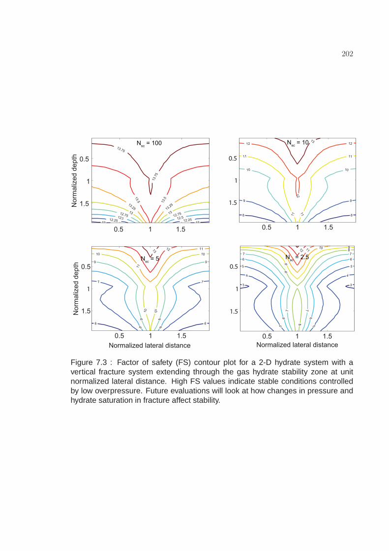
202
12 1212.25 12.25
12.5 12.5
12.75 12.7513 13
13.25 13.25
13.5
13.5
13.7513.7
5
No
rma
lize
d d
ep
th
0.5 1 1.5
0.5
1
1.5
8 8
9 9
10 10
11
11
11
11
12
12
1213
0.5 1 1.5
0.5
1
1.5
6 6
7 7
8 8
9
9
9
9
10
10
10
10
11
111213
Normalized lateral distance
No
rma
lize
d d
ep
th
0.5 1 1.5
0.5
1
1.5
3 3
4 4
5
5
5
5
6
6
6
6
7
7
7
7
8
8
8
9
9101112
Normalized lateral distance
0.5 1 1.5
0.5
1
1.5
Nsc
= 100 Nsc
= 10
Nsc
= 5 Nsc
= 2.5
Figure 7.3 : Factor of safety (FS) contour plot for a 2-D hydrate system with avertical fracture system extending through the gas hydrate stability zone at unitnormalized lateral distance. High FS values indicate stable conditions controlledby low overpressure. Future evaluations will look at how changes in pressure andhydrate saturation in fracture affect stability.

203
7.4 Conclusions
A short additional routine in the 2-D hydrate accumulation simulator is developed
to perform the factor of safety calculations. This approximation provides a reliable
stability calculation for regional slope failures in hydrate-bearing heterogeneous
sediments. This simple assessment can identify potentially unstable regions that
may require more advanced failure analysis, such as for deep-seated rotational
failures (e.g., Bishop, 1955). Therefore, this analysis provides an initial stability
calculation and identifies regions that warrant detailed stability calculations.

204
Chapter 8
Conclusions and Future Work
8.1 Conclusions
Generalized numerical models developed in this thesis determine factors
governing hydrate and free gas distribution in marine sediment. This chapter
summarizes the conclusions of this dissertation and highlights some future
research directions that stem from this study. The overall conclusions of this thesis
can be divided into three broad categories:
1. Pore water chemistry above gas hydrate systems
2. Lithology and fluid flow governing hydrate distribution
3. Slope failure in subsea sediments
Pore Water Chemistry across Sulfate-Methane Transition and Gas Hydrate
Systems
Previous 1-D models showed depth of the sulfate-methane transition (SMT) as a
direct proxy to evaluate average gas hydrate saturation in marine sediments. This
research revisits and revises an existing 1-D model and includes two competing

205
reduction pathways for porewater sulfate causing the SMT in shallow sediment.
The revised 1-D model includes constituents such as dissolved CH4, SO2−4 , DIC,
Ca2+, δ13C of DIC, gas hydrate and free gas which enhances our understanding
of carbon cycling processes in shallow sediment below the seafloor, specifically
the chemical changes across the SMT. The model is tested with site-specific
parameters at three distinct hydrate settings with differing carbon chemistry. The
simulated pore water profiles resemble those measured at the sites, and the model
explains the similarities and differences in pore water chemistry. At all sites, an
upward flux of CH4 consumes most net SO2−4 at a shallow SMT, and calcium
carbonate removes a portion of DIC at this horizon. However, a large flux of
13C-enriched HCO−3 enters the SMT from depth at Site 1230 and 1244, but not
at Site KC151-3. This leads to elevated concentrations of pore water DIC with a
δ13C much greater than that of CH4 (> -60 0/00), even though AOM causes the
SMT. The proportion of DIC flux from depth determines the concentration and
δ13C of DIC at the SMT. The addition of HCO−3 from depth impacts the slope
of certain concentration crossplots. Crucially, neither the DIC concentration nor
its carbon isotope composition at the SMT can be used to discriminate between
sulfate reduction pathways. A 1:1 flux balance between alkalinity (essentially DIC)
and sulfate across the SMT confirms that AOM is the dominant cause for SMT in
these systems. Thus, the upward methane flux consuming the pore water sulfate to
form the SMT relates the SMT depth, fluid flux and the average hydrate saturation

206
in marine gas hydrate systems.
Effects of Heterogeneous Lithology and Focused Fluid Flow on Gas Hydrate
Distribution
A generalized 2-D numerical model has been developed to simulate spatial and
temporal distribution of gas hydrate and free gas in marine sediments over geologic
timescales. Fracture network systems and dipping sand layers are common
examples of lithologic heterogeneities in natural gas hydrate systems and are
simulated using the 2-D model.
Simulations with a vertical fracture network, which extends through the gas
hydrate stability zone and which has a permeability much greater than surrounding
shale, show that focused fluid flow causes higher saturations of gas hydrate
(25-70%) and free gas (30-60%) within the fracture network compared to the
surrounding shale. Simulations with dipping sand layers of high permeability also
result in elevated saturations of gas hydrate (60%) and free gas (40%) within the
sand because of focused fluid flow.
Permeability anisotropy, with a vertical to horizontal permeability ratio on the
order of 10−2, enhances gas hydrate concentrations within high permeability
conduits because anisotropy enhances transport of methane-charged fluid to high
permeability conduits. The 2-D, heterogeneous models quantify how focused
fluid flow through high permeability zones affects local hydrate accumulation and
207
saturation. Increased fluid flux and deep source methane input result in enhanced
concentrations of hydrate and free gas, and also increase the flow focusing effects.
From these 2-D results, hydrate and free gas saturations can be characterized
by the local Peclet number (localized, focused, vertical, advective fluid flux relative
to diffusion); which is consistent with Peclet number characterization in 1-D
homogeneous systems. This characterization suggests that even in lithologically
complex systems, local hydrate and free gas saturations can be characterized by
basic parameters (local flux and diffusivity). To illustrate the importance of local
flux on simple and complex natural hydrate systems this generalized model can be
used to simulate hydrate distribution for specific field examples such as the Walker
Ridge in the Gulf of Mexico where enhanced hydrate saturation is noted in dipping
sand layers.
Effect of Gas Hydrate Distribution on Slope Failure in Subsea Sed iments
The infinite slope approximation evaluates the slope’s factor of safety to elucidate
the potential for slope failure in subsea sediments associated with the hydrate
accumulation model. This approximation provides a reliable stability criterion for
regional slope failures in hydrate-bearing heterogeneous sediments. This simple
assessment identifies potentially unstable regions that may require more advanced
failure analysis and provides an initial stability calculation to identify regions that
warrant detailed stability calculations.

208
8.2 Future Research Directions
This thesis highlights some primary factors which govern gas hydrate and free
gas distribution in marine sediments. However, some other factors emerge out as
future research directions that will contribute to a more complete understanding of
gas hydrate distribution and accumulation in marine sediments.
1. Enhanced saturations in complex lithology
2. Amplitude attenuation and chaotic zones
3. Coexistence of hydrate and gas phases in GHSZ
4. Sensitivity analysis to model slope failure condition
5. Application of models and case studies
Enhanced Saturations of Gas Hydrate and Free Gas
The 2-D model developed in this study can be used to simulate lateral migration
and elevated concentration of gas hydrate and free gas in heterogeneous marine
sediments to illustrate field examples where focused fluid flow enhances hydrate
and free gas saturation. The model can be adapted to illustrate the accumulation
of hydrate occurrence sufficiently concentrated for economic gas production
enhanced by focused fluid flow within high permeability conduits formed because
of lithology and geometry. In addition to stratigraphic features, the potential
of structural traps in focusing hydrate and free gas could also be examined.
The future research would also identify parameters and factors controlling the

209
phenomenon of localized upward migration of free gas along fracture systems
and lateral transfer to dipping sediment beds that could lead to chaotic zones and
possible accumulation of concentrated hydrates. It is of paramount importance
to understand whether localized upwelling of free gas represents its escape from
deeper sources of methane or if it offers potential for concentrated accumulation of
hydrate.
Amplitude Attenuation and Chaotic Zones due to Hydrate Dist ribution
Preferential hydrate formation in coarse-grained, heterogeneous sediments can
be simulated by coupling the fluid flux and the permeability distribution. The
acoustic impedance can be computed from the lithology and hydrate distribution,
and synthetic seismograms can be constructed to quantify the level of attenuation
as a function of the system parameters. Furthermore, these simulations can
be used to validate the hypothesis that preferential accumulation of hydrates in
heterogeneous lithology result in amplitude attenuation. Focused flux of free gas
into the stratified hydrate stability zone should be modeled to investigate governing
conditions that lead to formation of chaotic zones. Modeling chaotic zones and
seismic wipeouts would elucidate the migration of free gas into the hydrate stability
zone which results in regions of strongly contrasting acoustic impedance.

210
Co-existence of Hydrate and Free Gas Phases
The two-dimensional model described in this thesis simulates spatial and temporal
saturations of gas hydrate and free gas in pore space coupled with salinity
(or chlorinity). Salinity profiles generated using this model is dependent on
hydrate formation and dissociation and varies with depth and lateral dimension.
This invariant salinity due to hydrate formation and dissociation shifts the phase
equilibrium and alters the solubility of methane. A flash calculation routine can
be developed coupled with the current simulator to calculate different components
(methane, water and chloride) existing in different phases (aqueous, hydrate and
free gas). At every time-step, new values of salinity will be computed, which would
alter the phase equilibrium and methane solubility in all gridblocks. The flash
calculation routine would calculate the new amounts of different components in
thermodynamic equilibrium. This would result in free gas phase invasion into the
GHSZ. These models will be used to exemplify co-existence of hydrate and free
gas phases within the gas hydrate stability zone (GHSZ). High gas flux from depth
scenarios will be simulated to illustrate cases where hydrate, free gas and water
phases would co-exist within the GHSZ. Field examples like Hydrate Ridge would
represent such simulations which will show peak hydrate and free gas saturations
close to the seafloor. Gas venting from the seafloor or chimney structures as
observed in seismic studies could also be explained using these simulations.
Models simulating high water flux from depth would sweep the chlorides and

211
reduce local salinity, thereby forming peak hydrate at the base of the hydrate
stability zone with very little or no free gas within the GHSZ as observed in hydrate
settings such as the Blake Ridge.
Modeling Slope Failure Conditions in Subsea Sediments
A new aspect of modeling slope failure will be to evaluate how the stability
parameters (e.g., friction angle, cohesion) vary with lithology and hydrate
saturation. Some of these data exist (Waite et al., 2009) however they are
limited. We will continue to search the literature for other stability data and will
run sensitivity studies and parameter to isolate the key driving forces for unstable
conditions. There will be dynamic interactions between hydrate saturation, which
will increase cohesion and friction angle and thus increase stability, but can
also influence overpressure and decrease stability. With hydrate formation,
cohesive forces which are currently assumed to be constant will change and
significantly affect the slope stability. The feedbacks between permeability, hydrate
accumulation, and slope stability should be explored as an extension of this study.
Application of Models to Interpretation of Case Studies
The fully developed 2-D numerical model can be applied to case studies involving
the interpretation of geochemical and geophysical data. Interesting data already
available from the Gulf of Mexico, East sea in Korea, Nankai trough in Japan,

212
Integrated Ocean Drilling Program (IODP) legs, National Gas Hydrate Program
(NGHP) expeditions in the Krishna-Godavari basin and Mahanadi basin in India
where this generalized model can be adapted to understand the localized hydrate
and associated free gas distribution and accumulation. Previously, the depth of
SMT has been used to interpret average hydrate saturation. In this study, it is
shown that AOM is the dominant sulfate reduction pathway causing the SMT at
steady-state conditions. Indeed, if AOM causes the SMT, and the SMT depth can
be used to evaluate the upward methane flux and the average hydrate saturation,
these one-dimensional models can be used for quick assessment of hydrate
saturation and distribution using SMT depth as the primary input. This idea can
be extended to develop proxies to find favorable conditions for economic gas
production and recovery using the correlations developed in the study relating the
local SMT depth, local fluid flux, local hydrate saturation and other local parameters
even in lithologically complex gas hydrate systems.

213
Bibliography
Allison, P.A., S.P. Hesslebo, and C.E. Brett (2008), Methane seeps on an EarlyJurassic dysoxic seafloor , Palaeogeogr. Palaeoclimatol. Palaeoecol., 270,230-238, doi:10.1016/j.palaeo.2008.01.033.
Archer D. (2007), Methane hydrate stability and anthropogenic climate change,Biogeosciences, 4, 521-544.
Archer, D., B.A. Buffett, and V. Brovkin (2009), Ocean methane hydrates as aslow tipping point in the global carbon cycle, Proc. Natl. Acad. Sci. U.S.A.,106(49), 20596-20601, doi:10.1073/pnas.0800885105.
Archie, G.E. (1942), The electrical resistivity log as an aid in determining somereservoir characteristics, Trans. Am. Inst. Min. Metall. Pet. Eng., 146,54-62.
Bear J. (1988), Dynamic of fluids in porous media, New York, DoverPublications Inc.
Berner, R.A. (1980), Early Diagenesis: A Theoretical Approach, Princeton Univ.Press, Princeton, N.J.
Bhatnagar G. (2008), Accumulation of gas hydrates in marine sediments, Ph.D.dissertation, Rice University.
Bhatnagar, G., W.G. Chapman, G.R. Dickens, B. Dugan, and G.J. Hirasaki(2007), Generalization of gas hydrate distribution and saturation in marinesediments by scaling of thermodynamic and transport processes, Am. J.Sci., 307, 861-900, doi:10.2475/06.2007.01.
Bhatnagar, G., W.G. Chapman, G.R. Dickens, B. Dugan, and G.J. Hirasaki(2008a), Sulfate-methane transition as a proxy for average methanehydrate saturation in marine sediments, Geophys. Res. Lett., 35, L03611,doi:10.1029/2007GL032500.
Bhatnagar, G., W.G. Chapman, G.R. Dickens, B. Dugan, and G.J. Hirasaki(2008b), Effect of Overpressure on Gas Hydrate Distribution, Proc. 6thInternational Conference on Gas Hydrates (ICGH), Vancouver, BritishColumbia, Canada, July 6-10, 2008.

214
Bhatnagar, G., S. Chatterjee, W.G. Chapman, B. Dugan, G.R. Dickens, and G.J.Hirasaki (2011), Analytical theory relating the depth of the sulfate-methanetransition to gas hydrate distribution and saturation, Geochem. Geophys.Geosyst., 12, Q03003, doi:10.1029/2010GC003397.
Biddle, J.F., J.S. Lipp, M. Lever, K. Lloyd, K. Sorensen, R. Anderson, H.F.Fredricks, M. Elvert, T.J. Kelly, D.P. Schrag, M.L. Sogin, J.E. Brenchley,A. Teske, C.H. House, and K. Hinrichs (2006), Heterotrophic Archaeadominate sedimentary subsurface ecosystems off Peru, Proc. Natl. Acad.Sci. U.S.A., 103, 10, 3846-3851.
Bishop, A.W. (1955), The use of the slip circle in the stability analysis of earthslopes, Geotechnique, 5, 7-17.
Bohrmann, G., J. Greinert, E. Suess, and M.E. Torres (1998), Authigeniccarbonates from the Cascadia subduction zone and their relation togas hydrate stability, Geology, 26, 647-650, doi:10.1130/0091-7613,026-0647:ACFTCS-2.3.CO;2.
Borowski, W.S., and C.K. Paull (1997), The gas hydrate detection problem:Recognition of shallow-subbottom gas hazards in deep-water areas,OTC-8297, Proc. Offshore Tech. Conf., 1, 211-216, Houston, Tex.
Borowski, W.S., C.K. Paull, and W. Ussler III (1996), Marine pore water sulfateprofiles indicate in situ methane flux from underlying gas hydrate, Geology,24(7), 655-658.
Borowski, W.S., C.K. Paull, and W. Ussler III (1999), Global and local variationsof interstitial sulfate gradients in deep-water, continental margin sediments:Sensitivity to underlying methane and gas hydrates, Mar. Geol., 159,131-154, doi:10.1016/S0025-3227(99)00004-3.
Borowski, W.S., N. Cagatay, Y. Ternois, and C.K. Paull (2000), Datareport: Carbon isotopic composition of dissolved CO2, CO2 gas, andmethane, Blake-Bahama Ridge and northeast Bermuda Rise, ODPLeg 172, Proc. Ocean Drill. Program, Sci. Res., 172, 1-16,doi:10.2973/odp.proc.sr.172.201.2000.
Botz, R., E. Faber, M.J. Whiticar, and J.M. Brooks (1988), Authigeniccarbonates in sediments from the Gulf of Mexico, Earth Planet. Sci. Lett.,88, 263-272, doi:10.1016/0012-821X(88)90083-0.

215
Boudreau, B.P., and J.T. Westrich (1984), The dependence of bacterialsulfate reduction on sulfate concentration in marine sediments, Geochim.Cosmochim. Acta, 48, 2503-2516, doi:10.1016/0016-7037(84)90301-6.
Briaud, J.L., and A. Chaouch (1997), Hydrate melting in soil aroundhot conductor, J. Geotech. Geoenviron. Eng., 123, 645-653,doi:10.1061/(ASCE)1090-0241(1997)123:7(645).
Buffett, B.A., and D. Archer (2004), Global inventory of methane clathrate:Sensitivity to changes in the deep ocean, Earth Planet. Sci. Lett., 227,185-199, doi:10.1016/j.epsl.2004.09.005.
Burdige, D. (2011), Temperature dependence of organic matter remineralizationin deeply-buried marine sediments, Earth Planet. Sci. Lett., 311, 396-410,doi: 10.1016/j.epsl.2011.09.043.
Campbell, K.A. (2006), Hydrocarbon seep and hydrothermal ventpaleoenvironments and paleontology: Past developments and futureresearch directions, Palaeogeogr. Palaeoclimatol. Palaeoecol., 232,362-407, doi:10.1016/j.palaeo.2005.06.018.
Castellini, D.G., G.R. Dickens, G.T. Snyder, and C.D. Ruppel (2006), Bariumrecycling in shallow sediment above active mud volcanoes in the Gulf ofMexico, Chem. Geol., 226, 1-30, doi:10.1016/j.chemgeo.2005.08.008.
Chatterjee, S., G.R. Dickens, G. Bhatnagar, W.G. Chapman, B. Dugan, G.T.Snyder, and G.J. Hirasaki (2011a), Pore water sulfate, alkalinity, andcarbon isotope profiles in shallow sediment above marine gas hydratesystems: A numerical modeling perspective, J. Geophys. Res., 116,B09103, doi:10.1029/2011JB008290.
Chatterjee S., G. Gu, G. Bhatnagar, W.G. Chapman, G.R. Dickens, B. Duganand G.J. Hirasaki (2011b), Effects of heterogeneous lithology and focusedfluid flow on gas hydrate distribution in marine sediments, Proc. 7thInternational Conference on Gas Hydrates (ICGH), Edinburgh, Scotland,United Kingdom, July 17-21, 2011.
Claypool, G.E., A.V. Milkov, Y.J. Lee, M.E. Torres, W.S. Borowski, and H.Tomaru (2006), Microbial methane generation and gas transport in shallowsediments of an accretionary complex, southern Hydrate Ridge (ODP Leg204), offshore Oregon, USA, Proc. Ocean Drill. Program, Sci. Res., 204,1-52, doi:10.2973/odp.proc.sr.204.113.2006.

216
Collett, T.S. (2002), Energy resource potential of natural gas hydrates, AAPGBull., 86, 1971-1992.
Conrad, R. (2005), Quantification of methanogenic pathways using stablecarbon isotopic signatures: A review and a proposal, Org. Geochem.,36, 739-752, doi:10.1016/j.orggeochem.2004.09.006.
Cook, A.E., D. Goldberg, and R.L. Kleinberg (2008), Fracture-controlled gashydrate systems in the northern Gulf of Mexico, Mar. Pet. Geol., 25,932-941, doi:10.1016/j.marpetgeo.2008.01.013.
Coulomb, C.A. (1776), Essai sur une application des regles des maximis etminimis a quelquels problemesde statique relatifs, a la architecture, Mem.Acad. Roy. Div. Sav., 7, 343-387.
D’Hondt., S.L., S. Rutherford and A.J. Spivack (2002), Metabolic activity ofsubsurface life in deep-sea sediments, Science, 295(5562), 2067-2070,doi:10.1126/science.1064878.
D’Hondt, S.L., B.B. Jorgensen, D.J. Miller et al. (2003), Proc. ODP,Init. Repts., 201: College Station, TX (Ocean Drilling Program),doi:10.2973/odp.proc.ir.201.2003.
Daigle, H., and B. Dugan (2010a), Origin and evolution of fracture-hostedmethane hydrate deposits, J. Geophys. Res., 115, B11103,doi:10.1029/2010JB007492.
Daigle, H., and B. Dugan (2010b), Effects of multiphase methane supply onhydrate accumulation and fracture generation, Geophys. Res. Lett., 37,L20301, doi:10.1029/2010GL044970.
Davie, M.K., and B.A. Buffett (2001), A numerical model for the formationof gas hydrate below the seafloor, J. Geophys. Res., 106, 497-514,doi:10.1029/2000JB900363.
Davie, M.K., and B.A. Buffett (2003a), Sources of methane for marinegas hydrate: Inferences from a comparison of observations andnumerical models, Earth Planet. Sci. Lett., 206, 51-63,doi:10.1016/S0012-821X(02)01064-6.
Davie, M.K., and B.A. Buffett (2003b), A steady state model for marine hydrateformation: Constraints on methane supply from pore water sulfate profiles,

217
J. Geophys. Res., 108(B10), 2495, doi:10.1029/2002JB002300.
Dickens, G.R. (2001a), The potential volume of oceanic methane hydrateswith variable external conditions, Org. Geochem., 32, 1179-1193,doi:10.1016/S0146-6380(01)00086-9.
Dickens, G.R. (2001b), Sulfate profiles and barium fronts in sediment onthe Blake Ridge: Present and past methane fluxes through a largegas hydrate reservoir, Geochim. Cosmochim. Acta, 65, 529-543,doi:10.1016/S0016-7037(00)00556-1.
Dickens, G.R. (2003), Rethinking the global carbon cycle with a large, dynamicand microbially mediated gas hydrate capacitor, Earth Planet. Sci. Lett.,213, 169-183, doi:10.1016/S0012-821X(03)00325-X.
Dickens, G.R. (2011), Down the Rabbit Hole: toward appropriate discussion ofmethane release from gas hydrate systems during the Paleocene-Eocenethermal maximum and other past hyperthermal events, Clim. Past, 7,831-846, doi:10.5194/cp-7-831-2011.
Dickens, G.R. and M.S. Quinby-Hunt (1994), Methane hydrate stability inseawater, Geophys. Res. Lett., 21, 21152118.
Dickens, G.R. and M.S. Quinby-Hunt (1997), Methane hydrate stability inseawater: A simple theoretical approach for geophysical applications, J.Geophys. Res., 102(B1), 773-783, doi:10.1029/96JB02941.
Dickens, G.R., and G.T. Snyder (2009), Interpreting upward methane flux, Firein the Ice, Winter, 7-10.
Dickens, G.R., C.K. Paull, and P. Wallace, and the ODP Leg 164Shipboard Scientific Party (1997), Direct measurement of in situ methanequantities in a large gas hydrate reservoir, Nature, 385, 426-428,doi:10.1038/385426a0.
Dickens, G.R., D. Schroeder, K-U. Hinrichs, and the Leg 201 Scientific Party(2003), The pressure core sampler (PCS) on ODP Leg 201: generaloperations and gas release, In D’Hondt, S.L., B.B. Jorgensen, D.J. Milleret al., Proc. ODP, Init. Repts., 201: College Station, TX (Ocean DrillingProgram), 1-22.

218
Donohue, C.M., G.T. Snyder, and G.R. Dickens (2005), Data report: Majorcation concentrations of interstitial waters collected from deep sedimentsof eastern equatorial Pacific and Peru margin (ODP Leg 201), In D’Hondt,S.L., B.B. Jorgensen, D.J. Miller, (Eds.), Proc. ODP, Sci. Res., 201, 1-19.
Dugan B., Ph.D. Thesis (2003), Hydrodynamics of the US Mid-AtlanticContinental Slope, Offshore New Jersey, Pennsylvania State University.
Dugan, B. (2008), Fluid flow in the Keathley Canyon 151 mini-basin,northern Gulf of Mexico, Mar. Pet. Geol., 25, 919-923,doi:10.1016/j.marpetgeo.2007.12.005.
Dugan, B., and P.B. Flemings (2000), Overpressure and fluid flow in the NewJersey continental slope: implications for slope failure and cold seeps,Science, 289, 288-291.
Dugan, B., and P.B. Flemings (2002), Fluid flow and stability of the UScontinental slope offshore New Jersey from the Pleistocene to the present,Geofluids, 2, 137-146.
Egeberg, P.K., and G.R. Dickens (1999), Thermodynamic and pore waterhalogen constraints on gas hydrate distribution at ODP Site 997 (BlakeRidge), Chem. Geol., 153, 53-79, doi:10.1016/S0009-2541(98)00152-1.
Flemings, P.B., X. Liu, and W. Winters (2003), Critical pressure and multiphaseflow in Blake Ridge hydrates, Geology, 31, 1057-1060.
Formolo, M.J., T.W. Lyons, C. Zhang, C. Kelley, R. Sassen, J. Horita, and D.R.Cole (2004), Quantifying carbon sources in the formation of authigeniccarbonates at gas hydrate sites in the Gulf of Mexico, Chem. Geol., 205,253-264, doi:10.1016/j.chemgeo.2003.12.021.
Frederick, J.M., and B.A. Buffett (2011), Topography- and fracture-driven fluidfocusing in layered ocean sediments, Geophys. Res. Lett., 38, L08614,doi:10.1029/2010GL046027.
Garg, S.K., J.W. Pritchett, A. Katoh, K. Baba, and T. Fujii (2008), Amathematical model for the formation and dissociation of methanehydrates in the marine environment, J. Geophys. Res., 113, B01201,doi:10.1029/2006JB004768.

219
Gieskes, J.M., T. Gamo, and H. Brumsack (1991), Chemical methods forinterstitial water analysis aboard JOIDES Resolution, ODP Tech, Note, 15.
Gering, K.L. (2003), Simulations of methane hydrate phenomena over geologictimescales. Part I : Effect of sediment compaction rates on methanehydrate and free gas accumulations, Earth Planet. Sci. Lett., 206, 6581.
Goni, M.A., K.C. Ruttenberg, and T.I. Eglington (1998), A reassessment ofthe sources and importance of land-derived organic matter in surfacesediments from the Gulf of Mexico, Geochim. Cosmochim. Acta, 62,3055-3075, doi:10.1016/S0016-7037(98)00217-8.
Greinert, J., G. Bohrmann, and E. Suess (2001), Methane-venting and gashydrate-related carbonates at the hydrate ridge: Their classification,distribution and origin, in Natural Gas Hydrates: Occurrence, Distribution,and Detection, Geophys. Monogr. Ser., 124, edited by C. K. Paull and W.P. Dillon, 99-113, AGU, Washington, D.C.
Gu, G., P. Jaiswal, W.G. Chapman, C.A. Zelt, G.J. Hirasaki (2008),Compositional Effect on Hydrate/Free Gas Transition and BSR, Eos Trans.AGU, 89(53), Fall Meet. Suppl., Abstract, OS41D-1256.
Gu, G., G.R. Dickens, G. Bhatnagar, F.S. Colwell, G.J. Hirasaki, and W.G.Chapman (2011), Abundant Early Palaeogene marine gas hydratesdespite warm deep ocean temperatures, Nat. Geosci., 4, 848-851,doi:10.1038/ngeo1301.
Gutierrez, M., and M. Wangen (2005), Modeling of compaction andoverpressuring in sedimentary basins, Mar. Pet. Geol., 22(3), 351-363.
Haeckel, M., E. Suess, K. Wallman, and D. Rickert (2004), Rising methanegas bubbles form massive hydrate layers at the seafloor, Geochim.Cosmochim. Acta, 68, 4335-4345.
Hesse, R., and W.E. Harrison (1981), Gas hydrates (clathrates) causingpore water freshening and oxygen isotope fractionation in deep-watersedimentary sections of terrigenous continental margins, Earth Planet.Sci. Lett., 55, 453-462.
Hiruta, A., G.T. Snyder, H. Tomaru, and R. Matsumoto (2009), Geochemicalconstraints for the formation and dissociation of gas hydrate in an area ofhigh methane flux, eastern margin of the Japan Sea, Earth Planet. Sci.

220
Lett., 279, 326-339, doi:10.1016/j.epsl.2009.01.015.
Hornbach, M.J., D.M. Saffer, and W.S. Holbrook (2004), Critically pressuredfree-gas reservoirs below gas hydrate provinces, Nature, 427, 142-144.
Iversen, N., and B.B. Jorgensen (1993), Diffusion coefficients of sulfateand methane in marine sediments: Influence of porosity, Geochim.Cosmochim. Acta, 57, 571-578, doi:10.1016/0016-7037(93)90368-7.
Jones, E., T. Latham, D. McConnell, M. Frye, J. Hunt Jr., W. Shedd, D.Shelander, R. Boswell, K. Rose, C. Ruppel, D. Hutchinson, T.S. Collett,B. Dugan, W. Wood (2008), Scientific Objectives of the Gulf of Mexico GasHydrate JIP Leg II Drilling, Paper OTC 19501, Proc. Offshore Tech. Conf.,Houston TX, 5-8 May 2008.
Kastner, M., K.A. Kvenvolden, and T.D. Lorenson (1998), Chemistry, isotopiccomposition, and origin of a methane-hydrogen sulfide hydrate at theCascadia subduction zone, Earth Planet. Sci. Lett., 28, 337344.
Kastner, M., M.E. Torres, E. Solomon, and A.J. Spivack (2008a), Marine porefluid profiles of dissolved sulfate: Do they reflect in situ methane fluxes?,Fire in the Ice, Summer, p.6-8.
Kastner, M., G.E. Claypool, and G. Robertson (2008b), Geochemicalconstraints on the origin of the pore fluids and gas hydrate distributionat Atwater Valley and Keathley Canyon, northern Gulf of Mexico, Mar. Pet.Geol., 25, 860-872, doi:10.1016/j.marpetgeo.2008.01.022.
Kharaka, Y.K., A.S. Maest, W.W. Carothers, L.M. Law, and P.J.Lamothe (1987), Geochemistry of metal-rich brines from centralMississippi Salt Dome basin, USA, Appl. Geochem., 2, 543-561,doi:10.1016/0883-2927(87)90008-4.
Kim, J.H., M.H. Park, U. Tsunogai, T.J. Cheong, B.J. Ryu, Y.J. Lee, H.C. Han,J.H. Oh, and H.W. Chang (2007), Geochemical characterization of theorganic matter, pore water constituents and shallow methane gas in theeastern part of the Ulleung Basin, East Sea (Japan Sea), Isl. Arc, 16,93-104, doi:10.1111/j.1440-1738.2007.00560.x.
Kim, J. H., M.H. Park, J.H. Chun, and Y.J. Lee (2011), Molecular and isotopicsignatures in sediments and gas hydrate of the central/southwesternUlleung Basin: High alkalinity escape fuelled by biogenically sourced

221
methane, Geo Mar. Lett., 31, 37-49, doi:10.1007/s00367-010-0214-y.
Klauda, J.B., and S.I. Sandler (2005), Global distribution of methane hydrate inocean sediment, Energy Fuels, 19, 459-470, doi:10.1021/ef049798o.
Kleinberg R.L, C. Flaum, D.D. Griffin, P.G. Brewer, G.E. Malby, E.T. Peltzer, andJ.P. Yesinowski (2003), Deep sea NMR: Methane hydrate growth habitatin porous media and its relationship to hydraulic permeability, depositaccumulation, and submarine slope stability, J. Geophys. Res., 108,B102508, doi:10.1029/2003JB002389.
Kraemer, M., R.M. Owen, and G.R. Dickens (2000), Lithology of the upper gashydrate zone, Blake Outer Ridge: A link between diatoms, porosity, andgas hydrate, In Paull, C.K., R. Matsumoto, P.J. Wallace, and W.P. Dillon,editors, Proc. ODP, Sci. Res., 164, 229-236, College Station, TX. OceanDrilling Program.
Kvenvolden, K.A. (1988), Methane hydrate - A major reservoir of carbon in theshallow geosphere, Chem. Geol., 71:41-51.
Kvenvolden, K.A. (1993), Gas hydrates: Geological perspective and globalchange, Rev. Geophys., 31, 173-187, doi:10.1029/93RG00268.
Kvenvolden, K.A. (1995), A review of the geochemistry of methanein natural gas hydrate, Org. Geochem., 23, 997-1008,doi:10.1016/0146-6380(96)00002-2.
Kvenvolden, K.A. and M. Kastner (1990), Gas hydrates of the Peruvian outercontinental margin, In Suess, E. and von Huene, et al., R., editors,Proc. ODP, Sci. Res., 112, 517-526, College Station, TX, Ocean DrillingProgram.
Kwon, T.H., K.I. Song, and G.C. Cho (2010), Destabilization of marinegas hydrate-bearing sediments induced by a hot wellbore: A numericalapproach, Energy Fuels, 24, 5493-5507, doi:10.1021/ef100596x.
Lambe, T.W. and R.V. Whitman (1969), Soil Mechanics, John Wiley & Sons,New York.
Lee, M.W., and T.S. Collett (2006), Gas hydrate and free gas saturationsestimated from velocity logs on Hydrate Ridge, offshore Oregon, U.S.A.,Proc. ODP, Sci. Res., 204, 1-25, doi:10.2973/odp. proc.sr.204.103.2006.

222
Lee, M.W., and T.S. Collett (2008), Integrated analysis of well logsand seismic data to estimate gas hydrate concentrations at KeathleyCanyon, northern Gulf of Mexico, Mar. Pet. Geol., 25, 924-931,doi:10.1016/j.marpetgeo.2007.09.002.
Li, Y., and S. Gregory (1974), Diffusion of ions in sea water and indeep-sea sediments, Geochim. Cosmochim. Acta, 38, 703-714,doi:10.1016/0016-7037(74)90145-8.
Lisiecki, L.E., and T.D. Herbert (2007), Automated composite depthscale construction and estimates of sediment core extension,Paleoceanography, 22, PA4213, doi:10.1029/2006PA001401.
Liu, X., and P.B. Flemings (2006), Passing gas through the hydrate stabilityzone at southern Hydrate Ridge, offshore Oregon, Earth Planet. Sci. Lett.,67:3403-3421.
Liu, X.L., and P.B. Flemings (2007), Dynamic multiphase flow model ofhydrate formation in marine sediments, J. Geophys. Res., 112, B03101,doi:10.1029/2005JB004227.
Lorenson, T.D., G.E. Claypool, and J.A. Dougherty (2008), Natural gasgeochemistry of sediments drilled on the Gulf of Mexico JIP cruise, Mar.Pet. Geol., 25, 873-883, doi:10.1016/j.marpetgeo.2008.01.017.
Loseth, T.M. (1998), Submarine massflow sedimentation: Computer modelingand basin fill stratigraphy Springer Press.
Lowenstein, T.K., M.N. Timofeeff, S.T. Brennan, L.A. Hardie, and R.M. Demicco(2001), Oscillations in Phanerozoic seawater chemistry: Evidence fromfluid inclusions, Science, 294, 1086-1088, doi:10.1126/science.1064280.
Luff, R., and K. Wallman (2003), Fluid flow, methane fluxes, carbonateprecipitation and biogeochemical turnover in gas hydrate-bearingsediments at Hydrate Ridge, Cascadia Margin: Numerical modelingand mass balances, Geochim. Cosmochim. Acta, 67, 3403-3421,doi:10.1016/S0016-7037(03)00127-3.
MacKay, M.E., R.D. Jarrard, G.K. Westbrook, R.D Hyndman (1994), and theShipboard Scientific Party of Ocean Drilling Program Leg 146, Origin ofbottom-simulating reflectors: Geophysical evidence from the Cascadiaaccretionary prism, Geolog, 22, 459-462.

223
Macpherson, G.L. (1989), Lithium, boron and barium in formation watersand sediments, northwestern Gulf of Mexico sedimentary basin, Ph.D.dissertation, Univ. of Tex., Austin.
Malinverno, A. (2010), Marine gas hydrates in thin sand layers that soakup microbial methane, Earth Planet. Sci. Lett., 292, 399-408,doi:10.1016/j.epsl.2010.02.008.
Malinverno, A., and J.W. Pohlman (2011), Modeling sulfate reductionin methane hydrate-bearing continental margin sediments: Does asulfate-methane transition require anaerobic oxidation of methane?,Geochem. Geophys. Geosyst., 12, Q07006, doi:10.1029/2011GC003501.
Malinverno, A., M. Kastner, M.E. Torres, and U.G. Wortmann (2008), Gashydrate occurrence from pore water chlorinity and downhole logs ina transect across the northern Cascadia margin (Integrated OceanDrilling Program Expedition 311), J. Geophys. Res., 113, B08103,doi:10.1029/2008JB005702.
Marquardt M., C. Hensen, E. Pinero, K. Wallmann and M. Haeckel (2010), Atransfer function for the prediction of gas hydrate inventories in marinesediments, Biogeosciences, 7, 2925-2941.
Meister, P., M. Prokopenko, C.G. Skilbeck, M. Watson, and J.A. McKenzie(2005), Data report: compilation of total organic and inorganic carbon datafrom Peru margin and eastern equatorial Pacific drill sites (ODP Legs 112,138, and 201). In Jorgensen, B.B., S.L. D’Hondt, and D.J. Miller, (eds.),Proc. ODP, Sci. Res., 201: College Station, TX (Ocean Drilling Program),1-20, doi:10.2973/odp.proc.sr.201.105.2005.
Meister, P., J.A. Mckenzie, C. Vasconcelos, S. Bernasconi, M. Frank, M.Gutjahr, and D.P. Schrag (2007), Dolomite formation in the dynamic deepbiosphere: results from the Peru Margin, Sedimentology, 54, 1007-1031,doi:10.1111/j.1365-3091.2007.00870.x.
Middleburg, J. (1989), A simple rate model for organic-matter decomposition inmarine-sediments, Geochim. Cosmochim. Acta, 53, 7, 1577-1581.
Milkov, A.V. (2004), Global estimates of hydrate-bound gas in marinesediments: How much is really out there?, Earth Sci. Rev., 66, 183-197,doi:10.1016/j.earscirev.2003.11.002.

224
Milkov, A.V. (2005), Molecular and stable isotope compositions of naturalgas hydrates: A revised global dataset and basic interpretations inthe context of geological settings, Org. Geochem., 36, 681-702,doi:10.1016/j.orggeochem.2005.01.010.
Milkov, A.V., and R. Sassen (2000), Thickness of the gas hydrate stability zone,Gulf of Mexico continental slope, Mar. Pet. Geol., 17:981991.
Milkov, A.V., G.E. Claypool, Y.J. Lee, W. Xu, G.R. Dickens, and W.S.Borowski, and the ODP Leg 204 Scientific Party (2003), In situ methaneconcentrations at Hydrate Ridge, offshore Oregon: New constraints on theglobal gas hydrate inventory from an active margin, Geology, 31, 833-836,doi:10.1130/G19689.1.
Milkov, A.V., G.R. Dickens, G.E. Claypool, Y.J. Lee, W.S. Borowski, M. E. Torres,W. Xu, H. Tomaru, A.M. Trehu, and P. Schultheiss (2004), Co-existenceof gas hydrate, free gas, and brine within the regional gas hydratestability zone at Hydrate Ridge (Oregon margin): Evidence from prolongeddegassing of a pressurized core, Earth Planet. Sci. Lett., 222, 829-843,doi:10.1016/j.epsl.2004.03.028.
Milkov, A.V., G.E. Claypool, Y.J. Lee, and R. Sassen (2005), Gas hydratesystems at Hydrate Ridge offshore Oregon inferred from molecular andisotopic properties of gas hydrate-bound and void gases, Geochim.Cosmochim. Acta, 69, 1007-1026, doi:10.1016/j.gca.2004.08.021.
Mucci, A. (1983), The solubility of calcite and aragonite in seawater at varioussalinities, temperature, and one atmosphere total pressure, Am. J. Sci.,283, 780-799.
Nimblett, J., and C. Ruppel (2003), Permeability evolution during the formationof gas hydrates in marine sediments, J. Geophys. Res., 108(B9), 2420,doi:10.1029/2001JB001650.
Nixon, M.F. and J.L.H. Grozic (2007), Submarine slope failure due to gashydrate dissociation: a preliminary quantification, Can. Geotech. J., 44,314-325.
Paull, C.K., and R. Matsumoto (2000), Leg 164 overview, Proc. ODP, Sci. Res.,164, 3-10, doi:10.2973/odp.proc.sr.163.204.2000.

225
Paull, C.K., R. Matsumoto, P.J. Wallace, and W.P. Dillon (1996), Proc. ODP,Init. Repts., 164, Ocean Drilling Program, College Station, Tex, doi:10.2973/odp.proc.ir.164.1996.
Paull, C.K., T.D. Lorenson, G.R. Dickens, W.S. Borowski, W. Ussler III, and K.Kvenvolden (2000a), Comparisons of in situ and core gas measurementsin ODP Leg 164 bore holes, Ann. N. Y. Acad. Sci., 912, 23-31,doi:10.1111/j.1749-6632.2000.tb06756.x.
Paull, C.K., T.D. Lorenson, W.S. Borowski, W. Ussler III, K. Olsen, andN.M. Rodriguez (2000b), Isotopic composition of CH4, CO2 species,and sedimentary organic matter within samples from the Blake Ridge:Gas source implications, Proc. OP, Sci. Res., 164, 67-78,doi:10.2973/odp.proc.sr.164.207.2000.
Paull, C.K., R. Matsumoto, P.J. Wallace, and W.P. Dillon (eds) (2000c), Proc.ODP Sci. Res., 164, College Station, TX, Ocean Drilling Program.
Paull, C.K., W. Ussler III, T. Lorenson, W. Winters, and J. Dougherty (2005),Geochemical constraints on the distribution of gas hydrates in the Gulf ofMexico, Geo Mar. Lett., 25, 273-280, doi:10.1007/s00367-005-0001-3.
Pecher, I.A., N. Kukowski, C. Huebscher, J. Greinert, J. Bialas (2001), Thelink between bottom-simulating reflections and methane flux into the gashydrate stability zone: new evidence from Lima Basin, Peru Margin, EarthPlanet. Sci. Lett., 185(3/4): 343-354.
Peckmann, J., and V. Thiel (2004), Carbon cycling at ancient methane-seeps,Chem. Geol., 205, 443-467, doi:10.1016/j.chemgeo.2003.12.025.
Pohlman, J., C. Ruppel, D.R. Hutchinson, R. Downer, and R.B. Coffin (2008),Assessing sulfate reduction and methane cycling in a high salinity porewater system in the northern Gulf of Mexico, Mar. Pet. Geol., 25, 942-951,doi:10.1016/j.marpetgeo.2008.01.016.
Pohlman, J., M. Kaneko, V.B. Heuer, R.B. Coffin, and M. Whiticar (2009),Methane sources and production in the northern Cascadia margingas hydrate system, Earth Planet. Sci. Lett., 287, 504-512,doi:10.1016/j.epsl.2009.08.037.
Price, P.B., and T. Sowers (2004), Temperature dependence of metabolic ratesfor microbial growth, maintenance, and survival, Proc. Natl. Acad. Sci.,

226
USA, 101, 4631-4636.
Reeburgh, W.S. (1976), Methane consumption in Cariaco trenchwaters and sediments, Earth Planet. Sci. Lett., 28, 337-344,doi:10.1016/0012-821X(76)90195-3.
Rempel, A.W., and B.A. Buffett (1997), Formation and accumulation ofgas hydrate in porous media, J. Geophys. Res., 102, 10151-10164,doi:10.1029/97JB00392.
Riedel, M., T.S. Collett, M.J. Malone, and the Expedition 311 Scientists, eds(2006), Proc. IODP, 311, Washington, D.C., Integrated Ocean DrillingProgram Management International Inc.
Rodriguez, N.M., C.K. Paull, and W.S. Borowski (2000), Zonation of authigeniccarbonates within gas hydrate-bearing sedimentary sections on the BlakeRidge: Offshore southeastern North America, Proc. ODP, Sci. Res., 164,301-312, doi:10.2973/odp.proc.sr.164.227.2000.
Roy, R.N., L.N. Roy, K.M. Vogel, C. Porter-Moore, T. Pearson, C.E. Good, F.J.Millero, D.M. Campbell (1993), The dissociation constants of carbonic acidin seawater at salinities 5 to 45 and temperatures 0 to 45(oC), Mar. Chem.,44, 2-4, 249-267, doi:10.1016/0304-4203(93)90207-5.
Rubey W.W., and M.K. Hubbert (1959), Role of fluid pressure in mechanicsof overthrust faulting; ii. Overthrust belt in geosynclinal area of westernWyoming in light of fluid pressure hypothesis, Geol. Soc. Am. Bull., 70,167-206.
Ruppel, C., R. Boswell, and E. Jones (2008), Scientific results fromGulf of Mexico Gas Hydrates Joint Industry Project Leg 1 Drilling:Introduction and overview, Mar. Pet. Geol., 25, 819-829,doi:10.1016/j.marpetgeo.2008.02.007.
Scholz, N.A., M. Riedel, G.D. Spence, R.D. Hyndman, T. James, N. Naegeli,B. Dugan, J. Pohlman, T. Hamilton (2011), Do dissociating gas hydratesplay a role in triggering submarine slope failures? A case study from thenorthern Cascadia margin, Proc. 7th International Conference on GasHydrates, 17-21 July 2011, Edinburgh, Scotland.
Schnurle, P., C.S. Liu (2011), Numerical modeling of gas hydrateemplacements in oceanic sediments, Mar. Pet. Geol., 28, 1856-1869,

227
doi:10.1016/j.marpetgeo.2011.03.011.
Shipboard Scientific Party (1988), Site 685, In Suess, E., R. von Huene, et al.,Proc. ODP, Init. Repts., 112, College Station, TX, Ocean Drilling Program,597-704, doi:10.2973/odp.proc.ir.112.116.1988.
Shipboard Scientific Party (1996), Sites 997, In Paull, C. K., R.Matsumoto, P.J. Wallace, and W.P. Dillon et al., Proc. ODP, Init.Repts., 164, College Station, TX, Ocean Drilling Program, 277-334,doi:10.2973/odp.proc.ir.164.110.1996.
Shipboard Scientific Party (2003a), Site 1230, In D’Hondt, S.L., B.B. Jorgensen,D.J. Miller, et al., Proc. ODP, Init. Repts., 201: College Station, TX (OceanDrilling Program), 1-107, doi:10.2973/odp.proc.ir.201.111.2003.
Shipboard Scientific Party (2003b), Site 1244, In Trehu, A.M, Bohrmann, G.,Rack, F.R., Torres, M.E., et al., Proc. ODP, Init. Rep., 204, College Station,TX, Ocean Drilling Program, 1-132, doi:10.2973/odp.proc.ir.204.103.2003.
Sloan, E.D. (2003), Fundamental principles and applications of natural gashydrates, Nature, 426(6964), 353-359.
Sloan, E.D.J., and C. Koh (2007), Clathrate Hydrates of Natural Gases, 3rd ed.,CRC Press, Boca Raton, Fla.
Smith J.E. (1971), The dynamics of shale compaction and evolution of pore-fluidpressures, Math. Geol. 3, 239-263.
Smith, D.C. (2005), Data report: dissolved organic carbon in interstitialwaters, equatorial Pacific and Peru margin, ODP Leg 201. InJorgensen, B.B., S. L. D’Hondt, and D. J. Miller, (Eds.), Proc. ODPSci. Res., 201, College Station, TX, Ocean Drilling Program, 1-10,doi:10.2973/odp.proc.sr.201.111.2005.
Snyder, G.T., A. Hiruta, R. Matsumoto, G.R. Dickens, H. Tomaru, R. Takeuchi,J. Komatsubara, Y. Ishida, and H. Yu (2007), Pore water profilesand authigenic mineralization in shallow marine sediments above themethane-charged system on Umitaka Spur, Japan Sea, Deep-Sea Res.,Part II, 54, 1216-1239, doi:10.1016/j.dsr2.2007.04.001.
Spivack, A.J., C. McNeil, N.G. Holm, and K.U. Hinrichs (2006), Determinationof in situ methane based on analysis of void gas. In Jorgensen, B.B., S.L.

228
D’Hondt, D.J. Miller et al., Proc. ODP, Sci., Res., 201, College Station, TX,Ocean Drilling Program, 1-11.
Subramanian, S., A.L. Ballard, R.A. Kini, S.F. Dec, and E.D. Sloan (2000),Structural transitions in methane plus ethane gas hydrates - part i: uppertransition point and applications, Chem. Eng. Sci., 55(23):5763-5771.
Suess, E., R. von Huene, et al. (1988), Proc. ODP, Init. Repts., 112, CollegeStation, TX, Ocean Drilling Program, doi:10.2973/odp.proc.ir.112.1988.
Sultan, N., P. Cochonat, J.P. Foucher, and J. Mienert (2004), Effect of gashydrates melting on seafloor slope instability, Mar. Geol., 213, 379-401.
Torres, M.E., and W.D. Rugh (2006), Data report: Isotopic characterization ofdissolved inorganic carbon in pore waters, Leg 204, Proc. ODP, Sci. Res.,204, doi:10.2973/odp.proc.sr.204.117.2006.
Torres, M.E., and M. Kastner (2009), Data report: Clues about carbon cyclingin methane-bearing sediments using stable isotopes of the dissolvedinorganic carbon, IODP Expedition 311, Proc. Integrated Ocean Drill.Program, 311, doi:10.2204/iodp.proc.311.206.2009.
Torres, M.E., K. Wallman, A.M. Trehu, G. Bohrmann, W.S. Borowski, andH. Tomaru (2004), Gas hydrate growth, methane transport, and chlorideenrichment at the southern summit of Hydrate Ridge, Cascadia margin offOregon, Earth Planet. Sci. Lett., 226, 225241.
Trehu, A.M, G. Bohrmann, F.R. Rack, M.E. Torres, et al., (2003), Proc.ODP, Init. Repts., 204, College Station, TX, Ocean Drilling Program,doi:10.2973/odp.proc.ir.204.2003.
Trehu, A.M., P.E. Long, M.E. Torres, G. Bohrmann, F.R. Rack, T.S. Collett, etal. (2004), Three-dimensional distribution of gas hydrate beneath southernHydrate Ridge: Constraints from ODP Leg 204, Earth Planet. Sci. Lett.,222, 845-862, doi:10.1016/j.epsl.2004.03.035.
Valentine, D.L., and W.S. Reeburgh (2000), New perspectives onanaerobic methane oxidation, Environ. Microbiol., 2, 477-484,doi:10.1046/j.1462-2920.2000.00135.x.
von Huene, R., and Pecher, I.A. (1999), Vertical tectonics and the origins ofBSRs along the Peru margin, Earth Planet. Sci. Lett., 166(1-2), 47-55.

229
Waite, W.F, C. Santamarina, D. Cortes, B. Dugan, N. Espinoza, J. Germaine,J. Jang, J. Jung, T. Kneafsey, H. Shin, K. Soga, W. Winters, T-S. Yun(2009), Physical properties of hydrate-bearing sediments, Rev. Geophys.,47, RG4003, doi:10.1029/2008RG000279.
Wallman, K., G. Aloisi, M. Haeckel, A. Obzhirov, G. Pavlova, and P. Tishchenko(2006), Kinetics of organic matter degradation, microbial methanegeneration, and gas hydrate formation in anoxic marine sediments,Geochim. Cosmochim. Acta, 70, 3905-3927.
Walsh, M.R., S.H. Hancock, S.J. Wilson, S.L. Patil, G.J. Moridis, R. Boswell,T.S. Collett, C.A. Koh, and E.D. Sloan (2009), Preliminary report on thecommercial viability of gas production from natural gas hydrates, EnergyEcon., 31, 815-823, doi:10.1016/j.eneco.2009.03.006.
Weinberger, J.L. and K.M. Brown (2006), Fracture networks and hydratedistribution at Hydrate Ridge, Oregon, Earth Planet. Sci. Lett., 245(1),123136.
Weinberger, J.L., K.M. Brown, and P.E. Long (2005), Painting a picture of gashydrate distribution with thermal images, Geophys. Res. Lett., 32, L04609,doi:10.1029/2004GL021437.
Wellsbury P., K. Goodman, T. Barth, B.A. Cragg, S.P. Barnes, and R.J. Parkes(1997), Deep marine biosphere fuelled by increasing organic matteravailability during burial and heating, Nature, 388, 573-576.
Westbrook, G.K., B. Carson, and R.J. Musgrave et al., editors (1994), Proc.ODP, Init. Repts., 146 (Pt. 1), College Station, TX, Ocean Drilling Program.
Winters, W.J., B. Dugan, and T.S. Collett (2008), Physical propertiesof sediments from Keathley Canyon and Atwater Valley, JIP Gulf ofMexico gas hydrate drilling program, Mar. Pet. Geol., 25, 896-905,doi:10.1016/j.marpetgeo.2008.01.018.
Xu, W., and C. Ruppel (1999), Predicting the occurrence, distribution, andevolution of methane gas hydrate in porous marine sediments, J. Geophys.Res., 104, 5081-5095, doi:10.1029/1998JB900092.
Yang, X.S. and A.C. Fowler (1998), Fast and slow compaction in sedimentarybasins, SIAM J. Appl. Math., 59(1), 365-385.

230
Yu, X., J. Li, J. Gong, J. Chen, X. Jin, L. Young-Lee, H. Li, and J. Xu (2006),Stable carbon and nitrogen isotopic composition of gas hydrate-bearingsediment from Hydrate Ridge, Cascadia Margin, Sci. China Ser. D: EarthSci., 49, 872-880.
Zatsepina, O.Y., and B.A. Buffett (1998), Thermodynamic conditions for thestability of gas hydrate in the seafloor, J. Geophys. Res., 103(B10),2412724139, doi:10.1029/98JB02137.
Zeikus, J.G., and M.R. Winfrey (1976), Temperature limitations ofmethanogenesis in aquatic sediments, Appl. Environ. Microbiol., 31,99-107.

231
Appendix A
Chemical Reactions - Methanogenesis
Methanogenesis is complex but can be represented with a simplified set of
reactions (e.g., Conrad, 2005)
Fermentation:
6CH2O+ 2H2O −→ 2CH3COOH+ 2CO2 + 4H2 (A.1)
Acetate methanogenesis and CO2 reduction:
2CH3COOH −→ 2CH4 + 2CO2 (A.2)
CO2 + 4H2 −→ CH4 + 2H2O (A.3)
Overall reaction:
2CH2O −→ CH4 + CO2 (A.4)

232
The carbon dioxide generated will form DIC:
CO2 +H2O −→ HCO−3 +H+ (A.5)
Carbon isotope fractionation during methanogenesis is also complex and depends
on the composition of precursors, various fractionation factors, and the relative
contribution of methanogenic pathways (e.g., Conrad, 2005). By combining
fermentation and both pathways for methanogenesis (equations A.1-A.4), we have
implicitly integrated carbon isotope fractionation within intermediate reactions.

233
Appendix B
Carbon Isotope Composition of Organic Matter atSite 1230E
These measurements were made by Bill Peterson in sediment cores recovered at
Site 1230E drilled during Leg 201 operations (Dickens G.R., pers. comm., 2008).
Pore water data was not collected at this hole. This hole was drilled primarily to
analyze the bulk sediment for C and N masses and their respective carbon isotope
compositions. A total of 34 samples of bulk sediment were analyzed from the upper
24 m for their carbon isotope composition. The average value as tabulated below
is -22 0/00.

234
Table B.1 : Carbon Isotope Composition of Organic Matter at Site 1230E
Core Section Section top (m) Interval (cm) Depth (mcd) a TOC (%) b δ13C (0/00)1H 1 0 20-22 0.21 2.3 -21.11H 1 0 35-37 0.36 2.7 -21.71H 1 0 140-142 1.41 1.8 -22.21H 2 1.5 40-42 1.91 3.6 -21.92H 1 4 25-27 4.26 2.4 -22.32H 1 4 63-67 4.65 2.8 -22.22H 2 5.5 85-87 6.36 2.4 -22.72H 3 7 31-33 7.32 3.0 -22.12H 3 7 65-67 7.66 2.6 -22.42H 3 7 71-73 7.72 2.3 -22.22H 3 7 112-114 8.13 2.3 -22.12H 3 7 125-127 8.26 2.6 -22.32H 4 8.5 5-7 8.56 2.6 -22.62H 4 8.5 23-27 8.75 2.4 -22.62H 4 8.5 123-127 9.75 2.7 -22.92H 4 8.5 143-144 9.935 2.0 -22.42H 5 10 75-78 10.765 2.6 -22.22H 5 10 95-97 10.96 2.2 -22.62H 5 10 126-127 11.265 2.3 -22.82H 6 11.5 45-47 11.96 2.7 -22.22H 6 11.5 105-107 12.56 2.3 -22.72H 7 13 25-27 13.26 2.1 -22.82H 7 13 65-67 13.66 2.3 -22.63H 1 13.5 70-72 14.21 2.7 -22.63H 1 13.5 120-122 14.71 2.7 -22.73H 2 15 20-22 15.21 2.1 -23.03H 2 15 70-72 15.71 2.6 -23.53H 3 16.5 20-22 16.71 2.3 -22.83H 3 16.5 120-122 17.71 2.2 -22.93H 4 18 20-22 18.21 2.3 -22.63H 4 18 70-72 18.71 2.5 -23.23H 5 19.5 20-22 19.71 2.6 -22.53H 5 19.5 70-72 20.21 2.2 -22.94H 1 23 120-122 24.21 2.2 -22.4
aDepth scales are reported (mcd) although core gaps and overlaps adjustments were not madeto the sample data.
bTOC refers to the amount of C (by mass) in the original sample prior to acidification.

235
Appendix C
1-D Mathematical Model for Pore Water Constituentsin Shallow Sediments
Compiling all the component mass balance equations described in previous
publications (Bhatnagar et al., 2007, 2008a; Chatterjee et al., 2011a), and
normalizing them with the help of the scaling scheme developed in Bhatnagar
et al. (2007), we discuss the dimensionless mass balance equations for all the
components that constitute our model.
Organic carbon
Particulate organic carbon lands on the seafloor and gets buried as a result
of sedimentation. A small portion of this amount is utilizable (labile) under
microbial action. Microbes act on this labile fraction to consume pore water SO2−4
by organoclastic sulfate reduction (Equation 3.2) and to generate methane by
the methanogenesis reaction (Equation 3.3). The dimensionless mass balance
equation for labile organic carbon is:
∂
∂t
[(1− φ)α
]+ Pe1
∂
∂z
[(1 + γ
γ
)Usedα
]= −Da(1− φ)α

236
−
[(1− φ)(1 + γφ)
1 + γSw
]DsMPOCcs,oDmMSO4
cm,eqb
DaPOCαcls. (C.1)
Initial and boundary conditions
Initially, there is no organic carbon in the sediment. At t = 0, organic carbon lands
on the seafloor and organic carbon content in the sediment is normalized to this
seafloor value.
α(z, 0) = 0, α(0, t) = 1. (C.2)
where α is the dimensionless organic carbon content in sediment, normalized by
the amount of initial organic carbon (αo) that lands on the seafloor at the time of
deposition. cji represents mass fraction of component i in phase j, Sj represents
saturation of phase j in pore space, Di and Mi represent the diffusivity and
molecular weight of component i. Subscripts w, POC, m, s, b, Ca, CaCO3 denote
water, particulate organic carbon, CH4, SO2−4 , DIC (or HCO−
3 ), Ca2+, calcite,
respectively. Superscripts sed, l, h, and g represent the sediment, liquid, hydrate
and free gas phases respectively. We scale vertical depth as z = z/Lt, where Lt
is the depth to the base of the GHSZ. Time is normalized by combining Lt and
diffusivity of methane Dm (t = t/(L2t/Dm)).
The two Peclet numbers Pe1, Pe2 and the three Damkohler numbers Da, DaAOM
and DaPOC are defined as:
Pe1 =Uf,sedLt
Dm
, P e2 =Uf,extLt
Dm
,

237
Da =λL2
t
Dm
(Methanogenesis), DaAOM =ρwcm,eqb
MCH4
λAOML2t
Dm
(AOM),
DaPOC =ρwcm,eqb
MPOC
λPOCL2t
Ds
(OSR). (C.3)
where Uf,sed is the fluid flux due to sedimentation and compaction, Uf,ext is the
upward fluid flux due to external sources and λ, λAOM and λPOC represent the rate
of three kinetic reactions. The fluid flux due to sedimentation-compaction, Uf,sed
is related to the sedimentation rate at the seafloor (S) and the reduced porosities
(Bhatnagar et al., 2007)
The reduced porosity parameters (φ and γ) and the normalized sediment flux,
Used are defined as in (Bhatnagar et al., 2007; Chatterjee et al., 2011a). Porosity
loss due to compaction is modeled as a function of effective stress, which leads to
a porosity profile with respect to depth (Berner, 1980; Bhatnagar et al., 2007).
Methane
Methane forms from the organic carbon in the sediment pore space due to
methanogenesis (Equation 3.3) that can accumulate as dissolved gas, hydrate,
and free gas. The dissolved CH4 can also react with the pore water sulfate by AOM
reaction (Equation 3.1). Following Bhatnagar et al. (2007, 2008a), the three-phase
(liquid, hydrate and free gas) dimensionless methane mass balance equation is
rewritten to include the AOM and methanogenesis reaction in dimensionless form

238
as:
∂
∂t
[(1 + γφ
γ
)((1− Sh − Sg)c
lm + Shρhc
hm + Sgρg c
gm
)]+
(1 + γ
γ
)(Pe1 + Pe2)
∂clm∂z
+
(1 + γ
γ
)∂
∂z
[−Pe1Us(1 + γφ)
γ(1− φ)Shc
hwρhc
lm +
Pe1Us(1 + γφ)
γ(1− φ)(Shρhc
hm + Sgρg c
gm)
]
=∂
∂z
[(1 + γφ
γ
)Sw
∂clm∂z
]+
MCH4ρsedDa(1− φ)αβ
2MPOC
−
(1 + γφ
γ
)SwMCH4
cs,oDaAOM clmcls
MSO4cm,eqb
. (C.4)
where ρi is the density of phase j normalized by water density ρw, the methane
mass fraction in phase j (cjm) is scaled by the methane solubility in the liquid phase
at the base of the GHSZ (cm,eqb), while SO2−4 , DIC, and Ca2+ mass fractions in pore
water (cls, clb, and clCa) are normalized to their respective seawater values, (cs,o, cb,o,
and cCa,o):
cim =cim
cm,eqb
for i ∈ {l, h, g} , cls =clscs,o
, clb =clbcb,o
, clCa =clCa
cCa,o
. (C.5)
Initial and boundary conditions
Initially, there is no methane in the pore fluids, consequently, no hydrates or free
gas. Seafloor methane is set to zero and a finite value is specified at the bottom

239
boundary.
clm(z, 0) = 0, clm(0, t) = 0, clm(Lz, t) = cm,ext = cm,eqb(Lz). (C.6)
Sulfate
As discussed above, the pore water sulfate can be consumed by two sources: (a)
dissolved CH4 in pore fluid, and (b) the organic carbon in the sediment. The overall
dimensionless sulfate mass balance equation incorporating both these reduction
pathways is (Bhatnagar et al., 2007, 2008a; Chatterjee et al., 2011a):
∂
∂t
[(1 + γφ
γ
)Swc
ls
]+
(1 + γ
γ
)∂
∂z
[(Pe1 + Pe2 −
Pe1Us(1 + γφ)
γ(1− φ)Shc
hwρh
)cls
]
=∂
∂z
[(1 + γφ
γ
)Ds
Dm
Sw∂cls∂z
]−
[(1 + γφ)
γSw
]DaAOM clmc
ls
−
[(1 + γφ)(1− φ)
1 + γSw
]Ds
2Dm
ρsedDaPOCαβcls. (C.7)
Initial and boundary conditions
At initial time, pore space contains seawater, so pore water SO2−4 is at its seawater
concentration. At the seafloor, sulfate concentration is set to its seawater value
and there is no sulfate specified at the bottom boundary.
cls(z, 0) = 1, cls(0, t) = 1, cls(Lz, t) = cs,ext = 0, (C.8)

240
Dissolved inorganic carbon (DIC)
As a result of the two sulfate consumption reactions; AOM (Equation 3.1) and
OSR (Equation 3.2), DIC is formed in stoichiometric amounts. However, DIC is
also formed in deep sediment as a result of methanogenesis (Equation 3.3) and
this DIC can upflux from depth and mix with the DIC generated by the AOM at the
SMT. The overall DIC mass balance equation includes accumulation, advection,
and diffusion terms, source terms discussed in the three reactions above and the
sink term where calcium reacts with the DIC to precipitate as calcite (or dolomite).
The dimensionless mass balance equation is shown as (Chatterjee et al., 2011a):
∂
∂t
[(1 + γφ
γ
)Swc
lb
]+
(1 + γ
γ
)∂
∂z
[(Pe1 + Pe2 −
Pe1Us(1 + γφ)
γ(1− φ)Shc
hwρh
)clb
]
=∂
∂z
[(1 + γφ
γ
)Db
Dm
Sw∂clb∂z
]+
MHCO3cm,eqb
2MPOCcb,oρsedDa(1− φ)αβ
+
[1 + γφ
γSw
]MHCO3
cs,oMSO4
cb,oDaAOM clmc
ls
+
[(1 + γφ)(1− φ)
1 + γSw
]MHCO3
cs,oMSO4
cb,o
Ds
Dm
ρsedDaPOCαβcls−
[1 + γφ
γSw
]CCa,o
Cb,o
∆cCaCO3
∆t.
(C.9)
Initial and boundary conditions
At initial time, pore space contains seawater, so DIC present in pore water is at its
seawater concentration. At the seafloor, DIC is set to its seawater value and there

241
is finite DIC concentration specified at the bottom boundary.
clb(z, 0) = 1, clb(0, t) = 1, clb(Lz, t) = cb,ext, (C.10)
Calcium
Pore water calcium can advect and diffuse in the pore space and react with DIC
to precipitate as authigenic carbonates. The overall dimensionless mass balance
equation is expressed as (Chatterjee et al., 2011a):
∂
∂t
[(1 + γφ
γ
)Swc
lCa
]+
(1 + γ
γ
)∂
∂z
[(Pe1 + Pe2 −
Pe1Us(1 + γφ)
γ(1− φ)Shc
hwρh
)clCa
]
=∂
∂z
[(1 + γφ
γSw
)DCa
Dm
∂clCa
∂z
]−
[1 + γφ
γSw
]∆cCaCO3
∆t. (C.11)
Initial and boundary conditions
At initial time, pore space contains seawater, so Ca2+ present in pore water is at
its seawater concentration. At the seafloor, calcium is set to its seawater value and
there is finite Ca2+ concentration specified at the bottom boundary (in equilibrium
with DIC at depth).
clCa(z, 0) = 1, clCa(0, t) = 1, clCa(Lz, t) = cCa,ext, (C.12)

242
Carbon isotope composition of CH4 and DIC
In addition to the CH4 and DIC concentration, we need to account for changes in
the carbon isotope composition in pore fluids. Our model accounts for advection,
diffusion and fractionation of carbon isotope due to various reactions associated
with the carbon (especially for CH4 and DIC). The overall dimensionless mass
balance equations for carbon isotopes of CH4 and DIC are shown as (Chatterjee
et al., 2011a):
12C and 13C of CH4:
∂
∂t
[(1 + γφ
γ
)((1− Sh − Sg)c
lm + Shρhc
hm + Sgρg c
gm
)δ13CCH4
]
+
(1 + γ
γ
)(Pe1 + Pe2)
∂(clmδ
13CCH4
)
∂z
−
(1 + γ
γ
)∂
∂z
[Pe1Us(1 + γφ)
γ(1− φ)Shc
hwρhc
lmδ
13CCH4
]
+
(1 + γ
γ
)∂
∂z
[Pe1Us(1 + γφ)
γ(1− φ)(Shρhc
hm + Sgρg c
gm)δ
13CCH4
]
=∂
∂z
[(1 + γφ
γ
)Sw
∂(clmδ
13CCH4
)
∂z
]+
MCH4ρsedDa(1− φ)αβδ13CCH4,meth
2MPOC
−
(1 + γφ
γ
)SwMCH4
cs,oDaAOM clmclsδ
13CCH4
MSO4cm,eqb
. (C.13)
12C and 13C of DIC:
∂
∂t
[(1 + γφ
γ
)Swc
lbδ
13CHCO3
]

243
+
(1 + γ
γ
)∂
∂z
[(Pe1 + Pe2 −
Pe1Us(1 + γφ)
γ(1− φ)Shc
hwρh
)clbδ
13CHCO3
]
=∂
∂z
[(1 + γφ
γ
)Db
Dm
Sw
∂(clbδ
13CHCO3
)
∂z
]+MHCO3
cm,eqb
2MPOCcb,oρsedDa(1−φ)αβδ13CHCO3, meth
+
[1 + γφ
γSw
]MHCO3
cs,oMSO4
cb,oDaAOM clmc
lsδ
13CCH4
+
[(1 + γφ)(1− φ)
1 + γSw
]MHCO3
cs,oMSO4
cb,o
Ds
Dm
ρsedDaPOCαβclsδ
13CHCO3, POC
−
[1 + γφ
γSw
]CCa,o
Cb,o
∆(cCaCO3δ13CHCO3
)
∆t. (C.14)
where δ13CCH4, δ13CPOC and δ13CHCO3
are the δ13C of CH4, POC and DIC,
respectively, δ13CCH4, meth and δ13CHCO3, meth are the δ13C of CH4 and DIC
generated by methanogenesis, and δ13CHCO3, POC is the δ13C of DIC generated
by OSR.
Initial and boundary conditions
At initial time, pore space contains seawater, so seawater conditions exist at all
depth. The δ13C is calculated relative to a marine carbonate. Therefore, the δ13C
is set to its seawater value at the seafloor.
δ13CCH4(z, 0) = δ13CHCO3
(z, 0) = 0, δ13CCH4(0, t) = δ13CHCO3
(0, t) = 0. (C.15)

244
The basal boundary (Lz) values of δ13C of CH4 (δ13CCH4) and DIC (δ13CHCO3
) are
specified as observed in field data at Site 1230 (Biddle et al., 2006).
δ13CCH4(Lz, t) = δ13CCH4,ext = −70 0/00, , δ13CHCO3
(Lz, t) = δ13CHCO3,ext = +17 0/00.
(C.16)
During methanogenesis, a range of solid organic carbon with a range of carbon
isotope compositions produces CH4 relatively depleted in 13C, and DIC relatively
enriched in 13C. The pathways involved are somewhat complex, especially
regarding isotope fractionation (Conrad, 2005). To simplify the modeling,
we assume a fixed (site-specific) δ13C for labile POC (δ13CPOC), and a fixed
(site-specific) δ13C for CH4 generated during methanogenesis (δ13CCH4, meth). The
δ13CCH4, meth values are determined by computing the average values of δ13C of
CH4 measured at Site 1230. For Site 1230, the values are:
δ13CPOC = −22 0/00, δ13CCH4,meth = −65 0/00. (C.17)
This implies that the fractionation factor (εm) and the δ13C of DIC generated during
methanogenesis (δ13CHCO3, meth) will also be fixed. Fractionation factor (εm) is
defined as the ratio of δ13C of labile POC and CH4.
εm =δ13CPOC + 1000
δ13CCH4,meth + 1000. (C.18)

245
The δ13CHCO3, meth values and the fractionation factors at Site 1230 are calculated
using the carbon isotope compositions δ13CPOC , and δ13CCH4, meth .
δ13CHCO3,meth = +21 0/00, εm = 1.046. (C.19)
The carbon isotope composition of DIC (δ13CHCO3) generated by OSR is equated
to that of POC (δ13CPOC). For Site 1230:
δ13CHCO3,POC = δ13CPOC = −22 0/00. (C.20)

246
Appendix D
Analytical Theory Relating Fluid Flux and theAverage Hydrate Saturation
An analytical theory is developed to relate the average hydrate saturation to the
fluid flux through porous media in any orientation to the vertical axis (Figure D.1).
This model revisits the approach developed by Bhatnagar et al., (2011) to correlate
the depth of the SMT to the average hydrate saturation in marine sediments
dominated by methane rising with pore fluids from depth. Likewise, in this model, it
is assumed that there is no microbial generation of methane, and methane-charged
pore fluids rising from depth is the only source of methane. Furthermore, pore
water sulfate is assumed to be absent in pore fluids and methane can escape into
the seafloor even though some of the detailed pore water chemistry models have
been published in the last decade relating sulfate and methane fluxes at the SMT in
shallow sediments (e.g. Davie and Buffett., 2003b; Bhatnagar et al., 2008b, 2011;
Chatterjee et al., 2011a; Malinverno and Pohlman, 2011).

247
Water mass balance
For simplicity, steady-state water mass balance is expressed as:
d
dz
[Ufc
lwρw +
Us
1− φφShc
hwρh
]= 0, 0 < z < Lt (D.1)
The invariant steady-state water flux can be restated as:
Ufclwρw +
Us
1− φφShc
hwρh = FH2O = (Uf,sed + Uf,ext cos θ)ρw, 0 < z < Lt (D.2)
where θ is the dip angle relative to the vertical axis. The net fluid (liquid) flux,
Uf , sediment flux, Us, and the fluid flux due to sedimentation and compaction,
Uf,sed, are assumed to be vertical; whereas the external fluid flow, Uf,ext is
along the permeable conduit inclined at angle θ to the vertical. Therefore,
the vertical component of the external fluid flux, Uf,ext cos θ is added to the
sedimentation-compaction driven fluid flux, Uf,sed to obtain the net vertical fluid
flux. Assuming low methane solubility in water, clw is approximated as unity and
normalizing gas hydrate density by water density:
Uf = (Uf,sed + Uf,ext cos θ)−Us
1− φφShc
hwρh, 0 < z < 1 (D.3)

248
Uf,e
xt c
os
θ
U f,ext
Uf,sed
θ
Fluid flux a
nd diffu
sion
seafloor (z = 0)d
ep
th, z
sediment flux
GH
SZ
, L
t
L t
cos θ
Figure D.1 : Schematic of porous media inclined at angle θ to the vertical. Thediagram illustrates the lengths, depths and fluxes in geologic systems that aredescribed in the model.
Methane mass balance
The steady-state two-phase (dissolved and hydrate), methane mass balance
between the seafloor (z = 0) and the base of the GHSZ (z = Lt) is expressed
assuming Sg = 0 and no methane formation by methanogenesis reaction:
d
dz
[Ufc
lmρw +
Us
1− φφShc
hmρh − φ(1− Sh)ρwDm
dclmdz
cos θ
]= 0
, 0 < z < Lt (D.4)
where Uf is the total water flux, Us is the sediment flux, Sh is the gas hydrate
saturation, and chm is the mass fraction of methane in the hydrate phase (a constant,
chm = 0.134) for structure I hydrate (Sloan and Koh, 2007). Therefore, steady-state

249
methane mass flux can be rewritten as:
Ufclmρw +
Us
1− φφShc
hmρh − φ(1− Sh)ρwDm
dclmdz
cos θ = FCH4
, 0 < z < Lt (D.5)
where FCH4, is the methane mass flux. Using the same scaling scheme discussed
in the main text and in (Bhatnagar et al., 2007, 2011), sediment flux is scaled
by Uf,sed, methane mass fractions by methane solubility at the base of the GHSZ
(cm,eqb) and substituting Uf as in equation D.3. The scaled methane mass flux is:
Qclm +Pe1Us
1− φ
(1 + γ
γ
)(1 + γφ
γ
)Shρh
(chm − chwc
lm
)−
(1 + γφ
γ
)(1− Sh)
dclmdz
cos θ
=FCH4
Lt
Dmcm,eqb
(1 + γ
γ
)= fCH4
, 0 < z < 1 (D.6)
where fCH4is normalized methane mass flux and Q is defined as:
Q =
(1 + γ
γ
)(Pe1 + Pe2 cos θ) (D.7)
The depth domain can be divided into two distinct regions: between the seafloor
and the shallowest occurrence of gas hydrate, (1 − Lh) and from this depth to the
base of the GHSZ where (Lh) is the thickness of the gas hydrate occurrence zone
(GHOZ). Normalized methane mass flux (Equation D.6) is rewritten for these two
zones with simplified expressions as discussed in Bhatnagar et al., (2011). For the

250
lower region 1− Lh < z < 1, Sh is set to zero as z → 1− L+h :
fCH4=
Qcm,sol(1− Lh)
1− exp[
Qcos θ
[g(1− Lh)− g(0)
]] , 0 < z < 1− Lh
fCH4= Qcm,sol(z)−
(1 + γφ
γ
)c′
m,sol(z) cos θ , 1− Lh < z < 1 (D.8)
where cm,sol(z) is the methane solubility at any depth z and is defined as a
single-parameter model, cm,sol(z) = exp(−r2(1 − z)) as shown in (Bhatnagar et
al., 2011) and g(z) represents the integral of the porosity term and is defined as:
g(z) =
∫ 1−Lh
0
(γ
1 + γφ
)dz =
Ntφγz + γ2 ln[η(1 + γ) + (1− η)ezNtφ
]
(1 + γ)Ntφ
(D.9)
The unknown parameter, Lh is solved by equating the two methane mass fluxes in
the two distinct zones (equation D.8) at z = 1− Lh for different values of Q.
Rearranging equation D.6 and following the theory discussed in Bhatnagar et
al., (2011), the gas hydrate profile is rewritten as a function of the scaled depth z,
as follows:
Sh(z) =
(fCH4
−Qcm,sol(z)(
1+γφγ
)
)+ c
′
m,sol(z) cos θ
[Pe1Us
1−φ
(1+γγ
)ρh (chm − chwcm,sol (z)) + c
′
m,sol(z) cos θ] , 1− Lh < z < 1 (D.10)
The mass fraction part of the first term in the denominator of equation (D.10)
(chm − chwcm,sol(z)
)can be simplified further. In the main text, chm was defined as

251
chm = chm/clm,eqb, which for most marine systems is of the order of chm = 0.134/10−3 ≈
102. The remaining terms, chwcm,sol (z) and c′
m,sol(z) are usually less than unity
implying that that chm is approximately two orders of magnitude greater than the
remaining terms in the denominator. Thus, this approximates and simplifies
equation (D.10) as:
Sh(z) ≈
(fCH4
−Qcm,sol(z)(
1+γφγ
)
)+ c
′
m,sol(z) cos θ
Pe1Us
1−φ
(1+γγ
)ρhchm
, 1− Lh < z < 1 (D.11)
Integrating this saturation profile over the entire depth between the seafloor and the
base of GHSZ and multiplying the integral by Pe1, average hydrate flux, Pe1〈Sh〉
can be defined as a function of system parameters:
Pe1〈Sh〉 ≈
∫ 1
1−Lh
(fCH4
−Qcm,sol(z)(
1+γφγ
)
)+ c
′
m,sol(z) cos θ
Us
1−φ
(1+γγ
)ρhchm
dz (D.12)
Specifying the dip angle of the configuration (θ), and other system parameters, and
varying external fluid flux, Pe2, top of gas hydrate zone, 1 − Lh is first computed.
Using this value and other system parameters, average hydrate flux Pe1〈Sh〉 is
evaluated. The average hydrate saturation, 〈Sh〉 can be easily computed from this
product since Pe1 is a constant parameter at a given geologic setting as it depends
on sedimentation rate at the seafloor. Therefore, the fluid flux within a flow conduit
in any orientation (to the vertical axis) is related to the average hydrate saturation

252
in these gas hydrate systems using a simple analytical formulation.