abstract making forecasts for chaotic processes...
TRANSCRIPT

ABSTRACT
Title of dissertation: MAKING FORECASTS FOR CHAOTIC PROCESSESIN THE PRESENCE OF MODEL ERROR
Christopher M. Danforth, Doctor of Philosophy, 2006
Dissertation directed by: Professor James A. YorkeDepartment of MathematicsDepartment of Physics
&Professor Eugenia KalnayDepartment of Atmospheric and Oceanic Science
Numerical weather forecast errors are generated by model deficiencies and by errors in the
initial conditions which interact and grow nonlinearly. With recent progress in data assimilation,
the accuracy in the initial conditions has been substantially improved so that accounting for sys-
tematic errors associated with model deficiencies has become even more important to ensemble
prediction and data assimilation applications. This dissertation describes two new methods for
reducing the effect of model error in forecasts.
The first method is inspired by Leith (1978) who proposed a statistical method to account for
model bias and systematic errors linearly dependent on the flow anomalies. DelSole and Hou (1999)
showed this method to be successful when applied to a very low order quasi-geostrophic model
simulation with artificial “model errors.” However, Leith’s method is computationally prohibitive
for high-resolution operational models. The purpose of the present study is to explore the feasibility
of estimating and correcting systematic model errors using a simple and efficient procedure that
could be applied operationally, and to compare the impact of correcting the model integration with
statistical corrections performed a posteriori. An elementary data assimilation scheme (Newtonian
relaxation) is used to compare two simple but realistic global models, one quasi-geostrophic and one
based on the primitive equations, to the NCEP reanalysis (approximating the real atmosphere).
The 6-hour analysis increments are separated into the model bias (obtained by time averaging the
errors over several years), the periodic (seasonal and diurnal) component of the errors, and the

non-periodic errors. An estimate of the systematic component of the non-periodic errors linearly
dependent on the anomalous state is generated. Forecasts corrected during model integration
with a seasonally-dependent estimate of the bias remain useful longer than forecasts corrected
a posteriori. The diurnal correction (based on the leading EOFs of the analysis increments) is
also successful. State-dependent corrections using the full dimensional Leith scheme and several
years of training actually make the forecasts worse due to sampling errors in the estimation of
the covariance. A sparse approximation of the Leith covariance is derived using univariate and
spatially localized covariances. The sparse Leith covariance results in small regional improvements,
but is still computationally prohibitive. Finally, SVD is used to obtain the coupled components of
the increment and forecast anomalies during the training period. The corresponding heterogeneous
correlation maps are used to estimate and correct by regression the state-dependent errors during
the model integration. Although the global impact of this computationally efficient method is
small, it succeeds in reducing state-dependent model systematic errors in regions where they are
large. The method requires only a time series of analysis increments to estimate the error covariance
and uses negligible additional computation during a forecast. As a result, it should be suitable for
operational use at virtually no computational expense.
The second method is inspired by the dynamical systems theory of shadowing. Making a
prediction for a chaotic physical process involves specifying the probability associated with each
possible outcome. Ensembles of solutions are frequently used to estimate this probability distri-
bution. However, for a typical chaotic physical system H and model L of that system, no solution
of L remains close to H for all time. We propose an alternative and show how to “inflate” or
systematically perturb the ensemble of solutions of L so that some ensemble member remains close
to H for orders of magnitude longer than unperturbed solutions of L. This is true even when the
perturbations are significantly smaller than the model error.

MAKING FORECASTS FOR CHAOTIC PROCESSESIN THE PRESENCE OF MODEL ERROR
by
Christopher M. Danforth
Dissertation submitted to the Faculty of the Graduate School of theUniversity of Maryland, College Park in partial fulfillment
of the requirements for the degree ofDoctor of Philosophy
2006
Advisory Commmittee:
Professor James A. Yorke, Chair/AdvisorProfessor Eugenia Kalnay, Co-AdvisorDr. Robert F. CahalanProfessor James CartonProfessor Kenneth Berg

c© Copyright by
Christopher M. Danforth
2006

ACKNOWLEDGMENTS
I owe tremendous gratitude to several people for making this dissertation possible. First, I
would like to thank my wife Katherine, without whom I would have abandoned mathematics long
ago to pursue a mediocre professional career in some obscure and intellectually vapid recreation
like table tennis. I am only able to play with numbers for a living because she does the real
work. She is a daily inspiration to Harper, and to me. I would also like to thank my father
Steve for his academic guidance; I would be ill prepared for taking the next step without him.
To my mother Janet, sister Laura, grandparents Marilyn and James Gilmore, Judy and John
Danforth, and cousin Duke Mandell, thank you for spiritual support throughout my education. I
would also like to acknowledge the McLaughlin, Gilmore, Walradt, Danforth, and Reid families for
many wonderful discussions and adventures. This dissertation is as much a product of my family’s
dedication as it is mine.
I will be forever indebted to my advisors, Professor Eugenia Kalnay and Professor James A.
Yorke for giving me the opportunity to do research at the forefront of modern science. Our collab-
orations have been the highlight of my 20 plus years of education. I thank Eugenia for lending me
so many of her brilliant ideas, for her positive attitude, for her innumerable kindnesses, and for her
relentless encouragement, even in the face of my computational illiteracy and misspelling of ’prin-
cipal.’ I thank Jim Yorke for taking the time to train me to think critically, and to communicate
effectively. To him I owe much of my ability to identify, critique, refine, and describe succinctly
(on paper and in speech) the research issues which are of fundamental scientific importance. I will
remember fondly our many hours of brainstorming over Zazz until we finally determined what it
was we were actually doing. I would also like to thank Robert F. Cahalan for several thought
provoking discussions, for the invitation to visit NASA Goddard on several occasions, and for so
generously funding my time here at Maryland with so little in return.
ii

I would like to acknowledge Joaquim Ballabrera, Tim Sauer, Istvan Szunyogh, Brian Hunt,
Ed Ott, Eric Kostelich, Bill Dorland, Harland Glaz, Diane O’Leary, Howard Elman, Vasu Misra,
V. Krishnamurthy, Timothy DelSole, Zoltan Toth, S. Saha, Jeff Whitaker, Tom Hamill, Craig
Bishop, Carolyn Reynolds, William Campbell, Peter Houtekamer, Milija Zupanski, Wayne Hayes,
and DJ Patil for comments and suggestions. Thanks to Chip Ross, George Ruff, Bonnie Shulman,
Mark Semon, and Mrs. Servidio for showing me how rewarding mathematics can be. Thanks to
Franco Molteni and Fred Kucharski for kindly providing the QG and SPEEDY models. Thanks
as well to James Carton and Kenneth Berg for serving on my dissertation committee and being
willing to read my thesis. I would also like to thank the people who run the AMSC program,
namely C. David Levermore, Alverda McCoy, and Liz Wincek, for assisting me in applying for
jobs and jumping through all of the necessary Graduate School hoops.
Thanks to Aaron Lott, JT Halbert, Dong-Wook Lee, Yue Xiao, Bob Shuttleworth, Danny
Dunlavy, Suzanne Sindi, Alfredo Nava-Tudela, John Harlim, Elana Fertig, Hong Li, Shu-Chi Yang,
Dagmar Merkova, Gyorgyi Gyarmati, James Crispino, Sam Younkin, Ian Frommer, Ryan Lance,
Nicholas Mecholsky, and Takemasa Miyoshi for computational assistance, presentation refinement,
and lunchtime company. Thanks to the Tucker and Legore families, and Jim Burns for inspirational
scientific discourse. Thanks to James Madaio, Andy Reece, Taylor Mandell, and Jeb Bartow for
spiritual lifts. Thanks to the Mandell, Callagy, Lamanna, Schweppe, Humphreys, Wichowski,
Mazzone, Gillespie, Kerr, Hole, Knake, Hastings, Lescure, Splaine, Veasey, Thomas, Higgins,
Randlett, Ballantyne, King, Hale, Vanzino, Caputo, Price, and Lafontaine families, as well as
Thomas Leahy, Matthew Blaisdell, Chris Shaw, Rana Parshad, Gustavo Rhode, Jeff Heath, Nick
Long, Jane Holsapple Long, Matt Hoffman, Tom Hill, Marcus Eyth, Paul Gastonguay, Jarad
Shofer, and Damon Gulczynski for providing athletic and social diversions. To Squirrel Islanders
everywhere, and to those I have failed to mention, thank you for providing a much needed vacation
from mathematics.
I would like to thank NASA Goddard Space Flight Center and the National Oceanic and
Atmospheric Administration for funding my research and supporting my education on NASA-
iii

ESSIC grant 5-26058 and NOAA THORPEX grant NOAA/NA040AR4310103.
iv

TABLE OF CONTENTS
List of Tables vii
List of Figures viii
1 Introduction 1
2 Estimating and Correcting Global Weather Model Error 3
2.1 Motivation . . . . . . . . . . . . . . . . . . . . . . . . . . . . . . . . . . . . . . . . 3
2.2 Global Circulation Models . . . . . . . . . . . . . . . . . . . . . . . . . . . . . . . . 7
2.2.1 The Quasi-Geostrophic Model . . . . . . . . . . . . . . . . . . . . . . . . . . 7
2.2.2 The SPEEDY Model . . . . . . . . . . . . . . . . . . . . . . . . . . . . . . . 8
2.3 Training . . . . . . . . . . . . . . . . . . . . . . . . . . . . . . . . . . . . . . . . . . 9
2.4 State-Independent Correction . . . . . . . . . . . . . . . . . . . . . . . . . . . . . . 15
2.4.1 Monthly Bias Correction . . . . . . . . . . . . . . . . . . . . . . . . . . . . . 15
2.4.2 Error Growth . . . . . . . . . . . . . . . . . . . . . . . . . . . . . . . . . . . 19
2.4.3 Diurnal Bias Correction . . . . . . . . . . . . . . . . . . . . . . . . . . . . . 20
2.5 State-Dependent Correction . . . . . . . . . . . . . . . . . . . . . . . . . . . . . . . 21
2.5.1 Leith’s Empirical Correction Operator . . . . . . . . . . . . . . . . . . . . . 21
2.5.2 Covariance Localization . . . . . . . . . . . . . . . . . . . . . . . . . . . . . 24
2.5.3 Low-Dimensional Approximation . . . . . . . . . . . . . . . . . . . . . . . . 27
2.5.4 Low-Dimensional Correction . . . . . . . . . . . . . . . . . . . . . . . . . . 30
2.6 Summary and Discussion . . . . . . . . . . . . . . . . . . . . . . . . . . . . . . . . 33
3 Making Forecasts for Chaotic Physical Processes 38
3.1 Motivation . . . . . . . . . . . . . . . . . . . . . . . . . . . . . . . . . . . . . . . . 38
3.2 Shadowing . . . . . . . . . . . . . . . . . . . . . . . . . . . . . . . . . . . . . . . . . 39
3.3 Stalking . . . . . . . . . . . . . . . . . . . . . . . . . . . . . . . . . . . . . . . . . . 44
3.4 Discussion . . . . . . . . . . . . . . . . . . . . . . . . . . . . . . . . . . . . . . . . . 46
v

4 Conclusion 50
vi

LIST OF TABLES
2.1 Error growth rate parameters β (day−1) and δ (day−1) for the logistic error growth
model (2.12), estimated from the time average 500hPa November 1987 AC for con-
trol and debiased model forecasts. State-independent online correction significantly
reduces the component of the error growth resulting from model deficiencies. . . . 20
2.2 Comparison of Leith’s dense correction operator with its corresponding sparse and
low-dimensional approximations, including the number of flops needed to generate
the state-dependent correction per time-step. Numbers are time averaged improve-
ments in crossing time of AC = 0.6 for daily 5-day 500hPa geopotential height
forecasts made with model (2.27) during January of 1987, measured against the
crossing time observed in forecasts made by the online state-independent corrected
SPEEDY model M++. Univariate covariances were used to calculate the dense Leith
operator so that it may be applied block by block. . . . . . . . . . . . . . . . . . . 33
vii

LIST OF FIGURES
2.1 Schematic illustrating the direct insertion procedure for generating time series of
model forecasts and analysis increments. xt(t) is the NCEP Reanalysis at time t;
it is used as an estimate of the truth. xf6(t + 1) is the 6-hour forecast generated
from the initial condition xt(t); δxa6(t + 1) = xt(t) − xf
6(t + 1) is the 6-hour error
correction or analysis increment in an operational setting. . . . . . . . . . . . . . 10
2.2 Schematic illustrating the nudging procedure for generating time series of model
forecasts and analysis increments. xt(t) is the NCEP Reanalysis at time t; it is
used as an estimate of the truth. xf6(t + 2) is the 6-hour forecast generated from the
initial condition xf6(t + 1) using a forcing that is corrected or nudged by δxa
6(t + 1) =
xt(t + 1)− xf6(t + 1). . . . . . . . . . . . . . . . . . . . . . . . . . . . . . . . . . . . 11
2.3 Mean RMS error at 500hPa as a function of relaxation time scale τ (relative to
the interval h between observations of the reanalysis), verifying against reanalysis
during relaxation. As expected, the optimal τ is equal to h for both the QG and
SPEEDY models. However, nudging is successful for longer relaxation times as well. 12
2.4 Mean 6-hour analysis increment < δxa6 > (shades) and 5-year reanalysis climatology
< xt > (contours) in SPEEDY forecasts of zonal velocity u[m/s], temperature T [K],
and specific humidity Q[g/kg] at two levels during January (left) and July (right)
from 1982-1986. . . . . . . . . . . . . . . . . . . . . . . . . . . . . . . . . . . . . . 14
2.5 QG model forecasts, verified against the 1991-2000 NCEP reanalysis, remain useful
(AC > 0.6) for approximately 2 days. When the same forecast is post-processed
to remove the bias fields < δxa6 >, < δxa
12 >, ..., < δxa48 >, the forecasts remain
useful for 26% (12 hours) longer. However, when the online corrected (debiased)
QG model is used to generate the forecasts, they remain useful for 38% (18 hr) longer. 17
viii

2.6 (Top row) Average November 1987 AC of biased, post-processed, and debiased
SPEEDY forecasts at 500hPa. Online bias correction is slightly more effective than
post-processing the biased forecast. (Bottom row) Relative improvement (Ib/Ia) in
crossing time of AC = 0.6 at three different levels (solid = 200, dashed = 500, dash-
dot = 850hPa) vs month. SPEEDY forecasts are typically more useful at upper
levels (see second row), improvements are more evident at lower levels and higher
latitudes (not shown). For example, biased forecasts of Z at 850hPa are typically
useful for 20hr in April, debiased model forecasts are useful for 36hr. . . . . . . . . 18
2.7 Mean 6-hour analysis increment < δxa6 > in debiased SPEEDY model forecasts
of u[m/s] (top left), T [K] (top right), and Q[g/kg] (bottom) during January from
1982-1986. The debiased SPEEDY model exhibits significantly less bias in 6-hour
forecasts of the dependent sample, especially in polar regions (compare with Figure
2.4). . . . . . . . . . . . . . . . . . . . . . . . . . . . . . . . . . . . . . . . . . . . . 19
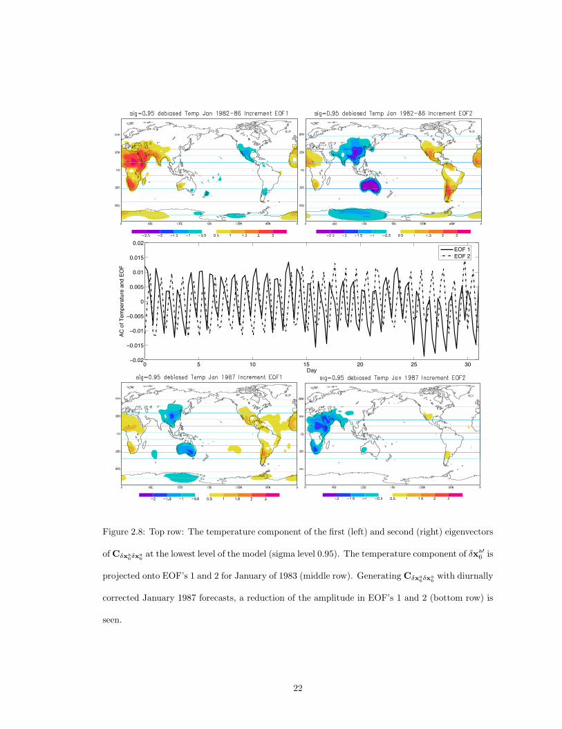
2.8 Top row: The temperature component of the first (left) and second (right) eigenvec-
tors of Cδxa6δxa
6at the lowest level of the model (sigma level 0.95). The temperature
component of δxa′6 is projected onto EOF’s 1 and 2 for January of 1983 (middle row).
Generating Cδxa6δxa
6with diurnally corrected January 1987 forecasts, a reduction of
the amplitude in EOF’s 1 and 2 (bottom row) is seen. . . . . . . . . . . . . . . . . 22
2.9 Explained variance as a function of the number of SVD modes of the dense and sparse
Leith correction operators. SVD is performed on the univariate covariance block
corresponding to zonal wind at sigma level 0.2. The sparse constraints imposed on
the empirical correction operator concentrate more of the variance into the dominant
modes of the spectrum. . . . . . . . . . . . . . . . . . . . . . . . . . . . . . . . . . 26
2.10 The SVD of Cδxa6x
f6identifies coupled signals between the analysis increments (shades)
and model states (contours) in winds u and v, and temperature T at sigma level
0.95 (left column) and 0.2 (right column) for January 1982-1986. . . . . . . . . . . 29
ix

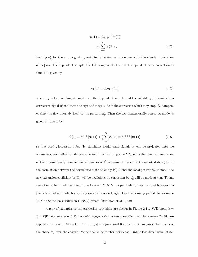
2.11 (Top row) Coupled signals uck (shades) and vk (contours) between SPEEDY forecast
errors and states. SVD mode k = 2 in T [K] at sigma level 0.95 (left) suggests that
warm anomalies over the western Pacific are typically too warm. Mode k = 3 in
u[m/s] at sigma level 0.2 (right) suggests that fronts of the shape v3 over the eastern
Pacific should be farther northeast. (Middle row) 6-hour forecast generated by the
online state-independent corrected model M++ (contours) and analysis increment
(shades) in T [K] at sigma level 0.95 for January 30, 1987 (left) and u[m/s] at sigma
level 0.2 for January 18, 1987 (right). (Bottom row) Online low-dimensional state-
dependent correction improves the local RMS error by 21% in T (left) and 14% in
u (right). . . . . . . . . . . . . . . . . . . . . . . . . . . . . . . . . . . . . . . . . . 34
3.1 For a given initial state, models L and H will produce different trajectories. σ
balls are shown around states p0, pT, p2T of a trajectory of H. If σ is small (a),
shadowing fails in a single step of the process. Increasing σ (b), some trajectories of
L remain close to a trajectory of H for time T. These trajectories are given by JT.
For sufficiently close hyperbolic systems L and H, this procedure can be carried out
for arbitrarily long times with small σ. . . . . . . . . . . . . . . . . . . . . . . . . . 39
3.2 Most physical systems are non-hyperbolic. In 2a, the dynamics contract in one
dimension as pT → HT(pT) ≡ p2T. The ellipse E2T ≈ LT(JT) intersects the σ-ball
surrounding p2T, the intersection is denoted J2T. As p2T → HT(p2T) ≡ p3T, the
dynamics expand in both dimensions. The intersection of LT(J2T) and Nσ(p3T)
is empty and shadowing fails. In 2b, Eϕ2T is the ellipse E2T inflated by ϕ. In 2c,
the intersection of Eϕ2T and Nσ(p2T) is denoted Jϕ
2T. Note that Jϕ2T contains p2T.
Despite expansion in both dimensions, the intersection of LT(Jϕ2T) and Nσ(p3T) is
nonempty. In practice, this procedure is successful at time T+1 if JϕT contains pT. 42
3.3 In the 40 dimensional system discussed later, the number of expanding directions
varies from 8 to 23 depending on the state investigated. As a trajectory is followed,
the same fluctuations in the local number of expanding directions are observed. . 43
x

3.4 Stalking time for model (3.1) measured in days as a function of relative inflation ϕ/µ,
where ϕ is the inflation, µ = 10−6 is model error (0 < ϕ < µ), and σ is shadowing
distance. Trajectories of (1) initially separated by 10−16 are uncorrelated after 25
days. If ϕ/µ = 0, the stalking time is the (brief) traditional shadowing time. If ϕ
= µ, the stalking time is infinite. The σ = 10µ curve illustrates the phenomenon in
Fig. 3.1a, where stalking failures occur because the shadowing distance is too small.
Increasing σ by a factor 10, the shadowing time (ϕ = 0) increases by a factor of 10. 45
3.5 The distance between an H trajectory and the nearest trajectory of the ensemble el-
lipsoid is plotted vs. time, averaged over 5000 independent 25-day ensemble forecasts
(solid) and their corresponding continually inflated ensemble forecasts (dotted). The
vertical axis is in units of the initial diameter of the ensemble. . . . . . . . . . . . . 47
3.6 The ensemble diameter in each of the 40 directions spanned by the ensemble is
plotted as a function of the semi-axis number (major = SVD mode 1), averaged over
5000 independent 40-day ensemble forecasts (solid blue) and their corresponding
continually inflated ensemble forecasts (dashed red). The magnitude of inflation
is 1% of the initial ensemble diameter; the vertical axis is in units of the initial
diameter of the ensemble. The average number of expanding directions in system
(3.1), namely 13, is evident from the intersection of each curve. The continually
inflated ensemble forecasts maintain uncertainty in contracting directions (where
predictions are vulnerable to Unstable Dimension Variability); expanding directions
are not effected by the inflation. . . . . . . . . . . . . . . . . . . . . . . . . . . . . . 48
xi

Chapter 1
Introduction
Predicting the behavior of a chaotic physical system H using a model L has three obstacles:
uncertainty in initial state, chaos, and model errors, i.e. differences between L and H. Given the
initial state of H, the initial state of L which will yield the trajectory that best matches the physical
system is unknown. The accepted procedure is to choose a large collection or ensemble of initial
states and follow their L trajectories. Each individual L trajectory represents a possible outcome;
the collection represents a probability distribution of possible outcomes and describes the evolution
of uncertainty in forecasts generated by L. However, since each ensemble member is integrated with
the same model L, the forecast distribution is unable to represent model errors. As a result, the
ensemble spread (variance) is typically smaller than the difference between the forecast ensemble
mean and the future state of H.
When making predictions of H using L, one of two assumptions is usually made: either
there is no model error (i.e. the model is perfect, e.g. Szunyogh et al. (2005)), or the model error
is statistically random (e.g. Buizza et al. (1999)). The first assumption is useful for evaluating
the dynamical sources of error, namely those which are related to uncertainty in initial conditions
and chaos. For lack of a more sophisticated method of parameterizing model error, predictability
studies which make the second assumption typically include a stochastic component and hope that
this noise will represent behavior that the model L fails to resolve. While this technique may be
useful in increasing the ensemble spread, we feel that the assumption of random errors upon which
the method is based is unrealistic.
This dissertation aims to develop new methods for estimating and correcting flow dependent
model errors in numerical predictions of chaotic physical systems. The first method, described in
Chapter 2, is a statistical correction procedure designed to empirically train a global weather
model to predict its own error, measured relative to the best available estimate of the state of
the atmosphere. The second method, described in Chapter 3, attempts to combine ideas from the
shadowing theory of dynamical systems with current ensemble prediction techniques to increase
1

the length of time for which numerical trajectories of L will remain close to true solutions of the
physical system H. The methods are shown to be successful in improving forecasts made by weather
models of varying sophistication. Consideration is also given to the computational cost of each
method. The dissertation concludes with a discussion of future applications of these techniques.
2

Chapter 2
Estimating and Correcting Global Weather Model Error
2.1 Motivation
Numerical weather forecasting errors grow with time as a result of two contributing factors. First,
atmospheric instabilities amplify uncertainties in the initial conditions, causing indistinguishable
states of the atmosphere to diverge rapidly on small scales. This phenomenon is known as internal
error growth. Second, model deficiencies introduce errors during the model integration leading to
external error growth. These deficiencies include inaccurate forcings and parameterizations used
to represent the effect of sub-grid scale physical processes as well as approximations in numeri-
cal differentiation and integration, and result in large scale systematic forecast errors. Current
efforts to tackle internal error growth focus on improving the estimate of the state of the atmo-
sphere through assimilation of observations and ensemble forecasting (Anderson 2001, Whitaker
and Hamill 2002, Ott et al. 2004, Hunt et al. 2004). Ideally, model deficiencies should be addressed
by generating more accurate approximations of the forcing, improving the physical parameteriza-
tions, or by increasing the grid density to resolve smaller scale processes. However, unresolved
phenomena and model errors will be present no matter how accurate the parameterizations are,
no matter how fine the grid resolution becomes. As a result, it is important to develop empirical
algorithms to correct forecasts to account for model errors. Empirical methods which consider the
model a ‘black box’ are particularly valuable because they are independent of the model. As the
methods of data assimilation and generation of initial perturbations become more sophisticated
and reduce the internal error, the impact of model deficiencies and their dependence on the ‘flow
of the day’ become relatively more important (Hamill and Snyder 2000, Houtekamer and Mitchell
2001, Kalnay 2003).
Estimates of the systematic model error may be derived empirically using the statistics
of the short term forecast errors, measured relative to a reference time series. For example, the
mean short-term forecast error provides a sample estimate of the stationary component of the
model error bias. The output of operational numerical weather prediction models is typically post-
3

processed to account for any such known biases in the forecast field by Model Output Statistics
(MOS, Glahn and Lowry 1972, Carter et al. 1972). However, offline bias correction has no
dynamic effect on the forecast; internal and external errors are permitted to interact nonlinearly
throughout the integration as they grow and eventually saturate. A more robust approach to error
correction should be to estimate the short term forecast errors as a function of the model state.
A corresponding state-dependent correction would then be made every time step of the model
integration to retard growth in the component of the error generated by the model deficiencies.
Several studies have produced promising results by empirical correction in simulations using simple
Global Circulation Models (GCMs) with artificial model errors.
Leith (1978) derived a state-dependent empirical correction to a simple dynamical model
by minimizing the tendency errors relative to a reference time series. Leith’s correction operator
attempts to predict the error in the model tendency as a function of the model state. While
Leith’s empirically estimated state-dependent correction term is only optimal for a linear model,
it is shown to reduce the nonlinear model’s bias. However, the technique is subject to sampling
errors and requires many orders of magnitude more computation time during the forecast than the
biased model integration alone. The method is discussed in detail in section 6.
Faller and Schemm (1977) used a similar technique on coarse and fine grid versions of
a modified Burgers equation model. Statistical correction of the coarse-grid model by multiple
regression to parameterize the effects of sub-grid scale processes improved forecast skill. However,
the model equations were found to be insensitive to small perturbations of the initial conditions.
They concluded that the coarse-grid errors were due entirely to truncation and that the procedure
was sensitive to sampling errors. Schemm et al. (1981) introduced two procedures for statistical
correction of numerical predictions when verification data are only available at discrete times. Time
interpolation was found to introduce errors into the regression equations, rendering the procedure
useless. Applying corrections only when verification data were available, they were successful in
correcting artificial model errors, but the procedure failed on the NMC Barotropic-Mesh model.
Later, Schemm and Faller (1986) dramatically reduced the small scale 12-hr errors of the NMC
4

model. Errors at the larger scales grew due to randomization of the residual errors by the regression
equations.
Klinker and Sardeshmukh (1992) used January 1987 6-hour model integrations to estimate
the state-independent tendency error in operational ECMWF forecasts. By switching off each
individual parameterization, they isolated the contribution to the error of each term. They found
that the model’s gravity wave parameterization dominated the 1-day forecast error. Saha (1992)
used a simple Newtonian relaxation or nudging of a low-resolution version of the NMC operational
forecast model to estimate systematic errors. Verifying against the hi-resolution model, Saha was
able to reduce systematic errors in independent forecasts by adding artificial sources and sinks to
correct errors in heat, momentum, and mass. Nudging and a posteriori correction were seen to
give equivalent forecast improvements.
By nudging of several low-resolution GCMs towards a high-resolution model, Kaas et al.
(1999) estimated empirical orthogonal functions (EOFs) for horizontal diffusion. They found that
the kinetic energy dissipation due to unresolved scales varied strongly with model resolution.
The EOF corrections were most effective in reducing the climatological errors of the model whose
resolution was closest to that of the high-resolution model. D’Andrea and Vautard (2000) estimated
the time-derivative errors of the 3-level global QG model of Marshall and Molteni (1993) by
finding the model forcing which minimized the 6-hour forecast errors relative to a reference time
series. They derived a flow-dependent empirical parameterization from the mean tendency error
corresponding to the closest analogues in the reference time series. The subsequent corrected
forecasts exhibited improved climate statistics in the Euro-Atlantic region, but not in others.
DelSole and Hou (1999) perturbed the parameters of a 2-layer quasi-geostrophic (QG) model
on a 8× 10 grid (Ngp = 160 degrees of freedom) to generate a ‘nature’ run and then modified it to
create a ‘model’ containing a primarily state-dependent error. They found that a state-independent
error correction did not improve the forecast skill. By adding a state-dependent empirical correction
to the model, inspired by the procedure proposed by Leith, they were able to extend forecast skill
up to the limits imposed by observation error. However, Leith’s technique requires the solution
5

of a Ngp-dimensional linear system. As a result, before the procedure can be considered useful
for operational use, a low-dimensional representation of Leith’s empirical correction operator is
required.
Renwick and Wallace (1995) used several low-dimensional techniques described by Brether-
ton et al. (1992) to identify predictable anomaly patterns in 14 winters of Northern Hemisphere
500-mb height fields. The most predictable anomaly pattern in ECMWF operational model fore-
casts was found to be similar to the leading EOF of the analyzed 500-mb height anomaly field.
Applying canonical correlation analysis to the dependent sample (first 7 winters), they found the
amplitude of the leading pattern to be well predicted and showed the forecast skill to increase
with the amplitude of the leading pattern. The forecast skill of the independent sample (second
7 winters) was not well related to the patterns derived from the dependent sample. A posteriori
statistical correction of independent sample forecasts slightly decreased RMS errors, but damped
forecast amplitude considerably. They concluded that continuing model improvements should
provide better results than statistical correction and skill prediction in an operational setting.
Ferranti et al (2002) used Singular Value Decomposition (SVD) (Golub and Van Loan
1996) analysis to identify the relationship between fluctuations in the North Atlantic Oscillation
and ECMWF operational forecasts errors in 500hPa height for 7 winters in the 1990’s. They found
that the anomalous westerly (easterly) flow over the eastern north Atlantic (western Europe) was
weakened by a consistent underestimation of the magnitude of pressure anomalies over Iceland.
Large (small) error amplitudes were seen to be located in regions of the maximum westerly (east-
erly) wind anomaly, the trend was reversed on the flanks of the jet. The flow-dependent component
of the errors accounted for 10% of the total error variance.
The purpose of the present study is to explore the feasibility of estimating and correcting
systematic model errors using a simple and efficient procedure that could be applied operationally.
The monthly, diurnal, and state-dependent components of the short term forecast errors are esti-
mated for two simple but realistic GCMs using the NCEP reanalysis as truth. Section II describes
the two GCMs used for the numerical experiments. Section III describes the simple method of
6

data assimilation used to generate a time series of model forecasts and the technique used to
estimate the corresponding systematic errors. Section IV illustrates the substantial forecast im-
provement resulting from state-independent correction of monthly model forcing when verifying
against independent data. Section V describes attempts to generate full dimensional and low order
empirical estimates of model error as a function of the model state, using Leith’s method and a
new computationally inexpensive approach based on SVD. The paper concludes with a discussion
of implications for operational use and future directions of research.
2.2 Global Circulation Models
2.2.1 The Quasi-Geostrophic Model
The first model used in this study was developed by Marshall and Molteni (1993), it has been
used for many climate studies (e.g. D’Andrea and Vautard 2000). The model is based on spher-
ical harmonics, with triangular truncation at wavenumber 21. The QG model has three vertical
levels (800, 500, 200hPa) and integrates the quasi-geostrophic potential vorticity equation with
dissipation and forcing:
q = −J(ψ,q)−D(ψ) + S (2.1)
where ψ is the streamfunction and q is the potential vorticity (q ≈ ∇2ψ). J represents the Jacobian
operator of ψ and q. The linear dissipation D is dependent on ψ and orography, and includes a
relaxation coupling the three vertical levels. The forcing term S is time-independent but varies
spatially, representing the average effects of diabatic heating and advection by the divergent flow.
This forcing is determined by requiring that the time averaged values of the other terms in (2.1)
are zero. In other words, the forcing is defined so the vorticity tendency is zero for the climatology
(given by the mean NCEP reanalysis streamfunction during January and February from 1980 to
1990, the model simulates a perpetual winter). If the climatological streamfunction and vorticity
are denoted as ψ and q, the time average of (2.1) can be written
7

S =< J(ψ, q) > + < D(ψ) > + < J(ψ′, q′) > (2.2)
where the brackets are ensemble averages over time and primes represent deviations from this
time average. The first two terms in (2.2) generate a mean state, the last term adds the average
contribution of transient eddies (D’Andrea and Vautard 2000).
2.2.2 The SPEEDY Model
The primitive-equation model used in this study (known as SPEEDY, for ‘Simplified Parameter-
izations, primitivE-Equation DYnamics,’ Molteni 2003) has triangular truncation T30 at 7 sigma
levels (0.950, 0.835, 0.685, 0.510, 0.340, 0.200, 0.080). The basic prognostic variables are vorticity
(ζ), divergence (∇), absolute temperature (T ), specific humidity (Q), and the logarithm of sur-
face pressure (log(ps)). These variables are post-processed into zonal and meridional wind (u, v),
geopotential height (Z), T , Q, and log(ps) at pressure levels (925, 850, 700, 500, 300, 200, 100hPa).
The model dissipation and time-dependent forcing are determined by climatological fields of sea
surface temperature (SST), surface temperature and moisture in the top soil layer (about 10cm),
snow depth, bare-surface albedo, and fractions of sea ice, land-sea, and land-surface covered by
vegetation. The model contains parameterizations of large-scale condensation, convection, clouds,
short-wave and long-wave radiation, surface fluxes, and vertical diffusion (Molteni 2003). No di-
urnal variation exists in the model forcing; forcing fields are updated daily.
Despite the approximations made in deriving each model, they produce realistic simulations
of extratropical variability, especially in the Northern Hemisphere (Marshall and Molteni 1993,
Molteni 2003). The SPEEDY model also provides a more realistic simulation of the tropics, as well
as the seasonal cycle. Since the model forcings (including SST) are determined by the climatology,
one cannot expect realistic simulations of interannual variability. More advanced GCMs include
not only observed SST but also changes in greenhouse gases and aerosols, as well as more advanced
physical parameterizations. Despite the absence of variable forcing, if run for a long period of time
(decades), both models reproduce a realistic climatology. While they were designed for climate
8

simulations, each model produces forecasts that remain useful globally for about 2 days.
2.3 Training
A pair of simple schemes were used to estimate model errors. The schemes are advantageous in that
they provide estimates of model errors at the analysis time, when they are still small and growing
linearly, and because they can be carried out at the cost of essentially one model integration. The
first procedure is inspired by Leith (1978), who integrated “true” initial conditions for 6 hours to
measure the difference between the forecast and the verifying analysis. A schematic illustrating
the procedure, hereafter referred to as direct insertion, is shown in Figure 2.1.
Writing x(t) for the GCM state vector at step t and M(x(t)) for the model tendency at step
t, the model tendency equation is given by
x(t) = M(x(t)
)(2.3)
The analysis increment at step t is given by the difference between the truth xt(t) and the model
forecast state xfh(t), namely
δxah(t) = xt(t)− xf
h(t) (2.4)
where h is the forecast lead time, typically h = 6hr.
The second (alternative) procedure for estimating model errors is Newtonian relaxation or
nudging (Hoke and Anthres 1976, Leith 1991, Saha 1992), done by adding an additional forcing
term to relax the model state towards the reference time series. When reference data is available
(every 6 hours), the tendency equation during nudging is given by
x(t) = M(x(t)
)+δxa
h(t)τ
(2.5)
At intermediate time steps, when data is unavailable, the tendency is given by (2.3). A schematic
illustrating the nudging scheme is shown in Figure 2.2 If the relaxation time scale τ is too large,
model errors will grow before the time derivative can respond (Kalnay 2003). If τ is chosen too
9

xt(t)
x6f(t+1)
xt(t+1)
NCEP Reanalysis
x6f(t+2)
xt(t+2)
forecast
-
=
-
analysisincrement x6
a(t+1) x6a(t+2)!!
IC
Figure 2.1: Schematic illustrating the direct insertion procedure for generating time series of
model forecasts and analysis increments. xt(t) is the NCEP Reanalysis at time t; it is used as an
estimate of the truth. xf6(t + 1) is the 6-hour forecast generated from the initial condition xt(t);
δxa6(t + 1) = xt(t)−xf
6(t + 1) is the 6-hour error correction or analysis increment in an operational
setting.
10

xt(t)
x6f(t+1)
xt(t+1)
NCEP Reanalysis
x6f(t+2)
xt(t+2)
x6a(t+1) x6
a(t+2)
xt(t+3)
nudged forcing M(x) + x6a(t+1)
6hr
x6f(t+3)
x6a(t+2)! ! !
!
analysisincrement
forecast
M(x) + x6a(t+2)
6hr!
Figure 2.2: Schematic illustrating the nudging procedure for generating time series of model fore-
casts and analysis increments. xt(t) is the NCEP Reanalysis at time t; it is used as an estimate
of the truth. xf6(t + 2) is the 6-hour forecast generated from the initial condition xf
6(t + 1) using
a forcing that is corrected or nudged by δxa6(t + 1) = xt(t + 1)− xf
6(t + 1).
small, the tendency equation will diverge. Figure 2.3 shows that the sensitivity of the assimilation
error to τ for the QG and the SPEEDY models is similar, and that the optimal time scale is
τ = 6hr, corresponding to the frequency (h) of the assimilation. This choice for τ generates
analysis increments whose statistical properties (e.g. mean, variance, EOFs) are qualitatively very
similar to those obtained through direct insertion. As a result, for the remainder of the discussion
we will only consider time series generated by direct insertion.
The reference time series used to estimate model errors is given by the NCEP reanalysis.
NCEP reanalysis values of model prognostic variables are available in 6 hour increments, they are
interpolated to the model grid and denoted at step t by xt(t). Observations of the reanalysis are
taken as truth with no added noise or sparsity; observational noise is the focus of much research
11

1 2 10 50 100 2000
2
4
6
8
10
12
14RM
S Er
ror a
t 500
hPa
! / h
QG " (km2/s)SPEEDY Temp (K)
Figure 2.3: Mean RMS error at 500hPa as a function of relaxation time scale τ (relative to the
interval h between observations of the reanalysis), verifying against reanalysis during relaxation.
As expected, the optimal τ is equal to h for both the QG and SPEEDY models. However, nudging
is successful for longer relaxation times as well.
in data assimilation (e.g. Ott et al. 2004) but its influence is ignored in this context since the
reanalysis is already an approximation of the evolution of the atmosphere. Direct insertion is
performed with the QG model by integrating NCEP reanalysis wintertime vorticity for the years
between 1980 and 1990. The SPEEDY model is integrated using NCEP reanalysis values of ζ, ∇,
T , Q, and log(ps) for the years between 1982 and 1986. A longer time period was used to train
the QG model because it has an order of magnitude fewer degrees of freedom than the SPEEDY
model.
The time series of analysis increments is separated by month and denoted δxa6(t)
Nreft=1 (Nref =
12

31×4×5 (days x 6-hour intervals x years) for January training of SPEEDY). The time-average of the
analysis increments (bias) is given by < δxa6 > = 1
Nref
∑Nreft=1 δx
a6(t) and < xt > = 1
Nref
∑Nreft=1 xt(t)
is the 5-year reanalysis climatology for the month in which steps t = 1, ..., Nref occur. The method
of direct insertion is also used to generate < δxah > for h = 6j (j = 2, 3, ..., 8), giving 12-hour, 18-
hour, ..., and 48-hour mean bias estimates. These estimates will be used to make an a posteriori
bias correction. The reanalysis states, model forecasts, and corresponding analysis increments are
then separated into their anomalous and time average components, namely
xt′(t) = xt(t)− < xt > (2.6)
xf′6 (t) = xf
6(t)− < xt > (2.7)
δxa′6 (t) = δxa
6(t)− < δxa6 > (2.8)
Figure 2.4 illustrates the bias calculated from 5 years of 6-hour SPEEDY forecasts of u, T ,
and Q for January and July. These state-independent errors are clearly associated with contrasts in
land-sea forcing, topographic forcing, and the position of the jet. The zonal wind and temperature
exhibit a large polar bias, especially in the winter hemisphere. The 6-hour zonal wind errors show
an underestimation of the westerly jets of 2-5 m/s east of the Himalayan mountain range (January)
and east of the Australian Alps (July), especially on the poleward side. The mean temperature
error over Greenland is larger during the Northern Hemisphere winter. There is little humidity bias
in the polar regions, most likely due to the lack of moisture variability near the poles. The SPEEDY
convection parameterization evidently transports too little moisture from lower levels (which are
too moist) to upper levels (which are too dry). The following section describes attempts to correct
the model forcing to account for this bias.
13

Figure 2.4: Mean 6-hour analysis increment < δxa6 > (shades) and 5-year reanalysis climatology
< xt > (contours) in SPEEDY forecasts of zonal velocity u[m/s], temperature T [K], and specific
humidity Q[g/kg] at two levels during January (left) and July (right) from 1982-1986.
14
2.4 State-Independent Correction
2.4.1 Monthly Bias Correction
In this section, the impact of correcting for the bias of the model during the model integration is
compared with a correction a posteriori, as done, for example in MOS. In both cases the impact of
the corrections on 5-day forecasts is verified using periods independent from the training periods.
The initial conditions for QG forecasts are taken from the wintertime NCEP reanalysis data
between 1991 and 2000, and for the SPEEDY forecasts are taken from the NCEP reanalysis
data for 1987.
The control forecast is started from reanalysis initial conditions and integrated with the
original biased forcing M(x). The forecast corrected a posteriori is generated by computing xf6(1)+
< δxa6 > at step 1, xf
12(2)+< δxa12 > at step 2, ..., xf
48(8)+< δxa48 > at step 8, etc.. The corrections
in u, v, T , Q, and log(ps) at all levels are obtained from the training period for each month of
the year, and attributed to day 15 of each month. The correction is a daily interpolation of the
monthly mean analysis increment; e.g. on February 1, the time-dependent 6-hour bias correction
is of the form
< δxa6(jan) > + < δxa
6(feb) >2
(2.9)
so that the corrections are temporally smooth.
An online corrected or debiased model forecast is generated with the same initial condition,
but with a corrected model forcing M+. The tendency equation for the debiased model forecast is
given by
x = M(x) +< δxa
6 >
h≡ M+(x) (2.10)
where the bias correction is divided by 6 hours because it was computed for 6 hour forecasts but
it is applied every time step. The skill of each forecast is measured by the Anomaly Correlation
(AC), given at time t by
15

AC =∑Ngp
s=1 xf′(s) · xt′(s) cos2(φs)√∑Ngps=1
(xf′(s) cos(φs)
)2√∑Ngp
s=1
(xt′(s) cos(φs)
)2(2.11)
where φs is the latitude of grid point s and Ngp is the number of degrees of freedom in the model
state vector. The AC is essentially the inner product of the forecast anomaly and the reanalysis
anomaly, with each grid point contribution weighted by the cosine of its latitude and normalized
so that a perfect forecast has an AC of 1. It is common to consider that the forecast remains useful
if AC > 0.6.
Figure 2.5 illustrates the success of the bias correction for the QG model. Both the a
posteriori and the online correction of the bias significantly increase the forecast skill. However,
the improvement obtained with the online correction is larger than that obtained with the a
posteriori correction, indicating that the correction made during the model integration reduces the
model error growth. Applying the bias correction every 6 hours for a single time step gave slightly
worse results than applying it every time step.
Similar results were obtained for the SPEEDY model and are presented for the 500hPa zonal
wind, temperature, and geopotential height in Figure 2.6 (top row) for the month of November
1987. In order to show the vertical and monthly dependence of the correction, the time of crossing
of AC=0.6 is plotted for 3 vertical levels for the control (second row) and online corrected (debiased)
SPEEDY forecasts (third row) as a function of the month. The bottom row presents the relative
improvement. For the wind, the debiasing leads to an increase in the length of useful skill of over
60% at 850hPa (where the errors are largest), about 50% at 500hPa, and about 10% at 200hPa,
where the errors are smallest. For the temperature, where the skill is less dependent on pressure
level, the improvements are between 20% and 40% at all levels. There is not much dependence on
the annual cycle, possibly because the verification is global.
As in the QG model, a bias correction made during the model integration is more effective
than a bias correction performed a posteriori, although they both result in significant improve-
ments. This is important because it indicates that the model deficiencies do not simply add errors;
external errors are amplified by internal error growth. Further iteration of the procedure does not
16

0 1 2 3 4 50
0.2
0.4
0.6
0.8
1
Day
Fore
cast
AC
with
Rea
nalys
is
QG controla posterioridebiaseduseful
Figure 2.5: QG model forecasts, verified against the 1991-2000 NCEP reanalysis, remain useful
(AC > 0.6) for approximately 2 days. When the same forecast is post-processed to remove the
bias fields < δxa6 >, < δxa
12 >, ..., < δxa48 >, the forecasts remain useful for 26% (12 hours) longer.
However, when the online corrected (debiased) QG model is used to generate the forecasts, they
remain useful for 38% (18 hr) longer.
17

! " #
!$%
!$&
!$'
!$(
!$)
!$*
!$+
"
,-.
/!0123
45678-9:;<=;>1:?;@7-2-A.919
! " #
!$%
!$&
!$'
!$(
!$)
!$*
!$+
"
,-.
B7CD76-:E67
! " #
!$%
!$&
!$'
!$(
!$)
!$*
!$+
"
,-.
F75D5:72:1-A;GH:
IJKK,L,7M1-973<;J59:761561
2 4 6 8 10 120
1
2
3
4
Month
Use
ful S
PEED
Y fo
reca
st [d
ays]
2 4 6 8 10 120
1
2
3
4
Month2 4 6 8 10 12
0
1
2
3
4
Month
200hPa500hPa850hPa
2 4 6 8 10 120
1
2
3
4
Month
Use
ful D
ebia
sed
SPEE
DY
fore
cast
2 4 6 8 10 120
1
2
3
4
Month2 4 6 8 10 12
0
1
2
3
4
Month
200hPa500hPa850hPa
2 4 6 8 10 120
0.2
0.4
0.6
0.8
1
Month
Rel
ativ
e Im
prov
emen
t
2 4 6 8 10 120
0.2
0.4
0.6
0.8
1
Month2 4 6 8 10 12
0
0.2
0.4
0.6
0.8
1
Month
200hPa500hPa850hPa
Ia Ib
Figure 2.6: (Top row) Average November 1987 AC of biased, post-processed, and debiased
SPEEDY forecasts at 500hPa. Online bias correction is slightly more effective than post-processing
the biased forecast. (Bottom row) Relative improvement (Ib/Ia) in crossing time of AC = 0.6 at
three different levels (solid = 200, dashed = 500, dash-dot = 850hPa) vs month. SPEEDY fore-
casts are typically more useful at upper levels (see second row), improvements are more evident at
lower levels and higher latitudes (not shown). For example, biased forecasts of Z at 850hPa are
typically useful for 20hr in April, debiased model forecasts are useful for 36hr.
18

Figure 2.7: Mean 6-hour analysis increment < δxa6 > in debiased SPEEDY model forecasts of
u[m/s] (top left), T [K] (top right), and Q[g/kg] (bottom) during January from 1982-1986. The
debiased SPEEDY model exhibits significantly less bias in 6-hour forecasts of the dependent sample,
especially in polar regions (compare with Figure 2.4).
improve model forecasts. That is, finding the mean 6-hour forecast error in the debiased model
M+ (2.10) and correcting the forcing again does not extend the usefulness of forecasts.
The positive impact of the interactive correction is also indicated by an essentially negligible
mean error in the debiased QG model (not shown). The correction of SPEEDY by < δxa6 > removes
the large polar errors from the mean error fields, but some of the sub-polar features remain with
smaller amplitudes (compare Figure 2.7 with Figure 2.4). This suggests that a nonlinear correction
to the SPEEDY model forcing may be more effective.
2.4.2 Error Growth
Dalcher and Kalnay (1987) and Reynolds et al. (1994) parameterized the growth rates of internal
and external error with an extension of the logistic equation, namely
19

α = (βα+ δ)(1− α) (2.12)
where α is the variance of the error anomalies, β is the growth rate of error anomalies due to
instabilities (internal), and δ is the growth rate due to model deficiencies (external). These error
growth rate parameters may be estimated from the AC for the control and debiased model forecasts.
The 500hPa November 1987 estimates of these growth rates (Table 2.1) demonstrate significant
reduction in the external error growth rate resulting from online state-independent error correction.
The only exception is the moisture, suggesting that the correction of the moisture bias may require
a re-tuning of the original model parameterizations that were derived with the original bias. As
could be expected, bias correction changes the internal error growth rate much less than the
external rate.
model growth rate u v T Q
control internal (β) .866 .811 .940 .892
debiased internal (β) .872 .799 .873 .885
control external (δ) .184 .161 .126 .175
debiased external (δ) .110 .108 .093 .183
Table 2.1: Error growth rate parameters β (day−1) and δ (day−1) for the logistic error growth
model (2.12), estimated from the time average 500hPa November 1987 AC for control and debiased
model forecasts. State-independent online correction significantly reduces the component of the
error growth resulting from model deficiencies.
2.4.3 Diurnal Bias Correction
In addition to the time-averaged analysis increments, the leading EOFs of the anomalous analysis
increments are computed to identify the time-varying component. The spatial covariance of these
increments over the dependent sample (recomputed using the debiased model M+) is given by
Cδxa6δxa
6≡ < δxa′
6 δxa′>6 >. The two leading eigenvectors of Cδxa
6δxa6
identify patterns of diurnal
20
variability which are poorly represented by the model (see Figure 2.8 top row). Since SPEEDY
solar forcing is constant over each 24-hour period, it fails to resolve diurnal changes in forcing
due to the rotation of the earth. Consequently, SPEEDY underestimates (overestimates) the near
surface daytime (nighttime) temperatures. This trend is most evident over land in the tropics and
summer hemisphere.
The time-dependent amplitude of the leading modes can be estimated by projecting the
leading eigenvectors of Cδxa6δxa
6onto δxa′
6 (t) over the dependent sample. As expected from the
wavenumber 1 structure of the EOFs, the signals are out of phase by 6 hours (see Figure 2.8
middle row). An estimate of time dependence of the diurnal component of the error is generated
by averaging the projection over the daily cycle for the years 1982-1986. A diurnal correction of
the seasonally debiased model M+ is then computed online by linearly interpolating EOF’s 1 and
2 as a function of the time of day. The diurnally corrected model is denoted M++. Correction of
the debiased SPEEDY forcing to include this diurnal component reduced the 6-hour temperature
forecast errors for the independent sample (1987), most notably over land (see Figure 2.8 bottom
row). Although more sophisticated GCMs include diurnal forcings, it is still common for their
forecast errors to have a significant diurnal signal. This signal can be estimated and corrected as
has been done here.
2.5 State-Dependent Correction
2.5.1 Leith’s Empirical Correction Operator
The time series of anomalous analysis increments provides a residual estimate of the linear state-
dependent model error. Leith (1978) suggested that these increments could be used to form a
state-dependent correction. Leith sought an improved model of the form
x = M++(x)
+ Lx′ (2.13)
where Lx′ is the state-dependent error correction. The tendency error of the improved model is
given by
21
! " #! #" $! $" %!!!&!$
!!&!#"
!!&!#
!!&!!"
!
!&!!"
!&!#
!&!#"
!&!$
'()
*+,-.,/01203(4530,(67,89:
89:,#89:,$
Figure 2.8: Top row: The temperature component of the first (left) and second (right) eigenvectors
of Cδxa6δxa
6at the lowest level of the model (sigma level 0.95). The temperature component of δxa′
6 is
projected onto EOF’s 1 and 2 for January of 1983 (middle row). Generating Cδxa6δxa
6with diurnally
corrected January 1987 forecasts, a reduction of the amplitude in EOF’s 1 and 2 (bottom row) is
seen.
22

g = xt −(M++(xt) + Lxt′) (2.14)
where xt is the instantaneous time derivative of the reanalysis state. The mean square tendency
error of the improved model is given by < g>g >. Minimizing this tendency error with respect to
L, Leith’s state-dependent correction operator is given by
L =<(xt −M++(xt)
)′xt′> >< xt′xt′> >−1 (2.15)
where xt is approximated with finite differences by
xt ≈ xt(t + ∆t)− xt(t)∆t
(2.16)
and ∆t = 6hr for the reanalysis. Note that the term xt −M++(xt) can then be estimated at time
t using only the analysis increments, namely
xt −M++(xt) ≈ xt(t + ∆t)− xt(t)∆t
− xf∆t(t + ∆t)− xt(t)
∆t
=xt(t + ∆t)− xf
∆t(t + ∆t)∆t
=δxa
∆t(t + ∆t)∆t
(2.17)
This method of approximating xt −M++(xt) is attractive because the analysis increments of an
operational model are typically generated during pre-implementation testing. As a result, the
operator L may be estimated with no additional model integrations.
To estimate L, we first recompute the time series of residuals δxa′6 (t) using the online debiased
and diurnally corrected model M++. The cross covariance (Bretherton et al. 1992) of the analysis
increments with their corresponding reanalysis states is given by Cδxa6x
t ≡< δxa′6 xt′> >, the lagged
cross covariance is given by Cδxa6x
tlag≡< δxa′
6 (t)xt′>(t− 1) >, and the reanalysis state covariance
is given by Cxtxt ≡< xt′xt′> >. The covariances can be computed offline separately on time series
pairs δxa′6 and xt′ corresponding to each month so that each month has its own covariance matrices.
23

In computing the covariance matrices, we found that weighting each grid point by the cosine of
latitude made little difference, a result consistent with Wallace et al. (1992).
The finite difference approximation of xt −M++(xt) given by (2.17) results in an estimate
of L in terms of the covariance matrices Cδxa6x
tlag
and Cxtxt . The empirical correction operator is
given by
L = Cδxa6x
tlag
Cxtxt−1 (2.18)
Note that w = Cxtxt−1 ·x′ is the anomalous state normalized by its empirically derived covariance;
Lx′ = Cδxa6x
tlag
w is the best estimate of the anomalous analysis increment correction corresponding
to the anomalous model state x′ over the dependent sample. Assuming that sampling errors are
small and that the external forecast error evolves linearly with respect to lead time, this correction
should improve the forecast model M++. Of course, internal forecast errors grow exponentially
with lead time, but those forced by model error tend to grow linearly (e.g. Dalcher and Kalnay
1987, Reynolds et al. 1994). Therefore, the Leith operator should provide a useful estimate of the
state-dependent model error.
Using a model with very few degrees of freedom and errors designed to be strongly state-
dependent, DelSole and Hou (1999) found that the Leith operator was successful in correcting
state-dependent errors relative to a nature run. However, direct computation of Lx′ requires
O(N3gp) floating point operations (flops) every time step. For the global QG model, Ngp = O(104),
for the SPEEDY model, Ngp = O(105), and for operational models Ngp = O(107). It is clear
that this operation would be prohibitive. Approaches to reduce the dimensionality of the Leith
correction are now described.
2.5.2 Covariance Localization
Covariance matrices Cδxa6x
tlag
and Cxtxt may be computed offline using the dependent sample. To
make the computation more feasible, correlations between different anomalous dynamical variables
at the same level are ignored, e.g. u and T at sigma level 0.510 in SPEEDY. Correlations between
24

identical anomalous dynamical variables at different levels, e.g. q at 800hPa and 500hPa in QG,
are ignored as well. Miyoshi et al. (2005) found these correlations to be significantly smaller
than those between identical variables at the same level in the SPEEDY model. The assumption
of univariate and uni-level covariances could be removed in an operational implementation by
combining geostrophically balanced variables into a single variable before computing covariances,
as is usually done in variational data assimilation (Parrish and Derber 1992). To further simplify
evaluation of the procedure, we consider only covariance at identical levels for the variables u,
v, and T ; covariance in Q and log(ps) are ignored. In doing so, a block diagonal structure is
introduced to Cδxa6x
tlag
and Cxtxt , with each block corresponding to the covariance of a single
variable at a single level.
A localization constraint is also imposed on the covariance matrices by setting to zero
all covariance elements corresponding to grid points farther than 3000km away from each other;
in an infinite dependent sample, these covariance elements would be approximately zero. This
constraint imposes a sparse, banded structure on each block in Cδxa6x
tlag
and Cxtxt . Together, the
two constraints significantly reduce the flops required to compute Lx′. Another advantage of the
reduced operator is that it is less sensitive to sampling errors related to the length of the reanalysis
time series. Figure 2.9 illustrates the variance explained by the first few SVD modes of the dense
and sparse correction operators corresponding to the January zonal wind at sigma level 0.2. The
localization constraint is imposed on the covariance block corresponding to u at sigma level 0.2 in
January for both Cδxa6x
tlag
and Cxtxt before SVD of L = Cδxa6x
tlag
Cxtxt−1. The explained variance
is given by
r(j) =∑j
i=1 σi∑Nui=1 σi
(2.19)
where σi is the ith singular value and the univariate covariance block is Nu × Nu. It is useful in
determining how many modes may be truncated in approximating the correction operator L. To
explain 90% of the variance, more than 400 modes of the dense correction operator are required
whereas only 40 are required of the sparse operator. Covariance localization has the effect of
25

100 200 300 400 5000
0.2
0.4
0.6
0.8
1
SVD mode
Expl
aine
d Va
rianc
e
sparse Ldense L
Figure 2.9: Explained variance as a function of the number of SVD modes of the dense and sparse
Leith correction operators. SVD is performed on the univariate covariance block corresponding to
zonal wind at sigma level 0.2. The sparse constraints imposed on the empirical correction operator
concentrate more of the variance into the dominant modes of the spectrum.
concentrating the physically important correlations into the leading modes.
To test Leith’s empirical correction procedure, several 5-day forecasts similar to those de-
scribed earlier are performed. The initial conditions are taken from a sample independent of that
which was used to estimate the correction operator L. The first forecast is made with the online
state-independent corrected model M++. A second forecast is made using the state-dependent
error corrected model (2.13). Forecasts corrected online by the dense (univariate covariance) oper-
ator L performed approximately 10% worse (and took approximately 100 times longer to generate)
than those corrected by the sparse operator, indicating the problems of sampling without localiza-
26

tion. Even when using the sparse operator, the generation of forecasts corrected online still took
a prohibitively long time, and only improved forecasts by one hour. This indicates that despite
attempts to reduce the dimensionality of the correction operator, the sparse correction still re-
quires too many flops to be useful with an operational model. A further reduction of the degrees
of freedom is described below, using only the relevant structure of the correction operator.
2.5.3 Low-Dimensional Approximation
An alternative formulation of Leith’s correction operator is introduced here, based on the corre-
lation of the leading SVD modes. The dependent sample of anomalous analysis increments and
model forecasts are normalized at each grid point by their standard deviation so that they have
unit variance, they are denoted δxa′6 and xf′
6 . They are then used to compute the cross covariance,
given by Cδxa6x
f6≡< δxa′
6 xf′6
>>; normalization is required to make Cδxa
6xf6
a correlation matrix.
The matrix is then restricted to the same univariate covariance localization as previously described.
The cross covariance is then decomposed to identify pairs of spatial patterns that explain as much
of possible of the mean-squared temporal covariance between the fields δxa′6 and xf′
6 . The SVD is
given by
Cδxa6x
f6
= UΣV> =Ngp∑k=1
ukσkv>k (2.20)
where the columns of the orthonormal matrices U and V are the left and right singular vectors
uk and vk. Σ is a diagonal matrix containing singular values σk whose magnitude decreases with
increasing k. The leading patterns u1 and v1 associated with the largest singular value σ1 are
the dominant coupled signals in the time series δxa′6 and xf′
6 respectively (Bretherton et al. 1992).
Patterns uk and vk represent the kth most significant coupled signals. Expansion coefficients or
Principal Components (PCs) ak(t), bk(t) are obtained by projecting the coupled signals uk, vk
onto δxa′6 and xf′
6 as follows
27

ak(t) = u>k · δxa′6 (t)
bk(t) = v>k · xf′6 (t) (2.21)
PCs describe the magnitude and time dependence of the projection of the coupled signals onto the
reference time series.
The heterogeneous correlation maps indicate how well the dependent sample of normalized
anomalous analysis increments can be predicted from the principal components bk (derived from
the normalized forecast state anomalies xf′6 ). It is computed by
ρ[δxa′6 (t),bk(t)] =
( σk√< b2
k(t) >
)uk (2.22)
This map is the vector of correlation coefficients between the grid point values of the normalized
anomalous analysis increments δxa′6 and the kth expansion coefficient of xf′
6 , namely bk. The
SPEEDY heterogeneous correlation maps (Figure 2.10) corresponding to the three leading coupled
SVD modes between the normalized anomalous analysis increments and model states illustrate
a significant relationship between the structure of the 6-hour forecast error and the model state,
at least for the dependent sample. Locally, the time correlation reaches values of 60 − 80%, but
the global average is still small. The dominant three signals in the model state time series xf′6 ,
namely v1,v2,v3, are plotted in contours. The corresponding signals in the analysis increments
δxa′6 , namely u1,u2, and u3, are used to generate the heterogeneous correlation maps ρ1, ρ2, and
ρ3 (see (2.22)) plotted in shades. The three signals are superimposed for simplicity. Large local
correlations are indicative of persistent patterns whose magnitude and/or physical location are
consistently misrepresented by SPEEDY. For example, coupled signal 1 in v at sigma level 0.2
indicates that patterns of the shape v1 should be farther east. Coupled signal 3 for the same
variable suggests strengthening anomalies of the shape v3. Coupled signal 2 in u at sigma level
0.95 suggests weakening anomalies of the shape v2.
28

1
2 3
213 12 3
1
2
3
1
23
12
3
Figure 2.10: The SVD of Cδxa6x
f6
identifies coupled signals between the analysis increments (shades)
and model states (contours) in winds u and v, and temperature T at sigma level 0.95 (left column)
and 0.2 (right column) for January 1982-1986.
29

2.5.4 Low-Dimensional Correction
The most significant computational expense required by Leith’s empirical correction involves solv-
ing the Ngp-dimensional linear system Cxtxtw(T) = x′(T) for w at each time T during a forecast
integration. Taking advantage of the cross covariance SVD and assuming that Cδxa6x
tlag≈ Cδxa
6xf6
and Cxtxt ≈ Cxf6x
f6, a reduction in computation for this operation may be achieved by expressing
w = Cxfxf−1x′ as a linear combination of the orthonormal right singular vectors vk. The assump-
tions are reasonable since we are attempting to estimate the tendency error at time T, not T + 6
hours. The empirical correction operator is given by
Lx′ = Cδxa6x
f6
Cxf6x
f6
−1x′
= Cδxa6x
f6w
= UΣV>w =Ngp∑k=1
ukσkv>k ·w ≈K∑
k=1
ukσkv>k ·w (2.23)
where for K < Ngp, only the component of w in the K-dimensional space spanned by the right
singular vectors vk can contribute to this empirical correction. This dependence can be exploited
as follows.
Assume the model state at time T during a forecast integration is given by x(T). The nor-
malized state anomaly x′(T) is given by x′(T) = x(T)− < xt >, normalized at state vector element
s by the standard deviation of xf′6 over the dependent sample. The component of x′(T) explained
by the signal vk may then be estimated by computing the new expansion coefficient (PC) bk(T)
= v>k · x′(T). The right PC covariance over the dependent sample is given by Cbb =< bb> >,
calculated using bk from (2.21). The linear system
Cbbγ(T) = b(T) (2.24)
may then be solved for γ at time T. The cost of solving (2.24) is O(K2) where K is the number of
SVD modes retained, as opposed to the O(Ngp2) linear system required by Leith’s full dimensional
Leith empirical correction. The solution of (2.24) gives an approximation of w(T), namely
30
w(T) = Cxfxf−1x′(T)
≈K∑
k=1
γk(T)vk (2.25)
Writing uck for the error signal uk weighted at state vector element s by the standard deviation
of δxa6 over the dependent sample, the kth component of the state-dependent error correction at
time T is given by
ek(T) = uckσkγk(T) (2.26)
where σk is the coupling strength over the dependent sample and the weight γk(T) assigned to
correction signal uck indicates the sign and magnitude of the correction which may amplify, dampen,
or shift the flow anomaly local to the pattern uck. Then the low-dimensionally corrected model is
given at time T by
x(T) = M++(x(T)
)+
1h
K∑k=1
ek(T) ≡ M+++(x(T)
)(2.27)
so that during forecasts, a few (K) dominant model state signals vk can be projected onto the
anomalous, normalized model state vector. The resulting sum ΣKk=1ek is the best representation
of the original analysis increment anomalies δxa′6 in terms of the current forecast state x(T). If
the correlation between the normalized state anomaly x′(T) and the local pattern vk is small, the
new expansion coefficient bk(T) will be negligible, no correction by uck will be made at time T, and
therefore no harm will be done to the forecast. This fact is particularly important with respect to
predicting behavior which may vary on a time scale longer than the training period, for example
El Nino Southern Oscillation (ENSO) events (Barnston et al. 1999).
A pair of examples of the correction procedure are shown in Figure 2.11. SVD mode k =
2 in T [K] at sigma level 0.95 (top left) suggests that warm anomalies over the western Pacific are
typically too warm. Mode k = 3 in u[m/s] at sigma level 0.2 (top right) suggests that fronts of
the shape v3 over the eastern Pacific should be farther northeast. Online low-dimensional state-
31

dependent correction improves the local RMS error by 21% in 6-hour forecasts of T (bottom left)
and 14% in u (bottom right). Retaining K = 10 modes of the SVD, state-dependent correction by
(2.27) of both the QG and SPEEDY models improved forecasts by a few hours. This indicates that
only a small component of the error can be predicted given the model state over the independent
sample (1987). The low-dimensional correction outperformed the sparse Leith operator (Table
2.2) indicating that the SVD truncation reduces spurious correlations unaffected by the covariance
localization. Correction by K = 5 and K = 20 modes of the SVD were slightly less successful.
Heterogeneous correlation maps for modes K > 20 did not exceed 60% for the dependent sample.
The corrections are more significant in regions where ρ is large and at times in which the state
anomaly projects strongly on the leading SVD modes (see examples in Figure 2.11), but the
global averaged improvement is small. Nevertheless, given that the computational expense of the
low-dimensional correction is orders of magnitude smaller than that of even the sparse correction
operator, and the results are better, it seems to be a promising approach to generating state-
dependent corrections.
The low-dimensional representation of the error is advantageous compared to Leith’s cor-
rection operator for several reasons. First, it reduces the sampling errors which have persisted
despite covariance localization by identifying the most robust coupled signals between the analy-
sis increment and forecast state anomalies. Second, the added computation is trivial; it requires
solving a K-dimensional linear system and computing K inner products for each variable at each
level. Finally, the SVD signals identified by the technique can be used by modelers to isolate flow
dependent model deficiencies. In ranking these signals by strength, SVD gives modelers the ability
to evaluate the relative importance of various model errors.
Covariance localization (which led to better results when using the Leith operator) is vali-
dated by comparing the signals uk and vk obtained from the SVD of the sparse and dense versions
of Cδxa6x
f6. The most significant structures in the dominant patterns (e.g. u1, v1) of the sparse
covariance matrix are very similar to those obtained from the dense version. However, the domi-
nant patterns in the dense covariance matrix also contain spurious noisy structures related to the
32

Dense L Sparse L Low-D Approx
Flops per time step O(N3gp) O(N2
gp) O(Ngp)
Global Improvement −8% (-4hr) 2% (1hr) 4% (2hr)
NH Extratropics Improvement −6% (-3hr) 4% (2hr) 6% (3hr)
Table 2.2: Comparison of Leith’s dense correction operator with its corresponding sparse and low-
dimensional approximations, including the number of flops needed to generate the state-dependent
correction per time-step. Numbers are time averaged improvements in crossing time of AC = 0.6 for
daily 5-day 500hPa geopotential height forecasts made with model (2.27) during January of 1987,
measured against the crossing time observed in forecasts made by the online state-independent
corrected SPEEDY model M++. Univariate covariances were used to calculate the dense Leith
operator so that it may be applied block by block.
nonphysical, nonzero covariance between distant grid points. Given a long enough reanalysis time
series, this structure would disappear. The structures identified in the sparse covariance matrix are
thus good approximations of the physically meaningful structures of the dense covariance matrix.
Qualitatively similar structures (e.g. mean, variance, EOFs) were observed when training was
limited to just one year, suggesting that an operational implementation of this method should not
require several years of training.
2.6 Summary and Discussion
This paper considers the estimation and correction of state-independent (seasonal and diurnal),
and state-dependent model errors of a pair of simple GCMs. The two approaches used to create the
time series of analysis increments and model states needed for training (direct insertion and nudging
towards a reanalysis used as an estimate of the true atmosphere) are simple; they require essentially
a single long model integration and give similar estimates of the bias. In an operational setting,
time series of model states and analysis increments are already available from pre-implementation
testing.
33
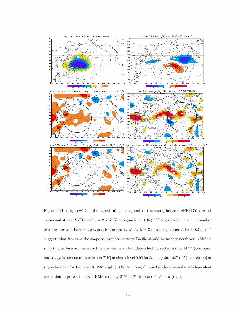
Figure 2.11: (Top row) Coupled signals uck (shades) and vk (contours) between SPEEDY forecast
errors and states. SVD mode k = 2 in T [K] at sigma level 0.95 (left) suggests that warm anomalies
over the western Pacific are typically too warm. Mode k = 3 in u[m/s] at sigma level 0.2 (right)
suggests that fronts of the shape v3 over the eastern Pacific should be farther northeast. (Middle
row) 6-hour forecast generated by the online state-independent corrected model M++ (contours)
and analysis increment (shades) in T [K] at sigma level 0.95 for January 30, 1987 (left) and u[m/s] at
sigma level 0.2 for January 18, 1987 (right). (Bottom row) Online low-dimensional state-dependent
correction improves the local RMS error by 21% in T (left) and 14% in u (right).
34

Although the procedure is inspired by Leith (1978) and DelSole and Hou (1999), it is tested
here using realistic models, and using as nature a reanalysis under the assumption that it is much
closer to the real atmosphere than any model. The online state-independent correction, including
the EOFs associated with the diurnal cycle, resulted in a significant improvement in the forecast
skill (as measured by the AC). Unlike Saha (1992), this improvement was larger than that obtained
by a posteriori corrections of the bias, indicating the importance of correcting the error during the
integration. The results are also significantly different from those of DelSole and Hou (1999),
who obtained a very small improvement from the state-independent correction, and a very large
improvement from the state-dependent correction using Leiths formulation. Their results were
probably optimistic in that the model errors were by construction very strongly state-dependent.
The results presented here, found using global atmospheric models and comparing with a reanalysis
of the real atmosphere, are probably more realistic with respect to the relative importance of
mean and state-dependent corrections. Nevertheless, our results are probably optimistic since the
improvement of the debiased model M+ (2.10) relative to the biased model M (2.3) is larger for
the simple GCMs tested here than could be expected in an operational model. It is not clear how
large the analysis increment and forecast state coupled signal size would be for more sophisticated
models, but operational evidence suggests that state dependent errors are not negligible.
It was necessary to introduce a horizontal and vertical localization of the components of
Leith’s empirical correction operator to reduce sampling problems. Multi-level and multivariate
covariances were ignored to make the computation practical. The assumptions underlying the
localization require model dependent empirical verification; implementation on a more realistic
model may require that the localization be multivariate in order to have a balanced correction.
The Leith-DelSole-Hou method with the original dense covariance matrix makes forecasts worse.
With the sparse covariance however, there is an improvement of about 1 hour, still at a large
computational cost.
A new method of state-dependent error correction was introduced, based on SVD of coupled
analysis increment and forecast state anomalies. The cross covariance is the same as that which
35

appears in the Leith method, but it would be prohibitive to compute it using an operational model.
The new method, based on using the SVD heterogeneous correlation maps as the basis of linear
regression, doubles the improvement and is many orders of magnitude faster. The method can be
applied at a rather low cost, both in the training and in the correction phases, and yields significant
forecast improvements, at least for the simple but realistic global QG and SPEEDY models. It
could be applied with low computational cost and minimal sampling problems to data assimilation
and ensemble prediction, applications where accounting for model errors has been found to be
important. The method may be particularly useful for forecasting of severe weather events where
a posteriori bias correction will typically weaken anomalies. The patterns identified by SVD could
also be used to identify sources of model deficiencies and thereby guide future model improvements.
Error correction may necessitate a re-tuning of the model parameterizations, as suggested
by the humidity results in Table 2.1. Another disadvantage is that operational model upgrades
may require fresh computation of the dominant increment and state anomaly signals. However,
analysis increments generated during pre-implementation tests of an operational model can be
used as a dependent sample to estimate the model error and state anomaly covariance. With such
a collection of past data, it may not be necessary to run an operational model in order to generate
the necessary sample.
Flow-dependent estimates of model error are of particular interest to the community at-
tempting to develop an efficient Ensemble Kalman Filter for data assimilation (Bishop et al. 2001,
Whitaker and Hamill 2002, Ott et al. 2004, Hunt et al. 2004). Naive data assimilation proce-
dures assume the model error to be constant, and represent its effect by adding random noise to
each ensemble member. More sophisticated procedures add a random selection of observed model
tendencies to each ensemble member, or artificially increase the background forecast uncertainty
through variance inflation. The SVD technique described in this paper can be combined with an
ensemble based data assimilation scheme to provide time and state-dependent estimates of the
model error, for example in the Local Ensemble Transform Kalman Filter (LETKF) being de-
veloped by the chaos group at the University of Maryland (Ott et al. 2004, Hunt et al. 2004).
36

The empirical correction method described here involves local computations commensurate with
the treatment of covariance localization in the LETKF. In a data assimilation implementation,
the SVD method would involve appending a K-dimensional estimate of the model error to each
ensemble member.
37
Chapter 3
Making Forecasts for Chaotic Physical Processes
3.1 Motivation
Many scientific disciplines require accurate predictions of the future state of chaotic physical sys-
tems. Astronomers attempt to predict the trajectories of bodies in the solar system for thousands
of years into the future (Sussman and Wisdom, 1992), as well as the evolution of galactic clusters
(Hayes, 2003). Plasma physicists use nonlinear models to predict magnetic storms and solar wind
(Valdivia et al., 1996). Oceanographers forecast sea-surface temperatures in an attempt to predict
the likelihood of El Nino Southern Oscillation (ENSO) events in the major oceans up to a year in
advance (Barnston et al., 1999). Meteorologists attempt to predict the path of violent hurricanes
with hours of lead time, and larger scale patterns up to a week in advance Patil et al. (2001).
Predicting the behavior of a chaotic physical system H using a model L has three obstacles:
uncertainty in initial state, chaos, and model errors, i.e. differences between L and H. Given the
initial state p0 of H, the initial state of L which will yield the trajectory that best matches the
physical system is unknown. The accepted procedure is to choose a large collection or ensemble
of initial states and follow their L trajectories.
For example, when L is a Global Weather Model and H is the behavior of the atmosphere, an
initial state for L is an estimate of the state of the atmosphere over the entire planet. Forecasters
view the initial state of the atmosphere as uncertain, but lying within a known ball in state space.
The radius σ of this ball corresponds to measurement uncertainties. They choose a finite ensemble
of initial states in this ball. Forecasters then take the trajectories of L for each initial state in the
ensemble, for example at time T=3 days later, as predictions. If all such trajectories yield similar
behavior at time T, e.g. rain, then the forecaster predicts rain. If the trajectories of L disagree
at time T, then the prediction is a nontrivial probability distribution. Even if the model error is
small, such a probabilistic forecast will be completely wrong if the H trajectory diverges from the
ensemble.
For a chaotic system with imprecise initial state, a perfect L forecast at time T consists of a
38

Figure 3.1: For a given initial state, models L and H will produce different trajectories. σ balls
are shown around states p0, pT, p2T of a trajectory of H. If σ is small (a), shadowing fails in a
single step of the process. Increasing σ (b), some trajectories of L remain close to a trajectory of
H for time T. These trajectories are given by JT. For sufficiently close hyperbolic systems L and
H, this procedure can be carried out for arbitrarily long times with small σ.
probability distribution which accurately describes the likelihood of all possible outcomes. Denote
the state of H at time T by pT. A forecaster hopes that the ensemble is quite close to pT at
time T. However, only a finite ensemble is followed. Given this limitation, the modeler’s goal is
that some linear combination of ensemble members remains within the σ-ball around pt for the
duration of the forecast (t = 0, 1, ..., T).
3.2 Shadowing
The above goal could likely be met if the chaos were of the type called “hyperbolic.” Hyperbolicity
is not defined here, but hyperbolic systems have the following property (Gregobi et al., 1990). Let
39
(pt)bt=a be a trajectory of a hyperbolic H. Given a σ > 0, when system L is sufficiently close to
H, there exists some trajectory (yt)bt=a of L such that |yt − pt| < σ for all t ∈ [a,b]. In other
words, each trajectory of H is σ-shadowed by a trajectory of L. The shadowing property exists
for hyperbolic systems in part because the number of expanding (contracting) directions remains
constant in such systems. Much of shadowing theory has been developed for hyperbolic systems.
Unfortunately, hyperbolic systems are so special that they have been irrelevant to virtually all
realistic chaotic physical processes. In this chapter, we propose an improved ensemble approach
that is more likely to meet the modeler’s goal for non-hyperbolic systems.
Do Any Trajectories of L Give Accurate Predictions? In Fig. 3.1, the ensemble of
initial states is represented as a disk of radius σ. J0 is the set of states within σ of the true initial
state p0, Lt(J0) denotes the trajectories of L at time t of each state in J0. Ht(p0) denotes the
trajectory of H at time t. Nσ(pt) is the set of states within σ of pt at time t. As the trajectories
of L are followed forward in time, the disk is expected to expand in some directions and contract
in others forming a rough ellipsoid. Some ellipsoid axes rapidly become very thin, shrinking to
zero thickness exponentially fast. If σ is chosen sufficiently small, after a modest time T no state
in LT(J0) is within σ of HT(p0). On the other hand, if σ is chosen large enough, the entire
attractor will be included and shadowing is trivial. In Fig. 3.1b, σ is chosen such that LT(J0)
has states within σ of pT. Looking at longer prediction times jT, we ask if any single trajectory
of the ensemble remains within σ of p0, pT, ... , pjT. To answer, at time T all trajectories of
L farther than σ from pT are ignored. The remaining trajectories lie in JT, the intersection of
LT(J0) and Nσ(pT). Fig. 3.1c illustrates that it is possible to continue this procedure, restricting
to the trajectories of L that stay within σ of pjT for each j. As long as this set is non-empty, some
members of the ensemble of trajectories of L give accurate predictions.
Unstable Dimension Variability : Fig. 3.1 shows a ball of initial states J0 contracting
in one direction and expanding in another into an ellipse. When the dimension is greater than two
and H is chaotic, it is likely that the number of independent contracting and expanding directions
will vary from state to state, see Fig. 3.3. Such ‘unstable dimension variability’ has been shown
40

to result in shadowing failures, where no trajectory of L stays within σ of an H trajectory (Yuan
and Yorke, 2000). In Fig. 3.2a, the behavior changes locally from one expanding dimension to two
and shadowing fails. Increasing σ by a factor of 10 would not prevent such failures.
Outline of our Forecast Method : Given a set of states that fill out an ellipsoid Eϕt and
represent a prediction at time t, a prediction at time t+1 is produced as follows.
1. Apply L for one time step, yielding L1(Eϕt ) ≈ Et+1.
2. ‘Inflate’ (see below) the ellipsoid Et+1 by ϕ, yielding Eϕt+1.
Steps 1 and 2 constitute our continually inflated ensemble approach. Strictly for nota-
tional simplicity, we inflate only once each time unit. Current ensemble procedures use only step
1. Adding step 2 is our proposed alternative. It makes the procedure more robust in meeting the
aforementioned modeler’s goal. In practice, a limitation of the ensemble method of prediction is
that one encounters nonlinearities which distort the ellipsoids. Therefore, the perturbations and
time steps in this paper are chosen sufficiently small for linear approximations to be appropriate.
That is, we consider only the case where Eϕt is a very small ellipsoid.
Step 1: Calculating L1(E) for an Ellipsoid E : Given an ellipsoid E, L1(E) is approx-
imated as follows. Choose an ensemble consisting of s, the center of E, and states sk (k = 1, 2,
..., K) on the surface of E so that the line from s to sk is the kth semi-axis of E. Note that the
ensemble is redefined each time Step 1 is applied. The image L1(E) is approximated by the ellipsoid
of linear combinations L1(s) +∑K
k=1 βk(L1(sk) − L1(s)) such that∑K
k=1β2k ≤ 1. Of course, this
ellipsoid is not quite L1(E). Another limitation of the ensemble forecasting method is that many
ensemble members may be needed to accurately represent the probability distribution described
by the ellipsoid. In this paper, K is chosen to be equal to the dimension of L. This choice would
be computationally prohibitive for systems with millions of dimensions.
Step 2: How to Inflate an Ellipsoid : Given an ellipsoid E, write ek for the orthonormal
basis of unit vectors parallel to the semi-axes. Let γk > 0 be the corresponding semi-axis lengths.
ek and γk can be computed with the Singular Value Decomposition. The thin semi-axes are
defined to be those which satisfy γk < σ. The ellipsoid Eϕ inflated by ϕ is the ellipsoid with the
41

Figure 3.2: Most physical systems are non-hyperbolic. In 2a, the dynamics contract in one dimen-
sion as pT → HT(pT) ≡ p2T. The ellipse E2T ≈ LT(JT) intersects the σ-ball surrounding p2T, the
intersection is denoted J2T. As p2T → HT(p2T) ≡ p3T, the dynamics expand in both dimensions.
The intersection of LT(J2T) and Nσ(p3T) is empty and shadowing fails. In 2b, Eϕ2T is the ellipse
E2T inflated by ϕ. In 2c, the intersection of Eϕ2T and Nσ(p2T) is denoted Jϕ
2T. Note that Jϕ2T
contains p2T. Despite expansion in both dimensions, the intersection of LT(Jϕ2T) and Nσ(p3T) is
nonempty. In practice, this procedure is successful at time T+1 if JϕT contains pT.
42

5 10 15 20 25 30 35
10
15
20
Days
# Ex
pand
ing
Dire
ctio
ns
Figure 3.3: In the 40 dimensional system discussed later, the number of expanding directions varies
from 8 to 23 depending on the state investigated. As a trajectory is followed, the same fluctuations
in the local number of expanding directions are observed.
same center as E and with axes aligned with those of E, but with each thin semi-axis increased by
ϕ. The process of inflation carries any state u in the ellipsoid E to a state uϕ in Eϕ 1.
Testing the Effect of Inflation : To test whether the “modelers’ goal” is met, after
each inflation all states of Eϕt+1 that lie more than σ from pt+1 are discarded. If the intersection
(denoted Jϕt+1) of Eϕ
t+1 and Nσ(pt+1) is empty, shadowing has failed. If Jϕt+1 is nonempty, its
complicated shape is approximated by an ellipsoid Gt+1 lying inside Jϕt+1. In doing so, even more
states are discarded, but the approximation procedure is computationally tractable. There is no
unique choice of Gt+1. The center of Gt+1 is chosen to be the mean of a uniform distribution of
states in Jϕn+1. The axes of Gt+1 are chosen parallel to ek. These approximations are repeated
each time step. As long as the procedure succeeds, the modeler’s goal is met.
Since each inflation introduces a small amount of uncertainty into the forecast, as little
inflation as possible should be used. However, since the procedure only inflates in thin directions,1Let γϕ
k be the semi-axis lengths after inflation. Given the ensemble L1(sk), L1 (s) used to generate E, the
ensemble that generates Eϕ is created as follows. Choose coefficients ρk so that u =PK
k=1 ρkγkek. Then uϕ =PKk=1 ρkγϕ
k ek. That is, when u is expanded in terms of semi-axis vectors γkek, uϕ is the corresponding sum using
the inflated semi-axis vectors γϕk ek.
43

the additional uncertainty will be damped out if the thin directions continue to contract (illus-
trated in Fig. 3.6). Should the dynamics local to the ensemble experience unstable dimension
variability and thin directions begin to expand, some ensemble members should remain close to
the H trajectory.
Model : We use a simple model to represent atmospheric behavior, the N -dimensional
governing equations, given by Lorenz and Emanuel (1998) are
dxi
dt= xi−1(xi+1 − xi−2)− xi + F (3.1)
for i = 1, 2, ... N , where the subscripts are treated as periodic with period N . For example,
xN+1 ≡ x1 so that the variables form a cyclic chain. Each variable represents an unspecified scalar
meteorological quantity, such as temperature, at N equally spaced grid sites on a latitude circle. In
our experiments, N = 40 and F = 8 as in Lorenz and Emanuel (1998). This model shares certain
properties with many atmospheric models: a nonlinear advection term, a linear term representing
loss of energy to thermal dissipation, and a constant forcing term F to provide energy. The time
unit represents the dissipative decay time of 5 days (Lorenz and Emanuel, 1998). There are 13
positive Lyapunov exponents.
3.3 Stalking
Stalking is an aggressive form of shadowing in which the ellipsoids Et are inflated as described
above. Let (pt)bt=a be a sequence representing the true solution (H trajectory). Then given a
shadowing distance σ > 0 and an inflation ϕ > 0, (pt)bt=a is ϕ-σ-stalked so long as Jϕt is
nonempty for all t ∈ [a,b]. The states contained in (Jϕt )bt=a are called stalking trajectories. If ϕ
= 0 (no inflation), a stalking trajectory is called a shadowing trajectory. The interval [a,b] is
referred to as the stalking time. If no stalking trajectories exist for reasonable σ and ϕ over an
interval of time relevant to prediction, L is an inadequate approximation of H.
An H Trajectory : Equation (1) represents L. A trajectory pt representing H is obtained as
follows. Given p0, take one fourth order Runge-Kutta time step of size 10−2 and denote the result
44

! !"# !"$ !"% !"&'!!#
'!!
'!#
'!$
((()(!
*+,-./01(+/23(45,6*7
!(8('!!!!!(8('!!!!(8('!!
!Figure 3.4: Stalking time for model (3.1) measured in days as a function of relative inflation
ϕ/µ, where ϕ is the inflation, µ = 10−6 is model error (0 < ϕ < µ), and σ is shadowing distance.
Trajectories of (1) initially separated by 10−16 are uncorrelated after 25 days. If ϕ/µ = 0, the
stalking time is the (brief) traditional shadowing time. If ϕ = µ, the stalking time is infinite. The
σ = 10µ curve illustrates the phenomenon in Fig. 3.1a, where stalking failures occur because the
shadowing distance is too small. Increasing σ by a factor 10, the shadowing time (ϕ = 0) increases
by a factor of 10.
45

L1(p0). For each t, choose pt+1 randomly from a uniform distribution such that pt+1 is within µ
of L1(pt). µ represents model error, the difference between L and H. Fix µ = 10−6 and repeat for
t = 0, 1, ..., 107. We say (pt)bt=a is a µ-pseudo-trajectory of L because |pt − L1(pt−1)| ≤ µ for
all t ∈ [a,b]. We then see how long we can ϕ-σ-stalk pt with an ensemble of ϕ-pseudo-trajectories
of (1). If ϕ ≥ µ, the H trajectory is itself trivially a ϕ-σ-stalking trajectory.
Finding the Stalking Time : The shadowing distance σ and the inflation ϕ are fixed
throughout each integration and explore the parameter space in ϕ, recording the average stalking
time. In Fig. 3.4, the stalking time vs. the relative inflation ϕ/µ is plotted for model (3.1). When
σ = 1000µ, with no inflation (ϕ = 0) the shadowing time is approximately 2 days. Decreasing the
shadowing distance by a factor of 10 to σ = 100µ and inflating by ϕ = 40% of the model error
µ gives the same stalking time. When the H trajectory is generated by adding systematic error
during integration, slightly more inflation is required to achieve the same results.
Forecasting Improvement : To measure the effect of inflation on forecasts (where Jt is
unknown), 5000 independent 25-day H trajectories are calculated. Prediction of an H trajectory is
made by following an ellipsoid of trajectories of L, with and without inflation. Fig. 3.5 plots the
average distance between the H trajectory and the nearest trajectory of L for ensemble forecasts
and continually inflated ensemble forecasts. Ensemble forecasts continually inflated by 50% of the
model error produce trajectories of L within σ of an H trajectory for 5 times longer than traditional
ensemble forecasts.
3.4 Discussion
We find that modest inflation substantially increases shadowing time. Our “continually inflated
ensemble” approach is guaranteed to succeed in the linear regime for inflation in all directions with
ϕ ≥ µ. We, however, inflate only thin axes and investigate cases where ϕ < µ, so the method can
fail (as illustrated in Fig. 3.4). In practice, the magnitude µ of the model error is unknown, it
must be estimated by trial and error. If all directions are inflated, it may be possible to decrease
σ. While this paper deals only with a toy model where all distances are quite small, we hope the
46

0 5 10 15 20 2510!10
10!5
100
105
Day
Dis
tanc
e Fr
om E
nsem
ble
/ Ini
tial E
nsem
ble
Spre
ad
no inflation! / µ = 50%
Figure 3.5: The distance between an H trajectory and the nearest trajectory of the ensemble
ellipsoid is plotted vs. time, averaged over 5000 independent 25-day ensemble forecasts (solid) and
their corresponding continually inflated ensemble forecasts (dotted). The vertical axis is in units
of the initial diameter of the ensemble.
47

!" #" $" %"!"!!"
!""
&'()*+,-).
&/012345)6432-)7)/0/8/43)9:5-4,
;0<-584/08=)&:-<852>
Ination = 1%Ination = 0
Day 0
Day 10
Day 20
Day 30
Day 40
Figure 3.6: The ensemble diameter in each of the 40 directions spanned by the ensemble is plotted
as a function of the semi-axis number (major = SVD mode 1), averaged over 5000 independent 40-
day ensemble forecasts (solid blue) and their corresponding continually inflated ensemble forecasts
(dashed red). The magnitude of inflation is 1% of the initial ensemble diameter; the vertical axis
is in units of the initial diameter of the ensemble. The average number of expanding directions in
system (3.1), namely 13, is evident from the intersection of each curve. The continually inflated
ensemble forecasts maintain uncertainty in contracting directions (where predictions are vulnerable
to Unstable Dimension Variability); expanding directions are not effected by the inflation.
48

approach can be adapted to practical high-dimensional systems.
For any moderate shadowing distance σ, no trajectory of L remains within σ of a typical
complex high-dimensional physical system H. Orrell et al. (2001) estimate that forecasts generated
by the European Center for Medium-Range Weather Forecasting (ECMWF) operational weather
model are dominated by model errors during the first 3 days, and that shadowing the real atmo-
sphere fails after 6 hours, for a reasonable σ. In other words, no trajectories of L initially within
observational uncertainty σ remain consistent beyond small T. During the first few days of an
operational forecast, inflating the contracting directions of the ensemble of L trajectories every few
hours may improve the tracking time. Inflation is not currently used for weather forecasting, but
it is used in data assimilation, the practice of combining observations with forecasts to generate
the initial set of states for an ensemble.
49

Chapter 4
Conclusion
This dissertation has developed two new methods for estimating and correcting model error in
numerical predictions of chaotic physical systems. While they have been applied here to model
simulations of atmospheric behavior, these procedures may be used to improve numerical pre-
dictions of the future state of any chaotic physical system whose model contains error. Several
possible directions of future research have suggested themselves during the course of this project;
a select few are described here.
The time series of analysis increments and 6-hour forecasts generated during pre-implementation
testing of the National Center for Environmental Prediction (NCEP) Global Forecast System
(GFS) will be correlated and decomposed in the manner described in Chapter 2. For this explo-
ration, we plan to experiment with different multivariate covariance localization procedures. If the
resulting SVD spectrum is flat, the NCEP GFS most likely will not benefit from state-dependent
empirical correction. If the SVD identifies coupled signals which are statistically significant, the
model should benefit from implementation of our procedure. If the procedure is successful in
testing, we hope it will be adopted in practice and used to improve the forecasts released by the
National Weather Service.
Some more basic questions we may be able to answer with our empirical correction tech-
nique are: What component of the model dynamics can be captured from the statistics of the
dependent sample? If we remove all of the physical parameterizations, or one particular physical
parameterization, how do low-dimensional online corrected forecasts compare to those made by the
model with full physics? The answer to this question may be used to evaluate the utility of each
particular parameterization. The result may also be used, along with the error patterns described
in Chapter 2, to guide future model improvements.
We also hope to adapt the techniques described in Chapter 2 into the Local Ensemble
Transform Kalman Filter (LETKF) being developed by the chaos group at the University of
Maryland (Ott et al., 2004). Our empirical model error correction method is extremely inexpensive,
50

and involves local computations commensurate with the treatment of covariance localization in
LETKF. Many data assimilation procedures assume the model error to be constant, and represent
its effect by adding random noise to each ensemble member. More sophisticated procedures add a
random selection of observed model tendencies to each ensemble member, or artificially increase the
background forecast uncertainty through variance inflation (a concept similar to the continually
inflated ensemble forecast method described in Chapter 3). In a data assimilation implementation,
our method would involve appending a K-dimensional estimate of the model error to each ensemble
member (where K is the number of SVD modes retained in the empirical correction scheme).
A number of parameters of the statistical correction algorithm have been either estimated
empirically, or defined in a sub-optimal way due to computational limitations. We are interested
in investigating the optimal values of the horizontal and vertical covariance localization distance,
and the length of time required for training to ensure sampling errors are minimal for a given
localization. For univariate covariances and a spatial localization of 3000km, we observed similar
fields (e.g. mean, variance, EOFs) when comparing separate years for a given month (e.g. January
1982 and January 1983), but the time required for sampling errors to be small may be longer for
more sophisticated models and multivariate covariances. A more intelligent localization would take
into account, for example, the fact that spatial correlations are known to be much longer at higher
altitudes where there are no mountains to provide physical barriers between synoptic patterns. The
observational localization should be done in a manner similar to Gaspari and Cohn (1999). I hope
to develop an empirical method for generating flow-dependent covariance localization constraints.
In forcing the SVD patterns to be local, we have ignored state-dependent errors which
depend on the global flow. This dependence could be estimated by transforming the time series of
analysis increments and corresponding forecasts into spectral space and computing the covariance
of their respective spectral coefficients. Such a covariance matrix should not be localized; coupling
between slow and fast modes should not be ignored. However, the covariance would have the
dimension of the spectral truncation, so it would be cheap to generate computationally, as opposed
to covariances with the dimension of the model state vector.
51

The NCEP Reanalysis estimate of the state of the atmosphere is sensitive to changes in
the Earth observing system (weather stations, buoys, satellites, etc.). Since this estimate is used
to calibrate changes in the NCEP operational model, each update in observing technology results
in a jump in the behavior of the model. The techniques developed in Chapter 2 can be used to
identify and reduce jumps in the NCEP Reanalysis by comparing the systematic errors before and
after observing system upgrades. A new reanalysis could be generated, resulting in an operational
model that is less sensitive to future changes in the Earth observing system.
Several theoretical questions remain unanswered as well. We may be able to use our tech-
nique to assist in determining whether it is best during a data assimilation scheme to correct the
background forecast in the direction of the observations when generating an analysis, or to cor-
rect the observations in the direction of the forecast state. The traditional paradigm in numerical
weather prediction is to provide the model with the best available estimate of the atmospheric
state, irrespective of whether that state is reasonably close to the attractor of the model. If the
model attractor and that of nature are very close, there is little difference between the best esti-
mate of the atmospheric state and the state of the model that corresponds to this best estimate.
However, the model attractor and the attractor of nature are not particularly close, as evidenced
by the growth of forecast errors due to model deficiencies. The patterns identified by the bias
and SVD techniques described in Chapter 2 could be used to identify the mapping between the
attractor of nature (sampled by the observations) and the model attractor.
Several issues relating to the continually inflated ensemble forecast method remain to be
addressed as well. For example, how does one estimate the amount of model error when modeling
a physical system. For the case of the atmosphere, observational accuracy and density (temporal
and spatial) will remain poor enough that a finite difference approximation of the model tendency
error, e.g. (2.14), is unlikely to provide a complete picture of the flow-dependent error for several
years. Can the inflation required to numerically shadow the observations be used as a metric
for determining the magnitude of model error? I hope to estimate the stalking time of solutions
to more sophisticated weather models. More specifically, I would like pose the question: Does
52

stalking time necessarily increase with increasing spatial and temporal resolution? In answering
this question, we will also need to address the main deficiency of the continually inflated ensemble
forecast method: the number of ensemble members needed to represent the ellipsoid completely is
no less than the dimension of the state vector. It remains to be seen whether using 100 inflated
ensemble perturbations in a space of size 107 can produce trajectories which shadow longer than
uninflated ensemble forecasts.
53

BIBLIOGRAPHY
Anderson, J., 2001: An ensemble adjustment filter for data assimilation. Monthly Weather Review ,
129.
Anosov, D., 1967: Geodesic flows and closed riemannian manifolds with negative curvature. Proc.
Steklov Inst. Math., 90.
Barnston, A., M. Glantz, and Y. He, 1999: Predictive skill of statistical and dynamical climate
models in sst forecasts during the 1997-98 el nino episode and the 1998 la nina onset. Bulletin
of the American Meteorological Society , 80.
Barreto, E. and P. So, 2000: Mechanisms for the development of unstable dimension variability and
the breakdown of shadowing in coupled chaotic systems. Physical Review Letters, 85, 2490–2493.
Bishop, C., B. Etherton, and S. Majumdar, 2001: Adaptive sampling with the ensemble transform
kalman filter. part i: The theoretical aspects. Monthly Weather Review , 129, 420–436.
Bowen, R., 1975: ω-limit sets for axiom a diffeomorphisms. Journal of Differential Equations, 18.
Bretherton, C., C. Smith, and J. Wallace, 1992: An intercomparison of methods for finding coupled
patterns in climate data. Journal of Climate, 5, 541–560.
Buizza, R., M. Miller, and T. N. Palmer, 1999: Stochastic representation of model uncertainties in
the ecmwf ensemble prediction system. Quarterly Journal of the Royal Meteorological Society ,
125, 2887–2908.
Carter, G., J. Dallavalle, and H. Glahn, 1989: Statistical forecasts based on the national meteoro-
logical center’s numerical weather prediction system. Weather Forecasting , 4, 401–412.
Dalcher, A. and E. Kalnay, 1987: Error growth and predictability in operational ecmwf forecasts.
Tellus, 39, 474–491.
D’Andrea, F. and R. Vautard, 2000: Reducing systematic errors by empirically correcting model
errors. Tellus, 52A, 21–41.
54

Danforth, C. M., E. Kalnay, and T. Miyoshi, 2005: Estimating and correcting global weather
model error. Accepted pending revision by Monthly Weather Review .
Danforth, C. M. and J. A. Yorke, 2006: Making forecasts for chaotic physical processes. Submitted
to Physical Review Letters.
Dawson, S., C. Gregobi, T. Sauer, and J. Yorke, 1994: Obstructions to shadowing when a lyapunov
exponent fluctuates about zero. Physical Review Letters, 73, 1927–1930.
DelSole, T. and A. Y. Hou, 1999: Emprical correction of a dynamical model. part 1: Fundamental
issues. Monthly Weather Review , 127, 2533–2545.
Faller, A. and D. Lee, 1975: Statistical corrections to numerical prediction equations. Monthly
Weather Review , 103, 845–855.
Faller, A. and C. Schemm, 1977: Statistical corrections to numerical prediction equations. ii.
Monthly Weather Review , 105, 37–56.
Ferranti, L., E. Klinker, A. Hollingsworth, and B. Hoskins, 2002: Diagnosis of systematic forecast
errors dependent on flow anomalies. Quarterly Journal of the Royal Meteorological Society , 128,
1623–1640.
Gaspari, G. and S. E. Cohn, 1999: Construction of correlation functions in two and three dimen-
sions. Quarterly Journal of the Royal Meteorological Society , 125, 723–757.
Glahn, H. and D. Lowry, 1972: The use of model output statistics in objective weather forecasting.
Journal of Applied Meteorology , 11, 1203–1211.
Golub, G. and C. V. Loan, 1996: Matrix Computations. Johns Hopkins University Press, Baltimore,
MD.
Gregobi, C., S. M. Hammel, J. Yorke, and T. Sauer, 1990: Shadowing of physical trajectories in
chaotic dynamics: Containment and refinement. Physical Review Letters, 65, 1527–1530.
55

Hamill, T. and C. Snyder, 2000: A hybrid ensemble kalman filter-3d variational analysis scheme.
Monthly Weather Review , 128, 2905–2919.
Hayes, W., 2003: Shadowing high-dimensional hamiltonian systems: The gravitational n-body
problem. Physical Review Letters, 90.
Hoke, J. E. and R. A. Anthes, 1976: The initialization of numerical models by a dynamic initial-
ization technique. Monthly Weather Review , 104, 1551–1556.
Houtekamer, P. and H. Mitchell, 2001: A sequential ensemble kalman filter for atmospheric data
assimilation. Monthly Weather Review , 129, 796–811.
Hunt, B., E. Kalnay, E. Kostelich, E. Ott, D. Patil, T.Sauer, I. Szunyogh, J. Yorke, and A. Zimin,
2004: Four-dimensional ensemble kalman filtering. Tellus, 56, 273–277.
Kaas, E., A. Guldberg, W. May, and M. Deque, 1999: Using tendency errors to tune parame-
terization of unresolved dynamical scale interactions in atmospheric general circulation models.
Tellus, 51, 612–629.
Kalnay, E., 2003: Atmospheric Modelling, Data Assimilation and Predictability . Cambridge Uni-
versity Press.
Klinker, E. and P. Sardeshmukh, 1992: The diagnosis of mechanical dissipation in the atmosphere
from large-scale balance requirements. Journal of the Atmospheric Sciences, 49, 608–627.
Kostelich, E., I. Kan, C. Gregobi, E. Ott, and J. Yorke, 1997: Unstable dimension variability: A
source of nonhyperbolicity in chaotic systems. Physica D , 109, 81–90.
Leith, C. E., 1978: Objective methods for weather prediction. Annual Review of Fluid Mechanics,
10, 107–128.
— 1991: Data assimilation in meteorology and oceanography. Advances in Geophysics, 33, 141–
266.
56

Lorenz, E. and K. Emanuel, 1998: Optimal sites for supplementary weather observations: Simu-
lation with a small model. Journal of the Atmospheric Sciences, 55.
Marshall, J. and F. Molteni, 1993: Toward a dynamical understanding of planetary-scale flow
regimes. Journal of the Atmospheric Sciences, 50, 1792–1818.
Miyoshi, T., E. Kalnay, and C. Danforth, 2005: Ensemble kalman filtering with a primitive-
equation global model part ii: Imperfect model experiments. In preparation.
Molteni, F., 2003: Atmospheric simulations using a gcm with simplified physical parametrizations.
i: model climatology and variability in multi-decadal experiments. Climate Dynamics, 20, 175–
191.
Orrell, D., L. Smith, J. Barkmeijer, and T. Palmer, 2001: Model error in weather forecasting.
Nonlinear processes in geophysics, 8, 357–371.
Ott, E., B. Hunt, I. Szunyogh, A. Zimin, E. Kostelich, M. C. T. Sauer, E. Kalnay, D. Patil, and
J. Yorke, 2004: A local ensemble kalman filter for atmospheric data assimilation. Tellus, 56,
415–428.
Parrish, D. and J. Derber, 1992: The national meteorological center’s spectral statistical-
interpolation analysis system. Monthly Weather Review , 120, 1747–1763.
Patil, D., E. Ott, B. Hunt, E.Kalnay, and J. Yorke, 2001: Local low dimensionality of atmospheric
dynamics. Physical Review Letters, 86, 5878–5881.
Renwick, J. and J. Wallace, 1995: Predictable anomaly patterns and the forecast skill of northern
hemisphere wintertime 500-mb height fields. Monthly Weather Review , 123, 2114–2131.
Reynolds, C., P. J. Webster, and E. Kalnay, 1994: Random error growth in nmc’s global forecasts.
Monthly Weather Review , 122, 1281–1305.
Saha, S., 1992: Response of the nmc mrf model to systematic error correction within integration.
Monthly Weather Review , 120, 345–360.
57

Sauer, T., 2002: Shadowing breakdown and large errors in dynamical simulations of physical
systems. Physical Review E , 65.
Schemm, C., D. Unger, and A. Faller, 1981: Statistical corrections to numerical predictions. iii.
Monthly Weather Review , 109, 96–109.
Schemm, J.-K. and A. Faller, 1986: Statistical corrections to numerical predictions. iv. Monthly
Weather Review , 114, 2402–2417.
Sussman, G. and J. Wisdom, 1992: Choatic evolution of the solar system. Science, 257.
Szunyogh, I., E. Kostelich, G. Gyarmati, D. Patil, B. Hunt, E. Kalnay, E. Ott, and J. Yorke, 2005:
Assessing a local ensemble kalman filter: perfect model experiments with the ncep global model.
Tellus, 57, 528–545.
Valdivia, J., A. Sharma, and K. Papadopoulos, 1996: Prediction of magnetic storms by nonlinear
models. Geophysical Research Letters, 23.
Wallace, J., C. Smith, and C. Bretherton, 1992: Singular value decomposition of wintertime sea
surface temperature and 500-mb height anomalies. Journal of Climate, 5, 561–576.
Whitaker, J. and T. Hamill, 2002: Ensemble data assimilation without perturbed observations.
Monthly Weather Review , 130.
Widmann, M., 2005: One-dimensional cca and svd, and their relationship to regression maps.
Journal of Climate, 18, 2785–2792.
Yuan, G. and J. Yorke, 2000: An open set of maps for which every point is absolutely nonshad-
owable. Proceedings of the American Mathematical Society , volume 128, 909–918.
58