Advances in Combining Generalizability Theory and Item Response Theory

By

Jinnie Choi

A dissertation submitted in partial satisfaction of the

requirements for the degree of

Doctor of Philosophy

in

Education

in the

Graduate Division

of the

University of California, Berkeley

Committee in charge:

Professor Mark R. Wilson, Chair

Professor Derek C. Briggs

Professor Sophia Rabe-Hesketh

Professor Alan E. Hubbard

Fall 2013

1

Abstract

Advances in Combining Generalizability Theory and Item Response Theory

by

Jinnie Choi

Doctor of Philosophy in Education

University of California, Berkeley

Professor Mark R. Wilson, Chair

Motivated by the recent discourses on approaches to combine generalizability

theory (GT) and item response theory (IRT), this study suggests an approach that

answers to some of the issues raised by previous research on combining GT and IRT.

The main idea of the proposed approach is to recognize that IRT models can be written

in terms of a latent continuous response and that a classic IRT model can be modeled

directly using standard GT with items as a fixed facet. Once this is recognized, treating

items as a random facet or considering other facets such as raters, become relatively

straightforward extensions. The resulting models are logistic mixed models that contain

the parameter of interest: the variance components needed for the generalizability and

dependability coefficients. The models can be estimated by straightforward ML

estimation. Extensive simulation studies were conducted to evaluate the performance of

the proposed approach under various measurement situations. The results suggested

that the proposed approach gives overall accurate results, in particular, when

estimating the generalizability coefficients. The use of the proposed method is

illustrated with large-scale data sets from classroom assessment (the Carbon Cycle 2008-

2009 data set) and standardized tests (the PISA 2009 U.S. Science data set). The

empirical results were presented and interpreted in the context of the G study and the D

study in GT as well as a Wright Map in IRT. The results demonstrated the flexibility of

the proposed approach with respect to incorporating extra complications in

measurement situations (e.g., multidimensionality, polytomous responses) and further

explanatory variables (e.g., rater facet).

i

Table of Contents

Abstract.......................................................................................................................................... 1

Acknowledgements .................................................................................................................... iii

Chapter 1 Combining Generalizability Theory and Item Response Theory ....................... 1

1.1 Motivation ........................................................................................................................... 1

1.2 Previous Approaches to Combine GT and IRT ............................................................. 6

Kolen and Harris’ (1987) approach .................................................................................... 6

Patz, Junker, Johnson, & Mariano’s (2002) approach ...................................................... 8

Briggs & Wilson’s (2007) approach .................................................................................... 9

Other approaches ................................................................................................................ 12

Lessons learned ................................................................................................................... 12

1.3 Combining GT and IRT ................................................................................................... 14

Modeling framework ......................................................................................................... 14

Estimation ............................................................................................................................ 17

Comparison of the approaches to combine GT and IRT ............................................... 23

1.4 Purpose of the Study ........................................................................................................ 30

1.5 Research Questions .......................................................................................................... 30

1.6 Description of the Chapters ............................................................................................ 31

Chapter 2 Simulation Study ..................................................................................................... 32

2.1 Introduction ...................................................................................................................... 32

Simulation One ................................................................................................................... 32

Simulation Two ................................................................................................................... 32

2.2 Methods ............................................................................................................................. 33

Factors that determined simulation conditions ............................................................. 33

Stochastic models for generating item response data ................................................... 35

ii

Analytical models for estimation of random effects ..................................................... 39

Method for comparing the results .................................................................................... 41

2.3 Results ................................................................................................................................ 42

Effects of simulation factors on estimation of the person variance components ...... 42

Effects of simulation factors on estimation of the item variance components .......... 50

Effects of simulation factors on estimation of the rater variance components .......... 57

Effects of simulation factors on estimation of the interactions between the facets ... 59

Effects of simulation factors on estimation of the generalizability coefficients ........ 62

Summary of simulation results ......................................................................................... 66

Chapter 3 Empirical Study ....................................................................................................... 70

3.1 Data .................................................................................................................................... 70

Data Set One: PISA 2009 U.S. Science data ..................................................................... 70

Data Set Two: Carbon Cycle 2008-2009 data .................................................................. 71

3.2 Methods ............................................................................................................................. 72

3.2 Results ................................................................................................................................ 74

Illustration One: PISA 2009 U.S. Science data using the suggested approach .......... 74

Illustration Two: 2008-2009 Carbon Cycle data using the suggested approach ........ 78

Chapter 4 Conclusion ................................................................................................................ 90

4.1 Summary ........................................................................................................................... 90

4.2 Discussion .......................................................................................................................... 91

References ................................................................................................................................... 93

Appendix Summary of Estimation Details ........................................................................... 99

iii

Acknowledgements

This dissertation could not have been produced without the support of a number

of people. First, I am deeply grateful for the support and commitment of my advisor,

Professor Mark Wilson. His guidance and encouragement made this dissertation

possible, and his generosity and patience over the years helped me learn and grow

significantly, both personally and professionally. I also acknowledge with great

appreciation the advice from my committee members, Professors Sophia Rabe-Hesketh,

Derek Briggs, and Alan Hubbard. I am indebted to not only their commitment and

belief in this project, but also for their constructive and critical comments that provided

great insight and invaluable help in navigating a broad array of topics and issues

involved in combining generalizability theory and item response theory. I also wish to

thank my friend Alex Mikulin for generously letting me access his powerful private

machine so that I could successfully tackle the extensive simulation study.

I have been fortunate to have great mentors and colleagues who kindly shared

their personal and professional journeys with me during my graduate studies. I am

particularly grateful to Professors Sang-Jin Kang and Guemin Lee at Yonsei University,

and Dr. Yang-Boon Kim at KEDI for their continuous encouragement to aim for

academic excellence. I note in particular my deep gratitude to Dr. Nelson Lim at RAND

Corporation and Drs. Damian Betebenner, Scott Marion, and Brian Gong at the Center

for Assessment, whose mentorship and support were instrumental along the way. My

sincere thanks go to the members and alumni of the Berkeley Evaluation and

Assessment Research Center, in particular, Dr. Karen Draney, Dr. Yong-Sang Lee and

Hyo-Jeong Shin. I truly appreciate Professors Ravit Golan Duncan, Youngsuk Suh at

Rutgers Univesrity, Professor Sun-Joo Cho at Vanderbilt University, Professor Su-

Young Kim at Ewha University, and Professor Won-Chan Lee at University of Iowa for

their caring mentorship and guidance to sail across academia. I send heartful thanks to

Ms. Ilka Williams at Graduate School of Education for her caring advice that made this

journey pleasurable.

On the road, I benefited tremendously from having delightful friendships with

Sun-Young, Jayoung, Haryun, Jimin, Min Kang, Jeong Wha, Joon-Hee, Hyung-Joon,

Woo Kyoung, Sang-Hyun, Hyunji, Eun-Joo, Ji-Young, Ji Seung, Minjeong, Sun-Young &

Jumin, Seung Joon, Mikey, Helen, Henry, Lilly, Heeju, Andrew, Hishin, In-Hee, Shi-

Ying, Yoon-Jeon, and many more wonderful individuals that always inspire me. Above

all, I wish to express my sincere gratitude to my loving husband Jay, my parents Yong-

Nam Choi and Hye-Soon Kwak, and all members of my immediate and extended

family. They provide unconditional love, care and support that touch every aspect of

my life. I dedicate this dissertation to you.

1

Chapter 1 Combining Generalizability Theory and Item Response

Theory

1.1 Motivation

This study is motivated by the recent discourses on approaches to combine two

coexisting measurement theories: generalizability theory (GT; Brennan, 2001; Cronbach,

Gleser, Nanda, & Rajaratnam, 1972; Shavelson, Webb, & Rowley, 1989) and item

response theory (IRT; Hambleton & Swamanathan, 1985; Lord, 1980; Rasch, 1960). Each

provides sets of practical tools and techniques for quantifying educational and

psychological measurement inquiries. This study starts from a belief that, by combining

GT and IRT, we can gain advantages of both GT and IRT. Previous research (Briggs &

Wilson, 2007; Kolen & Harris, 1987) shows that this can be achieved by using certain

modeling techniques that provide information which incorporates GT and IRT. This

dissertation advances previous efforts by demonstrating and evaluating an approach

that addresses features of GT and IRT together.

GT is a statistical theory for evaluating the dependability (or reliability) of

behavioral measurements (Shavelson & Webb, 2006). In GT, a test score or a behavioral

measurement is considered as an observation at a measurement situation. GT assumes

randomly parallel observations sampled from a universe of admissible observations, which

is defined as a set of all possible observations that decision makers consider to be

acceptable substitutes for the observation in hand (Shavelson & Webb, 2006). Typically,

persons are considered as the object of measurement. A universe of admissible

observations is defined using conditions or characteristic features of a behavioral

measurement, called facets (e.g., test items (i), test forms (f), raters (k), testlets (h)). For

example, by considering items as a facet, the universe of admissible observations

includes all possible items. The relationship between the facets is called a sampling

design. The facets can be either crossed with (×) or nested within (:) another facet. There

is a formal notation that is used to represent the different sampling designs. For

example, a simple p × i design means that all persons (p) answer the same items. As

another example, all persons can be crossed with items that are nested within testlets: p

× (i : h).

GT involves two types of studies, called generalizability studies (G study) and

decision studies (D study). The G study focuses on understanding different sources of

measurement error by quantifying the variance components due to persons, each facet,

and their interactions. In other words, the variance components can be understood as

the main effects of the facets and the interaction effects between the facets. The variance

2

component for the person main effect is called the universe score variance and is

analogous to true-score variance in classical test theory (Shavelson & Webb, 2006). In

practice, the variance components are usually estimated using analysis of variance

(ANOVA).

The D study uses these estimated variance components, and focuses on designing

efficient measurement procedures (Brennan, 2001a). Based on the G results, the D study

provides summary coefficients on hypothetical sampling situations, which together

reflect a universe of generalization, which is a sub- or a full set of the cross-product of the

facets. For example, suppose we decide to construct a universe of generalization with I

levels for the item facet (i.e., I items) and K levels for the rater facet (i.e., K raters). Then,

the D study will provide results which apply to i items and k raters, where and

. Note that a universe of generalization can contain either a finite or an infinite

number of levels for facets, depending on the intention of the decision makers.

In particular, the D study distinguishes between relative and absolute decisions

for which a behavioral measurement is used. First, a relative (norm-referenced) decision

focuses on the rank ordering of the object of measurement. Second, an absolute

(domain-referenced) decision focuses on the level of an individual’s performance

independent of the performances of others.

For relative decisions, a ‘generalizability coefficient’ is used and is defined as the

ratio of universe score variance to itself plus the variance of the measurement errors for

relative decisions. For absolute decisions, an ‘index of dependability’ is used and defined

similarly as the ratio of universe score variance to itself plus the variance of the

measurement errors for absolute decisions. Depending on relative or absolute decisions,

different terms enter the measurement error variance for the dependability index and

the generalizability coefficient. The measurement error variance for a relative decision is

defined so that it consists of the variance components, or main and/or interaction

effects, that will affect people’s ranking. For instance, when the same items are used for

everyone, the main effect of items will not affect people’s ranking. The generalizability

coefficient for relative decisions need not contain the main effects of items in the

measurement error variance. The measurement error variance for absolute decision is

defined so that it consists of the effects that will affect the measurement even though

they do not change people’s ranking. For instance, even though people took different

set of items in different occasions, the main effects of items and occasions will affect the

performance level on the test. The index of dependability for absolute decisions will

contain the main effects of items and occasions in the measurement error variance.

3

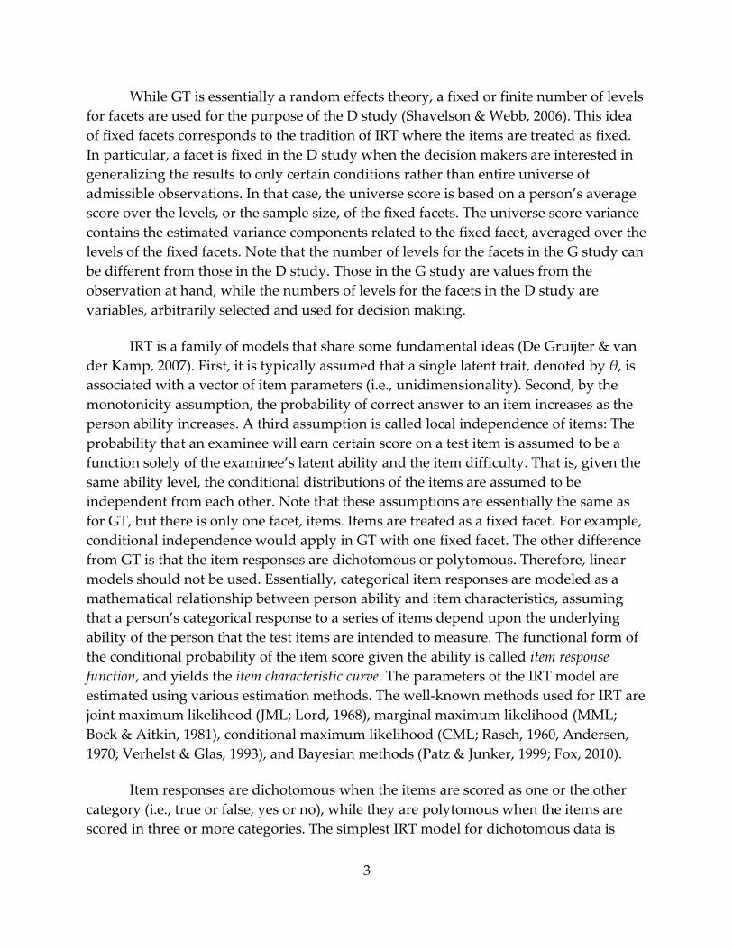
While GT is essentially a random effects theory, a fixed or finite number of levels

for facets are used for the purpose of the D study (Shavelson & Webb, 2006). This idea

of fixed facets corresponds to the tradition of IRT where the items are treated as fixed.

In particular, a facet is fixed in the D study when the decision makers are interested in

generalizing the results to only certain conditions rather than entire universe of

admissible observations. In that case, the universe score is based on a person’s average

score over the levels, or the sample size, of the fixed facets. The universe score variance

contains the estimated variance components related to the fixed facet, averaged over the

levels of the fixed facets. Note that the number of levels for the facets in the G study can

be different from those in the D study. Those in the G study are values from the

observation at hand, while the numbers of levels for the facets in the D study are

variables, arbitrarily selected and used for decision making.

IRT is a family of models that share some fundamental ideas (De Gruijter & van

der Kamp, 2007). First, it is typically assumed that a single latent trait, denoted by θ, is

associated with a vector of item parameters (i.e., unidimensionality). Second, by the

monotonicity assumption, the probability of correct answer to an item increases as the

person ability increases. A third assumption is called local independence of items: The

probability that an examinee will earn certain score on a test item is assumed to be a

function solely of the examinee’s latent ability and the item difficulty. That is, given the

same ability level, the conditional distributions of the items are assumed to be

independent from each other. Note that these assumptions are essentially the same as

for GT, but there is only one facet, items. Items are treated as a fixed facet. For example,

conditional independence would apply in GT with one fixed facet. The other difference

from GT is that the item responses are dichotomous or polytomous. Therefore, linear

models should not be used. Essentially, categorical item responses are modeled as a

mathematical relationship between person ability and item characteristics, assuming

that a person’s categorical response to a series of items depend upon the underlying

ability of the person that the test items are intended to measure. The functional form of

the conditional probability of the item score given the ability is called item response

function, and yields the item characteristic curve. The parameters of the IRT model are

estimated using various estimation methods. The well-known methods used for IRT are

joint maximum likelihood (JML; Lord, 1968), marginal maximum likelihood (MML;

Bock & Aitkin, 1981), conditional maximum likelihood (CML; Rasch, 1960, Andersen,

1970; Verhelst & Glas, 1993), and Bayesian methods (Patz & Junker, 1999; Fox, 2010).

Item responses are dichotomous when the items are scored as one or the other

category (i.e., true or false, yes or no), while they are polytomous when the items are

scored in three or more categories. The simplest IRT model for dichotomous data is

4

Rasch model (Rasch, 1960). The Rasch model assumes that the probability of a correct

response is a monotonically increasing function of a single latent trait and the easiness

of the items. In polytomous IRT models, the probability of getting a certain score for an

item by a student is modeled as a function of continuous latent student ability and the

item characteristic(s). Different models accommodate a variety of polytomous data

where there are different comparisons to which the probability of target score can be

made, and the different assumptions between the ordered score categories exist. Some

of the popular polytomous IRT models include Bock’s (1972) nominal response model,

Andrich’s (1978) rating scale model, Masters’ (1982) partial credit model, and

Samejima’s (1969) graded response model.

IRT analyses are employed when substantive concern is on examining how the

measurement items behave in relation with persons’ ability. For example, assume that

the persons answer the items in a test that are scored dichotomously. In classical test

theory (CTT), the observed sum score is modeled as a function of true score and

measurement error. The measurement error variance is assumed to be constant across

persons. In IRT, particularly in the Rasch model (Rasch, 1960), the probability of an item

response is modeled as a function of person ability and item difficulty. Traditionally,

the measurement error itself is not specified within the IRT model but would be the

difference between the ability estimate and the true ability. The standard error of

measurement is the corresponding standard deviation of the ability estimate. The

person variance is the true score variance. The individual person abilities and

individual item difficulties are modeled and estimated given the data and model

assumptions.

The IRT assumptions are useful in estimating parameters when the test data

collection design is unbalanced and incomplete, and when it is reasonable to assume

that data are missing at random. For example, in large-scale educational assessments

such as the National Assessment of Educational Progress (NAEP), it is unrealistic to

administer a same set of items to every test taker at every test occasion with every test

form, etc. In such cases, IRT analyses are used for building a linking item pool for

multiple forms. Dorans, Pommerich & Holland (2007) states, “…with incomplete,

poorly connected item response data, IRT methods might be the only way to link scores.

Compared to the observed score linking procedures, model-based IRT linking

procedures possess the potential for addressing complex linking problems. Here the

strong assumptions of IRT enable it to replace data with assumptions to provide an

answer that might be a solution to an otherwise intractable problem.” (p. 357)

5

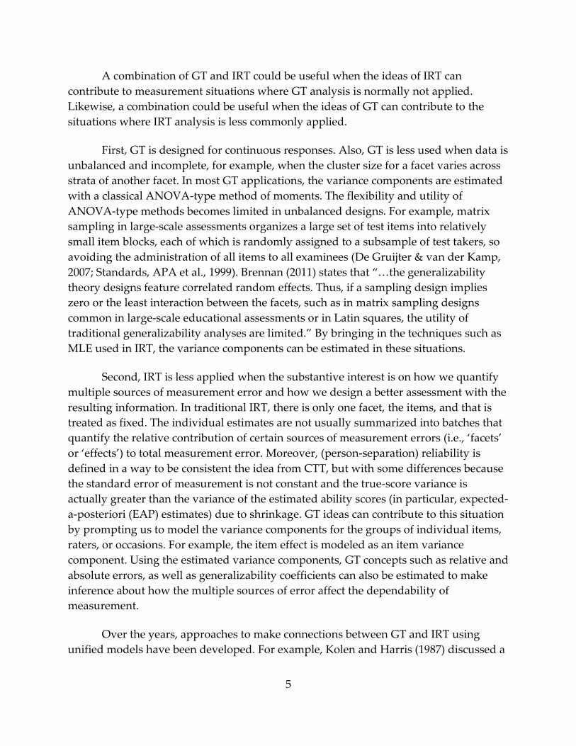
A combination of GT and IRT could be useful when the ideas of IRT can

contribute to measurement situations where GT analysis is normally not applied.

Likewise, a combination could be useful when the ideas of GT can contribute to the

situations where IRT analysis is less commonly applied.

First, GT is designed for continuous responses. Also, GT is less used when data is

unbalanced and incomplete, for example, when the cluster size for a facet varies across

strata of another facet. In most GT applications, the variance components are estimated

with a classical ANOVA-type method of moments. The flexibility and utility of

ANOVA-type methods becomes limited in unbalanced designs. For example, matrix

sampling in large-scale assessments organizes a large set of test items into relatively

small item blocks, each of which is randomly assigned to a subsample of test takers, so

avoiding the administration of all items to all examinees (De Gruijter & van der Kamp,

2007; Standards, APA et al., 1999). Brennan (2011) states that “…the generalizability

theory designs feature correlated random effects. Thus, if a sampling design implies

zero or the least interaction between the facets, such as in matrix sampling designs

common in large-scale educational assessments or in Latin squares, the utility of

traditional generalizability analyses are limited.” By bringing in the techniques such as

MLE used in IRT, the variance components can be estimated in these situations.

Second, IRT is less applied when the substantive interest is on how we quantify

multiple sources of measurement error and how we design a better assessment with the

resulting information. In traditional IRT, there is only one facet, the items, and that is

treated as fixed. The individual estimates are not usually summarized into batches that

quantify the relative contribution of certain sources of measurement errors (i.e., ‘facets’

or ‘effects’) to total measurement error. Moreover, (person-separation) reliability is

defined in a way to be consistent the idea from CTT, but with some differences because

the standard error of measurement is not constant and the true-score variance is

actually greater than the variance of the estimated ability scores (in particular, expected-

a-posteriori (EAP) estimates) due to shrinkage. GT ideas can contribute to this situation

by prompting us to model the variance components for the groups of individual items,

raters, or occasions. For example, the item effect is modeled as an item variance

component. Using the estimated variance components, GT concepts such as relative and

absolute errors, as well as generalizability coefficients can also be estimated to make

inference about how the multiple sources of error affect the dependability of

measurement.

Over the years, approaches to make connections between GT and IRT using

unified models have been developed. For example, Kolen and Harris (1987) discussed a

6

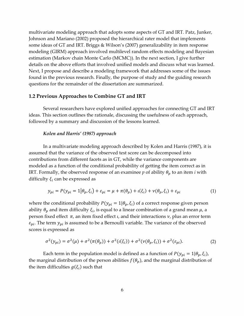
multivariate modeling approach that adopts some aspects of GT and IRT. Patz, Junker,

Johnson and Mariano (2002) proposed the hierarchical rater model that implements

some ideas of GT and IRT. Briggs & Wilson’s (2007) generalizability in item response

modeling (GIRM) approach involved multilevel random effects modeling and Bayesian

estimation (Markov chain Monte Carlo (MCMC)). In the next section, I give further

details on the above efforts that involved unified models and discuss what was learned.

Next, I propose and describe a modeling framework that addresses some of the issues

found in the previous research. Finally, the purpose of study and the guiding research

questions for the remainder of the dissertation are summarized.

1.2 Previous Approaches to Combine GT and IRT

Several researchers have explored unified approaches for connecting GT and IRT

ideas. This section outlines the rationale, discussing the usefulness of each approach,

followed by a summary and discussion of the lessons learned.

Kolen and Harris’ (1987) approach

In a multivariate modeling approach described by Kolen and Harris (1987), it is

assumed that the variance of the observed test score can be decomposed into

contributions from different facets as in GT, while the variance components are

modeled as a function of the conditional probability of getting the item correct as in

IRT. Formally, the observed response of an examinee p of ability to an item i with

difficulty can be expressed as

| ) (1)

where the conditional probability of a correct response given person

ability and item difficulty , is equal to a linear combination of a grand mean , a

person fixed effect , an item fixed effect , and their interactions , plus an error term

. The term is assumed to be a Bernoulli variable. The variance of the observed

scores is expressed as

(2)

Each term in the population model is defined as a function of ,

the marginal distribution of the person abilities , and the marginal distribution of

the item difficulties such that

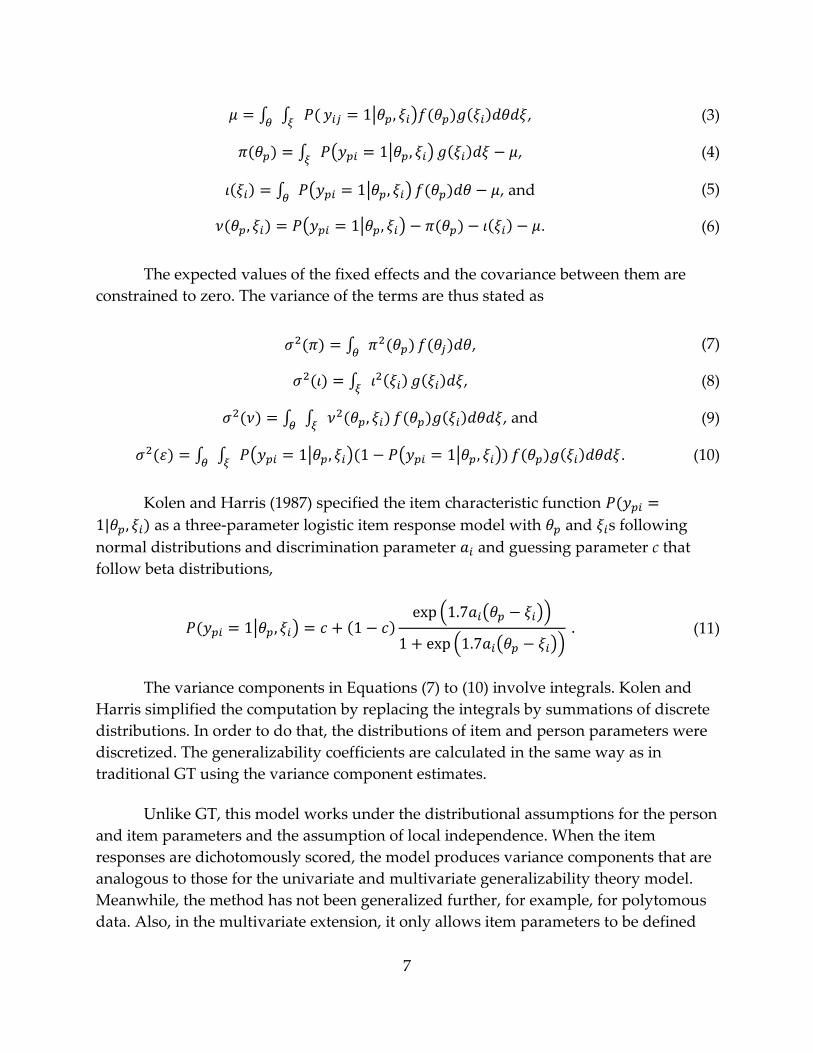
7

∫ ∫

| ) , (3)

∫ ( | ) , (4)

∫ ( | ) , and (5)

( | ) . (6)

The expected values of the fixed effects and the covariance between them are

constrained to zero. The variance of the terms are thus stated as

∫ , (7)

∫ , (8)

∫ ∫ , and (9)

∫ ∫ ( | ) ( | ) . (10)

Kolen and Harris (1987) specified the item characteristic function

as a three-parameter logistic item response model with and s following

normal distributions and discrimination parameter and guessing parameter c that

follow beta distributions,

| ) ( ( ))

( ( )) (11)

The variance components in Equations (7) to (10) involve integrals. Kolen and

Harris simplified the computation by replacing the integrals by summations of discrete

distributions. In order to do that, the distributions of item and person parameters were

discretized. The generalizability coefficients are calculated in the same way as in

traditional GT using the variance component estimates.

Unlike GT, this model works under the distributional assumptions for the person

and item parameters and the assumption of local independence. When the item

responses are dichotomously scored, the model produces variance components that are

analogous to those for the univariate and multivariate generalizability theory model.

Meanwhile, the method has not been generalized further, for example, for polytomous

data. Also, in the multivariate extension, it only allows item parameters to be defined

8

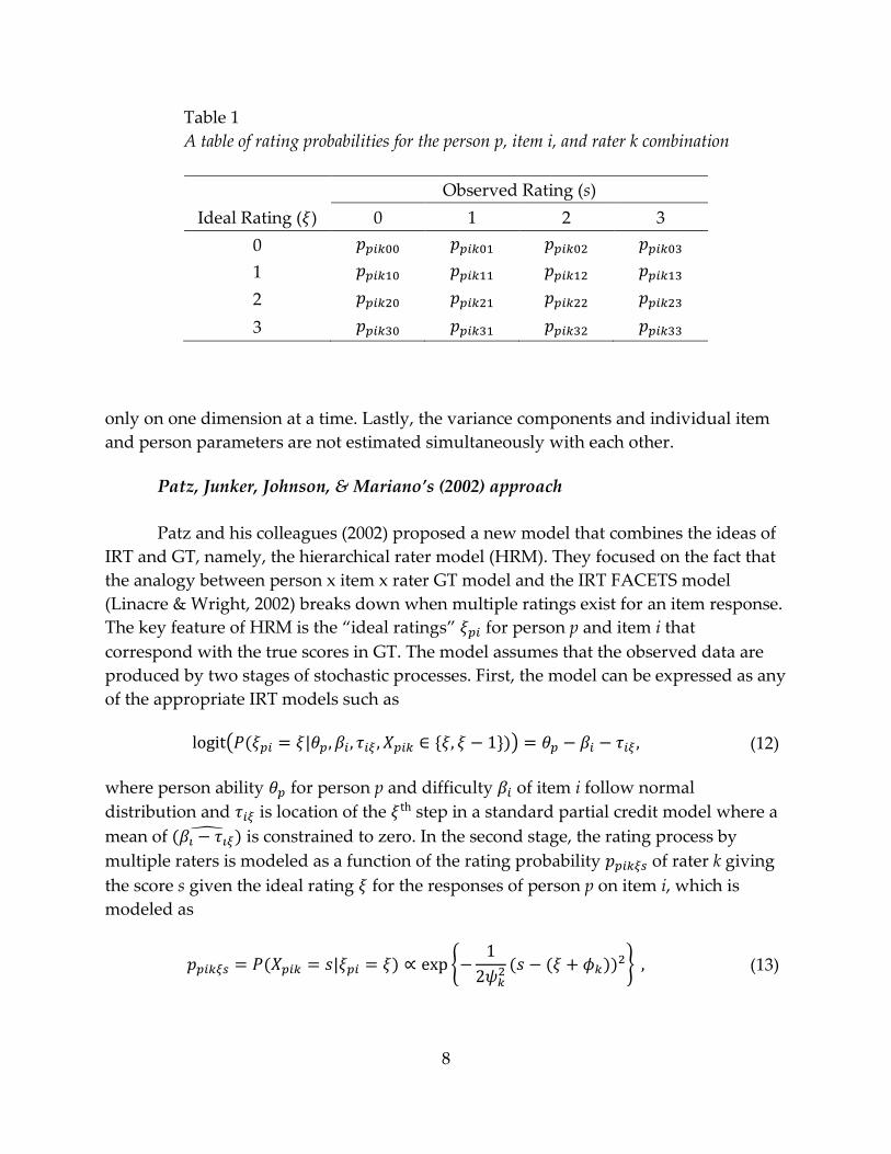
Table 1

A table of rating probabilities for the person p, item i, and rater k combination

Observed Rating (s)

Ideal Rating ( ) 0 1 2 3

0

1

2

3

only on one dimension at a time. Lastly, the variance components and individual item

and person parameters are not estimated simultaneously with each other.

Patz, Junker, Johnson, & Mariano’s (2002) approach

Patz and his colleagues (2002) proposed a new model that combines the ideas of

IRT and GT, namely, the hierarchical rater model (HRM). They focused on the fact that

the analogy between person x item x rater GT model and the IRT FACETS model

(Linacre & Wright, 2002) breaks down when multiple ratings exist for an item response.

The key feature of HRM is the “ideal ratings” for person p and item i that

correspond with the true scores in GT. The model assumes that the observed data are

produced by two stages of stochastic processes. First, the model can be expressed as any

of the appropriate IRT models such as

( ) (12)

where person ability for person p and difficulty of item i follow normal

distribution and is location of the step in a standard partial credit model where a

mean of is constrained to zero. In the second stage, the rating process by

multiple raters is modeled as a function of the rating probability of rater k giving

the score s given the ideal rating for the responses of person p on item i, which is

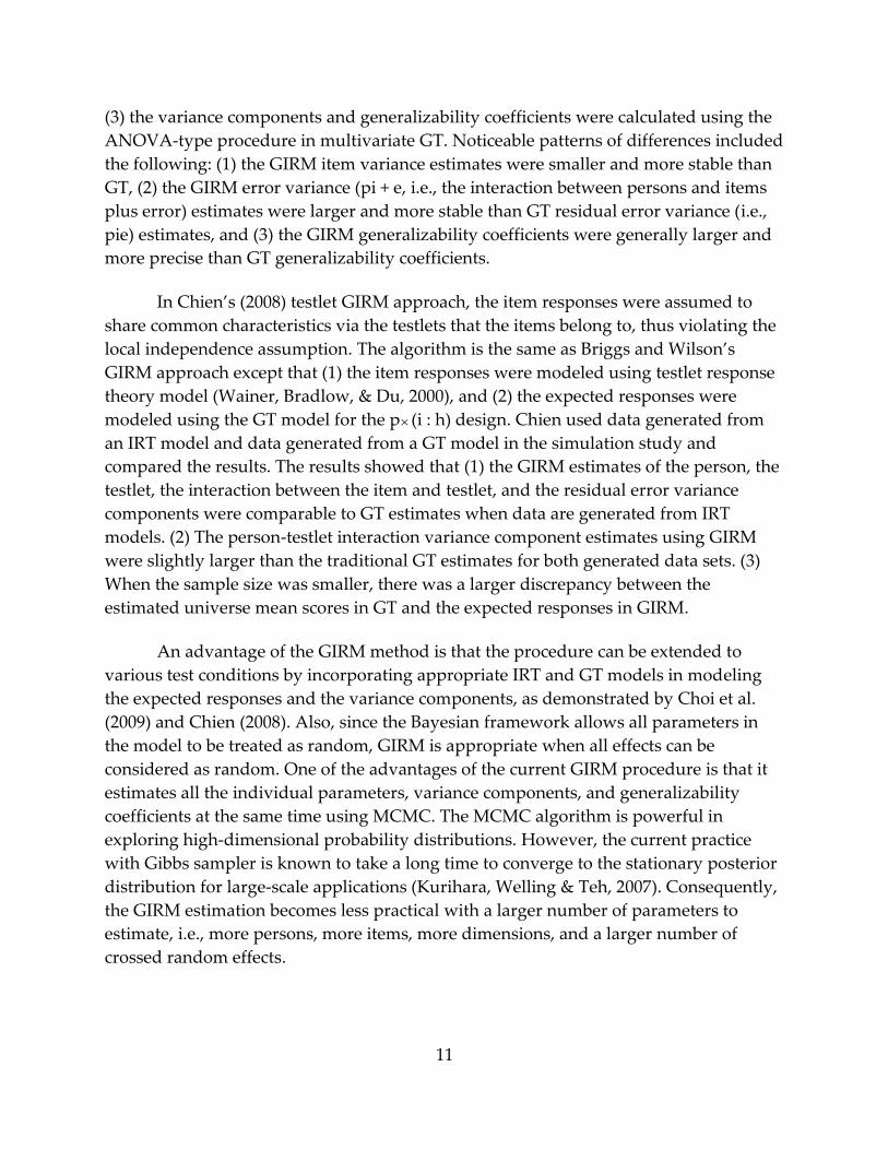
modeled as

{

} (13)

9

where is bias, or severity of rater k and is variability, or standard deviation of

rater k’s ratings for the person p, item i, and observed score s combination. Table 1

shows an example set of rating probabilities that describes the signal detection process.

The observed data is assumed to be a product of the signal detection using the

modeled rating probabilities.

The authors view this model as the GT model that includes the terms for the

different sources of measurement error, with modifications to reflect the discrete nature

of the rating data as in IRT. The model parameters are estimated using an MCMC

algorithm. The authors see HRM as appropriate when it is reasonable to assume

dependence between multiple ratings of the same responses. Particularly, they see

HRM as useful when the effects of items are assumed be constant across the persons

and raters, and the effects of raters are assumed to vary across the items and persons.

However, HRM does not offer direct correspondents of the generalizability coefficients

because the size of variance components changes depending on the latent proficiency

and ideal ratings (Patz et al., 2002).

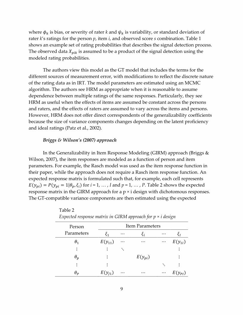
Briggs & Wilson’s (2007) approach

In the Generalizability in Item Response Modeling (GIRM) approach (Briggs &

Wilson, 2007), the item responses are modeled as a function of person and item

parameters. For example, the Rasch model was used as the item response function in

their paper, while the approach does not require a Rasch item response function. An

expected response matrix is formulated such that, for example, each cell represents

for i = 1, … , I and p = 1, … , P. Table 2 shows the expected

response matrix in the GIRM approach for a p × i design with dichotomous responses.

The GT-compatible variance components are then estimated using the expected

Table 2

Expected response matrix in GIRM approach for p × i design

Person

Parameters

Item Parameters

10

response matrix. More formally, the algorithm can be described as follows. Note that

following presentation is based on the example with a p × i design and the Rasch item

response function.

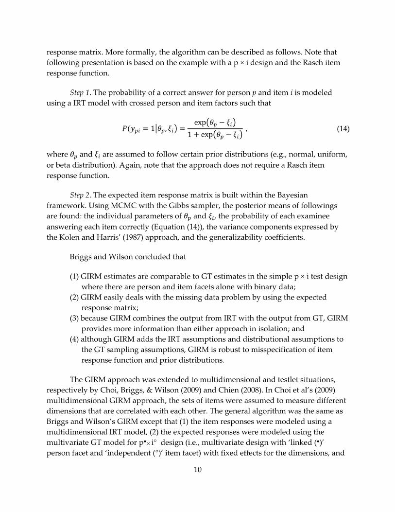
Step 1. The probability of a correct answer for person p and item i is modeled

using a IRT model with crossed person and item factors such that

| ) ( )

( ) (14)

where and are assumed to follow certain prior distributions (e.g., normal, uniform,

or beta distribution). Again, note that the approach does not require a Rasch item

response function.

Step 2. The expected item response matrix is built within the Bayesian

framework. Using MCMC with the Gibbs sampler, the posterior means of followings

are found: the individual parameters of and , the probability of each examinee

answering each item correctly (Equation (14)), the variance components expressed by

the Kolen and Harris’ (1987) approach, and the generalizability coefficients.

Briggs and Wilson concluded that

(1) GIRM estimates are comparable to GT estimates in the simple p × i test design

where there are person and item facets alone with binary data;

(2) GIRM easily deals with the missing data problem by using the expected

response matrix;

(3) because GIRM combines the output from IRT with the output from GT, GIRM

provides more information than either approach in isolation; and

(4) although GIRM adds the IRT assumptions and distributional assumptions to

the GT sampling assumptions, GIRM is robust to misspecification of item

response function and prior distributions.

The GIRM approach was extended to multidimensional and testlet situations,

respectively by Choi, Briggs, & Wilson (2009) and Chien (2008). In Choi et al’s (2009)

multidimensional GIRM approach, the sets of items were assumed to measure different

dimensions that are correlated with each other. The general algorithm was the same as

Briggs and Wilson’s GIRM except that (1) the item responses were modeled using a

multidimensional IRT model, (2) the expected responses were modeled using the

multivariate GT model for p● i° design (i.e., multivariate design with ‘linked (●)’

person facet and ‘independent (°)’ item facet) with fixed effects for the dimensions, and

11

(3) the variance components and generalizability coefficients were calculated using the

ANOVA-type procedure in multivariate GT. Noticeable patterns of differences included

the following: (1) the GIRM item variance estimates were smaller and more stable than

GT, (2) the GIRM error variance (pi + e, i.e., the interaction between persons and items

plus error) estimates were larger and more stable than GT residual error variance (i.e.,

pie) estimates, and (3) the GIRM generalizability coefficients were generally larger and

more precise than GT generalizability coefficients.

In Chien’s (2008) testlet GIRM approach, the item responses were assumed to

share common characteristics via the testlets that the items belong to, thus violating the

local independence assumption. The algorithm is the same as Briggs and Wilson’s

GIRM approach except that (1) the item responses were modeled using testlet response

theory model (Wainer, Bradlow, & Du, 2000), and (2) the expected responses were

modeled using the GT model for the p(i : h) design. Chien used data generated from

an IRT model and data generated from a GT model in the simulation study and

compared the results. The results showed that (1) the GIRM estimates of the person, the

testlet, the interaction between the item and testlet, and the residual error variance

components were comparable to GT estimates when data are generated from IRT

models. (2) The person-testlet interaction variance component estimates using GIRM

were slightly larger than the traditional GT estimates for both generated data sets. (3)

When the sample size was smaller, there was a larger discrepancy between the

estimated universe mean scores in GT and the expected responses in GIRM.

An advantage of the GIRM method is that the procedure can be extended to

various test conditions by incorporating appropriate IRT and GT models in modeling

the expected responses and the variance components, as demonstrated by Choi et al.

(2009) and Chien (2008). Also, since the Bayesian framework allows all parameters in

the model to be treated as random, GIRM is appropriate when all effects can be

considered as random. One of the advantages of the current GIRM procedure is that it

estimates all the individual parameters, variance components, and generalizability

coefficients at the same time using MCMC. The MCMC algorithm is powerful in

exploring high-dimensional probability distributions. However, the current practice

with Gibbs sampler is known to take a long time to converge to the stationary posterior

distribution for large-scale applications (Kurihara, Welling & Teh, 2007). Consequently,

the GIRM estimation becomes less practical with a larger number of parameters to

estimate, i.e., more persons, more items, more dimensions, and a larger number of

crossed random effects.

12

Other approaches

Some approaches discussed the ways to combine GT and IRT without involving

unified modeling frameworks. First, Linacre (1993) suggested conducting both GT and

IRT analyses when it is necessary to complement each other. He illustrated that a three-

facet (e.g., person × item × rater) situation can be analyzed using both GT on the raw

score scale and IRT FACETS model (Linacre, 1989) on the logit scale. He suggested that

researchers select either GT or IRT, or use both, based on the purpose of the analysis:

use GT when interest is on obtaining group-level summary of measurement process on

the raw score scale, and use IRT when interest is on estimating individual

measurements independently from the particularities of the facets and from the fixed

experimental designs. Many researchers followed Linacre’s suggestion and used both

the IRT FACETS and the GT models, for example, for performance assessments of

English as Second Language students (Lynch & McNamara, 1998), for English

assessment (MacMillan, 2000), for writing assessments of college sophomores

(Sudweeks, Reeve, & Bradshaw, 2005), for problem-solving assessments (Smith &

Kulikowich, 2004), and for clinical examinations (Iramaneerat, Yudkowsky, Myford, &

Downing, 2008). A caution is necessary in conducting separate GT and IRT analyses

together because standard GT and IRT applications employ the same terms with

different definitions. For example, in GT, the standard error of measurement (SEM) is

defined for relative and absolute measurement, as the square roots of the absolute or

relative error variance, respectively. In IRT, SEM also represents the uncertainty in the

score assigned to an examinee, just as in GT. However, technically, IRT SEM is defined

as the square root of the inverse of the test information function at the estimated ability.

There are also different terminologies with similar meanings. For example, the p × (i : h)

design in GT is equivalent to the unidimensional testlet (or item bundle) design in IRT.

Second, other approaches have been suggested for combining the results of GT

and IRT for correcting person measurement error. For example, Bock, Brennan, &

Muraki (2002) described how results from GT and IRT can be combined to correct for

the effect of multiple ratings on precision of IRT scale-score estimation and item

parameter estimation. Li (2009) also implemented an information correction method for

person estimates from testlet-based tests using results from GT and IRT analyses.

Lessons learned

All three approaches have practical advantages and disadvantages. Kolen &

Harris’s (1987) proposal laid a cornerstone of combining the IRT and GT models via

modeling the GT variance components using the probability of responses defined by

13

IRT functions. The approach produced a set of GT-compatible variance components as

well as individual person and item parameter estimates. However, complications in

extending the algorithm may lie in how the model was formulated with the single and

double integrals of the marginal distributions of the varying effects. The integration

problem was dealt with by discretizing the person and item distributions to replace

integrals with summations, and the sums may not have been properly weighted. Also,

it is unclear how the method can be extended to polytomous data. Also, their approach

does not provide concurrent estimation of variance components and the individual

person and item parameters.

Patz et al (2002)’ approach played an important part in formally stating a model,

the hierarchical rater model (HRM), that can be viewed as a modified GT model and as

a modified IRT (FACETS) model at the same time. The model was particularly designed

for the multiple ratings situation. The key feature of polytomous HRM is the ideal

rating in an ordinal outcome space, which realizes its mapping by signal detection

process using the pre-set rating probability of the multiple ratings given the ideal

ratings. It is noteworthy that, traditionally, the rater issue had been researched mostly

under GT framework (Bock et al. , 2002). Along with the similar approaches such as

Wilson and Hoskens’ (2001) rater bundle model and Verhelst and Verstralen’s (2001)

IRT model for multiple raters, the HRM brought up an important issue of estimating

rater effects using a new IRT-inspired model that can fit in the context of GT and IRT.

However, the ways to obtain the generalizability coefficients using HRM were not yet

fully developed, as Patz et al note:

“..as with most IRT-based models (and in contrast to models motivated from

Normal distribution theory), location and scale parameters are tied together, so

that the sizes of the variance components that make up the generalizability

coefficients change as we move along the latent proficiency and ideal rating

scales.”

The GIRM approach invoked the necessary conversation in the psychometric

community by clearly elaborating on the idea of combining GT and IRT within the

Bayesian framework. (1) Addressing the new insights such as random treatment of the

traditionally fixed item facet using Bayesian method, and (2) establishing a concept of

the expected response matrix, were the key elements to the GIRM approach that put

forward the efforts to combine the two theories. However, the practical benefit of the

GIRM approach relative to conducting IRT and GT in sequence was not established in

Briggs & Wilson (2007), nor in its extensions by Chien (2008) and Choi et al (2009).

Given that GIRM produced results similar to GT applied to observed response data, it

14

requires additional benefits for the users to be able to choose more demanding GIRM

computations with WinBUGS as an alternative for the simpler GT estimation. Also,

Bayesian method is powerful when prior distribution is meaningful. The GIRM

variance components are estimated, although within the Bayesian framework, using an

ANOVA-like method of moments. Since the method of moments is free from

distributional assumptions, the use of the Bayesian method in GIRM needs to be more

rigorously justified as the sampling assumptions in GIRM are potentially dubious

(Briggs & Wilson, 2007). In addition, the results were found to be robust to

misspecification of prior distributions of person and item parameters.

The focus of this study is to suggest an approach that answers to some of the

issues raised by previous research on combining GT and IRT. In the next section, I

describe the proposed approach and compare it with the previous approaches to

combine GT and IRT.

1.3 Combining GT and IRT

In this section, an approach for combining GT and IRT is described. The

proposed approach simultaneously produces results relevant to GT and IRT, such as

multiple variance component estimates, individual random effects, and generalizability

coefficients.

Modeling framework

The main idea of the proposed method is following: instead of deriving some

statistics from the IRT model that can be analyzed using methods for continuous

responses, I recognize that IRT models can be written in terms of a latent continuous

response and that a classic IRT model can be modeled directly using standard GT with

items as a fixed facet. Once this is recognized, treating items as a random facet or

considering other facets such as raters, become relatively straightforward extensions.

The resulting models are logistic mixed models and can be estimated by MLE. This

method is neither ad-hoc, nor multi-stage, but straightforward ML estimation of a

model that contains the parameter of interest: the variance components needed for the

generalizability and dependability coefficients.

The combination of GT and IRT ideas becomes simpler when GT and IRT

features are expressed in the same language. The following models are expressed as

generalized linear mixed models (Breslow & Clayton, 1993; Fahrmeir & Tutz, 2001). The

key elements of the combined models include: a latent response specification, a logit

link, and a linear predictor specified as a crossed random effects model.

15

In this approach, dichotomous and polytomous responses are modeled using a

latent response formulation. Consider a multifaceted measurement design with person,

item, and rater facets (i.e., person × item × rater). For dichotomous responses, the

underlying continuous response of the pth person to the ith item rated by the kth rater

is modeled using a classical latent response model

, (15)

where designates the true score for person p for every possible combination of

items i, and raters k, because has zero mean for every person. Note that the universe

score is the expected value of this score for a given person over the population of items

and raters. The observed response is modeled as a threshold that takes the value of

1 if and 0 otherwise. Note that for continuous responses such as the ones

modeled in traditional GT, . I assume that the term has a standard

logistic distribution with zero mean and variance ⁄ .

The linear predictor is defined as a three-way crossed random effects model

with interactions. The effects are not considered nested but crossed, assuming that each

person is allowed to answer any item, each person’s responses can be rated by any

rater, and each rater can rate any item. The model can be written as

(16)

where can be interpreted as the grand mean in the universe of admissible

observations and also as the average logit of the probability of response 1 averaging

over all persons, items, and raters. The term denotes random effects. The uppercase

alphabetical superscript (i.e., P, I, …, IK) is an identifier for the random effects and the

lowercase subscript (i.e., p, i, k, pi, pk, and ik) is an identifier for the varying units. For

example, for the term , the superscripts indicate that this is the random effect for the

item main effect and the subscripts indicate that this is the value of this variable for item

i. In the case of , the superscripts indicate that this is the random effect for the

person by rater interaction and the subscripts indicate that this is the value of this

variable for person p and rater k. The model considers the interaction effects and the

cluster-specific main effects to vary at the same level because the interactions are

crossed with the factors that define the main effects. The universe score is . This

specification is consistent with Shi, Leite, & Algina’s (2010) approach on crossed

random effects modeling with interaction effects. The distribution of the random effects

are specified as ,

, ,

,

, and

. The three way interaction term is confounded with

16

. How the choice of the distribution of random effects will impact the results is

testable. However, it is not the focus of this dissertation to evaluate the distributional

choice.

The linear predictor can be expanded to accommodate more complex

measurement situations. For example, the continuation ratio approach is taken for

polytomous data, following Tutz’s (1990) parameterization in his sequential stage

modeling (De Boeck et al., 2011). The term takes the value of 1 if and 0

if , where c (c = 0, …, C–1) denotes the category score and C denotes the

number of score categories including the score 0. The linear predictor for

unidimensional polytomous data is specified as

∑

(17)

where the variable takes the value 1 if the item response rated by the kth rater is

greater than c for c = 1, …, C–1, 0 otherwise. The term denotes the cth step difficulty

of the ith item. It is assumed that the vector of item step difficulties

have a multivariate normal distribution,

with a (C 1) × (C 1) covariance matrix in which variance is denoted by and

covariance is denoted by . Here, it is assumed that having multiple categories for

items does not affect the random interaction effect between items and other factors.

Therefore, the interaction term between item and other factors remains the same as in

Equation (16).

In the case of multidimensionality, the model for dichotomous data is specified

as

∑

(18)

and for multidimensional polytomous data as

∑

∑

(19)

with the number of dimensions D and the variable . The value of is 1 if the ith

item maps onto the dth dimension, 0 otherwise. The term denotes the ability of the

17

pth person on the dth dimension. The vector of person abilities

is assumed to have a multivariate normal distribution,

with a D × D covariance matrix in which variance is denoted by

and covariance is denoted by

. Again, it is assumed that multidimensionality

does not affect the random interaction effect between persons and other factors.

Therefore, the interaction term between person and other factors remains the same as in

Equation (16).

Estimation

As discussed in the motivation section, a combined approach is useful in

situations where GT or IRT alone is typically used but GT and IRT ideas can be still

useful. Those situations include unbalanced and incomplete data, as well as the

situations where there are more than two sources of variation. In view of the fact that

investigation is necessary to understand which estimation method works for

unbalanced data with more than two facets, this section limits its focus to two-facet data

because less is known about how to estimate three-way crossed random effects variance

components with unbalancedness (Brennan, 2001a).

Estimation of the variance components. Estimating variance components is the

focus of G studies. A selection of variance component estimation methods for

unbalanced and incomplete discrete data with partially crossed random effects model

are briefly reviewed below. The maximum likelihood using Laplace approximation

used in the lmer() function in R is used for the proposed approach.

Henderson’s Method 1 for continuous responses. For unbalanced data or partially

crossed, incomplete data, a variation of the ANOVA method, Henderson’s Method 1

(Henderson, 1953), has been widely used (Searle, Casella, & McCulloch, 2009). It

provides an alternative set of sums of squares using the adjusted ‘T’ terms (Brennan,

2001; Huynh, 1977), which do not exist in typical ANOVA tables for balanced designs. It

is also suggested for the GT analysis in unbalanced designs due to missing data because

it does not require distributional-form assumptions and is applicable regardless of the

size of data (Brennan, 2001a). For example, the observed continuous response of the pth

person to the ith item is modeled as

(20)

18

where is the grand mean, is the person effect, is the item effect, and is the

residual. The sample size is denoted by ∑ ∑ where the indicator variable

for empty cells and otherwise. The T terms are defined as

∑ ∑

,

⁄ ,

∑

⁄ , ∑

⁄ . (21)

One also calculates;

∑

⁄ ,

∑

⁄ ,

⁄ ,

⁄ (22)

to get the following variance component estimates.

(23)

( )

(24)

(25)

Restricted maximum likelihood estimation for continuous responses. The Maximum

likelihood (ML) estimation method (Fisher, 1922; Hartley & Rao, 1967) is readily

applicable for a variety of cases, including both balanced and unbalanced data for

multiple classification designs. Despite its wide applicability, ML is known for the

negative bias of its variance and covariance estimators because ML uses the estimate of

mean rather than the true mean in the estimation of the variance and covariance (Sahai

& Ojeda, 2005). A modification of ML, restricted maximum likelihood (REML) approach

(Thompson, 1962; Patterson & Thompson, 1971), or residual maximum likelihood, is

often suggested as an alternative. REML uses a linear combination of original data in

calculation of the likelihood and does not estimate the fixed effects. By doing so, REML

takes into account of the loss of the degrees of freedom from the estimation of fixed

effects, and reduces the downward bias in variance component estimation (Crawley,

2007; Millar, 2011; Skrondal & Rabe-Hesketh, 2004). When the number of clusters is

large enough, REML and ML perform similarly (Skrondal & Rabe-Hesketh, 2004). For

estimating variance components in categorical data, REML cannot be used because it

uses an identity link function.

19

Maximum likelihood with Laplace approximation. The problem of evaluating

integrals of the likelihood function becomes difficult when the integrals do not have

closed form solutions due to categorical responses or multiple random effects with high

dimensions. When it is reasonable to assume that the integrand of the likelihood is

approximately bell-shaped (Small, 2010), the Laplace approximation is often used. The

Laplace approximation is also computationally efficient in approximating the integral of

mixed models with multiple crossed random grouping variables (Bates, 2010). In

Appendix 1, the Laplace approximation method is summarized based on the exposition

given by Bates (2010). In short, the joint likelihood function of parameters given the data

is assumed to follow a normal distribution approximately. The likelihood function is

than efficiently solved using a second-order Taylor expansion. Some cautions are

suggested as following: the Laplace approximation is good when the sample size is

large enough so that the posterior density of the random effect is approximately normal

(Skrondal & Rabe-Hesketh, 2004). When the posterior density is not normal, higher

order Laplace approximations produce more accurate estimates (Breslow & Lin, 1995;

Raudenbush, Yang, & Yosef, 2000). The asymptotic bias of the MLE based on the

Laplace approximation increases with (1) more discreteness (fewer possibilities for the

response), (2) for smaller cluster sizes, and (3) for mixed models where there is near

nonidentifiability (Joe, 2008).

In this research, the variance components of the proposed model are estimated

using maximum likelihood with the Laplace approximation. Currently, the lmer()

function (Bates, 2010) implemented in R statistical environment (R Development Core

Team, 2011) is known for its capacity for estimating multiple cross-classified random

variables using the Laplace approximation with higher efficiency. The conditional

means of the random effects were used for estimation of the individual realizations of

the random effects (Bates, 2010).

Estimation of the generalizability coefficients. The generalizability coefficients

are only useful in the context of D studies. Several issues should be considered before

estimating the generalizability coefficients. First, the decision makers need to decide

what the universe of generalization will be, and whether to consider facets as fixed or

random. Depending on decision makers’ interest and the definition of the universe of

generalization, he or she may reduce the levels of a facet, select, or ignore a facet for a D

study. The decision makers have to decide whether to consider a facet as fixed or

random. When they are interested in generalizing the results to only certain conditions

rather than the entire universe of admissible observations, they can fix the number of

levels for facets in the D study to the total number of levels in the universe of

generalization. Or, they can consider a facet as random: When the intended universe of

20

generalization is infinitely large, the facets with reduced number of levels can be still

considered as random (Shavelson & Webb, 2006). Importantly, this means that by

considering items as a random facet, we can generalize to all items in the universe of

admissible items, unlike traditional IRT.

Second, the decision makers need to decide which sampling design to use for the

D study. GT allows the decision maker to use different designs in G and D studies

(Shavelson & Webb, 2006). For example, even if the G study design is unbalanced, the D

study may use a balanced design (Brennan, 2001a). For another example, although G

studies should use crossed designs whenever possible to avoid confounding of effects,

D studies may use nested designs for convenience or for increasing sample size, which

typically reduces estimated error variance and, hence, increases estimated

generalizability (Shavelson & Webb, 2006).

In particular, when the G study and the D study designs both have unbalanced

and incomplete sampling designs, the challenge in the D study is that the facet variance

component estimates cannot be simply divided by the sample size for each facet. Also,

in unbalanced designs, different sets of quadratic forms often lead to different estimates

of variance components, and the generalizability coefficients calculated using them

(Brennan, 2001a). Generally, unbalanced-ness with respect to crossing facets involves

more complications than unbalanced-ness with respect to nesting. In addition, many-

facet designs (e.g., person × item × rater) involve more complications than single facet

designs (e.g, person × item).

In this study, I illustrate the situation where the G study involves crossed facets

(i.e., person × item × rater) with an unbalanced design and the D study involves the

same crossed facets with a balanced design. In this case, the D study can use the

estimates of the variance components from the unbalanced G study in exactly the same

way as in balanced D studies (Brennan, 2001a). The item and rater facets are considered

random.

First, using the estimated variance components, the generalizability coefficient

can be calculated for the relative decision. In GT terms, is defined as the

ratio of the universe score variance ( to the sum of itself plus the relative error

variance ( :

(26)

21

Specifically, the universe score variance ( is defined as the variance of all the

scores in the population of all the persons, items, and raters:

(

) (27)

where denotes the variance of .

The relative error variance includes only the measurement error variance

relevant to the relative rank order between persons. Note that in the D study, the

measurement error variance is defined based on the mean over multiple observations

(e.g., multiple items) of the facet (Shavelson & Webb, 2006). Also, the variance of is

included in the error to take into account the variance of the underlying logit. In a

balanced person x item x rater design, the relative error variance ( is defined as

(

) ( )

⁄

(28)

where where denotes the variance of averaged over the number of levels for

the D study facets, I’ denotes the number of items in the D study, and K’ denotes the

number of raters in the D study. Finally, is given by:

⁄

(29)

Next, the index of dependability for absolute decisions is defined as the ratio

of the universe score variance ( to the sum of itself plus the absolute error variance

( :

. (30)

The absolute error variance focuses on the measurement error variance of a

person that is attributed by the measurement facets regardless of how other people do

on the test. Thus, it accounts for the variance related to another random facet, for

example, items or raters. Here the denominator also includes the variance of the

underlying logit. In a balanced person × item × rater design, the relative error variance

( is defined as

22

(

) ( )

⁄

(31)

Consequently, is

⁄

(32)

In the multidimensional and/or polytomous case, the generalizability coefficient

and the index of dependability for multivariate GT were calculated using the composite

variance component estimates (Brennan, 2001a). For multidimensional dichotomous

data,

⁄

(33)

and

⁄

(34)

while for multidimensional polytomous data, the index of dependability changes into

⁄

(35)

where is the composite of universe score variance for D dimensions, and

is the composite of item variance components for C–1 categories. Formally,

the composite variance components are defined as

∑

∑∑ (36)

∑

∑∑ (37)

assuming that the covariance between categories or dimensions exist. The category

weight is defined as

for c = (1, …, C–1). R is the total number of responses and

is the number of responses that correspond to the category score c. The dimension

23

weight is defined as

for d = (1, …, D) where is the number of responses that

correspond to the dimension d.

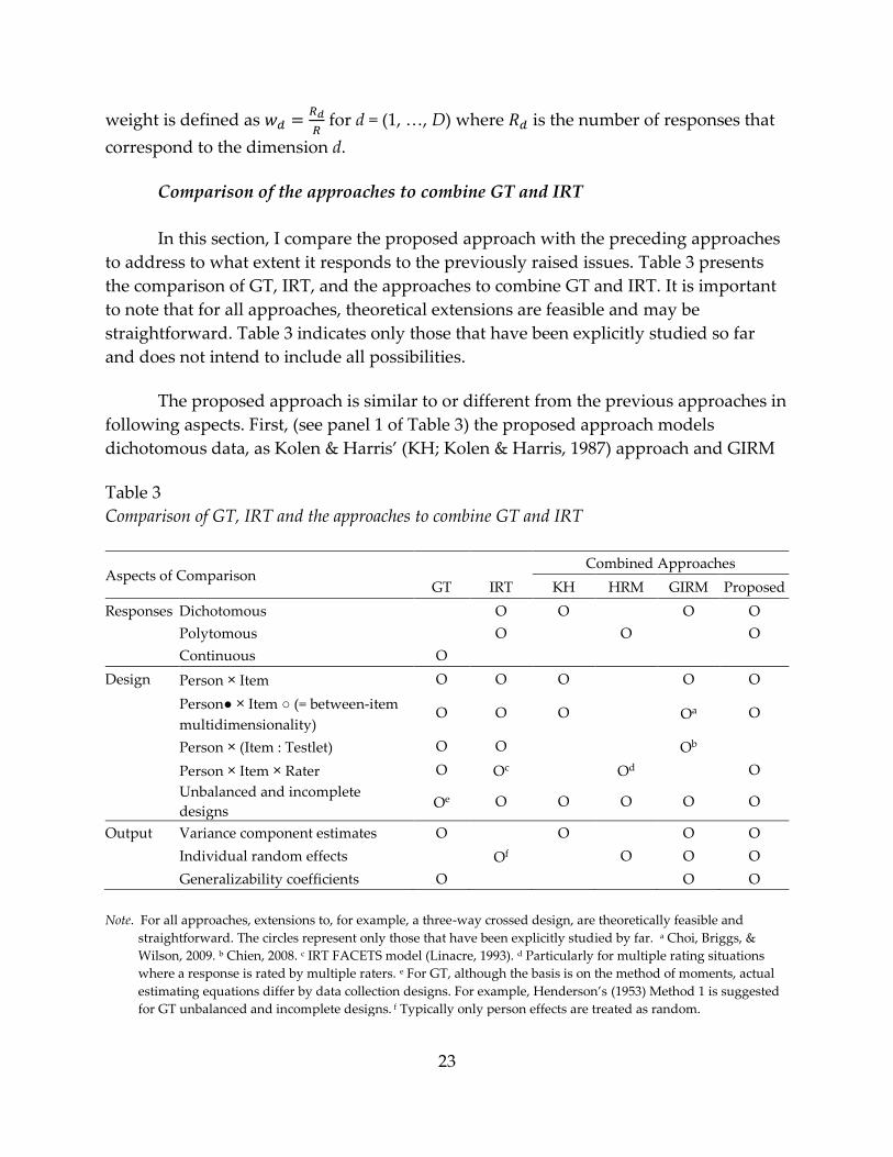
Comparison of the approaches to combine GT and IRT

In this section, I compare the proposed approach with the preceding approaches

to address to what extent it responds to the previously raised issues. Table 3 presents

the comparison of GT, IRT, and the approaches to combine GT and IRT. It is important

to note that for all approaches, theoretical extensions are feasible and may be

straightforward. Table 3 indicates only those that have been explicitly studied so far

and does not intend to include all possibilities.

The proposed approach is similar to or different from the previous approaches in

following aspects. First, (see panel 1 of Table 3) the proposed approach models

dichotomous data, as Kolen & Harris’ (KH; Kolen & Harris, 1987) approach and GIRM

Table 3

Comparison of GT, IRT and the approaches to combine GT and IRT

Aspects of Comparison Combined Approaches

GT IRT KH HRM GIRM Proposed

Responses Dichotomous

O O

O O

Polytomous

O

O

O

Continuous O

Design Person × Item O O O

O O

Person● × Item ○ (= between-item

multidimensionality) O O O

Oa O

Person × (Item : Testlet) O O

Ob

Person × Item × Rater O Oc

Od

O

Unbalanced and incomplete

designs Oe O O O O O

Output Variance component estimates O

O

O O

Individual random effects

Of

O O O

Generalizability coefficients O

O O

Note. For all approaches, extensions to, for example, a three-way crossed design, are theoretically feasible and

straightforward. The circles represent only those that have been explicitly studied by far. a Choi, Briggs, &

Wilson, 2009. b Chien, 2008. c IRT FACETS model (Linacre, 1993). d Particularly for multiple rating situations

where a response is rated by multiple raters. e For GT, although the basis is on the method of moments, actual

estimating equations differ by data collection designs. For example, Henderson’s (1953) Method 1 is suggested

for GT unbalanced and incomplete designs. f Typically only person effects are treated as random.

24

(Briggs & Wilson, 2007; Choi et al., 2009) do. It also models polytomous data as HRM

(Patz et al., 2002) does. All three previous ones and the proposed approach are closer to

IRT and depart from GT by dealing with discrete data rather than continuous data.

Second, in terms of data collection designs (see panel 2 of Table 3), the proposed

approach specifies models for person by item (i.e., Rasch 1PL), multivariate person by

item (i.e., between-item multidimensionality), and person by item by rater situations,

but not the testlet situation. KH has not been extended beyond two facet designs. HRM

mainly deals with the three facet design with multiple raters. The GIRM approach is the

most flexible among the previous combining approaches: it is also theoretically

straightforward to extend GIRM to three-way crossed design, although it is not

explicitly studied so far. The proposed approach and all other previous approaches are

similar to IRT and depart from GT by treating the unbalanced and incomplete designs

equally with the balanced designs in estimation process. In detail, the proposed

approach implements MLE with a Laplace approximation to the integral for variance

component estimation. It adds some of the advantages of MLE such as much faster

estimation of the model parameters compared to MCMC used in GIRM.

Third, (see panel 3 of Table3) the proposed approach provides estimates for

variance components, individual random effects, and generalizability coefficients, as

GIRM does. Although, Kolen & Harris (1987) discusses the estimation of individual

random effects as an area for further development, it is unclear from literature how

their approach has further developed. As discussed in previous chapter, HRM does not

provide variance component estimates.

A comparison of four estimation methods. The following small study illustrates how

different the variance component estimates and generalizability coefficient can be when

different methods are used for a binary, unbalanced and incomplete data set. A

comparison of four estimation methods demonstrates the following: first, depending on

the use of link function to model the dichotomous responses, the variance components

are estimated on different scales while the generalizability coefficients are estimated on

the same ratio scale. Second, the comparability between the GT method and the GIRM

method on dichotomous data (Briggs & Wilson, 2007) appears to be less obvious, (to be

precise, without proper correction to the procedure,) when data is unbalanced and

incomplete. In addition, the results differ by how the missing data is treated in

estimation. The results motivate further study on the effects of the discrete nature of

data and missingness on estimation of variance components and generalizability

coefficients.

25

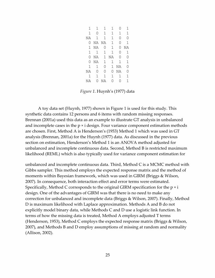
A toy data set (Huynh, 1977) shown in Figure 1 is used for this study. This

synthetic data contains 12 persons and 6 items with random missing responses.

Brennan (2001a) used this data as an example to illustrate GT analysis in unbalanced

and incomplete cases in the p × i design. Four variance component estimation methods

are chosen. First, Method A is Henderson’s (1953) Method 1 which was used in GT

analysis (Brennan, 2001a) for the Huynh (1977) data. As discussed in the previous

section on estimation, Henderson’s Method 1 is an ANOVA method adjusted for

unbalanced and incomplete continuous data. Second, Method B is restricted maximum

likelihood (REML) which is also typically used for variance component estimation for

unbalanced and incomplete continuous data. Third, Method C is a MCMC method with

Gibbs sampler. This method employs the expected response matrix and the method of

moments within Bayesian framework, which was used in GIRM (Briggs & Wilson,

2007). In consequence, both interaction effect and error terms were estimated.

Specifically, Method C corresponds to the original GIRM specification for the p × i

design. One of the advantages of GIRM was that there is no need to make any

correction for unbalanced and incomplete data (Briggs & Wilson, 2007). Finally, Method

D is maximum likelihood with Laplace approximation. Methods A and B do not

explicitly model binary data, while Methods C and D use a logistic link function. In

terms of how the missing data is treated, Method A employs adjusted T terms

(Henderson, 1953), Method C employs the expected response matrix (Briggs & Wilson,

2007), and Methods B and D employ assumptions of missing at random and normality

(Allison, 2002).

1 1 1 1 0 1

1 0 1 1 1 1

NA 1 1 1 0 0

0 NA NA 1 0 1

1 NA 0 1 0 NA

1 1 1 1 0 1

0 NA 1 NA 0 0

0 NA 1 1 1 1

1 1 0 1 NA 0

NA 0 0 0 NA 0

1 1 1 1 1 1

NA 0 NA 0 0 1

Figure 1. Huynh’s (1977) data

26

In terms of the D study, note that how to calculate the generalizability

coefficients for Huynh’s data was not suggested in Brennan (2001a) or in the

urGENOVA (Brennan, 2001b) output that uses Huynh’s data. Although the G study

design was unbalanced, GT allows a different design for the D study. I decided to study

how the results will be generalized to a balanced p × i design. The generalizability

coefficients were calculated based on the traditional GT definitions for balanced p × i

design with an additional error term for Method C and D using the following formula;

(38)

(39)

where is the variance component of averaged over the number of levels for

the facet . In this example, there is only one facet, items, and the number of levels for

the D study item facet is .

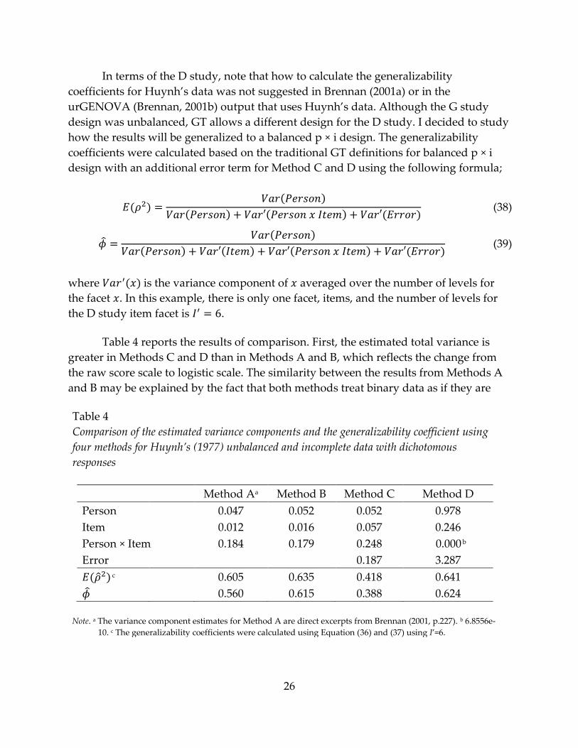
Table 4 reports the results of comparison. First, the estimated total variance is

greater in Methods C and D than in Methods A and B, which reflects the change from

the raw score scale to logistic scale. The similarity between the results from Methods A

and B may be explained by the fact that both methods treat binary data as if they are

Table 4

Comparison of the estimated variance components and the generalizability coefficient using

four methods for Huynh’s (1977) unbalanced and incomplete data with dichotomous

responses

Method Aa Method B Method C Method D

Person

0.047 0.052 0.052 0.978

Item

0.012 0.016 0.057 0.246

Person × Item 0.184 0.179 0.248 0.000 b

Error

0.187 3.287

c

0.605 0.635 0.418 0.641

0.560 0.615 0.388 0.624

Note. a The variance component estimates for Method A are direct excerpts from Brennan (2001, p.227). b 6.8556e-

10. c The generalizability coefficients were calculated using Equation (36) and (37) using I’=6.

27

continuous. Second, in terms of variance component estimates, there is a noticeable

similarity between Method C and Methods A and B, when compared to Method D. This

can be attributable to Method C using the expected responses matrix to transform

discrete data to be continuous so that the G study models can be used for estimation. In

other words, transformation to continuous responses makes Method C similar to

Methods A and B, and also making it different than Method D which models discrete

responses. However, Method C is not exactly corrected for unbalanced and incomplete

data. This simply means, unintentionally, that the G study model that is used within

Method C strictly follows the model for a ‘balanced’ p × i design, in the same way as

illustrated in the previous studies (Briggs & Wilson, 2007; Chien, 2008; Choi et al., 2009).

This explains the fact that Method C item and person × item variance component

estimates are larger than those from Methods A and B, because the model assumes

more items than the data actually has. Third, the fact that the smallest generalizability

coefficient occurs for Method C again suggest the need for correction of the procedure

for unbalanced data. Because the numerator (i.e. person variance) stays the same for all

cases, the generalizability coefficients decrease only when the denominator (i.e.,

measurement error variances) becomes larger. For both and , the measurement

error variance increased due to overestimation of item and person by item interaction

variance components. On the contrary, the generalizability coefficient from Method D

was comparable to that for Methods A and B, especially to Method B, which uses the

same maximum likelihood approach in treating missing data.

Figure 2. Comparison of estimated relative and absolute SEMs

from Methods A,B,C and D

28

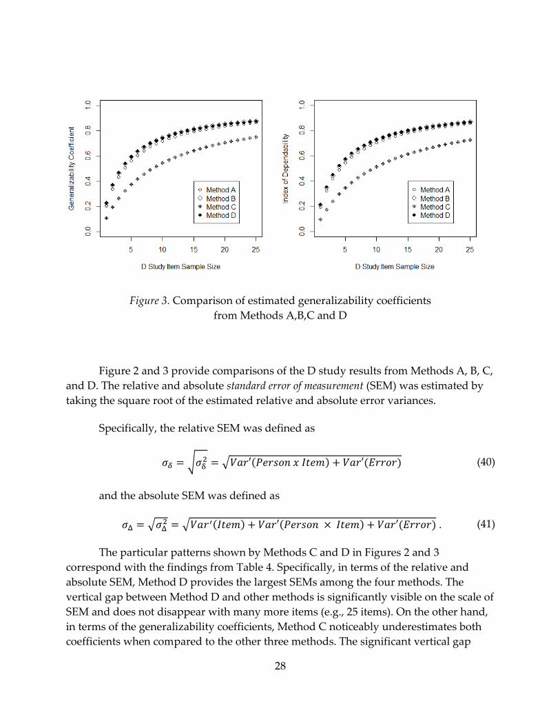
Figure 3. Comparison of estimated generalizability coefficients

from Methods A,B,C and D

Figure 2 and 3 provide comparisons of the D study results from Methods A, B, C,

and D. The relative and absolute standard error of measurement (SEM) was estimated by

taking the square root of the estimated relative and absolute error variances.

Specifically, the relative SEM was defined as

√ √ (40)

and the absolute SEM was defined as

√ √ . (41)

The particular patterns shown by Methods C and D in Figures 2 and 3

correspond with the findings from Table 4. Specifically, in terms of the relative and

absolute SEM, Method D provides the largest SEMs among the four methods. The

vertical gap between Method D and other methods is significantly visible on the scale of

SEM and does not disappear with many more items (e.g., 25 items). On the other hand,

in terms of the generalizability coefficients, Method C noticeably underestimates both

coefficients when compared to the other three methods. The significant vertical gap

29

between Method C and other methods also does not disappear as the D study item

sample size increases to many, such as 25 items.

Some warrants are necessary in relating the findings in Table 4, Figure 2 and

Figure 3 to comparison of approaches to combine GT and IRT. First, most importantly,

the variance components models are directly estimated by Henderson’s Method 1 and

REML, pretending that the data are continuous. While the assumption of continuity

may be considered insensible, this approach can be backed up by Hyunh (1977) and

Brennan’s (2001) approach where they illustrated the use of Henderson’s Method 1

using the dichotomous data set shown in Figure 1 Also, Brennan (2001a) demonstrated

the use of REML using a test data with 26 dichotomously scored items to assess

comparability between the variance component estimates from the various estimation

procedures. In contrast, the GIRM method generates continuous data so that the

variance components models can be used for estimation. Second, the result is limited to

two-way crossed design. Further investigation is necessary to generalize the findings to

more than two facets. Third, the compared methods only represent the estimation

methods of GT, GIRM and the proposed approach. The estimation methods

representing IRT and HRM are not included in comparison because variance

components are not estimated in typical IRT and HRM applications. Kolen & Harris

(KH; 1987) was not included in the comparison because the estimation method could

not be replicated due to the following reason. In KH, two steps were taken to estimate

the variance components. First, the distributions of person and item parameters were

specified: for the purpose of the paper, it was assumed that the person and item

parameters were distributed normally. The integrals in the models were replaced by

summation in practice, by using discretized distributions. The authors indicate that a

process of iteration and inspection was used to produce ability and item parameters

that would be associated with the variance components. Then, using these distributions,

the variance components are calculated. It was decided that more specific information

on the convergence criteria is necessary to replicate this procedure.

The results motivate further research on the following. In suggesting an

estimation method for an approach to combine GT and IRT, the robustness of the

generalizability coefficient estimates may not become a concern. However, the effects of

the discrete nature of data (e.g., more than two categories), the degree of missingness in

data, the violation of normality assumptions, and more complex designs (e.g., person by

item by rater design, multidimensionality) on estimation of variance components and

generalizability coefficients are still unknown and need to be examined.

30

1.4 Purpose of the Study

The goal of these reviews has been to understand what has and has not been

achieved from preceding efforts. The goal of the study is to suggest and evaluate a

proposal that possibly solves this set of problems that we learned from the past, and to

open a new line of discussion that will lead to more potential developments. I describe

how the proposed model specifies a latent response formulation as a function of cross-

classified person, item, and rater random effects and the variance components for each

facet. Specifically, the purposes of this research are to report on the performance of the

proposed approach in various measurement situations via a simulation study, to

illustrate the use of the proposed method for analyzing large-scale data sets from

classroom assessment and standardized tests, and finally, to discuss what we have

learned and suggest an avenue of research for those who are interested in future

endeavors.

The result of this study will allow the readers to understand and speculate more

about how the new approach addresses the issues it inherited from its preceding efforts,

and what can be achieved by the proposed approach. Also, the results of this study will

encourage collaboration between those who specialize in GT and IRT by articulating the

kinds of questions to ask in order to find a more efficient alternative to achieve the

combined benefits of GT and IRT.

1.5 Research Questions

This study aims to answer following research questions. First, how accurate are

the results of the proposed approach in various measurement conditions? In order for

the inferences to be valid, it is necessary to evaluate and understand how the proposed

method behaves, especially when the model assumptions are violated in ways we think

is common in many real assessment situations. I present results from extensive

simulation studies for dichotomous and polytomous responses with

multidimensionality and multiple raters. The full model of the proposed approach

includes the main and interaction terms of the three random effects (i.e., person, item,

and rater) crossed with each other. The random person, item, and rater parameters and

the variance components were estimated using the lmer() function (Bates, Maechler, &

Bolker, 2011) in R Statistical Environment (R Development Core Team, 2011). The

distance between the generating values and the estimated values were quantifed using

the root mean squared errors (RMSE). Then, a set of multiple regression models were

fitted to examine the main effects and two-way interaction effects of simulation factors

on the recovery of the various parameters.

31

Second, how is the proposed approach applied to real data sets? I demonstrate

applications of our approach to two large-scale data sets. One is large-scale

standardized test data: the Programme for International Student Assessment (PISA)

2009 Science data set, which includes 3,617 students from the United States who

responded to 53 science items. The second one is classroom assessment data from the

2008-2009 Carbon Cycle project, which was supported by the National Science

Foundation: Developing a Research-based Learning Progression on Carbon-

Transforming Processes in Socio-Ecological Systems (NSF 0815993). It includes 1,371

students’ responses to 19 items, polytomously scored by 8 raters.

Third, what have we learned and what do we still not know now? In

summarizing the results and discuss what we have learned from the studies, the

conclusion went back to the central question and focused on identifying the common

ground between GT and IRT, and evaluating the proposed approach as an alternative

that promises more effective application and further collaboration between GT and IRT.

1.6 Description of the Chapters

This chapter consisted of three parts: (1) a motivation of combining GT and IRT,

(2) a review of previous approaches to combine GT and IRT, and (3) an introduction of

an approach. Chapter 2 presents the design and results of the simulation studies that

examined the impact of various measurement conditions on accuracy of estimates

produced by the proposed approach. In Chapter 3, the use of the proposed method is

illustrated using two empirical data sets. It is composed of two parts: (1) the results

from the analysis of the PISA 2009 data set, and (2) the results from the analyses of the

large-scale classroom assessment data set which includes polytomous responses,

multidimensionality and multiple raters. In Chapter 4, I summarize the results and

discuss further directions of research.

32

Chapter 2 Simulation Study

2.1 Introduction

The goal of the simulation study was to examine the impact of violations of

assumptions on the random effects and generalizability coefficients. Traditional IRT

assumptions, for example, the assumption of conditional independence, are violated by

dependence that can be introduced by raters. Traditional GT assumptions are violated

when the crossed or nested relationships among the facets do not match a specific

design but are determined by complexity in measurement situations, such as random

assignments of test forms and item blocks. The simulation studies described in this

chapter involved a three-facet crossed design (person × item × rater) without and with

the interaction effects among the facets. Reflecting the violations of traditional

assumptions, sets of unbalanced and incomplete data were generated. Two sets of

simulation studies were conducted. Table 5 summarizes the differences between the

two simulations.

Simulation One

First, an extensive simulation study was conducted to determine the simulation

factors that affect the variance component estimates of the main effects. Based on the

eight factors, which will be discussed in the Methods section (e.g., the number of

persons, the number of raters, the proportion of random missing data, the number of

person dimensions, etc.), I constructed a factorial design with 576 simulation conditions.

I generated 100 replication data sets for each of the conditions based on the three-facet

models without interactions, and I fitted the models without interaction effects to the

data sets. I examined the effects of varying factors on the resulting variance component

estimates and generalizability coefficients by testing the significance of the effects of

varying factors on the bias and the root mean squared error ( ( )) of the estimates.

Simulation Two

Second, based on the results from Simulation One, I selected several factors that

significantly affected the accuracy of the variance component estimates and the

generalizability coefficients. I constructed a factorial design with 144 simulation

conditions. I generated 10 replication data sets for each of the conditions based on the

three-facet models ‘with’ interactions. I fitted the models ‘with’ interaction effects and

examined the effects of varying factors on the resulting estimates. I took this somewhat

33

Table 5

Differences between Simulation One and Simulation Two

Aspects Simulation One Simulation Two

Generating model person × item × rater

without interactions

person × item × rater

with interactions

Estimating model person × item × rater

without interactions

person × item × rater

with interactions

Number of simulation factors 8 (5 types) 6 (4 types)

Number of simulation conditions 576 144

Number of replications 100 10

indirect route to the final simulations due to the extended time needed for the

calibration of models with interaction.

In the following section, I describe the factors that determined the simulation

conditions, followed by the specific methods for the simulation study. The methods and

results from both Simulations One and Two are described together because they mostly

share the same specifications in data generation and the same criteria for the outcome

evaluation.

2.2 Methods

Factors that determined simulation conditions

In Simulation One, five types of factors were used in data generation: (a) the

number of persons, items and raters, (b) the number of valid score categories, (c) the

number of ability dimensions that items are designed to measure, (d) the proportion of

missing responses, and (e) the skewness in the distribution of persons and items. For

example, the number of raters was either one or five, while the proportion of missing

responses was either 0.1% or 0.3% in the study.

Based on the results from Simulation One, I identified four types of factors that

significantly affected the accuracy of variance component estimates and the

generalizability coefficients: (a) the number of persons and items, (b) the number of

valid score categories, (c) the number of ability dimensions that items are designed to

measure, and (d) the skewness in the distribution of persons and items. That is,

34

Simulation Two dropped two factors from Simulation One: the number of raters and

the proportion of missing responses. As will be seen in the results section, the effects of

these two types of factors on the estimates of the variance components and the

generalizability coefficients were not statistically significant. The following paragraphs

describe the factors used in Simulation One and Two in detail.

The number of persons, items, and raters. Let p = 1, …, P be the persons and i = 1,

…, I be the items, and k = 1, …, K be the raters in a simulated data set. The total number

of persons, , was either 100 or 500. The total number of items, , was either 50 or 100.

The number of raters was either K = 1 which means no rater effect was considered in

analyzing the data, or 5. Note that the number of raters was set to five in

Simulation Two.

The number of valid score categories. Let c = 1, …, C be the notation for score

categories of the items in a simulated data set. The number of valid score categories for

all items, C, was either 2 or 4. For example, when a response is scored as 0 when

incorrect and 1 when correct, the number of valid score categories is 2. When a response

is scored polytomously with partial credits, for example, 0 if incorrect, 1 and 2 if

partially correct, and 3 if fully correct, then the number of valid score categories is 4.

The number of ability dimensions. A set of items can measure either one latent

domain or multiple domains in real testing situations. Let d = 1, …, D be the person

dimensions in a simulated data set. The number of ability dimensions, D, was either 1

or 3 in this study. In the case of multidimensionality, I assumed that each item measures

only one dimension. When D = 3, the number of items for the 3 dimensions were , ,

and where and were randomly sampled integers within the range of 1 to

.

The proportion of missing responses. Let m be the proportion of random missing

responses in a simulated data set. Either m = 0.1% or 0.3% of all item responses were

randomly selected and recoded as missing. This factor was used only in Simulation

One.

The skewness in the distribution of persons and items. In this study, I assume

skewness in both person and item distributions to reflect situations where the normality

assumptions are violated: the examinees are mostly at the lower or upper end of the

performance spectrum, that is, most of the items are either too easy or too difficult for

the examinees. A skewed normal distribution (Azzalini, 1985) is defined by a location

parameter , a scale parameter , and a shape parameter . The distribution is right

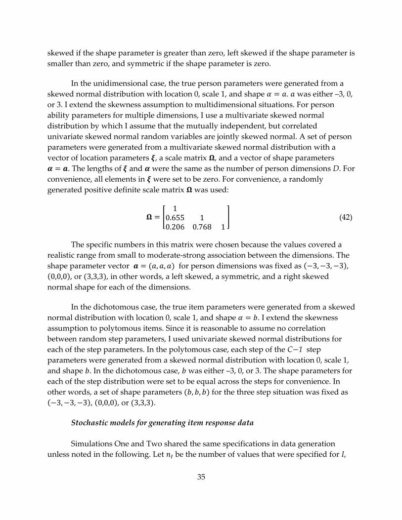
35

skewed if the shape parameter is greater than zero, left skewed if the shape parameter is

smaller than zero, and symmetric if the shape parameter is zero.

In the unidimensional case, the true person parameters were generated from a

skewed normal distribution with location 0, scale 1, and shape . was either –3, 0,

or 3. I extend the skewness assumption to multidimensional situations. For person

ability parameters for multiple dimensions, I use a multivariate skewed normal

distribution by which I assume that the mutually independent, but correlated

univariate skewed normal random variables are jointly skewed normal. A set of person

parameters were generated from a multivariate skewed normal distribution with a

vector of location parameters , a scale matrix , and a vector of shape parameters

. The lengths of and were the same as the number of person dimensions D. For

convenience, all elements in were set to be zero. For convenience, a randomly

generated positive definite scale matrix was used:

[

] (42)

The specific numbers in this matrix were chosen because the values covered a

realistic range from small to moderate-strong association between the dimensions. The

shape parameter vector for person dimensions was fixed as ,

, or , in other words, a left skewed, a symmetric, and a right skewed

normal shape for each of the dimensions.

In the dichotomous case, the true item parameters were generated from a skewed

normal distribution with location 0, scale 1, and shape . I extend the skewness

assumption to polytomous items. Since it is reasonable to assume no correlation

between random step parameters, I used univariate skewed normal distributions for

each of the step parameters. In the polytomous case, each step of the C 1 step

parameters were generated from a skewed normal distribution with location 0, scale 1,

and shape . In the dichotomous case, was either –3, 0, or 3. The shape parameters for

each of the step distribution were set to be equal across the steps for convenience. In

other words, a set of shape parameters for the three step situation was fixed as

, , or .

Stochastic models for generating item response data

Simulations One and Two shared the same specifications in data generation

unless noted in the following. Let be the number of values that were specified for I,

36

Table 6

True mean and variance for person and item random effects, translated from location,

scale and shape parameters of skewed normal distribution

Univariate

Conditions Multivariate Conditions

= 0 0 0

= 1 1 1 [

] [

] [

]

3 0 3

= 0.757 0 0.757

0.427 1 0.427 [

] [

] [

]

for P, and so on. In Simulation One, the varying simulation factors resulted in a

(2 2 2) 2 2 2 (3 3) = 576

factorial design. In Simulation Two, the varying simulation factors resulted in a

(2 2) 2 2 (3 3) = 144 factorial design. For

each condition, the item response data was generated by the following algorithm.

1. Sample the person parameter from a skewed normal distribution

~

for p = 1, …, . The true mean and variance of a skewed normal

distribution are defined as:

√

,

, (43)

where

√ (Azzalini, 1985). Table 6 presents the true values used in data

generation.

When D > 1, sample the vector of person parameters

for p = 1, …, and d = 1, …, D from a multivariate skewed normal distribution

. The true mean vector and the variance–covariance matrix of

this distribution are:

√ , , (44)

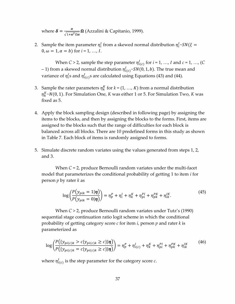
37

where

√ (Azzalini & Capitanio, 1999).

2. Sample the item parameter from a skewed normal distribution

~

for i = 1, …, .

When C > 2, sample the step parameter for i = 1, …, and c = 1, …, (C

– 1) from a skewed normal distribution ~ . The true mean and

variance of s and

s are calculated using Equations (43) and (44).

3. Sample the rater parameters for k = (1, …, ) from a normal distribution

~ . For Simulation One, K was either 1 or 5. For Simulation Two, K was

fixed as 5.

4. Apply the block sampling design (described in following page) by assigning the

items to the blocks, and then by assigning the blocks to the forms. First, items are

assigned to the blocks such that the range of difficulties for each block is

balanced across all blocks. There are 10 predefined forms in this study as shown

in Table 7. Each block of items is randomly assigned to forms.

5. Simulate discrete random variates using the values generated from steps 1, 2,

and 3.

When C = 2, produce Bernoulli random variates under the multi-facet

model that parameterizes the conditional probability of getting 1 to item i for

person p by rater k as

( ( )

( ))

(45)

When C > 2, produce Bernoulli random variates under Tutz’s (1990)

sequential stage continuation ratio logit scheme in which the conditional

probability of getting category score c for item i, person p and rater k is

parameterized as

( ( )

( ))

(46)

where is the step parameter for the category score c.

38

When D > 1 and C = 2, produce Bernoulli random variables under the

multi-facet model that parameterizes the probability of getting 1 to item i for

person p on dimension d by rater k as

( ( )

( ))

(47)

When D > 1 and C > 2,

( ( )

( ))

(48)

Note that the fixed effects for all models were set as .

6. Finally, in order to create incompleteness in all simulated data sets, generate

missing data by randomly selecting and deleting m % of all item responses. For

Simulation One, m was either 0.1% or 0.3%. For Simulation Two, m was fixed as

0.1%.

Block sampling design. In this study, a block sampling design was adopted in

generating all data sets to mimic large-scale testing practices. In a typical block

sampling design, a person takes only a sample of items from a population of items, or

an item bank. The items are first organized into multiple blocks of items. A set of blocks

is then assigned to construct test forms, each of which is then assigned to each student.

In this study, a design with 10 blocks of items and 10 test forms was adopted. Each item

block included randomly sampled items that represent a range of difficulties.

Following the design in Table 7, a set of 3 item blocks was assigned to the 10 test forms.

Each student gets randomly assigned to only one test form that includes 3 × items

from 3 item blocks. The random assignment of items to blocks and persons to forms

followed a uniform distribution. Since each student only takes 30% of the total items,

the person by item response data matrix is only 30% full, in other words, 70% missing

by design. Based on this design, each item is answered by P × 0.3 students, each student

answers I × 0.3 items. Each of the five raters was assigned to score 2 item blocks, which

are randomly sampled without replacement from the total of 10 item blocks. Thus, each

block of items was rated by only one rater.

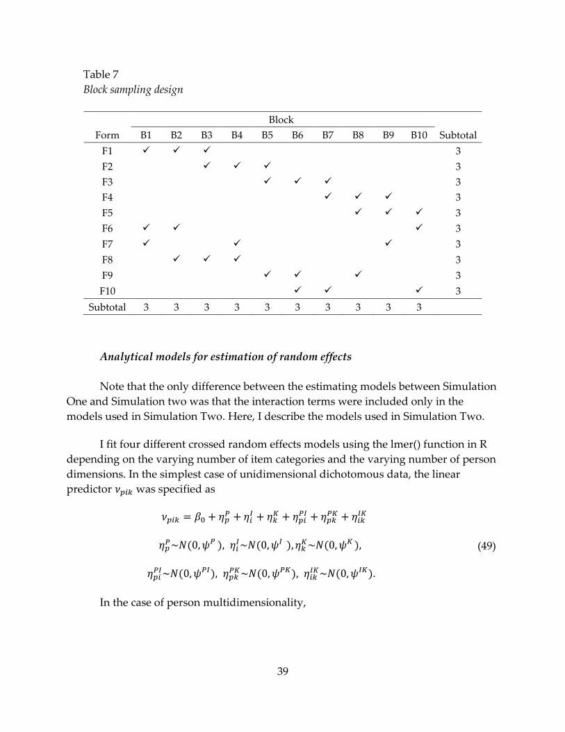
39

Table 7

Block sampling design

Block

Form B1 B2 B3 B4 B5 B6 B7 B8 B9 B10 Subtotal

F1 3

F2 3

F3 3

F4 3

F5 3

F6 3

F7 3

F8 3

F9 3

F10 3

Subtotal 3 3 3 3 3 3 3 3 3 3

Analytical models for estimation of random effects

Note that the only difference between the estimating models between Simulation

One and Simulation two was that the interaction terms were included only in the

models used in Simulation Two. Here, I describe the models used in Simulation Two.

I fit four different crossed random effects models using the lmer() function in R

depending on the varying number of item categories and the varying number of person

dimensions. In the simplest case of unidimensional dichotomous data, the linear

predictor was specified as

.

(49)

In the case of person multidimensionality,

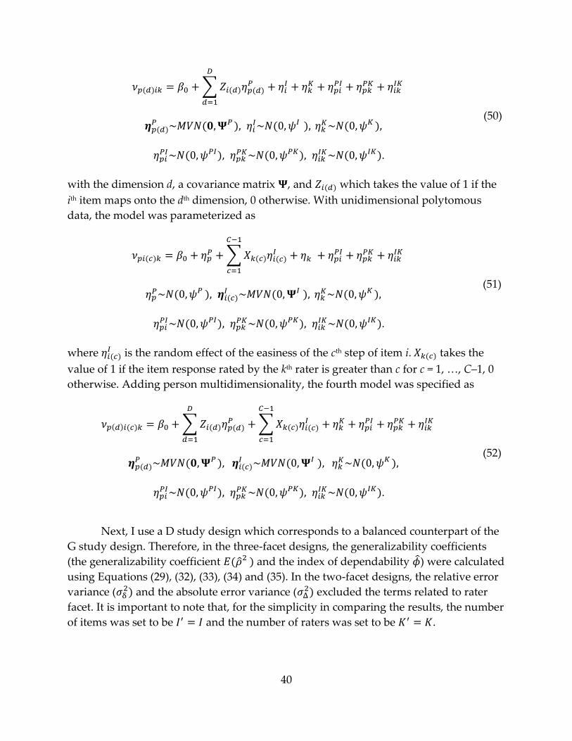
40

∑

.

(50)

with the dimension d, a covariance matrix , and which takes the value of 1 if the

ith item maps onto the dth dimension, 0 otherwise. With unidimensional polytomous

data, the model was parameterized as

∑

.

(51)

where is the random effect of the easiness of the cth step of item i. takes the

value of 1 if the item response rated by the kth rater is greater than c for c = 1, …, C–1, 0

otherwise. Adding person multidimensionality, the fourth model was specified as

∑

∑

.

(52)

Next, I use a D study design which corresponds to a balanced counterpart of the

G study design. Therefore, in the three-facet designs, the generalizability coefficients

(the generalizability coefficient and the index of dependability ) were calculated

using Equations (29), (32), (33), (34) and (35). In the two-facet designs, the relative error

variance ( and the absolute error variance (

excluded the terms related to rater

facet. It is important to note that, for the simplicity in comparing the results, the number

of items was set to be and the number of raters was set to be .

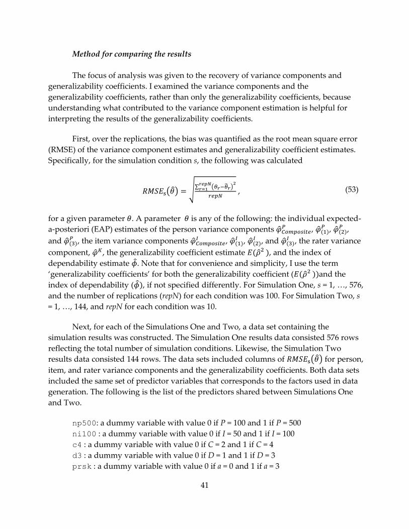
41

Method for comparing the results

The focus of analysis was given to the recovery of variance components and

generalizability coefficients. I examined the variance components and the

generalizability coefficients, rather than only the generalizability coefficients, because

understanding what contributed to the variance component estimation is helpful for

interpreting the results of the generalizability coefficients.

First, over the replications, the bias was quantified as the root mean square error

(RMSE) of the variance component estimates and generalizability coefficient estimates.

Specifically, for the simulation condition s, the following was calculated

( ) √∑ ( )

, (53)

for a given parameter . A parameter is any of the following: the individual expected-

a-posteriori (EAP) estimates of the person variance components ,

, ,

and , the item variance components

, ,

, and , the rater variance

component, , the generalizability coefficient estimate , and the index of

dependability estimate . Note that for convenience and simplicity, I use the term

‘generalizability coefficients’ for both the generalizability coefficient ( and the

index of dependability ( , if not specified differently. For Simulation One, s = 1, …, 576,

and the number of replications (repN) for each condition was 100. For Simulation Two, s

= 1, …, 144, and repN for each condition was 10.

Next, for each of the Simulations One and Two, a data set containing the

simulation results was constructed. The Simulation One results data consisted 576 rows

reflecting the total number of simulation conditions. Likewise, the Simulation Two

results data consisted 144 rows. The data sets included columns of ( ) for person,

item, and rater variance components and the generalizability coefficients. Both data sets

included the same set of predictor variables that corresponds to the factors used in data

generation. The following is the list of the predictors shared between Simulations One

and Two.

np500: a dummy variable with value 0 if P = 100 and 1 if P = 500

ni100 : a dummy variable with value 0 if I = 50 and 1 if I = 100

c4 : a dummy variable with value 0 if C = 2 and 1 if C = 4

d3 : a dummy variable with value 0 if D = 1 and 1 if D = 3

prsk : a dummy variable with value 0 if a = 0 and 1 if a = 3

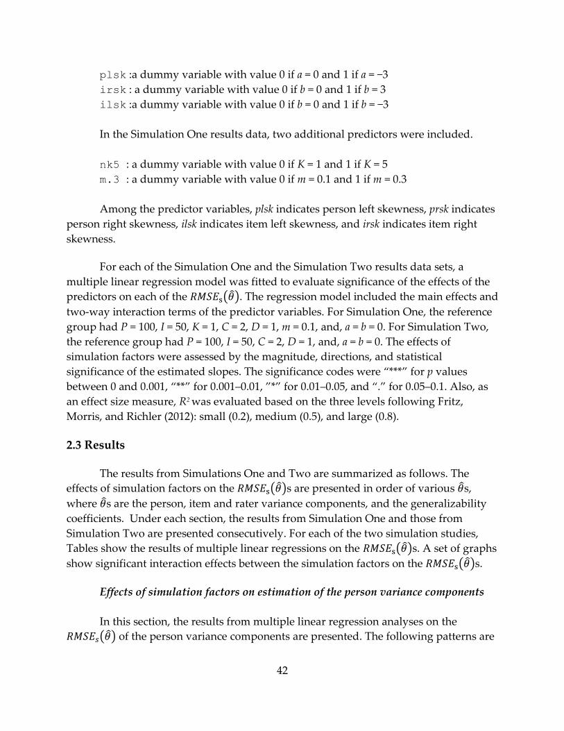
42

plsk :a dummy variable with value 0 if a = 0 and 1 if a = −3

irsk : a dummy variable with value 0 if b = 0 and 1 if b = 3

ilsk :a dummy variable with value 0 if b = 0 and 1 if b = −3

In the Simulation One results data, two additional predictors were included.

nk5 : a dummy variable with value 0 if K = 1 and 1 if K = 5

m.3 : a dummy variable with value 0 if m = 0.1 and 1 if m = 0.3

Among the predictor variables, plsk indicates person left skewness, prsk indicates

person right skewness, ilsk indicates item left skewness, and irsk indicates item right

skewness.

For each of the Simulation One and the Simulation Two results data sets, a

multiple linear regression model was fitted to evaluate significance of the effects of the

predictors on each of the ( ). The regression model included the main effects and

two-way interaction terms of the predictor variables. For Simulation One, the reference

group had P = 100, I = 50, K = 1, C = 2, D = 1, m = 0.1, and, a = b = 0. For Simulation Two,

the reference group had P = 100, I = 50, C = 2, D = 1, and, a = b = 0. The effects of

simulation factors were assessed by the magnitude, directions, and statistical

significance of the estimated slopes. The significance codes were “***” for p values

between 0 and 0.001, “**” for 0.001–0.01, ”*” for 0.01–0.05, and “.” for 0.05–0.1. Also, as

an effect size measure, R2 was evaluated based on the three levels following Fritz,

Morris, and Richler (2012): small (0.2), medium (0.5), and large (0.8).

2.3 Results

The results from Simulations One and Two are summarized as follows. The

effects of simulation factors on the ( )s are presented in order of various s,

where s are the person, item and rater variance components, and the generalizability

coefficients. Under each section, the results from Simulation One and those from

Simulation Two are presented consecutively. For each of the two simulation studies,

Tables show the results of multiple linear regressions on the ( )s. A set of graphs

show significant interaction effects between the simulation factors on the ( )s.

Effects of simulation factors on estimation of the person variance components

In this section, the results from multiple linear regression analyses on the

( ) of the person variance components are presented. The following patterns are

43

expected to be seen in the regression results in Tables 8, 9 and 10. First, when other

variables are consistent, a larger number of students will increase the accuracy in

estimation of the person variance components. Second, more person dimensions means

less number of items because the total number of items are divided by the number of

dimensions. Thus, more dimensions will decrease accuracy in estimation of the

composite person variance component estimates. Third, given the same conditions, a

greater number of items will increase the accuracy in estimation of person variance

components. On the other hand, having more raters does not mean having more data

because multiple raters are assigned to the subgroup of items to rate. Thus, a greater

number of raters will decrease the accuracy in estimation of person variance

components. Fourth, skewness in person generating distribution will decrease the

accuracy in estimation of the person variance components thus increase the ( )s

of person variance components.

Simulation One. Table 8 and 9 show four sets of results from multiple linear

regression analyses on the ( ) of the person variance components from

Simulation One. Note that the first set of columns (CVP) includes both the results for

the ( )s of the person variance component estimates in the case of

unidimensionality and those of the composite person variance component estimates in

the case of multidimensionality.

A summary of the results follows. The full regression models explained from 61.6% to

94.5% of the total variance of the ( )s of the person variance components. First, I

looked at the results for the composite person variance component (CVP) in the first

column. As expected, having a larger number of students significantly reduced

( )s of the person variance components. Next, holding other variables constant,

the composite person variance components were significantly further from the

generating values (0.285) than the person variance components, in the case of

multidimensionality. Regarding the skewness, the person skewness had significant

interaction effects with the number of students. With larger number of students, the

estimates were significantly closer to the generating values. When person distribution

was skewed to the right, having more students was less effective in reducing the

( )s (–0.163 – 0.080 + 0.100 = 0.143) than when it was normally distributed. With

added person left and right skewness, the increase in ( )s became greater (0.285

– 0.081 + 1.334 = 1.538, 0.285 – 0.080 + 1.325 = 1.530). Lastly, having a greater number of

items and raters decreased the ( )s, but the effects were not statistically

significant. It is an interesting finding that, although the item and rater effects are

crossed with persons, the accuracy of the person variance components depends on the

characteristics of persons, but not significantly on the item and rater characteristics.

44

Table 8

Simulation One: Regressions of the ( ) of person variance components

on simulation factors

CVP R2 =0.9454 D1 R2 =0.6156 D2 R2 =0.7253 D3 R2 =0.6609

Estimate SE

Estimate SE

Estimate SE

Estimate SE

(Intercept) 0.186 0.056 ** 0.222 0.051 *** 0.318 0.051 *** 0.273 0.056 ***

np500 -0.163 0.049 *** -0.119 0.046 * -0.185 0.046 *** -0.123 0.051 *

ni100 -0.017 0.049

0.058 0.046

0.012 0.046

-0.033 0.051

c4 -0.046 0.049

-0.008 0.046

-0.023 0.046

-0.023 0.051

d3 0.285 0.049 ***

nk5 -0.009 0.049

0.065 0.046

-0.047 0.046

0.005 0.051

m.3 -0.010 0.049

0.013 0.046

-0.048 0.046

0.021 0.051

plsk -0.081 0.056

0.261 0.053 *** 0.286 0.053 *** 0.358 0.058 ***

prsk -0.080 0.056

0.267 0.053 *** 0.287 0.053 *** 0.375 0.058 ***

ilsk 0.009 0.056

0.012 0.053

-0.106 0.053 * 0.004 0.058

irsk 0.032 0.056

0.046 0.053

-0.018 0.053

0.027 0.058

np500:ni100 0.022 0.031

0.014 0.031

-0.008 0.031

0.043 0.034

np500:c4 0.055 0.031 . 0.026 0.031

0.003 0.031

0.042 0.034

np500:d3 -0.003 0.031

np500:nk5 0.043 0.031

0.016 0.031

0.030 0.031

0.043 0.034

np500:m.3 -0.004 0.031

-0.035 0.031

-0.022 0.031

0.011 0.034

np500:plsk 0.055 0.038

0.087 0.038 * 0.163 0.038 *** -0.017 0.041

np500:prsk 0.100 0.038 ** 0.120 0.038 ** 0.200 0.038 *** -0.004 0.041

np500:ilsk 0.018 0.038

0.036 0.038

0.064 0.038 . 0.018 0.041

np500:irsk 0.001 0.038

0.024 0.038

0.011 0.038

0.005 0.041

ni100:c4 0.004 0.031

-0.055 0.031 . -0.011 0.031

0.009 0.034

ni100:d3 0.025 0.031

ni100:nk5 0.028 0.031

-0.045 0.031

0.007 0.031

0.048 0.034

ni100:m.3 -0.031 0.031

-0.002 0.031

-0.011 0.031

-0.028 0.034

ni100:plsk 0.008 0.038

0.015 0.038

0.022 0.038

-0.003 0.041

ni100:prsk -0.013 0.038

-0.013 0.038

0.024 0.038

-0.032 0.041

ni100:ilsk 0.042 0.038

0.023 0.038

0.013 0.038

0.023 0.041

ni100:irsk -0.014 0.038

-0.009 0.038

-0.023 0.038

-0.032 0.041

c4:d3 0.010 0.031

c4:nk5 0.043 0.031

0.056 0.031 . 0.018 0.031

0.005 0.034

c4:m.3 -0.013 0.031

-0.030 0.031

0.026 0.031

0.008 0.034

c4:plsk -0.014 0.038

0.032 0.038

-0.032 0.038

-0.016 0.041

c4:prsk 0.036 0.038

0.080 0.038 * -0.033 0.038

0.038 0.041

c4:ilsk -0.013 0.038

-0.084 0.038 * 0.045 0.038

-0.018 0.041

c4:irsk -0.013 0.038

-0.013 0.038

0.007 0.038

-0.002 0.041

d3:nk5 -0.046 0.031

d3:m.3 0.038 0.031

d3:plsk 1.334 0.038 ***

d3:prsk 1.325 0.038 ***

d3:ilsk -0.020 0.038

d3:irsk -0.005 0.038

nk5:m.3 -0.008 0.031

-0.029 0.031

0.005 0.031

-0.055 0.034

nk5:plsk -0.047 0.038

-0.091 0.038 * -0.001 0.038

-0.038 0.041

nk5:prsk -0.026 0.038

-0.103 0.038 ** -0.005 0.038

0.007 0.041

nk5:ilsk -0.045 0.038

-0.019 0.038

0.020 0.038

-0.020 0.041

45

Table 9

Simulation One: Regressions of the ( ) of person variance components

on simulation factors (continued)

CVP R2 =0.9454 D1 R2 =0.6156 D2 R2 =0.7253 D3 R2 =0.6609

Estimate SE

Estimate SE

Estimate SE

Estimate SE

nk5:irsk -0.048 0.038

-0.016 0.038

-0.036 0.038

-0.038 0.041

m.3:plsk 0.068 0.038 . 0.068 0.038 . 0.029 0.038

0.089 0.041 *

m.3:prsk 0.026 0.038

0.025 0.038

0.067 0.038 . 0.005 0.041

m.3:ilsk 0.007 0.038

0.029 0.038

0.017 0.038

-0.002 0.041

m.3:irsk -0.009 0.038

-0.015 0.038

0.040 0.038

-0.018 0.041

plsk:ilsk 0.015 0.046

0.013 0.046

0.028 0.046

0.005 0.051

plsk:irsk -0.004 0.046

-0.042 0.046

0.021 0.046

0.015 0.051

prsk:ilsk -0.077 0.046 . -0.046 0.046

-0.066 0.046

-0.012 0.051

prsk:irsk -0.013 0.046

-0.054 0.046

0.003 0.046

0.000 0.051

Next, the remaining three sets of columns show the results for the person ability

estimates for the three dimensions (D1, D2 and D3), in the case of multidimensionality.

Overall, the increase in the number of students decreased the gap between the

generating values and the estimated values (–0.119, –0.185, and –0.123) when all other

variables were consistent. The skewness in the distributions increased the gap

(0.261~0.375) given the same covariates as expected. The effects slightly decreased with

the interaction with the number of students (for np500:plsk, –0.119 + 0.261 + 0.087 =

0.229, –0.185 + 0.286 + 0.163 = 0.264, –0.123 + 0.358 – 0.017 = 0.252, and for np500:prsk, –

0.119 + 0.267 + 0.120 = 0.268, –0.185 + 0.287 + 0.200 = 0.302, –0.123 + 0.375 –0.004 = 0.248).

Again, against my expectation, the main effects of the number of raters and the number

of item categories were not significant for any dimension. Meanwhile, the interactions

between the number of raters and the person skewness, as well as the interactions

between the number of item categories and the person skewness were significant for

Dimension 1. Having more raters in the condition with person skewness slightly

decreased the ( )s for the person variance components. However, given the

overall significant effects of person skewness and overall insignificant effects of having

more items and raters on the ( )s, it is reasonable to assume that the significance

of the interaction effects are due to the significant main effects of skewness predictors.

Figure 5 visualizes the four significant interaction effects between the significant

main effects on the ( )s of person dimensions D1 and D2. The ( )s

decreased for all cases as the number of students increased, while the rates of decrease

were greater for the normal person distributions than for the skewed person

distributions.

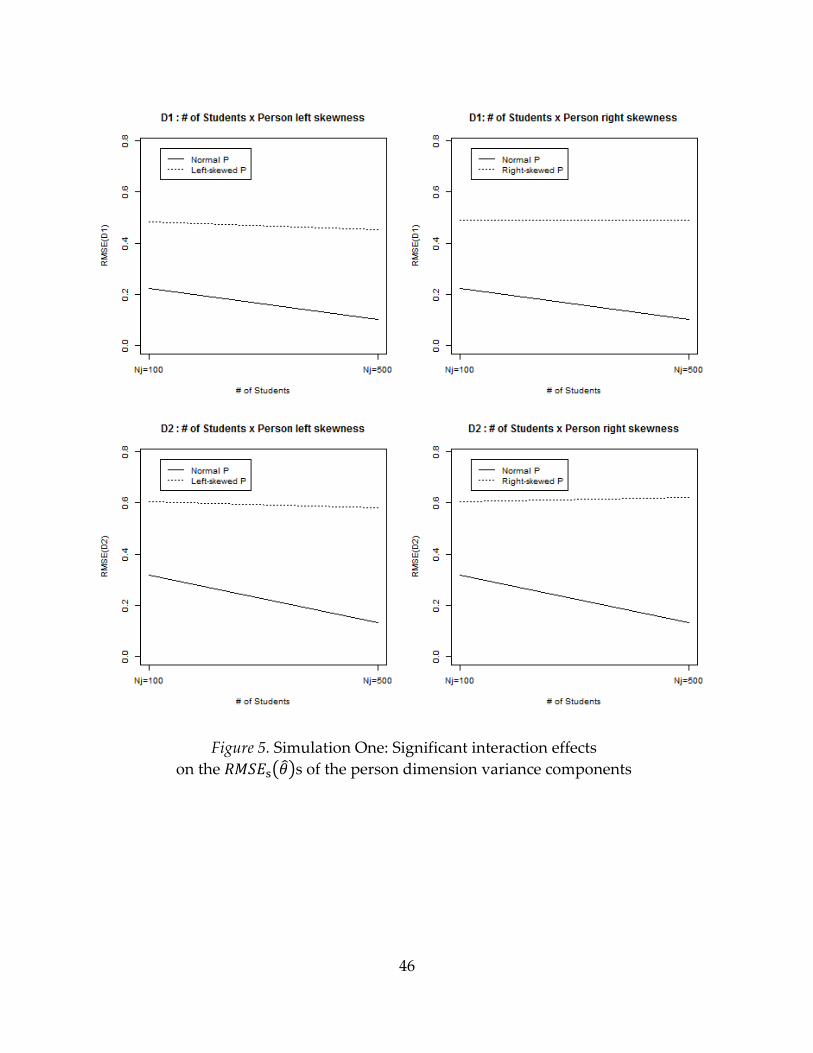
46

Figure 5. Simulation One: Significant interaction effects

on the ( )s of the person dimension variance components

47

Simulation Two. Table 10 shows four sets of results from multiple linear

regression analyses on the ( ) of the person variance components from

Simulation Two.

Some results were similar to the results from Simulation One. As expected,

having a greater student sample size decreased the ( )s of the person variance

components. Also, the effect of multidimensionality was to increase the ( )s of

the composite person variance component. The skewness in the person distributions

significantly increased the ( )s of the person variance components.

Unlike the results from Simulation One, the composite person variance

component estimates became less accurate due to the number of item categories as well

as the number of person dimensions. The number of item categories had significant

interaction effects with not only the number of person distributions, but also with the

skewness in person distributions. However, with added person left and right skewness,

the ( )s were reduced (0.080 – 0.102 – 0.094 = –0.116, 0.080 – 0.071 – 0.154 = –

0.145).

Compared to Simulation One, the adjusted R-squared values increased for all the

person variance components (CVP: 0.9454 to 0.9921, D1: 0.6156 to 0.8638, D2: 0.7253 to

0.9964, D3: 0.6609 to 0.8876), indicating that the regression model explained the variance

in the ( )s of the person variance components when the results were based on

the three-facet model with interaction terms. Note that the regression model used here

is simpler than the regression model used in Simulation One, because this model does

not have two predictors (nk5 and m.3).

Figure 6 visualizes the six significant interaction effects between the significant

main effects on the ( )s of the composite person variance component. Most

dramatically, the ( )s increased for all cases with more item categories and more

dimensions. From unidimensionality to multidimensionality, the degrees of increase in

the ( )s were greater when the person distributions were skewed. Among the

simulation factors shown in Figure 6, the number of dimensions showed the largest

effect size, depicted by a greater gap between either the locations or the slopes of D = 1

and D = 3.

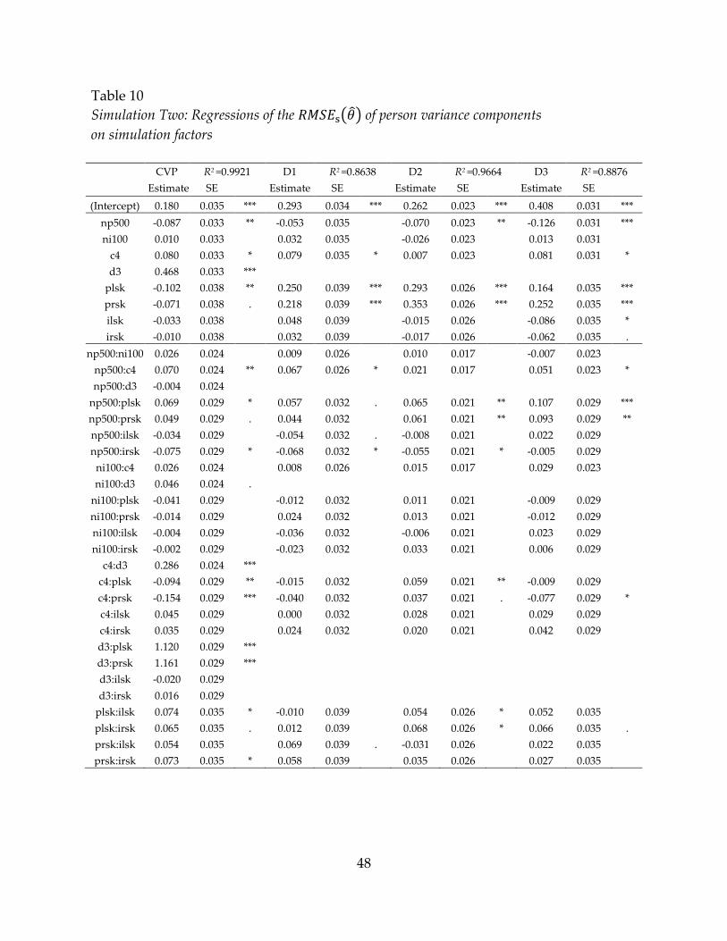
48

Table 10

Simulation Two: Regressions of the ( ) of person variance components

on simulation factors

CVP R2 =0.9921 D1 R2 =0.8638 D2 R2 =0.9664 D3 R2 =0.8876

Estimate SE

Estimate SE

Estimate SE

Estimate SE

(Intercept) 0.180 0.035 *** 0.293 0.034 *** 0.262 0.023 *** 0.408 0.031 ***

np500 -0.087 0.033 ** -0.053 0.035 -0.070 0.023 ** -0.126 0.031 ***

ni100 0.010 0.033 0.032 0.035 -0.026 0.023 0.013 0.031

c4 0.080 0.033 * 0.079 0.035 * 0.007 0.023 0.081 0.031 *

d3 0.468 0.033 ***

plsk -0.102 0.038 ** 0.250 0.039 *** 0.293 0.026 *** 0.164 0.035 ***

prsk -0.071 0.038 . 0.218 0.039 *** 0.353 0.026 *** 0.252 0.035 ***

ilsk -0.033 0.038 0.048 0.039 -0.015 0.026 -0.086 0.035 *

irsk -0.010 0.038 0.032 0.039 -0.017 0.026 -0.062 0.035 .

np500:ni100 0.026 0.024 0.009 0.026 0.010 0.017 -0.007 0.023

np500:c4 0.070 0.024 ** 0.067 0.026 * 0.021 0.017 0.051 0.023 *

np500:d3 -0.004 0.024

np500:plsk 0.069 0.029 * 0.057 0.032 . 0.065 0.021 ** 0.107 0.029 ***

np500:prsk 0.049 0.029 . 0.044 0.032 0.061 0.021 ** 0.093 0.029 **

np500:ilsk -0.034 0.029 -0.054 0.032 . -0.008 0.021 0.022 0.029

np500:irsk -0.075 0.029 * -0.068 0.032 * -0.055 0.021 * -0.005 0.029

ni100:c4 0.026 0.024 0.008 0.026 0.015 0.017 0.029 0.023

ni100:d3 0.046 0.024 .

ni100:plsk -0.041 0.029 -0.012 0.032 0.011 0.021 -0.009 0.029

ni100:prsk -0.014 0.029 0.024 0.032 0.013 0.021 -0.012 0.029

ni100:ilsk -0.004 0.029 -0.036 0.032 -0.006 0.021 0.023 0.029

ni100:irsk -0.002 0.029 -0.023 0.032 0.033 0.021 0.006 0.029

c4:d3 0.286 0.024 ***

c4:plsk -0.094 0.029 ** -0.015 0.032 0.059 0.021 ** -0.009 0.029

c4:prsk -0.154 0.029 *** -0.040 0.032 0.037 0.021 . -0.077 0.029 *

c4:ilsk 0.045 0.029 0.000 0.032 0.028 0.021 0.029 0.029

c4:irsk 0.035 0.029 0.024 0.032 0.020 0.021 0.042 0.029

d3:plsk 1.120 0.029 ***

d3:prsk 1.161 0.029 ***

d3:ilsk -0.020 0.029

d3:irsk 0.016 0.029

plsk:ilsk 0.074 0.035 * -0.010 0.039 0.054 0.026 * 0.052 0.035

plsk:irsk 0.065 0.035 . 0.012 0.039 0.068 0.026 * 0.066 0.035 .

prsk:ilsk 0.054 0.035 0.069 0.039 . -0.031 0.026 0.022 0.035

prsk:irsk 0.073 0.035 * 0.058 0.039 0.035 0.026 0.027 0.035

49

Figure 6. Simulation Two: Significant interaction effects

on the ( )s of the person variance components

50

Effects of simulation factors on estimation of the item variance components

Tables 11, 12, and 13 show the results from multiple linear regression analyses on

the ( ) of the item variance components. Several patterns are expected to be

seen. First, a greater number of items should increase the accuracy in estimation of the

item variance components, thus decreasing the ( )s. Second, a greater number of

item categories should not affect the ( )s of the composite item variance

estimates because the available data (i.e., the number of students) for the whole items

are the same regardless of the item categories. Third, item skewness should increase the

( )s of the item variance component estimates. Fourth, the number of persons

and raters should not have significant effects on the accuracy in estimation of the item

variance components.

Simulation One. The results from multiple linear regression analyses on the

( ) of the item variance components from Simulation One are presented in

Tables 11 and 12. Note that the first set of columns (CVI) contains both the results for

the ( )s of the item variance component estimates in the case of dichotomous

data, as well as the results for the ( )s of the composite item variance component

estimates in the case of polytomous data.

The results are as follows. The regression models with all covariates explained

from 14.8% to 32.6% of the total variance in ( )s of the item variance

components. In terms of effect size, the adjusted R-squared values are smaller than

medium (0.5). First, I looked at the first set of columns for the composite item variance

components (CVI). Overall, as expected, having more items (–0.073) and item skewness

(–0.087 and –0.105) decreased the gap between the generating values and the estimated

values. Also as expected, having more item categories did not affect (0.000) the

precision of estimates for the CVIs for the dichotomous data, as compared to that for the

polytomous data. The person and rater numbers did not affect the ( )s for the

item variance components.

There were several main effects for which significance turned into insignificance

by interaction with other variables. Specifically, with more categories, the amount of

decrease in the ( ) by item skewness was reduced (0.000 – 0.087 + 0.057 = – 0.030,

0.000 – 0.105 + 0.060 = –0.045). While the main effects of the number of raters and person

skewness increased the ( )s of item variance components, the interaction effects

between them decreased the gap between the generating values and the estimated

values. However, it seems reasonable to consider these changes less important because

the values only move around zero on the logit scale.

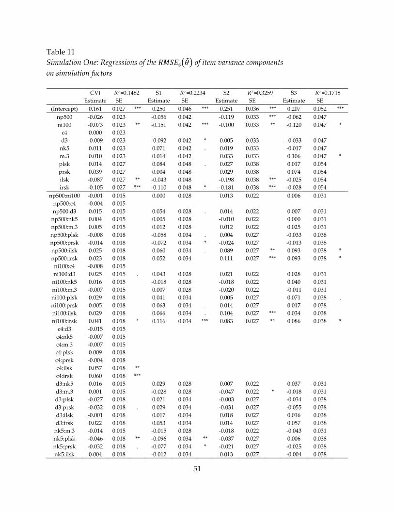
51

Table 11

Simulation One: Regressions of the ( ) of item variance components

on simulation factors

CVI R2 =0.1482 S1 R2 =0.2234 S2 R2 =0.3259 S3 R2 =0.1718

Estimate SE

Estimate SE

Estimate SE

Estimate SE

(Intercept) 0.161 0.027 *** 0.250 0.046 *** 0.251 0.036 *** 0.207 0.052 ***

np500 -0.026 0.023

-0.056 0.042

-0.119 0.033 *** -0.062 0.047

ni100 -0.073 0.023 ** -0.151 0.042 *** -0.100 0.033 ** -0.120 0.047 *

c4 0.000 0.023

d3 -0.009 0.023

-0.092 0.042 * 0.005 0.033

-0.033 0.047

nk5 0.011 0.023

0.071 0.042 . 0.019 0.033

-0.017 0.047

m.3 0.010 0.023

0.014 0.042

0.033 0.033

0.106 0.047 *

plsk 0.014 0.027

0.084 0.048 . 0.027 0.038

0.017 0.054

prsk 0.039 0.027

0.004 0.048

0.029 0.038

0.074 0.054

ilsk -0.087 0.027 ** -0.043 0.048

-0.198 0.038 *** -0.025 0.054

irsk -0.105 0.027 *** -0.110 0.048 * -0.181 0.038 *** -0.028 0.054

np500:ni100 -0.001 0.015

0.000 0.028

0.013 0.022

0.006 0.031

np500:c4 -0.004 0.015

np500:d3 0.015 0.015

0.054 0.028 . 0.014 0.022

0.007 0.031

np500:nk5 0.004 0.015

0.005 0.028

-0.010 0.022

0.000 0.031

np500:m.3 0.005 0.015

0.012 0.028

0.012 0.022

0.025 0.031

np500:plsk -0.008 0.018

-0.058 0.034 . 0.004 0.027

-0.033 0.038

np500:prsk -0.014 0.018

-0.072 0.034 * -0.024 0.027

-0.013 0.038

np500:ilsk 0.025 0.018

0.060 0.034 . 0.089 0.027 ** 0.093 0.038 *

np500:irsk 0.023 0.018

0.052 0.034

0.111 0.027 *** 0.093 0.038 *

ni100:c4 -0.008 0.015

ni100:d3 0.025 0.015 . 0.043 0.028

0.021 0.022

0.028 0.031

ni100:nk5 0.016 0.015

-0.018 0.028

-0.018 0.022

0.040 0.031

ni100:m.3 -0.007 0.015

0.007 0.028

-0.020 0.022

-0.011 0.031

ni100:plsk 0.029 0.018

0.041 0.034

0.005 0.027

0.071 0.038 .

ni100:prsk 0.005 0.018

0.063 0.034 . 0.014 0.027

0.017 0.038

ni100:ilsk 0.029 0.018

0.066 0.034 . 0.104 0.027 *** 0.034 0.038

ni100:irsk 0.041 0.018 * 0.116 0.034 *** 0.083 0.027 ** 0.086 0.038 *

c4:d3 -0.015 0.015

c4:nk5 -0.007 0.015

c4:m.3 -0.007 0.015

c4:plsk 0.009 0.018

c4:prsk -0.004 0.018

c4:ilsk 0.057 0.018 **

c4:irsk 0.060 0.018 ***

d3:nk5 0.016 0.015

0.029 0.028

0.007 0.022

0.037 0.031

d3:m.3 0.001 0.015

-0.028 0.028

-0.047 0.022 * -0.018 0.031

d3:plsk -0.027 0.018

0.021 0.034

-0.003 0.027

-0.034 0.038

d3:prsk -0.032 0.018 . 0.029 0.034

-0.031 0.027

-0.055 0.038

d3:ilsk -0.001 0.018

0.017 0.034

0.018 0.027

0.016 0.038

d3:irsk 0.022 0.018

0.053 0.034

0.014 0.027

0.057 0.038

nk5:m.3 -0.014 0.015

-0.015 0.028

-0.018 0.022

-0.043 0.031

nk5:plsk -0.046 0.018 ** -0.096 0.034 ** -0.037 0.027

0.006 0.038

nk5:prsk -0.032 0.018 . -0.077 0.034 * -0.021 0.027

-0.025 0.038

nk5:ilsk 0.004 0.018

-0.012 0.034

0.013 0.027

-0.004 0.038

52

Table 12

Simulation One: Regressions of the ( ) of item variance components

on simulation factors (continued)

CVI R2 =0.1482 S1 R2 =0.2234 S2 R2 =0.3259 S3 R2 =0.1718

Estimate SE

Estimate SE

Estimate SE

Estimate SE

nk5:irsk 0.018 0.018 -0.004 0.034 0.009 0.027 0.026 0.038

m.3:plsk 0.010 0.018

-0.038 0.034

-0.015 0.027

-0.032 0.038

m.3:prsk 0.016 0.018

0.021 0.034

-0.011 0.027

-0.030 0.038

m.3:ilsk 0.006 0.018

0.010 0.034

0.007 0.027

-0.030 0.038

m.3:irsk -0.015 0.018

-0.047 0.034

0.016 0.027

-0.077 0.038 *

plsk:ilsk -0.003 0.022

-0.065 0.042

0.012 0.033

0.034 0.047

plsk:irsk 0.015 0.022

0.002 0.042

-0.016 0.033

0.002 0.047

prsk:ilsk -0.004 0.022

-0.007 0.042

0.026 0.033

-0.013 0.047

prsk:irsk -0.010 0.022

0.035 0.042

-0.006 0.033

-0.048 0.047

Figure 7 depicts the significant interaction effects between the statistically

significant main effects on the ( )s of the composite item variance component

(CVI). The effect was very small on the logit scale (less than 0.05 logit). As the number

of items or students gets greater, the effects of skewness and missingness in data

become smaller.

Next, the results on the step variance components are shown in the remaining

three sets of columns (S1, S2 and S3). For polytomous data, having a larger number of

items significantly reduced the ( )s (–0.151, –0.100, and –0.120), as expected.

Item skewness also significantly reduced the ( )s (–0.043, –0.198, –0.025 for left-

skewness and –0.110, –0.181, –0.028 for right-skewness). Interestingly, having a larger

number of students also reduced the ( )s (–0.056, –0.119, –0.062), but the effects

significantly changed with item skewness (–0.056 – 0.043 + 0.060 = –0.039, –0.119 – 0.198

+ 0.089 = –0.228, –0.062 – 0.025 + 0.093 = 0.006 for left-skewness, –0.056 – 0.110 + 0.052 = –

0.114, –0.119 – 0.181 + 0.111 = –0.189, –0.062 – 0.028 + 0.093 = 0.003 for right-skewness).

The number of items had significant interaction effects with item skewness that reduced

the amount of decrease in ( )s (–0.151 – 0.043 + 0.066 = –0.128, –0.100 – 0.198 +

0.104 = –0.194, –0.120 – 0.025 + 0.034 = –0.111 for left-skewness, –0.151 – 0.110 + 0.116 = –

0.145, –0.100 – 0.181 + 0.083 = –0.198, –0.120 – 0.028 + 0.086 = –0.062 for right-skewness).

Overall, the ( )s became close to zero or decreased more under interaction with

item skewness.

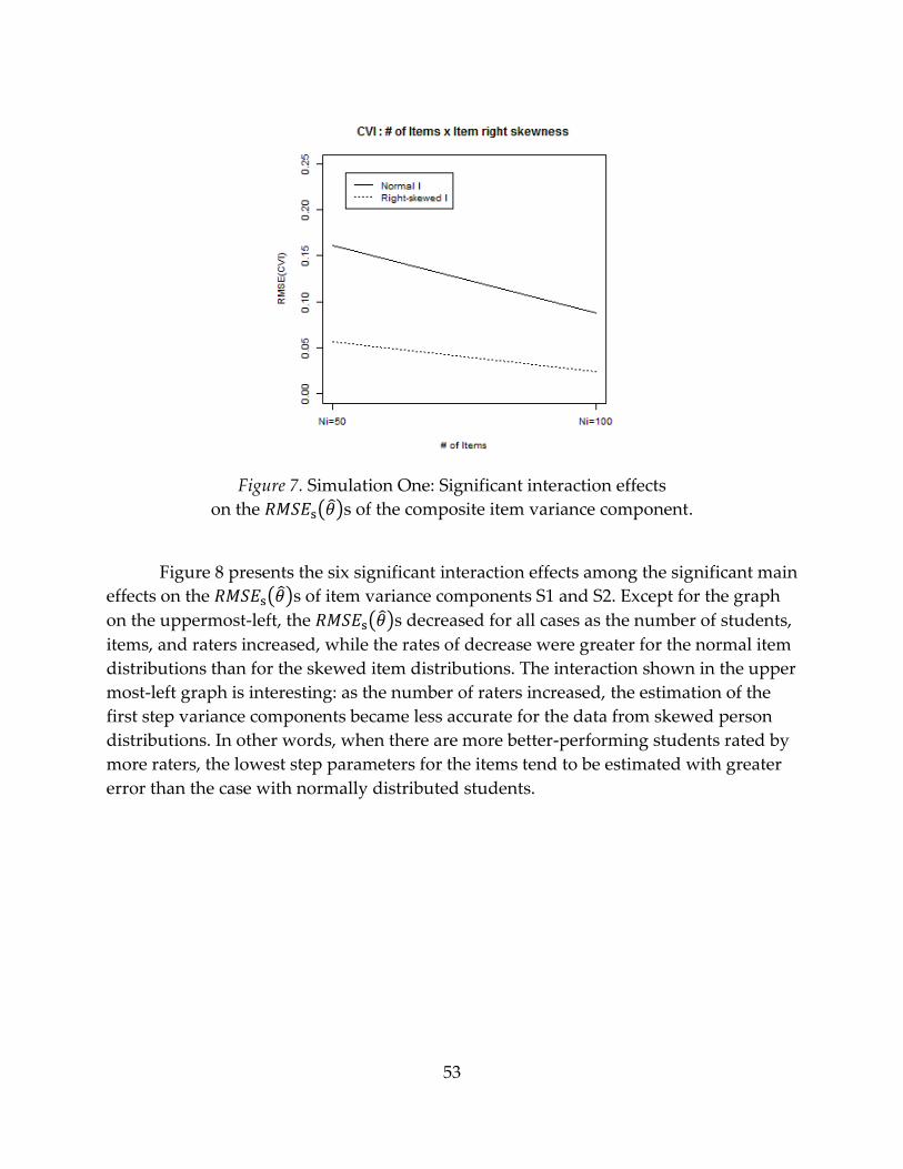
53

Figure 7. Simulation One: Significant interaction effects

on the ( )s of the composite item variance component.

Figure 8 presents the six significant interaction effects among the significant main

effects on the ( )s of item variance components S1 and S2. Except for the graph

on the uppermost-left, the ( )s decreased for all cases as the number of students,

items, and raters increased, while the rates of decrease were greater for the normal item

distributions than for the skewed item distributions. The interaction shown in the upper

most-left graph is interesting: as the number of raters increased, the estimation of the

first step variance components became less accurate for the data from skewed person

distributions. In other words, when there are more better-performing students rated by

more raters, the lowest step parameters for the items tend to be estimated with greater

error than the case with normally distributed students.

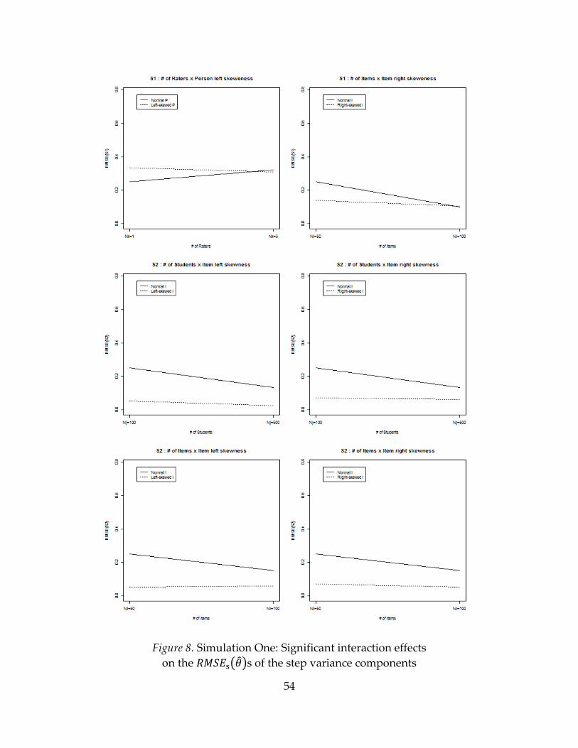
54

Figure 8. Simulation One: Significant interaction effects

on the ( )s of the step variance components

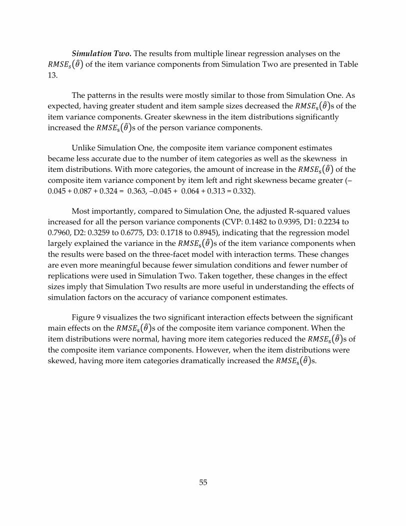
55

Simulation Two. The results from multiple linear regression analyses on the

( ) of the item variance components from Simulation Two are presented in Table

13.

The patterns in the results were mostly similar to those from Simulation One. As

expected, having greater student and item sample sizes decreased the ( )s of the

item variance components. Greater skewness in the item distributions significantly

increased the ( )s of the person variance components.

Unlike Simulation One, the composite item variance component estimates

became less accurate due to the number of item categories as well as the skewness in

item distributions. With more categories, the amount of increase in the ( ) of the

composite item variance component by item left and right skewness became greater (–

0.045 + 0.087 + 0.324 = 0.363, –0.045 + 0.064 + 0.313 = 0.332).

Most importantly, compared to Simulation One, the adjusted R-squared values

increased for all the person variance components (CVP: 0.1482 to 0.9395, D1: 0.2234 to

0.7960, D2: 0.3259 to 0.6775, D3: 0.1718 to 0.8945), indicating that the regression model

largely explained the variance in the ( )s of the item variance components when

the results were based on the three-facet model with interaction terms. These changes

are even more meaningful because fewer simulation conditions and fewer number of

replications were used in Simulation Two. Taken together, these changes in the effect

sizes imply that Simulation Two results are more useful in understanding the effects of

simulation factors on the accuracy of variance component estimates.

Figure 9 visualizes the two significant interaction effects between the significant

main effects on the ( )s of the composite item variance component. When the

item distributions were normal, having more item categories reduced the ( )s of

the composite item variance components. However, when the item distributions were

skewed, having more item categories dramatically increased the ( )s.

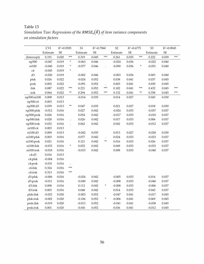
56

Table 13

Simulation Two: Regressions of the ( ) of item variance components

on simulation factors

CVI R2 =0.9395 S1 R2 =0.7960 S2 R2 =0.6775 S3 R2 =0.8945

Estimate SE

Estimate SE

Estimate SE

Estimate SE

(Intercept) 0.191 0.020 *** 0.319 0.045 *** 0.261 0.035 *** 0.222 0.039 ***

np500 -0.047 0.019 * -0.063 0.046

-0.024 0.036

-0.022 0.040

ni100 -0.040 0.019 * -0.077 0.046 . -0.090 0.036 * -0.051 0.040

c4 -0.045 0.019 *

d3 -0.020 0.019

-0.002 0.046

-0.003 0.036

0.003 0.040

plsk 0.026 0.022

-0.024 0.052

0.038 0.041

0.037 0.045

prsk 0.002 0.022

-0.091 0.052 . 0.003 0.041

0.030 0.045

ilsk 0.087 0.022 *** 0.221 0.052 *** 0.182 0.041 *** 0.432 0.045 ***

irsk 0.064 0.022 ** 0.294 0.052 *** 0.132 0.041 ** 0.358 0.045 ***

np500:ni100 0.008 0.013

-0.014 0.035

0.014 0.027

0.045 0.030

np500:c4 0.003 0.013

np500:d3 0.039 0.013 ** 0.047 0.035

0.021 0.027

0.018 0.030

np500:plsk -0.012 0.016

0.027 0.042

-0.024 0.033

-0.037 0.037

np500:prsk 0.026 0.016

0.054 0.042

-0.017 0.033

-0.010 0.037

np500:ilsk 0.028 0.016 . 0.026 0.042

0.017 0.033

0.006 0.037

np500:irsk 0.032 0.016 . 0.062 0.042

0.042 0.033

-0.012 0.037

ni100:c4 0.003 0.013

ni100:d3 0.009 0.013

-0.042 0.035

0.013 0.027

-0.028 0.030

ni100:plsk 0.003 0.016

0.077 0.042 . 0.024 0.033

-0.023 0.037

ni100:prsk 0.021 0.016

0.121 0.042 ** 0.016 0.033

0.026 0.037

ni100:ilsk -0.033 0.016 * 0.032 0.042

0.049 0.033

-0.033 0.037

ni100:irsk -0.018 0.016

-0.015 0.042

0.008 0.033

-0.040 0.037

c4:d3 0.016 0.013

c4:plsk -0.004 0.016

c4:prsk -0.031 0.016 .

c4:ilsk 0.324 0.016 ***

c4:irsk 0.313 0.016 ***

d3:plsk -0.006 0.016

-0.024 0.042

-0.005 0.033

0.014 0.037

d3:prsk -0.011 0.016

-0.049 0.042

-0.008 0.033

-0.040 0.037

d3:ilsk 0.008 0.016

0.112 0.042 * -0.008 0.033

-0.006 0.037

d3:irsk 0.003 0.016

0.048 0.042

0.014 0.033

0.043 0.037

plsk:ilsk -0.023 0.020

-0.003 0.052

-0.047 0.041

-0.017 0.045

plsk:irsk -0.002 0.020

-0.106 0.052 * -0.006 0.041

0.069 0.045

prsk:ilsk -0.019 0.020

-0.013 0.052

-0.041 0.041

-0.038 0.045

prsk:irsk 0.001 0.020

-0.041 0.052

0.036 0.041

-0.012 0.045

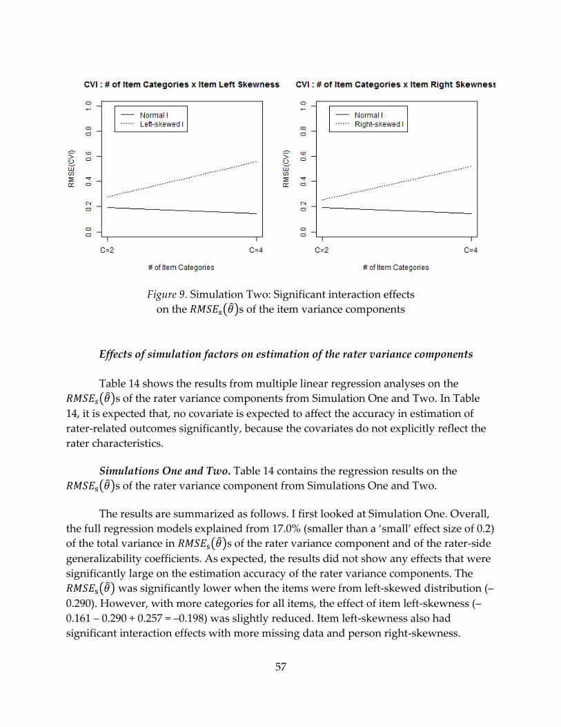
57

Figure 9. Simulation Two: Significant interaction effects

on the ( )s of the item variance components

Effects of simulation factors on estimation of the rater variance components

Table 14 shows the results from multiple linear regression analyses on the

( )s of the rater variance components from Simulation One and Two. In Table

14, it is expected that, no covariate is expected to affect the accuracy in estimation of

rater-related outcomes significantly, because the covariates do not explicitly reflect the

rater characteristics.

Simulations One and Two. Table 14 contains the regression results on the

( )s of the rater variance component from Simulations One and Two.

The results are summarized as follows. I first looked at Simulation One. Overall,

the full regression models explained from 17.0% (smaller than a ‘small’ effect size of 0.2)

of the total variance in ( )s of the rater variance component and of the rater-side

generalizability coefficients. As expected, the results did not show any effects that were

significantly large on the estimation accuracy of the rater variance components. The

( ) was significantly lower when the items were from left-skewed distribution (–

0.290). However, with more categories for all items, the effect of item left-skewness (–

0.161 – 0.290 + 0.257 = –0.198) was slightly reduced. Item left-skewness also had

significant interaction effects with more missing data and person right-skewness.

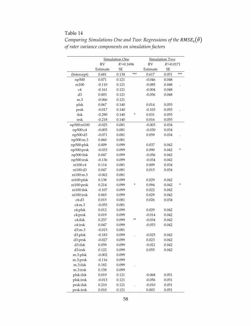
58

Table 14

Comparing Simulations One and Two: Regressions of the ( )

of rater variance components on simulation factors

Simulation One Simulation Two

RV R2=0.1696 RV R2=0.0171

Estimate SE

Estimate SE

(Intercept) 0.681 0.134 *** 0.617 0.051 ***

np500 0.071 0.121

-0.046 0.048

ni100 -0.110 0.121

-0.085 0.048 .

c4 -0.161 0.121

-0.004 0.048

d3 0.003 0.121

-0.056 0.048

m.3 -0.066 0.121

plsk 0.067 0.140

0.014 0.055

prsk -0.017 0.140

-0.103 0.055 .

ilsk -0.290 0.140 * 0.031 0.055

irsk -0.218 0.140

0.016 0.055

np500:ni100 -0.025 0.081

-0.003 0.034

np500:c4 -0.005 0.081

-0.030 0.034

np500:d3 -0.071 0.081

0.059 0.034 .

np500:m.3 0.060 0.081

np500:plsk 0.009 0.099

0.037 0.042

np500:prsk -0.033 0.099

0.090 0.042 *

np500:ilsk 0.047 0.099

-0.056 0.042

np500:irsk -0.136 0.099

-0.034 0.042

ni100:c4 0.114 0.081

0.009 0.034

ni100:d3 0.047 0.081

0.015 0.034

ni100:m.3 -0.062 0.081

ni100:plsk 0.138 0.099

0.029 0.042

ni100:prsk 0.214 0.099 * 0.094 0.042 *

ni100:ilsk -0.107 0.099

0.022 0.042

ni100:irsk 0.065 0.099

0.029 0.042

c4:d3 0.015 0.081

0.026 0.034

c4:m.3 -0.055 0.081

c4:plsk 0.012 0.099

0.029 0.042

c4:prsk 0.019 0.099

-0.014 0.042

c4:ilsk 0.257 0.099 ** -0.034 0.042

c4:irsk 0.047 0.099

-0.053 0.042

d3:m.3 -0.015 0.081

d3:plsk -0.183 0.099 . -0.025 0.042

d3:prsk -0.027 0.099

0.023 0.042

d3:ilsk 0.059 0.099

-0.021 0.042

d3:irsk 0.122 0.099

0.055 0.042

m.3:plsk -0.002 0.099

m.3:prsk -0.116 0.099

m.3:ilsk 0.182 0.099 .

m.3:irsk 0.158 0.099

plsk:ilsk 0.019 0.121

-0.068 0.051

plsk:irsk -0.013 0.121

-0.056 0.051

prsk:ilsk 0.210 0.121 . -0.010 0.051

prsk:irsk 0.010 0.121

0.003 0.051

59

In Simulation Two, the adjusted R-squared values significantly decreased

compared to Simulation One (0.1696 to 0.0171). The results did not show any significant

effects of the predictors on the estimation accuracy of the rater variance components.

All estimates fell below the absolute value of 0.103 (with SE 0.055). Considering both

the low R-squared value and the fact that I did not expect significant effects on rater

variance components, Simulation Two provides more effective results than Simulation

One.

Effects of simulation factors on estimation of the interactions between the facets

Table 15 shows the results from multiple linear regression analyses on the

( )s of the interaction variance components (person × item, person × rater, and

item × rater) from Simulation Two. Recall that Simulation One did not have interaction

terms in either generating or estimating model. It is expected that, if person facet is

included in the interaction term, the patterns of the results will be similar to the results

on the person variance components from Simulation Two. Likewise, if item facet is

included in the interaction term, the patterns of the results will be similar to the results

on the item variance components from Simulation Two, but less so when person facet is

also involved. Whether or not the rater facet is involved will not determine the patterns

in the results, because the accuracy of the rater variance component estimates was not

sensitive to the predictors in the regression model.

The regression models explained from 92.7% to 99.7% of the total variance of the

( )s of the interaction variance components. First, I looked at the results for the

person × item interaction variance component in the first set of columns. Noticeably,

having more item categories (0.736) and more items (0.198) increased the ( )s of

the person × item interaction variance component. The interaction effect between the

number of item categories and the number of items was also significant, but the effect of

more item categories was not reduced, but rather increased, by the interaction effect

(0.736 + 0.198 – 0.116 = 0.818). More importantly, the pattern in the results did not seem

to be similar to the results on the person or item variance components. For example, the

main effects of the skewness in the person distribution were not significant, as opposed

to what I found in the results on person variance components. Also, the main effects of

the skewness in the item distribution were not significant, as opposed to the results on

item variance components.

Next, similarly to the person × item interaction results, the ( )s of the

person × rater interaction variance component also increase with more item categories

(0.128). While more students decrease the ( )s (–0.055), the effect reverts via the

60

Table 15

Simulation Two: Regressions of the ( ) of the interaction variance

components on simulation factors

P×I R2 =0.9974 P×R R2 =0.9272 I×R R2 =0.9716

Estimate SE

Estimate SE

Estimate SE

(Intercept) 0.174 0.009 *** 0.122 0.013 *** 0.170 0.020 ***

np500 0.011 0.008

-0.055 0.012 *** -0.030 0.019

ni100 0.198 0.008 *** 0.013 0.012

0.016 0.019

c4 0.736 0.008 *** 0.128 0.012 *** 0.312 0.019 ***

d3 0.002 0.008

0.029 0.012 * 0.009 0.019

plsk 0.008 0.010

0.008 0.014

-0.010 0.021

prsk 0.017 0.010 . -0.017 0.014

-0.005 0.021

ilsk 0.002 0.010

0.007 0.014

0.144 0.021 ***

irsk 0.004 0.010

-0.004 0.014

0.173 0.021 ***

np500:ni100 0.002 0.006

0.017 0.008 * -0.007 0.013

np500:c4 0.004 0.006

0.038 0.008 *** -0.003 0.013

np500:d3 -0.003 0.006

-0.016 0.008 . 0.008 0.013

np500:plsk -0.015 0.007 * -0.003 0.010

0.019 0.016

np500:prsk -0.013 0.007 . -0.003 0.010

0.012 0.016

np500:ilsk -0.016 0.007 * 0.007 0.010

0.011 0.016

np500:irsk -0.014 0.007 . 0.015 0.010

0.008 0.016

ni100:c4 -0.116 0.006 *** 0.041 0.008 *** 0.016 0.013

ni100:d3 0.011 0.006 . -0.008 0.008

-0.030 0.013 *

ni100:plsk -0.005 0.007

-0.007 0.010

-0.002 0.016

ni100:prsk 0.000 0.007

0.005 0.010

0.007 0.016

ni100:ilsk 0.001 0.007

-0.003 0.010

0.049 0.016 **

ni100:irsk 0.009 0.007

0.000 0.010

0.011 0.016

c4:d3 -0.010 0.006 . 0.005 0.008

0.024 0.013 .

c4:plsk -0.003 0.007

0.005 0.010

-0.025 0.016

c4:prsk -0.011 0.007

0.007 0.010

-0.010 0.016

c4:ilsk 0.000 0.007

-0.009 0.010

0.130 0.016 ***

c4:irsk -0.004 0.007

0.006 0.010

0.110 0.016 ***

d3:plsk 0.003 0.007

-0.006 0.010

0.017 0.016

d3:prsk -0.001 0.007

-0.002 0.010

0.002 0.016

d3:ilsk -0.002 0.007

-0.013 0.010

0.005 0.016

d3:irsk 0.002 0.007

-0.022 0.010 * 0.004 0.016

plsk:ilsk 0.020 0.009 * -0.013 0.013

-0.001 0.020

plsk:irsk 0.002 0.009

-0.007 0.013

-0.010 0.020

prsk:ilsk 0.004 0.009

0.013 0.013

-0.005 0.020

prsk:irsk -0.006 0.009

0.005 0.013

-0.007 0.020

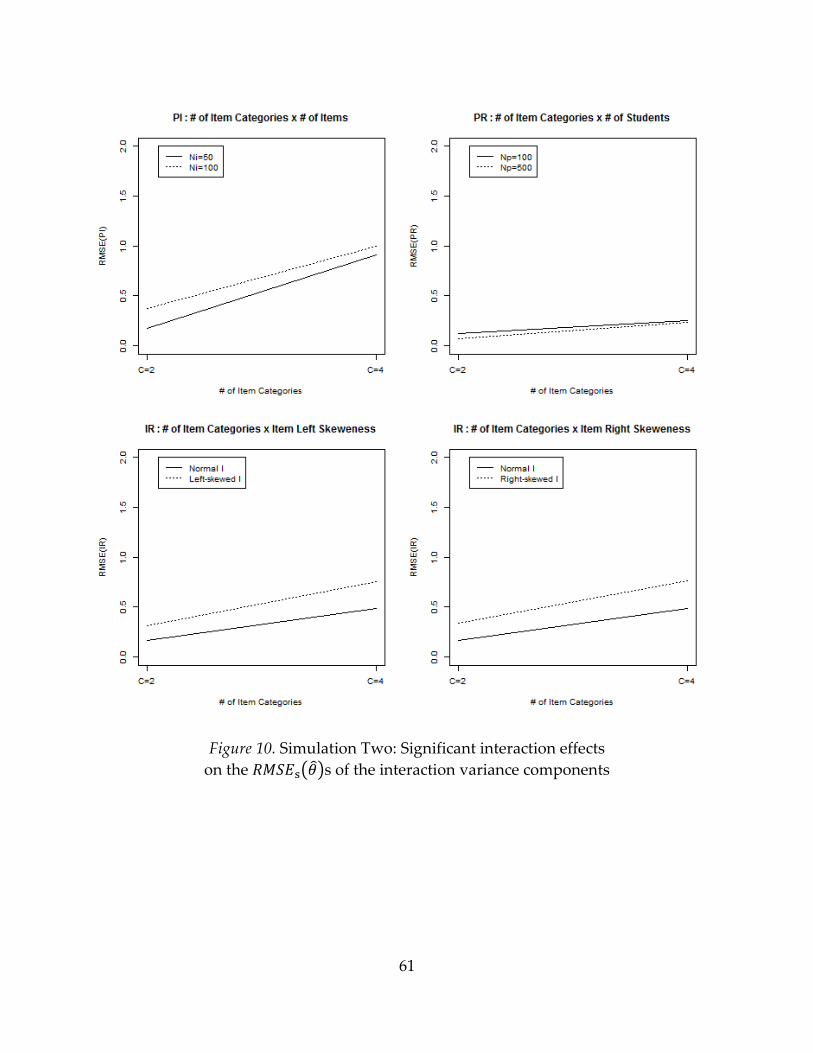
61

Figure 10. Simulation Two: Significant interaction effects

on the ( )s of the interaction variance components

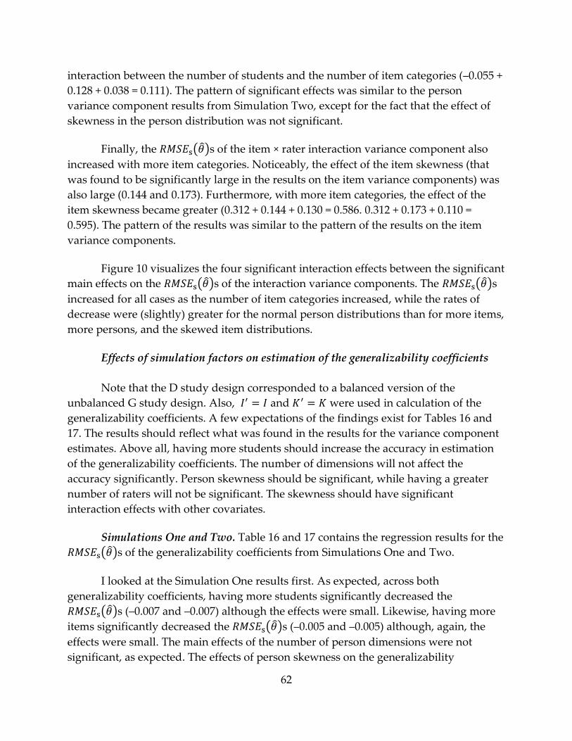
62

interaction between the number of students and the number of item categories (–0.055 +

0.128 + 0.038 = 0.111). The pattern of significant effects was similar to the person

variance component results from Simulation Two, except for the fact that the effect of

skewness in the person distribution was not significant.

Finally, the ( )s of the item × rater interaction variance component also

increased with more item categories. Noticeably, the effect of the item skewness (that

was found to be significantly large in the results on the item variance components) was

also large (0.144 and 0.173). Furthermore, with more item categories, the effect of the

item skewness became greater (0.312 + 0.144 + 0.130 = 0.586. 0.312 + 0.173 + 0.110 =

0.595). The pattern of the results was similar to the pattern of the results on the item

variance components.

Figure 10 visualizes the four significant interaction effects between the significant

main effects on the ( )s of the interaction variance components. The ( )s

increased for all cases as the number of item categories increased, while the rates of

decrease were (slightly) greater for the normal person distributions than for more items,

more persons, and the skewed item distributions.

Effects of simulation factors on estimation of the generalizability coefficients

Note that the D study design corresponded to a balanced version of the

unbalanced G study design. Also, and were used in calculation of the

generalizability coefficients. A few expectations of the findings exist for Tables 16 and

17. The results should reflect what was found in the results for the variance component

estimates. Above all, having more students should increase the accuracy in estimation

of the generalizability coefficients. The number of dimensions will not affect the

accuracy significantly. Person skewness should be significant, while having a greater

number of raters will not be significant. The skewness should have significant

interaction effects with other covariates.

Simulations One and Two. Table 16 and 17 contains the regression results for the

( )s of the generalizability coefficients from Simulations One and Two.

I looked at the Simulation One results first. As expected, across both

generalizability coefficients, having more students significantly decreased the

( )s (–0.007 and –0.007) although the effects were small. Likewise, having more

items significantly decreased the ( )s (–0.005 and –0.005) although, again, the

effects were small. The main effects of the number of person dimensions were not

significant, as expected. The effects of person skewness on the generalizability

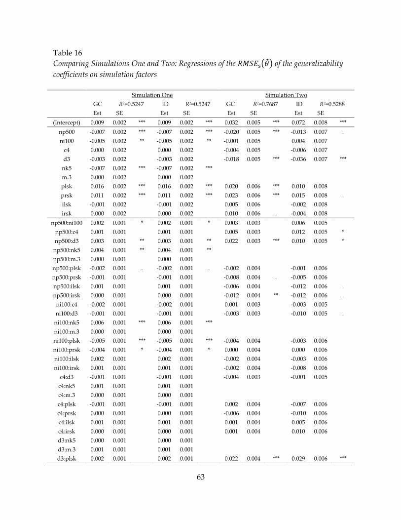
63

Table 16

Comparing Simulations One and Two: Regressions of the ( ) of the generalizability

coefficients on simulation factors

Simulation One Simulation Two

GC R2=0.5247 ID R2=0.5247 GC R2=0.7687 ID R2=0.5288

Est SE

Est SE

Est SE Est SE

(Intercept) 0.009 0.002 *** 0.009 0.002 *** 0.032 0.005 *** 0.072 0.008 ***

np500 -0.007 0.002 *** -0.007 0.002 *** -0.020 0.005 *** -0.013 0.007 .

ni100 -0.005 0.002 ** -0.005 0.002 ** -0.001 0.005 0.004 0.007

c4 0.000 0.002

0.000 0.002

-0.004 0.005 -0.006 0.007

d3 -0.003 0.002

-0.003 0.002

-0.018 0.005 *** -0.036 0.007 ***

nk5 -0.007 0.002 *** -0.007 0.002 ***

m.3 0.000 0.002

0.000 0.002

plsk 0.016 0.002 *** 0.016 0.002 *** 0.020 0.006 *** 0.010 0.008

prsk 0.011 0.002 *** 0.011 0.002 *** 0.023 0.006 *** 0.015 0.008 .

ilsk -0.001 0.002

-0.001 0.002

0.005 0.006 -0.002 0.008

irsk 0.000 0.002

0.000 0.002

0.010 0.006 . -0.004 0.008

np500:ni100 0.002 0.001 * 0.002 0.001 * 0.003 0.003 0.006 0.005

np500:c4 0.001 0.001

0.001 0.001

0.005 0.003 0.012 0.005 *

np500:d3 0.003 0.001 ** 0.003 0.001 ** 0.022 0.003 *** 0.010 0.005 *

np500:nk5 0.004 0.001 ** 0.004 0.001 **

np500:m.3 0.000 0.001

0.000 0.001

np500:plsk -0.002 0.001 . -0.002 0.001 . -0.002 0.004 -0.001 0.006

np500:prsk -0.001 0.001

-0.001 0.001

-0.008 0.004 . -0.005 0.006

np500:ilsk 0.001 0.001

0.001 0.001

-0.006 0.004 -0.012 0.006 .

np500:irsk 0.000 0.001

0.000 0.001

-0.012 0.004 ** -0.012 0.006 .

ni100:c4 -0.002 0.001

-0.002 0.001

0.001 0.003 -0.003 0.005

ni100:d3 -0.001 0.001

-0.001 0.001

-0.003 0.003 -0.010 0.005 .

ni100:nk5 0.006 0.001 *** 0.006 0.001 ***

ni100:m.3 0.000 0.001

0.000 0.001

ni100:plsk -0.005 0.001 *** -0.005 0.001 *** -0.004 0.004 -0.003 0.006

ni100:prsk -0.004 0.001 * -0.004 0.001 * 0.000 0.004 0.000 0.006

ni100:ilsk 0.002 0.001

0.002 0.001

-0.002 0.004 -0.003 0.006

ni100:irsk 0.001 0.001

0.001 0.001

-0.002 0.004 -0.008 0.006

c4:d3 -0.001 0.001

-0.001 0.001

-0.004 0.003 -0.001 0.005

c4:nk5 0.001 0.001

0.001 0.001

c4:m.3 0.000 0.001

0.000 0.001

c4:plsk -0.001 0.001

-0.001 0.001

0.002 0.004 -0.007 0.006

c4:prsk 0.000 0.001

0.000 0.001

-0.006 0.004 -0.010 0.006

c4:ilsk 0.001 0.001

0.001 0.001

0.001 0.004 0.005 0.006

c4:irsk 0.000 0.001

0.000 0.001

0.001 0.004 0.010 0.006

d3:nk5 0.000 0.001

0.000 0.001

d3:m.3 0.001 0.001

0.001 0.001

d3:plsk 0.002 0.001

0.002 0.001

0.022 0.004 *** 0.029 0.006 ***

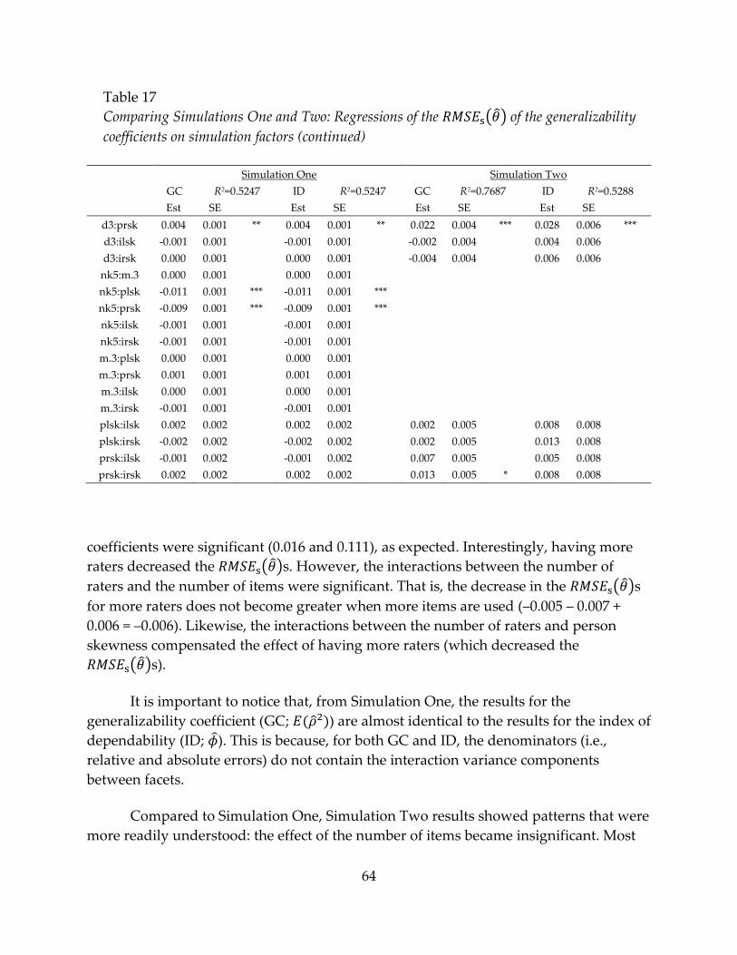
64

Table 17

Comparing Simulations One and Two: Regressions of the ( ) of the generalizability

coefficients on simulation factors (continued)

Simulation One Simulation Two

GC R2=0.5247 ID R2=0.5247 GC R2=0.7687 ID R2=0.5288

Est SE

Est SE

Est SE Est SE

d3:prsk 0.004 0.001 ** 0.004 0.001 ** 0.022 0.004 *** 0.028 0.006 ***

d3:ilsk -0.001 0.001

-0.001 0.001

-0.002 0.004 0.004 0.006

d3:irsk 0.000 0.001

0.000 0.001

-0.004 0.004 0.006 0.006

nk5:m.3 0.000 0.001

0.000 0.001

nk5:plsk -0.011 0.001 *** -0.011 0.001 ***

nk5:prsk -0.009 0.001 *** -0.009 0.001 ***

nk5:ilsk -0.001 0.001

-0.001 0.001

nk5:irsk -0.001 0.001

-0.001 0.001

m.3:plsk 0.000 0.001

0.000 0.001

m.3:prsk 0.001 0.001

0.001 0.001

m.3:ilsk 0.000 0.001

0.000 0.001

m.3:irsk -0.001 0.001

-0.001 0.001

plsk:ilsk 0.002 0.002

0.002 0.002

0.002 0.005 0.008 0.008

plsk:irsk -0.002 0.002

-0.002 0.002

0.002 0.005 0.013 0.008

prsk:ilsk -0.001 0.002

-0.001 0.002

0.007 0.005 0.005 0.008

prsk:irsk 0.002 0.002

0.002 0.002

0.013 0.005 * 0.008 0.008

coefficients were significant (0.016 and 0.111), as expected. Interestingly, having more

raters decreased the ( )s. However, the interactions between the number of

raters and the number of items were significant. That is, the decrease in the ( )s

for more raters does not become greater when more items are used (–0.005 – 0.007 +

0.006 = –0.006). Likewise, the interactions between the number of raters and person

skewness compensated the effect of having more raters (which decreased the

( )s).

It is important to notice that, from Simulation One, the results for the

generalizability coefficient (GC; ) are almost identical to the results for the index of

dependability (ID; ). This is because, for both GC and ID, the denominators (i.e.,

relative and absolute errors) do not contain the interaction variance components

between facets.

Compared to Simulation One, Simulation Two results showed patterns that were

more readily understood: the effect of the number of items became insignificant. Most

65

Figure 11. Simulation Two: Significant interaction effects

on the ( )s of the generalizability coefficients

66

of all, the GC and ID results showed slightly different pattern with noticeably different

adjusted R-squared values (0.7687 and 0.5288). Similar to the case for the person

variance component results, the number of dimensions (–0.018 and –0.036) and person

skewness (0.020, 0.023 and 0.010, 0.015) have significant main and interaction effects on

the ( )s of the generalizability coefficients, although the effects were all small.

Figure 11 visualizes the four significant interaction effects between the significant

main effects on the ( )s of the generalizability coefficients from Simulation Two.

The ( )s decreased for all cases as the number of dimensions increased, except

for the item right-skewed distributions. The rates of decrease were greater for the

normal person distributions than for the skewed item distributions.

Summary of simulation results

In this chapter, I examined the effects of simulation factors on estimation

accuracy ( ( )) of the variance components and generalizability coefficients. I

conducted two simulations: Simulation One consisted of 100 replications for each of the

576 simulation conditions that were constructed based on a set of simulation factors.

The models used in data generation and estimation only included the main effects of

the person, item and rater facets. Simulation Two consisted of 10 replications for each of

the 144 simulation conditions that were constructed based on the same set of simulation

factors, excluding the number of raters and the proportion of missing responses. The

models used in data generation and estimation included the main effects of and the

interaction effects between the person, item and rater facets.

For both Simulations One and Two, I constructed the Simulation One and the

Simulation Two results data sets that include the ( )s of the person and item

variance components and the generalizability coefficients for each simulation condition.

I fit a multiple linear regression model to examine the effects of various simulation

factors on the accuracy of estimates. The main effects and the two-way interaction

effects of all simulation factors were specified as predictors in the model.

Simulation One. Among the various person and item variance components, the

composite variance components are the most important to look at because they, not the

variance components of dimensions and categories, are used to calculate the

generalizability coefficients.

Overall, person skewness only affected estimation accuracy of the person

variance components and item skewness only affected estimation accuracy of the item

variance components. Meanwhile, the accuracy of rater variance components was

67

affected by both person and item skewness, although the effect disappeared with

increase in the number of persons and items.

The adjusted R-squared for the person variance components and the

generalizability coefficients ranged from 0.6156 to 0.9454, indicating a greater than

medium to a large effect size. Cautions are necessary in interpreting the regression

results for the ( )s of item and rater variance components. The adjusted R-

squared for the items ranged from 0.1482 to 0.3259 and those for the raters was to

0.1696. Additionally, in the case of item and rater variance component estimates, the

effects of simulation factors were less than 0.2 on the logit scale for the variance

components. Following summarizes the results in more detail.

(1) For the person composite variance, having more students decreased the

( )s while having more dimensions increased them. This is expected

because more data will tend to increase the accuracy in estimation of the

parameters. The estimates became less accurate when the person distribution

was either left- or right-skewed in addition to multidimensionality. This is a

reasonable finding because the estimation procedure assumes normality. This

implies that examination of the person-side data distribution is important

because skewness in person distributions, especially in the case of

multidimensional assessment, results in less accurate estimates of person

variance components.

(2) For the item composite variance, having more items improved the accuracy of

variance component estimation, as expected. Interestingly, skewness in item

distribution decreased ( )s. However, via interaction effects, the

amount of ( ) reduction by skewness became smaller for the situations

with more items and for those with more categories for all items. This means

that controlling for other variables, the item variance components are more

accurate when the items are mostly difficult or mostly easy. This effect seems

to show more clearly when items are dichotomous and smaller in number.

(3) For the rater variance component, the left-skewness of the item distribution

seemed to decrease the ( ). However, when more item categories and

more missingness in data were added to item left-skewness, the effect

disappeared. This suggests that rater variance components are less accurate

when the items are mostly difficult or mostly easy, but can be estimated more

accurately when items are polytomous and greater in number.

68

(4) The results for the ( )s of the generalizability coefficient showed

similar patterns with the results of the index of dependability. For the

generalizability coefficients GC and ID, having more students significantly

decreased ( )s. Particularly with interactions, having more dimensions

and skewed person distributions together increased ( )s. This

suggests that when a multidimensional assessment is used to measure the

ability of mostly high-proficient students (person left-skewness) or that of

mostly low-proficient students (person right-skewness), the generalizability

coefficients will be less accurate.

Simulation Two. Overall, Simulation Two showed significant difference from

Simulation One with respect to how simulation factors affect the accuracy of the

variance component estimates and the generalizability coefficients. This may have

resulted from several differences that Simulation Two involved: inclusion of

interactions between facets in data generating and estimating models, and a slightly

simpler regression model.

Compared to Simulation One, the adjusted R-squared for the person variance

components and the generalizability coefficients increased noticeably, showing strong

effect sizes (ranging from 0.8638 to 0.9964) The adjusted R-squared for the regression

results for the ( )s of item variance components also increased significantly

(ranging from 0.6775 to 0.9395) However, the adjusted R-squared for the rater variance

components plummeted to 0.0171. Although a lower R-squared value was expected for

the rater variance components, caution is necessary in interpreting the results.

Nevertheless, the fact that the adjusted R-squared values from Simulation Two

are mostly much greater than those from Simulation One, coupled with the fact that the

number of replications were smaller in Simulation Two, suggest that Simulation Two is

more effective in explaining how the varying simulation factors affect the accuracy in

estimating the variance component and the generalizability coefficients. A detailed

summary is presented in the following.

(5) For the person composite variance, the results were similar to Simulation

One. However, the composite person variance components became less

accurate with more item categories as well as more person dimensions. With

person skewness, the effect of having more item categories was reduced.

69

(6) For the item composite variance, having more items improved the accuracy of

variance component estimation, as expected. Unlike Simulation One, with

more items as well as skewness in the item distribution, ( )s increased.

(7) For the rater variance component, Simulation One and Two results did not

differ significantly, except for the fact that the adjusted R-squared value

dropped to below 0.1 for Simulation Two. Since the predictors are not directly

related to rater characteristics, low adjusted R-squared value is not

surprising.

(8) For all three interaction variance components between three facets, having

more item categories decreased the accuracy of the estimated variance

components. With more students, the person × rater interaction variance

component became more accurate. With skewed item distributions, the item ×

rater interaction variance component became less accurate.

(9) Unlike the case for Simulation One, the results for the generalizability

coefficients showed slightly different patterns and adjusted R-squared values

with the results of the indices of dependability, as expected. Having more

person dimensions and greater person skewness significantly affected the

accuracy of the estimated generalizability coefficients. However, the effect

sizes were all very small.

70

Chapter 3 Empirical Study

The purpose of this empirical study is to illustrate the suggested approach

described in Chapter 1 using real data sets. In this chapter, I first introduce the two real

assessment data sets. Next, I describe methods that are used to analyze both data sets.

Then, for each data set, the following results are presented: the G study variance

components that were estimated using the maximum likelihood with Laplace

approximation implemented in the lmer() function in R, the generalizability coefficients

that are estimated in the context of D studies, and the predicted individual random

effects.

3.1 Data

Data Set One: PISA 2009 U.S. Science data

The first data set is a unidimensional dichotomous data set: the U.S. portion of

the PISA 2009 Science assessment data (Organization for Economic Cooperation and

Development [OECD], 2011). PISA is an international assessment that measures 15-

year-old students’ reading, mathematics, and science literacy. The PISA 2009 science

assessment focused on measuring the students’ scientific literacy that consists of four

interrelated aspects: recognizing context, understanding the natural world with

knowledge, demonstrating competencies of scientific inquiry, and demonstrating

motivated and interested attitude towards scientific inquiry (OECD, 2011). The

assessment items were designed based on context, knowledge, and competencies: the

test questions required the use of the scientific competencies within a context, involving

the application of scientific knowledge. For example, each of the assessment items are

designed to be related to each of the scientific knowledge categories:

“Question 2 of the ACID RAIN (science example 1) assesses students’ knowledge

of science in the category ‘Physical systems’. Question 3 of ACID RAIN focuses

on students’ knowledge about science in the category ‘Scientific inquiry,’ but

assumes some knowledge of science (category ‘Physical systems’) that students

can be expected to possess.”(OECD, 2009)

Information on how the items are related to the construct is useful in examining

whether the data reflects the hypothetical multidimensionality. However, because the

item-level information was only partially available from the PISA public inventory, a

unidimensional model was fitted to these data. Also, for illustrative purposes, I selected

just the U.S. subset of the international data set, which includes 3,617 U.S. students and

53 dichotomously scored science items.

71

The data were reshaped into the long format. From the long-format data, the

rows with missing responses were deleted. This resulted in a response vector with a

length of 82,834. The resulting data set was unbalanced and incomplete: the number of

items answered by each student ranged from 3 to 36 across students. The number of

students who answered each item ranged from 666 to 1,609 across items. The following

is the list of variables in the data:

y : binary response to the item with value 1 if correct and 0 if incorrect

respid : response identifier that corresponds to the row number

of the response vector

stuid : student identifier

itemid : item identifier

Data Set Two: Carbon Cycle 2008-2009 data

The second data set has three features that illuminate the utility of the proposed

method: multidimensionality, polytomous responses, and multiple raters. The data

were collected by researchers at Michigan State University and the University of

California at Berkeley for the Carbon Cycle project, which was supported by the

National Science Foundation: Developing a Research-based Learning Progression on

Carbon-Transforming Processes in Socio-Ecological Systems (NSF 0815993). The

participants were U.S. students from the state of Michigan in grades 4 through 12

during the 2008–2009 school year. After the data were cleaned, the data consisted of 869

students, including 190 elementary students, 346 middle school students, and 333 high

school students.

The 19 items in the data set represented six ability dimensions. The items were

polytomously scored into four categories (0, 1, 2, 3) by eight raters. The numbers of

items designed to measure each of the six dimensions were 3, 3, 3, 2, 3, and 5,

respectively. The data sampling design was unbalanced and incomplete. That is, not

every item measured all six domains, not every item was rated by all eight raters, not

every person answered all items, not every item had four category scores, and so on.

The reshaping of the data, based on Tutz’s (1990) sequential stage continuation

ratio logit, resulted in a response vector with a length of 18,695. The resulting data set

was unbalanced and incomplete: the number of students who answered each item

ranged from 69 to 454 across items. The number of items answered by each student

ranged from 2 to 11 across students. The number of raters who rated each item ranged

from 6 to 8 across items. The variables in the data are listed below.

72

y : original polytomous response to the item (0, 1, 2 or 3)

respid : response identifier that corresponds to the row number

stuid : student identifier

itemid : item identifier

raterid : rater identifier

category : identifier for the three steps (1, 2, or 3)

tutz : recoded binary response following Tutz’s scheme

newitem : identifier for the item * threshold combination

dimension : identifier for the six dimensions

Additionally, in order to simplify the analysis using the proposed method for the

three facet situation (i.e., person, item, and rater), we dichotomized the Carbon Cycle

data set so that all of the original polytomous responses were recoded as 1 if the original

score was the highest among the scored categories for the item, as 0 otherwise. The

dichotomization and reshaping resulted in a response vector with a length of 5,957.

3.2 Methods

The measurement scenarios and corresponding data sampling designs from the

PISA 2009 and the Carbon Cycle 2008-2009 empirical data sets are summarized in Table

18. The empirical illustrations in this chapter include all of the eight possible

measurement scenarios based on the three measurement facets (i.e., person

(unidimension vs. multidimension), item (dichotomous vs. polytomous), and raters

(single vs. multiple)). Thus, the PISA data correspond to a very simple example, and the

Carbon Cycle data correspond to a much more complex one.

Based on the eight measurement scenarios, I fitted eight different models to the

data sets. A unidimensional model without the rater facet was fitted to the PISA 2009

U.S. Science data set. Next, four models for the dichotomous responses were fitted to

the dichotomized Carbon Cycle 2008-2009 data set: two models with person and item

facets only, and the other two models with person, item and rater facets. The remaining

four models for the polytomous responses were fitted to the original polytomous

Carbon Cycle 2008-2009 data set: two models with person and item facets and the other

two models with additional rater facet. All fitted models included the main effects and

the interaction effects among the facets.

The models were estimated using the R statistical environment. Estimation of the

models produced three sets of outcomes: (a) the variance component estimates, (b) the

generalizability coefficients, and (c) the individual random effects. First, maximum

likelihood estimation with the Laplace approximation was used to estimate the variance

73

Table 18.

Summary of measurement scenarios from the PISA 2009 U.S. science data and the 2008–2009

Carbon Cycle data

Measurement Scenario

Data

Design PISA

2009

CC

0809

Unidimensional Dichotomous Single rater person × item

Multiple raters person × item × rater

Polytomous Single rater person × item

Multiple raters person × item × rater

Multidimensional Dichotomous Single rater person × item

Multiple raters person × item × rater

Polytomous Single rater person × item

Multiple raters person × item × rater

components. Note that the standard errors of the estimated variance components are

not provided by lmer() function in R. Arguably, the use of standard errors for the

purpose of evaluating the variance parameter estimates is not sensible, because the

distribution of the variance parameter estimates is not symmetric and does not

converge to a normal distribution (Baayen, Davidson, & Bates 2008). In this study, I

consider that the inclusion of the variance component is already justified in the GT

context, where the sampling designs are intentionally specified. Thus, I focus on the

variance component estimates, not on the standard errors of the variance components.

Second, the estimation of the generalizability coefficients was performed in the context

of the D study that involves crossed facets with a balanced design, using the variance

component estimates from lmer(). The argument for justifying the selection of a

balanced design instead of an unbalanced design for the D study, is given on page 19.

Finally, the conditional means of the random effects were used for prediction of the

individual random effects (Bates, 2010).

In the next section, I first present the results from PISA 2009 U.S. Science data

analyses and then those from the Carbon Cycle 2008-2009 data analyses. For each

illustration, I present the variance component estimates, the generalizability coefficients,

and the predicted individual random effects. Particularly, with respect to the Carbon

Cycle data, I describe the comparisons among the results from the eight models.

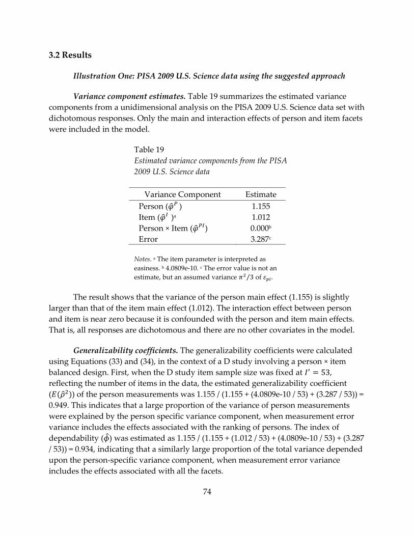
74

3.2 Results

Illustration One: PISA 2009 U.S. Science data using the suggested approach

Variance component estimates. Table 19 summarizes the estimated variance

components from a unidimensional analysis on the PISA 2009 U.S. Science data set with

dichotomous responses. Only the main and interaction effects of person and item facets

were included in the model.

Table 19

Estimated variance components from the PISA

2009 U.S. Science data

Variance Component Estimate

Person ( ) 1.155

Item ( )a 1.012

Person × Item ( ) 0.000b

Error 3.287c

Notes. a The item parameter is interpreted as

easiness. b 4.0809e-10. c The error value is not an

estimate, but an assumed variance ⁄ of .

The result shows that the variance of the person main effect (1.155) is slightly

larger than that of the item main effect (1.012). The interaction effect between person

and item is near zero because it is confounded with the person and item main effects.

That is, all responses are dichotomous and there are no other covariates in the model.

Generalizability coefficients. The generalizability coefficients were calculated

using Equations (33) and (34), in the context of a D study involving a person × item

balanced design. First, when the D study item sample size was fixed at ,

reflecting the number of items in the data, the estimated generalizability coefficient

( ) of the person measurements was 1.155 / (1.155 + (4.0809e-10 / 53) + (3.287 / 53)) =

0.949. This indicates that a large proportion of the variance of person measurements

were explained by the person specific variance component, when measurement error

variance includes the effects associated with the ranking of persons. The index of

dependability ( ) was estimated as 1.155 / (1.155 + (1.012 / 53) + (4.0809e-10 / 53) + (3.287

/ 53)) = 0.934, indicating that a similarly large proportion of the total variance depended

upon the person-specific variance component, when measurement error variance

includes the effects associated with all the facets.

75

Figure 12. D study SEMs and estimated generalizability

coefficients of PISA 2009 U.S. Science Data

Given the large values of the estimated generalizability coefficients at , a

D study with varying sample size is useful for determining minimum requirements for

the number of levels for the item facet to achieve reasonable levels of generalizability.

Figure 12 shows relative and absolute SEMs and estimated generalizability coefficients

for the conditions with . The patterns in Figure 12 show that the

generalizability coefficients for person measurement becomes greater than 0.8 at

approximately 15 items.

Individual random effects. Across the 3,617 students, the predicted person

random effects ranged from -2.689 to 2.417 (with the mean constrained to zero). Across

the 53 items, the predicted item random effects ranged from -1.955 to 2.451 with mean -

0.001. Both the person and item random effects were normally distributed. The fixed

effect (i.e., the grand mean or the intercept) was estimated as 0.168 (SE 0.140). The fixed

effect needs to be added to the predicted person random effects to make inference on

person abilities. Figure 13 shows predicted person random effects and 95% prediction

intervals, sorted by standard normal quantiles of the person random effects. As

expected, the random effects around the mean have narrower 95% prediction intervals

than ones towards the tails of the distribution, although the effect is not very great.

76

Figure 13. Predicted person random effects (points) and 95% prediction intervals (lines),

sorted by the standard normal quantiles of the person random effects. X axis indicates

standard normal quantiles and Y axis indicates the logit scale.

Next, Figure 14 presents the distribution of predicted item random effects along

with 95% prediction intervals. Here, the item random effects are interpreted as easiness.

For example, on average for the students in the data, S256Q01 was the easiest item. As

expected, the prediction intervals become slightly narrower for the items around the

center of the distribution and become slightly wider for the items towards the tails.

However, compared to the person random effects, the item random effects have much

smaller prediction intervals, indicating more accuracy in prediction.

77

Figure 14. Predicted item random effects (points) and 95% prediction intervals (lines). X

axis indicates the logit scale and Y axis indicates items, sorted by the standard normal

quantiles of the item random effects.

78

Illustration Two: 2008-2009 Carbon Cycle data using the suggested approach

In following sections, the results are presented in order of the variance

component estimates, the generalizability coefficients and the individual random

effects. In particular, I compare the results from eight different models under the

sections on variance component estimates and generalizability coefficients. Then I take

one set of results (from the multidimensional model with the rater facet fitted to

original polytomous data) to present a D study (a balanced person × item × rater design)

and the individual random effects.

Variance component estimates. Table 20 presents the results from the analyses of

the dichotomized Carbon Cycle data and the original polytomous Carbon Cycle data

sets. Unidimensional models with and without rater effect (UD and UD+R) and

multidimensional models with and without rater effect (MD and MD+R) were fitted to

both data sets.

Dichotomized data vs. polytomous data. In the results using the dichotomous data,

the person variance component estimates (2.613, 1.820, 3.241, 2.383) are greater than the

item (0.620, 0.696, 0.516, 0.584) and rater variance component estimates (0.500, 0.497)

across the models. The item (0.696, 0.584) and rater variance component estimates

(0.500, 0.497) are similar to each other between the two models with the rater facet. The

person × item interaction effects are all near zero, indicating that they are confounded

with person and item main effects. Among the four models, the unidimensional model

with the rater facet fits the best.

In the results using the polytomous data, the person variance component

estimates (2.395, 1.863) are greater than the item variance component estimates (1.858,

1.842) and also the rater variance component estimates (0.113) for the multidimensional

models. However, for the unidimensional models, the item variance component

estimates (2.013, 2.055) are greater than the person variance component estimates (1.879,

1.374) and the rater variance component estimates (0.118). Unlike the dichotomous

results, item (2.013, 2.055, 1.858, 1.842) and rater variance component estimates (0.118,

0.113) are no longer similar to each other: rather, the differences between the two are

more than 1.7 logit for the two models with the rater facet. Also, unlike the

dichotomous results, the person × item interaction effects (0.317, 0.232, 0.240, 0.166) are

not near zero. This implies that the person and item main effects are no longer

confounded with the interaction effect because the models account for the additional

information via the item steps. Among the four models, again, the unidimensional

model with the rater facet fits the best. It is not sensible to compare the model fit

79

Table 20

Estimated variance components from the 2008–2009 Carbon Cycle data

Variance

Component

Dichotomized Data

Original Polytomous Data

UD UD+R MD MD+R

UD UD+R MD MD+R

Wghtsa Est Est Est Est Wghts Est Est Est Est

Person ( )

2.613 1.820 3.241(c)b 2.383 (c)

1.879 1.374 2.395(c) 1.863(c)

Dim 1 ( ) 0.144

3.545 2.242 0.138

2.883 2.158

Dim 2 ( ) 0.141

3.228 1.740 0.140

2.168 1.545

Dim 3 ( ) 0.123

1.941 2.047 0.128

1.217 1.060

Dim 4 ( ) 0.144

2.806 2.534 0.152

1.833 1.592

Dim 5 ( ) 0.196

3.293 2.552 0.195

2.298 1.715

Dim 6 ( ) 0.253

2.414 1.273 0.249

1.744 1.062

Item ( )

0.620 0.696 0.516 0.584

2.013(c) 2.055(c) 1.858(c) 1.842(c)

Step 1 ( ) 0.362 2.983 3.368 2.648 3.006

Step 2 ( )

0.352 0.675 0.679 0.562 0.567

Step 3 ( 0.285 2.009 1.684 2.004 1.504

Rater ( )

0.500

0.497

0.118

0.113

Person × Item ( ) 0.000c 0.000d 0.000e 0.000f

0.317 0.232 0.240 0.166

Person × Rater ( )

0.229

0.233

0.293

0.294

Item × Rater ( )

0.697

0.706

0.423

0.412

Error

3.287g 3.287 3.287 3.287

3.287 3.287 3.287 3.287

AIC

5,138 4,880 5,176 5,006

12,153 11,890 12,174 11,924

BIC

5,154 4,927 5,370 5,201

12,239 12,000 12,456 12,230

Deviance

5,130 4,866 5,118 4,948

12,131 11,862 12,102 11,846

Notes. UD: unidimensional model. UD+R: unidimensional model with rater facet. MD: multidimensional

model. MD+R: multidimensional model with rater facet. a The weights represent, for person dimensions,

the number of item responses per each dimension divided by the total number of responses, and for item

steps, the number of responses per each step divided by the total number of responses. b The (c) marks

are for the weighted or composite variance component estimates calculated with Equations (31) and (32).

Covariance between the dimensions and covariance between steps are squared values of estimated

correlations from each model. The estimated correlations between the random effects are reported in

Table 21 c 2.2535e-12. d 9.6232e-19. e 7.5166e-10. f 7.4746e-10. g The error value is not an estimate, but an

assumed variance ⁄ of or .

between the models fitted to the dichotomized data set and ones fitted to the

polytomous data set because data lengths differed significantly.

Unidimensional models vs. multidimensional models. For both dichotomized and

polytomous data sets, with or without the rater facet, the person variance component

80

Table 21

Correlations among six person dimensions and those among three item steps

for the 2008-2009 Carbon Cycle data

Data Model Variance Components Correlations

Dichotomous MD Person Dim2 0.919

Dim3 0.932 0.999

Dim4 0.980 0.823 0.841

Dim5 0.995 0.953 0.962 0.956

Dim6 0.978 0.981 0.987 0.917 0.994

MD+R Person Dim2 0.933

Dim3 0.941 1.000

Dim4 0.972 0.822 0.835

Dim5 1.000 0.929 0.937 0.975

Dim6 0.993 0.969 0.974 0.938 0.992

Polytomous UD Item Step2 0.469

Step3 0.621 0.740

UD+R Item Step2 0.428

Step3 0.612 0.739

MD Person Dim2 1.000

Dim3 1.000 1.000

Dim4 0.834 0.834 0.834

Dim5 0.995 0.995 0.995 0.886

Dim6 0.998 0.998 0.998 0.868 0.999

Item Step2 0.472

Step3 0.658 0.757

MD+R Person Dim2 1.000

Dim3 1.000 1.000

Dim4 0.841 0.841 0.841

Dim5 0.974 0.974 0.974 0.877

Dim6 0.998 0.998 0.998 0.874 0.981

Item Step2 0.434

Step3 0.675 0.737

estimates increased from the unidimensional (2.613, 1.820, 1.879, 1.374) to the

multidimensional results (3.241, 2.383, 2.395, 1.863). On the other hand, the item

variance component estimates decreased from the unidimensional (0.620, 0.696, 2.013,

2.055) to the multidimensional results (0.516, 0.584, 1.858, 1.842), corresponding to the

slight decrease in the person × item interaction effects from the unidimensional (0.317,

0.232) to the multidimensional polytomous results (0.240, 0.166). The rater variance

components were similar across the unidimensional (0.500, 0.118) and the

multidimensional models (0.497, 0.113). This pattern implies that multidimensional

81

models capture the person effects that were shadowed by the item main effects and the

person × item interaction effects in the unidimensional results. Between the

unidimensional models and the multidimensional models, the model fits were not so

different but the variance component estimates were quite different. Overall, the

unidimensional model with the rater facet fitted the best for both dichotomized and

polytomous data sets.

Models with a rater facet vs. models without a rater facet. Across all situations,

including a rater facet in the model decreased the person variance component estimates

(from 2.613, 3.241, 1.879, 2.395 to 1.820, 2.383, 1.374, 1.863). The item variance

component estimates did not change noticeably with inclusion of the rater facet (from

0.620, 0.516, 2.013, 1.858 to 0.696, 0.584, 2.055, 1.842). The interactions between the

person and rater facets (0.229, 0.233, 0.293, 0.294) were smaller than the interactions

between the item and rater facets (0.697, 0.706, 0.423, 0.412), indicating that the effect of

raters differed more across items than across people. The models with a rater facet fitted

better than the models without a rater facet.

Table 21 shows estimated correlations between the random effects in each model.

The squared values of these correlations were used to compute the composite variance

component estimates calculated with Equations (31) and (32). Overall, the correlations

between the person random effects (dimensions) are all very strong. Coupled with the

model fit results (where the unidimensional model with the rater facet fitted the best to

both dichotomized and polytomous data), the strong correlations between the

dimensions supports the unidimensional interpretation of the data.

In the context of the lmer() function, the multidimensional (MD, MD+R) models

allow for correlation (in the unconditional distribution) of the random effects for the

same person. That is, the unconditional distribution of these random effects allows for

correlation of the random effects for the same person (Bates, 2010). For example,

persons with higher Dimension 1 ability may, on average, have higher ability on

Dimension 2. Likewise, the polytomous models (in the lower panel of the table) allow

for correlation (in the unconditional distribution) of the random effects for the same

item. That is, the model allows for the possibility that items with a higher Step 1

easiness many have a higher Step 2 easiness on average. The results show that some of

the estimated within-person correlations of the random effect for the Dimension 1 and

the random effects for the Dimension 2 and 3 are 1, that is, completely collinear. The

correlation estimates close to 1 or -1 indicates that the covariance matrix of the

unconditional distribution is close to singular, and that there is a strong systematic

82

Table 22

Estimated Generalizability Coefficients from the 2008–2009 Carbon Cycle Data

for the D study with fixed and .

D Study

Estimates

Dichotomized Data Original Polytomous Data

UD UD+R MD MD+R UD UD+R MD MD+R

(p×I)a (p×I×K)b (p×I) (p×I×K) (p×I) (p×I×K) (p×I) (p×I×K)

Relative SEM 0.147 0.224 0.147 0.225 0.196 0.265 0.185 0.214

Absolute SEM 0.233 0.392 0.221 0.385 0.380 0.443 0.363 0.425

0.947 0.890 0.957 0.914 0.906 0.838 0.928 0.897

0.918 0.823 0.936 0.861 0.832 0.756 0.868 0.814

Notes. UD: unidimensional model. UD+R: unidimensional model with rater facet. MD: multidimensional

model. MD+R: multidimensional model with rater facet. a balanced person × item D study design. b

balanced person × item × rater D study design.

relationship between these quantities. This again suggests a unidimensional

interpretation.

Generalizability coefficients. The generalizability coefficients were calculated

using Equations (33) and (34), in the context of two D study designs: the balanced

person × item design (noted as p × I) for UD and MD results, and the balanced person ×

item × rater design (noted as p × I × K) for UD+R and MD+R results. Table 22 shows the

estimated generalizability coefficients from each model. The D study item sample size

was fixed at and the D study rater sample size was fixed at , reflecting the

number of items and raters in the data.

The results show that, overall, the generalizability coefficients of the Carbon

Cycle person measurement were high, ranging from 0.756 to 0.957. The generalizability

coefficients were the highest (0.957, 0.936) when the Carbon Cycle data was

dichotomized, and when the model accounted for the multidimensionality (MD).

Between the dichotomized data and the polytomous data, the generalizability

coefficients were slightly higher with dichotomized data, indicating smaller relative and

absolute error in person measurement. Between the unidimensional models and the

multidimensional models, the generalizability coefficients were slightly higher for the

multidimensional models, indicating smaller relative and absolute error in person

83

Figure 15. D study SEMs and the generalizability coefficients from the

multidimensional model with the rater facet fitted to

the polytomous 2008-2009 Carbon Cycle data

84

measurement. Lastly, including the rater facet slightly increased the relative and

absolute error in person measurement and decreased the generalizability coefficients.

Next, I chose the most complex measurement situation (MD+R with polytomous

data) to illustrate the use of D studies and the individual random effects. In Figure 15, a

D study was conducted to determine the minimum requirement for the number of

levels for the item and rater facet to achieve a high level of generalizability, e.g., over

0.8.

The generalizability coefficient graph on the bottom left of Figure 15 shows that,

considering items, the generalizability coefficient becomes greater than 0.8 at about 25

items regardless of the number of raters. Now, considering raters, the generalizability

coefficient becomes greater than 0.8 at about three raters and at least about five items.

The index of dependability graph on the bottom right of Figure 15 shows lower values

than the generalizability coefficients, reflecting the fact that absolute errors are greater

than the relative errors. Similar to the generalizability coefficient graph, the curves

stabilize with at least about five items. Also, the curves become similar to each other

with at least about three raters.

Individual random effects. Figure 16 presents the predicted person random

effects and the 95% prediction intervals for each dimension, sorted by the standard

normal quantiles of the person random effects. Across the 869 students, the predicted

person random effects for the six dimensions ranged from around -2.5 (-2.882, -2.439, -

2.248, -2.511, -2.032) to around 3.7 (4.290, 3.630, 3.007, 3.688, 3.856, 3.058) with means

near zero (0.006, 0.005, 0.004, 0.005, 0.005, 0.005). Interestingly, the 95% prediction

intervals were slightly wider around the mean than the upper end of the distribution.

This implies that less information was available for the middle range students than for

the higher performing students. The histograms of the random effects showed slight

positive skewness (skewed to the right) for all dimensions, indicating quite a few

number of students who performed exceptionally better than the other students.

Next, Figure 17 presents the distribution of the predicted item random effects

along with the 95% prediction intervals. Because of the way the equation is written,

higher measures for the item random effect are indicative of easier items. Of course, the

longer the prediction intervals are, the greater the inaccuracy of the prediction is. For

example, on average for the students and the raters in the data, Step 1 of Item 7 was the

easiest compared to other item random effects. However, likely due to lack of data, the

prediction here was the least accurate (the longest line). Note that the responses were

scored as 0, 1, 2, and 3 and Step 1 corresponds to going from 0 to 1, Step 2 corresponds

to going from 1 to 2, and Step 3 corresponds to going from 2 to 3. Across the 53 items,

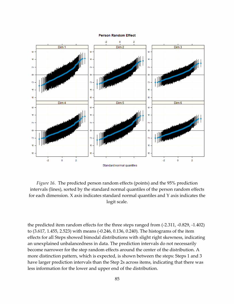
85

Figure 16. The predicted person random effects (points) and the 95% prediction

intervals (lines), sorted by the standard normal quantiles of the person random effects

for each dimension. X axis indicates standard normal quantiles and Y axis indicates the

logit scale.

the predicted item random effects for the three steps ranged from (-2.311, -0.829, -1.402)

to (3.617, 1.455, 2.523) with means (-0.246, 0.136, 0.240). The histograms of the item

effects for all Steps showed bimodal distributions with slight right skewness, indicating

an unexplained unbalancedness in data. The prediction intervals do not necessarily

become narrower for the step random effects around the center of the distribution. A

more distinction pattern, which is expected, is shown between the steps: Steps 1 and 3

have larger prediction intervals than the Step 2s across items, indicating that there was

less information for the lower and upper end of the distribution.

86

Figure 17. The predicted item random effects (points) and the 95% prediction intervals

(lines). X axis indicates the logit scale and Y axis indicates items, sorted by the standard

normal quantiles of the Step 3 item random effects.

Figure 18. The predicted rater random effects (points) and the 95% prediction intervals

(lines). X axis indicates the logit scale and Y axis indicates raters, sorted by the standard

normal quantiles of the rater random effects.

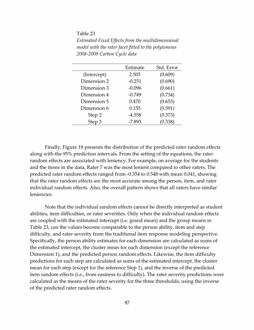
87

Table 23

Estimated Fixed Effects from the multidimensional

model with the rater facet fitted to the polytomous

2008-2009 Carbon Cycle data

Estimate Std. Error

(Intercept) 2.505 (0.609)

Dimension 2 -0.251 (0.690)

Dimension 3 -0.096 (0.661)

Dimension 4 -0.749 (0.734)

Dimension 5 0.470 (0.653)

Dimension 6 0.155 (0.591)

Step 2 -4.558 (0.373)

Step 3 -7.893 (0.338)

Finally, Figure 18 presents the distribution of the predicted rater random effects

along with the 95% prediction intervals. From the setting of the equations, the rater

random effects are associated with leniency. For example, on average for the students

and the items in the data, Rater 7 was the most lenient compared to other raters. The

predicted rater random effects ranged from -0.354 to 0.548 with mean 0.041, showing

that the rater random effects are the most accurate among the person, item, and rater

individual random effects. Also, the overall pattern shows that all raters have similar

leniencies.

Note that the individual random effects cannot be directly interpreted as student

abilities, item difficulties, or rater severities. Only when the individual random effects

are coupled with the estimated intercept (i.e. grand mean) and the group means in

Table 23, can the values become comparable to the person ability, item and step

difficulty, and rater severity from the traditional item response modeling perspective.

Specifically, the person ability estimates for each dimension are calculated as sums of

the estimated intercept, the cluster mean for each dimension (except the reference

Dimension 1), and the predicted person random effects. Likewise, the item difficulty

predictions for each step are calculated as sums of the estimated intercept, the cluster

mean for each step (except for the reference Step 1), and the inverse of the predicted

item random effects (i.e., from easiness to difficulty). The rater severity predictions were

calculated as the means of the rater severity for the three thresholds, using the inverse

of the predicted rater random effects.

88

The benefit of having the set of the predicted person, item, and rater effects is

explicitly shown through Figure 19, a modified version of a Wright Map (Wilson, 2005).

Using this Figure, one can compare the location of the distributions of the person, item,

and rater characteristics on the same logit scale, which gives an insight into how easy it

was for the students to be given the target score on the items by the raters. The

distribution of person ability scores are displayed as kernel density estimates on the

logit scale. As discussed in the results on the person random effects, the ability

distributions of the six dimensions are positively skewed towards the upper end, and

shared similar locations and dispersions (which corresponds to the interpretations of

unidimensionality above). Next, the three groups of points on vertical lines represent

the step difficulties for the items. The location of the points can be interpreted as where

the students on average have a 50% probability to get a particular score or above as

compared to a score below that. Since the data had four possible scores (0, 1, 2, or 3),

there are three steps or thresholds between the scores. Most of the students had more

than a 50% chance to achieve the first thresholds of all items. In other words, for most of

the students, getting the score 1 or above versus 0 was relatively easy. Confirming the

findings from Figure 17, the first threshold for Item 7 was the easiest for all students.

The second thresholds of the items were reasonably located near the means of the

person distributions, implying that on average students were able to get score 2 on most

items with about a 50% probability of success. Getting the highest score was generally

difficult for the students, particularly for Items 1, 5, 6, 9, and 15.

Last, the raters were generally non-separable from each other except for Raters 7

and 6 who were on average more lenient than the others in giving any scores

(compared to the score just below) for the items to the students.

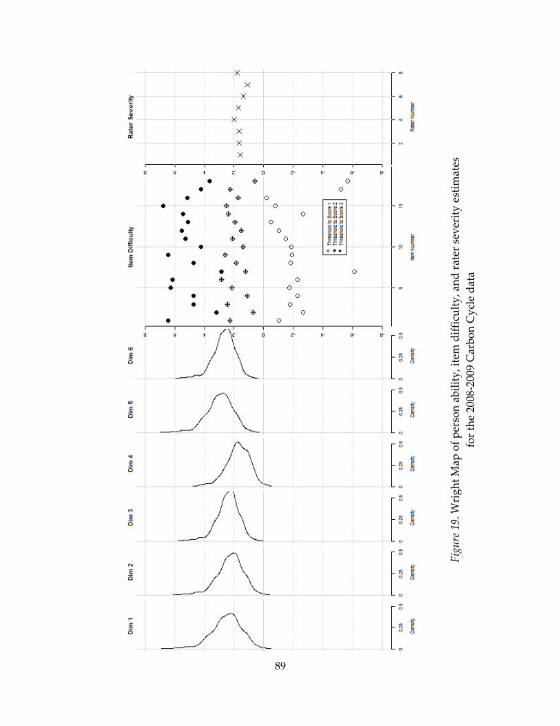
89

Fig

ure

19.

Wri

gh

t M

ap o

f p

erso

n a

bil

ity

, ite

m d

iffi

cult

y, a

nd

rat

er s

ever

ity

est

imat

es

for

the

2008

-200

9 C

arb

on

Cy

cle

dat

a

90

Chapter 4 Conclusion

4.1 Summary

In this study, I suggested an approach for combining GT and IRT. I recognize

that IRT models can be written in terms of a latent continuous response and that a

classic IRT model can be modeled directly using a simple GT design with items as a

fixed facet. The resulting logistic mixed models extend a classic IRT model by treating

items as a random facet or considering other facets such as raters. The advantage of the

proposed approach is that it allows a straightforward ML estimation of individual

random effects as well as the variance components needed for the generalizability

coefficients.

Through extensive simulation studies, the accuracy of the results from the

proposed approach in various measurement conditions was evaluated. In conclusion,

data suggested that the proposed approach gives overall accurate results, in particular,

when estimating generalizability coefficients. While more students and skewness in

person distributions showed a significant interaction effect on the accuracy of the

generalizability coefficients, the effect sizes were all very small.

With respect to the estimation of the variance components, the accuracy of the

estimated variance components of person, item, rater and the interactions between

those three facets were mostly affected by the sample size and the skewness in

generating distributions of person and items. In general, and not surprisingly, more

data increased the accuracy of the estimated person variance components. Furthermore,

the factors such as the number of person dimensions and the number of item score

categories (e.g., polytomous responses) showed significant interaction effects with

skewness in person and item distributions. For example, the person variance

components became less accurate when there were more items and more dimensions in

the data, while this effect became smaller with skewness in person distributions. In

terms of item variance components, having more items increased the accuracy of the

estimates. Interestingly, the results showed that the estimated item variance

components become more accurate with skewness in item generating distributions,

especially when there are only a few items and when the items are scored

dichotomously. The results suggested that with more items and polytomous scoring,

this ‘unexpected benefit’ of item skewness disappears. The effects of simulation factors

on estimation of the rater variance component could not be explained well by the

current simulation study, because the simulation factors mostly concerned person-side

and item-side characteristics. Furthermore, the rater variance components can also be

91

affected by item skewness, but become more accurate when there are more items and

when the items were polytomous. The comparisons between Simulation One and

Simulation Two results suggest that the study of the effects of simulation factors

become more informative when the generating and estimating model includes not only

main facet effects but also the interaction effects among the facets.

In addition, applications of the proposed approach were illustrated using two

large-scale data sets. The results demonstrated another advantage of the proposed

approach: its flexibility with respect to incorporating extra complications in

measurement situations (e.g., multidimensionality, polytomous responses) and further

explanatory variables (e.g., rater facet). The variance components and the

generalizability coefficients were presented in the context of the G study and the D

study. Also, predicted individual random effects were presented by taking advantage of

the usefulness of a Wright Map.

4.2 Discussion

The results of this study suggested that the accuracy of item and rater variance

component estimates are affected in a statistically significant way, although only

slightly in terms of effect size, by a complex interplay between skewness in item

distribution and the number of items as well as the number of item categories. Of

course, the accuracy of those variance components affects the accuracy of the

measurement errors and thus the generalizability coefficients. The results may offer a

route to design a better assessment where the number of items, the number of scoring

categories, and the distribution of item difficulties can be carefully chosen. Moreover,

an extended D study may allow incorporation of the number of response categories for

items and the distribution of item difficulty to inform future assessment design.

While the proposed approach applies to the case of a crossed three-facet situation

with unbalanced and incomplete data, it can be generalized to other measurement

situations, both simpler and more complex ones. A simpler example is a balanced

design with no missing data, or a design where the facets are nested. In fact, nested or

multilevel designs can be found commonly in educational data where students are

nested in classrooms or in teachers. A more complex example is an unbalanced design

with more than three crossed facets. For example, in addition to person, item, and rater

facets, one could include an occasion facet that involves repeated measurement. Such

attempts on at generalizations may offer a closer connection between existing GT

designs and IRT models. Currently, research is underway to extend the comparison

between the previous combining methods and the proposed approach to such

92

alternative designs. The new results from these studies will (hopefully) provide a basis

to understand currently unclear issues in the combining of GT and IRT (e.g., how to

conceptualize D studies and generalizability coefficients), and to evaluate

methodological advantages and disadvantages of the existing and proposed approaches

more comprehensively.

In the meantime, whether the proposed method is extendable to different

designs, such as nested designs or designs with more than three facets, partly depend

on the estimation methods. Until recently, estimation of crossed random effects models

has been limited to a relatively small number of random effects, or facets, and their

levels. Even though the flexibility of the proposed approach allows straightforward

extension of the models to those situations, questions remain regarding how to estimate

the variance components in the models with increased number of crossed random

facets. Moreover, incorporating other item parameters such as discrimination

differences or guessing in IRT models may add more challenges in estimation and

interpretation. It will be interesting to investigate what advanced and/or alternative

estimation methods might ensue in extending the approaches to combine GT and IRT.

Finally, the results showed that the interaction between person and item facets is

confounded with person and item main effects when the response data is dichotomous.

This finding was consistent across two-facet and three-facet designs, and

unidimensional and multidimensional situations. Thus, it may be that developing

polytomous items will allow researchers to capture the measurement error due to

interactions between person ability and item difficulties in the crossed multifacet

designs with or without multidimensionality.

93

References

Allison, P. D. (2002). Missing data: Quantitative applications in the social

sciences. British Journal of Mathematical and Statistical Psychology, 55(1), 193–196.

American Educational Research Association, American Psychological Association,

National Council on Measurement in Education, Joint Committee on Standards

for Educational, & Psychological Testing (US). (1999). Standards for educational and

psychological testing. American Educational Research Association.

Andersen, E. B. (1970). Asymptotic properties of conditional maximum-likelihood

estimators. Journal of the Royal Statistical Society. Series B (Methodological), 283–301.

Andrich, D. (1978). A rating formulation for ordered response categories. Psychometrika,

43, 561–573.

Azzalini, A. (1985). A class of distributions which includes the normal ones.

Scandinavian Journal of Statistics, 12, 171–178.

Azzalini, A., & Capitanio, A. (2003). Distributions generated by perturbation of

symmetry with emphasis on a multivariate skew t‐distribution. Journal of the

Royal Statistical Society: Series B (Statistical Methodology), 65(2), 367–389.

Baayen, R. H., Davidson, D. J., & Bates, D. M. (2008). Mixed-effects modeling with

crossed random effects for subjects and items. Journal of memory and

language, 59(4), 390–412.

Bates, D. M. (2010). lme4: Mixed-effects modeling with R. URL http://lme4.r-forge.r-

project.org/book.

Bates, D. M., Maechler, M., & Bolker, B. (2011). lme4: Linear mixed-effects models using S4

classes. URL http://cran.r-project.org

Bock, R. D. (1972). Estimating item parameters and latent ability when responses are

scored in two or more nominal categories. Psychometrika, 37(1), 29–51.

Bock, R. D., & Aitkin, M. (1981). Marginal maximum likelihood estimation of item

parameters: Application of an EM algorithm. Psychometrika, 46(4), 443–459.

94

Bock, R. D., Brennan, R. L., & Muraki, E. (2002). The information in multiple

ratings. Applied psychological measurement, 26(4), 364–375.

Brennan, R. L. (2001a). Generalizability theory. New York, NY: Springer.

Brennan, R. L. (2001b). Manual for urGENOVA. Version 2.1. Iowa Testing Programs.

Brennan, R. L. (2011). Using Generalizability Theory to Address Reliability Issues for PARCC

Assessments: A White Paper. Center for Advanced Studies in Measurement and

Assessment (CASMA), University of Iowa.

Breslow, N. E. & Lin, X. (1995). Bias correction in generalized linear mixed models with

a single component of dispersion, Biometrika, 82, 81–91.

Breslow, N. E., & Clayton, D. G. (1993). Approximate inference in generalized linear

mixed models. Journal of the American Statistical Association, 88, 9–25.

Briggs, D. C., & Wilson, M. R. (2007). Generalizability in item response modeling.

Journal of Educational Measurement, 44(2), 131–155.

Chien, Y.-.M. (2008). An investigation of testlet-based item response models with a

random facets design in generalizability theory. Doctoral dissertation. The University

of Iowa.

Choi, J., Briggs, D. C., & Wilson, M. R. (2009, April). Multidimensional extension of the

generalizability in item response modeling (GIRM). Paper presented at the 2009

National Council on Measurement in Education Annual Meeting, San Diego, CA.

Crawley, M. J. 2007. The R book. Wiley, West Sussex, UK.

Cronbach, L. J., Gleser, G. C., Nanda, H., & Rajaratnam, N. (1972). The dependability of

behavioral measurements: Theory of generalizability for scores and profiles. New York,

NY: Wiley.

De Boeck, P., Bakker, M., Zwitser, R., Nivard, M., Hofman, A., Tuerlinckx, F., &

Partchev, I. (2011). The estimation of item response models with the lmer

function from the lme4 package in R. Journal of Statistical Software, 39, 1–28.

De Gruijter, D. N., & van der Kamp, L. J. T. (2007). Statistical test theory for the behavioral

sciences. CRC Press.

95

Dorans, N. J., Pommerich, M., & Holland, P. W. (Eds.). (2007). Linking and aligning scores

and scales. New York, NY: Springer.

Fahrmeir, L., & Tutz, G. (2001). Multivariate statistical modeling based on generalized linear

models (2nd ed.). New York, NY: Springer.

Fisher, R. A. (1922). On the mathematical foundations of theoretical

statistics.Philosophical Transactions of the Royal Society of London. Series A,

Containing Papers of a Mathematical or Physical Character, 222, 309–368.

Fox, J. P. (2010). Bayesian item response modeling. New York, NY: Springer.

Hambleton, R. K., & Swaminathan, H. (1984). Item response theory: Principles and

applications (Vol. 7). New York, NY: Springer.

Hartley, H. O., & Rao, J. N. K. (1967). Maximum-likelihood estimation for the mixed

analysis of variance model. Biometrika, 54(1-2), 93–108.

Henderson, C. R. (1953). Estimation of variance and covariance components. Biometrics,

9, 227–252.

Huynh, H. (1977, April). Estimation of the KR20 reliability coefficient when data are

incomplete. Paper presented at the annual meeting of the American Educational

Research Association, New York, NY.

Iramaneerat, C., Yudkowsky, R., Myford, C., & Downing, S. (2008). Quality control of

an OSCE using generalizability theory and many-faceted Rasch measurement.

Advances in Health Sciences Education, 13(4), 479–493.

Joe, H. (2008). Accuracy of Laplace approximation for discrete response mixed models.

Computational Statistics and Data Analysis, 52, 5066–5074.

Kolen, M., & Harris, D. (1987, April). A multivariate test theory model based on item response

theory and generalizability theory. Paper presented in annual meeting of the

American Educational Research Association, Washington, DC.

Kurihara, K., Welling, M., & Teh, Y. W. (2007, January). Collapsed Variational Dirichlet

Process Mixture Models. International Joint Conferences on Artificial Intelligence, 7,

2796–2801.

96

Li, F. (2009). An information correction method for testlet-based test analysis: From the

perspectives of item response theory and generalizability theory. Doctoral dissertation.

The University of Maryland.

Linacre, J. M. (1989). Many-faceted Rasch measurement. Chicago: MESA Press

Linacre, J. M. (1993, April). Generalizability theory and many-facet Rasch measurement.

Paper presented at the annual meeting of the American Educational Research

Association, Atlanta, GA.

Linacre, J. M., & Wright, B. D. (2002). Construction of measures from many-facet

data. Journal of Applied Measurement, 3(4), 486–512.

Lord, F. M. (1968). Some test theory for tailored testing. No. RB-68-38. Princeton, NJ:

Educational Testing Service.

Lord, F. M. (1980). Applications of item response theory to practical testing problems.

Hillsdale, NJ: Erlbaum.

Lynch, B. K., & McNamara, T. F. (1998). Using G-theory and many-facet Rasch

measurement in the development of performance assessments of the ESL

speaking skills of immigrants. Language Testing, 15(2), 158–180.

MacMillan, P. D. (2000). Classical, generalizability, and multifaceted Rasch detection of

interrater variability in large, sparse data sets. Journal of Experimental Education,

68, 167–190.

Masters, G. N. (1982). A Rasch model for partial credit scoring. Psychometrika, 47, 149–

174.

Millar, R. B. (2011). Maximum likelihood estimation and inference: with examples in R, SAS

and ADMB (Vol. 111). John Wiley & Sons.

Organization for Economic Cooperation and Development. (2009). PISA 2009 assessment

framework – Key competencies in reading, mathematics and science. Paris, France.

Organization for Economic Cooperation and Development. (2011). PISA 2009 technical

report. Paris, France.

Patterson, H. D., & Thompson, R. (1971). Recovery of inter-block information when

block sizes are unequal. Biometrika, 58, 545–554.

97

Patz, R. J., & Junker, B. W. (1999). Applications and extensions of MCMC in IRT:

Multiple item types, missing data, and rated responses. Journal of educational and

behavioral statistics, 24(4), 342–366.

Patz, R. J., Junker, B. W., Johnson, M. S., & Mariano, L. T. (2002). The hierarchical rater

model for rated test items and its application to large-scale educational

assessment data. Journal of Educational and Behavioral Statistics, 27(4), 341–384.

R Development Core Team (2011). R: A language and environment for statistical

computing. R Foundation for Statistical Computing, Vienna, Austria. ISBN 3-

900051-07-0, URL http://www.r-project.org/.

Rasch, G. (1960). Probabilistic models for some intelligence and attainment tests.

Copenhagen, Denmark: Denmarks Pedagogiske Institut.

Raudenbush, S. W., Yang, M., & Yosef, M. (2000). Maximum likelihood for hierarchical

models via higher-order, multivariate LaPlace approximation.Journal of

Computational and Graphical Statistics, 9(1), 141–157.

Sahai, H. & Ojeda, M. M. (2005). Analysis of variance from random models: theory, methods,

applications, and data analyses. Boston, MA: Birkhauser.

Samejima, F. (1969). Estimation of latent ability using a response pattern of graded

scores. Psychometrika monograph supplement.

Searle, S. R., Casella, G., & McCulloch, C. E. (2009). Variance components (Vol. 391).

Wiley.com

Shavelson, R. J., & Webb, N. M. (2006). Generalizability theory. Handbook of

complementary methods in education research, 309–322.

Shavelson, R. J., Webb, N. M., & Rowley, G. L. (1989). Generalizability theory. American

Psychologist, 44(6), 922.

Shi, Y., Leite, W., & Algina, J. (2010). The impact of omitting the interaction between

crossed factors in cross‐classified random effects modelling. British Journal of

Mathematical and Statistical Psychology, 63(1), 1–15.

Skrondal, A., & Rabe-Hesketh, S. (2004). Generalized latent variable modeling: Multilevel,

longitudinal, and structural equation models. Boca Raton, FL: Chapman & Hall/CRC.

98

Small, C. G. (2010). Expansions and asymptotics for statistics. CRC Press.

Smith, E. V., & Kulikowich, J. M. (2004). An application of generalizability theory and

many-facet Rasch measurement using a complex problem solving skills

assessment. Educational and Psychological Measurement, 64, 617–639.

Sudweeks, R. R., Reeve, S., & Bradshaw, W. S. (2005). A comparison of generalizability

theory and many-facets Rasch measurement in an analysis of college sophomore

writing. Assessing Writing, 9(3), 239–261.

Thompson, W. A. (1962). The problem of negative estimates of variance

components. The Annals of Mathematical Statistics, 33(1), 273–289.

Tutz, G. (1990). Sequential item response models with an ordered response. British

Journal of Mathematical and Statistical Psychology, 43, 39–55.

Verhelst, N. D., & Glas, C. A. (1993). A dynamic generalization of the Rasch

model. Psychometrika, 58(3), 395–415.

Verhelst, N. D., & Verstralen, H. H. (2001). An IRT model for multiple raters. In Essays

on item response theory (pp. 89-108). New York, NY: Springer.

Wainer, H., Bradlow, E. T., & Du, Z. (2002). Testlet response theory: An analog for the

3PL model useful in testlet-based adaptive testing. Computerized adaptive testing:

Theory and practice, 245–269.

Wilson, M., & Hoskens, M. (2001). The rater bundle model. Journal of Educational and

Behavioral Statistics, 26(3), 283–306.

99

Appendix Summary of Estimation Details

The following summarizes the details of the computational methods for fitting

linear mixed models, as implemented in the lme4 package. For more details, see

Chapter 5 of Bates (2010).

The variance of the q-dimensional random effect vector is defined as a function

of the variance-component parameter vector ,

, (54)

where the scale parameter is assumed , and a covariance matrix satisfies a

multivariate Gaussian random variable such that .

Given the response vector , the joint density function of is evaluated

at the observed vector . The continuous conditional density can be

expressed as a function of an unnormalized conditional density , of which integral

∫ is the same as the likelihood that needs to be evaluated for the model fitting.

Since the integral does not have a closed form (for the kinds of mixed model that

lmer() implements), it is evaluated using the Laplace approximation that utilizes the

Cholesky factor and the conditional mode . The conditional mode of realizations u

of the random variable given is defined as a maximizer of the conditional

density. It is also defined as a minimizer of a penalized residual sum of squares (PRSS)

criterion, which is a function of the parameters given the data,

‖ ‖ ‖ ‖ , (55)

where is the mean of the conditional density given . The Cholesky factor is

defined as the sparse lower triangular matrix with positive diagonal elements

such that

(56)

where the dummy matrix and the identity matrix extends predictor expressions.

The sparse triangular matrix can be efficiently evaluated even with large data

sets by the fill-reducing permutation that reduces the number of non-zeros in the factor.

After evaluating and solving for , the likelihood can be conveniently expressed as a

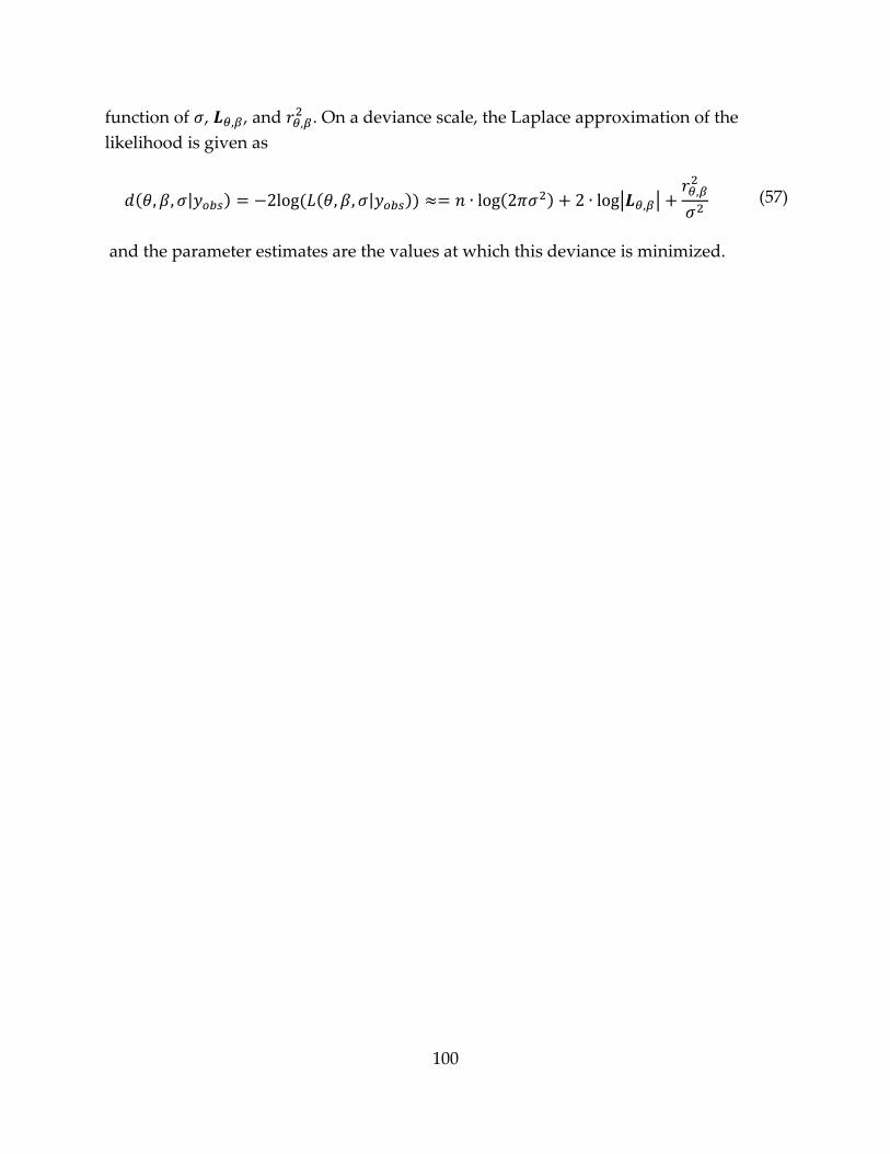
100

function of , , and . On a deviance scale, the Laplace approximation of the

likelihood is given as

| |

(57)

and the parameter estimates are the values at which this deviance is minimized.