abstract robust coarse spaces for systems of pdes via

JOHANNES KEPLER UNIVERSITY LINZ

Institute of Computational Mathematics

Abstract Robust Coarse Spaces for

Systems of PDEs via Generalized

Eigenproblems in the Overlaps

Nicole Spillane

Frédérik Nataf

Laboratoire Jacques-Louis Loins, CNRS UMR 7598

Université Pierre et Marie Curie, 75005 Paris, France

Victorita Dolean

Laboratoire J.-A. Dieudonné, CNRS UMR 6621

Université de Nice-Sophia Antipolis, 06108 Nice Cedex 02, France

Patrice Hauret

Centre de Technologie de Ladoux, Manufacture des Pneumatiques Michelin

63040 Clermont-Ferrand, Cedex 09, France

Clemens Pechstein

Institute of Computational Mathematics, Johannes Kepler University

Altenberger Str. 69, 4040 Linz, Austria

Robert Scheichl

Department of Mathematical Sciences, University of Bath,

Bath BA27AY, UK

NuMa-Report No. 2011-07 November 2011

A4040 LINZ, Altenbergerstraÿe 69, Austria

Technical Reports before 1998:

1995

95-1 Hedwig BrandstetterWas ist neu in Fortran 90? March 1995

95-2 G. Haase, B. Heise, M. Kuhn, U. LangerAdaptive Domain Decomposition Methods for Finite and Boundary ElementEquations.

August 1995

95-3 Joachim SchöberlAn Automatic Mesh Generator Using Geometric Rules for Two and Three SpaceDimensions.

August 1995

1996

96-1 Ferdinand KickingerAutomatic Mesh Generation for 3D Objects. February 1996

96-2 Mario Goppold, Gundolf Haase, Bodo Heise und Michael KuhnPreprocessing in BE/FE Domain Decomposition Methods. February 1996

96-3 Bodo HeiseA Mixed Variational Formulation for 3D Magnetostatics and its Finite ElementDiscretisation.

February 1996

96-4 Bodo Heise und Michael JungRobust Parallel Newton-Multilevel Methods. February 1996

96-5 Ferdinand KickingerAlgebraic Multigrid for Discrete Elliptic Second Order Problems. February 1996

96-6 Bodo HeiseA Mixed Variational Formulation for 3D Magnetostatics and its Finite ElementDiscretisation.

May 1996

96-7 Michael KuhnBenchmarking for Boundary Element Methods. June 1996

1997

97-1 Bodo Heise, Michael Kuhn and Ulrich LangerA Mixed Variational Formulation for 3D Magnetostatics in the Space H(rot)∩

H(div)February 1997

97-2 Joachim SchöberlRobust Multigrid Preconditioning for Parameter Dependent Problems I: TheStokes-type Case.

June 1997

97-3 Ferdinand Kickinger, Sergei V. Nepomnyaschikh, Ralf Pfau, Joachim Schöberl

Numerical Estimates of Inequalities in H1

2 . August 199797-4 Joachim Schöberl

Programmbeschreibung NAOMI 2D und Algebraic Multigrid. September 1997

From 1998 to 2008 technical reports were published by SFB013. Please seehttp://www.sfb013.uni-linz.ac.at/index.php?id=reports

From 2004 on reports were also published by RICAM. Please seehttp://www.ricam.oeaw.ac.at/publications/list/

For a complete list of NuMa reports seehttp://www.numa.uni-linz.ac.at/Publications/List/

http://www.sfb013.uni-linz.ac.at/index.php?id=reports

http://www.ricam.oeaw.ac.at/publications/list/

http://www.numa.uni-linz.ac.at/Publications/List/

ABSTRACT ROBUST COARSE SPACES FOR SYSTEMS OF PDES

VIA GENERALIZED EIGENPROBLEMS IN THE OVERLAPS

NICOLE SPILLANE1, VICTORITA DOLEAN2, PATRICE HAURET3, FREDERIK NATAF1,CLEMENS PECHSTEIN4, AND ROBERT SCHEICHL5

Abstract. Coarse spaces are instrumental in obtaining scalability for domain decompo-sition methods for partial differential equations (PDEs). However, it is known that mostpopular choices of coarse spaces perform rather weakly in the presence of heterogeneitiesin the PDE coefficients, especially for systems of PDEs. Here, we introduce in a varia-tional setting a new coarse space that is robust even when there are such heterogeneities.We achieve this by solving local generalized eigenvalue problems in the overlaps of sub-domains that isolate the terms responsible for slow convergence. We prove a generaltheoretical result that rigorously establishes the robustness of the new coarse space andgive some numerical examples on two and three dimensional heterogeneous PDEs andsystems of PDEs that confirm this property.

Keywords: coarse spaces, overlapping Schwarz method, two-level methods, generalized eigenvectors,problems with large coefficient variation

Mathematics Subject Classification (2000): 65F10, 65N22, 65N30, 65N55

1. Introduction

The effort to reach scalability in domain decomposition methods has led to the designof so called two-level methods. Each of these methods is characterized by two ingredients:a coarse space and a formulation of how this coarse space is incorporated into the domaindecomposition method. We will work in the already extensively studied framework ofthe overlapping additive Schwarz preconditioner [30, 28], and focus on the definition ofa suitable coarse space with the aim to achieve robustness with regard to heterogeneitiesin any of the coefficients in the PDEs. This type of problem arises in many applications,such as subsurface flows or linear elasticity. One way to avoid long stagnation in Schwarzmethods is to build the subdomains in such a way that the variations in the coefficientsare small or nonexistent inside each subdomain. In this configuration, classical coarsespaces that are based on these subdomain partitions are known to be robust, see e.g. [10,9, 20, 5, 6]. Recently, some authors also extended these results for scalar elliptic problemsto certain classes of coefficients that are not resolved by the subdomain partition andto operator dependent coarse spaces, see e.g. [16, 25, 22, 14, 26] as well as [31] and thereferences therein.

Date: 2 November 2011.1 Laboratoire Jacques-Louis Lions, CNRS UMR 7598, Universite Pierre et Marie Curie, 75005 Paris,

France, [email protected], [email protected] Laboratoire J.-A. Dieudonne, CNRS UMR 6621, Universite de Nice-Sophia Antipolis, 06108 Nice Cedex02, France, [email protected] Centre de Technologie de Ladoux, Manufacture des Pneumatiques Michelin, 63040 Clermont-Ferrand,Cedex 09, France, [email protected] Institute of Computational Mathematics, Johannes Kepler University, Altenberger Str. 69, 4040 Linz,Austria, [email protected] Department of Mathematical Sciences, University of Bath, Bath BA27AY, UK, [email protected].

1

2 N. SPILLANE, V. DOLEAN, F. NATAF, C. PECHSTEIN, AND R. SCHEICHL

However, ideally we would prefer methods that are robust for any partition into subdo-mains and regardless of the coefficient distribution. A class of such stable coarse spaceshas been presented among the literature on Schwarz methods for scalar elliptic PDEs in[15, 13, 27, 12], as well as in earlier work on algebraic multigrid (AMG) methods in [2, 3].The key ingredient in these coarse spaces is the solution of a generalized eigenvalue problemon each subdomain (or on each coarse element in spectral AMGe). While these spaces areindeed robust for any arbitrary coefficient distribution, they do not discriminate betweencoefficient variations that influence only the solution in the interior of the subdomains andthose that are actually responsible for the lack of robustness of standard coarse spaces. Aconsequence of this is that the resulting coarse space is often unnecessarily large.

A related but slightly different coarse space for scalar elliptic PDEs, based on general-ized eigenvalue problems for the Dirichlet-to-Neumann operator on the boundary of eachsubdomain, has recently been introduced and analyzed in [8, 7]. However, although thecoarse space size is largely reduced in this approach, this gain comes at the expense ofbeing not uniformly robust for arbitrary coefficient variations. The lack of robustnessfor some coefficient distributions is evident in the theoretical convergence analysis in [7],where a weighted Poincare inequality is needed to prove a stable weak approximationproperty for the coarse space in the part of each subdomain that is overlapped by othersubdomains. This type of inequality is very powerful, but it does not apply in the verygeneral setting of arbitrary coefficient variations that we wish to maintain (cf. [23]).

The terms in the overlapped regions arise naturally in the convergence calculations sothey provide valuable information. In this article, in order to be more general and toavoid the need for weighted Poincare type inequalities, while still discriminating betweencoefficient variations that are crucial for robustness and those which are not, we definethe generalized eigenproblems directly in the overlapped regions. Apart from the obviousattraction of providing a fully robust coarse space that is in general significantly smallerthan that proposed in [15], another significant advantage of the proposed approach is thatits fully abstract setting allows us to consider a very wide range of symmetric positivedefinite systems of equations. The method was first and briefly introduced in [29] by thesame authors and we give here a detailed proof of the previously stated convergence resultalong with some extensive numerical results.

One disadvantage of the earlier methods proposed in [14, 8] is that they need weightedmass matrices either in each subdomain or on its boundary. The mass matrices appearon the right hand side of the generalized eigenproblems in those approaches. In practice,this requires coefficient and mesh information. As in the more recent article [12], we donot need any mass matrices in our approach here. The right hand side of the generalizedeigenproblems is constructed from element stiffness matrices and a family of partitionof unity functions/operators. Thus, we only have to assume access to some topologicalinformation to build a suitable partition of unity and to the element stiffness matrices (as inAMGe methods, cf. [3]), which is reasonable in standard FE packages such as FreeFEM++[17]. The preconditioners can then be implemented fully algebraically, providing a viableoption for simulations on physical problems without the need to rewrite entire codes.

Our approach and our analysis are clearly related to those in [12], but fundamentallydifferent. The analysis in [12] is not given in the fully discrete setting. The analysisassumes that the product of an eigenfunction with a partition of unity function is againin the (abstract) finite element space. This assumption is of course violated for standardspaces, and to get back into the space, an additional interpolation operator is needed. Inthe practical implementation the authors of [12] use such an interpolation operator, but atheoretical proof of the stability of this interpolation operator is not given. In fact, sucha stable interpolation operator does not exist yet to our knowledge. We circumvent theuse of interpolation operators by the use of partition of unity operators that work directly

GENEO: A ROBUST COARSE SPACE FOR SYSTEMS OF PDES 3

on the degrees of freedom. This way, we maintain a fully abstract setting and our theoryapplies to the fully discrete method.

In Section 2 we define the problem that we solve and introduce the two-level additiveSchwarz framework along with some elements of generalized eigenvalue problem theory.In Section 3 we define the abstract procedure to construct robust coarse spaces based onGeneralized Eigenproblems in the Overlap (which we will refer to as the GenEO coarsespace) and give the main convergence result (Theorem 3.21). Section 4 gives detailedguidelines on how to implement the two-level Schwarz preconditioner with the GenEOcoarse space in a finite element code. Finally in Section 5 we test our method for Darcyand linear elasticity and make sure that it converges indeed robustly even for highly varyingcoefficients in two and three dimensions.

2. Preliminaries and notations

2.1. Problem Description. Given a Hilbert space V , a symmetric and coercive bilinearform a : V × V → R and an element f in the dual space V ′, we consider the abstractvariational problem: Find v ∈ V such that

(1) a(v, w) = 〈f, w〉, for all w ∈ V,

where 〈·, ·〉 denotes the duality pairing. This variational problem is associated with anelliptic boundary value problem (BVP) on a given polygonal (polyhedral) domain Ω ⊂ R

d

(d = 2 or 3) with suitable boundary conditions posed in a suitable space V of functionson Ω.

We consider a discretization of the variational problem (1) with finite elements basedon a mesh Th of Ω:

Ω =⋃

τ∈Thτ.

Let Vh ⊂ V denote the chosen conforming space of finite element functions. In the casewhere a(·, ·) is a bilinear form derived from a system of PDEs, Vh is a space of vectorfunctions. The discretization of (1) then reads: Find vh ∈ Vh such that

(2) a(vh, wh) = 〈f, wh〉, for all wh ∈ Vh.

Let φknk=1 be a basis for Vh with n := dim(Vh), then from (2) we can derive a linear

system

(3) Av = f ,

where the coefficients of the stiffness matrix A ∈ Rn×n and the load vector f ∈ R

n aregiven by Ak,l = a(φl, φk) and fk = 〈f, φk〉, where k, l = 1, . . . , n, and v is the vector ofcoefficients corresponding to the unknown finite element function vh in (2).

The basis φknk=1 can be quite arbitrary but it should fulfil a unisolvence property,

such that the basis functions supported on each element τ ∈ Th are linearly independentwhen restricted to τ . This is the case for standard finite element bases.

The only significant assumption we make on the problem is that the stiffness matrix A

is assembled from positive semi-definite element stiffness matrices.

Assumption 2.1. Let Vh(τ) = v|τ : v ∈ Vh. We assume that there exist positivesemi-definite bilinear forms aτ : Vh(τ) × Vh(τ) → R, for all τ ∈ Th, such that

a(v, w) =∑

τ∈Th

aτ (v|τ , w|τ ), for all v, w ∈ Vh.

Remark 2.2. If the variational problem is obtained from integrating local forms on thedomain then this is not a problem at all. For instance in the case of the Darcy equation


we can write for all v, w ∈ H10 (Ω):

a(v, w) =

∫

Ωκ∇v · ∇w =

∑

τ∈Th

∫

τ

κ∇v · ∇w =∑

τ∈Th

aτ (v|τ , w|τ ).

2.2. Additive Schwarz setting. In order to automatically construct a robust two-level Schwarz preconditioner for (3), we first partition our domain Ω into a set of non-overlapping subdomains Ω′

jNj=1 resolved by Th using for example a graph partitioner

such as METIS [18] or SCOTCH [4]. Each subdomain Ω′j is then extended to a domain

Ωj by adding one or several layers of mesh elements in the sense of Definition 2.3, thuscreating an overlapping decomposition Ωj

Nj=1 of Ω.

Definition 2.3. Given a subdomain D′ ⊂ Ω which is resolved by Th, the extension of D′

by one layer of elements is

D = Int( ⋃

k∈dof(D′)

supp(φk)), where dof(D′) := k : supp(φk) ∩ D′ 6= ∅,

and Int(·) denotes the interior of a domain. Extensions by more than one layer can thenbe defined recursively.

The proof of the following lemma is a direct consequence of Definition 2.3.

Lemma 2.4. For every degree of freedom k, with 1 ≤ k ≤ n, there is a subdomain Ωj,

with 1 ≤ j ≤ N , such that supp(φk) ⊂ Ωj .

Now, for each j = 1, . . . , N , let

Vh(Ωj) := v|Ωj: v ∈ Vh

denote the space of restrictions of functions in Vh to Ωj . Furthermore, let

Vh,0(Ωj) := v|Ωj: v ∈ Vh, supp (v) ⊂ Ωj

denote the space of finite element functions supported in Ωj . By definition, the extensionby zero of a function v ∈ Vh,0(Ωj) to Ω lies again in Vh. We denote the correspondingextension operator by

(4) R⊤j : Vh,0(Ωj) → Vh .

Lemma 2.4 guarantees that Vh =∑N

j=1 R⊤j Vh,0(Ωj). The adjoint of R⊤

j

Rj : V ′h → Vh,0(Ωj)

′ ,

called the restriction operator, is defined by 〈Rjg, v〉 = 〈g, R⊤j v〉, for v ∈ Vh,0(Ωj), g ∈ V ′

h.

However, for the sake of simplicity, we will often leave out the action of R⊤j and view

Vh,0(Ωj) as a subspace of Vh.

The final ingredient is a coarse space VH ⊂ Vh which will be defined later. Let R⊤H :

VH → Vh denote the natural embedding and RH its adjoint. Then the two-level additiveSchwarz preconditioner (in matrix form) reads

(5) M−1AS,2 = RT

HA−1H RH +

N∑

j=1

RTj A−1

j Rj , AH := RHARTH and Aj := RjART

j ,

where Rj , RH are the matrix representations of Rj and RH with respect to the basisφk

nk=1 and the chosen basis of the coarse space VH . As usual for standard elliptic BVPs,

Aj corresponds to the original (global) system matrix restricted to subdomain Ωj withDirichlet conditions on the artificial boundary ∂Ωj \ ∂Ω.

To simplify the notation, if D is the union of elements of Th and

Vh(D) := v|D : v ∈ Vh,


we write, for any v, w ∈ Vh(D),

aD(v, w) :=∑

τ∈D

aτ (v|τ , w|τ ) and |v|a,D =√

aD(v, v),

where the latter is the energy seminorm. The definition of aD(·, ·) extends naturally tov, w ∈ Vh(D′), for any D ⊂ D′ ⊂ Ω which simplifies notations. On each of the local spacesVh,0(Ωj) the bilinear form aΩj

(·, ·) is positive definite since

aΩj(v, w) = a(R⊤

j v, R⊤j w), for all v, w ∈ Vh,0(Ωj),

and because a(·, ·) is coercive on V . For the same reason, the matrix Aj in (5) is invertible.Hence, | · |a,Ωj

becomes a norm on Vh,0(Ωj) and so we write

‖v‖a,Ωj=

√aΩj

(v, v), for all v ∈ Vh,0(Ωj).

If D = Ω, we omit the domain from the subscript and write ‖ · ‖a instead of ‖ · ‖a,Ω.We use here the abstract framework for additive Schwarz (see [30, Chapter 2]). In the

following we summarize the most important ingredients.

Definition 2.5. We define k0 = maxτ∈Th

(#Ωj : 1 ≤ j ≤ N, τ ⊂ Ωj

).

This means that each point in Ω belongs to at most k0 of the subdomains Ωj .

Lemma 2.6. With k0 as in Definition 2.5, the largest eigenvalue of M−1AS,2 A satisfies

λmax(M−1AS,2 A) ≤ k0 + 1.

Proof. See, e.g., [11, Section 4]. ¤

Definition 2.7 (Stable decomposition). Given a coarse space VH ⊂ Vh, local subspacesVh,0(Ωj)1≤j≤N and a constant C0, a C0-stable decomposition of v ∈ Vh is a family offunctions zj0≤j≤N that satisfies

(6) v =N∑

j=0

zj , with z0 ∈ VH , zj ∈ Vh,0(Ωj), for j ≥ 1,

and

(7) ‖z0‖2a +

N∑

j=1

‖zj‖2a,Ωj

≤ C20 ‖v‖

2a .

Theorem 2.8. If every v ∈ Vh admits a C0-stable decomposition (with uniform C0), thenthe smallest eigenvalue of M−1

AS,2 A satisfies

λmin(M−1AS,2 A) ≥ C−2

0 .

Therefore, the condition number of the two-level Schwarz preconditioner (5) can be boundedby

κ(M−1AS,2A) ≤ C2

0 (k0 + 1).

Proof. The statement is a direct consequence of [30, Lemma 2.5] and Lemma 2.6. ¤

In the following, we will construct a C0-stable decomposition in a specific framework,but prior to that we will provide in an abstract setting, a sufficient and simplified conditionof stability.


Lemma 2.9. Using the notations introduced in Definition 2.7, if there exists a constantC1 such that

(8) ‖zj‖2a,Ωj

≤ C1|v|2a,Ωj

, for all j = 1, . . . , N,

then the decomposition (6) is C0-stable with C20 = 2 + C1k0(2k0 + 1) where k0 is given in

Definition 2.5.

Proof. From (8) and Definition 2.5 we get successively

(9)N∑

j=1

‖zj‖2a,Ωj

≤ C1

N∑

j=1

|v|2a,Ωj≤ C1k0 ‖v‖

2a .

We also have:

(10) ‖z0‖2a =

∥∥∥∥∥∥v −

N∑

j=1

zj

∥∥∥∥∥∥

2

a

≤ 2 ‖v‖2a + 2

∥∥∥∥∥∥

N∑

j=1

zj

∥∥∥∥∥∥

2

a

,

and from Definition 2.5 and (9) we get

(11)

∥∥∥∥∥∥

N∑

j=1

zj

∥∥∥∥∥∥

2

a

≤ k0

N∑

j=1

‖zj‖2a,Ωj

≤ C1k20 ‖v‖

2a .

Using (11) in (10) yields

(12) ‖z0‖2a ≤ 2(1 + C1k

20) ‖v‖

2a .

By adding (9) and (12) we get (7) with C20 = 2 + C1k0(2k0 + 1). ¤

When ‖z0‖2a can be bounded directly in terms of ‖v‖2

a (independently of the coefficientvariation), this lemma is superfluous and leads to a suboptimal quadratic dependence onk0. In general, however, it is not possible to provide such a uniform bound on ‖z0‖

2a, which

is why Lemma 2.9 is in fact absolutely crucial for our analysis.

2.3. Abstract generalized eigenproblems. In order to construct the coarse space wewill use generalized eigenvalue problems in each subdomain. Since several variations ofgeneralized eigenvalue problems exist in the literature (particularly concerning the inter-pretation of the ‘infinite eigenvalue’), we state the definition that we use.

Definition 2.10 (Generalized eigenvalue problem). Let V be a finite-dimensional Hilbert

space, let a : V × V → R and b : V × V → R be two symmetric bilinear forms. Then the

generalized eigenvalues associated with the so called ‘pencil’ (a, b) are the following values

λ ∈ R ∪ +∞: either λ ∈ R and there exists p ∈ V \0 such that

(13) a(p, v) = λ b(p, v), for all v ∈ V ,

or λ = +∞ and there exists p ∈ V \0 such that

b(p, v) = 0, for all v ∈ V , and a(p, v) 6= 0, for a certain v ∈ V .

In both cases p is called a generalized eigenvector associated with the eigenvalue λ.

The definition above allows for infinite eigenvalues. This results from the fact that if

(+∞, p) is an eigenpair for the pencil (a, b) then (0, p) is an eigenpair for the pencil (b, a)and there is no reason to discriminate between both formulations. In cases where thebilinear form b is positive definite the problem can be simplified and crucial properties onthe eigenvalues and eigenvectors arise. In particular, this leads quite naturally to optimalprojectors onto subspaces of the functional space as the next lemma shows in an abstractsetting.


Lemma 2.11. Now let a be positive semi-definite and b positive definite, and let the

eigenpairs (pk, λk)dim(eV )k=1 of the generalized eigenvalue problem (13) be ordered such that

0 ≤ λ1 ≤ . . . ≤ λdim(eV )

and b(pk, pl) = δkl , for any 1 ≤ k, l ≤ dim(V ).

Then, for any integer 1 ≤ m < dim(V ), the projection

Πmv :=

m∑

k=1

b(v, pk)pk

is a-orthogonal, and thus

(14) |Πmv|ea ≤ |v|ea and |v − Πmv|ea ≤ |v|ea, for all v ∈ V .

Additionally, if m is such that λm+1 > 0, we have the stability estimate

‖v − Πmv‖2eb

≤1

λm+1|v − Πmv|2

ea, for all v ∈ V .

Proof. Due to the additional assumptions on a and b, the generalized eigenvalue problemcan be simplified to a standard eigenvalue problem, for which the existence of eigenvec-

tors pkdim(eV )k=1 with associated non-negative real eigenvalues λk

dim(eV )k=1 is guaranteed by

standard spectral theory. Moreover, pkdim(eV )k=1 can be chosen such that it is a basis of V

fulfilling the orthogonality conditions:

a(pk, pl) = b(pk, pl) = 0 ∀k 6= l, |pk|2eb

= 1 and |pk|2ea = λk.

Now let v ∈ V be fixed. From the b-orthonormality of the basis we get

v =

dim(eV )∑

k=1

b(v, pk)pk.

For any index set I ⊂ 1, ...,dim(V ), the a-orthogonality implies∣∣∣∣∣∑

k∈I

b(v, pk)pk

∣∣∣∣∣

2

ea

=∑

k∈I

b(v, pk)2|pk|

2ea.

Thus|v|2

ea = |Πmv|2ea + |v − Πmv|2

ea.

and (14) follows directly. Finally,

‖v − Πmv‖2eb

=∥∥∥

dim(eV )∑

k=m+1

b(v, pk) pk

∥∥∥2

eb

=

dim(eV )∑

k=m+1

b(v, pk)2 (by the b-orthonormality of pk)

=

dim(eV )∑

k=m+1

b(v, pk)2 1

λk|pk|

2ea (since λk = |pk|

2ea)

≤1

λm+1

dim(eV )∑

k=m+1

b(v, pk)2 |pk|

2ea (since λ1 ≤ . . . ≤ λ

dim(eV ))

=1

λm+1|v − Πmv|2

ea (by the a-orthogonality of pk).


¤

This lemma will be one of the core arguments to prove the existence of a stable decom-position onto the new GenEO (Generalized Eigenproblems in the Overlap) coarse spaceand the local subspaces.

3. Algebraic construction of a robust coarse space and its analysis

In this section we introduce the coarse space and give a bound on the condition numberof the two-level additive Schwarz method with this coarse space along with a rigorousproof of this result. The proof will consist in proving the existence of a stable splitting forany function in Vh in the sense of Definition 2.7.

3.1. The coarse space. The GenEO coarse space is constructed as follows. In eachsubdomain we pose a suitable generalized eigenproblem and select a number of low frequenteigenfunctions. These local functions are converted into global coarse basis functions usinga partition of unity operator. As mentioned before, the eigenproblems are restricted to theoverlapping zone, which is introduced in the next definition. Following this definition, wewill then define the partition of unity operator, which will appear both in the eigenproblemsthemselves and in the construction of the coarse basis functions.

Definition 3.1 (Overlapping zone). For each subdomain Ωj (1 ≤ j ≤ N), the overlappingzone is given by

Ωj = x ∈ Ωj : ∃ j′ 6= j such that x ∈ Ωj′.

We will also require the set of degrees of freedom associated with Vh(Ωj), as well asthose associated with Vh,0(Ωj), for 1 ≤ j ≤ N .

Definition 3.2. Given a subdomain D that is a union of elements from Th, let

dof(D) := k = 1, . . . , n : supp (φk) ∩ D 6= ∅

denote the set of degrees of freedom that are “active” in D, including those associated withthe boundary. Similarly, we denote by

dof(D) := k : 1 ≤ k ≤ n and supp(φk) ⊂ D

the set of internal degrees of freedom in D.

Remark 3.3. Since the basis functions φk of Vh fulfil a unisolvence property on eachelement they also fulfil a unisolvence property on each subdomain Ωj, in other words thefunctions φk|Ωj

k∈dof(Ωj)(resp. φk|Ωj

k∈dof(Ωj)) are linearly independent. A direct con-

sequence is that these functions form a basis of Vh(Ωj) (resp. Vh,0(Ωj)).

Now we can introduce the partition of unity operators. Recall that, for any v ∈ Vh, wewrite v =

∑nk=1 vk φk.

Definition 3.4 (Partition of unity). For any degree of freedom k, 1 ≤ k ≤ n, let µk denotethe number of subdomains for which k is an internal degree of freedom, i.e.

µk := # j : 1 ≤ j ≤ N and k ∈ dof(Ωj).

Then, for 1 ≤ j ≤ N , the local partition of unity operator Ξj : Vh(Ωj) → Vh,0(Ωj) is definedby

Ξj(v) :=∑

k∈dof(Ωj)

1

µkvk φk|Ωj

, for all v ∈ Vh(Ωj).


Lemma 3.5. The operators Ξj from Definition 3.4 form a partition of unity in the fol-lowing sense:

(15)

N∑

j=1

R⊤j Ξj(v|Ωj

) = v, for all v ∈ Vh.

Moreover,

(16) Ξj(v)|Ωj\Ω

j= v|Ωj\Ω

j, for all v ∈ Vh(Ωj) and 1 ≤ j ≤ N.

Proof. Property (15) follows directly from the definition. To show (16), let v ∈ Vh(Ωj)and recall that by definition

Ξj(v)|Ωj\Ω

j=

∑

k∈dof(Ωj)

1

µkvk φk|Ωj\Ω

j.

Now note that if µk > 1, then φk|Ωj\Ω

j= 0. Hence,

Ξj(v)|Ωj\Ω

j=

∑

k∈dof(Ωj) s.t. µk=1

vk φk|Ωj\Ω

j=

∑

k∈dof(Ωj\Ω

j )

vk φk|Ωj\Ω

j,

but this is also the definition of v|Ωj\Ω

j. ¤

Next we define the local generalized eigenproblems for the GenEO coarse space.

Definition 3.6 (Generalized Eigenproblems in the Overlaps). For each j = 1, . . . , N , wedefine the following generalized eigenvalue problem

(17) aΩj(p, v) = λ bj(p, v), for all v ∈ Vh(Ωj).

where bj(p, v) := aΩ

j(Ξj(p), Ξj(v)), for all p, v ∈ Vh(Ωj).

Remark 3.7. Although the form of the bilinear forms bj(·, ·) seems somewhat artificial,we will see below that it actually arises naturally in the analysis. We will also see that wecould have chosen a different partition of unity operator, provided it satisfies the propertiesin Lemma 3.5. The eigenvalues in Lemma 3.19 are dimensionless quantities and do notchange when the coordinates of the mesh are rescaled.

The GenEO coarse space is now constructed (locally) as the span of a suitable subsetof eigenfunctions in (17). To obtain a global coarse space we apply the partition of unityoperators.

Definition 3.8 (GenEO coarse space). For each j = 1, . . . , N , let (pjk)

mj

k=1 be the eigen-functions of the eigenproblem (17) in Definition 3.6 corresponding to the mj smallesteigenvalues. Then,

VH := spanR⊤j Ξj(p

jk) : k = 1, . . . , mj ; j = 1, . . . , N,

where Ξj are the partition of unity operators from Definition 3.4 and R⊤j are the extension

operators defined in (4).

Consequently, we can also make explicit the final component in Definition 5 of thematrix form M−1

AS,2 of the additive Schwarz preconditioner, namely the prolongation ma-

trix RTH . The columns of the rectangular matrix RT

H ∈ Rn×dim(VH) are simply the vector

representations of the functions R⊤j Ξj(p

jk) : k = 1, . . . , mj ; j = 1, . . . , N with respect to

the finite element basis φknk=1. Clearly dim (VH) =

∑Nj=1 mj and a strategy for selecting

mj will be given below. This completes the definition of M−1AS,2.


supp(φk)

supp(φk)

supp(φk)supp(φk)

k ∈ βj1 k ∈ βj

2 k ∈ βj3

supp(φk) 6⊂ Ωj supp(φk) ⊂ Ωj \ Ωj supp(φk) ⊂ Ωj ,

supp(φk) 6⊂ Ωj \ Ωj

Figure 1. Three types of finite element basis functions on each subdomainΩj . The hashed surface is the overlap Ω

j .

3.2. Analysis of the preconditioner. To confirm the robustness of the above coarsespace and to bound the condition number of M−1

AS,2A via Theorem 2.8 we will now showthat there is a stable splitting for each v ∈ Vh in the sense of Definition 2.7. First wewill give some results on the local subspaces Ωj , then we use them to show that theeigenproblems from Definition 3.6 are well defined and that the eigenpairs have some

particular properties. In order to do this we define a subspace Vj of each Vh(Ωj) on whichthe restriction of the local generalized eigenproblems satisfy the hypotheses of Lemma 2.11.This leads to local projectors onto subspaces of Vh(Ωj) which satisfy stability estimates.These stability estimates will generalize to the whole of Vh(Ωj) and enable us to split anyv ∈ Vh in a “C0-stable” manner.

Definition 3.9. We partition the set dof(Ωj) of degrees of freedom in Vh(Ωj) into threesets (see also Figure 1):

βj1 := dof(Ωj) \ dof(Ωj) (the DOFs on the boundary of Ωj),

βj2 := dof(Ωj\Ω

j ) (the interior DOFs in Ωj\Ω

j ),

βj3 := dof(Ωj) \ dof(Ωj\Ω

j ) (the DOFs in the overlap, incl. the inner boundary).

From these index sets we define subsets of functions of Vh(Ωj)

Bj1 := span

φk|Ωj

k∈β

j1

, Bj2 := span

φk|Ωj

k∈β

j2

and Bj3 := span

φk|Ωj

k∈β

j3

,

such that

Vh(Ωj) = Bj1 ⊕ Bj

2 ⊕ Bj3.

The following simple properties will be used frequently in the following.

Lemma 3.10. For any 1 ≤ j ≤ N , the following properties are true

(1) supp (v) ⊂ Ωj , for all v ∈ Bj

1,

(2) Bj1 = Ker(Ξj),

(3) Bj2 = v ∈ Vh(Ωj) : v|Ω

j= 0,

(4) aΩjis coercive on Bj

2.

Proof.

(1) For any basis function φk with k ∈ βj1, Lemma 2.4 implies that there is another

subdomain Ωj′ with supp(φk) ⊂ Ωj′ , and so supp(φk) ∩ (Ωj \ Ωj ) = ∅.


(2) Let v ∈ Vh(Ωj). Then

v ∈ Ker(Ξj) ⇔ vk = 0, for all k ∈ dof(Ωj) ⇔ v =∑

k∈βj1

vkφk|Ωj∈ Bj

1 .

(3) It is clear from the definition of Bj2 that Bj

2 ⊂ v ∈ Vh(Ωj) : v|Ω

j= 0. Conversely,

if v|Ω

j= 0, then from the unisolvence property, vk = 0, for all k ∈ dof(Ω

j ) =

βj1 ∪ βj

3, and therefore v ∈ Vh(Ωj) : v|Ω

j= 0 ⊂ Bj

2 also.

(4) The previous property implies that Bj2 ⊂ Vh,0(Ωj) and so

aΩj(v, w) = a(R⊤

j v, R⊤j w) for all v, w ∈ Bj

2.

The coercivity of aΩj(·, ·) on Bj

2 follows from the coercivity of a(·, ·). ¤

To carry out a robustness analysis we need to make the following two assumptions.

Assumption 3.11. For any 1 ≤ j ≤ N , aΩjis coercive on Bj

1.

Assumption 3.12. For any 1 ≤ j ≤ N , aΩ

jis coercive on Bj

3.

Note that by the first property in Lemma 3.10, Assumption 3.11 is equivalent to as-

suming that, for any 1 ≤ j ≤ N , aΩ

jis coercive on Bj

1.

Remark 3.13. Assumptions 3.11 and 3.12 are not too restrictive. If all the elementstiffness matrices are positive definite, then aΩj

and aΩ

jare positive definite on the whole

of Vh(Ωj). For the Darcy equation or linear elasticity, the element stiffness matrices are

not positive definite. However, any function v ∈ Bj1 satisfies vk = 0, for k 6∈ βj

1, and

any function v ∈ Bj3 vanishes on the boundary of Ωj (by that we mean that vk = 0, for

k ∈ β1j ). Therefore, in the Darcy case and in the case of standard H1-conforming finite

elements, Assumptions 3.11 and 3.12 hold if each of the sets βj1 and βj

3 contains at least

one DOF. To make the assumptions hold for linear elasticity, the sets βj1 and βj

3 needto contain enough DOFs to fix the rigid body modes in Ω

j , i.e., at least 3(d − 1) DOFs.

Hence, for standard H1-conforming finite elements, it is sufficient to have d non-collinearpoints (with associated DOFs for all components of the vector function) that lie on theouter boundary ∂Ωj, respectively in Ω

j \ ∂Ωj.

The final technical hurdle to construct a stable splitting is that we cannot apply theabstract Lemma 2.11 to the specific eigenproblems used in the construction of the GenEOcoarse space VH directly, because the bilinear forms bj(·, ·) := aΩ

j(Ξj(·), Ξj(·)) from Defi-

nition 17 are not necessarily positive definite on all of Vh(Ωj)× Vh(Ωj), for all 1 ≤ j ≤ N .

To complete the analysis we thus need to define a suitable subspace Vj ⊂ Vh(Ωj) such that

bj is positive definite on Vj × Vj .

Definition 3.14. Let the spaces Vj and Wj be defined by

Vj := v ∈ Vh(Ωj) : aΩj(v, w) = 0, for all w ∈ Wj where Wj := Bj

1 ⊕ Bj2 .

Lemma 3.15. Under Assumption 3.11,

Vh(Ωj) = Vj ⊕ Wj .

Proof. Since aΩjis coercive on Bj

1 (cf. Assumption 3.11) and on Bj2 (cf. Lemma 3.10 (4))

and since functions in Bj1 and Bj

2 have disjoint supports, we also have that aΩjis coercive on

Wj . It follows from the definition of Vj (via some simple linear algebra) that Vj∩Wj = 0

and that dim(Vj) = dim(Vh(Ωj)) − dim(Wj). ¤


Remark 3.16. While this lemma shows that Vj and Bj3 contain the same degrees of

freedom, it does not imply that Vj = Bj3. The functions in Vj are extended “discrete

PDE-harmonically” to the whole of Ωj, while those in Bj3 are extended by zero. The har-

monic extension into Ωj \ Ωj is always well defined because of the coercivity of aΩj

on Bj2

(cf. Lemma 3.10 (4)). The fact that the harmonic extension onto Bj1 is well defined is a

consequence of Assumption 3.11.

The role of Assumption 3.12 becomes clear in the next lemma.

Lemma 3.17. Under Assumptions 3.11 and 3.12, for j = 1, ..., N , the bilinear form

bj(·, ·) := aΩ

j(Ξj(·), Ξj(·)) is positive definite on Vj × Vj.

Proof. Let v ∈ Vj such that bj(v, v) = 0. We need to show that necessarily v = 0.

There exists a unique decomposition v = v1 + v2 + v3, such that vi ∈ Bji . The second

property in Lemma 3.10 states that Bj1 = Ker(Ξj), and so

Ξj(v1) = 0.

From the definition of Ξj it is obvious that Ξj |Bj2

: Bj2 → Bj

2 is the identity, and so

Ξj(v2) ∈ Bj2 and in particular from the third property in Lemma 3.10

supp (Ξj(v2)) ∩ Ωj = ∅.

From these two remarks and the definition of bj it follows that

(18) bj(v, v) = aΩ

j(Ξj(v3), Ξj(v3)).

Moreover, from the definition of Ξj it is also obvious that Ξj |Bj3

: Bj3 → Bj

3 is a bijection,

and so Ξj(v3) ∈ Bj3. Now, (18) and Assumption 3.12 imply that Ξj(v3) = 0. The fact that

Ξj |Bj3

is a bijection in turn implies that v3 = 0, and so v ∈ Wj . From Lemma 3.15, we

know that Vj ∩ Wj = 0, and so v = 0 which ends the proof. ¤

We can now apply Lemma 2.11 to the restriction of the GenEO eigenproblems to Vj×Vj

and characterize the entire spectrum (including the infinite eigenvalues).

Lemma 3.18. For each j = 1, ..., N , consider the generalized eigenproblem (17) in Defi-nition 3.6.

(i) There are dim(Vj) finite eigenvalues 0 ≤ λj1 ≤ λj

2 ≤ . . . ≤ λj

dim(eVj)< ∞ (counted

according to multiplicity) with corresponding eigenvectors denoted by pjk

dim(eVj)k=1 and

normalized to form an orthonormal basis of Vj with respect to bj(·, ·).

(ii) There are dim(Wj) infinite eigenvalues λj

dim(eVj)+1= . . . = λj

dim(Vh(Ωj))= ∞ with

associated eigenvectors denoted by pjk

dim(Vh(Ωj))

dim(eVj)+1forming a basis of Wj.

Proof. Since Vh(Ωj) = Vj ⊕ Wj (cf. Lemma 3.15) and aΩj(v, w) = bj(v, w) = 0, for all

v ∈ Vj and w ∈ Wj , the eigenproblem (17) can be decoupled into two eigenproblems: one

on Vj and one on Wj .

Since, according to Lemma 3.17, bj(·, ·) is coercive on Vj × Vj , we can apply Lemma 2.11

with V 7→ Vj , a 7→ aΩj, and b 7→ bj to analyse the restriction of (17) to Vj . This completes

the proof of (i).


For the restriction of (17) to Wj , we prove that all vectors in Wj are eigenvectors

associated with the eigenvalue +∞ in the sense of Definition 2.10. Let v ∈ Wj . ThenΞj(v)|Ω

j= 0 and so in particular

(19) aΩ

j(Ξj(v), Ξj(w)) = 0 for all v, w ∈ Wj .

Moreover, we have already seen in the proof of Lemma 3.15 that aΩjis coercive on Wj ,

and so

(20) aΩj(v, v) 6= 0 for all v ∈ Wj\0.

Due to (19) and (20), any v ∈ Wj is indeed an eigenvector to the eigenvalue +∞ in the

sense of Definition 2.10. We can use any set of linearly independent vectors in Wj to form

a basis, e.g. pjk

dim(Vh(Ωj))

k=dim(eVj)+1= φk|Ωj

k∈β

j1∪β

j2

. ¤

We are now ready to define the crucial projection operators onto the local componentsof the GenEO coarse space that satisfy suitable stability estimates.

Lemma 3.19 (Local stability estimate). Let j ∈ 1, ..., N and let (pjk, λ

jk)

dim(Vh(Ωj))k=1

be as defined in Lemma 3.18. Suppose that mj ∈ 1, . . . ,dim(Vh(Ωj)) − 1 such that

0 < λjmj+1 < ∞. Then, the local projection operator

Πjmj

v :=

mj∑

k=1

aΩ

j(Ξj(v), Ξj(p

jk)) pj

k

satisfies

(21) |Πjmj

v|a,Ωj≤ |v|a,Ωj

and |v − Πjmj

v|a,Ωj≤ |v|a,Ωj

, for all v ∈ Vh(Ωj),

as well as the stability estimate

(22)∣∣∣Ξj(v − Πj

mjv)

∣∣∣2

a,Ω

j

≤1

λjmj+1

∣∣∣v − Πjmj

v∣∣∣2

a,Ωj

, for all v ∈ Vh(Ωj).

Proof. The condition λjmj+1 < ∞, ensures that mj ≤ dim(Vj), so Πj

mj maps to Vj . There-

fore, for all v ∈ Vj , the estimates in (21) and (22) can be deduced from Lemma 2.11 again,

with V 7→ Vj , a 7→ aΩj, b 7→ bj , and m 7→ mj .

To prove the result for all v ∈ Vh(Ωj), we use again the fact that Vh(Ωj) = Vj ⊕ Wj and

that aΩj(v, w) = 0, for all v ∈ Vj and w ∈ Wj . Let v = vV + vW ∈ Vh(Ωj) with vV ∈ Vj

and vW ∈ Wj . Then Πjmjv = Πj

mjvV and so (21) follows due to the aΩj-orthogonality of

Vj and Wj . Estimate (22) follows similarly from Ξj(vW )|Ω

j= 0. ¤

Lemma 3.20 (Stable decomposition). Let v ∈ Vh and suppose the definitions and nota-tions of Lemma 3.19 hold. Then, the decomposition

z0 :=N∑

j=1

Ξj(Πjmj

v|Ωj), zj := Ξj(v|Ωj

− Πjmj

v|Ωj), for j = 1, . . . , N,

is C0-stable with

C20 = 2 + k0(2k0 + 1) max

1≤j≤N

(1 +

1

λjmj+1

).


Proof. By definition ‖zj‖2a,Ωj

= |Ξj(v − Πjmjv|Ωj

)|2a,Ω

j+ |Ξj(v − Πj

mjv|Ωj)|2

a,Ωj\Ω

j.

However, due to property (16) in Lemma 3.5, Ξj is the identity for restrictions of functionsto Ωj \ Ω

j , and so

‖zj‖2a,Ωj

=∣∣Ξj(v − Πj

mjv|Ωj

)∣∣2a,Ω

j

+∣∣v − Πj

mjv|Ωj

∣∣2a,Ωj\Ω

j

.

Now we can apply Lemma 3.19 to get

‖zj‖2a,Ωj

≤(1 +

1

λjmj+1

)∣∣v − Πjmj

v|Ωj

∣∣2a,Ωj

≤(1 +

1

λjmj+1

)|v|2a,Ωj

,

where in the last step we have used (21). ¤

With this stable decomposition we can now state our main result on the convergenceof the two-level Schwarz preconditioner with the new GenEO coarse space. It followsimmediately from Theorem 2.8 and Lemma 3.20.

Theorem 3.21 (Bound on the condition number). Let Assumptions 2.1, 3.11, and 3.12hold. Suppose that the coarse space VH is given by Definition 3.8 and M−1

AS,2 is as defined

in (5). Then we can bound the condition number for the two-level Schwarz method by

κ(M−1AS,2A) ≤ (1 + k0)

[2 + k0(2k0 + 1) max

1≤j≤N

(1 +

1

λjmj+1

)],

where k0 is given in Definition 2.5.

The only parameters that need to be chosen in our coarse space are the numbers mj

of eigenmodes on each subdomain Ωj , 1 ≤ j ≤ N , to be included in the coarse space. Wesuggest the following choice which recovers the condition number estimate for problemswith no strong coefficient variation.

Corollary 3.22. For any j, 1 ≤ j ≤ N , let

(23) mj := min

m : λj

m+1 >δj

Hj

,

where δj is a measure of the width of the overlap Ωj and Hj = diam (Ωj). Then

κ(M−1AS,2A) ≤ (1 + k0)

[2 + k0(2k0 + 1) max

1≤j≤N

(1 +

Hj

δj

)].

Note that the number of subdomains and the coefficient variations do not appear inthis bound on the condition number. This means that we have established rigorously thatthe algorithm is robust with respect to these two parameters. The size of the coarse spaceinduced by the criterion does however depend on the geometry of the coefficient variationin the overlaps. We will confirm this in Section 5.

4. Implementation

In this section we would like to address implementation issues of the proposed algorithminvolving the GenEO coarse space. In the sections above, we have worked with functionspaces as they are more convenient in the analysis. However, as we will demonstrate below,our algorithm requires only abstract information of the problem in form of the elementstiffness matrices and no further information on the mesh, the finite element spaces, orany coefficients. Indeed, for running the algorithm we need

(i) the list dof(τ) of degrees of freedom associated with each element τ ∈ Th,(ii) the element stiffness matrix Aτ = (aτ (φl, φk))k, l∈dof(τ) associated with each ele-

ment τ ∈ Th.

Unless the overlapping subdomain partition is available a priori, we additionally need


(iii) the number ℓ of layers which determine the amount of overlap.

Before going into details, we note that as for the classical two-level overlapping Schwarzmethod (see, e.g. [30, Sect. 3]), our algorithm can be parallelized straightforwardly. Inparticular, the solution of the eigenproblems in the preprocessing step and the subdomainsolves during each PCG iteration can be performed fully in parallel.

4.1. Preprocessing. We need the overlapping partition Ω =⋃N

j=1 Ωj in form of thelist of elements associated with each subdomain Ωj . To obtain this, we first create the

connectivity graph of the elements (using the lists dof(τ) from (i)) and partition it intodisjoint sets of elements which make up the non-overlapping subdomains Ω′

j using for

instance METIS [18] or SCOTCH [4]. Then, for each (global) DOF k, we build the list

elem(k) = τ ∈ Th : k ∈ dof(τ)

of elements where DOF k is active. This list realizes supp(φk) without knowing the basisfunction φk itself. In a second step we add ℓ layers to each non-overlapping subdomain Ω′

j

according to Definition 2.3, which finally results in a list T jh of elements per (overlapping)

subdomain Ωj . From T jh , we construct

dof(Ωj) =⋃

τ∈T j

h

dof(τ)

(cf. Definition 3.2). Then we can compute the set

dof(Ωj) = k ∈ dof(Ωj) : ∀τ ∈ elem(k) : τ ∈ T jh

of internal degrees of freedom in Ωj (cf. Definition 3.4). One should keep in mind thatφk|Ωj

k∈dof(Ωj)is a basis for Vh(Ωj) and that φk|Ωj

k∈dof(Ωj) is a basis for Vh,0(Ωj).

Finally, by generating the subdomain ownership for each element,

owner(τ) = j = 1, . . . , N : τ ∈ T jh ,

it is straightforward to get the list

T j,h =

τ ∈ T j

h : owner(τ) \ j 6= ∅

of elements that make up the overlapping zone Ωj for each j = 1, . . . , N .

4.2. The eigenproblems. For each subdomain Ωj , j = 1, . . . , N we use a local renum-

bering of the degrees of freedom dof(Ωj) of Vh(Ωj). By assembling the element stiffness

matrices for the selected DOFs over the elements τ ∈ T jh , we get the subdomain “Neu-

mann” matrix Aj . For the same renumbering of DOFs, we assemble only over the elements

τ ∈ T j,h and obtain the “Neumann” matrix A

j associated to the overlapping zone Ωj .

Note that Aj and A

j have the same format, but A

j usually contains a block of zeros.From Definition 3.4, we see immediately that the action of the operator Ξj can be coded

by a diagonal matrix Xj , where the diagonal entry corresponding to the global DOF k isequal to 1/µk, if k ∈ dof(Ωj), and zero otherwise.

With these notations, the eigenproblem given in Definition 3.6 reads: Find the eigen-

vectors pjk ∈ R

#dof(Ωj) and eigenvalues λjk ∈ R ∪ +∞ that satisfy

(24) Ajpjk = λj

k Bjpjk ,

whereBj = XjA

jXj .

To get the coarse basis functions, we need to solve these eigenproblems (at least we needsufficiently many eigenpairs corresponding to low frequent modes) and to then select mj

of these eigenfunctions for our coarse space. With the criterion suggested in (23), we need


measures δj and Hj for the width of the overlapping zone and the subdomain diameter,respectively. If the mesh can be assumed to be quasi-uniform, we may replace the ratioδj/Hj by the number of layers of extension we applied in subdomain Ωj divided by thenumber of layers Ωj contains in total (which is available via the connectivity graph).

4.3. The preconditioner. Having selected the eigenvectors pjk, the coarse basis functions

are given by the vectors RT

j Xjpjk, where the matrix R

T

j maps the renumbered DOFs tothe global DOFs and fills the rest of the vector with zeros. The columns of the matrix

RTH are exactly the vectors R

T

j Xjpjk, where j = 1, . . . , N , k = 1, . . . , mj . The coarse

matrix AH = RHARTH can be efficiently assembled subdomain-wise by using the fact

that the coarse basis functions corresponding to two subdomains only interact when thesubdomains overlap. Thus, in a parallel regime, we basically only need next-neighborcommunication.

For each subdomain, we introduce a renumbering of the DOFs of Vh,0(Ωj) in dof(Ωj)(i.e. only the interior DOFs). This may differ from the numbering employed in theeigenproblems that were defined on all DOFs. By assembling the element stiffness matrices

for these DOFs over the elements τ ∈ T jh , we get the subdomain “Dirichlet” matrix Aj

(alternatively, one can just get the entries of Aj directly from those of the global matrix

A). The matrix RTj simply describes the mapping of the renumbered DOFs to the global

DOFs. It differs from RT

j in that it only maps from the interior DOFs on Ωj . This

completes the definition of the preconditioner M−1AS,2.

Clearly, once the information above is stored and the matrices Aj are factorized, each

application of M−1AS,2 (within the PCG) can be carried out efficiently.

4.4. An alternative way of solving the eigenproblems. The size of the (algebraic)eigenproblem (24) to be solved in each subdomain can be reduced. By rearranging the

local DOFs dof(Ωj) with respect to the sets βj1, βj

2, and βj3 (cf. Definition 3.9), the matrices

Aj and Bj take the following block form

Aj =

A11

j 0 A13

j

0 A22

j A23

j

(A13

j )T (A23

j )T A33

j

, Bj =

0 0 00 0 00 0 B33

j

,

where Akl

j = aΩj(φm, φn)

n∈βj

k,m∈β

j

l

. The two zero blocks in Aj are due the fact that the

supports of functions in Bj1 and Bj

2 are always disjoint. Since A11

j is the matrix version of

the bilinear form aΩ

j(·, ·) : Bj

1 × Bj1 → R, and since Assumption 3.11 states that aΩ

j(·, ·)

is coercive on B1, it follows that the block A11

j is positive definite and thus invertible.

Similarly, A22j is positive definite due to Lemma 3.10 (4).

Suppose that (pjk, λj

k) is an eigenpair of (24) with λjk < ∞ and let p

j,lk , l = 1, . . . , 3

denote the blocks of pjk with respect to βj

l . Then it follows by block-elimination that

Sj pj,3k = λj

kB33j p

j,3k(25)

with Sj = A33

j − A13

j [A11

j ]−1A13

j − A23

j [A22

j ]−1A23

j . The two remaining blocks can thenbe computed from

pj,1k = −[A

11

j ]−1A13

j pj,3k ,

pj,2k = −[A

22

j ]−1A23

j pj,3k


(i.e. via discrete harmonic extension). Since we are only interested in the eigenpairs withfinite eigenvalues, we can solve eigenproblem (25) instead of (24). Due to the appearanceof the Schur complement Sj and because we are interested only in the first few eigenpairs,an iterative eigensolver seems appropriate, e.g., we could use the inverse power method

[21] or the LOBPCG method [19], maybe using a suitable regularization of A33

jj or Sj as apreconditioner. This, however, will be the subject of future research. Note finally, that the

blocks pj,2k never need to be calculated in practice as they are annihilated by the matrix

Xj .

5. Numerical results

We have introduced an algorithm for a wide range of problems. In this section we test itsefficiency on the three-dimensional Darcy equation and on the two- and three-dimensionallinear elasticity equations with heterogeneous coefficients. We have used FreeFem++ [17]to define the test cases and build all the finite element data. The eigenvalue problems weresolved using LAPACK [1]. For the remainder (including the subdomain solves and thecoarse solve) we have used Matlab. Throughout this section we compare three methods.

(1) The first one is the one-level additive Schwarz method (referred to as AS), defined

by the preconditioner M−1AS,1 =

∑Nj=1 RT

j A−1j Rj .

(2) The second one (referred to as ZEM for Zero Energy Modes) is the two-level

method given by (5) with the coarse space VH := spanRTj Ξj(q

jk)j,k where the

qjk span the kernel of the subdomain operator. For the Darcy equation these

are the constant functions and for elasticity the rigid body modes. In the floatingsubdomains that do not touch the Dirichlet boundary, this basically coincides withchoosing mj = dim(ker(aΩj

)) in our GenEO method.(3) The third method (referred to as GenEO) is the two-level method introduced here

where, except for one test where we specify otherwise, for j = 1, . . . , N , the numbermj is chosen according to (23).

For each of these method we use the Preconditioned Conjugate Gradient (PCG) solver.

As a stopping criterion we apply ‖v−v‖∞‖v‖∞

< 10−6 where v is the solution of (2) obtained

via a direct solver on the global problem. Of course this criterion is not practical but inthis context we have chosen it to ensure a fair comparison.

In the tables below, we provide the number of PCG iterations needed to reach conver-gence. We have also computed condition number estimates for each of the preconditionedmatrices using the Rayleigh-Ritz procedure [24] on the Krylov subspaces within PCG. Wedo not give any detail on the maximal and minimal eigenvalue. However, we can reportthat adding/enriching the coarse space leads to larger minimal eigenvalues, whereas themaximal eigenvalue depends only on the geometry. This is in agreement with Lemma 2.6and Theorem 2.8. Finally, for the ZEM and the GenEO coarse spaces, we display thedimension of the coarse space VH .

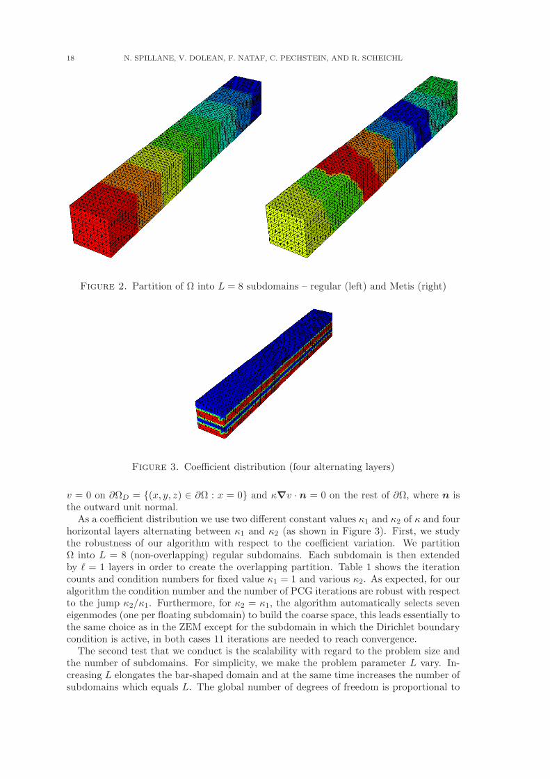
In both three-dimensional cases (Sections 5.1 and 5.2), in order to study scalability, weuse the domain Ω = [0, L]×[0, 1]×[0, 1] and a regular tetrahedral mesh of (10L+1×11×11)nodes which we divide into L horizontally side by side subdomains. We will either usea regular partition into L unit cubes (Figure 2 (left)) or an automatic partition into Lsubdomains using Metis (Figure 2 (right)). The two dimensional case (Section 5.3) willpresent results for more general partitions.

5.1. The Darcy equation. With the domain Ω given above, we solve the followingproblem: Find v ∈ H1(Ω) such that

−∇ · (κ(x, y, z)∇v) = 0 in Ω,


Figure 2. Partition of Ω into L = 8 subdomains – regular (left) and Metis (right)

Figure 3. Coefficient distribution (four alternating layers)

v = 0 on ∂ΩD = (x, y, z) ∈ ∂Ω : x = 0 and κ∇v · n = 0 on the rest of ∂Ω, where n isthe outward unit normal.

As a coefficient distribution we use two different constant values κ1 and κ2 of κ and fourhorizontal layers alternating between κ1 and κ2 (as shown in Figure 3). First, we studythe robustness of our algorithm with respect to the coefficient variation. We partitionΩ into L = 8 (non-overlapping) regular subdomains. Each subdomain is then extendedby ℓ = 1 layers in order to create the overlapping partition. Table 1 shows the iterationcounts and condition numbers for fixed value κ1 = 1 and various κ2. As expected, for ouralgorithm the condition number and the number of PCG iterations are robust with respectto the jump κ2/κ1. Furthermore, for κ2 = κ1, the algorithm automatically selects seveneigenmodes (one per floating subdomain) to build the coarse space, this leads essentially tothe same choice as in the ZEM except for the subdomain in which the Dirichlet boundarycondition is active, in both cases 11 iterations are needed to reach convergence.

The second test that we conduct is the scalability with regard to the problem size andthe number of subdomains. For simplicity, we make the problem parameter L vary. In-creasing L elongates the bar-shaped domain and at the same time increases the number ofsubdomains which equals L. The global number of degrees of freedom is proportional to


AS ZEM GenEOκ2 it cond it cond dim it cond dim1 16 229 11 6.3 8 11 8.4 7

102 27 230 19 22 8 13 8.4 14104 29 230 23 210 8 15 8.4 14106 26 230 22 230 8 11 8.4 14

Table 1. 3D Darcy: number of PCG iterations (it), condition number(cond) and coarse space dimension (dim) vs. jump in κ for κ1 = 1, ℓ = 1added layers, L = 8 regular subdomains

Regular

AS ZEM GenEOsub glob DOF it cond it cond dim it cond dim4 4840 14 51 15 51 4 10 8.4 68 9680 26 230 22 230 8 11 8.4 1416 19360 51 980 36 970 16 13 8.4 3032 38720 103 4000 61 3900 32 13 8.4 62

Metis with criterion given by (26)AS ZEM GenEO

sub glob DOF it cond it cond dim it cond dim4 4840 21 67 18 63 4 9 3.0 198 9680 36 290 29 280 8 9 3.0 4016 19360 65 1200 45 1200 16 11 3.1 8132 38720 123 4900 79 4700 32 11 3.1 171

Table 2. 3D Darcy: number of PCG iterations (it), condition number(cond) and coarse space dimension (dim) vs. problem size for κ1 = 1,κ2 = 106, ℓ = 1 added layers, L (sub) subdomains

L. Table 2 gives the results for different problem sizes (we display the number of subdo-mains and the total number of degrees of freedom) and for regular and irregular partitions.For irregular partitions, the choice of mj becomes more tricky since the diameter of thesubdomain is not necessarily relevant and there is no correlation between the diametersof the subdomains for two ‘Metis’ decompositions into L and L′ subdomains as soon asL 6= L′. However, for the regular decomposition all floating subdomains are identical. Wenotice that in these subdomains Ωj the number of selected eigenvectors is mj = 2 andλ3 = 0.5. The quantity that appears in the condition number bound in Theorem 3.21 is

max1≤j≤N

(1

λjmj+1

). In order for the bound on the condition number given by theorem in

the irregular case to be at least as strict as in the regular case, for the ‘Metis’ simulationin Table 2 we define

(26) mj := min

m : λjm+1 > 0.5

,

in each subdomain. We would like to point to the low and stable condition numbers inboth the regular and irregular subdomain cases.

Finally, Table 3 studies the dependence on the amount of overlap, or equivalently onthe number ℓ of layers added to each non-overlapping subdomain. We can see that forthis example, increasing the amount of overlap improves convergence without increasingthe dimension of the coarse space.


AS ZEM GenEOℓ it cond it cond dim it cond dim1 26 230 22 230 8 11 8.4 142 22 150 18 150 8 9 5.4 143 16 110 15 110 8 9 4.0 144 15 92 13 92 8 7 3.3 14

Table 3. 3D Darcy: number of PCG iterations (it), condition number(cond) and coarse space dimension (dim) vs. number of added layers ℓ bywhich each domain is extended, for L = 8 regular subdomains, κ1 = 1 andκ2 = 106

AS ZEM GenEOL glob DOF it cond it cond dim it cond dim4 14520 79 2 .4 · 10 3 54 2 .9 · 10 2 24 16 10 468 29040 177 1 .3 · 10 4 87 1 .0 · 10 3 48 16 10 10216 58080 378 1 .5 · 10 5 145 1 .4 · 10 3 96 16 10 214

Table 4. 3D Elasticity: number of PCG iterations (it), condition num-ber (cond), and coarse space dimension (dim) vs. number of regular sub-domains, for ℓ = 1 added layers, g = 10, (E1, ν1) = (2 · 1011, 0.3) and(E2, ν2) = (2 · 107, 0.45).

5.2. The linear elasticity equations. For the second family of tests the equations arethe following. Find v = (v1, v2, v3)

T ∈ H1(Ω)3 such that

−div(σ(v)) = f , in Ω,

v = (0, 0, 0)T on ∂ΩD = (x, y, z) ∈ ∂Ω : x = 0 and σ(v) ·n = 0 on the rest of ∂Ω, wherethe stress tensor σ(v), the Lame coefficients λ and µ and the right hand side are given by

σij(v) = 2µεij(v) + λδijdiv(v), εij(v) = 1

2

(∂vi

∂xj+

∂vj

∂xi

), f = (0, 0, g)T ,

µ = E2(1+ν) , λ = Eν

(1+ν)(1−2ν) .

Here E and ν denote respectively Young’s modulus and Poisson’s ratio, and we will letboth parameters vary discontinuously over the domain. Again we use four alternatinglayers as shown in Figure 3 of coefficients between two sets of values (E1, ν1) and (E2, ν2).Table 4 displays the iteration counts, condition numbers, and coarse space dimensions forpartitions into different numbers of regular subdomains (the parameter choices are givenbelow the table). Note that for GenEO, we need only 16 PCG iterations in all cases. Asan example, Figure 4 shows the convergence profile for the case where Ω is split into 16regular subdomains.

5.3. The two-dimensional linear elasticity equations. In this subsection we dealwith the two-dimensional linear elasticity equations with again a Dirichlet boundary con-dition at x = 0. In this case, the ZEM coarse space consists of three rigid body modesper subdomain. Here we choose Ω = (0, 1) × (0, 1) and use a structured simplicial meshwith 81 × 81 nodes. The coefficient distribution is sketched on the left hand side of Fig-ure 5: on the two regions indicated by the two different colors, we take the parameters(E1, ν1) = (2 · 1011, 0.3) and (E2, ν2) = (2 · 107, 0.45).

This time, we keep the problem size fixed, but we make the number of subdomains vary.In all cases, we use a Metis partition and extend the non-overlapping subdomains by ℓ = 2layers. As shown in Figure 5 (right) for a decomposition into 64 subdomains there are


0 50 100 150 200 250 300 350 40010

−7

10−6

10−5

10−4

10−3

10−2

10−1

100

Iteration count

Err

or

No coarse spaceZEM coarse spaceGenEO coarse space

Figure 4. (3D Elasticity) Relative error vs. iteration count for L = 16regular subdomains

AS ZEM GenEOsub glob DOF it it dim it dim4 13122 90 94 12 36 3616 13122 169 179 48 39 11225 13122 222 157 75 40 16664 13122 317 196 192 39 343

Table 5. 2D Elasticity: number of PCG iterations (it) and coarse spacedimension (dim) vs. number of Metis subdomains for fixed problem size

many floating subdomains. Table 5 shows the iteration counts and coarse space dimensionsfor different Metis partitions (the chosen parameters are given below the table). From theiteration counts we see that the GenEO method is scalable.

It is not surprising that the coarse space dimension grows with the number of subdo-mains because we construct local coarse basis functions per subdomain. Note howeverthat for the case of 64 subdomains, the coarse space dimension of 343 is still compara-ble to average dimension 205 of a subdomain problem. To find the optimal partition interms of CPU time, one must clearly take the cost of the subdomain solves into account,and additionally the cost of the eigensolves in the setup of the method. For this seriesof tests no estimates for the condition number of the preconditioned matrices are givenas in some cases (but for all three types of preconditioners), the Rayleigh-Ritz procedurereturned one or a few negative eigenvalues, which is probably due to large floating pointerror propagation due to the high contrast. For more extensive results for two dimensionalelasticity, see [29].

6. Conclusion

In this article we have introduced a coarse space for problems given by symmetricpositive definite bilinear forms. In order to remain as general as possible, we did so usingan abstract formulation. We thoroughly proved a bound for the condition number of theoverlapping two-level additive Schwarz preconditioner for this coarse space. This bounddoes not depend on any of the coefficients in the equations or on the way the domain is split


IsoValue-1.05053e+105.28263e+091.58079e+102.63332e+103.68584e+104.73837e+105.79089e+106.84342e+107.89595e+108.94847e+101.0001e+111.10535e+111.21061e+111.31586e+111.42111e+111.52636e+111.63162e+111.73687e+111.84212e+112.10525e+11

E

Figure 5. 2D Elasticity: coefficient distribution (left) – Metis decompo-sition into 64 subdomains (right)

into subdomains. Numerical results on two-dimensional and three-dimensional problemsare in agreement with the fact that the method is robust with regard to heterogeneitiesand rather irregular subdomains. We also gave details on how to implement the coarsespace construction insisting on the fact that given a finite element code no additionalelementary matrices need to be computed. This means that the method is quite easilyapplicable to simulations of actual physical problems and it is our ambition to do so.

Along the way we have identified promising leads for further improving the efficiencyof the method. In the near future there are three main ideas for further investigations.The first one is to take advantage of the fact that the partition of unity can be chosendifferently since the proof holds as long as the partition of unity is defined by individualweights per interior degree of freedom in each subdomain. The second idea is to optimizethe eigenvalue computations. Although this is a purely parallel task, this is the mostcostly part in building the coarse space. Finally, the formulation of the GenEO coarsespace makes it particularly well suited for a multilevel parallel implementation and thiswould boost efficiency as it would deal with the ‘large’ coarse spaces which can occur ifwe select many low frequency modes.

References

[1] E. Anderson, Z. Bai, and C. Bischof. LAPACK Users’ guide, volume 9. Society for Industrial Mathe-matics, 1999.

[2] M. Brezina, C. Heberton, J. Mandel, and P. Vanek. An iterative method with convergence rate chosena priori. Technical Report 140, University of Colorado Denver, CCM, University of Colorado Denver,April 1999. Earlier version presented at 1998 Copper Mountain Conference on Iterative Methods,April 1998.

[3] T. Chartier, R. D. Falgout, V. E. Henson, J. Jones, T. Manteuffel, S. McCormick, J. Ruge, and P. S.Vassilevski. Spectral AMGe (ρAMGe). SIAM J. Sci. Comput., 25(1):1–26, 2003.

[4] C. Chevalier and F. Pellegrini. PT-SCOTCH: a tool for efficient parallel graph ordering. Parallel

Computing, 6-8(34):318–331, 2008.[5] C. R. Dohrmann and O. B. Widlund. An overlapping Schwarz algorithm for almost incompressible

elasticity. SIAM J. Numer. Anal., 47(4):2897–2923, 2009.[6] C. R. Dohrmann and O. B. Widlund. Hybrid domain decomposition algorithms for compressible and

almost incompressible elasticity. Internat. J. Numer. Methods Engrg., 82(2):157–183, 2010.[7] V. Dolean, F. Nataf, R. Scheichl, and N. Spillane. Analysis of a two-level Schwarz method with

coarse spaces based on local Dirichlet–to–Neumann maps. submitted, 2011. http://hal.archives-ouvertes.fr/hal-00586246/.

[8] V. Dolean, F. Nataf, N. Spillane, and H. Xiang. A coarse space construction based on local Dirichletto Neumann maps. SIAM J. on Scientific Computing, 33:1623–1642, 2011.

[9] M. Dryja, M. V. Sarkis, and O. B. Widlund. Multilevel Schwarz methods for elliptic problems withdiscontinuous coefficients in three dimensions. Numer. Math., 72(3):313–348, 1996.


[10] M. Dryja, B. F. Smith, and O. B. Widlund. Schwarz analysis of iterative substructuring algorithmsfor elliptic problems in three dimensions. SIAM J. Numer. Anal., 31(6):1662–1694, 1994.

[11] Maksymilian Dryja and Olof B. Widlund. Domain decomposition algorithms with small overlap. SIAM

J. Sci. Comput., 15(3):604–620, 1994.[12] Y. Efendiev, J. Galvis, R. Lazarov, and J. Willems. Robust domain decomposition preconditioners for

abstract symmetric positive definite bilinear forms. Arxiv preprint arXiv:1105.1131, 2011. submitted.[13] Y. Efendiev, J. Galvis, and P. S. Vassilevski. Spectral element agglomerate algebraic multigrid methods

for elliptic problems with high contrast coefficients. In Y. Huang, R. Kornhuber, O. Widlund, andJ. Xu, editors, Domain Decomposition Methods in Science and Engineering XIX, volume 78 of Lecture

Notes in Computational Science and Engineering, pages 407–414, Berlin, 2011. Springer.[14] J. Galvis and Y. Efendiev. Domain decomposition preconditioners for multiscale flows in high-contrast

media. Multiscale Model. Simul., 8(4):1461–1483, 2010.[15] J. Galvis and Y. Efendiev. Domain decomposition preconditioners for multiscale flows in high contrast

media: Reduced dimension coarse spaces. Multiscale Modeling & Simulation, 8(5):1621–1644, 2010.[16] I. G. Graham, P. O. Lechner, and R. Scheichl. Domain decomposition for multiscale PDEs. Numer.

Math., 106(4):589–626, 2007.[17] Frederic Hecht. FreeFem++. Numerical Mathematics and Scientific Computation. Laboratoire J.L.

Lions, Universite Pierre et Marie Curie, http://www.freefem.org/ff++/, 3.7 edition, 2010.[18] G. Karypis and V. Kumar. METIS: A software package for partitioning unstructured graphs, partition-

ing meshes, and computing fill-reducing orderings of sparse matrices. Technical report, Department ofComputer Science, University of Minnesota, 1998. http://glaros.dtc.umn.edu/gkhome/views/metis.

[19] A. V. Knyazev. Toward the optimal preconditioned eigensolver: locally optimal block preconditionedconjugate gradient method. SIAM J. Sci. Comput., 23(2):517–541, 2001.

[20] J. Mandel and M. Brezina. Balancing domain decomposition for problems with large jumps in coeffi-cients. Math. Comp., 65(216):1387–1401, 1996.

[21] B.N. Parlett. The symmetric eigenvalue problem, volume 20. Society for Industrial Mathematics, 1998.[22] C. Pechstein and R. Scheichl. Scaling up through domain decomposition. Appl. Anal., 88(10-11):1589–

1608, 2009.[23] C. Pechstein and R. Scheichl. Weighted Poincare inequalities. NuMa-Report 2010-10, Institute of

Computational Mathematics, Johannes Kepler University, Linz, December 2010. submitted.[24] Y. Saad. Iterative methods for sparse linear systems. Society for Industrial Mathematics, 2003.[25] R. Scheichl and E. Vainikko. Additive Schwarz with aggregation-based coarsening for elliptic problems

with highly variable coefficients. Computing, 80(4):319–343, 2007.[26] R. Scheichl, P. S. Vassilevski, and L. T. Zikatanov. Mutilevel methods for elliptic problems with highly

varying coefficients on non-aligned coarse grids. Preprint LLNL-JRNL-404462, Lawrence LivermoreNational Laboratory, CA, 2010.

[27] R. Scheichl, P. S. Vassilevski, and L. T. Zikatanov. Weak approximation properties of elliptic projec-tions with functional constraints. Preprint LLNL-JRNL-462079, Lawrence Livermore National Labo-ratory, CA, 2011. To appear in Multiscale Model. Simul.

[28] B. F. Smith, P. E. Bjørstad, and W. Gropp. Domain decomposition: parallel multilevel methods for

elliptic partial differential equations. Cambridge University Press, 2004.[29] N. Spillane, V. Dolean, P. Hauret, F. Nataf, C. Pechstein, and R. Scheichl. A robust two level

domain decomposition preconditioner for systems of PDEs. C. R. Mathematique, 2011. In print,http://hal.archives-ouvertes.fr/hal-00630892.

[30] A. Toselli and O. B. Widlund. Domain decomposition methods—algorithms and theory, volume 34 ofSpringer Series in Computational Mathematics. Springer-Verlag, Berlin, 2005.

[31] P. S. Vassilevski. Multilevel block factorization preconditioners. Springer-Verlag, New York, 2008.

Latest Reports in this series

2009

[..]

2010

[..]2010-04 Clemens Hofreither, Ulrich Langer and Clemens Pechstein

Analysis of a Non-standard Finite Element Method Based on Boundary IntegralOperators

June 2010

2010-05 Helmut GfrererFirst-Order Characterizations of Metric Subregularity and Calmness of Con-straint Set Mappings

July 2010

2010-06 Helmut GfrererSecond Order Conditions for Metric Subregularity of Smooth Constraint Sys-tems

September 2010

2010-07 Walter ZulehnerNon-standard Norms and Robust Estimates for Saddle Point Problems November 2010

2010-08 Clemens HofreitherL2 Error Estimates for a Nonstandard Finite Element Method on PolyhedralMeshes

December 2010

2010-09 Michael Kolmbauer and Ulrich LangerA frequency-robust solver for the time-harmonic eddy current problem December 2010

2010-10 Clemens Pechstein and Robert ScheichlWeighted Poincaré inequalities December 2010

2011

2011-01 Huidong Yang and Walter ZulehnerNumerical Simulation of Fluid-Structure Interaction Problems on HybridMeshes with Algebraic Multigrid Methods

February 2011

2011-02 Stefan Takacs and Walter ZulehnerConvergence Analysis of Multigrid Methods with Collective Point Smoothersfor Optimal Control Problems

February 2011

2011-03 Michael KolmbauerExistance and Uniqueness of Eddy Current Problems in Bounded and Un-bounded Domains

May 2011

2011-04 Michael Kolmbauer and Ulrich LangerA Robust Preconditioned-MinRes-Solver for Distributed Time-Periodic EddyCurrent Optimal Control

May 2011

2011-05 Michael Kolmbauer and Ulrich LangerA Robust FEM-BEM Solver for Time-Harmonic Eddy Current Problems May 2011

2011-06 Markus Kollmann and Michael KolmbauerA Preconditioned MinRes Solver for Time-Periodic Parabolic Optimal ControlProblems

August 2011

2011-07 Nicole Spillane, Victorita Dolean, Patrice Hauret, Frédérik Nataf, ClemensPechstein and Robert ScheichlAbstract Robust Coarse Spaces for Systems of PDEs via Generalized Eigen-problems in the Overlaps

November 2011

From 1998 to 2008 reports were published by SFB013. Please seehttp://www.sfb013.uni-linz.ac.at/index.php?id=reports

From 2004 on reports were also published by RICAM. Please seehttp://www.ricam.oeaw.ac.at/publications/list/

For a complete list of NuMa reports seehttp://www.numa.uni-linz.ac.at/Publications/List/

http://www.sfb013.uni-linz.ac.at/index.php?id=reports

http://www.ricam.oeaw.ac.at/publications/list/

http://www.numa.uni-linz.ac.at/Publications/List/

abstract robust coarse spaces for systems of pdes via

Documents