abstract the design of small propellers operating at low
TRANSCRIPT
ABSTRACT
The Design of Small Propellers Operating at Low Reynolds
Numbers and Associated Experimental Evaluation
William R. Liller III, M.S.M.E.
Mentor: Kenneth W. Van Treuren, D. Phil.
Small-scale Unmanned Aerial Systems (UASs) are becoming increasingly
important in the fields of intelligence, surveillance, and reconnaissance. As the desire for
higher payloads and longer flight times increases, so does the need to optimize the
performance of UAS components. It has been found that small UASs using propeller and
electric motor combinations are susceptible to decreased efficiencies while operating in
low Reynolds numbers conditions. This work details contributions made by Baylor
University, in collaboration with the United States Air Force Academy, which include a
custom propeller design, analysis, and solid-modeling code for experimental propeller
models and a propeller test stand for use in the Baylor University subsonic wind tunnel
with accompanying data acquisition code. As a result of the 46 custom propellers
designed and tested, an efficiency increase of 7 % and noise signature decrease of 12 dB
has been achieved when compared to stock propellers on UASs of interest.
Page bearing signatures is kept on file in the Graduate School.
The Design of Small Propellers Operating at Low Reynolds
Numbers and Associated Experimental Evaluation
by
William R. Liller III, B.S.M.E.
A Thesis
Approved by the Department of Mechanical Engineering
___________________________________
William Jordan, Ph.D., Chairperson
Submitted to the Graduate Faculty of
Baylor University in Partial Fulfillment of the
Requirements for the Degree
of
Master of Science in Mechanical Engineering
Approved by the Thesis Committee
___________________________________
Kenneth W. Van Treuren, D. Phil., Chairperson
___________________________________
Lesley M. Wright, Ph.D.
___________________________________
Scott M. Koziol, Ph.D.
___________________________________
Charles F. Wisniewski, Ph.D.
Accepted by the Graduate School
August 2015
___________________________________
J. Larry Lyon, Ph.D., Dean

Copyright © 2015 by William R. Liller III
All rights reserved
iv
TABLE OF CONTENTS
LIST OF FIGURES ......................................................................................................... viii
LIST OF TABLES .......................................................................................................... xvii
NOMENCLATURE ...................................................................................................... xviii
ACKNOWLEDGMENTS ........................................................................................... xxviii
DEDICATION .................................................................................................................xxx
CHAPTER ONE ..................................................................................................................1
Introduction ..............................................................................................................1
Unmanned Aerial Vehicles/Unmanned Aerial Systems ..............................1
Categories of UAS .......................................................................................3
HALE UAS—Northrop Grumman, Global Hawk...........................3
MALE UAS—General Atomics Aeronautical, Predator .................4
LASE UAS—Aerovironment Puma AE ..........................................5
Objectives and Scope of this Study .............................................................7
Increasing Efficiency and Reducing Noise Signature .....................8
Presentation Outline .....................................................................................8
CHAPTER TWO .................................................................................................................9
Literature Survey .....................................................................................................9
A Survey of Low Reynolds Number Effects on Propellers and Airfoils .....9
Low Reynolds Number Propeller Operation ...................................9
Low Reynolds Number Airfoil Operation .....................................12
Propeller and Airfoil Design and Analysis Schemes .................................15
Propeller Design and Analysis .......................................................16
Airfoil Design and Analysis...........................................................18
Experimental Testing and Considerations of Propellers Operating at Low
Reynolds Numbers .........................................................................19
Experimental Low Reynold Number Testing of Propellers ..........19
Experimental Considerations for Small Propeller Testing ............23
Chapter Two Concluding Remarks ............................................................25
CHAPTER THREE ...........................................................................................................26
Theoretical Background .........................................................................................26
Propeller Theory ........................................................................................26
v
One-Dimensional Propeller Theory ...............................................26
Airfoil Theory ................................................................................30
Blade Element Theory ...................................................................34
Blade Element and Momentum Theory .........................................37
QMIL and QPROP Formulation ....................................................42
Airfoil Noise ..............................................................................................50
Turbulent Boundary Layer Trailing Edge Noise ...........................52
Separated Flow Noise ....................................................................53
Laminar Boundary Layer Vortex Shedding Noise ........................54
Trailing-Edge Bluntness Vortex Shedding Noise ..........................54
Turbulent Inflow Noise ..................................................................55
Tip Vortex Formation Noise ..........................................................56
The Directivity Function ................................................................57
Propeller Wind Tunnel Corrections ...........................................................58
Propeller-Motor Matching .........................................................................63
Chapter Three Concluding Remarks ..........................................................68
CHAPTER FOUR ..............................................................................................................69
Experimental Method.............................................................................................69
Bearcontrol .................................................................................................69
The Governing Code ......................................................................71
The Propeller Design and Analysis Subroutine .............................74
The Propeller Noise Prediction Subroutine ...................................84
The Solid-Modeling Automation Subroutine ................................88
Testing Facilities ........................................................................................88
Baylor Testing Facility—Experimental Setup ...............................89
Baylor Testing Facility—Experimental Method ...........................96
USAFA Testing Facility ..............................................................104
Chapter Four Concluding Remarks .........................................................106
CHAPTER FIVE .............................................................................................................107
Experimental Results ...........................................................................................107
USAFA Testing Facility Results .............................................................107
Summer 2014, Commercial Propeller Experimental Evaluation.108
Summer 2014, Custom Propeller Design Characteristics ............110
Summer 2014, Custom Propeller Results ....................................119
Initial Custom Propeller Designs .....................................119
Constant Chord, RPM Study............................................124
SLA Hub Study ................................................................127
Varying Angle of Attack, Constant Chord Study ............131
Varying Angle of Attack, Varying Chord Study .............133
Summer 2014 Tip Treatments .........................................136
Fall 2014, Custom Propeller Design and Experimental
Evaluation ........................................................................139
vi
Custom Tip Design Study, Fall 2014 ...............................140
Airfoil Study, Fall 2014 ...................................................146
Multi-Blade and Increased Diameter Study .....................152
Baylor Testing Facility Results ................................................................158
Baylor Testing Facility Validation...............................................158
Baylor Test Stand Uncertainty Calculations ....................167
Custom Propellers Tested at the Baylor Testing Facility ............168
Chapter Five Concluding Remarks ..........................................................175
CHAPTER SIX ................................................................................................................176
Conclusions and Recommendations ....................................................................176
Summary ..................................................................................................176
Design Recommendations for High Efficiency and
Low Noise Propellers ...............................................................................177
Experiment Improvement Recommendations and Future Work .............178
Airfoil Data ..................................................................................178
Bearcontrol ...................................................................................179
Experimental Setup and Method ..................................................180
Concluding Remarks ................................................................................180
APPENDICES .................................................................................................................181
Appendix A ..........................................................................................................182
Bearcontrol User Guide ...........................................................................182
Program Description ....................................................................182
System Requirements...................................................................182
Quick Start Example ....................................................................182
Adding a New Airfoil Folder .......................................................194
Supplemental Codes.....................................................................196
Appendix B ..........................................................................................................201
Bearcontrol GUI and Called Function Code ............................................201
Bearcontrol GUI Background Code.............................................201
Air Properties Function ................................................................234
Propeller Blade Geometry Function ............................................235
Plane Macro Function ..................................................................250
Spline Macro Function .................................................................255
NAFNoise Input File Creation Function......................................258
NAFNoise Output Reader Function.............................................262
Appendix C ..........................................................................................................265
Test GUI LabView Block Diagram .........................................................265
vii
Appendix D ..........................................................................................................266
Baylor Propeller Test Stand Lab Procedure.............................................266
Propeller Test Stand Description .................................................266
Component Warm-up and Calibration .........................................266
Running the Experiment ..............................................................270
Appendix E ..........................................................................................................272
Bearcontrol Supplemental Code 1 and Subsequent Functions: Constant
Chord Helper ................................................................................272
Constant Chord Helper Code .......................................................272
Shell Sort Code ............................................................................280
Spline Fit and Interpolation Function ..........................................280
hh Function ..................................................................................281
fd Function ...................................................................................281
Spline Interpolation Function ......................................................281
Constant Chord Propeller Geometry Function ............................282
Constant Chord Plane Macro Function ............................295
Constant Chord Spline Macro Function ..........................301
Appendix F...........................................................................................................304
Bearcontrol Supplemental Code 2 and Subsequent Functions: Propeller
TipHelper .....................................................................................304
Propeller Tip Helper Function .....................................................304
Shell Sort Code ............................................................................314
Spline Fit and Interpolation Function ..........................................314
hh Function ..................................................................................315
fd Function ...................................................................................315
Spline Interpolation Function ......................................................316
Tip Treated Blade Geometry Function ........................................316
Tip Treated Blade Plane Macro Function ....................................329
Tip Treated Blade Spline Macro Function...................................335
REFERENCES ................................................................................................................338
viii
LIST OF FIGURES
Figure 1.1: Predator XP UAS [1] .........................................................................................2
Figure 1.2: Northrop Grumman Global Hawk UAS [3] ......................................................3
Figure 1.3: Predator B UAS [5] ...........................................................................................4
Figure 1.4: Aerovironment Puma AE [6] ............................................................................6
Figure 2.1: NACA 16 Series Propeller Efficiencies vs. Reynolds Number [9] .................10
Figure 2.2: APC 9x4.5 LP09045e Coefficient of Thrust vs. Advance Ratio Plot [10] .....11
Figure 2.3: APC 9x4.5 LP09045e Coefficient of Power vs. Advance Ratio Plot [10] ......11
Figure 2.4: APC 9x4.5 LP09045e Efficiency vs. Advance Ratio Plot [10].......................12
Figure 2.5: E387 (E) Airfoil Cl vs. Cd Reynolds Number Effects [11] ...........................13
Figure 2.6: Laminar Separation Bubble Smoke Visualization, E387 Airfoil [12] ............14
Figure 2.7: Oil Flow Visualization and Conceptual Illustration of the Relationship
Between the Skin Friction and the Surface Oil Flow Features [13] ......................14
Figure 2.8: UIUC Propeller Test Rig [8] ...........................................................................20
Figure 2.9: Wright State University Propeller Test Rig [26] .............................................21
Figure 2.10: Tracy Propeller Test Rig Configuration [30] ................................................22
Figure 3.1: One-Dimensional Propeller Analyis Illustration [33] .....................................27
Figure 3.2: Airfoil Nomenclature Definitions [35] ............................................................30
Figure 3.3: Angle of Attack Definition [36] ......................................................................31
Figure 3.4: Definition of Lift and Drag on an Airfoil [36] ................................................32
Figure 3.5: Coefficient of Lift vs. Angle of Attack [35] ....................................................33
Figure 3.6: Airfoil Cross-section Geometric Properties [36] .............................................35
ix
Figure 3.7: Decomposition of Lift and Drag into Thrust and Torque [36] ........................36
Figure 3.8: Velocity Decomposition and Angle Definitions [36] ......................................38
Figure 3.9: Velocity Decomposition at Radial Location, r [36] ........................................43
Figure 3.10: Propeller Geometry and Angle Definitions at some
Radial Coordinate, r [36] .......................................................................................45
Figure 3.11: Velocity Parameterization through Phi [36] ..................................................46
Figure 3.12: Observer Location Coordinate System[45] ...................................................57
Figure 3.13: Glauert Correction Theoretical Flow Scenario [33] ......................................59
Figure 3.14: Glauert Correction, 9" Diameter Propeller, Blockage Ratio = 0.11 ..............62
Figure 3.15: Motor Circuit Diagram [49] ..........................................................................64
Figure 3.16: Electric Motor Performance for Varying Input Voltages [49] ......................65
Figure 3.17: Propeller and Motor Parameter Comparison [49] .........................................67
Figure 4.1: Bearcontrol GUI ..............................................................................................71
Figure 4.2: Bearcontrol Execution Flow Chart ..................................................................72
Figure 4.3: Solid-modeling Macro Output, a) reference planes for each airfoil section,
b) each splined airfoil section at designed geometric pitch on its designated
reference plane and c) solid model of designed blade ...........................................74
Figure 4.4: QMIL/QPROP Default Propeller Motor Characteristics ................................75
Figure 4.5: Required Airfoil Performance Parameters: a) Cl vs. Cd Plot and Associated
Parameters, b) Cl vs. Angle of Attack Plot and Associated Parameters [51] ........77
Figure 4.6: QMIL Input File ..............................................................................................79
Figure 4.7: QMIL Output/QPROP Input File ....................................................................80
Figure 4.8: QPROP Output File .........................................................................................81
Figure 4.9: NAFNoise Input File .......................................................................................86
Figure 4.10: NAFNoise Output File ..................................................................................87
x
Figure 4.11: Baylor University Subsonic Wind Tunnel ....................................................89
Figure 4.12: Baylor Propeller Test Stand ..........................................................................90
Figure 4.13: ACT-3X Panel Tachometer ...........................................................................91
Figure 4.14: Brüel & Kjær Type 2270 Handheld Analyzer ...............................................92
Figure 4.15: Omega zSeries zED-THPB-LCD Atmospheric Conditions Monitor............93
Figure 4.16: Propeller Test Stand GUI ..............................................................................94
Figure 4.17: Load Cell, Torque Transducer, Panel Tachometer and Microphone DAQ
Hardware ................................................................................................................95
Figure 4.18: Futaba Remote Control and Receiver ...........................................................95
Figure 4.19: Tunnel Velocity vs. Tunnel Motor Controller Frequency .............................96
Figure 4.20: Torque Transducer Calibration .....................................................................97
Figure 4.21: Typical Torque Calibration Chart .................................................................98
Figure 4.22: Load Cell Calibration Setup ..........................................................................99
Figure 4.23: Typical Load Cell Calibration Chart .............................................................99
Figure 4.24: SHIMP Digital Stroboscope ........................................................................100
Figure 4.25: Typical Panel Tachometer Calibration Chart ..............................................101
Figure 4.26: Typical Current Transducer Chart ...............................................................102
Figure 4.27: Sound Calibrator Type 4231 and Microphone ............................................102
Figure 4.28: USAFA Testing Facility DAQ System .......................................................105
Figure 5.1: UASa Stock Propeller: ACC 13x10 ..............................................................107
Figure 5.2: ACC Commercial Propellers, Efficiency vs. RPM,
T = 2.5 lbf, V = 44 ft/s ..........................................................................................109
Figure 5.3: ACC Commercial Propellers, SPL vs. RPM,
T = 2.5 lbf, V = 44 ft/s ..........................................................................................109
Figure 5.4: Propeller Design Nomenclature Clarification ...............................................111
xi
Figure 5.5: "Solid Propeller Example" ............................................................................111
Figure 5.6: "SLA Hub Propeller" Example, Assembled ..................................................111
Figure 5.7: "SLA Hub Propeller" Example, Disassembled .............................................112
Figure 5.8: "Aluminum Hub Propeller" Example, Disassemble .....................................112
Figure 5.9: "Aluminum Hub Propeller" Example, Assembled ........................................112
Figure 5.10: Custom Designed Propeller Tip Profile Nomenclature ...............................113
Figure 5.11: Tip "Wiggle" Nomenclature ........................................................................114
Figure 5.12: Normalized Clark Y Airfoil Coordinates [21] ............................................117
Figure 5.13: Clark Y, Coefficient of Lift vs. Angle of Attack, Re=100000 [21] ............117
Figure 5.14: Clark Y, Coefficient of Lift vs. Angle of Attack, Re = 100000 [21] ..........118
Figure 5.15: Clark Y, Cl vs. Cd vs. Angle of Attack, Re = 100000 [21] ........................118
Figure 5.16: TP1 Custom Propeller .................................................................................120
Figure 5.17: TP2 Custom Propeller .................................................................................120
Figure 5.18: TP3 Custom Propeller .................................................................................121
Figure 5.19: TP4 Custom Propeller .................................................................................121
Figure 5.20: TP1-TP4 and ACC 13x10 (UASa Stock), Efficiency vs. RPM
T = 2.5 lbf, V = 44 ft/s ..........................................................................................122
Figure 5.21: TP1-TP4 and ACC 13x10 (UASa Stock), SPL vs. RPM
T = 2.5 lbf, V = 44 ft/s ..........................................................................................122 Figure 5.22: TP5 Custom Propeller .................................................................................124
Figure 5.23: TP6 Custom Propeller .................................................................................124
Figure 5.24: TP7 Custom Propeller .................................................................................125
Figure 5.25: TP1-TP7 and ACC 13x10 (UASa Stock), Efficiency vs. RPM
T = 2.5 lbf, V = 44 ft/s ..........................................................................................126
Figure 5.26: TP1-TP7 and ACC 13x10 (UASa Stock), SPL vs. RPM
T = 2.5 lbf, V = 44 ft/s ..........................................................................................126
xii
Figure 5.27: Print Finish Problems, Roughness and Inconsistent Trailing Edge ............127
Figure 5.28: TP8: SLA Hub Implementation ..................................................................128
Figure 5.29: High Resolution Print Orientation ...............................................................128
Figure 5.30: TP13 Custom Propeller ...............................................................................129
Figure 5.31: TP8 Custom Propeller .................................................................................129
Figure 5.32: SLA Hub and Solid Hub Comparison, Efficiency vs. RPM
T = 2.5 lbf, V = 44 ft/s ..........................................................................................130
Figure 5.33: SLA Hub and Solid Hub Comparison, SPL vs. RPM
T = 2.5 lbf, V = 44 ft/s ..........................................................................................130
Figure 5.34: TP11 Custom Propeller ...............................................................................131
Figure 5.35: TP12 Custom Propeller ...............................................................................131
Figure 5.36: TP14 Custom Propeller ...............................................................................131
Figure 5.37: Constant Chord, Varying Angle of Attack Study, Efficiency vs. RPM
T = 2.5 lbf, V = 44 ft/s ..........................................................................................132
Figure 5.38: Constant Chord, Varying Angle of Attack Study, SPL vs. RPM
T = 2.5 lbf, V = 44 ft/s ..........................................................................................132
Figure 5.39: TP15 Custom Propeller ...............................................................................134
Figure 5.40: TP17 Custom Propeller ...............................................................................134
Figure 5.41: TP18 Custom Propeller ...............................................................................134
Figure 5.42: Varying Angle of Attack, Varying Chord Study, Efficiency vs. RPM
T = 2.5 lbf, V = 44 ft/s ..........................................................................................135
Figure 5.43: Varying Angle of Attack, Varying Chord Study, SPL vs. RPM
T = 2.5 lbf, V = 44 ft/s ..........................................................................................135
Figure 5.44: TP9 Custom Propeller .................................................................................136
Figure 5.45: TP10 Custom Propeller ...............................................................................136
Figure 5.46: TP16 Custom Propeller ...............................................................................137
xiii
Figure 5.47: Summer 2014 Tip Treatments, Efficiency vs. RPM
T = 2.5 lbf, V = 44 ft/s ..........................................................................................137
Figure 5.48: Summer 2014 Tip Treatments, SPL vs. RPM
T = 2.5 lbf, V = 44 ft/s ..........................................................................................138
Figure 5.49: Fall 2014 Tip Treatment Profiles ................................................................143
Figure 5.50: TP19 Custom Propeller, Taper 1 Tip Treatment .........................................144
Figure 5.51: TP20 Custom Propeller, Taper 2 Tip Treatment .........................................144
Figure 5.52: TP21 Custom Propeller, Half Circle Tip Treatment ...................................144
Figure 5.53: TP22 Custom Propeller, Oval 1 Tip Treatment ..........................................144
Figure 5.54: TP23 Custom Propeller, Oval 2 Tip Treatment ..........................................144
Figure 5.55: Fall 2014 Tip Treatments, Efficiency vs. RPM
T = 2.5 lbf, V = 44 ft/s ..........................................................................................145
Figure 5.56: Fall 2014 Tip Treatments, SPL vs. RPM
T = 2.5 lbf, V = 44 ft/s ..........................................................................................145
Figure 5.57: Airfoil Study, Normalized Airfoil Coordinates [21] ...................................147
Figure 5.58: Airfoil Study, Coefficient of Lift vs. Angle of Attack,
Re=100,000 [21] ..................................................................................................147
Figure 5.59: Airfoil Study, Coefficient of Drag vs. Coefficient of Lift,
Re = 100,000 [21] ................................................................................................148
Figure 5.60: Airfoil Study, Cl vs. Cd vs. Angle of Attack, Re = 100,000 [21] ................148
Figure 5.61: TP29 Custom Propeller ClarkY Angle of Attack = 7.6° .............................150
Figure 5.62: TP32 Custom Propeller, GM15 Angle of Attack = 5.1° .............................150
Figure 5.63: TP34 Custom Propeller, Geo417 Angle of Attack = 7.1° ...........................150
Figure 5.64: TP38 Custom Propeller, FX63-137 Angle of Attack = 9.3° .......................150
Figure 5.65: Fall 2014 Airfoil Study, Efficiency vs. RPM, T = 2.5 lbf, V = 44 ft/s ........151
Figure 5.66: Fall 2014 Airfoil Study, SPL vs. RPM, T = 2.5 lbf, V = 44 ft/s ..................151
Figure 5.67: TP24 Custom Propeller, MIL 2 Blade.........................................................152

xiv
Figure 5.68: TP25 Custom Propeller, MIL 3 Blade.........................................................153
Figure 5.69: TP26 Custom Propeller, MIL 4 Blade.........................................................153
Figure 5.70: TP27 Custom Propeller, MIL 5 Blade.........................................................154
Figure 5.71: TP40 Custom Propeller, GM15 Oval 2, 2 Blade .........................................154
Figure 5.72: TP43 Custom Propeller, GM15 Oval 2, 5 Blade .........................................155
Figure 5.73: Fall 2014 Multi-Blade/Diameter Study, Efficiency vs. RPM,
T = 2.5 lbf, V = 44 ft/s ..........................................................................................156
Figure 5.74: Fall 2014 Multi-Blade/Diameter Study, SPL vs. RPM,
T = 2.5 lbf, V = 44 ft/s ..........................................................................................157
Figure 5.75: UASb Stock Propeller: APC 9x6 ................................................................158
Figure 5.76: Baylor Experiment Repeatability, APC 9x6, Thrust vs. RPM,
V = 44 ft/s ............................................................................................................159
Figure 5.77: Baylor Experiment Repeatability, APC 9x6, Torque vs. RPM,
V = 44 ft/s ............................................................................................................159
Figure 5.78: Baylor Experiment Repeatability, APC 9x6, Efficiency vs. RPM,
V = 44 ft/s ............................................................................................................160
Figure 5.79: Facility Comparison, APC 9x6, Thrust vs. RPM,
V = 44 ft/s ............................................................................................................161
Figure 5.80: Facility Comparison, APC 9x6, Torque vs. RPM,
V = 44 ft/s ............................................................................................................162
Figure 5.81: Facility Comparison, APC 9x6, Efficiency vs. RPM,
V = 44 ft/s ............................................................................................................162
Figure 5.82: Glauert Correction Application, APC 9x6,Thrust vs. RPM,
V = 44 ft/s ............................................................................................................163
Figure 5.83: Glauert Correction Application, APC 9x6, Torque vs. RPM,
V = 44 ft/s ............................................................................................................164
Figure 5.84: Glauert Correction Application, APC 9x6, Efficiency vs. RPM,
V = 44 ft/s ............................................................................................................164
Figure 5.85: Density Correction Application, APC 9x6, Thrust vs. RPM,
V = 44 ft/s ............................................................................................................166
xv
Figure 5.86: Density Correction Application, APC 9x6, Torque vs. RPM,
V = 44 ft/s ............................................................................................................166
Figure 5.87: Density Correction Application, APC 9x6, Efficiency vs. RPM,
V = 44 ft/s ............................................................................................................167
Figure 5.88: Normalized S4233 Airfoil Coordinates [21] ...............................................169
Figure 5.89: S4233 Coefficient of Lift vs. Alpha, Re = 60,200 [21] ...............................170
Figure 5.90: S4233 Coefficient of Lift vs. Coefficient of Drag, Re = 60,200 [21] .........170
Figure 5.91: S4233 Cl/Cd vs. Alpha, Re = 60,200 [21]....................................................171
Figure 5.92: TPXa Rapid Prototyped Propeller ...............................................................171
Figure 5.93: TPXc Rapid Prototyped Propeller ...............................................................172
Figure 5.94: APC 9x6/TPXa/TPXc Propeller Efficiency Comparison,
T = 0.5 lbf, V = 44 ft/s ..........................................................................................173
Figure 5.95: APC 9x6/TPXa/TPXc In-Tunnel Propeller Noise Comparison,
T = 0.5 lbf, V = 44 ft/s ..........................................................................................173
Figure 5.96: APC 9x6/TPXa/TPXc Tunnel Inlet Propeller Noise Comparison,
T = 0.5 lbf, V = 44 ft/s ..........................................................................................174
Figure A.1: Bearcontrol GUI ...........................................................................................183
Figure A.2: Creating a runfolder ......................................................................................184
Figure A.3: Filled Out Propeller Specifications ..............................................................185
Figure A.4: r/R Location of approximately 0.5 ...............................................................186
Figure A.5: Specified Design CL Locations ....................................................................186
Figure A.6: Desired run types ..........................................................................................187
Figure A.7: Performance prediction plots ........................................................................188
Figure A.8: Current run folder post calculations .............................................................189
Figure A.9: Pre-modeled hub positioning ........................................................................190
Figure A.10: New macro..................................................................................................191
xvi
Figure A.11: Visual basic window...................................................................................191
Figure A.12: Blank macros ..............................................................................................192
Figure A.13: “Importing” macros into SolidWorks .........................................................192
Figure A.14: planes.swp on completion ..........................................................................193
Figure A.15: Product of planes.swp and foils.swp ..........................................................193
Figure A.16: foils folder ..................................................................................................194
Figure A.17: Files in foils folder......................................................................................194
Figure A.18: foilpoints.txt file .........................................................................................195
Figure A.19: Base Airfoil Point Ordering Scheme ..........................................................195
Figure A.20: foilprops.txt ................................................................................................196
Figure A.21: Tip Profile Example ...................................................................................198
Figure A.22: Tip Profile Data File ...................................................................................199
Figure C.1: Test GUI Block Diagram ..............................................................................265
Figure D.1: Baylor Propeller Test Stand..........................................................................266
Figure D.2: Torque Cell Calibration ................................................................................267
Figure D.3: Torque Cell Calibration Curve and Curve Fit ..............................................268
Figure D.4: Load Cell Calibration ...................................................................................268
Figure D.5: Load Cell Calibration ...................................................................................269
xvii
LIST OF TABLES
Table 1.1: UAS Classification Comparison .........................................................................7
Table 4.1: Description of Geometric Constraints for Use in QMIL ..................................76
Table 4.2: QPROP Propeller Analysis Outputs Summary.................................................81
Table 4.3: Noise Prediction Subroutine Input Variables ...................................................84
Table 4.4: Background Calculated/Read-in NAFNoise Input File Variables....................85
Table 5.1: Summer 2014 Custom Designed Propellers,
V=44 ft/s Altitude =7000 ft .................................................................................115
Table 5.2: Fall 2014 Custom Propeller Design Summary ...............................................139
Table 5.3: Baylor Facility Sound Measurement Repeatability, APC 9x6,
V=44 ft/s, T=0.5 lbf ..............................................................................................161
Table 5.4: Propeller Efficiency Uncertainty Calculation Example,
Baylor Test Stand, Final Data Point ....................................................................168
Table 5.5: TPXa Design Point Specifications..................................................................168
xviii
NOMENCLATURE
𝐴 Circular Area of Rotating Propeller Plane
𝐴𝑡𝑢𝑛𝑛𝑒𝑙 Cross Sectional Area of the Wind Tunnel Test Section
𝐴𝑠𝑙𝑖𝑝 Area of the Slipstream Corresponding with 𝑢𝐺1
𝐴𝑆𝑡 Strouhal Number Based Empirical Spectral Shape
𝑎 Speed of Sound, Negative of the Dividend of 𝑐𝑐𝑐 and 𝑙𝑡𝑟𝑒𝑎𝑡𝑚𝑒𝑛𝑡𝑠
𝑎0 𝑐𝑙 vs. 𝛼 Plot, Linear Region Slope
B Number of Propeller Blades
BET Blade Element Theory
BEMT Blade Element and Momentum Theory
BR Blockage Ratio
𝐶𝑓 Skin Friction
𝐶𝑃 Coefficient of Power
𝐶𝑇 Coefficient of Thrust
𝐶𝑇,𝐶 USAFA Facility Coefficient of Thrust
𝐶𝑇,𝑊 Baylor Facility Coefficient of Thrust
𝐶𝐴𝐷 Computer Aided Design
𝐶𝐷0 Coefficient of Drag at Zero Lift
𝐶𝐷2𝑙 The Quotient of Δ𝐶𝑑 and Δ𝐶𝐿2 for the Lower Portion of the Drag Curve
𝐶𝐷2𝑢 The Quotient of Δ𝐶𝑑 and Δ𝐶𝐿2 for the Upper Portion of the Drag Curve
𝐶𝐿0 Coefficient of Lift at a Zero Angle of Attack
xix
𝐶𝐿_𝑎 Slope of the Linear Portion of the Lift Curve
𝐶𝐿𝐶𝐷0 Coefficient of Lift at the Minimum Drag Value
𝐶𝐿𝑚𝑎𝑥 Maximum Coefficient of Lift in the Linear Portion of Lift Curve
𝐶𝐿𝑚𝑖𝑛 Minimum Coefficient of Lift in the Linear Portion of the Lift Curve
𝐶ℎ𝑜𝑟𝑑𝑖 Chord Length of ith Airfoil Cross-section
𝑐𝑐𝑐 Chord Length of Original Flat Tip Propeller
𝑐 Chord
𝑐𝑑 Coefficient of Drag
𝑐𝑙 Coefficient of Lift
𝑐𝑙,0 𝑐𝑙 at 𝛼 = 0, 𝑐𝑙 vs. 𝛼 Plot
𝑐𝑙,𝑚𝑎𝑥 Maximum Coefficient of Lift
𝑐0 Speed of Sound
𝑐𝑐𝑖 Array from Zero to 𝑐𝑐𝑐
𝐷 Drag
𝐷ℎ̅̅̅̅ Directivity Function
𝐷𝐿̅̅ ̅ Low Frequency Directivity Function
DOS Disk Operating System
𝑑𝐴 Elemental Area
𝑑𝐷 Elemental Drag
𝑑𝐿 Elemental Lift
𝑑𝑟 Elemental Airfoil Cross Section Width
𝑑𝑇 Elemental Thrust
𝑑𝑄/𝑟 Elemental Torque

xx
𝑑Ψ Elemental Intermediate Flow Angle
𝐹 Force
𝑓 Frequency
𝐺1 Empirical Relation Used in Airfoil Noise Calculations
𝐺2 Empirical Relation Used in Airfoil Noise Calculations
𝐺3 Empirical Relation Used in Airfoil Noise Calculations
𝐺4 Empirical Relation Used in Airfoil Noise Calculations
𝐺5 Empirical Relation Used in Airfoil Noise Calculations
GBU Guided Bomb Unit
GPS Global Positioning System
HALE High Altitude, Long Endurance
ℎ Trailing-Edge Thickness
𝐼 Sound Intensity
𝐼𝑚 Motor Current
𝐼𝑚,0 Motor Current at Zero Load
𝐼𝑟𝑒𝑓 Reference Sound Intensity
𝐼𝑡𝑢𝑟𝑏 Turbulence Intensity
ISR Intelligence, Surveillance, and Reconnaissance
𝐽 Advance Ratio
JDAM Joint Direct Attack Munition
𝐾 Local Wave Number
𝐾𝑣 Motor Speed Constant
𝐾1 Empirical Relation Used in Airfoil Noise Calculations
xxi
𝐾𝑑𝑒𝑠 QMIL Design Condition Specification Parameter
𝑘 Curve Modification Factor
L Lift
LASE Low Altitude, Short Endurance
LBL-VS Laminar Boundary Layer Vortex Shedding
𝐿𝐷𝐸𝑆 QMIL Design Condition Specification Parameter
𝐿𝐹𝐶 Low-Frequency Correction Factor
𝑙 Turbulence Length Scale
𝑙𝑐 Characteristic Length
𝑙𝑖 An Array from Zero to 𝑙𝑡𝑟𝑒𝑎𝑡𝑚𝑒𝑛𝑡
𝑙𝑡𝑖𝑝 Spanwise Extent of Separation Zone at the Tip
𝑙𝑡𝑟𝑒𝑎𝑡𝑚𝑒𝑛𝑡 Radial Length of Tip Treatment
M Mach Number
𝑀𝑐 Convective Mach Number
𝑀𝑚𝑎𝑥 Maximum Mach Number in Separated Flow Region Near Tip
MALE Medium Altitude, Long Endurance
MATLAB Technical Computing Language Utilized in this Work
MIL Minimum Induced Loss
NACA National Advisory Committee for Aeronautics
NAFNoise NREL Airfoil Noise
NI National Instruments
NREL National Renewable Energy Laboratory
𝑛 Rotational Speed in Cycles Per Second
xxii
𝑛𝐶 Cycles per Second at the USAFA Facility
𝑛𝑊 Cycles per Second at the Baylor Facility
𝑃𝑒𝑙𝑒𝑐𝑡𝑟𝑖𝑐 Power Supplied to the Motor
𝑃𝑠ℎ𝑎𝑓𝑡 Power of the Motor Output Shaft
𝑃𝑡𝑜𝑡 Total Pressure
𝑃𝑡𝑜𝑡1 Station 1 Total Pressure
𝑃𝑡𝑜𝑡2 Station 2 Total Pressure
𝑝 Freestream Static Pressure
𝑝𝑟𝑚𝑠 Root Mean Square Sound Pressure
𝑝𝑟𝑚𝑠𝑟𝑒𝑓 Reference Root Mean Square Sound Pressure
𝑝1 Wind Tunnel Pressure Outside of the Slipstream
𝑝′ Freestream Static Pressure Before The Disk
𝑄 Propeller Torque
𝑄𝑚 Motor Torque
QMIL Propeller design code
QPROP Propeller analysis code
𝑅 Propeller Radius
𝑅𝑚 Motor Resistance
𝑅𝑒 Reynolds Number
𝑅𝑒𝑟𝑒𝑓 Reference Reynolds Number
𝑅𝐸𝑒𝑥𝑝 Airfoil Coefficient of Drag Adjustment Factor
𝑅𝑂𝑆 Remote Optical Sensor
𝑅𝑃𝑀 Rotations Per Minute
xxiii
ℛ Newton Residual
𝑟 Radial Location/Coordinate Along Propeller Blade
𝑟𝑒 Observer Distance
𝑟𝑖 Radial Location of 𝐶ℎ𝑜𝑟𝑑𝑖
𝑆 Compressible Sears Function
𝑆 Planform Area
SPL Sound Pressure Level
𝑆𝑃𝐿𝐼𝑛𝑓𝑙𝑜𝑤 Turbulent Inflow Noise Production
𝑆𝑃𝐿𝐼𝑛𝑓𝑙𝑜𝑤𝐻 High Frequency Turbulent Inflow Noise Production
𝑆𝑃𝐿𝐿𝐵𝐿−𝑉𝑆 Laminar Boundary Layer Vortex Shedding Noise Production
𝑆𝑃𝐿𝑃 Pressure Side Airfoil Noise Production
𝑆𝑃𝐿𝑆 Suction Side Airfoil Noise Production
𝑆𝑃𝐿𝑇𝐸𝐵−𝑉𝑆 Trailing-Edge Bluntness Vortex Shedding Noise Production
𝑆𝑃𝐿𝑇𝑖𝑝 Tip Vortex Formation Noise Production
𝑆𝑃𝐿𝛼 Separation Airfoil Noise Production
𝑆𝑡 Strouhal Number
𝑆𝑡𝑝𝑒𝑎𝑘′ Peak Strouhal Number Based on Re
𝑆𝑡𝑝𝑒𝑎𝑘′′ Peak Strouhal Number Based on h and 𝛿𝑎𝑣𝑔
∗
𝑆𝑡1 Empirical Relation Used in Airfoil Noise Calculations
𝑆𝑡′ Strouhal Number Based on 𝛿𝑃, 𝑆𝑡𝑝𝑒𝑎𝑘′ , and 𝑅𝑒𝑟𝑒𝑓
𝑆𝑡′′ Strouhal Number Based on h, 𝑆𝑡𝑝𝑒𝑎𝑘′′ , 𝐺4, and 𝐺5
𝑆𝑡′′′ Strouhal Number based on 𝑙𝑡𝑖𝑝
𝑠 Suction Surface Length, Curve Adjusting Exponent
xxiv
𝑇 Propeller Thrust
𝑇𝐶 Thrust Produced at USAFA Facility
𝑇𝑊 Thrust Produced at Baylor Facility
TBL-TE Turbulent Boundary Layer Trailing Edge
TEB-VS Trailing-Edge Bluntness Vortex Shedding
TP Test Propeller, Test Prop
TSR Tip Speed Ratio
𝑈 Intermediate Total Velocity Component
𝑈𝑅𝐴𝑁𝐷,𝑋 Random Uncertainty Associated with a Measurement
𝑈𝑆𝑌𝑆,𝑋 Systematic Uncertainty Associated with a Measurement
𝑈𝑉 Uncertainty Associated with Velocity Calculation
𝑈𝑎 Intermediate Axial Velocity Component
𝑈𝑡 Intermediate Tangential Velocity Component
𝑈∞ Wind Tunnel Free Stream Velocity
𝑈𝜂 Uncertainty Associated with Propeller Efficiency
UAS Unmanned Aerial System
UAV Unmanned Aerial Vehicle
UIUC University of Illinois at Urbana Champaign
USAFA United States Air Force Academy
𝑢 Total Externally Induced Velocity
𝑢𝑎 Externally Induced Axial Velocity
𝑢𝐺 Velocity Through Propeller Plane
𝑢𝐺0 Wind Tunnel Velocity Outside of the Slipstream
xxv
𝑢𝐺1 Velocity of Slipstream “Far” Downstream of the Propeller
𝑢𝑡 Externally Induced Tangential Velocity
𝑉 Tunnel Datum Velocity
𝑉 Velocity of the UAS
𝑉𝐸𝑀𝐹 Back-Elecromagnetic Field
𝑉𝑚 Motor Voltage
𝑉𝑡 Propeller Tip Speed
𝑉′ Equivalent Free Airspeed
𝑣 Induced Velocity Due to Lift Across Rotor Plane
𝑣𝑎 Axially Induced Velocity Due to Lift
𝑣𝑡 Tangentially Induced Velocity Due to Lift
𝑣1 Induced Velocity Increase Across the Rotor Plane
W Airfoil/Propeller Resultant Velocity
𝑊𝑎 Freestream/Axial Velocity
𝑊𝑜 BET Resultant Velocity
𝑊𝑡 Tangential Velocity
XFOIL Airfoil design/analysis code, Dr. Mark Drela, MIT
𝑥 Non-Dimensionalized Blade Station, Simplification Parameter, Airfoil
Geometry Coordinate
𝑥𝑒 Observer Location Coordinated used in Airfoil Noise Calculations
𝑦 Airfoil Geometry Coordinate
𝑦𝑒 Observer Location Coordinate used in Airfoil Noise Calculations
𝑧𝑒 Observer Location Coordinate used in Airfoil Noise Calculations
xxvi
Greek
𝛼, 𝐴𝑜𝐴 Angle of Attack
𝛼𝐺 Ratio of the Propeller and Wind Tunnel Areas
𝛼𝐿=0 Angle of Attack at Zero Lift Production
𝛼𝑜 BET Angle of Attack
𝛼𝑡𝑖𝑝 Angle of Attack at the Tip
𝛽 Propeller/Rotor Geometric Pitch Angle
𝛽0 Baseline Pitch Distribution
𝛽2 Relation Used in Airfoil Noise Calculations
Γ Local Blade Circulation
Δ𝛼 Change in Angle of Attack
Δ𝛽 Radially-constant Specified Pitch Change
Δ𝐶𝐷 Change in Coefficient of Drag
Δ𝐶𝐿 Change in Coefficient of Lift
Δ𝐾1 Empirical Relation Used in Airfoil Noise Calculations
Δ𝑝 Change In Pressure Across The Rotor
Δ𝑟 Width of Airfoil Section
𝛿𝑃 Laminar Boundary Layer Thickness, Pressure Side
𝛿𝑎𝑣𝑔∗ Average Displacement Thickness
𝛿∗ Turbulent Boundary Layer Displacement Thickness
𝜖 Coefficient of Lift and Drag Ratio
𝜂 Propeller Efficiency, Airfoil Element Efficiency
𝜂𝑖 Blade Section Induced Efficiency
xxvii
𝜂𝑚 Motor Efficiency
𝜂𝑝 Blade Section Profile Efficiency
𝜂𝑠𝑦𝑠𝑡𝑒𝑚 Propeller-Motor System Efficiency
�̅� Overall Efficiency
Θ𝑒 Directivity Angle
𝜃 Induced Angle
𝜆 Advance Ratio
𝜆𝐺 Ratio of Tunnel Datum Velocity and Equivalent Free Airspeed
𝜆𝑤 Wake Advance Ratio
𝜇 Dynamic Viscosity
𝜌 Freestream Density
𝜎 Blade Solidity Ratio
𝜎𝐺 Ratio of the Propeller Slipstream and Propeller Areas
𝜏𝐺 Nondimensional Parameter Relating Thrust to Mass Flux
Φ Resultant Velocity Vector Angle
Φ𝑒 Directivity Angle
Φ𝑜 BET Resultant Velocity Vector Angle
𝜓 Intermediate Flow Angle, Dummy Variable
Ψ Solid Angle Between Airfoil Sides Near Trailing Edge
Ω Angular Velocity

xxviii
ACKNOWLEDGMENTS
First, it is necessary to thank the United States Air Force Academy, Dr. Charles
Wisniewski, and Dr. Tom McLaughlin for not only providing the necessary funding that
allowed the work presented in this document to be completed, but also for the
opportunity to work on a project that aligns so closely with my skill set and engineering
interests.
Dr. Kenneth Van Treuren was a key influence in my success during my time at
Baylor University. His constant support and valuable research insights helped me grow
both personally and professionally, giving me the drive to complete the research
presented in this work.
Other faculty I must thank include Dr. Lesley Wright who was the first professor
to encourage me to pursue a graduate degree in addition to serving on my thesis
committee, Dr. Scott Koziol whose participation on my thesis committee paid divedends
while the final revisions to my thesis were made, Dr. Stephen McClain who helped
troubleshoot a number of data acquisition issues, Mr. Dan Hromadka and Mr. Ken
Ulibari who helped troubleshoot different components in the experimental test rig, Mr.
Ashley Orr who machined components for the experimental test rig, Mrs. Minnie Simcik
and Mrs. Jodi Branch who each assisted with administrative questions throughout my
time at Baylor University, Dr. David Jack for access to study space in the Baylor
Research and Innovation Collaborative, and finally Dr. Carolyn Skurla who assisted with
many registration and graduation questions I had along the way.

xxix
The enjoyment I experienced during graduate school would not have been
possible without the fellow students who endured these years with me. Thanks are due to
Michael Hughes, Timothy Shannon, and Travis Watson for their assistance with
installing and removing the test rig from the wind tunnel. Other student peers who
persisted through the coursework alongside myself include Blake Heller, Ricardo
Betancourt, and fellow lab-mates Brandon Heller, Tyler Pharris and Olivia Hirst.
Finally, the steadiest of support systems, my friends and family, must be
recognized. Siblings and fellow Baylor Bears Jackson Liller and Kathryn Liller have
aided me multiple times throughout our years together on this storied campus. My
brothers and sisters not in the immediate vicinity, Jessy Liller, Tiffany Liller, Samuel
Liller, Joshua Liller, and Jarrett Massey have always had words of encouragement for
me. Support in many forms has come from my mother Patti Garcia, father Randy Liller
and step mother Tracy Liller. Thanks also go out to extended family on both my mother
and father’s sides. Many friends including, but not limited to, Tyler Coker, Justin
Berumen, Cole Brentham, Brady Desko, and Ashley Pontiff have also given me much to
be thankful for. Without the love and encouragement from my siblings, parents, and
friends I would not be where I am today.

xxx
To my parents, Patti Garcia and Randy Liller
1
CHAPTER ONE
Introduction
The increasing utilization of Unmanned Aerial Vehicles (UAVs), or Unmanned
Aerial Systems (UASs), has created the desire for longer flight times, higher payloads,
and reduced noise signatures. Improvements made to the propulsion system of an UAS
can improve each of the three categories. This chapter will acquaint the reader with
UASs, highlight areas identified for improvement of small UASs, and explain the
objectives/scope of the current study. In summary, this thesis investigates the design of
small propellers operating at low Reynolds numbers (Re ≤ 100,000) and associated
experimental validation.
Unmanned Aerial Vehicles/Unmanned Aerial Systems
Throughout the remainder of the text, the nomenclature Unmanned Aerial System
(UAS), will be used instead of Unmanned Aerial Vehicle (UAV). UAV is an outdated
nomenclature that does not adequately describe modern aircraft in this class. The ever-
increasing number of components added to the aircraft that work together to accomplish a
mission is better described as a system. Examples of components in UAS include their
power source (fuel tank\battery), powerplant (gas turbine engine or gas turbine
engine/intenal combustion engine/electric motor and propeller combination), surveillance
technology (cameras, communication technology, sensors, global positioning system),
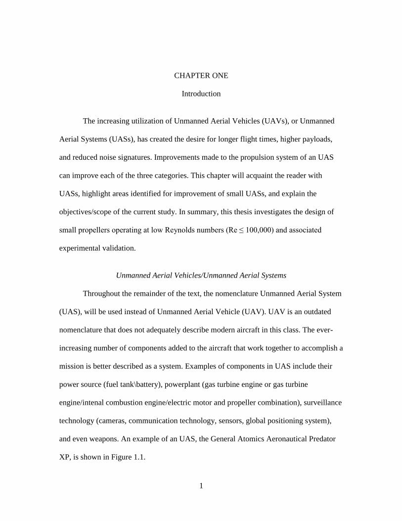
and even weapons. An example of an UAS, the General Atomics Aeronautical Predator
XP, is shown in Figure 1.1.
2
Figure 1.1: Predator XP UAS [1]
Characteristics of the Predator XP are listed below along with general definitions
of each characteristic [1]:
Powerplant—Aircraft propulsion system—Heavily modified Rotax 914 Turbo 4
Cylinder Engine.
Wing Span: 55 ft
Length: 27 ft
Max Airspeed: 120 KTAS
Max Altitude: 25,000 ft
Max Endurance: 35 hr
Some of the on-board systems include a triple-redundant flight control system, solid-state
digital avionics, Lynx multi-mode radar, Global Positioning System (GPS), automatic
takeoff and landing system, and air-to-ground weapons delivery capability.
3
Categories of UAS
There is a wide variety of UASs in existence. Categories of UASs will be
discussed by giving overviews of different classes of UASs highlighted in [2]. The list
will begin with a High Altitude, Long Endurance (HALE) UAS, the Northrop Grumman
Global Hawk [3].
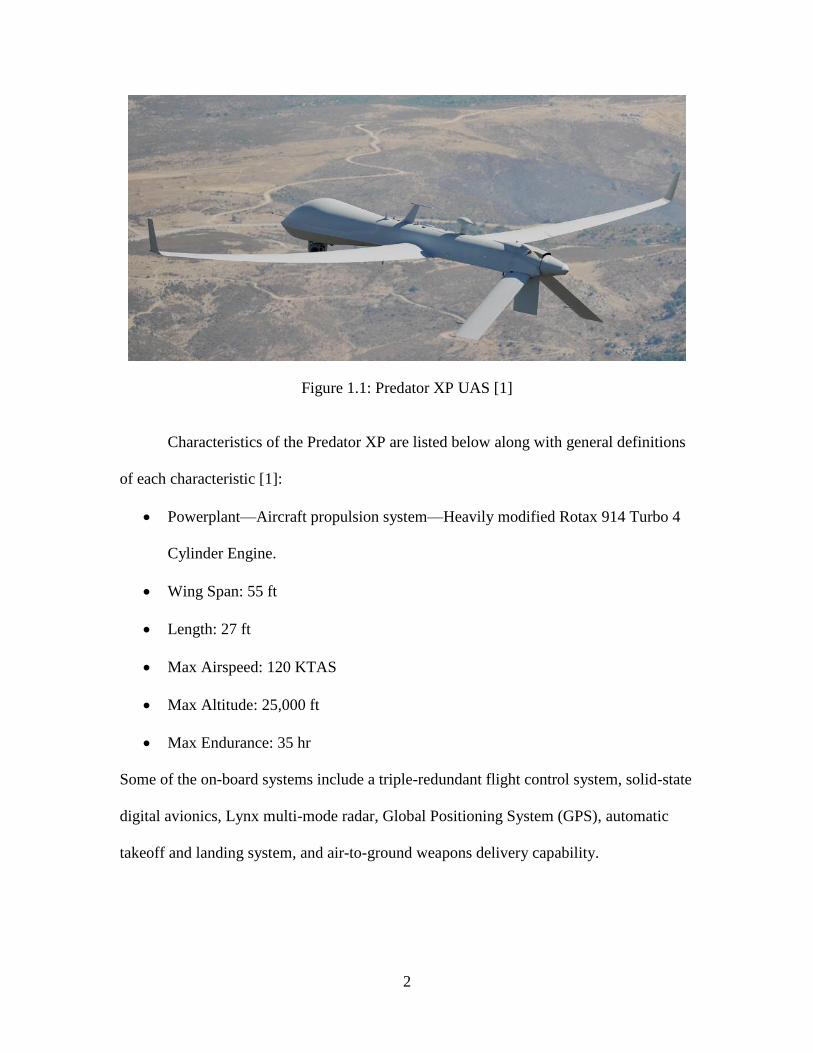
HALE UAS—Northrop Grumman Global Hawk
The Northrop Grumman Global hawk UAS is pictured in Figure 1.2. This aircraft
is designed to provide comprehensive ISR over large geographical areas. It is described
Figure 1.2: Northrop Grumman Global Hawk UAS [3]
as a versatile vehicle that is capable of full-scale combat, in addition to its surveillance
capabilities. The following are specifications of the aircraft available [3]:
Powerplant: Rolls Royce AE3007H turbo fan engine
Wingspan: 130.9 ft
Length: 47.6 ft
Loiter Airspeed: 310 KTAS
Maximum Altitude: 60,000 ft
4
Maximum Endurance: 32+ hrs
Reconnaissance technology includes a synthetic, aperture radar/moving target indicator, a
high resolution electro-optical digital camera, and a third-generation infrared sensor. This
sensor suite can exceed 32 hours of operation. Immediate differences can be seen when
comparing the Global Hawk with the Predator XP such as the differences in physical
characteristics and capabilities. The much larger Global Hawk is capable of a payload
that is nearly ten times that of the Predator XP. In addition to the higher payload, the
Global Hawk boasts a higher airspeed by 190 knots TAS and maximum altitude by
35,000 ft. Although the specified endurance is shorter than that of the Predator XP by
three hours, the Rolls Royce AE3007H turbo fan engine [4] gives the Global Hawk a
larger deployment radius due to its higher airspeed capabilities.
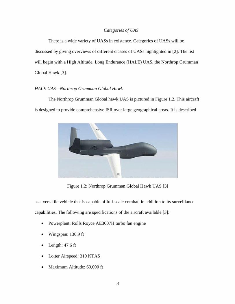
MALE UAS—General Atomics Aeronautical, Predator B
The UAS previously mentioned and in this chapter, Predator XP, belongs to this
class. An additional Medium Altitude, Long Endurance (MALE) UAS will be
Figure 1.3: Predator B UAS [5]
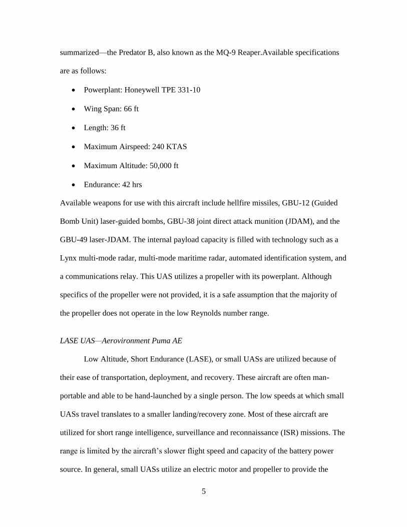
5
summarized—the Predator B, also known as the MQ-9 Reaper.Available specifications
are as follows:
Powerplant: Honeywell TPE 331-10
Wing Span: 66 ft
Length: 36 ft
Maximum Airspeed: 240 KTAS
Maximum Altitude: 50,000 ft
Endurance: 42 hrs
Available weapons for use with this aircraft include hellfire missiles, GBU-12 (Guided
Bomb Unit) laser-guided bombs, GBU-38 joint direct attack munition (JDAM), and the
GBU-49 laser-JDAM. The internal payload capacity is filled with technology such as a
Lynx multi-mode radar, multi-mode maritime radar, automated identification system, and
a communications relay. This UAS utilizes a propeller with its powerplant. Although
specifics of the propeller were not provided, it is a safe assumption that the majority of
the propeller does not operate in the low Reynolds number range.
LASE UAS—Aerovironment Puma AE
Low Altitude, Short Endurance (LASE), or small UASs are utilized because of
their ease of transportation, deployment, and recovery. These aircraft are often man-
portable and able to be hand-launched by a single person. The low speeds at which small
UASs travel translates to a smaller landing/recovery zone. Most of these aircraft are
utilized for short range intelligence, surveillance and reconnaissance (ISR) missions. The
range is limited by the aircraft’s slower flight speed and capacity of the battery power
source. In general, small UASs utilize an electric motor and propeller to provide the
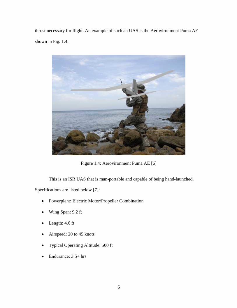
6
thrust necessary for flight. An example of such an UAS is the Aerovironment Puma AE
shown in Fig. 1.4.
Figure 1.4: Aerovironment Puma AE [6]
This is an ISR UAS that is man-portable and capable of being hand-launched.
Specifications are listed below [7]:
Powerplant: Electric Motor/Propeller Combination
Wing Span: 9.2 ft
Length: 4.6 ft
Airspeed: 20 to 45 knots
Typical Operating Altitude: 500 ft
Endurance: 3.5+ hrs
7
The Puma’s airframe, which weighs 13.5 lbs is capable of carrying an electro-optical
camera in addition to an infrared camera. The ISR capabilities are capable of being
utilized within a range of 15 km.
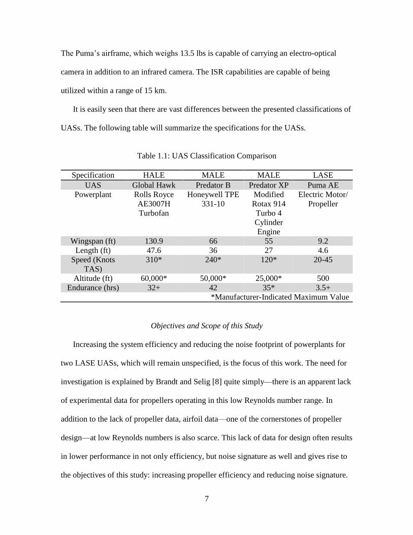
It is easily seen that there are vast differences between the presented classifications of
UASs. The following table will summarize the specifications for the UASs.
Table 1.1: UAS Classification Comparison
Specification HALE MALE MALE LASE
UAS Global Hawk Predator B Predator XP Puma AE
Powerplant Rolls Royce
AE3007H
Turbofan
Honeywell TPE
331-10
Modified
Rotax 914
Turbo 4
Cylinder
Engine
Electric Motor/
Propeller
Wingspan (ft) 130.9 66 55 9.2
Length (ft) 47.6 36 27 4.6
Speed (Knots
TAS)
310* 240* 120* 20-45
Altitude (ft) 60,000* 50,000* 25,000* 500
Endurance (hrs) 32+ 42 35* 3.5+
*Manufacturer-Indicated Maximum Value
Objectives and Scope of this Study
Increasing the system efficiency and reducing the noise footprint of powerplants for
two LASE UASs, which will remain unspecified, is the focus of this work. The need for
investigation is explained by Brandt and Selig [8] quite simply—there is an apparent lack
of experimental data for propellers operating in this low Reynolds number range. In
addition to the lack of propeller data, airfoil data—one of the cornerstones of propeller
design—at low Reynolds numbers is also scarce. This lack of data for design often results
in lower performance in not only efficiency, but noise signature as well and gives rise to
the objectives of this study: increasing propeller efficiency and reducing noise signature.
8
Increasing Efficiency and Reducing Noise Signature
In order to accomplish the objectives of this study, it was necessary to design,
theoretically analyze, manufacture, and experimentally evaluate propellers quickly. This
need gave rise to two automated systems used to meet the goals: a custom propeller
design code named Bearcontrol and a LabView VI code to automate the experimental
testing. Given that the user has the necessary airfoil data for the propeller design, these
two programs make it possible in most cases to design, manufacture, and test a propeller
in a single day. As a result of these two programs, significantly improved propellers have
been designed and their test results compared with commercial propellers in use on the
two UASs of interest.
Presentation Outline
The organization of this thesis will be as follows. Chapter Two will provide a
comprehensive literature survey of airfoil testing/data/codes, propeller design codes,
propeller testing, and finally noise considerations. Chapter Three will illustrate the theory
necessary to understand airfoil and propeller nomenclature and fluid mechanics. Chapter
Four will explain the experimental method used in this work. Chapter Five will present
results from this study. Chapter Six will provide a summary of the thesis, design
recommendations for increasing the efficiencies and reducing noise signatures of small
propellers, and draw conclusions for improving the current design and theoretical
analysis process, experimental setup, and experimental method.
9
CHAPTER TWO
Literature Survey
This chapter will explore previous research related to small propeller design,
theoretical analysis, and experimental evaluation. The surveyed research will be divided
into the following sections: low Reynolds numbers effects on propellers and airfoils,
propeller and airfoil design and analysis programs, and finally experimental testing and
considerations of propellers operating at low Reynolds numbers.
A Survey of Low Reynolds Numbers Effects on Propellers and Airfoils
This section investigates research associated with low Reynolds number operation
of propellers and airfoils. In particular, the presented research will lend insight to the flow
phenomena associated with the lower performance of propellers and airfoils operating in
this Reynolds number range.
Low Reynolds Number Propeller Operation
Reynolds number effects on the operation of propellers have been noted as early
as 1986 by R.M. Bass [9] in an experiment in which full scale propellers were scaled
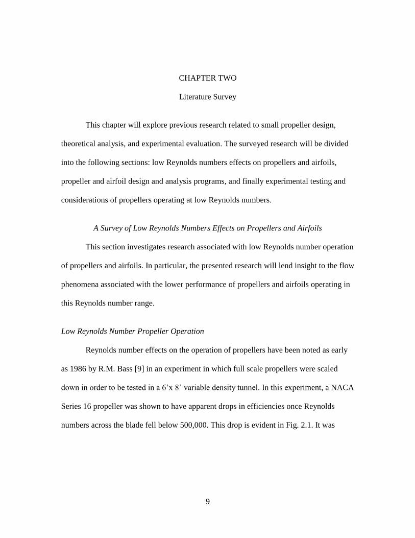
down in order to be tested in a 6’x 8’ variable density tunnel. In this experiment, a NACA
Series 16 propeller was shown to have apparent drops in efficiencies once Reynolds
numbers across the blade fell below 500,000. This drop is evident in Fig. 2.1. It was
10
Figure 2.1: NACA 16 Series Propeller Efficiencies vs. Reynolds Number [9]
concluded from the experiments that for Reynolds numbers below half a million, scaling
down a propeller would not be suitable for full-scale prediction as the model behavior is
erratic. While this test propeller is not operating at the Reynolds numbers of interest for
small UASs, the results from this experiment contribute to the understanding of the
performance of small UAS propellers.
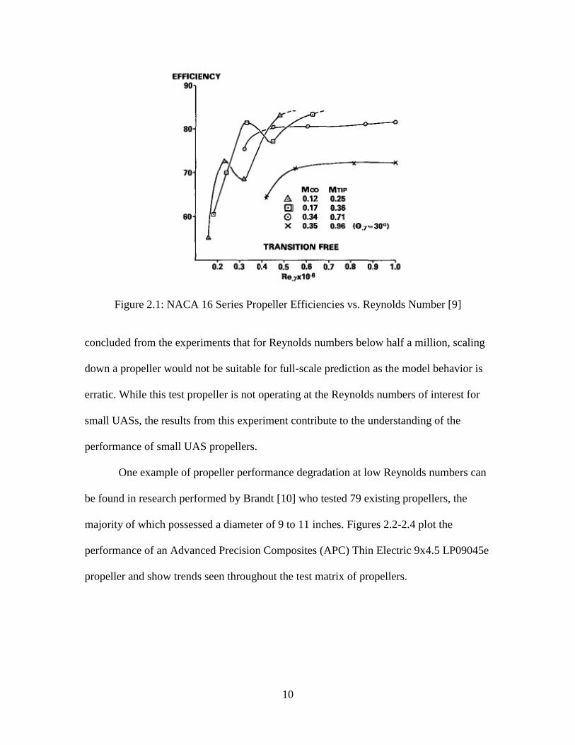
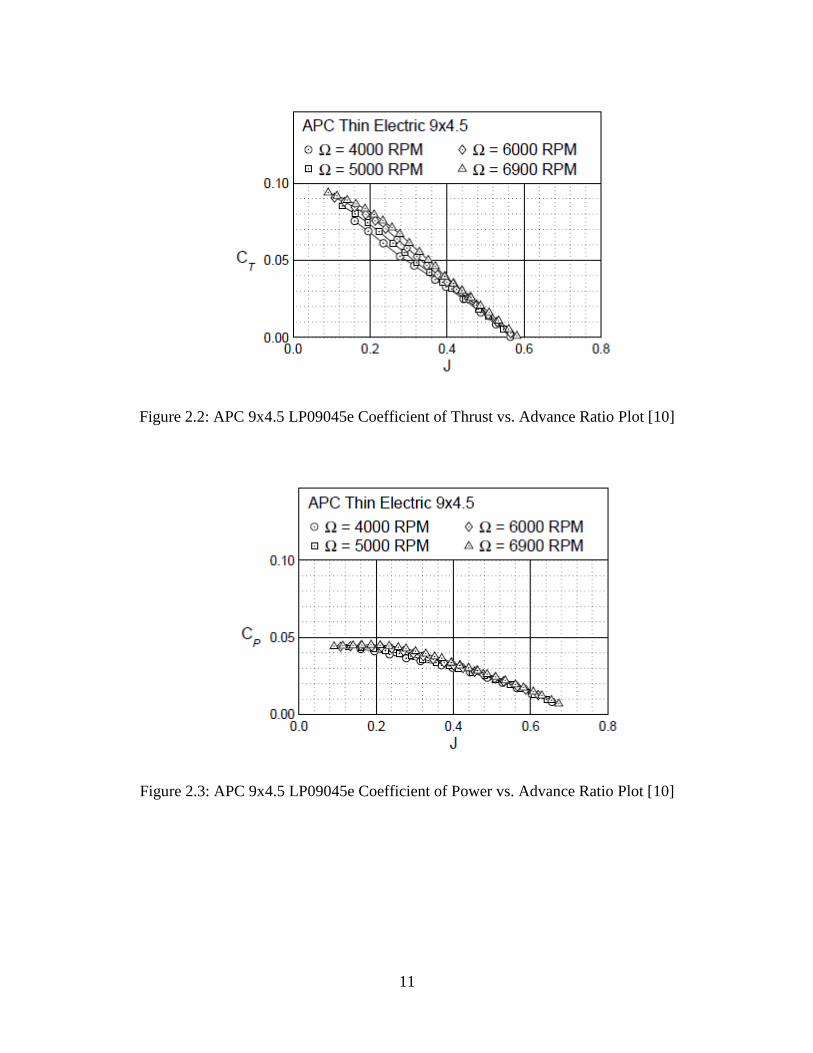
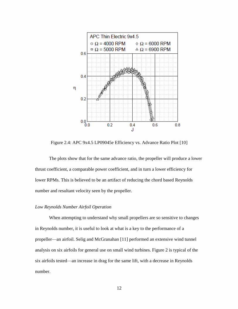
One example of propeller performance degradation at low Reynolds numbers can
be found in research performed by Brandt [10] who tested 79 existing propellers, the
majority of which possessed a diameter of 9 to 11 inches. Figures 2.2-2.4 plot the
performance of an Advanced Precision Composites (APC) Thin Electric 9x4.5 LP09045e
propeller and show trends seen throughout the test matrix of propellers.
11
Figure 2.2: APC 9x4.5 LP09045e Coefficient of Thrust vs. Advance Ratio Plot [10]
Figure 2.3: APC 9x4.5 LP09045e Coefficient of Power vs. Advance Ratio Plot [10]
12
Figure 2.4: APC 9x4.5 LP09045e Efficiency vs. Advance Ratio Plot [10]
The plots show that for the same advance ratio, the propeller will produce a lower
thrust coefficient, a comparable power coefficient, and in turn a lower efficiency for
lower RPMs. This is believed to be an artifact of reducing the chord based Reynolds
number and resultant velocity seen by the propeller.
Low Reynolds Number Airfoil Operation
When attempting to understand why small propellers are so sensitive to changes
in Reynolds number, it is useful to look at what is a key to the performance of a
propeller—an airfoil. Selig and McGranahan [11] performed an extensive wind tunnel
analysis on six airfoils for general use on small wind turbines. Figure 2 is typical of the
six airfoils tested—an increase in drag for the same lift, with a decrease in Reynolds
number.
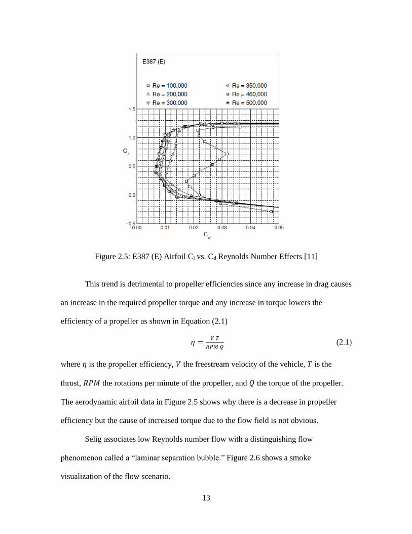
13
Figure 2.5: E387 (E) Airfoil Cl vs. Cd Reynolds Number Effects [11]
This trend is detrimental to propeller efficiencies since any increase in drag causes
an increase in the required propeller torque and any increase in torque lowers the
efficiency of a propeller as shown in Equation (2.1)
𝜂 =𝑉 𝑇
𝑅𝑃𝑀 𝑄 (2.1)
where 𝜂 is the propeller efficiency, 𝑉 the freestream velocity of the vehicle, 𝑇 is the
thrust, 𝑅𝑃𝑀 the rotations per minute of the propeller, and 𝑄 the torque of the propeller.
The aerodynamic airfoil data in Figure 2.5 shows why there is a decrease in propeller
efficiency but the cause of increased torque due to the flow field is not obvious.
Selig associates low Reynolds number flow with a distinguishing flow
phenomenon called a “laminar separation bubble.” Figure 2.6 shows a smoke
visualization of the flow scenario.
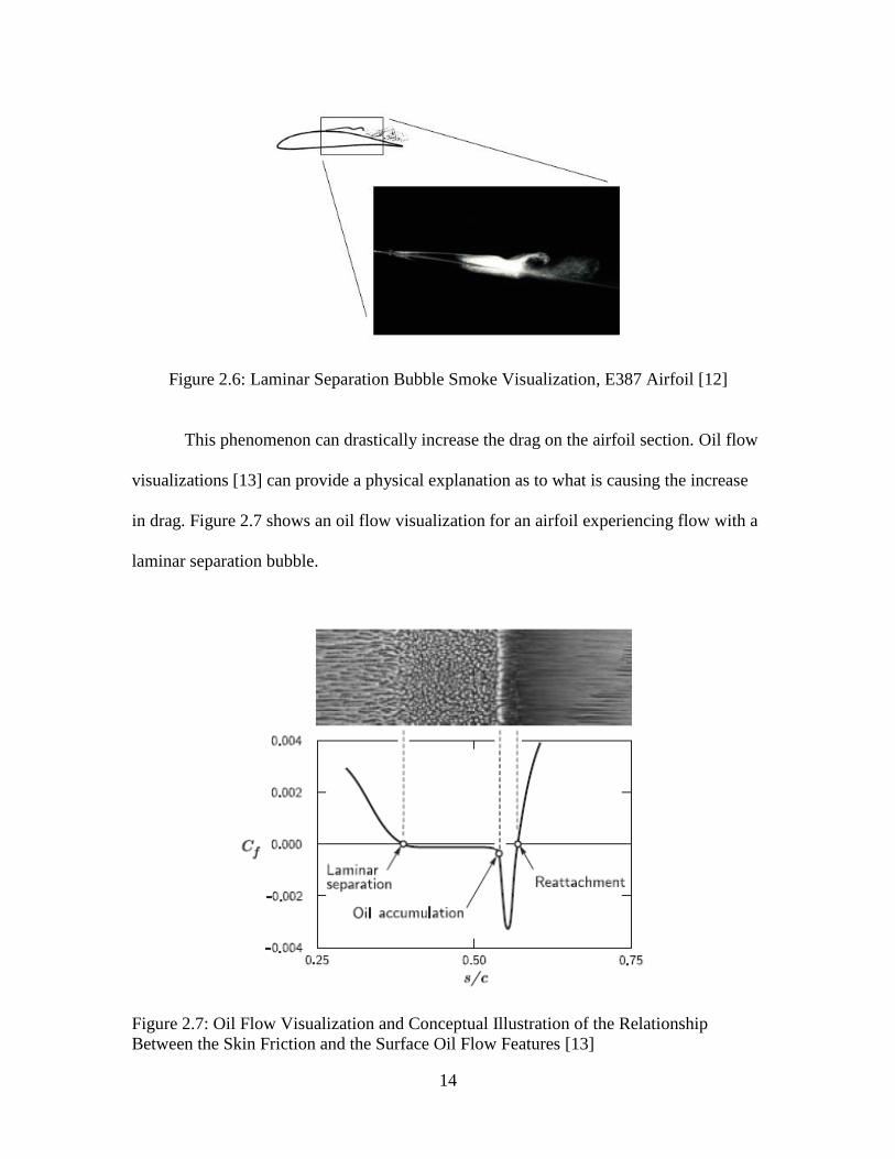
14
Figure 2.6: Laminar Separation Bubble Smoke Visualization, E387 Airfoil [12]
This phenomenon can drastically increase the drag on the airfoil section. Oil flow
visualizations [13] can provide a physical explanation as to what is causing the increase
in drag. Figure 2.7 shows an oil flow visualization for an airfoil experiencing flow with a
laminar separation bubble.
Figure 2.7: Oil Flow Visualization and Conceptual Illustration of the Relationship
Between the Skin Friction and the Surface Oil Flow Features [13]
15
The visualization in the figure shows a section of the suction side of an airfoil
experiencing flow from left to right, with the flow visualization oil in place. The
conceptual illustration in the figure shows the relationship between the skin friction, 𝐶𝑓,
and the corresponding locations on the airfoil. The area between the separation and
reattachment points is where the bubble occurs. The separation and recirculation of the
flow in this region increases the drag on the airfoil considerably.
The elimination of this laminar separation bubble through the use of trips/trip
strips/trip wires has also been studied by various groups. Trip wires promote transition to
turbulent flow to delay the flow from separating on the airfoil. Huber and Mueller [14]
studied the effects of trip wires on a Wortmann FX 63-137 airfoil tested at a Reynolds
number of 100,000. The effects of the trip wires varied with the location and height, but
ultimately this airfoil was deemed a high performance low Reynolds number airfoil even
in off-design conditions as no trip orientation made a vast improvement to the
aerodynamic performance. Gopalarathnam et al. [15] also studied the effects of trip
wires. In this study three different airfoils were tested at two Reynolds numbers, 100,000
and 300,000. At each Reynolds number, for each airfoil, five conditions were tested—a
clean airfoil, and then trips located at 0.1c, 0.2c, 0.3c, and 0.4c. For the conditions tested
the study noted that airfoils with trips do not hold any clear advantage over airfoils
designed for good performance in the clean conditions.
Propeller and Airfoil Design and Analysis Tools
This next section will explore two propeller design and analysis tools available
and used by various research efforts.The suitablility of each tool reported will be
discussed as well as general implementation protocols.
16
Propeller Design and Analysis
Various propeller design and analysis programs are available for use from
freeware programmers across the internet. Two of the more widely used programs will be
discussed here. The design features and implementation requirements for each will be
noted.
The first program investigated was JavaProp [16]. This is a propeller design and
analysis code based on the framework of equations presented by Adkins [17]. It provides
the basic tools necessary to design, analyze, and create a solid model of a propeller, but
limitations within the program exist. In order to design a propeller, the following inputs
are required:
Number of blades.
Flight speed.
Propeller diameter.
Selected distribution of airfoil lift and drag coefficients.
Thrust or shaft power.
Air density.
The default design procedure will create an optimum propeller as defined by Adkins [17].
Options exist to account for a shrouded rotor, add a square tip, and even import a custom
propeller geometry in computer aided design (CAD) compatible format. Outputs of the
program include the usual propeller coefficients in addition to thrust, power, efficiency,
flight velocity, and the propeller geometry. The designs can be analyzed at a single
operating point or over a range of velocities. Limitations of the program include the
17
minimal selection of airfoil cross-sections to use in design, the inability to import airfoil
cross-sections as a user, and the lack of detail in the analysis of the propeller.
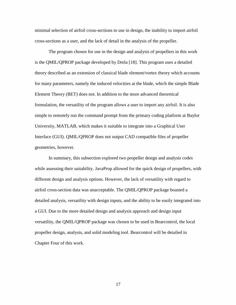
The program chosen for use in the design and analysis of propellers in this work
is the QMIL/QPROP package developed by Drela [18]. This program uses a detailed
theory described as an extension of classical blade element/vortex theory which accounts
for many parameters, namely the induced velocities at the blade, which the simple Blade
Element Theory (BET) does not. In addition to the more advanced theoretical
formulation, the versatility of the program allows a user to import any airfoil. It is also
simple to remotely run the command prompt from the primary coding platform at Baylor
University, MATLAB, which makes it suitable to integrate into a Graphical User
Interface (GUI). QMIL/QPROP does not output CAD compatible files of propeller
geometries, however.
In summary, this subsection explored two propeller design and analysis codes
while assessing their suitability. JavaProp allowed for the quick design of propellers, with
different design and analysis options. However, the lack of versatility with regard to
airfoil cross-section data was unacceptable. The QMIL/QPROP package boasted a
detailed analysis, versatility with design inputs, and the ability to be easily integrated into
a GUI. Due to the more detailed design and analysis approach and design input
versatility, the QMIL/QPROP package was chosen to be used in Bearcontrol, the local
propeller design, analysis, and solid modeling tool. Bearcontrol will be detailed in
Chapter Four of this work.

18
Airfoil Design and Analysis
As with propeller design and analysis, there exists similar open software tools for
airfoils. The most commonly used code, XFOIL [19], will be discussed as it is widely
used and is the choice for airfoil analysis in this thesis. In addition to the code, an
extensive airfoil database created by the University of Illinois Urbana-Champaign
(UIUC) will be explored.
XFOIL [19] is the airfoil design and analysis tool utilized by many and used in
this work. First introduced in, 1989 [20], XFOIL has the following capabilities:
Viscous/Inviscid analysis of airfoils.
Aifoil design through an interactive specification of surface speed distributions.
Airfoil redesign through interactive specification of surface speed distributions
and/or typical airfoil geometric parameters.
Airfoil Blending.
Drag polar calculation with fixed/varying Reynolds/Mach numbers.
Write/read of airfoil geometry and polar save files.
Various plotting of results.
The versatility of XFOIL gives users who may not possess the time or resources for
experimental evaluation of airfoils an option to attain theoretical performance
predictions. Also, although not directly utilized in this work, the program offers methods
of designing or altering airfoils.
Another valuable tool regarding airfoil design and analysis is the UIUC Applied
Aerodynamics Group Airfoil Coordinates Database [21]. This website contains the
geometry coordinates of over 1500 airfoils some of which are accompanied by drag polar
19
data. Many other resources also contain the results of experimental wind tunnel testing of
airfoils such as the Summary of Low-Speed Airfoil Data Volumes and Airfoils at Low
Speeds [11, 22-25].
In summary, XFOIL, airfoil databases such as the one created by UIUC, and
experimental research of airfoil performance has been explored in this subsection. When
available, experimental data was preferred when designing propellers for this work. If
none was available, XFOIL was utilized to theoretically obtain lift and drag coefficients
of airfoil cross-sections at desired Reynolds numbers.
Experimental Testing and Considerations of Propellers Operating at
Low Reynolds Numbers
This section will explore research that is associated with the experimental
evaluation of propellers operating at low Reynolds numbers. The subsections will discuss
experimental setups of different propeller test stands and wind tunnel corrections used in
propeller testing.
Experimental Low Reynolds Number Testing of Small Propellers
In recent years the testing of small propellers has increased, likely due to the
increase in utilization of small UAS. The following section will survey different studies
and their associated experimental methods used to test propellers in this category.
Brandt and Selig [8] tested small propellers (9-11 inches in diameter) in the low
Reynolds number range of 50,000 to 100,000. Testing took place in the University of
Illinois at Urbana Champaign (UIUC) subsonic wind tunnel. The test section was
reported to have nominal cross-sectional dimensions of 2.8 x 4.0 ft and the maximum
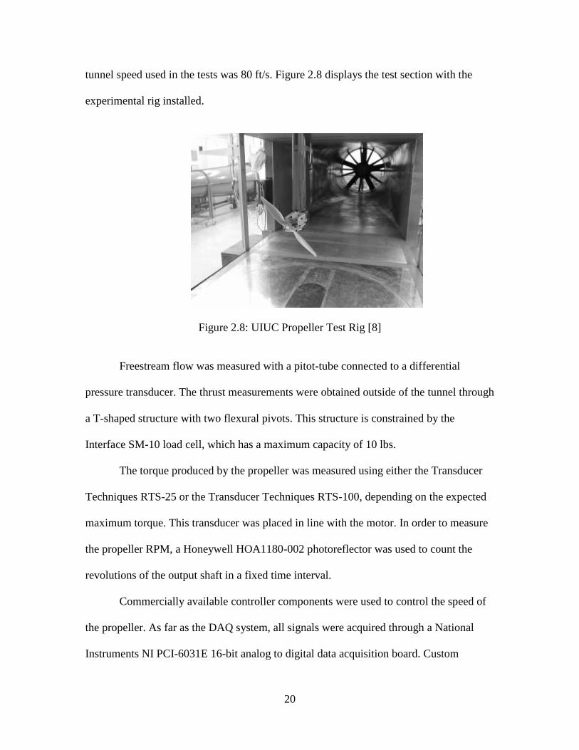
20
tunnel speed used in the tests was 80 ft/s. Figure 2.8 displays the test section with the
experimental rig installed.
Figure 2.8: UIUC Propeller Test Rig [8]
Freestream flow was measured with a pitot-tube connected to a differential
pressure transducer. The thrust measurements were obtained outside of the tunnel through
a T-shaped structure with two flexural pivots. This structure is constrained by the
Interface SM-10 load cell, which has a maximum capacity of 10 lbs.
The torque produced by the propeller was measured using either the Transducer
Techniques RTS-25 or the Transducer Techniques RTS-100, depending on the expected
maximum torque. This transducer was placed in line with the motor. In order to measure
the propeller RPM, a Honeywell HOA1180-002 photoreflector was used to count the
revolutions of the output shaft in a fixed time interval.
Commercially available controller components were used to control the speed of
the propeller. As far as the DAQ system, all signals were acquired through a National
Instruments NI PCI-6031E 16-bit analog to digital data acquisition board. Custom
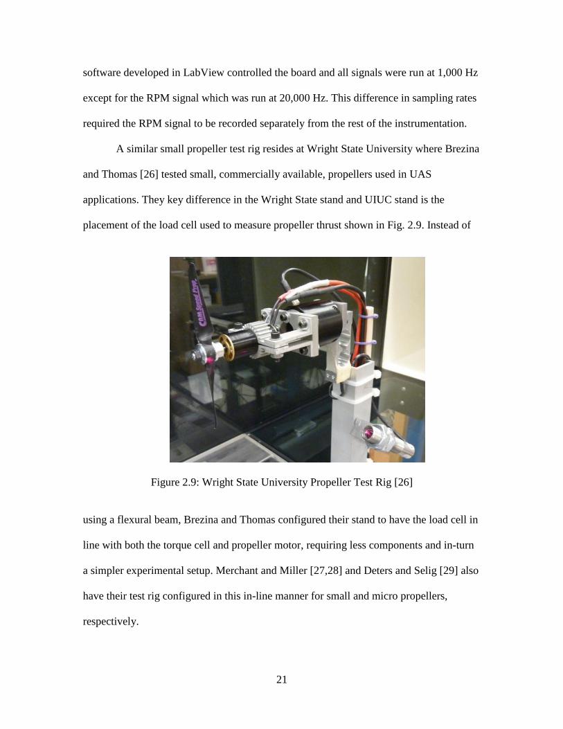
21
software developed in LabView controlled the board and all signals were run at 1,000 Hz
except for the RPM signal which was run at 20,000 Hz. This difference in sampling rates
required the RPM signal to be recorded separately from the rest of the instrumentation.
A similar small propeller test rig resides at Wright State University where Brezina
and Thomas [26] tested small, commercially available, propellers used in UAS
applications. They key difference in the Wright State stand and UIUC stand is the
placement of the load cell used to measure propeller thrust shown in Fig. 2.9. Instead of
Figure 2.9: Wright State University Propeller Test Rig [26]
using a flexural beam, Brezina and Thomas configured their stand to have the load cell in
line with both the torque cell and propeller motor, requiring less components and in-turn
a simpler experimental setup. Merchant and Miller [27,28] and Deters and Selig [29] also
have their test rig configured in this in-line manner for small and micro propellers,
respectively.
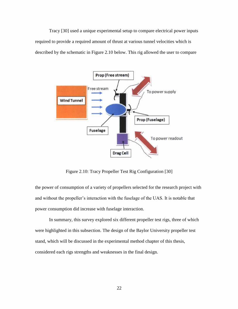
22
Tracy [30] used a unique experimental setup to compare electrical power inputs
required to provide a required amount of thrust at various tunnel velocities which is
described by the schematic in Figure 2.10 below. This rig allowed the user to compare
Figure 2.10: Tracy Propeller Test Rig Configuration [30]
the power of consumption of a variety of propellers selected for the research project with
and without the propeller’s interaction with the fuselage of the UAS. It is notable that
power consumption did increase with fuselage interaction.
In summary, this survey explored six different propeller test rigs, three of which
were highlighted in this subsection. The design of the Baylor University propeller test
stand, which will be discussed in the experimental method chapter of this thesis,
considered each rigs strengths and weaknesses in the final design.
23
Experimental Considerations for Small Propeller Testing
When testing propellers in a wind tunnel, it is often necessary to consider
corrections to the experimental data to account for the interaction between the propeller
flow field and the wind tunnel walls. This section of the chapter will survey a selection of
wind tunnel corrections.
Chen and Liou [31] experimentally researched wind tunnel blockage effects on
the power coefficients of small, horizontal-axis wind turbines. In the research, they varied
the following parameters to obtain relationships between each and a blockage correction
factor (BF):
Tip Speed Ratios (TSR)—the speed of the tip of a blade on the wind turbine.
Blockage Ratio (BR)—the quotient of the disc area of the wind turbine to the
cross-sectional area of the wind tunnel.
Rotor Pitch Angles (𝛽)—designated geometric pitch angle of the respective wind
turbine.
Tunnel Freestream Velocities (𝑈∞)—set velocity in the wind tunnel.
The quantitative data showed that the BF becomes significant as TSR and BR increase,
and when 𝛽 decreases.
Fitzgerald [32] explored a selection of wind tunnel blockage corrections including
the Glauert Correction, Maskell Correction, Ashill and Keating Correction, Hensel’s
Area-Ratio Method, Hackett-Wilsden Method, and the Sorensen and Mikkelsen Method.
Brief descriptions of each correction follow.
24
Glauert Correction: This correction seeks an equivalent free airspeed at which the
propeller would produce the same thrust and torque at the same angular velocity if
the flow were not contained by the tunnel walls.
Maskell Correction: This correction uses experimentally derived drag coefficient
relations in conjunction with relations describing wake distortion due to the wall
constraints to generate a blockage correction.
Ashill and Keating Correction: This correction uses a two component velocity
method in conjunction with equations for the perturbation potential in free air
flow and that due to the wall constraints to assess the differences in perturbation
potentials.
Hensel’s Area-Ratio Method: This correction uses point and line sources to model
revolving bodies, and finite straight and swept wings.
Hackett-Wilsden Method: This method uses one of two corrections, depending on
whether or not the flow on the model is predominately separated or not. For cases
in which it is mainly attached, the global correction method is used. For cases in
which the flow is manyly separated, a point by point correction over the surface
of the model to obtain corrected pressure coefficients.
Sorensen and Mikkelsen Method: This method uses the conservation of
momentum to model wind tunnel blockage of wind turbines. Similarly to the
Glauert correction, an equivalent free airspeed is calculated based on the
framework of equations presented in the method.
25
After extensive comparison of the corrections through application of each to propeller
testing conducted for the project, Fitzgerald recommends the long standing Glauert
Correction, which was utilized in the work of this thesis.
The Glauert Correction [33] theoretically seeks to find an equivalent free airspeed
for a propeller based on the operating conditions in the tunnel by applying the
conservation of momentum to the scenario. The equivalent airspeed is defined as the free
airspeed in which the propeller would produce the same thrust and torque at an equivalent
RPM. Glauert notes that the equivalent free airspeed for a propeller operating in a wind
tunnel is usually less than the freestream velocity measured in the tunnel.
In summary, it is clear that wind tunnel corrections are needed in experiments
similar to what was performed in this work. After surveying various corrections, the
Glauert Correction was chosen because of its long standing use and the recommendation
from Fitzgerald who studied the differences between correction methods at length.
Chapter Two Concluding Remarks
This chapter explored relevant research pertaining to the work completed in this
thesis. First characteristics of propellers and airfoils operating at low Reynolds numbers
were discussed. Propeller and airfoil design and analysis followed. Last, experimental
propeller test rigs and accompanying considerations were examined.
26
CHAPTER THREE
Theoretical Background
This chapter will detail the theoretical background necessary to understand airfoil
and propeller theory as used in this work. The background will begin with one-
dimensional propeller theory, move on to airfoil theory, blade-element theory (BET),
blade element momentum theory (BEMT), and finally the theory used in the design
procedure of this work—an extension of the classical blade-element/vortex theory
formulated by Mark Drela of MIT.
Propeller Theory
One-Dimensional Propeller Theory
This section will begin with the simplest theory that describes propeller
operation—one-dimensional propeller theory, also known as momentum theory. The
example given will closely follow that of Roskam et al. [34]. This theory begins by
replacing the plane of propeller rotation with a thin actuator disk which is considered to
have an infinite number of blades and be uniformly loaded. In the case described, the
flow will be considered incompressible, and as a result of the one-dimensional analysis,
irrotational. Inflow and outflow are considered to be uniform and steady. A depiction of
the scenario for a propeller with positive thrust is shown in Figure 3.1. At Station 0, the
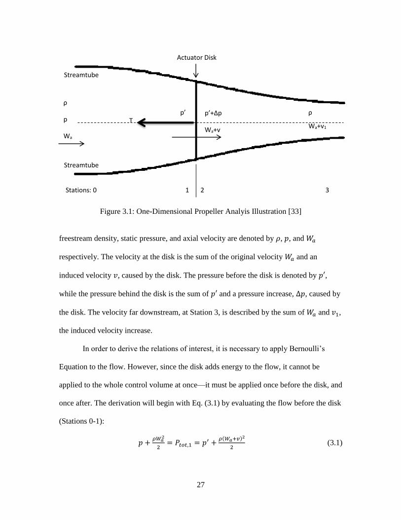
27
Figure 3.1: One-Dimensional Propeller Analyis Illustration [33]
freestream density, static pressure, and axial velocity are denoted by 𝜌, 𝑝, and 𝑊𝑎
respectively. The velocity at the disk is the sum of the original velocity 𝑊𝑎 and an
induced velocity 𝑣, caused by the disk. The pressure before the disk is denoted by 𝑝′,
while the pressure behind the disk is the sum of 𝑝′ and a pressure increase, Δ𝑝, caused by
the disk. The velocity far downstream, at Station 3, is described by the sum of 𝑊𝑎 and 𝑣1,
the induced velocity increase.
In order to derive the relations of interest, it is necessary to apply Bernoulli’s
Equation to the flow. However, since the disk adds energy to the flow, it cannot be
applied to the whole control volume at once—it must be applied once before the disk, and
once after. The derivation will begin with Eq. (3.1) by evaluating the flow before the disk
(Stations 0-1):
𝑝 +𝜌𝑊𝑎
2
2= 𝑃𝑡𝑜𝑡,1 = 𝑝′ +
𝜌(𝑊𝑎+𝑣)2
2 (3.1)
Actuator Disk
Streamtube
T
Streamtube
p’
Wa+v
ρ
p
Wa
ρ
Wa+v1
p’+Δp
Stations: 0 1 2 3
28
Next, using Bernoulli’s equation, the flow after the disk (Stations 2-3) is given by Eq.
(3.2)
𝑝 +𝜌(𝑊𝑎+𝑣1)2
2= 𝑃𝑡𝑜𝑡,2 = 𝑝′ + 𝛥𝑝 +
𝜌(𝑊𝑎+𝑣)2
2 (3.2)
where the total pressure before and after the disk are represented by 𝑃𝑡𝑜𝑡,1 and 𝑃𝑡𝑜𝑡,2,
respectively. If the difference of these two variables is evaluated, a relation for 𝛥𝑝 may
be found as shown in Eq. (3.3).
𝑃𝑡𝑜𝑡,2 − 𝑃𝑡𝑜𝑡,1 = 𝛥𝑝 = 𝑝 +𝜌(𝑊𝑎+𝑣1)2
2− (𝑝 +
𝜌𝑊𝑎2
2) = 𝜌 (𝑊𝑎 +
𝑣1
2) 𝑣1 (3.3)
With the change in pressure known across the disk, obtaining the thrust is simply a matter
of multiplying Eq. (3.3) by the area of the disk, 𝐴. Equation (3.4) represents the thrust of
a one-dimensional propeller disk.
𝑇 = 𝐴𝛥𝑝 = 𝐴𝜌 (𝑊𝑎 +𝑣1
2) 𝑣1 (3.4)
In order to predict the induced velocity far downstream, 𝑣1, it is necessary to apply the
conservation of linear momentum, represented by Eq. (3.5)
∑�⃗� = ∫ 𝜌𝑊𝑎⃗⃗ ⃗⃗⃗⃗
𝑆(𝑊𝑎⃗⃗ ⃗⃗⃗⃗ ∙ 𝑑𝐴) (3.5)
where ∑�⃗� is the total force acting on the control volume bounded by Station 0 and
Station 3. With the knowledge that the thrust, 𝑇, is acting in the opposite direction of ∑�⃗�,
the equation can be reduced as follows
𝑇 = 𝜌𝑊𝑎{−(𝑊𝑎 + 𝑣)𝐴} + 𝜌(𝑊𝑎 + 𝑣1){(𝑊𝑎 + 𝑣)𝐴} = 𝜌𝐴(𝑊𝑎 + 𝑣)𝑣1 (3.6)
If Eqs. (3.4) and (3.6) are equated, it can be seen that the induced velocity far
downstream is twice that of the induced velocity at the propeller disk. This is shown in
Eq. (3.7) below
𝑣1 = 2𝑣 (3.7)
29
In order to solve for 𝑣, Eqs. (3.6) and (3.7) must be combined to produce Eq. (3.8)
𝑇 = 2𝜌𝐴(𝑊𝑎 + 𝑣)𝑣 (3.8)
The induced velocity, 𝑣, may then be isolated and expressed by Eq. (3.9):
𝑣 = −𝑊𝑎
2+ √(
𝑊𝑎
2)
2
+𝑇
2𝐴𝜌 (3.9)
According to this theory, keeping the induced velocity as small as possible is the key to
high propeller efficiencies. This can be seen by examining the equation for propeller
efficiency.
The propeller efficiency can be thought of as the quotient of the power output and
required power input of the propeller. The power output of the propeller, which is in the
numerator of the efficiency equation, is the product of the thrust produced and the
freestream velocity at Station 0. The required input power of the propeller, which is in the
denominator of the efficiency equation, is equivalent to the product of the thrust caused
by the air pressure on the propeller disk and the air velocity passing through the disk.
This definition may be written as follows in Eq. (3.10)
𝜂 =𝑇𝑊𝑎
𝑇(𝑊𝑎+𝑣)=
𝑊𝑎
𝑊𝑎+𝑣 (3.10)
It is important to note that this definition of propeller efficiency would coincide with an
ideal, uninstalled propeller. Equation (3.10) will over-predict efficiency of a real-world,
installed propeller because of assumptions applied to this theory. Many factors will
induce losses such as non-uniform flow, blade profile drag, flow rotation, propeller-
fuselage interaction, propeller-wing interaction, and in some cases compressible flow
effects.
In summary, this is a simple theory that allows the characterization of an ideal
propeller in ideal flow situations. It is worth noting that this theory cannot provide
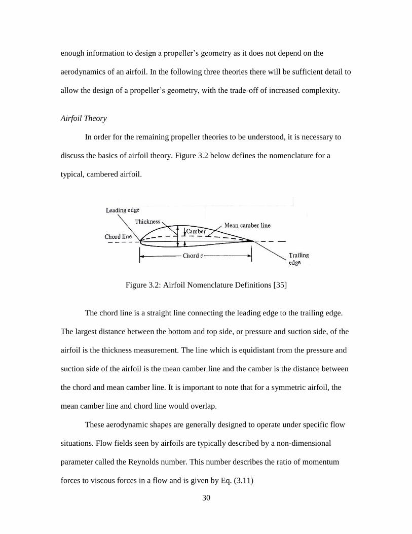
30
enough information to design a propeller’s geometry as it does not depend on the
aerodynamics of an airfoil. In the following three theories there will be sufficient detail to
allow the design of a propeller’s geometry, with the trade-off of increased complexity.
Airfoil Theory
In order for the remaining propeller theories to be understood, it is necessary to
discuss the basics of airfoil theory. Figure 3.2 below defines the nomenclature for a
typical, cambered airfoil.
Figure 3.2: Airfoil Nomenclature Definitions [35]
The chord line is a straight line connecting the leading edge to the trailing edge.
The largest distance between the bottom and top side, or pressure and suction side, of the
airfoil is the thickness measurement. The line which is equidistant from the pressure and
suction side of the airfoil is the mean camber line and the camber is the distance between
the chord and mean camber line. It is important to note that for a symmetric airfoil, the
mean camber line and chord line would overlap.
These aerodynamic shapes are generally designed to operate under specific flow
situations. Flow fields seen by airfoils are typically described by a non-dimensional
parameter called the Reynolds number. This number describes the ratio of momentum
forces to viscous forces in a flow and is given by Eq. (3.11)
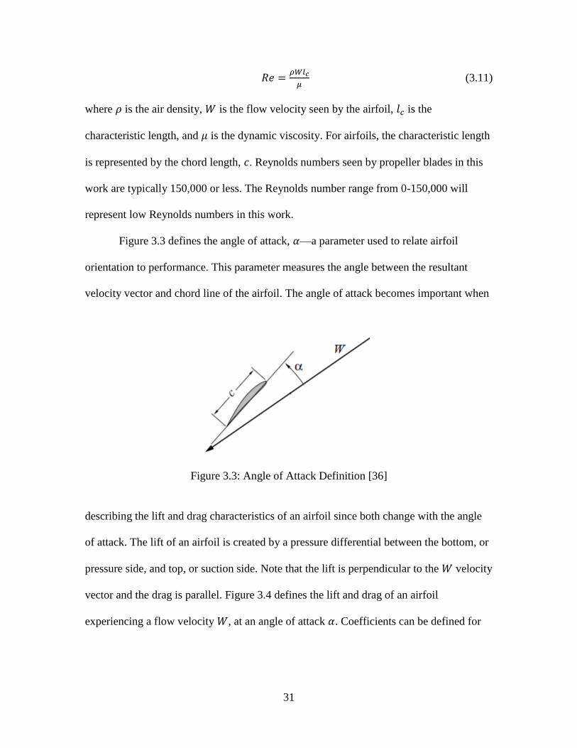
31
𝑅𝑒 =𝜌𝑊𝑙𝑐
𝜇 (3.11)
where 𝜌 is the air density, 𝑊 is the flow velocity seen by the airfoil, 𝑙𝑐 is the
characteristic length, and 𝜇 is the dynamic viscosity. For airfoils, the characteristic length
is represented by the chord length, 𝑐. Reynolds numbers seen by propeller blades in this
work are typically 150,000 or less. The Reynolds number range from 0-150,000 will
represent low Reynolds numbers in this work.
Figure 3.3 defines the angle of attack, 𝛼—a parameter used to relate airfoil
orientation to performance. This parameter measures the angle between the resultant
velocity vector and chord line of the airfoil. The angle of attack becomes important when
Figure 3.3: Angle of Attack Definition [36]
describing the lift and drag characteristics of an airfoil since both change with the angle
of attack. The lift of an airfoil is created by a pressure differential between the bottom, or
pressure side, and top, or suction side. Note that the lift is perpendicular to the 𝑊 velocity
vector and the drag is parallel. Figure 3.4 defines the lift and drag of an airfoil
experiencing a flow velocity 𝑊, at an angle of attack 𝛼. Coefficients can be defined for
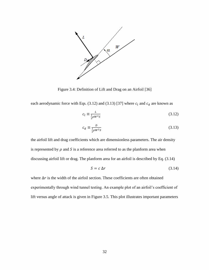
32
Figure 3.4: Definition of Lift and Drag on an Airfoil [36]
each aerodynamic force with Eqs. (3.12) and (3.13) [37] where 𝑐𝑙 and 𝑐𝑑 are known as
𝑐𝑙 ≡𝐿
1
2𝜌𝑊2𝑆
(3.12)
𝑐𝑑 ≡𝐷
1
2𝜌𝑊2𝑆
(3.13)
the airfoil lift and drag coefficients which are dimensionless parameters. The air density
is represented by 𝜌 and 𝑆 is a reference area referred to as the planform area when
discussing airfoil lift or drag. The planform area for an airfoil is described by Eq. (3.14)
𝑆 = 𝑐 Δ𝑟 (3.14)
where Δ𝑟 is the width of the airfoil section. These coefficients are often obtained
experimentally through wind tunnel testing. An example plot of an airfoil’s coefficient of
lift versus angle of attack is given in Figure 3.5. This plot illustrates important parameters
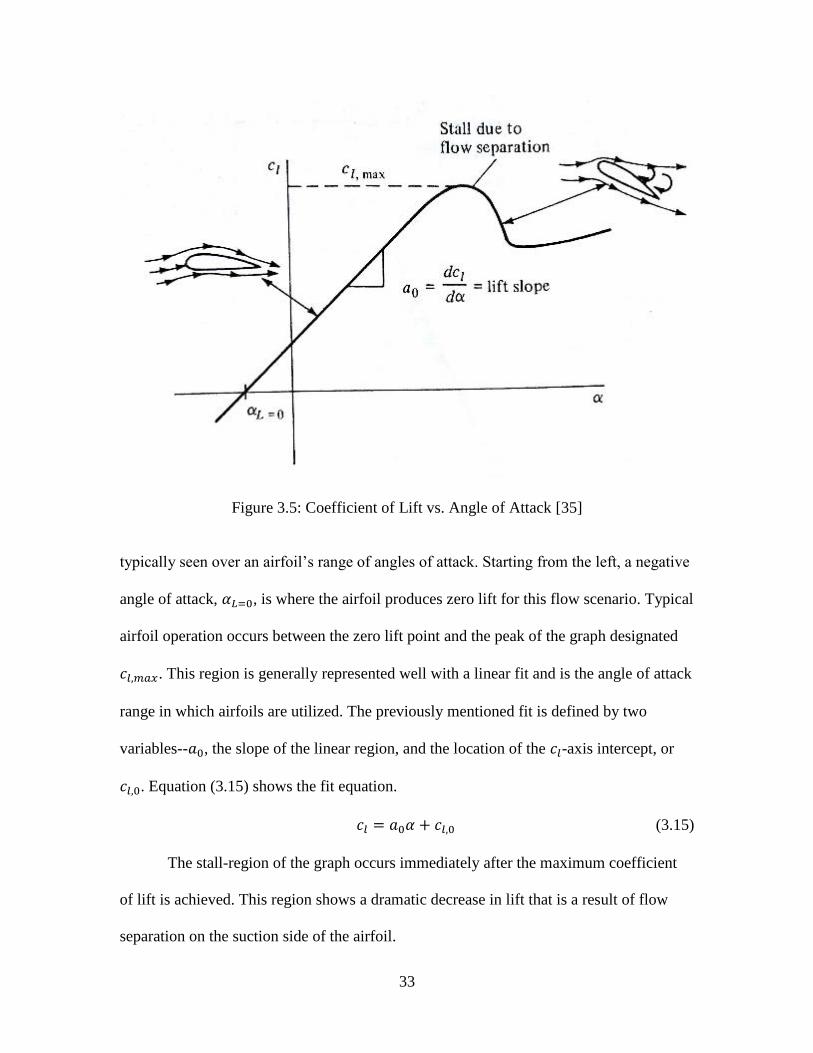
33
Figure 3.5: Coefficient of Lift vs. Angle of Attack [35]
typically seen over an airfoil’s range of angles of attack. Starting from the left, a negative
angle of attack, 𝛼𝐿=0, is where the airfoil produces zero lift for this flow scenario. Typical
airfoil operation occurs between the zero lift point and the peak of the graph designated
𝑐𝑙,𝑚𝑎𝑥. This region is generally represented well with a linear fit and is the angle of attack
range in which airfoils are utilized. The previously mentioned fit is defined by two
variables--𝑎0, the slope of the linear region, and the location of the 𝑐𝑙-axis intercept, or
𝑐𝑙,0. Equation (3.15) shows the fit equation.
𝑐𝑙 = 𝑎0𝛼 + 𝑐𝑙,0 (3.15)
The stall-region of the graph occurs immediately after the maximum coefficient
of lift is achieved. This region shows a dramatic decrease in lift that is a result of flow
separation on the suction side of the airfoil.
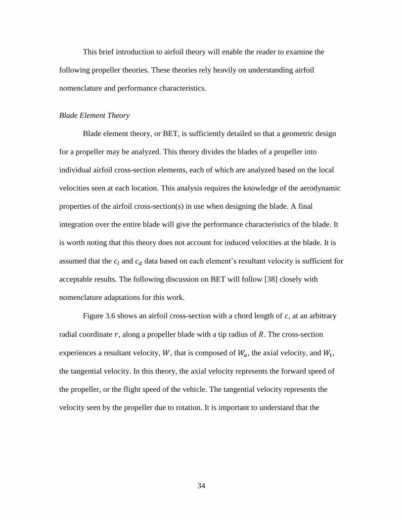
34
This brief introduction to airfoil theory will enable the reader to examine the
following propeller theories. These theories rely heavily on understanding airfoil
nomenclature and performance characteristics.
Blade Element Theory
Blade element theory, or BET, is sufficiently detailed so that a geometric design
for a propeller may be analyzed. This theory divides the blades of a propeller into
individual airfoil cross-section elements, each of which are analyzed based on the local
velocities seen at each location. This analysis requires the knowledge of the aerodynamic
properties of the airfoil cross-section(s) in use when designing the blade. A final
integration over the entire blade will give the performance characteristics of the blade. It
is worth noting that this theory does not account for induced velocities at the blade. It is
assumed that the 𝑐𝑙 and 𝑐𝑑 data based on each element’s resultant velocity is sufficient for
acceptable results. The following discussion on BET will follow [38] closely with
nomenclature adaptations for this work.
Figure 3.6 shows an airfoil cross-section with a chord length of 𝑐, at an arbitrary
radial coordinate 𝑟, along a propeller blade with a tip radius of 𝑅. The cross-section
experiences a resultant velocity, 𝑊, that is composed of 𝑊𝑎, the axial velocity, and 𝑊𝑡,
the tangential velocity. In this theory, the axial velocity represents the forward speed of
the propeller, or the flight speed of the vehicle. The tangential velocity represents the
velocity seen by the propeller due to rotation. It is important to understand that the
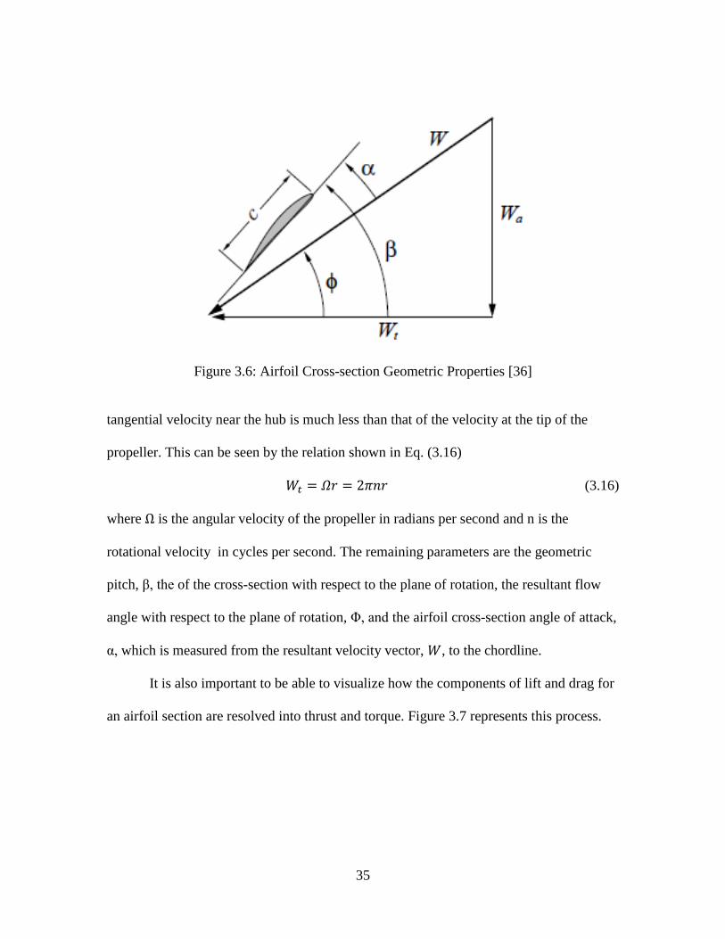
35
Figure 3.6: Airfoil Cross-section Geometric Properties [36]
tangential velocity near the hub is much less than that of the velocity at the tip of the
propeller. This can be seen by the relation shown in Eq. (3.16)
𝑊𝑡 = 𝛺𝑟 = 2𝜋𝑛𝑟 (3.16)
where Ω is the angular velocity of the propeller in radians per second and n is the
rotational velocity in cycles per second. The remaining parameters are the geometric
pitch, β, the of the cross-section with respect to the plane of rotation, the resultant flow
angle with respect to the plane of rotation, Φ, and the airfoil cross-section angle of attack,
α, which is measured from the resultant velocity vector, 𝑊, to the chordline.
It is also important to be able to visualize how the components of lift and drag for
an airfoil section are resolved into thrust and torque. Figure 3.7 represents this process.
36
.
Figure 3.7: Decomposition of Lift and Drag into Thrust and Torque [36]
The elemental lift and drag vectors 𝑑𝐿 and 𝑑𝐷, are shown on the airfoil to the left.
Components of these vectors may be taken in order to calculate more useful information
relevant to propellers such as the elemental thrust and torque, or 𝑑𝑇 and 𝑑𝑄/𝑟, for each
element. It can be seen that the elemental thrust may computed with Eq. (3.17)
𝑑𝑇 = 𝑑𝐿𝑐𝑜𝑠𝛷 − 𝑑𝐷𝑠𝑖𝑛𝛷 =1
2 𝜌 𝑊2 𝑐 𝑑𝑟 (𝑐𝑙𝑐𝑜𝑠𝛷 − 𝑐𝑑𝑠𝑖𝑛𝛷) (3.17)
where 𝑑𝑟 is the elemental width of the airfoil cross-section. Similarly, it can be seen that
the elemental torque may be described by Eq. (3.18)
𝑑𝑄 = (𝑑𝐿𝑠𝑖𝑛𝛷 + 𝑑𝐷𝑐𝑜𝑠𝛷)𝑟 =1
2 𝜌 𝑊2 𝑐 𝑟 𝑑𝑟 (𝑐𝑙𝑠𝑖𝑛𝛷 + 𝑐𝑑𝑐𝑜𝑠𝛷) (3.18)
With the definitions of Eqs. (3.17) and (3.18) the blade efficiency of each element can be
calculated as
𝜂 =𝑊𝑑𝑇
𝛺𝑑𝑄=
𝑊(𝑐𝑙𝑐𝑜𝑠𝛷−𝑐𝑑𝑠𝑖𝑛𝛷)
𝛺𝑟(𝑐𝑙𝑠𝑖𝑛𝛷+𝑐𝑑𝑐𝑜𝑠𝛷)= 𝑡𝑎𝑛𝛷
𝑐𝑙𝑐𝑜𝑠𝛷−𝑐𝑑𝑠𝑖𝑛𝛷
𝑐𝑙𝑠𝑖𝑛𝛷+𝑐𝑑𝑐𝑜𝑠𝛷 (3.19)
An integration over each blade must now be performed in order to determine the total
thrust, torque, and efficiency of the propeller. In order to do so, the aerodynamic
characteristics at each cross-section across the blade must be known—these change
37
across the blade due to the change in 𝑊𝑡 as shown in Eq. (3.16). Once this data is known,
Eqs. (3.20) through (3.22) may be used in order to determine the thrust, torque, and
efficiency of the propeller
𝑇 = ∫ 𝑑𝑇𝑅
0=
1
2𝜌𝐵 ∫ 𝑊2𝑐(𝑐𝑙𝑐𝑜𝑠𝛷 − 𝑐𝑑𝑠𝑖𝑛𝛷)𝑑𝑟
𝑅
0 (3.20)
𝑄 = ∫ 𝑑𝑄𝑅
0=
1
2𝜌𝐵 ∫ 𝑊2𝑐 𝑟(𝑐𝑙𝑠𝑖𝑛𝛷 − 𝑐𝑑𝑐𝑜𝑠𝛷)𝑑𝑟
𝑅
0 (3.21)
𝜂 =∫ 𝑊 𝑑𝑇
𝑅0
𝛺 ∫ 𝑑𝑄𝑅
0
(3.22)
where the density is considered incompressible, or constant, and 𝐵 represents the number
of blades on the propeller.
In conclusion, this theory allows for the analysis of specific propellers with
radially varying geometric shapes with the trade-off of increased complexity. Although
the required computations for this method are involved, it is simple enough to code into a
computer program. This theory is more detailed than the one-dimensional theory, but it
too possesses assumptions that simplify the flow analysis and introduces losses in the
prediction. These assumptions do not account for induced velocities at the blades, swirl in
the slipstream, non-uniform flow, or propeller blockage.
Blade Element Momentum Theory
Blade element momentum theory (BEMT) accounts for induced velocities created
by the production of lift on each propeller blade. Again, the discussion on BEMT will
follow [39] closely, with nomenclature adaptations for this work.
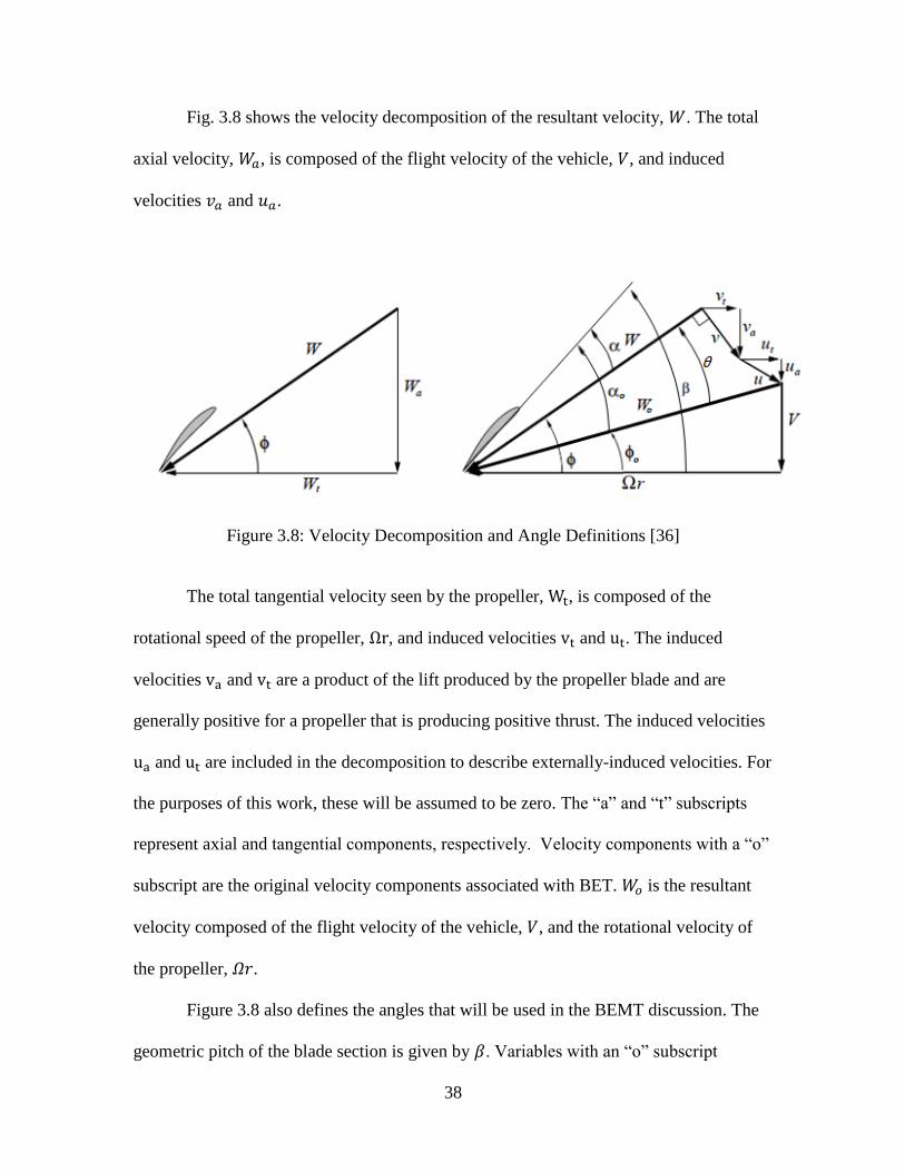
38
Fig. 3.8 shows the velocity decomposition of the resultant velocity, 𝑊. The total
axial velocity, 𝑊𝑎, is composed of the flight velocity of the vehicle, 𝑉, and induced
velocities 𝑣𝑎 and 𝑢𝑎.
Figure 3.8: Velocity Decomposition and Angle Definitions [36]
The total tangential velocity seen by the propeller, Wt, is composed of the
rotational speed of the propeller, Ωr, and induced velocities vt and ut. The induced
velocities va and vt are a product of the lift produced by the propeller blade and are
generally positive for a propeller that is producing positive thrust. The induced velocities
ua and ut are included in the decomposition to describe externally-induced velocities. For
the purposes of this work, these will be assumed to be zero. The “a” and “t” subscripts
represent axial and tangential components, respectively. Velocity components with a “o”
subscript are the original velocity components associated with BET. 𝑊𝑜 is the resultant
velocity composed of the flight velocity of the vehicle, 𝑉, and the rotational velocity of
the propeller, 𝛺𝑟.
Figure 3.8 also defines the angles that will be used in the BEMT discussion. The
geometric pitch of the blade section is given by 𝛽. Variables with an “o” subscript
39
designate angles associated with the velocity vectors discussed in BET. Those angles
without the subscript are associated with the velocity components that account for the
previously defined induced velocities. Equations (3.23) through (3.25) define the
remaining angles in the figure
𝛼 = 𝛽 − 𝛷 (3.23)
𝛼𝑜 = 𝛽 − 𝛷𝑜 (3.24)
𝜃 = 𝛷 − 𝛷𝑜 (3.25)
where 𝛼 is the angle of attack and 𝛷 the resultant flow angle after accounting for induced
velocities, 𝛼𝑜 is the angle of attack and 𝛷𝑜 the resultant flow angle not accounting for
induced velocities, and 𝜃 is the induced angle given by the difference of the two resultant
flow angles.
With the velocity components and angles defined, the BEMT can be examined.
First, the definition of elemental thrust (neglecting the section drag term) for a 𝐵-bladed
propeller will be rewritten in Eq. (3.26) according to the updated flow scenario shown in
Fig. 3.8
𝐵𝑑𝑇 = 𝐵𝑑𝐿 𝑐𝑜𝑠𝛷 =1
2𝐵 𝑐𝑙 𝑊
2 𝑐 𝑑𝑟 𝑐𝑜𝑠𝛷 (3.26)
From Figure 3.8, it can also be discerned that the induced velocity component in the
thrust direction is given by Eq. (3.27)
𝑣𝑎 = 𝑣 𝑐𝑜𝑠𝛷 (3.27)
which, when coupled with momentum theory, where 𝑑𝐴 = 2𝜋𝑟𝑑𝑟, can show that the
total elemental thrust for a 𝐵-bladed propeller may also be written as shown in Eq. (3.28)
𝐵𝑑𝑇 = 𝜌(2𝜋𝑟𝑑𝑟)(𝑉 + 𝑣 𝑐𝑜𝑠𝛷)(2𝑣 𝑐𝑜𝑠𝛷) (3.28)
40
If Eqs. (3.26) and (3.28) are set equal to each other, a definition for the induced velocity,
𝑣, may be found as shown in Eq. (3.29)
𝑣 =𝐵 𝑐𝑙 𝑐 𝑊2
8 𝜋 𝑟(𝑉+𝑣 𝑐𝑜𝑠𝛷) (3.29)
If the induced angle, 𝜃, is assumed to be small, the following relations can be justified in
order to make simplifications to Eq. (3.29) above
sin(𝛷) = sin(𝛷𝑜 + 𝜃) ≈ 𝑠𝑖𝑛𝛷𝑜 + 𝜃 𝑐𝑜𝑠𝛷𝑜 (3.30)
𝑡𝑎𝑛𝜃 = 𝑣/𝑊 ≈ 𝜃 (3.31)
When Eqs. (3.30) and (3.31) are coupled with the relation between the coefficient of lift,
the lift curve slope, and the angle of attack in Eqs. (3.32)
𝑐𝑙 = 𝑎0𝛼𝑜 = 𝑎0(𝛽 − 𝛷𝑜 − 𝜃) (3.32)
Equation (3.29) may be written in terms of the induced angle, 𝜃 as shown in Eq. (3.33)
𝜃 ≈ 𝐵 (𝑐
8𝜋𝑟)
𝑎0(𝛽−𝛷𝑜−𝜃)
𝑠𝑖𝑛𝛷𝑜+𝜃𝑐𝑜𝑠𝛷𝑜 (3.33)
In order to solve for 𝜃, two more variables will be introduced. The first is known as the
solidity ratio, or the ratio of the total blade area to that of the disk—this is denoted by 𝜎.
The second is the non-dimensionalized blade station, denoted by x. These are represented
by the relations in Eqs. (3.34) and (3.35). For simplicity, the chord of the blade will be
assumed to be constant in this example.
𝜎 =𝐵𝑐𝑅
𝜋𝑅2 =𝐵𝑐
𝜋𝑅 (3.34)
𝑥 =𝑟
𝑅 (3.35)
With these two definitions, it can be shown that Eq. (3.33) can be rewritten as shown by
Eq. (3.36)
𝜃2𝑐𝑜𝑠𝛷𝑜 + 𝜃 (𝑠𝑖𝑛𝛷𝑜 +𝜎𝑎0
8𝑥) −
𝜎𝑎0
8𝑥(𝛽 − 𝛷𝑜) = 0 (3.36)
41
The following solution for 𝜃 can be obtained by solving Eq. (3.36)
𝜃 =1
2 𝑐𝑜𝑠𝛷𝑜{− (𝑠𝑖𝑛𝛷𝑜 +
𝑎0𝜎
8𝑥) + √(𝑠𝑖𝑛𝛷𝑜 +
𝑎0𝜎
8𝑥)
2
+ 4 𝑐𝑜𝑠𝛷𝑜𝑎0𝜎
8𝑥(𝛽 − 𝛷𝑜) } (3.37)
In order to compute the induced velocity, the following assumptions must first be made
𝑐𝑜𝑠𝛷𝑜 ≈ 1 (3.38)
𝑠𝑖𝑛𝛷𝑜 ≈𝑉
𝑊𝑜≈
𝑉
𝑥𝑉𝑡 (3.39)
𝑊𝑜 = 𝑥𝑉𝑡 (3.40)
where 𝑉𝑡 is the propeller tip speed. It is also important to note the following relations
from Fig. 3.8
𝑣
𝑊𝑜= 𝑡𝑎𝑛𝜃 (3.41)
which, since 𝜃 is considered small, means
𝑣 ≈ 𝑊𝑜𝜃 ≈ 𝑥𝑉𝑡𝜃 (3.42)
When the assumptions and relations are applied, Eq. (3.43) may be found for the induced
velocity
𝑣 = 𝑉𝑡 {− (𝑉
2𝑉𝑡+
𝑎0𝜎
16) + √(
𝑉
2𝑉𝑡+
𝑎0𝜎
16)
2
+𝑎0𝜎𝛽𝑥
8−
𝑎0𝜎𝑉
8𝑉𝑡} (3.43)
The author of [39] notes that Eq. (3.43) is often used to calculate the induced
velocity in situations where there is “very high” thrust. A simplification may be made for
“low thrust” situations in which the 𝜃2 term in Eq. (3.36) may be neglected. When this is
done, Eq. (3.44) is produced.
𝜃 =𝛽−𝛷𝑜
1+8𝑥𝑠𝑖𝑛𝛷𝑜
𝜎𝑎0
(3.44)
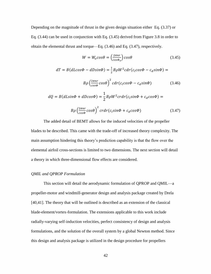
42
Depending on the magnitude of thrust in the given design situation either Eq. (3.37) or
Eq. (3.44) can be used in conjunction with Eq. (3.45) derived from Figure 3.8 in order to
obtain the elemental thrust and torque—Eq. (3.46) and Eq. (3.47), respectively.
𝑊 = 𝑊𝑜𝑐𝑜𝑠𝜃 = (2𝜋𝑛𝑟
𝑐𝑜𝑠𝛷𝑜) 𝑐𝑜𝑠𝜃 (3.45)
𝑑𝑇 = 𝐵(𝑑𝐿𝑐𝑜𝑠𝛷 − 𝑑𝐷𝑠𝑖𝑛𝛷) =1
2𝐵𝜌𝑊2𝑐𝑑𝑟(𝑐𝑙𝑐𝑜𝑠𝛷 − 𝑐𝑑𝑠𝑖𝑛𝛷) =
𝐵𝜌 (2𝜋𝑛𝑟
𝑐𝑜𝑠𝛷𝑐𝑜𝑠𝜃)
2
𝑐𝑑𝑟(𝑐𝑙𝑐𝑜𝑠𝛷 − 𝑐𝑑𝑠𝑖𝑛𝛷) (3.46)
𝑑𝑄 = 𝐵(𝑑𝐿𝑠𝑖𝑛𝛷 + 𝑑𝐷𝑐𝑜𝑠𝛷) =1
2𝐵𝜌𝑊2𝑐𝑟𝑑𝑟(𝑐𝑙𝑠𝑖𝑛𝛷 + 𝑐𝑑𝑐𝑜𝑠𝛷) =
𝐵𝜌 (2𝜋𝑛𝑟
𝑐𝑜𝑠𝛷𝑐𝑜𝑠𝜃)
2
𝑐𝑟𝑑𝑟(𝑐𝑙𝑠𝑖𝑛𝛷 + 𝑐𝑑𝑐𝑜𝑠𝛷) (3.47)
The added detail of BEMT allows for the induced velocities of the propeller
blades to be described. This came with the trade-off of increased theory complexity. The
main assumption hindering this theory’s prediction capability is that the flow over the
elemental airfoil cross-sections is limited to two dimensions. The next section will detail
a theory in which three-dimensional flow effects are considered.
QMIL and QPROP Formulation
This section will detail the aerodynamic formulation of QPROP and QMIL—a
propeller-motor and windmill-generator design and analysis package created by Drela
[40,41]. The theory that will be outlined is described as an extension of the classical
blade-element/vortex-formulation. The extensions applicable to this work include
radially-varying self-induction velocities, perfect consistency of design and analysis
formulations, and the solution of the overall system by a global Newton method. Since
this design and analysis package is utilized in the design procedure for propellers
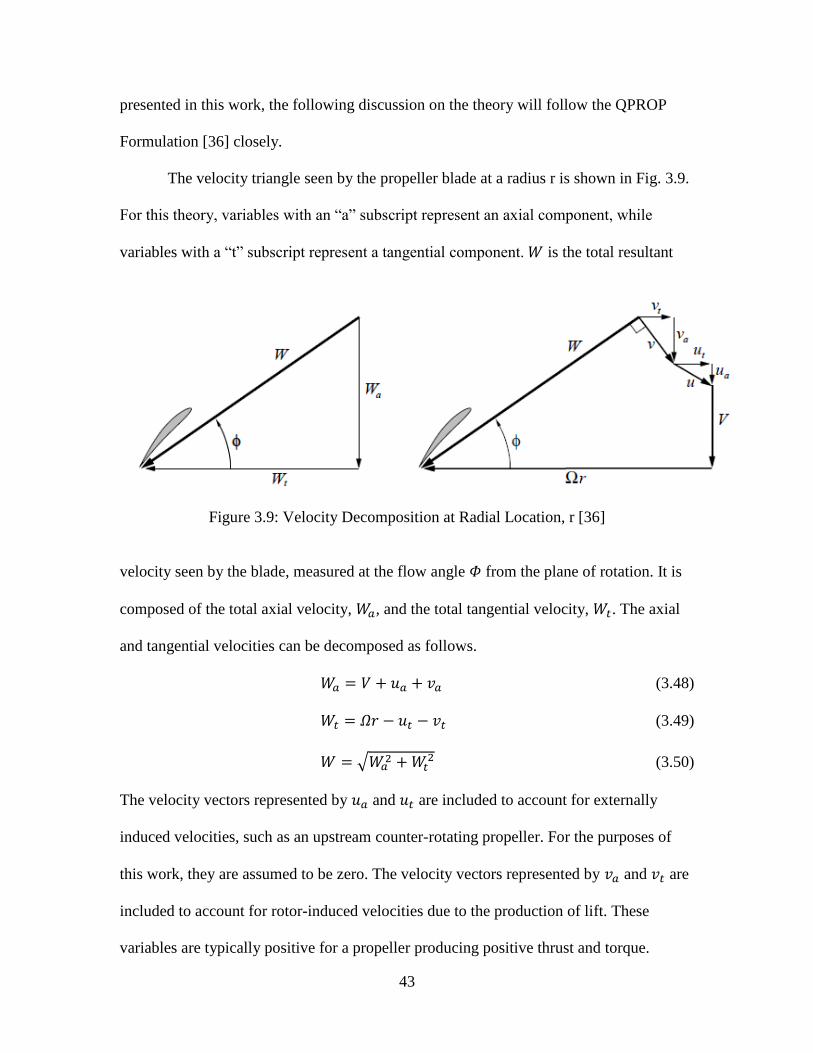
43
presented in this work, the following discussion on the theory will follow the QPROP
Formulation [36] closely.
The velocity triangle seen by the propeller blade at a radius r is shown in Fig. 3.9.
For this theory, variables with an “a” subscript represent an axial component, while
variables with a “t” subscript represent a tangential component. 𝑊 is the total resultant
Figure 3.9: Velocity Decomposition at Radial Location, r [36]
velocity seen by the blade, measured at the flow angle 𝛷 from the plane of rotation. It is
composed of the total axial velocity, 𝑊𝑎, and the total tangential velocity, 𝑊𝑡. The axial
and tangential velocities can be decomposed as follows.
𝑊𝑎 = 𝑉 + 𝑢𝑎 + 𝑣𝑎 (3.48)
𝑊𝑡 = 𝛺𝑟 − 𝑢𝑡 − 𝑣𝑡 (3.49)
𝑊 = √𝑊𝑎2 + 𝑊𝑡
2 (3.50)
The velocity vectors represented by 𝑢𝑎 and 𝑢𝑡 are included to account for externally
induced velocities, such as an upstream counter-rotating propeller. For the purposes of
this work, they are assumed to be zero. The velocity vectors represented by 𝑣𝑎 and 𝑣𝑡 are
included to account for rotor-induced velocities due to the production of lift. These
variables are typically positive for a propeller producing positive thrust and torque.
44
The tangentially induced velocity is defined in the formulation document by
examining its relationship between the torque imparted by the rotor on the fluid, and the
circulation, Γ, on the rotor blades from Helmholtz’s Theorem. The development of the
relationship described by Eq. (3.51) can be seen in the QMIL Formulation document
[36].
𝑣𝑡 =𝐵𝛤
4𝜋𝑟
1
𝐹√1+(4𝜆𝑤𝑅
𝜋𝐵𝑟)
2 (3.51)
Considering the assumption from Fig. 3.9 that the 𝑣 is perpendicular to 𝑊, the axial,
rotor-induced velocity can be found with the following equation.
𝑣𝑎 = 𝑣𝑡𝑊𝑡
𝑊𝑎 (3.52)
It was mentioned in [36] that the Equation (3.52) is correct for the case of a non-
contracting helical wake which has the same pitch at all radii and that the above
assumption is only correct for a lightly-loaded rotor having the Goldstein circulation
distribution. The relation is expected to be good for general rotors, even if they may not
meet the assumption’s requirements to be completely correct.
Next it is necessary to define various angles that describe the airfoil orientation
with regards to the flow and physical geometry of the propeller. Figure 3.10 shows the
propeller geometry and angle definitions for an airfoil section with a chord length of 𝑐, at
some radial location 𝑟. The local angle of attack seen by the blade at the radial location is
given by
𝛼(𝑟) = 𝛽 − 𝛷 = 𝛽 − arctan (𝑊𝑎
𝑊𝑡) (3.53)
45
where 𝛽 is the geometric pitch of the blade at the 𝑟, location. This airfoil section
produces local lift and drag coefficients (𝑐𝑙 and 𝑐𝑑) which will be defined by the
following
𝑐𝑙 = 𝑐𝑙(𝛼, 𝑅𝑒, 𝑀𝑎) (3.54)
𝑐𝑑 = 𝑐𝑑(𝛼, 𝑅𝑒, 𝑀𝑎) (3.55)
where 𝑅𝑒 and 𝑀𝑎 represent the Reynolds and Mach numbers seen by the blade at the
radial location. The local blade circulation is a function of the coefficient of lift, and is
Figure 3.10: Propeller Geometry and Angle Definitions at a Radial Coordinate, r [36]
defined in [36] as seen in Eq. (3.56). The local analysis solution of the radial circulation
𝛤 =1
2𝑊 𝑐 𝑐𝑙 (3.56)
distribution 𝛤(𝑟) can be calculated for each radius independently through the Newton
method. The analysis necessitates a given blade geometry, i.e. 𝑐(𝑟), 𝛽(𝑟), airfoil
properties 𝑐𝑙(𝛼, 𝑅𝑒, 𝑀𝑎) and 𝑐𝑑(𝛼, 𝑅𝑒, 𝑀𝑎) for each radial location, and operating
variables 𝑉 and 𝛺. The program iterates on the dummy variable 𝜓, shown in Fig. 3.11
instead of directly on Γ.

46
Figure 3.11: Velocity Parameterization through Phi [36]
Intermediate velocity components 𝑈𝑎, 𝑈𝑡, and 𝑈 are composed as follows. These
velocities are composed of the overall velocities imposed on the rotor excluding the self-
induced velocities 𝑣𝑎 and 𝑣𝑡. The parameterization of the remaining variables is also
shown here in Eqs. (3.57) through (3.67).
𝑈𝑎 = 𝑉 + 𝑢𝑎 (3.57)
𝑈𝑡 = 𝛺𝑟 − 𝑢𝑡 (3.58)
𝑈 = √𝑈𝑎2 + 𝑈𝑡
2 (3.59)
𝑊𝑎(𝜓) =1
2𝑈𝑎 +
1
2𝑈 sin 𝜓 (3.60)
𝑊𝑡(𝜓) =1
2𝑈𝑡 +
1
2𝑈 cos 𝜓 (3.61)
𝑣𝑎(𝜓) = 𝑊𝑎 − 𝑈𝑎 (3.62)
𝑣𝑡(𝜓) = 𝑈𝑡 − 𝑊𝑡 (3.63)
47
𝛼(𝜓) = 𝛽 − arctan (𝑊𝑎
𝑊𝑡) (3.64)
𝑊(𝜓) = √𝑊𝑎2 + 𝑊𝑡
2 (3.65)
𝑅𝑒(𝜓) =𝜌𝑊𝑐
𝜇 (3.66)
𝑀𝑎(𝜓) =𝑊
𝑎 (3.67)
The circulation relations from the Helmoltz theorem also require parameterization with the
angle 𝜓. These relations can be found in [36].
The Newton residual is the relation given by Eq. (3.68) in terms of the
parameterized variables.
ℛ(𝜓) = 𝛤 −1
2𝑊 𝑐 𝑐𝑙(𝛼, 𝑅𝑒, 𝑀𝑎) (3.68)
A Newton update of the parameterization angle 𝜓 given by
𝑑𝜓 = −ℛ
𝑑ℛ/𝑑𝜓 (3.69)
𝜓 ← 𝜓 + 𝑑𝜓 (3.70)
is described to decrease |ℛ| in each succeeding Newton iteration. With a quadratic
convergence, few iterations are generally needed to drive the residual to machine zero.
To complete the analysis procedure described above, it is necessary for the rotor to
have a prescribed flight velocity 𝑉, and rotation rate 𝛺, or advance ratio λ. In addition,
geometry specifications in the form of a pitch distribution are required. This can be given
by
𝛽(𝑟) = 𝛽0(𝑟) + 𝛥𝛽 (3.71)
where 𝛽0 is the baseline pitch distribution and 𝛥𝛽 is the radially-constant specified pitch
change. This is not always the procedure necessitated, especially in design situations
where the chord 𝑐, and pitch 𝛽 will be treated as unknowns. In both design and analysis
48
scenarios, parametric derivatives of Γ are necessary to complete the iteration procedure to
calculate the overall circulation distribution. These derivatives and the subsequent
calculations necessary to compute this distribution can be found in [36].
Once the iteration procedure is complete at each radial location and the overall
circulation distribution Γ(𝑟) is known, the calculations of the overall thrust and torque
may be completed. Figure 3.7 shows the blade lift and drag forces, as well as the resolved
thrust and torque components through the resultant flow angle Φ. Relations for the
elemental lift, drag, thrust, and torque relations in Eqs. (3.72) through (3.75) may also be
derived from Fig. 3.7.
𝑑𝐿 = 𝐵1
2𝜌𝑊2𝑐𝑙 𝑐 𝑑𝑟 (3.72)
𝑑𝐷 = 𝐵1
2𝜌𝑊2𝑐𝑑𝑐 𝑑𝑟 (3.73)
𝑑𝑇 = 𝑑𝐿𝑐𝑜𝑠𝜙 − 𝑑𝐷𝑠𝑖𝑛𝜙 = 𝐵1
2𝜌𝑊2(𝑐𝑙𝑐𝑜𝑠𝜙 − 𝑐𝑑𝑠𝑖𝑛𝜙)𝑐 𝑑𝑟 (3.74)
𝑑𝑄 = (𝑑𝐿𝑠𝑖𝑛𝜙 + 𝑑𝐷𝑐𝑜𝑠𝜙)𝑟 = 𝐵1
2𝜌𝑊2(𝑐𝑙𝑠𝑖𝑛𝜙 + 𝑐𝑑𝑐𝑜𝑠𝜙)𝑐 𝑟 𝑑𝑟 (3.75)
It can also be seen from the velocity triangle in Fig. 3.7, that the overall resultant velocity
is related to the overall tangential and overall axial velocities in Eqs. (3.76) and (3.77).
𝑊𝑐𝑜𝑠𝜙 = 𝑊𝑡 (3.76)
𝑊𝑠𝑖𝑛𝜙 = 𝑊𝑎 (3.77)
This allows the thrust and torque components to be alternatively expressed in terms of the
circulation and net velocity components, Eqs. (3.78) through (3.80).
𝑑𝑇 = 𝜌𝐵Γ(𝑊𝑡 − 𝜖𝑊𝑎)𝑑𝑟 (3.78)
𝑑𝑄 = 𝜌𝐵Γ(𝑊𝑎 + 𝜖𝑊𝑡)𝑟 𝑑𝑟 (3.79)
𝜖 =𝑐𝑑
𝑐𝑙 (3.80)
49
The local efficiency may also be expressed as follows in Eq. (3.81).
𝜂 =𝑉
Ω
𝑑𝑇
𝑑𝑄=
𝑉
Ω𝑟
𝑐𝑙𝑐𝑜𝑠𝜙−𝑐𝑑𝑠𝑖𝑛𝜙
𝑐𝑙𝑠𝑖𝑛𝜙+𝑐𝑑𝑐𝑜𝑠𝜙=
𝑉
Ω𝑟
𝑊𝑡−𝜖𝑊𝑎
𝑊𝑎+𝜖𝑊𝑡 (3.81)
The local efficiency may also be decomposed in to induced and profile efficiencies as
shown in Eqs. (3.82) through (3.84).
𝜂 = 𝜂𝑖𝜂𝑝 (3.82)
𝜂𝑖 =1−𝑣𝑡 𝑈𝑡⁄
1+𝑣𝑎 𝑈𝑎⁄ (3.83)
𝑛𝑝 =1−𝜖𝑊𝑎 𝑊𝑡⁄
1+𝜖𝑊𝑡 𝑊𝑎⁄ (3.84)
Now the overall thrust and torque may be obtained by numerically integrating the
previously defined elemental relations along the entirety of the blade with Eqs. (3.85) and
(3.86).
𝑇 = 𝜌𝐵 ∫ Γ(𝑊𝑡 − 𝜖𝑊𝑎)𝑑𝑟 𝑅
0≃ 𝜌𝐵 ∑ Γ(𝑊𝑡 − 𝜖𝑊𝑎)Δ𝑟𝑟 (3.85)
𝑄 = 𝜌𝐵 ∫ Γ(𝑊𝑎 + 𝜖𝑊𝑡)𝑟 𝑑𝑟 ≃ 𝜌𝐵 ∑ Γ(𝑊𝑎 + 𝜖𝑊𝑡)𝑟 Δ𝑟𝑟𝑅
0 (3.86)
The program utilizes the midpoint rule for the numerical integrations. The overall
efficiency can then be described by Eq. (3.87).
�̅� =𝑉𝑇
Ω𝑄 (3.87)
For a design case, it is also necessary to use parametric differentiation based on
the design constraints. The Minimum Induced Loss (MIL) constraints were the only
constraints outlined in [36] that were utilized in this work. The parametric derivatives,
along with the MIL constraints used in design and analysis cases in this work can be
referenced in the QMIL Formulation document [36]. These design constraints maximize
the overall induced efficiency for the specified radius and operating conditions. Drela

50
notes that this is the analog of an elliptically-loaded wing, which has a spanwise-constant
induced-drag to lift ratio.
This formulation is the most detailed propeller analysis and/or design theory
described in this work. Unlike previous theories described, circulation in the flow is
accounted for. The increased complexity does not increase computational times. The
DOS program that executes this theory typically runs in seconds on modern computers. It
allows a user to design a propeller for given conditions and then analyze it in great detail
in a time efficient manner.
Airfoil Noise
Another area of needed improvement in propeller design is the reduction of the
noise footprint. Although this work has only measured noise levels of different propeller
designs, the relationships between noise and various propeller operating parameters have
been identified through empirical data, and propeller noise predictions for given
geometries have begun to be adapted to the design/analysis process. These noise
predictions have been made possible through the use of a semi-empirical aeroacoustic
noise prediction code called NAFNoise [42] developed by the National Renewable
Energy Laboratory (NREL). Although NAFNoise was originally developed for airfoil
cross sections used in wind turbines, investigations into the theory behind its predictions
have shown that the code is also applicable to propeller operation.
This code predicts the noise of any two-dimensional airfoil shape for the
following five types of airfoil noise sources: turbulent boundary layer trailing-edge noise,
separated flow noise, laminar boundary layer vortex-shedding noise, trailing edge
bluntness noise, and turbulent inflow noise. These sources are assumed to generate noise
51
independently of each other because the mechanisms of each noise are fundamentally
different or occur in different locations along a blade. These sources are superimposed to
obtain a total noise for each airfoil analyzed. The prediction models for the first four
sources of noise are based on work originally developed by Brooks, Pope, and Marcolini
[43] in which these individuals performed detailed noise measurements on a NACA 0012
airfoil. The empirical turbulent inflow noise model is based on the work of Amiet [44].
Improvements have been made to each model in the following forms. The modeling of
any airfoil shape has been realized through the utilization of XFOIL [20], which produces
boundary calculations. These calculations can be used as inputs for the models of Brooks,
Pope, and Marcolini [43]. The final two improvements implement a turbulent inflow
noise correction to account for the airfoil shape.
These calculations can be applied to each blade section from the design process
and summed for an approximate total blade noise, relative to an observer position. It is
important to note that the code assumes two-dimensional flow for each airfoil noise
calculation and does not include a means of predicting noise produced by tip vortex
formulations. The following discussion will follow Moriarty and Migliore’s Semi-
Empirical Aeroacoustic Noise Prediction Code for Wind Turbines [45] which details the
theories implemented in NAFNoise.
Each model relates the characteristics of the airfoil geometry and flowfield to a
resulting SPL. The SPL is related to the sound intensity, and in turn root mean square
pressure level by Eq. (3.88):
𝑆𝑃𝐿 = 10 log (𝐼
𝐼𝑟𝑒𝑓) = 20 log (
𝑝𝑟𝑚𝑠
𝑝𝑟𝑚𝑠𝑟𝑒𝑓
) (3.88)
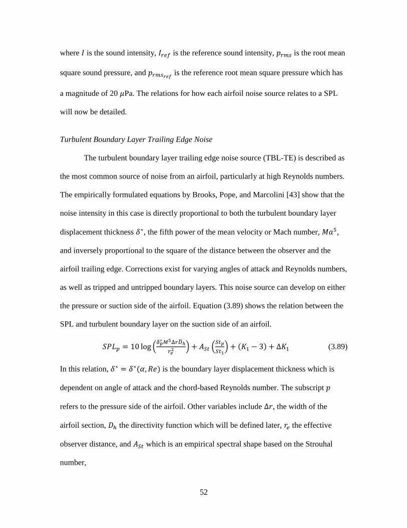
52
where 𝐼 is the sound intensity, 𝐼𝑟𝑒𝑓 is the reference sound intensity, 𝑝𝑟𝑚𝑠 is the root mean
square sound pressure, and 𝑝𝑟𝑚𝑠𝑟𝑒𝑓 is the reference root mean square pressure which has
a magnitude of 20 𝜇Pa. The relations for how each airfoil noise source relates to a SPL
will now be detailed.
Turbulent Boundary Layer Trailing Edge Noise
The turbulent boundary layer trailing edge noise source (TBL-TE) is described as
the most common source of noise from an airfoil, particularly at high Reynolds numbers.
The empirically formulated equations by Brooks, Pope, and Marcolini [43] show that the
noise intensity in this case is directly proportional to both the turbulent boundary layer
displacement thickness 𝛿∗, the fifth power of the mean velocity or Mach number, 𝑀𝑎5,
and inversely proportional to the square of the distance between the observer and the
airfoil trailing edge. Corrections exist for varying angles of attack and Reynolds numbers,
as well as tripped and untripped boundary layers. This noise source can develop on either
the pressure or suction side of the airfoil. Equation (3.89) shows the relation between the
SPL and turbulent boundary layer on the suction side of an airfoil.
𝑆𝑃𝐿𝑝 = 10 log (𝛿𝑝
∗ 𝑀5Δ𝑟�̅�ℎ
𝑟𝑒2 ) + 𝐴𝑆𝑡 (
𝑆𝑡𝑝
𝑆𝑡1) + (𝐾1 − 3) + Δ𝐾1 (3.89)
In this relation, 𝛿∗ = 𝛿∗(𝛼, 𝑅𝑒) is the boundary layer displacement thickness which is
dependent on angle of attack and the chord-based Reynolds number. The subscript 𝑝
refers to the pressure side of the airfoil. Other variables include Δ𝑟, the width of the
airfoil section, 𝐷ℎ the directivity function which will be defined later, 𝑟𝑒 the effective
observer distance, and 𝐴𝑆𝑡 which is an empirical spectral shape based on the Strouhal
number,
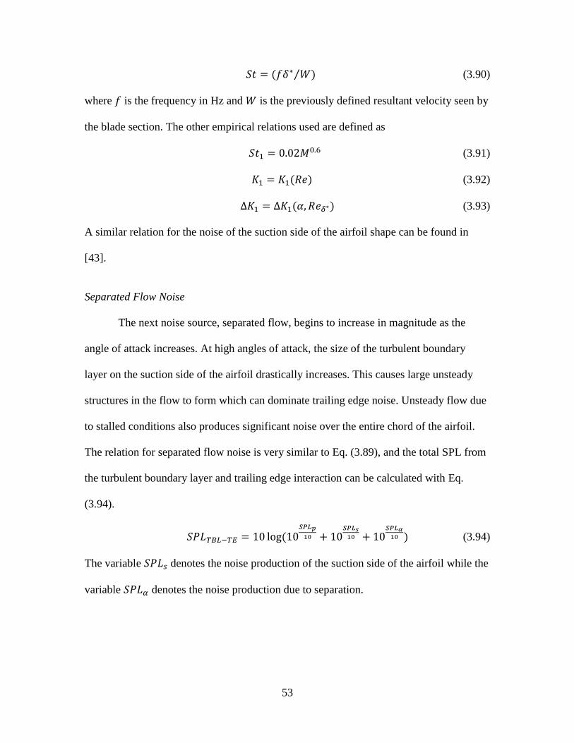
53
𝑆𝑡 = (𝑓𝛿∗ 𝑊)⁄ (3.90)
where 𝑓 is the frequency in Hz and 𝑊 is the previously defined resultant velocity seen by
the blade section. The other empirical relations used are defined as
𝑆𝑡1 = 0.02𝑀0.6 (3.91)
𝐾1 = 𝐾1(𝑅𝑒) (3.92)
Δ𝐾1 = Δ𝐾1(𝛼, 𝑅𝑒𝛿∗) (3.93)
A similar relation for the noise of the suction side of the airfoil shape can be found in
[43].
Separated Flow Noise
The next noise source, separated flow, begins to increase in magnitude as the
angle of attack increases. At high angles of attack, the size of the turbulent boundary
layer on the suction side of the airfoil drastically increases. This causes large unsteady
structures in the flow to form which can dominate trailing edge noise. Unsteady flow due
to stalled conditions also produces significant noise over the entire chord of the airfoil.
The relation for separated flow noise is very similar to Eq. (3.89), and the total SPL from
the turbulent boundary layer and trailing edge interaction can be calculated with Eq.
(3.94).
𝑆𝑃𝐿𝑇𝐵𝐿−𝑇𝐸 = 10 log(10𝑆𝑃𝐿𝑝
10 + 10𝑆𝑃𝐿𝑠
10 + 10𝑆𝑃𝐿𝛼
10 ) (3.94)
The variable 𝑆𝑃𝐿𝑠 denotes the noise production of the suction side of the airfoil while the
variable 𝑆𝑃𝐿𝛼 denotes the noise production due to separation.
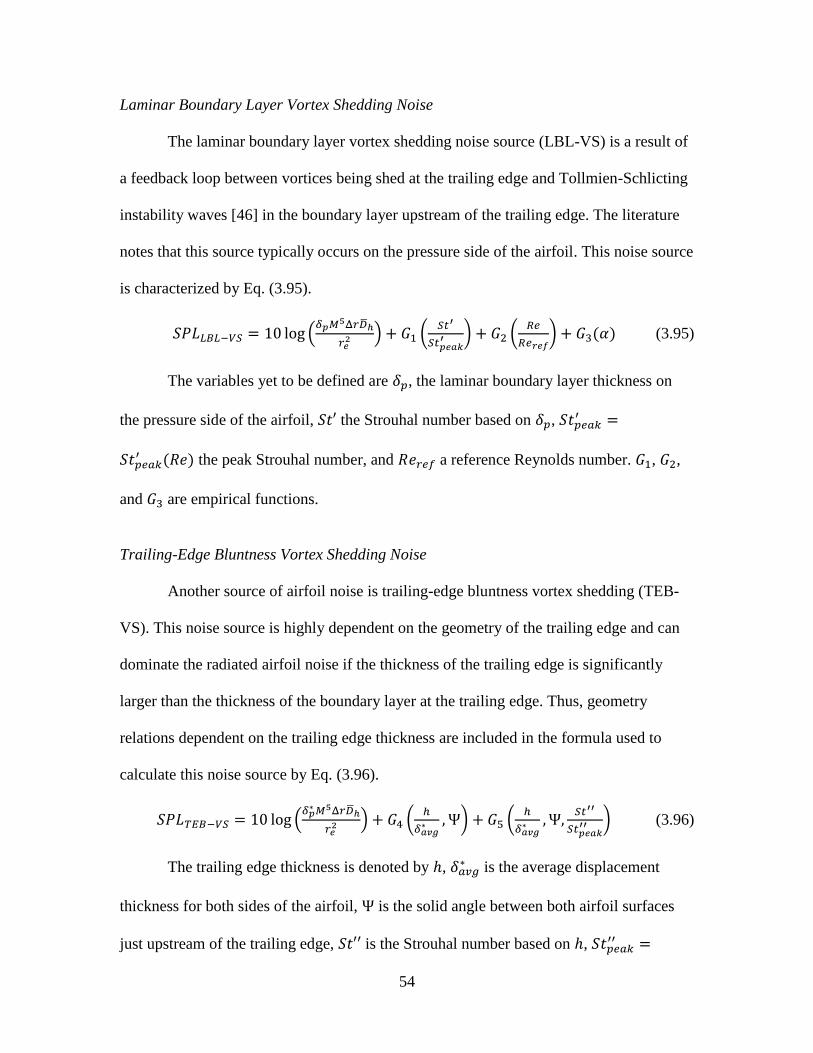
54
Laminar Boundary Layer Vortex Shedding Noise
The laminar boundary layer vortex shedding noise source (LBL-VS) is a result of
a feedback loop between vortices being shed at the trailing edge and Tollmien-Schlicting
instability waves [46] in the boundary layer upstream of the trailing edge. The literature
notes that this source typically occurs on the pressure side of the airfoil. This noise source
is characterized by Eq. (3.95).
𝑆𝑃𝐿𝐿𝐵𝐿−𝑉𝑆 = 10 log (𝛿𝑝𝑀5Δ𝑟�̅�ℎ
𝑟𝑒2 ) + 𝐺1 (
𝑆𝑡′
𝑆𝑡𝑝𝑒𝑎𝑘′ ) + 𝐺2 (
𝑅𝑒
𝑅𝑒𝑟𝑒𝑓) + 𝐺3(𝛼) (3.95)
The variables yet to be defined are 𝛿𝑝, the laminar boundary layer thickness on
the pressure side of the airfoil, 𝑆𝑡′ the Strouhal number based on 𝛿𝑝, 𝑆𝑡𝑝𝑒𝑎𝑘′ =
𝑆𝑡𝑝𝑒𝑎𝑘′ (𝑅𝑒) the peak Strouhal number, and 𝑅𝑒𝑟𝑒𝑓 a reference Reynolds number. 𝐺1, 𝐺2,
and 𝐺3 are empirical functions.
Trailing-Edge Bluntness Vortex Shedding Noise
Another source of airfoil noise is trailing-edge bluntness vortex shedding (TEB-
VS). This noise source is highly dependent on the geometry of the trailing edge and can
dominate the radiated airfoil noise if the thickness of the trailing edge is significantly
larger than the thickness of the boundary layer at the trailing edge. Thus, geometry
relations dependent on the trailing edge thickness are included in the formula used to
calculate this noise source by Eq. (3.96).
𝑆𝑃𝐿𝑇𝐸𝐵−𝑉𝑆 = 10 log (𝛿𝑝
∗ 𝑀5Δ𝑟�̅�ℎ
𝑟𝑒2 ) + 𝐺4 (
ℎ
𝛿𝑎𝑣𝑔∗ , Ψ) + 𝐺5 (
ℎ
𝛿𝑎𝑣𝑔∗ , Ψ,
𝑆𝑡′′
𝑆𝑡𝑝𝑒𝑎𝑘′′ ) (3.96)
The trailing edge thickness is denoted by ℎ, 𝛿𝑎𝑣𝑔∗ is the average displacement
thickness for both sides of the airfoil, Ψ is the solid angle between both airfoil surfaces
just upstream of the trailing edge, 𝑆𝑡′′ is the Strouhal number based on ℎ, 𝑆𝑡𝑝𝑒𝑎𝑘′′ =
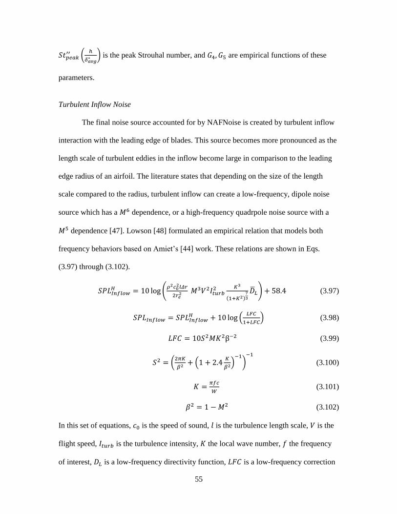
55
𝑆𝑡𝑝𝑒𝑎𝑘′′ (
ℎ
𝛿𝑎𝑣𝑔∗ ) is the peak Strouhal number, and 𝐺4, 𝐺5 are empirical functions of these
parameters.
Turbulent Inflow Noise
The final noise source accounted for by NAFNoise is created by turbulent inflow
interaction with the leading edge of blades. This source becomes more pronounced as the
length scale of turbulent eddies in the inflow become large in comparison to the leading
edge radius of an airfoil. The literature states that depending on the size of the length
scale compared to the radius, turbulent inflow can create a low-frequency, dipole noise
source which has a 𝑀6 dependence, or a high-frequency quadrpole noise source with a
𝑀5 dependence [47]. Lowson [48] formulated an empirical relation that models both
frequency behaviors based on Amiet’s [44] work. These relations are shown in Eqs.
(3.97) through (3.102).
𝑆𝑃𝐿𝐼𝑛𝑓𝑙𝑜𝑤𝐻 = 10 log (
𝜌2𝑐02𝑙𝛥𝑟
2𝑟𝑒2 𝑀3𝑉2𝐼𝑡𝑢𝑟𝑏
2 𝐾3
(1+𝐾2)73
�̅�𝐿) + 58.4 (3.97)
𝑆𝑃𝐿𝐼𝑛𝑓𝑙𝑜𝑤 = 𝑆𝑃𝐿𝐼𝑛𝑓𝑙𝑜𝑤𝐻 + 10 log (
𝐿𝐹𝐶
1+𝐿𝐹𝐶) (3.98)
𝐿𝐹𝐶 = 10𝑆2𝑀𝐾2β−2 (3.99)
𝑆2 = (2𝜋𝐾
𝛽2 + (1 + 2.4𝐾
𝛽2)−1
)−1
(3.100)
𝐾 =𝜋𝑓𝑐
𝑊 (3.101)
𝛽2 = 1 − 𝑀2 (3.102)
In this set of equations, 𝑐0 is the speed of sound, 𝑙 is the turbulence length scale, 𝑉 is the
flight speed, 𝐼𝑡𝑢𝑟𝑏 is the turbulence intensity, 𝐾 the local wave number, 𝑓 the frequency
of interest, 𝐷𝐿 is a low-frequency directivity function, 𝐿𝐹𝐶 is a low-frequency correction
56
factor, and 𝑆 is the compressible Sears function. For the purposes of this work, this noise
source is neglected because of the testing conditions of the propellers where there is
negligible turbulence in the inflow.
Tip Vortex Formation Noise
Although NAFNoise does not account for noise produced as a result of tip vortex
formation, it is in the interest of the future work of this project to note formulations
related to it. This source is fundamentally different from the others in that it is a result of
flow that cannot be considered or assumed to be anything but three-dimensional. This
source can add significant amounts of noise at higher frequencies. Brooks, Pope, and
Marcolini [43] formulated by Eq. (3.103) for an untwisted, constant chorded blade.
𝑆𝑃𝐿𝑇𝑖𝑝 = 10 log (𝑀2𝑀𝑚𝑎𝑥
5 𝑙𝑡𝑖𝑝2 �̅�ℎ
𝑟𝑒2 ) − 30.5(log(𝑆𝑡′′′ + 0.3)2 + 126 (3.103)
In this relation, 𝑀𝑚𝑎𝑥 = 𝑀𝑚𝑎𝑥(𝛼𝑡𝑖𝑝) is the maximum Mach number within the separated
flow region near the tip, 𝛼𝑡𝑖𝑝 is the angle of attack at the tip, and 𝑙𝑡𝑖𝑝 = 𝑙𝑡𝑖𝑝(𝛼𝑡𝑖𝑝) is the
spanwise extent of the separation zone which is dependent on the spanwise lift
distribution and shape of the tip. 𝑆𝑡′′′ is the Strouhal number based on 𝑙𝑡𝑖𝑝. There are
methods suggested by the literature to modify Eq. 3.103 to provide a crude
approximation of a twisted, tapered blade which involves calculating an equivalent 𝛼𝑡𝑖𝑝,
but will not be further discussed as these modifications were not incorporated in this
work.
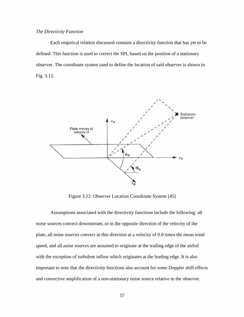
57
The Directivity Function
Each empirical relation discussed contains a directivity function that has yet to be
defined. This function is used to correct the SPL based on the position of a stationary
observer. The coordinate system used to define the location of said observer is shown in
Fig. 3.12.
Figure 3.12: Observer Location Coordinate System [45]
Assumptions associated with the directivity functions include the following: all
noise sources convect downstream, or in the opposite direction of the velocity of the
plate, all noise sources convect in this direction at a velocity of 0.8 times the mean wind
speed, and all noise sources are assumed to originate at the trailing edge of the airfoil
with the exception of turbulent inflow which originates at the leading edge. It is also
important to note that the directivity functions also account for some Doppler shift effects
and convective amplification of a non-stationary noise source relative to the observer.
58
High-frequency noise sources, excluding high-angle separation and turbulent inflow
noise, are corrected by Eq. (3.104).
�̅�𝐻(Θ𝑒 , Φ𝑒) ≈2 sin2(
1
2Θ𝑒) sin2 Φ𝑒
(1+𝑀 cos Θ𝑒)(1+(𝑀+𝑀𝑐) cos Θ𝑒)2 (3.104)
Here, 𝑀 is the Mach number of the airfoil section, 𝑀𝑐 is the convective Mach number,
and angles Θ𝑒 and Φ𝑒 are the directivity angles defined above. Low-frequency noise
sources are calculated using Eq. (3.105).
�̅�𝐿(Θ𝑒 , Φ𝑒) ≈sin2 Θ𝑒 sin2 Φ𝑒
(1+𝑀 cos Θ𝑒) (3.105)
It is important to note from the literature that when both directivity angles are equal to
ninety degrees, both directivity functions equal one. Also, that when Θ𝑒 approaches
shallow upstream angles, i.e. one-hundred and eighty degrees, �̅�𝐻 becomes increasingly
inaccurate.
In summary, the theory behind NAFNoise allows a noise production prediction of
a propeller blade by analyzing each section of the blade and providing a prediction. These
predictions can be summed across each blade to achieve the total blade noise. Although it
lacks noise prediction tools for hub effects and tip vortex formation formulations, it is a
suitable basis for providing qualitative noise comparisons for different propeller designs.
Propeller Wind Tunnel Corrections
When experimentally testing a propeller in a wind tunnel with a closed test
section it is often necessary to consider a velocity correction to the clean tunnel datum
velocity. This need arises due to the blockage and disruptions to a tunnel’s usually
uniform flow caused by the propeller itself and any instrumentation or mounting
structures in the test section. According to Glauert [33], this correction is “an equivalent
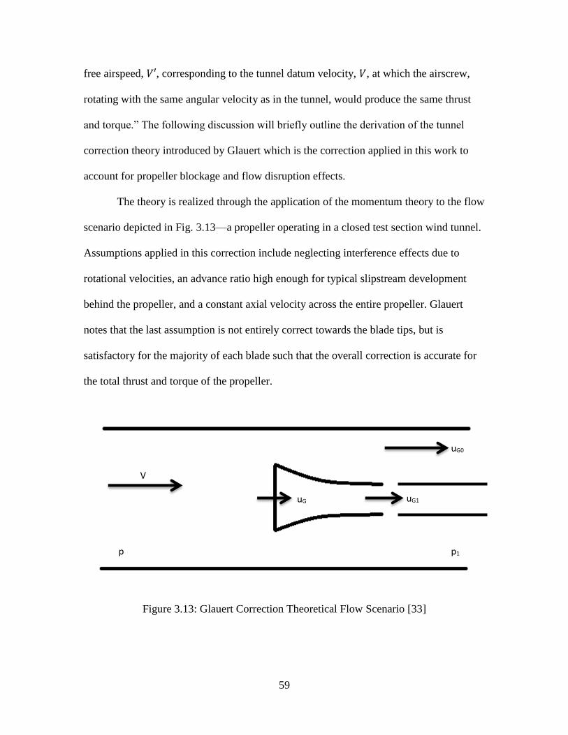
59
free airspeed, 𝑉′, corresponding to the tunnel datum velocity, 𝑉, at which the airscrew,
rotating with the same angular velocity as in the tunnel, would produce the same thrust
and torque.” The following discussion will briefly outline the derivation of the tunnel
correction theory introduced by Glauert which is the correction applied in this work to
account for propeller blockage and flow disruption effects.
The theory is realized through the application of the momentum theory to the flow
scenario depicted in Fig. 3.13—a propeller operating in a closed test section wind tunnel.
Assumptions applied in this correction include neglecting interference effects due to
rotational velocities, an advance ratio high enough for typical slipstream development
behind the propeller, and a constant axial velocity across the entire propeller. Glauert
notes that the last assumption is not entirely correct towards the blade tips, but is
satisfactory for the majority of each blade such that the overall correction is accurate for
the total thrust and torque of the propeller.
Figure 3.13: Glauert Correction Theoretical Flow Scenario [33]
V
uG uG1
uG0
p1 p
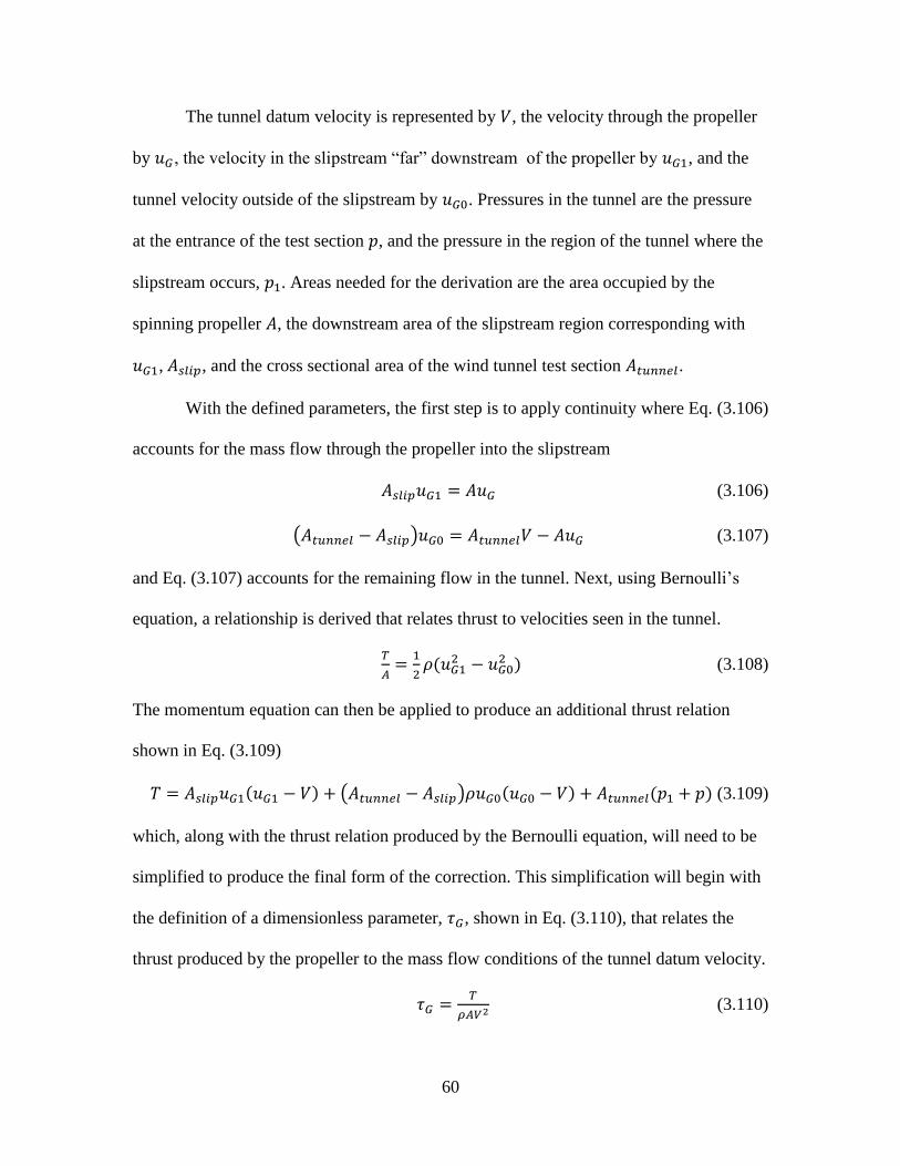
60
The tunnel datum velocity is represented by 𝑉, the velocity through the propeller
by 𝑢𝐺 , the velocity in the slipstream “far” downstream of the propeller by 𝑢𝐺1, and the
tunnel velocity outside of the slipstream by 𝑢𝐺0. Pressures in the tunnel are the pressure
at the entrance of the test section 𝑝, and the pressure in the region of the tunnel where the
slipstream occurs, 𝑝1. Areas needed for the derivation are the area occupied by the
spinning propeller 𝐴, the downstream area of the slipstream region corresponding with
𝑢𝐺1, 𝐴𝑠𝑙𝑖𝑝, and the cross sectional area of the wind tunnel test section 𝐴𝑡𝑢𝑛𝑛𝑒𝑙.
With the defined parameters, the first step is to apply continuity where Eq. (3.106)
accounts for the mass flow through the propeller into the slipstream
𝐴𝑠𝑙𝑖𝑝𝑢𝐺1 = 𝐴𝑢𝐺 (3.106)
(𝐴𝑡𝑢𝑛𝑛𝑒𝑙 − 𝐴𝑠𝑙𝑖𝑝)𝑢𝐺0 = 𝐴𝑡𝑢𝑛𝑛𝑒𝑙𝑉 − 𝐴𝑢𝐺 (3.107)
and Eq. (3.107) accounts for the remaining flow in the tunnel. Next, using Bernoulli’s
equation, a relationship is derived that relates thrust to velocities seen in the tunnel.
𝑇
𝐴=
1
2𝜌(𝑢𝐺1
2 − 𝑢𝐺02 ) (3.108)
The momentum equation can then be applied to produce an additional thrust relation
shown in Eq. (3.109)
𝑇 = 𝐴𝑠𝑙𝑖𝑝𝑢𝐺1(𝑢𝐺1 − 𝑉) + (𝐴𝑡𝑢𝑛𝑛𝑒𝑙 − 𝐴𝑠𝑙𝑖𝑝)𝜌𝑢𝐺0(𝑢𝐺0 − 𝑉) + 𝐴𝑡𝑢𝑛𝑛𝑒𝑙(𝑝1 + 𝑝) (3.109)
which, along with the thrust relation produced by the Bernoulli equation, will need to be
simplified to produce the final form of the correction. This simplification will begin with
the definition of a dimensionless parameter, 𝜏𝐺, shown in Eq. (3.110), that relates the
thrust produced by the propeller to the mass flow conditions of the tunnel datum velocity.
𝜏𝐺 =𝑇
𝜌𝐴𝑉2 (3.110)
61
Using 𝜏𝐺, the following two thrust relations can be expressed as
2𝜏𝐴𝑠𝑙𝑖𝑝(𝐴 − 𝐴𝑠𝑙𝑖𝑝)(𝐴𝑡𝑢𝑛𝑛𝑒𝑙 − 𝐴𝑠𝑙𝑖𝑝)𝑉2 = 𝐴𝑡𝑢𝑛𝑛𝑒𝑙(𝐴𝑢𝐺 − 𝐴𝑠𝑙𝑖𝑝𝑉)2 (3.111)
𝜏𝐺𝐴𝑠𝑙𝑖𝑝(𝐴𝑡𝑢𝑛𝑛𝑒𝑙𝐴 − 𝐴𝑠𝑙𝑖𝑝2 )𝑉2 = 𝐴𝑡𝑢𝑛𝑛𝑒𝑙𝐴𝑢𝐺(𝐴𝑢𝐺 − 𝐴𝑠𝑙𝑖𝑝𝑉) (3.112)
which now necessitate the introduction of the equivalent airspeed parameter 𝑉′. In free
air, the thrust of a propeller can be defined as
𝑇 = 2𝐴𝜌𝑢𝐺(𝑢𝐺 − 𝑉′) = 2𝜏𝐺𝑉2 + 𝑉′2 (3.113)
where the tunnel datum velocity and equivalent airspeed are related by
𝑉 = 𝜆𝐺𝑉′ (3.114)
and
𝑥2 = 1 + 2𝜏𝐺𝜆2 (3.115)
where 𝜆𝐺 is a parameter relating the tunnel datum velocity to the equivalent airspeed
velocity and 𝑥 is a simplification parameter, the velocity across the propeller disc for the
free air condition may be obtained in Eq. (3.116).
𝑢𝐺 =(𝑥+1)𝑉
2𝜆 (3.116)
If Eq. (3.116) and the two area ratios are known,
𝛼𝐺 =𝐴
𝐴𝑡𝑢𝑛𝑛𝑒𝑙 (3.117)
𝜎𝐺 =𝐴𝑠𝑙𝑖𝑝
𝐴 (3.118)
which are the propeller-tunnel and slipstream-propeller area ratios, are substituted into
Eqs. (3.111) and (3.112), the following set of equations can be realized which completes
the derivation.
𝑥−1
𝑥+1=
(1−𝜎𝐺)(1−𝛼𝐺𝜎𝐺)
𝜎𝐺(1−𝛼𝐺𝜎𝐺2)
2 (3.119)
62
𝜆𝐺 = 1 + (𝑥 − 1)𝛼𝐺𝜎𝐺2 −
(2𝜎𝐺−1)𝑥−1
2𝜎𝐺 (3.120)
𝜏𝐺 =(𝑥+1)(𝑥−1)
2𝜆𝐺2 (3.121)
In order to implement these equations, an iterative method is necessary since the
area of a slipstream of a propeller is generally not readily available. In conjunction with
knowns 𝛼𝐺 and 𝜏𝐺, this method requires that a user must guess a value of 𝜎𝐺 to evaluate
Eq. (3.119) which is then used to evaluate Eq. (3.120). A check is performed with Eq.
(3.121) to see if the original guess was correct in comparison with the known 𝜏𝐺. If not,
successive iterations are necessary until this is the case. Glauert notes that the slipstream-
propeller ratio lies between 0.5 and 1, which provides a good initial guess. This set of
equations can be programmed on a computer to calculate operating thrusts quickly and
produce plots similar to Figure 3.14. where the ratio of the tunnel datum velocity and
Figure 3.14: Glauert Correction, 9" Diameter Propeller, Blockage Ratio = 0.11
0 0.5 1 1.5 2 2.51
1.01
1.02
1.03
1.04
1.05
1.06
= T / ( A V)
V /
V'
63
equivalent free airspeed is plotted versus a range of thrusts each divided by the air
density, propeller rotational area, and the tunnel datum velocity. The data from the plots
can be used to find the equivalent free airspeed. In conclusion, this theory allows a user to
correct wind tunnel datum speed 𝑉, by finding an approximate free airspeed at which the
propeller would operate to produce the same thrust and torque conditions.
Propeller-Motor Matching
When considering small UAS propulsion system efficiency improvements,
choosing the correct motor to compliment a propeller is just as important as the design of
the propeller itself. A mismatch of these two components will lead to unsatisfactory
overall efficiencies, no matter how efficient the motor or propeller are when considered
individually. Although this work only considered propeller design, future researchers can
benefit from the following discussion that will outline propeller-motor matching theory
given by Drela, [49].
The circuit diagram in Fig. 3.15 will serve as the model of the electric motor. In
order to derive the relations used in matching a motor with a propeller, it is necessary to
develop equations to characterize key motor characteristics in terms of the motor voltage
and current, 𝑉𝑚 and 𝐼𝑚. The first of these equations is shown in Fig. 3.16, where the
back-electromagnetic field 𝑉𝐸𝑀𝐹 is shown to be equivalent to the quotient of the rotation
rate of the motor, Ω, and the so-called motor speed constant, 𝐾𝑣, which will need units of
𝑟𝑎𝑑
𝑠 𝑉𝑜𝑙𝑡 as opposed to
𝑅𝑃𝑀
𝑉𝑜𝑙𝑡 for this discussion. The remaining equations needed, can be
derived through the implementation of typical circuitry laws and relations and are given
by Eqs. (3.122) through (3.126)
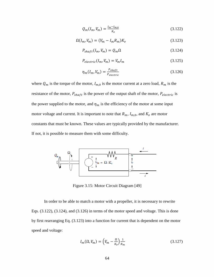
64
𝑄𝑚(𝐼𝑚, 𝑉𝑚) =𝐼𝑚−𝐼𝑚,0
𝐾𝑣 (3.122)
Ω(𝐼𝑚, 𝑉𝑚) = (𝑉𝑚 − 𝐼𝑚𝑅𝑚)𝐾𝑣 (3.123)
𝑃𝑠ℎ𝑎𝑓𝑡(𝐼𝑚, 𝑉𝑚) = 𝑄𝑚Ω (3.124)
𝑃𝑒𝑙𝑒𝑐𝑡𝑟𝑖𝑐(𝐼𝑚, 𝑉𝑚) = 𝑉𝑚𝐼𝑚 (3.125)
𝜂𝑚(𝐼𝑚, 𝑉𝑚) =𝑃𝑠ℎ𝑎𝑓𝑡
𝑃𝑒𝑙𝑒𝑐𝑡𝑟𝑖𝑐 (3.126)
where 𝑄𝑚 is the torque of the motor, 𝐼𝑚,0 is the motor current at a zero load, 𝑅𝑚 is the
resistance of the motor, 𝑃𝑠ℎ𝑎𝑓𝑡 is the power of the output shaft of the motor, 𝑃𝑒𝑙𝑒𝑐𝑡𝑟𝑖𝑐 is
the power supplied to the motor, and 𝜂𝑚 is the efficiency of the motor at some input
motor voltage and current. It is important to note that 𝑅𝑚, 𝐼𝑚,0, and 𝐾𝑣 are motor
constants that must be known. These values are typically provided by the manufacturer.
If not, it is possible to measure them with some difficulty.
Figure 3.15: Motor Circuit Diagram [49]
In order to be able to match a motor with a propeller, it is necessary to rewrite
Eqs. (3.122), (3.124), and (3.126) in terms of the motor speed and voltage. This is done
by first rearranging Eq. (3.123) into a function for current that is dependent on the motor
speed and voltage:
𝐼𝑚(Ω, 𝑉𝑚) = (𝑉𝑚 −Ω
𝐾𝑣)
1
𝑅𝑚 (3.127)
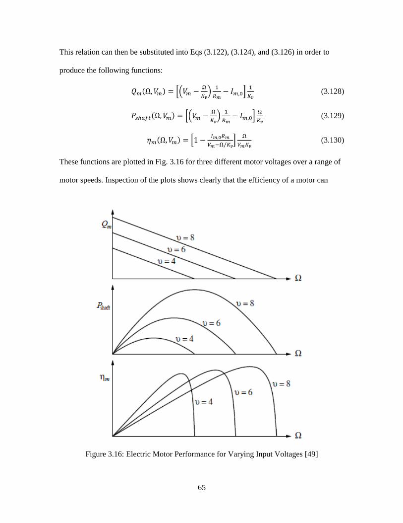
65
This relation can then be substituted into Eqs (3.122), (3.124), and (3.126) in order to
produce the following functions:
𝑄𝑚(Ω, 𝑉𝑚) = [(𝑉𝑚 −Ω
𝐾𝑣)
1
𝑅𝑚− 𝐼𝑚,0]
1
𝐾𝑣 (3.128)
𝑃𝑠ℎ𝑎𝑓𝑡(Ω, 𝑉𝑚) = [(𝑉𝑚 −Ω
𝐾𝑣)
1
𝑅𝑚− 𝐼𝑚,0]
Ω
𝐾𝑣 (3.129)
𝜂𝑚(Ω, 𝑉𝑚) = [1 −𝐼𝑚,0𝑅𝑚
𝑉𝑚−Ω 𝐾𝑣⁄]
Ω
𝑉𝑚𝐾𝑣 (3.130)
These functions are plotted in Fig. 3.16 for three different motor voltages over a range of
motor speeds. Inspection of the plots shows clearly that the efficiency of a motor can
Figure 3.16: Electric Motor Performance for Varying Input Voltages [49]
66
vary widely based on the voltage input, and even more so based on the operating speed.
In order to match a motor to a given propeller design, it is first necessary to be
able to characterize the propeller at a given flight velocity (usually the design point) in
terms of thrust, 𝑇, torque, 𝑄, and efficiency, 𝜂—each over a range of rotational operating
speeds. Experimentally, various researchers have been able to achieve the necessary
propeller characterization as discussed in the literature survey of Chapter 2.
Next, it must be realized that comparisons will only hold any relevant, physical
meaning if Eq. (3.131) holds:
𝑄𝑚(Ω, 𝑉𝑚) = 𝑄(Ω, 𝑉) (3.131)
which constrains any comparisons made to rotational speeds in which the motor and
propeller possess the same torque.
Finally, the propeller thrust, propeller torque, motor torque, and propeller and
motor efficiencies may be plotted at a specified flight velocity and motor voltage in order
to determine the goodness of the propeller-motor combination. Figure 3.17 shows four
plots which can be used to make the comparison. The third plot shows the point in which
the constraint described by Eq. (3.131) holds true.
It is at this rotational speed that comparisons between the motor and propeller will
be made. It can be seen from
𝜂𝑠𝑦𝑠𝑡𝑒𝑚 = 𝜂 𝜂𝑚 (3.132)
where 𝜂𝑠𝑦𝑠𝑡𝑒𝑚 is the efficiency of the propeller-motor combination, that the propeller-
motor combination shown in Fig. 3.17 has a poor efficiency at the chosen operating
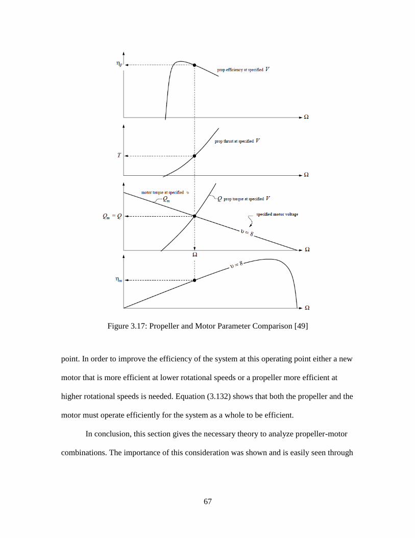
67
Figure 3.17: Propeller and Motor Parameter Comparison [49]
point. In order to improve the efficiency of the system at this operating point either a new
motor that is more efficient at lower rotational speeds or a propeller more efficient at
higher rotational speeds is needed. Equation (3.132) shows that both the propeller and the
motor must operate efficiently for the system as a whole to be efficient.
In conclusion, this section gives the necessary theory to analyze propeller-motor
combinations. The importance of this consideration was shown and is easily seen through
68
the system efficiency described in Eq. (3.132). If both components do not operate near
the peak of their efficiency curves for a specified flight velocity and input voltage, the
system as a whole will suffer.
Chapter Three Concluding Remarks
As a whole, this chapter provides the necessary theoretical background to
understand the design, analysis, and experimental work completed in this thesis. It began
with one-dimensional propeller theory, moved to airfoil theory, BET, BEMT, and finally
the QMIL/QPROP formulation used in the design work in this thesis. After propeller
theory, noise sources on the blades of propellers were characterized by examining the
theory implemented in NAFNoise. In order to ensure experimental wind tunnel testing
accurately modeled real-world conditions, Glauert’s wind tunnel interference correction
for propellers was derived. Finally, propeller-motor combinations were discussed along
with their effects on the efficiency of the system as a whole. The following chapter will
describe the experimental method—or the application of these theories used in this work.
69
CHAPTER FOUR
Experimental Method
This chapter will cover the experimental method used in this work. In particular,
this discussion will begin with a description of the Baylor MATLAB code used to
streamline the design, theoretical analysis, solid-modeling, and fabrication of a small
propeller. The second section of the chapter will detail the two testing facilities, each
facility’s testing apparatus, and experimental procedures. The testing facility at Baylor
University will be discussed first and in greater detail than the USAFA testing facility.
The testing facility at the USAFA will then be discussed, mainly citing the key
differences between the two facilities.
Bearcontrol
Bearcontrol is the Baylor MATLAB code that has streamlined the propeller
design, analysis, solid-modeling, and in turn, fabrication of the propellers experimentally
tested in this work. In general, this program enables a user to design a propeller and have
the printed model in a single day. Bearcontrol accomplishes this task by providing a
platform from which a user can control multiple programs at once. The programs handled
by Bearcontrol are QMIL for the propeller design, QPROP for the motor and propeller
performance analysis, NAFNoise for the propeller noise prediction, and SolidWorks for
the solid-modeling. The following list gives additional detail of each program’s
background and capabilities.
70
QMIL [41]—the first of two command prompt programs in a propeller design and
analysis package developed by Drela. This program designs a propeller geometry
based on physical and design point operation constraints using the theory outlined
in the QMIL and QPROP Formulation section of Chapter Three of this thesis.
The output file is conveniently the input file for the propeller analysis program
QPROP.
QPROP [40]—the second of the two command prompt programs developed by
Drela. This program analyzes the geometric design from QMIL using the theory
outlined in the QMIL and QPROP Formulation section of Chapter Three of this
thesis. It is possible for QPROP to analyze propeller designs not created by QMIL
as long as the QPROP input file is in the correct format.
NAFNoise [42]—an airfoil noise prediction command prompt program developed
by the National Renewable Energy Laboratory. This program predicts the noise
of individual airfoils using the theory outlined in the Airfoil Noise section of
Chapter Three of this thesis.
SolidWorks [50]—the 3D CAD program created by DASSAULT SYSTEMS.
Bearcontrol creates solid-modeling macros for use in the SolidWorks Application
Programming Interface (API) to automate the creation of the propeller 3D models.
Bearcontrol employs these programs to create a useful and comprehensive propeller
production tool that has dramatically improved the propeller manufacturing, and
propeller testing capabilities in this project. A user guide for Bearcontrol is available in
Appendix A.
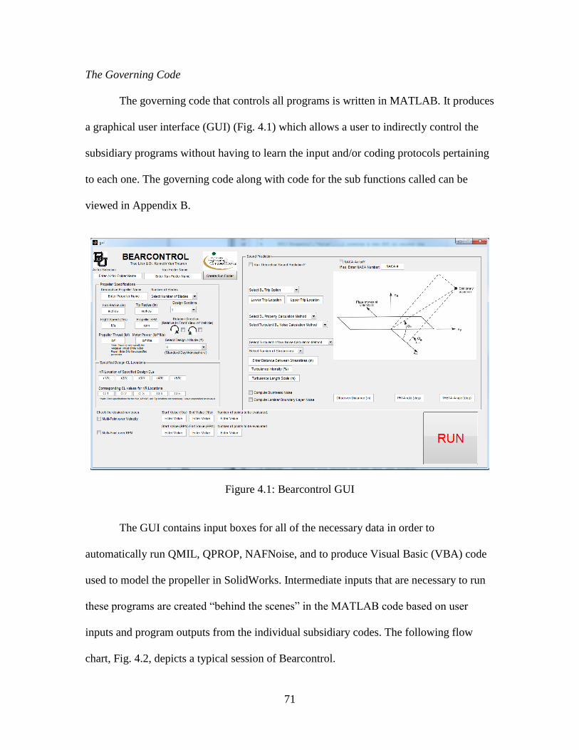
71
The Governing Code
The governing code that controls all programs is written in MATLAB. It produces
a graphical user interface (GUI) (Fig. 4.1) which allows a user to indirectly control the
subsidiary programs without having to learn the input and/or coding protocols pertaining
to each one. The governing code along with code for the sub functions called can be
viewed in Appendix B.
Figure 4.1: Bearcontrol GUI
The GUI contains input boxes for all of the necessary data in order to
automatically run QMIL, QPROP, NAFNoise, and to produce Visual Basic (VBA) code
used to model the propeller in SolidWorks. Intermediate inputs that are necessary to run
these programs are created “behind the scenes” in the MATLAB code based on user
inputs and program outputs from the individual subsidiary codes. The following flow
chart, Fig. 4.2, depicts a typical session of Bearcontrol.
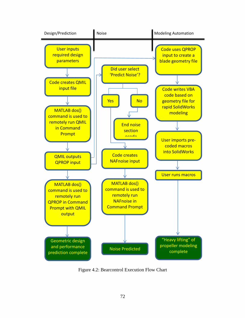
72
Figure 4.2: Bearcontrol Execution Flow Chart
Noise Predicted
Code creates NAFnoise input
file
Yes
User inputs
required design parameters
MATLAB dos() command is used to remotely run QMIL
in Command Prompt
Code creates QMIL input file
QMIL outputs QPROP input
MATLAB dos() command is used to
remotely run QPROP in Command Prompt with QMIL
output
Geometric design and performance
prediction complete
Code uses QPROP input to create a
blade geometry file
Code writes VBA code based on
geometry file for rapid SolidWorks
modeling
Did user select ‘Predict Noise’?
No
MATLAB dos() command is used to
remotely run NAFnoise in
Command Prompt
User imports pre-coded macros
into SolidWorks
End noise section ocode
User runs macros
Design/Prediction Noise Modeling Automation
“Heavy lifting” of propeller modeling
complete
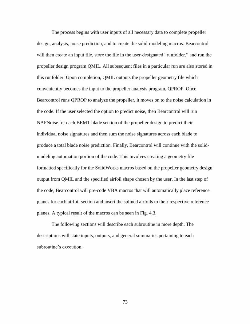
73
The process begins with user inputs of all necessary data to complete propeller
design, analysis, noise prediction, and to create the solid-modeling macros. Bearcontrol
will then create an input file, store the file in the user-designated “runfolder,” and run the
propeller design program QMIL. All subsequent files in a particular run are also stored in
this runfolder. Upon completion, QMIL outputs the propeller geometry file which
conveniently becomes the input to the propeller analysis program, QPROP. Once
Bearcontrol runs QPROP to analyze the propeller, it moves on to the noise calculation in
the code. If the user selected the option to predict noise, then Bearcontrol will run
NAFNoise for each BEMT blade section of the propeller design to predict their
individual noise signatures and then sum the noise signatures across each blade to
produce a total blade noise prediction. Finally, Bearcontrol will continue with the solid-
modeling automation portion of the code. This involves creating a geometry file
formatted specifically for the SolidWorks macros based on the propeller geometry design
output from QMIL and the specified airfoil shape chosen by the user. In the last step of
the code, Bearcontrol will pre-code VBA macros that will automatically place reference
planes for each airfoil section and insert the splined airfoils to their respective reference
planes. A typical result of the macros can be seen in Fig. 4.3.
The following sections will describe each subroutine in more depth. The
descriptions will state inputs, outputs, and general summaries pertaining to each
subroutine’s execution.
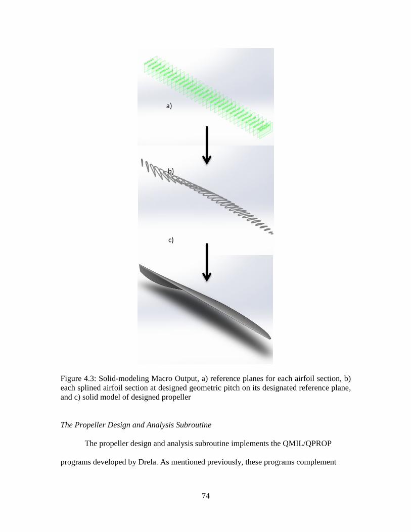
74
Figure 4.3: Solid-modeling Macro Output, a) reference planes for each airfoil section, b)
each splined airfoil section at designed geometric pitch on its designated reference plane,
and c) solid model of designed propeller
The Propeller Design and Analysis Subroutine
The propeller design and analysis subroutine implements the QMIL/QPROP
programs developed by Drela. As mentioned previously, these programs complement
a)
b)
c)
75
each other in that the output of QMIL is the input of QPROP. In order for QMIL to
design a propeller geometry and QPROP to analyze the propeller and motor combination,
several inputs are required. The first input is a motor file which contains the necessary
data to characterize the motor. Only the default motor has been utilized in this work, and
its input file is shown in Fig. 4.4 where 𝑅 is the resistance of the motor, 𝐼0 is the motor
Figure 4.4: QMIL/QPROP Default Propeller Motor Characteristics
current with a zero load, and 𝐾𝑣 is motor speed constant which is usually given by the
manufacturer. As long as these three constants are known, any motor could be used to
analyze the performance of the propeller and motor combination.
The next inputs, shown in Table 4.1, constrain the geometry and aerodynamic
operating conditions for the propeller design. These include the number of blades desired,
the radius of the propeller hub, the radius of the propeller, the desired number of airfoil
cross sections in the propeller, and finally the airfoil cross section with associated
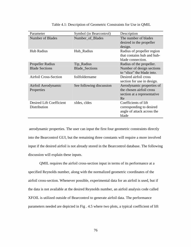
76
Table 4.1: Description of Geometric Constraints for Use in QMIL
Parameter Symbol (in Bearcontrol) Description
Number of Blades Number_of_Blades The number of blades
desired in the propeller
design.
Hub Radius Hub_Radius Radius of propeller region
that contains hub and hub-
blade connection.
Propeller Radius Tip_Radius Radius of the propeller.
Blade Sections Blade_Sections Number of design sections
to “slice” the blade into.
Airfoil Cross-Section foilfoldername Desired airfoil cross
section for use in design.
Airfoil Aerodynamic
Properties
See following discussion Aerodynamic properties of
the chosen airfoil cross
section at a representative
Re
Desired Lift Coefficient
Distribution
xldes, cldes Coefficients of lift
corresponding to desired
angle of attack across the
blade
aerodynamic properties. The user can input the first four geometric constraints directly
into the Bearcontrol GUI, but the remaining three constants will require a more involved
input if the desired airfoil is not already stored in the Bearcontrol database. The following
discussion will explain these inputs.
QMIL requires the airfoil cross-section input in terms of its performance at a
specified Reynolds number, along with the normalized geometric coordinates of the
airfoil cross-section. Whenever possible, experimental data for an airfoil is used, but if
the data is not available at the desired Reynolds number, an airfoil analysis code called
XFOIL is utilized outside of Bearcontrol to generate airfoil data. The performance
parameters needed are depicted in Fig . 4.5 where two plots, a typical coefficient of lift
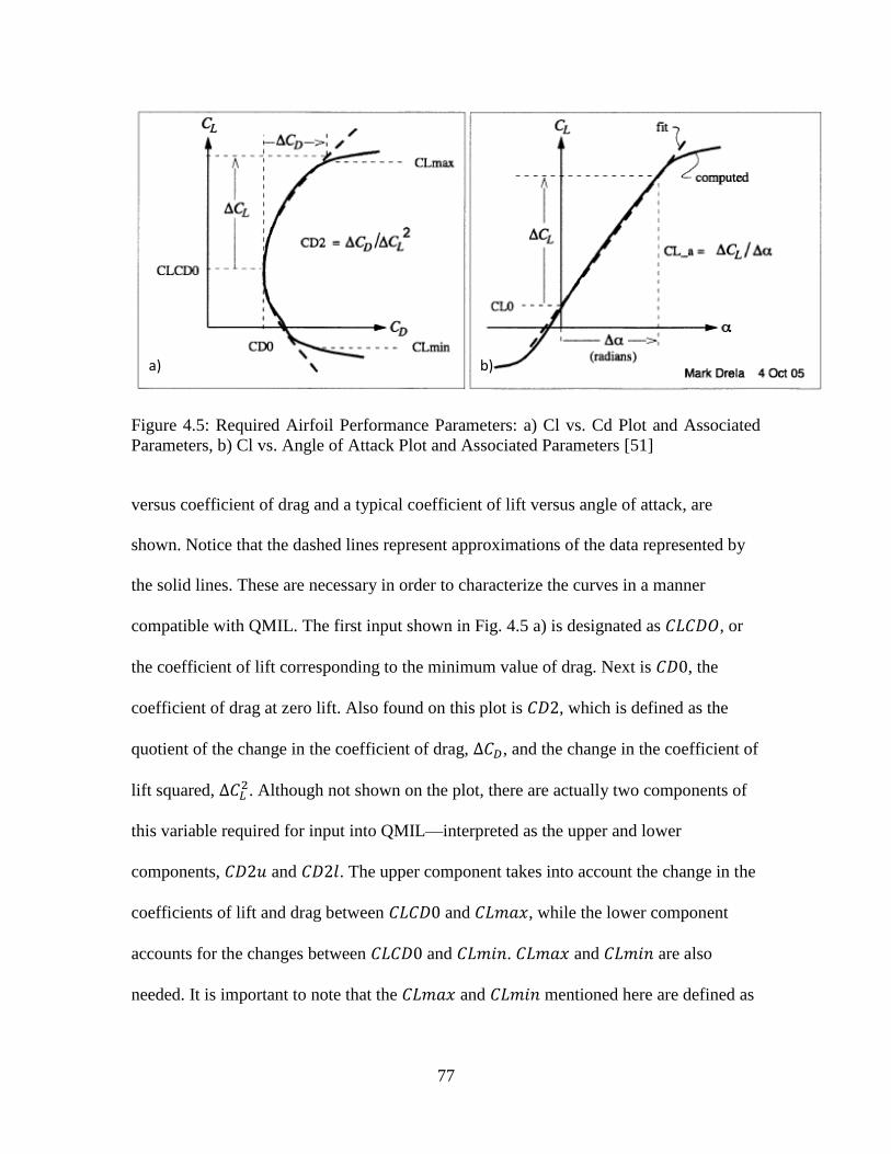
77
Figure 4.5: Required Airfoil Performance Parameters: a) Cl vs. Cd Plot and Associated
Parameters, b) Cl vs. Angle of Attack Plot and Associated Parameters [51]
versus coefficient of drag and a typical coefficient of lift versus angle of attack, are
shown. Notice that the dashed lines represent approximations of the data represented by
the solid lines. These are necessary in order to characterize the curves in a manner
compatible with QMIL. The first input shown in Fig. 4.5 a) is designated as 𝐶𝐿𝐶𝐷𝑂, or
the coefficient of lift corresponding to the minimum value of drag. Next is 𝐶𝐷0, the
coefficient of drag at zero lift. Also found on this plot is 𝐶𝐷2, which is defined as the
quotient of the change in the coefficient of drag, Δ𝐶𝐷, and the change in the coefficient of
lift squared, Δ𝐶𝐿2. Although not shown on the plot, there are actually two components of
this variable required for input into QMIL—interpreted as the upper and lower
components, 𝐶𝐷2𝑢 and 𝐶𝐷2𝑙. The upper component takes into account the change in the
coefficients of lift and drag between 𝐶𝐿𝐶𝐷0 and 𝐶𝐿𝑚𝑎𝑥, while the lower component
accounts for the changes between 𝐶𝐿𝐶𝐷0 and 𝐶𝐿𝑚𝑖𝑛. 𝐶𝐿𝑚𝑎𝑥 and 𝐶𝐿𝑚𝑖𝑛 are also
needed. It is important to note that the 𝐶𝐿𝑚𝑎𝑥 and 𝐶𝐿𝑚𝑖𝑛 mentioned here are defined as
a) b)
78
shown in Fig. 4.5, not the 𝐶𝑙,𝑚𝑎𝑥 that would usually denote the maximum coefficient of
lift before the airfoil stalls.
The first input shown in Fig. 4.5 b) is the coefficient of lift at a zero angle of
attack, 𝐶𝐿0. This is followed by 𝐶𝐿_𝑎, or the slope of the “linear” portion of the
coefficient of lift versus alpha curve. These two parameters are used to describe this
linear region with the following equation
𝐶𝐿(𝛼) = 𝐶𝐿𝑎𝛼 + 𝐶𝐿0 (4.1)
which is bounded between the 𝐶𝐿𝑚𝑎𝑥 and 𝐶𝐿𝑚𝑖𝑛 parameters previously mentioned.
QMIL will only utilize this linear region. To complete the airfoil properties input, two
more parameters are also required—the Reynolds number at which the original data was
obtained (either from experimental results or theoretical predictions), 𝑅𝐸𝑟𝑒𝑓, and
𝑅𝐸𝑒𝑥𝑝. 𝑅𝐸𝑒𝑥𝑝 is a user defined value that adjusts the drag curve associated with the
chosen airfoil if airfoil cross-sections across the blade experience a different Reynolds
number than the original reference value. In Bearcontrol, these airfoil properties are
stored in a specified input file that the program can access whenever needed. The process
of characterizing a new airfoil is a one-time procedure. Finally, the user can input the
desired coefficient of lift distribution, usually corresponding to the airfoil’s Cl/Cdmax,
across the blade directly into the Bearcontrol GUI.
The other inputs that QMIL requires can be described as flight design point
constraints. These include the flight speed of the vehicle, the desired propeller operating
rotational speed, the desired operating thrust or motor power (the parameter not specified
must be entered as zero), and two parameters, 𝐿𝑑𝑒𝑠 and 𝐾𝑄𝑑𝑒𝑠 which specify the MIL
design condition discussed in Chapter Three of this thesis.
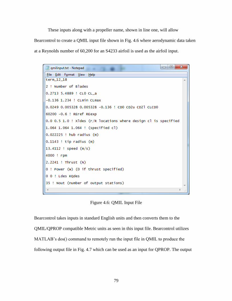
79
These inputs along with a propeller name, shown in line one, will allow
Bearcontrol to create a QMIL input file shown in Fig. 4.6 where aerodynamic data taken
at a Reynolds number of 60,200 for an S4233 airfoil is used as the airfoil input.
Figure 4.6: QMIL Input File
Bearcontrol takes inputs in standard English units and then converts them to the
QMIL/QPROP compatible Metric units as seen in this input file. Bearcontrol utilizes
MATLAB’s dos() command to remotely run the input file in QMIL to produce the
following output file in Fig. 4.7 which can be used as an input for QPROP. The output
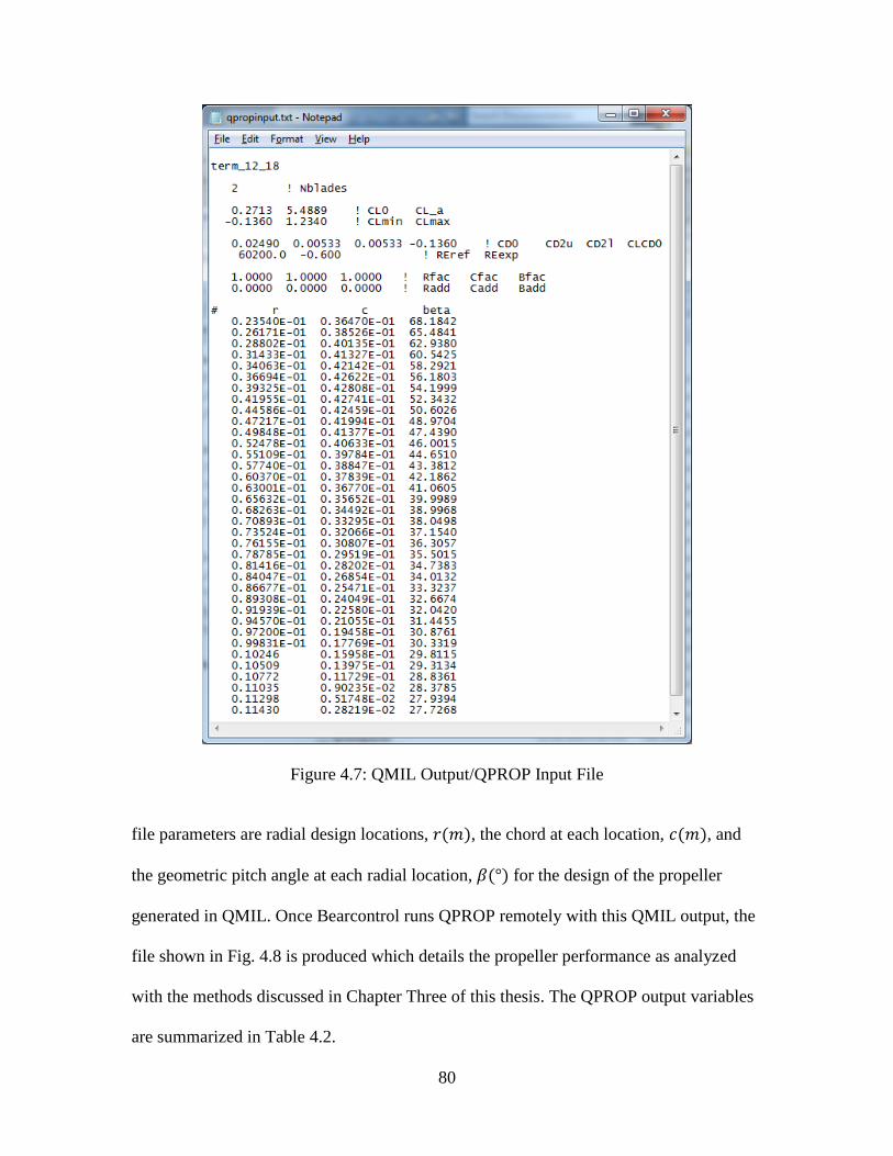
80
Figure 4.7: QMIL Output/QPROP Input File
file parameters are radial design locations, 𝑟(𝑚), the chord at each location, 𝑐(𝑚), and
the geometric pitch angle at each radial location, 𝛽(°) for the design of the propeller
generated in QMIL. Once Bearcontrol runs QPROP remotely with this QMIL output, the
file shown in Fig. 4.8 is produced which details the propeller performance as analyzed
with the methods discussed in Chapter Three of this thesis. The QPROP output variables
are summarized in Table 4.2.
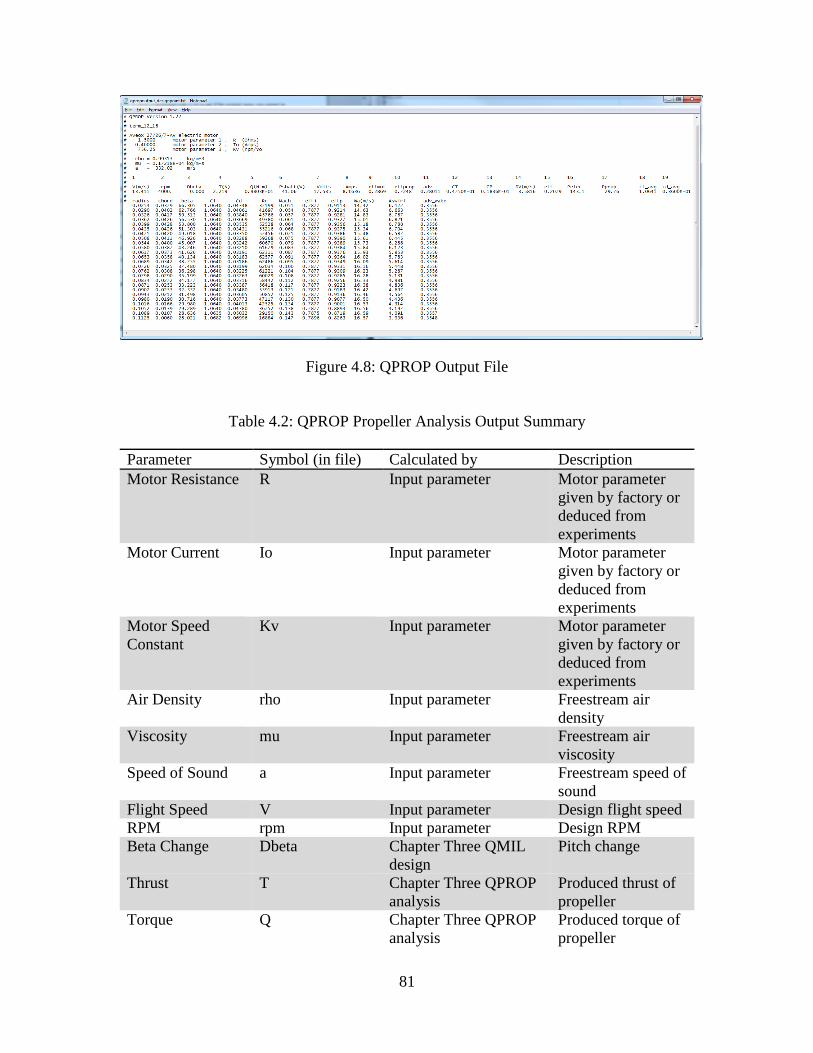
81
Figure 4.8: QPROP Output File
Table 4.2: QPROP Propeller Analysis Output Summary
Parameter Symbol (in file) Calculated by Description
Motor Resistance R Input parameter Motor parameter
given by factory or
deduced from
experiments
Motor Current Io Input parameter Motor parameter
given by factory or
deduced from
experiments
Motor Speed
Constant
Kv Input parameter Motor parameter
given by factory or
deduced from
experiments
Air Density rho Input parameter Freestream air
density
Viscosity mu Input parameter Freestream air
viscosity
Speed of Sound a Input parameter Freestream speed of
sound
Flight Speed V Input parameter Design flight speed
RPM rpm Input parameter Design RPM
Beta Change Dbeta Chapter Three QMIL
design
Pitch change
Thrust T Chapter Three QPROP
analysis
Produced thrust of
propeller
Torque Q Chapter Three QPROP
analysis
Produced torque of
propeller
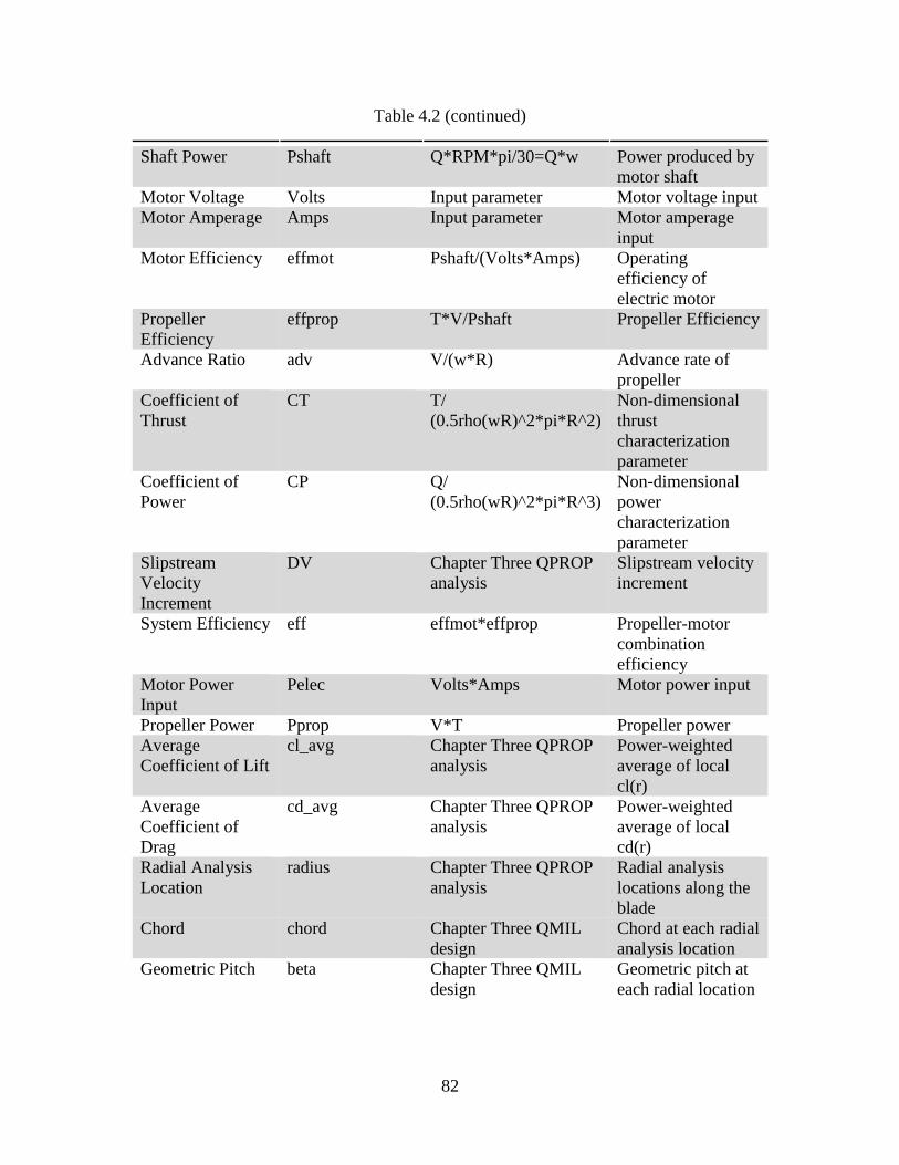
82
Table 4.2 (continued)
Shaft Power Pshaft Q*RPM*pi/30=Q*w Power produced by
motor shaft
Motor Voltage Volts Input parameter Motor voltage input
Motor Amperage Amps Input parameter Motor amperage
input
Motor Efficiency effmot Pshaft/(Volts*Amps) Operating
efficiency of
electric motor
Propeller
Efficiency
effprop T*V/Pshaft Propeller Efficiency
Advance Ratio adv V/(w*R) Advance rate of
propeller
Coefficient of
Thrust
CT T/
(0.5rho(wR)^2*pi*R^2)
Non-dimensional
thrust
characterization
parameter
Coefficient of
Power
CP Q/
(0.5rho(wR)^2*pi*R^3)
Non-dimensional
power
characterization
parameter
Slipstream
Velocity
Increment
DV Chapter Three QPROP
analysis
Slipstream velocity
increment
System Efficiency eff effmot*effprop Propeller-motor
combination
efficiency
Motor Power
Input
Pelec Volts*Amps Motor power input
Propeller Power Pprop V*T Propeller power
Average
Coefficient of Lift
cl_avg Chapter Three QPROP
analysis
Power-weighted
average of local
cl(r)
Average
Coefficient of
Drag
cd_avg Chapter Three QPROP
analysis
Power-weighted
average of local
cd(r)
Radial Analysis
Location
radius Chapter Three QPROP
analysis
Radial analysis
locations along the
blade
Chord chord Chapter Three QMIL
design
Chord at each radial
analysis location
Geometric Pitch beta Chapter Three QMIL
design
Geometric pitch at
each radial location
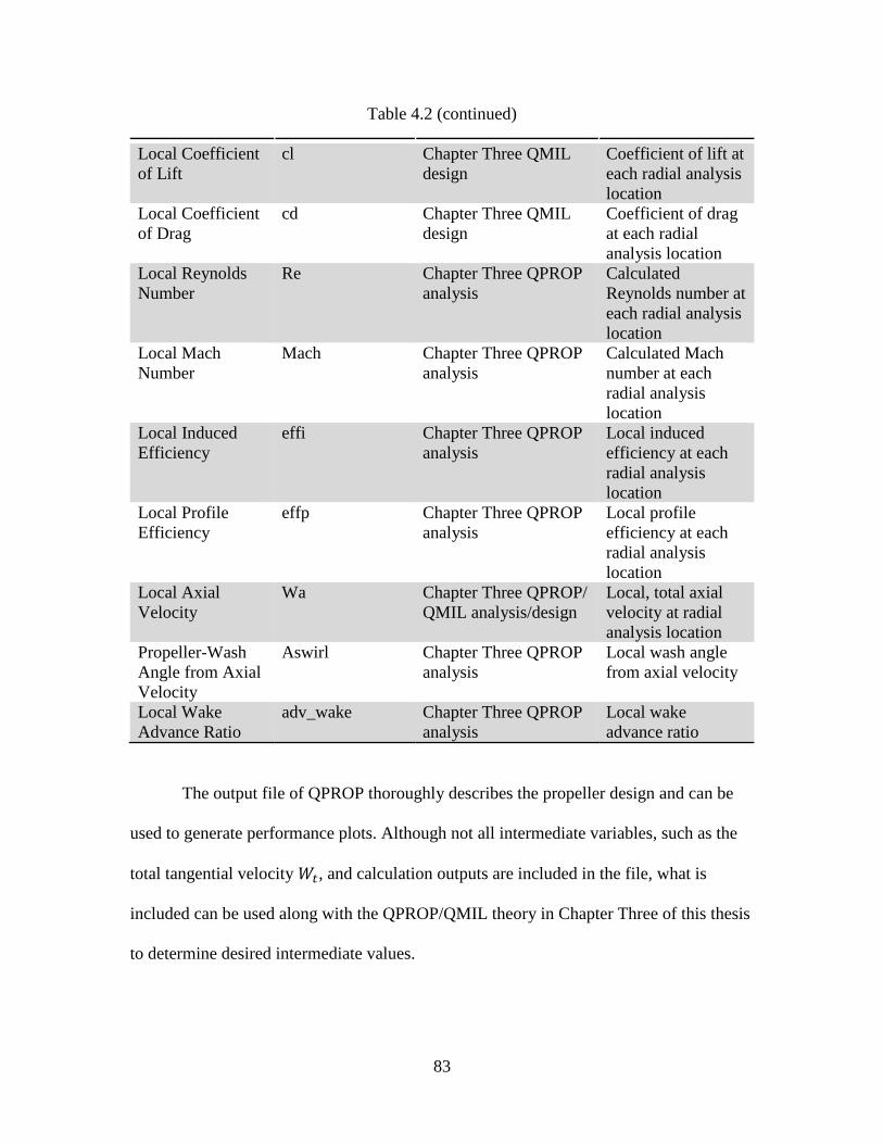
83
Table 4.2 (continued)
Local Coefficient
of Lift
cl Chapter Three QMIL
design
Coefficient of lift at
each radial analysis
location
Local Coefficient
of Drag
cd Chapter Three QMIL
design
Coefficient of drag
at each radial
analysis location
Local Reynolds
Number
Re Chapter Three QPROP
analysis
Calculated
Reynolds number at
each radial analysis
location
Local Mach
Number
Mach Chapter Three QPROP
analysis
Calculated Mach
number at each
radial analysis
location
Local Induced
Efficiency
effi Chapter Three QPROP
analysis
Local induced
efficiency at each
radial analysis
location
Local Profile
Efficiency
effp Chapter Three QPROP
analysis
Local profile
efficiency at each
radial analysis
location
Local Axial
Velocity
Wa Chapter Three QPROP/
QMIL analysis/design
Local, total axial
velocity at radial
analysis location
Propeller-Wash
Angle from Axial
Velocity
Aswirl Chapter Three QPROP
analysis
Local wash angle
from axial velocity
Local Wake
Advance Ratio
adv_wake Chapter Three QPROP
analysis
Local wake
advance ratio
The output file of QPROP thoroughly describes the propeller design and can be
used to generate performance plots. Although not all intermediate variables, such as the
total tangential velocity 𝑊𝑡, and calculation outputs are included in the file, what is
included can be used along with the QPROP/QMIL theory in Chapter Three of this thesis
to determine desired intermediate values.
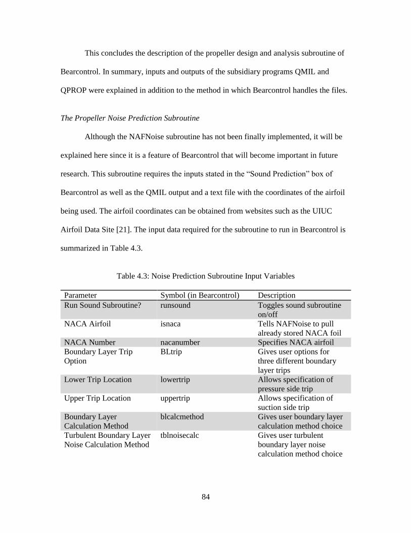
84
This concludes the description of the propeller design and analysis subroutine of
Bearcontrol. In summary, inputs and outputs of the subsidiary programs QMIL and
QPROP were explained in addition to the method in which Bearcontrol handles the files.
The Propeller Noise Prediction Subroutine
Although the NAFNoise subroutine has not been finally implemented, it will be
explained here since it is a feature of Bearcontrol that will become important in future
research. This subroutine requires the inputs stated in the “Sound Prediction” box of
Bearcontrol as well as the QMIL output and a text file with the coordinates of the airfoil
being used. The airfoil coordinates can be obtained from websites such as the UIUC
Airfoil Data Site [21]. The input data required for the subroutine to run in Bearcontrol is
summarized in Table 4.3.
Table 4.3: Noise Prediction Subroutine Input Variables
Parameter Symbol (in Bearcontrol) Description
Run Sound Subroutine? runsound Toggles sound subroutine
on/off
NACA Airfoil isnaca Tells NAFNoise to pull
already stored NACA foil
NACA Number nacanumber Specifies NACA airfoil
Boundary Layer Trip
Option
BLtrip Gives user options for
three different boundary
layer trips
Lower Trip Location lowertrip Allows specification of
pressure side trip
Upper Trip Location uppertrip Allows specification of
suction side trip
Boundary Layer
Calculation Method
blcalcmethod Gives user boundary layer
calculation method choice
Turbulent Boundary Layer
Noise Calculation Method
tblnoisecalc Gives user turbulent
boundary layer noise
calculation method choice
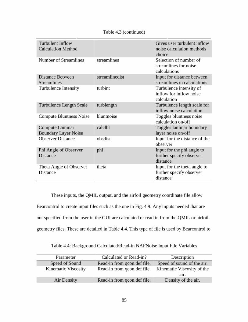
85
Table 4.3 (continued)
Turbulent Inflow
Calculation Method
Gives user turbulent inflow
noise calculation methods
choice
Number of Streamlines streamlines Selection of number of
streamlines for noise
calculations
Distance Between
Streamlines
streamlinedist Input for distance between
streamlines in calculations
Turbulence Intensity turbint Turbulence intensity of
inflow for inflow noise
calculation
Turbulence Length Scale turblength Turbulence length scale for
inflow noise calculation
Compute Bluntness Noise bluntnoise Toggles bluntness noise
calculation on/off
Compute Laminar
Boundary Layer Noise
calclbl Toggles laminar boundary
layer noise on/off
Observer Distance obsdist Input for the distance of the
observer
Phi Angle of Observer
Distance
phi Input for the phi angle to
further specify observer
distance
Theta Angle of Observer
Distance
theta Input for the theta angle to
further specify observer
distance
These inputs, the QMIL output, and the airfoil geometry coordinate file allow
Bearcontrol to create input files such as the one in Fig. 4.9. Any inputs needed that are
not specified from the user in the GUI are calculated or read in from the QMIL or airfoil
geometry files. These are detailed in Table 4.4. This type of file is used by Bearcontrol to
Table 4.4: Background Calculated/Read-in NAFNoise Input File Variables
Parameter Calculated or Read-in? Description
Speed of Sound Read-in from qcon.def file. Speed of sound of the air.
Kinematic Viscosity Read-in from qcon.def file. Kinematic Viscosity of the
air.
Air Density Read-in from qcon.def file. Density of the air.
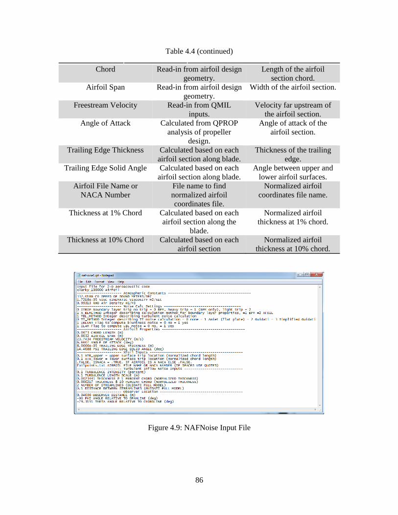
86
Table 4.4 (continued)
Chord Read-in from airfoil design
geometry.
Length of the airfoil
section chord.
Airfoil Span Read-in from airfoil design
geometry.
Width of the airfoil section.
Freestream Velocity Read-in from QMIL
inputs.
Velocity far upstream of
the airfoil section.
Angle of Attack Calculated from QPROP
analysis of propeller
design.
Angle of attack of the
airfoil section.
Trailing Edge Thickness Calculated based on each
airfoil section along blade.
Thickness of the trailing
edge.
Trailing Edge Solid Angle Calculated based on each
airfoil section along blade.
Angle between upper and
lower airfoil surfaces.
Airfoil File Name or
NACA Number
File name to find
normalized airfoil
coordinates file.
Normalized airfoil
coordinates file name.
Thickness at 1% Chord Calculated based on each
airfoil section along the
blade.
Normalized airfoil
thickness at 1% chord.
Thickness at 10% Chord Calculated based on each
airfoil section
Normalized airfoil
thickness at 10% chord.
Figure 4.9: NAFNoise Input File
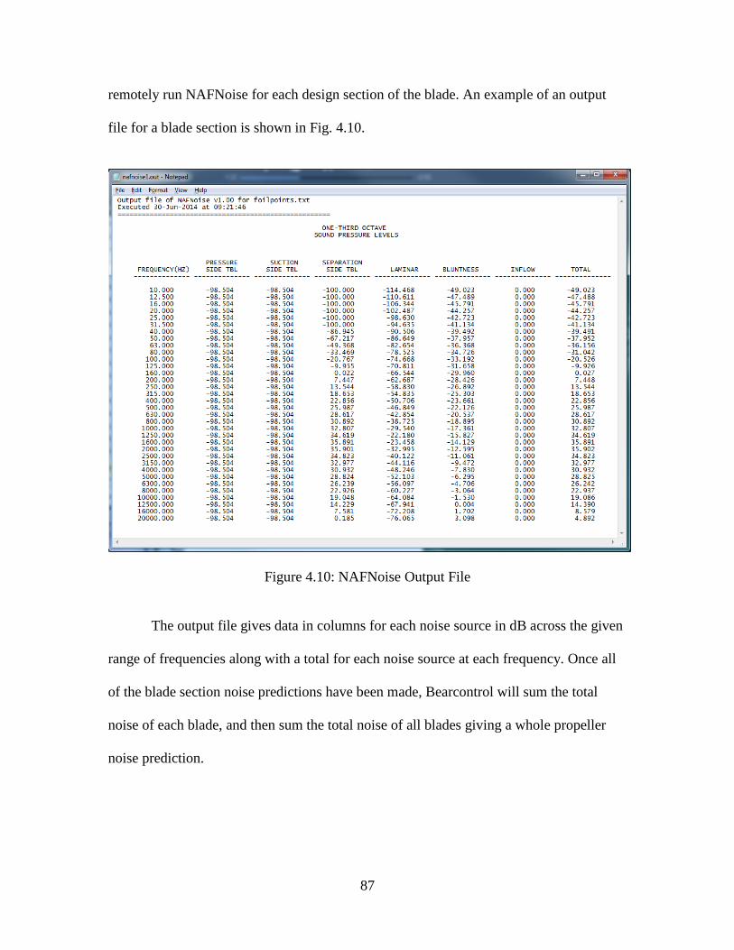
87
remotely run NAFNoise for each design section of the blade. An example of an output
file for a blade section is shown in Fig. 4.10.
Figure 4.10: NAFNoise Output File
The output file gives data in columns for each noise source in dB across the given
range of frequencies along with a total for each noise source at each frequency. Once all
of the blade section noise predictions have been made, Bearcontrol will sum the total
noise of each blade, and then sum the total noise of all blades giving a whole propeller
noise prediction.
88
The Solid-Modeling Automation Subroutine
The solid-modeling subroutine in Bearcontrol creates run-specific, pre-coded
macros for a user to import into SolidWorks and automatically model the majority of the
propeller. The only input required from the user is the airfoil geometry coordinate file
which is also an input for the noise subroutine. Bearcontrol will use this geometry file
along with the QMIL output file to create three files. First, Bearcontrol will create a
master geometry file that contains the geometric coordinates for every airfoil section in
the blade design from the QMIL output. This is accomplished by reading the geometry
specifications (radial location, chord, and geometric pitch angle) from the QMIL output
and applying necessary mathematical operations to the original, normalized airfoil
geometry coordinate file to have the points represent the design for every radial section.
The points for each airfoil are concatenated in the master geometry file that will be read
later as needed. Next, Bearcontrol pre-codes the “plane macro,” which will insert
reference planes in to SolidWorks with respect to each radial design location from the
QMIL output file. Finally, a “spline macro” is created which will insert the airfoil point
data already splined together on each reference plane as dictated by the geometric design
of the propeller. Typical outputs of these two macros can be seen in Fig. 4.3. To date, the
remainder of the solid modeling of the propeller is completed by the user. This includes
lofting over the airfoil sections at each radial design location and creating/modeling the
blade to hub connection.
Testing Facilities
The two testing facilities utilized in this research are not co-located—the first
testing facility is in Waco, Texas at Baylor University and the second is located at the
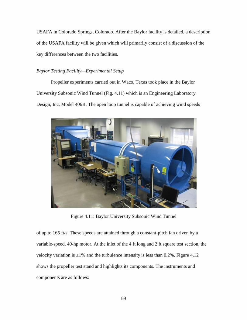
89
USAFA in Colorado Springs, Colorado. After the Baylor facility is detailed, a description
of the USAFA facility will be given which will primarily consist of a discussion of the
key differences between the two facilities.
Baylor Testing Facility—Experimental Setup
Propeller experiments carried out in Waco, Texas took place in the Baylor
University Subsonic Wind Tunnel (Fig. 4.11) which is an Engineering Laboratory
Design, Inc. Model 406B. The open loop tunnel is capable of achieving wind speeds
Figure 4.11: Baylor University Subsonic Wind Tunnel
of up to 165 ft/s. These speeds are attained through a constant-pitch fan driven by a
variable-speed, 40-hp motor. At the inlet of the 4 ft long and 2 ft square test section, the
velocity variation is ±1% and the turbulence intensity is less than 0.2%. Figure 4.12
shows the propeller test stand and highlights its components. The instruments and
components are as follows:
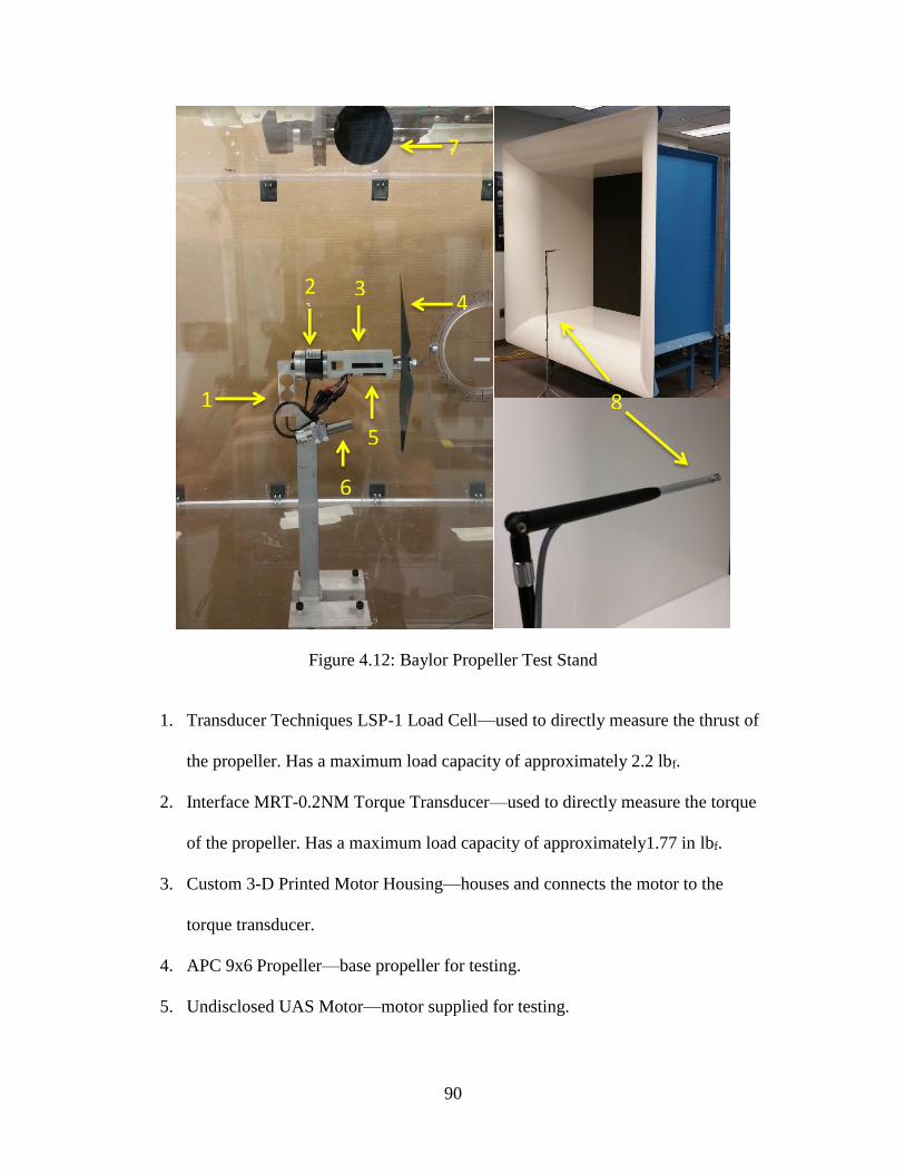
90
Figure 4.12: Baylor Propeller Test Stand
1. Transducer Techniques LSP-1 Load Cell—used to directly measure the thrust of
the propeller. Has a maximum load capacity of approximately 2.2 lbf.
2. Interface MRT-0.2NM Torque Transducer—used to directly measure the torque
of the propeller. Has a maximum load capacity of approximately1.77 in lbf.
3. Custom 3-D Printed Motor Housing—houses and connects the motor to the
torque transducer.
4. APC 9x6 Propeller—base propeller for testing.
5. Undisclosed UAS Motor—motor supplied for testing.
7
2 3 4
6
5
1 8
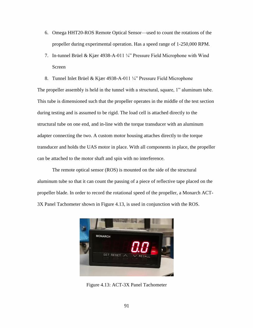
91
6. Omega HHT20-ROS Remote Optical Sensor—used to count the rotations of the
propeller during experimental operation. Has a speed range of 1-250,000 RPM.
7. In-tunnel Brüel & Kjær 4938-A-011 ¼” Pressure Field Microphone with Wind
Screen
8. Tunnel Inlet Brüel & Kjær 4938-A-011 ¼” Pressure Field Microphone
The propeller assembly is held in the tunnel with a structural, square, 1” aluminum tube.
This tube is dimensioned such that the propeller operates in the middle of the test section
during testing and is assumed to be rigid. The load cell is attached directly to the
structural tube on one end, and in-line with the torque transducer with an aluminum
adapter connecting the two. A custom motor housing attaches directly to the torque
transducer and holds the UAS motor in place. With all components in place, the propeller
can be attached to the motor shaft and spin with no interference.
The remote optical sensor (ROS) is mounted on the side of the structural
aluminum tube so that it can count the passing of a piece of reflective tape placed on the
propeller blade. In order to record the rotational speed of the propeller, a Monarch ACT-
3X Panel Tachometer shown in Figure 4.13, is used in conjunction with the ROS.
Figure 4.13: ACT-3X Panel Tachometer
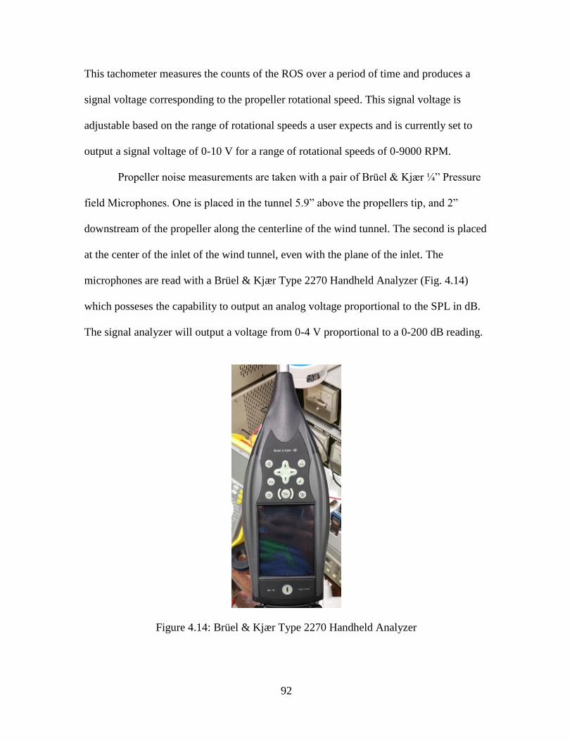
92
This tachometer measures the counts of the ROS over a period of time and produces a
signal voltage corresponding to the propeller rotational speed. This signal voltage is
adjustable based on the range of rotational speeds a user expects and is currently set to
output a signal voltage of 0-10 V for a range of rotational speeds of 0-9000 RPM.
Propeller noise measurements are taken with a pair of Brüel & Kjær ¼” Pressure
field Microphones. One is placed in the tunnel 5.9” above the propellers tip, and 2”
downstream of the propeller along the centerline of the wind tunnel. The second is placed
at the center of the inlet of the wind tunnel, even with the plane of the inlet. The
microphones are read with a Brüel & Kjær Type 2270 Handheld Analyzer (Fig. 4.14)
which posseses the capability to output an analog voltage proportional to the SPL in dB.
The signal analyzer will output a voltage from 0-4 V proportional to a 0-200 dB reading.
Figure 4.14: Brüel & Kjær Type 2270 Handheld Analyzer
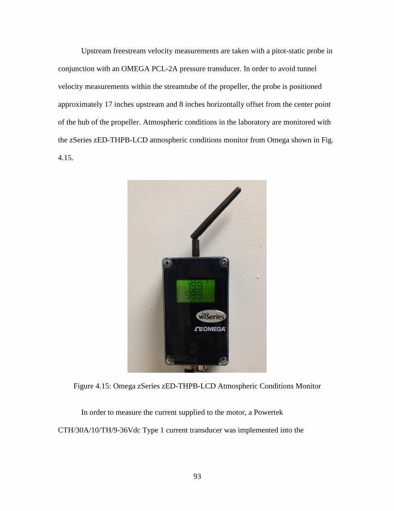
93
Upstream freestream velocity measurements are taken with a pitot-static probe in
conjunction with an OMEGA PCL-2A pressure transducer. In order to avoid tunnel
velocity measurements within the streamtube of the propeller, the probe is positioned
approximately 17 inches upstream and 8 inches horizontally offset from the center point
of the hub of the propeller. Atmospheric conditions in the laboratory are monitored with
the zSeries zED-THPB-LCD atmospheric conditions monitor from Omega shown in Fig.
4.15.
Figure 4.15: Omega zSeries zED-THPB-LCD Atmospheric Conditions Monitor
In order to measure the current supplied to the motor, a Powertek
CTH/30A/10/TH/9-36Vdc Type 1 current transducer was implemented into the
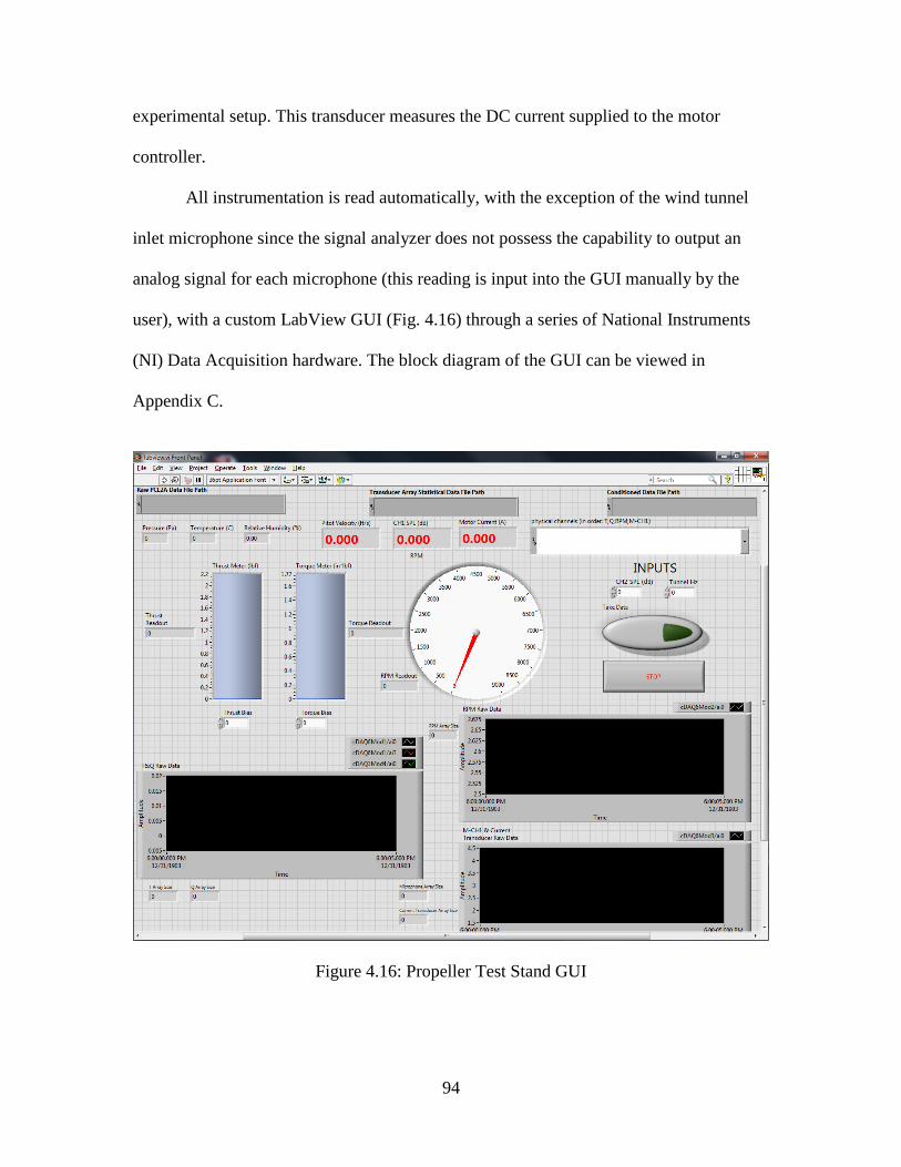
94
experimental setup. This transducer measures the DC current supplied to the motor
controller.
All instrumentation is read automatically, with the exception of the wind tunnel
inlet microphone since the signal analyzer does not possess the capability to output an
analog signal for each microphone (this reading is input into the GUI manually by the
user), with a custom LabView GUI (Fig. 4.16) through a series of National Instruments
(NI) Data Acquisition hardware. The block diagram of the GUI can be viewed in
Appendix C.
Figure 4.16: Propeller Test Stand GUI
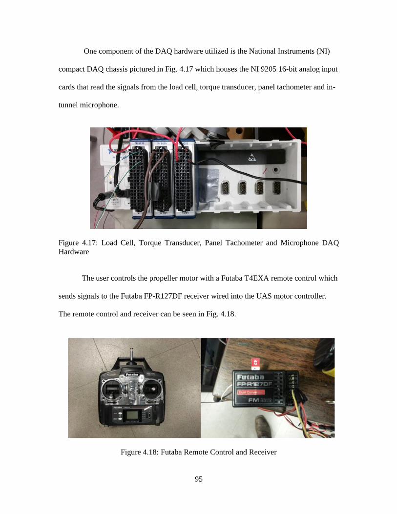
95
One component of the DAQ hardware utilized is the National Instruments (NI)
compact DAQ chassis pictured in Fig. 4.17 which houses the NI 9205 16-bit analog input
cards that read the signals from the load cell, torque transducer, panel tachometer and in-
tunnel microphone.
Figure 4.17: Load Cell, Torque Transducer, Panel Tachometer and Microphone DAQ
Hardware
The user controls the propeller motor with a Futaba T4EXA remote control which
sends signals to the Futaba FP-R127DF receiver wired into the UAS motor controller.
The remote control and receiver can be seen in Fig. 4.18.
Figure 4.18: Futaba Remote Control and Receiver
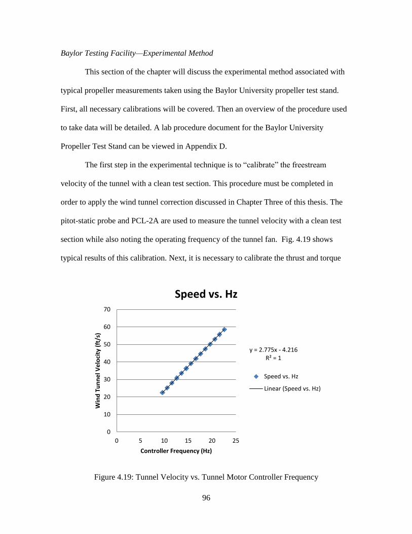
96
Baylor Testing Facility—Experimental Method
This section of the chapter will discuss the experimental method associated with
typical propeller measurements taken using the Baylor University propeller test stand.
First, all necessary calibrations will be covered. Then an overview of the procedure used
to take data will be detailed. A lab procedure document for the Baylor University
Propeller Test Stand can be viewed in Appendix D.
The first step in the experimental technique is to “calibrate” the freestream
velocity of the tunnel with a clean test section. This procedure must be completed in
order to apply the wind tunnel correction discussed in Chapter Three of this thesis. The
pitot-static probe and PCL-2A are used to measure the tunnel velocity with a clean test
section while also noting the operating frequency of the tunnel fan. Fig. 4.19 shows
typical results of this calibration. Next, it is necessary to calibrate the thrust and torque
Figure 4.19: Tunnel Velocity vs. Tunnel Motor Controller Frequency
y = 2.775x - 4.216R² = 1
0
10
20
30
40
50
60
70
0 5 10 15 20 25
Win
d T
un
ne
l Ve
loci
ty (
ft/s
)
Controller Frequency (Hz)
Speed vs. Hz
Speed vs. Hz
Linear (Speed vs. Hz)
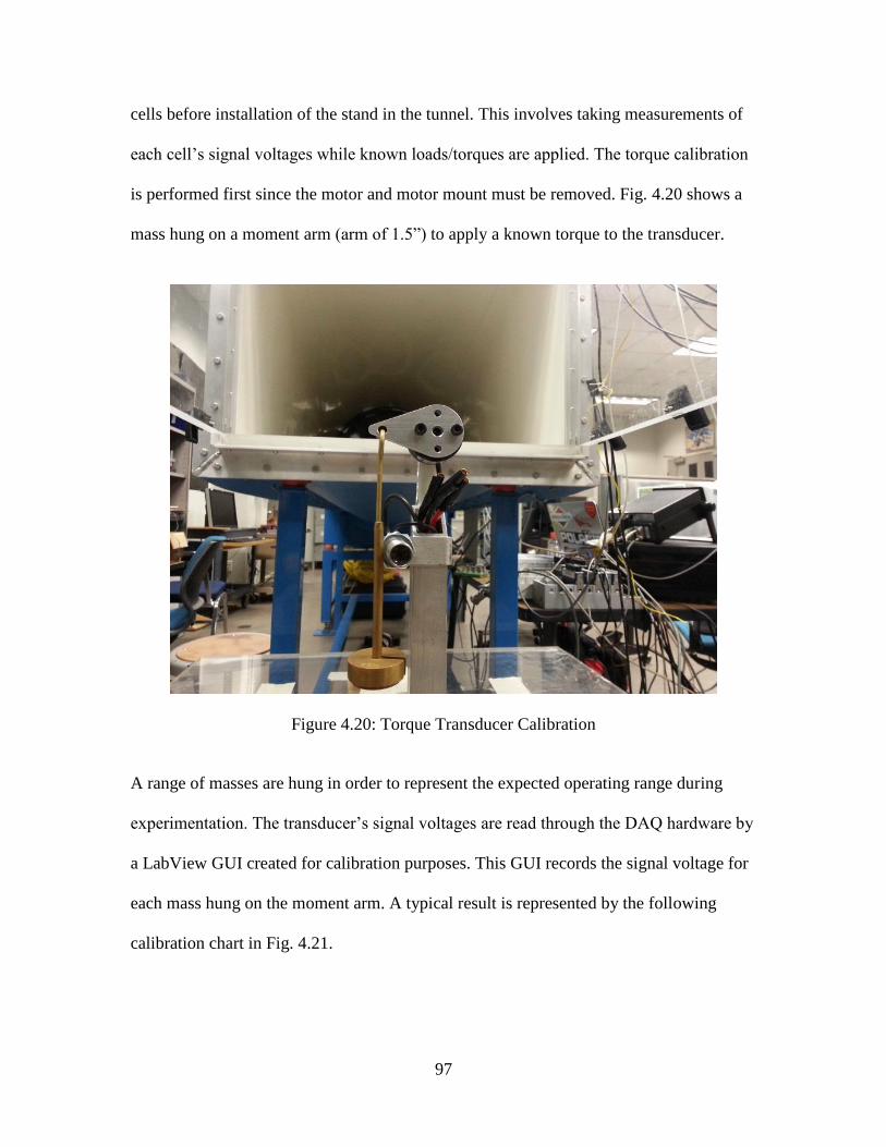
97
cells before installation of the stand in the tunnel. This involves taking measurements of
each cell’s signal voltages while known loads/torques are applied. The torque calibration
is performed first since the motor and motor mount must be removed. Fig. 4.20 shows a
mass hung on a moment arm (arm of 1.5”) to apply a known torque to the transducer.
Figure 4.20: Torque Transducer Calibration
A range of masses are hung in order to represent the expected operating range during
experimentation. The transducer’s signal voltages are read through the DAQ hardware by
a LabView GUI created for calibration purposes. This GUI records the signal voltage for
each mass hung on the moment arm. A typical result is represented by the following
calibration chart in Fig. 4.21.
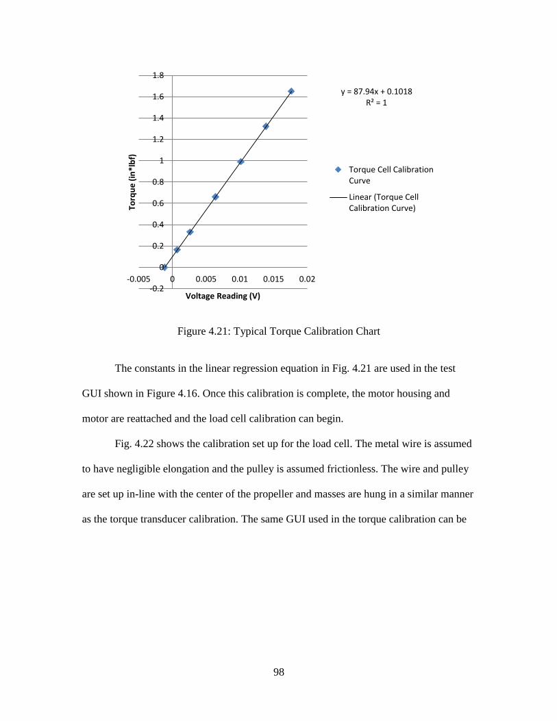
98
Figure 4.21: Typical Torque Calibration Chart
The constants in the linear regression equation in Fig. 4.21 are used in the test
GUI shown in Figure 4.16. Once this calibration is complete, the motor housing and
motor are reattached and the load cell calibration can begin.
Fig. 4.22 shows the calibration set up for the load cell. The metal wire is assumed
to have negligible elongation and the pulley is assumed frictionless. The wire and pulley
are set up in-line with the center of the propeller and masses are hung in a similar manner
as the torque transducer calibration. The same GUI used in the torque calibration can be
y = 87.94x + 0.1018R² = 1
-0.2
0
0.2
0.4
0.6
0.8
1
1.2
1.4
1.6
1.8
-0.005 0 0.005 0.01 0.015 0.02
Torq
ue
(in
*lb
f)
Voltage Reading (V)
Torque Cell CalibrationCurve
Linear (Torque CellCalibration Curve)
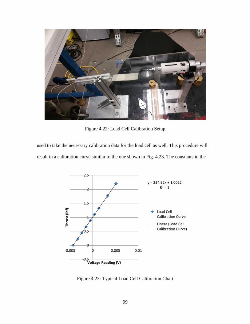
99
Figure 4.22: Load Cell Calibration Setup
used to take the necessary calibration data for the load cell as well. This procedure will
result in a calibration curve similar to the one shown in Fig. 4.23. The constants in the
Figure 4.23: Typical Load Cell Calibration Chart
y = 234.92x + 1.0022R² = 1
-0.5
0
0.5
1
1.5
2
2.5
-0.005 0 0.005 0.01
Thru
st (
lbf)
Voltage Reading (V)
Load CellCalibration Curve
Linear (Load CellCalibration Curve)
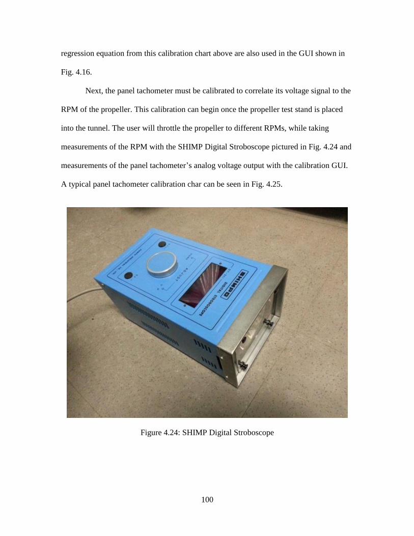
100
regression equation from this calibration chart above are also used in the GUI shown in
Fig. 4.16.
Next, the panel tachometer must be calibrated to correlate its voltage signal to the
RPM of the propeller. This calibration can begin once the propeller test stand is placed
into the tunnel. The user will throttle the propeller to different RPMs, while taking
measurements of the RPM with the SHIMP Digital Stroboscope pictured in Fig. 4.24 and
measurements of the panel tachometer’s analog voltage output with the calibration GUI.
A typical panel tachometer calibration char can be seen in Fig. 4.25.
Figure 4.24: SHIMP Digital Stroboscope
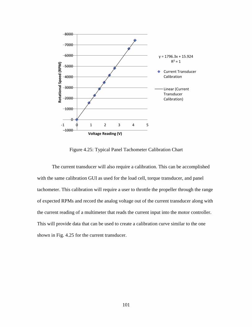
101
Figure 4.25: Typical Panel Tachometer Calibration Chart
The current transducer will also require a calibration. This can be accomplished
with the same calibration GUI as used for the load cell, torque transducer, and panel
tachometer. This calibration will require a user to throttle the propeller through the range
of expected RPMs and record the analog voltage out of the current transducer along with
the current reading of a multimeter that reads the current input into the motor controller.
This will provide data that can be used to create a calibration curve similar to the one
shown in Fig. 4.25 for the current transducer.
y = 1796.3x + 15.924R² = 1
-1000
0
1000
2000
3000
4000
5000
6000
7000
8000
-1 0 1 2 3 4 5
Ro
tati
on
al S
pe
ed
(R
PM
)
Voltage Reading (V)
Current TransducerCalibration
Linear (CurrentTransducerCalibration)
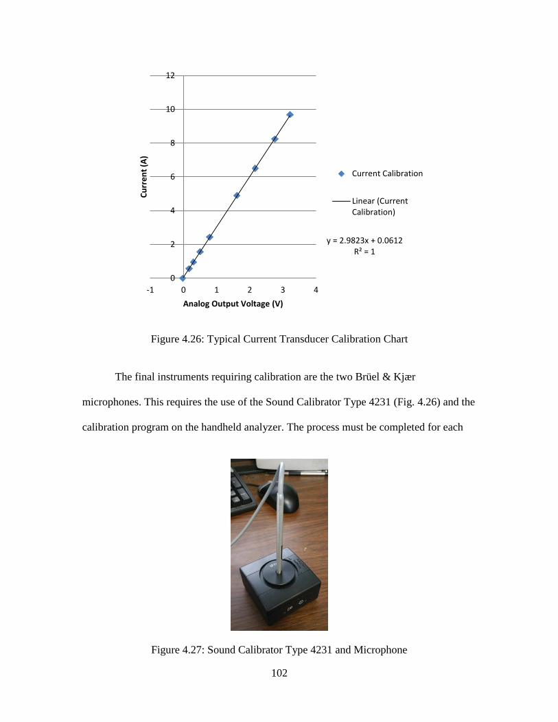
102
Figure 4.26: Typical Current Transducer Calibration Chart
The final instruments requiring calibration are the two Brüel & Kjær
microphones. This requires the use of the Sound Calibrator Type 4231 (Fig. 4.26) and the
calibration program on the handheld analyzer. The process must be completed for each
Figure 4.27: Sound Calibrator Type 4231 and Microphone
y = 2.9823x + 0.0612R² = 1
0
2
4
6
8
10
12
-1 0 1 2 3 4
Cu
rre
nt
(A)
Analog Output Voltage (V)
Current Calibration
Linear (CurrentCalibration)

103
microphone and is recommended that it completed each time the propeller test stand is
reinstalled in the wind tunnel. The process is simple in that it only requires the user to
turn on the calibrator, then run the calibration program on the signal analyzer.
Once the calibrations are complete, propeller testing can begin. The typical
testing procedure involves taking data for a range of rotational speeds at a single wind
tunnel velocity. The procedure is completed as follows:
1. Balance propeller and install on the motor.
2. Ensure that the testing environment will remain free of any noise sources that may
adversely influence measurements of the testing apparatus during the entirety of
the experiment.
3. With instrumentation warmed up as necessary to avoid thermal drift, open the
propeller test GUI in LabView, enter necessary file save paths, run the GUI, and
turn on the propeller receiver, remote control, and power supplies in that order.
4. Zero the thrust and torque readings on the GUI with the bias controls.
5. Enter the Wind Tunnel Inlet Microphone reading into the GUI.
6. Ensure that the Signal Analyzer Analog Output corresponds to the In-Tunnel
Microphone.
7. Take a data point without the wind tunnel running.
8. Turn on the wind tunnel controller to the frequency corresponding to the desired
tunnel velocity.
9. Enter the Wind Tunnel Inlet Microphone reading into the GUI.
10. Ensure that the Signal Analyzer Analog Output corresponds to the In-Tunnel
Microphone.
104
11. Note whether or not the propeller spins due to the aerodynamic forces imposed by
the set wind tunnel velocity and then take a data point.
12. Throttle the propeller to first RPM that produces positive thrust.
13. Enter Wind Tunnel Inlet Microphone reading into the GUI.
14. Ensure that the Signal Analyzer Analog Output corresponds to the In-Tunnel
Microphone.
15. Take a data point.
16. Throttle the propeller to the next desired RPM.
17. Repeat steps 12-15 for each data point.
18. Once test is complete throttle down the propeller, turn off the wind tunel, power
off the propeller motor power supplies, motor receiver, motor remote control, and
signal analyzer in that order. Also stop the test GUI in LabView.
The data reduction of the measurements is built into the GUI, along with the statistical
analysis of the measurements taken so that uncertainty measurements may be completed
during post-processing.
This experimental set up allows a user the ability to measure key variables
necessary in order to make comparisons between the measured results and theoretical
predictions. Further automation of the data reduction is possible.
USAFA Testing Facility
Replicating the USAFA testing facility’s test stand was of great importance when
constructing the test stand at Baylor. This was done in order to eliminate variables when
validating measurements between the two locations. This section of the chapter will
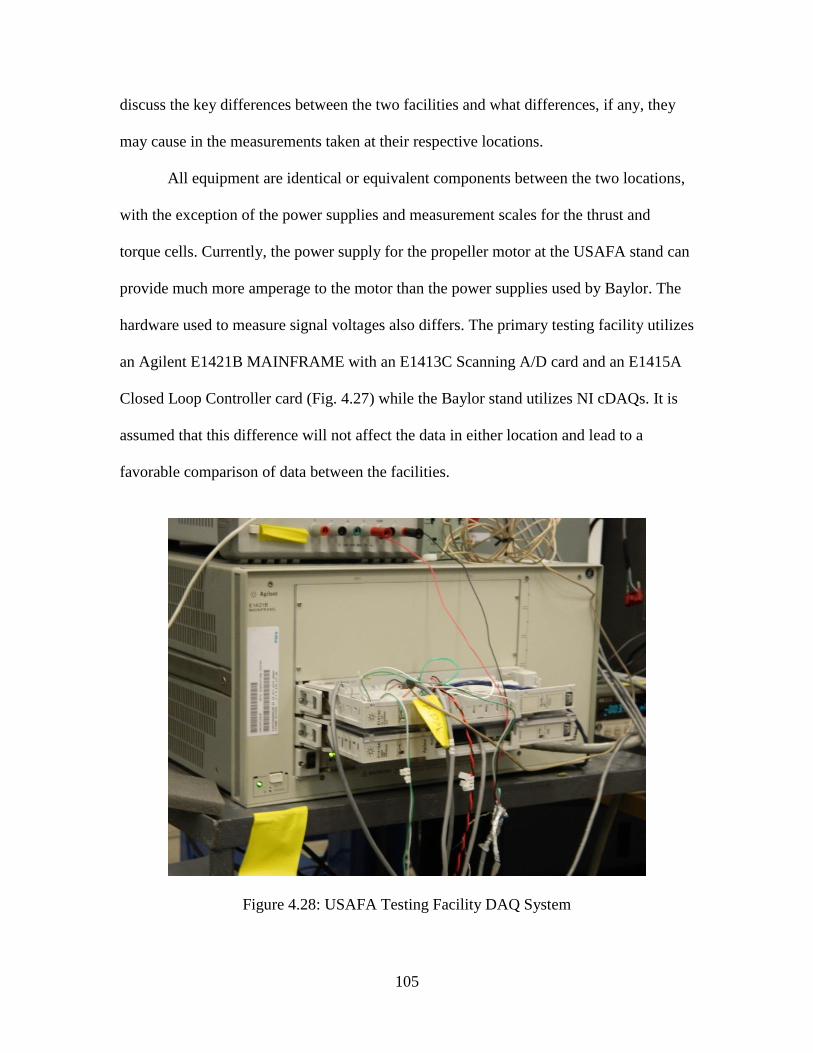
105
discuss the key differences between the two facilities and what differences, if any, they
may cause in the measurements taken at their respective locations.
All equipment are identical or equivalent components between the two locations,
with the exception of the power supplies and measurement scales for the thrust and
torque cells. Currently, the power supply for the propeller motor at the USAFA stand can
provide much more amperage to the motor than the power supplies used by Baylor. The
hardware used to measure signal voltages also differs. The primary testing facility utilizes
an Agilent E1421B MAINFRAME with an E1413C Scanning A/D card and an E1415A
Closed Loop Controller card (Fig. 4.27) while the Baylor stand utilizes NI cDAQs. It is
assumed that this difference will not affect the data in either location and lead to a
favorable comparison of data between the facilities.
Figure 4.28: USAFA Testing Facility DAQ System
106
The final key difference between the two test locations is the cross-sectional area
of the test sections. The USAFA facility has a 3’x 3’square test section with a 9 ft2 area.
This more than doubles the area of the Baylor wind tunnel which measures 2’x 2’ with a
4 ft2 area. The propeller blockage of a 9” diameter propeller at Baylor is approximately
11% while the blockage at the USAFA is approximately 5%. Wind tunnel blockage
corrections are taken into account at both locations as necessary, however, at the USAFA
these corrections are small to non-existant depending on propeller diameter.
Chapter Four Concluding Remarks
In conclusion, this chapter detailed the propeller design, theoretical propeller
performance prediction, experimental setup, and experimental procedures used in this
work. Bearcontrol gives a user the ability to rapidly design, theoretically analyze, and
solid-model propellers in SolidWorks while the experimental test stands lead to timely
evaluation of manufactured propeller models.
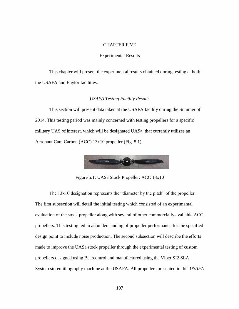
107
CHAPTER FIVE
Experimental Results
This chapter will present the experimental results obtained during testing at both
the USAFA and Baylor facilities.
USAFA Testing Facility Results
This section will present data taken at the USAFA facility during the Summer of
2014. This testing period was mainly concerned with testing propellers for a specific
military UAS of interest, which will be designated UASa, that currently utilizes an
Aeronaut Cam Carbon (ACC) 13x10 propeller (Fig. 5.1).
Figure 5.1: UASa Stock Propeller: ACC 13x10
The 13x10 designation represents the “diameter by the pitch” of the propeller.
The first subsection will detail the initial testing which consisted of an experimental
evaluation of the stock propeller along with several of other commercially available ACC
propellers. This testing led to an understanding of propeller performance for the specified
design point to include noise production. The second subsection will describe the efforts
made to improve the UASa stock propeller through the experimental testing of custom
propellers designed using Bearcontrol and manufactured using the Viper SI2 SLA
System stereolithography machine at the USAFA. All propellers presented in this USAFA
108
Testing Facility Results section were compared at the baseline operating condition
of producing 2.5 lbf of thrust at a wind tunnel velocity of 44 ft/s. Reynolds numbers seen
by propellers tested, both manufactured and custom, did not exceed 200,000 along the
length of the blade at the operating point of UASa. The uncertainties reported for the
USAFA test stand include a 1.4% uncertainty in the efficiency, and a 0.61 dB uncertainty
in the SPL reading [52].
Summer 2014, Commercial Propeller Experimental Evaluation
The initial study examined propellers operating in the low Reynolds number range
through the experimental evaluation of varying pitch, diameter, and number of blades in
the ACC Series. No design data was available from Aeronaut, so no theoretical
comparison could be done. As a reminder, the propeller operating requirements of UASa,
2.5 lbf of thrust at a flight velocity of 44 ft/s, were used as the point of comparison
between propellers. Figs. 5.2 and 5.3 plot propeller efficiency and SPL versus RPM for
the ACC propellers tested with varying pitch, diameter, and number of blades. Note that
for a propeller with a third designation such as ACC 13x10x3, the 3 represents the
number of propeller blades. If there is no third designation, the propeller is assumed to be
two bladed. The two plots show a variety of trends that were the basis for the design of
custom propellers. Fig. 5.2 shows that, in general, larger diameter and multi-bladed
propellers have higher efficiencies. These trends also translate to lower noise production.
The effect of pitch does not seem to follow an apparent trend, even between propellers
with the same diameter and number of blades.
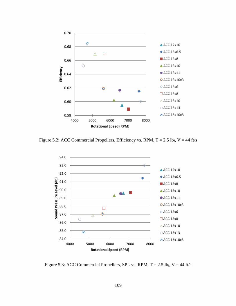
109
Figure 5.2: ACC Commercial Propellers, Efficiency vs. RPM, T = 2.5 lbf, V = 44 ft/s
Figure 5.3: ACC Commercial Propellers, SPL vs. RPM, T = 2.5 lbf, V = 44 ft/s
0.58
0.60
0.62
0.64
0.66
0.68
0.70
4000 5000 6000 7000 8000
Effi
cie
ncy
Rotational Speed (RPM)
ACC 12x10
ACC 13x6.5
ACC 13x8
ACC 13x10
ACC 13x11
ACC 13x10x3
ACC 15x6
ACC 15x8
ACC 15x10
ACC 15x13
ACC 15x10x3
84.0
85.0
86.0
87.0
88.0
89.0
90.0
91.0
92.0
93.0
94.0
4000 5000 6000 7000 8000
Sou
nd
Pre
ssu
re L
eve
l (d
B)
Rotational Speed (RPM)
ACC 12x10
ACC 13x6.5
ACC 13x8
ACC 13x10
ACC 13x11
ACC 13x10x3
ACC 15x6
ACC 15x8
ACC 15x10
ACC 15x13
ACC 15x10x3
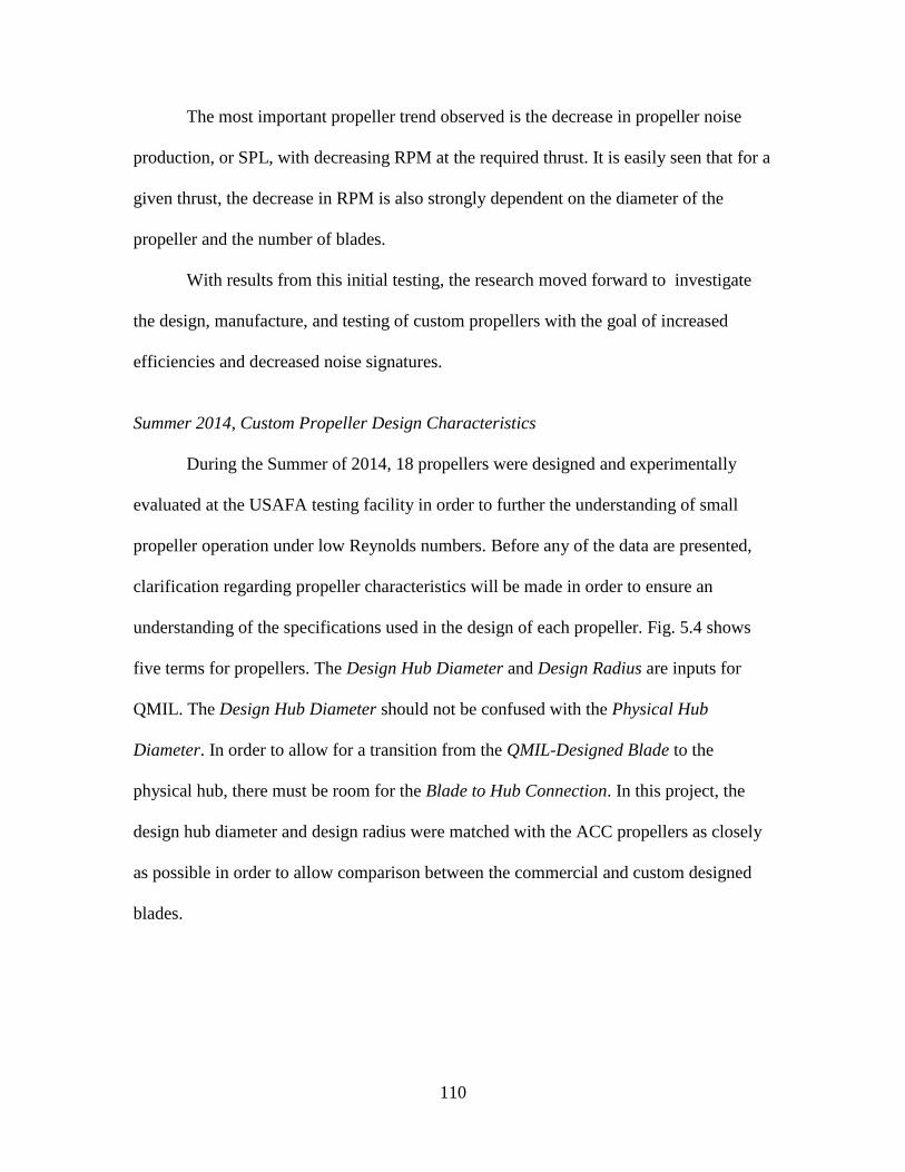
110
The most important propeller trend observed is the decrease in propeller noise
production, or SPL, with decreasing RPM at the required thrust. It is easily seen that for a
given thrust, the decrease in RPM is also strongly dependent on the diameter of the
propeller and the number of blades.
With results from this initial testing, the research moved forward to investigate
the design, manufacture, and testing of custom propellers with the goal of increased
efficiencies and decreased noise signatures.
Summer 2014, Custom Propeller Design Characteristics
During the Summer of 2014, 18 propellers were designed and experimentally
evaluated at the USAFA testing facility in order to further the understanding of small
propeller operation under low Reynolds numbers. Before any of the data are presented,
clarification regarding propeller characteristics will be made in order to ensure an
understanding of the specifications used in the design of each propeller. Fig. 5.4 shows
five terms for propellers. The Design Hub Diameter and Design Radius are inputs for
QMIL. The Design Hub Diameter should not be confused with the Physical Hub
Diameter. In order to allow for a transition from the QMIL-Designed Blade to the
physical hub, there must be room for the Blade to Hub Connection. In this project, the
design hub diameter and design radius were matched with the ACC propellers as closely
as possible in order to allow comparison between the commercial and custom designed
blades.
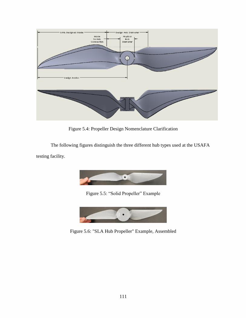
111
Figure 5.4: Propeller Design Nomenclature Clarification
The following figures distinguish the three different hub types used at the USAFA
testing facility.
Figure 5.5: “Solid Propeller” Example
Figure 5.6: "SLA Hub Propeller" Example, Assembled
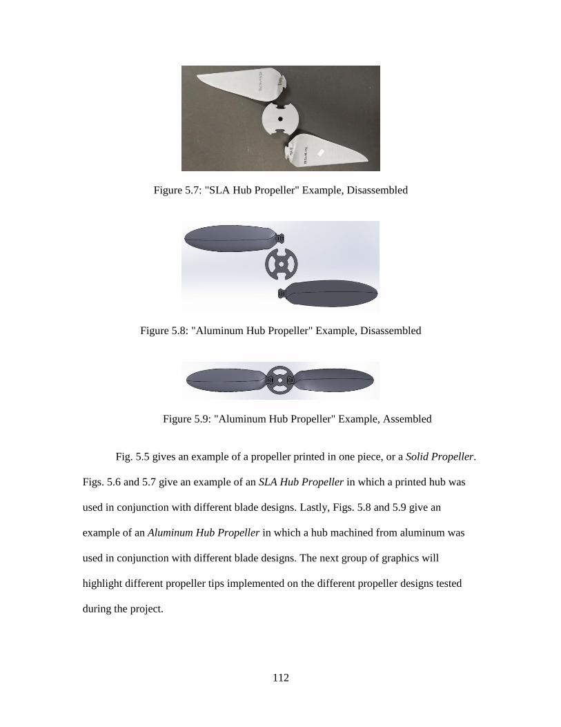
112
Figure 5.7: "SLA Hub Propeller" Example, Disassembled
Figure 5.8: "Aluminum Hub Propeller" Example, Disassembled
Figure 5.9: "Aluminum Hub Propeller" Example, Assembled
Fig. 5.5 gives an example of a propeller printed in one piece, or a Solid Propeller.
Figs. 5.6 and 5.7 give an example of an SLA Hub Propeller in which a printed hub was
used in conjunction with different blade designs. Lastly, Figs. 5.8 and 5.9 give an
example of an Aluminum Hub Propeller in which a hub machined from aluminum was
used in conjunction with different blade designs. The next group of graphics will
highlight different propeller tips implemented on the different propeller designs tested
during the project.
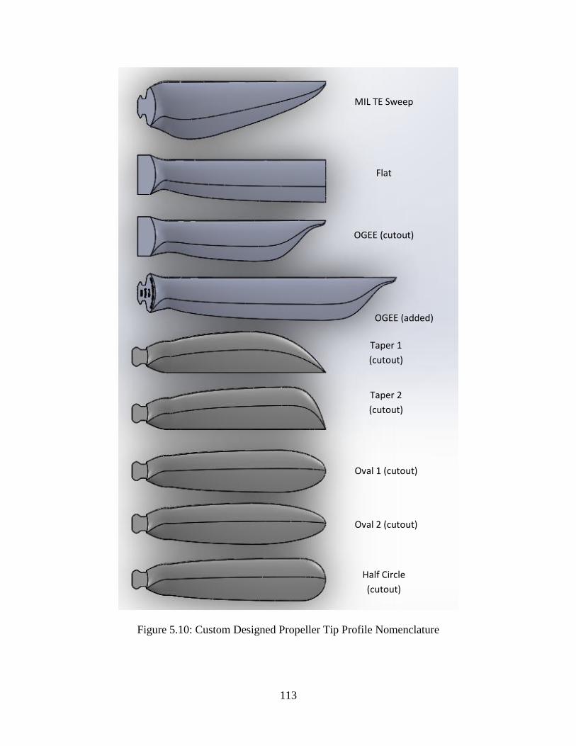
113
Figure 5.10: Custom Designed Propeller Tip Profile Nomenclature
MIL TE Sweep
Flat
OGEE (cutout)
Taper 1
(cutout)
Taper 2
(cutout)
Oval 1 (cutout)
OGEE (added)
Oval 2 (cutout)
Half Circle
(cutout)
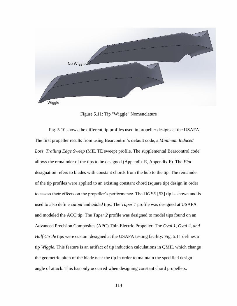
114
Figure 5.11: Tip "Wiggle" Nomenclature
Fig. 5.10 shows the different tip profiles used in propeller designs at the USAFA.
The first propeller results from using Bearcontrol’s default code, a Minimum Induced
Loss, Trailing Edge Sweep (MIL TE sweep) profile. The supplemental Bearcontrol code
allows the remainder of the tips to be designed (Appendix E, Appendix F). The Flat
designation refers to blades with constant chords from the hub to the tip. The remainder
of the tip profiles were applied to an existing constant chord (square tip) design in order
to assess their effects on the propeller’s performance. The OGEE [53] tip is shown and is
used to also define cutout and added tips. The Taper 1 profile was designed at USAFA
and modeled the ACC tip. The Taper 2 profile was designed to model tips found on an
Advanced Precision Composites (APC) Thin Electric Propeller. The Oval 1, Oval 2, and
Half Circle tips were custom designed at the USAFA testing facility. Fig. 5.11 defines a
tip Wiggle. This feature is an artifact of tip induction calculations in QMIL which change
the geometric pitch of the blade near the tip in order to maintain the specified design
angle of attack. This has only occurred when designing constant chord propellers.
No Wiggle
Wiggle
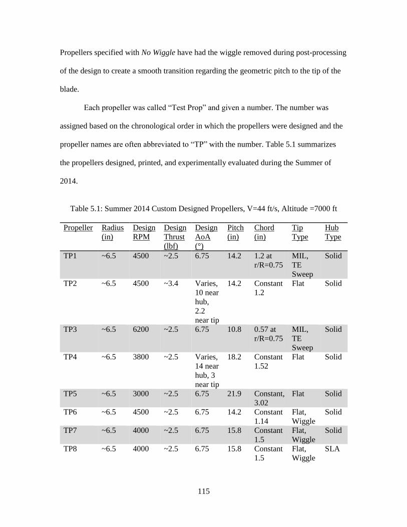
115
Propellers specified with No Wiggle have had the wiggle removed during post-processing
of the design to create a smooth transition regarding the geometric pitch to the tip of the
blade.
Each propeller was called “Test Prop” and given a number. The number was
assigned based on the chronological order in which the propellers were designed and the
propeller names are often abbreviated to “TP” with the number. Table 5.1 summarizes
the propellers designed, printed, and experimentally evaluated during the Summer of
2014.
Table 5.1: Summer 2014 Custom Designed Propellers, V=44 ft/s, Altitude =7000 ft
Propeller Radius
(in)
Design
RPM
Design
Thrust
(lbf)
Design
AoA
(°)
Pitch
(in)
Chord
(in)
Tip
Type
Hub
Type
TP1 ~6.5 4500 ~2.5 6.75 14.2 1.2 at
r/R=0.75
MIL,
TE
Sweep
Solid
TP2 ~6.5 4500 ~3.4 Varies,
10 near
hub,
2.2
near tip
14.2 Constant
1.2
Flat Solid
TP3 ~6.5 6200 ~2.5 6.75 10.8 0.57 at
r/R=0.75
MIL,
TE
Sweep
Solid
TP4 ~6.5 3800 ~2.5 Varies,
14 near
hub, 3
near tip
18.2 Constant
1.52
Flat Solid
TP5 ~6.5 3000 ~2.5 6.75 21.9 Constant,
3.02
Flat Solid
TP6 ~6.5 4500 ~2.5 6.75 14.2 Constant
1.14
Flat,
Wiggle
Solid
TP7 ~6.5 4000 ~2.5 6.75 15.8 Constant
1.5
Flat,
Wiggle
Solid
TP8 ~6.5 4000 ~2.5 6.75 15.8 Constant
1.5
Flat,
Wiggle
SLA
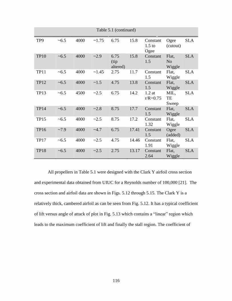
116
Table 5.1 (continued)
TP9 ~6.5 4000 ~1.75 6.75 15.8 Constant
1.5 to
Ogee
Ogee
(cutout)
SLA
TP10 ~6.5 4000 ~2.9 6.75
(tip
altered)
15.8 Constant
1.5
Flat,
No
Wiggle
SLA
TP11 ~6.5 4000 ~1.45 2.75 11.7 Constant
1.5
Flat,
Wiggle
SLA
TP12 ~6.5 4000 ~1.5 4.75 13.8 Constant
1.5
Flat,
Wiggle
SLA
TP13 ~6.5 4500 ~2.5 6.75 14.2 1.2 at
r/R=0.75
MIL,
TE
Sweep
SLA
TP14 ~6.5 4000 ~2.8 8.75 17.7 Constant
1.5
Flat,
Wiggle
SLA
TP15 ~6.5 4000 ~2.5 8.75 17.2 Constant
1.32
Flat,
Wiggle
SLA
TP16 ~7.9 4000 ~4.7 6.75 17.41 Constant
1.5
Ogee
(added)
SLA
TP17 ~6.5 4000 ~2.5 4.75 14.46 Constant
1.91
Flat,
Wiggle
SLA
TP18 ~6.5 4000 ~2.5 2.75 13.17 Constant
2.64
Flat,
Wiggle
SLA
All propellers in Table 5.1 were designed with the Clark Y airfoil cross section
and experimental data obtained from UIUC for a Reynolds number of 100,000 [21]. The
cross section and airfoil data are shown in Figs. 5.12 through 5.15. The Clark Y is a
relatively thick, cambered airfoil as can be seen from Fig. 5.12. It has a typical coefficient
of lift versus angle of attack of plot in Fig. 5.13 which contains a “linear” region which
leads to the maximum coefficient of lift and finally the stall region. The coefficient of
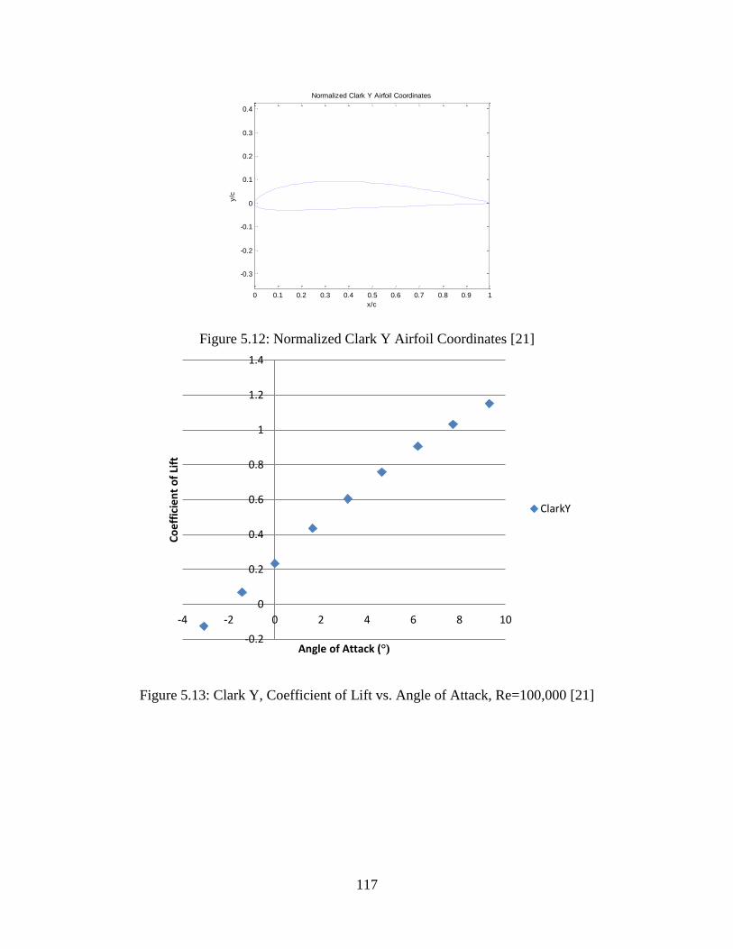
117
Figure 5.12: Normalized Clark Y Airfoil Coordinates [21]
Figure 5.13: Clark Y, Coefficient of Lift vs. Angle of Attack, Re=100,000 [21]
0 0.1 0.2 0.3 0.4 0.5 0.6 0.7 0.8 0.9 1
-0.3
-0.2
-0.1
0
0.1
0.2
0.3
0.4
Normalized Clark Y Airfoil Coordinates
x/c
y/c
-0.2
0
0.2
0.4
0.6
0.8
1
1.2
1.4
-4 -2 0 2 4 6 8 10
Co
eff
icie
nt
of
Lift
Angle of Attack (°)
ClarkY
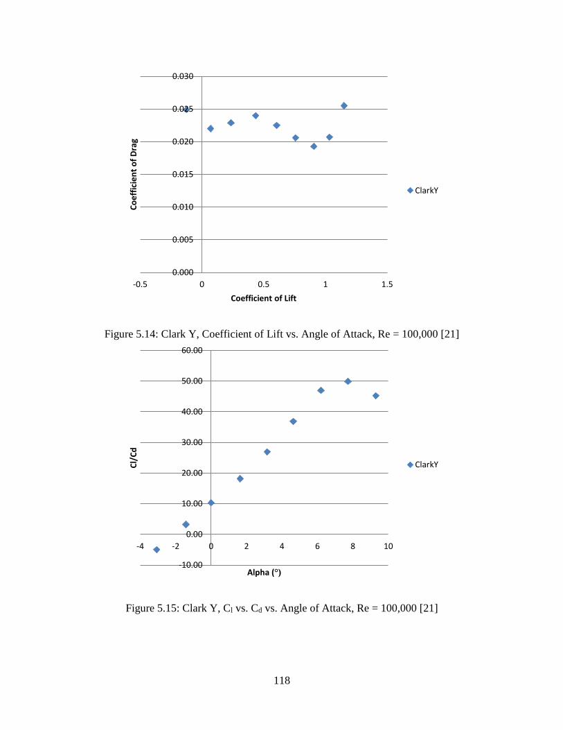
118
Figure 5.14: Clark Y, Coefficient of Lift vs. Angle of Attack, Re = 100,000 [21]
Figure 5.15: Clark Y, Cl vs. Cd vs. Angle of Attack, Re = 100,000 [21]
0.000
0.005
0.010
0.015
0.020
0.025
0.030
-0.5 0 0.5 1 1.5
Co
eff
icie
nt
of
Dra
g
Coefficient of Lift
ClarkY
-10.00
0.00
10.00
20.00
30.00
40.00
50.00
60.00
-4 -2 0 2 4 6 8 10
Cl/
Cd
Alpha (°)
ClarkY
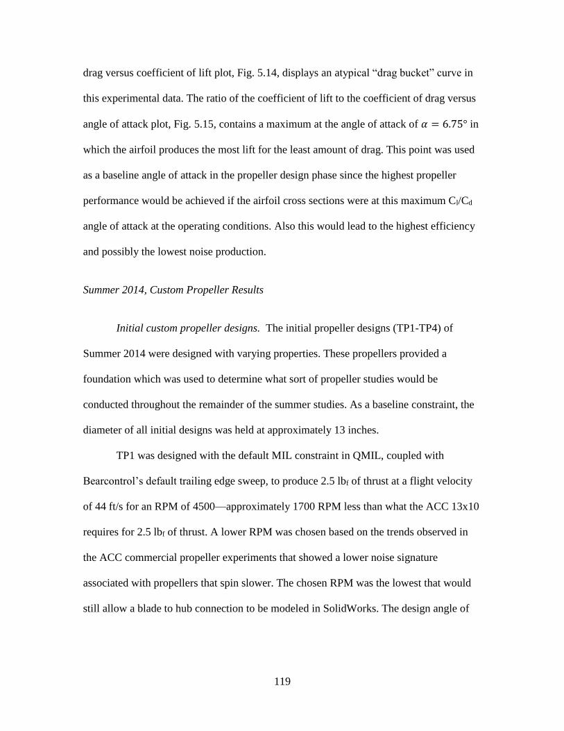
119
drag versus coefficient of lift plot, Fig. 5.14, displays an atypical “drag bucket” curve in
this experimental data. The ratio of the coefficient of lift to the coefficient of drag versus
angle of attack plot, Fig. 5.15, contains a maximum at the angle of attack of 𝛼 = 6.75° in
which the airfoil produces the most lift for the least amount of drag. This point was used
as a baseline angle of attack in the propeller design phase since the highest propeller
performance would be achieved if the airfoil cross sections were at this maximum Cl/Cd
angle of attack at the operating conditions. Also this would lead to the highest efficiency
and possibly the lowest noise production.
Summer 2014, Custom Propeller Results
Initial custom propeller designs. The initial propeller designs (TP1-TP4) of
Summer 2014 were designed with varying properties. These propellers provided a
foundation which was used to determine what sort of propeller studies would be
conducted throughout the remainder of the summer studies. As a baseline constraint, the
diameter of all initial designs was held at approximately 13 inches.
TP1 was designed with the default MIL constraint in QMIL, coupled with
Bearcontrol’s default trailing edge sweep, to produce 2.5 lbf of thrust at a flight velocity
of 44 ft/s for an RPM of 4500—approximately 1700 RPM less than what the ACC 13x10
requires for 2.5 lbf of thrust. A lower RPM was chosen based on the trends observed in
the ACC commercial propeller experiments that showed a lower noise signature
associated with propellers that spin slower. The chosen RPM was the lowest that would
still allow a blade to hub connection to be modeled in SolidWorks. The design angle of
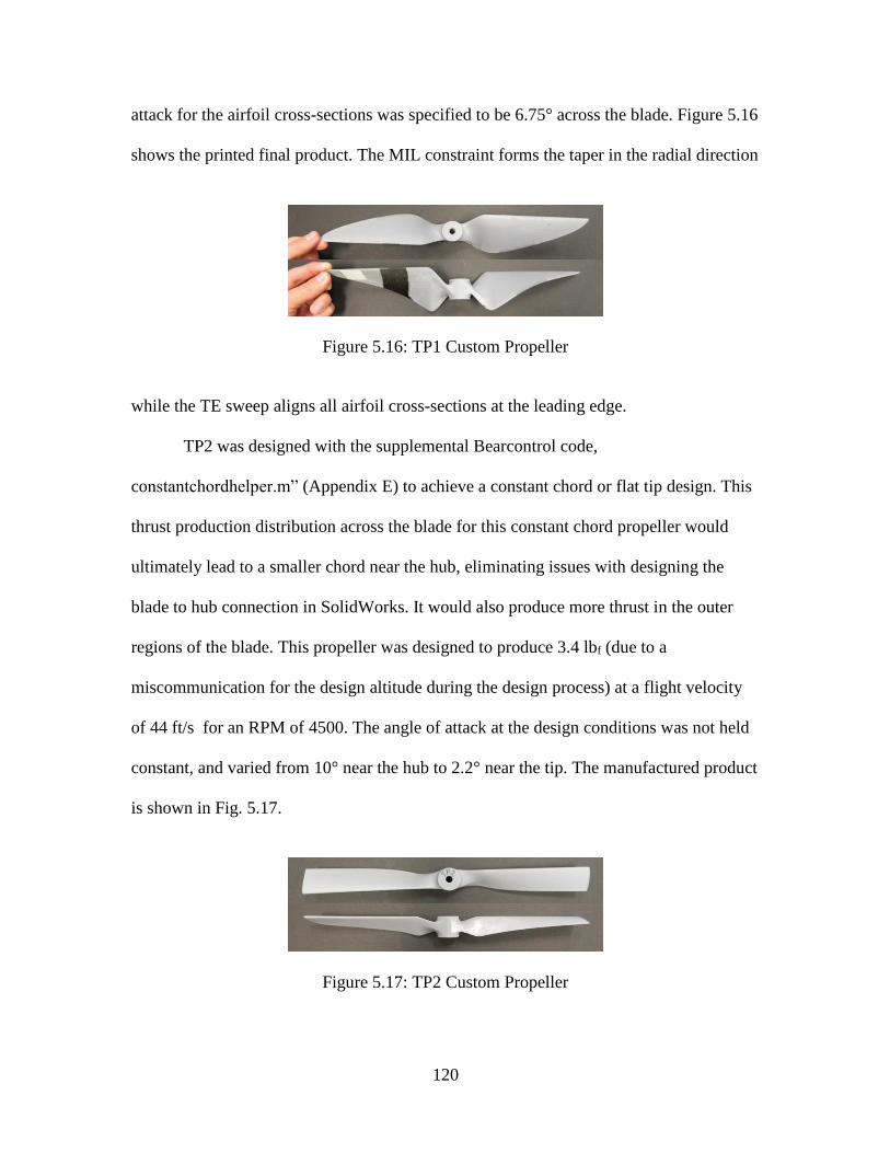
120
attack for the airfoil cross-sections was specified to be 6.75° across the blade. Figure 5.16
shows the printed final product. The MIL constraint forms the taper in the radial direction
Figure 5.16: TP1 Custom Propeller
while the TE sweep aligns all airfoil cross-sections at the leading edge.
TP2 was designed with the supplemental Bearcontrol code,
constantchordhelper.m” (Appendix E) to achieve a constant chord or flat tip design. This
thrust production distribution across the blade for this constant chord propeller would
ultimately lead to a smaller chord near the hub, eliminating issues with designing the
blade to hub connection in SolidWorks. It would also produce more thrust in the outer
regions of the blade. This propeller was designed to produce 3.4 lbf (due to a
miscommunication for the design altitude during the design process) at a flight velocity
of 44 ft/s for an RPM of 4500. The angle of attack at the design conditions was not held
constant, and varied from 10° near the hub to 2.2° near the tip. The manufactured product
is shown in Fig. 5.17.
Figure 5.17: TP2 Custom Propeller
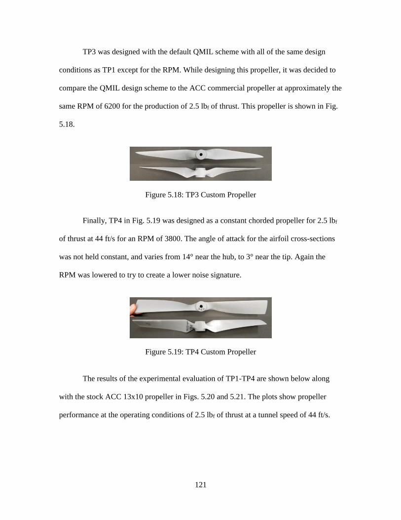
121
TP3 was designed with the default QMIL scheme with all of the same design
conditions as TP1 except for the RPM. While designing this propeller, it was decided to
compare the QMIL design scheme to the ACC commercial propeller at approximately the
same RPM of 6200 for the production of 2.5 lbf of thrust. This propeller is shown in Fig.
5.18.
Figure 5.18: TP3 Custom Propeller
Finally, TP4 in Fig. 5.19 was designed as a constant chorded propeller for 2.5 lbf
of thrust at 44 ft/s for an RPM of 3800. The angle of attack for the airfoil cross-sections
was not held constant, and varies from 14° near the hub, to 3° near the tip. Again the
RPM was lowered to try to create a lower noise signature.
Figure 5.19: TP4 Custom Propeller
The results of the experimental evaluation of TP1-TP4 are shown below along
with the stock ACC 13x10 propeller in Figs. 5.20 and 5.21. The plots show propeller
performance at the operating conditions of 2.5 lbf of thrust at a tunnel speed of 44 ft/s.
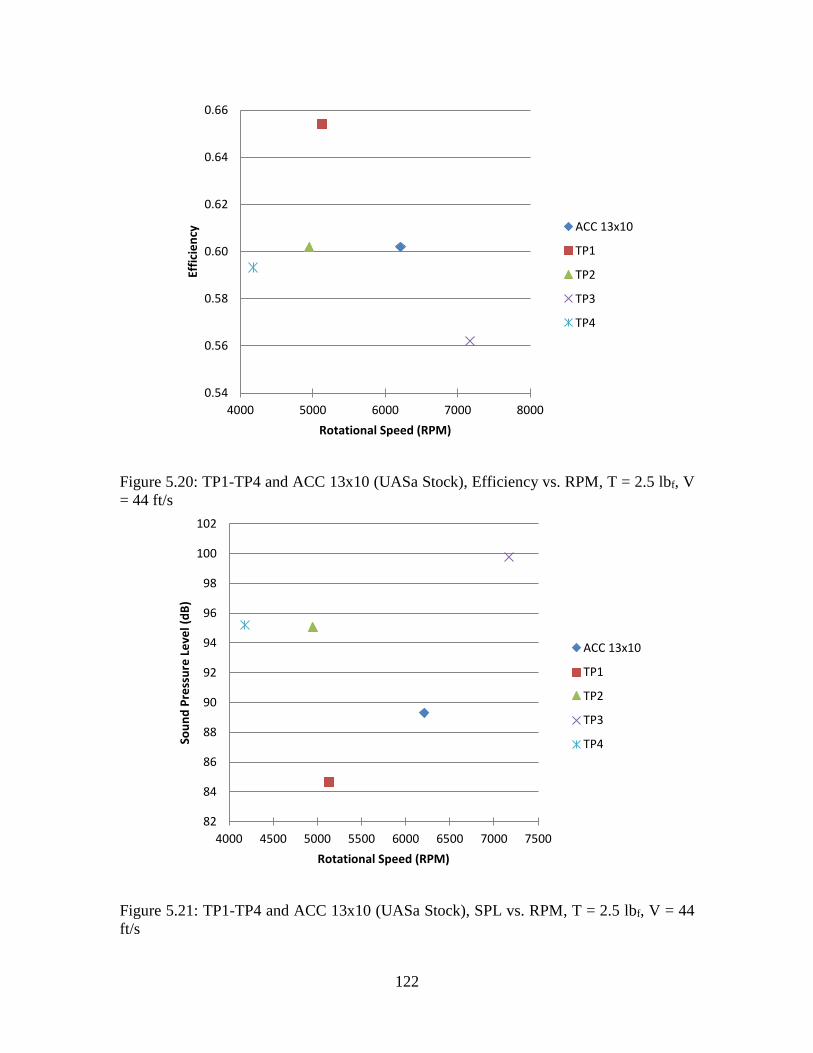
122
Figure 5.20: TP1-TP4 and ACC 13x10 (UASa Stock), Efficiency vs. RPM, T = 2.5 lbf, V
= 44 ft/s
Figure 5.21: TP1-TP4 and ACC 13x10 (UASa Stock), SPL vs. RPM, T = 2.5 lbf, V = 44
ft/s
0.54
0.56
0.58
0.60
0.62
0.64
0.66
4000 5000 6000 7000 8000
Effi
cie
ncy
Rotational Speed (RPM)
ACC 13x10
TP1
TP2
TP3
TP4
82
84
86
88
90
92
94
96
98
100
102
4000 4500 5000 5500 6000 6500 7000 7500
Sou
nd
Pre
ssu
re L
eve
l (d
B)
Rotational Speed (RPM)
ACC 13x10
TP1
TP2
TP3
TP4
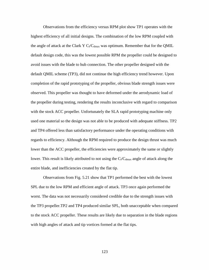
123
Observations from the efficiency versus RPM plot show TP1 operates with the
highest efficiency of all initial designs. The combination of the low RPM coupled with
the angle of attack at the Clark Y Cl/Cdmax was optimum. Remember that for the QMIL
default design code, this was the lowest possible RPM the propeller could be designed to
avoid issues with the blade to hub connection. The other propeller designed with the
default QMIL scheme (TP3), did not continue the high efficiency trend however. Upon
completion of the rapid prototyping of the propeller, obvious blade strength issues were
observed. This propeller was thought to have deformed under the aerodynamic load of
the propeller during testing, rendering the results inconclusive with regard to comparison
with the stock ACC propeller. Unfortunately the SLA rapid prototyping machine only
used one material so the design was not able to be produced with adequate stiffness. TP2
and TP4 offered less than satisfactory performance under the operating conditions with
regards to efficiency. Although the RPM required to produce the design thrust was much
lower than the ACC propeller, the efficiencies were approximately the same or slightly
lower. This result is likely attributed to not using the Cl/Cdmax angle of attack along the
entire blade, and inefficiencies created by the flat tip.
Observations from Fig. 5.21 show that TP1 performed the best with the lowest
SPL due to the low RPM and efficient angle of attack. TP3 once again performed the
worst. The data was not necessarily considered credible due to the strength issues with
the TP3 propeller.TP2 and TP4 produced similar SPL, both unacceptable when compared
to the stock ACC propeller. These results are likely due to separation in the blade regions
with high angles of attack and tip vortices formed at the flat tips.
124
The initial custom propeller study provided a baseline with which to design
propellers for the remainder of the summer. The following will detail the remaining
propeller studies and associated experimental results.
Constant chord, RPM study. This study sought to determine the effects of
holding all design parameters constant except for the RPM and chord length for constant
chorded blades. TP5-TP7 were all designed with a diameter of approximately 13 inches
to produce 2.5 lbf of thrust at a tunnel velocity of 44 ft/s with an angle of attack of 6.75°
across the entire blade. TP5 was designed for 3000 RPM, TP6 for 4500 RPM, and TP7
for 4000 RPM. Figs. 5.22-5.24 display the final products of the design and manufacture
for each propeller.
Figure 5.22: TP5 Custom Propeller
Figure 5.23: TP6 Custom Propeller
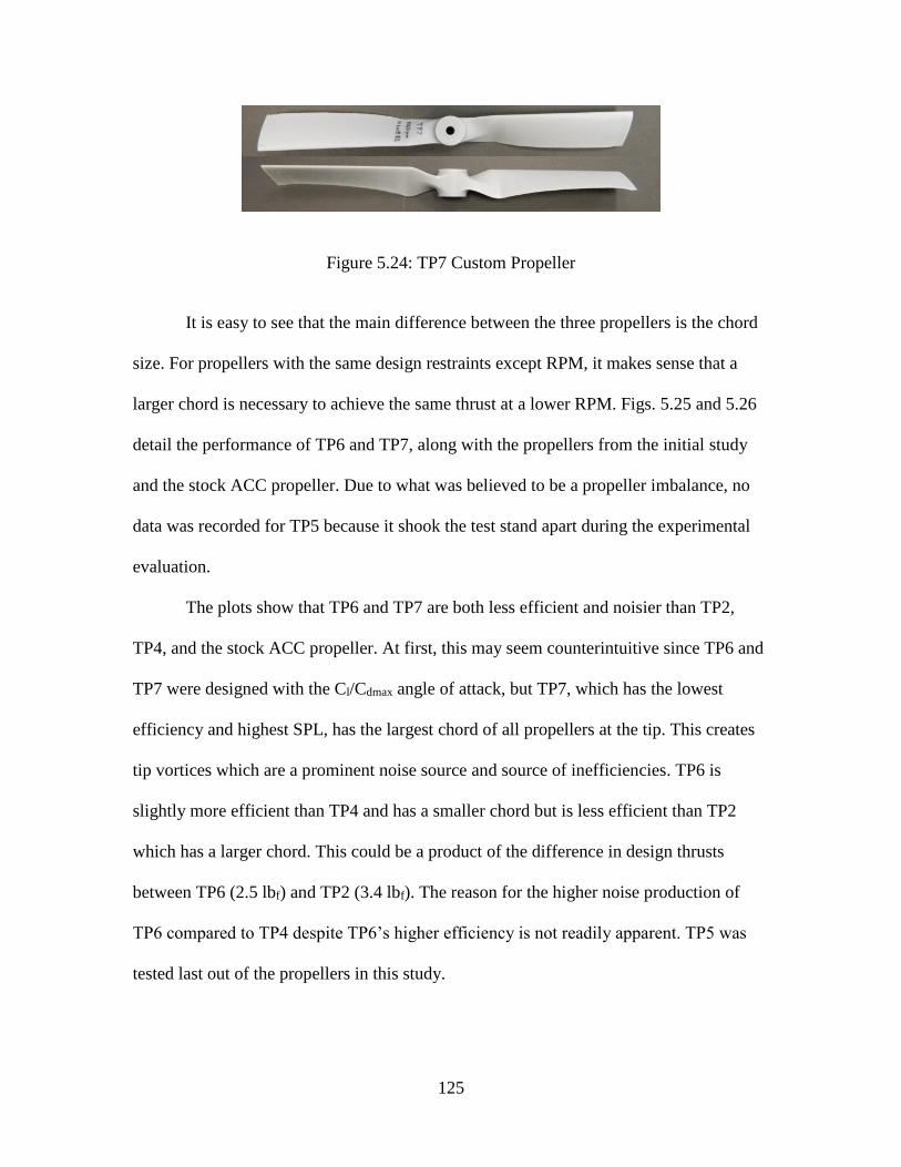
125
Figure 5.24: TP7 Custom Propeller
It is easy to see that the main difference between the three propellers is the chord
size. For propellers with the same design restraints except RPM, it makes sense that a
larger chord is necessary to achieve the same thrust at a lower RPM. Figs. 5.25 and 5.26
detail the performance of TP6 and TP7, along with the propellers from the initial study
and the stock ACC propeller. Due to what was believed to be a propeller imbalance, no
data was recorded for TP5 because it shook the test stand apart during the experimental
evaluation.
The plots show that TP6 and TP7 are both less efficient and noisier than TP2,
TP4, and the stock ACC propeller. At first, this may seem counterintuitive since TP6 and
TP7 were designed with the Cl/Cdmax angle of attack, but TP7, which has the lowest
efficiency and highest SPL, has the largest chord of all propellers at the tip. This creates
tip vortices which are a prominent noise source and source of inefficiencies. TP6 is
slightly more efficient than TP4 and has a smaller chord but is less efficient than TP2
which has a larger chord. This could be a product of the difference in design thrusts
between TP6 (2.5 lbf) and TP2 (3.4 lbf). The reason for the higher noise production of
TP6 compared to TP4 despite TP6’s higher efficiency is not readily apparent. TP5 was
tested last out of the propellers in this study.
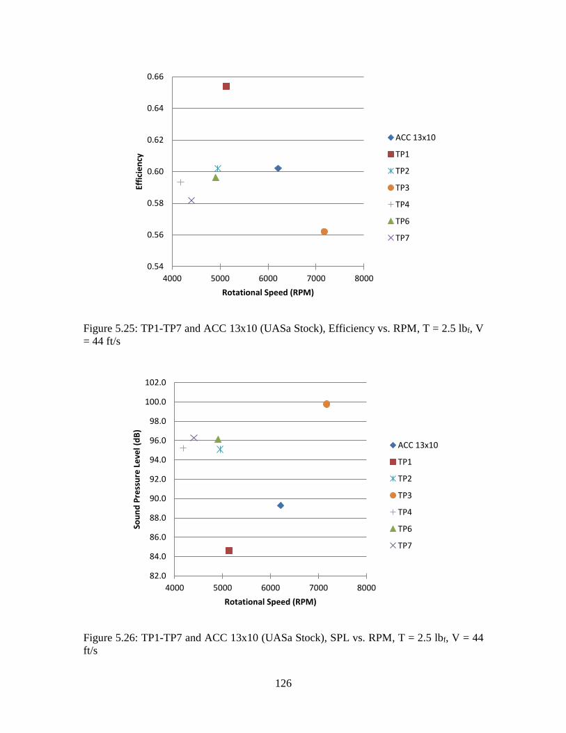
126
Figure 5.25: TP1-TP7 and ACC 13x10 (UASa Stock), Efficiency vs. RPM, T = 2.5 lbf, V
= 44 ft/s
Figure 5.26: TP1-TP7 and ACC 13x10 (UASa Stock), SPL vs. RPM, T = 2.5 lbf, V = 44
ft/s
0.54
0.56
0.58
0.60
0.62
0.64
0.66
4000 5000 6000 7000 8000
Effi
cie
ncy
Rotational Speed (RPM)
ACC 13x10
TP1
TP2
TP3
TP4
TP6
TP7
82.0
84.0
86.0
88.0
90.0
92.0
94.0
96.0
98.0
100.0
102.0
4000 5000 6000 7000 8000
Sou
nd
Pre
ssu
re L
eve
l (d
B)
Rotational Speed (RPM)
ACC 13x10
TP1
TP2
TP3
TP4
TP6
TP7
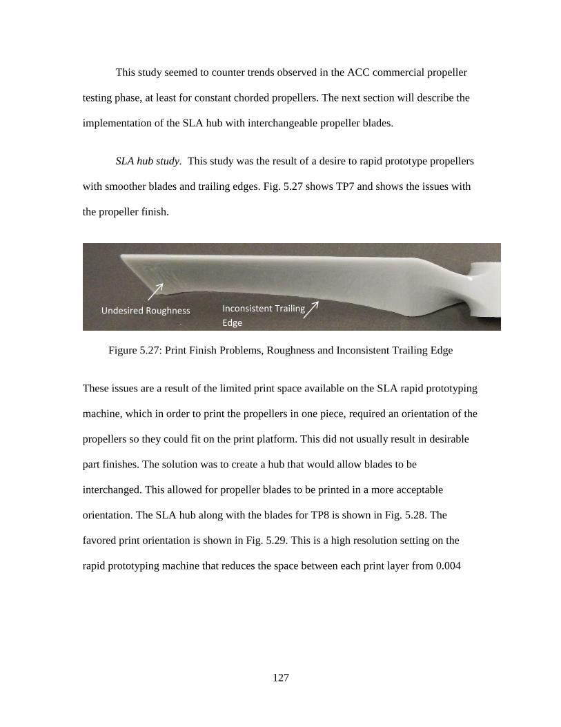
127
This study seemed to counter trends observed in the ACC commercial propeller
testing phase, at least for constant chorded propellers. The next section will describe the
implementation of the SLA hub with interchangeable propeller blades.
SLA hub study. This study was the result of a desire to rapid prototype propellers
with smoother blades and trailing edges. Fig. 5.27 shows TP7 and shows the issues with
the propeller finish.
Figure 5.27: Print Finish Problems, Roughness and Inconsistent Trailing Edge
These issues are a result of the limited print space available on the SLA rapid prototyping
machine, which in order to print the propellers in one piece, required an orientation of the
propellers so they could fit on the print platform. This did not usually result in desirable
part finishes. The solution was to create a hub that would allow blades to be
interchanged. This allowed for propeller blades to be printed in a more acceptable
orientation. The SLA hub along with the blades for TP8 is shown in Fig. 5.28. The
favored print orientation is shown in Fig. 5.29. This is a high resolution setting on the
rapid prototyping machine that reduces the space between each print layer from 0.004
Undesired Roughness Inconsistent Trailing
Edge
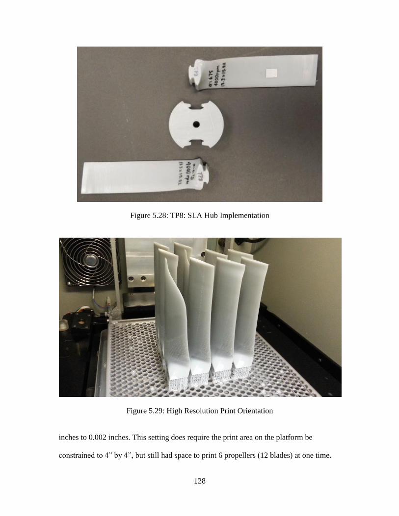
128
Figure 5.28: TP8: SLA Hub Implementation
Figure 5.29: High Resolution Print Orientation
inches to 0.002 inches. This setting does require the print area on the platform be
constrained to 4” by 4”, but still had space to print 6 propellers (12 blades) at one time.
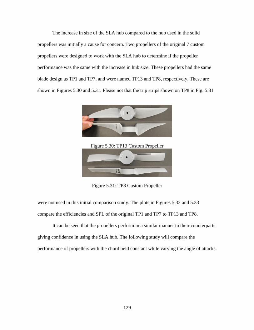
129
The increase in size of the SLA hub compared to the hub used in the solid
propellers was initially a cause for concern. Two propellers of the original 7 custom
propellers were designed to work with the SLA hub to determine if the propeller
performance was the same with the increase in hub size. These propellers had the same
blade design as TP1 and TP7, and were named TP13 and TP8, respectively. These are
shown in Figures 5.30 and 5.31. Please not that the trip strips shown on TP8 in Fig. 5.31
Figure 5.30: TP13 Custom Propeller
Figure 5.31: TP8 Custom Propeller
were not used in this initial comparison study. The plots in Figures 5.32 and 5.33
compare the efficiencies and SPL of the original TP1 and TP7 to TP13 and TP8.
It can be seen that the propellers perform in a similar manner to their counterparts
giving confidence in using the SLA hub. The following study will compare the
performance of propellers with the chord held constant while varying the angle of attacks.
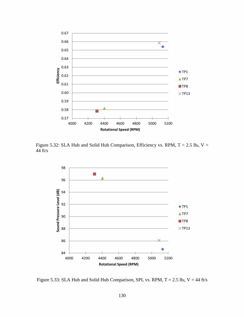
130
Figure 5.32: SLA Hub and Solid Hub Comparison, Efficiency vs. RPM, T = 2.5 lbf, V =
44 ft/s
Figure 5.33: SLA Hub and Solid Hub Comparison, SPL vs. RPM, T = 2.5 lbf, V = 44 ft/s
0.57
0.58
0.59
0.60
0.61
0.62
0.63
0.64
0.65
0.66
0.67
4000 4200 4400 4600 4800 5000 5200
Effi
cie
ncy
Rotational Speed (RPM)
TP1
TP7
TP8
TP13
84
86
88
90
92
94
96
98
4000 4200 4400 4600 4800 5000 5200
Sou
nd
Pre
ssu
re L
eve
l (d
B)
Rotational Speed (RPM)
TP1
TP7
TP8
TP13
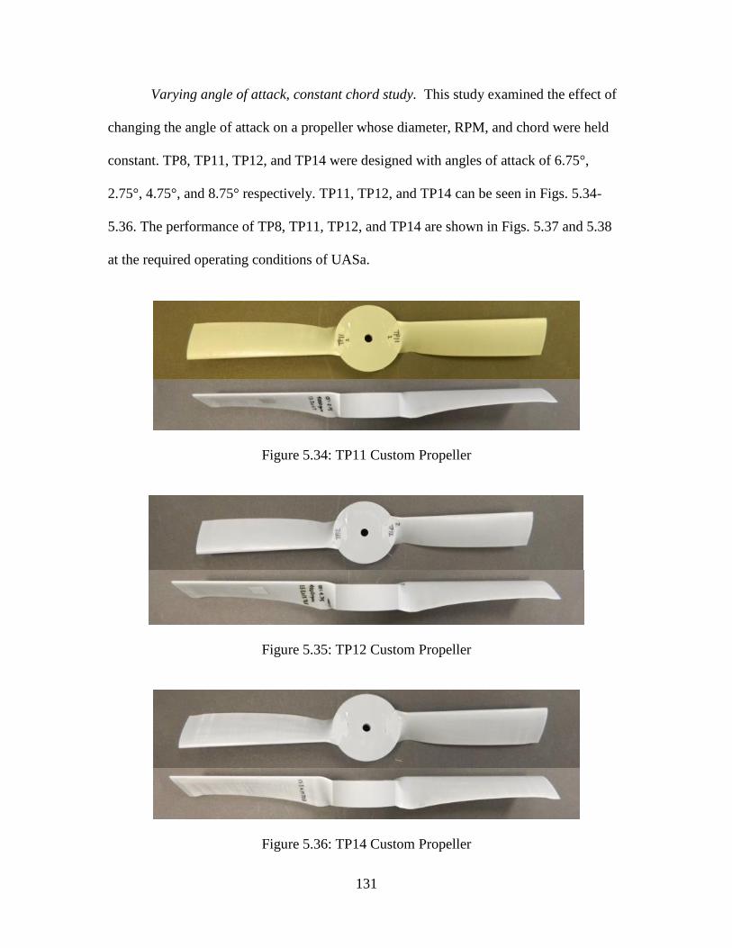
131
Varying angle of attack, constant chord study. This study examined the effect of
changing the angle of attack on a propeller whose diameter, RPM, and chord were held
constant. TP8, TP11, TP12, and TP14 were designed with angles of attack of 6.75°,
2.75°, 4.75°, and 8.75° respectively. TP11, TP12, and TP14 can be seen in Figs. 5.34-
5.36. The performance of TP8, TP11, TP12, and TP14 are shown in Figs. 5.37 and 5.38
at the required operating conditions of UASa.
Figure 5.34: TP11 Custom Propeller
Figure 5.35: TP12 Custom Propeller
Figure 5.36: TP14 Custom Propeller
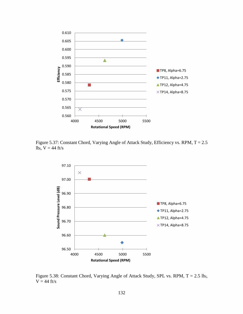
132
Figure 5.37: Constant Chord, Varying Angle of Attack Study, Efficiency vs. RPM, T = 2.5
lbf, V = 44 ft/s
Figure 5.38: Constant Chord, Varying Angle of Attack Study, SPL vs. RPM, T = 2.5 lbf,
V = 44 ft/s
0.560
0.565
0.570
0.575
0.580
0.585
0.590
0.595
0.600
0.605
0.610
4000 4500 5000 5500
Effi
cie
ncy
Rotational Speed (RPM)
TP8, Alpha=6.75
TP11, Alpha=2.75
TP12, Alpha=4.75
TP14, Alpha=8.75
96.50
96.60
96.70
96.80
96.90
97.00
97.10
4000 4500 5000 5500
Sou
nd
Pre
ssu
re L
eve
l (d
B)
Rotational Speed (RPM)
TP8, Alpha=6.75
TP11, Alpha=2.75
TP12, Alpha=4.75
TP14, Alpha=8.75
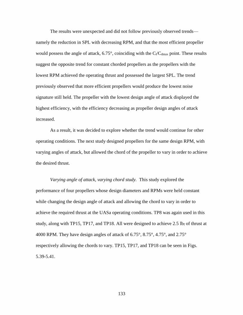
133
The results were unexpected and did not follow previously observed trends—
namely the reduction in SPL with decreasing RPM, and that the most efficient propeller
would possess the angle of attack, 6.75°, coinciding with the Cl/Cdmax point. These results
suggest the opposite trend for constant chorded propellers as the propellers with the
lowest RPM achieved the operating thrust and possessed the largest SPL. The trend
previously observed that more efficient propellers would produce the lowest noise
signature still held. The propeller with the lowest design angle of attack displayed the
highest efficiency, with the efficiency decreasing as propeller design angles of attack
increased.
As a result, it was decided to explore whether the trend would continue for other
operating conditions. The next study designed propellers for the same design RPM, with
varying angles of attack, but allowed the chord of the propeller to vary in order to achieve
the desired thrust.
Varying angle of attack, varying chord study. This study explored the
performance of four propellers whose design diameters and RPMs were held constant
while changing the design angle of attack and allowing the chord to vary in order to
achieve the required thrust at the UASa operating conditions. TP8 was again used in this
study, along with TP15, TP17, and TP18. All were designed to achieve 2.5 lbf of thrust at
4000 RPM. They have design angles of attack of 6.75°, 8.75°, 4.75°, and 2.75°
respectively allowing the chords to vary. TP15, TP17, and TP18 can be seen in Figs.
5.39-5.41.
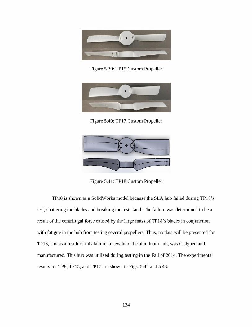
134
Figure 5.39: TP15 Custom Propeller
Figure 5.40: TP17 Custom Propeller
Figure 5.41: TP18 Custom Propeller
TP18 is shown as a SolidWorks model because the SLA hub failed during TP18’s
test, shattering the blades and breaking the test stand. The failure was determined to be a
result of the centrifugal force caused by the large mass of TP18’s blades in conjunction
with fatigue in the hub from testing several propellers. Thus, no data will be presented for
TP18, and as a result of this failure, a new hub, the aluminum hub, was designed and
manufactured. This hub was utilized during testing in the Fall of 2014. The experimental
results for TP8, TP15, and TP17 are shown in Figs. 5.42 and 5.43.
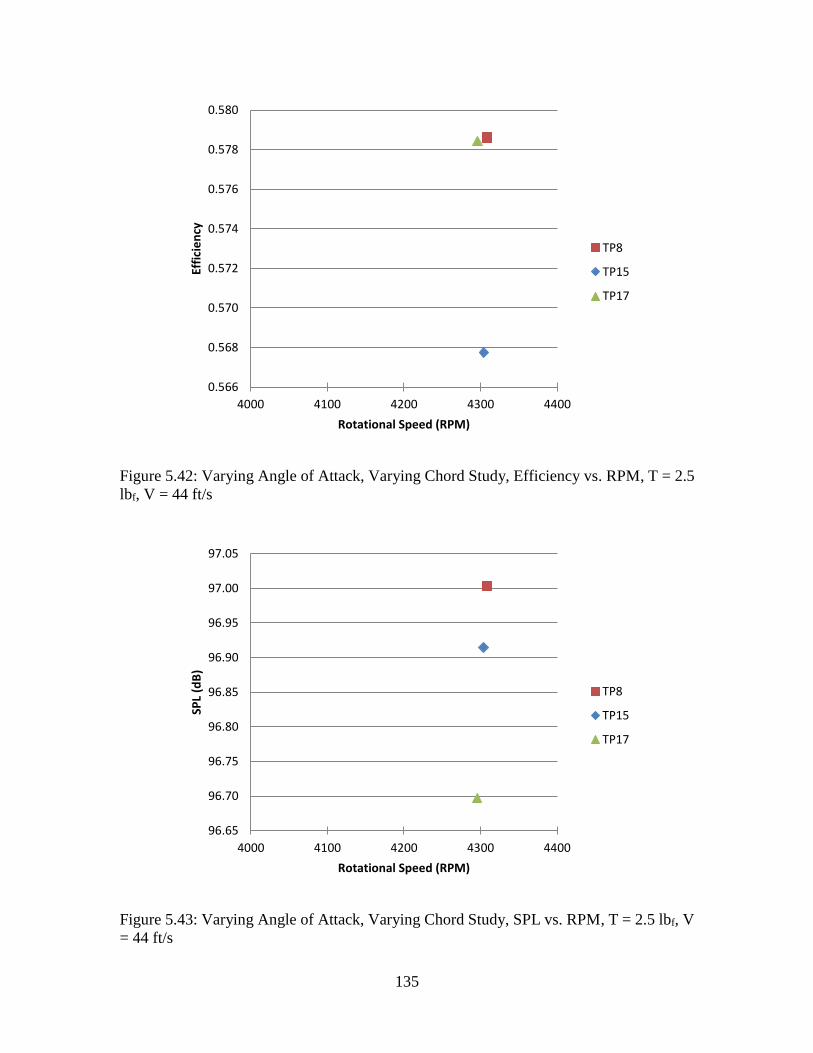
135
Figure 5.42: Varying Angle of Attack, Varying Chord Study, Efficiency vs. RPM, T = 2.5
lbf, V = 44 ft/s
Figure 5.43: Varying Angle of Attack, Varying Chord Study, SPL vs. RPM, T = 2.5 lbf, V
= 44 ft/s
0.566
0.568
0.570
0.572
0.574
0.576
0.578
0.580
4000 4100 4200 4300 4400
Effi
cie
ncy
Rotational Speed (RPM)
TP8
TP15
TP17
96.65
96.70
96.75
96.80
96.85
96.90
96.95
97.00
97.05
4000 4100 4200 4300 4400
SPL
(dB
)
Rotational Speed (RPM)
TP8
TP15
TP17
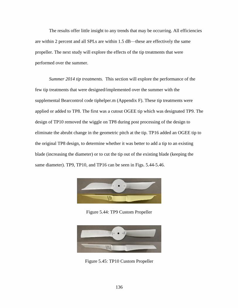
136
The results offer little insight to any trends that may be occurring. All efficiencies
are within 2 percent and all SPLs are within 1.5 dB—these are effectively the same
propeller. The next study will explore the effects of the tip treatments that were
performed over the summer.
Summer 2014 tip treatments. This section will explore the performance of the
few tip treatments that were designed/implemented over the summer with the
supplemental Bearcontrol code tiphelper.m (Appendix F). These tip treatments were
applied or added to TP8. The first was a cutout OGEE tip which was designated TP9. The
design of TP10 removed the wiggle on TP8 during post processing of the design to
eliminate the abrubt change in the geometric pitch at the tip. TP16 added an OGEE tip to
the original TP8 design, to determine whether it was better to add a tip to an existing
blade (increasing the diameter) or to cut the tip out of the existing blade (keeping the
same diameter). TP9, TP10, and TP16 can be seen in Figs. 5.44-5.46.
Figure 5.44: TP9 Custom Propeller
Figure 5.45: TP10 Custom Propeller
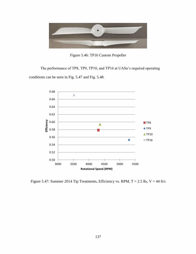
137
Figure 5.46: TP16 Custom Propeller
The performance of TP8, TP9, TP10, and TP16 at UASa’s required operating
conditions can be seen in Fig. 5.47 and Fig. 5.48.
Figure 5.47: Summer 2014 Tip Treatments, Efficiency vs. RPM, T = 2.5 lbf, V = 44 ft/s
0.50
0.52
0.54
0.56
0.58
0.60
0.62
0.64
0.66
0.68
3000 3500 4000 4500 5000 5500
Effi
cie
ncy
Rotational Speed (RPM)
TP8
TP9
TP10
TP16
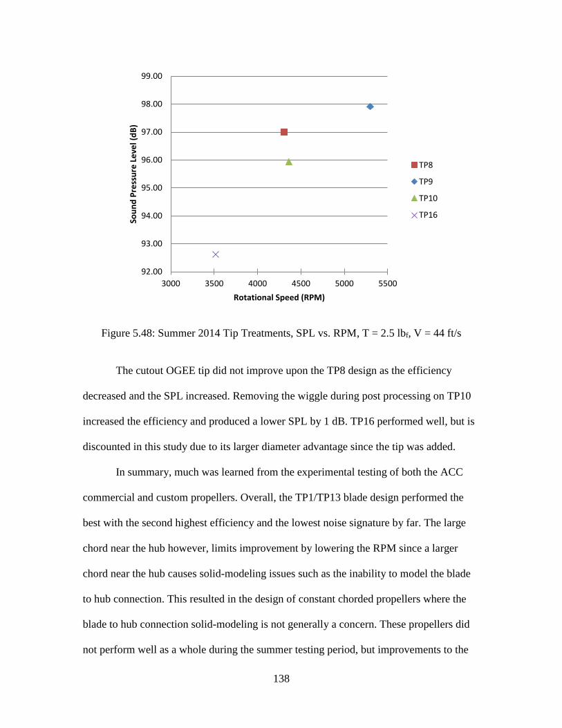
138
Figure 5.48: Summer 2014 Tip Treatments, SPL vs. RPM, T = 2.5 lbf, V = 44 ft/s
The cutout OGEE tip did not improve upon the TP8 design as the efficiency
decreased and the SPL increased. Removing the wiggle during post processing on TP10
increased the efficiency and produced a lower SPL by 1 dB. TP16 performed well, but is
discounted in this study due to its larger diameter advantage since the tip was added.
In summary, much was learned from the experimental testing of both the ACC
commercial and custom propellers. Overall, the TP1/TP13 blade design performed the
best with the second highest efficiency and the lowest noise signature by far. The large
chord near the hub however, limits improvement by lowering the RPM since a larger
chord near the hub causes solid-modeling issues such as the inability to model the blade
to hub connection. This resulted in the design of constant chorded propellers where the
blade to hub connection solid-modeling is not generally a concern. These propellers did
not perform well as a whole during the summer testing period, but improvements to the
92.00
93.00
94.00
95.00
96.00
97.00
98.00
99.00
3000 3500 4000 4500 5000 5500
Sou
nd
Pre
ssu
re L
eve
l (d
B)
Rotational Speed (RPM)
TP8
TP9
TP10
TP16
139
flat tip design were achieved through the addition of tip treatments. These observations
guided the designs of the propellers tested in the Fall of 2014.
Fall 2014, Custom Propeller Design and Experimental Evaluation
This section of the chapter will detail the experimental results of propellers
designed and manufactured during the Fall semester of 2014. The propellers were
designed at Baylor University then printed and tested at the USAFA. Tip treatments, the
utilization of new airfoil cross-sections, and multiple bladed propeller designs were the
focus of this study. Table 5.2 summarizes all of the propellers designed and tested during
this period.
Table 5.2: Fall 2014 Custom Propeller Design Summary
Propeller Radius
(in)
Design
RPM
Design
Thrust
(lbf)
Design
AoA
(°)
Tip Airfoil
Cross-
Section
TP19 ~6.5 4000 2.11 7.6 Taper 1 ClarkY
TP20 ~6.5 4000 1.72 7.6 Taper 2 ClarkY
TP21 ~6.5 4000 2.23 7.6 Half
Circle
ClarkY
TP22 ~6.5 4000 2.05 7.6 Oval 1 ClarkY
TP23 ~6.5 4000 2.23 7.6 Oval 2 ClarkY
TP24 ~6.5 4500 2.5 7.6 MIL ClarkY
TP25 ~6.5 4000 2.5 7.6 MIL ClarkY
TP26 ~6.5 3500 2.5 7.6 MIL ClarkY
TP27 ~6.5 3000 2.5 7.6 MIL ClarkY
TP28 ~6.5 4000 2.5 5.6 Flat,
Wiggle
ClarkY
TP29 ~6.5 4000 2.5 7.6 Flat,
Wiggle
ClarkY
TP30 ~6.5 4000 2.5 9.6 Flat,
Wiggle
ClarkY
TP31 ~6.5 4000 2.5 3.1 Flat,
Wiggle
GM15
TP32 ~6.5 4000 2.5 5.1 Flat,
Wiggle
GM15
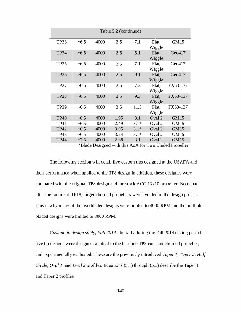
140
Table 5.2 (continued)
TP33 ~6.5 4000 2.5 7.1 Flat,
Wiggle
GM15
TP34 ~6.5 4000 2.5 5.1 Flat,
Wiggle
Geo417
TP35 ~6.5 4000 2.5 7.1 Flat,
Wiggle
Geo417
TP36 ~6.5 4000 2.5 9.1 Flat,
Wiggle
Geo417
TP37 ~6.5 4000 2.5 7.3 Flat,
Wiggle
FX63-137
TP38 ~6.5 4000 2.5 9.3 Flat,
Wiggle
FX63-137
TP39 ~6.5 4000 2.5 11.3 Flat,
Wiggle
FX63-137
TP40 ~6.5 4000 1.95 3.1 Oval 2 GM15
TP41 ~6.5 4000 2.49 3.1* Oval 2 GM15
TP42 ~6.5 4000 3.05 3.1* Oval 2 GM15
TP43 ~6.5 4000 3.54 3.1* Oval 2 GM15
TP44 ~7.5 4000 2.68 3.1 Oval 2 GM15
*Blade Designed with this AoA for Two Bladed Propeller
The following section will detail five custom tips designed at the USAFA and
their performance when applied to the TP8 design In addition, these designes were
compared with the original TP8 design and the stock ACC 13x10 propeller. Note that
after the failure of TP18, larger chorded propellers were avoided in the design process.
This is why many of the two bladed designs were limited to 4000 RPM and the multiple
bladed designs were limited to 3000 RPM.
Custom tip design study, Fall 2014. Initially during the Fall 2014 testing period,
five tip designs were designed, applied to the baseline TP8 constant chorded propeller,
and experimentally evaluated. These are the previously introduced Taper 1, Taper 2, Half
Circle, Oval 1, and Oval 2 profiles. Equations (5.1) through (5.3) describe the Taper 1
and Taper 2 profiles
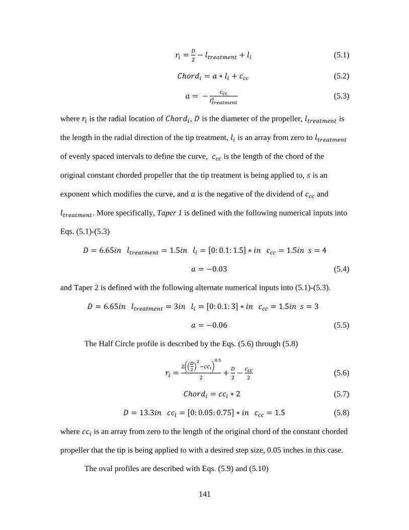
141
𝑟𝑖 =𝐷
2− 𝑙𝑡𝑟𝑒𝑎𝑡𝑚𝑒𝑛𝑡 + 𝑙𝑖 (5.1)
𝐶ℎ𝑜𝑟𝑑𝑖 = 𝑎 ∗ 𝑙𝑖 + 𝑐𝑐𝑐 (5.2)
𝑎 = −𝑐𝑐𝑐
𝑙𝑡𝑟𝑒𝑎𝑡𝑚𝑒𝑛𝑡𝑠 (5.3)
where 𝑟𝑖 is the radial location of 𝐶ℎ𝑜𝑟𝑑𝑖, 𝐷 is the diameter of the propeller, 𝑙𝑡𝑟𝑒𝑎𝑡𝑚𝑒𝑛𝑡 is
the length in the radial direction of the tip treatment, 𝑙𝑖 is an array from zero to 𝑙𝑡𝑟𝑒𝑎𝑡𝑚𝑒𝑛𝑡
of evenly spaced intervals to define the curve, 𝑐𝑐𝑐 is the length of the chord of the
original constant chorded propeller that the tip treatment is being applied to, 𝑠 is an
exponent which modifies the curve, and 𝑎 is the negative of the dividend of 𝑐𝑐𝑐 and
𝑙𝑡𝑟𝑒𝑎𝑡𝑚𝑒𝑛𝑡. More specifically, Taper 1 is defined with the following numerical inputs into
Eqs. (5.1)-(5.3)
𝐷 = 6.65𝑖𝑛 𝑙𝑡𝑟𝑒𝑎𝑡𝑚𝑒𝑛𝑡 = 1.5𝑖𝑛 𝑙𝑖 = [0: 0.1: 1.5] ∗ 𝑖𝑛 𝑐𝑐𝑐 = 1.5𝑖𝑛 𝑠 = 4
𝑎 = −0.03 (5.4)
and Taper 2 is defined with the following alternate numerical inputs into (5.1)-(5.3).
𝐷 = 6.65𝑖𝑛 𝑙𝑡𝑟𝑒𝑎𝑡𝑚𝑒𝑛𝑡 = 3𝑖𝑛 𝑙𝑖 = [0: 0.1: 3] ∗ 𝑖𝑛 𝑐𝑐𝑐 = 1.5𝑖𝑛 𝑠 = 3
𝑎 = −0.06 (5.5)
The Half Circle profile is described by the Eqs. (5.6) through (5.8)
𝑟𝑖 =2((
𝐷
2)
2−𝑐𝑐𝑖)
0.5
2+
𝐷
2−
𝑐𝑐𝑐
2(5.6)
𝐶ℎ𝑜𝑟𝑑𝑖 = 𝑐𝑐𝑖 ∗ 2 (5.7)
𝐷 = 13.3𝑖𝑛 𝑐𝑐𝑖 = [0: 0.05: 0.75] ∗ 𝑖𝑛 𝑐𝑐𝑐 = 1.5 (5.8)
where 𝑐𝑐𝑖 is an array from zero to the length of the original chord of the constant chorded
propeller that the tip is being applied to with a desired step size, 0.05 inches in this case.
The oval profiles are described with Eqs. (5.9) and (5.10)
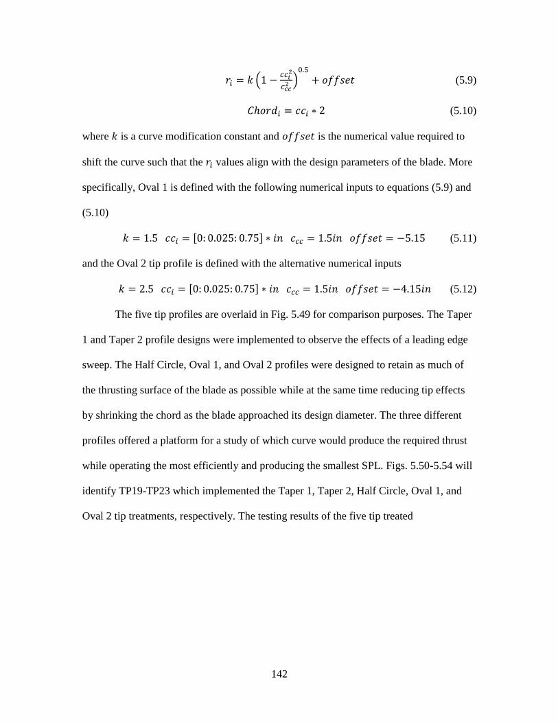
142
𝑟𝑖 = 𝑘 (1 −𝑐𝑐𝑖
2
𝑐𝑐𝑐2 )
0.5
+ 𝑜𝑓𝑓𝑠𝑒𝑡 (5.9)
𝐶ℎ𝑜𝑟𝑑𝑖 = 𝑐𝑐𝑖 ∗ 2 (5.10)
where 𝑘 is a curve modification constant and 𝑜𝑓𝑓𝑠𝑒𝑡 is the numerical value required to
shift the curve such that the 𝑟𝑖 values align with the design parameters of the blade. More
specifically, Oval 1 is defined with the following numerical inputs to equations (5.9) and
(5.10)
𝑘 = 1.5 𝑐𝑐𝑖 = [0: 0.025: 0.75] ∗ 𝑖𝑛 𝑐𝑐𝑐 = 1.5𝑖𝑛 𝑜𝑓𝑓𝑠𝑒𝑡 = −5.15 (5.11)
and the Oval 2 tip profile is defined with the alternative numerical inputs
𝑘 = 2.5 𝑐𝑐𝑖 = [0: 0.025: 0.75] ∗ 𝑖𝑛 𝑐𝑐𝑐 = 1.5𝑖𝑛 𝑜𝑓𝑓𝑠𝑒𝑡 = −4.15𝑖𝑛 (5.12)
The five tip profiles are overlaid in Fig. 5.49 for comparison purposes. The Taper
1 and Taper 2 profile designs were implemented to observe the effects of a leading edge
sweep. The Half Circle, Oval 1, and Oval 2 profiles were designed to retain as much of
the thrusting surface of the blade as possible while at the same time reducing tip effects
by shrinking the chord as the blade approached its design diameter. The three different
profiles offered a platform for a study of which curve would produce the required thrust
while operating the most efficiently and producing the smallest SPL. Figs. 5.50-5.54 will
identify TP19-TP23 which implemented the Taper 1, Taper 2, Half Circle, Oval 1, and
Oval 2 tip treatments, respectively. The testing results of the five tip treated
143
Figure 5.49: Fall 2014 Tip Treatment Profiles
3
3.5
4
4.5
5
5.5
6
6.5
7
-0.5 0.0 0.5 1.0 1.5 2.0
Rad
ial L
oca
tio
n (
in)
Chord (in)
Taper 1
Taper 2
Half Circle
Oval 1
Oval 2
Lead
ing
Edge
Trai
ling
Edge
144
Figure 5.50: TP19 Custom Propeller, Taper 1 Tip Treatment
Figure 5.51: TP20 Custom Propeller, Taper 2 Tip Treatment
Figure 5.52: TP21 Custom Propeller, Half Circle Tip Treatment
Figure 5.53: TP22 Custom Propeller, Oval 1 Tip Treatment
Figure 5.54: TP23 Custom Propeller, Oval 2 Tip Treatment
propellers, TP8, and the stock ACC 13x10 propeller at the required UASa operating
conditions are shown below in Fig. 5.55 and Fig. 5.56.
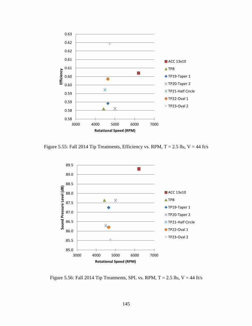
145
Figure 5.55: Fall 2014 Tip Treatments, Efficiency vs. RPM, T = 2.5 lbf, V = 44 ft/s
Figure 5.56: Fall 2014 Tip Treatments, SPL vs. RPM, T = 2.5 lbf, V = 44 ft/s
0.58
0.58
0.59
0.59
0.60
0.60
0.61
0.61
0.62
0.62
0.63
3000 4000 5000 6000 7000
Effi
cie
ncy
Rotational Speed (RPM)
ACC 13x10
TP8
TP19-Taper 1
TP20-Taper 2
TP21-Half Circle
TP22-Oval 1
TP23-Oval 2
85.0
85.5
86.0
86.5
87.0
87.5
88.0
88.5
89.0
89.5
3000 4000 5000 6000 7000
Sou
nd
Pre
ssu
re L
eve
l (d
B)
Rotational Speed (RPM)
ACC 13x10
TP8
TP19-Taper 1
TP20-Taper 2
TP21-Half Circle
TP22-Oval 1
TP23-Oval 2
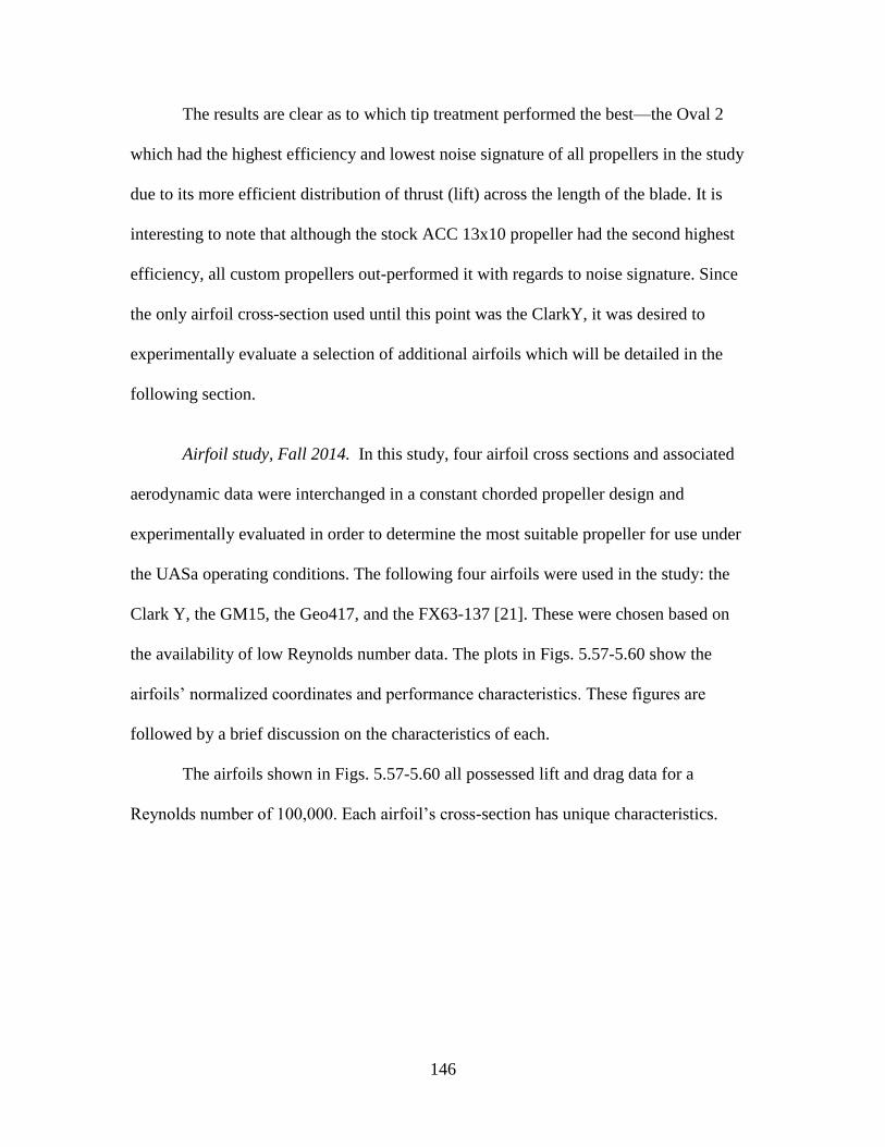
146
The results are clear as to which tip treatment performed the best—the Oval 2
which had the highest efficiency and lowest noise signature of all propellers in the study
due to its more efficient distribution of thrust (lift) across the length of the blade. It is
interesting to note that although the stock ACC 13x10 propeller had the second highest
efficiency, all custom propellers out-performed it with regards to noise signature. Since
the only airfoil cross-section used until this point was the ClarkY, it was desired to
experimentally evaluate a selection of additional airfoils which will be detailed in the
following section.
Airfoil study, Fall 2014. In this study, four airfoil cross sections and associated
aerodynamic data were interchanged in a constant chorded propeller design and
experimentally evaluated in order to determine the most suitable propeller for use under
the UASa operating conditions. The following four airfoils were used in the study: the
Clark Y, the GM15, the Geo417, and the FX63-137 [21]. These were chosen based on
the availability of low Reynolds number data. The plots in Figs. 5.57-5.60 show the
airfoils’ normalized coordinates and performance characteristics. These figures are
followed by a brief discussion on the characteristics of each.
The airfoils shown in Figs. 5.57-5.60 all possessed lift and drag data for a
Reynolds number of 100,000. Each airfoil’s cross-section has unique characteristics.
147
Figure 5.57: Airfoil Study, Normalized Airfoil Coordinates [21]
Figure 5.58: Airfoil Study, Coefficient of Lift vs. Angle of Attack, Re = 100,000 [21]
0 0.1 0.2 0.3 0.4 0.5 0.6 0.7 0.8 0.9 1
-0.3
-0.2
-0.1
0
0.1
0.2
0.3
0.4
x/c
y/c
ClarkY
GM15
Geo417
FX63-137
-0.5
0
0.5
1
1.5
2
-10 -5 0 5 10 15
Co
eff
icie
nt
of
Lift
Angle of Attack (°)
ClarkY
GM15
Geo417
FX63-137
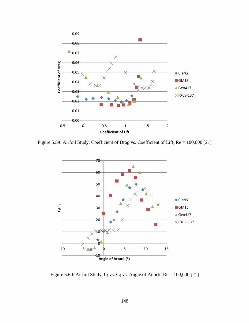
148
Figure 5.59: Airfoil Study, Coefficient of Drag vs. Coefficient of Lift, Re = 100,000 [21]
Figure 5.60: Airfoil Study, Cl vs. Cd vs. Angle of Attack, Re = 100,000 [21]
0.00
0.01
0.02
0.03
0.04
0.05
0.06
0.07
0.08
0.09
-0.5 0 0.5 1 1.5 2
Co
eff
icie
nt
of
Dra
g
Coefficient of Lift
ClarkY
GM15
Geo417
FX63-137
-10
0
10
20
30
40
50
60
70
-10 -5 0 5 10 15
Cl/
Cd
Angle of Attack (°)
ClarkY
GM15
Geo417
FX63-137
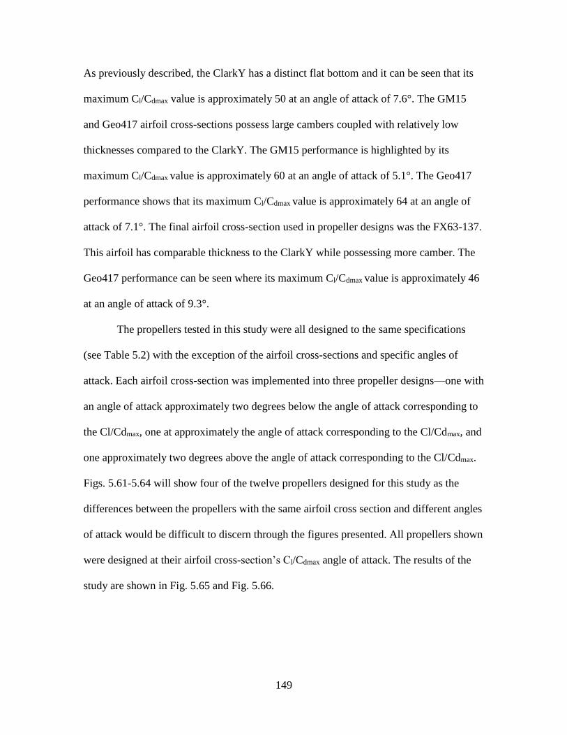
149
As previously described, the ClarkY has a distinct flat bottom and it can be seen that its
maximum Cl/Cdmax value is approximately 50 at an angle of attack of 7.6°. The GM15
and Geo417 airfoil cross-sections possess large cambers coupled with relatively low
thicknesses compared to the ClarkY. The GM15 performance is highlighted by its
maximum Cl/Cdmax value is approximately 60 at an angle of attack of 5.1°. The Geo417
performance shows that its maximum Cl/Cdmax value is approximately 64 at an angle of
attack of 7.1°. The final airfoil cross-section used in propeller designs was the FX63-137.
This airfoil has comparable thickness to the ClarkY while possessing more camber. The
Geo417 performance can be seen where its maximum Cl/Cdmax value is approximately 46
at an angle of attack of 9.3°.
The propellers tested in this study were all designed to the same specifications
(see Table 5.2) with the exception of the airfoil cross-sections and specific angles of
attack. Each airfoil cross-section was implemented into three propeller designs—one with
an angle of attack approximately two degrees below the angle of attack corresponding to
the Cl/Cdmax, one at approximately the angle of attack corresponding to the Cl/Cdmax, and
one approximately two degrees above the angle of attack corresponding to the Cl/Cdmax.
Figs. 5.61-5.64 will show four of the twelve propellers designed for this study as the
differences between the propellers with the same airfoil cross section and different angles
of attack would be difficult to discern through the figures presented. All propellers shown
were designed at their airfoil cross-section’s Cl/Cdmax angle of attack. The results of the
study are shown in Fig. 5.65 and Fig. 5.66.
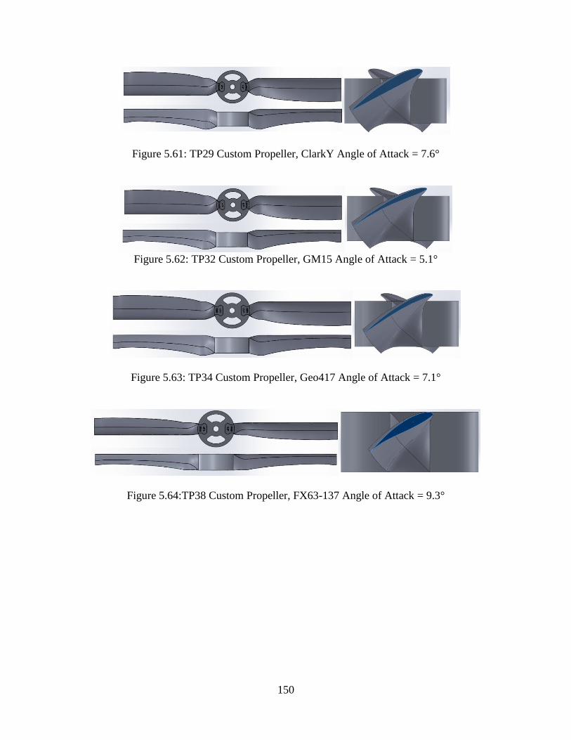
150
Figure 5.61: TP29 Custom Propeller, ClarkY Angle of Attack = 7.6°
Figure 5.62: TP32 Custom Propeller, GM15 Angle of Attack = 5.1°
Figure 5.63: TP34 Custom Propeller, Geo417 Angle of Attack = 7.1°
Figure 5.64:TP38 Custom Propeller, FX63-137 Angle of Attack = 9.3°
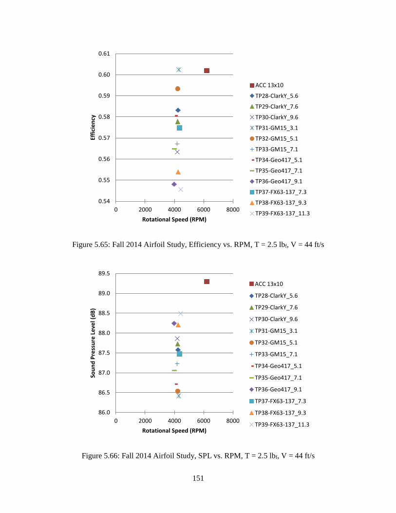
151
Figure 5.65: Fall 2014 Airfoil Study, Efficiency vs. RPM, T = 2.5 lbf, V = 44 ft/s
Figure 5.66: Fall 2014 Airfoil Study, SPL vs. RPM, T = 2.5 lbf, V = 44 ft/s
0.54
0.55
0.56
0.57
0.58
0.59
0.60
0.61
0 2000 4000 6000 8000
Effi
cie
ncy
Rotational Speed (RPM)
ACC 13x10
TP28-ClarkY_5.6
TP29-ClarkY_7.6
TP30-ClarkY_9.6
TP31-GM15_3.1
TP32-GM15_5.1
TP33-GM15_7.1
TP34-Geo417_5.1
TP35-Geo417_7.1
TP36-Geo417_9.1
TP37-FX63-137_7.3
TP38-FX63-137_9.3
TP39-FX63-137_11.3
86.0
86.5
87.0
87.5
88.0
88.5
89.0
89.5
0 2000 4000 6000 8000
Sou
nd
Pre
ssu
re L
eve
l (d
B)
Rotational Speed (RPM)
ACC 13x10
TP28-ClarkY_5.6
TP29-ClarkY_7.6
TP30-ClarkY_9.6
TP31-GM15_3.1
TP32-GM15_5.1
TP33-GM15_7.1
TP34-Geo417_5.1
TP35-Geo417_7.1
TP36-Geo417_9.1
TP37-FX63-137_7.3
TP38-FX63-137_9.3
TP39-FX63-137_11.3
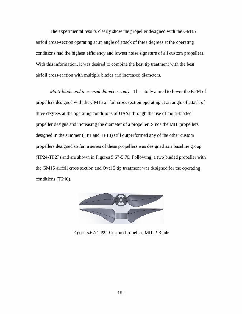
152
The experimental results clearly show the propeller designed with the GM15
airfoil cross-section operating at an angle of attack of three degrees at the operating
conditions had the highest efficiency and lowest noise signature of all custom propellers.
With this information, it was desired to combine the best tip treatment with the best
airfoil cross-section with multiple blades and increased diameters.
Multi-blade and increased diameter study. This study aimed to lower the RPM of
propellers designed with the GM15 airfoil cross section operating at an angle of attack of
three degrees at the operating conditions of UASa through the use of multi-bladed
propeller designs and increasing the diameter of a propeller. Since the MIL propellers
designed in the summer (TP1 and TP13) still outperformed any of the other custom
propellers designed so far, a series of these propellers was designed as a baseline group
(TP24-TP27) and are shown in Figures 5.67-5.70. Following, a two bladed propeller with
the GM15 airfoil cross section and Oval 2 tip treatment was designed for the operating
conditions (TP40).
Figure 5.67: TP24 Custom Propeller, MIL 2 Blade
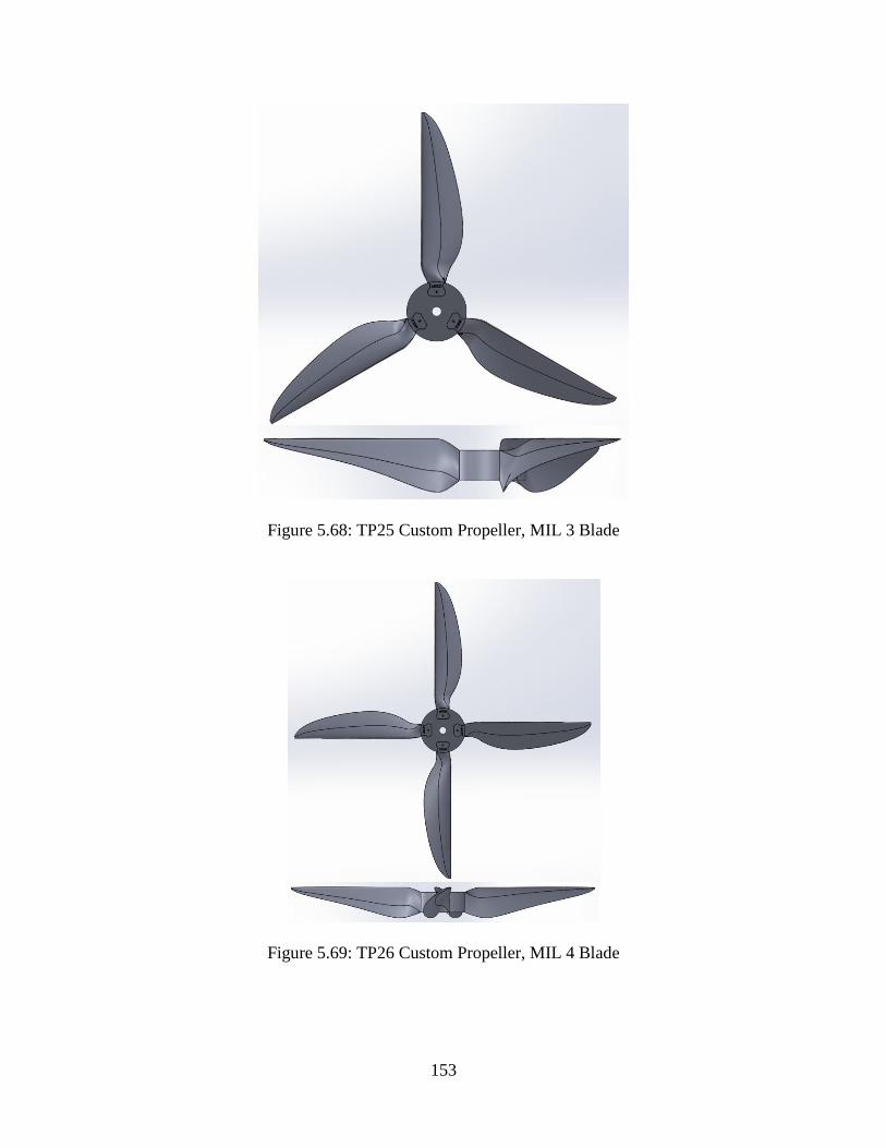
153
Figure 5.68: TP25 Custom Propeller, MIL 3 Blade
Figure 5.69: TP26 Custom Propeller, MIL 4 Blade
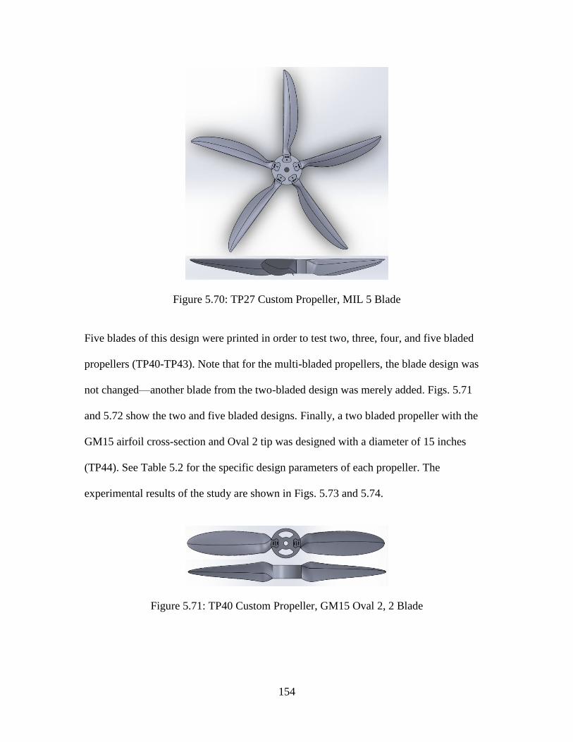
154
Figure 5.70: TP27 Custom Propeller, MIL 5 Blade
Five blades of this design were printed in order to test two, three, four, and five bladed
propellers (TP40-TP43). Note that for the multi-bladed propellers, the blade design was
not changed—another blade from the two-bladed design was merely added. Figs. 5.71
and 5.72 show the two and five bladed designs. Finally, a two bladed propeller with the
GM15 airfoil cross-section and Oval 2 tip was designed with a diameter of 15 inches
(TP44). See Table 5.2 for the specific design parameters of each propeller. The
experimental results of the study are shown in Figs. 5.73 and 5.74.
Figure 5.71: TP40 Custom Propeller, GM15 Oval 2, 2 Blade
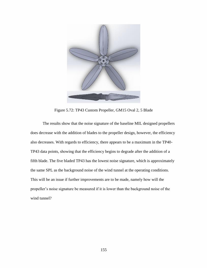
155
Figure 5.72: TP43 Custom Propeller, GM15 Oval 2, 5 Blade
The results show that the noise signature of the baseline MIL designed propellers
does decrease with the addition of blades to the propeller design, however, the efficiency
also decreases. With regards to efficiency, there appears to be a maximum in the TP40-
TP43 data points, showing that the efficiency begins to degrade after the addition of a
fifth blade. The five bladed TP43 has the lowest noise signature, which is approximately
the same SPL as the background noise of the wind tunnel at the operating conditions.
This will be an issue if further improvements are to be made, namely how will the
propeller’s noise signature be measured if it is lower than the background noise of the
wind tunnel?
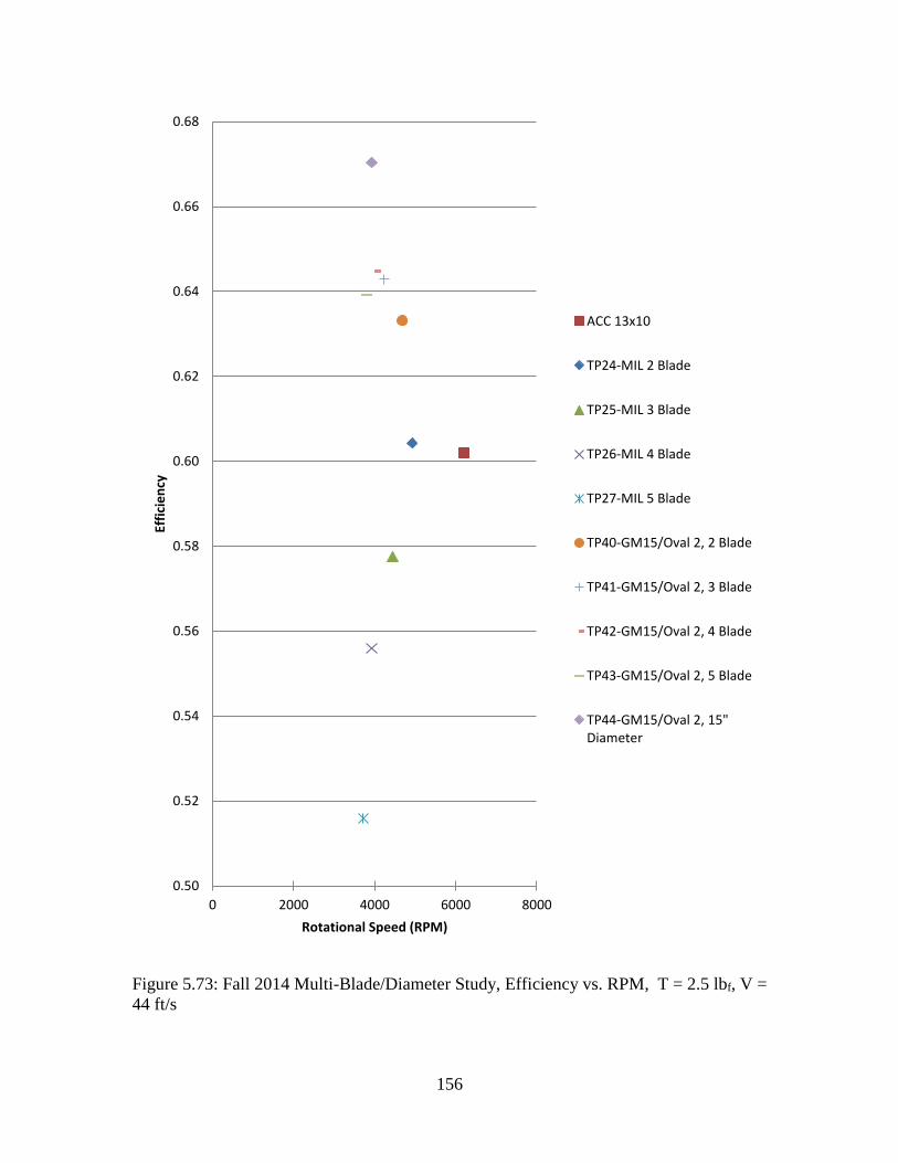
156
Figure 5.73: Fall 2014 Multi-Blade/Diameter Study, Efficiency vs. RPM, T = 2.5 lbf, V =
44 ft/s
0.50
0.52
0.54
0.56
0.58
0.60
0.62
0.64
0.66
0.68
0 2000 4000 6000 8000
Effi
cie
ncy
Rotational Speed (RPM)
ACC 13x10
TP24-MIL 2 Blade
TP25-MIL 3 Blade
TP26-MIL 4 Blade
TP27-MIL 5 Blade
TP40-GM15/Oval 2, 2 Blade
TP41-GM15/Oval 2, 3 Blade
TP42-GM15/Oval 2, 4 Blade
TP43-GM15/Oval 2, 5 Blade
TP44-GM15/Oval 2, 15"Diameter
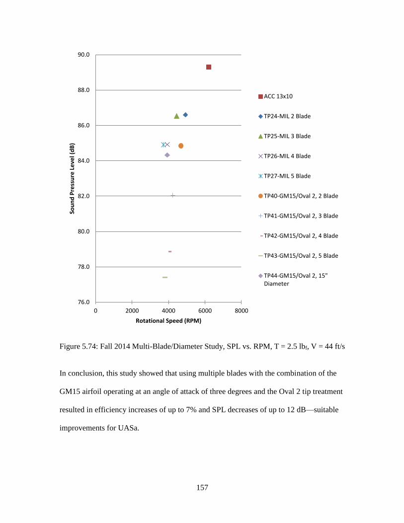
157
Figure 5.74: Fall 2014 Multi-Blade/Diameter Study, SPL vs. RPM, T = 2.5 lbf, V = 44 ft/s
In conclusion, this study showed that using multiple blades with the combination of the
GM15 airfoil operating at an angle of attack of three degrees and the Oval 2 tip treatment
resulted in efficiency increases of up to 7% and SPL decreases of up to 12 dB—suitable
improvements for UASa.
76.0
78.0
80.0
82.0
84.0
86.0
88.0
90.0
0 2000 4000 6000 8000
Sou
nd
Pre
ssu
re L
eve
l (d
B)
Rotational Speed (RPM)
ACC 13x10
TP24-MIL 2 Blade
TP25-MIL 3 Blade
TP26-MIL 4 Blade
TP27-MIL 5 Blade
TP40-GM15/Oval 2, 2 Blade
TP41-GM15/Oval 2, 3 Blade
TP42-GM15/Oval 2, 4 Blade
TP43-GM15/Oval 2, 5 Blade
TP44-GM15/Oval 2, 15"Diameter
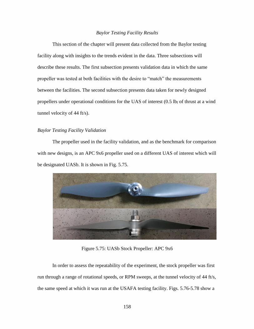
158
Baylor Testing Facility Results
This section of the chapter will present data collected from the Baylor testing
facility along with insights to the trends evident in the data. Three subsections will
describe these results. The first subsection presents validation data in which the same
propeller was tested at both facilities with the desire to “match” the measurements
between the facilities. The second subsection presents data taken for newly designed
propellers under operational conditions for the UAS of interest (0.5 lbf of thrust at a wind
tunnel velocity of 44 ft/s).
Baylor Testing Facility Validation
The propeller used in the facility validation, and as the benchmark for comparison
with new designs, is an APC 9x6 propeller used on a different UAS of interest which will
be designated UASb. It is shown in Fig. 5.75.
Figure 5.75: UASb Stock Propeller: APC 9x6
In order to assess the repeatability of the experiment, the stock propeller was first
run through a range of rotational speeds, or RPM sweeps, at the tunnel velocity of 44 ft/s,
the same speed at which it was run at the USAFA testing facility. Figs. 5.76-5.78 show a
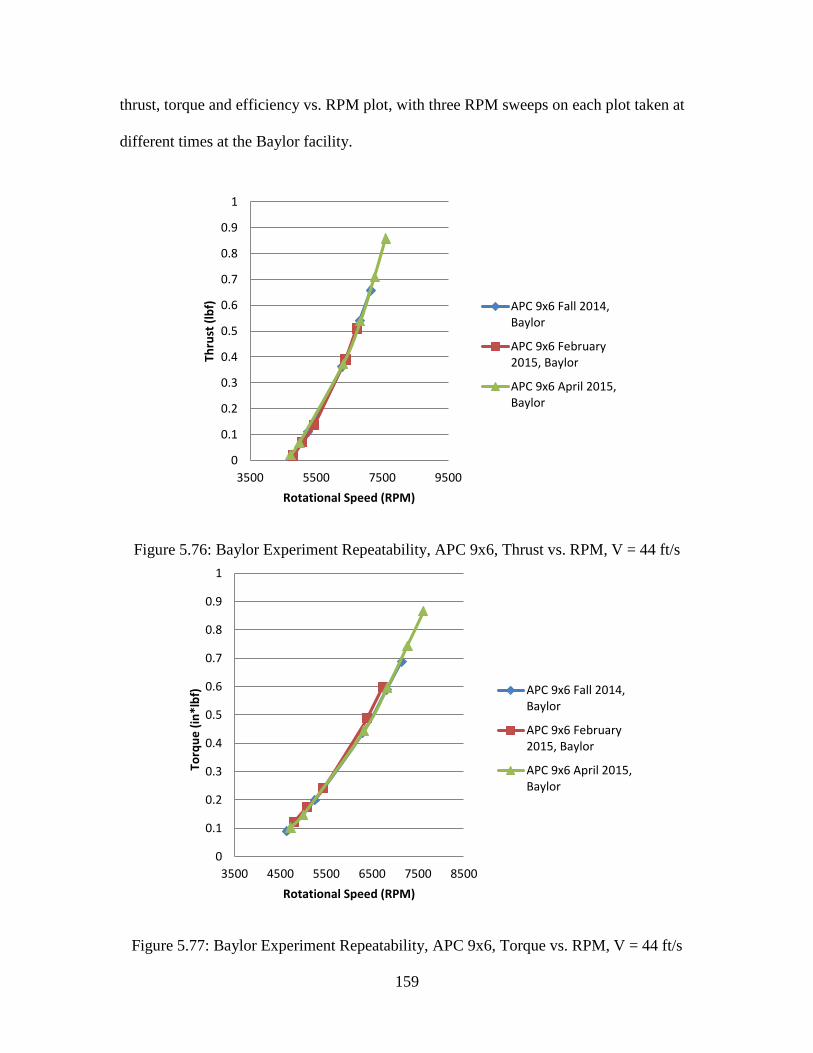
159
thrust, torque and efficiency vs. RPM plot, with three RPM sweeps on each plot taken at
different times at the Baylor facility.
Figure 5.76: Baylor Experiment Repeatability, APC 9x6, Thrust vs. RPM, V = 44 ft/s
Figure 5.77: Baylor Experiment Repeatability, APC 9x6, Torque vs. RPM, V = 44 ft/s
0
0.1
0.2
0.3
0.4
0.5
0.6
0.7
0.8
0.9
1
3500 5500 7500 9500
Thru
st (
lbf)
Rotational Speed (RPM)
APC 9x6 Fall 2014,Baylor
APC 9x6 February2015, Baylor
APC 9x6 April 2015,Baylor
0
0.1
0.2
0.3
0.4
0.5
0.6
0.7
0.8
0.9
1
3500 4500 5500 6500 7500 8500
Torq
ue
(in
*lb
f)
Rotational Speed (RPM)
APC 9x6 Fall 2014,Baylor
APC 9x6 February2015, Baylor
APC 9x6 April 2015,Baylor
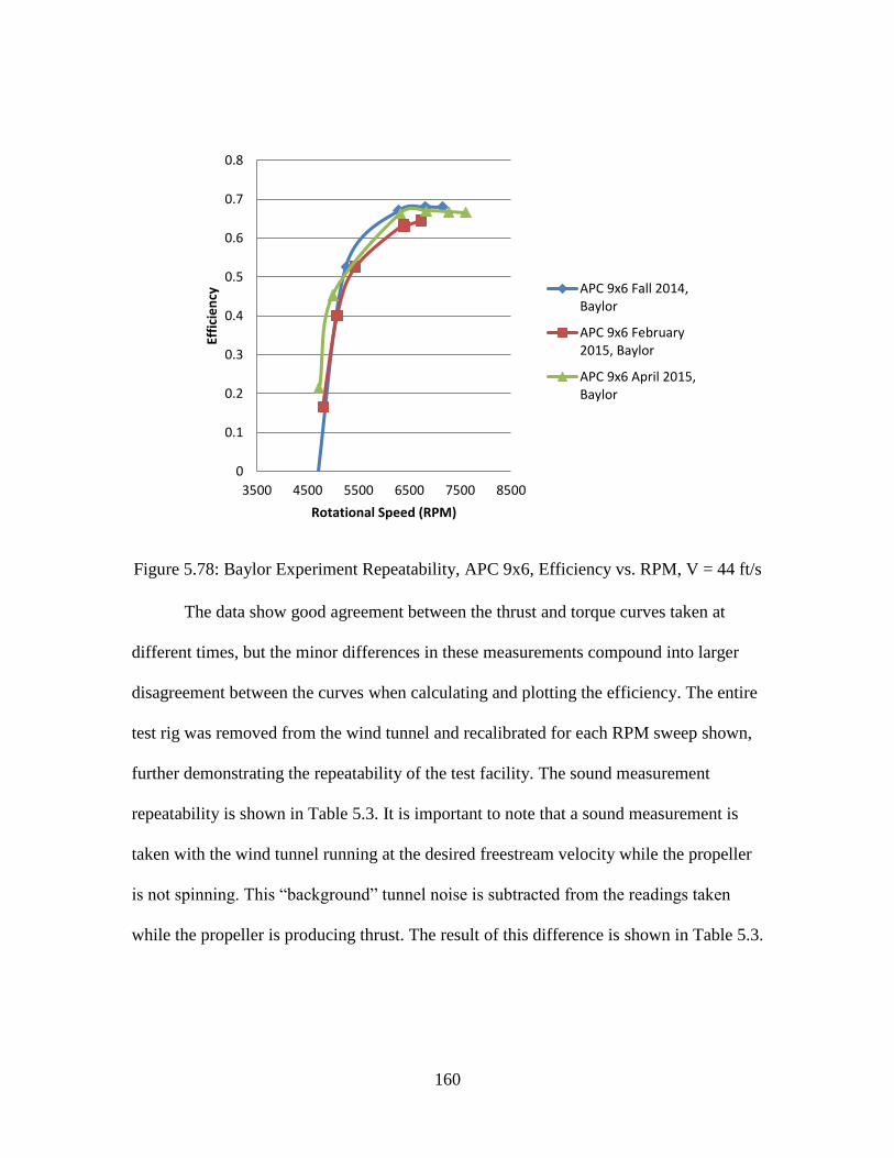
160
Figure 5.78: Baylor Experiment Repeatability, APC 9x6, Efficiency vs. RPM, V = 44 ft/s
The data show good agreement between the thrust and torque curves taken at
different times, but the minor differences in these measurements compound into larger
disagreement between the curves when calculating and plotting the efficiency. The entire
test rig was removed from the wind tunnel and recalibrated for each RPM sweep shown,
further demonstrating the repeatability of the test facility. The sound measurement
repeatability is shown in Table 5.3. It is important to note that a sound measurement is
taken with the wind tunnel running at the desired freestream velocity while the propeller
is not spinning. This “background” tunnel noise is subtracted from the readings taken
while the propeller is producing thrust. The result of this difference is shown in Table 5.3.
0
0.1
0.2
0.3
0.4
0.5
0.6
0.7
0.8
3500 4500 5500 6500 7500 8500
Effi
cie
ncy
Rotational Speed (RPM)
APC 9x6 Fall 2014,Baylor
APC 9x6 February2015, Baylor
APC 9x6 April 2015,Baylor
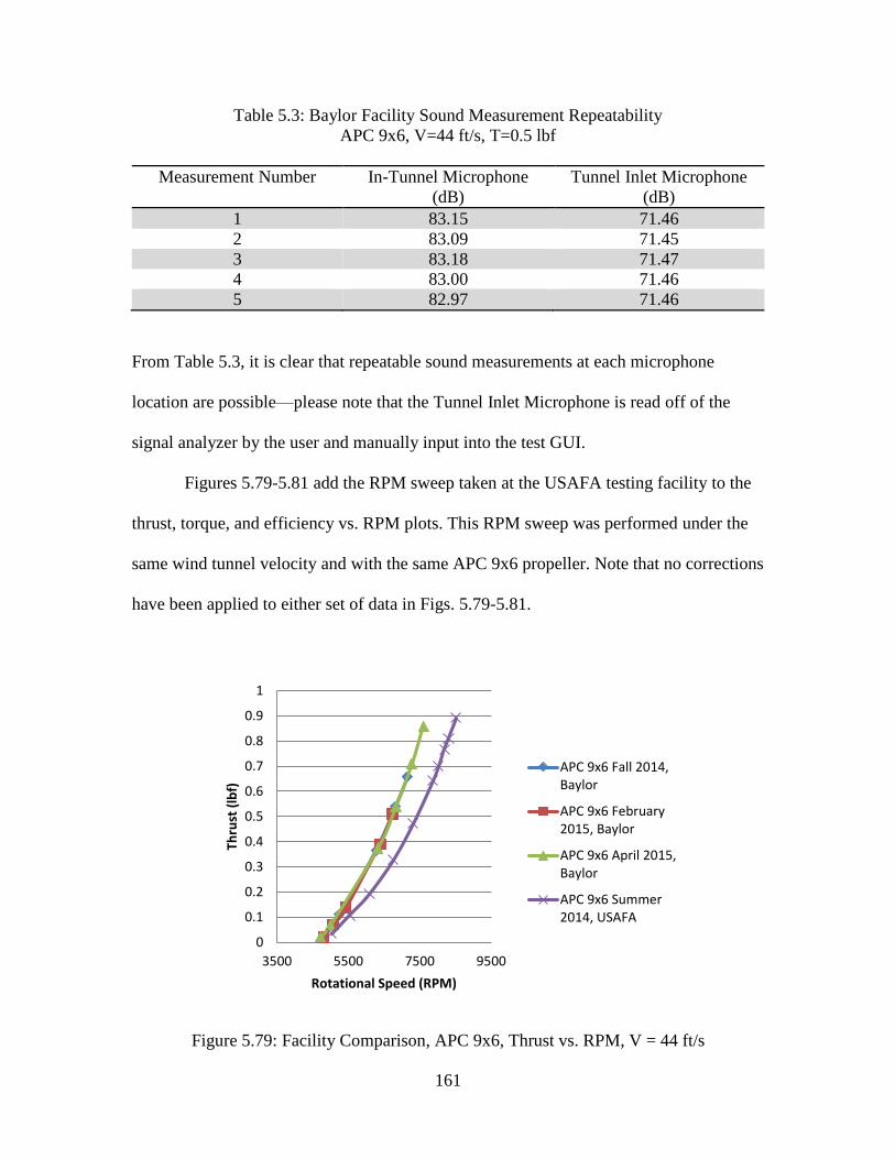
161
Table 5.3: Baylor Facility Sound Measurement Repeatability
APC 9x6, V=44 ft/s, T=0.5 lbf
Measurement Number In-Tunnel Microphone
(dB)
Tunnel Inlet Microphone
(dB)
1 83.15 71.46
2 83.09 71.45
3 83.18 71.47
4 83.00 71.46
5 82.97 71.46
From Table 5.3, it is clear that repeatable sound measurements at each microphone
location are possible—please note that the Tunnel Inlet Microphone is read off of the
signal analyzer by the user and manually input into the test GUI.
Figures 5.79-5.81 add the RPM sweep taken at the USAFA testing facility to the
thrust, torque, and efficiency vs. RPM plots. This RPM sweep was performed under the
same wind tunnel velocity and with the same APC 9x6 propeller. Note that no corrections
have been applied to either set of data in Figs. 5.79-5.81.
Figure 5.79: Facility Comparison, APC 9x6, Thrust vs. RPM, V = 44 ft/s
0
0.1
0.2
0.3
0.4
0.5
0.6
0.7
0.8
0.9
1
3500 5500 7500 9500
Thru
st (
lbf)
Rotational Speed (RPM)
APC 9x6 Fall 2014,Baylor
APC 9x6 February2015, Baylor
APC 9x6 April 2015,Baylor
APC 9x6 Summer2014, USAFA
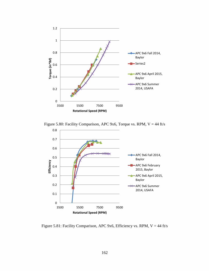
162
Figure 5.80: Facility Comparison, APC 9x6, Torque vs. RPM, V = 44 ft/s
Figure 5.81: Facility Comparison, APC 9x6, Efficiency vs. RPM, V = 44 ft/s
0
0.2
0.4
0.6
0.8
1
1.2
3500 5500 7500 9500
Torq
ue
(in
*lb
f)
Rotational Speed (RPM)
APC 9x6 Fall 2014,Baylor
Series2
APC 9x6 April 2015,Baylor
APC 9x6 Summer2014, USAFA
0
0.1
0.2
0.3
0.4
0.5
0.6
0.7
0.8
3500 5500 7500 9500
Effi
cie
ncy
Rotational Speed (RPM)
APC 9x6 Fall 2014,Baylor
APC 9x6 February2015, Baylor
APC 9x6 April 2015,Baylor
APC 9x6 Summer2014, USAFA
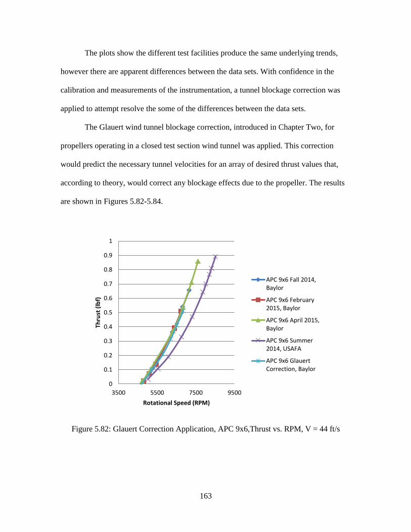
163
The plots show the different test facilities produce the same underlying trends,
however there are apparent differences between the data sets. With confidence in the
calibration and measurements of the instrumentation, a tunnel blockage correction was
applied to attempt resolve the some of the differences between the data sets.
The Glauert wind tunnel blockage correction, introduced in Chapter Two, for
propellers operating in a closed test section wind tunnel was applied. This correction
would predict the necessary tunnel velocities for an array of desired thrust values that,
according to theory, would correct any blockage effects due to the propeller. The results
are shown in Figures 5.82-5.84.
Figure 5.82: Glauert Correction Application, APC 9x6,Thrust vs. RPM, V = 44 ft/s
0
0.1
0.2
0.3
0.4
0.5
0.6
0.7
0.8
0.9
1
3500 5500 7500 9500
Thru
st (
lbf)
Rotational Speed (RPM)
APC 9x6 Fall 2014,Baylor
APC 9x6 February2015, Baylor
APC 9x6 April 2015,Baylor
APC 9x6 Summer2014, USAFA
APC 9x6 GlauertCorrection, Baylor
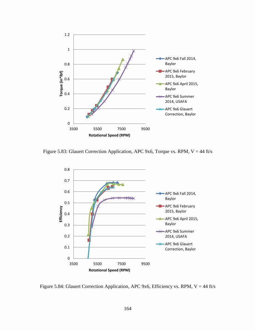
164
Figure 5.83: Glauert Correction Application, APC 9x6, Torque vs. RPM, V = 44 ft/s
Figure 5.84: Glauert Correction Application, APC 9x6, Efficiency vs. RPM, V = 44 ft/s
0
0.2
0.4
0.6
0.8
1
1.2
3500 5500 7500 9500
Torq
ue
(in
*lb
f)
Rotational Speed (RPM)
APC 9x6 Fall 2014,Baylor
APC 9x6 February2015, Baylor
APC 9x6 April 2015,Baylor
APC 9x6 Summer2014, USAFA
APC 9x6 GlauertCorrection, Baylor
0
0.1
0.2
0.3
0.4
0.5
0.6
0.7
0.8
3500 5500 7500 9500
Effi
cie
ncy
Rotational Speed (RPM)
APC 9x6 Fall 2014,Baylor
APC 9x6 February2015, Baylor
APC 9x6 April 2015,Baylor
APC 9x6 Summer2014, USAFA
APC 9x6 GlauertCorrection, Baylor
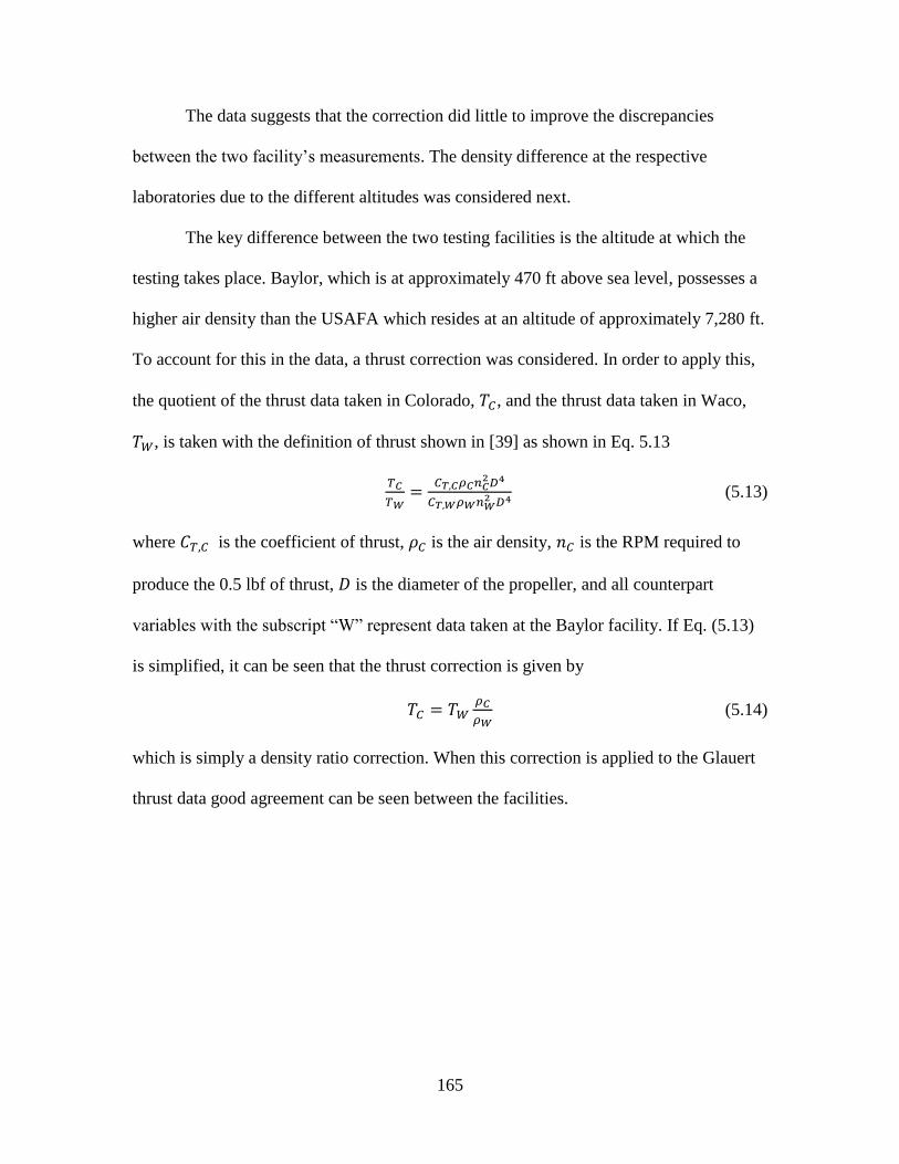
165
The data suggests that the correction did little to improve the discrepancies
between the two facility’s measurements. The density difference at the respective
laboratories due to the different altitudes was considered next.
The key difference between the two testing facilities is the altitude at which the
testing takes place. Baylor, which is at approximately 470 ft above sea level, possesses a
higher air density than the USAFA which resides at an altitude of approximately 7,280 ft.
To account for this in the data, a thrust correction was considered. In order to apply this,
the quotient of the thrust data taken in Colorado, 𝑇𝐶, and the thrust data taken in Waco,
𝑇𝑊, is taken with the definition of thrust shown in [39] as shown in Eq. 5.13
𝑇𝐶
𝑇𝑊=
𝐶𝑇,𝐶𝜌𝐶𝑛𝐶2𝐷4
𝐶𝑇,𝑊𝜌𝑊𝑛𝑊2 𝐷4 (5.13)
where 𝐶𝑇,𝐶 is the coefficient of thrust, 𝜌𝐶 is the air density, 𝑛𝐶 is the RPM required to
produce the 0.5 lbf of thrust, 𝐷 is the diameter of the propeller, and all counterpart
variables with the subscript “W” represent data taken at the Baylor facility. If Eq. (5.13)
is simplified, it can be seen that the thrust correction is given by
𝑇𝐶 = 𝑇𝑊𝜌𝐶
𝜌𝑊(5.14)
which is simply a density ratio correction. When this correction is applied to the Glauert
thrust data good agreement can be seen between the facilities.
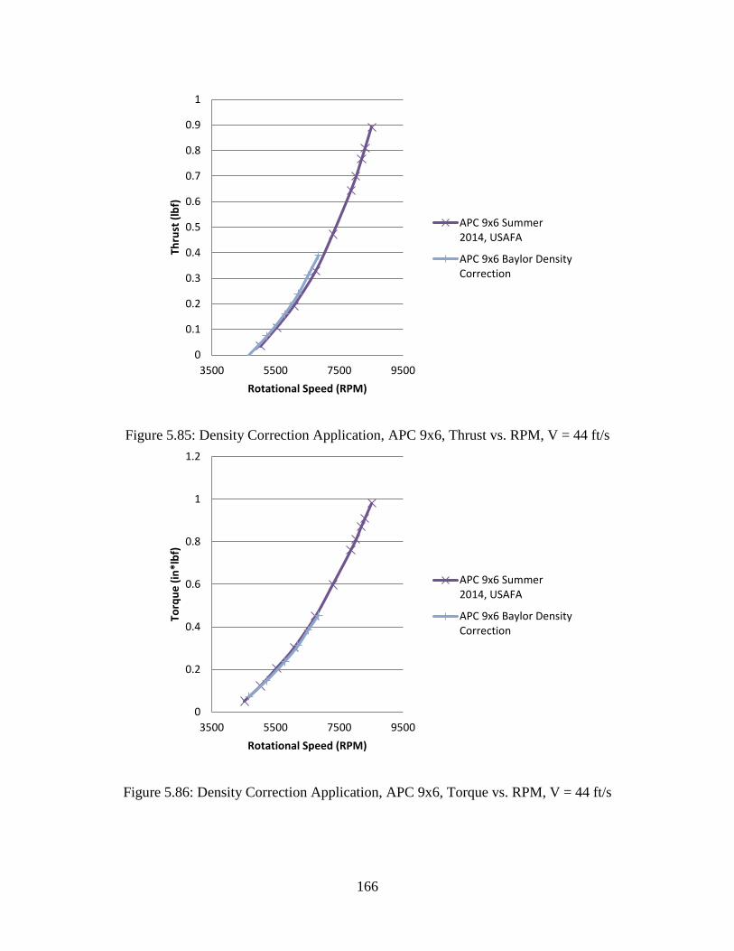
166
Figure 5.85: Density Correction Application, APC 9x6, Thrust vs. RPM, V = 44 ft/s
Figure 5.86: Density Correction Application, APC 9x6, Torque vs. RPM, V = 44 ft/s
0
0.1
0.2
0.3
0.4
0.5
0.6
0.7
0.8
0.9
1
3500 5500 7500 9500
Thru
st (
lbf)
Rotational Speed (RPM)
APC 9x6 Summer2014, USAFA
APC 9x6 Baylor DensityCorrection
0
0.2
0.4
0.6
0.8
1
1.2
3500 5500 7500 9500
Torq
ue
(in
*lb
f)
Rotational Speed (RPM)
APC 9x6 Summer2014, USAFA
APC 9x6 Baylor DensityCorrection
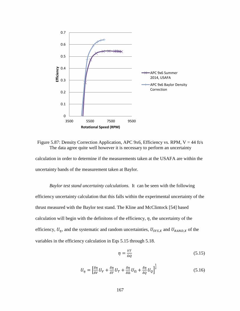
167
Figure 5.87: Density Correction Application, APC 9x6, Efficiency vs. RPM, V = 44 ft/s
The data agree quite well however it is necessary to perform an uncertainty
calculation in order to determine if the measurements taken at the USAFA are within the
uncertainty bands of the measurement taken at Baylor.
Baylor test stand uncertainty calculations. It can be seen with the following
efficiency uncertainty calculation that this falls within the experimental uncertainty of the
thrust measured with the Baylor test stand. The Kline and McClintock [54] based
calculation will begin with the definitons of the efficiency, 𝜂, the uncertainty of the
efficiency, 𝑈𝜂, and the systematic and random uncertainties, 𝑈𝑆𝑌𝑆,𝑋 and 𝑈𝑅𝐴𝑁𝐷,𝑋 of the
variables in the efficiency calculation in Eqs 5.15 through 5.18.
𝜂 =𝑉𝑇
Ω𝑄 (5.15)
𝑈𝜂 = [𝛿𝜂
𝛿𝑉𝑈𝑉 +
𝛿𝜂
𝛿𝑇𝑈𝑇 +
𝛿𝜂
𝛿Ω𝑈Ω +
𝛿𝜂
𝛿𝑄𝑈𝑄]
1
2(5.16)
0
0.1
0.2
0.3
0.4
0.5
0.6
0.7
3500 5500 7500 9500
Effi
cie
ncy
Rotational Speed (RPM)
APC 9x6 Summer2014, USAFA
APC 9x6 Baylor DensityCorrection
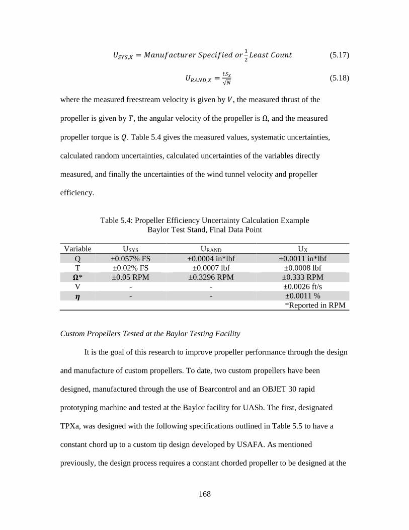
168
𝑈𝑆𝑌𝑆,𝑋 = 𝑀𝑎𝑛𝑢𝑓𝑎𝑐𝑡𝑢𝑟𝑒𝑟 𝑆𝑝𝑒𝑐𝑖𝑓𝑖𝑒𝑑 𝑜𝑟1
2𝐿𝑒𝑎𝑠𝑡 𝐶𝑜𝑢𝑛𝑡 (5.17)
𝑈𝑅𝐴𝑁𝐷,𝑋 =𝑡𝑆𝑥
√𝑁 (5.18)
where the measured freestream velocity is given by 𝑉, the measured thrust of the
propeller is given by 𝑇, the angular velocity of the propeller is Ω, and the measured
propeller torque is 𝑄. Table 5.4 gives the measured values, systematic uncertainties,
calculated random uncertainties, calculated uncertainties of the variables directly
measured, and finally the uncertainties of the wind tunnel velocity and propeller
efficiency.
Table 5.4: Propeller Efficiency Uncertainty Calculation Example
Baylor Test Stand, Final Data Point
Variable USYS URAND UX
Q ±0.057% FS ±0.0004 in*lbf ±0.0011 in*lbf
T ±0.02% FS ±0.0007 lbf ±0.0008 lbf
𝛀* ±0.05 RPM ±0.3296 RPM ±0.333 RPM
V - - ±0.0026 ft/s
𝜼 - - ±0.0011 %
*Reported in RPM
Custom Propellers Tested at the Baylor Testing Facility
It is the goal of this research to improve propeller performance through the design
and manufacture of custom propellers. To date, two custom propellers have been
designed, manufactured through the use of Bearcontrol and an OBJET 30 rapid
prototyping machine and tested at the Baylor facility for UASb. The first, designated
TPXa, was designed with the following specifications outlined in Table 5.5 to have a
constant chord up to a custom tip design developed by USAFA. As mentioned
previously, the design process requires a constant chorded propeller to be designed at the
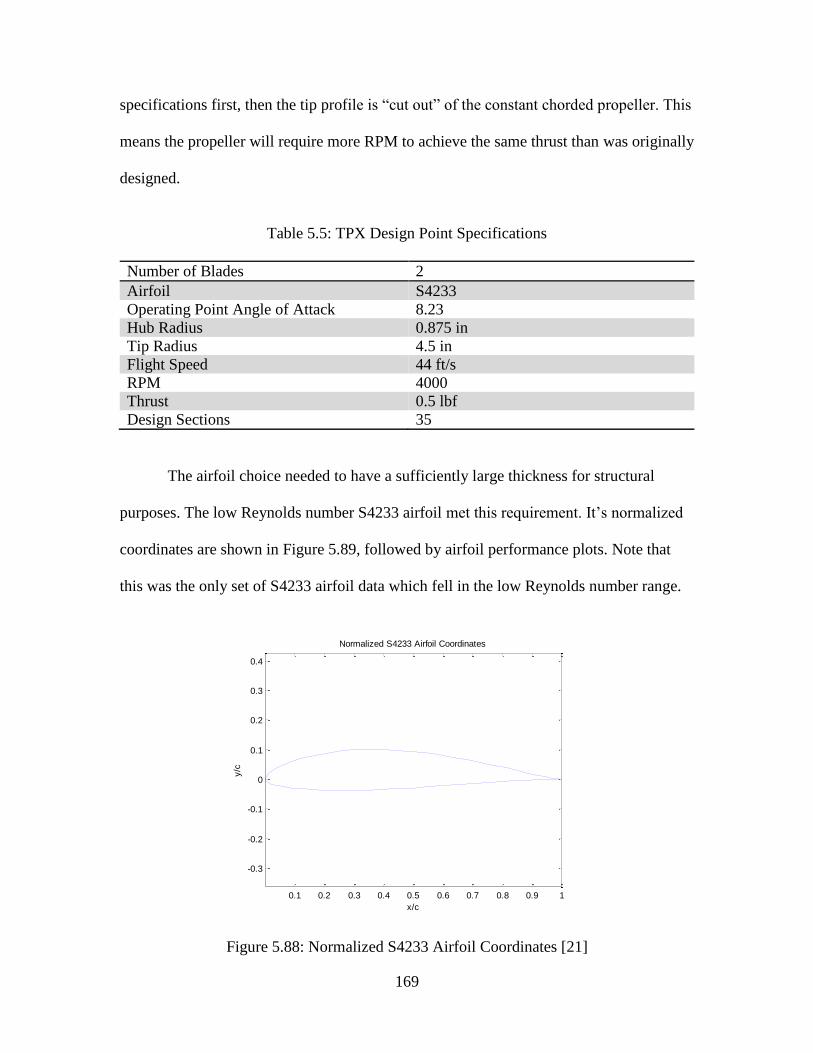
169
specifications first, then the tip profile is “cut out” of the constant chorded propeller. This
means the propeller will require more RPM to achieve the same thrust than was originally
designed.
Table 5.5: TPX Design Point Specifications
Number of Blades 2
Airfoil S4233
Operating Point Angle of Attack 8.23
Hub Radius 0.875 in
Tip Radius 4.5 in
Flight Speed 44 ft/s
RPM 4000
Thrust 0.5 lbf
Design Sections 35
The airfoil choice needed to have a sufficiently large thickness for structural
purposes. The low Reynolds number S4233 airfoil met this requirement. It’s normalized
coordinates are shown in Figure 5.89, followed by airfoil performance plots. Note that
this was the only set of S4233 airfoil data which fell in the low Reynolds number range.
Figure 5.88: Normalized S4233 Airfoil Coordinates [21]
0.1 0.2 0.3 0.4 0.5 0.6 0.7 0.8 0.9 1
-0.3
-0.2
-0.1
0
0.1
0.2
0.3
0.4
Normalized S4233 Airfoil Coordinates
x/c
y/c
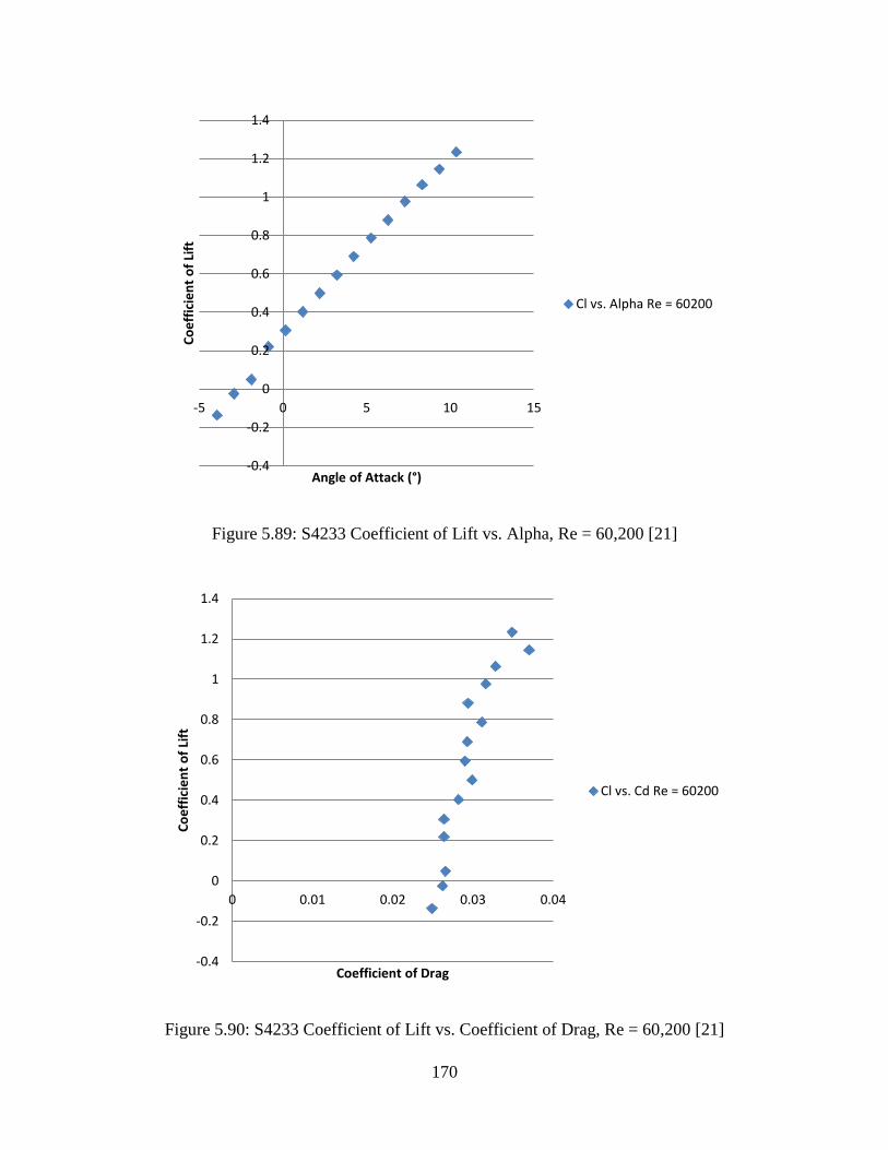
170
Figure 5.89: S4233 Coefficient of Lift vs. Alpha, Re = 60,200 [21]
Figure 5.90: S4233 Coefficient of Lift vs. Coefficient of Drag, Re = 60,200 [21]
-0.4
-0.2
0
0.2
0.4
0.6
0.8
1
1.2
1.4
-5 0 5 10 15
Co
eff
icie
nt
of
Lift
Angle of Attack (°)
Cl vs. Alpha Re = 60200
-0.4
-0.2
0
0.2
0.4
0.6
0.8
1
1.2
1.4
0 0.01 0.02 0.03 0.04
Co
eff
icie
nt
of
Lift
Coefficient of Drag
Cl vs. Cd Re = 60200
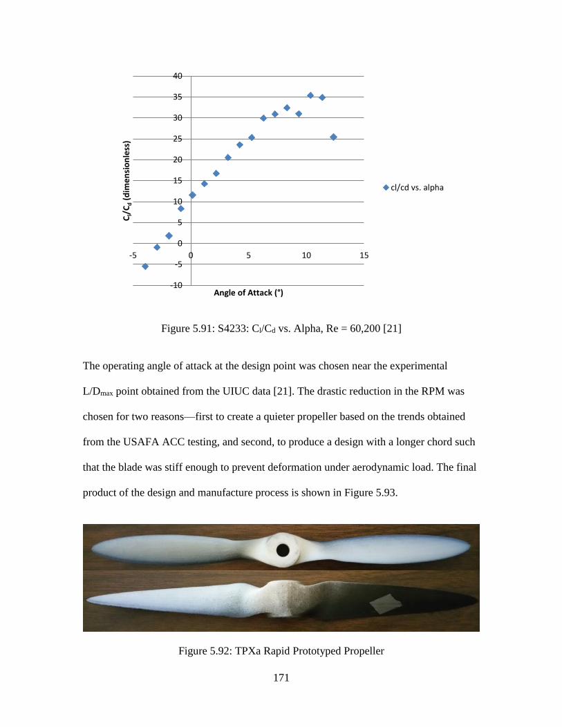
171
Figure 5.91: S4233: Cl/Cd vs. Alpha, Re = 60,200 [21]
The operating angle of attack at the design point was chosen near the experimental
L/Dmax point obtained from the UIUC data [21]. The drastic reduction in the RPM was
chosen for two reasons—first to create a quieter propeller based on the trends obtained
from the USAFA ACC testing, and second, to produce a design with a longer chord such
that the blade was stiff enough to prevent deformation under aerodynamic load. The final
product of the design and manufacture process is shown in Figure 5.93.
Figure 5.92: TPXa Rapid Prototyped Propeller
-10
-5
0
5
10
15
20
25
30
35
40
-5 0 5 10 15
Cl/
Cd
(dim
en
sio
nle
ss)
Angle of Attack (°)
cl/cd vs. alpha
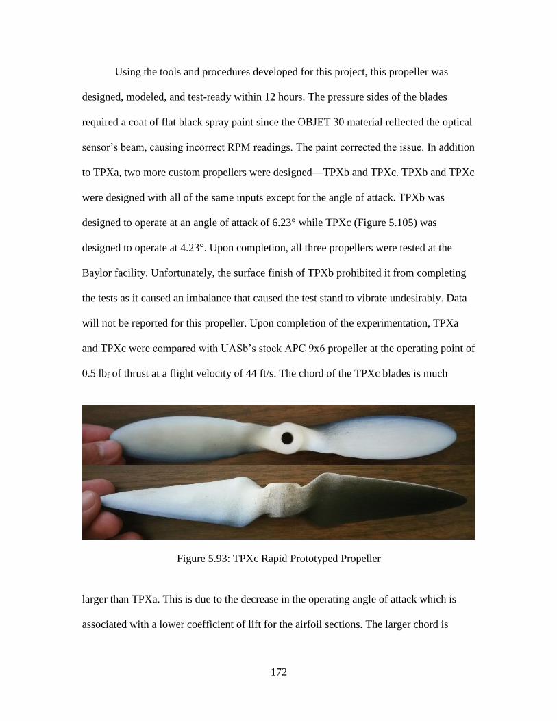
172
Using the tools and procedures developed for this project, this propeller was
designed, modeled, and test-ready within 12 hours. The pressure sides of the blades
required a coat of flat black spray paint since the OBJET 30 material reflected the optical
sensor’s beam, causing incorrect RPM readings. The paint corrected the issue. In addition
to TPXa, two more custom propellers were designed—TPXb and TPXc. TPXb and TPXc
were designed with all of the same inputs except for the angle of attack. TPXb was
designed to operate at an angle of attack of 6.23° while TPXc (Figure 5.105) was
designed to operate at 4.23°. Upon completion, all three propellers were tested at the
Baylor facility. Unfortunately, the surface finish of TPXb prohibited it from completing
the tests as it caused an imbalance that caused the test stand to vibrate undesirably. Data
will not be reported for this propeller. Upon completion of the experimentation, TPXa
and TPXc were compared with UASb’s stock APC 9x6 propeller at the operating point of
0.5 lbf of thrust at a flight velocity of 44 ft/s. The chord of the TPXc blades is much
Figure 5.93: TPXc Rapid Prototyped Propeller
larger than TPXa. This is due to the decrease in the operating angle of attack which is
associated with a lower coefficient of lift for the airfoil sections. The larger chord is
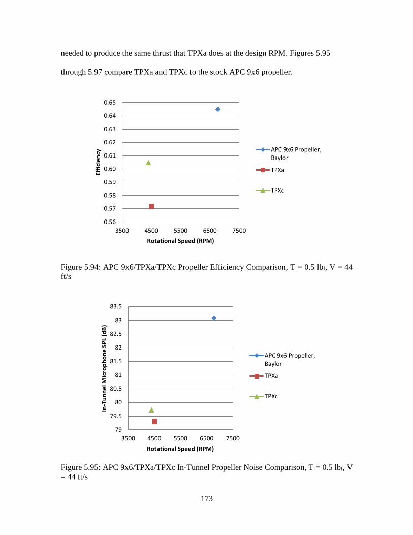
173
needed to produce the same thrust that TPXa does at the design RPM. Figures 5.95
through 5.97 compare TPXa and TPXc to the stock APC 9x6 propeller.
Figure 5.94: APC 9x6/TPXa/TPXc Propeller Efficiency Comparison, T = 0.5 lbf, V = 44
ft/s
Figure 5.95: APC 9x6/TPXa/TPXc In-Tunnel Propeller Noise Comparison, T = 0.5 lbf, V
= 44 ft/s
0.56
0.57
0.58
0.59
0.60
0.61
0.62
0.63
0.64
0.65
3500 4500 5500 6500 7500
Effi
cie
ncy
Rotational Speed (RPM)
APC 9x6 Propeller,Baylor
TPXa
TPXc
79
79.5
80
80.5
81
81.5
82
82.5
83
83.5
3500 4500 5500 6500 7500
In-T
un
ne
l Mic
rop
ho
ne
SP
L (d
B)
Rotational Speed (RPM)
APC 9x6 Propeller,Baylor
TPXa
TPXc
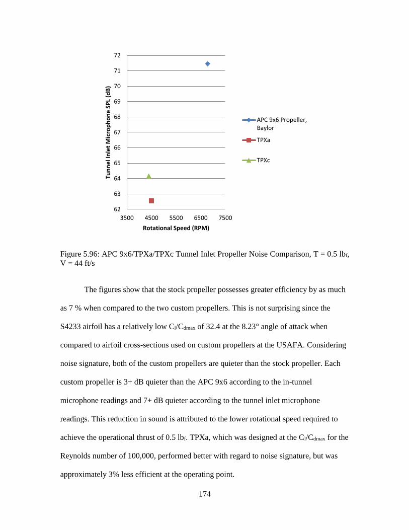
174
Figure 5.96: APC 9x6/TPXa/TPXc Tunnel Inlet Propeller Noise Comparison, T = 0.5 lbf,
V = 44 ft/s
The figures show that the stock propeller possesses greater efficiency by as much
as 7 % when compared to the two custom propellers. This is not surprising since the
S4233 airfoil has a relatively low Cl/Cdmax of 32.4 at the 8.23° angle of attack when
compared to airfoil cross-sections used on custom propellers at the USAFA. Considering
noise signature, both of the custom propellers are quieter than the stock propeller. Each
custom propeller is 3+ dB quieter than the APC 9x6 according to the in-tunnel
microphone readings and 7+ dB quieter according to the tunnel inlet microphone
readings. This reduction in sound is attributed to the lower rotational speed required to
achieve the operational thrust of 0.5 lbf. TPXa, which was designed at the Cl/Cdmax for the
Reynolds number of 100,000, performed better with regard to noise signature, but was
approximately 3% less efficient at the operating point.
62
63
64
65
66
67
68
69
70
71
72
3500 4500 5500 6500 7500
Tun
ne
l In
let
Mic
rop
ho
ne
SP
L (d
B)
Rotational Speed (RPM)
APC 9x6 Propeller,Baylor
TPXa
TPXc
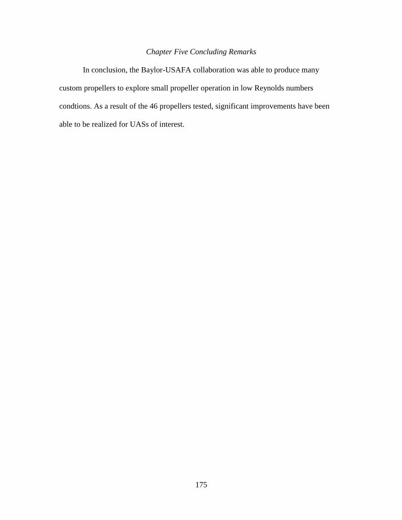
175
Chapter Five Concluding Remarks
In conclusion, the Baylor-USAFA collaboration was able to produce many
custom propellers to explore small propeller operation in low Reynolds numbers
condtions. As a result of the 46 propellers tested, significant improvements have been
able to be realized for UASs of interest.
176
CHAPTER SIX
Conclusions and Recommendations
Summary
In summary, this work first introduced the reader to a variety of UAS categories
while highlighting the need for improvement of performance and noise characteristics for
small UASs. It then surveyed a selection of relevant aerodynamic research, introduced
the theory used throughout the work, detailed the process in which the USAFA and
Baylor collaboration designs, analyzes, and manufactures test propellers, and explained
both the experimental setup and method. Finally, it presented the results of the
experimentation completed.
Three different categories of UASs were introduced—HALE, MALE, and LASE
UASs. As the sizes of these UASs decreased, so did their capabilities such as endurance
and flight speed. LASE UASs, the smallest vehicles introduced, are utilized due to their
ease of transportation, deployment, and recovery. Increasing the efficiency of the
powerplants of these UASs was noted as the objective of this study.
Different low Reynolds number airfoil and propeller operation effects were
explored. Phenomena such as a laminar separation bubbles on the suction side of airfoils
and reduced efficiencies of propellers due to low Reynolds numbers were seen. In
addition, experimental test rigs in use at other universities to evaluate propellers were
investigated. These observations contributed to the designs of the USAFA and Baylor
propeller test rigs.
177
Many propeller design theories were presented in this work. The QMIL/QPROP
propeller design and analysis package was ultimately utilized. Other propeller design and
analysis theories detailed were the one-dimensional propeller theory, BET, and BEMT.
The theory behind the NREL program NAFNoise was also introduced to explain the
airfoil noise prediction code. Other theories detailed were the Glauert wind tunnel
correction for propellers operating in a closed test section wind tunnel and propeller-
motor matching theory.
A custom MATLAB code and GUI, Bearcontrol, was introduced. This was the
cornerstone of propeller design, theoretical analysis, and manufacturing of test propellers
in this work. It reduced the manufacture time of propellers from the order of weeks to
hours. Once propellers were manufactured, they were evaluated with either the USAFA
or Baylor propeller test stand which were each designed with accompanying DAQ
hardware and code to allow for time efficient testing.
Finally the results of the 46 propellers tested were presented. Many studies that
varied different design parameters led to improved performance. The highest efficiency
increase was 7%, while the highest noise reduction was 12 dB. Although these studies
have yet to lead to empirical design correlations, recommendations can be made based on
these results.
Design Recommendations for High Efficiency and Low Noise Propellers
The propellers with the highest efficiencies and lowest noise signatures all
achieved their high performance by operating at a low RPM. Not all propellers with a low
RPM performed well. Examples of propellers that did not perform well were all constant
chord test propellers with a flat tip. On the other hand, the best performing propellers
178
were constant chord propellers with tip treatments. An example of this is TP40 which
used a GM15 airfoil cross section operating at two degrees below the Cl/Cdmax angle of
attack with a constant chord out to the custom Oval 2 tip treatment. Next, if the geometric
constraints of the UAS allow, the designer should increase the diameter of the propeller.
This recommendation is based on the efficiency performance of TP44. Although this
propeller only possessed two blades, it had a higher efficiency than all propellers in its
study. In order to continue to reduce the noise of the propeller, more blades could be
added. The data presented in this work suggests that there will be a maximum with regard
to efficiency as blades are added even though the noise production continued to drop.
This will inevitably lead to a tradeoff the designer will need to address with consideration
of the design situation.
Experiment Improvement Recommendations and Future Work
The basis of small propeller design, analysis, manufacture, and experimental
evaluation presented in this work opens the door to future research. The following
sections will detail improvements that can be made to the current procedures and
experiment to further improve propeller performance.
Airfoil Data
One constantly glaring issue dealt with in this research is the lack of airfoil data at
low Reynolds numbers. As the design of the propellers evolved to constant chord blades
with tip treatments, this became even more of an issue since the Reynolds number can
vary greatly across these blades. Equipment and procedures [55] exist at Baylor
University in order to conduct experiments to obtain this data.
179
Bearcontrol
Although Bearcontrol has improved the production of test propellers as seen in
this work, there still exists room for improvement. The first recommended improvement
would be to integrate the supplemental codes into the main Bearcontrol GUI. While these
codes are being integrated, it would benefit the research effort to investigate a more time
efficient propeller chord iteration procedure in the supplemental code
constantchordhelper.m. Based on the user’s initial guess, the current propeller chord
iteration procedure could possibly cause the program to run for hours. This would save
additional time in the design of constant chord and tip treated propellers.
Next, the integration of the NREL airfoil noise prediction code NAFNoise should
be finished. While this implementation is taking place, it would also be advantageous to
add a subroutine that predicts tip vortex formation noise. These Bearcontrol updates
would give users the ability to theoretically predict the noise of propellers and compare
(qualitatively at the least) different designs without experiments.
As the propeller designs move to blades with varying Reynolds numbers and as
more low Reynolds number airfoil data becomes available, it would benefit future
research to update the QMIL/QPROP code with the necessary constraints and subroutines
to take in airfoil data at multiple Reynolds numbers and apply it across the blade in the
design and analysis scenarios. For most cases, this would likely lead to a better
theoretical analysis prediction.
It would also benefit future research to implement a propeller blade
stress/deformation prediction routine in the Bearcontrol code. This could give researchers
the ability to predict whether or not a certain propeller blade design would deform
180
significantly under aerodynamic loading. This prediction capability would prevent wasted
material and time that would otherwise be used unknowingly.
Finally, in order to analyze the powerplant system as a whole, a motor selection
method should be integrated into the GUI. This would allow for the selection of
QMIL/QPROP’s default motor, or a custom motor defined by the user.
Experimental Setup and Method
Although the experimental setup and method of the Baylor test stand allows for
the time efficient evaluation of test propellers, there still exists room for improvement.
First, the current power supplies for the propeller motor do not provide sufficient
amperage. A more suitable power supply would increase the propeller testing capabilities
of the stand.
The DAQ GUI and code can be improved through further automation. The first
step would be to automate the uncertainty calculations. Next, it is recommended that a
MATLAB script or Excel macro be created and tailored to the output files of the GUI.
This script would perform any further data reduction or plotting not able to be
accomplished in the GUI.
Concluding Remarks
In summary, this work produced the means to design, theoretically analyze,
manufacture, and experimentally evaluate small propellers rapidly. The 46 propellers
tested led to improved propeller performance and provided framework for the exploration
of future designs.

181
APPENDICES

182
APPENDIX A
Bearcontrol User Guide
Bearcontrol User Guide Version 2.0
Trae Liller
Baylor University
Department of Mechanical Engineering
Program Description
Bearcontrol is a program written in MATLAB that gives a user the ability to quickly
design a propeller, predict its performance, and then model it in SolidWorks. The
overarching MATLAB code allows the user to control design, analysis, and modeling
programs through a user friendly GUI. This ultimately results in a mostly automated
process that allows an individual who is unfamiliar with command prompt programs and
SolidWorks modeling to design, analyze and model a propeller in a time efficient
manner.
System Requirements
Bearcontrol will run in conjunction with the following programs:
Matlab R2013a
Solidworks 2013 x64 Edition
QMIL Version 1.10
QPROP Version 1.21
Bearcontrol may or may not work with previous versions of the above programs.
All calculations and macros have been tested on a PC computer with the following
specifications in no more than 5 minutes for the default design scheme:
Intel Core2 Quad CPU Q9505 @ 2.83 GHz
RAM: 8.00 GB
System Type: 64-bit
With this program it is possible to design and model a propeller in under five minutes.
Quick Start Example
The following steps will illustrate the use of the GUI in conjunction with one of the pre-
packaged airfoil sections. The versatility of Bearcontrol will allow a user to input their
own airfoil cross-section data—this procedure will be discussed later in this document.
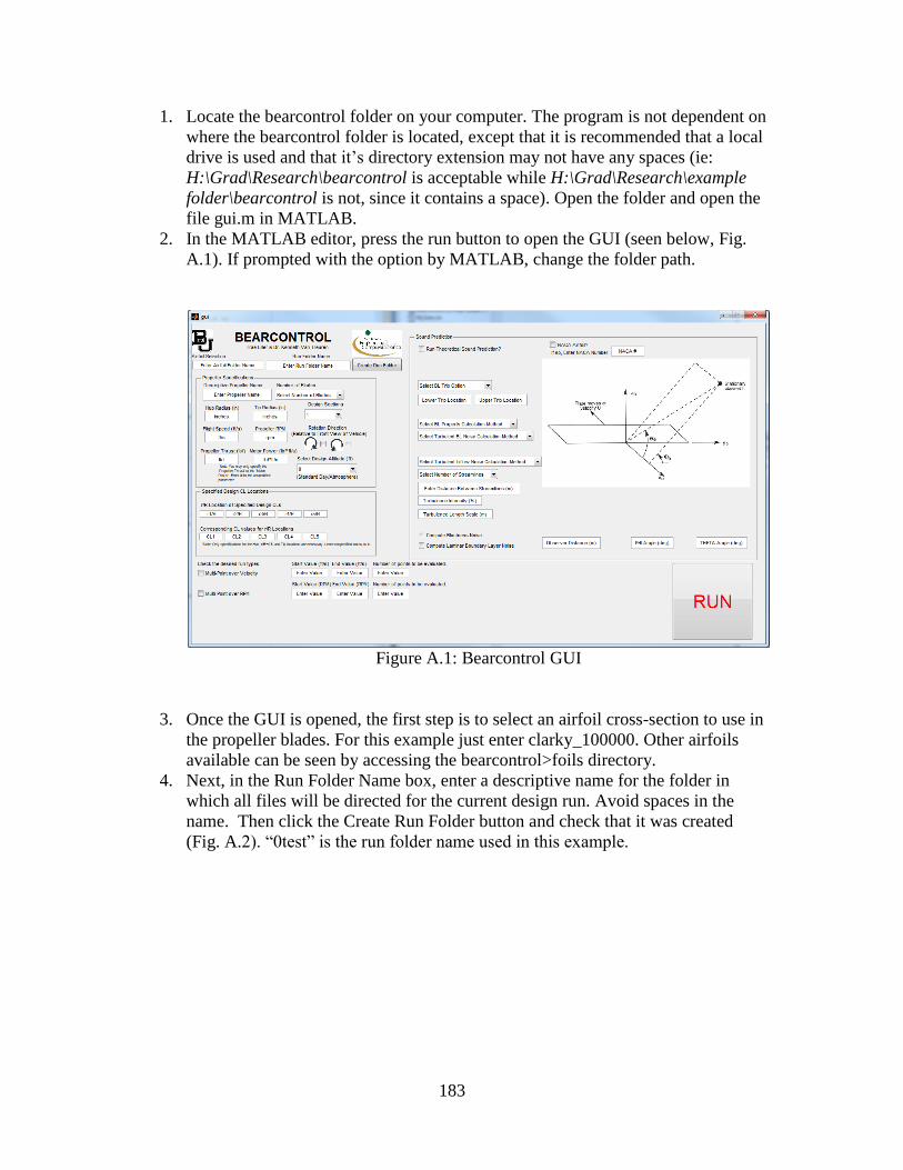
183
1. Locate the bearcontrol folder on your computer. The program is not dependent on
where the bearcontrol folder is located, except that it is recommended that a local
drive is used and that it’s directory extension may not have any spaces (ie:
H:\Grad\Research\bearcontrol is acceptable while H:\Grad\Research\example
folder\bearcontrol is not, since it contains a space). Open the folder and open the
file gui.m in MATLAB.
2. In the MATLAB editor, press the run button to open the GUI (seen below, Fig.
A.1). If prompted with the option by MATLAB, change the folder path.
Figure A.1: Bearcontrol GUI
3. Once the GUI is opened, the first step is to select an airfoil cross-section to use in
the propeller blades. For this example just enter clarky_100000. Other airfoils
available can be seen by accessing the bearcontrol>foils directory.
4. Next, in the Run Folder Name box, enter a descriptive name for the folder in
which all files will be directed for the current design run. Avoid spaces in the
name. Then click the Create Run Folder button and check that it was created
(Fig. A.2). “0test” is the run folder name used in this example.
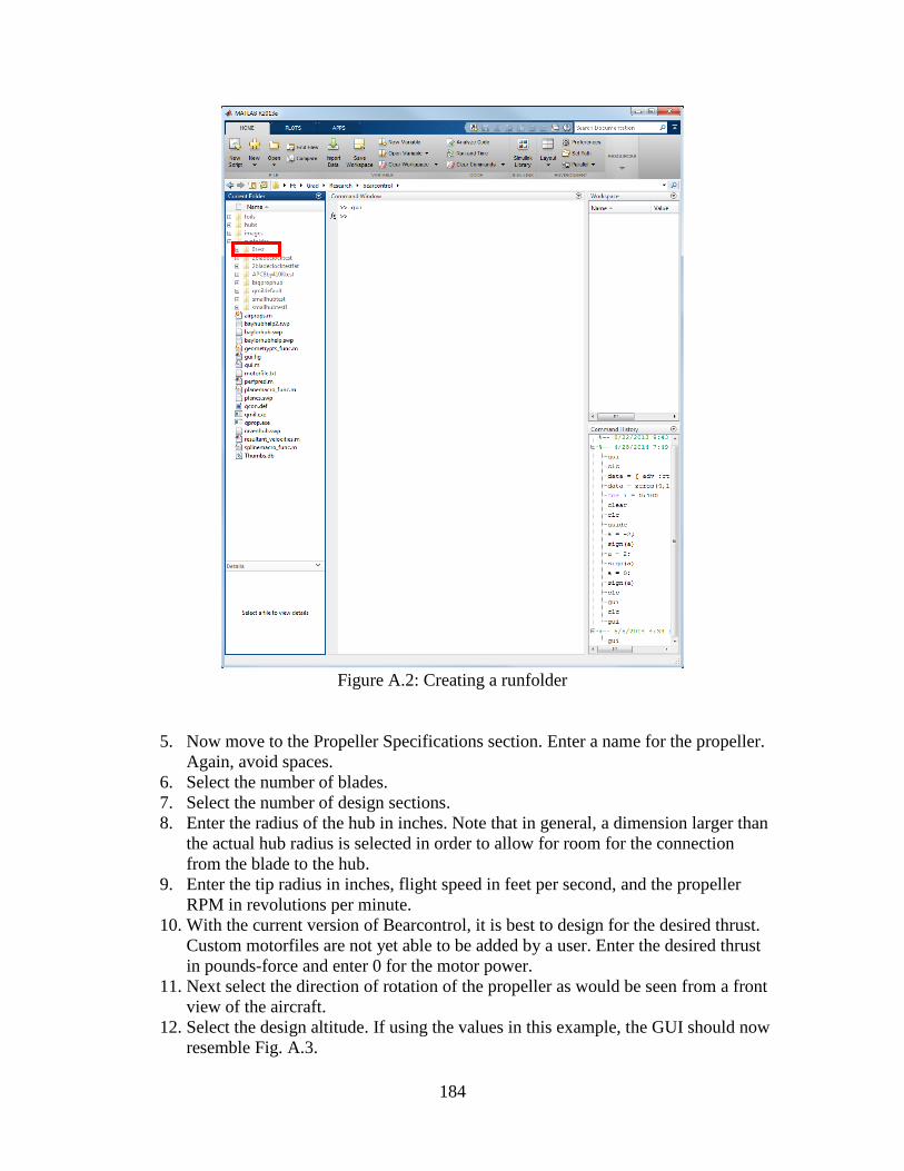
184
Figure A.2: Creating a runfolder
5. Now move to the Propeller Specifications section. Enter a name for the propeller.
Again, avoid spaces.
6. Select the number of blades.
7. Select the number of design sections.
8. Enter the radius of the hub in inches. Note that in general, a dimension larger than
the actual hub radius is selected in order to allow for room for the connection
from the blade to the hub.
9. Enter the tip radius in inches, flight speed in feet per second, and the propeller
RPM in revolutions per minute.
10. With the current version of Bearcontrol, it is best to design for the desired thrust.
Custom motorfiles are not yet able to be added by a user. Enter the desired thrust
in pounds-force and enter 0 for the motor power.
11. Next select the direction of rotation of the propeller as would be seen from a front
view of the aircraft.
12. Select the design altitude. If using the values in this example, the GUI should now
resemble Fig. A.3.
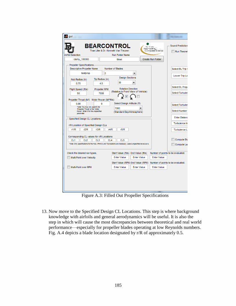
185
Figure A.3: Filled Out Propeller Specifications
13. Now move to the Specified Design CL Locations. This step is where background
knowledge with airfoils and general aerodynamics will be useful. It is also the
step in which will cause the most discrepancies between theoretical and real world
performance—especially for propeller blades operating at low Reynolds numbers.
Fig. A.4 depicts a blade location designated by r/R of approximately 0.5.
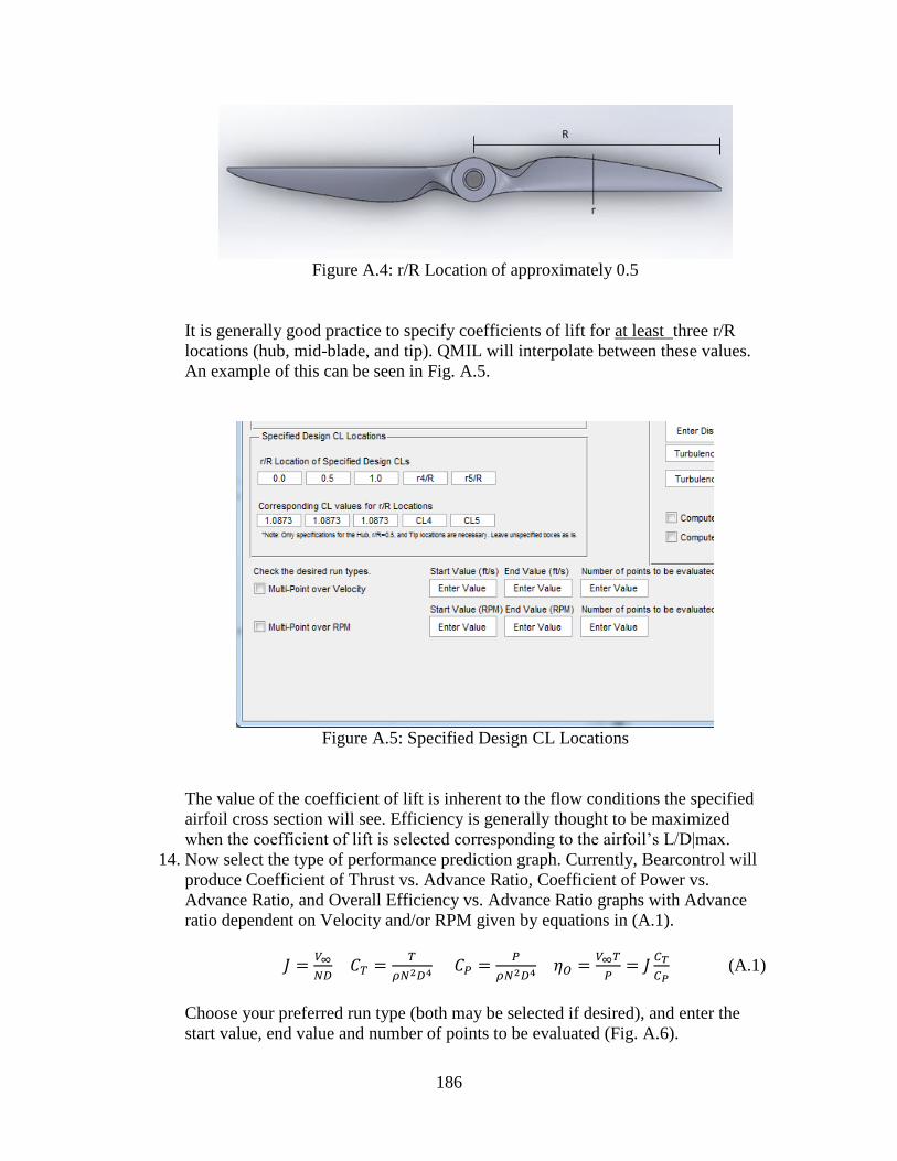
186
Figure A.4: r/R Location of approximately 0.5
It is generally good practice to specify coefficients of lift for at least three r/R
locations (hub, mid-blade, and tip). QMIL will interpolate between these values.
An example of this can be seen in Fig. A.5.
Figure A.5: Specified Design CL Locations
The value of the coefficient of lift is inherent to the flow conditions the specified
airfoil cross section will see. Efficiency is generally thought to be maximized
when the coefficient of lift is selected corresponding to the airfoil’s L/D|max.
14. Now select the type of performance prediction graph. Currently, Bearcontrol will
produce Coefficient of Thrust vs. Advance Ratio, Coefficient of Power vs.
Advance Ratio, and Overall Efficiency vs. Advance Ratio graphs with Advance
ratio dependent on Velocity and/or RPM given by equations in (A.1).
𝐽 =𝑉∞
𝑁𝐷 𝐶𝑇 =
𝑇
𝜌𝑁2𝐷4 𝐶𝑃 =𝑃
𝜌𝑁2𝐷4 𝜂𝑂 =𝑉∞𝑇
𝑃= 𝐽
𝐶𝑇
𝐶𝑃 (A.1)
Choose your preferred run type (both may be selected if desired), and enter the
start value, end value and number of points to be evaluated (Fig. A.6).
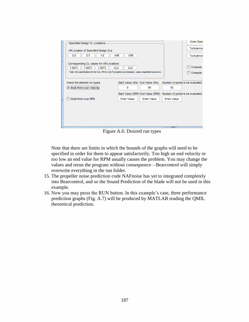
187
Figure A.6: Desired run types
Note that there are limits in which the bounds of the graphs will need to be
specified in order for them to appear satisfactorily. Too high an end velocity or
too low an end value for RPM usually causes the problem. You may change the
values and rerun the program without consequence—Bearcontrol will simply
overwrite everything in the run folder.
15. The propeller noise prediction code NAFnoise has yet to integrated completely
into Bearcontrol, and so the Sound Prediction of the blade will not be used in this
example.
16. Now you may press the RUN button. In this example’s case, three performance
prediction graphs (Fig. A.7) will be produced by MATLAB reading the QMIL
theoretical prediction.
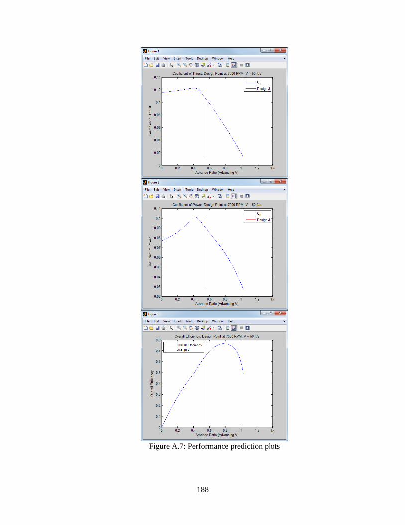
188
Figure A.7: Performance prediction plots
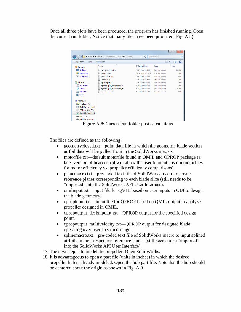
189
Once all three plots have been produced, the program has finished running. Open
the current run folder. Notice that many files have been produced (Fig. A.8):
Figure A.8: Current run folder post calculations
The files are defined as the following:
geometryclosed.txt—point data file in which the geometric blade section
airfoil data will be pulled from in the SolidWorks macros.
motorfile.txt—default motorfile found in QMIL and QPROP package (a
later version of bearcontrol will allow the user to input custom motorfiles
for motor efficiency vs. propeller efficiency comparisons).
planemacro.txt—pre-coded text file of SolidWorks macro to create
reference planes corresponding to each blade slice (still needs to be
“imported” into the SolidWorks API User Interface).
qmilinput.txt—input file for QMIL based on user inputs in GUI to design
the blade geometry.
qpropinput.txt—input file for QPROP based on QMIL output to analyze
propeller designed in QMIL.
qpropoutput_designpoint.txt—QPROP output for the specified design
point.
qpropoutput_multivelocity.txt—QPROP output for designed blade
operating over user specified range.
splinemacro.txt—pre-coded text file of SolidWorks macro to input splined
airfoils in their respective reference planes (still needs to be “imported”
into the SolidWorks API User Interface).
17. The next step is to model the propeller. Open SolidWorks.
18. It is advantageous to open a part file (units in inches) in which the desired
propeller hub is already modeled. Open the hub part file. Note that the hub should
be centered about the origin as shown in Fig. A.9.
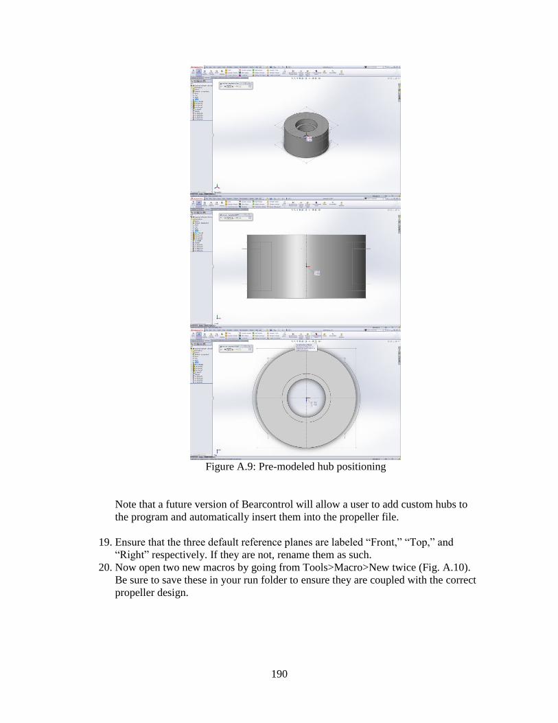
190
Figure A.9: Pre-modeled hub positioning
Note that a future version of Bearcontrol will allow a user to add custom hubs to
the program and automatically insert them into the propeller file.
19. Ensure that the three default reference planes are labeled “Front,” “Top,” and
“Right” respectively. If they are not, rename them as such.
20. Now open two new macros by going from Tools>Macro>New twice (Fig. A.10).
Be sure to save these in your run folder to ensure they are coupled with the correct
propeller design.
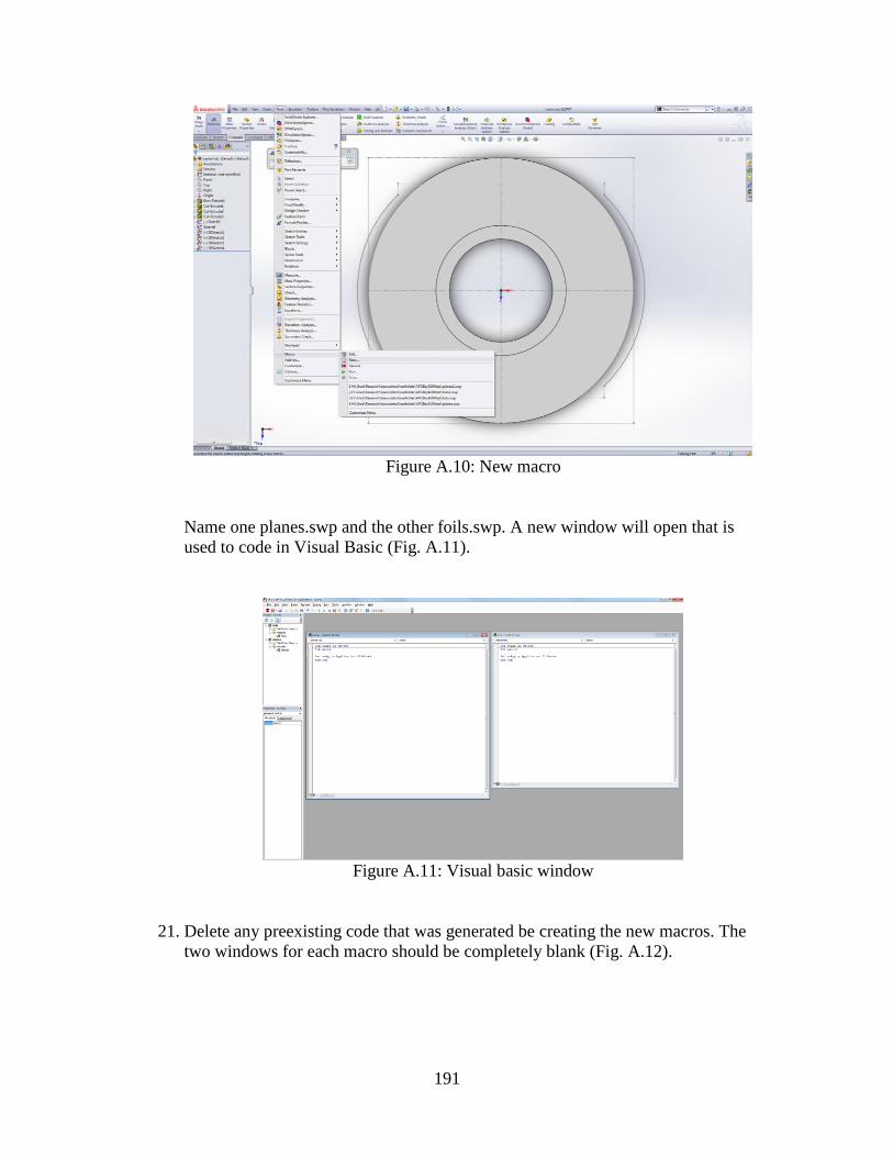
191
Figure A.10: New macro
Name one planes.swp and the other foils.swp. A new window will open that is
used to code in Visual Basic (Fig. A.11).
Figure A.11: Visual basic window
21. Delete any preexisting code that was generated be creating the new macros. The
two windows for each macro should be completely blank (Fig. A.12).
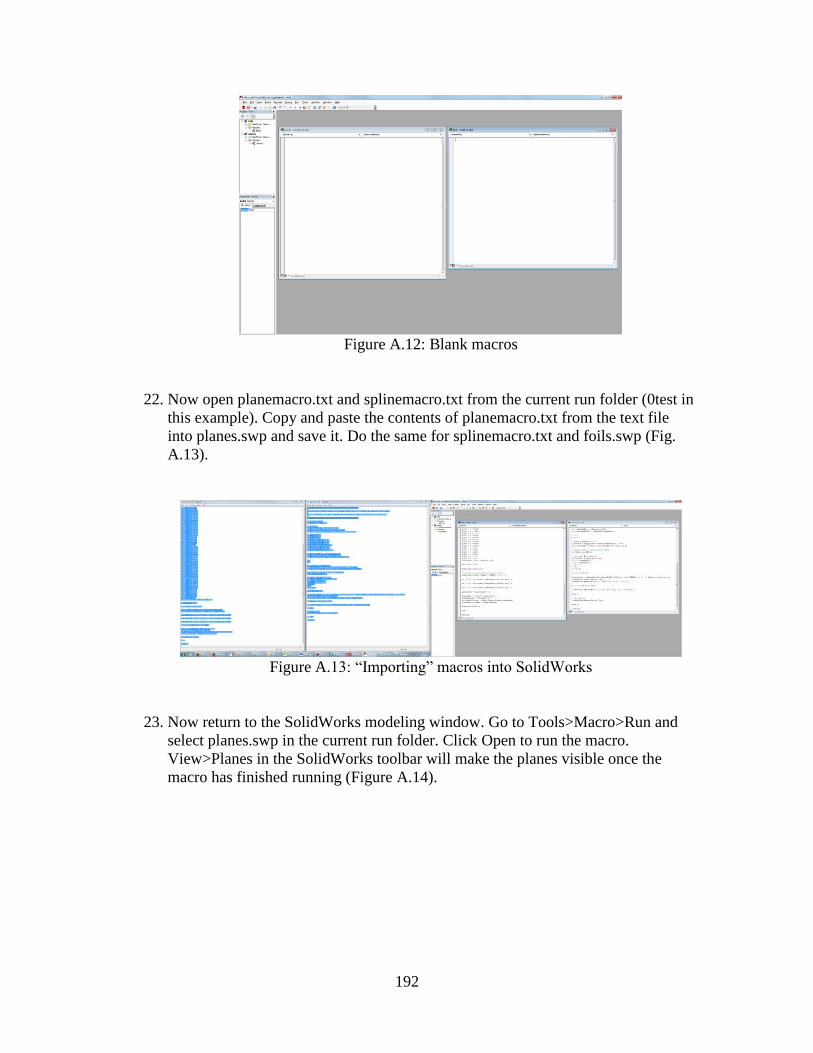
192
Figure A.12: Blank macros
22. Now open planemacro.txt and splinemacro.txt from the current run folder (0test in
this example). Copy and paste the contents of planemacro.txt from the text file
into planes.swp and save it. Do the same for splinemacro.txt and foils.swp (Fig.
A.13).
Figure A.13: “Importing” macros into SolidWorks
23. Now return to the SolidWorks modeling window. Go to Tools>Macro>Run and
select planes.swp in the current run folder. Click Open to run the macro.
View>Planes in the SolidWorks toolbar will make the planes visible once the
macro has finished running (Figure A.14).
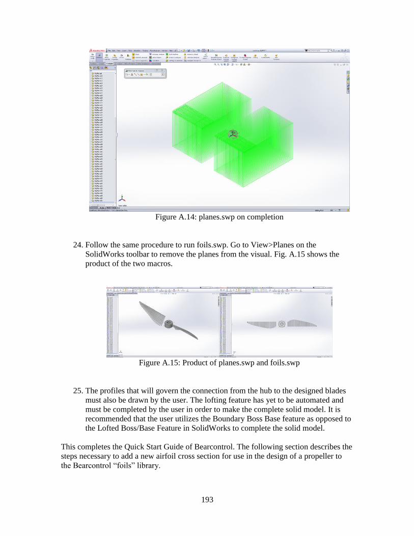
193
Figure A.14: planes.swp on completion
24. Follow the same procedure to run foils.swp. Go to View>Planes on the
SolidWorks toolbar to remove the planes from the visual. Fig. A.15 shows the
product of the two macros.
Figure A.15: Product of planes.swp and foils.swp
25. The profiles that will govern the connection from the hub to the designed blades
must also be drawn by the user. The lofting feature has yet to be automated and
must be completed by the user in order to make the complete solid model. It is
recommended that the user utilizes the Boundary Boss Base feature as opposed to
the Lofted Boss/Base Feature in SolidWorks to complete the solid model.
This completes the Quick Start Guide of Bearcontrol. The following section describes the
steps necessary to add a new airfoil cross section for use in the design of a propeller to
the Bearcontrol “foils” library.
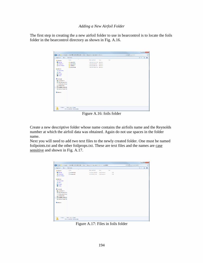
194
Adding a New Airfoil Folder
The first step in creating the a new airfoil folder to use in bearcontrol is to locate the foils
folder in the bearcontrol directory as shown in Fig. A.16.
Figure A.16: foils folder
Create a new descriptive folder whose name contains the airfoils name and the Reynolds
number at which the airfoil data was obtained. Again do not use spaces in the folder
name.
Next you will need to add two text files to the newly created folder. One must be named
foilpoints.txt and the other foilprops.txt. These are text files and the names are case
sensitive and shown in Fig. A.17.
Figure A.17: Files in foils folder
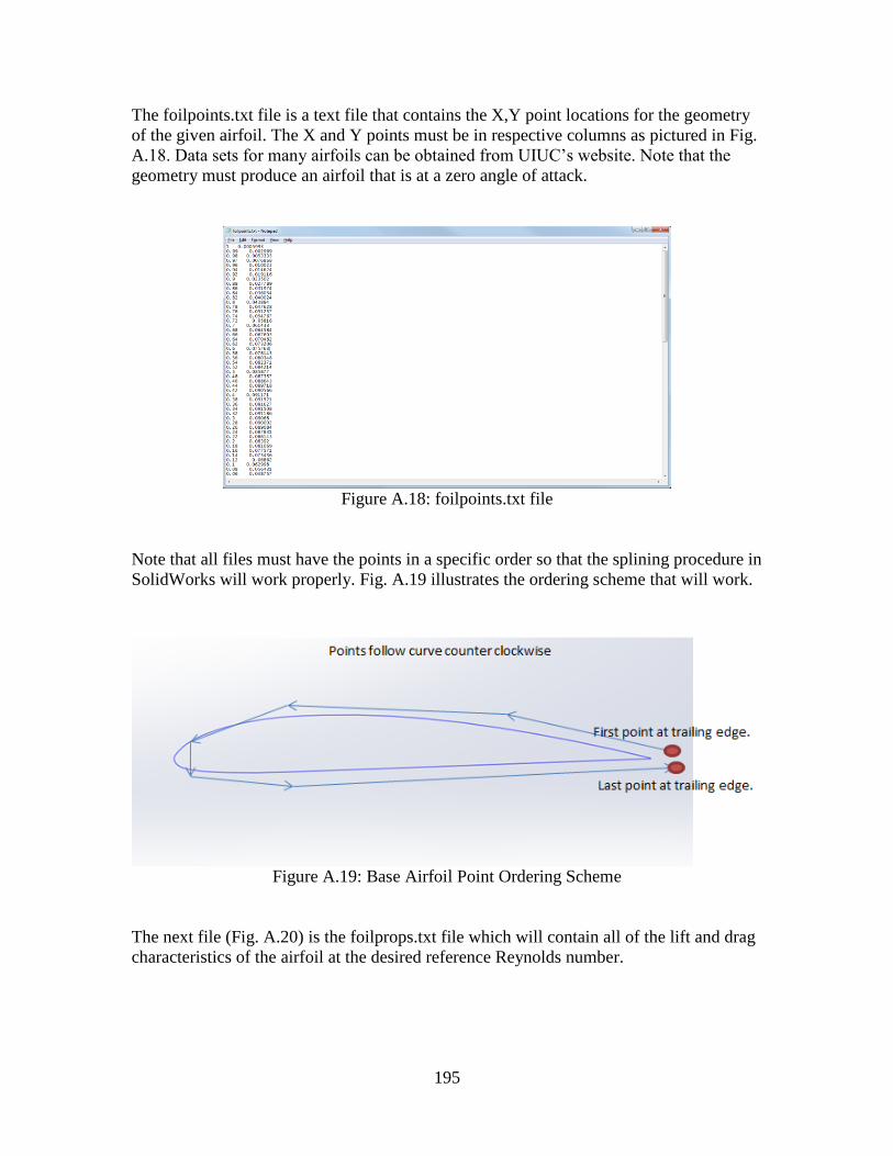
195
The foilpoints.txt file is a text file that contains the X,Y point locations for the geometry
of the given airfoil. The X and Y points must be in respective columns as pictured in Fig.
A.18. Data sets for many airfoils can be obtained from UIUC’s website. Note that the
geometry must produce an airfoil that is at a zero angle of attack.
Figure A.18: foilpoints.txt file
Note that all files must have the points in a specific order so that the splining procedure in
SolidWorks will work properly. Fig. A.19 illustrates the ordering scheme that will work.
Figure A.19: Base Airfoil Point Ordering Scheme
The next file (Fig. A.20) is the foilprops.txt file which will contain all of the lift and drag
characteristics of the airfoil at the desired reference Reynolds number.
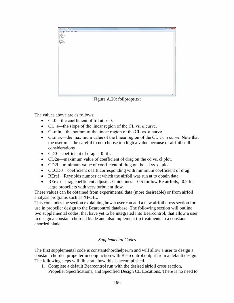
196
Figure A.20: foilprops.txt
The values above are as follows:
CL0—the coefficient of lift at α=0.
CL_a—the slope of the linear region of the CL vs. α curve.
CLmin—the bottom of the linear region of the CL vs. α curve.
CLmax—the maximum value of the linear region of the CL vs. α curve. Note that
the user must be careful to not choose too high a value because of airfoil stall
considerations.
CD0—coefficient of drag at 0 lift.
CD2u—maximum value of coefficient of drag on the cd vs. cl plot.
CD2l—minimum value of coefficient of drag on the cd vs. cl plot.
CLCD0—coefficient of lift corresponding with minimum coefficient of drag.
REref—Reynolds number at which the airfoil was run at to obtain data.
REexp—drag coefficient adjuster. Guidelines: -0.5 for low Re airfoils, -0.2 for
large propellers with very turbulent flow.
These values can be obtained from experimental data (more desireable) or from airfoil
analysis programs such as XFOIL.
This concludes the section explaining how a user can add a new airfoil cross section for
use in propeller design to the Bearcontrol database. The following section will outline
two supplemental codes, that have yet to be integrated into Bearcontrol, that allow a user
to design a constant chorded blade and also implement tip treatments to a constant
chorded blade.
Supplemental Codes
The first supplemental code is constantchordhelper.m and will allow a user to design a
constant chorded propeller in conjunction with Bearcontrol output from a default design.
The following steps will illustrate how this is accomplished.
1. Complete a default Bearcontrol run with the desired airfoil cross section,
Propeller Specifications, and Specified Design CL Locations. There is no need to
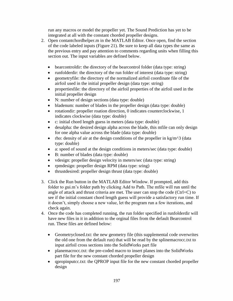
197
run any macros or model the propeller yet. The Sound Prediction has yet to be
integrated at all with the constant chorded propeller designs.
2. Open contantchordhelper.m in the MATLAB Editor. Once open, find the section
of the code labeled inputs (Figure 21). Be sure to keep all data types the same as
the previous entry and pay attention to comments regarding units when filling this
section out. The input variables are defined below.
bearcontroldir: the directory of the bearcontrol folder (data type: string)
runfolderdir: the directory of the run folder of interest (data type: string)
geometryfile: the directory of the normalized airfoil coordinate file of the
airfoil used in the initial propeller design (data type: string)
propertiesfile: the directory of the airfoil properties of the airfoil used in the
initial propeller design
N: number of design sections (data type: double)
bladenum: number of blades in the propeller design (data type: double)
rotationdir: propeller roation direction, 0 indicates counterclockwise, 1
indicates clockwise (data type: double)
c: initial chord length guess in meters (data type: double)
desalpha: the desired design alpha across the blade, this mfile can only design
for one alpha value across the blade (data type: double)
rho: density of air at the design conditions of the propeller in kg/m^3 (data
type: double)
a: speed of sound at the design conditions in meters/sec (data type: double)
B: number of blades (data type: double)
vdesign: propeller design velocity in meters/sec (data type: string)
rpmdesign: propeller design RPM (data type: sring)
thrustdesired: propeller design thrust (data type: double)
3. Click the Run button in the MATLAB Editor Window. If prompted, add this
folder to gui.m’s folder path by clicking Add to Path. The mfile will run until the
angle of attack and thrust criteria are met. The user can stop the code (Ctrl+C) to
see if the initial constant chord length guess will provide a satisfactory run time. If
it doesn’t, simply choose a new value, let the program run a few iterations, and
check again.
4. Once the code has completed running, the run folder specified in runfolderdir will
have new files in it in addition to the orginal files from the default Bearcontrol
run. These files are defined below:
Geometryclosed.txt: the new geometry file (this supplemental code overwrites
the old one from the default run) that will be read by the splinemacrocc.txt to
input airfoil cross sections into the SolidWorks part file
planemacrocc.txt: the pre-coded macro to insert planes into the SolidWorks
part file for the new constant chorded propeller design
qpropinputcc.txt: the QPROP input file for the new constant chorded propeller
design
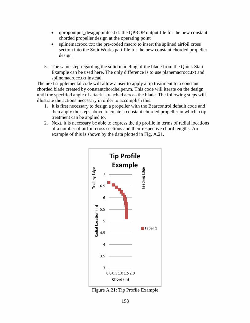
198
qpropoutput_designpointcc.txt: the QPROP output file for the new constant
chorded propeller design at the operating point
splinemacrocc.txt: the pre-coded macro to insert the splined airfoil cross
section into the SolidWorks part file for the new constant chorded propeller
design
5. The same step regarding the solid modeling of the blade from the Quick Start
Example can be used here. The only difference is to use planemacrocc.txt and
splinemacrocc.txt instead.
The next supplemental code will allow a user to apply a tip treatment to a constant
chorded blade created by constantchordhelper.m. This code will iterate on the design
until the specified angle of attack is reached across the blade. The following steps will
illustrate the actions necessary in order to accomplish this.
1. It is first necessary to design a propeller with the Bearcontrol default code and
then apply the steps above to create a constant chorded propeller in which a tip
treatment can be applied to.
2. Next, it is necessary be able to express the tip profile in terms of radial locations
of a number of airfoil cross sections and their respective chord lengths. An
example of this is shown by the data plotted in Fig. A.21.
Figure A.21: Tip Profile Example
3
3.5
4
4.5
5
5.5
6
6.5
7
0.0 0.5 1.0 1.5 2.0
Rad
ial L
oca
tio
n (
in)
Chord (in)
Tip Profile Example
Taper 1
Lead
ing
Edge
Trai
ling
Edge
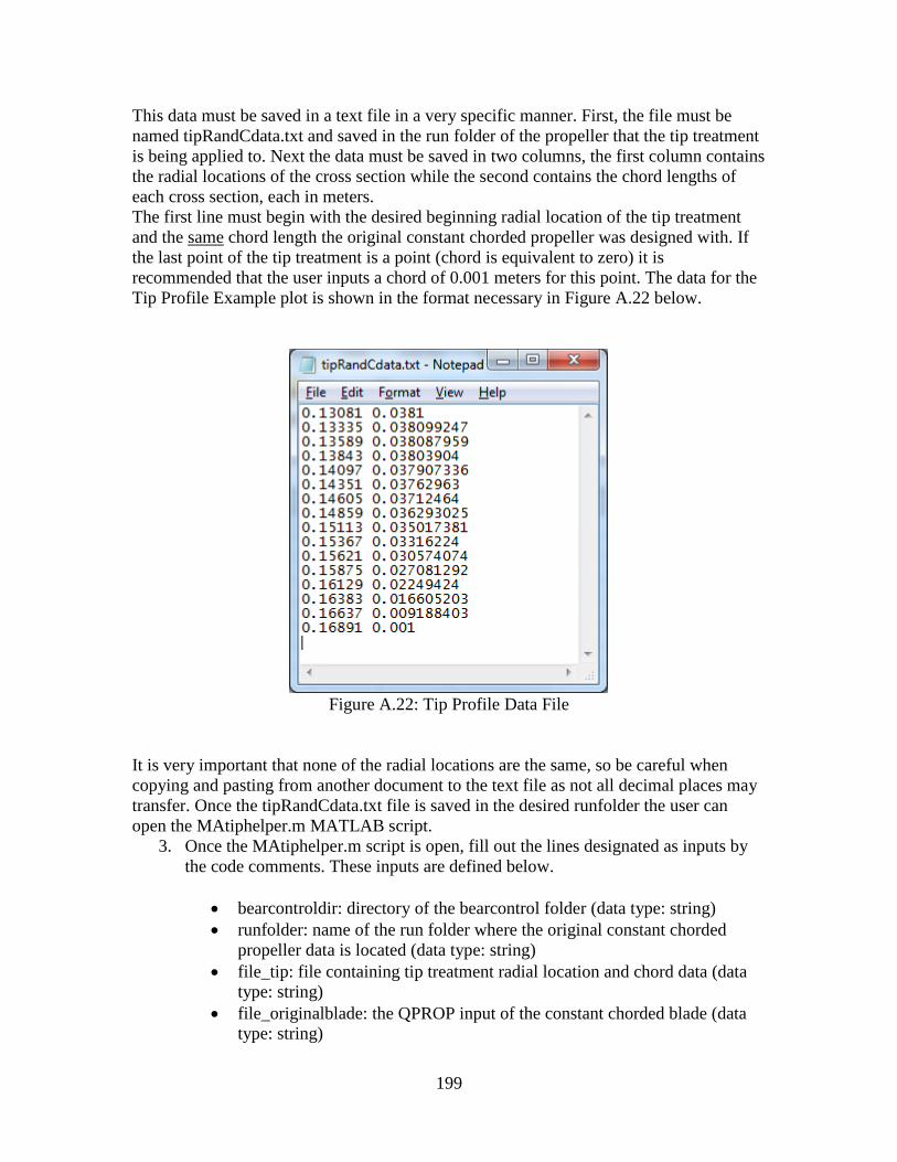
199
This data must be saved in a text file in a very specific manner. First, the file must be
named tipRandCdata.txt and saved in the run folder of the propeller that the tip treatment
is being applied to. Next the data must be saved in two columns, the first column contains
the radial locations of the cross section while the second contains the chord lengths of
each cross section, each in meters.
The first line must begin with the desired beginning radial location of the tip treatment
and the same chord length the original constant chorded propeller was designed with. If
the last point of the tip treatment is a point (chord is equivalent to zero) it is
recommended that the user inputs a chord of 0.001 meters for this point. The data for the
Tip Profile Example plot is shown in the format necessary in Figure A.22 below.
Figure A.22: Tip Profile Data File
It is very important that none of the radial locations are the same, so be careful when
copying and pasting from another document to the text file as not all decimal places may
transfer. Once the tipRandCdata.txt file is saved in the desired runfolder the user can
open the MAtiphelper.m MATLAB script.
3. Once the MAtiphelper.m script is open, fill out the lines designated as inputs by
the code comments. These inputs are defined below.
bearcontroldir: directory of the bearcontrol folder (data type: string)
runfolder: name of the run folder where the original constant chorded
propeller data is located (data type: string)
file_tip: file containing tip treatment radial location and chord data (data
type: string)
file_originalblade: the QPROP input of the constant chorded blade (data
type: string)
200
geometry_text: the normalized airfoil coordinates file in the foils folder
(datatype: string)
vdesign: design flight velocity (data type: string)
rpmdesign: design propeller RPM (data type: string)
desalpha: design angle of attack across the propeller blade (data type:
double)
rho: density of air at design operating conditions (data type: double)
a: speed of sound at design operating conditions (data type: double)
B: number of blades (data type: double)
bladenum: number of blades (data type: double)
N: number of design sections (data type: double)
rotationdir: direction of propeller rotation with respect to a front view of
aircraft, 0 indicates counter clock wise, 1 indicates clock wise (data type:
double)
sweep: indicates the sweep method to design with, 0 indicates a trailing to
leading edge sweep, 1 indicates a leading to trailing edge sweep, and 2
indicates no sweep (data type: double)
tiptype: indicates how the tip is implemented, 0 indicates the tip will be
cutout of the constant chord design, 1 indicates it will be added to the end
4. Once the inputs are complete, the user may press the Run button in the MATLAB
Editor. Add to Path if the option is given. Note that the loop will iterate until the
specified angle of attack is achieved across the blade. It will not iterate for a
specified thrust. A future version will have an option to iterate for a specified
thrust through a tiptype option that will search for the solution between a cutout
and added tip to achieve the desired thrust while maintaining the required angle of
attack across the blade.
5. Upon completion, the program will output new files to the run folder. These are
defined below:
geometryclosed.txt: the script will overwrite the old file to contain the new
geometry for the propeller blade with the tip treatment
planemacroMA.txt: pre-coded text file that contains the macro to insert
planes for the new propeller design
qpropinputMA.txt: the input created for QPROP for the tip treated
propeller design.
qpropoutput_designpointMA.txt: the analysis output of QPROP for the tip
treated propeller design
splinemacroMA.txt: the pre-coded text file that contains the macro to
insert the splined airfoil cross sections for the new propeller design
6. The same steps from the Quick Start Example can be used to model the propeller
except the user would implement planemacroMA.txt and splinemacroMA.txt
instead.
201
APPENDIX B
Bearcontrol GUI and Called Function Code
%Bearcontrol GUI Background Code %March 2015 %Trae Liller %This function calls the Bearcontrol GUI and executes subroutines of
the %program when the "RUN" button is pressed.
function varargout = gui(varargin) % GUI MATLAB code for gui.fig % GUI, by itself, creates a new GUI or raises the existing % singleton*. % % H = GUI returns the handle to a new GUI or the handle to % the existing singleton*. % % GUI('CALLBACK',hObject,eventData,handles,...) calls the local % function named CALLBACK in GUI.M with the given input arguments. % % GUI('Property','Value',...) creates a new GUI or raises the % existing singleton*. Starting from the left, property value pairs
are % applied to the GUI before gui_OpeningFcn gets called. An % unrecognized property name or invalid value makes property
application % stop. All inputs are passed to gui_OpeningFcn via varargin. % % *See GUI Options on GUIDE's Tools menu. Choose "GUI allows only
one % instance to run (singleton)". % % See also: GUIDE, GUIDATA, GUIHANDLES
% Edit the above text to modify the response to help gui
% Last Modified by GUIDE v2.5 17-Jun-2014 13:32:02
% Begin initialization code - DO NOT EDIT gui_Singleton = 1; gui_State = struct('gui_Name', mfilename, ...
'gui_Singleton', gui_Singleton, ... 'gui_OpeningFcn', @gui_OpeningFcn, ... 'gui_OutputFcn', @gui_OutputFcn, ... 'gui_LayoutFcn', [] , ... 'gui_Callback', []);
if nargin && ischar(varargin{1}) gui_State.gui_Callback = str2func(varargin{1});
end
202
if nargout [varargout{1:nargout}] = gui_mainfcn(gui_State, varargin{:}); else gui_mainfcn(gui_State, varargin{:}); end % End initialization code - DO NOT EDIT
% --- Executes just before gui is made visible. function gui_OpeningFcn(hObject, eventdata, handles, varargin) % This function has no output args, see OutputFcn. % hObject handle to figure % eventdata reserved - to be defined in a future version of MATLAB % handles structure with handles and user data (see GUIDATA) % varargin command line arguments to gui (see VARARGIN)
% Choose default command line output for gui handles.output = hObject;
% Update handles structure guidata(hObject, handles);
%obtaining directory of this mfile bearcontroldir = pwd;
%obtaining images used in GUI and implementing clockwise = [bearcontroldir,'\images\clockwise.jpg']; anticlockwise = [bearcontroldir,'\images\anticlockwise.jpg']; bu = [bearcontroldir,'\images\bu.jpg']; rogers = [bearcontroldir,'\images\rogers.png']; obsdist = [bearcontroldir,'\images\observerdistance.jpg']; axes(handles.axes3); imshow(clockwise) axes(handles.axes4); imshow(anticlockwise) axes(handles.axes5); imshow(bu) axes(handles.axes6); imshow(rogers) axes(handles.axes7); imshow(obsdist)
% UIWAIT makes gui wait for user response (see UIRESUME) % uiwait(handles.figure1);
% --- Outputs from this function are returned to the command line. function varargout = gui_OutputFcn(hObject, eventdata, handles) % varargout cell array for returning output args (see VARARGOUT); % hObject handle to figure % eventdata reserved - to be defined in a future version of MATLAB % handles structure with handles and user data (see GUIDATA)
% Get default command line output from handles structure
203
varargout{1} = handles.output;
%%%%%%%%%%%%%%%%%%%%%%%%%%%%%%%%%%%%%%%%%%%%%%%%%%%%%%%%%%%%%%%%%%%%%%%
%%%% %%%%%%%%%%%%%%%%%%%%%%%%%%%%%%%%%%%%%%%%%%%%%%%%%%%%%%%%%%%%%%%%%%%%%%%
%%%% %GUI object
functions%%%%%%%%%%%%%%%%%%%%%%%%%%%%%%%%%%%%%%%%%%%%%%%%%%%%%% %%%%%%%%%%%%%%%%%%%%%%%%%%%%%%%%%%%%%%%%%%%%%%%%%%%%%%%%%%%%%%%%%%%%%%%
%%%% %%%%%%%%%%%%%%%%%%%%%%%%%%%%%%%%%%%%%%%%%%%%%%%%%%%%%%%%%%%%%%%%%%%%%%%
%%%%
%Propeller Name
Functions%%%%%%%%%%%%%%%%%%%%%%%%%%%%%%%%%%%%%%%%%%%%%%%%%% function Propeller_Name_Input_Callback(Propeller_Name_hObject,...
eventdata, handles) % hObject handle to Propeller_Name_Input (see GCBO) % eventdata reserved - to be defined in a future version of MATLAB % handles structure with handles and user data (see GUIDATA)
% Hints: get(hObject,'String') returns contents of Propeller_Name_Input
as % text % str2double(get(hObject,'String')) returns contents of % Propeller_Name_Input as a double
% --- Executes during object creation, after setting all properties. function Propeller_Name_Input_CreateFcn(hObject, eventdata, handles) % hObject handle to Propeller_Name_Input (see GCBO) % eventdata reserved - to be defined in a future version of MATLAB % handles empty - handles not created until after all CreateFcns
called
% Hint: edit controls usually have a white background on Windows. % See ISPC and COMPUTER. if ispc && isequal(get(hObject,'BackgroundColor'),...
get(0,'defaultUicontrolBackgroundColor')) set(hObject,'BackgroundColor','white');
end
%Number of Blades
Functions%%%%%%%%%%%%%%%%%%%%%%%%%%%%%%%%%%%%%%%%%%%%%%%% % --- Executes on selection change in Number_of_Blades. function Number_of_Blades_Callback(hObject, eventdata, handles) % hObject handle to Number_of_Blades (see GCBO) % eventdata reserved - to be defined in a future version of MATLAB % handles structure with handles and user data (see GUIDATA)
% Hints: contents = cellstr(get(hObject,'String')) returns
Number_of_Blades % contents as cell array % contents{get(hObject,'Value')} returns selected item from
204
% Number_of_Blades
% --- Executes during object creation, after setting all properties. function Number_of_Blades_CreateFcn(hObject, eventdata, handles) % hObject handle to Number_of_Blades (see GCBO) % eventdata reserved - to be defined in a future version of MATLAB % handles empty - handles not created until after all CreateFcns
called
% Hint: popupmenu controls usually have a white background on Windows. % See ISPC and COMPUTER. if ispc && isequal(get(hObject,'BackgroundColor'),... get(0,'defaultUicontrolBackgroundColor')) set(hObject,'BackgroundColor','white'); end
%Radial Locations for Cl Specification
Functions%%%%%%%%%%%%%%%%%%%%%%%%%%% function r1_Callback(hObject, eventdata, handles) % hObject handle to r1 (see GCBO) % eventdata reserved - to be defined in a future version of MATLAB % handles structure with handles and user data (see GUIDATA)
% Hints: get(hObject,'String') returns contents of r1 as text % str2double(get(hObject,'String')) returns contents of r1 as a % double
% --- Executes during object creation, after setting all properties. function r1_CreateFcn(hObject, eventdata, handles) % hObject handle to r1 (see GCBO) % eventdata reserved - to be defined in a future version of MATLAB % handles empty - handles not created until after all CreateFcns
called
% Hint: edit controls usually have a white background on Windows. % See ISPC and COMPUTER. if ispc && isequal(get(hObject,'BackgroundColor'),... get(0,'defaultUicontrolBackgroundColor')) set(hObject,'BackgroundColor','white'); end
function r2_Callback(hObject, eventdata, handles) % hObject handle to r2 (see GCBO) % eventdata reserved - to be defined in a future version of MATLAB % handles structure with handles and user data (see GUIDATA)
% Hints: get(hObject,'String') returns contents of r2 as text % str2double(get(hObject,'String')) returns contents of r2 as a % double
% --- Executes during object creation, after setting all properties. function r2_CreateFcn(hObject, eventdata, handles) % hObject handle to r2 (see GCBO) % eventdata reserved - to be defined in a future version of MATLAB
205
% handles empty - handles not created until after all CreateFcns
called
% Hint: edit controls usually have a white background on Windows. % See ISPC and COMPUTER. if ispc && isequal(get(hObject,'BackgroundColor'),...
get(0,'defaultUicontrolBackgroundColor')) set(hObject,'BackgroundColor','white');
end
function r3_Callback(hObject, eventdata, handles) % hObject handle to r3 (see GCBO) % eventdata reserved - to be defined in a future version of MATLAB % handles structure with handles and user data (see GUIDATA)
% Hints: get(hObject,'String') returns contents of r3 as text % str2double(get(hObject,'String')) returns contents of r3 as a % double
% --- Executes during object creation, after setting all properties. function r3_CreateFcn(hObject, eventdata, handles) % hObject handle to r3 (see GCBO) % eventdata reserved - to be defined in a future version of MATLAB % handles empty - handles not created until after all CreateFcns
called
% Hint: edit controls usually have a white background on Windows. % See ISPC and COMPUTER. if ispc && isequal(get(hObject,'BackgroundColor'),...
get(0,'defaultUicontrolBackgroundColor')) set(hObject,'BackgroundColor','white');
end
function r4_Callback(hObject, eventdata, handles) % hObject handle to r4 (see GCBO) % eventdata reserved - to be defined in a future version of MATLAB % handles structure with handles and user data (see GUIDATA)
% Hints: get(hObject,'String') returns contents of r4 as text % str2double(get(hObject,'String')) returns contents of r4 as a % double
% --- Executes during object creation, after setting all properties. function r4_CreateFcn(hObject, eventdata, handles) % hObject handle to r4 (see GCBO) % eventdata reserved - to be defined in a future version of MATLAB % handles empty - handles not created until after all CreateFcns
called
% Hint: edit controls usually have a white background on Windows. % See ISPC and COMPUTER. if ispc && isequal(get(hObject,'BackgroundColor'),...
get(0,'defaultUicontrolBackgroundColor')) set(hObject,'BackgroundColor','white');
end
206
function r5_Callback(hObject, eventdata, handles) % hObject handle to r5 (see GCBO) % eventdata reserved - to be defined in a future version of MATLAB % handles structure with handles and user data (see GUIDATA)
% Hints: get(hObject,'String') returns contents of r5 as text % str2double(get(hObject,'String')) returns contents of r5 as a % double
% --- Executes during object creation, after setting all properties. function r5_CreateFcn(hObject, eventdata, handles) % hObject handle to r5 (see GCBO) % eventdata reserved - to be defined in a future version of MATLAB % handles empty - handles not created until after all CreateFcns
called
% Hint: edit controls usually have a white background on Windows. % See ISPC and COMPUTER. if ispc && isequal(get(hObject,'BackgroundColor'),... get(0,'defaultUicontrolBackgroundColor')) set(hObject,'BackgroundColor','white'); end
%Cl Specification
Functions%%%%%%%%%%%%%%%%%%%%%%%%%%%%%%%%%%%%%%%%%%%%%%%% function cl1_Callback(hObject, eventdata, handles) % hObject handle to cl1 (see GCBO) % eventdata reserved - to be defined in a future version of MATLAB % handles structure with handles and user data (see GUIDATA)
% Hints: get(hObject,'String') returns contents of cl1 as text % str2double(get(hObject,'String')) returns contents of cl1 as a % double
% --- Executes during object creation, after setting all properties. function cl1_CreateFcn(hObject, eventdata, handles) % hObject handle to cl1 (see GCBO) % eventdata reserved - to be defined in a future version of MATLAB % handles empty - handles not created until after all CreateFcns
called
% Hint: edit controls usually have a white background on Windows. % See ISPC and COMPUTER. if ispc && isequal(get(hObject,'BackgroundColor'),... get(0,'defaultUicontrolBackgroundColor')) set(hObject,'BackgroundColor','white'); end
function cl2_Callback(hObject, eventdata, handles) % hObject handle to cl2 (see GCBO) % eventdata reserved - to be defined in a future version of MATLAB % handles structure with handles and user data (see GUIDATA)
% Hints: get(hObject,'String') returns contents of cl2 as text
207
% str2double(get(hObject,'String')) returns contents of cl2 as a % double
% --- Executes during object creation, after setting all properties. function cl2_CreateFcn(hObject, eventdata, handles) % hObject handle to cl2 (see GCBO) % eventdata reserved - to be defined in a future version of MATLAB % handles empty - handles not created until after all CreateFcns
called
% Hint: edit controls usually have a white background on Windows. % See ISPC and COMPUTER. if ispc && isequal(get(hObject,'BackgroundColor'),...
get(0,'defaultUicontrolBackgroundColor')) set(hObject,'BackgroundColor','white');
end
function cl3_Callback(hObject, eventdata, handles) % hObject handle to cl3 (see GCBO) % eventdata reserved - to be defined in a future version of MATLAB % handles structure with handles and user data (see GUIDATA)
% Hints: get(hObject,'String') returns contents of cl3 as text % str2double(get(hObject,'String')) returns contents of cl3 as a % double
% --- Executes during object creation, after setting all properties. function cl3_CreateFcn(hObject, eventdata, handles) % hObject handle to cl3 (see GCBO) % eventdata reserved - to be defined in a future version of MATLAB % handles empty - handles not created until after all CreateFcns
called
% Hint: edit controls usually have a white background on Windows. % See ISPC and COMPUTER. if ispc && isequal(get(hObject,'BackgroundColor'),...
get(0,'defaultUicontrolBackgroundColor')) set(hObject,'BackgroundColor','white');
end
function cl4_Callback(hObject, eventdata, handles) % hObject handle to cl4 (see GCBO) % eventdata reserved - to be defined in a future version of MATLAB % handles structure with handles and user data (see GUIDATA)
% Hints: get(hObject,'String') returns contents of cl4 as text % str2double(get(hObject,'String')) returns contents of cl4 as a % double
% --- Executes during object creation, after setting all properties. function cl4_CreateFcn(hObject, eventdata, handles) % hObject handle to cl4 (see GCBO) % eventdata reserved - to be defined in a future version of MATLAB % handles empty - handles not created until after all CreateFcns
called
208
% Hint: edit controls usually have a white background on Windows. % See ISPC and COMPUTER. if ispc && isequal(get(hObject,'BackgroundColor'),... get(0,'defaultUicontrolBackgroundColor')) set(hObject,'BackgroundColor','white'); end
function cl5_Callback(hObject, eventdata, handles) % hObject handle to cl5 (see GCBO) % eventdata reserved - to be defined in a future version of MATLAB % handles structure with handles and user data (see GUIDATA)
% Hints: get(hObject,'String') returns contents of cl5 as text % str2double(get(hObject,'String')) returns contents of cl5 as a % double
% --- Executes during object creation, after setting all properties. function cl5_CreateFcn(hObject, eventdata, handles) % hObject handle to cl5 (see GCBO) % eventdata reserved - to be defined in a future version of MATLAB % handles empty - handles not created until after all CreateFcns
called
% Hint: edit controls usually have a white background on Windows. % See ISPC and COMPUTER. if ispc && isequal(get(hObject,'BackgroundColor'),... get(0,'defaultUicontrolBackgroundColor')) set(hObject,'BackgroundColor','white'); end
%Hub Radius
Function%%%%%%%%%%%%%%%%%%%%%%%%%%%%%%%%%%%%%%%%%%%%%%%%%%%%%%% function Hub_Radius_Callback(hObject, eventdata, handles) % hObject handle to Hub_Radius (see GCBO) % eventdata reserved - to be defined in a future version of MATLAB % handles structure with handles and user data (see GUIDATA)
% Hints: get(hObject,'String') returns contents of Hub_Radius as text % str2double(get(hObject,'String')) returns contents of
Hub_Radius % as a double
% --- Executes during object creation, after setting all properties. function Hub_Radius_CreateFcn(hObject, eventdata, handles) % hObject handle to Hub_Radius (see GCBO) % eventdata reserved - to be defined in a future version of MATLAB % handles empty - handles not created until after all CreateFcns
called
% Hint: edit controls usually have a white background on Windows. % See ISPC and COMPUTER. if ispc && isequal(get(hObject,'BackgroundColor'),... get(0,'defaultUicontrolBackgroundColor')) set(hObject,'BackgroundColor','white');
209
end
%Flight Speed
Functions%%%%%%%%%%%%%%%%%%%%%%%%%%%%%%%%%%%%%%%%%%%%%%%%%%%% function Flight_Speed_Callback(hObject, eventdata, handles) % hObject handle to Flight_Speed (see GCBO) % eventdata reserved - to be defined in a future version of MATLAB % handles structure with handles and user data (see GUIDATA)
% Hints: get(hObject,'String') returns contents of Flight_Speed as text % str2double(get(hObject,'String')) returns contents of
Flight_Speed % as a double
% --- Executes during object creation, after setting all properties. function Flight_Speed_CreateFcn(hObject, eventdata, handles) % hObject handle to Flight_Speed (see GCBO) % eventdata reserved - to be defined in a future version of MATLAB % handles empty - handles not created until after all CreateFcns
called
% Hint: edit controls usually have a white background on Windows. % See ISPC and COMPUTER. if ispc && isequal(get(hObject,'BackgroundColor'),...
get(0,'defaultUicontrolBackgroundColor')) set(hObject,'BackgroundColor','white');
end
%Propeller RPM
Functions%%%%%%%%%%%%%%%%%%%%%%%%%%%%%%%%%%%%%%%%%%%%%%%%%%% function Prop_RPM_Callback(hObject, eventdata, handles) % hObject handle to Prop_RPM (see GCBO) % eventdata reserved - to be defined in a future version of MATLAB % handles structure with handles and user data (see GUIDATA)
% Hints: get(hObject,'String') returns contents of Prop_RPM as text % str2double(get(hObject,'String')) returns contents of Prop_RPM
as % a double
% --- Executes during object creation, after setting all properties. function Prop_RPM_CreateFcn(hObject, eventdata, handles) % hObject handle to Prop_RPM (see GCBO) % eventdata reserved - to be defined in a future version of MATLAB % handles empty - handles not created until after all CreateFcns
called
% Hint: edit controls usually have a white background on Windows. % See ISPC and COMPUTER. if ispc && isequal(get(hObject,'BackgroundColor'),...
get(0,'defaultUicontrolBackgroundColor')) set(hObject,'BackgroundColor','white');
end
210
%Tip Radius
Functions%%%%%%%%%%%%%%%%%%%%%%%%%%%%%%%%%%%%%%%%%%%%%%%%%%%%%% function Tip_Radius_Callback(hObject, eventdata, handles) % hObject handle to Tip_Radius (see GCBO) % eventdata reserved - to be defined in a future version of MATLAB % handles structure with handles and user data (see GUIDATA)
% Hints: get(hObject,'String') returns contents of Tip_Radius as text % str2double(get(hObject,'String')) returns contents of
Tip_Radius % as a double
% --- Executes during object creation, after setting all properties. function Tip_Radius_CreateFcn(hObject, eventdata, handles) % hObject handle to Tip_Radius (see GCBO) % eventdata reserved - to be defined in a future version of MATLAB % handles empty - handles not created until after all CreateFcns
called
% Hint: edit controls usually have a white background on Windows. % See ISPC and COMPUTER. if ispc && isequal(get(hObject,'BackgroundColor'),... get(0,'defaultUicontrolBackgroundColor')) set(hObject,'BackgroundColor','white'); end
%Number of Design Sections
Functions%%%%%%%%%%%%%%%%%%%%%%%%%%%%%%%%%%%%%%% % --- Executes on selection change in Blade_Sections. function Blade_Sections_Callback(hObject, eventdata, handles) % hObject handle to Blade_Sections (see GCBO) % eventdata reserved - to be defined in a future version of MATLAB % handles structure with handles and user data (see GUIDATA)
% Hints: contents = cellstr(get(hObject,'String')) returns
Blade_Sections % contents as cell array % contents{get(hObject,'Value')} returns selected item from % Blade_Sections
% --- Executes during object creation, after setting all properties. function Blade_Sections_CreateFcn(hObject, eventdata, handles) % hObject handle to Blade_Sections (see GCBO) % eventdata reserved - to be defined in a future version of MATLAB % handles empty - handles not created until after all CreateFcns
called
% Hint: popupmenu controls usually have a white background on Windows. % See ISPC and COMPUTER. if ispc && isequal(get(hObject,'BackgroundColor'),... get(0,'defaultUicontrolBackgroundColor')) set(hObject,'BackgroundColor','white'); end
211
%Motor Power Specification
Functions%%%%%%%%%%%%%%%%%%%%%%%%%%%%%%%%%%%%%%% function Motor_Power_Callback(hObject, eventdata, handles) % hObject handle to Motor_Power (see GCBO) % eventdata reserved - to be defined in a future version of MATLAB % handles structure with handles and user data (see GUIDATA)
% Hints: get(hObject,'String') returns contents of Motor_Power as text % str2double(get(hObject,'String')) returns contents of
Motor_Power % as a double
% --- Executes during object creation, after setting all properties. function Motor_Power_CreateFcn(hObject, eventdata, handles) % hObject handle to Motor_Power (see GCBO) % eventdata reserved - to be defined in a future version of MATLAB % handles empty - handles not created until after all CreateFcns
called
% Hint: edit controls usually have a white background on Windows. % See ISPC and COMPUTER. if ispc && isequal(get(hObject,'BackgroundColor'),...
get(0,'defaultUicontrolBackgroundColor')) set(hObject,'BackgroundColor','white');
end
%Propeller Thrust Specification
Functions%%%%%%%%%%%%%%%%%%%%%%%%%%%%%%%%%% function Prop_Thrust_Callback(hObject, eventdata, handles) % hObject handle to Prop_Thrust (see GCBO) % eventdata reserved - to be defined in a future version of MATLAB % handles structure with handles and user data (see GUIDATA)
% Hints: get(hObject,'String') returns contents of Prop_Thrust as text % str2double(get(hObject,'String')) returns contents of
Prop_Thrust % as a double
% --- Executes during object creation, after setting all properties. function Prop_Thrust_CreateFcn(hObject, eventdata, handles) % hObject handle to Prop_Thrust (see GCBO) % eventdata reserved - to be defined in a future version of MATLAB % handles empty - handles not created until after all CreateFcns
called
% Hint: edit controls usually have a white background on Windows. % See ISPC and COMPUTER. if ispc && isequal(get(hObject,'BackgroundColor'),...
get(0,'defaultUicontrolBackgroundColor')) set(hObject,'BackgroundColor','white');
end
212
%Runfolder Naming
Functions%%%%%%%%%%%%%%%%%%%%%%%%%%%%%%%%%%%%%%%%%%%%%%%% function runfoldername_Callback(hObject, eventdata, handles) % hObject handle to runfoldername (see GCBO) % eventdata reserved - to be defined in a future version of MATLAB % handles structure with handles and user data (see GUIDATA)
% Hints: get(hObject,'String') returns contents of runfoldername as
text % str2double(get(hObject,'String')) returns contents of % runfoldername as a double
% --- Executes during object creation, after setting all properties. function runfoldername_CreateFcn(hObject, eventdata, handles) % hObject handle to runfoldername (see GCBO) % eventdata reserved - to be defined in a future version of MATLAB % handles empty - handles not created until after all CreateFcns
called
% Hint: edit controls usually have a white background on Windows. % See ISPC and COMPUTER. if ispc && isequal(get(hObject,'BackgroundColor'),... get(0,'defaultUicontrolBackgroundColor')) set(hObject,'BackgroundColor','white'); end
%Runfolder Create
Function%%%%%%%%%%%%%%%%%%%%%%%%%%%%%%%%%%%%%%%%%%%%%%%%% % --- Executes on button press in runfoldercreate. function runfoldercreate_Callback(hObject, eventdata, handles) % hObject handle to runfoldercreate (see GCBO) % eventdata reserved - to be defined in a future version of MATLAB % handles structure with handles and user data (see GUIDATA)
%creating run specific folder currentrunfolder = get(handles.runfoldername,'String'); mkdir('runfolder',currentrunfolder) copyfile('motorfile.txt',['runfolder\',currentrunfolder]) bearcontroldir = pwd; runfolderdir = [bearcontroldir,'\runfolder\',currentrunfolder];
%Altitude Selection
Functions%%%%%%%%%%%%%%%%%%%%%%%%%%%%%%%%%%%%%%%%%%%%%% % --- Executes on selection change in density. function density_Callback(hObject, eventdata, handles) % hObject handle to density (see GCBO) % eventdata reserved - to be defined in a future version of MATLAB % handles structure with handles and user data (see GUIDATA)
% Hints: contents = cellstr(get(hObject,'String')) returns density
contents %as cell array
213
% contents{get(hObject,'Value')} returns selected item from
density
% --- Executes during object creation, after setting all properties. function density_CreateFcn(hObject, eventdata, handles) % hObject handle to density (see GCBO) % eventdata reserved - to be defined in a future version of MATLAB % handles empty - handles not created until after all CreateFcns
called
% Hint: popupmenu controls usually have a white background on Windows. % See ISPC and COMPUTER. if ispc && isequal(get(hObject,'BackgroundColor')...
, get(0,'defaultUicontrolBackgroundColor')) set(hObject,'BackgroundColor','white');
end
%Run Propeller Analysis Over Velocity Range Selection
Function%%%%%%%%%%%%% % --- Executes on button press in multivelocity. function multivelocity_Callback(hObject, eventdata, handles) % hObject handle to multivelocity (see GCBO) % eventdata reserved - to be defined in a future version of MATLAB % handles structure with handles and user data (see GUIDATA)
% Hint: get(hObject,'Value') returns toggle state of multivelocity
%Run Propeller Analysis Over RPM Range Selection
Function%%%%%%%%%%%%%%%%%% % --- Executes on button press in multiRPM. function multiRPM_Callback(hObject, eventdata, handles) % hObject handle to multiRPM (see GCBO) % eventdata reserved - to be defined in a future version of MATLAB % handles structure with handles and user data (see GUIDATA)
% Hint: get(hObject,'Value') returns toggle state of multiRPM
%Start Range MultiRPM
Functions%%%%%%%%%%%%%%%%%%%%%%%%%%%%%%%%%%%%%%%%%%%% function startvalRPM_Callback(hObject, eventdata, handles) % hObject handle to startvalRPM (see GCBO) % eventdata reserved - to be defined in a future version of MATLAB % handles structure with handles and user data (see GUIDATA)
% Hints: get(hObject,'String') returns contents of startvalRPM as text % str2double(get(hObject,'String')) returns contents of
startvalRPM % as a double
% --- Executes during object creation, after setting all properties. function startvalRPM_CreateFcn(hObject, eventdata, handles)
214
% hObject handle to startvalRPM (see GCBO) % eventdata reserved - to be defined in a future version of MATLAB % handles empty - handles not created until after all CreateFcns
called
% Hint: edit controls usually have a white background on Windows. % See ISPC and COMPUTER. if ispc && isequal(get(hObject,'BackgroundColor'),... get(0,'defaultUicontrolBackgroundColor')) set(hObject,'BackgroundColor','white'); end
%End Range MultiRPM
Functions%%%%%%%%%%%%%%%%%%%%%%%%%%%%%%%%%%%%%%%%%%%%%% function endvalRPM_Callback(hObject, eventdata, handles) % hObject handle to endvalRPM (see GCBO) % eventdata reserved - to be defined in a future version of MATLAB % handles structure with handles and user data (see GUIDATA)
% Hints: get(hObject,'String') returns contents of endvalRPM as text % str2double(get(hObject,'String')) returns contents of
endvalRPM % as a double
% --- Executes during object creation, after setting all properties. function endvalRPM_CreateFcn(hObject, eventdata, handles) % hObject handle to endvalRPM (see GCBO) % eventdata reserved - to be defined in a future version of MATLAB % handles empty - handles not created until after all CreateFcns
called
% Hint: edit controls usually have a white background on Windows. % See ISPC and COMPUTER. if ispc && isequal(get(hObject,'BackgroundColor'),... get(0,'defaultUicontrolBackgroundColor')) set(hObject,'BackgroundColor','white'); end
%Points to be Evaluated
MultiRPM%%%%%%%%%%%%%%%%%%%%%%%%%%%%%%%%%%%%%%%%%%% function stepRPM_Callback(hObject, eventdata, handles) % hObject handle to stepRPM (see GCBO) % eventdata reserved - to be defined in a future version of MATLAB % handles structure with handles and user data (see GUIDATA)
% Hints: get(hObject,'String') returns contents of stepRPM as text % str2double(get(hObject,'String')) returns contents of stepRPM
as a % double
% --- Executes during object creation, after setting all properties. function stepRPM_CreateFcn(hObject, eventdata, handles) % hObject handle to stepRPM (see GCBO)
215
% eventdata reserved - to be defined in a future version of MATLAB % handles empty - handles not created until after all CreateFcns
called
% Hint: edit controls usually have a white background on Windows. % See ISPC and COMPUTER. if ispc && isequal(get(hObject,'BackgroundColor'),...
get(0,'defaultUicontrolBackgroundColor')) set(hObject,'BackgroundColor','white');
end
%Start range
MultiVelocity%%%%%%%%%%%%%%%%%%%%%%%%%%%%%%%%%%%%%%%%%%%%%%%%% function startvalv_Callback(hObject, eventdata, handles) % hObject handle to startvalv (see GCBO) % eventdata reserved - to be defined in a future version of MATLAB % handles structure with handles and user data (see GUIDATA)
% Hints: get(hObject,'String') returns contents of startvalv as text % str2double(get(hObject,'String')) returns contents of
startvalv as %a double
% --- Executes during object creation, after setting all properties. function startvalv_CreateFcn(hObject, eventdata, handles) % hObject handle to startvalv (see GCBO) % eventdata reserved - to be defined in a future version of MATLAB % handles empty - handles not created until after all CreateFcns
called
% Hint: edit controls usually have a white background on Windows. % See ISPC and COMPUTER. if ispc && isequal(get(hObject,'BackgroundColor')...
, get(0,'defaultUicontrolBackgroundColor')) set(hObject,'BackgroundColor','white');
end
%End Range
MultiVelocity%%%%%%%%%%%%%%%%%%%%%%%%%%%%%%%%%%%%%%%%%%%%%%%%%%% function endvalv_Callback(hObject, eventdata, handles) % hObject handle to endvalv (see GCBO) % eventdata reserved - to be defined in a future version of MATLAB % handles structure with handles and user data (see GUIDATA)
% Hints: get(hObject,'String') returns contents of endvalv as text % str2double(get(hObject,'String')) returns contents of endvalv
as a %double
% --- Executes during object creation, after setting all properties. function endvalv_CreateFcn(hObject, eventdata, handles) % hObject handle to endvalv (see GCBO) % eventdata reserved - to be defined in a future version of MATLAB
216
% handles empty - handles not created until after all CreateFcns
called
% Hint: edit controls usually have a white background on Windows. % See ISPC and COMPUTER. if ispc && isequal(get(hObject,'BackgroundColor')... , get(0,'defaultUicontrolBackgroundColor')) set(hObject,'BackgroundColor','white'); end
%Points to be Evaluated
MultiVelocity%%%%%%%%%%%%%%%%%%%%%%%%%%%%%%%%%%%%%% function stepv_Callback(hObject, eventdata, handles) % hObject handle to stepv (see GCBO) % eventdata reserved - to be defined in a future version of MATLAB % handles structure with handles and user data (see GUIDATA)
% Hints: get(hObject,'String') returns contents of stepv as text % str2double(get(hObject,'String')) returns contents of stepv as
a %double
% --- Executes during object creation, after setting all properties. function stepv_CreateFcn(hObject, eventdata, handles) % hObject handle to stepv (see GCBO) % eventdata reserved - to be defined in a future version of MATLAB % handles empty - handles not created until after all CreateFcns
called
% Hint: edit controls usually have a white background on Windows. % See ISPC and COMPUTER. if ispc && isequal(get(hObject,'BackgroundColor')... , get(0,'defaultUicontrolBackgroundColor')) set(hObject,'BackgroundColor','white'); end
%ldmax
Functions%%%%%%%%%%%%%%%%%%%%%%%%%%%%%%%%%%%%%%%%%%%%%%%%%%%%%%%%%%% % --- Executes on button press in ldmax. function ldmax_Callback(hObject, eventdata, handles) % hObject handle to ldmax (see GCBO) % eventdata reserved - to be defined in a future version of MATLAB % handles structure with handles and user data (see GUIDATA)
% Hint: get(hObject,'Value') returns toggle state of ldmax
%Airfoil Folder Selection
Functions%%%%%%%%%%%%%%%%%%%%%%%%%%%%%%%%%%%%%%%% function foilfoldername_Callback(hObject, eventdata, handles) % hObject handle to foilfoldername (see GCBO) % eventdata reserved - to be defined in a future version of MATLAB % handles structure with handles and user data (see GUIDATA)
217
% Hints: get(hObject,'String') returns contents of foilfoldername as
text % str2double(get(hObject,'String')) returns contents of % foilfoldername as a double
% --- Executes during object creation, after setting all properties. function foilfoldername_CreateFcn(hObject, eventdata, handles) % hObject handle to foilfoldername (see GCBO) % eventdata reserved - to be defined in a future version of MATLAB % handles empty - handles not created until after all CreateFcns
called
% Hint: edit controls usually have a white background on Windows. % See ISPC and COMPUTER. if ispc && isequal(get(hObject,'BackgroundColor'),...
get(0,'defaultUicontrolBackgroundColor')) set(hObject,'BackgroundColor','white');
end
%Propeller Rotation Direction
Functions%%%%%%%%%%%%%%%%%%%%%%%%%%%%%%%%%%%% % --- Executes on button press in clockwise. function clockwise_Callback(hObject, eventdata, handles) % hObject handle to clockwise (see GCBO) % eventdata reserved - to be defined in a future version of MATLAB % handles structure with handles and user data (see GUIDATA)
% Hint: get(hObject,'Value') returns toggle state of clockwise
% --- Executes on button press in anticlockwise. function anticlockwise_Callback(hObject, eventdata, handles) % hObject handle to anticlockwise (see GCBO) % eventdata reserved - to be defined in a future version of MATLAB % handles structure with handles and user data (see GUIDATA)
% Hint: get(hObject,'Value') returns toggle state of anticlockwise
%Noise: Boundary Layer Trip Selection
Functions%%%%%%%%%%%%%%%%%%%%%%%%%%%% % --- Executes on selection change in BLtrip. function BLtrip_Callback(hObject, eventdata, handles) % hObject handle to BLtrip (see GCBO) % eventdata reserved - to be defined in a future version of MATLAB % handles structure with handles and user data (see GUIDATA)
% Hints: contents = cellstr(get(hObject,'String')) returns BLtrip
contents % as cell array % contents{get(hObject,'Value')} returns selected item from
BLtrip
% --- Executes during object creation, after setting all properties. function BLtrip_CreateFcn(hObject, eventdata, handles)
218
% hObject handle to BLtrip (see GCBO) % eventdata reserved - to be defined in a future version of MATLAB % handles empty - handles not created until after all CreateFcns
called
% Hint: popupmenu controls usually have a white background on Windows. % See ISPC and COMPUTER. if ispc && isequal(get(hObject,'BackgroundColor'),... get(0,'defaultUicontrolBackgroundColor')) set(hObject,'BackgroundColor','white'); end
%Noise: Boundary Layer Property Calculation Method Selection
Functions%%%%% % --- Executes on selection change in blcalcmethod. function blcalcmethod_Callback(hObject, eventdata, handles) % hObject handle to blcalcmethod (see GCBO) % eventdata reserved - to be defined in a future version of MATLAB % handles structure with handles and user data (see GUIDATA)
% Hints: contents = cellstr(get(hObject,'String')) returns blcalcmethod % contents as cell array % contents{get(hObject,'Value')} returns selected item from % blcalcmethod
% --- Executes during object creation, after setting all properties. function blcalcmethod_CreateFcn(hObject, eventdata, handles) % hObject handle to blcalcmethod (see GCBO) % eventdata reserved - to be defined in a future version of MATLAB % handles empty - handles not created until after all CreateFcns
called
% Hint: popupmenu controls usually have a white background on Windows. % See ISPC and COMPUTER. if ispc && isequal(get(hObject,'BackgroundColor'),... get(0,'defaultUicontrolBackgroundColor')) set(hObject,'BackgroundColor','white'); end
%Noise: Turbulent BL Noise Calculation Method Selection
Functions%%%%%%%%%% % --- Executes on selection change in tblnoisecalc. function tblnoisecalc_Callback(hObject, eventdata, handles) % hObject handle to tblnoisecalc (see GCBO) % eventdata reserved - to be defined in a future version of MATLAB % handles structure with handles and user data (see GUIDATA)
% Hints: contents = cellstr(get(hObject,'String')) returns tblnoisecalc % contents as cell array % contents{get(hObject,'Value')} returns selected item from % tblnoisecalc
% --- Executes during object creation, after setting all properties.
219
function tblnoisecalc_CreateFcn(hObject, eventdata, handles) % hObject handle to tblnoisecalc (see GCBO) % eventdata reserved - to be defined in a future version of MATLAB % handles empty - handles not created until after all CreateFcns
called
% Hint: popupmenu controls usually have a white background on Windows. % See ISPC and COMPUTER. if ispc && isequal(get(hObject,'BackgroundColor'),...
get(0,'defaultUicontrolBackgroundColor')) set(hObject,'BackgroundColor','white');
end
%Noise: Turbulent Inflow Noise Calculation Method
Selection%%%%%%%%%%%%%%%% % --- Executes on selection change in turbulentinflowcalc. function turbulentinflowcalc_Callback(hObject, eventdata, handles) % hObject handle to turbulentinflowcalc (see GCBO) % eventdata reserved - to be defined in a future version of MATLAB % handles structure with handles and user data (see GUIDATA)
% Hints: contents = cellstr(get(hObject,'String')) returns
% turbulentinflowcalc contents as cell array % contents{get(hObject,'Value')} returns selected item from
% turbulentinflowcalc
% --- Executes during object creation, after setting all properties. function turbulentinflowcalc_CreateFcn(hObject, eventdata, handles) % hObject handle to turbulentinflowcalc (see GCBO) % eventdata reserved - to be defined in a future version of MATLAB % handles empty - handles not created until after all CreateFcns
called
% Hint: popupmenu controls usually have a white background on Windows. % See ISPC and COMPUTER. if ispc && isequal(get(hObject,'BackgroundColor'),...
get(0,'defaultUicontrolBackgroundColor')) set(hObject,'BackgroundColor','white');
end
%Noise: Trailing Edge Bluntness Calculation
Function%%%%%%%%%%%%%%%%%%%%%%% % --- Executes on button press in bluntnoise. function bluntnoise_Callback(hObject, eventdata, handles) % hObject handle to bluntnoise (see GCBO) % eventdata reserved - to be defined in a future version of MATLAB % handles structure with handles and user data (see GUIDATA)
% Hint: get(hObject,'Value') returns toggle state of bluntnoise
%Noise: Laminar Boundary Layer Noise
Calculation%%%%%%%%%%%%%%%%%%%%%%%%%%%
220
% --- Executes on button press in calclbl. function calclbl_Callback(hObject, eventdata, handles) % hObject handle to calclbl (see GCBO) % eventdata reserved - to be defined in a future version of MATLAB % handles structure with handles and user data (see GUIDATA)
% Hint: get(hObject,'Value') returns toggle state of calclbl
%Noise: Suction Surface Trip
Functions%%%%%%%%%%%%%%%%%%%%%%%%%%%%%%%%%%%%% function uppertrip_Callback(hObject, eventdata, handles) % hObject handle to uppertrip (see GCBO) % eventdata reserved - to be defined in a future version of MATLAB % handles structure with handles and user data (see GUIDATA)
% Hints: get(hObject,'String') returns contents of uppertrip as text % str2double(get(hObject,'String')) returns contents of
uppertrip as % a double
% --- Executes during object creation, after setting all properties. function uppertrip_CreateFcn(hObject, eventdata, handles) % hObject handle to uppertrip (see GCBO) % eventdata reserved - to be defined in a future version of MATLAB % handles empty - handles not created until after all CreateFcns
called
% Hint: edit controls usually have a white background on Windows. % See ISPC and COMPUTER. if ispc && isequal(get(hObject,'BackgroundColor'),... get(0,'defaultUicontrolBackgroundColor')) set(hObject,'BackgroundColor','white'); end
%Noise: Pressure Surface Trip
Functions%%%%%%%%%%%%%%%%%%%%%%%%%%%%%%%%%%%% function lowertrip_Callback(hObject, eventdata, handles) % hObject handle to lowertrip (see GCBO) % eventdata reserved - to be defined in a future version of MATLAB % handles structure with handles and user data (see GUIDATA)
% Hints: get(hObject,'String') returns contents of lowertrip as text % str2double(get(hObject,'String')) returns contents of
lowertrip as % a double
% --- Executes during object creation, after setting all properties. function lowertrip_CreateFcn(hObject, eventdata, handles) % hObject handle to lowertrip (see GCBO) % eventdata reserved - to be defined in a future version of MATLAB % handles empty - handles not created until after all CreateFcns
called
221
% Hint: edit controls usually have a white background on Windows. % See ISPC and COMPUTER. if ispc && isequal(get(hObject,'BackgroundColor'),... get(0,'defaultUicontrolBackgroundColor')) set(hObject,'BackgroundColor','white'); end
%Noise: Select Number of Streamlines
Functions%%%%%%%%%%%%%%%%%%%%%%%%%%%%% % --- Executes on selection change in streamlines. function streamlines_Callback(hObject, eventdata, handles) % hObject handle to streamlines (see GCBO) % eventdata reserved - to be defined in a future version of MATLAB % handles structure with handles and user data (see GUIDATA)
% Hints: contents = cellstr(get(hObject,'String')) returns streamlines % contents as cell array % contents{get(hObject,'Value')} returns selected item from % streamlines
% --- Executes during object creation, after setting all properties. function streamlines_CreateFcn(hObject, eventdata, handles) % hObject handle to streamlines (see GCBO) % eventdata reserved - to be defined in a future version of MATLAB % handles empty - handles not created until after all CreateFcns
called
% Hint: popupmenu controls usually have a white background on Windows. % See ISPC and COMPUTER. if ispc && isequal(get(hObject,'BackgroundColor'),... get(0,'defaultUicontrolBackgroundColor')) set(hObject,'BackgroundColor','white'); end
%Noise: Distance between Streamlines
Functions%%%%%%%%%%%%%%%%%%%%%%%%%%%%% function streamlinedist_Callback(hObject, eventdata, handles) % hObject handle to streamlinedist (see GCBO) % eventdata reserved - to be defined in a future version of MATLAB % handles structure with handles and user data (see GUIDATA)
% Hints: get(hObject,'String') returns contents of streamlinedist as
text % str2double(get(hObject,'String')) returns contents of % streamlinedist as a double
% --- Executes during object creation, after setting all properties. function streamlinedist_CreateFcn(hObject, eventdata, handles) % hObject handle to streamlinedist (see GCBO) % eventdata reserved - to be defined in a future version of MATLAB % handles empty - handles not created until after all CreateFcns
called
222
% Hint: edit controls usually have a white background on Windows. % See ISPC and COMPUTER. if ispc && isequal(get(hObject,'BackgroundColor'),... get(0,'defaultUicontrolBackgroundColor')) set(hObject,'BackgroundColor','white'); end
%Noise: Observer Distance
Function%%%%%%%%%%%%%%%%%%%%%%%%%%%%%%%%%%%%%%%%% function obsdist_Callback(hObject, eventdata, handles) % hObject handle to obsdist (see GCBO) % eventdata reserved - to be defined in a future version of MATLAB % handles structure with handles and user data (see GUIDATA)
% Hints: get(hObject,'String') returns contents of obsdist as text % str2double(get(hObject,'String')) returns contents of obsdist
as a % double
% --- Executes during object creation, after setting all properties. function obsdist_CreateFcn(hObject, eventdata, handles) % hObject handle to obsdist (see GCBO) % eventdata reserved - to be defined in a future version of MATLAB % handles empty - handles not created until after all CreateFcns
called
% Hint: edit controls usually have a white background on Windows. % See ISPC and COMPUTER. if ispc && isequal(get(hObject,'BackgroundColor'),... get(0,'defaultUicontrolBackgroundColor')) set(hObject,'BackgroundColor','white'); end
%Nosie: Phi Angle
Function%%%%%%%%%%%%%%%%%%%%%%%%%%%%%%%%%%%%%%%%%%%%%%%%% function phi_Callback(hObject, eventdata, handles) % hObject handle to phi (see GCBO) % eventdata reserved - to be defined in a future version of MATLAB % handles structure with handles and user data (see GUIDATA)
% Hints: get(hObject,'String') returns contents of phi as text % str2double(get(hObject,'String')) returns contents of phi as a % double
% --- Executes during object creation, after setting all properties. function phi_CreateFcn(hObject, eventdata, handles) % hObject handle to phi (see GCBO) % eventdata reserved - to be defined in a future version of MATLAB % handles empty - handles not created until after all CreateFcns
called
% Hint: edit controls usually have a white background on Windows. % See ISPC and COMPUTER.
223
if ispc && isequal(get(hObject,'BackgroundColor'),... get(0,'defaultUicontrolBackgroundColor'))
set(hObject,'BackgroundColor','white'); end
%Noise: Theta angle
Functions%%%%%%%%%%%%%%%%%%%%%%%%%%%%%%%%%%%%%%%%%%%%%% function theta_Callback(hObject, eventdata, handles) % hObject handle to theta (see GCBO) % eventdata reserved - to be defined in a future version of MATLAB % handles structure with handles and user data (see GUIDATA)
% Hints: get(hObject,'String') returns contents of theta as text % str2double(get(hObject,'String')) returns contents of theta as
a % double
% --- Executes during object creation, after setting all properties. function theta_CreateFcn(hObject, eventdata, handles) % hObject handle to theta (see GCBO) % eventdata reserved - to be defined in a future version of MATLAB % handles empty - handles not created until after all CreateFcns
called
% Hint: edit controls usually have a white background on Windows. % See ISPC and COMPUTER. if ispc && isequal(get(hObject,'BackgroundColor'),...
get(0,'defaultUicontrolBackgroundColor')) set(hObject,'BackgroundColor','white');
end
%Noise: Is the Airfoil NACA?
Functions%%%%%%%%%%%%%%%%%%%%%%%%%%%%%%%%%%%%% % --- Executes on button press in isnaca. function isnaca_Callback(hObject, eventdata, handles) % hObject handle to isnaca (see GCBO) % eventdata reserved - to be defined in a future version of MATLAB % handles structure with handles and user data (see GUIDATA)
% Hint: get(hObject,'Value') returns toggle state of isnaca
function nacanumber_Callback(hObject, eventdata, handles) % hObject handle to nacanumber (see GCBO) % eventdata reserved - to be defined in a future version of MATLAB % handles structure with handles and user data (see GUIDATA)
% Hints: get(hObject,'String') returns contents of nacanumber as text % str2double(get(hObject,'String')) returns contents of
nacanumber % as a double
224
% --- Executes during object creation, after setting all properties. function nacanumber_CreateFcn(hObject, eventdata, handles) % hObject handle to nacanumber (see GCBO) % eventdata reserved - to be defined in a future version of MATLAB % handles empty - handles not created until after all CreateFcns
called
% Hint: edit controls usually have a white background on Windows. % See ISPC and COMPUTER. if ispc && isequal(get(hObject,'BackgroundColor'),... get(0,'defaultUicontrolBackgroundColor')) set(hObject,'BackgroundColor','white'); end
%Noise: Turbulence Intensity of Inflow
Functions%%%%%%%%%%%%%%%%%%%%%%%%%%% function turbint_Callback(hObject, eventdata, handles) % hObject handle to turbint (see GCBO) % eventdata reserved - to be defined in a future version of MATLAB % handles structure with handles and user data (see GUIDATA)
% Hints: get(hObject,'String') returns contents of turbint as text % str2double(get(hObject,'String')) returns contents of turbint
as % a double
% --- Executes during object creation, after setting all properties. function turbint_CreateFcn(hObject, eventdata, handles) % hObject handle to turbint (see GCBO) % eventdata reserved - to be defined in a future version of MATLAB % handles empty - handles not created until after all CreateFcns
called
% Hint: edit controls usually have a white background on Windows. % See ISPC and COMPUTER. if ispc && isequal(get(hObject,'BackgroundColor'),... get(0,'defaultUicontrolBackgroundColor')) set(hObject,'BackgroundColor','white'); end
%Noise: Turbulence Length Scale
Functions%%%%%%%%%%%%%%%%%%%%%%%%%%%%%%%%%% function turblength_Callback(hObject, eventdata, handles) % hObject handle to turblength (see GCBO) % eventdata reserved - to be defined in a future version of MATLAB % handles structure with handles and user data (see GUIDATA)
% Hints: get(hObject,'String') returns contents of turblength as text % str2double(get(hObject,'String')) returns contents of
turblength % as a double
% --- Executes during object creation, after setting all properties.
225
function turblength_CreateFcn(hObject, eventdata, handles) % hObject handle to turblength (see GCBO) % eventdata reserved - to be defined in a future version of MATLAB % handles empty - handles not created until after all CreateFcns
called
% Hint: edit controls usually have a white background on Windows. % See ISPC and COMPUTER. if ispc && isequal(get(hObject,'BackgroundColor'),...
get(0,'defaultUicontrolBackgroundColor')) set(hObject,'BackgroundColor','white');
end
%Noise: Run Noise Prediction?
Function%%%%%%%%%%%%%%%%%%%%%%%%%%%%%%%%%%%%% % --- Executes on button press in runsound. function runsound_Callback(hObject, eventdata, handles) % hObject handle to runsound (see GCBO) % eventdata reserved - to be defined in a future version of MATLAB % handles structure with handles and user data (see GUIDATA)
% Hint: get(hObject,'Value') returns toggle state of runsound
%%%%%%%%%%%%%%%%%%%%END GUI OBJECT SECTION OF
CODE%%%%%%%%%%%%%%%%%%%%%%%%%
%%%%%%%%%%%%%%%%%%%%%%%%%%%%%%%%%%%%%%%%%%%%%%%%%%%%%%%%%%%%%%%%%%%%%%%
%%%% %%%%%%%%%%%%%%%%%%%%%%%%%%%%%%%%%%%%%%%%%%%%%%%%%%%%%%%%%%%%%%%%%%%%%%%
%%%% % --- Executes when GUI button RUN is pressed-----
%%%%%%%%%%%%%%%%%%%%%%%%% %%%%%%%%%%%%%%%%%%%%%%%%%%%%%%%%%%%%%%%%%%%%%%%%%%%%%%%%%%%%%%%%%%%%%%%
%%%% %%%%%%%%%%%%%%%%%%%%%%%%%%%%%%%%%%%%%%%%%%%%%%%%%%%%%%%%%%%%%%%%%%%%%%%
%%%%
%Run button
Functions%%%%%%%%%%%%%%%%%%%%%%%%%%%%%%%%%%%%%%%%%%%%%%%%%%%%%% function RUN_Callback(hObject, eventdata, handles) % hObject handle to RUN (see GCBO) % eventdata reserved - to be defined in a future version of MATLAB % handles structure with handles and user data (see GUIDATA)
%getting prop name (line 1 of qmil input) prop_name = get(handles.Propeller_Name_Input,'String');
%getting number of blades (line 2 of qmil input) bladenum = get(handles.Number_of_Blades,'Value'); if bladenum == 1, error('Select the number of blades'),end bladenum = num2str(bladenum);
%getting number of design sections (line 16 of qmil input) slices = get(handles.Blade_Sections,'Value');
226
%choosing an airfoil
foilfolder = get(handles.foilfoldername,'String'); bearcontroldir = pwd;
foilfolderdir = [bearcontroldir,'\foils\',foilfolder]; geometryfile = [bearcontroldir,'\foils\',foilfolder... ,'\foilpoints.txt']; foilpropfile = [bearcontroldir,'\foils\',foilfolder... ,'\foilprops.txt'];
file = fopen(foilpropfile,'r'); foilprops = textscan(file,'%f\r',10); fclose(file); foilprops = cell2mat(foilprops);
cl0 = num2str(foilprops(1)); cla = num2str(foilprops(2)); clmin = num2str(foilprops(3)); clmax = num2str(foilprops(4)); cd0 = num2str(foilprops(5)); cd2u = num2str(foilprops(6)); cd2l = num2str(foilprops(7)); clcd0 = num2str(foilprops(8)); reref = num2str(foilprops(9)); reexp = num2str(foilprops(10));
%Propeller Specifications
hubr =
num2str(str2num(get(handles.Hub_Radius,'String'))/39.3700787402); tipr =
num2str(str2num(get(handles.Tip_Radius,'String'))/39.3700787402); thrust = num2str(str2num(get(handles.Prop_Thrust,'String'))... *4.44822); %0.2248090247334889 vinf = num2str(str2num(get(handles.Flight_Speed,'String'))/3.28084); rpm = get(handles.Prop_RPM,'String'); mpower =
num2str(str2num(get(handles.Motor_Power,'String'))/0.737562149);
%Specified Design CL Locations r1onR = get(handles.r1,'String'); r2onR = get(handles.r2,'String'); r3onR = get(handles.r3,'String'); r4onR = get(handles.r4,'String'); r5onR = get(handles.r5,'String');
cl1loc = get(handles.cl1,'String'); cl2loc = get(handles.cl2,'String'); cl3loc = get(handles.cl3,'String'); cl4loc = get(handles.cl4,'String'); cl5loc = get(handles.cl5,'String');
%%%%%%%%%%%%%%%%%%%%%%%%%%%%%%%%%%%%%%%%%%%%%%%%%%%%%%%%%%%%%%%%%%%%%%%
%%%%
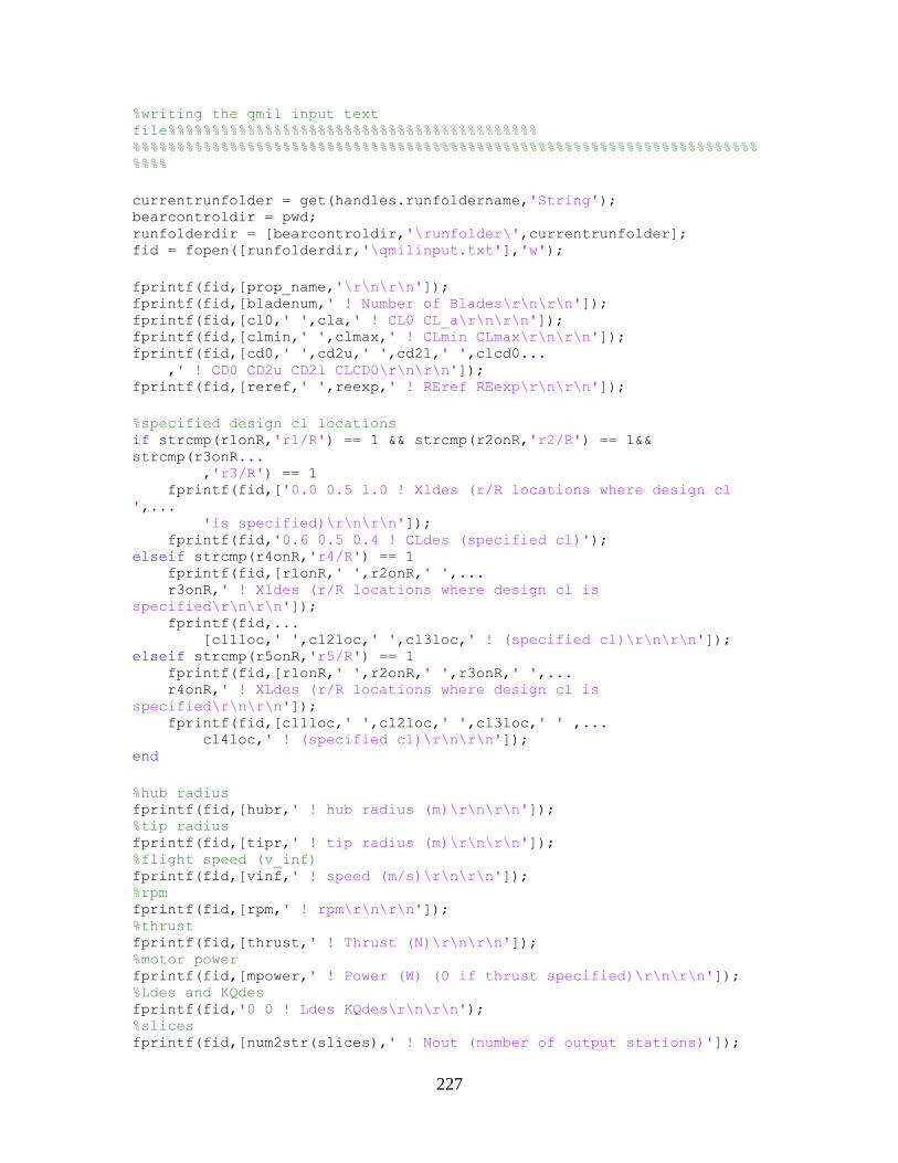
227
%writing the qmil input text
file%%%%%%%%%%%%%%%%%%%%%%%%%%%%%%%%%%%%%%%%%% %%%%%%%%%%%%%%%%%%%%%%%%%%%%%%%%%%%%%%%%%%%%%%%%%%%%%%%%%%%%%%%%%%%%%%%
%%%%
currentrunfolder = get(handles.runfoldername,'String'); bearcontroldir = pwd; runfolderdir = [bearcontroldir,'\runfolder\',currentrunfolder]; fid = fopen([runfolderdir,'\qmilinput.txt'],'w');
fprintf(fid,[prop_name,'\r\n\r\n']); fprintf(fid,[bladenum,' ! Number of Blades\r\n\r\n']); fprintf(fid,[cl0,' ',cla,' ! CL0 CL_a\r\n\r\n']); fprintf(fid,[clmin,' ',clmax,' ! CLmin CLmax\r\n\r\n']); fprintf(fid,[cd0,' ',cd2u,' ',cd2l,' ',clcd0... ,' ! CD0 CD2u CD2l CLCD0\r\n\r\n']); fprintf(fid,[reref,' ',reexp,' ! REref REexp\r\n\r\n']);
%specified design cl locations if strcmp(r1onR,'r1/R') == 1 && strcmp(r2onR,'r2/R') == 1&&
strcmp(r3onR... ,'r3/R') == 1 fprintf(fid,['0.0 0.5 1.0 ! Xldes (r/R locations where design cl
',... 'is specified)\r\n\r\n']); fprintf(fid,'0.6 0.5 0.4 ! CLdes (specified cl)'); elseif strcmp(r4onR,'r4/R') == 1 fprintf(fid,[r1onR,' ',r2onR,' ',... r3onR,' ! Xldes (r/R locations where design cl is
specified\r\n\r\n']); fprintf(fid,... [cl1loc,' ',cl2loc,' ',cl3loc,' ! (specified cl)\r\n\r\n']); elseif strcmp(r5onR,'r5/R') == 1 fprintf(fid,[r1onR,' ',r2onR,' ',r3onR,' ',... r4onR,' ! XLdes (r/R locations where design cl is
specified\r\n\r\n']); fprintf(fid,[cl1loc,' ',cl2loc,' ',cl3loc,' ' ,... cl4loc,' ! (specified cl)\r\n\r\n']); end
%hub radius fprintf(fid,[hubr,' ! hub radius (m)\r\n\r\n']); %tip radius fprintf(fid,[tipr,' ! tip radius (m)\r\n\r\n']); %flight speed (v_inf) fprintf(fid,[vinf,' ! speed (m/s)\r\n\r\n']); %rpm fprintf(fid,[rpm,' ! rpm\r\n\r\n']); %thrust fprintf(fid,[thrust,' ! Thrust (N)\r\n\r\n']); %motor power fprintf(fid,[mpower,' ! Power (W) (0 if thrust specified)\r\n\r\n']); %Ldes and KQdes fprintf(fid,'0 0 ! Ldes KQdes\r\n\r\n'); %slices fprintf(fid,[num2str(slices),' ! Nout (number of output stations)']);
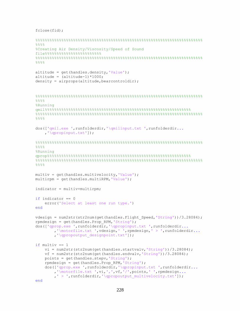
228
fclose(fid);
%%%%%%%%%%%%%%%%%%%%%%%%%%%%%%%%%%%%%%%%%%%%%%%%%%%%%%%%%%%%%%%%%%%%%%%
%%%% %Creating Air Density/Viscosity/Speed of Sound
file%%%%%%%%%%%%%%%%%%%%%%%% %%%%%%%%%%%%%%%%%%%%%%%%%%%%%%%%%%%%%%%%%%%%%%%%%%%%%%%%%%%%%%%%%%%%%%%
%%%%
altitude = get(handles.density,'Value'); altitude = (altitude-1)*1000; density = airprops(altitude,bearcontroldir);
%%%%%%%%%%%%%%%%%%%%%%%%%%%%%%%%%%%%%%%%%%%%%%%%%%%%%%%%%%%%%%%%%%%%%%%
%%%% %Running
qmil%%%%%%%%%%%%%%%%%%%%%%%%%%%%%%%%%%%%%%%%%%%%%%%%%%%%%%%%%%%%%% %%%%%%%%%%%%%%%%%%%%%%%%%%%%%%%%%%%%%%%%%%%%%%%%%%%%%%%%%%%%%%%%%%%%%%%
%%%%
dos(['qmil.exe ',runfolderdir,'\qmilinput.txt ',runfolderdir... ,'\qpropinput.txt']);
%%%%%%%%%%%%%%%%%%%%%%%%%%%%%%%%%%%%%%%%%%%%%%%%%%%%%%%%%%%%%%%%%%%%%%%
%%%% %Running
qprop%%%%%%%%%%%%%%%%%%%%%%%%%%%%%%%%%%%%%%%%%%%%%%%%%%%%%%%%%%%%% %%%%%%%%%%%%%%%%%%%%%%%%%%%%%%%%%%%%%%%%%%%%%%%%%%%%%%%%%%%%%%%%%%%%%%%
%%%%
multiv = get(handles.multivelocity,'Value'); multirpm = get(handles.multiRPM,'Value');
indicator = multiv+multirpm;
if indicator == 0 error('Select at least one run type.') end
vdesign = num2str(str2num(get(handles.Flight_Speed,'String'))/3.28084); rpmdesign = get(handles.Prop_RPM,'String'); dos(['qprop.exe ',runfolderdir,'\qpropinput.txt ',runfolderdir... ,'\motorfile.txt ',vdesign,' ',rpmdesign,' > ',runfolderdir... ,'\qpropoutput_designpoint.txt']);
if multiv == 1 vi = num2str(str2num(get(handles.startvalv,'String'))/3.28084); vf = num2str(str2num(get(handles.endvalv,'String'))/3.28084); points = get(handles.stepv,'String'); rpmdesign = get(handles.Prop_RPM,'String'); dos(['qprop.exe ',runfolderdir,'\qpropinput.txt ',runfolderdir... ,'\motorfile.txt ',vi,',',vf,'/',points,' ',rpmdesign... ,' > ',runfolderdir,'\qpropoutput_multivelocity.txt']); end
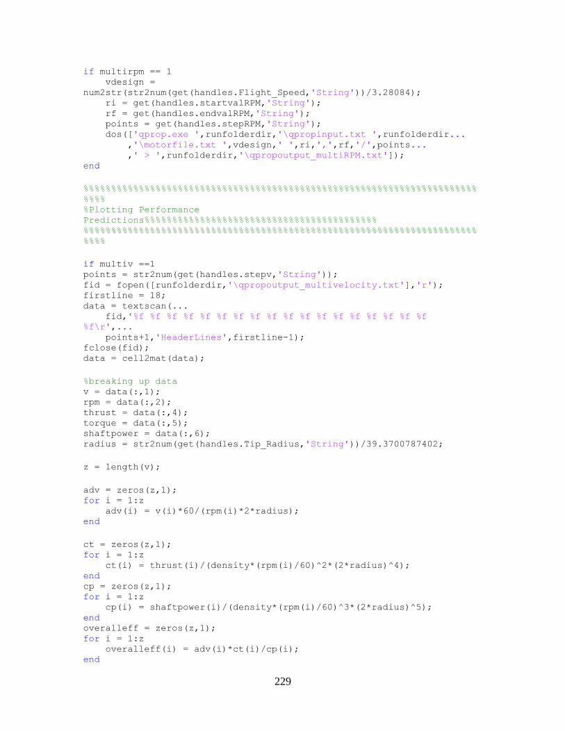
229
if multirpm == 1 vdesign =
num2str(str2num(get(handles.Flight_Speed,'String'))/3.28084); ri = get(handles.startvalRPM,'String'); rf = get(handles.endvalRPM,'String'); points = get(handles.stepRPM,'String'); dos(['qprop.exe ',runfolderdir,'\qpropinput.txt ',runfolderdir...
,'\motorfile.txt ',vdesign,' ',ri,',',rf,'/',points... ,' > ',runfolderdir,'\qpropoutput_multiRPM.txt']);
end
%%%%%%%%%%%%%%%%%%%%%%%%%%%%%%%%%%%%%%%%%%%%%%%%%%%%%%%%%%%%%%%%%%%%%%%
%%%% %Plotting Performance
Predictions%%%%%%%%%%%%%%%%%%%%%%%%%%%%%%%%%%%%%%%%%% %%%%%%%%%%%%%%%%%%%%%%%%%%%%%%%%%%%%%%%%%%%%%%%%%%%%%%%%%%%%%%%%%%%%%%%
%%%%
if multiv ==1 points = str2num(get(handles.stepv,'String')); fid = fopen([runfolderdir,'\qpropoutput_multivelocity.txt'],'r'); firstline = 18; data = textscan(...
fid,'%f %f %f %f %f %f %f %f %f %f %f %f %f %f %f %f %f %f
%f\r',... points+1,'HeaderLines',firstline-1);
fclose(fid); data = cell2mat(data);
%breaking up data v = data(:,1); rpm = data(:,2); thrust = data(:,4); torque = data(:,5); shaftpower = data(:,6); radius = str2num(get(handles.Tip_Radius,'String'))/39.3700787402;
z = length(v);
adv = zeros(z,1); for i = 1:z
adv(i) = v(i)*60/(rpm(i)*2*radius); end
ct = zeros(z,1); for i = 1:z
ct(i) = thrust(i)/(density*(rpm(i)/60)^2*(2*radius)^4); end cp = zeros(z,1); for i = 1:z
cp(i) = shaftpower(i)/(density*(rpm(i)/60)^3*(2*radius)^5); end overalleff = zeros(z,1); for i = 1:z
overalleff(i) = adv(i)*ct(i)/cp(i); end
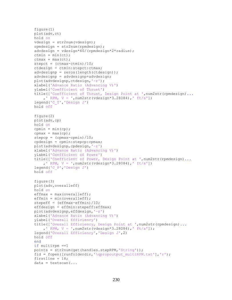
230
figure(1) plot(adv,ct) hold on vdesign = str2num(vdesign); rpmdesign = str2num(rpmdesign); advdesign = vdesign*60/(rpmdesign*2*radius); ctmin = min(ct); ctmax = max(ct); stepct = (ctmax-ctmin)/10; ctdesign = ctmin:stepct:ctmax; advdesignp = zeros(length(ctdesign)); advdesignp = advdesignp+advdesign; plot(advdesignp,ctdesign,'-r'); xlabel('Advance Ratio (Advancing V)') ylabel('Coefficient of Thrust') title(['Coefficient of Thrust, Design Point at ',num2str(rpmdesign)... ,' RPM, V = ',num2str(vdesign*3.28084),' ft/s']) legend('C_T','Design J') hold off
figure(2) plot(adv,cp) hold on cpmin = min(cp); cpmax = max(cp); stepcp = (cpmax-cpmin)/10; cpdesign = cpmin:stepcp:cpmax; plot(advdesignp,cpdesign,'-r') xlabel('Advance Ratio (Advancing V)') ylabel('Coefficient of Power') title(['Coefficient of Power, Design Point at ',num2str(rpmdesign)... ,' RPM, V = ',num2str(vdesign*3.28084),' ft/s']) legend('C_P','Design J') hold off
figure(3) plot(adv,overalleff) hold on effmax = max(overalleff); effmin = min(overalleff); stepeff = (effmax-effmin)/10; effdesign = effmin:stepeff:effmax; plot(advdesignp,effdesign,'-r') xlabel('Advance Ratio (Advancing V)') ylabel('Overall Efficiency') title(['Overall Efficiency, Design Point at ',num2str(rpmdesign)... ,' RPM, V = ',num2str(vdesign*3.28084),' ft/s']); legend('Overall Efficiency','Design J',2) hold off end if multirpm ==1 points = str2num(get(handles.stepRPM,'String')); fid = fopen([runfolderdir,'\qpropoutput_multiRPM.txt'],'r'); firstline = 18; data = textscan(...
231
fid,'%f %f %f %f %f %f %f %f %f %f %f %f %f %f %f %f %f %f
%f\r',... points+1,'HeaderLines',firstline-1);
fclose(fid); data = cell2mat(data);
%breaking up data v = data(:,1); rpm = data(:,2); thrust = data(:,4); torque = data(:,5); shaftpower = data(:,6); radius = str2num(get(handles.Tip_Radius,'String'))/39.3700787402;
z = length(v);
adv = zeros(z,1); for i = 1:z
adv(i) = v(i)*60/(rpm(i)*2*radius); end
ct = zeros(z,1); for i = 1:z
ct(i) = thrust(i)/(density*(rpm(i)/60)^3*(2*radius)^4); end
cp = zeros(z,1); for i = 1:z
cp(i) = shaftpower(i)/(density*(rpm(i)/60)^3*(2*radius)^5); end
overalleff = zeros(z,1); for i = 1:z
overalleff(i) = adv(i)*ct(i)/cp(i); end
figure(4) plot(adv,ct) hold on vdesign = vdesign; rpmdesign = rpmdesign; radpersdesign = rpmdesign*2*pi/60; advdesign = vdesign/(radpersdesign*radius); ctmin = min(ct); ctmax = max(ct); stepct = (ctmax-ctmin)/10; ctdesign = ctmin:stepct:ctmax; advdesignp = zeros(length(ctdesign)); advdesignp = advdesignp+advdesign; plot(advdesignp,ctdesign,'-r'); xlabel('Advance Ratio (Advancing RPM)') ylabel('Coefficient of Thrust') title(['Coefficient of Thrust, Design Point at ',num2str(rpmdesign)...
,' RPM, V = ',num2str(vdesign*3.28084),' ft/s'])
legend('C_t','Design J')
232
hold off
figure(5) plot(adv,cp) hold on cpmin = min(cp); cpmax = max(cp); stepcp = (cpmax-cpmin)/10; cpdesign = cpmin:stepcp:cpmax; plot(advdesignp,cpdesign,'-r') xlabel('Advance Ratio (Advancing RPM)') ylabel('Coefficient of Power') title(['Coefficient of Power, Design Point at ',num2str(rpmdesign)... ,' RPM, V = ',num2str(vdesign*3.28084),' ft/s']) legend('C_P','Design J') hold off
figure(6) plot(adv,overalleff) hold on effmax = max(overalleff); effmin = min(overalleff); stepeff = (effmax-effmin)/10; effdesign = effmin:stepeff:effmax; plot(advdesignp,effdesign,'-r') xlabel('Advance Ratio (Advancing RPM)') ylabel('Overall Efficiency') title(['Overall Efficiency, Design Point at ',num2str(rpmdesign)... ,' RPM, V = ',num2str(vdesign*3.28084),'ft/s']); legend('Overall Efficiency','Design J',2) hold off end
%%%%%%%%%%%%%%%%%%%%%%%%%%%%%%%%%%%%%%%%%%%%%%%%%%%%%%%%%%%%%%%%%%%%%%%
%%%% %Creating
Macros%%%%%%%%%%%%%%%%%%%%%%%%%%%%%%%%%%%%%%%%%%%%%%%%%%%%%%%%%%% %%%%%%%%%%%%%%%%%%%%%%%%%%%%%%%%%%%%%%%%%%%%%%%%%%%%%%%%%%%%%%%%%%%%%%%
%%%% %number of blades bladenum = str2double(bladenum); %rotation direction clockwise = get(handles.clockwise,'value'); anticlockwise = get(handles.anticlockwise,'value'); indicator2 = clockwise+anticlockwise; if indicator2 == 2 error('only one rotation direction may be selected') end if indicator2 == 0 error('select a rotation direction') end if clockwise == 1 rotationdir = 1; end if anticlockwise == 1; rotationdir = 0;
233
end %calling outside functions %create geometry file geometrypts_func(slices,geometryfile,runfolderdir,rotationdir,bladenum)
; %create reference plane macro planemacro_func(slices,runfolderdir,bladenum); %create splined airfoil cross section macro splinemacro_func(slices,runfolderdir,bladenum);
%Sound Prediction runsound = get(handles.runsound,'Value'); if runsound == 0, end if runsound == 1
%calling necessary variables for sound prediction bltrip = get(handles.BLtrip,'Value'); blcalcmethod = get(handles.blcalcmethod,'Value'); tbncalcmethod = get(handles.tblnoisecalc,'Value'); tbinflowcalcmethod = get(handles.turbulentinflowcalc,'Value'); calcblunt = get(handles.bluntnoise,'Value'); calcLBL = get(handles.calclbl,'Value'); uppertrip = get(handles.uppertrip,'String'); lowertrip = get(handles.lowertrip,'String'); isnaca = get(handles.isnaca,'Value'); nacanumber = get(handles.nacanumber,'String'); turbint = get(handles.turbint,'String'); turblength = get(handles.turblength,'String'); streamlines = get(handles.streamlines,'Value'); streamlinedist = get(handles.streamlinedist,'String'); obsdist = get(handles.obsdist,'String'); phi = get(handles.phi,'String'); theta = get(handles.theta,'String');
vinf = num2str(str2num(get(handles.Flight_Speed,'String'))/3.28084); rpm = get(handles.Prop_RPM,'String'); N = get(handles.Blade_Sections,'Value');
%createnafnoise folder(s) mkdir([runfolderdir,'\noise']);
copyfile(geometryfile,[bearcontroldir,'\nafnoise\foilpoints.txt']);
noiseinputs = [runfolderdir,'\noise'];
%run NAFnoise nafnoise_input(bearcontroldir,geometryfile,runfolderdir,vinf,rpm,N,... foilfolder,... bltrip,blcalcmethod,tbncalcmethod,tbinflowcalcmethod,calcblunt,...
calcLBL,uppertrip,lowertrip,isnaca,nacanumber,turbint,turblength,... streamlines,streamlinedist,obsdist,phi,theta,noiseinputs); nafnoise_output(noiseinputs); end
234
%END gui.m
code%%%%%%%%%%%%%%%%%%%%%%%%%%%%%%%%%%%%%%%%%%%%%%%%%%%%%%%%%
%Air Properties Function %March 2015 %Trae Liller %This function is for use in conjunction with BearControl and QPROP.
Given %an altitude, it will retrieve the corresponding air density, dynamic %viscosity and speed of sound for Standard Day Atmosphere.
function [density] = airprops(altitude,bearcontroldir)
%Standar Day Atmosphere Data data = [0 0.002377 1116.4 3.737*10^(-7);... 1000 0.002308 1112.6 3.717*10^(-7);... 2000 0.002241 1108.7 3.697*10^(-7);... 3000 0.002175 1104.9 3.677*10^(-7);... 4000 0.002111 1101 3.657*10^(-7);... 5000 0.002048 1097.1 3.637*10^(-7);... 6000 0.001987 1093.2 3.616*10^(-7);... 7000 0.001927 1089.3 3.596*10^(-7);... 8000 0.001869 1085.3 3.576*10^(-7);... 9000 0.001811 1081.4 3.555*10^(-7);... 10000 0.001756 1077.4 3.534*10^(-7);... 11000 0.001701 1073.4 3.514*10^(-7);... 12000 0.001648 1069.4 3.493*10^(-7);... 13000 0.001596 1065.4 3.472*10^(-7);... 14000 0.001546 1061.4 3.451*10^(-7);... 15000 0.001496 1057.4 3.430*10^(-7);... 16000 0.001448 1053.3 3.409*10^(-7);... 17000 0.001401 1049.2 3.388*10^(-7);... 18000 0.001355 1045.1 3.367*10^(-7);... 19000 0.001311 1041 3.346*10^(-7);... 20000 0.001267 1036.9 3.325*10^(-7)];
%Creating appropriate row variable based on user input in Bearcontrol
GUI row = altitude/1000+1;
%Calling appropriate data with row variable density = data(row,2); %english units visc = data(row,4); %english units m = data(row,3); %english units
%Converting to SI units for use with QMIL/QPROP density = density*515.3788179999993; %si units kg/m^3 visc = visc*47.8802687; %si units kg/ms m = m*0.3048; %si units m/s
%Creating air properties file for use in QMIL/QPROP airfile = fopen([bearcontroldir,'\qcon.def'],'w'); %rho kg/m^3
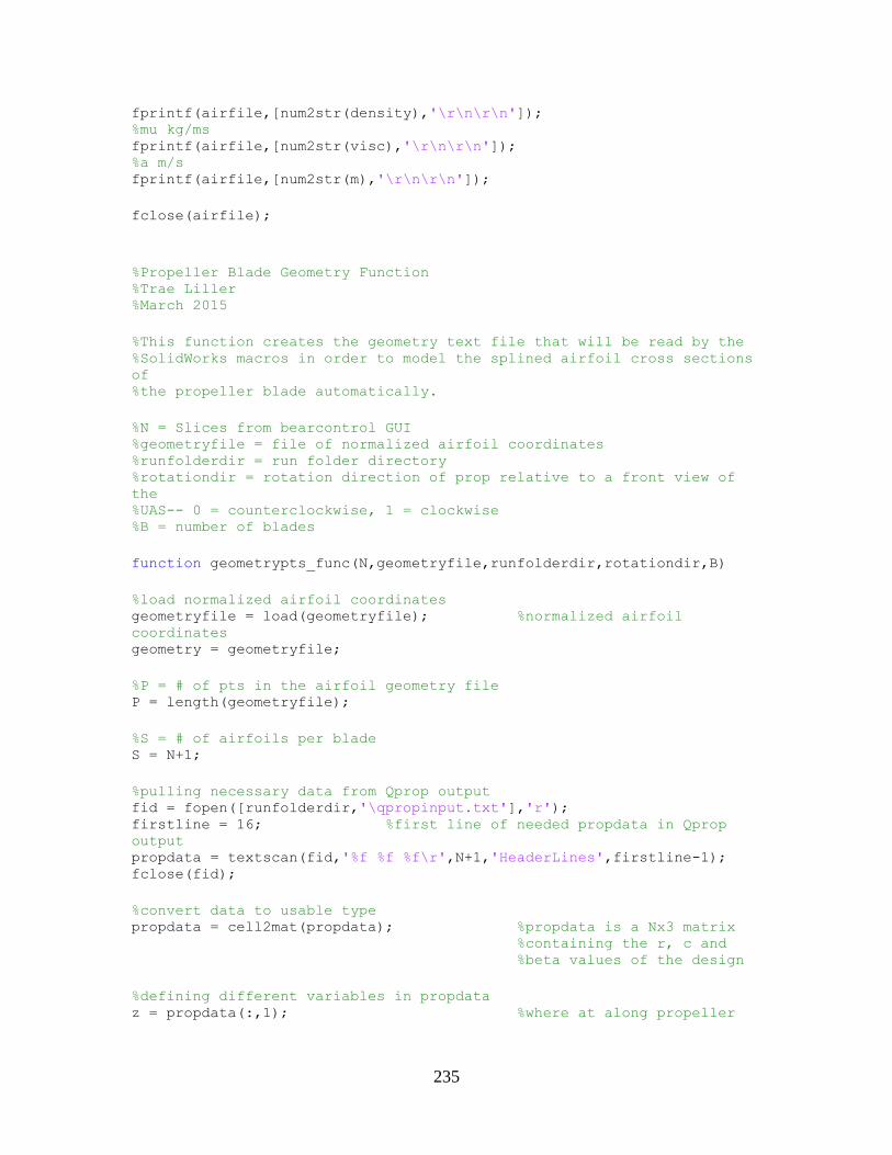
235
fprintf(airfile,[num2str(density),'\r\n\r\n']); %mu kg/ms fprintf(airfile,[num2str(visc),'\r\n\r\n']); %a m/s fprintf(airfile,[num2str(m),'\r\n\r\n']);
fclose(airfile);
%Propeller Blade Geometry Function %Trae Liller %March 2015
%This function creates the geometry text file that will be read by the %SolidWorks macros in order to model the splined airfoil cross sections
of %the propeller blade automatically.
%N = Slices from bearcontrol GUI %geometryfile = file of normalized airfoil coordinates %runfolderdir = run folder directory %rotationdir = rotation direction of prop relative to a front view of
the %UAS-- 0 = counterclockwise, 1 = clockwise %B = number of blades
function geometrypts_func(N,geometryfile,runfolderdir,rotationdir,B)
%load normalized airfoil coordinates geometryfile = load(geometryfile); %normalized airfoil
coordinates geometry = geometryfile;
%P = # of pts in the airfoil geometry file P = length(geometryfile);
%S = # of airfoils per blade S = N+1;
%pulling necessary data from Qprop output fid = fopen([runfolderdir,'\qpropinput.txt'],'r'); firstline = 16; %first line of needed propdata in Qprop
output
propdata = textscan(fid,'%f %f %f\r',N+1,'HeaderLines',firstline-1); fclose(fid);
%convert data to usable type propdata = cell2mat(propdata); %propdata is a Nx3 matrix
%containing the r, c and %beta values of the design
%defining different variables in propdata z = propdata(:,1); %where at along propeller
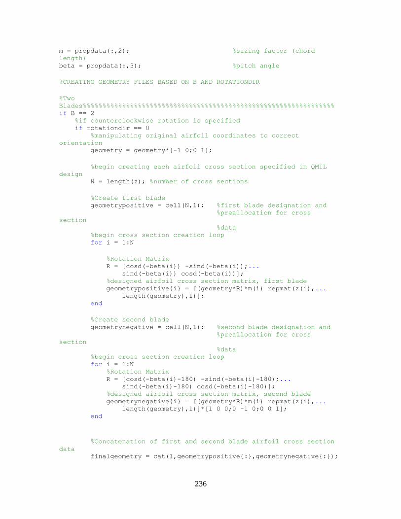
236
m = propdata(:,2); %sizing factor (chord
length) beta = propdata(:,3); %pitch angle
%CREATING GEOMETRY FILES BASED ON B AND ROTATIONDIR
%Two
Blades%%%%%%%%%%%%%%%%%%%%%%%%%%%%%%%%%%%%%%%%%%%%%%%%%%%%%%%%%%%%%%%% if B == 2 %if counterclockwise rotation is specified if rotationdir == 0 %manipulating original airfoil coordinates to correct
orientation geometry = geometry*[-1 0;0 1];
%begin creating each airfoil cross section specified in QMIL
design N = length(z); %number of cross sections
%Create first blade geometrypositive = cell(N,1); %first blade designation and %preallocation for cross
section %data %begin cross section creation loop for i = 1:N
%Rotation Matrix R = [cosd(-beta(i)) -sind(-beta(i));... sind(-beta(i)) cosd(-beta(i))]; %designed airfoil cross section matrix, first blade geometrypositive{i} = [(geometry*R)*m(i) repmat(z(i),... length(geometry),1)]; end
%Create second blade geometrynegative = cell(N,1); %second blade designation and %preallocation for cross
section %data %begin cross section creation loop for i = 1:N %Rotation Matrix R = [cosd(-beta(i)-180) -sind(-beta(i)-180);... sind(-beta(i)-180) cosd(-beta(i)-180)]; %designed airfoil cross section matrix, second blade geometrynegative{i} = [(geometry*R)*m(i) repmat(z(i),... length(geometry),1)]*[1 0 0;0 -1 0;0 0 1]; end
%Concatenation of first and second blade airfoil cross section
data finalgeometry = cat(1,geometrypositive{:},geometrynegative{:});
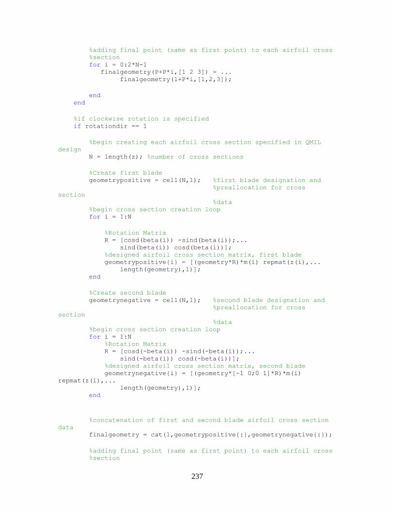
237
%adding final point (same as first point) to each airfoil cross %section for i = 0:2*N-1
finalgeometry(P+P*i,[1 2 3]) = ... finalgeometry(1+P*i,[1,2,3]);
end end
%if clockwise rotation is specified if rotationdir == 1
%begin creating each airfoil cross section specified in QMIL
design N = length(z); %number of cross sections
%Create first blade geometrypositive = cell(N,1); %first blade designation and
%preallocation for cross
section %data
%begin cross section creation loop for i = 1:N
%Rotation Matrix R = [cosd(beta(i)) -sind(beta(i));...
sind(beta(i)) cosd(beta(i))]; %designed airfoil cross section matrix, first blade geometrypositive{i} = [(geometry*R)*m(i) repmat(z(i),...
length(geometry),1)]; end
%Create second blade geometrynegative = cell(N,1); %second blade designation and
%preallocation for cross
section
%data %begin cross section creation loop for i = 1:N
%Rotation Matrix R = [cosd(-beta(i)) -sind(-beta(i));...
sind(-beta(i)) cosd(-beta(i))]; %designed airfoil cross section matrix, second blade geometrynegative{i} = [(geometry*[-1 0;0 1]*R)*m(i)
repmat(z(i),... length(geometry),1)];
end
%concatenation of first and second blade airfoil cross section
data finalgeometry = cat(1,geometrypositive{:},geometrynegative{:});
%adding final point (same as first point) to each airfoil cross %section
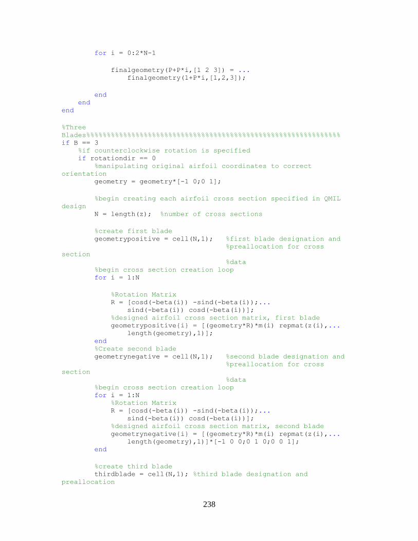
238
for i = 0:2*N-1
finalgeometry(P+P*i,[1 2 3]) = ... finalgeometry(1+P*i,[1,2,3]);
end end end
%Three
Blades%%%%%%%%%%%%%%%%%%%%%%%%%%%%%%%%%%%%%%%%%%%%%%%%%%%%%%%%%%%%%% if B == 3 %if counterclockwise rotation is specified if rotationdir == 0 %manipulating original airfoil coordinates to correct
orientation geometry = geometry*[-1 0;0 1];
%begin creating each airfoil cross section specified in QMIL
design N = length(z); %number of cross sections
%create first blade geometrypositive = cell(N,1); %first blade designation and %preallocation for cross
section %data %begin cross section creation loop for i = 1:N
%Rotation Matrix R = [cosd(-beta(i)) -sind(-beta(i));... sind(-beta(i)) cosd(-beta(i))]; %designed airfoil cross section matrix, first blade geometrypositive{i} = [(geometry*R)*m(i) repmat(z(i),... length(geometry),1)]; end %Create second blade geometrynegative = cell(N,1); %second blade designation and %preallocation for cross
section %data %begin cross section creation loop for i = 1:N %Rotation Matrix R = [cosd(-beta(i)) -sind(-beta(i));... sind(-beta(i)) cosd(-beta(i))]; %designed airfoil cross section matrix, second blade geometrynegative{i} = [(geometry*R)*m(i) repmat(z(i),... length(geometry),1)]*[-1 0 0;0 1 0;0 0 1]; end
%create third blade thirdblade = cell(N,1); %third blade designation and
preallocation
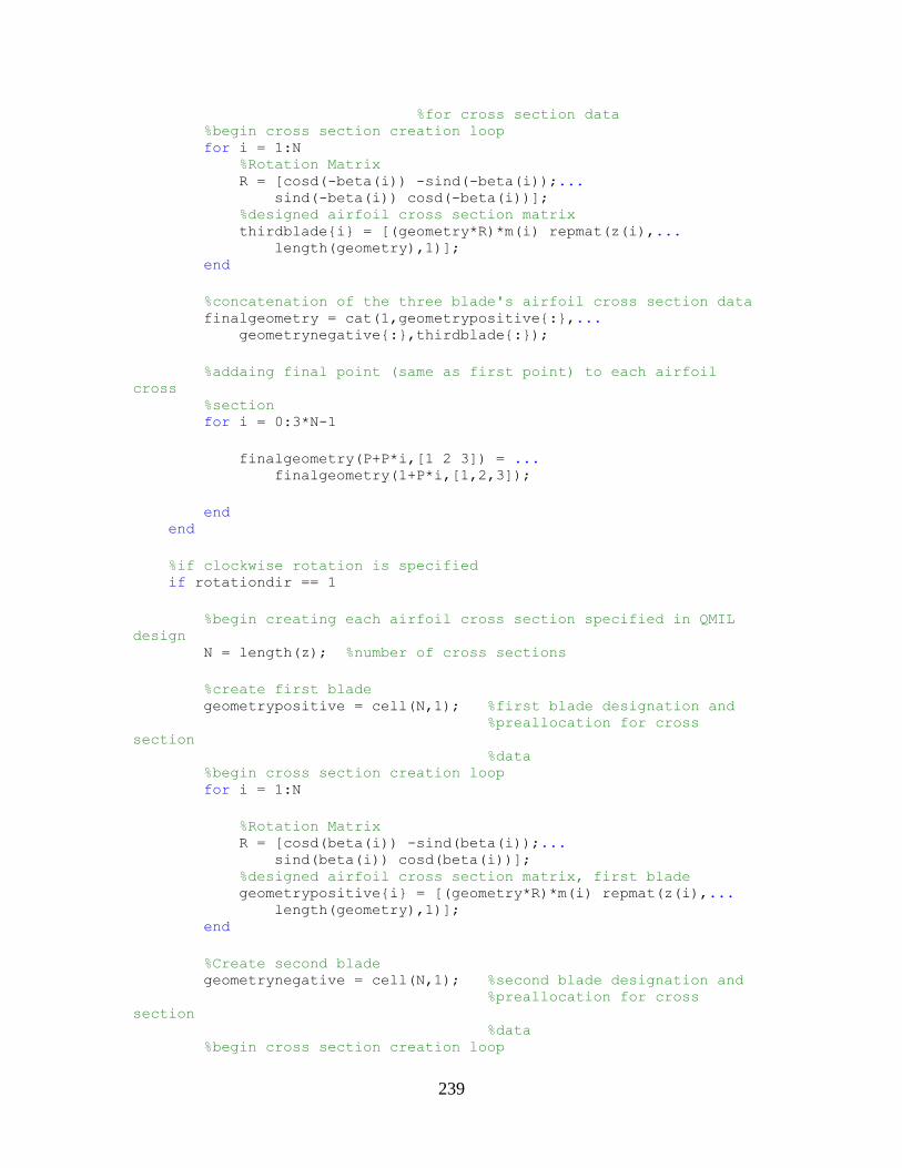
239
%for cross section data %begin cross section creation loop for i = 1:N
%Rotation Matrix R = [cosd(-beta(i)) -sind(-beta(i));...
sind(-beta(i)) cosd(-beta(i))]; %designed airfoil cross section matrix thirdblade{i} = [(geometry*R)*m(i) repmat(z(i),...
length(geometry),1)]; end
%concatenation of the three blade's airfoil cross section data finalgeometry = cat(1,geometrypositive{:},...
geometrynegative{:},thirdblade{:});
%addaing final point (same as first point) to each airfoil
cross %section for i = 0:3*N-1
finalgeometry(P+P*i,[1 2 3]) = ... finalgeometry(1+P*i,[1,2,3]);
end end
%if clockwise rotation is specified if rotationdir == 1
%begin creating each airfoil cross section specified in QMIL
design N = length(z); %number of cross sections
%create first blade geometrypositive = cell(N,1); %first blade designation and
%preallocation for cross
section %data
%begin cross section creation loop for i = 1:N
%Rotation Matrix R = [cosd(beta(i)) -sind(beta(i));...
sind(beta(i)) cosd(beta(i))]; %designed airfoil cross section matrix, first blade geometrypositive{i} = [(geometry*R)*m(i) repmat(z(i),...
length(geometry),1)]; end
%Create second blade geometrynegative = cell(N,1); %second blade designation and
%preallocation for cross
section %data
%begin cross section creation loop
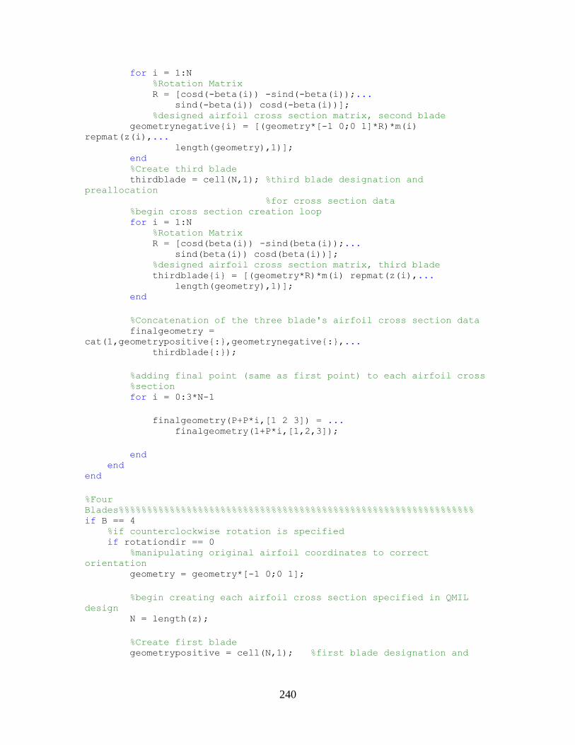
240
for i = 1:N %Rotation Matrix R = [cosd(-beta(i)) -sind(-beta(i));... sind(-beta(i)) cosd(-beta(i))]; %designed airfoil cross section matrix, second blade geometrynegative{i} = [(geometry*[-1 0;0 1]*R)*m(i)
repmat(z(i),... length(geometry),1)]; end %Create third blade thirdblade = cell(N,1); %third blade designation and
preallocation %for cross section data %begin cross section creation loop for i = 1:N %Rotation Matrix R = [cosd(beta(i)) -sind(beta(i));... sind(beta(i)) cosd(beta(i))]; %designed airfoil cross section matrix, third blade thirdblade{i} = [(geometry*R)*m(i) repmat(z(i),... length(geometry),1)]; end
%Concatenation of the three blade's airfoil cross section data finalgeometry =
cat(1,geometrypositive{:},geometrynegative{:},... thirdblade{:});
%adding final point (same as first point) to each airfoil cross %section for i = 0:3*N-1
finalgeometry(P+P*i,[1 2 3]) = ... finalgeometry(1+P*i,[1,2,3]);
end end end
%Four
Blades%%%%%%%%%%%%%%%%%%%%%%%%%%%%%%%%%%%%%%%%%%%%%%%%%%%%%%%%%%%%%%% if B == 4 %if counterclockwise rotation is specified if rotationdir == 0 %manipulating original airfoil coordinates to correct
orientation geometry = geometry*[-1 0;0 1];
%begin creating each airfoil cross section specified in QMIL
design N = length(z);
%Create first blade geometrypositive = cell(N,1); %first blade designation and
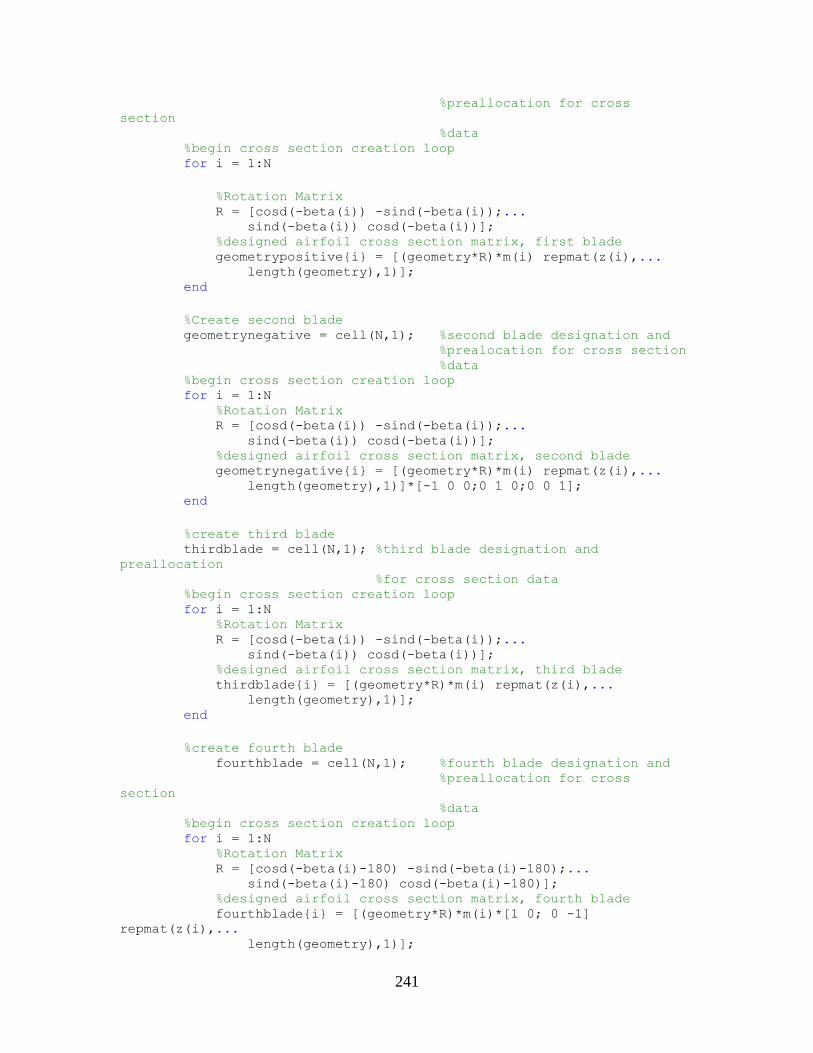
241
%preallocation for cross
section %data
%begin cross section creation loop for i = 1:N
%Rotation Matrix R = [cosd(-beta(i)) -sind(-beta(i));...
sind(-beta(i)) cosd(-beta(i))]; %designed airfoil cross section matrix, first blade geometrypositive{i} = [(geometry*R)*m(i) repmat(z(i),...
length(geometry),1)]; end
%Create second blade geometrynegative = cell(N,1); %second blade designation and
%prealocation for cross section %data
%begin cross section creation loop for i = 1:N
%Rotation Matrix R = [cosd(-beta(i)) -sind(-beta(i));...
sind(-beta(i)) cosd(-beta(i))]; %designed airfoil cross section matrix, second blade geometrynegative{i} = [(geometry*R)*m(i) repmat(z(i),...
length(geometry),1)]*[-1 0 0;0 1 0;0 0 1]; end
%create third blade thirdblade = cell(N,1); %third blade designation and
preallocation %for cross section data
%begin cross section creation loop for i = 1:N
%Rotation Matrix R = [cosd(-beta(i)) -sind(-beta(i));...
sind(-beta(i)) cosd(-beta(i))]; %designed airfoil cross section matrix, third blade thirdblade{i} = [(geometry*R)*m(i) repmat(z(i),...
length(geometry),1)]; end
%create fourth blade fourthblade = cell(N,1); %fourth blade designation and
%preallocation for cross
section %data
%begin cross section creation loop for i = 1:N
%Rotation Matrix R = [cosd(-beta(i)-180) -sind(-beta(i)-180);...
sind(-beta(i)-180) cosd(-beta(i)-180)]; %designed airfoil cross section matrix, fourth blade fourthblade{i} = [(geometry*R)*m(i)*[1 0; 0 -1]
repmat(z(i),... length(geometry),1)];
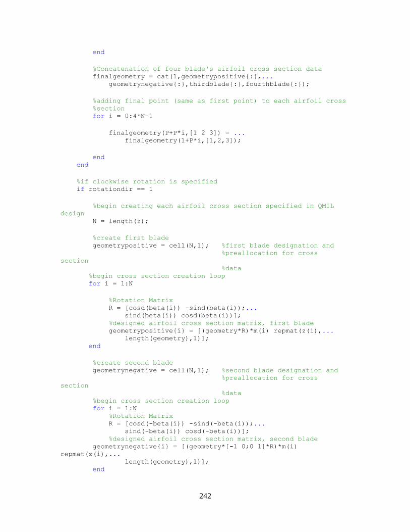
242
end
%Concatenation of four blade's airfoil cross section data finalgeometry = cat(1,geometrypositive{:},... geometrynegative{:},thirdblade{:},fourthblade{:});
%adding final point (same as first point) to each airfoil cross %section for i = 0:4*N-1
finalgeometry(P+P*i,[1 2 3]) = ... finalgeometry(1+P*i,[1,2,3]);
end end
%if clockwise rotation is specified if rotationdir == 1
%begin creating each airfoil cross section specified in QMIL
design N = length(z);
%create first blade geometrypositive = cell(N,1); %first blade designation and %preallocation for cross
section %data %begin cross section creation loop for i = 1:N
%Rotation Matrix R = [cosd(beta(i)) -sind(beta(i));... sind(beta(i)) cosd(beta(i))]; %designed airfoil cross section matrix, first blade geometrypositive{i} = [(geometry*R)*m(i) repmat(z(i),... length(geometry),1)]; end
%create second blade geometrynegative = cell(N,1); %second blade designation and %preallocation for cross
section %data %begin cross section creation loop for i = 1:N %Rotation Matrix R = [cosd(-beta(i)) -sind(-beta(i));... sind(-beta(i)) cosd(-beta(i))]; %designed airfoil cross section matrix, second blade geometrynegative{i} = [(geometry*[-1 0;0 1]*R)*m(i)
repmat(z(i),... length(geometry),1)]; end
243
%create third blade thirdblade = cell(N,1); %third blade designation and
preallocation %for cross section data
%begin cross section creation loop for i = 1:N
%Rotation Matrix R = [cosd(beta(i)) -sind(beta(i));...
sind(beta(i)) cosd(beta(i))]; %designed airfoil cross section matrix, third blade thirdblade{i} = [(geometry*R)*m(i) repmat(z(i),...
length(geometry),1)]; end
%create fourth blade fourthblade = cell(N,1); %fourth blade designation and
%preallocation for cross
section %data
%begin cross section creation loop for i = 1:N
%Rotation Matrix R = [cosd(beta(i)) -sind(beta(i));...
sind(beta(i)) cosd(beta(i))]; %designed airfoil cross section matrix, fourth blade fourthblade{i} = [(geometry)*R*m(i)*[-1 0;0 1]...
repmat(z(i), length(geometry),1)]; end
%Concatenation of four blade's airfoil cross section data finalgeometry =
cat(1,geometrypositive{:},geometrynegative{:},... thirdblade{:},fourthblade{:});
%adding final point(same as first point) to each airfoil cross %section for i = 0:4*N-1
finalgeometry(P+P*i,[1 2 3]) = ... finalgeometry(1+P*i,[1,2,3]);
end end
end
%Translating blades as necessary to center on hub (origin of part file
in %Solid
Works)%%%%%%%%%%%%%%%%%%%%%%%%%%%%%%%%%%%%%%%%%%%%%%%%%%%%%%%%%%%%% %First Blade maxx1 = max(finalgeometry(1:P,1)); minx1 = min(finalgeometry(1:P,1)); maxy1 = max(finalgeometry(1:P,2)); miny1 = min(finalgeometry(1:P,2)); %determining x-center of first airfoil if sign(maxx1) == 0;
middlex1 = minx1/2;
244
end if sign(minx1) == 0; middlex1 = maxx1/2; end
if sign(maxx1) + sign(minx1) == 2 middlex1 = (maxx1-minx1)/2; end if sign(maxx1) + sign(minx1) == -2 middlex1 = (maxx1-minx1)/2; end
if sign(maxx1) + sign(minx1) == 0 middlex1 = (maxx1+minx1)/2; end
%determining y-center of first airfoil if sign(maxy1) == 0; middley1 = miny1/2; end if sign(minx1) == 0; middley1 = maxy1/2; end
if sign(maxy1) + sign(miny1) == 2 middley1 = (maxy1-miny1)/2; end if sign(maxy1) + sign(miny1) == -2 middley1 = (maxy1-miny1)/2; end
if sign(maxy1) + sign(miny1) == 0 middley1 = (maxy1+miny1)/2; end
%Deciding how to translate x
values%%%%%%%%%%%%%%%%%%%%%%%%%%%%%%%%%%%% if middlex1 >= 0 transx1 = -middlex1; end if middlex1 < 0 transx1 = -middlex1; end
%Deciding how to translate y
values%%%%%%%%%%%%%%%%%%%%%%%%%%%%%%%%%%%%
if middley1 >= 0 transy1 = -middley1; end if middley1 < 0 transy1 = -middley1; end
%Second Blade
245
maxx2 = max(finalgeometry(P*S+1:P*(S+1),1)); minx2 = min(finalgeometry(P*S+1:P*(S+1),1)); maxy2 = max(finalgeometry(P*S+1:P*(S+1),2)); miny2 = min(finalgeometry(P*S+1:P*(S+1),2)); %determining x-center of first airfoil if sign(maxx2) == 0;
middlex2 = minx2/2; end if sign(minx2) == 0;
middlex2 = maxx2/2; end
if sign(maxx2) + sign(minx2) == 2 middlex2 = (maxx2-minx2)/2;
end if sign(maxx2) + sign(minx2) == -2
middlex2 = (maxx2-minx2)/2; end
if sign(maxx2) + sign(minx2) == 0 middlex2 = (maxx2+minx2)/2;
end
%determining y-center of first airfoil if sign(maxy2) == 0;
middley2 = miny2/2; end if sign(miny2) == 0;
middley2 = maxy2/2; end
if sign(maxy2) + sign(miny2) == 2 middley2 = (maxy2-miny2)/2;
end if sign(maxy2) + sign(miny2) == -2
middley2 = (maxy2-miny2)/2; end
if sign(maxy2) + sign(miny2) == 0 middley2 = (maxy2+miny2)/2;
end
%Deciding how to translate x
values%%%%%%%%%%%%%%%%%%%%%%%%%%%%%%%%%%%% if middlex2 >= 0
transx2 = -middlex2; end if middlex2 < 0
transx2 = -middlex2; end
%Deciding how to translate y
values%%%%%%%%%%%%%%%%%%%%%%%%%%%%%%%%%%%%
if middley2 >= 0
246
transy2 = -middley2; end if middley2 < 0 transy2 = -middley2; end
%Third Blade if B == 3 maxx3 = max(finalgeometry(2*P*S+1:2*P*S+P,1)); minx3 = min(finalgeometry(2*P*S+1:2*P*S+P,1)); maxy3 = max(finalgeometry(2*P*S+1:2*P*S+P,2)); miny3 = min(finalgeometry(2*P*S+1:2*P*S+P,2)); %determining x-center of first airfoil if sign(maxx3) == 0; middlex3 = minx3/2; end if sign(minx3) == 0; middlex3 = maxx3/2; end
if sign(maxx3) + sign(minx3) == 2 middlex3 = (maxx3-minx3)/2; end if sign(maxx3) + sign(minx3) == -2 middlex3 = (maxx3-minx3)/2; end
if sign(maxx3) + sign(minx3) == 0 middlex3 = (maxx3+minx3)/2; end
%determining y-center of first airfoil if sign(maxy3) == 0; middley3 = miny3/2; end if sign(miny3) == 0; middley3 = maxy3/2; end
if sign(maxy3) + sign(miny3) == 2 middley3 = (maxy3-miny3)/2; end if sign(maxy3) + sign(miny3) == -2 middley3 = (maxy3-miny3)/2; end
if sign(maxy3) + sign(miny3) == 0 middley3 = (maxy3+miny3)/2; end
%Deciding how to translate x
values%%%%%%%%%%%%%%%%%%%%%%%%%%%%%%%%%%%% if middlex3 >= 0 transx3 = -middlex3; end
247
if middlex3 < 0 transx3 = -middlex3; end
%Deciding how to translate y
values%%%%%%%%%%%%%%%%%%%%%%%%%%%%%%%%%%%%
if middley3 >= 0 transy3 = -middley3; end if middley3 < 0 transy3 = -middley3; end end
%Fourth Blade if B == 4 %third blade maxx3 = max(finalgeometry(2*P*S+1:2*P*S+P,1)); minx3 = min(finalgeometry(2*P*S+1:2*P*S+P,1)); maxy3 = max(finalgeometry(2*P*S+1:2*P*S+P,2)); miny3 = min(finalgeometry(2*P*S+1:2*P*S+P,2)); %determining x-center of first airfoil if sign(maxx3) == 0; middlex3 = minx3/2; end if sign(minx3) == 0; middlex3 = maxx3/2; end
if sign(maxx3) + sign(minx3) == 2 middlex3 = (maxx3-minx3)/2; end if sign(maxx3) + sign(minx3) == -2 middlex3 = (maxx3-minx3)/2; end
if sign(maxx3) + sign(minx3) == 0 middlex3 = (maxx3+minx3)/2; end
%determining y-center of first airfoil if sign(maxy3) == 0; middley3 = miny3/2; end if sign(miny3) == 0; middley3 = maxy3/2; end
if sign(maxy3) + sign(miny3) == 2 middley3 = (maxy3-miny3)/2; end if sign(maxy3) + sign(miny3) == -2 middley3 = (maxy3-miny3)/2; end
248
if sign(maxy3) + sign(miny3) == 0 middley3 = (maxy3+miny3)/2; end
%Deciding how to translate x
values%%%%%%%%%%%%%%%%%%%%%%%%%%%%%%%%%%%% if middlex3 >= 0 transx3 = -middlex3; end if middlex3 < 0 transx3 = -middlex3; end
%Deciding how to translate y
values%%%%%%%%%%%%%%%%%%%%%%%%%%%%%%%%%%%%
if middley3 >= 0 transy3 = -middley3; end if middley3 < 0 transy3 = -middley3; end
%fourth blade maxx4 = max(finalgeometry(3*P*S+1:3*P*S+P,1)); minx4 = min(finalgeometry(3*P*S+1:3*P*S+P,1)); maxy4 = max(finalgeometry(3*P*S+1:3*P*S+P,2)); miny4 = min(finalgeometry(3*P*S+1:3*P*S+P,2));
%determining x-center of first airfoil if sign(maxx4) == 0; middlex4 = minx4/2; end if sign(minx4) == 0; middlex4 = maxx4/2; end
if sign(maxx4) + sign(minx4) == 2 middlex4 = (maxx4-minx4)/2; end if sign(maxx4) + sign(minx4) == -2 middlex4 = (maxx4-minx4)/2; end
if sign(maxx4) + sign(minx4) == 0 middlex4 = (maxx4+minx4)/2; end
%determining y-center of first airfoil if sign(maxy4) == 0; middley4 = miny4/2; end if sign(miny4) == 0; middley4 = maxy4/2; end
249
if sign(maxy4) + sign(miny4) == 2 middley4 = (maxy4-miny4)/2;
end if sign(maxy4) + sign(miny4) == -2
middley4 = (maxy4-miny4)/2; end
if sign(maxy4) + sign(miny4) == 0 middley4 = (maxy4+miny4)/2;
end
%Deciding how to translate x
values%%%%%%%%%%%%%%%%%%%%%%%%%%%%%%%%%%%% if middlex4 >= 0
transx4 = -middlex4; end if middlex4 < 0
transx4 = -middlex4; end
%Deciding how to translate y
values%%%%%%%%%%%%%%%%%%%%%%%%%%%%%%%%%%%%
if middley4 >= 0 transy4 = -middley4;
end if middley4 < 0
transy4 = -middley4; end
end
%Translating respective
values%%%%%%%%%%%%%%%%%%%%%%%%%%%%%%%%%%%%%%%%%%%%% %First Blade finalgeometry(1:(P*S),1) = finalgeometry(1:(P*S),1)+transx1; finalgeometry(1:(P*S),2) = finalgeometry(1:(P*S),2)+transy1; %Second Blade finalgeometry((P*S+1):(P*2*S),1) =...
finalgeometry((P*S+1):(P*S*2),1)+transx2; finalgeometry((P*S+1):(P*2*S),2) =...
finalgeometry((P*S+1):(P*S*2),2)+transy2; %Third Blade if B == 3 finalgeometry((2*P*S+1):(3*P*S),1) = ...
finalgeometry((2*P*S+1):(3*P*S),1)+transx3; finalgeometry((2*P*S+1):(3*P*S),2) = ...
finalgeometry((2*P*S+1):(3*P*S),2)+transy3; end
if B == 4 finalgeometry((2*P*S+1):(3*P*S),1) = ...
finalgeometry((2*P*S+1):(3*P*S),1)+transx3; finalgeometry((2*P*S+1):(3*P*S),2) = ...
finalgeometry((2*P*S+1):(3*P*S),2)+transy3;
250
finalgeometry((3*P*S+1):(4*P*S),1) = ... finalgeometry((3*P*S+1):(4*P*S),1)+transx4; finalgeometry((3*P*S+1):(4*P*S),2) = ... finalgeometry((3*P*S+1):(4*P*S),2)+transy4; end
%Writing Geometry File geometryfile = fopen([runfolderdir,'\geometryclosed.txt'],'w');
for k = 1:length(finalgeometry) fprintf(geometryfile,[num2str(finalgeometry(k,1)),' ',... num2str(finalgeometry(k,2)),' ',... num2str(finalgeometry(k,3)),'\r\n']); end fclose(geometryfile); end
%Plane Macro Function %Trae Liller %March 2015 %This function will produce a macro based on inputs given in the
bearcontol %GUI and intermediate calculations that will create a reference plane
for %each airfoil in the designed propeller blade.
function planemacro_func(N,runfolderdir,bladenum) %N = number of slices selected in BEARCONTROL GUI %runfolderdir = location of the current run folder %bladenum = number of blades
% Loading geometry file load([runfolderdir,'\geometryclosed.txt']) data = geometryclosed; % data S = N+1; if bladenum == 2 P = length(data)/(2*S); % # of points in airfoil file end if bladenum == 3 P = length(data)/(3*S); end if bladenum ==4 P = length(data)/(4*S); end planemacro = fopen([runfolderdir,'\planemacro.txt'],'w');
if bladenum == 2
%Opening statements in macro code fprintf(planemacro,'''Preconditions: New Part file opened\r\n'); fprintf(planemacro,'''Postconditions: S number of planes
created\r\n\r\n');
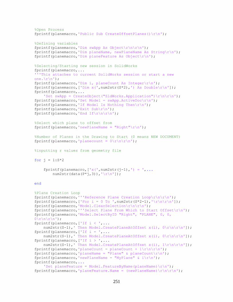
251
%Open Process fprintf(planemacro,'Public Sub CreateOffsetPlanes()\r\n');
%Defining variables fprintf(planemacro,'Dim swApp As Object\r\n\r\n'); fprintf(planemacro,'Dim planeName, newPlaneName As String\r\n'); fprintf(planemacro,'Dim planeFeature As Object\r\n');
%Selecting/Starting new session in SolidWorks fprintf(planemacro,... '''This attaches to current SolidWorks session or start a new
one.\r\n'); fprintf(planemacro,'Dim i, planeCount As Integer\r\n'); fprintf(planemacro,['Dim x(',num2str(S*2),') As Double\r\n']); fprintf(planemacro,...
'Set swApp = CreateObject("SldWorks.Application")\r\n\r\n'); fprintf(planemacro,'Set Model = swApp.ActiveDoc\r\n'); fprintf(planemacro,'If Model Is Nothing Then\r\n'); fprintf(planemacro,'Exit Sub\r\n'); fprintf(planemacro,'End If\r\n\r\n');
%Select which plane to offset from fprintf(planemacro,'newPlaneName = "Right"\r\n');
%Number of Planes in the Drawing to Start (0 means NEW DOCUMENT) fprintf(planemacro,'planecount = 0\r\n\r\n');
%inputting r values from geometry file
for j = 1:S*2
fprintf(planemacro,['x(',num2str(j-1),') = ',... num2str(data(P*j,3)),'\r\n']);
end
%Plane Creation Loop fprintf(planemacro,'''Reference Plane Creation Loop\r\n\r\n'); fprintf(planemacro,['For i = 0 To ',num2str(S*2-1),'\r\n\r\n']); fprintf(planemacro,'Model.ClearSelection\r\n\r\n'); fprintf(planemacro,'''Select Plane From Which to Start Offset\r\n'); fprintf(planemacro,'Model.SelectByID "Right", "PLANE", 0, 0,
0\r\n\r\n'); fprintf(planemacro,['If i < ',...
num2str(S-1),' Then Model.CreatePlaneAtOffset x(i), 0\r\n\r\n']); fprintf(planemacro,['If i = ',...
num2str(S-1),' Then Model.CreatePlaneAtOffset x(i), 0\r\n\r\n']); fprintf(planemacro,['If i > ',...
num2str(S-1),' Then Model.CreatePlaneAtOffset x(i), 1\r\n\r\n']); fprintf(planemacro,'planeCount = planeCount + 1\r\n\r\n'); fprintf(planemacro,'planeName = "Plane" & planeCount\r\n'); fprintf(planemacro,'newPlaneName = "MyPlane" & i\r\n'); fprintf(planemacro,...
'Set planeFeature = Model.FeatureByName(planeName)\r\n'); fprintf(planemacro,'planeFeature.Name = (newPlaneName)\r\n\r\n');
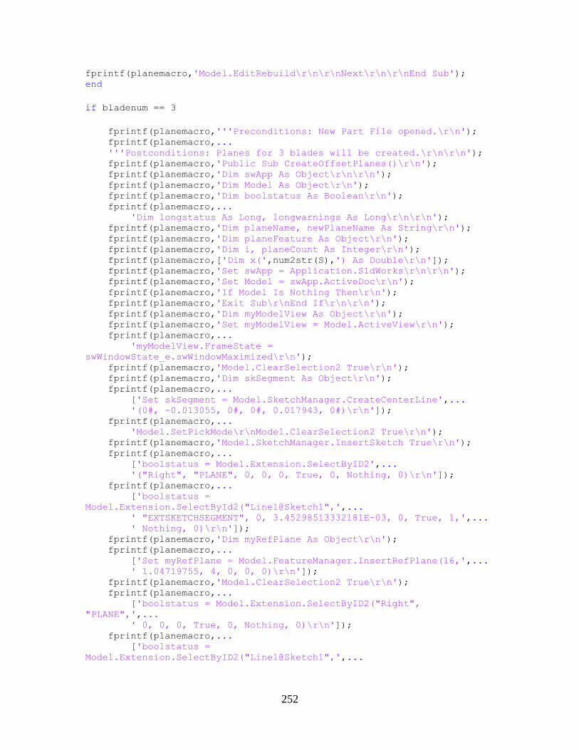
252
fprintf(planemacro,'Model.EditRebuild\r\n\r\nNext\r\n\r\nEnd Sub'); end
if bladenum == 3
fprintf(planemacro,'''Preconditions: New Part File opened.\r\n'); fprintf(planemacro,... '''Postconditions: Planes for 3 blades will be created.\r\n\r\n'); fprintf(planemacro,'Public Sub CreateOffsetPlanes()\r\n'); fprintf(planemacro,'Dim swApp As Object\r\n\r\n'); fprintf(planemacro,'Dim Model As Object\r\n'); fprintf(planemacro,'Dim boolstatus As Boolean\r\n'); fprintf(planemacro,... 'Dim longstatus As Long, longwarnings As Long\r\n\r\n'); fprintf(planemacro,'Dim planeName, newPlaneName As String\r\n'); fprintf(planemacro,'Dim planeFeature As Object\r\n'); fprintf(planemacro,'Dim i, planeCount As Integer\r\n'); fprintf(planemacro,['Dim x(',num2str(S),') As Double\r\n']); fprintf(planemacro,'Set swApp = Application.SldWorks\r\n\r\n'); fprintf(planemacro,'Set Model = swApp.ActiveDoc\r\n'); fprintf(planemacro,'If Model Is Nothing Then\r\n'); fprintf(planemacro,'Exit Sub\r\nEnd If\r\n\r\n'); fprintf(planemacro,'Dim myModelView As Object\r\n'); fprintf(planemacro,'Set myModelView = Model.ActiveView\r\n'); fprintf(planemacro,... 'myModelView.FrameState =
swWindowState_e.swWindowMaximized\r\n'); fprintf(planemacro,'Model.ClearSelection2 True\r\n'); fprintf(planemacro,'Dim skSegment As Object\r\n'); fprintf(planemacro,... ['Set skSegment = Model.SketchManager.CreateCenterLine',... '(0#, -0.013055, 0#, 0#, 0.017943, 0#)\r\n']); fprintf(planemacro,... 'Model.SetPickMode\r\nModel.ClearSelection2 True\r\n'); fprintf(planemacro,'Model.SketchManager.InsertSketch True\r\n'); fprintf(planemacro,... ['boolstatus = Model.Extension.SelectByID2',... '("Right", "PLANE", 0, 0, 0, True, 0, Nothing, 0)\r\n']); fprintf(planemacro,... ['boolstatus =
Model.Extension.SelectById2("Line1@Sketch1",',... ' "EXTSKETCHSEGMENT", 0, 3.45298513332181E-03, 0, True, 1,',... ' Nothing, 0)\r\n']); fprintf(planemacro,'Dim myRefPlane As Object\r\n'); fprintf(planemacro,... ['Set myRefPlane = Model.FeatureManager.InsertRefPlane(16,',... ' 1.04719755, 4, 0, 0, 0)\r\n']); fprintf(planemacro,'Model.ClearSelection2 True\r\n'); fprintf(planemacro,... ['boolstatus = Model.Extension.SelectByID2("Right",
"PLANE",',... ' 0, 0, 0, True, 0, Nothing, 0)\r\n']); fprintf(planemacro,... ['boolstatus =
Model.Extension.SelectByID2("Line1@Sketch1",',...
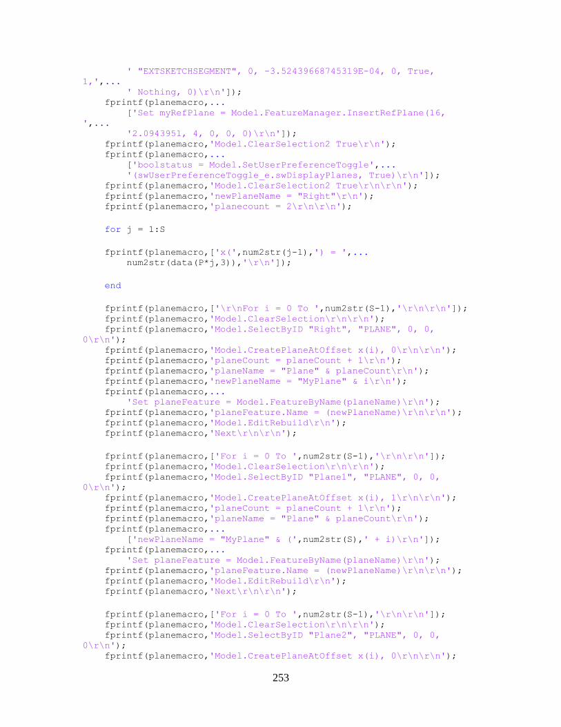
253
' "EXTSKETCHSEGMENT", 0, -3.52439668745319E-04, 0, True,
1,',... ' Nothing, 0)\r\n']); fprintf(planemacro,... ['Set myRefPlane = Model.FeatureManager.InsertRefPlane(16,
',... '2.0943951, 4, 0, 0, 0)\r\n']); fprintf(planemacro,'Model.ClearSelection2 True\r\n'); fprintf(planemacro,... ['boolstatus = Model.SetUserPreferenceToggle',... '(swUserPreferenceToggle_e.swDisplayPlanes, True)\r\n']); fprintf(planemacro,'Model.ClearSelection2 True\r\n\r\n'); fprintf(planemacro,'newPlaneName = "Right"\r\n'); fprintf(planemacro,'planecount = 2\r\n\r\n');
for j = 1:S
fprintf(planemacro,['x(',num2str(j-1),') = ',... num2str(data(P*j,3)),'\r\n']);
end
fprintf(planemacro,['\r\nFor i = 0 To ',num2str(S-1),'\r\n\r\n']); fprintf(planemacro,'Model.ClearSelection\r\n\r\n'); fprintf(planemacro,'Model.SelectByID "Right", "PLANE", 0, 0,
0\r\n'); fprintf(planemacro,'Model.CreatePlaneAtOffset x(i), 0\r\n\r\n'); fprintf(planemacro,'planeCount = planeCount + 1\r\n'); fprintf(planemacro,'planeName = "Plane" & planeCount\r\n'); fprintf(planemacro,'newPlaneName = "MyPlane" & i\r\n'); fprintf(planemacro,... 'Set planeFeature = Model.FeatureByName(planeName)\r\n'); fprintf(planemacro,'planeFeature.Name = (newPlaneName)\r\n\r\n'); fprintf(planemacro,'Model.EditRebuild\r\n'); fprintf(planemacro,'Next\r\n\r\n');
fprintf(planemacro,['For i = 0 To ',num2str(S-1),'\r\n\r\n']); fprintf(planemacro,'Model.ClearSelection\r\n\r\n'); fprintf(planemacro,'Model.SelectByID "Plane1", "PLANE", 0, 0,
0\r\n'); fprintf(planemacro,'Model.CreatePlaneAtOffset x(i), 1\r\n\r\n'); fprintf(planemacro,'planeCount = planeCount + 1\r\n'); fprintf(planemacro,'planeName = "Plane" & planeCount\r\n'); fprintf(planemacro,... ['newPlaneName = "MyPlane" & (',num2str(S),' + i)\r\n']); fprintf(planemacro,... 'Set planeFeature = Model.FeatureByName(planeName)\r\n'); fprintf(planemacro,'planeFeature.Name = (newPlaneName)\r\n\r\n'); fprintf(planemacro,'Model.EditRebuild\r\n'); fprintf(planemacro,'Next\r\n\r\n');
fprintf(planemacro,['For i = 0 To ',num2str(S-1),'\r\n\r\n']); fprintf(planemacro,'Model.ClearSelection\r\n\r\n'); fprintf(planemacro,'Model.SelectByID "Plane2", "PLANE", 0, 0,
0\r\n'); fprintf(planemacro,'Model.CreatePlaneAtOffset x(i), 0\r\n\r\n');
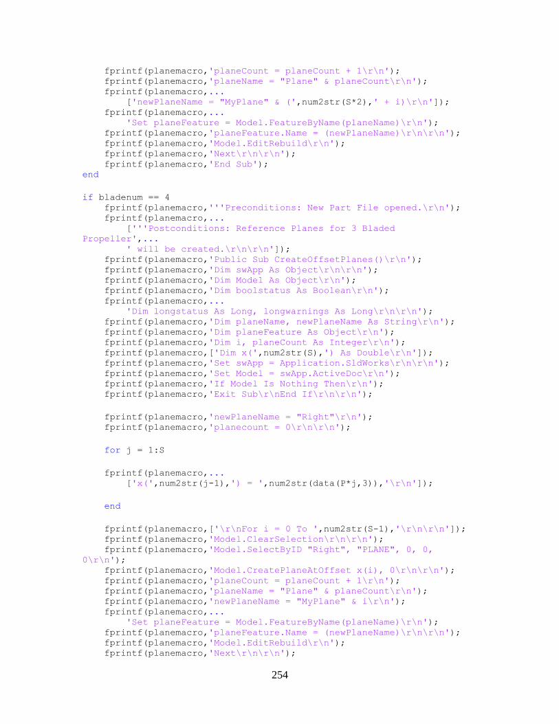
254
fprintf(planemacro,'planeCount = planeCount + 1\r\n'); fprintf(planemacro,'planeName = "Plane" & planeCount\r\n'); fprintf(planemacro,... ['newPlaneName = "MyPlane" & (',num2str(S*2),' + i)\r\n']); fprintf(planemacro,... 'Set planeFeature = Model.FeatureByName(planeName)\r\n'); fprintf(planemacro,'planeFeature.Name = (newPlaneName)\r\n\r\n'); fprintf(planemacro,'Model.EditRebuild\r\n'); fprintf(planemacro,'Next\r\n\r\n'); fprintf(planemacro,'End Sub'); end
if bladenum == 4 fprintf(planemacro,'''Preconditions: New Part File opened.\r\n'); fprintf(planemacro,... ['''Postconditions: Reference Planes for 3 Bladed
Propeller',... ' will be created.\r\n\r\n']); fprintf(planemacro,'Public Sub CreateOffsetPlanes()\r\n'); fprintf(planemacro,'Dim swApp As Object\r\n\r\n'); fprintf(planemacro,'Dim Model As Object\r\n'); fprintf(planemacro,'Dim boolstatus As Boolean\r\n'); fprintf(planemacro,... 'Dim longstatus As Long, longwarnings As Long\r\n\r\n'); fprintf(planemacro,'Dim planeName, newPlaneName As String\r\n'); fprintf(planemacro,'Dim planeFeature As Object\r\n'); fprintf(planemacro,'Dim i, planeCount As Integer\r\n'); fprintf(planemacro,['Dim x(',num2str(S),') As Double\r\n']); fprintf(planemacro,'Set swApp = Application.SldWorks\r\n\r\n'); fprintf(planemacro,'Set Model = swApp.ActiveDoc\r\n'); fprintf(planemacro,'If Model Is Nothing Then\r\n'); fprintf(planemacro,'Exit Sub\r\nEnd If\r\n\r\n');
fprintf(planemacro,'newPlaneName = "Right"\r\n'); fprintf(planemacro,'planecount = 0\r\n\r\n');
for j = 1:S
fprintf(planemacro,... ['x(',num2str(j-1),') = ',num2str(data(P*j,3)),'\r\n']);
end
fprintf(planemacro,['\r\nFor i = 0 To ',num2str(S-1),'\r\n\r\n']); fprintf(planemacro,'Model.ClearSelection\r\n\r\n'); fprintf(planemacro,'Model.SelectByID "Right", "PLANE", 0, 0,
0\r\n'); fprintf(planemacro,'Model.CreatePlaneAtOffset x(i), 0\r\n\r\n'); fprintf(planemacro,'planeCount = planeCount + 1\r\n'); fprintf(planemacro,'planeName = "Plane" & planeCount\r\n'); fprintf(planemacro,'newPlaneName = "MyPlane" & i\r\n'); fprintf(planemacro,... 'Set planeFeature = Model.FeatureByName(planeName)\r\n'); fprintf(planemacro,'planeFeature.Name = (newPlaneName)\r\n\r\n'); fprintf(planemacro,'Model.EditRebuild\r\n'); fprintf(planemacro,'Next\r\n\r\n');
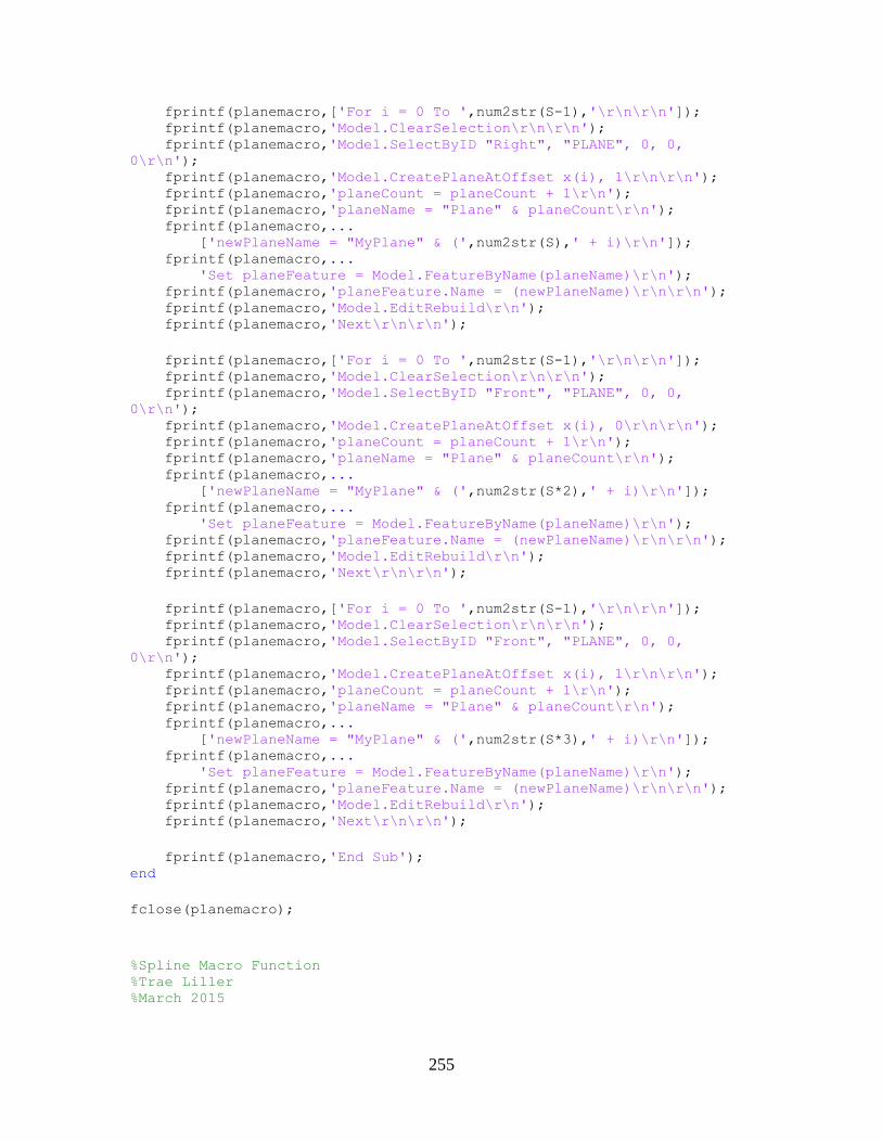
255
fprintf(planemacro,['For i = 0 To ',num2str(S-1),'\r\n\r\n']); fprintf(planemacro,'Model.ClearSelection\r\n\r\n'); fprintf(planemacro,'Model.SelectByID "Right", "PLANE", 0, 0,
0\r\n'); fprintf(planemacro,'Model.CreatePlaneAtOffset x(i), 1\r\n\r\n'); fprintf(planemacro,'planeCount = planeCount + 1\r\n'); fprintf(planemacro,'planeName = "Plane" & planeCount\r\n'); fprintf(planemacro,...
['newPlaneName = "MyPlane" & (',num2str(S),' + i)\r\n']); fprintf(planemacro,...
'Set planeFeature = Model.FeatureByName(planeName)\r\n'); fprintf(planemacro,'planeFeature.Name = (newPlaneName)\r\n\r\n'); fprintf(planemacro,'Model.EditRebuild\r\n'); fprintf(planemacro,'Next\r\n\r\n');
fprintf(planemacro,['For i = 0 To ',num2str(S-1),'\r\n\r\n']); fprintf(planemacro,'Model.ClearSelection\r\n\r\n'); fprintf(planemacro,'Model.SelectByID "Front", "PLANE", 0, 0,
0\r\n'); fprintf(planemacro,'Model.CreatePlaneAtOffset x(i), 0\r\n\r\n'); fprintf(planemacro,'planeCount = planeCount + 1\r\n'); fprintf(planemacro,'planeName = "Plane" & planeCount\r\n'); fprintf(planemacro,...
['newPlaneName = "MyPlane" & (',num2str(S*2),' + i)\r\n']); fprintf(planemacro,...
'Set planeFeature = Model.FeatureByName(planeName)\r\n'); fprintf(planemacro,'planeFeature.Name = (newPlaneName)\r\n\r\n'); fprintf(planemacro,'Model.EditRebuild\r\n'); fprintf(planemacro,'Next\r\n\r\n');
fprintf(planemacro,['For i = 0 To ',num2str(S-1),'\r\n\r\n']); fprintf(planemacro,'Model.ClearSelection\r\n\r\n'); fprintf(planemacro,'Model.SelectByID "Front", "PLANE", 0, 0,
0\r\n'); fprintf(planemacro,'Model.CreatePlaneAtOffset x(i), 1\r\n\r\n'); fprintf(planemacro,'planeCount = planeCount + 1\r\n'); fprintf(planemacro,'planeName = "Plane" & planeCount\r\n'); fprintf(planemacro,...
['newPlaneName = "MyPlane" & (',num2str(S*3),' + i)\r\n']); fprintf(planemacro,...
'Set planeFeature = Model.FeatureByName(planeName)\r\n'); fprintf(planemacro,'planeFeature.Name = (newPlaneName)\r\n\r\n'); fprintf(planemacro,'Model.EditRebuild\r\n'); fprintf(planemacro,'Next\r\n\r\n');
fprintf(planemacro,'End Sub'); end
fclose(planemacro);
%Spline Macro Function
%Trae Liller %March 2015
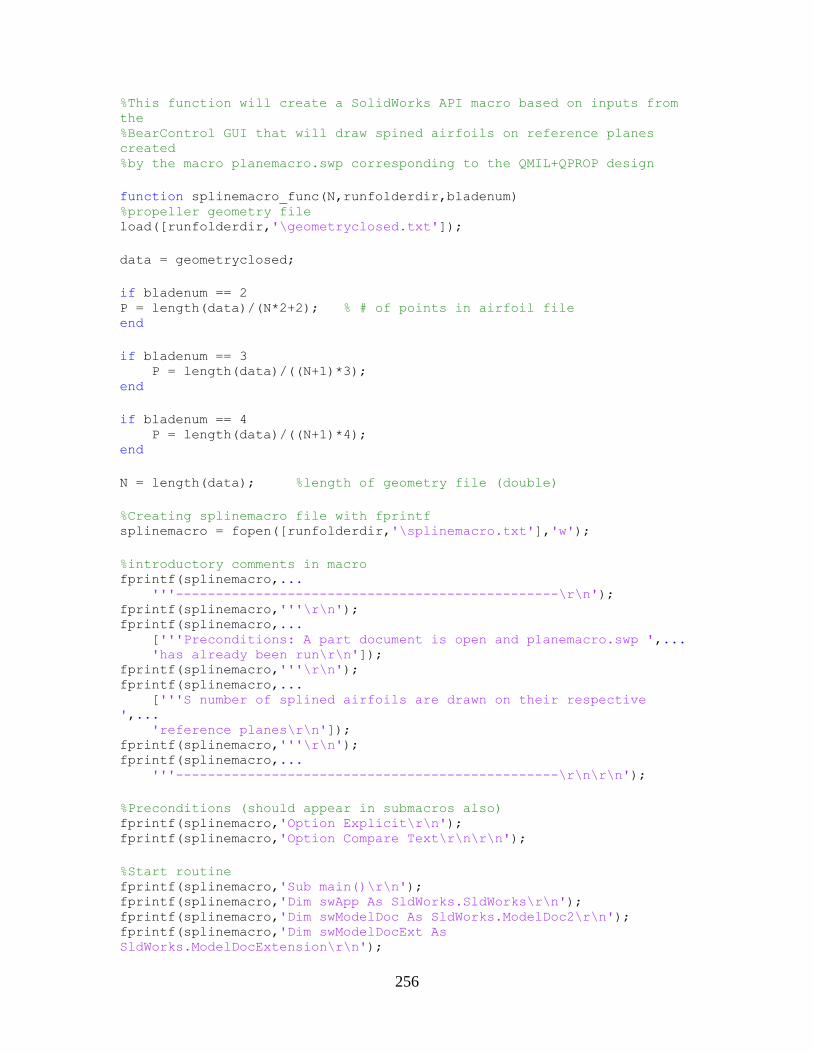
256
%This function will create a SolidWorks API macro based on inputs from
the %BearControl GUI that will draw spined airfoils on reference planes
created %by the macro planemacro.swp corresponding to the QMIL+QPROP design
function splinemacro_func(N,runfolderdir,bladenum) %propeller geometry file load([runfolderdir,'\geometryclosed.txt']);
data = geometryclosed;
if bladenum == 2 P = length(data)/(N*2+2); % # of points in airfoil file end
if bladenum == 3 P = length(data)/((N+1)*3); end
if bladenum == 4 P = length(data)/((N+1)*4); end
N = length(data); %length of geometry file (double)
%Creating splinemacro file with fprintf splinemacro = fopen([runfolderdir,'\splinemacro.txt'],'w');
%introductory comments in macro fprintf(splinemacro,... '''------------------------------------------------\r\n'); fprintf(splinemacro,'''\r\n'); fprintf(splinemacro,... ['''Preconditions: A part document is open and planemacro.swp ',... 'has already been run\r\n']); fprintf(splinemacro,'''\r\n'); fprintf(splinemacro,... ['''S number of splined airfoils are drawn on their respective
',... 'reference planes\r\n']); fprintf(splinemacro,'''\r\n'); fprintf(splinemacro,... '''------------------------------------------------\r\n\r\n');
%Preconditions (should appear in submacros also) fprintf(splinemacro,'Option Explicit\r\n'); fprintf(splinemacro,'Option Compare Text\r\n\r\n');
%Start routine fprintf(splinemacro,'Sub main()\r\n'); fprintf(splinemacro,'Dim swApp As SldWorks.SldWorks\r\n'); fprintf(splinemacro,'Dim swModelDoc As SldWorks.ModelDoc2\r\n'); fprintf(splinemacro,'Dim swModelDocExt As
SldWorks.ModelDocExtension\r\n');
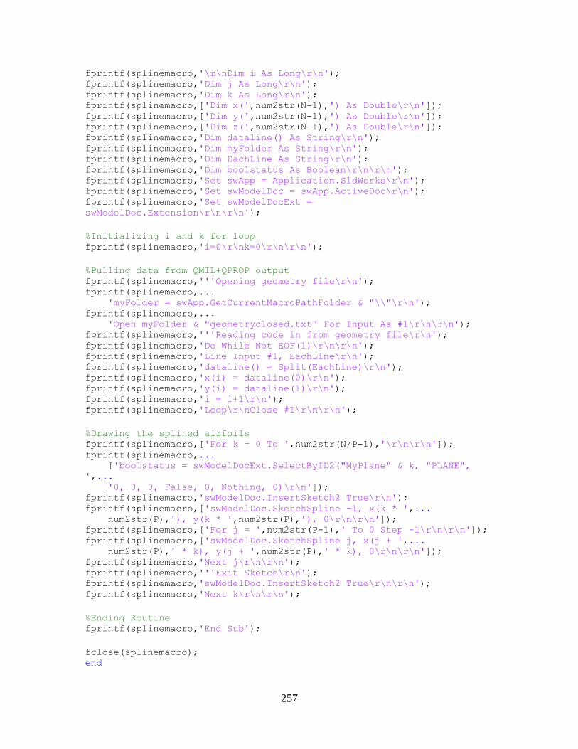
257
fprintf(splinemacro,'\r\nDim i As Long\r\n'); fprintf(splinemacro,'Dim j As Long\r\n'); fprintf(splinemacro,'Dim k As Long\r\n'); fprintf(splinemacro,['Dim x(',num2str(N-1),') As Double\r\n']); fprintf(splinemacro,['Dim y(',num2str(N-1),') As Double\r\n']); fprintf(splinemacro,['Dim z(',num2str(N-1),') As Double\r\n']); fprintf(splinemacro,'Dim dataline() As String\r\n'); fprintf(splinemacro,'Dim myFolder As String\r\n'); fprintf(splinemacro,'Dim EachLine As String\r\n'); fprintf(splinemacro,'Dim boolstatus As Boolean\r\n\r\n'); fprintf(splinemacro,'Set swApp = Application.SldWorks\r\n'); fprintf(splinemacro,'Set swModelDoc = swApp.ActiveDoc\r\n'); fprintf(splinemacro,'Set swModelDocExt =
swModelDoc.Extension\r\n\r\n');
%Initializing i and k for loop fprintf(splinemacro,'i=0\r\nk=0\r\n\r\n');
%Pulling data from QMIL+QPROP output fprintf(splinemacro,'''Opening geometry file\r\n'); fprintf(splinemacro,...
'myFolder = swApp.GetCurrentMacroPathFolder & "\\"\r\n'); fprintf(splinemacro,...
'Open myFolder & "geometryclosed.txt" For Input As #1\r\n\r\n'); fprintf(splinemacro,'''Reading code in from geometry file\r\n'); fprintf(splinemacro,'Do While Not EOF(1)\r\n\r\n'); fprintf(splinemacro,'Line Input #1, EachLine\r\n'); fprintf(splinemacro,'dataline() = Split(EachLine)\r\n'); fprintf(splinemacro,'x(i) = dataline(0)\r\n'); fprintf(splinemacro,'y(i) = dataline(1)\r\n'); fprintf(splinemacro,'i = i+1\r\n'); fprintf(splinemacro,'Loop\r\nClose #1\r\n\r\n');
%Drawing the splined airfoils fprintf(splinemacro,['For k = 0 To ',num2str(N/P-1),'\r\n\r\n']); fprintf(splinemacro,...
['boolstatus = swModelDocExt.SelectByID2("MyPlane" & k, "PLANE",
',... '0, 0, 0, False, 0, Nothing, 0)\r\n']);
fprintf(splinemacro,'swModelDoc.InsertSketch2 True\r\n'); fprintf(splinemacro,['swModelDoc.SketchSpline -1, x(k * ',...
num2str(P),'), y(k * ',num2str(P),'), 0\r\n\r\n']); fprintf(splinemacro,['For j = ',num2str(P-1),' To 0 Step -1\r\n\r\n']); fprintf(splinemacro,['swModelDoc.SketchSpline j, x(j + ',...
num2str(P),' * k), y(j + ',num2str(P),' * k), 0\r\n\r\n']); fprintf(splinemacro,'Next j\r\n\r\n'); fprintf(splinemacro,'''Exit Sketch\r\n'); fprintf(splinemacro,'swModelDoc.InsertSketch2 True\r\n\r\n'); fprintf(splinemacro,'Next k\r\n\r\n');
%Ending Routine fprintf(splinemacro,'End Sub');
fclose(splinemacro);
end
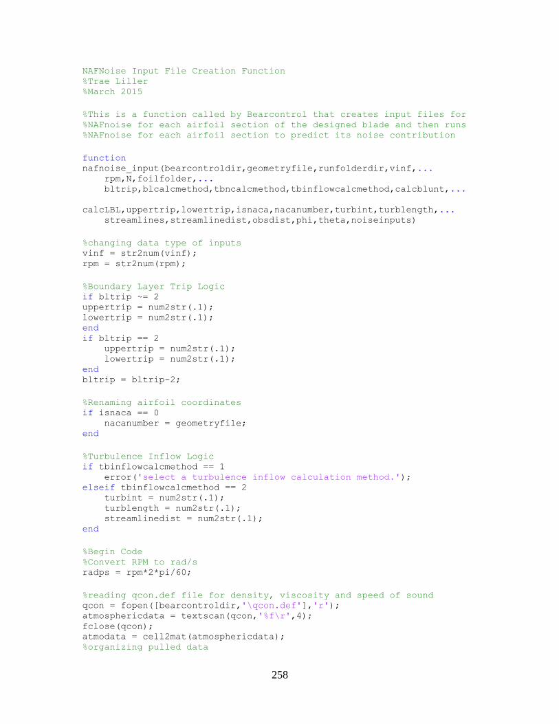
258
NAFNoise Input File Creation Function %Trae Liller %March 2015
%This is a function called by Bearcontrol that creates input files for %NAFnoise for each airfoil section of the designed blade and then runs %NAFnoise for each airfoil section to predict its noise contribution
function
nafnoise_input(bearcontroldir,geometryfile,runfolderdir,vinf,... rpm,N,foilfolder,... bltrip,blcalcmethod,tbncalcmethod,tbinflowcalcmethod,calcblunt,...
calcLBL,uppertrip,lowertrip,isnaca,nacanumber,turbint,turblength,... streamlines,streamlinedist,obsdist,phi,theta,noiseinputs)
%changing data type of inputs vinf = str2num(vinf); rpm = str2num(rpm);
%Boundary Layer Trip Logic if bltrip ~= 2 uppertrip = num2str(.1); lowertrip = num2str(.1); end if bltrip == 2 uppertrip = num2str(.1); lowertrip = num2str(.1); end bltrip = bltrip-2;
%Renaming airfoil coordinates if isnaca == 0 nacanumber = geometryfile; end
%Turbulence Inflow Logic if tbinflowcalcmethod == 1 error('select a turbulence inflow calculation method.'); elseif tbinflowcalcmethod == 2 turbint = num2str(.1); turblength = num2str(.1); streamlinedist = num2str(.1); end
%Begin Code %Convert RPM to rad/s radps = rpm*2*pi/60;
%reading qcon.def file for density, viscosity and speed of sound qcon = fopen([bearcontroldir,'\qcon.def'],'r'); atmosphericdata = textscan(qcon,'%f\r',4); fclose(qcon); atmodata = cell2mat(atmosphericdata); %organizing pulled data
259
rho = atmodata(1); %density mu = atmodata(2); %viscosity a = atmodata(3); %speed of sound
%reading qprop output file fid = fopen([runfolderdir,'\qpropoutput_designpoint.txt'],'r'); firstline = 21; points = 25; flowdata = textscan(fid,'%f %f %f %f %f %f %f %f %f %f %f %f\r',...
points+1,'HeaderLines',firstline-1); fclose(fid); flowdata = cell2mat(flowdata);
%organizing data from output file Wa = flowdata(:,10); %axial velocity n = length(Wa); %length of vectors r = flowdata(:,1); %radial locations chord = flowdata(:,2); %chord lengths beta = flowdata(:,3); %beta angles
%backing out W, total velocity seen by each section across the span span = zeros(n,1); span(1) = (r(2)-r(1)); for i = 2:n-1
span(i) = (r(i+1)-r(i))/2+(r(i)-r(i-1))/2; end span(n) = (r(n)-r(n-1)); v_a = Wa - vinf; %axial induced v v_t = zeros(N,1);
for i = 1:n v_t(i) = -(sqrt(radps^2*r(i)^2-4*v_a(i)*Wa(i))... %tangential induced
v -radps*r(i))/2;
end Wt = zeros(n,1); %tangential
velocity for i = 1:n Wt(i) = r(i).*radps-v_t(i); end aoa = zeros(n,1); %angle of attack for i = 1:n aoa(i) = beta(i) - atand(Wa(i)/Wt(i)); end W = zeros(n,1); %total velocity for i = 1:n
W(i) = sqrt(Wa(i)^2 + Wt(i)^2); end
geometry = load(geometryfile); %base airfoil points %P = # of pts in the airfoil geometry file P = length(geometry); %S = # of airfoils per blade
geometryx = geometry(:,1); geometryy = geometry(:,2);
260
%calculating trailing edge thickness and angle based on geometry points
and %chord length trail = zeros(n,1); for i = 1:n trail(i) = abs(geometryy(1)*chord(i)-geometryy(P)*chord(i)); end
i = 1; yupper = max(geometryy); while (1) if geometryy(i) == yupper, break, end i = i+1; end xupper = geometryx(i);
i = 1; ylower = min(geometryy); while(1) if geometryy(i) == ylower, break, end i = i+1; end xlower = geometryx(i);
upperangle = atand(yupper/xupper); lowerangle = abs(ylower/xlower); trailangle = upperangle+lowerangle;
[row, col] = find((geometryx-.01)==min(abs(geometryx-.01))); onepercthick = zeros(n,1); for i = 1:n onepercthick(i) = chord(i)*abs(geometryy(row(1),1)-... geometryy(row(2),1)); end
[row1, col1] = find((geometryx-.1)==min(abs(geometryx-.1))); tenpercthick = zeros(n,1); for i = 1:n tenpercthick(i) = chord(i)*abs(geometryy(row1(1),1)-... geometryy(row1(2),1)); end
%converting data types to create input files a = num2str(a); mu = num2str(mu); rho = num2str(rho); bltrip = num2str(bltrip); blcalcmethod = num2str(blcalcmethod-1); tbncalcmethod = num2str(tbncalcmethod-2); tbinflowcalcmethod = num2str(tbinflowcalcmethod-2); calcblunt = num2str(calcblunt); calcLBL = num2str(calcLBL); streamlines = num2str(streamlines);
%input file creation loop for each airfoil cross section
261
for i = 1:25 fid = fopen([noiseinputs,'\nafnoise',... num2str(i),'.ipt'],'w'); fprintf(fid,'Input file for 2-D aeroacoustic code\r\n'); fprintf(fid,[foilfolder,' Airfoil\r\n']); fprintf(fid,['---------------------- Atmospheric Constants ----------
',... '-------------------------------\r\n']); fprintf(fid,[a,' C0 SPEED OF SOUND METERS/SEC\r\n']); fprintf(fid,[mu,' VISC KINEMATIC VISCOSITY M2/SEC\r\n']); fprintf(fid,[rho,' RHO Air Density KG/M3\r\n']); fprintf(fid,['---------------------- Noise Calc Settings ------------
',... '--------------------------\r\n']); fprintf(fid,[bltrip,' ITRIP Boundary layer trip no trip = 0 BPM,',... ' heavy trip = 1 (BPM only), light trip = 2\r\n']); fprintf(fid,[blcalcmethod,' X_BLMETHOD Integer describing
calculation',... ' method for boundary layer properties, =1 BPM =2 XFOIL\r\n']); fprintf(fid,[tbncalcmethod,' TBL_METHOD Integer describing
turbulent',... ' noise calculation\r\n']); fprintf(fid,[tbinflowcalcmethod,' TI_METHOD Integer describing TI',... ' noise calculation = 0 none = 1 Amiet (flat plate) = 2',... ' Guidati = 3 Simplified Guidati\r\n']); fprintf(fid,[calcblunt,' IBLUNT Flag to compute bluntness noise =
0',... ' no = 1 yes\r\n']); fprintf(fid,[calcLBL,' ILAM Flag to compute LBL noise',... ' = 0 no, = 1 yes\r\n']);
fprintf(fid,['---------------------- Airfoil Properties -------------
',... '----------------------------\r\n']); fprintf(fid,[num2str(chord(i)),' CHORD LENGTH (m)\r\n']); fprintf(fid,[num2str(span(i)),' AIRFOIL SPAN (m)\r\n']); fprintf(fid,[num2str(W(i)),' FREESTREAM VELOCITY (m/s)\r\n']); fprintf(fid,[num2str(aoa(i)),' ANGLE OF ATTACK (deg)\r\n']); fprintf(fid,[num2str(trail(i)),' TRAILING EDGE THICKNESS (m)\r\n']); fprintf(fid,... [num2str(trailangle),' PSI TRAILING EDGE SOLID ANGLE (deg)\r\n']); fprintf(fid,['---------------------- Xfoil Inputs -------------------
',... '--------------------------- \r\n']); fprintf(fid,[uppertrip,' XTR_upper = upper surface trip location',... ' (normalized chord length)\r\n']); fprintf(fid,[lowertrip,' XTR_lower = lower surface trip location',... ' (normalized chord length)\r\n']); if isnaca == 0 isnacaa = '.FALSE.'; else isnacaa = '.TRUE.'; end fprintf(fid,...
262
[num2str(isnacaa),' ISNACA = .TRUE. IF AIRFOIL IS A NACA
ELSE',... ' .FALSE.\r\n']); %0 = .FALSE. %1 = .TRUE. if isnaca == 0 fprintf(fid,['foilpoints.txt AIRFOIL FILE NAME OR NACA NUMBER',... ' (IF SPACES USE QUOTES)\r\n']); end
if isnaca == 1 fprintf(fid,[nacanumber,' AIRFOIL FILE NAME OR NACA NUMBER',... ' (IF SPACES USE QUOTES)\r\n']); end
fprintf(fid,['---------------------- Turbulent Inflow Noise Inputs --
',... '---------------------------\r\n']); fprintf(fid,[turbint,' TURBULENCE INTENSITY (percent)\r\n']); fprintf(fid,[turblength,' TURBULENCE LENGTH SCALE (m)\r\n']); fprintf(fid,[num2str(onepercthick(i)),' THICKNESS @ 1 PERCENT
CHORD',... ' (NORMALIZED THICKNESS)\r\n']); fprintf(fid,[num2str(tenpercthick(i)),' THICKNESS @ 10 PERCENT
CHORD',... ' (NORMALIZED THICKNESS)\r\n']); fprintf(fid,[streamlines,' NUMBER OF STREAMLINES',... ' (GUIDATI FULL MODEL)\r\n']); fprintf(fid,[streamlinedist,' DISTANCE BETWEEN STREAMLINES',... ' (GUIDATI FULL MODEL)\r\n']); fprintf(fid,['---------------------- Observer Location -----------',... '------------------------------\r\n']); fprintf(fid,[obsdist,' OBSERVER DISTANCE (m)\r\n']); fprintf(fid,[phi,' PHI ANGLE RELATIVE TO SPANLINE (deg)\r\n']); fprintf(fid,[theta,' THETA ANGLE RELATIVE TO CHORDLINE (deg)\r\n']); fclose(fid); end %Running NAFnoise for each airfoil section for i = 1:25 dos([bearcontroldir,'\NAFnoise\NAFNoise.exe ',... noiseinputs,'\nafnoise',num2str(i),'.ipt']); end
%NAFNoise Output Reader Function %Trae Liller %March 2015 %This is a function called by Bearcontrol that takes all of the output %files of nafnoise_input, and adds the sound predictions of each cross %section together to create a noise prediction for the entire propeller %(blade contribution only, no motor, hub, etc.)
function soundpressurelevel = nafnoise_output(noiseinputs) %reading nafnoise output file
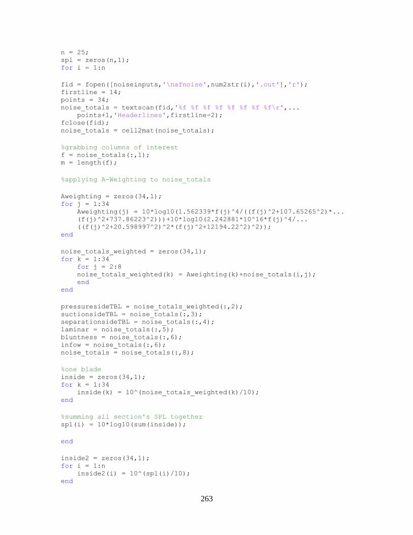
263
n = 25; spl = zeros(n,1); for i = 1:n
fid = fopen([noiseinputs,'\nafnoise',num2str(i),'.out'],'r'); firstline = 14; points = 34; noise_totals = textscan(fid,'%f %f %f %f %f %f %f %f\r',...
points+1,'Headerlines',firstline-2); fclose(fid); noise_totals = cell2mat(noise_totals);
%grabbing columns of interest f = noise_totals(:,1); m = length(f);
%applying A-Weighting to noise_totals
Aweighting = zeros(34,1); for j = 1:34
Aweighting(j) = 10*log10(1.562339*f(j)^4/((f(j)^2+107.65265^2)*... (f(j)^2+737.86223^2)))+10*log10(2.242881*10^16*f(j)^4/... ((f(j)^2+20.598997^2)^2*(f(j)^2+12194.22^2)^2));
end
noise_totals_weighted = zeros(34,1); for k = 1:34
for j = 2:8 noise_totals_weighted(k) = Aweighting(k)+noise_totals(i,j); end
end
pressuresideTBL = noise_totals_weighted(:,2); suctionsideTBL = noise_totals(:,3); separationsideTBL = noise_totals(:,4); laminar = noise_totals(:,5); bluntness = noise_totals(:,6); infow = noise_totals(:,6); noise_totals = noise_totals(:,8);
%one blade inside = zeros(34,1); for k = 1:34
inside(k) = 10^(noise_totals_weighted(k)/10); end
%summing all section's SPL together spl(i) = 10*log10(sum(inside));
end
inside2 = zeros(34,1); for i = 1:n
inside2(i) = 10^(spl(i)/10); end

264
spl1blade = 10*log10(sum(inside2)) soundpressurelevel = 10*log10(10^(spl1blade/10)+10^(spl1blade/10));
soundpressurelevel end
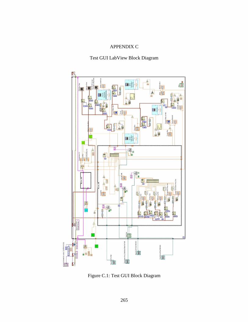
265
APPENDIX C
Test GUI LabView Block Diagram
Figure C.1: Test GUI Block Diagram
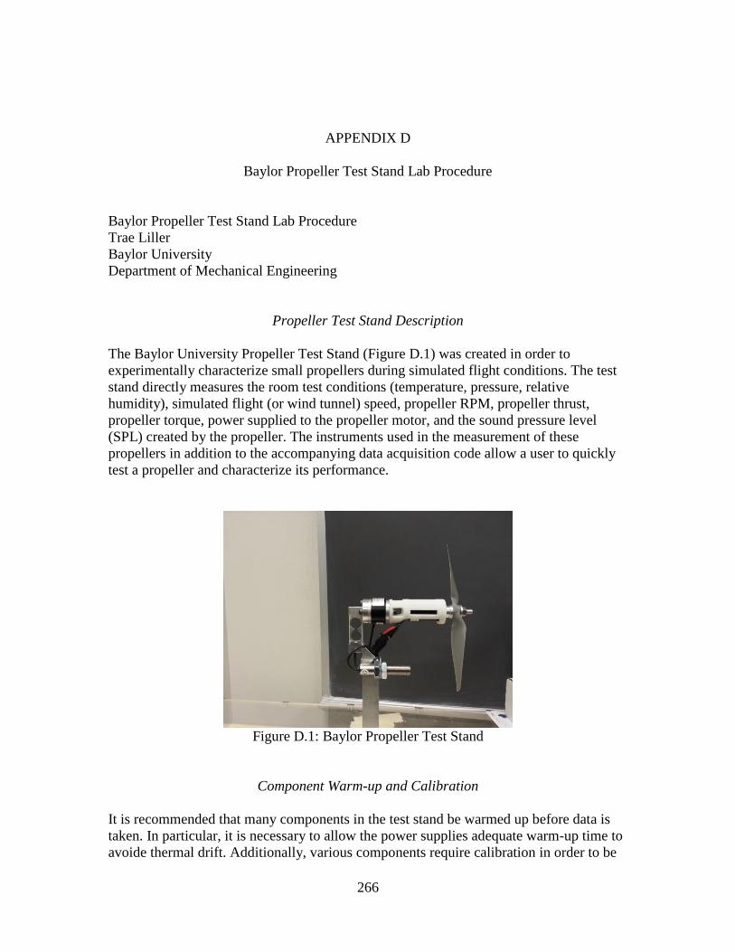
266
APPENDIX D
Baylor Propeller Test Stand Lab Procedure
Baylor Propeller Test Stand Lab Procedure
Trae Liller
Baylor University
Department of Mechanical Engineering
Propeller Test Stand Description
The Baylor University Propeller Test Stand (Figure D.1) was created in order to
experimentally characterize small propellers during simulated flight conditions. The test
stand directly measures the room test conditions (temperature, pressure, relative
humidity), simulated flight (or wind tunnel) speed, propeller RPM, propeller thrust,
propeller torque, power supplied to the propeller motor, and the sound pressure level
(SPL) created by the propeller. The instruments used in the measurement of these
propellers in addition to the accompanying data acquisition code allow a user to quickly
test a propeller and characterize its performance.
Figure D.1: Baylor Propeller Test Stand
Component Warm-up and Calibration
It is recommended that many components in the test stand be warmed up before data is
taken. In particular, it is necessary to allow the power supplies adequate warm-up time to
avoide thermal drift. Additionally, various components require calibration in order to be
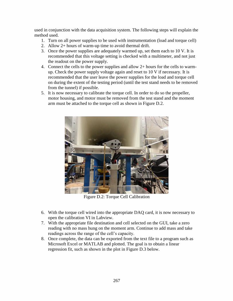
267
used in conjunction with the data acquisition system. The following steps will explain the
method used.
1. Turn on all power supplies to be used with instrumentation (load and torque cell)
2. Allow 2+ hours of warm-up time to avoid thermal drift.
3. Once the power supplies are adequately warmed up, set them each to 10 V. It is
recommended that this voltage setting is checked with a multimeter, and not just
the readout on the power supply.
4. Connect the cells to the power supplies and allow 2+ hours for the cells to warm-
up. Check the power supply voltage again and reset to 10 V if necessary. It is
recommended that the user leave the power supplies for the load and torque cell
on during the extent of the testing period (until the test stand needs to be removed
from the tunnel) if possible.
5. It is now necessary to calibrate the torque cell. In order to do so the propeller,
motor housing, and motor must be removed from the test stand and the moment
arm must be attached to the torque cell as shown in Figure D.2.
Figure D.2: Torque Cell Calibration
6. With the torque cell wired into the appropriate DAQ card, it is now necessary to
open the calibration VI in Labview.
7. With the appropriate file destination and cell selected on the GUI, take a zero
reading with no mass hung on the moment arm. Continue to add mass and take
readings across the range of the cell’s capacity.
8. Once complete, the data can be exported from the text file to a program such as
Microsoft Excel or MATLAB and plotted. The goal is to obtain a linear
regression fit, such as shown in the plot in Figure D.3 below.
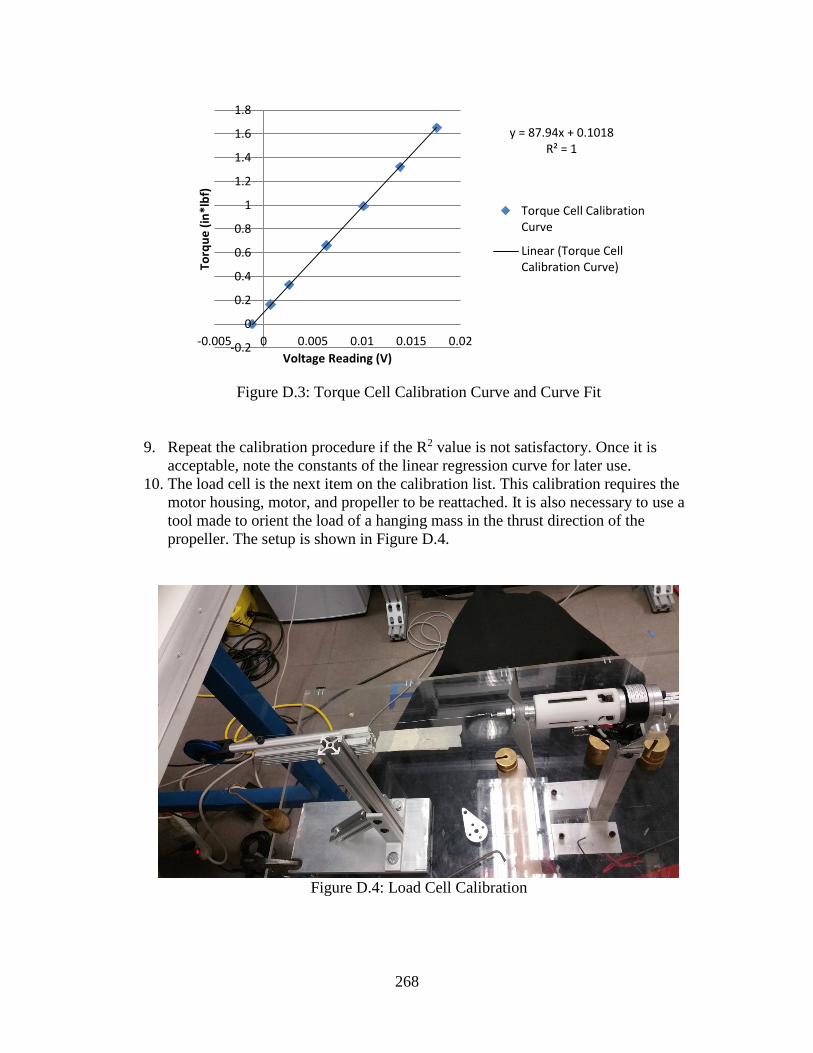
268
Figure D.3: Torque Cell Calibration Curve and Curve Fit
9. Repeat the calibration procedure if the R2 value is not satisfactory. Once it is
acceptable, note the constants of the linear regression curve for later use.
10. The load cell is the next item on the calibration list. This calibration requires the
motor housing, motor, and propeller to be reattached. It is also necessary to use a
tool made to orient the load of a hanging mass in the thrust direction of the
propeller. The setup is shown in Figure D.4.
Figure D.4: Load Cell Calibration
y = 87.94x + 0.1018R² = 1
-0.2
0
0.2
0.4
0.6
0.8
1
1.2
1.4
1.6
1.8
-0.005 0 0.005 0.01 0.015 0.02
Torq
ue
(in
*lb
f)
Voltage Reading (V)
Torque Cell CalibrationCurve
Linear (Torque CellCalibration Curve)
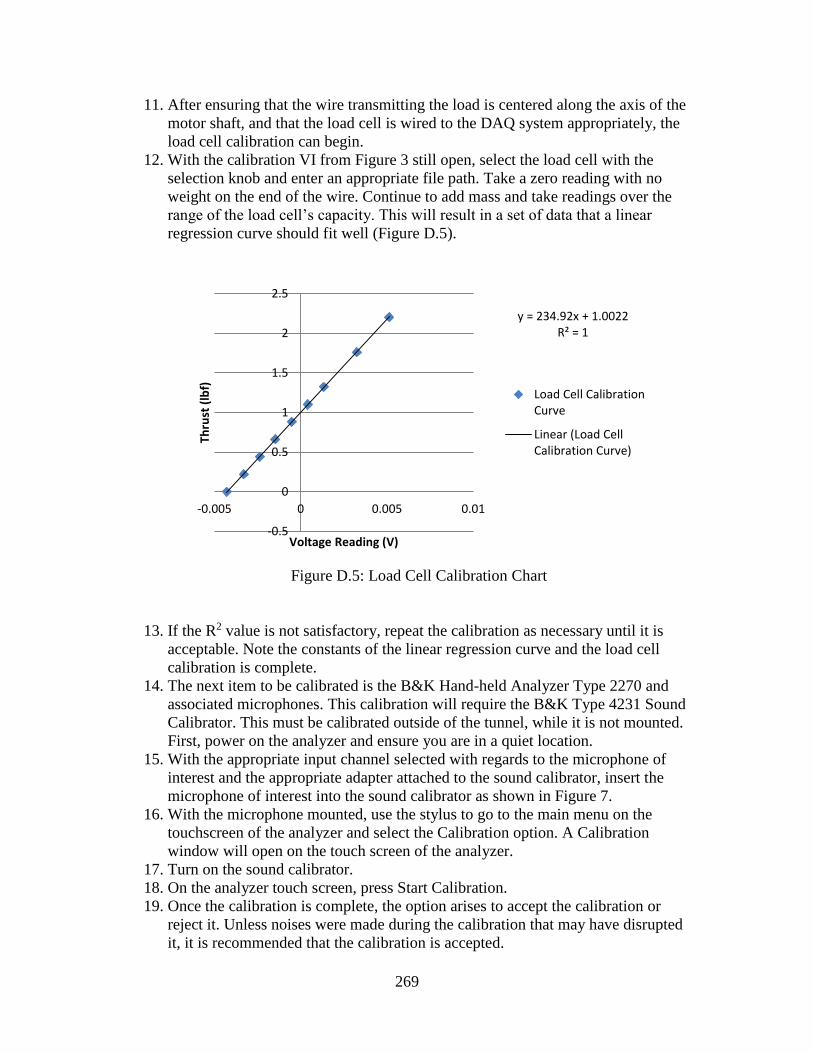
269
11. After ensuring that the wire transmitting the load is centered along the axis of the
motor shaft, and that the load cell is wired to the DAQ system appropriately, the
load cell calibration can begin.
12. With the calibration VI from Figure 3 still open, select the load cell with the
selection knob and enter an appropriate file path. Take a zero reading with no
weight on the end of the wire. Continue to add mass and take readings over the
range of the load cell’s capacity. This will result in a set of data that a linear
regression curve should fit well (Figure D.5).
Figure D.5: Load Cell Calibration Chart
13. If the R2 value is not satisfactory, repeat the calibration as necessary until it is
acceptable. Note the constants of the linear regression curve and the load cell
calibration is complete.
14. The next item to be calibrated is the B&K Hand-held Analyzer Type 2270 and
associated microphones. This calibration will require the B&K Type 4231 Sound
Calibrator. This must be calibrated outside of the tunnel, while it is not mounted.
First, power on the analyzer and ensure you are in a quiet location.
15. With the appropriate input channel selected with regards to the microphone of
interest and the appropriate adapter attached to the sound calibrator, insert the
microphone of interest into the sound calibrator as shown in Figure 7.
16. With the microphone mounted, use the stylus to go to the main menu on the
touchscreen of the analyzer and select the Calibration option. A Calibration
window will open on the touch screen of the analyzer.
17. Turn on the sound calibrator.
18. On the analyzer touch screen, press Start Calibration.
19. Once the calibration is complete, the option arises to accept the calibration or
reject it. Unless noises were made during the calibration that may have disrupted
it, it is recommended that the calibration is accepted.
y = 234.92x + 1.0022R² = 1
-0.5
0
0.5
1
1.5
2
2.5
-0.005 0 0.005 0.01
Thru
st (
lbf)
Voltage Reading (V)
Load Cell CalibrationCurve
Linear (Load CellCalibration Curve)
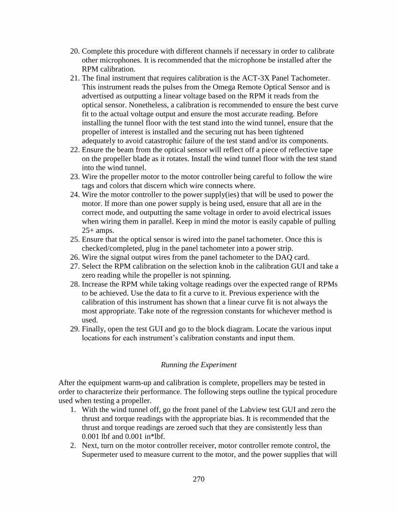
270
20. Complete this procedure with different channels if necessary in order to calibrate
other microphones. It is recommended that the microphone be installed after the
RPM calibration.
21. The final instrument that requires calibration is the ACT-3X Panel Tachometer.
This instrument reads the pulses from the Omega Remote Optical Sensor and is
advertised as outputting a linear voltage based on the RPM it reads from the
optical sensor. Nonetheless, a calibration is recommended to ensure the best curve
fit to the actual voltage output and ensure the most accurate reading. Before
installing the tunnel floor with the test stand into the wind tunnel, ensure that the
propeller of interest is installed and the securing nut has been tightened
adequately to avoid catastrophic failure of the test stand and/or its components.
22. Ensure the beam from the optical sensor will reflect off a piece of reflective tape
on the propeller blade as it rotates. Install the wind tunnel floor with the test stand
into the wind tunnel.
23. Wire the propeller motor to the motor controller being careful to follow the wire
tags and colors that discern which wire connects where.
24. Wire the motor controller to the power supply(ies) that will be used to power the
motor. If more than one power supply is being used, ensure that all are in the
correct mode, and outputting the same voltage in order to avoid electrical issues
when wiring them in parallel. Keep in mind the motor is easily capable of pulling
25+ amps.
25. Ensure that the optical sensor is wired into the panel tachometer. Once this is
checked/completed, plug in the panel tachometer into a power strip.
26. Wire the signal output wires from the panel tachometer to the DAQ card.
27. Select the RPM calibration on the selection knob in the calibration GUI and take a
zero reading while the propeller is not spinning.
28. Increase the RPM while taking voltage readings over the expected range of RPMs
to be achieved. Use the data to fit a curve to it. Previous experience with the
calibration of this instrument has shown that a linear curve fit is not always the
most appropriate. Take note of the regression constants for whichever method is
used.
29. Finally, open the test GUI and go to the block diagram. Locate the various input
locations for each instrument’s calibration constants and input them.
Running the Experiment
After the equipment warm-up and calibration is complete, propellers may be tested in
order to characterize their performance. The following steps outline the typical procedure
used when testing a propeller.
1. With the wind tunnel off, go the front panel of the Labview test GUI and zero the
thrust and torque readings with the appropriate bias. It is recommended that the
thrust and torque readings are zeroed such that they are consistently less than
0.001 lbf and 0.001 in*lbf.
2. Next, turn on the motor controller receiver, motor controller remote control, the
Supermeter used to measure current to the motor, and the power supplies that will
271
be used to power the propeller motor, in that order. Ensure the propeller is
controllable by increasing the throttle on the remote control. Throttle to zero RPM
once the check is complete.
3. Turn on the wind tunnel to the desired operating condtion and take another data
point with the test GUI.
4. Throttle up the propeller until a positive thrust readout is shown on the test GUI.
Ensuring that any current or sound readouts necessary are filled out on the GUI,
take the data point for the throttle setting.
5. Increase the throttle by the desired RPM increment and repeat step 4 until all data
points are taken. Note that the Supermeter can read a maximum of 10 amps
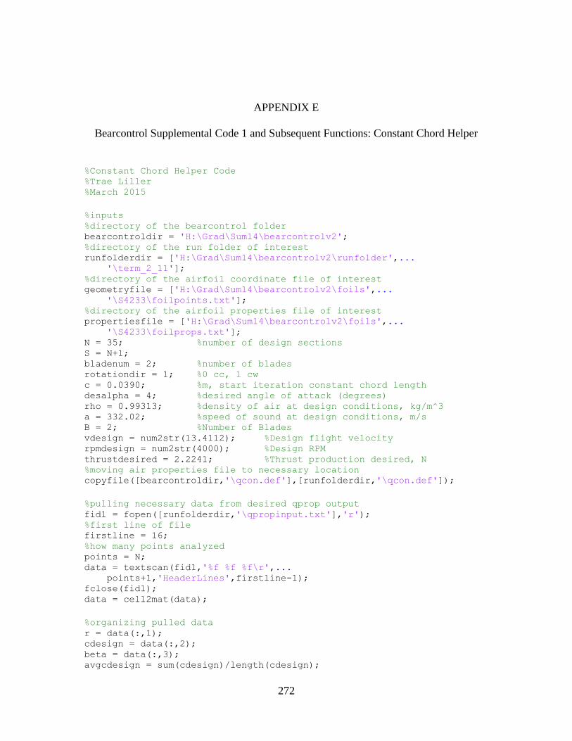
272
APPENDIX E
Bearcontrol Supplemental Code 1 and Subsequent Functions: Constant Chord Helper
%Constant Chord Helper Code %Trae Liller %March 2015
%inputs %directory of the bearcontrol folder bearcontroldir = 'H:\Grad\Sum14\bearcontrolv2'; %directory of the run folder of interest runfolderdir = ['H:\Grad\Sum14\bearcontrolv2\runfolder',... '\term_2_11']; %directory of the airfoil coordinate file of interest geometryfile = ['H:\Grad\Sum14\bearcontrolv2\foils',... '\S4233\foilpoints.txt']; %directory of the airfoil properties file of interest propertiesfile = ['H:\Grad\Sum14\bearcontrolv2\foils',... '\S4233\foilprops.txt']; N = 35; %number of design sections S = N+1; bladenum = 2; %number of blades rotationdir = 1; %0 cc, 1 cw c = 0.0390; %m, start iteration constant chord length desalpha = 4; %desired angle of attack (degrees) rho = 0.99313; %density of air at design conditions, kg/m^3 a = 332.02; %speed of sound at design conditions, m/s B = 2; %Number of Blades vdesign = num2str(13.4112); %Design flight velocity rpmdesign = num2str(4000); %Design RPM thrustdesired = 2.2241; %Thrust production desired, N %moving air properties file to necessary location copyfile([bearcontroldir,'\qcon.def'],[runfolderdir,'\qcon.def']);
%pulling necessary data from desired qprop output fid1 = fopen([runfolderdir,'\qpropinput.txt'],'r'); %first line of file firstline = 16; %how many points analyzed points = N; data = textscan(fid1,'%f %f %f\r',... points+1,'HeaderLines',firstline-1); fclose(fid1); data = cell2mat(data);
%organizing pulled data r = data(:,1); cdesign = data(:,2); beta = data(:,3); avgcdesign = sum(cdesign)/length(cdesign);
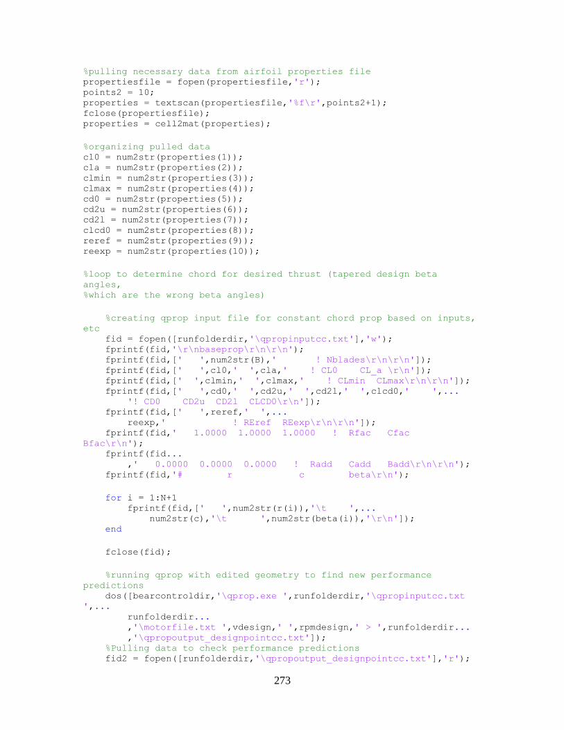
273
%pulling necessary data from airfoil properties file propertiesfile = fopen(propertiesfile,'r'); points2 = 10; properties = textscan(propertiesfile,'%f\r',points2+1); fclose(propertiesfile); properties = cell2mat(properties);
%organizing pulled data cl0 = num2str(properties(1)); cla = num2str(properties(2)); clmin = num2str(properties(3)); clmax = num2str(properties(4)); cd0 = num2str(properties(5)); cd2u = num2str(properties(6)); cd2l = num2str(properties(7)); clcd0 = num2str(properties(8)); reref = num2str(properties(9)); reexp = num2str(properties(10));
%loop to determine chord for desired thrust (tapered design beta
angles, %which are the wrong beta angles)
%creating qprop input file for constant chord prop based on inputs,
etc fid = fopen([runfolderdir,'\qpropinputcc.txt'],'w'); fprintf(fid,'\r\nbaseprop\r\n\r\n'); fprintf(fid,[' ',num2str(B),' ! Nblades\r\n\r\n']); fprintf(fid,[' ',cl0,' ',cla,' ! CL0 CL_a \r\n']); fprintf(fid,[' ',clmin,' ',clmax,' ! CLmin CLmax\r\n\r\n']); fprintf(fid,[' ',cd0,' ',cd2u,' ',cd2l,' ',clcd0,' ',...
'! CD0 CD2u CD2l CLCD0\r\n']); fprintf(fid,[' ',reref,' ',...
reexp,' ! REref REexp\r\n\r\n']); fprintf(fid,' 1.0000 1.0000 1.0000 ! Rfac Cfac
Bfac\r\n'); fprintf(fid...
,' 0.0000 0.0000 0.0000 ! Radd Cadd Badd\r\n\r\n'); fprintf(fid,'# r c beta\r\n');
for i = 1:N+1 fprintf(fid,[' ',num2str(r(i)),'\t ',...
num2str(c),'\t ',num2str(beta(i)),'\r\n']); end
fclose(fid);
%running qprop with edited geometry to find new performance
predictions dos([bearcontroldir,'\qprop.exe ',runfolderdir,'\qpropinputcc.txt
',... runfolderdir... ,'\motorfile.txt ',vdesign,' ',rpmdesign,' > ',runfolderdir... ,'\qpropoutput_designpointcc.txt']);
%Pulling data to check performance predictions fid2 = fopen([runfolderdir,'\qpropoutput_designpointcc.txt'],'r');
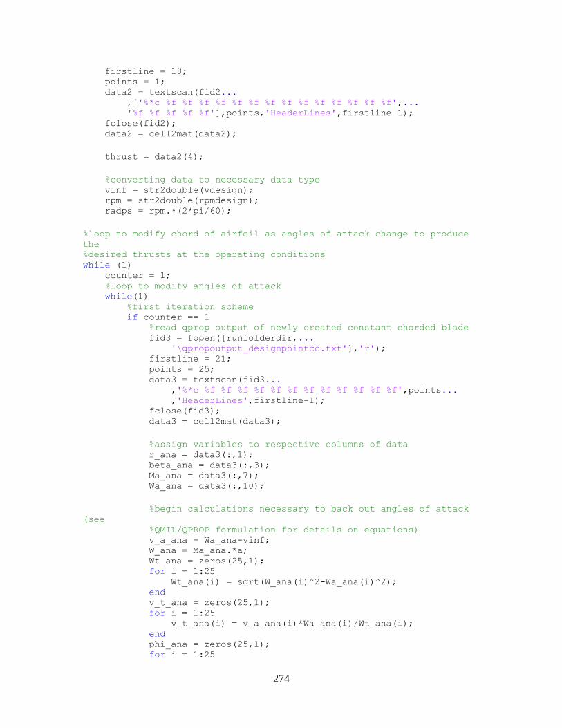
274
firstline = 18; points = 1; data2 = textscan(fid2... ,['%*c %f %f %f %f %f %f %f %f %f %f %f %f %f %f',... '%f %f %f %f %f'],points,'HeaderLines',firstline-1); fclose(fid2); data2 = cell2mat(data2);
thrust = data2(4);
%converting data to necessary data type vinf = str2double(vdesign); rpm = str2double(rpmdesign); radps = rpm.*(2*pi/60);
%loop to modify chord of airfoil as angles of attack change to produce
the %desired thrusts at the operating conditions while (1) counter = 1; %loop to modify angles of attack while(1) %first iteration scheme if counter == 1 %read qprop output of newly created constant chorded blade fid3 = fopen([runfolderdir,... '\qpropoutput_designpointcc.txt'],'r'); firstline = 21; points = 25; data3 = textscan(fid3... ,'%*c %f %f %f %f %f %f %f %f %f %f %f %f',points... ,'HeaderLines',firstline-1); fclose(fid3); data3 = cell2mat(data3);
%assign variables to respective columns of data r_ana = data3(:,1); beta_ana = data3(:,3); Ma_ana = data3(:,7); Wa_ana = data3(:,10);
%begin calculations necessary to back out angles of attack
(see %QMIL/QPROP formulation for details on equations) v_a_ana = Wa_ana-vinf; W_ana = Ma_ana.*a; Wt_ana = zeros(25,1); for i = 1:25 Wt_ana(i) = sqrt(W_ana(i)^2-Wa_ana(i)^2); end v_t_ana = zeros(25,1); for i = 1:25 v_t_ana(i) = v_a_ana(i)*Wa_ana(i)/Wt_ana(i); end phi_ana = zeros(25,1); for i = 1:25

275
phi_ana(i) = atand(Wa_ana(i)/Wt_ana(i)); end alpha_ana = zeros(25,1); for i = 1:25
alpha_ana(i) = beta_ana(i)-phi_ana(i); end
%Calculate difference between current angles of attack and
the %desired angle of attack difference = alpha_ana - desalpha;
%subtract this difference from the current geometric
pitches beta_ana_diff = zeros(25,1); for i = 1:25
beta_ana_diff(i) = beta_ana(i) - difference(i); end
end
if sum(abs(difference)) <= 1, break, end
%splining alphas vs. r to determine alpha at geometry r's %setting up dependent variable array to spline r_splinestart = zeros(N+1,1); for i = 1:N+1
if r(i)>min(r_ana) if r(i)<max(r_ana)
r_splinestart(i,1) = r(i); end
end end r_splinestart = r_splinestart(r_splinestart~=0);
r_spline = zeros(length(r_ana)+length(r_splinestart),1); for i = 1:(length(r_splinestart)+length(r_ana))
if i <= length(r_splinestart) r_spline(i) = r_splinestart(i);
end if i > length(r_splinestart)
i = i - length(r_splinestart); r_spline(i+length(r_splinestart)) = r_ana(i);
end end
r_spline = shellsort(r_spline);
%fitting a spline to extrapolate necessary values beta_spline = splinefitandinterp(r_ana,beta_ana,r_spline); beta_spline = beta_spline'; Wa_spline = splinefitandinterp(r_ana,Wa_ana,r_spline); Ma_spline = splinefitandinterp(r_ana,Ma_ana,r_spline); %calculations with splined data v_a_spline = Wa_spline-vinf; W_spline = Ma_spline.*a;
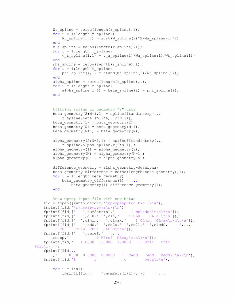
276
Wt_spline = zeros(length(r_spline),1); for i = 1:length(r_spline); Wt_spline(i,1) = sqrt(W_spline(i)^2-Wa_spline(i)^2); end v_t_spline = zeros(length(r_spline),1); for i = 1:length(r_spline) v_t_spline(i,1) = v_a_spline(i)*Wa_spline(i)/Wt_spline(i); end phi_spline = zeros(length(r_spline),1); for i = 1:length(r_spline) phi_spline(i,1) = atand(Wa_spline(i)/Wt_spline(i)); end alpha_spline = zeros(length(r_spline),1); for i = 1:length(r_spline) alpha_spline(i,1) = beta_spline(i) - phi_spline(i); end
%fitting spline to geometry "r" data beta_geometry(2:N-1,1) = splinefitandinterp(... r_spline,beta_spline,r(2:N-1)); beta_geometry(1) = beta_geometry(2); beta_geometry(N) = beta_geometry(N-1); beta_geometry(N+1) = beta_geometry(N);
alpha_geometry(2:N-1,1) = splinefitandinterp(... r_spline,alpha_spline,r(2:N-1)); alpha_geometry(1) = alpha_geometry(2); alpha_geometry(N) = alpha_geometry(N-1); alpha_geometry(N+1) = alpha_geometry(N);
difference_geometry = alpha_geometry-desalpha; beta_geometry_difference = zeros(length(beta_geometry),1); for i = 1:length(beta_geometry) beta_geometry_difference(i) = ... beta_geometry(i)-difference_geometry(i); end
%new Qprop input file with new betas fid = fopen([runfolderdir,'\qpropinputcc.txt'],'w'); fprintf(fid,'\r\nbaseprop\r\n\r\n'); fprintf(fid,[' ',num2str(B),' ! Nblades\r\n\r\n']); fprintf(fid,[' ',cl0,' ',cla,' ! CL0 CL_a \r\n']); fprintf(fid,[' ',clmin,' ',clmax,' ! CLmin CLmax\r\n\r\n']); fprintf(fid,[' ',cd0,' ',cd2u,' ',cd2l,' ',clcd0,' ',... '! CD0 CD2u CD2l CLCD0\r\n']); fprintf(fid,[' ',reref,' ',... reexp,' ! REref REexp\r\n\r\n']); fprintf(fid,' 1.0000 1.0000 1.0000 ! Rfac Cfac
Bfac\r\n'); fprintf(fid... ,' 0.0000 0.0000 0.0000 ! Radd Cadd Badd\r\n\r\n'); fprintf(fid,'# r c beta\r\n');
for i = 1:N+1 fprintf(fid,[' ',num2str(r(i)),'\t ',...
277
num2str(c),'\t ',... num2str(beta_geometry_difference(i)),'\r\n']);
end
fclose(fid);
%running QPROP to determine new performance characteristics dos([bearcontroldir,'\qprop.exe ',runfolderdir...
,'\qpropinputcc.txt ',runfolderdir... ,'\motorfile.txt ',vdesign,' ',rpmdesign,' >
',runfolderdir... ,'\qpropoutput_designpointcc.txt']);
%reading qprop output fid4 =
fopen([runfolderdir,'\qpropoutput_designpointcc.txt'],'r'); firstline = 21; points = 25; data4 = textscan(fid4,'%f %f %f %f %f %f %f %f %f %f %f
%f\r',... points,'HeaderLines',firstline-1);
fclose(fid4); data4 = cell2mat(data4); %organizing pulled data r_int = data4(:,1); beta_int = data4(:,3); Ma_int = data4(:,7); Wa_int = data4(:,10); %calculations to determine AoA v_a_int = Wa_int-vinf; W_int = Ma_int.*a; Wt_int = zeros(25,1); for i = 1:25
Wt_int(i) = sqrt(W_int(i)^2-Wa_int(i)^2); end v_t_int = zeros(25,1); for i = 1:25
v_t_int(i) = v_a_int(i)*Wa_int(i)/Wt_int(i); end phi_int = zeros(25,1); for i = 1:25
phi_int(i) = atand(Wa_int(i)/Wt_int(i)); end alpha_int = zeros(25,1); for i = 1:25
alpha_int(i) = beta_int(i)-phi_int(i); end difference_int = alpha_int - desalpha;
%loop prescribing beta change based on difference_int beta_int_difference = zeros(25,1); for i = 1:25
if difference_int(i) < 0 beta_int_difference(i) = beta_int(i)+0.01;
elseif difference_int(i) > 0 beta_int_difference(i) = beta_int(i)-0.01;
elseif difference_int(i) == 0
278
beta_int_difference(i) = beta_int(i); end end
%Splining new data to be able to input back into QPROP beta_splineinput =
splinefitandinterp(r_ana,beta_int_difference... ,r_spline); beta_splineinput = beta_splineinput'; beta_input(2:N-1,1) = splinefitandinterp(... r_spline,beta_splineinput,r(2:N-1)); beta_input(1) = beta_input(2); beta_input(N) = beta_input(N-1); beta_input(N+1) = beta_input(N);
%New QPROP input file to determine new performance
characteristics fid5 = fopen([runfolderdir,'\qpropinputcc.txt'],'w'); fprintf(fid,'\r\nbaseprop\r\n\r\n'); fprintf(fid,[' ',num2str(B),' ! Nblades\r\n\r\n']); fprintf(fid,[' ',cl0,' ',cla,' ! CL0 CL_a \r\n']); fprintf(fid,[' ',clmin,' ',clmax,' ! CLmin CLmax\r\n\r\n']); fprintf(fid,[' ',cd0,' ',cd2u,' ',cd2l,' ',clcd0,' ',... '! CD0 CD2u CD2l CLCD0\r\n']); fprintf(fid,[' ',reref,' ',... reexp,' ! REref REexp\r\n\r\n']); fprintf(fid,' 1.0000 1.0000 1.0000 ! Rfac Cfac
Bfac\r\n'); fprintf(fid... ,' 0.0000 0.0000 0.0000 ! Radd Cadd Badd\r\n\r\n'); fprintf(fid,'# r c beta\r\n');
for i = 1:N+1 fprintf(fid5,[' ',num2str(r(i)),'\t ',... num2str(c),'\t ',... num2str(beta_input(i)),'\r\n']); end
fclose(fid5); %running the new file to determine performance characteristics dos([bearcontroldir,'\qprop.exe ',runfolderdir... ,'\qpropinputcc.txt ',runfolderdir... ,'\motorfile.txt ',vdesign,' ',rpmdesign,' >
',runfolderdir... ,'\qpropoutput_designpointcc.txt']); %reading new performance file fid6 =
fopen([runfolderdir,'\qpropoutput_designpointcc.txt'],'r'); firstline = 21; points = 25; data5 = textscan(fid6,'%f %f %f %f %f %f %f %f %f %f %f
%f\r',... points,'HeaderLines',firstline-1); fclose(fid6); data5 = cell2mat(data5); %organizing data
279
r_ana = data5(:,1); beta_ana = data5(:,3); Ma_ana = data5(:,7); Wa_ana = data5(:,10); %begin calculations to back out angles of attack v_a_ana = Wa_ana-vinf; W_ana = Ma_ana.*a; Wt_ana = zeros(25,1); for i = 1:25
Wt_ana(i) = sqrt(W_ana(i)^2-Wa_ana(i)^2); end v_t_ana = zeros(25,1); for i = 1:25
v_t_ana(i) = v_a_ana(i)*Wa_ana(i)/Wt_ana(i); end phi_ana = zeros(25,1); for i = 1:25
phi_ana(i) = atand(Wa_ana(i)/Wt_ana(i)); end alpha_ana = zeros(25,1); for i = 1:25
alpha_ana(i) = beta_ana(i)-phi_ana(i); end
%end AoA modification loop if iterations go to 500 counter = counter+1; if counter == 500, break, end
end
%Open QPROP output to read thrust output of propeller fid7 = fopen([runfolderdir,'\qpropoutput_designpointcc.txt'],'r'); firstline = 18; points = 1; data2 = textscan(fid7...
,['%*c %f %f %f %f %f %f %f %f %f %f %f %f %f %f',... '%f %f %f %f %f'],points,'HeaderLines',firstline-1);
fclose(fid7); data2 = cell2mat(data2);
finalthrust = data2(4); %difference between design's thrust and desired thrust finalsign = finalthrust-thrustdesired; %loop end criteria if abs(finalsign) <= .01, break, end %Adjusting chord based on finalsign variable if finalsign > 0
c = c-.0001; elseif finalsign < 0
c = c+.0001; end
end
%Running geometry points creation function geometrypts_funccc(N,geometryfile,runfolderdir,rotationdir,B); %running plane macro creation function planemacro_funccc(N,runfolderdir,bladenum);
280
%running spline macro creation function splinemacro_funccc(N,runfolderdir,bladenum);
%Shell Sort %Trae Liller %March 2015 %This function is called by constantchordhelper.m in order to sort c
radial %locations into their correct order.
function list = shellsort(list)
N = numel(list); increment = round(N/2);
while increment > 0
for i = (increment+1:N) temp = list(i); j = i; while (j >= increment+1) && (list(j-increment) > temp) list(j) = list(j-increment); j = j - increment; end
list(j) = temp;
end
if increment == 2 increment = 1; else increment = round(increment/2.2); end end end
%Spline Fit and Interpolation Function
%Trae Liller %March 2015 %This function fits a spline to a dataset and is used in supplementary %Bearcontrol codes. Adapted from Applied Numerical Methods with MATLAB %3rd Edition
function yy = splinefitandinterp(x,y,xx)
n = length(x);
if length(y)~=n, error('x and y must be same length'), end if any(diff(x))<=0, error('x must be strictly ascending'), end
m = length(xx);
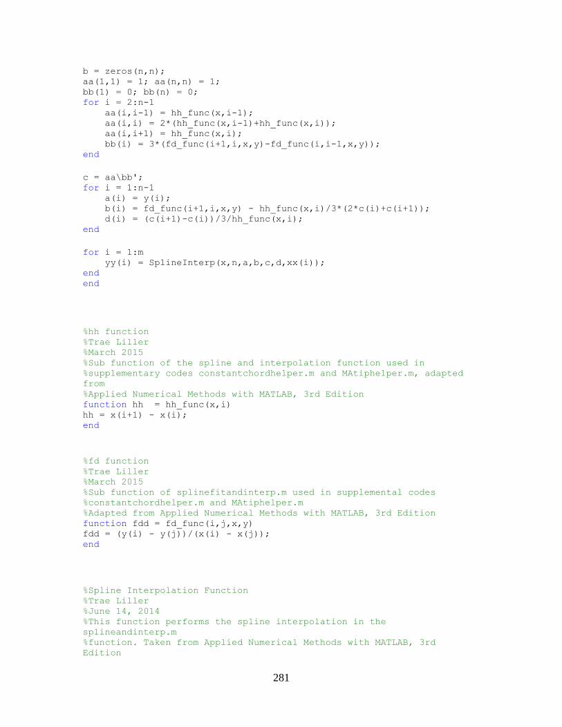
281
b = zeros(n,n); aa(1,1) = 1; aa(n,n) = 1; bb(1) = 0; bb(n) = 0; for i = 2:n-1
aa(i,i-1) = hh_func(x,i-1); aa(i,i) = 2*(hh_func(x,i-1)+hh_func(x,i)); aa(i,i+1) = hh_func(x,i); bb(i) = 3*(fd_func(i+1,i,x,y)-fd_func(i,i-1,x,y));
end
c = aa\bb'; for i = 1:n-1
a(i) = y(i); b(i) = fd_func(i+1,i,x,y) - hh_func(x,i)/3*(2*c(i)+c(i+1)); d(i) = (c(i+1)-c(i))/3/hh_func(x,i);
end
for i = 1:m yy(i) = SplineInterp(x,n,a,b,c,d,xx(i));
end end
%hh function %Trae Liller %March 2015 %Sub function of the spline and interpolation function used in %supplementary codes constantchordhelper.m and MAtiphelper.m, adapted
from %Applied Numerical Methods with MATLAB, 3rd Edition function hh = hh_func(x,i) hh = x(i+1) - x(i); end
%fd function %Trae Liller %March 2015 %Sub function of splinefitandinterp.m used in supplemental codes %constantchordhelper.m and MAtiphelper.m %Adapted from Applied Numerical Methods with MATLAB, 3rd Edition function fdd = fd_func(i,j,x,y) fdd = (y(i) - y(j))/(x(i) - x(j)); end
%Spline Interpolation Function
%Trae Liller %June 14, 2014 %This function performs the spline interpolation in the
splineandinterp.m %function. Taken from Applied Numerical Methods with MATLAB, 3rd
Edition
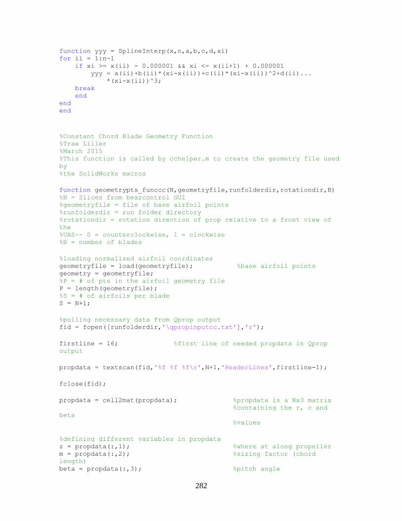
282
function yyy = SplineInterp(x,n,a,b,c,d,xi) for ii = 1:n-1 if xi >= x(ii) - 0.000001 && xi <= x(ii+1) + 0.000001 yyy = a(ii)+b(ii)*(xi-x(ii))+c(ii)*(xi-x(ii))^2+d(ii)... *(xi-x(ii))^3; break end end end
%Constant Chord Blade Geometry Function %Trae Liller %March 2015 %This function is called by cchelper.m to create the geometry file used
by %the SolidWorks macros
function geometrypts_funccc(N,geometryfile,runfolderdir,rotationdir,B) %N = Slices from bearcontrol GUI %geometryfile = file of base airfoil points %runfolderdir = run folder directory %rotationdir = rotation direction of prop relative to a front view of
the %UAS-- 0 = counterclockwise, 1 = clockwise %B = number of blades
%loading normalized airfoil coordinates geometryfile = load(geometryfile); %base airfoil points geometry = geometryfile; %P = # of pts in the airfoil geometry file P = length(geometryfile); %S = # of airfoils per blade S = N+1;
%pulling necessary data from Qprop output fid = fopen([runfolderdir,'\qpropinputcc.txt'],'r');
firstline = 16; %first line of needed propdata in Qprop
output
propdata = textscan(fid,'%f %f %f\r',N+1,'HeaderLines',firstline-1);
fclose(fid);
propdata = cell2mat(propdata); %propdata is a Nx3 matrix %containing the r, c and
beta %values
%defining different variables in propdata z = propdata(:,1); %where at along propeller m = propdata(:,2); %sizing factor (chord
length) beta = propdata(:,3); %pitch angle
283
%CREATING GEOMETRY FILES BASED ON B AND ROTATIONDIR %Two Blades if B == 2
%counter clock wise rotation if rotationdir == 0
%orienting the normalized coordinates appropriately based on %rotation direction geometry = geometry*[-1 0;0 1]; %number of cross sections N = length(z); %allocating space for the first blade geometrypositive = cell(N,1); %blade creation loop for i = 1:N
%Rotation Matrix R = [cosd(-beta(i)) -sind(-beta(i));...
sind(-beta(i)) cosd(-beta(i))]; %filling first blade matrix with design data geometrypositive{i} = [(geometry*R)*m(i) repmat(z(i),...
length(geometry),1)]; end %allocating space for the second blade geometrynegative = cell(N,1); %blade creation loop for i = 1:N
%Rotation Matrix R = [cosd(-beta(i)-180) -sind(-beta(i)-180);...
sind(-beta(i)-180) cosd(-beta(i)-180)]; %filling second blade matrix with design data geometrynegative{i} = [(geometry*R)*m(i) repmat(z(i),...
length(geometry),1)]*[1 0 0;0 -1 0;0 0 1]; end
%creating final geometry matrix for two bladed, cc rotating %propeller %concatenizing first and second blade matrices finalgeometry = cat(1,geometrypositive{:},geometrynegative{:});
%making the first and last point in each airfoil cross section
the %same to close the spline in the spline macro that will be
created %later by bearcontrol for i = 0:2*N-1
finalgeometry(P+P*i,[1 2 3]) = ... finalgeometry(1+P*i,[1,2,3]);
end end
%clockwise rotation if rotationdir == 1
%number of cross sections N = length(z); %allocating space for the first blade
284
geometrypositive = cell(N,1); %first blade creation loop for i = 1:N %Rotation Matrix R = [cosd(beta(i)) -sind(beta(i));... sind(beta(i)) cosd(beta(i))]; %filling first blade matrix with design data geometrypositive{i} = [(geometry*R)*m(i) repmat(z(i),... length(geometry),1)]; end %allocating space for the second blade geometrynegative = cell(N,1); %second blade creation loop for i = 1:N %Rotation Matrix R = [cosd(-beta(i)) -sind(-beta(i));... sind(-beta(i)) cosd(-beta(i))]; %filling second blade matrix with design data geometrynegative{i} = ... [(geometry*[-1 0;0 1]*R)*m(i) repmat(z(i),... length(geometry),1)]; end
%concatenizing first and second blade matrices finalgeometry = cat(1,geometrypositive{:},geometrynegative{:});
%making the first and last point in each airfoil cross section
the %same to close the spline in the spline macro that will be
created %later by bearcontrol. for i = 0:2*N-1
finalgeometry(P+P*i,[1 2 3]) = ... finalgeometry(1+P*i,[1,2,3]);
end end end
%If the design calls for 3 blades if B == 3 %counterclockwise rotation if rotationdir == 0 %orienting normalized airfoil coordinates according to rotation %direction geometry = geometry*[-1 0;0 1]; %number of cross sections N = length(z); %allocating space for the first blade geometrypositive = cell(N,1); %blade creation loop for i = 1:N %Rotation Matrix R = [cosd(-beta(i)) -sind(-beta(i));... sind(-beta(i)) cosd(-beta(i))];
285
%filling first blade matrix with design data geometrypositive{i} = [(geometry*R)*m(i) repmat(z(i),...
length(geometry),1)]; end %allocating space for the second blade geometrynegative = cell(N,1); %blade creation loop for i = 1:N
%Rotation Matrix R = [cosd(-beta(i)) -sind(-beta(i));...
sind(-beta(i)) cosd(-beta(i))]; %filling second blade matrix with design data geometrynegative{i} = [(geometry*R)*m(i) repmat(z(i),...
length(geometry),1)]*[-1 0 0;0 1 0;0 0 1]; end %allocating space for the third blade thirdblade = cell(N,1); %blade creation loop for i = 1:N
%Rotation Matrix R = [cosd(-beta(i)) -sind(-beta(i));...
sind(-beta(i)) cosd(-beta(i))]; %filling third blade matrix with design data thirdblade{i} = [(geometry*R)*m(i) repmat(z(i),...
length(geometry),1)]; end
%concatenizing blade matrices into one finalgeometry = cat(1,geometrypositive{:},...
geometrynegative{:},thirdblade{:}); %making the first and last point of each airfoil cross section
the %same to close the spline in the spline macro that will be
created %later by bearcontrol for i = 0:3*N-1
finalgeometry(P+P*i,[1 2 3]) = ... finalgeometry(1+P*i,[1,2,3]);
end end
%if the design calls for clock wise rotation if rotationdir == 1
%number of cross sections N = length(z); %allocating space for the first blade geometrypositive = cell(N,1); %blade creation loop for i = 1:N
%Rotation Matrix R = [cosd(beta(i)) -sind(beta(i));...
sind(beta(i)) cosd(beta(i))]; %filling first blade matrix with design data geometrypositive{i} = [(geometry*R)*m(i) repmat(z(i),...
286
length(geometry),1)]; end %allocating space for the second blade geometrynegative = cell(N,1); %blade creation loop for i = 1:N %Rotation Matrix R = [cosd(-beta(i)) -sind(-beta(i));... sind(-beta(i)) cosd(-beta(i))]; %filling second blade matrix with design data geometrynegative{i} = ... [(geometry*[-1 0;0 1]*R)*m(i) repmat(z(i),... length(geometry),1)]; end %allocating space for the third blade thirdblade = cell(N,1); %third blade creation loop for i = 1:N %Rotation Matrix R = [cosd(beta(i)) -sind(beta(i));... sind(beta(i)) cosd(beta(i))]; %filling third blade matrix with design data thirdblade{i} = [(geometry*R)*m(i) repmat(z(i),... length(geometry),1)]; end
%concatenizing three blade matrices into one finalgeometry =
cat(1,geometrypositive{:},geometrynegative{:},... thirdblade{:}); %closing the spline loop by ensuring first and final point are
the %same for each airfoil cross section for i = 0:3*N-1
finalgeometry(P+P*i,[1 2 3]) = ... finalgeometry(1+P*i,[1,2,3]);
end end end
%if the design calls for four blades if B == 4 %counter clockwise rotation if rotationdir == 0 %orienting the normalized airfoil coordinates appropirately
with %respect to the roatation direction geometry = geometry*[-1 0;0 1]; %number of airfoil cross sections N = length(z); %allocating space for the first blade geometrypositive = cell(N,1); %blade creation loop for i = 1:N
287
%Rotation Matrix R = [cosd(-beta(i)) -sind(-beta(i));...
sind(-beta(i)) cosd(-beta(i))]; %inputting design data into first blade matrix geometrypositive{i} = [(geometry*R)*m(i) repmat(z(i),...
length(geometry),1)]; end %allocating space for the second blade geometrynegative = cell(N,1); %second blade creation loop for i = 1:N
%Rotation Matrix R = [cosd(-beta(i)) -sind(-beta(i));...
sind(-beta(i)) cosd(-beta(i))]; %inputting design data into airfoil cross section matrix geometrynegative{i} = [(geometry*R)*m(i) repmat(z(i),...
length(geometry),1)]*[-1 0 0;0 1 0;0 0 1]; end %allocating space for the third blade thirdblade = cell(N,1); %third blade creation loop for i = 1:N
%Rotation Matrix R = [cosd(-beta(i)) -sind(-beta(i));...
sind(-beta(i)) cosd(-beta(i))]; %inputting design data into third blade matrix thirdblade{i} = [(geometry*R)*m(i) repmat(z(i),...
length(geometry),1)]; end
%allocating space for the fourth blade fourthblade = cell(N,1);
%fourth blade creation loop for i = 1:N
%Rotation Matrix R = [cosd(-beta(i)-180) -sind(-beta(i)-180);...
sind(-beta(i)-180) cosd(-beta(i)-180)]; %inserting design data into fourth blade matrix fourthblade{i} = [(geometry*R)*m(i)*[1 0; 0 -1]
repmat(z(i),... length(geometry),1)];
end
%concatenizing all four blade matrices into one matrix finalgeometry = cat(1,geometrypositive{:},...
geometrynegative{:},thirdblade{:},fourthblade{:}); %closing spline loop by ensuring first and last point of each %airfoil cross section is the same for i = 0:4*N-1
finalgeometry(P+P*i,[1 2 3]) = ... finalgeometry(1+P*i,[1,2,3]);
end end
288
%if clockwise rotation if rotationdir == 1 %number of airfoil cross sections N = length(z); %allocating space for the first blade geometrypositive = cell(N,1); %blade creation loop for i = 1:N %Rotation Matrix R = [cosd(beta(i)) -sind(beta(i));... sind(beta(i)) cosd(beta(i))]; %inputting design data into the first blade matrix geometrypositive{i} = [(geometry*R)*m(i) repmat(z(i),... length(geometry),1)]; end %allocating space for the second blade geometrynegative = cell(N,1); %second blade creation loop for i = 1:N %Rotation Matrix R = [cosd(-beta(i)) -sind(-beta(i));... sind(-beta(i)) cosd(-beta(i))]; %inputting design data into the second blade matrix geometrynegative{i} = ... [(geometry*[-1 0;0 1]*R)*m(i) repmat(z(i),... length(geometry),1)]; end %allocating space for the third blade thirdblade = cell(N,1); %third blade creation loop for i = 1:N %Rotation Matrix R = [cosd(beta(i)) -sind(beta(i));... sind(beta(i)) cosd(beta(i))]; %inputting data into the third blade matrix thirdblade{i} = [(geometry*R)*m(i) repmat(z(i),... length(geometry),1)]; end %allocating space for the fourth blade fourthblade = cell(N,1); %fourth blade creation loop for i = 1:N %Rotation Matrix R = [cosd(beta(i)) -sind(beta(i));... sind(beta(i)) cosd(beta(i))]; %filling fourth blade matrix with design data fourthblade{i} = [(geometry)*R*m(i)*[-1 0;0 1]... repmat(z(i), length(geometry),1)]; end
%concatenating four blades matrices into one finalgeometry =
cat(1,geometrypositive{:},geometrynegative{:},... thirdblade{:},fourthblade{:}); %ensuring first and last point of airfoil cross section data
are %the same to close the spline loop
289
for i = 0:4*N-1
finalgeometry(P+P*i,[1 2 3]) = ... finalgeometry(1+P*i,[1,2,3]);
end end end
%Translating blade to center on hub %First Blade maxx1 = max(finalgeometry(1:P,1)); minx1 = min(finalgeometry(1:P,1)); maxy1 = max(finalgeometry(1:P,2)); miny1 = min(finalgeometry(1:P,2)); %determining x-center of first airfoil if sign(maxx1) == 0; middlex1 = minx1/2; end if sign(minx1) == 0; middlex1 = maxx1/2; end
if sign(maxx1) + sign(minx1) == 2 middlex1 = (maxx1-minx1)/2; end if sign(maxx1) + sign(minx1) == -2 middlex1 = (maxx1-minx1)/2; end
if sign(maxx1) + sign(minx1) == 0 middlex1 = (maxx1+minx1)/2; end
%determining y-center of first airfoil if sign(maxy1) == 0; middley1 = miny1/2; end if sign(minx1) == 0; middley1 = maxy1/2; end
if sign(maxy1) + sign(miny1) == 2 middley1 = (maxy1-miny1)/2; end if sign(maxy1) + sign(miny1) == -2 middley1 = (maxy1-miny1)/2; end
if sign(maxy1) + sign(miny1) == 0 middley1 = (maxy1+miny1)/2; end
%Deciding how to translate x
values%%%%%%%%%%%%%%%%%%%%%%%%%%%%%%%%%%%%
290
if middlex1 >= 0 transx1 = -middlex1; end if middlex1 < 0 transx1 = -middlex1; end
%Deciding how to translate y
values%%%%%%%%%%%%%%%%%%%%%%%%%%%%%%%%%%%%
if middley1 >= 0 transy1 = -middley1; end if middley1 < 0 transy1 = -middley1; end
%Second Blade maxx2 = max(finalgeometry(P*S+1:P*(S+1),1)); minx2 = min(finalgeometry(P*S+1:P*(S+1),1)); maxy2 = max(finalgeometry(P*S+1:P*(S+1),2)); miny2 = min(finalgeometry(P*S+1:P*(S+1),2)); %determining x-center of first airfoil if sign(maxx2) == 0; middlex2 = minx2/2; end if sign(minx2) == 0; middlex2 = maxx2/2; end
if sign(maxx2) + sign(minx2) == 2 middlex2 = (maxx2-minx2)/2; end if sign(maxx2) + sign(minx2) == -2 middlex2 = (maxx2-minx2)/2; end
if sign(maxx2) + sign(minx2) == 0 middlex2 = (maxx2+minx2)/2; end
%determining y-center of first airfoil if sign(maxy2) == 0; middley2 = miny2/2; end if sign(miny2) == 0; middley2 = maxy2/2; end
if sign(maxy2) + sign(miny2) == 2 middley2 = (maxy2-miny2)/2; end if sign(maxy2) + sign(miny2) == -2 middley2 = (maxy2-miny2)/2; end
291
if sign(maxy2) + sign(miny2) == 0 middley2 = (maxy2+miny2)/2;
end
%Deciding how to translate x
values%%%%%%%%%%%%%%%%%%%%%%%%%%%%%%%%%%%% if middlex2 >= 0
transx2 = -middlex2; end if middlex2 < 0
transx2 = -middlex2; end
%Deciding how to translate y
values%%%%%%%%%%%%%%%%%%%%%%%%%%%%%%%%%%%%
if middley2 >= 0 transy2 = -middley2;
end if middley2 < 0
transy2 = -middley2; end
%Third Blade if B == 3
maxx3 = max(finalgeometry(2*P*S+1:2*P*S+P,1)); minx3 = min(finalgeometry(2*P*S+1:2*P*S+P,1)); maxy3 = max(finalgeometry(2*P*S+1:2*P*S+P,2)); miny3 = min(finalgeometry(2*P*S+1:2*P*S+P,2)); %determining x-center of first airfoil if sign(maxx3) == 0;
middlex3 = minx3/2; end if sign(minx3) == 0;
middlex3 = maxx3/2; end
if sign(maxx3) + sign(minx3) == 2 middlex3 = (maxx3-minx3)/2;
end if sign(maxx3) + sign(minx3) == -2
middlex3 = (maxx3-minx3)/2; end
if sign(maxx3) + sign(minx3) == 0 middlex3 = (maxx3+minx3)/2;
end
%determining y-center of first airfoil if sign(maxy3) == 0;
middley3 = miny3/2; end if sign(miny3) == 0;
middley3 = maxy3/2; end
292
if sign(maxy3) + sign(miny3) == 2 middley3 = (maxy3-miny3)/2; end if sign(maxy3) + sign(miny3) == -2 middley3 = (maxy3-miny3)/2; end
if sign(maxy3) + sign(miny3) == 0 middley3 = (maxy3+miny3)/2; end
%Deciding how to translate x
values%%%%%%%%%%%%%%%%%%%%%%%%%%%%%%%%%%%% if middlex3 >= 0 transx3 = -middlex3; end if middlex3 < 0 transx3 = -middlex3; end
%Deciding how to translate y
values%%%%%%%%%%%%%%%%%%%%%%%%%%%%%%%%%%%%
if middley3 >= 0 transy3 = -middley3; end if middley3 < 0 transy3 = -middley3; end end
%Fourth Blade if B == 4 %third blade maxx3 = max(finalgeometry(2*P*S+1:2*P*S+P,1)); minx3 = min(finalgeometry(2*P*S+1:2*P*S+P,1)); maxy3 = max(finalgeometry(2*P*S+1:2*P*S+P,2)); miny3 = min(finalgeometry(2*P*S+1:2*P*S+P,2)); %determining x-center of first airfoil if sign(maxx3) == 0; middlex3 = minx3/2; end if sign(minx3) == 0; middlex3 = maxx3/2; end
if sign(maxx3) + sign(minx3) == 2 middlex3 = (maxx3-minx3)/2; end if sign(maxx3) + sign(minx3) == -2 middlex3 = (maxx3-minx3)/2; end
if sign(maxx3) + sign(minx3) == 0 middlex3 = (maxx3+minx3)/2;
293
end
%determining y-center of first airfoil if sign(maxy3) == 0;
middley3 = miny3/2; end if sign(miny3) == 0;
middley3 = maxy3/2; end
if sign(maxy3) + sign(miny3) == 2 middley3 = (maxy3-miny3)/2;
end if sign(maxy3) + sign(miny3) == -2
middley3 = (maxy3-miny3)/2; end
if sign(maxy3) + sign(miny3) == 0 middley3 = (maxy3+miny3)/2;
end
%Deciding how to translate x
values%%%%%%%%%%%%%%%%%%%%%%%%%%%%%%%%%%%% if middlex3 >= 0
transx3 = -middlex3; end if middlex3 < 0
transx3 = -middlex3; end
%Deciding how to translate y
values%%%%%%%%%%%%%%%%%%%%%%%%%%%%%%%%%%%%
if middley3 >= 0 transy3 = -middley3;
end if middley3 < 0
transy3 = -middley3; end
%fourth blade maxx4 = max(finalgeometry(3*P*S+1:3*P*S+P,1)); minx4 = min(finalgeometry(3*P*S+1:3*P*S+P,1)); maxy4 = max(finalgeometry(3*P*S+1:3*P*S+P,2)); miny4 = min(finalgeometry(3*P*S+1:3*P*S+P,2));
%determining x-center of first airfoil if sign(maxx4) == 0;
middlex4 = minx4/2; end if sign(minx4) == 0;
middlex4 = maxx4/2; end
if sign(maxx4) + sign(minx4) == 2
294
middlex4 = (maxx4-minx4)/2; end if sign(maxx4) + sign(minx4) == -2 middlex4 = (maxx4-minx4)/2; end
if sign(maxx4) + sign(minx4) == 0 middlex4 = (maxx4+minx4)/2; end
%determining y-center of first airfoil if sign(maxy4) == 0; middley4 = miny4/2; end if sign(miny4) == 0; middley4 = maxy4/2; end
if sign(maxy4) + sign(miny4) == 2 middley4 = (maxy4-miny4)/2; end if sign(maxy4) + sign(miny4) == -2 middley4 = (maxy4-miny4)/2; end
if sign(maxy4) + sign(miny4) == 0 middley4 = (maxy4+miny4)/2; end
%Deciding how to translate x
values%%%%%%%%%%%%%%%%%%%%%%%%%%%%%%%%%%%% if middlex4 >= 0 transx4 = -middlex4; end if middlex4 < 0 transx4 = -middlex4; end
%Deciding how to translate y
values%%%%%%%%%%%%%%%%%%%%%%%%%%%%%%%%%%%%
if middley4 >= 0 transy4 = -middley4; end if middley4 < 0 transy4 = -middley4; end
end
%Translating respective
values%%%%%%%%%%%%%%%%%%%%%%%%%%%%%%%%%%%%%%%%%%%%% %First Blade finalgeometry(1:(P*S),1) = finalgeometry(1:(P*S),1)+transx1; finalgeometry(1:(P*S),2) = finalgeometry(1:(P*S),2)+transy1;
295
%Second Blade finalgeometry((P*S+1):(P*2*S),1) =...
finalgeometry((P*S+1):(P*S*2),1)+transx2; finalgeometry((P*S+1):(P*2*S),2) =...
finalgeometry((P*S+1):(P*S*2),2)+transy2; %Third Blade if B == 3 finalgeometry((2*P*S+1):(3*P*S),1) = ...
finalgeometry((2*P*S+1):(3*P*S),1)+transx3; finalgeometry((2*P*S+1):(3*P*S),2) = ...
finalgeometry((2*P*S+1):(3*P*S),2)+transy3; end
if B == 4 finalgeometry((2*P*S+1):(3*P*S),1) = ...
finalgeometry((2*P*S+1):(3*P*S),1)+transx3; finalgeometry((2*P*S+1):(3*P*S),2) = ...
finalgeometry((2*P*S+1):(3*P*S),2)+transy3; finalgeometry((3*P*S+1):(4*P*S),1) = ...
finalgeometry((3*P*S+1):(4*P*S),1)+transx4; finalgeometry((3*P*S+1):(4*P*S),2) = ...
finalgeometry((3*P*S+1):(4*P*S),2)+transy4; end
%Writing Geometry File geometryfile = fopen([runfolderdir,'\geometryclosed.txt'],'w');
for k = 1:length(finalgeometry) fprintf(geometryfile,[num2str(finalgeometry(k,1)),' ',...
num2str(finalgeometry(k,2)),' ',... num2str(finalgeometry(k,3)),'\r\n']);
end fclose(geometryfile); end %end
%Constant Chord Plane Macro Function %Trae Liller %March 2015 %This function will produce a macro based on inputs given in the
bearcontol %GUI and intermediate calculations that will create a reference plane
for %each airfoil cross section in the designed propeller blade.
function planemacro_funccc(N,runfolderdir,bladenum) %N = number of slices selected in BEARCONTROL GUI %runfolderdir is the location of the current run folder
% loading geometry file created by geometrypts_funccc.m so that
necessary % data may be pulled later load([runfolderdir,'\geometryclosed.txt'])
data = geometryclosed; % data
296
S = N+1; if bladenum == 2 P = length(data)/(2*S); % # of points in airfoil file end if bladenum == 3 P = length(data)/(3*S); end if bladenum ==4 P = length(data)/(4*S); end
%begin writing plane macro planemacro = fopen([runfolderdir,'\planemacrocc.txt'],'w');
%if design is 2 bladed if bladenum == 2
%Opening statements in macro code fprintf(planemacro,'''Preconditions: New Part file opened\r\n'); fprintf(planemacro,... ['''Postconditions: S number of reference planes will',... ' be drawn\r\n\r\n']);
%Open Process fprintf(planemacro,'Public Sub CreateOffsetPlanes()\r\n');
%Defining variables fprintf(planemacro,'Dim swApp As Object\r\n\r\n'); fprintf(planemacro,'Dim planeName, newPlaneName As String\r\n'); fprintf(planemacro,'Dim planeFeature As Object\r\n');
%Selecting/Starting new session in SolidWorks fprintf(planemacro,... ['''This will attach to current SolidWorks session or start',... ' a new one.\r\n']); fprintf(planemacro,'Dim i, planeCount As Integer\r\n'); fprintf(planemacro,['Dim x(',num2str(S*2),') As Double\r\n']); fprintf(planemacro,... 'Set swApp = CreateObject("SldWorks.Application")\r\n\r\n'); fprintf(planemacro,'Set Model = swApp.ActiveDoc\r\n'); fprintf(planemacro,'If Model Is Nothing Then\r\n'); fprintf(planemacro,'Exit Sub\r\n'); fprintf(planemacro,'End If\r\n\r\n');
%Select which plane to offset from fprintf(planemacro,'newPlaneName = "Right"\r\n');
%Number of Planes in the Drawing to Start (0 means NEW DOCUMENT) fprintf(planemacro,'planecount = 0\r\n\r\n');
%inputting r values from geometry file for j = 1:S*2
fprintf(planemacro,... ['x(',num2str(j-1),') = ',num2str(data(P*j,3)),'\r\n']);
297
end
%Plane Creation Loop fprintf(planemacro,'''Reference Plane Creation Loop\r\n\r\n'); fprintf(planemacro,['For i = 0 To ',num2str(S*2-1),'\r\n\r\n']); fprintf(planemacro,'Model.ClearSelection\r\n\r\n'); fprintf(planemacro,'''Select Plane From Which to Start Offset\r\n'); fprintf(planemacro,'Model.SelectByID "Right", "PLANE", 0, 0,
0\r\n\r\n'); fprintf(planemacro,['If i < ',num2str(S-1),...
' Then Model.CreatePlaneAtOffset x(i), 0\r\n\r\n']); fprintf(planemacro,['If i = ',num2str(S-1),...
' Then Model.CreatePlaneAtOffset x(i), 0\r\n\r\n']); fprintf(planemacro,['If i > ',num2str(S-1),...
' Then Model.CreatePlaneAtOffset x(i), 1\r\n\r\n']); fprintf(planemacro,'planeCount = planeCount + 1\r\n\r\n'); fprintf(planemacro,'planeName = "Plane" & planeCount\r\n'); fprintf(planemacro,'newPlaneName = "MyPlane" & i\r\n'); fprintf(planemacro,...
'Set planeFeature = Model.FeatureByName(planeName)\r\n'); fprintf(planemacro,'planeFeature.Name = (newPlaneName)\r\n\r\n'); fprintf(planemacro,'Model.EditRebuild\r\n\r\nNext\r\n\r\nEnd Sub'); end
%if design is 3 bladed if bladenum == 3
%opening Statements in macro code fprintf(planemacro,'''Preconditions: New Part File opened.\r\n'); fprintf(planemacro,...
['''Postconditions: Reference Planes for 3 Bladed Propeller
',... 'will be created.\r\n\r\n']);
%open Process fprintf(planemacro,'Public Sub CreateOffsetPlanes()\r\n');
%defining variables fprintf(planemacro,'Dim swApp As Object\r\n\r\n'); fprintf(planemacro,'Dim Model As Object\r\n'); fprintf(planemacro,'Dim boolstatus As Boolean\r\n'); fprintf(planemacro,...
'Dim longstatus As Long, longwarnings As Long\r\n\r\n'); fprintf(planemacro,'Dim planeName, newPlaneName As String\r\n'); fprintf(planemacro,'Dim planeFeature As Object\r\n'); fprintf(planemacro,'Dim i, planeCount As Integer\r\n'); fprintf(planemacro,['Dim x(',num2str(S),') As Double\r\n']); fprintf(planemacro,'Set swApp = Application.SldWorks\r\n\r\n'); fprintf(planemacro,'Set Model = swApp.ActiveDoc\r\n'); fprintf(planemacro,'If Model Is Nothing Then\r\n'); fprintf(planemacro,'Exit Sub\r\nEnd If\r\n\r\n'); fprintf(planemacro,'Dim myModelView As Object\r\n'); fprintf(planemacro,'Set myModelView = Model.ActiveView\r\n'); fprintf(planemacro,...
'myModelView.FrameState =
swWindowState_e.swWindowMaximized\r\n');
298
fprintf(planemacro,'Model.ClearSelection2 True\r\n'); fprintf(planemacro,'Dim skSegment As Object\r\n');
%Creating centerline with which to model reference planes with
respect %to fprintf(planemacro,... ['Set skSegment = Model.SketchManager.CreateCenterLine',... '(0#, -0.013055, 0#, 0#, 0.017943, 0#)\r\n']); fprintf(planemacro,... 'Model.SetPickMode\r\nModel.ClearSelection2 True\r\n'); fprintf(planemacro,'Model.SketchManager.InsertSketch True\r\n');
%creating two planes with which to model remaining two blades off
of %(first blade is modeled off of right plane) fprintf(planemacro,... ['boolstatus = Model.Extension.SelectByID2',... '("Right", "PLANE", 0, 0, 0, True, 0, Nothing, 0)\r\n']); fprintf(planemacro,... ['boolstatus = Model.Extension.SelectById2("Line1@Sketch1",
',... '"EXTSKETCHSEGMENT", 0, 3.45298513332181E-03, 0, True, 1, ',... 'Nothing, 0)\r\n']); fprintf(planemacro,'Dim myRefPlane As Object\r\n'); fprintf(planemacro,... ['Set myRefPlane = Model.FeatureManager.InsertRefPlane',... '(16, 1.04719755, 4, 0, 0, 0)\r\n']); fprintf(planemacro,'Model.ClearSelection2 True\r\n'); fprintf(planemacro,... ['boolstatus = Model.Extension.SelectByID2',... '("Right", "PLANE", 0, 0, 0, True, 0, Nothing, 0)\r\n']); fprintf(planemacro,... ['boolstatus = Model.Extension.SelectByID2',... '("Line1@Sketch1", "EXTSKETCHSEGMENT", 0, ',... '-3.52439668745319E-04, 0, True, 1, Nothing, 0)\r\n']); fprintf(planemacro,... ['Set myRefPlane = Model.FeatureManager.InsertRefPlane',... '(16, 2.0943951, 4, 0, 0, 0)\r\n']); fprintf(planemacro,'Model.ClearSelection2 True\r\n'); fprintf(planemacro,... ['boolstatus = Model.SetUserPreferenceToggle',... '(swUserPreferenceToggle_e.swDisplayPlanes, True)\r\n']); fprintf(planemacro,'Model.ClearSelection2 True\r\n\r\n'); fprintf(planemacro,'newPlaneName = "Right"\r\n'); fprintf(planemacro,'planecount = 2\r\n\r\n');
%insert plane r locations into text file for j = 1:S
fprintf(planemacro,... ['x(',num2str(j-1),') = ',num2str(data(P*j,3)),'\r\n']);
end
%plane creation loop for first blade
299
fprintf(planemacro,['\r\nFor i = 0 To ',num2str(S-1),'\r\n\r\n']); fprintf(planemacro,'Model.ClearSelection\r\n\r\n'); fprintf(planemacro,'Model.SelectByID "Right", "PLANE", 0, 0,
0\r\n'); fprintf(planemacro,'Model.CreatePlaneAtOffset x(i), 0\r\n\r\n'); fprintf(planemacro,'planeCount = planeCount + 1\r\n'); fprintf(planemacro,'planeName = "Plane" & planeCount\r\n'); fprintf(planemacro,'newPlaneName = "MyPlane" & i\r\n'); fprintf(planemacro,...
'Set planeFeature = Model.FeatureByName(planeName)\r\n'); fprintf(planemacro,'planeFeature.Name = (newPlaneName)\r\n\r\n'); fprintf(planemacro,'Model.EditRebuild\r\n'); fprintf(planemacro,'Next\r\n\r\n');
%plane creation loop for second blade fprintf(planemacro,['For i = 0 To ',num2str(S-1),'\r\n\r\n']); fprintf(planemacro,'Model.ClearSelection\r\n\r\n'); fprintf(planemacro,'Model.SelectByID "Plane1", "PLANE", 0, 0,
0\r\n'); fprintf(planemacro,'Model.CreatePlaneAtOffset x(i), 1\r\n\r\n'); fprintf(planemacro,'planeCount = planeCount + 1\r\n'); fprintf(planemacro,'planeName = "Plane" & planeCount\r\n'); fprintf(planemacro,...
['newPlaneName = "MyPlane" & (',num2str(S),' + i)\r\n']); fprintf(planemacro,...
'Set planeFeature = Model.FeatureByName(planeName)\r\n'); fprintf(planemacro,'planeFeature.Name = (newPlaneName)\r\n\r\n'); fprintf(planemacro,'Model.EditRebuild\r\n'); fprintf(planemacro,'Next\r\n\r\n');
%plane creation loop for third blade fprintf(planemacro,['For i = 0 To ',num2str(S-1),'\r\n\r\n']); fprintf(planemacro,'Model.ClearSelection\r\n\r\n'); fprintf(planemacro,'Model.SelectByID "Plane2", "PLANE", 0, 0,
0\r\n'); fprintf(planemacro,'Model.CreatePlaneAtOffset x(i), 0\r\n\r\n'); fprintf(planemacro,'planeCount = planeCount + 1\r\n'); fprintf(planemacro,'planeName = "Plane" & planeCount\r\n'); fprintf(planemacro,...
['newPlaneName = "MyPlane" & (',num2str(S*2),' + i)\r\n']); fprintf(planemacro,...
'Set planeFeature = Model.FeatureByName(planeName)\r\n'); fprintf(planemacro,'planeFeature.Name = (newPlaneName)\r\n\r\n'); fprintf(planemacro,'Model.EditRebuild\r\n'); fprintf(planemacro,'Next\r\n\r\n'); fprintf(planemacro,'End Sub');
end
%if design is 4 bladed if bladenum == 4
%opening comments fprintf(planemacro,'''Preconditions: New Part File opened.\r\n'); fprintf(planemacro,...
['''Postconditions: Reference Planes for 3 Bladed Propeller
',...
300
'will be created.\r\n\r\n']);
%defining variables fprintf(planemacro,'Public Sub CreateOffsetPlanes()\r\n'); fprintf(planemacro,'Dim swApp As Object\r\n\r\n'); fprintf(planemacro,'Dim Model As Object\r\n'); fprintf(planemacro,'Dim boolstatus As Boolean\r\n'); fprintf(planemacro,... 'Dim longstatus As Long, longwarnings As Long\r\n\r\n'); fprintf(planemacro,'Dim planeName, newPlaneName As String\r\n'); fprintf(planemacro,'Dim planeFeature As Object\r\n'); fprintf(planemacro,'Dim i, planeCount As Integer\r\n'); fprintf(planemacro,['Dim x(',num2str(S),') As Double\r\n']); fprintf(planemacro,'Set swApp = Application.SldWorks\r\n\r\n'); fprintf(planemacro,'Set Model = swApp.ActiveDoc\r\n'); fprintf(planemacro,'If Model Is Nothing Then\r\n'); fprintf(planemacro,'Exit Sub\r\nEnd If\r\n\r\n'); fprintf(planemacro,'newPlaneName = "Right"\r\n'); fprintf(planemacro,'planecount = 0\r\n\r\n');
%insert plane r locations to text file for j = 1:S
fprintf(planemacro,... ['x(',num2str(j-1),') = ',num2str(data(P*j,3)),'\r\n']);
end
%first blade plane creation loop fprintf(planemacro,['\r\nFor i = 0 To ',num2str(S-1),'\r\n\r\n']); fprintf(planemacro,'Model.ClearSelection\r\n\r\n'); fprintf(planemacro,'Model.SelectByID "Right", "PLANE", 0, 0,
0\r\n'); fprintf(planemacro,'Model.CreatePlaneAtOffset x(i), 0\r\n\r\n'); fprintf(planemacro,'planeCount = planeCount + 1\r\n'); fprintf(planemacro,'planeName = "Plane" & planeCount\r\n'); fprintf(planemacro,'newPlaneName = "MyPlane" & i\r\n'); fprintf(planemacro,... 'Set planeFeature = Model.FeatureByName(planeName)\r\n'); fprintf(planemacro,'planeFeature.Name = (newPlaneName)\r\n\r\n'); fprintf(planemacro,'Model.EditRebuild\r\n'); fprintf(planemacro,'Next\r\n\r\n');
%second blade plane creation loop fprintf(planemacro,['For i = 0 To ',num2str(S-1),'\r\n\r\n']); fprintf(planemacro,'Model.ClearSelection\r\n\r\n'); fprintf(planemacro,'Model.SelectByID "Right", "PLANE", 0, 0,
0\r\n'); fprintf(planemacro,'Model.CreatePlaneAtOffset x(i), 1\r\n\r\n'); fprintf(planemacro,'planeCount = planeCount + 1\r\n'); fprintf(planemacro,'planeName = "Plane" & planeCount\r\n'); fprintf(planemacro,... ['newPlaneName = "MyPlane" & (',num2str(S),' + i)\r\n']); fprintf(planemacro,... 'Set planeFeature = Model.FeatureByName(planeName)\r\n'); fprintf(planemacro,'planeFeature.Name = (newPlaneName)\r\n\r\n');
301
fprintf(planemacro,'Model.EditRebuild\r\n'); fprintf(planemacro,'Next\r\n\r\n');
%third blade plane creation loop fprintf(planemacro,['For i = 0 To ',num2str(S-1),'\r\n\r\n']); fprintf(planemacro,'Model.ClearSelection\r\n\r\n'); fprintf(planemacro,'Model.SelectByID "Front", "PLANE", 0, 0,
0\r\n'); fprintf(planemacro,'Model.CreatePlaneAtOffset x(i), 0\r\n\r\n'); fprintf(planemacro,'planeCount = planeCount + 1\r\n'); fprintf(planemacro,'planeName = "Plane" & planeCount\r\n'); fprintf(planemacro,...
['newPlaneName = "MyPlane" & (',num2str(S*2),' + i)\r\n']); fprintf(planemacro,...
'Set planeFeature = Model.FeatureByName(planeName)\r\n'); fprintf(planemacro,'planeFeature.Name = (newPlaneName)\r\n\r\n'); fprintf(planemacro,'Model.EditRebuild\r\n'); fprintf(planemacro,'Next\r\n\r\n');
%fourth blade plane creation loop fprintf(planemacro,['For i = 0 To ',num2str(S-1),'\r\n\r\n']); fprintf(planemacro,'Model.ClearSelection\r\n\r\n'); fprintf(planemacro,'Model.SelectByID "Front", "PLANE", 0, 0,
0\r\n'); fprintf(planemacro,'Model.CreatePlaneAtOffset x(i), 1\r\n\r\n'); fprintf(planemacro,'planeCount = planeCount + 1\r\n'); fprintf(planemacro,'planeName = "Plane" & planeCount\r\n'); fprintf(planemacro,...
['newPlaneName = "MyPlane" & (',num2str(S*3),' + i)\r\n']); fprintf(planemacro,...
'Set planeFeature = Model.FeatureByName(planeName)\r\n'); fprintf(planemacro,'planeFeature.Name = (newPlaneName)\r\n\r\n'); fprintf(planemacro,'Model.EditRebuild\r\n'); fprintf(planemacro,'Next\r\n\r\n');
fprintf(planemacro,'End Sub'); end
%end file writing fclose(planemacro);
%Constant Chord Spline Macro Function %Trae Liller %March 2015 %This function will create a SolidWorks API macro based on inputs from
the %BearControl GUI that will draw spined airfoils on reference planes
created %by the macro created by the MATLAB function, planemacro_funccc.m %corresponding to the QMIL+QPROP design
function splinemacro_funccc(N,runfolderdir,bladenum)
%loadingn geometry data to pull necessary data later
302
load([runfolderdir,'\geometryclosed.txt']);
data = geometryclosed;
if bladenum == 2 P = length(data)/(N*2+2); % # of points in airfoil file end
if bladenum == 3 P = length(data)/((N+1)*3); end
if bladenum == 4 P = length(data)/((N+1)*4); end
N = length(data); %length of geometry file (double)
%Creating splinemacro file with fprintf splinemacro = fopen([runfolderdir,'\splinemacrocc.txt'],'w');
%introductory comments in macro fprintf(splinemacro,... '''------------------------------------------------\r\n'); fprintf(splinemacro,'''\r\n'); fprintf(splinemacro,... ['''Preconditions: A part document is open and planemacro.swp ',... 'has already been run\r\n']); fprintf(splinemacro,'''\r\n'); fprintf(splinemacro,... ['''S number of splined airfoils are drawn on their respective',... ' reference planes\r\n']); fprintf(splinemacro,'''\r\n'); fprintf(splinemacro,... '''------------------------------------------------\r\n\r\n');
%Preconditions fprintf(splinemacro,'Option Explicit\r\n'); fprintf(splinemacro,'Option Compare Text\r\n\r\n');
%Start routine fprintf(splinemacro,'Sub main()\r\n'); fprintf(splinemacro,'Dim swApp As SldWorks.SldWorks\r\n'); fprintf(splinemacro,'Dim swModelDoc As SldWorks.ModelDoc2\r\n'); fprintf(splinemacro,'Dim swModelDocExt As
SldWorks.ModelDocExtension\r\n'); fprintf(splinemacro,'\r\nDim i As Long\r\n'); fprintf(splinemacro,'Dim j As Long\r\n'); fprintf(splinemacro,'Dim k As Long\r\n'); fprintf(splinemacro,['Dim x(',num2str(N-1),') As Double\r\n']); fprintf(splinemacro,['Dim y(',num2str(N-1),') As Double\r\n']); fprintf(splinemacro,['Dim z(',num2str(N-1),') As Double\r\n']); fprintf(splinemacro,'Dim dataline() As String\r\n'); fprintf(splinemacro,'Dim myFolder As String\r\n'); fprintf(splinemacro,'Dim EachLine As String\r\n');
303
fprintf(splinemacro,'Dim boolstatus As Boolean\r\n\r\n'); fprintf(splinemacro,'Set swApp = Application.SldWorks\r\n'); fprintf(splinemacro,'Set swModelDoc = swApp.ActiveDoc\r\n'); fprintf(splinemacro,'Set swModelDocExt =
swModelDoc.Extension\r\n\r\n');
%Initializing i and k for loop fprintf(splinemacro,'i=0\r\nk=0\r\n\r\n');
%Pulling data from geometry file fprintf(splinemacro,'''Opening geometry file\r\n'); fprintf(splinemacro,...
'myFolder = swApp.GetCurrentMacroPathFolder & "\\"\r\n'); fprintf(splinemacro,...
'Open myFolder & "geometryclosed.txt" For Input As #1\r\n\r\n'); fprintf(splinemacro,'''Reading code in from geometry file\r\n'); fprintf(splinemacro,'Do While Not EOF(1)\r\n\r\n'); fprintf(splinemacro,'Line Input #1, EachLine\r\n'); fprintf(splinemacro,'dataline() = Split(EachLine)\r\n'); fprintf(splinemacro,'x(i) = dataline(0)\r\n'); fprintf(splinemacro,'y(i) = dataline(1)\r\n'); fprintf(splinemacro,'i = i+1\r\n'); fprintf(splinemacro,'Loop\r\nClose #1\r\n\r\n'); %Drawing the splined airfoils fprintf(splinemacro,['For k = 0 To ',num2str(N/P-1),'\r\n\r\n']); fprintf(splinemacro,...
['boolstatus = swModelDocExt.SelectByID2("MyPlane" & k, "PLANE",
',... '0, 0, 0, False, 0, Nothing, 0)\r\n']);
fprintf(splinemacro,'swModelDoc.InsertSketch2 True\r\n'); fprintf(splinemacro,['swModelDoc.SketchSpline -1, x(k * ',...
num2str(P),'), y(k * ',num2str(P),'), 0\r\n\r\n']); fprintf(splinemacro,['For j = ',num2str(P-1),' To 0 Step -1\r\n\r\n']); fprintf(splinemacro,['swModelDoc.SketchSpline j, x(j + ',...
num2str(P),' * k), y(j + ',num2str(P),' * k), 0\r\n\r\n']); fprintf(splinemacro,'Next j\r\n\r\n'); fprintf(splinemacro,'''Exit Sketch\r\n'); fprintf(splinemacro,'swModelDoc.InsertSketch2 True\r\n\r\n'); fprintf(splinemacro,'Next k\r\n\r\n');
%Ending Routine fprintf(splinemacro,'End Sub');
fclose(splinemacro);
end
304
APPENDIX F
Bearcontrol Supplemental Code 2 and Subsequent Functions: Propeller Tip Helper
%Propeller Tip Helper Function %Trae Liller %July 10, 2014 %This mfile is used to apply tip treatments to constant chorded
propellers %designed with constantchordhelper.m
clear all close all clc
%inputs%%%%%%%%%%%%%%%%%%%%%%%%%%%%%%%%%%%%%%%%%%%%%%%%%%%%%%%%%%%%%%%%
%%%% %directory of the bearcontrol folder bearcontroldir = 'H:\Grad\Tdocs\bearcontrolv2'; %runfolder extension runfolder = '\term4_16c'; %tip file extension file_tip = '\tipRandCdata.txt'; %original constant chorded propeller QPROP input file_originalblade = '\qpropinputcc.txt'; %normalized airfoil coordinate location geometry_text = '\S4233\foilpoints.txt'; %airfoil properties location foil_properties = '\S4233\foilprops.txt';
%design flight velocity vdesign = '13.4112'; %m/s %design propeller RPM rpmdesign = '4000'; %RPM %desired operating angle of attack of propeller airfoil cross sections desalpha = 4 .32; %degrees %density rho = 0.99313; %kg/m^3 %speed of sound a = 332.02; %m/s %number of blades B = 2; bladenum = 2; %number of design sections N = 35; %rotation direction rotationdir = 1; %0 indicates counter clockwise, 1 indicates %clockwise %sweep type sweep = 2; % 0 = TE to LE sweep, 1 = LE to TE sweep, %2 = no sweep/rounded
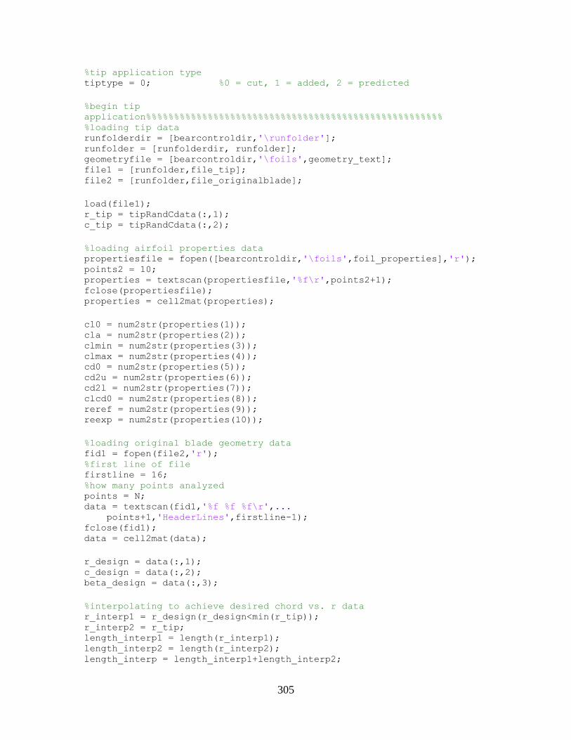
305
%tip application type tiptype = 0; %0 = cut, 1 = added, 2 = predicted
%begin tip
application%%%%%%%%%%%%%%%%%%%%%%%%%%%%%%%%%%%%%%%%%%%%%%%%%%%%% %loading tip data runfolderdir = [bearcontroldir,'\runfolder']; runfolder = [runfolderdir, runfolder]; geometryfile = [bearcontroldir,'\foils',geometry_text]; file1 = [runfolder,file_tip]; file2 = [runfolder,file_originalblade];
load(file1); r_tip = tipRandCdata(:,1); c_tip = tipRandCdata(:,2);
%loading airfoil properties data propertiesfile = fopen([bearcontroldir,'\foils',foil_properties],'r'); points2 = 10; properties = textscan(propertiesfile,'%f\r',points2+1); fclose(propertiesfile); properties = cell2mat(properties);
cl0 = num2str(properties(1)); cla = num2str(properties(2)); clmin = num2str(properties(3)); clmax = num2str(properties(4)); cd0 = num2str(properties(5)); cd2u = num2str(properties(6)); cd2l = num2str(properties(7)); clcd0 = num2str(properties(8)); reref = num2str(properties(9)); reexp = num2str(properties(10));
%loading original blade geometry data fid1 = fopen(file2,'r'); %first line of file firstline = 16; %how many points analyzed points = N; data = textscan(fid1,'%f %f %f\r',...
points+1,'HeaderLines',firstline-1); fclose(fid1); data = cell2mat(data);
r_design = data(:,1); c_design = data(:,2); beta_design = data(:,3);
%interpolating to achieve desired chord vs. r data r_interp1 = r_design(r_design<min(r_tip)); r_interp2 = r_tip; length_interp1 = length(r_interp1); length_interp2 = length(r_interp2); length_interp = length_interp1+length_interp2;
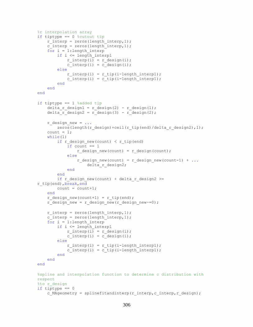
306
%r interpolation array if tiptype == 0 %cutout tip r_interp = zeros(length_interp,1); c_interp = zeros(length_interp,1); for i = 1:length_interp if i <= length_interp1 r_interp(i) = r_design(i); c_interp(i) = c_design(i); else r_interp(i) = r_tip(i-length_interp1); c_interp(i) = c_tip(i-length_interp1); end end end
if tiptype == 1 %added tip delta_r_design1 = r_design(2) - r_design(1); delta_r_design2 = r_design(3) - r_design(2);
r_design_new = ... zeros(length(r_design)+ceil(r_tip(end)/delta_r_design2),1); count = 1; while(1) if r_design_new(count) < r_tip(end) if count == 1 r_design_new(count) = r_design(count); else r_design_new(count) = r_design_new(count-1) + ... delta_r_design2; end end if r_design_new(count) + delta_r_design2 >=
r_tip(end),break,end count = count+1; end r_design_new(count+1) = r_tip(end); r_design_new = r_design_new(r_design_new~=0);
r_interp = zeros(length_interp,1); c_interp = zeros(length_interp,1); for i = 1:length_interp if i <= length_interp1 r_interp(i) = r_design(i); c_interp(i) = c_design(i); else r_interp(i) = r_tip(i-length_interp1); c_interp(i) = c_tip(i-length_interp1); end end end
%spline and interpolation function to determine c distribution with
respect %to r_design if tiptype == 0 c_MAgeometry = splinefitandinterp(r_interp,c_interp,r_design);
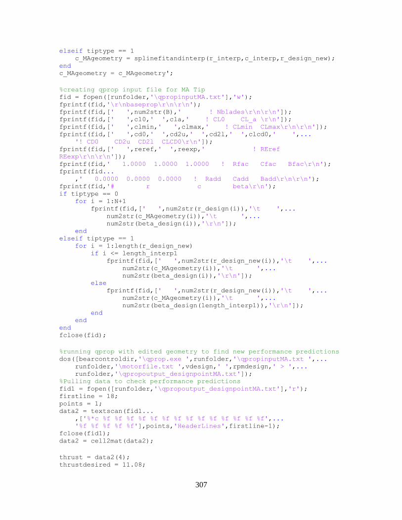
307
elseif tiptype == 1 c_MAgeometry = splinefitandinterp(r_interp,c_interp,r_design_new);
end c_MAgeometry = c_MAgeometry';
%creating qprop input file for MA Tip fid = fopen([runfolder,'\qpropinputMA.txt'],'w'); fprintf(fid,'\r\nbaseprop\r\n\r\n'); fprintf(fid,[' ',num2str(B),' ! Nblades\r\n\r\n']); fprintf(fid,[' ',cl0,' ',cla,' ! CL0 CL_a \r\n']); fprintf(fid,[' ',clmin,' ',clmax,' ! CLmin CLmax\r\n\r\n']); fprintf(fid,[' ',cd0,' ',cd2u,' ',cd2l,' ',clcd0,' ',...
'! CD0 CD2u CD2l CLCD0\r\n']); fprintf(fid,[' ',reref,' ',reexp,' ! REref
REexp\r\n\r\n']); fprintf(fid,' 1.0000 1.0000 1.0000 ! Rfac Cfac Bfac\r\n'); fprintf(fid...
,' 0.0000 0.0000 0.0000 ! Radd Cadd Badd\r\n\r\n'); fprintf(fid,'# r c beta\r\n'); if tiptype == 0
for i = 1:N+1 fprintf(fid,[' ',num2str(r_design(i)),'\t ',...
num2str(c_MAgeometry(i)),'\t ',... num2str(beta_design(i)),'\r\n']);
end elseif tiptype == 1
for i = 1:length(r_design_new) if i <= length_interp1
fprintf(fid,[' ',num2str(r_design_new(i)),'\t ',... num2str(c_MAgeometry(i)),'\t ',... num2str(beta_design(i)),'\r\n']);
else fprintf(fid,[' ',num2str(r_design_new(i)),'\t ',...
num2str(c_MAgeometry(i)),'\t ',... num2str(beta_design(length_interp1)),'\r\n']);
end end
end fclose(fid);
%running qprop with edited geometry to find new performance predictions dos([bearcontroldir,'\qprop.exe ',runfolder,'\qpropinputMA.txt ',...
runfolder,'\motorfile.txt ',vdesign,' ',rpmdesign,' > ',... runfolder,'\qpropoutput_designpointMA.txt']);
%Pulling data to check performance predictions fid1 = fopen([runfolder,'\qpropoutput_designpointMA.txt'],'r'); firstline = 18; points = 1; data2 = textscan(fid1...
,['%*c %f %f %f %f %f %f %f %f %f %f %f %f %f %f',... '%f %f %f %f %f'],points,'HeaderLines',firstline-1);
fclose(fid1); data2 = cell2mat(data2);
thrust = data2(4); thrustdesired = 11.08;
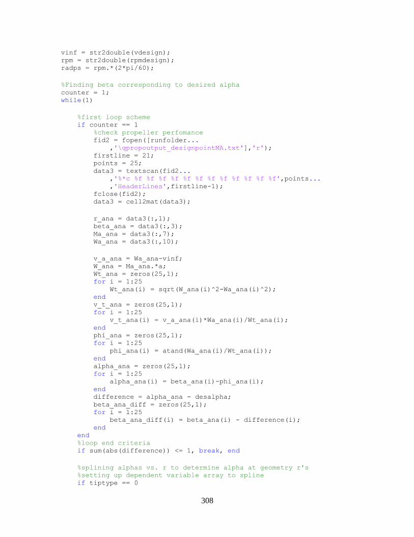
308
vinf = str2double(vdesign); rpm = str2double(rpmdesign); radps = rpm.*(2*pi/60);
%Finding beta corresponding to desired alpha counter = 1; while(1)
%first loop scheme if counter == 1 %check propeller perfomance fid2 = fopen([runfolder... ,'\qpropoutput_designpointMA.txt'],'r'); firstline = 21; points = 25; data3 = textscan(fid2... ,'%*c %f %f %f %f %f %f %f %f %f %f %f %f',points... ,'HeaderLines',firstline-1); fclose(fid2); data3 = cell2mat(data3);
r_ana = data3(:,1); beta_ana = data3(:,3); Ma_ana = data3(:,7); Wa_ana = data3(:,10);
v_a_ana = Wa_ana-vinf; W_ana = Ma_ana.*a; Wt_ana = zeros(25,1); for i = 1:25 Wt_ana(i) = sqrt(W_ana(i)^2-Wa_ana(i)^2); end v_t_ana = zeros(25,1); for i = 1:25 v_t_ana(i) = v_a_ana(i)*Wa_ana(i)/Wt_ana(i); end phi_ana = zeros(25,1); for i = 1:25 phi_ana(i) = atand(Wa_ana(i)/Wt_ana(i)); end alpha_ana = zeros(25,1); for i = 1:25 alpha_ana(i) = beta_ana(i)-phi_ana(i); end difference = alpha_ana - desalpha; beta_ana_diff = zeros(25,1); for i = 1:25 beta_ana_diff(i) = beta_ana(i) - difference(i); end end %loop end criteria if sum(abs(difference)) <= 1, break, end
%splining alphas vs. r to determine alpha at geometry r's %setting up dependent variable array to spline if tiptype == 0
309
m = N+1; mm = r_design;
end if tiptype == 1
m = length(r_design_new); mm = r_design_new;
end r_splinestart = zeros(m,1); for i = 1:m
if mm(i)>min(r_ana) if mm(i)<max(r_ana)
r_splinestart(i,1) = mm(i); end
end end r_splinestart = r_splinestart(r_splinestart~=0);
r_spline = zeros(length(r_ana)+length(r_splinestart),1); for i = 1:(length(r_splinestart)+length(r_ana))
if i <= length(r_splinestart) r_spline(i) = r_splinestart(i);
end if i > length(r_splinestart)
i = i - length(r_splinestart); r_spline(i+length(r_splinestart)) = r_ana(i);
end end
r_spline = shellsort(r_spline);
%fitting a spline to extrapolate necessary values beta_spline = splinefitandinterp(r_ana,beta_ana,r_spline); beta_spline = beta_spline'; Wa_spline = splinefitandinterp(r_ana,Wa_ana,r_spline); Ma_spline = splinefitandinterp(r_ana,Ma_ana,r_spline);
%calculations with splined data v_a_spline = Wa_spline-vinf; W_spline = Ma_spline.*a; Wt_spline = zeros(length(r_spline),1); for i = 1:length(r_spline);
Wt_spline(i,1) = sqrt(W_spline(i)^2-Wa_spline(i)^2); end v_t_spline = zeros(length(r_spline),1); for i = 1:length(r_spline)
v_t_spline(i,1) = v_a_spline(i)*Wa_spline(i)/Wt_spline(i); end phi_spline = zeros(length(r_spline),1); for i = 1:length(r_spline)
phi_spline(i,1) = atand(Wa_spline(i)/Wt_spline(i)); end alpha_spline = zeros(length(r_spline),1); for i = 1:length(r_spline)
alpha_spline(i,1) = beta_spline(i) - phi_spline(i); end
%fitting spline to geometry "r" data
310
if tiptype == 0 beta_geometry(2:N-1,1) = splinefitandinterp(... r_spline,beta_spline,r_design(2:N-1)); beta_geometry(1) = beta_geometry(2); beta_geometry(N) = beta_geometry(N-1); beta_geometry(N+1) = beta_geometry(N);
alpha_geometry(2:N-1,1) = splinefitandinterp(... r_spline,alpha_spline,r_design(2:N-1)); alpha_geometry(1) = alpha_geometry(2); alpha_geometry(N) = alpha_geometry(N-1); alpha_geometry(N+1) = alpha_geometry(N);
elseif tiptype == 1 y = find(r_design_new>=min(r_spline),1,'first'); z = find(r_design_new<=max(r_spline),1,'last');
beta_geometry(y:z,1) = splinefitandinterp(... r_spline,beta_spline,r_design_new(y:z)); for i = 1:y-1 beta_geometry(i) = beta_geometry(i+1); end for i = z+1:length(r_design_new) beta_geometry(i) = beta_geometry(i-1); end
alpha_geometry(y:z,1) = splinefitandinterp(... r_spline,alpha_spline,r_design_new(y:z)); for i = 1:y-1 alpha_geometry(i) = alpha_geometry(i+1); end for i = z+1:length(r_design_new) alpha_geometry(i) = alpha_geometry(i-1); end
end
%moving towards desired alphas by taking the difference of alphas
away %from the beta values difference_geometry = alpha_geometry-desalpha; beta_geometry_difference = zeros(length(beta_geometry),1); for i = 1:length(beta_geometry) beta_geometry_difference(i) = ... beta_geometry(i)-difference_geometry(i); end
%writing new QPROP input with new beta values fid = fopen([runfolder,'\qpropinputMA.txt'],'w'); fprintf(fid,'\r\nbaseprop\r\n\r\n'); fprintf(fid,[' ',num2str(B),' ! Nblades\r\n\r\n']); fprintf(fid,[' ',cl0,' ',cla,' ! CL0 CL_a \r\n']); fprintf(fid,[' ',clmin,' ',clmax,' ! CLmin
CLmax\r\n\r\n']); fprintf(fid,[' ',cd0,' ',cd2u,' ',cd2l,' ',clcd0,' ',...
311
'! CD0 CD2u CD2l CLCD0\r\n']); fprintf(fid,[' ',reref,' ',reexp,' ! REref
REexp\r\n\r\n']); fprintf(fid,' 1.0000 1.0000 1.0000 ! Rfac Cfac
Bfac\r\n'); fprintf(fid...
,' 0.0000 0.0000 0.0000 ! Radd Cadd Badd\r\n\r\n'); fprintf(fid,'# r c beta\r\n');
if tiptype == 0 for i = 1:N+1
fprintf(fid,[' ',num2str(r_design(i)),'\t ',... num2str(c_MAgeometry(i)),'\t ',... num2str(beta_geometry_difference(i)),'\r\n']);
end elseif tiptype == 1
for i = 1:length(r_design_new) fprintf(fid,[' ',num2str(r_design_new(i)),'\t ',...
num2str(c_MAgeometry(i)),'\t ',... num2str(beta_geometry_difference(i)),'\r\n']);
end end
fclose(fid);
%running file to check performance dos([bearcontroldir,'\qprop.exe ',runfolder...
,'\qpropinputMA.txt ',runfolder... ,'\motorfile.txt ',vdesign,' ',rpmdesign,' > ',runfolder... ,'\qpropoutput_designpointMA.txt']);
fid4 = fopen([runfolder,'\qpropoutput_designpointMA.txt'],'r'); firstline = 21; points = 25; data4 = textscan(fid4,'%f %f %f %f %f %f %f %f %f %f %f %f\r',...
points,'HeaderLines',firstline-1); fclose(fid4); data4 = cell2mat(data4);
r_int = data4(:,1); beta_int = data4(:,3); Ma_int = data4(:,7); Wa_int = data4(:,10);
v_a_int = Wa_int-vinf; W_int = Ma_int.*a;
Wt_int = zeros(25,1); for i = 1:25
Wt_int(i) = sqrt(W_int(i)^2-Wa_int(i)^2); end v_t_int = zeros(25,1); for i = 1:25
v_t_int(i) = v_a_int(i)*Wa_int(i)/Wt_int(i); end phi_int = zeros(25,1);
for i = 1:25
312
phi_int(i) = atand(Wa_int(i)/Wt_int(i)); end alpha_int = zeros(25,1); for i = 1:25 alpha_int(i) = beta_int(i)-phi_int(i); end difference_int = alpha_int - desalpha;
%loop prescribing beta change based on difference_int beta_int_difference = zeros(25,1); for i = 1:25 if difference_int(i) < 0 beta_int_difference(i) = beta_int(i)+0.01; elseif difference_int(i) > 0 beta_int_difference(i) = beta_int(i)-0.01; elseif difference_int(i) == 0 beta_int_difference(i) = beta_int(i); end end
%splining to be able to interpolate values for a new qprop input
file beta_splineinput = splinefitandinterp(r_ana,beta_int_difference... ,r_spline); beta_splineinput = beta_splineinput'; if tiptype == 0 beta_input(2:N-1,1) = splinefitandinterp(... r_spline,beta_splineinput,r_design(2:N-1)); beta_input(1) = beta_input(2); beta_input(N) = beta_input(N-1); beta_input(N+1) = beta_input(N); elseif tiptype == 1 beta_input(y:z,1) = splinefitandinterp(... r_spline,beta_splineinput,r_design_new(y:z)); for i = 1:y-1 beta_input(i) = beta_input(i+1); end for i = z+1:length(r_design_new) beta_input(i) = beta_input(i-1); end
end
%writing new qprop input file fid5 = fopen([runfolder,'\qpropinputMA.txt'],'w'); fprintf(fid5,'\r\nbaseprop\r\n\r\n'); fprintf(fid5,[' ',num2str(B),' ! Nblades\r\n\r\n']); fprintf(fid5,[' ',cl0,' ',cla,' ! CL0 CL_a \r\n']); fprintf(fid5,[' ',clmin,' ',clmax,' ! CLmin
CLmax\r\n\r\n']); fprintf(fid5,[' ',cd0,' ',cd2u,' ',cd2l,' ',clcd0,' ',... '! CD0 CD2u CD2l CLCD0\r\n']); fprintf(fid5,[' ',reref,' ',reexp,' ! REref
REexp\r\n\r\n']); fprintf(fid5,' 1.0000 1.0000 1.0000 ! Rfac Cfac
Bfac\r\n');
313
fprintf(fid5... ,' 0.0000 0.0000 0.0000 ! Radd Cadd Badd\r\n\r\n');
fprintf(fid5,'# r c beta\r\n');
if tiptype == 0 for i = 1:N+1
fprintf(fid5,[' ',num2str(r_design(i)),'\t ',... num2str(c_MAgeometry(i)),'\t ',... num2str(beta_input(i)),'\r\n']);
end elseif tiptype == 1
for i = 1:length(r_design_new) fprintf(fid5,[' ',num2str(r_design_new(i)),'\t ',...
num2str(c_MAgeometry(i)),'\t ',... num2str(beta_input(i)),'\r\n']);
end end
fclose(fid5);
%running new qprop file to check performance dos([bearcontroldir,'\qprop.exe ',runfolder...
,'\qpropinputMA.txt ',runfolder... ,'\motorfile.txt ',vdesign,' ',rpmdesign,' > ',runfolder... ,'\qpropoutput_designpointMA.txt']);
fid6 = fopen([runfolder,'\qpropoutput_designpointMA.txt'],'r'); firstline = 21; points = 25; data5 = textscan(fid6,'%f %f %f %f %f %f %f %f %f %f %f %f\r',...
points,'HeaderLines',firstline-1); fclose(fid6); data5 = cell2mat(data5);
r_ana = data5(:,1); beta_ana = data5(:,3); Ma_ana = data5(:,7); Wa_ana = data5(:,10);
v_a_ana = Wa_ana-vinf; W_ana = Ma_ana.*a; Wt_ana = zeros(25,1); for i = 1:25
Wt_ana(i) = sqrt(W_ana(i)^2-Wa_ana(i)^2); end v_t_ana = zeros(25,1); for i = 1:25
v_t_ana(i) = v_a_ana(i)*Wa_ana(i)/Wt_ana(i); end phi_ana = zeros(25,1); for i = 1:25
phi_ana(i) = atand(Wa_ana(i)/Wt_ana(i)); end alpha_ana = zeros(25,1); for i = 1:25
alpha_ana(i) = beta_ana(i)-phi_ana(i);
314
end
%end criteria counter = counter+1; if counter == 500, break, end end if tiptype == 1 N = length(r_design_new)-1; end
%running the rest of the code in order to be able to model blade geometrypts_funcMAnew(N,geometryfile,runfolder,rotationdir,B,sweep); planemacro_funcMA(N,runfolder,bladenum); splinemacro_funcMA(N,runfolder,bladenum);
%Shell Sort Code %Trae Liller %March 2015 %This function is called by constantchordhelper.m in order to sort c
radial %locations into their correct order.
function list = shellsort(list)
N = numel(list); increment = round(N/2);
while increment > 0
for i = (increment+1:N) temp = list(i); j = i; while (j >= increment+1) && (list(j-increment) > temp) list(j) = list(j-increment); j = j - increment; end
list(j) = temp;
end
if increment == 2 increment = 1; else increment = round(increment/2.2); end end end
%Spline Fit and Interpolation Function
%Trae Liller
315
%March 2015 %This function fits a spline to a dataset and is used in supplementary %Bearcontrol codes. Adapted from Applied Numerical Methods with MATLAB %3rd Edition
function yy = splinefitandinterp(x,y,xx)
n = length(x);
if length(y)~=n, error('x and y must be same length'), end if any(diff(x))<=0, error('x must be strictly ascending'), end
m = length(xx); b = zeros(n,n); aa(1,1) = 1; aa(n,n) = 1; bb(1) = 0; bb(n) = 0; for i = 2:n-1 aa(i,i-1) = hh_func(x,i-1); aa(i,i) = 2*(hh_func(x,i-1)+hh_func(x,i)); aa(i,i+1) = hh_func(x,i); bb(i) = 3*(fd_func(i+1,i,x,y)-fd_func(i,i-1,x,y)); end
c = aa\bb'; for i = 1:n-1 a(i) = y(i); b(i) = fd_func(i+1,i,x,y) - hh_func(x,i)/3*(2*c(i)+c(i+1)); d(i) = (c(i+1)-c(i))/3/hh_func(x,i); end
for i = 1:m yy(i) = SplineInterp(x,n,a,b,c,d,xx(i)); end end %hh function %Trae Liller %March 2015 %Sub function of the spline and interpolation function used in %supplementary codes constantchordhelper.m and MAtiphelper.m, adapted
from %Applied Numerical Methods with MATLAB, 3rd Edition function hh = hh_func(x,i) hh = x(i+1) - x(i); end
%fd function %Trae Liller %March 2015 %Sub function of splinefitandinterp.m used in supplemental codes %constantchordhelper.m and MAtiphelper.m %Adapted from Applied Numerical Methods with MATLAB, 3rd Edition function fdd = fd_func(i,j,x,y) fdd = (y(i) - y(j))/(x(i) - x(j)); end
316
%Spline Interpolation Function
%Trae Liller %June 14, 2014 %This function performs the spline interpolation in the
splineandinterp.m %function. Taken from Applied Numerical Methods with MATLAB, 3rd
Edition
function yyy = SplineInterp(x,n,a,b,c,d,xi) for ii = 1:n-1 if xi >= x(ii) - 0.000001 && xi <= x(ii+1) + 0.000001 yyy = a(ii)+b(ii)*(xi-x(ii))+c(ii)*(xi-x(ii))^2+d(ii)... *(xi-x(ii))^3; break end end end
%Tip Treated Blade Geometry Function %Trae Liller %March 2015 %This mfile will use data from previous Bearcontrol runs in order to %create a geometry point file for all airfoil cross sections in the %designed propeller.
function
geometrypts_funcMAnew(N,geometryfile,runfolderdir,rotationdir,... B,sweep) %N = Slices from bearcontrol GUI %geometryfile = file of base airfoil points %runfolderdir = run folder directory %rotationdir = rotation direction of prop relative to a front view of
the %UAS-- 0 = counterclockwise, 1 = clockwise %B = number of blades %sweep = sweep direction, 0 indicates trailing to leading edge, 1
indicates %leading to trailing edge, and 2 indicates no sweep (usually used with
a %rounded tip profile.
geometryfile = load(geometryfile); %base airfoil points file geometry = geometryfile; %P = # of pts in the airfoil geometry file P = length(geometryfile); %S = # of airfoils per blade S = N+1;
%pulling necessary data from Qprop output fid = fopen([runfolderdir,'\qpropinputMA.txt'],'r');
firstline = 16; %first line of needed propdata in Qprop
output
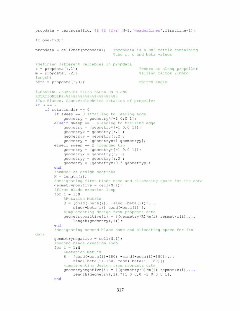
317
propdata = textscan(fid,'%f %f %f\r',N+1,'HeaderLines',firstline-1);
fclose(fid);
propdata = cell2mat(propdata); %propdata is a Nx3 matrix containing %the r, c and beta values
%defining different variables in propdata z = propdata(:,1); %where at along propeller m = propdata(:,2); %sizing factor (chord
length) beta = propdata(:,3); %pitch angle
%CREATING GEOMETRY FILES BASED ON B AND
ROTATIONDIR%%%%%%%%%%%%%%%%%%%%%%%% %Two Blades, Counterclockwise rotation of propeller if B == 2 if rotationdir == 0 if sweep == 0 %trailing to leading edge geometry = geometry*[-1 0;0 1]; elseif sweep == 1 %leading to trailing edge geometry = (geometry*[-1 0;0 1]); geometryx = geometry(:,1); geometryy = geometry(:,2); geometry = [geometryx+1 geometryy]; elseif sweep == 2 %rounded tip geometry = (geometry*[-1 0;0 1]); geometryx = geometry(:,1); geometryy = geometry(:,2); geometry = [geometryx+0.5 geometryy]; end %number of design sections N = length(z); %designating first blade name and allocating space for its data geometrypositive = cell(N,1); %first blade creation loop for i = 1:N %Rotation Matrix R = [cosd(-beta(i)) -sind(-beta(i));... sind(-beta(i)) cosd(-beta(i))]; %implementing design from propdata data geometrypositive{i} = [(geometry*R)*m(i) repmat(z(i),... length(geometry),1)]; end %designating second blade name and allocating spece for its
data geometrynegative = cell(N,1); %second blade creation loop for i = 1:N %Rotation Matrix R = [cosd(-beta(i)-180) -sind(-beta(i)-180);... sind(-beta(i)-180) cosd(-beta(i)-180)]; %implementing design from propdata data geometrynegative{i} = [(geometry*R)*m(i) repmat(z(i),... length(geometry),1)]*[1 0 0;0 -1 0;0 0 1]; end
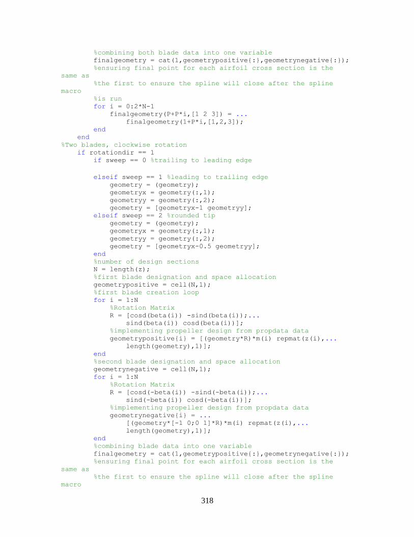
318
%combining both blade data into one variable finalgeometry = cat(1,geometrypositive{:},geometrynegative{:}); %ensuring final point for each airfoil cross section is the
same as %the first to ensure the spline will close after the spline
macro %is run for i = 0:2*N-1 finalgeometry(P+P*i,[1 2 3]) = ... finalgeometry(1+P*i,[1,2,3]); end end %Two blades, clockwise rotation if rotationdir == 1 if sweep == 0 %trailing to leading edge
elseif sweep == 1 %leading to trailing edge geometry = (geometry); geometryx = geometry(:,1); geometryy = geometry(:,2); geometry = [geometryx-1 geometryy]; elseif sweep == 2 %rounded tip geometry = (geometry); geometryx = geometry(:,1); geometryy = geometry(:,2); geometry = [geometryx-0.5 geometryy]; end %number of design sections N = length(z); %first blade designation and space allocation geometrypositive = cell(N,1); %first blade creation loop for i = 1:N %Rotation Matrix R = [cosd(beta(i)) -sind(beta(i));... sind(beta(i)) cosd(beta(i))]; %implementing propeller design from propdata data geometrypositive{i} = [(geometry*R)*m(i) repmat(z(i),... length(geometry),1)]; end %second blade designation and space allocation geometrynegative = cell(N,1); for i = 1:N %Rotation Matrix R = [cosd(-beta(i)) -sind(-beta(i));... sind(-beta(i)) cosd(-beta(i))]; %implementing propeller design from propdata data geometrynegative{i} = ... [(geometry*[-1 0;0 1]*R)*m(i) repmat(z(i),... length(geometry),1)]; end %combining blade data into one variable finalgeometry = cat(1,geometrypositive{:},geometrynegative{:}); %ensuring final point for each airfoil cross section is the
same as %the first to ensure the spline will close after the spline
macro
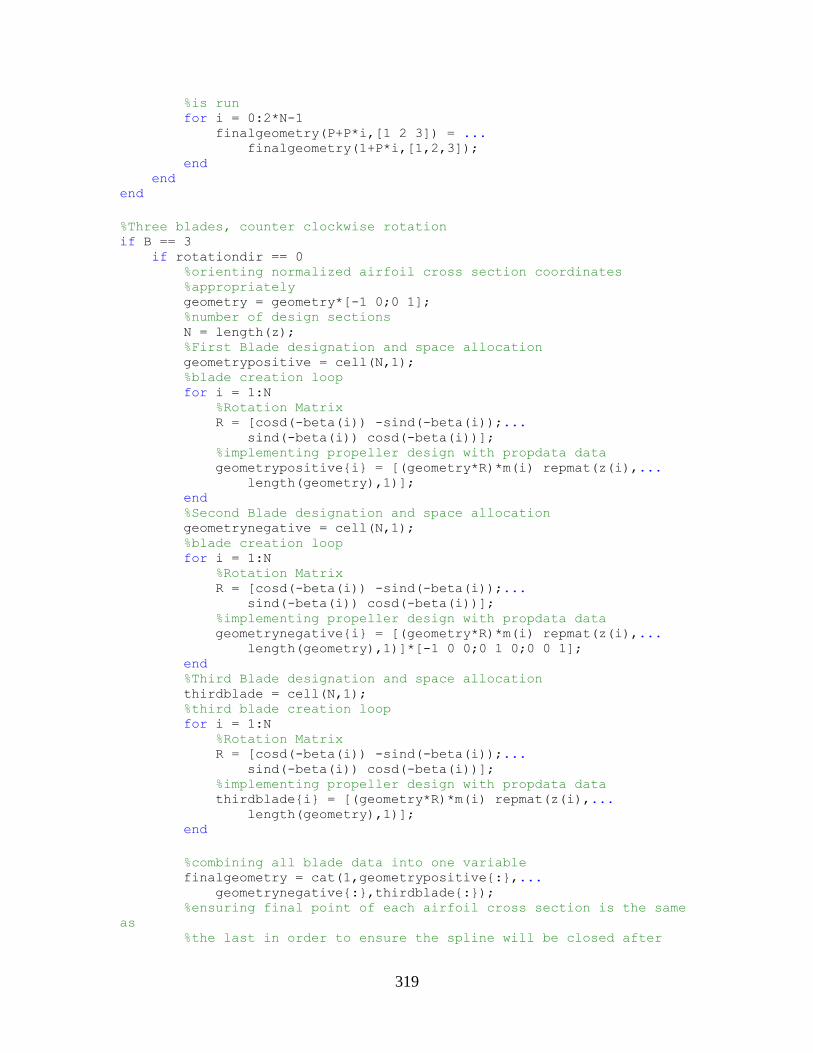
319
%is run for i = 0:2*N-1
finalgeometry(P+P*i,[1 2 3]) = ... finalgeometry(1+P*i,[1,2,3]);
end end
end
%Three blades, counter clockwise rotation if B == 3
if rotationdir == 0 %orienting normalized airfoil cross section coordinates %appropriately geometry = geometry*[-1 0;0 1]; %number of design sections N = length(z); %First Blade designation and space allocation geometrypositive = cell(N,1); %blade creation loop for i = 1:N
%Rotation Matrix R = [cosd(-beta(i)) -sind(-beta(i));...
sind(-beta(i)) cosd(-beta(i))]; %implementing propeller design with propdata data geometrypositive{i} = [(geometry*R)*m(i) repmat(z(i),...
length(geometry),1)]; end %Second Blade designation and space allocation geometrynegative = cell(N,1); %blade creation loop for i = 1:N
%Rotation Matrix R = [cosd(-beta(i)) -sind(-beta(i));...
sind(-beta(i)) cosd(-beta(i))]; %implementing propeller design with propdata data geometrynegative{i} = [(geometry*R)*m(i) repmat(z(i),...
length(geometry),1)]*[-1 0 0;0 1 0;0 0 1]; end %Third Blade designation and space allocation thirdblade = cell(N,1); %third blade creation loop for i = 1:N
%Rotation Matrix R = [cosd(-beta(i)) -sind(-beta(i));...
sind(-beta(i)) cosd(-beta(i))]; %implementing propeller design with propdata data thirdblade{i} = [(geometry*R)*m(i) repmat(z(i),...
length(geometry),1)]; end
%combining all blade data into one variable finalgeometry = cat(1,geometrypositive{:},...
geometrynegative{:},thirdblade{:}); %ensuring final point of each airfoil cross section is the same
as %the last in order to ensure the spline will be closed after
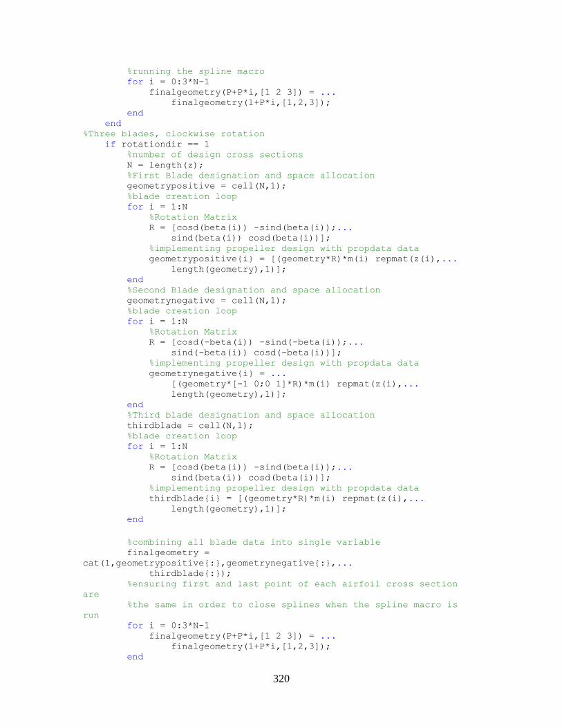
320
%running the spline macro for i = 0:3*N-1 finalgeometry(P+P*i,[1 2 3]) = ... finalgeometry(1+P*i,[1,2,3]); end end %Three blades, clockwise rotation if rotationdir == 1 %number of design cross sections N = length(z); %First Blade designation and space allocation geometrypositive = cell(N,1); %blade creation loop for i = 1:N %Rotation Matrix R = [cosd(beta(i)) -sind(beta(i));... sind(beta(i)) cosd(beta(i))]; %implementing propeller design with propdata data geometrypositive{i} = [(geometry*R)*m(i) repmat(z(i),... length(geometry),1)]; end %Second Blade designation and space allocation geometrynegative = cell(N,1); %blade creation loop for i = 1:N %Rotation Matrix R = [cosd(-beta(i)) -sind(-beta(i));... sind(-beta(i)) cosd(-beta(i))]; %implementing propeller design with propdata data geometrynegative{i} = ... [(geometry*[-1 0;0 1]*R)*m(i) repmat(z(i),... length(geometry),1)]; end %Third blade designation and space allocation thirdblade = cell(N,1); %blade creation loop for i = 1:N %Rotation Matrix R = [cosd(beta(i)) -sind(beta(i));... sind(beta(i)) cosd(beta(i))]; %implementing propeller design with propdata data thirdblade{i} = [(geometry*R)*m(i) repmat(z(i),... length(geometry),1)]; end
%combining all blade data into single variable finalgeometry =
cat(1,geometrypositive{:},geometrynegative{:},... thirdblade{:}); %ensuring first and last point of each airfoil cross section
are %the same in order to close splines when the spline macro is
run for i = 0:3*N-1 finalgeometry(P+P*i,[1 2 3]) = ... finalgeometry(1+P*i,[1,2,3]); end
321
end end
%Four blades, anti clock wise rotation if B == 4 if rotationdir == 0 %orienting normalized airfoil cross section data as necessary geometry = geometry*[-1 0;0 1]; %number of design sections N = length(z); %First Blade designation and space allocation geometrypositive = cell(N,1); %blade creation loop for i = 1:N %Rotation Matrix R = [cosd(-beta(i)) -sind(-beta(i));... sind(-beta(i)) cosd(-beta(i))]; %implementing propeller design with propdata data geometrypositive{i} = [(geometry*R)*m(i) repmat(z(i),... length(geometry),1)]; end %Second Blade designation and space allocation geometrynegative = cell(N,1); %blade creation loop for i = 1:N %Rotation Matrix R = [cosd(-beta(i)) -sind(-beta(i));... sind(-beta(i)) cosd(-beta(i))]; %implementing propeller design with propdata data geometrynegative{i} = [(geometry*R)*m(i) repmat(z(i),... length(geometry),1)]*[-1 0 0;0 1 0;0 0 1]; end %Third Blade designation and space allocation thirdblade = cell(N,1); %blade creation loop for i = 1:N %Rotation Matrix R = [cosd(-beta(i)) -sind(-beta(i));... sind(-beta(i)) cosd(-beta(i))]; %implementing propeller design with propdata data thirdblade{i} = [(geometry*R)*m(i) repmat(z(i),... length(geometry),1)]; end
%fourth blade designation and space allocation fourthblade = cell(N,1); %blade creation loop for i = 1:N %Rotation Matrix R = [cosd(-beta(i)-180) -sind(-beta(i)-180);... sind(-beta(i)-180) cosd(-beta(i)-180)]; %implementing propeller design using propdata data fourthblade{i} = [(geometry*R)*m(i)*[1 0; 0 -1]
repmat(z(i),... length(geometry),1)]; end
322
%combining all blade data into one variable finalgeometry = cat(1,geometrypositive{:},... geometrynegative{:},thirdblade{:},fourthblade{:}); %ensuring first and last point of each airfoil cross section
are %the same in order to close the splines when spline macro is
run for i = 0:4*N-1 finalgeometry(P+P*i,[1 2 3]) = ... finalgeometry(1+P*i,[1,2,3]); end end
%Four Blades, clockwise rotation if rotationdir == 1 %number of design sections N = length(z); %first blade designation and space allocation geometrypositive = cell(N,1); %blade creation loop for i = 1:N %Rotation Matrix R = [cosd(beta(i)) -sind(beta(i));... sind(beta(i)) cosd(beta(i))]; %implementing propeller design with propdata data geometrypositive{i} = [(geometry*R)*m(i) repmat(z(i),... length(geometry),1)]; end %Second Blade designation and space allocation geometrynegative = cell(N,1); %blade creation loop for i = 1:N %Rotation Matrix R = [cosd(-beta(i)) -sind(-beta(i));... sind(-beta(i)) cosd(-beta(i))]; %implementing propeller design with propdata data geometrynegative{i} = ... [(geometry*[-1 0;0 1]*R)*m(i) repmat(z(i),... length(geometry),1)]; end %third blade designation and space allocation thirdblade = cell(N,1); %blade creation loop for i = 1:N %Rotation Matrix R = [cosd(beta(i)) -sind(beta(i));... sind(beta(i)) cosd(beta(i))]; %implementing propeller design with propdata data thirdblade{i} = [(geometry*R)*m(i) repmat(z(i),... length(geometry),1)]; end
%fourth blade designation and space allocation fourthblade = cell(N,1); for i = 1:N %Rotation Matrix
323
R = [cosd(beta(i)) -sind(beta(i));... sind(beta(i)) cosd(beta(i))];
%implementing propeller design with propdata data fourthblade{i} = [(geometry)*R*m(i)*[-1 0;0 1]...
repmat(z(i), length(geometry),1)]; end
%combining all blade data into one variable finalgeometry =
cat(1,geometrypositive{:},geometrynegative{:},... thirdblade{:},fourthblade{:});
%ensuring first and last point of each airfoil cross section
are %the same so that splines will close when the spline macro is
run. for i = 0:4*N-1
finalgeometry(P+P*i,[1 2 3]) = ... finalgeometry(1+P*i,[1,2,3]);
end end
end
%THIS SECTION OF CODE IS HELD (WHILE BEING COMMENTED OUT) IN CASE THE
NEED %TO CENTER THE AIRFOILS ON THE ORIGIN ARISES. NOT TYPICALLY USED WHEN %APPLYING TIPS. % if any(sweep ~= 2) % %Translating blade to center on hub % %First Blade % maxx1 = max(finalgeometry(1:P,1)); % minx1 = min(finalgeometry(1:P,1)); % maxy1 = max(finalgeometry(1:P,2)); % miny1 = min(finalgeometry(1:P,2)); % %determining x-center of first airfoil % if sign(maxx1) == 0; % middlex1 = minx1/2; % end % if sign(minx1) == 0; % middlex1 = maxx1/2; % end %
% if sign(maxx1) + sign(minx1) == 2 % middlex1 = (maxx1-minx1)/2; % end % if sign(maxx1) + sign(minx1) == -2 % middlex1 = (maxx1-minx1)/2; % end %
% if sign(maxx1) + sign(minx1) == 0 % middlex1 = (maxx1+minx1)/2; % end %
% %determining y-center of first airfoil % if sign(maxy1) == 0; % middley1 = miny1/2; % end
324
% if sign(minx1) == 0; % middley1 = maxy1/2; % end % % if sign(maxy1) + sign(miny1) == 2 % middley1 = (maxy1-miny1)/2; % end % if sign(maxy1) + sign(miny1) == -2 % middley1 = (maxy1-miny1)/2; % end % % if sign(maxy1) + sign(miny1) == 0 % middley1 = (maxy1+miny1)/2; % end % % %Deciding how to translate x
values%%%%%%%%%%%%%%%%%%%%%%%%%%%%%%%%%% % if middlex1 >= 0 % transx1 = -middlex1; % end % if middlex1 < 0 % transx1 = -middlex1; % end % % %Deciding how to translate y
values%%%%%%%%%%%%%%%%%%%%%%%%%%%%%%%%%% % % if middley1 >= 0 % transy1 = -middley1; % end % if middley1 < 0 % transy1 = -middley1; % end % % %Second Blade % maxx2 = max(finalgeometry(P*S+1:P*(S+1),1)); % minx2 = min(finalgeometry(P*S+1:P*(S+1),1)); % maxy2 = max(finalgeometry(P*S+1:P*(S+1),2)); % miny2 = min(finalgeometry(P*S+1:P*(S+1),2)); % %determining x-center of first airfoil % if sign(maxx2) == 0; % middlex2 = minx2/2; % end % if sign(minx2) == 0; % middlex2 = maxx2/2; % end % % if sign(maxx2) + sign(minx2) == 2 % middlex2 = (maxx2-minx2)/2; % end % if sign(maxx2) + sign(minx2) == -2 % middlex2 = (maxx2-minx2)/2; % end % % if sign(maxx2) + sign(minx2) == 0 % middlex2 = (maxx2+minx2)/2; % end
325
%
% %determining y-center of first airfoil % if sign(maxy2) == 0; % middley2 = miny2/2; % end % if sign(miny2) == 0; % middley2 = maxy2/2; % end %
% if sign(maxy2) + sign(miny2) == 2 % middley2 = (maxy2-miny2)/2; % end % if sign(maxy2) + sign(miny2) == -2 % middley2 = (maxy2-miny2)/2; % end %
% if sign(maxy2) + sign(miny2) == 0 % middley2 = (maxy2+miny2)/2; % end %
% %Deciding how to translate x
values%%%%%%%%%%%%%%%%%%%%%%%%%%%%%%%%%% % if middlex2 >= 0 % transx2 = -middlex2; % end % if middlex2 < 0 % transx2 = -middlex2; % end %
% %Deciding how to translate y
values%%%%%%%%%%%%%%%%%%%%%%%%%%%%%%%%%% %
% if middley2 >= 0 % transy2 = -middley2; % end % if middley2 < 0 % transy2 = -middley2; % end %
% %Third Blade % if B == 3 % maxx3 = max(finalgeometry(2*P*S+1:2*P*S+P,1)); % minx3 = min(finalgeometry(2*P*S+1:2*P*S+P,1)); % maxy3 = max(finalgeometry(2*P*S+1:2*P*S+P,2)); % miny3 = min(finalgeometry(2*P*S+1:2*P*S+P,2)); % %determining x-center of first airfoil % if sign(maxx3) == 0; % middlex3 = minx3/2; % end % if sign(minx3) == 0; % middlex3 = maxx3/2; % end %
% if sign(maxx3) + sign(minx3) == 2 % middlex3 = (maxx3-minx3)/2; % end % if sign(maxx3) + sign(minx3) == -2
326
% middlex3 = (maxx3-minx3)/2; % end % % if sign(maxx3) + sign(minx3) == 0 % middlex3 = (maxx3+minx3)/2; % end % % %determining y-center of first airfoil % if sign(maxy3) == 0; % middley3 = miny3/2; % end % if sign(miny3) == 0; % middley3 = maxy3/2; % end % % if sign(maxy3) + sign(miny3) == 2 % middley3 = (maxy3-miny3)/2; % end % if sign(maxy3) + sign(miny3) == -2 % middley3 = (maxy3-miny3)/2; % end % % if sign(maxy3) + sign(miny3) == 0 % middley3 = (maxy3+miny3)/2; % end % % %Deciding how to translate x
values%%%%%%%%%%%%%%%%%%%%%%%%%%%%%%%%%% % if middlex3 >= 0 % transx3 = -middlex3; % end % if middlex3 < 0 % transx3 = -middlex3; % end % % %Deciding how to translate y
values%%%%%%%%%%%%%%%%%%%%%%%%%%%%%%%%%% % % if middley3 >= 0 % transy3 = -middley3; % end % if middley3 < 0 % transy3 = -middley3; % end % end % % %Fourth Blade % if B == 4 % %third blade % maxx3 = max(finalgeometry(2*P*S+1:2*P*S+P,1)); % minx3 = min(finalgeometry(2*P*S+1:2*P*S+P,1)); % maxy3 = max(finalgeometry(2*P*S+1:2*P*S+P,2)); % miny3 = min(finalgeometry(2*P*S+1:2*P*S+P,2)); % %determining x-center of first airfoil % if sign(maxx3) == 0; % middlex3 = minx3/2; % end
327
% if sign(minx3) == 0; % middlex3 = maxx3/2; % end %
% if sign(maxx3) + sign(minx3) == 2 % middlex3 = (maxx3-minx3)/2; % end % if sign(maxx3) + sign(minx3) == -2 % middlex3 = (maxx3-minx3)/2; % end %
% if sign(maxx3) + sign(minx3) == 0 % middlex3 = (maxx3+minx3)/2; % end %
% %determining y-center of first airfoil % if sign(maxy3) == 0; % middley3 = miny3/2; % end % if sign(miny3) == 0; % middley3 = maxy3/2; % end %
% if sign(maxy3) + sign(miny3) == 2 % middley3 = (maxy3-miny3)/2; % end % if sign(maxy3) + sign(miny3) == -2 % middley3 = (maxy3-miny3)/2; % end %
% if sign(maxy3) + sign(miny3) == 0 % middley3 = (maxy3+miny3)/2; % end %
% %Deciding how to translate x
values%%%%%%%%%%%%%%%%%%%%%%%%%%%%%%%%%% % if middlex3 >= 0 % transx3 = -middlex3; % end % if middlex3 < 0 % transx3 = -middlex3; % end %
% %Deciding how to translate y
values%%%%%%%%%%%%%%%%%%%%%%%%%%%%%%%%%% %
% if middley3 >= 0 % transy3 = -middley3; % end % if middley3 < 0 % transy3 = -middley3; % end %
% %fourth blade % maxx4 = max(finalgeometry(3*P*S+1:3*P*S+P,1)); % minx4 = min(finalgeometry(3*P*S+1:3*P*S+P,1)); % maxy4 = max(finalgeometry(3*P*S+1:3*P*S+P,2));
328
% miny4 = min(finalgeometry(3*P*S+1:3*P*S+P,2)); % % %determining x-center of first airfoil % if sign(maxx4) == 0; % middlex4 = minx4/2; % end % if sign(minx4) == 0; % middlex4 = maxx4/2; % end % % if sign(maxx4) + sign(minx4) == 2 % middlex4 = (maxx4-minx4)/2; % end % if sign(maxx4) + sign(minx4) == -2 % middlex4 = (maxx4-minx4)/2; % end % % if sign(maxx4) + sign(minx4) == 0 % middlex4 = (maxx4+minx4)/2; % end % % %determining y-center of first airfoil % if sign(maxy4) == 0; % middley4 = miny4/2; % end % if sign(miny4) == 0; % middley4 = maxy4/2; % end % % if sign(maxy4) + sign(miny4) == 2 % middley4 = (maxy4-miny4)/2; % end % if sign(maxy4) + sign(miny4) == -2 % middley4 = (maxy4-miny4)/2; % end % % if sign(maxy4) + sign(miny4) == 0 % middley4 = (maxy4+miny4)/2; % end % % %Deciding how to translate x
values%%%%%%%%%%%%%%%%%%%%%%%%%%%%%%%%%% % if middlex4 >= 0 % transx4 = -middlex4; % end % if middlex4 < 0 % transx4 = -middlex4; % end % % %Deciding how to translate y
values%%%%%%%%%%%%%%%%%%%%%%%%%%%%%%%%%% % % if middley4 >= 0 % transy4 = -middley4; % end % if middley4 < 0 % transy4 = -middley4;
329
% end %
% end % % %Translating respective
values%%%%%%%%%%%%%%%%%%%%%%%%%%%%%%%%%%%%%%%%%%% % %First Blade % finalgeometry(1:(P*S),1) = finalgeometry(1:(P*S),1)+transx1; % finalgeometry(1:(P*S),2) = finalgeometry(1:(P*S),2)+transy1; % %Second Blade % finalgeometry((P*S+1):(P*2*S),1) =... % finalgeometry((P*S+1):(P*S*2),1)+transx2; % finalgeometry((P*S+1):(P*2*S),2) =... % finalgeometry((P*S+1):(P*S*2),2)+transy2; % %Third Blade % if B == 3 % finalgeometry((2*P*S+1):(3*P*S),1) = ... % finalgeometry((2*P*S+1):(3*P*S),1)+transx3; % finalgeometry((2*P*S+1):(3*P*S),2) = ... % finalgeometry((2*P*S+1):(3*P*S),2)+transy3; % end % % if B == 4 % finalgeometry((2*P*S+1):(3*P*S),1) = ... % finalgeometry((2*P*S+1):(3*P*S),1)+transx3; % finalgeometry((2*P*S+1):(3*P*S),2) = ... % finalgeometry((2*P*S+1):(3*P*S),2)+transy3; % finalgeometry((3*P*S+1):(4*P*S),1) = ... % finalgeometry((3*P*S+1):(4*P*S),1)+transx4; % finalgeometry((3*P*S+1):(4*P*S),2) = ... % finalgeometry((3*P*S+1):(4*P*S),2)+transy4; % end % end
%Writing Geometry File geometryfile = fopen([runfolderdir,'\geometryclosed.txt'],'w');
for k = 1:length(finalgeometry) fprintf(geometryfile,[num2str(finalgeometry(k,1)),' ',...
num2str(finalgeometry(k,2)),' ',... num2str(finalgeometry(k,3)),'\r\n']);
end fclose(geometryfile); end %END CODE
%Tip Treated Blade Plane Macro Function %Trae Liller
%March 2015 %This function will produce a macro based on inputs given in the
bearcontol %GUI and intermediate calculations that will create a reference plane
for %each airfoil in the designed propeller blade.
330
function planemacro_funcMA(N,runfolderdir,bladenum) %N = number of slices selected in BEARCONTROL GUI %runfolderdir is the location of the current run folder %bladenum is the number of blades
load([runfolderdir,'\geometryclosed.txt']) % geometry file data = geometryclosed; % data S = N+1; if bladenum == 2 P = length(data)/(2*S); % # of points in airfoil file end if bladenum == 3 P = length(data)/(3*S); end if bladenum ==4 P = length(data)/(4*S); end planemacro = fopen([runfolderdir,'\planemacroMA.txt'],'w');
if bladenum == 2
%Opening statements in macro code fprintf(planemacro,'''Preconditions: New Part file opened\r\n'); fprintf(planemacro,['''Postconditions: S number of reference planes
',... 'will be drawn\r\n\r\n']);
%Open Process fprintf(planemacro,'Public Sub CreateOffsetPlanes()\r\n');
%Defining variables fprintf(planemacro,'Dim swApp As Object\r\n\r\n'); fprintf(planemacro,'Dim planeName, newPlaneName As String\r\n'); fprintf(planemacro,'Dim planeFeature As Object\r\n');
%Selecting/Starting new session in SolidWorks fprintf(planemacro,['''This will attach to current SolidWorks session
',... 'or start a new one.\r\n']); fprintf(planemacro,'Dim i, planeCount As Integer\r\n'); fprintf(planemacro,['Dim x(',num2str(S*2),') As Double\r\n']); fprintf(planemacro,... 'Set swApp = CreateObject("SldWorks.Application")\r\n\r\n'); fprintf(planemacro,'Set Model = swApp.ActiveDoc\r\n'); fprintf(planemacro,'If Model Is Nothing Then\r\n'); fprintf(planemacro,'Exit Sub\r\n'); fprintf(planemacro,'End If\r\n\r\n');
%Select which plane to offset from fprintf(planemacro,'newPlaneName = "Right"\r\n');
%Number of Planes in the Drawing to Start (0 means NEW DOCUMENT) fprintf(planemacro,'planecount = 0\r\n\r\n');
%inputting r values from geometry file
331
for j = 1:S*2
fprintf(planemacro,['x(',num2str(j-1),') = ',... num2str(data(P*j,3)),'\r\n']);
end
%Plane Creation Loop fprintf(planemacro,'''Reference Plane Creation Loop\r\n\r\n'); fprintf(planemacro,['For i = 0 To ',num2str(S*2-1),'\r\n\r\n']); fprintf(planemacro,'Model.ClearSelection\r\n\r\n'); fprintf(planemacro,'''Select Plane From Which to Start Offset\r\n'); fprintf(planemacro,'Model.SelectByID "Right", "PLANE", 0, 0,
0\r\n\r\n'); fprintf(planemacro,['If i < ',num2str(S-1),... ' Then Model.CreatePlaneAtOffset x(i), 0\r\n\r\n']); fprintf(planemacro,['If i = ',num2str(S-1),... ' Then Model.CreatePlaneAtOffset x(i), 0\r\n\r\n']); fprintf(planemacro,['If i > ',num2str(S-1),... ' Then Model.CreatePlaneAtOffset x(i), 1\r\n\r\n']); fprintf(planemacro,'planeCount = planeCount + 1\r\n\r\n'); fprintf(planemacro,'planeName = "Plane" & planeCount\r\n'); fprintf(planemacro,'newPlaneName = "MyPlane" & i\r\n'); fprintf(planemacro,... 'Set planeFeature = Model.FeatureByName(planeName)\r\n'); fprintf(planemacro,'planeFeature.Name = (newPlaneName)\r\n\r\n'); fprintf(planemacro,'Model.EditRebuild\r\n\r\nNext\r\n\r\nEnd Sub'); end
%Three blade macro code if bladenum == 3
fprintf(planemacro,'''Preconditions: New Part File opened.\r\n'); fprintf(planemacro,['''Postconditions: Reference Planes for 3 ',... 'Bladed Propeller will be created.\r\n\r\n']); fprintf(planemacro,'Public Sub CreateOffsetPlanes()\r\n'); fprintf(planemacro,'Dim swApp As Object\r\n\r\n'); fprintf(planemacro,'Dim Model As Object\r\n'); fprintf(planemacro,'Dim boolstatus As Boolean\r\n'); fprintf(planemacro,... 'Dim longstatus As Long, longwarnings As Long\r\n\r\n'); fprintf(planemacro,'Dim planeName, newPlaneName As String\r\n'); fprintf(planemacro,'Dim planeFeature As Object\r\n'); fprintf(planemacro,'Dim i, planeCount As Integer\r\n'); fprintf(planemacro,['Dim x(',num2str(S),') As Double\r\n']); fprintf(planemacro,'Set swApp = Application.SldWorks\r\n\r\n'); fprintf(planemacro,'Set Model = swApp.ActiveDoc\r\n'); fprintf(planemacro,'If Model Is Nothing Then\r\n'); fprintf(planemacro,'Exit Sub\r\nEnd If\r\n\r\n'); fprintf(planemacro,'Dim myModelView As Object\r\n'); fprintf(planemacro,'Set myModelView = Model.ActiveView\r\n'); fprintf(planemacro,... 'myModelView.FrameState =
swWindowState_e.swWindowMaximized\r\n'); fprintf(planemacro,'Model.ClearSelection2 True\r\n'); fprintf(planemacro,'Dim skSegment As Object\r\n');
332
fprintf(planemacro,['Set skSegment = Model.SketchManager.',... 'CreateCenterLine(0#, -0.013055, 0#, 0#, 0.017943, 0#)\r\n']); fprintf(planemacro,... 'Model.SetPickMode\r\nModel.ClearSelection2 True\r\n'); fprintf(planemacro,'Model.SketchManager.InsertSketch True\r\n'); fprintf(planemacro,['boolstatus = Model.Extension.SelectByID2',... '("Right", "PLANE", 0, 0, 0, True, 0, Nothing, 0)\r\n']); fprintf(planemacro,['boolstatus = Model.Extension.SelectById2',... '("Line1@Sketch1", "EXTSKETCHSEGMENT", 0, 3.45298513332181E-
03',... ', 0, True, 1, Nothing, 0)\r\n']); fprintf(planemacro,'Dim myRefPlane As Object\r\n'); fprintf(planemacro,... ['Set myRefPlane = Model.FeatureManager.InsertRefPlane',... '(16, 1.04719755, 4, 0, 0, 0)\r\n']); fprintf(planemacro,'Model.ClearSelection2 True\r\n'); fprintf(planemacro,['boolstatus = Model.Extension.SelectByID2',... '("Right", "PLANE", 0, 0, 0, True, 0, Nothing, 0)\r\n']); fprintf(planemacro,['boolstatus = Model.Extension.SelectByID2',... '("Line1@Sketch1", "EXTSKETCHSEGMENT", 0, ',... '-3.52439668745319E-04, 0, True, 1, Nothing, 0)\r\n']); fprintf(planemacro,['Set myRefPlane = Model.FeatureManager.',... 'InsertRefPlane(16, 2.0943951, 4, 0, 0, 0)\r\n']); fprintf(planemacro,'Model.ClearSelection2 True\r\n'); fprintf(planemacro,['boolstatus =
Model.SetUserPreferenceToggle',... '(swUserPreferenceToggle_e.swDisplayPlanes, True)\r\n']); fprintf(planemacro,'Model.ClearSelection2 True\r\n\r\n'); fprintf(planemacro,'newPlaneName = "Right"\r\n'); fprintf(planemacro,'planecount = 2\r\n\r\n');
for j = 1:S
fprintf(planemacro,['x(',num2str(j-1),') = ',... num2str(data(P*j,3)),'\r\n']);
end
fprintf(planemacro,['\r\nFor i = 0 To ',num2str(S-1),'\r\n\r\n']); fprintf(planemacro,'Model.ClearSelection\r\n\r\n'); fprintf(planemacro,'Model.SelectByID "Right", "PLANE", 0, 0,
0\r\n'); fprintf(planemacro,'Model.CreatePlaneAtOffset x(i), 0\r\n\r\n'); fprintf(planemacro,'planeCount = planeCount + 1\r\n'); fprintf(planemacro,'planeName = "Plane" & planeCount\r\n'); fprintf(planemacro,'newPlaneName = "MyPlane" & i\r\n'); fprintf(planemacro,... 'Set planeFeature = Model.FeatureByName(planeName)\r\n'); fprintf(planemacro,'planeFeature.Name = (newPlaneName)\r\n\r\n'); fprintf(planemacro,'Model.EditRebuild\r\n'); fprintf(planemacro,'Next\r\n\r\n');
fprintf(planemacro,['For i = 0 To ',num2str(S-1),'\r\n\r\n']); fprintf(planemacro,'Model.ClearSelection\r\n\r\n'); fprintf(planemacro,'Model.SelectByID "Plane1", "PLANE", 0, 0,
0\r\n');
333
fprintf(planemacro,'Model.CreatePlaneAtOffset x(i), 1\r\n\r\n'); fprintf(planemacro,'planeCount = planeCount + 1\r\n'); fprintf(planemacro,'planeName = "Plane" & planeCount\r\n'); fprintf(planemacro,...
['newPlaneName = "MyPlane" & (',num2str(S),' + i)\r\n']); fprintf(planemacro,...
'Set planeFeature = Model.FeatureByName(planeName)\r\n'); fprintf(planemacro,'planeFeature.Name = (newPlaneName)\r\n\r\n'); fprintf(planemacro,'Model.EditRebuild\r\n'); fprintf(planemacro,'Next\r\n\r\n');
fprintf(planemacro,['For i = 0 To ',num2str(S-1),'\r\n\r\n']); fprintf(planemacro,'Model.ClearSelection\r\n\r\n'); fprintf(planemacro,'Model.SelectByID "Plane2", "PLANE", 0, 0,
0\r\n'); fprintf(planemacro,'Model.CreatePlaneAtOffset x(i), 0\r\n\r\n'); fprintf(planemacro,'planeCount = planeCount + 1\r\n'); fprintf(planemacro,'planeName = "Plane" & planeCount\r\n'); fprintf(planemacro,...
['newPlaneName = "MyPlane" & (',num2str(S*2),' + i)\r\n']); fprintf(planemacro,...
'Set planeFeature = Model.FeatureByName(planeName)\r\n'); fprintf(planemacro,'planeFeature.Name = (newPlaneName)\r\n\r\n'); fprintf(planemacro,'Model.EditRebuild\r\n'); fprintf(planemacro,'Next\r\n\r\n'); fprintf(planemacro,'End Sub');
end
%four blade macro code if bladenum == 4
fprintf(planemacro,'''Preconditions: New Part File opened.\r\n'); fprintf(planemacro,...
['''Postconditions: Reference Planes for 3 Bladed Propeller
',... 'will be created.\r\n\r\n']);
fprintf(planemacro,'Public Sub CreateOffsetPlanes()\r\n'); fprintf(planemacro,'Dim swApp As Object\r\n\r\n'); fprintf(planemacro,'Dim Model As Object\r\n'); fprintf(planemacro,'Dim boolstatus As Boolean\r\n'); fprintf(planemacro,...
'Dim longstatus As Long, longwarnings As Long\r\n\r\n'); fprintf(planemacro,'Dim planeName, newPlaneName As String\r\n'); fprintf(planemacro,'Dim planeFeature As Object\r\n'); fprintf(planemacro,'Dim i, planeCount As Integer\r\n'); fprintf(planemacro,['Dim x(',num2str(S),') As Double\r\n']); fprintf(planemacro,'Set swApp = Application.SldWorks\r\n\r\n'); fprintf(planemacro,'Set Model = swApp.ActiveDoc\r\n'); fprintf(planemacro,'If Model Is Nothing Then\r\n'); fprintf(planemacro,'Exit Sub\r\nEnd If\r\n\r\n');
fprintf(planemacro,'newPlaneName = "Right"\r\n'); fprintf(planemacro,'planecount = 0\r\n\r\n');
for j = 1:S
fprintf(planemacro,['x(',num2str(j-1),') = ',...
334
num2str(data(P*j,3)),'\r\n']);
end
fprintf(planemacro,['\r\nFor i = 0 To ',num2str(S-1),'\r\n\r\n']); fprintf(planemacro,'Model.ClearSelection\r\n\r\n'); fprintf(planemacro,'Model.SelectByID "Right", "PLANE", 0, 0,
0\r\n'); fprintf(planemacro,'Model.CreatePlaneAtOffset x(i), 0\r\n\r\n'); fprintf(planemacro,'planeCount = planeCount + 1\r\n'); fprintf(planemacro,'planeName = "Plane" & planeCount\r\n'); fprintf(planemacro,'newPlaneName = "MyPlane" & i\r\n'); fprintf(planemacro,... 'Set planeFeature = Model.FeatureByName(planeName)\r\n'); fprintf(planemacro,'planeFeature.Name = (newPlaneName)\r\n\r\n'); fprintf(planemacro,'Model.EditRebuild\r\n'); fprintf(planemacro,'Next\r\n\r\n');
fprintf(planemacro,['For i = 0 To ',num2str(S-1),'\r\n\r\n']); fprintf(planemacro,'Model.ClearSelection\r\n\r\n'); fprintf(planemacro,'Model.SelectByID "Right", "PLANE", 0, 0,
0\r\n'); fprintf(planemacro,'Model.CreatePlaneAtOffset x(i), 1\r\n\r\n'); fprintf(planemacro,'planeCount = planeCount + 1\r\n'); fprintf(planemacro,'planeName = "Plane" & planeCount\r\n'); fprintf(planemacro,... ['newPlaneName = "MyPlane" & (',num2str(S),' + i)\r\n']); fprintf(planemacro,... 'Set planeFeature = Model.FeatureByName(planeName)\r\n'); fprintf(planemacro,'planeFeature.Name = (newPlaneName)\r\n\r\n'); fprintf(planemacro,'Model.EditRebuild\r\n'); fprintf(planemacro,'Next\r\n\r\n');
fprintf(planemacro,['For i = 0 To ',num2str(S-1),'\r\n\r\n']); fprintf(planemacro,'Model.ClearSelection\r\n\r\n'); fprintf(planemacro,'Model.SelectByID "Front", "PLANE", 0, 0,
0\r\n'); fprintf(planemacro,'Model.CreatePlaneAtOffset x(i), 0\r\n\r\n'); fprintf(planemacro,'planeCount = planeCount + 1\r\n'); fprintf(planemacro,'planeName = "Plane" & planeCount\r\n'); fprintf(planemacro,... ['newPlaneName = "MyPlane" & (',num2str(S*2),' + i)\r\n']); fprintf(planemacro,... 'Set planeFeature = Model.FeatureByName(planeName)\r\n'); fprintf(planemacro,'planeFeature.Name = (newPlaneName)\r\n\r\n'); fprintf(planemacro,'Model.EditRebuild\r\n'); fprintf(planemacro,'Next\r\n\r\n');
fprintf(planemacro,['For i = 0 To ',num2str(S-1),'\r\n\r\n']); fprintf(planemacro,'Model.ClearSelection\r\n\r\n'); fprintf(planemacro,'Model.SelectByID "Front", "PLANE", 0, 0,
0\r\n'); fprintf(planemacro,'Model.CreatePlaneAtOffset x(i), 1\r\n\r\n'); fprintf(planemacro,'planeCount = planeCount + 1\r\n'); fprintf(planemacro,'planeName = "Plane" & planeCount\r\n'); fprintf(planemacro,...
335
['newPlaneName = "MyPlane" & (',num2str(S*3),' + i)\r\n']); fprintf(planemacro,... 'Set planeFeature = Model.FeatureByName(planeName)\r\n'); fprintf(planemacro,'planeFeature.Name = (newPlaneName)\r\n\r\n'); fprintf(planemacro,'Model.EditRebuild\r\n'); fprintf(planemacro,'Next\r\n\r\n');
fprintf(planemacro,'End Sub'); end
fclose(planemacro);
%Tip Treated Blade Spline Macro Function %Trae Liller %March 2015
%this function will create a SolidWorks API macro based on inputs from
the %BearControl GUI that will draw spined airfoils on reference planes
created %by the macro planemacro.swp corresponding to the QMIL+QPROP design
function splinemacro_funcMA(N,runfolderdir,bladenum)
load([runfolderdir,'\geometryclosed.txt']);
data = geometryclosed;
if bladenum == 2 P = length(data)/(N*2+2); % # of points in airfoil file end
if bladenum == 3 P = length(data)/((N+1)*3); end
if bladenum == 4 P = length(data)/((N+1)*4); end
N = length(data); %length of geometry file (double)
%Creating splinemacro file with fprintf splinemacro = fopen([runfolderdir,'\splinemacroMA.txt'],'w');
%introductory comments in macro fprintf(splinemacro,... '''------------------------------------------------\r\n'); fprintf(splinemacro,'''\r\n'); fprintf(splinemacro,... ['''Preconditions: A part document is open and planemacro.swp ',... 'has already been run\r\n']); fprintf(splinemacro,'''\r\n');
336
fprintf(splinemacro,... ['''S number of splined airfoils are drawn on their ',... 'respective reference planes\r\n']);
fprintf(splinemacro,'''\r\n'); fprintf(splinemacro,...
'''------------------------------------------------\r\n\r\n');
%Preconditions (should appear in submacros also) fprintf(splinemacro,'Option Explicit\r\n'); fprintf(splinemacro,'Option Compare Text\r\n\r\n');
%Start routine fprintf(splinemacro,'Sub main()\r\n'); fprintf(splinemacro,'Dim swApp As SldWorks.SldWorks\r\n'); fprintf(splinemacro,'Dim swModelDoc As SldWorks.ModelDoc2\r\n'); fprintf(splinemacro,'Dim swModelDocExt As
SldWorks.ModelDocExtension\r\n'); fprintf(splinemacro,'\r\nDim i As Long\r\n'); fprintf(splinemacro,'Dim j As Long\r\n'); fprintf(splinemacro,'Dim k As Long\r\n'); fprintf(splinemacro,['Dim x(',num2str(N-1),') As Double\r\n']); fprintf(splinemacro,['Dim y(',num2str(N-1),') As Double\r\n']); fprintf(splinemacro,['Dim z(',num2str(N-1),') As Double\r\n']); fprintf(splinemacro,'Dim dataline() As String\r\n'); fprintf(splinemacro,'Dim myFolder As String\r\n'); fprintf(splinemacro,'Dim EachLine As String\r\n'); fprintf(splinemacro,'Dim boolstatus As Boolean\r\n\r\n'); fprintf(splinemacro,'Set swApp = Application.SldWorks\r\n'); fprintf(splinemacro,'Set swModelDoc = swApp.ActiveDoc\r\n'); fprintf(splinemacro,'Set swModelDocExt =
swModelDoc.Extension\r\n\r\n');
%Initializing i and k for loop fprintf(splinemacro,'i=0\r\nk=0\r\n\r\n');
%Pulling data from QMIL+QPROP output fprintf(splinemacro,'''Opening geometry file\r\n'); fprintf(splinemacro,...
'myFolder = swApp.GetCurrentMacroPathFolder & "\\"\r\n'); fprintf(splinemacro,...
'Open myFolder & "geometryclosed.txt" For Input As #1\r\n\r\n'); fprintf(splinemacro,'''Reading code in from geometry file\r\n'); fprintf(splinemacro,'Do While Not EOF(1)\r\n\r\n'); fprintf(splinemacro,'Line Input #1, EachLine\r\n'); fprintf(splinemacro,'dataline() = Split(EachLine)\r\n'); fprintf(splinemacro,'x(i) = dataline(0)\r\n'); fprintf(splinemacro,'y(i) = dataline(1)\r\n'); fprintf(splinemacro,'i = i+1\r\n'); fprintf(splinemacro,'Loop\r\nClose #1\r\n\r\n');
%Drawing the splined airfoils fprintf(splinemacro,['For k = 0 To ',num2str(N/P-1),'\r\n\r\n']); fprintf(splinemacro,...
['boolstatus = swModelDocExt.SelectByID2("MyPlane" & k, "PLANE",
',... '0, 0, 0, False, 0, Nothing, 0)\r\n']);
337
fprintf(splinemacro,'swModelDoc.InsertSketch2 True\r\n'); fprintf(splinemacro,['swModelDoc.SketchSpline -1, x(k * ',... num2str(P),'), y(k * ',num2str(P),'), 0\r\n\r\n']); fprintf(splinemacro,['For j = ',num2str(P-1),' To 0 Step -1\r\n\r\n']); fprintf(splinemacro,['swModelDoc.SketchSpline j, x(j + ',... num2str(P),' * k), y(j + ',num2str(P),' * k), 0\r\n\r\n']); fprintf(splinemacro,'Next j\r\n\r\n'); fprintf(splinemacro,'''Exit Sketch\r\n'); fprintf(splinemacro,'swModelDoc.InsertSketch2 True\r\n\r\n'); fprintf(splinemacro,'Next k\r\n\r\n');
%Ending Routine fprintf(splinemacro,'End Sub'); fclose(splinemacro); end
338
REFERENCES
[1] General Atomics Aeronautical, 2015, “Predator XP RPA,” General Atomics
Aeronautical, http://www.ga-asi.com/predator-xp (accessed May 10, 2015).
[2] Watts, A.C., Ambrosia, V. G., and Hinkley, E.A., 2012, "Unammed Aircraft Systems
in Remote Sensing and Scientific Research: Classification and Considerations of
Use," ISSN 2072-4294, Remote Sens. 21012, 4, 1671-1692.
[3] Northrop Grumman Corporation, 2015, “Global Hawk Program Distinctions,”
Northrop Grumman, http://www.northropgrumman.com/Capabilities/GlobalHawk
/Pages/GlobalHawkProgramDistinctions.aspx (accessed May 10, 2015).
[4] Lockhart, G., 2015, “Global Hawk Program Distinctions,” Northrop Grumman,
http://www.northropgrumman.com/capabilities/rq4block10globalhawk/documents
/hale_factsheet.pdf (accessed May 10, 2015).
[5] General Atomics Aeronautical, 2015, “Predator B RPA,” General Atomics
Aeronautical, http://www.ga-asi.com/predator-b (accessed May 10, 2015).
[6] Aerovironment, 2015, “Puma AE,” Aerovironment, http://www.avinc.com/img/
media_gallery/puma_ae_web.jpg (accessed May 10, 2015).
[7] Aerovironment, 2015, “Puma AE,” Aerovironment, http://www.avinc.com/downloads
/DS_Puma_Online_10112013.pdf (accessed May 10, 2015).
[8] Brandt, J. B., and Selig, M. S., 2011, "Propeller Performance Data at Low Reynolds
Numbers," AIAA 2011-1255, 49th AIAA Aerospace Science Meeting, 4-7
January 2011, Orlando, Florida. PDF.
[9] Bass, R., “Small scale wind tunnel testing of model propellers,” 24th Aerospace
Sciences Meeting, American Institute of Aeronautics and Astronautics.
[10] Brandt, J. B., 2005, “Small-Scale Propeller Performance at Low Speeds,” University
of Illinois at Urbana-Champaign, Champaign.
[11] Selig, M. S., and McGranahan, B. D., 2004, "Wind Tunnel Aerodynamic Tests of
Six Airfoils for Use on Small Wind Turbines," NREL/SR-500-34515.
[12] Selig, M. S., 2003, “Low Reynolds Number Airfoil Design Lecture Notes,” von
Karman Institute for Fluid Dynamics or NATO-RTO/AVT
339
[13] McGranahan, B. D., and Selig, M. S., 2003, "Surface Oil Flow Measurements on
several Airfoils at Low Reynolds Numbers," AIAA 2003-4067, 21st AIAA
Applied Aerodynamics Conference, June 23-26, 21003, Orlando, Florida.
[14] Huber, A. F., and Mueller, T. J., 1987, "The Effect of Trip Wire Roughness on the
Performance of the Wortmann FX 63-137 Airfoil at Low Reynolds Numbers,"
Experiments in Fluids, 5(4), pp. 263-272.
[15] Gopalarathnam, A., Broughton, B. A., McGranahan, B. D., and Selig, M. S., 2003,
"Design of Low Reynolds Number Airfoils with Trips," Journal of Aircraft, 40(4),
pp 768-775.
[16] Hepperle, M., 2006, “JavaProp-Design and Analysis of Propellers,” JavaProp,
http://www.mh-aerotools.de/airfoils/javaprop.htm (accessed May 10, 2015).
[17] Adkins, C. N., 1994, “Design of Optimum Propellers,” Journal of Propulsion and
Power, Vol. 10, No. 5.
[18] QPROP, 2007, “QPROP Propeller/Windmill Analysis and Design,” QPROP,
http://web.mit.edu/drela/Public/web/qprop/ (accessed May 10, 2015).
[19] Drela, M. and Youngren, H., 2001, “XFOIL 6.9 User Primer,” XFOIL,
http://web.mit.edu/drela/Public/web/xfoil/xfoil_doc.txt (accessed May 10, 2015).
[20] Drela, M., 1989, “XFOIL: An Analysis and Design System for Low Reynolds
Number Airfoils,” Papers, http://web.mit.edu/drela/Public/papers/xfoil_sv.pdf
(accessed May 10, 2015).
[21] UIUC Applied Aerodynamics Group, 2015, “UIUC Airfoil Coordinates Database,”
UIUC Applied Aerodynamics Group, http://m-selig.ae.illinois.edu/ads/
coord_database.html (accessed May 10, 2015).
[22] Selig, M. S., Guglielmo, A. P., and Giguére, P., 1995, “Summary of Low-Speed
Airfoil Data,” Volume 1, SoarTech Publications, Virginia Beach.
[23] Selig, M. S., Lyon, C. A., and Giguére, P., 1996, “Summary of Low-Speed Airfoil
Data,” Volume 2, SoarTech Publications, Virginia Beach.
[24] Selig, M. S., Broeren, A. P., and Giguére, P., 1997, “Summary of Low-Speed Airfoil
Data,” Volume 3, SoarTech Publications, Virginia Beach.
[25] Selig, M. S., Donovan, and Fraser, 1989, “Airfoils at Low Speeds,”H.A. Stokely,
Virginia Beach.
340
[26] Brezina, A. J., and Thomas, S. K., 2013, "Measurements of Static and Dynamic
Performance Characteristics of Electric Propulsions Systems," AIAA 2013-0500,
51st AIAA Aerospace Sciences Meeting, 7-10 January 2013, Grapevine, Texas.
[27] Merchant, M. P., 2004, "Propeller Performance Measurement for Low Reynolds
Number Unmanned Aerial Vehicle Applications," Master's thesis, Wichita State
University, Wichita , Kansas.
[28] Merchant, M. P., and Miller, L. S., 2006, "Propeller Performance Measurement for
Low Reynolds Number UAV Applications," AIAA 2006-1127, 44th AIAA
Aerospace science Meeting and Exhibit, 9-12 January 2006, Reno, Nevada.
[29] Deters, R. W., and Selig, M. S., 2008, "Static Testing of Micro Propellers," AIAA
2008-6246, 26th AIAA Applied Aerodynamics Conference, 18-21 August 2008,
Honolulu, Hawaii.
[30] Tracy, I. P., 2011, "Propeller Design and Analysis for Small, Autonomous UAV," BS
thesis, Massachusetts Institute of Technology, Cambridge, Massachusetts.
[31] Chen, T.Y., Liou, L.R., 2010, “Blockage corrections in wind tunnel tests of small
horizontal-axis wind turbines,” Experimental Thermal and Fluid Science 35
(2011) 565-569.
[32] Fitzgerald, R. E., 2007, “Wind Tunnel Blockage Corrections for Propellers,”
Master’s Thesis, University of Maryland, College Park, Maryland.
[33] Glauert, H., 1947, The elements of aerofoil and airscrew theory, Cambridge
University Press, New York, pp. 222-229, Chap. XVII
[34] Roskam, J., Lan, C.T., 1997, Airplane Aerodynamics and Performance,
DARcorporation, Lawrence, Kansas, pp. 266-274, Chap 7.
[35] Anderson, J. D., 2011, Fundamentals of AERODYNAMICS, McGraw-Hill, New
York, pp. 318-321, Chap. 4.
[36] Drela, M., 2006, “QPROP Formulation,” QPROP User and Theory Documents.
[37] Brandt, S. A., Stiles, R. J., Bertin, J. J., and Whitford, R., 2004, “Introduction to
Aeronautics: A Design Perspective,” 2nd Edition, American Institute of
Aeronautics and Astronautics, Reston, Virginia, pp. 86. Chap. 3.
[38] Roskam, J., Lan, C.T., 1997, Airplane Aerodynamics and Performance,
DARcorporation, Lawrence, Kansas, pp. 275-276, Chap 7.
[39] Roskam, J., Lan, C.T., 1997, Airplane Aerodynamics and Performance,
DARcorporation, Lawrence, Kansas, pp. 277-281, Chap 7.
341
[40] Drela, M., 2006, “QPROP User Guide,” QPROP User and Theory Documents.
[41] Drela, M., 2006, “QMIL User Guide,” QPROP User and Theory Documents.
[42] NWTC Information Portal (NAFNoise), 2014, “NAFNoise,” NREL,
https://nwtc.nrel.gov/NAFNoise (accessed May 10, 2015).
[43] Brooks, T. F., Pope, D. S., and Marcolini, M. A., 1989, Airfoil Self-Noise and
Prediciton,” NASA Reference Publication 1218, National Aeronautics and Space
Administration, USA.
[44] Amiet, R.K., 1975, “Acoustic Radiation from an Airfoil in a Turbulent Stream,”
Journal of Sound Vibration (41:4), pp. 407-420.
[45] Moriarty, P. and Migliore, P., 2003, “Semi-Empirical Aero Acoustic Noise Prediction
Code for Wind Turbines,” NREL/TP-500-34478, NREL, Golden, CO.
[46] Schlichting, H., 1979, “Boundary-Layer Theory,” 7th Edition, McGraw-Hill, New
York.
[47] Wagner, S., Bareiss, R., and Guidati, G., 1996, “Wind Turbine Noise,” Springer-
Verlag, New York.
[48] Lowson, M. V., 1992, “Assessment and Prediction of Wind Turbine Noise,” Flow
Solutions report 92/19, ETSU W/13/00284/REP Bristol, England.
[49] Drela, M., 2005, “DC Motor/Propeller Matching,” Lecture Notes.
[50] SolidWorks, 2015, “SolidWorks,” DASSAULT SYSTEMES,
https://www.solidworks.com/ (accessed May 25, 2015).
[51] QPROP Propeller Characterization, “Propeller Characterization for QPROP,”
QPROP, http://web.mit.edu/drela/Public/web/qprop/prop_measure.pdf (accessed
May 25, 2015).
[52] Wisniewski, C.F., Byerley, A. R., Heiser, W. H., Van Treuren, K. W., Liller, W. R.,
and Wisniewski, N., “Experimental Evaluation of Open Propeller Aerodynamic
Performance and Aero-acoustic Behavior,” AIAA 33rd Applied Aerodynamics
Conference, Dallas, TX, June 22-26, 2015.
[53] Landgrebe, A. J., Bellinger, D. E., 1974, “Experimental Investigation of Model
Variable-Geometry and OGEE Tip Rotors,” NASA Contractor Report,
Washington, D. C.
[54] Kline, S. J., and F. A. McClintock: "Describing Uncertainties in Single-Sample
Experiments", Mech. Eng., p. 3, January 1953

342
[55] Burdett, T. A., 2012, "Aerodynamic Design Considerations for Small-Scale, Fixed-
Pitch, Horizontal-Axis Wind Turbines Operating in Class 2 Winds," Master's
Thesis, Baylor University, Waco, Texas.