• I

ANALYSIS OF CONCRETE-FILLED STEEL TUBULAR BEAM-COLUMNS

by

1 2 W. F. Chen and C. H. Chen

ABSTRACT

The elastic-plastic behavior of pin-ended, concrete­filled steel tubular columns, loaded either symmetrically or unsymmetrically about either of the two axes is studied using the Column Curvature Curve method. Two types of cross sec­tion are considered: circular shapes and square shapes. Three types of stress-strain relationship for concrete are studied: (a) uniaxial state of stress; (b) triaxial state of stress, the. effect being assumed to increase the ductility only; not the strength; (c) triaxial state of stress, the ef­fect being assumed to increase both the ductility and strength.

Using the corresponding stress-strain curves for concrete, interaction curves relating axial force, end moment, and slen­derness ratio are presented for the maximum load carrying capacity of the.bearn-colurnns. The results obtained are corn~ pared with those from tests reported elsewhere, and good agree­ment is observed.

1Associate Professor of Civil Engineering, Lehigh University, Bethlehem, Pennsylvania.

2Teaching Assistant, Department of Civil Engineering, Carnegie­Mellon University, Pittsburgh, Pennsylvania; formerly, research Assistant, Fritz Lab., Department of Civil Engineering, Lehigh University, Bethlehem, Pennsylvania.

•

2

1. INTRODUCTION

For an axially loaded straight composite column, the approach using the tangent modulus concept is sufficient for predicting the maximum load carrying capacity of the column in most cases [11,13]. Should there be end eccentricities in addition, the Column Deflection Curve method (CDC's) described by von Karman for predicting the load deflection curves and the maximum loads can be applied [13]. It has been found [13] that the analytical predictions based on uniaxial strength of concrete give satisfactory results when compared with the re­sults of test~. However, the theoretical prediction is con­servative for shorter columns but quite accurate for columns with length-to-depth ratios (t/t ratios) of 15 or more [11,13].

Since the concrete in a concrete-filled steel tubular column is laterally confined, the strength and ductility of the concrete must be considerably greater than that for simi­lar unconfined concrete. Tests reported in Ref. 13 have indicated qualitatively the triaxial effects of such confined concrete in short concrete-filled columns. However, there has been little attempt made theoretically to trace the column curves or the interaction curves for combined axial load and bending moment taking the triaxial effects of confined con­crete into account. Theoretical development of such curves for various degrees of confinement of concrete is one of the objectives of this paper.

A realistic design for axially loaded columns must consider the fact that an actual column is geometrically and materially imperfect, and the load cannot be applied axially along the center line. Thus, all columns must be treated as beam-columns (deflection problem) , not as straight columns (eigenvalue problem, tangent-modulus method). Herein, an additional objective will be to demonstrate that the maximum load carrying capacity of an axially loaded concrete-filled tubular column can be predicted accurately by assuming a certain amount of eccentricity in axial load application.

Studies of simply-supported concrete-filled tubular columns under symmetric end loads have been made by previous investigators. However, information in terms of interaction curves for the unsymmetric cases has been scarcely reported. To help fill part of this gap will be the third objective of this paper.

,.,., I

.;,/

) ..

3

2. MOMENT-CURVATURE-THRUST RELATIONSHIP

On the basis of existing experimental evidence [2,12] it is assumed that the unconfined or confined concrete stress-strain curve can be represented by the curve shown in Fig. l(a). The curve consists of three regions: region A-0 in common with Hognestad's second degree parabola [9], region 0-1 and region 1-2 being straight lines. They are separated by the points (f;,Eo) and (af~,Elu) as shown in the figure. By choosing suitable values for the parameters a, f;, E0 ,

Elu' and E2u' a confined or unconfined concrete stress-strain curve can be closely represented.

Three types of stress-strain relationships of concrete will be considered in what follows. On the basis of Burdette and Hilsdorf's tests [2] on confined concrete specimens, Eu = 0.0035, 0.0060, and 0.0160 will be taken. herein as the ulti­mate concrete strains in compression as shown in Fig. l(b). The initial slope Ec(= 2f~/£0 ) is related to the maximum stress f~ by Hognestad's equation. The concrete stress corresponding to the three concrete ultimate strains are given in the figure. The following three cases are studied:

Case 1 Complete interaction takes place between the steel and the concrete, and each material is subjected to uniaxial state of stress (curve marked 1 in Fig. lb).

Case 2 Complete interaction takes place be­tween the steel and the concrete, but the triaxial state of stress in con­crete is assumed to increase its duc­tility only; not the stress level (curve marked 2 in Fig. lb). Uniax­ial state of stress for the steel is af?sumed.

Case 3 Complete interaction takes place be­tween the steel and the concrete and the triaxial state of stress in con­crete is assumed to increase not only its ductility but also the stress level (curve marked 3 in Fig. lb) • Uniaxial state of stress is assumed for the steel.

In the development of the moment-curvature relationship, the following assumptions are made:

•

•

"

(1) The concrete has no tensile strength; (2) The stress-strain relationship for

steel is elastic-perfectly plastic; (3) Plane sections remains plane after

bending.

4

The theoretical determination of the moment-curvature relationship for a given section with a constant axial force can be accomplished by an incremental precedure using an iterative process. Details of the procedure are given in Ref. 6.

Figures 2 and 3 show some theoretical moment-curvature c~rves obtained for a circular and a square concrete-filled section with different amounts of axial force. For a given axial force, there are three moment-curvature curves shown corresponding to the three stress-strain curves proposed in Fig. l(b). The curves of Figs. 2 and 3 are non-dirnensionalized with respect to the quantities M0 , P0 , and ~- The value of M0 is the ultimate bending moment when the axial load is zero, the value P0 is the ultimate axial load when there is no bend­ing, and ~0 is the maximum curvature corresponding to the value of M0 • The values for M0 , P0 , and ~0 are also shown in the figures. Each curve is terminated at the state when crushing of the concrete at the top compression fiber commen­ces.

The moment-curvature curves of Figs. 2 and 3 may be divided into three regions: elastic region, primary plastic region, and secondary plastic region [4]. They are separated by the points (M1 , ¢1) and (M 2 , 42), with the ultimate moment and ultimate curvature being Mpc and ¢pc· Introducing the nondimensional variables

M ¢

¢ p ( 1) m =- = T' p = M I p

0 0 0

the moment-curvature curves of Figs. 2 and 3 can be fitted closely by the following three equations [ 5]

In the elastic region (0 ~ ¢ ~ ¢1)

m = a¢ ( 2)

I;n the primary plastic region (¢1 < ¢ < ¢2)

= b c m - ¢T72 ( 3)

In the secondary plastic region (¢ 2 < ¢ < ¢pc)

f m = m pc - ¢"2

5

(4)

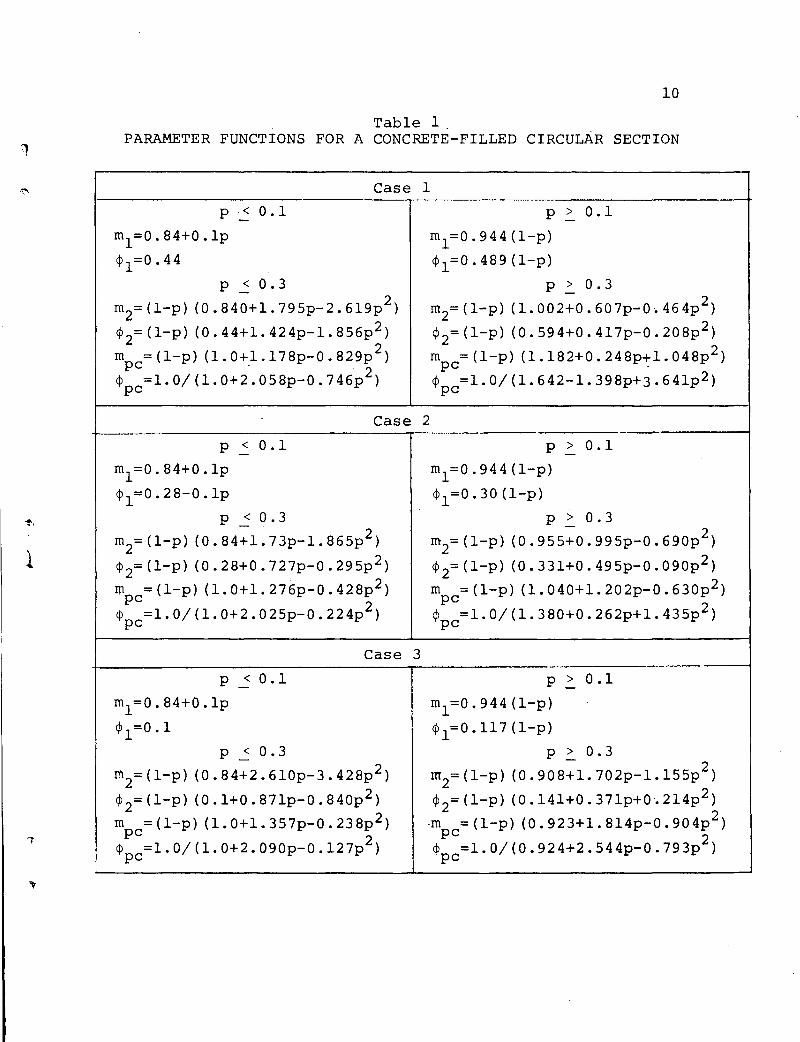
In these equations a, b, c, and f are arbitrary constants. These constants can be evaluated easily by solving simulta­neous equations which will arise if the particular values ¢1, ¢ 2 , and ¢pc are inserted and the moments equated to the appropriate moments m1 , m2 , and mpc· The points (ml,¢1)1 . (m2,¢2), and (mpc,¢pc) should be treated as arbitrary curve­fitting parameters. The parameters will be functions of axial force only and may be expressed as polynomials of p. Details of obtaining these functions are given in Ref. 6.

As an example, the parameter functions have been·obtained for the sections shown in Figs. 2 and 3. Values obtained are given in Table 1 and Table 2 for the three types of concrete stress-strain curves proposed in Fig. l(b). The moment-curva­ture curves computed from the approximate equations and the actual curves of Figs. 2 and 3 for the case of confined con­crete (case 3) are compared in Fig. 4 for the circular section and in Fig. 5 for the square section. These comparisons show that the approximate moment-curvature equations are suffi­ciently accurate for practical use.

3. COLUMN CURVATURE CURVE METHOD FOR BEAM-COLUMN ANALYSIS

Solutions that describe the elastic-plastic in-plane (two-dimensional) behavior of columns and beam-columns are the most highly developed aspect of column research in re­cent years and the basic techniques are given in several texts. The Column Deflection Curve method (CDC) for obtain­ing the so-called "exact" solution is an excellent one. More recently, an approach using the Column Curvature Curve method (CCC) has been introduced to simplify the CDC method [1]. The CCC method uses curvature instead of deflection as the variable, and analytical solutions obtained are accurate [3,4].

The CCC approach to the solution of concrete-filled tubular column problems is adopted herein for the theoretical analysis since details of the method of computation have al­ready been programmed for a digital computer (CDC Digital Com­puter) using the m-¢-p results obtained in the previous dis­cussion. Thus, the numerical results for the column problem can be obtained directly. Details of the &elution are given in Refs. 1 and 10.

')

""··

' ...

6

The direct results from the CCC program are the values of axial force, end curvatures (end moments) and maximum curvature (maximum moment) of the beam-column. The maximum load carrying capacity of the beam-column, at which the beam-column will fail either by the instability of the beam-column or by the crushing of the critical concrete cross section, is also indicated in the output of the program.

4. NUMERICAL RESULTS

Axially Loaded Columns - Column Curves

The problems to be theoretically investigated should consist of determining the behavior and maximum strengths of concrete­filled tubular columns which are initially curved, eccentrically loaded, and contain residual stresses in the steel tube. There is little experimental data concerning columns of this kind, and in choosing the value of an equivalent imperfection, it is neces­sary to assume that all these probable imperfections can be com­pensated sufficiently by assuming an initial eccentricity in axial load application to be 0.001£ for a circular section and 0.002£ for a square section, where £ is the length of the column.

If this initial eccentricity is introduced, the analysis of an axially loaded column is reduced to the problem of compres­sion of an eccentrically loaded column. A solution for this case has been discussed in the previous section by using CCC method. The results of the analysis are shown in Fig. 6 for a circular tube having a yield point of 58,000 psi, wall thickness 0.23 inches, and outside tube diameter 3.5 inches, and in Fig. 7 for a square tube having a yield point of 47,000 psi, wall thickness 0.129 inches and outside width 3 inches. The curves give the limiting values of the load producing failure for two sets of the initial eccentricity e/t. For each initial eccentricity, three column curves are shown corresponding to the three types of con­crete stress-strain relationship proposed in Fig. l(b). The theoretically obtained curves show that, in the case of £/t ratio greater than 15 for the circular column or 20 for the square column, the effect of the triaxial state of stress in concrete on the column strength is unimportant for such columns.

The test results of Knowles and Park [ll] are also plotted in Figs. 6 and 7. The measured initial eccentricities in the axial load application are 0 and 0.09 for the circular column and 0 and 0.1 for the square column. The average concrete com­pressive cylinder strength is 5,925 psi. It is seen that, in

l )

7

the case of 1/t > 15 and especially for large eccentricities, practically all the test points can be predicted accurately by the beam-column analysis neglecting the triaxial state of stress in concrete. The test points also show that, for 1/t < 15 and especially for small eccentricities, the effect of the triaxial state of stress in concrete in the case of the square tube is much less than that attained with the circular tube. In the case of square columns, the triaxial effect of concrete on column strength may be predicted accurately by using the concrete stress­strain curve 3 (case 3) proposed in Fig. l(b). In the case of circular columns, the increase in strength of concrete stress­strain curve may be in the order of a= 1.2 [see Fig. l(a)].

Eccentrically Loaded Columns - Interaction Curves

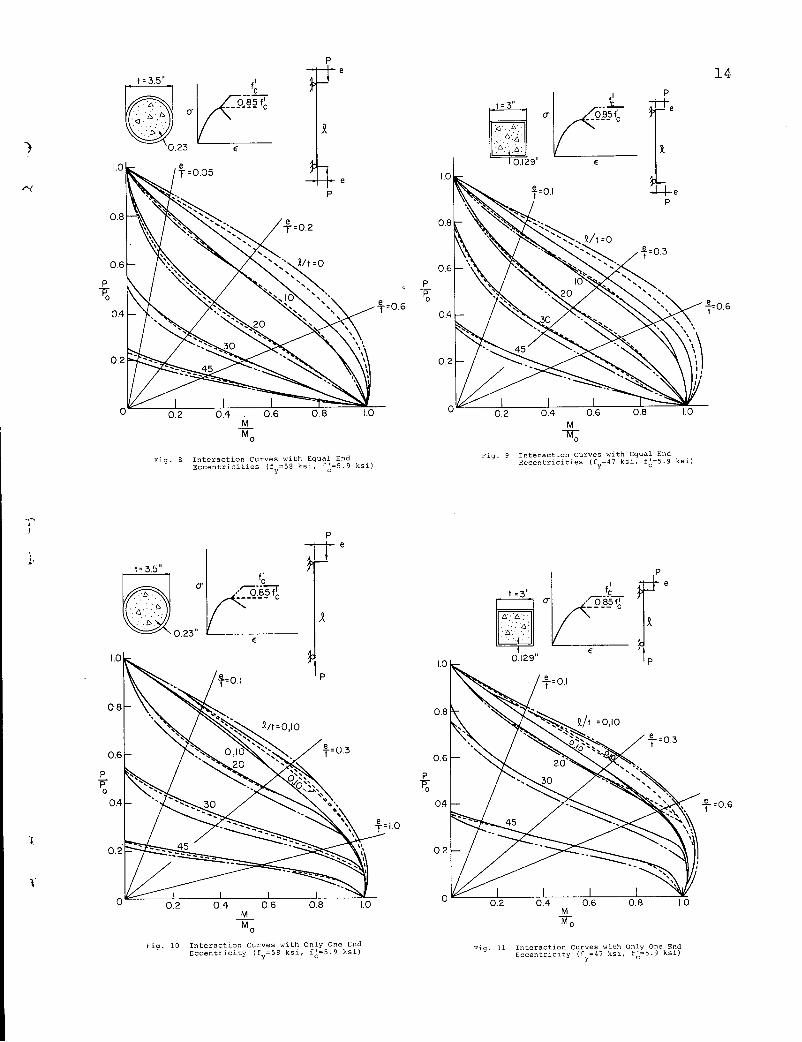
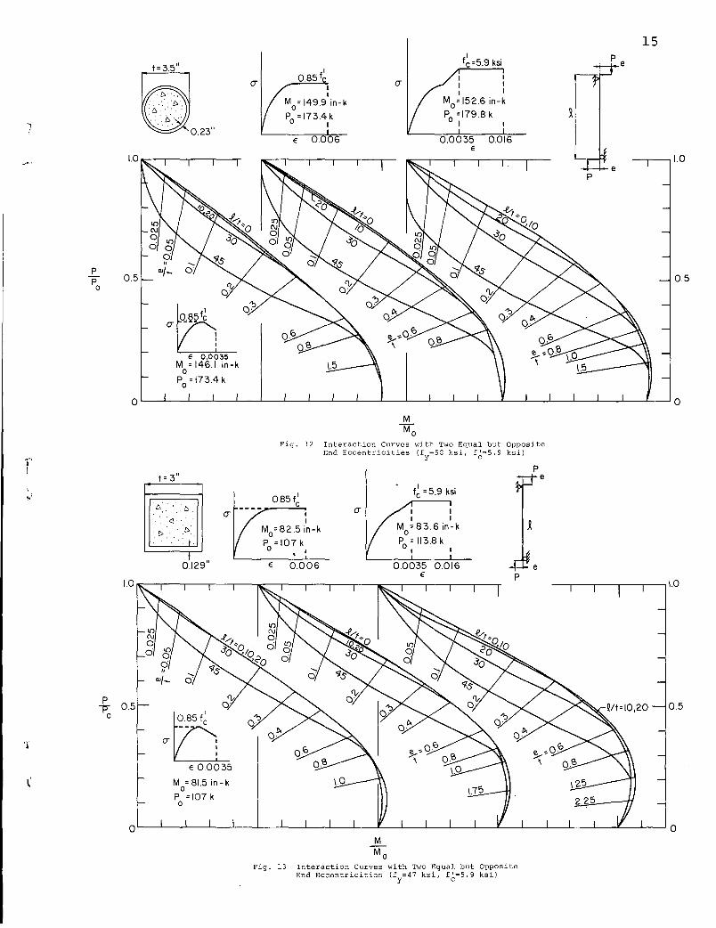
Interaction curves for combinations of axial force and end moment that can be safely supported by the concrete-filled steel tubular column are shown in Figs. 8 to 13 for the two types of cross section and three types of concrete stress-strain curves considered in the preceding sections. The curves have been com­puted numerically using the m-¢-p curves of Figs. 2 and 3. Fiqs. 8 and 9 give the curves for a loading condition in which two equal end eccentricities cause the column to bend in sin~le cur­vature; Figs. 10 and 11 show the curves for the case where only one end eccentricity exists; and Figs. 12 and 13 give the curves for a·loading condition in which two equal but opposite end eccen­tricities cause the column to bend in double curvature.

The effect of the triaxial state of stress in concrete on the maximum strength of a concrete-filled beam-column may be seen in Figs. 8 to 13 which give three comparable interaction curves for each value of 1/t ratio considered. It is seen that the difference between the upper and lower curves corresponding to the concrete stress-strain curves 1 to 3 of Fig. l(b) is quite significant when the values of slenderness ratio of the beam-column are small, but the difference becomes relatively small when the values of slenderness ratio are increased. The curves also show thftt, in the case of unsymmetric loading and especially for the double curvature case, the interaction curves corresponding to the same concrete stress-strain curve are practically identical to each other for columns with ~/t ratios of 10 or less. Thus, as a basis for determining.the composite column strength for columns with 1/t ratios of 15 or more it is justifiable to assume that the unconfined stress-strain curve for concrete is sufficient for the a·nalysis of pin-ended col­umns, loaded symmetrically or unsymmetrically. In the case of columns having 1/t ratios less than 15, the composite column may be assumed to be so short that the instability effect of the

" . , }

·a

column can be neglected and a confined concrete stress-strain curve should be used in the analysis •

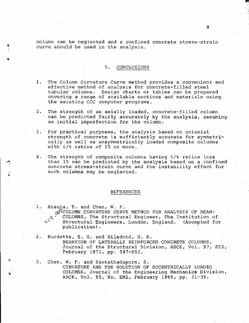
5. CONCLUSIONS

1. The Column Curvature Curve method provides .a convenient and effective method of analysis for concrete-filled steel tubular columns. Design charts or tables can be prepared covering a range of available sections and materials using the existing CCC computer programs.

2. The strength of an axially loaded, concrete~filled column can be predicted fairly accurately by the analysis, assuming an initial imperfection for the column.

3. For practical purposes, the analysis based on uniaxial strength of concrete is sufficiently accuratefor symmetri­cally as well as unsymmetrically loaded.composite columns with ~/t ratios of 15 or more.

4. The strength of composite columns having ~/t ratios less than 15 can be predicted by the analysis based on a confined concrete streps-strain curve and the instability effect for such columns may be neglected.

1.

REFERENCES

Atsuta, T. and Chen, W. F. · ~COLUMN CURVATURE CURVE METHOD FOR ANALYSIS OF BEAM­

~· COLUMNS, The Structural Engineer, The Institution of ~~ · Structural Engineers, London, England. (Accepted for

publication) .

2. Burdette, E. G. and Hilsdord, H. K. BEHAVIOR OF LATERALLY REINFORCED.CONCRETE COLUMNS, Journal of the Structural Division, ASCE, Vol. 97, ST2, February 1971, pp. 587-602.

3. Chen, W. F. and Santathadaporn, S. CURVATURE AND THE SOLUTION OF ECCENTRICALLY LOADED COLUMNS, Journal of the Engineering Mechanics Division, ASCE, Vol. 95, No. EMl, February 1969, pp. 21-39.

... .,

1 I

'

9

4 . Chen, W. F. GENERAL SOLUTION OF INELASTIC BEAM~COLUMN PROBLEM, Journal of the Engineering Mechanics Division, ASCE, Vol. 96, No. EM4, August 1970, pp. 421-441

5. Chen, W. F. FURTHER STUDIES OF INELASTIC BEAM-COLUMN PROBLEM, Journal of the Structural Division, ASCE, Vol. 97, No. ST2, February 1971, pp. 529-544.

6. Chen, A. C. T. and Chen, W. F. SOLUTIONS TO VARIOUS REINFORCED CONCRETE BEAM-COLUMN PROBLEMS, Fritz Engineering Laboratory Report No. 370.2, Lehigh University, September 1970.

7. Furlong, R. W. STRENGTH OF STEEL-ENCASED-CONCRETE BEAM.COLUMNS, Journal of the Structural Division, ASCE, Vol. 93, ST5, October 1967.

8. Furlong, R. W. DESIGN OF STEEL-ENCASED-CONCRETEBEAM.,.-COLUMNS, Journal of the Structural Division, ASCE, Vol. 94, STl, January 1968, pp. 267-281.

9. Hognestad, E. A. A STUDY OF COMBINED BENDING AND AXIAL LOAD IN REINFORCED CONCRETE MEMBERS, Bulletin No. 399, University of Illi­nois Engineering Experiment Station, Urbana.,. Illinois, 1951.

10. Iyengar, S. N. and Chen, W. F. COMPUTER PROGRAM FOR AN INELASTIC BEAM~COLUMN PROBLEM; Fritz Engineering Laboratory Report No. 331.7, Lehigh University, Bethlehem, Pennsylvania, May 1970.

11. Knowles, R. B. and Park, R. STRENGTH OF CONCRETE FILLED STEEL TUBULAR COLUMNS, Journal of the Structural Division, ASCE, Vol. 95, ST12, December 1969, pp. 2526-2587.

12. Kent, D. c. and Park, R. FLEXURAL MEMBERS WITH CONFINED CONCRETE, Journal of the Structural Division, ASCE, Vol. 97, ST7, July 1971, pp . 19 6 9-19 9 0 .

13. Neogi, P. K., Sent, H. K., and Chapman, J. C. CONCRETE-FILLED TUBULAR STEEL COLUMNS UNDER ECCENTRIC LOADING, The Structural Engineer, The Institution of Structural Engineers, London, England, Vol. 47, No. 5, May 1969.

10

Table 1. PARAMETER FUNCTIONS FOR A CONCRETE-FILLED CIRCULAR SECTION

Case 1 1-------------------------------~---------------------------------~

p _::: 0.1

m1=0.84+0.lp

4>1=0.44

p < 0. 3

m2

= (1-p) (0. 840+1. 795p-2. 619p2 )

4>2= (1-p) (0. 44+1. 424p-l. 856p2)

m =(1-p) (1.0+1.178p-0.829p 2 ) pc . tjJ =l.0/(1.0+2.058p-0.746p 2 ) pc

p > 0.1

m1=0.944(1-p)

¢1=0.489(1-p)

p ~ 0.3

m2=(1-p) (1.002+0.607p-0.464p 2 )

¢2

= (1-p) (0. 594+0. 417p-O. 208p2)

m = (1-p) (1.182+0. 248p+l. 048p2 ) pc .. ¢ =l.0/(1.642-1.398p+3.64lp2) pc

Case 2

p .:5_ 0.1

m1=0.84+0.lp

4>1=0.28-0.lp

p < 0. 3

m2=(1-p) (0.84~1.73p-1.86Sp2 )

¢2= (1-p) (0. 28+0. 727p-0. 295p2)

m =(1-p) (l.O+l.276p-0.428p2) pc 2

¢ =l.0/(1.0+2.025p-0.224p ) pc

Case 3

p > 0.1

m1=0.944(1-p)

¢1=0.30(1-p)

p > 0.3

m2=(1-p) (0.955~0.995p-0.690p 2 )

¢2=(1-p) (0.331+0.495p-0.090p2)

m = (1-p) (1. 040+1. 202p-O. 630p2) pc

¢ =l.0/(1.380+0.262p+1.43Sp2 ) pc

~-----------------------------r-----------------------------~ p_:::0.1

m1=0.84+0.lp

¢1=0.1

p _::: 0.3

m2

= (1-p) (0. 84+2. 610p-3. 428p2)

¢2

= (1-p) (0 .1+0. 87lp-O. 840p2)

m =(1-p) (1.0+1.357p-0.238p 2 ) pc 2

¢pc=l.0/(1.0+2.090p-0.127p )

p ~ 0.1

m1=0.944(1-p)

¢1=0.117(1-p)

p > 0.3 - 2

m2

= (1-p) (0. 908+1. 702p-1.155p )

¢2=(1-p) (O.l41+0.37lp+0·.214p2)

-m =(1-p) (0.923+1.814p-0.904p2 ) pc 2

¢ =1.0/(0.924+2.544p-0.793p ) pc

~ I

11

Table 2 PARAMETER FUNCTIONS FOR A CONCRETE-FILLED SQUARE SECTION

Case 1

p < 0. 3

.m1=(1-p) (0.84+2.086p-4.857p 2 )

¢1=(1-p) (0.27+0.676p-1.762p 2 )

m2=(l-p) (0.84+2.705p~3.589p 2 ) ¢2= (1-p) (0. 27+1. 325p-l. 227p 2 )

rtlpc= (1-p) (1. 00+1. 553p-O. 732p2)

¢pc=l.0/(1.0+3.217p-0.048p2 )

Case 2

p < 0. 3 - 2

)Jl1=(1-p) (0.84+2.086p-4.857p ) 2 ¢ 1=(1-p) (0.15+0.367p-0.889p )

m'2= ( 1-p) (0. 84+2. 324p-l. 6 84p 2 ) 2

¢2=(1-p) (0.15+0.839p-0.495p ) 2 m = (1-p) (1. 0+1. 638p-O. 428p )

pc 2 ¢ =1.0/(1.0+3.236p-0.016p ) pc

Case 3

p < 0. 3

m1=(1-p) (0.84+2.086p-4.857p 2 )

¢1=(1-p) (0.05+0.226p-0.59Sp 2 )

m2= (1-p) (0. 84+2. 506p-l. 65Sp 2 )

¢2= (1-p) (0. 05+0. 625p-0. 640p2)

m =(1-p) (l.O+l.758p-0.319p2) pc ¢pcc::(1-p) (1.0+3.441p-0.042p2)

p 2. 0.3

!f\1=1.03(1-p)

¢1=0.31(1-p)

m,2

= ( 1-p) ( 1.171+0. 655p-O. 434p 2 ) 2 ¢2=(1-p) (0.432+0.476p-0.202p )

m =(1-p) (1.195+0.883p-0.667p 2 ) pc

cp =0.64-0.433p pc

p > 0.3

m1=1.03(1-p)

¢1=0.18(1-p) 2 m

2=(1-p) (1.264+0.548p-0.470p )

cp 2 = ( 1-p ) ( 0 . 3 4 2 + 0 • 0 1 0 p+ 0 . 131 p 2 )

m =(1-p) (0.929+2.208p-1.543p2 ) pc

cp =1.0/(1.103+2.983p-0.320p2) pc

p 2. 0.3

m1 = 1. 0 3 ( 1-p)

¢1=0.064(1-p) 2 m

2=(1-p) (0.912+2.357p-1.964p )

cp 2 = ( 1-p) ( 0 . 13 2 + 0 • 13 3 p+ 0 . 0 8 3 3 p 2 ) . 2

m =(1-p) (0.749+3.155p-2.184p) pc 2

cp =(1-p) (0.439+6.262p-3.213p ) pc

"')

I I ...

(j

M Mo

2 fl

I (j 0.85fc

I 0.72 fc

(a) Stress-Strain Relationship For Concrete

0.0023 0.0035

2-....

0.006

E

12

3-..

0.016

(b) Three Types Of Stress- Strain Relationship Of Concrete

Fig. l Proposed Stress-Strain Relationship for Unconfined or Confined Concrete

® Mwt066

® <l>oc• 4.071

0.738 2.292

0.424 2.054

t'ig. 2 Comparisons of Theoretical Moment Curvatur'1 Curves for A Concrete-Filled Circular Section (M

0 .. 146,1 in-K, P

0 .. 173.4K, 40 .. 0.0026)

M

Yo

case® 0.826 1.768

0.480 1.606

0.129"~'"' -~

Fig. 3 Comparisons of Theoretical M.orncnt. curvature Curves for A concrete­t'illed S<.~uare Section (M0=8l.'i in-K, P

0 .. 10'/K, 1,0 "'0.0036)

"i I

••

\ '\

p

Po

0.4

0.2

0

0.2

•

•

® . .

0.2 0.4 0.6 <P <Po

0.8 1.0

Fig. 4 Moment-Curvature curves for A Circular Shape (Exact curves Shmm Dashed)

cr

• fy= 58,000 psi

E p

t=OOOI f

+=0.09+0001 + • Test Data, Knowles And Pork

g_ -t-

Fig. 6 Comparison of Column Test Results with Theory

1.2

p

Po

0.5

0.6

0.4

0.2

~ ~

E

13

oL-----~o~.2~--~oL.4~--~o~.6~--~o~.8~----~~.o~----~1.2 <P ~

Fig. 5 Moment-Curvature Curves for A Square Shape (Exact Curves Shown Dashed)

•

t=3"

.

3"

0.129"

~= 0.1 + 0.002 ..&_ t t

• Test Data , Knowles And Pork

Fig. 7 Comparsion of Column Test Results with Theory

)

T' )

i .~:·~·i 0 23 E

Fig. 8

Fig. 10

M

~ Interaction Curves with ~qua~_;n~ ksi) Eccentricities (fy=SS ks~, fc- ·

M

~ Interaction curves wit~ On~~ OnekE~~ Eccentricity (fy=SB ksJ., fc-5.9 Sl.

p

t=0.6 ~

p p;

1.0

Fig. 9

Fig. 11

M

~

p

r .:.J___j....e

p

Interaction curves with ~qua~_ End ksi) Eccentricities {fy=47 ksl., fc- 5 · 9

~~ 1

=

3

".· cr. ____ .. r-=--=-o_._a··-5-t'_ - ---- '

E 0.129"

M

Mo

14

toG

r

p

Po

p

~

0.5

t=3.5"

. .

0.23"

E 0.0035 M = 146.1 in-k

0 P

0 = 173.4 k

t = 3"

I 0.129"

<'\, a·

~C_ E 0.0035

M0=81.5 in-k

p = 107 k 0

I I

M0

= 149.9 in-k

P0

= 173.4 k I

I fc=5.9 ksi

M

~ Fig. 12 Interaction Curves with Two Equal but Opposite

End Eccentricities (fy=SB ksi, f~=5.9 ksi)

I 0.85 fc

I I

M0=82.5 in-k

P0

= 107 k ' I

E 0.006

M

~

I I I I

M=83.6in-k 0

P0

= 113.8 k 1 I

0.0035 0.016 E

Fig. 13 Interaction Curves with Two Equal but Opposite End Eccentricities (fy=47 ksi, f~=5.9 ksi)

15

0.5

0.5