abstract thesis: large-scale evacuation routing and
TRANSCRIPT

ABSTRACT
Title of Thesis: LARGE-SCALE EVACUATION ROUTING AND SCHEDULING OPTIMIZATION WITH UNINTERRUPTED TRAFFIC FLOW
Xuechi Zhang, Master of Science, 2014
Directed By: Dr. Ali Haghani
Department of Civil Engineering
In many emergency management operations, an efficient evacuation strategy is of great
importance because if it is successful, it has the ability to significantly reduce the loss of property
and human life. This thesis develops a routing and scheduling optimization framework for large-
scale vehicular evacuation. To guarantee high optimization efficiency, we consider the routing
and scheduling optimization as a two-stage problem instead of optimizing them as a whole (i.e.
using time-space network). In the first phase, a multiple-objective binary programming model,
with the objectives of minimizing the network clearance time and total in-network time is
proposed to find an optimal routing plan. In the second phase, a simulation-based scheduling
Heuristic is proposed to dynamically generate the time-dependent departure rates. A real-world
evacuation scenario in Eastern Shore of Maryland is studied by using the proposed optimization
model. The calculation results indicate a good optimization capability and flexibility of the
proposed model.

LARGE-SCALE EVACUATION ROUTING AND SCHEDULING OPTIMIZATION WITH UNINTERRUPTED TRAFFIC FLOW
By
Xuechi Zhang
Thesis submitted to the Faculty of the Graduate School of the
University of Maryland, College Park, in partial fulfillment
of the requirements for the degree of
Master of Science
2014
Advisory Committee:
Professor Ali Haghani, Chair
Professor Paul Schonfeld
Professor Lei Zhang

© Copyright by
Xuechi Zhang
2014

Dedication
To Dandan and my beloved parents
ii

Acknowledgements
First of all, I would like to express my sincere appreciation to my advisor, Dr.
Ali Haghani, for his guidance, support and encouragement during the period of my
master study. I was so honored to join his research group and benefit from his broad-
range knowledge. His understanding, patience and valuable advice have been the
keys to the success of this work. Thanks are extended to the other committee
members, Dr. Paul Schonfeld and Dr. Lei Zhang. Their constructive suggestions and
comments are of great significance.
In addition, I would like to thank Dr. A.M. Afshar for his support with the
real-world data. Also I am grateful to the group members for their valuable comments
and suggestions during my presentation. Special thanks go to Dr. K. Farokhi and Dr.
M. Hamedi, R. Olarte and H. Chang. I really benefited a lot from the insightful
suggestions from you guys.
Finally, with deep sense of gratitude, I especially want to express so many
thanks to my parents, Dandan and my sister, who have been encouraging and
supporting me all of the way along my master studies. Without their tremendous love
and encouragement, I would not have been able to concentrate on my study and
overcome some hard times through these two years.
iii

Table of Contents
Dedication ................................................................................................................................. ii
Acknowledgements .................................................................................................................. iii
Table of Contents ..................................................................................................................... iv
List of Tables ........................................................................................................................... vi
List of Figures ......................................................................................................................... vii
Chapter 1 : Introduction ............................................................................................................ 1
1.1 Research Background .................................................................................................. 1
1.2 Research Objectives and Scope of Work ..................................................................... 3
1.3 Thesis Organization ..................................................................................................... 4
Chapter 2 : Literature Review ................................................................................................... 5
2.1 Macroscopic Approaches ............................................................................................. 5
2.2 Microscopic Approaches ............................................................................................. 8
2.3 Mesoscopic Approaches ............................................................................................ 10
Chapter 3 : Routing Optimization Model ............................................................................... 14
3.1 Mathematical Network Representation ...................................................................... 14
3.2 Notations .................................................................................................................... 17
3.3 Model Formulation .................................................................................................... 19
3.3.1 Network Clearance Time .................................................................................. 19
3.3.2 Total Travel Time ............................................................................................. 21
3.3.3 Total In-Network Time ..................................................................................... 22
3.3.4 Objective Function ............................................................................................ 25
3.3.5 Constraints ........................................................................................................ 27
3.4 Solution Approach ..................................................................................................... 32
Chapter 4 : Scheduling Optimization Model .......................................................................... 37
4.1 Introduction ................................................................................................................ 37
4.2 Traffic Simulator ........................................................................................................ 38
4.3 Scheduling Heuristic .................................................................................................. 38
Chapter 5 : Case Study ............................................................................................................ 46
5.1 Introduction ................................................................................................................ 46
5.2 Case Study I ............................................................................................................... 46
iv

5.2.1 Problem Definition ............................................................................................ 46
5.2.2 Demonstration of the Routing Optimization Procedure .................................... 48
5.3 Case Study II .............................................................................................................. 54
5.3.1 Problem Introduction and Statement ................................................................. 54
5.3.2 Evacuation Network and Demand Description ................................................. 56
5.3.3 Numerical Experiments ..................................................................................... 62
Chapter 6 : Thesis Summary ................................................................................................... 77
6.1 Contributions ............................................................................................................. 77
6.2 Future Research ......................................................................................................... 78
Bibliography ........................................................................................................................... 80
v
List of Tables
Table 4-1: Pseudo Code of the Traffic Simulator ....................................................... 39 Table 4-2: Pseudo Code of the Proposed Simulation based Scheduling Heuristic..... 41 Table 5-1: Optimized Routing Plan for each T (network clearance time) .................. 48 Table 5-2: Routing Plan 1 for Case Study 1 ............................................................... 50 Table 5-3: Routing Plan 2 for Case Study 1 ............................................................... 51 Table 5-4: Routing Plan 3 for Case Study 1 ............................................................... 52 Table 5-5: Routing Plan 4 for Case Study 1 ............................................................... 53 Table 5-6: Evacuation Demand Distribution in Eastern Shore Maryland .................. 63 Table 5-7: Optimized Evacuation Routes (one route per source) ............................... 63 Table 5-8: Optimized Evacuation Routes (two routes per source) ............................. 67 Table 5-9: Optimized Evacuation Routes (three routes per source) ........................... 68 Table 5-10: Sensitivity Analysis of Network Clearance Time (sec) with respect to different (α, β) Pair...................................................................................................... 73
vi

List of Figures
Figure 2-1: Flow Chart of Discrete Simulation based Optimization .......................... 12 Figure 3-1: An Example of a Real-world Evacuation Network ................................. 15 Figure 3-2: Corresponding Network Representation Graph of the Example in Figure 3-1 ............................................................................................................................... 15 Figure 3-3: Node labelling illustration on a 4-leg intersection (left) and a 6-leg intersection (right) ....................................................................................................... 16 Figure 3-4: Label each node with a unique two-indices based ID .............................. 17 Figure 3-5: Representation of total in-network time and network clearance time with respect to a general evacuation curve ......................................................................... 23 Figure 3-6: An example that two evacuation plan having same network clearance time but different total in-network time .............................................................................. 26 Figure 3-7: Method of transform a single source node into several parallel dummy nodes ........................................................................................................................... 28 Figure 3-8: Arcs that conflict with arc [(i,m),(i,n)] with no common nodes .............. 31 Figure 3-9: Arcs that conflict with arc [(i,m),(i,n)] with exactly one common node . 32 Figure 3-10: Flow Chart of the Routing Optimization Solution Approach ................ 36 Figure 4-1: Flow Chart of the Simulation based Scheduling Heuristic ...................... 45 Figure 5-1: Evacuation Network of Case Study 1 ...................................................... 47 Figure 5-2: Optimal Value versus Different T ............................................................ 49 Figure 5-3: In-Network Evacuation Demand V.S. Evacuation Time ......................... 54 Figure 5-4: Map of Eastern Shore of Maryland .......................................................... 55 Figure 5-5: Major Evacuation Network for Maryland Eastern Shore[2] ..................... 57 Figure 5-6: Case that the interchange capacity is overestimated ................................ 59 Figure 5-7: Four special network nodes (Dummy node) in case study II ................... 60 Figure 5-8: Sub-network representation for intersection with at most four legs ........ 61 Figure 5-9: Sub-network representation for interchange between freeways .............. 61 Figure 5-10: Comparison of Performance Indicators among the three proposed routing plans................................................................................................................ 69 Figure 5-11: Time-dependent Discharging Rate of the Optimal Scheduling Strategy (All sources have the same priority 1) ........................................................................ 74 Figure 5-12: Time-dependent Discharging Rate of the Optimal Scheduling Strategy (Sources in Ocean city have a higher priority equal to 2, and other sources have priority 1) .................................................................................................................... 75 Figure 5-13: Time-Dependent Evolution Curve of the Total Evacuated Demand under the Optimal Routing and Scheduling Strategy............................................................ 76 Figure 5-14: Time-dependent Remaining Demand Curves in Ocean City Area with respect to different Priorities ....................................................................................... 76
vii

Chapter 1 : Introduction
1.1 Research Background
Potential hazards exist in people’s daily lives every day. From the perspective of cause,
hazards can be classified into two categories: manmade hazards and natural hazards. Manmade
hazards are events like terrorist attacks, chemical leaks or explosions and nuclear leakage.
Natural hazards are events like hurricanes, earthquakes, tsunamis and other naturally occurring
disasters. However, there is no single hazard or disaster that exists absolutely independent from
any other hazards or disasters. The inter-relationship among all kinds of hazards cannot be
ignored in the emergency management process. For instance, a secondary disaster like a tsunami
can occur following an earthquake, and a prescriptive terrorist attack can lead to a serious
nuclear leakage. To prepare for these events, society should be alert and have a set of integrated
operation plans to respond to these hazards. The core of emergency management operations is to
protect human beings to the largest extent. People’s safety shall always take the highest priority,
which means evacuation operations in emergency situations to protect human safety are of the
highest importance.
Due to high population density, urban areas are extremely vulnerable to the above-mentioned
hazards. In other words, evacuation is more likely to occur in an urban area. In urban areas,
designing efficient evacuation plans is the responsibility of emergency management agencies or
authorities. However, the problem is not that easy to solve. The high density of evacuee
population and the complexity of the urban transportation network can pose challenges. Various
problems occur simultaneously when dealing with the large population and making use of the
1

complex transportation network. Several critical questions regarding the urban evacuations are
summarized below:
1) In the evacuation preparation stage, how should we assemble and manage a large number
of evacuees to efficiently start the following evacuation?
2) Among the intricate urban roadways, which ones should be picked out for the special use
of evacuation?
3) Should we mandatorily assign evacuation egress to the evacuees in an emergency
situation?
4) Due to the large number of evacuees and limited roadway capacity, how do we come up
with a staging evacuation strategy (i.e. loading the evacuees onto network in an optimal
order)?
5) How do we control intersections so as to guarantee a smooth evacuation operation?
The aforementioned concerns show that evacuation planning for urban areas deserves more
consideration than that in rural areas, due to high population density and intricate transportation
systems. In the literature so far, seldom are there works directly dealing with the evacuation
routing and scheduling planning inside an urbanized area with many of evacuation sources. The
most critical problem for a large-scale urban evacuation is the intersection control and bottleneck
identification. Actually, the intersection cannot be viewed as simply a network transshipment
node. One reason is that the movements happening inside an intersection have multiple
constraints. Another important reason is that a turn movement inside an intersection always has
a relatively low travelling speed in comparison with the travelling speed in a general roadway
link. As a consequence, the bottleneck is more likely to occur at an intersection due the low
2

speed of turn movements. The research detailed in this paper uses these considerations to
propose a realistic and efficient evacuation operation framework specifically in an urbanized area.
1.2 Research Objectives and Scope of Work
This study aims to deal with a large-scale vehicle-based evacuation routing and
scheduling optimization for a large population density. Due to the significance of prescriptive
evacuation planning, there are abundant advanced techniques emerging these years. To avoid
redundant efforts, a comprehensive literature review on the vehicular evacuation has been
conducted.
Based on the historical works in the literature, two research goals are set and fulfilled.
Specifically, an evacuation routing optimization model and a network-loading algorithm are
proposed separately to better assist the emergency decision maker to manage the overall
evacuation process. Instead of optimizing the routing and scheduling as a whole by making use
of a time-space network, this research calculates the routing and scheduling decision variables
separately. This is mainly because a complex network with a large evacuation demand makes it
nearly impossible to acknowledge the optimal network clearance time, which is essential to
expand an evacuation network along a discrete time horizon. In addition, the solution calculation
of a time-space network is extremely time-consuming. Consequently, this type of model is
rarely used in reality.
To achieve the first goal (i.e. routing optimization), a bi-level binary programming model
with multiple objective functions is formulated. The objectives of this model are to minimize
both the network clearance time and the total in-network time, which consists of route traverse
time and average network loading delay. To better guarantee the evacuation process is smooth
3

and effective, intersection movement conflicts are eliminated during the optimization process. In
other words, the optimization process is conducted by constructing a set of uninterrupted traffic
flows. Meanwhile, the evacuation bottleneck for each evacuation path is identified during the
optimization process. To achieve the second goal, a simulation-based scheduling heuristic (i.e.
discharging algorithm) is proposed. A mesoscopic traffic simulator is implemented and
incorporated in this algorithm so as to feedback the real-time traffic state to the heuristic. Two
case studies are used to conduct the calculation experiments, one is based on a fabricated urban
grid network, and the second one is based on a real-world evacuation scenario from the Eastern
Shore of Maryland.
1.3 Thesis Organization
Subsequent chapters of this thesis are organized as follows. In Chapter 2, a literature
review is provided. To better understand the related literatures, the review work further
classifies the current techniques based on three levels. They are, macroscopic methodology,
mesoscopic methodology and microscopic methodology. Chapter 3 describes the development
of the aforementioned evacuation routing optimization model. A specific solution approach is
developed and illustrated at the end of this chapter. In Chapter 4, to come up with an optimal
demand discharging strategy, a simulation-based evacuation heuristic is developed and discussed.
Chapter 5 conducts several case studies to test the proposed optimization framework, and the
experiment results are summarized and discussed. Finally, Chapter 6 concludes the overall work
and provides some future work directions.
4

Chapter 2 : Literature Review
Evacuations happen in various kinds of emergency situations, like a fire in a building, a
terrorist attack, or a large-scale hurricane. In terms of applications, evacuation research can be
further divided into two main tracks. One is pedestrian-specific evacuation, and the other one is
vehicle-based evacuation. This work specifically deals with evacuation optimization in terms of
vehicle-based scenarios. Thus, the literature review here mainly focuses on the current
techniques belonging to this track. Some detailed literatures on pedestrian-based evacuations
can be found in the works of Schreckenberg and Som (2002), Kuligowski and Richard (2005),
and Helbing and Anders (2009). To investigate and understand the abundant literature in a well-
organized manner, the review work here further classifies the vehicle based evacuation
techniques into three categories. They are evacuation planning techniques by a macroscopic
approach, a mesoscopic approach and a microscopic approach, respectively. In addition to the
related techniques, the advantages and drawbacks of each category of approaches is also
discussed at the end of each subsection.
2.1 Macroscopic Approaches
Macroscopic approaches are mainly used to approximately estimate the lower bounds for
the evacuation time, like network clearance time and total evacuation time (Hamacher and
Stevanus, 2002). Models belonging to this type of approach do not consider any individual
behaviors during the evacuation process. Instead, they always model the whole situation as flow
transmission and evolution process. The main way to deal with this flow-optimization problem
is based on the work of Ford and Fulkerson (1958), in which a maximal amount of flow has to be
sent from a source node to a sink node in a given time of period. This optimization concept can
be explicitly extended to a vehicle-based evacuation scenario by letting the source node be the
5

assembly point of evacuees and letting the sink node be the safety exit. Yamada (1996) proposes
a network flow approach to a city emergency evacuation planning. In his model, evacuation
sources and safety points are predefined in a given urban transportation network. Then the
optimization is conducted based on a shortest path problem and a maximal flow and minimal
cost problem. Prescriptive evacuation routes and lower bounds of evacuation time are outputs of
his model. However, due to the absence of a real-world simulation study, the lower bound is not
validated. Cova and Justin (2003) formulate the evacuation process as a lane-based mixed-
integer programming problem with the objective of minimizing total evacuation distance. This
model first distinguishes the vehicle-based evacuation problem with other flow-based evacuation
problems in history. That is, the traffic conflict within intersections is very important.
Obviously, an intersection cannot simply be viewed as a transshipment node in the evacuation
network. The turn movements conflict and intersection capacity play a significant role during
the evacuation process. Thus, Cova and Justin (2003) incorporate the conflict elimination
constraints in their linear model, which is specifically used for a vehicle-based evacuation
scenario in an urban area. In addition, a simulation model according to HCM is built to validate
the model’s outputs. Kim et al. (2007) present the first macroscopic approach for finding a
contraflow network reconfiguration to minimize the evacuation time. These concepts
dramatically enlarge the solution search space. Thus, they propose a greedy algorithm to produce
a satisfied solution. Using the same concepts as Kim et al. (2007), Xie et al. (2010) come up
with a bi-level optimization model in which lane reversal and conflict elimination are optimized
to assist the dynamic traffic assignment optimization.
The cell transmission model (CTM)-based evacuation planning optimization is also
classified as a macroscopic approach. Although CTM-based optimization models make the
6

evacuation evolution more accurate, it still does not incorporate the inter-relationship between
each evacuee. In other words, it is still a kind of network flow optimization problem but with a
higher network resolution. Based on CTM, Ziliaskopoulos (2000) proposes a linear
programming model for optimum dynamic traffic assignment problem (DTA). DTA can be
extended to an evacuation problem just by substituting OD pair information with sources and
sinks information. Liu et al (2006) proposed a revised CTM-based optimization model with two-
level objectives, one is to maximize the throughput and the other one it to minimize the total
evacuation time. In addition, Liu et al. (2007) built an evacuation specific optimization model on
the foundation of Ziliaskopoulos (2000)’s linear programming model. However, due to the huge
amounts of decision variables, Liu et al. (2007) did not directly calculate their model. Instead,
two heuristic models are proposed to find a satisfied solution. It partially reflects that the CTM-
based evacuation model is not practical for a large-scale evacuation scenario (i.e. evacuation in
an urbanized area). Some other CTM-based evacuation optimization models are Liu et al. (2006)
and Kalafatas and Peeta (2009). In the work of Kalafatas and Peeta (2009), lane reversal
concepts are also used to augment the roadway capacity. Moreover, based on the concept of
CTM, Zhang and Chang (2011) developed a Cellular Automata-based model for simulating
vehicular-pedestrian mixed flows in a congested network. Then they applied this mixed flow
concept into evacuation and proposed an integrated linear model for the design of optimized flow
plans for massive mixed pedestrian-vehicle flows within an evacuation zone (Zhang and Chang
(2013)).
In addition, the geographical information system (GIS) has gradually become an
important part in evacuation optimization and management because of its excellent capacity of
processing big data and a more intuitional visualization. Church and Cova (2000) first proposed
7

a GIS-based optimization model that identifies small areas or neighborhoods with a high ratio of
population of exit capacity in terms of an evacuation network. Although their model does not
explicitly generate the egress routing and scheduling information, it is of great significance to
prioritize the evacuation schedule during a staged evacuation process. Similarly, Chen et al.
(2009) came up with an evacuation risk assessment model while considering pre- and post-
disaster factors. As for the evacuation routing optimization with GIS system, Saadatsereshit et al.
(2009) develop multi-objective evolutionary algorithms with the goal of optimally distributing
the population into the safe areas. Ye et al. (2012) conducted spatial analysis for mapping
evacuee demand distribution with the constraints of shelter space accessibility in an earthquake
scenario. These GIS-based evacuation routing models do not explicitly deal with specific
dynamic traffic control during an urban evacuation, but they can efficiently assist the evacuation
management agency to manage the whole evacuation from a macroscopic view.
2.2 Microscopic Approaches
Optimization models from microscopic views are mostly simulation-based since it is
difficult to capture all network operational constraints and driver responses fully with
mathematical formulations. For instance, Chen et al. (2007) investigated impact of different
signal timing plans for urban evacuation by using arterial corridors. Zou et al. (2005) developed
a simulation-based framework for the Ocean City area (Maryland) and investigated the
efficiency of six given evacuation plans. Similar work has been done in the work of Liu et al.
(2005). Meanwhile there are also some analytical models aiming to optimally solve the vehicle-
based evacuation planning. For example, when considering interplay among all evacuation
vehicles, Chien and Vivek (2007) explicitly formulated the evacuation time as the summation of
waiting delay and traverse time for a single street evacuation situation. Then, a classical
8
mathematical optimization method is used to find the optimal solution. However, this type of
method is not practical, especially for a large-scale evacuation scenario. Since the number of
decision variables is huge, it is impossible to directly solve the analytic equation for an optimal
solution. After 1999’s Hurricane Floyd evacuation in costal South California, Dow and Susan
(2002) conducted a survey to investigate the relationships between evacuation issues (i.e.
evacuation time, evacuation distance and evacuation method) and people’s decisions. They
concluded that transportation issues are of huge significance during an evacuation process, as
they not only impede people’s evacuation but also influence people’s final decision in
microscopic way. With this type of consideration, Chen et al. (2006) built a microscopic
simulation model to investigate the network clearance time in the Florida Keys when it comes to
a hurricane landfall. Questions like the number of people who will be stranded if the evacuation
routes are impassible during a particular scenario are answered. At the same time, Chen and
Franklin (2006) also take advantage of their agent-based microscopic simulation model to
analyze the efficiency of simultaneous and staging evacuation strategies, respectively. A key
conclusion is that staging evacuation strategy has a better performance in an urban evacuation
scenario. In considering the impact of human’s behavior on the evacuation time estimates
(ETEs), Lindell and Carla (2007) investigate the principal behavioral variables that affect
hurricane ETEs. The critical behavioral assumptions further enrich the evacuation analysis in a
microscopic view. Lindell (2008) studies the human behavior in an emergency situation and
proposes a comprehensive human behavior-forecasting model. Based on that, an empirically
based large-scale evacuation time estimate mode (EMBLEM2) is built while taking the
evacuee’s behavior into consideration. Different from the macroscopic models, human
preparation time during an evacuation is also considered as part of the overall evacuation time.
9

A comprehensive review on travel behavior modeling in dynamic traffic simulation models for
evacuation can be found in Pel et al. (2012).
Some other literature in which microscopic simulation technique is used to plan an
evacuation are briefly summarized as follows. Jha et al. (2004) developed a microscopic
simulation model (MITSIMLab) for evaluating evacuation plans for the Los Alamos National
Laboratory (LANL). The scenarios adopted include full or partial closures of various roadways,
limited access to some special facilities and security delays at certain locations. The evolution
dynamics of the evacuation process is captured and analyzed in detail. Liu et al. (2007) proposed
to use a microscopic traffic simulation model to implement the short-term traffic control strategy
in order to dynamically guide the evacuation traffic flow. Lämmel et al. (2008) developed a
simulation model based on the MATSim framework to generate an optimal evacuation traffic
assignment (i.e. Nash equilibrium). Agent dynamics based on a FIFO queue model are
incorporated in their model. This agent-based simulation model provides plausible results
regarding the predicted evacuation time and bottlenecks.
2.3 Mesoscopic Approaches
Macroscopic models only have the capability of roughly estimating the evacuation time.
As a result, the corresponding optimal routing and scheduling guidance are generated in ideal
conditions and by relying on too many assumptions. While evacuation planning in a
microscopic way indeed provides more realistic details during the whole process, simulating a
single particular plan will take a huge amount of calculation time, let alone for millions of
optional plans. In considering the performance gap between these two methodologies, a
mesoscopic approach in dealing with evacuation optimization becomes more and more popular.
Jain and Smith (1997) first proposed a vehicular traffic flow model based on M/G/C/C state-
10

dependent queuing models. With this queuing model, the congestion of traffic flow with
Markovian arrivals on a single road link can be statistically captured. This model is first taken
into the evacuation optimization in the work of Stepanov and Smith (2009), in which an integer
programming model is proposed to minimize the average travel distance and network clearance
time. Their model provides congestion probability on each roadway link, which can be pre-
limited within an upper bound. However, only routing guidance is provided using this model.
When it comes to an evacuation scenario with a huge population, scheduling guidance is of
extremely significance because we cannot simultaneously load all of the demand into the
transportation network. In addition, Stepanov and Smith (2009) do not provide flow-control
strategies within an intersection. From the perspectives of eliminating movement conflicts at an
intersection, Bretschneider and Kimms (2011) develop a mixed-integer programming model to
optimize the routing and scheduling problem by using a time-expanded network approach.)
Although they name their model as a basic mathematical flow optimization framework, traffic
dynamics with lane-based resolution are integrated. Thus, this model is also classified as a
mesoscopic approach. Due to the high calculation complexity of a time-expanded network, a
heuristic is also proposed in their work to generate satisfactory solutions. However, the main
drawback of a time-expanded network optimization is that a proper time horizon must be given
at the beginning. In real world scenarios, this time horizon is difficult to estimate, especially for
a problem with large demand. If the time horizon is estimated below the value of the optimal
condition, no feasible solution can be found; if it is overestimated, the output we get is just a sub-
optimal solution. Therefore, a time-expanded network is only suitable to a small size problem.
Another practical way of mesoscopic optimization is discrete simulation-based
optimization. As is shown in Figure 2-1, this type of optimization method takes advantage of a
11

discrete traffic simulator together with a set of Heuristics to dynamically assign and load the
evacuation demand to the transportation network. Sbayti and Mahmassani (2006) make use of a
successive average-based iterative heuristic to determine the departure times for an evacuation
process in consideration of the influence of background traffic. A traffic simulator called
DYNASMART-P is used to propagate the vehicles on their prescribed paths and determine the
state of the system. At the end of the discrete simulation, a time-dependent staging evacuation
policy is generated for each selected origin. Afshar and Haghani (2008) developed a
comprehensive heuristic framework for dynamic evacuation with the Spread-Squeeze concept.
In their framework, a set of spread methods and a set of squeeze methods are proposed
separately. This gives the flexibility of the application of these Spread-Squeeze heuristics to
different size evacuation scenarios. Although Afshar and Haghani (2008) do not explicitly
consider the routing determination process, their optimization framework can be extended to a
routing and scheduling optimization framework with the introduction of some dynamic routing
algorithms.
Figure 2-1: Flow Chart of Discrete Simulation based Optimization
In this research, the evacuation optimization is considered a two-level problem (i.e. routing and
scheduling). In the upper level, a routing optimization model is formulated as a binary integer
programming problem with the objective to minimize the total evacuation time. During the
routing optimization process, intersection conflicts are eliminated and the uninterrupted
12

evacuation flow paths are generated. In the lower level, with the input of the prescriptive egress
routes, a greedy algorithm based on a discrete traffic simulator is proposed to dynamically
determine the time-dependent departure rate for each source.
13

Chapter 3 : Routing Optimization Model
3.1 Mathematical Network Representation
The real world transportation network is abstractly represented by a directed graph G (N,
A) with node set N and arc set A. In this model, every intersection of the evacuation network is
replaced by a set of intersection nodes (As is shown in Figure 3-1and Figure 3-2). The
decomposition of an intersection aims to further model the movement conflicts within an
intersection. Thus, node set N consists of four types of nodes: source nodes, transshipment nodes,
sink nodes as well as a dummy node connecting every sink. The travel time and capacity on any
arc connecting the real destination node and the dummy node are set to 0 and infinity,
respectively. In a real world scenario, a source node might be any evacuation assembly point,
like exit point of a specific district block, or entrance ramp of a freeway. Sink nodes can be
shelters or exits of a particular hazard area. Transshipment nodes usually denote intersections or
some specific roadway inner points. Sometimes a source node or a sink node can also function
as a transshipment node. Arc set A consists of all the directed arcs connecting nodes in N.
14

Figure 3-1: An Example of a Real-world Evacuation Network
Figure 3-2: Corresponding Network Representation Graph of the Example in Figure 3-1
To facilitate the representation of movement conflicts within an intersection, a two-
indices based node notation is used here. The detailed demonstration of this type of network
element notation is illustrated in the work of Bretschneider and Alf Kimms (2011). For this type
15

of notation, any node is labeled with a unique number pair (i,m). The first index i usually
classifies a set of nodes with common properties or sharing a common intersection. For example,
all nodes adjacent to intersection i can be labeled as (i,m), which indicates this is the mth node
within intersection i. Thus, a directed arc can be labeled as [(i,m),(j,n)], which represents the arc
from node (i,m) to node (j,n). In addition, to facilitate the conflicts modeling within an
intersection i, we assume the nodes are incrementally labeled clockwise within an intersection
(see Figure 3-3 and Figure 3-4). Here, a two-indices based node notation is used.
Figure 3-3: Node labelling illustration on a 4-leg intersection (left) and a 6-leg intersection (right)
16
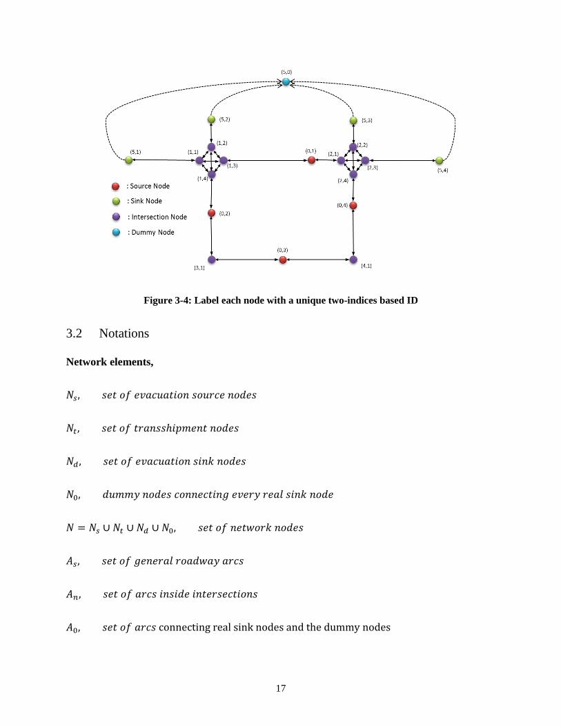
Figure 3-4: Label each node with a unique two-indices based ID
3.2 Notations
Network elements,
𝑁𝑁𝑠𝑠, 𝑠𝑠𝑠𝑠𝑠𝑠 𝑜𝑜𝑜𝑜 𝑠𝑠𝑒𝑒𝑒𝑒𝑒𝑒𝑒𝑒𝑒𝑒𝑠𝑠𝑒𝑒𝑜𝑜𝑒𝑒 𝑠𝑠𝑜𝑜𝑒𝑒𝑠𝑠𝑒𝑒𝑠𝑠 𝑒𝑒𝑜𝑜𝑛𝑛𝑠𝑠𝑠𝑠
𝑁𝑁𝑡𝑡, 𝑠𝑠𝑠𝑠𝑠𝑠 𝑜𝑜𝑜𝑜 𝑠𝑠𝑠𝑠𝑒𝑒𝑒𝑒𝑠𝑠𝑠𝑠ℎ𝑒𝑒𝑖𝑖𝑖𝑖𝑠𝑠𝑒𝑒𝑠𝑠 𝑒𝑒𝑜𝑜𝑛𝑛𝑠𝑠𝑠𝑠
𝑁𝑁𝑑𝑑 , 𝑠𝑠𝑠𝑠𝑠𝑠 𝑜𝑜𝑜𝑜 𝑠𝑠𝑒𝑒𝑒𝑒𝑒𝑒𝑒𝑒𝑒𝑒𝑠𝑠𝑒𝑒𝑜𝑜𝑒𝑒 𝑠𝑠𝑒𝑒𝑒𝑒𝑠𝑠 𝑒𝑒𝑜𝑜𝑛𝑛𝑠𝑠𝑠𝑠
𝑁𝑁0, 𝑛𝑛𝑒𝑒𝑖𝑖𝑖𝑖𝑑𝑑 𝑒𝑒𝑜𝑜𝑛𝑛𝑠𝑠𝑠𝑠 𝑒𝑒𝑜𝑜𝑒𝑒𝑒𝑒𝑠𝑠𝑒𝑒𝑠𝑠𝑒𝑒𝑒𝑒𝑐𝑐 𝑠𝑠𝑒𝑒𝑠𝑠𝑠𝑠𝑑𝑑 𝑠𝑠𝑠𝑠𝑒𝑒𝑟𝑟 𝑠𝑠𝑒𝑒𝑒𝑒𝑠𝑠 𝑒𝑒𝑜𝑜𝑛𝑛𝑠𝑠
𝑁𝑁 = 𝑁𝑁𝑠𝑠 ∪ 𝑁𝑁𝑡𝑡 ∪ 𝑁𝑁𝑑𝑑 ∪ 𝑁𝑁0, 𝑠𝑠𝑠𝑠𝑠𝑠 𝑜𝑜𝑜𝑜 𝑒𝑒𝑠𝑠𝑠𝑠𝑛𝑛𝑜𝑜𝑠𝑠𝑠𝑠 𝑒𝑒𝑜𝑜𝑛𝑛𝑠𝑠𝑠𝑠
𝐴𝐴𝑠𝑠, 𝑠𝑠𝑠𝑠𝑠𝑠 𝑜𝑜𝑜𝑜 𝑐𝑐𝑠𝑠𝑒𝑒𝑠𝑠𝑠𝑠𝑒𝑒𝑟𝑟 𝑠𝑠𝑜𝑜𝑒𝑒𝑛𝑛𝑛𝑛𝑒𝑒𝑑𝑑 𝑒𝑒𝑠𝑠𝑒𝑒𝑠𝑠
𝐴𝐴𝑛𝑛, 𝑠𝑠𝑠𝑠𝑠𝑠 𝑜𝑜𝑜𝑜 𝑒𝑒𝑠𝑠𝑒𝑒𝑠𝑠 𝑒𝑒𝑒𝑒𝑠𝑠𝑒𝑒𝑛𝑛𝑠𝑠 𝑒𝑒𝑒𝑒𝑠𝑠𝑠𝑠𝑠𝑠𝑠𝑠𝑠𝑠𝑒𝑒𝑠𝑠𝑒𝑒𝑜𝑜𝑒𝑒𝑠𝑠
𝐴𝐴0, 𝑠𝑠𝑠𝑠𝑠𝑠 𝑜𝑜𝑜𝑜 𝑒𝑒𝑠𝑠𝑒𝑒𝑠𝑠 connecting real sink nodes and the dummy nodes
17

𝐴𝐴 = 𝐴𝐴𝑠𝑠 ∪ 𝐴𝐴𝑛𝑛 ∪ 𝐴𝐴0, 𝑠𝑠𝑠𝑠𝑠𝑠 𝑜𝑜𝑜𝑜 𝑒𝑒𝑠𝑠𝑠𝑠𝑛𝑛𝑜𝑜𝑠𝑠𝑠𝑠 𝑒𝑒𝑠𝑠𝑒𝑒𝑠𝑠
(𝑒𝑒,𝑖𝑖),
𝑒𝑒𝑒𝑒𝑛𝑛𝑠𝑠𝑖𝑖 𝑜𝑜𝑜𝑜 𝑒𝑒 𝑒𝑒𝑠𝑠𝑠𝑠𝑛𝑛𝑜𝑜𝑠𝑠𝑠𝑠 𝑒𝑒𝑜𝑜𝑛𝑛𝑠𝑠,𝑛𝑛ℎ𝑠𝑠𝑠𝑠𝑠𝑠 �𝑒𝑒 > 0, 𝑒𝑒𝑜𝑜𝑛𝑛𝑠𝑠 (𝑒𝑒,𝑖𝑖) 𝑏𝑏𝑠𝑠𝑟𝑟𝑜𝑜𝑒𝑒𝑐𝑐𝑠𝑠 𝑠𝑠𝑜𝑜 𝑒𝑒𝑒𝑒𝑠𝑠𝑠𝑠𝑠𝑠𝑠𝑠𝑠𝑠𝑒𝑒𝑠𝑠𝑒𝑒𝑜𝑜𝑒𝑒 𝑒𝑒𝑒𝑒 = 0, 𝑜𝑜𝑠𝑠ℎ𝑠𝑠𝑠𝑠𝑛𝑛𝑒𝑒𝑠𝑠𝑠𝑠
[(𝑒𝑒,𝑖𝑖), (j, n)], directed arc from node (𝑒𝑒,𝑖𝑖) 𝑠𝑠𝑜𝑜 𝑒𝑒𝑜𝑜𝑛𝑛𝑠𝑠 (j, n)
Traffic parameters,
𝑒𝑒[(𝑖𝑖,𝑚𝑚),(j,n)], 𝑒𝑒𝑒𝑒𝑖𝑖𝑒𝑒𝑒𝑒𝑒𝑒𝑠𝑠𝑑𝑑 𝑜𝑜𝑜𝑜 𝑒𝑒𝑠𝑠𝑒𝑒 [(𝑒𝑒,𝑖𝑖), (j, n)],𝑖𝑖𝑠𝑠𝑒𝑒𝑠𝑠𝑒𝑒𝑠𝑠𝑠𝑠𝑛𝑛 𝑒𝑒𝑒𝑒 𝑒𝑒𝑠𝑠ℎ/𝑖𝑖𝑒𝑒𝑒𝑒
𝑠𝑠[(𝑖𝑖,𝑚𝑚),(j,n)], 𝑠𝑠𝑖𝑖𝑖𝑖𝑠𝑠𝑒𝑒𝑠𝑠𝑠𝑠𝑛𝑛 𝑠𝑠𝑠𝑠𝑒𝑒𝑒𝑒𝑠𝑠𝑟𝑟 𝑠𝑠𝑒𝑒𝑖𝑖𝑠𝑠 𝑜𝑜𝑒𝑒 𝑒𝑒𝑠𝑠𝑒𝑒 [(𝑒𝑒,𝑖𝑖), (j, n)],𝑖𝑖𝑠𝑠𝑒𝑒𝑠𝑠𝑒𝑒𝑠𝑠𝑠𝑠𝑛𝑛 𝑒𝑒𝑒𝑒 𝑖𝑖𝑒𝑒𝑒𝑒
𝐷𝐷(0,𝑘𝑘), 𝑛𝑛𝑠𝑠𝑖𝑖𝑒𝑒𝑒𝑒𝑛𝑛 𝑜𝑜𝑜𝑜 𝑠𝑠𝑒𝑒𝑒𝑒𝑒𝑒𝑒𝑒𝑠𝑠𝑠𝑠𝑠𝑠 𝑒𝑒𝑒𝑒 𝑜𝑜𝑠𝑠𝑒𝑒𝑐𝑐𝑒𝑒𝑒𝑒 (0,𝑠𝑠),𝑛𝑛ℎ𝑠𝑠𝑠𝑠𝑠𝑠 (0,𝑠𝑠) ∈ 𝑁𝑁𝑠𝑠
𝜃𝜃𝑖𝑖 , 𝑛𝑛𝑠𝑠𝑐𝑐𝑠𝑠𝑠𝑠𝑠𝑠 𝑜𝑜𝑜𝑜 𝑒𝑒𝑒𝑒𝑠𝑠𝑠𝑠𝑠𝑠𝑠𝑠𝑠𝑠𝑒𝑒𝑠𝑠𝑒𝑒𝑜𝑜𝑒𝑒 𝑒𝑒
𝐿𝐿[(𝑖𝑖,𝑚𝑚),(𝑖𝑖,𝑛𝑛)], 𝑠𝑠𝑠𝑠𝑠𝑠 𝑜𝑜𝑜𝑜 𝑒𝑒𝑒𝑒𝑠𝑠𝑠𝑠𝑠𝑠𝑠𝑠𝑠𝑠𝑒𝑒𝑠𝑠𝑒𝑒𝑜𝑜𝑒𝑒 𝑟𝑟𝑠𝑠𝑐𝑐 𝑒𝑒𝑒𝑒𝑛𝑛𝑒𝑒𝑒𝑒𝑠𝑠𝑠𝑠 𝑒𝑒𝑠𝑠 𝑠𝑠ℎ𝑠𝑠 𝑟𝑟𝑠𝑠𝑜𝑜𝑠𝑠ℎ𝑒𝑒𝑒𝑒𝑛𝑛 𝑠𝑠𝑒𝑒𝑛𝑛𝑠𝑠 𝑜𝑜𝑜𝑜 𝑒𝑒𝑠𝑠𝑒𝑒 [(𝑒𝑒,𝑖𝑖), (𝑒𝑒,𝑒𝑒)],
where 𝐿𝐿[(𝑖𝑖,𝑚𝑚),(𝑖𝑖,𝑛𝑛)] = �𝑖𝑖 𝑖𝑖𝑜𝑜𝑛𝑛𝜃𝜃𝑖𝑖 + 1,⋯ ,𝜃𝜃𝑖𝑖 − �(𝜃𝜃𝑖𝑖 − 𝑒𝑒 + 1)𝑖𝑖𝑜𝑜𝑛𝑛𝜃𝜃𝑖𝑖��
𝑅𝑅[(𝑖𝑖,𝑚𝑚),(𝑖𝑖,𝑛𝑛)],
𝑠𝑠𝑠𝑠𝑠𝑠 𝑜𝑜𝑜𝑜 𝑒𝑒𝑒𝑒𝑠𝑠𝑠𝑠𝑠𝑠𝑠𝑠𝑠𝑠𝑒𝑒𝑠𝑠𝑒𝑒𝑜𝑜𝑒𝑒 𝑟𝑟𝑠𝑠𝑐𝑐 𝑒𝑒𝑒𝑒𝑛𝑛𝑒𝑒𝑒𝑒𝑠𝑠𝑠𝑠 𝑒𝑒𝑠𝑠 𝑠𝑠ℎ𝑠𝑠 𝑠𝑠𝑒𝑒𝑐𝑐ℎ𝑠𝑠ℎ𝑒𝑒𝑒𝑒𝑛𝑛 𝑠𝑠𝑒𝑒𝑛𝑛𝑠𝑠 𝑜𝑜𝑜𝑜 𝑒𝑒𝑠𝑠𝑒𝑒 [(𝑒𝑒,𝑖𝑖), (𝑒𝑒,𝑒𝑒)],
where 𝑅𝑅[(𝑖𝑖,𝑚𝑚),(𝑖𝑖,𝑛𝑛)] = 𝐿𝐿[(𝑖𝑖,𝑛𝑛),(𝑖𝑖,𝑚𝑚)]
𝑀𝑀, 𝑒𝑒 𝑖𝑖𝑠𝑠𝑠𝑠𝑠𝑠𝑠𝑠𝑠𝑠 𝑟𝑟𝑒𝑒𝑠𝑠𝑐𝑐𝑠𝑠 𝑒𝑒𝑒𝑒𝑖𝑖𝑏𝑏𝑠𝑠𝑠𝑠, 𝑒𝑒. 𝑠𝑠.𝑀𝑀 𝑒𝑒𝑠𝑠 𝑠𝑠𝑠𝑠𝑠𝑠 𝑐𝑐𝑠𝑠𝑠𝑠𝑒𝑒𝑠𝑠𝑠𝑠𝑠𝑠 𝑠𝑠ℎ𝑒𝑒𝑒𝑒 𝑠𝑠𝑜𝑜𝑠𝑠𝑒𝑒𝑟𝑟 𝑒𝑒𝑒𝑒𝑖𝑖𝑏𝑏𝑠𝑠𝑠𝑠 𝑜𝑜𝑜𝑜 𝑠𝑠𝑜𝑜𝑒𝑒𝑠𝑠𝑒𝑒𝑠𝑠 𝑒𝑒𝑜𝑜𝑛𝑛𝑠𝑠𝑠𝑠
18

Decision variables
𝛼𝛼[(𝑖𝑖,𝑚𝑚),(j,n)](0,𝑘𝑘) �1, 𝑒𝑒𝑠𝑠𝑒𝑒 [(𝑒𝑒,𝑖𝑖), (j, n)] 𝑒𝑒𝑠𝑠 𝑒𝑒𝑠𝑠𝑠𝑠𝑛𝑛 𝑏𝑏𝑑𝑑 𝑠𝑠𝑜𝑜𝑒𝑒𝑠𝑠𝑒𝑒𝑠𝑠 (0,𝑠𝑠)
0, 𝑜𝑜𝑠𝑠ℎ𝑠𝑠𝑠𝑠𝑛𝑛𝑒𝑒𝑠𝑠𝑠𝑠
𝛾𝛾[(𝑖𝑖,𝑚𝑚),(𝑖𝑖,𝑛𝑛)] �1, 𝑒𝑒𝑠𝑠𝑒𝑒 [(𝑒𝑒,𝑖𝑖), (𝑒𝑒,𝑒𝑒)] 𝑛𝑛𝑒𝑒𝑠𝑠ℎ𝑒𝑒𝑒𝑒 𝑒𝑒𝑒𝑒𝑠𝑠𝑠𝑠𝑠𝑠𝑠𝑠𝑠𝑠𝑒𝑒𝑠𝑠𝑒𝑒𝑜𝑜𝑒𝑒 𝑒𝑒 𝑒𝑒𝑠𝑠 𝑖𝑖𝑒𝑒𝑒𝑒𝑠𝑠𝑠𝑠𝑛𝑛 𝑒𝑒𝑖𝑖 𝑒𝑒𝑒𝑒 𝑠𝑠ℎ𝑠𝑠 𝑠𝑠𝑜𝑜𝑒𝑒𝑠𝑠𝑒𝑒𝑒𝑒𝑐𝑐 𝑖𝑖𝑟𝑟𝑒𝑒𝑒𝑒
0, 𝑜𝑜𝑠𝑠ℎ𝑠𝑠𝑠𝑠𝑛𝑛𝑒𝑒𝑠𝑠𝑠𝑠
3.3 Model Formulation
3.3.1 Network Clearance Time
Network clearance time is the time duration to evacuate the overall evacuees out of the
emergency region. This measurement indicator is of great significance in evacuation planning,
since the evolution of a disaster is always exponential and we need to evacuate the people to
some safety areas as fast as we can. A more general definition of network clearance time is time
difference between the time point at which the last evacuee gets out of the evacuation region and
the time point at which the evacuation process starts. However, when the evacuation demand is
relatively large (i.e. the overall demand cannot be loaded into the network at once or
simultaneously), it is very hard to calculate the time point at which the last evacuee (e.g. vehicle)
is able to get out of the emergency region (i.e. reaching its safety destination). Therefore, we
need to find some quantifying techniques to approximate the network clearance time when the
evacuation demand is large so as to set the minimization of this indicator as the optimization
objective. Given a set of equilibrium evacuation flow upon an evacuation network, we define the
network’s bottleneck as the link which has the largest ratio of its total serving demand and its
capacity. In our case, the bottleneck arc [(i,m),(j,n)]* can be figured out by calculating the
following maximum equation.
19
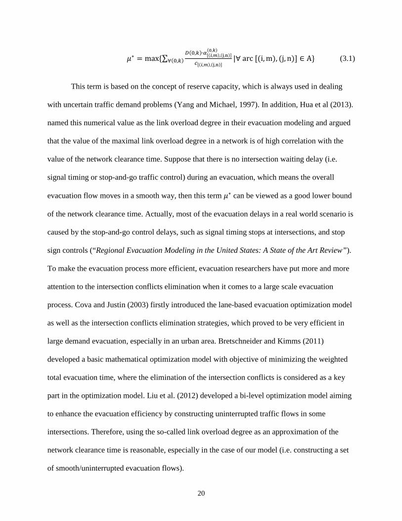
𝜇𝜇∗ = max {∑𝐷𝐷(0,𝑘𝑘)∙𝛼𝛼[(𝑖𝑖,𝑚𝑚),(j,n)]
(0,𝑘𝑘)
𝑐𝑐[(𝑖𝑖,𝑚𝑚),(j,n)]∀(0,𝑘𝑘) |∀ arc [(i, m), (j, n)] ∈ A} (3.1)
This term is based on the concept of reserve capacity, which is always used in dealing
with uncertain traffic demand problems (Yang and Michael, 1997). In addition, Hua et al (2013).
named this numerical value as the link overload degree in their evacuation modeling and argued
that the value of the maximal link overload degree in a network is of high correlation with the
value of the network clearance time. Suppose that there is no intersection waiting delay (i.e.
signal timing or stop-and-go traffic control) during an evacuation, which means the overall
evacuation flow moves in a smooth way, then this term 𝜇𝜇∗ can be viewed as a good lower bound
of the network clearance time. Actually, most of the evacuation delays in a real world scenario is
caused by the stop-and-go control delays, such as signal timing stops at intersections, and stop
sign controls (“Regional Evacuation Modeling in the United States: A State of the Art Review”).
To make the evacuation process more efficient, evacuation researchers have put more and more
attention to the intersection conflicts elimination when it comes to a large scale evacuation
process. Cova and Justin (2003) firstly introduced the lane-based evacuation optimization model
as well as the intersection conflicts elimination strategies, which proved to be very efficient in
large demand evacuation, especially in an urban area. Bretschneider and Kimms (2011)
developed a basic mathematical optimization model with objective of minimizing the weighted
total evacuation time, where the elimination of the intersection conflicts is considered as a key
part in the optimization model. Liu et al. (2012) developed a bi-level optimization model aiming
to enhance the evacuation efficiency by constructing uninterrupted traffic flows in some
intersections. Therefore, using the so-called link overload degree as an approximation of the
network clearance time is reasonable, especially in the case of our model (i.e. constructing a set
of smooth/uninterrupted evacuation flows).
20

3.3.2 Total Travel Time
Travel time of a particular evacuee during an evacuation is defined as the time period it
takes to travel out of the emergency region. In other words, the travel time of an evacuee is
calculated as the time difference between its network-loading time point and the safety-arrival
time point. This term can be further described by the following equation with the aforementioned
notations,
Ttraverse(𝑠𝑠) = ∑ 𝑠𝑠[(𝑖𝑖,𝑚𝑚),(j,n)][(𝑖𝑖,𝑚𝑚),(j,n)]∈𝑟𝑟 (3.2)
Where Ttraverse(𝑠𝑠) denotes the traveling time of route r. Here it is simply the summation
of the travel time of each roadway segments that is covered in route r. This is also called
leadtime in some network flow problems (Lin, Yi-Kuei, 2003). With the route travel time
calculated this way, the total travel time during an evacuation can be derived as,
𝑇𝑇𝑇𝑇 = ∑ 𝐷𝐷(0,𝑘𝑘) ∙ ∑ [𝛼𝛼[(𝑖𝑖,𝑚𝑚),(j,n)](0,𝑘𝑘) ∙ 𝑠𝑠[(𝑖𝑖,𝑚𝑚),(j,n)]][(𝑖𝑖,𝑚𝑚),(j,n)]∈𝐴𝐴(0,𝑘𝑘)∈𝑁𝑁𝑠𝑠 (3.3)
Where 𝐷𝐷(0,𝑘𝑘) is the evacuation demand of source (0,k), and the inner summation
∑ [𝛼𝛼[(𝑖𝑖,𝑚𝑚),(j,n)](0,𝑘𝑘) ∙ 𝑠𝑠[(𝑖𝑖,𝑚𝑚),(j,n)]][(𝑖𝑖,𝑚𝑚),(j,n)]∈𝐴𝐴 associates the route evacuation time with decision variable
𝛼𝛼[(𝑖𝑖,𝑚𝑚),(j,n)](0,𝑘𝑘) .
The total travel time is always a significant performance measure in traffic assignment
problem, where the objective is minimizing the total travel time among the overall demand to
reach a system optimal condition. However, the link travel time 𝑠𝑠[(𝑖𝑖,𝑚𝑚),(j,n)] is usually of high
variance and cannot be deemed as a constant in the general traffic assignment problem since the
traffic control level is relatively low (i.e. the traffic demand is always loaded into the network
simultaneously and every single vehicle is thought to be greedy). But the evacuation operation is
21

quite different with the case in general traffic assignment problems. Due to the large evacuation
demand and limited egress, the traffic managers or operation authorities always take a high level
of traffic control during the evacuation process in order to avoid the “traffic explosion”. In other
words, to provide the maximal network throughput per time unit, the emergency authorities
always expect the evacuation flow travels exactly at the capacity of the roadway segments in the
planning stage. Hence, it is realistic to fix the link travel time as its capacity travel time when we
are planning an evacuation, and this is always the case in the evacuation research literature.
3.3.3 Total In-Network Time
Here we define another time measure of an evacuation process, i.e. total in-network time.
Just as it literally indicates, the in-network time of a specific evacuee is the total duration it takes
to get out the emergency area or reach to its safety destination since the evacuation process starts.
Different with the definition of the travel time in the above paragraph, the in-network time of a
specific evacuee additionally includes the preparation time and loading waiting delay for this
evacuee to get into its egress route at its source. As is illustrated in Figure 3-5, the total in-
network time is exactly the integral of the non-arrival demand curve in terms of the evacuation
duration. Suppose that every evacuee is able to load into the network in a very short time period
(i.e. ignore the preparation stage). It is noted that when the evacuation demand is relatively small
against the evacuation network, in which case all of the evacuees can start their evacuation
simultaneously, there is no waiting delay for loading resulting from the limited network capacity.
Hence, the total in-network time will be equal to the total travel time discussed in the previous
paragraph. However, this is not always the case in the real-world large-scale evacuation scenario,
where the evacuation demand is large and the network capacity is very limited (Chen. et. at.
2006 and Chien. et al. 2007). Thus, a stage based evacuation strategy must be taken, and the
22

waiting delay no longer can be ignored (like the case of Liu et al. 2006). In many real-world
cases, the waiting delay of a particular evacuee is even several times of its in-network travel time
to its destination.
Total In-Network Time
Figure 3-5: Representation of total in-network time and network clearance time with respect to a general evacuation curve
In our basic mathematical model, we assume the preparation time of each evacuee can be
ignored in comparison with the average loading waiting delay and the evacuation traveling time.
Therefore, the total in-network time can be analytically derived as two parts, one is the loading
waiting delay and the other one is the total evacuation traveling time. The calculation of total
evacuation traveling time can just be achieved by using equation (3.3). Here we only need to
derive the formula to calculate the total loading waiting delay.
From the perspective of basic network flow problem, the average loading waiting delay
of a specific source is determined (or constrained) by the bottleneck capacity on its egress route.
We further assume the serving time of an arc can be approximately equal to the ratio of its
0
100
200
300
400
500
600
700
800
900
1000
0 2 4 6 8 1 0 1 2 1 4 1 6 1 8 2 0 2 2 2 4 2 6 2 8 3 0
Dem
and
with
in E
vacu
atio
n Re
gion
Time Duration
N U M B E R O F I N - N E T W O R K E V A C U E E V . S . T I M E D U R A T I O N
Total In-Network Time
Network Clearance Time
23

accumulative demand and its capacity (as is calculated in equation 3.4). This is also referred as
the reserve capacity of a network link, which is always used in uncertain traffic demand
assignment problem (Hai et al. 1997)
𝑇𝑇𝑠𝑠𝑠𝑠𝑟𝑟𝑠𝑠𝑠𝑠([(𝑒𝑒,𝑖𝑖), (j, n)]) = ∑ 𝐷𝐷(0,𝑘𝑘)∙𝛼𝛼[(𝑖𝑖,𝑚𝑚),(j,n)]
(0,𝑘𝑘)(0,𝑘𝑘)∈𝑁𝑁𝑠𝑠
𝑐𝑐[(𝑖𝑖,𝑚𝑚),(j,n)] (3.4)
This physical meaning of term is not difficult to understand. It is just the time duration
that roadway segment [(i,m), (j,n)] is consistently used by a set of traverse demand
∑ 𝐷𝐷(0,𝑘𝑘) ∙ 𝛼𝛼[(𝑖𝑖,𝑚𝑚),(j,n)](0,𝑘𝑘)
(0,𝑘𝑘)∈𝑁𝑁𝑠𝑠 . For a real-world scenario with uninterrupted evacuation traffic
flows, this formula is valid and can be directly used to identify the route bottleneck. This is
because for an uninterrupted evacuation flow scenario every roadway link is consistently serving
its traffic demand. In other words, a serving gap between two groups of arrival demand does not
exist. Moreover, this concept can also be applied to a scenario with interrupted traffic flows (e.g.
traffic conflicts at an intersection), and only some adjustments need to be made at these conflict
points. For instance, at an intersection with signal timing control to avoid two movement
conflicts (e.g. northbound traffic versus westbound traffic), we can divide and allocate the
intersection capacity to these two traffic routes according to the signal timing ratio. Hence we
can conceptually assume that each arc is still consistently serving its arrival demands during the
whole evacuation process. Therefore, the average waiting delay (e.g. minute/veh) for a source
with egress route r can be derived as:
𝐸𝐸[𝑇𝑇𝑇𝑇(𝑠𝑠)} = 12∙ max {∑ 𝐷𝐷(0,𝑘𝑘) ∙ 𝛼𝛼[(𝑖𝑖,𝑚𝑚),(j,n)]
(0,𝑘𝑘) ∙ 1𝑐𝑐[(𝑖𝑖,𝑚𝑚),(j,n)]
(0,𝑘𝑘)∈𝑁𝑁𝑠𝑠 |∀[(𝑒𝑒,𝑖𝑖), (j, n)] ∈ 𝑠𝑠} (3.5)
Equation (3.5) can be further interpreted as, if an evacuee (e.g. vehicle) is going to traverse route
r to reach its safety destination, then 𝐸𝐸[𝑇𝑇𝑇𝑇(𝑠𝑠)} gives the expected value that how long should
24
this evacuee wait to get loaded onto this route. This expected estimation is valid based on two
assumptions:
(1) The linear relationship between the link serving time and its arrival demand (i.e. the
capacity of each link is unchanged);
(2) Each roadway link is consistently serving its arrival demand during the evacuation
process (i.e. uninterrupted evacuation flow, at most merge and diverge are accepted).
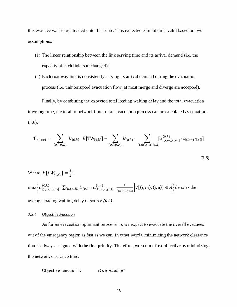
Finally, by combining the expected total loading waiting delay and the total evacuation
traveling time, the total in-network time for an evacuation process can be calculated as equation
(3.6).
Tin−net = � 𝐷𝐷(0,𝑘𝑘) ∙ 𝐸𝐸[TW(0,k)](0,𝑘𝑘)∈𝑁𝑁𝑠𝑠
+ � 𝐷𝐷(0,𝑘𝑘) ∙ � [𝛼𝛼[(𝑖𝑖,𝑚𝑚),(j,n)](0,𝑘𝑘) ∙ 𝑠𝑠[(𝑖𝑖,𝑚𝑚),(j,n)]]
[(𝑖𝑖,𝑚𝑚),(j,n)]∈𝐴𝐴(0,𝑘𝑘)∈𝑁𝑁𝑠𝑠
(3.6)
Where, 𝐸𝐸[𝑇𝑇𝑇𝑇(0,𝑘𝑘)] = 12∙
max �𝛼𝛼[(𝑖𝑖,𝑚𝑚),(j,n)](0,𝑘𝑘) ∙ ∑ 𝐷𝐷(𝑞𝑞,𝑡𝑡) ∙ 𝛼𝛼[(𝑖𝑖,𝑚𝑚),(j,n)]
(𝑞𝑞,𝑡𝑡) ∙ 1𝑐𝑐[(𝑖𝑖,𝑚𝑚),(j,n)]
(𝑞𝑞,𝑡𝑡)∈𝑁𝑁𝑠𝑠 �∀[(𝑒𝑒,𝑖𝑖), (j, n)] ∈ 𝐴𝐴� denotes the
average loading waiting delay of source (0,k).
3.3.4 Objective Function
As for an evacuation optimization scenario, we expect to evacuate the overall evacuees
out of the emergency region as fast as we can. In other words, minimizing the network clearance
time is always assigned with the first priority. Therefore, we set our first objective as minimizing
the network clearance time.
Objective function 1: 𝑀𝑀𝑒𝑒𝑒𝑒𝑒𝑒𝑖𝑖𝑒𝑒𝑀𝑀𝑠𝑠: 𝜇𝜇∗
25

From another perspective, the throughput of the evacuation network is also expected to
be maximized during the evacuation process. Since the severity of the emergency hazard or risk
is relatively low at the beginning of the evacuation, it is always rational and reasonable to
evacuate the people intensively during this early time period. This is sort of the concept of
greedy algorithm that if we are not quite confirmed when there will be a “deadly hazards
explosion”, what we are preferring to do is to evacuate as many people as we can from the time
point the evacuation alarm is distributed. As is illustrated in Figure 3-6, if there are two
independent evacuation plans named Plan 1 and Plan 2, which have the same network clearance
time, absolutely Plan 2 is much better than Plan 1 since its total in-network time is much lower.
In other words, Plan 2 guarantees we can evacuate many more people earlier.
Figure 3-6: An example that two evacuation plan having same network clearance time but different total in-network time
Therefore, we set our second objective function as minimizing the total in-network time.
Objective function 2: 𝑀𝑀𝑒𝑒𝑒𝑒𝑒𝑒𝑖𝑖𝑒𝑒𝑀𝑀𝑠𝑠: Tin−net
0100200300400500600700800900
1000
1 3 5 7 9 11 13 15 17 19 21 23 25 27 29 31
Dem
and
Still
In E
meg
renc
y Ar
ea
Time Duration
In-Network demand of two evacuation plans with the same network clearance time
Plan 1
Plan 2
26

It is noted that the total in-network time also includes the total travel time during the
evacuation process as we discussed in the previous section. In addition to the total evacuation
travel time, the total in-network time also contains the total expected loading waiting delay,
which is determined by the O-D routes’ bottlenecks.
3.3.5 Constraints
Constraints of this model can be classified into three classes. The first class of constraints
is related to the evacuation route connectivity and destination capacity limitation, and the second
class of constraints deals with the intersection conflicts elimination. Finally, the third class of
constraints further guarantees the routing consistency within intersection.
Before going through the description of constraints, the solution structure is necessary to
be illustrated first. As is declared at the beginning of this chapter, the routing optimization model
here aims to come up with a set of efficient evacuation routes to cope with the evacuee demand
in one or multiple sources. First of all, we must guarantee that for each evacuee demand source,
there must be at least one egress route assigned to it so that the evacuees can be successfully
evacuated out. Exactly one egress route might be effective to a specific evacuation source if the
total demand of this source is not that high (e.g. several hundreds of vehicles). However, when
the evacuation demand in a particular source with multiple egresses is relatively high, only one
evacuation route is likely to impede the evacuation efficiency. Hence, we need to make our
routing optimization model capable of coming up with multiple evacuation routes for a particular
source if it is necessary. To achieve this goal, we can take advantage of a simple network
representation technique. The traditional method to represent a source within a network is just
abstract it as a single network node with a provided demand. Here we can choose to duplicate a
specific source as multiple dummy nodes. They have the same geographical information but only
27

the demand on each duplicated dummy node changes. As is shown in Figure 3-7, if we divide a
single source node into four geographically identical dummy source nodes and use our routing
optimization model to calculate based on this revised network, we can come up with at most four
different evacuation routes for the original source. Further, if the optimized routes for all of the
duplicated dummy nodes are the same, we conclude that the best routing plan for this original
source is to use only one egress route. Putting it this way, we are able to use the most basic
network connectively constraints to guarantee that there is at least one outgoing rout for each of
the evacuation source.
Figure 3-7: Method of transform a single source node into several parallel dummy nodes
First Class Constraints (Route Connectivity and Destination Capacity):
� α[(0,k)(j,n)](0,k)
(j,n)∈µ−[(0,k)]
= 1
for each source node (0, k) (1)
egress 1
egress 2
egress 3
egress 4
egress 1
egress 2
egress 3
egress 4
source 1 source 1-1
source 1-2
source 1-3 source 1-4
Duplicate a single source to four identical dummy sources Single Source Node
28

� α[(j,n),(i,m)](0,k) −
(j,n)∈µ+[(i,m)]
� α[(i,m),(j,n)](0,k)
(j,n)∈µ−[(i,m)]
= 0
for each source node (0, k), and each transshipment node (i, m) of (0, k) (2)
� α[(i,m)(j,n)](0,k)
(i,m)∈µ+[(j,n)]
= 1
for each (0, k) ∈ Ns, and (j, n) equal to N0 (3)
� � 𝐷𝐷(0,𝑘𝑘)α[(i,m)(j,n)](0,k)
(i,m)∈µ+[(j,n)]∀(0,𝑘𝑘)
≤ 𝐶𝐶(𝑗𝑗,𝑛𝑛)
for each (j, n) ∈ Nd (4)
It is noted that the source node (0,k) mentioned in the above formulations can either be an
original source node or a duplicated dummy source node. This is up to the abstracted network
structure. Notations 𝜇𝜇−[(𝑒𝑒,𝑖𝑖)] and 𝜇𝜇+[(𝑒𝑒,𝑖𝑖)], respectively, represent set of successor nodes and
set of predecessor nodes of node (i,m). Constraint (1) guarantees that for each source node, there
is exactly one route outgoing from it. Constraint (2) indicates that, for each transshipment node,
if a route goes into it, then the route must go out. Constraint (3) guarantees that for each source
node there must be a sink node allocated to it. Constraints together (1-3) say that for each source
node there is exactly one egress route linking it to a sink node. Constraint (4) limits the allocated
evacuee demand at a specific exit point by considering the capacity of this destination node (e.g.
shelter capacity or exiting freeway capacity).
Second Class Constraints (Movement Conflicts Elimination)
As is discussed at the beginning of this chapter, most of the evacuation delays and
inefficiencies are coming from stop-and-go controls, especially in an urban area. However, many
29

of the evacuation optimization studies ignored the significant role of intersection or freeway
interchanges, and they just deemed the intersection as a network node in their modeling. The
optimization results of the models that treat the issue this way might be far more inaccurate in
comparison with that in a real world scenario. For instance, turn movements at an intersection
are always operating at a much lower speed. Thus, too many turn movements at an intersection
make the intersection a bottleneck. This fact can never be recognized if the intersection is just
simplified as a network node. As a consequence, more and more researchers in the evacuation
literature are beginning to consider how to construct uninterrupted evacuation flows in terms of
intersection control, which is proved to greatly shorten the evacuation process, e.g. Cova and
Johnson (2003), Xie et al. (2010), Bretschneider and Kimms (2011), Liu and Luo (2012).
Bretschneider and Alf Kimms (2011) first presented a mathematical formulation of the
intersection conflicts elimination in terms of the intersection-related constraint described in Cova
and Justin (2003). The model here takes advantage of the work in Bretschneider and Alf Kimms
(2011) and presents a more general form of the conflicts elimination constraints.
γ[(i,m),(i,n)] + γ[(i,h),(i,k)] ≤ 1,∀h ∈ L[(i,m),(i,n)],∀k ∈ R[(i,m),(i,n)]
γ[(i,m),(i,n)] + γ[(i,h),(i,k)] ≤ 1,∀h ∈ R[(i,m),(i,n)],∀k ∈ L[(i,m),(i,n)]
for each intersection node (i, m), and ∀n ∉ {(m mod θi) + 1, (θi + m − 2)modθi + 1}
(5)
Constraints (5) guarantee that there are no movement conflicts depicted in Figure 3-8, i.e.
conflict between two arcs with no common nodes. The above inequality equations are suitable
for any general intersections. In other words, they are applicable to intersections with four or
more legs. (In real world situations, a four-leg intersection is more common).
30

Figure 3-8: Arcs that conflict with arc [(i,m),(i,n)] with no common nodes
γ[(i,m),(i,n)] + γ[(i,h),(i,k)] ≤ 1,∀ k ∈ L[(i,n),(i,m)] and h = n
for each intersection node (i, m), and ∀n ≠ (θi + m − 2)modθi + 1 (6)
γ[(i,m),(i,n)] + γ[(i,h),(i,k)] ≤ 1,∀ h ∈ L[(i,n),(i,m)] and k = m
for each intersection node (i, m), and ∀n ≠ (θi + m − 2)modθi + 1 (7)
Constraints (6) and (7) eliminate the movement conflicts of the type depicted in Figure 3-9,
i.e. conflict between two arcs with exactly one common node (i.e. straight versus left turn or left
turn versus left turn). The above inequalities are suitable for any general intersection. In other
words, they are applicable to intersections with three or more legs. (In real world situations,
three-leg and four-leg intersections are more common. Five or more leg intersections are not
common but can be seen in some urban areas, e.g. Downtown of Washington D.C.)
31

Figure 3-9: Arcs that conflict with arc [(i,m),(i,n)] with exactly one common node
In addition, to maintain the routing consistency within a controlled intersection,
constraints (9) with the introduction of a big number M are added to the model (i.e. if an
intersection arc is prohibited then it cannot be used by any route).
� 𝛼𝛼[(𝑖𝑖,𝑚𝑚),(𝑖𝑖,𝑛𝑛)](0,𝑘𝑘)
(0,𝑘𝑘)∈𝑁𝑁𝑠𝑠
≤ 𝑀𝑀 ∙ 𝛾𝛾[(𝑖𝑖,𝑚𝑚),(𝑖𝑖,𝑛𝑛)],
for each intersection arc [(𝑒𝑒,𝑖𝑖), (𝑒𝑒,𝑒𝑒)] within intersection i (9)
𝛼𝛼[(𝑖𝑖,𝑚𝑚),(j,n)](0,𝑘𝑘) and 𝛾𝛾[(𝑖𝑖,𝑚𝑚),(𝑖𝑖,𝑛𝑛)] ∈ {0,1} (10)
3.4 Solution Approach
Due to the bi-level characteristics and nonlinearity of the objective functions
demonstrated above, the optimization problem cannot be directly solved with the current
algorithms implemented in LP solvers, e.g. CPLEX, Gurobi, etc. Hence, a specific solution
approach for the optimization model is developed and introduced in this section. To begin with,
the bi-level objective functions are recalled here:
32

Objective function 1, MINIMIZE:
𝜇𝜇∗ = max { �𝐷𝐷(0,𝑠𝑠) ∙ 𝛼𝛼[(𝑖𝑖,𝑚𝑚),(j,n)]
(0,𝑘𝑘)
𝑒𝑒[(𝑖𝑖,𝑚𝑚),(j,n)]∀(0,𝑘𝑘)
|∀ arc [(i, m), (j, n)] ∈ A}
Objective function 2, MINIMIZE:
Tin−net = � 𝐷𝐷(0,𝑘𝑘) ∙ 𝐸𝐸[TW(0,k)](0,𝑘𝑘)∈𝑁𝑁𝑠𝑠
+ � 𝐷𝐷(0,𝑘𝑘) ∙ � [𝛼𝛼[(𝑖𝑖,𝑚𝑚),(j,n)](0,𝑘𝑘) ∙ 𝑠𝑠[(𝑖𝑖,𝑚𝑚),(j,n)]]
[(𝑖𝑖,𝑚𝑚),(j,n)]∈𝐴𝐴(0,𝑘𝑘)∈𝑁𝑁𝑠𝑠
Where, 𝐸𝐸[𝑇𝑇𝑇𝑇(0,𝑘𝑘)] = 12∙ max �𝛼𝛼[(𝑖𝑖,𝑚𝑚),(j,n)]
(0,𝑘𝑘) ∙ ∑ 𝐷𝐷(𝑞𝑞,𝑡𝑡) ∙ 𝛼𝛼[(𝑖𝑖,𝑚𝑚),(j,n)](𝑞𝑞,𝑡𝑡) ∙ 1
𝑐𝑐[(𝑖𝑖,𝑚𝑚),(j,n)](𝑞𝑞,𝑡𝑡)∈𝑁𝑁𝑠𝑠 �∀[(𝑒𝑒,𝑖𝑖), (j, n)] ∈ 𝐴𝐴�
Observing the structure of the first objective function (i.e. minimizing the network
clearance time), we can understand that 𝜇𝜇∗ represents the total serving time of the network
bottleneck, which is exactly the link having the largest total serving time in the evacuation
process. In other words, we are minimizing the upper bound of the total serving times among the
overall network links. Thus, we can introduce an upper bound T in terms of the total serving time
for each link and aggregate these newly inequalities into our constraints pool.
1𝑐𝑐[(𝑖𝑖,𝑚𝑚),(j,n)]
∙ ∑ 𝐷𝐷(0,𝑘𝑘) ∙ 𝛼𝛼[(𝑖𝑖,𝑚𝑚),(𝑖𝑖,𝑛𝑛)](0,𝑘𝑘)
(0,𝑘𝑘)∈𝑁𝑁𝑠𝑠 ≤ T,∀[(𝑒𝑒,𝑖𝑖), (𝑒𝑒, 𝑒𝑒)] ∈ 𝐴𝐴 (11)
At this time point (i.e. eliminating the first objective function by adding a set of new constraints),
we obtain a sub-problem with regard to a particular T. For each sub-problem, this pre-fixed
upper bound T is exactly the term we want to minimize in our original problem (i.e. the network
clearance time). In each sub-problem, inequality constraints (11) guarantee that the total serving
time of each evacuation link is bounded by duration T. Actually this can be viewed as another
way to mitigate the routing congestion.
33

Now let us observe the structure of the second objective function (i.e. minimizing the
total in-network time). This objective function consists of two independent parts, the first one is
the total loading waiting time that is determined by the egress routes’ arrival demand, and the
second one is the total evacuation travel time that only is determined by the routes’ length. After
introducing the new sets of upper bound constraints to the original problem, we can see that a
pre-fixed upper bound T not only limits the total serving time of the network bottleneck (i.e.
network clearance time), but also put a limit to the total serving time of each individual link. It is
just the total serving time of each individual link that determines the expected total loading
waiting delay expressed as the first part of objective function 2. Putting it another way, a lower
pre-fixed upper bound T in constraints (11) not only lowers the network clearance time, but also
automatically reduces the expected total loading waiting delay as a part of objective function 2.
Therefore, if we introduced a pre-fixed upper bound T as the constraints for each individual link,
we can simply use the total travel time as our sub-problem’s performance indicator. Hence, a
linear sub-optimization problem with regard to a pre-fixed T can be written as below,
Objective function:
𝑀𝑀𝑒𝑒𝑒𝑒𝑒𝑒𝑖𝑖𝑒𝑒𝑀𝑀𝑠𝑠: � 𝐷𝐷(0,𝑘𝑘) ∙ � [𝛼𝛼[(𝑖𝑖,𝑚𝑚),(j,n)](0,𝑘𝑘) ∙ 𝑠𝑠[(𝑖𝑖,𝑚𝑚),(j,n)]]
[(𝑖𝑖,𝑚𝑚),(j,n)]∈𝐴𝐴(0,𝑘𝑘)∈𝑁𝑁𝑠𝑠
Subject to:
Constraints: (1) - (10), and,
1𝑐𝑐[(𝑖𝑖,𝑚𝑚),(j,n)]
∙ ∑ 𝐷𝐷(0,𝑘𝑘) ∙ 𝛼𝛼[(𝑖𝑖,𝑚𝑚),(𝑖𝑖,𝑛𝑛)](0,𝑘𝑘)
(0,𝑘𝑘)∈𝑁𝑁𝑠𝑠 ≤ T,∀[(𝑒𝑒,𝑖𝑖), (𝑒𝑒, 𝑒𝑒)] ∈ 𝐴𝐴 (11)
Intuitively speaking, when the evacuation demand is very large, a relatively small T of
each link is more attractive to the system optimization. This indicates that the evacuation demand
34

is distributed more evenly among the network links such that the total loading waiting delay will
correspondingly decrease. Instead, the sub-optimization problem with a large T only seeks for
the shortest evacuation route of each evacuation source, regardless of the loading waiting delay.
Thus, we can start to solve the sub-optimization problem with a relatively small T and iteratively
increase it until each of the sources chooses the shortest path to the destination. By solving and
comparing each of these sub-optimization problems, we are guaranteed to find a close-to optimal
solution to the original bi-level nonlinear programming model. The calculation process is further
described in Figure 3-10.
35

Figure 3-10: Flow Chart of the Routing Optimization Solution Approach
Sub-optimization Problem with T
Infeasible?
LP Solver
Start 𝑇𝑇 = 𝑇𝑇0
𝑇𝑇 = 𝑇𝑇 + ∆𝑠𝑠
T >T*?
Terminate
Record the Sub-Optimal Solution
Pick the Sub-Optimal Solution with Least Total In-Network Time and T
Y
Y
N
N
36

Chapter 4 : Scheduling Optimization Model
4.1 Introduction
The optimization model in Chapter 3 generates a set of evacuation route(s) for each
source from a macroscopic perspective. Since the evacuation demand is high, the overall
demand cannot realistically be loaded into the network simultaneously. Thus, a scheduling
strategy based on which the demand is efficiently discharged is necessary. This chapter aims to
develop an optimal scheduling model to further determine the departure rate of each source.
There are two types of methodology that optimally determine the scheduling information: a
linear programming approach based on a time-space network, and a heuristic approach. In
considering the high evacuation demand (e.g. millions of vehicles), which will need an extremely
large time-space network, the heuristic approach proves to be more efficient in dealing with such
an optimization problem (Lu et al. (2005)).
Lu et al. (2005) propose an optimal algorithm to solve routing and scheduling
optimizations with the objective of minimizing the total evacuation time in a capacitated network.
The experimental tests on this algorithm present pretty good results. Although they claim this
algorithm is suitable in an evacuation scenario, they do not provide any specific evacuation
scenarios that can directly adopt it. However, in terms of the evacuation situation studied in this
paper (i.e. vehicle based evacuation), the algorithm will be invalid due to two reasons: (1)
conflicted traffic flows cannot move on simultaneously at an intersection, and (2) the network
node (i.e. intersection or freeway interchange) is not able to store any demand (evacuee vehicles).
In other words, in the highway-based evacuation scenario, once a group of vehicles is loaded into
the network, they have to move until reaching their destination. This is quite different from the
37
scenario of a building evacuation, in which a demand group can be temporarily stored in a
transshipment node (e.g. a big space in the building). Therefore, based on their greedy
scheduling concepts, we developed a simulation based scheduling heuristic to dynamically
determine the discharge rate for each source. The output of routing optimization model in
Chapter 3 are set as the input of this heuristic. Moreover, in order to be more realistic, the
interplays among traffic flow are incorporated in this heuristic by attaching a mesoscopic traffic
simulator. The corresponding traffic simulator and algorithm are described separately in the
following sections.
4.2 Traffic Simulator
For the scheduling heuristic, a mesoscopic traffic simulator implemented by Afshar and
Haghani (2008) is taken advantage of in this chapter. The Pseudo code of the traffic simulator is
described in Table 4-1.
4.3 Scheduling Heuristic
Before introducing the scheduling heuristic, some necessary assumptions are made as shown
below.
Assumptions:
1) Roadway capacity is constant, which is equal to the traffic flow at the critical density;
2) Evacuation priority of each source is predefined, and the evacuation priority ranking
approaches can be referred to in Church and Cova (2000);
38

Table 4-1: Pseudo Code of the Traffic Simulator
Load network
Load demand (Loading vehicles from each Source)
For each time interval t,
For each link a,
Identify number of vehicles entering the link from each O-D path
Identify number of vehicles leaving the link to their O-D path
Identify number of vehicles present in the link
Calculate link travel time by Equation (4.1)
Assign exit time to vehicles entering link in current t
Next Link
Next t, unless all vehicles have reached their destinations
𝑒𝑒𝑖𝑖 = �𝑒𝑒𝑓𝑓 − 𝑒𝑒𝑚𝑚𝑖𝑖𝑛𝑛� ∙ �1 − 𝛼𝛼 � 𝑘𝑘𝑖𝑖𝑘𝑘𝑗𝑗𝑗𝑗𝑚𝑚
�𝛽𝛽� + 𝑒𝑒𝑚𝑚𝑖𝑖𝑛𝑛 (4.1)
Where,
𝑒𝑒𝑖𝑖 = speed on link 𝑒𝑒 𝑒𝑒𝑓𝑓 = free flow speed on link 𝑒𝑒
𝑒𝑒𝑚𝑚𝑖𝑖𝑛𝑛 = minimum speed on link 𝑒𝑒
𝑠𝑠𝑖𝑖 = density on link 𝑒𝑒
𝑠𝑠𝑗𝑗𝑗𝑗𝑚𝑚 = jam density on link 𝑒𝑒
𝛼𝛼,𝛽𝛽 are sensitivity parameters
39

It is noted that this traffic simulator assumes vehicle speed on a particular link, which
only depends on the prior and prevailing conditions of that link; traffic entering at a later time
does not affect the travel speed of the vehicles already in the link.
In the above assumptions, the first one indicates that the roadway capacity is only
determined by its geometry characteristics, i.e. number of lanes and free flow speed. It is always
a fixed value during the flow dynamics. However, the roadway throughput is affected by the
amount of traffic flow on it. As for the second assumption, the evacuation priority of each
separate source is usually predefined according to their vulnerability. For example, in a hurricane
or flood evacuation, the sources within the coastal area are always considered with a high
evacuation priority since these areas are more vulnerable to the disasters.
As for the demand discharging process, we expect to make full use of the network
capacity, since this can make the network provide the largest throughput. However, if the
discharging rate is too high, the network will suffer a big congestion, which will in turn result a
larger network clearance time. Therefore, the core is to find an appropriate time-dependent
discharging rate for each source. In Chapter 3 we show that the maximal throughput of a specific
route is determined by its bottleneck. The bottleneck of a specific route is identified by
considering both its future arrival demand and its capacity. Here we define the bottleneck of a
specific route r as,
𝑟𝑟(r) = max {∑𝐷𝐷(𝑟𝑟)𝑒𝑒(𝑟𝑟)
|𝑟𝑟 ∈ 𝑠𝑠}
where, ∑𝐷𝐷(𝑟𝑟) is the total un-arrived demand of arc l and c(l) denotes the capacity of this arc.
With this type of concept, the dynamic network loading heuristic is provided in Table 4-2.
40

Table 4-2: Pseudo Code of the Proposed Simulation based Scheduling Heuristic
Algorithm: Simulation-Based Capacity Constrained Scheduling Algorithm
Phase I (Initialization):
Input and Preprocessing:
1) Directed Network 𝐆𝐆(𝐍𝐍,𝐀𝐀) with a set of nodes N and a set of arcs A;
2) Set of evacuation routes 𝑹𝑹 = {𝑹𝑹(𝒏𝒏)|𝒏𝒏 ∈ 𝑵𝑵𝒔𝒔}, where 𝐑𝐑(𝐧𝐧) = {𝐚𝐚𝐧𝐧𝟏𝟏 ,𝐚𝐚𝐧𝐧𝟐𝟐 ,⋯ ,𝐚𝐚𝐧𝐧𝐤𝐤} and
𝐚𝐚𝐧𝐧𝐤𝐤 ∈ 𝑨𝑨;
3) Demand 𝐃𝐃(𝐧𝐧) of each route;
4) Evacuation priority 𝐏𝐏(𝐧𝐧) of each source (route);
5) Capacity 𝒄𝒄(𝐚𝐚𝒌𝒌) of each arc 𝐚𝐚𝐤𝐤 ∈ 𝐀𝐀;
6) For each arc ak, initialize its serving sets 𝐒𝐒(𝐚𝐚𝐤𝐤) = {𝐧𝐧|∀𝐧𝐧 𝐚𝐚𝐧𝐧𝐚𝐚 𝐚𝐚𝐤𝐤 ∈ 𝐑𝐑(𝐧𝐧)} ;
7) Loading attraction factor for each source 𝛂𝛂 (usually greater than 1), and discharging
reduction factor 𝛃𝛃 (usually smaller than 1, but should be strictly smaller than 𝛂𝛂)
8) Heuristic Time interval ∆𝐭𝐭, during which a batch of vehicles will be discharged
9) Set the initial time point of the simulation with t = 0;
Notations in the calculation iteration:
(1) 𝑳𝑳(𝒏𝒏, 𝒕𝒕): Time-dependent maximal discharging rate of source n at time interval t
(2) 𝜽𝜽𝒂𝒂𝒌𝒌(𝒕𝒕): Time-dependent flow attraction factor of arc 𝐚𝐚𝐤𝐤
(3) 𝑫𝑫𝑫𝑫𝒔𝒔𝒄𝒄𝑫𝑫𝒂𝒂𝑫𝑫𝑫𝑫𝑫𝑫(𝒏𝒏, 𝒕𝒕): Number of vehicles discharged from source n during time
interval (𝒕𝒕, 𝒕𝒕 + ∆𝐭𝐭)
(4) 𝚪𝚪: Total number of vehicles getting out of the network by time point t
(5) 𝑨𝑨𝑫𝑫𝑫𝑫𝑫𝑫𝑨𝑨𝑫𝑫𝑨𝑨(𝒕𝒕 − ∆𝐭𝐭, 𝒕𝒕): Number of vehicles exiting the network within time interval
41

(𝒕𝒕 − ∆𝐭𝐭, 𝒕𝒕)
Phase II (Loading Iteration):
Do
Determine the flow attraction factors for each arc 𝐚𝐚𝐤𝐤 by using the following logics:
For each arc 𝐚𝐚𝐤𝐤 ∈ 𝑨𝑨:
If 𝐚𝐚𝐤𝐤 is congested (i.e. traffic density is over than its critical density):
Set 𝜽𝜽𝒂𝒂𝒌𝒌(𝒕𝒕) = 𝜷𝜷
Else
Set 𝜽𝜽𝒂𝒂𝒌𝒌(𝒕𝒕) = 𝜶𝜶
End
For each source n with route R(n) and demand 𝐃𝐃(𝐧𝐧) > 𝟎𝟎:
Determine its maximal potential discharging rate according to the capacity as
well as the flow attraction factor of each arc 𝐚𝐚𝐤𝐤 ∈ 𝐑𝐑(𝐧𝐧) by using the following
logic function:
𝑳𝑳(𝒏𝒏, 𝒕𝒕) = 𝐦𝐦𝐦𝐦𝐧𝐧 {𝜽𝜽𝒂𝒂𝒌𝒌(𝒕𝒕) ∙ 𝐜𝐜(𝐚𝐚𝐤𝐤)𝑷𝑷(𝒏𝒏)
∑ 𝑷𝑷(𝒏𝒏′) ∙ 𝟏𝟏{𝑫𝑫(𝒏𝒏′)>𝟎𝟎}𝒏𝒏′∈𝑺𝑺(𝒂𝒂𝒌𝒌) |∀ 𝐚𝐚𝐤𝐤 ∈ 𝑹𝑹(𝒏𝒏)}
Determine the amount of vehicles to be discharged from source n by using the
following logic:
𝑫𝑫𝑫𝑫𝒔𝒔𝒄𝒄𝑫𝑫𝒂𝒂𝑫𝑫𝑫𝑫𝑫𝑫(𝒏𝒏, 𝒕𝒕) = 𝐦𝐦𝐦𝐦𝐧𝐧 {𝑫𝑫(𝒏𝒏),𝑳𝑳(𝒏𝒏, 𝒕𝒕) ∙ ∆𝐭𝐭}
Update the remaining demand of source n:
𝑫𝑫(𝒏𝒏) = 𝑫𝑫(𝒏𝒏) −𝑫𝑫𝑫𝑫𝒔𝒔𝒄𝒄𝑫𝑫𝒂𝒂𝑫𝑫𝑫𝑫𝑫𝑫(𝒏𝒏, 𝒕𝒕)
End
Load the determined discharged vehicles into the simulation network;
42

Run Traffic Simulator for duration ∆𝐭𝐭;
Update the simulation clock by: 𝐭𝐭 = 𝐭𝐭 + ∆𝐭𝐭
Update and record the number of exiting vehicles by:
𝚪𝚪 = 𝚪𝚪 + 𝑨𝑨𝑫𝑫𝑫𝑫𝑫𝑫𝑨𝑨𝑫𝑫𝑨𝑨(𝒕𝒕 − ∆𝐭𝐭)
While: 𝚪𝚪 < ∑𝑫𝑫(𝒏𝒏)
A brief flow chart of this algorithm is demonstrated in Figure 4-1: Flow Chart of the
Simulation based Scheduling Heuristic.
In the above algorithm, two heuristic factors are introduced. They are, loading attraction
factor α and discharging reduction factor β. This is because even though the traffic congestion of
a specific route is due to the total arrived demand from multiple sources, these separate demands
might not be arriving at this bottleneck simultaneously, especially at the beginning of the
evacuation process. If we determine the discharge rate for these sources strictly according to the
capacity of their prescriptive routes, there might be capacity waste within some time period due
to the different arrival time of the flow from these sources. Thus, during the evacuation process,
we expect to fully make use of the roadway capacity by introducing this loading attraction factor
α. However, this might also cause traffic congestion if these flows nearly arrive at the same
network link simultaneously. Therefore, we additionally introduce the reduction factor β. It aims
to reduce the traffic congestion, which is caused by the loading attraction factor α. In other
words, if a link (not necessary the current bottleneck) suffers a traffic congestion, the reduction
factor will decrease the discharging rate of its sources below the normal condition in the next
iteration. In addition, the evacuation priority of each source is also taken advantaged of to
determine its discharging rate. The incorporation of the source specific priority in the loading
43

heuristic is simple. That is, the roadways’ capacities are divided and reserved for each of the
sources based on their weighted evacuation priorities. As is indicated in the above algorithm, a
source with a relatively high evacuation priority is usually assigned with a larger discharging rate
by reserving more roadway capacity for it. This is further illustrated in the numerical experiment
of the real world scenario at the end of Chapter 5.
44

Figure 4-1: Flow Chart of the Simulation-based Scheduling Heuristic
Relate each arc (roadway) with its on-
serving source
Adjust the flow attraction factor
according to its current traffic condition
Pick up the minimal reserved capacity for
each source and determine its
discharging amount in the next time slot
Reserve the capacity of each arc to each of its on-serving source based on evacuation
priority and flow attraction factor
Run Traffic Simulator to the next discharging decision
round
Update the unserved demand, arrived
demand and feedback the traffic condition on
each link
Start
All Demand get out
STOP and Output Results
N
Y
45
Chapter 5 : Case Study
5.1 Introduction
In this chapter, numerical experiments are conducted in terms of two scenarios. The first
case study is a based on a fabricated urban grid network with totally 16 intersections, 9
evacuation sources and 6 safety destinations. The second case study is conducted upon a real-
world scenario of Maryland Eastern Shore evacuation with pre-selected optional evacuation
networks and real-world demand. The experiment parameters and corresponding results analysis
are demonstrated and discussed in the following sections.
The computation experiment of the numerical study is in Windows 8.1 operating system
environment running on an X64-processor-based computer with CPU 2.60GHz and 6.00 GB
memory. The routing optimization model in Chapter 3 is implemented with C++ and
CPLEX_12.51 Concert in Visual Studio 2012. The scheduling simulation model in Chapter 4 is
implemented with C++ STL in Visual Studio 2012.
5.2 Case Study I
5.2.1 Problem Definition
A case study is conducted to test and demonstrate the aforementioned optimization model
with a fictional evacuation network described in Figure 5-1. There are a total of nine evacuation
sources and six safety destinations, i.e. sources: (0, 1), (0, 2), (0, 3), (0, 4), (0, 5), (0, 6), (0, 7), (0,
8) and (0, 9), and sinks: (20, 1), (20, 2), (20, 3), (20, 4), (20, 5), (20, 6). In addition, a dummy
sink node (0, 0) is constructed by linking a virtual arc from each safety destination. The travel
time and capacity on each virtual arc are assumed to be 0 and infinity, respectively. The
rectangle areas in Figure 5-1 represent intersections, and arcs within the rectangles indicate the
46

movement directions at the corresponding intersection. There are a total of 222 arcs and 69
nodes, including the dummy node in the example network. Without loss of generality, we
assume the capacity of each real roadway equals to 1,200 vehicles per hour. The corresponding
travel time on each intersection arc is three seconds; on each general roadway, it is one minute.
In addition, the evacuation demand on each source is equal to 300 vehicles. It is noted that the
routing optimization model does not consider lane reversal optimization. However, as is
explicitly shown, the six exit links can be fully taken advantage of during the evacuation process.
Therefore, in the following calculation, we double the capacity of each exit link. In other words,
we assume no traffic flow gets into the network through the evacuation via the exit links.
Figure 5-1: Evacuation Network of Case Study 1
47

5.2.2 Demonstration of the Routing Optimization Procedure
At the beginning of the optimization process, we first transform the original routing
optimization model into numerous sub-optimization problems. To solve the problem with high
resolution, we use the time unit minutes instead of hours. The iterative results of the
corresponding optimization process are described in Table 5-1 and Figure 5-2. In addition, details
of each routing plan are described in Table 5-2, Table 5-3, Table 5-4 and Table 5-5.
Table 5-1: Optimized Routing Plan for each T (network clearance time)
T (minutes or iterations)
Solution Status
Routing Plan Total Waiting Delay
Total Travel Time
Total Evacuation
Time 0 ~ 30 Infeasible N/A N/A N/A N/A 30 ~ 44 Feasible Routing Plan
1 34875 9915 44790
45 ~ 59 Feasible Routing Plan 2
49500 9600 59100
60 ~ 67 Feasible Routing Plan 3
63000 9600 72600
68 ~ 134 Feasible Routing Plan 4
42750 9600 52350
135 + Feasible Routing Plan 3
63000 9600 72600
48

Figure 5-2: Optimal Value versus Different T
With the above iteration results, a sub-optimal solution is found, i.e. routing plan 1.
Although routing plan 1 has a relatively larger total travel time than the other three plans, the
total waiting delay of this plan is significantly smaller. Therefore, routing plan 1 is chosen as the
ultimate optimal solution from the perspective of total evacuation time. However, routing plan 1
cannot be explicitly proved to be the optimal solution of the original nonlinear binary
programming problem, but it is satisfactory enough since it reduces the total evacuation time by
nearly 40 percent in comparison with the shortest path evacuation strategy (i.e. Routing Plan 3).
0
10000
20000
30000
40000
50000
60000
70000
80000
1 9 17 25 33 41 49 57 65 73 81 89 97 105
113
121
129
137
145
min
utes
T (Network Clearance Time)
Total Waiting Delay
Total Travel Time
Total Evacuation Time
49

Table 5-2: Routing Plan 1 for Case Study 1
Source
Node Route Bottleneck
(0,1) (0, 1)->(10, 1)->(10, 4)->(1, 2)->(1, 3)->(20, 1)->(0, 0) (10,4)->(1,2)
(0,2) (0, 2)->(1, 1)->(1, 3)->(20, 1)->(0, 0) (1,3)->(20,1)
(0,3) (0, 3)->(2, 1)->(2, 3)->(20, 2)->(0, 0) (0,3)->(2,1)
(0,4) (0, 4)->(11, 1)->(11, 3)->(0, 1)->(10, 1)->(10, 4)->(1, 2)->(1,
3)->(20, 1)->(0, 0) (10,4)->(1,2)
(0,5) (0, 5)->(5, 1)->(5, 4)->(6, 2)->(6, 4)->(20, 5)->(0, 0) (5,4)->(6,2)
(0,6) (0, 6)->(12, 1)->(12, 4)->(7, 2)->(7, 4)->(8, 2)->(8, 4)->(9,
2)->(9, 4)->(20, 6)->(0, 0) (8,4)->(9,2)
(0,7) (0, 7)->(14, 3)->(14, 4)->(15, 2)->(15, 4)->(16, 2)->(16, 3)-
>(9, 1)->(9, 4)->(20, 6)->(0, 0) (9,4)->(20,6)
(0,8) (0, 8)->(8, 1)->(8, 4)->(9, 2)->(9, 4)->(20, 6)->(0, 0) (8,4)->(9,2)
(0,9) (0, 9)->(4, 1)->(4, 3)->(0, 2)->(1, 1)->(1, 3)->(20, 1)->(0, 0) (1,3)->(20,1)
50

Table 5-3: Routing Plan 2 for Case Study 1
Source
Node Route Bottleneck
(0,1) (0, 1)->(10, 1)->(10, 4)->(1, 2)->(1, 3)->(20, 1)->(0, 0) (1,3)->(20,1)
(0,2) (0, 2)->(1, 1)->(1, 3)->(20, 1)->(0, 0) (0,2)->(1,1)
(0,3) (0, 3)->(2, 1)->(2, 3)->(20, 2)->(0, 0) (0,3)->(2,1)
(0,4) (0, 4)->(11, 1)->(11, 4)->(4, 2)->(4, 3)->(0, 2)->(1, 1)->(1,
3)->(20, 1)->(0, 0) (0,2)->(1,1)
(0,5) (0, 5)->(5, 1)->(5, 4)->(6, 2)->(6, 4)->(20, 5)->(0, 0) (5,4)->(6,2)
(0,6) (0, 6)->(12, 1)->(12, 4)->(7, 2)->(7, 4)->(8, 2)->(8, 4)->(9,
2)->(9, 4)->(20, 6)->(0, 0) (8,4)->(9,2)
(0,7) (0, 7)->(7, 1)->(7, 4)->(8, 2)->(8, 4)->(9, 2)->(9, 4)->(20, 6)-
>(0, 0) (8,4)->(9,2)
(0,8) (0, 8)->(8, 1)->(8, 4)->(9, 2)->(9, 4)->(20, 6)->(0, 0) (8,4)->(9,2)
(0,9) (0, 9)->(4, 1)->(4, 3)->(0, 2)->(1, 1)->(1, 3)->(20, 1)->(0, 0) (0,2)->(1,1)
51

Table 5-4: Routing Plan 3 for Case Study 1
Source
Node Route Bottleneck
(0,1) (0, 1)->(10, 1)->(10, 4)->(1, 2)->(1, 3)->(20, 1)->(0, 0) (1,3)->(20,1)
(0,2) (0, 2)->(1, 1)->(1, 3)->(20, 1)->(0, 0) (0,2)->(1,1)
(0,3) (0, 3)->(2, 1)->(2, 3)->(20, 2)->(0, 0) (0,3)->(2,1)
(0,4) (0, 4)->(11, 1)->(11, 4)->(4, 2)->(4, 3)->(0, 2)->(1, 1)->(1,
3)->(20, 1)->(0, 0) (0,2)->(1,1)
(0,5) (0, 5)->(8, 3)->(8, 4)->(9, 2)->(9, 4)->(20, 6)->(0, 0) (8,4)->(9,2)
(0,6) (0, 6)->(12, 1)->(12, 4)->(7, 2)->(7, 4)->(8, 2)->(8, 4)->(9,
2)->(9, 4)->(20, 6)->(0, 0) (8,4)->(9,2)
(0,7) (0, 7)->(7, 1)->(7, 4)->(8, 2)->(8, 4)->(9, 2)->(9, 4)->(20, 6)-
>(0, 0) (8,4)->(9,6)
(0,8) (0, 8)->(8, 1)->(8, 4)->(9, 2)->(9, 4)->(20, 6)->(0, 0) (8,4)->(9,2)
(0,9) (0, 9)->(4, 1)->(4, 3)->(0, 2)->(1, 1)->(1, 3)->(20, 1)->(0, 0) (0,2)->(1,1)
52

Table 5-5: Routing Plan 4 for Case Study 1
Source
Node Route Bottleneck
(0,1) (0, 1)->(10, 1)->(10, 4)->(1, 2)->(1, 3)->(20, 1)->(0, 0) (10,4)->(1,2)
(0,2) (0, 2)->(1, 1)->(1, 3)->(20, 1)->(0, 0) (1,3)->(20,1)
(0,3) (0, 3)->(2, 1)->(2, 3)->(20, 2)->(0, 0) (0,3)->(2,1)
(0,4) (0, 4)->(11, 1)->(11, 3)->(0, 1)->(10, 1)->(10, 4)->(1, 2)->(1,
3)->(20, 1)->(0, 0) (10,4)->(1,2)
(0,5) (0, 5)->(5, 1)->(5, 4)->(6, 2)->(6, 4)->(20, 5)->(0, 0) (5,4)->(6,2)
(0,6) (0, 6)->(12, 1)->(12, 4)->(7, 2)->(7, 4)->(8, 2)->(8, 4)->(9,
2)->(9, 4)->(20, 6)->(0, 0) (8,4)->(9,2)
(0,7) (0, 7)->(7, 1)->(7, 4)->(8, 2)->(8, 4)->(9, 2)->(9, 4)->(20, 6)-
>(0, 0) (8,4)->(9,2)
(0,8) (0, 8)->(8, 1)->(8, 4)->(9, 2)->(9, 4)->(20, 6)->(0, 0) (8,4)->(9,2)
(0,9) (0, 9)->(4, 1)->(4, 3)->(0, 2)->(1, 1)->(1, 3)->(20, 1)->(0, 0) (1,3)->(20,1)
The scheduling heuristic demonstrated in Chapter 4 is used to simulate the overall evacuation
process of each sub-optimal routing plan. Figure 5-3 depicts the relationship between in-network
demand and evacuation time. The simulation results indicate that the network clearance time for
routing plan 1, plan 2, plan 3 and plan 4 are 38 minutes, 55 minutes, 72 minutes and 59 minutes,
respectively.
53

Figure 5-3: In-Network Evacuation Demand V.S. Evacuation Time
5.3 Case Study II
5.3.1 Problem Introduction and Statement
The Eastern Shore of Maryland is located east of Chesapeake Bay and consists of nine of
the state’s counties. They are Caroline County, Cecil County, Dorchester County, Kent County, Queen
Anne's County, Somerset County, Talbot County, Wicomico County, and Worcester County. This area
has a population of around 420,000 (2004 census). However, the population of Ocean City in the summer
peak season can reach 150,000 to 300,000 compared with 7,000 to 25,000 during the off-peak season.
The large population as well as the unique geographic location make both the Ocean City and other
recreation areas located in the shore vulnerable to the threat of hurricanes. In addition, as is shown in the
map of Figure 5-4, there are only five outbound traffic egresses (i.e. Chesapeake Bay Bridge, MD-213,
DE-71, DE-1 and DE-72) for this area, which emphasizes the need for designing a set of efficient
emergency evacuation plans. The problem we are concerned with here is to find an efficient and effective
evacuation plans including routing and scheduling in the case of natural disaster such as hurricane or
flooding. To be more specific, given the evacuation demand from each location, we are aiming at finding
0
500
1000
1500
2000
2500
3000
1 4 7 10 13 16 19 22 25 28 31 34 37 40 43 46 49 52 55 58 61 64 67 70 73
In-N
etw
ork
Evac
uatio
n De
man
d
Evacuation Time (minute)
Routing Plan 1 Routing Plan 2 Routing Plan 3 Routing Plan 4
54

an optimal evacuation routing strategy with the shortest duration (i.e. network clearance) and the maximal
evacuation throughput (i.e. minimal total in-network time of the evacuees). Based on the routing plan and
predefined evacuation priority (vulnerability), the departure scheduling arrangement will be further
determined with the goal of mitigating the traffic congestion and maximizing the network throughput.
Figure 5-4: Map of Eastern Shore of Maryland
55

5.3.2 Evacuation Network and Demand Description
The evacuation network and demand data for the Eastern Shore of Maryland is provided
by Afshar and Haghani (2007) in their final evacuation report to the Maryland SHA. The
selection of the entire evacuation network was based on two complementary data sources, one is
roads’ map from Google and the other one is a detailed micro-simulation file in CORSIM. The
geographic structure of the entire evacuation network is shown in Figure 5-5. With further
refinement, the roadways that are not in the general evacuation direction are eliminated and the
resulting network consists of all major outbound roadways (including both arterials and freeways)
in the area of the Maryland Eastern Shore.
The amount and location of the major demand generation points (evacuation sources) are
obtained by aggregating the sparsely distributed demand generation points. For example, if there
are minor roads linking several different demand generation points to the same freeway entrance
ramp or arterial entrance point and these demand generation points are geographically close to
each other, then these demand points can be further aggregated to be a major demand point with
access to the network. For instance, network point 16 shown in Figure 5-5 is a major demand
point (with vehicle amounts approximately to 114,000) located in Salisbury City with several
major freeway ramps. Here the sparsely distributed evacuation demand point within the area of
Salisbury City are aggregated and deemed as a major source point, since these separate demand
points have the same entrance points (or access) to the major evacuation network. In other words,
the role of the minor roadways is to connect all of these closed demand generation points and
lead them to the ramps or arterial accesses of the major evacuation network.
56

Figure 5-5: Major Evacuation Network for Maryland Eastern Shore[2]
57
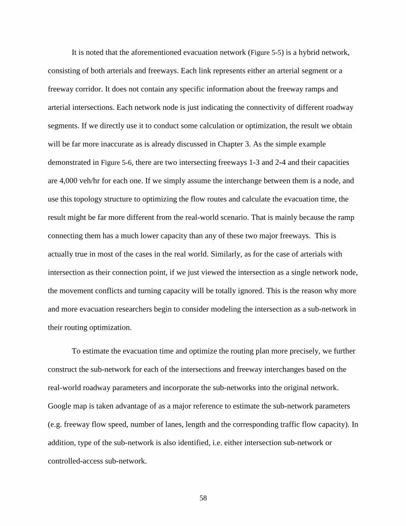
It is noted that the aforementioned evacuation network (Figure 5-5) is a hybrid network,
consisting of both arterials and freeways. Each link represents either an arterial segment or a
freeway corridor. It does not contain any specific information about the freeway ramps and
arterial intersections. Each network node is just indicating the connectivity of different roadway
segments. If we directly use it to conduct some calculation or optimization, the result we obtain
will be far more inaccurate as is already discussed in Chapter 3. As the simple example
demonstrated in Figure 5-6, there are two intersecting freeways 1-3 and 2-4 and their capacities
are 4,000 veh/hr for each one. If we simply assume the interchange between them is a node, and
use this topology structure to optimizing the flow routes and calculate the evacuation time, the
result might be far more different from the real-world scenario. That is mainly because the ramp
connecting them has a much lower capacity than any of these two major freeways. This is
actually true in most of the cases in the real world. Similarly, as for the case of arterials with
intersection as their connection point, if we just viewed the intersection as a single network node,
the movement conflicts and turning capacity will be totally ignored. This is the reason why more
and more evacuation researchers begin to consider modeling the intersection as a sub-network in
their routing optimization.
To estimate the evacuation time and optimize the routing plan more precisely, we further
construct the sub-network for each of the intersections and freeway interchanges based on the
real-world roadway parameters and incorporate the sub-networks into the original network.
Google map is taken advantage of as a major reference to estimate the sub-network parameters
(e.g. freeway flow speed, number of lanes, length and the corresponding traffic flow capacity). In
addition, type of the sub-network is also identified, i.e. either intersection sub-network or
controlled-access sub-network.
58

Figure 5-6: Case that the interchange capacity is overestimated
Before providing the detailed sub-network information at each intersection or freeway
interchange, it is necessary to mention that there are four special network nodes, which neither
belong to the type of intersection nor the interchange section between freeways. They are, node
16, 22, 23 and 29, which denote Salisbury, Federalsburg, Bridgeville and Denton, respectively
(Figure 5-7). Actually, these four nodes are dummy nodes representing a central area of a small
town (center of a major demand source). There are many minor roadways inside these dummy
nodes connecting all of the demand generation points, therefore, we assume that the flow
capacity within them are very high and just consider them as large transshipment nodes.
C= 4,000 veh/hr
C= 4,000 veh/hr
1
2
3
4
C= 4,000 veh/hr
C= 4,000 veh/hr
1
2
3
4 C= 1,800 veh/hr
Abstracted Scenario Real-world Case
59

Figure 5-7: Four special network nodes (Dummy node) in case study II
Among all of the 50 network nodes demonstrated in Figure 5-5, totally 20 of them are
arterial intersections with at most four legs. They are, node 11, 12, 2, 3, 6, 8, 10, 49, 19, 20, 21,
24, 25, 50, 28, 30, 33, 34, 36, 39 and 40. Without loss of generality, all of traffic movements
within these intersections can be further represented by the following network structure (Figure
5-8). Actually, for intersection with three legs, this sub-network structure can also be used to
model its insider movements, and we just need to disable the 4th node (i,4) and all of the links
connected with it (i.e. only using the first three sub-nodes). As is illustrated in Chapter 3,
constraints (5 - 7) can be used to eliminate all of the movement conflicts within this intersection
sub-network (merge and diverge are as movement conflicts here).
Dummy Node 16
Dummy Node 23
Dummy Node 22
Dummy Node 29
60

Figure 5-8: Sub-network representation for intersection with at most four legs
In addition to the various types of network nodes mentioned above in the studied
evacuation network, there is another type of transshipment node that cannot be ignored, i.e. the
controlled-access region (i.e. interchange) between freeways. Due to the geometric properties of
freeways, there does not exist any traffic conflicts within the controlled-access region. Thus the
traffic conflicts elimination constraints are not required for this type of sub-networks (e.g. traffic
flow 1->3 is not conflicted with traffic flow 2->4). Only the capacities of the interchange ramps
make a difference (Figure 5-9).
Figure 5-9: Sub-network representation for interchange between freeways
1
2
4
3 (i,1)
(i,2)
(i,4)
(i,3)
Turn movements (i.e. right turn or left turn) Straight movements (i.e.no turn
within intersection)
1
2
4
3 (i,1)
(i,2)
(i,4)
(i,3)
Freeway changing movement (i.e. ramp merge or diverge) Straight movements (i.e. not
taking the exit ramp)
61

For each arterial intersection or freeway interchange, we use the aforementioned labeling
method to label the sub-network nodes. For example, node 49 is an arterial intersection with 3
legs, we label the sub-network nodes inside this intersection as (49,1), (49,2) and (49,3). The
directed link (49,1)-(49,2) means the movement from the 1st leg to the 2nd leg within this
intersection. Moreover, for any dummy node, non-intersection and non-interchange node, we
simple label it with (n,0), where n is the ID of this node in the original network. For example,
directed link (1,0)-(4,4) means the movement from source node 1 to the 4th leg of intersection
node 4.
5.3.3 Numerical Experiments
In this section, routing optimization is conducted upon the given evacuation network
demonstrated in the last section. Totally 192080 evacuation demand is considered within this
network. The demand distribution is shown in the Table 5-6. Here we assume each source is a
node, because we can reasonably view each node as an access point to the major evacuation
network in the real-world scenario. In other words, in each sub-region of the evacuation area, the
demand has to get into the evacuation network through these access points, e.g. controlled ramps
of the freeway, and collectors to the major arterial.
To begin with, we consider exactly one route for each of the sources, and use the routing
optimization model to figure out these evacuation routes. By taking advantage of the solution
approach demonstrated at the end of chapter 3, we find the optimal solution with minimal
network clearance time 30 hours, total evacuation time 653611 hours and total in-network time
3.34082e+006 hours. The corresponding evacuation routes of this optimal solution are listed as
below.
62

Table 5-6: Evacuation Demand Distribution in Eastern Shore Maryland
Source Node Total Demand (Vehicles)
2 45,850 1 43,830 3 20,700 9 20,000
20 17,400 26 16,800 16 11,400 40 6,400 36 6,200 46 3,500
Table 5-7: Optimized Evacuation Routes (one route per source)
Source Optimized evacuation route Bottleneck (network link)
Average Network-
Loading Waiting Time (hour)
1 1->4->5->8->10->49->21->50->27->48->44 (1,0)-(4,4) 14.95 16 16->17->19->23->25->29->30->47->31->32 (23,0)-(25,4) 12.84 2 2->1->4->45->7->15->16->17->19->23->24->28->35->39->43 (1,0)-(4,4) 14.95 26 26->30->31->32 (31,1)-(31,2) 14.60 3 3->6->10->49->21->23->25->29->30->31->32 (31,1)-(31,2) 14.60 36 36->47->31->32 (31,2)-(32,0) 8.44 40 40->42 (40,3)-(42,0) 2.13 46 46->11->13->16->18->20->26->30->31->32 (31,1)-(31,2) 14.60 9 9->10->49->21->50->27->48->44 (10,2)-(49,1) 14.09 20 20->26->30->31->32 (31,1)-(31,2) 14.60
From the results of Table 5-7 we can see, 8 out of the 10 routes have the bottleneck
located in the intersection or freeway interchange region. Actually, this is always ignored if we
do not consider the movement within intersection and freeway interchange as a sub-network. In
other words, if we just simply view the arterial intersection or freeway interchange as a single
node (indicating the connectivity of two roadways), we are not able to identify the bottleneck,
which indicates the network clearance time, properly. The estimated network clearance time for
63

the above routing strategy is around 30 hours. However, an argument might occur regarding this
amount of network clearance time, since there exists multiple egresses for each source while we
only optimize the routing problem by assigning exactly one route to each of these sources. In
other words, the question is that if we assign more than one route to some of the sources can we
obtain a lower network clearance time.
Before we further seek for multiple routes optimization results, we introduce a lover
bound calculation technique for the network clearance time. Suppose a directed network G(N,A),
where N denotes the set of network nodes and A denotes the set of network arcs. Let S be the set
of all source nodes within G and T be the set of all exit arcs (link connected to sink nodes) of G.
Then the network clearance time must have a lower bound calculated by,
LNC = ∑ 𝑛𝑛(𝑒𝑒)𝑛𝑛∈𝑆𝑆∑ 𝑒𝑒(𝑒𝑒, 𝑗𝑗)(𝑖𝑖,𝑗𝑗)∈𝑇𝑇�
where, 𝑛𝑛(𝑒𝑒) denotes the demand at source n, and c(i,j) denotes the capacity of arc (i,j). This
lower bound of network clearance time is very obvious, since all of the arcs in set T (i.e. exit arcs)
constitute the minimal cut between this evacuation network and the outside regions. In other
words, even though every non-exit link inside the network has an infinite capacity and zero
travel time, the throughput of this network can never exceed its total exit links’ capacity.
Now we can take advantage of this technique to check the lower bound of the network
clearance time for the Eastern Shore Maryland in two ways. The first one is that considering the
entire Eastern Shore region as a whole, we can directly calculate this value. The second one is
that we consider a sub-network of this whole region by referring the minimal cut of this sub-
network (i.e. the ocean city island, since it possesses half of the total demand). The lower bounds
of the network clearance time by taking these two ways are,
64

• Considering the entire region as a whole, the corresponding exit arcs are 31-32, 40-41,
40-42, 39-43 and 48-44. The capacities of these five exiting links are 4500, 1250, 1500,
3000 and 3000 in vehicles per hour, respectively. The total demand within this whole
region is 192080 vehicles. Hence,
LNC_1 =192080
4500 + 1250 + 1500 + 3000 + 3000= 14.49 ℎ𝑜𝑜𝑒𝑒𝑠𝑠𝑠𝑠
• Considering the ocean city island as a sub-network, the corresponding exit arcs (i.e. the
minimal cut from the rest of the network) are 1-4, 2-5, 3-6 and 9-10. The capacities of
these four exiting links of ocean city are 3000, 1500, 1000 and 1000. The total demand in
ocean city is 130380 vehicles. Hence,
LNC_2 =130380
3000 + 1500 + 1000 + 1000= 20.05 ℎ𝑜𝑜𝑒𝑒𝑠𝑠𝑠𝑠
Therefore, we derive a lower bound of the network clearance time for the whole network,
which is LNC = min�𝐿𝐿𝑁𝑁𝐶𝐶1 , 𝐿𝐿𝑁𝑁𝐶𝐶2� = 20.05 ℎ𝑜𝑜𝑒𝑒𝑠𝑠𝑠𝑠
In comparison with the lower bound (i.e. 20.05 hours), the optimal routing strategy with
exactly one route for each source is not that desirable, since its network clearance time is around
30 hours. A careful examination of the network structure and the demand distribution indicates
that each optimal route has to burden a huge amount of demand. However, the route capacity
compared with its serving demand is very small, which is of high possibility to lead to a large
clearance time. Therefore, it is necessary to investigate whether enlarging the number of
evacuation route for each of the sources is effective to further minimize the network clearance.
Hence, two more optimization experiments are additionally conducted. These are, assigning each
source with two evacuation routes and assigning each source with three evacuation routes. This
can be done by taking advantage of the “Dummy-Node” technique introduced in Chapter 3 (i.e.
65

replicating the single source node by multiple dummy nodes with the original demand evenly re-
distributed). The optimization results indicate that enlarging the number of the evacuation routes
for each source to 3 indeed decreases the network clearance time. The optimal network clearance
times are 22.0 hours for the two-route strategy and 20.7 hours for the three-route strategy. The
corresponding routing results are shown in Table 5-8 and Table 5-9, respectively.
It is noted that in the multiple-route routing strategies (at most 2-route per source and at
most 3-route per source), the multiple optimized routes for a given source node might overlap
with the other one(s). In some cases, the resulting egress routes for a given source might even be
completely the same. For example, for the optimized evacuation routes with two routes per
source instance, the two routes of source 26 are completely same. However, this type of solution
is not contradictory with the definition “2-route evacuation plan”, because this solution indicates
that if we assign two routes for source 26, the optimal routing plan for each route is 26->30->47-
>31->32. In other words, even in the 2-route optimization problem, the best routing plan for this
source is using only one route. Therefore, this type of solution provides the optimization
approach great flexibility. We can think it as “at most two routes assignment” problem.
Moreover, the performance indicator for the three different routing plans (i.e. network clearance
time, total travel time and total in-network time) defined in Chapter 3 are compared in Figure
5-10. As is shown, the “at most three routes” optimization approach gives a pretty good solution
with the network clearance time 20.7 hours, which is only 3.24% larger than the lower bound
(20.05 hours). Meanwhile, with the lower network clearance time, both of the “at most two
routes” and “at most three routes” evacuation plans have a much smaller total in-network time
than the “exactly one route” evacuation plan. In addition, the total travel time of these three
routing plans are similar with each other. That is due to the objective function, which aims to
66

seek a solution with a minimal total travel time. The total travel times of the last two routing
plans are a little bit larger than that of the first routing plan. These results can be referred to the
route structure of each plan. In the last two routing plans, some detours are generated to avoid
larger bottleneck, i.e. minimizing the network clearance time.
Table 5-8: Optimized Evacuation Routes (two routes per source)
Source Optimized evacuation route Bottleneck (network link)
Average Network-
Loading Waiting Time (hour)
1 1->4->45->7->15->17->19->23->24->28->35->39->43 1->2->3->6->10->49->21->50->27->48->44
(1,0)-(4,4) (3,2)-(6,1)
10.923 10.957
16 16->17->19->23->24->28->35->39->43 16->17->19->23->25->29->30->47->31->32
17,3-19,4 30,3-47,1
9.0025 10.95
2 2->5->8->10->49->21->50->27->48->44 2->1->4->45->7->15->16->18->20->26->30->31->32
10,2-49,1 30,1-30,2
10.8067 10.9563
26 26->30->47->31->32 26->30->47->31->32
30,3-47,1 30,3-47,1
10.95 10.95
3 3->2->1->4->45->7->15->16->17->19->23->25->29->30->47->31->32 3->2->1->4->45->7->15->17->19->23->24->28->35->39->43
30,3-47,1 1,0-4,4
10.95 10.9233
36 36->47->31->32 36->47->31->32
31,2-32,0 31,2-32,0
9.20833 9.20833
40 40->42 40->42
40,3-42,0 40,3-42,0
2.13333 2.13333
46 46->11->13->16->18->20->26->30->31->32 46->11->13->16->18->20->26->30->31->32
40,3-42,0 40,3-42,0
10.9563 10.9563
9 9->10->49->21->50->27->48->44 9->10->49->21->50->27->48->44
10,2-49,1 10,2-49,1
10.8067 10.8067
20 20->26->30->31->32 20->26->30->31->32
30,1-30,2 30,1-30,2
10.9563 10.9563
67

Table 5-9: Optimized Evacuation Routes (three routes per source)
Source Optimized evacuation route Bottleneck (network link)
Average Network-
Loading Waiting Time (hour)
1 1->4->45->7->15->17->19->23->24->28->35->39->43 1->4->45->16->17->19->23->24->28->35->39->43
1->4->45->7->15->16->17->19->23->24->28->35->39->43
17,3-19,4 17,3-19,4 17,3-19,4
10.2408 10.2408 10.2408
16 16->18->20->26->30->31->32 16->18->20->26->30->47->31->32
16->18->20->26->30->31->32
26,2-30,1 26,2-30,1 26,2-30,1
10.3415 10.3415 10.3415
2 2->1->4->45->7->15->16->18->20->26->30->31->32 2->5->7->15->17->19->23->24->28->35->39->43
2->5->8->10->49->21->50->27->48->44
26,2-30,1 17,3-19,4 2,2-5,4
10.3415 10.2408 10.1887
26 26->30->47->31->32 26->30->31->32
26->30->47->31->32
26,2-30,1 26,2-30,1 26,2-30,1
10.3415 10.3415 10.3415
3 3->6->10->49->21->50->27->48->44 3->6->10->49->21->23->25->29->30->47->31->32
3->6->10->49->21->50->27->48->44
3,2-6,1 3,2-6,1 3,2-6,1
10.35 10.35 10.35
36 36->47->31->32 36->47->31->32 36->47->31->32
31,2-32,0 31,2-32,0 31,2-32,0
8.60911 8.60911 8.60911
40 40->42 40->42 40->42
40,3-42,0 40,3-42,0 40,3-42,0
2.133 2.133 2.133
46 46->11->13->16->17->19->23->25->29->30->47->31->32 46->11->13->16->18->20->26->30->31->32
46->11->13->16->17->19->23->25->29->30->47->31->32
17,3-19,4 26,2-30,1 17,3-19,4
10.2408 10.3415 10.2408
9 9->10->49->21->50->27->48->44 9->10->49->21->50->27->48->44 9->10->49->21->50->27->48->44
31,2-32,0 31,2-32,0 31,2-32,0
9.999 9.999 9.999
20 20->26->30->31->32 20->26->30->31->32
20->26->30->47->31->32
26,2-30,1 26,2-30,1 26,2-30,1
10.3415 10.3415 10.3415
68

Figure 5-10: Comparison of performance indicators among the three proposed routing plans
Since the 3rd routing plan outperforms the other two, we accept it as the optimal routing
strategy and run the scheduling heuristic based on it. Note that the simulation based discharging
heuristic presented in Chapter 4 has two heuristic factors, the loading attraction factor α and
discharging reduction factor β, which have a significant impact on the network clearance time.
Recall that the loading attraction factor α aims to fully make use of the route capacity from a
greedy perspective. While the discharging reduction factor β aims to relieve the traffic
congestion resulted by α. Thus, choosing an appropriate pair of (α, β) is of great significance in
determining the optimal discharging strategy. Actually, the value of the heuristic factors (α, β) is
problem-specific. For example, if the evacuation route of each source is independent of the
others (i.e. no link is going to be shared by more than two sources), the best discharging strategy
is loading exactly according to the route bottleneck capacity. Therefore, for a specific evacuation
scenario, it is necessary to conduct a set of sensitivity analysis to further figure out what the
corresponding (α, β) pair should be. Based on the 3rd routing plan, sensitivity analysis of the
heuristic factors (α, β) is conducted by running the simulation-based heuristic multiple times.
653611 662688 655617
3.34E+06
2.68E+06 2.56E+0649.63%
9.73%3.24% 0
0.1
0.2
0.3
0.4
0.5
0.6
0.00E+005.00E+051.00E+061.50E+062.00E+062.50E+063.00E+063.50E+064.00E+06
route per source at most 2 routes persource
at most 3 routes persource
TOTA
L TI
ME
(HO
URS
)
Total Travel Time and Total In-Network Time of Three Strategies
Total Travel Time Total In-Network Time LP Gap
69

The time interval of the mesoscopic traffic simulator is chosen as 20 seconds in consideration of
the average link length of the studied network. There is no doubt that the lower the simulation
interval is, the higher simulation resolution will be. However it will substantially increase the
simulation burden since we have millions of vehicles passing through the network. Results (i.e.
network clearance time in seconds) with respect to different (α, β) pairs are shown and color-
shaded in Table 5-10. The unit of the network clearance time is chosen as seconds in order to
have a more clear view of the result values. As is shown in Table 5-10, the best simulation results
are coming from the (α, β) pair equal to (1.6, 0.9). The corresponding network clearance time is
78,660 seconds (i.e. 21.85 hours). It is noted that, when the loading attraction factor α is fixed as
1.0, the network clearance time is always 99,200 seconds (i.e. 27.55 hours) and not sensitive to
the change of the discharging reduction factor β. This is mainly because if we set the flow
attraction factor as 1, all of the traffic flows will move under the critical traffic density. In other
words, no traffic congestion will be detected by the heuristic. Thus, the discharging rate
reduction will never be conducted during the loading process (i.e. discharging reduction factor β
will never be used). However, if the loading attraction factor exceeds 1.0, which means there is a
possibility that the traffic congestion occurs, an appropriate factor discharging reduction factor β
will positively contribute to the evacuation by relieving the traffic congestion. For example, in
this evacuation scenario, when the attraction factor α exceeds 2.0 (e.g. 2.2), a lower β (0.7) has a
better discharging effect over the β equal to 0.9 or 0.8. In addition, the discharging reduction
factor β should not be set as a very low value (e.g. below 0.5), otherwise the network clearance
time will be very high, since a very low β over-reduces the discharging rate. In all, the loading
attraction factor and discharging reduction factor should be chosen appropriately in order to
70

make the evacuation process more stable. Either too large α or too low β will substantially
increase the network clearance time by bringing too much variance to the system.
Since (α, β) equal to (1.6, 0.9) makes the discharging heuristic provide a set of traffic
loading strategies with a more satisfactory network clearance time (i.e. 21.85 hours), we choose
it as the heuristic factors in the scheduling algorithm described in Chapter 4 to come up with the
discharging strategies. The corresponding time-dependent discharging rate is shown in Figure
5-11and Figure 5-12. The resulting evolution curve of the total evacuated demand is shown in
Figure 5-13. The discharging rate is adjusted every 1 minute within the scheduling heuristic. As
can be seen, the last group of vehicles is discharged at the time point around 1152 minute (i.e.
19.2). After that, it will take approximately 21.8 – 19.2 = 2.6 hours for all of the in-network
vehicles to arrive at destinations.
In addition, we also investigate the impact of the evacuation priority on the evacuation
process. As mentioned at the end of Chapter 4, the heuristic discharging rate of a particular
source will be affected by its prescriptive evacuation priority. Further, the time-dependent
discharging rate of a specific source will be high if it has a higher priority in comparison with
other sources. Because we expect to allocate more network capacity to the source with a high
priority. In this case study, sources located in Ocean City are assigned with a higher evacuation
priority to see what happens if the scheduling Heuristic is operating in such a hybrid priority
scenario. The corresponding results are shown in Figure 5-13 and Figure 5-14. From Figure 5-13
we can see, the network clearance time does not change too much for the scenario in which
Ocean City has a larger priority. However, the time-dependent remaining demand in Ocean City
area of the ‘Hybrid’ scheduling strategy is lower than that of the ‘Homogeneous’ strategy. In
other words, if we assign a higher evacuation priority to the Ocean City area, the time-dependent
71

throughput of its demand will increase. But the increased throughput will not be significant for
this case (i.e. increasing the priority of the whole Ocean City Area). The intrinsic reason for this
is that Ocean City has a huge percentage of the total evacuation demand in the whole Eastern
Shore Area (i.e. 67.9%). In other words, the main competition of reserving the network capacity
during the evacuation is coming from itself. Therefore, if we increase the evacuation priority of
the Ocean City area simultaneously, the throughput of this area will be increased, but will not be
that significant.
72

Table 5-10: Sensitivity Analysis of Network Clearance Time (sec) with Respect to Different (α, β) Pairs
Discharging Reduction Factor (β)
0.9 0.8 0.7 0.6 0.5 0.4 0.3 0.2
Loading Attraction Factor (α)
1.0 99,200 99,200 99,200 99,200 99,200 99,200 99,200 99,200
1.2 82,940 83,060 83,560 85,420 86,420 88,160 89,940 88,780
1.4 79,600 80,460 81,620 83,420 84,460 86,440 89,500 93,400
1.6 78,660 80,620 81,480 85,360 87,760 88,680 90,340 91,640
1.8 79,220 80,500 81,780 85,400 88,160 88,980 91,320 96,220
2.0 80,280 84,320 82,020 84,920 86,340 88,760 90,900 90,820
2.2 83,840 86,600 82,200 85,180 88,000 89,720 91,340 91,880
2.4 83,890 85,600 83,360 84,960 86,720 88,760 90,800 94,720
2.6 84,000 85,740 82,680 85,200 88,880 89,740 90,400 92,340
73
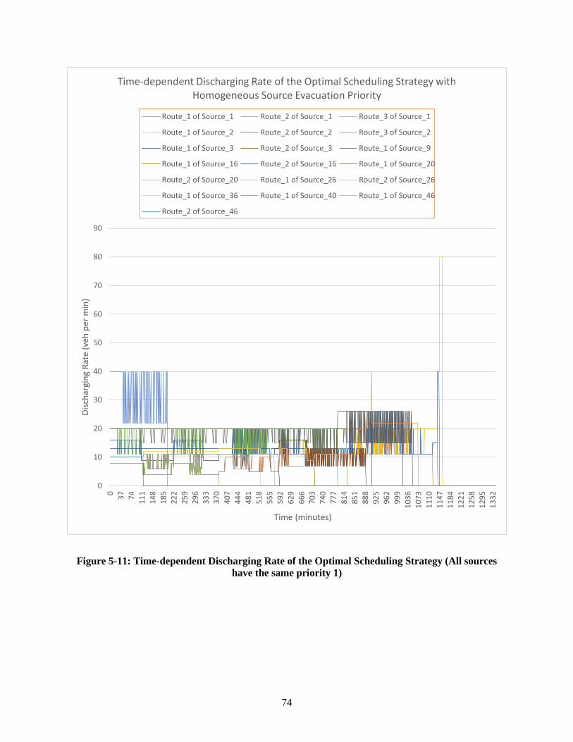
Figure 5-11: Time-dependent Discharging Rate of the Optimal Scheduling Strategy (All sources have the same priority 1)
0
10
20
30
40
50
60
70
80
90
0 37 74 111
148
185
222
259
296
333
370
407
444
481
518
555
592
629
666
703
740
777
814
851
888
925
962
999
1036
1073
1110
1147
1184
1221
1258
1295
1332
Disc
harg
ing
Rate
(veh
per
min
)
Time (minutes)
Time-dependent Discharging Rate of the Optimal Scheduling Strategy with Homogeneous Source Evacuation Priority
Route_1 of Source_1 Route_2 of Source_1 Route_3 of Source_1
Route_1 of Source_2 Route_2 of Source_2 Route_3 of Source_2
Route_1 of Source_3 Route_2 of Source_3 Route_1 of Source_9
Route_1 of Source_16 Route_2 of Source_16 Route_1 of Source_20
Route_2 of Source_20 Route_1 of Source_26 Route_2 of Source_26
Route_1 of Source_36 Route_1 of Source_40 Route_1 of Source_46
Route_2 of Source_46
74

Figure 5-12: Time-dependent Discharging Rate of the Optimal Scheduling Strategy (Sources in Ocean city have a higher priority equal to 2, and other sources have priority 1)
0
10
20
30
40
50
60
70
80
90
0 37 74 111
148
185
222
259
296
333
370
407
444
481
518
555
592
629
666
703
740
777
814
851
888
925
962
999
1036
1073
1110
1147
1184
1221
1258
1295
1332
Disc
harg
ing
Rate
(veh
per
min
)
Time (minutes)
Time-dependent Discharing Rate of the Optimal Scheduling Strategy with Hybrid Source Evacuation PriorityRoute_1 of Source_1 Route_2 of Source_1 Route_3 of Source_1
Route_1 of Source_2 Route_2 of Source_2 Route_3 of Source_2
Route_1 of Source_3 Route_2 of Source_3 Route_1 of Source_9
Route_1 of Source_16 Route_2 of Source_16 Route_1 of Source_20
Route_2 of Source_20 Route_1 of Source_26 Route_2 of Source_26
Route_1 of Source_36 Route_1 of Source_40 Route_1 of Source_46
Route_2 of Source_46
75

Figure 5-13: Time-Dependent Evolution Curve of the Total Evacuated Demand under the Optimal Routing and Scheduling Strategy
Figure 5-14: Time-dependent Remaining Demand Curves in Ocean City Area with respect to different Priorities
0
50000
100000
150000
200000
250000
0.0
0.8
1.7
2.5
3.3
4.2
5.0
5.8
6.7
7.5
8.3
9.2
10.0
10.8
11.7
12.5
13.3
14.2
15.0
15.8
16.7
17.5
18.3
19.2
20.0
20.8
21.7
Evac
uate
d De
man
d
Time (Hours)
Evacuated Demand V.S. Evacuation Time under the Optimal Routing and Scheduling Strategy
Homogeneous Priority Hybrid Priority
0
20000
40000
60000
80000
100000
120000
140000
0 49 98 147
196
245
294
343
392
441
490
539
588
637
686
735
784
833
882
931
980
1029
1078
1127
1176
1225
1274
1323Re
mai
ning
Dem
and
in O
cean
City
Time (Minute)
Remaining Demand Curves in Ocean City Area with respect to different Priority
Ocean City with P=2 Ocean City with P=1
76

Chapter 6 : Thesis Summary
6.1 Contributions
In this research, a framework for large-scale routing and scheduling optimization was
developed for the case of uninterrupted traffic flows. Instead of considering the routing and
scheduling in a single problem (using a time-space network), we built the routing and scheduling
models separately (i.e. in two phases) so as to enhance the planning efficiency in an urgent real
world evacuation scenario. Moreover, the two-phase optimization of the routing and scheduling
decision models also provides a high flexibility when using these models. In other words, either
the routing optimization model or the scheduling heuristic can be separately adopted for a
particular scenario, and they need not be used together. For example, if the evacuation routes
have been pre-selected already by some other techniques, then one only needs to use the
scheduling heuristic to further determine the demand discharging rate and view the simulation
results.
Before demonstrating the optimization models, three significant evacuation performance
measures were introduced and derived based on the uninterrupted flow scenario. They are,
network clearance time, total travel time and total in-network time. The significance and
application of these three performance indicators were discussed and compared. Thereafter the
routing and scheduling decision process was formulated as a two-phase optimization framework.
In the first phase, a multiple-objective binary programming model with multiple objective
functions was formulated. Network clearance time and total in-network time were adopted as
the evacuation performance measurements in the routing model. In addition, to better guarantee
the a smooth and more effective evacuation process, intersection movement conflicts were
eliminated during the optimization process, since conducting the evacuation process based on
77

uninterrupted traffic flow is proved to be more efficient and effective in recent studies. A general
mathematical formulation of the intersection conflicts elimination constraints were provided as
well. Specifically for the proposed optimization model, a specific iteration-based linear solution
approach was developed. The solution approach was tested in the case studies and shown to be
effective to give the routing plan with both a minimal network clearance time and total in-
network time. In the second phase, a simulation-based scheduling heuristic was developed with
the concept from greedy algorithms. This heuristic is able to dynamically determine the
discharging rate of each evacuation source with the assistance of an embedded mesoscopic
traffic simulator. Meanwhile, the traffic condition of each time interval during the whole
evacuation process can also be given from the embedded traffic simulator.
With numerical experiments in the case studies, the proposed optimization framework is
proved to be of high optimization capability, as well as high calculation efficiency. In addition,
due to the two-phase property of the optimization framework (i.e. considering the routing and
scheduling separately), the proposed model is of high flexibility to be used in a real-world
scenario. For example, either the routing optimization or the scheduling heuristic can be used
separately. Therefore, the overall optimization framework is useful to an emergency-planning
agency in their various planning stages for a large-scale evacuation operation.
6.2 Future Research
There are two promising and interesting future research directions related to the work done
here:
1) The routing optimization model in this thesis is a binary integer programming model,
which aims to determine one or one more evacuation path for each source. However,
78

there is a limitation of this optimization model. That is, we come up with one or more
routes for a specific source by introducing parallel dummy nodes upon this source, but
the demand on each parallel dummy node is evenly distributed from the original source
during the calculation. Otherwise, if we think the demand of each dummy node as
another set of decision variables, the model becomes non-linear both in the constraints
and objectives. For example, if we want to find three paths for a source with total demand
equal to 3000, we assume each of the three dummy nodes has a demand equal to 1000.
Therefore, in the future research, we can investigate how to effectively distribute the
original demand among the dummy nodes in order to further mitigate the flow congestion
determined by the total demand of each path that has not yet arrived.
2) The main concept of the routing and scheduling optimization model is to maximize the
network throughput while avoiding the traffic flow congestion. In other words, making
full use of the evacuation network is the core. Therefore, another perspective of viewing
that is to firstly consider the routing planning phase with concept of maximal flow
minimal cost problem. Thereafter, some network extraction techniques should be used to
extract a set of feasible routes from these continuous flows to serve as the optimal
evacuation paths. Meanwhile, the demand distribution on each extracted route is obtained
as well.
79

Bibliography
1. Afshar, Abbas Mohasel, and Ali Haghani. "Heuristic framework for optimizing hurricane
evacuation operations." Transportation Research Record: Journal of the Transportation
Research Board 2089.1 (2008): 9-17.
2. Afshar, Abbas Mohasel, and Ali Haghani. “Maryland Eastern Shore Evacuation Plan”.
State Highway Administration Research Report. May. 2007.
3. Bretschneider, Sarah, and Alf Kimms. "A basic mathematical model for evacuation
problems in urban areas." Transportation research part A: policy and practice 45.6 (2011):
523-539.
4. Chen, Ming, Lichun Chen, and Elise Miller-Hooks. "Traffic signal timing for urban
evacuation." Journal of urban planning and development 133.1 (2007): 30-42.
5. Chen, Xiang, Mei-Po Kwan, Qiang Li, and Jin Chen. "A model for evacuation risk
assessment with consideration of pre-and post-disaster factors." Computers, Environment
and Urban Systems36.3 (2012): 207-217.
6. Chen, Xuwei, and Franklin B. Zhan. "Agent-based modelling and simulation of urban
evacuation: relative effectiveness of simultaneous and staged evacuation strategies."
Journal of the Operational Research Society 59.1 (2006): 25-33.
7. Chen, Xuwei, John W. Meaker, and F. Benjamin Zhan. "Agent-based modeling and
analysis of hurricane evacuation procedures for the Florida Keys." Natural Hazards 38.3
(2006): 321-338.
80

8. Chien, Steven I., and Vivek V. Korikanthimath. "Analysis and modeling of simultaneous
and staged emergency evacuations." Journal of Transportation Engineering 133.3 (2007):
190-197.
9. Church, Richard L., and Thomas J. Cova. "Mapping evacuation risk on transportation
networks using a spatial optimization model." Transportation Research Part C: Emerging
Technologies 8.1 (2000): 321-336.
10. Cova, Thomas J., and Justin P. Johnson. "A network flow model for lane-based
evacuation routing." Transportation Research Part A: Policy and Practice 37.7 (2003):
579-604.
11. Dow, Kirstin, and Susan L. Cutter. "Emerging hurricane evacuation issues: hurricane
Floyd and South Carolina." Natural hazards review 3.1 (2002): 12-18.
12. Ford, Lester Randolph, and Delbert Ray Fulkerson. "Constructing maximal dynamic
flows from static flows." Operations research 6.3 (1958): 419-433.
13. Hamacher, Horst W., and Stevanus A. Tjandra. "Mathematical modelling of evacuation
problems–a state of the art." Pedestrian and evacuation dynamics2002.227-266 (2002): 1-
2.
14. Helbing, Dirk, and Anders Johansson. Pedestrian, crowd and evacuation dynamics.
Springer New York, 2009.
15. Hua, Jingyi, Gang Ren, Yang Cheng, Chen Yu, and Bin Ran. "Evacuation in Large-scale
Transportation Network: A Bi-Level Control Method with Uncertain Arterial Demand."
Transportation Research Board 92nd Annual Meeting. No. 13-2254. 2013.
16. Jain, Rajat, and J. MacGregor Smith. "Modeling vehicular traffic flow using M/G/C/C
state dependent queueing models." Transportation Science 31.4 (1997): 324-336.
81

17. Jha, Mithilesh, Katie Moore, and Behruz Pashaie. "Emergency evacuation planning with
microscopic traffic simulation." Transportation Research Record: Journal of the
Transportation Research Board 1886.1 (2004): 40-48.
18. Kalafatas, Georgios, and Srinivas Peeta. "Planning for evacuation: insights from an
efficient network design model." Journal of infrastructure systems 15.1 (2009): 21-30.
19. Kim, Sangho, Shashi Shekhar, and Manki Min. "Contraflow transportation network
reconfiguration for evacuation route planning." Knowledge and Data Engineering, IEEE
Transactions on 20.8 (2008): 1115-1129.
20. Kuligowski, Erica D., and Richard D. Peacock. A review of building evacuation models.
US Department of Commerce, National Institute of Standards and Technology, 2005.
21. Lämmel, Gregor, Marcel Rieser, and Kai Nagel. "Large scale microscopic evacuation
simulation." Pedestrian and Evacuation Dynamics 2008. Springer Berlin Heidelberg,
2010. 547-553.
22. Lindell, Michael K., and Carla S. Prater. "Critical behavioral assumptions in evacuation
time estimate analysis for private vehicles: Examples from hurricane research and
planning." Journal of Urban Planning and Development 133.1 (2007): 18-29.
23. Liu, Henry X., Jeff X. Ban, Wenteng Ma, and Pitu B. Mirchandani. "Model reference
adaptive control framework for real-time traffic management under emergency
evacuation." Journal of urban planning and development 133.1 (2007): 43-50.
24. Liu, Henry X., Xiaozheng He, and Xuegang Ban. "A cell-based many-to-one dynamic
system optimal model and its heuristic solution method for emergency evacuation."
Proceedings of the 86th Annual Meeting Transportation Research Board, Washington,
DC, USA. 2007.
82

25. Liu, Ying, Nan Zou, and Gang-Len Chang. "An integrated emergency evacuation system
for real-time operations-a case study of ocean city, maryland under hurricane attacks."
Intelligent Transportation Systems, 2005. Proceedings. 2005 IEEE. IEEE, 2005.
26. Liu, Ying, Xiaorong Lai, and Gang-Len Chang. "Cell-based network optimization model
for staged evacuation planning under emergencies." Transportation Research Record:
Journal of the Transportation Research Board 1964.1 (2006): 127-135.
27. Liu, Ying, Xiaorong Lai, and Gang-Len Chang. "Two-level integrated optimization
system for planning of emergency evacuation." Journal of transportation Engineering
132.10 (2006): 800-807.
28. Liu, Yue, and Zhenke Luo. "A Bi-Level Model for Planning Signalized and
Uninterrupted Flow Intersections in an Evacuation Network." Computer-Aided Civil and
Infrastructure Engineering 27.10 (2012): 731-747.
29. Lu, Qingsong, Betsy George, and Shashi Shekhar. "Capacity constrained routing
algorithms for evacuation planning: A summary of results." Advances in spatial and
temporal databases. Springer Berlin Heidelberg, 2005. 291-307.
30. Pel, Adam J., Michiel CJ Bliemer, and Serge P. Hoogendoorn. "A review on travel
behaviour modelling in dynamic traffic simulation models for evacuations."
Transportation 39.1 (2012): 97-123.
31. Saadatseresht, Mohammad, Ali Mansourian, and Mohammad Taleai. "Evacuation
planning using multiobjective evolutionary optimization approach." European Journal of
Operational Research 198.1 (2009): 305-314.
83

32. Sbayti, Hayssam, and Hani S. Mahmassani. "Optimal scheduling of evacuation
operations." Transportation Research Record: Journal of the Transportation Research
Board 1964.1 (2006): 238-246.
33. Schreckenberg, Michael, and Som Deo Sharma. Pedestrian and evacuation dynamics.
Berlin: Springer, 2002.
34. Southworth, F. Regional Evacuation Modeling in the United States: A State of the Art
Review. Report No.38 ORNL-TM/11740, Oak Ridge National Laboratory, Oak Ridge,
TN, 1991.
35. Stepanov, Alexander, and James MacGregor Smith. "Multi-objective evacuation routing
in transportation networks." European Journal of Operational Research198.2 (2009): 435-
446.
36. Yamada, Takeo. "A network flow approach to a city emergency evacuation planning."
International Journal of Systems Science 27.10 (1996): 931-936.
37. Yang, Hai, and Michael GH Bell. "A capacity paradox in network design and how to
avoid it." Transportation Research Part A: Policy and Practice 32.7 (1998): 539-545.
38. Xie, Chi, Dung-Ying Lin, and S. Travis Waller. "A dynamic evacuation network
optimization problem with lane reversal and crossing elimination strategies."
Transportation research part E: logistics and transportation review 46.3 (2010): 295-316.
39. Zhang, Xin, and Gang-Len Chang. "Cellular automata-based model for simulating
vehicular-pedestrian mixed flows in a congested network." Transportation Research
Record: Journal of the Transportation Research Board 2234.1 (2011): 116-124.
84

40. Zhang, Xin, and Gang-Len Chang. "An optimization model for guiding pedestrian-
vehicle mixed flows during an emergency evacuation." Journal of Intelligent
Transportation Systems just-accepted (2013).
41. Ziliaskopoulos, Athanasios K. "A linear programming model for the single destination
system optimum dynamic traffic assignment problem." Transportation science 34.1
(2000): 37-49.
42. Zou, Nan, Shu-Ta Yeh, Gang-Len Chang, Alvin Marquess, and Michael Zezeski.
"Simulation-based emergency evacuation system for Ocean City, Maryland, during
hurricanes." Transportation Research Record: Journal of the Transportation Research
Board 1922.1 (2005): 138-148.
85