abstract title: integrating software behavior into dynamic
TRANSCRIPT

ABSTRACT Title: INTEGRATING SOFTWARE BEHAVIOR INTO
DYNAMIC PROBABILISTIC RISK ASSESSMENT Dongfeng Zhu, Doctor of Philosophy 2005 Directed By: Associate Professor Carol Smidts, Professor Ali Mosleh
Department of Mechanical Engineering
Software plays an increasingly important role in modern safety-critical systems.
Although research has been done to integrate software into the classical Probability
Risk Assessment (PRA) framework, current PRA practice overwhelmingly neglects
the contribution of software to system risk. The objective of this research is to
develop a methodology to integrate software contributions in the Dynamic
Probabilistic Risk Assessment (DPRA) environment.
DPRA is considered to be the next generation of PRA techniques. It is a set of
methods and techniques in which simulation models that represent the behavior of the
elements of a system are exercised in order to identify risks and vulnerabilities of the
system. DPRA allows consideration of dynamic interactions of system elements and
physical variables. The fact remains, however, that modeling software for use in the
DPRA framework is also quite complex and very little has been done to address the
question directly and comprehensively.

This dissertation describes a framework and a set of techniques to extend the DPRA
approach to allow consideration of the software contributions on system risk. The
framework includes a software representation, an approach to incorporate the
software representation into the DPRA environment SimPRA, and an experimental
demonstration of the methodology.
This dissertation also proposes a framework to simulate the multi-level objects in the
simulation based DPRA environment. This is a new methodology to address the state
explosion problem. The results indicate that the DPRA simulation performance is
improved using the new approach. The entire methodology is implemented in the
SimPRA software. An easy to use tool is developed to help the analyst to develop the
software model.
This study is the first systematic effort to integrate software risk contributions into the
dynamic PRA environment.
INTEGRATING SOFTWARE BEHAVIOR INTO DYNAMIC PROBABILISTIC RISK ASSESSMENT
By
Dongfeng Zhu.
Dissertation submitted to the Faculty of the Graduate School of the University of Maryland, College Park, in partial fulfillment
of the requirements for the degree of Doctor of Philosophy
2005
Advisory Committee: Associate Professor Carol Smidts, Co-Chair / Co-Advisor Professor Ali Mosleh, Co-Chair / Co-Advisor Assistant Professor Michel Cukier Professor Dave Akin Professor Shapour Azarm Dr. Michael Stamatelatos

© Copyright by Dongfeng Zhu
2005

ii
Dedication
To my family.

iii
Acknowledgements
I wish to express my sincere gratitude to Dr. Carol Smidts and Dr. Ali Mosleh for
their support, patience, and encouragement throughout my graduate studies. Without
their immense help in guiding my research and this dissertation would have been
impossible.
I owe special thanks to the contributions of Dr. Ming Li and Dr. Frank Greon for their
tremendous help during the research, as colleague and as friends.
I am fortunate to have been able to work on this project with a talented and dedicated
team of UMD researchers consisting of Dr. Yunwei Hu, Thiago Pirest, and Hamed
Nejad. Special thanks are presented to my colleagues: Dr. Bin Li, Dr. Avik Sinha,
Yuan Wei, Susmita Ghose, Anand Ladda, Wende Kong, Ying Shi, and Jun Dai for
their help and the support they provided to this project.
I would like to thank Dr. Michael Stamatelatos, Dr. Dave Akin, Dr. Shapour Azarm
and Dr. Michel Cukier for agreeing to be on my committee.
Thanks to my wife, Yuan, for supporting me with love and understanding. My parents
receive my deepest gratitude and love for their dedication and support.

iv
Table of Contents
Dedication ..................................................................................................................... ii
Acknowledgements...................................................................................................... iii
Table of Contents......................................................................................................... iv
List of Tables ............................................................................................................... ix
List of Figures ............................................................................................................. xii
Glossary ...................................................................................................................... xv
Chapter 1: Introduction ................................................................................................. 1
1.1 Research Objective ............................................................................................. 1
1.2 Research Statement............................................................................................. 1
1.3 Approach............................................................................................................. 3
1.4 Content................................................................................................................ 5
1.5 Summary of Research Contributions .................................................................. 7
Chapter 2: Background ................................................................................................. 8
2.1 Software modeling in classical PRA................................................................... 8
2.2 Dynamic PRA environment.............................................................................. 11
2.3 SimPRA environment ....................................................................................... 14
2.3.1 Introduction................................................................................................ 14
2.3.2 Software Representation in DPRA ............................................................ 15
2.4 Teamwork ......................................................................................................... 17
2.5 Glossary of terms .............................................................................................. 18

v
Chapter 3: Software Modeling Requirements in DPRA............................................. 20
3.1 General Modeling Requirement........................................................................ 20
3.2 Simulation Requirements.................................................................................. 20
3.3 Interaction Requirements .................................................................................. 22
Software-Software interactions........................................................................... 23
Software-Hardware interactions ......................................................................... 24
Software-Human interactions ............................................................................. 24
3.4 Non-Functional Requirements .......................................................................... 25
3.5 Discussion ......................................................................................................... 28
Chapter 4: Software Representation Framework for simulation ................................ 29
4.1 Overview........................................................................................................... 29
4.2 Key Concept...................................................................................................... 30
4.3 Behavior Model ................................................................................................ 34
4.3.1 Overview.................................................................................................... 34
4.3.2 Simulation-based Finite State Machine (SFSM) ....................................... 38
4.3.3 Deterministic Model .................................................................................. 40
4.3.4 Stochastic Model........................................................................................ 44
4.3.5 Summary .................................................................................................... 53
4.4 Simulation Guidance Model ............................................................................. 55
4.4.1 Overview.................................................................................................... 55
4.4.2 Interactions with other models................................................................... 55
4.4.3 Simulation Knowledge Base (SKB) .......................................................... 58
Chapter 5: Integrating the Software Representation into SimPRA ............................ 61

vi
5.1 State Explosion Issue ........................................................................................ 61
5.2 SimPRA environment ....................................................................................... 62
5.2.1 Overview.................................................................................................... 62
5.2.2 Guidance Rule in the single-level SimPRA environment.......................... 63
5.2.2 Integrating Software into the single-level SimPRA................................... 66
5.3 Enhanced SimPRA environment ...................................................................... 74
5.3.1 Overview.................................................................................................... 74
5.3.2 Enhanced Planner....................................................................................... 75
5.3.3 Enhanced Scheduler................................................................................... 78
5.3.4 Software Guidance Model in SimPRA...................................................... 84
5.4 Integration ......................................................................................................... 84
Chapter 6: Experimental Demonstration --- Propulsion System Mission and Design
Problem....................................................................................................................... 86
6.1 Introduction....................................................................................................... 86
Mission Profile.................................................................................................... 86
Design Description.............................................................................................. 87
6.2 Simulation Model.............................................................................................. 91
6.2.1 Overview.................................................................................................... 91
6.2.1 Software Model.......................................................................................... 91
6.3 Discussion ......................................................................................................... 94
Chapter 7: Experimental Demonstration --- PACS ................................................... 96
7.1 PACS System Introduction ............................................................................... 96
7.2 Simulation Model.............................................................................................. 97

vii
7.2.1 Overview.................................................................................................... 97
7.2.2 Software Model........................................................................................ 100
7.3 Traditional vs. Dynamic.................................................................................. 107
7.4 Multi-level Simulation .................................................................................... 110
7.5 Comparison of software model vs. Real code ................................................ 111
Step 1: Define a complete operation profile for PACS..................................... 112
Step 2: Inject software failures into PACS ....................................................... 113
Step 3: Test PACS. ........................................................................................... 114
Step 4: Build a software model based on different levels of knowledge.......... 118
Step 5: Inject the software code into the simulation environment and compare
the results .......................................................................................................... 126
Step 6: Quantitative coverage results................................................................ 127
7.6 Discussion ....................................................................................................... 130
7.7 Summary ......................................................................................................... 132
Chapter 8: Procedure to Develop the Software Model in Case of Objective Data.. 133
8.1 Approach......................................................................................................... 133
Step 1: Build the executable low-level model for the software. ....................... 133
Step 2: Define a multi-level structure for the software model.......................... 134
Step 3: Obtain the operational profile for the software..................................... 141
Step 4: Define the possible software failure modes.......................................... 142
Step 5: Test the software using the operational profile..................................... 142
Step 6: Analyze the test results ......................................................................... 145
Step 7: Estimate the probability for undetected software failures .................... 146

viii
Step 8: Inject the software failures in the executable software model.............. 147
8.2 Discussion ....................................................................................................... 147
Chapter 9: Conclusion and Future Work ................................................................. 148
9.1 Conclusion ...................................................................................................... 148
9.2 Future Work .................................................................................................... 150
9.2.1 Large scale validation .............................................................................. 150
9.2.2 Software-related knowledge .................................................................... 150
9.2.3 Software-testing knowledge..................................................................... 151
9.3 Acknowledgement .......................................................................................... 153
Bibliography ............................................................................................................. 154

ix
List of Tables
Table 1. Comparison of the software representation methodologies.......................... 29
Table 2. Software-guidance model vs. System-behavior model................................. 56
Table 3. Software-Guidance model vs. Software-Behavior Model ............................ 56
Table 4. Software-guidance model vs. System Scheduler.......................................... 57
Table 5. An example for the system level knowledge base........................................ 76
Table 6. Mission Profile (table used in previous version) ......................................... 87
Table 7. Common Cause Failure Modeling Values................................................... 89
Table 8. Failure Mode and Effects Analysis.............................................................. 90
Table 9. Reliability Data ............................................................................................ 91
Table 10. Software failure examples for PACS........................................................ 102
Table 11. Time requirement factor table for PACS.................................................. 104
Table 12. Multi-level simulation: Run-time for different levels of detail (within
SimPRA)................................................................................................................... 111
Table 13. Multi-level simulation: Run-time for different levels of detail (in Isolation)
................................................................................................................................... 111
Table 14. User records .............................................................................................. 113
Table 15. Database used in PACS ............................................................................ 114
Table 16. Test results for PACS ............................................................................... 115
Table 17. Failure probabilities for PACS (from high-level test results from Table 16)
................................................................................................................................... 115

x
Table 18. Operational Profile for High-level PACS................................................. 116
Table 19. Testing results for card validation ............................................................ 116
Table 20. Failure probability for card validation ...................................................... 117
Table 21. Testing results for PIN validation (right card).......................................... 117
Table 22. Testing results for PIN validation (wrong card) ....................................... 117
Table 23. Failure probabilities for PIN validation (right card)................................. 117
Table 24. Failure probabilities for PIN validation (wrong card) .............................. 118
Table 25. Simulation results for high-level PACS model......................................... 119
Table 26. Simulation results for low-level PACS model.......................................... 121
Table 27. Failure probabilities for high-level testing – strategy 2 (Bayesian approach)
................................................................................................................................... 123
Table 28. Failure probabilities for card validation – strategy 2 (Bayesian approach)
................................................................................................................................... 124
Table 29. Failure probabilities for PIN validation (right Card) - strategy 2 (Bayesian
approach)................................................................................................................... 124
Table 30. Failure probabilities for PIN validation (wrong card) - strategy 2 (Bayesian
approach)................................................................................................................... 124
Table 31. Testing time for PACS............................................................................. 124
Table 32. Failure probabilities for time-delay failure (Bayesian approach)............. 124
Table 33. Simulation results for high-level software model – strategy 2 (Bayesian
approach)................................................................................................................... 125
Table 34. Simulation results for low-level software model – strategy 2 (Bayesian
approach)................................................................................................................... 125

xi
Table 35. PACS simulation results (software code without coverage guidance) .... 127
Table 36. Coverage information for PACs low-level simulation ............................. 128
Table 37. Example scenarios for different levels...................................................... 130

xii
List of Figures
Figure 1 Overview of the software representation in SimPRA environment ............... 5
Figure 2: Structure of the adaptive scheduling DPRA environment [38]................... 15
Figure 3. Teamwork chart for SimPRA...................................................................... 18
Figure 4. Relationship between the Multi-Layer structure and the Multi-Level
structure....................................................................................................................... 32
Figure 5. Software functional decomposition............................................................. 35
Figure 6. The highest logic level system diagram for LOCAT .................................. 36
Figure 7. Example Software System LOCAT ............................................................ 37
Figure 8. Typical structure used to control the level of model detail used in simulation
..................................................................................................................................... 42
Figure 9. Abstraction Knowledge Base ...................................................................... 42
Figure 10. AKB for software example in Figure 5 ..................................................... 44
Figure 11. Value-related failure modeling in SFSM .................................................. 45
Figure 12. Delay failure modeling in SFSM............................................................... 46
Figure 13. Delay component for time-related failure in SFSM.................................. 46
Figure 14. Different fault injection methods for an example system LOCAT ........... 47
Figure 15. Structure of the Failure-Injection Knowledge Base .................................. 50
Figure 16. AKB for software example in Figure 14 ................................................... 52
Figure 17. Pump control system ................................................................................. 59
Figure 18. General framework for adaptive learning.................................................. 63
xiii
Figure 19. The use of information in the SimPRA environment................................ 64
Figure 20. SimPRA environment............................................................................... 65
Figure 21. Software branch point generation adjustment factor................................. 69
Figure 22. The effect of the adjust factor to the branch generation............................ 71
Figure 23. wa vs. the total number of branch point requests in the space shuttle
example ....................................................................................................................... 73
Figure 24. Software failure branch point generation procedure ................................. 73
Figure 25. Sample scenarios consisting of multi-level objects................................... 74
Figure 26. Planner update cycle.................................................................................. 76
Figure 27. Example ESD constucted from a pre-defined plan ................................... 78
Figure 28. Simulation level of detail adjustment logic ............................................... 80
Figure 29. Part of an example plan ............................................................................. 82
Figure 30 Data flow in the enhanced SimPRA scheduler........................................... 83
Figure 31: Software Guidance update mechanism ..................................................... 84
Figure 32. Propulsion System Mission Profile ........................................................... 87
Figure 33. Thruster Assembly Schematic.................................................................. 89
Figure 34. High level software overview for PSAM benchmark problem................. 92
Figure 35. Central control software representation for PSAM benchmark problem.. 93
Figure 36. Failure recovery mechanism for PSAM benchmark problem................... 93
Figure 37. State Diagram for assembly control software ........................................... 94
Figure 38. High-level model overview for the PACS system .................................... 98
Figure 39. Detailed PACS behavior model............................................................... 100
Figure 40. Level 1 abstraction for PACS.................................................................. 101

xiv
Figure 41. Detailed simulation model for Read_PIN ............................................... 102
Figure 42. Abstraction knowledge base for PACS ................................................... 103
Figure 43. Extract of the plan for the PACS simulation ........................................... 105
Figure 44. Probability estimation from SimPRA...................................................... 106
Figure 45. Example scenario for PACS.................................................................... 106
Figure 46. ESD for the PACS System (The initiator is fire. Gray place holders
indicate the presence of software contributions). ..................................................... 108
Figure 47. Software model with failure injected (gate control module).................. 118
Figure 48. Software model for PACS (card validation module) .............................. 120
Figure 49. Software model for PACS (PIN validation module)............................... 121
Figure 50. Area studied for coverage analysis.......................................................... 127
Figure 51. Simulation results from different strategies ............................................ 131
Figure 52. Error introduced in the deterministic behavior........................................ 136
Figure 53. High-level event vs. low-level events ..................................................... 138
Figure 54. A chain of events ..................................................................................... 138
Figure 55. High-level function f vs. low-level function f ......................................... 140
Figure 56. Different conditions for software testing................................................. 144
Figure 57. New framework for branch exploration .................................................. 152

xv
Glossary
AKB Abstraction Knowledge Base
DPRA Dynamic Probabilistic Risk Assessment
ESD Event Sequence Diagram
ET Event Tree
FSM Finite State Machine
FIKB Failure Injection Knowledge Base
IE Initiating Event
PACS Personnel Access Control System
PRA Probabilistic Risk Assessment
SFSM Simulation-based Finite State Machine
SimPRA Simulation-based Probabilistic Risk Analysis
SKB Simulation Knowledge Base
UML Unified Modeling Language

1
Chapter 1: Introduction
1.1 Research Objective
The objective of this research is to extend current dynamic PRA methodology to
integrate software behavior and risk contributions in the risk assessment process.
Accordingly this research proposes a multi-level software representation and an
approach to integrate such representation into the Simulation-based dynamic PRA
(SimPRA) environment. The adaptive rules for adjusting multi-level components are
designed in this research. It is shown that such adaptive rules increase the efficiency
of the simulation, and mitigate the state explosion issue in Dynamic PRA
environment. A case study is conducted demonstrate the usefulness of the framework
and the methodology.
1.2 Research Statement
Modern safety critical systems usually are complex hybrid systems of hardware,
software, and human operators. By taking over many of the hardware and human
tasks, software is increasingly playing an important role in the systems. This naturally
translates into an increase in the software’s contribution to the system risk. A
significant number of system failures can be attributed to software failures, such as
the well known Northeast Blackout of 2003, Therac-25 radiation overdose accidents,
NASA Mars Climate Orbiter, Mariner I Venus Probe, and Ariane 5 accidents.

2
Probabilistic Risk Assessment (PRA) is a methodology for identifying and assessing
the probability of situations leading to undesired state of a system. It has been widely
used to assess the likelihood of accident scenarios following an initiating failure or
perturbation event. Classical PRA focuses on answering three basic questions: (i)
What can go wrong? (ii) What is the consequence? (iii) What’s the likelihood of such
events? PRA is used to assess, predict, and reduce the risk of large technological
systems. NASA, for example, requires PRA for all manned missions as well as for all
missions with nuclear payloads or nuclear fuel. PRA has been proven to be a
systematic, logical, and comprehensive methodology for risk assessment. In classical
PRA method, the analysts need to construct separate models describing system
vulnerabilities and risks. However the dynamic interactions among the components
inside the system often make it infeasible to identify and predict all the possible
scenarios. Enumeration of risk scenarios in case of highly complex and hybrid
systems of hardware, software and human components is very difficult using the
classical PRA method. The quality of a PRA is completely analyst dependent.
Some research has been conducted on the integration of software into the traditional
PRA framework [1-3]. However the classical PRA framework is widely believed to
be very limiting when it comes to identifying software and human contributions to
system risk. Dynamic Probabilistic Risk Assessment (DPRA) is a set of methods and
techniques in which executable models that represent the behavior of the elements of
a system are exercised in order to identify risks and vulnerabilities of the system [4].
Using the DPRA method, the analyst no longer needs to identify and enumerate all
the possible risk scenarios manually. The computer model explores the possible

3
scenarios based on the system model. This observation has been one of the bases of
the argument for the need for DPRA. The fact remains however that modeling
software for use in the DPRA framework, is also quite complex and very little has
been done to address the question directly and comprehensively. This research
focuses on the software modeling for use in a simulation-based dynamic PRA
environment.
1.3 Approach
A software representation methodology is proposed. The software model is integrated
into the SimPRA dynamic PRA simulation environment. The software representation
is a conceptual model of the software that allows consideration of software as an
integral component of the system and contributor to risk, to the same level as humans
or hardware. A multi-level software representation framework is established for the
SimPRA environment. It includes both a behavior model and a simulation guidance
model. The behavior model is an executable model. It is plugged into the system
model to represent the software behavior. It is able to capture all phenomena that fall
within the scope of the analysis. The software guidance model is used to guide the
simulation to explore scenarios of interest instead of a wide-scale exploration. The
software guidance model interacts with the high-level planner and scheduler to better
estimate the total system risk.
The software behavior model is a combination of a deterministic model and stochastic
model. The deterministic model is used to simulate the behavior of the software, as

4
well as the interaction between the software and other parts of the system. The
stochastic model is superimposed onto the deterministic model to represent the
uncertain behavior of the software, e.g., software failures. Finite State Machine (FSM)
is chosen to build the deterministic behavior model. Finite state machine has been
defined as: “a computational model consisting of a finite number of states and
transitions between these states, possibly with accompanying actions” [5, 6].
Simulation-based Finite State Machine (SFSM) is defined by adding simulation-
related components to traditional FSM. Multiple controllable variables are defined in
the behavior model including simulation level of detail, software failure injection,
failure level of detail. The values of the variables are controlled by the guidance
model.
The guidance model adjusts the behavior model based on the requirements from the
high-level scheduler and planner. Meanwhile, the software guidance model also
provides information to update the planner. An adaptive guidance rule is designed in
the high-level planner, scheduler and the software guidance model to adjust the
software simulation level of detail to the appropriate level for different scenarios
based on simulation result and prior knowledge. It is demonstrated that this increases
the simulation efficiency and mitigates the state explosion problem in dynamic PRA.
A complete procedure to build the software representation and integrate the software
representation into SimPRA environment is provided. Figure 1 presents an overview
of the software modeling in the SimPRA environment.

5
GuidanceModel
Planner
Scheduler
HW
HMMulti-Layer
SoftwareBehaviour
Model
SW
Planner
Scheduler
HW
SW HM
Figure 1 Overview of the software representation in SimPRA environment
1.4 Content
Chapter 2 presents an overview of the related work and motivation for this research.
Software modeling in classical PRA and dynamic PRA are also introduced. The
difference in modeling methodologies between traditional PRA environment and
Dynamic PRA environment is described. The SimPRA environment is reviewed.
Chapter 3 summarizes the software modeling requirements in dynamic PRA
environment. The requirements are discussed in terms of general modeling
requirements, simulation requirements, interaction requirements, and non-functional
requirements.
Chapter 4 presents the proposed software representation methodology, based on the
software modeling requirements. The software behavior model and guidance model
are also established.

6
The integration of the software representation into the SimPRA environment is
described in Chapter 5. This includes a detailed description of the adaptive scheduling
in SimPRA environment. The state explosion problem in dynamic PRA environment
is described and possible approaches to mitigate it are discussed. A new multi-level
simulation based approach is proposed. The necessary modification to the SimPRA
environment is summarized. The detailed integration procedure is presented at the
end of the chapter.
Chapter 6 describes the implementation of the software representation on a parallel
system. The methodology has been applied to the benchmark problem proposed for
an invited session on advanced PRA methods in PSAM 2006. The benchmark
problem is a Propulsion System Mission and Design Problem proposed by NASA
headquarters.
Chapter 7 presents an application of the methodology for a Personnel Access Control
System (PACS). PACS is a relatively complex system with human, software and
hardware involved. A complete system model is developed. The integration process is
discussed. A 3-level software abstraction is defined. The model is then used in the
modified SimPRA software to generate risk scenarios and corresponding probabilities.
At the end of the chapter, a comparison between using the classical PRA
methodology and dynamic PRA methodology are summarized using this example.
Chapter 8 develops a procedure to establish a consistently quantified software model
when code is available and objective test data can be obtained.
Chapter 9 concludes this dissertation by highlighting the contribution and also the
limitation of the approach. Possible future research topics are also discussed.

7
1.5 Summary of Research Contributions
The significant contributions of this dissertation are as follows:
1. Development of a software representation for dynamic PRA environment:
This research is the first effort to develop a methodology to systematically
identify software contributions to the system risk in a dynamic PRA
environment. Since the methodology is built on current PRA techniques and
since a tool is provided, it is expected that PRA practitioners should find it
easy to use and understand.
2. Development of a methodology for simulating multi-level objects in the
dynamic PRA environment: This is a new methodology to address the state
explosion problem in simulation-based dynamic PRA methodologies. Our
results indicate that the use of the proposed approach improves the DPRA
simulation performance.
3. Enhancement of the simulation based dynamic PRA (SimPRA) environment.
SimPRA is more complete PRA modeling environment with the addition of
the software model. An easy to use tool is developed for the end user. The
methods development and tool enhancements achieved in this research are
significant steps forward in improving capabilities for conducting risk analysis
of complex systems, particularly those offered by dynamic PRA
methodologies. The modeling procedures and tools proposed here also help in
developing procedures to enhance the system design and development
activities.

8
Chapter 2: Background
2.1 Software modeling in classical PRA
PRA has been applied to large complex systems for over 30 years. It is required as
part of the risk management process in the US Nuclear Regulatory Commission
(NRC) and National Aeronautical and Space Administration (NASA).
The first full scale application of PRA methods was the Reactor Safety Study WASH-
1400 [7]. Since its completion in 1975, NRC has been exploring ways of
systematically applying PRA to nuclear plants. A “PRA procedure guide” was
developed by NRC in 1983 in the background of increasing application of PRA
methods within the nuclear industry and the regulatory process. This guide describes
the principal methods used in PRA and provides general guidance for performing
PRAs for nuclear power plants [8].
NASA instituted a number of programs for PRA analysis after the Challenger
accident in 1986 [9]. After the extensive review of NASA safety policy, NASA
managers decided to use PRA as one of the bases for the support of decisions
regarding improvements in Space Shuttle safety. Office of Safety and Mission
Assurance at NASA headquarters published several handbooks to enhance the PRA
expertise at NASA [10]. Software tools such as QRAS have been designed to
automate the PRA analysis procedure [11].
However, current PRA practice effectively neglects the contributions of software. The

9
consequence is that one of the major potential causes of safety-critical system failures
is not included in the analysis.
Some related research has been conducted in recent years. But the focus has been
mostly on the software risk assessment itself rather than as an integral part of the
PRA super-structure [12-14]. A literature review for the recent work is found in [15].
We briefly summarize it below.
Dugan [13] used fault trees for software reliability analysis. Lutz [14] investigated the
use of fault trees to study the root causes of safety-related software errors in safety-
critical embedded systems. The research results are used to identify methods by
which requirements errors can be prevented.
A risk index factor has been developed by Lee to quantify the risk associated with
individual software components in programs developed for space flight applications
[16]. The risk index attempts to quantify the risk, utilizing the results from software
complexity analysis, the evaluation of test coverage, and a failure modes and effects
analysis.
Schneidewind’s model [17] was used to quantify the reliability of the shuttle’s on-
board system software. Ammarrt [12] presented a methodology of risk assessment of
functional-requirement specifications for complex real-time software systems using a
heuristic risk assessment technique based on CPN (colored Petri-net) models. Yacoub
[18] presents a methodology for risk assessment at the architectural level by
developing heuristic risk factors for architectural elements using complexity factors
and severity. These studies stay at the software component level without
consideration of the PRA super-structure.

10
Li’s study is the first step towards a systematic approach to integrating software into a
traditional PRA framework [1-3]. This framework of integrating software into the
traditional PRA environment follows the standard PRA procedure.
The so-called test-based approach has been designed to integrate software
contributions into PRA analysis [3]. Using this approach, software related failures
need to be identified first. A software-related failure modes taxonomy has been
established and validated by Li [2]. Once the software-related failure modes have
been identified, the system- and software-related functions need to be identified in the
system failure scenarios. The input tree and output tree need to be defined per
function and per scenario. The basic procedure of Li’s approach is:
1. Identify events/components controlled/supported by software in MLD, accident
scenarios, fault trees;
2. Specify the functions involved;
3. Model software function in Event Sequence Diagram (ESD), or Event Tree (ET),
and fault trees;
4. Identify (i.e., estimate probability of) the input tree;
5. Quantify the input tree;
6. Develop and perform software safety tests;
7. Build and quantify the output tree.
The test-based approach has several limitations.
First, the methodology is test based; therefore it assumes the availability of source
code. Also it precludes risk analysis during other software life-cycle phases. An
analytical approach needs to be developed to handle the risk analysis prior to the

11
source-code stage.
Second, the testing is performed at the software-component level, implying that the
risk scenarios should also model the software at that level. That may not produce
sufficient detail in some risk analyses. Modifications are required to study the
software at a lower level.
The third limitation is that the analyst is still responsible for identifying the risk
scenarios, as well as the input and output tree. The quality of the risk assessment
depends greatly on the analyst. Meanwhile, if the software needs to be studied at a
lower level, software-failure propagation will become a major obstacle for the analyst
in exploring all the possible risk scenarios.
The final limitation is the quality of the software operational profile. A profile is
defined as a set of disjoint (only one can occur at a time) alternatives with the
probability that each will occur [19]. The detailed software operational profile is
essential to the final risk assessment quality in the traditional PRA framework. In the
test-based approach, the functional profile needs to be defined for each function in
each scenario. In a complex hybrid system, obtaining a detailed functional profile is
usually very time-consuming and costly. The analyst needs to strike a balance
between the degree of profile detail and the final cost, which also limits the final risk-
assessment quality.
2.2 Dynamic PRA environment
Dynamic PRA refers to an approach to identification and quantification of risk

12
scenarios of complex systems. The essence of this approach is the probabilistic
simulation of the dynamic behavior of the system using the models of the system
elements and rules of their internal and external interactions. Due to the fact that risk
scenario generation in DPRA is more detailed, and context-rich, it is generally
believed that software can be more realistically modeled in such framework. A
literature review for different DPRA methodologies is found in [4, 20]. We briefly
summarize it below.
Amendola proposed an approach to incorporate process dynamics with stochastic
transitions in 1981 [21]. After that, different approaches have been attempted to
solve the DPRA problems.
Some research proposes extensions to include the dynamic feathers in the traditional
ET/FT methods [22, 23]. Others introduced graphic tools to capture the dynamic
feathers, such as Petri-Net [24-26], Dynamic Flowgraph [27], Go-Flow [28], and
Dynamic Event Sequence Diagram [29-31]. The mathematic framework was
proposed for probabilistic dynamics by several researchers [32, 33]. The close form
analytical solution is hard to find for large systems using DPRA methodologies. The
simulation-based methods present great potential to solve DPRA problems.
The simulation-based DPRA methodology provides a framework for explicitly
capturing the influence of time and process dynamics on risk scenarios. Using the
DPRA approach, a formal representation of the system behavior needs to be
constructed for the hardware, software, and human components. A set of rules needs
to be prescribed to systematically decompose the system. The executable model is
then used to simulate the behavior of the system and the physical processes taking

13
place in the system, as a function of time. The event sequences are generated
automatically by controlling the stochastic events in the model, such as hardware,
software, and human failures. Each sequence represents a unique combination of
timing and occurrence of the stochastic events. The system vulnerabilities, defined as
the elements inside the system that could bring the system to an undesirable state, are
identified, using the sequence simulation results. This significantly reduces the need
for specialized risk models developed by the analyst, thus closing the gap between the
design and risk assessment process.
Current DPRA frameworks largely rely on two strategies, which are referred to as
systematic exploration (Discrete Dynamic Event Tree Simulation) and random
exploration (Continuous Event Tree Simulation). The Discrete Dynamic Event Tree
(DDET) methods systematically explore a large number of scenarios by introducing,
at set points in time, branch points whose branches represent distinct courses of
events, thus leading to distinct sequences of events. All possible branches of the
system evolution are simulated systematically [34, 35]. Continuous Event Tree (CET)
simulation does not involve the discretization of the event sequence space. The event
sequences are randomly generated by randomly deciding on the occurrence and
timing of events. Biasing techniques are typically applied in the DPRA approaches
based on CET simulation [36, 37].
DPRA is considered to be the next generation of PRA techniques. The technique is
not currently in use because of the state explosion problem, which needs resolution,
and because some components, such as software and human behavior, are currently
not systematically modeled. The recent progress in computational methods and in

14
state explosion solutions makes DPRA a more practical PRA technique. However, the
software model still needs to be systematically studied, and new solutions are still
needed to mitigate the state explosion problem.
There is no generally accepted software presentation methodology in DPRA
environment. Most DPRA methodologies either neglect the software contribution to
the system risk in comparison to hardware component contributions, or treat the
software component in the same way as hardware components. Software failures
however are in general the result of faults or flaws possibly introduced in the logic of
the software design, or in the code-implementation of that logic. These may or may
not produce an actual functional failure, depending on whether or not they are found
by an execution path activated according to the specific inputs to the software that
drive the execution at a specific time [10].
Thus, software contribution to the system risk is highly input condition depended.
The relationship between software failures and different input conditions should be
modeled inside the DPRA environment.
2.3 SimPRA environment
2.3.1 Introduction
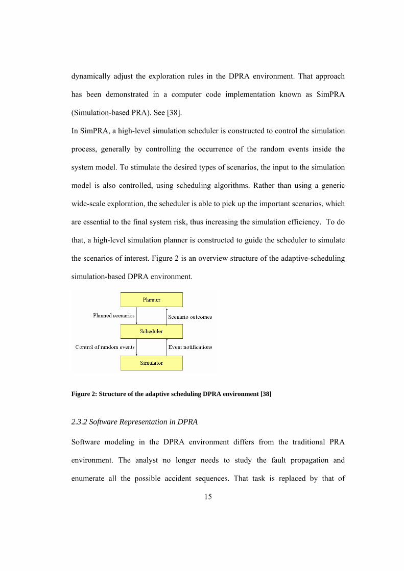
An adaptive-scheduling simulation-based DPRA environment has been developed at
the University of Maryland [38, 39]. Entropy-based biasing techniques are used to
adaptively guide the simulation towards events and end-states of interest. The prior
knowledge of the systems and knowledge gained during simulation are used to
15
dynamically adjust the exploration rules in the DPRA environment. That approach
has been demonstrated in a computer code implementation known as SimPRA
(Simulation-based PRA). See [38].
In SimPRA, a high-level simulation scheduler is constructed to control the simulation
process, generally by controlling the occurrence of the random events inside the
system model. To stimulate the desired types of scenarios, the input to the simulation
model is also controlled, using scheduling algorithms. Rather than using a generic
wide-scale exploration, the scheduler is able to pick up the important scenarios, which
are essential to the final system risk, thus increasing the simulation efficiency. To do
that, a high-level simulation planner is constructed to guide the scheduler to simulate
the scenarios of interest. Figure 2 is an overview structure of the adaptive-scheduling
simulation-based DPRA environment.
Figure 2: Structure of the adaptive scheduling DPRA environment [38]
2.3.2 Software Representation in DPRA
Software modeling in the DPRA environment differs from the traditional PRA
environment. The analyst no longer needs to study the fault propagation and
enumerate all the possible accident sequences. That task is replaced by that of

16
building an executable software model and identifying possible software-related
initiating events. The simulation environment will explore the scenario space, based
on the system model, which includes model of the hardware, human and software
elements. In this approach an executable software model first needs to be constructed
to simulate the software behaviors. The software-related failure modes need to be
identified similarly, as in the traditional PRA framework. The selected failure modes
will be superimposed on the executable behavior model as stochastic events. The
software-related failures are controlled by the simulation guidance model during
simulation, based on the predefined rules for exploring the risk-scenarios space,
following the selected initiating events.
Based on the above description, the software representation in the adaptive-
scheduling DPRA environment should include both a behavior model and a software
guidance model. The behavior model is an executable model. It will be plugged into
the system environment to simulate the software behavior. It should be able to capture
all phenomena that fall within the scope of the analysis. The software guidance model
guides the simulation to explore scenarios of interest instead of a wide-scale
exploration. The software guidance model should also interact with the high-level
planner and scheduler to better estimate the total system risk. See Figure 1
The software representation is established based on the information available. The
following assumptions and limitations are implied in this dissertation:
• Basic information about the software is obtainable.
• The software model can only be built based on information available. It can
not go beyond the level of information available.

17
• The software model is not guaranteed to be correct once the information is
limited. But the software model can be refined once the analyst gets more
information.
2.4 Teamwork
The research of SimPRA environment is a teamwork result. All team members
contribute their individual efforts to make this research come true. The whole team
includes Professor Ali Mosleh, Dr. Frank Greon, Dr. Yunwei Hu, Hamed Nejad,
Thiago Tinoco Pires, and me. My contribution to this research includes designing the
software model, implementing the software representation in SimPRA, developing a
methodology to simulate multi-level objects, and enhancing current SimPRA
environment to simulate multi-level objects. Figure 3 presents a teamwork chart to
identify the contributions from each individual team member.

18
GuidanceModel
Planner
Scheduler
HW
HMMulti-Layer
SoftwareBehaviour
Model
SW
Hamed Nejad
Yunwei Hu
Thiago Pires
scheduler
planner
human model
Dongfeng Zhu
integration
software model
multi-level SimPRA
Figure 3. Teamwork chart for SimPRA
2.5 Glossary of terms
The following terms are used in this dissertation:
1. Model: an abstraction of the real-life system. Models are used to obtain
predictions of the behavior of real system, especially how one or more
changes in various aspects of the modeled system would affect the other
aspects of the system. [38, 40]
2. Event: following the convention of discrete event simulation, an event is

19
defined as an instantaneous occurrence that changes the system configuration.
[41]
a. Random Events are the events whose occurrences are depicted by a
stochastic model and can be controlled by the simulation environment.
b. Deterministic Events are induced by the deterministic rules.
3. Scheduling: the process of controlling the generation of event sequences. It is
done by deciding on the occurrence and timing of the random events in the
model.
4. Branch Point: a point in the simulation of the system at which the occurrence
of a random event is considered by the algorithm controlling the simulation.
Each branch point will have two or more branches, corresponding to
occurrence of possible events.
5. End State: a classification of the condition of the system at the end of an event
sequence.
6. Scenario: One simulation realization as a sequence of events from the
Initiating Event (IE) to one End State (ES).
7. One round of simulation: One round of simulation is defined as a specific
number of scenarios generated before updating the plan. In other words, it is
the number of event sequences of one updating interval
8. Plan updating interval: The planner is part of SimPRA. It serves as a map for
exploration. The scenarios of interest are highlighted in the planner. The map
will be updated after each round of simulation.

20
Chapter 3: Software Modeling Requirements in DPRA
This chapter describes the basic requirements that a successful integration of software
behavior models in DPRA must meet.
3.1 General Modeling Requirement
From a general modeling perspective, the software model should be:
Simple in methodology
Easy to learn. The basic modeling concept should be easy to understand
Easy to use, with acceptable modeling costs
Quickly and seamlessly developed
Accompanied with a tool to help end users build the model
Easily and economically maintained and modified
Reusable
3.2 Simulation Requirements
From the simulation perspective, there are different requirements for the behavior
model and the guidance model. The software behavior model should have the
following characteristics:
Complete. Since the model needs to capture all phenomena that fall within
the scope of the analysis, the software model should be able to represent

21
most (ideally, all) of the software systems and software characteristics as
they relate to risk assessment.
Executable and linkable. The behavior model should be executable and
linkable with other elements, such as humans and hardware, inside the
DPRA framework. This is a basic requirement of the simulation
environment.
Hierarchical. First the model should have a hierarchical structure from the
lines of code to the coarser-grained software model. Meanwhile, different
levels of abstraction should also be defined to simulate the software behavior
at each level. Secondly one needs to model the software at different stages of
the software development life-cycle: requirement, design and code. The
modeling method should be usable at various stages and should also be
updatable as the analysts get more information about the real software.
Flexible. The level of the abstraction should be flexible and controlled by the
simulation scheduler. As was specified in the hierarchical requirements,
different levels of abstraction should be constructed, and the scheduler
should be able to flexibly control the simulation level of detail, based on the
different simulation requirements.
Controllable Stochastic Events. The behavior model is a combination of
deterministic model and stochastic model. Stochastic events represent
possible software failures inside the behavior model. The latter should be
controllable by the software scheduler and the high-level system scheduler.
During simulation, the stochastic events will be triggered to study the impact

22
of possible software faults.
Explorable. The simulation scheduler should be able to perform a systematic
exploration of the software model behavior.
The software guidance model is designed to guide the simulation to explore scenarios
of interest. It also interacts with the high-level simulation scheduler to automatically
adjust the software level of detail used in the simulation, based on prior knowledge
and previous simulation results. To fit into the DRPA simulation environment, the
guidance model should:
Capture common software vulnerabilities
Include a software scheduler to control the stochastic events inside the behavior
model
Adjust the software simulation rules, based on prior simulation results
Adjust the software simulation rules, upon requests from the high-level system
simulation scheduler
3.3 Interaction Requirements
Modern safety-critical systems are usually X-ware systems [42]. The systems consist
of interacting X-ware components of hardware, software, and human operators.
Software components thus interact with hardware, and human components within the
simulation environment. Therefore, we should also establish the software model
requirements from an interaction perspective.
Interaction in X-ware systems is defined as mutual or reciprocal action or influence in

23
relation to certain functions. It results in the exchange of matter, energy, force, and/or
information [42]. The system functions are achieved via the interactions of
components. As there are three types of components in X-ware systems (hardware,
software, and human), the interactions between any two components need to be
studied separately.
Software-Software interactions
Interaction between two software takes place via information exchange. The
information can be categorized into value-related information and time-related
information [43].
Value-related information
Amount: the total number or quantity of input or output
Value: The value taken by the input or output
Range: the limits of input/output’s quantities.
Type: a set of data with values having defined characteristics
Time-related information
Time: the point at which the ith input/output element is available or feeds
into/out of the software
Rate: the frequency at which the input is sent or the output is received
Duration: the time period during which the input or the output lasts
Load: the quantity that can be carried at one time by a specified input or
output medium
Software interactions need to be modeled in the software representation. The

24
representation should also have the capability to model all value-related failure modes
as well as time-related failure modes.
Software-Hardware interactions
Software interaction with hardware can be simplified as an information exchange.
Software obtains hardware-state information and then sends command signals to the
hardware. From this perspective, this interaction is similar to a software-software
interaction. Both value-related failure modes and time-related failure modes need to
be considered.
The hardware can also act as a support medium for software, such as memory, CPU,
etc. In that sense, support failure modes should also be modeled inside the software
representation.
Software-Human interactions
For complex, critical, and reliability-demanding operating environments, the
software/human interaction is equally important. Information related to human
detection can be divided into the following categories: visual detection, auditory
detection, olfactory detection, and tactual detection. Tactual detection and olfactory
detection usually invoke human/hardware interactions. When considering
human/software interaction, we usually need to consider the following characteristics:
• Auditory interaction
Spectrum; Frequency; Amplitude; Relative intensity
• Visual interaction

25
Overall layout; Position; Distance; Size; Color; Contrast; Brightness; Flash rate
These characteristics need to be added to the software output to human as additional
factors. Different value of these factors can influence human detection capability to
software output. These factors can be represented using value-related information and
time-related information. For instance, the relationship between distance and human
movement time can be modeled using Fitts’ Law [44]. The movement time can be
future used in the human model to predict the performance of operators using
complex system. Fitts’ law is stated as follows:
MT = a + b log2(2A/W) (3.1)
where
• MT = movement time
• a,b = regression coefficients
• A = distance of movement from start to target center
• W = width of the target
3.4 Non-Functional Requirements
A non-functional requirement is defined as a software requirement that describes not
what the software will do, but how the software will do it, as in for example, software
performance requirements, software external interface requirements, software design
constraints, and software quality attributes. [43] Nonfunctional requirements are
difficult to test; therefore, they are usually evaluated subjectively.
To model the software completely, the software representation should also be able to

26
capture the related non-functional requirements, which can be summarized in the
following categories:
Design constraints:
cost and delivery date
development process to be used
platform
accuracy requirements
interface requirement: describe how the system is to interface with its
environment, users, and other systems. (e.g., user interfaces) and their
qualities (e.g., user-friendliness)
response time: the time that elapses from when a user issues a command to
when the system provides enough results for the user to continue to work
throughput: computations or transactions per minute
technology to be used
resource usage
Lifecycle requirements
flexibility: the ability to handle requirement changes
installability: ease of system installation
operability: ease of everyday operation
allowance for maintainability and enhancement
allowance for reusability: describes the percentage of the system, measured
in lines of code, that must be designed generically, so that it can be reused
usability and availability: a quality that measures the amount of time that a

27
system is running and able to provide services to its users
robustness, recovery from failure
reliability: an important quality of software that measures the frequency of
failures, as encountered by testers and end-users
security requirements
portability: the capacity to be moved to different platforms or operating
systems
Other requirements
economic requirements
organization requirements
political requirements
Among all these requirements, we need to consider the requirements related to
software behavior and system risk. From that perspective, we mainly consider design
constraints, including the following:
• platform;
• accuracy requirements;
• interface requirements;
• response time;
• throughput; resource usage
The non-functional requirements should be captured inside the behavior model. The
simulation environment should have the capability to simulate different overload
situations to check for software vulnerability.

28
3.5 Discussion
In this chapter, the software modeling-requirements in the DPRA environment are
summarized from different perspectives.
The simulation requirements are basic requirements imposed by the simulation
environment. The software representation developed in this dissertation meets the
simulation requirements. The software methodology should be able to model all time-
related information and value-related information in order to model the interaction
requirements and the non-functional requirements. The methodology developed in the
following chapter ensures the integration of value-related information and time-
related information. It is the author’s belief that general modeling requirements are
met. A modeling tool is developed for software representation that is easy to learn,
easy to use, and easily maintained. The methodology is designed to be reusable.

29
Chapter 4: Software Representation Framework for simulation
4.1 Overview
Among the available methodologies for modeling software behavior are: finite-state
charts [6], UML [45], Petri-Net[46], and pattern concepts [47]. Those methods, and
others, fall into one of two broad categories: 1) those based on software data flow,
representing the software through decomposition of the system into dataflow
diagrams that capture the successive transformations of system input into system
output, and 2) those that model the procedural stages of the software, represented in
the form of states and transitions between those states, leading to a finite-state chart.
Because of its ability to model reactive systems, the latter seems appropriate for our
purpose.
Table 1 compares some existing software representations with respect to the
modeling requirements:
Executable Hierarchical FlexibleExplorableComplete Easy to learn
Easy to use
Reusable Tool Support
Pattern No No NA No No Good TBD Yes NA UML Engine
required No NA No TBD Fair TBD Partially Available
FSM Partially Yes Yes Yes TBD Very Good
TBD Partially Available
Petri-Net
Partially Yes No Yes TBD Good TBD Partially Available
Table 1. Comparison of the software representation methodologies

30
Table 1 shows that two of the criteria can not be assessed since completeness can
never be fully proven. No experimental evidence exists which would allow us to
conclude on the respective ease of use of the modeling approaches considered. Thus
we conclude based on the remaining factors that FSM best fits our purpose.
FSM has been defined as: A computational model consisting of a finite number of
states and transitions between these states, possibly with accompanying actions [5].
FSM accepts input events (or stimuli) that cause an output (or action) and possibly a
change in state. Both the output actions and the next state of the machine are pure
functions of input event and current state. Transitions can be separated into two parts:
conditions and transitions. Transitions are triggered when the conditions are true.
There are two concepts of states. 1) A condition or mode of existence that a system,
component, or simulation may be in; and 2) the values assumed at a given instant by
the variables that define the characteristics of a system, component, or simulation.
The concept of simulation-based Finite State Machine (SFSM) is defined in the
following sections. The model is based on FSM but integrates all the simulation-
required components.
4.2 Key Concept
The following concepts will to be used in the sections that follow.
1) Multi-Layer Software Representation
The software representation is defined during different stages of the software
development life-cycle. In this sense, it is a multi-layer software representation

31
starting with the requirement specification and continuing through the design
specification and coding stages. The software representation is refined after more
information becomes available. At any given time point in the software-
development life cycle, the software representation also has a multi-level structure.
(See next definition, below.)
2) Multi-Level Software Representation
The multi-level abstractions may be viewed as a hierarchical structure of software
representations from the lines of code to the coarser-grained software model. The
level of detail used in simulation is dynamically adjusted, based on the different
simulation requirements.
The relationship between the Multi-Layer and Multi-Level structure is illustrated in
Figure 4.
Requirement
Design
Code
......
Level 1
Level 2
Lowest Level
Level 3
......
Multi-Layer Multi-Level

32
Figure 4. Relationship between the Multi-Layer structure and the Multi-Level structure
3) Failure Modes
Failure modes fm are defined as the observable typically functional ways in which a
system, a component, an operator, a piece of software, or a process can fail. All the
failure modes considered in this dissertation belong to the pre-defined failure modes
set.
msm Ff ∈ (4.1)
4) Failure Sets
Failure-mode Sets Fms is simply a set of failure modes. A pre-defined failure-mode set
is defined in the following sections.
{ }mnmmms fffF ,,, 21 L= (4.2)
5) Stochastic Failures
Stochastic failures are the real failures injected at random, and according to a
stochastic model, in the software behavior model. Each stochastic failure is a
realization of a selected failure mode. Each failure has the following attributes:
Failure location
Failure mode
Stochastic properties (e.g., occurrence probabilities)
6) Abstraction
Abstraction techniques are defined as techniques that derive simpler representations
while maintaining the validity of the simulation results with respect to the questions
being addressed by the simulation. [48] Abstraction techniques can be categorized

33
into three broad techniques: model boundary modification, model behavior
modification and model form modification [48] [49]. Model boundary modification
refers to the modification of the input variable space. Model behavior modification
involves modification of behaviors within a model rather than the inputs to a model.
Model form modification refers to modification of model form, characterized by a
simplication of the input-output transformation within a model or model component.
In this research, functional abstraction and continuous abstraction are defined for
software abstraction based on the nature of software. Functional abstraction is an
abstraction of the discrete structure of the software. Functional abstraction can be
defined for all high-level functions. However, the lowest level function can not be
abstracted in this way. Functional abstraction is a mixed modification of model
boundary modification and model behavior modification.
Continuous abstraction is a mathematical abstraction of the continuous behavior of
basic functions. For instance, a complex equation using physical quantities, such as
temperature and pressure, i.e. continuous variables, can be abstracted using a look-up
table. Continuous abstraction focuses on model form modification.
7) Functional Abstraction vs. Functional Decomposition
Functional decomposition is a methodology used to break down complex systems
into low-level tasks or functions. A hierarchical function tree can be constructed
using the functional decomposition methodology. Functional abstraction is an abstract
description of high-level functions in the function tree. Use of functional abstraction
disables all sub-functions under high-level function.

34
4.3 Behavior Model
4.3.1 Overview
The behavior model is designed to capture all possible software behavior within the
scope of analysis. The real software is used directly in the previously mentioned test-
based methodology proposed for the classical PRA framework. Clearly, the software
itself could also be used as the behavior model in the DPRA environment. But using
the software directly in the simulation environment may be unacceptable for any of
the following reasons:
1) The software code is not available.
2) Software development is still in the requirement stage or the design stage.
3) The execution of the real software is time-consuming, which makes it
unacceptable for the purpose of simulation.
Software failures include requirement and implementation failures. Both types are
naturally included if the real software is used directly as the behavior model. There
are no controllable variables, so the software representation is merely a software-
behavior model. The software model gets inputs from the simulation environment and
provides outputs to hardware and human models.
In most cases the software-behavior model needs to be constructed separately by the
analyst. The behavior model can be constructed from the information available and
then refined after the analyst receives more information about the software. The
analyst may start with the information available from the software requirement
document, the design document, or the real source code. The closer to the real
35
software, the less uncertainty there will be in the final risk estimation, since the
representation is a more accurate description of reality.
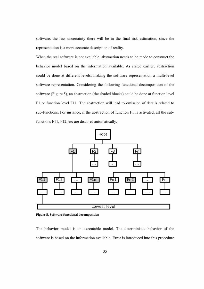
When the real software is not available, abstraction needs to be made to construct the
behavior model based on the information available. As stated earlier, abstraction
could be done at different levels, making the software representation a multi-level
software representation. Considering the following functional decomposition of the
software (Figure 5), an abstraction (the shaded blocks) could be done at function level
F1 or function level F11. The abstraction will lead to omission of details related to
sub-functions. For instance, if the abstraction of function F1 is activated, all the sub-
functions F11, F12, etc are disabled automatically.
Root
F1 F2 F3 Fn
.........
F11 F12 ... F1m
... ... ... ...
Lowest level
Fn1 Fn2 ... Fnl
... ... ... ...
Figure 5. Software functional decomposition
The behavior model is an executable model. The deterministic behavior of the
software is based on the information available. Error is introduced into this procedure

36
if the information is not accurate, but it can be reduced when the analyst receives
more information. The abstraction can be defined at different functional levels. The
behavior needs to be clearly defined for each level of abstraction.
Consider, for example, a software system LOCAT1 which calculates the projectile’s
coordinates. LOCAT receives real-time t from the TRAC hardware and computes the
corresponding (x, y) Cartesian coordinates and outputs the results. The highest logic
level system diagram is illustrated in Figure 6.
TRACHardware LOCAT OUTPUTt x,y
TRAC system
Figure 6. The highest logic level system diagram for LOCAT
LOCAT is composed of sub-functions realtimeCalculation and outputResult. Sub-
function realtimeCalculation can be further decomposed to sub-functions get_time
and cal_coordinate. Sub-function get_time retrieves time information from TRAC
hardware and validates the time received from TRAC hardware. Sub-function
cal_coordinate calculates x,y coordinates for the given time. Sub-function
outputResult outputs the results to the external device.
1 . The software is a part of a real-time simple projectile tracking system for the Army’s all weather Doppler radar
system called TRAC. It is part of a host software subsystem called COMP

37
getTime * calCoordinate
realtimeCalculation
outputResult *
Figure 7. Example Software System LOCAT
The abstraction behavior has been defined for function LOCAT, also for sub-function
realtimeCalculation. In this system the software function LOCAT can be modeled at
the abstraction level of LOCAT or at the lower abstraction levels realtimeCalculation
and outputResult, or at the detailed levels getTime, calCoordinate, outputResult. For
each level, the detailed behavior needs to be defined deterministically. The level of
detail is controlled by the software guidance model during simulation. Error is
introduced when simulating at a high-level, but can be eliminated when simulating at
the lowest level.
The software behavior model is constructed, based on an expected software behavior
that omits all the failures introduced during software implementation. The
implementation failures should be modeled also as stochastic events. The detailed
failure information should be simulated in the abstraction model during simulation.
The software failures can be injected at the selected level. The software function
outputs are influenced by the failures, even when the detailed locations of the
software faults are not available. So the software failures will be injected at the output
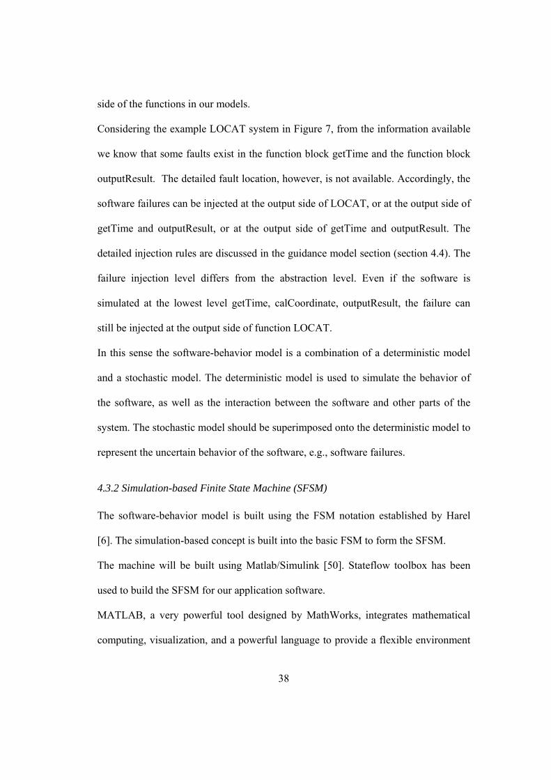
38
side of the functions in our models.
Considering the example LOCAT system in Figure 7, from the information available
we know that some faults exist in the function block getTime and the function block
outputResult. The detailed fault location, however, is not available. Accordingly, the
software failures can be injected at the output side of LOCAT, or at the output side of
getTime and outputResult, or at the output side of getTime and outputResult. The
detailed injection rules are discussed in the guidance model section (section 4.4). The
failure injection level differs from the abstraction level. Even if the software is
simulated at the lowest level getTime, calCoordinate, outputResult, the failure can
still be injected at the output side of function LOCAT.
In this sense the software-behavior model is a combination of a deterministic model
and a stochastic model. The deterministic model is used to simulate the behavior of
the software, as well as the interaction between the software and other parts of the
system. The stochastic model should be superimposed onto the deterministic model to
represent the uncertain behavior of the software, e.g., software failures.
4.3.2 Simulation-based Finite State Machine (SFSM)
The software-behavior model is built using the FSM notation established by Harel
[6]. The simulation-based concept is built into the basic FSM to form the SFSM.
The machine will be built using Matlab/Simulink [50]. Stateflow toolbox has been
used to build the SFSM for our application software.
MATLAB, a very powerful tool designed by MathWorks, integrates mathematical
computing, visualization, and a powerful language to provide a flexible environment

39
for technical computing. The open architecture makes it easy to use MATLAB and its
companion products to explore data, create algorithms, and create custom tools that
provide early insights and competitive advantages.
Simulink, a toolbox extension of Matlab, is an interactive tool for modeling,
simulating, and analyzing dynamic, multi-domain systems. It allows the user
accurately describe, simulate, evaluate, and refine a system’s behavior through
standard and custom block libraries. Simulink integrates seamlessly with MATLAB,
providing immediate access to an extensive range of analysis and design tools.
Simulink is a very good tool for control-system design, signal-processing system
design, communications-system design, and other simulation applications. Stateflow
is another toolbox for MATLAB. It is a graphical design and development tool for
simulating complex reactive systems based on FSM theory. Stateflow and simulink
together will be used to construct a software representation for our examples.
Some key notions of SFSM are defined in the following:
[State]
State is defined as a condition or mode of existence that a system, component,
or simulation may be in [5]. A state can be dissected into sub-states. There are
two types of states: exclusive state and parallel state. Exclusive states are used
for the software models that are mutually exclusive. Parallel states are used to
model parallel software, which means that two or more states can be active at
the same time [50].
States have labels that can specify actions executed in a sequence based upon
action type. The action types are “entry”, “during”, “exit” and “on”.

40
“Entry” action is executed when the state is entered. “During” action is
executed when the system stays in the state. “Exit” action is executed when
the system exit the state. “On event” action is executed when the given event
occurs and the system stays in the state.
[Transition]
Transition can be separated into two parts: the conditions and the transitions.
The transitions are triggered when the conditions are true. Actions can be
associated with both conditions and transitions. Transitions are not
decomposable, and all of the transition is executed instantaneously.
[Action]
Actions can be associated with states, conditions, or transitions. An action can
be a function call, the broadcast of an event, the assignment of a value to a
variable. It can be served as an interface to load the real software.
[Internal Variables]
Internal variables are defined inside the SFSM. They will be used to describe
the internal states of the software. They are also used to define control
information for the guidance model.
The basic concept of the SFSM is discussed above. Simulation-based elements are
added in the following sections.
4.3.3 Deterministic Model
Construction of the deterministic model is based on the information available. Multi-
layer abstraction can be employed during different stages of the software

41
development life cycle. Construction of the behavior model can be based on the
software-requirement document, the software-design document, and the software
code. The model is continually refined as more information becomes available.
Given the available information, the behavior model is also a multi-level model.
Multi-level abstraction is defined for selected functions which meet the following
criteria:
1) The execution of the functions is time-consuming (during simulation), and
2) The selected functions are not important for certain scenarios.
Different function blocks have different simulation priorities. The simulation level of
detail may be different for different sub-function blocks. Even for the same function
block, the priority changes in different contexts. The software guidance model
(section 4.4) dynamically adjusts the simulation level of detail.
The simulation level of detail is defined as an internal variable. The simulation
environment controls the values of the internal variables. The software is executed at
different levels based on the value of the control variables. (See Figure 8)

42
Figure 8. Typical structure used to control the level of model detail used in simulation
An abstraction knowledge base (AKB) needs to be defined before the simulation. A
tree structure is used to construct the AKB (See Figure 9). Use of high-level
abstraction will automatically disable all the low-level abstraction. The reason is
obvious; the use of “Abstract_Model” (see Figure 8) disables all details in the
software state “Detail_Model”.
Root
Abstraction 1 Abstraction n...
Abstraction 11 Abstraction 1n...
... ... ...
Figure 9. Abstraction Knowledge Base
A node of the AKB tree is described by the following equation:
{ }{ }njcjcpli NNNffiAKB
,,11,,,,,L=
= (4.3)
I is the abstraction-function index; the index uniquely defines the abstraction

43
function; the index value for Root is always 0;
fi represents the function name in the functional-decomposition structure (see
Figure 5);
fl represents the function level in the functional-decomposition structure (see
Figure 5);
Np represents the parent node of the current node; the value is -1 for the Root
node;
Ncj represents the child nodes of the current node; the value is -1 if there is no
child node available;
n represents the number of child nodes of the current node.
Only the structure-related information is stored in AKB. The simulation-related
information about the abstraction level of detail is stored in a separate knowledge
base. The detail of this knowledge base is introduced in the guidance model (section
4.4).
Considering the software example in Figure 5, the tree structure of AKB can be
represented by the following figure:
Root
F1 Fn2
F11 F1m
0, Root, 0, -1, {1,2}
1, F1, 1, 0, {3,4}
2, Fn2, n, 0, {-1}
3, F11, 2, 1, {-1}
4, F1m, 2, 1, {-1}

44
Figure 10. AKB for software example in Figure 5
The nodes of the AKB tree are described on the right side of Figure 10.
4.3.4 Stochastic Model
The stochastic model simulates the uncertain behavior of the software, e.g., software
failures. Uncertain behavior should be controlled by the software scheduler and the
high-level system scheduler. Using this mechanism, the simulation environment can
simulate the implementation failures in the real software and analyze their impact on
the whole system.
Failure Modes
Failure modes are defined as the observable ways in which a system, a component, an
operator, a piece of software, or a process can fail. A taxonomy of software-related
failure modes has been proposed in [4]. Software failures may originate either within
the software itself or from the software interface with its operational environment.
Failure modes, therefore, can be classified as either software functional-failure modes
(failure modes of the software itself) or software interaction-failure modes
(input/output failure modes, support-failure modes and environmental-impact factors).
In this research, input/output (I/O) failure modes are considered first. The I/O failure
modes include value-related failure modes (amount, value, range and type) and time-
related failure modes (time, rate, duration and load). Function failure modes generate
different function outputs and, as such can be covered by the above failure modes.

45
The effect of a support failure2 will be covered in future research. The definition of
the following failure mode set is based on the above information.
[ ] [ ]},,,,,,,{ loaddurationratetimeTtyperangeamountvalueTF tvs = (4.4)
The above set is used as a pre-defined generic failure-mode set in this research.
The value-related failure model uses the SFSM structure in Figure 11:
Figure 11. Value-related failure modeling in SFSM
Time related failures are complex, compared with value-related failures. Figure 12
presents the structure used for modeling a delay failure. Figure 13 shows the structure
for the delay unit.
2 The “support” failure modes include failures due to competition for computing resource and the computing
platform physical features. The failure modes due to resource competition are deadlock and lockout. The impact of
physical failures on software can be decomposed further into the impact of CPU failures, memory failures and I/O
devices failures
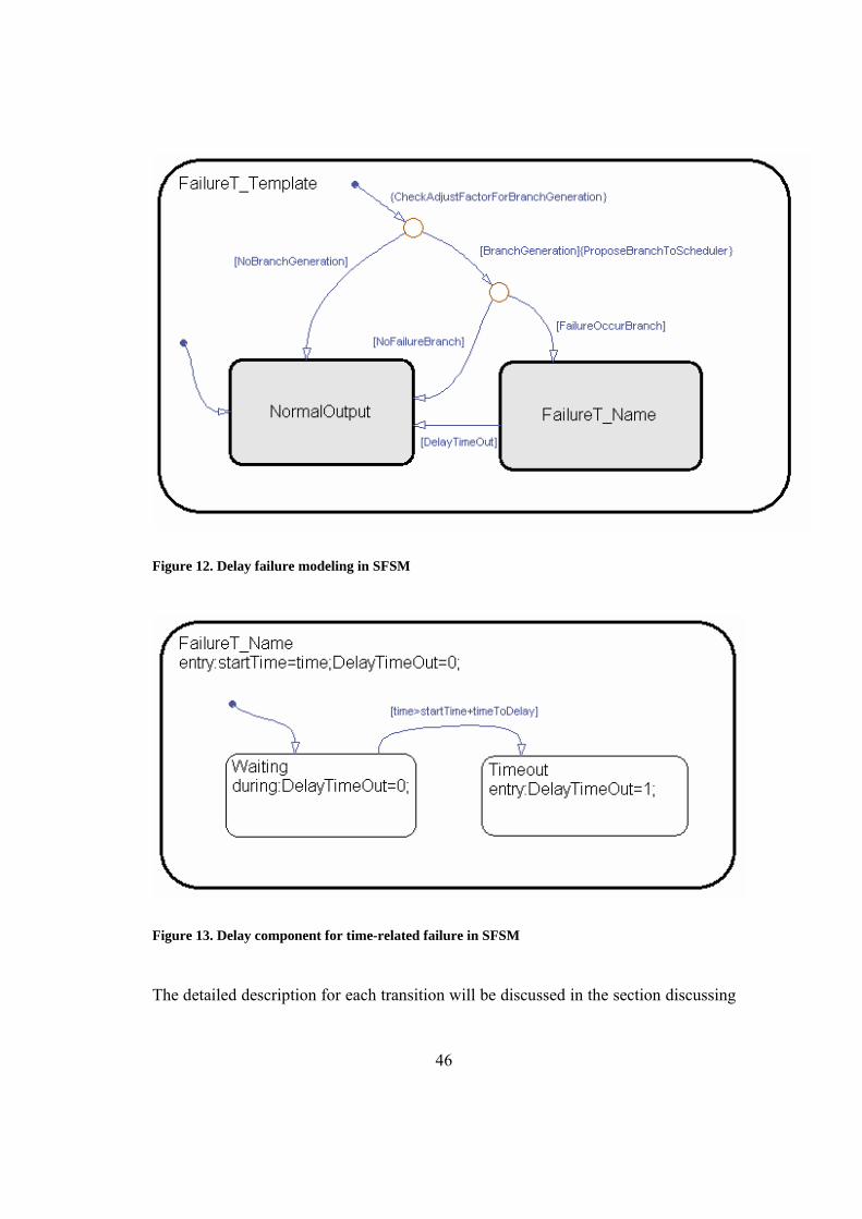
46
Figure 12. Delay failure modeling in SFSM
Figure 13. Delay component for time-related failure in SFSM
The detailed description for each transition will be discussed in the section discussing

47
the integration of the software model into the SimPRA environment (chapter 5).
Failure Injection
The selected software failures are injected into the software behavior model. Failures
are injected at the output side of software functions. They can be injected at different
software levels.
Considering the software example in Figure 7, it is known that some faults exist in
sub-function getTime and function outputResult.
getTime * calCoordinate
realtimeCalculation
outputResult *
LOCAT
F
getTime * calCoordinate
realtimeCalculation
outputResult *
LOCAT
F F
Figure 14. Different fault injection methods for an example system LOCAT
For the same type of failure mode, a high-level software failure is the combined result
of low-level failures. In the example system, the software failure at the function
LOCAT level is the abstraction of software failures at the sub function

48
realtimeCalculation and outputResult levels. Software failures belonging to similar
failure modes should not be modeled at different levels simultaneously.
The failure-injection level is different from the abstraction level Li. For example, in
Figure 14, the output failure can be injected at the level of function LOCAT.
However, the abstraction level of detail may be at the lowest level. In other words, the
failure can still be injected at the high-level, even if the detailed code is used in the
behavior model. The level of failure injection cannot go lower than the level of
abstraction for an obvious reason. The failure cannot be injected at the sub-functions
getTime and calCoordinate levels if they are not modeled at all.
The failure-injection location is determined by the analysts. The different injection
level is dynamically adjusted by the guidance model.
Failure Probability Quantification
The selection of software failure modes is based on expert opinion and previous
experience. Failure probabilities are estimated using statistical data, expert judgment,
or the test-based methodology mentioned in section 2.1, once the code is available.
For example, there are two databases for the Space Shuttle Group Project: one for the
history of the software code and another that records every error ever made on the
software project. As a result of the vast amount of data collected in the databases, the
Space Shuttle Software Group has written software that predicts the amount of errors
that should be expected. The data in the database is quite detailed: it contains
information on possible failures in the software code, and the probability of failure.
That information can be used to inject failures into the software representation and
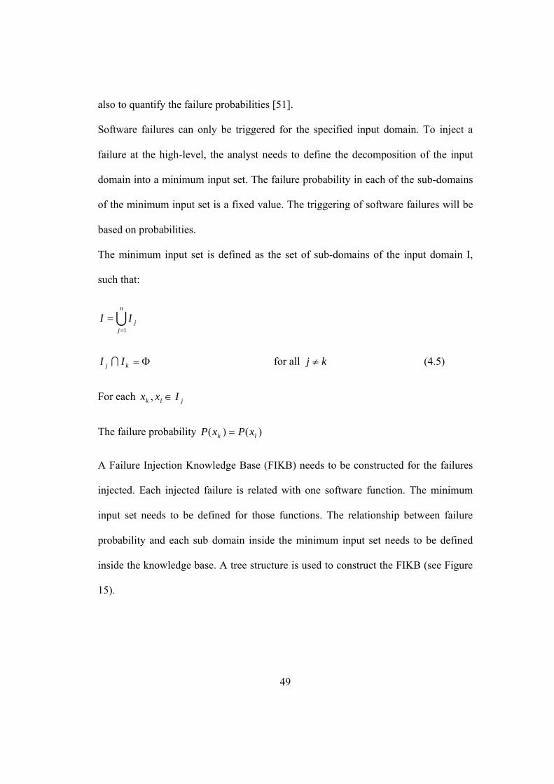
49
also to quantify the failure probabilities [51].
Software failures can only be triggered for the specified input domain. To inject a
failure at the high-level, the analyst needs to define the decomposition of the input
domain into a minimum input set. The failure probability in each of the sub-domains
of the minimum input set is a fixed value. The triggering of software failures will be
based on probabilities.
The minimum input set is defined as the set of sub-domains of the input domain I,
such that:
Un
jjII
1=
=
Φ=kj II I for all kj ≠ (4.5)
For each jlk Ixx ∈,
The failure probability )()( lk xPxP =
A Failure Injection Knowledge Base (FIKB) needs to be constructed for the failures
injected. Each injected failure is related with one software function. The minimum
input set needs to be defined for those functions. The relationship between failure
probability and each sub domain inside the minimum input set needs to be defined
inside the knowledge base. A tree structure is used to construct the FIKB (see Figure
15).

50
Root
Failure 1 Failure n...
Failure 11 Failure 1n...
... ... ...
Figure 15. Structure of the Failure-Injection Knowledge Base
Each node inside the FIKB can be presented using the following equation.
{ } { }{ }njjijiinjcjcplmi pfIINNNffiFIKB
,,1,,11 ,,,,,,,,,LL
L==
= Un
jjii II
1=
= (4.6)
I is the software-failure index; the index uniquely defines the injected
software failures;
fmi represents the name of the injected software-failure modes (see
Figure 5);
fl represents the injected software-failure level in the functional-
decomposition structure (see
Figure 5);

51
Np represents the parent node of the current node; the value is -1 for the Root
node;
Ncj represents the child nodes of the current node; the value is -1 if there is no
child node available;
n represents the number of child nodes of the current node.
Ii represents the input domain of the software-failure related function;
Iji represents each sub-domain of the minimum-input set; the size of the
minimum-input set is n;
pfji represents the failure probability for the sub-domain Iji;
n represents the number of sub-domains.
Fmi and fl are used in the guidance model to control the activation of the software
failures at different levels. Once the failures are activated, the relationship between Iji
and pfji is used to decide whether or not the failures are to be triggered for specific
input from the simulation environment.
Considering the example system in Figure 14, the failure can be injected at the level
of LOCAT as failure failure_LOCAT; it can also be injected at the level of sub-
function realtimeCalculation as failure_realtimeCalculation and sub-function
outputResult as failure_outputResult. FIKB can be represented using the tree
structure in Figure 16

52
Root
Failure_LOCAT
Failure_realtimeCalculation Failure_outputResult
Figure 16. AKB for software example in Figure 14
The guidance model controls the activation of software failures. High-level failures
and low-level failures can not be actived at the same time. In Figure 16,
Failure_realtimeCalculation and Failure_outputResult become invisible once
Failure_LOCAT is actived. Once the failure is activated, the relationship between Iji
and pfji defined for that failure is used to decide whether or not the failures are to be
triggered for specific input from the simulation environment.

53
4.3.5 Summary
The deterministic model and the stochastic behavior models were introduced in
previous sections. Several controllable variables are defined inside the behavior
model. Multi-level abstraction structure is constructed in the deterministic model. The
simulation level of detail is controlled by the guidance model (section 4.4). Software
failures are injected through the stochastic model. The failure modes and locations are
selected by the analysts. Different failure-injection levels are defined in the stochastic
model. The software failures are triggered in the guidance model. The detailed
mechanism used is discussed in the following sections.
To summarize, we can use the following equation to represent every component in
the software behavior model.
{ }njLSLSLSLB
mkfff
dfBdfLBLiLS
iijiiiiii
kdkis
iisiiisiiiii
,,1)1()1()1()1(,,1,
)1(*,*]),1([,,)(
21
~~
LL
L
=+⊕⊕+⊕+=+==
⎭⎬⎫
⎩⎨⎧ −⎥⎦
⎤⎢⎣⎡++=
(4.7)
I is the software component name or (index), which uniquely defines the
software components;
di is a Boolean variable indicating whether one will simulate Si at an abstract
level ; di is controlled by the scheduler;
Li is the current level of detail of the function Si in the software
representation; Li is a relative value. (For a given component, the current level
of detail may be different, depending on the definition of the baseline in the
software representation. The baseline is defined as level 0 of the software
54
component. The baseline needs to be unified for the whole software
representation before the simulation);
Bi is the detail behavior model of the software component Si;
~
iB is the abstract behavior model of the software component Si;
fis is a set of stochastic failures injected at the output side of the normal
behavior model of the software component Si;
~
isf is a set of stochastic failures injected at the output side of the abstract
behavior model of the software component Si (The structure of ~
isf is similar
as that of fis) ;
fk is a single software failure injected for this software function;
fkd is a Boolean variable indicating whether this failure is activated or not (fkd
is controlled by the simulation guidance model) ;
m is the total number of software failures injected for this software function;
⊕ represents that Bi is composed by the sub-function Sij.
If no abstraction is defined for the software component, equation 4.7 becomes a
solely functional decomposition of the software component. To explore the system
vulnerabilities, the software simulation-guidance model controls all the controllable
variables inside the behavior model.

55
4.4 Simulation Guidance Model
4.4.1 Overview
The high-level guidance model guides the simulation to explore scenarios of interest,
in lieu of doing a wide-scale exploration. In this sense the guidance model is not
necessarily a complete representation of the software system. Instead, it may be
fragmentary, covering only specific parts of the system. The key elements of the
software can be identified and built into the guidance model. General knowledge
about the software and common vulnerabilities should also be defined in the guidance
model. Meanwhile, a software scheduler needs to be constructed inside the guidance
model to control the stochastic behavior of the software and to communicate with the
high-level system scheduler.
The guidance model simultaneously interacts with the system-behavior model, the
software-behavior model, and the high-level system scheduler (See Figure 1). The
high-level scheduler provides high-level simulation requirements. The system-
behavior model provides hardware inputs and human inputs. The software-guidance
model adjusts the software-behavior model, based on the inputs from the system-
behavior model and the high-level system scheduler. The software-behavior model
generates the software outputs, based on the inputs from the guidance model.
4.4.2 Interactions with other models
Guidance Model vs. System Behavior Model
The relationship between the guidance model and the system behavior model is

56
relatively clear. The system-behavior model provides the input to the software and
receives the output from the software. The guidance model works as an intermediate
layer. Let Is-sw be the input from the system-behavior model to the software-behavior
model. Let Osw-s be the output from the software-behavior model to the system-
behavior model.
The input/output for the software-guidance model is:
Input from the system-behavior model Is-sw
Output to the system-behavior model Osw-s
Table 2. Software-guidance model vs. System-behavior model
Guidance Model vs. Multi-level Software-Behavior Model
The software-guidance model provides the software input to the software-behavior
model and controls the execution of the multi-level software model using control
variables. The system input to the software Is-sw comes from the system-behavior
model. The control variables include abstraction level of detail L, which of the pre-
existing software failure types ft should be activated and also the failure simulation
level of detail fL. The values of L, ft and fL are calculated based on the detailed
guidance rules.
The input/output for the software guidance model is:
Input from the software-behavior model Osw-s
Output to the software-behavior model Is-sw L ft fL
Table 3. Software-Guidance model vs. Software-Behavior Model

57
Guidance Models vs. High-Level System Scheduler
The relationship between the guidance model and the high-level system scheduler is
the most complex. The high-level system scheduler provides the high-level
requirements. The guidance model calculates the value of the control variables, based
on the simulation requirements and the inputs from the system model. It provides the
system scheduler with the simulation-level control information and the failure-
injection information. Also, the guidance model decides branch generation and
provides the result back to the high-level system scheduler. Let Rh be the high-level
requirements from the system scheduler. Let B be the branch-generation information.
The input/output for the software guidance model is:
Input from High-Level System Scheduler Rh
Output to High-Level System Scheduler B L ft fL
Table 4. Software-guidance model vs. System Scheduler
Rh includes:
Simulation level of detail control factor RL
Injected failure type Rft; Injected failure level of detail Rfl
Simulation time requirement factors Rt
There is no direct control from the high-level scheduler for a particular variable, if the
value of that variable is -1
The guidance model interacts with the enhanced SimPRA environment to adjust the
controllable variables. The enhanced high-level planner and scheduler are presented
in Chapter 5. The detailed guidance rules are discussed thereafter.

58
4.4.3 Simulation Knowledge Base (SKB)
A Simulation Knowledge Base (SKB) is constructed inside the software-guidance
model to store prior knowledge about the software system. SKB, AKB, and FIKB
together serve as the knowledge base for the software model.
The following information is stored in the SKB as prior knowledge:
1. Time-factor related information
The relationship between the high-level scheduler Simulation time requirement
factors Rt and the simulation level of detail control factor RL are stored in the
knowledge base. When there is no direct control from the high-level system
scheduler, the guidance model decides the simulation level of detail based on the time
requirements factor from the high-level system scheduler.
The relationship between Rt and RL is not necessarily a 1-to-1 relationship. When the
relationship between Rt and RL is 1-to-many, the probability for each pair should also
be defined in SKB.
That type of node in SKB can be described using the following equation:
{ }{ }LnLti RRRtypeiSKB L,,,, 1= (4.8)
I is the node index (the index uniquely defines the node in the SKB);
typei represents the type of node;
Rt represents the simulation time requirements factor from the high-level
scheduler;
RL represents the simulation level of detail;
2. Prior knowledge

59
The relationship between the pre-defined condition and the simulation level of detail
is stored in this part. It is an interface that can be modified by the analysts for
different applications. The pre-defined condition can be configured differently in
different environments. For instance, in the example system in Figure 17, let us
assume that the pump-control software is designed to maintain the life-support system
for the Space Shuttle, based on the temperature, pressure, and time. When the system
is in a relatively safe range, there is no need to simulate the control software in detail.
A high-level lookup table is used to simulate the software-deterministic behavior. The
lookup table is a continuous abstraction for the detailed control equation. When the
system reaches the danger area, the lookup table is not accurate enough, so the low-
level detailed control equation is used to simulate the software behavior.
Temperature
Pressure
Pump Control Software
Life Support System
Temperature, Pressure,Time
Low Level:Detailed Equation
High Level:
Lookup Table
Software
Scheduler
Danger
Safe
Sensitive
Figure 17. Pump control system
The relationship between the simulation level of detail (High/Low) and the
predefined condition (Range of Temperature + Pressure) is defined in this part of
SKB.

60
This type of node in SKB can be described using the following equation:
{ }{ }LnLi RRCtypeiSKB L,,,, 1= (4.9)
I is the node index (the index uniquely defines the node in the SKB);
typei represents the type of node;
C represents the pre-defined condition in the system model;
RL represents the simulation level of detail;
The above information is simply the type of information we studied to this point.
SKB can be further enriched later to store more simulation-related prior knowledge.

61
Chapter 5: Integrating the Software Representation into
SimPRA
5.1 State Explosion Issue
Dynamic Probabilistic Risk Assessment (DPRA) of complex systems is considered to
be the next generation of PRA techniques. It is not currently in wide use because of
state explosion issues that need resolution. DPRA is a set of methods and techniques
in which executable models representing the behavior of the elements of a system are
exercised in order to identify risks and vulnerabilities of the system, by simulating a
variety of sequences of events that are representative of the possible true behaviors of
the system. The event sequences typically share a single initial condition but are
varied by introducing, at various points in the event sequence, possible deviations due
to hardware and software failures, as well as human actions. The set of simulated
sequences is then analyzed to gain insights into courses of events leading to
undesirable end states, as well as their likelihood.
State explosion is a well-known problem that impedes the implementation of DPRA
techniques. The major weakness of the approach based on state space-exploration is
that the size of the state-space grows exponentially with the number of branches
generated and thus creates the state space explosion problem.
Different approaches have been proposed to solve the state explosion issue. One
approach is to employ a conservative assumption and merge the system states or the

62
end states, thus reducing the branch generations. A second approach is through
distributed computing which would reduce the loads on a single computer. Another
approach is to bias the simulation toward interesting events and end states. That
approach would include the use of a knowledge-driven high-level planner to guide the
simulation, as well as an entropy-based biasing of the scenarios. The simulation
scheduler drives the actual-risk scenarios. The SimPRA environment is a real
implementation of the third approach.
5.2 SimPRA environment
5.2.1 Overview
SimPRA is an adaptive scheduling simulation-based DPRA environment developed
by the University of Maryland under a grant from NASA Ames Research Laboratory.
[38] Prior knowledge of the systems and knowledge gained during simulation are
used to dynamically adjust the exploration rules in the DPRA environment. In
SimPRA, a high-level simulation scheduler is constructed to control the simulation
process, generally by controlling the occurrence of the random events inside the
system model. Instead of using a generic wide-scale exploration, the scheduler is able
to pick out important scenarios, which are essential to the final system risk, thus
increasing the simulation efficiency. To do this, a high-level simulation planner was
constructed to guide the scheduler.

63
5.2.2 Guidance Rule in the single-level SimPRA environment
The adaptive exploration strategy used in SimPRA is based on an adaptive learning
procedure. A general framework of adaptive learning procedure is described in Figure
18. It is believed that there is always information available prior to the experiments.
The information gained from past data can be used to alter the exploration strategy of
future exploration to more efficiently address the area of interest.
Figure 18. General framework for adaptive learning
In the current SimPRA environment, two kinds of knowledge are used to guide the
simulation. The first category is prior knowledge, including the system-specific
knowledge, such as the design of a system, plus generally applicable knowledge, such
as the experience from similar systems. The second category is knowledge obtained
during simulation, which is used to adaptively guide the simulation towards the
scenarios of interest and to fairly distribute the simulation among possible scenarios.
For instance, the event sequences generated can be used to modify the focus of
exploration.

64
Figure 19. The use of information in the SimPRA environment
The SimPRA environment includes a planner, a scheduler, and the system simulator
(see Figure 20).
The planner serves as a map for exploration. The scenarios of interest are highlighted
in the planner. The map should not necessarily be accurate and complete; it will be
updated after each round of simulation. There are two types of updating. The first
type is automatic updating after simulating a specific number of event sequences. A
second type of updating needs the analysts’ intervention. The result of simulation
may disagree with the plan. The discrepancy is highlighted for further investigation
by the analysts [52].
The scheduler manages the simulation process, including saving system states,
deciding the branch selection, and restarting the simulation. The scheduler guides the

65
simulation toward the plan generated by the planner. The scenarios with high
importance would be explored with higher priority, while all other scenarios also
have a chance to be simulated. The objective of the scheduler guidance includes [40]:
• Maintain sufficient coverage of important scenarios in the plan
• Guide simulation toward areas of greatest uncertainty
• Continuously adjust priorities, based on simulation results
• Avoid test areas known to definitely lead to a specific end state
• Cover all possible event-sequence space
Figure 20. SimPRA environment
Whenever it comes to a branching point, the system simulator proposes transitions
(branches) to the scheduler. The scheduler retrieves the information of the proposed
transitions and decides which branch to explore. The exploration command is sent

66
back to the simulation, and the simulation model executes the command, continuing
the simulation until another branching point or end state is reached.
There are two types of stochastic events in the system model: time-based events and
demand-based events. One type of stochastic behavior of a component can be
described by the probability distribution function of time-to-failure. There is another
class of failure. The probabilistic branching stochastic process has a set of outcomes,
each with of a probability of occurrence. The timing of the occurrence is not random;
instead, the outcomes at that point of time are random [38]. In our model, software
failures are considered to be demand-based failures3 , which means the software
failure is not triggered unless that part of the software is executed in the simulation
environment.
Software aging is another phenomenon discussed in the literature, where the error
conditions actually accrue with time and/or load, resulting in performance
degradation and/or failures. The typical causes include memory bloating and leaking,
unreleased file-locks, data corruption, storage space fragmentation and accumulation
of round-off errors [53]. This type of failure is not considered in this dissertation.
5.2.2 Integrating Software into the single-level SimPRA
Software reliability is defined in [54] by the Institute of Electrical and Electronics
Engineers as:
3 One should not confuse the concept of time-based event with the concept introduced later of delayed software
execution.

67
“Software reliability is the probability that the software will not cause the failure of
a product or of a mission for a specified time under specified conditions; this
probability is a function of the inputs to and use of the product, as well as a function
of the existence of faults in the software; the inputs to the product will determine
whether an existing fault is encountered or not.”
From the definition, it is clear that software reliability is a function of the context in
which the software operates. Software faults are triggered by specific input conditions.
Unlike hardware, software does not deteriorate with operation time. However, the
passing of time is still used as a parameter in some software reliability models due to
the fact that it usually associates with the count of software execution cycles, which
has a direct link with the probability of occurrence/non-occurrence of a specific input
condition.
Software risk models have been categorized as black-box unconditional software
reliability formulations and conditional risk formulations in the “Probabilistic Risk
Assessment Procedures Guide for NASA Managers and Practitioners” [10]. In the
conditional risk model, the presence of a software failure event is determined by two
basic constituents, namely:
• The “input condition” event that triggers the execution of a certain logic path
in the software
• The “software response” to that condition, as determined by the internal logic
path execution.
In our software representation, software failures are injected at the output of the

68
selected functions. The logic path from the beginning of the software input to that
selected function is already modeled inside the software behavior representation. The
internal logic of the selected function and the detailed location of the failure are
unknown to us. The failure probability is related with the input condition. The analyst
needs to divide the input domain into minimum input sets. Within each minimum
input set, the failure occurrence probability is treated as a uniform distribution.
All the failure-related information is stored in FIKB. The detailed structure of FIKB
is defined in chapter 4. Software failures are treated as demand-based failures. There
are some differences between software failures and hardware failures.
The first difference is that demand-based software failures are usually loaded more
frequently compared with other demand-based components in the simulation
environment.
In SimPRA, a branch point is proposed when a component with demand-based failure
is demanded in the system simulation. For instance, human action can be considered
as a demand-based component. When a human action is required in the simulation
environment, the human proposes different actions with different probabilities to the
scheduler. The scheduler picks one branch based on the scheduling rule. A branch
point is generated whenever the human action is demanded.
Software is different due to the reason that software requests are much more intensive
compared with other components. Considering the space shuttle thrust control
software, a software output is needed for every single step of the simulation. If there
is a software failure injected at the output of the thrust control software, it means a
branch point request is generated for every single time step in the simulation, which is

69
not efficient and is very time-consuming. The branch point request should be reduced
to an acceptable level.
In order to get unbiased estimation of the final system risk, we introduced the concept
of adjustment factor wa. Adjustment factor wa is a weigh factor ranging from 0 to 1. It
is used to adjust the number of software branch point requests (See Figure 21)
Figure 21. Software branch point generation adjustment factor
In Figure 21, only wa percent of software execution proposes a branch point to the
system scheduler. In order to make the final result unbiased, the adjustment factor
should be considered when the software proposes a transition to the system scheduler.
Assume the natural software failure probability is P. When the software proposes a
transition to the system scheduler, the probability used should be P/ wa. In this way,
the final branch probability remains identical. Indeed:

70
PwwP
aa
=× (5.1)
Also the occurrence of the branch points remains the same. Assume that the software
is executed n times. Before applying the adjust factor wa, the probability for the ith
execution to be selected is:
Pips =)( (5.2)
After applying the adjust factor wa, the probability for the ith event to be selected into
the group proposing branch generation requests is
awgip =∈ )( (5.3)
Within the group, the probability for each event to be selected is
as w
Pgiip =∈ )|( (5.4)
So the probability for the the ith execution to be selected is
PwPwgiipgipip
aass =×=∈×∈= )|()()(' (5.5)
Comparing the equation (5.2) and equation (5.5), one can see that the probability for
the ith execution to be selected remains the same. Thus the occurrence of the branch
points remains the same.
The total branch generation requests decrease after applying the adjust factor wa.
Before applying wa, the branch generation requests are proposed to the system
scheduler at every time step when the software is executed. Two branches are
generated if there are only two possible branches for each request. See Figure 22 a)

71
F F F F F
S S S S S
Wa
F
S
S
S
S
1-Wa Wa
FS
1-Wa 1-Wa
a) Before applying the adjust factor
b) After applying the adjust factor
Figure 22. The effect of the adjust factor to the branch generation
After applying wa, only wa percent of the software execution proposes the branch
generation requests to the system scheduler. Two branches are generated for each
request. For the rest of the software execution, no branch generation requests are
proposed to the system scheduler. Thus only one branch is generated. (See Figure 22
b)
Assume that the actual software execution can be represented using a Poisson
distribution with parameter λ. The number of branches generated after time T is:
Before applying wa 2×Tλ
After applying wa )1())1(2( aaa wTwwT +×=−+×× λλ
The adjustment factor can be selected by the analyst. But the value of the adjustment
factor should be greater than the natural probability of the software failure P.
Pwa >≥1 (5.6)
Considering a software function with the following input domain, the failure
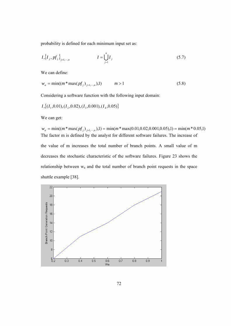
72
probability is defined for each minimum input set as:
{ }njjj pfII
,,1,,
L= U
n
jjII
1=
= (5.7)
We can define:
)1),)max(*min(( ,,1 njja pfmw L== 1>m (5.8)
Considering a software function with the following input domain:
{ })05.0,(),001.0,(),02.0,(),01.0,(, 4321 IIIII
We can get:
)1,05.0*min()1),05.0,001.0,02.0,01.0max(*min()1),)max(*min(( ,,1 mmpfmw njja === = L
The factor m is defined by the analyst for different software failures. The increase of
the value of m increases the total number of branch points. A small value of m
decreases the stochastic characteristic of the software failures. Figure 23 shows the
relationship between wa and the total number of branch point requests in the space
shuttle example [38].

73
Figure 23. wa vs. the total number of branch point requests in the space shuttle example
Comparing Figure 21 with the software failure template of Figure 11 and Figure 12,
the transitions within the template should be clear at this point.
The second difference is that the software failure probability is not a fixed value as in
other demand-based components. The failure probability is input condition dependent.
In FIKB, different failure probabilities are defined for different minimum input sets.
When the software-behavior model proposes a branch point to the scheduler, the
request is sent to the software-guidance model to get the failure probability based on
the input value. The guidance model queries FIKB to get the actual failure
probabilities and further sends the request to the system scheduler. (See Figure 24)
Software BehaviorModel
(Propose branch Point)
SoftwareGuidance Model
System Scheduler
FIKB
Input Condition +name of software failure
Input Condition +name of software failure
name of software failure +Failure Probabilities
name of software failure +Failure Probabilities
Figure 24. Software failure branch point generation procedure
The detailed rules used in the system scheduler to select a branch based on its value
measure can be found in [38].

74
5.3 Enhanced SimPRA environment
5.3.1 Overview
The state explosion issue was discussed in section 5.1. Three different approaches to
solve the problem were introduced. In this section, an alternative approach is
presented, in which a multi-level simulation environment is constructed; multi-level
objects are defined within the simulation environment; multi-layer planner and
scheduler are constructed and dynamically used to guide the risk simulation at the
right level of detail and abstraction. That reduces the branch generation and mitigates
the state explosion problem.
The initial levels of the multi-level objects are defined by the analysts in the plan. The
simulation results are used to adjust the level of detail to an appropriate level. The
multi-level objects are simulated at a relatively high-level when they are not
important for the end states of interest (see Figure 25).
Figure 25. Sample scenarios consisting of multi-level objects
An enhanced multi-level SimPRA environment is constructed and provisions are

75
provided to use software models at different levels of detail and fidelity. The
innovative aspect of the approach is that the selection of the most appropriate level of
detail is initially specified by the analyst in the Planner, but then automatically
adjusted during the various rounds of simulation according to an entropy-based rule.
5.3.2 Enhanced Planner
As we discussed before, the planner is designed to guide the simulation towards a
smarter and faster way to assess the risks of the system and generate useful
knowledge about the contribution of different classes of scenarios. The goal of the
plan is to guide the system to fail in such a way that the user’s knowledge about the
system is increased. The planning process that is suggested is dynamic, meaning that
the plan is updated by the results of the simulation. Figure 26 shows the cycle that the
planner goes through to guide the simulation in a dynamic way [38, 52].

76
Figure 26. Planner update cycle
A high-level Scripting Language (SL), similar to a programming language, is defined
in [38, 55] to represent the types of knowledge including physical and mathematical
knowledge as well as temporal knowledge.
In the enhanced SimPRA environment, a special Level Control Node (LCN) is added
to SL to represent the level information for multi-level objects. The LCN is added to
the scenarios generated in the plan. The structure of the LCN can be represented as:
},,{ valuetypeLCN
The type of level control nodes includes:
1. Undefined: the level control information is undefined.
2. Direct level control: the direct value for the level of simulation
3. Time Factor: the time factor required at this point (see section 4.4.3)
LCN is used to control the simulation level of detail for the multi-level objects. For
the direct level control, a System Level Knowledge Base (SLKB) is constructed
separately to associate the value of the level control with the level of detail for the
software, human and hardware. (See Table 5 for an example)
LCN Control Value Hardware level Software Level Human Level 1 1 1 1 2 1 2 2 3 1 3 2
Table 5. An example for the system level knowledge base
Inside the knowledge base, each row represents a compatible combination of the level
of detail for different sub-components. For each combination, the input/output of the

77
connected components needs to be compatible. For instance, if the software output is
connected to the human input, the number of output from the software model needs to
be compatible with the human input requirements. In other words, the human model
needs to be able to understand the software input and process the software input at the
level used.
The planner is loaded into the scheduler at the beginning of the simulation. The
simulation level of detail is adjusted adaptively based on the information in the plan,
the information in the guidance model of different components, and the previous
simulation results. After each round of simulation, the planner is updated, based on
the prior simulation results. The detailed adaptive scheduling rule and the updating
mechanism will be discussed in the following sections.
At the beginning of each simulation, the scheduler loads the plan from the plan file
generated by the planner. An ESD is constructed based on the scenarios within the
plan. LCN at the beginning of the scenario indicates that this plan is a multi-level
model. For instance, the following is an example plan.
LCN,1,1
BP1|BP2|LCN|BP3|End_1!H
BP1|BP4|BP5|BP6|End_2!L
BP1|BP4|BP5|BP7|End_1!H
BP1|BP8|LCN|BP9|End_2!L
An enhanced ESD with LCN can be constructed using the multi-level plan (See
Figure 27).

78
LCN BP1 BP2
BP4
BP8
LCN
BP5
BP7
BP6
LCN BP9
BP3
Figure 27. Example ESD constucted from a pre-defined plan
5.3.3 Enhanced Scheduler
The enhanced scheduler is established to handle multi-level objects in the simulation
model. The scheduler loads the plan at the beginning of the simulation. If the ESD
from the plan starts with LCN, the scheduler initializes the multi-level objects based
on the information in the first LCN.
The scheduler controls the level of multi-level objects based on the following logic.
1. If LCN contains the direct control information, scheduler reads the level
information from LCN; queries the system level knowledge base to get the
detailed simulation level for each sub-component; sets the simulation level of
detail for all multi-level objects. If there is no direct control information, go to
step 2;
2. If LCN contains time factor requirements4, the scheduler sends the time factor
requirements to the sub-components guidance model. In our case, the system
4 The time factor for different LCN is defined separately based on the input from the analyst. The value of time
factor for different LCN may be different.

79
scheduler sends an information request to the software guidance model, the
guidance model queries SKB to get the level control information based on the
time factor requirement and sends it back to the high-level scheduler; the high
level scheduler queries SLKB to check the compatibility of the level
information received from each sub-component and obtain a valid
combination; the scheduler sets the simulation level of detail for all multi-
level objects based on the combination.
3. If LCN is undefined, the scheduler sends this information to the sub-
component guidance models. The guidance model decides the simulation level
based on the information in SKB and sends it back to the high-level scheduler;
the high level scheduler queries SLKB to check the compatibility of the level
information received from each sub-component and obtain a valid
combination; the scheduler sets the simulation level of detail for all multi-
level objects based on the combination.
As discussed before, the plan is updated during simulation. In SimPRA, user could
specify the number of event sequences of one updating interval, and number of
updating round.
After the simulation has started, the enhanced scheduler will control the simulation
level of detail during each simulation. The simulation continues until it reaches a
LCN node. The level control logic is the same for all LCNs within the plan. The
simulation level of detail for multi-level objects only changes when the simulation
reaches LCN. The level information is adjusted based on the logic in Figure 28.

80
Initialize multi-levelcomponentsStart Simulation Simulation in
Progress LCN reached? Get level controlinformation
Differenct fromcurrent level?
Adjust the simulationlevel of detail
No
Yes
No
Yes
Branch Pointproposed and
selected
Figure 28. Simulation level of detail adjustment logic
The plan is updated after one round of simulation. The information in LCN is updated
based on the simulation results. A post simulation analysis is executed after each
round of simulation. The switching mechanism is based on Shannon’s entropy
measure [56-58] and its application to simulation branch generation introduced in
[38]. In this research the entropy-based branch control is extended to simulation level
control.
For a event sequence with two end states, let x be our degree of belief that end state E
will be reached, and let our belief regarding this probability be described by a Beta
distribution
( ) ( )( )βα
βαπβα
,1,|
11
Bexxx
−− −⋅= (5.9)
where 1α − and 1β − respectively represent the number of times that end states 1
and 2 are observed in a total of 2α β+ − sequences. Then the entropy measure is
equal to
( | , ) ( 1) ( ( ) ( )) ( 1) ( ( ) ( )) ln ( , )I x Beα β α ψ α ψ α β β ψ β ψ α β α β= − ⋅ − + + − ⋅ − + −
(5.10) where, ( )zψ is the digamma function,
81
'( )( ) ln ( )( )
d zz zdz z
ψ Γ= Γ =
Γ (5.11)
which for integer arguments can be computed as (Abramowitz)
1
1
1( )m m
α
ψ α γ−
=
= − +∑ (5.12)
such that
1 11
1 1
1 1 1( ) ( )m m mm m m
α β α βα
α
ψ α ψ α β+ − + −−
= = =
− + = − = −∑ ∑ ∑ (5.13)
For large values of z, the digamma function can be approximated efficiently by
( ) ( ) 2ln zzz −≈ψ (5.14)
After N simulation, the entropy reaches its maximum value when 1α − = N or
1β − =N. The entropy reaches its minimum value when 1α − = 1β − = N/2. A small
value of entropy indicates a state of ignorance about the outcome of the scenario. A
large value of entropy indicates a good confidence about the outcome of the scenario.
The entropy value is calculated for each multi-level object in the plan. It is used
together with the conditional end state probability after this node. The conditional
probability for end state of interest is calculated. It is a value ranging from 0 to 1. A
large value indicates that the execution of the failure in this multi-level object has a
large probability to lead the simulation to the end state of interest.
Considering the plan in Figure 29, software model is adjusted to the high-level after
LCN1.

82
SWLCN1
Figure 29. Part of an example plan
Software failures are executed after LCN1, the result of simulation indicates the
entropy for the software failure is high and the conditional probability to the end state
of interest is high, which indicates that we have a high confidence that the execution
of the software failure greatly influences the simulation to the end state of interest. In
this case, the software model should be further decomposed to get more accurate
results. In the reverse case, it indicates that the execution of the software failure does
not have a great influence to lead the simulation to the end state of interest. In this
case, the software model should stay at a relatively high-level.
The threshold for entropy and the conditional probability is defined by the analyst
before simulation begins. It can be further updated after each round of simulation.
After each round of simulation, the entropy value and the conditional probability for
each multi-level object is calculated and compared with the level information in the
previous LCN. If the value of entropy indicates that the simulation level should be
adjusted, the scheduler submits a request to the multi-level objects guidance models.
In our case, the system scheduler submits a request to the software guidance model to
check if any updates are available. If no further updates are available for the software,
the plan is treated as the best plan available. The simulation results are calculated
based on this plan.

83
Figure 30 describes a high-level overview of the data flows in the enhanced
scheduler:
Start Simulation
Define the planAnalyst
Load plan intoscheduler
Initialize multi-levelobjects
Start one round ofsimulation
Use entropy to selectbranch in each
simulation
Finish One round
No
Calculate entropy foreach multi-level object
Need update?
Submit request tosoftware guidance
No further updateavailable
Stop updating?
Success
Fail
No
Yes
No
Yes
Yes
Figure 30 Data flow in the enhanced SimPRA scheduler

84
The use of entropy-based strategies in the dynamic PRA environment to select
different branches is discussed in [39].
5.3.4 Software Guidance Model in SimPRA
The software guidance model receives the update request from the system scheduler.
The basic updating algorithm is presented in Figure 31.
Start Simulation
Initialize the level andfailure information
Simulation in progress
Receiving updatingcommand from
scheduler
Level can go futher?Adjust simulation level
Failure can bedecomposed?Decompose failure
Updatesuccess
Fail to Update
No
No
Yes
Yes
Figure 31: Software Guidance update mechanism
5.4 Integration
The approach to integrate the software model into the dynamic simulation

85
environment is as follows:
1 Identify the boundary of the software. Decompose the software into independent
software blocks. Each block is modeled separately.
2 Define the information available and construct the executable behavior model
using SFSM. (section 4.3.2)
3 Define the multi-level structure for the selected functions. In this step, the analyst
needs to choose the functions first. Then define the abstraction method and build
the high-level abstraction model for the selected functions. (section 4.3.3)
4 Select the software failures based on the available information, including the
failure type and different failure levels. Inject the software failures into the
behavior model. (section 4.3.4)
5 Construct AKB and FIKB using the software modeling tool. (section 4.3.3 and
section 4.3.4)
6 Build the software guidance model; establish the interface between the guidance
model and other models. (section 4.4)
7 Establish SKB. The analyst needs to categorize the prior knowledge available,
define the interface and summarize it in SKB. (section 4.4.3)
8 Integrate the software components in the high-level planner. The multi-level
abstraction information should be included in the plan generated. (section 5.3)
9 Run the simulation and update the plan using the simulation results. (section 5.3)

86
Chapter 6: Experimental Demonstration --- Propulsion System
Mission and Design Problem
6.1 Introduction
The benchmark problem is a multi-phase mission involving an ion propulsion system
needed for a science mission to the outer solar system. The propulsion system is
needed only in some of the phases, during which thrust is continually provided.
Mission Profile
An ion propulsion system is needed for a science mission to the outer solar system.
Figure 32 depicts the mission phases, along with the propulsion system operating
time during each phase in hours of Mission Elapsed Time (MET). Table 6 conveys
the same information in tabular form. For those phases where the propulsion system
only operates during part of the phase (e.g. Phases 4 & 5), thrust is continually
provided from the beginning of the phase until the specified operating time expires.
Phase No. 1 2 3 6 7
ON
Thrusters
OFF
MET [hour] 0 5520 14899 28039 41179 66180 68038 780395856 68538
4 5

87
Figure 32. Propulsion System Mission Profile
Mission Phase No. Duration (Hours) Propulsion System Operating Time (Hours)
1 5520.0 5520.0 2 336.0 0 3 9043.2 9043.2 4 26280.0 13140.0 5 26858.5 25001.0 6 500.0 0 7 9501.5 9501.5
Table 6. Mission Profile (table used in previous version)
Design Description
The propulsion system consists of 5 thruster assemblies and a single propellant
supply. Each assembly has:
1) propulsion power unit (PPU), and
2) ion engines
When an assembly is operating, the PPU provides power to just one ion engine. The
other engine will be in a standby mode, unless failed.
During Phase 1 the success criterion is propulsion from 2 assemblies. In all
subsequent phases where the propulsion system is operating, the success criterion is
propulsion from 3 assemblies.
Relative to the assembly operation, the strategy is to use Assemblies 1 through 2
during the first phase. During subsequent phases, Assemblies 1 through 3 will furnish
propulsion, if available.
Failure of an assembly causes it to be replaced by the lowest numbered standby
assembly. For example, if assembly 1 fails in Phase 1, the strategy is to actuate

88
Assembly 3. If no further failures occur during Phase 1, assemblies 2, 3 & 4 will
furnish propulsion at the beginning of Phase 3.
Basically, standby assemblies remain in standby until they are needed to replace a
failed assembly, and they are actuated in series (i.e., the lowest numbered assembly is
first selected).
Figure 33 is a schematic of a thruster assembly. In assessing the mission risk input
power failures are modeled separately, so the propulsion system model can ignore a
loss of power from that support system.
The strategy for thruster assembly operation is to begin with power from the PPU
going to Ion Engine A. Ion Engine A will continue to be the operating engine of the
assembly until the engine fails. At that time the strategy is to:
• shutdown the PPU;
• switch the PPU to Ion Engine B; then
• reenergize the PPU and operate with Ion Engine B.
There are no intermediate switches between a PPU and the ion engines. All switches
are integral to the PPU.
Figure 33 also depicts a propellant supply to each engine. The propellant is a noble
gas from a common storage tank. The engine ionizes and accelerates the propellant
to produce thrust. Since the propellant supply is part of the propulsion system, it
must be included in the system model.

89
Figure 33. Thruster Assembly Schematic
Common cause failures (CCF) should be assessed using the conditional probability
values from Table 7 by the CCF model of choice. No specific CCF model is
endorsed, but any simplification or approximation of CCF probabilities must be based
on calculations using the values below.
Group Size Group Conditional Failure Probability [%] 2 8.0 3 4.0 4 2.0 5 1.0
Table 7. Common Cause Failure Modeling Values
Table 8 is a failure mode and effects analysis for the propulsion system. Reliability
data are listed in Table 9.
Component Failure Mode Effect PPU Fails to start on demand Assembly failure
PPU
Ion A
Ion B
Input Power
Propellant (to A)
Propellant (to B)

90
Component Failure Mode Effect Failure to operate Failure to shutdown on
demand5
Ion Engine A Fails to start on demand6 Loss of redundancy Failure to operate Ion Engine B Fails to start on demand Assembly failure Failure to operate Propellant Valve A Failure to open on demand Loss of Ion Engine A Failure to close on demand System failure External leakage Propellant Valve B Failure to open on
demand7 Loss of Ion Engine B
Failure to close on demand System failure External leakage Propellant tank External leakage System failure Propellant distribution lines
External leakage System failure
Table 8. Failure Mode and Effects Analysis
Component Type Failure Mode Value PPU Fails to start on demand 1×10⁻⁴ (per demand) Failure to operate 1×10⁻⁶ (per hour) Failure to shutdown on
demand 1×10⁻⁵ (per demand)
Fails to switch to Ion Engine B
2×10⁻⁶ (per demand)
Ion Engine Fails to start on demand 3×10⁻⁵ (per demand) Failure to operate 2×10⁻⁵ (per hour)
5 Failure of a PPU to shutdown on demand will burn it out rather quickly. This results in an assembly
failure because the PPU is permanently disabled.
6 An ion engine is shutdown on demand be shutting down its PPU and closing its propellant valve. Hence,
failure to shutdown on demand is not an ion engine failure mode. However, the power surge
experienced when an ion engine is started (i.e., when its PPU initially supplies power) subjects an ion
engine to appreciable internal stresses that can result in failure to start on demand.
7 If Ion Engine A fails in an assembly, the strategy for transferring to Ion Engine B includes terminating
propellant flow to the failed engine and opening Propellant Valve B.

91
Component Type Failure Mode Value Failure to shutdown on
demand 3×10⁻⁶ (per demand)
Propellant Valve Failure to open on demand 3×10⁻⁴ (per demand) Failure to close on demand 3×10⁻⁴ (per demand) External leakage 5×10⁻⁵ (per hour) Propellant tank External leakage 1×10⁻⁶ (per hour) Propellant distribution lines
External leakage 1×10⁻⁶ (per hour)
Table 9. Reliability Data
Predicated upon the above mission and design descriptions, the time-dependent
reliability of the propulsion system over the planned mission should be quantified.
6.2 Simulation Model
6.2.1 Overview
The benchmark system is a system with hardware components and software
components. The whole software system is a parallel running software system with 6
sub software-components: 1 central control unit and 5 thruster assembly control
software. The central control software controls the status of the 5 assemblies by
sending control signals. The thruster assembly control software receives the
command from the central control software; controls the working status of the
assembly; and sends the status of the assembly back to the central control unit.
6.2.1 Software Model
Figure 34 shows a high level overview for the software model.

92
Figure 34. High level software overview for PSAM benchmark problem
The central control software controls the status of the assemblies during different
phases of the mission (See Figure 35). During each phase, the central control software
monitors the status of each assembly. If any working assembly fails, the control unit
powers off the failure unit and turns on the backup assembly (Figure 36). If there is
no backup assembly available, software control unit sends a signal to the simulation
environment to indicate the system failure.

93
Figure 35. Central control software representation for PSAM benchmark problem
Figure 36. Failure recovery mechanism for PSAM benchmark problem

94
There are 4 different states for each assembly during the mission: Standby, working,
switching and failure. A state diagram for the assembly is represented in Figure 37.
Figure 37. State Diagram for assembly control software
6.3 Discussion
In this chapter, a detailed software representation is presented to represent the parallel
control software based on the mission profile. No software failure is represented in
the original mission profile. But the simulation model can be easily extended to
introduce software malfunction failure modes. The impact of the software failures to
the system risk can be fully studied based on the simulation results, i.e., risk scenarios
leading to predefined End States are in form of specific realizations of time dependent
sequences of events. End State probabilities are based on grouping of such

95
realizations [59].
In the next chapter, a software model is constructed for a complex system. Different
types of software failure are injected in the software model. Three levels of
abstraction are defined. The whole integration process is studied in detail.

96
Chapter 7: Experimental Demonstration --- PACS
7.1 PACS System Introduction
The PACS system is a simplified version of an automated personnel-entry-access
system (gate) used to limit physical access to rooms, buildings, or other facilities to
authorized persons, to whom coded identification (ID) cards have been issued. The ID
card contains the person’s name and social security number. Users insert their ID
cards into a reader. The system searches for a match in the system’s updateable
database, requests the user’s four-digit Personal Identification Number (PIN),
validates the PIN, and unlocks a turnstile gate for entry. A single-line display screen
and a 12-key keyboard provide communication between the system and its users. A
security officer monitors a duplicate message on his/her console with override
capability.
The software system initially displays the message “INSERT CARD,” then checks a
register for a 0 or 1 value to determine if the card has been inserted into the card
reader. Given a positive response (value 1), it reads the nine-digit social security
number and the twenty-character last name and validates that data against the
information in the card database. If the card is valid, the software displays the
message “ENTER PIN”. Should the card not be readable then the message “RETRY”
is posted for a maximum of three tries, after which the system posts the message “See
Officer”. A duplicate message is sent to the officer.

97
The PACS system involves two humans (the user and the guard) and six hardware
components (the card reader, keyboard, single-line digital message display unit, the
guard’s display unit, guard reset unit, and a gate).
In the event of fire, the user needs to pass through the gate within sixty seconds. The
guard may notice the fire right away and open the gate directly. If the guard does not
open the gate, the user needs to pass through the gate using his ID card and PIN. The
user’s stress increases as the remaining time decreases. The guard may leave his
position in case of fire. Even when the actions of the user are correct, hardware
failures may generate incorrect inputs to the software. Software implementation or
requirements failures may be another reason for a delay in the opening of the gate.
The complex interaction among software, hardware, human and environment finally
leads to two end states. The end result may be either loss of occupant or successful
escape.
7.2 Simulation Model
7.2.1 Overview
Let us model the example system at the requirements stage. The software, human,
hardware and environment factors are modeled separately. Figure 38 shows a high-
level overview of the final system model.

98
Figure 38. High-level model overview for the PACS system

99
There follows the description of each block:
• FireEnvironment: This block simulates the fire initiator. The environment
factor evolves as the fire unfolds and so does the Human Performance
Influence Factor Stress. From Figure 38, we can see that the output of this
block serves as an input to the human modeling blocks.
• UserInput, GuardInput: These two blocks are human modeling blocks. The
human receives input from the software and control command information
from the high-level system scheduler. The human then performs different
actions, based on the inputs. For instance, the user may insert card, input PIN,
etc. Human stress increases as the time remaining decreases, causing the user
and the guard to be more prone to errors. The guard will leave his position
when the time remaining is less than 10 seconds.
• Hardware block: The hardware components are simulated in this modeling
block. The hardware serves as a bridge between humans and software. If a
hardware failure occurs, the corresponding software input may be incorrect
even if the human’s input is correct. The gate may not open even if the
software generates the right open gate command when a failure of the turnstile
gate hardware occurs.
• Software block: The software representation. Detailed procedures for building
the model are discussed in the following sections.
The hardware and human modeling blocks are not the focus of this research;
therefore, they are not discussed in detail.

100
7.2.2 Software Model
Below are the detailed steps for building the software representation.
Step 1: Identify the boundary of the software. PACS is an independent software
system; therefore, PACS is modeled as a whole unit.
Step 2: Model the PACS behavior, based on the software requirements specification.
The PACS model is implemented using Matlab/Simulink. Figure 39 shows a high-
level view of the PACS software model:
Figure 39. Detailed PACS behavior model
Step 3: Define the multi-level structure for PACS. Three levels are defined.
The highest level is to treat PACS as a single block (Abstract PACS in Figure 40).
User card information, User PIN input, and guard inputs are treated as one single
input. The output is gate status (open or not). The time necessary for human input and
software execution is added as the PACS execution delay.
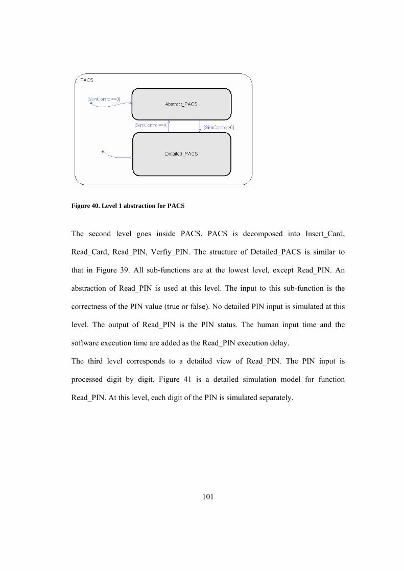
101
Figure 40. Level 1 abstraction for PACS
The second level goes inside PACS. PACS is decomposed into Insert_Card,
Read_Card, Read_PIN, Verfiy_PIN. The structure of Detailed_PACS is similar to
that in Figure 39. All sub-functions are at the lowest level, except Read_PIN. An
abstraction of Read_PIN is used at this level. The input to this sub-function is the
correctness of the PIN value (true or false). No detailed PIN input is simulated at this
level. The output of Read_PIN is the PIN status. The human input time and the
software execution time are added as the Read_PIN execution delay.
The third level corresponds to a detailed view of Read_PIN. The PIN input is
processed digit by digit. Figure 41 is a detailed simulation model for function
Read_PIN. At this level, each digit of the PIN is simulated separately.

102
Figure 41. Detailed simulation model for Read_PIN
Step 4: From past experience, typical software failures are selected for different
abstraction levels. Below are some of the failures injected:
Level Function Failure Modes Failure Description 1 PACS Value A value failure is injected at the output of
PACS; gate does not open even if the user inserts the correct card and inputs the correct PIN.
1 PACS Time A delay failure is injected at the output of PACS; gate opening is delayed even if the user inserts the correct card and inputs the correct PIN.
2 Read_PIN Time An infinite time delay is injected for any abnormal PIN input.
3 Done_Input Function 8 If the input is not “enter” as expected, Function Done_Input leads the software to a crash state.
Table 10. Software failure examples for PACS
Step 5: The Software AKB and FIKB are constructed automatically, based on the
PACS software model. PACS is a small example with only a three-layer abstraction;
8 This is a real fault at the lowest code level which is not controllable.

103
so, the structure of the knowledge base is relatively simple. Figure 42 is the structure
for the abstraction knowledge. Because of the nature of the abstraction knowledge
base, only the functions with abstractions are modeled in the knowledge base.
PACS
Read_PIN
Lowest level
Figure 42. Abstraction knowledge base for PACS
Step 6: Build the software guidance model; establish the interface between the
guidance model and other models. The software model is integrated in the whole
system model (see Figure 38). The input/output interfaces are defined and connected
to the rest of the system model.
Step 7: Establish SKB. The analyst needs to categorize the prior knowledge available,
define the interface and summarize it in SKB.
Two types of information are categorized and stored in SKB. The first type is the
time-related information. A simple knowledge base is constructed to build the
relationship between the high-level system scheduler time requirements and
controllable variables. In the PACS example, the time requirements factor from the
high-level scheduler includes three different values.
Time Requirement Factor Simulation Level
Low 3

104
Medium 2 High 1 Table 11. Time requirement factor table for PACS
The second category is the prior knowledge information. Based on prior knowledge,
the user has a very low probability to exit the gate if the time remaining is less than
10 seconds since the guard is no longer available and the user will easily make a
mistake in such a short time. PACS is simulated at the highest level if the pre-defined
condition is true.
Tremaining < 10s, RL = 1
Step 8: Integrate the software components in the high-level planner. Software input
and output vary, depending on the software level. The human input should also be
defined separately for different levels. The multi-level abstraction information is
included in the plan generated. The following scenario is part of the plan generated.
In the event of a gate failure, the probability that the gate will open is low even if the
software issues the gate open command. In this scenario, PACS is executed at the
highest level. In the case of a keyboard failure, PACS is executed at the second level
since there is a high probability that the software will receive a wrong PIN even if the
user inputs the right PIN through the keyboard (See Figure 43).

105
FireGate
HardwareFailure
PACS to level1
PACS defaultlevel 3
Read_Card KeyboardError
PACS to level2
HumanInsert Card
Figure 43. Extract of the plan for the PACS simulation
In the high-level system scheduler, a knowledge base is constructed to store the
relationship between the software simulation level of detail and the human simulation
level of detail. The human simulation level of detail is adjusted automatically with the
software simulation level of detail by the high-level system scheduler.
Step 9: Run the simulation and update the plan using the simulation results. The
initial plan for the multi-level objects may not be perfect. The plan is updated
automatically based on the simulation results.
Running the simulation model based on the pre-defined plan, the cumulative
distribution of the two end states are obtained through SimPRA. (See Figure 44)

106
Figure 44. Probability estimation from SimPRA
A list of scenarios is generated as part of the simulation results. Here is one example
scenario:
FireProtection
OffFire
t=0 second
Guard OpenGate
t=4 second
Guard ResetUnit
hardwarefailure
t=5 second
User InputsRight Card
t=19 second
User InputsWrong PIN
t=38 second
Guard OpensGate
t=41 second
Guard ResetUnit
hardwarefailure
t=42 second
Loss ofOccupants
t=60 second
User InputsWrong Card
t=52 second
Figure 45. Example scenario for PACS

107
7.3 Traditional vs. Dynamic
PACS has been studied in [3] using the traditional PRA methodology. The ESD in
Figure 46 is used to model the system evolution. Software components are included
in the ESD and quantified using the test-based methodology.
The ESD in Figure 46 is a simplified version with conservative assumptions. The
guard intervention is restricted to the beginning of the fire. If the guard fails to take
action, the user will only have one chance to escape the gate using his card or PIN.
Failure to insert the right card or to input the right PIN all lead to loss of occupants.
The assumption here is that the guard always opens the gate directly in case of fire if
the guard is in his position. If the guard is not in his position, no one is going to open
the gate or reset the system thus the user only has one chance to insert the right card
and input the right PIN. The logic here seems clear and complete under this
assumption. But it is not. For instance, the dynamic scenario in Figure 45 is not
covered in this ESD. The following story can be retrieved from Figure 45:
The guard noticed the fire immediately and decided to open the gate directly. He
pressed the gate open button but the gate did not open due to a hardware failure in
the guard reset unit. The user tried to exit the gate using his card and PIN. The guard
stayed in his position to reset the system if needed. Even if the guard can not open the
gate directly, he can still reset the system and allow the user multiple trials. The user
inserted the right card but input the wrong PIN due to stress. The guard reset the
system but the user failed to get out before 60 second.

108
EmergencyExit
PACS(2)B1
LED1Yes
No
Yes
Safe
Safe
Loss of
Occupants
Safe
No
Yes
FireProtection
YesSafe
No
Loss ofOccupants
Guardthere
Guardaction
T1< TcriticalYes
No
Loss ofOccupants
Delay
PACS(1)B3
GateDelay of
opening of
gateT2< Tcritical
Yes Yes Yes
No
NoNoNo
PACS (3)B2
GateDelay of
opening ofgate
T2< TcriticalT3< TcriticalYes Yes
NoNo No
Fire
No
Sequence 1
Sequence 2
Sequence 3
Sequence 4
Sequence 5-6
Sequence 7
Sequence 8-11
56
8 9 10 11
The userinsert the
card
Yes
Yes
Delay
The userinsert the
PINDelay
Delay Safe
Loss ofOccupants
PACS (4)B2
GateDelay of
opening ofgate
T2< TcriticalT3< TcriticalYes Yes
NoNo No
Sequence 12
Sequence 13-1513 14 15
YesThe userinsert the
PIN
Figure 46. ESD for the PACS System (The initiator is fire. Gray place holders indicate the presence of software contributions).
109
Apparently this scenario fits into the assumptions used to create Figure 46 but is not
covered in the ESD. The reason is complex. The dynamic interactions among the
components make it difficult for the analyst to identify and predict all the possible
scenarios. Meanwhile the count of scenarios increases dramatically if the analyst
needs to consider the details of the system. The analyst has to model at a relatively
high-level to explore all possible scenarios. In the ESD in Figure 46, the software
related blocks B1, B2, B3 in the ESD represent a group of events. For instance, block
B1 in Figure 46 represents the Read Card function. Two different branches originate
from block B1: correct card is read or failure to read card. Considering the second
branch, the possible reason for failing to read the card includes a failure of the
software function Read_Card, a failure of the card reader hardware, and human
failure. If the analyst needs to unfold all these blocks, the size of the ESD will
increase dramatically. Using the dynamic PRA methodology, the analyst only needs
to construct the behavior model and the simulation environment explores all the
scenarios automatically. The level of detail can be easily changed. Meanwhile, once
the system model has been constructed, only small modifications are needed to obtain
results under different assumptions.
Compared with the traditional PRA methodology, software modeling in the DPRA
environment has the following benefits:
• The dynamic methodology generates more information in the output.
The scenarios generated in the dynamic environment include time-related
information. The ESD used in the traditional methodology is conservative. Time-

110
related information is generated in the ESD.
• The system model generated using the dynamic methodology can be easily
and economically maintained and modified.
If a new failure needs to be included in the system analysis, the entire ESD in the
traditional methodology may need to be reconstructed and all components may need
to be re-quantified if the operational profile is different. In the dynamic environment,
the result can be obtained easily by running the simulation after adding the new
failure in the system model.
• The system and software models generated using the dynamic methodology
are reusable.
The system and software model generated in the dynamic environment can be easily
reused for a different system if similar components exist.
7.4 Multi-level Simulation
The system model for PACS is a multi-level model, as described in section 7.2.
Running the simulation at different levels generates different results. PACS has been
executed under the following three different cases:
Case 1: The execution of PACS has been maintained at the highest level: level 1;
Case 2: The execution of PACS has been maintained at the lowest level: level 3;
Case 3: The simulation level of detail is dynamically adjusted by the simulation
environment.
The following results are generated after 500 runs:

111
Time Used (s) Success Loss of Occupant Case 1 412.26 0.891 0.109 Case 2 463.61 0.947 0.053 Case 3 447.28 0.928 0.072 Table 12. Multi-level simulation: Run-time for different levels of detail (within SimPRA)
In Table 12, the “time used” factor is influenced by both the software model and other
parts of the simulation environment. Table 13 displays the run time obtained when the
contribution of the software model is isolated from the simulation environment.
Time Used (s) Case 1 187.985 Case 2 219.063 Case 3 213.469 Table 13. Multi-level simulation: Run-time for different levels of detail (in Isolation)
7.5 Comparison of software model vs. Real code
In this section an experiment is designed to validate the software model when
compared with the real code. All hardware failures are removed from the PACS
system model. The guard action is restricted to responding to the user’s requests. In
other words, the guard will not open the gate before the user inserts his card, or inputs
his PIN. Also the guard will not leave when the time left is small. The software
models are built based on different levels of knowledge from analysts. The profile for
PACS is completely defined. Value-related failures are injected into PACS and
testing is performed on the real code. Analysts design the software model based on
the results from different levels of test results. The models are integrated into the
simulation environment. The results are obtained and compared with those obtained

112
using the code directly in the simulation environment.
Here are the basic procedures for this experiment:
1. Define a complete operation profile for PACS
2. Inject software failures into PACS code
3. Test PACS; different levels of results are obtained based on the number of
rounds of tests performed
4. Build a software model based on different levels of knowledge; integrate the
software model into the simulation environment and run the simulation
5. Integrating the software code into the simulation environment; the IO part of
the software model is modified to fit the simulation environment; compare the
simulation results with the results from step 5.
6. Calculate quantitative coverage information through the comparison of
scenarios generated
Step 1: Define a complete operation profile for PACS
All hardware failures are removed from the current PACS system model. In that way,
the influence of hardware failure is isolated from the final system risk estimation.
Final results are influenced only by the software model and the human decisions. The
following profile is used for the human:
• The probability for a user to insert a right/wrong card is 0.55/0.45
• The probability for a user to insert a right/wrong PIN is 0.55/0.45
• The probability for a guard to accept/reject a user request to open the gate is
0.5/0.5

113
Assume PACS is used in a building with 10 employees with SSNs and PINs as
follows:
Name SSN PIN Jacob 212590000 0000 Michael 212590001 1111 Joshua 212590002 2222 Matthew 212590003 3333 Andrew 212590004 4444 Christopher 212590005 5555 Joseph 212590006 6666 Nicholas 212590007 7777 Daniel 212590008 8888 William 212590009 9999 Table 14. User records
The following assumptions apply:
• Only the first 5 people have the authorization to pass through the gate.
• All four numbers in a PIN are the same. There are only 10 different PINs
available during simulation.
• All cards used during simulation belong to the 10 records in Table 14.
For each user, the probability of inserting the right/wrong card is 0.55/0.45. The first
5 cards in Table 14 are treated as right cards; the rest, as wrong cards. The
right/wrong cards are uniformly distributed in the set of right/wrong cards. Once the
user inserts the card, the probability of inputting a right PIN is 0.55. The probability
of a user inputting a wrong PIN is 0.45. The wrong PINs are uniformly distributed in
the set of wrong PINs.
Step 2: Inject software failures into PACS
A correct database should contain the first 5 records in Table 14. Now assume that the

114
database is erroneous, and the following information is the information actually
stored in the database.
SSN Name PIN 212590000 Jacob 0000 212590001 Michael 5555 212590002 Joshua 2222 212590003 Matthew 3333 212590004 Andrew 4444 212590005 Christopher 5555 212590006 Joseph 6666 212590001 Michael 1111 Table 15. Database used in PACS
The following errors are observed in the database:
1. There are two records for Michael in Table 15; the first record contains the
wrong PIN
2. Christopher and Joseph are not supposed to be in the database
Because of those errors, the following different value-related failure modes exist in
PACS:
1. A user with a correct card and correct PIN cannot enter the gate
2. A user with an unauthorized card and right PIN can enter the gate
3. A user with a correct card and wrong PIN can enter the gate
Those failures are typical in this type of system. The failure probability for each
failure mode can be obtained through software testing.
Step 3: Test PACS.
A test environment is designed using visual C++. The software input is sampled from
the database in Table 14. Assume that the analyst has no knowledge about the actual

115
failures residing in the software; using the original design information, tests are
performed at different software levels.
[High-level Testing]
The first testing is performed on the entire software. The following results are
obtained after the indicated number of tests:
Number of Tests 10 100 1000 10000 Right Card, Right PIN, Success 6 58 542 5385 Right Card, Right PIN, Fail 0 7 74 741 Right Card, Wrong PIN, Success 0 1 18 186 Right Card, Wrong PIN, Fail 1 8 100 1060 Wrong Card, Right PIN, Success 3 19 222 2196 Wrong Card, Right PIN, Fail 0 0 0 0 Wrong Card, Wrong PIN, Success 0 0 0 0 Wrong Card, Wrong PIN, Fail 0 5 26 209 Wrong Card, Fail 0 2 18 225 Table 16. Test results for PACS
Based on the test results, the failure probabilities can be calculated for different
inputs:
Conditional Probability Input Failure 10 100 1000 10000
Right Card, Right PIN Fails to go through 0 0.108 0.120 0.121 Right Card, Wrong PIN Goes through 0 0.111 0.153 0.149 Wrong Card, Right PIN Goes through 1 1 1 1 Wrong Card, Wrong PIN Goes through N/A 0 0 0 Table 17. Failure probabilities for PACS (from high-level test results from Table 16)
From the results in Table 17, we observe that more software failures are detected after
enough rounds of testing are performed. In this example, all software failures can be
detected after a certain rounds of testing.
In this example, the high-level operational profile for PACS is influenced by software

116
errors. Theoretically, a user with a wrong card shall not be able to go through the
gate, and a user with a right card and the right PIN can always go through. The high-
level human input profile can be calculated, based on the theoretical probabilities; but
this method is inaccurate because of software failures. In this example, multiple
software failures are observed after software testing. So the high-level operational
profile should also be updated based on test results. The operational profile for the
human can be calculated based on the test results in Table 16.
Conditional Probability Input 10 100 1000 10000
Right Card, Right PIN 0.6 0.65 0.616 0.6126 Right Card, Wrong PIN 0.1 0.09 0.118 0.1246 Wrong Card, Right PIN 0.3 0.19 0.222 0.2196 Wrong Card, Wrong PIN 0 0.05 0.026 0.0209 Wrong Card, No PIN Input 0 0.02 0.018 0.0225 Table 18. Operational Profile for High-level PACS
[Low-level Testing]
The second test is performed at a detailed level. The testing is performed for sub-
functions: Card validation and PIN validation. The following table shows the test
results for card validation:
Total Tests 10 100 1000 10000 Right Card, PIN Entry Process can proceed 7 56 544 5500 Right Card, Fail 0 0 0 0 Wrong Card, PIN Entry Process can proceed 1 20 192 1825 Wrong Card, Fail 2 24 264 2675 Table 19. Testing results for card validation
Based on the test results, the failure probabilities can be calculated for different
inputs:

117
Conditional Probability Input Failure 10 100 1000 10000
Right Card Fails to go through 0 0 0 0 Wrong Card Goes through 0.333 0.455 0.421 0.406 Table 20. Failure probability for card validation
A further test is performed for PIN validation. It is performed separately and
conditioned on the types of card validation. Table 21 lists the PIN validation test
results when the user has used a right card to pass the card validation stage. Table 22
lists the PIN validation test results when the user has used a wrong card to pass the
card validation stage.
Total Tests 10 100 1000 10000 Right Card, Right PIN, pass 3 35 450 4345 Right Card, Right PIN, fail 2 18 97 1038 Right Card, Wrong PIN, pass 0 0 7 100 Right Card, Wrong PIN, fail 5 47 446 4517 Table 21. Testing results for PIN validation (right card)
Total Tests 10 100 1000 10000 Wrong Card, Right PIN, pass 7 62 575 5624 Wrong Card, Right PIN, fail 0 0 0 0 Wrong Card, Wrong PIN, pass 0 0 0 0 Wrong Card, Wrong PIN, fail 3 38 425 4376 Table 22. Testing results for PIN validation (wrong card)
The failure probabilities can be calculated from the test results:
Conditional Probability Input Failure 10 100 1000 10000
Right Card, Right PIN Fails to go through 0.4 0.340 0.177 0.193 Right Card, Wrong PIN Goes through 0 0 0.016 0.022 Table 23. Failure probabilities for PIN validation (right card)
Input Failure Conditional Probability

118
10 100 1000 10000 Wrong Card, Right PIN Goes through 1 1 1 1 Wrong Card, Wrong PIN Goes through 0 0 0 0 Table 24. Failure probabilities for PIN validation (wrong card)
Step 4: Build a software model based on different levels of knowledge
The software model can be constructed from the test results. There are two different
strategies. The first is to inject only those detected failures. The second, more
conservative one, is to inject all possible failure modes using probability estimation.
[Results of Strategy 1]
A high-level software model is constructed using the test results in Table 16. The
observed software failures are injected into SimPRA. (See Figure 47)
Figure 47. Software model with failure injected (gate control module)

119
The failure probabilities are stored in FIKB. The probability is obtained from
different test results:
• Case 1: 10 tests
• Case 2: 100 tests
• Case 3: 1000 tests
• Case 4: 10000 tests
The system is modeled at the highest level. The operational profile is based on the test
results in Table 18. The following results are obtained after 500 runs:
Test Case Escape Success LossOfOccupant Time Case 1 0.658 0.342 244.08 Case 2 0.877 0.123 252.20 Case 3 0.929 0.071 260.92 Case 4 0.895 0.105 269.88
Table 25. Simulation results for high-level PACS model
A detailed-level software model is constructed using the test results in Table 19,
Table 21, and Table 22. The observed software failures are injected into the Software
model. (See Figure 48 and Figure 49)

120
Figure 48. Software model for PACS (card validation module)

121
Figure 49. Software model for PACS (PIN validation module)
The failure probability is determined from the test results in Table 19, Table 21, and
Table 22. The following is obtained after 500 runs:
Test Case Escape Success LossOfOccupant Time Case 1 0.823 0.177 304.52 Case 2 0.873 0.127 317.23 Case 3 0.858 0.142 327.75 Case 4 0.893 0.107 346.05
Table 26. Simulation results for low-level PACS model
[Results of Strategy 2]
For the second strategy, all possible failure modes are injected into the software
model, including failure modes not detected after several rounds of testing.
There are 8 different types of failures defined for the software model:

122
amount, value, range, type, time, rate, duration, and load
Rate is defined as the frequency at which the input is sent or the output is received.
Duration is defined as the time period during which the input or the output lasts. Load
is defined as the quantity that can be carried at one time by a specified input or output
medium. These types of failure modes are typical in real time system with heavy
loads, for instance, a server which processes requests from large amounts of clients
simultaneously. PACS is a gate control system running on a single computer. The
time interval between two human inputs is usually several seconds. The process time
for every input is less than 0.001 second. Rate, duration, and load are not applicable
for PACS.
Amount, range, and type are the inputs from the human model. The human inputs are
limited to a fixed amount of inputs in step 1. The testing is performed based on the
input profile. There are no range, amount, or type failures existing in the profile.
Assuming that the tester has a perfect knowledge about the inputs from the human,
amount, range, and type failure modes are not considered in this experiment.
The remaining failure modes value and time need to be explored. Three types of
software failures are injected and detected in PACS. There are some other failures
based on the logic of the software.
1. A user with a correct card and a correct PIN cannot enter the gate (included)
2. A user with an unauthorized card and a right PIN can enter the gate (included)
3. A user with a correct card and a wrong PIN can enter the gate (included)
4. A user with an unauthorized card and a wrong PIN can enter the gate
If a specific software failure mode is not detected, the Bayesian approach with non-

123
informative priors is used to estimate the failure probability. One common used non-
informative priors is Beta(0.5, 0.5) [60]. The beta distribution is used to model the
probability of the failure modes.
11 )1()()()()( −− −
ΓΓ+Γ
= βα
βαβαπ qqq (7.1)
Binomial distribution is used as the likelihood function:
NqqN
qN )1(0
),|0Pr( 0 −⎟⎟⎠
⎞⎜⎜⎝
⎛= (7.2)
Since Beta distribution is conjugate with the Binomial distribution used as a
likelihood function, the posterior function is a beta distribution Beta(0.5, 0.5+N).
The mean value of the posterior distribution is used as the estimation of the
undetected software failure probability.
Nq
+=
+=
15.0
βαα (7.3)
Based on that, the failure probabilities are recalculated for Table 17, Table 20, Table
23 and Table 24.
Conditional Probability Input Failure 10 100 1000 10000
Right Card, Right PIN Fails to go through 0.071 0.108 0.120 0.121 Right Card, Wrong PIN Goes through 0.25 0.111 0.153 0.149 Wrong Card, Right PIN Goes through 0.5 1 1 1 Wrong Card, Wrong PIN Goes through 0.5 0.083 0.019 0.002 Table 27. Failure probabilities for high-level testing – strategy 2 (Bayesian approach)
Conditional Probability Input Failure 10 100 1000 10000
Right Card Fails to go through 0.063 0.009 9.2e-4 9.1e-5 Wrong Card Goes through 0.333 0.455 0.421 0.406

124
Table 28. Failure probabilities for card validation – strategy 2 (Bayesian approach)
Conditional Probability Input Failure 10 100 1000 10000
Right Card, Right PIN Fails to go through 0.4 0.340 0.177 0.193 Right Card, Wrong PIN Goes through 0.083 0.010 0.016 0.022 Table 29. Failure probabilities for PIN validation (right Card) - strategy 2 (Bayesian approach)
Conditional Probability Input Failure 10 100 1000 10000
Wrong Card, Right PIN Goes through 1 1 1 1 Wrong Card, Wrong PIN Goes through 0.125 0.013 0.001 1.1e-4 Table 30. Failure probabilities for PIN validation (wrong card) - strategy 2 (Bayesian approach)
Time-related failure mode is another type of failure mode to be considered. In the
performance requirements section in PACS Software Requirements Specification
(SRS), it states that the data validation should take less than 1 second. The testing
time is collected for different rounds of testing.
Total Number of Tests 10 100 1000 10000 Total Time Used (second) NO9 NO 1 4 Average Time for each validation NO NO 0.001 0.0004 Table 31. Testing time for PACS
No time delay is observed in Table 31. The same equation is used to estimate the
probability for time delay failures.
Total Number of Tests 10 100 1000 10000 Failure Probability 0.045 4.95e-3 4.995e-4 5e-5
Table 32. Failure probabilities for time-delay failure (Bayesian approach)
9 Not Observable (i.e. < 1s)
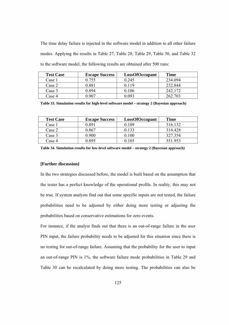
125
The time delay failure is injected in the software model in addition to all other failure
modes. Applying the results in Table 27, Table 28, Table 29, Table 30, and Table 32
to the software model, the following results are obtained after 500 runs:
Test Case Escape Success LossOfOccupant Time Case 1 0.755 0.245 234.094 Case 2 0.881 0.119 232.844 Case 3 0.894 0.106 242.172 Case 4 0.907 0.093 262.703
Table 33. Simulation results for high-level software model – strategy 2 (Bayesian approach)
Test Case Escape Success LossOfOccupant Time Case 1 0.891 0.109 316.132 Case 2 0.867 0.133 314.428 Case 3 0.900 0.100 327.354 Case 4 0.895 0.105 351.953
Table 34. Simulation results for low-level software model – strategy 2 (Bayesian approach)
[Further discussion]
In the two strategies discussed before, the model is built based on the assumption that
the tester has a perfect knowledge of the operational profile. In reality, this may not
be true. If system analysts find out that some specific inputs are not tested, the failure
probabilities need to be adjusted by either doing more testing or adjusting the
probabilities based on conservative estimations for zero events.
For instance, if the analyst finds out that there is an out-of-range failure in the user
PIN input, the failure probability needs to be adjusted for this situation since there is
no testing for out-of-range failure. Assuming that the probability for the user to input
an out-of-range PIN is 1%, the software failure mode probabilities in Table 29 and
Table 30 can be recalculated by doing more testing. The probabilities can also be

126
recalculated using a conservative assumption. The extreme case is to assume the
failure always happens once the user inputs an out-of-range value. In this case, if the
failure mode is related with invalid PIN input, the probability can be adjusted using
the following equation:
01.099.0* += oldnew pp (7.4)
This is an extremely conservative assumption. But it is normally enough for low
probability events at the beginning of the simulation. If the simulation results indicate
that this part of the system is important, the model can be refined using more testing
results if needed.
Step 5: Inject the software code into the simulation environment and compare the
results
The real code is injected into the PACS model. The IO part is reconstructed to fit into
the simulation environment. In that way, the input/output is processed in the
simulation environment. The human model is modified to generate the real input from
the input space (Table 14) for the software. The detailed card information and the PIN
information are selected and sent to the software model. The card/PIN data are
validated using the real code.
The total number of lines of code (LOC) for PACS is 553, for the IO process part,
185. So the code coverage for this analysis is 66.55%. It can be increased when the
human model is refined to incorporate the details of IO processes.
A coverage related criterion is added to the simulation environment to ensure that all
software input can be covered during simulation. The following results are obtained

127
after 500 runs:
Total Simulation Runs Escape Success LossOfOccupant Time 500 0.883 0.117 414.91 Table 35. PACS simulation results (software code without coverage guidance)
Step 6: Quantitative coverage results
A post-simulation tool is designed to analyze the scenarios generated during
simulation. The first guard action and the sequence of events prior to it are used to
categorize the system level scenarios. See Figure 50 for the area studied inside the
scenario. A quantitative coverage is assessed for the system level scenarios by
comparing the results obtained from the code and from the software model
simulation.
FireProtection
OffFire User Card
ActionUser PIN
Action User RetryGuardAction End State
Area Studied
Figure 50. Area studied for coverage analysis
[Code simulation]
The simulation results produce 74 different scenarios if one uses the real software
code.
[Low-Level Simulation]
The following coverage information is obtained after studying the low-level
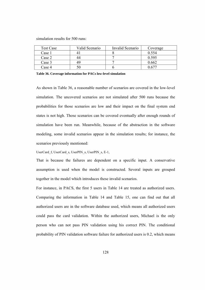
128
simulation results for 500 runs:
Test Case Valid Scenario Invalid Scenario Coverage Case 1 41 8 0.554 Case 2 44 7 0.595 Case 3 49 7 0.662 Case 4 50 6 0.677
Table 36. Coverage information for PACs low-level simulation
As shown in Table 36, a reasonable number of scenarios are covered in the low-level
simulation. The uncovered scenarios are not simulated after 500 runs because the
probabilities for those scenarios are low and their impact on the final system end
states is not high. Those scenarios can be covered eventually after enough rounds of
simulation have been run. Meanwhile, because of the abstraction in the software
modeling, some invalid scenarios appear in the simulation results; for instance, the
scenarios previously mentioned:
UserCard_f, UserCard_s, UserPIN_s, UserPIN_s, E-1,
That is because the failures are dependent on a specific input. A conservative
assumption is used when the model is constructed. Several inputs are grouped
together in the model which introduces these invalid scenarios.
For instance, in PACS, the first 5 users in Table 14 are treated as authorized users.
Comparing the information in Table 14 and Table 15, one can find out that all
authorized users are in the software database used, which means all authorized users
could pass the card validation. Within the authorized users, Michael is the only
person who can not pass PIN validation using his correct PIN. The conditional
probability of PIN validation software failure for authorized users is 0.2, which means

129
20% of the users with correct card can not pass through the PIN validation using the
correct PIN. That is the conditional failure probability used if all users with correct
card are grouped as one input: correct card. Based on the probability, the following
scenario becomes possible.
UserCard_f, UserCard_s, UserPIN_s, UserPIN_s, E-1,
But in reality, Michael is the only authorized user who can not pass PIN validation
using his correct PIN. All other authorized users could pass the PIN validation using
the correct PIN. Checking the scenario above, a user uses the correct card to pass card
validation but fails to pass the PIN validation using his correct PIN at the first try.
This indicates that the user could only be Michael. In the scenario, the user uses his
correct PIN again and goes through the gate successfully. In reality, this is not the
case since Michael will never be able to go through the gate using his correct PIN.
This can be solved by either using the real code in the simulation or by building all
detailed inputs into the software model.
Checking the results in Table 26 and Table 36 reveals that even with the uncovered
scenarios and invalid scenarios, the software model still captures the major scenarios
during simulation and produces reasonably accurate results.
[High-level Simulation]
The scenarios generated for the high-level simulation contain basic events different
from the low-level simulation and the code simulation. The card input event and the
PIN input event are grouped as:
• RCRP: Right Card, Right PIN
• RCWP: Right Card, Wrong PIN

130
• WCRP: Wrong Card, Right PIN
• WCWP: Wrong Card, Wrong PIN
• WCNP: Wrong Card, No PIN input anymore
The detailed input events for low-level simulation are grouped together. For instance,
the following combinations of basic events all belong to RCRP:
• UserCard_s, UserPIN_s
• UserCard_f, UserCard_s, UserPIN_f, UserPIN_s
• UserCard_f, UserCard_f, UserCard_s, UserPIN_f, UserPIN_s
The relationship between high-level scenarios and low-level scenarios is a one-to-
many relationship. There is a mapping among simulation results at different levels.
Table 37 presents one example scenario from each level. Scenario 15 in the code
simulation corresponds to Scenario 95 in level 1 simulation and Scenario 2 in level 0
simulation.
Level Example scenarios Code 15 : { FireProtection_Off@0 ,
UserCard_f(Christopher,1,5555)@7 , UserPIN_f(3333,5555)@17 , UserPIN_f(1111,5555)@30 , UserPIN_s(5555,5555)@44 , E-1@48 , } [ES-1 , 9.01E-1 , 48.0]
Level 1 95 : { FireProtection_Off@0 , UserCard_f@8 , CardValidation@9 , UserPIN_f@16 , UserPIN_f@28 , UserPIN_s@41 , E-1@47 , } [ES-1 , 3.63E-1 , 47.0]
Level 0 2 : { FireProtection_Off@0 , WCRP@34 , swVal@35, E-1@36 , } [ES-1 , 3.58E0 , 36.0]
Table 37. Example scenarios for different levels
7.6 Discussion
Comparing the results from different strategies and code simulation, the following

131
figure is obtained.
Figure 51. Simulation results from different strategies
From Figure 51, the following phenomena are observed:
1 The low level model simulation generates a better result compared with the high
level model simulation as expected.
2 When the number of tests is small, the conservative strategy increases the result
performance dramatically for the high-level simulation. The reason for this is that
most of the software failures are not detected after a small amount of tests. Using a
conservative strategy, the impacts of the undetected failures are effectively

132
represented.
3 When the number of tests is sufficient, the difference between the result from
strategy 1 and conservative strategy 2 becomes small.
4 Enough testing can ensure a good estimation of risk
7.7 Summary
This chapter introduces the gate-control system (PACS), and the whole modeling
process is studied using our methodology. The experimental-validation results show
that:
1. Using a software model in the simulation environment leads to a reasonably
accurate estimate for the end-state probability.
2. The software model can be refined after the analyst obtains more test results;
the accuracy of end-state probabilities increases when the model improves.
3. High-level simulation is less time-consuming, but this comes at the expense of
lower scenario resolution.
4. A smart adaptive simulation captures the benefits from both low-level
simulation and high-level simulation; the simulation is less time consuming
and produces sufficient details.

133
Chapter 8: Procedure to Develop the Software Model in Case
of Objective Data
The integration approach is discussed in Chapter 5. This chapter provides further
guidance on how to establish an accurate software representation when code is
available and objective test data can be obtained. The procedure presented is based on
lessons learnt from our experimental demonstration in Chapter 7. This approach can
be used in addition to the integration approach discussed in Chapter 5.
8.1 Approach
Step 1: Build the executable low-level model for the software.
In the first step, the analyst needs to decide how to abstract the real software. The
lowest level abstraction for the software needs to be defined. The following
constrains restrict the analyst’s modeling alternative to specific low-level models:
• Inputs/outputs resolution from other models (human, hardware, software): the
software model can not go beyond the level of resolution that other models
can understand/produce.
• Limits imposed by the code: the lowest level of abstraction can not go beyond
the code resolution as expected.
• Limits of the characteristic of the input/output variables: the software model
can not go beyond the natural resolution of the input/output variables.

134
• The lowest level software model should not break the dependences between
input variables.
An executable software model needs to be built using SFSM based on the abstraction.
(Section 4.3)
In the case of PACS, the input/output resolution of the human model stays at the level
of correct card, wrong card, correct PIN and wrong PIN. This limits the lowest level
of the PACS software model. The detailed card inputs and PIN inputs are grouped
together as correct card and wrong card, correct PIN and wrong PIN. This is used as
lowest input unit in the software model.
Step 2: Define a multi-level structure for the software model.
In this step, the analyst first needs to choose the functions to be abstracted, then
define the abstraction methods and build the multi-level abstraction model for the
software. The abstraction technique includes functional abstraction and continuous
abstraction, which were introduced in section 4.2.
Functional abstraction leads to the omission of details related to sub-functions.
Continuous abstraction focuses on input-output transformations resulting from
functional computations. Errors are introduced during the abstraction process. These
errors fall into two groups, which are explained below.
The scenarios generated in the DPRA environment contain a sequence of stochastic
events resulting from model execution, and timing of occurrence. In between the
points of occurrence of these random events, the behavior of the system is typically
modeled using deterministic models describing the physical and other processes

135
taking place in the system.
The first group of errors modifies the deterministic behavior. Both abstraction
techniques change the input/output relationship, i.e. if the expected behavior is )(if ,
the modified behavior is )()( iif ε+ . )(iε is the error introduced into the deterministic
behavior. This group of errors can be quantified before the simulation. It is usually
small at the component level.
For instance, π≤≤= xxxf 0)sin()(
Assume the abstraction function is
)12(1)(~
−−=πxabsxf
The error introduced is represented by the shaded area in Figure 52.
136
Figure 52. Error introduced in the deterministic behavior
The second group of errors modifies the stochastic events, such as software failures.
There are three types of errors in this group:
• Event error: the high-level events are usually a combination of low-level
stochastic events. This thus introduces the event error. Normally the event
error is acceptable if it does not influence the global behavior of the event.
• Time error: the time of occurrence of the event is different since the details of
the low-level events are not modeled in the high-level abstraction
• Probability error: the probability of the event changes due to abstraction. The
probability needs to be quantified using testing results. Probability error is
introduced when the value of the probability used is not accurate.
If the functional abstraction groups multiple stochastic events together, the event error
will be introduced and the time error will be introduced also. The probability of the
high-level event can be quantified using the high-level test result. The probability
error is introduced if the test result is not accurate.
Figure 53 a) presents a high-level event RCRP. The high-level event presents the
combination of the low-level events in Figure 53 b). At the high level, based on the
test results in Table 18 (10000 test cases), the characteristics of this event can be
defined as:
Probability p = 0.6126
The time needed for this event is uniformly distributed between 14 seconds and 52
seconds.

137
At the low level, based on the test results in Table 19, Table 21, and Table 22 (10000
test cases), the characteristics of the low level events can be defined as:
7327.0406.0*45.055.0)_|(*)_(
)_|(*)_(),_(
=+=+
=cardwrongsuccesspcardwrongp
cardrightsuccesspcardrightpsuccessvalidationcardp
2673.07327.01),_(1),_( =−=−= successvalidationcardpfailvalidationcardp
The time needed for card validation is uniformly distributed between 6 seconds and 8
seconds.
4777.0022.0*7327.0
55.0*45.01*7327.01827.0*55.0807.0*
7327.055.0*55.0
)_,_|(*)_,_()_,_|(*)_,_()_,_|(*)_,_(
)_,_|(*)_,_(),_(
=++=
+++=
cardwrongPINwrongsuccesspcardwrongPINwrongpcardrightPINwrongsuccesspcardrightPINwrongpcardwrongPINrightsuccesspcardwrongPINrightp
cardrightPINrightsuccesspcardrightPINrightpsuccessvalidationPINp
5223.04777.01),_(1),_( =−=−= successvalidationPINpfailvalidationPINp
The time needed for PIN validation is uniformly distributed between 6 seconds and 8
seconds.
Comparing the high-level event RCRP, the low-level events are card_validation and
PIN_validation. The high-level event is a combination of the low-level events. The
event is different thus event error exists in this situation. The time occurrence of the
high-level event RCRP should map to the last event in the low-level sequence, time
error is introduced if the occurrence of the event is not modeled correctly. Probability
error will be introduced also if the probability used at the high-level is not accurate.

138
CardValidation1
PINValidation1
Pass
CardValidation2
CardValidation3
Pass
Fail
FailPass
PINValidation2
PINValidation3
Pass
Fail
Fail
Pass
Pass
RCRP
a) High level Event - Right Card Right PIN
b) Low level Events
Fail
Pass
Figure 53. High-level event vs. low-level events
The continuous abstraction does not deal with the combination of multiple stochastic
events. But the accumulation of the errors, introduced in the deterministic behavior,
over a chain of events may exceed a threshold which will lead to the occurrence of a
different stochastic event.
f g h
f' g' h'
e1 e2 e3
e
Figure 54. A chain of events

139
For instance, considering the chain of events in Figure 54, errors are introduced in the
abstraction of function f, g, and h. The propagation of the errors leads to an
accumulated error є. If the error is large enough, it may influence the execution of the
stochastic events following, such as the possible occurrence of a software failure. In
this way, the event error and the probability error are introduced. If the continuous
abstraction changes the software execution time, the time error is introduced also.
The abstraction is recommended for the functions with the following characteristics:
• The execution of the function is time-consuming. The abstraction can be a
functional abstraction to reduce the complexity of the software function. It can
also be a continuous abstraction to simplify the calculation process.
• The function interacts with other models multiple times sequentially in one
run. The functional abstraction should be used to group several interactions in
one single time step if applicable. The sequential inputs from the interactions
need to be combined together.
Assuming the sequential inputs to the software function are f1 to fn, it needs to
be combined as one single input:
),,( 111 ni ffI L= 1)(},,{ 1 == ∑m
mm IpIII L (8.1)
m represents the number of different combinations for sequential inputs f1 to
fn.
Other models need to be updated to be able to understand and produce this
type of inputs.
The improvement brought to the computational complexity includes two components:

140
1. The computation time decreases due to abstraction
f
f1 f2 f3
f4 f5
Figure 55. High-level function f vs. low-level function f
Figure 55 presents a high-level abstraction model for function f and the low-level
model for function f. Assume that the execution of each function block takes 1 time
cycle. The execution of the high-level model only takes one time step. The low-level
model contains two paths: Path1 (f1, f2, f3), Path2 (f1, f4, f5, f3).
The average execution time is
4*)2(3*)1( pathpPathptLL += (8.2)
Generally, the average execution time can be represented as:
∑=
=n
iLL iPathtiPathpt
1
)_(*)_( (8.3)
The time decreases by the factor of LLt1 .
2. The number of branches generated decreases due to the grouping of multiple
stochastic events.

141
Assume n different sequences of low-level stochastic events are grouped into
1 event in the high-level model. The branches generated decrease by the factor
of 1/n.
In Figure 53, the high-level event includes six low-level stochastic events
sequences. The branches generated will decrease by the factor of 1/6.
The analyst needs to make a balance between the errors introduced during abstraction
and the improvement brought to the computational complexity.
Step 3: Obtain the operational profile for the software
In this step, the analyst needs to obtain the operational profile [19] for the software
from the software requirements and the system requirements. The test is conducted
based on this profile. The profile is an external input profile from other models
(hardware, software, human).
If unexpected inputs to the software model are observed during the simulation, the
profile needs to be updated. More testing needs to be conducted or the conservative
estimation can be used to adjust the test results (See section 7.5 step 4). The
conservative estimation can be obtained through the following equation:
qqpp oldnew +−= )1(* (8.4)
Pnew is the new failure probability estimation
Pold is the original failure probability obtained through testing.
q represents the probability of the unexpected input detected
In the case of PACS, for each user, the probability of inserting the right/wrong card is
0.55/0.45. The right/wrong cards are uniformly distributed in the set of right/wrong

142
cards. Once the user inserts the card, the probability of inputting a right PIN is 0.55.
Step 4: Define the possible software failure modes
Based on the logic of the software, all possible software failure modes are defined in
this step. There are eight types of failure modes defined for the software model. These
are value, range, amount, type, time, rate, duration, and rate. The definition of the
failure modes can be found in [2]. The analyst needs to study the applicability of each
failure mode.
In the case of PACS, amount, range, value, load, duration, and rate failure are not
applicable. All possible value failures and time failures are defined and studied for
PACS.
Step 5: Test the software using the operational profile
In this step, the software is tested using the operational profile defined in step 3. The
test is performed at different levels.
Assume that the external profile defined in step 3 is represented as:
ii niipII ,,1)}(,{ L== (8.5)
The profile for the software function to be tested is presented as:
fif niipII ,,1)}(,{ L== (8.6)
The output is represented as
oif niipOO ,,1)}(,{ L== (8.7)
If II f ⊆ , which means that the software function to be tested is only related with the
external profile, the software can be tested directly. (case a in Figure 56)

143
If 21 fff III U= , II f ⊆1 , 12 swf OI ⊆ (8.8)
which means the inputs of the software to be tested are not only from the external
profile, but also dependent on the outputs of the other software to be tested (software
component 1) (case b in Figure 56), the software profile needs to be updated in the
following condition.
If unexpected software failures are observed in the test result for software component
1, and the software failures detected introduce some unexpected outputs, the profile
for software function f needs to be updated to reflect the new inputs from software
component 1.
1'
swOO ∉ '' OII ff ∪= (8.9)

144
Input(Human, Software,
Hardware)
Softwareto be
Tested
a) Software inputs are from external models
Input(Human, Software,
Hardware)
b) Software inputs are from external models and the execution of other software to be tested
SoftwareComponent
1
Software tobe Tested
Figure 56. Different conditions for software testing
The probability of the software failure is calculated using the following equation:
casestesttotalofnumberfailureswithcasestestofnumberp = (8.10)
In the case of PACS, the test is performed at the high level and the low level. The
input profile of the high level test is only influenced by the human model. Thus it can
be tested directly using the operation profile. The low-level test includes the tests for
card validation and PIN validation. The inputs of card validation are only from the

145
human model. It can be tested directly using the profile obtained from the human
model. Based on the design document, the perfect card validation should have the
following results:
• A user with a right card can pass the card validation
• A user with a wrong card can not pass the card validation
The following software failures are detected during testing of card validation:
• A user with a right card can not pass the card validation
• A user with a wrong card can pass the card validation
Since the input profile of PIN validation is dependent on the human input and the
results from card validation, it needs to be updated based on the software failure
detected. The initial input profile for PIN validation only includes:
• PIN profile for the user with a correct card
Based on software failures observed in the implementation of the function card
validation, the following profile should be added to the original profile:
• PIN profile for the user with a wrong card that passes the card validation
The PIN validation function needs to be tested for both conditions.
Step 6: Analyze the test results
The test results are analyzed in this step. The software failure modes need to be
quantified using the test results. The test results are first categorized based on the type
of inputs and outputs. The conditional probability for each failure mode is calculated
if the failure mode is observed.
If the software failure introduces unexpected output, and the output serves as an input

146
to next sequential component, it may introduce a new combination of sequential
inputs. If the high-level abstraction model combines the sequential inputs during
abstraction, and the newly discovered sequence does not belong to the original
combination set, the new sequence combination needs to be added as a new input to
the high level model.
IIffI mnm ∉= ++ 1''
1 )},,{(1L 1+= mIII U (8.11)
Also the probability profile for each input to the high-level model needs to be
replaced based on the profile observed in the test results.
For instance, in the case of PACS, Table 16 lists the high-level test results for PACS.
The results are categorized based on the inputs (right card, wrong card, right PIN,
wrong PIN) and output (success, fail). The probability for each failure mode is
calculated and presented in Table 17. In this case, the high-level operation profile is
influenced by software errors. Thus the profile is updated as in Table 18.
Step 7: Estimate the probability for undetected software failures
If some software failures defined in step 5 are not discovered in the simulation results,
the conservative estimation should be used to estimate the failure probability. The
estimation can be done using the Bayesian Approach defined in Chapter 6. The
probability for the failure after N tests can be calculated using the following equation:
Nq
+=
15.0 (8.12)
In the case of PACS, some failure modes are not detected after a small amount of
testing. The probability of the undetected failure modes are estimated using the
147
conservative estimation. The simulation results indicate that the undetected software
failures are effectively represented using the conservative estimation.
Step 8: Inject the software failures in the executable software model
The software failures are injected in the multi-level software model defined in step 2.
AKB and FIKB needs to be constructed based on the testing results
8.2 Discussion
The approach defined in this chapter is applicable to the case when the real software
is available. If the real software is not available, the software failures need to be
quantified using expert judgment or statistical data from similar projects. The basic
steps for this case are:
Step 1: Build the executable low-level model for the software.
Step 2: Define multi-level structure for the software model.
Step 3: Define the possible software failure modes.
Step 4: Quantify the probabilities of software failure modes using expert judgment or
statistical data.
Step 5: Inject the software failures in the executable software model.

148
Chapter 9: Conclusion and Future Work
9.1 Conclusion
DPRA is a methodology to assess the probability of failure or success of a mission.
The current DPRA environments do not allow modeling of software risk contribution.
This dissertation describes a framework and a set of techniques to extend the DPRA
approach to allow consideration of the software contributions on system risk. The
framework includes a software representation, an approach to incorporate the
software representation into the DPRA environment SimPRA, and an experimental
demonstration of the methodology.
Here are the major contributions:
• Systematically identify the software modeling requirements for simulation-
based DPRA environments
• Assess the existing software representations with respect to the DPRA
modeling requirements
• Extend the concept of FSM to SFSM and apply it to the area of software
modeling DPRA environments
• Establish a software representation framework including a software behavior
model and a software guidance model
• Build a multi-level software representation using functional abstraction and
continuous abstraction techniques

149
• Integrate the failure mode taxonomy developed by Li [2] in the software
representation
• Develop the mechanism to separate the software-related knowledge with the
system-related knowledge
• Define the structure for AKB, FIKB, SKB
• Propose a framework to simulate the multi-level objects in the simulation-
based DPRA environment
• Enhance the current single-level SimPRA to support multi-level objects in the
modeling framework
• Apply the concept of entropy to dynamically control the simulation level of
detail for the multi-level objects
• Implement the entire methodology in the SimPRA software
• Develop an easy to use tool to help the analyst develop the software model
• Conduct an experimental demonstration to study the quantification aspects of
the software model when objective test data is available
o Develop a consistently quantified software representation
o Embed software profile information in the software model
o Cover the failure mode taxonomy developed by Li
o Obtain data from testing
o Account for the dependencies between model components
o Compare the software model simulation results with the simulation
using the real code

150
• Formalize a procedure to establish a consistently quantified software model
when code is available and objective test data can be obtained
9.2 Future Work
This dissertation describes a framework for integrating software into Dynamic PRA.
It is the first study of its kind. More research is needed. Below are some possible
avenues for future research:
9.2.1 Large scale validation
Although a case study has been provided, which demonstrates the applicability of this
framework and of the set of techniques developed, the methodology should be
applied to a large system. Problems that arise in that process need to be identified,
and their solutions should be provided.
9.2.2 Software-related knowledge
Different types of prior software-related knowledge may exist. In this dissertation, the
time-factor information was added to SKB and supported by the multi-level scheduler
and planner. In future research, different types of software-related information could
be defined and added to SKB. For instance, different software-abstraction levels
could be associated with different levels of accuracy in the results. The accuracy-
related factor could then be added to SKB.. The current multi-level simulation
environment provides an open interface which easily allows the introduction of new
types of knowledge.

151
9.2.3 Software-testing knowledge
SimPRA uses two types of information to guide the simulation: prior knowledge and
knowledge obtained during the simulation.
In this dissertation, the knowledge obtained during simulation is mainly entropy-
based information. Knowledge about the relationship between branch selection and
end-state probabilities is summarized after simulation. The information gain is
dynamically updated to adjust the simulated branch selection process.
Other types of information can also be used to adaptively adjust the simulation, for
instance, the software test coverage information. Various software coverage indices
(i.e. statement coverage, branch coverage, etc) can be calculated after simulation. In
subsequent simulations an uncovered statement, branch could receive additional
weighting compared with statement, branches already covered.
In the current SimPRA environment, when the system simulator proposes transitions
to the scheduler, the scheduler retrieves the information for the proposed transitions
and decides which branch to explore, based on the previous simulation results. The
new framework can be upgraded to include the instruction from sub-component
guidance model. (See Figure 57)
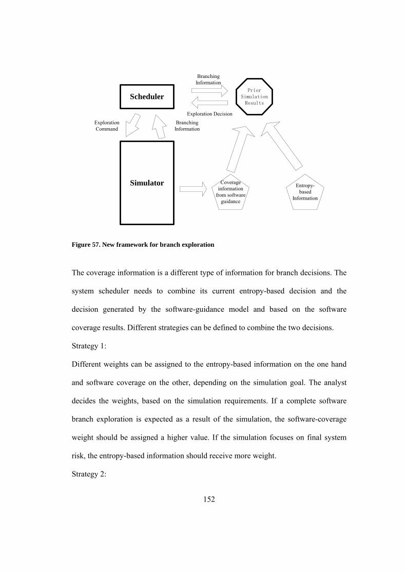
152
Scheduler
Simulator
BranchingInformation
ExplorationCommand
PriorSimulationResults
BranchingInformation
Exploration Decision
Entropy-based
Information
Coverageinformation
from softwareguidance
Figure 57. New framework for branch exploration
The coverage information is a different type of information for branch decisions. The
system scheduler needs to combine its current entropy-based decision and the
decision generated by the software-guidance model and based on the software
coverage results. Different strategies can be defined to combine the two decisions.
Strategy 1:
Different weights can be assigned to the entropy-based information on the one hand
and software coverage on the other, depending on the simulation goal. The analyst
decides the weights, based on the simulation requirements. If a complete software
branch exploration is expected as a result of the simulation, the software-coverage
weight should be assigned a higher value. If the simulation focuses on final system
risk, the entropy-based information should receive more weight.
Strategy 2:

153
An adaptive-selection strategy can be defined, based on the simulation process. If the
entropy-based information is insufficient initially because of a lack of simulation
results, the system scheduler may base its decision on the coverage information
received from the software-guidance model. If entropy-based uncertainty is low after
many rounds of simulation, the system scheduler can select branches based mainly on
entropy-based information.
9.3 Acknowledgement
This work was supported in part by the Space Vehicle Technology Institute under
grant NCC3-989 jointly funded by NASA and DOD within the NASA Constellation
University Institutes Project, with Claudia Meyer as the project manager. This work
was also sponsored in part through a grant from the NASA Ames Research Center,
Engineering of Complex Systems Program.

154
Bibliography
1. Li, B., et al. Integrating software into PRA. in 14th IEEE International Symposium on Software Reliability Engineering (ISSRE2003). 2003. Denver.
2. Li, B., M. Li, and C. Smidts, Integrating Software into PRA: A taxonomy of Software Related Failures, in Sixth IEEE International Symposium on High Assurance Systems Engineering. 2001: Boca Raton, Florida.
3. Li, B., M. Li, and C. Smidts. Integrating Software into PRA: A Test-Based Approach. in International Conference on Probabilistic Safety Assessment and Management (PSAM7). 2004. Berlin
4. Labeau, P.E., C. Smidts, and S. Swaminathan, Dynamic Reliability: towards an integrated platform for probabilistic risk assessment. Reliability Engineering and System Safety, 2000. 68(3): p. 219-254.
5. Standards Coordinating Committee of the IEEE Computer Society, IEEE Standard Glossary of Software Engineering Terminology, IEEE Std 610.12. 1990.
6. Harel, D., StateCharts: A visual formalism for complex system, Science of Computer Program. 1987. p. 231-274.
7. US Nuclear Regulatory Commission, Reactor Safety Study (WASH-1400 (NUREG-75/014)). , US Nuclear Regulatory Commission Washington DC USA, Editor. 1975.
8. US Nuclear Regulatory Commission, PRA procedures guide: A guide to the performance of probabilistic risk assessment for nuclear power plants (NUREG/CR-2300), US Nuclear Regulatory Commission Washington DC USA, Editor. 1983.
9. Paté-Cornell, E. and R. Dillon, Probabilistic risk analysis for the NASA space shuttle: a brief history and current work. Reliability Engineering and System Safety, 2001. 74(3): p. 345-352.
10. Stamatelatos, M., et al., Probabilistic Risk Assessment Procedures Guide for NASA Managers and Practitioners., NASA, Editor. 2002.
11. Groen, F., et al. QRAS - the Quantitative Risk Assessment System. in Reliability and Maintainability Symposium. 2002.
12. Ammar, H.H., T. Nikzadeh, and J.B. Dugan, Risk Assessment of software-system specifications. IEEE Transactions on Reliability, 2001. 50(2).
13. Dugan, J.B., Software Reliability Analysis Using Fault Tree, M. Lyu, Editor. 1995, Mc. Graw Hill: New York.
14. Lutz, R.R. Analyzing Software Requirements Errors in Safety-Critical Embedded Systems. in IEEE International Symposium on Requirement Engineering. 1992.
15. Li, B., Integrating Software into PRA (Probabilistic Risk Assessment), in Reliability Engineering, Department of Mechanical Engineering. 2004, University of Maryland: College Park.

155
16. Lee, A.T. and T.R. Gunn. A Quantitative Risk Assessment Method for Space Flight Software Systems. in Fourth International Symposium on Software Reliability Engineering. 1993. Denver, Colorado.
17. Schneidewind, N.F. and T.W. Keller, Applying Reliability Models to the Space Shuttle. IEEE Software, 1992.
18. Yacoub, S.M. and H.H. Ammar, A methodology for Architecture-level Reliability Risk Analysis. IEEE Transactions on Software Engineering, 2002. 28(6).
19. Musa, J.D., Operational profiles in software-reliability engineering. Software, IEEE, 1993. 10(2): p. 14-32.
20. Siu, N., Risk Assessment for dynamic systems: An overview. Reliability Engineering and System Safety, 1994. 43(1): p. 43-73.
21. Amendola, A. and G. Reina, Event sequences and consequence spectrum: a methodology for probabilistic transient analysis. Nuclear Science and Engineering, 1981. 77(3): p. 297-315.
22. Dugan, J.B., S.J. Bavuso, and M.A. Boyd, Dynamic Fault-tree Model for Fault-Tolerant Computer Systems. IEEE Transactions on Reliability, 1992. 41(3): p. 363-377.
23. Cepin, M. and B. Mavko, A dynamic fault tree. Reliability Engineering and System Safety, 2002. 75(1): p. 83-91.
24. Petri, C.A., Kommunikation mit Automaten, in Mathematics and Physics 1962, Technische Universität Darmstadt: German.
25. Desel, J. and G. Juhás, "What Is a Petri Net?" Informal Answers for the Informed Reader. Unifying Petri Nets : Advances in Petri Nets, 2001. 2128.
26. Murata, T., Petri nets: Properties, analysis and applications. Proceedings of IEEE, 1989. 77(4): p. 541-580.
27. Houtermans, M., et al., The dynamic flowgraph methodology as a safety analysis tool: programmable electronic system design and verification. Safety Science, 2002. 40(9): p. 813-833.
28. Matsuoka, T. and M. Kobayashi, GO-FLOW: A New Reliability Analysis Methodology. Nuclear Science and Engineering, 1988. 98: p. 64-78.
29. Swaminathan, S. and C. Smidts, The event sequence diagram framework for dynamic probabilistic risk assessment. Reliability Engineering and System Safety, 1999. 63(1): p. 73-90.
30. Swaminathan, S. and C. Smidts, Identification of missing scenarios in ESDs using probabilistic dynamics. Reliability Engineering and System Safety, 1999. 66(3): p. 275-279.
31. Swaminathan, S. and C. Smidts, The mathematical formulation for the event sequence diagram framework. Reliability Engineering and System Safety, 1999. 65(2): p. 103-118.
32. Devooght, J. and C. Smidts, Probabilistic dynamics as a tool for dynamic PSA. Reliability Engineering and System Safety, 1996. 52(3): p. 185-196.
33. Izquierdo, J. and P.E. Labeau. The Stimulus-Driven Theory of Probabilistic Dynamics as a Framework for Probabilistic Safety Assessment. in PSAM7. 2004.
34. Cojazzi, G., The DYLAM approach for the dynamic reliability analysis of

156
systems. Reliability Engineering and System Safety, 1996. 52(3): p. 279-296. 35. Hsueh, K.S. and A. Mosleh, The development and application of the accident
dynamic simulator for dynamic probabilistic risk assessment of nuclear power plants. Reliability Engineering and System Safety, 1996. 52(3): p. 297-314.
36. Labeau, P.E., Probabilistic dynamics: Estimation of generalized unreliability through efficient Monte Carlo simulation. Annals Of Nuclear Energy, 1996. 23(17): p. 1355-1369.
37. Smidts, C. and J. Devooght, Probabilistic reactor dynamics. II. A Monte Carlo study of a fast reactor transient. Nuclear Science and Engineering, 1992(111): p. 241-256.
38. Mosleh, A., et al., Simulation-Based Probabilistic Risk Analysis Report. 2004, Center for Risk and Reliability, University of Maryland.
39. Hu, Y., F. Groen, and A. Mosleh. An Entropy-Based Exploration Strategy in Dynamic PRA. in International Conference on Probabilistic Safety Assessment and Management (PSAM7). 2004. Berlin.
40. Hu, Y., A guided simulation methodology for Dynamic Probabilistic Risk Assessment of complex systems, in Reliability Engineering Program, Department of Mechanical Engineering. 2005, University Of Maryland: College Park.
41. Carson, J.S., Introduction to Modeling and Simulation, Paper presented at the Winter Simulation Conference. 2004.
42. Tan, Z., Methodology for Analyzing Reliability of X-Ware Systems, in Reliability Engineering. 2001, University of Maryland: College Park.
43. Sage, A.P. and J.D. Palmer, Software systems engineering. Wiley Systems Engineering Series. 1990, New York: Wiley-Interscience.
44. Fitts, P.M. and J.R. Peterson, Information capacity of discrete motor responses. Journal of Experimental Psychology, 1964(67): p. 103-112.
45. Rational Software Co., Unified Modeling Language v. 1.1, Semantics, . 1997. 46. Peterson, J.L., Petri Net Theory and the Modeling of Systems. 1981,
Englewood Cliffs, N.J.: Prentice Hall PTR. x, 290 p. 47. Gamma, E., Design Patterns: Elements of Reusable Object-Oriented
Software. 1995, Mass.: Addison-Wesley Longman Reading. 48. Frantz, F.K. A taxonomy of Model Abstraction Techniques. in Winter
Simulation Conference. 1995. Washington DC. 49. Caughlin, D. and A.F. Sisti. A summary of Model Abstraction Techniques. in
Enabling Technology for Simulation Sciense Conference. 1997. Orlando, FL. 50. The Mathworks Inc, MATLAB User’s Manual, Revised for Matlab 6.0
(Release 12). 2000. 51. Fishman, C., They Write the Right Stuff,
http://www.fastcompany.com/online/06/writestuff.html, in Fastcompany. 1996. p. 95.
52. Nejad, H. and A. Mosleh. Automated Risk Scenario Generation Using System Functional and Structural Knowledge. in Proceedings of ASME International Mechanical Engineering Congress and Exposition. 2005. Orlando: The American Society of Mechanical Engineers.
53. Garg, S., et al. A methodology for detection and estimation of software aging.

157
in The Ninth International Symposium on Software Reliability Engineering. 1998. Paderborn
54. The Institute of Electrical and Electronics Engineers, IEEE Standard dictionary of measures to produce reliable software, ANSI/IEEE Std. 982.1. 1988.
55. Nejad, H. and A. Mosleh, Guided Simulation for Risk-Based Design. ASME Journal of Mechanical Design, forthcoming July 2006.
56. Lindley, D.V., On the Measure of Information Provided by an Experiment. Annals of Statistics, 1956. 27(4): p. 986-1005.
57. Shannon, C.E., Mathematical theory of communication. The Bell Labs Technical Journal, 1948(27): p. 379-457.
58. Shannon, C.E. and W. Weaver, The mathematical theory of communication. 1949, Urbana,: University of Illinois Press. v (i.e. vii), 117 p.
59. Mosleh, A., et al. Solution of the Phased-Mission Benchmark Problem Using the SimPRA Dynamic PRA Approach. in International Conference on Probabilistic Safety Assessment and Management (PSAM) 2006. 2006.
60. Geisser, S., On Prior Distributions for Binary Trials. The American Statistician, 1984(38): p. 244-251.