ABSTRACT

Title of dissertation: INTEGRATED PRODUCTION-DISTRIBUTIONSCHEDULING IN SUPPLY CHAINS

Guruprasad Pundoor, Doctor of Philosophy, 2005

Dissertation directed by: Dr. Zhi-Long Chen, Associate ProfessorRobert H. Smith School of Business

We consider scheduling issues in different configurations of supply chains. The primary

focus is to integrate production and distribution activities in the supply chain in order

to optimize the tradeoff between total cost and service performance. The cost may be

based on actual expenses such as the expense incurred during the distribution phase, and

service performance can be expressed in terms of time based performance measures such

as completion times and tardiness. Our goal is to achieve the following objectives: (i) To

propose various integrated production-distribution scheduling models that closely mirror

practical supply chain operations in some environments. (ii) To develop computationally

effective optimization based solution algorithms to solve these models. (iii) To provide

managerial insights into the potential benefits of coordination between production and

distribution operations in a supply chain.

We analyze four different configurations of supply chains. In the first model, we consider

a setup with multiple manufacturing plants owned by the same firm. The manufacturer

receives a set of distinct orders from the retailers before a selling season, and needs to

determine the order assignment, production schedule, and distribution schedule so as to

optimize a certain performance measure of the supply chain. The second model deals with

a supply chain consisting of one supplier and one or more customers, where the customers

set due dates on the orders they place. The supplier has to come up with an integrated

production-distribution schedule that optimizes the tradeoff between maximum tardiness

and total distribution cost. In the third model, we study an integrated production and dis-

tribution scheduling model in a two-stage supply chain consisting of one or more suppliers,

a warehouse, and a customer. The objective is to find jointly a cyclic production sched-

ule at each supplier, a cyclic delivery schedule from each supplier to the warehouse, and a

cyclic delivery schedule from the warehouse to the customer so that the customer demand

for each product is satisfied fully at minimum total production, inventory and distribution

cost. In the fourth model, we consider a system with one supplier and one customer with

a set of orders placed at the beginning of the planning horizon. Unlike the earlier models,

here each order can have a different size. Since the shipping capacity per batch is finite, we

have to solve an integrated production-distribution scheduling and order-packing problem.

Our objective is to minimize the number of delivery batches subject to certain service per-

formance measures such as the average lead time or compliance with deadlines for the orders.

Keywords: supply chain, production and distribution scheduling, NP-completeness, linear

and integer programming, heuristic, dynamic programming, worst-case analysis, asymptotic

analysis, column generation, order packing.

INTEGRATED PRODUCTION-DISTRIBUTION SCHEDULING INSUPPLY CHAINS

by

Guruprasad Pundoor

Dissertation submitted to the Faculty of the Graduate School of theUniversity of Maryland, College Park in partial fulfillment

of the requirements for the degree ofDoctor of Philosophy

2005

Advisory Committee:

Professor Zhi-Long Chen (Chairman/Advisor)Professor Michael BallProfessor Michael FuProfessor Jeffrey HerrmannProfessor Itir Karaesmen

c©Copyright by

Guruprasad Pundoor

2005

DEDICATION

To my parents

ii

ACKNOWLEDGMENTS

I would like to express my sincere gratitude to Dr. Zhi-Long Chen, my advisor, whose

guidance, enthusiastic support, and advice throughout this research project were invaluable.

I was extremely lucky to have him as my advisor and I look forward to continue working

with him in the future.

I am grateful to Dr. Michael Ball, Dr. Michael Fu, Dr. Jeffrey Herrmann (Dean’s

representative), and Dr. Itir Karaesmen for agreeing to serve on my committee; their

suggestions at the proposal stage have helped hone my thesis.

I would like to thank the Robert H. Smith School of Business and the National Science

Foundation (grants DMI-0196536 and DMI-0421637) for supporting me financially through

my doctoral studies. In addition to this thesis, I have also had opportunities to work with

other faculty members at the Smith School; these have further enriched my experience in

graduate school. I would like to extend my special thanks to Dr. Arjang Assad, Dr. Bruce

Golden, Dr. Itir Karaesmen and Dr. Raghavan. I am grateful to Dr. Anandalingam for the

several rewarding discussions; his ever helpful and approachable nature has been a source

of inspiration to me. I would like to thank Ms. Mary Slye at the Ph.D program office for

her help with administrative matters.

Thanks are also due to my friends and colleagues who made my stay here for the last

three years very memorable. Last but not least, very special thanks go to my parents who

have helped me in all phases of my life.

iii

Contents

1 Introduction 1

1.1 Order Assignment and Scheduling in a Supply Chain with Multiple Suppliers

Serving One Customer . . . . . . . . . . . . . . . . . . . . . . . . . . . . . . 2

1.2 Optimizing the Tradeoff between Delivery Tardiness and Distribution Cost

in a Supply Chain with One Supplier Serving Multiple Customers . . . . . 4

1.3 Joint Cyclic Production and Delivery Scheduling in a Two-Stage Supply Chain 6

1.4 Integrating Order Scheduling with Packing and Delivery in a One Supplier -

One Customer Supply Chain . . . . . . . . . . . . . . . . . . . . . . . . . . 8

1.5 Literature Review . . . . . . . . . . . . . . . . . . . . . . . . . . . . . . . . 9

1.6 Summary . . . . . . . . . . . . . . . . . . . . . . . . . . . . . . . . . . . . . 18

2 Order Assignment and Scheduling in a Supply Chain 20

2.1 Introduction . . . . . . . . . . . . . . . . . . . . . . . . . . . . . . . . . . . . 20

2.2 Problems and Preliminary Results . . . . . . . . . . . . . . . . . . . . . . . 23

2.3 Problem P1: Minimizing αDtotal + (1 − α)TC . . . . . . . . . . . . . . . . 28

2.3.1 Problem P1 with α = 0 or α = 1 . . . . . . . . . . . . . . . . . . . . 29

2.3.2 Problem P1 with Agreeable Processing Times . . . . . . . . . . . . . 32

2.3.3 Problem P1 with Production Costs Proportional to Processing Times 35

iv

2.3.4 General Problem P1 . . . . . . . . . . . . . . . . . . . . . . . . . . . 41

2.4 Problem P2: Minimizing TC subject to Dtotal ≤ D . . . . . . . . . . . . . 54

2.4.1 A Heuristic for Problem P2 . . . . . . . . . . . . . . . . . . . . . . . 56

2.5 Problem P3: Minimizing αDmax + (1 − α)TC . . . . . . . . . . . . . . . . 60

2.6 Problem P4: Minimizing TC subject to Dmax ≤ D . . . . . . . . . . . . . . 70

2.6.1 A Note on Problem P4 . . . . . . . . . . . . . . . . . . . . . . . . . . 74

2.7 Conclusions . . . . . . . . . . . . . . . . . . . . . . . . . . . . . . . . . . . . 75

3 Scheduling a Production-Distribution System to Optimize the Tradeoff between De-

livery Tardiness and Distribution Cost 82

3.1 Introduction . . . . . . . . . . . . . . . . . . . . . . . . . . . . . . . . . . . . 82

3.2 Analysis of the Problem Solvability . . . . . . . . . . . . . . . . . . . . . . 86

3.2.1 P1A and P2A: The Problems with Agreeable Processing Times and

Due Dates . . . . . . . . . . . . . . . . . . . . . . . . . . . . . . . . . 87

3.2.2 P1: The Problem with One Customer and General Processing Times

and Due Dates . . . . . . . . . . . . . . . . . . . . . . . . . . . . . . 92

3.3 A Heuristic for the Problem with Multiple Customers when 0 < α < 1 . . . 97

3.3.1 An Optimality Property . . . . . . . . . . . . . . . . . . . . . . . . . 97

3.3.2 The Heuristic . . . . . . . . . . . . . . . . . . . . . . . . . . . . . . . 98

3.3.3 Evaluating the Heuristic . . . . . . . . . . . . . . . . . . . . . . . . . 106

3.4 Value of Production-Distribution Integration . . . . . . . . . . . . . . . . . 115

3.5 Conclusions . . . . . . . . . . . . . . . . . . . . . . . . . . . . . . . . . . . . 118

4 Joint Cyclic Production and Delivery Scheduling in a Two-Stage Supply Chain 124

4.1 Introduction . . . . . . . . . . . . . . . . . . . . . . . . . . . . . . . . . . . . 124

v

4.2 The Model under Policy (i) . . . . . . . . . . . . . . . . . . . . . . . . . . . 129

4.2.1 An Optimality Property . . . . . . . . . . . . . . . . . . . . . . . . . 129

4.2.2 Optimal Solution for the Single-Supplier Case . . . . . . . . . . . . . 137

4.2.3 A Heuristic Solution for the Multiple-Supplier Case . . . . . . . . . 139

4.3 The Model under Policy (ii) . . . . . . . . . . . . . . . . . . . . . . . . . . . 145

4.3.1 A Heuristic Solution . . . . . . . . . . . . . . . . . . . . . . . . . . . 147

4.3.2 The Value of Warehouse . . . . . . . . . . . . . . . . . . . . . . . . . 151

4.3.3 Other Insights . . . . . . . . . . . . . . . . . . . . . . . . . . . . . . 155

4.4 Conclusions . . . . . . . . . . . . . . . . . . . . . . . . . . . . . . . . . . . . 157

5 Integrating Order Scheduling with Packing and Delivery 165

5.1 Introduction . . . . . . . . . . . . . . . . . . . . . . . . . . . . . . . . . . . . 165

5.2 Problems and Preliminary Results . . . . . . . . . . . . . . . . . . . . . . . 168

5.3 The Deadline Problem . . . . . . . . . . . . . . . . . . . . . . . . . . . . . 173

5.3.1 Solvability of Cases (ii) and (iii) . . . . . . . . . . . . . . . . . . . . 174

5.3.2 Heuristics for Cases (i) and (ii) . . . . . . . . . . . . . . . . . . . . . 180

5.3.3 Computational Experiment . . . . . . . . . . . . . . . . . . . . . . . 185

5.4 The Lead Time Problem . . . . . . . . . . . . . . . . . . . . . . . . . . . . . 191

5.4.1 Solvability of Cases (ii) and (iii) . . . . . . . . . . . . . . . . . . . . 191

5.4.2 Heuristics for Cases (i), (ii) and (iii) . . . . . . . . . . . . . . . . . . 196

5.4.3 Computational Experiment . . . . . . . . . . . . . . . . . . . . . . . 202

5.5 Extensions . . . . . . . . . . . . . . . . . . . . . . . . . . . . . . . . . . . . . 209

5.5.1 Inventory Consideration . . . . . . . . . . . . . . . . . . . . . . . . . 209

5.5.2 Random Order Arrivals . . . . . . . . . . . . . . . . . . . . . . . . . 211

5.6 Conclusions . . . . . . . . . . . . . . . . . . . . . . . . . . . . . . . . . . . . 212

vi

6 Conclusions 220

Bibliography 224

vii

List of Tables

2.1 Computational Results of Heuristics H1-BASE and H1-IMP . . . . . . . . . 78

2.2 Computational Results of Heuristic H2 . . . . . . . . . . . . . . . . . . . . . 79

2.3 Computational Results of Heuristic H3 . . . . . . . . . . . . . . . . . . . . . 80

2.4 Computational Results of Heuristic H4 . . . . . . . . . . . . . . . . . . . . . 81

3.1 Computational Results of Heuristic H1 . . . . . . . . . . . . . . . . . . . . . 121

3.2 Relative improvement from the first sequential approach to the integrated

approach . . . . . . . . . . . . . . . . . . . . . . . . . . . . . . . . . . . . . . 122

3.3 Relative improvement from the second sequential approach to the integrated

approach . . . . . . . . . . . . . . . . . . . . . . . . . . . . . . . . . . . . . . 123

4.1 Average and maximum relative gaps (%) between the optimal solution and

the solution provided by heuristic H1. . . . . . . . . . . . . . . . . . . . . . 159

4.2 Average and maximum relative gaps (%) between the optimal solution and

the solution provided by heuristic H2. . . . . . . . . . . . . . . . . . . . . . 160

4.3 Relative cost reductions (%) due to the warehouse when there are two suppliers161

4.4 Relative cost reductions (%) due to the warehouse when there are four suppliers162

4.5 Relative cost reductions (%) due to the warehouse when there are eight suppliers163

viii

4.6 Average number of deliveries from the suppliers to the warehouse per pro-

duction cycle at the suppliers . . . . . . . . . . . . . . . . . . . . . . . . . . 164

5.1 Average gap for the deadline problem under Case (i) . . . . . . . . . . . . . 214

5.2 Average gap for the deadline problem under Case (ii) . . . . . . . . . . . . . 215

5.3 Average gap for the lead time problem under Case (i) . . . . . . . . . . . . 216

5.4 Average gap for the lead time problem under Case (ii) and Case (iii) . . . . 217

5.5 Average gap for the deadline problem under Case (i) with inventory costs . 218

5.6 Average gap for the deadline problem under Case (i) with random arrivals . 219

ix

List of Figures

2.1 The supply chain . . . . . . . . . . . . . . . . . . . . . . . . . . . . . . . . . 23

2.2 Asymptotic optimality behavior for the average gap for H1-IMP and H3 . . 77

2.3 Asymptotic optimality behavior for the maximum gap for H1-IMP and H3 . 77

3.1 The supply chain . . . . . . . . . . . . . . . . . . . . . . . . . . . . . . . . . 84

3.2 Average gap for the two sequential approaches . . . . . . . . . . . . . . . . 117

4.1 A two-stage supply chain . . . . . . . . . . . . . . . . . . . . . . . . . . . . 125

4.2 Inventory level at the warehouse over one inventory cycle when Mw = 213 . 130

4.3 Inventory level at supplier i when Ti = 3Ri . . . . . . . . . . . . . . . . . . 146

4.4 Average improvement with the warehouse . . . . . . . . . . . . . . . . . . . 153

5.1 The supply chain . . . . . . . . . . . . . . . . . . . . . . . . . . . . . . . . . 168

x

Chapter 1

Introduction

The primary difference between analyzing a supply chain and analyzing a production sys-

tem or a distribution system is that in a supply chain, we may have to simultaneously

consider different and sometimes conflicting objectives from different participants, or dif-

ferent departments within the same participant. For example, minimizing production costs

at the production department may have to be carried out by taking into account the dis-

tribution costs at the distribution department. Similarly, minimizing distribution costs at

the distribution department may have to consider the delivery lead time performance. Or,

optimizing the distribution costs at a supplier by sending large shipments may have to put

up with an increase in the inventory holding costs at the warehouse. Though production

scheduling and distribution scheduling have separately been studied extensively, very little

work has been done that integrates these two operations in supply chains. Supply chain

level decision making is very crucial for most of the businesses that exist today. This opens

up a very promising area of research.

In this work, we consider scheduling issues in different configurations of supply chains.

The primary focus is to integrate production and distribution activities in the supply chain

1

in order to optimize the tradeoff between total cost and service performance. The cost may

be based on actual expenses such as the expense incurred during the distribution phase, and

service performance can be expressed in terms of time based performance measures such

as completion times and tardiness. Our goal is to achieve the following objectives: (i) To

propose various integrated production-distribution scheduling models that closely mirror

practical supply chain operations in some environments. (ii) To develop computationally

effective optimization based solution algorithms to solve these models. Our solution ap-

proaches can be used as decision tools by practitioners. (iii) To provide managerial insights

into the potential benefits of coordination between production and distribution operations

in a supply chain. We make use of techniques ranging from simple first order conditions to

mixed integer programming formulations. The different supply chain systems are discussed

next.

1.1 Order Assignment and Scheduling in a Supply Chain with Multi-

ple Suppliers Serving One Customer

Consider the global supply chain of a manufacturer with a number of manufacturing plants

(suppliers). The manufacturer produces time-sensitive products, such as toys, fashion ap-

parel, or high-tech products that typically have a large variety, a short life cycle, and are

sold in a very short selling season. Because of high demand uncertainty of the products,

retailers typically do not place orders until reliable market information is available shortly

before a selling season. On the other hand, since there are significant markdowns for unsold

products at the end of the selling season, the manufacturer runs a high risk if he/she starts

production early before receiving orders from the retailers. As a result, the manufacturer

2

would not start production until orders from the retailers have been placed shortly before

the selling season. Due to the fact that there is only a limited amount of production time

available, in order to deliver the orders to the retailers as soon as possible at a low cost,

the manufacturer has to schedule the production and distribution operations in a coordi-

nated and efficient manner. We consider a simplified version of the order assignment and

scheduling problem faced by the manufacturer in the above-described supply chain. In this

problem, the manufacturer receives a set of distinct orders from the retailers before a selling

season, and needs to determine (i) which orders to be assigned to which plants, (ii) how to

schedule the production of the assigned orders at each plant, and (iii) how to schedule the

distribution of the completed orders from each plant to the distribution center (DC), so as

to optimize a certain performance measure of the supply chain. Due to the variations in

productivity and labor costs at different plants, the processing time and cost of an order are

dependent on the plant to which it is assigned. Completed orders are delivered in shipments

from the plants to the DC. Each shipment can carry up to a certain number of orders and

is associated with a certain distribution time and a certain distribution cost. We consider

the following four performance measures:

P1: Minimizing a weighted sum of the total lead time and total cost, i.e. αDtotal + (1 −

α)TC, where α ∈ [0, 1] is a given constant, representing the decision-maker’s relative

preference on Dtotal and TC.

P2: Minimizing the total cost TC subject to the constraint that the total lead time is no

more than a given threshold, i.e. Dtotal ≤ D, where D is a given constant.

P3: Minimizing a weighted sum of the maximum lead time and total cost, i.e. αDmax +

(1 − α)TC, where α ∈ [0, 1] is a given constant, as in problem P1.

3

P4: Minimizing the total cost TC subject to the constraint that the maximum lead time

is no more than a given threshold, i.e. Dmax ≤ D, where D is a given constant.

Here TC includes both the production and distribution costs, Dtotal represents the

sum of lead times of all the orders, and Dmax represents the maximum lead time among

all the orders. We either prove that a problem is intractable, or provide an efficient exact

algorithm for the problem. All the four problems are in general NP-hard, and fast heuristics

have been proposed for each of them. Worst-case and asymptotic performance of two of the

heuristics have been analyzed. Each heuristic has been evaluated computationally and the

results show that each heuristic is in general capable of generating near optimal solutions.

Some simplified polynomially solvable cases of the problem are also considered. We also

compare the performance of the integrated approach by empirically testing our approach

with an approach that optimizes the production and distribution parts independent of each

other. It is not uncommon to find an improvement of 10% or more in the performance

measure by choosing our integrated approach.

1.2 Optimizing the Tradeoff between Delivery Tardiness and Distrib-

ution Cost in a Supply Chain with One Supplier Serving Multiple

Customers

The second model deals with a make-to-order production-distribution system with one

supplier and one or more customers. The customers (e.g. distributors or retailers) often

set due dates on the orders they place with the supplier and there is typically a penalty

imposed on the supplier if the orders are not completed and delivered to the customers on

time. Hence the supplier would like to meet the due dates as much as possible. Another

4

factor the supplier has to consider is the total distribution cost for order delivery. Since

different orders may have different due dates, delivering more orders on time might require

the supplier to make a larger number of shipments leading to higher total distribution cost.

Completed orders are delivered in batches to the customers. Since each customer is located

at a distinct location, we assume that only orders from the same customer can be batched

together to form a delivery shipment and orders from different customers must be delivered

separately. The supplier has to find a production and distribution schedule that achieves

some balance between delivery timeliness and total distribution cost.

We focus on the maximum tardiness as the measure for delivery timeliness. Hence

the objective is to minimize the total cost, where total cost is given as a weighted sum

of the total distribution cost and the maximum tardiness. The objective function is then

defined as αTmax + (1 − α)G, 0 ≤ α ≤ 1, where Tmax is the maximum tardiness and G is

the total distribution cost. G can be expressed as the sum of costs corresponding to each

delivery batch. It can be seen that when α is close to 0, more emphasis is given to the total

distribution cost and when α is close to 1, more emphasis is given to Tmax.

We study the solvability of various cases of the problem. We also analyze a special case

where the processing times and the due dates are agreeable. Let pij and dij represent the

processing time and due date of an order j from customer i respectively. In the case of

agreeable processing times and due dates, if jobs u and v from customer i have processing

times piu ≤ piv, then their due dates follow the relation diu ≤ div. We give a polynomial

time algorithm for the general problem with a single-customer. We also show that the

multiple-customer problem for an arbitrary number is customers is NP-hard even when the

processing times and the due dates are agreeable. We develop a fast and asymptotically

optimal heuristic for the general case. We also evaluate the performance of the heuristic

5

computationally by using lower bounds obtained by a column generation approach. Finally,

we study the value of production-distribution integration by comparing our integrated ap-

proach with a sequential approach where scheduling decisions for order processing are made

first, followed by order delivery decisions, without a joint consideration. Results show that

the integrated approach leads to good improvements in performance under cases where the

contribution due to the maximum tardiness is significant in the objective function value.

1.3 Joint Cyclic Production and Delivery Scheduling in a Two-Stage

Supply Chain

In the third model, we study an integrated production and distribution scheduling model in

a two-stage supply chain consisting of one or more suppliers, a warehouse, and a customer.

The first two models looked at a make-to-order scenario over a finite horizon of time where

each order is distinct. In this model, we consider an infinite horizon cyclic scenario where

there is only one product and the demand rate at the customer is assumed to be constant

over time. This model extends the concepts of economic lot sizing problems to jointly con-

sider the delivery of product to the customer in a two-stage supply chain. The objective

is to find jointly a cyclic production schedule at each supplier, a cyclic delivery schedule

from each supplier to the warehouse, and a cyclic delivery schedule from the warehouse to

the customer so that the customer demand for each product is satisfied fully at minimum

total production, inventory and distribution cost. We study the problem under various

production and delivery scheduling policies. One of the commonly made assumptions in

the literature for this category of problems is that the cycle time at one stage is an inte-

gral multiple of the cycle time at its immediate successor. This assumption simplifies the

6

inventory calculations and it can also be shown that the assumption is optimal under many

cases. We also consider the special case where the production cycle time at the supplier is

the same as the delivery cycle time from the supplier to the warehouse.

We give either optimal approaches or heuristic methods to solve the problem under two

policies on production and delivery cycle times. Under policy (i), the production cycle time

at each supplier is identical to the delivery cycle time from the supplier to the warehouse.

Under policy (ii), the production cycle time at each supplier is an integer multiple of the

delivery cycle time from that supplier to the warehouse, and the delivery cycle time from a

supplier to the warehouse is an integer multiple of the delivery cycle time from the warehouse

to the customer. For policy (i), we prove that there exists an optimal solution where the

delivery cycle time from a supplier to the warehouse is an integer multiple of the delivery

cycle time from the warehouse to the customer. Based on this property, we show that there

is a closed-form optimal solution to the problem with a single supplier under policy (i), and

develop an efficient heuristic for the problem with multiple suppliers. The problem under

policy (ii) is solved by a heuristic approach. Both heuristics are shown to perform very

well for an extensive set of test problems. We also computationally evaluate the value of

warehouse in our two-stage supply chain.

An important use of this study is to make operational decisions regarding the delivery

intervals in a two-stage supply chain. The models can also be used to make strategic

decisions related to configuring or making changes to a supply chain. For example, we

could use the heuristics to choose between a single-stage and a two-stage supply chain.

Given that a warehouse has to be built, we could use this study to analyze the total costs

corresponding to various locations of the potential warehouse. We could use the heuristics

to analyze the trade-offs involved in moving an existing warehouse to a new location. This

7

model can also be used to analyze the effect of reducing the setup cost or setup time on the

performance of the entire supply chain.

1.4 Integrating Order Scheduling with Packing and Delivery in a One

Supplier - One Customer Supply Chain

In the fourth model, we study integrated production-distribution scheduling in a make-to-

order supply chain that consists of one supplier and one customer, where different orders

may have different delivery capacity requirements. The supplier receives a set of orders from

the customer at the beginning of the planning horizon. The supplier needs to process all

the orders at a single production line, pack the completed orders to form delivery batches,

and deliver the batches to the customer. Each order has a weight and the total weight of

the orders that are packed in each delivery batch must not exceed a capacity limit. Each

delivery batch incurs a fixed distribution cost regardless of the total weight it carries. The

problem is to find jointly a schedule for order processing at the supplier, a way of packing

completed orders to form delivery batches, and a delivery schedule from the supplier to the

customer such that the total distribution cost is minimized subject to the constraint that

a given customer service level is guaranteed. We consider two customer service constraints

- meeting the given deadlines of the orders; or requiring the average delivery lead time of

the orders to be within a given threshold. We consider the following different scenarios:

(i) Non-splittable production and delivery: An order cannot be split in terms of produc-

tion or delivery, i.e. it is not allowed to preempt the processing of an order and a

finished order must be delivered in one batch.

8

(ii) Non-splittable production, but splittable delivery: An order cannot be split in terms

of production, but can be split in terms of delivery, i.e. no processing preemption

is allowed, but a finished order can be split into multiple parts delivered in multiple

batches.

(iii) Splittable production and delivery: An order can be split in terms of both production

and delivery, i.e. both processing preemption and delivery split of an order are allowed.

We clarify the complexity of each problem by either proving its intractability or providing

an efficient algorithm for it. We then develop fast heuristics for the intractable problems

and analyze their worst-case performance. We propose column generation based approaches

for finding lower bounds of the objective values of various problems, and use those bounds

to evaluate the performance of the heuristics computationally. Our results indicate that

all the heuristics are capable of generating near optimal solution quickly for the respective

problems. We also consider two extensions: one in which inventory costs at the supplier

are considered and another in which a fraction of the orders may dynamically arrive after

the production has begun for the other orders. In the second case, it may be necessary to

update an existing schedule in order to accommodate the new arrivals.

1.5 Literature Review

There is a huge body of literature on the production-distribution problems, models, net-

works, or systems. As pointed out in the survey by Chen (2004), many existing models study

strategic or tactical levels of decisions, and very few have addressed integrated decisions at

the detailed scheduling level. See Vidal and Goetschalckx (1997) and Owen and Daskin

(1998) for reviews, and Jayaraman and Pirkul (2001), Dasci and Verter (2001), and Shen

9

et al. (2003) for recent results in this area. A major portion of the broad literature in the

production-distribution area is on the following two classes of problems: (i) Problems that

integrate inventory replenishment decisions across multiple stages of the supply chain. See,

among others, Williams (1983), Muckstadt and Roundy (1993), Pyke and Cohen (1994),

Bramel et al. (2000), and Boyaci and Gallego (2001). (ii) Problems that integrate inventory

and distribution decisions. See, among others, Burns et al. (1985), Speranza and Ukovich

(1994), Chan et al. (1997), Bertazzi and Speranza (1999). These problems either ignore or

oversimplify production operations (e.g. assuming instantaneous production without pro-

duction time or capacity consideration). On the other hand, in our models, we deal at

the operational level as opposed to the strategic or tactical levels and explicitly consider

scheduling operations.

Our models are different from many existing models that integrate production and

distribution decisions (e.g. Cohen and Lee 1988, Chandra and Fisher 1994, Hahm and

Yano 1995, Fumero and Vercellis 1999, Sarmiento and Nagi 1999). In many existing models,

inventory costs are a significant portion of the total cost, and production and distribution are

indirectly linked through inventory and their linkage is not as intimate as in our problems.

None of these models is applicable to the scheduling models we study. The few existing

models that do address joint scheduling decisions of production and distribution are either

special cases of our models or have a different structure from our problems. None of these

models considers production costs. Many of them consider only time based performance

measure in the objective function without taking into account any associated production or

transportation costs. Most existing results that integrate production with transportation

activities consider one of the following two special cases: (i) transportation costs are assumed

to be zero, and hence the objective is optimize a job performance only; (ii) transportation

10

times are assumed to be zero, i.e. job delivery can be done instantaneously. Potts (1980),

Hall and Shmoys (1992), and Woeginger (1994, 1998) study a model in which orders are

first processed in a single plant and then delivered to their customers. The objective is

to minimize the maximum order lead time. Since transportation cost is not considered

as a part of the objective in their model, each order is delivered as a separate shipment

immediately after it is processed. Hence distribution scheduling is trivial, and production

scheduling is the only decision to make. Lee and Chen (2001) and Li et al. (2005) study

various problems of minimizing the maximum or total completion time of orders subject

to the constraint that there are a limited number of transporters available for job delivery.

Because of this restriction, a number of orders may have to be delivered together in a single

shipment. Hall et al. (2001) investigate a similar model with the restriction that there are

a fixed set of delivery dates at which the completed orders can be delivered. Herrmann and

Lee (1993), Chen (1996), Yuan (1996), Cheng et al. (1996), Wang and Cheng (2000), and

Hall and Potts (2003) consider a different set of models that treat both delivery lead time

and transportation cost as part of the objective, but assume that the order delivery is done

instantaneously without any transportation time. The lead time performance is measured

by total weighted delivery earliness and tardiness of orders in the problems studied by

Herrmann and Lee, Chen, Yuan, and Cheng et al. The problems considered by Wang and

Cheng and Hall and Potts have different structures than ours.

The only paper that studies problems with delivery lead time and transportation cost as

part of the objective function and with nonzero delivery times is by Chen and Vairaktarakis

(2005). However, as in the problems studied in all of the above-cited papers, in their

problems production costs are not considered and all the orders are processed in a single

plant and hence any subset of jobs can be delivered in the same shipment as long as the

11

total size does not exceed the shipment capacity. As we will note later, several special cases

of our first model reduce to some of the problems considered by Chen and Vairaktarakis.

Scheduling problems with maximum tardiness related objectives have been studied ex-

tensively in the machine scheduling area (e.g. Pinedo 2002). However, most of the existing

studies in this area consider only production operations. One of the earliest results is the

EDD rule (Jackson, 1955) that minimizes the maximum tardiness by scheduling the orders

in the non-decreasing order of their due dates on a single machine. When we consider order

delivery along with order processing, we may want to batch together a set of orders for ship-

ping in order to reduce the total distribution cost. So batching becomes important. Even

if an order in a batch is processed early, it has to wait till all the other orders in the batch

are processed before getting delivered. Webster and Baker (1995) and Potts and Kovalyov

(2000) provide an extensive review of research in the area of scheduling with batching.

However, many of the models described there differ from our model since batching in those

models is done to take care of setup times between orders from different families instead

of distribution. These problems deal only with the production part and do not consider

production-delivery integration. For example, dynamic programming based and branch and

bound based algorithms have been proposed to minimize the maximum tardiness for the

single machine case with batch setup times (Ghosh and Gupta 1997, Hariri and Potts 1997).

One of the models studied in this thesis integrates production with distribution opera-

tions where each order may have different delivery capacity requirements. As we will see, the

added packing decision makes the problems more challenging and requires different solution

approaches than the models that assume the same delivery weight for each order. We con-

sider various cases where an order may or may not be split for processing or delivery. Both

cases of non-splittable and splittable order processing are widely considered in production

12

scheduling literature (see, e.g. Pinedo 2002). While most distribution and routing models

in the literature consider the case of non-splittable order delivery, there are a few models

(see, e.g. Dror and Trudeau 1989, Belenguer et al. 2000) that consider the case of splittable

order delivery. We are aware of only one production-distribution scheduling paper (Chang

and Lee 2004) that assumes that each order has a generally different weight, thus incorpo-

rating order packing as a part of the scheduling decision. However, in the model considered

by Chang and Lee, there is only a single delivery vehicle available to deliver all the orders.

So the vehicle may not be available to deliver a batch of orders even if all the orders in it

have completed processing because the vehicle has to return to the processing facility after

delivery in order to pick up the next delivery batch. Also the objective in the Chang and

Lee’s model is to optimize a delivery time related performance without considering delivery

costs. Chang and Lee study several problems by proposing heuristics for them and analyze

the worst-case performance of the heuristics. In our model, there is no limit on the number

of delivery vehicles and each batch is delivered by a separate vehicle immediately after the

orders in it have completed processing.

The models that consider production time and capacity constraints can be divided into

two broad classes based on how the demand is modeled. One class of models deals with

dynamic demand patterns over a finite planning horizon and seeks to find a joint dynamic

production and distribution schedule at a minimum total cost over the planning horizon.

Recent publications in this area include Dogan and Goetschalckx (1999), Sabri and Beamon

(2000), Jayaraman and Pirkul (2001), and Kaminsky and Simchi-Levi (2003). Because the

demand varies with time, it is unlikely that closed-form optimal solutions exist for this

class of models. Often, mathematical programming based solution approaches are used.

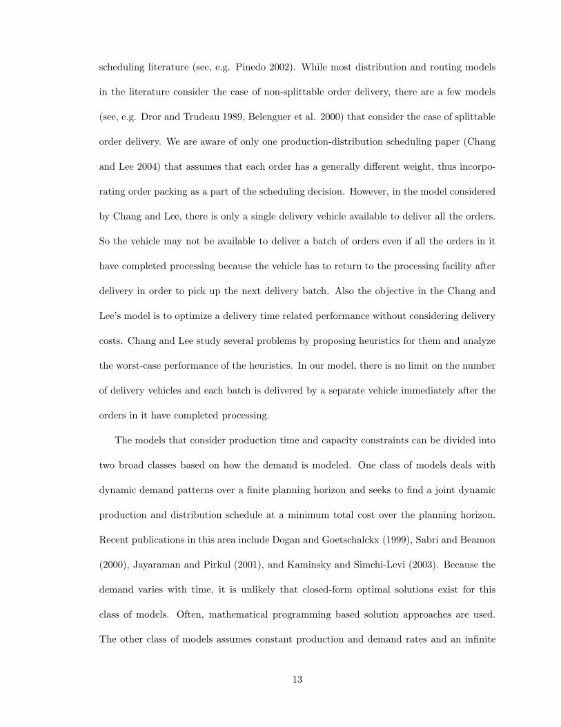
The other class of models assumes constant production and demand rates and an infinite

13

planning horizon, and seeks to find a joint cyclic production and delivery schedule at a

minimum total cost per unit time. Closed-form optimal solutions may be available for this

class of models under some policies on the relationship between the production and delivery

cycles. Since the third model we study belongs to the second class of models mentioned

here, we provide a detailed review of the related literature in this area in the following

paragraphs.

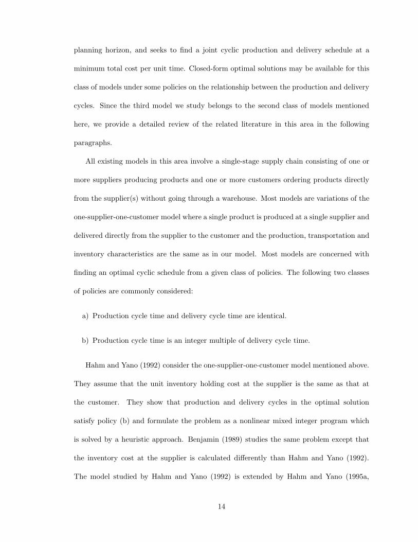
All existing models in this area involve a single-stage supply chain consisting of one or

more suppliers producing products and one or more customers ordering products directly

from the supplier(s) without going through a warehouse. Most models are variations of the

one-supplier-one-customer model where a single product is produced at a single supplier and

delivered directly from the supplier to the customer and the production, transportation and

inventory characteristics are the same as in our model. Most models are concerned with

finding an optimal cyclic schedule from a given class of policies. The following two classes

of policies are commonly considered:

a) Production cycle time and delivery cycle time are identical.

b) Production cycle time is an integer multiple of delivery cycle time.

Hahm and Yano (1992) consider the one-supplier-one-customer model mentioned above.

They assume that the unit inventory holding cost at the supplier is the same as that at

the customer. They show that production and delivery cycles in the optimal solution

satisfy policy (b) and formulate the problem as a nonlinear mixed integer program which

is solved by a heuristic approach. Benjamin (1989) studies the same problem except that

the inventory cost at the supplier is calculated differently than Hahm and Yano (1992).

The model studied by Hahm and Yano (1992) is extended by Hahm and Yano (1995a,

14

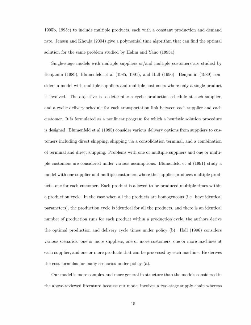
1995b, 1995c) to include multiple products, each with a constant production and demand

rate. Jensen and Khouja (2004) give a polynomial time algorithm that can find the optimal

solution for the same problem studied by Hahm and Yano (1995a).

Single-stage models with multiple suppliers or/and multiple customers are studied by

Benjamin (1989), Blumenfeld et al (1985, 1991), and Hall (1996). Benjamin (1989) con-

siders a model with multiple suppliers and multiple customers where only a single product

is involved. The objective is to determine a cyclic production schedule at each supplier,

and a cyclic delivery schedule for each transportation link between each supplier and each

customer. It is formulated as a nonlinear program for which a heuristic solution procedure

is designed. Blumenfeld et al (1985) consider various delivery options from suppliers to cus-

tomers including direct shipping, shipping via a consolidation terminal, and a combination

of terminal and direct shipping. Problems with one or multiple suppliers and one or multi-

ple customers are considered under various assumptions. Blumenfeld et al (1991) study a

model with one supplier and multiple customers where the supplier produces multiple prod-

ucts, one for each customer. Each product is allowed to be produced multiple times within

a production cycle. In the case when all the products are homogeneous (i.e. have identical

parameters), the production cycle is identical for all the products, and there is an identical

number of production runs for each product within a production cycle, the authors derive

the optimal production and delivery cycle times under policy (b). Hall (1996) considers

various scenarios: one or more suppliers, one or more customers, one or more machines at

each supplier, and one or more products that can be processed by each machine. He derives

the cost formulas for many scenarios under policy (a).

Our model is more complex and more general in structure than the models considered in

the above-reviewed literature because our model involves a two-stage supply chain whereas

15

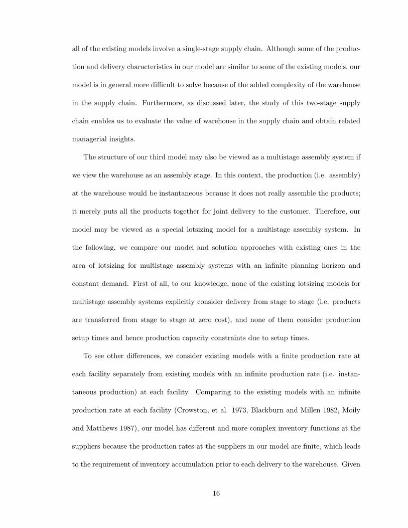
all of the existing models involve a single-stage supply chain. Although some of the produc-

tion and delivery characteristics in our model are similar to some of the existing models, our

model is in general more difficult to solve because of the added complexity of the warehouse

in the supply chain. Furthermore, as discussed later, the study of this two-stage supply

chain enables us to evaluate the value of warehouse in the supply chain and obtain related

managerial insights.

The structure of our third model may also be viewed as a multistage assembly system if

we view the warehouse as an assembly stage. In this context, the production (i.e. assembly)

at the warehouse would be instantaneous because it does not really assemble the products;

it merely puts all the products together for joint delivery to the customer. Therefore, our

model may be viewed as a special lotsizing model for a multistage assembly system. In

the following, we compare our model and solution approaches with existing ones in the

area of lotsizing for multistage assembly systems with an infinite planning horizon and

constant demand. First of all, to our knowledge, none of the existing lotsizing models for

multistage assembly systems explicitly consider delivery from stage to stage (i.e. products

are transferred from stage to stage at zero cost), and none of them consider production

setup times and hence production capacity constraints due to setup times.

To see other differences, we consider existing models with a finite production rate at

each facility separately from existing models with an infinite production rate (i.e. instan-

taneous production) at each facility. Comparing to the existing models with an infinite

production rate at each facility (Crowston, et al. 1973, Blackburn and Millen 1982, Moily

and Matthews 1987), our model has different and more complex inventory functions at the

suppliers because the production rates at the suppliers in our model are finite, which leads

to the requirement of inventory accumulation prior to each delivery to the warehouse. Given

16

this and the fact that there are capacity constraints in our model but not in those existing

models, the solution approaches used in those papers cannot be applied to our model.

All the existing models with a finite production rate at each facility (Schwarz and Schrage

1975, Moily 1986, Atkins et al. 1992) assume that the production rates are non-increasing

across the system (i.e. from components to final products), whereas this assumption does

not hold in our model if our model is viewed as a multistage assembly system. Crowston,

et al. (1973) show the property that under this assumption and without the capacity

constraint due to setup times, the lot size at each facility is an integer multiplier of that at

each immediately succeeding facility. This property is similar to one of the results we prove

in our model. However, our result is proved without this assumption and with the capacity

constraint. Schwarz and Schrage (1975) use this property to formulate the problem as an

integer program. They propose a branch-and-bound algorithm for getting optimal solutions

and a heuristic procedure that optimizes the system as a collection of two-stage systems by

ignoring multistage interaction effects. In addition to the non-increasing-production-rates

assumption, the models studied by Moily (1986) and Atkins et al. (1992) assume that

the product is transferred from one stage to the next immediately and continuously upon

its completion, whereas in our model all the units in a delivery shipment are transferred

together. Because of this difference, how inventory accumulates and hence the inventory

function at various facilities in our model are different from the models considered in these

existing papers. Atkins et al. (1992) derive some theoretical results for which the non-

increasing-production-rates assumption is a key. The solution approach used by Moily

(1986) is different from the approach we use. His approach is based on a one-time rounding

of any non-integer multipliers obtained without taking into account its effects on the other

participants of the system.

17

As quick response is becoming more critical in many supply chains, the linkage between

production and distribution is becoming ever more intimate. Consequently, joint consid-

eration of order processing and delivery scheduling is becoming crucial in achieving quick

response at minimum cost. Because of this growing importance, an increasing amount of re-

search has been devoted to integrated production-distribution scheduling models in the last

several years. However, this area is relatively new and more research is needed. The models

we study in this paper contribute to this area by analyzing various production-distribution

scheduling models.

1.6 Summary

The objective of this work is to study integrated production and distribution scheduling

decisions in various supply chains. While a lot of literature exists on exclusive production

scheduling or distribution scheduling, our study shows that optimizing these performance

measures independently may lead to a suboptimal system solution. With increasing compe-

tition, supply chain optimization as opposed to individual operation optimization becomes

crucial. This study aims to provide numerous insights and approaches to implement supply

chain scheduling decisions integrating production and distribution operations.

In Chapters 2 through 5, we cover the four different supply chain models. In Chapter

2, we consider a setup with multiple manufacturing plants owned by the same firm where

the firm has to decide on the order allocation and production and distribution scheduling.

Chapter 3 deals with the make-to-order production-distribution system with one supplier

and one or more customers where we look at due dates and distribution costs. In Chapter 4,

we study an integrated production and distribution scheduling model in a two-stage supply

chain to find a cyclic production schedule at each supplier, a cyclic delivery schedule from

18

each supplier to the warehouse, and a cyclic delivery schedule from the warehouse to the

customer so that the customer demand for each product is satisfied fully at minimum total

production, inventory and distribution cost. Chapter 5 combines order processing with

packing decisions for delivery in a make-to-order supply chain with one supplier and one

customer. Chapter 6 gives the conclusions and scope for further work.

19

Chapter 2

Order Assignment and Scheduling in a

Supply Chain

2.1 Introduction

Globalization has become a competitive strategy for many manufacturing firms due to the

cheaper labor and raw material costs overseas. About a fifth of the output of American

companies is produced abroad and around 53% of American firms are multinational (Dornier

et al. 1998). The supply chain of a typical American multinational manufacturer may

consist of a number of plants located at several foreign countries and a central distribution

center (DC) in the United States where products are received from overseas plants and

distributed to many domestic retail stores. In such a supply chain, production costs and

productivity may vary significantly from plant to plant due to variations in labor costs

and skills in the different countries. Also, in such a supply chain, transportation costs are

generally higher, and distribution lead times longer than in a domestic supply chain.

Now consider the global supply chain of a manufacturer who produces time-sensitive

20

products, such as toys, fashion apparel, or high-tech products that typically have a large

variety, a short life cycle, and are sold in a very short selling season (Hammond and Raman

1996, Johnson 2001). Because of high demand uncertainty of the products, retailers typically

do not place orders until reliable market information is available shortly before a selling

season. On the other hand, since there are significant markdowns for unsold products at

the end of the selling season, the manufacturer runs a high risk if it starts production early

before it receives orders from the retailers. As a result, the manufacturer would not start

production until orders from the retailers have been placed shortly before the selling season.

Due to the fact that there is only a limited amount of production time available, in order

to deliver the orders to the retailers as soon as possible at a low cost, the manufacturer

has to schedule the production and distribution operations in a coordinated and efficient

manner. In this chapter we consider a simplified version of the order assignment and

scheduling problem faced by the manufacturer in the above-described supply chain. In this

problem, the manufacturer receives a set of distinct orders from the retailers before a selling

season, and needs to determine (i) which orders to be assigned to which plants, (ii) how to

schedule the production of the assigned orders at each plant, and (iii) how to schedule the

distribution of the completed orders from each plant to the DC, so as to optimize a certain

performance measure of the supply chain. Due to the variations in productivity and labor

costs at different plants, the processing time and cost of an order are dependent on the

plant to which it is assigned. Completed orders are delivered in shipments from the plants

to the DC. Each shipment can carry up to a certain number of orders and is associated

with a certain distribution time and a certain distribution cost. Since the products are

time-sensitive, an important factor related to the performance of the supply chain is the

delivery lead time, i.e. the time between the placement of an order by a retailer and its

21

delivery to the retailer. We assume that the DC is located close to the retailers, such that

the delivery time and cost from the DC to the retailers are negligible, compared to the

delivery time and cost from the plants to the DC. Therefore, the lead time of an order in

our problem is the time between the placement of the order and its delivery to the DC.

Another important factor related to the performance of the supply chain is cost. The total

cost in this supply chain consists of production costs for processing the orders at the plants

and distribution costs for the delivery of completed orders from the plants to the DC.

Since finished products are rarely held at the plants or DC for a long time in such a time-

sensitive supply chain, inventory cost of finished products is negligible and not considered.

We consider four different performance measures of the supply chain, each of which takes

into account both the delivery lead time and the total cost. A problem corresponding to

each performance measure is studied separately. The problems we study integrate order

assignment, production scheduling (for order processing at the plants), and distribution

scheduling (for the delivery of completed orders from the plants to the DC).

In the broader literature of supply chain management, a tremendous amount of research

has been done on various strategic and tactical problems in the past decade. However,

very few results have addressed scheduling issues in a supply chain. On the other hand,

as quick response is becoming more and more critical in many manufacturing and service

supply chains, the linkage between production and distribution is becoming ever more inti-

mate. Consequently, optimal scheduling of orders across different stages of a supply chain

is becoming crucial in achieving quick response at minimum cost. This chapter has two

objectives. Our first objective is to analyze the computational complexity of various cases

of the problems we consider by either proving that a problem is intractable (i.e., NP-hard)

or providing an efficient exact algorithm for the problem. Our second objective is to design

22

fast heuristics for NP-hard problems that are capable of generating near optimal solutions.

We evaluate the performance of the heuristics by analyzing their worst-case and asymp-

totic performances and conducting computational experiments. This chapter is organized

as follows. In Section 2.2, we specify the notation, define the problems, and give some

optimality properties of the problems. We then study the problems in Sections 2.3 through

2.6, respectively. Finally, in Section 2.7 we conclude the chapter.

2.2 Problems and Preliminary Results

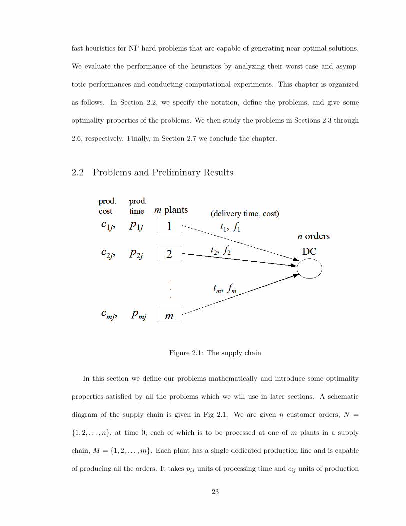
Figure 2.1: The supply chain

In this section we define our problems mathematically and introduce some optimality

properties satisfied by all the problems which we will use in later sections. A schematic

diagram of the supply chain is given in Fig 2.1. We are given n customer orders, N =

1, 2, . . . , n, at time 0, each of which is to be processed at one of m plants in a supply

chain, M = 1, 2, . . . ,m. Each plant has a single dedicated production line and is capable

of producing all the orders. It takes pij units of processing time and cij units of production

23

cost for plant i to process order j, for i ∈ M and j ∈ N . Each order only needs to be

processed by one of the plants once without interruption. Completed orders are delivered

to a distribution center (DC) in the supply chain. The delivery time and delivery cost of a

shipment from plant i ∈ M to the DC are ti and fi, respectively. Each delivery shipment has

a capacity limit; it can carry up to b orders. We assume that each order takes up the same

amount of capacity of a shipment and that partial delivery of an order is not possible. The

problem is to assign each order to a plant, schedule the processing of the orders assigned to

each plant, and schedule the delivery of the completed orders from each plant to the DC, so

as to optimize a given objective function that takes into account delivery lead time, total

production cost, and total distribution cost. To schedule the processing of assigned orders

at each plant, we need to determine which sequence of the orders to use and when to start

processing each order. Similarly, to schedule the delivery of the completed orders, we need

to determine how many shipments to use at each plant, which orders to be delivered in each

shipment, and when each shipment should depart from the plant. For a given schedule, we

define:

TC: the total cost of production and distribution

Cj: the completion time of order j ∈ N which is the time when order j completes

processing at the plant to which it is assigned.

Dj : the delivery time of order j ∈ N which is the time when order j ∈ N is delivered

to the DC.

Since all the orders are given at time 0, Dj also represents the lead time of order j. We

consider the following two functions for measuring the delivery lead time performance of

the supply chain:

24

(i) total lead time of the orders, Dtotal =∑

j∈N Dj.

(ii) maximum lead time of the orders, Dmax = maxDj |j ∈ N.

These two functions are analogous to two widely used functions for measuring customer

service in the production scheduling literature (e.g. Pinedo 2002), total completion time

Ctotal =∑

j∈N Cj , and maximum completion time Cmax = maxCj |j ∈ N. In the tradi-

tional scheduling literature, it is implicitly assumed that once an order completes processing

it is delivered to its customer immediately without any transportation time or cost, and

hence Cj is treated as the lead time of order j. However, in our problems, since trans-

portation cost is considered, an order may be delivered together with some other orders

and hence it may not be delivered immediately after it is processed. Moreover, there are

transportation times in our problems. Hence Dj > Cj and Dj , instead of Cj, is the lead

time of order j.

We consider the following four problems, each with a different objective:

P1: Minimizing a weighted sum of the total lead time and total cost, i.e. αDtotal +

(1 − α)TC, where α ∈ [0, 1] is a given constant, representing the decision-maker’s relative

preference on Dtotal and TC.

P2: Minimizing the total cost TC subject to the constraint that the total lead time is no

more than a given threshold, i.e. Dtotal ≤ D, where D is a given constant.

P3: Minimizing a weighted sum of the maximum lead time and total cost, i.e. αDmax +

(1 − α)TC, where α ∈ [0, 1] is a given constant, as in problem P1.

P4: Minimizing the total cost TC subject to the constraint that the maximum lead time is

no more than a given threshold, i.e. Dmax ≤ D, where D is a given constant.

We note that several special cases of the problems P1 and P3 are related to some existing

25

scheduling problems in the literature. The special case of P1 and P3 with a single plant (i.e.

m = 1) are equivalent to two of the problems studied by Chen and Vairaktarakis (2004).

They give polynomial-time algorithms for finding optimal solutions to those problems. In

the single-plant case, there are no order assignment decisions to be made and production

costs can be ignored, and hence the problems are much easier. However, as we will see later,

the general cases of P1 and P3 with multiple plants are NP-hard. In this chapter, we focus

on the multi-plant problems only. If we view each plant as an unrelated parallel machine

and assume zero production costs and zero delivery times and costs, then P1 and P3 reduce

to the classical unrelated parallel machine scheduling problems with total completion time

and maximum completion time of orders as the objective function, respectively. It is known

that the unrelated parallel machine total completion time problem can be formulated as an

assignment problem and solved in polynomial time (Horn 1973), and the unrelated parallel

machine maximum completion time problem is NP-hard (Garey and Johnson 1979).

We say that a set of orders assigned to some plant i are in SPT order (shortest-

processing-time-first order) if they are sequenced in the non-decreasing order of their process-

ing times pij and orders with equal processing times are sequenced in the same order as

their indices. In the following, we present some preliminary results about the structure of

an optimal schedule.

Lemma 1 There exists an optimal schedule for all the problems P1, P2, P3, and P4 in which

all of the following hold: (1) The orders assigned to each plant are scheduled in the SPT

order, (2) There is no inserted idle time between orders processed at each plant, (3) The

departure time of each shipment is the time when all the orders in it complete processing,

(4) All the orders that are delivered in the same shipment are processed consecutively at a

plant.

26

Proof (1) If any order violates this rule, we can rearrange the orders in the SPT order

without increasing the objective function value. If the violating orders are in the same

shipment, there will not be any change in the value of the objective function as each order

has to wait for the other orders in the shipment before it gets delivered, and hence the

sequence of orders within a batch does not matter. If the orders that violate this rule are

in different shipments, then after re-sequencing the orders in the SPT order, we can adjust

each shipment such that it consists of the jobs at the same positions in the new sequence

as in the original sequence. This will lead to a decrease in the departure times of some

shipments and hence a decrease in the objective value. (2), (3), and (4) can be proved

easily. We omit the proofs for them.

Lemma 2 There exists an optimal schedule for all the problems P1, P2, P3, and P4 in which

the number of orders delivered in an earlier shipment from a plant is greater than or equal

to the number of orders delivered in a later shipment from the same plant.

Proof Consider two consecutive shipments S1 and S2 from some plant i ∈ M , where S1 is

delivered earlier than S2. Suppose that there are n1 and n2 orders in S1 and S2, respectively,

such that n1 < n2. Let u1 and u2 denote the completion time of the last order in S1 and

S2 respectively. The contribution of the orders in S1 and S2 to the total lead time Dtotal

is thus given by

F (S1, S2) = n1(u1 + ti) + n2(u2 + ti)

Now we move the first order in S2 to S1. Let the processing time of this order be p.

Then the contribution of the orders in S1 and S2 to Dtotal becomes

G(S1, S2) = (n1 + 1)(u1 + p + ti) + (n2 − 1)(u2 + ti)

27

Since no other shipments are involved, the total contribution to Dtotal by the orders

in the shipments other than S1 and S2 remains the same. Therefore, the value of Dtotal is

decreased by

F (S1, S2) − G(S1, S2) = u2 − u1 − (n1 + 1)p

By Lemma 1(1), we can assume that all the orders in S1 and S2 are in SPT order. Thus

the processing time of each order in S1 is no more than p, whereas that of each order in S2 is

at least p. By the assumption that n1 < n2, we have u2−u1 ≥ n2p ≥ (n1 +1)p. This means

that F (S1, S2) −G(S1, S2) ≥ 0, i.e. the value Dtotal is not increased after moving the first

order of S2 to S1. Clearly, the values Dmax and TC both remain the same. Therefore, the

objective value of each of the problems P1, P2, P3, P4 is not increased after moving the

first order of S2 to S1. We can repeat this until the number of orders in S1 is equal to that

in S2.

2.3 Problem P1: Minimizing αDtotal + (1 − α)TC

We first discuss two extreme cases of the problem with α = 1 or α = 0. We then show

that the general problem P1 with 0 < α < 1 is NP-hard, propose two heuristics for the

problem, and evaluate both theoretical and computational performance of the heuristics.

The following two special cases of problem P1 arise in many practical situations and hence

are considered separately: (i) the order processing times are agreeable, i.e. there exists an

ordering of the orders, denoted as ([1], . . . , [n]) which is a permutation of (1, . . . , n), such

that pi[1] ≤ . . . ≤ pi[n], for all i ∈ M ; (ii) the production costs of orders at each plant are

proportional to the processing times of the orders, i.e. cij = γipij for i ∈ M and j ∈ N ,

where γi represents the production cost per unit processing time at plant i. We give dynamic

28

programming algorithms with a time complexity polynomial in n and exponential in m for

these problems.

2.3.1 Problem P1 with α = 0 or α = 1

In problem P1 with α = 1, since no cost is considered, each order is delivered in a separate

shipment immediately after it completes processing. This case of the problem can be for-

mulated as an assignment problem as follows. For k, j ∈ N , and i ∈ M , define a parameter

a(k,i)j = kpij + ti which is the contribution to Dtotal by order j if it is scheduled to the kth

last position at plant i. Define a binary variable x(k,i)j to be 1 if order j is scheduled as the

kth last order at plant i, and 0 otherwise. The following assignment problem formulates

problem P1 with α = 1.

min∑

k∈N

∑

i∈M

∑

j∈N

a(k,i)jx(k,i)j

Subject to:

∑

k∈N

∑

i∈M

x(k,i)j = 1 j ∈ N

∑

j∈N

x(k,i)j ≤ 1 k ∈ N i ∈ M

x(k,i)j ∈ 0, 1 k ∈ N, i ∈ M, j ∈ N

It is well-known that solving the LP relaxation of this formulation yields an integer

solution. Thus problem P1 with α = 1 is solvable in polynomial time.

Problem P1 with α = 0 is to minimize the total production and distribution cost. This

problem can be solved by the following procedure which has a time complexity polynomial

in n and exponential in m. Since Dtotal is not considered, each delivery shipment at each

plant should deliver as many orders as possible in order to minimize the total transportation

29

cost. Suppose that there are ni orders assigned to plant i ∈ M in an optimal solution.

Then dnib e shipments are used at plant i and hence the total distribution cost is fixed as

∑i∈Mdni

b efi . The problem is then reduced to minimizing the total production cost, which

can be formulated as the following transportation problem. Define xij to be 1 if order j is

assigned to plant i, and 0 otherwise.

min∑

i∈M

∑

j∈N

cijxij

Subject to:

∑

i∈M

xij = 1 j ∈ N

∑

j∈N

xij = ni i ∈ M i ∈ M

xij ∈ 0, 1 i ∈ M, j ∈ N

Solving the LP relaxation of this formulation gives an integer solution. Therefore, for

a given combination of (n1, . . . , nm), problem P1 with α = 0 can be solved in polynomial

time. We can enumerate all possible combinations of (n1, . . . , nm) with n1 + . . . + nm = n,

and for each combination solve such a transportation problem. The solution with the lowest

total production and distribution cost is then optimal to problem P1 with α = 0. Since

there are no more than nm possible combinations of (n1, . . . , nm) with n1 + . . . + nm = n,

the above procedure is polynomial for problem P1 with α = 0 and a fixed m. However,

when the number of plants m is arbitrary, problem P1 with α = 0 becomes NP-hard, which

is proved in the following theorem.

Theorem 1 Problem P1 with α = 0 and an arbitrary number of plants is strongly NP-hard.

Proof We prove this by a reduction from the Minimum Cover (MC) problem, which is

known to be strongly NP-complete (Garey and Johnson 1979).

30

MC: Given a set S with h elements S = 1, . . . , h, a collection Q of u subsets of S,

Q = S1, . . . , Su, where Si is a subset of S, for i = 1, . . . , u, and a positive integer v ≤ u,

does there exist a subset Q′ of Q with |Q′| ≤ v, such that every element of S belongs to at

least one member of Q′?

Given this instance of MC, we consider an instance of the recognition version of P1

defined by:

Number of orders, n = h, and set of orders, N = S

Number of plants, m = u, and set of plants, M = 1, . . . , u.

Order processing times, pij = 0, for i ∈ M and j ∈ N .

Order production costs, cij = 0 if j ∈ Si, and 2u otherwise, for i ∈ M and j ∈ N .

Delivery times, ti = 0, and delivery costs, fi = 1 for i ∈ M .

Shipment capacity, b = h.

Threshold of objective value, Z = v.

We show that there is a schedule to this instance of P1 with the objective value no more

than Z if and only if there is a solution to MC.

(If part) Without loss of generality, we assume that Q′ = S1, . . . , Sw with w ≤ v is

a solution to MC. We construct a solution to P1 as follows. For each j ∈ N , define

Pj = i ∈ 1, . . . , w|j ∈ Si, and assign order j to any plant i ∈ Pj . Since every element

of S is covered by Si for some i ∈ 1, . . . , w, every order j ∈ N gets assigned to a plant in

M . Use one shipment to deliver all the orders assigned to each plant. This gives a solution

to P1. Since order j is assigned to a plant i with j ∈ Si, the production cost of order j is

0. Thus the total production and distribution cost of this solution is no more than w ≤ Z.

(Only If part) Given a solution to P1 with the total production and distribution cost no more

than Z, we can conclude that all the orders are assigned to plants where their production

31

costs are zero. This is because if an order was assigned to a plant with a positive production

cost, then the total cost would be more than 2u > Z. Let k be the number of plants where

orders are assigned. Clearly, k ≤ v. Without loss of generality, suppose that all the orders

are assigned to plants 1, . . . , k. If order j is assigned to plant i ∈ 1, . . . , k, then j ∈ Si

because otherwise cij would be nonzero. This means that S1, . . . , Sk is a solution to MC.

2.3.2 Problem P1 with Agreeable Processing Times

In many practical situations, given a set of orders, there is a clear ordering with respect to

their processing times, regardless of which plant they are processed. For example, if order

1 requires more time than order 2 if processed at one plant, it is likely to be the same case

at every other plant. In this case of the problem, we say that the order processing times

are agreeable, i.e. there exists an ordering of the orders, denoted as ([1], . . . , [n]) which is a

permutation of (1, . . . , n), such that pi[1] ≤ pi[2] ≤ . . . ≤ pi[n], for all i ∈ M .

We give a dynamic programming algorithm to solve P1 with agreeable processing times.

We say that a set of orders assigned to plant i are in LPT order (longest-processing-time-first

order) if they are sequenced in the non-increasing order of their processing times pij and

orders with equal processing times are sequenced in the reverse order of their indices. Since

the processing times are agreeable, both the SPT and LPT order of a given set of orders

remains the same regardless of which plant they are assigned to. This property enables us to

use a common sequence of the orders in the dynamic program. Our DP algorithm considers

the orders in LPT order and assigns them to a plant backward from the last position to the

first. The resulting forward sequence of the orders assigned to a plant by this algorithm is

thus in SPT order, satisfying Lemma 1 (1).

32

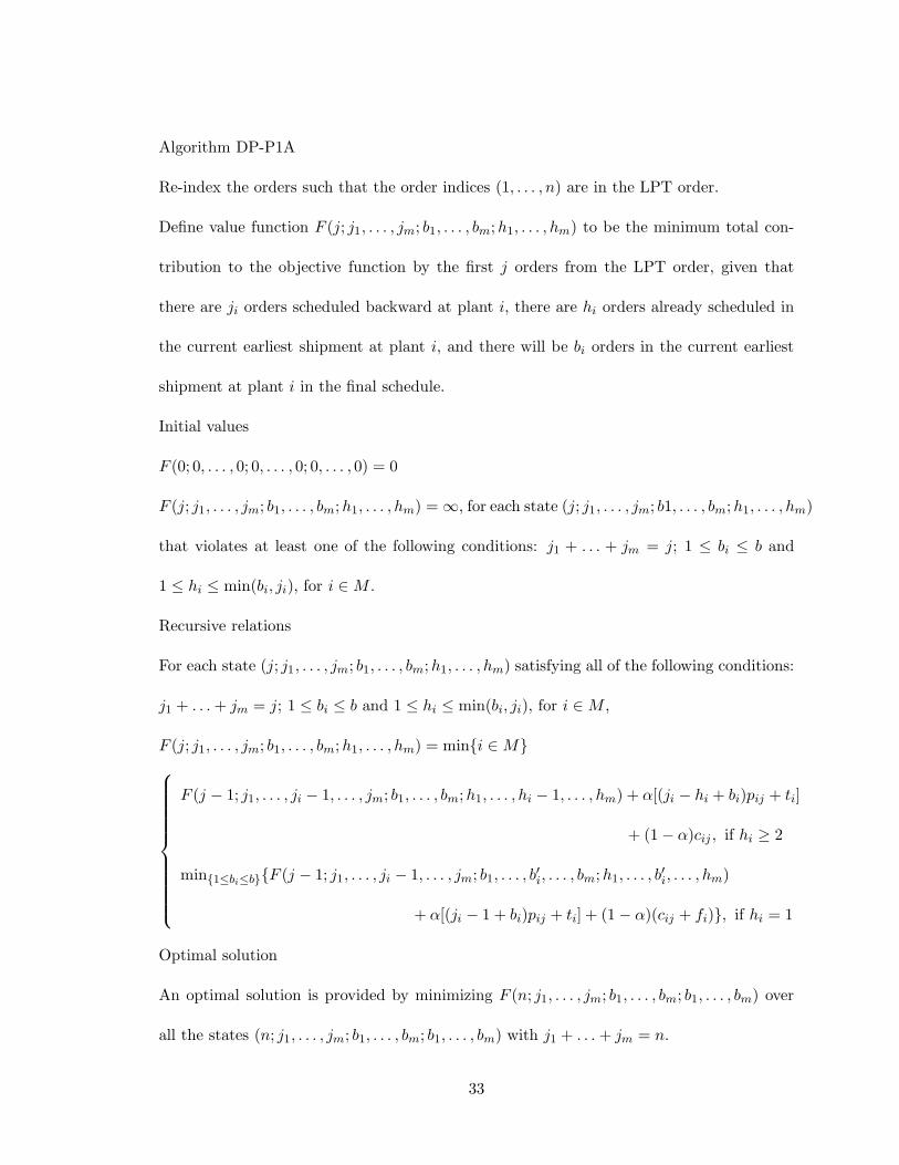
Algorithm DP-P1A

Re-index the orders such that the order indices (1, . . . , n) are in the LPT order.

Define value function F (j; j1, . . . , jm; b1, . . . , bm;h1, . . . , hm) to be the minimum total con-

tribution to the objective function by the first j orders from the LPT order, given that

there are ji orders scheduled backward at plant i, there are hi orders already scheduled in

the current earliest shipment at plant i, and there will be bi orders in the current earliest

shipment at plant i in the final schedule.

Initial values

F (0; 0, . . . , 0; 0, . . . , 0; 0, . . . , 0) = 0

F (j; j1, . . . , jm; b1, . . . , bm;h1, . . . , hm) = ∞, for each state (j; j1, . . . , jm; b1, . . . , bm;h1, . . . , hm)

that violates at least one of the following conditions: j1 + . . . + jm = j; 1 ≤ bi ≤ b and

1 ≤ hi ≤ min(bi, ji), for i ∈ M .

Recursive relations

For each state (j; j1, . . . , jm; b1, . . . , bm;h1, . . . , hm) satisfying all of the following conditions:

j1 + . . . + jm = j; 1 ≤ bi ≤ b and 1 ≤ hi ≤ min(bi, ji), for i ∈ M ,

F (j; j1, . . . , jm; b1, . . . , bm;h1, . . . , hm) = mini ∈ M

F (j − 1; j1, . . . , ji − 1, . . . , jm; b1, . . . , bm;h1, . . . , hi − 1, . . . , hm) + α[(ji − hi + bi)pij + ti]

+ (1 − α)cij , if hi ≥ 2

min1≤bi≤bF (j − 1; j1, . . . , ji − 1, . . . , jm; b1, . . . , b′i, . . . , bm;h1, . . . , b

′i, . . . , hm)

+ α[(ji − 1 + bi)pij + ti] + (1 − α)(cij + fi), if hi = 1

Optimal solution

An optimal solution is provided by minimizing F (n; j1, . . . , jm; b1, . . . , bm; b1, . . . , bm) over

all the states (n; j1, . . . , jm; b1, . . . , bm; b1, . . . , bm) with j1 + . . . + jm = n.

33

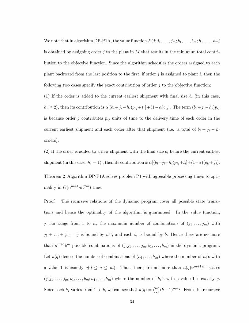
We note that in algorithm DP-P1A, the value function F (j; j1, . . . , jm; b1, . . . , bm;h1, . . . , hm)

is obtained by assigning order j to the plant in M that results in the minimum total contri-

bution to the objective function. Since the algorithm schedules the orders assigned to each

plant backward from the last position to the first, if order j is assigned to plant i, then the

following two cases specify the exact contribution of order j to the objective function:

(1) If the order is added to the current earliest shipment with final size bi (in this case,

hi ≥ 2), then its contribution is α[(bi +ji−hi)pij + ti]+(1−α)cij . The term (bi +ji−hi)pij

is because order j contributes pij units of time to the delivery time of each order in the

current earliest shipment and each order after that shipment (i.e. a total of bi + ji − hi

orders).

(2) If the order is added to a new shipment with the final size bi before the current earliest

shipment (in this case, hi = 1) , then its contribution is α[(bi+ji−hi)pij+ti]+(1−α)(cij+fi).

Theorem 2 Algorithm DP-P1A solves problem P1 with agreeable processing times to opti-

mality in O(nm+1mb2m) time.

Proof The recursive relations of the dynamic program cover all possible state transi-

tions and hence the optimality of the algorithm is guaranteed. In the value function,

j can range from 1 to n, the maximum number of combinations of (j1, . . . , jm) with

j1 + . . . + jm = j is bound by nm, and each bi is bound by b. Hence there are no more

than nm+1bm possible combinations of (j, j1, . . . , jm; b1, . . . , bm) in the dynamic program.

Let u(q) denote the number of combinations of (h1, . . . , hm) where the number of hi’s with

a value 1 is exactly q(0 ≤ q ≤ m). Thus, there are no more than u(q)nm+1bm states

(j, j1, . . . , jm; b1, . . . , bm;h1, . . . , hm) where the number of hi’s with a value 1 is exactly q.

Since each hi varies from 1 to b, we can see that u(q) =(m

q

)(b − 1)m−q. From the recursive

34

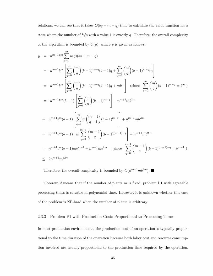
relations, we can see that it takes O(bq + m − q) time to calculate the value function for a

state where the number of hi’s with a value 1 is exactly q. Therefore, the overall complexity

of the algorithm is bounded by O(y), where y is given as follows:

y = nm+1bmm∑

q=0

u(q)(bq + m − q)

= nm+1bm

m∑

q=0

(m

q

)(b − 1)m−q(b − 1)q +

m∑

q=0

(m

q

)(b − 1)m−qm

= nm+1bm

m∑

q=0

(m

q

)(b − 1)m−q(b − 1)q + mbm

(since

m∑

q=0

(m

q

)(b − 1)m−q = bm )

= nm+1bm(b − 1)

m∑

q=0

(m

q

)(b − 1)m−q

+ nm+1mb2m

= nm+1bm(b − 1)

m∑

q=1

m

(m − 1q − 1

)(b − 1)m−q

+ nm+1mb2m

= nm+1bm(b − 1)

m

m−1∑

q=0

(m − 1

q

)(b − 1)(m−1)−q

+ nm+1mb2m

= nm+1bm(b − 1)mbm−1 + nm+1mb2m (sincem−1∑

q=0

(m − 1

q

)(b − 1)(m−1)−q = bm−1 )

≤ 2nm+1mb2m

Therefore, the overall complexity is bounded by O(nm+1mb2m).

Theorem 2 means that if the number of plants m is fixed, problem P1 with agreeable

processing times is solvable in polynomial time. However, it is unknown whether this case

of the problem is NP-hard when the number of plants is arbitrary.

2.3.3 Problem P1 with Production Costs Proportional to Processing Times

In most production environments, the production cost of an operation is typically propor-

tional to the time duration of the operation because both labor cost and resource consump-

tion involved are usually proportional to the production time required by the operation.

35

Therefore, it is reasonable to assume that the production costs of orders at each plant are

proportional to the processing times of the orders, i.e. cij = γipij for i ∈ M and j ∈ N ,

where γi represents the production cost per unit processing time at plant i.

We show that problem P1 under this assumption can be solved to optimality by a

dynamic programming algorithm which has a time complexity polynomial in n and ex-

ponential in m, meaning that the algorithm is polynomial if the number of plants m is

fixed. Before presenting the algorithm, we first introduce some definitions to be used in

the algorithm. Denote the SPT list of the orders with respect to their processing times at

plant i by SPTi = ([i1], [i2], . . . , [in]), where [ih] denotes the hth order in SPTi. The m lists

SPT1, . . . , SPTm are in general different because the processing times may not be agreeable.

Define SPTiu to be the set of the first u orders in SPTi, i.e. SPTiu = [i1], . . . , [iu].

For some given k1, . . . , km with each ki ≤ n, if we know that all the orders in the joint

set Y mi=1SPTiki

have been scheduled, then we know exactly which orders are left in each list

SPTi, for i ∈ M . Note that some of the orders in SPTi\SPTikimay have been covered

by the set Y mi=1SPTiki

. Thus the remaining orders in each list SPTi is in general a subset

of SPTi\SPTiki. Given k1, . . . , km, and the fact that all the orders in Y m

i=1SPTikihave

been scheduled, we can know the remaining orders in each set SPTi in polynomial time

(polynomial in n and m). Similarly, for some given q ∈ M , if we know that all the orders

in the joint set Y mi=1,i 6=qSPTiki

have been scheduled, then we can know exactly which orders

are remaining in SPTq in polynomial time.

Our DP algorithm is based on the following result.

Lemma 3 There exists an optimal schedule π = (π1, . . . , πm), where πi is the schedule at

plant i, such that if we divide π arbitrarily into two parts, left part denoted as πL =

(π1L, . . . , πmL) and right part denoted as πR = (π1R, . . . , πmR), where (πiL, πiR) = πi, for

36

every i ∈ M , then there exists some i ∈ M such that ui = yi, where ui is the first order

in πiR, and yi is the first order in the SPT sequence of the orders in the set ∪q∈MπqR with

respect to the processing times at plant i.

Proof We prove this by showing that any schedule that violates this lemma can be trans-

formed into a schedule that satisfies this lemma with an equal or lower total cost. Given a

schedule π, suppose that there is a partition of π = (πL, πR) such that under this partition

ui 6= yi for every i ∈ M . Define order set Y = y1, . . . , ym. Let H denote the subset of

plants where the orders from Y are scheduled. There are two cases:

Case 1: If |H| = m, then each plant processes exactly one order from the set Y . Let y[i]

denote the order from Y which is processed at plant i, for i ∈ M . Create a new schedule

by modifying πR as follows: For i ∈ M , if ui = y[i], then remove y[i] from πiR, and move

yi from where it is scheduled in πR to the position of y[i]; otherwise, move yi from where

it is scheduled in πR to the position right before ui in πiR so that yi becomes the first

order in the new πiR. It can be easily verified that every order in this new schedule has

a processing time no greater than that of the order scheduled in the same position in the

original schedule. Since the production costs of the orders at each plant are proportional to

their processing times, it can be seen that this new schedule has a total cost no more than

that of the original schedule.

Case 2: If |H| ≤ m − 1, then define Y1 = yi|i ∈ H, and H1 = i ∈ H| plant i processes

some order yj ∈ Y1. Clearly, Y1 ⊆ Y and H1 ⊆ H. There are two cases again. If

|H| = |H1|, then each plant in H processes exactly one order from Y1. Following the same

approach as in Case 1, we can construct a new schedule where yi ∈ Y1 becomes the first

order in πiR, for every i ∈ H1, and this new schedule has a total cost no more than that of

π. If |H| > |H1|, then follow the same argument as in Case 2 to further find a subset H2 of

37

H1 and a subset Y2 of Y1 such that Y2 = yi|i ∈ H1, and H2 = i ∈ H1| plant i processes

some order yj ∈ Y2. Again there are two cases to consider: |H1| = |H2| or |H1| > |H2|.

Continue this process, and eventually we will have |Hq−1| = |Hq| for some q(q < m) and

apply the same argument as in Case 1.

For i ∈ M , let SPTiR denote the SPT sequence of the orders in the set ∪q∈MπqR with

respect to the processing times at plant i. Lemma 3 implies that we can build an optimal

schedule step by step as follows. Suppose that we have built a partial schedule πL. Next we

can append the first order in the list SPTiR to the end of πiL for some plant i ∈ M . Since

we do not know the exact plant i ∈ M where we should add an order to, we can try every

i ∈ M (i.e. for every i ∈ M , we try to append the first order of SPTiR to the end of πiL),

and select the resulting schedule with the lowest total cost. This observation enables us to

develop a dynamic programming algorithm for the problem. The DP algorithm schedules

the orders in SPT order at each plant forward from the first position to the last. Suppose

that a partial schedule πL has been built, the algorithm next tries to append the first order

of SPTiR to the end of πiL, for every i ∈ M , and selects the resulting schedule with the

lowest total cost. We describe the details of the algorithm below.

Algorithm DP-P1P

Define value function F (n1, . . . , nm; k1, . . . , km; b1, . . . , bm;h1, . . . , hm) to be the minimum

total contribution of the orders in a partial schedule where:

(i) there are exactly ni orders at plant i in the final schedule,

(ii) ji orders have been scheduled currently at plant i,

(iii) the current last order scheduled at plant i is order [iki],

(iv) the size of the current last shipment at plant i in the final schedule is bi, and

38

(v) there are hi orders already scheduled in the current last shipment at plant i.

Initial values

F (n1, . . . , nm; 0, . . . , 0; 0, . . . , 0; 0, . . . , 0; 0, . . . , 0) = 0, for any state with n1 + . . . + nm = n.

F (n1, . . . , nm; j1, . . . , jm; k1, . . . , km; b1, . . . , bm;h1, . . . , hm) = ∞, for each infeasible state

(n1, . . . , nm; j1, . . . , jm; k1, . . . , km; b1, . . . , bm;h1, . . . , hm). For a state to be feasible, all

the following conditions must be satisfied: n1 + . . . + nm = n; and for every i ∈ M ,

1 ≤ ji ≤ min(ki, ni), 0 ≤ ki ≤ n, hi ≤ bi, bi ≤ min(b, ni), and the set Y mi=1SPTiki

contains

exactly j1 + . . . + jm orders.

Recursive relations

For each feasible state (n1, . . . , nm; j1, . . . , jm; k1, . . . , km; b1, . . . , bm;h1, . . . , hm):

F (n1, . . . , nm; j1, . . . , jm; k1, . . . , km; b1, . . . , bm;h1, . . . , hm) = mini∈M

F (n1, . . . , nm; j1, . . . , ji − 1, . . . , jm; k1, . . . , k′i, . . . , km; b1, . . . , bm;h1, . . . , hi − 1, . . . , hm)

+ α[(ni − ji + hi)pi[iki] + ti] + (1 − α)ci[iki], if hi ≥ 2

min1≤bi≤bF (n1, . . . , nm; j1, . . . , ji − 1, . . . , jm; k1, . . . , k′i, . . . , km; b1, . . . , b

′i, . . . , bm;

h1, . . . , b′i, . . . , hm) + α[(ni − ji + hi)pi[iki] + ti] + (1 − α)(ci[iki] + fi), if hi = 1

where k′i is such that order [ik′

i] is the order immediately before order [iki] among the

remaining orders in the list SPTi after the orders in the set Y mv=1,v 6=iSPTvkv have been

scheduled.

Optimal solution

An optimal solution is provided by:

minimizing F (n1, . . . , nm;n1, . . . , nm; k1, . . . , km; b1, . . . , bm; b1, . . . , bm) over all the feasible

states (n1, . . . , nm;n1, . . . , nm; k1, . . . , km; b1, . . . , bm; b1, . . . , bm) with n1 + . . . + nm = n.

We note that in this algorithm the partial schedule corresponding to the state (n1, . . . , nm;

39

j1, . . . , jm; k1, . . . , km; b1, . . . , bm; h1, . . . , hm) contains exactly all the orders in the set

Y mi=1SPTiki

. The value function F (n1, . . . , nm; j1, . . . , jm; k1, . . . , km; b1, . . . , bm; h1, . . . , hm)

is obtained by selecting one of the following m alternatives with the lowest total contribu-

tion: Appending order [iki] to the end of a partial schedule at plant i ∈ M . The partial

schedule right before order [iki] is added to plant i contains exactly the orders in the

set (Y mv=1,v 6=iSPTvkv )Y SPTik′

i, where k′

i is defined in the algorithm and is unique given

k1, . . . , km. There are two possible ways for adding order [iki] to plant i:

(1) If the order is added to the current last shipment with final size bi (in this case, hi ≥ 2),

then its contribution is α[(ni − ji + hi)pi[iki] + ti] + (1 − α)ci[iki].

(2) If the order is added to a new shipment with the final size bi after the current last

shipment (in this case, hi = 1) , then its contribution is α[(ni − ji + hi)pi[iki] + ti] + (1 −

α)(ci[iki] + fi).

Theorem 3 Algorithm DP-P1P solves problem P2 with production costs proportional to

processing times to optimality in O(n3mmb2m) time.

Proof The algorithm schedules orders at each plant forward from the first position to the

last. Lemma 2 shows that given a partial schedule πL as defined in the statement of the

lemma, it is sufficient to consider the following m possible state transitions from a state with

j orders to a state with j +1 orders in the dynamic program: appending order yi to the end

of πiL, for i ∈ M . In the algorithm, state (n1, . . . , nm; j1, . . . , ji, . . . , jm; k1, . . . , ki, . . . , km)

can be transitioned from (n1, . . . , nm; j1, . . . , ji − 1, . . . , jm; k1, . . . , k′i, . . . , km) by adding

order [iki] to the end of the schedule at plant i, for i ∈ M . All these state transitions are

considered in the algorithm, which guarantees the optimality of the algorithm.

There are at most O(n3mbm) combinations of (n1, . . . , nm; j1, . . . , jm; k1, . . . , km, b1, . . . , bm)

considered in the dynamic program. Let u(q) denote the number of combinations of

40

(h1, . . . , hm) where the number of hi’s with a value 1 is exactly q (0 ≤ q ≤ m). Thus,

there are no more than u(q)n3mbm states in the DP where the number of hi’s with a value

1 is exactly q. By a similar argument as in the proof of Theorem 2, it can be shown that

the overall time complexity of the algorithm is bounded by O(n3mmb2m).

Theorem 3 shows that for a fixed number of plants m, the problem P1 with production

costs proportional to processing times is solvable in polynomial time. However, due to the

high-order time complexity of the algorithm, this algorithm is only of theoretical value and it

is impractical to apply it to actually solving the problem. Faster heuristics or approximation

algorithms have to be developed to solve the problem.

2.3.4 General Problem P1

Theorem 4 Problem P1 with 0 < α < 1 and an arbitrary number of plants is strongly

NP-hard.

Proof We prove this by a reduction from the strongly NP-hard Minimum Cover (MC)

problem, an instance of which is given in the proof of Theorem 1. Given this instance of

MC, we consider an instance of the recognition version of problem P1 defined exactly the

same way as the one defined in the proof of Theorem 1 except the following parameters:

Order processing times, pij = 0 if j ∈ Si, and d (1−α)α ev + 1 otherwise, for i ∈ M and j ∈ N .

Order production costs, cij = pij for i ∈ M and j ∈ N .

Threshold of objective value, Z = (1 − α)v.

By similar arguments as in the proof of Theorem 1, we can show that there is a schedule

to this instance of P1 with the objective value no more than Z if and only if there is a

solution to MC. We omit the details of the proof.

41

The complexity of the problem P1 with 0 < α < 1 and a fixed number of plants remains

open.

In the remainder of this subsection, we propose two heuristics for solving the general

problem P1. Before presenting the heuristics, we first derive an upper bound on the size of a

shipment containing a given order at each plant. Let bmax,i,j denote the maximum possible

size of a shipment containing order j at plant i in an optimal schedule. Denote the SPT order

of the orders at plant i by ([i1], [i2], . . . , [in]). Suppose that the size of a shipment B con-

taining order j at plant i is x, and B consists of orders (< i1 >,< i2 >, . . . , < ix >) (where

(< i1 >,< i2 >, . . . , < ix >) is a subset of ([i1], [i2], . . . , [in])). Clearly, pi,<iu> ≥ pi,[iu], for

u = 1, . . . , x. The following computational procedure finds an upper bound on x, and this

upper bound is defined as bmax,i,j.

Procedure MAXSIZE

Step 0: Initially let x = b (which is the largest possible).

Step 1: Given x, check if the total cost of the orders in shipment B can be reduced by

splitting it into two shipments. There are x−1 different ways of splitting this shipment into

two, E1 and E2, with E1 consisting of the first y orders, i.e. E1 = (< i1 >, . . . , < iy >),

and E2 the last x − y orders, i.e. E2 = (< i, y + 1 >, . . . , < ix >), for y = 1, . . . , x − 1.

For each y = 1, ..., x − 1, compute a lower bound of the cost reduction due to the splitting,

denoted as Ry as follows:

Ry ≥ αy(pi,[i,y+1] + pi,[i,y+2] + . . . + pi,[ix−1] + maxpi,[ix], pij) − (1 − α)fi

where αy(pi,[i,y+1]+pi,[i,y+2]+. . .+pi,[ix−1]+maxpi,[ix], pij) is a lower bound of the decrease

in total lead time of the orders in E1 and (1 − α)fi is the increase in delivery cost.

Step 2: Find z ∈ 1, . . . , x − 1 such that Rz = maxRy|y = 1, . . . , x − 1. If Rz ≥ 0, then

42

the shipment size x should be reduced; update x = x − 1 and go to Step 1. If Rz < 0,

then stop, and the current x is the maximum size of a shipment containing order j at plant i.

We first give a base heuristic for solving the general problem P1. Subsequently, we will

propose an improved heuristic for P1 based on this base heuristic. The heuristics also works

for the problem P1 with α = 0 (which is proved in Theorem 1 to be NP-hard if the number

of plants m is arbitrary). The base heuristic consists of an initialization step, where some

parameters used in later steps are calculated, and a two-phase procedure, where the orders

are assigned to the plants in the first phase, and then the orders assigned to each plant are

scheduled in the second phase. The order assignment problem in the first phase is solved as

a standard assignment problem where the cost of assigning an order to a particular position

of a plant is heuristically derived based on relevant parameters of the order and the pa-

rameters calculated in the initialization step. The order scheduling problem in the second

phase is solved by a dynamic programming algorithm.

Heuristic H1-BASE

Initialization: Run procedure MAXSIZE to derive the maximum shipment sizes bmax,i,j

for i ∈ M and j ∈ N . Define parameters Dih and eui, for i ∈ M,h = 1, . . . , n − 1, and

u = 1, . . . , b, as follows:

∆ih = the minimum difference of processing times of two orders that are h orders apart in

the SPT order of the orders at plant i. That is, if the SPT order of the orders at plant i

is ([i1], [i2], . . . , [in]), then: ∆ih = minpi,[i,q+h] − pi,[iq]|q = 1, 2, . . . , n− h (which is always

nonnegative).

43

eui =

12u [∆i1 + 3∆i3 + 5∆i5 + . . . + (u − 1)∆i,u−1], if u is even

12u [2∆i2 + 4∆i4 + 6∆i6 + . . . + (u − 1)∆i,u−1], if u is odd

Phase 1: For k = 1, . . . , n, i = 1, . . . ,m, and j = 1, . . . , n, define parameter

a(k,i)j = α(kpij + ti) + (1 − α)cij + min1≤u≤bmax,i,j

αpij(u − 1)/2 + (1 − α)fi/u + αeui (2.1)

Define a binary variable x(k,i)j to be 1 if order j is scheduled as the kth last order at

plant i, and 0 otherwise. Solve the following assignment problem. Let the optimal solution

be denoted as π1.

min G =∑

k∈N

∑

i∈M

∑

j∈N

a(k,i)jx(k,i)j

Subject to:

∑

k∈N

∑

i∈M

x(k,i)j = 1 j ∈ N

∑

j∈N

x(k,i)j ≤ 1 k ∈ N i ∈ M

x(k,i)j ∈ 0, 1 k ∈ N, i ∈ M, j ∈ N

Phase 2: Given π1, for the orders scheduled at each plant, find an optimal delivery schedule

with respect to the objective function of P1. Let the solution be denoted as π2.

We note that the cost coefficients a(k,i)j in the assignment problem formulated in Phase

1 of the heuristic are defined in (2.1) based on the following observation. If order j is

scheduled as the kth last order at plant i, then the contribution of order j to the objective

value is exactly α((k + r)pij + ti) + (1 − α)(cij + fi/q), where q is the number of orders in

the shipment containing order j and r is the number of orders scheduled before order j in

this shipment. Since we do not know the values of q and r, the term involving q and r, i.e.,

44

αrpij +(1−α)fi/q, is approximated by min1≤u≤bmax,i,jαpij(u−1)/2+(1−α)fi/u+αeui.

It can be shown that the orders are scheduled in the SPT order at each plant in the solution

π1 generated in Phase 1. In Phase 2, the problem of finding an optimal delivery schedule at

each plant i ∈ M given the order processing schedule π1 can be solved in polynomial time by

the following dynamic programming algorithm. Suppose that there are ni orders processed

by plant i and their SPT order is ([i1], . . . , [ini]), where the notation [ih] represents the

index of the hth order. Let C[ij] denote the time when order [ij] completes processing at

plant i under schedule π1.

Algorithm DP-PHASE2

Define value function V (j) = minimum total cost of a schedule for the first j orders

[i1], . . . , [ij].

Initial condition: V (0) = 0.

Recursive relation: For j = 1, . . . , ni,

V (j) = minV (j − h) + αh(C[ij] + ti) + (1 − α)fi|h = 1, ...,min(b, j)

Optimal solution: V (ni).

The optimality of algorithm DP-PHASE2 follows from the fact that the recursive re-

lation tries every possible size h of the last delivery shipment. This algorithm has a time

complexity O(nib).

For ease of presentation, in the remainder of this subsection, we denote the objective

function of problem P1 as F (i.e. F = αDtotal +(1−α)TC), that of a particular schedule π

as F (π), and that of an optimal schedule as F ∗. Similarly, we denote the objective function

of the assignment problem in Phase 1 of the heuristic as G and that of a particular solution

45

π as G(π).

Lemma 4 F ∗ ≥ G(π1), where π1 is the solution generated in Phase 1 of the heuristic H1-

BASE.

Proof Given an optimal solution π∗ of P1 that satisfies Lemma 1, consider any shipment of

orders, denoted as B, at any plant i. Suppose that there are h(1 ≤ h ≤ minbmax,i,j|j ∈ B)

orders in B which are indexed as ([h], [h − 1], . . . , [1]), and that order [1] is scheduled at

the kth last position at plant i, for some k ≥ 1. Since π∗ satisfies Lemma 1, the orders are

scheduled in the SPT order at each plant. This means that

pi[1] ≥ pi[2] ≥ . . . ≥ pi[h] (2.2)

The total contribution of the orders in B to the objective function F under schedule π∗,

denoted as C(B), is

C(B) =h∑

j=1

[α(k + h − 1)pi[j] + αti + (1 − α)ci[j]

]+ (1 − α)fi

=h∑

j=1

[α(k + j − 1)pi[j] + α(h − j)pi[j] + αti + (1 − α)ci[j] + (1 − α)fi/h

](2.3)

In the following we derive a lower bound of C(B). First we evaluate the summation

∑hj=1(h − j)pi[j]. Consider two cases of h:

Case 1: if h is even, i.e. h = 2g, for some integer g ≥ 1, then by (2.2),

h∑

j=1

(h − j)pi[j] =g∑

j=1

[(h − j)pi[j] + (j − 1)pi[h−j+1]

]

=g∑

j=1

[(h − 1)

2pi[j] +

(h − 1)2

pi[h−j+1] +h − 2j + 1

2(pi[j] − pi[h−j+1])

]

≥g∑

j=1

[(h − 1)

2pi[j] +

(h − 1)2

pi[h−j+1] +h − 2j + 1

2∆i,h−2j+1

]

=h∑

j=1

[(h − 1)

2pi[j]

]+ hehi =

h∑

j=1

[(h − 1)

2pi[j] + ehi

]

46

Case 2: if h is odd, i.e. h = 2g + 1, for some integer g ≥ 0, then by (2.2),

h∑

j=1

(h − j)pi[j] =g∑

j=1

[(h − j)pi[j] + (j − 1)pi[h−j+1]

]+ gpi[g+1]

=g∑

j=1

[(h − 1)

2pi[j] +

(h − 1)2

pi[h−j+1] +h − 2j + 1

2(pi[j] − pi[h−j+1])

]

+ gpi[g+1]

≥g∑

j=1

[(h − 1)

2pi[j] +

(h − 1)2

pi[h−j+1] +h − 2j + 1

2∆i,h−2j+1

]+ gpi[g+1]

=h∑

j=1

[(h − 1)

2pi[j]

]+ hehi =

h∑

j=1

[(h − 1)

2pi[j] + ehi

]

Combining the above two cases of h, we have

h∑

j=1

(h − j)pi[j] ≥h∑

j=1

[(h − 1)

2pi[j] + ehi

](2.4)

By (2.3) and (2.4), the total contribution of the orders in shipment B to the objective

function F under schedule π∗ satisfies the following:

C(B) ≥h∑

j=1

[α(k + j − 1)pi[j] + α

(h − 1)2

pi[j] + αehi + αti + (1 − α)ci[j] + (1 − α)fi

h

]

=h∑

j=1

[α((k + j − 1)pi[j] + ti

)+ (1 − α)ci[j] + α

(h − 1)2

pi[j] + (1 − α)fi

h+ αehi

]

≥h∑

j=1

a(k+j−1,i)[j] by (2.1)

This means that under schedule π∗, the total contribution of the orders in B to F

is greater than or equal to the total contribution of the same orders to G if they are

scheduled at the same positions. Since this is true for every shipment at every plant, we

have: F ∗ = F (π∗) ≥ G(π∗). Since π1 is optimal with respect to G, G(π∗) ≥ G(π1).

Therefore, F ∗ ≥ G(π1).

Lemma 4 shows that the optimal objective value of the assignment problem in Phase 1

of the heuristic is a lower bound of the optimal objective value of problem P1. The following

theorem gives the worst-case performance of the heuristic.

47

Theorem 5 Let π2 be the schedule generated by heuristic H1-BASE. Then F (π2) ≤ bmaxF∗,

where bmax = maxbmax,i,j|i ∈ M, j ∈ N. In other words, the worst-case performance ratio

of heuristic H1-BASE for problem P1 is bounded by bmax. Furthermore, this bound is tight.

Proof Based on solution π1 obtained in Phase 1 of the heuristic, we construct a solution

Γ to problem P1 as follows. Let the order assignment and order sequence at each plant be

exactly the same as in π1, and deliver each order separately immediately after it completes

processing. Then we have the following two results:

(i) F (Γ) ≥ F (π2) because in π2 orders are delivered optimally given the order assignment

and sequences as specified by π1.

(ii) In Γ, if order j is scheduled at the kth last position at plant i, its contribution to the

objective function F is α(kpij + ti) + (1 − α)cij + (1 − α)fi ≤ bmax,i,ja(k,i)j , where a(k,i)j is

defined in (2.1).

Result (ii) implies that F (Γ) ≤ bmaxG(π1). By Lemma 4 and Result (i), we have

F (π2) ≤ bmaxF∗.

To show that this bound is tight, consider the following instance of the problem: there

are b orders N = 1, . . . , b and b plants M = 1, . . . , b with pij = cij = 0, ti = 0, and

fi = f , for i ∈ M and j ∈ N , where f is any positive constant. For this example, applying

procedure MAXSIZE does not reduce the maximum size of a shipment because splitting a

shipment into two does not reduce the total cost. Therefore, bmax,i,j = b for i ∈ M and

j ∈ N . In Phase 1 of the heuristic, a(k,i)j = (1 − α)f/b for k, j ∈ N and i ∈ M . One of

the optimal solutions of the assignment problem in Phase 1 is to assign one order to each

plant. If this solution is used to generate the final solution in Phase 2, each order will be

delivered in a separate shipment. The objective value of this solution is (1 − α)bf . On the

other hand, an optimal solution to problem P1 is to schedule all the orders at a single plant

48

and deliver them by one shipment, which yields the optimal objective value (1−α)f . Thus

the ratio of the objective value generated by the heuristic and the optimal objective value

is b.

Theorem 3 means that the worst-case performance ratio of H1-BASE is input data

dependent and may be large when b is large. However, the next theorem shows that the

heuristic is capable of generating near-optimal solutions for problems with a large number

of orders.

Theorem 6 If all the order processing times pij in problem P1 are nonzero and finite, then

the solution π2 generated by H1-BASE is asymptotically optimal for P1 when n goes to

infinity with m and b fixed.

Proof There are two cases to consider: (i) α = 0; (ii) α > 0.

In Case (i), the problem is to minimize total production and transportation cost. In

this case, in an optimal schedule, all the delivery shipments are full (i.e. with a size b)

except possibly one at each plant. Thus bmax,i,j = b, for i ∈ M and j ∈ N . By (2.1),

a(k,i)j = cij + fi/b. This means that the assignment problem in Phase 1 of the heuristic

assumes that the contribution to the transportation cost by each order assigned to plant i is

fi/b, which underestimates the true contribution if it is delivered in a shipment with a size

less than b. In schedule π2 generated in Phase 2, all the delivery shipments are full except

possibly one shipment at each plant. Therefore, there are at most b−1 orders at each plant

whose contribution to the transportation cost is underestimated by the assignment problem

in Phase 1. This implies that F (π2) ≤ G(π1) + (f1 + . . . + fm). By Lemma 2.3 and the fact

that F ∗ ≤ F (π2), we have

F ∗ ≤ F (π2) ≤ F ∗ + (f1 + . . . + fm) (2.5)

49

When n → ∞, with m fixed, F ∗ dominates f1 + . . .+ fm, i.e. limn→∞f1+...+fm

F ∗ = 0. By

(2.5), we have

limn→∞

F (π2) − F ∗

F ∗ = 0

In Case (ii), we construct a solution Γ to problem P1 based on solution π1 generated in

Phase 1 as follows. Let the order assignment and order sequence at each plant be exactly the

same as in π1, and deliver each order in a separate shipment immediately after it completes

processing. Since orders in π2 are delivered optimally given π1, we have F (Γ) ≥ F (π2).

Hence, by Lemma 4,

G(π1) ≤ F ∗ ≤ F (π2) ≤ F (Γ) (2.6)

In Γ, if order j is scheduled at the kth last position at some plant i, its contribution to

the objective function F is q(k,i)j = α(kpij + ti)+(1−α)cij +(1−α)fi. Let F1(Γ) and F2(Γ)

denote the part of F (Γ) contributed by the cost terms α(kpij + ti)+(1−α)cij and (1−α)fi,

respectively. Also, let G1(π1) and G2(π1) denote the part of G(π) contributed by the cost

terms α(kpij + ti) + (1 − α)cij and min1≤u≤bmax,iαpij(u − 1)/2 + (1 − α)fi/u + αeui,

respectively. Since Γ has the same order assignment and sequence at each plant as π1, we

have

F1(Γ) = G1(π1) (2.7)

Since all the order processing times pij are nonzero and finite, there exists a positive

integer L such that αkpij ≥ αkL > (1−α)fi for k greater than a certain value, and the gap

between αkpij and (1−α)fi grows linearly with k. As n → ∞, F1(Γ) dominates F2(Γ), i.e.

limn→∞F2(Γ)F1(Γ) = 0. Similarly, as n → ∞, G1(π1) dominates G2(π1), i.e. limn→∞

G2(π1)G1(π1) = 0.

This, along with (2.7), implies that

limn→∞

F (Γ) − G(π1)G(π1)

= limn→∞

F2(Γ) − G2(π1)F1(Γ) + G2(π1)

= 0

50

By (2.6), this implies that

0 ≤ limn→∞

F (π2) − F ∗

F ∗ ≤ limn→∞

F (Γ) − G(π1)G(π1)

= 0

This means that limn→∞F (π2)−F ∗

F ∗ = 0 i.e., π2 is asymptotically optimal for P1 as n

goes to infinity.

Our computational experiment (described later) shows that heuristic H1-BASE is capa-

ble of generating near optimal solutions for most of our test problems. However, for a small

subset of the test problems with a relatively large b and small n, the performance is not

satisfactory. Since the heuristic we propose in the next section for problem P2 builds on this

heuristic, it is worthwhile to improve the performance of this heuristic as much as possible.

We therefore propose another heuristic which tries to improve the solution generated by

H1-BASE by lowering the maximum shipment size bmax,i,j for each order j at each plant i

and rerunning H1-BASE with the revised bmax,i,j.

Heuristic H1-IMP

Step 1: Revise the maximum batch size bmax,i,j for each order j ∈ N at each plant i ∈ M

based on the solution π2 generated by H1-BASE as follows. Suppose there are qi shipments

of orders scheduled at plant i ∈ M in the solution π2. Let Bi1, . . . , Biqi be those shipments

scheduled in this order. For each order j ∈ N and each plant i ∈ M , if pij is between the

processing times of two orders within some shipment Bir, then redefine bmax,i,j to be equal

to |Bir|. If pij is between the processing times of two orders which are in two separate

shipments Bir and Bi,r+1, then redefine bmax,i,j to be equal to |Bi,r+1|.

Step 2: Re-run Heuristic H1-BASE with the revised bmax,i,j. Let the solution generated in

Phase 2 be π′2. Choose the better one of π2 (generated by the original heuristic H1-BASE)

51

and π′2 as the solution for problem P1. Denote this solution as πIMP

2 .

We note that with the revised shipment sizes bmax,i,j, the solution generated in Phase 1,

denoted as π′1, may not satisfy Lemma 4, i.e. G(π′

1) is not necessarily a lower bound of F ∗.

This is because the revised bmax,i,j may not be a valid upper bound of the size of a batch

containing order j at plant i. However, the solution πIMP2 generated by H1-IMP satisfies

Theorems 5 and 6 because it is always no worse than π2.

Next we conduct a computational experiment to evaluate the performance of H1-BASE

and H1-IMP based on random test problems generated as follows.

a. Number of orders n ∈ 50, 100, 200; number of plants m ∈ 2, 4, 8; shipment capacity

b ∈ 3, 6, 12

b. Order processing times pij are independently generated from a uniform distribution

U [10, 100]

c. Two types of order production costs cij are considered. Type 1: cij are independently

generated from a uniform distribution U [10, 500]; Type 2: cij are proportional to production

times, i.e. cij = γipij where γi are independently generated from a uniform distribution

U [1, 10]

d. Transportation times ti are independently generated from a uniform distribution U [100, 1000];

transportation costs per delivery shipment fi is proportional to the delivery times, i.e.

fi = ρiti, where ρi ∈ 0.5, 1, 2

e. Weighting parameter in the objective function α ∈ 0.2, 0.5, 0.8.

We note that test problems generated this way represent a wide variety of practical

situations as follows: (i) The delivery time ti varies from 1 to 100 times an order processing

time pij ; (ii) The average delivery cost per shipment fi (about 550ρi) varies from 1 to 4

52

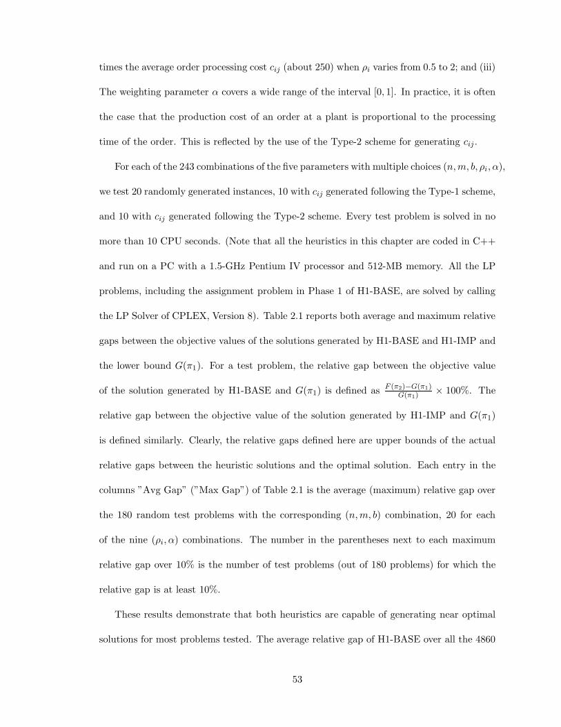
times the average order processing cost cij (about 250) when ρi varies from 0.5 to 2; and (iii)

The weighting parameter α covers a wide range of the interval [0, 1]. In practice, it is often

the case that the production cost of an order at a plant is proportional to the processing

time of the order. This is reflected by the use of the Type-2 scheme for generating cij .

For each of the 243 combinations of the five parameters with multiple choices (n,m, b, ρi, α),

we test 20 randomly generated instances, 10 with cij generated following the Type-1 scheme,

and 10 with cij generated following the Type-2 scheme. Every test problem is solved in no

more than 10 CPU seconds. (Note that all the heuristics in this chapter are coded in C++

and run on a PC with a 1.5-GHz Pentium IV processor and 512-MB memory. All the LP

problems, including the assignment problem in Phase 1 of H1-BASE, are solved by calling

the LP Solver of CPLEX, Version 8). Table 2.1 reports both average and maximum relative

gaps between the objective values of the solutions generated by H1-BASE and H1-IMP and

the lower bound G(π1). For a test problem, the relative gap between the objective value

of the solution generated by H1-BASE and G(π1) is defined as F (π2)−G(π1)G(π1)

× 100%. The

relative gap between the objective value of the solution generated by H1-IMP and G(π1)

is defined similarly. Clearly, the relative gaps defined here are upper bounds of the actual

relative gaps between the heuristic solutions and the optimal solution. Each entry in the

columns ”Avg Gap” (”Max Gap”) of Table 2.1 is the average (maximum) relative gap over

the 180 random test problems with the corresponding (n,m, b) combination, 20 for each

of the nine (ρi, α) combinations. The number in the parentheses next to each maximum

relative gap over 10% is the number of test problems (out of 180 problems) for which the

relative gap is at least 10%.

These results demonstrate that both heuristics are capable of generating near optimal

solutions for most problems tested. The average relative gap of H1-BASE over all the 4860

53

test problems is 1.36%, whereas that of H1-IMP is 1.05%, a more than 20% improvement

from H1-BASE. Figures 2.2 and 2.3 show the asymptotic optimality property of H1-IMP

with respect to the number of orders. There are a total of 100 test problems (about 2% of

all the test problems used) for which H1-BASE generates a solution with a 10% or more

relative gap, whereas this number is 35 (about 0.7%) in the case of H1-IMP. It can also be

observed that the relative gap generally decreases with n and increases with m and b.

2.4 Problem P2: Minimizing TC subject to Dtotal ≤ D

We first show that the problem is at least ordinarily NP-hard even with two plants m = 2

and under the two special cases noted in the beginning of Section 2.3: (i) order processing

times are agreeable; (ii) production costs are proportional to processing times. Then we

propose a heuristic for the general problem P2 and evaluate its performance computation-

ally.

Theorem 7 Problem P2 is at least ordinarily NP-hard even when there are only two plants

and both of the two special cases (i) and (ii) hold.

Proof We prove this by a reduction from the known ordinarily NP-hard Equal-Size Par-

tition Problem (ESPP) (Garey and Johnson 1979): ESPP:Given 2h items H = 1, . . . , 2h.

Each item i ∈ H has a known integer size ai, such that∑

i∈H ai = 2A, for some integer

A. The question asks: does there exist a subset of the items Q ⊆ H such that it contains

exactly h items and the total size∑

j∈Q aj = A?

Given an instance of ESPP, we create the following instance for the recognition version

of our problem:

Number of orders n = 2h, and order set N = H

54

Number of plants m = 2

Shipment capacity b = h

Transportation cost of a shipment f1 = f2 = M sufficiently large

Transportation time t1 = t2 = 0

Processing time of order j ∈ N : p1j = Aaj , p2j = aj

Production cost of order j ∈ N : c1j = aj , c2j = Aaj

Upper bound on total delivery time D = hA2 + hA

Threshold on total cost F = 2M + A2 + A.

We prove that there is a solution to our problem with the total production and trans-

portation cost no more than F and total delivery time no more than D if and only if there

exists a solution to ESPP.

(If part) Given a subset Q ⊆ H for ESPP with∑

j∈Q aj = A and |Q| = h, we construct a

solution to our problem as follows. Process orders from Q at plant 1 and deliver them in

one shipment at time A2. Process the rest of the orders at plant 2 and deliver them in one

shipment at time A. In this schedule, Dtotal =∑

j∈Q Dj +∑

j∈H\Q Dj = h∑

j∈Q Aaj +

h∑

j∈H\Q aj = hA2 + hA = D, the total production cost is∑

j∈Q c1j +∑

j∈H\Q c2j =

∑j∈Q aj + A

∑j∈H\Q aj = A + A2, and the total transportation cost is 2M . Therefore the

total cost is exactly F .

(Only if part) Given a solution to our problem with the total cost no more than F and total

delivery time of the orders no more than D, we can conclude that there must be at most

two shipments because otherwise the total cost would be more than 3M > F . Since b = h,

in this solution, there must be exactly two shipments, each containing exactly h orders.

Consider two cases:

55

Case 1: If the orders of both shipments are processed at plant 1, then Dtotal will be more

than (∑

j∈H p1j)h = (∑

j∈H Aaj)h = 2hA2 > D. This violates the constraint that Dtotal

is no more than D.

Case 2: If the orders of both shipments are processed at plant 2, then the total cost will be

more than 2f2 +∑

j∈H c2j = 2M +∑

j∈H Aaj = 2M + 2A2 > F , which is in contradiction

with the fact that the total cost of the schedule is no more than F .

Hence each plant processes the orders of one shipment. Let R denote the set of orders

processed at plant 1. Then the total delivery time of orders is

Dtotal =

∑

j∈R

p1j

h +

∑

j∈N\R

p2j

h = hA

∑

j∈R

aj + h

2A −

∑

j∈R

aj

≤ D

which means that∑

j∈R aj ≤ A. The total cost is

TC = f1 + f2 +∑

j∈R

c1j +∑

j∈N\R

c2j = 2M +∑

j∈R

aj + A

2A −

∑

j∈R

aj

≤ F

which means that∑

j∈R aj ≥ A. Therefore,∑

j∈R aj = A and subset R is a solution to

ESPP.

In the constructed instance of our problem, there are only two plants and both of the

special cases (i) and (ii) hold. Hence we can conclude that problem P2 with two plants and

under the two special cases is at least ordinarily NP-hard.

We note that problem P1 with either of the special cases (i), (ii) and a fixed number of

plants is solvable in polynomial time. Theorem 7 means that problem P2 is more difficult

than problem P1 at least for the case when m is fixed and processing times are agreeable

or production costs are proportional to processing times.

2.4.1 A Heuristic for Problem P2

The logic of the heuristic is based on the following observation regarding problem P1.

56

Lemma 5 The total delivery time of orders Dtotal in an optimal solution of P1 is non-

increasing with the weighting parameter α in the objective function of the problem, whereas

the total cost TC in an optimal solution of P1 is non-decreasing with α.

Proof We prove the first part of the result by contradiction. The second part can be

proved similarly. Suppose that there exists α1, α2 ∈ [0, 1] with α2 > α1 such that the

total delivery time in the optimal solution of P1 with α = α2 is greater than that in the

optimal solution of P1 with α = α1. Let ρi be the optimal solution of P1 with α = αi for

i = 1, 2. Denote the total delivery time and total cost in a solution ρ by Dtotal(ρ) and

TC(ρ), respectively. We have

α1Dtotal(ρ1) + (1 − α1)TC(ρ1) ≤ α1Dtotal(ρ2) + (1 − α1)TC(ρ2) (2.8)

α2Dtotal(ρ2) + (1 − α2)TC(ρ2) ≤ α2Dtotal(ρ1) + (1 − α2)TC(ρ1) (2.9)

By (2.9), we have

TC(ρ1) ≥ α2[Dtotal(ρ2) − Dtotal(ρ1)]/(1 − α2) + TC(ρ2)

which implies that

α1Dtotal(ρ1) + (1 − α1)TC(ρ1)

≥ α1Dtotal(ρ1) + (1 − α1)α2[Dtotal(ρ2) − Dtotal(ρ1)]/(1 − α2) + (1 − α1)TC(ρ2)

≥ α1Dtotal(ρ1) + α2[Dtotal(ρ2) − Dtotal(ρ1)] + (1 − α1)TC(ρ2) (since α2 > α1)

= α1Dtotal(ρ2) + (1 − α1)TC(ρ2) + (α2 − α1)[Dtotal(ρ2) − Dtotal(ρ1)]

> α1Dtotal(ρ2) + (1 − α1)TC(ρ2)

(since α2 > α1 and by assumption Dtotal(ρ2) > Dtotal(ρ1))

which is in contradiction with (2.8). This shows that the assumption that Dtotal(ρ2) >

Dtotal(ρ1) cannot hold.

57

Lemma 5 means that problem P2 is equivalent to the problem of finding a minimum

α0 ∈ [0, 1] such that the total delivery time of the orders in an optimal solution of problem

P1 with α = α0 is no more than D. Based on this observation, we propose a heuristic to

solve P2 by solving P1 multiple times, each time with a different α in the objective function.

The framework of the heuristic essentially follows the well-known line search algorithm in

the nonlinear programming literature (e.g. Bazaraa et al. 1993). It searches for a minimum

possible α0 ∈ [0, 1] such that when P1 with α = α0 is solved by Heuristic H1-IMP of Section

2.3, the total delivery time of the orders in the solution is no more than D.

Heuristic H2

Step 0: Set α0 = 0. Apply Heuristic H1-IMP to problem P1 with α = α0. If the solution

is feasible to problem P2 (i.e. if Dtotal ≤ D in this solution), then stop. This solution is

optimal to P2 and it is adopted. Otherwise, set δ = 0.5, and α0 = 0.5.

Step 1: Apply Heuristic H1-IMP to problem P1 with α = α0. If the solution is feasible to

problem P2, set δ = δ/2 and α0 = α0 − δ. Otherwise, set δ = δ/2 and α0 = α0 + δ. Repeat

Step 1 until δ reaches a prespecified error tolerance (e.g. 0.01). Adopt the last feasible

solution to P2.

Along with a feasible solution to problem P2, a lower bound of the optimal objective

value of P2 is obtained by Heuristic H2 as follows. Let π∗ denote an optimal solution of

P2. For every α0 tried in the heuristic, let LB(α0) denote the optimal objective value of

the assignment problem in Phase 1 of Heuristic H1-BASE. By Lemma 4, LB(α0) is a lower

bound of the optimal objective value of problem P1 with α = α0. Thus, LB(α0) is also a

58

lower bound of the objective value of solution π∗ for P1 with α = α0, i.e.

LB(α0) ≤ α0Dtotal(π∗) + (1 − α0)TC(π∗)

which implies that

[LB(α0) − α0Dtotal(π∗)]/(1 − α0) ≤ TC(π∗)

Since Dtotal(π∗) ≤ D, the above inequality further means that

[LB(α0) − α0D]/(1 − α0) ≤ TC(π∗)

Since this is true for every α0 ∈ [0, 1], we can take the maximum of the left-hand side of

the above inequality over all the α0 values that are tried in H2 as a lower bound of TC(π∗),

i.e.

TC(π∗) ≥ max [LB(α0) − α0D]/(1 − α0)| all α0 tried in H2 (2.10)

Now we computationally evaluate the performance of H2. All the parameters except D

are generated exactly the same way as in the test for H1-BASE and H1-IMP in Section 2.3.

Parameter D is given by D = D1 +β(D0 −D1) where β ∈ 0.25, 0.5, 0.75, and D1 and D0

are minimum and maximum possible values of total delivery time of orders in a schedule,

respectively. The value of D1 is equal to the total delivery time of the orders in the solution

of problem P1 with α = 1 obtained by solving the assignment problem formulated in Section

2.3. The value of D0 is equal to the total delivery time of the orders in the solution of P1

with α = 0 obtained by H1-IMP.

Similar to the computational experiment in Section 2.3, for each of the 243 combinations

of the five parameters with multiple choices (n,m, b, ρi, β), we test 20 randomly generated

instances, 10 with cij generated following the Type-1 scheme, and 10 with cij generated fol-

lowing the Type-2 scheme. Table 2.2 reports the computational results, where each column

59

except the last one represents the same performance measure as the corresponding on in

Table 2.1. The relative gap of a test problem is the relative gap between the objective value

of the solution generated by H2 and the lower bound given on the right-hand side of (10).

Since the computational times required by large problems are not negligible (e.g. within 10

seconds), we also report the average CPU times in seconds in the column ”CPU (seconds)”.

The variance of CPU times over the 180 test problems for each (n,m, b) combination is very

small. Hence we do not report the maximum CPU times.

It can be seen from the results in Table 2.2 that (i) the average gap over all the prob-

lems with 50, 100, and 200 orders are 8.54%, 4.93%, and 3.08%, respectively; and (ii) the

percent of test problems with 50, 100, and 200 orders that have a relative gap over 10%

are 29.8%, 12.0%, and 3.7%, respectively. These results show that the performance of H2

improves with the number of orders n in a test problem. For fixed n, the heuristic performs

better for problems with smaller m and b. Overall it is capable of generating near-optimal

solutions for most test problems with 100 orders or more. Although we are unable to prove

it, we conjecture that H2 is asymptotically optimal for problem P2 when the number of

orders n goes to infinity with m and b fixed.

2.5 Problem P3: Minimizing αDmax + (1 − α)TC

When α = 0, this problem reduces to the problem of minimizing total production and

distribution cost TC, which has been discussed in Section 2.3. When α ∈ (0, 1], the problem

is at least ordinarily NP-hard even with a fixed number of plants and agreeable processing

times. This is because the following special case of the problem: m = 2, pij = pj , cij =

0, ti = 0, fi = 0 for all i ∈ M and j ∈ N , is equivalent to the parallel machine maximum

completion time scheduling problem, a known ordinarily NP-hard problem (Garey and

60

Johnson 1979). The following result holds for problem P3.

Lemma 6 There exists an optimal solution of P3 in which all the delivery shipments, except

possibly one, at each plant, are full. More precisely, if there are hi orders scheduled at plant

i ∈ M , where hi = ub + v , for some integers u ≥ 0 and 0 ≤ v < b, then ub orders are

delivered in u full shipments and v orders are delivered in a partial shipment.

Proof Clearly, in problem P3, Dmax = maxPi + ti|i ∈ M, where Pi denotes the total

processing time of the orders assigned to plant i. Given an assignment of orders to each

plant, Dmax is independent of how the delivery shipments are formed. Thus given an

assignment of the orders to the plants, the problem reduces to minimizing total production

and distribution cost TC, which is equivalent to minimizing the total distribution cost

because the total production cost is fixed once an order assignment is given. It can be seen

that the order delivery schedule given in the statement of the lemma minimizes the total

distribution cost for a given order assignment. Thus there exists an optimal overall schedule

that follows such a delivery schedule.

In the remainder of this section, we propose a linear programming based heuristic for

problem P3, analyze the worst-case and asymptotic performance of the heuristic, and evalu-

ate its performance computationally. We first consider a slightly different problem denoted

as P3′. Everything else in P3′ is the same as in P3 except that each order is required to be

delivered in a separate shipment and the transportation cost of a shipment from plant i ∈ M

is defined to be fi/b. In an optimal solution of P3′, there may exist some plants where no

orders are scheduled due to, for example, very large transportation times ti and production

costs cij associated with these plants. If we require that all the orders be scheduled on a

61

subset of plants Q ⊆ M only, then P3′ can be formulated as the following integer program:

IP (Q) : Z(Q) = min αDmax + (1 − α)∑

i∈Q

n∑

=1

(cij +

fi

b

)xij (2.11)

Subject to:

Dmax ≥n∑

=1

pijxij + ti, for i ∈ Q (2.12)

∑

i∈Q

xij = 1, for j ∈ N (2.13)

xij ∈ 0, 1 for i ∈ Q, j ∈ N (2.14)

where each binary variable xij is defined to be 1 if order j is assigned to plant i ∈ Q, and 0

otherwise, and variable Dmax is the maximum delivery time of the orders. Constraint (2.12)

defines Dmax, and Constraint (2.13) ensures that each order is assigned to one of the plants

in Q. It should be noted that Constraint (2.12) implies that there is at least one order

scheduled at each plant in Q because otherwise Dmax does not have to be greater than or

equal to ti. This means that problem P3′ is not equivalent to IP(M). Instead, problem P3′

is equivalent to the problem of finding a subset Q ⊆ M with a minimum possible objective

value Z(Q).

We are interested in the LP relaxation of IP (Q), denoted as LP (Q). Denote the op-

timal objective value of LP (Q) by ZLP (Q). Clearly, if we can find a subset Q ⊆ M such

that ZLP (Q) is minimum possible, then ZLP (Q) is a lower bound of the optimal objective

value of problem P3′. We propose the following procedure to find such a subset Q without

solving the LP relaxation for every subset of M .

Algorithm LB

Step 0: Reindex the plants in the nonincreasing order of transportation times ti. Let Qi be

the subset of the plants i, i + 1, ...,m.

62

Step 1: For i = 1, . . . ,m, solve LP (Qi) and get the optimal objective value ZLP (Qi).

Step 2: Let U denote the subset of plants Qi with the lowest objective value ZLP (Qi), and

let u = |U |.

Algorithm LB solves m linear programs, and hence is polynomial in both n and m.

Theorem 8 The value ZLP (U) generated by Algorithm LB is a valid lower bound of the

optimal objective value of problem P3′ .

Proof We prove this by contradiction. Suppose that a subset of plants A ⊆ M , where

A 6= U , gives a lower objective value ZLP (A) than ZLP (U). Construct a new set of plants

A′ as follows: Set t = maxti|i ∈ A, and define A′ = A ∪ i ∈ M |ti ≤ t. Since A′ = Qi

for some i, LP (A′) is one of the LPs solved in Algorithm LB. Thus

ZLP (U) ≤ ZLP (A′) (2.15)

Since every feasible solution to problem LP (A) is also feasible for problem LP (A′), with

the same objective value, we have

]ZLP (A′) ≤ ZLP (A) (2.16)

From (2.15) and (2.16), we get: ZLP (U) ≤ ZLP (A), which contradicts our earlier claim.

Therefore, ZLP (U) gives a valid lower bound for P3′.

Corollary 9 The value ZLP (U) generated by Algorithm LB is a valid lower bound of the

optimal objective value of problem P3.

Proof In problem P3, if order j ∈ N is assigned to plant i ∈ M , then the contribution

of order j to the total transportation and production cost is at least cij + fi/b, whereas in

63

problem P3′ that contribution is exactly cij + fi/b. This means that the optimal objective

value of P3′ is a lower bound of that of P3. Then, the corollary follows immediately from

Theorem 8.

Lemma 7 In an optimal basic solution of LP (U), if n ≥ u− 1, then at least (n− u + 1) xij

variables take the value 1, where U is the subset of the plants found by Algorithm LB and

u is the number of plants in U .

Proof Since there are n + u constraints in LP (U) in addition to the non-negativity con-

straints, in an optimal basic solution (which can be obtained by the simplex method), there

are no more than n + u variables which may take positive values. Since variable Dmax

takes a positive value, there are at most (n + u − 1) xij variables with a positive value

in an optimal basic solution of LP (U). Given an optimal basic solution of LP (U), for

j ∈ N , let Kj be the subset of variables in the set xij , i ∈ U with a positive value. Define

N1 = j ∈ N ||Kj | = 1, and N2 = j ∈ N ||Kj | ≥ 2. Constraint (2.13) implies that for

j ∈ N1, the only variable in Kj takes the value 1. Clearly, each Kj contains a distinct set

of variables. Thus

n + u − 1 ≥ |N1| + 2|N2| = |N1| + 2(n − |N1|) = 2n − |N1|

which implies that |N1| ≥ n − u + 1. This establishes the lemma.

Now we are ready to describe our heuristic for problem P3. The heuristic generalizes the

approach proposed by Potts (1985) for the classical parallel machine maximum completion

time scheduling problem, which can be viewed as a special case of our problem with no

production costs and distribution times and costs, i.e. cij = 0, ti = 0, fi = 0 for all i ∈ M

and j ∈ N . Potts formulates his problem as an integer program which can be viewed as a

64

special case of IP (M), and assigns jobs to machines based on the optimal solution of the

LP relaxation of this integer program. Although we follow Potts’ idea, our heuristic is not

a trivial generalization because our problem P3 is much more complex. Furthermore, since

our problem is more general, our analysis of the heuristic performance are different from his.

Heuristic H3

Step 1: Run Algorithm LB to obtain a subset of plants U and an optimal basic solution

of LP (U). Define subset of orders J = j ∈ N |xij = 1 for some i ∈ U in this solution.

Lemma 7 implies that there are at least n − u + 1 orders in J and at most u − 1 orders in

N\J .

Step 2: (Create a schedule for orders in J) Assign each order j ∈ J to plant i ∈ U with

xij = 1. Schedule the orders assigned to each plant in an arbitrary sequence. Schedule order

delivery such that it satisfies Lemma 6. Denote the resulting partial schedule (containing

the orders from J only) by σ1.

Step 3:(Create a separate schedule for orders in N\J) Enumerate all possible assignments

of the no more than u − 1 orders in N\J to the plants in U till the following termination

condition is satisfied. For each such assignment, schedule the orders at each plant in an

arbitrary sequence. Schedule order delivery such that it satisfies Lemma 6. If the total

contribution of the orders to the objective value of P3 is less than or equal to ZLP (U), then

stop. Denote the resulting partial schedule (containing the orders from N\J only) by σ2.

If no schedule satisfies the termination condition, then take the schedule with the lowest

total contribution to the objective value of P3, and denote this partial schedule by σ2.

Step 4: Concatenate schedules σ1 and σ2 at each plant. Reschedule order delivery in the

concatenated schedule at each plant such that it satisfies Lemma 6. Denote the final sched-

65

ule by σ.

We note that Step 3 is done independent of Step 2, and there may exist two partial

delivery shipments at each plant i ∈ U if we just concatenate σ1 and σ2 without reoptimizing

its delivery schedule in Step 4. The enumeration procedure in Step 3 may generate a

maximum of uu−1 schedules. Thus the worst-case time complexity of H3 is polynomial in

n but exponential in m. However, if m is fixed, H3 is a polynomial-time algorithm. We

also note that the termination condition in Step 3 may not always be satisfied. However,

for a problem with a large number of orders, ZLP (U) is sufficiently large such that the

termination condition may be satisfied at an early stage, and hence only a small number of

schedules may be generated in Step 3.

Next we analyze the worst-case and asymptotic performance of heuristic H3. We denote

the total contribution of the orders in a schedule π to the objective value of P3 by FP3(π),

and that to the objective value of P3′ by FP3′(π). Let F ∗P3 denote the optimal objective

value of P3.

Theorem 10 FP3(σ) ≤ (b + 1)F ∗P3, i.e. the worst-case performance ratio of Heuristic H3 for

problem P3 is no more than b + 1.

Proof Since σ1 generated in Step 2 of the heuristic only includes the orders j ∈ N with

xij = 1 for some i ∈ M in the solution of LP(U), we have FP3′(σ1) ≤ ZLP (U). By Corollary

9, ZLP (U) ≤ F ∗P3. Therefore,

FP3′(σ1) ≤ ZLP (U) ≤ F ∗P3 (2.17)

There are two cases associated with σ2 generated in Step 3 of the heuristic:

66

Case (i): If σ2 satisfies the termination condition, then FP3(σ2) ≤ ZLP (U). By (2.17),

FP3(σ2) ≤ F ∗P3.

Case (ii): If σ2 does not satisfy that condition, then σ2 is an optimal schedule for the orders

in N\J . Since only a subset of orders is involved in σ2, FP3(σ2) ≤ F ∗P3.

Therefore, in both cases, we have

FP3(σ2) ≤ F ∗P3 (2.18)

In σ1, since the delivery schedule satisfies Lemma 6, there is at most one partial shipment

at each plant i ∈ U . Define V to be the subset of plants in U where there is a partial delivery

shipment. Consider the total contribution of the orders in σ1 to the objective value of P3′

(in this case, each order is delivered as a separate shipment with the delivery cost of each

shipment from plant i being fi/b). We have

FP3′(σ1) ≥∑

i∈V

fi/b (2.19)

and

FP3(σ1) ≤ FP3′(σ1) +∑

i∈V

(b − 1)fi/b (2.20)

Inequality (2.20) holds because in problem P3, the total transportation cost of a partial

shipment at plant i is fi, while under problem P3′, the total transportation cost of a partial

shipment at plant i is at least fi/b. By (2.17), (2.19) and (2.20), we have

FP3(σ1) ≤ FP3′(σ1) + (b − 1)FP3′(σ1) = bFP3′(σ1) ≤ bZLP (U) (2.21)

Since the concatenated schedule is reoptimized with respect to delivery schedule in Step

4 of the heuristic, FP3(σ) ≤ FP3(σ1) + FP3(σ2). By (2.17), (2.18) and (2.21), we have

FP3(σ) ≤ bZLP (U) + F ∗P3 ≤ (b + 1)F ∗

P3.

67

This establishes the theorem.

Theorem 11 Solution σ generated by heuristic H3 is asymptotically optimal for problem P3

when n goes to infinity with m and b fixed.

Proof Since u ≤ m which is fixed, the contribution of the u − 1 orders in N\J to the

objective value of P3 under any schedule is always bounded from above. On the other

hand, the objective value of P3 under any schedule becomes infinity when n goes to infinity.

Therefore,

limn→∞

FP3(σ2)F ∗

P3

= 0 (2.22)

As discussed in the proof of Theorem 10, there is at most one partial shipment at each

plant i ∈ U . Define V to be the subset of plants in U where there is a partial delivery

shipment. Since |V | ≤ u ≤ m and fi for i ∈ V are all finite, we have

limn→∞

∑i∈V fi

F ∗P3

= 0 (2.23)

Thus,

limn→∞

FP3(σ) − F ∗P3

F ∗P3

≤ limn→∞

FP3(σ1) + FP3(σ2) − F ∗P3

F ∗P3

≤ limn→∞

FP3′(σ1) +∑

i∈V (b − 1)fi/b + FP3(σ2) − F ∗P3

F ∗P3

by (2.20)

≤ limn→∞

∑i∈V (b − 1)fi/b + FP3(σ2)

F ∗P3

by (2.17)

= 0 by (2.22) and (2.23)

This establishes the theorem.

To evaluate the performance of heuristic H3, we conduct a computational experiment

as follows. All the parameters except the weighting parameter in the objective function α

68

are generated exactly the same way as in the test for H1-BASE and H1-IMP in Section 2.3.

Three values of α are tested: α ∈ 0.5, 0.9, 0.99. We found that instances with α < 0.5

gave results similar to those with α = 0.5, and these three values of α gave a relatively large

variety of results. It should be noted that in practice, α is determined by the preference (or

utility function) of the decision maker which may vary widely from firm to firm.

Similar to the computational experiment in Section 2.3, for each of the 243 combinations

of the five parameters with multiple choices (n,m, b, ρi, α), we test 20 randomly generated

instances, 10 with cij generated following the Type-1 scheme, and 10 with cij generated

following the Type-2 scheme. Table 2.3 reports the computational results, where each

column represents the same performance measure as the corresponding one in Table 2.1.

The relative gap of a test problem is the relative gap between the objective value of the

solution generated by heuristic H3 and the lower bound ZLP (U) generated in Step 1 of the

heuristic. Since every test problem is solved within a small amount of CPU time, we do not

report the CPU times in the table.

From Table 2.3 we can derive that (i) the average gap over all the problems with 50,

100, and 200 orders are 5.23%, 3.11%, and 1.96%, respectively; and (ii) the percent of test

problems with 50, 100, and 200 orders that have a relative gap over 10% are 12.8%, 3.8%,

and 0.9%, respectively. These results show that the H3 is capable of generating near-optimal

solutions for most of the problems tested. Furthermore, its performance improves with the

number of orders n in a test problem with fixed m and b. Figures 2.2 and 2.3 show the

asymptotic optimality property of H3 with respect to the number of orders.

69

2.6 Problem P4: Minimizing TC subject to Dmax ≤ D

The problem even with two plants (i.e. m = 2) is at least ordinarily NP-hard because even

finding a feasible solution to the problem with m = 2 and ti = 0 for i ∈ M is as hard as

the ordinarily NP-complete Partition problem (Garey and Johnson 1979). We use the idea

developed in Section 2.5 to design a heuristic for this problem with a general number of

plants. Because of the constraint Dmax ≤ D, no orders will be assigned to a plant i with

ti > D−pi,min, where pi,min = minpij|j ∈ N, and hence such a plant can be removed from

M . Therefore, without loss of generality, we assume that ti ≤ D − pi,min, for all i ∈ M .

We first consider a slightly different problem denoted as P4′. Everything else in P4′ is

the same as in P4 except that each order is required to be delivered in a separate shipment

and the transportation cost of a shipment from plant i ∈ M is defined to be fi/b. Problem

P4′ can be formulated as the following integer program:

IP ′ : Z = min∑

i∈M

n∑

=1

(cij +

fi

b

)xij (2.24)

Subject to:

n∑

=1

pijxij + ti ≤ D, for i ∈ M (2.25)

∑

i∈M

xij = 1, for j ∈ N (2.26)

xij ∈ 0, 1 for i ∈ M, j ∈ N (2.27)

where binary variable xij is defined to be 1 if order j ∈ N is assigned to plant i ∈ M , and 0

otherwise. This formulation is similar to IP (Q) given in Section 2.5 for problem P3′ with

a given subset of plants Q.

Clearly, if the LP relaxation problem of IP ′, denoted as LP ′, is infeasible, then problems

P4′ and P4 are both infeasible. To avoid this uninteresting case, we assume that LP ′ is

70

always feasible. Let Z ′LP denote the optimal objective value of the LP relaxation problem

LP ′. Using similar arguments as in the proof of Corollary 9, it can be proved that Z ′LP is a

valid lower bound for the optimal objective value of problem P4. Also, by similar arguments

as in the proof of Lemma 7, it can be shown that in an optimal basic solution of LP ′, if

n ≥ m, there are at least (n − m) xij variables taking the value 1, and at most m orders

with fractional xij values. Next we describe the heuristic for problem P4.

Heuristic H4

Step 1: Solve the LP relaxation problem LP ′ and get an optimal basic solution. Define

subset of orders J = j ∈ N |xij = 1 for some i ∈ M in this solution.

Step 2: Assign each order j ∈ J to plant i ∈ M with xij = 1. Schedule the orders assigned

to each plant in an arbitrary sequence. Schedule order delivery such that it satisfies Lemma

6. Denote the resulting partial schedule (containing the orders from J only) by σ1.

Step 3: Enumerate all possible assignments of the no more than m orders in N\J to the

plants in M . For each such assignment, let Pi be the total processing times of all the orders

assigned to plant i ∈ M (including the orders in σ1 which have been scheduled in Step 2).

If Pi + ti > D for some i ∈ M , then this assignment is infeasible and discarded. Otherwise,

schedule delivery shipments of all the orders assigned to each plant i ∈ M (including orders

in σ1) such that the delivery schedule satisfies Lemma 6. If no assignment of the orders in

N\J to the plants in M leads to a feasible schedule, then go to Step 4. Otherwise, stop; the

feasible schedule generated corresponding to one of the assignments with the lowest total

cost is adopted. Let this solution be denoted as σ.

Step 4: Decrease the current D (the right-hand side of (2.25)) by 0.1pmax, where pmax =

maxpij |i ∈ M, j ∈ N. Re-run Step 1 with the updated D. If LP ′ with the new D value is

71

not feasible, then stop; this heuristic fails to produce a feasible solution. Otherwise, re-run

Steps 2 and 3 with the originally given D.

We note that Steps 1 and 2 of H4 are very similar to the same steps of H3. However,

unlike Step 3 of H3 where a separate schedule is created for the orders in J , Step 3 of H4

adds orders in J to the schedule σ1 created earlier. In case no feasible solution is generated

in Step 3, Step 4 is used in H4 to generate a new solution of xij by solving a slightly modified

LP relaxation problem. Then Steps 2 and 3 are repeated given this new solution of xij .

The quantity 0.1pmax used in Step 4 (by which D is reduced) is heuristically set.

It can be seen that the algorithm has a polynomial time complexity if the number of

plants m is fixed. As we noted earlier, even finding a feasible solution for problem P4 is

NP-hard. Therefore, any polynomial-time heuristic including H4 may fail to find a feasible

solution for P4 even if there is a feasible solution. However, if the given constant D satisfies

a certain condition, then H4 always generates a feasible solution to P4. This is stated in

the following theorem.

Theorem 12 If the given constant D is such that the LP relaxation problem LP ′ with the

right-hand side of (2.25) replaced by D − pmax is feasible, then it is guaranteed that H4

generates a feasible solution to problem P4.

Proof Suppose that the heuristic has not generated a feasible solution for problem P4

after D has been reduced for nine times, i.e. the current D is the original D minus 0.9pmax.

Since LP ′ with the right-hand side of (2.25) replaced by D − pmax is feasible, every LP ′

involved in each of these nine iterations is also feasible. When D is reduced for the tenth

time, i.e. D becomes the original D minus pmax, since the corresponding LP ′ is feasible,

Step 1 generates an optimal basic solution, denoted as x0. Let Ji = j ∈ N |x0ij = 1, for

72

i ∈ M . Constraint (2.25) in LP ′ implies that

∑

j∈Ji

pijx0ij + ti ≤ D − pmax, for i ∈ M

This means that after Step 2 is executed based on the solution x0, the total processing

time of the orders assigned to each plant i ∈ U under schedule σ1 is no more than D −

pmax − ti. Furthermore, as we noted earlier, there are at most m orders in N\J under

solution x0. In Step 3, if we assign each order j ∈ N\J to a different plant in M , then

the total processing time of all the orders (including the orders in σ1) assigned to a plant

i ∈ M is no more than D − ti. This implies that the solution generated following such an

assignment of orders in N\J to the plants is feasible to problem P4. Since Step 3 tries

every possible assignment of the orders in N\J to the plants, such a feasible solution to P4

is generated in Step 3. Therefore, the heuristic terminates with a feasible solution to P4.

Next we computationally evaluate the performance of H4. All the parameters except D

are generated exactly the same way as in the test for H1-BASE and H1-IMP in Section 2.3.

Parameter D is given by D = D1 +β(D0 −D1) where β ∈ 0.25, 0.5, 0.75, and D1 and D0

are minimum and maximum possible values of maximum delivery time Dmax of orders in a

schedule, respectively. The values of D1 is equal to the total delivery time of the orders in

the solution of problem P4 with α = 1 obtained by heuristic H3. Similarly, the value of D0

is equal to the total delivery time of the orders in the solution of problem P4 with α = 0

obtained by heuristic H3.

Similar to the computational experiments conducted in earlier sections, for each of the

243 combinations of the five parameters with multiple choices (n,m, b, ρi, β), we test 20

randomly generated instances, 10 with cij generated following the Type-1 scheme, and 10

with cij generated following the Type-2 scheme. The heuristic successfully generates a

73

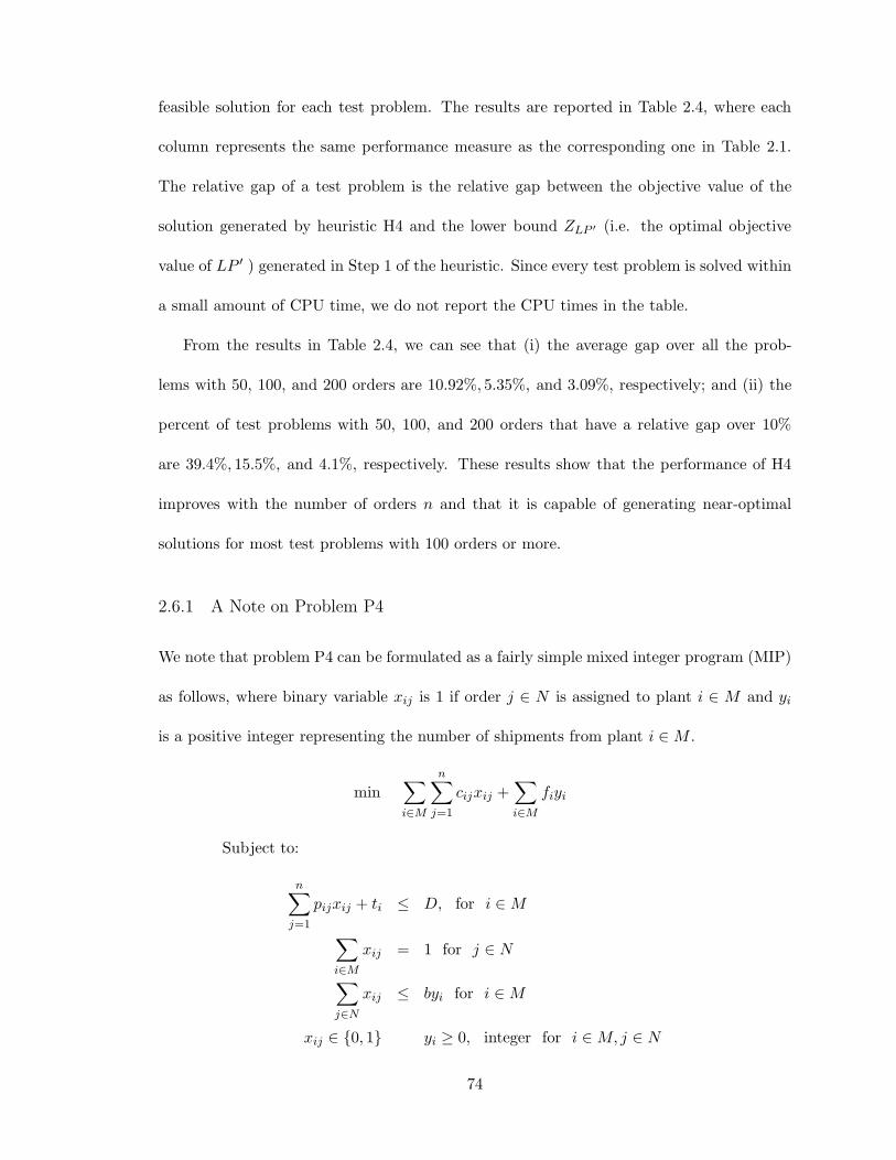
feasible solution for each test problem. The results are reported in Table 2.4, where each

column represents the same performance measure as the corresponding one in Table 2.1.

The relative gap of a test problem is the relative gap between the objective value of the

solution generated by heuristic H4 and the lower bound ZLP ′ (i.e. the optimal objective

value of LP ′ ) generated in Step 1 of the heuristic. Since every test problem is solved within

a small amount of CPU time, we do not report the CPU times in the table.

From the results in Table 2.4, we can see that (i) the average gap over all the prob-

lems with 50, 100, and 200 orders are 10.92%, 5.35%, and 3.09%, respectively; and (ii) the

percent of test problems with 50, 100, and 200 orders that have a relative gap over 10%

are 39.4%, 15.5%, and 4.1%, respectively. These results show that the performance of H4

improves with the number of orders n and that it is capable of generating near-optimal

solutions for most test problems with 100 orders or more.

2.6.1 A Note on Problem P4

We note that problem P4 can be formulated as a fairly simple mixed integer program (MIP)

as follows, where binary variable xij is 1 if order j ∈ N is assigned to plant i ∈ M and yi

is a positive integer representing the number of shipments from plant i ∈ M .

min∑

i∈M

n∑

j=1

cijxij +∑

i∈M

fiyi

Subject to:

n∑

j=1

pijxij + ti ≤ D, for i ∈ M

∑

i∈M

xij = 1 for j ∈ N

∑

j∈N

xij ≤ byi for i ∈ M

xij ∈ 0, 1 yi ≥ 0, integer for i ∈ M, j ∈ N

74

We tried to solve this formulation directly by calling the MIP solver of CPLEX for

various problem sizes. Our test results showed that the CPU time CPLEX requires to solve

a problem increases exponentially with the number of orders n, number of plants m, and the

shipment size b. CPLEX is capable of finding optimal solutions for problems with up to 100

orders within a few CPU seconds. However, to find an optimal solution for problems with

200 or more orders, CPLEX usually takes a very long time (1000 CPU seconds if m ≤ 8

and b ≤ 3, and more than one day if m ≥ 8 and b ≥ 4). It can be concluded that solving P4

directly as a mixed integer program by CPLEX is generally not going to work for problems

with 200 or more orders. The fast heuristic H4 proposed here can be used to get a near

optimal solution for such problems.

2.7 Conclusions

In this chapter, we have studied four problems related to order assignment and scheduling

in a supply chain. Computational complexity of various cases of the problems have been

clarified, and polynomial-time exact algorithms have been proposed for some special cases

of the problems. All of the four problems are in general NP-hard, and fast heuristics have

been proposed for each of them. Worst-case and asymptotic performance of two of the

heuristics have been analyzed. Each heuristic has been evaluated computationally and the

results show that each heuristic is capable of generating near optimal solutions for most

test problems with 100 or more orders.

The analyses and solution approaches developed in this chapter can be generalized to

certain extensions of our problems. We have assumed that each plant is capable of processing

all the orders. In a more general setting, each plant i ∈ M may only be qualified to produce

a subset of orders Ni ⊆ N . In this case, all the heuristics developed in the chapter still

75

work after minor modifications. In H1-BASE, we can define a(k,i)j to be a sufficiently large

number, instead of the quantity given in (1), for every combination of (k, i, j) with j /∈ Ni,

such that order j will not be assigned to plant i in the solution of the assignment problem

in Phase 1 of the heuristic. The results on the worst-case and asymptotic performance

of the heuristic are still valid. Similarly, in the formulations IP (Q) and IP ′ involved in

heuristics H3 and H4, respectively, we can define the production cost cij of order j /∈ Ni at

plant i ∈ M to be sufficiently large such that order j will not be assigned to plant i in the

solution of the LP relaxation of these formulations. All the results about these heuristics

still hold.

We have assumed that the shipment capacity from different plants is identical. In a more

general setting, different plants may be associated with different transportation modes, for

example, trucks are used for delivering orders from some plants to the DC whereas air

freight is used by some others. Hence the capacity of the shipments from different plants

may be different. The heuristics proposed in the chapter can be extended fairly easily to

this more general case of the problems.

76

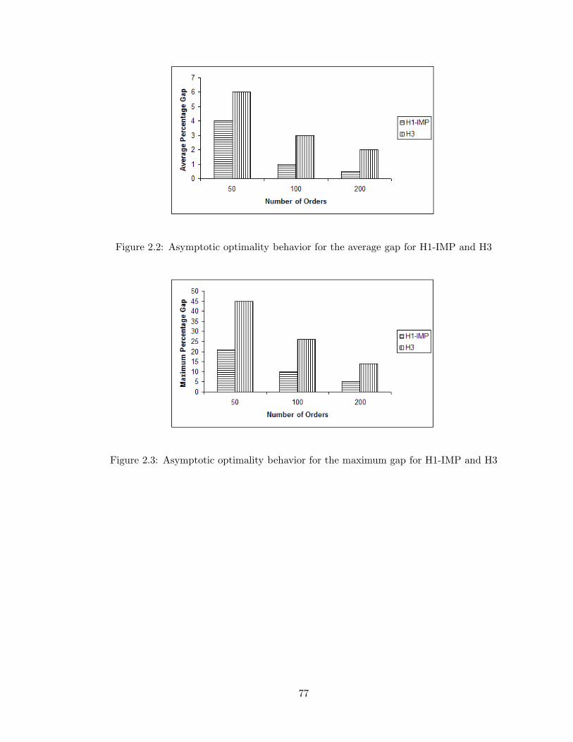
Figure 2.2: Asymptotic optimality behavior for the average gap for H1-IMP and H3

Figure 2.3: Asymptotic optimality behavior for the maximum gap for H1-IMP and H3

77

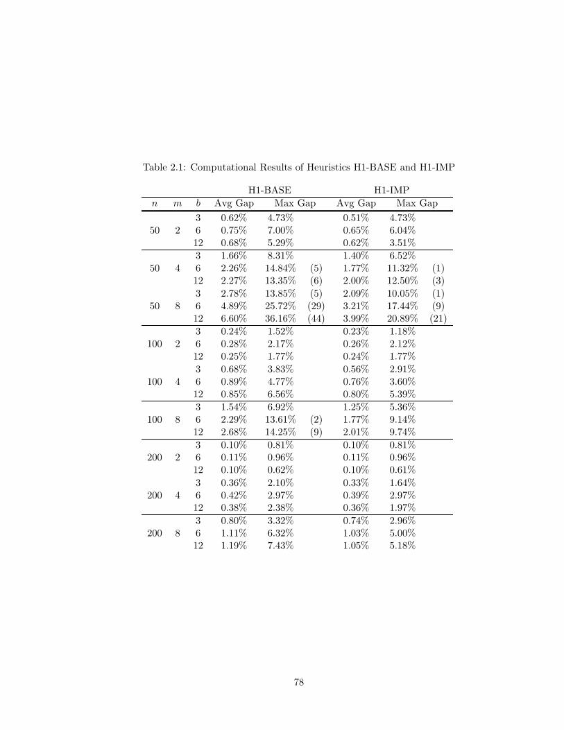
Table 2.1: Computational Results of Heuristics H1-BASE and H1-IMP

H1-BASE H1-IMPn m b Avg Gap Max Gap Avg Gap Max Gap

3 0.62% 4.73% 0.51% 4.73%50 2 6 0.75% 7.00% 0.65% 6.04%

12 0.68% 5.29% 0.62% 3.51%3 1.66% 8.31% 1.40% 6.52%

50 4 6 2.26% 14.84% (5) 1.77% 11.32% (1)12 2.27% 13.35% (6) 2.00% 12.50% (3)3 2.78% 13.85% (5) 2.09% 10.05% (1)

50 8 6 4.89% 25.72% (29) 3.21% 17.44% (9)12 6.60% 36.16% (44) 3.99% 20.89% (21)3 0.24% 1.52% 0.23% 1.18%

100 2 6 0.28% 2.17% 0.26% 2.12%12 0.25% 1.77% 0.24% 1.77%3 0.68% 3.83% 0.56% 2.91%

100 4 6 0.89% 4.77% 0.76% 3.60%12 0.85% 6.56% 0.80% 5.39%3 1.54% 6.92% 1.25% 5.36%

100 8 6 2.29% 13.61% (2) 1.77% 9.14%12 2.68% 14.25% (9) 2.01% 9.74%3 0.10% 0.81% 0.10% 0.81%

200 2 6 0.11% 0.96% 0.11% 0.96%12 0.10% 0.62% 0.10% 0.61%3 0.36% 2.10% 0.33% 1.64%

200 4 6 0.42% 2.97% 0.39% 2.97%12 0.38% 2.38% 0.36% 1.97%3 0.80% 3.32% 0.74% 2.96%

200 8 6 1.11% 6.32% 1.03% 5.00%12 1.19% 7.43% 1.05% 5.18%

78

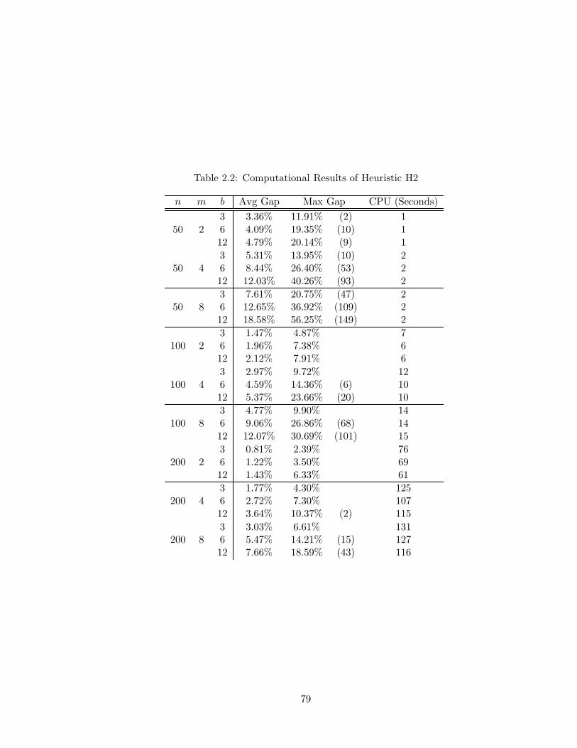
Table 2.2: Computational Results of Heuristic H2

n m b Avg Gap Max Gap CPU (Seconds)3 3.36% 11.91% (2) 1

50 2 6 4.09% 19.35% (10) 112 4.79% 20.14% (9) 13 5.31% 13.95% (10) 2

50 4 6 8.44% 26.40% (53) 212 12.03% 40.26% (93) 23 7.61% 20.75% (47) 2

50 8 6 12.65% 36.92% (109) 212 18.58% 56.25% (149) 23 1.47% 4.87% 7

100 2 6 1.96% 7.38% 612 2.12% 7.91% 63 2.97% 9.72% 12

100 4 6 4.59% 14.36% (6) 1012 5.37% 23.66% (20) 103 4.77% 9.90% 14

100 8 6 9.06% 26.86% (68) 1412 12.07% 30.69% (101) 153 0.81% 2.39% 76

200 2 6 1.22% 3.50% 6912 1.43% 6.33% 613 1.77% 4.30% 125

200 4 6 2.72% 7.30% 10712 3.64% 10.37% (2) 1153 3.03% 6.61% 131

200 8 6 5.47% 14.21% (15) 12712 7.66% 18.59% (43) 116

79

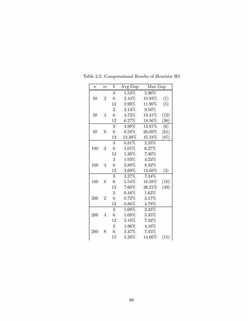
Table 2.3: Computational Results of Heuristic H3

n m b Avg Gap Max Gap3 1.53% 5.96%

50 2 6 2.44% 10.93% (1)12 2.99% 11.90% (5)3 3.14% 9.50%

50 4 6 4.73% 13.41% (12)12 6.27% 18.56% (36)3 4.98% 14.81% (6)

50 8 6 8.58% 26.08% (61)12 12.38% 45.18% (87)3 0.81% 2.25%

100 2 6 1.01% 6.27%12 1.26% 7.40%3 1.93% 4.22%

100 4 6 2.89% 8.32%12 3.69% 13.08% (3)3 3.27% 7.34%

100 8 6 5.54% 18.58% (10)12 7.60% 26.21% (49)3 0.48% 1.62%

200 2 6 0.72% 3.17%12 0.86% 4.78%3 1.09% 2.43%

200 4 6 1.69% 5.35%12 2.18% 7.32%3 1.96% 4.16%

200 8 6 3.47% 7.45%12 5.20% 14.66% (15)

80

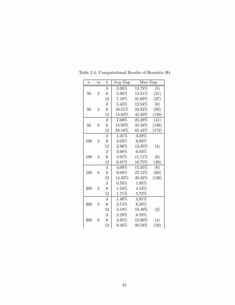
Table 2.4: Computational Results of Heuristic H4

n m b Avg Gap Max Gap3 3.26% 13.78% (5)

50 2 6 5.30% 13.51% (21)12 7.18% 21.69% (37)3 5.45% 12.84% (6)

50 4 6 10.51% 23.92% (92)12 14.82% 42.29% (129)3 7.69% 25.29% (41)

50 8 6 15.93% 45.58% (136)12 28.18% 85.43% (172)3 1.31% 3.59%

100 2 6 2.03% 6.68%12 2.96% 13.35% (4)3 2.68% 6.83%

100 4 6 4.91% 11.11% (6)12 6.81% 16.75% (40)3 4.09% 15.35% (6)

100 8 6 9.08% 25.12% (69)12 14.33% 40.32% (126)3 0.76% 1.95%

200 2 6 1.24% 4.53%12 1.71% 5.72%3 1.46% 4.91%

200 4 6 2.74% 6.20%12 4.19% 10.49% (3)3 2.29% 6.70%

200 8 6 4.95% 12.90% (4)12 8.46% 20.58% (59)

81

Chapter 3

Scheduling a Production-DistributionSystem to Optimize the Tradeoff betweenDelivery Tardiness and Distribution Cost

3.1 Introduction

We consider a make-to-order production-distribution system consisting of one supplier and

one or more customers. At the beginning of a planning horizon, each customer places a

set of orders with the supplier. The supplier needs to process these orders and deliver the

completed orders to the customers. Each order has a due date specified by the customer.

Ideally, each customer wishes to receive her orders from the supplier by their respective

due dates. However, since order deliveries incur distribution costs, the supplier wishes to

consolidate the order delivery as much as possible to minimize the total distribution cost.

Delivery consolidation implies that some completed orders may have to wait for other orders

to be completed so that they can be delivered in the same shipment. Hence, some orders

may be delivered to their customers after their due dates, resulting in a tradeoff between

delivery timeliness and total distribution cost. The problem we consider in this chapter is

to find a joint schedule for order processing and delivery so that the tradeoff between the

maximum delivery tardiness and total distribution cost is optimized.

This problem is often faced by manufacturers who make time-sensitive products such

82

as fashion apparel and toys, which typically have large product types and sell only during

specific seasons. Consider the production and distribution scheduling decisions such a man-

ufacturer needs to make. The customers (e.g. distributors or retailers) often set due dates

on the orders they place with the manufacturer and there is typically a penalty imposed on

the manufacturer if the orders are not completed and delivered to the customers on time.

Hence the manufacturer would like to meet the due dates as much as possible. Another

factor the manufacturer has to consider is the total cost for order processing and delivery.

Since the products are time-sensitive, orders are delivered shortly after their completion

and thus we assume that little inventory cost is incurred. The manufacturer’s total cost is

mainly contributed by production and distribution operations. The total production cost

for a fixed set of orders is normally fixed and independent of the production schedule used.

Therefore, the manufacturer should focus on the distribution cost when considering the to-

tal cost. Since different orders may have different due dates, delivering more orders on time

might require the manufacturer to make a larger number of shipments leading to higher

total distribution cost. Therefore, the manufacturer has to find a production and distribu-

tion schedule that achieves some balance between delivery timeliness and total distribution

cost. In practice, the maximum tardiness of orders and the total tardiness of orders are the

two commonly used measurements for delivery timeliness. They represent the worst and

average service level with respect to meeting order due dates, respectively. In this chapter,

we focus on the maximum tardiness as the measurement for delivery timeliness.

The schematic of the supply chain is given in Fig 3.1. In the following we describe the

model to be studied in this chapter. There are one supplier and m (m ≥ 1) customers

M = 1, . . . ,m located at different locations in a given production-distribution system.

At the beginning of a planning horizon, the supplier receives ni orders from each customer

83

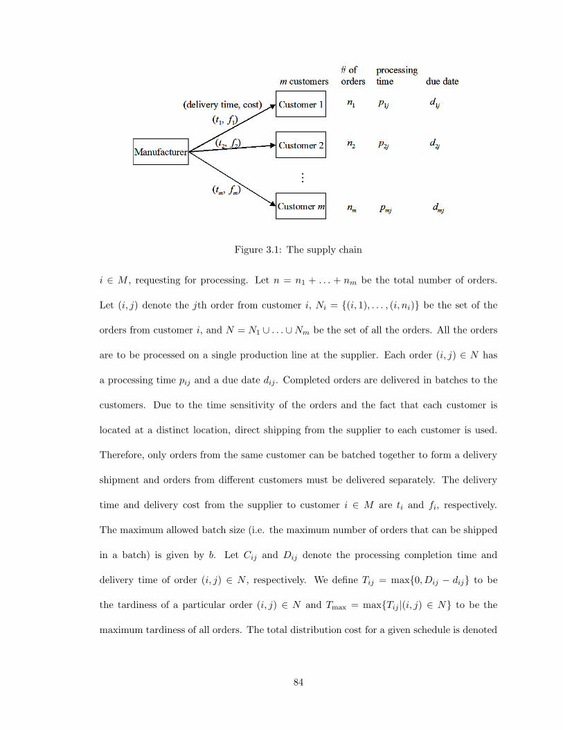
Figure 3.1: The supply chain

i ∈ M , requesting for processing. Let n = n1 + . . . + nm be the total number of orders.

Let (i, j) denote the jth order from customer i, Ni = (i, 1), . . . , (i, ni) be the set of the

orders from customer i, and N = N1 ∪ . . . ∪ Nm be the set of all the orders. All the orders

are to be processed on a single production line at the supplier. Each order (i, j) ∈ N has

a processing time pij and a due date dij . Completed orders are delivered in batches to the

customers. Due to the time sensitivity of the orders and the fact that each customer is

located at a distinct location, direct shipping from the supplier to each customer is used.

Therefore, only orders from the same customer can be batched together to form a delivery

shipment and orders from different customers must be delivered separately. The delivery

time and delivery cost from the supplier to customer i ∈ M are ti and fi, respectively.

The maximum allowed batch size (i.e. the maximum number of orders that can be shipped

in a batch) is given by b. Let Cij and Dij denote the processing completion time and

delivery time of order (i, j) ∈ N , respectively. We define Tij = max0,Dij − dij to be

the tardiness of a particular order (i, j) ∈ N and Tmax = maxTij |(i, j) ∈ N to be the

maximum tardiness of all orders. The total distribution cost for a given schedule is denoted

84

as G, and G = f1x1 + . . . + fmxm, where xi is the number of shipments used to deliver the

orders of customer i ∈ M .

The objective function should consider both Tmax and G. In order to achieve this, we

define a weighting factor α(0 ≤ α ≤ 1), which is based on the manufacturer’s relative

preference on the two measurements Tmax and G. The objective function is then defined as

αTmax + (1 − α)G. It can be seen that when α is close to 0, more emphasis is given to the

total distribution cost. On the other hand, when α is close to 1, more emphasis is given

to Tmax. In situations where the relative preference on the two measurements Tmax and G

is difficult to quantify, we can simply solve the problem multiple times with varying values

of a and pick one of the resulting solutions with the right level of balance between the two

measurements Tmax and G.

The remainder of the chapter is organized as follows. In Section 3.2, we analyze the

computational complexity of the problem under various cases. We give efficient algorithms

for the problem under several special cases and show that the problem under the general

case is NP-hard. In Section 3.3, we develop a quick heuristic for solving the general case

of the problem. We show that the heuristic is asymptotically optimal with respect to the

number of orders. To evaluate the performance of the heuristic, we develop a column

generation based approach for generating lower bounds. Our computational experiment

shows that the heuristic is capable of generating near optimal solutions. In Section 3.4,

we compare the performance of the integrated production-distribution approach with two

sequential approaches that treat order processing and order delivery independent of each

other. Conclusions and scope for future work are given in Section 3.5.

85

3.2 Analysis of the Problem Solvability

In this section, we consider various cases of the problem. Since the problem with one

customer, i.e. m = 1, has a different complexity from the problem with multiple customers,

we consider these two cases separately. Another important case of the problem is when

processing times and due dates of the orders are agreeable, i.e. if piu ≤ piv, then diu ≤ div,

for 1 ≤ u, v ≤ ni and i ∈ M . This case arises in many practical environments where order

due dates are set as a given multiple of the processing times. We define all the cases of the

problem considered in this section as follows:

P1: The case where there is only one customer. In this case, for ease of presentation, we

drop the customer index i from the problem parameters. Thus the n orders involved in

the problem are N = 1, . . . , n, their processing times and due dates are p1, . . . , pn, and

d1, . . . , dn respectively, and the transportation time and transportation cost are t and f

respectively.

P1A: The case P1 with agreeable processing times and due dates.

P2: The case where there are multiple customers, i.e., m ≥ 2.

P2A: The case P2 with agreeable processing times and due dates.

Clearly, P1 is more general than P1A, and P2 is more general than the other three cases.

We study the solvability of a problem by either providing an efficient algorithm for finding

an optimal solution or proving that the problem is intractable. Each of these problems is

studied next.

Throughout the remainder of this chapter, we say that a set of orders from the same

customer are sequenced in EDD order (i.e. earliest due date first order) if they are sequenced

in the non-decreasing order of their due dates. We require that in case of a tie in due dates,

the orders are sequenced in the non-decreasing order of their processing times, and that if

86

both the due dates and the processing times are the same among a set of orders, they are

sequenced according to their indices. It can be seen that the above tie-breaking rule defines

a unique EDD sequence for a given set of orders.

For all the problems, it is assumed without loss of generality that the orders belonging

to each customer i ∈ M have been indexed in the EDD order, i.e. di1 ≤ di2 ≤ . . . dini for

i ∈ M . Also, it is easily seen that there exists an optimal schedule where there is no idle

time between the processing of orders at the supplier, and where the orders delivered in the

same shipment are processed consecutively at the supplier.

3.2.1 P1A and P2A: The Problems with Agreeable Processing Times and Due Dates

We first present a property of problem P1A.

Lemma 8 There exists an optimal solution for problem P1A where the orders are processedin EDD order.

Proof We prove this lemma by contradiction. Suppose that the lemma does not hold.

Then there exist two orders u and v such that u is processed before v and du > dv (and hence

pu > pv). Generate a new schedule by interchanging these two orders, keeping everything

else the same as before. If these two orders belong to the same delivery batch in the earlier

optimal solution, the value of Tmax will remain unchanged, and the new schedule will be

equivalent to the old one. Otherwise, the value of Tmax will either decrease or remain

unchanged because du > dv and pu > pv. The lemma follows immediately.

By a similar argument as in the proof of Lemma 8, we can prove the following result.

Hence it is stated without a proof.

Lemma 9 There exists an optimal schedule for problem P2A where the orders from eachcustomer are processed in their respective EDD order.

One of the problems considered by Hall and Potts (2003) can be viewed as a special case

of our problem P2 with b = n (i.e. there is no batch size limit), and ti = 0 for all i ∈ M

87

(i.e. there are no delivery times). They show that the result of Lemma 9 applies to their

problem where processing times and due dates are not assumed to be agreeable. Based

on this result, they propose an O(n2m+1) dynamic programming algorithm for finding an

optimal schedule for their problem. The idea of their algorithm is based on the following

observation: If the number of delivery batches to each customer in the final schedule is

given, then the total transportation cost is fixed. An optimal schedule can then be found

by trying out all possible ways of splitting the orders of each customer (sequenced in their

EDD order) into a desired number of batches. Their algorithm can be used to solve our

problem P2A after it is modified by incorporating the batch size constraint and delivery

times into their recursive relations. Since P1A can be viewed as a special case of P2A with

m = 1, we can conclude that both problems P1A and P2A with a fixed number of customers

m can be solved in polynomial time.

As we will see in the next section, when the processing times and due dates are not

agreeable, the result of Lemma 8 does not hold for problem P1 and hence the result of

Lemma 9 does not hold for problem P2 either. Consequently, the dynamic programming

algorithm of Hall and Potts (2003) does not work for our problems P1 or P2.

Next we consider the problem P2A with an arbitrary number of customers. The cases

when α = 0 or α = 1 can be solved very easily. When α = 0, the problem can be solved to

optimality by minimizing the number of delivery batches for each customer. Any production

schedule is optimal. To solve the problem when α = 1, we define for each order (i, j) ∈ N , a

shipping due date which is the latest time the order (i, j) should leave the supplier in order

to reach the customer without any tardiness. An optimal solution to this case is obtained by

processing the orders in a non-decreasing sequence of the shipping due dates and delivering

each order independently immediately after processing.

88

We show in the following that when 0 < α < 1, the problem P2A with an arbitrary m

is NP-hard.

Theorem 13 The problem P2A with 0 < α < 1 and an arbitrary number of customers isNP-hard.

Proof We prove this by reducing the Subset Sum problem, a known NP-hard problem, to

P2A. The Subset Sum problem can be stated as follows (Garey and Johnson 1979): Given a

set of v+1 positive integers a1, . . . , av, and B, does there exist a subset U ⊆ V = 1, . . . , v

such that∑

i∈U ai = B?

Define A =∑

i∈V ai and H = d2v(1 − α)/αe + v + B. We construct a corresponding

instance of problem P2A as follows.

Number of customers, m = v.

Number of orders from each customer, ni = 3, for i = 1, . . . ,m.

Processing times: pi1 = 1, pi2 = ai, pi3 = Hai, for i = 1, . . . ,m.

Due dates: di1 = d1 = m + B, di2 = d2 = m + B + (H + 1)(A − B), and

di3 = d3 = m + (H + 1)A, for i = 1, . . . ,m.

Transportation times and costs, ti = 0 and fi = 1 for i = 1, . . . ,m.

Maximum allowed batch size, b = 3.

Threshold cost, F = 2m(1 − α)

Clearly, the orders in this instance of P2A have agreeable processing times and due

dates. For ease of presentation, we call orders (i, 1), (i, 2) and (i, 3) from each customer

i ∈ M Type I, Type II, and Type III orders, respectively. We first prove the following

properties: In a solution to this instance of P2A with the objective value not exceeding F ,

(a) Type I and Type III orders from each customer will be in different delivery batches, (b)

89

There will be exactly 2m delivery batches, (c) There will be no tardy orders, (d) Orders of

Type II will always be in a delivery batch of size 2. The proof for each is given next:

(a)If a Type I order is batched with a Type III order, the tardiness of the Type I order will

be more than H − d1, and hence αTmax > F , which means that the objective value exceeds

F .

(b)If there are more than 2m batches, the objective value will be greater than F = (1−α)2m.

Since Type I and Type III orders cannot be put in the same batch, we need at least 2m

total batches. Hence we have exactly 2m batches.

(c)Since 2m batches account for the entire threshold value, there can be no contribution

from the tardiness part.

(d)This follows directly from parts (a) and (b).

Now we prove that there is a solution to the constructed instance of P2A with total cost

not exceeding F if and only if there is a solution to the instance of the Subset Sum problem.

(If part) Given a subset U ⊆ V such that∑

i∈U ai = B, we construct a schedule for the

instance of P2A as follows: First process all the Type I orders from customers i ∈ V \U and

deliver each of them in a separate shipment. Next process the Type I and Type II orders

from customers i ∈ U and deliver them in batches of two orders. Next process the Type II

and Type III orders from the customers i ∈ V \U and deliver them in batches of two orders.

Finally process the orders of Type III from the customers i ∈ U and deliver each of them

separately. Let the cardinality of set U be k. The cardinality of V \U is m−k. The delivery

time of the last batch with Type I and Type II orders is:

D1 = m +∑

i∈U

ai = m + B = d1

90

Hence all the Type I orders are delivered before or on their due date. Similarly, the

delivery time of the last batch with Type II and Type III orders is:

D2 = D1 + (H + 1)∑

i∈V \U

ai = m + B + (H + 1)(A − B) = d2

Therefore, all the Type II orders are delivered before or on their due date. Similarly,

the delivery time of the last Type III order in the schedule is:

D3 = D2 + H∑

i∈U

ai = m + B + (H + 1)(A − B) + HB = m + (H + 1)A = d3

We see that all the orders are delivered on time. The number of batches is given by:

(m − k) + k + (m − k) + k = 2m. Hence the total cost is F .

(Only if part) Let us assume that there are k batches that consist of orders of Type I and

II. Let the indices of the corresponding Type II orders form set U ⊆ V . Since no tardy

orders exist in the schedule (Result (c) proved earlier), all these orders should be delivered

no later than d1 = m + B. Therefore, the maximum delivery time for orders of Type I is:

D1 = m +∑

i∈U ai ≤ m + B, which means that

∑

i∈U

ai ≤ B (3.1)

Similarly, the delivery time D2 of the last batch with Type II and Type III orders should

not be greater than d2 = m + B + (H + 1)(A − B). Therefore,

D2 = D1 + (H + 1)∑

i∈V \U

ai = m +∑

i∈U

ai + (H + 1)∑

i∈V \U

ai = m + B + (H + 1)(A − B)

This means that m + A + H∑

i∈V \U ai ≤ m + HA − HB + A, which further implies

that H∑

i∈V \U ai ≤ H(A − B). Therefore,

∑

i∈U

ai ≥ B (3.2)

91

From (3.1) and (3.2), we see that∑

i∈U ai = B must hold. This means that set U is a

solution to the instance of the Subset Sum problem.

Combining the ”If” part and ”Only If” part, we have proved the theorem.

Theorem 13 implies that P2, the general case of the problem, is also NP-hard when

0 < α < 1 and the number of customers is arbitrary. When α = 0 or α = 1, P2 can

be solved in polynomial time by adopting the same approach as the ones described earlier

for P2A under those cases. The complexity of P2 with a fixed number of customers and

0 < α < 1 is an open problem.

3.2.2 P1: The Problem with One Customer and General Processing Times and DueDates

We note that processing orders in their EDD order at the supplier is not necessarily optimal

for this case of the problem. This is illustrated through the following example: Consider

4 orders with the following processing times and due dates: p1 = 1, p2 = 5, p3 = 1, and

p4 = 5; d1 = 2, d2 = 12, d3 = 13, and d4 = 14. The transportation time t = 0 while

the transportation cost f = 10. The maximum allowed batch size b = 2. Set α = 0.5.

Clearly, any solution to this problem will contain at least two delivery batches. Therefore,

the objective value cannot be less than 10. We can obtain exactly 10 by putting the first

and third orders in the first batch, and the rest in the second. Also, it can be seen that this

is the only batch configuration that will give an objective value of 10. But this configuration

violates the EDD rule. Hence we conclude that the EDD rule is not necessarily optimal for

the general problem P1.

To solve P1, we first consider two related problems, called auxiliary problem one (AP1),

and auxiliary problem two (AP2). We will solve our problem P1 by solving AP2 multiple

times, where AP2 is solved by solving AP1 multiple times. Suppose that each order j ∈ N

92

has a deadline ej. Problem AP1 is to schedule the production and distribution of the orders

such that a minimum number of delivery shipments are used and all the orders are delivered

to the customer before or at their deadlines. Problem AP2 is to schedule the production

and distribution of the orders to minimize their maximum tardiness Tmax subject to the

constraint that the number of delivery shipments is no more than h for a given integer h.

Later when we use AP1 to solve AP2, we will specify the deadline of each order ej to be dj

plus some allowed tardiness. We focus on AP1 first. We propose the following algorithm

to solve this problem. The algorithm schedules orders backwards and forms the delivery

shipments from the last to the first.

Algorithm A1

Step 0: Let the set of unscheduled orders be U = N . Set the departure time of the current

last shipment to be Q =∑

j∈N pj. Let k = 1.

Step 1: Find the subset of the orders that can be delivered in the kth last shipment without

violating their deadlines, S = j ∈ U |Q + t ≤ ej. If S is empty but U is not, then stop,

and the problem is infeasible.

Step 2: If |S| > b, select the b orders with the largest processing times from S. Otherwise,

select all the orders from S. Let X and P be the set of the selected orders and the total

processing time of these orders, respectively. Process the selected orders consecutively with-

out idle time in the time period [Q−P,Q]. Deliver them together in the kth last shipment

with departure time Q. Update Q = Q − P , and U = U\X. If U is empty, then stop, and

we have a feasible schedule that uses exactly k batches. Otherwise, let k = k + 1, and go

to Step 1.

93

Lemma 10 Algorithm A1 finds an optimal solution to the problem AP1 in O(n2 log n) time.

Proof We prove this by showing that any optimal solution π∗ to the problem AP1 can

be transformed to a feasible solution π generated by this algorithm without increasing the

number of shipments. Suppose that for some integer h ≥ 0, the kth last shipment in π∗

is exactly the same as the kth last shipment in π, for k = 1, . . . , h, but the (h + 1)st last

shipment in π∗ is different from the (h + 1)st last shipment in π. This implies that the set

of the unscheduled orders U before the (h + 1)st last shipment is formed is the same in

these two solutions. Also, the departure time Q of the (h + 1)st last shipment is the same

in these two solutions. Let S = j ∈ U |Q + t ≤ ej. There are two cases to consider as

follows:

Case (i): |S| > b. In this case, the (h + 1)st shipment in π contains b orders. If there are

less than b orders in the (h + 1)st shipment in π∗, we can move some orders in S that are

scheduled in earlier shipments to the (h+1)st last shipment so that this shipment contains b

orders. If there are b orders in the (h+1)st shipment in π∗, we can interchange some orders

in this shipment with some other orders in S that are scheduled in earlier shipments but

with larger processing times. It can be seen that in both cases the resulting new solution is

still feasible and the number of shipments is not increased. Thus the (h + 1)st shipment in

π∗ can be transformed such that it becomes exactly the same as the (h + 1)st shipment in

π.

Case (ii): |S| ≤ b. It can be similarly proved that in this case we can also transform the

(h + 1)st shipment in π∗ such that it becomes exactly the same as the (h + 1)st shipment

in π without increasing the number of shipments.

This shows that the solution found by the algorithm is optimal. The algorithm carries

out at most n iterations, each consisting of Steps 1 and 2. Since Step 1 takes at most O(n)

94

time and Step 2 takes at most O(n log n) time, the overall complexity of the algorithm is

bounded by O(n2 log n).

Next we consider the second auxiliary problem AP2 which is to schedule the production

and distribution of the orders to minimize their maximum tardiness Tmax subject to the

constraint that the number of delivery shipments is no more than h for a given integer h,

where dnb e ≤ h ≤ n. It can be seen that the value of Tmax is non-increasing with the value

of h in the optimal solution of this problem. Based on this observation, we propose the

following line search algorithm to find the optimal Tmax given h.

Algorithm A2

Step 0: Let TLB and TUB denote a lower bound and an upper bound of the maximum

delivery tardiness Tmax of orders respectively. Initially, let TLB be the maximum tardiness

of orders if they are processed in the EDD order and each order is delivered separately,

and let TUB be the maximum tardiness of orders if they are processed in the EDD order

and all are delivered in full shipments except possibly the last several orders which may be

delivered in a partial shipment. Clearly, TLB ≥ 0 and TUB ≤ t+P , where P = p1+ . . .+pn.

Step 1: Let T 0 = 12(TLB +TUB). Define auxiliary problem one AP1 by imposing a deadline

on each order j ∈ N, ej = dj +T 0. Solve this problem by Algorithm A1, and let the optimal

number of shipments used be k.

Step 2: If k > h, let TLB = T 0. Otherwise, let TUB = T 0. If TUB − TLB < 1, stop. The

only integer in the interval [TLB , TUB] is adopted as the solution value of Tmax. Otherwise,

go to Step 1.

95

Lemma 11 Algorithm A2 finds an optimal solution to the problem AP2 in O(n2(log n)(log(P+t))) time, where P = p1 + . . . + pn.

Proof As we observed earlier, the value of Tmax is non-increasing with the value of h in the

optimal solution of this problem. Thus the solutions T 0 found in the line search involved

in the algorithm are guaranteed to converge to the optimal solution if an infinitely many

iterations are carried out. However, since the optimal value of Tmax must be an integer,

there is no need to carry out an infinite number of iterations. As soon as the gap between

TLB and TUB becomes less than 1, there is at most one integer that can be contained in

the interval [TLB , TUB]. Since this line search guarantees that the interval [TLB , TUB] at

each iteration contains the optimal solution, there must be an integer in this interval even

when the width of this interval is less than 1. This shows that the algorithm does find the

optimal solution.

The number of iterations in the line search is bounded by O(log(P + t)). Since it takes

O(n2 log n) time to run Algorithm A1 in each iteration, the overall computational time is

bounded by O(n2(log n)(log(P + t))).

We propose the following algorithm based on A2 for solving our problem P1.

Algorithm A3

Step 1: For h = dnb e, . . . , n, do the following: Define an auxiliary problem AP2 with the

number of delivery shipments no more than h. Solve the problem by applying Algorithm

A2. Let πh and Tmax(πh) be the optimal schedule and its maximum tardiness found by the

algorithm.

Step 2: Find u such that αTmax(πu) + (1 − α)uf = minαTmax(πh) + (1 − α)hf |h =

dnb e, . . . , n. Then schedule πu is optimal to problem P1 with the objective value αTmax(πu)+

96

(1 − α)uf .

Theorem 14 Algorithm A3 finds an optimal solution to the problem P1 in O(n3(log n)(log(P+t))) time, where P = p1 + . . . + pn.

Proof By the definition of problem AP2, it can be seen that problem P1 is equivalent to

finding the best h such that αTmax(πh)+ (1−α)hf is minimum. This shows the optimality

of the Algorithm A3. Since at most n auxiliary problems AP2 are solved in the algorithm,

by Lemma 11, the overall complexity of A3 is bounded by O(n3(log n)(log(P + t))) time.

Since the input size of our problem P1 is at least∑

j∈N (dlog pje + dlog dje) + dlog te ≥

n + log(P + t), Algorithm A3 is polynomial.

3.3 A Heuristic for the Problem with Multiple Customers when 0 <

α < 1

In this section, we propose and evaluate a heuristic for the problem P2. Since P2 is a more

general case of P2A, the heuristic is also applicable to P2A. We first prove an optimality

property. Then we develop the heuristic and prove it to be asymptotically optimal. We

propose a linear programming based approach for obtaining tight lower bounds and use

column generation to solve the linear programming formulations to optimality. A set of

computational experiments is carried out to evaluate the performance of the heuristic.

3.3.1 An Optimality Property

We define the SEDD sequence for a given set of orders as follows. Consider the shipping

due dates of the orders as defined in Section 3.2. Arrange the orders in the non-decreasing

order of their shipping due dates. In case of a tie, arrange the orders in the non-decreasing

order of their processing times. If both the shipping due dates and the processing times

97

are the same, arrange them by their customer index followed by their order index. It can

be seen that the above tie-breaking rule defines a unique SEDD sequence for a given set of

orders. Also, in the SEDD sequence, orders from the same customer are sequenced in their

EDD order.

Lemma 12 There exists an optimal schedule for P2 where: (i)The orders that are deliveredin the same batch are processed in their EDD sequence at the supplier; (ii) The first ordersof the batches form an SEDD sequence; (iii)Let u denote the first order processed in aparticular batch. All the orders that come before u in the SEDD sequence of all the ordersof N are processed before this batch of orders.

Proof (i) Since all the orders in a batch are delivered at the same time, the tardiness of

the batch is not influenced by the processing sequence of the orders in them. So we choose

a sequence that is in the EDD order for the set of orders in the batch.

(ii) By (i), we can assume that the orders in each batch are processed in the EDD sequence.

Let u be the first order in a batch. Suppose there exists an order v that is the first order

in some earlier batch and has a shipping due date larger than that of u. Then we can

move the batch containing order v to a position immediately after the batch containing

order u without increasing the objective value. We can do this for every pair of batches

that violates the lemma. In cases where two batches have their first orders with the same

shipping due dates, the relative sequence of these two batches does not affect the tardiness

value. Hence there exists an optimal solution where the first orders in the batches reflect

the unique SEDD sequence.

(iii) This follows directly from (i) and (ii)

3.3.2 The Heuristic

The heuristic first solves a single-customer auxiliary problem for each customer indepen-

dently in such a way that the contribution due to the other customers is taken care of

98

indirectly. Then it puts together the schedules for individual customers to obtain a com-

bined schedule. We make use of Lemmas 9 and 12. That is, schedules are built such that

the orders from each customer follow the EDD sequence and the set of first orders from

every batch follows the SEDD sequence. Although Lemma 9 is not valid for the general

problem P2, we will show that forcing the EDD sequence for each customer does not affect

the results significantly when the number of orders is large.

Define CSEDDij as the completion time of order (i, j) ∈ N at the supplier when all of the

orders from N are processed in the SEDD sequence. The single-customer auxiliary problem

for customer i ∈ M , denoted as AUXi, is defined as follows: Schedule the processing and

delivery of the orders from Ni subject to the following two constraints: (i) the orders are

processed in the EDD order at the supplier and (ii) the departure time of each delivery

batch B containing (i, j) as the first order is required to be the sum of CSEDDij and the total

processing time of the remaining orders in the batch, i.e.∑

(i,u)∈B piu − pij . The objective

of problem AUXi is to minimize the maximum delivery tardiness of the orders given that

the orders are delivered in a given number of delivery batches. Due to Constraint (ii), a

feasible schedule to AUXi may contain idle time between the processing of the last order

in one batch and the first order in the next batch. We present the heuristic next.

Heuristic H1

Step 1: Create an auxiliary problem AUXi, as described earlier, for each customer i ∈ M .

Solve AUXi, for i ∈ M , by the following dynamic programming algorithm, denoted as

DP1, where the value function F (j, k) is defined to be the minimum value of the maximum

tardiness for the first j orders (i, 1), (i, 2), . . . , (i, j) when they are delivered in k batches.

99

DP1

Initial values: F (0, 0) = 0.

Recursive relations: For j = 1, . . . , ni, and k = d jbe, . . . , j,

F (j, k) = min1≤q≤minb,j

max

F (j − q, k − 1), max

0, CSEDD

i,j−q+1 +

j∑u=j−q+2

piu + ti − di,j−q+1

(3.3)

Let T imax(k) = F (ni, k) denote the maximum tardiness for customer i when the orders

of customer i are delivered in k batches. Let Λi(k) denote the corresponding batch config-

urations for customer i. Let Γi = T imax(k)|k = dni

b e, . . . , ni, and Γ = Γ1 ∪ Γ2 ∪ . . . Γm.

Clearly, |Γ| ≤∑m

i=1 (ni − dni/be + 1).

Step 2: For each x ∈ Γ, and each customer i ∈ M , define ki(x) = mink ∈ dni/be, . . . , ni

|T imax(k) ≤ x if there exists some k ∈ dni/be, . . . , ni with T i

max(k) ≤ x, and ki(x) = ∞

otherwise. Find x∗ ∈ Γ such that

αx∗ + (1 − α)∑

i∈M

fiki(x∗) = minx∈Γ

αx + (1 − α)

∑

i∈M

fiki(x)

(3.4)

and the corresponding batch configurations Λi(ki(x∗)) for each customer i ∈ M . Let πi

denote the schedule for customer i corresponding to the value function F (ni, ki(x∗)) (Note

that πi is optimal to the problem AUXi with ki(x∗) delivery batches).

Step 3: Sequence all the batches determined by the batch configurations Λi(ki(x∗))|i ∈ M

obtained in Step 2 such that the first orders of the batches form the SEDD sequence. This

gives a feasible schedule π for the original problem. Calculate the objective value of π.

In the algorithm DP1, the recursive relation (3.3) enumerates all possible sizes q of the

current last delivery batch. Hence DP1 solves AUXi optimally for all possible number of

delivery batches k. In Step 2, the selected value of maximum tardiness x∗ optimizes the

overall objective when each customer is considered separately.

100

Next we estimate the time complexity of the heuristic. For each customer i ∈ M , the

time required by DP1 is O(n2i b). Thus the overall time needed in Step 1 of the heuristic

is O(n2b). In Step 2, there are no more than n values in the set Γ. For each value x ∈ Γ,

ki(x) for customer i ∈ M can be found by doing a line search for T imax(k) corresponding

to values of k between dni/be and ni. This takes O(log ni) steps. Therefore, the total

complexity of this for all the customers is O(∑

i∈M log ni) which is bounded by O(m log n).

Step 3 requires O(n log n) steps. Hence the overall complexity of the heuristic is bounded

by O(n2b + nm log n).

Lemma 13 Denote the optimal objective value of the problem P2 as F*. Then

F ∗ ≥ αx∗ + (1 − α)∑

i∈M

fiki(x∗) − α ((b − 1)pmax + 2tmax − 2tmin) (3.5)

where x∗ is as defined in (3.4), pmax = maxpij|(i, j) ∈ N, tmax = maxti|i ∈ M, and

tmin = minti|i ∈ M.

Proof Given an optimal schedule S∗ of the problem P2 that follows Lemma 12, we con-

struct a schedule S′ such that there are same number of delivery batches in S′ as in S∗,

and each batch in S′ contains the same number of orders from the same customer as in the

corresponding batch in S∗. But in S′ , the orders from each customer are scheduled in their

EDD sequence. So the actual set of orders in any batch in S′ may be different from that in

the corresponding batch in S∗. Each batch in S′ is shipped at a time that is the sum of the

completion time CSEDDij of the first order (i, j) in the batch and the total processing time

of the other orders in the batch. Note that schedule S′ may not be feasible to P2 because

there may be overlap between batches of orders from different customers. Also, note that

schedule S′ gets enumerated implicitly in Step 1 of the heuristic. We can easily see that

the total distribution cost in S′ is the same as that in S∗.

101

Let Dij(S′) and Dij(S∗) denote the delivery time of order (i, j) in S′ and S∗ respectively.

Similarly, let Tij(S′) = max0,Dij(S′) − dij and Tij(S∗) = max0,Dij(S∗) − dij denote

the tardiness of order (i, j) in S′ and S∗ respectively. The maximum tardiness of orders

in S′ is determined solely based on the first order in each batch. Consider the first order,

denoted as (i, u) in a particular batch of orders from customer i ∈ M in schedule S′. Let τ

denote the sum of processing times of all the orders except (i, u) in the batch. Evidently,

τ ≤ (b − 1)pmax. Let Q denote the set of all orders up to and including order (i, u) in the

SEDD sequence of N . Clearly, CSEDDiu =

∑(i,j)∈Q pij . Thus we have:

Diu(S′) = CSEDDiu + τ + ti =

∑

(i,j)∈Q

pij + τ + ti ≤∑

(i,j)∈Q

pij + (b − 1)pmax + tmax (3.6)

Now consider the last batch in S∗ that contains an order from Q. Suppose that this

batch belongs to customer k ∈ M . Denote the first order in this batch as (k, v). Note that

(k, v) belongs to Q. We have the following:

Dkv(S∗) ≥∑

(i,j)∈Q

pij + tmin (3.7)

From (3.6) and (3.7), we have:

Diu(S′) − Dkv(S∗) ≤ (b − 1)pmax + tmax − tmin (3.8)

Since (i, u) is the last order in Q, the shipping due dates follow the relation: d′iu ≥ d′kv.

Therefore, diu − ti ≥ dkv − tk, which implies that diu − dkv ≥ tmin − tmax. This, along with

(3.8), implies that

(Diu(S′) − diu) − (Dkv(S∗) − dkv) ≤ (b − 1)pmax + 2tmax − 2tmin (3.9)

Inequality (3.9) implies that

Tiu(S′) − Tkv(S∗) ≤ (b − 1)pmax + 2tmax − 2tmin (3.10)

102

Inequalities (3.8) through (3.10) are valid for the first order (i, u) of any batch in S′. DP1

in the heuristic H1 considers all choices of batch configurations at every customer including

the configurations that appear in schedule S′. In Step 2 of H1, αx∗ +(1−α)∑

i∈M fiki(x∗)

is obtained by putting together these values in such a way that the combined value for all

the customers is minimum. Therefore, this value will not be greater than the one obtained

by combining the values at individual customers in S′. Hence,

αx∗ + (1 − α)∑

i∈M

fiki(x∗) ≤ F ∗ + α((b − 1)pmax + 2tmax − 2tmin) (3.11)

This completes the proof.

Lemma 14 Let FH1 represent the objective value of the schedule π obtained by the heuristic

H1. Then,

FH1 ≤ αx∗ + (1 − α)∑

i∈M

fiki(x∗) + α(b − 1)(m − 1)pmax (3.12)

Proof Let us consider an arbitrary batch ω of customer i ∈ M in the schedule π generated

in Step 3 of the heuristic. Denote the first order in the batch as (i, u). Let Diu(πi) and

Diu(π) denote the delivery times of this batch in the schedule πi generated in Step 2 and

in the schedule π respectively. By the definition of problem AUXi and the fact that pii is

optimal to the problem AUXi with ki(x∗) delivery batches, we have:

Diu(πi) = CSEDDiu +

∑

(i,j)∈ω

pij − piu + ti (3.13)

Since in schedule π, the first orders of the batches form SEDD sequence and the orders

from each customer are sequenced in EDD order, there can be at most one batch scheduled

before ω from every customer other than i, that contains orders which come after (i, u)

in the SEDD sequence of all the orders of N . Even in those batches, there should be at

103

least one order in each batch that comes before order (i, u) in the SEDD sequence of all the

orders of N . Therefore, we have:

Diu(π) ≤

CSEDD

iu +∑

(i,j)∈ω

pij − piu + ti

+ (b − 1)(m − 1)pmax (3.14)

Let Tiu(πi) and Tiu(π) denote the tardiness of the batch ω in schedules πi and π, re-

spectively. Then by (3.13) and (3.14), we have,

Tiu(π) − Tiu(πi) ≤ Diu(π) − Diu(πi) ≤ (b − 1)(m − 1)pmax (3.15)

Here the first relation is not an equality to take into account cases where the batch

is delivered before its due date. Relation (3.15) is valid for all the batches and hence

(b − 1)(m − 1)pmax gives an upper bound on the difference in maximum tardiness possible

between the schedules πi and π, for every i ∈ M . Since in the schedule π, the batch

configurations Λi(ki(x∗)) generated in Step 2 is used for each customer i ∈ M , the total

distribution cost incurred by the orders of Ni in π is exactly fiki(x∗), which is the same

as in schedule πi. Since the sum of the objective values of the schedules πi over all i ∈ M

is αx∗ + (1 − α)∑

i∈M fiki(x∗), the objective value FH1 of the schedule π satisfies (3.12).

This completes the proof.

Theorem 15 If order processing times pij, delivery times ti, and delivery costs fi are drawn

from distributions over finite intervals [L1, U1], [L2, U2], and [L3, U3], respectively, with 0 <

L1 ≤ U1 < ∞, 0 < L2 ≤ U2 < ∞, and 0 < L3 ≤ U3 < ∞, then the solution generated by

the heuristic H1 is asymptotically optimal for problem P2 with 0 < α < 1 when n goes to

infinity, with m and b fixed.

Proof As in the proofs of Lemmas 13 and 14, let F ∗ and FH1 represent the optimal

objective value of the problem P2, and the objective value of the schedule π generated by

104

the heuristic respectively. Combining the inequalities (3.5) and (3.12), we have,

FH1 ≤ F ∗ + α((b − 1)pmax + 2tmax − 2tmin) + α(b − 1)(m − 1)pmax

= F ∗ + α((b − 1)mpmax + 2tmax − 2tmin)

which means that,

FH1 − F ∗

F ∗ ≤ α((b − 1)mpmax + 2tmax − 2tmin)F ∗ (3.16)

For fixed b, the total distribution cost, and therefore F ∗, increases to infinity as the

number of orders n increases to infinity. Since pmax < ∞, tmax < ∞, α < 1, and m and b

are fixed, α((b − 1)mpmax + 2tmax − 2tmin) is finite. Hence, by (3.16), we have,

limn→∞

FH1 − F ∗

F ∗ ≤ limn→∞

α((b − 1)mpmax + 2tmax − 2tmin)F ∗ = 0

This shows the theorem.

When a batch is being formed for a particular customer, heuristic H1 ignores the effect

due to the batches formed for the orders of all other customers. This leads to an increase in

the tardiness value when we move from Step 2 to Step 3. One way to limit this increase is

to reduce the maximum allowed batch size for a few customers and then run the heuristic

again. Doing this may lead to an increase in the number of delivery batches for these

customers. But on the other hand, it may also lead to smaller batches being formed, which

helps reduce the maximum tardiness value. If we reduce the maximum allowed batch size

for those customers that have low transportation costs, the reduction in the maximum

tardiness may outweigh the increase in the total distribution cost. Another way to improve

an existing solution is to replace the order completion times (CSEDDij ) in Step 1 with the

actual order completion times obtained using the heuristic. In doing so, we replace the

hypothetical completion time values of Step 1 with something that is more realistic and

105

accounts for the batching of orders. These values can be used to obtain the sequences for

Step 2 and subsequently Step 3. This approach favors the formation of smaller batches

whenever the delay due to batching starts to accumulate. We include these two procedures

as improvement schemes while implementing the heuristic.

In the next section, we describe how to obtain a tight lower bound for the problems P2

and P2A using column generation.

3.3.3 Evaluating the Heuristic

To evaluate the performance of heuristic H1, we need to obtain tight lower bounds. Though

Lemma 13 provides a valid lower bound of the optimal objective value of problem P2, our

computational tests show that this lower bound is very loose. In this section, we present

a linear programming based procedure for obtaining tight lower bounds. We will give an

IP formulation for a problem closely related to P2 and describe a procedure for obtaining

valid lower bounds using the LP relaxation of this IP formulation.

A sequential search approach for obtaining lower bounds

We first consider a closely related problem, denoted as CRP, which is to minimize the total

distribution cost subject to the constraint that the maximum tardiness of the orders, Tmax,

is no more than a given value T0. We will see later that a lower bound of the optimal

objective value of the problem P2 can be obtained by utilizing lower bounds of the optimal

objective values of the problem CRP with various values of T0.

We first formulate CRP as an IP problem. Let Ωi be the set of all feasible schedules for

a single batch of orders from customer i, for i ∈ M . A feasible schedule ω ∈ Ωi for a batch

of orders from customer i ∈ M specifies which orders are in the batch, the starting time of

106

the first order, the processing completion time of the last order, and the time these orders

are delivered to the customer. All feasible schedules for a batch satisfy the constraint that

the maximum delivery tardiness of the orders in the batch is no more than the given value

T0. We define the following parameters:

Q = total processing times of all the orders =∑

(i,j)∈N pij

gω = transportation cost of schedule ω ∈ Ωi = fi

ajω = 1 if order (i, j) is covered in schedule ω ∈ Ωi and 0 otherwise.

τtω = 1, if time interval [t, t + 1] is covered by schedule ω ∈ Ωi and 0 otherwise.

Also, we define a variable xω to be 1 if schedule ω ∈ Ωi is used and 0 otherwise. Then

CRP can be formulated as the following set partitioning type binary IP formulation:

[SP ] min∑

i∈M

∑

ω∈Ωi

gωxω (3.17)

Subject to:

∑

ω∈Ωi

ajωxω = 1 i ∈ M, j = 1, . . . , ni (3.18)

∑

i∈M

∑

ω∈Ωi

τtωxω = 1 t = 0, 1, . . . , Q − 1 (3.19)

xω ∈ 0, 1 ω ∈ ∪i∈MΩi (3.20)

In [SP], the objective function is to minimize the total distribution cost. Equation (3.18)

ensures that each order gets covered exactly once by some schedule. Equation (3.19) ensures

that each time slot in the interval [0, Q] is covered exactly once.

We denote the LP relaxation of [SP] as [LSP] where the constraint (3.20) is replaced by

”xω ≥ 0”. Clearly, the optimal objective value of [LSP] is a lower bound of that of CRP.

We will develop a column generation based algorithm to solve [LSP].

107

Next we describe how to get a lower bound for problem P2 by solving [LSP]. Let Ψ

denote the set of all possible values of Tmax in a feasible schedule of problem P2. Since

the order processing times and the due dates are integer valued, there is only a finite

number of values in the set Ψ. The minimum value of Tmax, denoted as Tminmax , is obtained

when the orders are processed in their SEDD order and then shipped individually. The

maximum value possible for Tmax, denoted as Tmaxmax , is given by the maximum tardiness of

orders if they are processed in their SEDD order and all are delivered in full batches except

possibly last several orders that are delivered in a partial batch. Let LBCRP (T0) denote

the optimal objective value of [LSP] with Tmax no more than T0. Then it can be seen that

LBP2 = minαT0 + (1 − α)LBCRP (T0)|T0 ∈ Ψ is a valid lower bound of P2. However, it

may not be necessary to solve [LSP] for each value of T0 in Ψ.

Next we give a procedure for getting a lower bound for P2 based on the above observa-

tions.

Algorithm A4

Step 0: Set the lower bound, LB = ∞. Set T0 = Tmaxmax .

Step 1: Solve [LSP]. Let the optimal objective value be Z∗.

Step 2: Obtain the actual maximum tardiness value corresponding to the current optimal

solution of [LSP], denoted as T amax, which is defined to be the maximum tardiness among

all the batches ω ∈ Ωi, i ∈ M whose corresponding variable in [LSP] has a positive value.

If αT amax + (1 − α)Z∗ < LB, set LB = αT a

max + (1 − α)Z∗.

Step 3: Set T0 = T amax − 1. If T0 ≥ Tmin

max, go to Step 1. Otherwise, STOP and LB gives a

lower bound for P2.

108

It should be noted that due to the way we reduce in Step 3, we need not solve the [LSP]

for each and every integer value of Tmax between Tminmax and Tmax

max .

Column generation for solving [LSP]

Due to the large number of columns in the formulation [LSP], it is impractical to solve

it directly. We resort to a column generation approach. In each iteration of the column

generation approach, we first solve a master problem, which is [LSP] with only a subset of

the columns (i.e. single-batch schedules) from each set Ωi. Then we use the dual variable

values of the master problem to form a subproblem corresponding to each customer to find

schedules ω ∈ Ωi with a negative reduced cost. We add to the master problem several

columns with negative reduced costs generated while solving these subproblems. Then we

solve the master problem again. We repeat this till there are no more columns that can be

generated by solving the subproblems that give negative reduced costs. At that point, we

have the optimal solution to [LSP].

An initial set of columns for [LSP] can be generated by processing all the orders in the

SEDD sequence and delivering them individually. We use ρij and γt to denote the dual

variable value corresponding to the constraint set (3.18) and (3.19) of [LSP], respectively.

Then the reduced cost rω of a column corresponding to ω ∈ Ωi, i ∈ M , is given by:rω =

gω −∑

j∈ω ajωρij −∑

t∈ω τtωγt. The ith subproblem (for customer i ∈ M) is to select

columns ω ∈ Ωi with the minimum value of rω. Before we present an algorithm for solving

this subproblem, we first note that the following are true for each column ω ∈ Ω1∪ . . .∪Ωm:

(a) All the orders in the column belong to the same customer

(b) There are no more than b orders in the column

(c) The maximum tardiness for the orders in the column is not greater than the given value

109

T0

(d) The completion time of the last order in the column must be no more than Q, the total

processing times of all the orders in N .

By Lemma 9, for the special case of the problem P2A, in addition to (a)-(d) above,

the orders in a batch will be consecutive orders from the EDD sequence for the customer.

For the general case of the problem P2, the orders in a batch of a customer may not be

consecutive in the EDD sequence for that customer. Hence the number of potential columns

is much higher in the case of P2.

In the following, we develop a dynamic programming algorithm for solving the ith sub-

problem, for any i ∈ M . The algorithm is presented for the case of problem P2, and can be

simplified slightly for the case of P2A.

Algorithm DP2

Define the value function F (u, v, q, t) as the minimum reduced cost of a schedule of a

batch with q orders that contains order (i, u) as the first order and (i, v) as the last order

which is completed at time t, where v ≥ u, q ≤ b and t ≤ minQ, diu + T0 − ti.

Initial values

F (u, u, 1, t) = fi − ρiu −t−1∑

h=t−piu

γh, for u ∈ 1, . . . , ni, t ∈ piu, . . . , minQ, diu + T0 − ti

F (u, u, q, t) = ∞, if q > 1 or t /∈ piu, . . . , minQ, diu + T0 − ti

Recursive relations

For u ∈ 1, . . . , ni, v ∈ u, . . . , ni, q ∈ 1, . . . , b, and t ∈ piu, . . . ,minQ, diu + T0 −

ti,

F (u, v, q, t) = minF (u, k, q − 1, t − piv) − ρiv −t−1∑

h=t−piv

γh|k = u, . . . , v − 1 (3.21)

110

Optimal solution

For a fixed u ∈ 1, . . . , ni, an optimal schedule with order (i, u) as the first order is

found by minimizing F (u, v, q, t) over all possible (v, q, t) satisfying: v ≥ u, 1 ≤ q ≤ b, and

piu ≤ t ≤ minQ, diu + T0 − ti. Among the ni such schedules found, the one with the

minimum F is optimal to subproblem i.

Lemma 15 Algorithm DP2 solves the ith subproblem optimally in time O(n3i bQ).

Proof The term −ρiv−∑t−1

h=t−pivγh in the recursive relation (3.21) is the total contribution

to the reduced cost made by order (i, v) which is scheduled in the interval [t − piv, t). The

recursive relation enumerates all possible orders (i, k) that can be scheduled before the

current last order (i, v). Thus the optimality is guaranteed. There are a total of O(n2i bQ)

states in the dynamic program and it takes O(ni) time to compute the value for each state,

thus the overall time needed by the algorithm is O(n3i bQ).

Algorithm DP2 can be made more efficient for the ith subproblem in the case of problem

P2A. As we pointed out earlier, for problem P2A, each delivery batch for a customer

consists of consecutive orders from the EDD sequence of the orders of that customer. Thus,

q = v−u+1 in each state of the dynamic program, which means that we can actually drop

q from each state and the recursive relation (3.21) can be modified as:

F (u, v, t) = F (u, v − 1, t − piv) − ρiv −t−1∑

h=t−piv

γh

The time complexity of the DP becomes O(nibQ).

In solving [LSP], some techniques can be used to speed up the algorithm. For example,

it is not necessary to run DP2 for every choice of the first order (i, u) in each iteration of

111

the column generation. We use a cyclic scheme for running DP2 in which we start with

order (i, 1) as the first order in the first iteration of the column generation and continue

with (i, 2) as the first order and so on until we generate a certain number of columns with

a negative reduced cost, and then in the next iteration of the column generation we start

from the last order considered in the last iteration as the first order in the batch.

Computational results

In this section, we describe the computational experiment to evaluate the performance of the

heuristic H1. The results obtained from the heuristic are compared with the lower bound

generated using the column generation approach. Test problems are randomly generated

as follows:

(a) Total number of orders n ∈ 20, 30, 40; number of customers m ∈ 2, 4; shipment

capacity b ∈ 2, 4; The orders are assigned to customers randomly, with each order having

an equal probability for getting assigned to a particular customer.

(b) Order processing times pij are independently generated from a uniform distribution

U [1, 10].

(c) Transportation times ti are independently generated from a uniform distribution U [10, 100];

transportation cost per delivery shipment fi is set equal to the transportation times.

(d) Order due dates dij are independently generated from a uniform distribution U [pmin +

tmin, λ((pmin + pmax)n/2 + (tmin + tmax)/2)], where pmin and pmax are the minimum and

maximum order processing times respectively, and tmin and tmax are the minimum and

maximum transportation times. Value of λ determines how tight the due dates are. We

test three different levels: λ ∈ 0.5, 1, 1.5. Two types of due dates are considered: special

(corresponding to problem P2A) and general (corresponding to problem P2). For the special

112

case, due dates are made agreeable with the processing times. To ensure this, the same

random seed is used to generate both the processing time and the due date for an order.

For the general case, the due dates are generated independent of the processing times.

(e) Weighting parameter in the objective function α ∈ 0.5, 0.75, 0.9. The values for α are

chosen so that we are able to demonstrate the effect of varying weights on the production

and distribution part. The contribution due to the production part is small compared to

that of the distribution part when α = 0.5, the two are comparable when α = 0.75, and

when α = 0.9, the production part dominates.

For each of the 108 combinations of (n,m, b, λ, α), we test ten different randomly gen-

erated problem instances. Five of these are with special due dates (i.e. for problem P2A)

while the remaining five are assigned general due dates (i.e. for problem P2). Hence we test

a total of 1080 problem instances. The programs were written in C and all LP problems

involved were solved by calling the LP solver of CPLEX 8.0. The code was run on a PC

with a 1.5-GHz Pentium IV processor and 512-MB memory. Every problem instance was

successfully solved by the heuristic with no more than 1 CPU second. On the other hand,

the computational time for the column generation procedure was observed to increase at

an exponential rate. For problem instances with general due dates, it took around 45 CPU

minutes per instance when the number of orders was set at 40. Moreover, the computer ran

out of memory when the number of orders was increased beyond 40 for shipment capacity

4.

Table 3.1 reports both average and maximum relative gaps between the objective values

ZH1 of the solutions generated by the heuristic H1 and the lower bound LBP2 generated by

solving [LSP] by the column generation approach. The relative gap is defined as ZH1−LBP2LBP2

×

100% . Clearly, the relative gap defined here is an upper bound of the actual relative gap

113

between the heuristics solutions and the optimal solution. Each entry in the columns ”Avg

Gap” of Table 3.1 is the average relative gap over the random test problems with the

corresponding (n,m, b, α) combination. Note that the results corresponding to different

values of λ have been put together for ease of presentation. In order to account for this, we

have presented the maximum gap values in each category along with the average.

These results demonstrate that the heuristic is capable of generating near optimal solu-

tions for most problems tested. Due to the excessive computational time needed for getting

lower bounds by the column generation approach for larger problems, we did not test on

larger problems. However, by the asymptotic optimality of the heuristic (Theorem 15), it

can be expected that the heuristic will also perform well for larger problems.

Some other conclusions can be made based on the results in Table 3.1. It can be seen

that in general, for a given number of orders n, the performance of the heuristic deteriorates

as the maximum allowed batch size b increases. This can be explained by the fact that

when we increase the maximum allowed batch size b, the schedules π1, . . . , πm generated

from individual customers in Step 2 are more likely to overlap with one another and hence

the final combined schedule p generated in Step 3 is more different from these individual

schedules, which leads to a negative effect on the performance of the heuristic. The heuristic

performs considerably better when the due dates are proportional to the processing times.

This is expected since this heuristic is developed based on this special case. In general, when

the number of orders n is high compared to the number of customers m or the maximum

allowed batch size b, the heuristic is more likely to generate near optimal solutions.

114

3.4 Value of Production-Distribution Integration

The problems we have studied integrate order processing and order delivery decisions in

order to optimize a combined objective function. However, production and distribution

decisions are often treated separately and sequentially in the literature. Most production

scheduling models consider order processing only, whereas most distribution models assume

that orders to be delivered have been processed and are only concerned with the total

distribution cost.

In this section, we analyze the value of such integration. We compare the integrated

scheduling approach considered in this chapter with two typical sequential approaches that

treat order processing and order delivery sequentially with no or only partial integration.

In both the sequential approaches, the production part assumes that each order (i, j) ∈ N

once completed processing is delivered to its customer immediately without considering

the possibility of delivery consolidation with other orders, i.e. Dij = Cij + ti, and tries to

minimize the maximum tardiness of orders Tmax. Clearly, scheduling the orders in the SEDD

order is optimal in this part. The distribution part of the first sequential approach tries

to minimize the distribution cost G only, given the SEDD processing sequence of orders.

As a result, the orders completed in the production part are delivered to the customers

using a minimum possible number of shipments. Thus, for each customer i ∈ M , the orders

(i, (k − 1)b + 1), . . . , (i, kb) are delivered together as the kth shipment for k = 1, . . . , bni/bc,

and the remaining orders as the last shipment. The total overall cost αTmax + (1 − α)G of

this approach can be calculated accordingly. In this sequential approach, production and

distribution are treated totally separately and there is no integration at all.

In the second sequential approach, given the SEDD processing sequence of the orders, the

distribution part tries to minimize the integrated objective function αTmax+(1−α)G. Since

115

the production part does not consider this overall objective, production and distribution

is only partially integrated in this sequential approach. In the distribution part of this

approach, an optimal distribution schedule can be obtained by applying the first two steps

of heuristic H1 to the given SEDD production sequence of the orders with the following two

modifications: (i) in the single-customer auxiliary problem AUXi for customer i ∈ M , the

departure time of a delivery batch B is redefined simply as the completion time CSEDDij of

the last order (i, j) in B; (ii) the recursive relation (3.3) of DP1 is replaced by the following:

F (j, k) = min1≤q≤minb,j

max

F (j − q, k − 1),max

0, CSEDD

ij + ti − di,j−q+1

Then the total cost of this approach is given by (3.4).

We conduct a computational experiment to evaluate the possible improvement that can

be achieved for the integrated objective function, αTmax +(1−α)G, from the two sequential

approaches to the integrated approach. More specifically, we calculate the relative gap of

the objective value of the solution generated by a sequential approach and that generated

by the heuristic H1: ZSEQ−ZH1

ZSEQ×100% , where ZSEQ and ZH1 represent the objective values

of the solutions found by a sequential approach and the heuristic H1 respectively. Since the

heuristic solution is used instead of the optimal solution for the integrated approach, this

relative gap is a lower bound of the relative gap between the sequential approaches and the

optimal integrated approach. This gap gives an indication of the percentage savings that

we can obtain by resorting to an integrated approach.

Test problems are generated exactly the same way as in Section 3.3.3 except that the

number of orders n ∈ 25, 50, 100. Tables 3.2 and 3.3 report the average and maximum

gap values for the test problems between the two sequential approaches and the integrated

approach. Over all the test problems, the average gap between the first sequential approach

and the integrated approach is 6.08% for P2A and 7.35% for P2, whereas that between the

116

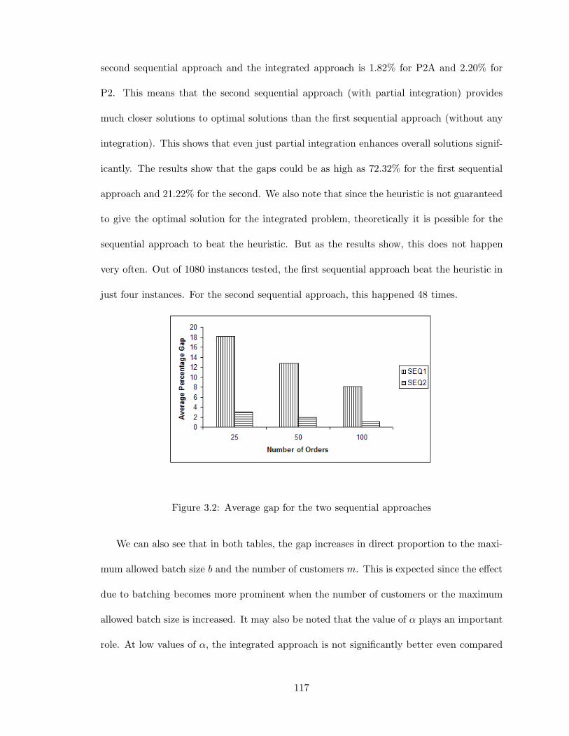
second sequential approach and the integrated approach is 1.82% for P2A and 2.20% for

P2. This means that the second sequential approach (with partial integration) provides

much closer solutions to optimal solutions than the first sequential approach (without any

integration). This shows that even just partial integration enhances overall solutions signif-

icantly. The results show that the gaps could be as high as 72.32% for the first sequential

approach and 21.22% for the second. We also note that since the heuristic is not guaranteed

to give the optimal solution for the integrated problem, theoretically it is possible for the

sequential approach to beat the heuristic. But as the results show, this does not happen

very often. Out of 1080 instances tested, the first sequential approach beat the heuristic in

just four instances. For the second sequential approach, this happened 48 times.

Figure 3.2: Average gap for the two sequential approaches

We can also see that in both tables, the gap increases in direct proportion to the maxi-

mum allowed batch size b and the number of customers m. This is expected since the effect

due to batching becomes more prominent when the number of customers or the maximum

allowed batch size is increased. It may also be noted that the value of α plays an important

role. At low values of α, the integrated approach is not significantly better even compared

117

to the first sequential approach since we are laying emphasis on the distribution cost and the

first sequential approach minimizes this. But as the value of α increases, we see a significant

increase in the gap. When everything else is kept constant, increasing the number of orders

n leads to a decrease in the gap for both the sequential approaches. This is shown in Fig 3.2.

This is explained by the fact that the heuristic H1 is essentially a local perturbation around

the SEDD sequence. When the number of orders is increased, the change in tardiness value

through this local perturbation does not increase proportionately. Hence in general, when

the number of orders is very high compared to the maximum allowed batch size or the

number of customers, the performance of heuristic H1 is not significantly better than that

of the sequential approach. The integrated approach leads to good improvements in per-

formance under cases where the contribution due to the maximum tardiness is significant

in the objective function value.

3.5 Conclusions

In this chapter, we have studied the production-distribution system with one supplier and

one or more customers. Our goal was to optimize a combined objective function that con-

sidered both the maximum tardiness and total distribution cost. It was seen that for an

arbitrary number of customers, the problem is NP-hard even in the special case where the

processing times and the due dates are agreeable. A fast heuristic has been proposed that

is asymptotically optimal when the number of orders goes to infinity. Computational tests

show that the heuristic is capable of generating near optimal solutions. We have also demon-

strated that there is distinct advantage of using the integrated production-distribution ap-

proach as compared to the two sequential approaches that try to optimize production and

delivery sequentially with no or only partial integration.

118

It should be noted that though we have assumed b, the maximum allowed batch size,

to be the same for every customer, it is not difficult to extend the heuristic and all the

other algorithms to the case where the maximum allowed batch size is dependent on the

customers. All the results presented in the chapter still hold. We have shown that in the

case when the processing times and due dates are agreeable, there exists a procedure that is

polynomial in the number of orders that can solve the problem optimally. The complexity

of the case with general processing times and due dates and a fixed number of customers is

left as an open problem.

In the case when there is no batch size limit, i.e. b = n, the problems P2A and P2

with an arbitrary number of customers are still NP-hard because the same NP-hardness

proof given in Section 3.2.1 still works for this case. On the other hand, when b = n, both

problems P1 and P2 with a fixed number of customers can be solved in polynomial time

by the O(n2m+1) dynamic programming algorithm of Hall and Potts (2003) mentioned in

Section 3.2.1 after it is slightly modified to take transportation times ti into account. The

O(n3(log n)(log(P + t))) algorithm given in Section 3.2.2 still works for problem P1 with

n = b. However, the algorithm of Hall and Potts has a lower time complexity.

In this chapter, we have not considered shipments that can serve more than one cus-

tomer. Such a problem would include routing decisions for each shipment. When sharing

of shipments across different customers is allowed, the shortest route may not always be

the best since we have to take into account the tardiness for the orders delivered at each

customer. Consequently, we cannot define the shipping due dates any more as the or-

ders of a customer may be routed through some other customers before getting delivered.

New algorithms would be needed to solve such a problem. We believe that the value of

production-distribution integration would be even greater in this case because it would

119

require a closer production-distribution linkage in order to fully take advantage of order

consolidation across different customers.

120

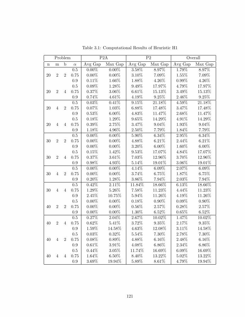
Table 3.1: Computational Results of Heuristic H1

Problem P2A P2 Overalln m b α Avg Gap Max Gap Avg Gap Max Gap Avg Gap Max Gap

0.5 0.00% 0.00% 3.58% 8.97% 1.79% 8.97%20 2 2 0.75 0.00% 0.00% 3.10% 7.09% 1.55% 7.09%

0.9 0.11% 1.66% 1.88% 4.26% 0.99% 4.26%0.5 0.09% 1.28% 9.49% 17.97% 4.79% 17.97%

20 2 4 0.75 0.37% 3.06% 6.61% 15.13% 3.49% 15.13%0.9 0.74% 4.61% 4.19% 9.25% 2.46% 9.25%0.5 0.03% 0.41% 9.15% 21.18% 4.59% 21.18%

20 4 2 0.75 0.07% 1.03% 6.88% 17.48% 3.47% 17.48%0.9 0.53% 6.00% 4.83% 11.47% 2.68% 11.47%0.5 0.18% 1.29% 9.65% 14.29% 4.91% 14.29%

20 4 4 0.75 0.39% 2.75% 3.47% 9.04% 1.93% 9.04%0.9 1.18% 4.96% 2.50% 7.79% 1.84% 7.79%0.5 0.00% 0.00% 5.90% 6.34% 2.95% 6.34%

30 2 2 0.75 0.00% 0.00% 4.88% 6.21% 2.44% 6.21%0.9 0.00% 0.00% 3.20% 6.00% 1.60% 6.00%0.5 0.15% 1.42% 9.53% 17.07% 4.84% 17.07%

30 2 4 0.75 0.37% 3.61% 7.03% 12.96% 3.70% 12.96%0.9 0.98% 4.93% 5.14% 19.01% 3.06% 19.01%0.5 0.00% 0.00% 4.14% 6.09% 2.07% 6.09%

30 4 2 0.75 0.00% 0.00% 3.74% 6.75% 1.87% 6.75%0.9 0.20% 1.28% 3.86% 7.94% 2.03% 7.94%0.5 0.42% 2.11% 11.84% 18.66% 6.13% 18.66%

30 4 4 0.75 1.29% 5.26% 7.58% 11.23% 4.44% 11.23%0.9 2.45% 10.75% 5.94% 11.26% 4.19% 11.26%0.5 0.00% 0.00% 0.18% 0.90% 0.09% 0.90%

40 2 2 0.75 0.00% 0.00% 0.56% 2.57% 0.28% 2.57%0.9 0.00% 0.00% 1.30% 6.52% 0.65% 6.52%0.5 0.27% 2.04% 2.67% 10.02% 1.47% 10.02%

40 2 4 0.75 0.62% 5.41% 3.72% 9.35% 2.17% 9.35%0.9 1.59% 14.58% 4.63% 12.08% 3.11% 14.58%0.5 0.03% 0.32% 5.54% 7.30% 2.78% 7.30%

40 4 2 0.75 0.08% 0.89% 4.88% 6.16% 2.48% 6.16%0.9 0.61% 3.91% 4.08% 6.86% 2.34% 6.86%0.5 0.44% 3.05% 11.74% 16.69% 6.09% 16.69%

40 4 4 0.75 1.64% 6.50% 8.40% 13.22% 5.02% 13.22%0.9 3.69% 19.94% 5.89% 8.61% 4.79% 19.94%

121

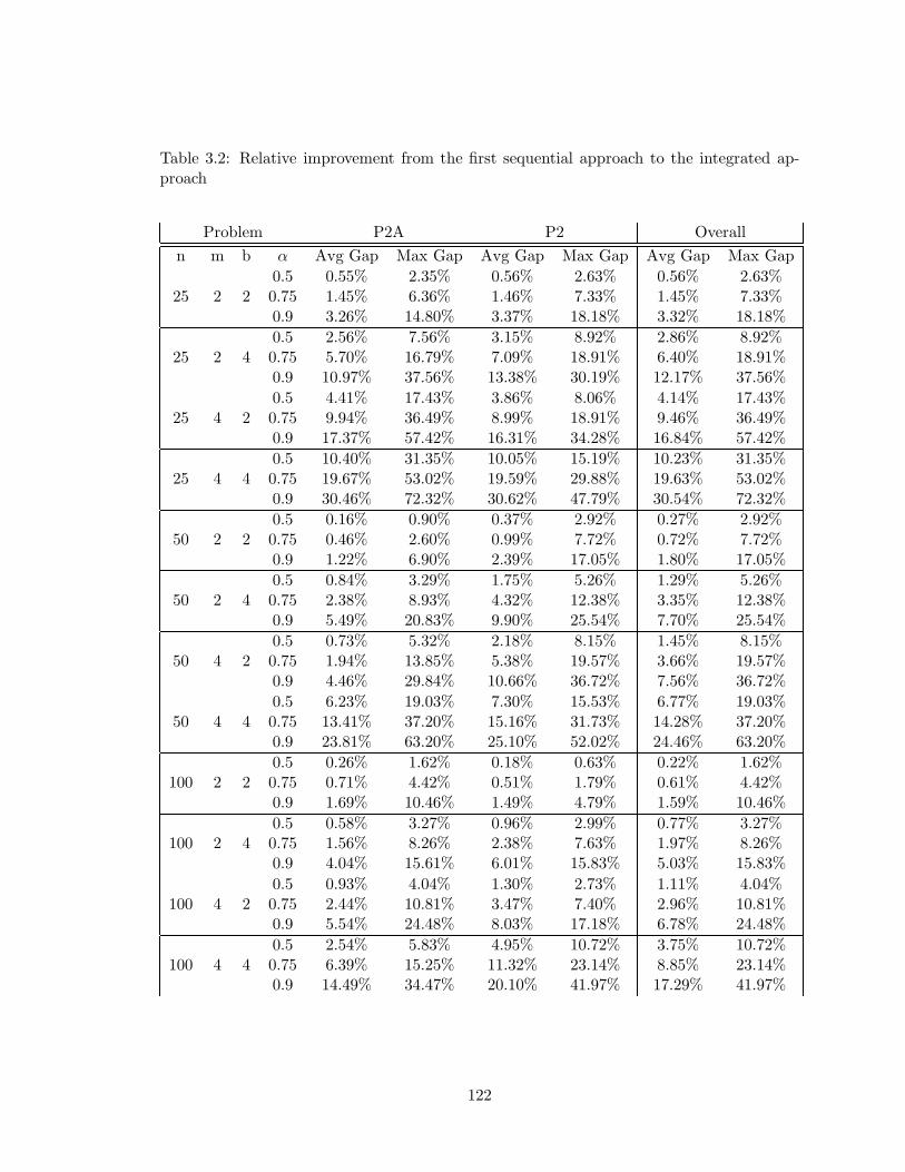
Table 3.2: Relative improvement from the first sequential approach to the integrated ap-proach

Problem P2A P2 Overalln m b α Avg Gap Max Gap Avg Gap Max Gap Avg Gap Max Gap

0.5 0.55% 2.35% 0.56% 2.63% 0.56% 2.63%25 2 2 0.75 1.45% 6.36% 1.46% 7.33% 1.45% 7.33%

0.9 3.26% 14.80% 3.37% 18.18% 3.32% 18.18%0.5 2.56% 7.56% 3.15% 8.92% 2.86% 8.92%

25 2 4 0.75 5.70% 16.79% 7.09% 18.91% 6.40% 18.91%0.9 10.97% 37.56% 13.38% 30.19% 12.17% 37.56%0.5 4.41% 17.43% 3.86% 8.06% 4.14% 17.43%

25 4 2 0.75 9.94% 36.49% 8.99% 18.91% 9.46% 36.49%0.9 17.37% 57.42% 16.31% 34.28% 16.84% 57.42%0.5 10.40% 31.35% 10.05% 15.19% 10.23% 31.35%

25 4 4 0.75 19.67% 53.02% 19.59% 29.88% 19.63% 53.02%0.9 30.46% 72.32% 30.62% 47.79% 30.54% 72.32%0.5 0.16% 0.90% 0.37% 2.92% 0.27% 2.92%

50 2 2 0.75 0.46% 2.60% 0.99% 7.72% 0.72% 7.72%0.9 1.22% 6.90% 2.39% 17.05% 1.80% 17.05%0.5 0.84% 3.29% 1.75% 5.26% 1.29% 5.26%

50 2 4 0.75 2.38% 8.93% 4.32% 12.38% 3.35% 12.38%0.9 5.49% 20.83% 9.90% 25.54% 7.70% 25.54%0.5 0.73% 5.32% 2.18% 8.15% 1.45% 8.15%

50 4 2 0.75 1.94% 13.85% 5.38% 19.57% 3.66% 19.57%0.9 4.46% 29.84% 10.66% 36.72% 7.56% 36.72%0.5 6.23% 19.03% 7.30% 15.53% 6.77% 19.03%

50 4 4 0.75 13.41% 37.20% 15.16% 31.73% 14.28% 37.20%0.9 23.81% 63.20% 25.10% 52.02% 24.46% 63.20%0.5 0.26% 1.62% 0.18% 0.63% 0.22% 1.62%

100 2 2 0.75 0.71% 4.42% 0.51% 1.79% 0.61% 4.42%0.9 1.69% 10.46% 1.49% 4.79% 1.59% 10.46%0.5 0.58% 3.27% 0.96% 2.99% 0.77% 3.27%

100 2 4 0.75 1.56% 8.26% 2.38% 7.63% 1.97% 8.26%0.9 4.04% 15.61% 6.01% 15.83% 5.03% 15.83%0.5 0.93% 4.04% 1.30% 2.73% 1.11% 4.04%

100 4 2 0.75 2.44% 10.81% 3.47% 7.40% 2.96% 10.81%0.9 5.54% 24.48% 8.03% 17.18% 6.78% 24.48%0.5 2.54% 5.83% 4.95% 10.72% 3.75% 10.72%

100 4 4 0.75 6.39% 15.25% 11.32% 23.14% 8.85% 23.14%0.9 14.49% 34.47% 20.10% 41.97% 17.29% 41.97%

122

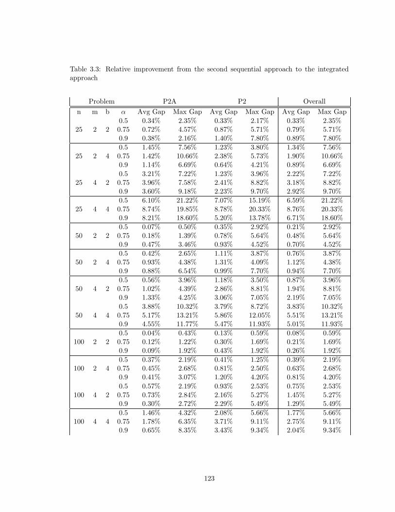
Table 3.3: Relative improvement from the second sequential approach to the integratedapproach

Problem P2A P2 Overalln m b α Avg Gap Max Gap Avg Gap Max Gap Avg Gap Max Gap

0.5 0.34% 2.35% 0.33% 2.17% 0.33% 2.35%25 2 2 0.75 0.72% 4.57% 0.87% 5.71% 0.79% 5.71%

0.9 0.38% 2.16% 1.40% 7.80% 0.89% 7.80%0.5 1.45% 7.56% 1.23% 3.80% 1.34% 7.56%

25 2 4 0.75 1.42% 10.66% 2.38% 5.73% 1.90% 10.66%0.9 1.14% 6.69% 0.64% 4.21% 0.89% 6.69%0.5 3.21% 7.22% 1.23% 3.96% 2.22% 7.22%

25 4 2 0.75 3.96% 7.58% 2.41% 8.82% 3.18% 8.82%0.9 3.60% 9.18% 2.23% 9.70% 2.92% 9.70%0.5 6.10% 21.22% 7.07% 15.19% 6.59% 21.22%

25 4 4 0.75 8.74% 19.85% 8.78% 20.33% 8.76% 20.33%0.9 8.21% 18.60% 5.20% 13.78% 6.71% 18.60%0.5 0.07% 0.50% 0.35% 2.92% 0.21% 2.92%

50 2 2 0.75 0.18% 1.39% 0.78% 5.64% 0.48% 5.64%0.9 0.47% 3.46% 0.93% 4.52% 0.70% 4.52%0.5 0.42% 2.65% 1.11% 3.87% 0.76% 3.87%

50 2 4 0.75 0.93% 4.38% 1.31% 4.09% 1.12% 4.38%0.9 0.88% 6.54% 0.99% 7.70% 0.94% 7.70%0.5 0.56% 3.96% 1.18% 3.50% 0.87% 3.96%

50 4 2 0.75 1.02% 4.39% 2.86% 8.81% 1.94% 8.81%0.9 1.33% 4.25% 3.06% 7.05% 2.19% 7.05%0.5 3.88% 10.32% 3.79% 8.72% 3.83% 10.32%

50 4 4 0.75 5.17% 13.21% 5.86% 12.05% 5.51% 13.21%0.9 4.55% 11.77% 5.47% 11.93% 5.01% 11.93%0.5 0.04% 0.43% 0.13% 0.59% 0.08% 0.59%

100 2 2 0.75 0.12% 1.22% 0.30% 1.69% 0.21% 1.69%0.9 0.09% 1.92% 0.43% 1.92% 0.26% 1.92%0.5 0.37% 2.19% 0.41% 1.25% 0.39% 2.19%

100 2 4 0.75 0.45% 2.68% 0.81% 2.50% 0.63% 2.68%0.9 0.41% 3.07% 1.20% 4.20% 0.81% 4.20%0.5 0.57% 2.19% 0.93% 2.53% 0.75% 2.53%

100 4 2 0.75 0.73% 2.84% 2.16% 5.27% 1.45% 5.27%0.9 0.30% 2.72% 2.29% 5.49% 1.29% 5.49%0.5 1.46% 4.32% 2.08% 5.66% 1.77% 5.66%

100 4 4 0.75 1.78% 6.35% 3.71% 9.11% 2.75% 9.11%0.9 0.65% 8.35% 3.43% 9.34% 2.04% 9.34%

123

Chapter 4

Joint Cyclic Production and DeliveryScheduling in a Two-Stage Supply Chain

4.1 Introduction

Production and distribution operations are the two most important operational functions

in a supply chain. It is critical to plan and schedule these two functions in a coordinated

manner in order to achieve optimal operational performance of the supply chain. In this

chapter, we study an integrated production and distribution scheduling model in a two-

stage supply chain consisting of one or more suppliers, a warehouse, and a customer. Each

supplier manufactures a unique item at a constant rate. The customer’s demand for each

item is constant and known in advance. Each supplier manufactures its item in batches and

there is a setup time and setup cost incurred for every production batch. Manufactured

items are shipped directly from the suppliers to the warehouse, and from the warehouse to

the customer. In the delivery from the warehouse to the customer, different products from

the suppliers are consolidated and shipped together. There are inventory holding costs at

all the facilities (suppliers, warehouse, and customer) and there are transportation costs for

deliveries from the suppliers to the warehouse and from the warehouse to the customer. The

objective is to find a joint cyclic production and delivery schedule over an infinite planning

horizon to minimize the total production, inventory and transportation cost per unit time.

124

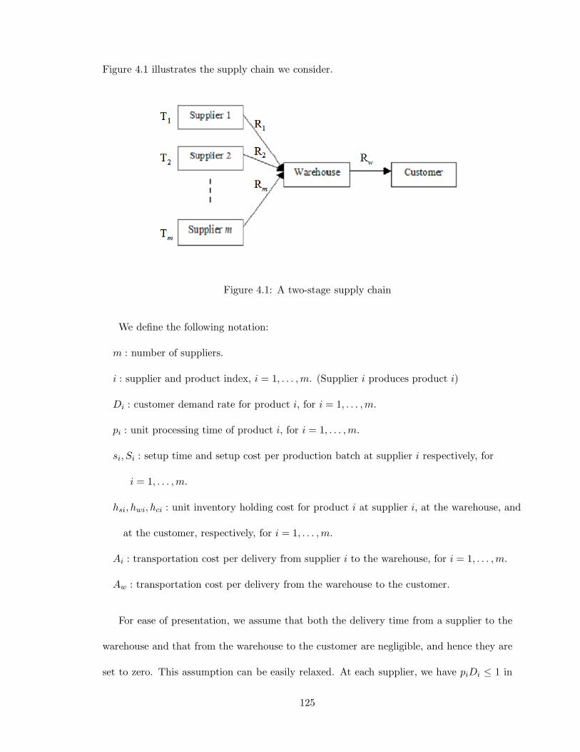
Figure 4.1 illustrates the supply chain we consider.

Figure 4.1: A two-stage supply chain

We define the following notation:

m : number of suppliers.

i : supplier and product index, i = 1, . . . ,m. (Supplier i produces product i)

Di : customer demand rate for product i, for i = 1, . . . ,m.

pi : unit processing time of product i, for i = 1, . . . ,m.

si, Si : setup time and setup cost per production batch at supplier i respectively, for

i = 1, . . . ,m.

hsi, hwi, hci : unit inventory holding cost for product i at supplier i, at the warehouse, and

at the customer, respectively, for i = 1, . . . ,m.

Ai : transportation cost per delivery from supplier i to the warehouse, for i = 1, . . . ,m.

Aw : transportation cost per delivery from the warehouse to the customer.

For ease of presentation, we assume that both the delivery time from a supplier to the

warehouse and that from the warehouse to the customer are negligible, and hence they are

set to zero. This assumption can be easily relaxed. At each supplier, we have piDi ≤ 1 in

125

order to satisfy the customer demand subject to the capacity constraint (the inequality is

strict unless the setup time is zero). We also assume that the unit inventory holding cost

of a product at the customer is the highest whereas that at the supplier is the lowest, i.e.

hsi ≤ hwi ≤ hci, for i = 1, . . . ,m. This assumption reflects the situation in many supply

chains where the customers (e.g. retailers) are located at the most populated areas and

hence have the highest unit inventory holding cost because of the tight space limit, whereas

the suppliers (e.g. plants) are located at places with very low holding costs.

Given these parameters, we need to find a joint cyclic production and delivery schedule,

which is equivalent to finding the following cycle times and the relative positions of these

cycles:

Ti : time between successive production setups at supplier i, for i = 1, . . . ,m.

Ri : time between successive deliveries from supplier i to the warehouse, for i = 1, . . . ,m.

Rw : time between successive deliveries from the warehouse to the customer.

Since the schedules are cyclic, in each production or delivery cycle, exactly the same

amount will be produced or delivered. Consequently, for i = 1, . . . ,m, in each production

cycle at supplier i, TiDi units of product i need to be produced, and in each delivery cycle

from supplier i to the warehouse, RiDi units of product i need to be delivered. Clearly,

there is only one product involved in a production batch at each supplier and in a delivery

from a supplier to the warehouse. However, all the m products are included in a delivery

from the warehouse to the customer. That is, in each delivery cycle from the warehouse to

the customer, RwD1 units of product 1, RwD2 units of product 2, ..., and RwDm units of

product m need to be delivered.

We consider the following two policies for production and delivery cycles:

i) Production cycle time at each supplier is the same as the delivery cycle time from

126

that supplier to the warehouse, i.e. Ti = Ri, for i = 1, . . . ,m.

ii) Production cycle time at each supplier is an integer multiple of the delivery cycle time

from that supplier to the warehouse, and the delivery cycle time from a supplier to the

warehouse is an integer multiple of the delivery cycle time from the warehouse to the

customer, i.e. Ti = MsiRi and Ri = MwiRw, for i = 1, . . . ,m, where Ms1, . . . ,Msm

and Mw1, . . . ,Mwm are all positive integers.

These policies are similar to some commonly considered policies for similar models in the

literature. Our consideration of these policies is partially justified by the following result.

Lemma 16 In an optimal cyclic schedule to our model, Ti ≥ Ri ≥ Rw, for i = 1, . . . ,m.

Proof We prove this by contradiction. In a given cyclic schedule, if Ri < Rw for some

supplier i, we modify this schedule by increasing Ri such that Ri = Rw. Delivery from

supplier i to the warehouse is less frequent in the modified schedule, which brings down

the per-period transportation cost. The inventory cost will also decrease or remain the

same. This is because hsi ≤ hwi and when we set Ri = Rw, the products wait at the

suppliers instead of the warehouse. Hence the modified schedule has a lower total cost.

Similarly, if Ti < Ri for some supplier i in a given schedule, we modify this schedule by

increasing Ti such that Ti = Ri. It can be seen that in this modified schedule both the total

production setup cost and the total inventory cost at supplier i are lower than before. The

inventory costs go down since in the modified schedule, the products for a delivery batch

get processed continuously, with just one setup in the beginning and without a break for

setups in between. So on an average, products spend less time waiting at the suppliers.

Hence the modified schedule has a lower total cost.

This result implies that there is no need to consider policies that either require the

delivery cycle time from the warehouse to the customer to be greater than that from a

127

supplier to the warehouse or require the delivery cycle time from a supplier to the warehouse

to be greater than the production cycle time at that supplier. However, all the schedules

that satisfy policy (i) or (ii) are only a subset of the schedules that satisfy Lemma 1. Hence

an optimal cyclic schedule that satisfies policy (i) or (ii) may not be optimal to our model.

On the other hand, schedules that satisfy these policies are easier to implement in practice

than those that satisfy Lemma 1 but not these policies.

The remainder of this chapter is organized as follows. We then study our model under

policy (i) and that under policy (ii) in Sections 4.2 and 4.3, respectively. In Section 4.2, we

will show that in an optimal cyclic schedule under policy (i), the delivery cycle time from

each supplier to the warehouse is an integer multiple of the delivery cycle time from the

warehouse to the customer, i.e. Ri = MwiRw, for i = 1, . . . ,m and some positive integers

Mw1, . . . ,Mwm. We will show that for the model with a single supplier, an optimal cyclic

schedule can be obtained by closed-form formulas. For the model with multiple suppliers,

we propose a heuristic and evaluate the performance of the heuristic computationally. In

Section 4.3, we propose and computationally evaluate a heuristic for the problem under

policy (ii) with multiple suppliers. We then evaluate the value of warehouse in our two-

stage supply chain by comparing this supply chain with a single-stage supply chain without

the warehouse. The total cost obtained through our heuristic for the two-stage model under

policy (ii) is compared to the total cost obtained by an optimal algorithm from the literature

for the single-stage model without the warehouse. Managerial insights are derived based on

an extensive set of computational tests. It is conceptually well-understood that a warehouse

plays an important role in a supply chain; it consolidates different products and positions

the inventory closer to customers, and hence saves on transportation and inventory costs.

Our study here attempts to quantify these benefits for the supply chain we consider. Finally,

128

we conclude the chapter in Section 4.4.

4.2 The Model under Policy (i)

We first prove an optimality property and derive the various cost components for the model

under policy (i) in Section 4.2.1. We then give an optimal solution to the case with a single

supplier in Section 4.2.2, and propose a heuristic for the case with multiple suppliers and

evaluate its performance in Section 4.2.3.

4.2.1 An Optimality Property

Theorem 16 In an optimal cyclic schedule under policy (i), the delivery cycle time fromeach supplier to the warehouse is an integer multiple of the delivery cycle time from thewarehouse to the customer, i.e. Ri = MwiRw for some positive integer Mwi, for i = 1, . . . ,m.

Proof We prove the theorem for the single-supplier case first and then extend the result to

the case with multiple suppliers. When we have only one supplier, we discard the supplier

subscript in our notation. Hence the production cycle time and the delivery cycle time from

the supplier to the warehouse are denoted as T and R respectively. Under policy (i), we have

T = R. Suppose that Mw = R/Rw is not an integer. We show that the total cost of a new

schedule where both the production cycle time at the supplier and the delivery cycle time

from the supplier to the warehouse are increased to dMweRw is not greater than that of the

original schedule. Before giving a formal analysis, we explain through a diagram the various

categories of inventory at the warehouse when Mw is not an integer. The inventory level

over time at the warehouse repeats every kR units of time, where k is the smallest integer

such that kR/Rw is an integer. The period of kR time units is hence called an inventory

cycle) of the warehouse. For illustration purposes, let us assume Mw = 213 . Figure 4.2

shows the inventory level at the warehouse over one entire inventory cycle, i.e. over 3R

time units (k = 3 here).

129

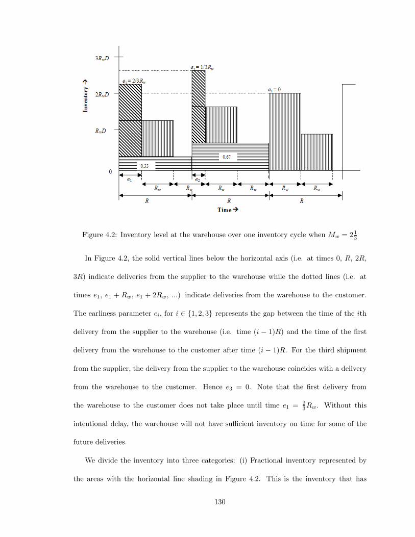
Figure 4.2: Inventory level at the warehouse over one inventory cycle when Mw = 213

In Figure 4.2, the solid vertical lines below the horizontal axis (i.e. at times 0, R, 2R,

3R) indicate deliveries from the supplier to the warehouse while the dotted lines (i.e. at

times e1, e1 + Rw, e1 + 2Rw, ...) indicate deliveries from the warehouse to the customer.

The earliness parameter ei, for i ∈ 1, 2, 3 represents the gap between the time of the ith

delivery from the supplier to the warehouse (i.e. time (i − 1)R) and the time of the first

delivery from the warehouse to the customer after time (i − 1)R. For the third shipment

from the supplier, the delivery from the supplier to the warehouse coincides with a delivery

from the warehouse to the customer. Hence e3 = 0. Note that the first delivery from

the warehouse to the customer does not take place until time e1 = 23Rw. Without this

intentional delay, the warehouse will not have sufficient inventory on time for some of the

future deliveries.

We divide the inventory into three categories: (i) Fractional inventory represented by

the areas with the horizontal line shading in Figure 4.2. This is the inventory that has

130

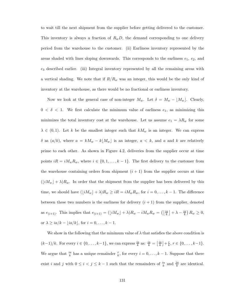
to wait till the next shipment from the supplier before getting delivered to the customer.

This inventory is always a fraction of RwD, the demand corresponding to one delivery

period from the warehouse to the customer. (ii) Earliness inventory represented by the

areas shaded with lines sloping downwards. This corresponds to the earliness e1, e2, and

e3 described earlier. (iii) Integral inventory represented by all the remaining areas with

a vertical shading. We note that if R/Rw was an integer, this would be the only kind of

inventory at the warehouse, as there would be no fractional or earliness inventory.

Now we look at the general case of non-integer Mw. Let δ = Mw − bMwc. Clearly,

0 < δ < 1. We first calculate the minimum value of earliness e1, as minimizing this

minimizes the total inventory cost at the warehouse. Let us assume e1 = λRw for some

λ ∈ (0, 1). Let k be the smallest integer such that kMw is an integer. We can express

δ as (a/k), where a = kMw − kbMwc is an integer, a < k, and a and k are relatively

prime to each other. As shown in Figure 4.2, deliveries from the supplier occur at time

points iR = iMwRw, where i ∈ 0, 1, . . . , k − 1. The first delivery to the customer from

the warehouse containing orders from shipment (i + 1) from the supplier occurs at time

(biMwc + λ)Rw. In order that the shipment from the supplier has been delivered by this

time, we should have (biMwc + λ)Rw ≥ iR = iMwRw, for i = 0, . . . , k − 1. The difference

between these two numbers is the earliness for delivery (i + 1) from the supplier, denoted

as e(i+1). This implies that e(i+1) = (biMwc + λ)Rw − iMwRw =(⌊

iak

⌋+ λ − ia

k

)Rw ≥ 0,

or λ ≥ ia/k − bia/kc, for i = 0, . . . , k − 1.

We show in the following that the minimum value of λ that satisfies the above condition is

(k−1)/k. For every i ∈ 0, . . . , k−1, we can express iak as: ia

k =⌊

iak

⌋+ r

k , r ∈ 0, . . . , k−1.

We argue that iak has a unique remainder r

k , for every i = 0, . . . , k − 1. Suppose that there

exist i and j with 0 ≤ i < j ≤ k − 1 such that the remainders of iak and ja

k are identical.

131

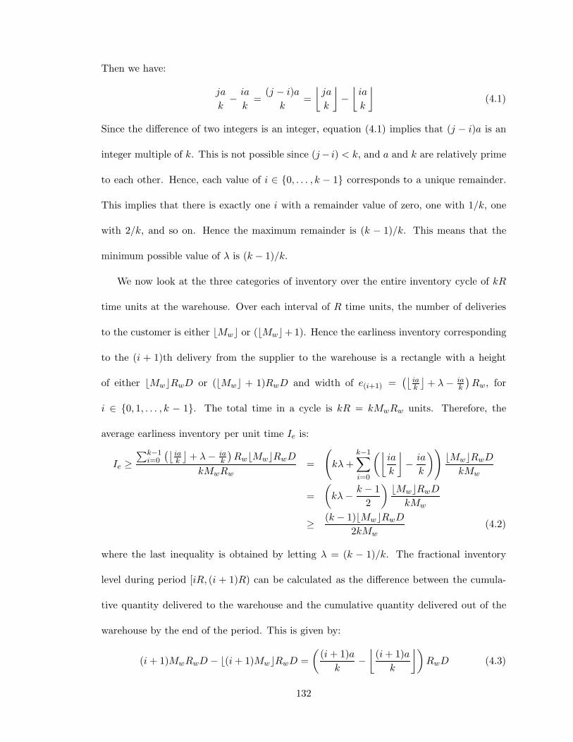
Then we have:

ja

k− ia

k=

(j − i)ak

=⌊

ja

k

⌋−⌊

ia

k

⌋(4.1)

Since the difference of two integers is an integer, equation (4.1) implies that (j − i)a is an

integer multiple of k. This is not possible since (j− i) < k, and a and k are relatively prime

to each other. Hence, each value of i ∈ 0, . . . , k − 1 corresponds to a unique remainder.

This implies that there is exactly one i with a remainder value of zero, one with 1/k, one

with 2/k, and so on. Hence the maximum remainder is (k − 1)/k. This means that the

minimum possible value of λ is (k − 1)/k.

We now look at the three categories of inventory over the entire inventory cycle of kR

time units at the warehouse. Over each interval of R time units, the number of deliveries

to the customer is either bMwc or (bMwc+1). Hence the earliness inventory corresponding

to the (i + 1)th delivery from the supplier to the warehouse is a rectangle with a height

of either bMwcRwD or (bMwc + 1)RwD and width of e(i+1) =(⌊

iak

⌋+ λ − ia

k

)Rw, for

i ∈ 0, 1, . . . , k − 1. The total time in a cycle is kR = kMwRw units. Therefore, the

average earliness inventory per unit time Ie is:

Ie ≥∑k−1

i=0

(⌊iak

⌋+ λ − ia

k

)RwbMwcRwD

kMwRw=

(kλ +

k−1∑

i=0

(⌊ia

k

⌋− ia

k

))bMwcRwD

kMw

=(

kλ − k − 12

)bMwcRwD

kMw

≥ (k − 1)bMwcRwD

2kMw(4.2)

where the last inequality is obtained by letting λ = (k − 1)/k. The fractional inventory

level during period [iR, (i + 1)R) can be calculated as the difference between the cumula-

tive quantity delivered to the warehouse and the cumulative quantity delivered out of the

warehouse by the end of the period. This is given by:

(i + 1)MwRwD − b(i + 1)MwcRwD =(

(i + 1)ak

−⌊

(i + 1)ak

⌋)RwD (4.3)

132

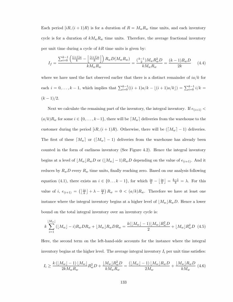
Each period [iR, (i + 1)R) is for a duration of R = MwRw time units, and each inventory

cycle is for a duration of kMwRw time units. Therefore, the average fractional inventory

per unit time during a cycle of kR time units is given by:

If =

∑k−1i=0

((i+1)a

k −⌊

(i+1)ak

⌋)RwD(MwRw)

kMwRw=

(k−12 )MwR2

wD

kMwRw=

(k − 1)RwD

2k(4.4)

where we have used the fact observed earlier that there is a distinct remainder of ia/k for

each i = 0, . . . , k − 1, which implies that∑k−1

i=0 ((i + 1)a/k − b(i + 1)a/kc) =∑k−1

i=0 i/k =

(k − 1)/2.

Next we calculate the remaining part of the inventory, the integral inventory. If e(i+1) <

(a/k)Rw for some i ∈ 0, . . . , k−1, there will be dMwe deliveries from the warehouse to the

customer during the period [iR, (i + 1)R). Otherwise, there will be (dMwe − 1) deliveries.

The first of these dMwe or (dMwe − 1) deliveries from the warehouse has already been

counted in the form of earliness inventory (See Figure 4.2). Hence the integral inventory

begins at a level of bMwcRwD or (bMwc − 1)RwD depending on the value of e(i+1). And it

reduces by RwD every Rw time units, finally reaching zero. Based on our analysis following

equation (4.1), there exists an i ∈ 0 . . . k − 1, for which iak −

⌊iak

⌋= k−1

k = λ. For this

value of i, e(i+1) =(⌊

iak

⌋+ λ − ia

k

)Rw = 0 < (a/k)Rw. Therefore we have at least one

instance where the integral inventory begins at a higher level of bMwcRwD. Hence a lower

bound on the total integral inventory over an inventory cycle is:

k

bMwc∑

i=1

(bMwc − i)RwDRw + bMwcRwDRw =k(bMwc − 1)bMwcR2

wD

2+ bMwcR2

wD (4.5)

Here, the second term on the left-hand-side accounts for the instance where the integral

inventory begins at the higher level. The average integral inventory Ii per unit time satisfies:

Ii ≥k (bMwc − 1) bMwc

2kMwRwR2

wD +bMwcR2

wD

kMwRw=

(bMwc − 1) bMwcRwD

2Mw+

bMwcRwD

kMw(4.6)

133

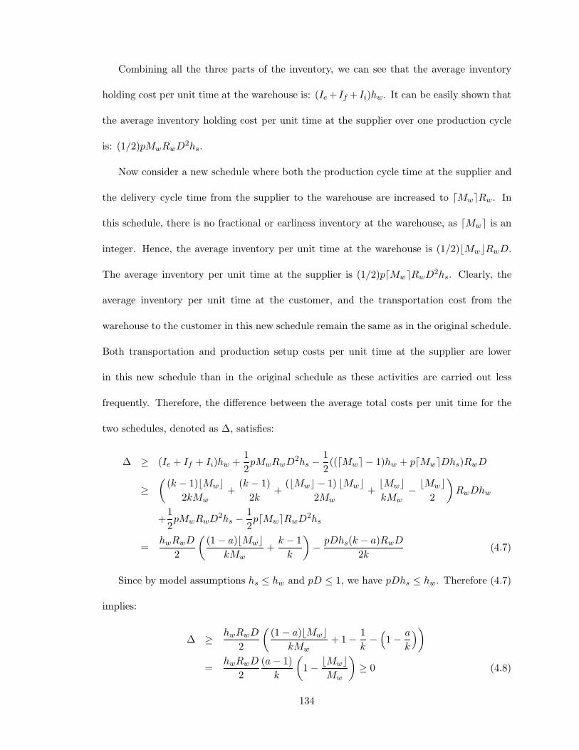
Combining all the three parts of the inventory, we can see that the average inventory

holding cost per unit time at the warehouse is: (Ie + If + Ii)hw. It can be easily shown that

the average inventory holding cost per unit time at the supplier over one production cycle

is: (1/2)pMwRwD2hs.

Now consider a new schedule where both the production cycle time at the supplier and

the delivery cycle time from the supplier to the warehouse are increased to dMweRw. In

this schedule, there is no fractional or earliness inventory at the warehouse, as dMwe is an

integer. Hence, the average inventory per unit time at the warehouse is (1/2)bMwcRwD.

The average inventory per unit time at the supplier is (1/2)pdMweRwD2hs. Clearly, the

average inventory per unit time at the customer, and the transportation cost from the

warehouse to the customer in this new schedule remain the same as in the original schedule.

Both transportation and production setup costs per unit time at the supplier are lower

in this new schedule than in the original schedule as these activities are carried out less

frequently. Therefore, the difference between the average total costs per unit time for the

two schedules, denoted as ∆, satisfies:

∆ ≥ (Ie + If + Ii)hw +12pMwRwD2hs −

12((dMwe − 1)hw + pdMweDhs)RwD

≥(

(k − 1)bMwc2kMw

+(k − 1)

2k+

(bMwc − 1) bMwc2Mw

+bMwckMw

− bMwc2

)RwDhw

+12pMwRwD2hs −

12pdMweRwD2hs

=hwRwD

2

((1 − a)bMwc

kMw+

k − 1k

)− pDhs(k − a)RwD

2k(4.7)

Since by model assumptions hs ≤ hw and pD ≤ 1, we have pDhs ≤ hw. Therefore (4.7)

implies:

∆ ≥ hwRwD

2

((1 − a)bMwc

kMw+ 1 − 1

k−(1 − a

k

))

=hwRwD

2(a − 1)

k

(1 − bMwc

Mw

)≥ 0 (4.8)

134

This proves that the total cost of the new schedule is not greater than that of the original

schedule. In the multiple-supplier case, we can generate a new schedule by increasing both

Ti and Ri to RwdRi/Rwe whenever (Ri/Rw) is not an integer. By the above proof, the

total cost related to each product i ∈ 1, . . . ,m is not greater than that in the original

schedule. Thus the average total cost in this new schedule is not greater than that in the

original schedule.

By Theorem 16, we can focus on schedules where Ri/Rw is integer valued for each

supplier i = 1, . . . ,m. In the following, we derive the average total cost per unit time in

such a schedule. We have seen in the proof of Theorem 16 how to calculate the average

inventory costs at the supplier and at the warehouse for the single-supplier case when R/Rw

is integer valued. Extending that to the case with multiple suppliers, we get the following

equation for the average total inventory cost per unit time, denoted as IC:

IC =12

(m∑

i=1

hsipiD2i Ri

)+

12

(m∑

i=1

hwiDi(Ri − Rw)

)+

12

(m∑

i=1

hciDi

)Rw (4.9)

where the first, second, and third term corresponds to the average inventory cost per unit

time at the suppliers, at the warehouse, and at the customer, respectively.

The average total production setup cost per unit time, denoted as SC, and the average

total distribution cost per unit time, denoted as DC, are given below:

SC =m∑

i=1

Si

Ti=

m∑

i=1

Si

Ri(4.10)

DC =m∑

i=1

Ai

Ri+

Aw

Rw(4.11)

135

Therefore, the average total cost per unit time, denoted as TC, is given as:

TC = IC + SC + DC

=m∑

i=1

Si

Ri+

12

(m∑

i=1

hsipiD2i Ri

)+

12

(m∑

i=1

hwiDi(Ri − Rw)

)

+12

(m∑

i=1

hciDi

)Rw +

m∑

i=1

Ai

Ri+

Aw

Rw

=m∑

i=1

(Si + Ai)Ri

+m∑

i=1

αiRi + βRw +Aw

Rw

=m∑

i=1

Qi

Ri+

m∑

i=1

αiRi + βRw +Aw

Rw(4.12)

where Qi = Si + Ai, αi = (hsipiDi + hwi)Di/2, and β =∑m

i=1(hci − hwi)Di/2.

Our objective is to find the values for Rw and R1, . . . , Rm that minimizes TC subject

to the production constraint. The production constraint requires that the production cycle

time Ti at each supplier i is sufficient to produce the required quantity along with the setup

time, i.e. si + piDiTi ≤ Ti. This means that Ti ≥ τi, i.e. Ri ≥ τi, as Ri = Ti under policy

(i), where τi = si/(1 − piDi). So we can formulate our problem under policy (i) as follows:

Minimize TC (4.13)

Subject to: Ri ≥ τi, ∀i ∈ 1, . . . ,m (4.14)

Ri

Rwis a positive integer, ∀i ∈ 1, . . . ,m (4.15)

Rw ≥ 0 (4.16)

The average total cost per unit time TC given in equation (4.12) is a separable function of

the variables Rw and R1, . . . , Rm, and corresponding to each variable, the function is convex.

Hence without the constraint (4.15), the above formulation can be solved optimally using

the first order Karush-Kuhn-Tucker (KKT) conditions. But the presence of the integrality

constraint makes this problem more complicated. In the next two sections, we will show a

136

way to obtain the optimal solution in the case of a single supplier and propose a heuristic

for the multiple-supplier case.

4.2.2 Optimal Solution for the Single-Supplier Case

In this section, we derive the optimal solution in the case where there is only one supplier.

For simplicity, we drop the supplier subscript from our notation. The total cost given in

(4.12) can be rewritten as:

TC =Q

R+ αR + βRw +

Aw

Rw(4.17)

where Q = S + A, α = (hspD + hw)D/2, and β = (hc − hw)D/2. Our objective is to find

the values of R and Rw that minimize TC subject to the constraints that R ≥ τ and R/Rw

is a positive integer, where τ = s/(1 − pD).

Define R′ = max√

Q/α, τ

and R′w =

√Aw/β. If we ignore the integrality constraint,

it can be shown by the first order KKT conditions that the optimal solution to this problem

is given by R = R′ and Rw = R′w. Let M ′

w = R′/R′w. Then we have the following result:

Theorem 17 Let R∗ and R∗w be the optimal values of R and Rw for the single-supplier

problem under policy (i). Then,

R∗w = Max

√Q + M∗

wAw

M∗w(αM∗

w + β),

τ

M∗w

(4.18)

R∗ = M∗wR∗

w (4.19)

where M∗w ∈ maxbM ′

wc, 1, dM ′we.

Proof We prove this by transforming our problem to an equivalent problem studied by

Hahm and Yano (1992). Their supply chain consists of one supplier and one customer, with

no warehouse in-between. We use the subscript y to denote the parameters involved in

their problem. Their objective is to find the production cycle time Ty at the supplier and

the delivery cycle time Ry from the supplier to the warehouse such that the average total

137

cost per unit time is minimized. They show that in an optimal schedule, Ty is an integer

multiple of Ry, and formulate their problem as the following optimization model:

MinimizeSy

Ty+

12(1 − pyDy)DyhyTy + pyD

2yhyRy +

Ay

Ry

Subject to: Ty ≥ sy

1 − pyDy

Ty

Ryis a positive integer

Ry ≥ 0

where Ty and Ry are the decision variables and every other notation represents a problem

parameter in the same way as the corresponding notations in our problem. In their problem,

the unit holding costs at the supplier and at the customer are assumed to be equal and is

represented by hy.

This formulation is identical to our formulation with the following substitutions:

Sy = S + A (4.20)

Ay = Aw (4.21)

12(1 − pyDy)Dyhy =

12(hspD + hw)D (4.22)

pyD2yhy =

12(hc − hw)D (4.23)

sy

1 − pyDy=

s

1 − pD(4.24)

If we are able to find non-negative Sy, sy, py,Dy , Ay, and hy satisfying (4.20) - (4.24) and

the capacity constraint pyDy ≤ 1, then we can use the optimal solution from the Hahm and

Yano model as the optimal solution for our model. The optimal solution for their problem

is what we have given in equations (4.18) and (4.19) (with the corresponding substitutions

of the parameters).

138

It can be easily shown that Sy, Ay,Dy, py, hy, and sy that are defined by (4.20), (4.21),

and the following equations, respectively, satisfy (4.20) - (4.24) and pyDy ≤ 1:

Dy = D

py =hc − hw

2hspD2 + hcD + hwD

hy = hspD +12(hc + hw)

sy =2s

(1 − pD)(hspD + hw)

(2hspD + hc + hw)

This completes the proof.

By Theorem 17, if MaxbM ′wc, 1 = dM ′

we, then the optimal solution is uniquely defined

by (4.18) and (4.19). Otherwise, we only need to compare two solutions, one with M∗w =

MaxbM ′wc, 1 and the other with M∗

w = dM ′we, and the one with a lower objective value

TC is the optimal solution to the problem.

4.2.3 A Heuristic Solution for the Multiple-Supplier Case

We first give an alternate representation for the problem defined in (4.13) - (4.16), where

we substitute the variables Ri by MwiRw, for i = 1, . . . ,m:

Minimizem∑

i=1

Qi

MwiRw+

m∑

i=1

αiMwiRw + βRw +Aw

Rw(4.25)

Subject to: MwiRw ≥ τi, ∀i ∈ 1, . . . ,m (4.26)

Mwi is a positive integer, ∀i ∈ 1, . . . ,m (4.27)

Rw ≥ 0 (4.28)

The heuristic in this section tries to find a near optimal solution (Mw1, . . . ,Mwm, Rw) to

the above formulation. Since there are multiple suppliers involved, the choice of Mwi at

139

one supplier can influence the choice of Mwi at another supplier. If we just try two values

of Mwi at each supplier as in the optimal solution for the single-supplier case shown in the

previous subsection, the resulting solution is unlikely to be optimal or even local optimal.

Our heuristic keeps trying different values of Mwi’s for the suppliers until a local optimal

solution is found. More specifically, in each iteration, the heuristic chooses one supplier and

fixes the Mwi values for all the other m − 1 suppliers. Then it finds the values for Rw, Ri,

and Mwi for the chosen supplier using an approach similar to the one used for the single-

supplier problem. If the resulting total cost is lower, then the value of Mwi for the chosen

supplier is updated and fixed in the next several iterations along with the Mwi values at

(m − 2) other suppliers. The procedure stops when no improvement is found in one round

of iterations across all the suppliers.

Heuristic H1

Step 1: Set R0i = Max

√Qi

αi, τi

, R0

w =√

Awβ , M0

wi = R0i /R

0w, for i = 1, . . .,m. Let j = 1

be the index of the supplier to be considered next. Set the iteration counter c = 0, and the

non-improvement counter n = 0. Set the total cost TC0 = ∞.

Step 2: Set c = c + 1. For supplier j, let M ′wj = R0

j/R′w where

R′w = Max

√√√√∑m

i=1,i 6=jQi

M0wi

+ Aw∑m

i=1,i 6=j αiM0wi + β

, max

τi

M0wi

, ∀i 6= j

(4.29)

Set Mwj = maxbM ′

wjc, 1

and get the corresponding Rw as follows:

Rw = Max

√√√√∑m

i=1,i 6=jQi

M0wi

+ Qj

Mwj+ Aw

∑mi=1,i 6=j αiM0

wi + αjMwj + β,

τj

Mwj, max

τi

M0wi

, ∀i 6= j

(4.30)

Calculate the total cost TC of the solution (Mw1, . . . ,Mwm, Rw) with Mwj = Mwj, Mwi =

140

M0wi for i 6= j, and Rw = Rw. Similarly, set Mwj = dM ′

wje and get the corresponding Rw

and the total cost, TC, of the corresponding solution. Choose the solution with a lower

total cost. Let the total cost of this solution be TCj .

Step 3: If c < m, let M0wj be equal to the Mwj corresponding to the solution generated

in Step 2. If c ≥ m and TCj < TC0, let TC0 = TCj and M0wj be equal to the Mwj

corresponding to the solution generated in Step 2, and reset n = 0. If c ≥ m and TCj ≥

TC0, let n = n + 1.

Step 4: If n = m, there has been no improvement for any supplier in the last m iterations,

and hence STOP. Otherwise, if j = m, set j = 1, else set j = j + 1. Go to Step 2.

In the first m iterations, the heuristic finds an integer solution for the variables Mwj

at each supplier. After these iterations, the heuristic tries to improve the existing feasible

solution, choosing one supplier at a time. By the first order KKT conditions, it can be

shown that the values R01, . . . , R

0m and R0

w defined in Step 1 of the heuristic are optimal

to the problem (4.13) - (4.16) without the integrality requirement (4.15). Hence the values

M0w1, . . . ,M

0wm and R0

w defined in Step 1 are optimal to the problem (4.25) - (4.28) if the

integrality constraint (4.27) is relaxed. Similarly, under the condition that Mwi is fixed as

M0wi for all i 6= j, it can be shown that the solution (M ′

wj , R′w) defined in Step 2 is optimal

to the remaining problem (4.25) - (4.28) with the integrality constraint relaxed. Since M ′wj

may not be an integer, in Step 2, two integer solutions of Mwj rounded from M ′wj are

evaluated. It can be easily verified that if M0wi is an integer for all i 6= j, then the solution

generated in Step 2 is feasible to the problem (4.25) - (4.28).

Before evaluating the performance of the heuristic H1 computationally, we derive a lower

and an upper bound on the Mwi’s in an optimal solution to the problem (4.25) - (4.28).

141

For i = 1, . . . ,m, define Yi = αiR0i + Qi/R

0i , where R0

i is defined in Step 1 of the heuristic.

Clearly, Ri = R0i is the optimal solution and Yi is the optimal objective value of the problem

minαiRi + Qi/Ri | Ri ≥ τi. Let ZH1 denote the objective value of the solution obtained

by heuristic H1 for the problem (4.25) - (4.28). Then in any optimal solution of the problem

(4.25) - (4.28), we have

βRw + Aw/Rw ≤ ZH1 −m∑

i=1

Yi

Since the left-hand side of the above inequality is a convex function of Rw, it implies that

in any optimal solution of the problem (4.25) - (4.28), Rw ∈ [RLw, RU

w ], where

RLw =

(ZH1 −

∑mi=1 Yi

)−√

(ZH1 −∑m

i=1 Yi)2 − 4βAw

2β

RUw =

(ZH1 −

∑mi=1 Yi

)+√

(ZH1 −∑m

i=1 Yi)2 − 4βAw

2β

Define Yw = βR0w + Aw/R0

w, where R0w is defined in Step 1 of the heuristic. Clearly Yw is

the optimal objective value of the problem minβRw + Aw/Rw. In any optimal solution

of the problem (4.13) - (4.15), we have

αiRi + Qi/Ri ≤ ZH1 −m∑

j=1

Yj + Yi − Yw, for i = 1, . . . ,m

Since the left-hand side of the above inequality is a convex function of Ri, it implies that in

any optimal solution of the problem (4.13) - (4.15), Ri ∈ [RLi , RU

i ], for i = 1, . . . ,m, where

RLi = max

(ZH1 −

∑mj=1 Yj + Yi − Yw

)−√(

ZH1 −∑m

j=1 Yj + Yi − Yw

)2− 4αiQi

2αi, τi

RUi = max

(ZH1 −

∑mj=1 Yj + Yi − Yw

)+

√(ZH1 −

∑mj=1 Yj + Yi − Yw

)2− 4αiQi

2αi, τi

Based on the above-derived lower and upper bounds of Rw and R1, . . . , Rm, we can conclude

that in any optimal solution to the problem (4.25) - (4.28), the value of Mwi is within the

interval [MLwi,M

Uwi], where ML

wi = dRLi /RU

we, and MUwi = bRU

i /RLwc.

142

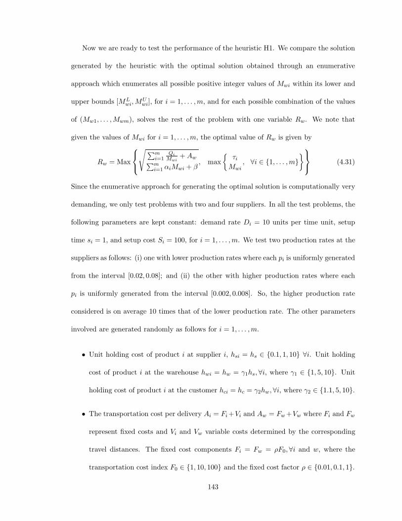
Now we are ready to test the performance of the heuristic H1. We compare the solution

generated by the heuristic with the optimal solution obtained through an enumerative

approach which enumerates all possible positive integer values of Mwi within its lower and

upper bounds [MLwi,M

Uwi], for i = 1, . . . ,m, and for each possible combination of the values

of (Mw1, . . . ,Mwm), solves the rest of the problem with one variable Rw. We note that

given the values of Mwi for i = 1, . . . ,m, the optimal value of Rw is given by

Rw = Max

√∑mi=1

QiMwi

+ Aw∑mi=1 αiMwi + β

, max

τi

Mwi, ∀i ∈ 1, . . . ,m

(4.31)

Since the enumerative approach for generating the optimal solution is computationally very

demanding, we only test problems with two and four suppliers. In all the test problems, the

following parameters are kept constant: demand rate Di = 10 units per time unit, setup

time si = 1, and setup cost Si = 100, for i = 1, . . . ,m. We test two production rates at the

suppliers as follows: (i) one with lower production rates where each pi is uniformly generated

from the interval [0.02, 0.08]; and (ii) the other with higher production rates where each

pi is uniformly generated from the interval [0.002, 0.008]. So, the higher production rate

considered is on average 10 times that of the lower production rate. The other parameters

involved are generated randomly as follows for i = 1, . . . ,m.

• Unit holding cost of product i at supplier i, hsi = hs ∈ 0.1, 1, 10 ∀i. Unit holding

cost of product i at the warehouse hwi = hw = γ1hs,∀i, where γ1 ∈ 1, 5, 10. Unit

holding cost of product i at the customer hci = hc = γ2hw,∀i, where γ2 ∈ 1.1, 5, 10.

• The transportation cost per delivery Ai = Fi +Vi and Aw = Fw +Vw where Fi and Fw

represent fixed costs and Vi and Vw variable costs determined by the corresponding

travel distances. The fixed cost components Fi = Fw = ρF0,∀i and w, where the

transportation cost index F0 ∈ 1, 10, 100 and the fixed cost factor ρ ∈ 0.01, 0.1, 1.

143

Thus a value of 0.01 for the fixed cost factor implies very low fixed cost, while a value

of 1 implies relatively high fixed cost. The variable cost components Vi and Vw are

generated as follows. We assume that the suppliers are symmetrically arranged along

a vertical line above and below a horizontal line through the customer so that the

distance between neighboring suppliers is 0.2 units, and the horizontal distance from

each supplier to the customer is one unit. For example, if there are two suppliers, then

the (x, y) coordinates of the two suppliers are (0,−0.1), (0, 0.1) while those of the

customer are (1, 0). We consider three cases of the warehouse location: the warehouse

is located at (x, 0), where x ∈ 0.2, 0.5, 0.8. The distance between any two locations

is calculated as the Euclidean distance. The variable cost Vi and Vw are calculated as

the product of the transportation cost index F0 and the Euclidean distance between

the respective origin and destination.

For a given problem instance, while all the suppliers have the same holding costs, setup

costs, and fixed transportation costs, they differ in their processing times (and hence capac-

ity) and the variable transportation costs. We calculate the relative percentage gap between

the total cost of the heuristic solution and that of the optimal solution. The relative gap

(%) is defined as ZH1−Z∗

Z∗ × 100%, where ZH1 is the objective of the solution provided by

the heuristic H1 and Z∗ is the optimal objective value. For each combination of parameters

(pi, hs, γ1, γ2, F0, ρ, x), we test five different random instances. Table 4.1 shows the results

of our computational tests. Due to space restrictions, we aggregate the results correspond-

ing to the two different ranges of production rates (pi), three different values of the holding

costs at the supplier (hs), and the three different fixed cost factors (ρ). We provide both the

average and maximum gaps for each entry corresponding to a combination of (γ1, γ2, F0, x).

Thus each entry corresponds to 90 different problem instances. The overall average gap

144

has a very small value of 0.18%. The average gap with two suppliers is 0.13% while that

with four suppliers is 0.23%. The maximum among all the random test instances is 7.83%.

The heuristic is very fast. In most cases, the convergence was achieved within one round of

iterations between all the suppliers. In none of the cases, the CPU time was more than one

second. Therefore, we can conclude that the heuristic is capable of generating near optimal

solutions quickly for almost all the problems tested.

In general, the performance of the heuristic improves as we increase the value of γ2, the

holding cost multiplier for the customer. This is intuitive since when the holding cost at the

customer increases, the frequency of deliveries from the warehouse to the customer relative

to the frequency of delivery from the suppliers to the warehouse goes up. In other words,

the values of Mwi’s increase. Hence the difference in the solution value for a small deviation

from the optimal value for Mwi’s would be small. Also, when we increase the value of x

(i.e. move the warehouse closer to the customer), the gap in general decreases. The reason

for this is the same as the earlier one. When the warehouse is closer to the customer, the

values of Mwi’s increase and the heuristic performs better. In summary, the heuristic seems

to perform very well for most of the cases tested.

4.3 The Model under Policy (ii)

In our analysis so far, we have had the restriction that there can be only one delivery from a

supplier to the warehouse in each production cycle at the supplier. In this section, we study

the model under policy (ii) which relaxes this constraint and allows for multiple deliveries

to the warehouse per production cycle at a supplier. It should be noted that when multiple

deliveries per production cycle are allowed at the suppliers, Theorem 16 does not necessarily

hold. However, Policy (ii) requires a feasible schedule to satisfy that theorem, i.e. there are

145

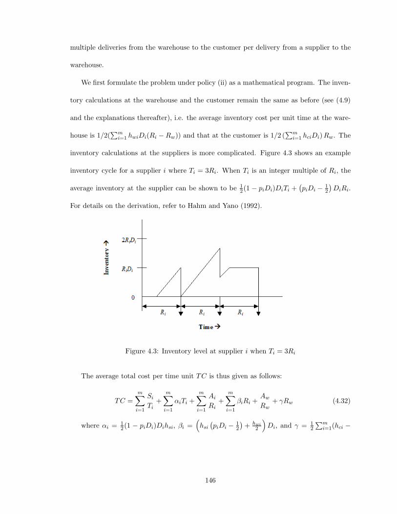
multiple deliveries from the warehouse to the customer per delivery from a supplier to the

warehouse.

We first formulate the problem under policy (ii) as a mathematical program. The inven-

tory calculations at the warehouse and the customer remain the same as before (see (4.9)

and the explanations thereafter), i.e. the average inventory cost per unit time at the ware-

house is 1/2(∑m

i=1 hwiDi(Ri − Rw)) and that at the customer is 1/2 (∑m

i=1 hciDi)Rw. The

inventory calculations at the suppliers is more complicated. Figure 4.3 shows an example

inventory cycle for a supplier i where Ti = 3Ri. When Ti is an integer multiple of Ri, the

average inventory at the supplier can be shown to be 12(1 − piDi)DiTi +

(piDi − 1

2

)DiRi.

For details on the derivation, refer to Hahm and Yano (1992).

Figure 4.3: Inventory level at supplier i when Ti = 3Ri

The average total cost per time unit TC is thus given as follows:

TC =m∑

i=1

Si

Ti+

m∑

i=1

αiTi +m∑

i=1

Ai

Ri+

m∑

i=1

βiRi +Aw

Rw+ γRw (4.32)

where αi = 12(1 − piDi)Dihsi, βi =

(hsi

(piDi − 1

2

)+ hwi

2

)Di, and γ = 1

2

∑mi=1(hci −

146

hwi)Di. Our problem under policy (ii) can be formulated as follows:

Minimize TC (4.33)

Subject to: Ti ≥ τi, ∀i ∈ 1, . . . ,m (4.34)

Ti

Riis a positive integer, ∀i ∈ 1, . . . ,m (4.35)

Ri

Rwis a positive integer, ∀i ∈ 1, . . . ,m (4.36)

Rw ≥ 0 (4.37)

We propose a heuristic in Section 4.3.1 to solve this problem, and use this heuristic

to study the value of warehouse in Section 4.3.2. Some other insights obtained from our

computational experiments are provided in Section 4.3.3.

4.3.1 A Heuristic Solution

The idea of the heuristic is similar to that of heuristic H1 proposed in Section 2. The

formulation (4.33) - (4.37) can be written as follows with Ms1, . . . ,Msm, Mw1, . . . ,Mwm,

and Rw as the decision variables:

Minimizem∑

i=1

Si

MsiMwiRw+

m∑

i=1

αiMsiMwiRw +m∑

i=1

Ai

MwiRw

+m∑

i=1

βiMwiRw +Aw

Rw+ γRw (4.38)

Subject to: MsiMwiRw ≥ τi, ∀i ∈ 1, . . . ,m (4.39)

Msi and Mwi are positive integers, ∀i ∈ 1, . . . ,m (4.40)

Rw ≥ 0 (4.41)

The heuristic tries to find a near optimal solution (Ms1, . . . ,Msm,Mw1, . . . ,Mwm, Rw) to

the formulation (4.38) - (4.41) through the following iterative procedure: In each iteration,

the heuristic chooses one supplier and fixes the Msi and Mwi values for all the other m− 1

147

suppliers. Then it solves the remaining problem with three decision variables Rw,Msi, and

Mwi for the chosen supplier using an approach similar to the one in heuristic H1. In solving

this problem, we try out four different combinations of Msi and Mwi values for the chosen

supplier, and the best solution is used. If the resulting total cost is lower, then the value of

Msi and Mwi for the chosen supplier are updated and fixed in the next several iterations.

The procedure stops when no improvement is found in one round of iterations across all the

suppliers.

Heuristic H2

Step 1: Set T 0i = Max

√Si/αi, τi

, R0

i =√

Ai/βi, and R0w =

√Aw/γ, M0

si = T 0i

R0i,

M0wi = R0

iR0

w, for i = 1, . . . ,m. Set supplier index j = 1, the iteration counter c = 0, and the

non-improvement counter n = 0. Set the total cost TC0 = ∞.

Step 2: Set c = c + 1. For supplier j, let Msj = maxbM0

sjc, 1

. Let M ′wj =

R′j

R′w, where

R′j = Max

√√√√Sj

Msj+ Aj

αjMsj + βj,

τj

Msj

(4.42)

R′w = Max

√√√√∑m

i=1,i 6=j

(Si

M0si

+ Ai

)1

M0wi

+ Aw∑m

i=1,i 6=j(αiM0si + βi)M0

wi + γ, max

τi

M0siM

0wi

, ∀i6=j

(4.43)

Set Mwj = maxbM0

wjc, 1

, and define Rw as follows:

Rw = Max

√√√√∑n

i=1,i 6=j

(Si

M0si

+ Ai

)1

M0wi

+ Aw +(

Sj

Msj+ Aj

)1

Mwj∑ni=1,i 6=j(αiM0

si + βi)M0wi + γ + (αjMsj + βj)Mwj

,τj

MsjMwj, max

τi

M0siM

0wi

∀i6=j

(4.44)

Calculate the total cost TC of the solution (Ms1, . . . ,Msm,Mw1, . . . ,Mwm, Rw) with Msj =

Msj, Mwj = Mwj at supplier j, Msi = M0si and Mwi = M0

wi for i 6= j, and Rw = Rw.

Similarly, calculate the total costs of the other three solutions where only the values of

148

(Msj , Mwj) are defined differently to be(max

bM0

sjc, 1

, dM0wje),(dM0

sje,maxbM0

wjc, 1)

,

and(dM0

sje, dM0wje), respectively. Choose the solution with the lowest total cost. Let the

total cost of this solution be TCj.

Step 3: If c ≤ m, let M0sj and M0

wj be equal to the Msj and Mwj corresponding to the

solution chosen in Step 2. If c ≥ m and TCj < TC0, let TC0 = TCj and let M0sj and M0

wj

be equal to the Msj and Mwj corresponding to the solution chosen in Step 2, and reset

n = 0. If c ≥ m and TCj ≥ TC0, let n = n + 1.

Step 4: If n = m, there has been no cost improvement for any supplier in the last set of

iterations, and hence STOP. Otherwise, if j = m, set j = 1, else set j = j + 1. Go to Step

2.

Similar to heuristic H1, in the first m iterations, we find an integer solution for the two

variables (Msj,Mwj) at each supplier. After these iterations, we try to improve the existing

feasible solution, choosing one supplier at a time.

We evaluate the performance of heuristic H2 by comparing the solution generated by

it with the optimal solution obtained by an enumerative approach which enumerates all

possible positive integer values of Msi and Mwi within their valid lower and upper bounds,

for i = 1, . . . ,m. We will discuss how to generate a valid lower and upper bound for each

of these variables in the paragraphs that follow. Given the values of these variables, the

optimal value of Rw is given by

Rw = Max

√√√√∑n

i=1

(Si

Msi+ Ai

)1

Mwi+ Aw

∑ni=1(αiM0

si + βi)Mwi + γ, Max

τi

MsiMwi, i = 1, . . . ,m

(4.45)

A lower and upper bound of each M variable in the formulation (4.38) - (4.41) can be

derived in the same way as what we have done for the M variables in the formulation (4.25)

149

- (4.27) in Section 2. For i = 1, . . . ,m, define Ui = αiT0i + Si/T

0i , and Vi = βiR

0i + Ai/R

0i ,

and define W = γR0w + Aw/R0

w, where T 0i , R0

i , and R0w are defined in Step 1 of heuristic

H2. Let ZH2 denote the objective value of the solution obtained by heuristic H2 for the

problem (4.38) - (4.41). Then in any optimal solution of the problem, we have

γRw + Aw/Rw ≤ ZH2 −m∑

i=1

(Ui + Vi)

βjRj + Aj/Rj ≤ ZH2 −m∑

i=1

(Ui + Vi) + Vj − W, for j = 1, . . . ,m

αjTj + Sj/Tj ≤ ZH2 −m∑

i=1

(Ui + Vi) + Uj − W, for j = 1, . . . ,m

which imply that in any optimal solution of the problem (4.38) - (4.41), Rw ∈ [RLw, RU

w ],

Rj ∈ [RLj , RU

j ] and Tj ∈ [TLj , TU

j ], for j = 1, . . . ,m, where

RLw =

(ZH2 −

∑mi=1(Ui + Vi)

)−√

(ZH2 −∑m

i=1(Ui + Vi))2 − 4γAw

2γ

RUw =

(ZH2 −

∑mi=1(Ui + Vi)

)+√

(ZH2 −∑m

i=1(Ui + Vi))2 − 4γAw

2γ

RLj =

(ZH2 −

∑mi=1(Ui + Vi) + Vj − W

)−√

(ZH2 −∑m

i=1(Ui + Vi) + Vj − W )2 − 4βjAj

2βj

RUj =

(ZH2 −

∑mi=1(Ui + Vi) + Vj − W

)+√

(ZH2 −∑m

i=1(Ui + Vi) + Vj − W )2 − 4βjAj

2βj

T Lj = max

(ZH2 −

∑mi=1(Ui + Vi) + Uj − W

)−√(

ZH2 −∑m

i=1(Ui + Vi) + Uj − W)2 − 4αjSj

2αj, τj

T U

j = max

(ZH2 −

∑mi=1(Ui + Vi) + Uj − W

)+√(

ZH2 −∑m

i=1(Ui + Vi) + Uj − W)2 − 4αjSj

2αj, τj

Based on the above-derived lower and upper bounds of Rw, R1, . . . , Rm, and T1, . . . , Tm,

we can conclude that in any optimal solution to the problem (4.38) - (4.41), the values of

Msi and Mwi, for every i = 1, . . . ,m, are within the interval [MLsi,M

Usi ] and [ML

wi,MUwi],

respectively, where MLsi = dTL

i /RUi e, MU

si = bTUi /RL

i c, MLwi = dRL

i /RUwe, and MU

wi =

bRUi /RL

wc.

150

Now we are ready to test the performance of heuristic H2. The parameter settings for

the experiments are exactly the same as the ones for heuristic H1. Since the computational

complexity for the enumeration procedure for policy (ii) is much higher than the enumera-

tion procedure under policy (i), it is not possible to test for four suppliers within reasonable

amounts of computational time. Hence we test cases with two and three suppliers. The

results are shown in Table 4.2. Here again, the results are very good. The overall average

gap is 0.16% while the maximum gap is 4.61%. The average and maximum for the two

supplier cases are 0.19% and 4.61% respectively, while that for the three supplier cases are

0.12% and 3.88% respectively. The heuristic is very fast and none of the test instances

took more than one second of CPU time. We see a trend similar to that of H1. When the

multiplier values (Msi’s and Mwi’s) are large (such as low holding cost at the warehouse

with high holding cost at the customer), the gap is very close to zero.

4.3.2 The Value of Warehouse

In the supply chains we consider, there is a warehouse between the suppliers and the cus-

tomer and the products from the suppliers are consolidated at the warehouse for delivery to

the customer. It is well-understood conceptually that the presence of a warehouse can lower

the transportation and inventory costs compared to a single-stage supply chain where there

is no warehouse between the suppliers and the customer. There are several simulation stud-

ies that compare freight consolidation through a warehouse and direct shipments based on

transportation costs. For example, the study by Bagchi and Davis (1988) shows that direct

shipments from vendors are almost always more expensive. Cooper (1984) compares freight

consolidation across time and customers, use of warehouses, and direct less-than-truckload

distribution systems on the basis of distribution costs and delivery times for selected prod-

151

uct characteristics and demand patterns. She concludes that in general consolidation lowers

costs but this may lead to an increase in the delivery time. These existing studies focus

on transportation costs only and do not consider production operations and costs in the

system. To our knowledge, no existing studies have investigated the value of consolidation

or warehouses from a total system cost point of view. In this section, we computationally

evaluate the typical reduction of total production, inventory and transportation cost that

can be achieved by the use of a warehouse in the supply chain we consider. More specifically,

we compare the total costs per unit time for the following two supply chains:

1) The two-stage supply chain considered in this chapter where there are m suppliers,

one warehouse, and one customer;

2) A single-stage supply chain where there are also m suppliers and one customer as in

our supply chain, but with no warehouse between the suppliers and the customer, and

the product at each supplier is directly delivered to the customer.

We define the relative cost reduction with the addition of a warehouse as Z∗1−Z∗

2Z∗

1×100%,

where Z∗1 and Z∗

2 are the optimal total cost per unit time in the single-stage and two-stage

supply chains, respectively. Since there is no delivery consolidation in the single-stage supply

chain, that problem can be viewed as m separate single-supplier problems, each equivalent

to the model considered by Hahm and Yano (1992). Therefore, we solve the m separate

single-stage single-supplier problems optimally by applying the solution approach of Hahm

and Yano, and get the optimal total cost Z∗1 . We use heuristic H2 to solve the problem

with the two-stage supply chain, and use the total cost of the solution obtained by H2,

denoted as ZH2, to replace Z∗2 in calculating the relative cost reduction. Thus the relative

cost reduction we get in our computational test is a lower bound of the actual relative cost

reduction.

152

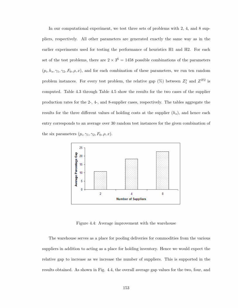
In our computational experiment, we test three sets of problems with 2, 4, and 8 sup-

pliers, respectively. All other parameters are generated exactly the same way as in the

earlier experiments used for testing the performance of heuristics H1 and H2. For each

set of the test problems, there are 2 × 36 = 1458 possible combinations of the parameters

(pi, hs, γ1, γ2, F0, ρ, x), and for each combination of these parameters, we run ten random

problem instances. For every test problem, the relative gap (%) between Z∗1 and ZH2 is

computed. Table 4.3 through Table 4.5 show the results for the two cases of the supplier

production rates for the 2-, 4-, and 8-supplier cases, respectively. The tables aggregate the

results for the three different values of holding costs at the supplier (hs), and hence each

entry corresponds to an average over 30 random test instances for the given combination of

the six parameters (pi, γ1, γ2, F0, ρ, x).

Figure 4.4: Average improvement with the warehouse

The warehouse serves as a place for pooling deliveries for commodities from the various

suppliers in addition to acting as a place for holding inventory. Hence we would expect the

relative gap to increase as we increase the number of suppliers. This is supported in the

results obtained. As shown in Fig. 4.4, the overall average gap values for the two, four, and

153

eight supplier cases are 10.75%, 18.18%, and 22.71% respectively. The few negative values

in the tables indicate instances where adding a warehouse increases the total costs. Again

we notice that the magnitude and the occurrence of negative values in general go down when

we increase the number of suppliers. For all the results, in general, the relative gap increases

as the holding cost at the customer goes up, or when the variable transportation cost goes

up. The gap also increases with a reduction in the fixed cost factor value. The explanations

for these are straightforward. All these changes make the warehouse an inexpensive transit

point. The effect of the location of the warehouse on total cost is more involved. When both

the holding cost at the customer and the variable transportation cost are high, we would

like to have small and frequent shipments to save on the holding costs at the customer,

but would like to avoid traveling long distances to contain the transportation expense. So

it is advantageous to have the warehouse at close proximity to the customer site. On the

other hand, if the holding cost at the customer is low when the transportation cost is high,

we would like to make large shipments from the warehouse to the customer anyway, and

hence placing the warehouse close to the supplier would reduce the delivery expenses from

the supplier to the warehouse. Hence we see that in the tables, the relative gap increases

with the value of x for the first case, and the gap decreases with x for the second. Finally,

we can see from these tables that the production rates of the suppliers have some impact

on the relative gap, but not as significant as the other parameters. Hence the suppliers’

production rates do not seem to play a critical role in deciding whether to use a warehouse

or not in the supply chain.

154

4.3.3 Other Insights

In this subsection, we discuss some other insights obtained from our computational experi-

ments.

Theoretically, policy (ii) should always give solutions that are at least as good as the

ones under policy (i) in terms of total cost. Since our heuristics do not guarantee to generate

optimal solutions, we can not assert that H2 will always dominate H1. But in general, since

both the heuristics have been shown to perform well in the computational experiments, we

can expect H2 to provide better solutions than H1 in most cases. That is the reason why

we chose H2 as the benchmark for the two-stage supply chain while evaluating the value of

warehouse in the previous subsection. In fact, a comparison between the solutions obtained

by H1 and H2 justify this choice. Due to the lack of space, we do not give any detailed

reports on this. Instead, we provide a summary of our findings. Out of a total of 14580

test problems for the two supplier case, there were only 6 cases where H1 beat H2. Even in

those cases, the gaps are very small in magnitude. The same holds true for the four supplier

case. With the eight supplier problem instances, there was not even a single test problem

for which H1 gave a total cost that was lower than the one given by H2. On average, the

objective values from H2 were 28.36%, 29.85%, and 30.24% lower than the objective values

from H1 for the two, four, and eight supplier cases respectively.

Another interesting insight obtained is about the multipliers Msi in the model under

policy (ii). A multiplier Msi represents the number of delivery cycles from supplier i to the

warehouse per production cycle at supplier i. Table 4.6 shows the average number of Msi’s

aggregated over the three cases of the number of suppliers (m) and the three cases of the

holding cost at the suppliers (hsi).

We would expect the multipliers to depend on the location of the warehouse. For

155

example, if the warehouse is closer to the suppliers, then the transportation cost from the

suppliers to the warehouse is going to be lower and hence there will be more shipments

from the suppliers per production cycle. This is supported in the results as the multipliers

drop when the warehouse location is moved from x = 0.2 to x = 0.5 or x = 0.8. Similarly,

we would expect the multiplier to decrease with the variable or fixed transportation cost.

This is reflected in the table as the multipliers drop with ρ or F0. We would expect the

shipments from the suppliers to become more frequent (hence smaller) as the holding cost

at the warehouse is increased. This observation is also supported in the table by the fact

that the multipliers increase with γ1.

Production rates can also play a crucial role. Production rates influence both the pro-

duction batch size and the inventory holding costs. If the production is too slow along

with a positive setup time, this may place restrictions on the batch size hence leading to

higher costs. The effect of production rates on the inventory holding cost is slightly more

complicated. A higher production rate may in fact be undesirable. This is because in the

case of higher production rates, an item that is meant for a future shipment gets ready at

an earlier time compared to a system with a lower production rate. This leads to increased

waiting time for that item before getting shipped, thus resulting in an increased inventory

holding cost at the supplier. Hence a higher production rate has both positive and negative

impacts. As mentioned in Section 2, many studies in the past assumed infinite production

rates at the suppliers. But Table 4.6 shows that changes in the production rate can signifi-

cantly impact the number of delivery cycles from the suppliers per production cycle. When

the production rates are increased by a factor of ten, the production-delivery cycle time

ratio drops significantly. In many cases, the ratio drops by more than 75% of its original

value.

156

4.4 Conclusions

In this study, we have studied a joint cyclic production and distribution scheduling problem

in a two-stage supply chain with one or more suppliers, one warehouse, and one customer.

We have given either optimal approaches or heuristic methods to solve the problem under

two policies on production and delivery cycles. For the case with common production

and delivery cycle at each supplier (policy (i)), we have proved that there exists an optimal

solution where the delivery cycle time from a supplier to the warehouse is an integer multiple

of the delivery cycle time from the warehouse to the customer. Based on this property, we

have shown that there is a closed-form optimal solution to the problem with a single supplier

under policy (i), and developed an efficient heuristic for the general problem under policy

(i). The problem under policy (ii), which is more general than policy (i), is solved by a

heuristic approach. Both heuristics are shown to perform very well for an extensive set

of test problems. We have also computationally evaluated the value of warehouse in our

two-stage supply chain. Various managerial insights have been reported.

An important use of this study is to make operational decisions regarding the delivery

intervals in a two-stage supply chain. The approaches provided in this chapter are easy

to implement. Moreover, computationally they are very efficient. The models can also be

used to make strategic decisions related to configuring or making changes to a supply chain.

For example, we could use the heuristics to choose between a single-stage and a two-stage

supply chain. Given that a warehouse has to be built, we could use this study to analyze

the total costs corresponding to various locations of the potential warehouse. We could use

the heuristics to analyze the trade-offs involved in moving an existing warehouse to a new

location. This model can also be used to analyze the effect of reducing the setup cost or

setup time on the performance of the entire supply chain. For example, reducing the setup

157

cost or setup time at the supplier would enable more frequent deliveries from the supplier to

the warehouse, thus saving on the average inventory costs. A trade-off between this savings

and the increase in the total transportation costs and the expenses related to reducing the

setup time and costs can be used to analyze whether it is worth trying for a reduction in

the setup cost or time.

158

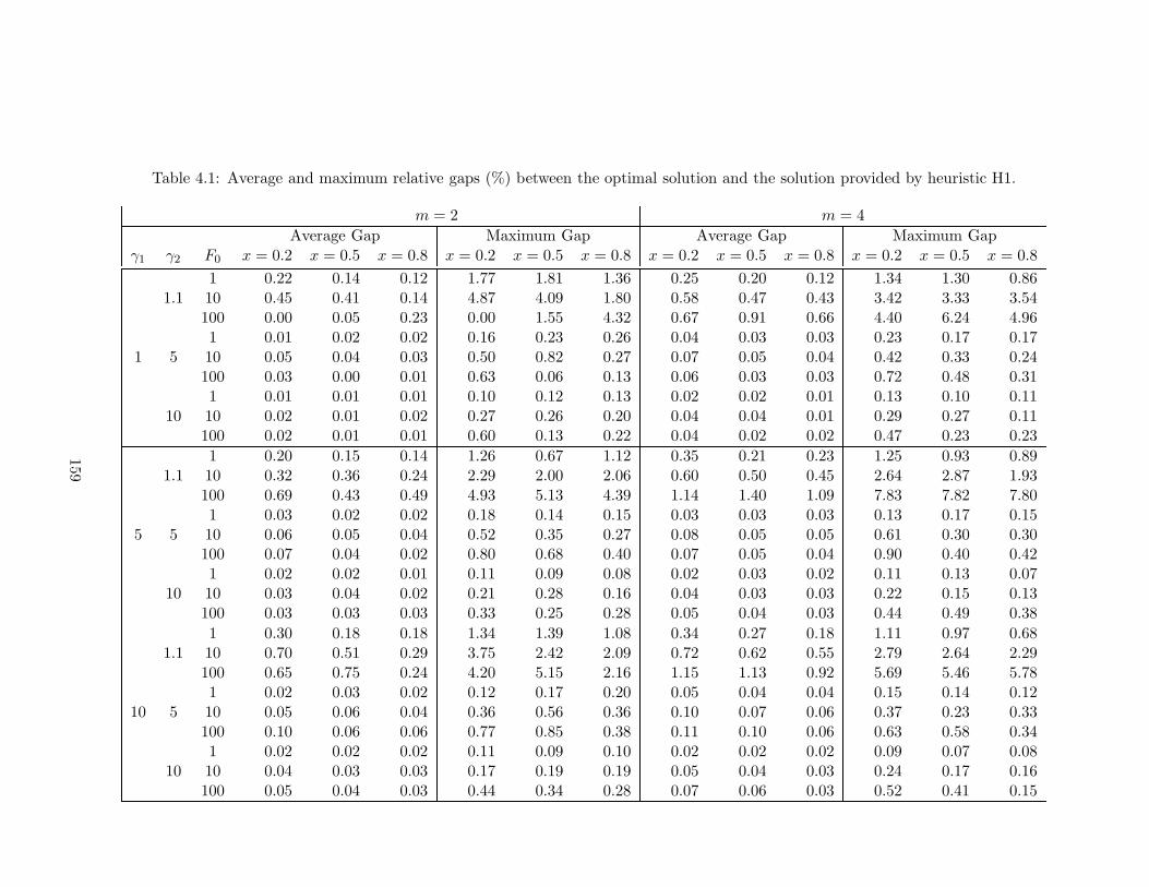
Table 4.1: Average and maximum relative gaps (%) between the optimal solution and the solution provided by heuristic H1.

m = 2 m = 4Average Gap Maximum Gap Average Gap Maximum Gap

γ1 γ2 F0 x = 0.2 x = 0.5 x = 0.8 x = 0.2 x = 0.5 x = 0.8 x = 0.2 x = 0.5 x = 0.8 x = 0.2 x = 0.5 x = 0.81 0.22 0.14 0.12 1.77 1.81 1.36 0.25 0.20 0.12 1.34 1.30 0.86

1.1 10 0.45 0.41 0.14 4.87 4.09 1.80 0.58 0.47 0.43 3.42 3.33 3.54100 0.00 0.05 0.23 0.00 1.55 4.32 0.67 0.91 0.66 4.40 6.24 4.961 0.01 0.02 0.02 0.16 0.23 0.26 0.04 0.03 0.03 0.23 0.17 0.17

1 5 10 0.05 0.04 0.03 0.50 0.82 0.27 0.07 0.05 0.04 0.42 0.33 0.24100 0.03 0.00 0.01 0.63 0.06 0.13 0.06 0.03 0.03 0.72 0.48 0.311 0.01 0.01 0.01 0.10 0.12 0.13 0.02 0.02 0.01 0.13 0.10 0.11

10 10 0.02 0.01 0.02 0.27 0.26 0.20 0.04 0.04 0.01 0.29 0.27 0.11100 0.02 0.01 0.01 0.60 0.13 0.22 0.04 0.02 0.02 0.47 0.23 0.231 0.20 0.15 0.14 1.26 0.67 1.12 0.35 0.21 0.23 1.25 0.93 0.89

1.1 10 0.32 0.36 0.24 2.29 2.00 2.06 0.60 0.50 0.45 2.64 2.87 1.93100 0.69 0.43 0.49 4.93 5.13 4.39 1.14 1.40 1.09 7.83 7.82 7.801 0.03 0.02 0.02 0.18 0.14 0.15 0.03 0.03 0.03 0.13 0.17 0.15

5 5 10 0.06 0.05 0.04 0.52 0.35 0.27 0.08 0.05 0.05 0.61 0.30 0.30100 0.07 0.04 0.02 0.80 0.68 0.40 0.07 0.05 0.04 0.90 0.40 0.421 0.02 0.02 0.01 0.11 0.09 0.08 0.02 0.03 0.02 0.11 0.13 0.07

10 10 0.03 0.04 0.02 0.21 0.28 0.16 0.04 0.03 0.03 0.22 0.15 0.13100 0.03 0.03 0.03 0.33 0.25 0.28 0.05 0.04 0.03 0.44 0.49 0.381 0.30 0.18 0.18 1.34 1.39 1.08 0.34 0.27 0.18 1.11 0.97 0.68

1.1 10 0.70 0.51 0.29 3.75 2.42 2.09 0.72 0.62 0.55 2.79 2.64 2.29100 0.65 0.75 0.24 4.20 5.15 2.16 1.15 1.13 0.92 5.69 5.46 5.781 0.02 0.03 0.02 0.12 0.17 0.20 0.05 0.04 0.04 0.15 0.14 0.12

10 5 10 0.05 0.06 0.04 0.36 0.56 0.36 0.10 0.07 0.06 0.37 0.23 0.33100 0.10 0.06 0.06 0.77 0.85 0.38 0.11 0.10 0.06 0.63 0.58 0.341 0.02 0.02 0.02 0.11 0.09 0.10 0.02 0.02 0.02 0.09 0.07 0.08

10 10 0.04 0.03 0.03 0.17 0.19 0.19 0.05 0.04 0.03 0.24 0.17 0.16100 0.05 0.04 0.03 0.44 0.34 0.28 0.07 0.06 0.03 0.52 0.41 0.15

159

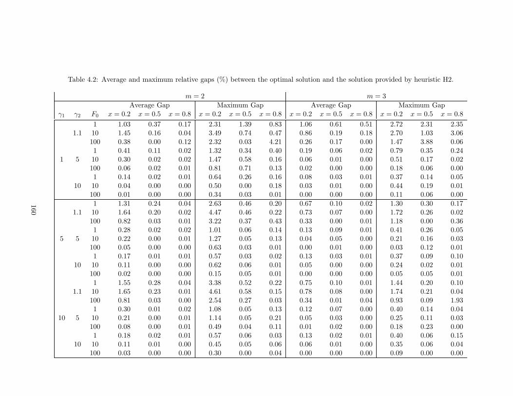
Table 4.2: Average and maximum relative gaps (%) between the optimal solution and the solution provided by heuristic H2.

m = 2 m = 3Average Gap Maximum Gap Average Gap Maximum Gap

γ1 γ2 F0 x = 0.2 x = 0.5 x = 0.8 x = 0.2 x = 0.5 x = 0.8 x = 0.2 x = 0.5 x = 0.8 x = 0.2 x = 0.5 x = 0.81 1.03 0.37 0.17 2.31 1.39 0.83 1.06 0.61 0.51 2.72 2.31 2.35

1.1 10 1.45 0.16 0.04 3.49 0.74 0.47 0.86 0.19 0.18 2.70 1.03 3.06100 0.38 0.00 0.12 2.32 0.03 4.21 0.26 0.17 0.00 1.47 3.88 0.061 0.41 0.11 0.02 1.32 0.34 0.40 0.19 0.06 0.02 0.79 0.35 0.24

1 5 10 0.30 0.02 0.02 1.47 0.58 0.16 0.06 0.01 0.00 0.51 0.17 0.02100 0.06 0.02 0.01 0.81 0.71 0.13 0.02 0.00 0.00 0.18 0.06 0.001 0.14 0.02 0.01 0.64 0.26 0.16 0.08 0.03 0.01 0.37 0.14 0.05

10 10 0.04 0.00 0.00 0.50 0.00 0.18 0.03 0.01 0.00 0.44 0.19 0.01100 0.01 0.00 0.00 0.34 0.03 0.01 0.00 0.00 0.00 0.11 0.06 0.001 1.31 0.24 0.04 2.63 0.46 0.20 0.67 0.10 0.02 1.30 0.30 0.17

1.1 10 1.64 0.20 0.02 4.47 0.46 0.22 0.73 0.07 0.00 1.72 0.26 0.02100 0.82 0.03 0.01 3.22 0.37 0.43 0.33 0.00 0.01 1.18 0.00 0.361 0.28 0.02 0.02 1.01 0.06 0.14 0.13 0.09 0.01 0.41 0.26 0.05

5 5 10 0.22 0.00 0.01 1.27 0.05 0.13 0.04 0.05 0.00 0.21 0.16 0.03100 0.05 0.00 0.00 0.63 0.03 0.01 0.00 0.01 0.00 0.03 0.12 0.011 0.17 0.01 0.01 0.57 0.03 0.02 0.13 0.03 0.01 0.37 0.09 0.10

10 10 0.11 0.00 0.00 0.62 0.06 0.01 0.05 0.00 0.00 0.24 0.02 0.01100 0.02 0.00 0.00 0.15 0.05 0.01 0.00 0.00 0.00 0.05 0.05 0.011 1.55 0.28 0.04 3.38 0.52 0.22 0.75 0.10 0.01 1.44 0.20 0.10

1.1 10 1.65 0.23 0.01 4.61 0.58 0.15 0.78 0.08 0.00 1.74 0.21 0.04100 0.81 0.03 0.00 2.54 0.27 0.03 0.34 0.01 0.04 0.93 0.09 1.931 0.30 0.01 0.02 1.08 0.05 0.13 0.12 0.07 0.00 0.40 0.14 0.04

10 5 10 0.21 0.00 0.01 1.14 0.05 0.21 0.05 0.03 0.00 0.25 0.11 0.03100 0.08 0.00 0.01 0.49 0.04 0.11 0.01 0.02 0.00 0.18 0.23 0.001 0.18 0.02 0.01 0.57 0.06 0.03 0.13 0.02 0.01 0.40 0.06 0.15

10 10 0.11 0.01 0.00 0.45 0.05 0.06 0.06 0.01 0.00 0.35 0.06 0.04100 0.03 0.00 0.00 0.30 0.00 0.04 0.00 0.00 0.00 0.09 0.00 0.00

160

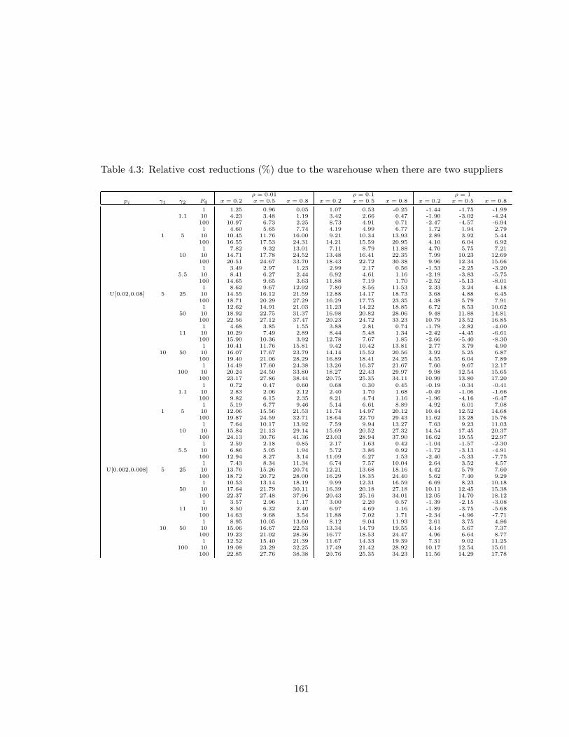
Table 4.3: Relative cost reductions (%) due to the warehouse when there are two suppliers

ρ = 0.01 ρ = 0.1 ρ = 1pi γ1 γ2 F0 x = 0.2 x = 0.5 x = 0.8 x = 0.2 x = 0.5 x = 0.8 x = 0.2 x = 0.5 x = 0.8

1 1.25 0.96 0.05 1.07 0.53 -0.25 -1.44 -1.75 -1.991.1 10 4.23 3.48 1.19 3.42 2.66 0.47 -1.90 -3.02 -4.24

100 10.97 6.73 2.25 8.73 4.91 0.71 -2.47 -4.57 -6.941 4.60 5.65 7.74 4.19 4.99 6.77 1.72 1.94 2.79

1 5 10 10.45 11.76 16.00 9.21 10.34 13.93 2.89 3.92 5.44100 16.55 17.53 24.31 14.21 15.59 20.95 4.10 6.04 6.921 7.82 9.32 13.01 7.11 8.79 11.88 4.70 5.75 7.21

10 10 14.71 17.78 24.52 13.48 16.41 22.35 7.99 10.23 12.69100 20.51 24.67 33.70 18.43 22.72 30.38 9.96 12.34 15.661 3.49 2.97 1.23 2.99 2.17 0.56 -1.53 -2.25 -3.20

5.5 10 8.41 6.27 2.44 6.92 4.61 1.16 -2.19 -3.83 -5.75100 14.65 9.65 3.63 11.88 7.19 1.70 -2.52 -5.13 -8.011 8.62 9.67 12.92 7.80 8.56 11.53 2.33 3.24 4.18

U[0.02,0.08] 5 25 10 14.55 16.12 21.59 12.88 14.17 18.73 3.68 4.88 6.45100 18.71 20.29 27.29 16.29 17.75 23.35 4.38 5.79 7.911 12.62 14.91 21.03 11.23 14.22 18.85 6.72 8.53 10.62

50 10 18.92 22.75 31.37 16.98 20.82 28.06 9.48 11.88 14.81100 22.56 27.12 37.47 20.23 24.72 33.23 10.79 13.52 16.851 4.68 3.85 1.55 3.88 2.81 0.74 -1.79 -2.82 -4.00

11 10 10.29 7.49 2.89 8.44 5.48 1.34 -2.42 -4.45 -6.61100 15.90 10.36 3.92 12.78 7.67 1.85 -2.66 -5.40 -8.301 10.41 11.76 15.81 9.42 10.42 13.81 2.77 3.79 4.90

10 50 10 16.07 17.67 23.79 14.14 15.52 20.56 3.92 5.25 6.87100 19.40 21.06 28.29 16.89 18.41 24.25 4.55 6.04 7.891 14.49 17.60 24.38 13.26 16.37 21.67 7.60 9.67 12.17

100 10 20.24 24.50 33.80 18.27 22.43 29.97 9.98 12.54 15.65100 23.17 27.86 38.44 20.75 25.35 34.11 10.99 13.80 17.201 0.72 0.47 0.60 0.68 0.30 0.45 -0.19 -0.34 -0.41

1.1 10 2.83 2.06 2.12 2.40 1.70 1.68 -0.49 -1.06 -1.66100 9.82 6.15 2.35 8.21 4.74 1.16 -1.96 -4.16 -6.471 5.19 6.77 9.46 5.14 6.61 8.89 4.92 6.01 7.08

1 5 10 12.06 15.56 21.53 11.74 14.97 20.12 10.44 12.52 14.68100 19.87 24.59 32.71 18.64 22.70 29.43 11.62 13.28 15.761 7.64 10.17 13.92 7.59 9.94 13.27 7.63 9.23 11.03

10 10 15.84 21.13 29.14 15.69 20.52 27.32 14.54 17.45 20.37100 24.13 30.76 41.36 23.03 28.94 37.90 16.62 19.55 22.971 2.59 2.18 0.85 2.17 1.63 0.42 -1.04 -1.57 -2.30

5.5 10 6.86 5.05 1.94 5.72 3.86 0.92 -1.72 -3.13 -4.91100 12.94 8.27 3.14 11.09 6.27 1.53 -2.40 -5.33 -7.751 7.43 8.34 11.34 6.74 7.57 10.04 2.64 3.52 4.57

U[0.002,0.008] 5 25 10 13.76 15.26 20.74 12.21 13.68 18.16 4.42 5.79 7.60100 18.72 20.72 28.00 16.29 18.35 24.40 5.62 7.40 9.291 10.53 13.14 18.19 9.99 12.31 16.59 6.69 8.23 10.18

50 10 17.64 21.79 30.11 16.39 20.18 27.18 10.11 12.45 15.38100 22.37 27.48 37.96 20.43 25.16 34.01 12.05 14.70 18.121 3.57 2.96 1.17 3.00 2.20 0.57 -1.39 -2.15 -3.08

11 10 8.50 6.32 2.40 6.97 4.69 1.16 -1.89 -3.75 -5.68100 14.63 9.68 3.54 11.88 7.02 1.71 -2.34 -4.96 -7.711 8.95 10.05 13.60 8.12 9.04 11.93 2.61 3.75 4.86

10 50 10 15.06 16.67 22.53 13.34 14.79 19.55 4.14 5.67 7.37100 19.23 21.02 28.36 16.77 18.53 24.47 4.96 6.64 8.771 12.52 15.40 21.39 11.67 14.33 19.39 7.31 9.02 11.25

100 10 19.08 23.29 32.25 17.49 21.42 28.92 10.17 12.54 15.61100 22.85 27.76 38.38 20.76 25.35 34.23 11.56 14.29 17.78

161

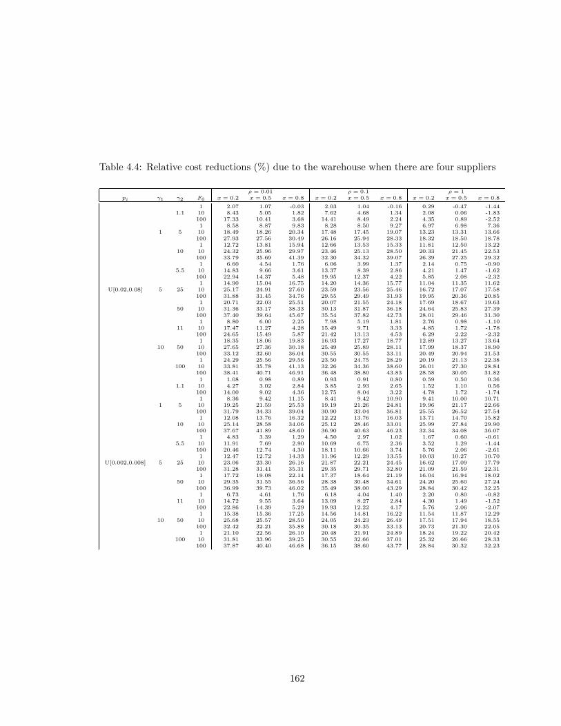
Table 4.4: Relative cost reductions (%) due to the warehouse when there are four suppliers

ρ = 0.01 ρ = 0.1 ρ = 1pi γ1 γ2 F0 x = 0.2 x = 0.5 x = 0.8 x = 0.2 x = 0.5 x = 0.8 x = 0.2 x = 0.5 x = 0.8

1 2.07 1.07 -0.03 2.03 1.04 -0.16 0.29 -0.47 -1.441.1 10 8.43 5.05 1.82 7.62 4.68 1.34 2.08 0.06 -1.83

100 17.33 10.41 3.68 14.41 8.49 2.24 4.35 0.89 -2.521 8.58 8.87 9.83 8.28 8.50 9.27 6.97 6.98 7.36

1 5 10 18.49 18.26 20.34 17.48 17.45 19.07 13.23 13.31 13.66100 27.93 27.56 30.49 26.16 25.94 28.33 18.32 18.50 18.781 12.72 13.81 15.94 12.66 13.53 15.33 11.81 12.50 13.22

10 10 24.32 25.96 29.97 23.46 25.13 28.50 20.33 21.45 22.53100 33.79 35.69 41.39 32.30 34.32 39.07 26.39 27.25 29.321 6.60 4.54 1.76 6.06 3.99 1.37 2.14 0.75 -0.90

5.5 10 14.83 9.66 3.61 13.37 8.39 2.86 4.21 1.47 -1.62100 22.94 14.37 5.48 19.95 12.37 4.22 5.85 2.08 -2.321 14.90 15.04 16.75 14.20 14.36 15.77 11.04 11.35 11.62

U[0.02,0.08] 5 25 10 25.17 24.91 27.60 23.59 23.56 25.46 16.72 17.07 17.58100 31.88 31.45 34.76 29.55 29.49 31.93 19.95 20.36 20.851 20.71 22.03 25.51 20.07 21.55 24.18 17.69 18.67 19.63

50 10 31.36 33.17 38.33 30.13 31.87 36.18 24.64 25.83 27.39100 37.40 39.64 45.67 35.54 37.82 42.73 28.01 29.46 31.301 8.80 6.00 2.25 7.98 5.19 1.81 2.76 0.98 -1.10

11 10 17.47 11.27 4.28 15.49 9.71 3.33 4.85 1.72 -1.78100 24.65 15.49 5.87 21.42 13.13 4.53 6.29 2.22 -2.321 18.35 18.06 19.83 16.93 17.27 18.77 12.89 13.27 13.64

10 50 10 27.65 27.36 30.18 25.49 25.89 28.11 17.99 18.37 18.90100 33.12 32.60 36.04 30.55 30.55 33.11 20.49 20.94 21.531 24.29 25.56 29.56 23.50 24.75 28.29 20.19 21.13 22.38

100 10 33.81 35.78 41.13 32.26 34.36 38.60 26.01 27.30 28.84100 38.41 40.71 46.91 36.48 38.80 43.83 28.58 30.05 31.821 1.08 0.98 0.89 0.93 0.91 0.80 0.59 0.50 0.36

1.1 10 4.27 3.02 2.84 3.85 2.93 2.65 1.52 1.10 0.56100 14.00 9.02 4.36 12.75 8.04 3.22 4.78 1.72 -1.741 8.36 9.42 11.15 8.41 9.42 10.90 9.41 10.00 10.71

1 5 10 19.25 21.59 25.53 19.19 21.26 24.81 19.96 21.17 22.66100 31.79 34.33 39.04 30.90 33.04 36.81 25.55 26.52 27.541 12.08 13.76 16.32 12.22 13.76 16.03 13.71 14.70 15.82

10 10 25.14 28.58 34.06 25.12 28.46 33.01 25.99 27.84 29.90100 37.67 41.89 48.60 36.90 40.63 46.23 32.34 34.08 36.071 4.83 3.39 1.29 4.50 2.97 1.02 1.67 0.60 -0.61

5.5 10 11.91 7.69 2.90 10.69 6.75 2.36 3.52 1.29 -1.44100 20.46 12.74 4.30 18.11 10.66 3.74 5.76 2.06 -2.611 12.47 12.72 14.33 11.96 12.29 13.55 10.03 10.27 10.70

U[0.002,0.008] 5 25 10 23.06 23.30 26.16 21.87 22.21 24.45 16.62 17.09 17.79100 31.28 31.41 35.31 29.35 29.71 32.80 21.09 21.59 22.311 17.72 19.08 22.14 17.37 18.64 21.19 16.04 16.94 18.02

50 10 29.35 31.55 36.56 28.38 30.48 34.61 24.20 25.60 27.24100 36.99 39.73 46.02 35.49 38.00 43.29 28.84 30.42 32.251 6.73 4.61 1.76 6.18 4.04 1.40 2.20 0.80 -0.82

11 10 14.72 9.55 3.64 13.09 8.27 2.84 4.30 1.49 -1.52100 22.86 14.39 5.29 19.93 12.22 4.17 5.76 2.06 -2.071 15.38 15.36 17.25 14.56 14.81 16.22 11.54 11.87 12.29

10 50 10 25.68 25.57 28.50 24.05 24.23 26.49 17.51 17.94 18.55100 32.42 32.21 35.88 30.18 30.35 33.13 20.73 21.30 22.051 21.10 22.56 26.10 20.48 21.91 24.89 18.24 19.22 20.42

100 10 31.81 33.96 39.25 30.55 32.66 37.01 25.32 26.66 28.33100 37.87 40.40 46.68 36.15 38.60 43.77 28.84 30.32 32.23

162

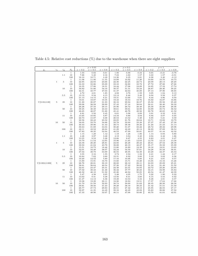
Table 4.5: Relative cost reductions (%) due to the warehouse when there are eight suppliers

ρ = 0.01 ρ = 0.1 ρ = 1pi γ1 γ2 F0 x = 0.2 x = 0.5 x = 0.8 x = 0.2 x = 0.5 x = 0.8 x = 0.2 x = 0.5 x = 0.8

1 1.03 0.82 0.61 1.06 0.88 0.24 0.65 -0.21 -0.781.1 10 7.88 5.40 2.16 7.03 4.82 1.57 3.22 1.57 -0.51

100 16.10 10.71 4.49 14.26 9.25 2.81 6.28 3.40 -0.121 11.08 11.06 11.55 10.89 10.92 11.26 10.60 10.70 10.73

1 5 10 22.85 22.83 23.66 22.36 22.25 22.74 20.09 20.13 20.20100 34.33 33.86 35.09 33.10 32.80 33.72 27.72 27.88 27.661 16.35 17.06 18.31 16.44 17.06 18.09 16.95 17.32 17.74

10 10 30.82 31.86 34.16 30.37 31.31 33.24 28.87 29.46 30.25100 42.31 43.77 47.03 41.37 42.64 45.09 37.13 37.96 38.651 4.72 4.01 1.85 4.82 3.76 1.59 3.05 1.84 0.13

5.5 10 13.12 9.34 4.15 12.14 8.46 3.48 6.04 3.58 0.37100 21.14 14.15 6.21 19.31 12.66 5.01 8.44 4.86 0.501 19.01 18.87 19.35 18.43 18.53 18.76 16.92 16.87 16.86

U[0.02,0.08] 5 25 10 31.20 30.87 31.93 30.16 29.94 30.57 25.50 25.56 25.49100 39.06 38.58 39.99 37.43 37.16 38.04 30.41 30.40 30.321 26.28 27.33 29.15 25.96 26.72 28.48 25.30 25.90 26.36

50 10 39.25 40.49 43.43 38.61 39.61 42.00 34.99 35.74 36.52100 46.65 48.07 51.60 45.41 46.78 49.56 39.78 40.65 41.521 6.81 5.50 2.45 6.61 5.06 2.09 3.91 2.33 0.21

11 10 15.65 10.85 4.87 14.34 9.86 4.04 6.94 4.07 0.45100 22.73 15.07 6.68 20.53 13.52 5.49 8.95 5.21 0.591 22.56 22.43 23.52 22.05 21.76 22.64 19.71 19.82 19.79

10 50 10 34.05 33.70 34.88 32.78 32.69 33.39 27.37 27.43 27.39100 40.43 39.96 41.42 38.74 38.48 39.39 31.20 31.23 31.141 30.64 31.69 34.04 30.20 31.07 33.22 28.72 29.32 29.98

100 10 42.11 43.52 46.64 41.29 42.40 45.14 36.93 37.69 38.54100 47.83 49.35 52.94 46.53 47.99 50.81 40.57 41.44 42.321 1.15 1.29 1.12 1.18 1.26 1.06 1.14 0.93 0.80

1.1 10 4.48 3.97 3.48 4.19 3.84 3.40 2.94 2.42 1.86100 13.55 9.52 5.28 12.66 8.67 4.55 6.83 4.01 0.471 10.79 11.54 12.65 10.96 11.65 12.63 12.70 13.13 13.58

1 5 10 24.58 26.20 28.81 24.66 26.28 28.44 26.61 27.52 28.38100 39.50 41.04 43.78 38.88 40.19 42.27 35.17 35.58 35.991 15.51 16.73 18.46 15.80 16.89 18.39 18.18 18.91 19.65

10 10 32.01 34.48 38.07 32.24 34.50 37.61 34.28 35.58 36.91100 47.04 49.79 53.99 46.55 48.95 52.38 43.29 44.37 45.531 3.55 3.16 1.55 3.74 2.94 1.34 2.41 1.44 0.17

5.5 10 10.84 7.62 3.60 10.31 6.92 3.00 5.10 3.02 0.36100 19.20 12.52 5.89 17.44 10.96 5.00 8.21 4.81 0.571 15.89 15.91 16.70 15.60 15.71 16.28 15.05 15.16 15.26

U[0.002,0.008] 5 25 10 28.78 28.81 30.19 28.00 28.12 29.11 24.93 25.09 25.21100 38.61 38.64 40.54 37.26 37.42 38.82 31.34 31.49 31.501 22.61 23.47 25.31 22.48 23.31 24.83 22.72 23.26 23.85

50 10 37.02 38.43 41.46 36.42 37.77 40.23 34.15 34.98 35.84100 46.32 48.10 51.92 45.26 46.94 50.05 40.54 41.47 42.391 5.47 4.38 2.05 5.48 4.05 1.75 3.20 1.90 0.22

11 10 13.62 9.41 4.28 12.56 8.51 3.60 6.15 3.55 0.42100 21.27 14.12 6.36 19.28 12.53 5.34 8.28 4.81 0.571 19.38 19.29 20.11 18.90 18.94 19.51 17.57 17.64 17.66

10 50 10 31.79 31.59 32.93 30.74 30.69 31.62 26.45 26.56 26.58100 39.81 39.56 41.23 38.28 38.18 39.33 31.42 31.51 31.591 26.77 27.73 29.83 26.51 27.42 29.13 25.95 26.55 27.17

100 10 39.97 41.35 44.49 39.16 40.49 43.02 35.83 36.66 37.50100 47.33 48.96 52.67 46.11 47.68 50.66 40.70 41.61 42.61

163

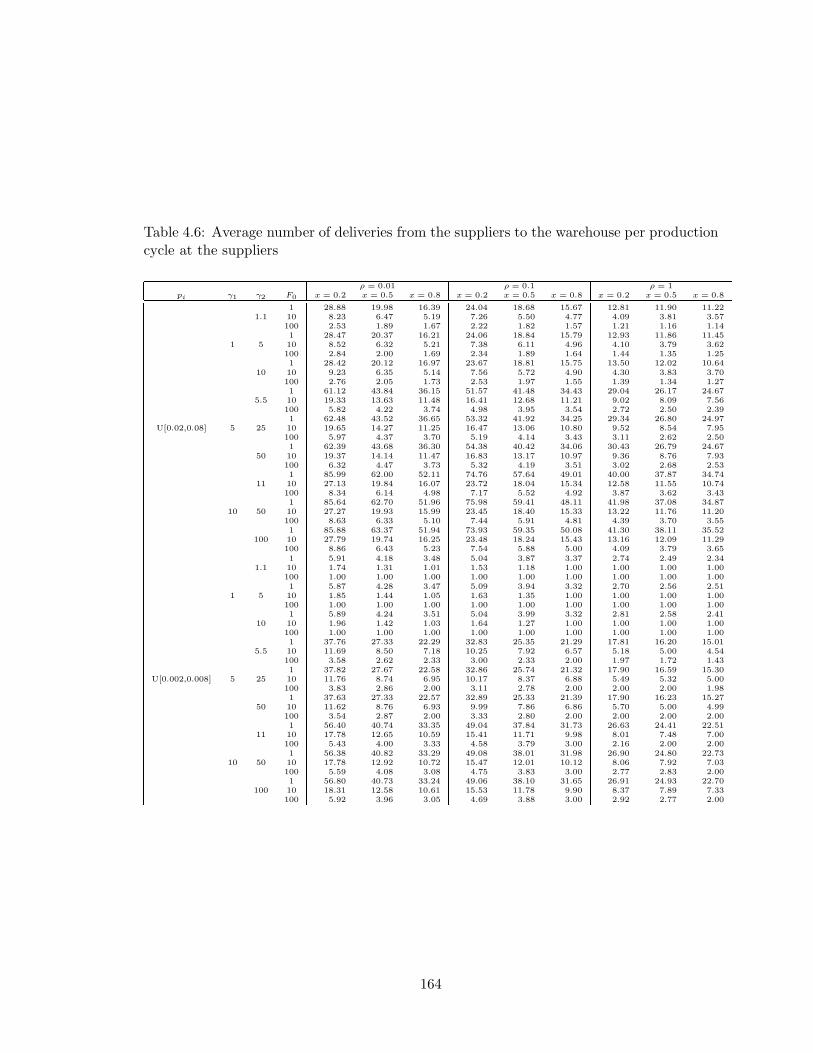
Table 4.6: Average number of deliveries from the suppliers to the warehouse per productioncycle at the suppliers

ρ = 0.01 ρ = 0.1 ρ = 1pi γ1 γ2 F0 x = 0.2 x = 0.5 x = 0.8 x = 0.2 x = 0.5 x = 0.8 x = 0.2 x = 0.5 x = 0.8

1 28.88 19.98 16.39 24.04 18.68 15.67 12.81 11.90 11.221.1 10 8.23 6.47 5.19 7.26 5.50 4.77 4.09 3.81 3.57

100 2.53 1.89 1.67 2.22 1.82 1.57 1.21 1.16 1.141 28.47 20.37 16.21 24.06 18.84 15.79 12.93 11.86 11.45

1 5 10 8.52 6.32 5.21 7.38 6.11 4.96 4.10 3.79 3.62100 2.84 2.00 1.69 2.34 1.89 1.64 1.44 1.35 1.251 28.42 20.12 16.97 23.67 18.81 15.75 13.50 12.02 10.64

10 10 9.23 6.35 5.14 7.56 5.72 4.90 4.30 3.83 3.70100 2.76 2.05 1.73 2.53 1.97 1.55 1.39 1.34 1.271 61.12 43.84 36.15 51.57 41.48 34.43 29.04 26.17 24.67

5.5 10 19.33 13.63 11.48 16.41 12.68 11.21 9.02 8.09 7.56100 5.82 4.22 3.74 4.98 3.95 3.54 2.72 2.50 2.391 62.48 43.52 36.65 53.32 41.92 34.25 29.34 26.80 24.97

U[0.02,0.08] 5 25 10 19.65 14.27 11.25 16.47 13.06 10.80 9.52 8.54 7.95100 5.97 4.37 3.70 5.19 4.14 3.43 3.11 2.62 2.501 62.39 43.68 36.30 54.38 40.42 34.06 30.43 26.79 24.67

50 10 19.37 14.14 11.47 16.83 13.17 10.97 9.36 8.76 7.93100 6.32 4.47 3.73 5.32 4.19 3.51 3.02 2.68 2.531 85.99 62.00 52.11 74.76 57.64 49.01 40.00 37.87 34.74

11 10 27.13 19.84 16.07 23.72 18.04 15.34 12.58 11.55 10.74100 8.34 6.14 4.98 7.17 5.52 4.92 3.87 3.62 3.431 85.64 62.70 51.96 75.98 59.41 48.11 41.98 37.08 34.87

10 50 10 27.27 19.93 15.99 23.45 18.40 15.33 13.22 11.76 11.20100 8.63 6.33 5.10 7.44 5.91 4.81 4.39 3.70 3.551 85.88 63.37 51.94 73.93 59.35 50.08 41.30 38.11 35.52

100 10 27.79 19.74 16.25 23.48 18.24 15.43 13.16 12.09 11.29100 8.86 6.43 5.23 7.54 5.88 5.00 4.09 3.79 3.651 5.91 4.18 3.48 5.04 3.87 3.37 2.74 2.49 2.34

1.1 10 1.74 1.31 1.01 1.53 1.18 1.00 1.00 1.00 1.00100 1.00 1.00 1.00 1.00 1.00 1.00 1.00 1.00 1.001 5.87 4.28 3.47 5.09 3.94 3.32 2.70 2.56 2.51

1 5 10 1.85 1.44 1.05 1.63 1.35 1.00 1.00 1.00 1.00100 1.00 1.00 1.00 1.00 1.00 1.00 1.00 1.00 1.001 5.89 4.24 3.51 5.04 3.99 3.32 2.81 2.58 2.41

10 10 1.96 1.42 1.03 1.64 1.27 1.00 1.00 1.00 1.00100 1.00 1.00 1.00 1.00 1.00 1.00 1.00 1.00 1.001 37.76 27.33 22.29 32.83 25.35 21.29 17.81 16.20 15.01

5.5 10 11.69 8.50 7.18 10.25 7.92 6.57 5.18 5.00 4.54100 3.58 2.62 2.33 3.00 2.33 2.00 1.97 1.72 1.431 37.82 27.67 22.58 32.86 25.74 21.32 17.90 16.59 15.30

U[0.002,0.008] 5 25 10 11.76 8.74 6.95 10.17 8.37 6.88 5.49 5.32 5.00100 3.83 2.86 2.00 3.11 2.78 2.00 2.00 2.00 1.981 37.63 27.33 22.57 32.89 25.33 21.39 17.90 16.23 15.27

50 10 11.62 8.76 6.93 9.99 7.86 6.86 5.70 5.00 4.99100 3.54 2.87 2.00 3.33 2.80 2.00 2.00 2.00 2.001 56.40 40.74 33.35 49.04 37.84 31.73 26.63 24.41 22.51

11 10 17.78 12.65 10.59 15.41 11.71 9.98 8.01 7.48 7.00100 5.43 4.00 3.33 4.58 3.79 3.00 2.16 2.00 2.001 56.38 40.82 33.29 49.08 38.01 31.98 26.90 24.80 22.73

10 50 10 17.78 12.92 10.72 15.47 12.01 10.12 8.06 7.92 7.03100 5.59 4.08 3.08 4.75 3.83 3.00 2.77 2.83 2.001 56.80 40.73 33.24 49.06 38.10 31.65 26.91 24.93 22.70

100 10 18.31 12.58 10.61 15.53 11.78 9.90 8.37 7.89 7.33100 5.92 3.96 3.05 4.69 3.88 3.00 2.92 2.77 2.00

164

Chapter 5

Integrating Order Scheduling with Packingand Delivery

5.1 Introduction

We consider a make-to-order supply chain consisting of one supplier (e.g. manufacturer)

and one customer (e.g. retailer) where the supplier makes time sensitive products such as

fashion apparel and customized high-tech products for the customer. At the beginning of the

planning horizon, the customer places a set of orders with the supplier. The supplier needs to

process these orders on a single dedicated production line, pack the completed orders to form

delivery batches, and deliver the batches to the customer. Because of the time sensitivity

of the products, the customer imposes a service requirement on the delivery timeliness of

the orders she places with the supplier. The supplier needs to meet the imposed service

requirement on the one hand, and minimize the total cost incurred for order processing

and delivery on the other hand. Since the products are time sensitive, orders are delivered

shortly after their completion and thus we assume that little inventory cost is incurred.

The supplier’s total cost is mainly contributed by production and distribution operations.

The total production cost for a fixed set of orders is normally fixed and independent of the

production schedule used. Therefore, the supplier needs to focus on the distribution cost

when considering the total cost. Each order has a weight and the total weight of the orders

165

that can be packed in each delivery batch must not exceed a capacity limit. Each delivery

batch incurs a fixed distribution cost regardless of the total weight it carries.

The problem is to find jointly a schedule for order processing at the supplier, a way

of packing completed orders to form delivery batches, and a delivery schedule from the

supplier to the customer such that the total distribution cost is minimized subject to the

constraint that a given customer service level is guaranteed. We consider two customer

service constraints:

(a) Meeting the given deadlines of the orders.

(b) Requiring the average delivery lead time of the orders to be within a given threshold.

The problem with each of those constraints is studied separately. For ease of presen-

tation, we call the problem with the service constraint (a) the deadline problem, and the

problem with the service constraint (b) the lead time problem. For each problem, we

consider the following three cases for the way an order can be produced and delivered:

(i) Non-splittable production and delivery: An order cannot be split in terms of production

or delivery, i.e. it is not allowed to preempt the processing of an order and a finished order

must be delivered in one batch.

(ii) Non-splittable production, but splittable delivery: An order cannot be split in terms of

production, but can be split in terms of delivery, i.e. no processing preemption is allowed,

but a finished order can be split into multiple parts delivered in multiple batches.

(iii) Splittable production and delivery: An order can be split in terms of both production

and delivery, i.e. both processing preemption and delivery split of an order are allowed.

There are practical situations that justify each case. Splitting an order for either produc-

tion or delivery may require extra setups. Furthermore, to ease order tracking and handling,

the customer may require that an order be delivered wholly in one shipment. Hence, order

166

splitting may not be desirable. On the other hand, allowing order splitting may improve

service level or/and lower distribution cost. So depending on the requirements, the supplier

may or may not be allowed to split production and/or delivery of orders. The problems

we consider integrate order processing scheduling, finished order packing and batching, and

order delivery scheduling.

In this chapter, we clarify the computational complexity of the various problems we

consider by either proving that a problem is intractable (i.e. NP-hard) or providing an

efficient exact algorithm for it. For the NP-hard problems, we design fast heuristics that

are capable of generating near optimal solutions. We analyze the worst-case performance of

each heuristic, and computationally evaluate their performance using randomly generated

test instances. The remainder of the chapter is organized as follows. In Section 5.2, we

define the problems and give some optimality properties. We then study the deadline

problem in Section 5.3, and the lead time problem in Section 5.4, respectively. We look at

three different cases, Case (i), Case (ii), and Case (iii), for both the deadline and the lead

time versions. Both Cases (i) and (ii) of both problems are shown to be strongly NP-hard.

Case (iii) of the deadline problem is solved optimally by a polynomial algorithm, whereas

Case (iii) of the lead time problem is shown to be strongly NP-hard. A heuristic is proposed

for each of the NP-hard problems. Column generation based approaches are proposed to

find lower bounds of the objective values of those problems. Those lower bounds are then

used to evaluate the performance of the heuristics. We provide two extensions in Section

5.5. Finally, we conclude the chapter in Section 5.6.

167

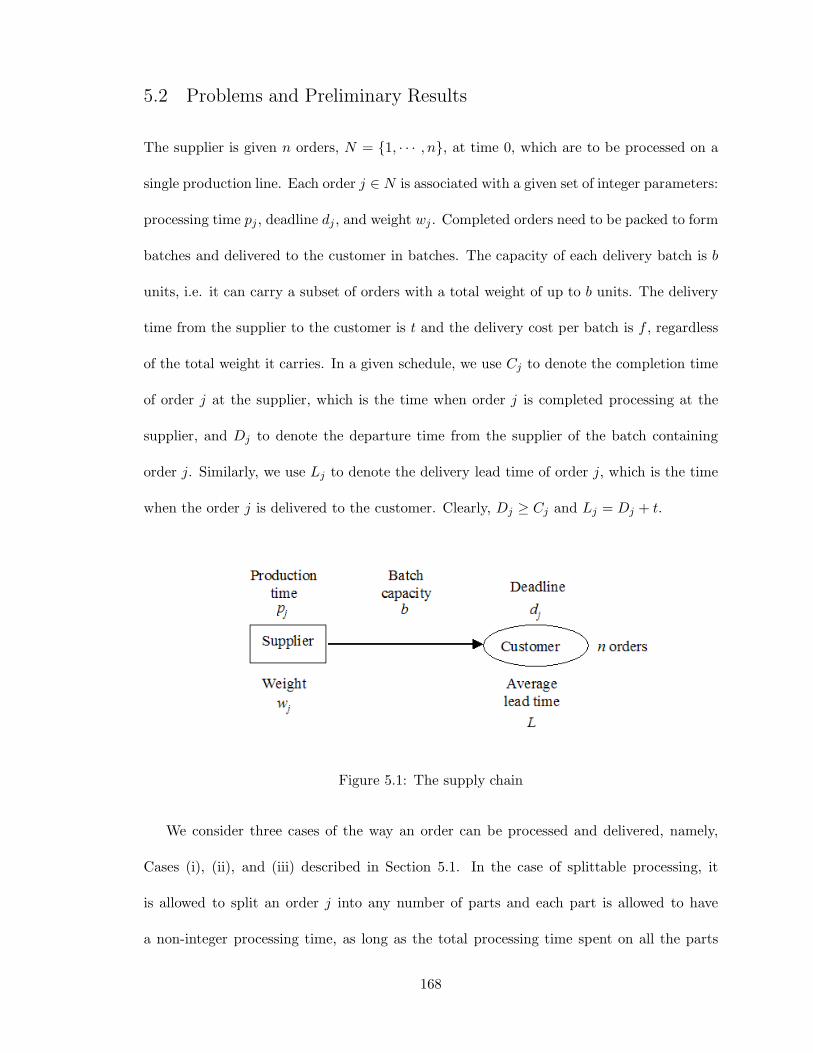
5.2 Problems and Preliminary Results

The supplier is given n orders, N = 1, · · · , n, at time 0, which are to be processed on a

single production line. Each order j ∈ N is associated with a given set of integer parameters:

processing time pj , deadline dj , and weight wj . Completed orders need to be packed to form

batches and delivered to the customer in batches. The capacity of each delivery batch is b

units, i.e. it can carry a subset of orders with a total weight of up to b units. The delivery

time from the supplier to the customer is t and the delivery cost per batch is f , regardless

of the total weight it carries. In a given schedule, we use Cj to denote the completion time

of order j at the supplier, which is the time when order j is completed processing at the

supplier, and Dj to denote the departure time from the supplier of the batch containing

order j. Similarly, we use Lj to denote the delivery lead time of order j, which is the time

when the order j is delivered to the customer. Clearly, Dj ≥ Cj and Lj = Dj + t.

Figure 5.1: The supply chain

We consider three cases of the way an order can be processed and delivered, namely,

Cases (i), (ii), and (iii) described in Section 5.1. In the case of splittable processing, it

is allowed to split an order j into any number of parts and each part is allowed to have

a non-integer processing time, as long as the total processing time spent on all the parts

168

together is equal to pj. In this case, the completion time of an order is the completion

time of its last part, and the departure time of an order is the departure time of the batch

containing the last part of the order. We assume that the weight of each split part is linearly

proportional to its processing time, i.e. if a part of order j requires a processing time τ ,

then the its weight is τwj/pj , where the ratio wj/pj , which we call the filling-rate of order

j, is the amount of weight corresponding to every unit of the processing time of order j.

In the case of non-splittable delivery, an order j cannot be packed into a batch until its

completion time Cj because the entire order has to be packed in the same batch. In the

case of splittable delivery, any part of an order is available for delivery once this part is

completed processing. The lead time of an order, if it is split into multiple parts delivered

in multiple batches, is the time when the batch containing its last part is delivered to the

customer.

We study two problems. The first one, called the deadline problem, is to minimize the

number of delivery batches used subject to the service constraint (a) described in Section

5.1. That is, each order must be delivered to the customer no later than its deadline, or

Lj ≤ dj for j ∈ N . The second problem, called the lead time problem, is to minimize the

number of delivery batches used subject to the service constraint (b) described in Section

5.1. That is, the average lead time of the orders should be no more than a given threshold L,

or (∑

j∈N Lj)/n ≤ L. In our model, since all the orders are delivered to the same customer

and the delivery time of any batch is the same, we can simplify these constraints as follows.

We can redefine the deadline of each order j to be dj − t such that the service constraint

(a) is equivalent to the constraint that the departure time Dj of order j is no later than the

redefined deadline of j. Similarly, if we redefine the average lead time threshold to be L− t,

then the service constraint (b) is equivalent to the constraint that the average departure

169

time of the orders from the supplier is no more than the redefined threshold. Therefore, for

ease of presentation, in the remainder of the chapter, we assume that the given deadlines of

orders dj ’s and the lead time threshold L have been redefined so that the constraint in the

deadline problem becomes Dj ≤ dj for j ∈ N , and that in the lead time problem becomes

(∑

j∈N Dj)/n ≤ L.

To illustrate the differences between the three cases mentioned, consider the following

problem instance for the deadline problem. We have five orders and the maximum batch

size is given by b = 19. The five orders have the following parameters: p1 = p2 = p3 = 20,

p4 = p5 = 10; d1 = 23, d2 = d3 = 61, d4 = d5 = 80; w1 = 17, w2 = w3 = w4 = w5 = 10.

We note that the sum of weights of all the orders is 57 and since the maximum batch size

is 19, we need a minimum of three delivery batches. Below we give the optimal solutions

for each case:

Case (i): We will have a total of five delivery batches in the optimal solution and each

order will ship in a batch of its own. This is because each order has a weight more than

19/2 = 9.5 and hence no two full orders can fit in one batch.

Case (ii): The optimal solution will have a total of four delivery batches. This is because,

in order to obtain just three batches, we need all the batches to be full, including the first

batch. The first batch has to get full by time t = d1 = 23 and the only way for this to

happen is to process order 4 or 5 immediately after processing order 1 (orders 2 and 3 have

a lower filling-rate). But if this is done, then one of the orders 2 or 3 will miss their deadline

since we cannot preempt the production of order 4 or 5 once it is started. Hence the first

batch cannot be full, and we will need a total of four batches. One possible solution with

four batches is as follows: first batch will have just the first order, second batch will have

the second order and 910 th of the third order, the third batch will have the rest of the third

170

order, and 110 th of the fourth order, and the fourth batch will have the rest. Hence the first

batch will ship at time t = 20, the second will ship at t = 58, the third will ship at t = 61,

and the fourth will ship at t = 80.

Case (iii): The following solution will meet all the deadlines with exactly three batches and

hence it will be the optimal solution for Case (iii). Process order 1, 110th of order 2, and

110th of order 4 for the first batch. Process the remaining part of order 2 and then order 3

for the second batch. Process the remaining part of order 4, and ship it along with order

5 in the third batch. Thus the first batch will ship at time t = 23, the second will ship at

t = 61, and the third will ship at t = 80.

The above example shows that the optimal solution will vary depending on the re-

strictions on production process or delivery batching. Next, we present some optimality

properties that will be used in later sections. The first result holds for all the problems. It

is fairly straightforward and hence we omit the proof. The second result holds for Cases

(ii) and (iii) of both problems.

Lemma 17 There exists an optimal schedule for all the three cases of both problems where(1) There is no inserted idle time between orders and partial orders processed at the supplier.(2) The departure time of each batch is the time when processing of all the orders and partialorders in it are complete.(3) All the orders and partial orders that are delivered in the same batch are processedconsecutively at the supplier.

Lemma 18 There exists an optimal schedule for Case (ii) and Case (iii) of both problemswhere(1) If a delivery batch contains a partial order which is not the first part of an order, thenthis batch is full.(2) In each delivery batch containing partial orders, the weight of each partial order is aninteger.

Proof (1) Suppose that there is a delivery batch B in a given optimal schedule π that is

not full but contains a part of some order j ∈ N which is not the first part of j. Let the

171

total weight of the orders and parts of orders in this batch be v with v < b, and the weight

of the part of order j contained in this batch be vj with vj < wj . Clearly, the remaining

part of order j has a weight wj −vj and is contained in one or more batches delivered earlier

than batch B. There are two cases as follows. Case 1: If b − v ≥ wj − vj , we move all

the earlier parts of order j to batch B. After that, the part of order j in batch B becomes

either a whole order or the first part of it. Case 2: If b− b < wj − vj, we move a portion of

the earlier parts of order j with a total weight b− v to batch B. After that, batch B is full.

In both cases, neither the completion time of each order nor the total number of batches

used is increased, and thus the new schedule is still optimal.

(2) Suppose that in a given optimal schedule π, batch B is the last batch that violates

this property, i.e. each partial order in every batch delivered later than B has an integer

weight and there are partial orders in B with a non-integer weight. Let k be the number

of partial orders in B with a non-integer weight. Let j1, · · · , jk denote those orders, and

fractional values vj1 , · · · , vjkdenote their weights. For h = 1, · · · , k, since the total weight

of all the parts of order jh delivered later than batch B has an integer total weight, one or

more parts of jh must be delivered earlier than batch B and the total weight of those parts

is fractional. This means that the part of order jh, for h = 1, · · · , k, delivered in batch B is

not the first part of the order. By Property (1), we can assume that batch B is full. Thus

the total weight of the orders in B is b, an integer. Since a whole order has an integer weight

and each partial order in B other than j1, · · · , jk has an integer weight, the total weight of

the parts of orders j1, · · · , jk in B is an integer. Let αh (0 < α < 1) be the fractional part

of the weight of the part of order jh in B, for h = 1, · · · , k. Let ρ = α1 + · · · + αk. Clearly,

ρ ≤ k−1 and ρ is an integer. Let ju, for some u ∈ 1, · · · , k, be the order with the highest

filling-rate (recall that it is defined to be the ratio wj/pj) among the orders j1, · · · , jk. Let

172

β be the total weight of the parts of orders j1, · · · , ju−1, ju+1, · · · , jk contained in batches

earlier than B. It can be easily verified that

β ≥u−1∑

h=1

(1 − αh) +k∑

h=u+1

(1 − αh) = (k − 1) − ρ + αu ≥ αu

We use a portion of order ju contained in B with the weight αu to exchange portion of the

orders j1, · · · , ju−1, ju+1, · · · , jk contained in batches earlier than B with an equal weight.

Since order ju has the highest filling-rate, this exchange will result in a schedule where each

batch is delivered no later than in schedule π. After this exchange, the weight of order ju

in batch B is lowered by αu units and thus becomes an integer. We can apply the same

idea to the remaining orders with a fractional weight in batch B, j1, · · · , ju−1, ju+1, · · · , jk,

and eventually every one of them will have an integer weight in B.

5.3 The Deadline Problem

In this section we consider the three cases of the deadline problem. Clearly, Case (i) of the

problem is strongly NP-hard because the classical bin-packing problem, which is strongly

NP-hard (Garey and Johnson 1979), is a special case of it with sufficiently large dj for

j ∈ N such that the deadline constraint is always satisfied under any processing schedule.

In Section 5.3.1, we clarify the computational complexity of the other two cases of the

problem. We show that Case (ii) of the problem is strongly NP-hard, whereas there is

a polynomial algorithm for Case (iii) of the problem. In Section 5.3.2, we propose two

heuristics, one for Case (i), and one for Case (ii), respectively. We analyze the worst-case

performance of the heuristics. In Section 5.3.3, we do a computational experiment on the

heuristics. For Case (i), we propose a column generation approach to find a valid lower

bound. Since Case (iii) is a relaxation of Case (ii), the optimal objective value of Case (iii)

173

is a lower bound for Case (ii). We use these lower bounds to evaluate the performance of

the heuristics computationally.

5.3.1 Solvability of Cases (ii) and (iii)

We first clarify the complexity of Case (ii) of the problem.

Theorem 18 The deadline problem with non-splittable production but splittable delivery isstrongly NP-hard.

Proof We prove the theorem by a reduction from the 3-partition problem (3PP), a known

strongly NP-hard problem (Garey and Johnson 1979).

3PP: Given a set of 3n elements, A = 1, · · · , 3n, a positive integer H, and a positive

integer size ai for each element i ∈ A with H/4 < ai < H/2, such that the total size of

elements in A is exactly nH, can A be partitioned into n disjoint subsets A1, · · · , An such

that each Ai contains exactly 3 elements of A and has a total size equal to H?

We construct the following instance for our problem where there are 5n orders consisting

of three types:

Type 1: n orders N1 = 11, · · · , 1n with parameters: p1i = 9H,w1i = 9H, d1i = 30H(i −

1) + 10H, for i = 1, · · · , n.

Type 2: n orders N2 = 21, · · · , 2n with parameters: p2i = 20H,w2i = 10H, d2i = 30Hi,

for i = 1, · · · , n.

Type 3: 3n orders N3 = 31, · · · , 33n with parameters: p3i = ai, w3i = ai, d3i = 30Hn, for

i = 1, · · · , 3n.

Maximum delivery batch size: b = 10H.

Threshold value for the objective function: 2n delivery batches.

(If part) If there is a solution to 3PP, we construct a solution to the above instance of our

problem as follows. Process the orders in the sequence (11, 3A1 , 21, 12, 3A2 , 22, · · · , 1n, 3An , 2n),

174

where the subset 3Ai = 3j | j ∈ Ai, for i = 1, · · · , n. Make a total of 2n deliveries where,

for k = 1, · · · , n, the (2k − 1)th delivery covers order 1k and the 3 orders of 3Ak, and the

(2k)th delivery covers order 2k. We can see that in this solution, all the delivery batches

are full, and all the orders satisfy their deadlines.

(Only If part) Recall that we defined the filling-rate of an order j in Section 5.2 as the

ratio of its weight to its processing time wj/pj . We denote the filling-rate of order j to be

fj. Clearly, fj = 1 for j ∈ N1 ∪ N3 and fj = 0.5 for j ∈ N2. Since we cannot have more

than 2n delivery batches and since the total weight of orders is 20nH, there are exactly 2n

delivery batches and all the delivery batches are full in any optimal solution. The minimum

total processing time required by the orders and partial orders in a full delivery batch is

min10H/fj , | j ∈ N1 ∪ N2 ∪ N3 = 10H.

Let ti denote the time at which the ith delivery batch becomes full (i.e. ti is the

departure time of this batch). Let Sj denote the time at which order j begins processing.

Let us consider the first delivery batch. Since d11 = 10H and since it takes a minimum of

10H time units to fill a delivery batch completely, order 11 has to be in the first delivery

batch. Hence t1 = 10H. Since w11 = 9H, there is some empty space in the first delivery

batch after processing order 11. This has to be filled with one or more orders or partial

orders because every delivery batch must be full. If a second Type-1 order is processed

after order 11, since p1i = 9H, it will be completely processed at time18H, which implies

that S21 ≥ 18H, and hence C21 = S21 + p21 ≥ 38H > d21 . So putting a second Type-1

order after order 11 will lead us to an infeasible solution. If we put any Type-2 order 2i

after order 11, it will take H/f2i = 2H units of time to fill up the first delivery batch. This

means that t1 = 9H + 2H = 11H > d11 , again resulting in an infeasible solution. So the

only option is to process one or more Type-3 orders to go with order 11 in the first delivery

175

batch to be shipped at time t1 = 10H. We denote by φ the set of Type-3 orders in the

first delivery batch either partially or entirely along with order 11. There are two cases to

consider:

Case 1:∑

j∈φ pj > H. In this case, the first Type-2 order will have a starting time

S21 > 9H + H = 10H and hence C21 = S21 + p21 > 30H = d21 . Hence, this case is not

feasible.

Case 2:∑

j∈φ pj < H. Denote pφ =∑

j∈φ pj . In this case, the total weight of the orders in

φ is∑

j∈φ wj = pφ and the delivery batch will not be full with just these orders and order 11.

There will be an empty space equivalent to H−pφ units of weight and H−pφ units of time to

go before the departure time of the first delivery t1 = 10H. We will have to add a part of a

Type-1 or/and a part of a Type-2 order to make the first delivery batch full. If we add a part

of a Type-1 order, then by a similar argument used earlier, this will result in the first Type-2

order getting completed later than its deadline. So we will have to add a part of Type-2

order instead. This will take (H−pφ)/0.5 = 2H−2pφ time units to fill up the spare space of

the first delivery batch. So t1 would become 9H + pφ +2H − 2pφ = 11H − pφ > 10H = d11 ,

resulting in an infeasible solution.

From the above cases, it is clear that∑

j∈φ pj = H and the first batch contains entire

order 11 and entire orders in φ. Once the first batch is full at time t1 = 10H, we have to start

processing order 21 immediately so that C21 = t1 +p21 = 30H = d21 . Since w21 = 10H, this

order will be shipped individually in the second delivery batch at t2 = 30H. And once this

is done, we look at the third delivery batch and we are in a situation that is exactly the same

as the first delivery batch. Hence, continuing this, we can see that each odd numbered batch

will contain one Type-1 order and three Type-3 orders that add to a weight of H, and each

even numbered batch will contain one Type-2 order shipped independently. Define subsets

176

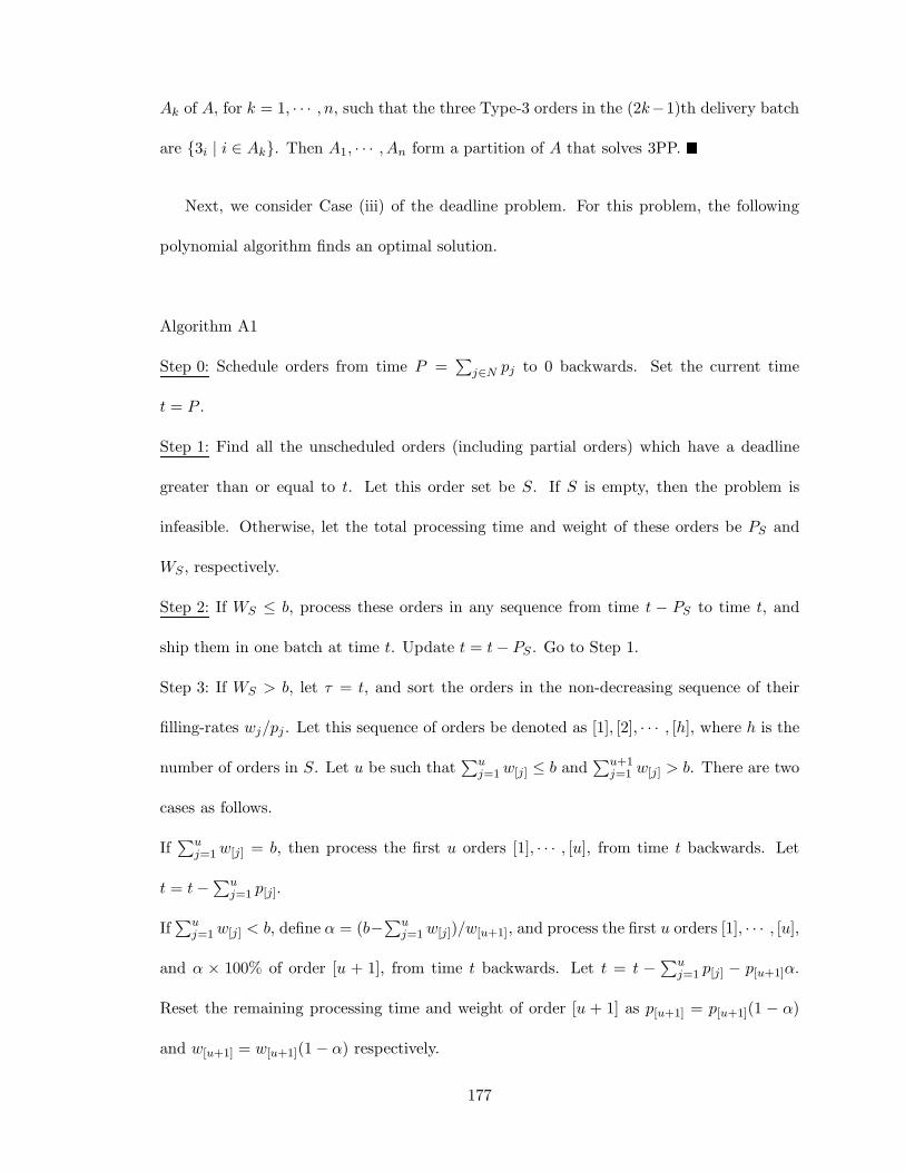
Ak of A, for k = 1, · · · , n, such that the three Type-3 orders in the (2k−1)th delivery batch

are 3i | i ∈ Ak. Then A1, · · · , An form a partition of A that solves 3PP.

Next, we consider Case (iii) of the deadline problem. For this problem, the following

polynomial algorithm finds an optimal solution.

Algorithm A1

Step 0: Schedule orders from time P =∑

j∈N pj to 0 backwards. Set the current time

t = P .

Step 1: Find all the unscheduled orders (including partial orders) which have a deadline

greater than or equal to t. Let this order set be S. If S is empty, then the problem is

infeasible. Otherwise, let the total processing time and weight of these orders be PS and

WS , respectively.

Step 2: If WS ≤ b, process these orders in any sequence from time t − PS to time t, and

ship them in one batch at time t. Update t = t − PS . Go to Step 1.

Step 3: If WS > b, let τ = t, and sort the orders in the non-decreasing sequence of their

filling-rates wj/pj . Let this sequence of orders be denoted as [1], [2], · · · , [h], where h is the

number of orders in S. Let u be such that∑u

j=1 w[j] ≤ b and∑u+1

j=1 w[j] > b. There are two

cases as follows.

If∑u

j=1 w[j] = b, then process the first u orders [1], · · · , [u], from time t backwards. Let

t = t −∑u

j=1 p[j].

If∑u

j=1 w[j] < b, define α = (b−∑u

j=1 w[j])/w[u+1], and process the first u orders [1], · · · , [u],

and α × 100% of order [u + 1], from time t backwards. Let t = t −∑u

j=1 p[j] − p[u+1]α.

Reset the remaining processing time and weight of order [u + 1] as p[u+1] = p[u+1](1 − α)

and w[u+1] = w[u+1](1 − α) respectively.

177

Deliver all the orders and partial orders that have been processed in this step in one ship-

ment at time τ . Go to Step 1.

Theorem 19 Algorithm A1 finds an optimal solution to the deadline problem with splittableproduction and delivery in O(n2logn) time.

Proof We first estimate the computational time of the algorithm. Each iteration of the

algorithm (running Steps 1, and 2 or 3, once) schedules a new batch of orders selected from

a set S, where S includes all eligible orders and partial orders. Since the weight of each

order is no more than the batch capacity, if S is not empty, then in either Step 2 or Step 3,

at least one order or partial order k ∈ S is 100% covered by this batch. In case k is a partial

order, clearly its remaining part is covered in a later batch (which has been generated by

the algorithm in an earlier iteration since the algorithm schedules orders backwards). This

means that order k is completely covered in batches generated in this and earlier iterations.

So we can conclude that after each iteration of the algorithm, at least one new order is

completely covered. Since there are n orders, the algorithm stops after at most n iterations.

In each iteration, we may need to arrange at most n orders and partial orders in the non-

decreasing sequence of wj/pj. This has a time requirement of O(nlogn). So the overall

computational complexity of the algorithm is O(n2logn).

To show that the solution π generated by Algorithm A1 is optimal, we show that any

optimal solution π∗ can be transformed to π without increasing the number of delivery

batches. Suppose that for some integer h ≥ 0, the kth last batch in π∗ is exactly the same

(i.e. contains the same set of orders, each with the same weight or partial weight) as the kth

last batch in π, for k = 0, · · · , h, but the (h+1)th last batch in π∗, denoted as Bh+1(π∗), is

different from the (h + 1)th last batch in π, denoted as Bh+1(π). We can easily show that

the set S obtained in the (h + 1)th iteration in Step 1 of algorithm A1 is the same for both

178

π and π∗. Define Ws and Ps to be the total processing time and weight of the orders in S,

respectively. There are two cases as follows.

Case 1: If WS ≤ b, then by the algorithm, all the orders of S are included in Bh+1(π). Since

Bh+1(π∗) 6= Bh+1(π), and since S contains all the eligible orders and partial orders that

may be delivered in Bh+1(π∗), there exists some order j ∈ S which is not entirely included

in Bh+1(π∗). We can move the remaining part of order j, which must be scheduled in an

earlier batch in π∗, to batch Bh+1(π∗). This will not increase the departure time of any

batch, and hence is feasible. Furthermore, the number of batches is not increased. We can

continue this procedure until Bh+1(π∗) = Bh+1(π).

Case 2: If WS > b, then by Step 3 of the algorithm, the first u orders and a part of the

(u+1)th order with the lowest filling-rates among all the orders in S are included in Bh+1(π),

and this is a full batch. If batch Bh+1(π∗) is not full, then we can move some orders or/and

parts of some orders of S scheduled in earlier batches in π∗ to batch Bh+1(π∗) to make

it a full batch without increasing the departure time of any batch or the total number of

batches. Now we can assume that Bh+1(π∗) is also a full batch, but different than Bh+1(π).

Suppose that, for some 1 ≤ k ≤ u, Bh+1(π∗) contains the first k orders [1], · · · , [k] in exactly

the same amount as it is contained in Bh+1(π), but contains only a portion (which can be

0%) of order [k+1] that is contained in Bh+1(π). Then there must exist one or more orders,

denoted by set Q, in Bh+1(π∗) that have a higher filling-rate than order [k + 1]. We can

swap part of order [k + 1] scheduled in earlier batches with part of orders of Q in π∗ such

that after swapping the amount of order [k + 1] in Bh+1(π∗) becomes exactly the same as

that in batch Bh+1(π). This will not increase the departure time of any batch or the total

number of batches. We can continue such a swapping procedure until Bh+1(π∗) = Bh+1(π).

179

5.3.2 Heuristics for Cases (i) and (ii)

In this section, we propose a heuristic for Case (i) and Case (ii) of the deadline problem,

respectively.

In the heuristic for Case (i), a delivery batch departs at the time corresponding to the

earliest deadline among all the orders in the delivery batch. Thus a delivery batch is said to

be available at time t if and only if t is not greater than the departure time of the delivery

batch.

Heuristic H1

Step 0: Reindex orders in their EDD sequence. Process the orders in the sequence of their

order indices without idle time. Let j = 1.

Step 1: Consider order j. Fit it in the first feasible and available delivery batch. If the

order cannot be fit into any of the available delivery batches, open a new delivery batch.

Step 2: Set j = j + 1. If j ≤ n, go to Step 1. Else STOP.

Theorem 20 The worst-case performance ratio of Heuristic H1 for the deadline problemwith non-splittable production and delivery is bounded by 3.

Proof Note that in H1, the delivery batches are delivered in the order in which they are

opened and a new delivery batch can be opened due to one of the following reasons:

i) The order under consideration does not fit into any available delivery batches.

ii) All earlier delivery batches have been delivered and hence there are no delivery batches

available.

We divide the delivery batches into two categories: Category S contains those delivery

batches that were opened because of (i), category U contains all the other delivery batches.

180

In this arrangement, we will have alternating series of S and U type delivery batches (e.g.

one U type delivery batch followed by three S type delivery batches followed by two U type

followed by two S type). If a particular series of S type delivery batches has an odd number

of members, put the last delivery batch in the preceding U type to that series. Thus S will

have even numbered delivery batches in each segment. Let s and u be the total number of

such delivery batches in S and U respectively. We argue that the optimal solution will have

at least maxd s

2e, u

delivery batches. If this is the case, then the worst case-ratio for our

heuristic is s+umaxd s

2e,u ≤ 3.

It can be easily shown that all the orders in S add upto a total weight of at least sb2 . So

we need at least d s2e delivery batches for those orders. Let us look at the U type delivery

batches. Let the sum of processing times of all the orders up to the first order in the ith

U type delivery batch be denoted as Pi. Let the delivery batch be denoted as Ui, and

the index for the first order in Ui be denoted as xi. Thus Pi is the sum of processing

times of all the orders with an index k such that k ≤ xi. Consider all the orders up to

x2. The sum of their processing times is P2. But since at P2, U1 has already left, we have

P2 ≥ dx1 , the deadline corresponding to the first order in the first U category delivery

batch. This shows that whichever sequence the production is carried out, at least one order

from 1, · · · , x1, · · · , x2 gets ready after dx1 and that order has to be shipped in a different

delivery batch after dx1 . Let this particular order in the optimal solution be denoted as y2.

Note also that dx2 is the highest deadline among all the orders in x1, · · · , x2 and hence

dx2 ≥ dy2 . Now consider x3. Since at P3, U2 has already left, we have P3 ≥ dx2 , the deadline

corresponding to the first order in U2. This means that whichever sequence the production

is carried out, at least one order from 1, · · · , x1, · · · , x2, · · · , x3 gets ready after dx2 (and

dy2) and that order has to be shipped in a delivery batch that is different from the delivery

181

batch containing x2 or y2. Let this order in the optimal solution be y3. Proceeding like

this, we can see that corresponding to each U category delivery batch, there should be a

separate shipment. This shows that minimum number of shipments required is bound from

below by u.

Therefore, the minimum number of delivery batches for the optimal solution for our

problem is: maxd s

2e, u

. Thus the worst-case ratio is: s+umaxd s

2e,u . If u ≥ d s

2e, it implies

that s ≤ 2u. On the other hand, when u < d s2e, we have s ≤ 2d s

2e. Therefore, the worst-case

ratio is bound by 3.

The heuristic for Case (ii) generates a feasible solution by modifying the solution gen-

erated by Algorithm A1 for Case (iii) of the problem given in Section 5.3. Note that the

solution generated by Algorithm A1 allows production preemption and hence is generally

not feasible to Case (ii). Below we give the heuristic and its worst-case complexity.

Heuristic H2

Step 0: Run Algorithm A1. Let the processing sequence of the orders in the solution gen-

erated by Algorithm A1 be π0. If there is no production preemption in this solution, then

STOP, and this solution is optimal to Case (ii).

Step 1: Examine the processing sequence π0 from time P =∑

j∈N pj to 0 backwards.

Whenever there is a partial order j, move all the other parts of this order (which must be

scheduled earlier) to the position immediately before this partial order so that the whole

order j is processed without preemption after this rearrangement. Let the new processing

sequence of the orders be π.

Step 2: Given the processing sequence of the orders π (where there is no production pre-

emption), find a packing and delivery schedule by the following procedure:

182

Step 2.0: Reindex the orders such that π = (n, n− 1, · · · , 1). Consider orders in π from

time P =∑

j∈N pj to 0 backwards. Set the current time t = P , and the current order

k = 1. Define the remaining processing time and weight of the current order to be p′1 = p1

and w′1 = w1, respectively. No order has been assigned to a batch yet.

Step 2.1: If every order or partial order has been assigned to a batch, STOP. Find the

maximum integer h with h ≥ k such that all the orders k, · · · , h in π have a deadline

greater than or equal to t. Let P ′ = p′k +∑h

j=k+1 pj and W ′ = w′k +

∑hj=k+1 wj be the

total processing time and weight of the remaining part of order k and the entire orders

k + 1, · · · , h, respectively. Consider the next batch.

Step 2.2: If W ′ ≤ b, ship the remaining part of order k and the entire orders k+1, · · · , h

in one batch at time t. Update t = t − P ′, k = h + 1, p′k = ph+1 and w′k = wh+1. Go to

Step 2.1.

Step 2.3: If W ′ > b, find r with k ≤ r < h such that w′k +

∑rj=k+1 wj ≤ b and

w′k +

∑r+1j=k+1 wj > b. Define α = (b − w′

k −∑r

j=k+1 wj)/wr+1. Ship the following orders

in one batch at time t: the remaining part of order k, the entire orders k + 1, · · · , r, and

α×100% of order r+1. Update t = t−p′k −∑r

j=k+1 pj −αpr+1, k = r+1, p′k = (1−α)pr+1

and w′k = (1 − α)wr+1. Go to Step 2.1.

The processing sequence π0 generated in Step 0 of the heuristic may have production

preemptions. However, the new sequence π generated in Step 1 does not have any production

preemption. Step 2 forms delivery batches based on the processing sequence π such that a

maximum amount of weight possible is included in each batch.

Theorem 21 The worst-case performance ratio of Heuristic H2 for the deadline problemwith non-splittable production but splittable delivery is bounded by 2.

Proof Let x0, xH2, and x∗ be, respectively, the number of batches in the solution generated

183

by Algorithm A1 (for Case (iii)), that in the solution generated by Heuristic H2 (for Case

(ii)), and that in the optimal solution of Case (ii). Since Case (iii) is a relaxation of Case

(ii), we have:

x∗ ≥ x0 (5.1)

In Heuristic H2, given the processing sequence of orders π, Step 2 forms delivery batches

backwards from time P to time 0 and a maximum amount of weight is assigned to each

batch. It can be easily shown that

Claim 1: The number of batches generated in Step 2 is the minimum possible given the

processing sequence π and the fact that the batches formed satisfy the property that orders

delivered together in a batch are processed consecutively in π.

Let B01 , · · · , B0

x0 denote the x0 batches in the solution generated by Algorithm A1, where

a batch with a smaller index is delivered earlier. It can be seen that there is at most one

partial order in each batch B0k, for k = 1, · · · , x0, whose last part is included in this batch.

For k = 1, · · · , x0, let [k] denote the order index of such partial order in B0k, where [k] is a null

order (with 0 processing time and weight) if no such partial order exists in B0k. Clearly, [1]

must be null because it is not possible for batch B01 to contain a partial order whose last part

is included in it. In Step 1 of the heuristic, for every such partial order, all the other parts

of this order which are processed earlier are moved to the position immediately before this

partial order. This means that the processing sequence π generated in Step 1 of the heuristic

has the following structure: (B01 \ R1, [2], B0

2 \ R2, [3], · · · , B0x0−1 \ Rx0−1, [x0], B0

x0 \ Rx0),

where Rk = [k], · · · , [x0].

Now we generate a new packing and delivery schedule based on the processing sequence

π as follows: Deliver all the orders in B01 \ R1 in one batch, and for k = 2, · · · , x0, deliver

order [k] in one batch if [k] is not a null order, and all the orders in B0k \ Rk in one batch.

184

The departure time of each batch is set to be the completion time of the last order in

the batch. It can be easily seen that both the departure time of the batch containing the

orders of B0k \ Rk and that of the batch containing a single order [k] in this new schedule

are no later than that of batch B0k in the schedule generated by Algorithm A1. Thus, the

deadline of each order is met in this new schedule. Also, it can be seen that there is no

production preemption in this new schedule. Therefore, this new schedule is feasible for

Case (ii). Furthermore, this new schedule is based on the processing sequence π and the

orders delivered in each batch are processed consecutively. Since there are at most 2x0

batches in this new schedule, by Claim 1, we have:

xH2 ≤ 2x0 (5.2)

By (5.1) and (5.2), we have: xH2 ≤ 2x∗. This shows the theorem.

5.3.3 Computational Experiment

In this section, we test the performance of the heuristics proposed for Cases (i) and (ii) of

the deadline problem. We use column generation to obtain a lower bound for the problem

under Case (i). We use the optimal objective value of Case (iii) of the problem obtained by

Algorithm A1 as a lower bound for Case (ii). These lower bounds are used to evaluate the

performance of Heuristics H1 and H2 computationally based on randomly generated test

instances.

Column generation for Case (i)

We first given an integer programming formulation for Case (i) of the problem. Let Ω

denote the set of all feasible delivery batch configurations. A batch ω ∈ Ω is defined based

on the following parameters: (i) the departure time the batch, and (ii) the set of orders in

the batch. Let xω be a binary variable that is 1 if batch ω is part of the final solution, and

185

0 otherwise. Since the sequence in which the orders in a batch are processed does not affect

the solution, we assume that in any batch, the orders are processed in the reverse sequence

of their indices (this makes the description of DP1, to be given later, simpler). We assume

that the orders have been indexed in their EDD sequence with ties in due dates broken

based on the increasing order of their processing times. We define the following parameters:

P =∑

j∈N pj = total processing time of the orders

ajω = 1 if order j is covered in batch ω and 0 otherwise

btω = 1 if there is an order in batch ω which is processed over a period of time that covers

interval [t, t + 1], and 0 otherwise

We have the following formulation:

[IP1] min∑

ω∈Ω

xω (5.3)

Subject to:

∑

ω∈Ω

ajωxω = 1 ∀j ∈ N (5.4)

∑

ω∈Ω

btωxω = 1 ∀t ∈ 0, · · · , P − 1 (5.5)

xω ∈ 0, 1 ∀ω ∈ Ω (5.6)

In [IP1], the objective function minimizes the number of batches. Constraint (5.4)

ensures that each order is covered in the final schedule. Constraint (5.5) ensures that every

time slot in the interval [0, P ] is covered exactly once. We denote the LP relaxation of [IP1]

as [LP1], where constraint (5.6) is replaced by xω ≥ 0. Clearly, the optimal solution value

for [LP1] is lower bound for [IP1] and hence for Case (i) of our problem.

Since the number of batches in Ω can be extremely large, we do not solve [LP1] directly.

Instead, we use a column generation approach to generate necessary batches only. In the

column generation approach, we solve a master problem with a subset of columns, and

186

then solve a subproblem to obtain new columns with a negative reduced cost. We iterate

between the master problem and the subproblem till no more new columns with negative

reduced costs are found.

An initial set of columns can be generated by processing all the orders in the sequence

of their deadlines and shipping each order independently. We use πj and σt to denote the

dual variable value corresponding to the constraint set (5.4) and (5.5) respectively. Then

the reduced cost rω of the column corresponding to ω ∈ Ω is given by: rω = 1−∑

j∈ω πj −

∑tωe−1t=tωs

σt, where the orders of batch ω are processed in the time interval [tωs, tωe]. The

subproblem in each iteration of the column generation algorithm is to find a batch ω ∈ Ω

with the minimum rω.

In the following, we develop a dynamic programming (DP) algorithm for solving the

subproblem.

Algorithm DP1

Reindex the orders in their EDD order.

Define the value function Fe(j, t, w) as the minimum reduced cost of a batch consisting of a

subset of the first j orders 1, · · · , j, given that the batch departs at time e, all the orders

in the batch have a deadline at or later than time e, the total weight of the orders in the

batch is w, and the total processing time of the orders in the batch is t, where 0 ≤ e ≤ P ,

1 ≤ j ≤ n, 0 ≤ t ≤ e, 0 ≤ w ≤ b.

Initial Values

Fe(0, 0, 0) = 1 for 0 ≤ e ≤ P .

Fe(j, t, w) = ∞ for any state (e, j, t, w) violating any of the following conditions: 0 ≤ e ≤ P ,

1 ≤ j ≤ n, 0 ≤ t ≤ e, 0 ≤ w ≤ b.

187

Recursive Relations

Fe(j, t, w) =

min

Fe(j − 1, t, w), Fe(j − 1, t − pj , w − wj) − πj −∑

τ∈[e−t,e−(t−pj+1)] στ

if dj ≥ e

Fe(j − 1, t, w), otherwise

Optimal Solution is found by solving:

min Fe(j, t, w)|1 ≤ j ≤ n, pmin ≤ e ≤ P, pmin ≤ t ≤ e, 0 ≤ w ≤ b, where pmin is the mini-

mum processing time among all the orders.

Lemma 19 Algorithm DP1 solves the problem of finding the minimum reduced cost opti-mally in O(nbP 2) time.

Proof The term −πj −∑

τ∈[e−t,e−(t−pj+1)] στ in the recursive relation is the contribution

made by order j to the reduced cost if it is started processing at time e−t. This enumerates

all possible orders that can be placed in an existing partially filled batch. So the optimality

is guaranteed. Since e and t could take (P +1) different values each, j could take n different

values, and w could take (b + 1) different values, the time complexity of the algorithm is

O(nbP 2).

Computational results

For H1, in addition to trying the first fit approach for the orders, we also try the best

fit approach when an order is put in a batch among the available batches that gives the

minimum amount of the leftover space. We take the better of the two solutions and compare

it with the lower bound obtained through column generation described in the previous

subsection. For Case (ii), since Case (iii) is a relaxed version of Case (ii), the optimal

objective value of Case (iii) is a lower bound of the optimal objective value of Case (ii).

188

Therefore, we use this lower bound for Case (ii). We generate random test problems with

the following parameter configurations:

a. Number of orders n ∈ 20, 40, 60

b. Delivery batch capacity, b = 20

c. Order processing times are independently generated from a uniform distribution U [1, 20]

d. Order sizes are independently generated from a random distribution U [1, xb] where

x ∈ 0.5, 0.75, 1

f. Three cases of deadlines are considered: High, Medium, and Low. We define these

based on the average number of delivery batches resulting out of the deadline settings. Let

hl = d∑

j∈N wj/be, and hu = n. Clearly, hl and hu are lower and bounds on the number

of delivery batches required to deliver all the orders. Initial values of order deadlines are

randomly generated from the distribution U [1, αP ], where α is a parameter we use to control

the tightness of the deadlines. We will specify later how the value of α is set. Given α,

let d′j be the initial deadline of order j generated. The actual value of the deadline of

order j is set to be maxd′j , Pj, where Pj is the total processing time of order j and the

orders sequenced before j in an EDD sequence of the orders based on their initial deadlines.

Clearly, Pj is the minimum possible value for the deadline of order j in order for the problem

to be feasible. The value of α is set so that the average number of delivery batches in the

solutions generated by the heuristic is approximately equal to hl + 0.2(hu − hl) for the

High case, hl + 0.5(hu − hl) for the Medium case, and hl + 0.8(hu − hl) for the Low case,

respectively.

We test five randomly generated problem instances for each combination of the para-

meters. Since we have a total of 3× 3× 3 = 27 different combination of parameters, we get

a total of 135 different problem instances. For each instance, we calculate the relative gap

189

ZH−ZLB

ZLB ×100% where ZH is the solution given by a heuristic H1 or H2 and ZLB is a lower

bound which is generated by the column generation approach for Case (i), and Algorithm

A1 applied to Case (iii) for Case (ii).

Table 5.1 gives the results for Case (i). The overall average and maximum gaps are

5.27% and 22.22% respectively. The average gaps for the High, Medium, and Low deadline

cases are 1.88%, 6.04%, and 7.89% respectively. The heuristic performs the best under tight

deadlines because when the deadlines are tight, most orders get shipped independently and

hence most of the delivery batches are not full even in the optimal solution. When the

deadlines are loose, delivery batches consolidate multiple orders and the performance of

the heuristic is bound by the first-fit or the best-fit heuristic that is used to batch the

orders. The average gaps for the 20, 40, and 60 order instances are 5.07%, 6.17%, and

4.57% respectively, and for the three different average order sizes are 4.83%, 5.50%, and

5.47% respectively. Hence we do not observe any trend in both cases.

For Case (ii), the results are given in Table 5.2. The overall average gap is 0.69% while

the maximum gap is 12.50%. There were 19 out of 135 instances for which the heuristic

solution was not equal to the lower bound (i.e. was not optimal). But there was only one

problem instance where the heuristic solution had two extra bins, in all the other cases, the

difference was just one. The average gaps for the High, Medium, and Low deadline cases

are 0.13%, 0.71%, and 1.23% respectively. Again, this is because probability for partial

orders and hence production preemption is higher when the deadlines are loose rather than

tight. The average gaps for the 20, 40, and 60 order instances are 0.58%, 0.81%, and 0.67%

respectively, and for the three different average order sizes are 0.56%, 0.59%, and 0.91%

respectively. While we do not observe any trend with respect to the number of orders, the

gaps seem to increase when the average size of the orders is increased. This may be due

190

to the fact that the impact of having a partial order in a batch (and hence possibility of

preemption) is higher when the order sizes are large compared to when they are small.

5.4 The Lead Time Problem

In this section we consider the three cases of the lead time problem. Clearly, Case (i) of the

problem is strongly NP-hard because the classical bin-packing problem, which is strongly

NP-hard (Garey and Johnson 1979), is a special case of it if we set the threshold of the

average lead time L sufficiently large such that the average lead time constraint is always

satisfied under any processing schedule. In Section 5.4.1, we show that both Case (ii) and

Case (iii) of the problem are strongly NP-hard. In Section 5.4.2, we propose a heuristic

for each case of the problem. We analyze the worst-case performance of the heuristics. In

Section 5.4.3, we do a computational experiment on the heuristics. We use a lower bound

generated by a column generation approach for each of the three problems. It is shown

that the heuristics are capable of generating near optimal solutions for all the cases of the

problem.

5.4.1 Solvability of Cases (ii) and (iii)

In this section we show that both Case (ii) and Case (iii) of the lead time problem are

strongly NP-hard. We first give a result which will be used later in the NP-hardness proof.

Lemma 20 Given any positive integer k and any k constants E1, · · · , Ek with E1 < E2 <· · · < Ek, the following holds:

∑kj=1 Ejyj ≥ 3

∑kj=1 Ej for any non-negative integers

y1, · · · , yk satisfying:∑k

j=i yj ≥ 3(k − i + 1) for all i = 1, · · · , k, and∑k

j=1 yj = 3k.

Proof We show this by induction on k. The result is clearly true when k = 1. Assuming

that the result holds when k = u for some positive integer u ≥ 1, we need to prove that the

result holds when k = u + 1. When k = u + 1, given any non-negative integers y1, · · · , yk

191

satisfying:∑k

j=i yj ≥ 3(k− i+1) for all i = 1, · · · , k, and∑k

j=1 yj = 3k, there are two cases

to consider: (i) yu+1 = 3; (ii) yu+1 ≥ 4.

In case (i), y1, · · · , yu satisfy:∑u

j=i yj ≥ 3(u− i+1) for all i = 1, · · · , u, and∑u

j=1 yj =

3u. Thus by the induction assumption,∑u

j=1 Ejyj ≥ 3∑u

j=1 Ej, which, together with the

fact that yu+1 = 3, implies that∑u+1

j=1 Ejyj ≥ 3∑u+1

j=1 Ej .

In case (ii), let y′u = yu + yu+1 − 3, and y′j = yj for j = 1, · · · , u − 1. Clearly, y′1, · · · , y′u

satisfy:∑u

j=i y′j ≥ 3(u − i + 1) for all i = 1, · · · , u, and

∑uj=1 y′j = 3u. We have

u+1∑

j=1

Ejyj = 3Eu+1 + (yu+1 − 3)Eu+1 +u∑

j=1

yjEj

≥ 3Eu+1 +u∑

j=1

y′jEj (since Eu+1 > Eu)

≥ 3Eu+1 + 3u∑

j=1

Ej (by induction assumption)

= 3u+1∑

j=1

Ej

The above shows that the result holds when k = u + 1 under both cases of yu+1. This

completes the proof.

Theorem 22 The lead time problem with non-splittable production but splittable deliveryis strongly NP-hard.

Proof We prove this by a reduction from the 3-partition problem (3PP) described in the

proof of Theorem 1. Given an instance of 3PP, we construct the following instance for

problem under Case (ii): 3n orders with the order set N = A = 1, · · · , 3n, each order

j ∈ N has a processing time pj = MH − aj and a weight wj = MH + aj , the batch size is

b = 3MH +H, the lead time threshold is L = 1/2(3MH −H)(n+1), and the threshold for

the number of deliveries is n, where M is a sufficiently large integer, e.g. M ≥ 3n2 +5n+2.

(If Part) If there is a partition A1, · · · , An of A for the 3PP instance such that each Ai,

for i = 1, · · · , n, contains exactly 3 elements and its total size is H, then we construct

192

a schedule for the problem instance as follows. Process the orders of A1, · · · , An in this

sequence with an arbitrary sequence among the three orders from the same subset. For

each i = 1, · · · , n, the three orders of Ai complete processing at time (3MH − H)i, and

the total size of these three orders is 3MH + H = b. Deliver the three orders of Ai in one

batch at time (3MH − H)i, for i = 1, · · · , n. It can be seen that in this joint production

and delivery schedule, the average delivery time of all the orders is exactly L and the total

number of deliveries is n.

(Only If Part) Given a schedule π for the problem instance with an average delivery time no

more than L and the number of deliveries no more than n, we can conclude that in schedule

π there are exactly n delivery batches and each batch is full. This is because the total size

of all the orders together is 3nMH + nH = nb and hence at least n deliveries are needed.

Let Vj be the set of orders that are entirely delivered in the jth batch or whose very last

parts are delivered in the jth batch (i.e. Di is equal to the departure time of this batch for

all i ∈ Vj) in schedule π. Let xj be the number of orders in Vj , and Tj be the departure

time of delivery batch j in schedule π. The following results hold in schedule π.

Claim 1: x1 + · · · + xi ≤ 3i, for i = 1, · · · , n. We prove this by contradiction. Suppose for

some i, x1 + · · · + xi ≥ 3i + 1, then the total weight of the orders in V1 ∪ · · · ∪ Vi is more

than (3i +1)MH > i(3MH +H) = ib. This means that more than i batches are needed to

deliver those orders, which is a contradiction with the fact that those orders are delivered

in exactly i batches in π.

Claim 2: M−1M+1bi ≤ Ti ≤ bi, for i = 1, · · · , n. By the time Ti, i full batches of orders have

completed processing. To fill one unit of weight, we need at least minpj/wj | j ∈ N =

(MH−amax)/(MH+amax) ≥ (MH−H)/(MH+H) = (M−1)/(M +1) units of processing

time, where amax = maxaj | j ∈ A. Similarly, to fill one unit of weight, we need at most

193

maxpj/wj | j ∈ N = (MH − amin)/(MH + amin) ≥ 1 unit of processing time. Thus, the

time when i batches are fully filled, Ti satisfies: M−1M+1bi ≤ Ti ≤ bi.

By Claim 1, and the fact that x1+· · ·+xn = 3n, we can see that xi+· · ·+xn ≥ 3(n−i+1)

for i = 1, · · · , n. By Claim 2, we can see that, for i = 1, · · · , n − 1,

Ti+1 ≥ M − 1M + 1

b(i + 1) = bi + b − 2(bi + b)M + 1

≥ Ti + b[1 − 2n + 2M + 1

] (5.7)

Next we show that x1 = · · · = xn = 3 by contradiction. Suppose that there exists some

1 ≤ k ≤ n such that xk+1 = · · · = xn = 3 and xk > 3. Define yk−1 = xk−1 + xk − 3, and

yi = xi for i = 1, · · · , k − 2. It can be easily verified that y1, · · · , yk−1 satisfy:∑k−1

j=i yj ≥

3[(k − 1) − i + 1] for all i = 1, · · · , k − 1, and∑k−1

j=1 yj = 3(k − 1). Thus by Lemma 20, we

havek−1∑

j=1

yjTj ≥ 3k−1∑

j=1

Tj (5.8)

Then the total delivery time of the orders in schedule π is

n∑

i=1

xiTi =n∑

i=k+1

3Ti + xkTk +k−1∑

i=1

xiTi

>

n∑

i=k+1

3Ti + 3Tk + (xk − 3)(Tk−1 + b[1 − 2n + 2M + 1

]) +k−1∑

i=1

xiTi (by (5.7)

>

n∑

i=k

3Ti + b[1 − 2n + 2M + 1

] + (xk−1 + xk − 3)Tk−1 +k−2∑

i=1

xiTi (since xk > 3)

=n∑

i=k

3Ti + b[1 − 2n + 2M + 1

] +k−1∑

j=1

yjTj

≥n∑

i=k

3Ti + b[1 − 2n + 2M + 1

] + 3k−1∑

j=1

Tj (by (5.8))

=n∑

i=1

3Ti + b[1 − 2n + 2M + 1

]

≥ 3b(n2 + n)(M − 1)2(M + 1)

+ b[1 − 2n + 2M + 1

] (by Claim 2)

= 3/2b(n2 + n) +b

M + 1(M − 3n2 − 5n − 1)

> 3nL, (by the fact that M > 3n2 + 5n + 1 and b > 3MH − H)

194

which is in contradiction with the fact that the mean delivery time of the orders in π is

no more than L. Therefore, x1 = · · · = xn = 3. This means that in schedule π, for every

i = 1, · · · , n, the first i delivery batches together deliver the first 3i orders and possibly a

part of the (3i+1)th order. Let the processing time and weight of the part of the (3i+1)th

order covered in the ith batch be denoted as αi and βi. If the ith batch does not cover a

part of the (3i + 1)th order, we can simply let αi = βi = 0. Let the processing sequence of

orders under schedule π be denoted as ([1], · · · , [3n]). The total weight of the orders covered

in the first i batches is 3iMH +∑3i

j=1 a[j] + βi = ib, which implies that

3i∑

j=1

a[j] = iH − βi (5.9)

The total processing time of the orders covered in the first i batches is Ti = 3iMH −

∑3ij=1 a[j] + αi. By (5.9), we have Ti = 3iMH − iH + αi + βi. Since the average delivery

time of the orders in π, 3∑n

i=1 Ti

3n must be no more than L, we have αi = βi = 0 for all i =

1, · · · , n. This, together with (5.9), means that∑3i

j=1 a[j] = iH for i = 1, · · · , n. Therefore,

∑3ij=3i−2 a[j] = H for i = 1, · · · , n, and the subsets [1], [2], [3], [4], [5], [6], · · · , [3n −

2], [3n − 1], [3n] form a solution to the 3PP instance.

Theorem 23 The lead time problem with splittable production and delivery is stronglyNP-hard.

Proof It can be easily checked that all the results proved in the proof of Theorem 22 up

to the result x1 = · · · = xn = 3 in the “Only If” part apply to the problem with Case (iii) as

well. The arguments given there after the result x1 = · · · = xn = 3 is shown are applicable

to Case (ii) only, but can be slightly modified as follows to work for the problem with Case

(iii). The result x1 = · · · = xn = 3 means that in schedule π, for every i = 1, · · · , n, the first

i delivery batches together deliver 3i orders and possibly parts of some other orders. Let

195

the total processing time and total weight of the parts of the other orders covered in these

batches be denoted as αi and βi. Let the completion sequence of orders under schedule π

be denoted as ([1], · · · , [3n]). The rest of the proof is the exactly the same as that in the

proof of Theorem 22.

5.4.2 Heuristics for Cases (i), (ii) and (iii)

We first propose a heuristic for Case (i) of the lead time problem. The heuristic is a dynamic

programming based approach. For any given number of delivery batches m, the dynamic

program involved finds a schedule with a minimum total delivery time among a subset

of feasible schedules with exactly m delivery batches. The dynamic program builds up a

schedule step by step from time 0 onward, and in each step a subset of orders is scheduled

for processing and delivery. To schedule a given subset of orders Q ⊆ N starting from a

given time t in a particular step, the following procedure is used.

Procedure BFD

Input: A subset of orders Q and a starting time t for the first order.

Step 1: Assign the orders of Q to delivery batches using the well-known Best-Fit-Decreasing

(BFD) rule (see, e.g. Coffman et al. 1997) for the classical bin-packing problem. Let h be

the number of batches formed. Let Pk be the total processing time of the orders assigned

to batch k, for k = 1, · · · , h.

Step 2: Let τ = t. For k = 1, · · · , h, process the orders of batch k from time τ to τ + Pk

and deliver this batch at time τ + Pk, and update τ = τ + Pk. The total delivery time of

the orders of Q can be calculated accordingly.

196

Next we describe the heuristic. Let m = d∑

j∈N wj/Be. Clearly, at least m delivery

batches is necessary to deliver the n orders of N .

Heuristic H3

Step 0: Reindex the orders of N such that p1 ≤ · · · ≤ pn.

Step 1: Run the following dynamic programming algorithm.

Define value function F (i, j) to be the minimum total delivery time of the first j orders

1, · · · , j given that they are processed from time 0 without idle time and that they are

delivered in i batches.

Initial conditions: F (0, 0) = 0 and F (i, j) = ∞ for any (i, j) satisfying: i < 0 or i = 0 and

j > 0. Recursive relations: For i = m, · · · , n, and j = 1, · · · , n,

F (i, j) = minF (i − g(v + 1, j), v) + G(v + 1, j) | v = 0, · · · , j − 1,

where g(v + 1, j) is the number of delivery batches formed by applying the procedure BFD

to the subset of orders Q = v+1, · · · , j with the starting time t =∑v

j=1 pj , and G(v+1, j)

is the corresponding total delivery time of the orders of Q.

Solutions: For i = m, · · · , n, F (i, n) is the minimum total delivery time of all the n orders

among all the schedules with exactly i delivery batches that are covered by the dynamic

program. Let the corresponding schedule be S(i, n).

Step 2: Let q be the minimum possible i (m ≤ i ≤ n) with F (i, n) ≤ nL. The schedule

found by this heuristic is S(q, n) and the number of delivery batches is q.

The dynamic program considers all the schedules with the following structure: The

order sequence can be divided into a number of blocks such that (i) orders across differ-

ent blocks are scheduled in SPT order, (ii) the orders within a block are scheduled by the

197

procedure BFD and consequently they are divided into one or more subsets by the BFD

rule, each delivered by a separate batch. Note that the orders within each block is not

necessarily scheduled in SPT order. For ease of presentation, we call a schedule with the

above structure a block-SPT-BFD schedule. The schedule found by the heuristic S(q, n) is

optimal among all the block-SPT-BFD schedules.

Theorem 24 The worst-case performance ratio of Heuristic H3 for the lead time problemwith non-splittable production and delivery is bounded by 3.

Proof Given an optimal schedule π for the problem under Case (i), let z∗ and L∗ be the

number of delivery batches used and the mean delivery time of the orders in π, respectively.

Clearly, L∗ ≤ L. Let n∗i denote the number of orders and T ∗

i the completion time of the

last order in the ith batch of π, for i = 1, · · · , z∗. We construct a block-SPT-BFD schedule

ρ based on π using the following procedure:

(i) Sequence the n orders in SPT order. Without loss of generality, suppose this sequence

is (1, · · · , n).

(ii) Divide this sequence into z∗ blocks of consecutive orders, denoted as R1, · · · , Rz∗ , such

that the ith block Ri consists of the n∗i orders:

∑i−1u=1 n∗

u + 1, · · · ,∑i

u=1 n∗u. Let the com-

pletion time of the last order of Ri be Ei. It can be easily shown that

Ei ≤ T ∗i , for i = 1, · · · , z∗. (5.10)

(iii) For i = 1, · · · , z∗, if the total weight of the orders in Ri, denoted as Wi, is no more than

the batch size b, then deliver all the orders of Ri in a single batch at time Ei. Otherwise,

apply the procedure BFD to the orders Q = Ri with starting time t = Ei−1. Let ri be the

resulting number of delivery batches covering the orders of Ri. Clearly, the delivery time of

each batch is no more than Ei. By (5.10), we can conclude that the average delivery time

198

of the orders in ρ is no more than that in π and hence is no more than L. This means that

ρ is a feasible schedule.

In the above procedure (iii), for i = 1, · · · , z∗, if Wi > b, then Wi > rib/2 for the

following reason. For k = 1, · · · , ri, let Xk be the total weight of the orders assigned to the

kth delivery batch. Thus Wi =∑ri

k=1 Xk. By the BFD rule used to assign orders to batches,

we can see that Xu+Xu+1 > b for u = 1, · · · , ri−1 and Xri +X1 > b. Summing both sides of

these ri inequalities up, we have∑ri

u=1 Xu ≥ rib/2. Define set H1 = i | ri = 1, 1 ≤ i ≤ z∗

and H2 = 1, · · · , z∗ \ H1. Denote the total number of deliveries in schedule ρ by q(ρ).

Then,

q(ρ) = |H1| +∑

i∈H2

ri

≤ z∗ + (2∑

i∈H2

Wi)/b

≤ z∗ + 2(z∗∑

i=1

Wi)/b

≤ z∗ + 2z∗

= 3z∗ (5.11)

Since the dynamic program in the heuristic considers all block-SPT-BFD schedules including

ρ, the schedule found by the heuristic S(q, n) has the number of delivery batches q no more

than q(ρ). This, together with (5.11), shows that the number of delivery batches in schedule

S(q, n) is at most 3 times that the optimal number of delivery batches.

Next, we propose a heuristic for Cases (ii) and (iii) of the lead time problem. The

general idea and structure of the heuristic are similar to that of the heuristic H3 for Case

(i) of the problem. It is also dynamic programming based and the DP tries to find optimal

schedules among a subset of feasible schedules only. However, since partial delivery of an

order is allowed in Cases (ii) and (iii) of the problem, the procedure used to schedule a given

199

subset of orders in each step of the DP is different. As in the heuristic H3, the dynamic

program involved builds up a schedule step by step from time 0 onward. In each step, a

subset of consecutive orders is taken from the initial SPT sequence of the orders and sched-

uled for processing and delivery by the following procedure FB with Q being the subset

of the orders to be considered and t the starting time for the processing of the first order of Q.

Procedure FB

Input: A subset of orders Q and a starting time for the first order t.

Step 1: Specify a sequence of the orders in Q and denote it by ([1], · · · , [u]), where u = |Q|.

Step 2: Let h = d∑u

j=1 w[j]/be. Assign the orders of Q to h delivery batches using the follow-

ing full-batch (FB) rule. Take the whole orders [1], · · · , [i1] and a portion α (0 < α < 1) of

order [i1 +1] such that∑i1

j=1 w[j] +αw[i1+1] = b, and assign them to the first delivery batch.

Take the remaining part of order [i1 +1] and a number of whole orders [i1 +2], · · · , [i2] and

possibly a partial order [i2 + 1] such that their total weight is exactly b, and assign them

to the second delivery batch. Repeat the above until all the orders are assigned. Let h be

the number of batches formed. Clearly, all the batches except possibly the last one are full.

Let Pk be the total processing time of the orders assigned to batch k, for k = 1, · · · , h.

Step 3: Let τ = t. For k = 1, · · · , h, process the orders of batch k from time τ to τ + Pk

and deliver this batch at time τ + Pk, and update τ = τ + Pk. The total delivery time of

the orders of Q can be calculated accordingly.

Our heuristic H4 for Case (ii) (and Case (iii)) is exactly the same as the heuristic H3

except that within the DP algorithm the procedure FB is used to schedule a subset of orders

Q. We omit the details of the heuristic.

200

Heuristic H4 considers all the schedules with the following structure: The order sequence

can be divided into a number of blocks such that (i) orders across different blocks are sched-

uled in SPT order, (ii) the orders within a block are scheduled by the procedure FB and

consequently they are divided into one or more subsets by the FB rule, each delivered by

a separate batch. We call a schedule with the above structure block-SPT-FB schedule. If

we always use the same relative sequence of orders in Step 1 of the procedure FB, then the

schedule found by the heuristic S(q, n) is optimal among all the block-SPT-FB schedules

where the orders in each block follow the same relative sequence.

Theorem 25 The worst-case performance ratio of Heuristic H4 for Cases (ii) and (iii) of thelead time problem is bounded by 2.

Proof Given an optimal schedule π for Case (ii) or (iii) of the problem, let z∗ and L∗ be the

number of delivery batches used and the mean delivery time of the orders in π, respectively.

Clearly, L∗ ≤ L. Let Ti be the delivery time of the ith batch in π. For i = 1, · · · , z∗, let n∗i

denote the number of orders who are either entirely covered or whose last part is covered

in the ith batch of π.

We construct a block-SPT-FB schedule ρ based on π by the following procedures:

(i) Sequence the n orders in SPT order. Without loss of generality, suppose this sequence

is (1, · · · , n).

(ii) Divide this sequence into z∗ blocks of consecutive orders, denoted as R1, · · · , Rz∗ , such

that the ith block Ri consists of the n∗i orders:

∑i−1u=1 n∗

u + 1, · · · ,∑i

u=1 n∗u.

(iii) For i = 1, · · · , z∗, apply the procedure FB (where the same sequence of orders as the

one used in the heuristic is used in Step 1) to the orders Q = Ri with starting time t = Ei−1

(where E0 = 0). Let ri be the resulting number of delivery batches covering the orders

of Ri. By a similar argument as in the proof of Theorem 24, it can be shown that the

201

departure time of each of the ri batches corresponding to block Ri is no later than Ti, and

hence ρ is a feasible block-SPT-FB schedule.

In the above procedure (iii), since the procedure FB generates for each block at most one

batch which is less than full, the total weight of the orders in Ri, denoted as Wi, satisfies,

Wi ≥ (ri − 1)B, for i = 1, · · · , z∗ (5.12)

Denote the total number of deliveries in schedule ρ by q(ρ). Then, by (5.12), we have

q(ρ) =z∗∑

i=1

ri = z∗ +z∗∑

i=1

(ri − 1)

≤ z∗ + (z∗∑

i=1

Wi)/B

≤ z∗ + z∗ = 2z∗ (5.13)

Since the dynamic program in the heuristic considers all block-SPT-FB schedules including

ρ, the schedule S(q, n) found by the heuristic has the number of delivery batches q no more

than q(ρ). This, together with (5.13), shows that the number of delivery batches in schedule

S(q, n) is at most 2 times that the optimal number of delivery batches.

5.4.3 Computational Experiment

We use column generation to obtain a lower bound for each case of the lead time problem.

These lower bounds are used to evaluate the performance of Heuristics H3 and H4 proposed

in the previous subsection.

Column generation for Case (i)

In this section, we describe the column generation based approach to obtain a lower bound

for Case (i). Since the approach is very similar to the one used for the deadline problem

under Case (i) in Section 5.3.3, we only give a brief description.

202

It can be easily proved that the number of delivery batches in an optimal solution for

Case (i) is a non-increasing function of the threshold value L on the mean lead time. We

use this property to get a lower bound of Case (i). We first consider the following dual

problem: Find the minimum mean lead time of the orders subject to the constraint that

no more than m delivery batches can be used. Let Zdual(m) be the optimal objective value

of this dual problem. Then m∗ = minm | Zdual(m) ≤ L is the optimal objective value

of Case (i). If LBdual(m) is a lower bound of Zdual(m), then it can be easily shown that

m′ = minm | LBdual(m) ≤ L is a lower bound of the optimal objective value of Case (i).

Based on this observation, we can find a lower bound of the optimal objective value of Case

(i) as follows.

We first formulate the dual problem as the following integer program, where the para-

meters Ω, ω, aiω, biω are all defined exactly the same way as in Section 5.3.3:

[IP2] min1n

∑

ω∈Ω

fωxω (5.14)

Subject to:

∑

ω∈Ω

xω ≤ m (5.15)

∑

ω∈Ω

ajωxω = 1 ∀j ∈ N (5.16)

∑

ω∈Ω

btωxω = 1 ∀t ∈ 0, · · · , P − 1 (5.17)

xω ∈ 0, 1 ∀ω ∈ Ω (5.18)

In [IP2], fω is the sum of delivery times for the orders in ω. Constraint (5.15) ensures

that there are no more than m delivery batches. The rest of the constraints are the same

as the ones in [IP1]. We use [LP2] to denote the LP relaxation of [IP2] and Z∗LP2(m) to

denote the optimal objective value of [LP2] when the number of batches that can be used

is restricted to m. Our algorithm for obtaining a lower bound for Case (i) using [LP2] is

203

described next:

Algorithm A2

Step 0: Run heuristic H3 and let the resulting solution be ZH3. Set k∗ = ZH3 and k =

ZH3 − 1.

Step 1: Solve [LP2] with m = k.

Step 2.1: If ZLP2(k) ≤ L, and k > d∑

j∈N wj/be, set k∗ = k and k = k − 1. Goto Step 1.

Step 2.2: If ZLP2(k) ≤ L, and k = d∑

j∈N wj/be, STOP. k∗ = k is a valid lower bound for

Case (i).

Step 2.3: If ZLP2(k) > L, or k = d∑

j∈N wj/be, STOP. k∗ is a valid lower bound for Case

(i).

Algorithm A2 decreases the value of m till the optimal objective value of [LP2] goes

above the allowed threshold L, or till the number of allowed batches reaches its lower

bound. Since ZH3 ≤ n, the number of iterations involved in Algorithm A2 is at most n.

We use a column generation approach to solve [LP2] at every iteration. The columns are

added using a dynamic programming approach which is very similar to the one described

in Section 5.3.3. Without loss of generality, we assume that the orders are indexed in the

SPT order, with ties broken arbitrarily. To initialize the column generation procedure, a

dummy column with a very high objective value is introduced. We use γ, πj and σt to

denote the dual variable value corresponding to the constraint sets (5.15), (5.16) and (5.17)

respectively. Then the reduced cost rω of a column corresponding to ω ∈ Ω is given by:

rω = fω/n − γ −∑

j∈ω πj −∑

t∈[tωs,tωe−1] σt.

In the following, we describe the dynamic programming (DP) algorithm for solving the

subproblem.

204

Algorithm DP2

Define the value function Fe(j, t, w) as the minimum reduced cost of a batch consisting of

a subset of the first j orders 1, · · · , j, given that the batch departs at time e, the total

current weight of the batch is w and the total processing time of the orders in the batch is

t, where 0 ≤ e ≤ P , 1 ≤ j ≤ n, 0 ≤ t ≤ e, 0 ≤ w ≤ b.

Initial Values

Fe(0, 0, 0) = −γ for 0 ≤ e ≤ P .

Fe(j, t, w) = ∞ for any state (e, j, t, w) violating any of the following conditions: 0 ≤ e ≤ P ,

1 ≤ j ≤ n, 0 ≤ t ≤ e, 0 ≤ w ≤ b.

Recursive Relations

Fe(j, t, w) = min

Fe(j − 1, t, w), Fe(j − 1, t − pj , w − wj) + e/n− πj −∑

τ∈[e−t,e−(t−pj+1)] στ

Optimal Solution is obtained by solving:

min Fe(j, t, w)|1 ≤ j ≤ n, pmin ≤ e ≤ P, pmin ≤ t ≤ e, 0 ≤ w ≤ b, where pmin is the mini-

mum processing time among all the orders.

Similar to Algorithm DP1, we can show that DP2 solves the problem of finding the

minimum reduced cost optimally in O(P 2nb) time.

Column generation for Cases (ii) and (iii)

In this section, we use column generation to obtain a lower bound for Cases (ii) and (iii).

Since the approach is very similar to the one used for Case (i), we only give a brief descrip-

tion.

Similar to Case (i) of the problem, we do a search on the number of batches. But instead

205

of using an exact formulation, we formulate a relaxed problem. This is done because in the

exact formulation, the complexity of the subproblem is much more than that for Case

(i) and hence it can be extremely time-consuming to obtain the optimal solutions of the

LP relaxations even for small sized problems. In the relaxed problem, we assume that

production is splittable for both cases and for each order delivered in multiple batches, a

lower bound is used for the lead time of the order. For any order j, if αj units of its weight

wj is included in a batch with departure time e, we measure the contribution to the lead

time of order j made by this partial order as (αj/wj)e. By lemma 18, we need to check

for only integer values of αj . In order to ensure that all the DP states have integer values

for t, in the test problems we set the processing time of an order j as τjwj , where τj is a

positive integer drawn randomly. This ensures that we have a finite number of states for

the dynamic program. The master LP formulation, denoted as [LP3] is exactly the same as

[LP2], except that in each batch ω ∈ Ω, we now allow any number of partial orders to be

included as long as their total weight does not exceed the batch capacity.

In the DP for the subproblem (denoted as DP3), we define value function Fe(j, t, w)

similar to Case (i). At each stage, the recursive relations check for every possible value of

αj for an order j. Since the details of the DP are very similar to that of DP2, we only give

the recursive relations:

Recursive Relations

Fe(j, t, w) = minFe(j − 1, t, w),minαj∈[1,wj ]Fe(j − 1, t − αjpj/wj , w − αj)+

eαj

wjn −πjαj/wj −∑

τ∈[e−t,e−t+αjpj/wj−1] στ

Since wj ≤ b for any order j, the computational complexity of the recursive relations is

206

given by O(b). Proceeding along the same lines as lemma 19, we can show that DP3 solves

the problem of finding the minimum reduced cost optimally in O(P 2nb2) time.

Since any feasible solution to Case (ii) and Case (iii) is also feasible to [LP3], and since

the contribution by ω ∈ Ω in [LP3] to the objective function is a lower bound on the

actual contribution in Case (ii) and Case (iii), [LP3] gives a valid lower bound to both the

problems.

Computational results

In this section, we compare heuristics H3 and H4 with valid lower bounds obtained through

column generation. The parameter settings for H3 are exactly the same as the ones used in

Section 5.3.3 except that instead of the deadlines, we vary the lead time threshold to obtain

a wide range for the number of delivery batches. For H4, the settings are similar to that

of H3. The only differences are in the number of orders and the way the processing times

for the orders are derived. Since the column generation approach is more computationally

involved for [LP3], we could test only problems with 20, 25, and 30 orders. The processing

times for the orders are set as xjwj, where xj is selected randomly from the set 1, 2, 3

and wj is the weight of order j (this is to ensure that the DP is tractable, as mentioned in

the description of the column generation approach).

Table 5.3 reports the results for Case (i). The overall average and maximum gaps are

given by 1.64% and 11.11% respectively. The average gaps for the High, Medium, and Low

sum of lead time cases are 0.78%, 1.12%, and 3.03% respectively. The heuristic performs

better under tight lead times because when the lead time constraint is tight, most orders

get shipped independently and hence most of the delivery batches are not full even in

the optimal solution. When the lead time constraint is loose, delivery batches consolidate

207

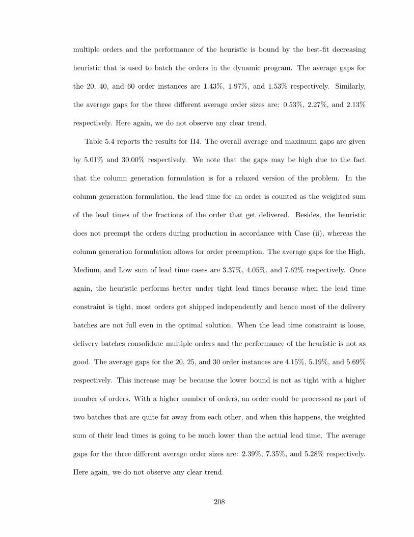
multiple orders and the performance of the heuristic is bound by the best-fit decreasing

heuristic that is used to batch the orders in the dynamic program. The average gaps for

the 20, 40, and 60 order instances are 1.43%, 1.97%, and 1.53% respectively. Similarly,

the average gaps for the three different average order sizes are: 0.53%, 2.27%, and 2.13%

respectively. Here again, we do not observe any clear trend.

Table 5.4 reports the results for H4. The overall average and maximum gaps are given

by 5.01% and 30.00% respectively. We note that the gaps may be high due to the fact

that the column generation formulation is for a relaxed version of the problem. In the

column generation formulation, the lead time for an order is counted as the weighted sum

of the lead times of the fractions of the order that get delivered. Besides, the heuristic

does not preempt the orders during production in accordance with Case (ii), whereas the

column generation formulation allows for order preemption. The average gaps for the High,

Medium, and Low sum of lead time cases are 3.37%, 4.05%, and 7.62% respectively. Once

again, the heuristic performs better under tight lead times because when the lead time

constraint is tight, most orders get shipped independently and hence most of the delivery

batches are not full even in the optimal solution. When the lead time constraint is loose,

delivery batches consolidate multiple orders and the performance of the heuristic is not as

good. The average gaps for the 20, 25, and 30 order instances are 4.15%, 5.19%, and 5.69%

respectively. This increase may be because the lower bound is not as tight with a higher

number of orders. With a higher number of orders, an order could be processed as part of

two batches that are quite far away from each other, and when this happens, the weighted

sum of their lead times is going to be much lower than the actual lead time. The average

gaps for the three different average order sizes are: 2.39%, 7.35%, and 5.28% respectively.

Here again, we do not observe any clear trend.

208

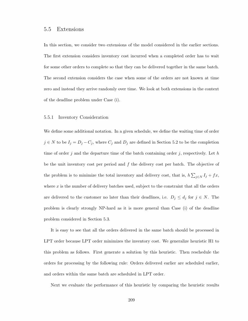
5.5 Extensions

In this section, we consider two extensions of the model considered in the earlier sections.

The first extension considers inventory cost incurred when a completed order has to wait

for some other orders to complete so that they can be delivered together in the same batch.

The second extension considers the case when some of the orders are not known at time

zero and instead they arrive randomly over time. We look at both extensions in the context

of the deadline problem under Case (i).

5.5.1 Inventory Consideration

We define some additional notation. In a given schedule, we define the waiting time of order

j ∈ N to be Ij = Dj −Cj, where Cj and Dj are defined in Section 5.2 to be the completion

time of order j and the departure time of the batch containing order j, respectively. Let h

be the unit inventory cost per period and f the delivery cost per batch. The objective of

the problem is to minimize the total inventory and delivery cost, that is, h∑

j∈N Ij + fx,

where x is the number of delivery batches used, subject to the constraint that all the orders

are delivered to the customer no later than their deadlines, i.e. Dj ≤ dj for j ∈ N . The

problem is clearly strongly NP-hard as it is more general than Case (i) of the deadline

problem considered in Section 5.3.

It is easy to see that all the orders delivered in the same batch should be processed in

LPT order because LPT order minimizes the inventory cost. We generalize heuristic H1 to

this problem as follows. First generate a solution by this heuristic. Then reschedule the

orders for processing by the following rule: Orders delivered earlier are scheduled earlier,

and orders within the same batch are scheduled in LPT order.

Next we evaluate the performance of this heuristic by comparing the heuristic results

209

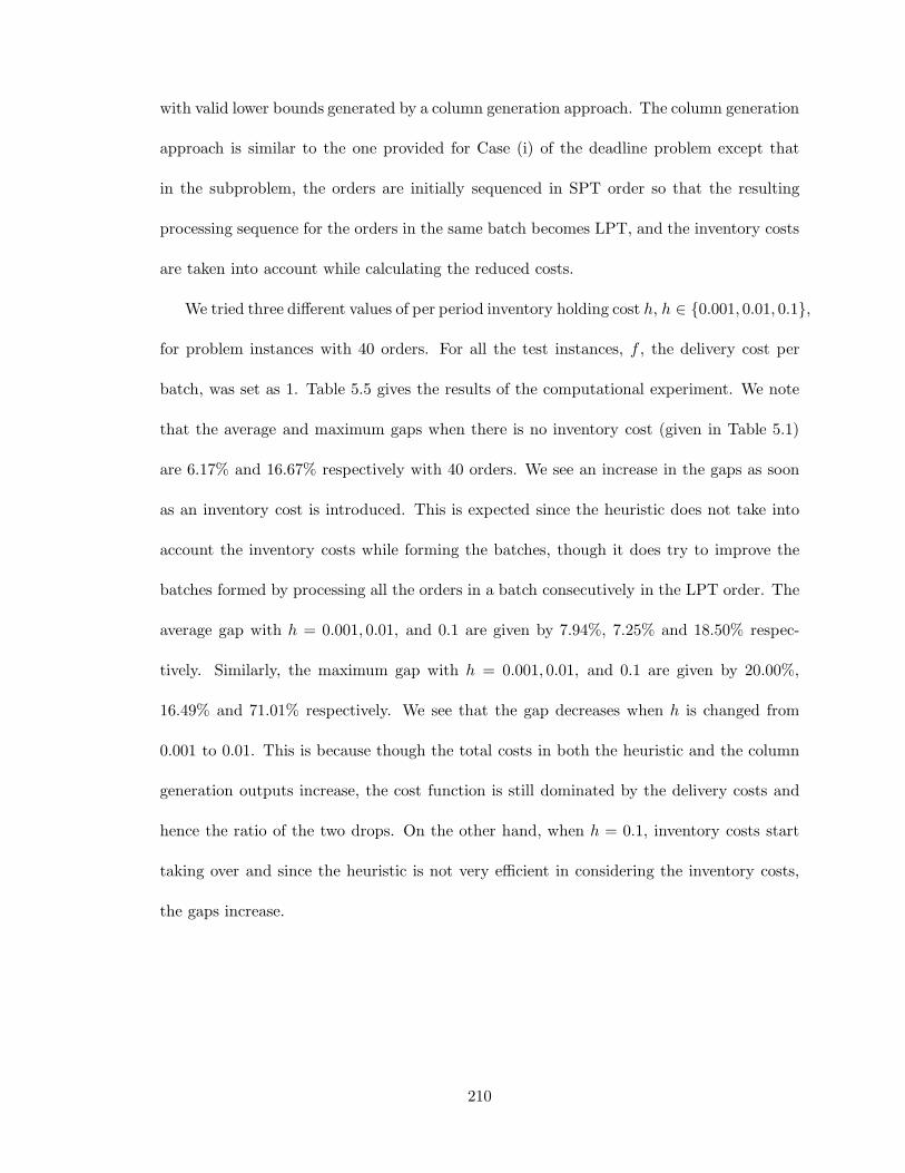
with valid lower bounds generated by a column generation approach. The column generation

approach is similar to the one provided for Case (i) of the deadline problem except that

in the subproblem, the orders are initially sequenced in SPT order so that the resulting

processing sequence for the orders in the same batch becomes LPT, and the inventory costs

are taken into account while calculating the reduced costs.

We tried three different values of per period inventory holding cost h, h ∈ 0.001, 0.01, 0.1,

for problem instances with 40 orders. For all the test instances, f , the delivery cost per

batch, was set as 1. Table 5.5 gives the results of the computational experiment. We note

that the average and maximum gaps when there is no inventory cost (given in Table 5.1)

are 6.17% and 16.67% respectively with 40 orders. We see an increase in the gaps as soon

as an inventory cost is introduced. This is expected since the heuristic does not take into

account the inventory costs while forming the batches, though it does try to improve the

batches formed by processing all the orders in a batch consecutively in the LPT order. The

average gap with h = 0.001, 0.01, and 0.1 are given by 7.94%, 7.25% and 18.50% respec-

tively. Similarly, the maximum gap with h = 0.001, 0.01, and 0.1 are given by 20.00%,

16.49% and 71.01% respectively. We see that the gap decreases when h is changed from

0.001 to 0.01. This is because though the total costs in both the heuristic and the column

generation outputs increase, the cost function is still dominated by the delivery costs and

hence the ratio of the two drops. On the other hand, when h = 0.1, inventory costs start

taking over and since the heuristic is not very efficient in considering the inventory costs,

the gaps increase.

210

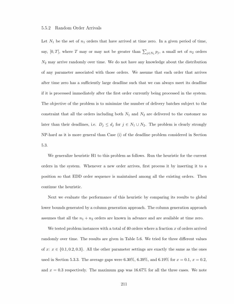
5.5.2 Random Order Arrivals

Let N1 be the set of n1 orders that have arrived at time zero. In a given period of time,

say, [0, T ], where T may or may not be greater than∑

j∈N1pj , a small set of n2 orders

N2 may arrive randomly over time. We do not have any knowledge about the distribution

of any parameter associated with those orders. We assume that each order that arrives

after time zero has a sufficiently large deadline such that we can always meet its deadline

if it is processed immediately after the first order currently being processed in the system.

The objective of the problem is to minimize the number of delivery batches subject to the

constraint that all the orders including both N1 and N2 are delivered to the customer no

later than their deadlines, i.e. Dj ≤ dj for j ∈ N1 ∪ N2. The problem is clearly strongly

NP-hard as it is more general than Case (i) of the deadline problem considered in Section

5.3.

We generalize heuristic H1 to this problem as follows. Run the heuristic for the current

orders in the system. Whenever a new order arrives, first process it by inserting it to a

position so that EDD order sequence is maintained among all the existing orders. Then

continue the heuristic.

Next we evaluate the performance of this heuristic by comparing its results to global

lower bounds generated by a column generation approach. The column generation approach

assumes that all the n1 + n2 orders are known in advance and are available at time zero.

We tested problem instances with a total of 40 orders where a fraction x of orders arrived

randomly over time. The results are given in Table 5.6. We tried for three different values

of x: x ∈ 0.1, 0.2, 0.3. All the other parameter settings are exactly the same as the ones

used in Section 5.3.3. The average gaps were 6.30%, 6.39%, and 6.19% for x = 0.1, x = 0.2,

and x = 0.3 respectively. The maximum gap was 16.67% for all the three cases. We note

211

that the average and the maximum gaps were 6.17% and 16.17% respectively for the 40

order case in Section 5.3.3. Thus there is only a very marginal increase in the average gap.

This can be explained as follows: When the deadlines are tight, most of the orders anyway

get processed close to their deadlines and as long as an order arrives with sufficient time

left for its processing, the production schedule will not change in general. On the other

hand, when the deadlines are not tight, the production sequence does not make much of

a difference to the heuristic since most of the orders will anyway be able to combine with

most of the other orders, whichever sequence they are processed in. Hence, though the

production sequence may get affected, there may not be any effect on the final number of

delivery batches. So as long as the fraction of orders that arrive at time t > 0 is not very

large, or as long as the late orders are well spread over the time horizon, the effect on the

final solution may not be significant. But when x approaches 1, or when all the late orders

arrive at a time very close to their deadlines, other complications may arise. One example

is the non-availability of any order for processing at a particular time because none of the

remaining orders have arrived. This may lead to idle time in the schedule and may even

lead to an infeasible problem instance.

5.6 Conclusions

In this study, we have analyzed an integrated production-distribution scheduling model in a

supply chain with one supplier and one customer. We have considered a scenario where the

orders generally have different sizes while the delivery batch capacity is finite. Production-

distribution scheduling decisions have to be made jointly with the order packing decisions.

Our objective was to minimize the distribution costs while ensuring that a time related ser-

vice constraint is satisfied. Computational complexity of various cases of the problem have

212

been clarified and we have provided either polynomial time optimal algorithms or fast and

efficient heuristics for all the cases. We also looked at an extension that considered inven-

tory costs and another extension that allowed for changes in the schedule to accommodate

random arrivals.

Some of the production-distribution scheduling models in the literature look at settings

with multiple suppliers and/or multiple customers. But in those problems, order packing is

not considered. In our model, order sizes add one more dimension to the problem making

it more complicated. Still it will be interesting to look at such setups and there may be

special cases of the problems with multiple suppliers and/or multiple customers that are

solvable in polynomial time. But we conjecture that the general versions of all those prob-

lems will be strongly NP-hard. Another extension to the model includes making delivery

costs dependent on the weight carried by each batch (eg. having a fixed cost per batch

and a variable cost per capacity utilized). Again, since our problem is a special case of this

version, all the NP-hard problems of our model will still be NP-hard for this extension.

213

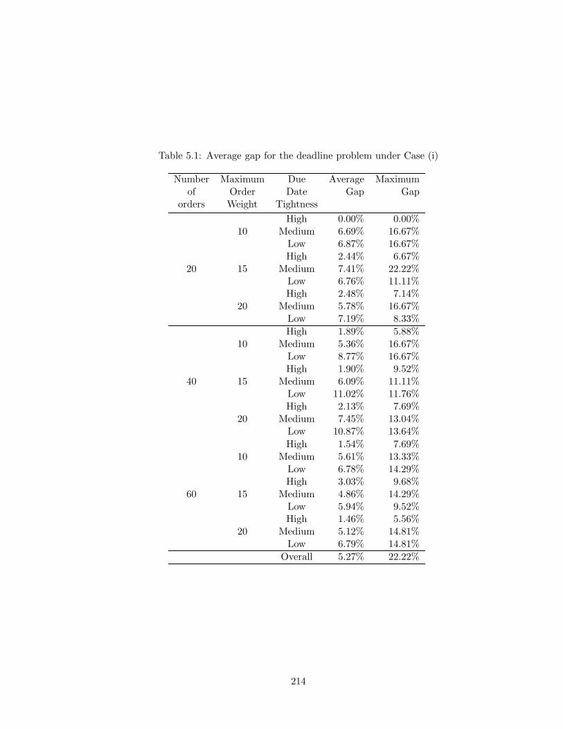
Table 5.1: Average gap for the deadline problem under Case (i)

Number Maximum Due Average Maximumof Order Date Gap Gap

orders Weight TightnessHigh 0.00% 0.00%

10 Medium 6.69% 16.67%Low 6.87% 16.67%High 2.44% 6.67%

20 15 Medium 7.41% 22.22%Low 6.76% 11.11%High 2.48% 7.14%

20 Medium 5.78% 16.67%Low 7.19% 8.33%High 1.89% 5.88%

10 Medium 5.36% 16.67%Low 8.77% 16.67%High 1.90% 9.52%

40 15 Medium 6.09% 11.11%Low 11.02% 11.76%High 2.13% 7.69%

20 Medium 7.45% 13.04%Low 10.87% 13.64%High 1.54% 7.69%

10 Medium 5.61% 13.33%Low 6.78% 14.29%High 3.03% 9.68%

60 15 Medium 4.86% 14.29%Low 5.94% 9.52%High 1.46% 5.56%

20 Medium 5.12% 14.81%Low 6.79% 14.81%

Overall 5.27% 22.22%

214

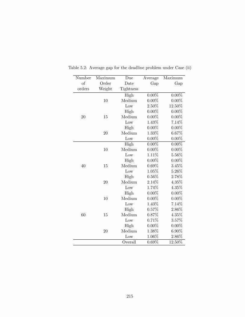
Table 5.2: Average gap for the deadline problem under Case (ii)

Number Maximum Due Average Maximumof Order Date Gap Gap

orders Weight TightnessHigh 0.00% 0.00%

10 Medium 0.00% 0.00%Low 2.50% 12.50%High 0.00% 0.00%

20 15 Medium 0.00% 0.00%Low 1.43% 7.14%High 0.00% 0.00%

20 Medium 1.33% 6.67%Low 0.00% 0.00%High 0.00% 0.00%

10 Medium 0.00% 0.00%Low 1.11% 5.56%High 0.00% 0.00%

40 15 Medium 0.69% 3.45%Low 1.05% 5.26%High 0.56% 2.78%

20 Medium 2.14% 4.35%Low 1.74% 4.35%High 0.00% 0.00%

10 Medium 0.00% 0.00%Low 1.43% 7.14%High 0.57% 2.86%

60 15 Medium 0.87% 4.35%Low 0.71% 3.57%High 0.00% 0.00%

20 Medium 1.38% 6.90%Low 1.06% 2.86%

Overall 0.69% 12.50%

215

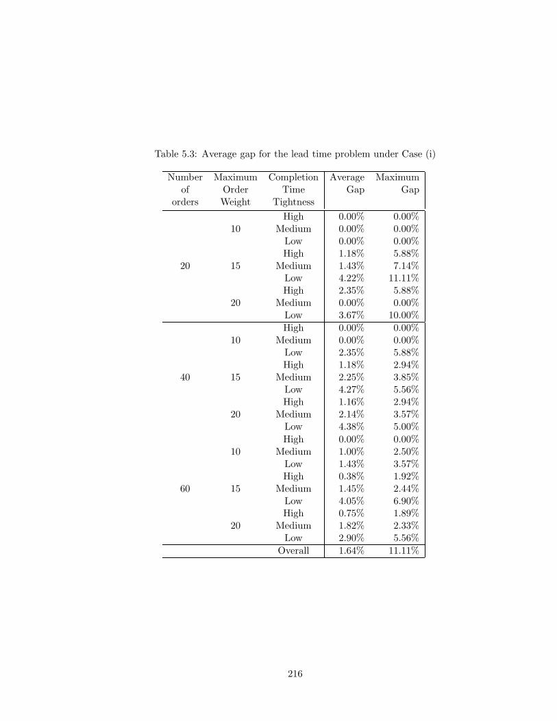
Table 5.3: Average gap for the lead time problem under Case (i)

Number Maximum Completion Average Maximumof Order Time Gap Gap

orders Weight TightnessHigh 0.00% 0.00%

10 Medium 0.00% 0.00%Low 0.00% 0.00%High 1.18% 5.88%

20 15 Medium 1.43% 7.14%Low 4.22% 11.11%High 2.35% 5.88%

20 Medium 0.00% 0.00%Low 3.67% 10.00%High 0.00% 0.00%

10 Medium 0.00% 0.00%Low 2.35% 5.88%High 1.18% 2.94%

40 15 Medium 2.25% 3.85%Low 4.27% 5.56%High 1.16% 2.94%

20 Medium 2.14% 3.57%Low 4.38% 5.00%High 0.00% 0.00%

10 Medium 1.00% 2.50%Low 1.43% 3.57%High 0.38% 1.92%

60 15 Medium 1.45% 2.44%Low 4.05% 6.90%High 0.75% 1.89%

20 Medium 1.82% 2.33%Low 2.90% 5.56%

Overall 1.64% 11.11%

216

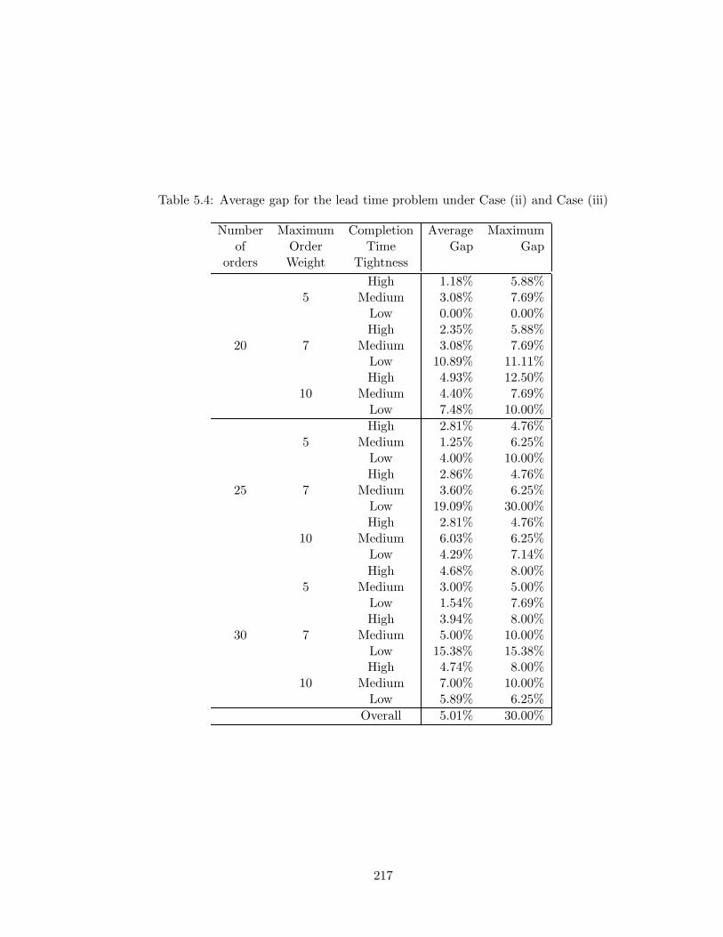
Table 5.4: Average gap for the lead time problem under Case (ii) and Case (iii)

Number Maximum Completion Average Maximumof Order Time Gap Gap

orders Weight TightnessHigh 1.18% 5.88%

5 Medium 3.08% 7.69%Low 0.00% 0.00%High 2.35% 5.88%

20 7 Medium 3.08% 7.69%Low 10.89% 11.11%High 4.93% 12.50%

10 Medium 4.40% 7.69%Low 7.48% 10.00%High 2.81% 4.76%

5 Medium 1.25% 6.25%Low 4.00% 10.00%High 2.86% 4.76%

25 7 Medium 3.60% 6.25%Low 19.09% 30.00%High 2.81% 4.76%

10 Medium 6.03% 6.25%Low 4.29% 7.14%High 4.68% 8.00%

5 Medium 3.00% 5.00%Low 1.54% 7.69%High 3.94% 8.00%

30 7 Medium 5.00% 10.00%Low 15.38% 15.38%High 4.74% 8.00%

10 Medium 7.00% 10.00%Low 5.89% 6.25%

Overall 5.01% 30.00%

217

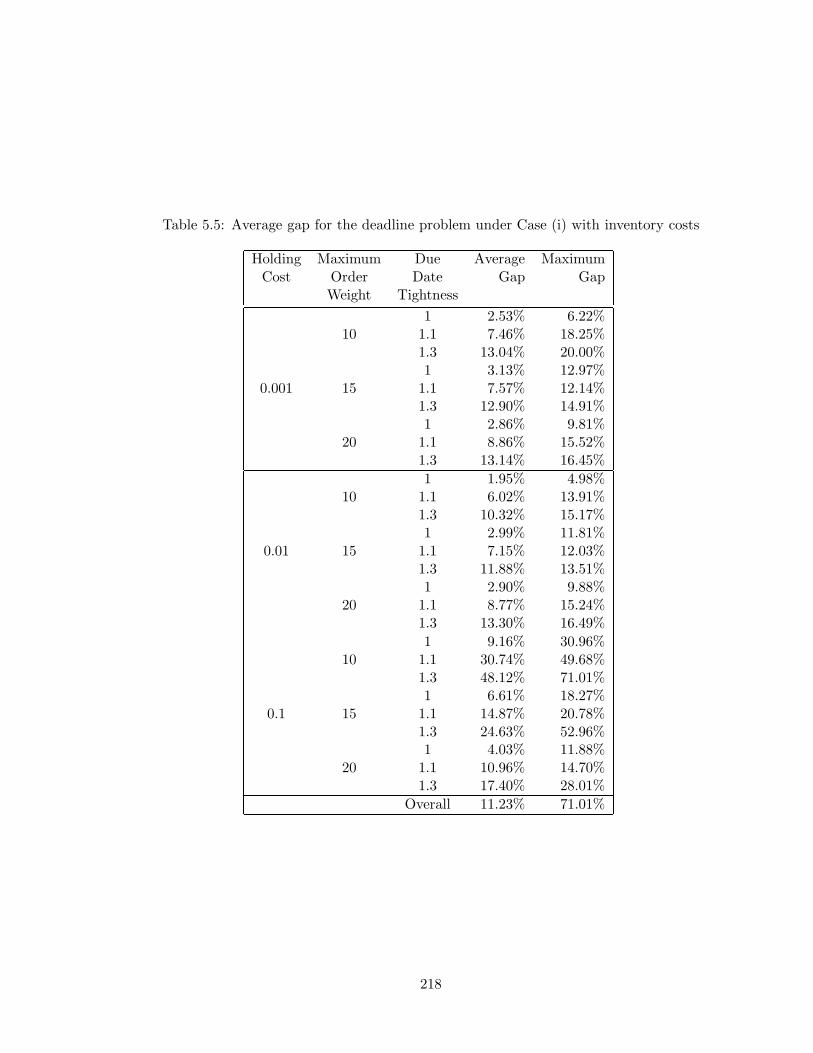
Table 5.5: Average gap for the deadline problem under Case (i) with inventory costs

Holding Maximum Due Average MaximumCost Order Date Gap Gap

Weight Tightness1 2.53% 6.22%

10 1.1 7.46% 18.25%1.3 13.04% 20.00%1 3.13% 12.97%

0.001 15 1.1 7.57% 12.14%1.3 12.90% 14.91%1 2.86% 9.81%

20 1.1 8.86% 15.52%1.3 13.14% 16.45%1 1.95% 4.98%

10 1.1 6.02% 13.91%1.3 10.32% 15.17%1 2.99% 11.81%

0.01 15 1.1 7.15% 12.03%1.3 11.88% 13.51%1 2.90% 9.88%

20 1.1 8.77% 15.24%1.3 13.30% 16.49%1 9.16% 30.96%

10 1.1 30.74% 49.68%1.3 48.12% 71.01%1 6.61% 18.27%

0.1 15 1.1 14.87% 20.78%1.3 24.63% 52.96%1 4.03% 11.88%

20 1.1 10.96% 14.70%1.3 17.40% 28.01%

Overall 11.23% 71.01%

218

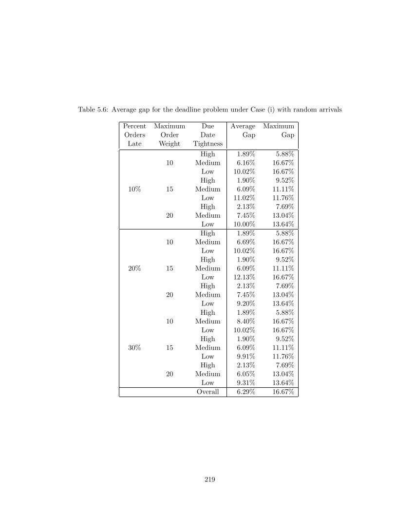
Table 5.6: Average gap for the deadline problem under Case (i) with random arrivals

Percent Maximum Due Average MaximumOrders Order Date Gap GapLate Weight Tightness

High 1.89% 5.88%10 Medium 6.16% 16.67%

Low 10.02% 16.67%High 1.90% 9.52%

10% 15 Medium 6.09% 11.11%Low 11.02% 11.76%High 2.13% 7.69%

20 Medium 7.45% 13.04%Low 10.00% 13.64%High 1.89% 5.88%

10 Medium 6.69% 16.67%Low 10.02% 16.67%High 1.90% 9.52%

20% 15 Medium 6.09% 11.11%Low 12.13% 16.67%High 2.13% 7.69%

20 Medium 7.45% 13.04%Low 9.20% 13.64%High 1.89% 5.88%

10 Medium 8.40% 16.67%Low 10.02% 16.67%High 1.90% 9.52%

30% 15 Medium 6.09% 11.11%Low 9.91% 11.76%High 2.13% 7.69%

20 Medium 6.05% 13.04%Low 9.31% 13.64%

Overall 6.29% 16.67%

219

Chapter 6

Conclusions

In this thesis, we have considered various production-distribution scheduling problems in

a supply chain setting. In the second chapter, we analyzed four problems related to order

assignment and scheduling in a supply chain with one or more suppliers and one cus-

tomer. Computational complexity of various cases of the problems have been clarified, and

polynomial-time exact algorithms have been proposed for some special cases of the prob-

lems. All the four problems are in general NP-hard, and fast heuristics have been proposed

for each of them. We have analyzed the worst-case and asymptotic performance of two of

the heuristics. We have also tested each heuristic computationally.

In the third chapter, we studied a due-date based problem involving one supplier and one

or more customers. We saw that for an arbitrary number of customers, the problem is NP-

hard even in the special case where the processing times and the due dates are agreeable. A

fast heuristic has been proposed that is asymptotically optimal when the number of orders

goes to infinity. Computational tests show that the heuristic is capable of generating near

optimal solutions.

In the fourth chapter, we studied a joint cyclic production and distribution scheduling

problem in a two-stage supply chain with one or more suppliers, one warehouse, and one

customer. We have given either optimal approaches or heuristic methods to solve the

220

problem under two policies on production and delivery cycles. For the case with common

production and delivery cycle at each supplier (policy (i)), we have proved that there exists

an optimal solution where the delivery cycle time from a supplier to the warehouse is an

integer multiple of the delivery cycle time from the warehouse to the customer. Based on

this property, we have shown that there is a closed-form optimal solution to the problem

with a single supplier under policy (i), and developed an efficient heuristic for the general

problem under policy (i). The problem under policy (ii), which is more general than policy

(i), is solved by a heuristic approach. Both the heuristics were shown to perform well in

the computational tests.

In the fifth chapter, we looked at a problem with one supplier and one customer where

different jobs may have different weights for delivery. The objective was to arrive at an

integrated production and distribution schedule that minimizes the total distribution cost.

We minimize the number of shipments subject to time based performance measures such

as deadlines or the average lead times. We considered six different cases, three for the

deadline version and three for the lead time version. Except for one case for which an

optimal polynomial time algorithm was given, all the remaining were shown to be NP-hard.

We have given heuristics with known worst-case performance for all the NP-hard cases.

We carried out computational tests to analyze the performance of these heuristcs, where

the output from the heuristic was compared with a lower bound obtained through column

generation. The heuristics were able to obtain optimal or near-optimal solutions for most

of the problem instances tested.

As mentioned in Chapter 1, the aim of this thesis is three-fold: (i) To propose various

integrated production-distribution scheduling models that closely mirror pracitical supply

chain operations in some environments. (ii) To develop computationally effective optimiza-

221

tion based solution algorithms to solve these models. Our solution approaches can be used

as decision tools by practitioners. (iii) To provide managerial insights into the potential

benefits of coordination between production and distribution operations in a supply chain.

Many supply chains may involve more than just one or two stages. Though we have not

given closed form equations or algorithms for more complicated supply chains, the insights

from the study can still be carried over. In many cases, a simple coordination mechanism

between two adjacent stages in a supply chain may itself prove very powerful.

The various models studied in this thesis also give an insight into the system charac-

teristics that would benefit significantly from coordination. If a system is such that service

based performance measure is not crucial, then it may not be worth the effort to coordi-

nate the production and distribution activities. For example, in Model 1, if the lead time

performance is not crucial (the value of α is low or the lead time constraint is not very

binding), then the production sequence does not matter significantly. It may be sufficient

to just assign the orders to plants in a cost-effective way and then deliver them in as few

delivery batches as possible. Similarly in Model 2, if the deadlines are not very tight, then

the sequential approaches may not differ significantly from the integrated approach in terms

of performance. But in cases where the system is congested, or when the system is such that

the production constraints are tight, integration will become important. Similarly, in Model

3, integration becomes more crucial as the benefits from consolidation begin to increase,

for example, when the distribution activities have low fixed costs but high variable costs,

or when the number of suppliers is high. So depending on the supply-chain, integrated

production-distribution scheduling may result in significant savings.

Various extensions to this study could be considered. We have not explored routing

options in models that involve more than one supplier or more than one customer. In

222

all the models studied, it has been assumed that direct shipments take place between the

supplier and the customer. It will be interesting to analyze the effects of introducing routing

decisions into the model. We have considered a setup where the overall supply chain cost

is minimized. This assumes a cooperative setup. In many instances, different parts of the

supply chain may be owned by different firms. A competitive setup may be more appropriate

under such circumstances. In our study, we assume that all the orders (or demand rate) are

known at the beginning. A dynamic setup where orders become known over time would be

an interesting extension. We did a limited study of this extension by allowing dynamic order

arrivals for Case (i) of the deadline model in Chapter 5. If dynamic arrivals are allowed,

order assignment and/or scheduling will also have to be carried out dynamically and it may

be necessary to partially modify an existing schedule when a new order is received. All

the extensions proposed here will in general be NP-hard but it may be possible to propose

efficient heuristics or solve some special cases optimally in polynomial time.

223

Bibliography

[1] Atkins, D. and M. Queyranne, “Lot Sizing Policies for Finite Production Rate Assembly

Systems”, Operations Research, 40 (1992), 126 - 141.

[2] Bagchi, P.K. and F.W. Davis, “Some Insights into Inbound Freight Consolidation”,

International Journal of Physical Distribution and Materials Management, 18(6) (1988)

27-33.

[3] Bazaraa, M.S., H.D. Sherali, and C.M. Shetty, “Nonlinear Programming: Theory and

Algorithms”, Second Edition, John Wiley & Sons, Inc. New York, (1993).

[4] Belenguer, J.M., M.C. Martinez, and E. Mota, “A lower bound for the split delivery

vehicle routing problem”, Operations Research, 48 (2000), 801-810.

[5] Benjamin, J., “An analysis of inventory and transportation costs in a constrained net-

work”, Transportation Science, 23(3) (1989), 177-183.

[6] Bertazzi, L. and M.G. Speranza, “Minimizing Logistics Costs in Multistage Supply

Chains”, Naval Research Logistics, 46 (1999), 399-417.

[7] Blackburn, J.D. and R.A. Millen, “Improved heuristics for multi-stage requirement plan-

ning systems”, Management Science, 28 (1982), 44 - 56.

[8] Blumenfeld, D.E., L.D. Burns and C.F. Daganzo, “Synchronizing Production and Trans-

portation Schedules”, Transportation Research, 25B (1991), 23-37.

224

[9] Blumenfeld, D.E., L.D. Burns, J.D. Diltz, and C.F. Daganzo, “Analyzing Tradeoffs

between Transportation, Inventory and Production Costs on Freight Networks”, Trans-

portation Research, 19B (1985), 361-380.

[10] Boyaci, T. and G. Gallego, “Serial Production/Distribution Systems under Service

Constraints”, Manufacturing & Service Operations Management, 3 (2001), 43-50.

[11] Bramel, J., S. Goyal, and P. Zipkin, “Coordination of Production/Distribution Net-

works with Unbalanced Leadtimes”, Operations Research, 48 (2000), 570-577.

[12] Burns, L.D., R.W. Hall, D.E. Blumenfeld, and C.F. Daganzo, “Distribution Strategies

that Minimize Transportation and Inventory Costs”, Operations Research, 33 (1985),

469-490.

[13] Chan, L.M.A., A. Muriel, and D. Simchi-Levi, “Supply-chain management: Integrating

inventory and transportation”, Working Paper, Department of Industrial Engineering

and Management Sciences, Northwestern University, (1997).

[14] Chandra, P. and M.L. Fisher, “Coordination of production and distribution planning”,

European Journal of Operational Research, 72 (1994), 503-517.

[15] Chang, Y.-C., and C.-Y. Lee, “Machine scheduling with job delivery coordination”,

European Journal of Operational Research, 158 (2004), 470-487.

[16] Chen, Z.-L, “Scheduling and common due date assignment with earliness-tardiness

penalties and batch delivery costs”, European Journal of Operational Research, 93

(1996), 49-60.

[17] Chen, Z.-L., “Integrated Production and Distribution Operations: Taxonomy, Mod-

els, and Review”, In Handbook of Quantitative Supply Chain Analysis: Modeling in

225

the E-Business Era, Eds: D. Simchi-Levi, S.D. Wu and Z.-J. Shen. Kluwer Academic

Publishers, (2004).

[18] Chen, Z.-L. and G.L. Vairaktarakis, “Integrated scheduling of production and distrib-

ution operations”, Management Science, Forthcoming (2005).

[19] Cheng, T.C.E., V.S. Gordon, and M.Y. Kovalyov, “Single machine scheduling with

batch deliveries”, European Journal of Operational Research, 94 (1996), 277-283.

[20] Coffman, Jr., E.G., M.R. Garey, and D.S. Johnson, “Approximation algorithms for

bin packing: a survey.” In: D.S. Hochbaum (editor), Approximation Algorithms for

NP-hard Problems, PWS Publishing, Boston, (1997), 46-93.

[21] Cohen, M.A. and H.L. Lee, “Strategic analysis of integrated production-distribution

systems: models and methods”, Operations Research, 36 (1988), 212-228.

[22] Cooper, M., “Cost and Delivery Time Implications of Freight Consolidation and Ware-

housing Strategies”, International Journal of Physical Distribution and Materials Man-

agement, 14(6) (1984), 47 - 67.

[23] Crowston, W.B., M. Wagner, and J.F. Williams, “Economic Lot Size Determination

in Multi-stage Assembly System”, Management Science, 19 (1973), 517 - 527.

[24] Dasci, A. and V. Verter, “A Continuous Model for Production-Distribution System

Design”,

[25] European Journal of Operational Research, 129 (2001), 287-298.

[26] Dogan, K. and M. Goetschalckx, “A Primal Decomposition Method for the Integrated

Design of Multi-Period Production-Distribution Systems”, IIE Transactions, 31 (1999),

1027 - 1036.

226

[27] Dornier, P.-P., R. Ernst, M. Fender, and P. Kouvelis, “Global Operations and Logistics:

Text and Cases”, John Wiley & Sons, Inc, (1998).

[28] Dror, M., and P. Trudeau, “Savings by split delivery routing”, Transportation Science,

23 (1989), 23-37.

[29] Fumero, F. and C. Vercellis, “Synchronized development of production, inventory, and

distribution schedules”, Transportation Science, 33(1999), 330-340.

[30] Garey, M.R. and D.S. Johnson, “Computers and Intractability: A Guide to the Theory

of NP-Completeness”, W.H. Freeman, San Francisco, (1979).

[31] Ghosh, J.B. and Gupta, J.N.D., “Batch scheduling to minimize maximum lateness”,

Operations Research Letters, 21 (1997), 77-80.

[32] Hahm, J. and C.A. Yano, “The Economic Lot and Delivery Scheduling Problem: The

Single Item Case”, International Journal of Production Economics, 28 (1992), 235-252.

[33] Hahm, J. and C.A. Yano, “Economic Lot and Delivery Scheduling Problem: The

Common Cycle Case”, IIE Transactions, 27 (1995a), 113-125.

[34] Hahm, J. and C.A. Yano, “Economic Lot and Delivery Scheduling Problem: The

Nested Schedule Case”, IIE Transactions, 27 (1995b), 126-139.

[35] Hahm, J. and C.A. Yano, “Economic Lot and Delivery Scheduling Problem: Powers of

Two Policies”, Transportation Science, 29 (1995c), 222-241.

[36] Hall, L.A. and D.B. Shmoys, “Jackson’s rule for single-machine scheduling: making a

good heuristic better”, Mathematics of Operations Research, 17 (1992), 22-35.

227

[37] Hall, N.G., M. Lesaoana, and C.N. Potts, “Scheduling with fixed delivery dates”,

Operations Research, 49 (2001), 134-144.

[38] Hall, N.G. and C.N. Potts, “Supply chain scheduling: Batching and delivery”, Opera-

tions Research, 51 (2003), 566-584.

[39] Hall, R.W., “On the Integration of Production and Distribution: Economic Order and

Production Quantity Implications”, Transportation Research, 30B (1996), 387-403.

[40] Hammond, J.H. and A. Raman, “Sport Obermeyer, Ltd”, Harvard Business School

Case #9-695-022 (1996).

[41] Hariri, A.M.A and Potts, C.N., “Single machine scheduling with batch set-up times to

minimize maximum lateness”, Annals of Operations Research, 70 (1997), 75-92.

[42] Herrmann, J. and C.-Y. Lee, “On scheduling to minimize earliness-tardiness and batch

delivery costs with a common due date”, European Journal of Operational Research, 70

(1993), 272-288.

[43] Horn, W.A, “Minimizing average flow time with parallel machines”, Operations Re-

search, 21 (1973), 846-847.

[44] Jackson, J.R., “Scheduling a production line to minimize maximum tardiness”, Re-

search Report 43, Management Science Research Project, University of California, Los

Angeles, (1995).

[45] Jayaraman, V. and H. Pirkul, “Planning and Coordination of Production and Distrib-

ution Facilities for Multiple Commodities”, European Journal of Operational Research,

133 (2001), 394-408.

228

[46] Jensen, M.T. and M. Khouja, “An Optimal Polynomial Time Algorithm for the Com-

mon Cycle Economic Lot and Delivery Scheduling Problem”, European Journal of Op-

erational Research, 156 (2004), 305-311.

[47] Johnson, M.E., “Learning from toys: Lessons in managing supply chain risk from the

toy industry”, California Management Review, 43 (2001), 106-124.

[48] Kaminsky, P. and D. Simchi-Levi, “Production and distribution lot sizing in a two

stage supply chain”. IIE Transactions, 35 (2003), 1065-1074.

[49] Lee, C.-Y. and Z.-L. Chen, “Machine scheduling with transportation considerations”

Journal of Scheduling, 4 (2001), 3-24.

[50] Lee, C.-Y. and Li, C.-L., “On the fixed interval due-date scheduling problem”, Discrete

Applied Mathematics, 68 (1996), 101 - 117.

[51] Moily, J.P. “Optimal and Heuristic Procedures for Component Lot-splitting in Multi-

stage Manufacturing Systems”, Management Science, 32 (1986), 113 - 125.

[52] Moily, J.P. and J.P. Matthews, “Procedures for Determining Relative Frequencies of

Production/Order in Multistage Assembly Systems”, Decision Sciences, 18 (1987), 279

- 291.

[53] Muckstadt, J. and R. Roundy, “Analysis of Multistage Production Systems”, In Lo-

gistics of Production and Inventory, Handbooks in OR/MS, Volume 4, S. Graves, A.

Rinnooy Kan, and P. Zipkin (eds.), Elsevier, North-Holland, Amsterdam, 1993.

[54] Owen, S.H. and M.S. Daskin, “Strategic Facility Location: A Review”, European

Journal of Operational Research, 111 (1998), 423-447.

229

[55] Pinedo, M., “Scheduling: Theory, Algorithms, and Systems, 2nd Edition”, Prentice

Hall, Upper Saddle River, New Jersey, (2002).

[56] Potts, C.N., “Analysis of a heuristic for one machine sequencing with release dates and

delivery times”, Operations Research, 28 (1980), 1436-1441.

[57] Potts, C.N., “Analysis of a linear programming heuristic for scheduling unrelated par-

allel machines”, Discrete Applied Mathematics, 10 (1985), 155-164.

[58] Potts, C.N., and Kovalyov, M. Y., “Scheduling with batching: A review”, European

Journal of Operational Research, 120 (2000), 228-249.

[59] Pyke, D.F. and M.A. Cohen, “Multiproduct Integrated Production-Distribution Sys-

tems”, European Journal of Operational Research, 74 (1994), 18-49.

[60] Sabri, E. and B.M. Beamon, “A Multi-Objective Approach to Simultaneous Strategic

and Operational Planning in Supply Chain Design”, Omega, 28 (2000), 581 - 598.

[61] Sarmiento, A.M. and R. Nagi, “A review of integrated analysis of production-

distribution systems”, IIE Transactions, 31 (1999), 1061-1074.

[62] Schwarz, L.B. and L. Schrage, “Optimal and System Myopic Policies for Multi-echelon

Production-inventory Assembly Systems”, Management Science, 21 (1975), 1285 - 1294.

[63] Shen, Z.-J. M., C. Coullard, and M.S. Daskin, “A Joint Location-Inventory Model”,

Transportation Science, 37 (2003), 40 - 55.

[64] Speranza, M.G. and W. Ukovich, “Minimizing Transportation and Inventory Costs for

Several Products on a Single Link”, Operations Research, 42 (1994), 879-894.

230

[65] Vidal, C.J. and M. Goetschalckx, “Strategic Production-Distribution Models: A Crit-

ical Review with Emphasis on Global Supply Chain Models”, European Journal of

Operational Research, 98 (1997), 1-18.

[66] Wang, G. and T.C.E. Cheng, “Parallel machine scheduling with batch delivery costs”,

International Journal of Production Economics, 68 (2000), 177-183.

[67] Webster, S. and K.R. Baker, “Scheduling groups of jobs on a single machine”, Opera-

tions Research, 43 (1995), 692 - 703.

[68] Williams, J.F., “A Hybrid Algorithm for Simultaneous Scheduling of Production and

Distribution in Multi-Echelon Structures”, Management Science, 29 (1983), 77 - 92.

[69] Woeginger, G.J., “Heuristics for parallel machine scheduling with delivery times”, Acta

Informatica, 31 (1994), 503-512.

[70] Woeginger, G.J., “A polynomial-time approximation scheme for single-machine se-

quencing with delivery times and sequence-independent batch set-up times”, Journal of

Scheduling, 1 (1998), 79-87.

[71] Yuan, J., “A Note on the Complexity of Single-Machine Scheduling with a Common

Due Date, Earliness-Tardiness, and Batch Delivery Costs”, European Journal of Oper-

ational Research, 94 (1996), 203-205.

231