abstract title of document: cross sectional - drum

ABSTRACT

Title of Document: CROSS SECTIONAL EVALUATION OF POTENTIAL VOLATILE ORGANIC COMPOUND EXPOSURES AROUND U.S. SCHOOLS

Advisor: Dr. Amir Sapkota, Maryland Institute for Applied Environmental

Health

Volatile Organic Compounds (VOCs), characterized by high vapor pressure and

low water solubility, exist in gaseous phase at room temperature. Previous studies have

suggested exposure to VOCs may be associated with adverse health effects such as

asthma exacerbation and in some cases cancer. The major sources of outdoor VOCs

include traffic and industrial emissions. Ambient VOCs can react with Nitrogen Oxides

(NOx) in the presence of sunlight to form ground level ozone, one of the U.S.

Environmental Protection Agency (EPA) Criteria Air Pollutants. This thesis was

designed to investigate the potential VOCs exposure among U.S. schoolchildren.

Moreover, the influence of various neighborhood factors (urban vs. rural areas, distance

from highways, presence/absence of industries) on VOCs concentrations around U.S.

Schools was investigated. The findings of this thesis suggest that schools in urban areas,

near industries and traffic activity have higher concentrations of VOCs compared to those

not possessing such characteristics.

CROSS SECTIONAL EVALUATION OF POTENTIAL VOLATILE ORGANIC COMPOUND EXPOSURES AROUND U.S. SCHOOLS

By

Joanne Pérodin

Thesis submitted to the Faculty of the Graduate School of the University of Maryland, College Park, in partial fulfillment

of the requirements for the degree of Master of Public Health

2009 Advisory Committee: Professor Amir Sapkota, Chair Professor Betty Dabney Professor Sam Joseph Professor Amy Sapkota

© Copyright by Joanne Pérodin

2009

ii

Table of Contents

List of Figures ..................................................................................................................... ii List of Tables ..................................................................................................................... iii Acknowledgements ............................................................................................................ iv Chapter 1: Introduction ........................................................................................................1 Chapter 2: Background ........................................................................................................4

2.1 Volatile Organic Compounds ............................................................................................ 4

2.2 Sources of Volatile Organic Compounds .......................................................................... 6

2.2.1 Indoor Sources ......................................................................................................... 6

2.2.2 Outdoor Sources ...................................................................................................... 8

2.3 Volatile Organic Compounds and Health .......................................................................... 9

2.3.1 Volatile Organic Compound Exposures & Asthma ............................................... 10

2.3.2 Volatile Organic Compound Exposures & Cancer ................................................ 12

Chapter 3: Methods ............................................................................................................14 3.1 Instrument ....................................................................................................................... 14

3.1.1 Gas-Chromatograph Mass-Spectrometer ................................................................ 14

3.1.2 Calibration .............................................................................................................. 14

3.2 Chemicals ........................................................................................................................ 18

3.3 Air Sampling ................................................................................................................... 18

3.3.1 Study Site ................................................................................................................ 18

3.3.2 Sample Collection ................................................................................................... 19

3.4 Sample Analysis ............................................................................................................... 20

3.4.1 Sample Extraction ................................................................................................... 20

3.4.2 Sample Recovery .................................................................................................... 22

3.4.3 Limit of Detection ................................................................................................... 22

3.5 Statistical Methods ........................................................................................................... 24

Chapter 4: Results ..............................................................................................................25 Chapter 5: Discussion ........................................................................................................46 Chapter 6: Conclusion........................................................................................................51 Appendices .........................................................................................................................52 Bibliography ......................................................................................................................56

iii

List of Figures

1. Spectral peaks and calibration curve

2. Volatile organic compounds (VOCs) average concentration (µg/m3) by type

3. Volatile organic compounds (VOCs) average concentration (µg/m3) by presence

of industry

4. Volatile organic compounds (VOCs) average concentration (µg/m3) by highway

distance

5. Volatile organic compounds (VOCs) average concentration (µg/m3) by region

6. Association among five selected volatile organic compounds (VOCs)

iv

List of Tables

1. Location description by state

2. Compound retention time (RT), and limit of detection (LOD)

3. Total volatile organic compound (VOCs) average concentration (µg/m3)

4. Mean concentration (µg/m3) comparison (Regional concentration vs. Total

average)

5. Correlation between volatile organic compounds (VOCs) using Spearman’s Rank

Test

v

Acknowledgements

I owe my deepest gratitude to Dr. Amir Sapkota, my advisor. The completion of

this thesis would not have been possible without his continuous support, guidance, and

persistent help. Dr. Sapkota both encouraged and challenged me throughout my academic

program. “Keep chugging along”, is a supportive saying of Dr. Sapkota that I will never

forget.

I would like to thank my thesis committee members, Drs Betty Dabney, Sam

Joseph, and Amy Sapkota for their valuable suggestions throughout my academic journey

and thesis completion. The cooperation I received from each faculty member of the

Maryland Institute for Applied Environmental Health is truly acknowledged. I also wish

to acknowledge my colleagues at the institute for their assistance and support, with

special thanks going to Nicole Favaro, Erinna Kinney, Shirley Micallef, Rachel

Rosenberg, and Kristie Trousdale.

I am grateful to my strongest and most valuable supporters, my family. I want to

especially thank my parents, Daniel P. and Marie José B. Pérodin, who taught me the

value of hard work and have always been there to support me and encourage me in an

endeavor.

Words fail me to express my gratitude to those who have seen me in my most

stressful moments, provided me with endless support accompanied by the late-night

vi

editing of my thesis. I want to thank my friends Alecia Anderson, Samanmalee

Hewawasam, Negar Jahanbin, Soncia Shako and Aseem Sharma.

Lastly, I would like to thank all who have supported me both directly and

indirectly in completing my thesis.

1

CHAPTER 1: INTRODUCTION

Over the past decades, there have been increasing concerns about the effects of air

quality on human health. Despite environmental regulations, reduction in traffic and

industrial emissions, ongoing changes in infrastructure such as modern buildings for

better energy efficiency, and ventilation (Jones, 1999), high concentrations of toxic

agents in the air still remain across the United States.

The reported increase in asthma prevalence as well as the high cancer rates are

significant public health problems in the U.S. (CDC, 2006; American Cancer Society,

2009). Previous studies have shown that exposure to volatile organic compounds (VOCs)

may contribute to respiratory health deterioration as well as cancer risk (Delfino, R.J,

Gong, H., Linn, W. S., Hu, Y. & Pellizzari, E. D., 2003; Boeglin, M. L., Wessels, D. &

Henshel, D., 2006). Exposure to concentrations even below standard recommendations

can lead to an increase in asthma outcome by about 2 folds among children (Rumchev,

K., Spickett, J., Bulsara, M., Phillips, M. & Stick, S., 2004). Others have suggested that

air pollution from mobile sources, which include VOCs, may be related to the worldwide

increase in asthma (D’Amato, G., Liccardi, G., D’Amato, M., & Cazzola, M., 2001).

Likewise, chronic VOC exposure has also been linked with cancer (Guo, H., Lee, S. C.,

Chan, L. Y. & Li, W., 2004), many of which also originate from mobile sources. Studies

have also shown elevated risks for cancer among populations exposed to VOCs

(Woodruff, T. J., Caldwell, J., Cogliano, V. J. & Axelrad, D. A., 2000). The degree of

2

adverse health effect from exposure to VOCs may depend primarily upon the frequency,

duration of exposures (UNEP, 1994).

There are several sources of VOCs in indoor environments, including cleaning

products, solvents, off-gassing from furniture/carpets as well as cigarette smoking. In

addition to these indoor sources, outdoor sources also contribute to indoor levels of

VOCs as they readily penetrate indoors. Even though indoor concentrations of VOCs

have been shown to be much higher than outdoor concentrations, outdoor exposures also

remain a concern to the public health. The levels of outdoor VOCs depend upon several

factors including residential location (urban, semi-urban, rural), traffic density, and

industrial activities (Fischer et al., 2000; Lee, S.C., Chiu, M. Y., Ho, K. F., Zou, S. C. &

Wang, X., 2002). Despite this, very little is known about outdoor VOCs exposures among

vulnerable populations such as children. Therefore, characterizing VOC exposures to

such populations is important, as this information may be helpful in designing proper

intervention strategies. Within this context, the potential exposures taking place within

the school environment are important, as children spend a significant part of their day at

schools.

Hypothesis:

To estimate potential exposure to VOCs at schools, a cross sectional study was

carried out with the following hypotheses-

1) Schools in urban areas have higher VOCs concentration than schools in rural

areas,

3

2) Schools near major industries have higher VOCs concentration then those without

industries.

The variables used to test these hypotheses included presence and distance to mobile

sources (major traffic roads) and stationary sources (industry), type of location (urban,

rural), and region (Midwest, Northeast, South, and West).

The goal of this investigation was to find out whether some schoolchildren from

specific areas are potentially exposed to high levels of VOCs, thus putting them at

greater risk for potential acute and/or chronic health outcomes.

4

CHAPTER 2: BACKGROUND

2.1 Volatile Organic Compounds

Volatile organic compounds (VOCs) are carbon-based chemicals that exist in

gaseous forms at room temperature. They are characterized by high vapor pressure

and low water solubility. They are significant components of indoor as well as

outdoor air pollution. The list of VOCs contains hundreds of compounds, including

known human carcinogens such as benzene and 1,3-butadiene. The sources of these

VOCs can be anthropogenic as well as natural.

Previous studies have shown that VOCs can react with oxides of nitrogen

(NOx) that are released from combustion products such as vehicle exhausts and power

plants, in the presence of sunlight, to form ozone (Carter, 1994). Thus VOCs are

considered important from a regulatory standpoint, as they serve as a precursor to

ozone formation, an important Criteria Air Pollutant. Ground level ozone is made of

three oxygen atoms, and not directly released into the air, but formed through a

reaction of NOx and VOCs in the presence of sunlight. Ground level ozone, also

referred to as “bad” ozone is different from stratospheric ozone, referred to as the

“good” ozone naturally formed in the stratosphere, which protects earth from harmful

ultraviolet rays from the sun (US-Environmental Protection Agency). Therefore, one

of the strategies of reducing ground level ozone is to reduce its precursors, NOx and

VOCs.

5

The Clean Air Act, which describes the EPA’s task in protecting public

health, has classified areas throughout the U.S. according to their compliance with

national standards for ground-level ozone as attaining or not-attaining the federal

standards. An attainment area is one with air quality similar to or better than that of

the national ambient air quality standards (NAAQS) per the Clean Air Act. It should

be noted that an area is designated an attainment area for one pollutant basis. For

example, an area may be considered an attainment area for one pollutant and not for

another. Non-attainment areas are required to improve air quality by reducing VOC

emissions within their territory by 3% each year until the national standard for ozone

is met (American Chemistry Council, 2009).

Several factors associated with exposure to VOCs may affect health outcomes.

These factors include concentration of the agent, duration as well as frequency of

exposure, and the chemical agent involved (Paustenbach, 2000). Exposure to some

VOCs may have acute (asthma exacerbation) or chronic (cancer) adverse health

effects. The Environmental Protection Agency (EPA) developed an Integrated Risk

Information System (IRIS), which is a collection of electronic reports on specific

toxic substances found in the environment and presenting risk to human health. In this

collection many VOCs have been identified as: a) known human carcinogens (class

A), b) probable human carcinogen (class B), c) possible human carcinogen (class C),

and d) not human carcinogen (class D). However, carcinogenicity has not been

determined for many more VOCs due to inadequate data for carcinogenicity

classification, or lack of assessment by the IRIS.

6

2.2 Sources of VOCs

The sources of VOCs can be divided into two major categories: point or fixed

sources (stationary) and non-point or non-fixed sources (mobile). The major point

sources include man-made sources such as industries and small dry cleaning business

as well as natural sources such as forest fires and volcanoes. The non-point sources

included mobile sources such as on-road and off-road sources, as well as consumer

products (fragrances), and household cleaning products. The diverse nature of VOC

sources suggest that the compounds can be detected in the indoor as well as the

outdoor environment. A wide range of measures has been taken to regulate VOC

emissions from motor vehicles, power plants, industrial and commercial processes.

Some examples of regulatory measures are controlling VOC content in printing inks,

floor wax strippers, and reducing emission from devices on certain printing machines.

2.2.1 Indoor Sources

To provide comprehensive measures of indoor and outdoor sources of VOCs

among the U.S. population, the US-EPA conducted a Total Exposure Assessment

Methodology (TEAM) study, which began in 1980 (Wallace, 1987). This study,

broken down into three phases, provided a first quantitative measure of time activity

pattern and VOC exposures for the U.S. population. Phase I tested the methodology

for five months in Bayonne and Elizabeth, New Jersey, and Research Triangle Park,

North Carolina. Phase II, which last seventeen months, observed the differences

between the distribution of exposure to selected substances for selected populations

living in industrial/chemical manufacturing areas (Bayonne and Elizabeth, New

7

Jersey) to that in non-industrialized manufacturing areas (Greensboro, North

Carolina, and Devils Lake, North Dakota). Phase III consisted of applying the refined

version of the assessment from Phase II to California over a period of four months.

Further investigations were conducted in other cities throughout the U.S. under

separate VOC TEAM studies. Overall, results showed much higher VOC

concentrations in indoor than outdoor air. A later report showed about 99% of

personal exposure to benzene was from air, and highest concentrations were observed

for personal exposure, followed by indoor, then outdoor air (Wallace, 1991). The

study further showed that majority of Americans spend over 90% of their time

indoors (Edwards, R. D., Iurvelin, J., Saarela, K. & Jantunen, M., 2001). This result,

combined with earlier findings of higher indoor concentration (Wallace, 1987)

suggests that individuals may be exposed to high concentrations of VOCs throughout

their life. These findings brought the issue of indoor pollutants to the forefront and

highlighted that indoor concentrations of pollutants inside homes are very important

from an exposure perspective.

Among the compounds assessed in the TEAM study, 1,1,1-trichoroethane,

tetrachloroethylene, benzene, two xylene isomers, and ethyl benzene were present in

60-98% of all breath measurements and air samples (Wallace 1986). It was also

reported that indoor VOC concentrations were higher than outdoor concentrations.

Furthermore, the benzene levels inside homes of smokers were 30-50% higher than

that of non-smokers (Wallace, 1986). The authors later reported that benzene

concentrations were higher among smokers than non-smokers by 90% (Wallace,

8

1991). The TEAM study further showed that personal exposure to benzene was two

times higher than that of outdoor levels. The researchers attributed this elevation in

concentration level to “non-traditional sources of VOCs” including smoking, passive

smoking, attached garages, and use/storage of cleaning products inside homes

(Wallace, 1989). Subsequently, several studies have confirmed these findings (Lee et

al., 2002; Son, B., Breysse, P. & Yang, W., 2003; Sexton et al., 2004).

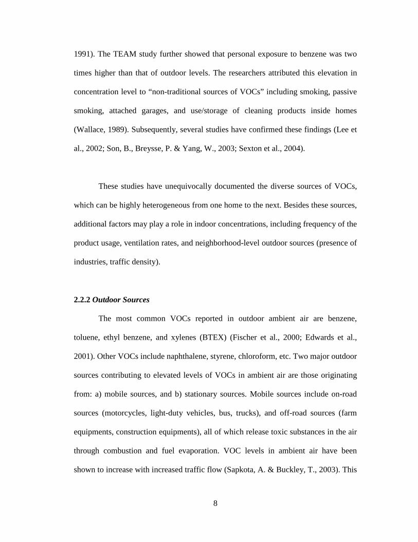
These studies have unequivocally documented the diverse sources of VOCs,

which can be highly heterogeneous from one home to the next. Besides these sources,

additional factors may play a role in indoor concentrations, including frequency of the

product usage, ventilation rates, and neighborhood-level outdoor sources (presence of

industries, traffic density).

2.2.2 Outdoor Sources

The most common VOCs reported in outdoor ambient air are benzene,

toluene, ethyl benzene, and xylenes (BTEX) (Fischer et al., 2000; Edwards et al.,

2001). Other VOCs include naphthalene, styrene, chloroform, etc. Two major outdoor

sources contributing to elevated levels of VOCs in ambient air are those originating

from: a) mobile sources, and b) stationary sources. Mobile sources include on-road

sources (motorcycles, light-duty vehicles, bus, trucks), and off-road sources (farm

equipments, construction equipments), all of which release toxic substances in the air

through combustion and fuel evaporation. VOC levels in ambient air have been

shown to increase with increased traffic flow (Sapkota, A. & Buckley, T., 2003). This

9

increase in VOC levels vary based on type and age of vehicle, speed of traffic, fuel

used, and environmental conditions of roads (Muezzinoglu, A., Odabasi, M. & Onat,

L., 2001; Sapkota & Buckley, 2003). Despite high concentrations of VOCs, effective

environmental regulations can lower concentrations in ambient air. Han et al. (2006)

have attributed reduction in VOC levels observed over the past decade in Mexico

City to the implementation of traffic emission controls there (Han, X. & Naeher, L.

P., 2006). However, VOC levels in Mexico City are still higher than many other cities

around the world (Gee, I. L. & Sollars, C. J., 1998).

The second category, stationary sources, includes industries, power plants and

small industries including dry cleaners. Pollutants from industries and power plants

are discharged into the atmosphere from smokestacks. Mintz and McWhinney

attributed 85% and 89% of VOCs observed in Fort Saskatchewan, Western Canada,

to the industry in those areas (Mintz, R. & McWhinney, R. D., 2008). In a separate

study conducted in Spain, researchers reported traffic emissions accounted for 60% of

ambient VOCs while those from industrial emissions accounted for 32% (Montserrat,

C. & Baldasano, J. M., 1996). Likewise, interesting data are available from Korea,

which has undergone a rapid industrial growth, especially in petrochemical industries

in the past 30 years. Na et al. reported higher VOC concentrations in Korean cities

located near petrochemical industries (Na, K., Kim, Y. P., Moon, K. C., Moon, I. &

Fung, K., 2001).

2.3 VOCs and Health

10

The extent to which VOCs affect human health is not well understood. Most of

the health effects identified are from occupational settings where exposures tend to be

an order of magnitude higher than those observed in environmental settings. In most

cases, VOCs act as irritants, causing acute effects such as watery eyes, itchy throat,

sneezing, and skin rash (US-EPA). These acute symptoms are usually temporary and

cease once the source of exposure has been identified and removed (EPA, 2009). But

in severe cases, VOCs can trigger exacerbation of asthma (Delfino et al., 2003), and,

in the case of chronic exposures, can lead to various adverse health outcomes

including kidney failure, liver failure, central nervous system damage, and cancer

(Ashley, D. L., Bonin, M. A., Cardinali, F. L., McCraw, J. M. & Wooten, J. V. ,

1996). Individuals with respiratory complications such as asthma, young children,

elders, and individuals highly sensitive to chemicals face greater risk for irritation and

health complications from exposure to VOCs.

2.3.1 VOC Exposures and Asthma

Asthma is an inflammatory disorder of the lungs characterized by episodic

and reversible symptoms of air-flow obstruction, and random airway hyperactivity.

Asthma affects all age groups, with millions of children suffering from this condition

(Mannino, D. M., Homa, D. M. & Petrowski, C. A., 1998). Though the rate of

mortality from asthma has decreased, ambulatory care has continued to grow since

2000 (Akinbami, 2006).

11

Exposure to mixtures of VOCs has been shown to increase neutrophils, a type

of white blood cells in the immune system, in nasal passages among non-smoking

young adult men (Koren, H. S. & Delvin, R. B., 1992). Delfino et al. (2003) who

observed an increase in asthma symptoms among Hispanic teenagers with high

concentrations of selected VOCs in breath and ambient air suggested that acute and

chronic exposure to air toxics may contribute to a decline in lung function and an

increase in exacerbation symptoms among asthmatics (Delfino et al., 2003). The EPA

defines air toxics as pollutants confirmed or suspected to be harmful to human health.

A recent study by Elliott et al. (2006) reported decrease in lung function with increase

exposure to VOCs from air fresheners, mothballs, and cleaning products (Elliott, L.,

Longnecker, M. P., Kissling, G. E. & London, S. J., 2006). Biomarkers, biological

indicators such as biomechanical metabolites from exposure to a chemical agent, have

also been used as strong indicators of VOCs exposure.

Recently several epidemiological studies have established association between

exposure to automobile exhaust and asthma. The findings suggested that asthmatic

children living close to roads with high traffic density experienced higher rates of

asthma exacerbation (Edwards et al., 1994; vanVliet, P., Knape, M., de Hartog, J.,

Janssen, N., Harssema, H, & Bunekreef, B., 1997; Carbajal-Arroyo et al., 2007).

Although the observed association may have also resulted from exposures to other

compounds such as particulate matter (PM) (Morgenstern et al., 2007; Brauer et al.,

2002) and nitrogen dioxide (NO2) (Gauderman et al., 2005; Nicolai et al., 2003) also

12

found in automobile exhausts, the possibility of VOC contribution cannot be ruled

out.

A case study investigated exposure to high VOC concentrations in a

residential area in Mont Chanin, France where industrial waste was dumped in the

mid 1980s. Results showed VOC levels as high as 433 µg/m3, inside homes.

Investigators also observed several health complications such as psychological

disorders and pulmonary irritation among the local residents and attributed such

outcomes to the unusually high levels of VOCs observed (Deloraine, A., Zmirou, D.

Tillier, C., Boucharlat, A. & Bouti, H., 1995).

2.3.2 VOC Exposures and Cancer

Cancer is characterized by uncontrolled growth, invasion, and sometimes

metastasis of a group of cells. In the uncontrolled growth, the cells undergo division

beyond the normal division limits (American Cancer Society, 2009). Cells intruding

and destroying adjacent tissues characterize the invasion. Metastasis, which mostly

occurs in advanced stages of the disease, is the spreading of cancerous cells to other

locations in the body via lymph or blood. Cancer can affect all age groups, but this

risk increases with age. Cancer can result from mutations from chemical carcinogens,

ionizing radiation, heredity, immune system dysfunction, and other causes that still

remain unknown (American Cancer Society).

13

Early studies focused on cancer and inherited genetic disorders,

chemotherapeutic agents, and ionizing radiation (Reynolds, P., Von Behren, J.,

Gunier, R. B., Goldberg, D. E., Hertz, A. & Smith, D. F., 2003). It is only in the past

decades that researchers have included toxic agents from emission sources in studies

on cancer (Pearson, R. L., Watchel, H. & Ebi, K. L., 2000). Despite the decrease in

cancer deaths in the U.S. (by 18.4% in men, and 10.5% in women), cancer of the

lungs and bronchus are among the most common types of cancer in both men and

women, with smoking having been shown as the most contributing risk factor (Doll,

R., Peto, R., Boreham, J. & Sutherland, I., 2005). Cancer has also been reported as the

second leading cause of death among children under the age of fourteen (American

Cancer Society, 2008).

Woodruff et al. (2000) estimated cancer risk with ambient concentrations of

toxic substances, using the EPA Cumulative Exposure Project (Woodruff et al.,

2000). Most of the cancer cases were attributable to exposure to VOCs (benzene, 1,3-

butadiene), and other toxic agents (chromium, formaldehyde). Similar findings were

observed in Great Britain in geographical clustering of children with leukemia living

near industries (oil refineries, oil storage sites, paper manufacturing) releasing large

emissions containing VOCs (Knox, 1997). This study suggested that childhood

cancer was associated with geographical location, later supported by a follow-up

study by Knox and Gilman (1998), who reported that the increase in cancer risk was

primarily attributable to exposures to benzene, 1,3-butadiene, NOx, and

benz(a)pyrene (Knox, E. G. & Gilman, E. A., 1998; Knox, 2005). On the other hand,

14

Wilkinson et al. (1999) who followed the same study design as Knox and Gilman

(1998), did not find any association between cancer risk among children and exposure

to oil refineries (Wilkinson et al., 1999). With scarce data on adverse health outcomes

from exposure to mixed agents, one cannot conclude whether VOCs were the primary

contributors to cancer outcomes from studies such as Knox and Gilman’s or if the

observed outcomes were associated with some confounding variables that were not

accounted for.

To date, most studies have brought more focus on single chemicals as

opposed to mixed exposures from indoor and outdoor air. Moreover, investigations

have taken place in areas such as workplaces, home, and stores near traffic arteries.

However, little has been done on outdoor VOCs air assessment near schools, where

children spend significant amounts of time. Therefore, it is important to evaluate the

air around these schools for VOCs to understand if there is an increased risk of

adverse health outcomes among the schoolchildren.

15

CHAPTER 3: METHODS

3.1 Instrument 3.1.1 Gas Chromatograph Mass-Spectrometer

The Gas Chromatograph Mass-Spectrometer (GC-MS) is an instrument used

for qualitative as well as quantitative analyses. During analysis, samples are

introduced into the system via injection through a heated injection port. Samples are

separated using a capillary column and introduced into the mass spectrometer, where

they get ionized. The ions are detected based on their mass to charge ratios (m/z).

Each chemical has a unique m/z, which enables the instrument to detect them with

high accuracy.

For this thesis, samples were analyzed with a Schimadzu GC-MS model

QP2010 (Shimadzu Scientific, Columbia, MD). Samples were analyzed in Selective

Ion Monitoring (SIM) mode.

3.1.2 Calibration

The GC-MS was calibrated to assess the GC-MS response and accuracy in

identifying compounds. The calibration would be used as a reference when

quantifying unknown agents by measuring the response of the unknown and using the

calibration curve to determine the concentration of the unknown. Seven calibration

standards were prepared using a method of serial dilution, with concentration ranging

from 0-2,000 ng/mL for each standard. A working stock solution of 40 µg/mL of

VOC mixture was prepared using 200 µg/mL VOC mixture with MTBE 55 analytes

16

stock solution (Ultra Scientific, Cat# DWM-596-1). Calibration standards were

prepared diluting known amounts of the compound of interest with calculated

amounts of carbon disulfide and acetone.

Exactly 10 µL of internal standards of volatile monitoring spiking solution

was added to each calibration standard. These standards were prepared in 1.5 mL

screw thread amber vials. A 1 µL aliquot was injected into the GC-MS using an auto

sampler injector (50oC, helium flow, 1.00 mL/min for 26 minutes). The 7-point

calibration curves were prepared each week. The GC-MS underwent a total of 8

calibrations. All calibration curves had a linear response with r-square greater than

0.98.

17

Figure 1. Spectral Peak for Chloroform with 50 ng/mL Concentration

8.25 8.50 8.75 9.00

0.5

1.0

1.5

2.0

2.5

3.0

3.5

4.0

4.5

(x100)

130.0049.00

979

Spectral Peak for Chloroform with 2,000 ng/mL Concentration

8.25 8.50 8.75 9.00

0.25

0.50

0.75

1.00

1.25

1.50

1.75

2.00

(x10,000)

130.0049.00

4732

0

Calibration Curve for 6 Standards and One Blank (r2= 0.99994)

0.00 0.25 0.50 0.75 Conc. Ratio0.00

0.25

0.50

0.75

1.00

1.25Area Ratio

Response Area

Response Area

Retention Time (min)

18

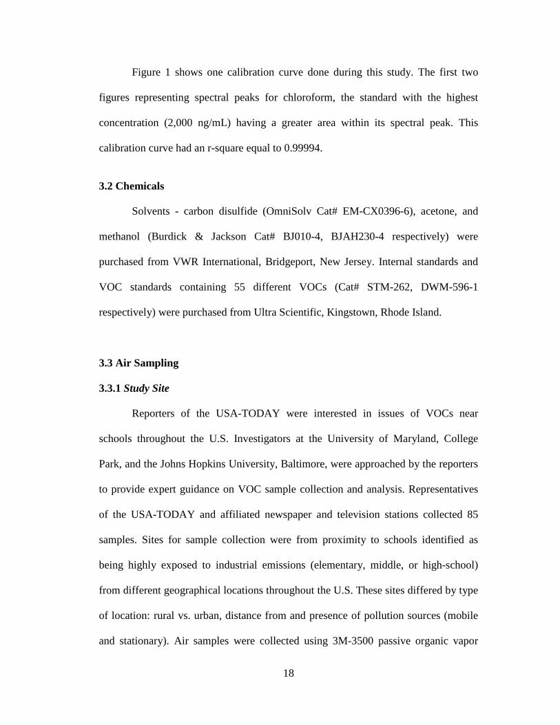
Figure 1 shows one calibration curve done during this study. The first two

figures representing spectral peaks for chloroform, the standard with the highest

concentration (2,000 ng/mL) having a greater area within its spectral peak. This

calibration curve had an r-square equal to 0.99994.

3.2 Chemicals

Solvents - carbon disulfide (OmniSolv Cat# EM-CX0396-6), acetone, and

methanol (Burdick & Jackson Cat# BJ010-4, BJAH230-4 respectively) were

purchased from VWR International, Bridgeport, New Jersey. Internal standards and

VOC standards containing 55 different VOCs (Cat# STM-262, DWM-596-1

respectively) were purchased from Ultra Scientific, Kingstown, Rhode Island.

3.3 Air Sampling

3.3.1 Study Site

Reporters of the USA-TODAY were interested in issues of VOCs near

schools throughout the U.S. Investigators at the University of Maryland, College

Park, and the Johns Hopkins University, Baltimore, were approached by the reporters

to provide expert guidance on VOC sample collection and analysis. Representatives

of the USA-TODAY and affiliated newspaper and television stations collected 85

samples. Sites for sample collection were from proximity to schools identified as

being highly exposed to industrial emissions (elementary, middle, or high-school)

from different geographical locations throughout the U.S. These sites differed by type

of location: rural vs. urban, distance from and presence of pollution sources (mobile

and stationary). Air samples were collected using 3M-3500 passive organic vapor

19

monitors (OVMs). The 3M-3500 OVMs are comprised of one charcoal adsorbent pad

to collect organic vapors in the air. Air samples are absorbed by the OVMs by the

process of diffusion where organic vapors move from high (ambient air) to low

concentration (into monitor).

3.3.2 Sample Collection

Once a location was identified, field staff placed OVM samplers within 100

yards from schools and 7-8 feet above the ground. A pail was used to protect the

samplers from excessive wind and rain. To ensure sufficient airflow for the diffusion

process, samplers were placed at least 3 feet from any walls.

At sampling location samplers were removed from their containers. The

airtight cap of the samplers was removed and replaced by a clear cap, the diffusive

cover. Samplers’ identification number, opening date and time were recorded in

sample log sheet. Samplers were then hung above ground level, and protected from

rain and/or high winds. Additional items recorded in the log sheet included location

of sampling, presence/absence of industries, major roads in the neighborhood,

population size of the town for subsequent evaluations. Sampling periods were 4 or 7

days. Periodical visits were done at collection sites to check monitors for any possible

damages, and any relevant observations were reported. If not properly stored, OVMs

can adsorb additional agents in the ambient air after the collection period. Thus,

protection of the OVMs after sampling is critical. At the end of collection period,

field staff removed and replaced samplers’ diffusive cover by the airtight cap. The

20

samplers were then placed in their original containers. Field staffs then recorded

ending date and time of sample collection in the log sheet. Sealed samplers were

shipped with ice packs in a zip lock bag to the lab.

Once delivered to the lab, samplers were removed from zip-lock bags,

observed for any physical damage, recorded, and placed in a freezer at -20 degrees

Celsius. To minimize contamination by other chemicals in the laboratory, all

monitors were assigned to one freezer free of other items.

3.4 Sample Analysis

3.4.1 Sample Extraction

For extraction, monitors were taken out of freezer, placed under the fume

hood and allowed to equilibrate to room temperature for one hour with airtight covers

in place. The airtight covers were removed, and replaced by the clear cap. The

monitors were spiked with 10 µL of internal standard (200 µg/mL), which consisted

of 1,2-dichloroethane-D4, toluene-D8, and 4-bromofluorobenzene in methanol

through a tab located on the clear cap. Tabs were closed immediately after each

spiking. Spiked monitors sat under fume hood at room temperature for an additional

hour. After the second hour, clear caps were removed, and using tefflon tweezers,

activated charcoal pads from the monitors were removed from the monitors and

placed into 12x32 screw thread amber vials with PTFE/Silicone caps. With a 100-

1000 µL pipette, 1mL of solvent mix (carbon disulfide and acetone, 1:2 v/v) was

added to each vial containing the charcoal pads spiked with 10 µL of internal

standards. Vials were put in a Bransonic sonication bath and sonicated for 45

21

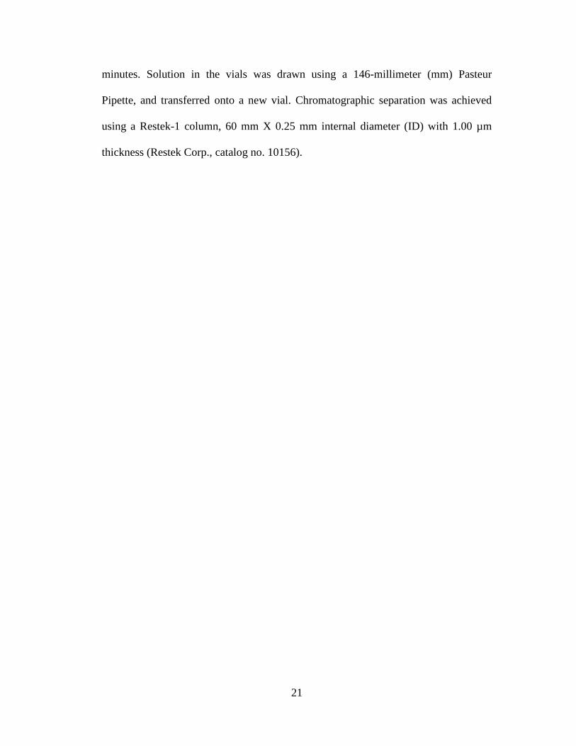
minutes. Solution in the vials was drawn using a 146-millimeter (mm) Pasteur

Pipette, and transferred onto a new vial. Chromatographic separation was achieved

using a Restek-1 column, 60 mm X 0.25 mm internal diameter (ID) with 1.00 µm

thickness (Restek Corp., catalog no. 10156).

22

3.4.2 Sample Recovery

We used a new set of blank monitors from our laboratory to determine sample

recovery. Nine monitors were injected with 20 µL of 40 µg/mL VOC mixture and left

at room temperature for one hour with the clear caps in place. The monitors were then

put back in their original containers and transferred to the assigned freezer. The

following morning, monitors were removed from the freezer and let sit at room

temperature for one hour. The monitors were then spiked with 15 µL internal

standards with a concentration of 200 µg/mL using a 2500 µg/mL volatile system

monitoring spiking solution with 3 analytes: 1,2-dichloroethane-D4, toluene-D8, and

4-bromofluorobenzene in methanol (Ultra Scientific, Cat# STM-262). Spiked

monitors sat at room temperature for one hour under the fume hood. Clear caps were

removed, and using tefflon tweezers the activated charcoal pads from the monitors

were transferred into 1.5mL screw thread amber vial, then extracted with 1.5mL

solvent mix (carbon disulfide and acetone, 1:2, v/v). All vials were sonicated for 45-

minutes using Bransonic sonicator. Sonicated solutions were then transferred into

new vials, using a new Pasteur pipette for each vial transfer. Sample recovery was

calculated as the percent of analyte recovered with respect to the spiked amount by

dividing the extracted concentration to the injected concentration.

3.4.3 Limit of Detection

Limit of Detection (LOD) refers to the lowest amount of an analyte that can

be distinguished from the background (absence) with a certain degree of confidence.

When an analyte was present at detectable levels on blank samples, LOD was

23

calculated using the blanks. When the analytes were not present at detectable level on

the blank samples, a lowest level spike was used for calculating LOD. In either case,

the samples allocated for LOD determination were handled the same way as badges

with actual samples in terms of transportation and delivery to and storage in the

laboratory. LOD was calculated by multiplying the field blank standard deviation by

three. Measured concentrations below the LOD were replaced with a value equal the

LOD divided by two. Seven monitors previously stored in the lab freezer, sat at room

temperature under the laboratory fume hood for one hour. Each monitor was then

spiked with 15uL internal standards of volatile system monitoring spiking solution

with 1,2-dichloroethane-D4, toluene-D8, 4-bromofluorobenzene in methanol,

recapped and sat for one hour. Charcoal films from monitors were rolled, transferred

into 1.5mL screw thread amber vials using teflon tweezers, and then extracted with

1.5mL solvent mix (carbon disulfide and acetone, 1:2, v/v). All vials were sonicated

for 45-minutes using Bransonic sonicator. Sonicated solutions were then transferred

into new vials, using a new Pasteur pipette for each vial transfer. The level of analyte

was calculated using the calibration curve. Following this step, the limit of detection

(LOD) was calculated by multiplying the standard deviation (SD) of the seven blank

samples by the Student’s t -value associated with 99% confidence interval with 6

degrees of freedom. For those compounds that were not detected on the blank

samples, 7 badges were spiked with low level of the analytes and the process was

repeated to calculate LOD. All samples that were below the LOD were assigned a

value that was ½ the LOD. All reported values were corrected for field blanks.

24

3.5 Statistical Methods

All statistical analyses were performed using the Intercooled Stata, version 10.0 for

Windows (Stata Corp., TX). Differences in VOC concentrations by region were

tested using the paired t-test. Correlations between compounds were tested using the

Spearman’s rank correlation. Statistical significance was associated with p<0.05.

25

CHAPTER 4: RESULTS

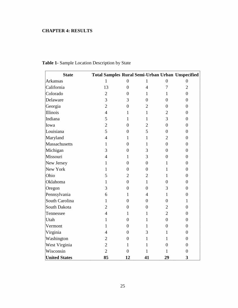
Table 1- Sample Location Description by State

State Total Samples Rural Semi-Urban Urban Unspecified Arkansas 1 0 1 0 0 California 13 0 4 7 2 Colorado 2 0 1 1 0 Delaware 3 3 0 0 0 Georgia 2 0 2 0 0 Illinois 4 1 1 2 0 Indiana 5 1 1 3 0 Iowa 2 0 2 0 0 Louisiana 5 0 5 0 0 Maryland 4 1 1 2 0 Massachusetts 1 0 1 0 0 Michigan 3 0 3 0 0 Missouri 4 1 3 0 0 New Jersey 1 0 0 1 0 New York 1 0 0 1 0 Ohio 5 2 2 1 0 Oklahoma 1 0 1 0 0 Oregon 3 0 0 3 0 Pennsylvania 6 1 4 1 0 South Carolina 1 0 0 0 1 South Dakota 2 0 0 2 0 Tennessee 4 1 1 2 0 Utah 1 0 1 0 0 Vermont 1 0 1 0 0 Virginia 4 0 3 1 0 Washington 2 0 1 1 0 West Virginia 2 1 1 0 0 Wisconsin 2 0 1 1 0 United States 85 12 41 29 3

26

4.1 General Characteristics of the Samples Collected

All samples were collected between August and October of 2008. The

characteristics of the locations where samples were collected are summarized in

Table 1. A total of eighty-five samples from 75 towns in 27 states were collected

throughout the US. Of the 85 samples, 12 were from rural areas and 28 were from

urban areas while 44 were from semi urban or non-specified areas. The majority of

the samples was collected in the vicinity of elementary schools (70), while a few were

collected around middle (5), and high (10) schools.

4.2 Recovery Rate

The recovery rate varied significantly across the different analytes and ranged

from 16.9% to 129.3%. Ten compounds had recovery rates above 100% (chloroform,

1,2-dichloroethane, 1,1,1-trichloroethane, carbon tetrachloride, 1,1,2-trichloroethane,

ethylbenzene, m,p-xylene, o-xylene, 2-chlorotoluene, chlorotoluene).

4.3 Limit of Detection (LOD)

The limit of detection (LOD) calculated from field blanks for the 18 VOCs are

provided in Table 2. Of the 18 VOCs sampled, four of the compounds (1,2-

dichloroethane, 1,1,1-trichloroethane, 1,1,2-trichloroethane, and bromoform) were

below the LOD in all instances. Likewise, compounds such as benzene, carbon

tetrachloride, toluene, m,p-xylene, and chlorotoluene were above LOD in majority of

the samples.

27

Table 2-Compound Retention Time (RT), and Limit of Detection (LOD)

Analyte Ion 1 (m/z)

Ion 2 (m/z)

RT (min)

LOD (µg/m3)

% >LOD

Chloroform 83 85 8.88 0.29 11%

Ethane, 1,2-dichloro 62 27 9.44 0.38 0%

Ethane, 1,1,1-trichloro- 97 99 9.65 0.38 0%

Benzene 78 77 10.2 0.50 66%

Carbon Tetrachloride 117 119 10.15 0.56 80%

1,1,2-Trichloroethane 97 83 12.36 0.51 0%

Toluene 91 92 12.66 0.35 100%

Chlorobenzene 112 77 14.71 0.44 33%

Ethylbenzene 91 106 15.12 0.45 48%

m,p-Xylene 91 106 15.95 0.45 80%

Bromoform 173 252 15.53 0.93 0%

Styrene 104 78 15.81 0.64 2%

o-Xylene 91 106 15.95 0.72 33%

1,2,3-Trichloropropane 75 110 16.12 0.68 24%

2-Chlorotoluene 91 126 17.45 0.59 4%

Chlorotoluene 91 126 17.53 0.59 58%

Dichlorobenzene 146 148 18.77 1.11 5%

Naphthalene 128 102 22.8 0.80 4%

28

The average distance of samplers from schools was 57.86 yards. Forty schools

were reported to be in proximity to industries with an average distance of 1.28 miles.

Fifteen schools were near highways with an average distance of 0.50 miles. Twenty-

four schools were near major roads with an average distance of 0.19 miles.

Altogether, eighteen VOCs were identified in this study. The descriptive

characteristics of the samples, including the mean, standard deviation, minima,

maxima, median, 25th, and 75% percentiles are in Table 3. Out of all samples, the

highest upper limit concentration was observed for benzene, chlorobenzene, and

toluene (76.36, 43.71, and 30.51 µg/m3 respectively). Likewise, the highest average

concentration was observed for toluene and benzene (4.86, and 2.28 µg/m3,

respectively).

29

Table 3-Total VOC average concentration (µg/m3)

1Median 2 Interquartile Ratio 3 25% percentile 4 75% percentile

Compounds Mean Std. Dev. Min Max P501 IQR 2 P253 P754

Chloroform 0.18 0.13 0.14 0.99 0.14 0.00 0.14 0.14 Ethane, 1,2-dichloro 0.19 0.00 0.19 0.19 0.19 0.00 0.19 0.19 Ethane, 1,1,1-trichloro- 0.19 0.00 0.19 0.19 0.19 0.00 0.19 0.19

Benzene 2.28 8.39 0.25 76.36 0.85 1.79 0.25 2.04 Carbon Tetrachloride 0.69 0.50 0.28 4.71 0.66 0.15 0.60 0.75 1,1,2-Trichloroethane 0.25 0.00 0.25 0.25 0.25 0.00 0.25 0.25

Toluene 4.86 4.72 0.36 30.51 3.50 2.60 2.28 4.88

Chlorobenzene 1.07 4.77 0.22 43.71 0.22 0.37 0.22 0.59

Ethylbenzene 0.59 0.61 0.23 3.33 0.23 0.41 0.23 0.64

M,p-Xylene 1.05 1.00 0.22 5.21 0.79 0.59 0.50 1.09

Bromoform 0.47 0.00 0.47 0.47 0.47 0.00 0.47 0.47

Styrene 0.34 0.13 0.32 1.39 0.32 0.00 0.32 0.32

o-Xylene 0.73 0.71 0.36 3.76 0.36 0.44 0.36 0.80 1,2,3-Trichloropropane 0.68 0.95 0.34 7.76 0.34 0.00 0.34 0.34

2-Chlorotoluene 0.33 0.19 0.30 1.60 0.30 0.00 0.30 0.30

Chlorotoluene 1.14 1.03 0.30 5.32 0.84 1.27 0.30 1.57

Dichlorobenzene 0.60 0.25 0.55 2.00 0.55 0.00 0.55 0.55

Naphthalene 0.45 0.37 0.40 3.74 0.40 0.00 0.40 0.40

30

4.3 Concentration Differences in Rural and Urban Areas

Figure 2 illustrates the distribution of mean concentration in rural and urban

areas. For all compounds, the mean concentrations measured were higher in the urban

areas than rural areas. In urban locations, toluene, benzene, and chlorobenzene were

the most dominant compounds, with concentrations of 6.40, 4.04, and 2.14 µg/m3

respectively. In rural locations, the concentrations of these compounds were 2.60,

0.95, and 0.49 µg/m3. The mean concentrations observed in the urban locations were

significantly higher then those observed for the rural locations (p<0.0001), as

determined by the two-tailed statistical t-test.

4.4 Concentration Differences by Presence of Industries

We compared VOC concentrations based on presence of industries. Figure 3

demonstrates the variation of concentrations for all compounds in areas with and

without industries. Overall average concentrations were higher in schools within

proximity to industries than schools without industries in their surroundings.

Toluene, benzene, chlorobenzene and m,p-xylene were the most dominant VOCs for

schools that were close to industries. For schools that were not near industries, the

most dominant VOCs were toluene, chlorotoluene, and benzene, although the

concentrations were much lower. We observed almost 3-fold higher benzene

concentrations in schools that were closer to the industries compared to those that had

no known industries in nearby areas.

31

Figure 2.

0

2

4

6

0

2

4

6

R u ra l

U rb a n

C h lo ro fo rm 1 ,2 -D ic h lo ro e th a n e 1 ,1 ,1 -T r ic h lo ro e th a n e

B e n z e n e C a rb o n T e t ra c h lo r id e 1 ,1 ,2 -T r ic h lo ro e th a n e

T o lu e n e C h lo ro b e n z e n e E th y lb e n z e n e

m ,p -X y le n e B ro m o fo rm S ty re n e

o -X y le n e 1 ,2 , -T r ic h lo ro p ro p a n e 2 -C h lo ro to lu e n e

C h lo ro to lu e n e D ic h lo ro b e n z e n e N a p h th a le n e

G ra p h s b y A re a T y p e

V O C A v e ra g e C o n c e n tra t io n (u g /m 3 ) b y A re a T y p e

32

Figure 3.

0

1

2

3

4

5

Compounds Compounds

No Yes

Chloroform 1,2-Dichloroethane 1,1,1-Trichloroethane

Benzene Carbon Tetrachloride 1,1,2-Trichloroethane

Toluene Chlorobenzene Ethylbenzene

m,p-Xylene Bromoform Styrene

o-Xylene 1,2,3-Trichloropropane 2-Chlorotoluene

Chlorotoluene Dichlorobenzene Naphthalene

Graphs by Industry

VOC Average Concentration (ug/m3) by Presence of Industry

33

4.5 Concentration differences by traffic

Information on presence of major roads near schools was available for thirty-

eight schools. Out of those thirty-eight schools, twenty-four schools were near major

roads. The distance of major roads from schools ranged from 10-1000 yards. Toluene

and chlorotoluene were the most dominant among schools less than 300 yards from

major roads. Toluene and benzene were the most dominant among schools more than

300 yards away from major roads. Toluene and benzene concentrations from schools

over 300 yards away from major roads were also higher than that of schools less than

300 yards away from major roads.

We also looked into presence of highways. Information on highways was

given for forty-three schools. Out of the forty-three reports, fourteen schools were

close to highways. Highway distances from schools were within 3600 yards. When

we observed VOCs concentrations between schools less than and over 500 yards from

highways, toluene and benzene were the most dominant compounds in both

categories (Fig. 4). Toluene was higher in the category less than 500 yards (6.5

µg/m3) compared to the category over 500 yards (3.42 µg/m3) away from highways.

Benzene was also higher in the category less than 500 yards (1.81 µg/m3) compared

to the category over 500 yards (1.73 µg/m3) away from highways.

35

Figure 4.

02

46

C om p o un d s C om p o un d s

< 5 0 0 ya rd s > 5 0 0 ya rd s

Ch lo rof orm 1 ,2 -D i ch lo roet ha ne 1, 1, 1-T r ich lor oet ha ne

B e nzene C arbo n Te tr ac hl ori de 1, 1, 2-T r ich lor oet ha ne

T ol uen e C hlo rob enze ne E th y lbe nze ne

m , p-X y le ne B ro mo fo rm S ty re ne

o- Xy len e 1 ,2 ,3 -Tr ic hl oro prop ane 2-Ch lo rot olu ene

Ch lo rot ol uen e D ichl oro ben zene Nap ht hal en e

G r aph s by h wy d is t

V O C A ve ra g e C on ce n tra t io n (u g /m 3 ) by H ig h wa y D i sta n ce

37

4.5 Concentration differences across regions

We also compared VOC concentrations by region where sampling locations

were divided into West, Midwest, South and Northeast (Fig. 5). In all regions,

toluene and benzene were the most dominant VOCs. Benzene concentration was the

highest in the Northeast. For the Northeast, benzene, toluene, and chlorobenzene had

average concentrations above 2 µg/m3, and these concentrations were above the total

average concentration for all 85 samples combined.

Table 4 describes the significance in regional concentration from total

concentration average. Chlorobenzene was significantly lower that the total average

in the Midwest, South and West regions. Benzene was significantly lower than the

total average in the South, and West regions. Toluene was significantly lower than the

total average in the South region. However, it is difficult to make a meaningful

interpretation of these results as the sampling sites were not randomly selected.

38

Figure 5.

02

46

80

24

68

M id w e s t N o rth E a st

S ou th W e s t

Ch lo roform 1 ,2 -Di ch lo roetha ne 1, 1,1-T rich lor oetha ne

B e nzene C arbo n Te tr achl ori de 1, 1,2-T rich lor oetha ne

T ol uen e C hlo rob enze ne E th y lbe nze ne

m ,p-X y le ne B ro mo fo rm S tyre ne

o- Xy len e 1 ,2 ,3 -Tr ichl oro prop ane 2-Ch lo rotolu ene

Ch lo rotol uen e D ichl oro ben zene Nap hthal en e

G raph s by R eg ion

VO C Avera g e C o n ce ntra tio n (u g/m 3 ) b y R eg io n

39

Table 4- Regional average concentration (µg/m3) vs. Total average concentration (µg/m3) for all 85

Region Variable Obs Mean1 Std.Err. Std. Dev. [95% Conf. Interval] Ho2 P-value3

Midwest

Chloroform 26 0.15 0.01 0.06 0.13-0.18 0.18 0.03 Ethane, 1,2-dichloro 26 0.19 0.00 0.00 0.19-0.19 0.19 . Ethane, 1,1,1-trichloro- 26 0.19 0.00 0.00 0.19-0.19 0.19 . Benzene 26 1.87 0.52 2.59 0.80-2.94 2.28 0.44 Carbon Tetrachloride 26 0.70 0.04 0.20 0.62-0.78 0.69 0.78 1,1,2-Trichloroethane 26 0.25 0.00 0.00 0.25-0.25 0.25 . Toluene 26 5.35 0.94 4.78 3.42-7.28 4.86 0.61 Chlorobenzene 26 0.57 0.14 0.69 0.29-0.85 1.07 0.001 Ethylbenzene 26 0.66 0.13 0.67 0.39-0.93 0.59 0.59 m,p-Xylene 26 1.21 0.22 1.11 0.77-1.66 1.05 0.46 Bromoform 26 0.47 0.00 0.00 0.47-0.47 0.47 . Styrene 26 0.34 0.02 0.11 0.30-0.39 0.34 0.92 o-Xylene 26 0.83 0.17 0.84 0.49-1.17 0.73 0.57 1,2,3-Trichloropropane 26 0.58 0.11 0.56 0.36-0.81 0.68 0.38 2-Chlorotoluene 26 0.31 0.01 0.06 0.29-0.34 0.33 0.12 Chlorotoluene 26 1.12 0.19 0.98 0.72-1.52 1.14 0.92 Dichlorobenzene 26 0.55 0.00 0.00 0.55-0.55 0.61 . Naphthalene 26 0.43 0.03 0.13 0.37-0.48 0.45 0.34

40


Northeast

Chloroform 11 0.25 0.08 0.26 0.08-0.43 0.18 0.37 Ethane, 1,2-dichloro 11 0.19 0.00 0.00 0.19-0.19 0.19 . Ethane, 1,1,1-trichloro- 11 0.19 0.00 0.00 0.19-0.19 0.19 . Benzene 11 8.72 6.82 22.62 -6.48-23.92 2.28 0.37 Carbon Tetrachloride 11 1.16 0.37 1.21 0.34-1.97 0.69 0.23 1,1,2-Trichloroethane 11 0.25 0.00 0.00 0.25-0.25 0.25 . Toluene 11 7.66 2.84 9.43 1.33-13.99 4.86 0.35 Chlorobenzene 11 4.97 3.93 13.02 -3.77-13.72 1.07 0.34 Ethylbenzene 11 0.99 0.34 1.14 0.22-1.75 0.59 0.28 m,p-Xylene 11 1.52 0.56 1.84 0.28-2.76 1.05 0.42 Bromoform 11 0.47 0.00 0.00 0.47-0.47 0.47 . Styrene 11 0.32 0.00 0.00 0.32-0.32 0.34 . o-Xylene 11 1.10 0.36 1.19 0.30-1.90 0.73 0.33 1,2,3-Trichloropropane 11 1.45 0.67 2.21 -0.03-2.94 0.68 0.27 2-Chlorotoluene 11 0.42 0.12 0.39 0.15-0.68 0.33 0.47 Chlorotoluene 11 1.53 0.34 1.14 0.77-2.29 1.14 0.28 Dichlorobenzene 11 0.84 0.15 0.49 0.50-1.17 0.61 0.16 Naphthalene 11 0.76 0.30 1.01 0.09-1.44 0.45 0.33

41


South

Chloroform 27 0.14 0.00 0.00 0.14-0.14 0.18 . Ethane, 1,2-dichloro 27 0.19 0.00 0.00 0.19-0.19 0.19 . Ethane, 1,1,1-trichloro- 27 0.19 0.00 0.00 0.19-0.19 0.19 . Benzene 27 1.15 0.16 0.82 0.83-1.48 2.28 0.0000 Carbon Tetrachloride 27 0.61 0.04 0.20 0.53-0.69 0.69 0.05 1,1,2-Trichloroethane 27 0.25 0.00 0.00 0.25-0.25 0.25 . Toluene 27 3.72 0.47 2.47 2.74-4.69 4.86 0.02 Chlorobenzene 27 0.47 0.07 0.39 0.32-0.63 1.07 0.0000 Ethylbenzene 27 0.44 0.06 0.31 0.32-0.56 0.59 0.02 m,p-Xylene 27 0.77 0.11 0.55 0.55-0.99 1.05 0.01 Bromoform 27 0.47 0.00 0.00 0.47-0.47 0.47 . Styrene 27 0.36 0.04 0.21 0.28-0.44 0.34 0.62 o-Xylene 27 0.61 0.08 0.44 0.43-0.78 0.73 0.15 1,2,3-Trichloropropane 27 0.53 0.09 0.45 0.35-0.70 0.68 0.09 2-Chlorotoluene 27 0.34 0.04 0.22 0.26-0.43 0.33 0.77 Chlorotoluene 27 1.19 0.23 1.18 0.72-1.65 1.14 0.84 Dichlorobenzene 27 0.60 0.05 0.28 0.49-0.71 0.61 0.91 Naphthalene 27 0.40 0.00 0.00 0.40-0.40 0.45 .

42

1 Regional average concentration 2 Total average concentration for all 85 samples 3 Significance of difference in concentration (p<0.05)


West

Chloroform 21 0.21 0.03 0.15 0.14-0.28 0.18 0.33 Ethane, 1,2-dichloro 21 0.19 0.00 0.00 0.19-0.19 0.19 . Ethane, 1,1,1-trichloro- 21 0.19 0.00 0.00 0.19-0.19 0.19 . Benzene 21 0.85 0.18 0.82 0.48-1.22 2.28 0.0000 Carbon Tetrachloride 21 0.54 0.05 0.21 0.45-0.64 0.69 0.005 1,1,2-Trichloroethane 21 0.25 0.00 0.00 0.25-0.25 0.25 . Toluene 21 4.26 0.53 2.41 3.16-5.36 4.86 0.27 Chlorobenzene 21 0.41 0.10 0.47 0.19-0.62 1.07 0.0000 Ethylbenzene 21 0.50 0.06 0.29 0.37-0.64 0.59 0.19 m,p-Xylene 21 0.95 0.12 0.56 0.70-1.21 1.05 0.44 Bromoform 21 0.47 0.00 0.00 0.47-0.47 0.47 . Styrene 21 0.32 0.00 0.00 0.32-0.32 0.34 . o-Xylene 21 0.59 0.08 0.38 0.42-0.77 0.73 0.11 1,2,3-Trichloropropane 21 0.58 0.13 0.58 0.31-0.84 0.68 0.42 2-Chlorotoluene 21 0.30 0.00 0.00 0.30-0.30 0.33 . Chlorotoluene 21 0.89 0.18 0.82 0.52-1.27 1.14 0.18 Dichlorobenzene 21 0.55 0.00 0.00 0.55-0.55 0.61 . Naphthalene 21 0.40 0.00 0.00 0.40-0.40 0.45 .

43

Figure 6- Association among Five Selected VOCs

B e n z e n e

C a rb o nT e t ra c h lo r id e

T o l u e n e

m , p -X y le n e

C h lo ro to lu e n e

0 50 1 0 0

0

5

0 5

0

1 0

2 0

3 0

0 1 0 2 0 3 0

0

2

4

6

0 2 4 60

2

4

6

44

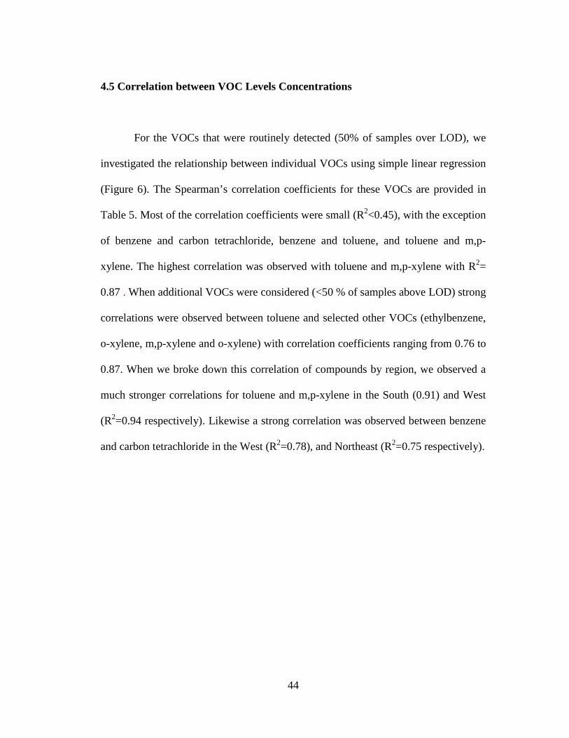
4.5 Correlation between VOC Levels Concentrations

For the VOCs that were routinely detected (50% of samples over LOD), we

investigated the relationship between individual VOCs using simple linear regression

(Figure 6). The Spearman’s correlation coefficients for these VOCs are provided in

Table 5. Most of the correlation coefficients were small (R2<0.45), with the exception

of benzene and carbon tetrachloride, benzene and toluene, and toluene and m,p-

xylene. The highest correlation was observed with toluene and m,p-xylene with R2=

0.87 . When additional VOCs were considered (<50 % of samples above LOD) strong

correlations were observed between toluene and selected other VOCs (ethylbenzene,

o-xylene, m,p-xylene and o-xylene) with correlation coefficients ranging from 0.76 to

0.87. When we broke down this correlation of compounds by region, we observed a

much stronger correlations for toluene and m,p-xylene in the South (0.91) and West

(R2=0.94 respectively). Likewise a strong correlation was observed between benzene

and carbon tetrachloride in the West (R2=0.78), and Northeast (R2=0.75 respectively).

45

Table 5- Correlation Between VOCs Using Spearman’s Rank Test

Chloroform Benzene Carbon Tetrachloride Toluene

Chloro benzene

Ethyl benzene m,p-Xylene Styrene o-Xylene

1,2,3- Trichloro propane

2-Chloro toluene Chlorotoluene

Dichloro benzene Naphthalene

Chloroform 1.00

Benzene 0.06 1.00

Carbon Tetrachloride 0.00 0.53 1.00

Toluene 0.33 0.50 0.19 1.00

Chlorobenzene 0.01 0.42 0.72 0.14 1.00

Ethylbenzene 0.37 0.42 0.16 0.81 0.06 1.00

m,p-Xylene 0.34 0.44 0.15 0.87 0.05 0.91 1.00

Styrene -0.05 -0.06 0.05 0.04 0.17 0.00 -0.08 1.00

o-Xylene 0.31 0.50 0.20 0.76 0.14 0.87 0.82 -0.10 1.00

1,2,3-Trichloropropane 0.16 0.14 0.23 -0.02 0.22 -0.08 -0.07 -0.09 -0.10 1.00

2-Chlorotoluene 0.24 0.05 0.21 0.03 0.11 0.08 0.03 -0.02 0.11 0.19 1.00

Chlorotoluene -0.04 0.26 0.74 0.22 0.22 0.19 0.22 0.12 0.28 -0.05 0.01 1.00

Dichlorobenzene 0.31 0.05 0.13 0.16 0.15 0.22 0.16 -0.05 0.26 0.18 0.32 0.22 1.00

Naphthalene 0.90 0.31 0.31 0.18 0.22 0.17 0.18 -0.03 0.20 0.38 0.41 0.15 0.54 1.00

46

CHAPTER 5: DISCUSSION

This thesis tested the hypotheses that schools in urban areas have higher VOCs

concentration than in rural areas, and that schools near industries have higher VOCs

concentration than those away from industries. Relatively few studies have looked into

all the variables in this study and VOC concentrations simultaneously. Data on outdoor

VOC concentrations near schools are also limited. To address this data gap, a total of 85

samples were collected from across the country, using passive organic vapor monitors.

Of all the VOCs measured, toluene had the highest mean concentration, followed

by benzene. These findings are consistent with what has been previously reported on

ambient environments (Gee & Sollars, 1999; Payne-Sturges, D. C., Burke, T. A.,

Breysse, P., Diener-West, P. & Buckley, T. J., 2004). Likewise, styrene, 2-chlorotoluene,

dichlorobenzene, and naphthalene were the least frequently detected. The compounds for

which most samples were below the LOD could be explained by the absence of sources

where sampling occurred.

This study indicates that urban areas had the highest VOC average concentrations.

Concentration levels were much higher for benzene, toluene, and chlorobenzene. Toluene

concentrations were higher in urban areas, areas closer to highways, and areas with

industries. These findings support the hypothesis that traffic and industrial emissions are

major sources of ambient toluene. Previous studies have shown the level of toluene to

vary closely with vehicle flow in areas characterized by heavy traffic density (Sapkota &

47

Buckley 2003). The high concentrations for benzene and toluene observed in the urban

areas are consistent with previous observations in El Paso (urban), Texas, and Underhill

(rural), Vermont (Mohamed, M. F., Kang, D. & Aneja, V. P., 2002), and Izmir, Turkey

(Muezzinoglu et al., 2001).

Our results are also consistent with the observed variation of VOCs in the urban

atmosphere (Yamamoto, N., Okayasu, H., Murayama, S., Mori, S., Hunahashi, K. &

Suzuki, K., 2000), suggesting that traffic activities contribute increased VOC

concentrations. Kwon et al. (2006), who observed outdoor-residential VOCs

concentrations, also reported similar findings. The highest mean VOCs concentrations in

that study were toluene (6.82 µg/m3), methyl tert-butyl ether (MTBE) (5.75 µg/m3), and

m,p-xylene (3.25 µg/m3). Burstyn et al. (2007) observed benzene levels in rural areas in

Western Canada (Burnstyn, I., You, X. I., Cherry, N. & Senthilselvan, A., 2007). Their

findings suggested that benzene maximum concentration level occurred in the winter

compared to the minimal concentration observed during summer months. The U.S.

Census Bureau defines an urban area as a community with a population density of 1,000

of more people per square mile. Son et al. (2003) examined two cities in Korea: Asan, a

medium city, with a population of about 200,000 and Seoul, the capital metropolitan city,

with a population of about 10 million people. Using the Spearman’s coefficient test,

outdoor/personal exposure had a strong correlation for benzene (r= 0.829) in Seoul, and

for ethylbenzene (r= 0.724) in Asan. These findings also reported strong indoor/outdoor

correlation with great significance for benzene (r= 0.653) and toluene (r= 0.605) in Seoul.

Our results also showed highest VOCs concentrations in the Northeast. The Northeast has

48

the highest population density (U.S. Census Estimates, 2006), with increase in traffic and

overcrowded cities, which may explain the high VOCs concentrations in our results.

Some of these concentrations have been shown to vary according to traffic flow and

hours of the day (Muezzinoglu et al., 2001).

Out of all eighteen compounds, higher concentrations of toluene followed by

benzene were observed. These results are in agreement with Mintz and McWhinney

(2008) who assessed VOCs concentrations in two towns from proximity to a highly

industrialized zone in the western area of Canada. In one site, situated downwind from

the industrialized zone, toluene and benzene were the highest concentrations. On the

other hand, the second site, which was closer to the city, had toluene and m,p-xylene with

the highest concentrations, toluene having levels about three times higher than that of the

first site. Na et al. (2001) observed VOCs concentration variation in Ulsan, Korea in

industrial areas, one near a petrochemical complex (industrial site) and the other near

residential and commercial (downtown site) areas. When VOCs concentrations were

combined, the industrial site had the greater total concentration. Benzene, p-xylene, and

styrene were much higher in the industrial site. Toluene and m-xylene had the same

average concentration in both industrial and downtown sites. These findings on toluene

contradicts our and Mintz and McWhinney results. This suggests that certain industries

may release higher concentrations of specific compounds.

The differences in VOCs concentration observed across the geographical areas

suggest that some health outcomes related to exposure may be more dominant in some

49

geographical locations compared to others. These adverse outcomes may also vary by

frequency, duration of exposure.

The Spearman’s coefficient test was performed and high correlations (r>0.80)

were detected for toluene and ethylbenzene, toluene and m,p-xylene, chloroform and

naphthalene, ethylebenzene andm,p-xylene, ethylbenzene and o-xylene, and m,p-xylene

and o-xylene (r=0.81; 0.87; 0.90; 0.91; 0.87; 0.82 respectively). The strength of the

observed correlation between compounds is consistent with those reported by

Muezzinoglu et al. (2001). Benzene primarily originated from traffic emissions in that

study, so any strong correlation with other compounds would suggest they also were

originating form traffic emission. Benzene correlated well with toluene, m,p-xylene, o-

xylene, and ethylbenzene (r2= 0.50; 0.65; 0.73; and 0.55 respectively) in locations near

highway. The strong correlations that we observed in our study suggest that these

compounds may also be originating from the same sources.

This study provided a snapshot of VOCs concentrations at a given point in time.

We established possible associations with several aspects influencing VOCs

concentrations. However, this study has several limitations. First, sampling locations

were not selected at random. Higher concentrations observed in the Northeast could be

explained by an increase in number of industries compared to other regions. Second, data

on presence of industry, major roads, and highways were available for only half of the

samples. We collected samples at one point in time over one season. Third, collected

samples included both weekdays and weekends. Variation in traffic flow over a full week

50

may have altered VOC concentrations, considering that weekends would have less traffic

flow than weekdays. Weather variation could have revealed different concentrations as

shown in previous studies. There was also a lack of data on industry smokestack height,

emission rate that would allow assessing how these emissions were distributed and

possibly affecting the community.

51

CHAPTER 6: CONCLUSION

Despite the limitations, this study provides the first quantitative estimates of

ambient VOCs concentrations near schools. Concentration levels were much higher in the

urban area compared to the rural area, area close to industries, and highways. Overall,

toluene and benzene had the highest average concentrations. The distribution of

compounds varied and suggests that some of these compounds might be originating from

different emission sources. The findings suggest that school children in some areas may

be exposed to high levels of VOCs. As a result of this study with the USA-TODAY, the

US-EPA announced an air-monitoring plan near 62 schools in 22 states that include small

towns and large cities throughout the U.S.

52

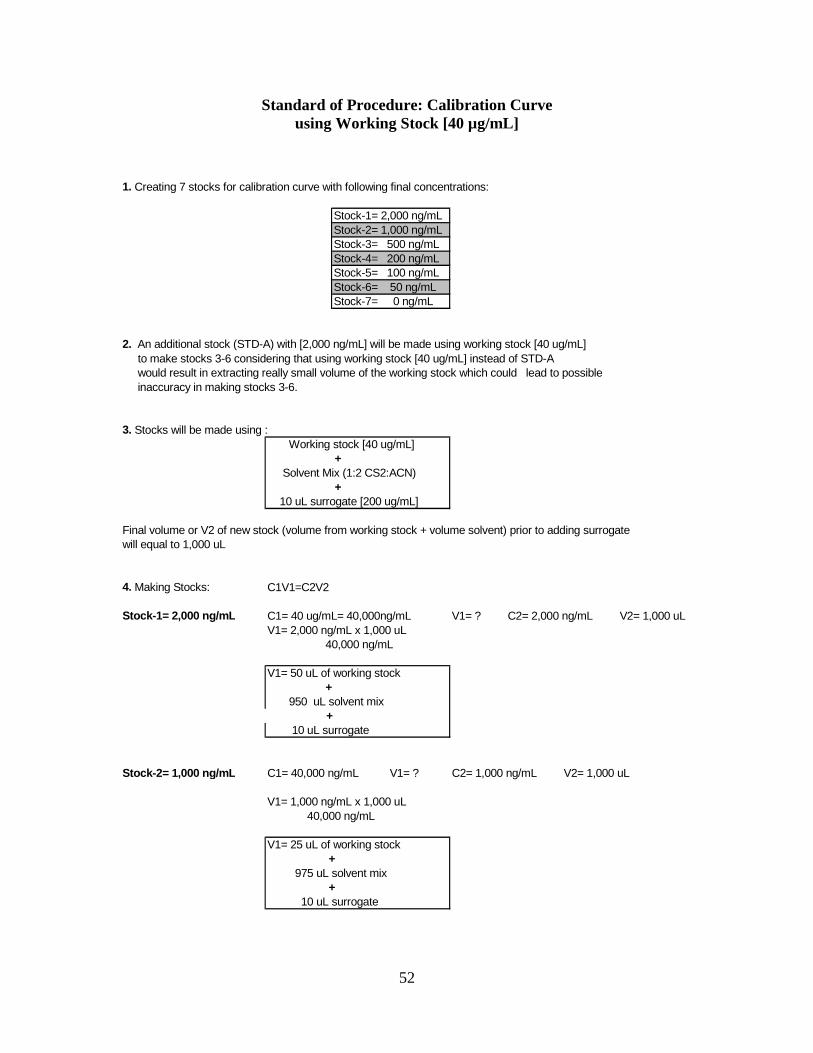
Standard of Procedure: Calibration Curve using Working Stock [40 µg/mL]

1. Creating 7 stocks for calibration curve with following final concentrations:

Stock-1= 2,000 ng/mLStock-2= 1,000 ng/mLStock-3= 500 ng/mLStock-4= 200 ng/mLStock-5= 100 ng/mLStock-6= 50 ng/mLStock-7= 0 ng/mL

2. An additional stock (STD-A) with [2,000 ng/mL] will be made using working stock [40 ug/mL] to make stocks 3-6 considering that using working stock [40 ug/mL] instead of STD-A would result in extracting really small volume of the working stock which could lead to possible inaccuracy in making stocks 3-6.

3. Stocks will be made using : Working stock [40 ug/mL] + Solvent Mix (1:2 CS2:ACN) + 10 uL surrogate [200 ug/mL]

Final volume or V2 of new stock (volume from working stock + volume solvent) prior to adding surrogatewill equal to 1,000 uL

4. Making Stocks: C1V1=C2V2

Stock-1= 2,000 ng/mL C1= 40 ug/mL= 40,000ng/mL V1= ? C2= 2,000 ng/mL V2= 1,000 uLV1= 2,000 ng/mL x 1,000 uL 40,000 ng/mL

V1= 50 uL of working stock + 950 uL solvent mix + 10 uL surrogate

Stock-2= 1,000 ng/mL C1= 40,000 ng/mL V1= ? C2= 1,000 ng/mL V2= 1,000 uL

V1= 1,000 ng/mL x 1,000 uL 40,000 ng/mL

V1= 25 uL of working stock + 975 uL solvent mix + 10 uL surrogate

53

Making STD-A to create stocks 3-6 using working stock [40 ug/mL]

STD-A= 2,000 ng/mL C1= 40,000 ng/mL V1= ? C2= 2,000 ng/mL V2= 1,000 uL

V1= 2,000 ng/mL x 1,000 uL 40,000 ng/mL

V1= 50 uL of working stock + 950 uL solvent mix

Stock-3= 500 ng/mL C1= 2,000 ng/mL V1= ? C2= 500 ng/mL V2= 1,000 uL

V1= 500 ng/mL x1,000 uL 2,000 ng/mL

V1= 250 uL of STD-A + 750 uL solvent mix + 10 uL surrogate


V1= 200 ng/mL x1,000 uL 2,000 ng/mL



V1= 100 ng/mL x1,000 uL 2,000 ng/mL


54


V1= 50 ng/mL x1,000 uL 2,000 ng/mL

V1= 25 uL STD-A + 975 uL solvent mix + 10 uL surrogate


Stock-7 will comprise of 1,000 uL of solvent mix and 10 uL surrogate

1,000 uL solvent mix + 10 uL surrogate

All 7 stocks are transferred to GCMS, sorting vials from least to most concentrated.

55

Extraction Procedure for Calculating Recovery Rate

Materials used: working stock [40 ug/mL]** 100 uL syringe

Internal Standard (IS) [200 ug/mL surrogate]OVM badge (7)

Badges are spiked with 20 uL of working stock [40 ug/mL]using syringe previously used to spike blanks

After first spike, tightly sealed badges sit for 10 mins

After 10 minutes, spike badges with 10 uL IS using 2-20 uL pipette

After second spike, tighly sealy badges sit for 3.5 hours

SONICATION

1. Badges are removed from plastic container in vial by rolling them using tefflon tweezers

2. Once in vials, add 1mL of solvent mix using 100-1000 uL pipette

3. Tightly sealed vials are placed in sonicator for 45 mins.

EXTRACTION

1. Extract sonicated solution and tranfer into fresh vial using Pasteur pipette.

ANALYSIS

**Mass for badges extracted with working stock20 uL of working stock x 40 ug/mL 10 uL IS x 200 ug/mL

= 20 uL x 40 ng/uL + = 10 uL x 200 ng/uL= 800 ng = 2000 ng

56

Bibliography

Adgate, J. L., Church, T. R., Ryan, A. D., Ramachandran, G., Fredrickson, A. L., Stock,

T. H. et al. (2004). Outdoor, Indoor, and Personal Exposure to VOCs in Children.

Environmental Health Perspectives, 112, 1386-1392.

Adgate, J. L., Eberly, L. E., Stroebel, C., Pellizzari, E. D., & Sexton, K. (2004).

Personal, indoor, and outdoor VOCs exposures in a probability sample of

children. Journal of Exposure Analysis and Environmental Epidemiology, 14, S4-

S13.

Akinbami, L. J. (2006). The state of childhood asthma, United States, 1980-2005.

Advance Data from Vital and Health Statistics, 381, Retrieved January 15,

2009, from the U.S Department of Health and Human Services, Centers for

Disease Control and Prevention National Center for Health Statistics database.

American Cancer Society. (2009). Cancer facts and figures 2009. Retrieved

February 10, 2009, from

http://www.cancer.org/docroot/stt/stt_0.asp?from=fast

American Chemistry Council (2009). Federal regulations on ground-level ozone.

Retrieved February 15, 2009, from

http://www.americanchemistry.com/s_acc/sec_solvents.asp?CID=1515&DID=58

01

Ashley, D. L., Bonin, M. A., Cardinali, F. L., McCraw, J. M., & Wooten, J. V.

(1994). Blood concentrations of volatile organic compounds in a

nonoccupationally exposed U.S. population and in groups with suspected

exposure. Clinical Chemistry, 40, 1401-1404.

57

Ashley, D. L., Bonin, M. A., Cardinali, F. L., McCraw, J. M & Wooten, J. V. (1996).

Measurement of volatile organic compounds in human blood. Environmental

Health Perspectives, 104, 871-877.

Boeglin, M. L., Wessels, D., & Henshel, D. (2006). An investigation of the relationship

between air emissions of volatile organic compounds and the incidence of cancer

in Indiana counties. Environmental Research, 100, 242-254.

Brauer, M., Hoek, G., Van Vliet, P., Meliefste, K., Fischer, P. H., Wijga, A. et al. (2002).

Air Pollution from Traffic and the Development of Respiratory Infections and

Asthmatic and Allergic Symptoms in Children. American Journal of Respiratory

and Critical Care Medicine, 166, 1092-1098.

Burstyn, I., You, X. I., Cherry, N. & Senthilselvan, A. (2007). Determinants of airborne

benzene concentration in rural areas of Western Canada. Atmospheric

Environment, 41, 7778-7787.

Carbajal-Arroyo, L., Barraza-Villarreal, A., Durand-Pardo, R., Moreno-Macías, H.,

Espinoza-Lain, R., Chiarella-Ortigosa, P. et al. (2007). Impact of traffic flow on

the asthma prevalence among school children in Lima, Peru. Journal of Asthma,

44, 197-202.

Carter, W. P. L. (1994). Development of ozone reactivity scales for volatile

organic compounds. Journal of the Air & Waste Management

Association, 44, 881-899.

Cohen,A. J., & Pope III, C.A. (1995). Lung cancer and air pollution.


Delfino, R. J., Gong, H., Linn, W. S., Hu, Y., & Pellizzari, E. D. (2003).

58

Respiratory symptoms and peak expiratory flow in children with asthma in

relation to volatile organic compounds in exhaled breath and ambient air. Journal

of Exposure Analysis and Environmental Epidemiology, 13, 348-363.

Deloraine, A., Zmirou, D., Tillier, C., Boucharlat, A., & Bouti, H. (1995). Case-Control

Assessment of the Short-Term Health Effects of an Industrial Toxic Waste

Landfill. Environmental Research, 68, 124-132.

Dockery, D. W., Pope, C. A., Xu, X., Spengler, J. D., Ware, J. H., Fay, M. E.

et al. (1993). An association between air pollution and mortality in six U.S. cities.

The New England Journal of Medicine, 329, 1753-1759.

Doll, R., Peto, R., Boreham, J. & Sutherland, I. (2005). Mortality from cancer in

relation to smoking: 50 years observations on British doctors. British Journal

of Cancer, 92, 426-429.

D’Amato, G., Liccardi, G., D’Amato, M., & Cazzola, M. (2001). The role of outdoor air

pollution and climatic changes on the rising trends in respiratory allergy.

Respiratory Medicine, 95, 606-611.

Edwards, J., Walters, S. & Griffiths, R. K. (1994). Hospital admissions for asthma in

preschool children: relationship to major roads in Birmingham, United Kingdom.

Archives of Environmental Health, 49, 223-227.

Edwards, R. D., Iurvelin, J., Saarela, K., & Jantunen, M. (2001). Volatile organic

compound concentrations measured in personal samples and residential indoor,

outdoor and workplace microenvironments in EXPOLIS-Helinski, Finland.

Atmospheric Environment, 35, 4531-4543.

59

Elliott, L., Longnecker, M. P., Kissling, G. E., & London, S. J. (2006). Volatile organic

compounds and pulmonary function in the Third National Health and Nutrition

Examination Survey, 1988-1994. Environmental Health Perspectives, 114, 1210-

1214.

Fischer, P. H., Hoek, G., van Reeuwijk, H., Briggs, D. J., Lebret, E., van Wijnen, J. H. et

al. (2000). Traffic-related differences in outdoor and indoor concentrations of

particles and volatile organic compounds in Amsterdam. Atmospheric


Fondelli, M. C., Bavazzano, P., Grechi, D., Gorini, G., Miligi, L., Marchese, G. et al.

(2008). Benzene exposure in a sample of population residing in a district of

Florence, Italy. Science of The Total Environment, 392, 41-49.

Gauderman, W. J., Avol, E., Lurmann, F., Kuenzli, H., Gilliland, F., Peters, J.

et al. (2005). Childhood asthma and exposure to traffic and nitrogen dioxide.

Epidemiology, 16, 737-743.

Gee, I. L., & Sollars, C. J. (1998). Ambient air levels of volatile organic

compounds in Latin American and Asian cities. Chemosphere, 36, 2497-2506.

Guo, H., Lee, S. C., Chan, L. Y., & Li, W. M. (2004). Risk assessment of exposure to

volatile organic compounds in different indoor environments. Environmental

Research, 94, 57-66.

Han, X., & Naeher, L. P. (2006). A review of traffic-related air pollution exposure

assessment studies in the developing world. Environment International, 32, 106-

120.

60

Jones, A. P. (1999). Indoor air quality and health. Atmospheric Environment, 33, 4535-

4564.

Katsouyanni, K., & Pershagen, G. (1997). Ambient air pollution and cancer.

Cancer Causes and Control, 8, 284-291.

Khan, F. I., & Ghoshal, A. (2000). Removal of Volatile Organic Compounds from

polluted air. Journal of Loss Prevention in the Process Industries, 13, 527-545.

Kim, Y. M., Harrad, S., & Harrison, R. M. (2002). Levels and Sources of Personal

Inhalation Exposure to Volatile Organic Compounds. Environmental Science &

Technology, 36, 5405-5410.

Klepeis, N. E., Nelson, W. C., Ott, W. R., Robinson, J. P., Tsang, A. M., Switzer, P. A.

U. L. et al. (2001). The National Human Activity Pattern Survey (NHAPS): a

resource for assessing exposure to environmental pollutants. J Expo Anal Environ

Epidemiol, 11, 231-252.

Knox, E. G., & Gilman, E. A. (1997). Hazard proximities of childhood cancers in Great

Britain from 1953-80. Journal of Epidemiology and Community Health, 51, 151-

159.

Knox, E. G., & Gilman, E. A. (1998). Migration patterns of children with cancer in

Britain. Journal of Epidemiology and Community Health, 52, 716-726.

Knox, E. G. (2005). Childhood cancers and atmospheric carcinogens. Journal of

Epidemiology and Community Health, 59, 101-105.

Koren, H. S. & Delvin, R. B. (1992). Exposure of humans o a volatile organic mixture.

III. Inflammatory response. Archives of Environmental Health, 47, 39-44.

61

Kuo, H.-W., Chiang, T.-F., Lo, I.-I., Lai, J.-S., Chan, C.-C., & Wang, J.-D. (1998).

Estimates of cancer risk from chloroform exposure during showering in Taiwan.

The Science of The Total Environment, 218, 1-7.

Kwon, J., Weisel, C. P., Turpin, B. J., Zhang, J., Korn, L. R., Morandi, M. T. et al.

(2006). Source proximity and outdoor-residential VOC concentrations: results

from the RIOPA study. Environmental Science & Technology, 40, 4074-4082.

Lee, S. C., Chiu, M. Y., Ho, K. F., Zou, S. C., & Wang, X. (2002). Volatile organic

compounds (VOCs) in urban atmosphere of Hong Kong. Chemosphere, 48, 375-

382.

Lin, Y. S., Egeghy, P. P., & Rappaport, S. M. (2008). Relationships between levels of

volatile organic compounds in air and blood from the general population. Journal

of Exposure Science and Environmental Epidemiology, 18, 421-429.

Loyo-Berrios, N. I., Irizarry, R., Hennessey, J. G., Tao, X. G., & Matanoski, G. (2007).

Air Pollution Sources and Childhood Asthma Attacks in Catano, Puerto Rico.

American Journal of Epidemiology, 165, 927-935.

Mannino, D. M., Homa, D. M. & Petrowski, C. A. (1998). Surveillance for asthma—

United States, 1960-1995. MMWR CDC Surveillance Summary, 47, 1-27.

McConnell, R., Berhane, K., Yao, L., Jerrett, M., Lurmann, F., Gilliland, F. et al. (2006).

Traffic, susceptibility, and childhood asthma. Environmental Health Perspectives,

114, 766-772.

Mintz, R., & McWhinney, R. D. (2008). Characterization of volatile organic compound

emission sources in Fort Saskatchewan, Alberta using principal compound

analysis. J Atmos Chem, 60, 83-101.

62

Mohamed, M. F., Kang, D., & Aneja, V. P. (2002). Volatile organic compounds in some

urban locations in United States. Chemosphere, 47, 863-882.

Montserrat, C. & Baldasano, J. M. (1995). Development of a source emission model for

atmospheric pollutants in the Barcelona area. Atmospheric Environment, 30, 309-

318.

Morgenstern, V., Zutavern, A., Cyrys, J., Brockow, I., Gehring, U., Koletzko, S. et al.

(2007). Respiratory health and individual estimated exposure to traffic-related air

pollutants in a cohort of young children. Occupational and Environmental

Medicine, 64, 8-16.

Muezzinoglu, A., Odabasi, M., & Onat, L. (2001). Volatile organic compounds in the air

of Izmir, Turkey. Atmospheric Environment, 35, 753-760.

Na, K., Kim, Y. P., Moon, K. C., Moon, I., & Fung, K. (2001). Concentrations of volatile

organic compounds in an industrial area of Korea. Atmospheric Environment, 35,

2747-2756.

Nicolai, T., Carr, D., Weiland, S. K., Duhme, H., von Ehrenstein, O., Wagner, C. et al.

(2003). Urban traffic and pollutant exposure related to respiratory outcomes and

atopy in a large sample of children. European Respiratory Journal, 21, 956-963.

Oftedal, B., Nafsad, P., Magnus, P., Bjørkly, S., & Skrondal, A. (2003). Traffic related

air pollution and acute hospital admission for respiratory diseases in Drammen,

Norway 1995-2000. European Journal of Epidemiology, 18, 671-675.

Paul, J. (1997). Improved air quality on Turkish roads: fuels and exhaust gas treatment.

Environmental Research Forum, 7-8, 145-152.Paustenbach, D. J. (2000). The

63

practice of exposure assessment: a state-of-the-art review. Journal of Toxicology

and Environmental Health, 3, 179-291.

Payne-Sturges, D. C., Burke, T. A., Breysse, P., Diener-West, P., & Buckley, T. J.

(2004). Personal exposure meets risk assessment: a comparison of measured and

modeled exposures and risks in an urban community. Environmental Health

Perspectives, 112, 589-598.

Pearson, R. L., Watchel, H. & Ebi, K. L. (2000). Distance-weighted traffic density in

proximity to a home is a risk factor for leukemia anad other childhood cancers.

Journal of Air Waste Management Association, 50, 175-180.

Peng, C. Y., & Lin, T. S. (2007). Volatile organic compound exposure of suburban

elementary students in taiwan. Bulletin of Environmental Contamination and

Toxicology, 78, 85-88.

Phillips, M., Herrera, J., Krishnan, S., Zain, M., Greenberg, J., & Cataneo, R. N. (1999).

Variation in volatile organic compounds in the breath of normal humans. Journal

of Chromatography B: Biomedical Sciences and Applications, 729, 75-88.

Rappaport, S. M., & Kupper, L. L. (2004). Variability of environmental exposures to

volatile organic compounds. Journal of Exposure Analysis and Environmental

Epidemiology, 14, 92-107.

Reynolds, P., Von Behren, J., Gunier, R. B., Goldberg, D. E., Hertz, A., & Smith, D. F.

(2003). Childhood Cancer Incidence Rates and Hazardous Air Pollutants in

California: An Exploratory Analysis. Environmental Health Perspectives, 111,

330.

64

Rumchev, K., Spickett, J., Bulsara, M., Phillips, M. & Stick, S. (2004). Association of

domestic exposure to volatile organic compounds with asthma in young children.

Thorax, 59, 746-751.

Sapkota, A., & Buckley, T. (2003). The mobile source effect on curbside 1,3-butadiene,

benzene, and particle-bound polycyclic aromatic hydrocarbons assessed at a

tollbooth. Journal of Air & Waste Management Association, 53, 740-748.

Sapkota, A., Williams, D., & Buckley, T. J. (2005). Tollbooth workers and mobile

source-related hazardous air pollutants: how protective is the indoor environment?

Environmental Science & Technology, 39, 2936-2943.

Sax, S. N., Bennett, D. H., Chillrud, S. N., Kinney, P. L., & Spengler, J. D. (2004).

Differences in source emission rates of volatile organic compounds in inner-city

residences of New York City and Los Angeles. J Expo Anal Environ Epidemiol,

14, S95-S109.

Sexton, K., Adgate, J. L., Ramachandran, G., Pratt, G. C., Mongin, S. J., Stock, T. H. et

al. (2004). Comparison of personal, indoor, and outdoor exposures to hazardous

air pollutants in three urban communities. Environmental Science & Technology,

38, 423-430.

Skov, H., Hansen, A. B., Lorenzen, G., Andersen, H. V., Løfstrøm, P., & Christensen, C.

S. (2001). Benzene exposure and the effect of traffic pollution in Copenhagen,

Denmark. Atmospheric Environment, 35, 2463-2471.

Son, B., Breysse, P., & Yang, W. (2003). Volatile organic compounds concentrations in

residential indoor and outdoor and its personal exposure in Korea. Environment

International, 29, 79-85.

65

U.S. Census Bureau. (2009). Population estimates. Retrieved February 10, 2009, from

U.S. Census Bureau database.

U.S. Environmental Protection Agency. (2009). Assessing outdoor air near schools.

Retrieved April 1, 2009, from

http://www.epa.gov/schoolair/index.html

van Vliet, P., Knape, M., de Hartog, J., Janssen, N., Harssema, H, & Bunekreef, B.

(1997). Motor vehicle exhaust and chronic respiratory symptoms in children

living near freeways. Environmental Research, 74, 122-132.

Vineis, P., Forastiere, F., Hoek, G., & Lipsett, M. (2004). Outdoor air pollution and lung

cancer: recent epidemiologic evidence. International Journal of Cancer, 111,

647-652.

United Nation Environment Program (1994). Air pollution in the world’s

megacities. Environment, 36, 5-37.

Wallace, L. (1986). Personal exposures, indoor and outdoor air concentrations, and

exhaled breath concentration of selected volatile organic compounds

measured for 600 residents of New Jersey, North Dakota, North Carolina and

California. Toxicological and Environmental Chemistry, 12, 215-236.

Wallace, L. (1987). The total exposure assessment methodology (TEAM) study.

United States: Environmental Protection Agency. Office of Research and

Development.

Wallace, L. (1989). Major sources of benzene exposure. Environmental Health

Perspectives, 82, 165-169.

Wallace, L. (1991). Comparison of risks from outdoor and indoor exposure to

66

toxic chemicals. Environmental Health Perspectives, 95, 7-13.

Wallace, L. (1996). Environmental exposure to benzene: an update.


Wallace, L. A. (2001). Human exposure to volatile organic pollutants: Implications for

Indoor Air Studies1. Annual Review of Energy and the Environment, 26, 269-301.

Wilkinson, P., Thakrar, B., Walls, P., Landon, M., Falconer, S., Grundy, C. et al. (1999).

Lymphohaematopoeitic malignancy around all industrial complexes that include

major oil refineries in Great Britain. Occupational & Environmental Medicine,

56, 577-580.

Woodruff, T. J., Caldwell, J., Cogliano, V. J., & Axelrad, D. A. (2000). Estimating

Cancer Risk from Outdoor Concentrations of Hazardous Air Pollutants in 1990.

Environmental Research, 82, 194-206.

Yamamoto, N., Okayasu, H., Murayama, S., Mori, S., Hunahashi, K. & Suzuki, K.

(2000). Measurement of volatile organic compounds in the urban atmosphere of

Yokohama, Japan, by an automated gas chromatography system. Atmospheric


Zhao, W., Hopke, P. K., & Karl, T. (2004). Source Identification of Volatile Organic

Compounds in Houston, Texas. Environmental Science & Technology, 38,

1338-1347.

abstract title of document: cross sectional - drum

Documents