abstract title of thesis: evaluation of ... - drum.lib.umd.edu
TRANSCRIPT

ABSTRACT
Title of Thesis: EVALUATION OF AN EXTENDED DUCT
AIR DELIVERY SYSTEM FOR SPACES
CONDITIONED BY ROOFTOP UNITS
Ryan Kennett, Master of Science, 2016
Thesis Directed By: Research Professor Yunho Hwang, Ph.D.
Department of Mechanical Engineering
Traditional air delivery to high-bay buildings involves ceiling level supply and return
ducts that create an almost-uniform temperature in the space. Problems with this
system include potential recirculation of supply air and higher-than-necessary return
air temperatures. A new air delivery strategy was investigated that involves changing
the height of conventional supply and return ducts to have control over thermal
stratification in the space. A full-scale experiment using ten vertical temperature
profiles was conducted in a manufacturing facility over one year. The experimental
data was utilized to validated CFD and EnergyPlus models. CFD simulation results
show that supplying air directly to the occupied zone increases stratification while
holding thermal comfort constant during the cooling operation. The building energy
simulation identified how return air temperature offset, set point offset, and
stratification influence the building’s energy consumption. A utility bill analysis for
cooling shows 28.8% HVAC energy savings while the building energy simulation
shows 19.3 – 37.4% HVAC energy savings.

EVALUATION OF AN EXTENDED DUCT AIR DELIVERY SYSTEM FOR
SPACES CONDITIONED BY ROOFTOP UNITS
by
Ryan Kennett
Thesis submitted to the Faculty of the Graduate School of the
University of Maryland, College Park, in partial fulfillment
of the requirements for the degree of
Master of Science
2016
Advisory Committee:
Research Professor Yunho Hwang, Chair
Professor Jelena Srebric
Associate Professor Bao Yang

© Copyright by
Ryan Kennett
2016

ii
Acknowledgements
I would like to gratefully acknowledge the support of the following people and
organizations, without whom this research would not have been possible. My advisor
Dr. Yunho Hwang for sharing his knowledge, guidance, and vision over the past two
years. Jan Muehlbauer for his skills in the lab and information you can’t find anywhere
else. XChanger Co. for their ideas, enthusiasm, and product. Holmatro Inc. and John
Freeburger for being welcoming and helpful during our measurement setup. Maryland
Industrial Partnership Program (MIPS) for facilitating this unique collaboration. Dr.
Reinhard Radermacher and Dr. Hoseong Lee for their consistently insightful feedback
during weekly meetings. And finally, my fellow researchers and friends at CEEE for
their daily support and motivation.

iii
Table of Contents
Acknowledgements ....................................................................................................... ii
Table of Contents ......................................................................................................... iii
List of Tables ............................................................................................................... vi
List of Figures ............................................................................................................ viii
Nomenclature ............................................................................................................... xi
1. Introduction ........................................................................................................... 1
1.1 Motivation ..................................................................................................... 1
1.2 Conventional Air Delivery Strategy for High Bay Buildings ....................... 2
1.3 Proposed Air Delivery System...................................................................... 4
1.4 Objective ....................................................................................................... 7
2. Experimental Work ............................................................................................... 7
2.1 Test Facility .................................................................................................. 7
2.2 Literature Review........................................................................................ 10
2.3 Instrumentations and Data Acquisition ....................................................... 13
2.4 Uncertainty Analysis ................................................................................... 15
3. Computational Fluid Dynamics Modeling.......................................................... 16
3.1 Literature Review........................................................................................ 16
3.2 Objective ..................................................................................................... 21
3.3 Governing Equations and Turbulence Modeling ........................................ 22
3.4 Geometry and Computational Grid ............................................................. 23

iv
3.5 Solver Settings ............................................................................................ 28
3.6 Boundary Conditions .................................................................................. 29
4. Building Energy Simulation ............................................................................... 32
4.1 Literature Review........................................................................................ 32
4.2 Room Air Modeling .................................................................................... 35
4.3 Weather Data .............................................................................................. 44
4.4 Schedules .................................................................................................... 45
4.5 Electrical and Thermal Loads ..................................................................... 47
4.5.1 Electrical Equipment ............................................................................... 47
4.5.2 Lights ...................................................................................................... 48
4.5.3 Occupants ................................................................................................ 49
4.6 Building Envelope and Surface Constructions ........................................... 49
4.6.1 Outer Walls ............................................................................................. 49
4.6.2 Interior Walls and Open Doorways ........................................................ 50
4.6.3 Floor ........................................................................................................ 51
4.6.4 Roof Construction ................................................................................... 51
4.7 Primary Systems (RTUs and air delivery) .................................................. 52
4.7.1 Cooling Coil ............................................................................................ 53
4.7.2 Heating Coil ............................................................................................ 56
4.7.3 Economizer Control ................................................................................ 56
4.7.4 Fans ......................................................................................................... 58

v
4.8 Infiltration ................................................................................................... 60
4.9 Retrofit Modeling........................................................................................ 62
4.9.1 Lights ...................................................................................................... 62
4.9.2 Rooftop Units .......................................................................................... 63
4.9.3 Air Compressor ....................................................................................... 64
5. Results Analysis and Discussion ........................................................................ 66
5.1 Experiment .................................................................................................. 66
5.1.1 Temperature Profiles ............................................................................... 66
5.1.2 Utility Bill Analysis ................................................................................ 70
5.2 CFD Modeling ............................................................................................ 78
5.2.1 Grid Sensitivity Analysis ........................................................................ 78
5.2.2 Model Validation .................................................................................... 81
5.2.3 Parametric Study ..................................................................................... 85
5.3 EnergyPlus Modeling.................................................................................. 91
5.3.1 Model Validation .................................................................................... 91
5.3.2 Energy Savings of Proposed System ...................................................... 94
6. Conclusions ......................................................................................................... 97
7. Future Work ........................................................................................................ 98
References ................................................................................................................ 100

vi
List of Tables
Table 1: Summary of literature reviewed for vertical stratification measurement ..... 13
Table 2: CFD research summaries – tall spaces, stratification, and heating season ... 20
Table 3: Size functions................................................................................................ 27
Table 4: Solver settings ............................................................................................... 29
Table 5: Temperature profile discretization time slots ............................................... 44
Table 6: Number of lighting fixtures in each room .................................................... 49
Table 7: Thermal properties of concrete floor ............................................................ 51
Table 8: Roof construction thermal properties ........................................................... 52
Table 9: Fan Static Pressure Drop (McQuiston et al., 2004) ...................................... 58
Table 10: Total Pressure Loss in Ducts ...................................................................... 59
Table 11: EnergyPlus Fan Object Inputs .................................................................... 59
Table 12: Rooftop unit specifications before and after retrofit................................... 63
Table 13: Air compressor model status ...................................................................... 65
Table 14: Monthly electricity and gas consumption before and after retrofits ........... 71
Table 15: Yearly energy savings of switching from metal halide to LED bulbs ........ 74
Table 16: RTU retrofit energy savings ....................................................................... 74
Table 17: Electricity savings due to XChanger calculated from utility bills .............. 75
Table 18: Facility gas consumption before and after retrofits .................................... 77
Table 19: Grid sensitivity number of cells .................................................................. 80

vii
Table 20: Parametric study test matrix ....................................................................... 85
Table 21: Parametric study results (averages over entire flow domain) ..................... 87
Table 22: Average temperature minus hypothetical thermostat temperature ............. 88
Table 23: Parametric study results; averages over the occupied zone ........................ 89
Table 24: ASHRAE guideline 14 requirements .......................................................... 91
Table 25: 2015 EnergyPlus model calibration statistics ............................................. 91
Table 26: Temperature profile corresponding to model and time period ................... 94
Table 27: Models used to compare fan controls and static pressure rise .................... 95
Table 28: Energy savings of XChanger based on EnergyPlus models ....................... 96

viii
List of Figures
Figure 1: Overhead Air Delivery (source: Bettinger West) .......................................... 3
Figure 2: Conventional system and new system in cooling and heating ...................... 5
Figure 3: XChanger box working mechanism (XChanger Co., 2016) ......................... 6
Figure 4: Test facility layout and pole location ............................................................ 8
Figure 5: Large manufacturing room with traditional air delivery ............................... 9
Figure 6: Assembly room thermal image (metal halide lights) .................................... 9
Figure 7: Lighting image: metal halide fixture (left) vs. LED fixture (right) ............. 10
Figure 8: Mixing ventilation (left) and XChanger (right) ........................................... 10
Figure 9: Floor-level air supply device by Singh and Olivieri (1988) ........................ 11
Figure 10: Temperature measurement pole ................................................................ 14
Figure 11: Procedure for generating a reliable CFD model ........................................ 17
Figure 12: Large manufacturing room with XChanger .............................................. 24
Figure 13: Chosen location for CFD simulation ......................................................... 25
Figure 14: CFD geometry ........................................................................................... 26
Figure 15: Mesh along the supply diffuser vertical plane........................................... 26
Figure 16: Y-star values for heat transfer surfaces ..................................................... 28
Figure 17: Temperature profile boundary condition for walls.................................... 31
Figure 18: Room temperature distribution modeling approaches............................... 33
Figure 19: Non-dimensional height room air model................................................... 36
Figure 20: Heat balance calculation procedure for non-uniform air temperature ...... 37

ix
Figure 21: Proposed method of accounting for thermostat offset............................... 42
Figure 22: Input thermostat temperatures ................................................................... 43
Figure 23: Manufacturing electrical equipment schedule ........................................... 46
Figure 24: Lighting schedule ...................................................................................... 47
Figure 25: Wall insulation properties (source: Masonry Advisory Council) ............. 50
Figure 26: Built-up roof construction (source: Lydick-Hooks Roofing) .................... 52
Figure 27: Typical air loop for a single space............................................................. 53
Figure 28: Quadratic performance curves for the RTUs ............................................ 55
Figure 29: Fan part load power as a function of flow fraction ................................... 60
Figure 30: Temperature profile measured during bay door opening .......................... 61
Figure 31: Air change rate due to infiltration ............................................................. 62
Figure 32: Map for thermocouple column naming ..................................................... 66
Figure 33: Average seasonal temperature of each thermocouple ............................... 67
Figure 34: Average measured temperature profile by room ....................................... 68
Figure 35: Monthly degree day regression for (a) heating, (b) cooling ...................... 72
Figure 36: Degree day normalization for daily data ................................................... 72
Figure 37: CDD increase from 2014 (baseline) to 2015 (post-retrofit) ...................... 73
Figure 38: Grid sensitivity – vertical temperature profiles ......................................... 80
Figure 39: Measured supply air temperature of one RTU from 8/30/15 – 9/2/15 ...... 82
Figure 40: (a) Baseline and (b) XChanger CFD model validation ............................. 83
Figure 41: Vertical temperature profile measurement locations ................................. 84

x
Figure 42: (a) Baseline and (b) XChanger with the opposite boundary conditions .... 85
Figure 43: ASHRAE definition of occupied zone ...................................................... 89
Figure 44: PPD contours for each case (only high velocity cases shown) ................. 90
Figure 45: Model versus measured daily electricity use ............................................. 92
Figure 46: Accuracy of simulated daily electricity consumption ............................... 92
Figure 47: Simulated and measured monthly gas use ................................................. 94

xi
Nomenclature
Abbreviations
CNC Computer Numerical Control
COP Coefficient of Performance
DV Displacement Ventilation
GFRC Glass Fiber Reinforced Concrete
MAT Mean Air Temperature
RANS Reynolds Averaged Navier Stokes
RAT Return Air Temperature
RTU Roof Top Unit
UFAD Under Floor Air Distribution
VAV Variable Air Volume
Symbols
amb Ambient (Outdoor)
𝐼𝑑𝑒𝑠𝑖𝑔𝑛 Design Infiltration (m3/s)
𝐹𝑠𝑐ℎ𝑒𝑑𝑢𝑙𝑒 Scheduled Fraction
v Velocity
�̇� Capacity (W)
Q Heat (J)
�̇� Volume flow rate (m3/s)

1
1. Introduction
1.1 Motivation
Commercial buildings accounted for 18% of the total U.S. energy consumption
in 2014 (EIA, 2015). Of this energy consumption, space heating constitutes 22.5%
and space cooling constitutes 14.8%. From 2003 to 2012, the number of commercial
buildings increased by 14% and the floor space of commercial buildings increased by
21%. An increase in the number and size of commercial buildings calls for more
efficient building energy use. Numerous strategies exist for conserving building
HVAC energy, such as more efficient primary systems, controls, and improvements
to the building envelope.
Control over indoor air distribution is another possible way to save HVAC
energy. Air distribution has been researched for roughly the past 35 years, focusing
particularly on underfloor air distribution (UFAD) and displacement ventilation (DV).
These strategies utilize low velocity supply air diffusers near the floor to provide
cooling to the occupied zone. Although large differences between simulated and
measured energy savings are reported in the literature, some researchers claim that
UFAD saves 30% cooling energy, particularly in spaces with tall ceilings (Alajmi et
al., 2010). However, these air distribution strategies do not lend themselves easily to
the retrofit of existing buildings because they require different supply air

2
temperatures and velocities than traditional, packaged heating and cooling systems
are designed to provide.
UFAD and DV raise an interesting question: how can thermal stratification be
utilized to influence thermal comfort, indoor air quality, and the room’s heating or
cooling load?
1.2 Conventional Air Delivery Strategy for High Bay Buildings
Typical high bay buildings, such as warehouses, storage facilities, or hangars,
use packaged rooftop units (RTUs) to condition indoor air. Due to high ceilings, often
over 6 m, strong thermal stratification can develop because the density of air
decreases as temperature increases. Cold, dense air accumulates near the floor, while
warmer air floats towards the ceiling. This stratification has implications on building
energy use and occupant thermal comfort.
Air is typically supplied and returned at ceiling level. This type of system will
henceforth be known as the conventional or overhead system. The corresponding
room air distribution strategy is called mixing ventilation. Air is often supplied
horizontally using a wall duct, terminal device, or conical diffuser. An introduction to
the design and behavior of the overhead system can be found in Heating, Ventilating,
and Air Conditioning (McQuiston, 2004). When high velocity air is supplied
horizontally near the ceiling, the jet of supply air attaches to the ceiling (the coanda
effect), which increases its throw. As the jet flows along the ceiling, room air is

3
entrained and the jet decreases velocity to less than about 0.25 m/s. The jet is
eventually fully mixed with the room air.
Figure 1: Overhead Air Delivery (source: Bettinger West)
McQuiston et al. point out that the conventional system is popular in
commercial applications because “the ceiling diffuser can handle larger quantities of
air at higher velocities than most other types” (McQuiston et al., 2004). With regards
to creating a uniform temperature in the space, the authors concluded that “the ceiling
diffuser is quite effective for cooling applications but generally poor for heating”.
One problem with the traditional design is that the ceiling-level return duct
draws the warmest air in the space. McQuiston described that “in spaces with very
high ceilings, atriums, sky-lights, or large vertical glass surfaces and where the
highest areas are not occupied, air stratification is a desirable energy-saving technique
and return grilles should not be located in those areas [near the ceiling]”.

4
Another problem with the conventional system occurs when supply air flows
into the return duct before fully mixing with the room air. This short circuiting of
supply air can be seen in Figure 1. Short circuiting is a waste of energy because the
fans and cooling coil must operate longer to satisfy the space load.
1.3 Proposed Air Delivery System
A new air delivery system has been proposed by a Maryland based company to
fix the two problems discussed above - returning the warmest air in the space and
short circuiting the supply air (XChanger Co., 2016). This system reconfigures the
location of supply and return ducts with the goal of saving energy and improving
thermal comfort. With regard to published literature, this system can be thought of as
a hybrid between the conventional, overhead system and UFAD or DV. It is a hybrid
in that the system is simply a retrofit of the overhead system’s ducting to produce a
vertical temperature gradient that can be found in UFAD or DV systems.
In cooling season, air is supplied low and returned at a middle level. The goal is
to condition only the occupied space. Of course, heat will still be transferred from the
upper portion to the lower portion of the space by convection and radiation. However,
the average temperature of the space will increase, which decreases the heat loss
through conduction to the outside.
In winter, air is supplied near the ceiling and the return duct is located in the
occupied zone. This configuration draws the warm air downward, thus destratifying

5
the space. Destratification reduces over-heating of the upper portion of the space and
makes for easier-to-reach set points.
Figure 2: Conventional system and new system in cooling and heating

6
Figure 3: XChanger box working mechanism (XChanger Co., 2016)
The XChanger system is incorporated into a building with fixed ductwork as a
retrofit or into a new building. During a retrofit, the existing ductwork is extended to
the floor where convenient. To switch from supplying low, returning high in the
summer to supplying high, returning low in the winter, the XChanger system has a
‘box’ with a single damper, as shown in Figure 3.

7
1.4 Objective
It is currently unknown how much energy the XChanger system will save a
typical building. The objective of this thesis is to determine the energy savings
associated with stratification in high bay buildings through experiment and modeling.
2. Experimental Work
2.1 Test Facility
Holmatro, a manufacturer of hydraulic rescue equipment from Glenn Burnie,
Maryland, has installed four energy conserving retrofits: LED lighting, higher SEER
rooftop units, the XChanger system, and a more efficient industrial air compressor.
Holmatro has allowed measurements to be taken at their test facility for over one
year. The purpose of the measurements was to track the performance and energy
savings of the XChanger system over the course of one year. The facility layout, large
manufacturing room, assembly room, lighting retrofit, and the XChanger retrofit can
be seen in Figure 4 through Figure 8.

8
Figure 4: Test facility layout and pole location
The site consists of four large rooms and several offices. The offices take up
two floors and have a central hallway running through the middle. The south side of
the building has two large bay doors that open roughly twice per day for a few
minutes to load and unload deliveries.
Thermocouple
Pole
Roof Top
Unit
Bay Door
1
5
3
4
2
6
7
9 10
8
Small Mfg. O
ffic
e S
pac
e
Storage
Assembly
Large Mfg.

9
Figure 5: Large manufacturing room with traditional air delivery
Figure 6: Assembly room thermal image (metal halide lights)

10
Figure 8: Mixing ventilation (left) and XChanger (right)
2.2 Literature Review
Researchers have used full-scale experiments to measure air distribution in
buildings, particularly with UFAD, DV, and heating high-bay buildings. Singh and
Olivieri tested a system very similar to the XChanger system that supplies and returns
air near the floor (1988). Their idea to change the supply and return duct location
stems from a desire to “eliminate either the effect of the induction of the upper level
hot air into the supply air stream or the pulling down of the upper level hot air by the
Figure 7: Lighting image: metal halide fixture (left) vs. LED fixture (right)

11
return air or both”. Through a series of ten tests, they reduced the height of supply
and return ducts from ceiling-level to floor-level. The authors showed that supplying
air in the bottom third of the room gives the most stratification and lowest occupied
zone temperature. The return duct height has little effect on stratification, though they
do not test low-level supply and high-level return.
Figure 9: Floor-level air supply device by Singh and Olivieri (1988)
Using the device shown in Figure 9, the authors showed that a room with this
device installed saves 33-50% RTU input power compared to a baseline room with a
“four sided box with grilles on each face and central return air”. The device in Figure

12
9 clearly resembles the XChanger and the air delivery ‘box’ that served as a baseline
clearly resembles the overhead system in Figure 5. Based on this research, the
XChanger system can be expected to save 33-50% HVAC energy in cooling, though
the taller ceiling height in this thesis may affect the results.
Saïd et al. (1995) studied the effects of thermal stratification in large aircraft
hangars during heating season. The heating system was the overhead down-draft air
delivery system. Sixteen T-type thermocouples measure temperature from six inches
off the floor to six inches from the ceiling. Temperatures were averaged over long
measurement periods, giving stratification ranging from 4 K to 11 K. Two distinct,
linear gradients are observed – one below 2 m and one above. Outdoor temperature
and ceiling fans are shown to have little effect on stratification. No energy savings are
reported from the experiment. BLAST simulations estimate a 38% reduction in gas
use with no stratification compared to 8 K stratification.
Wang et al. (2011) studied an UFAD system in an 8 m tall gym. They
conclude that supply air temperature influences the temperature gradient in the
occupied zone, airflow distribution influences the temperature gradient in the middle
of the room, and outside temperature has no influence on stratification.

13
Table 1: Summary of literature reviewed for vertical stratification measurement
Paper Year HVAC System Ceiling Height
[m] Stratification [K]
Singh and
Olivieri 1988
RTU with supply
and returns at
various heights
3.2
5.3
2.4 – 8.8
1.31
Said et al. 1995 Overhead heating 9.35 - 17.1 4 - 11
Wang et al. 2011 UFAD 8.0 7 - 19
2.3 Instrumentations and Data Acquisition
Ten vertical temperature poles were placed in the test facility, as shown in Figure
4. Each pole contains 13 thermocouples: one taped to the floor, one taped to the
ceiling, and 11 measuring air temperature. Aluminum tape was used to attach the
thermocouples to the floor and ceiling, insulating the thermocouple from air so that it
accurately measured surface temperature. The vertical temperature poles were
fastened to structural columns to avoid cluttering the shop floor and for access to an
electrical outlet. A local wireless network was installed for communication between
each DAQ board and a centrally located desktop computer. A mobile hotspot was
used for remote Internet access to this desktop computer. Temperatures were
measured over the course of one year, sampled every 20 seconds. Unfortunately, the
wireless network breaks down periodically and measurements must be restarted
manually.

14
Figure 10: Temperature measurement pole
Seven relative humidity (RH) sensors were installed with at least one in every
room. A one-time vertical RH profile was measured during cooling season to identify
a potential humidity gradient. No such gradient was found, unless it is less than the
measurement resolution of the sensors.
Five additional temperature measurements were made. One thermocouple from
the large manufacturing room was extended to a supply duct to measure supply air
temperature. Four wifi-enabled data loggers measured temperature and humidity of
one RTU at four locations: inside the duct near the ceiling (directly from the RTU),

15
supply duct grille (outlet into room), inside the return duct near the ceiling (directly to
the RTU), and return duct grille. The data loggers were used to measure heat loss
along the XChanger ducting.
A watt-hour meter measured electricity consumption of one electrical panel that
contains every RTU, except one, in the rooms that received the XChanger retrofit.
This meter was used to estimate the HVAC energy use during the utility bill analysis.
2.4 Uncertainty Analysis
All thermocouples were permanently wired to their respective DAQ boards and
calibrated in a temperature controlled water-glycol bath. The T-type thermocouples
have an uncertainty of 0.5 °C. The RH sensors were 2% accurate. The watt-hour
meter is 0.5% accurate.

16
3. Computational Fluid Dynamics Modeling
3.1 Literature Review
The use of computational Fluid Dynamics (CFD) modeling as a tool to study
the indoor environment dates back to Nielsen in the 1970s (Jones and Whittle, 1992).
Advances in CFD such as the Reynolds Averaged Navier Stokes (RANS)
formulation, Launder and Spalding’s k-ε turbulence model, and increased
computational speed allowed more complex phenomena to be studied. By 1980,
Gosman conducted a three-dimensional simulation using the k-ε turbulence model to
study velocity distributions in rooms of various geometry.
Steady progress was made through the present, including the development of
buoyant, low-Reynolds number models using the Boussinesq assumption (Chen,
1990), comparisons of various turbulence models for indoor flows (Chen, 1995;
Zhang et al., 2007), development of methods to simulate supply diffusers (Srebric,
2000), and recommendations for obtaining boundary conditions from experimental
data (Yuan et al., 1999; Chen and Srebric, 2002; Hajdukiewicz 2013).
Since CFD modeling has numerous potential pitfalls and subtleties, such as
improper numerical techniques (discretization, precision, gradient evaluation),
improper selection of boundary conditions (constant heat flux, constant temperature,
radiation, turbulence), and improper use of models (wall treatment, turbulence
modeling), there exists a need for a formal guide to utilizing CFD for the indoor

17
environment. A Procedure for Verification, Validation, and Reporting of Indoor
Environment CFD Analyses by Chen and Srebric fills this role and is included in
ASHRAE Fundamentals (2002). Verification is the identification of relevant physics
and suitable CFD codes for a particular problem. Validation refers to the ability of a
CFD code and user to reproduce experimental data through simulation. Reporting
provides best-practice recommendations for how CFD users should report their work
to ensure that it is complete and reproducible. This thesis will roughly follow the
procedure laid out by Chen and Srebric for verification, validation, and reporting as
well as the methodology provided by Hajdukiewics et al. (2013).
Figure 11: Procedure for generating a reliable CFD model (source:
Hajdukiewicz et al., 2013)

18
Part of model verification is ensuring that the solution is independent of the
computational grid used. More specifically, grid convergence is achieved when
further refinement of a grid produces results that asymptotically approach some value,
though not necessarily the experimental results (Roache, 1997). Model verification
also requires that all relevant physics be simulated. The work presented in this thesis
used ANSYS Fluent 15.0, which contains all modern CFD methods and techniques
relevant to indoor environment flows.
Model validation refers to validation of both the model and the user as a pair. It
was recommended by Chen and Zhai to ‘work your way up’ in complexity by
simulating increasingly difficult flows and comparing the results to experiment
(2004). Two of these flows were selected and attempted in order to gain confidence:
two-dimensional natural convection with heated, vertical walls and a simple three-
dimensional room with no flow obstacles. Although this exercise is easier than in
2004 due to increased computational speed, it was worthwhile to complete because it
requires the CFD user to understand modeling techniques relevant to the indoor
environment, like y+ values near walls, supply diffusers, and in cases with strong
natural convection, oscillatory solutions.
Several papers have been reviewed that are relevant to this thesis due to their
study of tall spaces with thermal stratification or relevant modeling techniques. Key
items of interest have been noted, such as turbulence model, density-temperature
coupling, and grid density. Although the required grid density is strongly dependent

19
on near-wall temperature gradient and velocity treatment, comparisons can be made
for simulations with comparable physics and models (i.e. RANS indoor environment
simulations with surfaces near room temperature).

20
Table 2: CFD research summaries – tall spaces, stratification, and heating season
Paper Title Authors Year
HVAC
System
Studied
Space
Type Model Details Results and Conclusions
CFD simulation and
evaluation of different heating
systems installed in low
energy building located in
sub-arctic climate
Risberg,
Vesterlund,
Westerlund,
Dahl
2015 Multiple Home
Sk-ε, scalable
wall functions
Boussinesq
7228 cells/m3
Tsupply = 35-45
°C
Convection-based heating
systems lead to discomfort due
to high air velocity
Emissivity and measured U-
value for wall boundaries
CFD-simulation of indoor
climate in low energy
buildings computational setup
Risberg,
Westerlund,
Hellstrom
2015 Overhead
heating
Two-room
home
Boussinesq
Sk-ε
7500 cells/m3
As outdoor temperature
increases, indoor stratification
decreases due to smaller heat
flux through wall
Indoor air environment and
heat recovery ventilation in a
passive school building: case
study for winter condition
Wang,
Kuckelkorn,
Zhao, Mu,
Spliethoff
2014
Heating,
supply low,
ceiling
return
Classroom Tsupply = 19 °C
1795 cells/m3
Displacement ventilation at
given supply temperature
satisfies thermal comfort
Horizontal pollutant gradients
CFD simulation of
temperature stratification for a
building space: validation and
sensitivity analysis
Gilani,
Montazeri,
Blocken
2013
Floor
supply,
ceiling
return
Empty
room with
single heat
source
SST k-ω
10852 cells/m3
y* < 1.8
ideal gas
UDF wall
temperature
Rk-ε model slightly
outperforms others except k-ω
Grid resolutions using
Roache GCI perform similarly
Stratified air distribution
systems in a large lecture
theatre: A numerical method
to optimize thermal comfort
and maximize energy saving
Cheng, Niu,
Gao 2012
Floor
supply,
ceiling
return
Theater
RNG k-ε
3758 cells/m3
Structured grid
Ceiling exhaust with 8 °C
stratification leads to cooling
load reduction of 16.5%
Calculation method for
energy savings

21
Cheng et al. (2012) simulated a stratified air distribution system in a five meter tall
auditorium. An extensive parametric study was conducted where the supply location was
changed from floor level in front of the occupants, floor level behind the occupants, and at desk
level. This particular building featured separate return and exhaust ducts. This configuration
allows the hottest air in the space to simply be exhausted, while the return is slightly cooler. The
results showed that the cooling coil load is reduced by 12.3 - 16.5% depending on the supply
configuration. The energy savings are explained to come from two sources: only the cooling load
in the occupied zone needs to be met (accounting for radiation from the upper zone) and the
splitting of return and exhaust ducts.
Very few simulations regarding heating can be found in the literature. The few papers that
were found are summarized in Table 2 and have to do mostly with heat pumps (low supply
temperature). The single exception involves an air heating system with supply air temperatures in
the range of 40-50 °C, the temperature range of most gas heating systems. Unfortunately, only
one paper provides model comparison with experimental data and its prediction was poor -
within 1.2 °C.
3.2 Objective
CFD modeling is used in this work to study the effect of XChanger geometry on the mean
temperature and velocity fields within the space. Particularly, supply height, return height, and
supply face area were studied. The goal was to understand the influence of each of these
parameters on the space and to recommend a set of parameters as the best performing for cooling
applications.
Supply air temperature and flow rate are critical design variables of an air delivery system.
Although other air delivery strategies, such as UFAD or displacement ventilation, may use

22
different supply air conditions than the conventional system, the goal of this work is to
investigate the XChanger performance for buildings conditioned by rooftop units. Since typical
packaged rooftop units have fixed supply air temperatures and flow rates, the supply air
conditions are not considered as design variables.
3.3 Governing Equations and Turbulence Modeling
A standard CFD software package, Fluent 15.0 with Gambit 2.4, was used. Standard
assumptions were made as follows:
Three-dimensional, incompressible flow
Negligible viscous dissipation in the energy equation
Boussinesq density-temperature coupling
Log-law velocity profile near walls
Mass Conservation 𝛻 ∙ (𝜌𝒖) = 0 (1)
Momentum Conservation 𝛿𝒖
𝛿𝑡+ (𝒖 ∙ 𝛻)𝒖 = 𝒈 + 𝜈𝛻2𝒖 (2)
Energy Conservation 𝛿𝐸
𝛿𝑡+ 𝛻 ∙ (𝒖 (𝐸 +
𝑝
𝜌)) = 𝛻 ∙ (𝑘 𝛻𝑇) (3)
The Boussinesq model, (4), treats density as a constant, except in the buoyancy term in the
momentum equation (Fluent, 2013).
Boussinesq Assumption 𝜌 = 𝜌0(1 − 𝛽𝛥𝑇) (4)
The constant 𝜌0 is called the reference density and only needs to be input when there are multiple
fluids present. β is the coefficient of thermal expansion. It was assumed to be 0.00343 1/K for air
at standard temperature and pressure. The Boussinesq assumption is valid when 𝛽𝛥𝑇 ≪ 1, which

23
is true for indoor environment flows. 𝛥𝑇 is the temperature difference between the fluid and a
reasonable reference temperature, like 293 K.
Indoor environment flows can be classified as low velocity, low Reynolds number (Re)
flows with flow regimes that can span laminar to turbulent flow (Zhai et al., 2007). Numerous
papers have been published that judge the relative strengths and applicability of turbulence
models to indoor environment flows, such Chen, 1995; Zhai et al., 2007; and Rohdin and
Moshfegh, 2011.
Reynolds averaged Navier-Stokes (RANS) models remain the most commonly used
turbulence models due to their robustness, speed, and large set of validation studies in the
literature. Of the RANS models, the k-ε model is most common. Of k-ε models, there exists the
standard, renormalization group (RNG), and realizable models. The RNG model is the most
common turbulence model for indoor environment flows and is generally the most accurate
(Zhai et al., 2007). The realizable k-ε model usually produces improved results for swirling flows
and separation flows. Shih et al. (1995) showed that the realizable model outperforms the RNG
model for predicting buoyancy in plumes. The realizable and RNG models were both tested
using the validated baseline CFD model in this study. The two models produced nearly identical
results, but the RNG model predicted turbulent viscosity ratios far exceeding the software’s
default maximum value. Therefore, the realizable model was chosen with the Fluent 15.0 default
coefficients as the turbulence model used in this work.
3.4 Geometry and Computational Grid
The influence of the XChanger system in the manufacturing rooms is of interest in this
study because they have the largest cooling load. Therefore, the CFD efforts were geared
towards these rooms. However, these rooms are too large to simulate with 1850 m2 floorspace.

24
Additionally, these rooms are served by multiple RTUs which further complicates the
simulation.
Figure 12: Large manufacturing room with XChanger
Since the large manufacturing room is too large to simulate and is served by six RTUs,
one sixth of the room was simulated, as shown in the red box of Figure 13: Chosen location for
CFD simulation. The boundary conditions for the ‘invisible’ walls is simply the measured
temperature profiles of the air in the space. The red box in Figure 13 can be seen as the far back
left corner of Figure 5. This geometry, RTU location, light location, and number of machines
were roughly replicated in the CFD model.

25
Figure 13: Chosen location for CFD simulation
The CFD model geometry is shown in Figure 14. The space is 9.1 m wide, 15.2 m long,
and 7.62 m tall (30x50x25 ft) for a total volume of 1,054 m3 (37500 ft3). Since the model
geometry only roughly replicates the real geometry, detailed surfaces are not necessary for the
occupants and machines. This ‘block’ approach for simulating occupants has been shown to
produce accurate mean air temperature and velocity fields sufficiently far from the occupant
(Topp et al., 2002).

26
Figure 14: CFD geometry
Figure 15: Mesh along the supply diffuser vertical plane
An unstructured mesh was used due to the decreased meshing time and effort required to
produce a mesh with ‘holes’ in the domain (holes for the lights). Per the Fluent user guide, the

27
log-law for mean velocity near the wall is known to be valid when the dimensionless wall
distance, y*, is between 30 and 300. Size functions were used iteratively with initial simulations
to ensure y* values were less than 300. Several important size functions are summarized in the
following table. The final mesh size was roughly 750,000 cells as determined by a grid
sensitivity analysis. See the Results section for more information.
Table 3: Size functions
Object Minimum Edge Length [m] Growth Rate
Floor, wall, ceiling 0.23 1.4
Inlet 0.03 1.2
Outlet 0.06 1.2
Occupants / Machines 0.15 1.3
Lights 0.06 1.4
The y* values are typically below 300. For example, Figure 16 shows the y* values of the
heat transfer surfaces. Only one cell is shown to have a y* value greater than 300. Notably, the
lights have a y* value less than the recommended minimum, 11.25. Such a fine mesh was used
here because the lights are small, yet it was desired to have at least two elements per edge. Since
y* values can be below the recommended minimum for the log-law treatment, ‘enhanced wall
functions’ were used. These ensure that the proper near-wall treatment, either the two-layer
model or wall functions, is used based on a surface’s y* value.

28
Figure 16: Y-star values for heat transfer surfaces
3.5 Solver Settings
Steady state temperature profiles were the main focus of this study. Therefore, the steady
state solver should be used. However, it was difficult to achieve convergence of all residuals to
less than 10-3. It is believed that convergence in this thesis was difficult to achieve because of a
coarse mesh (which is limited by computing resources). Therefore, the transient solver is used to
simulate steady state phenomena. Convergence is judged by plotting two parameters: the overall
heat transfer into the flow domain and vertical temperature profiles. The simulation runs until
these parameters reach steady state – typically 20 to 30 minutes simulation time.

29
Table 4: Solver settings
Setting Value Rationale
Time Transient See above
Gravity -9.81 m/s2
Density-temperature Boussinesq
Pressure-velocity coupling PISO Better for skew mesh
Gradient evaluation Green-Gauss Node Based Use with body force
weighted pressure
Pressure discretization Body Force Weighted Better buoyancy prediction
Other discretizations Second Order Upwind Default
3.6 Boundary Conditions
The large manufacturing room has a large open doorway to the small manufacturing room,
a bay door that opens about twice per day to the outside, and two large, automatic vinyl doors
that separate it from the storage room. The machine load and occupancy vary throughout the day.
Since it is difficult and unnecessary to take into account all of this phenomena to study
stratification, ‘representative’ boundary conditions have been created. The goal was to simulate
the same physics – forced and natural convection – that are present in the actual room.
Temperature measurements provided boundary conditions for the floor, wall, and ceiling.
When a constant temperature boundary condition is specified, radiation becomes irrelevant to
that surface. Since the floor, walls, and ceiling used constant temperature boundary conditions
from the experiment and these surfaces made up most of the heat transfer area in the domain,
radiation was neglected completely in the model. Further rationale for ignoring radiation came
from the objective of this simulation – studying thermal stratification. If the focus were on heat
transfer mechanisms within the space, radiation would be considered.

30
To simulate the occupants, a ‘block’ approach can be used, as in Top et al. (2002). They
showed that a rectangular block has similar global influence to a detailed rendering of a human.
A constant heat flux boundary condition was used for the surface of the occupants, 75 W/m2,
which produces 162.5 W per occupant. This value is typical of light, standing work.
The heat dissipation of CNC machines was difficult to know for several reasons. They
operated at continuous part-load ratios, had internal air or water cooled heat exchangers, and
stored heat due to their thermal mass. Therefore, they were assumed to have a constant surface
temperature of 40 °C. The motors had a surface temperature of 66 °C.
The inlet boundary condition was a flat, rectangular face with constant velocity in the
normal direction. The baseline unit has one duct that delivers air from the RTU to four
orthogonal 0.15 x 0.46 m supply grilles. The actual RTUs in this room are rated for 2.6 m3/s.
Supply air temperature has been measured to be in the range of 8 °C to 20 °C. Since the RTUs
cycle on and off and the supply temperature varies, it was difficult to assign a fixed value for the
supply air flow rate based on the installed RTU. Therefore, an ‘average’ flow rate and
temperature were used that produced results consistent with measurements. These values were
found to be 0.56 m3/s at 12 °C for the baseline simulation and 1.11 m3/s at 14 °C for the
XChanger simulation. Ideally, the same boundary conditions would be used for baseline and
XChanger cases. This discrepancy is discussed further in Section 5.2.2. The outlet boundary
condition is ‘outflow’ with zero pressure difference.
The temperature profiles specified vertically along the walls comes from the average
thermocouple value during the summer. The value of the floor, ceiling, and wall temperature can
be seen below. They were generated using a least-squares fit of the measured data and
implemented using user-defined functions.

31
Figure 17: Temperature profile boundary condition for walls

32
4. Building Energy Simulation
4.1 Literature Review
Since its inception in the 1970s due in part to the energy crisis, building energy
simulation has evolved from a simple load and sizing calculator to a well-established
branch of building science. Modern building energy simulation software is capable of
simulating the transient performance of a building, including conduction, convection,
and radiative heat transfer, solar heat gain, lighting, shading, and advanced HVAC
systems as well as performing basic economic and life cycle cost analyses.
Recent energy efficiency policies, like California’s stringent Title 24 standards,
and energy efficiency incentives, such as Leadership in Energy and Environmental
Design (LEED) accreditation, bring the use of building energy modeling into the
design process of new constructions and renovations as a low-cost design tool.
Various software packages have emerged as a result, such as EnergyPlus and its
predecessor DOE-2, as well as solutions using equation-based modeling in TRNSYS
and Modelica. DOE-2 evolved from the original BLAST software and was the
standard building energy modeling software in the U.S. for three decades. Funded by
the Department of Energy (DOE) in the late 1990s, EnergyPlus was developed to
include more advanced modeling capabilities using a modular software design that is
intended to attract third party development. Equation-based modeling using software
like TRNSYS and Modelica requires more expertise but can produce accurate results
for building performance, particularly for advanced topics like control systems
(Haugstetter, 2006).

33
The goal of building energy modeling in this thesis is to investigate the energy
savings of the installed retrofits, including efficient lighting, new RTUs, a new air
compressor, and the XChanger ducting system. EnergyPlus was chosen as the
simulation software because it is capable of capturing the known effects of installed
retrofits on the building, particularly the distribution of air temperature within each
room.
Simulating the effects of vertical temperature gradients, called room-air
modeling, has been implemented by researchers in many different ways. Room
airflow has been incorporated by coupling CFD modeling and building energy
simulation (Nielsen and Tryggvason, 1998; Srebric et al., 2000). Coupling CFD and
building energy simulation is useful for the purpose of calculating heat transfer
coefficients, return air conditions, and thermal comfort. It is noted that this method is
too costly to implement for an hour-to-hour simulation, but has merit when conducted
on a typical day in a season, such as a ‘design day’.
Figure 18: Room temperature distribution modeling approaches (source: Griffith, 2004)

34
Another method involves discretizing a space into zones, or small control
volumes, and solving for mass and energy conservation among the zones (Griffith,
and Chen 2003). These “zonal” models are able to predict air flow reasonably well,
but increase computational time by two orders of magnitude. Zonal models are not
currently included in commercially available software.
A third method of introducing room air flow into building energy simulations is
called “nodal” modeling. Nodes are used to spatially prescribe a flow path, gradient,
or property within a single zone. Nodal models require different inputs for each node
depending on the application. Nodal models have been developed for sidewall
displacement ventilation (Mundt, 1996), underfloor air distribution (UCSD models),
and numerous discretizations of vertical temperature gradient, such as single-gradient,
two-gradient, non-dimensional height, etc.
EnergyPlus has these nodal models available for use. For this thesis, the non-
dimensional height model is chosen. For information regarding room-air models and
the XChanger system, see Room Air Modeling. Uses of room air models in the
literature are scarce.
Pan et al. (2010) used non-dimensional height room air models to simulate an
80-130 m tall atrium. They also have experimental measurements and CFD modeling.
They found that the mixing model over-predicts the cooling load compared to the
room-air model by 88-212%. The cooling load reduction by using the room air model
was found to increase with the height of the space. It should be noted that this atrium
had both a return duct and exhaust duct, whereas the test facility used in this thesis
only has a return duct. Therefore, the discrepancy between mixing model and room-

35
air model will be lower. It was concluded that room-air modeling is necessary for tall
spaces. However, no experimental validation was provided for the room-air models in
that paper or any other paper found in the literature (with the exception of UFAD and
DV).
4.2 Room Air Modeling
The goal of the present work is to estimate the energy savings due to different
indoor vertical temperature profiles using EnergyPlus room-air modeling. The user-
defined, non-dimensional height room air model was chosen because measured
temperature profiles can be used directly. Additionally, inputs for return duct and
thermostat temperatures are available.
Figure 19 shows one example of a non-dimensional height room air object. The
vertical height is non-dimensionalized such that 0 represents the floor and 1
represents the ceiling. Temperatures are a function of height, where each height is
called a node. At every node, the user inputs the difference between the node
temperature and the room mean air temperature. The exhaust and return duct
temperature offsets can be input as well. Although there exists an input for thermostat
offset temperature, it is was found to not currently be used for anything other than
reporting of an output variable ZoneThermostatAirTemperature. All node
temperatures and offset temperatures float with the room’s mean air temperature, as
calculated in the EnergyPlus heat balance equations.

36
𝑇(𝑧) = 𝑇𝑎𝑖𝑟,𝑖 − 𝑇𝑀𝐴𝑇
Figure 19: Non-dimensional height room air model (source: EnergyPlus IO
manual)
The EnergyPlus non-dimensional height room air model is the result of a paper,
Framework for Coupling Room Air Models to Heat Balance Model Load and Energy
Calculations by Griffith and Chen in 2004. The authors alter the surface and air heat
balance equations to incorporate non-uniform room air temperatures. A brief summary
of their method is provided here.
EnergyPlus has two interacting loops: the air heat balance loop and the surface
heat balance loop. These loops communicate each time step using a predictor-
corrector approach to determine the thermal load of each zone. The addition of non-
uniform room air temperatures requires the temperature from what was the fully-
mixed model to now be implemented as a function of height. Figure 20 shows each
heat transfer mechanism implemented with the non-dimensional height room air
model in EnergyPlus.

37
Figure 20: Heat balance calculation procedure for non-uniform room air
temperature (source: Griffith and Chen, 2004)

38
While the outside face heat balance equations remain the same, the inside face
heat balance equations must be rewritten to include vertical temperature profiles.
Griffith and Chen (2004) altered the heat balance equations of Pedersen et al. (1997)
to include subscripts i for vertical height. In (5), the surface heat balance equation,
values for the convective heat transfer coefficients are obtained in the same manner as
the well-mixed model – correlations. However, now each surface assumes Ta,i is the
associated reference temperature. Additionally, it is assumed that the reference
temperature is assigned at a distance of roughly 0.1 m from the surface to ensure that
it is “outside the inner thermal boundary layer but not too far outside”.
Once the inside surface temperatures are found, they are passed to the air and
surface heat balance, (6). This �̇�sys value is then passed to the HVAC system loop.
(5)

39
�̇�𝑠𝑦𝑠 = ∑ 𝐴𝑖ℎ𝑐𝑖(𝑇𝑠𝑖,𝑗
− 𝑇𝑎𝑖,𝑗) + �̇�𝑐𝑜𝑛𝑣,𝑆 + �̇�𝐼𝑛𝑓𝑖𝑙
𝑖
(6)
Room air models have an input called ‘coupling’ which can be either direct or
indirect. Indirect coupling uses “values for Ta from the air model as a relative
distribution of differences [from set point temperature] and applies them to the
control set point in the load/energy routines”. With direct coupling, there is no notion
of control. In other words:
Indirect: 𝑇𝑎𝑖= 𝑇𝑠𝑒𝑡𝑝𝑜𝑖𝑛𝑡 + 𝛥𝑇𝑎𝑖
(7)
Direct: 𝑇𝑎𝑖= 𝑇𝑀𝐴𝑇 + 𝛥𝑇𝑎𝑖
(8)
The original paper that EnergyPlus documentation references includes both
types of coupling. However, EnergyPlus currently only uses indirect coupling for the
Mundt model. Therefore, the non-dimensional height room air object used in this
thesis uses direct coupling and control based on room mean air temperature.
Thermostat offset is implemented manually, as described later.
The return air temperature offset is coupled to the load calculation as follows.
When computing the zone thermal load, the �̇�sys value that has been previously
computed is multiplied by a load correction factor LCF, (9), as shown in (10).
𝐿𝐶𝐹 =
𝑇𝑠𝑢𝑝𝑝𝑙𝑦 − 𝑇𝑟𝑒𝑡𝑢𝑟𝑛
𝑇𝑠𝑢𝑝𝑝𝑙𝑦 − 𝑇𝑀𝐴𝑇
(9)
�̇�𝑠𝑦𝑠 = �̇�𝑠𝑦𝑠,𝑝𝑟𝑒𝑣𝑖𝑜𝑢𝑠 ∗ 𝐿𝐶𝐹 (10)
The load correction factor is constrained to be between -3 and 3, though is typically
close to unity.

40
The EnergyPlus heat balance routine iterates until convergence is met,
meaning the zone mean air temperature minus the zone set point temperature is less
than some tolerance, typically 0.4 ºC. In the original paper from Griffith and Chen
described above, the air loop iterated until the air temperature measured by the
thermostat minus zone set point temperature (the input) is within a tolerance. In other
words, EnergyPlus controls the space such that the mean air temperature is the
controlled variable, while in the original paper the space is controlled such that the air
temperature measured by the thermostat is the controlled variable. The EnergyPlus
Engineering Reference addresses this issue in the following way.
“The room air models are coupled to the heat balance routines using the
framework described by Griffith and Chen (2004). Their framework was
modified to include features needed for a comprehensive program for annual
energy modeling rather than one for hourly load calculations. The
formulation is largely shifted from being based on the set point temperature
to one based on the current mean air temperature. This is necessary to allow
for floating temperatures and dual set point control where there may be times
that the mean zone temperatures are inside the dead band.”
The XChanger system has been shown to change the temperature profile of a
space. For example, in summer the XChanger increased the difference between the
temperature at the thermostat and the mean air temperature by 0.61°C in the large
manufacturing room.
Summer Baseline: Tstat – TMAT = -0.71°C (11)
XChanger: Tstat – TMAT = -1.32°C (12)

41
However, this difference is not reflected in the EnergyPlus model because the model
controls the space temperature based on its mean air temperature, not set point
temperature. Therefore, a method has to be proposed to reflect the real thermostat.
The original implementation of room air models by Griffith and Chen would
be relatively simple for an experienced EnergyPlus developer to implement.
However, the complexity and sensitivity of the heat balance routines makes this task
difficult for an inexperienced developer. Additionally, special care must be taken to
ensure existence and uniqueness of solutions to the altered heat balance equations, as
in Zhai and Chen (2003). Therefore, a simpler approach is proposed that does not
involve altering the EnergyPlus source code.
Figure 21 shows the original room air model in EnergyPlus on the left and the
desired model on the right. Using Griffith and Chen’s notation, define:
Tsetpoint Input set point temperature
Tstat Temperature measured by the thermostat

42
Figure 21: Proposed method of accounting for thermostat offset
The original model’s heat balance equations act on the zone’s mean air temperature,
which is why the mean air temperature is equal to Tsetpoint for the original model. The
actual time-averaged measured data is in figure (b). To modify the baseline model to
produce the measured data, the set point of the zone must be increased by the amount
given by the ‘Thermostat Offset’ arrows. For this example, the XChanger thermostat
offset was 1.31°C and the baseline thermostat offset was 0.71°C. So, the thermostat
model input, Tsetpoint, was changed from 22.2°C (the test-facility’s set point) to
23.53°C (22.2+1.31) for the XChanger model and 22.93°C (22.2+0.71) for the
baseline model. Using this method, EnergyPlus will control the zone to its actual set

43
point, 22.2°C, as if there were a real thermostat sensing the temperature.
Figure 22: Input thermostat temperatures
Figure 22 shows the thermostat input temperature for each zone. Since the
experiment collected vertical temperature profiles for a full year, a choice had to be
made regarding discretizing the temperature profile inputs into EnergyPlus.

44
Theoretically, the measured temperature profiles could be averaged hourly and used
as an hourly input to EnergyPlus. The difficulty with this approach lies in creating the
schedule to control all 34,040 profiles (8,760 per room times 4 rooms). Another
difficulty is removing ‘misfit’ data points. Since this approach requires much
automation, a simple manual approach was taken.
The temperature profiles were discretized into six time slots and averaged
over these time slots. The six slots can be seen in Figure 22. They are as follows:
Table 5: Temperature profile discretization time slots
Name Start Date Stop Date
Baseline Winter January 1 March 23
Baseline Spring March 24 May 31
Baseline Summer June 1 July 25
XChanger Summer July 26 September 22
XChanger Fall September 23 November 30
XChanger Winter December 1 December 31
These time slots were chosen to coincide roughly with the change from heating to
shoulder season to cooling. XChanger was installed over two weeks in July, but it
was assumed that the temperature profiles switch between baseline and XChanger on
July 26, when the retrofit was completely finished.
4.3 Weather Data
For a building energy simulation that involves experimental validation, actual
weather data should be used. The test site is conveniently located next to Baltimore-
Washington International airport, which has a national weather service weather
station onsite. The weather data is uploaded to the Integrated Surface Hourly
Database. Notably, this database lacks solar radiation data required by EnergyPlus,

45
like diffuse horizontal and direct normal radiation flux. Since the online database is
difficult to access, the data is difficult to format, the data has ‘gaps’ that require
interpolation, and the data lacks solar radiation, numerous companies exist to access
and format this data for the building energy simulation community. For this thesis,
the data was purchased from one such company. The ASHRAE Clear Sky Model is
one of several models that estimate the solar fluxes, whose values were included in
the purchased weather file.
4.4 Schedules
The test facility operates as a typical manufacturing facility would be expected
to operate. The building is occupied by roughly 40 people from 6:00 am – 5:00 pm. A
standard work schedule has been assumed, with time given for lunch. Saturday has a
single shift from 5:00 am – 1:00 pm. The facility is closed on Sundays.
Lighting is controlled manually by the occupants, with the exception of the
occupancy controlled lighting in the offices. The shop lights are assumed to turn on at
6:00 am and off at 4:30 pm.
Electrical equipment, including manufacturing machines, the air compressor,
and plug loads, are assumed to operate on the same schedule as each other. Since the
test facility manufactures products from raw material, automated CNC machines are
run continuously. These machines, roughly 7 out of 13 machines, or 54%, only stop
running when they are reloaded with raw material. Therefore, the largest electrical
load in the space is at 54% full capacity even when the building is unoccupied. The
assumed schedule for the electrical loads on the shop floor is shown below.

46
The building heating and cooling set points are usually set to 22.2 °C and are
constant (i.e. no night time setback in heating season). Each rooftop unit has its own
thermostat, implying that there are multiple (up to six) thermostats in each room.
During site visits, thermostat set points were verified to be near 22.2 °C, but
sometimes deviated by up to 1.2 °C. The thermostats are manually set to heating
mode or cooling mode by the occupants to ensure that each room is entirely in
heating or entirely in cooling. In other words, this ensures that a single room will not
be both heated and cooled at the same time.
Infiltration is set to ‘always on’, which means that the EnergyPlus infiltration
model operates continually. Additionally, a model for the opening and closing of
garage doors has been developed. There is one garage door for the large
manufacturing room and two doors in the storage room. Based on temperature data
from nearby thermocouple poles, the doors open roughly twice a day around 8 am
and 3:30 pm for five minutes. Therefore, the infiltration schedule for these rooms is
set at 10% infiltration for when the doors are closed, and 100% infiltration when the
doors are opened. In the infiltration modeling, infiltration rates have been determined
Figure 23: Manufacturing electrical equipment schedule

47
that create an appropriate infiltration flow rate for this schedule. See Section 4.8 for
more information on infiltration.
Figure 24: Lighting schedule
4.5 Electrical and Thermal Loads
4.5.1 Electrical Equipment
Estimating the power consumption and heat dissipation of the shop’s electrical
equipment is very important because the site’s heating and cooling load depend on
accurately accounting for the heat put off by the large CNC machines. The site is
internally load-dominated, as shown in the Utility Bill Analysis. Some machines have
dedicated heat exchangers and fans for cooling. Others have liquid coolant. Since
there are so many different machines of different sizes and functionalities, the plug
load for the manufacturing rooms was determined during calibration. It was
determined that 35 W/m2 is a reasonable plug load for these rooms. The air
compressor in the large manufacturing room is treated as a separate plug load and

48
described in Section 4.9.3. As discussed in the model calibration section (see 5.3.1),
plug loads were decreased to 17.5 W/m2, a factor of 2, between May 4 and April 30.
The remaining plug loads were determined from an NREL report (Sheppy et al.,
2014). The average office has a plug load of roughly 10 W/m2. Since the office is
actually two stories lumped into one zone, it is given a plug load of 20 W/m2. The
storage and assembly rooms have a plug load of 12 W/m2. The equipment radiant
fraction is 0.3 for all equipment.
4.5.2 Lights
The number of shop lights used in the factory is summarized in Table 6. The
shop lights were replaced over a period from February 22, 2015 – March 15, 2015.
The old lights, 400 W metal halide lights, were replaced by 190 W LED light fixtures.
The metal halide light fixtures require 58 W for the ballast, so the entire fixture
consumes 458 W. This value is consistent with the recommendations in ASHRAE
Fundamentals (2005).
For a non-recessed light fixture, EnergyPlus calculates the convective heat from
lighting fixtures as in (13).
𝑄𝑐𝑜𝑛𝑣 = 1 − 𝑄𝑟𝑎𝑑𝑖𝑎𝑡𝑖𝑣𝑒 − 𝑄𝑣𝑖𝑠𝑖𝑏𝑙𝑒 (13)
The radiant light fraction is set at 0.42 and the visible light fraction is set to
0.18 based on the EnergyPlus documentation. Therefore, the convective heat fraction
is 0.4. Although it is expected that LED lights have a higher visible light fraction than
metal halide bulbs, the difference in heat transfer between visible and infrared is
negligible from the heating calculation’s perspective.

49
Table 6: Number of lighting fixtures in each room
Room Large Mfg. Small Mfg. Storage Assembly Total
Number of
Lights 33 25 21 66 145
4.5.3 Occupants
The production floor has roughly 20 workers at a time. According to ASHRAE
Fundamentals (2005), an adult male give off 234 watts of heat doing light bench work
in a factory setting. The 14 office worker give off 132 watts of heat each in
moderately active office work. Therefore, the total heat load of the occupants is 6.5
kW at peak occupancy. The occupancy schedule is given in Section 4.4. Shift times
were determined from a conversation with the site owner.
4.6 Building Envelope and Surface Constructions
4.6.1 Outer Walls
Since detailed site schematics were unobtainable, assumptions regarding the
outer wall, inner wall, floor, and ceiling constructions are assumed based on material
that is visible at the test site. The outer wall’s construction is known to be a 0.46 m
thick, four layer structure made of concrete blocks, rigid insulation, an air gap, and a
brick façade.

50
Figure 25: Wall insulation properties (source: Masonry Advisory Council)
4.6.2 Interior Walls and Open Doorways
The interior walls consist of either double-sided concrete block constructions or
standard gypsum board constructions. Since these constructions are simple and
relatively unimportant to the facility’s energy use, they are not shown in detail here.
The offices take up two floors of roughly 12 offices, with a central hallway on
each floor. This is not modeled fully due to its complexity. Instead, the office is
modeled as a single story, open room with one central wall running down the middle.
Since the offices are highly glazed, this wall ensures that the radiation from the
windows transfers heat to the office, rather than to the walls in the adjacent rooms.
There exist large open doorways between the rooms of the shop floor. Some
rooms have a motion-controlled vinyl doorway dividing them. This vinyl doorway is
modeled in EnergyPlus as if it were a thin wall. The doorways that do not have the
vinyl sheet are large, ‘garage door’ sized holes between the rooms. These doors are

51
modeled using the ‘air wall’ technique in EnergyPlus. An air wall allows for radiative
heat transfer, but not conduction or convection between zones. Additionally, an air
wall has no thermal mass. The test facility does have some airflow between rooms, so
the fact that the air wall does not take into account convective heat transfer between
zones is a source of error.
4.6.3 Floor
The site’s floor is known to be a 0.25 m thick concrete slab. The concrete is a
fiberglass reinforced type, called glass fiber reinforced concrete (GFRC). Hawileh
examined the thermal properties of GFRC (2011). These properties are listed below.
The EnergyPlus slab pre-processor was used to obtain ground temperatures.
Table 7: Thermal properties of concrete floor
Material Thickness [m]
Thermal
Conductivity
[W/m-K]
Density
[kg/m3]
Specific Heat
[J/kg-K]
Floor Slab
(GFRC) 0.254 4.0 1600 1310
4.6.4 Roof Construction
The roof is assumed to be of the ‘built-up’ type. Its construction is shown in the
image below, consisting of the corrugated metal roof deck, insulation, ‘built-up’ piles,
and gravel. The thermal properties are given in Table 8.

52
Figure 26: Built-up roof construction (source: Lydick-Hooks Roofing)
Table 8: Roof construction thermal properties
Material Thickness [m]
Thermal
Conductivity
[W/m-K]
Density
[kg/m3]
Specific Heat
[J/kg-K]
Roof Gravel 0.0127 0.38 881 1,674
Inter-piles 0.0095 0.162 1,121 1,464
Membrane 0.0095 0.2 800 1,000
Insulation 0.15 0.039 265 8,368
Decking 0.0015 45 7,680 418.4
4.7 Primary Systems (RTUs and air delivery)
The test facility is conditioned by rooftop units. These units have direct
expansion cooling systems and gas heating systems. For a list of installed RTUs, see
section 4.9 Retrofit Modeling. The offices are conditioned by two, 30 ton RTUs that
send air to a variable-air-volume (VAV) system. Each particular office has a VAV
box that determines the required air flow rate and reheat temperature (from electric
heaters). Although each room in the test facility is served by multiple RTUs, there is
no simple method in EnergyPlus to implement this. Therefore, each room is

53
conditioned by a single air loop that has the same capacity and flow rate as the actual
room. Each air loop consists of seven components in the following order:
1. Space
2. Zone mixer – connects space to RTU
3. Outdoor air mixer – also called economizer
4. Cooling coil – direct expansion cooling
5. Heating coil – gas heating
6. Fan – single speed fan. VAV system has variable speeds
7. Zone splitter – connects RTU to space
4.7.1 Cooling Coil
The EnergyPlus object Coil:Cooling:DX:SingleSpeed was used to model the
cooling coils before the retrofit. This object is provided with the room’s total installed
nominal capacity, rated air flow rate, average coefficient of performance (COP), rated
sensible heat ratio, and a variety of performance curves. The performance curves are
total cooling capacity as a function of return air wet-bulb temperature and outdoor
dry-bulb temperature, cooling capacity as a function of flow fraction (actual air flow
rate divided by rated air flow rate), the energy input ratio (inverse of COP) as a
Figure 27: Typical air loop for a single space

54
function return air wet-bulb temperature and outdoor dry-bulb temperature, and the
energy input ratio as a function of flow fraction.
These performance curves are biquadratic or quadratic curves. Since
manufacturer’s data only allows for the creation of the first two curves, the other two
use default values in OpenStudio. The first curve was determined by applying least-
squares regression on (14).
�̇�𝑐𝑜𝑜𝑙𝑖𝑛𝑔 = 𝑎 + 𝑏𝑇𝑤𝑏 + 𝑐𝑇𝑤𝑏2 + 𝑑𝑇𝑎𝑚𝑏 + 𝑒𝑇𝑎𝑚𝑏
2 + 𝑓𝑇𝑤𝑏𝑇𝑎𝑚𝑏 (14)
The regression results produced the following coefficients.
a = 1.15
b = -0.00796
c = 0.00104
d = -0.00403
e = -3.2E-05
f = -0.00031
The resulting coefficients predicted nearly the same capacity as the default values in
OpenStudio over a reasonable temperature range. This gives confidence to the use of
the default coefficients in the other performance curves. Capacity as a function of
flow fraction is given by (15).
�̇�𝑐𝑜𝑜𝑙𝑖𝑛𝑔 = 𝑎 + 𝑏(𝑓𝑓) + 𝑐(𝑓𝑓)2 (15)

55
a = 0.564
b = 0.826
c = -0.390
Figure 28: Quadratic performance curves for the RTUs
The facility had an RTU retrofit during the testing period. New, two-speed, high
efficiency RTUs replaced the old, single speed units. The low speed compressor
provides up to 55% full capacity. The air flow rate at low speed operation is assumed
to also be 55% the full air flow rate. The same performance curves are used for low
speed operation because reported performance data only contains two data points (at
least three points are required for the least squares fit).
Control of two speed units is accomplished in a straightforward manner. If the
cooling load is above zero but below the high speed capacity, then the unit operates in
low speed mode. When low speed isn’t providing enough capacity, then the unit
operates in high speed mode. When low speed satisfied the load, then it cycles on and
off like the single speed unit. This type of control is clearly a simplification of the
actual unit’s control because it requires that the unit knows the exact cooling load of
the space, rather than thermostat information.

56
4.7.2 Heating Coil
The heating capacity for each coil was originally set to the actual total heating
capacity installed in the room. A parasitic electricity consumption of zero is assumed.
The furnace efficiency of both old and new RTUs is 0.81 from the manufacturer’s
literature.
In the actual test facility, each room is served by two to six RTUs. By default,
gas heating coils in EnergyPlus operate at zero or 100 percent full capacity to meet
heating demand. This results in cyclic overheating in the model that is not present in
the actual space. Ideally, the EnergyPlus heating coils would have a part-load option
(to deal with multiple RTUs being modeled by a single, large RTU). However, this is
not easily implemented based on currently available objects. In other words, the
heating performance in the model has no part-load performance, whereas each room
in the test facility has part-load heating based on the number of RTUs in a given
room.
4.7.3 Economizer Control
The economizers take the return and outdoor air to produce exhaust and supply
air. Required outdoor air is set by specifying the required flow rate or flow fraction.
Control over economizer availability, required outdoor air flow rate, and control
scheme is provided to the user.
Some economizers in the test facility use enthalpy control while others use
differential enthalpy control. Enthalpy control involves measuring temperature and
RH of the outdoor air to calculate the enthalpy. This enthalpy then determines the
conditions to impose on the control variable, the amount of outdoor air to take in.

57
Enthalpy control takes moisture into consideration, which is an improvement over
dry-bulb temperature economizers. This ensures that the building will not become too
humid.
The exact enthalpy and temperature limits of the RTU’s economizer is not
known because the manufacturer does not publish such information. Therefore, a
typical control strategy has been created based on ASHRAE Standard 90.1 (2007).
Maryland is in climate zone 4a where a fixed enthalpy high limit shutoff of 65,128
J/kg is recommended. This means that the outdoor air ratio will be set to the
minimum allowed value when the outdoor air’s enthalpy is greater than 65,128 J/kg.
Differential enthalpy control does not require any user inputs because of the simple
control logic – if the outdoor enthalpy is less than return air enthalpy, increase the
outdoor air flow fraction.
Both enthalpy control and differential enthalpy control were implemented with a
known value of ‘minimum outdoor air ratio’ of 10%. This means that, when free
cooling is not possible, the building recycles 90% of its air with 10% coming from
outside for ventilation. When free cooling is possible (according to economizer
control), the controller increases the fraction of outdoor air (usually directly to 100%).
Although it is believed that the economizers were installed correctly at the test
facility, the implementation of economizers in EnergyPlus results in different trends
than the measured data shows. One possible reason for this is the fact that the
manufacturing rooms are in cooling during much of winter (a fact that was verified at
the test facility). Even with temperatures less than 0 ºC, the internal heat gains are so
large that the manufacturing rooms require cooling. Therefore, the economizer in

58
EnergyPlus draws in outdoor air for cooling and the building consumes far less
energy than the actual test facility uses in winter. The EnergyPlus model produces the
same trends as the measured electricity consumption when economizer control is
disabled during winter for the manufacturing rooms. Therefore, the economizer has
been disabled for in the two manufacturing rooms (however, outdoor air ratio is
constant at ten percent). The only economizer that is implemented is in the office,
with an outdoor air fraction varying between 0.1 – 1.0 based on enthalpy control.
4.7.4 Fans
The XChanger ducting will require that the RTU indoor fan operates with a
higher static pressure rise. Pressure drop can be broken between static, or friction
pressure, and dynamic pressure. Using the friction pressure-loss diagram in
McQuiston et al. (2004), a 0.45 m2 duct providing 2.36 m3/s (5000 CFM) produces a
4.5 Pa pressure drop per meter of duct.
Table 9: Fan Static Pressure Drop (McQuiston et al., 2004)
Evaporator Fan Static Pressure Drop (Pa)
Filter 7.46
Economizer (10% outdoor air) 6.71
Baseline Ducting (2 m) 9
XChanger Ducting (8 m) 36
Loss Coefficients, K (dimensionless)
90° Elbow 1.2
90° Elbow (vaned) 0.33
Supply Grille 0.36
𝑃𝑣 =
1
2𝜌𝑣2 = 77.76 𝑃𝑎
(16)

59
𝑃𝑙𝑜𝑠𝑠 = 𝑃𝑠𝑡𝑎𝑡𝑖𝑐 + ∑ 𝐾 ∗ 𝑃𝑣
(17)
The baseline ducting contains one un-vaned bend, while the XChanger
contains an average of three vaned bends and one un-vaned bends. Based on the
manufacturer’s specification for the average 12.5 ton RTUs used at the test facility,
each fan with an XChanger unit will use nominally 1.47 kW while the baseline fans
will use 0.78 kW.
Table 10: Total Pressure Loss in Ducts
Total Pressure Loss in Ducts (Pa)
System Baseline XChanger
Static 23.2 50.2
Dynamic 121.3 198.2
Total 144.5 248.4
Table 11: EnergyPlus Fan Object Inputs
EnergyPlus Two-Speed Fan Inputs
Pressure Rise 144.5 (baseline), 248.4 (XChanger)
Fan Total Efficiency 0.7
Minimum Flow Fraction 0.3
Motor Efficiency 0.93
Power Part Load Fraction PLF = .0013+.147ff+0.9506ff 2-.0998ff 3
EnergyPlus needs a power part load fraction as a function of flow fraction curve.
When sufficient data from the manufacturer is not available to generate a
performance curve, the curve should be taken from ASHRAE Standard 90.1 – 2013
appendix G. This is plotted below.
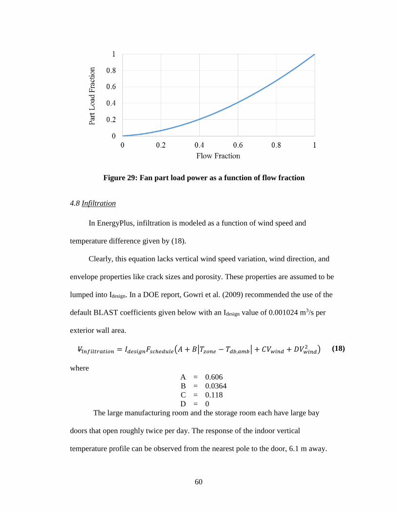
60
Figure 29: Fan part load power as a function of flow fraction
4.8 Infiltration
In EnergyPlus, infiltration is modeled as a function of wind speed and
temperature difference given by (18).
Clearly, this equation lacks vertical wind speed variation, wind direction, and
envelope properties like crack sizes and porosity. These properties are assumed to be
lumped into Idesign. In a DOE report, Gowri et al. (2009) recommended the use of the
default BLAST coefficients given below with an Idesign value of 0.001024 m3/s per
exterior wall area.
𝑉𝑖𝑛𝑓𝑖𝑙𝑡𝑟𝑎𝑡𝑖𝑜𝑛 = 𝐼𝑑𝑒𝑠𝑖𝑔𝑛𝐹𝑠𝑐ℎ𝑒𝑑𝑢𝑙𝑒(𝐴 + 𝐵|𝑇𝑧𝑜𝑛𝑒 − 𝑇𝑑𝑏,𝑎𝑚𝑏| + 𝐶𝑉𝑤𝑖𝑛𝑑 + 𝐷𝑉𝑤𝑖𝑛𝑑2 ) (18)
where
A = 0.606
B = 0.0364
C = 0.118
D = 0
The large manufacturing room and the storage room each have large bay
doors that open roughly twice per day. The response of the indoor vertical
temperature profile can be observed from the nearest pole to the door, 6.1 m away.

61
Figure 30 shows the opening of a bay door in the large manufacturing room on
February 15, 2016. The outdoor air temperature was 0.6°C and the wind speed was
10.8 m/s from the west (this building face is oriented towards the southwest).
Figure 30: Temperature profile measured during bay door opening
The bay door opening is modeled in EnergyPlus using infiltration. The
advantage of modeling the bay door opening using an infiltration object is that wind
speed is considered when calculating flowrate. Though the doors open at different
times each day, it is assumed in the model that they open at 8 am and 3:30 pm for five
minutes Monday through Friday. The air change rate due to infiltration can be seen in
Figure 31. Additionally, each room receives at least ten percent outdoor air through
mechanical ventilation.

62
Figure 31: Air change rate due to infiltration
4.9 Retrofit Modeling
4.9.1 Lights
The test facility underwent a lighting retrofit on the shop floor, switching from
metal halide bulbs to LED lights. The lighting electric and heat load are estimated
according to Section 4.5 of this thesis. Building the retrofit into EnergyPlus is
straightforward using scheduling to assign a given light object to be ‘on’ when
appropriate.
The lighting was replaced over the course of roughly three weeks. In the
simulation, each room switches from the old to new lights in a single day. Therefore,
the smooth, linear decrease in power consumption that the facility saw over the three
week installation period can be approximated by the model (as opposed to a simple
one-day switchover).

63
4.9.2 Rooftop Units
The test facility’s RTUs were retrofitted according to Table 12. The units serving
the manufacturing rooms, the rooms with the highest cooling demand, had an average
COP improvement from 2.56 to 3.58. The entire facility average COP improved from
2.92 to 3.44. An additional 151 kW of gas heating capacity and 35 kW of cooling
capacity were added to the facility. Upgrading the RTUs also introduces two stages of
cooling through the use of dual compressors. Both old and new units use air-side
economizers with enthalpy control. Therefore, it is assumed that the economizer
behavior is identical before and after the retrofit.
Table 12: Rooftop unit specifications before and after retrofit
To implement the RTU retrofit in EnergyPlus required adding another coil in
the air loop. Then, ‘on/off’ availability schedules are used to ensure the required coil

64
is on or off when it should be. The presence of an extra cooling coil in an air loop has
no effect on the air stream when the coil’s status is ‘off’.
4.9.3 Air Compressor
The test facility uses an industrial air compressor to supply compressed air for
manufacturing purposes. This compressor was replaced on October 14, 2015 with a
unit that uses 10 hp less electricity (7.4 kW). The efficiency of the old compressor
was not listed, so its heat output was calculated assuming the same efficiency as the
new compressor.
The energy consumption of industrial compressors using load/unload-type
control can be calculated in the manner provided by the Department of Energy
(2013). In the 35 days since installation, the air compressor was fully-loaded for 263
hours, or 31.3% of the time. To make the energy consumption calculation possible, it
is assumed that the unit operates either fully-loaded or fully-unloaded, the unloaded
capacity is 25% fully-loaded capacity, and the old compressor run-time was the same
as the new compressor. The result of this calculation is time averaged electricity
consumption of 21.7 kW for the old compressor and 18.1 kW for the new
compressor. From the manufacturer’s specifications, 94.4% of the input electricity is
dissipated as heat to the space.
The compressor is cooled using space air inside of its internal heat exchanger. To
save heating costs during winter, this hot air is directed back into the space. During
the other seasons, this air is exhausted outside. The date to switch from indoor
exhaust to outdoor exhaust was chosen based on when the site switches between
heating and cooling. This information is summarized in the following table. It should

65
be noted that the switch to heating was late, December 15, due to an unseasonably
warm December in 2015.
Table 13: Air compressor model status
Date Air Compressor
Model
Power
Consumption [kW]
Fraction of Heat
Loss to Ambient
Jan 1 – Feb 15,
before retrofit
Old compressor
exhaust to space 21.7 0
Feb 16 – Oct 14,
before retrofit
Old compressor
exhaust to ambient 21.7 1
Oct 15 – Dec 15,
after retrofit
New compressor
exhaust to ambient 18.1 1
Dec 16 – Dec
31, after retrofit
New compressor
exhaust to space 18.1 0
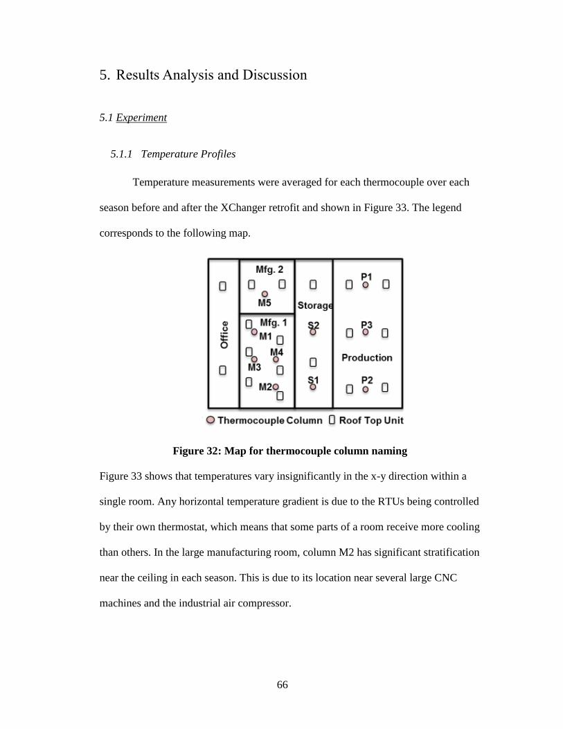
66
5. Results Analysis and Discussion
5.1 Experiment
5.1.1 Temperature Profiles
Temperature measurements were averaged for each thermocouple over each
season before and after the XChanger retrofit and shown in Figure 33. The legend
corresponds to the following map.
Figure 32: Map for thermocouple column naming
Figure 33 shows that temperatures vary insignificantly in the x-y direction within a
single room. Any horizontal temperature gradient is due to the RTUs being controlled
by their own thermostat, which means that some parts of a room receive more cooling
than others. In the large manufacturing room, column M2 has significant stratification
near the ceiling in each season. This is due to its location near several large CNC
machines and the industrial air compressor.

67
Figure 33: Average seasonal temperature of each thermocouple

68
Figure 34: Average measured temperature profile by room
Since horizontal temperature gradients within each room were not significant,
the thermocouple poles have been averaged by room for clarity in Figure 34. Since

69
the assembly room did not have any change in the ducting, there are very little
changes before and after the retrofit.
During the summer, the manufacturing rooms have almost continuous cooling
and therefore saw the greatest change under the XChanger retrofit. In the large
manufacturing room, XChanger maintained the same temperature in the occupied
zone while increasing the stratification in the upper zone by 1.8 K. In the small
manufacturing room, the temperature in the occupied zone decreased while the
temperature in the upper portion of the space increased. Since the storage room has a
low cooling load, the RTUs are not on very often. Therefore, the storage room had no
significant change in temperature profile during cooling season.
During the winter, however, the storage room realized the greatest benefit
from XChanger. The baseline winter had the greatest observed stratification in the
building – 7.1 K. Supplying air high and returning air above the occupied zone
reduced the temperature stratification to 3.5 K, a reduction of 50%. In particular, the
sharp gradient near the ceiling was reduced. The other rooms saw a negligible
difference during heating season. One possible explanation for this is that the
manufacturing rooms were in cooling for portions of the winter. One piece of
evidence to justify this claim is that the XChanger winter profile resembles baseline
summer (which both had high supply ducts) in their shape, especially near the ceiling.
During spring and fall, XChanger produced different effects in each room. In
the large manufacturing room, the temperature below 2 m was reduced by 1 K, while
the upper zone remained the same. In the storage room, the effect was the exact

70
opposite, with 1 K stratification near the ceiling and the same temperature in the
occupied zone. The small manufacturing room had no change whatsoever.
5.1.2 Utility Bill Analysis
Utility bills were obtained from January 2014 through March 2016. Since
2014 had no retrofits, it will act as a baseline to examine the four retrofits installed in
2015: LED lights in February, higher efficiency RTUs in June, XChanger in July, and
the air compressor in October.

71
Table 14: Monthly electricity and gas consumption before and after retrofits
Electricity Consumption [MWh]
Month 2014 2015 Difference Reduction
Jan 177.7 173.6 4.0 2.3%
Feb 159.7 165.3 -5.7 -3.6%
Mar 152.3 130.8 21.5 14.1%
Apr 166.9 137.4 29.5 17.7%
May 158.3 125.9 32.4 20.5%
Jun 165.2 145.9 19.3 11.7%
Jul 176.2 122.3 53.9 30.6%
Aug 166.1 125.7 40.5 24.3%
Sep 168.6 137.5 31.1 18.5%
Oct 157.6 117.7 39.9 25.3%
Nov 123.3 113.0 10.2 8.3%
Dec 148.1 112.4 35.6 24.1%
Total 1919.8 1607.5 312.3 16.3%
Gas Consumption [Therms]
Month 2014 2015 Difference Reduction
Jan 2,065 1,979 86 4.2%
Feb 2,176 1,916 260 11.9%
Mar 1,666 1,729 -63 -3.8%
Apr 1,133 1,000 133 11.7%
May 663 180 483 72.9%
Jun 156 46 110 70.5%
Jul 18 8 10 55.6%
Aug 24 8 16 66.7%
Sep 31 22 9 29.0%
Oct 99 133 -34 -34.3%
Nov 730 490 240 32.9%
Dec 1,325 1,002 323 24.4%
Total 10,086 8,513 1,573 15.6%
Based on Table 14, the facility had an average electricity savings of 16.3%
and average gas savings of 15.6% in 2015. The electricity savings peaked at 30.6%
during the hottest month, July. Since no retrofits were installed during January
through the third week in February, those months saw only a small change in energy
use that can be attributed to changes in plug load and other random variables. These

72
values do not account for weather differences between 2014 and 2015. It was
attempted to normalize gas and electricity use by degree days.
Figure 35: Monthly degree day regression for (a) heating, (b) cooling
Figure 36: Degree day normalization for daily data
Since the facility only uses natural gas for space heating, the gas use correlates
very well with heating degree days, with an R2 of 0.97. The electricity use, however,
does not correlate with cooling degree days on a monthly or daily basis, implying that
the building is dominated by internal loads, rather than external loads.

73
Although electricity does not correlate with ambient dry-bulb temperature, the
energy savings of Table 14 gain credibility by considering that 2015 was warmer in
every month of the year than in 2014. Based on ambient temperature, the results can
be considered conservative. However, other uncertainties such as building use and
plug load cannot be accounted for either.
Figure 37: CDD increase from 2014 (baseline) to 2015 (post-retrofit)
The energy savings of the lighting can be calculated directly. The results are
given in Table 15. The results agree with the values simulated using EnergyPlus, in
Table 17.
𝐸𝑙𝑖𝑔ℎ𝑡 = 𝑃𝑡𝑓 (19)
𝐸𝑓𝑎𝑐𝑖𝑙𝑖𝑡𝑦 = 𝐸𝑙𝑖𝑔ℎ𝑡 +
𝐸𝑙𝑖𝑔ℎ𝑡
𝐶𝑂𝑃
(20)
where
𝐸𝑙𝑖𝑔ℎ𝑡 = light’s electricity use [kWh]
𝑃 = light’s rated power consumption [kW]
𝑡 = time period of interest [h]
𝑓 = Use Factor, average value of light schedule
𝐸𝑓𝑎𝑐𝑖𝑙𝑖𝑡𝑦 = facility’s extra electricity use due to the light [kWh]
𝐶𝑂𝑃 = coefficient of performance for vapor compression cycle [-]

74
Table 15: Yearly energy savings of switching from metal halide to LED bulbs
The energy savings of the higher SEER RTUs has been simulated in
EnergyPlus using the validated 2015 model. The energy savings are shown in the
following table.
Table 16: RTU retrofit energy savings
Energy Savings due to Rooftop-Unit Retrofit [MWh]
Period
Beginning In: Jan Feb Mar Apr May Jun Jul Aug Sep Oct Nov Total
Old RTUs 146 129 128 117 141 133 130 139 116 108 111 1771
New RTUs 146 128 126 114 135 126 126 135 115 107 110 1740
Energy Saved Per Month 2.56
Energy Saved per Summer Months 4.88
Using the monthly calculated savings due to the lighting and RTU retrofits,
the energy savings due to XChanger can be estimated according to (21).
𝑋𝐶ℎ𝑎𝑛𝑔𝑒𝑟 𝐸𝑛𝑒𝑟𝑔𝑦 𝑆𝑎𝑣𝑖𝑛𝑔𝑠 = 𝐸2014 − 𝐸2015 − 𝛥𝐸𝐿𝑖𝑔ℎ𝑡𝑠 − 𝛥𝐸𝑅𝑇𝑈 − 𝛥𝐸𝐶𝑜𝑚𝑝𝑟𝑒𝑠𝑠𝑜𝑟 (21)
The lighting, RTU, and air compressor retrofit energy savings were calculated
through simulation using the validated 2015 EnergyPlus model. Each retrofit was
modeled as if it were the only retrofit installed in the facility. Then, the results were
compared with a baseline model that does not have that specific retrofit. Fluctuations
in the value of the difference in energy consumption between the two years can only
be explained by considering outdoor temperature, manufacturing output, and other
variables that are not controlled for.
Light
Fixture
Power
[W]
Use
Factor
Number
of Lights
Energy per Bulb
[kWh/bulb/year]
Energy
per 30
Days
[kWh]
Energy
per Year
[kWh]
Old 458 0.41 145
1,771 21,104 256,767
New 190 735 8,755 106,519

75
Table 17: Electricity savings due to XChanger calculated from utility bills
Electricity Savings due to:
Start Stop 2014
[MWh]
2015
[MWh]
Energy
Savings Lights RTU Compressor XChanger
1/23 2/20 160 165 -3.6% - - - -
2/20 3/20 152 131 14.1% 9.6% - - -
3/20 4/22 167 137 17.7% 11.0% - - -
4/22 5/20 158 126 20.5% 11.7% - - -
5/21 6/20 165 146 11.7% 11.4% - - -
6/20 7/22 176 122 30.6% 10.6% 5.1% - 14.9%
7/22 8/21 166 126 24.3% 11.9% 3.2% - 9.3%
8/21 9/21 169 137 18.5% 11.1% 2.7% - 4.7%
9/22 10/21 158 118 25.3% 11.8% 1.4% - 12.1%
10/21 11/19 123 113 8.3% 12.1% 0.7% 2.3% -6.9%
11/19 12/18 148 112 24.1% 11.5% 0.8% 2.3% 9.5%
12/18 1/21 174 132 24.1% 11.0% 0.3% 2.0% 10.8%
Start Stop 2015
[MWh]
2016
[MWh]
Energy
Savings Lights RTU Compressor XChanger
1/21 2/19 165 126 24.0% 10.5% 0.6% 2.0% 10.9%
2/19 3/22 131 129 1.0% 10.2% 0.6% 1.9% -11.6%
The gas use for space heating correlates very well with heating degree days.
Therefore, it makes sense to compare gas usage per heating degree day. However, to
compare the gas used in 2015 against 2014, the heat load of the lighting and
compressor retrofits must be added back because the lower electrical loads seen in
2015 mean that the facility needs more gas for space heating. Using the validated
2015 EnergyPlus model, it was found how much heat would have been added to the
space had each retrofit not occurred. This heat was converted to a “therm equivalent”
by converting Joules (EnergyPlus output) to therms, then dividing by the efficiency of
the gas furnace, 0.81. Since the heat output difference due to the compressor retrofit

76
is less than six therms equivalent for each period, it was ignored for simplicity.
Summer months were included for completion, but the results are omitted because a
negative therms-per-degree-day was calculated.
One source of error in this analysis is that ‘adding back’ the heat due to the
lighting retrofit is correct only when the facility is in heating operation during the
entire period considered. This is the reason that the shoulder seasons and summer had
negative therms-per-degree-day in 2015. This is also the reason that the calculated
‘Difference’ increases from 1/23/14 – 3/20/14. A better approach would include the
fraction of time the facility spent in heating. However, this is not readily available
from the experiment or as an EnergyPlus output variable.
The XChanger was switched from cooling operation (supply low, return high),
to heating operation (supply high, return low) on January 4, 2016. Therefore, half the
period from 12/18/15 – 1/21/16 and the whole period from 1/21/16 – 2/19/16 are
direct comparisons between baseline and XChanger systems. During these periods,
the XChanger saved 0.7 therms per heating degree day. This is a savings of 20.1 –
22.3% gas. However, this analysis is clearly subject to large uncertainties, as shown
in the first row when no retrofits were installed, yet the facility observed a difference
in therms-per-degree-day of 0.58.

77
Table 18: Facility gas consumption before and after retrofits
Start Stop 2014
[Therms]
2015
[Therms]
2015
Adjusted
for
Lights
HDD
2014
HDD
2015
2014
Therms
/ HDD
2015
Therms
/ HDD
Diffe
rence
1/23 2/20 2,176 1,916 - 576.6 600.3 3.77 3.19 0.58
2/20 3/20 1,666 1,729 1149 448.5 490.7 3.71 2.34 1.4
3/20 4/22 1,133 1,000 331 293.4 266.9 3.86 1.24 2.6
4/22 5/20 663 180 -474 98.1 86.8 6.76 - -
5/21 6/20 156 46 -703 20.1 26.8 7.76 - -
6/20 7/22 18 8 -616 2.5 1.1 7.20 - -
7/22 8/21 24 8 -702 6 1.7 4.00 - -
8/21 9/21 31 22 -679 17.7 14.5 1.75 - -
9/22 10/21 99 133 -507 89.6 119.5 1.10 - -
10/21 11/19 730 490 -128 261.5 166.5 2.79 - -
11/19 12/18 1,325 1,002 396 415.2 294.4 3.19 1.34 1.9
12/18 1/21 1,979 1,819 1268 594.8 475.7 3.33 2.66 0.7
Start Stop 2015
[Therms]
2016
[Therms]
2016
Adjusted
for
Lights
HDD
2015
HDD
2016
2015
[Therm
/ HDD]
2016
[Therm
/ HDD]
Diffe
rence
1/21 2/19 1,916 1,878 1327 600.3 535.4 3.19 2.48 0.7
2/19 3/22 1,729 1,094 579.8 514 490.7 315.6 3.52 1.63
Since the characteristics of this particular facility may differ from other
commercial buildings, it is beneficial to view the energy savings as a percentage of
total HVAC energy use. A watt-meter was placed on one electric panel to measure
the power consumption of a collection of rooftop-units serving both manufacturing
rooms and the storage room. The office and assembly spaces were not instrumented.
52.4% of installed cooling capacity was instrumented starting on July 31. Between
July 31 and September 24 (roughly the end of cooling season), the instrumented
RTUs consumed 41,089 kWh. Assuming that the cooling load is distributed evenly
throughout the facility, the entire facility will use 78,415 kWh over the same period.
Based on Table 17, the XChanger system saved the facility 7.0% energy in August

78
and September. Since the entire facility consumed 237,592 kWh during this period,
the XChanger system saved the facility 16,631 kWh.
Had the storage and manufacturing rooms not been installed with XChanger,
they would have used 41,089 + 16,631 kWh, or 57,720 kWh. Compared to what they
actually used, 41,089 kWh, XChanger saved these rooms 28.8% of HVAC energy.
Implicit in this figure is the assumption that the cooling load is distributed evenly
throughout the space. This assumption is necessary to estimate the energy
consumption of the facilities RTUs.
Based on this analysis of the utility bills, the XChanger system is expected to
save 9.6% total electricity, which is 28.8% of HVAC energy during cooling season.
During heating season, XChanger is expected to save 21.2% gas during heating
season.
5.2 CFD Modeling
5.2.1 Grid Sensitivity Analysis
Based on the initial simulations and literature review, a mesh of 750,000 cells
was selected. This grid was capable of producing y* values within the boundaries
defined by the wall-treatment, 30-300. Table 2 from the introduction shows the grid
density used by other researchers with similar physics and models, particularly
natural convection and k-ε turbulence modeling. Although grid density is not as
important as y* values for heat transfer or as important as local grid considerations,
like the grid near outlet diffuser, overall grid density is used here as a qualitative
initial benchmark. The reviewed literature typically had between 1,000-12,000
cells/m3. Denser grids typically corresponded to more ‘theoretical’ studies that focus

79
on a specific, local aspect of the simulation, like detailed heat transfer or detailed
diffuser configurations. Denser grids were also used for studies that had detailed
geometry and rigorous experimental data. Coarser grids typically correspond to
situations with less well-known boundary conditions or where the simulation goal is
of a larger scale, such as the mean temperature field under a new air delivery
configuration.
The grid used in this study has a grid density of roughly 715 cells/m3, which is
smaller than grids from the literature by about 25%. Since the geometry and heat
sources of this study are only representative of the actual test-facility, accurately
simulating heat transfer is not the primary goal. Therefore, low y* values (~30) and
detailed geometry are not necessary for a sufficiently good prediction of room
temperature and velocity distribution. A basic grid sensitivity test was conducted to
verify that a relatively coarse mesh produces stable results.
The sensitivity of spatial average vertical temperature profile to mesh density
was investigated for the overhead mixing ventilation case. Grid refinement was done
in increments of √2. When meshing, the size functions for all surfaces were changed
such that the face meshes were larger/smaller and the growth rate was larger/smaller.
The maximum cell edge length was set to 0.3 m, but never reached more than 0.23 m.

80
Table 19: Grid sensitivity number of cells
Grid Number of Cells
Coarse 531,783
Medium 767,347
Fine 1,077,543
Figure 38: Grid sensitivity – vertical temperature profiles
The coarse grid over-predicted stratification everywhere except in the region
0.3 m from the ceiling. This region saw a larger temperature gradient when the mesh
was refined. The edge length for the ceiling mesh was 0.229 m for the coarse mesh,
0.198 m for the medium mesh, and 0.183 m for the fine mesh. Temperature
measurements were made at the ceiling surface (surface temperature) and 0.3 m
below the ceiling. More measurements should be taken within 0-0.6 m from the
ceiling to determine which mesh more accurately predicted heat transfer from the
ceiling.
Since transient simulations were used for a steady-state problem (see Section
3.5 for convergence criteria), it is possible that the solution will have oscillations. The
solution was taken at a time when the oscillations in the temperature field were small.
However, the oscillations still impact the results slightly, which may explain the “S”

81
shape in the fine mesh’s temperature profile, above, because this is the height at
which the supply diffuser is located.
Since oscillatory convergence (in a transient sense), was observed, the grid
convergence index (GCI) method proposed by Roache does not easily apply.
Obviously, there exist formal grid convergence indices for transient studies.
However, qualitative grid convergence was acceptable for this study. Since the
medium mesh produces similar results to the fine mesh and has acceptable y* values,
it was chosen as an appropriate mesh size for the remaining cases.
5.2.2 Model Validation
The CFD model was validated using the average vertical temperature profiles
in the manufacturing room over the summer season. Since the time average
temperature profile was used, the boundary conditions should be some time average
as well. The boundary conditions for all heat transfer surfaces, like the walls,
occupants, and machines, were discussed in Section 3.6.
The supply air velocity and temperature in the actual facility vary significantly
between day and night. The RTU cycles on and off, as well as cycling between two
flow rates. An appropriate boundary condition for supply temperature and flow rate
was selected, then changed until the simulated average temperature profile matched
the time averaged measured temperature profile.

82
Figure 39: Measured supply air temperature of one RTU from 8/30/15 – 9/2/15
(note: some data is missing for this time period)
Based on Figure 39, the measured supply air temperature over the course of
several days, the average supply air temperature is 12.7 ºC. During intermittent
cooling, the temperature in the supply air duct cycles between about 11 ºC and 17 ºC.
Flowrate is not measured, though this RTU has two nominal speeds: 2.6 m3/s and 1.4
m3/s Since there are times that the RTU is not supplying air, it is expected that the
average supply air velocity is somewhere between 0 – 2.6 m3/s. It was found through
trial and error that 12 ºC and 0.56 m3/s (2 m/s face velocity) provide a very accurate
prediction of room air temperature for the baseline case. For the XChanger case, it
was found that 14 ºC and 1.12 m3/s (4 m/s face velocity) was best.

83
Figure 40: (a) Baseline and (b) XChanger CFD model validation
Figure 40 shows the model validation for vertical temperature profiles. The
lines with markers are the thermocouple values at each pole in the large
manufacturing room (averaged over the entire season). The black line is their average.
The light blue lines are the temperature profiles along four lines in the flow domain,
shown in Figure 41. Both cases were validated to within 0.2 ºC of the average
measured profile. This is within measurement uncertainty, or 0.5 ºC.

84
Figure 41: Vertical temperature profile measurement locations
Since the RTU was not changed, just the ducting, the supply air conditions
should not change between baseline and XChanger cases significantly. The validated
‘baseline boundary conditions’ and the validated ‘XChanger boundary conditions’
were swapped to the opposite case. The results are plotted in Figure 42. The baseline
model was over-cooled, which resulted in a uniform temperature distribution. The
XChanger model velocity was too low, which resulted in over-cooling the occupied
zone, a sharp temperature gradient between 1.5 m and 3 m, then uniform temperature
between 3 m and the ceiling.
It was not expected that the solution would be so sensitive to supply air
conditions. For example, the temperature profile from the XChanger case in Figure 42
has entirely different features than Figure 41 due to a 2 ºC decrease in temperature
and decreasing the velocity by a factor of two. Since a satisfactory explanation for
this sensitivity has not been found and it is unclear which set of boundary conditions
to proceed with, both sets of boundary conditions will be used for the parametric

85
study.
Figure 42: (a) Baseline and (b) XChanger with the opposite boundary conditions
5.2.3 Parametric Study
Each case below is simulated with the baseline and XChanger boundary
conditions, hereby referred to as ‘low velocity’ and ‘high velocity’, respectively.
Table 20: Parametric study test matrix
Case Description Supply Height
[m]
Return Height
[m]
Baseline Overhead, mixing ventilation 7.0 7.0
XChanger As installed 1.8 2.4
Case 1 “Preferred” installation 0.46 2.4
Case 2 Higher Return 1.8 5.5
Case 3 Double face area 0.46 2.4
Case 1 has the supply duct at the same height as the installed XChanger, but the
return duct is located at two-thirds height, instead of one-third. Case 2 is how the

86
XChanger company prefers to install units – supply near the floor and return just
above the occupied zone. Case 3 investigates a doubling of the supply air diffuser
face area and the corresponding decrease in inlet velocity.
A user-defined function in Fluent was created to calculate PMV and PPD
according to ISO-7730, which is the same as ASHRAE Standard 55 without the SET
model (Standard Effective Temperature). It is assumed that the relative humidity is
50%, the clo value is 0.6 (the uniform of the workers), the metabolic rate is 2 met
(typical of light machine work), and the radiant temperature is the same as the air
temperature. This choice of metabolic rate is rather high compared to typical office
settings and resulted in the occupants feeling slightly warm.
Table 21 lists results for the parametric study. Each value is averaged over the
entire flow domain. The ‘high velocity’ supply air boundary conditions (those found
for the XChanger case validation) were more appropriate for each of the three cases
because the low velocity boundary conditions resulted in significant stratification –
similar to the stratification seen on the right in Figure 42. Therefore, most analysis
will only consider the cases with ‘high velocity’ boundary conditions. The
stratification is taken as the average temperature difference between 0.2 m from the
floor and 0.2 m from the ceiling – where the lowest and highest temperatures are
usually observed.
Increasing the return duct height in Case 2 compared to the XChanger case
has the effect of reducing the average temperature in the space, reducing stratification
(particularly in the upper zone), and increasing the return air temperature. Case 1,
supplying at floor-level and returning at the same height as the installed XChanger,

87
shows an average temperature reduction of 0.4 K, a reduction in stratification of 0.8
K, and an increase in return air temperature comparable to Case 1. Supplying air near
the floor while increasing the supply diffuser area has the effect of greatly increasing
stratification and slightly increasing average air temperature.
Table 21: Parametric study results (averages over entire flow domain)
Whole Volume
Case Temp.
[ºC]
Velocity
[m/s]
PMV
[-]
PPD
[%]
RAT
[ºC]
Stratification
[K]
Baseline 22.5 0.11 0.6 14.2 22.0 2.3
XChanger 23.2 0.12 0.7 18.8 21.8 4.5
Case 1 Low Velocity 24.2 0.08 1.0 28.0 24.4 4.6
Case 1 High Velocity 22.8 0.11 0.7 16.7 22.3 3.7
Case 2 Low Velocity 23.5 0.07 0.8 21.7 24.5 6.8
Case 2 High Velocity 22.1 0.13 0.5 12.8 22.6 3.9
Case 3 Low Velocity 24.2 0.07 1.0 29.1 24.5 8.0
Case 3 High Velocity 23.1 0.07 0.7 20.9 22.6 6.3
Energy savings can generally be achieved by increasing the average air
temperature of the space, which decreases heat gain through the building envelope. It
would be misleading to simply point out which case in Table 21 saves the most
energy based on this criteria because these simulations have no concept of thermostat
control. In other words, a thermostat would control the room temperature such that
the temperature near the thermostat is at set point. In the simulation, the temperature
near the thermostat is not controlled. A better way to express the effect of average air
temperature is the difference between mean air temperature and temperature near the
location of a typical thermostat: 1.5 m height on the wall. This value expresses the
increase in mean air temperature from setpoint that a room would expect to see under
each case.

88
Based on Table 22, Case 3 would have the least heat gain from ambient due to
the excessive stratification and the baseline case would have the most heat gain from
ambient due to mixing. In Case 3, the high velocity case saw both a higher mean air
temperature and a lower thermostat temperature because the supply air jet reached the
wall (and this is where the thermostat would be located). The thermal comfort
implications of this need to be investigated.
Table 22: Average temperature minus hypothetical thermostat temperature
Case 𝑇𝑎𝑣𝑔 − 𝑇𝑡ℎ𝑒𝑟𝑚𝑜𝑠𝑡𝑎𝑡
Baseline 0.64
XChanger 1.81
Case 1 Low Velocity 3.20
Case 1 High Velocity 2.00
Case 2 Low Velocity 1.38
Case 2 High Velocity 1.31
Case 3 Low Velocity 1.92
Case 3 High Velocity 3.73
According to ASHRAE Standard 55-2013, the occupied zone is the region
that is 10 cm off the ground, below 1.8 m, and 0.3 m away from the walls. Table 23
shows the average values of several parameters over this region.

89
Figure 43: ASHRAE definition of occupied zone
Table 23: Parametric study results; averages over the occupied zone
Occupied Zone
Case Temperature
[ºC]
Velocity
[m/s]
PMV
[-]
PPD
[%]
Head-to-
Ankle [ºC]
Baseline 21.81 0.13 0.49 10.45 0.30
XChanger 21.51 0.20 0.39 9.12 0.38
Case 1 Low Velocity 20.30 0.13 0.21 8.53 3.59
Case 1 High Velocity 20.93 0.24 0.26 8.42 0.88
Case 2 Low Velocity 20.75 0.14 0.29 7.61 0.66
Case 2 High Velocity 20.89 0.20 0.27 7.40 0.21
Case 3 Low Velocity 19.90 0.09 0.16 8.79 4.89
Case 3 High Velocity 19.39 0.18 0.00 7.20 1.49
The average particular mean vote (PMV) and percent people dissatisfied
(PPD) are within acceptable ranges for each case considered. The baseline, mixing
ventilation had the most dissatisfied occupants, but by a negligible amount. ASHRAE
Standard 55 specifies that the head-to-ankle temperature difference be less than 3 °C
for seated occupants and 4 °C for standing occupants. Each case except the low-
velocity, large-diffuser case satisfied this criteria. Figure 44 shows contour plots for

90
each high velocity case in the plane of the supply diffuser. Although the ISO
7730:2005 thermal comfort model was intended for use in spaces with uniform
conditions, it is useful here to qualitatively view comfort.
The baseline case has uniform PPD less than 20% in the entire space. Clearly,
the other cases have PPD approaching 100% near the supply diffusers, yet acceptable
PPD outside the vicinity of the diffuser. Moreover, the large area diffuser, Case 3,
does not have an appreciable drop in PPD near the diffuser. Therefore, care should be
taken during installation to aim the diffuser away from occupants.
Figure 44: PPD contours for each case (only high velocity cases shown)
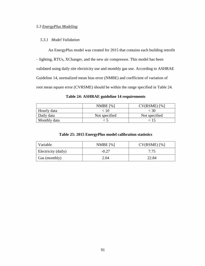
91
5.3 EnergyPlus Modeling
5.3.1 Model Validation
An EnergyPlus model was created for 2015 that contains each building retrofit
– lighting, RTUs, XChanger, and the new air compressor. This model has been
validated using daily site electricity use and monthly gas use. According to ASHRAE
Guideline 14, normalized mean bias error (NMBE) and coefficient of variation of
root mean square error (CVRSME) should be within the range specified in Table 24.
Table 24: ASHRAE guideline 14 requirements
NMBE [%] CV(RSME) [%]
Hourly data < 10 < 30
Daily data Not specified Not specified
Monthly data < 5 < 15
Table 25: 2015 EnergyPlus model calibration statistics
Variable NMBE [%] CV(RSME) [%]
Electricity (daily) -0.27 7.75
Gas (monthly) 2.04 22.84

92
Figure 45: Model versus measured daily electricity use
Figure 46: Accuracy of simulated daily electricity consumption
Jan/15 Feb Mar Apr May Jun Jul Aug Sep Oct Nov Dec Jan/16
1500
2000
2500
3000
3500
4000
4500
5000
5500
6000
6500
Date
Ele
ctr
icit
y C
on
sum
pti
on
[k
Wh
]
Daily Electricity Consumption
Measured
Simulated
0 1000 2000 3000 4000 5000 6000 70000
1000
2000
3000
4000
5000
6000
7000
Experiment [kWh]
Sim
ula
tio
n [
kW
h]
Model Accuracy: Electricity Consumption
-10%
-50%
+50% +10%

93
The model accurately predicts electricity use, as shown in the above three
figures. The NMBE and CV(RSME) values are within the ASHRAE specified range
except for the CV(RSME) value for gas. As shown in Figure 45, the model slightly
over-predicts electricity use in the summer and under-predicts electricity use in the
winter.
Before calibration, the model significantly over-predicted summer electricity.
This was addressed by decreasing the plug load by a factor of 2 between May 4 and
August 30. It is believed that the manufacturing output may be less during the
summer than during the rest of the year. One piece of justification for this theory is
the sudden increase in measured facility electricity on the first week in September.
Before calibration, the model also significantly under-predicted winter
electricity. This was accounted for by increasing the capacity of the VAV reheat for
the offices, because this is the only source of electric heating in the facility. The
actual capacity or number of VAV boxes is not known, but was assumed based on the
number and size of offices. The significant under-prediction of gas use in February
and March and the over-prediction of gas use in September prevent the model from
being considered calibrated.

94
Figure 47: Simulated and measured monthly gas use
5.3.2 Energy Savings of Proposed System
Two models were created based on the validated 2015 model – one with all
measured baseline temperature profiles and one with all measured XChanger
temperature profiles. The set point offset was also changed to correspond with the
appropriate temperature profiles (see Room Air Modeling). The temperature profile
used for each time period in each model is shown in Table 26. The names of the
temperature profiles correspond to the legend in Figure 34.
Table 26: Temperature profile corresponding to model and time period
Period Mixing ventilation model XChanger model
1/1 – 3/23 Baseline Winter XChanger Winter
3/24 – 5/31 Baseline Spring XChanger Fall
6/1 – 9/22 Baseline Summer XChanger Summer
9/23 – 11/31 Baseline Spring XChanger Fall
12/1 – 12/31 Baseline Winter XChanger Winter
Jan/15 Feb Mar Apr May Jun Jul Aug Sep Oct Nov Dec0
500
1000
1500
2000
Start Date of Billing Period
Gas
Co
nsu
mp
tio
n [
Th
erm
s]
Monthly Gas Consumption
Measured
Simulated

95
The XChanger adds additional ducting and several 90 degree elbows, as
discussed in Section 4.7.4. Therefore, fan static pressure rise will be greater in the ‘all
XChanger’ model compared with the baseline model. Since fan energy consumption
is the same order of magnitude as cooling coil energy consumption, which is common
for commercial buildings, the increased fan power could dominate the energy savings
due to stratification. For this reason, it is necessary to handle fan static pressure rise
accurately.
Two EnergyPlus models were created to show the sensitivity of fan power
consumption – one with equal pressure drop between baseline and XChanger and
another with the pressure drops calculated in Section 4.7.4. The fans used in the first
two models were Fan:VariableVolume objects. These fans never fully turn off – they
just operate at their minimum part load ratio when demand is low. One problem with
these models is that fan static pressure rise is defined at the fan’s nominal flow rate,
not as a function of air flow rate. This fact leads to large fan power consumption at
part load. Additionally, the fans do not cycle with coil operation, which is how the
real RTU operates. Table 27 shows each model’s details.
Table 27: Models used to compare fan controls and static pressure rise
Model Description
1 XChanger and baseline systems have the same pressure drop
2 𝛥𝑃𝐵𝑎𝑠𝑒𝑙𝑖𝑛𝑒 = 144.5 Pa, 𝛥𝑃𝑋𝐶ℎ𝑎𝑛𝑔𝑒𝑟= 248.4 Pa
The calculated HVAC energy savings of XChanger are shown in Table 28.
When fan power consumption is the same in baseline and XChanger models,

96
stratification alone saves 37.4% electricity and 7.7% gas. In other words, these
savings are realized by the room air modeling temperature profiles, return air offset,
and thermostat offset. When factoring fan pressure drop into the model, the savings
dropped to 19.3% electricity. The gas savings increased because the added heat of the
fans required less gas to be burned and should therefore not be considered a benefit.
As a percentage of the total facility electricity (i.e. not just HVAC energy), Model 1
shows a 5.0% electricity savings and Model 2 shows a 2.2% electricity savings.
Table 28: Energy savings of XChanger based on EnergyPlus models
Model HVAC Electricity Savings [%] Gas Savings [%]
1 37.4 7.7
2 19.3 25.2

97
6. Conclusions
A full-scale experiment was conducted in a high-bay test facility to measure the
effects of a new air delivery strategy. The experimental study shows that, in cooling,
supplying and returning air directly to the occupied zone produces an acceptable
temperature gradient in the occupied zone, while increasing stratification in the upper
portion of the space. In heating, supplying air from the ceiling vertically downward
while returning air in the occupied zone has the potential to reduce stratification,
though not eliminate it entirely. In both heating and cooling, the effects of the
installed system are more pronounced in rooms that have high cooling and heating
loads.
CFD modeling reveals the effects of supply and return duct location on room air
flow and stratification generation. Supplying air lower generally creates more
stratification and an acceptable temperature gradient in the occupied zone. Increasing
the supply diffuser face area while holding flow rate constant produces lower
velocities in the occupied zone, creates large temperature gradients in the occupied
zone, and produces the largest stratification observed. The room temperature gradient
is less sensitive to return duct height than supply duct height, though increasing the
return duct height slightly reduced stratification and the average room temperature.
Building energy simulation is used to show how stratification influences a
building’s energy use. A novel approach used room air modeling with 24 measured
temperature profiles over one year to capture the effects of return air temperature
offset, thermostat offset, and stratification. It was found that increased fan energy

98
consumption due to the XChanger system’s larger pressure drop can depreciate the
energy savings by 50%.
Based on the utility bill analysis and measured combined RTU power
consumption, XChanger saves the facility 28.8% HVAC electricity over the course of
one year. The EnergyPlus models bracket this result – not accounting for pressure
drop resulted in 37.4% HVAC electricity savings while accounting for pressure drop
resulted in 19.3% HVAC electricity savings. Building simulation results would be
closer to experimental results if the fans in EnergyPlus were simulated more
realistically (i.e. had pressure drop as a function of flow rate, not specified at the fan’s
nominal flow rate).
Gas consumption results for the experiment are inconclusive because the same
therm-per-degree-day value was calculated before and after XChanger was switched
to heating mode. Also, “savings” in terms of therm-per-degree-day were observed
before any retrofits took place. These unexpected results are observed because the
heating load in the space changed due to the other three retrofits over the
measurement period. Attempts were made to ‘add back’ the heat of these retrofits but
this approach adds uncertainty. Building energy simulation shows that XChanger
saves 7.7 – 25.2% gas, depending on fan power consumption.
7. Future Work
For this experiment, detailed measurement of RTU power consumption was too
costly due to the number of RTUs. Additionally, the effects of three retrofits in
addition to the XChanger system adds uncertainty to the calculated energy savings
because one must attribute a certain percentage of the energy savings to each retrofit.

99
Therefore, a future version of this study should be conducted on a simpler building,
where detailed RTU power consumption is measured before and after the ducting
retrofit. That retrofit should be the only retrofit installed in the entire facility. Sub-
hourly metering in addition to measured temperature profiles may provide insight into
observed differences between the building energy simulation results and measured
results.
The effects of duct height during heating operation should be investigated
using CFD simulation to answer the following questions: Does returning air in the
occupied zone draw air down, reducing stratification? Should air instead be both
supplied and returned in the occupied zone? If so, should the supply velocity be
increased to induce thermal mixing in the occupied zone?
Building energy simulation using room air modeling can address the
possibility of using different supply air conditions with different ducting
configurations. This would bridge the gap between this thesis and research in the
literature regarding displacement ventilation and underfloor air distribution. Also,
since the fan pressure drop has been shown to be a significant degradation of the
XChanger’s energy saving potential, the work in this thesis should include more
accurate fan models, such as the Fan:ComponentModel approach.

100
References
Alajmi, Ali, and Wid El-Amer. 2010. “Saving Energy by Using Underfloor-Air-
Distribution (UFAD) System in Commercial Buildings.” Energy Conversion and
Management, Global Conference on Renewables and Energy Efficiency for
Desert Regions (GCREEDER 2009), 51 (8): 1637–42.
doi:10.1016/j.enconman.2009.12.040.
“ANSYS Fluent Users Guide.pdf.” 2016. Accessed February 27.
“ASHRAE Standard 55 - 2013.” 2013. American Society of Heating a Refrigeration
Engineers.
“ASHRAE Standard 90.1.” 2007. American Society of Heating a Refrigeration
Engineers.
Aynsley, Richard. 2005. “Saving Heating Costs in Warehouses.” ASHRAE Journal 47
(12): 46–51.
Cheng, Yuanda, Jianlei Niu, and Naiping Gao. 2012a. “Thermal Comfort Models: A
Review and Numerical Investigation.” Building and Environment, International
Workshop on Ventilation, Comfort, and Health in Transport Vehicles
Cheng, Yuanda, Jianlei Niu, and Naiping Gao. 2012b. “Stratified Air Distribution
Systems in a Large Lecture Theatre: A Numerical Method to Optimize Thermal
Comfort and Maximize Energy Saving.” Energy and Buildings, Cool Roofs,
Cool Pavements, Cool Cities, and Cool World
Chen, Qingyan. 1990. “Prediction of Buoyant, Turbulent Flow by a Low-Reynolds-
Number K-Epsilon Model.” ASHRAE Transactions, vol. 96, 1990.
Chen, Qingyan.. 1995. “Comparison of Different K-ε Models for Indoor Air Flow
Computations.” Numerical Heat Transfer, Part B Fundamentals 28 (3): 353–69.
Chen, Q., and Z. Zhai. 2004. “The Use of CFD Tools for Indoor Environmental
Design.” Advanced Building Simulation, 119–40.
Efficiency, Energy, and Department of Energy. 2013. “Improving Compressed Air
System Performance.”

101
EIA. 2015. "U.S. Energy Information Administration - EIA - Independent Statistics
and Analysis." CBECS 2012: Building Stock Results. March 4, 2015. Accessed
January 13, 2016.
“Fluent User’s Guide - ANSYS Fluent Users Guide.pdf.” 2016. Accessed February
27.
Gilani, S., H. Montazeri, and B. Blocken. 2013. “CFD Simulation of Temperature
Stratification for a Building Space: Validation and Sensitivity Analysis.” In
Proceedings of BS2013: 13th Conference of International Building Performance
Simulation Association, Chambéry, France, August, 26–28.
Gowri, Krishnan, David W. Winiarski, and Ronald E. Jarnagin. 2009. Infiltration
Modeling Guidelines for Commercial Building Energy Analysis. Pacific
Northwest National Laboratory USA.
Griffith, Brent. 2002. “Incorporating Nodal and Zonal Room Air Models into
Building Energy Calculation Procedures.” MIT.
Griffith, Brent, and Qingyan Yan Chen. 2003. “A Momentum-Zonal Model for
Predicting Zone Airflow and Temperature Distributions to Enhance Building
Load and Energy Simulations.” HVAC&R Research 9 (3): 309–25.
Griffith, Brent, and Qingyan Yan Chen. 2004. “Framework for Coupling Room Air
Models to Heat Balance Model Load and Energy Calculations (RP-1222).”
HVAC&R Research 10 (2): 91–111.
Hajdukiewicz, Magdalena, Marco Geron, and Marcus M. Keane. 2013a. “Formal
Calibration Methodology for CFD Models of Naturally Ventilated Indoor
Environments.” Building and Environment 59 (January): 290–302.
Hajdukiewicz, Magdalena, Marco Geron, and Marcus M. Keane. 2013b. “Calibrated
CFD Simulation to Evaluate Thermal Comfort in a Highly-Glazed Naturally
Ventilated Room.” Building and Environment 70 (December): 73–89.
Hawileh, Rami A. 2011. Heat Transfer Analysis of Reinforced Concrete Beams
Reinforced with GFRP Bars. INTECH Open Access Publisher.
“ISO 7730:2005 - Ergonomics of the Thermal Environment -- Analytical
Determination and Interpretation of Thermal Comfort Using Calculation of the

102
PMV and PPD Indices and Local Thermal Comfort Criteria.” 2016. Accessed
January 18.
Jones, P.J., and G.E. Whittle. 1992. “Computational Fluid Dynamics for Building Air
Flow Prediction - Current Status and Capabilities.” Building and Environment
27 (3): 321–38.
McQuiston, Parker, and Spitler. 2004. Heating, Ventilating and Air Conditioning
Analysis and Design. 6 edition. Hoboken, N.J: Wiley.
Nielsen, Peter V., and Tryggvi Tryggvason. 1998. “Computational Fluid Dynamics
and Building Energy Performance Simulation.” Dept. of Building Technology
and Structural Engineering.
Pan, Yiqun, Yuming Li, Zhizhong Huang, and Gang Wu. 2010. “Study on Simulation
Methods of Atrium Building Cooling Load in Hot and Humid Regions.” Energy
and Buildings 42 (10): 1654–60.
Pedersen, Curtis, Daniel Fisher, and Richard Liesen. 1997. “Devolopment of a Heat
Balance Procedure for Calculating Cooling Loads.” In . Vol. 103 Part 2.
Risberg, Daniel, Mattias Vesterlund, Lars Westerlund, and Jan Dahl. 2015a. “CFD
Simulation and Evaluation of Different Heating Systems Installed in Low
Energy Building Located in Sub-Arctic Climate.” Building and Environment 89
(July): 160–69.
Risberg, Daniel, Mattias Vesterlund, Lars Westerlund, and Jan Dahl .2015b. “CFD
Simulation and Evaluation of Different Heating Systems Installed in Low
Energy Building Located in Sub-Arctic Climate.” Building and Environment 89
(July): 160–69.
Risberg, Daniel, Lars Westerlund, and Gunnar JI Hellström. 2015. “CFD-Simulation
of Indoor Climate in Low Energy Buildings Computational Setup.” Thermal
Science, no. 00: 167–167.
Roache, Patrick J. 1997. “Quantification of Uncertainty in Computational Fluid
Dynamics.” Annual Review of Fluid Mechanics 29 (1): 123–60.
Rohdin, P., and B. Moshfegh. 2011. “Numerical Modelling of Industrial Indoor
Environments: A Comparison between Different Turbulence Models and Supply

103
Systems Supported by Field Measurements.” Building and Environment 46 (11):
2365–74.
Saïd, M. N. A., R. A. MacDonald, and G. C. Durrant. 1996. “Measurement of
Thermal Stratification in Large Single-Cell Buildings.” Energy and Buildings 24
(2): 105–15.
Sheppy, Michael, Paul Torcellini, and Luigi Gentile-Polese. 2014. “An Analysis of
Plug Load Capacities and Power Requirements in Commercial Buildings.”
National Renewable Energy Laboratory (NREL), Golden, CO.
Singh, Trilochan, and J. B. Olivieri. 1988. “Thermal Stratification-A Means to
Reduce Cooling Loads in High Bay Industrial Buildings.”
Sørensen, D. N., and P. V. Nielsen. 2003. “Quality Control of Computational Fluid
Dynamics in Indoor Environments.” Indoor Air 13 (1): 2–17.
Srebric, Jelena. 2000. “Simplified Methodology for Indoor Environment Designs.”
Massachusetts Institute of Technology.
Srebric, Jelena, and Qingyan Chen. 2002. “Simplified Numerical Models for
Complex Air Supply Diffusers.” HVAC&R Research 8 (3): 277–94.
Srebric, Jelena, Qingyan Chen, Ph D. Leon R. Glicksman, and others. 2000. “A
Coupled Airflow-and-Energy Simulation Program for Indoor Thermal
Environment Studies (RP-927).” ASHRAE Transactions 106 (1): 465–76.
Topp, Claus, Peter V. Nielsen, and Dan Sorensen. 2002. “Application of Computer
Simulated Persons in Indoor Environmental Modeling / Discussion.” ASHRAE
Transactions 108: 1084.
Tsai, Ting-Ya, Ren-Hao Liou, and Yi-Jiun Peter Lin. 2014. “An Experimental Study
on the Indoor Environment Using UnderFloor Air Distribution System.”
Procedia Engineering, 37th National Conference on Theoretical and Applied
Mechanics (37th NCTAM 2013) & The 1st International Conference on
Mechanics (1st ICM), 79: 263–66.
Wang, Xin, Chen Huang, Weiwu Cao, Xuelei Gao, and Wen Liu. 2011.
“Experimental Study on Indoor Thermal Stratification in Large Space by under

104
Floor Air Distribution System (UFAD) in Summer.” Engineering 03 (04): 384–
88.
Wang, Yang, Jens Kuckelkorn, Fu-Yun Zhao, Mu-Lan Mu, and Hartmut Spliethoff.
2014. “Indoor Air Environment and Heat Recovery Ventilation in a Passive
School Building: A Case Study for Winter Condition.” ASHRAE Transactions
120: TT1–8.
Wetter, Michael, and Christoph Haugstetter. 2006. “Modelica versus TRNSYS–A
Comparison between an Equation-Based and a Procedural Modeling Language
for Building Energy Simulation.” In Proc. of the SimBuild, 2nd National
Conference of IBPSAUSA.
Woods, James E. 2004. “What Real-World Experience Says about the UFAD
Alternative.” ASHRAE Journal 46 (2): 3–13.
“XChanger Companies, Inc.” 2016. http://xcoinc.net/.
Yuan, Xiaoxiong, Qingyan Chen, and Leon Glicksman. 1999. “Measurements and
Computations of Room Airflow with Displacement Ventilation.” ASHRAE
Transactions 105: 340.
Zhai, Zhiqiang, and Qingyan (Yan) Chen. 2003. “Solution Characters of Iterative
Coupling between Energy Simulation and CFD Programs.” Energy and
Buildings 35 (5): 493–505.
Zhai, Zhiqiang, Zhao Zhang, Wei Zhang, and Qingyan Chen. 2007. “Evaluation of
Various Turbulence Models in Predicting Airflow and Turbulence in Enclosed
Environments by CFD: Part-1: Summary of Prevalent Turbulence Models.”
HVAC&R Research 13 (6).
Zhang, Zhao, Wei Zhang, Zhiqiang John Zhai, and Qingyan Yan Chen. 2007.
“Evaluation of Various Turbulence Models in Predicting Airflow and
Turbulence in Enclosed Environments by CFD: Part 2—Comparison with
Experimental Data from Literature.” HVAC&R Research 13 (6): 871–86.