abstract - university of southern california

International Reserves Before and After the Global Crisis: Is There No End to Hoarding?

Joshua Aizenman* University of Southern California and NBER

Yin-Wong Cheung†

City University of Hong Kong

Hiro Ito‡ Portland State University

March 2014

Abstract

We evaluate the global financial crisis (GFC) and the structural changes of recent years that have been associated with new patterns of hoarding international reserves. We confirm that the determining factors of international reserves are evolving with developments in the global economy. From 1999–2006, the pre-GFC period, gross saving is associated with higher international reserves in developing and emerging markets. An outward direct-investment effect is consistent with the view of diverting international assets from the international reserve account, the “Joneses’ effect” lends support to the rivalry hoarding motivation, and commodity price volatility induces hoarding against uncertainty. During the 2007–2009 GFC, those variables became insignificant or displayed the opposite effect, probably reflecting the frantic market conditions that prevent a normal economic relationship to hold. Nevertheless, the propensity to continue to trade displays a strong positive effect. The 2010–2012 post-crisis results are dominated by factors that have been mostly overlooked in earlier decades. While the effects of swap agreements and gross saving are in line with expectations, we find a change in the link between outward direct investment and international reserves in the pre- and post-crisis period. The macro-prudential policy is found to complement international reserve accumulation. Developed countries display very different demand behaviors for international reserves. Higher gross saving has been associated with lower international reserve holding because developed countries are more likely to deploy their savings in the global capital market. The presence of sovereign wealth funds is associated with a lower level of international reserve holding in industrial countries. Our predictive exercise affirms that if an emerging market economy experienced a deficiency in international reserves holdings in 2012, that economy tended to experience exchange-rate depreciation against the U.S. dollar during the recent adjustment to the news of tapering quantitative easing (QE) in 2013.

* Aizenman: Dockson Chair in Economics and International Relations, University of Southern California,

University Park, Los Angeles, CA 90089-0043. Phone: +1-213-740-4066. Email: [email protected]. † Cheung: Department of Economics and Finance, City University of Hong Kong, Tat Chee Ave, Kowloon Tong, Hong Kong, E-mail: [email protected] . ‡ Ito (corresponding author): Department of Economics, Portland State University, 1721 SW Broadway, Portland, OR 97201. Tel/Fax: +1-503-725-3930/3945. Email: [email protected] .

1

1. Introduction and Overview

The global financial crisis (GFC) has ended the “great moderation” era, bringing

instability to the fore of challenges facing policymakers in the U.S., the Eurozone, and other

OECD countries—i.e., volatility is back. Yet, for emerging markets, volatility never disappeared,

and the GFC is another crisis in the long sequence of turbulent events, this time originating from

the U.S. A key lesson of emerging markets’ growing financial integration has been a greater

exposure to capital flight and sudden-stop crises [see Calvo et al. (2004) on the empirics of

sudden stops]. With a lag, the emerging market substantially increased their international

reserves/GDP after the financial crises of the 1990s, recognizing the benefits of self-insurance

against the volatility associated with financial globalization. Indeed, the growing financial

integration of emerging markets during the 1990s and the ensuing crises were identified as key

factors in the structural changes of international reserves that increased the weight of financial

factors as well as the crises history among the determinants of international reserves/GDP

[Aizenman and Marion (2003), Aizenman and Lee (2007); Cheung and Ito (2009)]. The takeoff

of hoarding reserves by China and other countries in the 2000s and the crises affecting emerging

markets in the late 1990s and early 2000s added new factors to the list of controls that have

contributed to hoarding reserves, including mercantilist motives [Aizenman and Lee (2008)],

“keeping up with the Joneses,” [Cheung and Qian (2009)], and self-insurance against local

residents’ flight from domestic assets in the context of the trilemma [Obstfeld, Shambaugh, and

Taylor (2010); Aizenman, Chinn, and Ito (2010)].

The purpose of this paper is to evaluate whether the GFC and the structural changes of

recent years have been associated with new patterns of hoarding international reserves (IR). This

possibility is exemplified in the recent experience of China and South Korea, which have

undergone large structural changes that have impacted their international reserves/GDP in the

past decades. For China, the GFC and its aftermath have been associated with a sizable IR/GDP

decline [see Fig. 1] that has resulted in a rebalancing of the country’s export-led growth strategy

in the face of declining global demand, a liberalization of its outward foreign direct investment,

and the placing of greater emphasis on Chinese sovereign wealth funds (SWFs) [Aizenman,

Jinjarak, and Marion (2014)]. The GFC found South Korea struggling with confidence amid a

banking crisis. The initial sizable stock of IR failed to isolate Korea from massive deleveraging,

and the ensuing financial panic was ultimately abated with the help of the Fed’s special swap.

2

Arguably, the experience of Korea illustrated the need to supplement hoarding reserves with

prudential regulations dealing with balance-sheet exposure of systemic banking. Indeed, unlike

the 1997–1998 Korean crisis, the crisis this time did not lead to a further increase in Korea’s

reserves/GDP but to prudential regulatory changes [(Park (2010), Bruno and Shin (2014)]. The

experience of China and Korea raises the possibility that the GFC may induce structural changes,

thereby supplementing hoarding reserves with new policies [dynamic prudential regulations] and

institutions [financial stability boards and SWFs, among others]. These developments exemplify

a growing trend among emerging markets. The GFC and the resultant quantitative-easing policy

[QE] by the Fed and other central banks also led to large, hot money inflows to emerging

markets in search of yields. Emerging markets reacted to these developments by experimenting

with dynamic capital controls aimed at mitigating the resultant appreciation pressure and

reducing the exposure of future destabilizing outflows. These steps also included relaxing the

controls on outward flows at times of larger inflows and greater appreciation pressures, as has

been the case in China and other emerging markets [Aizenman and Pasricha (2013)].

The greater reliance on sovereign wealth funds in managing the public sector’s saving

pre-dates the GFC. The impetus for sovereign wealth-fund formation has been the recognition

that the mandate of the central bank is the conduct of monetary policy and financial stability.

Hence, the opportunity cost of reserves in practice may be of limited relevance for the central

bank’s operations.4 Therefore, once international reserves/GDP reach a high-enough level to

cover self-insurance needs, countries chartered by high savings rates may opt to manage their

own SWFs. The mandate of SWFs is to secure stable income for future generations; therefore a

SWF has a higher risk tolerance than the central bank, which is aimed at higher-than-expected

income and longer-term investments. These considerations suggest that a higher savings rate

would increase the level of international reverses/GDP,5 while the presence of SWFs may lower

international reserves/GDP for a given savings rate.

Against this background, we evaluate the stability of factors accounting for international

reserves, and the role of conditioning variables that were not studied sufficiently before the

4 This also explains the failure to find a stable and economically significant impact of the opportunity cost of reserves on the observed international reserves/GDP ratios. 5 Political economy considerations suggest another channel linking a lower gross savings rate with lower international reserves/GDP; such a scarcity of saving would make it harder for the central bank to maintain sizable hoarding of international reserves, as the reserve stock may be an administration’s target of opportunity at times of a fiscal crunch, as has been the experience of Argentina and Venezuela [Aizenman and Marion (2004)].

3

GFC—the presence of sovereign wealth funds, macro-prudential policies, access to bilateral

swap lines, saving rates, commodity terms of trade volatility, outward foreign investment, export

composition (shares of fuel, commodity, services, or manufacturing exports in total exports),

financial exposure, and various versions of the “keeping-up-with-the-Joneses” motives. The

presumption is that over time, the introduction of an SWF will reduce the exclusivity of IR as the

main financial buffer. Effective prudential regulations may reduce external borrowing and the

inflows of hot money thereby reducing the need for IR hoarding for self-insurance. Access to

bilateral swap lines may also mitigate the need for IR at times of peril, although this applies only

if the use of swap lines does not entail the stigma effect and the swap-line arrangements are

maintained. Export composition and terms of trade volatility matters in determining the volatility

of trade and the terms of trade, explaining patterns of pro-active leaning against the wind type of

exchange rate and hoarding reserves policies.

Previewing results, we group the explanatory variables into three broad factors. The

traditional macroeconomic factors include a propensity to import, trade openness, the volatility

of IR holdings, the opportunity cost of holding an IR, exchange-rate regime arrangement, and the

level of economic development. These variables capture the elements of an international reserve-

demand equation from vintage 1970s. The financial factors include domestic financial depth

(measured by M2/GDP), external financing, and capital flow. The third group includes several

factors that have come to the fore in recent discussions: the tenures of national-level SWFs;

bilateral currency-swap agreements; the implementation of macro-prudential policies, gross

saving; outward direct investment, the implicit-rivalry incentive (a.k.a catching-up-with-the-

Joneses’ effect); the composition of trade; and the discounted experience of past crises. We

confirm that the appropriate level of IR is not necessarily constant and determining factors

continue to evolve with developments in the global economy. In 1999–2006, the pre-GFC period,

gross saving was associated with higher international reserves in the developing and emerging

markets, the outward direct-investment effect was consistent with diverting international assets

from the IR account, the Joneses’ effect lent support to the implicit rivalry-hoarding motivation,

and commodity-price volatility induced hoarding against uncertainty. During the 2007–2009

GFC period, the additional variables that were significant in the previous period become

insignificant or displayed the opposite effect, probably reflecting the frantic market conditions

that prevented a normal economic relationship to hold. Nevertheless, the propensity to continue

4

to trade displays a strong positive effect. The post GFC 2010–2012 results are dominated by the

“recently added factors.” While the effects of swap agreements and gross saving are in line with

expectations, the positive outward direct-investment effect implies a change in the link between

outward direct investment and international reserves in the pre- and post-crisis period. Such a

change deserves further analysis in future studies. Some of the findings are unexpected and not

totally intuitive such as a negative Joneses’ effect among developing countries in Europe, the

banking-crisis effect, and the commodity-export effect. Interestingly, most of these non-intuitive

results disappeared (they became either insignificant or significant with the expected sign) when

we pooled the data from the three sample periods. In addition, the macro-prudential policy is

found to complement the international reserve-accumulation policy.

We repeated the exercise using data from developed countries. In line with previous

findings in the literature, the developed and developing countries display very different demand

behaviors for international reserves. Despite the differences, our results confirm that the recently

discussed factors including SWFs, the gross saving, the Joneses’ effect, and the trade

composition affect the international reserve-hoarding behavior of the developed economies in the

pre-GFC period. Our results indicate that the presence of SWFs tends to be accompanied by a

lower level of IR holding. Gross saving has a negative implication for IR holding possibly

because developed countries are more likely to deploy their savings in the global capital market.6

The Joneses’ effect is quite robust among the Asian countries, in both developed and developing

countries alike. Even variables that show up as significant could exhibit opposing effects on the

level of international reserves. For instance, in reference to the 1999–2006 sample, the money

stock, swap agreement, manufacture export, and banking crisis-experience variables have

opposing effects on the IR holdings of developing and developed countries. At the minimum, the

statistical-demand specification for international reserves evolves over time and is different

between developed and developing countries. It is possible that the two kinds of countries have

different motivations for holding international reserves due to their economic realities.

We close with an examination of the adequacy or excessiveness of IR holding in the

2010–2012 period. We confirm that the “fragile five” countries (Brazil, India, Indonesia, South

6 Akin to the Bretton Woods II argument by Dooley, et al. (2005, 2009), it could be argued that by holding international reserves, the monetary authorities of developing countries are playing the role of financial intermediary that cannot be provided effectively by their own domestic, shallow financial markets. In this sense, high savings in advanced economies can be directly invested overseas whereas those in developing economies often get funneled through monetary authorities in the form of holding international reserves.

5

Africa, and Turkey) do appear to be experiencing under-hoarding of IR in this period. Such a

situation reflects the vulnerability of these countries to the environment of the global economy in

the last few years. We test the degree to which economies with IR-holding levels below model

predictions are more susceptible to external shocks, focusing on the induced exchange rate

depreciation against the U.S. dollar between 2012 and 2013, a period dominated by QE tapering

news coming from the Fed. We confirm a negative and significant correlation between the

exchange rate depreciation against the U.S. dollar, the global vehicle currency, and the prediction

errors of IR holding. Therefore, a country that experiences a deficiency in IR holding tends to

also experience depreciation in its currency value against the U.S. dollar during the recent

adjustment to the tapering news.

Sections 2 and 3 outline the empirical specifications and report the estimation results.

Section 4 addresses the issue of over- or under-hoarding of international reserves and the link

between a deficiency in international reserves and exchange rate depreciation. Section 5 provides

concluding remarks.

2. Empirical Specifications

Our analysis examines annual data of more than 100 countries from 1999 to 2012. Given

existing evidence on different international reserve demand behaviors across different historical

time periods defined by global events, and across advanced and developing economies,7 our

empirical exercise considers a) advanced and developing economies separately, and b) three

disjointed sample periods; namely 1999-2006, 2007-2009, 2010-2012.

2.1 Models

We use the following regression equations to study the international reserve demand

behavior:

tir , = c + tiX ,' + tiY ,' + iD' + ti, , and (1)

tir , = c + tiX ,' + tiY ,' + tiZ ,' + iD' + ti, . (2)

The variable of interest is ,i tr = , ,/i t i tR GDP , where ,i tR and ,i tGDP are, respectively, generic

notations of economy i’s holding of international reserves and gross domestic product at time t, 7 The differential behaviors are noted in, for example, Bahmani-Oskooee (1988), Cheung and Ito (2008, 2009), Frenkel (1974a), Frenkel (1980), and Lizondo & Mathieson (1987).

6

and both variables are measured in US dollars. Scaling international reserves as a ratio to GDP

facilitates comparison across countries of different sizes. For brevity, we call the ratio ,i tr

international reserves (IR), henceforth.

The four types of determinants are: a) ,i tX (= , ,{ ; 1,..., })i k t xx k N includes the traditional

macro variables, b) ,i tY (= , ,{ ; 1,..., }i k t yy k N ) includes the financial variables, c) ,i tD

(= , ,{ ; 1,..., }i k t dd k N ) includes other characteristics of the economies, and d) ,i tZ

(= , ,{ ; 1,..., }i k t zz k N ) includes the possible determinants discussed during the GFC and

afterwards. Appendix 1 provides a complete list of variables, their definitions, and their sources.8

The coefficient vectors , , , and are conformable to the associated explanatory

variables. The intercept and disturbance term are given by c and ti , , respectively.

With (1) as a benchmark, the relevance of the determining factors that come to the fore

during and after the recent GFC could be gauged by comparing results from (2) and those from

(1).

2.2 Explanatory Variables

The traditional macroeconomic variables considered under Xit are motivated by extant

studies on international reserves including Frenkel (1974a, b), Frenkel and Jovanovic (1981),

Heller (1966), and Kelly (1970). These variables include the propensity to import, trade openness,

the volatility of IR holding, the opportunity cost of holding IR, and the level of economic

development. Thus, the Xit component of (1) captures the elements of an international reserve

demand equation of the 1970s vintage.

The main economy characteristic (Dit) discussed in the subsequent discussions is the

exchange rate regime arrangement. Frenkel (1980) and Flood and Marion (2002), for example,

report that exchange rate arrangements have effects on the holding of international reserves,

while Lane and Burke (2001) finds no significant effect. The other country-specific

characteristics including the past crisis experiences and geographical locations are considered

under Zit.

8 Cheung and Ito (2009), for example, adopted a comparable framework, and compared the relatively explanatory

powers of ,i tX , ,i tY , and ,i tD in historical periods between 1975 to 2005 using cross-sectional analysis.

7

Financial factors are playing an increasing role in the global economy in general and in

influencing the holding of international reserves in particular (Aizenman and Lee 2007). The

financial variables in itY include domestic financial depth (measured by M2/GDP) and external

financing capacity measured by net portfolio flow. The money stock in a developing economy is

considered as a proxy for potential magnitude of capital flight and, therefore, affects the demand

for international reserves, which act as a buffer against the ‘internal drain’ and alleviate the

adverse impact of sudden capital flight.9

There are different views on the implications of external financing for international

reserve holdings. One view is that economies with a large external financing exposure in the

forms of debts or portfolio flows (Aizenman et al., 2007; Feldstein, 1999) hold a high level of

international reserves to guide against the possibility of reverse capital flow.10 However, if

external financing is a substitute for international reserves, then the correlation between the two

variables will be negative. The external financing and capital flow data are drawn from Lane and

Milesi-Ferretti (2007 and updates)

The variations in international reserve holdings observed during and after the GFC have

led to further discussions on the determination of the appropriate amount of international

reserves. The variable Zit includes some of determining factors in the recent discussions.

Countries employ sovereign wealth funds (SWFs) to hold and manage their external

assets. Typically, the monetary authorities use their international reserves to fund SWF. This

suggests that the existence of a SWF can be negatively correlated with the level of international

reserve holding. However, the possibility of shifting external assets to a SWF offers a way to

divert political pressures on excessive holding of international reserves. If it is the case, then

holding of international reserves could even increase in the presence of a SWF. To assess the its

role, we include the dummy variable that represents the presence of national-level SWFs in our

analysis. In passing, we note that the use of the SWF tenure does not change the results reported

below.11

9 See, for example, de Beaufort Wijnholds and Kapteyn (2001), Calvo (1998, 2006), Aizenman and Lee (2007), and Obstfeld, et al. (2009) 10 Dooley et al. (2005, 2009), based on the Bretton Woods II system argument, also note that external financing flows and international reserves are positively related. 11 The information is from the SWF Institute (http://www.swfinstitute.org/fund-rankings/). Canadian or American SWFs are not included in the analysis because they are all managed by provincial or state level authorities, and are thereby not supposed to affect the holding of international reserves at the country level.

8

Bilateral currency swap agreements are another factor. If a country has access to hard

currencies via a swap arrangement, then it has less incentive to hold international reserves. The

information on swap agreements (regardless of the currency of the agreement) is from official

websites since the breakout of the 2008 global financial crisis.

The desire or the need to hold international reserves could be affected by the

implementation of macro prudential policies, which have attracted considerable discussions in

the global community after the GFC (Ostry et al., 2010; Ostry et al., 2011; The Strategy, Policy,

and Review Department, IMF, 2011). We included a qualitative variable that assumes a value of

one if a country has in place any of the macro prudential policies based on the information in

Lim, et al. (2012, 2013).

Countries with a high level of gross saving tend to run a current account surplus, and

accumulate international reserves, unless they are conscientiously investing abroad. Thus, a

country’s saving could be indicative of its holding of international reserves. By the same token, a

policy of promoting outward direct investment which is one means to deploy international assets

overseas and, thus, could be negatively correlated with the holding of international reserve. In

the subsequent empirical analyses, both gross saving and outward direct investment are

expressed as a ratio to GDP using the data from WDI, WEO, and UNCTAD.

Besides the usual economic considerations, the implicit rivalry incentive could drive

countries to accumulate international reserves in a “competitive” manner. The so-called catching

up with the Joneses effect was noted in Machlup (1966) and revived in, for example, Cheung and

Qian (2009) and Cheung and Sengupta (2011). Given the regional character of the Joneses effect,

we allow for countries in different regions to display different Joneses effects by interacting

regional-specific Joneses variables with the corresponding regional dummy variables.12

The composition of trade, in addition to trade intensity, is seen as a factor that can affect

the international reserve hoarding behavior. To this account, we explore the possible effects of,

say, shares of fuel, commodity, or manufacturing exports in total exports, commodity terms of

trade volatility, and the relative share of goods to services exports.

The potential effects of the experience of currency and/or banking crises are controlled

for in the empirical international reserve demand estimation. For each type of crisis, we

12 The regions are: “North and South America,” “Europe,” which includes Western, Central, and Eastern Europe, “East and South Asia,” “Middle-east and North Africa,” and “Sub-Saharan Africa.”

9

constructed a dummy variable based on the crisis experience in the preceding five-years; that is

from t-1 to t-5, using the formulation: Dc(t-1) + .95* Dc(t-2) + .90*Dc(t-3) + .85*Dc(t-4) + .80*Dc(t-5),

where Dc(.) = 1, if there is a crisis, and = 0, otherwise.13

The number of explanatory variables under all these categories considered in the entire

set of empirical exercises is larger than discussed in the previous paragraphs. For brevity, we

only discussed those that are significant in the subsequent analyses. Most of these data are

extracted from the World Development Indicator, International Financial Statistics, and the

IMF’s World Economy Outlook. The Data Appendix presents all these variables in detail.

3. Estimation Results

Most of the discussions of the hoarding of international reserves are driven by the

observed behaviors of developing countries. We thus focus our attention on developing countries.

Results derived from data of developed countries will be included for comparison purposes.

3.1 Basic Results – Developing Countries

The results of estimating equation (1) based on data from developing countries are

summarized in Table 1. The results are based on panel regressions allowing for country-fixed

effects. Indeed, we found that a model with fixed effects is statistically appropriate and,

according to the Hausman test, better than a random effects specification. To avoid the

endogeneity issue, all the right-hand-side variables are lagged by one year. The specification is

chosen using the following strategy. First, in the pre-test stage, we considered the 1999-2006

period, and examined the all the possible traditional macro, financial, and an economy’s

(institutional) characteristics variables; that is, Xit, Yit, and Dit. We sequentially dropped the

insignificant variables, and come up with the specification reported in column 2 of the Table.

Then, we fitted the model to the sample periods of 2007-09, 2010-12, and 1999-2006.

A few observations are in order. First, let us consider the results of the 1999-2006 sample.

The positive propensity to import effect is in accordance with the trade openness interpretation,

which suggests that a higher level international reserves should be held to cover a higher level of

imports (Frenkel, 1974b). The negative reserve volatility effect, however, is different from the

13 We assume that the weight diminishes by 5% every year; that is, the memory of a crisis among policy makers “depreciates” at the annual rate of 5%.

10

prediction of the buffer stock model of international reserves (Frenkel and Jovanovic, 1981). In

the current panel setting, the negative effect could be associated with the anecdotal observation

that large variations in a developing country’s international reserves are usually caused by large

drawn downs.

In addition to the internal drain and capital flight interpretation, the positive money

supply stock effect is also in line with the early monetarist model of balance of payments that

asserts, for example, an increase in international reserves is driven by an excess demand for

money (Courchene and Youssef, 1967; Johnson, 1958). The other financial variable, the net

value of portfolio liabilities, on the other hand, has a significantly negative effect on international

reserve holdings. One possible interpretation is that, on the average, these developing countries

treat international reserves and portfolio flows as substitutes.

The second observation is that the performance of these explanatory variables in the

relative tranquil 1999-2006 period is quite different from their performance during the GFC

crisis and post-crisis samples. The coefficient estimates of these variables could change in

magnitude, sign, and the level of significance. For instance, during the 2007-2009 crisis period,

the propensity to import is the only significant variable. During the post-crisis period, the import

propensity effect becomes negative – a finding that is counter-intuitive.14 When we pooled the

three sample periods, the estimation results resemble those of the pre-GFC 1999-2006 period,

with the exception that the net portfolio liabilities show no significant effect.

These results reinforce the previous findings that the empirical demand for international

reserves is time-varying, and its determining factors evolve over time (Cheung and Ito, 2008,

2009). Apparently, authorities respond to actual market conditions and adjust their reserve

holding behavior. An implication is that the optimal or appropriate level of international reserves

is not necessarily constant, and demand for international reserves is responding to developments

in the global economy.

3.2 The “New” Factors – Developing Countries

In this sub-section, we discuss the results pertaining to the variable Zit, that includes

determining factors proposed during the GFC and post-crisis periods.

14 It is noted that the import variable used in our analysis is the import to GDP ratio, which is an average, and not a marginal, measure of import propensity. Thus, the negative propensity result could be attributed to Heller’s (1966) argument which is based on marginal rather than average propensity.

11

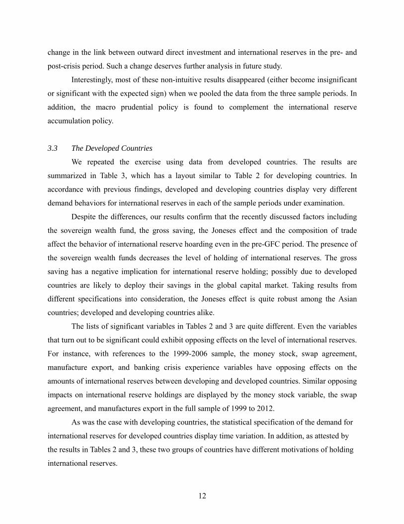
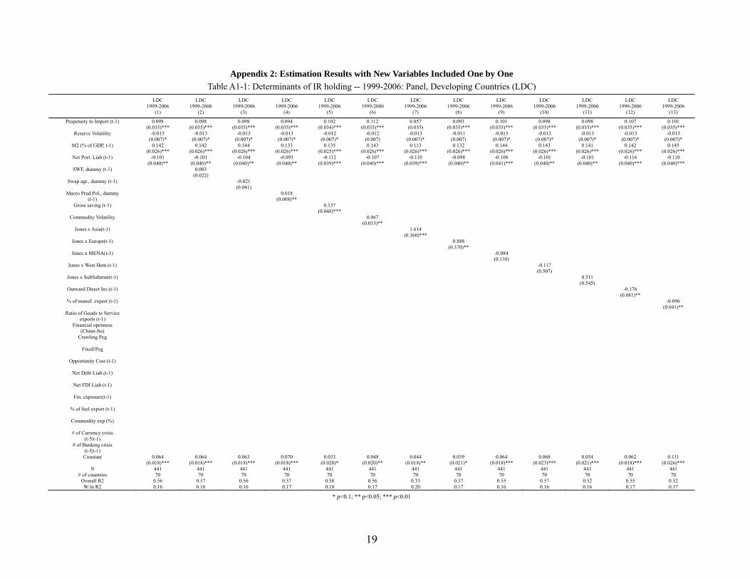
Using the specification in Table 1 as the starting point, we included elements of Zit,

individually and then jointly, in the panel regression. All these results are presented in the

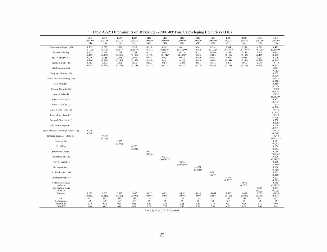
Appendix. In Table 2 we reported the parsimonious representations, which are obtained from

sequentially dropping the insignificant variables from the specifications reported under column

(26) of the tables in Appendix; that is, the specification that includes all the Zit variables.

One obvious observation is that these added variables have differential effects in the

different sample periods under consideration. Although they are “labelled” as recently discussed

factors, their effects on international reserve hoarding behavior are detected in the pre-GFC

period. Specifically, the grossing saving has the expected positive sign; a result that lends support

to the view that, for developing countries, grossing saving and holding of international reserves

could be linked via current account surplus; a high level of natonal saving leads to a better

current account and a high level of international reserve holding.

The outward direct investment effect is consistent with the view that investing overseas

helps divert international assets from the international reserve account. As anticipated, the

Joneses effect varies across country groups and historical time periods. The Joneses effects

displayed by Asian countries in the pre-GFC and full sample periods echo the results reported in

Cheung and Qian (2009). However, the rivalry in IR hoarding motivation is reversed during the

crisis period. Countries in other regions do not display a stable Joneses effect across the sample

periods. Nevertheless, the Joneses effect, if significant in the full sample, is always positive.

The two commodity price variables, the manufactures to export ratio, and the two crisis

variables do not perform consistently across sample periods. Some of the findings are not totally

intuitive. For instance, the negative banking crisis effect, manufactures effect, and commodity

export effect are not what we expected.

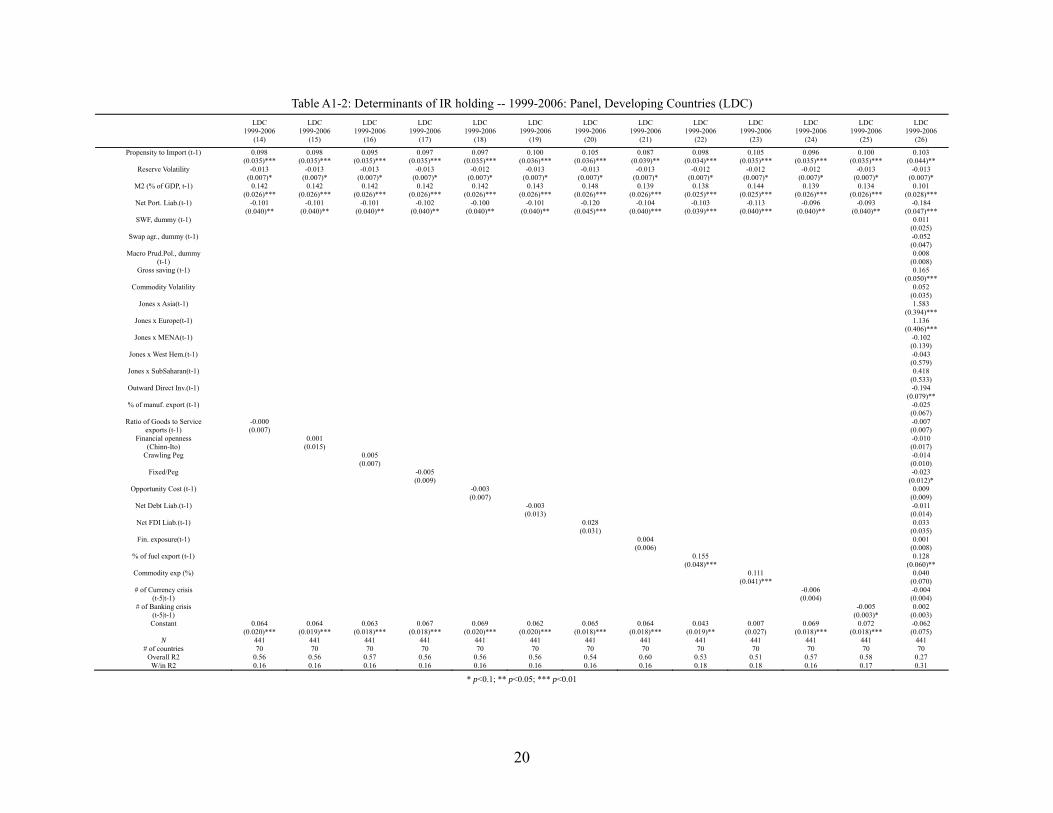
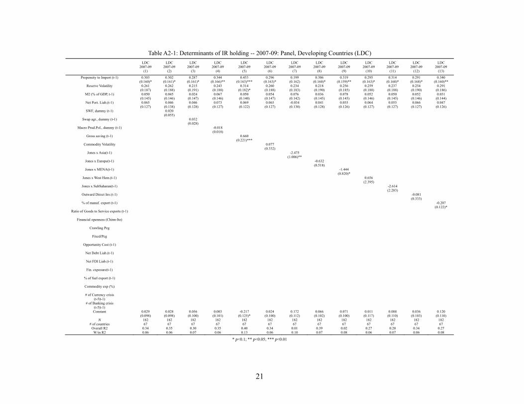
During the 2007-9 crisis period, those additional variables that were significant in the

previous period become insignificant or display the opposite effect. The change in the

performance of these variables may not be surprising as the crisis represents hectic market

conditions that prevent the normal economic relationship to hold. Nevertheless, the propensity to

trade still displays a strong positive effect.

The post crisis 2010-12 result may be the most surprising one. The list of significant

variables is dominated by the factors included Zit. While the effects of swap agreements and

gross saving are in line with expectations, the positive outward direct investment effect implies a

12

change in the link between outward direct investment and international reserves in the pre- and

post-crisis period. Such a change deserves further analysis in future study.

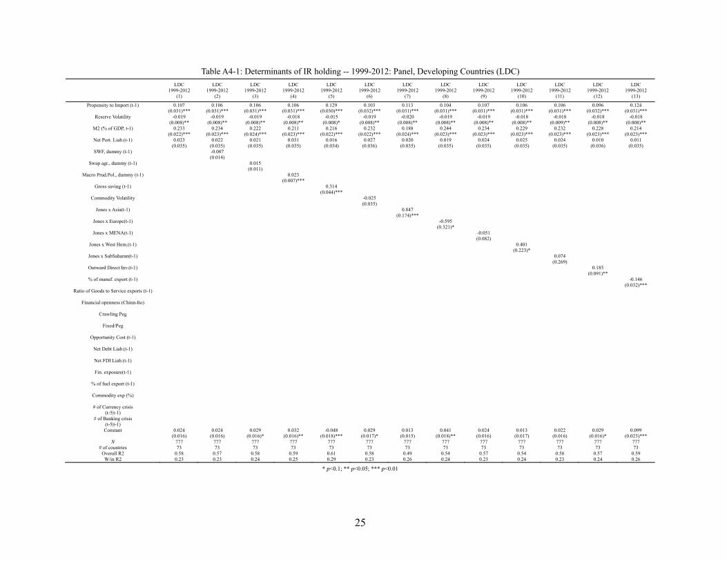
Interestingly, most of these non-intuitive results disappeared (either become insignificant

or significant with the expected sign) when we pooled the data from the three sample periods. In

addition, the macro prudential policy is found to complement the international reserve

accumulation policy.

3.3 The Developed Countries

We repeated the exercise using data from developed countries. The results are

summarized in Table 3, which has a layout similar to Table 2 for developing countries. In

accordance with previous findings, developed and developing countries display very different

demand behaviors for international reserves in each of the sample periods under examination.

Despite the differences, our results confirm that the recently discussed factors including

the sovereign wealth fund, the gross saving, the Joneses effect and the composition of trade

affect the behavior of international reserve hoarding even in the pre-GFC period. The presence of

the sovereign wealth funds decreases the level of holding of international reserves. The gross

saving has a negative implication for international reserve holding; possibly due to developed

countries are likely to deploy their savings in the global capital market. Taking results from

different specifications into consideration, the Joneses effect is quite robust among the Asian

countries; developed and developing countries alike.

The lists of significant variables in Tables 2 and 3 are quite different. Even the variables

that turn out to be significant could exhibit opposing effects on the level of international reserves.

For instance, with references to the 1999-2006 sample, the money stock, swap agreement,

manufacture export, and banking crisis experience variables have opposing effects on the

amounts of international reserves between developing and developed countries. Similar opposing

impacts on international reserve holdings are displayed by the money stock variable, the swap

agreement, and manufactures export in the full sample of 1999 to 2012.

As was the case with developing countries, the statistical specification of the demand for

international reserves for developed countries display time variation. In addition, as attested by

the results in Tables 2 and 3, these two groups of countries have different motivations of holding

international reserves.

13

4. Prediction Exercises

4.1 Are Developing Countries Over- or Under-Hoarding International Reserves?

In the last two decades or so, economists and policymakers alike have been debating on

the issue of the adequacy of international reserve holding. While deficiency in international

reserve holding can trigger economic and financial instabilities, excessive hoarding of

international reserves can create domestic economic over-heating and contribute to instability in

the global economy. An overarching issue of the debate is how to determine, either theoretically

or empirically, the appropriate or the optimal level of international reserves. A benchmark level is

required to assess whether the actual level of holdings is too much or too few.

The estimation results in the previous section clearly show that, even in the last one and a

half decades, the empirical demand function for international reserves changes over time and

includes different sets of factors over different time periods. Thus, if we use the estimated level

of international reserves as a reference point, the estimated degree of over- or under-hoarding

depends upon which empirical model is used to compute the benchmark.

To illustrate the point, we used the estimated models reported in Table 2 to generate

predictions of IR holding for developing countries. For each specification, we generate the

in-sample and out-of-sample forward predictions, but not backward predictions. For example,

using the model estimated for the 2007-2009 sample, we generate the in-sample predictions for

2007 to 2009, and the out-of-sample predictions for 2010 to 2012. These predictions and the

actual levels of international reserve holding are graphed in Figure 2.

One caveat in reading these graphs is that the predictions are generated without

country-fixed effects. We conceived that predictions made without country-fixed effects would

resemble the way international investors compare cross-country investment destinations for

arbitrage opportunities.15

Figure 2 includes actual and predicted holdings of international reserves of selected

individual countries and countries groups. The individual countries include Argentina, China,

Korea, Malaysia, Mexico, Thailand, and the “Fragile Five” of Brazil, India, Indonesia, South

15 Alternatively speaking, one could say that predictions with country-fixed effects are relevant for assessing whether the path of actual holdings of international reserves are higher or lower relative its historical tendency.

14

Africa, and Turkey. The country groups are the developing Asia excluding China, the Latin

America, and emerging market economies.

Let us consider the differences during the period of 2010 to 2012. The models of the

demand for international reserves estimated for the four sample periods could generate

predictions that are quite different from each other. Compared with those from the other two

specifications, the predictions from the 1999-2006 and 1999-2012 specifications are quite similar.

The observation is in accordance with the results in Table 2 – the data from the 1999-2006 and

1999-2012 sample periods yield relatively similar estimation results. Depending on individual

countries or country groups, predictions from the 2007-2009 or 2010-2012 specifications are

quite different from those of the specifications estimated from a longer time span.

These plots confirm the assertion that whether a country is under- or over-hoarding

international reserves depends on which estimation model is used as benchmark. China during

the 2010-2012 period, for example, is deemed to hold international reserves that are far more

than those predicted by the model estimated for the 2007-2009 period, are slightly less than those

by the 1999-2006 specification, and are about right by the other two model specifications. The

over-hoarding result delivered by the 2007-2009 specification is not unique to China. Indeed,

similar over-hoarding results are observed for other Asian economies and the group of Asian

economy excluding China included in Figure 2.

The “Fragile Five” – a recent acronym surfaced in the media that comprises Brazil, India,

Indonesia, South Africa and Turkey – are viewed by the market as vulnerable to the reverse of

the US quantitative easing (QE) policy. The graphs in Figure 2 indicate that these five countries

are likely to be deficient in international reserves during the period of 2010-2012; they are

considered under-hoarding by two or three of the four specifications under consideration. If it is

the case, the market’s concern is quite justified in view of their deteriorating current account

conditions.

Despite the wide variation of over- and under-hoarding estimates for individual countries,

the three selected country groups tend to hold international reserves less than predicted.

4.2 International Reserve Holdings and Currency Depreciation

How are the countries that are susceptible to external financial shocks doing lately? In

recent years, emerging market economies have ambivalent feelings about the spillovers from

15

advanced economies. On the one hand, emerging market economies benefit from the recovery of

advanced economies, which are their important trading partners. On the other hand, with

recovery underway, the advanced world will trigger the tapering policy to end the extremely low

interest rate policy, which in turn could cause massive outflow of capital from emerging market

economies. Indeed, the world witnessed on May 22, 2013 the adverse market effect of the

Federal Reserve chairman Ben S. Bernanke’s comment on tapering the QE policy on emerging

financial markets.

As amplified in the media, economies that are financially vulnerable, including the

Fragile Five discussed above, have been experiencing economic and financial stress. One sign of

economic and financial stress is exemplified by the value of the domestic currency. With

(anticipated) capital outflow and deteriorating economy performance, some emerging market

economies have experienced a noticeable depreciation of their currencies in recent years.

While our estimation of the demand for international reserves does not answer definitely

the question of whether a country is holding too much or too little international reserves, the

results may shed light on the relative sufficiency/deficiency of international reserves. To

investigate the issue, we study the possible links between our estimates of international reserves

holding and the observed exchange rate movements. Specifically, we investigate if the currency

stress is associated with the level of international reserve holding, which is interpreted as a

barometer of a country’s vulnerability to external financial shocks.

Figure 3 displays scatter diagrams of the magnitude of exchange rate depreciation and the

degree of over-hoarding of international reserves. The exchange rate depreciation is measured

against the US dollar, which is the prominent international currency. The difference between the

actual and predicted levels of international reserves is our proxy of the degree of over-hoarding;

that is, a positive difference implies over-hoarding while a negative one under-hoarding. If the

under-hoarding proxy is a reasonable measure of vulnerability to external financial shocks, we

expect it has a negative associate with exchange rate depreciation.

The scatter plots of the annual averages of exchange rate depreciation observed during

the year of 2013 and the over-hoarding proxies for the period of 2010-2012 display different

patterns. For instance, the proxies derived from the 2007-2009 model (Panel B) exhibit a wide

dispersion relative to those from other model specifications. Nonetheless, a (weak) negative

association of the two variables could be visualized in these four scatter plots.

16

To shed additional insight, we regress the rate of depreciation of the exchange rate against

the U.S. dollar on the proxy for international reserve over-hoarding, and report the results in

Table 4. Two over-hoarding proxies are considered: one is the average of the 2010 to 2012 values,

and the other is the proxy value as of 2012.

The estimation results lend support to the visual inspection that the two variables are

negatively related. All coefficient estimates are negative and, with the exception of the

1999-2006 case, statistically significant. The explanatory power, as given by the adjusted

R-square estimates, ranges from 2% to 7% for the significant cases. Apparently, the information

conveyed by the 2012 proxy for over-hoarding has a stronger impact for exchange rate

depreciation than the one embedded in the annual averages of 2010 to 2012.

Based on the presumption that the market will drive down the exchange rate value of a

country that experiences signs of external vulnerability amplified by its holding of international

reserves, our findings either lend support to this presumption or are indicative of the relevance of

the estimated demand models for international reserves (with the 1999-2006 model as a likely

exception). A strong inference is that, if a country holds a deficient amount of international

reserves, it tends to experience currency depreciation. The result will be reinforced by

intervention in the foreign exchange market that further depletes the holding of international

reserves.

5. Conclusions

Our analysis confirms structural changes associated with new patterns of hoarding

international reserves. While there is no end in sight for hoarding reserves, some of the new

factors may mitigate eventual reserve accumulation. The proliferation of sovereign wealth funds

and possible rebalancing of emerging markets that followed aggressive export-led growth before

the GFC may reduce reserve/GDP ratios of developing countries, as confirmed in the predictive

exercises using the latest data. However, these predictions should be taken with a grain of salt, as

there is no reason to expect future stability in the use of hoarding patterns in international

reserves.

17

Appendix 1 Data Definitions Macro/Traditional Variables (X):

Propensity to import – Imports as a ratio to GDP.

Reserve volatility – Standard deviations of the growth of IR holding in five year windows (t – 5 through t – 1) are used. The data are extracted from WDI and IFS.

Gross saving – Gross saving is used as % of GDP. WDI and WEO.

Opportunity cost of holding reserves – It is the difference between the long-term government bond yields and the U.S. 10-year government bond yields (Previously, I used the Treasury bill rates, not any more). For the countries for which the long-term bond yields data are not available, “lending rates” from the IFS are used. The data are from WDI and IFS.

Dummies for the fixed/pegged and crawling peg regimes – The Reinhart-Rogoff (2004) index is used to construct the exchange rate regime dummy variables. Their index ranges from 1 “no separate legal tender,” to 14 “Freely falling” (with increasing flexibility of exchange rate movement) and is a “de facto” index (in contrast to IMF’s “de jure” exchange rate regime classification). Here, as in Cheung and Ito, we aggregate these categories into three groups; namely “floating,” “Crawling Peg,” and “Fixed/Pegged.” The Reinhart and Rogoff index is updated to 2010. For 2011, we assume countries have the same exchange rate regime as in 2010.

Financial and Institutional Variables (Y):

M2 as % of GDP – M2 as a share of GDP (I used liquid liability ratios in the previous round)

Gross Portfolio Exposure – The sum of external assets and liabilities divided by GDP. The data are extracted from Lane-Milesi-Ferretti dataset. Previously, we used “net” exposure or change in the net exposure. Following Joshua’s advice, we now use the “gross” variable.

Currency, Banking, and Debt crisis – The number of crises in the window of time from t – 5 through t – 1 is counted for each type of crisis. The crisis dummies are the ones constructed in Aizenman and Ito (2013).

Net liabilities for FDI, debt, and portfolio investment – For each of the cross-border investment types, the net liabilities are calculated as <external liability minus external asset>, using the updated dataset of Lane and Milesi-Ferretti (2007 and updates).

De jure measure of financial openness – The index is based on Chinn and Ito (2006, 2008) and downloaded from http://web.pdx.edu/~ito/Chinn-Ito_website.htm .

Country Characteristic Variables (D):

Dummy variables are not tested because the estimations are conducted with fixed effects.

‘New’ Variables (Z)

Dummy for the sovereign wealth funds (SWF) – Using the data from the SWF Institute (http://www.swfinstitute.org/fund-rankings/), we assign the value of one for the country and

18

years in which the country of concern possesses a national-level SWF.

Dummy for bilateral swap agreements (SWAP) – This dummy takes the value of one if a country is in an agreement of a bilateral swap agreement (regardless of the currency of the agreement). The data are compiled using website information.

Dummy for macro prudential policies (MPP) – This dummy takes a value of one if a country has in place any of the macro prudential policies Lim, et al. (2013) compiled.

Gross saving – Gross saving is used as % of GDP. WDI and WEO.

Commodity TOT Volatility – Using the commodity terms of trade data compiled by Spatafora and Tytell (2009), we use the moving five-year standard deviations (in t-5 through t-1) of the change in the commodity TOT index as a proxy for commodity TOT volatility.16

Jones Effects – This variable is supposed to capture regional externality of IR holding and its computation is based on Cheung and Qian (2009). It is essentially the average of IR holding in the region country i belongs to, but it excludes the level of IR holding of country i itself. The regions are: “North and South America,” “Europe,” “East and South Asia,” “Middle-east and North Africa,” and “Sub-Saharan Africa.”17

Outward direct investment (ODI) – Outward direct investment as a share of GDP. The data are extracted from UNCTAD’s database.

Oil exporters – The dummy is assigned for oil exporters defined by the World Bank or Spatafora and Tytell (2009).

% of commodity exports – The “commodity exports” are the sum of fuel, food, agricultural goods, and minerals, all of which are extracted from WDI. It is shown as the share of total exports.

% of manufacturing exports – The data are from WDI. It is shown as the share of total exports.

Ratio of goods exports to service exports – Using the BoP data, we calculate the proportion of service exports in goods and service exports. Then, we come up with the ratio as (1 minus service exports as % of total exports)/(service exports as % of total exports).

Financial Exposure – We use the ratio of (total external assets + total external liabilities) to GDP. The data are based on Lane and Milesi-Ferretti (2007 and updates).

Currency and Banking Crises – We use the dummy for both currency and banking crisis episodes that are identified in Aizenman and Ito (2013). For the identification of currency crisis, Aizenman and Ito (2013) first calculate the exchange rate market pressure (EMP) against the base country (Aizenman, et al., 2008, Eichengreen, et al. 1995, 1996). For the countries whose data for the EMP are not available, the crisis dummy is supplemented by the currency crisis identification by Reinhart and Rogoff (2009). Their banking crisis data are essentially based on Laeven and Velancia (2008, 2010, 2012). We count the number of past crisis years over t-1 through t-5 for each type of crises while assigning weights on the crisis dummies depending on the year. That is, the crisis variables are calculated as: Dc(t-1) + .95* Dc(t-1) + .90*Dc(t-3) + .85*Dc(t-4) + .80*Dc(t-5). We assume that the weight diminishes by 5% every year, i.e., that the memory of a crisis among policy makers “depreciates” at the annual rate of 5%.

16 The original data are available up to 2009, but we obtained more updated data (up to 2011) from the authors. We thank authors for the generosity to share the data. 17 “Europe” includes Western, Central, and Eastern Europe.

19

Appendix 2: Estimation Results with New Variables Included One by One

Table A1-1: Determinants of IR holding -- 1999-2006: Panel, Developing Countries (LDC)

LDC LDC LDC LDC LDC LDC LDC LDC LDC LDC LDC LDC LDC 1999-2006 1999-2006 1999-2006 1999-2006 1999-2006 1999-2006 1999-2006 1999-2006 1999-2006 1999-2006 1999-2006 1999-2006 1999-2006 (1) (2) (3) (4) (5) (6) (7) (8) (9) (10) (11) (12) (13)

Propensity to Import (t-1) 0.098 0.098 0.098 0.094 0.102 0.112 0.057 0.093 0.101 0.098 0.098 0.107 0.101 (0.035)*** (0.035)*** (0.035)*** (0.035)*** (0.034)*** (0.035)*** (0.035) (0.035)*** (0.035)*** (0.035)*** (0.035)*** (0.035)*** (0.035)***

Reserve Volatility -0.013 -0.013 -0.013 -0.013 -0.012 -0.012 -0.013 -0.011 -0.013 -0.013 -0.013 -0.013 -0.013 (0.007)* (0.007)* (0.007)* (0.007)* (0.007)* (0.007) (0.007)* (0.007) (0.007)* (0.007)* (0.007)* (0.007)* (0.007)*

M2 (% of GDP, t-1) 0.142 0.142 0.144 0.133 0.135 0.143 0.113 0.132 0.144 0.143 0.141 0.142 0.145 (0.026)*** (0.026)*** (0.026)*** (0.026)*** (0.025)*** (0.026)*** (0.026)*** (0.026)*** (0.026)*** (0.026)*** (0.026)*** (0.026)*** (0.026)***

Net Port. Liab.(t-1) -0.101 -0.101 -0.104 -0.093 -0.112 -0.107 -0.110 -0.098 -0.108 -0.101 -0.101 -0.116 -0.110 (0.040)** (0.040)** (0.040)** (0.040)** (0.039)*** (0.040)*** (0.039)*** (0.040)** (0.041)*** (0.040)** (0.040)** (0.040)*** (0.040)***

SWF, dummy (t-1) 0.003 (0.022)

Swap agr., dummy (t-1) -0.021 (0.041)

Macro Prud.Pol., dummy 0.018 (t-1) (0.008)**

Gross saving (t-1) 0.157 (0.048)***

Commodity Volatility 0.067 (0.033)**

Jones x Asia(t-1) 1.614 (0.360)***

Jones x Europe(t-1) 0.888 (0.370)**

Jones x MENA(t-1) -0.084 (0.138)

Jones x West Hem.(t-1) -0.117 (0.507)

Jones x SubSaharan(t-1) 0.511 (0.545)

Outward Direct Inv.(t-1) -0.176 (0.081)**

% of manuf. export (t-1) -0.096 (0.041)**

Ratio of Goods to Service exports (t-1)

Financial openness (Chinn-Ito)

Crawling Peg

Fixed/Peg

Opportunity Cost (t-1)

Net Debt Liab.(t-1)

Net FDI Liab.(t-1)

Fin. exposure(t-1)

% of fuel export (t-1)

Commodity exp (%)

# of Currency crisis (t-5|t-1)

# of Banking crisis (t-5|t-1) Constant 0.064 0.064 0.063 0.070 0.033 0.048 0.044 0.039 0.064 0.068 0.054 0.062 0.111

(0.018)*** (0.018)*** (0.018)*** (0.018)*** (0.020)* (0.020)** (0.018)** (0.021)* (0.018)*** (0.023)*** (0.021)*** (0.018)*** (0.026)*** N 441 441 441 441 441 441 441 441 441 441 441 441 441

# of countries 70 70 70 70 70 70 70 70 70 70 70 70 70 Overall R2 0.56 0.57 0.56 0.57 0.58 0.56 0.33 0.37 0.55 0.57 0.52 0.55 0.52

W/in R2 0.16 0.16 0.16 0.17 0.18 0.17 0.20 0.17 0.16 0.16 0.16 0.17 0.17

* p<0.1; ** p<0.05; *** p<0.01

20



Propensity to Import (t-1) 0.098 0.098 0.095 0.097 0.097 0.100 0.105 0.087 0.098 0.105 0.096 0.100 0.103 (0.035)*** (0.035)*** (0.035)*** (0.035)*** (0.035)*** (0.036)*** (0.036)*** (0.039)** (0.034)*** (0.035)*** (0.035)*** (0.035)*** (0.044)**

Reserve Volatility -0.013 -0.013 -0.013 -0.013 -0.012 -0.013 -0.013 -0.013 -0.012 -0.012 -0.012 -0.013 -0.013 (0.007)* (0.007)* (0.007)* (0.007)* (0.007)* (0.007)* (0.007)* (0.007)* (0.007)* (0.007)* (0.007)* (0.007)* (0.007)*

M2 (% of GDP, t-1) 0.142 0.142 0.142 0.142 0.142 0.143 0.148 0.139 0.138 0.144 0.139 0.134 0.101 (0.026)*** (0.026)*** (0.026)*** (0.026)*** (0.026)*** (0.026)*** (0.026)*** (0.026)*** (0.025)*** (0.025)*** (0.026)*** (0.026)*** (0.028)***

Net Port. Liab.(t-1) -0.101 -0.101 -0.101 -0.102 -0.100 -0.101 -0.120 -0.104 -0.103 -0.113 -0.096 -0.093 -0.184 (0.040)** (0.040)** (0.040)** (0.040)** (0.040)** (0.040)** (0.045)*** (0.040)*** (0.039)*** (0.040)*** (0.040)** (0.040)** (0.047)***

SWF, dummy (t-1) 0.011 (0.025)

Swap agr., dummy (t-1) -0.052 (0.047)

Macro Prud.Pol., dummy 0.008 (t-1) (0.008)

Gross saving (t-1) 0.165 (0.050)***

Commodity Volatility 0.052 (0.035)

Jones x Asia(t-1) 1.583 (0.394)***

Jones x Europe(t-1) 1.136 (0.406)***

Jones x MENA(t-1) -0.102 (0.139)

Jones x West Hem.(t-1) -0.043 (0.579)


Outward Direct Inv.(t-1) -0.194 (0.079)**

% of manuf. export (t-1) -0.025 (0.067)

Ratio of Goods to Service -0.000 -0.007 exports (t-1) (0.007) (0.007)

Financial openness 0.001 -0.010 (Chinn-Ito) (0.015) (0.017)

Crawling Peg 0.005 -0.014 (0.007) (0.010)

Fixed/Peg -0.005 -0.023 (0.009) (0.012)*

Opportunity Cost (t-1) -0.003 0.009 (0.007) (0.009)

Net Debt Liab.(t-1) -0.003 -0.011 (0.013) (0.014)

Net FDI Liab.(t-1) 0.028 0.033 (0.031) (0.035)

Fin. exposure(t-1) 0.004 0.001 (0.006) (0.008)

% of fuel export (t-1) 0.155 0.128 (0.048)*** (0.060)**

Commodity exp (%) 0.111 0.040 (0.041)*** (0.070)

# of Currency crisis -0.006 -0.004 (t-5|t-1) (0.004) (0.004)

# of Banking crisis -0.005 0.002 (t-5|t-1) (0.003)* (0.003) Constant 0.064 0.064 0.063 0.067 0.069 0.062 0.065 0.064 0.043 0.007 0.069 0.072 -0.062

(0.020)*** (0.019)*** (0.018)*** (0.018)*** (0.020)*** (0.020)*** (0.018)*** (0.018)*** (0.019)** (0.027) (0.018)*** (0.018)*** (0.075) N 441 441 441 441 441 441 441 441 441 441 441 441 441


W/in R2 0.16 0.16 0.16 0.16 0.16 0.16 0.16 0.16 0.18 0.18 0.16 0.17 0.31

* p<0.1; ** p<0.05; *** p<0.01

21



Propensity to Import (t-1) 0.303 0.302 0.287 0.344 0.453 0.296 0.199 0.306 0.319 0.295 0.314 0.291 0.340 (0.160)* (0.161)* (0.161)* (0.166)** (0.163)*** (0.163)* (0.162) (0.160)* (0.159)** (0.163)* (0.160)* (0.168)* (0.160)**

Reserve Volatility 0.261 0.262 0.215 0.243 0.314 0.260 0.234 0.218 0.256 0.259 0.237 0.254 0.291 (0.187) (0.188) (0.191) (0.188) (0.182)* (0.188) (0.183) (0.190) (0.185) (0.188) (0.188) (0.190) (0.186)

M2 (% of GDP, t-1) 0.050 0.045 0.024 0.067 0.050 0.054 0.076 0.036 0.078 0.052 0.050 0.052 0.031 (0.145) (0.146) (0.147) (0.146) (0.140) (0.147) (0.142) (0.145) (0.145) (0.146) (0.145) (0.146) (0.144)

Net Port. Liab.(t-1) 0.065 0.046 0.046 0.073 0.069 0.065 -0.034 0.041 0.055 0.064 0.055 0.066 0.047 (0.127) (0.138) (0.128) (0.127) (0.122) (0.127) (0.130) (0.128) (0.126) (0.127) (0.127) (0.127) (0.126)

SWF, dummy (t-1) 0.020 (0.055)

Swap agr., dummy (t-1) 0.032 (0.028)

Macro Prud.Pol., dummy (t-1) -0.018 (0.018)

Gross saving (t-1) 0.660 (0.221)***


Jones x Asia(t-1) -2.475 (1.006)**

Jones x Europe(t-1) -0.632 (0.518)

Jones x MENA(t-1) -1.444 (0.820)*

Jones x West Hem.(t-1) 0.656 (2.395)

Jones x SubSaharan(t-1) -2.614 (2.283)

Outward Direct Inv.(t-1) -0.081 (0.333)

% of manuf. export (t-1) -0.207 (0.122)*



Crawling Peg

Fixed/Peg


Net Debt Liab.(t-1)

Net FDI Liab.(t-1)

Fin. exposure(t-1)


Commodity exp (%)


# of Banking crisis (t-5|t-1) Constant 0.029 0.028 0.056 0.003 -0.217 0.024 0.172 0.066 0.071 0.011 0.088 0.036 0.120

(0.098) (0.098) (0.100) (0.101) (0.125)* (0.100) (0.112) (0.102) (0.100) (0.117) (0.110) (0.103) (0.110) N 182 182 182 182 182 182 182 182 182 182 182 182 182

# of countries 67 67 67 67 67 67 67 67 67 67 67 67 67 Overall R2 0.34 0.35 0.30 0.35 0.40 0.34 0.01 0.39 0.02 0.27 0.20 0.34 0.27 W/in R2 0.06 0.06 0.07 0.06 0.13 0.06 0.10 0.07 0.08 0.06 0.07 0.06 0.08

* p<0.1; ** p<0.05; *** p<0.01

22



Propensity to Import (t-1) 0.302 0.273 0.311 0.315 0.255 0.343 0.411 0.241 0.314 0.334 0.331 0.308 0.413 (0.161)* (0.162)* (0.161)* (0.161)* (0.165) (0.156)** (0.156)*** (0.162) (0.159)* (0.159)** (0.159)** (0.160)* (0.184)**

Reserve Volatility 0.263 0.259 0.263 0.258 0.222 0.347 0.313 0.271 0.280 0.299 0.263 0.218 0.311 (0.189) (0.187) (0.188) (0.188) (0.190) (0.184)* (0.179)* (0.185) (0.186) (0.186) (0.185) (0.195) (0.193)

M2 (% of GDP, t-1) 0.049 0.085 0.048 0.051 0.058 0.053 0.052 0.120 0.045 0.034 0.001 0.037 0.096 (0.146) (0.148) (0.145) (0.145) (0.145) (0.141) (0.138) (0.148) (0.144) (0.144) (0.146) (0.146) (0.149)

Net Port. Liab.(t-1) 0.063 0.109 0.051 0.050 0.026 0.046 -0.038 0.055 0.046 0.051 0.056 0.049 -0.148 (0.128) (0.132) (0.129) (0.128) (0.131) (0.123) (0.124) (0.125) (0.126) (0.125) (0.125) (0.128) (0.143)

SWF, dummy (t-1) -0.001 (0.053)

Swap agr., dummy (t-1) 0.029 (0.029)


Gross saving (t-1) 0.410 (0.232)*

Commodity Volatility -0.180 (0.343)

Jones x Asia(t-1) -2.822 (1.080)**

Jones x Europe(t-1) 0.422 (0.693)

Jones x MENA(t-1) -1.072 (0.788)

Jones x West Hem.(t-1) -0.474 (2.991)

Jones x SubSaharan(t-1) -0.943 (2.149)

Outward Direct Inv.(t-1) 0.338 (0.396)

% of manuf. export (t-1) 0.070 (0.283)

Ratio of Goods to Service exports (t-1) 0.006 -0.018 (0.048) (0.048)

Financial openness (Chinn-Ito) -0.110 -0.274 (0.096) (0.102)***

Crawling Peg 0.023 0.073 (0.032) (0.051)

Fixed/Peg -0.033 0.038 (0.042) (0.064)

Opportunity Cost (t-1) 0.031 0.059 (0.026) (0.036)*

Net Debt Liab.(t-1) 0.222 0.176 (0.078)*** (0.088)**

Net FDI Liab.(t-1) 0.286 0.185 (0.082)*** (0.108)*

Fin. exposure(t-1) -0.021 0.006 (0.011)* (0.015)

% of fuel export (t-1) 0.342 0.171 (0.219) (0.270)

Commodity exp (%) 0.257 0.272 (0.135)* (0.311)

# of Currency crisis 0.052 0.065 (t-5|t-1) (0.027)* (0.030)**

# of Banking crisis 0.018 0.001 (t-5|t-1) (0.022) (0.025) Constant 0.022 0.093 0.012 0.032 0.022 0.025 0.052 0.054 -0.044 -0.110 0.039 0.036 -0.024

(0.112) (0.112) (0.100) (0.098) (0.097) (0.095) (0.093) (0.097) (0.108) (0.121) (0.097) (0.098) (0.374) N 182 182 182 182 182 182 182 182 182 182 182 182 182

# of countries 67 67 67 67 67 67 67 67 67 67 67 67 67 Overall R2 0.34 0.39 0.35 0.35 0.34 0.33 0.28 0.24 0.34 0.24 0.26 0.32 0.00 W/in R2 0.06 0.07 0.06 0.06 0.07 0.12 0.15 0.08 0.08 0.09 0.09 0.06 0.42

* p<0.1; ** p<0.05; *** p<0.01

23



Propensity to Import (t-1) -0.117 -0.124 -0.099 -0.117 -0.113 -0.114 -0.130 -0.132 -0.107 -0.126 -0.116 -0.133 -0.120 (0.060)* (0.060)** (0.060) (0.060)* (0.060)* (0.061)* (0.061)** (0.059)** (0.054)* (0.060)** (0.062)* (0.060)** (0.061)*

Reserve Volatility -0.147 -0.150 -0.117 -0.150 -0.119 -0.138 -0.157 -0.051 -0.115 -0.162 -0.148 -0.117 -0.158 (0.212) (0.212) (0.210) (0.213) (0.215) (0.216) (0.212) (0.213) (0.191) (0.212) (0.213) (0.210) (0.214)

M2 (% of GDP, t-1) 0.150 0.159 0.170 0.158 0.136 0.151 0.151 0.152 0.029 0.142 0.149 0.184 0.159 (0.094) (0.095)* (0.094)* (0.096) (0.096) (0.095) (0.094) (0.093) (0.089) (0.094) (0.095) (0.095)* (0.097)

Net Port. Liab.(t-1) -0.151 -0.148 -0.181 -0.152 -0.155 -0.152 -0.156 -0.165 -0.057 -0.156 -0.151 -0.104 -0.154 (0.127) (0.127) (0.126) (0.127) (0.127) (0.127) (0.127) (0.125) (0.116) (0.126) (0.127) (0.128) (0.127)

SWF, dummy (t-1) 0.040 (0.039)

Swap agr., dummy (t-1) -0.036 (0.020)*

Macro Prud.Pol., dummy (t-1) 0.005 (0.011)

Gross saving (t-1) 0.098 (0.116)


Jones x Asia(t-1) -0.922 (0.938)

Jones x Europe(t-1) -2.573 (1.248)**

Jones x MENA(t-1) 0.625 (0.133)***

Jones x West Hem.(t-1) -3.586 (2.996)


Outward Direct Inv.(t-1) 0.345 (0.187)*

% of manuf. export (t-1) 0.018 (0.043)



Crawling Peg

Fixed/Peg


Net Debt Liab.(t-1)

Net FDI Liab.(t-1)

Fin. exposure(t-1)


Commodity exp (%)


# of Banking crisis (t-5|t-1) Constant 0.214 0.199 0.197 0.206 0.196 0.205 0.274 0.322 0.265 0.375 0.212 0.187 0.201

(0.072)*** (0.074)*** (0.072)*** (0.074)*** (0.075)** (0.079)** (0.094)*** (0.088)*** (0.066)*** (0.153)** (0.075)*** (0.073)** (0.079)** N 154 154 154 154 154 154 154 154 154 154 154 154 154


W/in R2 0.07 0.08 0.10 0.07 0.08 0.07 0.08 0.11 0.25 0.09 0.07 0.10 0.07

* p<0.1; ** p<0.05; *** p<0.01

24



Propensity to Import (t-1) -0.072 -0.117 -0.114 -0.112 -0.119 -0.115 -0.118 -0.117 -0.113 -0.119 -0.123 -0.087 -0.032 (0.065) (0.060)* (0.060)* (0.060)* (0.060)* (0.061)* (0.060)* (0.060)* (0.061)* (0.060)* (0.060)** (0.063) (0.067)

Reserve Volatility -0.143 -0.146 -0.110 -0.099 -0.108 -0.144 -0.164 -0.150 -0.151 -0.155 -0.148 -0.145 0.060 (0.210) (0.214) (0.213) (0.213) (0.219) (0.213) (0.213) (0.214) (0.213) (0.213) (0.212) (0.210) (0.197)

M2 (% of GDP, t-1) 0.155 0.150 0.150 0.146 0.157 0.154 0.154 0.150 0.152 0.158 0.163 0.134 0.028 (0.093)* (0.095) (0.094) (0.094) (0.095) (0.096) (0.095) (0.095) (0.095) (0.096) (0.096)* (0.094) (0.095)

Net Port. Liab.(t-1) -0.103 -0.150 -0.149 -0.146 -0.139 -0.141 -0.116 -0.151 -0.147 -0.153 -0.148 -0.128 0.030 (0.129) (0.128) (0.126) (0.126) (0.128) (0.132) (0.132) (0.127) (0.128) (0.127) (0.127) (0.127) (0.133)

SWF, dummy (t-1) 0.062 (0.060)

Swap agr., dummy (t-1) -0.031 (0.020)


Gross saving (t-1) 0.337 (0.142)**


Jones x Asia(t-1) -1.384 (0.935)

Jones x Europe(t-1) -2.848 (1.188)**

Jones x MENA(t-1) 0.603 (0.137)***

Jones x West Hem.(t-1) -2.272 (3.177)


Outward Direct Inv.(t-1) 0.609 (0.247)**

% of manuf. export (t-1) -0.045 (0.075)

Ratio of Goods to Service exports (t-1) -0.041 -0.024 (0.024)* (0.024)

Financial openness (Chinn-Ito) -0.006 0.037 (0.058) (0.054)

Crawling Peg 0.027 0.013 (0.020) (0.038)

Fixed/Peg -0.036 -0.010 (0.023) (0.039)

Opportunity Cost (t-1) 0.015 -0.020 (0.021) (0.023)

Net Debt Liab.(t-1) -0.015 0.050 (0.049) (0.055)

Net FDI Liab.(t-1) 0.072 0.006 (0.076) (0.106)

Fin. exposure(t-1) -0.002 -0.036 (0.017) (0.028)

% of fuel export (t-1) -0.049 -0.017 (0.106) (0.131)

Commodity exp (%) -0.023 -0.080 (0.039) (0.072)

# of Currency crisis -0.022 -0.023 (t-5|t-1) (0.027) (0.047)

# of Banking crisis -0.017 -0.052 (t-5|t-1) (0.011) (0.013)*** Constant 0.241 0.217 0.192 0.219 0.187 0.208 0.237 0.218 0.220 0.221 0.209 0.215 0.596

(0.073)*** (0.079)*** (0.074)** (0.072)*** (0.082)** (0.076)*** (0.076)*** (0.080)*** (0.074)*** (0.074)*** (0.073)*** (0.072)*** (0.225)*** N 154 154 154 154 154 154 154 154 154 154 154 154 154


W/in R2 0.10 0.07 0.09 0.09 0.08 0.07 0.08 0.07 0.07 0.07 0.08 0.09 0.55

* p<0.1; ** p<0.05; *** p<0.01

25



Propensity to Import (t-1) 0.107 0.106 0.106 0.106 0.129 0.103 0.113 0.104 0.107 0.106 0.106 0.096 0.124 (0.031)*** (0.031)*** (0.031)*** (0.031)*** (0.030)*** (0.032)*** (0.031)*** (0.031)*** (0.031)*** (0.031)*** (0.031)*** (0.032)*** (0.031)***

Reserve Volatility -0.019 -0.019 -0.019 -0.018 -0.015 -0.019 -0.020 -0.019 -0.019 -0.018 -0.018 -0.018 -0.018 (0.008)** (0.008)** (0.008)** (0.008)** (0.008)* (0.008)** (0.008)** (0.008)** (0.008)** (0.008)** (0.009)** (0.008)** (0.008)**

M2 (% of GDP, t-1) 0.233 0.234 0.222 0.211 0.216 0.232 0.188 0.244 0.234 0.229 0.232 0.228 0.214 (0.022)*** (0.023)*** (0.024)*** (0.023)*** (0.022)*** (0.022)*** (0.024)*** (0.023)*** (0.023)*** (0.023)*** (0.023)*** (0.023)*** (0.023)***

Net Port. Liab.(t-1) 0.023 0.022 0.021 0.031 0.016 0.027 0.020 0.019 0.024 0.025 0.024 0.010 0.011 (0.035) (0.035) (0.035) (0.035) (0.034) (0.036) (0.035) (0.035) (0.035) (0.035) (0.035) (0.036) (0.035)

SWF, dummy (t-1) -0.007 (0.014)

Swap agr., dummy (t-1) 0.015 (0.011)

Macro Prud.Pol., dummy (t-1) 0.023 (0.007)***

Gross saving (t-1) 0.314 (0.044)***


Jones x Asia(t-1) 0.847 (0.174)***

Jones x Europe(t-1) -0.595 (0.321)*

Jones x MENA(t-1) -0.051 (0.082)

Jones x West Hem.(t-1) 0.401 (0.223)*


Outward Direct Inv.(t-1) 0.185 (0.091)**

% of manuf. export (t-1) -0.146 (0.032)***



Crawling Peg

Fixed/Peg


Net Debt Liab.(t-1)

Net FDI Liab.(t-1)

Fin. exposure(t-1)


Commodity exp (%)


# of Banking crisis (t-5|t-1) Constant 0.024 0.024 0.029 0.032 -0.048 0.029 0.013 0.041 0.024 0.013 0.022 0.029 0.099

(0.016) (0.016) (0.016)* (0.016)** (0.018)*** (0.017)* (0.015) (0.018)** (0.016) (0.017) (0.016) (0.016)* (0.023)*** N 777 777 777 777 777 777 777 777 777 777 777 777 777


W/in R2 0.23 0.23 0.24 0.25 0.29 0.23 0.26 0.24 0.23 0.24 0.23 0.24 0.26

* p<0.1; ** p<0.05; *** p<0.01

26



Propensity to Import (t-1) 0.105 0.108 0.101 0.102 0.102 0.094 0.123 0.073 0.113 0.121 0.107 0.109 0.091 (0.032)*** (0.031)*** (0.031)*** (0.031)*** (0.032)*** (0.031)*** (0.032)*** (0.033)** (0.031)*** (0.031)*** (0.031)*** (0.031)*** (0.035)***

Reserve Volatility -0.018 -0.018 -0.018 -0.020 -0.017 -0.009 -0.016 -0.022 -0.018 -0.017 -0.019 -0.018 -0.016 (0.008)** (0.008)** (0.008)** (0.008)** (0.008)** (0.009) (0.008)* (0.008)*** (0.008)** (0.008)** (0.008)** (0.008)** (0.009)*

M2 (% of GDP, t-1) 0.233 0.236 0.235 0.236 0.234 0.230 0.243 0.206 0.214 0.218 0.230 0.227 0.153 (0.022)*** (0.023)*** (0.022)*** (0.022)*** (0.022)*** (0.022)*** (0.023)*** (0.024)*** (0.022)*** (0.022)*** (0.023)*** (0.023)*** (0.027)***

Net Port. Liab.(t-1) 0.024 0.022 0.029 0.026 0.029 0.025 0.006 -0.025 0.025 0.011 0.026 0.032 -0.049 (0.035) (0.035) (0.035) (0.035) (0.035) (0.035) (0.036) (0.039) (0.035) (0.035) (0.035) (0.036) (0.039)

SWF, dummy (t-1) -0.024 (0.014)*

Swap agr., dummy (t-1) -0.009 (0.011)

Macro Prud.Pol., dummy (t-1) 0.020 (0.007)***

Gross saving (t-1) 0.264 (0.046)***


Jones x Asia(t-1) 0.559 (0.196)***

Jones x Europe(t-1) -0.583 (0.325)*

Jones x MENA(t-1) -0.104 (0.079)

Jones x West Hem.(t-1) 0.222 (0.250)


Outward Direct Inv.(t-1) -0.001 (0.093)

% of manuf. export (t-1) -0.036 (0.065)

Ratio of Goods to Service exports (t-1) 0.003 -0.013 (0.007) (0.007)*

Financial openness (Chinn-Ito) -0.017 -0.010 (0.015) (0.016)

Crawling Peg 0.022 0.011 (0.007)*** (0.011)

Fixed/Peg -0.020 -0.021 (0.009)** (0.013)

Opportunity Cost (t-1) -0.010 -0.008 (0.008) (0.008)

Net Debt Liab.(t-1) 0.036 0.019 (0.012)*** (0.014)

Net FDI Liab.(t-1) 0.040 0.020 (0.020)** (0.022)

Fin. exposure(t-1) 0.012 0.015 (0.004)*** (0.005)***

% of fuel export (t-1) 0.213 0.154 (0.045)*** (0.052)***

Commodity exp (%) 0.137 0.008 (0.032)*** (0.066)

# of Currency crisis -0.003 0.002 (t-5|t-1) (0.004) (0.005)

# of Banking crisis -0.005 0.002 (t-5|t-1) (0.003)* (0.003) Constant 0.020 0.031 0.013 0.029 0.036 0.038 0.020 0.035 -0.004 -0.041 0.026 0.028 0.018

(0.018) (0.017)* (0.016) (0.016)* (0.018)** (0.016)** (0.016) (0.016)** (0.016) (0.022)* (0.016) (0.016)* (0.071) N 777 777 777 777 777 777 777 777 777 777 777 777 777


W/in R2 0.23 0.24 0.24 0.24 0.24 0.24 0.24 0.24 0.26 0.25 0.23 0.24 0.36

* p<0.1; ** p<0.05; *** p<0.01

27

References

Aizenman, J., and H. Ito. 2013. Living with the Trilemma Constraint: Relative Trilemma Policy

Divergence, Crises, and Output Losses for Developing Countries. NBER Working Paper

No. 19448 (September). Cambridge: National Bureau of Economic Research.

Aizenman, J., M. D. Chinn, and H. Ito. 2008. “Assessing the Emerging Global Financial

Architecture: Measuring the Trilemma's Configurations Over Time.” NBER Working

Paper #14533. Cambridge: National Bureau of Economic Research.

Aizenman, J., M. D. Chinn, and H. Ito. 2010. "The Emerging Global Financial Architecture:

Tracing and Evaluating the New Patterns of the Trilemma's Configurations" (with Joshua

Aizenman and Menzie Chinn), Journal of International Money and Finance, Vol. 29, No.

4, p. 615-641 (2010).

Aizenman, J., Y. Jinjarak, and N. Marion. 2013. “China's Growth, Stability, and Use of

International Reserves. NBER Working Paper #19739. Cambridge: National Bureau of

Economic Research.

Aizenman, J. and J. Lee. 2007. “International Reserves: Precautionary Versus Mercantilist Views,

Theory and Evidence,” Open Economies Review 18, 191-214.

Aizenman, Joshua, Yeonho Lee, and Youngseop Rhee. 2007. “International Reserves

Management and Capital Mobility in a Volatile World: Policy Considerations and a Case

Study of Korea,” Journal of the Japanese and International Economies, 21, 1-15.

Aizenman, Joshua, and Nancy Marion. 2003. “The High demand for International Reserves in

the Far East: What’s Going On?” Journal of the Japanese and International Economies,

17, 370-400.

Aizenman, Joshua, and Nancy Marion. 2004. “International Reserve Holdings with Sovereign

Risk and Costly Tax Collection,” The Economic Journal, 114, 569–591.

Aizenman J. and G. Pasricha. 2013. “Why do emerging markets liberalize capital outflow

controls? Fiscal versus net capital flows concerns" Journal of International Money and

Finance, 2013, 39, pp: 28-64.

Bahmani-Oskooee, Mohsen. 1988. “Oil Price Shocks and Stability of the Demand For

International Reserves,” Journal of Macroeconomics, 10, 633-41.

Bruno, V. and H.S. Shin. 2014. “Capital Flows and the Risk-taking Channel of Monetary Policy,

mimeo, Princeton University.

Calvo Guillermo, Alejandro Izquierdo and Luis-Fernando Mejía, 2004. "On the empirics of

28

Sudden Stops: the relevance of balance-sheet effects," Proceedings, Federal Reserve

Bank of San Francisco.

Cheung, Y.-W. and H. Ito. 2009. “Cross-sectional analysis on the determinants of international

reserves accumulation.” International Economic Journal, Vol. 23, No. 4, p. 447-481.

December 2009).

Cheung, Y.-W. and X. Qian. 2009. “Hoarding of International Reserves: Mrs Machlup’s

Wardrobe and the Joneses. Review of International Economics, 17(4), 824–843.

Cheung, Y.-W. and Rajeswari Sengupta, 2011, Accumulation of Reserves and Keeping Up with

the Joneses: The Case of LATAM Economies, International Review of Economics

& Finance 20 (Jan), 19–31.

Chinn, Menzie D., and Hiro Ito. 2006. “What Matters for Financial Development? Capital

Controls, Institutions, and Interactions,” Journal of Development Economics, 81,

163-192.

Chinn, Menzie D., and Hiro Ito. 2008. “A New Measure of Financial Openness,” Journal of

Comparative Policy Analysis, Volume 10, Issue 3 (September), 309 - 322.

Courchene, Thomas J., and G.M. Youssef. 1967. “The Demand for International Reserves,”

Journal of Political Economy, 75, 404-413.

de Beaufort Wijnholds, J. Onno and Arie Kapteyn. 2001. “International Reserve Adequacy in

Emerging Market Economies”, IMF Working Paper 01/43.

Dooley, Michael P., David Folkerts-Landau, and Peter Garber. 2005. “International Financial

Stability: Asia, Interest Rates, and the Dollar,” Deutsche Bank Global Research.

Dooley, Michael P., David Folkerts-Landau, and Peter Garber. 2009. “Bretton Woods II Still

Defines The International Monetary System,” Pacific Economic Review, Blackwell

Publishing, vol. 14(3), 297-311, 08. Eichengreen, B., A. Rose, and C. Wyplosz. 1995. Exchange Market Mayhem: The Antecedents

and Aftermaths of Speculative Attacks. Economic Policy. 21 (October). pp. 249−312.

Eichengreen, B., A. Rose, and C. Wyplosz. 1996. Contagious Currency Crises: First Tests.

Scandinavian Journal of Economics. 98 (4). pp. 463−484.

Feldstein, Martin. 1999. “A Self-Help Guide for Emerging Markets,” Foreign Affairs, 78, 93 –

109.

Flood, Robert P., and Peter M. Garber. 1984. “Collapsing Exchange Rate Regimes: Some Linear

Examples,” Journal of International Economics, 17, August, 1-13.

29

Flood, Robert P., and Nancy Marion. 2002. “Holding International reserves in an Era of High

Capital Mobility,” IMF Working Paper 02/62.

Frenkel, Jacob A.. 1980. “International Reserves Under Pegged Exchange Rates and Managed

Float: Corrections and Extensions,” Journal of Monetary Economic,s 6, 295-302.

Frenkel, Jacob A.. 1974a. “The Demand for International Reserves by Developed and

Less-Developed Countries,” Economica, 41, 14-24.

Frenkel, Jacob A.. 1974b. “Openness and the Demand for International Reserves,” in Robert Z.

Albier (Ed.), National Monetary Policies and the International Financial System,

University of Chicago Press, Chicago.

Frenkel, Jacob A. and Boyan Jovanovic. 1981. “Optimal International reserves: A Stochastic

Framework,” Economic Journal, 91, 507-14.

Heller, Heinz Robert. 1966. “Optimal International Reserves,” Economic Journal, 76, 296-311.

Heller, Heinz Robert. 1968. “The Transactions Demand for International Means of Payment,”

Journal of Political Economy, 76, 141-145.

Johnson, Harry G.. 1958. International Trade and Economic Growth: Studies in Pure Theory,

Harvard University Press: Cambridge.

Kelly, Michael G.. 1970. “The Demand for International reserves,” American Economic Review,

59, 655-667.

Laeven, L. and F. Valencia. 2010. Resolution of Banking Crises: The Good, the Bad, and the

Ugly. IMF Working Paper 10/146. Washington, DC: International Monetary Fund.

Laeven, L. and F. Valencia. 2008. “Systematic Banking Crises: A New Database,” IMF Working

Paper WP/08/224, Washington, D.C.: International Monetary Fund.

Laeven, L. and F. Valencia. 2010. “Resolution of Banking Crises: The Good, the Bad, and the

Ugly,” IMF Working Paper No. 10/44. Washington, D.C.: International Monetary Fund.

Laeven, L. and F. Valencia. 2012. “Systematic Banking Crises: A New Database,” IMF Working

Paper WP/12/163, Washington, D.C.: International Monetary Fund.Levy-Yeyati, E. and F.

Sturzenegger. 2003. “To float or to fix: Evidence on the impact of exchange rate regimes on

growth.” The American Economic Review 93(4): 1173–1193.

Lane, Philip R., and Dominic Burke. 2001. “The Empirics of Foreign International Reserves,”

Open Economies Review, 12, 423-434.

30

Lane, P., and G. M. Milesi-Ferretti. 2007. The External Wealth of Nations Mark II: Revised and

Extended Estimates of Foreign Assets and Liabilities, 1970–2004. Journal of

International Economics 73(2): 223−250.

Lim, C. H., I. Krznar, F. Lipinsky, A. Otani, and X. Yu. 2013. “The Macroprudential Framework:

Policy Responsiveness and Institutional Arrangements.” IMF Working Paper, WP/13/166.

Washington, D.C.: International Monetary Fund.

Lizondo, Jose Saul, and Mathieson, Donald J. 1987. “The Stability of the Demand for

International Reserves,” Journal of International Money Finance, 6, 251-282.

Obstfeld, M., Shambaugh, J. C. and Taylor, A. M. 2010. “Financial Stability, the Trilemma, and

International Reserves.” American Economic Journal: Macroeconomics, 2: 57-94.

Machlup, Fritz. 1966. “The Need for Monetary Reserves,” Reprints in International Finance 5.

Princeton University.

Ostry, Jonathan D., Atish R. Ghosh, Karl Habermeier, Luc Laeven, Marcos Chamon, Mahvash S.

Qureshi, and Annamaria Kokenyne. 2011. “Managing Capital Inflows: What Tools to

Use?,” IMF Staff Discussion Note, SND/11/06.

Ostry, Jonathan D., Atish Ghosh, Karl Habermeier, Marcos Chamon, Mahvash S. Qureshi, and

Dennis B.S. Reinhardt. 2010. “Capital Inflows: The Role of Controls,” IMF Staff

Position Note 10/04.

Park, Y. C. 2010. “Reform of the Global Regulatory System: Perspectives of East Asia’s Emerging Economies, Proceedings, Annual World Bank Conference on Development Economics, pp. 187-212.

Reinhart, C. M. and K. S. Rogoff. 2004. “The Modern History of Exchange Rate Arrangements:

A Reinterpretation,” The Quarterly Journal of Economics, MIT Press, vol. 119(1), pages

1-48, February.

Roubini, Nouriel, and Jeffrey Sachs. 1989. “Government Spending and Budget Deficits in the

Industrial Countries,” Economic Policy, 8, 99-132.

Spatafora, N. and I. Tytell. 2009. “Commodity Terms of Trade: The History of Booms and

Busts. .” IMF Working Paper, WP/09/205. Washington, D.C.: International Monetary

Fund.

The Strategy, Policy, and Review Department, IMF (2011), “Recent Experiences in Managing

Capital Inflows – Cross-Cutting Themes and Possible Policy Framework,” IMF Policy

Paper, http://www.imf.org/external/np/pp/eng/2011/021411a.pdf.

31

Table 1: Determinants of Holdings of International Reserves -- Developing Countries

1999-2006 2007-09 2010-12 1999-2012

Propensity to Import (t-1) 0.098 0.303 -0.117 0.107 (0.035)*** (0.160)* (0.060)* (0.031)***

Reserve Volatility -0.013 0.261 -0.147 -0.019 (0.007)* (0.187) (0.212) (0.008)**

M2 (% of GDP, t-1) 0.142 0.050 0.150 0.233 (0.026)*** (0.145) (0.094) (0.022)***

Net Port. Liab.(t-1) -0.101 0.065 -0.151 0.023 (0.040)** (0.127) (0.127) (0.035)

Constant 0.064 0.029 0.214 0.024 (0.018)*** (0.098) (0.072)*** (0.016)

N 441 182 154 777 # of countries 70 67 58 73

Overall R2 0.56 0.34 0.15 0.58 W/in R2 0.16 0.06 0.07 0.23

* p<0.1; ** p<0.05; *** p<0.01

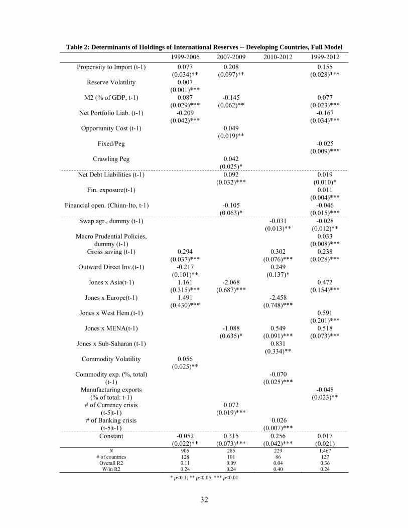
32

Table 2: Determinants of Holdings of International Reserves -- Developing Countries, Full Model

1999-2006 2007-2009 2010-2012 1999-2012

Propensity to Import (t-1) 0.077 0.208 0.155 (0.034)** (0.097)** (0.028)***

Reserve Volatility 0.007 (0.001)***

M2 (% of GDP, t-1) 0.087 -0.145 0.077 (0.029)*** (0.062)** (0.023)***

Net Portfolio Liab. (t-1) -0.209 -0.167 (0.042)*** (0.034)***

Opportunity Cost (t-1) 0.049 (0.019)**

Fixed/Peg -0.025 (0.009)***

Crawling Peg 0.042 (0.025)*

Net Debt Liabilities (t-1) 0.092 0.019 (0.032)*** (0.010)*

Fin. exposure(t-1) 0.011 (0.004)***

Financial open. (Chinn-Ito, t-1) -0.105 -0.046 (0.063)* (0.015)***

Swap agr., dummy (t-1) -0.031 -0.028 (0.013)** (0.012)**

Macro Prudential Policies, 0.033 dummy (t-1) (0.008)***

Gross saving (t-1) 0.294 0.302 0.238 (0.037)*** (0.076)*** (0.028)***

Outward Direct Inv.(t-1) -0.217 0.249 (0.101)** (0.137)*

Jones x Asia(t-1) 1.161 -2.068 0.472 (0.315)*** (0.687)*** (0.154)***

Jones x Europe(t-1) 1.491 -2.458 (0.430)*** (0.748)***

Jones x West Hem.(t-1) 0.591 (0.201)***

Jones x MENA(t-1) -1.088 0.549 0.518 (0.635)* (0.091)*** (0.073)***

Jones x Sub-Saharan (t-1) 0.831 (0.334)**

Commodity Volatility 0.056 (0.025)**

Commodity exp. (%, total) -0.070 (t-1) (0.025)***

Manufacturing exports -0.048 (% of total: t-1) (0.023)**

# of Currency crisis 0.072 (t-5|t-1) (0.019)***

# of Banking crisis -0.026 (t-5|t-1) (0.007)*** Constant -0.052 0.315 0.256 0.017

(0.022)** (0.073)*** (0.042)*** (0.021) N 905 285 229 1,467

# of countries 128 101 86 127 Overall R2 0.11 0.09 0.04 0.36 W/in R2 0.24 0.24 0.40 0.24

* p<0.1; ** p<0.05; *** p<0.01

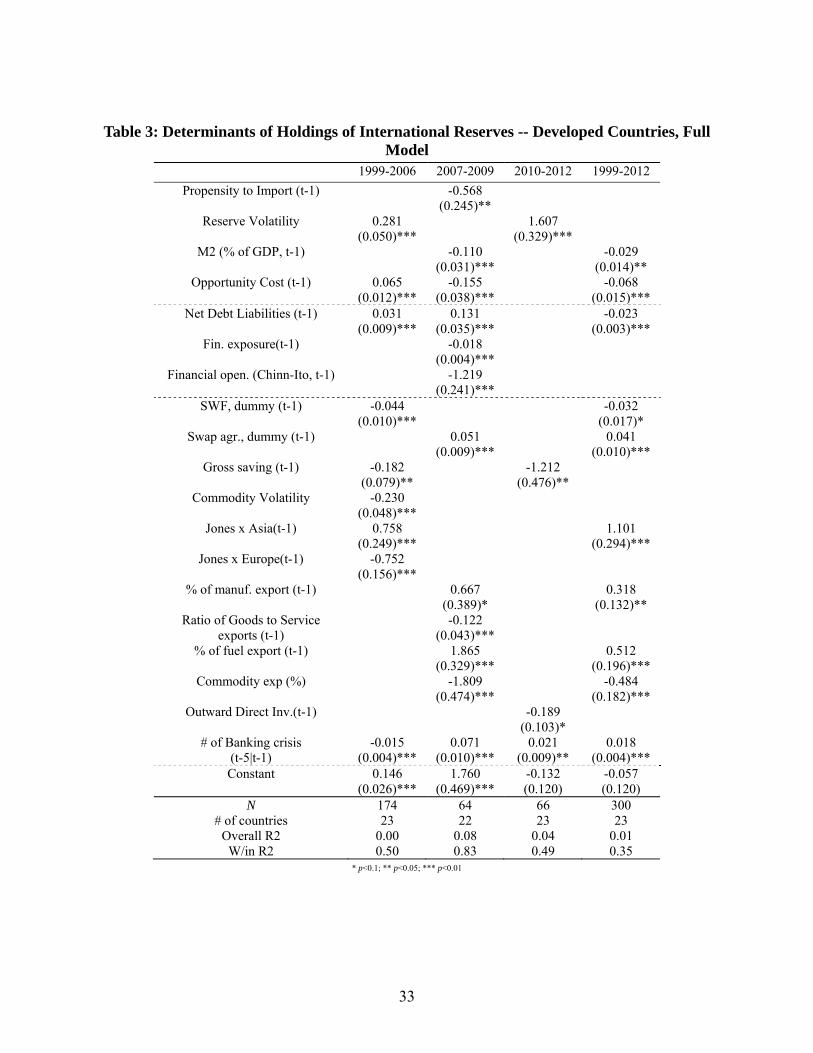
33

Table 3: Determinants of Holdings of International Reserves -- Developed Countries, Full Model

1999-2006 2007-2009 2010-2012 1999-2012

Propensity to Import (t-1) -0.568 (0.245)**

Reserve Volatility 0.281 1.607 (0.050)*** (0.329)***

M2 (% of GDP, t-1) -0.110 -0.029 (0.031)*** (0.014)**

Opportunity Cost (t-1) 0.065 -0.155 -0.068 (0.012)*** (0.038)*** (0.015)***

Net Debt Liabilities (t-1) 0.031 0.131 -0.023 (0.009)*** (0.035)*** (0.003)***

Fin. exposure(t-1) -0.018 (0.004)***

Financial open. (Chinn-Ito, t-1) -1.219 (0.241)***

SWF, dummy (t-1) -0.044 -0.032 (0.010)*** (0.017)*

Swap agr., dummy (t-1) 0.051 0.041 (0.009)*** (0.010)***

Gross saving (t-1) -0.182 -1.212 (0.079)** (0.476)**

Commodity Volatility -0.230 (0.048)***

Jones x Asia(t-1) 0.758 1.101 (0.249)*** (0.294)***

Jones x Europe(t-1) -0.752 (0.156)***

% of manuf. export (t-1) 0.667 0.318 (0.389)* (0.132)**

Ratio of Goods to Service -0.122 exports (t-1) (0.043)***

% of fuel export (t-1) 1.865 0.512 (0.329)*** (0.196)***

Commodity exp (%) -1.809 -0.484 (0.474)*** (0.182)***

Outward Direct Inv.(t-1) -0.189 (0.103)*

# of Banking crisis -0.015 0.071 0.021 0.018 (t-5|t-1) (0.004)*** (0.010)*** (0.009)** (0.004)*** Constant 0.146 1.760 -0.132 -0.057

(0.026)*** (0.469)*** (0.120) (0.120) N 174 64 66 300

# of countries 23 22 23 23 Overall R2 0.00 0.08 0.04 0.01 W/in R2 0.50 0.83 0.49 0.35

* p<0.1; ** p<0.05; *** p<0.01

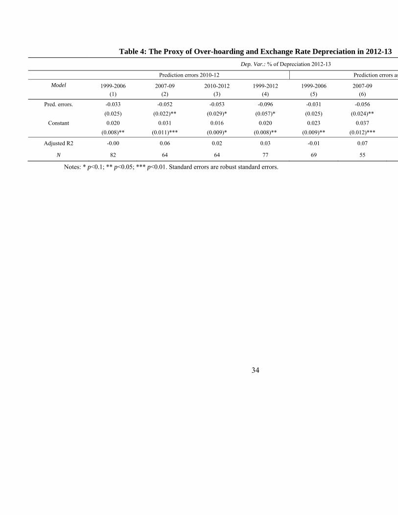
34

Table 4: The Proxy of Over-hoarding and Exchange Rate Depreciation in 2012-13

Dep. Var.: % of Depreciation 2012-13

Prediction errors 2010-12 Prediction errors as

Model 1999-2006 2007-09 2010-2012 1999-2012 1999-2006 2007-09 2 (1) (2) (3) (4) (5) (6)

Pred. errors. -0.033 -0.052 -0.053 -0.096 -0.031 -0.056

(0.025) (0.022)** (0.029)* (0.057)* (0.025) (0.024)**

Constant 0.020 0.031 0.016 0.020 0.023 0.037

(0.008)** (0.011)*** (0.009)* (0.008)** (0.009)** (0.012)***

Adjusted R2 -0.00 0.06 0.02 0.03 -0.01 0.07

N 82 64 64 77 69 55

Notes: * p<0.1; ** p<0.05; *** p<0.01. Standard errors are robust standard errors.

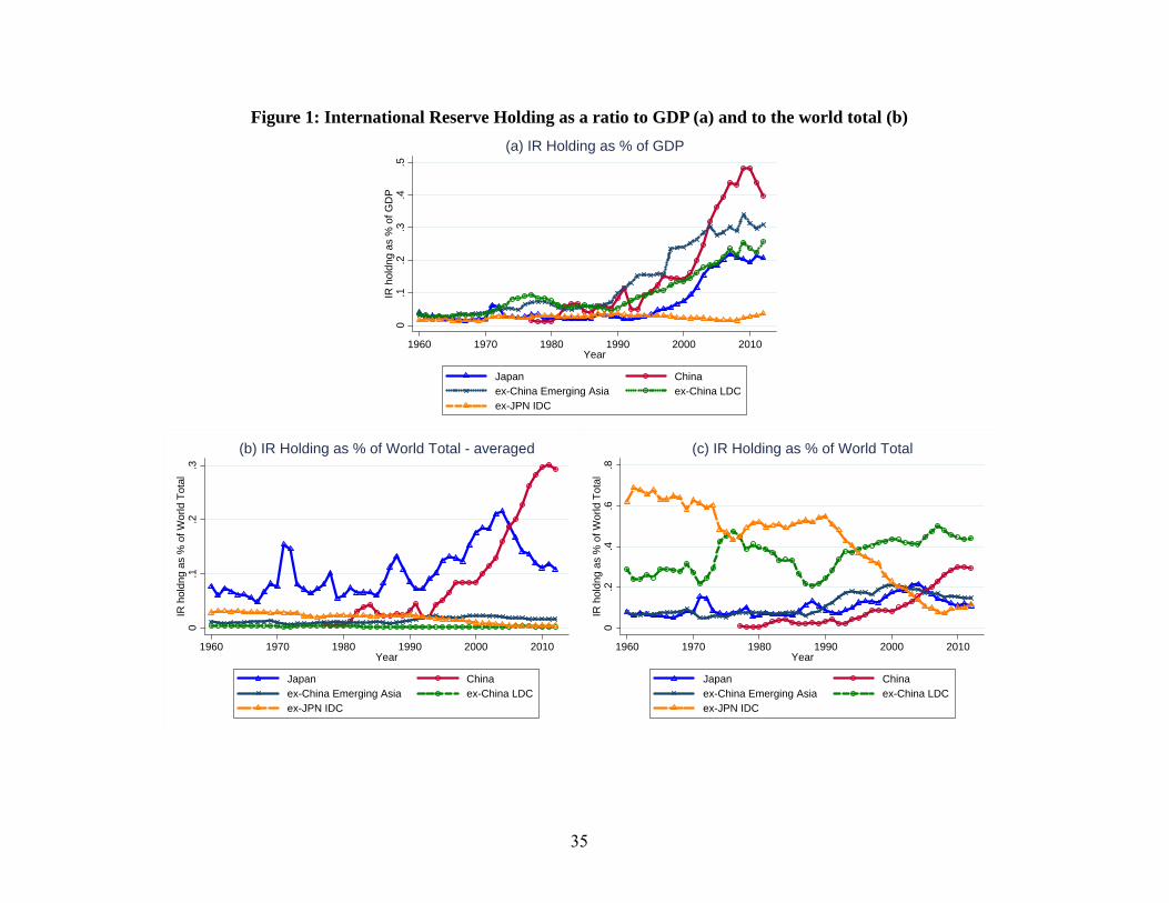
35

Figure 1: International Reserve Holding as a ratio to GDP (a) and to the world total (b)

0.1

.2.3

.4.5

IR h

oldn

g as

% o

f GD

P

1960 1970 1980 1990 2000 2010Year

Japan China ex-China Emerging Asia ex-China LDC ex-JPN IDC

(a) IR Holding as % of GDP

0.1

.2.3

IR h

oldn

g as

% o

f Wor

ld T

otal

1960 1970 1980 1990 2000 2010Year


(b) IR Holding as % of World Total - averaged

0.2

.4.6

.8IR

hol

dng

as %

of W

orld

Tot

al

1960 1970 1980 1990 2000 2010Year


(c) IR Holding as % of World Total

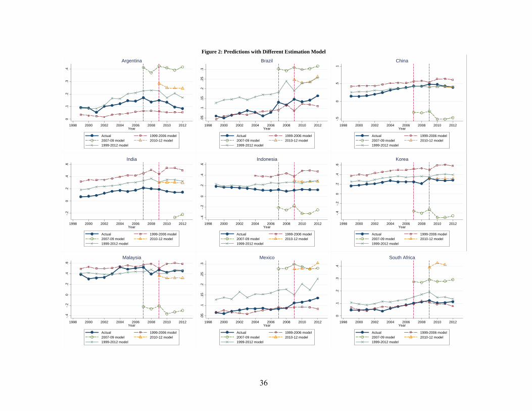
36

Figure 2: Predictions with Different Estimation Model

0.1

.2.3

.4

1998 2000 2002 2004 2006 2008 2010 2012Year

Actual 1999-2006 model 2007-09 model 2010-12 model 1999-2012 model

Argentina

.05

.1.1

5.2

.25

.3

1998 2000 2002 2004 2006 2008 2010 2012Year


Brazil

-.50

.51

1998 2000 2002 2004 2006 2008 2010 2012Year


China

-.20

.2.4

.6

1998 2000 2002 2004 2006 2008 2010 2012Year


India

-.4-.2

0.2

.4.6

1998 2000 2002 2004 2006 2008 2010 2012Year


Indonesia

-.4-.2

0.2

.4.6

1998 2000 2002 2004 2006 2008 2010 2012Year


Korea

-.4-.2

0.2

.4.6

1998 2000 2002 2004 2006 2008 2010 2012Year


Malaysia

.05

.1.1

5.2

.25

.3

1998 2000 2002 2004 2006 2008 2010 2012Year


Mexico

0.1

.2.3

.4

1998 2000 2002 2004 2006 2008 2010 2012Year


South Africa

37

Figure 2-cont: Predictions with Different Estimation Model

-.10

.1.2

.3.4

1998 2000 2002 2004 2006 2008 2010 2012Year


Turkey

-.4-.2

0.2

.4.6

1998 2000 2002 2004 2006 2008 2010 2012Year


Thailand

-.4-.2

0.2

.4.6

1998 2000 2002 2004 2006 2008 2010 2012Year


ex-China Developing East Asia

0.1

.2.3

.4

1998 2000 2002 2004 2006 2008 2010 2012Year


Latin America

.05

.1.1

5.2

.25

.3

1998 2000 2002 2004 2006 2008 2010 2012Year


Emerging Market Economies

38

Figure 3: Over-hoarding and Exchange Rate Depreciation

(a) 1999-2006 model (b) 2007-09 model

Argentina

Brazil

ChileColombia

Mexico

Venezuela

Jamaica

Trinidad and TobagoHong Kong

Indonesia

Korea, Rep.

MalaysiaPhilippines SingaporeThailandChina

-.10

.1.2

.3.4

.5%

dep

reci

atio

n of

exc

h. ra

te

-.4 -.2 0 .2 .4 .6 .8 1 1.2 1.4 1.6Pred. errors, 2010-12

Based on the 1999-2006 estimation w/out Fixed Effects

Pred. errors vs. % Depreciation of exch. rate

Argentina

Brazil

ChileColombia

Mexico

Venezuela

Jamaica

Trinidad and Tobago Hong Kong

Indonesia

Korea, Rep.


-.10

.1.2

.3.4

.5%

dep

reci

atio

n of

exc

h. ra

te

-.4 -.2 0 .2 .4 .6 .8 1 1.2 1.4 1.6Pred. errors, 2010-12



(c) 2010-12 model (d) 1999-2012 model

Argentina

Brazil

ChileColombia

Mexico

Venezuela

Jamaica

Hong Kong

Indonesia

Korea, Rep.


-.10

.1.2

.3.4

.5%

dep

reci

atio

n of

exc

h. ra

te

-.4 -.2 0 .2 .4 .6 .8 1 1.2 1.4 1.6Pred. errors, 2010-12



Argentina

Brazil

ChileColombia

Mexico

Venezuela

Jamaica

Trinidad and TobagoHong Kong

Indonesia

Korea, Rep.


-.10

.1.2

.3.4

.5%

dep

reci

atio

n of

exc

h. ra

te

-.4 -.2 0 .2 .4 .6 .8 1 1.2 1.4 1.6Pred. errors, 2010-12



abstract - university of southern california

Documents