ABSTRACT

Title of dissertation: VIDEO PROCESSING WITHADDITIONAL INFORMATION

Mahesh Ramachandran, Doctor of Philosophy, 2010

Dissertation directed by: Professor Rama ChellappaDepartment of Electrical and Computer Engineering

Cameras are frequently deployed along with many additionalsensors in aerial and

ground-based platforms. Many video datasets have metadatacontaining measurements

from inertial sensors, GPS units, etc. Hence the development of better video processing

algorithms using additional information attains special significance.

We first describe an intensity-based algorithm for stabilizing low resolution and low

quality aerial videos. The primary contribution is the ideaof minimizing the discrepancy

in the intensity of selected pixels between two images. Thisis an application of inverse

compositional alignment for registering images of low resolution and low quality, for

which minimizing the intensity difference over salient pixels with high gradients results

in faster and better convergence than when using all the pixels.

Secondly, we describe a feature-based method for stabilization of aerial videos and

segmentation of small moving objects. We use the coherency of background motion

to jointly track features through the sequence. This enables accurate tracking of large

numbers of features in the presence of repetitive texture, lack of well conditioned feature

windows etc. We incorporate the segmentation problem within the joint feature tracking

framework and propose the first combined joint-tracking andsegmentation algorithm.

The proposed approach enables highly accurate tracking, and segmentation of feature

tracks that is used in a MAP-MRF framework for obtaining dense pixelwise labeling of

the scene. We demonstrate competitive moving object detection in challenging video

sequences of the VIVID dataset containing moving vehicles and humans that are small

enough to cause background subtraction approaches to fail.

Structure from Motion (SfM) has matured to a stage, where theemphasis is on

developing fast, scalable and robust algorithms for large reconstruction problems. The

availability of additional sensors such as inertial units and GPS along with video cameras

motivate the development of SfM algorithms that leverage these additional measurements.

In the third part, we study the benefits of the availability ofa specific form of additional

information - the vertical direction (gravity) and the height of the camera both of which

can be conveniently measured using inertial sensors, and a monocular video sequence for

3D urban modeling. We show that in the presence of this information, the SfM equations

can be rewritten in a bilinear form. This allows us to derive afast, robust, and scalable

SfM algorithm for large scale applications. The proposed SfM algorithm is experimen-

tally demonstrated to have favorable properties compared to the sparse bundle adjustment

algorithm. We provide experimental evidence indicating that the proposed algorithm con-

verges in many cases to solutions with lower error than state-of-art implementations of

bundle adjustment. We also demonstrate that for the case of large reconstruction prob-

lems, the proposed algorithm takes lesser time to reach its solution compared to bundle

adjustment. We also present SfM results using our algorithmon the Google StreetView

research dataset, and several other datasets.

VIDEO PROCESSING WITH ADDITIONAL INFORMATION

by

Mahesh Ramachandran

Dissertation submitted to the Faculty of the Graduate School of theUniversity of Maryland, College Park in partial fulfillment

of the requirements for the degree ofDoctor of Philosophy

2010

Advisory Committee:Professor Rama Chellappa, Chair/AdvisorProfessor Ankur SrivastavaProfessor Richard LaProfessor David JacobsProfessor Min Wu

c© Copyright byMahesh Ramachandran

2010

I dedicate this dissertation to my parents

and my grandfather, Mr. P. P. Iyer.

ii

Acknowledgments

I am deeply indebted to my advisor, Prof. Rama Chellappa, forbeing a constant

source of support, guidance and funding through my doctoralstudies. Through these

years, I am lucky to have worked with Prof. Chellappa whom I have always deeply

admired. He believed in me and my potential through so many tough times that helped

me gain confidence to wade through rough waters and finally reach the destination. I

had more than a fair share of problems towards the start of my Ph.D, and his continued

support helped me get over them. Around the beginning of my doctoral studies, I had

concentration and memory problems linked to a deficit of attention, and I had to seek

professional and medical help. This particularly rough time, soon after I had stepped into

a new country made me wonder if I had made the right choice. My decision to fight on and

a never-say-die attitude was one of the best decisions I havemade, and the culmination

of my efforts, resulting in my PhD, would not have happened without Prof. Chellappa’s

encouragement and dissertation advise.

I would also like to thank medical doctors Dr. Krishnamoorthy Srinivas (India),

Dr. Joseph Marnell, Dr. Punja Sudhakar, and Dr. David Granite for helping me get

through the problems with my concentration. I was much better off with their advise and

treatment.

I specially thank Ashok for his collaboration and support through my doctoral stud-

ies. He helped me as a friend and as a collaborator, and I am really grateful for everything

I have learnt from him. My close interactions with him helpedme look at problems from

various points of view and sharpen my problem solving approach. I admire his clear

iii

thought process and his novel approach to research problems.

I thank my committee members, Prof. David Jacobs, Prof. Ankur Srivastava, Prof.

Min Wu and Prof. Richard La for their comments and questions about my dissertation

work, which helped me look at my work from various viewpoints.

I am fortunate to have spent my graduate school years with three exceptional friends,

Ashwin, Krishna and Aswin, whom I have known from my time at IIT Madras. They

were extremely supportive and helpful through my PhD studies. Special thanks to Ash-

win (whom I have known from high school) for being my roommateall through graduate

school. I have benefitted immensely through my brainstorming sessions with Ashwin and

Aswin while at UMD.

I thank all the members in CFAR who helped me directly or indirectly. Aravind was

particularly helpful with his sound advise. Thanks to Kaushik for being always available

to bounce ideas. I also thank Jagan, Kevin, Jian Li, Jie Shao,Zhanfeng, Yang, James,

Narayanan, Gaurav, Soma, Hao, Pavan, Dikpal, Mohammad, Seong-Wook, Sima, Jai,

Ming, Ming-Yu, Vishal for helping me on various occasions.

My friends at Greenbelt made my stay enjoyable and gave me good company off

work hours. Ashwin, Sebastian, Ranjit, Rajesh, Alankar were a great group to hang out

with and I have shared many memorable times with them. I also enjoyed being house-

mates with Sidharth and Sowmitra at various times.

This dissertation would not have been possible without the constant and unending

support of my family. I have been fortunate to have a family who always believed in me

and encouraged me in my pursuit of excellence. My love and gratitude to my parents,

Ramachandran (appa) and Girija (ammma), my kid brother Ganesh, my cousins Anusha,

iv

Arvind and Ravi, Naganathan chittappa and Radha chitti, my grandfathers P.P.Iyer (ap-

pappa) and Ganapati (sugar thatha) and grandmother Thailambal thathi. I also thank Dr.

Ramani Ramchandran and Ashley Skinner for being there whenever I needed them, dur-

ing the initial years of my graduate life. I have always enjoyed the thanksgiving parties

they organized at their home, to which I was invited by default.

I dedicate this dissertation to my parents and my grandfather, Mr. P. P. Iyer. Ap-

pappa (which in tamil means father’s father) was my role model through my childhood

years and was instrumental in my development and education.He was a great man and a

true visionary.

v

Table of Contents

List of Figures viii

List of Abbreviations xv

1 Introduction 11.1 Video Stabilization . . . . . . . . . . . . . . . . . . . . . . . . . . . . . 31.2 Structure from Motion . . . . . . . . . . . . . . . . . . . . . . . . . . . 41.3 Contributions . . . . . . . . . . . . . . . . . . . . . . . . . . . . . . . . 51.4 Outline . . . . . . . . . . . . . . . . . . . . . . . . . . . . . . . . . . . 7

2 Background and Prior Art 102.1 Background . . . . . . . . . . . . . . . . . . . . . . . . . . . . . . . . . 10

2.1.1 Camera Model . . . . . . . . . . . . . . . . . . . . . . . . . . . 102.1.2 Effect of Camera Motion . . . . . . . . . . . . . . . . . . . . . . 122.1.3 Image features . . . . . . . . . . . . . . . . . . . . . . . . . . . 132.1.4 Structure from Motion . . . . . . . . . . . . . . . . . . . . . . . 152.1.5 Feature based algorithms . . . . . . . . . . . . . . . . . . . . . . 17

2.2 Related work . . . . . . . . . . . . . . . . . . . . . . . . . . . . . . . . 182.2.1 Video Stabilization . . . . . . . . . . . . . . . . . . . . . . . . . 182.2.2 Video Mosaicking . . . . . . . . . . . . . . . . . . . . . . . . . 212.2.3 Structure from Motion . . . . . . . . . . . . . . . . . . . . . . . 22

3 Intensity-based Video Stabilization 283.1 Intensity-based alignment . . . . . . . . . . . . . . . . . . . . . . . .. . 28

3.1.1 Effect of region of registration . . . . . . . . . . . . . . . . . .. 303.1.2 Experiments . . . . . . . . . . . . . . . . . . . . . . . . . . . . 31

3.2 Video Mosaicking . . . . . . . . . . . . . . . . . . . . . . . . . . . . . . 333.2.1 Results . . . . . . . . . . . . . . . . . . . . . . . . . . . . . . . 35

4 Feature-based Stabilization and Motion Segmentation 384.1 Feature-based Image Registration . . . . . . . . . . . . . . . . . .. . . 38

4.1.1 Shortcomings of KLT tracking and background subtraction . . . . 384.1.2 Joint tracking . . . . . . . . . . . . . . . . . . . . . . . . . . . . 414.1.3 Robustness . . . . . . . . . . . . . . . . . . . . . . . . . . . . . 424.1.4 Segmentation . . . . . . . . . . . . . . . . . . . . . . . . . . . . 444.1.5 Joint Tracking and Segmentation Algorithm . . . . . . . . .. . . 46

4.1.5.1 Motion estimation . . . . . . . . . . . . . . . . . . . . 464.1.5.2 Membership probability estimation . . . . . . . . . . . 46

4.1.6 Initialization and Implementation . . . . . . . . . . . . . . .. . 484.1.7 Dense Segmentation . . . . . . . . . . . . . . . . . . . . . . . . 50

4.2 Experiments . . . . . . . . . . . . . . . . . . . . . . . . . . . . . . . . . 514.2.1 Metadata . . . . . . . . . . . . . . . . . . . . . . . . . . . . . . 514.2.2 Video sequence 1 . . . . . . . . . . . . . . . . . . . . . . . . . . 54

vi

4.2.3 Video sequence 2 . . . . . . . . . . . . . . . . . . . . . . . . . . 574.2.4 Video sequence 3 . . . . . . . . . . . . . . . . . . . . . . . . . . 60

4.3 Conclusions . . . . . . . . . . . . . . . . . . . . . . . . . . . . . . . . . 61

5 Fast Bilinear Structure from Motion 645.1 Problem Formulation . . . . . . . . . . . . . . . . . . . . . . . . . . . . 665.2 Fast Bilinear Estimation of SfM . . . . . . . . . . . . . . . . . . . . .. 73

5.2.1 Structure Iterations . . . . . . . . . . . . . . . . . . . . . . . . . 735.2.2 Motion Iterations . . . . . . . . . . . . . . . . . . . . . . . . . . 745.2.3 Out-of-plane motion refinement iterations . . . . . . . . .. . . . 765.2.4 Motion Estimation for Moving Objects . . . . . . . . . . . . . .77

5.3 Analysis of FBSFM . . . . . . . . . . . . . . . . . . . . . . . . . . . . . 795.3.1 Computational Complexity and Memory Requirements . .. . . . 795.3.2 Discussion . . . . . . . . . . . . . . . . . . . . . . . . . . . . . 80

5.4 Simulations . . . . . . . . . . . . . . . . . . . . . . . . . . . . . . . . . 825.4.1 Implementation . . . . . . . . . . . . . . . . . . . . . . . . . . . 825.4.2 Reconstruction problem generation . . . . . . . . . . . . . . .. 835.4.3 SfM Initialization . . . . . . . . . . . . . . . . . . . . . . . . . . 845.4.4 Comparative evaluation of bilinear alternation . . . .. . . . . . . 855.4.5 Comparison of FBSfM with SBA . . . . . . . . . . . . . . . . . 895.4.6 Comparison of convergence rates of FBSfM and SBA . . . . .. 925.4.7 Comparison with Linear multiview reconstruction andSBA . . . 95

5.4.7.1 Results with accurate calibration . . . . . . . . . . . . 965.4.7.2 Results with inaccurate calibration . . . . . . . . . . . 97

5.4.8 A note on alternation methods . . . . . . . . . . . . . . . . . . . 975.5 Experiments . . . . . . . . . . . . . . . . . . . . . . . . . . . . . . . . . 102

5.5.1 Experiments on an Indoor Handheld Sequence . . . . . . . . .. 1025.5.2 SfM on StreetView data . . . . . . . . . . . . . . . . . . . . . . 1045.5.3 SfM on Static Points in Aerial Video - 1 . . . . . . . . . . . . . .1105.5.4 SfM on Moving Objects in Aerial Video - 2 . . . . . . . . . . . . 111

5.6 Discussion and Conclusions . . . . . . . . . . . . . . . . . . . . . . . .112

6 Conclusions and Future Research Directions 1146.1 Summary . . . . . . . . . . . . . . . . . . . . . . . . . . . . . . . . . . 1146.2 Future work . . . . . . . . . . . . . . . . . . . . . . . . . . . . . . . . . 115

A Proofs of convergence 117

B Decomposition of homographies to obtain additional information 120

Bibliography 122

vii

List of Figures

1.1 The figure shows illustrations of the problem domains where our work isapplicable. Figure (1.1(a)) shows an image of a car with a setof camerasattached to the mount on top, collecting image sequences of the urbanscene. Figure (1.1(b)) shows a helicopter sensing the environment withcameras, IMUs and other sensors. Figure (1.1(c)) illustrates a UAV sur-veying the ground plane from a high altitude. These images were down-loaded from [1]. In all these cases, we have available additional informa-tion along with the sequences that can be used in our algorithmic framework. 6

1.2 An illustration of the pipelined video system developedas part of thework presented in this dissertation. . . . . . . . . . . . . . . . . . . .. . 6

2.1 3D imaging geometry. . . . . . . . . . . . . . . . . . . . . . . . . . . . 11

3.1 A plot of the number of iterations taken for convergence versus the stan-dard deviation of image pixel noise for different fractionsof number ofpixels used in the registration. As the number of salient pixels used forregistration decreases, the number of iterations used for convergence de-creases too. . . . . . . . . . . . . . . . . . . . . . . . . . . . . . . . . . 33

3.2 A plot of the geometric error versus the standard deviation of image pixelnoise for various ratios of salient pixels used in registration. For varioussaliency rations, accuracy of registration is almost similar. In some casesthe accuracy of registration is greater for lesser number ofpixels used. . . 33

3.3 This figure shows a mosaic of a sequence obtained by registering the im-ages of a sequence using the intensity-based stabilizationalgorithm. Ap-proximately30% of the pixels in each image were used for the purposeof registration. . . . . . . . . . . . . . . . . . . . . . . . . . . . . . . . . 36

3.4 This figure shows a mosaic of another sequence obtained byregisteringthe images using the intensity-based stabilization algorithm. Approxi-mately 30% of the pixels in each image were used for the purpose ofregistration. . . . . . . . . . . . . . . . . . . . . . . . . . . . . . . . . . 36

3.5 Figure 3.5(a) shows a sample image of a sequence capturedfrom an aerialplatform. The resolution is230 × 310 pixels. We use our algorithm tobuild a mosaic of the sequence. The regions of the image selected by ouralgorithm for minimizing the image difference error with the mosaic isshown in Figure 3.5(b). Note that these regions contribute the most to ourperception of image motion. . . . . . . . . . . . . . . . . . . . . . . . . 37

viii

4.1 This figure illustrates the failure of KLT feature tracking method. Fig-ure 4.1(a) shows an image with overlaid features. The red points areclassified to be on the background and blue points are classified to be onthe foreground. Ideally, blue points must be restricted to moving vehiclefeatures. Note the large number of blue points on the background indicat-ing misclassifications. Figure 4.1(b) shows an image with boxes overlaidon top, indicating detected moving blobs after a backgroundsubtractionalgorithm was applied on registered images. Notice the number of falselydetected moving objects. The underlying video sequence wasvery wellstabilized upon evaluation by a human observer, but outlierpixels nearedges show up as moving pixels in background subtraction. . .. . . . . . 40

4.2 This figure plots the estimated Y-displacement between two images es-timated by jointly tracking features with and without usingrobust lossfunctions. The red-curve plots the estimated displacementusing a sum-of-squares cost function (similar to traditional KLT). Theblue line showsthe ground-truth displacement and the green-curve shows the estimateddisplacement obtained by using robust loss-functions. . . .. . . . . . . . 44

4.3 This figure shows the distribution of feature dissimilarities produced bythe background model parameters for features lying on the background(inliers) and those on moving objects (outliers). The red curve plots thedistribution of dissimilarity for inliers and the blue curve plots the distri-bution for outliers. These distributions are obtained using the data-drivenapproach described in the text, and are empirically found tobe closest tothe lognormal distribution. . . . . . . . . . . . . . . . . . . . . . . . . . 48

4.4 This figure qualitatively compares the mosaics obtainedby stabilizing theoriginal sequence using a homography model and the fronto-parallel se-quence using a translation model. Figure (a) shows the mosaic obtainedusing the translation model. It is one part of a long mosaic ofaround550 frames. Figure (b) shows the mosaic obtained using the homographymodel. The distortion is clear towards the right side of the mosaic becauseof the gradual build up of errors in homography estimation. .. . . . . . . 53

ix

4.5 This figure shows results on four frames of the 100 frame long VIVIDVideo Sequence 1. Column (a) shows results on frame 14, column (b)shows results on frame 23, column (c) shows results on frame 50 and col-umn (d) shows results on frame 92. The top row in each column overlaysthe feature points tracked on each frame. The blue points areclassified tobe on the background and the red points are classified to be on the movingobjects. As the figures illustrate, the segmentation is veryaccurate and ismuch better than individual KLT tracking followed by RANSACbasedbackground feature selection. The middle row in each columnillustratesthe dense segmentations inferred from the feature segmentations. Thebackground and moving objects are plotted on different color channelsfor illustration. The bottom row in each column illustratesthe trackedboxes on the images which is the result of a blob tracking algorithm [2].Column (c) shows the only feature on the background which is misclassi-fied to be on the foreground. There is a false moving target initializationdue to this feature but this is quickly removed by the algorithm. . . . . . . 56

4.6 This figure shows the mosaic of 100 frames of the VIVID sequence 1.The moving objects are removed from the individual frames before mo-saicking. The absence of moving object trails on the mosaic illustratesthe accuracy of motion segmentation in this sequence. . . . . .. . . . . . 57

4.7 This figure shows results on four frames of the 190 frame long VIVIDVideo Sequence 2. Column (a) shows results on frame 1, column(b)shows results on frame 24, column (c) shows results on frame 91 andcolumn (d) shows results on frame 175. The top row in each columnoverlays the feature points tracked on each frame. The blue points areclassified to be on the background and the red points are classified to beon the moving objects. As the figures illustrate, the segmentation is veryaccurate and is much better than the results from individualKLT trackingfollowed by RANSAC-based background feature selection. The middlerow in each column illustrates the dense segmentations inferred from thefeature segmentations. The background and moving objects are plotted ondifferent color channels for illustration. The bottom row in each columnillustrates the tracked boxes on the images which is the result of a blobtracking algorithm [2]. Column (b) shows a feature on a stationary vehiclewhich is misclassified to be a a moving feature due to parallax-inducedmotion. . . . . . . . . . . . . . . . . . . . . . . . . . . . . . . . . . . . 59

4.8 This figure shows the mosaic of 190 frames of the VIVID sequence 2.The moving objects are removed from the individual frames before mo-saicking. The absence of moving object trails on the mosaic illustratesthe accuracy of motion segmentation in this sequence. . . . . .. . . . . . 60

x

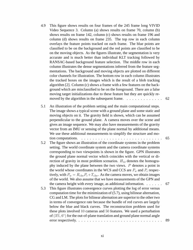
4.9 This figure shows results on four frames of the 245 frame long VIVIDVideo Sequence 3. Column (a) shows results on frame 70, column (b)shows results on frame 142, column (c) shows results on frame196 andcolumn (d) shows results on frame 235. The top row in each columnoverlays the feature points tracked on each frame. The blue points areclassified to be on the background and the red points are classified to beon the moving objects. As the figures illustrate, the segmentation is veryaccurate and is much better than individual KLT tracking followed byRANSAC-based background feature selection. The middle rowin eachcolumn illustrates the dense segmentations inferred from the feature seg-mentations. The background and moving objects are plotted on differentcolor channels for illustration. The bottom row in each column illustratesthe tracked boxes on the images which is the result of a blob trackingalgorithm [2]. Column (c) shows a frame with a few features onthe back-ground which are misclassified to be on the foreground. Thereare a falsemoving target initializations due to these feature but theyare quickly re-moved by the algorithm in the subsequent frame. . . . . . . . . . . .. . 62

5.1 An illustration of the problem setting and the main computational steps.The image shows a typical scene with a ground plane and some static andmoving objects on it. The gravity field is shown, which can be assumedperpendicular to the ground plane. A camera moves over the scene andgives an image sequence. We may also have measurements of thegravityvector from an IMU or sensing of the plane normal by additional means.We use these additional measurements to simplify the structure and mo-tion computations. . . . . . . . . . . . . . . . . . . . . . . . . . . . . . 65

5.2 The figure shows an illustration of the coordinate systems in the problemsetting. The world coordinate system and the camera coordinate systemscorresponding to two viewpoints is shown in the figure. GPN illustratesthe ground plane normal vector which coincides with the vertical or di-rection of gravity in most problem scenarios.H12 denotes the homogra-phy induced by the plane between the two views.P denotes a point inthe world whose coordinates in the WCS and CCS arePw andPc respec-tively, withPw = Rc2wPc+Tc2w. As the camera moves, we obtain imagesof the world. We also assume that we have measurements of the GPN andthe camera height with every image, as additional information. . . . . . . 67

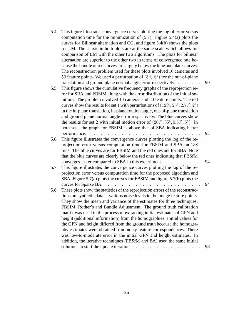
5.3 This figure illustrates convergence curves plotting thelog of error versuscomputation time for the minimization of (5.7), using bilinear alternation,CG and LM. The plots for bilinear alternation are superior tothe other twoin terms of convergence rate because the bundle of red curvesare largelybelow the blue and black curves. The reconstruction problemused forthese plots involved10 cameras and50 features. We used a perturbationof (3%, 6) for the out-of-plane translation and ground plane normal angleerror respectively. . . . . . . . . . . . . . . . . . . . . . . . . . . . . . . 89

xi

5.4 This figure illustrates convergence curves plotting thelog of error versuscomputation time for the minimization of (5.7). Figure 5.4(a) plots thecurves for Bilinear alternation and CG, and figure 5.4(b) shows the plotsfor LM. The x axis in both plots are at the same scale which allows forcomparison of LM with the other two algorithms. The plots forbilinearalternation are superior to the other two in terms of convergence rate be-cause the bundle of red curves are largely below the blue and black curves.The reconstruction problem used for these plots involved10 cameras and50 feature points. We used a perturbation of(3%, 6) for the out-of-planetranslation and ground plane normal angle error respectively. . . . . . . . 90

5.5 This figure shows the cumulative frequency graphs of the reprojection er-ror for SBA and FBSfM along with the error distribution of theinitial so-lutions. The problem involved10 cameras and50 feature points. The redcurves show the results for set 1 with perturbations of(12%, 25, 2.7%, 2)in the in-plane translation, in-plane rotaion angle, out-of-plane translationand ground plane normal angle error respectively. The blue curves showthe results for set 2 with initial motion error of(20%, 35, 0.5%, 5). Inboth sets, the graph for FBSfM is above that of SBA indicatingbetterperformance. . . . . . . . . . . . . . . . . . . . . . . . . . . . . . . . . 92

5.6 This figure illustrates the convergence curves plottingthe log of the re-projection error versus computation time for FBSfM and SBA on 138runs. The blue curves are for FBSfM and the red ones are for SBA. Notethat the blue curves are clearly below the red ones indicating that FBSfMconverges faster compared to SBA in this experiment. . . . . . .. . . . . 94

5.7 This figure illustrates the convergence curves plottingthe log of the re-projection error versus computation time for the proposed algorithm andSBA. Figure 5.7(a) plots the curves for FBSfM and figure 5.7(b) plots thecurves for Sparse BA. . . . . . . . . . . . . . . . . . . . . . . . . . . . . 94

5.8 These plots show the statistics of the reprojection errors of the reconstruc-tions on synthetic data at various noise levels in the image feature points.They show the mean and variance of the estimates for three techniques:FBSfM, Rother’s and Bundle Adjustment. The ground truth calibrationmatrix was used in the process of extracting initial estimates of GPN andheight (additional information) from the homographies. Initial values forthe GPN and height differed from the ground truth because thehomogra-phy estimates were obtained from noisy feature correspondences. Therewas low-to-moderate error in the initial GPN and height estimates. Inaddition, the iterative techniques (FBSfM and BA) used the same initialsolutions to start the update iterations. . . . . . . . . . . . . . . .. . . . 98

xii

5.9 These plots show the statistics of the reprojection errors of the reconstruc-tions on synthetic data at various noise levels in the image feature points.They show the mean and variance of the estimates for three techniques:FBSfM, Rother’s and Bundle Adjustment. There was a large error (fromground truth) in the calibration matrix that was used in the process of ex-tracting initial estimates of GPN and height (additional information) fromthe homographies. Hence, this experiment serves as a case where eval-uation was performed with high levels of error in the GPN and heights(from ground truth). FBSfM and BA were started with the same initialsolution for the reconstruction. . . . . . . . . . . . . . . . . . . . . . .. 99

5.10 These plots illustrate the reprojection errors of the reconstructions onsynthetic data. The reconstruction errors are plotted for 70 different tri-als. There is a uniformly distributed noise level of±4 pixels in the im-age features for the plot 5.10(a) and a noise level of±8 pixels for theplot 5.10(b). They serve to give an idea of how the various methods per-form for repeated trials of the same experiment. Results forthree dif-ferent techniques are shown: FBSfM, Rother’s and Bundle Adjustment.The ground truth calibration matrix was used in the process of extract-ing initial estimates of GPN and height (additional information) from thehomographies. Hence, this experiment serves as a case whereevaluationwas performed with low to moderate levels of error in the GPN and heights.100

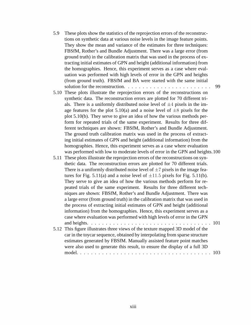
5.11 These plots illustrate the reprojection errors of the reconstructions on syn-thetic data. The reconstruction errors are plotted for 70 different trials.There is a uniformly distributed noise level of±7 pixels in the image fea-tures for Fig. 5.11(a) and a noise level of±11.5 pixels for Fig. 5.11(b).They serve to give an idea of how the various methods perform for re-peated trials of the same experiment. Results for three different tech-niques are shown: FBSfM, Rother’s and Bundle Adjustment. There wasa large error (from ground truth) in the calibration matrix that was used inthe process of extracting initial estimates of GPN and height (additionalinformation) from the homographies. Hence, this experiment serves as acase where evaluation was performed with high levels of error in the GPNand heights. . . . . . . . . . . . . . . . . . . . . . . . . . . . . . . . . . 101

5.12 This figure illustrates three views of the texture mapped 3D model of thecar in the toycar sequence, obtained by interpolating from sparse structureestimates generated by FBSfM. Manually assisted feature point matcheswere also used to generate this result, to ensure the displayof a full 3Dmodel. . . . . . . . . . . . . . . . . . . . . . . . . . . . . . . . . . . . . 103

xiii

5.13 This figure shows the top view of the reconstructed 3D points and thecamera path obtained by solving for structure and motion from 150 im-ages of the streetview sequence using the proposed algorithm. The redpoints show the camera centers and the green lines show the optical axisat each camera location. A few images in the sequence are shown in theleft of the figure. We can clearly distinguish the three intersecting roadsin the reconstruction, with the road in the middle approximately twice aswide as the other two roads. . . . . . . . . . . . . . . . . . . . . . . . . 105

5.14 This figure shows a texture mapped 3D model of the scene imaged in theStreetView sequence. Since the urban scene consists primarily of build-ings and other man-made structures, we fit several planes to the recon-structed 3D points. The textures for these planar patches were obtainedfrom the corresponding images, and these textures were applied to theplanar patches using the Blender 3D modeling tool. Novel views of thetexture-mapped model were rendered using the same tool. . . .. . . . . 106

5.15 This figure illustrates three different parts of the StreetView scene. Eachrow shows one particular facade present in the scene. The images in col-umn (a) show the original images from the sequence. The images in col-umn (b) show the synthesized images generated using the 3D model froma viewpoint that was similar to (a). The images in column (c) show thesynthesized images generated using the 3D model from a novelviewpointnot present in the original sequence. . . . . . . . . . . . . . . . . . . .. 107

5.16 This figure shows the trajectory of the camera in the StreetView sequenceobtained by solving for the SfM using our algorithm. The recovered tra-jectory was converted fro UTM coordinates to Latitude-longitude andoverlaid on the map in Google Earth. The trajectory reflects the pathtaken by the camera as inferred from the image sequences. Thecameramoves on the ’Smithfield Street’ in downtown Pittsburg. It starts from theintersection of Smithfield and1st avenue, goes past the intersection with’Blvd of the Allies’, and ends after the intersection with3rd avenue. . . . 108

5.17 This figure illustrates the convergence curves plotting the log of the re-projection error versus computation time for the proposed algorithm andSBA. Figure 5.7(a) plots the curves for FBSfM, and figure 5.7(b) plotsthe curves for Sparse BA. Figure 5.7(b) cuts off the time axisat1000 sec,however the maximum time taken was2140. . . . . . . . . . . . . . . . . 109

5.18 This figure illustrates the convergence curves plotting the log of the re-projection error versus computation time for FBSfM and SBA.The bluecurves are for FBSfM and the red ones are for SBA. The blue curves areclearly below the red ones indicating that FBSfM converges faster com-pared to SBA in this experiment. . . . . . . . . . . . . . . . . . . . . . . 110

5.19 Fig (5.19a) shows a snapshot of a moving car in the video sequence, withthe detected features shown in yellow dots. It also shows thereprojectedfeatures shown as green squares. Fig. (5.19b) shows the partially recon-structed 3D model of the car. . . . . . . . . . . . . . . . . . . . . . . . . 112

xiv

List of Abbreviations

3D 3 DimensionsBA Bundle AdjustmentCCS Camera Coordinate SystemCG Conjugate GradientFBSfM Fast Bilinear Structure from MotionGCT Global Convergence TheoremGPN Ground Plane NormalGPS Global Positioning SystemIMU Inertial Measurement UnitKLT Kanade Lucas TomasiLM Levenberg-MarquardtMAP Maximum A-PosterioriMAV Micro Air VehicleMRF Markov Random FieldRANSAC Random Sampling And ConsensusSBA Sparse Bundle AdjustmentSfM Structure from MotionSfPM Structure from Planar MotionSIFT Scale Invariant Feature TransformSLAM Simultaneous Localization and MappingSVD Singular Value DecompositionUAV Unmanned Air VehicleUTM Universal Transverse MercatorVIVID VIdeo Verification and IDentificationWCS World Coordinate System

xv

Chapter 1

Introduction

With advances in the development of Unmanned and Micro air vehicles, there is an

increasing need to process the video streams obtained from cameras on-board these aerial

platforms. Due to the erratic motion of these aerial platforms, robust stabilization of these

video sequences is an important video pre-processing task.In addition, acquisition of low-

resolution video sequences makes it necessary to mosaic thevideo sequences for better

visualization using a larger virtual field-of-view [3]. Generating mosaics of the scene

involves the detection and removal of moving object pixels,and hence robust moving

object detection becomes important.

Video stabilization refers to the compensation of the motion of pixels on the image

plane, when a video sequence is captured from a moving camera. Stabilization of a video

sequence is achieved by registering consecutive images of the sequence onto each other. A

parametric motion model such as an affine or homography modelis assumed for the image

sequence and the model parameters are estimated for every pair of consecutive frames

in the image sequence. The pairwise models are used to compute the transformations

registering each frame onto a global reference or mosaic.

Image registration is a widely researched topic in computervision, with applications

in mosaicing, medical imaging, motion detection, trackingetc. The two main approaches

for image registration are feature-based and intensity-based approaches. In the feature-

1

based approach, we identify corresponding image features (such as points and lines) in

an image sequence. Using these feature correspondences, wesolve for the motion pa-

rameters that register the images. In intensity-based approaches, we solve for the motion

parameters by minimizing the intensity difference betweenthe two images.

A video sequence acquired by an aerial platform consists of multiple moving targets

of interest moving in and out of the field-of-view of the camera. An important problem

involves the segmentation of the moving object pixels from the background. This is useful

both for mosaicing the background as well as moving target initialization for tracking. An

understanding of the motion of targets in video is necessaryfor several video inference

tasks such as activity analysis, video summarization etc.

Moving target pixels do not obey the solved background motion model after video

stabilization and do not register in consecutive frames. Moving targets are typically de-

tected by identifying the subset of pixels that are not aligned after video stabilization,

therefore motion detection results depend on the accuracy of video stabilization. Highly

accurate stabilization is extremely important for detecting small objects moving in similar

background texture.

Structure from Motion (SfM) refers to the task of recoveringthe 3D structure of a

scene and the motion of a camera from a video sequence. SfM hasbeen an active area

of research since Longuet-Higgins [4] eight-point algorithm. There have been several

different approaches to the SfM problem and we refer the reader to [5] and [6] for a

comprehensive survey of the various approaches.

2

1.1 Video Stabilization

Video stabilization refers to the compensation of the motion of pixels on the image

plane, when a video sequence is captured from a moving camera. Since several practical

applications just require video stabilization as opposed to complete estimation of camera

trajectory and scene structure, this is an important sub-problem that has received much

attention. Depending on the type of scenario and the type of motion involved, we have

different algorithms to achieve stabilization.

• Presence of a dominant plane in the scene:If a dominant plane is present, then we

can register all the frames using a planar perspective transformation (homography)

corresponding to that plane. For pixels that do not lie on theplane, we need to warp

them appropriately depending on the amount of parallax. This is a very common

assumption for aerial videos and surveillance cameras monitoring a scene with a

dominant ground-plane.

• Derotation of the image sequence:In some applications [7, 8], we may want to

estimate and remove the motion due to only the 3D rotation of the camera. This

corresponds to derotation of the image sequence.

• Mosaic construction:We may need to build an extended field-of-view mosaic of

the scene using images in the sequence. In this case, we need to accurately register

and blend the various images onto the mosaicing surface.

• Presence of moving objects:One objective of stabilization is to register the video

frames and segment out the moving objects from the scene. This involves detecting

3

independent motion that is different from ego-motion.

In this dissertation, we address the problems of stabilization and motion detection

in aerial videos. Our datasets consist of sequences obtained from low-quality and low-

resolution cameras which have very few prominent features in them, or sequences where

feature tracking is inherently a difficult problem because of repeated textures etc. In

addition, our objective is to detect moving vehicles and people in aerial videos when

these objects occupy a small area in the image.

1.2 Structure from Motion

The problem of SfM has gained renewed interest because of exciting new applica-

tions like 3D urban modeling, terrain estimation from UAVs and photo-tourism. Com-

panies like Google and Microsoft, through their StreetViewand WindowsLive products,

already support some applications such as large-scale urban visualization. Google has

been collecting image sequences from omnidirectional cameras over thousands of miles

of roads in several cities around the world. Through its StreetView application, it is now

possible to look at these image sequences geo-located on a map. Figure 1.1(a) shows an

image (downloaded from [1]) of a car with cameras attached toit, capturing images of

a city while driving. Fast, robust and scalable SfM algorithms would enable automatic

creation of 3D models of urban scenes from the sequence of images recorded using such

mobile cameras. This would enrich the content in current digital maps and potentially

provide 3D content with both structural information and textures overlaid.

To solve such large scale SfM applications, several technical challenges need to be

4

addressed. Firstly, most of these large scale image data collections usually involve the

presence of additional sensors such as inertial measurement units, global positioning sys-

tems etc. Traditional SfM approaches need to be adapted to efficiently incorporate such

additional sensor measurements into a consistent global estimation framework. Secondly,

the scale of models that need to be built are much larger than ever before. This means

that the algorithms developed for SfM must be fast, scalableand eminently paralleliz-

able. We consider the problem of SfM estimation in the presence of a specific form of

additional information that is frequently available, and propose a fast, scalable and robust

SfM algorithm.

1.3 Contributions

This dissertation consists of several contributions to important video processing

tasks such as stabilization, mosaicking, motion detectionand structure from motion in

aerial video sequences, that has resulted in a pipelined video processing system. Fig-

ure 1.2 illustrates the schematic of the pipelined video processing system. This disserta-

tion makes algorithmic contributions in all the individualblocks shown in the figure 1.2.

The list of contributions is as follows.

• We study the intensity-based alignment algorithm and its application for the stabi-

lization of low quality image sequences. We demonstrate that using only a subset

of salient pixels for registration, we can get better registration accuracies in lesser

computation time. This study is new, and has implications for registration algo-

rithms deployed on small devices with limited computational power.

5

(a) A car with attached cam-eras

(b) A helicopter with camerasand inertial sensors

(c) A UAV surveying theground plane

Figure 1.1: The figure shows illustrations of the problem domains where our work isapplicable. Figure (1.1(a)) shows an image of a car with a setof cameras attached tothe mount on top, collecting image sequences of the urban scene. Figure (1.1(b)) shows ahelicopter sensing the environment with cameras, IMUs and other sensors. Figure (1.1(c))illustrates a UAV surveying the ground plane from a high altitude. These images weredownloaded from [1]. In all these cases, we have available additional information alongwith the sequences that can be used in our algorithmic framework.

Video

Metadata

Ortho-rectificationof the frames

Stabilization &mosaicking

Moving targetdetection

3D modelextraction

Figure 1.2: An illustration of the pipelined video system developed as part of the workpresented in this dissertation.

• We propose a joint tracking and segmentation algorithm to exploit motion co-

herency of the background as well as solve for the class labels of features. Although

algorithms exist for tracking features jointly, the idea ofincorporating segmentation

within this framework and using the feature dissimilarities to infer membership

6

probabilities is new. The proposed approach produces highly accurate labeled fea-

ture tracks in a sequence that are uniformly distributed. This enables us to infer

dense pixelwise motion segmentation that is useful in moving target initialization.

• We demonstrate competent stabilization and motion detection results in several

challenging video sequences in the VIVID dataset. We also qualitatively com-

pare the improvement in image mosaics obtained using the information provided

by associated metadata.

• We consider the problem of SfM estimation in the presence of aspecific form of

additional information that is frequently available, and propose a fast, scalable and

robust SfM algorithm that is bilinear in the Euclidean frame.

• We describe simulation results demonstrating that the proposed algorithm leads to

solutions with lower error than SBA and takes lower time for convergence.

• We describe competitive reconstruction results on the Google StreetView research

dataset.

1.4 Outline

This dissertation is organized as follows.

In chapter 2, we provide the background theory in computer vision that is funda-

mental to the rest of the dissertation. We describe important camera and motion models

and describe how camera motion induces motion in the image. We describe how image

features extracted from image sequences are related among multiple views, and describe

7

the general methodology of feature-based algorithms. We review related work in stabi-

lization, mosaicking and structure from motion.

In chapter 3, we describe our work on intensity-based stabilization and present our

study on how a fraction of image pixels can be used for better registration at lower com-

putational cost. We describe registration and mosaicking results on low quality and low

resolution aerial datasets.

In chapter 4, we present our work on feature-based stabilization and motion seg-

mentation. We describe our algorithm for joint feature tracking and segmentation and

illustrate how it can be used for stabilizing video and detecting moving objects with high

accuracy and very few false alarms. We present competitive results on challenging se-

quences from the VIVID dataset and describe how the metadatais used in our algorithm.

Chapter 5 addresses the problem of structure from motion using aerial or ground-

based sequences with associated metadata. We present a fast, robust and scalable SfM

algorithm that uses additional measurements about gravityand height to express the SfM

equations in a bilinear form in the Euclidean frame. We analyze the computational com-

plexity and memory requirements of the algorithm. We present extensive simulation re-

sults that illustrate the favorable properties of the algorithm compared to bundle adjust-

ment in terms of speed. We present results on several real datasets such as VIVID, Google

StreetView research dataset etc.

Chapter 6 presents several future directions of research and concludes the disserta-

tion. Appendix A provides a proof of convergence of the proposed structure from motion

algorithm and appendix B describes how to decompose a set of homographies induced by

a plane in multiple views to obtain the plane normal vectors and heights that are useful

8

for our algorithm.

9

Chapter 2

Background and Prior Art

2.1 Background

Prior to discussing models for the global motion problem, itis worthwhile to verify

whether the apparent motion on the image induced by the camera motion can indeed be

approximated by a global model. This study takes into consideration an analytic model

for the camera as a projective device, the 3D structure of thescene being viewed, and

its corresponding image. We describe the model for a projective camera and study the

how the image of a world point moves as the camera undergoes general motion (three

translations and three rotations).

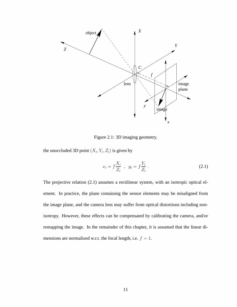
2.1.1 Camera Model

The imaging geometry of a perspective camera is shown in Fig.2.1. The origin

of the 3D coordinate system(X, Y, Z) lies at the optical centerC of the camera. The

retinal planeor image planeis normal to the optical axisZ, and is offset fromC by the

focal lengthf . Images of unoccluded 3D objects in front of the camera are formed on the

image plane. The 2D image plane coordinate system(x, y) is centered at theprincipal

point, which is the intersection of the optical axis with the imageplane. The orientation

of (x, y) is flipped with respect to(X, Y ) in Fig. 2.1, due to inversion caused by simple

transmissive optics. For this system, the image plane coordinate(xi, yi) of the image of

10

Z

C

planelens

X

image

image

Y

x

object

y

f

Figure 2.1: 3D imaging geometry.

the unoccluded 3D point(Xi, Yi, Zi) is given by

xi = fXi

Zi

, yi = fYi

Zi

. (2.1)

The projective relation (2.1) assumes a rectilinear system, with an isotropic optical el-

ement. In practice, the plane containing the sensor elements may be misaligned from

the image plane, and the camera lens may suffer from optical distortions including non-

isotropy. However, these effects can be compensated by calibrating the camera, and/or

remapping the image. In the remainder of this chapter, it is assumed that the linear di-

mensions are normalized w.r.t. the focal length, i.e.f = 1.

11

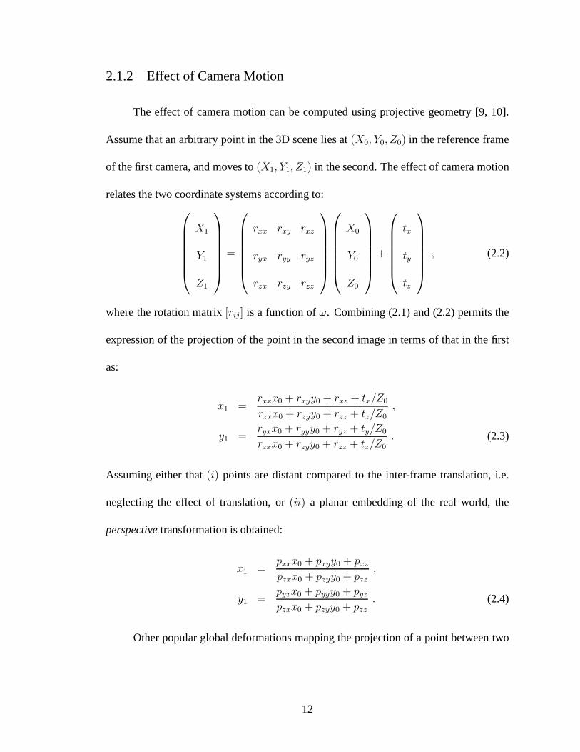
2.1.2 Effect of Camera Motion

The effect of camera motion can be computed using projectivegeometry [9, 10].

Assume that an arbitrary point in the 3D scene lies at(X0, Y0, Z0) in the reference frame

of the first camera, and moves to(X1, Y1, Z1) in the second. The effect of camera motion

relates the two coordinate systems according to:

X1

Y1

Z1

=

rxx rxy rxz

ryx ryy ryz

rzx rzy rzz

X0

Y0

Z0

+

tx

ty

tz

, (2.2)

where the rotation matrix[rij ] is a function ofω. Combining (2.1) and (2.2) permits the

expression of the projection of the point in the second imagein terms of that in the first

as:

x1 =rxxx0 + rxyy0 + rxz + tx/Z0

rzxx0 + rzyy0 + rzz + tz/Z0

,

y1 =ryxx0 + ryyy0 + ryz + ty/Z0

rzxx0 + rzyy0 + rzz + tz/Z0. (2.3)

Assuming either that(i) points are distant compared to the inter-frame translation, i.e.

neglecting the effect of translation, or(ii) a planar embedding of the real world, the

perspectivetransformation is obtained:

x1 =pxxx0 + pxyy0 + pxz

pzxx0 + pzyy0 + pzz

,

y1 =pyxx0 + pyyy0 + pyz

pzxx0 + pzyy0 + pzz

. (2.4)

Other popular global deformations mapping the projection of a point between two

12

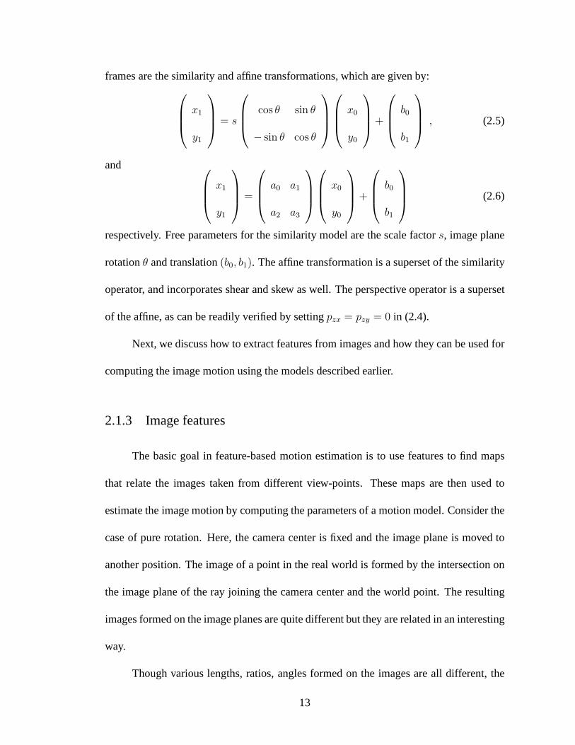
frames are the similarity and affine transformations, whichare given by:

x1

y1

= s

cos θ sin θ

− sin θ cos θ

x0

y0

+

b0

b1

, (2.5)

and

x1

y1

=

a0 a1

a2 a3

x0

y0

+

b0

b1

(2.6)

respectively. Free parameters for the similarity model arethe scale factors, image plane

rotationθ and translation(b0, b1). The affine transformation is a superset of the similarity

operator, and incorporates shear and skew as well. The perspective operator is a superset

of the affine, as can be readily verified by settingpzx = pzy = 0 in (2.4).

Next, we discuss how to extract features from images and how they can be used for

computing the image motion using the models described earlier.

2.1.3 Image features

The basic goal in feature-based motion estimation is to use features to find maps

that relate the images taken from different view-points. These maps are then used to

estimate the image motion by computing the parameters of a motion model. Consider the

case of pure rotation. Here, the camera center is fixed and theimage plane is moved to

another position. The image of a point in the real world is formed by the intersection on

the image plane of the ray joining the camera center and the world point. The resulting

images formed on the image planes are quite different but they are related in an interesting

way.

Though various lengths, ratios, angles formed on the imagesare all different, the

13

cross ratioremains the same [11]. Given four collinear pointsA,B,C andD on an image,

the cross ratio isACCB÷ AD

DBand it remains constant. In other words,AC

CB÷ AD

DB= AC

CB÷ AD

DB,

whereA, B, C andD are the corresponding points in the second image (formed after

rotating the camera about its axis).

Looking carefully, we can see that this intuition leads to a map relating the two

images. Given four corresponding points in general position in the two images, we can

map any point from one image to the other. Suppose we know thatA maps toA, B to B,

C to C andD to D. Then the point of intersection ofAB andCD (sayE) will map to

the point of intersection ofAB andCD (sayE). Now any pointF onABE will map to

point F such that the cross ratioAEEB÷ AF

FBis preserved. This way one can map each point

from one image to the other image. Such a map is called ahomography. As mentioned

before, such a map is defined by four corresponding points in general position. So, ifx

maps tox by homographyH, x′ = Hx. Note that such a map exist only in case of pure

rotation.

However, for planar scenes, homography relating the two views exist irrespective

of the motion involved. In the case of planar scene, there exist a homography relating the

first image to the real-world plane and another one mapping the real-world plane to the

second image plane, i.e.,

x1 = H1xp (2.7)

xp = H2x2 (2.8)

⇒ x1 = H1H2x2 = Hx2 (2.9)

whereH1 mapsx1, a point on first image plane toxp, the corresponding point on the

14

real plane whileH2 mapsxp to x2, the corresponding point on the second image plane.

Thus homographyH = H1H2 maps points from one image plane to the other. Such

a homography exists, no matter what the underlying motion between the two camera

positions is. This happens because the images formed by camera rotation (or in the case

of planar scenes) do not depend on the scene structure. On theother hand, when there are

depth variations in the scene, such a homography doesn’t exist between images formed

by camera translation.

In the case of depth variations, we can use SfM approaches to estimate the motion

of the camera. The estimated camera motion can be used to selectively stabilize the

image sequence for the camera motion (such as compensation of rotation, or sideways

translation etc.) The next section discusses about SfM and describes an algorithm for

SfM using image feature points.

2.1.4 Structure from Motion

Structure from motion refers to the task of inferring the camera motion and scene

structure from an image sequence taken from a moving camera,using either image fea-

tures or flow. We describe an illustrative algorithm for SfM using feature point tracks

in a sequence. Consider an image sequence withN images. Feature points are detected

and tracked throughout the sequence. Suppose the scene hasM features and their pro-

jections in each image are denoted byxi,j = (ui,j, vi,j)T wherei ∈ 1, · · · ,M denotes

the feature index andj ∈ 1, · · · , N denotes the frame index. For the sake of simplic-

ity, assume that all features are visible in all frames. The structure-from-motion problem

15

involves solving for the camera locations and the 3D coordinates of feature points in the

world coordinate system.

The camera poses are specified by a rotation matrixRj and a translation vectorTj

for j = 1, · · · , N . The coordinates of a point in the camera system and world system are

related byPc = RiPw +Ti, wherePc denotes the coordinates of a point in the camera co-

ordinate system, andPw denotes the coordinates of the same point in the world coordinate

system. The 3D coordinates of the world landmarks are denoted byX i = (Xi, Yi, Zi)T for

i = 1, · · · ,M . We assume an orthographic projection model for the camera.Landmarks

are projected onto the image plane according to the following equation:

ui,j

vi,j

= K ·

[

Rj Tj

]

X i (2.10)

In equation (2.10),K denotes the2× 3 camera matrix. Let the centroid of the3D points

beC and the centroid of the image projections of all features in each frame becj. We

can eliminate the translations from these equations by subtracting outC from all world

point locations andcj from the image projections of all features in thejth frame. Let

xi,j = xi,j − cj andXj = Xj − C. The projection equation can be rewritten as:

xi,j = Pj · Xi (2.11)

In equation (2.11),Pj = K · Rj denotes the2× 3 projection matrix of the camera.

We can stack up the image coordinates of the all the feature points in all the frames,

16

and write it in the factorization format as follows:

x1,1 · · · xM,1

.... . .

...

x1,N · · · xM,N

=

P1

...

PN

[

X1 · · · XM

]

(2.12)

The matrix on the left hand side of equation (2.12) is the measurement matrix, and it has

been written as a product of a2N × 3 projection matrix and a3 ×M structure matrix.

This factorization implies that the measurement matrix is of rank 3. This observation

leads to a factorization algorithm for solving for the projection matricesPj and the3D

point locationsXi. The details of the algorithm are described in detail in [12].

2.1.5 Feature based algorithms

We have seen that a homography can be used to map one image to the other in the

case of pure camera rotation, or a planar scene. If such a homography exists between

the images, four points are sufficient to specify it precisely. In practice, we extract a

number of features in each image and use feature matching algorithms [13] to establish

correspondence between the images. The resulting set of feature matches between two

images usually have a subset of wrong (“outlier”) matches due to errors in the feature

extraction and matching process. We handle these outliers in a RANSAC framework [14]

which attempts to find the motion parameters by first identifying the set of inlier feature

matches. If we have an image sequence, we use feature tracking algorithms like KLT [15]

to track a set of features through an image sequence. The correspondences specified by

these tracks are used to compute the motion model parameters.

Usually, neither the scene being viewed is planar nor the motion a pure rotation. In

17

such cases, there is no linear map that relates one image to the other unless one neglects

the effect of translation (similar to assumption made in (2.4)). In such cases, researchers

either make simplifying assumptions based on the domain knowledge or include addi-

tional constraints involving more views to take care of the limitations of the geometric

approach. In [16], Morimotoet al. demonstrate real time image stabilization that can han-

dle large image displacements based on a two-dimensional multi-resolution technique.

[17] propose an operation calledthreadingthat connects two consecutive Fundamental

matrices using the trifocal tensor as the thread. This makessure that consecutive camera

matrices are consistent with the 3D scene without explicitly recovering it.

2.2 Related work

2.2.1 Video Stabilization

Video stabilization involves registering consecutive pairs of images of a sequence to

each other using an appropriate motion model such as affine orhomography. Image regis-

tration methods have widespread applications and the techniques can be broadly classified

into intensity-based, flow-based and feature-based techniques.

In the intensity-based approach, the motion model parameters are solved by min-

imizing the sum of squared differences between the intensity values of corresponding

pixels of the two images after warping using the geometric transform. The inverse-

compositional alignment algorithm of Baker et. al. [18] is an efficient way to solve the

optimization problem to perform the alignment. Bartoli [19] generalized this when the

pair of images differ by a geometric and photometric transformation. In case the inten-

18

sity values of corresponding pixels between the two images are related by an unknown

transformation (such as in multi-sensor registration), implicit similarity functions in the

gradient domain have been used for registration purposes [20].

In the flow-based approach [21, 22], the optical flow between the pair of images is

used for registration. The registration may be either a full-frame warp obtained by fitting

a model to the flow, or a non-uniform warp using the dense motion vectors to take into

account the varying displacements of parallax pixels.

The feature-based approach relies on abstracting an image as a set of salient feature

points with associated geometric locations. Registrationis performed by finding corre-

sponding points between the images [23] and using this to estimate the motion model

parameters.

Detecting moving objects in a video sequence involves stabilization followed by

identifying the pixels that are in misregistration. Background subtraction [24] is one of

the most commonly used techniques to identify moving objects. When two registered im-

ages are subtracted, the pixels belonging to the backgroundhave a small absolute value.

However, the moving object pixels do not register using the background model and hence

light up with high values of absolute differences. However,even slight misregistrations

lead to false moving object detections which is a serious problem in the background sub-

traction framework.

Birchfield and Pundlik [25] propose a framework to combine local optic flow with

global Horn-Schunck constraints [26] for joint tracking offeatures and edges. They ex-

press the idea of motion coherence in terms of a smoothness prior. The key difference of

our work is that we incorporate motion coherence between features by solving a classifi-

19

cation problem to label features. The motion of features belonging to the same class are

solved jointly by computing the model parameters.

Sheikh et. al. [27] propose a background subtraction framework where they track

densely distributed points in a video and segment them into background and moving

points. They use feature segmentations to infer the piecewise dense image segmenta-

tion using MRF priors. The proposed work is similar to [27] inthat we also use the

segmented set of features for pixelwise segmentation and moving target detection. The

key difference is that the joint tracking and segmentation strategy enables us to track fea-

tures uniformly distributed in the image plane (including homogeneous regions) making

the segmentation step more reliable. The earlier work relies on accurately tracked indi-

vidual feature points and this assumption does not hold in our scenarios. In addition, we

use the foreground segmentations for target initialization and tracking.

Buchanan and Fitzgibbon [28] propose a feature tracking algorithm by combining

local and global motion models. More accurate tracks are obtained by generating predic-

tions of feature location using global models. Shi and Tomasi [15] proposed a method for

feature monitoring in KLT tracking, by measuring feature dissimilarities after registration

with an affine model. They use these dissimilarities as a criterion to judge the goodness of

feature tracks. We use feature dissimilarities produced bythe motion model as a measure

of the likelihood of the feature belonging to the model. These dissimilarities are used to

derive the probabilities of belonging to the common background model.

20

2.2.2 Video Mosaicking

Mosaicing is the process of compositing or piecing togethersuccessive frames of

the stabilized image sequence so as to virtually increase the field-of-view of the cam-

era [29]. This process is especially important for remote surveillance, tele-operation of

unmanned vehicles, rapid browsing in large digital libraries, and in video compression.

Mosaics are commonly defined only for scenes viewed by a pan/tilt camera, for which the

images can be related by a projective transformation. However, recent studies have looked

into qualitative representations, non-planar embeddings[30, 31] and layered models [32].

The newer techniques permit camera translation and gracefully handle the associated par-

allax. These techniques compute a “parallax image” [33] andwarp the off-planar image

pixels on the mosaic using the corresponding values in the parallax image. Mosaics rep-

resent the real world in 2D, on a plane or other manifold like the surface of a sphere or

“pipe”. Mosaics that are built on spherical or cylindrical surfaces belong to the class of

panoramic mosaics [34, 35]. For general camera motion, there are techniques to con-

struct a mosaic on an adaptive surface depending on the camera motion. Such mosaics,

called manifold mosaics, are described in [31, 36]. Mosaicsthat are not true projections

of the 3D world, yet present extended information on a plane are referred to asqualitative

mosaics.

Several options are available while building a mosaic. Asimplemosaic is obtained

by compositing several views of a static 3D scene from the same view point and different

view angles. Two alternatives exist, when the imaged scene has moving objects, or when

there is camera translation. Thestaticmosaic is generated by aligning successive images

21

with respect to the first frame of a batch, and performing a temporal filtering operation on

the stack of aligned images. Typical filters are pixelwise mean or median over the batch of

images, which have the effect of blurring out moving foreground objects. In addition, the

edges in the mosaic are smoothed, and sharp features are lost. Alternatively the mosaic

image can be populated with the first available information in the batch.

Unlike the static mosaic, thedynamicmosaic is not a batch operation. Successive

images of a sequence are registered to either a fixed or a changing origin, referred to

as thebackwardand forward stabilizedmosaics respectively. At any time instant, the

mosaic contains all the new information visible in the most recent input frame. The fixed

coordinate system generated by a backward stabilized dynamic mosaic literally provides a

snapshot into the transitive behavior of objects in the scene. This finds use in representing

video sequences using still frames. The forward stabilizeddynamic mosaic evolves over

time, providing a view port with the latest past informationsupplementing the current

image. This procedure is useful for generating an enlarged virtual field of view in the

remote operation of unmanned vehicles.

In order to generate a mosaic, the global motion of the scene is first estimated. This

information is then used to rewarp each incoming image to a chosen frame of reference.

Rewarped frames are combined in a manner suitable to the end application.

2.2.3 Structure from Motion

Structure from Motion algorithms can be broadly classified into the following cate-

gories: batch techniques, minimal solutions and recursiveframeworks. A comprehensive

22

survey may be found in [37].

In batch techniques, we jointly solve for the views of all thecameras and the struc-

ture of all the points. Bundle adjustment (BA) [38] is the representative algorithm in this

class, and it minimizes an error function measuring the disparity in the detected image

features and those generated from the current reconstruction. This is a non-linear least

squares minimization problem that is commonly solved usingthe Levenberg-Marquardt

(LM) [39] algorithm. The linear system corresponding to thenormal equations for LM is

intractable for large reconstruction problems. To handle large problems, the sparse struc-

ture of the Hessian matrix is used for efficiently solving thenormal equations resulting

in the Sparse Bundle Adjustment (SBA) [40] algorithm. The conjugate gradient (CG)

method [39] is another choice for optimizing the reprojection error that does not require

the solution of a large system; however suitable pre-conditioners are necessary for it to

work well [41]. In addition, its benefits have not yet been clearly demonstrated for large

scale problems.

Minimal solutions take a small subset of features as input and efficiently solve for

the views of two or three cameras. A recent and popular algorithm in this class is the

five-point algorithm which was proposed by Nister [42]. Because of the small number

of points and views, solving for the parameters is very efficient. However, there may be

multiple solutions and we need to disambiguate the various alternatives using additional

points. An issue with this technique is the propagation of error while trying to stitch the

various individual reconstructions together.

Recursive algorithms perform an online estimation of the state vector which is com-

posed of the location and orientation of the camera, and the 3D locations of the world

23

landmarks. The estimation proceeds in a prediction-updatecycle, where a motion model

is used to predict the camera location at the next time step, and this estimate is updated

using new observations. Simultaneus Localization and Mapping [43] methods also fall

within the recursive framework since they employ a recursive filter to estimate the camera

location in a causal fashion.

Another class of techniques is factorization-based approaches [12, 44] that take the

measurement matrix (containing the feature points observed in all views) and factorize it

into a product of the motion and structure matrices.

Although solving for 3D locations of points from feature tracks is important, it

is just one part of the problem. There are other open researchproblems in generating

texture-mapped 3D models of environments after solving forSfM from image sequences.

Researchers have been actively working on ways to perform 3Dmodel acquisition from

ground-based sequences. Fruh and Zakhor [45] describe an automatic method for fast,

ground-based acquisition of 3D city models using cameras and laser scanners. In [46],

they describe a method for merging ground-based and aerial images for generating 3D

models. Akbarzadeh et. al. [47] introduce a system for automatic, geo-registered 3D

reconstruction of urban scenes from video.

In spite of this large body of work in SfM, it is a very hard ill-posed and inverse

problem and very few of these algorithms provide satisfactory performance in real-world

scenarios. The main difficulties faced by these algorithms in real world scenarios are in

establishing correspondence across image sequences, feature tracking errors, mismatched

correspondences, occlusion etc.

Therefore, recent research has focussed on developing SfM algorithms in the pres-

24

ence of additional constraints on the problem. For instance, position information about

the cameras from Global Positioning Systems (GPS) can help us solve for the parame-

ters [48]. If inertial measurements from IMUs are available, we can reduce the ambigui-

ties in the SfM problem [49].

Our work is related to prior work in SfM literature that assume a visible dominant

plane in the scene. An important algorithm in this class is the use of the plane-plus-

parallax model for the recovery of 3D depth maps [50]. The multi-view constraints im-

posed by a plane were used by Rother [51] and Kaucic [52] to simplify the projective

reconstruction problem into a linear system of equations. Bartoli [53] derived a linear al-

gorithm for estimating the structure of objects moving on a plane in straight lines without

rotating. Reconstruction of objects moving in an unconstrained fashion was studied in

detail by Fitzgibbon and Zisserman [54].

A special case of our algorithm is Structure from Planar Motion (SfPM) where we

have a surveillance scenario with a static camera observingmoving objects on a plane.

In this case, the measurement matrix simplifies into a product of a motion and a structure

matrix that is of rank3. Li and Chellappa [55] describe a factorization algorithm for

solving for the structure and planar motion.

Another special case, leading to a linear multiview reconstruction, arises when

we know the homographies between successive images inducedby the planar scene.

Rother [51] stabilizes the images using homographies, and chooses a projective basis

where the problem becomes one of computing structure and motion of calibrated translat-

ing cameras. They derive linear equations for the camera centers and points, and simul-

taneously solve the resulting linear system for all camerasand points using SVD based

25

techniques. The performance of their algorithm is heavily dependent on the estimate of

the homographies. In addition, the memory and computational requirements of the algo-

rithm become infeasible when we have a large number of framesand points.

Our algorithm assumes approximate knowledge of a certain direction vector in each

image of the sequence and also the altitude from a plane perpendicular to this vector.

These quantities are well defined when we observe a dominant plane in the scene, but the

algorithm does not require the visibility of a plane (for stationary scenes). In this respect,

it is quite different from all other previous approaches.

The proposed algorithm belongs to the class of alternation algorithms that solve

for the structure and motion in an iterative fashion [44, 56]. These approaches solve

for the projective depths along with the motion and structure matrices and result in a

projective reconstruction. The projective depths are typically initialized to unity and later

refined iteratively. This has been reported to work well onlyin special settings where the

depth of each feature point remains approximately the same throughout the sequence [37].

This does not cover many important scenarios such as roadside urban sequences or aerial

videos where the altitude of the camera varies a lot. Our algorithm makes use of the

bilinear form in the Euclidean frame without slack variables. Hence it does not have any

restrictions on its use except that the gravity and height measurements must be available.

Oliensis and Hartley [57] published a critique on the factorization-like algorithms

suggested in [44, 56] for projective SfM. They investigatedthe theoretical basis for per-

forming the suggested iterations in order to decrease the error function. They analyzed the

stability and convergence of the algorithms and concluded theoretically and experimen-

tally that the Sturm-Triggs [44] as well as the slightly modified Mahamud [56] algorithm

26

converges to trivial solutions. They analyzed the error functions for these algorithms and

showed that the stationary points were either local minima that corresponded to trivial

solutions or they were saddle points of the error. Based on this analysis, we investigate

the stability and convergence properties of the proposed algorithm.

27

Chapter 3

Intensity-based Video Stabilization

The intensity-based registration algorithm of Baker et. al. [18], known as simulta-

neous inverse compositional alignment, iteratively minimizes the sum-squared difference

of pixel intensities between corresponding pixels of a pairof images. We discuss the

application of this algorithm for the registration of low-quality and low-resolution video

obtained from aerial platforms [3].

3.1 Intensity-based alignment

In intensity-based registration techniques, we assume a global parametric transfor-

mation that registers the two images. We pose the registration task as an optimization

problem involving the minimization of the intensity difference between the two images

registered using the current parameters. SupposeI1 andI2 are the two images to be reg-

istered. We solve the following minimization problem:

minp

∑

q∈R

‖I1(q)− I2(P (q; p))‖2 (3.1)

whereq denotes the coordinates of a pixel,p denotes the transformation parameters of the

registration model,P (q; p) denotes the global transformation applied to the pixelq, and

R is the region ofI1 over which the image intensity differences are computed.

Common choices of the motion modelP (q; p) used for registration are the affine

model, homography etc. The regionR over which the intensity differences are computed

28

is typically chosen to be the entire region of overlap between the registered images. The

minimization is performed using an iterative minimizationtechnique that linearizes the

objective function (using a Gauss-Newton approximation) at each iteration and computes

an update that minimizes the error. A pyramidal implementation of a Gauss-Newton

minimization procedure was introduced by Bergen et. al. [58]. More recently, Baker

et. al. proposed a fast “inverse compositional” algorithm [18] for minimizing (3.1).

We sketch the details of the inverse compositional algorithm. LetP (q; p) denote the

current transformation between the images. Let∆P (q; δp) denote an update to the current

transformation that reduces the image-difference error. We apply the update to the trans-

formation by composing the current transformation with theinverse of the incremental

transformation. The update rule isP (g; p)← P (∆P−1(q; δp); p).

The optimization (3.1) is performed overδp, the parameter of the incremental trans-

formation, and can be recast as follows:

minδp

∑

q∈R

∥

∥I1(q)− I2(P (∆P−1(q; δp); p))∥

∥

2(3.2)

The inverse compositional trick is to apply the incrementaltransformation to the first

imageI1 as opposed to the second image. The problem can be rewritten as:

minδp

∑

q∈R

‖I1(∆P (q; δp))− I2(P (q; p))‖2 (3.3)

We linearize this equation using a Taylor series expansion of the intensities ofI1 to obtain:

minδp

∑

q∈R

∥

∥I1(q) +∇IT1 (q)∇∆P (q; δp))− I2(P (q; p))

∥

∥

2(3.4)

This technique is applicable only when there is a correlation in the intensities of corre-

sponding pixels between the two images. Extensions of the inverse compositional al-

29

gorithm have been proposed [19] when the intensities of corresponding pixels are not

equal, but there is a relation between the intensities such as a gain and a bias, or an affine

transformation.

3.1.1 Effect of region of registration

Baker’s algorithm is traditionally applied to minimize thesum-of-squared intensity

difference of all the corresponding pixels in the image pair. In other words, the setR

denoted above is chosen to consist of all the pixels of the image. We argue that this most

common default choice does not necessarily result in betterregistrations. We point out

that using a subset of the image pixels for registration can result in better registration

results in lesser computation time. The following are two scenarios where registration

may be defined over a subset of pixels.

1. Multisensor image registration:Images taken from different sensors have no cor-

relation between their pixel intensities. Multisensor registration techniques use im-

plicit similarity functions that are defined for pixels marking prominent features or

with high gradient magnitudes.

2. Low-quality and low-resolution video:In videos obtained from airborne platforms

with small cameras, the noise level in intensities is high under low illumination con-

ditions. In these conditions, image motion is perceived dueto the motion of pixels

with high gradients defining prominent edges. This is because edges are preserved

under high image noise levels. Since pixels with small gradients do not contribute

towards perception of motion, perceptually better registration results may be ob-

30

tained by using only pixels with high image gradients for intensity-based registra-

tion.

We apply this concept to the registration of images in a videosequence, where the

noise levels in the images are high. We demonstrate that in this case, we improve the

convergence of the inverse compositional alignment algorithm by using a small subset of

image pixels for registration.

3.1.2 Experiments

We select a set of10 representative images from a video sequence captured from

a low-resolution camera onboard an aerial platform. The chosen images contain large

regions with very little texture information. In other words, the image gradients are very

small within these regions and hence these regions do not contribute towards the mea-

surement of image motion. Figure 3.5(a) illustrates a sample image from the dataset.

For each image, we estimate a homography transformation (bydisplacing four cho-

sen points by a pre-specified amount), and warp the images according to the homography.

We test the convergence properties of the registration algorithm by registering the orig-

inal and warped image, and measuring the convergence rate, number of iterations, etc.

We perform these experiments for various levels of distortion and various levels of Gaus-

sian noise added to one of the images. In applying the intensity-based algorithm, we first

compute the gradient magnitudes of the first image at each pixel, and then order the pixels

according to the gradient magnitudes. We select a chosen fraction of pixels (such as25%)

which have the highest gradient magnitudes and then use these pixels for registration. To

31

preserve the gradient information, we also select surrounding pixels within a small win-

dow. An illustration of the pixels selected from the image infigure 3.5(a) for use in one

run of the intensity-difference minimization is shown in Figure 3.5(b).

Figure 3.1 plots the standard deviation of image pixel noiseversus the number of

iterations taken for convergence. The figure shows five different curves corresponding

to the noise versus iterations plots when different percentages of pixels were used for

registration(100%, 83%, 62%, 41%, 24%). We observe a well-defined variation in the

number-of-iteration plots for various saliency ratios. Asthe saliency ratio decreases (im-

plying that we use fewer pixels for registration), the number of iterations needed for

convergence goes down. We also experimentally verified thatthe time-per-iteration of

registration goes down linearly with the number of pixels used.

Figure 3.2 plots the standard deviation of the image pixel noise versus the geomet-

ric error of registration. The geometric error is defined as the ground-truth registration

parameters and the solved parameters. The distance is measured as anL2 norm of the

difference between the two parameter vectors. From the plot, we observe that there is

little difference between the geometric registration error for the various registration trials

carried out at different saliency ratios. Unlike the plots for the number of iterations, we do

not observe a specific variation in the geometric error curves for different saliency ratios.

However, notice that for several noise levels, the geometric error obtained by registration

with the lowest saliency ratio is actually higher than the geometric error obtained with the

highest saliency ratio. These observations imply that we can do better registration of the

two images, by using fewer iterations (and lower computation time), by choosing a subset

of image pixels (salient pixels).

32

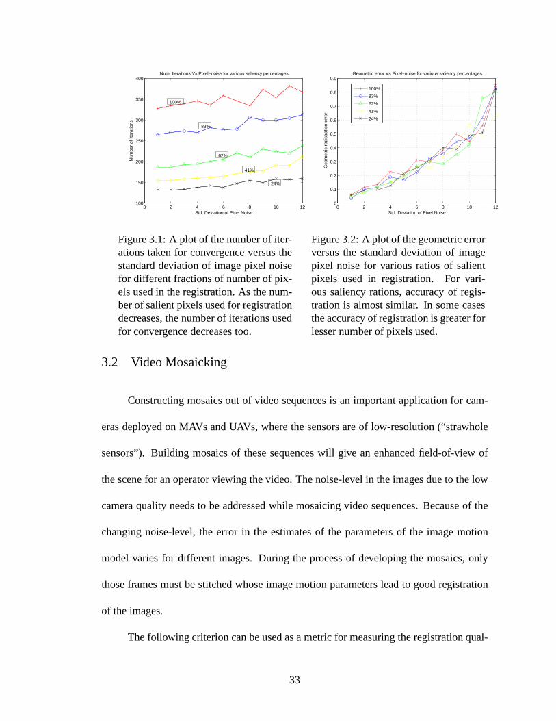
0 2 4 6 8 10 12100

150

200

250

300

350

400

Num

ber

of It

erat

ions

Std. Deviation of Pixel Noise

Num. Iterations Vs Pixel−noise for various saliency percentages

100%

83%

62%

41%

24%

Figure 3.1: A plot of the number of iter-ations taken for convergence versus thestandard deviation of image pixel noisefor different fractions of number of pix-els used in the registration. As the num-ber of salient pixels used for registrationdecreases, the number of iterations usedfor convergence decreases too.

0 2 4 6 8 10 120

0.1

0.2

0.3

0.4

0.5

0.6

0.7

0.8

0.9

Std. Deviation of Pixel Noise

Geo

met

ric r

egis

trat

ion

erro

r

Geometric error Vs Pixel−noise for various saliency percentages

100%

83%

62%

41%

24%

Figure 3.2: A plot of the geometric errorversus the standard deviation of imagepixel noise for various ratios of salientpixels used in registration. For vari-ous saliency rations, accuracy of regis-tration is almost similar. In some casesthe accuracy of registration is greater forlesser number of pixels used.

3.2 Video Mosaicking

Constructing mosaics out of video sequences is an importantapplication for cam-

eras deployed on MAVs and UAVs, where the sensors are of low-resolution (“strawhole

sensors”). Building mosaics of these sequences will give anenhanced field-of-view of

the scene for an operator viewing the video. The noise-levelin the images due to the low

camera quality needs to be addressed while mosaicing video sequences. Because of the

changing noise-level, the error in the estimates of the parameters of the image motion

model varies for different images. During the process of developing the mosaics, only

those frames must be stitched whose image motion parameterslead to good registration

of the images.

The following criterion can be used as a metric for measuringthe registration qual-

33

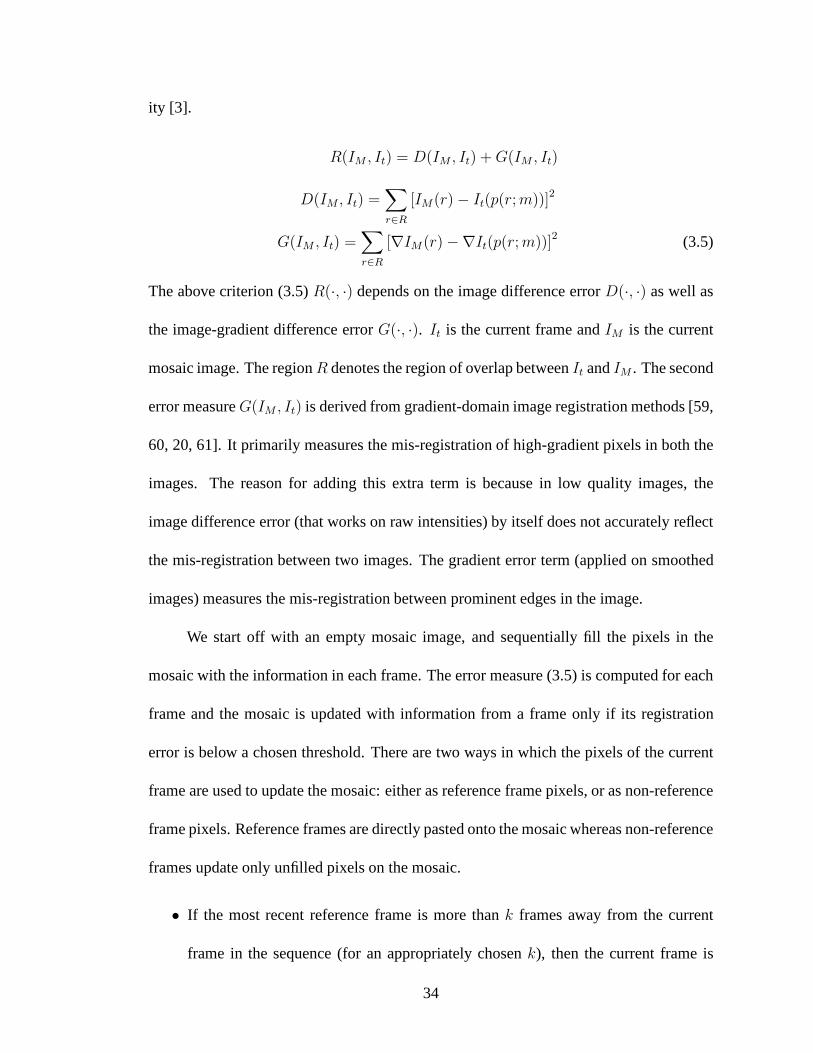
ity [3].

R(IM , It) = D(IM , It) +G(IM , It)

D(IM , It) =∑

r∈R

[IM(r)− It(p(r;m))]2

G(IM , It) =∑

r∈R

[∇IM(r)−∇It(p(r;m))]2 (3.5)

The above criterion (3.5)R(·, ·) depends on the image difference errorD(·, ·) as well as

the image-gradient difference errorG(·, ·). It is the current frame andIM is the current

mosaic image. The regionR denotes the region of overlap betweenIt andIM . The second

error measureG(IM , It) is derived from gradient-domain image registration methods [59,

60, 20, 61]. It primarily measures the mis-registration of high-gradient pixels in both the

images. The reason for adding this extra term is because in low quality images, the

image difference error (that works on raw intensities) by itself does not accurately reflect

the mis-registration between two images. The gradient error term (applied on smoothed

images) measures the mis-registration between prominent edges in the image.

We start off with an empty mosaic image, and sequentially fillthe pixels in the

mosaic with the information in each frame. The error measure(3.5) is computed for each

frame and the mosaic is updated with information from a frameonly if its registration

error is below a chosen threshold. There are two ways in whichthe pixels of the current

frame are used to update the mosaic: either as reference frame pixels, or as non-reference

frame pixels. Reference frames are directly pasted onto themosaic whereas non-reference

frames update only unfilled pixels on the mosaic.

• If the most recent reference frame is more thank frames away from the current

frame in the sequence (for an appropriately chosenk), then the current frame is

34

incorporated as a reference frame in the current frame as a reference frame.

• If the overlap between the current frame warped and the last reference frame (when

warped on the mosaic) falls below a threshold, we incorporate the current frame as

a reference frame.

• If neither of the above two conditions are satisfied, the current frame is incorporated

as a non-reference frame.

3.2.1 Results

We present some image mosaicks which are the results of the proposed registration

and mosaicking algorithm when it is applied on a video sequence captured using a video

camera onboard an MAV. The air-vehicle is flying in a jittery fashion and the video res-

olution (230 × 310) is small. In addition, there is a lot of motion between consecutive

frames of the sequence. In figs. 3.3 and 3.4, we show mosaics oftwo sequences that

we generated using our algorithms. Figure 3.5(a) illustrates an image of the sequence

and 3.5(b) illustrates the set of pixels in that image used for registration purposes.

35

Figure 3.3: This figure shows a mosaic of a sequence obtained by registering the imagesof a sequence using the intensity-based stabilization algorithm. Approximately30% ofthe pixels in each image were used for the purpose of registration.

Figure 3.4: This figure shows a mosaic of another sequence obtained by registering theimages using the intensity-based stabilization algorithm. Approximately30% of the pix-els in each image were used for the purpose of registration.

36

(a) Sample Image

(b) Selected regions for minimization shown in white

Figure 3.5: Figure 3.5(a) shows a sample image of a sequence captured from an aerialplatform. The resolution is230 × 310 pixels. We use our algorithm to build a mosaicof the sequence. The regions of the image selected by our algorithm for minimizing theimage difference error with the mosaic is shown in Figure 3.5(b). Note that these regionscontribute the most to our perception of image motion.

37

Chapter 4

Feature-based Stabilization and Motion Segmentation

4.1 Feature-based Image Registration

Intensity-based registration techniques described in thelast chapter are useful for

registering images when we have prior information about thesubset of pixels that belong

to the dominant motion model. If the image sequence containsmoving objects, we do

not know the moving object pixels prior to stabilization. Any measures for selecting a

salient set of pixels in one image may select pixels belonging to multiple motion layers.

Solving for the registration parameters using a pixel set containing outlier pixels not be-

longing to the motion model may lead to biased motion parameter estimates. In order

to handle moving objects in the scene, we need to segment out the different motion lay-

ers in the video along with solving for the parameters of the dominant motion model. A

feature-based representation of video is more convenient for the problem of registration

and segmentation.

4.1.1 Shortcomings of KLT tracking and background subtraction

Traditionally, features are tracked through the image sequence and RANSAC [14] is

used to identify the inlier features belonging to the dominant background motion model.

However, tracking errors lead to many misclassifications offeatures. Figure 4.1(a) il-

lustrates an example of an image from our aerial video dataset with KLT [62] tracked

38

features overlaid on it. The image has very few prominent features on the background,

and there are large regions of homogeneous texture. In addition, the road in the middle

contains repeated patterns making it difficult to solve for the correct displacement. These

tracking errors result in a large number of background features to be classified as outliers

by a model selection algorithm such as RANSAC.

When the video is stabilized using the solved background displacements and a back-

ground subtraction method is employed to detect moving objects, there are many spurious

motion blobs due to slight misregistrations at the edges. Figure 4.1(b) illustrates an im-

age with detected moving objects overlaid on top. Many of theboxes are false alarms

enclosing false motion blobs near edges. Some of these falsealarms may be reduced

by temporal filtering or choosing a higher threshold for motion detection. However, this

would fail to detect the small moving objects in the sequence.

We propose an algorithm for simultaneous registration and moving object detec-

tion that uses feature tracking but comes up with a dense motion segmentation of the

scene [63]. We assume a full-frame parametric background motion model and directly

solve for the model parameters using all the features belonging to the model. Since mul-

tiple features are used for solving the model parameters, this enables us to select a large

number of features, densely and uniformly distributed in the image plane, and use the

global motion constraint to accurately track the features.We will now describe the joint

tracking and segmentation algorithm.

39

(a) (b)

Figure 4.1: This figure illustrates the failure of KLT feature tracking method. Fig-ure 4.1(a) shows an image with overlaid features. The red points are classified to be onthe background and blue points are classified to be on the foreground. Ideally, blue pointsmust be restricted to moving vehicle features. Note the large number of blue points onthe background indicating misclassifications. Figure 4.1(b) shows an image with boxesoverlaid on top, indicating detected moving blobs after a background subtraction algo-rithm was applied on registered images. Notice the number offalsely detected movingobjects. The underlying video sequence was very well stabilized upon evaluation by ahuman observer, but outlier pixels near edges show up as moving pixels in backgroundsubtraction.

40

4.1.2 Joint tracking

Consider two consecutive imagesI andJ in a sequence. Assume that the image

motion comprises of a pure translational motion along theX andY axes. Assume that

N salient feature points(f1, f2, · · · , fN) have been detected in the imageI that need to

be tracked on imageJ . Let the image displacements be described byd which is a two-

tuple denoting the translations along thex andy directions of the image. The objective

is to solve ford by jointly tracking the set ofn feature points. We solve the following

optimization problem.

arg mind

N∑

i=1

∫ ∫

x∈W (fi)

[

J(x+1

2d)− I(x−

1

2d)

]2

· w(x− fi)dx (4.1)

In this optimization, the double integral denotes the accumulation of the objective func-

tion over a small window around the feature. The term

∫ ∫

x∈W (fi)

[

J(x+1

2d)− I(x−

1

2d)

]2

· w(x− fi)dx (4.2)

is the same as the objective function that is minimized in theLucas-Kanade feature track-

ing method [62], where one solves for the displacement of each feature patch separately,

and independently of other features. In our case, the difference is that we solve for a com-

mon displacement of a set of features that belong to the same motion model, by summing

the image patch difference errors for each feature. We solve(4.1) by expressing the im-

age intensitiesI andJ at a displaced pixel point in a Taylor series around the neighboring

pixel locations. The optimization (4.1) reduces to:

arg mind

∑

i

∫ ∫

x∈W (fi)

[

J(x)− I(x) + gTd]2· w(x− fi)dx (4.3)

41

where

g =

[

δδx

(

I+J2

)

δδy

(

I+J2

)

]T

(4.4)

We differentiate (4.3) with respect tod to get

∑

i

∫ ∫

x∈W (fi)

g ·[

J(x)− I(x) + gTd]

· w(x− fi)dx = 0 (4.5)

which simplifies to

∑

i

∫ ∫

x∈W (fi)

g(x) · g(x)Tw(x− fi)dx

d =

∑

i

∫ ∫

x∈W (fi)

[J(x)− I(x)] g(x)w(x− fi)dx

(4.6)

We solve the above linear system to obtain the solution ford as follows.

d =

∑

i

∫ ∫

x∈W (fi)

g(x) · g(x)Tw(x− fi)dx

−1

·∑

i

∫ ∫

x∈W (fi)

[J(x)− I(x)] g(x)w(x− fi)dx

(4.7)

This derivation is applicable when the image motion is described by a pure translation

model. A similar set of equations can be derived for more general models such as affine

motion. We assume a translation model for simplicity of derivation.

4.1.3 Robustness

In the joint tracking framework described above, the presence of outliers in the pool

of features can bias the translation estimates. The quadratic error function measuring the

sum squared differences of image patches is very sensitive to the presence of outliers that

do not follow background motion. To address this, we introduce robust metrics in the

optimization criterion (4.3) to make the solution robust tothe presence of outliers. We

42

use the Huber’s robust loss function defined as follows.

ρ(u) =

12u2 if |u| ≤ c

c(|u| − c2) if |u| > c

(4.8)

In robust joint-tracking the sum-of-squares objective function in (4.9) is modified using

the Huber loss function (4.8) to obtain the following robustoptimization problem.

arg mind

∑

i

∫ ∫

x∈W (fi)

ρ

(

J(x+1

2d)− I(x−

1

2d)

)

· w(x− fi)dx (4.9)

With the introduction of the robust loss-function, the optimization problem (4.9) can be

solved using gradient descent techniques such as the conjugate gradient method. The

advantage of introducing the robust metric is that the solution is much more resilient to

the presence of outliers in the pool of features used for joint tracking. We evaluate the

performance of joint tracking and the robustness to outliers introduced by the Huber loss

function. We choose a set of set of20 images from the dataset. For each image, we gen-

erate a second shifted image by translating the first image intheY direction. Then, we

simulate three moving image patches that move differently from the background. This

procedure effectively produces two images that are shiftedversions of each other except

for the moving image patches that do not follow the background motion. We select fea-

tures on the background and the moving patches and solve for the displacement jointly.

For the purposes of joint tracking, all features selected onthe moving patches are out-

liers. For different fractions of outliers in the feature pool, we compare the joint tracking

solution with the robust joint tracking solution. Figure 4.2 plots the solved displacements

for various fractions of outliers. The blue line indicates the ground truth displacement,

and the red curve indicates the averaged displacement obtained from joint tracking. It is

43

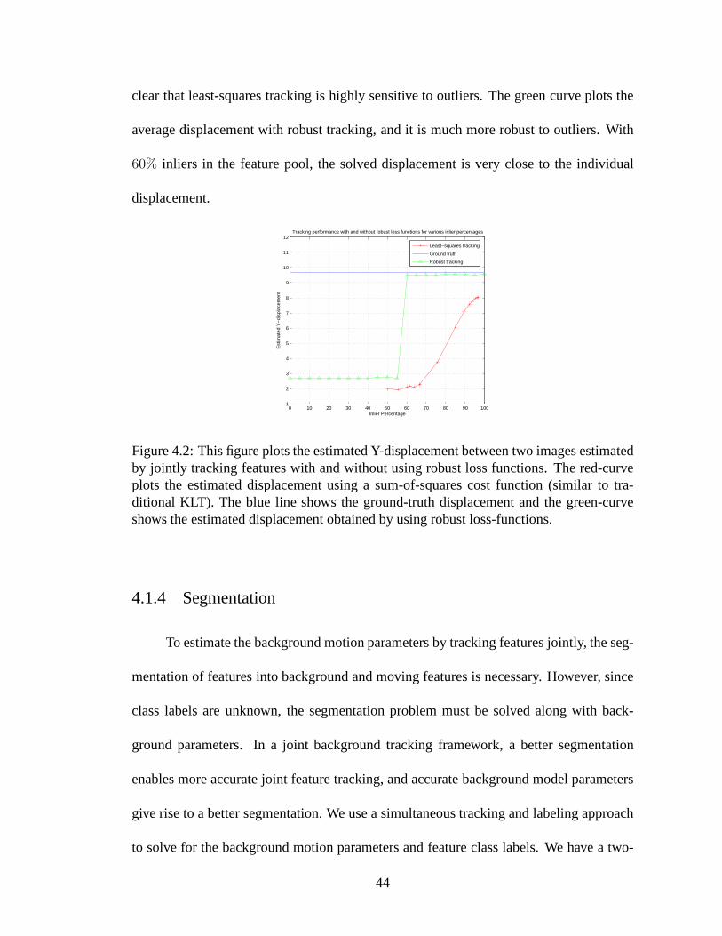
clear that least-squares tracking is highly sensitive to outliers. The green curve plots the

average displacement with robust tracking, and it is much more robust to outliers. With

60% inliers in the feature pool, the solved displacement is veryclose to the individual

displacement.

0 10 20 30 40 50 60 70 80 90 1001

2

3

4

5

6

7

8

9

10

11

12

Inlier Percentage

Est

imat

ed Y

−di

spla

cem

ent

Tracking performance with and without robust loss functions for various inlier percentages

Least−squares tracking

Ground truth

Robust tracking

Figure 4.2: This figure plots the estimated Y-displacement between two images estimatedby jointly tracking features with and without using robust loss functions. The red-curveplots the estimated displacement using a sum-of-squares cost function (similar to tra-ditional KLT). The blue line shows the ground-truth displacement and the green-curveshows the estimated displacement obtained by using robust loss-functions.

4.1.4 Segmentation

To estimate the background motion parameters by tracking features jointly, the seg-

mentation of features into background and moving features is necessary. However, since

class labels are unknown, the segmentation problem must be solved along with back-

ground parameters. In a joint background tracking framework, a better segmentation

enables more accurate joint feature tracking, and accuratebackground model parameters

give rise to a better segmentation. We use a simultaneous tracking and labeling approach

to solve for the background motion parameters and feature class labels. We have a two-

44

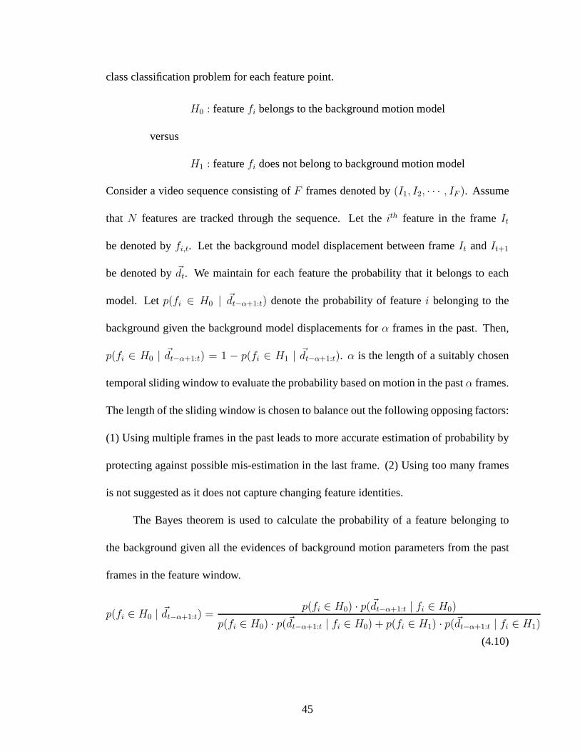
class classification problem for each feature point.

H0 : featurefi belongs to the background motion model

versus

H1 : featurefi does not belong to background motion model

Consider a video sequence consisting ofF frames denoted by(I1, I2, · · · , IF ). Assume

thatN features are tracked through the sequence. Let theith feature in the frameIt

be denoted byfi,t. Let the background model displacement between frameIt andIt+1

be denoted by~dt. We maintain for each feature the probability that it belongs to each

model. Letp(fi ∈ H0 | ~dt−α+1:t) denote the probability of featurei belonging to the

background given the background model displacements forα frames in the past. Then,

p(fi ∈ H0 | ~dt−α+1:t) = 1 − p(fi ∈ H1 | ~dt−α+1:t). α is the length of a suitably chosen

temporal sliding window to evaluate the probability based on motion in the pastα frames.

The length of the sliding window is chosen to balance out the following opposing factors:

(1) Using multiple frames in the past leads to more accurate estimation of probability by

protecting against possible mis-estimation in the last frame. (2) Using too many frames

is not suggested as it does not capture changing feature identities.

The Bayes theorem is used to calculate the probability of a feature belonging to

the background given all the evidences of background motionparameters from the past

frames in the feature window.

p(fi ∈ H0 | ~dt−α+1:t) =p(fi ∈ H0) · p(~dt−α+1:t | fi ∈ H0)

p(fi ∈ H0) · p(~dt−α+1:t | fi ∈ H0) + p(fi ∈ H1) · p(~dt−α+1:t | fi ∈ H1)

(4.10)

45

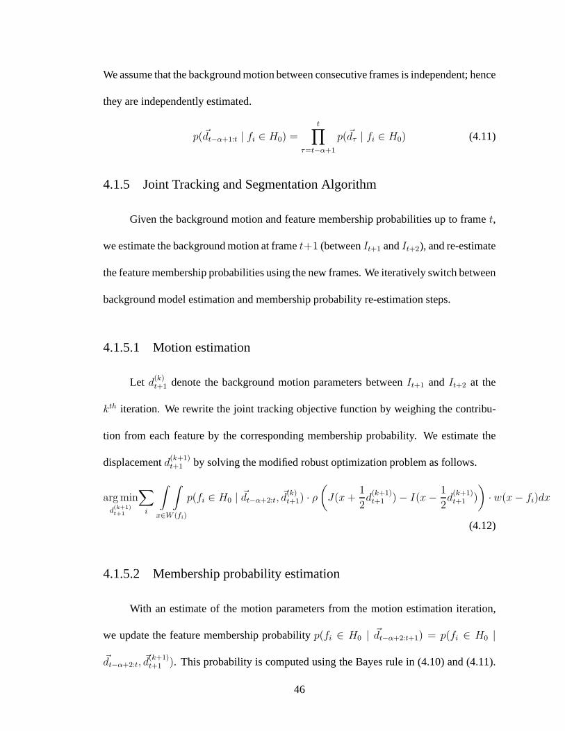
We assume that the background motion between consecutive frames is independent; hence

they are independently estimated.

p(~dt−α+1:t | fi ∈ H0) =

t∏

τ=t−α+1

p(~dτ | fi ∈ H0) (4.11)

4.1.5 Joint Tracking and Segmentation Algorithm

Given the background motion and feature membership probabilities up to framet,

we estimate the background motion at framet+1 (betweenIt+1 andIt+2), and re-estimate

the feature membership probabilities using the new frames.We iteratively switch between

background model estimation and membership probability re-estimation steps.

4.1.5.1 Motion estimation

Let d(k)t+1 denote the background motion parameters betweenIt+1 andIt+2 at the

kth iteration. We rewrite the joint tracking objective function by weighing the contribu-

tion from each feature by the corresponding membership probability. We estimate the

displacementd(k+1)t+1 by solving the modified robust optimization problem as follows.

arg mind(k+1)t+1

∑

i

∫ ∫

x∈W (fi)

p(fi ∈ H0 | ~dt−α+2:t, ~d(k)t+1) · ρ

(

J(x+1

2d

(k+1)t+1 )− I(x−

1

2d

(k+1)t+1 )

)

· w(x− fi)dx

(4.12)

4.1.5.2 Membership probability estimation

With an estimate of the motion parameters from the motion estimation iteration,

we update the feature membership probabilityp(fi ∈ H0 | ~dt−α+2:t+1) = p(fi ∈ H0 |

~dt−α+2:t, ~d(k+1)t+1 ). This probability is computed using the Bayes rule in (4.10)and (4.11).

46

The termp(dt | fi ∈ H0) measures the probability that the background displacementat

frameIt is dt using the single featurefi which is known to belong to the background. We

define this to be the probability that the displacement of feature locationfi,t from It to It+1

is dt. This is computed based on the intuition that ifdt is the true background displace-

ment, then the feature dissimilarity offi,t, computed as∫ ∫

x∈W (fi)

(It+1(x+ dt)− It(x)) ·

w(x − fi)dx, is low. On the other hand, ifdt is wrongly estimated, then the computed

dissimilarity is high. Therefore,p(dt | fi ∈ H0) is related to the probability of observing

the feature dissimilarity produced bydt given that the featurefi was an inlier.

We use a data-driven approach to find the distribution of feature dissimilarities. We

track KLT features individually through a small subset of the sequence and accumulate

the dissimilarities of the successfully tracked features.We compute the distribution of

the feature residues using histogram estimation techniques. Then we fit several differ-

ent parametric distributions to this histogram and find the best fitting distribution using

statistical tests. We found that the dissimilarities were distributed according to a three

parameter log-normal distribution as given below.

p(x) =

h

σ√

2π(x−θ)exp(− (log(x−θ)−ζ)2

2σ2 ) x > θ

0 x ≤ θ

(4.13)

whereθ is the threshold,σ is the shape parameter which is a positive real number, andζ

is the scale parameter which is a real number.

If the featurefi does not belong to the background model, then the background

model parameterdt leads to a relatively high residue for the feature ifdt is the correct

background displacement. The termp(dt | fi ∈ H1) measures the probability thatdt is

the background displacement given a featurefi that does not belong to the background.

47

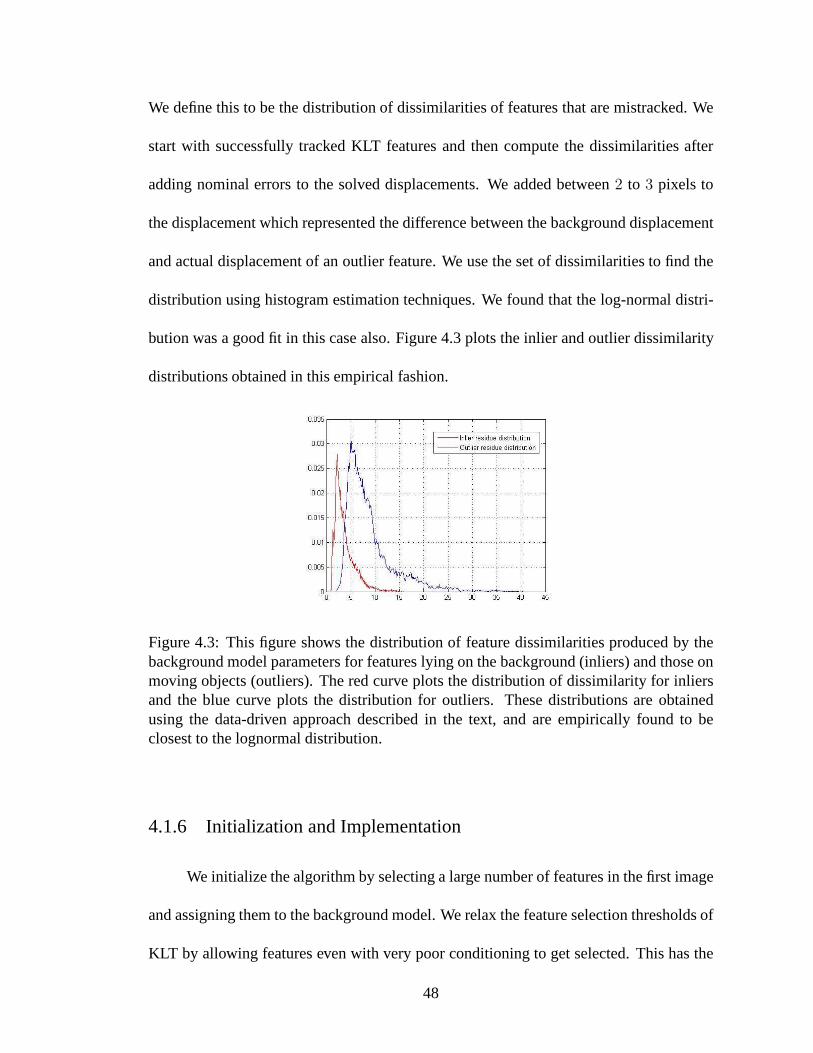
We define this to be the distribution of dissimilarities of features that are mistracked. We

start with successfully tracked KLT features and then compute the dissimilarities after

adding nominal errors to the solved displacements. We addedbetween2 to 3 pixels to

the displacement which represented the difference betweenthe background displacement

and actual displacement of an outlier feature. We use the setof dissimilarities to find the

distribution using histogram estimation techniques. We found that the log-normal distri-

bution was a good fit in this case also. Figure 4.3 plots the inlier and outlier dissimilarity

distributions obtained in this empirical fashion.

Figure 4.3: This figure shows the distribution of feature dissimilarities produced by thebackground model parameters for features lying on the background (inliers) and those onmoving objects (outliers). The red curve plots the distribution of dissimilarity for inliersand the blue curve plots the distribution for outliers. These distributions are obtainedusing the data-driven approach described in the text, and are empirically found to beclosest to the lognormal distribution.

4.1.6 Initialization and Implementation

We initialize the algorithm by selecting a large number of features in the first image

and assigning them to the background model. We relax the feature selection thresholds of

KLT by allowing features even with very poor conditioning toget selected. This has the

48

result of placing features inside homogenous regions alongwith locations in the image

with strong gradients. Since we track the background features jointly using the idea of

background motion coherence, the well-conditioned feature windows aid the motion es-

timation of poorly conditioned feature windows. This has the effect of producing feature

tracks that are uniformly distributed in the image which helps us in the dense segmenta-

tion step.

We iterate the joint tracking and segmentation steps until convergence for each suc-

cessive pair of images. Features whose probability of belonging to the background drops

below0.5 are labeled to be on the moving objects. The foregrond features are tracked in-

dividually using the traditional KLT equations. All the background features are assigned

the parameters of the jointly solved background model.

In practice, we have observed that the mislabeled features in the first frame (during

the initialization step) are quickly removed by the algorithm because their probability of

belonging to the background quickly drops below0.5. New features are initialized with

equal probability of being in the background or foreground.As the algorithm proceeds

through successive pairs of frames, these features are labeled very accurately.

The algorithm provides us with a set of feature tracks through the image sequence

that are accurately labeled into foreground and background. These features are almost

uniformly distributed on the image irrespective of the presence or absence of good fea-

tures to track.

49

4.1.7 Dense Segmentation

The joint tracking and segmentation described above gives us a set of feature tracks

distributed over the entire image area that is classified with high accuracy into features on

the background and features on the moving objects. The objective of motion segmenta-

tion is to obtain a binary labeling of the image into background and foreground regions

which involves labeling all pixels in the image. We use a MAP-MRF framework proposed

in [64, 27] to infer the class labels of all the pixels from thelabels of feature points. We

summarize this algorithm here, as proposed in [64, 27], for the sake of completeness.

Assume there areN pixels in the image indexed byi = 1, · · · , N. Let the pixel

labeling be denoted byL = [l1, l2, · · · , lN ] whereli ∈ 0, 1 denotes the label for pixel

i with 0 denoting background andi denoting foreground. Let the feature locations in the

image be represented byX = [x1, x2, · · · , xF ] wherexj corresponds to the location of

thejth feature andF denotes the number of features. We want to estimate

L∗ = arg maxL

p(L | X) (4.14)

Using Bayes theorem, we can factorp(L | X) ∝ p(L)p(X | L). p(X | L) can be split

using conditional independence asp(X | L) =∏F

j=1 p(xj | lj). Hence, we can rewrite

the likelihood as

p(L | X) ∝ p(L)F

∏

j=1

p(xj | lj) (4.15)

We need to definep(xj | lj) appropriately. This is done in [27] by learning a model for

background and foreground pixels using the labeled features. Assuming thatψb represents

the background model andψf represents the foreground model, the probability of the

50

feature pointxj given its class label is written as

p(xj | lj) =

p(xj | ψb) lj = 0

p(xj | ψf ) lj = 1

(4.16)

The modelsψb andψf are expressed as non-parametric densities in the joint color and

location(x, y, r, g, b) space. We use the Gaussian kernel in our experiments.

The smoothness prior is expressed in terms of an MRF that penalizes neighboring

pixels that have different labels.

p(L) ∝ exp

λN

∑

i=1

∑

j∈N(i)

(lilj + (1− li)(1− lj))

(4.17)

The likelihood can be written as

p(L | x) = λ

N∑

i=1

∑

j∈N(i)

(lilj+(1−li)(1−lj))+

N∑

i=1

li log p(xj | ψf)+

N∑

i=1

(1−li) log p(xj | ψb)

(4.18)

The optimal solution is efficiently computed using the graph-cuts algorithm [65, 66, 67].

4.2 Experiments

We present stabilization and moving object detection results on aerial sequences

from the VIdeo Verification and IDentification (VIVID) dataset. The dataset has associ-

ated metadata with telemetry measurements providing information about the rotation of

the camera.

4.2.1 Metadata

The aerial platform used to capture the images consists of a gimbal mounted with

the cameras. The gimbal provides measurements of the following quantities: platform

51

roll, pitch and heading, latitude, longitude and altitude,and sensor azimuth, elevation and

twist. Using these measurements, we can compute the position and orientation of the

camera in terms of a rotation matrixR and translation vectorT with respect to the world

coordinate system [68]. The3× 4 projection matrix between the image plane and world

plane is written asP = K · R ·

[

I −T

]

, whereK is the camera calibration matrix and

I is the3× 3 identity matrix. This projection matrix is used to transform each image of

the sequence into a fronto-parallel view.

If the camera roll is minimal in the video sequence and the altitude is high, then the

fronto-parallel transformations are accurate enough to assume a pure translation model for

the view-normalized image sequence. This simplified motionmodel due to the metadata

enables mosaicking of long sequences with minimal projective distortion. To compare

qualitatively the extent of the distortion in a mosaicked sequence with and without meta-

data, we tracked KLT features in an aerial sequence and its fronto-parallel equivalent.

We used these feature tracks along with RANSAC to compute theinterframe transfor-

mations using a homography model for the original sequence and a translation model for

the metadata normalized sequence. Figure 4.4 illustrates the mosaicks obtained using the

translation model and homography model. Using the constrained motion model imposed

by the metadata, we are able to mosaic long sequences of around 1700 frames without

distortion and limited buildup of error [21].

We use the fronto-parallel sequence for moving object detection using the joint

tracking and segmentation algorithm. We present results onthree different video se-

quences in the dataset.

52

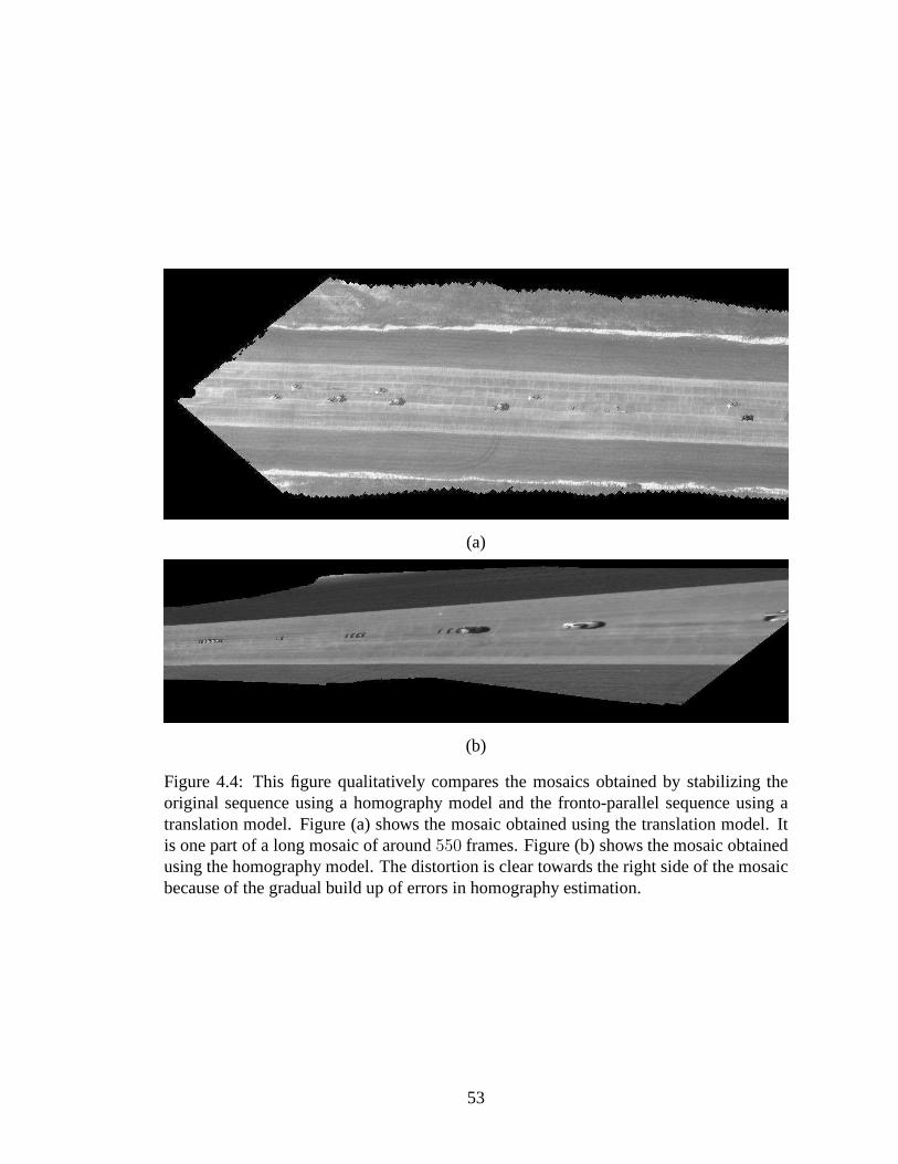
(a)

(b)

Figure 4.4: This figure qualitatively compares the mosaics obtained by stabilizing theoriginal sequence using a homography model and the fronto-parallel sequence using atranslation model. Figure (a) shows the mosaic obtained using the translation model. Itis one part of a long mosaic of around550 frames. Figure (b) shows the mosaic obtainedusing the homography model. The distortion is clear towardsthe right side of the mosaicbecause of the gradual build up of errors in homography estimation.

53

4.2.2 Video sequence 1

The first video sequence consists of a camera moving over a runway, surveying

vehicles moving on the runway. The sequence consists of moving vehicles entering and

leaving the field-of-view. The background may be modeled as aplane since there is no

parallax due to 3D objects on the air strip. Stabilizing the sequence is difficult due to the

textureless background. The presence of repeated textureson the road makes the regis-

tration problem even harder (since the regions of significant gradients repeat themselves

in the image).

We compared the performance of the proposed joint feature-tracking and segmentation-

based registration approach with the intensity-based approach and individual feature track-

ing approach. We select100 frames of the sequence and use the metadata to obtain

fronto-parallel views. We detected the prominent lines on the images and used them to

correct the small rotation-errors in camera-roll due to themetadata. This ensured that the

fronto-parallel sequence obeyed a pure-translation motion model throughout.

For the intensity-based method, we used the inverse compositional registration al-

gorithm studied in the earlier section to register consecutive sequences of frames. This

algorithm consistently registered the moving objects between consecutive frames, since

the gradients on the moving objects were much more prominentthan those on the back-

ground.

We tracked KLT features independently through the sequenceand solved for trans-

lation using RANSAC. We found that the presence of repeated textures in the sequence

was a serious problem for many feature points. In practice, we experienced registration

54

failures in multiple images of the sequence due to registration of the moving objects as

opposed to the background.

Finally, we used the proposed joint tracking and segmentation algorithm to solve

for inter-frame displacement parameters and motion segmentations. We initialized the

segmentation by choosing2500 features on the first frame automatically and labeling

all the features as belonging to the background. It must be emphasized that there was

no manual initialization or segmentation of any kind. This initialization of all features

to background incorrectly labels the features on the three moving vehicles as background

features. The joint tracking using robust cost function solves for the accurate displacement

and enables the classification block to correctly identify the mislabeled features. The

mislabeled features are subsequently removed and new features are initialized and tracked

on the moving objects.

Figure 4.5 illustrates the results of our algorithm on the sequence. For four dif-

ferent frames, we show the set of classified features overlaid on the images, the dense

segmentation and the tracking result. The classification offeatures into background and

foreground is extremely good throughout the sequence and wefound only one feature

on the background that was misclassified to be on the foreground. We used the set of

labeled features to infer the dense segmentation and obtainthe motion blobs. We found

that throughout the sequence, there was only one false moving target initialization in one

frame (due to a misclassified feature) that was quickly eliminated in subsequent frames.

Column (c) of figure 4.5 illustrates the frame with the false moving target initialization.

In comparison, a background subtraction followed by a blob-based tracking algorithm [2]

resulted in70 moving target initializations. Figure 4.6 illustrates a mosaic of the sequence

55

with the moving objects detected by the algorithm removed from the frames. The mosaic

has a very small artifact as a red patch belonging to a vehiclethat was not segmented out

completely in one frame.

(a) (b) (c) (d)

Figure 4.5: This figure shows results on four frames of the 100frame long VIVID VideoSequence 1. Column (a) shows results on frame 14, column (b) shows results on frame 23,column (c) shows results on frame 50 and column (d) shows results on frame 92. The toprow in each column overlays the feature points tracked on each frame. The blue points areclassified to be on the background and the red points are classified to be on the movingobjects. As the figures illustrate, the segmentation is veryaccurate and is much betterthan individual KLT tracking followed by RANSAC based background feature selection.The middle row in each column illustrates the dense segmentations inferred from thefeature segmentations. The background and moving objects are plotted on different colorchannels for illustration. The bottom row in each column illustrates the tracked boxes onthe images which is the result of a blob tracking algorithm [2]. Column (c) shows theonly feature on the background which is misclassified to be onthe foreground. There isa false moving target initialization due to this feature butthis is quickly removed by thealgorithm.

56

Figure 4.6: This figure shows the mosaic of 100 frames of the VIVID sequence 1. Themoving objects are removed from the individual frames before mosaicking. The absenceof moving object trails on the mosaic illustrates the accuracy of motion segmentation inthis sequence.

4.2.3 Video sequence 2

The second sequence consists of a group of humans walking together on a runway.

This sequence had sufficient features on the images as well asgradient information for

intensity-based stabilization. The group of people move asa single moving blob and

always lie within the field of view in the sequence. The chosensequence was190 frames

long. We compared the performance of intensity and feature based registrations with the

proposed joint tracking and segmentation approach for the purpose of stabilization and

moving object detection.

The intensity-based algorithm registered the background regions of all the frames

as expected. We used background subtraction techniques [2]on the stabilized sequence

to detect moving objects. On the entire sequence,45 false positives were detected due to

slight misregistrations near edges. In addition, the motion blobs corresponding to the true

moving objects were broken into multiple connected components for most of the frames.

Among the190 frames,49 of them had multiple connected components for the single

57

moving object, and55 of them had no detected blobs corresponding to the true moving

object. The absence of blobs was because the group of people moved slowly, and there

were homogeneous regions of relatively unvarying intensity within the blob.

In the feature-based algorithm, we track KLT features individually, use RANSAC

to identify a set of background tracks, and use them to solve for motion model parameters

between consecutive frames. We stabilize the sequence using the estimated homographies

and then identify moving blobs [2]. On the entire sequence, there were21 frames where

no blob was detected corresponding to the moving object. Onesingle blob was detected

in 88 of the frames,2− 3 blobs in65 frames and4− 5 blobs in16 frames. There were34

false positive moving objects that were tracked through thesequence.

When the joint tracking and segmentation algorithm was applied to the sequence,

it detected a single motion blob that enclosed the entire object in all the frames. There

were only5 false positive objects detected,3 of which were features in some frames lying

on off-planar objects. These features represented the parallax-induced motion between

frames of 3D objects on the plane. Only2 features clearly lying on the plane were mis-

classified by the algorithm to lie on moving objects. Figure 4.7 illustrates the results

of our algorithm on the sequence. For four different frames,we show the set of classi-

fied features overlaid on the images, the dense segmentationand the tracking result. The

classification of features into background and foreground is extremely good throughout

the sequence. Column (b) of figure 4.7 illustrates a frame with a feature on a stationary

vehicle that was classified as moving.

58

(a) (b) (c) (d)

Figure 4.7: This figure shows results on four frames of the 190frame long VIVID VideoSequence 2. Column (a) shows results on frame 1, column (b) shows results on frame 24,column (c) shows results on frame 91 and column (d) shows results on frame 175. The toprow in each column overlays the feature points tracked on each frame. The blue points areclassified to be on the background and the red points are classified to be on the movingobjects. As the figures illustrate, the segmentation is veryaccurate and is much betterthan the results from individual KLT tracking followed by RANSAC-based backgroundfeature selection. The middle row in each column illustrates the dense segmentationsinferred from the feature segmentations. The background and moving objects are plottedon different color channels for illustration. The bottom row in each column illustrates thetracked boxes on the images which is the result of a blob tracking algorithm [2]. Column(b) shows a feature on a stationary vehicle which is misclassified to be a a moving featuredue to parallax-induced motion.

59

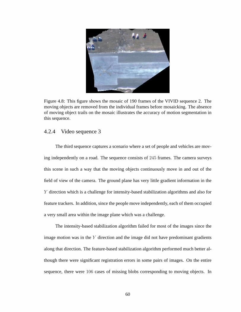
Figure 4.8: This figure shows the mosaic of 190 frames of the VIVID sequence 2. Themoving objects are removed from the individual frames before mosaicking. The absenceof moving object trails on the mosaic illustrates the accuracy of motion segmentation inthis sequence.

4.2.4 Video sequence 3

The third sequence captures a scenario where a set of people and vehicles are mov-

ing independently on a road. The sequence consists of245 frames. The camera surveys

this scene in such a way that the moving objects continuouslymove in and out of the

field of view of the camera. The ground plane has very little gradient information in the

Y direction which is a challenge for intensity-based stabilization algorithms and also for

feature trackers. In addition, since the people move independently, each of them occupied

a very small area within the image plane which was a challenge.

The intensity-based stabilization algorithm failed for most of the images since the

image motion was in theY direction and the image did not have predominant gradients

along that direction. The feature-based stabilization algorithm performed much better al-

though there were significant registration errors in some pairs of images. On the entire

sequence, there were106 cases of missing blobs corresponding to moving objects. In

60

many of the cases where a blob was detected corresponding to the moving people, the

blob was very small and did not enclose the humans. There were47 false target initial-

izations throughout the sequence for blobs which showed up on the background due to

misregistration and errors in background subtraction.

When the joint tracking and segmentation algorithm was applied, all the moving

objects were accurately detected in all the frames. There were 18 false positives due

to isolated background features that were classified as outliers. However, most of these

features were quickly removed by the algorithm since they obeyed the background model

in subsequent frames. Among the false positives, only3 of them were from background

features that were continually classified as moving. With this very simple filtering rule,

the number of false positives of our algorithm got down to3. These results illustrate the

competence of the proposed algorithm in stabilizing and detecting small moving objects

from aerial videos.

4.3 Conclusions

This chapter presents a joint tracking and segmentation algorithm to exploit motion

coherency of the background as well as solve for the class labels of features. Although al-

gorithms exist for tracking features jointly, the idea of incorporating segmentation within

this framework and using the feature dissimilarities to infer membership probabilities

yields robust results. The proposed approach produces highaccuracy labeled feature

tracks in a sequence that are uniformly distributed. This enables us to infer dense pixel-

wise motion segmentation that is useful in moving object initialization. We demonstrate

61

(a) (b) (c) (d)

Figure 4.9: This figure shows results on four frames of the 245frame long VIVID VideoSequence 3. Column (a) shows results on frame 70, column (b) shows results on frame142, column (c) shows results on frame 196 and column (d) shows results on frame 235.The top row in each column overlays the feature points tracked on each frame. Theblue points are classified to be on the background and the red points are classified to beon the moving objects. As the figures illustrate, the segmentation is very accurate andis much better than individual KLT tracking followed by RANSAC-based backgroundfeature selection. The middle row in each column illustrates the dense segmentationsinferred from the feature segmentations. The background and moving objects are plottedon different color channels for illustration. The bottom row in each column illustrates thetracked boxes on the images which is the result of a blob tracking algorithm [2]. Column(c) shows a frame with a few features on the background which are misclassified to beon the foreground. There are a false moving target initializations due to these feature butthey are quickly removed by the algorithm in the subsequent frame.

62

robust results in several challenging video sequences in the VIVID dataset. We also

qualitatively compare the improvement in image mosaics obtained using the information

provided by associated metadata containing telemetry information.

63

Chapter 5

Fast Bilinear Structure from Motion

In an urban environment, the additional sensors are not accurate enough to measure

the location precisely. In the presence of tall buildings, it is difficult to triangulate the GPS

position because of obstacles to the line-of-sight. In thischapter, we study the effect of

additional information, in the form of measurements of a direction vector and the height of

the camera center from a plane perpendicular to this vector.This type of side information

is frequently available and accurately measurable in several real-world scenarios such as

when onboard inertial measurements are available or when a dominant plane is present.

Inertial sensors like the inclinometer or gravitational sensors can provide sensing

of a certain direction while altimeters frequently found onUAVs can provide the required

height information. For example, when there is negligible camera acceleration, an ac-

celerometer measures the gravity and we can filter out the IMUmeasurements to get

good estimates of the gravity vector. When we do not have sideinformation but we ob-

serve a dominant plane in the scene, we can use the homographies between multiple views

to obtain estimates of the ground plane normal and height using a decomposition tech-

nique. In either case, we will show that this side information constrains the ill-posed SfM

problem in such a manner that the SfM equations become similar to a bilinear form in

its unknowns. We then describe a fast iterative procedure much like bilinear solvers that

can robustly solve for the SfM unknowns by minimizing the reprojection error [69, 70].

64

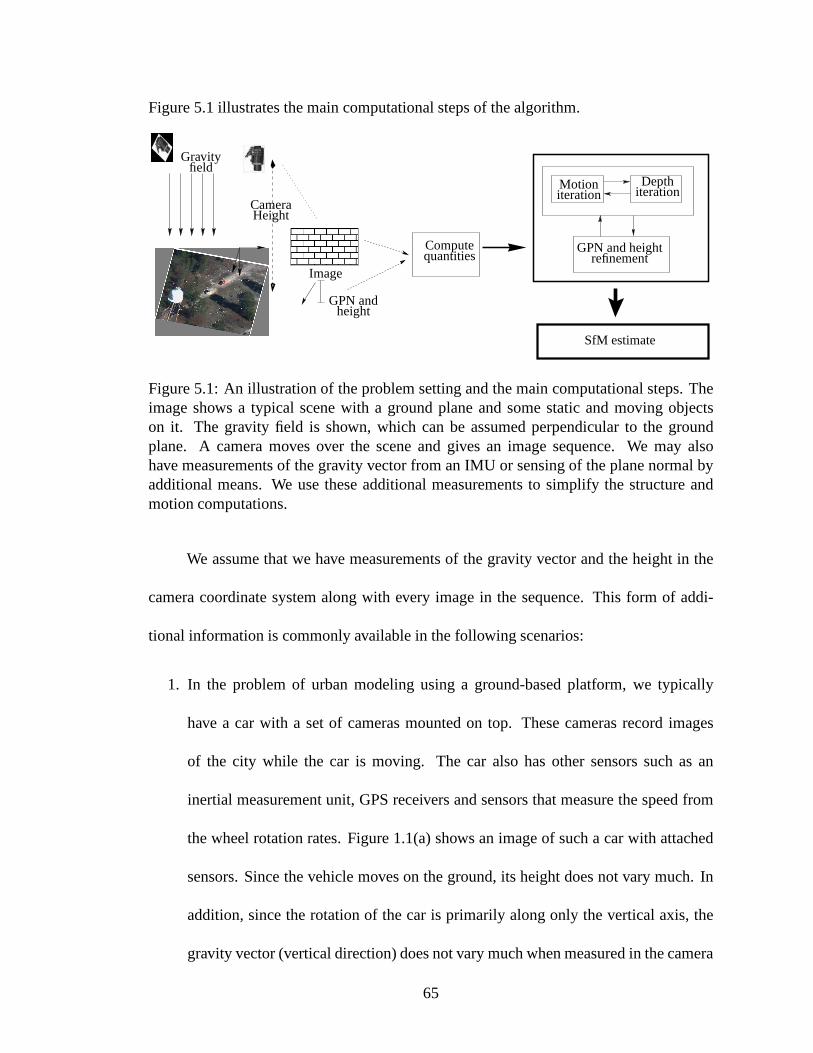
Figure 5.1 illustrates the main computational steps of the algorithm.

Motioniteration

Depthiteration

GPN and heightrefinement

SfM estimate

Computequantities

GPN andheight

Image

Gravityfield

CameraHeight

Figure 5.1: An illustration of the problem setting and the main computational steps. Theimage shows a typical scene with a ground plane and some static and moving objectson it. The gravity field is shown, which can be assumed perpendicular to the groundplane. A camera moves over the scene and gives an image sequence. We may alsohave measurements of the gravity vector from an IMU or sensing of the plane normal byadditional means. We use these additional measurements to simplify the structure andmotion computations.

We assume that we have measurements of the gravity vector andthe height in the

camera coordinate system along with every image in the sequence. This form of addi-

tional information is commonly available in the following scenarios:

1. In the problem of urban modeling using a ground-based platform, we typically

have a car with a set of cameras mounted on top. These cameras record images

of the city while the car is moving. The car also has other sensors such as an

inertial measurement unit, GPS receivers and sensors that measure the speed from

the wheel rotation rates. Figure 1.1(a) shows an image of such a car with attached

sensors. Since the vehicle moves on the ground, its height does not vary much. In

addition, since the rotation of the car is primarily along only the vertical axis, the

gravity vector (vertical direction) does not vary much whenmeasured in the camera

65

coordinate system. Both these quantities can be measured accurately using onboard

sensors.

2. With advances in Micro Air Vehicle (MAV) technology, MAVsare increasingly

being used for surveying and mapping environments. Figure 1.1(b) shows an illus-

tration of an MAV surveying a scene. These MAVs typically have IMUs, altimeters

etc that sense the required additional information. Our algorithm can be used in this

situation to solve for the structure and motion from video sequences.

3. In the scenario where a UAV observes the ground plane from moderate to high

altitudes, we describe how we can derive the necessary additional information from

the homographies induced by the plane from multiple views. We can decompose

these homographies [71] to solve for the ground-plane normal vector and heights

which can be used as initial solutions in our algorithm.

There are other kinds of additional information that can be leveraged to develop

video processing algorithms. For instance, the raw inertial measurements sense the accel-

eration and rotation rates that can potentially be fused with inertial sensors. Range data

from laser scanners found in ground-based platforms can be used with images for highly

accurate mapping. However, these additional data are outside the scope of the current

work.

5.1 Problem Formulation

We choose a World Coordinate System (WCS) with theZ axis along the vertical

direction, and theX andY axes perpendicular to this vector. If a ground plane is present

66

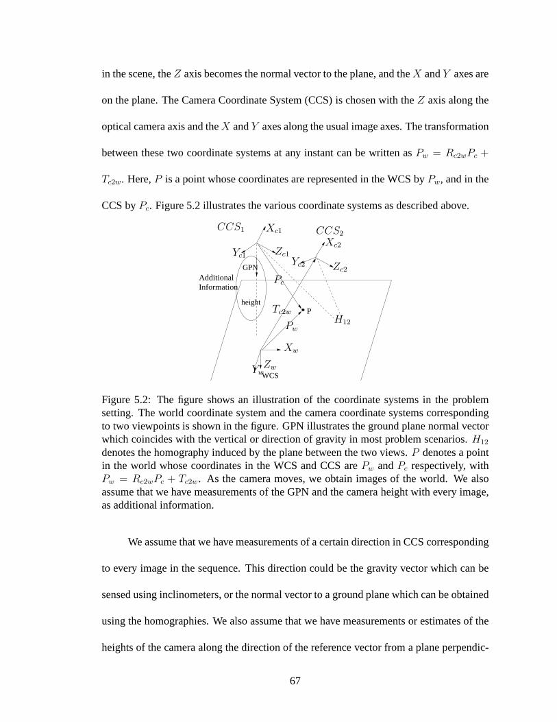
in the scene, theZ axis becomes the normal vector to the plane, and theX andY axes are

on the plane. The Camera Coordinate System (CCS) is chosen with theZ axis along the

optical camera axis and theX andY axes along the usual image axes. The transformation

between these two coordinate systems at any instant can be written asPw = Rc2wPc +

Tc2w. Here,P is a point whose coordinates are represented in the WCS byPw, and in the

CCS byPc. Figure 5.2 illustrates the various coordinate systems as described above.

WCS

P

GPN

height

AdditionalInformation

Xw

YwZw

Pw

Pc

Tc2w

Xc1

Yc1 Zc1

Xc2

Yc2 Zc2

H12

CCS1 CCS2

Figure 5.2: The figure shows an illustration of the coordinate systems in the problemsetting. The world coordinate system and the camera coordinate systems correspondingto two viewpoints is shown in the figure. GPN illustrates the ground plane normal vectorwhich coincides with the vertical or direction of gravity inmost problem scenarios.H12

denotes the homography induced by the plane between the two views.P denotes a pointin the world whose coordinates in the WCS and CCS arePw andPc respectively, withPw = Rc2wPc + Tc2w. As the camera moves, we obtain images of the world. We alsoassume that we have measurements of the GPN and the camera height with every image,as additional information.

We assume that we have measurements of a certain direction inCCS corresponding

to every image in the sequence. This direction could be the gravity vector which can be

sensed using inclinometers, or the normal vector to a groundplane which can be obtained

using the homographies. We also assume that we have measurements or estimates of the

heights of the camera along the direction of the reference vector from a plane perpendic-

67

ular to the vector.

A known reference vector in an unknown camera coordinate camera system fixes

two degrees of freedom of the rotation matrixRc2w. The unknown component is the

rotation of the CCS about an axis parallel to the reference direction vector. The full

rotation matrix can be shown to be split uniquely asRc2w = RpRg, whereRp is the

rotation along the direction vector, andRg is along an axis perpendicular to this vector.

We are now concerned with the estimation of the rotation along the direction vector (Rp),

and the translations along a plane perpendicular to this vector (x andy components of

Tc2w) in addition to the 3D locations of the world points. In the following, we refer

to in-plane motion as the component of translation parallelto theX − Y world plane

and rotation about theZ-axis (Rp). The out-of-plane motion is theZ-axis translation (z

component ofTc2w), and the rotationRg that changes the reference vector orientation in

the local coordinate system (CCS). Table 5.1 lists all the notations used in the following

derivations.

We write the transformation between the WCS and the CCS as:

P iw =

Xi

Yi

Zi

= R(t)p R(t)

g λti

xti

yti

1

+ T(t)c2w (5.1)

where the camera-to-world rotation matrix has been factorized into its two com-

ponents asR(t)c2w = R

(t)p R

(t)g . HereT (t)

c2w = [T(t)x , T

(t)y , T

(t)z ] whereT (t)

z is the height of

the camera.[xi, yi, 1]T is the image feature in homogeneous coordinates, which has been

normalized for the calibration matrix.P iw denotes the coordinates of theith point in the

68

Notation Meaning

P Coordinates of a point

subscript w Quantity expressed in WCS

subscript c Quantity expressed in CCS

subscript c2w Camera-to-world transformation

subscript ti Coordinates at frame t and feature i

index t Frame number

index i Feature number

T tx,y,z Translation coordinates at frame t

Rtg Out-of-plane rotation at frame t

Rtp In-plane rotation at frame t

m Number of frames

n Number of points

Table 5.1: This table lists common notations used in the derivations for purposes of read-ability.

69

WCS. From the additional measurements, we have estimates (initial values) ofR(t)g and

T(t)z . Using this information, we can rewrite (5.1) as

P iw =

cos θt sin θt 0

− sin θt cos θt 0

0 0 1

λti

uti

vti

wti

+ T(t)c2w (5.2)

where[uti, vti, wti]T = R

(t)g [xi, yi, 1]T , andR(t)

g is computed from the reference vector in

the side information.R(t)g is the rotation matrix that rotates the reference vector expressed

in the CCS to the reference vector expressed in the WCS.

We rearrange (5.2) to get (5.3) that relates the coordinatesof the feature point in

framet and featurei to the world coordinates and the camera positions.

λti

uti

vti

wti

=

cos θt − sin θt 0

sin θt cos θt 0

0 0 1

Xi − T(t)x

Yi − T(t)y

Zi − T(t)z

(5.3)

We eliminate the projective depthλti by taking ratios of the quantities as shown in (5.4)

uti/wti

vti/wti

=

cos θt − sin θt

sin θt cos θt

Xi−T(t)x

Zi−T(t)z

Yi−T(t)y

Zi−T(t)z

(5.4)

We rearrange (5.4) by multiplying both sides by(Zi − Tz) to obtain (5.5)

uti/wti

vti/wti

· (Zi − T(t)z ) =

cos θt − sin θt

sin θt cos θt

Xi − T(t)x

Yi − T(t)y

(5.5)

Let us now assume that we haven feature points that are observed inm frames. We have

equations similar to (5.5) for each feature point in every frame where it is visible. We

accumulate (5.5) for all the feature points in all views and write it in the factorization

70

format as shown in (5.6).

u11w11

u12w12

· · · u1n

w1n

v11w11

v12w12

· · · v1n

w1n

.... . . · · ·

um1wm1

um2wm2

· · · umn

wmn

vm1wm1

vm2wm2

· · · vmn

wmn

Z1 0 . . . 0

0 Z2 . . . 0

...

0 0 . . . Zn

−

T(1)z 0 . . . 0 0

0 T(1)z . . . 0 0

.... . .

...

0 0 . . . T(m)z 0

0 0 . . . 0 T(m)z

u11w11

· · · u1n

w1n

v11w11

· · · v1n

w1n

.... . . · · ·

um1wm1

· · · umn

wmn

vm1wm1

· · · vmn

wmn

=

cos θ1 − sin θ1 t(1)x

sin θ1 cos θ1 t(1)y

· · ·

cos θm − sin θm t(m)x

sin θm cos θm t(m)y

X1 · · · Xn

Y1 · · · Yn

1 · · · 1

(5.6)

We denote the measurement matrix asA, the diagonal matrix of camera heights

as Tz, and the productTzA = B. We denote the diagonal matrix of heights of feature

points from the ground plane asZ. The motion matrix on the right hand side isM

and the shape matrix isS. We can rewrite (5.6) concisely as:AZ − B = MS. Each

column of this matrix equation specifies the relation between the projections of a single

point in all the views. Each pair of rows specifies the relation between the projections

of all the points in a single view. In (5.4), the quantitiesT (t)x andT (t)

y refer to thex

andy components of translation measured along the WCS axes. In (5.6), the variables

t(t)x = −cosθtT

(t)x +sinθtT

(t)y andt(t)y = −sinθtT

(t)x −cosθtT

(t)y refer to the same quantities

measured in the CCS axes. This change of variables is done to enable a factorization

into the motion and shape matrices as shown. Note that our unknowns are the matrices

M,S, Z and (5.6) looks similar to a bilinear system in the elements of these matrices.

71

In practice, we have measurement errors in image features orin additional mea-

surements or both, and the measurement matrixA is not known exactly. We solve for the

unknown parameters(M,S, Z) by optimizing an objective function which is the Frobe-

nius norm of the difference between the matrices on each sideof (5.6). The cost function

is written as follows:

E = ‖A · Z − TzA−M · S‖2 (5.7)

In the above, because features may not be observed in all frames, some entries of the mea-

surement matrix are unknown (not measurable). However, in solving for the unknowns

using our algorithm, we do not need all entries of the measurement matrix. In this respect,

it has an advantage over factorization-based approaches.

This formulation yields an optimal solution in the maximum-likelihood sense when

Gaussian noise is added to the right hand side of (5.6). In practice, we can make a reason-

able assumption that the image feature locations are corrupted by Gaussian noise. How-

ever, the geometric transformations and the non-linearityin the rotation matrices do not

preserve the Gaussian nature of the error, and it is difficultto characterize the distribution

of the error in measurements in (5.6).

The scale ambiguity in SfM implies that we can decrease the error (5.7) by scaling

the camera positions and3D coordinates of points by any number larger than one. Since

we refine all components of motion in our algorithm, to guard against trivial reductions

in error functions because of such scaling, we impose the constraint:∥

∥Tz

∥

∥ = k wherek

is a constant.

72

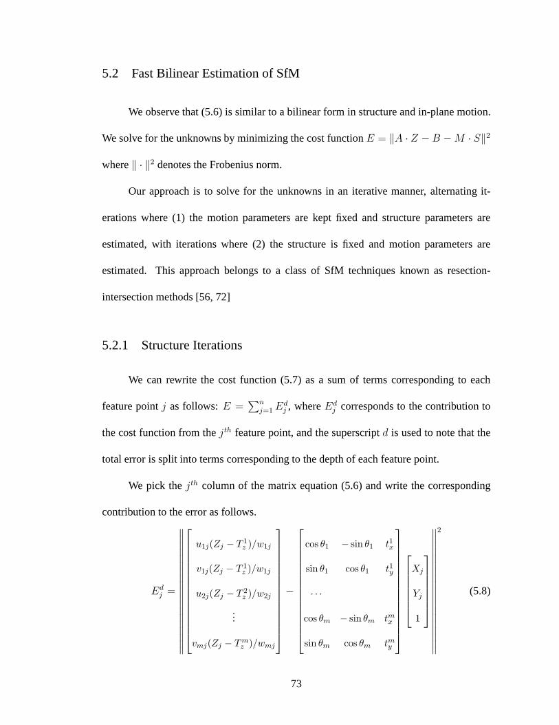
5.2 Fast Bilinear Estimation of SfM

We observe that (5.6) is similar to a bilinear form in structure and in-plane motion.

We solve for the unknowns by minimizing the cost functionE = ‖A · Z −B −M · S‖2

where‖ · ‖2 denotes the Frobenius norm.

Our approach is to solve for the unknowns in an iterative manner, alternating it-

erations where (1) the motion parameters are kept fixed and structure parameters are

estimated, with iterations where (2) the structure is fixed and motion parameters are

estimated. This approach belongs to a class of SfM techniques known as resection-

intersection methods [56, 72]

5.2.1 Structure Iterations

We can rewrite the cost function (5.7) as a sum of terms corresponding to each

feature pointj as follows:E =∑n

j=1Edj , whereEd

j corresponds to the contribution to

the cost function from thejth feature point, and the superscriptd is used to note that the

total error is split into terms corresponding to the depth ofeach feature point.

We pick thejth column of the matrix equation (5.6) and write the corresponding

contribution to the error as follows.

Edj =

∥

∥

∥

∥

∥

∥

∥

∥

∥

∥

∥

∥

∥

∥

∥

∥

∥

∥

∥

u1j(Zj − T1z )/w1j

v1j(Zj − T1z )/w1j

u2j(Zj − T2z )/w2j

...

vmj(Zj − Tmz )/wmj

−

cos θ1 − sin θ1 t1x

sin θ1 cos θ1 t1y

· · ·

cos θm − sin θm tmx

sin θm cos θm tmy

Xj

Yj

1

∥

∥

∥

∥

∥

∥

∥

∥

∥

∥

∥

∥

∥

∥

∥

∥

∥

∥

∥

2

(5.8)

73

We rewrite (5.8) to obtain

Edj =

∥

∥

∥

∥

∥

∥

∥

∥

∥

∥

∥

[

M(:, 1) M(:, 2) −A(:, i)

]

Xj

Yj

Zj

+ (B(:, j) +M(:, 3))

∥

∥

∥

∥

∥

∥

∥

∥

∥

∥

∥

2

(5.9)

In structure iterations, we minimize the error contribution Edj corresponding to each 3D

point indexed byj ∈ (1, · · · , n). In (5.9),M(:, 1) andM(:, 2) are the first and second

columns of the motion matrix, containing the cosine and sineterms. M(:, 3) contains

the in-plane components of translation.A(:, j) andB(:, j) are thejth columns of the

matricesA andB respectively. Recall thatB is the product of the heights matrixTz, and

the measurement matrixA. We minimize (5.9) w.r.t(Xj, Yj, Zj). The cost function is a

linear system in the variables(Xj, Yj, Zj) and the minimum is obtained by solving the

following linear system using linear least squares.

[

M(:, 1) M(:, 2) −A(:, j)

]

Xj

Yj

Zj

= −B(:, j) −M(:, 3) (5.10)

5.2.2 Motion Iterations

As in the case of depth refinement iterations, we can rewrite the cost function (5.7)

as a sum of terms corresponding to each frame as follows:E =∑m

i=1Emi , whereEm

i

corresponds to the contribution to the total cost function due to the motion variables of

the ith frame, and the superscriptm is used to note that the total error is split into terms

corresponding to the motion parameters of each frame. We extract the(2i − 1)th and

(2i)th rows from the matrix equation (5.6) and write the corresponding contribution to the

74

error as

Emi =

∥

∥

∥

∥

C(2i− 1, :)−

[

cos θi − sin θi tix

]

· S

∥

∥

∥

∥

2

+

∥

∥

∥

∥

C(2i, :)−

[

sin θi cos θi tiy

]

· S

∥

∥

∥

∥

2

(5.11)

where, theC = AZ − B denotes the left hand side of (5.6). We need to solve for

θi, tix, t

iy by minimizing (5.11). We set the derivative ofEm

i w.r.t (tix, tiy) to zero to

obtain

tix =1

n

n∑

k=1

C(2i− 1, k)−1

n

n∑

k=1

Xkcosθi +1

n

n∑

k=1

Yksinθi (5.12)

tiy =1

n

n∑

k=1

C(2i, k)−1

n

n∑

k=1

Xksinθi −1

n

n∑

k=1

Ykcosθi (5.13)

Denotingµ2i−1 andµ2i as the means ofC(2i− 1, :) andC(2i, :) respectively, andµX and

µY as the means of theX andY coordinates of feature points, we can write the solution

of tix andtiy as

tix = µ2i−1 − µX cos θi + µY sin θi (5.14)

tiy = µ2i − µY cos θi − µX sin θi (5.15)

We substitute the solution (5.15) in (5.11) and obtain

Emi =

∥

∥

∥

(

~X − µX

)

cos θi −(

~Y − µY

)

sin θi −(

C(2i− 1, :)T − µ2i−1

)

∥

∥

∥

2

+∥

∥

∥

(

~X − µX

)

sin θi +(

~Y − µY

)

cos θi −(

C(2i, :)T − µ2i

)

∥

∥

∥

2

(5.16)

where ~X and ~Y denote column vectors containing theX andY coordinates of all the

points. We set the derivative w.r.tθi to zero and simplify to obtain

n∑

k=1

(C(2i− 1, k)− µ2i−1) ((Xk − µX) sin θi + (Yk − µY ) cos θi) +

n∑

k=1

(C(2i, k)− µ2i) (− (Xk − µX) cos θi + (Yk − µY ) sin θi) = 0 (5.17)

75

We can simplify (5.17) to obtain

tan θi =(C(2i, :)− µ2i) ·

(

~X − µX

)

− (C(2i− 1, :)− µ2i−1) ·(

~Y − µY

)

(C(2i− 1, :)− µ2i−1) ·(

~X − µX

)

+ (C(2i, :)− µ2i) ·(

~Y − µY

) (5.18)

We obtain two possible solutions forθi from (5.18). One of them is a point of local

maxima and the other is a point of local minima. We choose the solution that corresponds

to the local minima.

We have described a technique to iteratively estimate the 3Dlocations, and the

in-plane components of motion. Each of the individual stepsonly involves solving a

linear system. In practice, we iterate these two steps a certain number of times, or until a

termination criterion is satisfied.

In both the depth and motion iterations, we solve linear systems that are of much

smaller size compared to the size of systems that we need to solve in techniques like bundle

adjustment etc. More details on the computational requirements are given in section 5.3.1

5.2.3 Out-of-plane motion refinement iterations

In case the measurements of the direction vector and the camera height are not ac-

curate, we may refine these parameters to obtain a better SfM estimate. We describe a

technique to refine these quantities. The idea is to refine theout-of-plane motion compo-

nents so that the error (5.7) decreases.

From (5.5), we have

uti/wti

vti/wti

· (Zi − T(t)z ) =

cos θt − sin θt

sin θt cos θt

Xi − T(t)x

Yi − T(t)y

(5.19)

Recall that(uti, vti, wti) is a function of the out-of-plane rotationR(t)g based on the rela-

76

tion:

uti

vti

wti

= R(t)g

xti

yti

1

(5.20)

In this step, we hold the 3D locationsP iw and the in-plane components of motionθt, T

tx, T

ty

fixed to their earlier estimates from the previous step. We perform a nonlinear refinement

of the heightT tz , and the normal vector at each frame separately. Note that this implies

that at any stage, we only refine three parameters simultaneously (in comparison to all the

cameras and points for a full bundle adjustment).

We refine the parameters by minimizing the following error function obtained from (5.5)

Eside =

m∑

t=1

∥

∥

∥

∥

∥

∥

∥

∥

uti/wti

vti/wti

· (Zi − T(t)z )−

cos θt − sin θt

sin θt cos θt

Xi − T(t)x

Yi − T(t)y

∥

∥

∥

∥

∥

∥

∥

∥

2

(5.21)

We minimize (5.21) using the Levenberg-Marquardt algorithm [39] to solve for the out-

of-plane motion parameters. This minimization involves only three parameters at any

stage (two for the out-of-plane motion and one for the cameraheight).

5.2.4 Motion Estimation for Moving Objects

We can incorporate the estimation of structure and motion ofobjects moving on

a plane, in the above framework. The objects of interest can be translating and rotating

on a plane, and we assume that we can measure the ground plane normal and height

with respect to the same plane. We reformulate the problem into one where the object is

stationary, and a separate camera is moving over each object. This approach is similar to

some earlier works [73]. The world coordinate of a point on a moving object changes

77

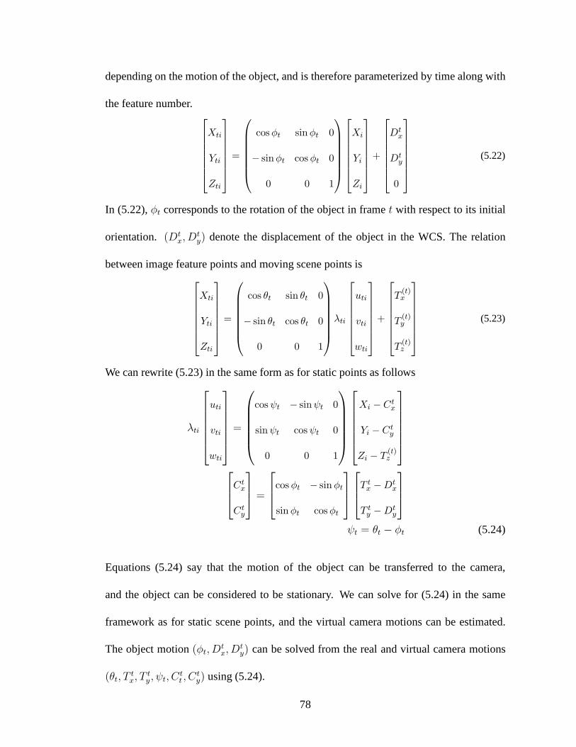
depending on the motion of the object, and is therefore parameterized by time along with

the feature number.

Xti

Yti

Zti

=

cosφt sinφt 0

− sinφt cosφt 0

0 0 1

Xi

Yi

Zi

+

Dtx

Dty

0

(5.22)

In (5.22),φt corresponds to the rotation of the object in framet with respect to its initial

orientation. (Dtx, D

ty) denote the displacement of the object in the WCS. The relation

between image feature points and moving scene points is

Xti

Yti

Zti

=

cos θt sin θt 0

− sin θt cos θt 0

0 0 1

λti

uti

vti

wti

+

T(t)x

T(t)y

T(t)z

(5.23)

We can rewrite (5.23) in the same form as for static points as follows

λti

uti

vti

wti

=

cosψt − sinψt 0

sinψt cosψt 0

0 0 1

Xi − Ctx

Yi − Cty

Zi − T(t)z

Ctx

Cty

=

cosφt − sinφt

sinφt cosφt

T tx −D

tx

T ty −D

ty

ψt = θt − φt (5.24)

Equations (5.24) say that the motion of the object can be transferred to the camera,

and the object can be considered to be stationary. We can solve for (5.24) in the same

framework as for static scene points, and the virtual cameramotions can be estimated.

The object motion(φt, Dtx, D

ty) can be solved from the real and virtual camera motions

(θt, Ttx, T

ty, ψt, C

tt , C

ty) using (5.24).

78

We initialize the iterations for a moving object by assuminga fixed height for all

feature points. In practice, we found that the technique wasnot very sensitive to this ini-

tialization in our sequences. In later sections we refer to the proposed method as FBSfM

which is an acronym for Fast Bilinear Structure from Motion.

5.3 Analysis of FBSFM

5.3.1 Computational Complexity and Memory Requirements

The main computations in our algorithm are in the solution ofthe linear systems in

the depth and motion iterations, and the refinement steps in the direction vector and height

refinements. Suppose there arem views ofn points, and that all points are visible in all

views. To emphasize, this assumption is not necessary for the purposes of the algorithm

but simplifies the process of quantifying the memory requirements.

As mentioned in [52], letSV D(a, b) = 4ab2 + 8b3 be the cost of carrying out a

singular value decomposition of a matrix witha rows andb columns. The following are

the main computational requirements:

• Depth Iterations: For each point, this involves solving a linear system of size

2m × 4 which is equivalent to a total cost ofn × SV D(2m, 4), wheren is the

number of points.

• Motion Iterations: For each view, this involves performing the computations

in (5.18, 5.15) which is equivalent to4n multiplications and6n additions and is

thereforeO(n) in computational cost. This accumulates to a total cost ofm×O(n),

79

wherem is the number of views.

• Direction vector and height refinement:We need to update only 4 parameters and

hence this requires the solution of a4 × 4 linear system. For all the frames, this

comes at a cost ofm× SV D(4, 4) = 768m per iteration.

Totally, each iteration of FBSfM has a computational cost ofO(mn). In compari-

son, one full bundle adjustment takes up computations of theorder ofO(nm+nm2+m3).

Rother’s system involves solving a linear system of size(3n+3m)× (3nm) whose com-

putational cost isSV D(3n+ 3m, 3nm) = 108(m3n2 +m2n3) + 216m3n3. We observe

that the peak computation for our individual steps increases only of the order ofO(mn).

5.3.2 Discussion

The FBSfM algorithm derived in the last section has the flavorof iterative methods

for projective structure from motion [56, 44]. Suppose we haven fixed pointsP1, P2, · · · , Pn

observed bym cameras, we can write the projection of thejth point on theith camera as:

pij =1

zij

MiPj (5.25)

whereMi denotes the3 × 4 projective matrix associated with theith camera, andzij

denotes the projective depth associated with thejth point in theith camera.

In a typical BA algorithm, we usually minimize the reprojection error which is

E =∑

i,j |pij −1

zijMiPj |

2 and solve for the camera locationsMi and point locations

Pj. This technique is commonly known as bundle adjustment and employs a non-linear

minimization method to optimize the objective function (reprojection error). This objec-

tive function is highly non-linear and is difficult to minimize and also is reported to have

80

many local minima [72]. To simplify the minimization, many authors consider the sim-

plified (but related) objective function:Elin =∑

i,j |zijpij −MiPj|2. Many projective

SfM algorithms in the literature minimize this objective function to solve for the SfM

parameters.

The proposed algorithm is similarly derived by scaling (5.4) by the(Zi−T(t)z ). The

difference is that unlike earlier techniques, we use the additional information to leverage

the bilinear form in the Euclidean frame, without using slack variables. Simulation re-

sults suggest clear advantages in speed and accuracy of the proposed algorithm when the

additional information has low error.

Convergence in error value: Our algorithm has three main iterations: depth itera-

tions, motion iterations and side-information refinement iterations. LetE(0) be the value

of the initial error. In the depth iterations, we find solutions for the(X, Y, Z) co-ordinates

that minimize the error with all other variables fixed. IfE(1) is the value of the error after

the depth iterations, we haveE(1) ≤ E(0). Next, in motion iterations, we find solutions

for the camera in-plane motion parameters that minimize theerror with all other variables

fixed. If E(2) is the error after motion iterations, we haveE(2) ≤ E(1). Similarly, if

E(3) is the error after side-information refinement, we haveE(3) ≤ E(2). Each iteration

finds solutions for the variables that decreases the error, hence the error is non-increasing.

Since the error is lower-bounded by zero, we conclude that the successive error values

after each iteration converge to a valueE∗.

Convergence of parameters: As noted in [56], the above argument does not im-

ply that the parameters converge or that the error convergesto a local minimum. We

prove that the error converges to a local minimum, and the parameters converge to the

81

optimal solution. We make use of the Global Convergence Theorem from optimization

theory [56]. We elaborate the proof in the appendix A of the dissertation.

Issue of trivial minima: Oliensis and Hartley [57] pointed out the issue of conver-

gence to solutions that were “trivial” in the sense of generating nonsensical structure and

motion solutions. In our algorithm, since we compute Euclidean structure and motion, we

are not affected by the same problems. In particular, we do not need to deal with “projec-

tive depths” that are considered as independent variables in the optimization. In all of our

experiments on synthetic and real sequences, we have observed that the iterations always

converge to meaningful results.

Convergence rate and speed of convergence: Iterations of low computational com-

plexity do not imply faster convergence rate or lower time-to-convergence. The proposed

algorithm falls within the class of alternation techniqueswhich are susceptible to flatlin-

ing and are slower than second-order newton methods in the average case [74]. We claim

based on strong experimental evidence that the proposed approach surprisingly violates

this conventional wisdom, for thespecificcase of large-sized problems starting from a

specificclass of initial solutions with low out-of-plane motion error and high levels of

in-plane motion error.

5.4 Simulations

5.4.1 Implementation

For BA, we use the SBA solver code [40] implemented in C. This uses LM mini-

mization for non-linear least squares. The normal equations are solved by using the Schur

82

complement to factor out the structure parameters and the resulting system is solved using

LU decomposition for the update to the camera parameters. The proposed algorithm was

also implemented in C with a MATLAB interface. The motion-structure alternation iter-

ations and out-of-plane motion refinement iterations were written in C and the interface

to switch between the two sets of iterations was written in MATLAB with system calls to

the corresponding C executables. Routines from OpenCV wereused to solve the linear

systems corresponding to motion iterations. The LM implementation in C [75] was used

for the non-linear least squares minimization corresponding to the out-of-plane motion

refinement iterations. The Conjugate gradient (CG) implementation in C [76] was used

in the experiments to compare with alternation for minimizing the bilinear system (5.7).

Computation time was measured using our implementation of ananosecond timer. The

reported times include the total time taken to execute all the operations within each C

implementation except disk I/O operations.

5.4.2 Reconstruction problem generation

A reconstruction problem was synthesized by generatingN points uniformly dis-

tributed within the cube specified by−20 ≤ X ≤ 20,−20 ≤ Y ≤ 20 and10 ≤ Z ≤ 40.

The coordinates of the camera locations were uniformly distributed in the cube specified

by −25 ≤ X ≤ 25, −25 ≤ Y ≤ 25, 55 ≤ Z ≤ 105. The choice of dimensions is for

illustration, and in practice the dimensions were scaled according to convenience. The

orientations of the cameras were chosen by first generating the directions of the principal

camera axes and then choosing the rotation angle of the camera around this axis. The

83

principal camera axis was chosen by generating a random point in theX − Y plane that

specifies the point of intersection of the principal axis with this plane. The rotation angle

of the camera axis around the principal axis was randomly chosen between0 to 2π. This

scheme for generating points and cameras ensured a wide variation in the camera matrices

and point locations, to mitigate any potential bias in the reported results to the choice of

reconstruction problem. Image feature points were obtained by reprojecting the 3D points

on the cameras based on perspective projection. The parameters of the camera were: fo-

cal length= 320, principal point= (320, 240) and image size= 640 × 480. Moderate

Gaussian noise was added to the reprojected image feature locations to simulate feature

detection errors.

5.4.3 SfM Initialization

Initial motion estimates are obtained by perturbing the ground truth motion. The

in-plane and out-of-plane motion components are perturbedseparately, with high errors

in in-plane components and low errors in out-of-plane motion components. Thex and

y locations are displaced by a vector that is oriented in a random direction in theXY

plane, and whose length is a specified fraction of the maximumdimension of the recon-

struction. For example, a70% error in the in-plane translation means that the camera

center was displaced by a vector of length0.7 × 50 in theXY plane. A60 error in the

in-plane rotation angleθ means thatθ was perturbed in either the clockwise or counter-

clockwise direction by60. A 10% error in the out-of-plane translation means that each

camera center was moved either in the positive or negativeZ direction by0.1× 40. The

84

ground plane normal is perturbed by adding a random vector toit such that the new vector

makes a pre-specified angle with the original vector. The initial values for the 3D coor-

dinates of feature points are obtained by triangulating each point using the image feature

locations and the initial camera motion parameters, after solving the linear system of a

structure iteration in (5.10)). All algorithms are initialized with the same initial solution

and executed on the identical machines under identical loading conditions when reporting

comparative results.

5.4.4 Comparative evaluation of bilinear alternation

We compare the performance of bilinear alternation, CG and LM for minimizing

the objective function in (5.7). The alternation approach chosen is the motion-structure it-

erations as described in the chapter, where (5.7) is minimized with respect to the in-plane

motion parameters only. We analyze the results of the minimization using the three ap-

proaches for various levels of out-of-plane motion error. Conventional wisdom suggests

that second-order newton methods perform best for the matrix factorization problem [74];

however the results of this experiment for the case of low out-of-plane motion error are

surprising because they suggest that bilinear alternationperforms fastest under the as-

sumed operating conditions.

A reconstruction problem is obtained by generating50 random world points and10

cameras as described above, with96.4% of the image feature measurements known. The

ground plane normal vector at each camera location is perturbed such that the new vector

makes angles of(0, 3, 6, 9, 12) with the ground-truth vector. The camera centers are

85

perturbed along theZ-axis of the WCS by errors of(0%, 3%, 5.2%, 13%, 26%, 39%, 52.1%).

For each choice of errors in out-of-plane motion components, we compare the perfor-

mance of the three algorithms on500 runs. The in-plane motion components are per-

turbed by a100% error in theX − Y locations and a90 error in the in-plane rotation

angle to obtain the starting point for the three approaches.The total number of runs of the

minimization for all cases was17500.

Let the final objective function error value of alternation,CG and LM after conver-

gence be denoted bya∗, c∗ andl∗ respectively. We have the following mutually exclusive

possibilities for each run: (1)a∗ = c∗ = l∗, (2) a∗ = c∗ < l∗, (3) c∗ = l∗ < a∗, (4)

a∗ = l∗ < c∗, (5) a∗ < min(c∗, l∗), (6) c∗ < min(a∗, l∗), and (7)l∗ < min(a∗, c∗). The

equality in the above expressions is understood to be withina small margin of tolerance.

Table 5.2 displays the percentage of runs falling into the above cases for each unique

choice of out-of-plane error.

The percentage of runs for which bilinear alternation performs suboptimally com-

pared to LM or CG (i.e. with higher error than the best of CG or LM) is listed in Table 5.3

for each choice of out-of-plane motion errors. This suggests that for moderate levels of

errors in the out-of-plane motion, alternation turns out tobe a suboptimal choice of algo-

rithm in roughly17% of cases. At low to moderate errors where we propose the use of

our algorithm, alternation turns out to be suboptimal in roughly 9% of cases. In practice,

since we switch between in-plane and out-of-plane iterations, the effect of suboptimality

in 9% of the cases does not adversely affect the structure and motion reconstruction.

We compared the number of iterations and times taken for eachalgorithm to reach

convergence, where the error function decreases by less than 0.00001%. We find that

86

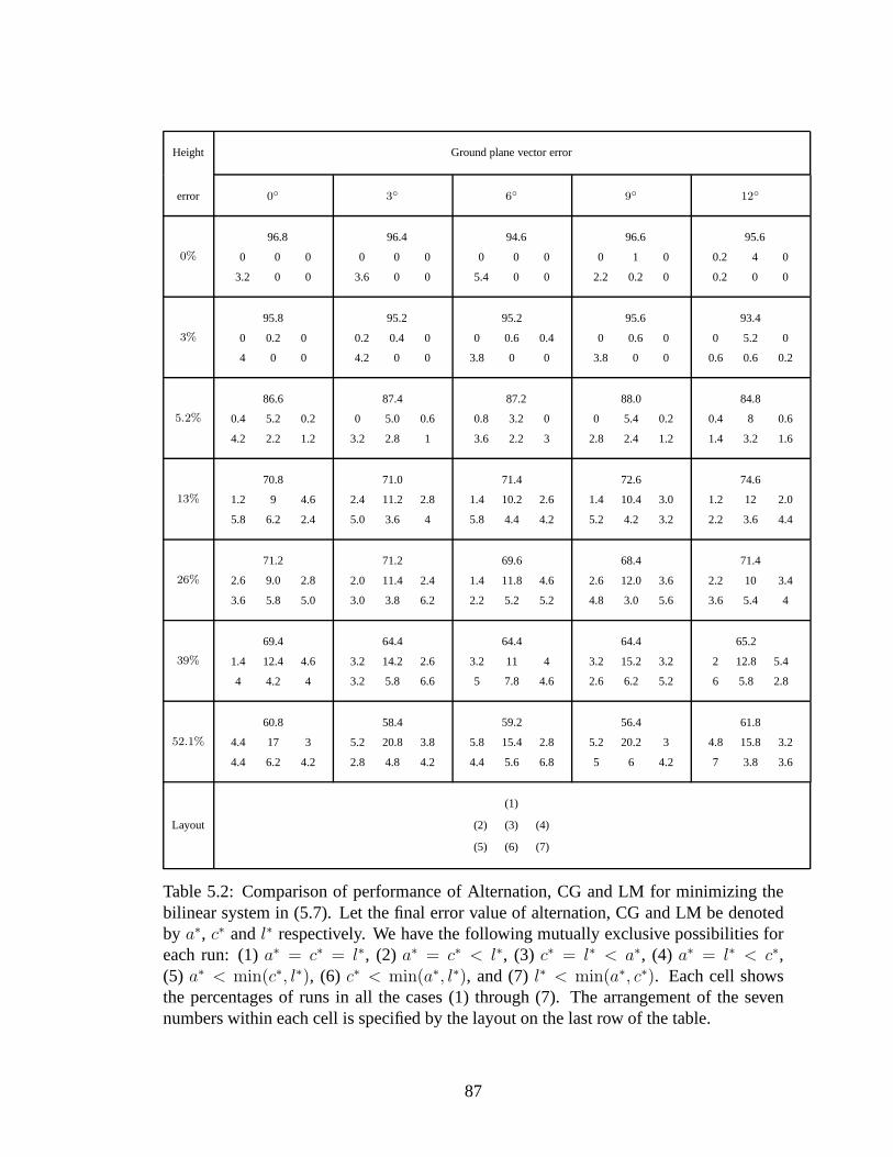
Height Ground plane vector error

error 0 3 6 9 12

0%

96.8

0 0 0

3.2 0 0

96.4

0 0 0

3.6 0 0

94.6

0 0 0

5.4 0 0

96.6

0 1 0

2.2 0.2 0

95.6

0.2 4 0

0.2 0 0

3%

95.8

0 0.2 0

4 0 0

95.2

0.2 0.4 0

4.2 0 0

95.2

0 0.6 0.4

3.8 0 0

95.6

0 0.6 0

3.8 0 0

93.4

0 5.2 0

0.6 0.6 0.2

5.2%

86.6

0.4 5.2 0.2

4.2 2.2 1.2

87.4

0 5.0 0.6

3.2 2.8 1

87.2

0.8 3.2 0

3.6 2.2 3

88.0

0 5.4 0.2

2.8 2.4 1.2

84.8

0.4 8 0.6

1.4 3.2 1.6

13%

70.8

1.2 9 4.6

5.8 6.2 2.4

71.0

2.4 11.2 2.8

5.0 3.6 4

71.4

1.4 10.2 2.6

5.8 4.4 4.2

72.6

1.4 10.4 3.0

5.2 4.2 3.2

74.6

1.2 12 2.0

2.2 3.6 4.4

26%

71.2

2.6 9.0 2.8

3.6 5.8 5.0

71.2

2.0 11.4 2.4

3.0 3.8 6.2

69.6

1.4 11.8 4.6

2.2 5.2 5.2

68.4

2.6 12.0 3.6

4.8 3.0 5.6

71.4

2.2 10 3.4

3.6 5.4 4

39%

69.4

1.4 12.4 4.6

4 4.2 4

64.4

3.2 14.2 2.6

3.2 5.8 6.6

64.4

3.2 11 4

5 7.8 4.6

64.4

3.2 15.2 3.2

2.6 6.2 5.2

65.2

2 12.8 5.4

6 5.8 2.8

52.1%

60.8

4.4 17 3

4.4 6.2 4.2

58.4

5.2 20.8 3.8

2.8 4.8 4.2

59.2

5.8 15.4 2.8

4.4 5.6 6.8

56.4

5.2 20.2 3

5 6 4.2

61.8

4.8 15.8 3.2

7 3.8 3.6

Layout

(1)

(2) (3) (4)

(5) (6) (7)

Table 5.2: Comparison of performance of Alternation, CG andLM for minimizing thebilinear system in (5.7). Let the final error value of alternation, CG and LM be denotedby a∗, c∗ andl∗ respectively. We have the following mutually exclusive possibilities foreach run: (1)a∗ = c∗ = l∗, (2) a∗ = c∗ < l∗, (3) c∗ = l∗ < a∗, (4) a∗ = l∗ < c∗,(5) a∗ < min(c∗, l∗), (6) c∗ < min(a∗, l∗), and (7)l∗ < min(a∗, c∗). Each cell showsthe percentages of runs in all the cases (1) through (7). The arrangement of the sevennumbers within each cell is specified by the layout on the lastrow of the table.

87

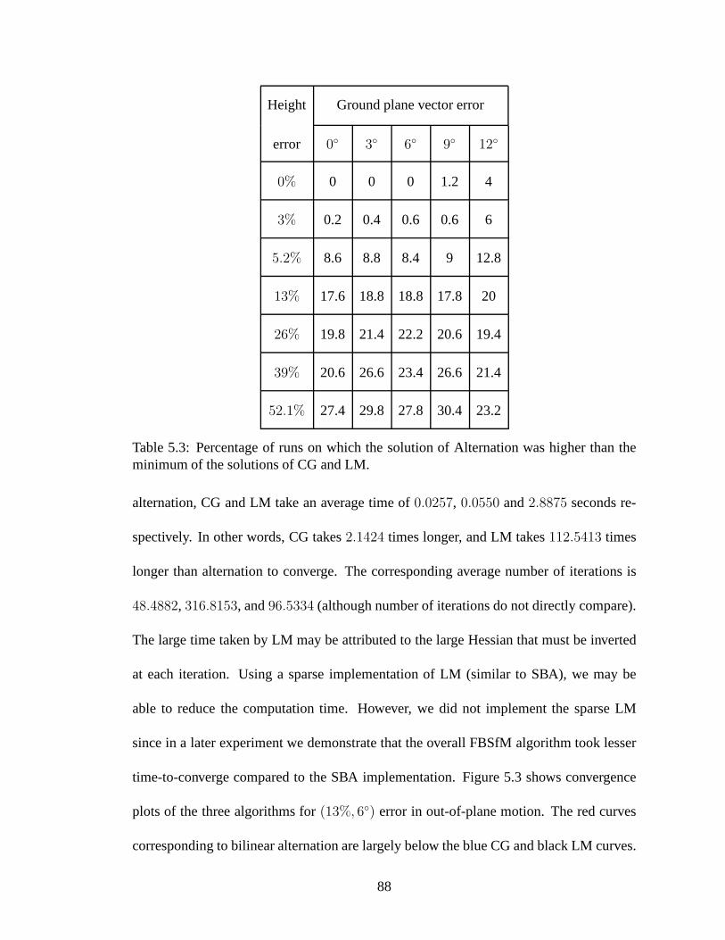
Height Ground plane vector error

error 0 3 6 9 12

0% 0 0 0 1.2 4

3% 0.2 0.4 0.6 0.6 6

5.2% 8.6 8.8 8.4 9 12.8

13% 17.6 18.8 18.8 17.8 20

26% 19.8 21.4 22.2 20.6 19.4

39% 20.6 26.6 23.4 26.6 21.4

52.1% 27.4 29.8 27.8 30.4 23.2

Table 5.3: Percentage of runs on which the solution of Alternation was higher than theminimum of the solutions of CG and LM.

alternation, CG and LM take an average time of0.0257, 0.0550 and2.8875 seconds re-

spectively. In other words, CG takes2.1424 times longer, and LM takes112.5413 times

longer than alternation to converge. The corresponding average number of iterations is

48.4882, 316.8153, and96.5334 (although number of iterations do not directly compare).

The large time taken by LM may be attributed to the large Hessian that must be inverted

at each iteration. Using a sparse implementation of LM (similar to SBA), we may be

able to reduce the computation time. However, we did not implement the sparse LM

since in a later experiment we demonstrate that the overall FBSfM algorithm took lesser

time-to-converge compared to the SBA implementation. Figure 5.3 shows convergence

plots of the three algorithms for(13%, 6) error in out-of-plane motion. The red curves

corresponding to bilinear alternation are largely below the blue CG and black LM curves.

88

In this plot, a lower curve implies a faster convergence rate. The plots show the same

trend for other choices of error levels. Figure 5.4 plots theconvergence curves of LM on

a separate figure so that the time axis can be chosen to be in linear scale.

10−4

10−3

10−2

10−1

100

3.5

4

4.5

5

5.5

6

6.5

7

7.5

Computation time in seconds

Log(

Err

or)

Convergence plots for Bilinear alternation, CG and LM

Bilinear

CG

LM

Figure 5.3: This figure illustrates convergence curves plotting the log of error versuscomputation time for the minimization of (5.7), using bilinear alternation, CG and LM.The plots for bilinear alternation are superior to the othertwo in terms of convergencerate because the bundle of red curves are largely below the blue and black curves. Thereconstruction problem used for these plots involved10 cameras and50 features. We useda perturbation of(3%, 6) for the out-of-plane translation and ground plane normal angleerror respectively.

The strong advantage in computation time along with the factthat alternation con-

verges to the same solution as CG and LM under low out-of-plane noise levels justifies its

use under the operating conditions of the dissertation (lowerror in out-of-plane motion).

5.4.5 Comparison of FBSfM with SBA

We generated a reconstruction problem with10 cameras and50 feature points and

96% of the image measurements known. Two sets of initial camera motion solutions

were generated for different choices of error levels in motion components. Set 1 had

perturbations of(12%, 25, 2.7%, 2) in the in-plane translation, in-plane angle, verti-

89

0 0.01 0.02 0.03 0.04 0.05 0.06 0.07 0.08 0.093

3.5

4

4.5

5

5.5

6

6.5

7

Computation time in arbitrary units

Log(

Err

or −

Glo

bal o

ptim

um)

Convergence plots for Bilinear alternation and Conjugate descent

BilinearCG

(a)

1 2 3 4 5 6 7 8 9 10 11 123

3.5

4

4.5

5

5.5

6

6.5

7

Computation time in arbitrary units

Log(

Err

or −

Glo

bal o

ptim

um)

Convergence plots for Levenberg−Marquardt

LM

(b)

Figure 5.4: This figure illustrates convergence curves plotting the log of error versuscomputation time for the minimization of (5.7). Figure 5.4(a) plots the curves for Bilinearalternation and CG, and figure 5.4(b) shows the plots for LM. Thex axis in both plotsare at the same scale which allows for comparison of LM with the other two algorithms.The plots for bilinear alternation are superior to the othertwo in terms of convergencerate because the bundle of red curves are largely below the blue and black curves. Thereconstruction problem used for these plots involved10 cameras and50 feature points. Weused a perturbation of(3%, 6) for the out-of-plane translation and ground plane normalangle error respectively.

cal position and ground plane normal vector respectively. Set 2 had perturbations of

(20%, 35, 0.5%, 5). Each set had900 different initial solutions. The structure initial-

izations were obtained by triangulating each 3D point usingimage feature locations and

initial camera parameters, after solving the linear system(5.10) of a structure iteration.

In set 1, minimum error reconstruction produced by SBA was0.3199 and that pro-

duced by our algorithm was0.3570. In 86% of the runs, the SBA reconstruction error was

lower than the minimum error produced by our algorithm. The slightly higher error of

our algorithm on successful runs compared to SBA is because we minimize the algebraic

as opposed to the reprojection error. On the remaining14% of the runs, SBA produced an

error of above5. In comparison, our algorithm produced an error lower than0.4 on 99%

of the runs. This illustrates the reliability of our algorithm in producing good reconstruc-

90

tions when initialized from a number of random initial solutions. In set 2,38% of the runs

had a lower reprojection error for SBA than for FBSfM. The distribution of reprojection

errors of both algorithms on each of the sets is illustrated in figure 5.5. The red curves are

for set 1 and the blue curves for set 2. The figure plots the cumulative distributions of the

reprojection error, hence a higher curve implies a better performing algorithm. In both

sets, the curve for FBSfM is largely above that for SBA indicating better performance.

We repeated the experiments on a reconstruction problem with 45 cameras and250

feature points, with96.4% measurements known. We obtained900 initial starting points

by perturbing with motion error of(30%, 25, 3.75%, 4). The initial reprojection errors

ranged from199.4611 to 3476.6 and the SBA code reported failures in minimization on

70.6% of the runs. On the remaining29.4% of the runs on which SBA succeeded, our

algorithm produced reconstructions whose final reprojection error ranged from0.6277 to

0.7603. SBA produced an error of0.3723 on 87.5% of the succeeded runs, and errors

ranging from9.0526 to 278.6074 on the remaining12.5% of the succeeded runs. On

the70.6% of the original runs on which SBA reported failures, our algorithm produced

reconstructions ranging from0.6209 to 0.7848, whereas the errors of SBA ranged from

208.28 to 1.0993e+ 05 (which were very close to the initial errors). These experimental

results clearly demonstrate the advantage of our algorithmover SBA, because it generally

avoids getting stuck in poor local minima and is more consistent in its results.

91

10−1

100

101

102

103

104

105

106

0

100

200

300

400

500

600

700

800

900

1000

Mean reprojection error

Run

cou

nt

Cumulative frequency graphs of reprojection error

FBSFM I

SBA I

Initial I

FBSFM II

SBA II

Initial II

Figure 5.5: This figure shows the cumulative frequency graphs of the reprojection errorfor SBA and FBSfM along with the error distribution of the initial solutions. The probleminvolved 10 cameras and50 feature points. The red curves show the results for set 1with perturbations of(12%, 25, 2.7%, 2) in the in-plane translation, in-plane rotaionangle, out-of-plane translation and ground plane normal angle error respectively. Theblue curves show the results for set 2 with initial motion error of (20%, 35, 0.5%, 5). Inboth sets, the graph for FBSfM is above that of SBA indicatingbetter performance.

5.4.6 Comparison of convergence rates of FBSfM and SBA

We compare the convergence rates of our algorithm with SBA ona reconstruction

problem with300 cameras and350 feature points, with62% of the image measurements

known. We generated350 initial solutions by perturbing the ground truth motion with a

3.33% error in the in-plane translation, a1% error in out-of-plane translation, a15 error

in the in-plane rotation angle and a4 error in the ground plane vector. SBA converged

successfully in157 of the350 runs, among which138 converged to the global minimum,

with a reprojection error of1.1316. On these138 runs, FBSfM converged to solutions

with errors ranging from1.1427 to 1.1432. Convergence of FBSfM was declared if the

number of iterations exceeded100 or if the error decreased by less than5e−5 or 0.0001%

whichever was higher. We attribute the slightly higher reprojection error of FBSfM to

the fact that it minimizes the algebraic error as opposed to the actual reprojection error.

92

Since the final errors of FBSfM are very close to those of SBA, we believe this is very

close to the global optimum. For the138 runs described earlier, the number of iterations

taken by FBSfM ranged from93 to 102 with an average of96.6 iterations and the total

computation time ranged from203.3 to 254.2 seconds with an average of223.6 seconds.

It is possible that because of the termination conditions, FBSfM had not converged to

its global optimum in a strict sense but had exhibited flatlining beyond100 iterations.

However, for practical purposes, this is not consequentialsince a minimum reprojection

error solution can be realized by directly minimizing the reprojection error using SBA.

Accumulated over all the runs, the amount of time taken for the out-of-plane motion

refinement iterations was49.5% of the total time spent. This fraction ranged from46% to

55.4% for all the runs.

Sparse BA required iterations ranging from45 to 4639 for convergence, with an

average number of iterations of484.3. Convergence was declared if the norm of the

update to the parameter vector was less than1E − 12. The total computation time taken

ranged from157 seconds to17864 seconds with132 of the138 runs requiring computation

time larger than the maximum time taken by FBSfM on all the runs.

Figure 5.6 shows the convergence plots for FBSfM (plotted inblue) and SBA (plot-

ted in red). SBA exhibits fast convergence when the solutionis very close to the global

minimum. On the other hand, FBSfM exhibits slow convergenceclose to the minimum.

Figure 5.7 plots the convergence curves of FBSfM and SBA in separate curves on linear

scale in the time axis. Although FBSfM is faster than SBA overall, these two algorithms

are good candidates to be used together in a hybrid approach.It must be noted that this

advantage in computation time is larger as the problem size increases (corresponding to

93

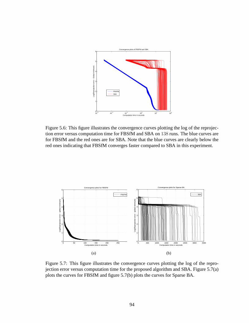
10−6

10−4

10−2

100

102

104

0

1

2

3

4

5

6

Computation time in seconds

Log(

Rep

roje

ctio

n er

ror

− G

loba

l min

imum

)

Convergence plots of FBSFM and SBA

FBSFM

SBA

Figure 5.6: This figure illustrates the convergence curves plotting the log of the reprojec-tion error versus computation time for FBSfM and SBA on138 runs. The blue curves arefor FBSfM and the red ones are for SBA. Note that the blue curves are clearly below thered ones indicating that FBSfM converges faster compared toSBA in this experiment.

0 50 100 150 200 250 3000

1

2

3

4

5

6

Computation time in seconds

Log(

Rep

roje

ctio

n er

ror

− g

loba

l min

imum

)

Convergence plots for FBSFM

FBSFM

(a)

0 500 1000 1500 2000 2500 3000 35000

1

2

3

4

5

6

Computation time in seconds

Log(

Rep

roje

ctio

n er

ror

− g

loba

l min

imum

)

Convergence plots for Sparse BA

SBA

(b)

Figure 5.7: This figure illustrates the convergence curves plotting the log of the repro-jection error versus computation time for the proposed algorithm and SBA. Figure 5.7(a)plots the curves for FBSfM and figure 5.7(b) plots the curves for Sparse BA.

94

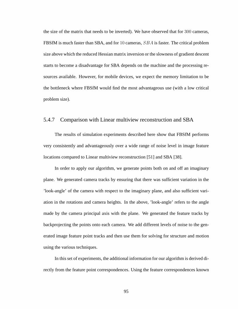
the size of the matrix that needs to be inverted). We have observed that for300 cameras,

FBSfM is much faster than SBA, and for10 cameras,SBA is faster. The critical problem

size above which the reduced Hessian matrix inversion or theslowness of gradient descent

starts to become a disadvantage for SBA depends on the machine and the processing re-

sources available. However, for mobile devices, we expect the memory limitation to be

the bottleneck where FBSfM would find the most advantageous use (with a low critical

problem size).

5.4.7 Comparison with Linear multiview reconstruction andSBA

The results of simulation experiments described here show that FBSfM performs

very consistently and advantageously over a wide range of noise level in image feature

locations compared to Linear multiview reconstruction [51] and SBA [38].

In order to apply our algorithm, we generate points both on and off an imaginary

plane. We generated camera tracks by ensuring that there wassufficient variation in the

’look-angle’ of the camera with respect to the imaginary plane, and also sufficient vari-

ation in the rotations and camera heights. In the above, ’look-angle’ refers to the angle

made by the camera principal axis with the plane. We generated the feature tracks by

backprojecting the points onto each camera. We add different levels of noise to the gen-

erated image feature point tracks and then use them for solving for structure and motion

using the various techniques.

In this set of experiments, the additional information for our algorithm is derived di-

rectly from the feature point correspondences. Using the feature correspondences known

95

to lie on the plane, we first compute the induced homography between the various virtual

images of the synthetic sequence. Then, we decompose these homography matrices and

obtain estimates of the ground plane normal and heights thatprovide the side information

for algorithm [71]. The decomposition process requires knowledge of the calibration ma-

trix of the camera, and is described in detail in the appendixB. The estimates of GPN

and height are inaccurate when we have errors in homography estimates (due to errors

in image features) or errors in the calibration matrix. Hence, we report results under

two scenarios: when we have (a) accurate camera calibrationand (b) inaccurate camera

calibration.

5.4.7.1 Results with accurate calibration

Figs. (5.8(a),5.8(b)) illustrate the mean reprojection error, and the deviation of these

reconstruction estimates at a range of noise levels for the three techniques. The ground

truth camera calibration was used in this case. Over a wide range of noise levels, we see

that FBSfM performs consistently and competitively. At very low noise levels, Rother’s

performs slightly better than FBSfM. But at realistic and high pixel noise levels, FBSfM

seems to perform the best.

The experiment was repeated for70 trials under scenarios with different pixel noise

levels. Fig. (5.10(a),5.10(b)) plot the reconstruction errors for each method for all the

trials. We observe that in different settings, both bundle adjustment (BA) and Rother’s

give bad solutions in many cases. BA is considered the gold standard in SfM algorithms

because it minimizes the reprojection error starting with agood initial solution. But it

96

involves a highly nonlinear iterative refinement and is prone to getting stuck at a local

minimum. The mean reprojection error of BA varies widely indicating that it may be

affected by local minima unlike FBSfM which is a lot more consistent.

5.4.7.2 Results with inaccurate calibration

The above experiments were repeated for the case where we hadlarge calibration

errors (around20% error in the focal lengths and camera center estimates). Themean

reprojection error plots (Fig. 5.9(a)) are similar, and thedeviations of the estimates are

lowest for FBSfM (Fig. 5.9(b)).

The experiment was repeated70 times under scenarios with different pixel noise

levels with an inaccurate calibration matrix as depicted inFig. (5.11(a),5.11(b)). The

observations from these figures is similar to the case of accurate calibration.

5.4.8 A note on alternation methods

A popular alternative to SBA that falls within the class of alternation algorithms

is resection-intersection [38]. This involves iterationswhere (1) the cameras are fixed

and structure variables are updated, and (2) the structure is fixed and camera matrices are

updated. Each iteration is of low complexity similar to our bilinear alternation, but it in-

volves non-linear minimization in all the iterations. The key difference of our work is the

use of additional measurements for the decomposition of motion parameters that leads to

a better performing algorithm for low out-of-plane noise conditions. Our experimental

results do not show a clear advantage over either SBA or resection-intersection from a

97

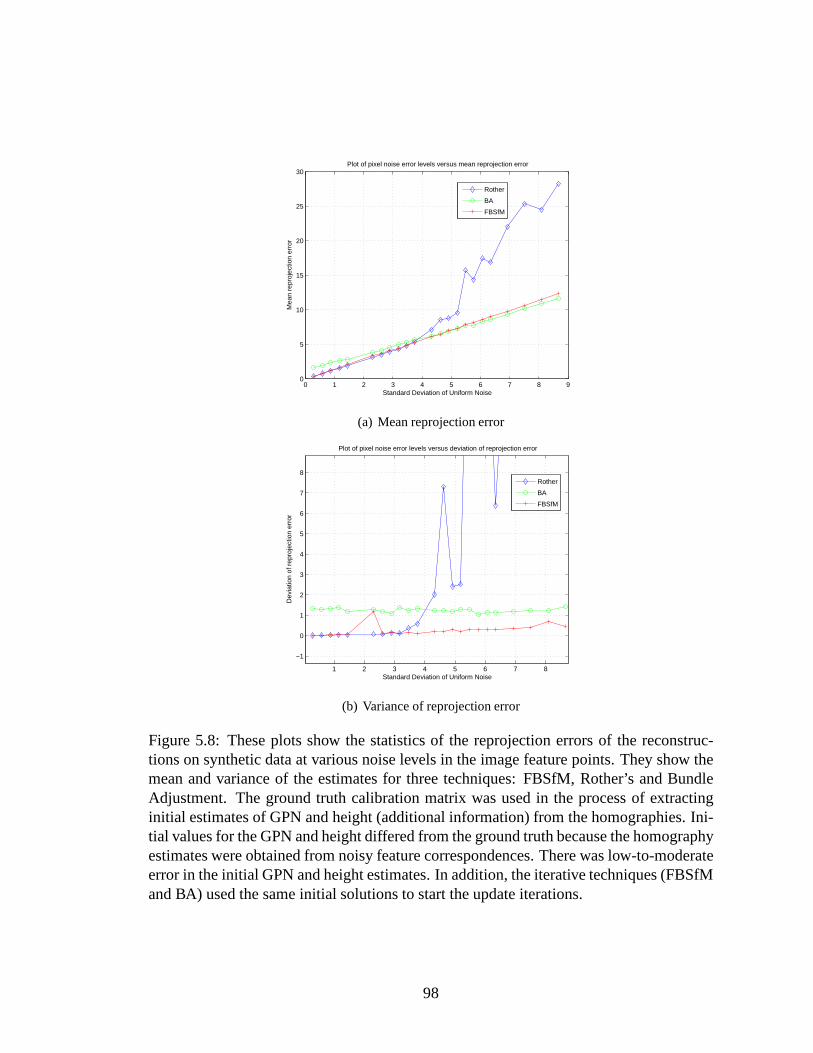
0 1 2 3 4 5 6 7 8 90

5

10

15

20

25

30

Standard Deviation of Uniform Noise

Mea

n re

proj

ectio

n er

ror

Plot of pixel noise error levels versus mean reprojection error

Rother

BA

FBSfM

(a) Mean reprojection error

1 2 3 4 5 6 7 8

−1

0

1

2

3

4

5

6

7

8

Standard Deviation of Uniform Noise

Dev

iatio

n of

rep

roje

ctio

n er

ror

Plot of pixel noise error levels versus deviation of reprojection error

Rother

BA

FBSfM

(b) Variance of reprojection error

Figure 5.8: These plots show the statistics of the reprojection errors of the reconstruc-tions on synthetic data at various noise levels in the image feature points. They show themean and variance of the estimates for three techniques: FBSfM, Rother’s and BundleAdjustment. The ground truth calibration matrix was used inthe process of extractinginitial estimates of GPN and height (additional information) from the homographies. Ini-tial values for the GPN and height differed from the ground truth because the homographyestimates were obtained from noisy feature correspondences. There was low-to-moderateerror in the initial GPN and height estimates. In addition, the iterative techniques (FBSfMand BA) used the same initial solutions to start the update iterations.

98

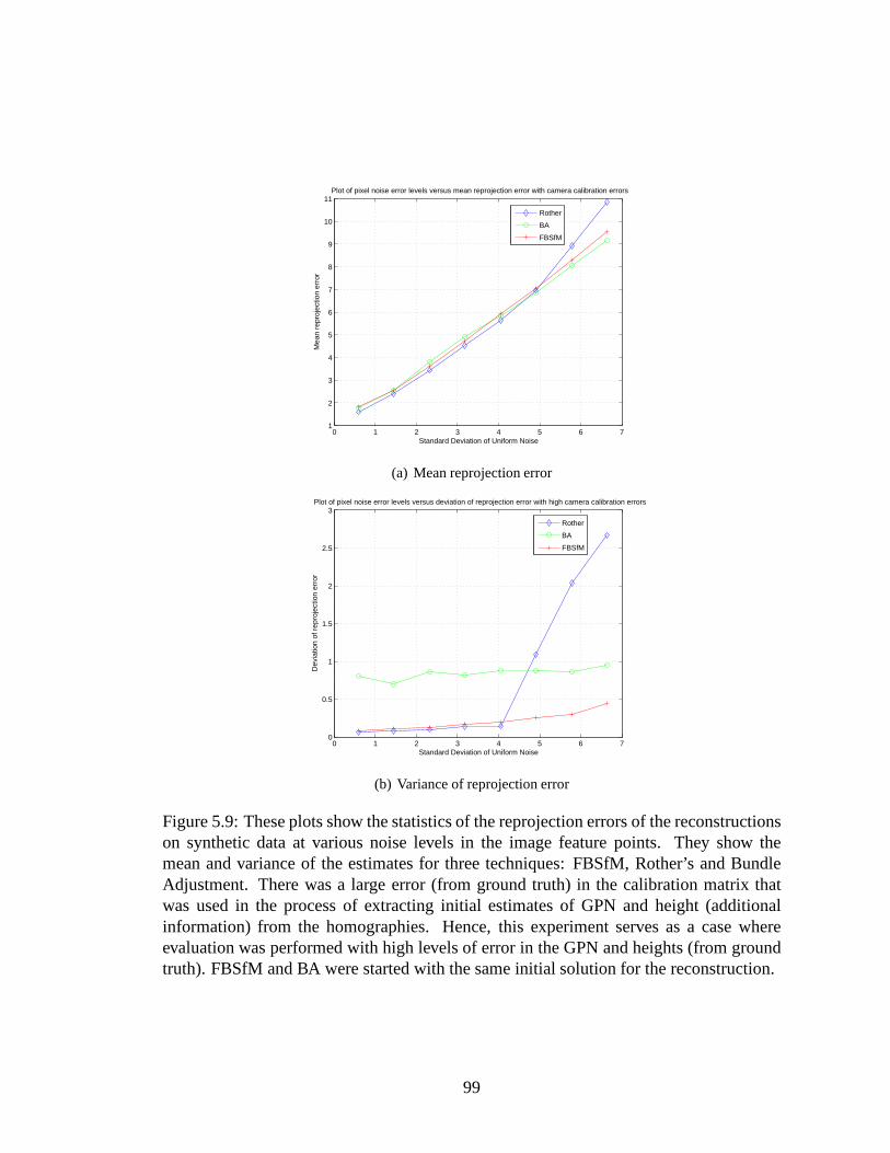
0 1 2 3 4 5 6 71

2

3

4

5

6

7

8

9

10

11

Standard Deviation of Uniform Noise

Mea

n re

proj

ectio

n er

ror

Plot of pixel noise error levels versus mean reprojection error with camera calibration errors

Rother

BA

FBSfM

(a) Mean reprojection error

0 1 2 3 4 5 6 70

0.5

1

1.5

2

2.5

3

Standard Deviation of Uniform Noise

Dev

iatio

n of

rep

roje

ctio

n er

ror

Plot of pixel noise error levels versus deviation of reprojection error with high camera calibration errors

Rother

BA

FBSfM

(b) Variance of reprojection error

Figure 5.9: These plots show the statistics of the reprojection errors of the reconstructionson synthetic data at various noise levels in the image feature points. They show themean and variance of the estimates for three techniques: FBSfM, Rother’s and BundleAdjustment. There was a large error (from ground truth) in the calibration matrix thatwas used in the process of extracting initial estimates of GPN and height (additionalinformation) from the homographies. Hence, this experiment serves as a case whereevaluation was performed with high levels of error in the GPNand heights (from groundtruth). FBSfM and BA were started with the same initial solution for the reconstruction.

99

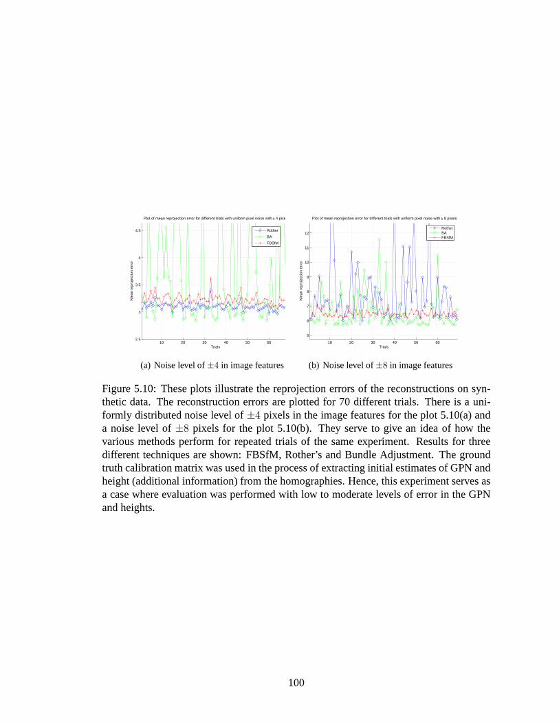
10 20 30 40 50 602.5

3

3.5

4

4.5

Trials

Mea

n re

proj

ectio

n er

ror

Plot of mean reprojection error for different trials with uniform pixel noise with ± 4 pixels

Rother

BA

FBSfM

(a) Noise level of±4 in image features

10 20 30 40 50 60

5

6

7

8

9

10

11

12

Trials

Mea

n re

proj

ectio

n er

ror

Plot of mean reprojection error for different trials with uniform pixel noise with ± 8 pixels

RotherBAFBSfM

(b) Noise level of±8 in image features

Figure 5.10: These plots illustrate the reprojection errors of the reconstructions on syn-thetic data. The reconstruction errors are plotted for 70 different trials. There is a uni-formly distributed noise level of±4 pixels in the image features for the plot 5.10(a) anda noise level of±8 pixels for the plot 5.10(b). They serve to give an idea of how thevarious methods perform for repeated trials of the same experiment. Results for threedifferent techniques are shown: FBSfM, Rother’s and BundleAdjustment. The groundtruth calibration matrix was used in the process of extracting initial estimates of GPN andheight (additional information) from the homographies. Hence, this experiment serves asa case where evaluation was performed with low to moderate levels of error in the GPNand heights.

100

0 10 20 30 40 50 605

5.5

6

6.5

7

7.5

8

8.5

Trials

Mea

n re

proj

ectio

n er

ror

Mean reprojection error for 55 trials with uniform noise with ± 7 pixels, at high calibration errors

RotherBAFBSfM

(a) Noise level of±7 in image features

0 10 20 30 40 50 608

10

12

14

16

18

20

22

Trials

Mea

n re

proj

ectio

n er

ror

Mean reprojection error for 55 trials with uniform noise with ± 11.5 pixels, at high calibration errors

RotherBAFBSfM

(b) Noise level of±11.5 in image features

Figure 5.11: These plots illustrate the reprojection errors of the reconstructions on syn-thetic data. The reconstruction errors are plotted for 70 different trials. There is a uni-formly distributed noise level of±7 pixels in the image features for Fig. 5.11(a) and anoise level of±11.5 pixels for Fig. 5.11(b). They serve to give an idea of how the variousmethods perform for repeated trials of the same experiment.Results for three differenttechniques are shown: FBSfM, Rother’s and Bundle Adjustment. There was a large error(from ground truth) in the calibration matrix that was used in the process of extracting ini-tial estimates of GPN and height (additional information) from the homographies. Hence,this experiment serves as a case where evaluation was performed with high levels of errorin the GPN and heights.

101

general class of initial solutions. However, the advantageshows up very clearly when

the out-of-plane motion is known (with low error) through sensor measurements. To the

best of our knowledge, we do not know of a previously proposedvariant of resection-

intersection for the specific setting discussed here. Earlier works [38] have evaluated the

most general variant of resection-intersection and have found it to be suboptimal com-

pared to SBA in terms of accuracy. Based on this study, we conclude that the cumulative

frequency graphs of resection-intersection are expected to be below that of SBA.

5.5 Experiments

5.5.1 Experiments on an Indoor Handheld Sequence

We report reconstruction results on an indoor image sequence taken with a digital

camera of a toy car resting on a plane. SIFT features were extracted and matched across

the image sequence. Inter-image homographies were estimated robustly using RANSAC,

and planar points were separated from those off the plane. The homographies were de-

composed as described in appendix B to obtain the additionalinformation. The repro-

jection errors for the three techniques FBSfM, Rothers’ andBA are shown in Table 5.4.

Figure 5.12 illustrates the texture mapped 3D model of the car. This is an example of a

short video sequence, with the number of keyframes being13 and the number of feature

points around60.

102

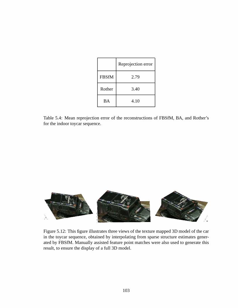
Reprojection error

FBSfM 2.79

Rother 3.40

BA 4.10

Table 5.4: Mean reprojection error of the reconstructions of FBSfM, BA, and Rother’sfor the indoor toycar sequence.

Figure 5.12: This figure illustrates three views of the texture mapped 3D model of the carin the toycar sequence, obtained by interpolating from sparse structure estimates gener-ated by FBSfM. Manually assisted feature point matches werealso used to generate thisresult, to ensure the display of a full 3D model.

103

5.5.2 SfM on StreetView data

The Google StreetView Research dataset consists of roadside image sequences and

metadata with the locations and orientations of the camera corresponding to each image,

solved using GPS and IMU measurements deployed onboard. Themetadata contained the

additional measurements in the form as required by the proposed algorithm. We chose a

segment of the dataset containing150 images when the car is moving on a single road.

We obtained feature tracks by SIFT feature detection and matching, and used RANSAC

and the epipolar constraint to prune out outliers. After these post-processing steps, we

obtained3145 distinct feature tracks in the sequence.

We obtained an initial solution for the camera motion by assuming a straight line

motion and placing the camera centers equally distributed on the line. We initialized

the out-of-plane camera rotation matrices using the direction vectors obtained from the

metadata, and the in-plane rotations were all fixed to zero. The heights of the cameras

were later fixed to the measurements obtained from the metadata. This provided an initial

solution for the camera motion. We used this initial motion and the feature trajectories

to triangulate the 3D points using structure iteration equations (5.10). The triangulated

3D locations were used as the initial structure solution. BothFBSfM and SBA were

initialized with the same starting point. The initial reprojection error was237.49. FBSfM

converged to a solution with an error of1.99 and SBA converged to a solution of111.88.

Figure 5.13 illustrates the top view of the reconstructed 3Dpoints and the camera path

corresponding to the FBSfM solution. When we initialized SBA with the final solution of

FBSfM, the reprojection error reduced to1.342.

104

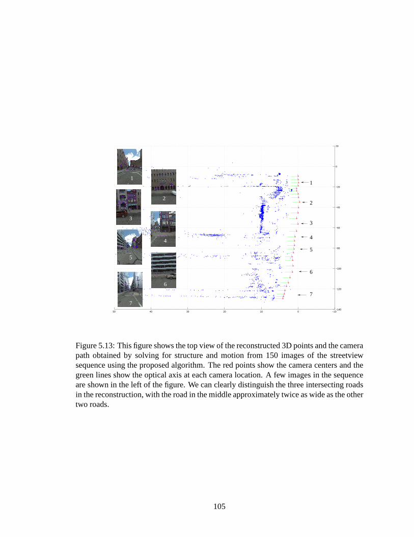
−140

−120

−100

−80

−60

−40

−20

0

20

−1001020304050

1

2

3

4

5

6

7

1

7

6

5

4

3

2

Figure 5.13: This figure shows the top view of the reconstructed 3D points and the camerapath obtained by solving for structure and motion from 150 images of the streetviewsequence using the proposed algorithm. The red points show the camera centers and thegreen lines show the optical axis at each camera location. A few images in the sequenceare shown in the left of the figure. We can clearly distinguishthe three intersecting roadsin the reconstruction, with the road in the middle approximately twice as wide as the othertwo roads.

105

Figure 5.14: This figure shows a texture mapped 3D model of thescene imaged in theStreetView sequence. Since the urban scene consists primarily of buildings and otherman-made structures, we fit several planes to the reconstructed 3D points. The texturesfor these planar patches were obtained from the corresponding images, and these textureswere applied to the planar patches using the Blender 3D modeling tool. Novel views ofthe texture-mapped model were rendered using the same tool.

Figure 5.14 illustrates the textured 3D model of the sequence generated using the

Blender modeling tool. Figure 5.15 illustrates novel viewssynthesized using the textured

3D model of figure 5.14 obtained using Blender software. Figure 5.16 illustrates the

trajectory of the camera overlaid on a map in Google Earth software.

Since we do not currently use sparse representations for measurement matrices, our

implementation was not suited to execute multiple trials onthe earlier sequence for mea-

suring computation times. Hence we select a subsequence with lesser number of feature

points. From the SfM solution with error1.342, we selected the first70 frames, and755

points with reprojection error less than3 for all frames. We used SBA for the755 point

subsequence and obtained an SfM reconstruction with error of 0.4013. We repeated the

camera configuration of the70 cameras twice by translating in theY andZ directions

by chosen distances. This produced a total of210 cameras. We generated the feature

points on the virtual cameras by reprojecting the original 3D points on each of the images

106

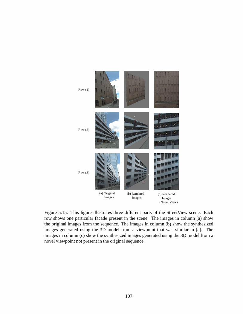
(a) Original Images

(b) Rendered Images

(c) Rendered Images (Novel View)

Row (3)

Row (2)

Row (1)

Figure 5.15: This figure illustrates three different parts of the StreetView scene. Eachrow shows one particular facade present in the scene. The images in column (a) showthe original images from the sequence. The images in column (b) show the synthesizedimages generated using the 3D model from a viewpoint that wassimilar to (a). Theimages in column (c) show the synthesized images generated using the 3D model from anovel viewpoint not present in the original sequence.

107

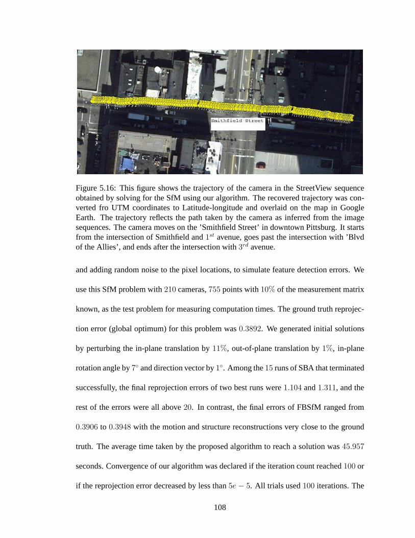
Figure 5.16: This figure shows the trajectory of the camera inthe StreetView sequenceobtained by solving for the SfM using our algorithm. The recovered trajectory was con-verted fro UTM coordinates to Latitude-longitude and overlaid on the map in GoogleEarth. The trajectory reflects the path taken by the camera asinferred from the imagesequences. The camera moves on the ’Smithfield Street’ in downtown Pittsburg. It startsfrom the intersection of Smithfield and1st avenue, goes past the intersection with ’Blvdof the Allies’, and ends after the intersection with3rd avenue.

and adding random noise to the pixel locations, to simulate feature detection errors. We

use this SfM problem with210 cameras,755 points with10% of the measurement matrix

known, as the test problem for measuring computation times.The ground truth reprojec-

tion error (global optimum) for this problem was0.3892. We generated initial solutions

by perturbing the in-plane translation by11%, out-of-plane translation by1%, in-plane

rotation angle by7 and direction vector by1. Among the15 runs of SBA that terminated

successfully, the final reprojection errors of two best runswere1.104 and1.311, and the

rest of the errors were all above20. In contrast, the final errors of FBSfM ranged from

0.3906 to 0.3948 with the motion and structure reconstructions very close tothe ground

truth. The average time taken by the proposed algorithm to reach a solution was45.957

seconds. Convergence of our algorithm was declared if the iteration count reached100 or

if the reprojection error decreased by less than5e− 5. All trials used100 iterations. The

108

algorithm probably exhibit flatlining behavior beyond100 iterations since the error was

decreasing very slowly. However, beyond this point, SBA is abetter choice for minimiz-

ing the reprojection error and can be used in a hybrid approach along with FBSfM. We

do not estimate the average time taken by SBA since none of theruns converged close to

the global optimum. However, the time taken for the two best runs were136.7 and138.5

seconds. Figure 5.18 plots the convergence curves for both algorithms. The bundle of

blue curves for FBSfM is clearly below the red ones of SBA indicating a faster overall

convergence rate. The curves suggest that towards the startof the minimization, FBSfM

converges faster but when the solution is close to the minima, SBA converges faster. Fig-

ure 5.17 plots the convergence curves for both algorithms inseparate graphs with the time

axis in linear scale.

0 10 20 30 40 50−1

0

1

2

3

4

5

6

7

Computation time in seconds

log(

Rep

roje

ctio

n er

ror

− g

loba

l opt

imum

)

Convergence plot of FBSFM

FBSFM

(a)

0 100 200 300 400 500 600 700 800 900

1

2

3

4

5

6

Computation time in seconds

log(

Rep

roje

ctio

n er

ror

− g

loba

l opt

imum

)

Convergence plot of SBA

SBA

(b)

Figure 5.17: This figure illustrates the convergence curvesplotting the log of the repro-jection error versus computation time for the proposed algorithm and SBA. Figure 5.7(a)plots the curves for FBSfM, and figure 5.7(b) plots the curvesfor Sparse BA. Figure 5.7(b)cuts off the time axis at1000 sec, however the maximum time taken was2140.

These results illustrate the computational advantages of FBSfM over SBA and make

it a good candidate for urban modeling which involves solving large reconstruction prob-

109

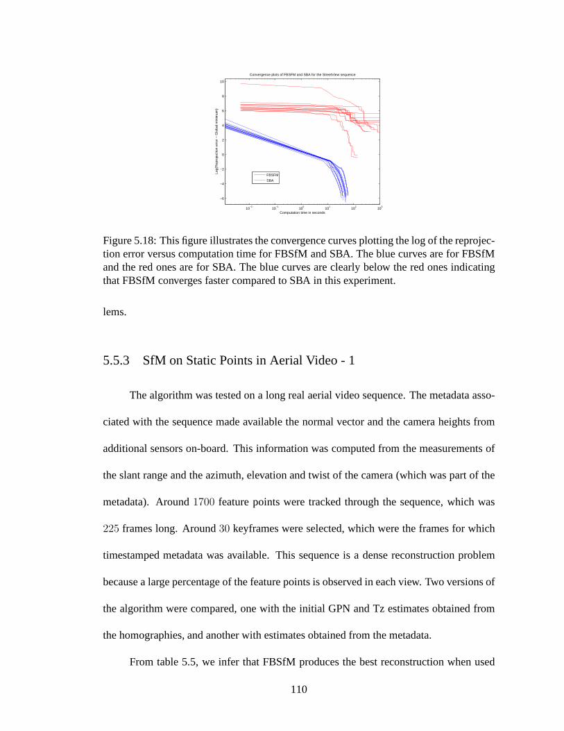
10−2

10−1

100

101

102

103

−6

−4

−2

0

2

4

6

8

10

Computation time in secondsLo

g(R

epro

ject

ion

erro

r −

Glo

bal m

inim

um)

Convergence plots of FBSFM and SBA for the StreetView sequence

FBSFM

SBA

Figure 5.18: This figure illustrates the convergence curvesplotting the log of the reprojec-tion error versus computation time for FBSfM and SBA. The blue curves are for FBSfMand the red ones are for SBA. The blue curves are clearly belowthe red ones indicatingthat FBSfM converges faster compared to SBA in this experiment.

lems.

5.5.3 SfM on Static Points in Aerial Video - 1

The algorithm was tested on a long real aerial video sequence. The metadata asso-

ciated with the sequence made available the normal vector and the camera heights from

additional sensors on-board. This information was computed from the measurements of

the slant range and the azimuth, elevation and twist of the camera (which was part of the

metadata). Around1700 feature points were tracked through the sequence, which was

225 frames long. Around30 keyframes were selected, which were the frames for which

timestamped metadata was available. This sequence is a dense reconstruction problem

because a large percentage of the feature points is observedin each view. Two versions of

the algorithm were compared, one with the initial GPN and Tz estimates obtained from

the homographies, and another with estimates obtained fromthe metadata.

From table 5.5, we infer that FBSfM produces the best reconstruction when used

110

with the metadata. With the homography-based estimates of GPN, the reprojection error

was worse, and this was to a largely due to a high reprojectionerror in one particular

frame. We feel this is because of a bad initial estimate of theGPNs and heights. The

homography decomposition step is sensitive to the calibration matrix. Rother’s method

requires the solution of a very large matrix equation which is highly time and memory

consuming. Hence we could perform a reconstruction for onlya few of the points. Bundle

adjustment requires the inversion of a large Hessian matrix. Our technique performs

faster than these techniques because at any iteration, the peak memory requirement is

very limited.

FBSfM with metadata FBSfM Rother BA

2.83 10.5 24.32 5.56

Table 5.5: Mean reprojection error for the long aerial videosequence in which we had225 frames and1700 features.

5.5.4 SfM on Moving Objects in Aerial Video - 2

We report experiments on reconstruction of moving objects on a planar scene. The

theoretical derivations suggest that the moving object is assumed stationary, and there is

a separate camera moving over it. We did not compute the inter-image homographies, but

obtained the GPN and height from the metadata, and estimate the structure and in-plane

motion using the bilinear algorithm without direction vector or height refinement.

Fig. (5.19a) shows a snapshot of a moving vehicle with detected and reprojected

features shown in yellow dots and green squares respectively. Fig. (5.19b) shows the

111

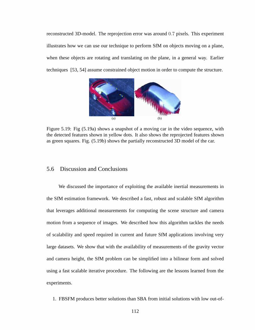
reconstructed 3D-model. The reprojection error was around0.7 pixels. This experiment

illustrates how we can use our technique to perform SfM on objects moving on a plane,

when these objects are rotating and translating on the plane, in a general way. Earlier

techniques [53, 54] assume constrained object motion in order to compute the structure.

(a) (b)

Figure 5.19: Fig (5.19a) shows a snapshot of a moving car in the video sequence, withthe detected features shown in yellow dots. It also shows thereprojected features shownas green squares. Fig. (5.19b) shows the partially reconstructed 3D model of the car.

5.6 Discussion and Conclusions

We discussed the importance of exploiting the available inertial measurements in

the SfM estimation framework. We described a fast, robust and scalable SfM algorithm

that leverages additional measurements for computing the scene structure and camera

motion from a sequence of images. We described how this algorithm tackles the needs

of scalability and speed required in current and future SfM applications involving very

large datasets. We show that with the availability of measurements of the gravity vector

and camera height, the SfM problem can be simplified into a bilinear form and solved

using a fast scalable iterative procedure. The following are the lessons learned from the

experiments.

1. FBSFM produces better solutions than SBA from initial solutions with low out-of-

112

plane motion error. We have compared the performance of bothfor as much as5

in ground plane vector error and5% in the camera vertical position error.

2. The total time taken by FBSFM to attain convergence (with termination conditions

set by a maximum number of iterations or minimum decrease in error) is less than

that of SBA for large-sized problems when initialized from starting points with low

error in out-of-plane motion.

3. When initialized from a large number of random starting points, FBSFM seems

to converge to solutions that are lower than those produced by SBA (as is demon-

strated by the cumulative frequency graphs).

The chapter provides a direction of research in SfM in the present context where

we have large video datasets with associated metadata, or data acquisition platforms with

multiple sensors.

One avenue for future research is to develop algorithms thatcombine video with the

raw data from inertial sensors for better SfM algorithms. Inertial measurements give us

the accelerations and rotation rates of the cameras which gives us more information about

the camera motion than the measurements of gravity vector and height. Such an algorithm

will potentially be more generally applicable in scenarioswhere we have cameras with

additional sensors.

113

Chapter 6

Conclusions and Future Research Directions

6.1 Summary

This dissertation revolves around the present day availability of video datasets with

metadata containing additional information from sensors such as inertial measurement

units, global positioning systems, wheel speed readers (inground-based platforms), mag-

netic compasses etc. The ubiquitous deployment of these additional sensors along with

cameras makes it possible to collect such metadata along with video sequences. With

additional data, the development of better video processing algorithms leveraging the ad-

ditional information is of prime research importance. In this dissertation, we propose

novel studies and algorithms for several video processing tasks such as stabilization, mo-

saicking, moving object detection and structure from motion, leveraging the presence of

metadata with video datasets. The contributions are summarized as follows.

1. We propose a methodology to reduce the computational costof intensity-based reg-

istration by using a subset of salient pixels with high gradients for the registration.

We study the variation of number of iterations and registration accuracy with the

number of pixels used for registration.

2. We propose a feature-based algorithm for stabilization and moving object detection

in aerial datasets with accompanying metadata. The metadata is useful because

114

it provides partial information about the camera motion that reduces the motion

model to a pure translation model. We propose and demonstrate the working of

a joint feature tracking and segmentation algorithm that stabilizes and identifies

moving objects in the video sequence

3. We use additional information about camera height and gravity direction to come

up with a fast, robust, and scalable algorithm for structurefrom motion. The pro-

posed algorithm, which we call Fast Bilinear Structure fromMotion (FBSfM) is

experimentally demonstrated to have favorable propertiescompared to the sparse

bundle adjustment algorithm. In specific scenarios with lowerror in the gravity and

height measurements, we are able to demonstrate that FBSfM is faster than bundle

adjustment, and produces more consistent results from a variety of initial solutions.

We also describe results on several real datasets includingthe Google StreetView

dataset.

6.2 Future work

There are several avenues for extending the work presented in this dissertation. In

chapter 4, we presented an algorithm for joint tracking and segmentation, where we used a

pure translation model for tracking the background features jointly. We assumed only one

motion model for the background and we classified features asinliers and outliers with

respect to the single background model. The outlier features were tracked as independent

KLT features. We plan to extend this framework under the assumption of multiple motion

models in the image sequence. The use of multiple motion models will extend the appli-

115

cation of this framework for more general scenes. In addition, though we have used the

pure translation model, the algorithm would work just as well if we solved the parameters

of a higher order model such as affine or homography. This willextend the applicability

of the algorithm for scenes with multiple planes.

In chapter 5, we presented a structure from motion algorithmleveraging the avail-

ability of gravity and height measurements obtained from inertial sensors. This leads to a

bilinear algorithm that is demonstrated to be fast and robust. However, we do not use the

complete information available from these sensors to fuse with image measurements. In

particular, fusing image features with rate measurements from a gyro and accelerometer

for estimating trajectory can lead to algorithms for a broader range of scenarios beyond

what is addressed in this dissertation.

116

Appendix A

Proofs of convergence

We reproduce the Global Convergence Theorem as stated in [77] for the sake of

completeness:

Theorem 1 (GCT):Consider a topological spaceX, a solution setΓ ⊂ X, and letA

be an algorithm onX. Suppose that givenx0, a sequence of pointsxk∞k=0 is generated

in X such that fork ≥ 0, xk+1 ∈ A(xk). Suppose

1. all the pointsXk are generated in a compact setS ∈ X,

2. there exists a continuous functionZ : X → R such that

• if x /∈ Γ, thenZ(y) < Z(x) for all y ∈ A(x)

• if x ∈ Γ, thenZ(y) ≤ Z(x) for all y ∈ A(x)

3. the mappingA is closed at points outsideΓ.

then the limit of any convergent subsequence ofxk belongs toΓ.

Let S denote the matrix containing the3D coordinates of all the points. LetMI

denote the matrix containing the in-plane motion parameters (tx, ty, θ) of all the frames,

andMO contain out-of-plane motion parameters(tz, φ, ψ) for all frames. We show using

the Global Convergence Theorem that the proposed FBSFM algorithm converges to a

solution(S∗,M∗I ,M

∗O) and the error converges to a local minimumE∗.

117

Let the setΩ denote the set of all valid structure and motion parameters such that

‖Tz‖2 = k, and the angles(θ, φ, ψ) ∈ [−π, π]. This set is a compact set of the parameter

spaceR3n+6m. Each iteration maps the current estimate of(MI ,MO, S) to the next one

computed according to the equations. In case of depth and motion iterations, this involves

solving linear systems. In case of side-information refinement iterations, this involves

performing gradient descent on the error functions. After each iteration, since the points

xk = (MkI ,M

kO, S

k) generated by the iterations belong toS, the first assumption of GCT

holds.

Let us define the descent functionZ to be the same as the error functionE (5.7)

being optimized. The solution setΓ ∈ X contains the critical points of the objective

function. Since the error is non-increasing, it is easily seen thatE(y) ≤ E(x) for anyx.

We have to show that the error is strictly decreasing when we apply the algorithm starting

from a point that is not in the solution setΓ. Alternately, we must show that after the

iterations, if the error is constant, then we started off from a point in the solution set. This

is proved using a very similar reasoning as done in [56, 78]. Hence, the second condition

of GCT is also satisfied.

To show that the mappingA is closed, we take an approach similar to [56, 78] and

decomposeA into elementary mappings corresponding to each iteration:

• A1 associates with(S(k),M(k)I ,M

(k)O ) the solutionS(k+1) obtained by solving the

depth iterations. This is a continuous point-to-point mapping, since the linear sys-

tem in (5.9) has a unique solution.

• A2 associates with(S(k+1),M(k)I ,M

(k)O ) the solutionM (k+1)

I obtained by solving the

118

motion iterations. This is a continuous point-to-point mapping, since the equations

in (5.15), (5.18) give rise to a unique solution.

• A3 associates with(S(k+1),M(k+1)I ,M

(k)O ) the solutionM (k+1)

O obtained by refining

the out-of-plane motion parameters using Levenberg-Marquardt (LM) iterations.

This is a continuous point-to-point mapping since LM computes its solutions using

line-search.

The composition of closed point-to-point mappings is itself closed [56, 77]. Since

all the conditions of GCT are satisfied, the FBSFM algorithm is globally convergent.

119

Appendix B

Decomposition of homographies to obtain additional information

When a dominant plane is present in the scene, we can use the plane normal and

the height from the plane as side information in our algorithm. We can accumulate the

homographies induced by the plane from multiple views and use a decomposition tech-

nique [71] to compute the plane normals and the heights. The inter-image homographies

are robustly estimated using RANSAC.

We briefly describe the technique that can be used to estimatethe ground plane nor-

mals, rotations, translations and other geometric parameters from a set of homographies

induced by a plane between multiple views.

SupposeHij is the homography from viewj to view i. It is expressed in terms

of rotations, translations and the ground plane normals asHij = Rij +tijnT

j

dj. Here,Qij

denotes quantities from viewj to view i, nj is the ground plane normal at viewj, anddj

is the corresponding perpendicular distance from the plane. We can compose a matrixG

containing the various homographies as follows:

G =

H11 · · · H1m

..... .

...

Hm1 · · · Hmm

(B.1)

The individual homographies are normalized so that their median singular value is1. The

Gmatrix can be decomposed asG = R+T NT whereG andR are3m×3m, T is 3m×m

andN is 3m×m with m being the number of views. Here,N is a block diagonal matrix

120

of all the normal vectors, andR, T , are a block matrices with the(i, j)th block composed

of Rij andTij respectively.

It has been shown in [12] that the matrixL = WGTW−1 has rank3, where

W = diag(I3, det(H21)I3, . . . det(Hm1)I3) (B.2)

L has three eigenvectors with eigenvalues ofλ = m. As the vector of ground plane

normals(n1, n2, . . . , nm) can be shown to be an eigenvector ofL with eigenvalue ofm,

it is a linear combination of the top three eigenvectors ofL. They elaborate a technique

to solve for the normals using these constraints. After recovering the normal vectors, the

translations and rotations can be solved usingT = GN − NUm andR = G−GNNT +

NUmNT , whereUm is anm×m matrix of ones. Thus, the heights from the ground plane

can be estimated using only the homography matrices and normals using the formula

dk = d1

nTk

H1kn1, wheredk is the height of the camera at viewk.

121

Bibliography

[1] “Google image search.” [Online]. Available: http://images.google.com/

[2] S.-W. Joo and R. Chellappa, “A multiple-hypothesis approach for multiobject visualtracking,” IEEE Trans. Image Processing, vol. 16, no. 11, pp. 2849–2854, Nov.2007.

[3] M. Ramachandran and R. Chellappa, “Stabilization and mosaicing of aerial videos,”in Proc. IEEE Int’l. Conf. on Image Processing, October 2006, pp. 345–348.

[4] H. C. Longuet-Higgins, “A computer algorithm for reconstructing a scene from twoprojections,”Nature, vol. 293, no. 1, pp. 133–135, 1981.

[5] O. Faugeras,Three-dimensional computer vision: A geometric viewpoint. MITPress, 1993.

[6] J. Oliensis, “A critique of structure from motion algorithms,” NEC Research Insti-tute, Technical Report, 2000.

[7] Y. S. Yao and R. Chellappa, “Selective stabilization of images acquired by un-manned ground vehicles,”IEEE Trans. Robotics and Automation, vol. 13, no. 5,pp. 693–708, October 1997.

[8] C. Morimoto and R. Chellappa, “Fast 3D stabilization andmosaic construction,”in Proc. IEEE Int’l Conf. on Computer Vision and Pattern Recognition, 1998, pp.660–667.

[9] A. Mitiche, Computational Analysis of Visual Motion. Plenum, 1994.

[10] O. Faugeras,Three-Dimensional Computer Vision. Cambridge, MA: MIT Press,1993.

[11] R. Hartley and Z. A.,Multiple View Geometry in computer vision. Cambridge, UK:Cambridge University Press, 2000.

[12] C. Tomasi and T. Kanade, “Shape and motion from image streams under orthog-raphy: a factorization method,”Int’l Journal Computer Vision, vol. 9, no. 2, pp.137–154, Nov 1992.

[13] D. Lowe, “Distinctive image features from scale-invariant keypoints,”InternationalJournal of Computer Vision, vol. 60, no. 2, pp. 91–110, 2004.

[14] M. Fischler and R. Bolles, “Random sample consensus: a paradigm for model fittingwith application to image analysis and automated cartography,” Commun. Assoc.Comp. Mach., vol. 24, pp. 381–395, 1981.

122

[15] J. Shi and C. Tomasi, “Good features to track,” inProc. IEEE Conf. Computer Visionand Pattern Recognition, 1994, pp. 593–600.

[16] C. Morimoto and R. Chellappa, “Fast electronic digitalimage stabilization for off-road navigation,” inReal-time Imaging, vol. 2, 1996, pp. 285–296.

[17] S. Avidan and A. Shashua, “Threading fundamental matrices,”IEEE Trans. on Pat-tern Analysis and Machine Intelligence, vol. 23, no. 1, pp. 73–77, January 2001.

[18] S. Baker and I. Matthews, “Lucas Kanade 20 years on: A unifying framework,”Int’lJournal of Computer Vision, vol. 56, no. 3, pp. 221–255, Feb 2004.

[19] A. Bartoli, “Groupwise geometric and photometric direct image registration,”IEEETrans. Pattern Analysis and Machine Intelligence, vol. 30, no. 12, pp. 221–255, Dec2008.

[20] Y. Keller and A. Averbuch, “Multisensor image registration via implicit similarity,”IEEE Trans. Pattern Analysis and Machine Intelligence, vol. 28, no. 5, May 2006.

[21] M. Ramachandran, A. Veeraraghavan, and R. Chellappa, “Video stabilization andmosaicing,” inThe Essential Guide to Video Processing, 2009, pp. 109–140.

[22] S. Srinivasan and R. Chellappa, “Noise-resilient estimation of optical flow by use ofoverlapped basis functions,”Journal of the Optical Society of America - A, vol. 16,no. 3, March 1999.

[23] P. H. S. Torr and A. Zisserman, “Feature-based methods for structure and motionestimation,” inWorkshop on Vision Algorithms: Theory and Practice, 1999.

[24] A. Elgammal, R. Duraiswami, D. Harwood, and L. Davis, “Background and fore-ground modeling using nonparametric kernel density estimation for visual surveil-lance,”Proceedings of the IEEE, vol. 90, no. 7, pp. 1151–1163, Jul 2002.

[25] S. Birchfield and S. Pundlik, “Joint tracking of features and edges,” inProc. IEEEInt’l Conf. on Computer Vision and Pattern Recognition, 2008, pp. 1–6.

[26] B. K. P. Horn and B. G. Schunck, “Determining optical flow,” Artificial Intelligence,vol. 17, no. 12, pp. 185–203, 1981.

[27] Y. Sheikh, O. Javed, and T. Kanade, “Background subtraction for freely movingcameras,” inProc. IEEE Int’l Conf. on Computer Vision, Oct. 2009.

[28] A. Buchanan and A. Fitzgibbon, “Combining local and global motion models forfeature point tracking,” inProc. IEEE Int’l Conf. Computer Vision and PatternRecognition, June 2007, pp. 1–8.

[29] M. Irani, P. Anandan, and S. Hsu, “Mosaic based representations of video se-quences and their applications,” inInternational Conference on Computer Vision,Cambridge, MA, 1995, pp. 605–611.

123

[30] B. Rousso, S. Peleg, I. Finci, and A. Rav-Acha, “Universal mosaicing using pipeprojection,” inInternational Conference on Computer Vision, Mumbai, India, 1998,pp. 945–952.

[31] S. Peleg, B. Rousso, A. Rav-Acha, and A. Zomet, “Mosaicing on adaptive mani-folds,” IEEE Trans. Pattern Analysis and Machine Intelligence, vol. 22, no. 10, pp.1144–1154, October 2000.

[32] J. Wang and E. Adelson, “Representing moving images with layers,”IEEE Trans.on Image Processing, vol. 3, no. 5, pp. 625–638, September 1994.

[33] R. Kumar, P. Anandan, and K. Hanna, “Shape recovery frommultiple views: aparallax based approach,” inARPA Image Understanding Workshop, Monterey, CA.2929 Campus Drive, Suite 260, San Mateo, California 94403: Morgan KauffmannPublishers, Nov. 1994. [Online]. Available: citeseer.ist.psu.edu/kumar94shape.html

[34] H.-Y. Shum and R. Szeliski, “Construction of panoramicmosaics with global andlocal alignment,”International Journal of Computer Vision, vol. 36, no. 2, pp. 101–130, February 2000.

[35] R. Szeliski,Image Alignment and Stitching: A Tutorial. Now Publishers Inc., 2006.

[36] S. Peleg and J. Herman, “Panoramic mosaics by manifold projection,” inProc. IEEEInt’l Conf. on Computer Vision and Pattern Recognition, 1997, pp. 338–343.

[37] R. Hartley and A. Zisserman,Multiple View Geometry in Computer Vision, 2nd ed.Cambridge University Press, 2004.

[38] B. Triggs, P. McLauchlan, R. Hartley, and A. Fitzgibbon, “Bundle adjustment - amodern synthesis,” inLecture Notes in Computer Science, vol. 1883. London, UK:Springer-Verlag, 2000.

[39] K. Madsen, H. Nielsen, and O. Tingleff,Methods for Non-Linear Least SquaresProblems, 2nd ed. Technical University of Denmark, 2004.

[40] M. I. A. Lourakis and A. A. Argyros, “SBA: A software package for generic sparsebundle adjustment,”ACM Trans. Math. Software, vol. 36, pp. 1–30, Jan. 2009.

[41] M. Byrod and K. Astrom, “Bundle adjustment using conjugate gradients with mul-tiscale preconditioning,” inProc. British Machine Vision Conference, London, UK,Sept. 2009.

[42] D. Nister, “An efficient solution to the five-point relative pose problem,”IEEE Trans.Pattern Analysis and Machine Intelligence, vol. 26, no. 6, pp. 756–770, June 2004.

[43] A. Davison, I. Reid, N. Molton, and O. Stasse, “Monoslam: Real-time single cameraslam,” IEEE Trans. Pattern Analysis and Machine Intelligence, vol. 29, no. 6, pp.1052–1067, June 2007.

124

[44] P. Sturm and B. Triggs, “A factorization-based algorithm for multi-image projectivestructure and motion,”Proc. European Conf. Computer Vision, Cambridge, UK,vol. 1, pp. 709–720, Apr. 1996.

[45] C. Fruh and A. Zakhor, “An automated method for large-scale, ground-based citymodel acquisition,”Int’l Journal Computer Vision, vol. 60, no. 1, pp. 5–24, Oct2004.

[46] C. Frueh and A. Zakhor, “Constructing 3D city models by merging ground-basedand airborne views,” inProc. IEEE Conf. Computer Vision and Pattern Recognition,June 2003.

[47] A. Akbarzadeh, “Towards urban 3D reconstruction from video,” in Int’l Symposiumon 3D Data, Processing, Visualization and Transmission, 2006.

[48] R. Carceroni, A. Kumar, and K. Daniilidis, “Structure from motion with known cam-era positions,” inProc. IEEE Int’l Conf. Computer Vision and Pattern Recognition,Washington DC, vol. 1, June 2006.

[49] G. Qian, Q. Zheng, and R. Chellappa, “Reduction of inherent ambiguities in struc-ture from motion problem using inertial data,” inProc. Int’l Conf. Image Processing,Vancouver, Canada, vol. 1, Sept. 2000.

[50] M. Irani, P. Anandan, and M. Cohen, “Direct recovery of planar-parallax from mul-tiple frames,”IEEE Trans. Pattern Analysis and Machine Intelligence, vol. 24, pp.1528–1534, 2002.

[51] C. Rother and S. Carlsson, “Linear multi view reconstruction and camera recoveryusing a reference plane,”Int’l Journal Computer Vision, vol. 49, no. 3, pp. 117–141,Sept. 2002.

[52] R. Kaucic, R. Hartley, and N. Dano, “Plane-based projective reconstruction,” inProc. Int’l Conf. Computer Vision, Vancouver, Cananda, vol. 1, July 2001.

[53] A. Bartoli, “The geometry of dynamic scenes - on coplanar and convergent linearmotions embedded in 3d static scenes,”Computer Vision and Image Understanding,vol. 98, no. 2, pp. 223–238, May 2005.

[54] A. Fitzgibbon and A. Zisserman, “Multibody structure and motion: 3-d reconstruc-tion of independently moving objects,” inProc. European Conf. Computer Vision,vol. 98, no. 2, May 2000, pp. 223–238.

[55] J. Li and R. Chellappa, “Structure from planar motion,”IEEE Trans. Image Process-ing, vol. 12, no. 1, pp. 234–778, November 2006.

[56] S. Mahamud, M. Hebert, Y. Omori, and J. Ponce, “Provably-convergent iterativemethods for projective structure from motion,”Proc. IEEE Conf. Computer Visionand Pattern Recognition, Honolulu, Hawaii, vol. 1, Dec. 2001.

125

[57] J. Oliensis and R. Hartley, “Iterative extensions of the sturm/triggs algorithm: Con-vergence and nonconvergence,”IEEE Trans. Pattern Analysis and Machine Intelli-gence, vol. 29, pp. 2217–2233, Dec. 2007.

[58] J. R. Bergen, P. Anandan, K. J. Hanna, and R. Hingorani, “Hierarchical model-basedmotion estimation,” inProc. European Conf. on Computer Vision, 1992, pp. 237–252.

[59] M. Irani and P. Anandan, “Robust multi-sensor image alignment,” inProc. IEEEInt’l Conf. on Computer Vision, January 1998, pp. 959–966.

[60] A. Zomet, A. Levin, S. Peleg, and Y. Weiss, “Seamless image stitching by minimiz-ing false edges,”IEEE Trans. Image Processing, vol. 15, no. 4, pp. 969–977, Apr2006.

[61] J. Pluim, J. Maintz, and M. Viergever, “Image registration by maximization of com-bined mutual information and gradient information,”IEEE Trans. Medical Imaging,vol. 19, no. 8, pp. 809–814, Aug 2000.

[62] B. D. Lucas and T. Kanade, “An iterative image registration technique with an appli-cation to stereo vision,” inInternational Joint Conference on Artificial Intelligence,1981, pp. 674–679.

[63] M. Ramachandran and R. Chellappa, “Gradient and feature-based video stabiliza-tion,” Submitted to IEEE Trans. Image Processing, 2010.

[64] Y. Sheikh and M. Shah, “Bayesian modeling of dynamic scenes for object detec-tion,” IEEE Trans. Pattern Analysis and Machine Intelligence, vol. 27, no. 11, pp.1778 –1792, Nov. 2005.

[65] Y. Boykov and V. Kolmogorov, “An experimental comparison of min-cut/max-flowalgorithms for energy minimization in vision.”IEEE Trans. on Pattern Analysis andMachine Intelligence, vol. 26, no. 9, pp. 1124–1137, Sep. 2004.

[66] Y. Boykov, O. Veksler, and R. Zabih, “Efficient approximate energy minimizationvia graph cuts,”IEEE Trans. on Pattern Analysis and Machine Intelligence, vol. 20,no. 12, pp. 1222–1239, Nov. 2001.

[67] V. Kolmogorov and R. Zabih, “What energy functions can be minimized via graphcuts?” IEEE Trans. on Pattern Analysis and Machine Intelligence, vol. 26, no. 2,pp. 147–159, Feb. 2004.

[68] C. Shekhar, “Semi-automatic video-to-site registration for aerial monitoring,” inProc. IEEE Int’l Conf. on Pattern Recognition, January 1998, pp. 959–966.

[69] M. Ramachandran, A. Veeraraghavan, and R. Chellappa, “Fast bilinear SfM withside information,” inProc. IEEE Int’l Conf. Computer Vision, Rio de Janeiro, Brazil ,Oct. 2007.

126

[70] ——, “A fast bilinear structure from motion algorithm using a video sequence andinertial sensors,”Under revision in IEEE Trans. Pattern Analysis and Machine In-telligence, 2010.

[71] E. Malis and R. Cipolla, “Camera calibration from unknown planar structures en-forcing the multi view constraints between collineations,” IEEE Trans. Pattern Anal-ysis and Machine Intelligence, vol. 24, pp. 1268–1272, Sept. 2002.

[72] B. Triggs, P. F. Mclauchlan, R. I. Hartley, and A. W. Fitzgibbon, BundleAdjustment – A Modern Synthesis, January 2000, vol. 1883. [Online]. Available:http://www.metapress.com/link.asp?id=PLVCRQ5BX753A2TN

[73] C. Yuan and G. Medioni, “3D reconstruction of background and objects moving onground plane viewed from a moving camera,” inProc. Int’l Conf. Computer Visionand Pattern Recognition, 2006.

[74] A. Buchanan and A. Fitzgibbon, “Damped Newton algorithms for matrix factoriza-tion with missing data,” inProc. IEEE Conf. Computer Vision and Pattern Recogni-tion, San Diego, CA, vol. 2, June 2005.

[75] M. Lourakis, “Levmar: Levenberg-Marquardt nonlinearleast squares algorithms inC/C++,” http://www.ics.forth.gr/∼lourakis/levmar/, Jul. 2004.

[76] W. W. Hager and H. Zhang, “CG DESCENT: A conjugate gradient method withguaranteed descent,”ACM Trans. Math. Software, vol. 32, pp. 113–137, Mar. 2006.

[77] D. Luenberger,Linear and Nonlinear Programming, 2nd ed. Addison-Wesley,1984.

[78] C.-P. Lu, G. Hager, and E. Mjolsness, “Fast and globallyconvergent pose estima-tion from video images,”IEEE Trans. Pattern Analysis and Machine Intelligence,vol. 22, no. 6, pp. 610–622, Jun 2000.

127