AC 2007-2294: USING SIMPLE EXPERIMENTS TO TEACH CORE CONCEPTS INTHE THERMAL AND FLUID SCIENCES

Gerald Recktenwald, Portland State UniversityGerald Recktenwald is an Associate Professor in the Mechanical and Materials EngineeringDepartment at Portland State Unviersity. He is a member of ASEE, ASME, IEEE and SIAM.

Robert Edwards, Pennsylvania State University-ErieRobert Edwards is currently a Lecturer in Engineering at The Pennsylvania State Erie - TheBehrend College where he teaches Statics, Dynamics, and Fluid and Thermal Science courses. Heearned a BS degree in Mechanical Engineering from Rochester Institute of Technology and anMS degree in Mechanical Engineering from Gannon University.

© American Society for Engineering Education, 2007

Using Simple Experiments to Teach Core Concepts

in the Thermal and Fluid Sciences

Introduction

This paper documents the start of a research project involving laboratory exercises for core undergraduate classes in the thermal and fluid sciences. Students perform experiments on everyday technology such as a hair dryer, a bicycle pump, a blender, a computer power supply, and a toaster, or very simple hardware such as a tank of water with a hole in it, or a pipe section with a change of area. The equipment is chosen because it is familiar to students, or at least that the physical principles of operation are easy to understand. The laboratory exercises are designed to confront students with conundrums and to expose their misperceptions about the engineering principles at work. Before describing our laboratory exercises, we review other innovations in laboratory-based instruction. Many laboratory courses in undergraduate engineering curricula do not encourage student curiosity. The typical laboratory involves canned or cookbook experiments (often unchanged after years of use) that require the student to record a predefined range of values from preconfigured instruments. We acknowledge that too many lab exercises in our own institutions fall into this category. This recognition is part of the motivation for our current research on laboratory-based engineering education. While there is some advantage to exposing students to preconfigured hardware that demonstrates a concept introduced in lecture, such laboratory experiences do not reflect the practice of engineering. The goal of typical laboratories is to reinforce ideas presented in lecture and to “prove” that the theory does apply to the “real world”. An unfortunate consequence of this type of laboratory exercise is to reinforce the misperception that the only purpose of a laboratory experiment is to set up a compare-and-contrast exercise for testing the agreement between theory and measurement. Of course, alternative models for laboratory experiences exist. Bilal et al. describe a laboratory-based course designed to improve understanding of the theory of mechanical vibrations1. The ideas are promising, but the assessment results reported by Bilal et al. were limited to surveys of student attitudes from one offering of an elective course with 15 students. Despite the limited sample size, it is encouraging to find such an example of an engineering laboratory course in which the purpose of the lab work is to teach basic concepts, not just confirm theories presented in lecture. Flora and Cooper describe four years of experience with a single inquiry-based laboratory experiment in a laboratory class having otherwise traditional experiments2. Flora and Cooper use the term “traditional” to means an experiment with a predetermined outcome. They use the term “inquiry-based” to mean an experiment with procedures defined by the students and having an outcome that is not known until the experiment is complete. Flora and Cooper evaluate the learning experience of students with a survey administered at the end of the class. They report that students believe that the inquiry-based experiment improved both their understanding of

basic concepts and their ability to apply theory introduced in a related course in environmental engineering. Another interesting result was that female students tended to believe more strongly than male students do that the inquiry-based experiment improved their learning of basic concepts. Golter et al. recently gave a progress report on the development of desktop-sized equipment for teaching fluid mechanics and heat transfer3. These units are designed to allow students to perform several experiments on miniature flow benches that fit on the writing surfaces of a typical lecture hall. Though the desktop systems are still under development, the idea holds promise for increasing the opportunities for hands-on learning and inquiry-based pedagogy. A common innovation in engineering laboratories involves the use of electronic sensors and computer-controlled data acquisition (DAQ). For example, DeLyser et al. developed a laboratory curriculum involving data acquisition for sophomore level electrical engineers4. The course focused more on data acquisition skills (A/D conversion, DAQ programming) than on the physical performance characteristics of the objects being scrutinized. A primary recommendation of DeLyser et al. is that students need to be better prepared for data acquisition programming before coming to class. Their experience suggests that if the primary goal is to teach principles of engineering science (e.g. thermodynamics, fluid mechanics, heat transfer), then the DAQ-based aspects of laboratory exercise should not consume inordinate amounts of student effort. Promising results have been reported for experiments involving simple data acquisition systems and simple experimental objects. Cyr et al. describe how LEGO building blocks, motors, and sensors—equipment that is sold as a toy—can be used to teach engineering principles 5. Rogers and Portsmore document an undergraduate engineering laboratory where LEGO equipment was used for data collection and to build the experimental equipment6. The use of LEGO components enabled students to conduct experiments in their dorms, which freed class time for data analysis and work on written and oral communication. Litwhiler and Lovell describe experiments with a USB-based data acquisitions system7, and with the sound card in a personal computer8. Both papers by Litwhiler and Lovell focus on the hardware and software implementation and do not provide assessment of student learning. The authors of these and other similar studies report positive student responses to the use of LEGO or USB-based DAQ. This has inspired us to incorporate low-cost USB-based DAQ in our laboratory exercises.

The Potential of Simple Laboratory Exercises

One way to characterize a laboratory exercise is according to the complexity of the physical object (or objects) that constitute the experimental apparatus. A handful of companies sell laboratory equipment with cleanly designed components for flow, heat transfer and energy analysis. Many engineering departments have laboratory equipment designed by faculty and manufactured by staff. Laboratory exercises with this type of hardware tend to use a cookbook approach because the equipment has a unique function: to create reliably controlled conditions that almost guarantee success for inexperienced student experimentalists. As stated before, these experiments have their place in demonstrating basic principles. However, we are interested in equipment that is used to teach the principles, not just provide a physical manifestation of principles presented in a lecture-format class.

We have designed experiments with relatively simple laboratory hardware to engage students in exploratory experiments. Simple hardware does not necessarily mean that the concepts investigated are simple to learn. Here we use the term simple to mean that the student needs little or no preparatory training before she can do meaningful work on the laboratory exercise. A nice example of this kind of simple experiment is provided by Butterfield, who reports on a laboratory exercise to determine the stable stacking height of blocks on an elastic base material9. The exercise requires a set of rigid blocks (e.g. wood or steel) and small sheets of flexible materials (e.g. plastic foam), and no electronic data acquisition equipment. Students experimentally determine the relationship between the shape of the blocks, the qualitative rigidity of the base sheet, and the achievable height of a column of blocks. Another approach to simple experiments is the use of everyday technology. Edwards describes an experiment to investigate energy conservation using a hair dryer10. That experiment is one of the suite of experiments we are developing in this research. The basic operation of the hair dryer is familiar to students (or quickly learned). The challenge is with defining the measurement protocol that allows the terms in the energy equation to be measured with sufficient accuracy. Good results can be obtained with simple sensors, but doing so requires attention to detail. We believe that this kind of laboratory exercise can provide a context for deeper student learning, and not just verification of theories presented in a lecture. Other instructors have developed simple laboratory exercises using everyday technology. Krupczak et al. created a laboratory-based course for non-science majors that involved the construction of items such as a basic DC motor, a simple radio, a loudspeaker and a CD-to-cassette adapter11. Anderson and Wilk developed table-top laboratory exercises in the thermal and fluid sciences12. Hesketh and Slater used simple experiments to introduce engineering concepts to freshmen and sophomore students13, 14. In a compelling example of simple hardware, Hesketh and Slater use a drip coffee maker to illustrate concepts from fluid mechanics, heat transfer, unit operations, mass transfer, properties of materials, electrical circuits and economics. A common thread in these reports is the premise that students are more likely to be engaged by experiments using familiar technologies.

Pedagogical Framework

The National Research Council report How People Learn provides a summary of cognitive science research related to student learning15. To be successful, laboratory exercises must engage and challenge student preconceptions and their novice framework for organizing knowledge of physics and mathematics. Laboratory exercises should also incorporate formative assessment to monitor and adapt the learning materials to changes in students’ conceptual frameworks as they move through the curriculum. It is widely believed that substantial student learning requires more than lectures and more than the execution of canned laboratory exercises15-19. Engineering educators have argued that differences in student learning styles should be recognized when developing educational materials20-22. “Hands-on” exercises are especially beneficial to students with concrete (sensing) and active learning styles. Laboratory exercises are assumed beneficial to student learning

because concepts introduced in lecture classes are presented in concrete form: students are able to verify that the theory applies to the physical world. Merely providing a hands-on experience is not enough, however. Students must be actively engaged in constructing meaning from the experience, regardless of the learning environment. Prince and Felder18 provide an overview of learning experiences based on a constructivist model of knowledge. They describe inquiry-based learning as “instruction so that as much learning as possible takes place in the context of answering questions and solving problems”. This approach is well suited to a laboratory environment. The laboratory exercises we are developing are designed to promote active learning: through guided inquiry with simple equipment, students make observations that illustrate qualitative features of standard engineering models. Students are first introduced to the hardware during an in-class demonstration. During lecture instruction after the demonstration, the measurements made during the demonstration are related to established theories. Students then return to the laboratory to test and deepen their understanding of the concepts presented in lecture. A good example of how cognitive science informs the development of educational materials is the Physics by Tutorial curriculum developed by McDermott and her group at the University of Washington16. Their research-based curriculum in physics is the model for our laboratory exercises. To our knowledge, this inquiry-based pedagogy has not been adapted to undergraduate engineering courses. Our use of a bicycle pump as an experimental apparatus was motivated by recent publications of McDermott and her colleagues on student understanding of ideal gas compression23-25. Our laboratory exercises are different from the Physics by Tutorial curriculum in some important ways. First, the courses supported by our laboratory exercises are for third year students in mechanical engineering and engineering technology, not freshman and sophomores in general physics classes. Hence, the students are more sophisticated, and the emphasis of the coursework is applied to engineering problems. The second difference is that our experiments use computer-based data acquisition, which adds quantitative analysis to the qualitative reasoning framework used in Physics by Tutorial. The third difference is that we are developing only seven experiments, not an entire curriculum for a year of courses. This last difference reflects the scope of the project, which is exploratory, and the practical recognition that the achievements of McDermott’s group have been amassed over two decades of work. The remainder of this paper describes prototype deployments of three experiments: tank draining, the sudden expansion, and the toaster. The hair dryer experiment has been described earlier10. The tank draining and sudden expansion experiments have been used as demonstrations in an undergraduate fluid mechanics course. The toaster experiment was used as a demonstration in a heat transfer course. Much work remains to be done before the curriculum we envision can be fully implemented and tested. We are currently developing the hardware and the first drafts of the learning materials to accompany the hardware. Starting in the spring academic term of 2007 we will begin formal assessment of student learning and changes in attitudes toward laboratory work. Despite the preliminary status of our efforts, we feel it is worthwhile to share these ideas with other interested instructors. We welcome any feedback.

Tank Draining Experiment

The tank draining experiment was used in an introductory fluid mechanics course for third year Mechanical Engineering and Civil Engineering students during Fall 2007. As depicted in Figure 1, two tall and narrow tanks of clear acrylic tubing are mounted on a wooden base. Both tanks have a small hole in the side a distance H from the base. To fill the tank, the hole is plugged with a stopper and water is poured through the open top. When the stopper is removed, a jet of water flows from the tank into a catch basin. A pressure transducer (Omega PX181B-001GV) is located opposite of the hole, also a distance H from the base. Similar tank draining experiments have been used in class demonstrations, in science museums, and by other authors26-29. For example, the supplemental material to the textbook by Munson, Young and Okiishi29 includes a video of water draining from three holes in a two liter soda bottle. Libii26, and Libii and Faseyitan27 describe a tank-draining experiment where the drain orifice is at the bottom of the tank. Saleta et al. use a configuration similar to that on the left half of Figure 128. The experiment we have developed uses a digital camera to measure the jet trajectory (like Saleta et al.) and a pressure transducer to measure the fluid height (like Libii and Faseyitan).

h1

H

p1

L1

catch basin

h2

H

L2

p2

catch basin

Figure 1 Tank draining apparatus: Straight cylinder on left, variable area cylinder on right.

In a laboratory session before the topic of hydrostatics is discussed in lecture, the students are asked to use measurements to determine the relationship between the “amount of water in the tank” and the pressure indicated by the transducer. Students add water to the tank in discrete increments. They record the depth of water with a meter stick and they record the output of the pressure transducer with a digital multimeter. From their practical experience or because they remember the lesson from a previous class in physics, some students recognize that the pressure measured by the transducer is only determined by the depth of water. We ask the students to plot the measured pressure versus depth measured with the meter stick. This experiment can be conducted in a laboratory, or as a demonstration in lecture.

The simple tank experiment is revisited later in the lecture component of class. A plot of pressure and depth in consistent units (pressure in pascals and depth in meters) is made during lecture, and a line fit to the data reveals that the numerical value of the slope is equal to the specific weight of the water. This exercise takes ten minutes of class time, but it gives concrete evidence to motivate the derivation of the hydrostatic equation. Data from the second tank (on the right in Figure 1) is presented to confirm the unique relationship between pressure and depth, regardless of the shape of the tank. The experiment is designed to cause students to confront the misperception that pressure is due to the “weight of water” above the plane in which the pressure is measured. A second experiment with the same tank apparatus is performed later in the term. The output of the pressure transducer is connected to a low-cost, USB-based data acquisition unit (National Instruments USB-6008). A LabVIEW program records the signal from the pressure transducer and displays a clock in large letters. The tank is filled with water and the stopper in the hole is removed. The jet of water issuing from the hole follows a parabolic arc. The experiment is designed to measure h(t), the depth of the water in the tank, and L(t), the distance the jet travels before it crosses the horizontal plane at the base of the tank. Figure 2 shows a photograph of the tank-draining experiment and a plot of some typical results. The computer monitor is arranged so that the clock display is clearly visible behind the jet. A digital camera is used to record the instantaneous jet position and the clock at several times during the experiment. From the sequence of photographs, a table of L versus t values is constructed. The water leaving the tank follows the path of a solid particle under the influence of gravity, and having an initial horizontal velocity Vjet. Applying the energy equation between the upper

free surface and the hole in the side of the tank gives Vjet = 2gh 1+ KL where KL is the

minor loss coefficient for the orifice. The formulas describing the tank draining are derived in the Appendix. The formula for Vjet combined with the formulas for particle motion gives

L = 2 Hh 1+ KL , where H is the height of the hole above the base plane. The plot in the right

hand side of Figure 2 shows typical measured data for L versus h, along with a least squares fit of

L = c h to the data. The data follows the model quite well, and the constant for the curve fit gives KL = 0.28 . The close agreement of the data to the model indicates that the energy equation

does a good job of predicting Vjet. Instructors can challenge student understanding in the lab by asking why the pressure transducer accurately measures the depth of water in the tank when the fluid in the tank is not stationary.

Figure 2 Photograph of the tank-draining experiment (left) and plot of L=f(t) data from the experiment.

The tank draining experiment is also used to study an ordinary differential equation that provides a model for the instantaneous depth of water in the tank h(t). As shown in the Appendix, applying mass conservation gives an ODE for dh/dt, which has the solution

h

h0

= 1−t

tmax

2

(1)

where h0 is the initial depth of the water, and tmax is time at which h = 0. Measured results follow the trend of Equation (1), but matching the measured data requires adjustment to do, the effective diameter of the opening. The effective opening is less that the physical size of the opening because the velocity profile at the opening is not uniform. In summary, we note that the tank apparatus can be used for in-class demonstrations, or as a part of a stand-alone laboratory course. We suggest that the tank-draining experiment be used twice as described above. The first laboratory exercise motivates understanding of and interest in the hydrostatic equation, and it exposes misperceptions about the role of container shape on hydrostatic pressure. The second laboratory exercise shows a practical application of the energy and mass conservation equations for time varying control volumes. Use of a digital camera for data collection is also interesting to students.

Sudden Expansion Experiment

The sudden expansion experiment was deployed in an introductory fluid mechanics course for third year Mechanical Engineering and Civil Engineering students during Fall 2007. Figure 3 depicts the main components of the laboratory apparatus. A blower draws air through a duct constructed from acrylic tubing of two diameters. The inlet end of the duct is open to the laboratory, and has diameter d1 and length L1. A longer section of tubing with diameter d2 > d1 connects the inlet section to the blower. The transition from d1 to d2 is abrupt.

Blower

Blastgate∆p

Velocityprobe

Inclinedmanometer

d2

d1

Q

Hand crankpositioning stage

L1

Figure 3. Schematic of sudden expansion apparatus

The flow rate through the duct is controlled by adjusting a sliding damper, also called a blast gate. Velocity downstream of the sudden expansion is measured by a thermal anemometer. The pressure change across the sudden expansion is measured with an inclined manometer (Dwyer 102.5) and a pressure transducer (Omega PX653-02D5V). The laboratory exercises for the sudden expansion involve two basic experiments: (1) measurement of the velocity profile downstream of the sudden expansion for a fixed volumetric flow rate, and (2) measurement of the pressure change across the sudden expansion as a function of flow rate (or centerline velocity). The air velocity is measured with a thermal anemometer (TSI Model 8455). This anemometer is typically used for velocity measurements in air-conditioning ducts, and it is much less expensive, fragile, and responsive than a hot wire anemometer used for turbulence measurements. The thermal anemometer is mounted on a manual positioning stage that allows the sensor to be moved radially across the larger duct (the duct with diameter d2 in Figure 3). The velocity sensor is connected to a signal conditioner, a power supply, and a data acquisition DAQ unit (National Instruments USB-6008). The DAQ is connected to a computer via a USB cable. The sudden expansion experiment has the highest hardware cost of the suite of experiments we are developing. Excluding the equipment that can be reused on other experiments (the DAQ unit, the power supply and the computer), the cost of the apparatus was approximately $2700 (U.S. prices in Summer 2006). The most expensive part of the system is the $1200 thermal anemometer. In designing the apparatus, we considered a pitot probe for velocity measurements. The pitot probe was rejected because it requires higher velocities to obtain easily measured pressures, and because it could not readily show fluctuations in the velocity. Although the thermal anemometer is not capable of making turbulence measurements, it clearly shows that the velocity in the pipe is unsteady. Data recording is partially automated with a LabVIEW virtual instrument. Students manually enter the probe position, blast gate position, and manometer reading for each operating condition. The virtual instrument collects a user-initiated sample of readings (typically 50 to 200) at a user-specified rate (typically 10 to 100 Hz) for the thermal anemometer and the pressure transducer. The average and the standard deviation of the pressure and velocity samples are stored along

with the data entered manually by the student. The virtual instrument also displays the velocity and pressure samples as functions of time and as histograms. These plots allow the student to see the magnitude of the fluctuations and whether the average and standard deviation of the signals are meaningful. The laboratory exercise provides opportunities to address student misperceptions and to introduce the concept of head loss. Students might have two misperceptions about this experiment. The first is the naïve assumption that the fluid pressure must always decrease in the direction of the flow. On homework assignments and exams, students can usually apply the steady flow energy equation or the Bernoulli equation to predict how area changes in a duct cause pressure changes. When working with real hardware, however, that classroom experience is often forgotten. We make a point to ask the students to predict both the sign and magnitude of the pressure change across the sudden expansion before they make any measurements. We then ask them to trace the pressure lines to determine which of the pressure taps is attached to the high side of the pressure transducer and which of the pressure taps is attached to the low side of the pressure transducer. Direct measurement shows that the pressure immediately downstream of the sudden expansion is higher than the pressure immediately upstream of the sudden expansion. The second misperception is that the Bernoulli equation applies to the sudden expansion. As we show with sample data below, the pressure rise across the sudden expansion is much less than that predicted by the Bernoulli equation. Figure 4 shows some typical velocity profile data from the sudden expansion experiment. The two sets of symbols are the data from the two sides of a single traverse from y = −R to

y = +R , where R is the inner radius of the pipe and y is the probe position measured from the

centerline. The two half-profiles are similar, which indicates the velocity profile is nearly, but not exactly, symmetrical. The horizontal line is the average velocity computed by numerical integration of the velocity profile. Although the flow is not fully developed, the average velocity at measuring station 2 (downstream of the sudden expansion) is close to one half of the maximum velocity at that location. The sudden expansion experiment is performed after students have studied the Bernoulli equation, but before they have studied head loss in pipe systems. Thus, students are presumed to be unfamiliar the concept of a minor loss coefficient and with the use of the steady flow energy equation for the analysis of head loss. For the data in Figure 4 the dimensionless pressure rise predicted by the Bernoulli equation is

Cp =d2

4

d14

−1 = 3.65 (2)

whereas the average measured value of the dimensionless pressure rise is

Cp =2(p2 − p1)

ρV22

= 0.31 (3)

This order of magnitude difference in the values of Cp provides concrete evidence that the Bernoulli equation clearly does not apply to the sudden expansion.

Figure 4. Example of the measured velocity profile for the sudden expansion experiment.

Figure 5. Measured minor loss coefficient from the sudden expansion experiment.

Figure 5 is a plot of the measured minor loss coefficient as a function of the centerline velocity downstream of the sudden expansion. The vertical axis is the minor loss coefficient KL

defined from hL = KL V2 2g where hL is the head loss. The measured head loss is computed

from a rearranged form of the steady-flow energy equation

hL = 1−d1

4

d24

+

2( p1 − p2 )

ρV12

(4)

where V1 is the average velocity in the small diameter pipe. In the sudden expansion experiment,

V1 is not measured so the value of V1 is estimated from V1 = V2(d22 /d1

2 ) where V2 is the average

velocity in the larger pipe. Furthermore, V2 is estimated as one half of the maximum velocity at section 2, which is supported by the data in Figure 4. The horizontal dashed line in Figure 5 is

the loss coefficient computed from the standard design formula hL = 1− d12

d22( )

2 recommended

in textbooks29. At the highest velocities achieved in the experiment, the measured loss coefficient is twice as large as the loss coefficient from the design formula.

Toaster

The toaster laboratory exercise involves measuring the temperature of two pieces of sheet metal that were placed inside an ordinary toaster. The demonstration provides a concrete example of heat transfer by thermal radiation. It also shows how surface properties can affect the rate of radiation. The equipment addresses the potential misperception that color of an object only affects its effectiveness at absorbing, not emitting, radiation. Two pieces of sheet metal are bent into the shape of a tall letter “U”. Figure 6 shows the sheet metal pieces with thermocouples attached. One of the U-shaped pieces is made from thin aluminum sheet. The other U-shaped piece is made from a heavier gage of sheet metal. After the second piece was formed from the heavier gage material, the outer surface was spray-painted with high temperature, flat black paint. The bent aluminum sheet is called the “shiny toast” and the painted sheet metal piece is called the “black toast”. Seven type-K thermocouples were attached to the inner surface of the metal toast with polyimide (Kapton) tape. Three thermocouples were attached to the shiny toast and four thermocouples were attached to the black toast. The thermocouples were connected to extension wires with reference junctions in an isothermal zone box. The measuring junction of one thermocouple was placed in an oil-filled glass tube that was located in a thermos filled with an ice/water mixture. This ice-point thermocouple provided the reference junction for the other thermocouples in the apparatus. The voltage output of the thermocouples was measured with a multiplexing digital multimeter (Agilent 34970A Digital Multimeter (DMM) and Switch Unit). The DMM was connected to a laptop via a serial cable. In the future we will deploy this experiment with a low cost USB-based DAQ unit (National Instruments USB-9211) that is capable of measuring four thermocouples. A LabVIEW program controls the DMM, records the temperature

measurements, and displays a strip-chart style plot of the temperatures as the experiment is running. The temperature data for the thermocouples was also saved for later analysis.

Figure 6 “Shiny” and “black” metal toast with thermocouples attached.

The sheet metal parts were placed into the separate slots of a toaster. The LabVIEW program was started, and the actuator lever on the front of the toaster was depressed to lower the sheet metal pieces and turn on the heating elements. At approximated 100 seconds after the toaster was turned on, the temperature of the hottest thermocouple approached 250 C, and the toaster was turned off. Other tests with the toaster show that the sheet metal toast gets considerably hotter than the core of a slice of bread. Figure 7 and Figure 8 show representative results from the toaster experiment. Figure 7 shows the temperatures measured by the seven thermocouples. The curves labeled S1 through S3 are the temperatures of the thermocouples attached to the shiny toast. The curves labeled B1 through B4 are the temperatures of the thermocouples attached to the black toast. The four thermocouples in the black toast disagree by ten or more degrees near t = 100 seconds and t = 200 seconds. At t = 100 the toaster was turned off, causing the metal pieces to lurch upward. When the toast lurched, some of the tape holding the thermocouples to the metal loosened, introducing variable thermal contact between the thermocouples and the metal surface. At approximately t = 130 seconds the black toast was removed from the toaster with a pair of pliers. Twisting of the thermocouples during the movement of the toast caused addition loss of contact between some of the thermocouples and the metal. Despite the anomalies in the temperature measurements, the trend in the data is clear: the black toast gets substantially hotter than the shiny toast.

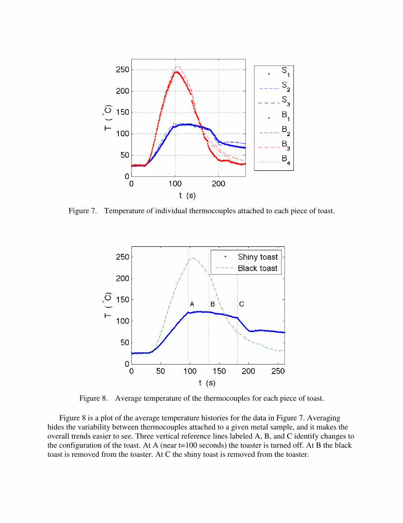
Figure 7. Temperature of individual thermocouples attached to each piece of toast.

Figure 8. Average temperature of the thermocouples for each piece of toast.

Figure 8 is a plot of the average temperature histories for the data in Figure 7. Averaging hides the variability between thermocouples attached to a given metal sample, and it makes the overall trends easier to see. Three vertical reference lines labeled A, B, and C identify changes to the configuration of the toast. At A (near t=100 seconds) the toaster is turned off. At B the black toast is removed from the toaster. At C the shiny toast is removed from the toaster.

The dramatic differences in temperature of the shiny and black toast provide motivation for students’ interest radiation heat transfer. The results in Figure 8 also provide good data to discuss multimode heat transfer. For example, the black toast not only heats up more quickly, but it also cools down more quickly. Note that the shiny toast cools relatively little between A, when the power is cut off and C when the shiny toast is removed from the toaster. The difference in cooling behavior of the two metal toast samples is because the black toast is a better emitter of radiation and when the power is cut off, the black toast is much warmer than the inner walls of the toaster, and air inside the toaster. The toast experiment presented here is a good in-class demonstration to motivate discussion of radiation heat transfer. After students attend lecture(s) on radiation, they return to the laboratory for more extensive experimental investigation. Measurements in the follow-up experiment include (1) comparison of additional surface properties, (2) use of thermocouples with radiation shields to measure the air temperature inside the toaster, (3) investigation of cooling in different ambient environments, e.g. comparing free and forced convection from a fan, and (4) introduction of heat and mass transfer by toasting bread instead of metal. Although the toaster experiment is the least expensive apparatus in our suite of experiments, it provides a rich environment for instruction by guided-inquiry.

Conclusions

This paper describes our early efforts to develop a set of experiments for teaching core concepts in the thermal and fluid sciences. The experiments provide a context for learning by guided inquiry. Our next step is to fully develop the curricular materials that accompany the physical equipment and measurements described here. To date we have constructed the hardware and used it in demonstrations and prototype experiments in student laboratories. In the coming months we will be deploying the experiments and curricular materials in a context that will allow formal assessment of student learning. We have designed an assessment plan to measure gains in student learning and to determine whether the laboratory exercises shift students’ attitudes toward laboratory work.

Bibliography

1. Bilal, N., Kess, H. R. & Adams, D. E. Reversing the Roles of Experiment and Theory in a

Roving Laboratory for Undergraduate Students in Mechanical Vibrations. International Journal of Engineering Education 21, 166-177 (2005).

2. Flora, J. R. V. & Cooper, A. T. Incorporating inquiry-based laboratory experiment in undergraduate environmental engineering laboratory. Journal of Professional Issues in Engineering Education and Practice 131, 19-25 (2005).

3. Golter, P., Van Wie, B., Windsor, J. & Held, G. in ASEE Annual Conference and Exposition (ASEE, Chicago, IL, 2006).

4. DeLyser, R. R., Quine, R. W., Rullkoetter, P. J. & Aremntrout, D. A sophomore capstone course in measurements and automated data acquisition. IEEE Transactions On Education 47, 453-458 (2004).

5. Cyr, M., Miragila, V., Nocera, T. & Rogers, C. A low-cost, innovative methodology for teaching engineering through experimentation. Journal of Engineering Education 86, 167-171 (1997).

6. Rogers, C. & Portsmore, M. in 2001 ASEE Annual Conference and Exposition (ASEE, Albuquerque, New Mexico, 2001).

7. Litwhiler, D. H. & Lovell, T. D. in 2005 ASEE Annual Conference and Exposition (Portland, Oregon, 2005).

8. Litwhiler, D. H. & Lovell, T. D. in 2005 ASEE Annual Conference and Exposition (Portland, Oregon, 2005).

9. Butterfield, R. Benefit without cost in a mechanics laboratory. Journal of Engineering Education 86, 315-320 (1997).

10. Edwards, R. in 2005 ASEE Annual Conference and Exposition (ASEE, Portland, Oregon, 2005).

11. Krupczak, J., Jr. et al. in ASEE Annual Conference and Exposition Session 1380 (ASEE, St. Louis, MO, 2000).

12. Anderson, A. & Wilk, R. in ASEE Annual Conference and Exposition Session 1566 (ASEE, St. Louis, MO, 2000).

13. Hesketh, R. P. & Slater, C. S. in 1997 ASEE Annual Conference and Exposition (ASEE, Milwaukee, Wisconsin, 1997).

14. Hesketh, R. P. & Slater, C. S. Innovative and economical bench-scale process engineering experiments. International Journal of Engineering Education 16, 327-334 (2000).

15. National Research Council. How People Learn: Brain, Mind, Experience, and School (National Academy Press, Washington, DC, 2000).

16. McDermott, L. C. Oerstead Medal Lecture 2001: "Physics education research - The key to student learning. American Journal of Physics 69, 1127-1137 (2001).

17. National Research Council. (eds. McCray, R. A., DeHaan, R. L. & Schuck, J. A.) (National Academy of Sciences, Washington, DC, 2003).

18. Prince, M. J. & Felder, R. M. Inductive teaching and learning methods: Definitions, comparisons, and research bases. Journal of Engineering Education 95, 123-138 (2006).

19. Redish, E. F. Implications of cognitive studies for teaching physics. American Journal of Physics 69, 796-803 (1994).

20. Felder, R. M. & Silverman, L. K. Learning and Teaching Styles in Engineering Education. Engineering Education 78, 674--681 (1998).

21. Felder, R. M. & Spurlin, J. Applications, Reliability and Validity of the Index of Learning Styles. International Journal of Engineering Education 21, 103-112 (2005).

22. Wankat, P. C. & Oreovicz, F. S. Teaching Engineering (McGraw-Hill, New York, 1993).

23. Kautz, C. H., Hereon, P. R. L., Loverude, M. E. & McDermott, L. C. Student understanding of the ideal gas law, Part I: A macroscopic perspective. American Journal of Physics 73, 1055-1063 (2005).

24. Kautz, C. H., Hereon, P. R. L., Shaffer, P. S. & McDermott, L. C. Student understanding of the ideal gas law, Part II: A microscopic perspective. American Journal of Physics 73, 1064-1071 (2005).

25. Loverude, M. E., Kautz, C. H. & Hereon, P. R. L. Student understanding of the first law of thermodynamics: Relating work to the adiabtic compression of an ideal gas. American Journal of Physics 70, 137-148 (2002).

26. Libii, J. N. Mechanics of the slow draining of a large tank under gravity. American Journal of Physics 71, 1204-1207 (2003).

27. Libii, J. N. & Faseyitan, S. O. in 1997 ASEE Annual Conference and Exposition (ASEE, Milwaukee, Wisconsin, 1997).

28. Saleta, M. E., Tobia, D. & Gil, S. Experimental study of Bernoulli's equation with losses. American Journal of Physics 73, 598-602 (2005).

29. Munson, B. R., Young, D. F. & Okiishi, T. H. Fundamentals of Fluid Mechanics (Wiley, New York, 2006).

Appendix: Mathematical Model of Tank Draining

The following derivation is similar to the analysis presented by Saleta et al.28, except that we do not include a loss term that is independent of fluid velocity. Assume the orifice in the side of the tank is small enough that the flow may be treated as quasistatic. In other words, neglect the acceleration of the top surface. Apply the energy equation between the top free surface (station 1) and the exit of the tank (station 2)

p2

γ+

V22

2g+ z2 =

p1

γ+

V12

2g+ z1 − hL (A.1)

where p is the static pressure, V is the local velocity, z is the elevation, and hL is the head loss. Since station 1 and station 2 are both open to the atmosphere, p2 and p1 are both zero. Note that V2 is the same as the jet velocity Vjet discussed in the body of this paper. Assume the head loss is concentrated at the exit and can be treated as a minor loss

hL = KL

V22

2g (A.2)

where KL is the minor loss coefficient. Mass conservation requires

V1A1 = V2ˆ A o (A.3)

where A1 is the area of the tank and ˆ A o is the effective area of the orifice. Using p1 = p2 = 0 ,

h = z1 − z2and substituting Equation (A.2) and Equation (A.3) into Equation (A.1) gives

V2 = C1 2gh (A.4)

with the constant C1 defined by

C1 =1

1+ KL −ˆ A o

A1

2 (A.5)

For the tanks used in our experiments, ˆ A o A1 <<1 so C1 is effectively

C1 =1

1+ KL

(A.6)

The velocity of the upper surface is

dh

dt= −V1 (A.7)

Combining Equation (A.3), (A.4), and (A.7) gives

dh

dt= −C2 h (A.8)

where C2 is another constant

C2 =ˆ A o

A1

C1 2gh (A.9)

With the initial condition h = h0 at t = 0 , Equation (A.8) can be integrated directly to obtain

h = h0 −C2

2t

2

(A.10)

Defining tmax as the time when h = 0 allows the solution to be written more compactly as

h

h0

= 1−t

tmax

2

(A.11)

where tmax and C2 are related by

tmax =2 h0

C2

(A.12)

The preceding equations describe how the depth of the fluid in the tank and the velocity of fluid leaving the tank vary as functions of time. Next, these quantities are related to the distance traveled by the fluid jet. The trajectory of the fluid jet leaving the tank is assumed to be determined by the physics of simple particle motion. If the effect of air resistance is neglected, an object falling under the

influence of gravity travels a distance H in time tf where H =1

2gt f

2 . In addition, during time tf an

object with initial horizontal velocity Vjet travels a horizontal distance L = Vjett f = Vjet 2 H g .

Substituting V2 = Vjet from Equation (A.2) gives

L =2 hH

1+ KL

(A.13)

Now, suppose that measured data L = f h( ) is available. A least squares curve fit can be used to

obtain the coefficient C3 in

L = C3 h (A.14)

With C3 known, Equation (A.13) and Equation (A.14) can be combined to compute KL

KL =4H

C32

−1 (A.15)

The preceding equations provide the relationships necessary to analyze the tank draining experiment. During the experiment, the data acquisition system records the output of the pressure transducer at a rate on the order of 1Hz.The digital camera is used to record images of the jet and computer screen displaying the system time. Roughly 10 to 20 images are recorded during a three to four minute draining duration. The data reduction proceeds in the following order.

1. Convert the pressure measurements to h(t).

2. Extract L = f(tj) from the digital photographs, where tj is the list of times for the photographs..

3. Interpolate in the h(t) data from the pressure transducer measurements to obtain hjet(tj).

4. Use a least squares curve fit of Equation (A.14) to the L versus hjet data to determine C3

5. Use Equation (A.15) to compute KL from the C3 obtained from the curve fit.