ac loss calculation of central solenoid model coil
TRANSCRIPT
JAERI-Research99-014
JP9950146
am
AC LOSS CALCULATION OF CENTRAL SOLENOID MODEL COIL
March 1999
Attila GILANYI*, Masato AKIBA, Yoshikazu OKUMURA,
Makoto SUGIMOTO, Yoshikazu TAKAHASHI andHiroshi TSUJI
Japan Atomic Energy Research Institute
(T319-1195
- (T319-H95
This report is issued irregularly.
Inquiries about availability of the reports should be addressed to Research
Information Division, Department of Intellectual Resources, Japan Atomic Energy
Research Institute, Tokai-mura, Naka-gun, Ibaraki-ken 319-1195, Japan.
© Japan Atomic Energy Research Institute, 1999
m /-

JAERI-Research 99-014
AC Loss Calculation of Central Solenoid Model Coil
Attila GILANYI*,Masato AKIBA, Yoshikazu OKUMURA,
Makoto SUGIMOTO, Yoshikazu TAKAHASHI and Hiroshi TSUJI
Department of Fusion Engineering Research
Naka Fusion Research Establishment
Japan Atomic Energy Research Institute
Naka-machi, Naka-gun, Ibaraki-ken
(Received January 28, 1999)
The AC loss of Central Solenoid Model Coil of ITER is calculated in order to
be able to determine the allowable excitation current shape in time with
respect to the available cooling capacity at liquid helium temperature.
In Part A the theory is summarized essential to present calculation. This
covers a semianalytical integral formulation to calculate the magnetic field
distribution in the cross-section of a coil and also 2D and 3D differential
formulations for eddy current calculation of jackets and structural steel compo-
nents, respectively.
In Part B the conditions and results of calculation are described in detail.
Losses are calculated separately in different components. Also the different
types of losses are separated, and only one of the followings is considered in
the same time; eddy current loss, ferromagnetic hysteresis loss, superconducting
hysteresis loss, coupling loss.
The low frequency eddy current loss calculations of structural stainless steel
components are carried out by ANSYS/EMAG code in 3D separately for tension
rods, plates and beams. The problem of loop currents is briefly discussed, but
the interaction between several components is not considered.
In the case of Incoloy jackets of conductors a 2D ANSYS code is used with
current force to obtain the eddy current losses. The ferromagnetic hysteresis
* Technical University of Budapest

JAERI-Research 99-014
loss of jackets are also roughly estimated based on measurement data.
The superconducting hysteresis and coupling losses of Nb3Sn strands are
estimated using measurement data and a calculated flux density distribution in
the cross-section of the model coil by a semi-analytical integral formulation.
The coupling is not considered during hysteresis loss calculation and an ideal
model is used for coupling loss calculation.
The losses of Butt-type and Lap-typejoints and roughly estimated based on
measurement data to make complete this study. Both the loss due to flux
change and the loss due to transport current are considered.
The individual loss components are summed up, compared and plotted in
time. The followings are concluded. The coupling loss was found to be the
largest 83% of the total AC loss supposing 50 msec characteristic time con-
stant. Also significant amount of heat is generated in structural steels, the
largest amount in lower tension plates and inner tension rods. Therefore
cooling is required for stainless steel structural components. The loss of joints
is not large, however concentrated, therefore joints should receive attention.
Specially Lap-type joints are critical components.
The eddy current and coupling power losses can be significantly decreased by
increasing the ramp-up time since they are proportional to the square of flux
change rate, while superconducting and ferromagnetic hysteresis power losses
decrease linearly with decreasing flux change rate. Joule losses are produced
in joints even after the energizing process of the magnet, when it is driven by
a constant excitation current. This propose us to keep the time of full power
operation short.
Keywords: CS Model Coil, AC Loss, Heat Generation, FEM, Eddy Current

JAERI-Research 99-014
cs
H wAttila GILANYI* • ®M MA
(1999 ••ff-lH 28 H g l t )
A -c li, -/
M * , CS
fi^(7?83% *
m * 2 ̂ T C S ̂ 3 >k% n
: T311-0193 ^«lf,


JAERI-Research 99-014
Contents
Part A 1
Overview of Theory
1. Introduction 3
2. Integral Approach 4
2.1 Current Carrying Circular Loop 5
2.2 Field Distribution in the Axis of a Thin Solenoid 6
2.3 Field Distribution in the Entire Cross-section of a Current
Carrying Circular Loop 8
2.4 Field Distribution in the Cross-section of a Circular Coil with
Rectangular Cross-section 10
2.5 Integral Formulations for Nonlinear Numerical Evaluation 10
2.6 Low Frequency Eddy Current Loss in a Cylindrical Rod 11
3. 3D Eddy Current Loss Calculation by FEM Using
Differential Formulation 12
3.1 Theoretical Background 12
3.2 Boundary and Interface Conditions 13
3.3 Post-processing 13
3.4 Time Derivative 13
4. 2D Differential Formulation 14
4.1 Current Force in 2D 14
4.2 Solution in Cylindrical Coordinate System 14
5. AC Loss of Superconducting Cables 15
5.1 Characterization of Superconductors 16
5.2 Superconducting Hysteresis (Characterization by BH-loop) 17
5.3 Superconducting Hysteresis Loss 20
5.4 Coupling Loss in Transverse Field 20
5.5 Self-field Loss 20
5.6 Summary 21
5.7 Measuring the Loss 21

JAERI-Research 99-014
Part B 23
Calculation Results
1. Introduction 25
1.1 Basic Consideration 25
1.2 Components of CS Model Coil (Electromagnetic Model) 26
2. Magnetic Field Distribution 28
3. Eddy Current Loss in Structural Components 31
3.1 Eddy Current Loss in Electrically Insulated Components 31
3.2 Eddy Current Loss Distribution 39
3.3 Eddy Currents in Connected Components 39
3.4 The Effect of BH-curve of Incoloy onto the Eddy Current Loss 40
3.5 Loop Currents 43
3.6 Temperature Increase in Structural Components 47
4. Loss Generated in Incoloy Jacket 49
4.1 Ferromagnetic Hysteresis Loss of Incoloy Jacket 49
4.2 Eddy Current Power Loss of Incoloy Jacket 51
4.3 Eddy Current Power Loss Dependence on Specific Resistivity
and Flux Change Rate 57
4.4 Eddy Current Power Loss Distribution in the Winding 57
4.5 The Effect of BH-curve of Incoloy onto the Eddy Current loss
of Jacket 58
5. AC Loss of Superconducting Cables 59
5.1 Superconducting Hysteresis Loss in Nb3Sn Filaments 59
5.2 Coupling Loss 61
6. Loss of Joints 62
7. Summary of Loss Calculation 63
7.1 Eddy Current Power Loss of Structural Elements 63
7.2 Loss of Incoloy Jacket 64
7.3 AC Loss of Superconducting Cable 65
7.4 Loss of Joints 66
7.5 Total Power Loss 67
7.6 Time History of Power Loss (without Insert Coil) 68
7.7 Decreasing the Loss 69
8. Conclusion 70
Acknowledgment 70
References 71
vi

JAERI-Research 99-014
§ >k
2.
2.1
2.2
2.3
2.4
2.5
2.6
3.
4.
3.1
3.2
3.3
3.4
. 2
4.1
4.2
5.
5.2
5.3
5.4
5.5
5.6
5.7
B
1.
1.1
1.2
2.
3.
3.1
3.2
3.3
1
3
4
& 5K- =^;K7>tt±WM5HF 6
8
K • ="( ̂ vffiMlHomWsftfi 1010
11
12
12
13
13
13
14
»iL7C (Current Force) WafA 14
P 1 4
15
16
17
20
20
20
21
23
25
25
26
28
31
31
39
39
vii

JAERI-Research 99-014
3.4 -{yanj • 3>zSy Y<?)#1RJ&%}&K£&MX,WLtik& 403.5 /iia^iiit, 433.6 £#«*&»£>ia£±# 47
4. -f^an-f •y>^7H:H4t^fE 494.1 ^ 3 D ^ • v>y^ M c ^ t S K^t'J v*$& 49
4.2 -fV3D>f • i / > ^ 7 H;f££f&M»fLJS£ 514.3 f / ^ n ^ . v > ^ 7 M::!&£-f*iffi*8IE$£ £**•*•£
rt&fct&ramM$<7>!£# 574.4 3'fJl'gii&rt £&£•*• &fla«fi£tl£ 574.5 ^ 3 D > f • vfry Y\Z%!ktZ>l®im:Mm£<VWm%>%)W: 58
5. Mmmmtt-VjcfamZ: 595.1 NbSSn&M&foVKZ'TV *s*Wz 595.2 jjg'g-ll^ 61
6. m%MWM ( y a O h) « n ^ 62
7. «^#P*fOtfci6 63
7.i %#m&m<r>mwtim9z 637.2 O 3 D > f • v > ^ 7 b<7)JM^ 647.3 j@«&£Ett<7)£SfE!t& 65
7.4 v a -f > h O | | ^ 66
7.5 CS^TIV • ajJWmZ: 677.6 H£<Oj§&Ji>& 687.7 jf£<7)fg;M& 69
8. t t tb 70m & 70
71
VIII

JAERI-Research 99-014
Part AOverview of Theory

This is a blank page.
JAERI-Research 99-014
1. Introduction
In Part A the theory essential to the loss calculation of CS Model Coil is summarized.In Section 2 integral approaches are reviewed. First a formula is given to determine the
magnetic field in the axis of a circular current carrying loop. Next the field distribution isdetermined in the axis of a thin solenoid. This is followed by a semi-analytical method usingelliptic integrals applicable to the calculation of flux density distribution in the cross-section ofa current carrying circular loop. Formulations for magnetic materials are also briefly discussed.
In Subsection 2.6 a simple formulation is introduced for low-frequency eddy current losscalculation of a conductive rod placed parallel to the magnetic field. The importance of thissimple test case is to understand the frequency and specific resistivity dependence of powerloss.
In Section 3 the 3D differential formulation is discussed for the eddy current losscalculation of tension rods, beams and plates.
In Section 4 some remarks are done for 2D eddy current calculations with differentialformulation. The current force is introduced in order to make possible the 2D simulation ofeddy currents in Incoloy jackets. To avoid problems with singularities in cylindrical coordinatesystem, two possible methods are briefly summarized.
The AC loss of superconducting cables is reviewed in the last section. The focus is on thehysteresis properties of superconductors and on the coupling, because these phenomenaproduce the main part of the loss.
- 3 -
JAERI-Research 99-014
2. Integral Approach
The magnetic field of quasi stationer currents can be described by the following set ofMaxwell's equations
TO/// = . / ,divB = 0,
B = M ) / / .Introducing the magnetic vector potential as B - rot A , we obtain
rot rot A - graddiv A - AA — //0./.Selecting the divergence of A to be zero
AA = -Mi>J
The solution for the magnetic vector potential can be obtained in the form of
A = -An
rAA 1 r(?A\ \ r d 1I—dV+ — f-—dS- — \A dS• r An J
s an r An • an rwhere S denotes the surface of volume V. If the components of A disappear enough far in theinfinity , we can write
A = ̂ [-dV Eq.2.1An*, r
From now on the vectors will be notified with upper bars till the end of this section. For a
current carrying circular loop introducing JdV - JSdl = Jdl we obtain
Eq.2.2An \ r
In a given point P the flux density is
An j r
Using the identityrot(uv) = uroiv + gradu x v
] _and substituting u = — and v - dl
rot— = —roldl + vrad— x dl = - —r x dlr r r r
because rotvdl - 0. By this we obtain the well-known Biot-Savart law
- / rJlxrH = —i—j- Eq. 2.3
An\ rwhich allows us to evaluate the magnetic field generated by a current carrying conductor witharbitrary shape. This is the starting point of many analytical and semi analytical formulations.
- 4 -

JAERI-Research 99-014
2.1 Current Carrying Circular loopFirst let us consider a circular loop with radius R and carrying current I as shown in Figure 2-1.
dH7
Figure 2-1.: Circular current carrying loop
The magnetic field in the axis of the circular loop will be evaluated starting from the Biot-Savart law, Eq.2.3. Considering just a small section of the coil its contribution can beexpressed as
An rIts axial component is
R
r
dl R
Anr rIntegrating for the whole length finally we obtain
1 n IR2 I R2
2 r3 ~ 2
5

JAERI-Research 99-014
2.2 Field distribution in the axis of a thin solenoidNext let us consider an ideal cylindrical solenoid with radius R and length 2a as illustrated
in Figure 2-2. Let N denote the number of turns.
R
Figure 2-2.: Geometry of a thin solenoid
Based on the previous result the field produced by a small section with dC, length is
A7 1 R2
The axial component of the magnetic field along the axis can be calculated by integration ontothe total length
Substituting sh{t) = (z-Q/ R the final result is
a-z a+z= + •
NI
This expression can be further simplified introducing a, and a2 angles as illustrated in Figure2-3:
NIH2 = — (cos or, -cosa 2 )
Figure 2-3.: Simplified notation
In the center the field intensity can be written as
- 6 -

JAERI-Research 99-014
NI
and at the end of the windingNI
H(±a) = ,2ylR2+4a2
As an example the profile of the flux density along the axis of a solenoid is plotted in Figure 2-4 with the following parameters: a=0.9m, R=l ,3m, N=540, I=46kA.
14 -,<
12
10
E 8
« 6
4-
20-
C
Flux density distribution along the axis
. ' • : • • • " • • .
. ' • • • • • • • • • : • ; • • : • • • • • v -
• • • • " - ' " • " . - • • - . . • •
• • . • • • • . • . • •
• • • • • - . . . . . . " . • ' • . " . • " " • -
) 0.5 1 1.5 2
X[m]
: • ' • - ' ' " • • ' • ' : ' • • • : • ' ' ' • • - . " • • ' •
- • • - . • • • . • "• . • ' • • • '
" " ' : • ' : ' ' • ' " : • / • • • • . • • ' . • ' ' : • •
. : • • • ' • • - , ; ' , : : • , " • • • " " • • • "
: " - ' - ' : / : • - . . ' • • ' ; . ; - - - - - ; -
• ' > " • • - " • • • • • " • . ' • • • ; : .' • . • ' . " :
MHiiuiife;::'.;-;::
> 2.5
Figure 2-4.: Flux density profile in the axis of a thin solenoid
- 7 -

JAERI-Research 99-014
2.3 Field distribution in the entire cross-section of a current carrying circularloopIn this section the field distribution is determined in the cross-section of a cylindrical conductorby a semi analytical method after Simonyi [1]. Instead of the direct application of Biot-Savartlaw, the magnetic vector potential is introduced and we start from Eq.2.2. The magnetic vectorpotential has only azimuthal component A9 because of the axial symmetry. The source point isdenoted as (r',z') and the observation point as (r,z) in the following.
A{r£)-BLtJL*K ' ' 4nJ
r -rIn r'cos(<p'-(p)d<p'
Setting <p = 02K
+ r2 +r'2-2rr'cos(<p'-<p)
r'd(p' cos <p'"Pv,<-j- 4 j n 77-
4 ; r o^J{z-z')
Introducing a new variable /?=
+r2+r'2-2rr'cos(p'
n- q?
d<p'=-2d/3
= 2sin2 fi-
(2 sin2 p-\\-2)dp
-zf +r2 +r '2-2rr '(2sin2 /?-l)
2n -z') +(r+r')2 -4rr'sin2p
"A (2sin2y9
2n :_ z y; ( r + o , j4rr' sin' sin2
Introducing k2 as4rr'
q> V ' / ~
In
The numerator can be reformulated as
. . 2 . 2 .. .„ .
I (2 sin2 P-X)dp
and the magnetic vector potential can be written as
- 8 -

JAERI-Research 99-014
')2+ r')
. 2 > / 2
1 -dfi / 2
Finally the magnetic vector potential can be expressed in cylindrical coordinate system as
where F() and E() are first and second order complete elliptic type integrals, respectively and
')2(z-z')2+(r+r')
F{k) = jJ
0 A / l - * 2 sin2 fi
E(k) = dp
The radial and the axial component of flux density formally can be obtained from the vectorpotential as
dA
fA
Instead of the differentiation it is easier to derive expressions directly for Br and Bz in similarway as for the vector potential. Without details the result can be written as follows:
r2 1Br(r,z) =
B,(r,z) =juol z
r yl(r+rf +(z-z')2 (r-rf +(z-z')2
Unfortunately the above formulations are singular if r=0, therefore we apply the result obtainedin Sec.2.2. in the axis:
%(r = 0,z):=0
32(r = 0,z): = Mo1
- 9 -
JAERI-Research 99-014
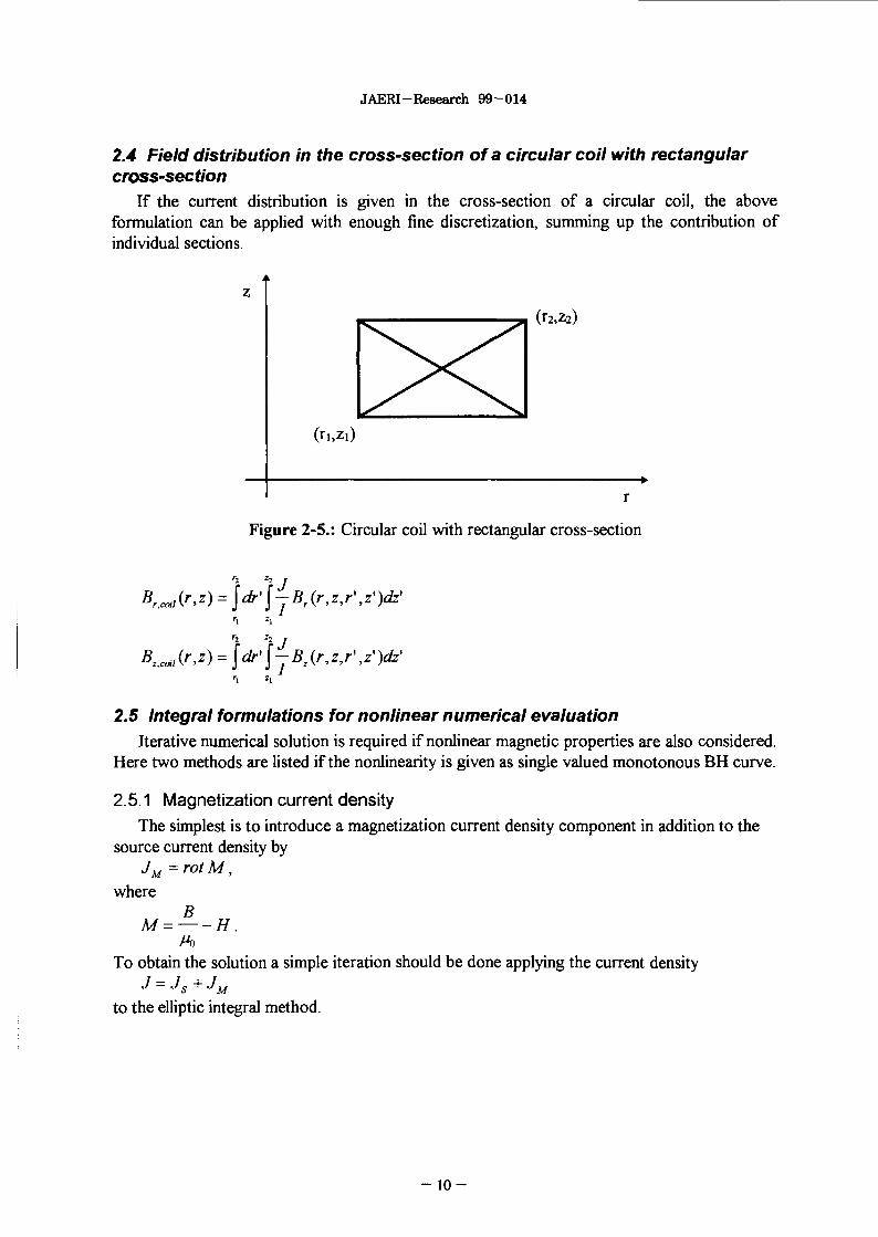
2.4 Field distribution in the cross-section of a circular coil with rectangularcross-section
If the current distribution is given in the cross-section of a circular coil, the aboveformulation can be applied with enough fine discretization, summing up the contribution ofindividual sections.
(r2,z2)
Figure 2-5.: Circular coil with rectangular cross-section
} .:u
J
2.5 Integral formulations for nonlinear numerical evaluationIterative numerical solution is required if nonlinear magnetic properties are also considered.
Here two methods are listed if the nonlinearity is given as single valued monotonous BH curve.
2.5.1 Magnetization current densityThe simplest is to introduce a magnetization current density component in addition to the
source current density byJM =rotM,
where
M = —-H.A)
To obtain the solution a simple iteration should be done applying the current density
to the elliptic integral method.
- 1 0 -
JAERI-Research 99-014
2.5.2 Solution method of Newman et al.An alternative approach is worked out by Newman et al. which requires the iterative
solution of the following integral equation
i, \r-n nu \r-rwhere M is the magnetization, J is the source current density and x is the magneticsusceptibility. Instead of this formulation a 2D differential formulation will be used to study themagnetic behavior of Incoloy jacket.
2.6 Low frequency eddy current loss in a cylindrical rodWe consider a long cylinder made of ferromagnetic or non-ferromagnetic material. The flux
density is supposed to be homogeneous and parallel to the axis. Moreover it is changing with aconstant rate, dB I dt - const. The induced electric field can be written as
§on a radius r where
d® , dB— r 7i .
dt dtWithin the cylinder for r < r0
r dB
Introducing p specific resistivity, the eddy current density J is given byr dB
J(r) = - — — .2p dt
The power loss per unit volume of the material is
V1 J 7rro2{ 2prl\dt) { %p\
The power loss is proportional to the square of the frequency. It also depends on the specificresistivity and the radius of the bar, however does not depend on the permeability as long asthe flux penetration is complete.
As an example the eddy current power loss is evaluated due to the z-component of the fieldin inner tension rod. The total length of an inner tension rod is 4476mm and its diameter is165mm. Only a short part of it (1775mm) is placed inside the coils. First the field profile iscalculated along the tension rod. The conductivity is set to <j = 2E6SI m.Substituting and integrating we obtain
A careful numerical integration results 53.2W power loss in one tension rod. This means53.2W*13sec=692J energy loss in one tension rod during the energizing of magnet.
- 11 -

JAERI-Research 99-014
3. 3D Eddy Current Loss Calculation by FEM Using DifferentialFormulation
A domain consisting of a conducting sub-domain without current source and a non-conducting sub-domain with current source is considered.
3.1 Theoretical backgroundIn present quasistatic case the following set of Maxwell's equations describes the field:
vxjy = y (3.1)0B
V X j L ~ dt { }
B = /JH (3.3)J = trE (3.4)
where a denotes the conductivity. Its numeric value strongly depends on the temperature,which has to be considered. Following from eq.3.2 the magnetic flux density has to besolenoidal
V£ = 0. (3.5)Eq.3.1 implies that
V./ = 0. (3.6)In practice this means that at interfaces between air and metal no normal component of currentis present. The eddy current analysis is carried out using magnetic vector potential A,introduced by means of the relation
B = VxA (3.7)satisfying identically eq.3.5. Introducing a scalar potential V, eq.3.2 is satisfied by defining theelectric field intensity as
dAE = - - - V V . (38)
The governing equation for A and V in the eddy current region can be obtained from eqs. 3.1,3.7 and 3.8:
1 dAVx juVxA + C7 dt +a ~°" ^ 3 9 )
In order to define A uniquely the Coulomb gauge is appliedVA = 0. (3.10)
ANSYS [5] replaces eq.3.9 by1 1 dA
X n X ~ n +a dt +<J ~ ' ( 'after Biro [6] and in order to satisfy the solenoidal requirement
Vcr +VF = 0\01)
is imposed. The non-conducting region is represented with the simple formula
V y — V Y A - 1 H n̂M
where Js is the source current density. An alternative approach is to use magnetic scalarpotential in the non-conducting region. In such a case the normal component of A also shouldbe specified on the interface by the constraint
- 1 2 -

JAERI-Research 99-014
A-n = 0,
for the unique solution.
3.2 Boundary and Interface ConditionsFlux-normal boundary conditions can be satisfied by setting the normal component of A to
zero. Flux-parallel conditions has to be satisfied setting the in-plane components of A to zero.For far-field simulation infinite elements has to be used. Periodic or cyclic symmetry can besatisfied prescribing constraint equations or coupling the nodes. An imposed external fieldrequires to set Ax, Ay, Az values to the necessary one. Finally a numerical value for V must befixed somewhere within the conducting region.
3.3 Post-processingThe current density is calculated over all of the finite elements where the conductivity is
different from zero. Next the power loss per unit volume is calculated and integrating for thetotal volume the power loss is obtained as
P(t) = \p[j{t)]2dv [Watt].V
Integrating according to the time, the energy loss (Joule heat) can be written ast
\t)dT [Joule].
3.4 Time derivativeIf the solution is done in the time domain, the following simple scheme can be used
where index k notes the previous solution step and k+1 the new solution step. The time step Atshould be enough small and constant 0 larger than 1/2 for a stable solution. We will use0=2/3.
- 1 3 -

JAERI-Research 99-014
4. 2D Differential Formulation
2D differential formulation will be applied to the eddy current loss calculation of Incoloyjackets in cylindrical coordinate system. The differential formulation of 2D problems is widelyused, therefore we do not repeat the derivations. However some remarks will be done onaxisymmetric problems and current force.
4.1 Current Force in 2DThe one component magnetic vector potential is selected to describe the 2D eddy current
problem. The governing equation can be written as
V x — VxA = JS -aA,M
where Js is the source current density. This formulation provides only voltage forced solution.If the total current has to be prescribed in the cross-section (current force) than the sourcecurrent term should be substituted [7] by
J+
J* =T
Conductor
where Tempter denotes the area of the cross-section of conductor in which the current shouldbe prescribed.
This is the situation in case of Incoloy jacket which carries only eddy currents, but the totalcurrent should be zero in the whole cross-section. Note, that the assembled matrix will includelong lines at vector potential values belonging to the jacket. This slows down the solutionprocedure and also requires additional storage capacity.
4.2 Solution in Cylindrical Coordinate SystemThe energy related functional for axisymmetric problems is
+ —fi\ dz ) //1, dr-2JsA9+aA9A9
There is a singularity in r=0, causing problem during the numerical solution. To eliminate thesingularity the modified vector potential should be introduced as follows
A<p'=~r o r Aw<=~-
In this case
i u\ dz ) u\ dr )
An other way is to select integration points far enough from the axis during finite elementprocessing. The solution in node points can be obtained by extrapolating the results obtained inintegration points.
- 1 4 -

JAERI- Research 99-014
5. AC Loss of Superconducting Cables
If an external field is applied to a bulk Type-II superconductor screening currents willappear. The change of external field results hysteresis loss because the screening currents donot decay themselves due to the zero resistance of supeconductor.
Under some condition the critical state of a superconductor may be unstable, because fluxmotion generates heat and the critical field depends on the temperature. They may cause fluxjump by positive feedback, which results in the loss of superconducting state abruptly. Againstflux jump fine filaments should be composed. Superconducting hysteresis loss also decreases iffine filaments are applied. In the practice for magnet winding filamentary composites are usedin which the fine filaments are embedded in a matrix of normal metal (usually copper) havinggood electrical conductivity. The good ductility of copper allow us to wind a magnet, the goodelectrical conductivity along the strand also give protection against flux jump and protect theconductor from burn-out if the magnet quenches. However the good conductivity of coppermatrix cause the coupling of filaments together in changing magnetic field by cross-over eddycurrents, resulting in coupling loss. Due to coupling the superconducting hysteresis loss alsoincreases, since the whole strand will behave like a thick superconductor. The coupling can besignificantly decreased by twisting the filaments. In addition we have to find an optimumchoice of electrical conductivity which is a compromise between the conflicting demands oflow AC. loss and good stability. In many case resistive alloy jacket is placed around eachfilament to increase the cross-over resistivity and hence decrease the coupling loss, but keepthe good conductivity along the strand.
The transport current itself produce a self-field. This is why the current flow is located in anoutermost shell.
From the strands conductors are constructed. The lager the magnet the lager the conductorin order to be protected during quenching. Strands are twisted together to reduce the magneticcoupling between them. They are also fully transposed to minimize a self-field effect
- 15
JAERI-Research 99-014
5.1 Characterization of SuperconductorsTo describe superconductivity several physical models were developed:
• 1935 London theory• 1950 Ginzburg-Landau theory• 1957 BCS theory (Barden-Cooper-Schrieffer)
There are also simple models used successfully in engineering. They use the E-J constitutiveequation. Here just a brief summary is given.
5.1.1 Critical state modelsBean model applies an idealized E-J relationship
jrJ = Je~r. if E*0 and
f = 0 if E--0,generally referred as critical state model.Kim-model also takes into consideration the critical current density dependence on the field as
where Jc0 and Bo are constants.Yasukochi model use an other relationship for the critical current density dependence
5.1.2 Flux flow and creep model
and
^ J [ ^ J ,/ J<J.{J-Je) if J>Je
where pf and pc denotes the flow and creep resistivity respectively while UQ is the pinning
potential.
- 1 6 -

JAERI-Research 99-014
5.2 Superconducting Hysteresis (characterization by BH-loop)In the following the hysteresis of superconductors is demonstrated. Let us consider a
superconducting slab of thickness 2a which is placed into He external magnetic field. Theaverage flux density above the slab can be written as
and the equivalent magnetization of the slab isB
M= — -He.M>
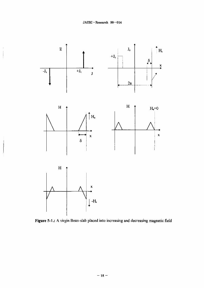
For the calculation of the magnetization, we should know the magnetic field distribution withinthe slab. The externally applied magnetic field induce a persistent current in thesuperconductor. Based on the critical state model the current density distribution has arectangular profile in shape resulting a linear profile of magnetic field within the slab. Ingeneral rotH = J should be applied, which is simplified now to
dHy
Increasing the magnetic field from zero to He value, the penetration depth is given by
x "•
To achieve full penetration 6=a an external field with amplitude
H, = Jflshould be applied. The flux density over the slab in case of full penetration is
The magnetization of the slab can be written asB. J a J a H
\d P_ 11 c / ~ _ c — —M ' = ^ ' = 2 -Jfi— 2 - " 2 •
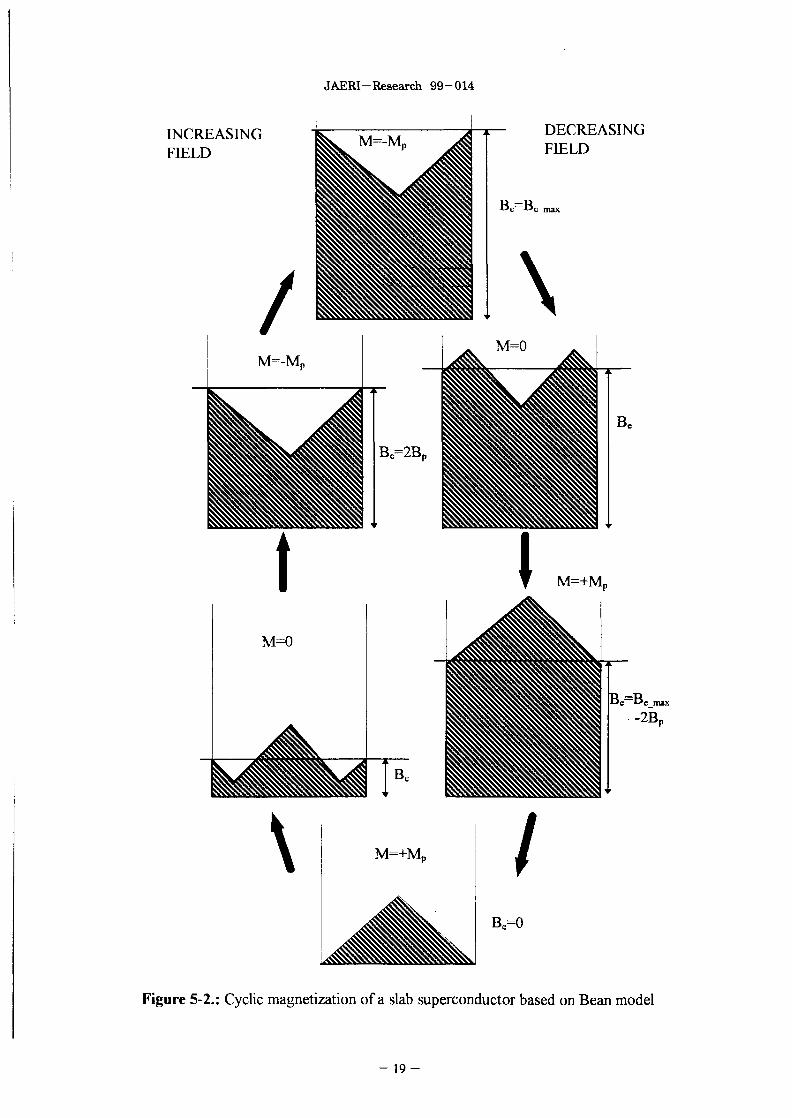
Increasing the field from a virgin state up to a maximum value HnuK<Hp and next decreasingback to zero, the average flux density is lager than zero. The changes of the field profile issummarized in Figure 5-1 for increasing and decreasing external magnetic field.
In CS Model Coil a cyclic trapezoidal unidirectional excitation current is applied which alsoproduces a cyclic unidirectional magnetic field. The maximum value of the field is over the fullpenetration. Flux profiles within a slab superconductor under the same excitation conditionsare plotted in Figure 5-2.
In case of a cylinder perpendicular to the field the external field necessary to achieve fullpenetration is
and the magnetization is
- 1 7 -
JAERI-Research 99-014
-Jc +Jc
+Jc
A
Jz
< 2a
5r^—W
_ _ _ . -— T
IH.
X
H t H t
A
He=0
A
H f
A A
-H,
Figure 5-1.: A virgin Bean-slab placed into increasing and decreasing magnetic field
- 1 8 -
JAERI-Research 99-014
INCREASINGFIELD
DECREASINGFIELD
\M=+MD
Be=0
Figure 5-2.: Cyclic magnetization of a slab superconductor based on Bean model
- 1 9 -
JAERI-Research 99-014
5.3 Superconducting hysteresis lossThe energy loss caused by superconducting hysteresis can be evaluated by the help of
Pointing vector
- j> ]*£ x Jidsdt = \§~EJdtdv + ̂ jjifdM .s v v
Where S is the surface of the V volume under interest. After some manipulation the energyloss over a full cycle can be expressed as
The energy loss per unit volume for cylinders over full penetration can be evaluated by theformula [2]
where Bm is the amplitude of a fully reversed cyclic external field. The critical current densitydependence on the magnetic field has to be also considered.
5.4 Coupling loss in transverse fieldThe coupling loss depends on the twist pitch length and the effective matrix resistivity,
since they determine the time constant of the system, and also depends on the excitation. Thetime constant can be written as [2]
2ft,Usually it is determined from measurements since it is difficult to calculate the effective matrixresistivity. If a trapezoidal excitation signal is applied with maximum value Bm and ramp uptime Tm which is large comparing to x, than the power loss and energy loss per unit volume canbe calculated from [2]
l Y 2B2m(
Tl pet Kin
These loss formulas are derived with some ideal assumptions. In the practice the external layerof filaments carries critical current density and this zone propagates toward the inner part ofstrands if it is necessary. The loss produced during propagation is called penetration loss. Thiscomponent of loss is not considered now.
5.5 Self-field lossEven if the filaments are well twisted and the coupling is reduced between them, the
transport current itself produce a circular field around the conductors which is associated withenergy loss as well. The only method to decrease self field loss is to fully transpose filamentsand strands. Also strand diameter should be small, presently it is 0.81 mm.
- 2 0 -
JAERI-Research 99-014
5.6 SummaryIn pulsed magnets the filaments should be as fine as possible because of two reasons. First
to avoid flux-jumping, second to decrease superconducting hysteresis loss. The transverseresistivity of the embedding copper matrix should be as high as possible in order to decreasecoupling loss. On the same time conductivity in the longitudinal direction must be high toprovide dynamic stability and to protect magnet during quenching. The AC loss of twistedsuperconducting filamentary composits consist ofI. superconducting hysteresis loss (the critical current density dependence on magnetic field
and the transport current should be considered),II. coupling loss (current through the copper matrix, current through the peripheral layer of
strand and eddy current in the peripheral layer),III. penetration loss andIV. self field loss.
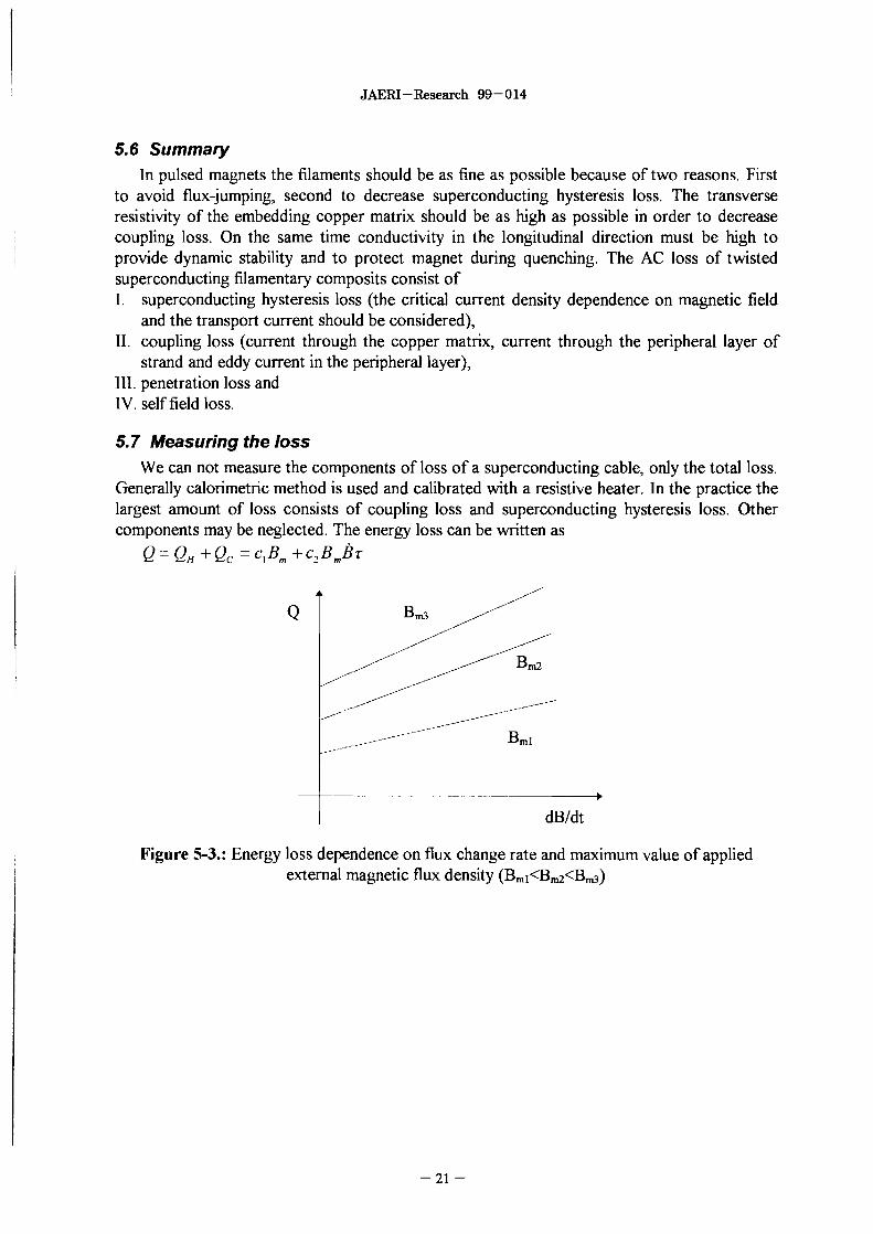
5.7 Measuring the lossWe can not measure the components of loss of a superconducting cable, only the total loss.
Generally calorimetric method is used and calibrated with a resistive heater. In the practice thelargest amount of loss consists of coupling loss and superconducting hysteresis loss. Othercomponents may be neglected. The energy loss can be written as
/~l /") i /^) , . D i ^ , L> D_-
ti — \JH + \JC — ̂ -\"m ' ^2 m ^
B
dB/dt
Figure 5-3.: Energy loss dependence on flux change rate and maximum value of appliedexternal magnetic flux density (Bm]<Bm2<Bm3)
- 2 1 -

JAERI-Research 99-014
PartBCalculation Results
- 2 3

This is a blank page.
JAERI-Research 99-014
1. Introduction
The Central Solenoid (CS) Model Coil is designed to produce magnetic field withmaximum flux density of 13T in case of 46kA excitation current. The coil will operate in"pulse mode". Present interest is to determine the total heat-loss produced in different parts ofthe magnet, namely the eddy current loss of supporting structures, the AC loss ofsuperconducting cables (including the superconducting hysteresis loss of Nb3Sn filaments, eddycurrent loss, coupling loss), the ferromagnetic hysteresis and eddy current loss of Incoloyjackets. Also the analysis of butt-type and lap-type joints is necessary. The produced loss canbe categorized as follows:
• Eddy current loss in Cu, Incoloy, stainless steel and other metal structures• Superconducting Hysteresis loss in Nb3Sn material• Ferromagnetic Hysteresis loss in Incoloy
1.1 Basic ConsiderationIn order to calculate the AC loss of superconductors, the eddy current loss and the
ferromagnetic hysteresis loss of the magnet,
"tola/ \Btotal ) ~ ''eddy current \"total ) ~^~ "SC ("total ) ~*~ " F e Hysteresis ("total ) '
the total magnetic flux density (Btoui) will be decomposed into two components; an ideal one(Bid<ai) and a perturbed component (Sp t̂m^d). The ideal component is generated by an ideal coilwhile the perturbed component is produced by eddy currents, superconducting hysteresis andferromagnetic hysteresis phenomena:
"total \"ideal s "perturbed ) ~ "ideal + "perturbed ("ideal )
Neglecting the perturbed part of the flux density we may receive a good approximation of theloss. (Not the ferromagnetic hysteresis or other phenomena are neglected but only theircontribution to the magnetic field.) The advantage of this simplification is, that we can considerthe components by one by one interacting with the ideal field component and finally obtain thetotal loss by summing up the contribution of individual parts. A simple calculation can show,that the contribution of low frequency eddy currents to the perturbed field can be reallyneglected. The contribution of ferromagnetic behavior will be discussed.
2 5 -

JAERI-Research 99-014
1.2 Components of CS Mode! Coil (Electromagnetic Model)The arrangement of winding and metal components of supporting structure are plotted inFigure I-I and Figure 1-2. The winding consist of modules, namely Inner Module-A, InnerMoule-B and Outer Module. In addition an Insert Coil is also placed inside. Two grades ofconductor are used. In Insert Coil and in Inner Module-A where the magnetic field is highCSl-type conductor is used, while in Inner Module-B and in Outer Module CS2-typeconductor is applied.
1/4 section of structure
Figure 1-1.: Arrangement of Winding of CS Model Coil
- 2 6 -

JAERI-Research 99-014
The supporting structure is manufactured from SS316 stainless steel. Figure 1-2 illustrates onequarter of the structure without the winding. There are totally 16 inner and 16 outer tensionrods in contact with 16 upper and 16 lower tension beams. Below tension beams tension platesare located. The lower plate support consist of 4 segments, called Lower tension plateshereafter. They are the most critical because of their large size. The upper side is much moredivided, consisting of 8 upper-inner tension plates and 16 upper-outer tension plates.
1/4 section of structure
Figure 1-2.: Arrangement of metal components of the supporting structure
- 2 7 -

JAERI-Research 99-014
2.
The major geometric parameters of winding and the maximum values of applied excitations arelisted in Table 2-1. First the distribution of magnetic flux density is calculated in the cross-section of the model coil and plotted for the center line in Figure 2-1. Next a simplification isintroduced. Instead of the complicated structure of Insert coil, Inner module and Outermodule, a simple solenoid is used with homogeneous source current distribution. Its innerdiameter is selected to be Rj=0.785m, its outer diameter R<>=1.81m and its height h=I.775m.The maximum value of excitation current density is set according to Table 2-2 to produce thesame field in the center, as it is in the case of detailed model. The field profile produced by thesimplified solenoid is plotted in Figure 2-2. Within the winding there is some differencebetween the two profiles.
Table 2-L: Major parameters of winding
Kind of ConductorInner RadiusOuter RadiusHeightLayer NumbersTurn NumbersCurrent per turnAverage Current Density
Insert CoilCS1
0.716m0.77m1.81m
130.87540kA
14.53MA/m2
Inner ModuleCS10.8m
1.0315m1.6596m
4122.9375
CS21.0315m1.347m1.6828m
6206.0625
46kA14.72MA/m2 17.85MA/m2
Outer ModuleCS2
1.377m1.79m
1.67776m8
273.9246kA
18.1845MA/m2
Table 2-2.: Maximum current density of simplified coil
" center
Jmax
With Insert Coil12.137T16.396 MA/m2
Without Insert Coil11.404T15.405 MA/m2
Both r and z-component of the flux density are plotted along inner tension rod in Figure 2-3,along outer tension rod in Figure 2-4 and along tension beam in Figure 2-5.
- 2 8 -

JAERI-Research 99-014
Field Distribution Along Inner Tension Rod
-Br
-Bz
Figure 2-3
Field Distribution Along Outer Tension Rod
-Br
-Bz
L[ml
3.5
3
2.5
2
1.5
1
0.5 •
0
Figure 2-4
Field Distribution Along Tension Beam
0.5 1
R[m]
1.5
-Br
-Bz
Figure 2-5
- 2 9 -

JAERI-Research 99-014
B in the Center of the Detailed Coil
Figure 2-1.: Field profile produced by the detailed coil
B in the Center of the Simplified Coil
Rim]
Figure 2-2.: Field profile produced by the simplified solenoid
- 3 0 -

JAERI-Research 99-014
3. Eddy Current Loss in Structural Components
The heat loss produced by eddy currents is calculated in the following components:• inner tension rods• outer tension rods• upper tension beams• lower tension beams• upper-inner tension plates• upper-outer tension plates• lower tension plates
The governing equation of the quasistatic electromagnetic problem is expressed in terms of themagnetic vector and electric scalar potentials. The numerical calculation is done by 3DANSYS/EMAG code. Only single components are considered, since it is supposed, that theyare electrically insulated from each other. Since the specific resistivity of metal stronglydepends on the temperature, a wide resistivity range is considered. However the temperaturedistribution is not taken into account within rods.For our convenience the current and current density change rates are defined as follows
dl= n*{ in Inner and Outer module
dt VI3 secy
— = n*\ ^~1-I in Insert Coildt \ 13 secy
dJ J16396MA*) . , . ,.„ J , . ,— = n*\ : in the simplified solenoiddt V Urn2 sec )
where n is the excitation rate factor. The calculations are done for n=l. The results can berecalculated for other specific resistivity values or excitation rate factor n if the currentdistribution is not changed by the formula
P
3.1 Eddy Current Loss in Electrically Insulated ComponentsThe assumptions and conditions for the numerical analysis were the following:
• The specific resistivity is lager than [10 8 Dm]
• The specific resistivity distribution is homogeneous• The magnetic property of lncoloy is not considered• Only one metal component is present in every time• The current increases linearly in time and n=l or n=l .07922• The simplified solenoid is used instead of the detailed one
Only the upper half of the CS model coil is considered because of the symmetry in axialdirection. The model coil is placed in the center of a global cylindrical coordinate system insuch a way that the axis of the solenoid is fitted to the z-axis and the origo is in the halfsymmetry plane. Moreover the <p~ 0 plane fits to the axis of an arbitrary chosen tension rod.The problem is cyclic in such that a slice of 22.5° degrees between 0=—ll.25° and<f> = 11.25° can be selected.
31

JAERI-Research 99-014
Tetrahedral elements with midpoints are used. The element type is SOLID97 withAX,AY,AZ and VOLT degrees of freedom in the metal and AX, AY and AZ DOF in the air.INFIN111 elements are used to model the infinite region with AX, AY and AZ DOF. Thesource current density as a body force is prescribed after rotating the element coordinatesystems parallel to the global cylindrical one.
Instead of the periodic boundary condition at the ^=-11.25° and ^=11.25° degreeplanes, flux-parallel conditions are applied. This deforms only the field produced by eddycurrents. This effect is small. Flux-normal conditions are applied at the z=0 plane. All of theflux parallel and perpendicular conditions are prescribed in the rotated nodal coordinatesystems. At the axis AX, AY and AZ are set to zero. The external nodes of the infinite surfaceare marked by infinite surface flags. In one node of the tension rod the time integrated scalarpotential is set to zero.
The power loss and energy loss are calculated by the time history post-processor.
The eddy currents in tension rods behave like the current of a voltage forced RL-circuit.Therefore switching transients occur. The eddy current calculation is terminated after reachingthe stationer power loss value.
- 3 2 -

JAERI-Research 99-014
3.1.1 Tension Rods
Table 3-1 Results of 3D ANSYS analysis
Inner tension rod
Inner tension rod
Outer tension rod
Outer tension rod
n=l
3248W
32.48W
535W
5.35W
n= 1.07922
3783W
37.83W
622W
6.22W
Specific resistivity
10 "Dm
10* Qm
\0*Qm
10 6O/w
Inner Tension Rod
0.4 0.6 0.8Time [sec]
1.2 1.4
Figure 3-1.: Time dependence of power loss in tension rod
Inner and Outer Tension Rods
- Inner-s-Inner-c-Outer-s- Outer-c
0.00E+O0 2.00E+07 4.00E+07 6.00E+07
Conductivity [S/m]
B.00E+07 1 00E+O8
Figure 3-2.: Power loss vs. conductivity in tension rods
- 3 3

JAERI-Research 99-014
Inner Tension Rod
3500
• Inner-s
O.OOE+00 2.00E-O7 4.00E-07 6.00E-07 8.00E-07 1.00E-06
Resistivity [Ohm*m]
Figure 3-3.: Power loss vs. resistivity in inner tension rod
Tension Rods
-Inner rod-Outer rod
0.2 0.4 0.8
Figure 3-4.: Power loss dependence on flux change rate in tension rods
Table 3-2 Equations to calculate power loss for specific resistivity values larger than 10
Inner
Outer
tension
tension
rod
rod
P-
P =
3.248*10"5 a
5.35*10 V *
*n
n2
2 3.248*105
P
5.35 *10~6
P
*«2 , ifn<l
«2 , ifn<l
- 3 4 -

JAERI-Research 99-014
3.1.2 Tension Beams
Table 3-3 Results of 3D ANSYS analysis of tension beams
Upper tension beam
Lower tension beam
n=l
733W
677W
n= 1.07922
854W
789W
Specific resistivity
10* Qm
10~8Q/w
900
800
700
600
500-
400
300
200
100
0
/
/
f/1 1 1 I ' I i 1 1 • " •
0.2 0.4 0.6 0.8 1
Time [sec]
1.2 1.4 1.6 1.8
Table 3-4 Power loss as a function of time produced in upper tension beam (p= 10 *Qm)
Upper and Lower Tension Beams
900
800
O.OOE+00 2.00E+07 4.00E+07 6.00E+07 8.00E+O7 1.00E+08
Conductivity [SAn]
Figure 3-5.: Power loss dependence on conductivity in tension beams
- 3 5

JAERI-Research 99-014
800
Upper Tension Beam
-Upper-s
O.OOE+00 2.00E-07 4.00E-O7 6.00E-07 8.00E-O7
Resistivity [Ohm'm]
1.O0E-O6
Figure 3-6.: Power loss dependence on specific resistivity in upper tension beam
Tension Beams
-Upper
-Lower
0.2 0.6 0.8
Figure 3-7.: Power loss dependence on flux change rate in tension beams
Table 3-5 Equations to calculate power loss for specific resistivity values larger than 10 Dm
Upper tension beam
Lower tension beam
7 33*10 6
P = 7.33*10 V * « 2 = *//2,ifn<lP
, 6.77*10 6 ,P - 6.77*10 6CT*«2 *nz,ifn<l
P
- 3 6 -

3.1.3 Tension Plates
JAERI-Research 99-014
Lower Tension Plate 2
0.05 0.1 0.15
Tune [sec]
0.25
Figure 3-8.: Power loss as a function of time in lower tension plate
Upper Inner Tension Plate
120
100
80
60
40
20
0
• • • •
0.02 0.04 0.06 0.08 0.1
Time [sec]
0.12 0.14 0.16 0.18
Figure 3-9
- 3 7 -
JAERI-Research 99-014
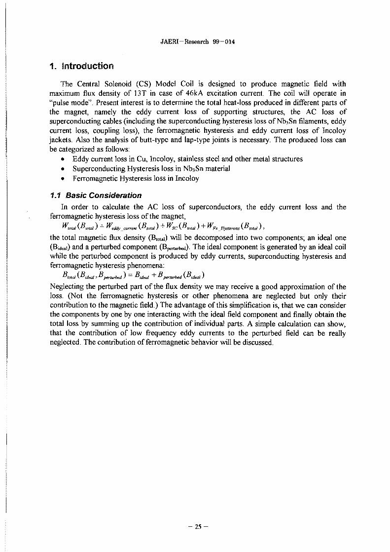
Upper Outer Tension Plate
-t- —i0.10.02 0.04 0.06
t[sec]
0.08
Figure 3-10
Tension Plates
0.8
-Upper-outer
- Upper-inner
-Lower
Figure 3-11.: Power loss dependence on flux change rate in tension plates
Table 3-6 Equations to calculate power loss for specific resistivity values larger than 10 8 Dm
Upper,
Upper,
Lower
Outer Tension
Inner Tension
Tension Plate
Plate
Plate
P
P
P
- 4.47536*10"6 a
- 5.4983 9*105 a
-4.71519*10"4cr
*n2
*n2
*n2
4.47536*106
P
5.49839*10 5
P4.71519*104
P
*n2
*n2
*n2
, if n<l
ifn<l
, if n<l
- 3 8 -
JAERI-Research 99-014
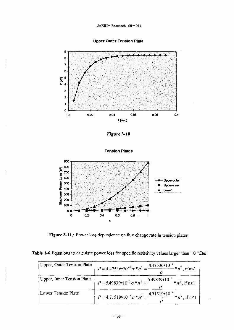
3.2 Eddy Current Loss DistnbutionThe absolute value of eddy current increases toward the sides of a component. Therefore
the eddy current power loss is also larger near sides. As an example the power loss distributionis plotted in the cross-section of an inner tension rod, at the center in Figure 3-13. There is alsoa distribution in power loss due to the inhomogeneous field distribution. This is illustrated inFigure 3-12 for an inner tension rod.
Power Loss Distribution Along Inner TensionRod Generated by Bz
Radiation•
Figure 3-12
INNER TENSION ROD
Heat flow
Heat flow
Power loss
R
Figure 3-13.: Power loss distribution in the cross-section of an inner tension rod at its center
3.3 Eddy Currents in Connected ComponentsIntroducing beams with plates together in the calculation the loss in beams increases a little bitwhile in plates decreases. Assembling the whole structure some loops can be also found. Thisis discussed in Section 3.5.
- 3 9 -

JAERI-Research 99-014
3.4 The Effect of BH-curve of Incoloy onto the eddy current lossIn this section not the ferromagnetic hysteresis loss is considered, but the change in eddy
current loss through the change of magnetic field distribution, because of the presence offerromagnetic material.
A 2D static nonlinear analysis is carried out with ANSYS code to obtain the flux densitydistribution in the cross-section of the magnet. For the nonlinear field calculation a singlevalued monotonically increasing BH curve was used plotted in Figure 3-14 instead of thehysteresis loop. A two-step solution sequence was applied to obtain the final solution. First anexcitation ramped through five substeps was introduced, each with one equilibrium iteration.Next the final solution was calculated over one substep, with 15 equilibrium iterations.
In the case of linear model the field profile does not change with increasing excitationcurrent, only the scale. With non-linear model outside the winding, the field is almost the same,like in linear case, however within the Incoloy winding at low excitation current it is different.A series of flux density profiles are plotted in Figure 3-15, Figure 3-16 and Figure 3-17 atdifferent excitation current values.
Not the numeric value of the field itself determines the eddy currents but the flux changerate. We define two paths in the cross-section of the magnet. Path-1 is in the mid-plane of thewinding and path-3 is in the upper plane of the winding. Figure 3-18 shows the flux densitychange in time in inner tension rod, where path-1 cross over it. Figure 3-19 and Figure 3-20are plotted for path-3. Figure 3-21 Figure 3-22 and Figure 3-23 are the same for outer tensionrod. At the very beginning of the excitation, the flux change rate is slightly higher in case of theferromagnetic model, however in the main part the curves run parallel with the curves of linearmodel. This means, that the flux change rate is the same and hence the eddy current loss is alsothe same.
We can conclude, that the eddy current loss can be evaluated with the linear model instructural steel components. The flux distribution is modified by the magnetic material.However the difference in flux change rate outside the Incoloy winding is small and hence theeddy current loss is not influenced in tension rods, beams and plates.
CQ
BH Curve of Incoloy at 4K
O.OE+00 1.0E+06 2.0E+06 3.0E+06
H[A/m]
4.0E+06 5.0E+06
Figure 3-14.: Single valued BH curve of Incoloy applied in nonlinear numerical analysis
- 4 0 -

JAERI-Research 99-014
-2.765kA|
-1.383kA
R[m]
Figure 3-15.: Magnetic flux density distribution in the center of magnet in case of1.383 kA and 2.765 kA excitation current
-5.53kA
-22.1kA
R[m]
Figure 3-16.: Magnetic flux density distribution in the center of magnet in case of5.53 kA and 22.1 kA excitation current
- 44.21 kA
- linear
R[ml
Figure 3-17.: Magnetic flux density distribution in the center of the magnet in case of44.21 kA excitation current with linear and nonlinear material models
41 -

JAERI-Research 99-014
B vs. time in inner tension rod, pathi
Bz-lin
Figure 3-18
B vs. time in inner tension rod, path3
Figure 3-19
B vs. time in inner tension rod, path3
Figure 3-20
B vs
-0.5
-1
-1.5
-2
-2.5
-3
time in outer
Ik 5
\
tension
10
rod,
T
iiI
pathi
—•— Bzin
time [sec]
Figure 3-21
B vs. time in outer tension rod, path3
—•— Bz-iinj
-+-* I
time [sec]
Figure 3-22
B vs. time in outer tension rod, path3
-Bf-Rn
-Br
Figure 3-23
- 4 2 -
JAERI-Research 99-014
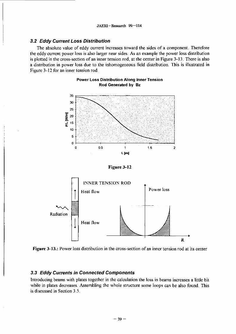
3.5 Loop Currents
3.5.1 FrameInner and outer tension rods together with lower and upper tension beams connected and
fixed mechanically produce a frame, which is a closed loop electrically, as illustrated in Figure3-24. If magnetic flux changing in time path through the frame, electromotive force is induced,which generates a large loop current, because of the small resistivity of the frame.
RTBU
u 2R TR
RTBL
Figure 3-24.: Frame and its circuit model
To obtain the loop current (I), generated by a given EMF, the DC resistivity of tension rods(Rro), upper and lower tension beams (RTBU ,RTBL) is estimated based on their geometry:
RDC =
TR
rmi
rm.
3.376/n 1= 158—
7770.0213 lm2
1.375m
1 =
0.52* 0.152m2
1.375m
0.47* 0.152m2
U
= 17.396—m
= 19.247-m
2Rm + RTBU + RTliL
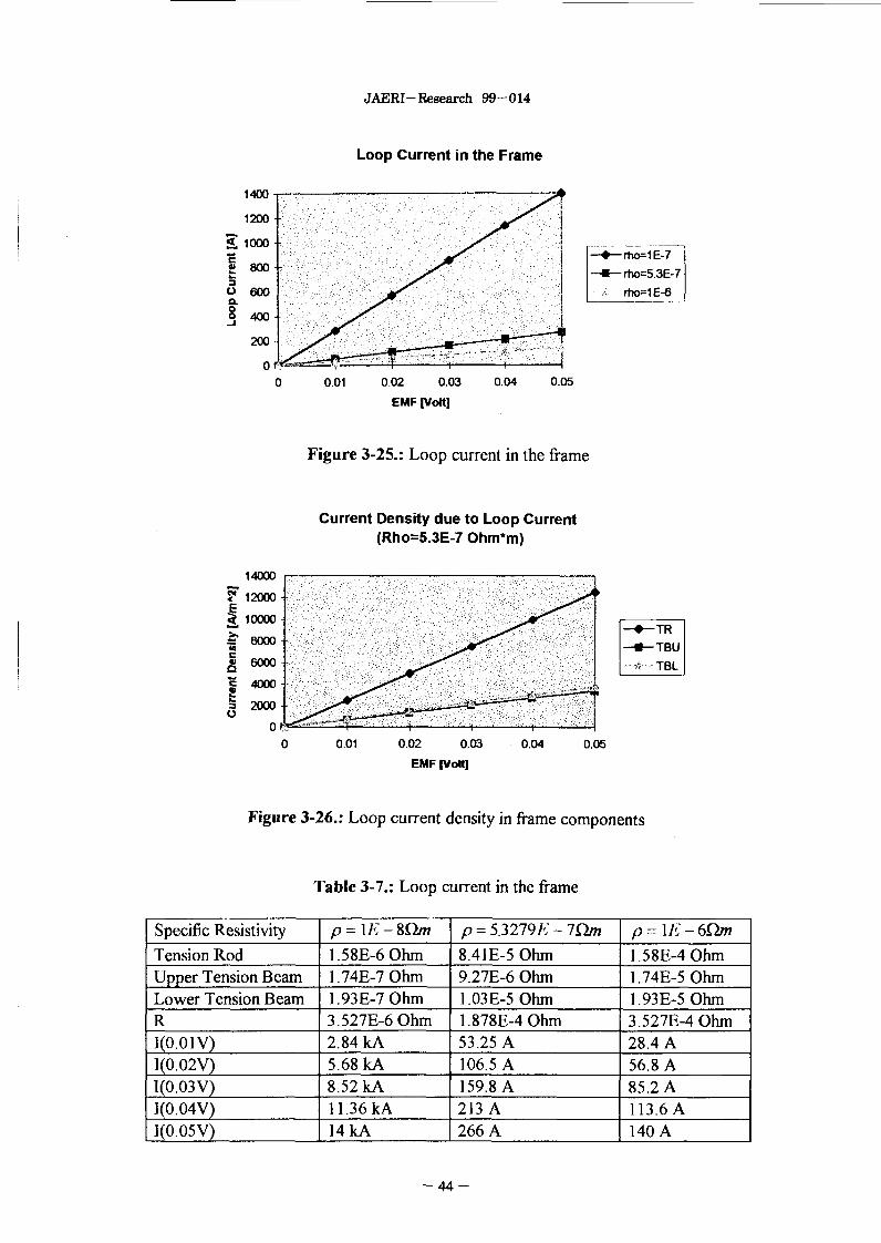
In Table 3-7 calculated resistivity values are listed, while in Figure 3-25 and Figure 3-26 loopcurrents and their densities are illustrated up to 0.05V electromotive force value. If loopcurrent is present, the loop current density is superposed onto the eddy current density oftension rods and beams hence increasing the power loss. In case of p=5.3E-7Qm specificresistivity and electromotive force less than 0.02V we may neglect the contribution of loopcurrents on the power loss.
- 4 3 -
JAERI-Research 99-014
Loop Current in the Frame
—•— rho=1E-7
—•— rho=5.3E-7
k rtio=1E-6
0.01 0.02 0.03
EMF [Volt]
0.04 0.05
Figure 3-25.: Loop current in the frame
14000
Current Density due to Loop Current(Rho=5.3E-7 Ohm*m)
0.01 0.02 0.03
EMF (Volt]
0.04 0.05
Figure 3-26.: Loop current density in frame components
Table 3-7.: Loop current in the frame
Specific Resistivity
Tension RodUpper Tension BeamLower Tension BeamR1(0.01 V)I(0.02V)T(0.03V)1(0.04 V)l(0.05V)
p=]E-$Qm
1.58E-6Ohm1.74E-7Ohm1.93E-7 Ohm3.527E-6 Ohm2.84 kA5.68 kA8.52 kA11.36kA14kA
p = 5.3279A' - IQm
8.41E-5 Ohm9.27E-6 Ohm1.03E-5 Ohm1.878E-4Ohm53.25 A106.5 A159.8 A213 A266 A
p = \E - 6Q/n
1.58E-4Ohm1.74E-5Ohm1.93E-5Ohm3.527E-4Ohm28.4 A56.8 A85.2 A113.6 A140 A
- 4 4 -

JAERI-Research 99-014
In the design the flux is parallel to the frame, so no flux path through it. However in thepractice small deviations may occur like:• Misplacement of winding-pack into vertical direction• Misplacement of winding-pack into horizontal direction• Miss-orientation of winding-pack
First the induced EMF is roughly estimated in case when the winding-pack is miss-oriented.The maximum deviation of winding-pack from the horizontal plane is 2 mm over 3620 mm.From this the maximum angle between the plane of frame and the axis of winding-pack can bedetermined:
2sin a =
3620Only field component perpendicular to the frame will induce loop current, which can beobtained as Bzsina. An effective area is calculated with respect to the field distribution. Insidethe coil and in the coil cross-section the z-component of the field is relatively large as indicatedwith the shaded area in Figure 3-24. Therefore we consider only this area in the fluxcalculation and decrease the effective area to one fourth of the original one. Moreover Bz is thelargest inside and decreases linearly toward the outer region, therefore the effective area will befurther decreased to half value, AeffcCtive
=l/8*Aframe where A&ame=4.64m2. Supposing lT/secinduction change rate in the decreased effective area the induced electromotive force isobtained in the frame:
d r dH.I , .. = 03mV .
3.5.2 Inter-frame loops
Frames are connected electrically with tension beams producing inter-frame loops. First onlythe radial component of field is considered. Permanent loops are ABCD and IJKL (connectedthrough EH and FG).
C
G
K
Figure 3-27.: Two frames connected with tension plates
- 4 5 -

JAERI-Research 99-014
If the winding-pack is introduced precisely, no EMF is induced in these loops, because theradial component of field opposite in sign in the upper and lower regions. However if thewinding-pack is miss-placed into vertical direction, flux will path through these loops. Thedistances between two inner tension rods (BC) and two outer tension rods (JK) are
f 22.5̂ 1A, = 2ft, sina = 1.130sinl I = 0.221/w
h2 = 2R2 s ina = 3.880sinf —-—J = 0.757/wsinf —-—J =If we move the winding-pack with x and suppose 1 8T at the upper tension beam and -1.8T atthe lower tension beam, than EMFi=0.06x Volt, and EMF2=0.21x Volt. Even if x=5cm,EMF2=10mV.
Next the z-direction of magnetic field is considered. Every upper outer tension plate iselectrically connected only to one tension beam. However upper outer plates connect twoframes and lower plates connect four frames. This cause an asymmetry with respect to theinduced voltage. We have to consider GFJ1EHLK loop which is plotted with thick line inFigure 3-27. The area what should be considered is
y = OD ,_D_ = O 2 8 1 5 5 / W 2
16 4The z-component of the induction in the place of upper outer tension plate is approximatelyIT, hence dB/dt=lT/13sec. The induced electromotive force is EMF=22mV.
For simplicity we will neglect the contribution of loop currents during loss calculation.
- 4 6 -

JAERI-Research 99-014
3.6 Temperature increase in structural componentsBefore operation all components of the Model Coil is cooled down to liquid helium
temperature. During the energizing process of the magnet the induced eddy currents heat upmetal components. As a row estimation of temperature increase we consider one cycle ofexcitation which includes an increasing and a decreasing part both with duration 13 sec.The component under examination is supposed to be insulated from its neighborhood and aninfinite large heat conductivity is supposed, which is realized by a homogeneous power lossdistribution. The temperature increase is evaluated by the formula
The specific heat data is summarized in Table 3-8 and plotted in Figure 3-28. The density issupposed to be pm = 7.S6J'3kg I nr1.
Table 3-8 Temperature dependence of specific heat of S S316
Temperature
4K
6K
8K
10K
20K
77K
273K
Specific Heat
2.206734 J kg"1 K"1
3.08733199 J kg"1 K"1
4.06794432 J kg"1 K"1
5.108969775 J kg"1 K"1
11.0069417 J kg"1 K"1
144 J kg"1 K"1
435 J kg"1 K"1
10
Temperature [K]
15 20
Figure 3-28 Specific heat vs. temperature of SS316
- 4 7 -
JAERI-Research 99-014
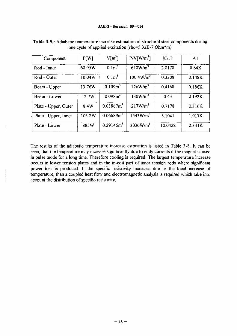
Table 3-9.: Adiabatic temperature increase estimation of structural steel components duringone cycle of applied excitation (rho=5.33E-7 Ohm*m)
Component
Rod - Inner
Rod - Outer
Beam - Upper
Beam - Lower
Plate - Upper, Outer
Plate - Upper, Inner
Plate - Lower
P[W]
60.95W
10.04W
13.76W
12.7W
8.4W
103.2W
885W
V[m3]
0.1m3
0.1m3
0.109m3
0.098m3
0.03867m3
0.06689m3
0.29146m3
P/V[W/m3]
610W/m3
100.4W/m3
126W/m3
130W/m3
217W/m3
1543W/m3
3036W/m3
ICdT
2.0178
0.3308
0.4168
0.43
0.7178
5.1041
10.0428
AT
0.84K
0.148K
0.186K
0.192K
0.316K
1.917K
2.341K
The results of the adiabatic temperature increase estimation is listed in Table 3-8. It can beseen, that the temperature may increase significantly due to eddy currents if the magnet is usedin pulse mode for a long time. Therefore cooling is required. The largest temperature increaseoccurs in lower tension plates and in the in-coil part of inner tension rods where significantpower loss is produced. If the specific resistivity increases due to the local increase oftemperature, than a coupled heat flow and electromagnetic analysis is required which take intoaccount the distribution of specific resistivity.
- 4 8 -

JAERI-Research 99-014
4. Loss Generated in Incoloy Jacket
4.1 Ferromagnetic Hysteresis Loss of Incoloy Jacket
In ferromagnetic materials the area of a closed minor or major loop gives the heat lossproduced in unit volume and can be calculated by
The hysteresis loss in INCOLOY is produced at relatively low field values because of thesaturation. For an exact field and loss calculation mathematical hysteresis models can be used,however this is not essential for a row estimation. As a first step it is enough to estimate theloss based on low temperature hysteresis loop measurements. At 4.2K the hysteresis loss ofINCOLOY908 was found to be Wio^^rnJ/cnrM^kJ/m3 for mild annealed plus heat treatedand Wio9s=4.1mJ/cnr'=4.1kJ/m3 for mild annealed specimens, magnetizing them on the majorloop (Goldfarb 1986). If a zero averaged triangular shape wave-form is used to excite the CSModel Coil large enough to drive the total volume of Incoloy jacket into saturation, than justthe total volume of Incoloy jacket used in CS1 and CS2-type conductors determine the loss.
Table 4-1 Geometric data of conductors
LocationInsert coilInner module1-4* layerInner module5- 10th layerOuter module10-18th layer
Length144m707m
1538m
2724m
TypeCS1CS1
CS2
CS2
Cross-section1440mm2
1440mm2
996mm2
996mm2
Volume0.20736m3
1.01808m3
1.53185m3
2.71310m3
Based on Table 4-1 the total volume is V=5.47m3. This would result in 24kJ heat loss per cyclein the total amount of jacket.
4.1.1 Magnetization HistoryThe hysteresis loss depends on the magnetization history. A trapezoidal shape excitation (in
the positive plane) applied repeatedly to the CS Model Coil magnetize the Incoloy jacket onlyon a minor hysteresis loop.
The loss strongly depends on the shape and extreme field values of the minor loop. Inpresent case the minimum value of field intensity produced by the excitation current is zero andthe maximum value is large enough to magnetize the jacket up to saturation. Consequently oneending point of the minor loop is in saturation while the other one is located at field valuesbetween zero and -He depending on the location of an actual conductor. The reason why H islowered can be explained by magnetic circuit models. If a closed magnetic circuit made offerromagnetic material is magnetized by an external field and next the field is switched off, thanwe move back to the remanent induction point where H=0. However in the case of Incoloyjacket the circuit is not closed since every conductor is wrapped with a coil insulator (1.5 mmthickness) and every layer is separated with a layer insulation (3 mm thickness). From magneticpoint of view this means that the ferromagnetic substance is cut into pieces by a large numberof air-gaps. In this magnetic circuit the constitutive equation and the Ampere's law have to be
- 4 9 -

JAERI-Research 99-014
satisfied in the same time. This results in the strong demagnetization of Incoloy jacket and arelative increase of loss comparing to a closed magnetic loop, as illustrated in Figure 4-1.
In present row estimation the loss of minor loop is set to one third of a complete cycle1.46mJ/cm3 which results in 8kJ heat loss in the whole winding during a complete period ofexcitation.
4.1.2 Characteristic Values of Hysteresis CurvesCharacteristic values of the hysteresis loop like coercive field and remanent induction also
get importance in the loss calculation. Unfortunately present measurement data carried out byGoldfarb (1986) on INCOLOY 908 does not give information about details. Moreover thehysteresis loss calculated from the area of the MH-loop is not in agreement with the loss data(probably measured by calorimetric technique). One possible explanation can be, that the sizeof the specimen was small (0.225 cm3) and probably very thin in order to avoid eddy currenteffect. However in such a case the domain structure may be different and also the number ofdomain walls may be too small. During magnetization the so called microscopic eddy currentscan be induced in the vicinity of domain walls, due to their fast movement. These microscopiceddy currents also produce loss. They may lose their importance in a larger specimen. Thisshould be verified by measurement.
The BH-curve measurements were carried out on mild annealed and aged specimens.However the conductor will be manufactured by a pull-down procedure followed by heattreatment. It would be important to measure BH-curve also on specimens prepared under thesame condition as the jacket is produced.
ClosedMagneticCircuit
B
OpenMagneticCircuit
B A
JH
Figure 4-1
- 5 0 -

JAERI-Research 99-014
4.2 Eddy Current Power Loss oflncoloy JacketAssumptions and conditions for the eddy current loss analysis of Incoloy jacket:
a) The superconductor is supposed to be insulated from the Incoloy jacket. This means thatno eddy currents can be closed through the superconductor, they flow in the jacket.
b) Instead of the modeling of the complicated spiral structure of the winding the conductor iscut into pieces and only one turn is considered in the same time, spanned into thehorizontal plane. By summing up the contribution of individual turns, the total loss isobtained. The basis of this simplification is the following: Let us consider one turn placedinto a homogeneous magnetic field slowly changing in time. The length of a turn isrelatively long and by further increasing it the power loss also increases linearly with thelength. The eddy currents are parallel with the coil except the end regions. In the realmagnet the field is not homogeneous, but there is a gradient along the length of coilresulting in a small eddy current component, which is not parallel to the coil. Since thegradient of field is small along one turn, a good approximation of loss can be obtained byapplying a piece-wise linear field distribution along the length of coil, where the fielddistribution is the same along one turn.
c) A simplified 2D axisymmetric model is applied to the cross-section of jacket. Only onejacket is considered in the same time for eddy current analysis and it is not excited frominside. The rest of winding is taken into account with its excitation current density and noeddy currents are considered. To satisfy the correct eddy current distribution in the cross-section of the selected jacket, the total current of jacket is forced to be zero. Since ANSYScan not apply directly the formula introduced in Part A for the current force, first anadditional voltage degree of freedom was introduced to the nodes of jacket and next theywere coupled. Finally the current was prescribed in one node.
d) The simplified solenoid model was used for the numerical calculation of Insert coil jackets,Inner Module-B and Outer Module jackets, while the detailed model was applied to theInner Module-A jackets.
e) The specific resistivity was set to p= \E -%Qm. The result can be recalculated for lagerspecific resistivity values or for smaller field rates.
f) The specific resistivity distribution is homogeneous in the jacket and does not depend onthe field.
g) Only half of the magnet is considered because of the symmetry.
For our convenience the layers are numbered as follows; Inner Module-A 1-4, Inner Module-B1-6, Outer Module 1-8. Conductors are also numbered starting from the center of the magnet.
- 5 1 -

JAERI-Research 99-014
As the magnet is energized eddy currents are built up through a short time transient. InFigure 4-2 the eddy current power loss is plotted in time generated in Insert Coil conductorNumber 2. Following the transient, in stationer state the power loss does not change anymoreif the resistance also does not change. (In case of temperature increase or due to magneto-resistance effect the resistance may increase.)
Insert Coil No. 2. (1E-8 Ohm*m)
0.02 0.04 0.06 0.08
Time [sec]
0.1 0.12 0.14 0.16
Figure 4-2.: Eddy Current Power Loss vs. Time in Insert Coil Jacket No.2
The individual turns are subjected to different fields depending on their location. Not onlythe amplitude of flux density is changing but its incidence angle as well. Therefore severalconductor were analyzed in every layer. The results are plotted in Figure 4-3 for Insert Coil, inFigure 4-4 and Figure 4-6 for Inner Module A and B and in Figure 4-8 for Outer Module. Thepower loss values are also plotted along the radius in Figure 4-5, Figure 4-7, and Figure 4-9.The power loss for the rest of conductors are interpolated and the total power loss is obtainedby summation and listed in Table 4-2, Table 4-3, Table 4-4, and Table 4-5.
- 5 2 -

JAERI-Research 99-014
4.2.1 Insert Coil
Table 4-2.: Stationer Eddy Current Power Loss in Insert Coil Incoloy Jacket(C SI-type conductor, p- 10 8Q/w, dl Idt- 46kA /13 sec, simplified model)
ConductorNo.2No.5No. 10No.15Total in Insert Coil
P[W]232W224W195W143W6000W
250
D.
o
200
150
t 100
.12 50
Eddy Current Loss of Winding in Insert Coil
-t-
6 8 10
Coil Number (n)
12 14 16
Figure 4-3
5 3 -

JAERI-Research 99-014
4.2.2 Inner Module-A
Table 4-3.: Stationer Eddy Current Power Loss in Inner Module-A lncoloy Jacket(CS 1 -type conductor,p= 10"8Dm, dl / dt = 46kA /13sec, detailed model)
ConductorNo.2No.5No. 10.No. 15Total in LayerTotal in InnerModule-A
Layer-1219.83W212.65W184.06W134.77W5672W
Layer-2205.85W199.42W174.11W134.89W5385W
Layer-3190.60W185.06W163.84W134.92W5075W
Layer-4174.4W169.84W153.08W134.57W4745W
20877W
Inner Module-A
6 8 10
Conductor Number
Figure 4-4
Inner Module-A
Figure 4-5
- 5 4 -

JAERI-Research 99-014
4.2.3 Inner Module-B
Table 4-4.: Stationer Eddy Current Power Loss in Inner Modul-B lncoloy Jacket(CS2-type conductor,p=]0*Qm,dI/dl = 46kA /13sec, simplified model)
ConductorNo.2No.5No. 10No. 15Total in LayerTotal in InnerModule-B
Layer-]88.48W86.95W81.30W74.47W2780W
Layer-2
2488W
Layer-365.63W64.99W63.06W63.54W2169W
Layer-4 Layer-5
3536W
Layer-634.16W34.67W37.57W47.16W1340W
12340W
Inner Module-B
6 8 10
Conductor Number
Figure 4-6
Inner Module-B
Figure 4-7
- 5 5 -
JAERI-Research 99-014
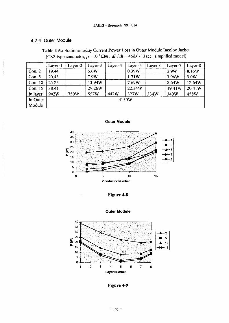
4.2.4 Outer Module
Table 4-5.: Stationer Eddy Current Power Loss in Outer Module Incoloy Jacket(CS2-type conductor, p - 10"8 Dm, dl I dt = 46kA /13 sec, simplified model)
Con. 2Con. 5Con. 10Con. 15In layerIn OuterModule
Layer-119.4420.4325.2538.41942W
Layer-2
750W
Layer-36.6W7.9W13.94W29.26W557W
Layer-4
442W
Layer-50.39W1.71W7.69W22.34W327W
Layer-6
334W
Layer-72.9W3.96W8.64W19.41W340W
Layer-88.16W9.0W12.64W20.41W458W
4150W
Outer Module
403530252015
1050
1
#^—• " >/^i
^ ^ ^ ^ ^ ^ ^
—•—1
— • — 3
—A—5
—X— 7
X "8
5 10
Conductor Number
15
Figure 4-8
Outer Module
3 4 5 6
Layer Number
Figure 4-9
- 5 6 -

JAERI-Research 99-014
4.3 Eddy Current Power Loss Dependence on Specific Resistivity and FluxChange Rate
Table 4-6.: Formulas for the calculation of eddy current power loss in modules
Insert Coil
Inner Module-A
Inner Module-B
Outer Module
s i 6*10 * ,/> = 6*10 V * « 2 = *n2
P, 2.0877*10 4 ,
P = 2.0877*10 V*/? 2 = *n2
P. , 1.234*10 4 ,
P - 1.234*10 4 o * n 2 *n2
P, , 4.15*10 5 ,
/ ' = 4.15*10 5CT*W2 = *n2
P
In Table 4-6 analytical formulas are listed for the loss calculation in different modules as afunction of current change rate and specific resistivity. In addition the power loss may alsodecrease with increasing field if magneto-resistance effect is significant ( Figure 4-10).
B t
Figure 4-10.: Power loss decrease due to magneto-resistance effect
4.4 Eddy Current Power Loss Distribution in the WindingThe distribution of stationer eddy current power loss generated in layers is illustrated in Figure4-11. Now the numbering starts at Inner Module-A, layer-1 and increases toward the OuterModule layers. A sharp drop in power loss can be observed between layer 4, where CSl-typeconductor is used, and layer-5, where CS2-type conductor is applied, since the size of CS2-type conductor is smaller than that of CS1.
Eddy Current Power Loss in Incoloy Jacket
1 2 3 4 5 6 7 8 9 10 11 12 13 14 15 16 17 18
Figure 4-11.: Eddy current power loss distribution within layers
- 5 7 -

JAERI-Research 99-014
4.5 The Effect ofBH-curve oflncoloy onto the Eddy Current loss of JacketSimilarly to Section 3.4 the flux change rate is studied within the Incoloy jacket, see Figure 4-12 and Figure 4-13. At the very beginning of the excitation, the flux change rate is significantlyhigher than in linear case resulting in an increased eddy current loss. However over saturationit is the same as in linear case. Due to the small duration of the increased part we may neglectthe difference and apply a linear model for loss calculation.
B vs. time in the winding
—•— BMin
Figure 4-12.: Flux density change in time inside the Incoloy windingduring the energizing of magnet
B vs. time in the winding
-Bz-Bz-Mn
Figure 4-13.: Flux density change in time inside the Incoloy windingduring the energizing of magnet
- 5 8

JAERI-Research 99-014
5. AC Loss of Superconducting Cables
We assume that AC losses consist only of hysteresis loss and coupling loss. Thecharacteristic parameters of superconducting cables are summarized in Table 5-1.
Table 5-1.: Characteristic parameters of strands and filaments
Number of strands in CSl-type cablesNumber of strands in CS2-type cablesComposite diameterNumber of filamentsFilament diameterCritical current density (for transport current)Hysteresis loss for cyclic fieldCu/non Cu ratio in strand
1152 NbsSn twisted filamentary composit720 Nb3Sn strand and 360Cu wired=0.81mmN=80372a=2.8u.mJc(B=12T)=580A/mm2=5.8 108A/m2
W,«(Bm=+-3T)= 110mJ/cm3
1.5
5.1 Superconducting hysteresis loss in Nb3Sn filamentsType-ll superconductor, NbsSn is used in CS Model coil which exhibit magnetic hysteresis
caused by the pinning of the filaments by lattice defects. The amplitude of the field which justpenetrates to the center of the sample is small
comparing to the applied transverse field,
/? = -=-> 100,BP
therefor the energy loss per unit volume over the full penetration can be evaluated by
Q =Bl 8
The energy loss generated below full penetration7)2
Qp = 0.623-^ < 25k/A,
will be neglected. However we have to take into consideration the dependence of criticalcurrent density on the actual magnetic field and evaluate the loss by the formula
If one knows the critical current density dependence as a function of magnetic field, cancalculate the superconducting hysteresis loss. Not the critical current density given in Table 5-1will be used, but the measured hysteresis loss data. The modified Yasukochi-model is used inorder to take into consideration the critical current density dependence on the magnetic field
v 2
Jcb 11
where Bc2=23.5T will be used considering T=4.2K temperature and 8—0.25% longitudinalstrain. After integration
- 5 9 -

JAERI-Research 99-014
e= -̂' l 2a/ cb\
1
B22
23.5
1
3B
3
2 + -r
1 12 5
5 I11"
Jo
Jcb can be determined from the measurement result of a single filament placed in transversemagnetic field and next can be used to evaluate the superconducting hysteresis loss in the CSModel Coil. Since filament diameter may strongly scatter in a strand, for loss calculation a newconstant, C is introduced which includes all of the unknown parameters
cb
5.1.1 Single Nb3Sn strand in cyclic transverse magnetic fieldTo determine the quality of Nb^Sn strands, the loss was measured in the case of fully
reversed cyclic excitation with 3T amplitude. The hysteresis loss was found to be 110mJ/cm3
projected to the non-copper volume. From thisC=69.182*103andJcb=2.91*10I0AT1/2/m2.
As an example the critical current densities at 5T and 12T are the followingJc(5T)=8*109A/m2
Jc(12T)=2*109A/m2.
5.1.2 Superconducting Hysteresis Loss in the CS Model CoilThe coupling between filaments and also between strands will be neglected during the
hysteresis loss calculation. Moreover the loss in case of trapezoidal shape excitation issupposed to be half of fully transverse cyclic field. Also the effect of transport current isneglected. The total loss coming from the superconducting hysteresis is obtained by summingup the loss for all of the filaments:
123.5 3 23.52 5'
2r,nA cycle
where the total non-copper areas of strands areA=l 152A8trand/2.5=237.45*10-6 m2
A=720Astrand/2.5=l48.4* 10"6 m2
(Aslrand=0.81 2TI/4=0. 51529973 5mm2).
for CSl-type cable andfor CS2-type cable.
Table 5-2.: Superconducting Hysteresis Loss in CS Model Coil(the effect of transport current is not included)
Insert CoilInner Module-AInner Module-BOuter ModuleTotal
With Insert CoilP[kW] (26sec)O.llkW0.51kW0.64kW0.83kW2.09kW
QJkJ/cycle]2.87kJ13.26kJ16.66U21.44kJ54.22kJ
Without Insert CoilP[kW] (26sec)00.51kW0.64kW0.82kW1.98kW
Q[kJ/cycle]013.28U16.68U21.40k J51.36kJ
- 6 0 -

JAERI-Research 99-014
5.2 Coupling LossLet l.m denote the ramp-up time and T the decay time constant of coupling currents. In presentapplication tm is set to 13 sec and x is supposed to be 50 msec both for CS1 and CS2-typeconductor including Cu-wires. Since tm is large comparing to T, the coupling power lossdensity can be written as
V
B2
T —4TT\0 7 5(f
•13*10 3 =470.873#iW
m
The energy loss density for a complete cycle is
ft,V
k)
^ cycle
Next we have to sum up the contribution of conductors in CS Model Coil depending on theirgeometric positions;
Q = 2PLwhere
A=l 152Asl].amr=593.625mm2
A=(360+720)Aslrand=556.524mm2
d^. 8127i/4=0.51529973 5mm2).
for CSl-type cable andfor CS2-type cable.
Table 5-3.: Coupling loss in CS Model Coil
n=l, x=50msec
Insert CoilInner Module-AInner Module-BOuter ModuleTotal
With Insert CoilP[kW]
6.16kW21.55kW20.36kW8.24kW56.3 lkW
Q[kJ/cycle]160kJ560kJ529kJ214kJ1464kJ
Without Insert CoilPfkWl
0
21.95kW20.54kW8.17kW50.67kW
Q[kJ/cycle]0570kJ534kJ212kJ1317kJ
The results can be recalculated for other time constant or ramp up time with the followingformulas:
n2r
50m secnz
1
50«?sec
iJ(/i = l,r = 50msec),
Measurements were carried out on a short piece of CS2-type conductor by K. Matsui et. al.[3]. The estimated time constant was found to be x=13 msec including Cu-wires. Timeconstant of CSl-type conductor is probably larger because it contains only superconductingstrands.
61 -

JAERI-Research 99-014
6. Loss of Joints
Two types of joints are applied in CS Model Coil, a Lap-type one and a Butt-type one. InInsert Coil and Inner Module only Lap-type joints are used, while in Outer Module Butt-typejoints except the terminal joints which are Lap-type. In Inner and Outer Modules twoconductors are winded parallel while in Insert Coil only one conductor is used. The number ofconductors are (2n-l)+2 and n+1 in modules and Insert Coil respectively, where n denotes thenumber of layers.
The loss has two origins. One part is AC loss due to the changing magnetic field, and theother part is caused by the large transport current. The following characteristic parameters willbe used for loss calculation after the measurement and estimation of Superconducting MagnetLaboratory, (see also [4]);
• AC Loss of Lap-type joint is 73 W if dB/dt=0.4T/sec• Resistivity of Lap-type joint is 6.4nQ at 46kA and B=4.5T• AC Loss of Butt-type joint is 6.7W if dB/dt=0.4T/sec• Resistivity of Butt-type joint is 3.7nQ at 46kA and B=4.5T
Different joints are located at different geometric locations above and below the upper andlower tension plates and affected by different fields. In this simple estimation this will not beconsidered. 0.2T/sec flux density change rate is supposed in outer module joints and 0.4T/secin inner module joints. The field dependence of contact resistivity will be also neglected.
In Table 6-1 the numerical values of power loss are summarized. The loss increase isparabolic due to transport current up to t j=l 3 sec, since the feeding current increases linearly;
P(0<t<t1)=PAC+Ptnux*(t/13)2.Over ti up to t2 the feeding current is constant (46kA) so no AC loss component is present;
P(tl<t<t2)=Pi aux.And finally between t2 and t} in the case of decreasing field the loss behaves similarly toincreasing case;
P(t2<t<t3)=PAC+P.max*(t3-t)2/132.
Table 6-1.: Loss of Joints in CS Model Coil
Insert CoilInner ModuleOuter Module
Total with Insert CoilTotal without Insert Coil
Type of Joints
Lap-type 2Lap-type 21Lap-type 2Butt-type 15
AC Loss ofJoints, PAc146W1533W37W25W1741W1595W
Pt max due to transportcurrent (I=46kA)20W284W27W117W448W428W
For other flux change rates the loss can be recalculated with the following formulas:PAc(n)=PAC(n=l)*n2
Ptmax(n)=Plmax(n=l)*n.The eddy currents caused by the changing magnetic field and the transport current are presentin the same time, therefore their interaction should be also considered. The loss due totransport current and eddy current can not be simple superposed. Unfortunately this interactioncause further increase in the loss.
- 6 2 -

JAERI-Research 99-014
7. Summary of Loss Calculation
7. 1 Eddy Current Power Loss of Structural Elements
Table 7-1 Power loss in case of p- 5.3279*10~7Qm specific resistivity and electricallyinsulated metal components
Component
Tension Rod - Inner
Tension Rod - Outer
Tension Beam - Upper
Tension Beam - Lower
Tension Plate - Upper, Outer
Tension Plate - Upper, Inner
Tension Plate - Lower
Total structural steels
One piece
60.95W
10.04W
13.76W
12.7W
8.4W
103.2W
885W
Number ofpieces
16
16
16
16
16
8
4
Total withInsert Coil
975.2W
160.6W
220.2W
203.2W
134.4W
825.6W
3540W
6059W
Total WithoutInsert Coil
861W
141.8W
194.4W
179.4W
118.7W
728.9W
3125.3W
5349W
Eddy Curren Power Loss in Structural Steels
Tension Rod-Inner16%
Tension Plate-Lower58%
Tension Rod-Outer
3%
Tension Beam-Upper
4%
Tension Beam-Lower3%
Tension Plate-Upper, Outer2%
iwision Plate-Upper, Inner
14%
- 6 3
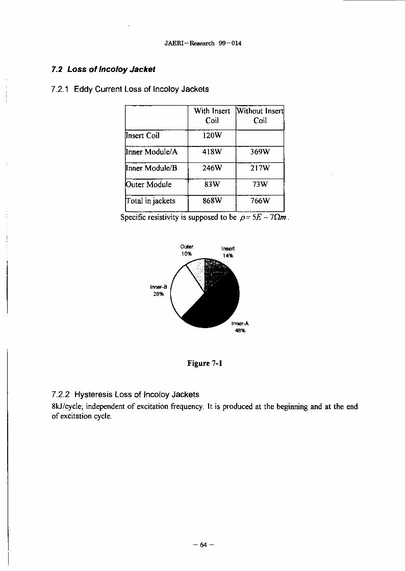
JAERI-Research 99-014
7.2 Loss of Incoloy Jacket
7.2.1 Eddy Current Loss of Incoloy Jackets
Insert Coil
Inner Module/A
[nner Module/B
Outer Module
Total in jackets
With InsertCoil
120W
418W
246W
83W
868W
Without InsertCoil
369W
217W
73W
766W
Specific resistivity is supposed to be p=5E- IQm.
Figure 7-1
7.2.2 Hysteresis Loss of Incoloy Jackets
8kJ/cycle; independent of excitation frequency. It is produced at the beginning and at the endof excitation cycle.
- 6 4 -

JAERI-Research 99-014
7.3 AC Loss of Superconducting cable
7.3.1 Superconducting Hysteresis Loss
Insert CoilInner Module-AInner Module-BOuter ModuleTotal
With Insert CoilPfkW] (26sec)0.1 lkW0.5 lkW0.64kW0.83kW2.09kW
Q[kJ/cycle]2.87kJ13.261J16.66kJ21.441J54.22kJ
Without Insert CoilP[kW] (26sec)00.5 lkW0.64kW0.82kW1.98kW
QrkJ/cycle]013.281J16.68U21.40kJ51.36W
Superconducting Hysteresis Loss
Insert Coil5%
Outer Module40%
Inner Module-A24%
Inner Module-B31%
7.3.2 Coupling Loss
n=l, x=50msec
Insert CoilInner Module-AInner Module-BOuter ModuleTotal
With Insert CoilPfkW]
6.16kW21.55kW20.36kW8.24kW56kW
Q[kJ/cycle]160kJ5601J529kJ2141J1464kJ
Without Insert CoilP[kW]
021.95kW20.54kW8.17kW50.67kW
Q[kJ/cycle]0570kJ534kJ212kJ1317kJ
Coupling Loss
Outer Module15%
Insert Coil11%
Inner Module-B36%
Inner Module-A38%
- 6 5 -

JAERI-Research 99-014
7.4 Loss of Joints
Insert Coil
Inner Module
Outer Module
Total with Insert Coil
Total without Insert Coil
146+20*(t/13)2 [W] if 0<t<t,20W if tt<t<t2
146+20*(t3-t)2/132[W] ift2<t<t3
1533+284*(t/13)2 [W] if 0<t<t,284W if ti<t<t2
1533+284*(t3-t)2/132 [W] ift2<t<t3
62+144*(t/13)2 [W] if 0<t<tj144W if ti<t<t2
62+144*(t3-t)2/132 [W] if t2<t<t3
1741+448*(t/13)2 [W] if 0<t<ti448W if tj<t<t2
1741+448*(t3-t)2/132 [W] ift2<t<t3
1595+428*(t/13)2 [W] if 0<t<t,428W if ti<t<t2
1595+428*(t3-t)2/132[W] ift2<t<t3
PAV(;=153W
PAVG=1628W
PAVG=H0W
PAVG=1890W
PAVG=1738W
Table 7-2.: Power Loss of Joints
- 6 6 -

JAERI-Research 99-014
7.5 Total Power Loss
46kA/13sec(n=l)Eddy Current Power Loss ofStructural Steel ComponentsEddy Current Loss of Incoloy JacketFerromagnetic Hysteresis Loss ofIncoloy JacketSuperconducting Hysteresis LossCoupling LossLoss of JointsTotal Power Loss in CSM
With Insert Coil6059W
868W308W (8kJ/cycle)
2090W (54.22kJ/cycle)56000W1890W67215W
Without Insert Coil5349W
766W300W (8kJ/cycle)
1980W(51.36kJ/cycle)50670W1738W60803W
Table 7-3.: Average Power Loss of CS Model Coil
Power Loss in CS Model Coil
Structural Steel9% Incoloy Jacket
2%
SuperconductingHysteresis
3%
Coupling83%
- 6 7 -

JAERI-Research 99-014
7.6 Time History of Power Loss (without Insert Coil)
46kA
Tl=13seciti
-**-T2 t2:;;, Tl=13sec „ T3
1 Eddy Current Power Loss in Structural Steels
Eddy Current Power Loss in Incoloy Jacket
766W
Ferromagnetic Power Loss in Incoloy Jacket
8kJ/2sec=4kW iSuperconducting Hysteresis Loss
:51kJ/26sec=1.96kW
Coupling loss of strands
+ Power Loss of Joints
1595+428*(t/13)2W
- 6 8 -

JAERI-Research 99-014
7.7 Decreasing the LossBoth the eddy current loss and the coupling loss is proportional to the square of flux
change rate. They can be drastically decreased if smaller current rate is applied (by increasingthe ramp up time). Examples are given in Table 7-4 and Table 7-5.
The eddy current loss can be also decreased if materials having higher specific resistivityvalues are used. If we allow a temperature increase in structural steels this leads also to theincrease of the specific resistivity and hence energy loss decrease. However the most effectivemethod is to change the geometry, cut large size metal components into smaller pieces.
The coupling loss can be decreased by increasing the cross-over resistivity or decreasingthe twist-pitch length.
In case of ferromagnetic hysteresis by careful heat treatment the area of BH-curve usuallycan be decreased or we have to select other material. An other possibility is not to decrease theexcitation current back to zero, but keep it on a small level (about 2kA) if the power supplysystem allow it.
Even if we do not decrease the loss, the energy balance should be kept. This can be doneby the proper selection of the T2 and T3 time constants which determine the duration of the flatpart of the trapezoidal excitation. The cooling system is supposed to operate with constantcapacity.
Table 7-4.: Power loss at decreased current rate (equivalent 0.5T/sec)
46kA/26sec (n=0.5)Eddy Current Power Loss ofStructural Steel ComponentsEddy Current Loss of Incoloy JacketFerromagnetic Hysteresis Loss ofIncoloy JacketSuperconducting Hysteresis LossCoupling LossLoss of JointsTotal Power Loss in CSM
With Insert Coil1515W
217W154W(8kJ/cycle)
1045W(54.22kJ/cycle)14000W510W17441W
Without Insert Coil1337W
192W154W(8kJ/cycle)
990W(51.36kJ/cycle)12668W470W15811W
Table 7-5.: Power loss at decreased current rate (equivalent 0.4T/sec)
46kA/32.5sec (n=0.4)Eddy Current Power Loss ofStructural Steel ComponentsEddy Current Loss of Incoloy JacketFerromagnetic Hysteresis Loss ofIncoloy JacketSuperconducting Hysteresis LossCoupling LossLoss of JointsTotal Power Loss in CSM
With Insert Coil970W
139W123W(8kJ/cycle)
836W (54.22kJ/cycle)8960W33 8W11366W
Without Insert Coil856W
123W123W(8kJ/cycle)
792W(51.36kJ/cycle)8107W312W10313W
- 6 9 -

JAERI-Research 99-014
8. Conclusion
Comparing the AC loss components generated during the energizing process of CS ModelCoil, the coupling loss was found to be the largest 83% of the total AC loss supposing 50 mseccharacteristic time constant. Its main part is generated in Tnner Modules.
Also significant amount of heat is generated in structural steels, 9% of the total AC loss.The largest contributions come from lower tension plates and inner tension rods, 58% and16% of the loss produced in structural steels, respectively. Present calculation shows thatcooling is required for stainless steel structural components to avoid the production of hotspots during a longer operation.
Joints should receive special care even if their contribution to the total loss is not so high,because losses are concentrated in a very small volume. An insufficient cooling may cause thequench of the whole magnet starting from joints. Problems may appear with Lap-type jointsbecause of the large AC loss.
The eddy current loss of lncoloy jackets is not significant with the supposed specificresistivity value, 5E-7Qm. However the real low temperature specific resistivity value shouldbe determined from eddy current measurements and the eddy current loss has to berecalculated. Ferromagnetic hysteresis loss is also produced in Tncoloy jackets at the verybeginning and at the end of an excitation cycle.
The eddy current and coupling power losses are proportional to the square of flux changerate, so they can be significantly decreased by decreasing the flux change rate. At decreasedflux change rate hysteresis losses (superconducting and ferromagnetic) get importance, sincethe energy loss does not change during a complete cycle. No AC losses are produced followingthe energizing process of the magnet, when it is driven by a constant excitation current.However Joule losses are produced on the nonzero resistivity of joints by the large transportcurrent. This propose us to keep short the full power operation and increase the time of fieldfree state.
Acknowledgment
The authors would like to thank to Dr. Ohta, general director of Naka FusionEstablishment to make this study possible and also for his kind encouragement. The authorsare also thankful to A. Prof. Y. Yoshida and Prof. K. Miya, University of Tokyo for theiradvice on literature and for their encouragement.
7 0 -

JAERI- Research 99-014
References
[1] K. Simonyi; Theoretical Electricity, Tankonyvkiado, Budapest, 1978.[2] Wilson; Superconducting Magnet, Clorendon Press, Oxford, 1983.[3] K. Matsui, Y. Takahashi, M. Nishi, K. Nunoya, T. Kato, H. Nakajima, T. Hiyama,
M. Sugimoto, T. Isono, K. Kawano, N. Koizumi, K. Hamada, T. Ando, H. Tsuji,S. Shimamoto, N. Shiga, N. Aoki, M. lchihara; Design and Fabrication of Superconducting
Cables for ITER Central Solenoid Model Coil, IEEE Trans. Magnetics, Vol. 32. No. 4,pp.2304-2307, 1996.
[4] K. Matsui, T. lto, Y. Takahashi, Y. Nunoya, M. Sugimoto, H. Fujisaki, H. Tsuji,S. Shimamoto; AC Loss Measurement of 46kA Conductor Joint for CS Model Coil, under
publication[5] Ansys Users's Manual for Revision 5.1, SAS IP Inc., 1994[6] O. Biro, K. Preis; On the use of magnetic vector potential in the finite element analysis of
three-dimensional eddy currents, IEEE Trans. Magnetics, Vol 25, No. 4, pp.3145-3159,1989.
[7] A. Konrad; Integrodifferential finite element formulation of two-dimensional steady-stateskin effect problems, IEEE Trans. Magnetics, Vol. 18, No. 1, 1982.
- 7 1 -

^(Si)iSi;
*
gH
H
¥
1
ft
B
B(*
s i *
3APelaft
asftIS
ftft
* D
r yy 71/
7 yX f^
ft
?' 7
t*
X '
T
v / 7
71/
A
T
y
71/
7
y
y
12 vmkgs
A
K
mol
cd
rad
sr
* 2 xs simmm
« 3
mi±x *
X.IV
-15
am&.
a
{$,f
•te
BS
ft
«s
y
y
; l /
«
J . tEt-'-.tt*. *, m *t
•Sfct. E l
a ay 9 9 y
9" 9 9 y•y o x ia
WiK 8ft ^
a/ j
ft
?j
ftttX
*
fit;X
a
fig
/"•
7
7
~̂
•y
•7
T/^
7U
7U
- :
f•y
iv yi - t- yx * ivn. — IV
•V h
— a y71/ h
7 7 K
— A
- /t y x
i - /<
X 7
y 'J —
u y o x i t— / y
9 x
u /f- -< IV b
»2>3
HzNPaJWCVF
ns
WbTH°Clm
lx
BqGySv
(ft© SI ¥.f4KX 5 1 1
s "m-kg/s2
N/m2
N-mJ/sA-sW/AC/VV/AA/VV-sWb/m2
Wb/A
cd-srlm/m2
s "
J/kgJ/kg
ft. t$, 0s , # . w>U y h 71/
h y
a f *• 71/ h
m-f-Kmma.
min, h, d
1, Lt
eVu
leV=1.60218xl0-"J
1 u= 1.66054 xlO"2' kg
*
7
y y x-
y h
• a —
i)
f
h.
y
IV
IV
-
y
KA
12 %
A
b
bar
Gal
Ci
R
rad
rem
1 A=0.1nm=10-'°m
1 b=100fm2=10-zlim2
lbar=0.1MPa=105Pa
lCi=3.7xl01°Bq
1 R=2.58xlO^'C/kg
l r a d = lcGy=10-2Gy
1 rem=lcSv=10 2Sv
fifft
1 0 "
1 0 ' 5
101 2
10s
10'
103
102
10'
10"
1 0 "
lO"3
10"
1 0 "
I O - 1 2
10"ls
I O - 1 8
HX
/ ^
•f
if
+
T
•f
-fe
-7
7"
t°
7
T
!HI!§
9
7
*"
D
9 ¥
•y
y -f-IJ
/
^ A (-
a2 °'
EPTGMk
h
da
d
c
mti
n
Pf
a
(ft)
fcfcX, 1 eVu ®(L«(i CODATA (D1986 ̂ f l lS
3. bar It,
4. ECfa«a*&fe^-efibar. barn is J;If
N( = 10'dyn)
1
9.80665
4.44822
kgf
0.101972
1
0.453592
lbf
0.224809
2.20462
1
tt m 1 Pa - s (N-s /m 2 )=10P(*TX-) ( g / ( cm-s ) )
ttttlff l m 2 / s - 1 0 4 S t ( x Y-9 X) (cm 2 / s )
ts
MPa( = 10bar)
1
0.0980665
0.101325
1.33322 xlO"4
6.89476 x 10⁻¹
kgf/cm2
10.1972
1
1.03323
1.35951 x 10"3
7.03070 x 1Q-*
a tm
9.86923
0.967841
1
1.31579x10"
6.80460 x 10"2
mmHg(Torr)
7.50062 x 10'
735.559
760
1
51.7149
Ibf/in2(psi)
145.038
14.2233
14.6959
1.93368 x SO"
1
X
IV
1
ft
m
J( = 10'erg)
1
9.80665
3.6 x 10⁶
4.18605
1055.06
1.35582
1.60218 x 10 '"
kgf'm
0.101972
1
3.67098 x 10s
0.426858
107.586
0.138255
1.63377 x 10"°
kW- h
2.77778x10-'
2.72407 x 10'6
1
1.16279 x 10"
2.93072 x 10 '
3.76616 x 10 '
4.45050 x l O " 6
cal(sHffi)0.238889
2.34270
8.59999 x 10 s
1
252.042
0.323890
3.82743 x 10"°
Btu
9.47813 x 10"
9.29487 x 10"
3412.13
3.96759x10"
1
1.28506 x 10"
1.51857x 10"22
ft • lbf
0.737562
7.23301
2.65522 x 10⁶
3.08747
778.172
1
1.18171 x 10""
eV
6.24150x10"
6.12082x 10"
2.24694x10"
2.61272x10"
6.58515 x 10²¹
8.46233 x 10'"
1
1 cal = 4.18605 J
= 4.184J
= 4.1855 J (15 "C)
= 4.1
II: 'f'¥= 75 kgf-m/s
= 735.499 W
3.7 x 10"
2.70270 x 10-
1
Umm
Gy
1
0.01
rad
100
1
C/kg
2.58 x 10"
R
3876
1
Sv
1
0.01
100
1
(86 <F

AC LOSS CALCUUTION OF CENTRAL SOLENOID MODEL COIL