accelerated by cuda technologymaxest.gct-game.net/content/vainmoinen/bachelor_thesis.pdfone of the...

FACULTY OF FUNDAMENTAL PROBLEMS OF TECHNOLOGY

WROCŁAW UNIVERSITY OF TECHNOLOGY

SOFTWARE RENDERER

ACCELERATED BY CUDA TECHNOLOGY

V1.1

WOJCIECH STERNA

B.Sc. Thesis written

under the supervision of

Marcin Zawada, Ph.D.

WROCŁAW 2011

AbstractNVIDIA’s CUDA technology allows for massively parallel and general-purpose code execution on GPU.One of the most common applications of parallelism is graphics processing. Although there are APIs thatallow for extremely fast hardware graphics processing (like OpenGL or Direct3D), inherently they sufferfrom lack of full programmability. The goal of this work is implementation of a software renderer usingCUDA technology and comparing its performance with that from fully hardwared one.

Contents1 Introduction 3

1.1 Fundamental Concepts . . . . . . . . . . . . . . . . . . . . . . . . . . . . . . . . . . . . . 31.2 Hardware and Software Rendering . . . . . . . . . . . . . . . . . . . . . . . . . . . . . . . 3

1.2.1 Shaders . . . . . . . . . . . . . . . . . . . . . . . . . . . . . . . . . . . . . . . . . 41.3 Goals of the Work . . . . . . . . . . . . . . . . . . . . . . . . . . . . . . . . . . . . . . . . 5

2 The Graphics Pipeline 52.1 World and Virtual Camera Definition . . . . . . . . . . . . . . . . . . . . . . . . . . . . . . 5

2.1.1 World . . . . . . . . . . . . . . . . . . . . . . . . . . . . . . . . . . . . . . . . . . 52.1.2 Virtual Camera . . . . . . . . . . . . . . . . . . . . . . . . . . . . . . . . . . . . . 7

2.2 Vertex Processing . . . . . . . . . . . . . . . . . . . . . . . . . . . . . . . . . . . . . . . . 82.2.1 Vertex Transformation . . . . . . . . . . . . . . . . . . . . . . . . . . . . . . . . . 82.2.2 Triangle Culling . . . . . . . . . . . . . . . . . . . . . . . . . . . . . . . . . . . . 152.2.3 Triangle Clipping . . . . . . . . . . . . . . . . . . . . . . . . . . . . . . . . . . . . 18

2.3 Pixel Processing . . . . . . . . . . . . . . . . . . . . . . . . . . . . . . . . . . . . . . . . . 202.3.1 Rasterization and Shading . . . . . . . . . . . . . . . . . . . . . . . . . . . . . . . 202.3.2 Perspective-Correct Interpolation . . . . . . . . . . . . . . . . . . . . . . . . . . . 232.3.3 Texture Mapping . . . . . . . . . . . . . . . . . . . . . . . . . . . . . . . . . . . . 25

3 Project Architecture 303.1 Class Diagram . . . . . . . . . . . . . . . . . . . . . . . . . . . . . . . . . . . . . . . . . . 313.2 Physical Structure . . . . . . . . . . . . . . . . . . . . . . . . . . . . . . . . . . . . . . . . 333.3 Flow Chart of the Graphics Pipeline . . . . . . . . . . . . . . . . . . . . . . . . . . . . . . 33

4 Implementation 334.1 Software Renderer Running on CPU . . . . . . . . . . . . . . . . . . . . . . . . . . . . . . 334.2 Making it Hardware by Speeding up with CUDA . . . . . . . . . . . . . . . . . . . . . . . 374.3 Performance Tests . . . . . . . . . . . . . . . . . . . . . . . . . . . . . . . . . . . . . . . . 41

5 Conclusions and Future Work 43

1 INTRODUCTION 3

1 IntroductionThis section starts with discussion of basic concepts that must be known to be able to fully understand thiswork. Finally, goals of the project are discussed.

1.1 Fundamental Concepts• raster image – a 2-dimensional array of pixels, where each pixel contains an n-bit value. Raster image

is usually used to store colors in its pixel values but in general this can be any kind of data.

• rendering – process of generating a raster image from a scene containing 3-dimensional objects froma fixed viewpoint defined by a virtual camera. Computer programs for rendering are usually referredto as renderers. Rendering techniques can be divided in two categories:

– image-order – images rendered with this set of techniques all follow the general rule:for every pixel: find object that covers it. Good time complexity. Ray-tracing isone of the techniques that generates images this way.

– object-order – images rendered with this set of techniques all follow the general rule:for every object: find pixels that are covered by it. Time complexity is worsethan in image-order rendering but in practice object-order renderers appear to be faster. OpenGLand Direct3D, the most popular graphics APIs for generating images in real-time, both performobject-order rendering.

• the graphics pipeline – set of stages that input graphics data is passed through to perform rendering.Stages are usually introduced in a way that makes better understanding of how an output image isgenerated. The graphics pipeline, in terms of this project, will be investigated in details in chapter 2.

• CUDA – technology developed by NVIDIA destined for parallel, general-purpose code execution byusing GPU (graphics processing unit). If a problem requires solving many instances of the same task(where all instances are independent from each other), then it can greatly benefit from CUDA. Atrivial example can be geometry vertex processing, where processing of one vertex does not influenceprocessing of any other vertex. This way many vertices can be handled at the same time.

It is assumed that the reader has a good understanding of fundamentals of analytical geometry (lines,planes), linear algebra (vectors, matrices) and calculus (partial derivatives).

1.2 Hardware and Software RenderingAn important thing is distinction between hardware and software renderers. The former ones use dedicatedhardware to perform rendering, whereas the latter are hardware independent. A deeper discussion aboutboth categories will take place now.

Hardware renderers, as they use dedicated hardware, are very fast in performing graphics related work sothey can be used in real-time applications. The two main APIs that let a programmer make use of hardwarerendering are Direct3D and OpenGL. Direct3D is being developed strictly by Microsoft and is available onlyon Windows, Xbox and Xbox 360. On the other hand OpenGL is under development of Khronos Group,which is a consortium formed of several corporations related to computer graphics, such as Intel, NVIDIAor ATI. The greatest advantage of OpenGL over Direct3D is that it is an open standard and is supportedby various operating systems (Windows, Linux, Mac OS). Both libraries offer very similar functionality

1 INTRODUCTION 4

and differ only in a way they exhibit it. This functionality is dependent on hardware that is being usedand as such Direct3D and OpenGL cannot go beyond a fixed set of available capabilities (the graphicspipeline is more or less fixed, thus it was called the fixed-function pipeline). Although today’s graphicshardware is programmable to some point by so-called shader programs, it will never reach a point of fullprogrammability.

Software renderers, on the other hand, are hardware independent since the code is usually executed ongeneral-purpose processors, rather than dedicated hardware. As such software renderers do not make use ofany specialized acceleration and thus are very slow. Important thing to note is that software renderers, justas hardware ones, also process geometry in some fixed way via the graphics pipeline. However, it is thisgraphics pipeline that can be modified in software renderers by a programmer at any time to fit new needs. Incase of hardware renderers the graphics pipeline can only be modified by GPUs (graphics processing units)manufacturers.

1.2.1 Shaders

A few words should be said about shaders. A shader is a small computer program that is executed on thegraphics card. As mentioned in the previous section, shaders introduce some level of programmability tohardware renderers. The two most recognized shader types are vertex and pixel shaders. Vertex shader isresponsible for processing at the level of a single vertex, whereas pixel shader is run for all pixels of a singlepolygon.

Listings 1 and 2 present example vertex and pixel shaders. The vertex shader simply transforms vertexposition and its normal vector and the job of the pixel shader is to visualize the transformed normal vector.

. . .

VS_OUTPUT main ( VS_INPUT i n p u t ){

VS_OUTPUT o u t p u t ;

/ / world−s p a c ef l o a t 4 p o s i t i o n = mul ( i n p u t . p o s i t i o n , wor ldTrans fo rm ) ;f l o a t 3 normal = mul ( i n p u t . normal , ( f l o a t 3 x 3 ) wor ldTrans fo rm ) ;

o u t p u t . p o s i t i o n = mul ( p o s i t i o n , v i e w P r o j T r a n s f o r m ) ;o u t p u t . normal = normal ;

r e t u r n o u t p u t ;}

Listing 1: A simple vertex shader.

. . .

PS_OUTPUT main ( PS_INPUT i n p u t ){

PS_OUTPUT o u t p u t ;

o u t p u t . c o l o r = f l o a t 4 ( i n p u t . normal , 1 . 0 f ) ;

r e t u r n o u t p u t ;}

Listing 2: A simple pixel shader.

2 THE GRAPHICS PIPELINE 5

It is important to realize that before the era of programmable GPUs neither OpenGL nor Direct3D appli-cation could do things like visualizing polygons’ normal vectors, as this feature was simply not implementedin the fixed-function pipeline.

1.3 Goals of the WorkThe goals of this work are the following:

• implement in software a selected subset of OpenGL;

• speed the implementation up with NVIDIA’s CUDA;

• compare the speed of a reference application using:

– the implemented software renderer running without CUDA

– the implemented software renderer running with CUDA

– OpenGL

The software renderer implemented for this work is called Vainmoinen1. Although the renderer runs insoftware it does nothing more than what the hardwared OpenGL can do. However, this is the best way toeffectively measure the performance of Vainmoinen with respect to OpenGL, and the influence of CUDA onthe speed.

2 The Graphics PipelineThis section investigates the graphics pipeline of Vainmoinen with focus on its theoretical and mathematicalaspects.

2.1 World and Virtual Camera DefinitionThe graphics pipeline construction should start with definition of a virtual world and camera that resideswithin that world. This is the top layer which interacts with the user.

2.1.1 World

The very first aspect of world definition is what type of geometry is to be supported by the graphics pipeline.Graphics APIs like OpenGL and Direct3D both offer three basic graphics primitives: points, lines andtriangles. OpenGL also supports quads and convex polygons. However, it is important to note that quadsand polygons can effectively be emulated with triangles.

There is a lot of advantages of using triangles over any other sort of polygons. Possibly the most impor-tant is that any three points (which are not collinear) will always reside in one plane. This feature is veryimportant because the math of planes is very well-known. So if there is, for example, a quad in 3-dimensionalspace, whose vertices do not reside in one plane, then operations like finding an intersection point with aray is much more difficult and the best solution would be to split the quad in two triangles (which both are

1The name comes from Väinämöinen, the main character in the Finnish national epic Kalevala. More information can be foundhere: http://en.wikipedia.org/wiki/V%C3%A4in%C3%A4m%C3%B6inen. The typo in the renderer’s name was intended.


v0 = (0.0, 64.0) v1 = (32.0, 64.0)

(0.0, 0.0) v2 = (32.0, 0.0)

+ =

Figure 1: Texture coordinates applied to a triangle.

planar) and look for intersection points of the ray with the triangles. In that case we end up with trianglesanyway so it does not make sense to bother with quads as well as any other forms of arbitrary polygons.As said, the math of planes is very well-known and so is the math of triangles. Direct3D, as opposed toOpenGL, does not even support quads or arbitrary polygons. Vainmoinen supports only triangles.

Discussion of other basic primitives types (points and lines) will be skipped as these are not so widelyused (and thus are not supported by Vainmoinen). However, it must be kept in mind that in some situationsthey tend to be very useful and so both OpenGL and Direct3D support them.

Every graphics primitive, no matter whether it is a point or a triangle, consists of vertices. A vertex inturn consists of a set of attributes. The very first (which is the only mandatory) is its position. The positionis usually represented with a 3- or 4-dimensional vector. Other attributes are optional and these can be acolor, normal vector, etc. OpenGL and Direct3D are very flexible in defining vertex attributes (the user canactually declare what they see fit). Vainmoinen offers only one fixed vertex type, which is composed ofposition, color and texture coordinate.

A word of explanation must go to texture coordinates. Texture coordinates are used in texture mapping— a process of displaying an image (texture) on a surface of a triangle. They define how the image will bemapped on the triangle’s surface. Let us assume there is a triangle and an image 64×64 pixels sized. Thegoal is to map the image on the triangle by specifying appropriate texture coordinates to the vertices of thetriangle. Figure 1 shows this process. The left-hand side of the figure presents a triangle and its verticesorganized in counter-clockwise order, with texture coordinates assigned (vertices’ positions do not concernus now). The image in the middle is the one to be mapped on the triangle. The texture coordinates determinewhich part of the image is to be "attached" to particular vertex (marked in the middle of the image with adashed triangle). Pixels belonging to the triangle will have their texture coordinates interpolated (more onthis later) based on the values at the vertices. The interpolated value can directly be used to sample (geta value from) the texture map (the image). The result is the textured triangle on the right-hand side of thefigure.

In the case presented here the texture coordinate (0,0) determines the left-hand top corner of an image.In various APIs this origin can also reside in left-hand bottom corner of an image so one should not besuprised to see their image being displayed upside down on a triangle.

The texture coordinates that have been used in the example above make use of the size of the image,which in this case is 64× 64. Now, if we were to use an image with a different size, say 128× 128, wewould also need to change the texture coordinates (32 to 64 and 64 to 128). This is a big inconvenience fora person that designs the virtual world. A much better solution is introduction of a unified texture space,where size of an image does not matter. The trick is to use coordinates in range [0,1] and rescale them in therenderer during rasterization. So this way the user (or a modelling package) that assigns texture coordinates


near

far

+R

+U

+F

E

Figure 2: The view frustum for perspective camera model.

does not have to worry about sizes of images that will be used. They only use the fixed range [0,1] and therenderer will rescale the image before sampling proper texels (pixels) from the texture map.

To sum everything up, the world in Vainmoinen is built strictly with triangles. Every triangle must haveits vertices defined. The definition of a vertex consists of assigning it a position, color and 2-dimensionaltexture coordinate.

2.1.2 Virtual Camera

Once the world has been defined it can be displayed on the screen. The virtual camera’s task is to choose thepart of the world that will be visible to the viewer. A model of camera that is most often used in (perspective)rendering uses a so-called view frustum. This model has a very nice feature that it is easily achievable withrelatively simple computations. Roughly speaking, the view frustum, in perspective model, is a pyramid thathas its top cut off, as depicted in figure 2.

There are two concepts associated with the camera. The first one is orientation in 3-dimensional space.To define the orientation a position and three normalized vectors, mutually perpendicular, must be specified.That triple forms the orthogonal basis. In figure 2 there are three such vectors which form the right-handedcoordinate system (since R×U = F , where × denotes the cross product) with the eye point E.

Given a point P in "global" Cartesian space we can easily find its coordinates P′ in so-called cameraspace (or view space). In camera space E is the origin, and the triple R, U and F serve as the cardinal axesX , Y and Z. Position of P in Cartesian space, but being defined in terms of camera space ([1]), is:

P = E + rR+uU + f F (1)

Assuming R, U and F form the orthogonal basis, the position of point P in camera space is P′ = (r,u, f ).


So the problem now is to determine r, u and f from equation 1. Let us compute r:

P = E + rR+uU + f F

rR = P−E−uU− f F

rR ·R = (P−E) ·R−uU ·R− f F ·R

r = (P−E) ·R

In the calculations above we utilized the facts: R ·R = 1, R ·U = 0 and R ·F = 0 (where · symbol denotes thedot product). Calculations of u and f are analogous.

The second concept related to the view frustum is the area that will be visible to the viewer. In figure 2it is marked with the grey region. To define that area, six values are used:

• distance n from the origin E to a so-called near plane (nothing in front of this plane will be rendered);

• distance f from the origin E to a so-called far plane (nothing behind this plane will be rendered);

• width of the near plane (which is controlled by two values, one defining bound in the −R direction,and one defining bound in the +R direction);

• height of the near plane (which is controlled by two values, one defining bound in the −U direction,and one defining bound in the +U direction).

To render the 3-dimensional world on the 2-dimensional screen we must take all the geometry that isvisible in the grey region and then project it to the near plane. The section 2.2.1 discusses in details thewhole process.

2.2 Vertex ProcessingVertex processing is the first of the two (the second is pixel processing) general stages that the input virtualworld goes through. The vertex processor has three main goals:

• transformation of vertices from the 3-dimensional representation to the 2-dimensional one;

• rejection from the pipeline of triangles that are not visible to the viewer (like those residing outsidethe view frustum);

• clipping of triangles that intersect the near plane of the view frustum.

All of these aspects are investigated in details in the following sections.

2.2.1 Vertex Transformation

Objects in the virtual world are made with triangles. Computer graphics artists usually use specializedsoftware, like Blender or 3D Studio Max, to create these objects. The artist usually creates their object insome local coordinate space of the graphics program. We can imagine an object being created with triangles,"standing" in the XZ plane, where Y = 0, somewhere around the origin point O = (0,0,0). An example isdepicted in figure 3.

Now let’s assume that this object has been loaded to the application, and we want it to be rendered atposition P = (3,0,5). We keep in mind, that the object has been modelled in its local coordinate space, at the


Figure 3: An object being modelled in Blender.

origin point O. So if we want to render the object at the position P, before rendering, we need to transformthis object. In this case transformation is simply a translation by a vector.

Given the input set of vertices I V that define the object (namely, the triangles of the object), we want toproduce the output set of vertices2 OV , translated by the point P (vertices are indexed with i):

OV i = I V i +P = I V i +(3,0,5)

The transformation that has just been carried out moves the object from so-called object space (or modelspace) to so-called world space. Thus the name of the transformation is world transformation.

One might wonder why bother with local coordinates if we could have set the object in point P directlyin the modelling program and import the already-transformed object. This is indeed true, but object spacehas some very important feature — instancing. What if we were to put five instances of the object in variousplaces? We would have to store five times more geometry for the same one object. By having the objectin the local coordinates (usually near the origin O = (0,0,0)) we can reuse its geometry many times, usingdifferent translation vectors (storing a pointer to an object and a translation vector takes much less memorythan storing the object itself). Of course, the number of generated output vertices will be the same, but wehave at least saved memory for the input set.

Direct translation by a vector is one form of altering positions of vertices. However, a much neater andcompact way is to use 4×4 matrices:

[x′ y′ z′ w′

]=[x y z 1

]1 0 0 00 1 0 00 0 1 0tx ty tz 1

=[x+ tx y+ ty z+ tz 1

]To form a 4× 4 translation matrix, it is enough to just put the translation vector in the last row (this isrow-major order) to the indentity matrix.

2Note that at this moment by referring to vertices, we actually refer to their positions, omitting colors and texture coordinates forthe sake of argument.


The matrix form of vector translation depicted above exhibits a very important concept — homogenouscoordinates. Homogenous coordinates are a way of transforming a 3-dimensional vertex through a 4× 4matrix. Since the vertex has three coordinates, it cannot be multiplied by the matrix. A solution is to extendthe triple (x,y,z) to the quadruple of general form (x,y,z,w). This way we actually move from the 3rd tothe 4th dimension. Of course, the additional dimension is rather dummy and we set a fixed value of 1 tothe w-coordinate. Note that after the transformation we end up with a vector that also satisfies w = 1, whatmeans that the output vector (x′,y′,z′) is in the same 3-dimensional space as the input vector (x,y,z). Theextension with w-coordinate had only one purpose — it allowed us to put a vector translation to a matrix.

A question that can arise now is whether the output vector’s w-coordinate is different than 1. The w-coordinate will be different than 1 if and only if the 4th column of the matrix (through which the inputvector is multiplied by) is different than [0 0 0 1]T. Translation matrix has the 4th column in that form sothe resulting w-coordinate is guaranteed to be 1 (if the input w-coordinate is 1). In case when it is not (likein perspective projection matrix that will be discussed later in this chapter), a projection must be appliedsuch that the w-component is equal to 1. It can be achieved by simply dividing all components of the outputvector by the w-component:[

x y z w]∼[ x

wyw

zw

ww

]=[ x

wyw

zw 1

]Note the ∼ symbol, which denotes "is equivalent to". A vertex before a so-called perspective division issaid to be in homogenous clip space. After the perspective division it holds almost the same information(from a geometrical point of view) as the input one, missing only the w-component. The output vertex is a3-dimensional representation of the 4-dimensional input vertex.

To shortly sum up why we use 4× 4 matrices in computer graphics is the fact that they can representlinear, affine and perspective transformations altogether within one single matrix. Since a whole lot ofmatrices (translation, rotation, reflection, projection) can be represented with 4×4 matrices, and moreoverall transformations can be combined via matrix multiplication in a single matrix, it is possible to derive one4× 4 matrix which, based on the virtual camera parameters, can transform a 3-dimensional vertex to its2-dimensional position on the screen (namely, on the view frustum’s near plane). The derivation process ofsuch one matrix is discussed throughout this section.

Once the objects have been transformed to global world space, it comes the time to utilize the virtualcamera we discussed in section 2.1.2. We do so by transforming all vertices from world space to view spacevia view transformation matrix. The goal of this matrix is simply to get world positions of the vertices withrespect to the camera’s position and orientation. We already know that we can compute a vertex’s position(given in "global" Cartesian space, and this space in this case is our world space) with respect to a cameravia equation 1. The final coordinates P′ = (r,u, f ) in camera space of a vertex P = (x,y,z) given in worldspace are:

r = (P−E) ·R

u = (P−E) ·U

f = (P−E) ·F

This transformation can be represented in a nice matrix form:

[r u f 1

]=[x y z 1

]1 0 0 00 1 0 00 0 1 0−Ex −Ey −Ez 1

Rx Ux Fx 0Ry Uy Fy 0Rz Uz Fz 00 0 0 1


+R

-F

+X

-Z

E

O

(x, y, z)

(a) The box and the camera in world space.

+R

-F

+X

-Z

E=O

(r, u, f)

(b) The box after transformation to view space.

Figure 4: A box and a camera in different spaces.

+Y

-Z

near

far

-n -f

y'

y

z

Figure 5: Projection of a point onto the near plane.

It is said that a picture is worth more than a thousand words. Figure 4 presents what this transformationactually does. As can be seen (a top-down view along the Y -axis), the view transformation simply moves(and rotates) objects in such a way, as if the camera was placed in the origin, having its basis vectors alignedwith the cardinal axes X , Y and Z of the world. Note that in view space the z-coordinate (or rather itsabsolute value) of a vertex is at the same time its distance to the camera. This will be very important indetermining which cover mutually, so that we can draw them in correct order.

It is worth noting that the introduction of view space in a way we introduced it is not mandatory. How-ever, it makes further processing of geometry (projection mostly) much easier and thus performing this stepis very popular.

After the objects have went through the world and view transformations, they can be projected on thenear plane of the view frustum. Projection is a relatively easy concept — we want the objects that are fartherfrom the camera to appear smaller on the near plane than the objects that are closer.

Let us examine a simple case of projection a point onto the near plane (our considerations will take placein the Y Z plane for simplicity), shown in figure 5. To find the projected point (of point (y,z)) on the near


plane3 at position (y′,−n), we simply use Thales theorem which in this case states that:

−ny′

=zy

y′ =−ny

z

The value of x′ can be analogously computed as:

x′ =−nx

z

Let us see how to encompass these equations in a matrix:

[x y z 1

]−n 0 0 00 −n 0 00 0 A 10 0 B 0

=[−nx −ny Az+B z

]∼[− nx

z − nyz A+ B

z 1]

It is obvious that a division cannot be included in a matrix operation. That is why we employ the w-coordinate here, in which we must put the input z-coordinate. This way we get the output vertex with w′ = z,and we can use the perspective division to obtain the final point.

It was quite easy to handle the x- and y- coordinates. A problem that remains is transformation of z.Quick considerations lead us to a conclusion, that we do not want the z-coordinate to be transformed at all,we just want to pass it as is through the matrix. So we must find suitable coefficients in the 3rd column ofthe perspective matrix. The first two we know are zeroes, what means that the output z-coordinate will notbe dependent on the input x- and y- coordinates. We put A and B later on what indicates that z′ will have aform of linear mapping (after the perspective division):

F(z) = A+Bz

(2)

If we just want the z to be passed as is, we need to map the range [−n,− f ] to the range [−n,− f ]. This waywe can solve equation 2 for A and B with the following constraints:

F(−n) = A+B−n

=−n

F(− f ) = A+B− f

=− f

Straight algebra manipulations lead to:

A = −(n+ f )

B = −n f

3Note that both the near and far planes have negative signs. This is correct because the input values n and f define the distancesfrom the planes (which are always positive). Here, we mark the coordinates, and since we are working in a right-handed coordinatesystem, with the camera looking down the negative Z-axis, the z-coordinates of the planes are −n and − f .


The final perspective projection matrix is:−n 0 0 00 −n 0 00 0 −(n+ f ) 10 0 −n f 0

Note that despite the output z-coordinate satisfies F(−n) =−n and F(− f ) =− f , it does not satisfy F(z) = zfor z in the range (−n,− f ). In fact, z-coordinates change with respect to 1

z curve, as equation 2 states.The perspective projection matrix that has just been derived is fully correct, but has one flaw — it

reflects the coordinates in homogenous clip space. The input x becomes −nx, for instance. We can avoidthis artifact by multiplying all coordinates by −1 before the matrix multiplication. This is fully allowedoperation because the output vertex position after the perspective division will remain unchanged:

k[x y z 1

]=[kx ky kz k

]∼[

kxk

kyk

kzk

kk

]=[x y z 1

]The multiplication by−1 effect is achieved simply by multiplying by−1 all entries of the perspective matrix:

[x y z 1

]n 0 0 00 n 0 00 0 −A −10 0 −B 0

=[nx ny −Az−B −z

]∼[− nx

z − nyz A+ B

z 1]

As can be noticed, the output vertex, after the perspective division, has not changed.At this moment all vertices have their positions on the near plane of the virtual camera. The next step is to

introducte orthogonal transformation, which will map all visible points (on the near plane) to the normalized[−1,1]× [−1,1]× [−1,1] unit cube. We want all vertices that lie within that cube to be visible to the camera.

We start with the four parameters of the virtual camera, which specify the camera near plane’s left (l),right (r), bottom (b) and top (t) bounds. We want the following linear mappings:

−1 = axl +bx

1 = axr+bx

−1 = ayb+by

1 = ayt +by

−1 = az(−n)+bz

1 = az(− f )+bz

Solving them yields:

ax =2

r− l

bx = − r+ lr− l


ay =2

t−b

by = − t +bt−b

az = − 2f −n

bz = −n+ ff −n

Written in matrix form: 2

r−l 0 0 0

0 2t−b 0 0

0 0 − 2f−n 0

− r+lr−l − t+b

t−b − n+ ff−n 1

After transformation of a vertex P = (x,y,z,1) through the world, view, perspective and orthogonal

matrices (but before the perspective divide!), the vertex will receive a new position P′ = (x′,y′,z′,w′) inhomogenous clip space, where determining whether a point is visible to the camera can be achieved bychecking the following constraints:

−w′ ≤ x′ ≤ w′

−w′ ≤ y′ ≤ w′

−w′ ≤ z′ ≤ w′

After dividing by w′ and receiving P′′ = (x′′,y′′,z′′,1), the constraints turn into the desired unit cube:

−1≤ x′′ ≤ 1

−1≤ y′′ ≤ 1

−1≤ z′′ ≤ 1

The final step is to map the unit cube to the screen. Let us say we have a screen sized width×height. Wewant to perform yet another linear mapping that will take the XY unit square of the unit cube to the rectangle[0,width]× [0,height].

The transformation matrix to window space:width

2 0 0 0

0 height2 0 0

0 0 1 0width

2height

2 0 1

One mind wonder why orthogonal and window transformations have not been carried out together, since

they both represent some sort of linear mappings. The reason is simply convenience. It is sometimes veryintuitive to introduce a sort of "normalization" (what orthogonal projection does).


Let us now remind all the matrices that an input vertex P = (x,y,z,1) must be passed through to finallyappear on the screen:

World =

m11 m12 m13 m14m21 m22 m23 m24m31 m32 m33 m34m41 m42 m43 m44

View =

1 0 0 00 1 0 00 0 1 0−Ex −Ey −Ez 1

Rx Ux Fx 0Ry Uy Fy 0Rz Uz Fz 00 0 0 1

Perspective =

n 0 0 00 n 0 00 0 n+ f −10 0 n f 0

Orthogonal =

2

r−l 0 0 0

0 2t−b 0 0

0 0 − 2f−n 0

− r+lr−l − t+b

t−b − n+ ff−n 1

Window =

width

2 0 0 0

0 height2 0 0

0 0 1 0width−1

2height−1

2 0 1

P′ = P∗World∗View∗Perspective∗Orthogonal∗Window

P′′ = (P′xP′w

,P′yP′w

,P′zP′w

,1)

The values P′′x and P′′y represent the vertex P’s position on the screen (screen space), and the value P′′zrepresents a scaled, non-uniformly distorted (due to perspective projection) distance of the vertex to thecamera, which is in the range [−1,1] (−1 means the vertex P lies on the near plane, 1 means the vertex Plies on the far plane).

Vainmoinen provides helper functions constructViewTransform for constructing View matrix andconstructProjTransform for constructing combined Perspective ∗Orthogonal matrix. The user doesnot have to take care of window transform, as this is applied by Vainmoinen internally.

2.2.2 Triangle Culling

Some triangles can be culled (rejected from further processing). There are two types of culling: view frustumculling and backface culling. The former one is responsible for rejecting triangles that are not visible in theview frustum — they do not have to be rasterized on the screen as they are simply not visible. The latter,backface culling, rejects triangles that face away from the camera. Introduction of a concept of a face of atriangle helps to eliminate around one half of visible triangles, that would not be seen anyway.


near

far

left right31

2

5

4

Figure 6: View frustum culling.

View frustum culling can be performed in world space. To do so, we must find equations of the viewfrustum planes, and check each triangle against these planes. Figure 6 depicts an example situation wheretriangles are to be tested for visibility against the view frustum (a top-down view).

Assuming the equations of the planes are known, the simplest algorithm for determining whether atriangle is outside the view frustum is to check whether all its vertices are on one side of a plane. Forexample, it is clear that triangle 1 is outside the view frustum, since all of its vertices lie on the outer side ofthe left plane (we assume that the planes’ normal vectors are directed to the view frustum). The same is truefor triangle 2, which lies on the outer side of the near plane.

The triangles marked as 3 and 4 will both be rendererd. The first one lies on the inner sides of all planesso it is obviously visible. Triangle 4 intersects the right plane and thus is also visible (it does not lie on theouter side of any plane).

The most interesting case is classification of triangle 5. Obviously, it is not visible in the view frustum,yet it will not be rejected. The problem is that the triangle intersects the right and top planes and hence doesnot lie on the outer side of either of them. At first it might seem to be a big problem, but in practice it ismeaningless. The triangle lies outside the view frustum and although it will be passed to the rasterizer, evenone processor’s cycle will be wasted for its rendering (only a few computations and memory will get wastedfor some other type of processing on a per-triangle basis).

Our considerations were related to world space. Of course, nothing prevents us from doing the visibil-ity tests in view space or even in homogenous clip space (before the perspective divide). That is whereVainmoinen (OpenGL and Direct3D also) does view frustum culling. It has a few advantages. Firstly, theview frustum planes have much neater representation in that space (since the view frustum is a cube). Sec-ondly, the renderer does not need to store the planes’ equations nor even compute them. All it expects is thecombined World ∗View ∗Perspective ∗Orthogonal matrix, then the renderer does view frustum culling,perspective divide, and finally transforms the visible vertices by the Window matrix.


0

1

2

(a) Counter-clockwise (CCW)ordering.

0

1

2(b) Clockwise (CW) or-dering.

Figure 7: Counter-clockwise (CCW) and clockwise (CW) vertices ordering.

The planes’ equations (in homogenous clip space) are:

le f t : x+w = 0

right : x−w = 0

bottom : y+w = 0

top : y−w = 0

near : z+w = 0

f ar : z−w = 0

Note that these are 4-dimensional hyperplanes. The left plane, for instance, has a 4-dimensional normalvector [1 0 0 1] and is away by 0 units from the origin (0,0,0,0).

The second type of culling is backface culling. The idea is to cull triangles that face away from thecamera. To do so, we must first introduce a concept of a side of a triangle to know whether it is consideredfront or back facing. This is related to order in which vertices of a triangle are specified. Figure 7 presentsthe two types of ordering that can be applied to a triangle: counter-clockwise (CCW) and clockwise (CW).

To detect what type of ordering has been applied to a triangle, the cross product can be used. Let us formtwo vectors from the vertices, v1v0 and v2v0. The resulting vector is perpendicular to both, and will pointout of this page if the ordering is CCW, or will point into this page if the ordering is CW.

The goal of backface culling is to reject either all triangles that have CCW ordering or CW ordering. Thetest is performed in window space, after projection of the triangles onto the screen.

One might wonder why to actually reject triangles with respect to their facing. The motivation is thatmost objects that we deal with in virtual worlds are, from mathematical standpoint, 2-manifolds, what simplymeans that the objects are closed volumes, where each edge is shared by exactly two triangles. With backfaceculling we can reject from the pipeline the triangles that are not visible to the camera (because they are innertriangles that are covered by outer triangles).

Let us consider a cube (which is a 2-manifold object) as depicted in figure 8. For the sake of argument letus deal with quads instead of triangles. The cube in figure 8 can be described with six quads: f ront = 0123,le f t = 7610, back = 4567, right = 3254, top = 7034 and bottom = 1652. Note that all these quads haveCCW ordering in world space — imagine standing in front of each quad and following the indices ofvertices of each quad’s definition. However, after projecting the vertices onto the screen plane, the ordering


0

1 2

3

4

56

7

Figure 8: A cube with numbered vertices.

near

fareye plane

12

3

3'E

Figure 9: Triangle clipping to the near and far planes.

of some quads changes. The ordering of quads f ront, right and top is still CCW, but the ordering of le f t,back and bottom switches to CW. Since the cube is a 2-manifold, we can safely reject le f t, back and bottomquads, as they are fully covered by f ront, right and top quads. This will be true for any set of CCW-orderedand CW-ordered triangles. In general, if triangle’s vertices in world space are given in some fixed (CCWor CW) order, and this order switches after transformation to screen space, then the triangle is certainlycovered by another triangle (in case when the triangle is part of a 2-manifold object) and can be rejected.

Vainmoinen expects the triangles to be passed in CCW order and will reject all those whose orderingswitches to CW after projection to screen space.

2.2.3 Triangle Clipping

There is one more step that must be applied to triangles before passing them to the pixel processor. Thisstep is triangle clipping. The triangles must be clipped to the near plane, and optionally can be clipped tothe other planes of the view frustum.

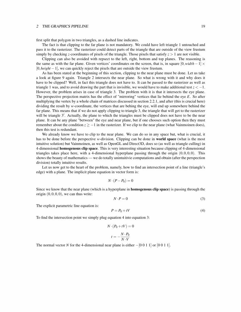
Let us take a look at figure 9. Triangle 1 intersects the far plane so only part of it is visible in the viewfrustum. If so, then we would like to cut off the part that is not visible, so that it does not get rendered by thepixel processor. We can clip the triangle to the far plane and reject the outside part. Note however, that theremaining part of the triangle has turned into a polygon with four vertices. To be able to process it, we must


first split that polygon in two triangles, as a dashed line indicates.The fact is that clipping to the far plane is not mandatory. We could have left triangle 1 untouched and

pass it to the rasterizer. The rasterizer could detect parts of the triangle that are outside of the view frustumsimply by checking z-coordinates of pixels of the triangle. Those pixels that satisfy z > 1 are not visible.

Clipping can also be avoided with repsect to the left, right, bottom and top planes. The reasoning isthe same as with the far plane. Given vertices’ coordinates on the screen, that is, in square [0,width−1]×[0,height−1], we can quickly reject the pixels that are outside the view frustum.

As has been stated at the beginning of this section, clipping to the near plane must be done. Let us takea look at figure 9 again. Triangle 2 intersects the near plane. So what is wrong with it and why does ithave to be clipped? Well, in fact this triangle does not have to. It can be passed to the rasterizer as well astriangle 1 was, and to avoid drawing the part that is invisible, we would have to make additional test z <−1.However, the problem arises in case of triangle 3. The problem with it is that it intersects the eye plane.The perspective projection matrix has the effect of "mirroring" vertices that lie behind the eye E. So aftermultiplying the vertex by a whole chain of matrices discussed in section 2.2.1, and after (this is crucial here)dividing the result by w-coordinate, the vertices that are behing the eye, will end up somewhere behind thefar plane. This means that if we do not apply clipping to triangle 3, the triangle that will get to the rasterizerwill be triangle 3′. Actually, the plane to which the triangles must be clipped does not have to be the nearplane. It can be any plane "between" the eye and near plane, but if one chooses such option then they mustremember about the condition z≥−1 in the rasterizer. If we clip to the near plane (what Vainmoinen does),then this test is redundant.

We already know we have to clip to the near plane. We can do so in any space but, what is crucial, ithas to be done before the perspective w-division. Clipping can be done in world space (what is the mostintuitive solution) but Vainmoinen, as well as OpenGL and Direct3D, does so (as well as triangle culling) in4-dimensional homogenous clip space. This is very interesting situation because clipping of 4-dimensionaltriangles takes place here, with a 4-dimensional hyperplane passing through the origin (0,0,0,0). Thisshows the beauty of mathematics — we do totally unintuitivie computations and obtain (after the perspectiondivision) totally intuitive results.

Let us now get to the heart of the problem, namely, how to find an intersection point of a line (triangle’sedge) with a plane. The implicit plane equation in vector form is:

N · (P−P0) = 0

Since we know that the near plane (which is a hyperplane in homogenous clip space) is passing through theorigin (0,0,0,0), we can thus write:

N ·P = 0 (3)

The explicit parametric line equation is:P = P0 + tV (4)

To find the intersection point we simply plug equation 4 into equation 3:

N · (P0 + tV ) = 0

t =−N ·P0

N ·VThe normal vector N for the 4-dimensional near plane is either −[0 0 1 1] or [0 0 1 1].


bounding box

triangle

screen

Figure 10: A triangle and its bounding box.

2.3 Pixel ProcessingWhen a triangle successfully gets out of the vertex processor it goes to the pixel processor, which draws thetriangle on the screen. This section discusses details of how this process is being proceed.

2.3.1 Rasterization and Shading

The goal of rasterization is to find all pixels that belong to a triangle, compute pixels’ attributes (like colorand texture coordinate) and finally shade the pixels. Attributes are computed by interpolating values thatcome from the vertices of the triangle. Shading process uses this interpolated values to produce the finalcolors of the pixels.

Finding pixels of a triangle is not a trivial task. The most naive method is to loop through all pixels of thescreen, and check each pixel if it belongs to the triangle. If it does, then attributes of the pixel are computed;if it does not, the loop goes to the next pixel. This method is very ineffective since a triangle can cover avery small portion of the screen, yet all screen’s pixels must be processed to rasterize it.

To strongly alleviate the processing power needed to process a single triangle, a very simple approachcan by utilized. The idea is to find a triangle’s bounding box in screen space, and process only pixels thatlie within that box. Figure 10 depicts a triangle and its bounding box.

Let us assume a triangle has screen space vertices v0 = (x0,y0), v1 = (x1,y1) and v2 = (x2,y2), and thescreen has resolution width×height. A bounding box for this triangle is defined as:

min3(a,b,c) = min(a,min(b,c))

max3(a,b,c) = max(a,max(b,c))

minx = max(min3(x0,x1,x2),0)

maxx = min(max3(x0,x1,x2),width−1)

miny = max(min3(y0,y1,y2),0)

maxy = min(max3(y0,y1,y2),height−1)

Having such defined bounding box we can now process the area [minx,miny]× [maxx,maxy] of pixels, ratherthan [0,0]× [width−1,height−1].


Altough we have greatly reduced the number of pixels that are to be processed, we still do not knowwhich of them belong to the triangle. To solve this issue we will employ so-called barycentric coordinates(based on discussion in [6]), that will not only help us to decide whether a pixel belongs to the triangle ornot, but will almost automatically perform interpolation of attributes.

An arbitrary vertex on a triangle’s plane can be represented as a weighted average of its vertices:

v = α∗ v0 +β∗ v1 + γ∗ v2 (5)

By adding to equation 5 the following constraint:

α+β+ γ = 1 (6)

the triple [α,β,γ] is reffered to as barycentric coordinates. Constraint 6 has a very nice property that guaran-tees that barycentric coordinates of a point on the triangle’s plane, that belongs to the triangle (excluding itsedges), satisfy the following inequalities:

0 < α < 1

0 < β < 1

0 < γ < 1

On the other hand, if the point belongs to the triangle, including its edges, then the inequalities turn into:

0≤ α≤ 1

0≤ β≤ 1

0≤ γ≤ 1

Equation 5 can be easily generalized to any attribute u (like color or texture coordinate):

u = α∗u0 +β∗u1 + γ∗u2

Let us consider signed distances marked in figure 11. To compute barycentric coordinates of point P, weuse the following formulas:

α =a2

a1

β =b2

b1

γ =c2

c1

The pseudocode in listing 3 shows how to rasterize a triangle on the screen by interpolating color valuesfrom its vertices.

1 a1 = d i s t a n c e ( v0 . p o s i t i o n . xy , l i n e _ v 1 v 2 )2 b1 = d i s t a n c e ( v1 . p o s i t i o n . xy , l i n e _ v 2 v 0 )3 c1 = d i s t a n c e ( v2 . p o s i t i o n . xy , l i n e _ v 0 v 1 )45 f o r y = minY t o maxY


v0

v1

v2

a1

b1

c1a2

b2

c2

P

Figure 11: Distances marked for barycentric coordinates computation.

6 f o r x = minX t o maxX78 a2 = d i s t a n c e ( ( x , y ) , l i n e _ v 1 v 2 )9 b2 = d i s t a n c e ( ( x , y ) , l i n e _ v 2 v 0 )

10 c2 = d i s t a n c e ( ( x , y ) , l i n e _ v 0 v 1 )1112 a l p h a = a2 / a113 b e t a = b2 / b114 gamma = c2 / c11516 i f ( a l p h a >= 0 and b e t a >= 0 and gamma >= 0)17 c o l o r B u f f e r ( x , y ) = a l p h a ∗v0 . c o l o r + b e t a ∗v1 . c o l o r + gamma∗v2 . c o l o r

Listing 3: Rasterization of a triangle.

In line 16 we check whether the coordinates are all greater than or equal to 0. Theoretically, we shouldalso check whether these coordinates are smaller than or equal to 1. However, from the constraint 6 weknow they all sum to 1 and thus none of them can exceed a value of 1. This way we can save three additionalcomparisons, what multiplied by the total number of pixels of the triangle quickly raises to a very highamount.

In the last line (17) of listing 3 an output color value for a pixel in coordinates (x,y) is computed. Theprocess of computing the output color is called shading. Here, we simply interpolate color values from thevertices of the triangle and put that color in the color buffer. A slightly more complicated approach would beto use texture coordinates, sample a texture and multiply the taken sample with the interpolated color. Thisis what Vainmoinen does and it will be discussed in more details later on.

As can be noticed in line 16, edges of the triangle are also rasterized (≥ instead of >). This means thatif there are two adjacent triangles that share the same edge, and the edge is passing through the centers ofpixels, then these pixels will be rasterized twice. In fact, this is not a big problem as this will not influencethe resulting image. A case when the image could be affected is rendering with semi-transparency. However,since Vainmoinen does not support transparency at all, this problem is left untouched. Anyway, if one wouldlike to solve this issue, they can find a neat solution in [6].

One crucial thing that the pseudocode in listing 3 misses is depth buffering. It is obvious that manytriangles will probably cover each other in screen space. This means that the triangles that are processedlast will eventually cover the triangles that have been rendered earlier. This is of course wrong behaviour


since the triangles on the list are definitely not sorted in back-to-front order with respect to the camera.To resolve this issue we can use z-coordinates. As we remember, z-coordinate in vertex’s position stores (inscreen space) a distance in range [−1,1] from the camera to the vertex. We can thus compute the interpolatedpixel’s distance from the camera. By introducing a so-called depth buffer (which has the size of the screen,just as the color buffer) we can keep tracking of closest pixels that appear on the screen. When a new pixelis to be drawn, we will first check if at its (x,y) coordinates there have already been drawn another pixel,which is closer to the camera than the new pixel we want to draw. If the pixel we want to draw has a smallerz-coordinate than the pixel that is already stored in the depth buffer, then we overwrite the color and depthbuffers values with the new ones. A modified rasterizing pseudocode with depth buffering is presented inlisting 4.

1 a1 = d i s t a n c e ( v0 . p o s i t i o n . xy , l i n e _ v 1 v 2 )2 b1 = d i s t a n c e ( v1 . p o s i t i o n . xy , l i n e _ v 2 v 0 )3 c1 = d i s t a n c e ( v2 . p o s i t i o n . xy , l i n e _ v 0 v 1 )45 f o r y = minY t o maxY6 f o r x = minX t o maxX78 a2 = d i s t a n c e ( ( x , y ) , l i n e _ v 1 v 2 )9 b2 = d i s t a n c e ( ( x , y ) , l i n e _ v 2 v 0 )

10 c2 = d i s t a n c e ( ( x , y ) , l i n e _ v 0 v 1 )1112 a l p h a = a2 / a113 b e t a = b2 / b114 gamma = c2 / c11516 i f ( a l p h a >= 0 and b e t a >= 0 and gamma >= 0)1718 z = a l p h a ∗v0 . p o s i t i o n . z + b e t a ∗v1 . p o s i t i o n . z + gamma∗v2 . p o s i t i o n . z1920 i f ( z < d e p t h B u f f e r ( x , y ) and z <= 1)2122 c o l o r B u f f e r ( x , y ) = a l p h a ∗v0 . c o l o r + b e t a ∗v1 . c o l o r + gamma∗v2 . c o l o r23 d e p t h B u f f e r ( x , y ) = z

Listing 4: Rasterization of a triangle with depth buffering.

The additional test in line 20 checks whether the z-coordinate is smaller than or equal to 1. This way pixelsthat are behind the far plane will not be rendered.

The depth buffer, to work correctly, must be initialized with a value greater than or equal to 1 before therasterization of triangles takes place.

2.3.2 Perspective-Correct Interpolation

Attributes interpolation performed in section 2.3.1 has one severe flaw — it ignores depths (distances to thecamera) of pixels. The problem is hardly seen on small triangles and during smooth colors interpolation butbecomes very apparent for large triangles and data that varies strongly across neighbouring pixels. Figure 12shows an incorrectly and correctly rendered triangle (the texture applied to the triangle has strong variationsin color).

In figure 12a the rectangle (two triangles) has been textured and texture coordinates have been interpo-lated in affine manner. Affine interpolation does not take into account depths of pixels because it is appliedin screen space, after projection onto the near plane of the view frustum. The z-coordinates of the pixels are


(a) Affine interpolation. (b) Perspective-correct interpolation.

Figure 12: Affine and perspective-correct interpolation.

ignored, which is not correct. To fix the problem, during interpolation, we need to consider the z-coordinatesto perform so-called perspective-correct interpolation, which is shown in figure 12b. The algorithm will bepresented here without any explanation why it works. A very nice derivation of the algoritm can be found in[5] and [4]. [2] gives clever tricks that improve performance.

To get a perspective-correct attribute upersp from an attribute u, we need to interpolate separately inaffine manner k = u

z , l = 1z , and compute upersp =

kl . Value z is in view space, that is, it can be read from

the w-component before the perspective division takes place. The computations, in terms of barycentriccoordinates, are:

k = au0

z0+b

u1

z1+ c

u2

z2

l = a1z0

+b1z1

+ c1z2

upersp =kl

upersp =a u0

z0

l+

b u1z1

l+

c u2z2

l

Again, note that z0, z1 and z2 are z-coordinates given in view space. They can be read from w-coordinatesof the vertices before the perspective division takes place.

Just for the sake of completion here are formulas for perspective-correct barycentric coordinates that canbe used directly with any attribute we want to be perspective-correct:

apersp =

aa f f inez0

lbpersp =

ba f f inez1

lcpersp =

ca f f inez2

l

The rasterization pseudocode with depth buffering and perspective-correct interpolation in shown inlisting 5.

a1 = d i s t a n c e ( v0 . p o s i t i o n . xy , l i n e _ v 1 v 2 )b1 = d i s t a n c e ( v1 . p o s i t i o n . xy , l i n e _ v 2 v 0 )c1 = d i s t a n c e ( v2 . p o s i t i o n . xy , l i n e _ v 0 v 1 )

f o r y = minY t o maxYf o r x = minX t o maxX

a2 = d i s t a n c e ( ( x , y ) , l i n e _ v 1 v 2 )b2 = d i s t a n c e ( ( x , y ) , l i n e _ v 2 v 0 )c2 = d i s t a n c e ( ( x , y ) , l i n e _ v 0 v 1 )


a l p h a = a2 / a1b e t a = b2 / b1gamma = c2 / c1

i f ( a l p h a >= 0 and b e t a >= 0 and gamma >= 0)

z = a l p h a ∗v0 . p o s i t i o n . z + b e t a ∗v1 . p o s i t i o n . z + gamma∗v2 . p o s i t i o n . z

i f ( z < d e p t h B u f f e r ( x , y ) and z <= 1)

l = a l p h a / z0 + b e t a / z1 + gamma / z2l = 1 . 0 f / la l p h a ∗= l / z0b e t a ∗= l / z1gamma ∗= l / z2

c o l o r B u f f e r ( x , y ) = a l p h a ∗v0 . c o l o r + b e t a ∗v1 . c o l o r + gamma∗v2 . c o l o rd e p t h B u f f e r ( x , y ) = z

Listing 5: Rasterization of a triangle with depth buffering and perspective-correct interpolation.

2.3.3 Texture Mapping

To map a texture to a triangle it is enough to interpolate (in perspective-correct manner) texture coordinates4

and use texture data (saved in a 32-bit RGBA array) from the point at which the texture coordinates indicate.Since texture coordinates are in normalized [0,1] range, they must be denormalized before sampling datafrom the texture. This process is a simple linear mapping:

nu = u∗widthnv = v∗height

where (u,v) are the original texture coordinates in [0,1] range, and (nu,nv) are the coordinates that are usedto sample the texture.

It is actually not true that texture coordinates that are assigned to vertices should be in [0,1] range. Infact they can be any positive number, but special behaviour occurs when they exceed 1. The behaviour isdependent on so-called texture addressing modes. The most popular one is called repeating (or wrapping),which simply repeats the texture. Figure 13 shows an example. As we can see, the texture coordinates areeither 0 or 2, what results in repeating the texture twice both horizontally and vertically. APIs like OpenGLor Direct3D support a few different texture addressing modes. Vainmoinen supports only repeating.

To use wrapping addressing mode it is enough to take a fractional part of the texture coordinates beforedenormalizing them:

nu = frac(u)∗widthnv = frac(v)∗height

Texture coordinates of pixels of a triangle form a floating-point, continous function. A texture is anarray of discretized pixel values, called texels. Sampling a texture is a process of mapping continous texturecoordinates to discretized texels of the texture. Let us say there is a texture 10× 10 pixels sized. There isalso a rectangle with pixels whose texture coordinates are in range [0,1]× [0,1]. After denormalizing the

4For a 2-dimensional texture, texture coordinates are usually referred to as (u,v) or (s, t).


(0, 0) (2, 0)

(2, 2)

Figure 13: Texture repeat addressing mode.

Figure 14: Point sampling of a small texture leads to poor visual quality.

texture coordinates are in area [0,10]× [0,10]. The simplest sampling algorithm (called point sampling) isto take a texture coordinate and reject its fractional part. For a pixel having texture coordinates (1.6,2.35)this means taking a sample indexed with (1,2).

More formally, given denormalized continous texture coordinate (u,v), the texture value T is:

i = buc

j = bvc

T = Ti, j

where Ti, j represents the value stored in the texture map T at the integer coordinates (i, j).Let us consider a rectangle whose size in screen space is 512×512 pixels, and a texture 64×64 pixels

sized. Applying such small texture to such big triangle means that every 8× 8 block of the rectangle willreceive exactly the same texture color, leading to poor visual quality. Figure 14 shows this problem.

A common way of reducing this problem is to use bilinear texture filtering ([4] and [2]). The idea is totake a block of 2×2 texels and average them in a linear manner both horizontally and vertically. The resultis depicted in figure 15.


Figure 15: Bilinear sampling greatly enhances visual quality.

Figure 16: Lack of mip-mapping causes severe artifacts on the distant triangles.

Given denormalized continous texture coordinate (u,v), the bilinearly filtered texture value T is:

i = buc

j = bvc

α = u− i

β = v− j

T = (1−α)(1−β)Ti, j +α(1−β)Ti+1, j +(1−α)βTi, j+1 +αβTi+1, j+1

where Ti, j represents the value stored in the texture map T at the integer coordinates (i, j).Bilinear texture filtering is a great remedy for texture magnification artifacts. Altough it may not be

that obvious at first glance, minification artifacts can also occur. Let us say there is a rectangle occupying16×16 pixels on the screen and a texture 128×128 pixels sized is mapped on the rectangle. It means thatfrom every 8× 8 block, one texel (for point filtering; four for bilinear) will be selected to cover a singlepixel of the rectangle. This will introduce sudden variations in texels that are selected to cover the pixels asthe camera moves around the scene, causing very unpleasant aliasing artifacts (figure 16). Speaking from apoint of view of signal processing, the block of texels that is applied to a single pixel contains high-frequencyinformation and only portion of this information is used (only one texel from the whole 8×8 block for pointfiltering), whereas the high-frequency information is rejected. Ideally, we would like to choose for everypixel not only one texel from the 8× 8 block, but the average of all texels. This can be achieved withmip-mapping (figure 17).


Figure 17: Mip-mapping applied. Altough the distant triangles have become blurry, aliasing artifacts havebeen completely eliminated (this is mostly noticeable during camera’s movement in real-time).

Figure 18: An example mipmaps chain.

The idea of mip-mapping ([4] and [2]) is to generate prefiltered versions of a texture at lower resolutions.As shown in figure 18, each smaller image is exactly half the width and half the height of the previous imagein the chain. The only job that mip-mapping does is simply selecting a proper mipmap from the chain andapplying it to the triangle. The selection process takes into account the size of the triangle on the screen andtakes the mipmap that is closest in size to this triangle.

To select a proper mipmap we need to detect the ratio of change of the texture coordinate with respect tothe window space coordinates of the pixel. Let n and m be the base-2 logarithms of the width and height ofa 2-dimensional texture (thus, the width and height of the texture are 2n and 2m). Let u(x,y) and v(x,y) befunctions that map window space coordinates (x,y) to texture coordinates (u,v). Define s(x,y) = 2nu(x,y)and t(x,y) = 2mv(x,y). The mipmap level mip of a pixel (x,y) is:

ρx =

√(

∂s∂x

)2 +(∂t∂x

)2 (7)

ρy =

√(

∂s∂y

)2 +(∂t∂y

)2 (8)

λ = log2[max(ρx,ρy)] (9)

mip = clamp[round(λ),0,max(n,m)] (10)

To compute the partial derivatives we first need to find the functions u(x,y) and v(x,y). Let us considerfinding u. We need to bound somehow the texture coordinate u of the pixel with its screen space coordinates


(x,y). One way to do so is to employ the 3-dimensional plane equation ([7]):

Ax+By+Cu+D = 0

This is pure abstraction that takes place here. The 3-dimensional plane equation is usually used in con-text of 3-dimensional planes, finding intersection points in 3-dimensions, etc. Here, we actually take a2-dimensional object ((x,y) coordinates of the pixel) and one of its attributes (u) and treat the triple ((x,y,u))as ordinary 3-dimensional coordinates, despite the fact that the geometrical interpretation of them does notmake any sense. However, we can use any of the known methods, including the geometrical ones, forcomputing the coefficients A, B, C, D. Slight manipulation of the plane equation gives us:

u = u(x,y) =−Ax+By+DC

From this we can find the derivatives of u(x,y) with respect to x and y:

∂u∂x

= −AC

∂u∂y

= −AC

In fact, what we need are partial derivatives of functions s(x,y) and t(x,y). Since we have just computedpartial derivatives of function u(x,y) and we know that s(x,y) = 2nu(x,y) then:

∂s∂x

= −2n AC

∂s∂y

= −2n AC

It is analogous for derivatives of t(x,y).The equations that we have just derived are correct but only for texture coordinates interpolated in affine

manner. Obviously, we would like to find the equations for perspectively-corrected texture coordinates. Todo so, instead of interpolating u, we need to interpolate f = u

z , as well as g = 1z . This leads to the following

equations:

A1x+B1y+C1uz+D1 = 0

A1x+B1y+C1 f +D1 = 0

A2x+B2y+C21z+D2 = 0

A2x+B2y+C2g+D2 = 0

f (x,y) = −A1x+B1y+C1

D1

g(x,y) = −A2x+B2y+C2

D2

3 PROJECT ARCHITECTURE 30

Perspectively-corrected texture coordinate is equal to the fraction fg . We need to find the partial derivatives

of this fraction:

(fg)′ =

f ′ ∗g− f ∗g′

g2

(fg)x =

fx ∗g− f ∗gx

g2 =− A1

D1g+ f A2

D2

g2

(fg)y =

fy ∗g− f ∗gy

g2 =− B1

D1g+ f B2

D2

g2

In terms of the initial equations:

∂u∂x

= (fg)x

∂u∂y

= (fg)y

∂s∂x

= 2n ∂u∂x

= 2n− A1

D1g+ f A2

D2

g2

∂s∂y

= 2m ∂u∂y

= 2m− B1

D1g+ f B2

D2

g2

The computation of t(x,y)’s derivatives is analogous.It is worth-noting that hardware renderers like OpenGL or Direct3D do not use all these analytical

equations that have just been carried out. Instead, the hardware always computes blocks of 2×2 pixels andcomputes the derivatives numerically. Vainmoinen uses the analytical equations.

As the camera moves around the scene, abrupt changes in the mipmap level selection occur, as depictedin figure 19. To alleviate this problem we can employ trilinear filtering. The idea is to pick not only one, buttwo mipmaps and linearly interpolate between the two. This will give a nice smooth transition of colors.

Given a level-of-detail parameter λ as in equation 9, the final texture color T of a pixel is:

mip1 = clamp(bλc,0,max(n,m)−1)

mip2 = mip1 +1

λ f rac = frac(max(λ,0))

T = (1−λ f rac)Tmip1 +λ f racTmip2

where Ti represents the sampled ith mipmap level, starting from the level 0 (the base level).

3 Project ArchitectureIn this section design aspects of Vainmoinen are discussed. The discussion starts with the class diagram,goes through the physical structure of files and finally ends with discussion of how the graphics pipelineworks.


(a) Point mipmap selection.

(b) Linear mipmap selection.

Figure 19: Comparison of point and linear mipmap selection algorithms. Note how linear mipmap selectionblends together two consecutive mipmap levels, leading to smooth change of colors.

3.1 Class DiagramThe Vainmoinen’s class diagram is presented in figure 20.

CPainter Provides abstract mechanism that supplies color buffer memory for the renderer.

CSDLPainter Implementation of CPainter that uses SDL’s ([3]) main video surface as the color buffer.

COGLPainter Implementation of CPainter that uses OpenGL’s pixel buffer object as the color buffer.

Vertex Structure describing a vertex. It consists of a position (4-dimensional vector (x,y,z,w)), color(3-dimensional RGB vector) and texture coordinate (2-dimensional (u,v) coordinates).

Triangle Structure composed of three instances of Vertex class.

CTrianglesBuffer Class that is a collection of triangles.

CTexture Class that contains mipmaps data. The mipmaps are filled with the data from BlossomEngine’sCImage class.

CRenderer The core singleton class that manages the whole rendering process.

DrawCall Stores information about the data that is to be rendered. A single draw call is made of a worldtransformation matrix, pointer to a triangle buffer, number of triangles that are to be rendered from thetriangle buffer and a texture. The renderer holds a list of draw calls. The user can issue a new draw call withCRenderer::draw method.


Figure 20: Vainmoinen’s class diagram.

4 IMPLEMENTATION 33

TriangleToRasterize This structure is used internally by CRenderer class. It describes a triangle that haspassed the vertex processing phase and goes to the pixel processor.

3.2 Physical StructureThe project is composed of the following header files:

• painter.hpp — contains definitions of CPainter, CSDLPainter and COGLPainter;

• geometry.hpp — contains definitions of Vertex and Triangle;

• triangles_buffer.hpp — contains definition of CTriangleBuffer;

• texture.hpp — contains definition of CTexture;

• renderer.hpp — contains definition of CRenderer;

• vainmoinen.hpp — includes all other files.

The source files:

• painter.cpp — implements CSDLPainter and COGLPainter;

• renderer.cpp — implements functions of CRenderer that run on CPU;

• renderer.cu — implements functions of CRenderer that run on GPU (using CUDA).

3.3 Flow Chart of the Graphics PipelineFigure 21 shows the flow chart of the graphics pipeline in Vainmoinen.

4 ImplementationThis section starts with a discussion of a sample piece of code that uses Vainmoinen to renderer a 3-dimensional scene. Next, issues related to porting code to CUDA are discussed. Finally, the performancetests are presented.

4.1 Software Renderer Running on CPUThe renderer executes the procedures depicted in figure 21. First, in the vertex processing phase, the rendererloops through the draw calls that have been called by the user. Triangles are taken from the triangle bufferassociated with every draw call and they are processed by the vertex shader. Next, the triangles are culled,clipped, and finally go to the pixel processor. The pixel processor loops through the triangles that have comefrom the vertex processor. It finds pixels that belong to every triangle, interpolates attributes in perspective-correct manner and passes them to the pixel shader to finally shade the pixels.

Listing 6 presents a sample code that uses Vainmoinen to render a cube.

4 IMPLEMENTATION 34

for $i: 0 to $drawCalls.size - 1 for $j: 0 to $drawCalls[$i].trianglesNum - 1

Triangle $triangle

for $k: 0 to 2 $triangle.vertices[$k] = runVertexShader( $drawCalls[$i].transform, $drawCalls[$i].trianglesBuffer.triangles[$j].vertices[$k])

if ([all vertices of $triangle are not visible]) continue

if ([all vertices of $triangle are visible]) processProspectiveTriangleToRasterize( $triangle, $drawCalls[$i].texture) continue

list<Vertex> $vertices $vertices.add($triangle.vertices[0]) $vertices.add($triangle.vertices[1]) $vertices.add($triangle.vertices[2])

$vertices = clipPolygonToPlaneIn4D($vertices, vec4(0, 0, -1, -1))

// triangulate the polygon formed of $vertices array if ($vertices.size >= 3) for $k: 0 to $vertice.size - 2 processProspectiveTriangleToRasterize( $vertices[0], $vertices[1 + $k], $vertices[2 + $k], $drawCalls[$i].texture)

runVertexProcessorVertex runVertexShader(mtx $transform, Vertex $input){ Vertex $output

$output.position = $input.position * $transform $output.color = $input.color $output.texCoord = $input.texCoord

return $output}

list<Vertex> clipPolygonToPlaneIn4D(list<Vertex> $vertices, vec4 $planeNormal){ list<Vertex> $clippedVertices;

for $i: 0 to $vertices.size - 1

$a = $i $b = ($i + 1) % $vertices.size

if ([$vertices[$a] and $vertices[$b] are on opposite sides of $planeNormal]) { [find intersection point $vertex and linearly interpolate attributes]

if ([$vertices[$a] is on the negative side of $planeNormal]) $clippedVertices.add($vertices[$a]) $clippedVertices.add($vertex) elseif ([$vertices[$b] is on the negative side of $planeNormal]) $clippedVertices.add($vertex) } elseif ([$vertices[$a] and $vertices[$b] are both on the negative side of $planeNormal]) { $clippedVertices.add($vertices[$a]) }

return $clippedVertices}

void processProspectiveTriangleToRasterize( Vertex $_v0, Vertex $_v1, Vertex $_v2, CTexture $_texture){ TriangleToRasterize $t

$t.v0 = $_v0 $t.v1 = $_v1 $t.v2 = $_v2 $t.texture = $_texture

$t.one_over_z0 = 1.0f / $t.v0.position.w $t.one_over_z1 = 1.0f / $t.v1.position.w $t.one_over_z2 = 1.0f / $t.v2.position.w

// project from homogenous coordinates to window coordinates $t.v0.position.divideByW() $t.v0.position *= $Renderer.windowTransform $t.v1.position.divideByW() $t.v1.position *= $Renderer.windowTransform $t.v2.position.divideByW() $t.v2.position *= $Renderer.windowTransform

if ([are vertices $t.v0, $t.v1 and $t.v2 in clockwise order in screen space]) return

[find bounding box of the triangle and store it in [$t.minX, $t.minY] x [$tmaxX, $t.maxY] square]

if ($t.maxX <= $t.minX or $t.maxY <= $t.minY) return

[compute the remaining attributes of $t]

$Renderer.trianglesToRasterize.add($t);}

for $i: 0 to $Renderer.trianglesToRasterize.size

TriangleToRasterize& $t = $Renderer.trianglesToRasterize[$i]

for $y: $t.minY to $t.maxY for $x: $t.minX to $t.maxX

[compute barycentric weights of point ($x, $y): $alpha, $beta, $gamma]

// is pixel (x, y) inside the triangle if ($alpha >= 0 and $beta >= 0 and $gamma >= 0)

$pixelIndex = $y*$Renderer.width + $x

$z_affine = $alpha*$t.v0.position.z + $beta*$t.v1.position.z + $gamma*$t.v2.position.z

if ($z_affine < $depthBuffer[$pixelIndex] and $z_affine <= 1)

// make barycentric weights to be perspective-correct $l = $alpha*$t.one_over_z0 + $beta*$t.one_over_z1 + $gamma*$t.one_over_z2 $l = 1 / $l $alpha *= $l * $t.one_over_z0 $beta *= $l * $t.one_over_z1

$gamma *= $l * $t.one_over_z2

$color_persp = $alpha*$t.v0.color + $beta*$t.v1.color + $gamma*$t.v2.color $texCoord_persp = $alpha*$t.v0.texCoord + $beta*$t.v1.texCoord + $gamma*t.v2.texCoord

[compute partial derivatives of texture coordinates]

&pixelColor = runPixelShader($t.texture, $color_persp, $texCoord_persp)

$colorBuffer[4*$pixelIndex + 0] = $pixelColor.red $colorBuffer[4*$pixelIndex + 1] = $pixelColor.green $colorBuffer[4*$pixelIndex + 2] = $pixelColor.blue $depthBuffer[$pixelIndex] = $z_affine

runPixelProcessor

vec3 runPixelShader(CTexture $texture, vec3 $color, vec2 $texCoord){ return $color * tex2D($texture, $texCoord)}

Figure 21: Vainmoinen’s graphics pipeline flow chart.

4 IMPLEMENTATION 35

1 c o n s t f l o a t& a s p e c t = A p p l i c a t i o n . g e t S c r e e n A s p e c t R a t i o ( ) ;23 f l o a t l e f t = −0.25 f ∗ a s p e c t ;4 f l o a t r i g h t = 0 . 2 5 f ∗ a s p e c t ;5 f l o a t bot tom = −0.25 f ;6 f l o a t t o p = 0 . 2 5 f ;7 f l o a t n e a r = 0 . 5 f ;8 f l o a t f a r = 100 .0 f ;9

10 mtx v i e w P r o j T r a n s f o r m =11 c o n s t r u c t V i e w T r a n s f o r m (12 camera . ge tEye ( ) ,13 camera . g e t R i g h t V e c t o r ( ) ,14 camera . ge tUpVec to r ( ) ,15 −camera . g e t F o r w a r d V e c t o r ( ) ) ∗16 c o n s t r u c t P r o j T r a n s f o r m ( l e f t , r i g h t , bottom , top , near , f a r ) ;1718 R e n d e r e r . b e g i n ( ) ;19 R e n d e r e r . c l e a r C o l o r B u f f e r ( ) ;20 R e n d e r e r . c l e a r D e p t h B u f f e r ( ) ;2122 R e n d e r e r . s e t T r i a n g l e s B u f f e r ( c u b e T r i a n g l e s B u f f e r ) ;23 R e n d e r e r . s e t T r a n s f o r m ( mtx : : t r a n s l a t e ( 3 . 0 f , 0 . 0 f , 5 . 0 f ) ∗ v i e w P r o j T r a n s f o r m ) ;24 R e n d e r e r . s e t T e x t u r e ( t e x t u r e ) ;25 R e n d e r e r . draw ( ) ;2627 R e n d e r e r . end ( f a l s e , f a l s e ) ;

Listing 6: Using Vainmoinen to render a cube.

In lines 3-8, parameters that describe the view frustum’s area are defined. Note that the near plane’sshape is not square but rectangular. This way the image will not be distorted if the screen is rectangular (thatis, its width is different from the height).

In lines 10-16, Vainmoinen’s helper functions are used to build the view and projection matrices. Thefunction that builds the view matrix takes as parameters the eye’s position and the basis vectors. Theseare taken from the CCamera object (from BlossomEngine), which provides nice mechanism for controllingvirtual camera in 3-dimensional environment. Note that the negative of the forward vector is taken becausethe BlossomEngine’s camera works in left-handed coordinate system.

Initialization of the rendering process takes place in lines 18-20. Part of this process is to clear the colorand depth buffers to some fixed value every frame.

In lines 22-25, a new draw call is created. First, the triangle buffer is set. Next, the transformation matrixwhich is a combined world and view-projection matrix. Finally, the texture is specified. Note that drawcommand in fact does not perform any rendering — it only creates the draw call with the values that havejust been set and adds it to the renderer’s queue.

In line 27, the whole rendering process starts.Obviously, the triangle buffer from listing 6 must have been filled with data before it can be used. Listing

7 shows this process.

V er t e x c u b e V e r t i c e s [ 2 4 ] ;

f o r ( i n t i = 0 ; i < 2 4 ; i ++)c u b e V e r t i c e s [ i ] . c o l o r = vec3 ( 1 . 0 f , 1 . 0 f , 1 . 0 f ) ;

c u b e V e r t i c e s [ 0 ] . p o s i t i o n = vec4 (−0.5 f , 0 . 5 f , 0 . 5 f ) ;

4 IMPLEMENTATION 36

c u b e V e r t i c e s [ 0 ] . t exCoord = vec2 ( 0 . 0 f , 0 . 0 f ) ;c u b e V e r t i c e s [ 1 ] . p o s i t i o n = vec4 (−0.5 f , −0.5 f , 0 . 5 f ) ;c u b e V e r t i c e s [ 1 ] . t exCoord = vec2 ( 0 . 0 f , 1 . 0 f ) ;c u b e V e r t i c e s [ 2 ] . p o s i t i o n = vec4 ( 0 . 5 f , −0.5 f , 0 . 5 f ) ;c u b e V e r t i c e s [ 2 ] . t exCoord = vec2 ( 1 . 0 f , 1 . 0 f ) ;c u b e V e r t i c e s [ 3 ] . p o s i t i o n = vec4 ( 0 . 5 f , 0 . 5 f , 0 . 5 f ) ;c u b e V e r t i c e s [ 3 ] . t exCoord = vec2 ( 1 . 0 f , 0 . 0 f ) ;

c u b e V e r t i c e s [ 4 ] . p o s i t i o n = vec4 ( 0 . 5 f , 0 . 5 f , 0 . 5 f ) ;c u b e V e r t i c e s [ 4 ] . t exCoord = vec2 ( 0 . 0 f , 0 . 0 f ) ;c u b e V e r t i c e s [ 5 ] . p o s i t i o n = vec4 ( 0 . 5 f , −0.5 f , 0 . 5 f ) ;c u b e V e r t i c e s [ 5 ] . t exCoord = vec2 ( 0 . 0 f , 1 . 0 f ) ;c u b e V e r t i c e s [ 6 ] . p o s i t i o n = vec4 ( 0 . 5 f , −0.5 f , −0.5 f ) ;c u b e V e r t i c e s [ 6 ] . t exCoord = vec2 ( 1 . 0 f , 1 . 0 f ) ;c u b e V e r t i c e s [ 7 ] . p o s i t i o n = vec4 ( 0 . 5 f , 0 . 5 f , −0.5 f ) ;c u b e V e r t i c e s [ 7 ] . t exCoord = vec2 ( 1 . 0 f , 0 . 0 f ) ;

c u b e V e r t i c e s [ 8 ] . p o s i t i o n = vec4 ( 0 . 5 f , 0 . 5 f , −0.5 f ) ;c u b e V e r t i c e s [ 8 ] . t exCoord = vec2 ( 0 . 0 f , 0 . 0 f ) ;c u b e V e r t i c e s [ 9 ] . p o s i t i o n = vec4 ( 0 . 5 f , −0.5 f , −0.5 f ) ;c u b e V e r t i c e s [ 9 ] . t exCoord = vec2 ( 0 . 0 f , 1 . 0 f ) ;c u b e V e r t i c e s [ 1 0 ] . p o s i t i o n = vec4 (−0.5 f , −0.5 f , −0.5 f ) ;c u b e V e r t i c e s [ 1 0 ] . t exCoord = vec2 ( 1 . 0 f , 1 . 0 f ) ;c u b e V e r t i c e s [ 1 1 ] . p o s i t i o n = vec4 (−0.5 f , 0 . 5 f , −0.5 f ) ;c u b e V e r t i c e s [ 1 1 ] . t exCoord = vec2 ( 1 . 0 f , 0 . 0 f ) ;

c u b e V e r t i c e s [ 1 2 ] . p o s i t i o n = vec4 (−0.5 f , 0 . 5 f , −0.5 f ) ;c u b e V e r t i c e s [ 1 2 ] . t exCoord = vec2 ( 0 . 0 f , 0 . 0 f ) ;c u b e V e r t i c e s [ 1 3 ] . p o s i t i o n = vec4 (−0.5 f , −0.5 f , −0.5 f ) ;c u b e V e r t i c e s [ 1 3 ] . t exCoord = vec2 ( 0 . 0 f , 1 . 0 f ) ;c u b e V e r t i c e s [ 1 4 ] . p o s i t i o n = vec4 (−0.5 f , −0.5 f , 0 . 5 f ) ;c u b e V e r t i c e s [ 1 4 ] . t exCoord = vec2 ( 1 . 0 f , 1 . 0 f ) ;c u b e V e r t i c e s [ 1 5 ] . p o s i t i o n = vec4 (−0.5 f , 0 . 5 f , 0 . 5 f ) ;c u b e V e r t i c e s [ 1 5 ] . t exCoord = vec2 ( 1 . 0 f , 0 . 0 f ) ;

c u b e V e r t i c e s [ 1 6 ] . p o s i t i o n = vec4 (−0.5 f , 0 . 5 f , −0.5 f ) ;c u b e V e r t i c e s [ 1 6 ] . t exCoord = vec2 ( 0 . 0 f , 0 . 0 f ) ;c u b e V e r t i c e s [ 1 7 ] . p o s i t i o n = vec4 (−0.5 f , 0 . 5 f , 0 . 5 f ) ;c u b e V e r t i c e s [ 1 7 ] . t exCoord = vec2 ( 0 . 0 f , 1 . 0 f ) ;c u b e V e r t i c e s [ 1 8 ] . p o s i t i o n = vec4 ( 0 . 5 f , 0 . 5 f , 0 . 5 f ) ;c u b e V e r t i c e s [ 1 8 ] . t exCoord = vec2 ( 1 . 0 f , 1 . 0 f ) ;c u b e V e r t i c e s [ 1 9 ] . p o s i t i o n = vec4 ( 0 . 5 f , 0 . 5 f , −0.5 f ) ;c u b e V e r t i c e s [ 1 9 ] . t exCoord = vec2 ( 1 . 0 f , 0 . 0 f ) ;

c u b e V e r t i c e s [ 2 0 ] . p o s i t i o n = vec4 (−0.5 f , −0.5 f , 0 . 5 f ) ;c u b e V e r t i c e s [ 2 0 ] . t exCoord = vec2 ( 0 . 0 f , 0 . 0 f ) ;c u b e V e r t i c e s [ 2 1 ] . p o s i t i o n = vec4 (−0.5 f , −0.5 f , −0.5 f ) ;c u b e V e r t i c e s [ 2 1 ] . t exCoord = vec2 ( 0 . 0 f , 1 . 0 f ) ;c u b e V e r t i c e s [ 2 2 ] . p o s i t i o n = vec4 ( 0 . 5 f , −0.5 f , −0.5 f ) ;c u b e V e r t i c e s [ 2 2 ] . t exCoord = vec2 ( 1 . 0 f , 1 . 0 f ) ;c u b e V e r t i c e s [ 2 3 ] . p o s i t i o n = vec4 ( 0 . 5 f , −0.5 f , 0 . 5 f ) ;c u b e V e r t i c e s [ 2 3 ] . t exCoord = vec2 ( 1 . 0 f , 0 . 0 f ) ;

T r i a n g l e c u b e T r i a n g l e s [ ] ={

c u b e V e r t i c e s [ 0 ] , c u b e V e r t i c e s [ 1 ] , c u b e V e r t i c e s [ 2 ] ,c u b e V e r t i c e s [ 0 ] , c u b e V e r t i c e s [ 2 ] , c u b e V e r t i c e s [ 3 ] ,c u b e V e r t i c e s [ 4 ] , c u b e V e r t i c e s [ 5 ] , c u b e V e r t i c e s [ 6 ] ,

4 IMPLEMENTATION 37

Figure 22: Rendering a cube in Vainmoinen.

c u b e V e r t i c e s [ 4 ] , c u b e V e r t i c e s [ 6 ] , c u b e V e r t i c e s [ 7 ] ,c u b e V e r t i c e s [ 8 ] , c u b e V e r t i c e s [ 9 ] , c u b e V e r t i c e s [ 1 0 ] ,c u b e V e r t i c e s [ 8 ] , c u b e V e r t i c e s [ 1 0 ] , c u b e V e r t i c e s [ 1 1 ] ,c u b e V e r t i c e s [ 1 2 ] , c u b e V e r t i c e s [ 1 3 ] , c u b e V e r t i c e s [ 1 4 ] ,c u b e V e r t i c e s [ 1 2 ] , c u b e V e r t i c e s [ 1 4 ] , c u b e V e r t i c e s [ 1 5 ] ,c u b e V e r t i c e s [ 1 6 ] , c u b e V e r t i c e s [ 1 7 ] , c u b e V e r t i c e s [ 1 8 ] ,c u b e V e r t i c e s [ 1 6 ] , c u b e V e r t i c e s [ 1 8 ] , c u b e V e r t i c e s [ 1 9 ] ,c u b e V e r t i c e s [ 2 0 ] , c u b e V e r t i c e s [ 2 1 ] , c u b e V e r t i c e s [ 2 2 ] ,c u b e V e r t i c e s [ 2 0 ] , c u b e V e r t i c e s [ 2 2 ] , c u b e V e r t i c e s [ 2 3 ]

} ;

c u b e T r i a n g l e s B u f f e r . c r e a t e ( 1 2 ) ;T r i a n g l e ∗ c u b e T r i a n g l e s B u f f e r D a t a = c u b e T r i a n g l e s B u f f e r . l o c k D a t a ( ) ;{

memcpy ( ( vo id ∗ ) c u b e T r i a n g l e s B u f f e r D a t a , ( vo id ∗ ) c u b e T r i a n g l e s , 12∗ s i z e o f ( T r i a n g l e ) ) ;}c u b e T r i a n g l e s B u f f e r . u n l o c k D a t a ( ) ;

Listing 7: Filling a triangle buffer with data.

The code is rather self-explanatory and will not be discussed in more details.Figure 22 shows a render from an application that uses Vainmoinen to render a cube. Note that the top

face of the cube appears blurry, as a higher mipmap level has been selected for it.

4.2 Making it Hardware by Speeding up with CUDAThe most performance-sensitive part of the graphics pipeline in Vainmoinen is, by no doubt, pixel process-ing. Since processing of every pixel is independent from processing the other ones, this stage can easily beparallelized with CUDA. However, porting of texture mapping has been left out as it would introduce muchof additional effort.

Vertex processing has not been parallelized at all. Firstly, the software renderer can handle quite easilya big number of triangles. Secondly, it has proven to be not that trivial to implement consistent data flowfrom the vertex stage to the pixel stage. The vertex processor takes as input a fixed number of triangles. Onthe output, it generates a varying number of triangles every frame. Since CUDA does not even allow fordynamic memory allocation while executing code on GPU, realizing this task introduces a lot of potentialproblems. All these have been bypassed simply by not involving CUDA to vertex processing at all.

4 IMPLEMENTATION 38

Working with CUDA on the most basic level is rather straightforward. A programmer defines a 1- or2-dimensional grid of blocks (the maximum number of blocks is 65535×65535). Every block can consistof a 1-, 2- or 3-dimensional array of threads (the maximum number of threads is 512× 512× 64). Everygraphics processor that supports CUDA has a fixed number of multiprocessors, where each multiprocessorhas a fixed number of cores. For instance, GeForce 240 GT has 12 multiprocessors, each one having 8 cores,what sums up to a total number of 96 cores (1.34GHz each). Roughly speaking, blocks in CUDA refer tomultiprocessors, whereas threads refer to cores. That means that if a graphics card has 12 multiprocessors,then it can run 12 blocks of threads independently. To run a parallelized kernel function on GPU, a program-mer only needs to implement it and within that function they can access the index of a block and a thread(via built-in variables) that is being executed. This can be used to, for example, index a pixel of a trianglethat this particular thread should process. During a kernel function call a programmer defines a number ofblocks and a number of threads per block that will run the kernel function.

Two slightly different algorithms have been implemented in Vainmoinen to support paralellized pixelprocessing in CUDA. Both algorithms use a triangle’s bounding box to form a rectangular grid of blocks,each having 16× 16 pixels (what sums up to 256 pixels, what is the half of the maximum numbers ofthreads per block in CUDA). A kernel function rasterizePixel is called for each pixel within a block.The function is very similar to the one presented in listing 5. The only difference is the beginning, depictedin the pseudocode in listing 8.

x = minX + th readX + 16∗ blockXy = minY + th readY + 16∗ blockY

i f ( x <= maxX and y <= maxY){

[ t h e a c t u a l p i x e l p r o c e s s i n g ]}

Listing 8: The pseudocode of rasterizePixel function.

Instead of the loop that goes through the pixels of the bounding box, the coordinates of the pixel are com-puted based on the block and thread indices. Note the (minX ,minY ) offset, which describes the lower leftcorner of the bounding box of the triangle. This way the blocks that process the triangle will cover thetriangle’s bounding box. Note also the additional condition that appears before the actual rendering takesplace. Since the blocks of threads have 16× 16 size, a bunch of blocks that cover the triangle will alwayscover the multiple of 16 in each dimension. For example, for a triangle having a bounding box whose sizeis 20×20, four 16×16 blocks will be used to cover that triangle. So the total number of pixels that will beprocessed is 32×32. To not get out of the 20×20 bound (and possibly violate a memory access), we needthe additional if-statement.

The algorithms that can be used in Vainmoinen to run pixel processing via CUDA both process thepixels in the exact same way. They differ only in a way the data is organized. The first algorithm, calledOne-Call-One-Triangle, as the name indicates, makes a single kernel function call for each triangle. Thisis very expensive solution in terms of CPU-GPU communication. However, on the other hand, it is veryfast in the actual computation. The reason for this is that the version of rasterizePixel for this algorithmtakes as arguments the information that comes from the triangle (TriangleToRasterize structure). Thesearguments, during the computation in the kernel function, are being held in fast shared memory of a block.So once the GPU receives all necessary information to process the triangle, every pixel has a fast access tothe data that describes the triangle. One-Call-One-Triangle algorithm is particularly fast for processing few,relatively big triangles. Listing 9 presents the algorithm in action.

4 IMPLEMENTATION 39

f o r ( u i n t i = 0 ; i < t r i a n g l e s T o R a s t e r i z e . s i z e ( ) ; i ++){

T r i a n g l e T o R a s t e r i z e& t = t r i a n g l e s T o R a s t e r i z e [ i ] ;

dim3 blocksNum ( ( t . maxX − t . minX + 1) / 16 + 1 , ( t . maxY − t . minY + 1) / 16 + 1) ;dim3 threadsNum ( 1 6 , 16) ;

r a s t e r i z e P i x e l <<<blocksNum , threadsNum >>>(c o l o r B u f f e r _ d e v i c e , d e p t h B u f f e r _ d e v i c e , width ,t . v0 ,t . v1 ,t . v2 ,t . t e x t u r e ,t . one_over_z0 ,t . one_over_z1 ,t . one_over_z2 ,t . minX ,t . maxX ,t . minY ,t . maxY ,t . one_over_v0ToLine12 ,t . one_over_v1ToLine20 ,t . one_over_v2ToLine01 ,t . a l p h a P l a n e ,t . b e t a P l a n e ,t . gammaPlane ,t . o n e _ o v e r _ a l p h a _ c ,t . o n e _ o v e r _ b e t a _ c ,t . one_over_gamma_c ,t . a l p h a _ f f x ,t . b e t a _ f f x ,t . gamma_ffx ,t . a l p h a _ f f y ,t . b e t a _ f f y ,t . gamma_ffy ) ;

}

Listing 9: One-Call-One-Triangle algorithm implementation.

Note that the arguments are passed in a "rough" form, rather than through a stucture. The reason is thatarguments passed to a kernel function, in general, all go to shared memory, but when passing a big structure(like TriangleToRasterize) it goes to global memory, which is much slower.

The second algorithm, One-Call-Many-Triangles, is much more economical in calling the kernel func-tion. Every frame it takes all triangles (representatives of TriangleToRasterize) and loads them to globalmemory. It also creates so-called virtual blocks. A virtual block is a structure composed of x and y coor-dinates of a block and an index to a triangle that this block will process (of course, only one of its 16× 16areas). During the kernel function call, a grid of size blocksNum×1 is created. This way, with only a singlecall, we can schedule computations of a number of blocks not only belonging to one particular triangle, butto any triangle (each virtual block contains an index to a triangle). The number of blocksNum is limitedto 65535 (CUDA requirement), so the maximum number of blocks that can be processed is 65535. A wayaround this problem is to use more than one kernel call if the number of blocks we want to process exceeds65535. One-Call-Many-Triangles algorithm avoids expensive CPU-GPU communication but does not makeuse of shared memory so CUDA threads need to download the triangles’ data from global memory. The al-gorithm is thus good in processing a big number of rather small triangles. Listing 10 presents the algorithm

4 IMPLEMENTATION 40

in action.

v e c t o r < v e c t o r < T r i a n g l e B l o c k >> t r i a n g l e s B l o c k s P a c k s ;v e c t o r < T r i a n g l e B l o c k > t e m p T r i a n g l e s B l o c k s ;

f o r ( u i n t i = 0 ; i < t r i a n g l e s T o R a s t e r i z e . s i z e ( ) ; i ++){

T r i a n g l e T o R a s t e r i z e& t = t r i a n g l e s T o R a s t e r i z e [ i ] ;

/ / w id th ∗ h e i g h t i s a t o t a l number o f v i r t u a l b l o c k s p e r t r i a n g l ei n t wid th = ( t . maxX − t . minX + 1) / 16 + 1 ;i n t h e i g h t = ( t . maxY − t . minY + 1) / 16 + 1 ;

/ / l oop t h r o u g h t h e v i r t u a l b l o c k s o f t h e t r i a n g l ef o r ( i n t x = 0 ; x < wid th ; x ++){

f o r ( i n t y = 0 ; y < h e i g h t ; y ++){

T r i a n g l e B l o c k t r i a n g l e B l o c k ;

t r i a n g l e B l o c k . x = x ;t r i a n g l e B l o c k . y = y ;t r i a n g l e B l o c k . t r i a n g l e I n d e x = i ;

/ / add t h e b l o c k t o t h e " t e m p o r a r y " l i s tt e m p T r i a n g l e s B l o c k s . push_back ( t r i a n g l e B l o c k ) ;

/ / i f t h e t o t a l number o f b l o c k s e x c e e d s t h e/ / maximum CUDA b l o c k s c o u n t i n one d imens ion ( 6 5 5 3 5 ) . . .i f ( t e m p T r i a n g l e s B l o c k s . s i z e ( ) == 65535){

/ / . . . add t h e l i s t t o t h e " l i s t o f l i s t s "t r i a n g l e s B l o c k s P a c k s . push_back ( t e m p T r i a n g l e s B l o c k s ) ;/ / c l e a r t h e " t e m p o r a r y " l i s tt e m p T r i a n g l e s B l o c k s . c l e a r ( ) ;

}}

}}

/ / add t h e r e m a i n i n g b l o c k s t o t h e " l i s t o f l i s t s "i f ( t e m p T r i a n g l e s B l o c k s . s i z e ( ) > 0 ){

t r i a n g l e s B l o c k s P a c k s . push_back ( t e m p T r i a n g l e s B l o c k s ) ;}

T r i a n g l e T o R a s t e r i z e ∗ t r i a n g l e s T o R a s t e r i z e _ d e v i c e ;T r i a n g l e B l o c k ∗ t r i a n g l e s B l o c k s _ d e v i c e ;

/ / copy t h e t r i a n g l e s t o g l o b a l memorycudaMal loc ( ( vo id ∗∗ )&t r i a n g l e s T o R a s t e r i z e _ d e v i c e , t r i a n g l e s T o R a s t e r i z e . s i z e ( ) ∗ s i z e o f (

T r i a n g l e T o R a s t e r i z e ) ) ;cudaMemcpy ( t r i a n g l e s T o R a s t e r i z e _ d e v i c e , &t r i a n g l e s T o R a s t e r i z e [ 0 ] , t r i a n g l e s T o R a s t e r i z e .

s i z e ( ) ∗ s i z e o f ( T r i a n g l e T o R a s t e r i z e ) , cudaMemcpyHostToDevice ) ;

/ / l oop t h r o u g h t h e packsf o r ( u i n t i = 0 ; i < t r i a n g l e s B l o c k s P a c k s . s i z e ( ) ; i ++){

4 IMPLEMENTATION 41

/ / copy a s i n g l e b l o c k s packcudaMal loc ( ( vo id ∗∗ )&t r i a n g l e s B l o c k s _ d e v i c e , t r i a n g l e s B l o c k s P a c k s [ i ] . s i z e ( ) ∗ s i z e o f (

T r i a n g l e B l o c k ) ) ;cudaMemcpy ( t r i a n g l e s B l o c k s _ d e v i c e , &t r i a n g l e s B l o c k s P a c k s [ i ] [ 0 ] , t r i a n g l e s B l o c k s P a c k s [ i

] . s i z e ( ) ∗ s i z e o f ( T r i a n g l e B l o c k ) , cudaMemcpyHostToDevice ) ;

dim3 threadsNum ( 1 6 , 16) ;r a s t e r i z e P i x e l <<< t r i a n g l e s B l o c k s P a c k s [ i ] . s i z e ( ) , threadsNum >>>(

c o l o r B u f f e r _ d e v i c e , d e p t h B u f f e r _ d e v i c e , width ,t r i a n g l e s T o R a s t e r i z e _ d e v i c e , t r i a n g l e s B l o c k s _ d e v i c e ) ;

/ / w a i t u n t i l a l l p r e v i o u s CUDA t a s k s have been f i n i s h e dc u d a T h r e a d S y n c h r o n i z e ( ) ;

c u d a F r e e ( t r i a n g l e s B l o c k s _ d e v i c e ) ;}

c u d a F r e e ( t r i a n g l e s T o R a s t e r i z e _ d e v i c e ) ;

Listing 10: One-Call-Many-Triangles algorithm implementation.

The code is self-explanatory and well-commented and thus will not be further discussed.

4.3 Performance TestsThe performance tests have been conducted using the following:

• Vainmoinen without CUDA5;

• Vainmoinen with CUDA using One-Call-One-Triangle algorithm;

• Vainmoinen with CUDA using One-Call-Many-Triangles algorithm;

• OpenGL.

The following hardware has been used:

• Intel Pentium Dual-Core CPU E6700 @ 3.20Ghz;

• NVIDIA GeForce 240 GT (96 cores @ 1.34Ghz each ≈ 128Ghz).

Screen’s resolution was 1300×700 (910000 pixels).

Test 1 This test renders n full-screen rectangles, one after another. Two versions have been prepared. Thefirst one renders the rectangles in back-to-front order. That means that every incoming rectangle is closer tothe camera than those that are already in the color buffer. This results in full processing of all pixels of allrectangles (to update the color and depth buffers with "closer" data). The second version, on the other hand,renders the rectangles in front-to-back order. In this case only pixels of the first rendered rectangle get to thecolor buffer, and pixels of all other rectangles are rejected because they are farther from the camera than thepixels that are already in the color buffer. This saves a lot of computations since the condition in line 20 inlisting 5 is not satisfied.

The following tables present time needed to render a frame for various n:

n = 15Texture mapping has been disabled so the tests are reliable with respect to Vainmoinen working with CUDA.

4 IMPLEMENTATION 42

Renderer 1st version time 2nd version timeVainmoinen without CUDA 110 ms 110 msVainmoinen with CUDA (One-Call-One-Triangle) 12 ms 12 msVainmoinen with CUDA (One-Call-Many-Triangles) 38 ms 38 msOpenGL 1 ms 1 ms

n = 10


n = 100


Vainmoinen working without CUDA depicts a more or less linear dependency based on the number ofpixels to be drawn. This is true for both versions. The time needed to render the rectangles in front-to-back order is 3 times smaller than the time needed to render in back-to-front order. The general idea ofsorting objects in front-to-back order before rendering them is a good one and can save a significant amountof the rendering time. Note that the savings would be even better if the shading process was much morecomplicated (longer pixel shader, using texture mapping for instance).

The best possible results of Vainmoinen are achieved with rendering via One-Call-One-Triangle algo-rithm. In the case of only one rectangle the timing is around 10 times better than in the case of Vainmoinenworking without CUDA. As the number of rectangles increases, the timing gets even better. With 100 rect-angles the performance is up to 45 times better. The timings clearly show that the more pixels to process,the faster CUDA gets over CPU. Note however that the second version of the test does not depict as bigadvantage as in the case of CPU. This may be due to expensive GPU’s memory accesses, whereas the actualcomputations are very fast.

The algorithm One-Call-Many-Triangles, due to a vast number of accesses to global memory, is defi-nitely a way slower than One-Call-One-Triangle. The timings show that it is more or less 5 times fasterthan CPU for the first version of the test, and around 3 times faster for the second version. However, as thenumber of pixels to process grow it is (for n = 100) 10 times slower than One-Call-One-Triangle algorithm.

OpenGL has clearly proven that hardwired silicon cannot be beaten by software rendering, even if accel-erated by the general GPU computing. Note the performance difference for the first and the second version.Graphics hardware provides a highly optimized mechanism for fast rejection of invisible pixels, much cleverthan the one used in Vainmoinen (probably due to specialized hardware architecture).

Test 2 The test renders 2500 cubes (that is, 30000 triangles), each one occupying area of 8×8 pixels, sothe cubes are very small for the viewer. The following table presents time needed to render a frame:

5 CONCLUSIONS AND FUTURE WORK 43

Renderer TimeVainmoinen without CUDA 24 msVainmoinen with CUDA (One-Call-One-Triangle) 415 msVainmoinen with CUDA (One-Call-Many-Triangles) 33 msOpenGL 22 ms

The results may be surprising at first glance. First of all Vainmoinen working without CUDA is fasterthan both versions working on GPU. In the case of One-Call-One-Triangle algorithm the massive slow downis caused by many calls of the kernel function. One-Call-Many-Triangles is much faster as it uses only asingle kernel call, but it also needs to upload the triangles (and virtual blocks) data to the GPU each frame.As a result this approach tends to be even a bit slower than using CPU only.

Note that OpenGL does not perform as well as one might have expected. This is not caused by thevertex or pixel processing (OpenGL handles these very easily) but by the number of draw calls. Each cubeis rendered with a single draw call what sums up to 2500 draw calls. Calling a draw call is a relativelyexpensive operation in both OpenGL and Direct3D6. If all cubes had been rendered with a single draw call(via so-called instancing for instance) the performance would have been much better.

5 Conclusions and Future WorkImplementation of an object-ordered software renderer has proven to be not that hard task as it had beenexpected. Certainly, much harder than the implementation itself, was a process of gaining the mathematicaland theoretical background. It is commonly believed that computer graphics in general is a form of a bridgethat connects the worlds of computer science and mathematics and implementation of a software renderervery quickly prooves that this statement is true.

At this point Vainmoinen supports a very small subset of OpenGL. Any further extension would mostprobably imply implementation of some other OpenGL’s functionality. Since Vainmoinen is a softwarerenderer, some parts could be implemented in a different way. The programmer is the one who decidesabout that — that is a strong point of software renderers.

Altough the initial implementation of the renderer was pretty straightforward, porting the code to makeit benefit from CUDA was much harder. CUDA has clearly shown that access to global memory is veryexpensive and thus should be avoided. CUDA depicts a massive speed up in cases when there is a lot ofcomputations to be performed with a relatively small amount of input data.

Some problems related to the use of CUDA in Vainmoinen are still there. First of all there have beentwo algorithms developed for scheduling computations on the GPU, where each one is preferred in differentsituation. A good idea to improve rendering via CUDA could be to use One-Call-One-Triangle algorithmonly for a few, big triangles, and use One-Call-Many-Triangles for the remaining triangles. Another problemconcerns floating-point precision. When the camera moves away from the triangles, parts of the trianglesthat are farther start to appear in front of the triangles that are closer to the camera. This problem does notshow up when Vainmoinen runs solely on CPU. Neither reason of this nor a solution has been found so theproblem remains unsolved.

6Every draw call requires CPU-GPU communication. It is often a very common problem in graphics engines to minimize CPU-GPUdata transfer, as this can very easily become a bottleneck in real-time applications.

REFERENCES 44

References[1] David H. Eberly. 3D Game Engine Design: A Practical Approach to Real-Time Computer Graphics.

Morgan Kaufmann, 2nd edition, 2006.

[2] Andre LaMothe. Tricks of the 3D Game Programming Gurus. SAMS Publishing, 2003.

[3] Sam Lantinga. Simple DirectMedia Layer. http://libsdl.org/.

[4] Eric Lengyel. Mathematics for 3D Game Programming and Computer Graphics. Charles River Media,2nd edition, 2004.

[5] Kok-Lim Low. Perspective-Correct Interpolation. Department of Computer Science, University of NorthCarolina at Chapel Hill, 2002.

[6] Peter Shirley, Steve Marschner, et al. Fundamentals of Computer Graphics. A K Peters, 3rd edition,2009.

[7] Randima Fernando, Mark J. Kilgard. The Cg Tutorial: The Definitive Guide to ProgrammableReal-Time Graphics. Addison-Wesley Professional, 2003.

accelerated by cuda technologymaxest.gct-game.net/content/vainmoinen/bachelor_thesis.pdfone of the...

Documents