accelerated motion chapter 3. acceleration definitions of acceleration
TRANSCRIPT

Accelerated MotionChapter 3

Acceleration
In Chapter 2 we dealt (mostly) with objects moving at a constant velocity (uniform motion).
But there are many cases where an object’s velocity isn’t constant.
We saw that Usain Bolt started from rest ( and eventually reached a maximum speed of .
Cars speed up and slow down.
Objects fall from a height.
Just as we were able to analyze motion by plotting position vs. time, we can gain additional insight into motion by plotting velocity vs. time.
We call the rate at which velocity changes with time the acceleration.

Definitions of Acceleration The average acceleration () of an object is defined to be the change in
velocity during some time interval divided by that time interval. Mathematically:
We can rearrange this to write an equation of motion.
, so
The instantaneous acceleration is the change in velocity at an instant in time. We can determine the instantaneous acceleration by drawing a tangent line on the velocity vs. time graph at the point in time at which we want to determine the instantaneous acceleration.
If the acceleration is constant then the average acceleration is the same as the instantaneous acceleration
Note that the units of acceleration are e.g., or , etc.

Simple Case of Accelerated Motion
0 5 10 15 20 25 30 350
10
20
30
40
50
60
70
80
90
100
Time Velocity0 05 1510 3015 4520 6025 7530 90
Velo
city
Time
𝑆𝑙𝑜𝑝𝑒=𝑟𝑖𝑠𝑒𝑟𝑢𝑛
=6020
=3
The slope of the velocity vs. time graph is the acceleration.In this case the acceleration is 3 in units of .

Deriving Equations of Motion in One Dimension If the velocity changes uniformly with time (i.e., the acceleration is
constant) then the average velocity over any time interval is ½ the sum of the values of velocity at the beginning and end of the interval. That is
From Chapter 2
But from previously
So substituting for and rearranging we get
We can also show that
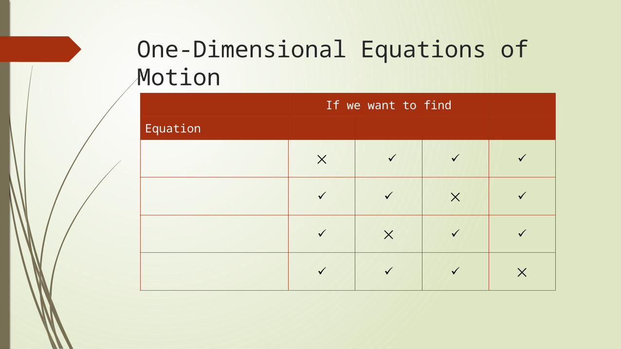
One-Dimensional Equations of Motion
If we want to find
Equation
✕ ✓ ✓ ✓
✓ ✓ ✕ ✓
✓ ✕ ✓ ✓
✓ ✓ ✓ ✕

Position with Constant Acceleration
0 10 20 30 40 50 600
1000
2000
3000
4000
5000
6000
7000
Time (s)
Posit
ion (
m)
Time (s)Position
(m)
0 0
10 250
20 1000
30 2250
40 4000
50 6250
Note that our equation of motion has the same form as the equation of a parabola . So the shape of the position vs. time graph for constant acceleration is that of a parabola.

Derived Velocity with Constant Acceleration
0 10 20 30 40 50 600
50
100
150
200
250
300
Time (s)
Velo
cit
y (
m/s
)
Time (s)Velocity
(m/s)
0 0
10 50
20 100
30 150
40 200
50 250
𝑠𝑙𝑜𝑝𝑒=200−10040−20
=10020
=5𝑚𝑠2
So from the position vs. time data we can determine the acceleration.

Displacement of an Object with Constant Acceleration
For an object moving at constant velocity , then .
So the area under a - graph is equal to the object’s displacement .
For this case .
Verify that you get the same answer using .
0 10 20 30 40 50 600
100
200
300
400
500
600
Time (s)V
elo
cit
y (
m/s
)
𝐴𝑟𝑒𝑎=𝐿×𝑊=50×300=15000
𝐴𝑟𝑒𝑎=12×𝐵×𝐻=
12×50×250=6250
Time (s) Velocity (m/s)
0 300
10 350
20 400
30 450
40 500
50 550

Constant Acceleration Graphical Example
Time (s) Position (m)0 500
10 80020 160030 290040 470050 7000
0 10 20 30 40 50 600
1000
2000
3000
4000
5000
6000
7000
8000
Time (s)
Posit
ion (
m)
0 10 20 30 40 50 600
50
100
150
200
250
300
Time (s)
Velo
cit
y (
m/s
)
Given
𝑑𝑓=𝑑𝑖+𝑣 𝑖 𝑡+12𝑎𝑡2
Time (s) Velocity (m/s)0 5
10 5520 10530 15540 20550 255
𝑣 𝑓=𝑣𝑖+𝑎𝑡
Note that the equation for has the same form as a parabola, i.e., and the equation for has the same form as a straight line, i.e., .

Activity
Linear Motion Simulation
For the case , calculate how much time it will take for the car to reach the 50m point. Then run the simulation with those values and see if your answer and the simulation agree. What is the car’s velocity when it reaches the 50m point?
For the case , calculate the position at which the car reverses direction. Then run the simulation with those values and see if your answer and the simulation agree. What does the shape of the position vs. time graph tell you about the acceleration?

An Example of Motion with Constant Acceleration—Free Fall
Gravity is an attractive force between any objects that have mass. We’ll look at gravitational forces in more detail later.
An object is in free fall when gravity is the only force acting on it to move it through space. (For now we’ll assume air resistance is negligible.)
Galileo performed experiments that led him to conclude that all objects in free fall had the same acceleration.
The acceleration due to gravity is given the symbol . It has a magnitude of and has a direction straight down (i.e., toward the center of the Earth.
Note that varies slightly with altitude and with one’s location on Earth. And we’ll see that the acceleration due to gravity is different away from the Earth’s surface.http://www.wolframalpha.com/widgets/view.jsp?id=d34e8683df527e3555153d979bcda9cf

Apollo 15 – Free Fall on the Moon (1971)
Apollo 15 Free Fall


Free Fall Example Problem 1
A stone is dropped into a well and is heard to hit the water 3.25s after being dropped. Determine the depth of the well.
Chose coordinate system so that at the top of the well; “up” is positive and “down” is negative.
Given: ;
Equation of motion:
𝑑𝑖=0
𝑑𝑓=?
+
-

Graphical Analysis 1
Time (s) Position (m)0.00 0.000.50 -1.231.00 -4.901.50 -11.032.00 -19.602.50 -30.633.00 -44.103.25 -51.76
Time (s) Velocity (m/s)0.00 0.000.50 -4.901.00 -9.801.50 -14.702.00 -19.602.50 -24.503.00 -29.403.25 -31.85
0.00 0.50 1.00 1.50 2.00 2.50 3.00 3.50
-60.00
-50.00
-40.00
-30.00
-20.00
-10.00
0.00
Time (s)
Posi
tion (
m)
0.00 0.50 1.00 1.50 2.00 2.50 3.00 3.50
-35.00
-30.00
-25.00
-20.00
-15.00
-10.00
-5.00
0.00
Time (s)V
elo
city
(m
/s)
𝑑𝑓=𝑑𝑖+𝑣 𝑖 𝑡+12𝑎𝑡2
𝑣 𝑓=𝑣𝑖+𝑎𝑡

Problem Solving Strategy
Draw a picture of the scenario and choose a coordinate system. The origin is usually the object’s initial position.
Choose which direction is the + direction, which is often the direction of initial motion.
Create a table or list of motion variables: Fill in the variables that are given (explicitly or
implicitly). Pick an equation that helps solve for the unknowns.

Simple Example
A car traveling on a straight road at 15 m/s accelerates uniformly to a speed of 21 m/s in 12 seconds. Find the total distance traveled by the car during this 12-second time interval.
𝑑𝑖 𝑑𝑓
Choose Given ,

Free Fall Example Problem 2
With what speed in mi/hr must an object be thrown to reach a maximum height of 100m?
Choose ; Given ;
Equation of motion:
Substitute:
How long after it reaches its maximum height will it take the object to fall back to its original position? What will its velocity be at that point?
𝑑𝑖
𝑑𝑓
+

Graphical Analysis 2
𝑑𝑓=𝑑𝑖+𝑣 𝑖 𝑡+12𝑎𝑡2
𝑣 𝑗=𝑣𝑖+𝑎𝑡
0.00 0.50 1.00 1.50 2.00 2.50 3.00 3.50 4.00 4.50 5.000.00
20.00
40.00
60.00
80.00
100.00
120.00
Time (s)
Posi
tion (
m)
0.00 0.50 1.00 1.50 2.00 2.50 3.00 3.50 4.00 4.50 5.000
5
10
15
20
25
30
35
40
45
50
Time (s)
Velo
city
(m
/s)

Example Problems 103. A spaceship far from any star or planet experiences a uniform
acceleration from 65.0 m/s to 162.0 m/s in 10 s. How far does it move?
110. Rocket-powered sleds are used to test the responses of humans to acceleration. Starting from rest, one sled can reach a speed of 444 m/s in 1.80 s and can be brought to a stop in again in 2.15 s.
Calculate the acceleration of the sled when starting and compare it with the magnitude of g.
Calculate the acceleration of the sled when braking and compare it with the magnitude of g.
115. A helicopter is rising at 5.0 m/s when a bag of its cargo is dropped. The bag falls for 2.o s.
What is the bag’s velocity?
How far has the bag fallen?
How far below the helicopter is the bag?Rocket sled video

Measuring Reaction Time Using Free Fall

One student holds the ruler vertically. The second student positions his/her fingers around the ruler at the bottom end of the ruler. The first student drops the ruler and the second student snaps his/her fingers shut as soon as the ruler is released. The reaction time can be determined from the following, where is the distance the ruler fell:
if is measured in cm.𝑑

Human Reaction Time
Human reaction time ranges from 0.1 to 0.5 seconds with a median around 0.215s