Clemson UniversityTigerPrints

All Dissertations Dissertations

12-2011

Accelerating Pattern Recognition Algorithms OnParallel Computing ArchitecturesKenneth RiceClemson University, krice@clemson.edu

Follow this and additional works at: https://tigerprints.clemson.edu/all_dissertations

Part of the Computer Engineering Commons

This Dissertation is brought to you for free and open access by the Dissertations at TigerPrints. It has been accepted for inclusion in All Dissertations byan authorized administrator of TigerPrints. For more information, please contact kokeefe@clemson.edu.

Recommended CitationRice, Kenneth, "Accelerating Pattern Recognition Algorithms On Parallel Computing Architectures" (2011). All Dissertations. 879.https://tigerprints.clemson.edu/all_dissertations/879

Accelerating Pattern Recognition Algorithms OnParallel Computing Architectures

A Dissertation

Presented to

the Graduate School of

Clemson University

In Partial Fulfillment

of the Requirements for the Degree

Doctor of Philosophy

Computer Engineering

by

Kenneth Lee Rice

December 2011

Accepted by:

Dr. John N. Gowdy, Committee Chair

Dr. Tarek M. Taha, Thesis Advisor

Dr. Damon L. Woodard

Dr. Stanley T. Birchfield

Dr. Walter B. Ligon III

Abstract

The move to more parallel computing architectures places more responsibility on the

programmer to achieve greater performance. The programmer must now have a greater un-

derstanding of the underlying architecture and the inherent algorithmic parallelism. Using

parallel computing architectures for exploiting algorithmic parallelism can be a complex

task. This dissertation demonstrates various techniques for using parallel computing ar-

chitectures to exploit algorithmic parallelism. Specifically, three pattern recognition (PR)

approaches are examined for acceleration across multiple parallel computing architectures,

namely field programmable gate arrays (FPGAs) and general purpose graphical processing

units (GPGPUs).

Phase-only filter correlation for fingerprint identification was studied as the first PR

approach. This approach’s sensitivity to angular rotations, scaling, and missing data was

surveyed. Additionally, a novel FPGA implementation of this algorithm was created using

fixed point computations, deep pipelining, and four computation phases. Communication

and computation were overlapped to efficiently process large fingerprint galleries. The

FPGA implementation showed approximately a 47 times speedup over a central processing

unit (CPU) implementation with negligible impact on precision.

For the second PR approach, a spiking neural network (SNN) algorithm for a char-

acter recognition application was examined. A novel FPGA implementation of the approach

was developed incorporating a scalable modular SNN processing element (PE) to efficiently

ii

perform neural computations. The modular SNN PE incorporated streaming memory, fixed

point computation, and deep pipelining. This design showed speedups of approximately 3.3

and 8.5 times over CPU implementations for 624 and 9,264 sized neural networks, respec-

tively. Results indicate that the PE design could scale to process larger sized networks

easily.

Finally for the third PR approach, cellular simultaneous recurrent networks (CSRNs)

were investigated for GPGPU acceleration. Particularly, the applications of maze traversal

and face recognition were studied. Novel GPGPU implementations were developed employ-

ing varying quantities of task-level, data-level, and instruction-level parallelism to achieve

efficient runtime performance. Furthermore, the performance of the face recognition appli-

cation was examined across a heterogeneous cluster of multi-core and GPGPU architectures.

A combination of multi-core processors and GPGPUs achieved roughly a 996 times speedup

over a single-core CPU implementation.

From examining these PR approaches for acceleration, this dissertation presents

useful techniques and insight applicable to other algorithms to improve performance when

designing a parallel implementation.

iii

Dedication

I am a man of humble beginnings. At an early age, I had a dream for myself.

During a time where my academic success did not reflect my dream, I knew I was capable

of achieving more, and I became convinced that one day I would. From that point forward,

I took the necessary steps to systematically improve my scholastic success. It was not an

easy transition. Along the way, there were many trials and tribulations. There were many

instances where I had to learn life lessons and gain invaluable experience. Along the way,

I met many influential people who dispensed vast knowledge to me. This knowledge will

continue to guide me moving forward.

Ultimately, I view this work as the culmination of the journey, the fulfillment of

my dream. Therefore, I dedicate this work to the time, effort, hard work, and persistence

that I committed to while achieving my dream. Additionally, I dedicate this work to the

people who supported me the most along the way, my parents Willie Lewis and Debra. To

my siblings Adrienne, Tyson, Jeffrey, and Stephanie, the ones who contributed immensely

to shaping my character. To my nephews Tykeyvious and Tyrese, the young ones whom

I inspire. To my friends Gerren, Anthony, Shayah, and David, the people who helped me

significantly during my journey. Lastly, I dedicate this work to my late great aunt Clara

and my late grandfather Willie Henry, the two people who showed me what the true value

of a person is measured by: the positive impact and influence they have on the ones they

leave behind.

iv

Acknowledgments

I want to acknowledgment the support I received during this work. Specifically, I

want to thank Dr. Tarek Taha. Without his help, vision, and mentorship, I would not have

completed this work. Also, I want to thank Dr. John Gowdy for supervising me through the

completion of my program. I want to thank the members of my dissertation committee (Dr.

Damon Woodard, Dr. Stanley Birchfield, and Dr. Walter Ligon) for their input. Especially,

I want to thank Dr. Woodard for adding another source of mentorship. Additionally, I

want to give a very special thanks to Dr. John Komo for providing me with immeasurable

wisdom, guidance, and professionalism during my time in graduate school.

This work was supported by grants from the Air Force Research Laboratory (in-

cluding the Information Directorate), a National Science Foundation CAREER award, and

a grant of computer time from the Department of Defense High Performance Computing

Modernization Program at the Naval Research Laboratory. Therefore, I want to thank those

funding agencies and grants. Additionally, I want to thank the Air Force Research Labora-

tory and Lawrence Livermore National Laboratory for providing access to their equipment

and/or data that supported this work. Along with them, I want to thank Dr. Daniel

Noneaker and Dr. Frankie Felder for financially supporting me during my time in graduate

school.

Lastly, I want to thank all of my collaborators who helped me in some form through-

out the years conducting research on my various projects. Among those, special thanks goes

v

to Dr. Abdul Awwal, Sumod Mohan, Pavan Yalamanchilli, Rommel Jalasutram, Christo-

pher Vutinas, Richard Leech, Michael Hutt, Dr. Ronald Miller, and Dr. Khan Iftekharuddin.

vi

Table of Contents

Title Page . . . . . . . . . . . . . . . . . . . . . . . . . . . . . . . . . . . . . . . i

Abstract . . . . . . . . . . . . . . . . . . . . . . . . . . . . . . . . . . . . . . . . ii

Dedication . . . . . . . . . . . . . . . . . . . . . . . . . . . . . . . . . . . . . . . iv

Acknowledgments . . . . . . . . . . . . . . . . . . . . . . . . . . . . . . . . . . v

List of Tables . . . . . . . . . . . . . . . . . . . . . . . . . . . . . . . . . . . . . ix

List of Figures . . . . . . . . . . . . . . . . . . . . . . . . . . . . . . . . . . . . . x

1 Introduction . . . . . . . . . . . . . . . . . . . . . . . . . . . . . . . . . . . . 11.1 Parallel computing architectures . . . . . . . . . . . . . . . . . . . . . . . . 21.2 Dissertation overview . . . . . . . . . . . . . . . . . . . . . . . . . . . . . . . 81.3 Contributions and outline . . . . . . . . . . . . . . . . . . . . . . . . . . . . 11

2 Phase-only Filter Based Optical Pattern Recognition for FingerprintIdentification . . . . . . . . . . . . . . . . . . . . . . . . . . . . . . . . . . . . 132.1 Introduction . . . . . . . . . . . . . . . . . . . . . . . . . . . . . . . . . . . . 132.2 Phase-only filter . . . . . . . . . . . . . . . . . . . . . . . . . . . . . . . . . 152.3 Distortion invariant recognition . . . . . . . . . . . . . . . . . . . . . . . . . 172.4 Hardware acceleration . . . . . . . . . . . . . . . . . . . . . . . . . . . . . . 282.5 Hardware performance . . . . . . . . . . . . . . . . . . . . . . . . . . . . . . 352.6 Summary . . . . . . . . . . . . . . . . . . . . . . . . . . . . . . . . . . . . . 40

3 Izhikevich Spiking Neural Networks for Character Recognition . . . . . 423.1 Introduction . . . . . . . . . . . . . . . . . . . . . . . . . . . . . . . . . . . . 423.2 Background . . . . . . . . . . . . . . . . . . . . . . . . . . . . . . . . . . . . 443.3 Character recognition algorithm . . . . . . . . . . . . . . . . . . . . . . . . . 463.4 Hardware implementation . . . . . . . . . . . . . . . . . . . . . . . . . . . . 493.5 Experimental setup . . . . . . . . . . . . . . . . . . . . . . . . . . . . . . . . 553.6 Results . . . . . . . . . . . . . . . . . . . . . . . . . . . . . . . . . . . . . . . 563.7 Summary . . . . . . . . . . . . . . . . . . . . . . . . . . . . . . . . . . . . . 57

4 Pattern Recognition Using Cellular Simultaneous Recurrent Networks 594.1 Introduction . . . . . . . . . . . . . . . . . . . . . . . . . . . . . . . . . . . . 59

vii

4.2 Background . . . . . . . . . . . . . . . . . . . . . . . . . . . . . . . . . . . . 614.3 High performance implementation . . . . . . . . . . . . . . . . . . . . . . . 714.4 Results . . . . . . . . . . . . . . . . . . . . . . . . . . . . . . . . . . . . . . . 774.5 Summary . . . . . . . . . . . . . . . . . . . . . . . . . . . . . . . . . . . . . 96

5 Conclusions . . . . . . . . . . . . . . . . . . . . . . . . . . . . . . . . . . . . 985.1 Performance summary . . . . . . . . . . . . . . . . . . . . . . . . . . . . . . 1015.2 Future work . . . . . . . . . . . . . . . . . . . . . . . . . . . . . . . . . . . . 103

A Neuron Model Parameters . . . . . . . . . . . . . . . . . . . . . . . . . . . 105

References . . . . . . . . . . . . . . . . . . . . . . . . . . . . . . . . . . . . . . . 106

viii

List of Tables

2.1 FPGA and software C implementations tested. . . . . . . . . . . . . . . . . 362.2 Sample fingerprint points of maximum correlation peak. . . . . . . . . . . . 372.3 Evaluation of FPGA with rotated images using sample 76. . . . . . . . . . . 382.4 Evaluation of FPGA with scaled images using sample 16. . . . . . . . . . . 392.5 Evaluation of FPGA with missing data images using sample 55. . . . . . . . 40

3.1 Structure of neural networks examined . . . . . . . . . . . . . . . . . . . . . 563.2 Device logic utilization. . . . . . . . . . . . . . . . . . . . . . . . . . . . . . 563.3 Hardware-accelerated timing breakdown. . . . . . . . . . . . . . . . . . . . . 573.4 Performance measures. . . . . . . . . . . . . . . . . . . . . . . . . . . . . . . 57

4.1 NVIDIA GPGPU composition for Tesla GPGPUs. . . . . . . . . . . . . . . 764.2 Timing breakdown for computation stages of GPGPU design. . . . . . . . . 794.3 Training times for increasing number of people. . . . . . . . . . . . . . . . . 844.4 Training times for increasing the number of PCA components. . . . . . . . 854.5 Training times for increasing number of samples per face sequence. . . . . . 864.6 Speedup comparison using the runtimes shown in Table 4.5. . . . . . . . . . 864.7 Training times using an increasing number of face sequences. . . . . . . . . 884.8 Speedup comparison using runtimes shown in Table 4.7. . . . . . . . . . . . 884.9 Training runtime performance for multi-core and multi-GPGPU. . . . . . . 91

5.1 Summary of acceleration performance. . . . . . . . . . . . . . . . . . . . . . 101

ix

List of Figures

1.1 The general structure of an FPGA . . . . . . . . . . . . . . . . . . . . . . . 51.2 General structure of a CUDA enabled GPGPU. . . . . . . . . . . . . . . . . 71.3 Parallelism division within CUDA enabled GPGPUs. . . . . . . . . . . . . . 8

2.1 A simple optical pattern recognition setup. . . . . . . . . . . . . . . . . . . 162.2 Correlation peak plot for sample six against a 100 sample gallery. . . . . . . 182.3 Several fingerprint images of the same finger (sample six) used as input. . . 192.4 Correlation peak vs. sample number. . . . . . . . . . . . . . . . . . . . . . . 192.5 Correlation peak vs. degree of rotation for sample 76. . . . . . . . . . . . . 202.6 Correlation peak vs. sample number for each degree of rotation. . . . . . . . 212.7 ROC curve for the sensitivity to rotation examination. . . . . . . . . . . . . 222.8 Correlation peak vs. scaling factor. . . . . . . . . . . . . . . . . . . . . . . . 232.9 Correlation peak vs. sample number for various scaling factors. . . . . . . . 242.10 ROC curve for the sensitivity to scaling examination. . . . . . . . . . . . . . 252.11 Example of input images with missing data. . . . . . . . . . . . . . . . . . . 262.12 Variation of correlation peak with respect to percentage of missing data. . . 272.13 Correlation peak vs. sample number for various missing data percentages. . 272.14 ROC curve for the sensitivity to missing data examination. . . . . . . . . . 282.15 Block diagram of the FPGA operations. . . . . . . . . . . . . . . . . . . . . 292.16 Diagram showing phase execution schedule. . . . . . . . . . . . . . . . . . . 312.17 Block diagram of the overall network. . . . . . . . . . . . . . . . . . . . . . 332.18 Fingerprint samples used to evaluate FPGA error rates. . . . . . . . . . . . 36

3.1 Spikes produced with Izhikevich model. . . . . . . . . . . . . . . . . . . . . 463.2 Training images. . . . . . . . . . . . . . . . . . . . . . . . . . . . . . . . . . 473.3 Illustration of network connections between level 1 and level 2 neurons. . . 483.4 Overall spiking neural network design on Cray XD1. . . . . . . . . . . . . . 503.5 Dataflow diagram for the SNN PE 23 stage pipeline design. . . . . . . . . . 523.6 State machine for spiking neural network controller. . . . . . . . . . . . . . 54

4.1 CSRN structure and composition. . . . . . . . . . . . . . . . . . . . . . . . . 634.2 Two layer GMLP network. . . . . . . . . . . . . . . . . . . . . . . . . . . . 644.3 Example of maze traversal problem. . . . . . . . . . . . . . . . . . . . . . . 654.4 Example of face rotation. . . . . . . . . . . . . . . . . . . . . . . . . . . . . 664.5 Training with a single person. . . . . . . . . . . . . . . . . . . . . . . . . . . 674.6 Training with multiple people. . . . . . . . . . . . . . . . . . . . . . . . . . . 684.7 CSRN network for face recognition. . . . . . . . . . . . . . . . . . . . . . . . 68

x

4.8 Gauss-Jordan elimination matrix inversion. . . . . . . . . . . . . . . . . . . 734.9 Flow chart for GPGPU CSRN mapping for MSEKF training. . . . . . . . . 744.10 System arrangement of the primary and associated secondary processes. . . 764.11 Maze traversal CPU vs. GPGPU training runtimes. . . . . . . . . . . . . . . 784.12 Maze traversal CPU vs. GPGPU testing runtimes. . . . . . . . . . . . . . . 784.13 CPU vs. GPGPU with extensions training runtimes. . . . . . . . . . . . . . 814.14 Graph of training time for multi-core and multi-GPGPU implementations. . 904.15 Graph of speedup for multi-core and multi-GPGPU implementations. . . . 914.16 Graph showing varying number of samples per face sequence. . . . . . . . . 944.17 Speedup graph for varying the number of samples per face sequence. . . . . 944.18 Graph of varying the number of face sequences. . . . . . . . . . . . . . . . . 954.19 Speedup graph for varying the number of face sequences. . . . . . . . . . . . 96

xi

Chapter 1

Introduction

Pattern recognition (PR) is a field of science that involves finding regularities in

data through the use of computer algorithms and using the discovered regularities to take

actions, such as classifying data into different categories [1]. PR’s importance is due to its

ability to establish relationships within data to perform very interesting and useful tasks.

Some of these tasks include applications in face detection and tracking, speech recognition,

fingerprint identification, medical diagnosis, machine vision, character recognition, financial

engineering, bioinformatics, geographical information processing, and text analysis.

Computational speed is a bottleneck in the development of PR applications. As

a result, some PR algorithms have an overwhelming computational intensity to be useful

in practical applications. In the past, chip designers were able to improve performance

by increasing a processor’s clock frequency. Eventually, issues regarding heat management

emerged. Finding efficient ways to dissipate heat became so problematic that further ac-

celeration of the system by frequency-scaling became impractical.

Along with combating rising heat concerns, other issues regarding higher frequency

affected processor design. When a processor operates at a higher frequency, the time avail-

able to do meaningful work per cycle along with the time for signals to traverse the width

of the chip decreases [2]. Therefore, additional cycles are required to allow signals to do

meaningful processing and/or propagate across the chip. Subsequently, performance gains

are pursued by performing more in parallel as opposed to serially, leading to current incor-

1

poration of parallel computing designs.

In recent times, the move to parallel computing represents an industry wide shift

to reduce power consumption while improving performance. Along with multi-core designs,

other parallel architectures have come into prominence to increase performance. The use

of general purpose graphical processing units (GPGPUs) found its way into high perfor-

mance computing. Also, unconventional heterogeneous computing architectures, such as

the IBM/Sony/Toshiba Cell broadband engine, and parallel platforms which blur the line

between hardware and software, such as field programmable gate arrays (FPGAs), are being

utilized for high performance computing. Given the inherent parallelism in many PR algo-

rithms, utilizing the advantages offered by parallel computing would be ideal for extracting

speed.

Unfortunately, gaining performance by exploiting parallel architectures can be a

complex task. With more control given to developers, obtaining greater performance implies

a deeper understanding of the underlying architecture as well as the inherent parallelism

present in the algorithm. The next section offers an overview of parallel computing archi-

tectures followed by an overview of the work presented in this thesis. Finally, the specific

contributions and the outline of this work are highlighted.

1.1 Parallel computing architectures

There are various types of parallel architectures available. These different archi-

tectures incorporate different physical arrangements such as tile, execution models such as

dataflow, and different memory structures such as cache mapped. Also, the architectures

vary in size, throughput, cache, power, and speed. This section gives an overview of select

parallel computing architectures as a survey of the work that has been performed in the

field.

Perhaps the forefather to modern multi-core designs is the Raw microprocessor [3].

In [4], the Raw microprocessor is evaluated for various tasks. The Raw microprocessor is a

2

tiled architecture that has 16 processor tiles. The processor tiles are designed to be one clock

cycle in wire propagation width, including the interior combinational logic. The authors

compare the performance of the Raw microprocessor to a 600 MHz Pentium III processor

using similar implementation parameters. They test for instruction level parallelism (ILP)

and stream application performance. Raw outperforms the Pentium III with programs in

both ILP and stream applications.

In [5], Baas et al. describe an asynchronous array of simple processors, better known

as AsAP. AsAP is a many-core system that uses task level parallelism and fine grained

processing elements to take advantage of the workload parallelism seen in digital signal

processing (DSP) applications. AsAP processors uses single-issue 64-word×32-bit instruc-

tion memory, 128-word×16-bit data memory, 16-bit arithmetic logic units (ALUs), 16×16

multipliers with a 40-bit accumulator, and four programmable address-generators. Each

processor use 54 general instructions and is globally asynchronous, locally synchronous

(GALS). Also, each processor is clocked externally by a single oscillator and has an in-

dependent internal oscillator. AsAP requires less than 1% of processor area which lowers

power consumption.

Pericas et al. [6] discuss FMC, a flexible heterogeneous multi-core processor. The

design of FMC executes single to many thread applications for high performance. This

is due to the architecture using a dynamic instruction window size along with multi-scan

execution. From this work, Pericas et al. show that their FMC design improves an ap-

plication’s floating point performance by 53% over next generation superscalar processors

and 12% over previous large instruction window designs. With integer computations, the

Pericas et al. design offers a 9% speedup over an out-of-order processor with a 256-entry

instruction window.

Zhong et al. [7] describe the Voltron architecture. By having two modes of operation,

the Voltron architecture takes advantage of instruction level and fine-grain thread level

parallelism to increase performance. In the first mode of operation, the architecture’s core

operates in lock-step creating a wide-issue very long instruction word (VLIW) processor to

3

exploit instruction level parallelism. In the second mode, the cores operate individually on

separate fine-grain threads to exploit fine-grain thread level parallelism. Zhong et al. show

that their Voltron architecture achieves a 1.46 times performance gain using a dual-core

system and 1.83 times performance gain using a quad-core system over a single-core design.

In [8], Sankaralingam et al. describe a prototype tiled architecture called TRIPS.

This architecture is a dataflow processor of tiles, where each tile is composed of one global

control tile, 16 execution tiles, four register tiles, four data tiles, and five instruction tiles

labeled GT , ET , RT , DT , and IT , respectively. The tiles can communicate in nearest

neighbor fashion while having a variety of different networks interconnecting them. Sankar-

alingam et al. describe the control protocols of this architecture and test its performance

against a clustered uniprocessor system. The TRIPS architecture shows a lot of promise.

Lastly in [9], Kapasi et al. describe Imagine, a stream processor, which exploits

data-level parallelism. Imagine is designed as a coprocessor to a general purpose processor

which would control the former by sending streaming commands. Within Imagine, there are

48 arithmetic logic units (ALUs) equally distributed into eight clusters. Kapasi et al. found

that this architecture achieves up to a sustainable 15 giga operations per second (GOPS)

for a variety of applications tested. They use KernelC and StreamC to compile code used

by the Imagine architecture.

1.1.1 FPGAs and GPGPUs

In this dissertation, FPGAs and GPGPUs were examined predominately for accel-

erated designs. Thus, this section gives an overview of FPGA and GPGPU operation and

briefly mentions their benefits in parallel computing.

1.1.1.1 FPGA overview

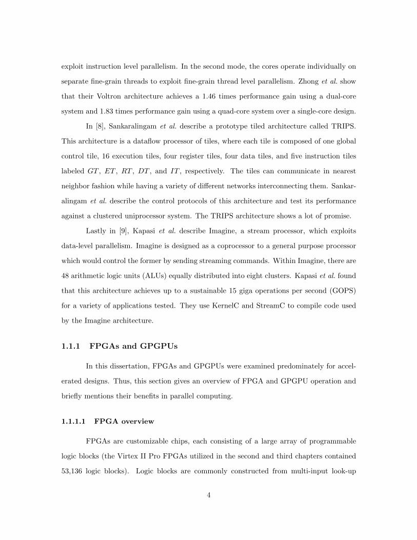
FPGAs are customizable chips, each consisting of a large array of programmable

logic blocks (the Virtex II Pro FPGAs utilized in the second and third chapters contained

53,136 logic blocks). Logic blocks are commonly constructed from multi-input look-up

4

LUT Flip‐Flop

Input 1

Input 2

Input N

Clock

Selector

Output

Multiplexer

ProgrammableInterconnects

Logic Block

Input/OutputBlocks

Figure 1.1: The general structure of an FPGA. This consists of logic and I/O blocks con-nected via programmable interconnects. Additionally, the internal structure of a logic blockis shown.

tables (LUTs) connected to flip-flops and possibly other memory elements. The LUTs

operate as truth tables and are responsible for implementing the functionality within the

logic blocks. The output of a logic block is generally selected from multiple values using a

multiplexer. Additionally, logic and input/output (I/O) blocks are all connected together

using an intricate array of programmable interconnections. Any operation can typically be

implemented efficiently through a combination of such logic blocks. Figure 1.1 shows an

example of the internal structure of an FPGA.

FPGAs are programmed using a hardware description language (HDL) such as Ver-

ilog or VHDL. HDLs are used to describe the behavior of a process as a custom hardware

circuit. After describing the process in HDL, FPGA specific software will perform various

analyses of the HDL description before mapping it to an FPGA. Finally, a bit file is gener-

5

ated. A bit file is the set of instructions that allocate an FPGA’s resources to implement a

process.

Algorithms with large amounts of parallelism can have their different components

mapped onto separate areas in an FPGA. Thus, an FPGA can implement multiple algorithm

components in parallel. In a processor, these different components would be evaluated seri-

ally, with each component being represented by a long sequential list of simple instructions.

Therefore, even though FPGAs operate at lower frequencies than processors (MHz versus

GHz), high spatial parallelism and the efficient hardware implementations allow FPGAs to

implement many algorithms faster than processors.

One of the main hurdles with using FPGAs is that programming them is signifi-

cantly more complex than programming general purpose processors. This is mainly because

algorithms have to be analyzed carefully to determine the different components that can

be evaluated in parallel. Additionally, each component needs to be mapped individually

onto the programmable logic blocks. Fortunately, the mappings for several standard opera-

tions (such as multiplication) are provided by FPGA vendors, thus reducing overall FPGA

programming time.

1.1.1.2 GPGPU overview

GPGPUs are quickly emerging as a premier acceleration platform. This is because

of the low learning curve for software developers. This leads to a reduced development

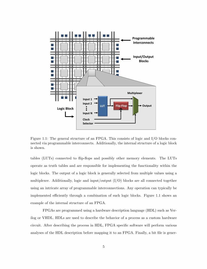
cycle when compared to other acceleration platforms such as FPGAs. Figure 1.2 shows

the general structure of a compute unified device architecture (CUDA) enabled GPGPU.

CUDA is a parallel computing architecture C programming language extension used to

program GPGPUs. CUDA enabled GPGPUs are composed of multiple scalar processors

(SPs) grouped together to form streaming multiprocessors (SMs). These SMs contain their

own shared memory, cache, multi-threaded instruction unit (MTI), and special functional

units (SFUs). All SMs have access to the same global memory.

Parallel execution using GPGPUs is accomplished by dividing a task among three

6

SM SM SM

MTI

Cache

SP

SP SP

SP

SFU SFU

SharedMemory

Global Memory

MTI

Cache

SP

SP SP

SP

SFU SFU

SharedMemory

MTI

Cache

SP

SP SP

SP

SFU SFU

SharedMemory

Figure 1.2: General structure of a CUDA enabled GPGPU.

types of operation: threads, thread blocks, and grids. Figure 1.3 illustrates how threads,

thread blocks, and grids are related to one another. GPGPU threads are lightweight ex-

ecution directives that can operate concurrently and have access to their own dedicated

local memory. A thread block is composed of a collection of threads operating on a code

sequence. Execution within a thread block occurs in batches of 16 threads where each

batch is referred to by the CUDA nomenclature as a half-warp. Furthermore, groups of two

batches, or 32 threads, are referred to as warps. When processing branching instructions,

threads belonging to different warps can branch and work on different code segments with-

out inhibition. However, the branching instructions of intra warp threads are performed

sequentially. A thread block can process up to eight different warps simultaneously. Lastly,

a thread block has its own dedicated shared memory.

A grid consists of a group of thread blocks. While grids do not have their own

local memories, they are able to access global memory. Grids are mapped over SMs, where

each SM is capable of processing several simultaneous thread blocks. Each thread block

7

Grid

Thread Thread Block

LocalMemory

SharedMemory

Global Memory

Figure 1.3: Parallelism division within CUDA enabled GPGPUs. This figure shows thecomposition and memory access of threads, thread blocks, and grids.

is capable of performing the execution for up to 1,024 active threads (or 512 for older

generation GPGPUs).

GPGPUs work on the principle of divide and conquer. In order to achieve the best

speedup performance possible, an application’s processing should be distributed within the

GPGPU among thousands of lightweight threads. Among various GPGPU applications,

memory access has been shown to be a bottleneck in the designs [10]. Therefore, GPGPUs

are more geared towards applications which have high compute-to-memory access ratios.

1.2 Dissertation overview

This dissertation explores the added benefits of using parallel computing architec-

tures to improve the runtime performance of PR applications. Different PR approaches

were examined with the performance benefits achieved by parallel systems to accelerate

them identified. While the first approach is a traditional PR algorithm, the second and

third approaches are biologically inspired algorithms.

Gaining momentum in the research community is the use of biologically inspired

8

approaches to solve PR problems. This follows from the efficiency in which the mammalian

brain performs PR tasks. The mammalian brain is a highly parallel structure that is fairly

homogeneous and composed of similar elements performing uniform processing [11]. The

sheer volume of parallelism in the mammalian brain is one of the key factors attributed to

enabling it to efficiently perform PR tasks. Researchers want to investigate combining this

parallelism with biologically inspired approaches to achieve similar levels of computational

efficiency as the mammalian brain when performing PR tasks. Therefore, large scale biolog-

ical inspired approaches adapted to PR have garnered great interest. Hence, the accelerated

implementations of the second and third approaches were examined to study their ability

to support large scale implementation.

The acceleration of the approaches is investigated using FPGAs for the first two

approaches and GPGPUs for the third. The first PR approach considered phase-only filter

based correlation for fingerprint pattern identification. In a previous work [12], a similar

correlation approach was utilized to examine the acceleration of a laser beam automatic

alignment algorithm. In [12], a novel Xilinx Virtex II Pro FPGA hardware acceleration

implementation of the automatic alignment algorithm’s correlation approach was developed

and achieved a speed increase of about 253 times over a software implementation. Based

on those results, the correlation approach given in [12] motivated the similar approach used

in this work towards fingerprints.

In this work, the main advantage of the phase-only filter based correlation approach

is that it is distortion tolerant and can be realized in optical or electronic parallel hardware.

Given that real world fingerprints are almost never perfect, distortion tolerance can prove

to be very important for this application. With large fingerprint databases, identification

can be a computationally challenging task. The high parallelism in phase-only filter cor-

relation makes this approach ideally suited to FPGA based hardware acceleration. From

that observation, a Xilinx Virtex II Pro FPGA system was employed to achieve notable im-

proved performance over a C implementation of the algorithm on a 2.2 GHz AMD Opteron

processor.

9

The second PR approach explored the feasibility of using FPGAs for large scale

simulations of the Izhikevich model. This work deals with the development of a modularized

processing element to evaluate a large number of Izhikevich spiking neurons in a pipelined

manner. This approach allows for easy scalability of the model to larger FPGAs.

Lastly, the third PR approach examined the acceleration of the cellular simulta-

neous recurrent networks (CSRNs) based pattern recognition, utilizing an NVIDIA Tesla

C2050 GPGPU coupled with a 2.67 GHz X5650 Intel Xeon multi-core processor. Using this

approach, two specific applications were examined for acceleration: maze traversals and

face recognition. For CSRN based maze traversal, several novel accelerated CSRN GPGPU

implementations were created for both the training and testing phases of operation. Ad-

ditionally, the use of several performance enhancing techniques to help improve GPGPU

CSRN computation were explored.

For CSRN based face recognition, only the training phase was examined. Several

parameters within the GPGPU implementation design were varied and compared to an

equivalent C programming language version compiled to take advantage of single instruc-

tion, multiple data (SIMD) commands. Large scale multi-core, multi-GPGPU, and multi-

core/GPGPU versions of CSRN based face recognition were created. The multi-core, multi-

GPGPU, and multi-core/GPGPU designs were tested on a newly established hybrid cluster

consisting of 78 Intel multi-core processors, 156 NVIDIA GPGPUs, and 1,716 PlayStation

3 consoles. While the acceleration performance of all systems improved linearly with the

addition of more resources, the performance benefit for using the same number of resources

is far greater for the implementations incorporating the use of GPGPUs. Given that there

are more cores than GPGPUs available, the implementations incorporating multi-cores scale

better on the cluster.

The acceleration study of these applications demonstrated the improvement to run-

time performance possible using parallel systems in multiple PR domains. Novel parallel

system implementations were created for each, and the analysis of their contribution to

overall runtime performance was performed. Additionally, this dissertation explored large

10

scale implementations of the CSRN biologically inspired approach using a heterogeneous

compute cluster. Finally, a discussion about common acceleration trends supported by the

three approaches concludes this work.

1.3 Contributions and outline

The following is an outline of the main contributions made in this dissertation.

• In the second chapter, phase-only filter correlation for fingerprint pattern identification

is discussed.

a) Evaluated algorithm performance under multiple distortions:

– Angular rotations, scaling, and missing data

b) Developed a novel FPGA implementation of this algorithm:

– Utilized fixed point computations, deep pipelines, and four computation

phases

– Overlapped computation and communication to efficiently process large gal-

leries

– Demonstrated negligible impact on precision using fixed point computations

– Achieved roughly 47 times performance speedup over an C implementation

• The third chapter studies the acceleration of Izhikevich SNN for character recognition.

a) Developed a novel FPGA implementation of the algorithm:

– Incorporated a scalable modular SNN processing element design for efficient

processing

– Utilized streaming memory, fixed point computations, and deep pipelines

– Achieved speedups of approximately 3.3 and 8.5 times over C implementa-

tions for 624 and 9,264 sized neuron network, respectively

– Portable design to perform larger sized networks using different FPGAs

11

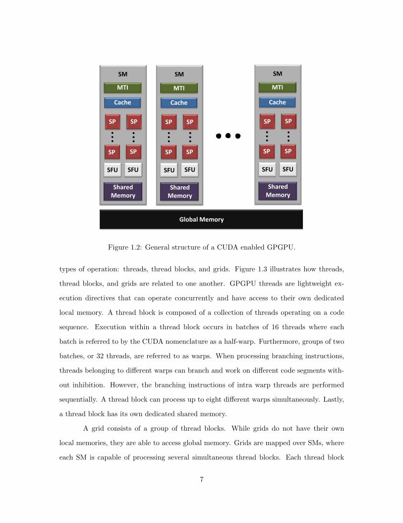
• CSRN based pattern recognition is explored in chapter four.

a) Developed novel CSRN GPGPU design for maze traversal:

– Used task-level and thread-level parallelism in addition to concurrent execu-

tion in design

– Explored methods to improve GPGPU matrix inversion within design

– Achieved average speedups of approximately 7.2 and 3.5 times, respectively,

for training and testing over a C implementation

b) Extended CSRN GPGPU design to face recognition application:

– Improved GPGPU thread occupancy and reduced global memory transac-

tions of design

– Evaluated design to demonstrate speedups greater than five times over a C

implementation for multiple algorithmic parameters

c) Scaled CSRN based face recognition designs to heterogeneous compute cluster:

– Exploited additional parallelism in design by porting it to heterogeneous

compute cluster

– Implemented a master-slave control scheme for design

– Evaluated speedup and scaling performance for systems using multi-core,

multi-GPGPU, and multi-core/GPGPU

– Demonstrated that multi-core/GPGPU system was capable of approximately

996 times speedup over a single-core C implementation

Finally, chapter five offers some closing remarks to conclude this work.

12

Chapter 2

Phase-only Filter Based Optical Pattern

Recognition for Fingerprint Identification

2.1 Introduction

Fingerprint based identification is utilized in a variety of tasks ranging from his-

torical [13] to modern commerce and security [14]. The unique and invariant nature of

fingerprints has led to several automatic approaches for their classification [15, 16]. In

classical approaches to fingerprint identification, such as structural [17, 18, 19], statistical

[20, 21], syntactical [22], and neural network methods [23], the classification of fingerprints

is accomplished by using local or global feature extraction. These approaches have various

shortcomings, such as processing speeds, higher power requirements, sensitivity to noise,

complexity in grammar rules, and complicated neural nets. One of the trends in fingerprint

identification is motivated by the application of optical filters and correlation to achieve

high processing speed and low power requirements. Fitz and Green [24] used hexagonal fast

Fourier transforms to classify fingerprints into whorls, loops and arches. The joint transform

correlator (JTC) to identify fingerprints was used by Fielding et al. [25] as a binary JTC,

by Rodolfo et al. [26] as a photorefractive JTC, and by Alam et al. [27] as a polarization

and fringe-adjusted JTC.

In real world applications, some of the major problems with fingerprint data are

13

that they get distorted or have portions missing when collected [28]. This distortion of

fingerprint data is usually generated from the image rotation and pressure variation of a

finger on the object where the finger is imprinted. In addition, recently developed charge-

coupled device sensors may only capture a partial fingerprint [29]. Consequently, the real

challenge is whether those distorted images are recognizable or not. Although numerous

methods of fingerprint identification have been established, none of them can completely

recognize a distorted fingerprint.

The performance of pattern recognition systems is influenced by two phenomena that

may contribute to the success or failure of these systems. The first is the affine transform

that may cause an image to change shape, simply because of the change in the observation

angle of the sensor gathering information. A second influence comes from the clutter present

in the scene. A human observer may recognize an object from a different point of view, but

clutter poses a real challenge to even a human. A phase-only filter, a variation of classical

matched filter (CMF), performs an edge enhancement on the picture and tries to match the

structure using more than the actual gray levels; thus it has the ability to see through the

clutter and match against the edges of the object.

In this chapter, first a phase-only filter based fingerprint identification approach

is presented. Tests conducted demonstrate that fingerprint identification using optically-

inspired correlator based phase-only filters [30, 31] can overcome problems of missing data or

limited distortions (such as scaling and rotation) and can be executed in parallel hardware

in both the optical and the electronic domains. Simulation work is performed to identify

the effects of distortion on the reliability of fingerprint recognition. The results show that

the algorithm is able to identify prints with up to 58% of the data missing on average.

Given the widespread use of fingerprinting, there are large galleries of prints that

have to be searched. This can be a time consuming process requiring high computational

throughputs. Specialized hardware, such as field programmable gate arrays (FPGAs), can

take advantage of the parallelism in many fingerprint algorithms to provide significant

speedups [32, 33, 34, 35] over conventional general purpose processors. These systems are

14

becoming very reasonable in terms of cost, with FPGA accelerator cards in a desktop

computing system costing an average of about $2,500 per FPGA at present.

Secondly, the FPGA based acceleration of the phase-only filter based fingerprint

identification algorithm is examined. The algorithm is implemented on a Virtex II Pro

FPGA and evaluated for its speedup over a C programming language implementation of

the algorithm on a 2.2 GHz AMD Opteron processor. Special emphasis is placed on both

the communication and computation aspects of the algorithm. This ensures that data

transfers to the FPGA (which can be a severe bottleneck in FPGA based systems) do not

hamper the performance and thus allows efficient processing of large galleries. The results

indicate that the FPGA can produce speedups of about 47 times over the conventional

general purpose processor for this algorithm. The phase-only matching filter utilized in this

chapter has applications in several other domains (such as sound localization [36], DNA

sequence alignment [37], etc). Therefore, the acceleration architecture presented can be

utilized for other applications as well.

2.2 Phase-only filter

The Fourier transform property of correlation provides the theoretical basis for op-

tical pattern recognition. This property states that the Fourier transform of the correlation

of two signals is found by multiplying the Fourier transforms of one signal with the complex

conjugate of the other signal [38]. The inverse transform of this multiplication produces the

correlation operation between the two signals.

A simple pattern recognition system can be simulated as shown in Figure 2.1. The

input function f(x, y) is present at the input plane and is illuminated by uniform coherent

light produced by a laser source and lens L1. The complex spatial filter [F ∗{h(x, y)}] is

situated at the Fourier plane. A lens, L2, is used to perform the Fourier transform of the

input information which appears at the focal plane. At this plane, the Fourier transform

F{f(x, y)} gets multiplied with the complex filter. A second lens, L3, placed one focal length

15

L1 L2

Inputplane

FourierPlane

L3Output

Laser

L1 L2

Inputplane

FourierPlane

L3Output

Laser

Figure 2.1: A simple optical pattern recognition setup.

away from the Fourier plane, performs another Fourier transform of the product of input

transform and the filter, consequently producing the desired correlation operation. If the

filter function h(x, y) is actually present in the input function f(x, y), a strong correlation

peak will be produced in the output plane at the location where the corresponding match

occurred. The Fourier transform of the input function f(x, y) is denoted by Equation (2.1)

where ux and uy are the frequency variables in the x and y directions.

F (Ux, Uy) = |F (Ux, Uy)| exp(jφ(Ux, Uy)) (2.1)

A complex matched filter which produces the autocorrelation function of f(x, y) is given by

the complex conjugate of the template Fourier spectrum as denoted by Equation (2.2).

HCMF (Ux, Uy) = F ∗(Ux, Uy) = |F (Ux, Uy)| exp(−jφ(Ux, Uy)) (2.2)

The corresponding phase-only filter (HPOF ) is obtained by setting the magnitude of HCMF

to unity:

HPOF (Ux, Uy) = exp(−jφ(Ux, Uy)) (2.3)

Using the Fourier transform theory of correlation, the inverse Fourier transformation of

the product of F (Ux, Uy) and HCMF (Ux, Uy) results in the convolution of f(x, y) and

f(−x,−y) [38]. This is the equivalent of the autocorrelation of f(x, y). The phase-only

16

cross-correlation of the input function and the filter function is shown in Equation (2.4).

CPOF (∆x,∆y) = F−1{F (Ux, Uy)HPOF (Ux, Uy)} (2.4)

Note that Equation (2.1) is implemented by lens L1, an spatial light modulator (SLM) is

used for encoding Equation (2.3), the product of Equation (2.4) is performed by the light

corresponding to Equation (2.1) passing through the SLM representing Equation (2.3), and

the final lens L2 performs the second Fourier transform of Equation (2.4).

In the realm of fingerprint recognition, it is desirable to find the closest match

between a probe fingerprint to be recognized and a gallery of fingerprints. The phase-only

match filter approach described above needs to be performed between the probe and each

of the gallery samples. The gallery sample that produces the highest peak value in the

filter output would be considered as the closest match to the probe image. An application,

namely phase-only correlation [33, 39], implemented recently, divides Equation (2.4) above

by the magnitude of the Fourier transform that appears in Equation (2.1), resulting in an

inverse filter type correlation output. Such filters would be a special case of the amplitude

modulated phase-only filter (AMPOF) [40, 41].

2.3 Distortion invariant recognition

This section details the performance evaluation of the phase-only match filter with

200 fingerprints collected from the DB2 Set A of the FVC2000 competition database [15].

The 200 fingerprints consist of two fingerprints obtained from 100 different individuals. This

allowed for the separation of the 200 fingerprints into two data sets: a 100 image template

set, and a 100 image probe set. The template set was used by the phase-only match filter

algorithm as the fingerprint gallery, and the probe set was used to test the functionality of

the algorithm.

17

0

1

2

3

4

5

6

0 10 20 30 40 50 60 70 80 90 100

Cor

rela

tion

Pea

k

Sample Number

Figure 2.2: Correlation peak plot for sample six against a 100 sample gallery.

Evaluation 1: Ability to identify known gallery sample Initially, the optical cor-

relator based phase-only filter approach for fingerprint analysis was examined to evaluate

its ability to identify a sample from the fingerprint gallery. For this evaluation, sample six

(of the fingerprint gallery) was correlated against the 100 samples in the gallery. Figure 2.2

shows the results of this test (performed in MATLAB). As seen by the spike at sample six

in Figure 2.2, the algorithm correctly matched the sample against the gallery.

Evaluation 2: Ability to identify variants of known gallery sample Fingerprints

produced in real-time will vary from one another. To examine the performance of the

algorithm for such a case, three probe images were chosen to test the algorithm, namely

S 1, S 2, and S 3 as shown in Figure 2.3. All three images correspond to the different scans

of the same finger (which is the sample six in the gallery). Figure 2.4 shows the result of

correlating these three probe images with the gallery samples. All three of the probe images

produced the highest correlation peak at sample six.

18

Sample 6 S_1 S_2 S_3

Figure 2.3: Several fingerprint images of the same finger (sample six) used as input.

1

1.5

2

2.5

3

3.5

111

2131

4151

6171

8191

Cor

rela

tion

Pea

k

Sample Number

S_1

S_2

S_3

Figure 2.4: Correlation peak vs. sample number. When the input images shown in Figure 2.3were used as input, all produced the highest correlation peak at the sample six.

19

0

0.5

1

1.5

2

2.5

3

3.5

4

4.5

5

-25 -20 -15 -10 -5 0 5 10 15 20 25

Cor

rela

tion

Pea

k

Degree Rotation (o)

Figure 2.5: Correlation peak vs. degree of rotation for sample 76. The correlation peakvaried with the increases in the angle of rotation (both in positive and negative direction).

Evaluation 3: Sensitivity to rotation In order to determine the sensitivity of the

algorithm to rotation, additional probe images were produced by rotating sample 76 of

the gallery samples from −25◦ to +25◦ at 1◦ intervals. Each of the rotated images was

correlated with all gallery samples. Figure 2.5 shows how the correlation peak varied with

different angles of rotation using sample 76 from the gallery as the base for rotation. The

autocorrelation produces the highest peak. Figure 2.6 shows the correlation peak between

the different rotated versions of sample 76 against the gallery for rotations between −10◦

to +10◦. In this particular example, the probe image was recognizable for the continuous

range of −8◦ to +8◦ angular shifts.

For a more thorough test of the algorithm’s sensitivity to rotation, all probe set

images were rotated from −25◦ to +25◦. Each resultant rotated probe set image was

correlated against all 100 samples in the gallery. Figure 2.7 shows a plot of the receiver

operating characteristic (ROC) curve for this examination. In generating the ROC curve,

the discrimination threshold was varied from 0 to 28,213,353. The number 28,213,353 was

20

-10-50 5

10

1

1.5

2

2.5

3

3.5

4

4.5

5

5.5

111

2131

4151

6171

8191

Degree Rotation (o)

Cor

rela

tion

Pea

k

Sample Number

-10

-9

-8

-7

-6

-5

-4

-3

-2

-1

0

1

2

3

4

5

6

7

8

9

10

Figure 2.6: Correlation peak vs. sample number for each degree of rotation. Within therange of −8◦ to +8◦, the highest correlation peaks appeared at sample number 76.

21

0

0.1

0.2

0.3

0.4

0.5

0.6

0.7

0.8

0.9

1

0 0.1 0.2 0.3 0.4 0.5 0.6 0.7 0.8 0.9 1

Fal

se A

ccep

t R

ate

False Reject Rate

Figure 2.7: ROC curve for the sensitivity to rotation examination. Here, the plot shows thefalse-accept rate vs. the false-reject rate. This ROC curve has an EER of approximately0.314.

chosen because it represents the peak correlation over all tests. The equal error rate (EER)

for the ROC curve is approximately 0.314. On average, the probe images were identified

correctly for the rotations between the range of −5.24◦ to +4.87◦.

Evaluation 4: Sensitivity to scaling To examine the effect of scaling the fingerprint

images, sample 16 from the gallery was chosen as the base image and was resized to produce

multiple probe images. The image was resized from 80% to 120% of its original size.

Figure 2.8 plots the maximum correlation peak of the scaled versions of sample 16 against

itself and against all gallery samples. In cases where both peaks are the same, the image

is correctly identified. Figure 2.9 plots the correlation of the scaled versions of sample 16

against all the gallery samples. These two figures show that within the continuous scaling

factors of 92% to 110%, the maximum values of all correlation peaks were coming from the

correlation of the probe images with the original image.

Similar to the rotation examination, scaled versions of the probe set samples ranging

22

0

1

2

3

4

5

85 89 93 97 101 105 109 113

Cor

rela

tion

Pea

k

Scaling Factor (%)

Sample 16

Database

Figure 2.8: Correlation peak vs. scaling factor. The left bars represent the highest corre-lation peak against all images in the gallery. The right bar represents the correlation peakagainst the original unscaled fingerprint image.

23

90100

110

1

2

3

4

5

6

7

111

2131

4151

6171

8191

Scaling Factor (%)

Cor

elat

ion

Pea

k

Sample Number

90

91

92

93

94

95

96

97

98

99

100

101

102

103

104

105

106

107

108

109

110

Figure 2.9: Correlation peak vs. sample number for various scaling factors. Within therange of 92% to 110% scaling factor, the images are be recognized correctly as matchingsample number 16.

24

0

0.1

0.2

0.3

0.4

0.5

0.6

0.7

0.8

0.9

1

0 0.1 0.2 0.3 0.4 0.5 0.6 0.7 0.8 0.9 1

Fal

se A

ccep

t R

ate

False Reject Rate

Figure 2.10: ROC curve for the sensitivity to scaling examination. Here, the plot shows thefalse-accept rate vs. the false-reject rate. This ROC curve has an EER of approximately0.298.

from 80% to 120% were created and correlated with the gallery samples. The same discrim-

ination threshold as the sensitivity to rotation tests was used to generate a ROC curve for

this examination (shown in Figure 2.10). The ROC curve generated for this examination

has an approximate EER of 0.298. On average, correct classification was made for the probe

images between scaling factors of 95.10% to 105.34%.

Evaluation 5: Sensitivity to missing data To examine the useful minimum usable

amount of fingerprint data required for identification, sample 55 was chosen as the base, and

additional probe images (an example is shown in Figure 2.11) were produced from sample 55

by artificially removing portions of data. Figure 2.12 shows the variation of correlation peak

with percentage of missing data when each missing data image was correlated with sample

55. It can be observed that the correlation peak decreases almost linearly with increases in

the percentage of data missing. Each image with missing data was also correlated with all

samples in the gallery to examine whether they could be identified correctly. Figure 2.13

25

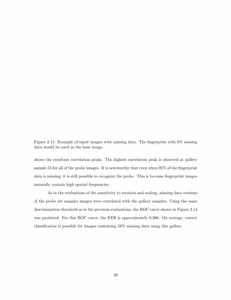
Figure 2.11: Example of input images with missing data. The fingerprint with 0% missingdata would be used as the base image.

shows the resultant correlation peaks. The highest correlation peak is observed at gallery

sample 55 for all of the probe images. It is noteworthy that even when 95% of the fingerprint

data is missing, it is still possible to recognize the probe. This is because fingerprint images

naturally contain high spatial frequencies.

As in the evaluations of the sensitivity to rotation and scaling, missing data versions

of the probe set samples images were correlated with the gallery samples. Using the same

discrimination threshold as in the previous evaluations, the ROC curve shown in Figure 2.14

was produced. For this ROC curve, the EER is approximately 0.306. On average, correct

classification is possible for images containing 58% missing data using this gallery.

26

0

0.5

1

1.5

2

2.5

3

3.5

4

4.5

5

0 10 20 30 40 50 60 70 80 90

Cor

rela

tion

Pea

k

Percentage of Missing Data (%)

Figure 2.12: Variation of correlation peak with respect to percentage of missing data.

95500

1

1.5

2

2.5

3

3.5

4

4.5

5

111

2131

4151

6171

8191

Percentage of Missing Data (%)

Cor

rela

tion

Pea

k

Sample Number

95

90

80

70

60

50

40

30

20

10

0

Figure 2.13: Correlation peak vs. sample number for various missing data percentages. Allthe highest correlation peaks appear at position 55 (correct identification). It is noted thatthe input with 95% missing data can still be recognized.

27

0

0.1

0.2

0.3

0.4

0.5

0.6

0.7

0.8

0.9

1

0 0.1 0.2 0.3 0.4 0.5 0.6 0.7 0.8 0.9 1

Fal

se A

ccep

t R

ate

False Reject Rate

Figure 2.14: ROC curve for the sensitivity to missing data examination. Here, the plot showsthe false-accept rate vs. the false-reject rate. This ROC curve has an EER of approximately0.306.

2.4 Hardware acceleration

2.4.1 FPGA design

The phase-only matched filter based fingerprint algorithm contains a fair amount

of parallelism. This allows a hardware implementation of the model to provide increased

performance over a fully software implementation. This section describes how the algorithm

can be implemented on FPGAs.

The FPGA fingerprint module was designed to implement the phase-only matched

filter algorithm described in section 2.3. This module correlates a stored collection of probe

images against a stored gallery of samples. The collection of probe images and gallery

samples are stored in a high speed off-chip memory. Figure 2.15 presents a system overview

of the FPGA fingerprint module. The system is pipelined to allow parallel processing of

different algorithm phases. Input data and intermediate values are stored in buffers. These

are on-chip memories on the FPGA. The probe images and gallery samples are loaded into

28

FFTShiftand

ConjugateMultiply

FFTShiftand

Find Max

MaxIndex

sw

swsw

swgn

sw

sw

Cos

Sin

mb2

fn

24-bitFFT

mb1

mb0

mb0

16-bitFFT

16-bitFFT

PhaseAngle

36/

32/

32/

24/

Phase 1b

Phase 2a

Phase 2b

Phase 1a

24/

16/

16/

11/

11/

24/

16/

24/

32/

24/

36/

8/

8/

Figure 2.15: Block diagram of the FPGA operations. The black boxes labeled “sw” areswitches.

the on-chip FPGA buffers “gn” and “fn” respectively.

Two-dimensional Fourier transforms need to be performed on the two input images.

This design utilizes two consecutive one-dimensional fast Fourier transforms (FFTs) —

first along the rows and then along the columns — to model a two-dimensional Fourier

transform. The FFT units were built using Xilinx-supplied library components. To enable

high-throughput computation, the system is pipelined into two alternating phases, with

each phase working on a separate gallery sample. Each phase is further subdivided into

two parts (as shown in Figure 2.15) that are evaluated serially. The computations in each

phase are described below:

a) Phase 1a:

29

The first one-dimensional row FFT for the first Fourier transforms is computed. This

is done simultaneously for both the probe image and gallery sample in two separate

pipelines. The inputs to this phase are unsigned 8-bit values. The outputs of these

operations are signed 16-bit values and are stored in the buffers labeled mb0.

b) Phase 1b:

The second one-dimensional column FFT to complete the first two-dimensional Fourier

transforms is computed using the data stored in “mb0” as input. This FFT is applied

simultaneously for the probe image and gallery sample. The result of the probe image’s

column FFT produces F (Ux, Uy) (Equation (2.1)). The output of the gallery sample

column FFT is normalized to the unit circle and conjugated to produce HPOF (Equation

(2.3)). HPOF is then multiplied by F (Ux, Uy). An FFT shift operation is executed in

parallel with the multiplication in order to center the image. This output is 36 bits wide

and is stored in the buffer labeled “mb1”.

c) Phase 2a:

The first one-dimensional row FFT for the second Fourier transform is evaluated. Since

this FFT is implemented with two 24-bit forward FFT units, they use only the most

significant 24 bits of the inputs (since the Xilinx FFT units can take at most a 24-bit

input). This introduces round-off errors as the computations take place in the integer

domain. The output is stored in the “mb2” buffer.

d) Phase 2b:

The second one-dimensional column FFT for the second Fourier transform is evaluated

here (corresponding to Equation (2.4)). The peak value in the FFT output is computed

in this phase as the FFT outputs stream out. To evaluate the peak value, the absolute

value of each FFT output is computed. These values are compared against previously

generated values to determine the peak location. The coordinates, amplitude of the peak,

and index of the gallery sample where the peak occurred are all stored and returned to

the processor upon processing all the gallery samples.

30

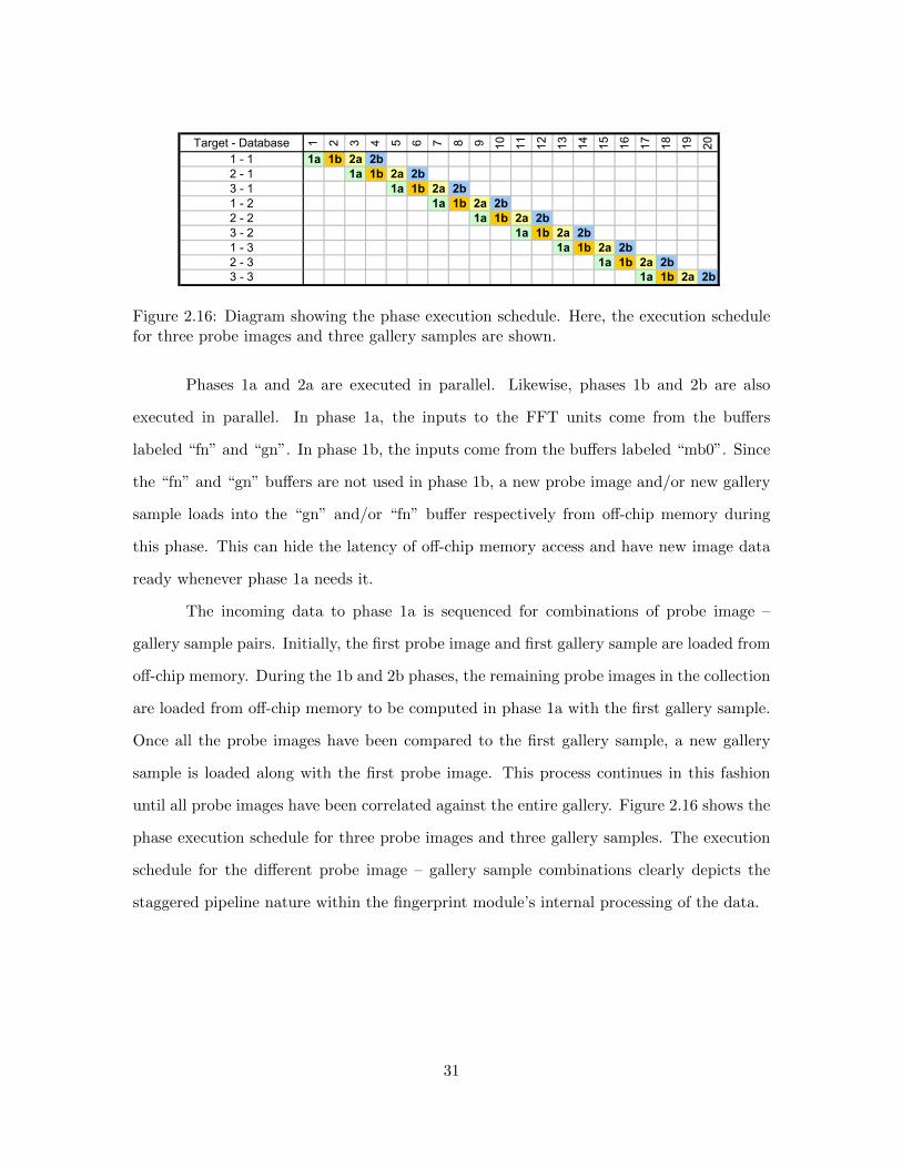
Target - Database 1 2 3 4 5 6 7 8 9 10 11 12 13 14 15 16 17 18 19 20

1 - 1 1a 1b 2a 2b2 - 1 1a 1b 2a 2b3 - 1 1a 1b 2a 2b1 - 2 1a 1b 2a 2b2 - 2 1a 1b 2a 2b3 - 2 1a 1b 2a 2b1 - 3 1a 1b 2a 2b2 - 3 1a 1b 2a 2b3 - 3 1a 1b 2a 2b

Figure 2.16: Diagram showing the phase execution schedule. Here, the execution schedulefor three probe images and three gallery samples are shown.

Phases 1a and 2a are executed in parallel. Likewise, phases 1b and 2b are also

executed in parallel. In phase 1a, the inputs to the FFT units come from the buffers

labeled “fn” and “gn”. In phase 1b, the inputs come from the buffers labeled “mb0”. Since

the “fn” and “gn” buffers are not used in phase 1b, a new probe image and/or new gallery

sample loads into the “gn” and/or “fn” buffer respectively from off-chip memory during

this phase. This can hide the latency of off-chip memory access and have new image data

ready whenever phase 1a needs it.

The incoming data to phase 1a is sequenced for combinations of probe image –

gallery sample pairs. Initially, the first probe image and first gallery sample are loaded from

off-chip memory. During the 1b and 2b phases, the remaining probe images in the collection

are loaded from off-chip memory to be computed in phase 1a with the first gallery sample.

Once all the probe images have been compared to the first gallery sample, a new gallery

sample is loaded along with the first probe image. This process continues in this fashion

until all probe images have been correlated against the entire gallery. Figure 2.16 shows the

phase execution schedule for three probe images and three gallery samples. The execution

schedule for the different probe image – gallery sample combinations clearly depicts the

staggered pipeline nature within the fingerprint module’s internal processing of the data.

31

2.4.2 System design

The performance improvement offered by the hardware based system is evaluated

using a Cray XD1 at the Naval Research Laboratory in Washington, DC. The Cray XD1

contains a large set of Xilinx FPGAs and 2.2 GHz AMD Opteron processors tightly coupled

together. The hardware design described in section 2.4 was implemented using on a Xilinx

Virtex II Pro FPGA on the Cray XD1. Although the Cray XD1 contained multiple FPGAs,

only one FPGA was utilized for this work. A more practical approach for FPGA acceleration

would be to use an FPGA card for desktop computing systems (such cards average about

$2,500 per FPGA at present). These contain one or more FPGAs and would be able to

replicate the performance seen in this chapter.

The four main modules implemented on the FPGA are a fingerprint module that per-

forms the distortion invariant phase-only filter operations, a direct memory access (DMA)

engine module provided by Cray Inc., an arbiter module which mediates the data transfers,

and an interface logic module provided by Cray Inc. The DMA module transfers data be-

tween the system DRAM and the high speed off-chip memory (SRAM) next to the FPGA.

The arbiter uses the DMA engine to route data to and from the fingerprint module, the

off-chip memory, and the AMD processor for the system (as shown in Figure 2.17). The

logic interface is used to transfer command and status signals between the AMD processor

and the fingerprint module on the FPGA.

The off-chip memory is a unit composed of four banks of memory. In this design,

three of the banks are utilized. The first two banks are used to store gallery samples. The

third bank is solely used to store probe images for processing. In each bank, the maximum

number of individual images that can be stored is 256. The first and second banks are

fed alternately to the FPGA for processing. When gallery samples in the first bank are

being used for processing by the FPGA, the arbiter allows the DMA engine to load data

into the second bank (and vice versa). Processing in this fashion completely hides the

latency of data transfers (which can otherwise be very performance limiting), thus allowing

processing of very large galleries with negligible slowdowns. It should be noted that none

32

FPGA

Off‐ChipMemory

FingerprintModule

Logic Interface

Arbiter

DMA Engine

QDRBank 1

QDRBank 2

QDRBank 3

AMD

Figure 2.17: Block diagram of the overall network.

of the related FPGA based approaches for fingerprint identification cited in section 2.4.3

examine the issue of data transfer into the FPGA (this can be prohibitively expensive and

has to be addressed in any FPGA based design).

2.4.3 Related FPGA work

Algorithms for fingerprint detection can be computationally intense, but at the same

time, can also have large degrees of parallelism. Several hardware acceleration approaches

have been proposed to take advantage of this parallelism, including FPGAs [32, 33, 34,

35] and System on Chip (SoC) designs [42]. Given that SoCs are typically custom built

components while FPGAs are available commercially off-the-shelf, the latter are generally

cheaper and thus preferable for hardware acceleration.

Lindoso and Entrena [32] compare the implementation of zero-mean normalized

cross-correlation in the spatial and spectral domains implemented on FPGAs. They apply

the designs to fingerprint detection on a Virtex 4 SX FPGA and observe average speedups

of at least two orders of magnitude over implementations on a 3.0 GHz Pentium 4 processor.

Their design splits an image into multiple horizontal segments, and processes all the rows

within a segment in parallel. Only one image is processed at a time. In contrast, the design

33

presented in this chapter achieves parallelism by processing multiple images (from different

stages of the algorithm) in parallel but only examines only row of each image at a time.

Danese et al. [33] implement a phase-only correlation algorithm on a 90 MHz Altera

Stratix II FPGA. As referenced in section 2.4.2, their algorithm differs from this chapter’s

implementation of the phase-only filter. The FPGA implementation provides a speedup of

seven times over an equivalent software design on a 2.2 GHz AMD Athlon 64 processor. As

in this chapter’s design, they evaluate only one row at a time for each image. However, there

is a major difference between their FPGA architecture and the one presented in this chapter.

This chapter’s design exploits algorithm level pipelining to achieve higher speedups while

Danese et al. evaluate their algorithm serially. In addition, this chapter’s design utilizes

specialized streaming memory resources in order to maintain the high data throughput

needed for pipelining.

Wang et al. [42] utilize a feature extraction approach for fingerprint identification.

They develop a custom SoC architecture containing a 32-bit RISC processor, a bit-serial

FPGA, and a 64 KB ROM. The bit-serial FPGA allows the system to have a modest degree

of reconfigurability. They show a significant performance gain over 100 MHz fixed point

DSP using their 50 MHz SoC.

Several groups have studied FPGA based hardware acceleration of fingerprint fea-

ture extraction algorithms for biometric applications. Garcıa and Navarro [34] implement

fingerprint ridge extraction for two software cases and one hardware-acceleration case. The

two software cases utilized a 50 MHz Xilinx Microblaze soft-processor and a 1.7 GHz Intel

Centrino processor. The hardware-accelerated case was implemented on a 50 MHz Xilinx

Microblaze with a Xilinx Spartan 3 FPGA acting as a coprocessor system. Using the co-

processor system, they observe an 11 times speedup over the Intel Centrino and a 370 times

speedup over the Microblaze software implementations. Lorenzo et al. [35] examined the

FPGA acceleration of fingerprint minutiae extraction. The FPGA was utilized to accelerate

the backend of the minutiae extraction routine. The algorithm required about 60s to 90s on

a 3.0 GHz Pentium 4 processor and less than 100ms on a 65 MHz Xilinx Virtex II FPGA.

34

2.5 Hardware performance

2.5.1 Experimental setup

The FPGA utilized on the Cray XD1 is initialized and controlled by a C program

running on the AMD processor. The C program was compiled with the GNU compiler

(GCC) using the −O3 optimization. To accurately compare the performance improvement

produced by the FPGA accelerator system, the phase-only matched filter based fingerprint

algorithm was implemented fully in C on the AMD processor. A FFT library developed

by Stefan Gustavson [43] was utilized in the full C implementation. Finally, a MATLAB

implementation of the algorithm was also developed to evaluate the accuracy of the model.

The 100 gallery samples (from section 2.3) were resized to 128×128 pixels in order to fit in

the FPGA on-chip buffers utilized.

2.5.2 Result

The FPGA system synthesized ran at 140 MHz. It utilized 72% of the available

FPGA’s logic and 91% of the onboard block RAM. Both the FPGA and the AMD processing

systems were tested with 256 probe fingerprint images. Two configurations where the only

difference was the number of gallery samples were examined. In the first configuration,

there were 256 gallery samples (as listed earlier), and there were 4,096 sample gallery in

the second configuration. Both the 256 and 4,096 sample galleries were constructed by

replicating the 100 sample gallery. Table 2.1 shows the timing breakdown and the FPGA

speedup over the C implementation for these two configurations. The runtime for the FPGA

system can be separated into FPGA input/output (I/O) time and FPGA compute time,

while the runtime for the C software implementation is simply the AMD compute time. The

time to read the image sample data from the hard disk (image reading time) is common to

both implementations and is therefore seen by both systems in the measure of their overall

time (this time is not considered in the other studies shown in section 2.4.3).

In configuration one, all 256 gallery samples fit in one off-chip memory bank for the

35

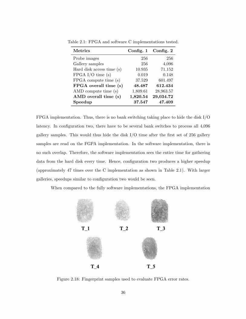
Table 2.1: FPGA and software C implementations tested.

Metrics Config. 1 Config. 2

Probe images 256 256Gallery samples 256 4,096Hard disk access time (s) 10.935 71.152FPGA I/O time (s) 0.019 0.148FPGA compute time (s) 37.529 601.497FPGA overall time (s) 48.487 612.434AMD compute time (s) 1,809.61 28,963.57AMD overall time (s) 1,820.54 29,034.72Speedup 37.547 47.409

FPGA implementation. Thus, there is no bank switching taking place to hide the disk I/O

latency. In configuration two, there have to be several bank switches to process all 4,096

gallery samples. This would thus hide the disk I/O time after the first set of 256 gallery

samples are read on the FGPA implementation. In the software implementation, there is

no such overlap. Therefore, the software implementation sees the entire time for gathering

data from the hard disk every time. Hence, configuration two produces a higher speedup

(approximately 47 times over the C implementation as shown in Table 2.1). With larger

galleries, speedups similar to configuration two would be seen.

When compared to the fully software implementations, the FPGA implementation

T_4 T_5

T_1 T_2 T_3

Figure 2.18: Fingerprint samples used to evaluate FPGA error rates.

36

Table 2.2: Sample fingerprint points of maximum correlation peak. These values are basedupon the FPGA and MATLAB outputs for the prints shown in Figure 2.18 (all values areto be multiplied by 107).

Image MATLAB FPGA Error(%)

T 1 4.25 4.23 0.46T 2 4.30 4.28 0.51T 3 4.65 4.63 0.39T 4 4.34 4.32 0.49T 5 4.09 4.07 0.48

incurs some round-off errors that are introduced within the FPGA’s rounding and fixed

point calculations. To evaluate the effects of this error, the outputs of the MATLAB and

the FPGA implementations were compared for five probe images as shown in Figure 2.18.

These probe images were searched against the 100 sample gallery on both implementations.

Table 2.2 shows the maximum point of correlation as well as the error for the algorithm

when computed by using both the MATLAB and FPGA implementations. All the exam-

ined probe fingerprints were correctly identified within the 100 sample gallery. As seen in

Table 2.2, the error generated by the FPGA implementation in comparison to the MATLAB

implementation is very small. For the probe images tested, this error is at most 0.51%.

Tables 2.3, 2.4, and 2.5 show the errors generated by using distorted images on

the FPGA for the three types of distortions studied (rotation, scaling, and missing data

respectively). The tests here were designed the same as the tests discussed in section 2.3

where the rotated distortions were generated using sample 76, the scaling distortions from

sample 16, and missing data distortions from sample 55. As in Table 2.2, the maximum

point of correlation for both MATLAB and FPGA implementations are shown in Tables

2.3, 2.4, and 2.5. In Tables 2.3, 2.4, and 2.5, the error is at most 1.34%, 0.51%, and 2.51%,

respectively. The error increases in Table 2.5 because the effect of FPGA implementation’s

round-off error is amplified when there is less input data available. Despite the error, both

the MATLAB and FPGA implementations chose the same final fingerprint classification for

all of the test cases in Tables 2.3, 2.4, and 2.5.

37

Table 2.3: Evaluation of FPGA with rotated images using sample 76. In all cases, theFPGA results matched the results of MATLAB. The peak correlation value shown forboth MATLAB and FPGA are to be multiplied by 106. The error compared to MATLABsimulation is listed.

Rotation(◦) MATLAB FPGA Error(%)

−10 10.02 9.84 1.79−9 9.63 9.44 1.95−8 9.70 9.84 1.42−7 9.88 9.88 0.00−6 9.39 9.38 0.05−5 9.44 9.44 0.02−4 9.52 9.59 0.79−3 10.27 10.26 0.06−2 10.36 10.34 0.18−1 11.02 10.91 0.97

0 10.96 11.09 1.161 10.50 10.64 1.342 9.99 9.99 0.033 9.70 9.70 0.044 9.44 9.44 0.045 9.60 9.61 0.086 9.18 9.19 0.097 9.77 9.79 0.208 9.10 9.09 0.139 9.07 8.96 1.24

10 9.23 9.23 0.07

38

Table 2.4: Evaluation of FPGA with scaled images using sample 16. In all cases, theFPGA results matched the results of MATLAB. The peak correlation value shown forboth MATLAB and FPGA are to be multiplied by 106. The error compared to MATLABsimulation is listed.

Scaling(%) MATLAB FPGA Error(%)

90 8.55 8.54 0.1391 8.62 8.60 0.1392 9.02 9.02 0.0393 9.67 9.65 0.2394 10.54 10.53 0.0995 9.61 9.59 0.2696 10.66 10.66 0.0297 11.67 11.66 0.0998 11.42 11.42 0.0399 12.97 12.98 0.09

100 39.04 38.84 0.51101 13.65 13.63 0.13102 12.45 12.45 0.03103 11.28 11.29 0.12104 10.38 10.38 0.02105 10.11 10.09 0.16106 9.36 9.37 0.11107 8.63 8.65 0.24108 9.47 9.47 0.02109 8.51 8.52 0.08110 8.61 8.61 0.03

39

Table 2.5: Evaluation of FPGA with missing data images using sample 55. In all cases,the FPGA results matched the results of MATLAB. The peak correlation value shown forboth MATLAB and FPGA are to be multiplied by 106. The error compared to MATLABsimulation is listed.

Missing(%) MATLAB FPGA Error(%)

0 9.89 9.90 0.1210 9.20 9.21 0.1020 9.17 9.18 0.0630 8.78 8.79 0.0940 9.00 9.00 0.0150 8.87 8.86 0.1460 7.76 7.75 0.0870 6.65 6.65 0.0080 6.15 6.01 2.2490 5.34 5.48 2.5195 5.10 5.23 2.47

2.6 Summary

Fingerprint identification is a PR technique applicable to a wide variety of appli-

cations. The phase-only filter based fingerprint identification approach highlighted in this

chapter has the main advantage that it is distortion tolerant and can be realized in optical

or electronic parallel hardware. Given that real world fingerprints are almost never perfect,

distortion tolerance can prove to be very important for fingerprint identification.

In this chapter, the performance of phase-only filter based fingerprint identification

was examined under various distortions. In the case of undistorted fingerprints, all finger-

print were correctly recognized within the gallery. In the case of distortions due to rotation,

the probe image was still recognizable if it was within an average range of −5.24◦ to +4.87◦

angular shifts from the original image. Distortions due to scaling gave an average scaling

factor range of 95.10% to 105.34% for reliable detection. The most interesting result is the

recognition of distorted fingerprints when the probe image has missing data. It was shown

that on average, probe images with up to 58% of their data missing can be successfully

identified using the phase-only filter.

The high parallelism in phase-only filter correlation makes it ideally suited to FPGA

40

based hardware acceleration. Therefore, the FPGA acceleration of the phase-only filter

based fingerprint identification was evaluated. The results showed that a Virtex II Pro

FPGA can provide a speedup of about 47 times over a C implementation of the algorithm

on a 2.2 GHz AMD Opteron processor. This demonstrates that hardware acceleration of

fingerprint identification can provide significant performance gains over general purpose

processors. The design presented can be useful for searching large fingerprint galleries (a

computationally intensive task).

41

Chapter 3

Izhikevich Spiking Neural Networks for Character

Recognition

3.1 Introduction

The brain utilizes a large collection of slow neurons operating in parallel to achieve

very powerful cognitive capabilities. There has been a strong interest amongst researchers

to develop large parallel implementations of cortical models on the order of animal or hu-

man brains. At this scale, the models have the potential to provide much stronger inference

capabilities than current generation computing algorithms [44]. A large domain of appli-

cations would benefit from the stronger inference capabilities including speech recognition,

computer vision, textual and image content recognition, robotic control, and data mining.

Several research groups are examining large scale implementations of neuron based

models [45, 46] and cortical column based models [47, 48] on high performance computing

clusters. IBM is utilizing a 32,768 processor Blue Gene/L system [45], while Los Alamos

National Laboratory is utilizing the Roadrunner supercomputer (one time fastest computer)

to model the human visual cortex [49].

Additionally, there is a strong interest in the design of specialized hardware ac-

celeration approaches for these neuromorphic algorithms to enable large scale simulations.

The SpiNNaker project is developing an ARM based chip multiprocessor to evaluate 1,000

42

leaky integrate-and-fire neurons [50]. Several researchers are examining the use of mem-

ristors [51, 52] for the design of neural circuits [53]. Gao and Hammerstrom [54] proposed

a simplified model of the neocortex based on spiking neurons and examined conceptual

implementations of the model using future CMOS and CMOL technologies.

One of the most common set of algorithms being examined for large scale simulation

and hardware acceleration is the spiking neural network (SNN) class of models. These

models capture neuronal behavior more accurately than traditional neural networks [55].

Several SNN models have been proposed recently. Of these, the integrate-and-fire model is

the most commonly utilized — both for algorithmic studies and hardware implementations.

Field programmable gate array (FPGA) implementations of the integrate-and-fire spiking

neuron model include [56, 57, 58, 59]. Shayai et al. [56] simulated a network of 161 quadratic

integrate-and-fire neurons and 1,610 synapses on a Virtex 5 FPGA. Upegui et al. [57] utilized

a Spartan II FPGA to implement a network of neurons based upon a simplified integrate-

and-fire neuron model. They also implemented Hebbian learning for the neurons in the

FPGA. Cassidy et al. [58] developed a spiking network of leaky integrate-and-fire neurons to

evaluate several experiments in a Spartan-3 FPGA. Pearson et al. [59] implemented a neural

processor using leaky integrate-and-fire neurons to perform neural network computations

on a Virtex II FPGA.

Izhikevich has shown [60] that the integrate-and-fire spiking neuron model is not

very biologically accurate and is unable to reproduce the spiking behavior of many neurons.

He proposed a new model [61] which has been shown to be almost as accurate as the highly

detailed Hodgkin-Huxley neuron model but with the low computational cost of the integrate-

and-fire model. Both the integrate-and-fire model and the Izhikevich model require 13

floating point operations per second (FLOPS) per neuron simulation, while the Hodgkin-

Huxley model requires 256 FLOPS. Therefore, for large scale simulations, the Izhikevich

model is significantly more attractive than the more commonly used integrate-and-fire.

Recent studies [62, 63, 64, 65] have implemented the Izhikevich neuron model instead

of the integrate-and-fire model on FPGAs. La Rosa et al. [62] and Fortuna et al. [63]

43

simulated two such neurons on an FPGA. Their primary objective was to examine the

feasibility of FPGA implementations of the model and to show that hardware can reproduce

the wide range of neuronal responses possible from the model. Mokhtar et al. [64] simulated

48 neurons based on the Izhikevich model on a Virtex II Pro FPGA for maze navigation.

Thomas and Wuk [65] develop a fully connected network of 1,024 Izhikevich spiking neurons

using a Virtex II Pro FPGA. Thomas and Wuk report that their implementation achieves

100 times real-time speed.

In this chapter, the feasibility of using FPGAs for large scale simulations of the

Izhikevich model is explored. A character recognition algorithm based on the Izhikevich

spiking neuron model presented in a previous paper [66] is utilized. The network in [66] was

scaled up in this chapter to evaluate the performance of large networks on FPGAs. The

primary contributions of this work are:

1) The design of a modularized processing element (PE) for implementing the Izhikevich

model on FPGAs. Multiple PEs can be placed on chip, with each PE able to process

a large number of neurons in a pipelined manner. The state of each neuron is stored

in on-chip memory. Additionally, a network with over 9,000 neurons using 25 PEs on a

Xilinx Virtex 4 FPGA was implemented.

2) The use of the PEs to evaluate a specific application on FPGAs using the Izhikevich

model. The results indicate that an FPGA implementation can provide a speedup of

about 8.5 times over a software implementation on a 2.2 GHz AMD Opteron core.

3.2 Background

Spiking neural models capture neuronal behavior more accurately than traditional

neural models. A neuron consists of three functionally distinct components called dendrites,

axons, and a soma. Each neuron is typically connected to over 10,000 other neurons. The

dendrites of a neuron collect input signals from other neurons, while the axons send output

signals to other neurons. Input signals coming in along dendrites can cause changes in the

44

ionic levels within the soma, which can cause the neuron’s membrane potential to change.

If this membrane potential crosses a certain threshold, the neuron is said to have fired or

spiked. In these events, the membrane potential rises rapidly for a short period of time (a

spike) and causes electrical signals to be transmitted along the axons of the neuron to other

neurons connected to it. Details of the spiking mechanism can be found in [67]. Spiking

is the primary mechanism by which neurons communicate with each other. Over the last

50 years, several models have been proposed that capture the spiking mechanism within a

neuron.

Izhikevich proposed a new spiking neuron model in 2003 [61] that is primarily based

on two differential equations (Equation (3.1) and Equation (3.2)). In these equations, t

represents the time iteration, Vt is the membrane potential of the neuron, It is the synaptic

current, and ut represents a membrane recovery parameter used to supply negative feedback

to the voltage. In the Izhikevich model, Vt represents the state of a neuron, while ut is an

associated parameter contributing to the state of a neuron. The values for Vt and ut are

updated using Equation (3.3) and (3.4), respectively.

δVtδt

= 0.04Vt2 + 5Vt + 140− ut + It (3.1)

δutδt

= a(bVt − ut) (3.2)

Vt+1 = Vt +δVt2δt

(3.3)

ut+1 = ut +δutδt

(3.4)

45

Time (ms)

Vo

ltag

e (m

V)

120

60

40

80

5

100

1510 3020 25 35 40-20

0

20

450

Figure 3.1: Spikes produced with Izhikevich model.

if Vt ≥ 30 mV, then

Vt ← c

ut ← ut + d

By tweaking the four constant parameters (a, b, c, and d), the model can reproduce almost

all types of neuronal responses seen in biological experiments. This makes the model almost

as versatile as the Hodgkin-Huxley model at a fraction of the computational cost of that

model. The same time step (1ms) and model parameters used by Izhikevich [60] were

utilized. The values of the constant parameters are given in Appendix A, while Figure 3.1

shows an example of spikes produced with this model.

3.3 Character recognition algorithm

The two layer spiking neural network algorithm for character recognition based on

the Izhikevich model presented earlier in [66] was utilized. In this model, the first layer

acted as input neurons, and the second layer as output neurons. The network was trained

46

Figure 3.2: Training images.

as shown in [66] to recognize the 48 different input images shown in Figure 3.2. These

images represent the 26 upper case letters (A–Z), 10 numerals (0–9), eight Greek letters,

and four symbols.

Input images were presented to the first layer of neurons (referred to as level 1), with

each image pixel corresponding to a separate input neuron. Thus, the number of neurons

in level 1 was equal to the number of pixels in the input image. The number of second layer

neurons (referred to as level 2) was equal to the number of training images. This is because

each level 2 neuron was encoded to fire only when it recognized one specific image. Lastly,

each level 1 neuron was connected to every level 2 neuron. A prototype of this network is

47

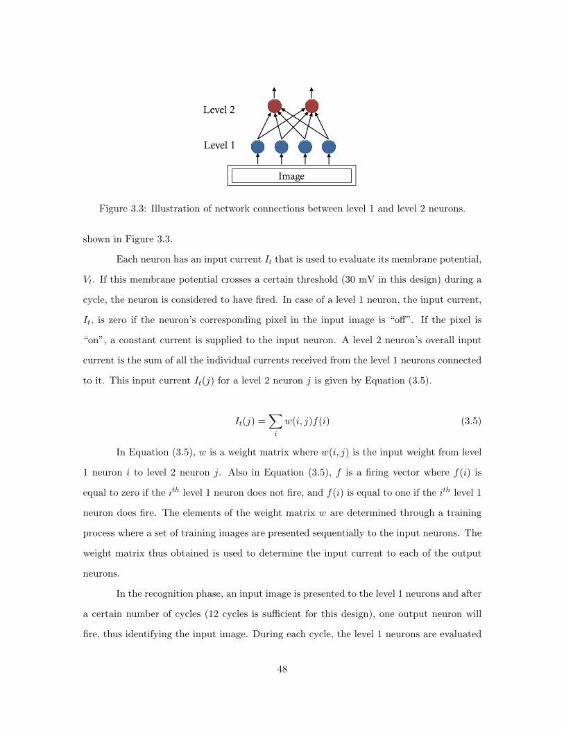
Level 2

Level 1

Image

Figure 3.3: Illustration of network connections between level 1 and level 2 neurons.

shown in Figure 3.3.

Each neuron has an input current It that is used to evaluate its membrane potential,

Vt. If this membrane potential crosses a certain threshold (30 mV in this design) during a

cycle, the neuron is considered to have fired. In case of a level 1 neuron, the input current,

It, is zero if the neuron’s corresponding pixel in the input image is “off”. If the pixel is

“on”, a constant current is supplied to the input neuron. A level 2 neuron’s overall input

current is the sum of all the individual currents received from the level 1 neurons connected

to it. This input current It(j) for a level 2 neuron j is given by Equation (3.5).

It(j) =∑i

w(i, j)f(i) (3.5)

In Equation (3.5), w is a weight matrix where w(i, j) is the input weight from level

1 neuron i to level 2 neuron j. Also in Equation (3.5), f is a firing vector where f(i) is

equal to zero if the ith level 1 neuron does not fire, and f(i) is equal to one if the ith level 1

neuron does fire. The elements of the weight matrix w are determined through a training

process where a set of training images are presented sequentially to the input neurons. The

weight matrix thus obtained is used to determine the input current to each of the output

neurons.

In the recognition phase, an input image is presented to the level 1 neurons and after

a certain number of cycles (12 cycles is sufficient for this design), one output neuron will

fire, thus identifying the input image. During each cycle, the level 1 neurons are evaluated

48

Algorithm 1 The recognition phase for the spiking neuron image recognition modelrepeat

for all level 1 neurons doRead input current ItCalculate neuron membrane potential Vt and recovery parameter utIf neuron fires, append neuron index to firing vector

end for–Barrier–for all level 2 neurons do

for all non-zero entry of firing vector (previous cycle) doAdd corresponding weight elements to input current ItCalculate neuron membrane potential Vt and recovery parameter utIf neuron fires, output is produced

end forend for–Barrier–

until level 2 neuron fires

based on the input image, and the firing vector is updated to indicate which of the level

1 neurons fired that cycle. In the same cycle, the firing vector generated in the previous

cycle is used to calculate the input current It to each level 2 neuron. The level 2 neuron

membrane potentials Vt are then calculated based on their input current It. This process

is described in detail in Algorithm 1. The Euler approach was utilized to solve equations

(3.1) and (3.2).

3.4 Hardware implementation

3.4.1 Structure

The hardware implementation of the SNN character recognition algorithm was de-

veloped on a Cray XD1. Only the recognition aspect of the algorithm was accelerated.

An AMD Opteron processor and a Xilinx FPGA were utilized to perform the processing.

Figure 3.4 shows the overall design of this system. The FPGA is connected to the AMD

processor through a high-speed interface logic module (adapted from designs provided by

Cray Inc.) and to an external SRAM bank through a direct memory access (DMA) interface

module. The latter is used to transfer data between the off-chip SRAM banks and both the

49

SNN Module

FPGA

AMD SRAM

DMAEngine

InterfaceLogic

SNNController

L2 CurrentModule

SNNPE

SNNPE

Figure 3.4: Overall spiking neural network design on Cray XD1.

AMD Opteron and FPGA.

A third module on the FPGA, the SNN module, implements the character recogni-

tion algorithm. This consists of the following three components:

1) SNN processing elements (PEs):

These implement the neuron computations given by Equation (3.1) and Equation (3.2).

Each PE evaluates a subset of the neurons and generates a local firing vector based on

this subset of neurons.

2) L2 current module:

This implements the computations in Equation (3.5) needed to generate the input cur-

rents for level 2 neurons. This involves examining all the local level 1 PE firing vectors

and then initiating the transfer of the level 2 neuron weights based on these firings.

3) SNN controller :

This unit coordinates the operations of the SNN PEs and the L2 current module to

implement the character recognition algorithm.

50

3.4.2 Processing element

Each SNN PE has a 23 stage pipeline and stores the parameters Vt, ut, It, and f

used in computations of Equations (3.1) – (3.4) locally in on-chip block RAM (BRAM).

All SNN PEs are connected to the L2 current module through a bus, on which the L2

current module is the arbiter. A dataflow diagram depicting the 23 stage pipeline is shown

in Figure 3.5. In Figure 3.5, the values in parentheses represent the associated delay in

terms of clock cycles. Additionally, the boxes represent the different computations required

for Equations (3.1) – (3.4) and are marked as follows:

A) Loading SNN neuron state (Vt), associated state parameter (ut), and input (It) into the

pipeline

B) Computing intermediate values (fv1, fv2, fv3, fv4, fv5, fv6, and fv7)

C) Computing δVtδt (Equation (3.1))

D) Computing δutδt (Equation (3.2))

E) Performing the Vt+1 update (Equation (3.3))

F) Performing the ut+1 update (Equation (3.4))

As seen in Figure 3.5, the neuron state (Vt), associated state parameter (ut), and

input (It) are processed through the pipeline in a top to bottom manner. Every clock cycle,

a new Vt, ut, and It load into the pipeline. Thus, as new data stream into the pipeline,

new outputs are produced every cycle after an initial 23 clock cycle delay. In this fashion,

computations are processed in a highly efficient and spatially parallel manner.

To reduce the logic resource footprint and to accelerate the operation of each PE,

the computations in Equations (3.1) – (3.5) were implemented in fixed point format instead

of floating point form. Tests using a variety of different fixed point representations indicated

that fixed point representations with less than 12 bits after the radix point will produce

incorrect character recognition as a result of high round off errors. Therefore, a fixed point

51

ItA: (1)

VtA: (1)

fv4 = 0.04 × fv1B: (6)

fv2 = 5 × VtB: (6)

fv1 = Vt × VtB: (7)

if Vt ≥ 30 thenut← ut + dVt← cA: (1)

utA: (1)

fv3 = b × VtB: (7)

fv5 = fv3 – utB: (1)

fv6 = It +140 – utB: (6)

fv7 = fv4 + fv2B: (6)

δVt⁄δt = fv6 + fv7C: (1)

δut⁄δt = a × fv5D: (7)

Vt+1 = Vt +δVt⁄2δt

E: (1)ut+1 = ut +

δut⁄δtF: (1)

(14) (13)

(13)

(7)

(20)

(5)

(7)

Figure 3.5: Dataflow diagram for the SNN PE 23 stage pipeline design. The neuron state(Vt), associated state parameter (ut), and input (It) process from top to bottom. The valuesin parentheses represent the delay in terms of clock cycles.

52

representation with 12 bits after the radix point was utilized. The number of bits before

the radix point increased from four to 32 bits as a result of maintaining precision across the

algorithm’s computations.

3.4.3 Operation

Before processing any images within the FPGA, the weight matrices w(i, j) for the

level 2 neurons need to be initialized. The weights are pre-calculated during the training

process and are stored initially in a file. These values are transferred into the SRAM

associated with the FPGA through the DMA module (only once). The weights are stored

in a 16-bit fixed point format with 12 bits after the radix point.

The interaction between the FPGA modules to evaluate the algorithm is coordinated

by the SNN controller module. A state machine depicting the overall process of the SNN

controller is shown in Figure 3.6. The following lists the interactions between the FPGA

modules based on this Figure 3.6.

a) Initialization and startup:

The binary image to be recognized is transferred to the FPGA’s on-chip BRAM through

the interface logic module. Once the binary image data has been written, the AMD pro-

cessor signals the SNN module on the FPGA to begin operation (step (a) in Figure 3.6).

b) Process neurons:

The PEs are designated to evaluate either level 1 or level 2 neurons. All neurons for a

given level are distributed evenly across the PEs for that level and are processed in this

step (step (b) in Figure 3.6). The objective of the processing is to determine a neuron’s

membrane potential, Vt. If this potential is 30 mV or higher, the neuron is considered

to have fired. When a neuron fires, the PE stores the neuron’s index in a local firing

vector and also sets a fired flag on the PE.

c) Examine level 2 firing vector :

In this step, each level 2 PE is examined to determine if its fired flag is set (step (c)

53

Yes

No

Yes

No

YesNo

(b) Process PEs

(f) Cycle++

(c) Process Lv2Fired Vector

(a) Start/Reset

(g) End

(e) ComputeLv2 Current

Cycle >12?

Any Lv1Fired?

Any Lv2Fired?

(d) Process Lv1Fired Vector

Figure 3.6: State machine for spiking neural network controller.

in Figure 3.6). The firing of a level 2 neuron indicates that a character was recognized.

If the flag is set, processing ends (step (g) in Figure 3.6), and the index of the level 2

neuron that fired is stored for later reading by the AMD processor. This index represents

the character that was recognized.

d) Examine level 1 firing vector :

In this step, each level 1 PE is examined in a round robin manner to determined if its

fired flag is set (step (d) in Figure 3.6). If any level 1 neuron fires, the computations in

Equation (3.5) have to be evaluated to determine the input current, It, for each level 2

neuron (step (e) in Figure 3.6).

Weight computations involve streaming the indices of the level 1 neurons that fired

(stored in the local firing vector of each PE) to the high speed off-chip SRAM. After an

11 cycle latency, this SRAM returns the level 2 neuron weights corresponding to the level

1 indices sent to it. A data read from the SRAM is a 64-bit word; therefore, four weight

54

values (16 bits each), corresponding to four level 2 neurons, are packed together into

each 64-bit SRAM word. The weight computations in Equation (3.5) are also evaluated

for four neurons at a time in the level 2 current module. The design was devised to

provide the SRAM with a continuous stream of indices to allow efficient processing of

weights.

e) Prepare for next simulation cycle:

The simulation cycle count is incremented (step (f) in Figure 3.6). If this cycle count is

less than 12, the SNN controller returns to step (b) to process another cycle. Otherwise,

the SNN controller ends operations by setting a finished flag and reports the cycle number

and image classification (index of level 2 node that fired) to the AMD processor.

3.5 Experimental setup

A fully software version and a hardware-accelerated version of the SNN recognition

algorithm on a Cray XD1 at the Naval Research Laboratory were developed. The Cray XD1

consisted of 144 Xilinx Virtex II Pro FPGAs, six Xilinx Virtex 4 FPGAs, and 864 AMD

Opteron 2.2 GHz cores (432 dual core processors). The fully software implementation was

written using the C programming language and was processed on a single AMD Opteron

core. The code was compiled with the GNU compiler (GCC) using the −O3 optimization.

Two character recognition networks were developed. One was trained on the 48

binary 24×24 pixel images shown in Figure 3.2. The second network utilized scaled versions

of these images (scaled to 96×96 pixels). The structures of the two networks are shown in

Table 3.1. The networks were tested with their training images.

The two networks in Table 3.1 were implemented on two types of FPGAs on the

Cray XD1. Network one was implemented on a Virtex II Pro FPGA, while network two

on a Virtex 4 FPGA. The Virtex II Pro accommodated six level 1 PEs and one level 2 PE.

The Virtex 4, with approximately three times the amount of logic in a Virtex II Pro, was

able to accommodate 25 level 1 PEs and one level 2 PE. The main difference between the

55

Table 3.1: Structure of neural networks examined. Input images are shown in a row×columnformat.

Model ParametersNetwork

1 2

Total SNN PEs 7 25Input Image(pixels) 24×24 96×96Level 1 neurons 576 9,216Level 2 neurons 48 48Total neurons 624 9,264

level 1 and 2 PEs was the amount of BRAM dedicated to the firing vector and the values

of the parameters a, b, c, and d in Equation (3.1) and Equation (3.2).

3.6 Results

The resource utilization of the two FPGA implementations is shown in Table 3.2.

The systems were clocked at or near the 199 MHz frequency limit of the Cray XD1. Table 3.3

shows the overall runtime of the FPGA based implementations and their timing breakdowns.

The “Data in time” is the time to read the input image from the hard drive and write it into

the FPGA BRAMs. This time is higher for network two as the image size for this network

is larger. The “Data out time” is the time to read the index of the level 2 neuron that fired

(representing the image classification) and to read the simulation cycle count needed for

recognition. This time is the same for both networks. The FPGA compute time measure

starts when the FPGA is signaled to start processing (after the input image is loaded) and

Table 3.2: Device logic utilization.

Utilization MetricsNetwork

1 2

Logic 75% 79%BRAM 27% 53%Speed 199 MHz 198 MHzFPGA Virtex II Pro Virtex 4

56

Table 3.3: Hardware-accelerated timing breakdown.

Timing Metrics(ms)Network

1 2

Data in time 0.015 0.105Data out time 0.003 0.003FPGA Compute time 0.014 0.082Total Runtime 0.032 0.190

ends when the FPGA signals the AMD processor that recognition has taken place.

Table 3.4 compares the runtime of the FPGA accelerated implementation with a

fully software implementation for both networks. Speedups of approximately 3.3 times and

8.5 times are seen for networks one and two, respectively. The speedup can be attributed

to multiple PEs operating in parallel and to having several neurons processed in parallel

through the 23 stage pipeline in each PE. The Virtex 4 implementation provides a higher

speedup than the Virtex II Pro implementation, primarily because the former has more

PEs on chip.

3.7 Summary

There has been a strong push recently to examine biological scale simulations of

neuromorphic algorithms to achieve stronger inference capabilities than current computing

algorithms. The recent Izhikevich spiking neuron model is ideally suited for such large scale

cortical simulations due to its efficiency and biological accuracy. This chapter explored

the feasibility of using FPGAs for large scale simulations of the Izhikevich model. The

Table 3.4: Performance measures.

Performance MetricsNetwork

1 2

Software time(ms) 0.105 1.613Hardware-Accelerated time(ms) 0.032 0.190Speedup 3.281 8.489

57

implementation of a character recognition algorithm based on the Izhikevich spiking neuron

model using two types of FPGAs was discussed. A modularized PE to evaluate a large

number of Izhikevich spiking neurons in a pipelined manner was developed. This PE based

design was easily scalable to larger FPGAs. Two network sizes were implemented and

showed significant speedups over equivalent software implementations (approximately 3.3

times for the 24×24 pixel image network on a Virtex II Pro and approximately 8.5 times

for the 96×96 pixel image network on a Virtex 4 over a 2.2 GHz AMD Opteron core). The

results indicate that FPGAs are suitable for large scale Izhikevich model based cortical

simulations.

58

Chapter 4

Pattern Recognition Using Cellular Simultaneous

Recurrent Networks

4.1 Introduction

A fundamental problem encountered by both biological and machine vision systems

is the recognition of familiar objects and patterns in the presence of affine transformations

such as translations, rotations and scaling. Vision scientists have widely hypothesized that

this problem is solved in the brain through distortion invariant recognition. Biological

systems are typically significantly more robust and faster when compared to machine vision

systems for distortion invariant recognition.

Cellular simultaneous recurrent networks (CSRNs) are a recent class of biologically

inspired algorithms that have several significant advantages over other neural algorithms

for distortion invariant image recognition. Firstly, they are more capable than regular re-

current networks (RNNs), such as the Elman network, in capturing temporal information.

Secondly, CSRNs combine the ideas of cellular neural networks (CNNs) with RNNs to dras-

tically reduce the number of adjustable weights in the network. CSRNs have been proven

more effective and flexible than intricately hand crafted solutions at addressing a wide

range of challenging problems, such as path optimization for maze traversal [68] and affine

image registration [69]. The same cannot be said of traditional specialized image recogni-

59

tion algorithms – for instance traditional face recognition algorithms cannot be applied to

optimization problems.

In [70], CSRNs were applied to pose invariant face recognition, a task where tradi-

tional computer vision methods underperform, and were shown to achieve an overall 77%

face recognition rate using the VidTIMIT database. Although powerful in image process-

ing capabilities, CSRNs have increasingly higher computational demands with larger input

problem sizes. In order to process large databases, efficient processing techniques for im-

plementing CSRNs should be investigated.

This chapter has two objectives. The first objective is to examine the acceleration

of the CSRN maze traversal problem used by Ilin et al. [68] on an NVIDIA Tesla C2050

general purpose graphical processing unit (GPGPU) coupled with a 2.67 GHz Intel Xeon

X5550 processor. This problem was explored to gain a better understanding of general

CSRN processing. Since the main bottleneck during training for all implementations is

a matrix inversion that occurs, different GPGPU methods to decrease the computational

impact of the matrix inversion are explored. The results indicate that average speedups of

approximately 7.2 times and 3.5 times are obtainable for the training and testing phases,

respectively, when compared to C implementations.

The second objective is to use insight from the CSRN based maze traversal design to

examine the acceleration of the training phase of the pose invariant face recognition CSRN

algorithm described in [70]. This part of the study utilized the recently established US Air

Force Condor cluster. The Condor cluster is a heterogeneous system consisting of 468 Intel

Xeon cores and 156 NVIDIA Tesla GPGPUs (a mix of C2050s, C2070s, and C1060s). The

Condor cluster also includes 1,716 PlayStation 3 consoles (PS3s); however, these were not

used in this study.

Multiple algorithmic parameters and input configurations were varied to compare

the performance of a single-core central processing unit (CPU) to a single GPGPU im-

plementation for the CSRN face recognition algorithm. The results show that the C2050

and C2070 single GPGPU implementations provide a speedup of five times or more over

60

single-core CPU implementations. Using 450 Xeon cores and 150 GPGPUs on the Condor

cluster, several large scale implementations of the CSRN algorithm were tested. Ultimately,

a CSRN network designed to recognize 1,000 different people was trained in approximately

69s. This result is significantly faster than a single-core implementation, which trains the

same CSRN network in 68,749s (roughly a 996 times speedup).

4.2 Background

4.2.1 Related work in high performance acceleration

In this chapter, various approaches to accelerate the general operation of CSRNs

are used. In particular, several GPGPU techniques are investigated to take advantage of

CSRN’s inherent parallelism. The results of other studies have demonstrated the effec-

tiveness of GPGPUs for accelerating neural networks applications [71, 72, 73, 74]. In [71],

Han and Taha investigate GPGPU acceleration of Izhikevich and Hodgkin-Huxley neural

models that resulted in performance speedups of 5.6 and 84.4 times, respectively, over CPU

implementations.

Additionally, this chapter investigates using a heterogeneous cluster of Intel multi-

core processors and NVIDIA GPGPUs to achieve even greater levels of acceleration. Other

research groups are exploring the benefits of utilizing multi-GPGPU architectures for high

performance computing [75, 76, 77]. In [75], Hampton et al. perform a systematic study

to reduce the time-to-solution when utilizing multi-core/multi-GPGPU architectures for

biomolecular simulations. The authors accelerate molecular dynamics within the LAMMPS

(large-scale atomic molecular massively parallel simulator) software package using NVIDIA

GPGPUs and present critical factors and key observations regarding multi-core/GPGPU

systems that contribute to system performance. In [76], de Camargo et al. utilize multiple

GPGPUs to accelerate large-scale Hodgkin-Huxley spiking neural networks. The authors

achieve an impressive speedup of about 40 times when their multi-GPGPU implementation

using two NVIDIA GTX 295 graphic boards (four GPGPUs total) was compared to an

61

equivalent CPU implementation using a 2.66 GHz Intel Core i7 920 multi-core processor

(four cores) for a network of 200,000 neurons.

Cevahir et al. [77] develop a conjugate gradient solver using multiple NVIDIA

GeForce 8800 GTS 512 GPGPUs. Specifically, the authors implement a fast sparse matrix-

vector multiplication algorithm (key component within the conjugate gradient solver rou-

tine) efficiently utilizing GPGPU resources. The authors perform a variety of tests com-

paring the performance of their implemented matrix-vector multiplication to a CPU im-

plementation using an AMD Phenom 9850 2.5 GHz multi-core processor (four cores) and

other GPGPU approaches. Their results reveal the greater overall performance of their

GPGPU implementation over other implementations for their experiments. Lastly, Cevahir

et al. compare the performance of their conjugate gradient solver using one, two, and four

GPGPUs. The two and four multi-GPGPU implementations achieved speedups of 1.7 times

and 2.8 times, respectively, over the single GPGPU design.

4.2.2 CSRN characteristics

A cellular neural network (CNN) consists of a set of identical cells arranged in a

geometric pattern [78]. Due to symmetry in the network, cells within a CNN are able

to share weights. This sharing of weights decreases the time required to train the CNN

because the total number of weights to train are less. This symmetry also aids CNNs in

solving problems with the same type of structural similarity. Lastly, CNN cells can vary

in complexity. For example, they can be a single neuron or a more complex multi-layered

perceptron (MLP). Differences between the cells lie mainly in the inputs they receive.

Simultaneous recurrent networks (SRNs) are a type of neural network, which have

been shown to have greater ability than MLPs [78, 79]. In a recurrent network, outputs

are fed back as inputs in subsequent iterations. The recurrent behavior in SRNs is an

attempt to emulate similar activity in the brain. The brain has feedback paths along with

feedforward paths [11].

A CSRN is the combination of a CNN and an SRN. The operation of CSRNs mimic

62

Input Pattern

CSRN Cells

Output Transformation

Figure 4.1: CSRN structure and composition.

the mammalian neocortex, a fairly uniform structure composed of similar elements, with

uniform processing [11]. The architecture of a CSRN is shown in Figure 4.1. The geometry

in the input pattern is reflected in the geometry of the CSRN’s cellular structure. Each

CSRN cell houses one network (shown as a box) for each component in the input pattern.

The cell outputs are combined to produce an overall network output.

An application where CSRNs have been shown to perform successfully is the gener-

alized two-dimensional maze traversal problem [68]. In [78], Pang et al. report that MLPs

are unable to solve the maze traversal problem, whereas a CSRN can do so easily.

4.2.3 CSRN cell structure

In this work, the CSRN cell structure used the generalized multi-layered perceptron

(GMLP) model shown in Figure 4.2. This GMLP model works in two layers. The first

layer acts as an input layer. It is composed of a bias node, two external input nodes, four

neighbor input nodes (corresponding to up, down, left, and right neighbor cell outputs),

and multiple recurrent nodes. The second layer acts as a hidden layer consisting of only the

recurrent nodes.

The nodes are fully connected between the first and second layer. Also, those

connections have weights associated with the bias node (ww) and weights associated with

63

Ws

ww

W

Bias

External

Recurrent

Neighbor

Output

Figure 4.2: Two layer GMLP network. One GMLP network is used for each cell in theCSRN. Nodes are fully connected between layers.

the remaining first and second layer nodes (W ). In forming the overall network cell output,

the second layer node output values are also aggregated as input from one node to all of

the succeeding nodes. In addition to the weighted outputs from the first layer nodes, the

last second layer node will receive all preceding second layer node outputs multiplied by a

weight from W as input. The output of the last second layer node is multiplied by a weight

scaling value (Ws). The result is observed as the output of the CSRN cell.

4.2.4 Pattern recognition applications

4.2.4.1 CSRN maze traversal

As was seen in [68], CSRNs were utilized for two-dimensional maze traversal by

Ilin et al. In this problem, each maze is composed of three classes of components: blocked

spaces, unblocked spaces, and the goal space. The objective is to find the shortest path

from any unblock space to the maze’s goal space. Figure 4.3 shows an example of the type

of mazes found in the maze traversal problem. In Figure 4.3 (a), the shaded squares are

blocked spaces and the white squares represent the unblocked spaces. The “x” is the goal

space. The only allowable movements are up, down, left, and right.

64

Figure 4.3: Example of maze traversal problem. This is where (a) shows an example mazewith blocked regions and a goal region, (b) shows the Manhattan distance from the goalspace for the maze seen in (a), and (c) shows the resultant directions for the maze seen in(a). Please note that for some maze positions, multiple directions may be valid.

Given the constraints of the problem, the shortest path can be computed by per-

forming a Manhattan distance measure for all positions in the unblocked spaces originating

from the goal space as shown in Figure 4.3 (b). The shortest path from any position in

the unblocked space is found by following the path of decreasing distance values to the goal

space. Figure 4.3 (c) shows the resultant directions (black arrows) for the maze shown in

Figure 4.3 (a).

For maze traversal, Ilin et al. mapped a CSRN to a two-dimensional maze where

each CSRN cell received its input from one maze position. Consequently, the total number

of CSRN cells necessary to process a maze would be the total number of positions in a maze.

Therefore, to process a maze the size of the one given in Figure 4.3, a CSRN containing at

least 49 cells would be required.

In the case of this application, each cell uses a 17 node GMLP model. Following

from Figure 4.2, the 17 node GMLP model has two layers, where the first layer consists

of 12 nodes (one bias, two external inputs, four neighbor nodes, and five recurrent nodes)

and the second layer consists of five nodes (five recurrent nodes). The bias node feeds a

constant value of one into the input layer. To indicate if the current cell is the goal space

or a blocked space, the two external input values take the value of zero (no) or one (yes),

respectively.

65

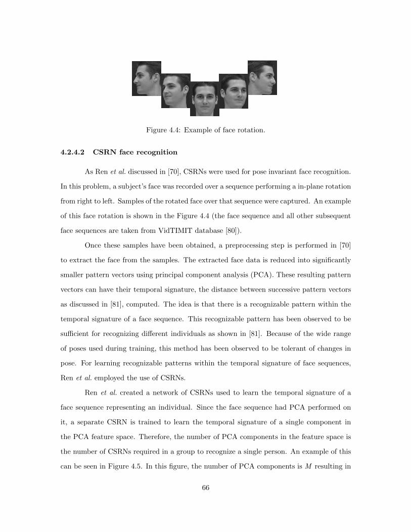
Figure 4.4: Example of face rotation.

4.2.4.2 CSRN face recognition

As Ren et al. discussed in [70], CSRNs were used for pose invariant face recognition.

In this problem, a subject’s face was recorded over a sequence performing a in-plane rotation

from right to left. Samples of the rotated face over that sequence were captured. An example

of this face rotation is shown in the Figure 4.4 (the face sequence and all other subsequent

face sequences are taken from VidTIMIT database [80]).

Once these samples have been obtained, a preprocessing step is performed in [70]

to extract the face from the samples. The extracted face data is reduced into significantly

smaller pattern vectors using principal component analysis (PCA). These resulting pattern

vectors can have their temporal signature, the distance between successive pattern vectors

as discussed in [81], computed. The idea is that there is a recognizable pattern within the

temporal signature of a face sequence. This recognizable pattern has been observed to be

sufficient for recognizing different individuals as shown in [81]. Because of the wide range

of poses used during training, this method has been observed to be tolerant of changes in

pose. For learning recognizable patterns within the temporal signature of face sequences,

Ren et al. employed the use of CSRNs.

Ren et al. created a network of CSRNs used to learn the temporal signature of a

face sequence representing an individual. Since the face sequence had PCA performed on

it, a separate CSRN is trained to learn the temporal signature of a single component in

the PCA feature space. Therefore, the number of PCA components in the feature space is

the number of CSRNs required in a group to recognize a single person. An example of this

can be seen in Figure 4.5. In this figure, the number of PCA components is M resulting in

66

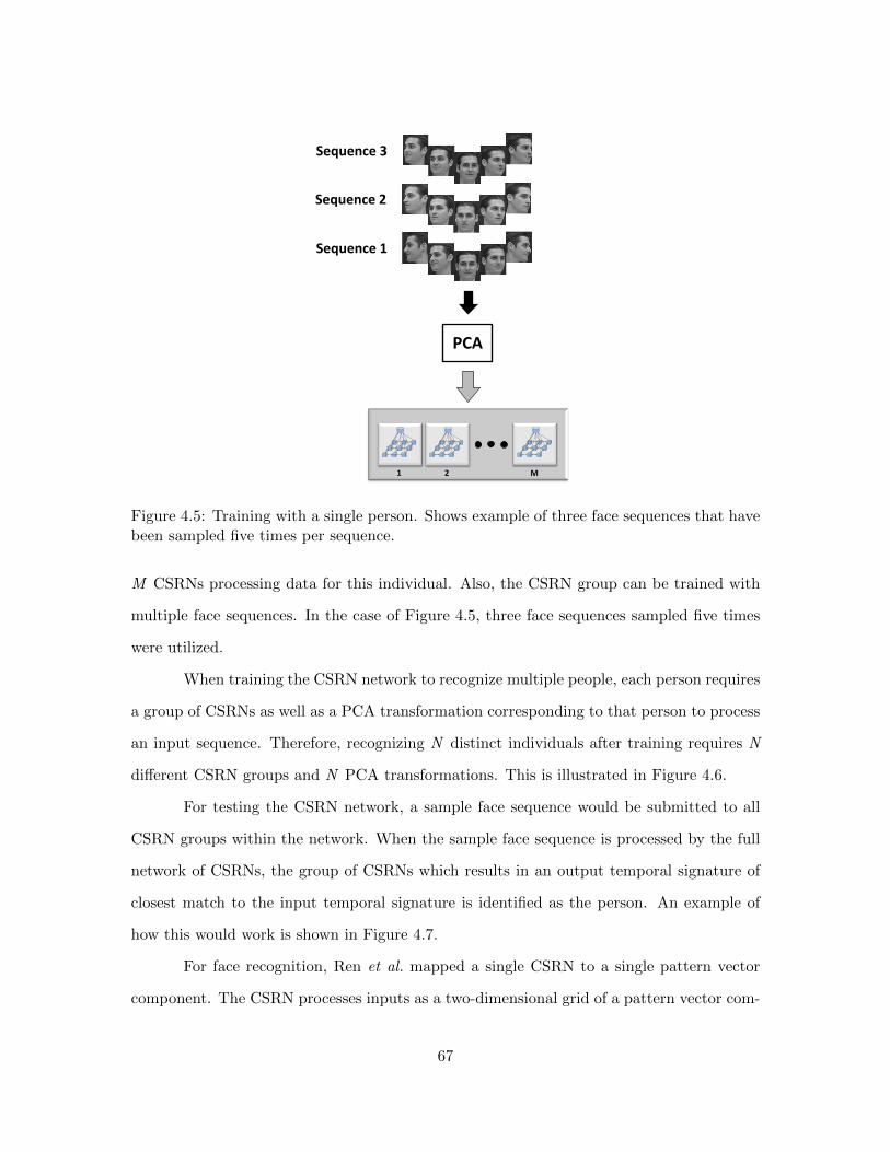
PCA

21 M

Sequence 2

Sequence 1

Sequence 3

Figure 4.5: Training with a single person. Shows example of three face sequences that havebeen sampled five times per sequence.

M CSRNs processing data for this individual. Also, the CSRN group can be trained with

multiple face sequences. In the case of Figure 4.5, three face sequences sampled five times

were utilized.

When training the CSRN network to recognize multiple people, each person requires

a group of CSRNs as well as a PCA transformation corresponding to that person to process

an input sequence. Therefore, recognizing N distinct individuals after training requires N

different CSRN groups and N PCA transformations. This is illustrated in Figure 4.6.

For testing the CSRN network, a sample face sequence would be submitted to all

CSRN groups within the network. When the sample face sequence is processed by the full

network of CSRNs, the group of CSRNs which results in an output temporal signature of

closest match to the input temporal signature is identified as the person. An example of

how this would work is shown in Figure 4.7.

For face recognition, Ren et al. mapped a single CSRN to a single pattern vector

component. The CSRN processes inputs as a two-dimensional grid of a pattern vector com-

67

PCA1

21 M

PCA2

21 M

Person 1 Person 2

Figure 4.6: Training with multiple people. Each person has an associated PCA transforma-tion as well as a collection of CSRNs to process the input face sequence PCA componentdata.

PCA1

21 M

PCA2

21 M

PCAN

21 M

Person 1 Person 2 Person N

Figure 4.7: CSRN network for face recognition. In this network, there are N groups of MCSRNs to process the face sequence. Each CSRN group corresponds to a different person.

68

ponent’s temporal signature values. Each CSRN cell receives a different temporal signature

value as input from that pattern vector. Therefore, if a face sequence has been sampled

10 times, resulting in nine temporal signatures, then a 3×3 grid of the temporal signature

data corresponding to one component in the pattern vector is submitted to a CSRN in the

network for processing.

In the case of this application, each CSRN cell uses a 27 node GMLP model. As

previously noted in Figure 4.2, the GMLP model has two layers where the first layer consists

of 17 nodes (one bias, two external inputs, four neighbor nodes, and 10 recurrent nodes) and

the second layer consists of 10 nodes (10 recurrent nodes). While the bias node constantly

feeds a value of one into the input layer, the first of the two external inputs becomes the

value of the temporal signature pattern vector. The second external input is set to one

whenever the pattern vector value equals zero. Otherwise, the second external input sets

to zero.

4.2.5 CSRN training

While CSRNs can be trained in several ways, the method which Ilin et al. [68]

observed to have the best results was the multi-stream extended Kalman filter (MSEKF)

training technique. MSEKF works mainly following Equations (4.1) – (4.4).

Γt = CtKtCtT +Rt (4.1)

Gt = KtCtTΓt

−1 (4.2)

wt+1 = wt +Gtαt (4.3)

Kt+1 = Kt −GtCtKt +Qt (4.4)

69

Here, t is the time iteration, Γt is the residual covariance, Ct is the state observation matrix

Jacobian, Kt is the predicted estimate covariance, Rt is the observation noise covariance,

Gt is the optimal Kalman gain, αt is the measurement residual, wt is the predicted state,

and Qt is the process noise covariance. For training, wt represents the shared weights for

the CSRN (W , ww, and Ws from Figure 4.2). Also, Ct and αt are computed based upon

wt.

Training of a single CSRN using MSEKF for both maze traversal and face recogni-

tion can be broken down into four stages as outlined in Algorithm 2. The CSRN feedforward

pass (CSRNFF) is for processing a data sample. During CSRNFF, the data sample is prop-

agated up through the GMLP contained within the CSRN cells. The output of CSRNFF is

used as the overall output and to compute αt. The CSRN feedback pass (CSRNFB) is used

mainly for helping computing Ct. During CSRNFB, the outputs of CSRNFF are propagated

back down through the GMLP contained within the CSRN cells. CSRNFF and CSRNFB

both iterate over a predefined number of intervals (10 for the experiments).

Once the outputs of both the CSRNFF and CSRNFB stages are obtained, Ct and αt

can be computed (CCA). After Ct and αt are computed, Kt+1 and wt+1 can be computed,

which consists of performing Equations (4.1) – (4.4) (UWK). Testing of a CSRN is done by

performing the CSRNFF stage for the associated data samples. Whereas a single CSRN is

trained and tested for CSRN based maze traversal, a network of CSRNs has to be trained

and tested for CSRN based face recognition. To train a network of CSRNs, the process

outlined by Algorithm 2 must be performed for all CSRNs within the network. Likewise for

testing, all CSRNs in the network have to perform the CSRNFF stage for their respective

data samples.

70

Algorithm 2 Pseudocode for CSRN MSEKF training.

// Over a set number of iterations (or until there is no change in weights)for each iteration do

// Iterate over all samples to compute a collective Ct and αtfor each data samples do

CSRN Feedforward Pass (CSRNFF)CSRN Feedback Pass (CSRNFB)Calculate Ct and αt (CCA)

end for// Perform CSRN network update

Update wt and Kt (UWK)end for

4.3 High performance implementation

4.3.1 CSRN computation issues

Using CSRNs in any application can quickly become a computationally intensive

task as the input size increases. However, in order to tackle really interesting problems,

CSRN input size needs to increase. The high computational cost comes largely during

training due to the matrix inversion of Γt as seen in Equation (4.2). Furthermore, additional

computational cost comes from performing the increasing amount of cellular computations

during the CSRNFF and CSRNFB stages. Therefore, CSRNs need a method to accelerate

the computations.

The ideal platform for CSRN acceleration is something that would take advantage of

both the inherent task-level parallelism (the cell computations of the CSRNFF and CSRNFB

stages) and the data-level parallelism (the vector and matrix operations of the CCA and

UWK stages) available. A platform that meets the aforementioned criteria is a GPGPU.

4.3.2 Mapping CSRNs to GPGPUs

When performing CSRN processing, GPGPUs can take advantage of the task-level

parallelism within the CSRNFF and CSRNFB stages and the data-level parallelism in the

CCA and UWK stages. For the CSRNFF and CSRNFB stages, the operations of several

CSRN cells (GMLP) map to a thread block. Additionally, the operations of each first layer

71

node GMLP map to a thread within the thread block. Some of the GMLP computations

of the second layer nodes have to be performed serially because of the data dependency

between the second layer nodes aggregated input.

For the CCA and UWK stage computations, the matrix/vector operations map to a

grid, such that each element within the matrix/vector operations would be processed by a

thread. The Γt matrix inversion that occurs as a part of Equation (4.2) is performed using a

parallel Gauss-Jordan elimination technique on the GPGPU adapted from [82]. Figure 4.8

shows an example of Gauss-Jordan elimination matrix inversion for a 3×3 matrix. In this

parallel Gauss-Jordan elimination technique, the initial matrix (matrix to be inverted) is

appended with the corresponding identity matrix. After this, both matrices will iteratively

follow a sequence of modifications for the number of rows in the matrix. These modifications

largely consist of dividing the pivot row, the observed row for the current iteration, by the

pivot value, the diagonal value for the current iteration.

Once the pivot row has been normalized, the values of the pivot column, the observed

column for the current iteration, must be zeroed out by adding a scalar multiple of the pivot

row to the non-pivot rows. This process is repeated for each row until all rows of the initial

matrix have been transformed into the identity matrix. At this point, the identity matrix

will be transformed into the inverse of the initial matrix. The pivot rows, pivot columns,

and pivot values described in this process can be seen in Figure 4.8.

In the GPGPU implementation of this technique, the entire initial matrix is gridded

over the GPGPU. In this fashion, several thread blocks may process the computations of a

single row. The threads within the thread block will compute the corresponding elements

within the rows from both the initial and identity matrices. To allow for the simultaneous

execution of thread blocks across multiple streaming multiprocessors (SMs), the data for

the initial and identity matrices are stored in global memory. Shared data, such as pivot

values for the row, will be fetched from global memory using one thread from each thread

block to be consumed by all threads within the thread block.

Figure 4.9 shows a representative flow chart of the GPGPU operations to train one

72

0.5 1 2 1 0 03 10 8 0 1 09 30 25 0 0 1

1 2 4 2 0 00 4 -4 -6 1 00 12 -11 -18 0 1

1 0 6 5 -0.5 00 1 -1 -1.5 0.25 00 0 1 0 -3 1

1 0 0 5 17.5 -60 1 0 -1.5 -2.8 10 0 1 0 -3 1

Initial Matrix Identity Matrix

After 1st Iteration

After 2nd Iteration

After 3rd Iteration

Figure 4.8: Gauss-Jordan elimination matrix inversion. All shaded regions represent mod-ified elements. Darkly shaded rows and columns represent the corresponding pivot rowand pivot column per iteration. The black shaded values represent the pivot values for thesubsequent iteration.

73

Yes

No

Yes No

End

Iteration< Max?

SubmitSample

Start

MoreSamples?

CSRNFF

CSRNFB

CCA

UWK

Figure 4.9: Flow chart for GPGPU CSRN mapping for MSEKF training. The modulesCSRNFF, CSRNFB, CCA, and UWK take place on GPGPU.

CSRN. For maze traversals, only one CSRN requires training. However, in the case of

face recognition, a network of CSRNs require training. For face recognition, the flow chart

shown in Figure 4.9 would be used to train all network CSRNs with their respective inputs.

4.3.3 Using multiple cores and GPGPUs

Given the increased amount of inherent parallelism within the face recognition ap-

plication, one can more effectively perform CSRN processing by distributing the CSRN

computations across multiple processing cores and/or GPGPUs. For multi-core and multi-

GPGPU implementations, message passing interface (MPI) protocol is used to communicate

between the multiple CPU cores and GPGPUs. The operations followed a master-slave de-

sign where one process is selected as the primary (master) process. The remaining processes

serve as secondary (slave) processes. The primary process directed the operations of the

secondary processes while the secondary processes performed the CSRN network computa-

tions. The number of CSRNs that each secondary process computes varies depending upon

the number of secondary processes available and the number of CSRNs that are within the

74

CSRN network. The primary process will process the input and distribute/collect the work

among the secondary processes in a round robin fashion.

At the start of operation, the primary process reads in the inputs and distributes

the network characteristics to all secondary processes. Then, the primary process sends

a personalized schedule and necessary inputs to each available secondary process. Once a

secondary process receives its input, it can begin operation. When finished, the secondary

process will send the primary process a special data packet to indicate that it has completed

processing. The primary process will then retrieve the output data from the secondary

process.

Whenever the primary process finds an available secondary process and more CSRN

data needs to be processed, the primary process will send the secondary process a new

work schedule as well as more CSRN input data. The primary process will continue the

aforementioned routine until all data has been processed and collected. In this fashion,

both training and testing can be performed.

For all of the multi-core and multi-GPGPU implementations, a single core performed

the operations of the primary process. In the multi-core implementation, one core was used

to perform the operations of a secondary process. In the multi-GPGPU implementation, the

secondary process was performed by one GPGPU using a single-core to transmit data via

MPI to the primary process and other secondary processes. Figure 4.10 shows a depiction

of this setup. The computing system utilized for the multi-core and multi-GPGPU imple-

mentations was the Condor cluster hosted at the Air Force Research Laboratory (AFRL)

Rome Research Site.

4.3.4 The Condor cluster

The Condor cluster is a high speed custom heterogeneous compute cluster capable

of approximately 1.5 GFLOPS per watt of computing power [83]. At the time of this

writing, this system comprised of 78 compute servers powered by 2.67 GHz Intel Xeon X5650

multi-core processor (six cores per multi-core processor resulting in 468 total CPU cores for

75

Communicationperformed using MPI

CSRNs can vary perSecondary Process

Directs operation ofSecondary Processes

Computes witheither CPU core or

GPGPU

SecondaryProcess1

PrimaryProcess

SecondaryProcess2

SecondaryProcessN

Figure 4.10: System arrangement of the primary and associated secondary processes.

computation) connected with 1,716 PS3s. The PS3s were used as a cost effective measure to

leverage the computational power of the IBM/Sony/Toshiba Cell broadband engine housed

inside of them. To extend the computing capabilities of this cluster, each compute server

connects to two NVIDIA Tesla GPGPUs, resulting in 156 total GPGPUs. Currently, there

are plans to update all C1060 GPGPUs with newer model GPGPUs. Within this cluster,

47 compute servers are connected to NVIDIA Tesla C2050 GPGPUs, seven compute servers

are connected to NVIDIA Tesla C2070 GPGPUs, and 24 compute servers are connected

to NVIDIA Tesla C1060 GPGPUs. Table 4.1 shows the composition of the three GPGPU

types.

The compute servers and PS3s were separated into six main divisions. Each division

Table 4.1: NVIDIA GPGPU composition for Tesla GPGPUs.

Metrics C1060 C2050/C2070GPGPU GPGPU

Condor cluster GPGPUs 48 94/14Speed(GHz) 1.3 1.15Streaming multiprocessors 30 14Scalar processors 8 32Global Memory(MB) 4,096 3,072/6,144

76

consisted of 13 compute servers and 286 PS3s. Infiniband as well as 10 Gb and 1 Gb ethernet

switches are used to network the compute servers and PS3s together.

4.4 Results

4.4.1 Maze traversal

4.4.1.1 Single-core CPU vs. single GPGPU

Two initial designs were implemented: a CPU version using the C programming

language with the OpenCV library [84, 85] and a GPGPU version using both the C pro-

gramming language and NVIDIA’s compute unified device architecture (CUDA) extension

[86, 87]. LU decomposition provided by OpenCV was used to invert Γt from Equation

(4.2) for all CPU implementations. The CPU implementation was performed using a 2.67

GHz Intel Xeon X5550 processor, and the GPGPU implementation was performed using a

combination of the same Intel Xeon processor and an NVIDIA Tesla C2050 GPGPU. The

GPGPU performed the CSRN operations while the Intel Xeon processor was used for setup

and communication purposes. The CPU implementations were compiled with the GNU

compiler (GCC) using the −O3 optimization.

Figure 4.11 shows the timing results of both implementations being used for the

CSRN maze traversal training phase. In this set of tests, the number of rows and columns

for the maze input samples were varied as shown along the x-axis. For each input maze

size, five samples were used. The total runtime to perform the training is shown along the

y-axis. All other parameters remained fixed. As can be seen in Figure 4.11, the GPGPU

implementation is slightly faster than the CPU implementation. For this set of tests, the

best observed speedup was approximately three times with an average speedup of about 2.1

times in favor of the GPGPU implementation.

Figure 4.12 shows the timing results of both implementations being used in the

CSRN maze traversal testing phase. As in the set of tests for training, the number of row

and columns for the maze input samples were varied as shown along the x-axis, while all

77

0

2000

4000

6000

8000

10000

5×5 10×10 15×15 20×20 25×25 30×30

Tim

e (s

)

Input Maze Size (Row×Column)

CPU

GPGPU

Figure 4.11: Maze traversal CPU vs. GPGPU training runtimes.

0

0.2

0.4

0.6

0.8

1

25×25 35×35 45×45 55×55 65×65 75×75 85×85 95×95

Tim

e (s

)

Input Maze Size (Row×Column)

CPU

GPGPU

Figure 4.12: Maze traversal CPU vs. GPGPU testing runtimes.

78

Table 4.2: Timing breakdown for computation stages of GPGPU design. Input maze sizesare shown in row×column format.

Computation Input Maze SizeStage 5×5 10×10 15×15

CSRNFF 2.07% 0.43% 0.06%CSRNFB 3.57% 0.62% 0.08%CCA 1.04% 0.17% 0.02%UWK 76.96% 97.11% 99.68%Overhead 16.36% 1.67% 0.17%

other parameters remained constant. In addition, 15 samples were used for each input

maze size. The total runtime to perform the testing is shown along the y-axis. As shown

in Figure 4.11, the GPGPU implementation is faster than the CPU implementation. For

this series of tests, the best observed speedup was 4.39 times with an average speedup of

approximately 3.5 in favor of the GPGPU implementation.

4.4.1.2 GPGPU design extensions

To achieve higher speedups, several design extensions were examined. Specifically,

the speedup performance of the training phase was closely examined, as it is the limiting

factor when processing larger datasets. For example, to train a CSRN using five 30×30

maze input samples required 5,143.12s, while testing using five 30×30 maze input samples

required 13.82ms on the GPGPU. Therefore, the average time required to compute each

stage was measured to capture the most time consuming part of the training phase. For

these measurements, the rows and columns of the input samples were varied (5×5 to 15×15

in 5×5 increments), and the number of input samples was fixed at five. Table 4.2 shows

these results of our measurements.

As highlighted in bold in Table 4.2, the limiting factor is clearly the UWK stage,

as it takes up the bulk of the computation. This result is not surprising, as the UWK

stage includes a time consuming matrix inversion within its computations. In order to

achieve improved speedup performance, the UWK stage was examined carefully for possible

79

modification. Therefore, the initial GPGPU implementation was modified following three

extensions.

Extension 1: Data caching of specific variables One method of decreasing the com-

putation time of the UWK stage is to incorporate caching. The slowest part of many

GPGPU applications is the time required to access global memory. By caching the data

acquired from global memory accesses, one can save time. From Equations (4.1) – (4.4)

of the UWK stage, the variables Ct, Gt, αt, and Kt can be cached because of their re-

peated use. The initial GPGPU implementation was modified to incorporate caching for

the aforementioned variables in the UWK stage. Unfortunately, the UWK stage showed

insignificant improvement from taking this action. This is mainly a result of the additional

computation required to processing 64-bit data (which we required to maintain precision).

Caching works better for data memory elements of 32 bit-width or less.

Extension 2: Reducing global memory accesses Since adding data caching showed

little effect, another method of decreasing the computation time of the UWK stage was

tried. As can be observed in the GPGPU implementation of Gauss-Jordan elimination,

one can dramatically reduce the number of accesses to global memory. This observation

can be seen from the example of Gauss-Jordan elimination given in Figure 4.8. After an

iteration of Gauss-Jordan elimination, only the shaded regions are modified. This is because

of the zeros present in the remaining areas offer no change to the non-pivot rows. Using

this knowledge, the GPGPU Gauss-Jordan elimination routine was modified to only access

global memory during the times in which there will be modification to the non-pivot rows.

By doing this, the amount of time necessary to compute UWK computation stage decreased

by approximately 57% when compared to the initial implementation.

Extension 3: Performing Gauss-Jordan normalization at end of computation

In Figure 4.8 during the computation of the Gauss-Jordan elimination routine, the pivot

row is normalized by the diagonal value every iteration. This normalization actually can be

80

0

1000

2000

3000

4000

5000

6000

7000

8000

9000

10000

5×5 10×10 15×15 20×20 25×25 30×30

Tim

e (s

)

Input Maze Size (Row×Column)

CPU

Initial

Ex. 1

Ex. 2

Ex. 3

Figure 4.13: CPU vs. GPGPU with extensions training runtimes. Initial refers to ouroriginal GPGPU implementation. Ex. 1, 2, and 3 refer to our incorporation of extensions1, 2, and 3 into our original GPGPU design.

postponed until after all iterations have been completed. Therefore, the GPGPU extension

2 implementation was updated to normalize only after all iterations of the Gauss-Jordan

routine were completed. By doing this, the number of global memory accesses during the

UWK stage were reduced which resulted in a slight reduction in the computation when

compared to extension 2 alone.

Figure 4.13 shows the effect that each extension had on the overall time when

compared against the CPU implementation. The most significant overall speedup occurs as

a result of extension 3. The best observed speedup acquired from extension 3 is 8.32 times

with an average speedup of approximately 7.2 times.

81

4.4.2 Face recognition

4.4.2.1 Improving the GPGPU design

For developing the face recognition GPGPU CSRN implementation, the extension

3 maze traversal GPGPU CSRN design was used as a base. In that design, only one

CSRN cell computation was performed per thread block. Given the small size of the maze

traversal CSRN cell GMLP (17 nodes), many threads were left idle. To improve the GPGPU

thread occupancy, the number of CSRN cell computations performed per thread block was

increased.

Since the face recognition CSRN cell GMLP is a 27 node network, the operations of

one GMLP can be performed using the threads associated with one warp (32 threads). Given

that a thread block can process multiple warps, a thread block can be utilized to process

several different CSRN cells simultaneously by exploiting instruction-level parallelism. For

the face recognition GPGPU CSRN design, four different CSRN cells were processed per

thread block, as this was observed to achieve good design performance.

Additionally during the CSRNFF and CSRNFB stages, shared memory is used to

store repeatedly used data such as W and ww (seen in Figure 4.2) during computation.

This reduces the number of times that global memory is accessed by copying the data down

into shared memory at the start of the process. The use of multiple warps benefits from

this because the shared W and ww data can be used among the various CSRN cells being

computed within a thread block, reducing the amount of traffic seen by global memory.

Using these CSRN cell computation advancements in addition to using better GPGPU

memory management, the CSRN GPGPU design improved.

4.4.2.2 Single-core CPU vs. single GPGPU

Two initial designs were implemented to examine how well CSRN based face recog-

nition maps to a GPGPU system. Akin to the maze traversal designs, the two initial face

recognition designs were a CPU version using the C programming language with OpenCV

82

library and a GPGPU version using both the C programming language and CUDA. The

CPU implementation was performed on a 2.67 GHz Intel Xeon X5650 multi-core processor

and the GPGPU implementation was performed on a combination of the same Intel Xeon

multi-core processor and the NVIDIA Tesla C1060, C2050, and C2070 GPGPUs.

One GPGPU design was developed for use among the three GPGPU platforms. One

expects the performance between the C2050 and C2070 GPGPUs to be identical because the

architectures are the same with the exception of global memory. The C2070 GPGPU has

twice the amount of global memory. However, using the newer generation GPGPUs (C2050s

and C2070s) can be expected to result in better performance than the older generation

GPGPUs (C1060s). A contributing reason is because the C2050 and C2070 have more

scalar processors (SPs) (the C2070 and C2050 have 208 more SPs than the C1060). In

addition, the C2050 and C2070 have the ability to perform up to four concurrent streams of

independent processing, while the C1060 performs one stream. Within the GPGPU design,

large numbers of SPs as well as multiple concurrent streams are utilized whenever possible.

While all three GPGPU implementations will offer improvements over an equivalent CPU

implementation, a significant edge will go to the C2050 and C2070.

During the experiments, the CPU implementation was compiled with GCC and

the Intel compiler (ICC) using all applicable optimization flags. ICC compiles code to

take advantage of single instruction, multiple data (SIMD) instructions; therefore, ICC’s

generated codes tend to have faster runtimes than GCC’s generated code. Lastly, the face

sequences for the experiments were taken from the Sheffield face database [88].

For using CSRN based face recognition, only the CSRN training phase of the al-

gorithm was accelerated, since this portion is the most time consuming. In doing so, four

experiments were conducted investigating how changes in the CSRN network parameters af-

fect GPGPU acceleration. The CSRN network parameters observed were number of people,

PCA components, samples per face sequence, and number of face sequences.

83

Table 4.3: Training times for increasing number of people. The implementations shownare GCC single-core CPU (G-CPU), ICC single-core CPU (I-CPU), C1060 GPGPU, C2050GPGPU, and C2070 GPGPU.

People G-CPU(s) I-CPU(s) C1060 C2050/C2070GPGPU(s) GPGPU(s)

1 189.67 33.18 11.12 6.482 379.27 66.24 21.06 12.293 568.84 99.32 31.09 18.444 757.71 132.38 41.47 24.665 948.04 165.45 52.01 30.826 1,137.66 198.53 62.09 38.927 1,327.19 231.62 72.87 42.988 1,516.62 264.72 82.61 51.789 1,706.18 297.79 92.96 55.44

10 1,891.93 330.83 103.80 61.64

Experiment 1: Varying number of people The first experiment involved testing the

single-core CPU and single GPGPU implementations using an increasing number of people.

The number of people varied from one to 10. A group of 10 CSRNs (10 PCA components)

utilizing face sequences that have been sampled nine times was used to identify a person.

Only one face sequence per person was used during training. The training was performed

using MSEKF. The training times for the experiment are shown in Table 4.3.

From the training times shown in Table 4.3, the average speedup for the ICC single-

core CPU, C1060 GPGPU, and C2050/C2070 GPGPU versions over the GCC single-core

CPU compilation is about 5.7, 18.1, and 30.3 times, respectively. Furthermore, the C1060

GPGPU and the C2050/C2070 GPGPU carry an average speedup over the ICC single-

core CPU of approximately 3.1 and 5.3 times, respectively. Given that the C2050/C2070

GPGPU implementations are faster than the C1060 implementation over all scenarios, the

inclusion of the C1060 GPGPUs will play a limiting factor in multi-GPGPU experiments.

As the number of people increased, the performance benefit achieved from using GPGPUs

stayed mostly the same. This can be expected since increasing the number of people is

equivalent to adding more CSRNs to the network.

84

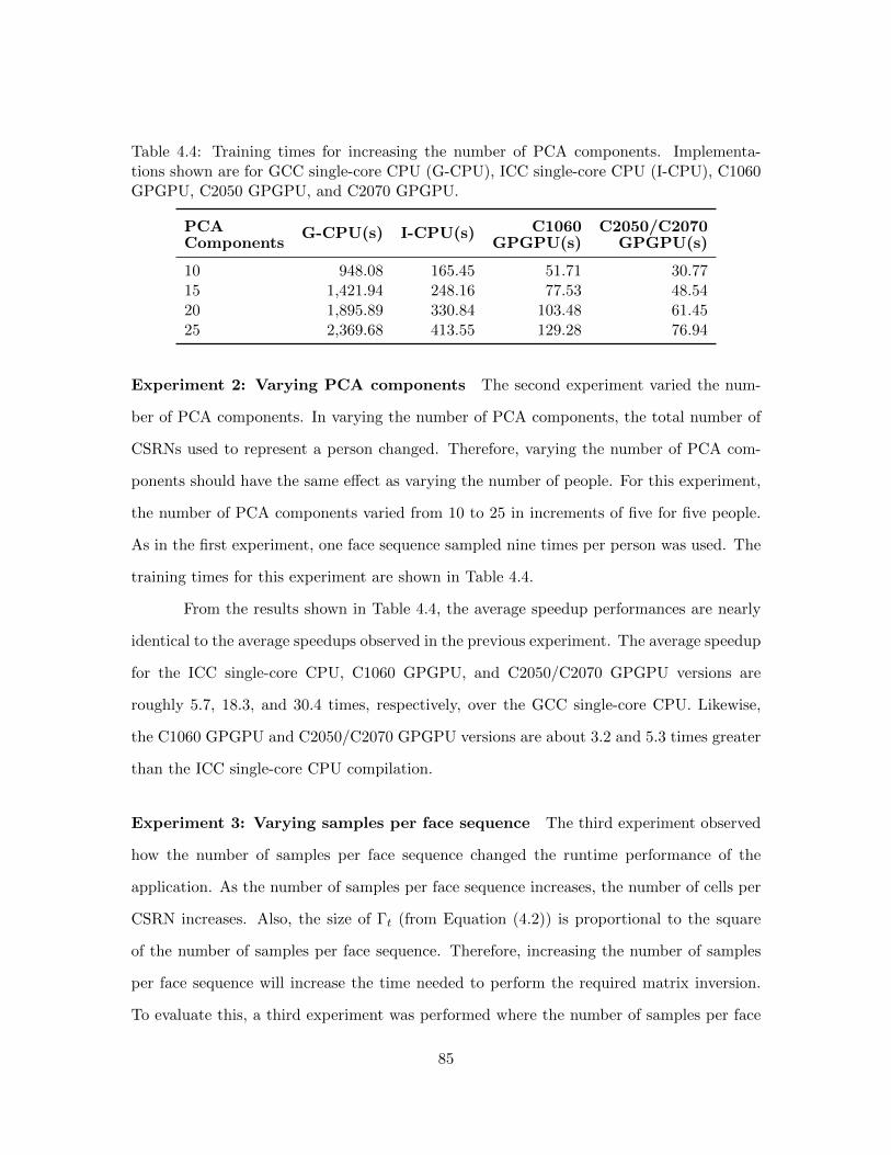
Table 4.4: Training times for increasing the number of PCA components. Implementa-tions shown are for GCC single-core CPU (G-CPU), ICC single-core CPU (I-CPU), C1060GPGPU, C2050 GPGPU, and C2070 GPGPU.

PCA G-CPU(s) I-CPU(s) C1060 C2050/C2070Components GPGPU(s) GPGPU(s)

10 948.08 165.45 51.71 30.7715 1,421.94 248.16 77.53 48.5420 1,895.89 330.84 103.48 61.4525 2,369.68 413.55 129.28 76.94

Experiment 2: Varying PCA components The second experiment varied the num-

ber of PCA components. In varying the number of PCA components, the total number of

CSRNs used to represent a person changed. Therefore, varying the number of PCA com-

ponents should have the same effect as varying the number of people. For this experiment,

the number of PCA components varied from 10 to 25 in increments of five for five people.

As in the first experiment, one face sequence sampled nine times per person was used. The

training times for this experiment are shown in Table 4.4.

From the results shown in Table 4.4, the average speedup performances are nearly

identical to the average speedups observed in the previous experiment. The average speedup

for the ICC single-core CPU, C1060 GPGPU, and C2050/C2070 GPGPU versions are

roughly 5.7, 18.3, and 30.4 times, respectively, over the GCC single-core CPU. Likewise,

the C1060 GPGPU and C2050/C2070 GPGPU versions are about 3.2 and 5.3 times greater

than the ICC single-core CPU compilation.

Experiment 3: Varying samples per face sequence The third experiment observed

how the number of samples per face sequence changed the runtime performance of the

application. As the number of samples per face sequence increases, the number of cells per

CSRN increases. Also, the size of Γt (from Equation (4.2)) is proportional to the square

of the number of samples per face sequence. Therefore, increasing the number of samples

per face sequence will increase the time needed to perform the required matrix inversion.

To evaluate this, a third experiment was performed where the number of samples per face

85

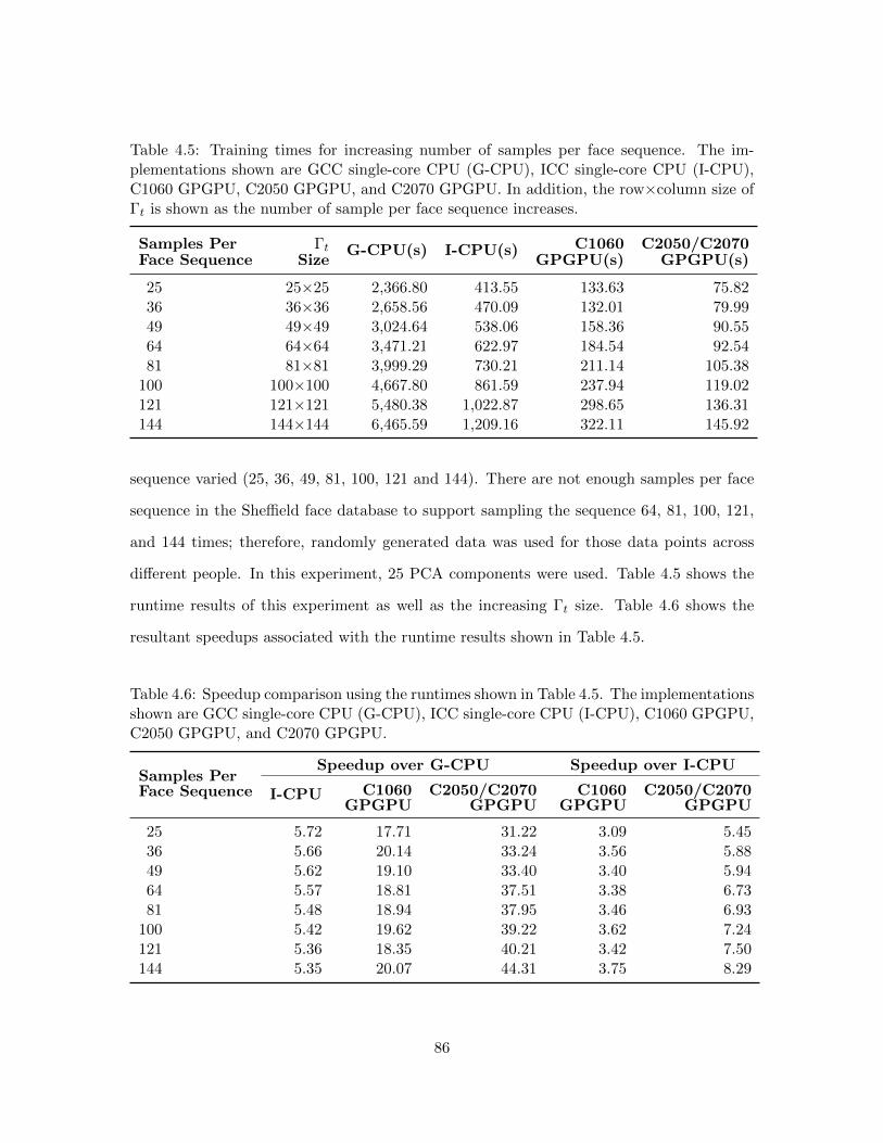
Table 4.5: Training times for increasing number of samples per face sequence. The im-plementations shown are GCC single-core CPU (G-CPU), ICC single-core CPU (I-CPU),C1060 GPGPU, C2050 GPGPU, and C2070 GPGPU. In addition, the row×column size ofΓt is shown as the number of sample per face sequence increases.

Samples Per Γt G-CPU(s) I-CPU(s) C1060 C2050/C2070Face Sequence Size GPGPU(s) GPGPU(s)

25 25×25 2,366.80 413.55 133.63 75.8236 36×36 2,658.56 470.09 132.01 79.9949 49×49 3,024.64 538.06 158.36 90.5564 64×64 3,471.21 622.97 184.54 92.5481 81×81 3,999.29 730.21 211.14 105.38

100 100×100 4,667.80 861.59 237.94 119.02121 121×121 5,480.38 1,022.87 298.65 136.31144 144×144 6,465.59 1,209.16 322.11 145.92

sequence varied (25, 36, 49, 81, 100, 121 and 144). There are not enough samples per face

sequence in the Sheffield face database to support sampling the sequence 64, 81, 100, 121,

and 144 times; therefore, randomly generated data was used for those data points across

different people. In this experiment, 25 PCA components were used. Table 4.5 shows the

runtime results of this experiment as well as the increasing Γt size. Table 4.6 shows the

resultant speedups associated with the runtime results shown in Table 4.5.

Table 4.6: Speedup comparison using the runtimes shown in Table 4.5. The implementationsshown are GCC single-core CPU (G-CPU), ICC single-core CPU (I-CPU), C1060 GPGPU,C2050 GPGPU, and C2070 GPGPU.

Samples PerSpeedup over G-CPU Speedup over I-CPU

Face Sequence I-CPU C1060 C2050/C2070 C1060 C2050/C2070GPGPU GPGPU GPGPU GPGPU

25 5.72 17.71 31.22 3.09 5.4536 5.66 20.14 33.24 3.56 5.8849 5.62 19.10 33.40 3.40 5.9464 5.57 18.81 37.51 3.38 6.7381 5.48 18.94 37.95 3.46 6.93

100 5.42 19.62 39.22 3.62 7.24121 5.36 18.35 40.21 3.42 7.50144 5.35 20.07 44.31 3.75 8.29

86

Here, the trend is that the performance benefit offered by the GPGPU implemen-

tation improves as the face sequence sampling increases. There is a moderate performance

benefit for the C1060 GPGPU implementation. However, there is a significant performance

benefit for the C2050/C2070 GPGPU implementation. The speedup performance shown in

the GPGPU implementations is expected because the number of CSRN cells computations

increase one-to-one with the number of samples per face sequence. For the single-core CPU

implementations, these additional CSRN cell computations are performed serially, whereas

they are performed in parallel for the GPGPU implementations.

Furthermore, the inversion of Γt for the GPGPU implementations can be performed

much faster than the single-core CPU implementations. This is a direct result of the par-

allelism involved in the GPGPU matrix inversion scheme. The larger the size of Γt, the

greater the advantage will be in favor of the GPGPU implementations.

Experiment 4: Varying face sequences Lastly, a fourth experiment observed how

varying the number of face sequences affects runtime performance. In this experiment,

increasing the number of face sequence increases the size of Γt proportionately. Specifically,

the number of rows and columns both increase by a multiple of the number of face sequences.

Thus, the duration of the UWK stage becomes longer as the time to invert Γt becomes

longer. In addition, multiple face sequences must be processed by the CSRN network

serially. This multiplies the time to perform the CSRNFF, CSRNFB, and CCA stages by

the number of face sequences to process.

To evaluate the fourth experiment, the number of different face sequences per person

used during training varied from one to five. Also, five people, 49 samples per sequence,

and 25 PCA components were used. Table 4.7 shows the results of this experiment. Also,

Table 4.7 shows the size of Γt as the number of face sequences increased. Table 4.8 shows

the resultant speedup performance.

The data shown in Table 4.7 and Table 4.8 reveal the advantage of the GPGPU

implementations. When compared to both single-core CPU implementations, the GPGPU

87

Table 4.7: Training times using an increasing number of face sequences. The implemen-tations shown are GCC single-core CPU (G-CPU), ICC single-core CPU (I-CPU), C1060GPGPU, C2050 GPGPU, and C2070 GPGPU implementations using an increasing numberof face sequences. In addition, the row×column size of Γt is shown as the number of facesequences increases.

Face Γt G-CPU(s) I-CPU(s) C1060 C2050/C2070Sequences Size GPGPU(s) GPGPU(s)

1 49×49 3,020.28 538.07 160.85 98.862 98×98 4,573.17 843.73 273.80 153.863 147×147 6,591.62 1,243.13 404.75 219.414 196×196 8,966.28 1,743.47 564.25 304.835 245×245 11,638.75 2,407.37 802.17 396.30

Table 4.8: Speedup comparison using runtimes shown in Table 4.7. The implementationsshown are GCC single-core CPU (G-CPU), ICC single-core CPU (I-CPU), C1060 GPGPU,C2050 GPGPU, and C2070 GPGPU.

FaceSpeedup over G-CPU Speedup over I-CPU

Sequences I-CPU C1060 C2050/C2070 C1060 C2050/C2070GPGPU GPGPU GPGPU GPGPU

1 5.61 18.78 30.55 3.35 5.442 5.42 16.70 29.72 3.08 5.483 5.30 16.29 30.04 3.07 5.674 5.14 15.89 29.41 3.09 5.725 4.83 14.51 29.37 3.00 6.07

88

implementations continue to maintain a speedup advantage. Similar to previous results,

the achieved speedup can be attributed to the parallel processing of the increasing CSRNFF

and CSRNFB computations and the CCA and UWK vector/matrix operations.

In the case of the GCC compilation, the C1060 and C2050/C2070 GPGPU imple-

mentations show a decrease in the available speedup. This is likely due to the increasing

amount of memory transfers. The increase in memory transfers result from the CPU need-

ing to send additional face sequence input data to the GPGPU. Memory transfers between

the CPU and GPGPU are very costly and decrease the amount of acceleration benefit

seen. The additional parallel resources within the C2050/C2070 GPGPU implementation

allow for a much slower decrease in acceleration when compared to the C1060 GPGPU

implementation.

In the case of the ICC compilation, the C1060 GPGPU implementation continues to

show this trend of decreasing speedup. However, the C2050/C2070 GPGPU shows a gradual

increase in speedup. The ICC compilation has a much faster decrease in acceleration in

comparison to the C2050/C2070 GPGPU implementation resulting in the gradual increase

in speedup.

4.4.2.3 Multi-core and multi-GPGPU

Multi-core and multi-GPGPU implementations of the algorithm were explored. The

main objective of this was to observe how CSRN based face recognition scales as more CPU

core/GPGPU resources are added. For these experiments only the ICC compilation results

are shown, as they are much faster than the GCC compilation.

Given that the Condor cluster is a heterogeneous cluster composed of three different

kinds of GPGPUs (94 C2050, 14 C2070, and 48 C1060), the best GPGPU combinations

possible are utilized when adding GPGPU resources. Since computations are bound by

the C1060s, the C2050s and C2070s are scheduled prior to the C1060s to ensure good

productivity. Specifically, the C2050s are added first and then the C2070s. At the time

of these experiments, only 10 of the 14 C2070 were available. Therefore, after adding 10

89

5.00

10.00

15.00

20.00

25.00

30.00

35.00

40.00

45.00

50.00

Series2

Series30

50

100

150

200

250

10 30 50 70 90 110 130 150

Tim

e (s

)

Secondary Processes

Multi-core

Multi-GPGPU

Figure 4.14: Graph of training time for multi-core and multi-GPGPU implementations.

C2070s, C1060s are added. The workload used for these experiments were one CSRN per

primary to secondary process transmission.

Figure 4.14 shows the runtime performance of a CSRN network designed to classify

five people using five face sequences, 49 samples per face sequence, and 25 PCA components.

For this CSRN network, Figure 4.14 shows the MSEKF training time decrease as the number

of secondary processes increased from 10 to 150 by increments of 10. In the case of the

multi-core implementation, the training time decreased from 254.26s to 20.58s using 10 to

150 secondary processes, respectively. For the multi-GPGPU implementation, the training

time decreased from 43.08s to 9.07s using 10 to 150 secondary processes, respectively.

Figure 4.15 shows the speedup for both the multi-core and multi-GPGPU imple-

mentations over the single-core ICC compiled CPU version. While both implementations

offer vast improvement over the single-core version, the multi-GPGPU implementation pro-

vides more speedup than the multi-core. However, the multi-core implementation appears

to scale better as the multi-GPGPU implementation levels off after 70 secondary processes.

With the inclusion of the slower C1060 GPGPUs, the scaling of the multi-GPGPU imple-

90

0

50

100

150

200

250

300

10 30 50 70 90 110 130 150

Sp

eed

up

Secondary Processes

Multi-core

Multi-GPGPU

Figure 4.15: Graph of speedup for multi-core and multi-GPGPU implementations.

mentation is hindered as expected. Once the number of secondary processes exceeds the

number of available C2050 (94) and C2070 (8) GPGPUs, the total efficiency of the multi-

GPGPU implementation declines as the C1060 GPGPUs are used. This is shown by the

decrease in speedup performance after 100 GPGPUs. As previously established in Tables

4.3 – 4.6, the C1060 GPGPUs process data slower than the C2050 and C2070 GPGPUs for

this application.

Table 4.9: Training runtime performance for multi-core and multi-GPGPU. The multi-coreand multi-GPGPU implementations are compared to GCC (G-CPU), ICC (I-CPU), C1060GPGPU, and C2050/C2070 GPGPU implementations.

Implementation Time(s) Speedup over Speedup overG-CPU I-CPU

G-CPU 11,638.75 1.00 0.21I-CPU 2,407.37 4.83 1.00C1060 GPGPU 782.89 14.87 3.07C2050/C2070 GPGPU 393.94 29.54 6.11multi-core 20.58 565.44 116.96multi-GPGPU 9.07 1,283.62 265.50

91

Table 4.9 shows the MSEKF training time and speedup performance for the multi-

core and multi-GPGPU implementation relative to the previously discussed implementa-

tions (GCC and ICC single-core CPU implementations and the C1060 and C2050/C2070

single GPGPU implementations) for the experiment of five people, 49 samples per face se-

quence, five face sequences, and 25 PCA components. The multi-core and multi-GPGPU

implementations for which timing results shown in Table 4.9 use 150 secondary processes.

The speedup shown is a comparison between all implementations to both GCC and ICC

single-core CPU implementations. From using the multi-GPGPU implementation, signifi-

cant speedups of approximately 1,283 and 265 times are observed when compared against

the GCC and ICC single-core CPU compilations, respectively. Table 4.9 demonstrates the

merits of the multi-GPGPU implementation.

4.4.2.4 Combining multi-core and multi-GPGPU

Given the limited GPGPU resources of the Condor cluster in comparison to the

ample amount of Intel multi-core processors available, the computational capabilities of both

multi-core and multi-GPGPU implementations should combine to take greater advantage

of cluster resources. Since each processor in the Condor cluster has six cores, only two cores

per processor were used in the multi-GPGPU implementation. The remaining four cores

were idle. To fully utilize each core in the system, the idle cores should perform CSRN

computations concurrently with the GPGPUs. Using both multi-core and multi-GPGPU

together, one can expect to achieve even greater runtime performance than using each alone.

For the multi-core, multi-GPGPU, and multi-core/GPGPU implementations, 75 of

the total 78 multi-core processors on the system were utilized. In this fashion, 450 cores

(one core for the primary process and 449 for the secondary processes) were used for the

multi-core implementation. The multi-GPGPU implementation used 150 (94 C2050s, 8

C2070s and 48 C1060s) GPGPUs operating as secondary processes and one core as the

primary process. Lastly, the multi-core/GPGPU implementation used one core as the

primary process and 299 cores as secondary processes. The remaining cores 150 cores used

92

GPGPUs as secondary processes. As before, the multi-core implementations were compiled

using ICC.

Also, more resources of the Condor cluster should be utilized to get an indica-

tion of the Condor cluster’s computational capability for CSRN based face recognition.

Therefore, two additional experiments were conducted to demonstrate the significant im-

pact on runtime performance of a system such as the Condor cluster has for this appli-

cation. Additionally, the runtime performances of the the multi-core, multi-GPGPU, and

multi-core/GPGPU implementations were compared. In these experiments, the number of

samples per face sequence and number of face sequences were varied.

Experiment 5: Varying samples per face sequence using large networks This

experiment observed the effect of varying the number of samples per face sequence has on

runtime performance for the multi-core, multi-GPGPU, and multi-core/GPGPU implemen-

tations. For this experiment, a randomly generated CSRN network to classify 1,000 people

using 10 PCA components and one face sequence per person was created. The number of

samples per face sequence varied using the following sample rates: 25, 36, 49, 81, 100, 121

and 144. This resulted in a full network of 10,000 CSRNs. Figure 4.16 shows the training

time results of this experiment, and Figure 4.17 shows the speedup performance over the

ICC single-core compilation.

As seen in Figure 4.16 and Figure 4.17, both implementations incorporating GPG-

PUs are faster than the multi-core implementation as the number of samples per face

sequence increases. The multi-core implementation speedup is shown to decrease as face

sequence samples increase. The multi-GPGPU and multi-core/GPGPU implementations

speedup performance improves while the samples per face sequence increase.

Another significant result is that the multi-GPGPU implementation is faster than

the multi-core implementation while using much less resources. The multi-GPGPU imple-

mentation uses 150 GPGPUs to act as secondary processes compared to the 449 cores that

the multi-core implementation uses. As expected, the multi-core/GPGPU implementation

93

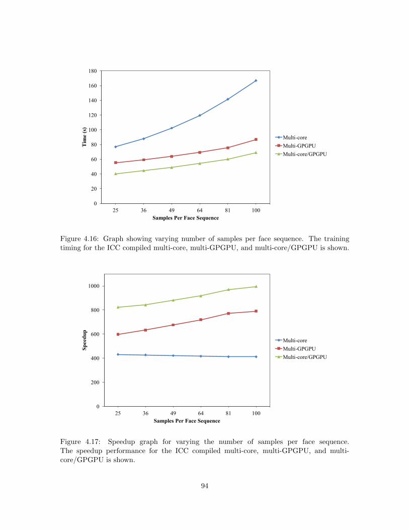
0

20

40

60

80

100

120

140

160

180

25 36 49 64 81 100

Tim

e (s

)

Samples Per Face Sequence

Multi-core

Multi-GPGPU

Multi-core/GPGPU

Figure 4.16: Graph showing varying number of samples per face sequence. The trainingtiming for the ICC compiled multi-core, multi-GPGPU, and multi-core/GPGPU is shown.

0

200

400

600

800

1000

25 36 49 64 81 100

Sp

eed

up

Samples Per Face Sequence

Multi-core

Multi-GPGPU

Multi-core/GPGPU

Figure 4.17: Speedup graph for varying the number of samples per face sequence.The speedup performance for the ICC compiled multi-core, multi-GPGPU, and multi-core/GPGPU is shown.

94

0

50

100

150

200

1 2 3 4 5

Tim

e (s

)

Face Sequences

Multi-core

Multi-GPGPU

Multi-core/GPGPU

Figure 4.18: Graph of varying the number of face sequences. The graph shows the trainingtiming for the ICC multi-core, multi-GPGPU, and multi-core/GPGPU implementations.

is faster than the multi-GPGPU implementation, as the the former uses the additional pro-

cessing power of cores during computation. As seen in Figure 4.17, the multi-core/GPGPU

implementation displays a speedup performance of approximately 823 to 996 times for 25

to 100 samples per face sequence, respectively.

Experiment 6: Varying face sequences using large networks This experiment ob-

served the behavior of the multi-core, multi-GPGPU, and multi-core/GPGPU implemen-

tations while varying the number of face sequences from one to five. To do this, another

randomly generated 1,000 person CSRN network using 10 PCA components was created.

The face sequences used in this network were sampled 25 times. Figure 4.18 and Figure 4.19

show the training time results and speedup performance of the ICC compiled multi-core,

multi-GPGPU, and multi-core/GPGPU implementations, respectively. The speedup per-

formance shown in Figure 4.19 uses the ICC single-core compilation as a base.

In Figure 4.18, as in the previous experiments, the multi-GPGPU implementation

maintains a lower training runtime when compared to the multi-core. As before, the multi-

95

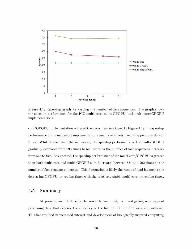
0

100

200

300

400

500

600

700

800

900

1 2 3 4 5

Sp

eed

up

Face Sequences

Multi-core

Multi-GPGPU

Multi-core/GPGPU

Figure 4.19: Speedup graph for varying the number of face sequences. The graph showsthe speedup performance for the ICC multi-core, multi-GPGPU, and multi-core/GPGPUimplementations.

core/GPGPU implementation achieved the lowest runtime time. In Figure 4.19, the speedup

performance of the multi-core implementation remains relatively fixed at approximately 431

times. While higher than the multi-core, the speedup performance of the multi-GPGPU

gradually decreases from 596 times to 520 times as the number of face sequences increases

from one to five. As expected, the speedup performance of the multi-core/GPGPU is greater

than both multi-core and multi-GPGPU as it fluctuates between 824 and 792 times as the

number of face sequences increase. This fluctuation is likely the result of load balancing the

decreasing GPGPU processing times with the relatively stable multi-core processing times.

4.5 Summary

At present, an initiative in the research community is investigating new ways of

processing data that capture the efficiency of the human brain in hardware and software.

This has resulted in increased interest and development of biologically inspired computing

96

approaches in software and hardware. One such biologically inspired approach involves

CSRNs. CSRNs have been demonstrated to be very useful in solving state transition type

problems, such as maze traversals. Although powerful in image processing capabilities,

CSRNs have high computational demands with increasing input problem size.

In this chapter, the runtime performance of CSRNs was examined for acceleration

using multiple CPU and GPGPU techniques for two CSRN based applications: maze traver-

sal and face recognition. For maze traversal, novel GPGPU CSRN implementations were

developed and utilized to observe average speedups of roughly 7.2 and 3.5 times for the

training and testing phases, respectively, when compared to C implementations. Using in-

sight from the maze traversal GPGPU CSRN design, the acceleration and scaling of the

training phase of CSRN based face recognition was examined using AFRL’s Condor cluster,

a large heterogeneous cluster of Intel Xeon multi-core processors, NVIDIA Tesla GPGPUs

(C1060, C2050, and C2070), and PS3s.

Initially, the runtime performance of CSRN based face recognition training using a

single GPGPU was compared to a single-core CPU implementation. The runtime perfor-

mances for the single-core CPU and single GPGPU implementations were examined under

change to various parameters. The C2050 and C2070 single GPGPU implementations pro-

vided a five times or more speedup over single-core CPU implementations. Taking advan-

tage of the Condor cluster, the runtime and speedup performances of large multi-core and

multi-GPGPU systems implementing CSRN based face recognition training were observed.

With 450 Intel Xeon cores and 150 GPGPUs, a CSRN network to classify 1,000 people was

trained in approximately 69s, which is roughly 996 times faster than the single-core CPU

implementation.

CSRN based pattern recognition combines the advantages of biologically neural

networks and computationally efficient recurrent networks. This algorithm is quite flexible,

and thus the results seen here for face recognition can potentially be applied to other types

of recognition tasks.

97

Chapter 5

Conclusions

Currently, improving processor performance by increasing clock frequency is imprac-

tical. Hence, the growing interest in parallel computing. Given the situation, algorithms

must now be redesigned to take advantage of the parallel architecture. Also, an applica-

tion’s acceleration can be improved by multiple factors. These factors are partly due to the

application’s inherit parallelism and target architecture’s ability to exploit that parallelism.

As seen in this dissertation’s parallel designs, field programmable gate arrays (FPGAs)

and general purpose graphical processing units (GPGPUs) present many different ways to

exploit parallelism. The FPGA designs take advantage of granular and spatial parallelism

through the use of deep pipelines and concurrent execution. The GPGPU design employs

the use of thousands of lightweight threads across many processing cores to achieve data-

level and task-level parallelism.

Since FPGAs extract parallelism at a much lower level than GPGPU, FPGA imple-

mentations require a greater understanding of the target algorithms. Greater understanding

along with greater control over the implementation can lead to much greater performance.

However, to achieve greater performance, a longer development time is typically seen.

GPGPUs offer improved performance to algorithms that involve a large number of

identical computations repeatedly performed over different inputs. This follows from the

inherent single instruction, multiple data (SIMD) structure of GPGPU architecture. Also,

this characteristic is commonly seen in many pattern recognition (PR) applications, leading

98

to the GPGPUs being a good developmental platform for them.

Additionally, studies have shown that given algorithm characteristics, certain com-

puting architectures may be more suitable than others. Che et al. [89] conduct a perfor-

mance study to create an application characteristic to platform mapping. For their study,

Che et al. examine the algorithmic behavior, code complexity, and performance of three

algorithms (Gaussian elimination, data encryption standard, and Needleman-Wunsch) de-

veloped for FPGA, GPGPU, and multi-core central processing unit (CPU) platforms. The

characterization presented by Che et al. is useful to help developers select the optimum

platform, based upon the type of application and desired performance. Lastly, Thomas

et al. [90] examine random number generation on a variety of different platforms: FPGA,

CPU, GPGPU, and massively parallel processor array (MPPA). Three different random

number distributions were explored: uniform, Gaussian, and exponential. Across the four

platforms, Thomas et al. show that different implementation methods were required for

optimal results.

Cope et al. [91] perform a case study to compare the performance of a GPGPU

and FPGA implementation. They analyze five algorithms (primary color correction, two-

dimensional convolution, video frame resizing, histogram equalization, and three-step non-

full-search motion vector estimation) on both platforms looking at arithmetic complexity,

memory access requirements, and data dependencies. From this study, Cope et al. show

that algorithms with many memory transactions and data dependency favor a FPGA im-

plementation, while algorithms with variable data reuse favor GPGPU implementations.

The studies presented in this dissertation explore the added benefits of using parallel

computing systems for PR applications. Three PR approaches were examined and tech-

niques to accelerate them were demonstrated for FPGA and GPGPU architectures. The

second chapter focused on the performance of phase-only filter based fingerprint identifica-

tion under various distortions as well as improving the algorithm’s performance using FPGA

acceleration. After measuring tolerances of phase-only filter based fingerprint identification,

the algorithm was accelerated using a novel Virtex II Pro FPGA design. This FPGA de-

99

sign provided a speedup of about 47 times over a C implementation. The performance

achieved was due to the FPGA’s highly pipelined design and overlapped computation and

communication.

The third chapter discussed the implementation of a modularized processing element

(PE) design of an Izhikevich spiking neuron model based character algorithm. This PE

design was evaluated using two different sized networks, one network processing 24×24 pixel

images and another processing 96×96 pixel images, operating on a two different FPGAs,

Virtex II Pro and Virtex 4, respectively. This PE based design is easily scalable to larger

FPGAs. The implemented networks showed significant speedups over equivalent software

implementations (approximately 3.3 times for the 24×24 pixel image network using a Virtex

II Pro and approximately 8.5 times for the 96×96 pixel image network using a Virtex 4).

The fourth chapter examined the acceleration and design of two cellular simultane-

ous recurrent network (CSRN) based pattern recognition applications: maze traversal and

face recognition. For CSRN based maze traversal, a novel accelerated NVIDIA GPGPU

implementation was developed. For the training and testing phase, the GPGPU implemen-

tation showed average speedups of approximately 7.2 and 3.5 times, respectively, over a C

implementation.

Using the CSRN based maze traversal GPGPU implementation as a building block,

an accelerated CSRN based face recognition GPGPU implementation was developed. The

GPGPU implementation provided a five times or more speedup relative to a C implemen-

tation under change to various parameters. Additionally, this implementation’s runtime

performance was examined as it scales using a heterogeneous compute cluster consisting of

Intel Xeon multi-core processors, NVIDIA Tesla GPGPUs, and Sony PlayStation 3 consoles.

Using 450 Xeon cores and 150 GPGPUs, a CSRN network designed to classify 1,000 people

completes in approximately 69s, which is roughly a 996 times speedup over a single-core

CPU implementation.

100

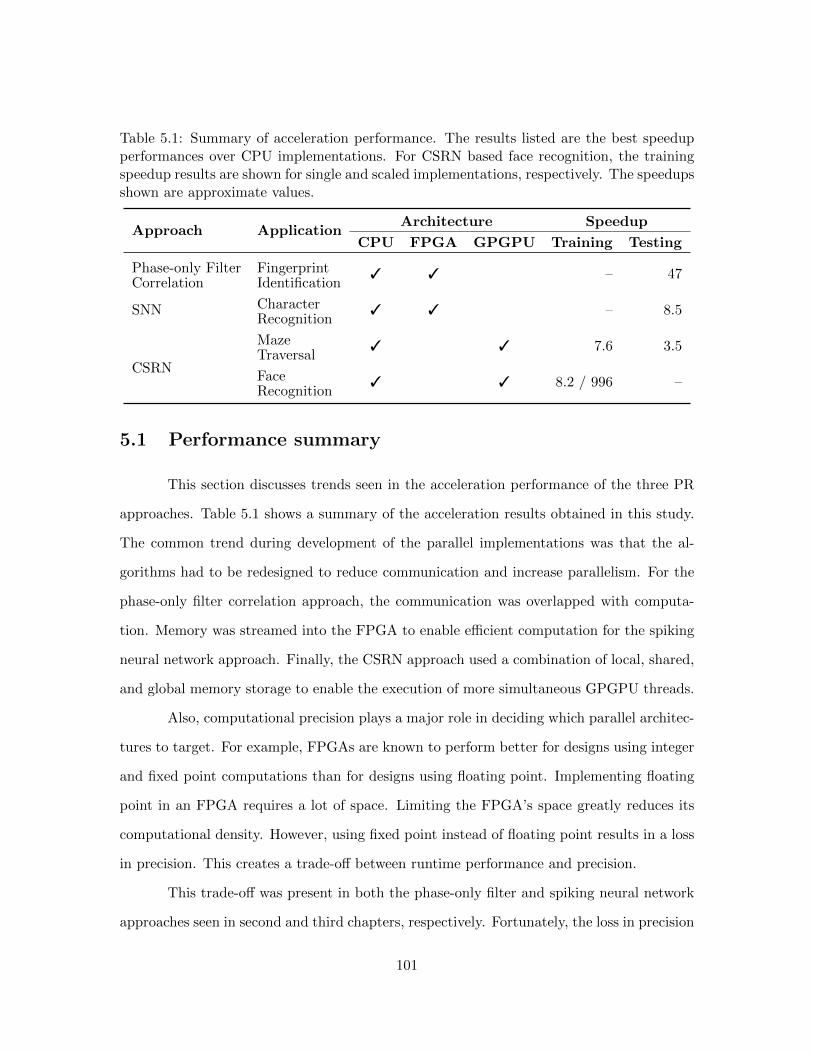
Table 5.1: Summary of acceleration performance. The results listed are the best speedupperformances over CPU implementations. For CSRN based face recognition, the trainingspeedup results are shown for single and scaled implementations, respectively. The speedupsshown are approximate values.

Approach ApplicationArchitecture Speedup

CPU FPGA GPGPU Training Testing

Phase-only Filter Fingerprint 3 3 – 47Correlation Identification

SNN Character 3 3 – 8.5Recognition

CSRN

Maze 3 3 7.6 3.5Traversal

Face 3 3 8.2 / 996 –Recognition

5.1 Performance summary

This section discusses trends seen in the acceleration performance of the three PR

approaches. Table 5.1 shows a summary of the acceleration results obtained in this study.

The common trend during development of the parallel implementations was that the al-

gorithms had to be redesigned to reduce communication and increase parallelism. For the

phase-only filter correlation approach, the communication was overlapped with computa-

tion. Memory was streamed into the FPGA to enable efficient computation for the spiking

neural network approach. Finally, the CSRN approach used a combination of local, shared,

and global memory storage to enable the execution of more simultaneous GPGPU threads.

Also, computational precision plays a major role in deciding which parallel architec-

tures to target. For example, FPGAs are known to perform better for designs using integer

and fixed point computations than for designs using floating point. Implementing floating

point in an FPGA requires a lot of space. Limiting the FPGA’s space greatly reduces its

computational density. However, using fixed point instead of floating point results in a loss

in precision. This creates a trade-off between runtime performance and precision.

This trade-off was present in both the phase-only filter and spiking neural network

approaches seen in second and third chapters, respectively. Fortunately, the loss in precision

101

was negligible for those designs. However, the CSRN approach presented in fourth chapter

requires at least 64-bit floating point precision. Given precision concerns, an FPGA design

of the CSRN approach would be impractical. In this case, the limitations of an FPGA

design were not applicable to GPGPUs, thus making the GPGPU the better architecture

to target.

When selecting a parallel platform to target, a developer should consider how well

an algorithm’s most time consuming computations map to the parallel platform. These

computations will serve as a limiting factor in the amount of speedup possible. If the time

consuming computations are highly parallelizable, then notable speedup performances can

be achieved.

As seen in the second chapter, the most time consuming computations were the

two-dimensional fast Fourier transforms (FFTs). As a result of FPGA logic constraints,

two consecutive one-dimensional FFTs utilizing the same FFT module were used. The

FFT modules operated with a deep pipeline, which mapped well to the spatially parallel

FPGA architecture. This contributed to the FPGA implementation providing roughly 47

times speedup over a CPU implementation.

The neural computations of the spiking neural network (SNN) approach seen in the

third chapter were the most time consuming. Individually, the neural computations were

not demanding. However, for a SNN on the scale of hundreds of thousands of neurons, the

neural computations will become expensive. The SNN PE design was pipelined for efficient

computation of a large number of neurons. The results in the third chapter are indicative

that the SNN PE will provide significant speedup performance for a growing number of

neural computations.

In the CSRN approach, matrix inversion was the most time consuming computation

while training. Relative to all training operations, the matrix inversion consumed over 90%

of the time. Additionally, for the face recognition application, the size of the matrix to

be inverted increases as input size increases (samples per face sequence and number of

face sequences). The time to invert the matrix significantly increases with the size of the

102

matrix. While using the GPGPU improved runtime performance, the data dependency and

global memory access pattern within matrix inversion limited the impact the GPGPU could

make. The results in the fourth chapter seem to suggest that the GPGPU may not be the

optimum architecture for algorithms in which matrix inversion dominates computation as

seen in CSRN training.

In summary, FPGAs have the following advantages over GPGPUs: greater flexibil-

ity, lower power consumption, higher computational density, and greater control. They have

the following relative disadvantages as well: longer development cycle, floating point limi-

tations, less onboard memory, and slower operating speeds. When deciding which platform

to target, the developer should consider the cost of precision, the ease of implementation,

memory constraints of underlying parallel architecture, and application characteristics such

as data dependency, algorithm complexity, and memory access behavior.

5.2 Future work

While the study of three PR approaches showed significant success, much work

remains. The real-time application of other phase-only filter based applications such as

the ones listed in [92, 93] should be explored. Additionally, the PEs presented in the

third chapter can be improved. For example, overlapping the data input/output with the

computations on the PEs would have almost doubled the speedups achieved. Also, the

performance and scalability of the PE based design onto newer FPGAs can be examined.

These would allow for more PEs to be implemented and enable them to run at higher speeds.

Finally, an investigation into the acceleration of larger, more biologically realistic models

(such as models with higher connectivity between the neurons) and the training of such

models can be performed. For the CSRN approach described in fourth chapter, alternative

CSRN based applications outside of face recognition can be investigated. Furthermore,

CSRNs developed for other parallel platforms can be examined.

The techniques to accelerate three PR approaches described in this dissertation

103

are applicable to other algorithms. The use of parallel computing architectures allow for

significant speedup performance as seen by the results. Generally, platforms such as FPGAs

allow for greater performance due to the considerable amount of developmental control.

Additionally, platforms such as GPGPUs offer significant speedups as well, but parallelism is

limited by the fixed architecture. The trade-off is the low development time when compared

to more flexible platforms.

104

Appendix A

Neuron Model Parameters

Excitatory neurons: a = 0.02, b = 0.2, c = −55, d = 4.

Inhibitory neurons: a = 0.06, b = 0.22, c = −65, d = 2.

Time step = 1ms.

105

References

[1] C. M. Bishop, Pattern recognition and machine learning. Information science andstatistics, Springer, 2006.

[2] R. Low, “Microprocessor trends: multicore, memory, and power developments,” Em-bedded Computing Design Annual Product Directory, September 2005.

[3] M. B. Taylor, J. Kim, J. Miller, D. Wentzlaff, F. Ghodrat, B. Greenwald, H. Hoff-man, P. Johnson, J.-W. Lee, W. Lee, A. Ma, A. Saraf, M. Seneski, N. Shnidman,V. Strumpen, M. Frank, S. Amarasinghe, and A. Agarwal, “The raw microproces-sor: a computational fabric for software circuits and general-purpose programs,” IEEEMicro, vol. 22, pp. 25–35, March–April 2002.

[4] M. B. Taylor, J. Psota, A. Saraf, N. Shnidman, V. Strumpen, M. Frank, S. Amaras-inghe, A. Agarwal, W. Lee, J. Miller, D. Wentzlaff, I. Bratt, B. Greenwald, H. Hoff-mann, P. Johnson, and J. Kim, “Evaluation of the raw microprocessor: an exposed-wire-delay architecture for ILP and streams,” in Proceedings of the 31st Annual Inter-national Symposium on Computer Architecture, pp. 2–13, June 2004.

[5] B. Baas, Z. Yu, M. Meeuwsen, O. Sattari, R. Apperson, E. Work, J. Webb, M. Lai,T. Mohsenin, D. Truong, and J. Cheung, “AsAP: A fine-grained many-core platformfor DSP applications,” IEEE Micro, vol. 27, pp. 34–45, March–April 2007.

[6] M. Pericas, A. Cristal, F. J. Cazorla, R. Gonzalez, D. A. Jimenez, and M. Valero, “Aflexible heterogeneous multi-core architecture,” in Proceedings of the 16th InternationalConference on Parallel Architecture and Compilation Techniques, PACT, pp. 13–24,September 2007.

[7] H. Zhong, S. A. Lieberman, and S. A. Mahlke, “Extending multicore architectures toexploit hybrid parallelism in single-thread applications,” in Proceedings of the IEEE13th International Symposium on High Performance Computer Architecture, HPCA,pp. 25–36, February 2007.

[8] K. Sankaralingam, R. Nagarajan, R. Mcdonald, R. Desikan, S. Drolia, M. S. Govindan,P. Gratz, D. Gulati, H. Hanson, C. Kim, H. Liu, N. Ranganathan, S. Sethumadhavan,S. Sharif, P. Shivakumar, S. W. Keckler, and D. Burger, “Distributed microarchitec-tural protocols in the TRIPS prototype processor,” in Proceedings of the 39th Annual

106

IEEE/ACM International Symposium on Microarchitecture, MICRO, pp. 480–491, De-cember 2006.

[9] U. J. Kapasi, W. J. Dally, S. Rixner, J. D. Owens, and B. Khailany, “The imaginestream processor,” in Proceedings of the IEEE International Conference on ComputerDesign: VLSI in Computers and Processors, pp. 282–288, September 2002.

[10] B. Jang, D. Schaa, P. Mistry, and D. Kaeli, “Exploiting memory access patterns toimprove memory performance in data-parallel architectures,” IEEE Transactions onParallel and Distributed Systems, vol. 22, pp. 105–118, January 2011.

[11] D. J. Felleman and D. C. V. Essen, “Distributed hierarchical processing in the primatecerebral cortex,” Cerebral Cortex, vol. 1, no. 1, pp. 1–47, 1991.

[12] A. A. S. Awwal, K. L. Rice, and T. M. Taha, “Hardware accelerated optical alignmentof lasers using beam-specific matched filters,” Applied Optics, vol. 48, pp. 5190–5196,September 2009.

[13] R. Fields and D. K. Molina, “A novel approach for fingerprinting mummified hands,”Journal of Forensic Sciences, vol. 53, no. 4, pp. 952–955, 2008.

[14] S. Ribaric, D. Ribaric, and N. Pavesic, “Multimodal biometric user-identification sys-tem for network-based applications,” IEE Proceedings – Vision, Image and Signal Pro-cessing, vol. 150, pp. 409–416, December 2003.

[15] D. Maltoni, D. Maio, A. K. Jain, and S. Prabhakar, Handbook of Fingerprint Recogni-tion (Second Edition). Springer Professional Computing, Springer, 2009.

[16] A. K. Jain and S. Pankanti, “Fingerprint classification and matching,” in Handbook forImage and Video Processing, Academic Press, 2000.

[17] A. K. Hrechak and J. A. McHugh, “Automated fingerprint recognition using structuralmatching,” Pattern Recognition, vol. 23, pp. 893–904, August 1990.

[18] D. K. Isenor and S. G. Zaky, “Fingerprint identification using graph matching,” PatternRecognition, vol. 19, pp. 113–122, April 1986.

[19] X. Jiang, W.-Y. Yau, and W. Ser, “Detecting the fingerprint minutiae by adaptivetracing the gray-level ridge,” Pattern Recognition, vol. 34, pp. 999–1013, May 2001.

[20] T. C. M. Rao, “Feature extraction for fingerprint classification,” Pattern Recognition,vol. 8, no. 3, pp. 181–192, 1976.

[21] S. Ohteru, H. Kobayashi, T. Kato, F. Nado, and H. Kimura, “Automated fingerprintclassifier,” in Proceedings of the Second International Conference on Pattern Recogni-tion, pp. 185–189, 1974.

[22] B. Moayer and K.-S. Fu, “A syntactic approach to fingerprint pattern recognition,”Pattern Recognition, vol. 7, no. 1–2, pp. 1–23, 1975.

107

[23] C. L. Wilson, G. T. Candela, and C. I. Watson, “Neural network fingerprint classifica-tion,” Journal of Artificial Neural Networks, vol. 1, no. 2, pp. 203–228, 1994.

[24] A. P. Fitz and R. J. Green, “Fingerprint classification using a hexagonal fast fouriertransform,” Pattern Recognition, vol. 29, no. 10, pp. 1587–1597, 1996.

[25] K. H. Fielding, J. L. Horner, and C. K. Makekau, “Optical fingerprint identification bybinary joint transform correlation,” Optical Engineering, vol. 30, no. 12, pp. 1958–1961,1991.

[26] J. F. Rodolfo, H. J. Rajbenbach, and J.-P. Huignard, “Performance of a photorefractivejoint transform correlator for fingerprint identification,” Optical Engineering, vol. 34,no. 4, pp. 1166–1171, 1995.

[27] M. S. Alam, A. M. El-Saba, E.-H. Horache, and S. Regula, “Joint transform corre-lation for fingerprint identification,” Advanced Optical and Quantum Memories andComputing, vol. 5362, no. 1, pp. 136–149, 2004.

[28] A. K. Jain, J. Feng, A. Nagar, and K. Nandakumar, “On matching latent fingerprints,”in Proceedings of the IEEE Computer Society Conference on Computer Vision andPattern Recognition Workshops, CVPRW, pp. 1212–1219, June 2008.

[29] T.-Y. Jea and V. Govindaraju, “A minutia-based partial fingerprint recognition sys-tem,” Pattern Recognition, vol. 38, pp. 1672–1684, October 2005.

[30] J. L. Horner and J. R. Leger, “Pattern recognition with binary phase-only filters,”Applied Optics, vol. 24, pp. 609–611, March 1985.

[31] A. M. Chowdhury and A. A. S. Awwal, “Optical pattern recognition of fingerprintsusing distortion-invariant phase-only filter,” in Photonic Devices and Algorithms forComputing (K. M. Iftekharuddin and A. A. S. Awwal, eds.), vol. 3805, pp. 162–170,1999.

[32] A. Lindoso and L. Entrena, “High performance FPGA-based image correlation,” Jour-nal of Real-Time Image Processing, vol. 2, no. 4, pp. 223–233, 2007.

[33] G. Danese, M. Giachero, F. Leporati, G. Matrone, and N. Nazzicari, “A dedicatedhardware for fingerprint authentication,” in Knowledge-Based Intelligent Informationand Engineering Systems (B. Apolloni, R. Howlett, and L. Jain, eds.), vol. 4693 ofLecture Notes in Computer Science, pp. 117–124, Springer Berlin / Heidelberg, 2007.

[34] M. L. Garcia and E. F. C. Navarro, “FPGA implementation of a ridge extractionfingerprint algorithm based on microblaze and hardware coprocessor,” in Proceedingsof the International Conference on Field Programmable Logic and Applications, FPL,pp. 1–5, August 2006.

[35] V. L. Lorenzo, P. H. Pellitero, J. Ignacio, M. Torre, and J. C. Villar, “Fingerprintminutiae extraction based on FPGA and MATLAB,” in XX Conference on Design ofCircuits and Integrated Systems, DCIS, November 2005.

108

[36] D. Nguyen, P. Aarabi, and A. Sheikholeslami, “Real-time sound localization usingfield-programmable gate arrays,” in Proceedings of the International Conference onMultimedia and Expo, vol. 2 of ICME, pp. 829–832, July 2003.

[37] A. K. Brodzik, “Phase-only filtering for the masses (of DNA data): a new approach tosequence alignment,” IEEE Transactions on Signal Processing, vol. 54, pp. 2456–2466,June 2006.

[38] K. K. Sharma, Optics: Principles and Applications. Academic Press, 2006.

[39] K. Ito, H. Nakajima, K. Kobayashi, T. Aoki, and T. Higuchi, “A fingerprint matchingalgorithm using phase-only correlation,” IEICE Transactions on Fundamentals of Elec-tronics, Communications and Computer Sciences, vol. 87, pp. 682–691, March 2004.

[40] A. A. S. Awwal, M. A. Karim, and S. R. Jahan, “Improved correlation discriminationusing an amplitude-modulated phase-only filter,” Applied Optics, vol. 29, pp. 233–236,January 1990.

[41] M. A. Karim and A. A. S. Awwal, Optical computing: an introduction. Wiley Seriesin Microwave and Optical Engineering, Wiley, 1992.

[42] Y. Wang, D. Li, T. Isshiki, and H. Kunieda, “A novel fingerprint SoC with bit se-rial FPGA engine,” Information Processing Society of Japan Digital Courier, vol. 1,pp. 226–233, 2005.

[43] “FFT code and related material.” http://www.jjj.de/fft/fftpage.html. [Online].

[44] T. Dean, “A computational model of the cerebral cortex,” in Proceedings of the NationalConference on Artificial Intelligence, vol. 20 of AAAI, pp. 938–943, 2005.

[45] R. Ananthanarayanan and D. S. Modha, “Anatomy of a cortical simulator,” in Proceed-ings of the 2007 ACM/IEEE Conference on Supercomputing, SC, pp. 1–12, November2007.

[46] H. Markram, “The blue brain project,” Nature Reviews Neuroscience, vol. 7, pp. 153–160, February 2006.

[47] C. Johansson and A. Lansner, “Towards cortex sized artificial neural systems,” NeuralNetworks, vol. 20, pp. 48–61, January 2007.

[48] Q. Wu, P. Mukre, R. Linderman, T. Renz, D. Burns, M. Moore, and Q. Qiu, “Per-formance optimization for pattern recognition using associative neural memory,” inProceedings of the IEEE International Conference on Multimedia and Expo, pp. 1–4,April 2008.

[49] J. Rickman, “Roadrunner supercomputer puts research at a new scale.” http://www.lanl.gov/news/index.php/fuseaction/home.story/story id/13602. [Online].

109

[50] M. M. Khan, D. R. Lester, L. A. Plana, A. Rast, X. Jin, E. Painkras, and S. B. Furber,“Spinnaker: Mapping neural networks onto a massively-parallel chip multiprocessor,”in Proceedings of the IEEE International Joint Conference on Neural Networks, IJCNN,pp. 2849–2856, June 2008.

[51] D. B. Strukov, G. S. Snider, D. R. Stewart, and R. S. Williams, “The missing memristorfound,” Nature, vol. 453, pp. 80–83, May 2008.

[52] L. Chua, “Memristor-the missing circuit element,” IEEE Transactions on Circuit The-ory, vol. 18, pp. 507–519, September 1971.

[53] B. Linares-Barranco and T. Serrano-Gotarredona, “Memristance can explain spike-time-dependent-plasticity in neural synapses,” Nature, no. 1, pp. 2–5, 2009. http://precedings.nature.com/documents/3010/version/1. [Online].

[54] C. Gao and D. Hammerstrom, “Cortical models onto CMOL and CMOS–architecturesand performance/price,” IEEE Transactions on Circuits and Systems I: Regular Pa-pers, vol. 54, pp. 2502–2515, November 2007.

[55] J. Vreeken, “Spiking neural networks, an introduction,” tech. rep., Institute for Infor-mation and Computing Sciences, Utrecht University, 2002.

[56] H. Shayani, P. J. Bentley, and A. M. Tyrrell, “Hardware implementation of a bio-plausible neuron model for evolution and growth of spiking neural networks on FPGA,”in Proceedings of the NASA/ESA Conference on Adaptive Hardware and Systems, AHS,pp. 236–243, June 2008.

[57] A. Upegui, C. A. Pena-Reyes, and E. Sanchez, “A hardware implementation of anetwork of functional spiking neurons with hebbian learning,” in Biologically In-spired Approaches to Advanced Information Technology (A. Ijspeert, M. Murata, andN. Wakamiya, eds.), vol. 3141 of Lecture Notes in Computer Science, pp. 233–243,Springer Berlin / Heidelberg, 2004.

[58] A. Cassidy, S. Denham, P. Kanold, and A. Andreou, “FPGA based silicon spikingneural array,” in Proceedings of the IEEE Biomedical Circuits and Systems Conference,BIOCAS, pp. 75–78, November 2007.

[59] M. Pearson, I. Gilhespy, K. Gurney, C. Melhuish, B. Mitchinson, M. Nibouche, andA. Pipe, “A real-time FPGA based, biologically plausible neural network processor,” inProceedings of the 15th International Conference on Artificial Neural Networks, vol. 2of ICANN, pp. 1021–1026, 2005.

[60] E. M. Izhikevich, “Which model to use for cortical spiking neurons?,” IEEE Transac-tions on Neural Networks, vol. 15, pp. 1063–1070, September 2004.

[61] E. M. Izhikevich, “Simple model of spiking neurons,” IEEE Transactions on NeuralNetworks, vol. 14, pp. 1569–1572, November 2003.

110

[62] M. La Rosa, E. Caruso, L. Fortuna, M. Frasca, L. Occhipinti, and F. Rivoli, “Neuronaldynamics on FPGA: Izhikevich’s model,” in Bioengineered and Bioinspired Systems II(R. A. Carmona and G. Linan-Cembrano, eds.), vol. 5839, pp. 87–94, 2005.

[63] L. Fortuna, M. Frasca, and M. La Rosa, “Emergent phenomena in neuroscience,”Advanced Topics on Cellular Self-Organizing Nets and Chaotic Nonlinear Dynamics toModel and Control Complex Systems, vol. 63, no. 6, pp. 39–53, 2008.

[64] M. Mokhtar, D. M. Halliday, and A. M. Tyrrell, “Hippocampus-inspired spiking neuralnetwork on FPGA,” in Evolvable Systems: From Biology to Hardware (G. Hornby,L. Sekanina, and P. Haddow, eds.), vol. 5216 of Lecture Notes in Computer Science,pp. 362–371, Springer Berlin / Heidelberg, 2008.

[65] D. B. Thomas and W. Luk, “FPGA accelerated simulation of biologically plausiblespiking neural networks,” in 17th IEEE Symposium on Field Programmable CustomComputing Machines, FCCM, pp. 45–52, April 2009.

[66] M. A. Bhuiyan, R. Jalasutram, and T. M. Taha, “Character recognition with twospiking neural network models on multicore architectures,” in IEEE Symposium onComputational Intelligence for Multimedia Signal and Vision Processing, CIMSVP,pp. 29–34, March–April 2009.

[67] W. Gerstner and W. M. Kistler, Spiking Neuron Models: Single Neurons, Populations,Plasticity. Cambridge University Press, 2002.

[68] R. Ilin, R. Kozma, and P. J. Werbos, “Beyond feedforward models trained by back-propagation: A practical training tool for a more efficient universal approximator,”IEEE Transactions on Neural Networks, vol. 19, no. 6, pp. 929–937, 2008.

[69] K. M. Iftekharuddin and K. Anderson, “Image registration under affine transformationusing cellular simultaneous recurrent networks,” Optics and Photonics for InformationProcessing IV, vol. 7797, no. 1, p. 77970E, 2010.

[70] Y. Ren, K. M. Iftekharuddin, and W. E. White, “Large-scale pose-invariant face recog-nition using cellular simultaneous recurrent network,” Applied Optics, vol. 49, no. 10,pp. B92–B103, 2010.

[71] B. Han and T. M. Taha, “Acceleration of spiking neural network based pattern recog-nition on NVIDIA graphics processors,” Applied Optics, vol. 49, pp. B83–B91, April2010.

[72] D. Strigl, K. Kofler, and S. Podlipnig, “Performance and scalability of GPU-basedconvolutional neural networks,” in Proceedings of the 18th Euromicro InternationalConference on Parallel, Distributed and Network-Based Processing, PDP, pp. 317–324,February 2010.

[73] R. Dolan and G. DeSouza, “GPU-based simulation of cellular neural networks for imageprocessing,” in Proceedings of the International Joint Conference on Neural Networks,IJCNN, pp. 730–735, June 2009.

111

[74] J. M. Nageswaran, N. Dutt, J. L. Krichmar, A. Nicolau, and A. Veidenbaum, “Ef-ficient simulation of large-scale spiking neural networks using CUDA graphics pro-cessors,” in Proceedings of the International Joint Conference on Neural Networks,IJCNN, pp. 2145–2152, June 2009.

[75] S. S. Hampton, S. R. Alam, P. S. Crozier, and P. K. Agarwal, “Optimal utilization ofheterogeneous resources for biomolecular simulations,” in Proceedings of the Interna-tional Conference for High Performance Computing, Networking, Storage and Analysis,SC, pp. 1–11, November 2010.

[76] R. Y. de Camargo, L. Rozante, and S. W. Song, “A multi-GPU algorithm for large-scale neuronal networks,” Concurrency and Computation: Practice and Experience,vol. 23, no. 6, pp. 556–572, 2011.

[77] A. Cevahir, A. Nukada, and S. Matsuoka, “Fast conjugate gradients with multipleGPUs,” in Computational Science – ICCS 2009 (G. Allen, J. Nabrzyski, E. Seidel,G. van Albada, J. Dongarra, and P. Sloot, eds.), vol. 5544 of Lecture Notes in ComputerScience, pp. 893–903, Springer Berlin / Heidelberg, 2009.

[78] X. Pang and P. J. Werbos, “Neural network design for J function approximation in dy-namic programming,” Math’l Modeling and Scientific Computing (a Principia ScientiaJournal), vol. 5, no. 2/3, 1996. http://arxiv.org/abs/adap-org/9806001.

[79] P. J. Werbos, The roots of backpropagation: from ordered derivatives to neural networksand political forecasting. Wiley-Interscience, 1994.

[80] C. Sanderson and K. K. Paliwal, “Polynomial features for robust face authentication,”in Proceedings of the International Conference on Image Processing, vol. 3, pp. 997–1000, June 2002.

[81] S. Gong, A. Psarrou, I. Katsoulis, and P. Palavouzis, “Tracking and recognition of facesequences,” in Proceedings of the European Workshop on Combined Real and SyntheticImage Processing for Broadcast and Video Production, pp. 97–112, 1994.

[82] “Thinking in CUDA: Gauss-Jordan elimination.” http://CUDAhacks.com/cms/Blog/tabid/64/EntryId/7/Thinking-in-CUDA-Gauss-Jordan-elimination.aspx. [Offline].

[83] “Condor supercomputer: DOD’s largest interactive supercomputer.” http://www.dodlive.mil/files/2010/12/CondorSupercomputerbrochure 101117 kb-3.pdf. [Online].

[84] “Open computer vision library.” http://sourceforge.net/projects/opencvlibrary/. [On-line].

[85] G. Bradski and A. Kaehler, Learning OpenCV: computer vision with the OpenCVlibrary. O’Reilly Series, O’Reilly, 2008.

[86] NVIDIA, “NVIDIA developer zone.” http://developer.nvidia.com/object/CUDA 3 2downloads.html. [Online].

112

[87] NVIDIA, “NVIDIA CUDA C programming guide, version 3.2, 2010.”http://developer.download.nvidia.com/compute/CUDA/3 2 prod/toolkit/docs/CUDA C Programming Guide.pdf. [Online].

[88] D. B. Graham and N. M. Allinson, “Characterizing virtual eigensignatures for gen-eral purpose face recognition,” in Face Recognition: From Theory to Applications(H. Wechsler, P. J. Phillips, V. Bruce, F. Fogelman-Soulie, and T. S. Huang, eds.),vol. 163 of NATO ASI Series F: Computer and Systems Sciences, pp. 446–456, 1998.http://www.sheffield.ac.uk/eee/research/iel/research/face. [Online].

[89] S. Che, J. Li, J. W. Sheaffer, K. Skadron, and J. Lach, “Accelerating compute-intensiveapplications with GPUs and FPGAs,” in Proceedings of the Symposium on ApplicationSpecific Processors, SASP, pp. 101–107, June 2008.

[90] D. B. Thomas, L. Howes, and W. Luk, “A comparison of CPUs, GPUs, FPGAs, andmassively parallel processor arrays for random number generation,” in Proceedingsof the ACM/SIGDA International Symposium on Field Programmable Gate Arrays,FPGA, pp. 63–72, 2009.

[91] B. Cope, P. Y. K. Cheung, W. Luk, and L. Howes, “Performance comparison of graphicsprocessors to reconfigurable logic: A case study,” IEEE Transactions on Computers,vol. 59, pp. 433–448, April 2010.

[92] X. Liang and J. S.-N. Jean, “Mapping of generalized template matching onto reconfig-urable computers,” IEEE Transactions on Very Large Scale Integration (VLSI) Sys-tems, vol. 11, pp. 485–498, June 2003.

[93] J. Jean, X. Liang, B. Drozd, K. Tomko, and Y. Wang, “Automatic target recognitionwith dynamic reconfiguration,” The Journal of VLSI Signal Processing, vol. 25, pp. 39–53, May 2000.

113