This is a repository copy of Accelerating slip rates on the Puente Hills blind thrust fault system beneath metropolitan Los Angeles, California, USA.

White Rose Research Online URL for this paper:http://eprints.whiterose.ac.uk/111877/

Version: Supplemental Material

Article:

Bergen, K.J., Shaw, J.H., Leon, L.A. et al. (8 more authors) (2017) Accelerating slip rates on the Puente Hills blind thrust fault system beneath metropolitan Los Angeles, California, USA. Geology. ISSN 1943-2682

https://doi.org/10.1130/G38520.1

eprints@whiterose.ac.ukhttps://eprints.whiterose.ac.uk/

Reuse

Unless indicated otherwise, fulltext items are protected by copyright with all rights reserved. The copyright exception in section 29 of the Copyright, Designs and Patents Act 1988 allows the making of a single copy solely for the purpose of non-commercial research or private study within the limits of fair dealing. The publisher or other rights-holder may allow further reproduction and re-use of this version - refer to the White Rose Research Online record for this item. Where records identify the publisher as the copyright holder, users can verify any specific terms of use on the publisher’s website.

Takedown

If you consider content in White Rose Research Online to be in breach of UK law, please notify us by emailing eprints@whiterose.ac.uk including the URL of the record and the reason for the withdrawal request.

Supplemental Materials 

This supplemental information provides a detailed description of the datasets and methods 

used to calculate fault slip rates, including an assessment of uncertainties. 

Probabilistic slip rate analysis 

We  developed  a  Monte  Carlo  simulation  approach  that  characterizes  uncertainties  in 

geometrical measurements from subsurface data and combines them with uncertainties in 

our age constraints to produce slip rate probability distributions. 

To  determine  relative  timing  and  magnitude  of  fault  slip,  we  rely  on  the  paleo‐fold 

geometries  recorded  by  growth  stratigraphy.  Growth  stratigraphy  has  been  used  in 

previous studies to characterize folding associated with blind‐thrust faults, providing limits 

on  fault  geometry  and  slip  rates  (Suppe  et  al.,  1992;  Shaw  and  Suppe,  1996;  Shaw  and 

Shearer, 1999; Leon et al., 2009). We adopt the results of recent studies that show vertical 

relief of growth strata in fault‐bend folds to be the best indicator of fault slip (Leon et al., 

2007;  Dolan  et  al.,  2003;  Leon  et  al.,  2009;  Benesh  et  al.,  2007;  Pratt  et  al.,  2002).  To 

measure the fold geometry above the LA segment, we used a collection of 43 oil  industry 

seismic  reflection profiles  that  image below ~300 m depth  (Figure 1d). A  shallow,  high‐ 

frequency  seismic  reflection  profile  was  acquired  along  Budlong  Avenue  in  central  LA 

across  the  shallowest portion of  the  forelimb observed  in  the  industry  seismic  reflection 

data (Figure 1C). These data target the uppermost layers of the fold, which record the late 

Pleistocene to Holocene activity of the underlying fault. A weight drop source was used to 

image in the 100 – 700 m depth range (Pratt et al., 2002). Multiple impacts per shot point 

GSA Data Repository 2017059

Accelerating slip rates on the Puente Hills blind thrust fault system beneath metropolitan Los Angeles, California, USABergen et al.

were  summed  to  suppress  electrical  and  traffic  noise.  Processing  techniques  were  as 

described  in  Pratt  et  al.  (2002).  The  most  recent  activity  on  the  LA  segment  was 

constrained by a series of eleven, 17 – 34 m deep continuously cored hollow‐stem auger 

boreholes (Figure 1B), and a 175‐m‐deep borehole drilled into the forelimb of the structure. 

 

To  quantify  deformation  rates  in  the  late Quaternary,  sequence  stratigraphic  boundaries 

were interpreted across our seismic reflection data based on diagnostic reflection patterns 

and well‐log correlations (Mitchum et al., 1977; Neal and Abreu, 2009).  In  the LA coastal 

plain,  sea  level  changed  during  the  Quaternary  due  to  global  ice  age  cycles  (Ponti  et  al., 

2007).  During  glacial  periods,  erosion  and  sediment  bypass  to  the  ocean  occurred, 

producing  unconformities.  During  the  interglacial  periods,  when  sea  levels  were  high, 

sediment  accumulated  in  the  basin.  These  cycles  of  sea  level  change  formed  diagnostic 

coarsening  and  fining  upwards  sediment  packages  that  reflect  progradation  and 

retrogradation of  the shoreline. Ponti et al.  (2007) used  these principles along with over 

300 well logs and 3D seismic reflection data to produce a sequence stratigraphic model in 

the Long Beach, California area for hydrologic and tectonic studies. This model was further 

developed  by  Ehman  and  Edwards  (2014).  We  extended  their  sequence  stratigraphic 

model  across  the  LA  basin  to  our  study  site  using  additional  well  logs  and  our  industry 

seismic reflection data. We measured thickness change across these sequence boundaries 

to  define  fault  activity  in  the  late  Quaternary.  Erosion  and  sediment  bypass  create  the 

potential for denudation of the paleo‐folds we seek to measure, which may add additional, 

uncharacterized uncertainty to our slip rates. 

  

Lithological  correlations  based  on  grain  size  and  color  define  the  fold  geometry  in  our 

borehole profile (Figure 1b). The shallow sediments sampled in our study are most likely 

overbank or sheetflood deposits related to periodic flooding of the LA River. Based on the 

work of Leon et al. (2007), we recognize that large slip events on the PHT blind‐thrust fault 

formed  fold  scarps  at  the  surface,  as  were  observed  after  the  1999,  Mw  7.6,  Chi‐Chi 

earthquake  (Chen  et  al.,  2007).  Subsequent  floods  buried  these  scarps,  forming  growth 

stratigraphy.  Our  borehole  profile  contains  a  discontinuous,  organic‐rich  soil  that 

buttresses the fold and overlies a continuous clay and silt  layer (Figure 1b). We interpret 

the organic‐rich soil as having formed due to ponding at the base of a paleo‐fold scarp that 

would have developed after deposition of the continuous clay and silt layer. We refer to this 

surface as top clay and use it to constrain the most recent deformation on the LA segment.  

 

Velocity model uncertainties  

The  depths  of  reflectors  in  our  seismic  reflection  data  are  functions  of  the  average 

compressional‐wave velocities !! from the seismic source at the surface to the impedance 

contrasts at depth that produced them. These in turn are functions of the interval velocities 

!!  of  the  overlying  materials  (sediments  and  fluids)  the  waves  passed  through: !! !

!!!!!

!!! !!!

!!! ,  where !!  is  the  one‐way  time  for  a  compressional  wave  to  travel  across 

depth  interval !.  Stacking  velocities  from  seismic  reflection  profiles  are  often  used  to 

estimate !!,  but  can  have  inaccuracies  of  10%  or  more,  particularly  at  shallow  depths 

where velocities increase rapidly and the straight‐raypath approximation used in common‐

midpoint velocity analyses does not hold. More accurate velocity determinations from the 

shallow  reflection  data,  such  as  pre‐stack  migration  methods,  are  difficult  to  implement 

because of the relatively low signal‐to‐noise ratio and limited offset range after muting the 

surface waves and refracted arrivals.  

 

Since we do not know the precise velocity structure, we instead determine the range of !! 

by performing simulations that vary the magnitude and ordering of !! . We accomplish this 

by  developing  an  autoregressive  (AR)  statistical  model  based  on  interval‐transit‐time 

compressional‐wave  velocities !!!∀∀! from  a  nearby  industry  well  that  we  characterize 

relative  to  the  Southern  California  Earthquake  Center  Community  Velocity  Model  v11.9 

with near‐surface geotechnical  layer  (CVMH) (Suess and Shaw, 2003; Plesch et al., 2007; 

Shaw  et  al.,  2015).  The  CVMH  data  are  extracted  at  the  center  of  each  model  grid  cell, 

yielding  8  vertical  velocity  profiles  at  250  m  spacing  across  our  study  area  (Data 

Repository Figure 2). The !!∀∀  data is from the Union‐Standard La Tijera E.H. 1 well (API: 

03700792), which is approximately 2.5 km east of our study site and likely contains similar 

lithologies.  Velocities  are  measured  at  0.15  m  (6  in.)  intervals  and  display  positive 

autocorrelation,  with  successive  observations  persisting  above  and  below  the  mean, 

suggesting an autoregressive process (Data Repository Figure 3). We perform AR modeling 

and  validation  using  the  ARfit  analysis  suite  of  Schneider  and  Neumaier  (2001)  and 

Neumaier  and  Schneider  (2001),  which  uses  a  stepwise  least  squares  algorithm  to 

determine  the  parameters  and  model  order  that  optimize  Schwarz’s  Bayesian  Criterion. 

The AR model assumes zero mean and normally distributed, temporally uncorrelated noise 

(residuals about the mean). The !!∀∀  data have a skewed distribution and non‐zero mean 

(Data Repository Figure 3), so we perform a log transformation to improve normality and 

detrend the data by the log of its mean to get the velocity noise !! we seek to characterize: 

!! ! ! ln!!∀∀ ! ln!!∀∀ .  Our  best‐fit  model  is: !! ! !!!!!!! ! !!!!!! ! !!!!!! ! !!  where 

!! ! !!!!! !!035 , !!! ! !!!066! !!055 ,  !! ! !!!14! !!035 ,  and  variance  ��� !

!!!!!!10!!  for  the  noise  vector !!!  (!  ranges  denote  95%  confidence  intervals).  We 

demonstrate  that  our  model  satisfies  the  correlation  conditions  using  the  modified  Li‐

Mcleod portmanteau test, which yields a significance level of 0.18, indicating that the noise 

is uncorrelated at a 95% confidence  level (Schneider and Neumaier, 2001; Neumaier and 

Scneider, 2001). 

 

We  use  a  Monte  Carlo  approach  to  simulate  average  velocities  for  depth  conversion  by 

adding  iterations  of  AR  noise  to  the  CVMH  interval  velocities,  and  then  calculating  the 

resulting averages. For a single iteration !,  the simulated interval velocity is characterized 

as  !!∀#!! !

!!!!!∀!!∀∀ ! !!∀#∃ ! !!∀#∃ ,  where  !!!!!!∀!!∀∀  is  the  back‐transformed 

simulation output, !!∀#∃  is the mean of the CVMH interval velocities at the position of the 

La Tijera well  that  shifts  the  simulations  to  their  correct  average position  relative  to  the 

CVMH (Data Repository Figure 3), and !!∀#∃  are the CVMH interval velocities at our study 

area. We initialize the simulations with zero mean values and discard the first 1000 points. 

For  each  simulation, we  calculate  average velocities  and  corresponding  travel  times,  and 

then  interpolate  the  average  velocities  onto  our  time  interpretations.  A  comparison  of 

simulated average velocities  to  the CVMH at  the La Tijera well  location  is  shown  in Data 

Repository Figure 4. The variance in average velocity decreases with depth as the number 

of sampled interval velocities above increases. We use the interpolated average velocities 

to depth‐convert our interpretations of the sequence boundaries. 

 

Seismic resolution uncertainties 

The  sequence  boundaries  used  to  define  fold  geometries  in  the  Pleistocene  may  contain 

subtle  unconformities  and  thin  beds  that  are  beyond  the  resolvable  limit  of  our  seismic 

reflection  data  due  to  attenuation  of  high  frequencies  at  depth.  We  must  therefore  also 

consider  the  impact  of  resolution  uncertainty  on  our  results.  Based  on  empirical !!! 

resolution  limits  from  synthetic  seismic  simulations  of  sequence  geometries  (Vail  et  al., 

1977), we conservatively bracketed our  interpretations of the crest and trough about the 

fold using !!! uniform distributions. To do this, we first estimated the dominant period !!  

along  each  interpreted  sequence  boundary  as  the  time  difference  to  the  adjacent, 

underlying  reflector,  measured  normal  to  the  sequence  boundary  to  account  for  folding, 

and halved to convert to one‐way time. We then extracted the simulated interval velocities 

within !!!!  of  the  sequence boundary one‐way  time and averaged  them  to estimate  the 

velocity !!!!∀#!  within  the  resolution  uncertainty  region.  Using  this,  we  calculated  the 

corresponding  wavelength  in  meters:  !! ! !!!!∀#!!! .  To  simulate  potential  sequence 

boundary  positions  within  the  resolution  range,  we  sampled  the  !!!!  resolution 

distribution separately for the trough and crest for each iteration !, and shifted each by the 

sampled value. To correspondingly shift the data across the fold, we calculated the slope of 

the lines defined by the crest and trough endpoints before and after adding the resolution 

uncertainty. We then shifted the fold data by the vertical difference between the two lines 

evaluated  at  each  horizontal  position.  Data  Repository  Figure  5  shows  an  example 

simulated fold geometry. 

 

 

Uplift, fault dip, and slip calculations 

To estimate uplift Ui, we used the difference between average stratal thickness on the crest 

and trough of the fold, calculated at 15 m increments normal to the overlying surfaces to 

account for regional dip (Data Repository Figure 5). To account for any potential thickness 

changes across the fold due to differential compaction, we used the exponential porosity‐

depth  relations  of  Athy  (1930)  to  estimate  the  decompacted  average  trough  and  crest 

thicknesses at  the time of deposition.  In the Athy relations,  the change  in porosity ! with 

depth z  is given by ! ! !!!!!!∀ , where !! is  the  initial porosity at  the surface and c  is an 

empirically  determined  compaction  coefficient. We  do  not  have  direct measurements  of 

porosity near our site, so we instead sample from a range of initial porosities !!!  (0.375 – 

0.8)  and  constants !!  (0.25  –  0.9)  for  each  iteration !,  consistent with  the  sands  and  silts 

present at our site (Sclater and Christie, 1980; Bahr et al., 2001; Allen and Allen, 2005). The 

decompacted thickness of a layer !!!! is given by: 

!!!!! !!!!

! !!!!! !!!!

!!

!!!!!!! ! !!

!!!!!! !!!!

!!

!!!!!

!!! ! !!

!!!!!!!  

where !!!!  and !!!!  are the decompacted bottom and top of the layer and !!!  and !!!  are the 

present‐day,  compacted  bottom  and  top  of  the  layer  (Allen  and  Allen,  2005).  These 

equations are solved by numerical iteration. 

 

Since the growth stratal geometries are consistent with fault‐bend folding theory, we used 

the  fault‐bend  fold  kinematic  model  (Suppe,  1983)  to  calculate  fault  dip  !! : 

!! ! tan!!!sin !!! !!! ! cos

! !!!!, where !!  is  the angle of  the axial  trace and  the  fault  is 

assumed to shallow to a bedding parallel detachment, similar to the geometry proposed for 

the  Santa  Fe  Springs  segment.  The  axial  trace  is  defined  as  the  angle  bisector  between 

folded and unfolded strata. We calculated dip using a first‐order least‐squares fit along the 

trough and steepest portion of the fold from which we calculated axial trace angles (Data 

Repository Figure 5). From the results of Benesh et al. (2007), the sequence boundary with 

the steepest fold dip should be used for fault dip calculation. We therefore use the steepest 

dipping, central portion of the Bent Spring sequence boundary to calculate fault dip. Due to 

our study’s urban setting, our seismic reflection profile was not acquired parallel to dip, so 

we  randomly  sampled  a  uniform  distribution  between  N55°W  and  N65°W  strike  for 

apparent  dip  corrections.  The  fault  dips !!  derived  from  these  measurements  were  then 

used to calculate fault slip !!  as !! ! !! sin!! . Uplift and fault dip were calculated from the 

same simulated geometry to ensuring proper correlation between measurements.  

 

We note  that alternative  fault‐related  fold kinematics would raise  the possibility of other 

relations between uplift and slip. Specifically, some classes of fault‐propagation folds (e.g., 

Suppe and Medwedeff, 1990) indicate a fixed but higher ratio of uplift to fault slip than do 

fault‐bend folds, while break‐through fault‐propagation folds and detachment folds suggest 

that uplift rates may decelerate over time with constant slip rate (e.g., Rockwell et al., 1988; 

Hubbard  et  al.,  2014).  However,  neither  fault‐propagation  nor  detachment  folds  are 

consistent with the growth structure at our site, which is a discrete feature localized above 

the anticlinal axis of the structure (Suppe, 1992; Pratt et al., 2002; Shaw et al., 2002; Dolan 

et  al.,  2003).  Moreover,  those  models  imply  that  the  ratio  of  uplift  to  slip  rate  would 

decreases  through  time  (see  Hubbard  et  al.,  2014).  This  would  enhance,  rather  than 

diminish, the calculated increase at our site. 

 

Age control and uncertainties 

Age  control  was  provided  by  accelerator  mass  spectrometer  radiocarbon  dating  (14C), 

infrared stimulated luminescence dating (IRSL), and sequence boundaries matched to δ18O 

curves. Radiocarbon ages were calibrated with Oxcal v.4.2.4 Reimer et al., 2013) and are 

shown with ±2σ bounds on Figure 1b. Detailed results are shown in Data Repository Table 

1a.  In  our  simulations, we  randomly  sampled  an  empirical  distribution  that  brackets  the 

burial  age of  the  top  clay using  the Oxcal  probability density  functions  for  samples  from 

well  8  and  well  5  (Figure  1B).  The  empirical  distribution  was  created  by  combining  the 

cumulative  density  function  of  the  well  8  sample  with  the  reflection  of  the  cumulative 

density function of the older well 5 sample, and assigning uniform probability between the 

two (Data Repository Figure 6). 

 

To define deposition and deformation rates  further  into the past,  light‐protected samples 

were obtained for single grain K‐feldspar IRSL dating at borehole D1 (Figure 1B, 1C). We 

used hollow‐stem auger drilling to collect samples down to ~40 m depth and mud‐rotary 

drilling to collect samples down to ~135 m depth. For the hollow‐stem auger drill rig, we 

used a split‐spoon sampling tool fitted with a stainless steel liner that was driven into the 

ground  in  front  of  the  drill  bit,  ensuring  an  in  situ  and  uncontaminated  sample  (Data 

Repository  Figure  7A).  The  liner  shielded  the  sediments  from  light‐exposure  when  the 

sample  was  recovered  at  the  surface.  Once  removed  from  the  split‐spoon  sampler,  the 

sample  liner was capped and placed  in a  light‐proof bag. For  the mud‐rotary drill  rig, we 

also used stainless steel liners inside a split‐spoon sampler. The sampling tool sat in front 

of the drill bit to avoid collecting sediment altered by the drilling process (Data Repository 

Figure 7B). We collected luminescence samples from only well‐compacted sediment (based 

on resistance to drilling), minimizing the risk that drilling mud would infiltrate pore space 

and contaminate the sample with younger or light‐exposed sediment grains.  

 

Single grain K‐feldspar post‐IR IRSL (Infra‐Red Stimulated Luminescence) determinations 

of  six  samples were used  to provide age  control  for  the upper 140m of  the  stratigraphic 

sequence (Data Repository Tables 1b, 2). This dating approach was developed specifically 

for application to fault slip‐rate and paleoseismology contexts, and has been assessed at a 

number of similar sites in California and elsewhere (Rhodes, 2015). 

 

Sediment  samples  were  extracted  from  steel  core  tubes  under  controlled  laboratory 

lighting  conditions  at  UCLA,  avoiding material  that might  have  been  exposed  to  daylight 

during  coring  operations.  After  suspension  separation  of  the  silty  component,  samples 

were  wet  sieved  and  the  180  ‐  212μm  fraction  retained.  After  dilute  HCl  treatment  and 

drying,  the  fraction  <2.58  g.cm‐3  was  separated  using  lithium  metatungstate  (LMT)  for 

each sample, and  these  fractions were subsequently  treated with dilute (10%) HF  for 10 

mins. to etch grain surfaces.  

 

Measurements were made at UCLA using a Risø automated TL‐DA‐20 luminescence reader 

fitted  with  a  single  grain  dual  laser  system.  A  single  aliquot  regenerative‐dose  (SAR) 

protocol  modified  from  that  of  Buylaert  et  al.  (2009)  for  application  to  single  grains. 

Measurement details are provided in Data Repository Table 1b. The signal used to estimate 

age was the background‐ subtracted initial IRSL at 225°C (the post‐IR IRSL; step 4 in Data 

Repository Table 2) corrected for sensitivity changes using the sensitivity measurement at 

225°C  (step  8  in  Data  Repository  Table  2).  The  sensitivity‐corrected  regenerative‐dose 

signals  were  fitted  with  an  exponential  (or  exponential  plus  linear)  function,  used  to 

estimate the equivalent dose (De) and 1‐sigma uncertainty values for each grain. After the 

measurement  of  the  equivalent  dose,  fading  measurements  were  performed  for  each 

measured grain. 

 

Data Repository Figure 8 shows the fading‐corrected apparent ages for each grain from the 

six post‐IR IRSL samples in stratigraphic order, with the uppermost sample (J0243) at the 

top. Results are plotted in rank order of signal sensitivity of the post‐IR IRSL to a fixed test 

dose within the SAR dating protocol, with the most sensitive grain at position 1, decreasing 

to  the  least  sensitive  grain  plotted.  These  plots  show  the  apparent  age  and  1‐sigma 

uncertainty  values  for  all  grains  that  provided  an  equivalent  dose  estimate;  grains  with 

insensitive IRSL responses display no growth or  large uncertainties on the De values, and 

consequently are not shown. All  samples provide De  estimates  for many grains (between 

70 and 230 results), corresponding to 35 to 80% yield from the 200 or 400 (J0246 only) 

grains measured.  

 

The sample responses fall into two broad groups. The first type of behavior is characterized 

by a  shared, uniform minimum De  value,  irrespective of  grain  sensitivity. The uppermost 

three samples display this behavior. For these samples, a shared minimum equivalent dose 

value was determined using the procedure described by Rhodes (2015) assuming an over‐

dispersion  value  of  15%  to  account  for  variations  in  single  grain  beta  dose  rate,  and 

differences  in  response  to  the  dating  protocol  applied.  This  procedure  is  conceptually 

similar  to  the  minimum  age  model  (MAM)  of  Galbraith  et  al.  (1998)  but  involves  fewer 

assumptions about the form of the overall dose distribution,  is  insensitive in applicability 

to  sample  size  (i.e.  the  number  of  results  available),  and  treats  dose  values  as  either 

included  or  excluded,  rather  than  fractionally  included  as  is  the  case  for  the  MAM.  The 

comparisons  of  single  grain  post‐IR  IRSL  with  independent  age  performed  by  Rhodes 

(2015) were made using this approach. In Data Repository Figure 8, grains included in this 

way are shown by solid symbols. 

 

The second behavior witnessed in these samples is clearly displayed by samples J0268 and 

J0247 from lower in the stratigraphy. Rhodes (2015) terms this behavior “declining base” 

as  the  plot  of  De  (or  as  in  this  case,  apparent  age)  vs.  rank  order  sensitivity  shows  a 

systematically declining minimum value.  Samples  from known‐age  locations  in California 

that  displayed  this  behavior  e.g.  late  Pleistocene  samples  with  good  radiocarbon  control 

from Rialto, CA) provided age estimates in agreement with independent control when the 

minimum  value  of  only  the  brightest  (most  sensitive)  grains  are  included  in  the  age 

calculations. The criterion for including grains depends on the rate of decline as function of 

rank order  sensitivity;  grains above  the point where  this  trend of  the minimum De  value 

declines  by  the  value  of  the  assumed  over‐dispersion  (in  this  case  15%)  from  its  initial 

value for the most sensitive grain are included, and those with rank order sensitivity below 

this point are excluded, as observed for samples J0268 and J0247 in Data Repository Figure 

8.  The  results  for  sample  J0246  had  lower  precision  on  average,  so  that  all  grains  were 

included in the age estimate. 

 

There  was  some  degree  of  variation  in  the  measured  mean  fading  values  for  different 

samples,  probably  arising  from  subtle  longer‐term  sensitivity  changes.  An  approach  that 

incorporated  the  measured  fading  values  and  the  independent  stratigraphic  and  age 

control  data  (for  the  highest  sample  only)  was  used.  Dose  rates  were  based  on  ICP‐MS 

values for U and Th, and ICP‐OES for K. Corrections for internal beta dose rate from K, and 

attenuation of external radiation by grain size and water content were performed, and the 

small  cosmic  radiation  dose  rate  contribution  calculated  as  in  Rhodes  et  al.  (2010).  The 

fading‐corrected age estimates are provided in Data Repository Table 1b, and shown by the 

dashed lines in Data Repository Figure 8. 

 

We used δ18O marine isotope stages (MIS) to define sequence boundary ages, based on the 

sequence  stratigraphic  model  of  Ponti  et  al.  (2007).  The  temporal  relationship  between 

sequence boundaries  and  changes  in base  level  remains  a  topic of  considerable  research 

(Törnqvist  et  al.,  2003).  As  such,  we  conservatively  bracket  the  ages  of  our  sequence 

boundaries  between  δ18O  minima  (corresponding  to  relative  sea  level  highstands)  and 

maxima  (corresponding  to  relative  sea  level  lowstands),  encompassing  the  range  of 

theorized  sequence  boundary  age  relationships.  Independent  age  constraints  within  the 

sequences,  including  thermoluminescence  ages,  volcanic  tephra,  paleontological  studies, 

and paleomagnetic susceptibility, support the age framework (Ponti et al., 2007; McDougall 

et  al.,  2012).  Using  the MIS  stages  of  Basinot  et  al.  (1994), we  placed  age  of  the Harbor 

sequence  boundary  between  MIS  7.1  and  6.2  (194  –  133  ka),  the  Bent  Spring  sequence 

boundary between MIS 9.3 and 8.2  (328 – 248 ka),  and  the Upper Wilmington sequence 

boundary between MIS 13.1 and 12.2 (474 – 434 ka). We sampled uniform distributions 

across these ranges in our simulations (Data Repository Figure 6). 

 

Slip rate calculation 

To produce slip rate probability distributions ��! , we divided our slip estimates between 

stratigraphic  markers !!  by  the  changes  in  time !!!  between  random  samples  from  the 

corresponding  age  distributions: ��! ! !! !!! .  We  performed  50,000  iterations  of  our 

Monte Carlo analysis. After 10,000 iterations, slip rate means varied by  less than 2.5% of 

the full simulation, but we performed additional iterations to better define the distributions 

and ensure adequate coverage of less frequent parameter combinations.  

   

Supplemental Figures 

 

 

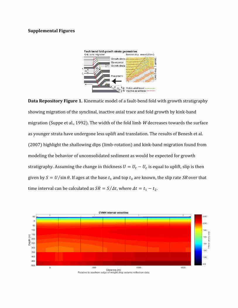
Data Repository Figure 1.  Kinematic model of a fault‐bend fold with growth stratigraphy 

showing migration of the synclinal, inactive axial trace and fold growth by kink‐band 

migration (Suppe et al., 1992). The width of the fold limb W decreases towards the surface 

as younger strata have undergone less uplift and translation. The results of Benesh et al. 

(2007) highlight the shallowing dips (limb‐rotation) and kink‐band migration found from 

modeling the behavior of unconsolidated sediment as would be expected for growth 

stratigraphy. Assuming the change in thickness ! ! !! ! !!  is equal to uplift, slip is then 

given by ! ! ! sin!. If ages at the base !! and top !! are known, the slip rate SR over that 

time interval can be calculated as �� ! ! ��, where �� ! !! ! !!. 

 

 

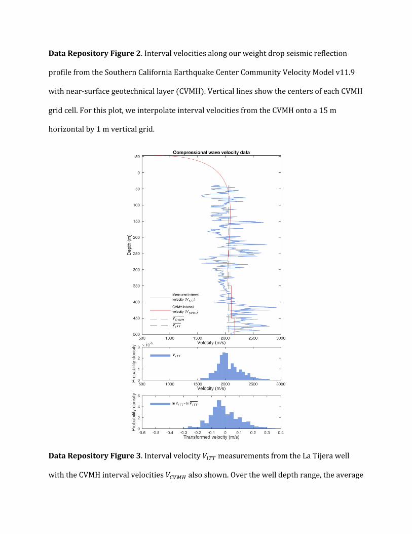
Data Repository Figure 2. Interval velocities along our weight drop seismic reflection 

profile from the Southern California Earthquake Center Community Velocity Model v11.9 

with near‐surface geotechnical layer (CVMH). Vertical lines show the centers of each CVMH 

grid cell. For this plot, we interpolate interval velocities from the CVMH onto a 15 m 

horizontal by 1 m vertical grid. 

 

Data Repository Figure 3. Interval velocity !!∀∀ !measurements from the La Tijera well 

with the CVMH interval velocities !!∀#∃ !also shown. Over the well depth range, the average 

velocities for each are very similar, with the observed data being slower by 20 m/s. A 

normalized histogram of the raw !!∀∀  is shown in the middle figure. It has a slightly 

lognormal distribution. We use a log transformation, as shown in the lower figure, to 

improve normality and better satisfy the requirements for Gaussian noise in the AR 

modeling approach. 

 

Data Repository Figure 4. Average velocities from our simulations compared to the CVMH 

average velocity at the La Tijera well location. Average velocities from the first 500 

simulations are plotted in semi‐transparent grey to give a sense of their density and range. 

All other statistics are based on data from 50,000 simulations. The average velocity 

variance decreases with depth because we are averaging over an increasing number of 

interval velocity samples with the same underlying distribution. 

 

 

Data Repository Figure 5. Thickness and dip measurement example. The position of the 

top clay does not vary as it is defined lithologically by our boreholes. 

 

 

Data Repository Figure 6. Probability density normalized age distributions. The 

combined probability distribution for top clay was produced by combining the cumulative 

distribution function for the 14C sample from well 8 with the reflection of the cumulative 

distribution function for the 14C sample from well 5. We assume uniform probability in 

between. We use uniform distributions for the sequence boundary ages. 

 

 

Data Repository Figure 7. Schematic diagram of hollow‐stem auger sampling technique. b. 

Schematic diagram of mud‐rotary drill rig sampling technique used for IRSL dating. c. 

Diagram of sample extraction from the stainless steel liner in the laboratory. The portion 

labeled NAA was used for ionizing dose‐rate determination and the portion labeled IRSL 

was used for luminescence measurement. 

 

4 c

m

IRS

L

4 c

m

15 c

m

4 cm

5 cm

C. Sample Extraction

Sampler:

2.5 - 15 cm

in front of

the drill bit

Drilling

mud

Drill bit

Drill String

Cable

Sam

ple

r

B. Mud-rotaryA. Hollow-stem auger

Cable

Sampler:

Driven 90

cm into the

ground in

front of the

drill tip

Drill

String

Sam

ple

r

  

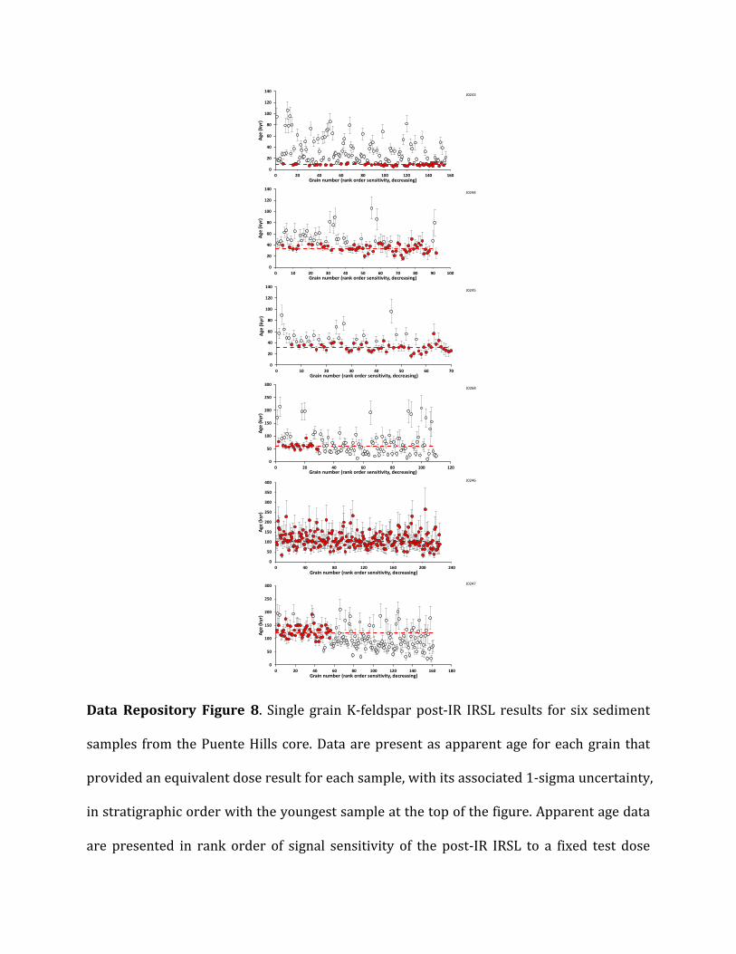
Data  Repository  Figure  8.  Single  grain K‐feldspar post‐IR  IRSL  results  for  six  sediment 

samples  from the Puente Hills  core. Data are present as apparent age  for each grain  that 

provided an equivalent dose result for each sample, with its associated 1‐sigma uncertainty, 

in stratigraphic order with the youngest sample at the top of the figure. Apparent age data 

are  presented  in  rank  order  of  signal  sensitivity  of  the  post‐IR  IRSL  to  a  fixed  test  dose 

J0243

J0244

J0245

J0268

J0246

J0247

0

20

40

60

80

100

120

140

0 20 40 60 80 100 120 140 160

Age (kyr)

Grain number (rank order sensitivity, decreasing)

0

20

40

60

80

100

120

140

0 10 20 30 40 50 60 70 80 90 100

Age (kyr)

Grain number (rank order sensitivity, decreasing)

0

20

40

60

80

100

120

140

0 10 20 30 40 50 60 70

Age (kyr)

Grain number (rank order sensitivity, decreasing)

0

50

100

150

200

250

300

0 20 40 60 80 100 120

Age (kyr)

Grain number (rank order sensitivity, decreasing)

0

50

100

150

200

250

300

350

400

0 40 80 120 160 200 240

Age (kyr)

Grain number (rank order sensitivity, decreasing)

0

50

100

150

200

250

300

0 20 40 60 80 100 120 140 160 180

Age (kyr)

Grain number (rank order sensitivity, decreasing)

within the SAR dating protocol, with  the most sensitive grain at position 1, decreasing to 

the  least  sensitive  grain  plotted.  A  variety  of  different  sample  responses  is  observed, 

corresponding  to  variations  in  K‐feldspar  behavior  likely  associated  with  changes  in 

sediment  sources  deposited  over  this  time  period  (last  interglacial  to  Holocene).  Solid 

symbols  show  results  for  grains  included  in  the  combined  age  estimate  for  that  sample, 

open symbols show excluded grains. See text for further details. 

 

 

Data Repository Figure 9. Probability normalized histograms of sedimentation rates. The 

2.5 – 97.5 percentile ranges are shown, along with median values for symmetric 

distributions and modal values for skewed distributions. Bin size is 0.1 mm/yr. 

 

 

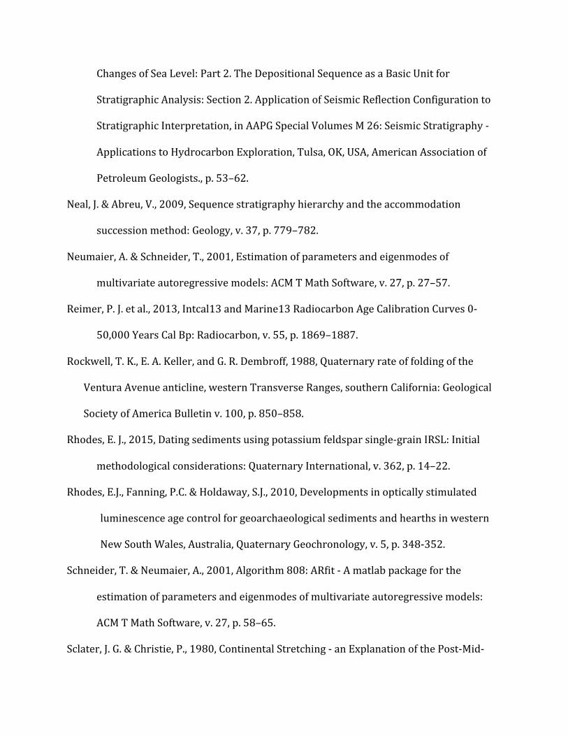
Data Repository Figure 10. Probability normalized histograms of uplift and horizontal 

shortening rates. The 2.5 – 97.5 percentile ranges for horizontal shortening rates (along the 

bottom axis) and for uplift rates (along the top axis), with median values for symmetric 

distributions and modal values for skewed distributions. Bin size is 0.1 mm/yr. 

a. Radiocarbon ages and sample details 

Borehole 

 

Sample type  Depth (m)  14C Age BP  13C  Calibrated age BP (1950) 

68.2% Probability  95.4% Probability 

D1  Small charcoal  7.47  6960 + 100  ‐25  7923 – 7902 (6.7%) 

7866 – 7692 (61.5%) 

7966 – 7617 (95.4%) 

 

D1  Medium 

charcoal 

8.69  7390  + 170  ‐25  8360 – 8043 (68.2%)  8544 – 7928 (94.7%) 

7895 – 7874 (0.7%) 

10  Bulk soil  15.93  9465 + 35  ‐25  10752 – 10659 (65.9%) 

10614 – 10610 (2.3%) 

11060 – 11036 (2.3%) 

10996 – 10978 (1.6%) 

10788 – 10584 (91.5%) 

2  Bulk soil  15.52  9980 + 40  ‐25  11602 – 11551 (14.7%) 

11494 – 11432 (16.5%) 

11412 – 11309 (37%) 

11620 – 11265 (95.4%) 

 

8  Bulk soil  16.16  10265 + 40  ‐25  12114 – 11957 (64.9%) 

11862 – 11849 (3.3%) 

12226 – 12217 (0.4%) 

12166 – 11819 (95%) 

5  Bulk soil  11.28  13780 + 210  ‐25  16980 – 16348 (68.2%)  17326 – 16090 (95.4%) 

 

b. IRSL ages and sample details 

Borehole Drilling

technique

Field Code Lab

code

Depth

(m)

Equivalent dose ± 1σ

uncertainty (Gy)

Total dose rate ± 1σ

uncertainty (mGy/yr)

Age ± 1σ

uncertainty (ka)

D1 Hollow-stem HS PHD1 30.5’-32’ J0243 9.4 30.9 ± 1.0 3.55 ± 0.18 8.70 ± 0.53

D1 Hollow-stem HS PHD1 65’-66.5’ J0244 20.0 117 ± 4 3.47 ± 0.24 33.7 ± 2.6

D1 Hollow-stem HS PHD1 75’-76.5’ J0245 23.0 107 ± 4 3.42 ± 0.22 31.4 ± 2.3

D1 Hollow-stem HS PHD1 131.5’-133’ J0228 40.2 192 ± 8 3.14 ± 0.21 61.1 ± 4.9

D1 Mud-rotary MR PHD2 395’-396.5’ J0246 120.5 317 ± 10 3.03 ± 0.20 105 ± 8

D1 Mud-rotary MR PHD2 444.5’-446’ J0247 135.5 403 ± 13 3.23 ± 0.20 125 ± 9

c. Sedimentation rate statistics (mm/yr)

  2.5%  Mean  Median  Mode  97.5%  σ  CVMH 

Top clay – Present  0.97  1.14  1.13  1.01  1.34  0.11  1.13 Harbor – Top clay  1.33  1.65  1.63  1.46  2.06  0.21  1.67 

Bent Spring – Harbor  0.54  0.91  0.85  0.81  1.58  0.27  0.87 Upper Wilmington – Bent Spring  0.4  0.6  0.59  0.55  0.91  0.13  0.6 

 

d. Slip rate statistics (mm/yr)

  2.5%  Mean  Median  Mode  97.5%  σ  CVMH 

Top clay – Present  1.13  1.4  1.38  1.33  1.73  0.16  1.36 

Harbor – Top clay  0.65  1.07  1.05  1.01  1.6  0.24  1.06 

Bent Spring – Harbor  0  0.48  0.45  0.01  1.3  0.36  0.45 Upper Wilmington – Bent Spring  0  0.26  0.22  0.01  0.8  0.23  0.24 

 

e. Uplift rate statistics (mm/yr)

  2.5%  Mean  Median  Mode  97.5%  σ  CVMH 

Top clay – Present  0.4  0.47  0.47  0.42  0.55  0.05  0.47 

Harbor – Top Clay  0.22  0.36  0.36  0.35  0.53  0.08  0.36 Bent Spring – Harbor  0  0.17  0.15  0.01  0.46  0.13  0.15 

Upper Wilmington – Bent Spring  0  0.09  0.08  0.01  0.25  0.07  0.08 

 

f. Horizontal shortening rate statistics (mm/yr)

  2.5%  Mean  Median  Mode  97.5%  σ  CVMH 

Top clay – Present  1.06  1.31  1.3  1.25  1.63  0.15  1.28 Harbor – Top Clay  0.61  1.01  0.99  0.95  1.5  0.23  0.99 

Bent Spring – Harbor  0  0.45  0.42  0.01  1.22  0.34  0.42 Upper Wilmington – Bent Spring  0  0.24  0.21  0.01  0.75  0.22  0.22 

 

g. Fault dip statistics (°)

  2.5%  Mean  Median  Mode  97.5%  σ  CVMH 

Fault Dip (°)  17.14  19.78  19.84  19.95  22.15  1.29  20.03 

 

Data Repository Table 1. Data tables from age determinations (a, b) and fault slip and 

geometry simulations (c – g). Table b. shows details for the combined single grain post‐IR 

IRSL data used in the depositional age model. For tables c – g, the 2.5% and 97.5% headings 

correspond to the 2.5 – 97.5 percentile ranges. Modes are calculated from histograms with 

0.1 mm/yr bins for rate estimates, and 0.1° bins for dip estimates. CVMH values correspond 

to fold geometries after depth conversion with the CVMH, with rates determined using 

mean ages. 

Data Repository Table 2.  Steps used in the post‐IR IRSL single aliquot regenerative‐dose 

(SAR) protocol applied to K‐feldspar single grains. Multiple cycles of measurement were 

made to 200 to 400 grains for each sample. 

 Supplemental references 

Allen, P. A. & Allen, J. R., 2005, Basin Analysis, Oxford, U.K., Blackwell Publishing. 

Bahr, D. B., Hutton, E., Syvitski, J. & Pratson, L. F., 2001, Exponential approximations to 

compacted sediment porosity profiles: Computers & Geosciences, v. 27, p. 691–700. 

Bassinot, F. C. et al., 1994, The Astronomical Theory of Climate and the Age of the Brunhes‐

Matuyama Magnetic Reversal: Earth and Planetary Science Letters, v. 126, p. 91–108.

SAR step Measurement parameters

1   Beta irradiation  0 (Nat), 20, 6.4, 64, 200, 640, 0, 20 Gy in turn

2   Preheat 1  60s at 250°C

3   IRSL50 1  2.5s 90% laser power at 50°C

4   IRSL225 2  2.5s 90% laser power at 225°C

5   Beta test dose  9 Gy

6   Preheat 2  60s at 250°C

7   IRSL50 S1 Sensitivity measurement  2.5s 90% laser power at 50°C

8   IRSL225 S2 Sensitivity measurement  2.5s 90% laser power at 225°C

9   Hot bleach – then return to 1  40s IRSL (diodes at 90% power) at 290°C

Benesh, N. P., Plesch, A., Shaw, J. H. & Frost, E. K., 2007, Investigation of growth fault bend 

folding using discrete element modeling: Implications for signatures of active folding 

above blind thrust faults, Journal of Geophysical Research, v. 112, B03S04, p. 2156‐

2202. 

Buylaert, J.P., Murray, A.S., Thomsen, K.J., Jain, M., 2009, Testing the potential of an elevated 

temperature IRSL signal from K‐feldspar,Radiation Measurements, v. 44, p. 560‐565. 

Chen, Y.‐G. et al., 2007, Coseismic fold scarps and their kinematic behavior in the 1999 Chi‐

Chi earthquake Taiwan, Journal of Geophysical Research, v. 112, B03S04, p. 2156‐

2202. 

Ehman, K. D. & Edwards, B. D., 2014, Sequence Stratigraphic Framework of Upper Pliocene 

to Holocene Deposits, Los Angeles Basin, California: Implications for Aquifer 

Architecture: Society for Sedimentary Geology (SEPM), ISBN: 978‐0‐9842302‐5‐9.   

Galbraith, R.F., Roberts, R.G., Laslett, G.M., Yoshida, H. & Olley, J.M. 1999, Optical dating of 

single and multiple grains of quartz from Jinmium rock shelter, northern Australia. 

Part I, experimental design and statistical models, Archaeometry, v. 41, p. 339–364. 

Hubbard, J., J. H. Shaw, J.F. Dolan, T. L. Pratt, L. McAuliffe, and T. K. Rockwell, 2014, 

Structure and seismic hazard of the Ventura Avenue anticline and Ventura fault, 

California: Prospect for large, multi‐segment ruptures in the Western Transverse 

Ranges: Bulletin of the Seismological Society of America, v. 104/3, p. 1070–1087. 

Leon, L. A., 2009, Paleoseismology of blind‐thrust faults beneath Los Angeles, California: 

Implications for the potential of system‐wide earthquakes to occur in an active fold‐

and‐thrust belt: Ph.D. Dissertation, University of Southern California, DAI/B 70‐07. 

Mitchum, R. M., Vail, P. R. & Thompson, S., III.,  1977, Seismic Stratigraphy and Global 

Changes of Sea Level: Part 2. The Depositional Sequence as a Basic Unit for 

Stratigraphic Analysis: Section 2. Application of Seismic Reflection Configuration to 

Stratigraphic Interpretation, in AAPG Special Volumes M 26: Seismic Stratigraphy ‐ 

Applications to Hydrocarbon Exploration, Tulsa, OK, USA, American Association of 

Petroleum Geologists., p. 53–62. 

Neal, J. & Abreu, V., 2009, Sequence stratigraphy hierarchy and the accommodation 

succession method: Geology, v. 37, p. 779–782. 

Neumaier, A. & Schneider, T., 2001, Estimation of parameters and eigenmodes of 

multivariate autoregressive models: ACM T Math Software, v. 27, p. 27–57. 

Reimer, P. J. et al., 2013, Intcal13 and Marine13 Radiocarbon Age Calibration Curves 0‐

50,000 Years Cal Bp: Radiocarbon, v. 55, p. 1869–1887. 

Rockwell, T. K., E. A. Keller, and G. R. Dembroff, 1988, Quaternary rate of folding of the 

Ventura Avenue anticline, western Transverse Ranges, southern California: Geological 

Society of America Bulletin v. 100, p. 850–858. 

Rhodes, E. J., 2015, Dating sediments using potassium feldspar single‐grain IRSL: Initial 

methodological considerations: Quaternary International, v. 362, p. 14–22. 

Rhodes, E.J., Fanning, P.C. & Holdaway, S.J., 2010, Developments in optically stimulated 

luminescence age control for geoarchaeological sediments and hearths in western 

New South Wales, Australia, Quaternary Geochronology, v. 5, p. 348‐352. 

Schneider, T. & Neumaier, A., 2001, Algorithm 808: ARfit ‐ A matlab package for the 

estimation of parameters and eigenmodes of multivariate autoregressive models: 

ACM T Math Software, v. 27, p. 58–65. 

Sclater, J. G. & Christie, P., 1980, Continental Stretching ‐ an Explanation of the Post‐Mid‐

Cretaceous Subsidence of the Central North‐Sea Basin: Journal of Geophysical 

Research, v. 85, p. 3711–3739. 

Suppe, J. Geometry and Kinematics of Fault‐Bend Folding: American Journal of Science, v. 

283, p. 684–721. 

Törnqvist, T. E., Wallinga, J. & Busschers, F. S., 2003, Timing of the last sequence boundary 

in a fluvial setting near the highstand shoreline—Insights from optical dating: 

Geology, v. 31, p. 279–282.