accelerator physics for health physicists -
TRANSCRIPT

1
Accelerator Physics for Health Physicists
J. Donald CossairtPh.D., C.H.P.
Applied Scientist IIIFermi National Accelerator Laboratory

2
Introduction• Goal is to improve knowledge and appreciation of the art of particle
accelerator physics • Accelerator health physicists should understand how the machines
work.• Accelerators have unique operational characteristics of importance
to radiation protection.– For their own understanding– To promote communication with accelerator physicists, operators, and
experimenters• This course will not make you an accelerator PHYSICIST!
– Limitations of both time and level prescript that.– For those who want to learn more, academic courses and the U. S.
Particle Accelerator School provide much comprehensive opportunities.• Much of the material is found in several of the references.
– Particularly clear or unique descriptions are cited among these.

3
A word about notation
• Vector notation will be used extensively.– Vectors are printed in italic boldface (e.g., E)– Their corresponding magnitudes are shown in italics
(e.g., E). • Variable names generally will follow the
published literature.• Consistency has not been achieved.
– This author cannot fix that by himself!– Chose to remain close to the literature– Watch the context!
4
Summary of relativistic relationships including Maxwell’s equations
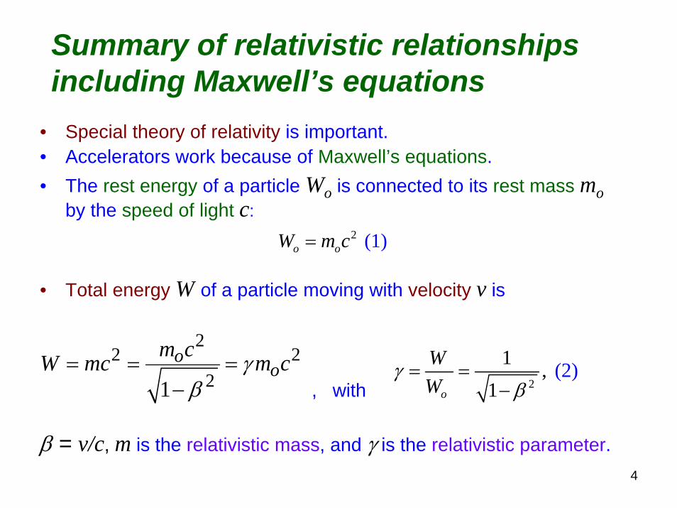
• Special theory of relativity is important.• Accelerators work because of Maxwell’s equations.• The rest energy of a particle Wo is connected to its rest mass mo
by the speed of light c:
• Total energy W of a particle moving with velocity v is
, with
β = v/c, m is the relativistic mass, and γ is the relativistic parameter.
2 (1)o oW m c=
22 2
21o
om cW mc m cγ
β= = =
− 2
1 , 1
(2)o
WW
γβ
= =−

5
Summary of relativistic relationships
Thus kinetic energy T=W-Wo,
and
Momentum p is related to relativistic m and v:
At high energies p≈T/c ≈W/c At low energies p2≈(2Wo/c2)T=2moT
Also,
2(3
1)o
omm mγ
β= =
−
2
1 (4)oWW
β ⎛ ⎞= − ⎜ ⎟⎝ ⎠
22 2
2
1 1 ( 2 (1 )) 5o oo o o
o
Wm Wp mv m c c W W T T Wm c W c c
γ β⎡ ⎤⎛ ⎞ ⎡ ⎤⎢ ⎥= = = − = − = +⎜ ⎟ ⎣ ⎦⎢ ⎥⎝ ⎠⎣ ⎦
2 2 2 2 4 )(6oW p c m c= +

6
Summary of relativistic relationships
• Convenient to work in a system of units where energy is in units of eV, MeV, etc.
• Velocities are then expressed in units of the speed of light (0<β<1), momenta as energy divided by c (e.g., MeV c-1, etc.), andmasses as energy divided by c2 (e.g., MeV c-2, etc.).
• In these so-called “energy” units W and m are numerically equivalent. One thus does not need the numerical value of c or c2
• Nearly always, if a particle energy is referred to as being, say, “100 MeV”, the kinetic energy T, not the total energy W, is meant.– Is an important distinction at low energies!

7
Maxwell’s equations
Maxwell’s equations in vacuum in SI units will be used. They connect
the electric field E [Volts (V) m-1] ,the magnetic field B [Tesla (T)] ,the charge density [Coulombs (C) m-3] ,and current density j(r,t) [Amperes (A) m-2] (units wrong in text!)at a location in space r at time t.
εo is the dielectric constant in vacuum [107/(4πc2) (C V-1 m-1])] μo is the permeability of free space [4π x 10-7 (V s A-1 m-1)],c2=1/(μo εo). This fact led Einstein to special relativity!
( , )tρ r

8
Maxwell’s equationsThe equations in differential (left) and integral forms (right) are
(Gauss’s Law), (7)
,(8)
(Faraday’s Law),(9)
(Ampere’s Law).(10)

9
Deflection of Charged Particles
Electromagnetic forces are used to accelerate, deflect, and focus charged particles. The Lorentz force F [Newtons (N)] on charge q (C) with velocity v (m s-1) due to applied electric field E (V m-1) and magnetic field B (T) is
where p is momentum in SI units and t is the time (s)
Static electric fields (i.e., dE/dt=0) accelerate or deccelerate charged particles
Static magnetic fields (dB/dt=0) can only deflect them. Nonstatic conditions couple these fields via Eqs. (9) and (10).
( ) , (11)dqdt
= × + =pF v B E

10
Some considerations• Nature and present-day technology have placed
constraints on the design of static deflection and focusing devices. – Static electric fields are limited a few MV m-1. – Ferromagnetic materials are limited to about 2 T and
superconductors to 4-10 T.• A common simplification is that the physical boundaries
of a given deflecting or focusing element exactly define the boundary of the electric or magnetic field. – For real components the fields extend beyond the geometrical
boundaries for short distances in fringe fields.– Fringe fields also deflect the particles.– The beam elements behave as if they are a bit larger than their
geometric profiles. – Thus the concepts of an effective boundary and an effective field
integral are used.

11
A digression on synchrotron radiation
• Accelerated charged particles radiate energy, even if the acceleration is purely centripetal.
• Thus particles even in a circular orbit lose energy by radiating it as photons.
• This is the basis for synchrotron radiation, or “light”sources.
• It also impacts accelerator physics– Has to be “fed” by RF energy– There are other subtle effects on beam properties.
• For highly relativistic energies, readily achieved for electrons, the photons emerge in a tight bundle along a tangent to any point on a circular orbit.

12
A digression on synchrotron radiation• The characteristic angle θc is defined to be the angle
where the intensity is 1/e (1/2.718) of that at the center
(12)
R
electrons
22
2 1 2θγ
βc = = −
synchrotronradiation
θγ
βc = = −1 1 2

13
A digression on synchrotron radiation• The power spectrum has a universal shape:
with median energy for electrons
for W (GeV) & bending radius R (meters). For singly-charged particles of other masses mx multiply by (me/mx)3.
10-5
10-4
10-3
10-2
10-1
100
10-4 10-3 10-2 10-1 100 101
Nor
mal
ized
Pow
er
Relative Photon Energy (ε/εc)
32.218 (keV) (13)cW
Rε =

14
A digression on synchrotron radiation• The radiated power P (watts) for circulating electron
current I (ma) is
For singly charged particles of other masses mx multiply by (me/mx)4.
• The LHC at CERN will be the first proton accelerator where synchrotron radiation is of crucial importance
• We see why synchrotron radiation sources all use electrons!
488.46 (14)W IPR
=

15
Deflection of Charged Particles by Static Electric FieldsFig. 1 shows purely electrostatic deflection (dE/dt=0 and
B=0) of a fast particle with initial momentum p=pz and velocity v.
Consider a particle of charge q passing through plates of length L biased at voltage V, & separated by distance δ(all SI units):

16
Pure electrostatic deflection
• From Eq. (7) the electric field E has a uniform value of V/δ oriented as shown.
• Initially, the components of the momentum arepz=p and px=py=0.
• Since B=0, Eq. (11) gives
• With no z-component of force, no change in pzoccurs in this system.
5) (1xx
dp VqE qdt δ
= =

17
Pure electrostatic deflection
For a “fast” particle, we ignore the small deviation from a “straight” path.
We can integrate over the time t needed to travel through the device and get px at the exit:
For q in units of electron charge this is already in eV/c.
Px in MeV/c is useful:
-1(kg m s ) (16(e a) )xitxV L V Lp q q
v cδ δ β= =
6 (16b)(exit) 10 xV Lp qδ β
−= ×

18
Pure electrostatic deflection
Look at the angular deflection Δθ (radians) and apply the small angle approximation:
for pz>>px
1 1 6 1 6tan tan 10 tan 10x
z z z
p qVL qELp p p
θδβ β
− − − − −⎡ ⎤ ⎡ ⎤ ⎡ ⎤Δ = = × = ×⎢ ⎥ ⎢ ⎥ ⎢ ⎥
⎣ ⎦ ⎣ ⎦ ⎣ ⎦
610 (17)qELp
θβ
−Δ ≈ ×

19
Uses of pure electrostatic deflection• Used as inflectors (injection) and electrostatic septa
(extraction). • At low energies conductor planes are used. • At high energies, planes of fine wires, as small as 50 μm
diameter, commonly approximate one or both of the parallel plates.
• These devices can be tens of meters long, have V > 100 kV.
• One conductive plane slices through the beam to split it by giving part of it a small momentum kick.
• Wires are used to minimize material struck by the beam.• Often used in conjunction with magnetic elements.

20
Electrostatic deflection radiation protection considerations• Especially for electrons, synchrotron radiation can result.• The deflection has to achieve the correct angle.• Wire septa can create locally strong electric fields
– Capable of ionizing residual gas atoms– Accelerate electrons across the gap as a dark current– Produce x-rays [Example: At Fermilab have seen > 1 mGy h-1]– This phenomena is not very reproducible (cleanliness, residual
pressure = “bad” vacuum, etc.)
• Activation of septa components by stray beam• Terminology and jargon: Small angles measured in
milliradians, readily becomes “mrad”, or even “mr” but absorbed dose is NOT being discussed.

21
Deflection of Charged Particles by Static Magnetic Fields
Fig. 2 shows a purely magnetostatic deflection with no electric field (dB/dt=0, E=0).
Eq. (11): ( ) ( )d q qdt
= = × + = ×pF v B E v B

22
Deflection of Charged Particles by Static Magnetic Fields• Due to the cross product, any component of p which is parallel to B will
not be altered by it. • Typically charged particles are deflected by dipole magnets with fields:
– Often nearly spatially uniform– Constant or slowly-varying compared with the time the particle is present.
• If – There is no component of p that is parallel to B– Energy loss from synchrotron radiation can be ignored
• Then– The magnetic force supplies the needed centripetal acceleration – The kinetic energy of the particle unchanged. – A circular path is followed (as shown in Fig. 2)
• A component of p parallel to B results in a spiral trajectory with that component conserved.

23
Deflection of Charged Particles by Static Magnetic FieldsEquating the centripetal force to the magnetic force for p perpendicular
to B gives
where m is the relativistic mass and p=mv.
Solving for R and making a convenient unit conversion:
In the far right-hand-side, q is now in # of electronic charges,
B remains in TeslaThe “300” factor is the speed of light in SI units divided by 106.
The useful product BR (T-m) is called the magnetic rigidity; Greek “ρ” is often used instead of R, so that the quantity is called “B-rho”.
2
( ) simplifies to ( 8) 1mvq qvBR
= × =F v B
-1 (SI units) (MeV c )(meters) = 299.79
(19)p pRqB qB
=

24
Deflection of Charged Particles by Static Magnetic Fields
Look at Fig. 2 again
For short magnets L<<R, The deflection Δθ for momentum p (MeV c-1) is given by
BL (T m) is called the field integral of the magnet system.
299.79 (radians (2) 0)L qBLR p
θΔ = =

25
Magnetic deflection radiation protection considerations
• Need to make calculations to miss objects, clear apertures, etc.
• Can use this to select charge states or momenta• Used to measure momenta, can be needed to assure
safe design of facilities downstream• Part of radiation safety system design
– Electro-mechanically, interlocks must be designed to high standards
– The design in terms of beam physics; to preclude unwanted charged particles, is just as important
• Usually, magnet current “off” is the easiest “safe”configuration.

26
Example of Bending Magnets
Fermilab 120 GeV Main Injector Bending Magnets
during assembly as assembledPhotos from Fermilab website

27
Focusing of Charged Particles
• Dominant technique: quadrupoles with “near static” fields– Electric quadrupoles– Magnetic quadrupoles
• Higher order multipoles; sextupoles, octupoles, etc. are used, beyond the scope of this course– Correct for imperfections from “ideal”
• Will also discuss other focusing techniques– Principally adaptations of dipole magnets

28
Quadrupole lenses• Will use Cartesian coordinates & “right-hand” rule• The z-axis, the optic axis, is into the screen• Values of x > 0 are “beam’s eye” left• Values of y > 0 are “beam’s eye” up• Below types are set to focus + charge the same way• Orientations differ due to Eq. (11) cross product• Electric and magnetic field lines are shown between the poles• Gap radius a is defined.• The length of the• quadrupole is L• See Fig. 3:

29
Quadrupole lenses“Ideal” pole pieces (equipotentials) are hyperbolae;
electric: x2-y2=+a magnetic: xy=+a2/2

30
Quadrupole lensesBo (T) is magnetic field at magnetic pole piecesEo=2V/a (V m-1) is electric field at electric pole piecesFor magnetic quad, the field components in the gap are:
For electric quad, use same Eqns. with Eo replacing BoThe gradients, gm (T m-1) and ge (V m-2) are defined.
(21) ox m
BB y g ya
= − = − (22)oy m
BB x g xa
= − = −

31
Quadrupole lenses-qualitative deflections(See p. 11 of chapter) Need >1 to focus in both planes!

32
Quadrupole lenses-let’s add mathIn the yz-plane of a magnetic quadrupole, apply Eq. (20):
Substitute Bx=-gmy, and get the angular deflection Δθ :
For electric quadrupole, apply Eq. (17):
And get
Note: For both Δθ is proportional to y, a feature of focusing of visible light by lenses.
For awhile, will treat electric and magnetic quads the same.
299.79 (radians (2) 0)L qBLR p
θΔ = =
299.79 (radia ( )s 2) 3nmqg yLp
θΔ =
610 (radians) (17)qELp
θβ
−Δ ≈ ×
610 (radians) (24)eqLg yp
θβ
−Δ = ×

33
Quadrupole lenses- focusing actionStart with particles traveling parallel to the z-axis displaced by y.After deflection by a small angle Δθ, will intercept the z-axis at
distance f:
Note that f is independent of y! This is the “thin lens” approximation, true if f>>L. f is, naturally, the focal length. See Fig. 4a:
6
(magnetic) tan
or (e
29
lectric) (25)
9.79
10
m
e
y y pfqLg
y pfqLg
θ θβ
θ
= ≈ =Δ Δ
≈ = ×Δ

34
Quadrupole lenses-thin lens equationThe analogy with “light” optics is true mathematically, we have the thin lens equation connecting the image distance zi, with
the object distance zo;
If f > 0 with zo >0 and zi >0, get a real image in the focusing plane.In the defocusing plane, f < 0, get a virtual image since for zo >0, zi <0.If lenses are thick, reference principal planes rather than center of the
quadrupole (more later!) See Fig. 4b:
1 (26)1 1 o iz z f
+ =

35
Quadrupole doubletsNeed multiple elements to focus in BOTH planes Quadrupole doublets (pair of 2) is the most common solutionSee Fig. 4c (yz-plane)and Fig. 4d (xz-plane)
Will assume quad 1 andquad 2 havedifferent focallengths. (Oftenquads are setup identical!)
36
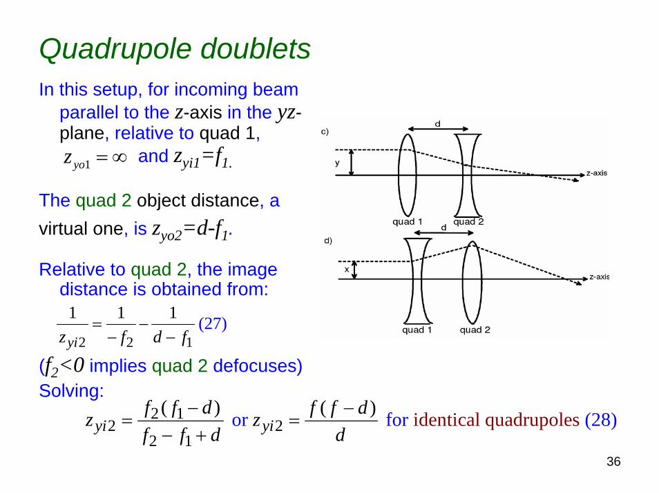
Quadrupole doubletsIn this setup, for incoming beam
parallel to the z-axis in the yz-plane, relative to quad 1,
and zyi1=f1.
The quad 2 object distance, a virtual one, is zyo2=d-f1.
Relative to quad 2, the image distance is obtained from:
(f2<0 implies quad 2 defocuses)Solving:
1yoz = ∞
2 2 1
1 1 1 (27)yiz f d f
= −− −
2 12 2
2 1 identical quadrupoor fo lesr (2( ) ( ) 8 yi yi
f f d f f dz zf f d d
− )−= =
− +

37
Quadrupole doubletsLikewise, for the xz-plane, the finalImage distance zxi2 is given by
Note that for identical quadrupoles,
Expected! This focused in yz beforexz. (Not identical to light optics!)Average focal length is f 2/d.
2 12 2
1 2identical quadrupoor for les (2( ) ( ) 9)xi xi
f f d f f dz zf f d d
+ += =
− +
2 2 )2 (30 xi yiz z f− =

38
Quadrupole triplets• More complicated systems overcome some limitations• A commonly used, elegant variant is that of the quadrupole
triplet– 3 quadrupoles, quad 1, quad 2, and quad 3– Alternate in polarity, quad 1 same as quad 3 opposite quad 2– Acts like a pair of quadrupole doublets placed back to back– Saves space, less distortion, acts (mostly!) like a single lens
• Useful special case:– Quad 1 and 3 have equal focal lengths f– Quad 2 has focal length ½ f (i.e., fields are 2x as strong or magnet
is 2x as long)– Separation distance is d between each pair.
• Effective focal length f* forf>>d is
1 22 (31* 2 )1
2d ff f df d
−⎡ ⎤⎛ ⎞
= + ≈⎢ ⎥⎜ ⎟⎝ ⎠⎣ ⎦

39
Examples of magnetic quadrupolesIndiana University Cyclotron Facility (IUCF) Fermilab Main Injector
Photo from IUCF website Photo from Fermilab website

40
Focusing Mechanisms by Dipole Magnets
• A variety of focusing mechanism using dipole magnets are possible
• Will discuss here several examples• There are many applications that use combinations of these
techniques, even with in the same magnet• Often used in combination with both kinds of quadrupoles, other
devices• Often necessary for proper functioning of accelerators• Uses:
– To focus beams on experimental targets– To separate particles by energy, mass, or momenta
Magnetic spectrometers to separate particles by momentaMass analyzersTo select beams for further acceleration
– In accelerators to assure desired beam properties

41
Sector magnets• Used to both bend and focus beams• Fig. 5 shows example
– Defines coordinate system, central ray, & median plane
• Generalized, non-uniform B field

42
Sector magnets• Field non-uniformity characterized by field index n, commonly
used at accelerators, used even for edges of uniform field magnets; If B decreases with increasing r, n >0.
(32a)constant /; equivalently, ( 3 b/
2 )z o n
nr dB BB B nR r dr r
− −⎛ ⎞= = =⎜ ⎟⎝ ⎠

43
Sector magnets; uniform field case• Uniform field implies by n=0• Has no radial component and hence no first order focusing
action• Still get geometric focusing
– Trajectories with r < R travel shorter distance in the field than trajectories with r > R , deflected less
– Have Barber’s Rule (see Fig. 6) : If α<180 degrees, α+γ1+γ2 =2π radians (180 degrees)

44
Sector magnets; non-uniform fields
Can use a Taylor expansion and the definition of the field index n to get a radial component of the field Br(z); above and below the midplane.
From symmetry, the 1st and all even-numbered terms vanish.
( )22
,0 2 (330( 0) )( ) ...
1! 2!rr
r r
B zB zz zB z Bz z
⎡ ⎤∂ =⎡ ⎤∂ == + + +⎢ ⎥⎢ ⎥∂ ∂⎣ ⎦ ⎣ ⎦

45
Sector magnets; non-uniform fields
With no electric currents or fields in the magnet gaps (the usual case!),Eq. (10):
and Eq. (32b)
leads to:
then
( )22
,0 2 (330( 0) )( ) ...
1! 2!rr
r r
B zB zz zB z Bz z
⎡ ⎤∂ =⎡ ⎤∂ == + + +⎢ ⎥⎢ ⎥∂ ∂⎣ ⎦ ⎣ ⎦
2
1( , ) ere, 0ho tc t
μ ∂∇× = + ∇× =
∂EB j r B
( 0) (34)( 0) or z nBB z B zz r R
∂ = ∂ == = −
∂ ∂
(35) or
nB zBR
−≈
(32b) o/ /
r dB B dB Bn ndr r dr r
−= = −

46
Sector magnets; non-uniform fields
The relationship between Br and z is linear!This linearity leads to focusing just as with quadrupoles!But, only get such focusing in both horizontal and vertical planes
simultaneously if 0 < n < 1Magnets with n = ½ are a VERY special case
Here the focal length f in both planes is the same, given by:
L is the central ray path length through the magnetf is measured from the magnet’s effective boundary, a principal planeEq. (36) ⇒ f > R, system length > 4R.
(35) or
nB zBR
−≈
1 1 sin 2 2
(36)Lf R R
⎛ ⎞= ⎜ ⎟⎝ ⎠

47
Sector magnets; weak and strong focusing• Limitation: f gets very Iarge at high energies because R gets large!• n < 1 is called weak focusing
–Used in cyclotrons, betatrons, synchrocyclotrons and 1st generationsynchrotrons (e.g., Bevatron, Cosmotron, ANL-ZGS era machines)
• n >> 1 is called strong focusing–Used in 2nd generation synchrotrons (e.g., Cornell, BNL-AGS, CERN-PS)–magnets “alternated” in sense of focusing to achieve overall focusing conditions. Hence, the term “alternating gradient”!
AGS magnet Cosmotron (3 GeV) and AGS (30 GeV) magnetsDiagrams from BNL website

48
Sector magnets; weak and strong focusing
• Alternating gradient magnets are expensive to make• Later synchrotrons (e.g., FNAL, CERN SPS, most
light sources) use uniform field dipoles with quadrupoles interleaved in a separated functionconfiguration to achieve strong focusing
• Separates the focusing and bending functions• Uniform field dipoles (n = 0) are cheaper to make• Magnets at large accelerators ignore the curvature of
the ring, are simply rectangles, a further simplification.

49
Entrance and exit edge focusing by uniform field dipoles• The edges or boundaries in uniform field dipoles (n=0) can give focusing
action• Get some radial focusing in edge fields• Works if pole pieces are not perpendicular to the beam optic access, rather
incident at angle ψ.• See Fig. 7 for horizontal plane views and coordinate system• For ψ > 0 and x>0, added path length through field gives additional
deflection angle: linearly proportional to x!tan (37)hx
Rψα =
50
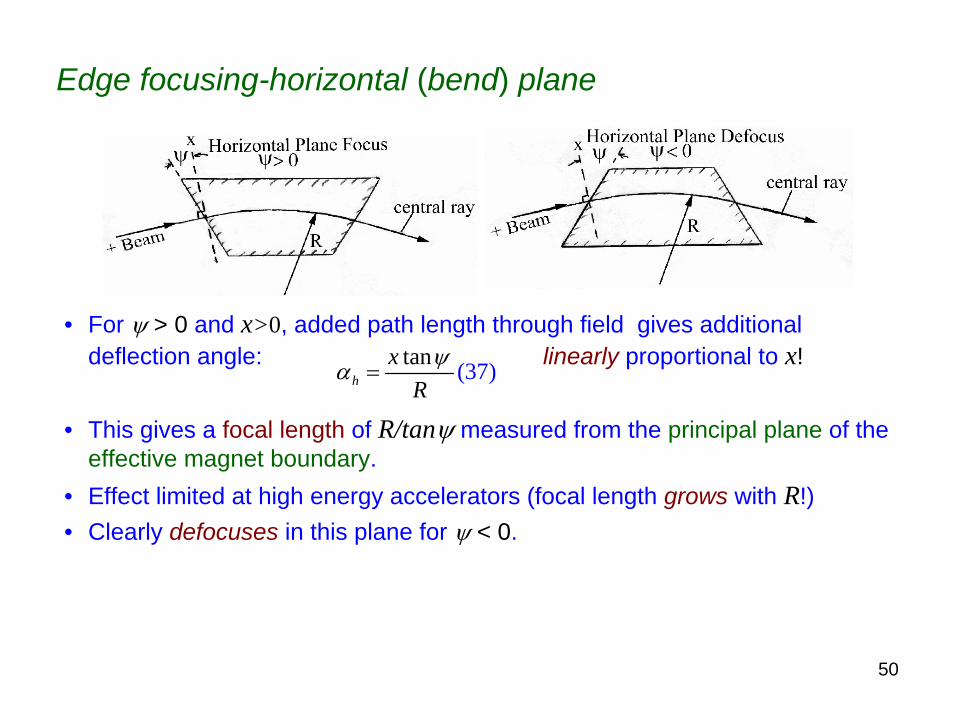
Edge focusing-horizontal (bend) plane
• For ψ > 0 and x>0, added path length through field gives additional deflection angle: linearly proportional to x!
• This gives a focal length of R/tanψ measured from the principal plane of the effective magnet boundary.
• Effect limited at high energy accelerators (focal length grows with R!)• Clearly defocuses in this plane for ψ < 0.
tan (37)hx
Rψα =

51
Edge focusing-vertical plane• What happens in the vertical plane? See Fig. 8.• Need to calculate the bending effect of fringe field.• Use Eq. (10)

52
Edge focusing-vertical planeis true because on our
integration loopB=0 on the left leg (go out far enough!)Bs=0 in the median plane due to symmetry (bottom leg)
Can thus get field integral of Bs.
But, Bs is only one component of the total component of the fringe field that is perpendicular to the pole piece.
53
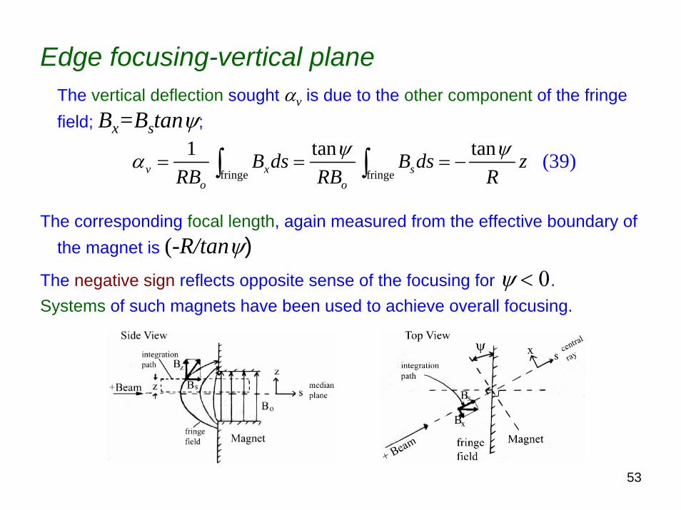
Edge focusing-vertical planeThe vertical deflection sought αv is due to the other component of the fringe field; Bx=Bstanψ;
The corresponding focal length, again measured from the effective boundary of the magnet is (-R/tanψ)
The negative sign reflects opposite sense of the focusing for ψ < 0.Systems of such magnets have been used to achieve overall focusing.
fringe fringe 1 tan 39ta )n (v x s
o o
B ds B ds zRB RB R
ψ ψα = = = −∫ ∫

54
Focusing features in combinationQuadrupole-Dipole-Dipole Multiple (QDDM) Spectrometer at the Indiana University Cyclotron Facility
Photo by J. D. Cossairt, Diagram from IUCF Report No.1-73

55
Radiation protection considerations related to beam
focusing• Effects ignored up to this point
– DispersionNo beam is perfectly monoenergeticMagnets will separate momentum components like the rainbow produced of “white” light by a glass prismdue to different R-valuesCommon to use dispersion matching to remove unwanted effects.Example: n=1/2 magnets at the former 83 inch Univ. of Michigan cyclotron. (Drawing from J. D. Cossairt, Ph. D. thesis)

56
Radiation protection considerations related to beam
focusing
• Effects ignored up to this point– aberrations, specifically chromatic aberration
(beam optic focal lengths are obviously momentum-dependent!)
– transverse emittanceProduct of angular divergence and transverse size
Typical units are π mm-milliradianIn an extracted beam transverse emittance is constant unless increased by scattering, space charge effects, etc.Cannot be decreased in an extracted beam
√ Making the beam smaller in transverse size will increase angular size
√ Shrinking the angular size (i.e., make beam more parallel), will increase the transverse size

57
Radiation protection considerations related to beam
focusing
• Above discussion based on beam being centered on the optic axis
• If beam is off-axis, other effects can happen– Usually undesirable– With quadrupoles, the magnets will act like dipoles and deflect
(bend) the entire beam instead of focusWill bend according to the field integral seen by the particlesThis is called beam steeringUsually results in undesired beam loss.

58
Present Accelerator Technology

59
Accelerators; Cockcroft-Walton Generators• Most elementary accelerator type• Used for first artificial nuclear reaction: p + 7Li -> 4He + 4He• Relies in elevating a terminal to high voltage• Uses high voltage rectifier “ladder” circuit – See Fig. 9.
• At terminal that contains the ion source, a voltage V is achieved.
• Particles of charge q are accelerated to T=qV (eV) (40).

60
Accelerators; Cockcroft-Walton generators
J. Cockcroft & E. Walton, Photo from Nobel Prizes website
• Limitations– Ion source has to sit at high voltage (fiber-optics now help with controls)– Usually device is located in a large metal-walled room
– “Sparking” limits V to about 1 MV, 750 kV is typical • Beam currents in the mA range are possible• Good duty factor, beam is on 100 % of the time• Used as injectors to other machines• Only used for ions, not electrons• Being replaced by other types of machines

61
Electrostatic accelerators; Cockcroft-WaltonsFermilab 750 keV Cockcroft-Walton H- Source
Photo from Fermilab website

62
Electrostatic accelerators; Van de Graaffs• Van de Graaff accelerators have been workhorses in research, both “pure” and
applied• Now used in some industrial processes• Used in both single-stage and tandem configurations• See Fig. 10, will discuss single-stage first

63
Electrostatic accelerators; Van de Graaffs
• Tandem configuration solves some problems• See Fig. 10

64
Electrostatic accelerators; Van de Graaffs
• 1st stage accelerates by T1=q1V• 2nd stage accelerates byT2=q2V• Final energy is T=(q1+q2)V (41)• Advantages
– Ion source is at ground potential R. Van de Graaff, photo from BNL website
– Uses HV twice– Very stable, “easy” to adjust energy by changing V– 100 per cent duty factor
– V up to 25 MV achieved– mA beam currents– Ions span periodic table

65
Electrostatic accelerators; Van de Graaffs
• Drawbacks– Still have the big tank of SF6 or other insulating gas– Available voltage V– Belt dust used to be a big problem – improvement is to use metal
pellets in nylon chains instead of belts – pellatrons!
• Confusing terminology; particle microamperes, (pμA)!– Used because of charge states, e.g. 6Li3+
– One electrical microampere (eμA) is 6.25 x 10¹² particles s-1 for singly-charged particles.
– One particle microampere is defined as a beam current of 6.25 x 10¹² particles s-1
– Thus, it only takes (6.25 x 10¹² particles s-1)/3 = 2.08 x 10¹²
particles s-1, 1/3 of a particle microampere, of these ions, to get one electrical microampere of electric current.

66
Radiation protection considerations of electrostatic accelerators• HV can result in dark current
– Can accelerate electrons and produce x-rays
• Conditioning can be a problem• Sparking arises as an issue• The 100 per cent duty factors can affect responses of
radiation safety instruments, usually favorably.• Single pass machines
– Implies that all beam can be lost unless demonstrated to be otherwise.
• Limitations lead one toward use of electromagnetic waves

67
Radiation protection considerations of electrostatic accelerators
The Yale University Tandem Van De Graaff
Photo from Yale University Wright Nuclear Structure Laboratory website

68
Electromagnetic waves
• Used to overcome limitations of potential drop machines
• Now used also in ion sources (not covered here)In most simple form, have electric field E(t) :
where Eo is the amplitude,
ξ is the phase angle (arbitrary)
ω (radians s-1) is the angular frequencyf (cycles s-1, Hz) is the radio-frequency (RF)
( ) cos( ), with (2 4 ) 2ot t f= ω + ξ ω = πE E

69
Electromagnetic waves
• Magnetic field B(t) has the same form
• Together E(t) and B(t) satisfy Maxwell’s Equations
• Vector flow of energy in free space is the Poynting Vector
• Waves in free space travel at speed c, have wavelength λ;
• No set of e-m waves is truly monochromatic, even for lasers
– Small spread of frequencies Δω about a mean ωο
– Wave pattern travels with a given group velocity, slightly < c– Individual oscillations travel with a phase velocity, slightly > c– Information goes with group velocity, “Einstein” is ok!
(group velocity)X(phase velocity) = c2 (in free space)
1( ) ( ) (43)( ) t t t= ×μo
S E B
(44)2c cf
πλ = =
ω

70
Resonant cavities
• Fig 11 (top frame) , example of the pill box RF cavity (side view, left, and end view, right)
• Beam goes along z-axis, cavity is L units long.
• Symmetry suggests cylindrical coordinates (r,φ,z) shown
• Need longitudinal electric field E (as shown) to accelerate particles

71
Resonant cavities
• An RF generator feeds waves into the cavity• In this example, excites in the transverse magnetic mode (TM)
• Symmetry: Fields independent of φ• Boundary condition: E(t) =0 at conductor at boundary, at r=Rc• Bessel’s Equation is involved, the solution is
( )cos (45 )z o oE E J r tcω⎛ ⎞= ω + ξ⎜ ⎟
⎝ ⎠

72
Resonant cavitiesThe solution is
Jo is the zero-order Bessel function! REALLY!
Must have Jo(ωRc/c)=0 (boundary condition)
Occurs only at certain values of ωRc/c , smallest (lowest frequency) one is:
( )cos (45 )z o oE E J r tcω⎛ ⎞= ω + ξ⎜ ⎟
⎝ ⎠
2.405 2.405 and (2
46)c cc c
c cfR R
ω = =π

73
Resonant cavitiesA good approximation to the Bessel
function is:
The magnetic field is axial, can use Eq. (10) to get B(t) from E(t)
Applying the right-hand rule,
if RF phase ξ is right for accelerating,magnetic field will help focus.
ωc is independent of L!Example: fc = 380 MHz for Rc = 0.3 m
cos (cos 0.6531 2.4
72
)05
4or r rJ
c c cω ω π ω⎛ ⎞ ⎛ ⎞ ⎛ ⎞≈ =⎜ ⎟ ⎜ ⎟ ⎜ ⎟
⎝ ⎠ ⎝ ⎠ ⎝ ⎠

74
Resonant cavitiesLength L is not irrelevant!Determines the time particle gets accelerated
Leads to the transit time factor Tf
Example: At β=1, Tf =0.9 => L/Rc ≈2/3Panofsky equation gives the energy gain for
gap crossing of particle with charge q:
energy added at peak fieldenergy added if field were staticfT =
/ 2cos sin
2 ( / 2)
( )
2
48
L
o o
fo
z LE dzc cT
E L Lc
⎛ ⎞ ⎛ ⎞ω ω⎜ ⎟ ⎜ ⎟β β⎝ ⎠ ⎝ ⎠= =
⎛ ⎞ω⎜ ⎟β⎝ ⎠
∫
cos (49) oW qE LξΔ =

75
Resonant cavities• Purity of any oscillatory situation, including RF and even radio, is
characterized by the quality factor Q
• Usually want highest possible value of Q– Energy efficiency– Tuning/performance goals
• Confusion of the terminology: RF quality factor, versus radiation protection quality factor
stored energyenergy lost per radian of oscillation
design frequencyfrequency separation between half-power points
o
Q
ωω
= =
=Δ

76
Resonant cavitiesFor pillbox, for surface resistivity (bulk resistivity divided by the skin depth) ρs,
For copper, ρs = 10-8-10-9 Ω, for fc at about 400 MHz, Q ≈ 104
Resistivity of niobium-based superconductors is about 105 times smaller –Advantage: superconductors!
Many other modes than this pillbox are possible and are used!The RF gradient (MV m-1) is important; not the same as the quadrupole gradient• Present limits are about 100 MV m-1
• Typical room temperature copper cavities operated at about 20 MV m-1
• Challenging to increase gradients– Example: SLAC uses 40 MW of line power to run two-mile linac at about 20 MV
m-1
– Would take 25 times more power to run at 100 MV m-1, if feasible from other considerations.
– Or one nuclear power station!
[ ]2.405
2 1 ((50)
/ )o
cs
cQR Lμ
=ρ +

77
Phase stability
E. McMillan, photo from Nobel Prizes website
See Fig. 11 (middle frame) – electric field as a function of arrival time of particles in an RF cavity
• Late particle gets a higher electric field, hence more kick• Early particle gets a lower electric field, hence less kick• Moves early and late particles closer to stable position at next RF gap• Very, very desirable phenomenon!

78
Phase stability
Sketch of surfer from SLAC website
If this did not work, would lose early and late particles!Note ocean surfers don’t ride the tops of the waves either!• Some observations
– Doesn’t work if phasing puts stable particle at the maximumlate particles get less kick, get lost
– Doesn’t work if stable particle arrives after maximumlose both late and early particles
– Doesn’t work on negative cycles unless deceleration wanted (This has been done for special purposes.)
• Each RF cycle creates a region in time consistent with stable motion, called RF buckets or just buckets.
• Particles occupying buckets are called bunches.

79
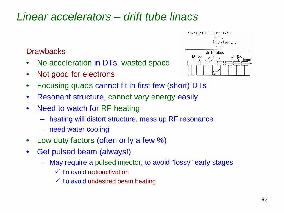
Linear accelerators – drift tube linacs
Fig. 11 (bottom frame) shows an Alvarez drift tube linac (DTL)Lower energy beam (from lower energy accelerator enters from leftEntire structure (tank) is conductive, fed with RF

80
Linear accelerators – drift tube linacs
L. Alvarez, Photo from Nobel Prizes website
• Beam is “Faraday shielded” from RF except in the gaps.• Acceleration occurs only in the gaps, not in the drift tubes• RF fields in all gaps are synchronized (in phase)• D the lengths of the drift tubes in this full wave mode must satisfy
• D is shorter at low velocities (nonrelativistic conditions, β << 1)λ is RF resonant wavelength, βc is the velocity at a given drift tubeλ/c is the time duration of 1 RF cycle Works best for 0.04 < β < 0.4.
(51)D = βλ
(44)2c cf
πλ = =
ω

81
Linear accelerators – drift tube linacs
• See why phase stability is needed?• Quadrupole magnets can go in drift tubes to focus• High beam currents (mA) available• Wideröe design was first, half-wave tubes used
– Q of such design is lower than for Alvarez type– But, Wideröe design is effective for low velocity ions (e.g., β
<0.03) and low frequencies (e.g., f <100 MHz)
82
Linear accelerators – drift tube linacs
Drawbacks• No acceleration in DTs, wasted space• Not good for electrons• Focusing quads cannot fit in first few (short) DTs• Resonant structure, cannot vary energy easily• Need to watch for RF heating
– heating will distort structure, mess up RF resonance– need water cooling
• Low duty factors (often only a few %)• Get pulsed beam (always!)
– May require a pulsed injector, to avoid “lossy” early stagesTo avoid radioactivationTo avoid undesired beam heating

83
Linear accelerators – drift tube linacsFermilab 750 kev to 116 MeV DTL
Photos from Fermilab website

84
Linear accelerators – coupled cavity linacs
• As β ->1, DTLs become inefficient and too long• Velocity β is no longer changing • Coupled-cavity structures are better
– Side-coupled version is popular– Cavities excited along their sides– Other possibilities exist and are used
• Standing wave (i.e., stationary mode) cavities– Effective in domain 0.4 < β < 1
– Provide 2 gaps per βλ– Used for both ions and electrons– Can used for colliders since standing wave is a superposition of 2
traveling waves from opposite directions
• Mechanical tolerances are important at large f, small λ.

85
Linear accelerators – coupled cavity linacsFermilab 116 - 400 MeV Side-Coupled Linac
Photo by J. D. Cossairt, Fermilab exhibits, cut-away view
Photo from Fermilab website

86
Linear accelerators – electron linacs• For electrions, at T= 3 MeV, β = 0.989!• Continuous, uniform wave guide looks tempting!
• Phase velocity exceeds c, form of wave would race ahead of particles
• Need longitudinal field component to accelerate, only have transverse fields if energy flow is longitudinal.
Recall:
• Solution: Break up wave guide into periodic structures• Act like individual resonant cavities• Eliminates wavelengths that do not “fit”• Commonly accomplished with loaded circular disks
• Resistance reduces phase velocity to below c• Called disk-loaded or iris-loaded waveguide• Can use high frequency RF, e.g., 3 GHz at SLAC
1( ) ( ) (43)( ) t t t= ×μo
S E B

87
Linear accelerators – electron linacs
SLAC 2-Mile disk-loaded linac
W. Panofsky, photos from SLAC website

88
Linear accelerators – recirculating electron linacs
Recirculating linacs• Line up sets of linacs to achieve desired energies in
steps• Intervening circular arcs of bending magnets direct the
beam between stages• Use linacs more than once (β = 1)• Especially with superconducting RF, continuous wave
mode (CW, near 100 % duty factor) becomes possibleThe Continuous Electron Beam Accelerator Facility
(CEBAF) is the most prominent example, operates in near continuous wave mode

89
Linear accelerators – CEBAF pictures
linac section bending magnet arcs
Photos from TJNAF website

90
Radio-frequency Quadrupoles (RFQs)
• Radio-frequency quadrupoles (RFQs) commonly operate in the velocity range of 0.01<β<0.06
• Combine the focusing capabilities of electric quadrupoles with the acceleration by RF fields.
• Are a type of linac. • Used only for protons and ions, not electrons• See Fig. 12

91
Radio-frequency Quadrupoles (RFQs)• 4 vanes are excited by RF as with• Note modulation, characterized by modulation parameter m• yz-plane modulation is out of phase with xz-plane modulation• Unit cell length L=βλ/2 with λ = RF wavelength
( ) cos( ), with (2 4 ) 2ot t f= ω + ξ ω = πE E

92
Radio-frequency Quadrupoles (RFQs)• Reasons for modulation
Need longitudinal electric field to accelerateNeed electric field on the optic (z) axis to accelerate most of the beam
• Phase stability, etc. applies in an RFQ• Get focusing and acceleration simultaneously

93
Radio-frequency Quadrupoles (RFQs)
• Some useful results
ΔW = energy gain per cell– Eo = spatial average of peak axial accelerating field over the cell (average axial
field)– Tf = transit time factor [See Eq. (48) ]– k = 1/λ, the wave number– A = accelerating efficiency [dependent on m, A=0 for m=1]– Vo is the applied voltage– A Vo = effective axial voltage over the length of the unit cell– integrals are over the unit cell length
sin( ) cos 21, , and . 4
(524
)zo o o
o z foz
o
o
LL
L
E kzdzq AV I kr AVW E E dz TL E dz
π ξ πβλ
Δ = = = = =∫∫
∫

94
Radio-frequency Quadrupoles (RFQs)
Io(kr) is the modified Bessel function of the first kind of zero order. Really!
Well approximated by:
Putting this all together
Note: more energy gain for off-axis particles (r>0)But, paths lengths for them are longer, phase stability
works!
sin( ) cos 21, , and . 4
(524
)zo o o
o z foz
o
o
LL
L
E kzdzq AV I kr AVW E E dz TL E dz
π ξ πβλ
Δ = = = = =∫∫
∫
( ) ( )2
( ) 1 . 4
53o
krI kr ≈ +
( ) c (o 4)s 5 o f oW qE T I kr L ξΔ =

95
Radio-frequency Quadrupoles (RFQs)• Some points
• Ideal vanes are hyperbolae, but circular rods have been used (hyperbolae are difficult to make!)
• Even trapezoidal longitudinal profiles, easier to make on a lathe have been used
• Superconducting RFQs are successful• Have been used to store, not accelerate particles
• Advantages/Disadvantages• At low velocities, available electric field focusing is stronger than
magnetic field focusing [remember the velocity factor in Eq. (11)]• RFQs have more compact infrastructure than some alternatives• Energy cannot be easily changed, a disadvantage

96
Radio-frequency Quadrupoles (RFQs)
RFQ on exhibit at Fermilab, photo by J. D. Cossairt

97
Radiation protection considerations (linacs)
• RF devices of considerable energy• Electrical and non-ionizing radiation hazards• Dark currents with associated production of x-rays Major
RF components often external to beam enclosures, hazards are accessible to personnel
• Special peculiarities– multipacting with avalanches (back-and-forth acceleration across
gaps)– electron field emission
– undesired heating (adds electrical impedance, reduces Q)
• Single pass machines-What is the worst case accident?• Effects of RF fields in radiation safety instrument
response. Faraday shields needed?

98
Cyclotrons, synchrocyclotrons, & betatrons -cyclotrons
• Have the advantage of using the RF structure repeatedly• Work best at low energies where
– Relativistic considerations do not dominate– Synchrotron radiation is neglible
• See top frame of Fig. 13 for the classic cyclotron
E. Lawrence & M. LivingstonPhotos from Nobel Prizes website

99
CyclotronsStart with Eq. (18)
We get
Taking the path as circular
the orbit period is 2πr/v & the orbit frequency is v/2πr
Get synchrotron angular frequency ωsyn
At low velocities have the similar cyclotron frequency ωcyc
2
(18 ) mv qvBR
=
(55)o
o
qBvm rγ
=
2
(5 )2 6o osyn
o o
qB qBm m
ω ππγ γ
= =
, for (57)1 ocyc
o
qBm
ω γ= ≈

100
Cyclotrons
Lack of radial dependence allowsorbit to be isochronous for constant magnetic field Bo.
RF frequency must be an integer multiple, the harmonic number h of the cyclotron frequency
Design constrains hE.g., in classic cyclotron, h has to be an odd number
(58)RF cychω ω=

101
Cyclotrons
• As particle energy increases, γ increases• Cannot just reduce RF frequency as implied by
• Will lose lower energy particles • Using Eqs, (5), (18), & (56) [SI units]
(56 )osyn
o
qBm
ωγ
=
1/ 2 1/ 22 22
1/ 22
1 1( ) ( )
1 (
(5)
9)
o o o o
syn o syn o syn o
o
syn
W W m c Wprm m c W r m c W r
WcW r
γγω γ ω γ ω γ
ω
⎡ ⎤ ⎡ ⎤⎛ ⎞ ⎛ ⎞= = − = −⎢ ⎥ ⎢ ⎥⎜ ⎟ ⎜ ⎟
⎢ ⎥ ⎢ ⎥⎝ ⎠ ⎝ ⎠⎣ ⎦ ⎣ ⎦
⎡ ⎤⎛ ⎞= −⎢ ⎥⎜ ⎟
⎢ ⎥⎝ ⎠⎣ ⎦
2
(18 ) mv pqvB qBr r
= → =

102
Cyclotrons
• To achieve synchronization, want to scale magnetic field strengthwith r
• Solve Eq. (59) for total energy W(r),
1/ 2 1/ 22 22
1/ 22
1 1( ) ( )
1 (
(5)
9)
o o o o
syn o syn o syn o
o
syn
W W m c Wprm m c W r m c W r
WcW r
γγω γ ω γ ω γ
ω
⎡ ⎤ ⎡ ⎤⎛ ⎞ ⎛ ⎞= = − = −⎢ ⎥ ⎢ ⎥⎜ ⎟ ⎜ ⎟
⎢ ⎥ ⎢ ⎥⎝ ⎠ ⎝ ⎠⎣ ⎦ ⎣ ⎦
⎡ ⎤⎛ ⎞= −⎢ ⎥⎜ ⎟
⎢ ⎥⎝ ⎠⎣ ⎦
1/ 22 2
2 (60) then( ) 1 ,syno
rW r W
cω
−⎡ ⎤⎛ ⎞
= −⎢ ⎥⎜ ⎟⎜ ⎟⎢ ⎥⎝ ⎠⎣ ⎦1/ 2 1/ 22 2 2 2
2 2 2 2
( )1 1 (61)syn o syn syn syn syn syn
z o o
m W r r rB W m
q qc qc c q cω γ ω ω ω ω ω
− −⎡ ⎤ ⎡ ⎤⎛ ⎞ ⎛ ⎞
= = = − = −⎢ ⎥ ⎢ ⎥⎜ ⎟ ⎜ ⎟⎜ ⎟ ⎜ ⎟⎢ ⎥ ⎢ ⎥⎝ ⎠ ⎝ ⎠⎣ ⎦ ⎣ ⎦

103
Cyclotrons
Useful to use particle or ion masses in atomic mass units mu (1.0 mu = 931.494 MeV c-2 = 1.66054x10⁻²⁷ kg)
& beam particle charge q in units of electronic charge by usingEq. (19)
where A is the atomic mass number, Bz remains in Tesla
Traditionally achieved using trim coils to increase Bz with r
1/ 2 1/ 22 2 2 2
2 2 2 2
( )1 1 (61)syn o syn syn syn syn syn
z o o
m W r r rB W m
q qc qc c q cω γ ω ω ω ω ω
− −⎡ ⎤ ⎡ ⎤⎛ ⎞ ⎛ ⎞
= = = − = −⎢ ⎥ ⎢ ⎥⎜ ⎟ ⎜ ⎟⎜ ⎟ ⎜ ⎟⎢ ⎥ ⎢ ⎥⎝ ⎠ ⎝ ⎠⎣ ⎦ ⎣ ⎦
-1 (SI units) (MeV c )(meters) = 299.79
(19)p pRqB qB
=
1/ 2 1/ 22 2 2 2
2 2
931.49 1 3.107 1 (62)299.79
syn syn syn synz
r rB A A
q c q cω ω ω ω
− −⎡ ⎤ ⎡ ⎤⎛ ⎞ ⎛ ⎞
= − = −⎢ ⎥ ⎢ ⎥⎜ ⎟ ⎜ ⎟⎜ ⎟ ⎜ ⎟⎢ ⎥ ⎢ ⎥⎝ ⎠ ⎝ ⎠⎣ ⎦ ⎣ ⎦

104
Cyclotrons• Result: isochronous cyclotron• Apollo 13: “Houston, we have a problem!”:
– Field index n<0 => radial component Br increases with r– Makes orbits unstable vertically (in the z -component)
• Solution: Create hills and valleys in the orbit plane, use sector and edge focusing) (see Fig. 13 lower frame)
• Alternative name: azimuthal varying field (AVF) cyclotron

105
CyclotronsSector magnets in cyclotrons: Indiana University Cyclotron Facility (IUCF)
Injector Main Stage
Photos by J. D. Cossairt
R. Pollock, photo from IUCF website

106
Cyclotrons
Example of conventional spiral ridge cyclotron:88” Cyclotron at LBNL
Photo from LBNL website

107
CyclotronsA superconducting spiral ridge cyclotron K-1200 Cyclotron
at National Superconducting Cyclotron Laboratory Michigan State University
Photos of K1200 and H. Blosser from NSCL website, labeled photo of interior of K1200 from R. Ronningen, NSCL

108
Cyclotrons• Flutter amplitude Fl measures differences between peak field in hills Bh&
lowest field in valleys Bv
• Momentum of extracted particles at radius R is p=γmoβc• Kinetic energy is
• Parameter K for ions of atomic mass number A and charge q is useful
• If RF voltage drop is Vo (MV), after n turns, Tn=qNVo (MeV)Solving Eq. (18) for orbit radius rn
(63)2h v
lave
B BFB−
=
( ) ( )2
2 (64)( )( ) 11o
o
p RT R m cm
γγ
= − =+
( )( )
( )
222 2 2 2 296.48( ) MeV (SI units) 1 1 a
(65mu
)oo
o
B Rq B RT R qKA m A
γγγ γ
⎛ ⎞= = = ⎜ ⎟+ + ⎝ ⎠
( )
( ) ( )
1/ 2
1/ 2 1/ 21/ 2
1
931.49 1 10.1018 299
(66.79
)
o oNN
o o
m AqNVprqB qB
AqNV AVN
qB B q
γ
γ γ
⎡ ⎤+⎣ ⎦= = =
+⎡ ⎤ +⎛ ⎞⎣ ⎦ = ⎜ ⎟⎝ ⎠

109
Synchrocyclotrons• Instead of increasing field with radius, modulate the RF
frequency with γ according to Eq. (56):
• Protons of 500 MeV to 1 GeV kinetic energy typical• Poor duty factor (only one group of protons at a time)• Cycle times often line power frequencies or
submultiples (in USA, 60 Hz, 30 Hz, 15, Hz, etc.)• Largely obsolete, superseded by
– Modern isochronous cyclotrons (lower energies)– synchrotrons (higher energies)
2
(5 )2 6o osyn
o o
qB qBm m
ω ππγ γ
= =

110
Synchrocyclotrons– Largest remaining; 1 GeV Petersburg Nuclear Physics
Institute, Russia (mass = 1 Eiffel Tower, 7-10 kTonne)
Photo from Petersburg Nuclear Physics Institute website

111
Betatrons
• Due to strong dependence on γ, cyclotrons are inappropriate for electrons.
• Historic solution was the betatron• Now nearly completely superseded by linacs and synchrotrons • Despite obsolescence will discuss here because the betatron
illustrates important features inherent in all circular accelerators• Only accelerator type that use electromagnetic induction to
operate.• Electrons are injected from some lower energy stage into an orbit
of radius R.• Acceleration occurs in this orbit of constant radius.• Have a ramped field, often at “line power” frequencies (USA = 60
Hz or submultiples)• Duty factor is similar to that of synchrocyclotrons

112
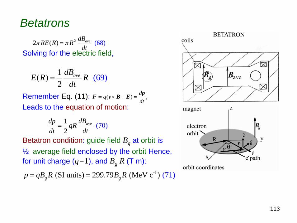
BetatronsStart with Eq. (9)
(67)
Relates integral of electric field E around orbit to rate of change of integral of rate of change of magnetic fieldinside orbit dB/dtSymmetry: E is not dependent on θEq. (67) becomes:
22 ( ) (68 )avedBRE R Rdt
π π=
113
Betatrons
Solving for the electric field,
Remember Eq. (11):Leads to the equation of motion:
Betatron condition: guide field Bg at orbit is½ average field enclosed by the orbit Hence, for unit charge (q=1), and Bg R (T m):
22 ( ) (68 )avedBRE R Rdt
π π=
1( ) 2
(69)avedBE R Rdt
=
( ) ,dqdt
= × + =pF v B E
1 2
(70)avedBdp qRdt dt
=
-1 (SI units) 299.79 (MeV c (71)) g gp qB R B R= =

114
BetatronsNeed to consider transverse stabilityField index n > 0 makes focusing plausible
Symmetry: B has two components; Bz and Br(Bθ =0) Eq. (11):gives an equation of motion in cylindrical coordinates (r,θ,z), knowing that p=mv
For small transverse deviations from the orbit:
ω=dθ/dt=v/R=qB/m
( ) ,dqdt
= × + =pF v B E
22 2 2
2 2ˆ ˆ )ˆ (72ˆz rvB vBd d r d d zr q q
dt dt dt dt m mθ⎡ ⎤⎛ ⎞= − − −⎢ ⎥⎜ ⎟
⎝ ⎠⎢ ⎥⎣ ⎦
r r + z = r z

115
BetatronsUsing the field index,
From Eq. (72) , equate the axial (z) components
Get harmonic oscillator solution:
Angular frequency is ω n1/2
Amplitude is zmax
Eq. (73) is that of an ordinary steel spring.Implies stability, good news indeed!
(35) or
nB zBR
−≈
22
2 ( 7 ) 3gqBd z v nz nzdt m R
ω= − = −
( )max( ) cos (74)z t z n tω φ⎡ ⎤= +⎣ ⎦

116
Betatrons
Radial (r) component is more difficultConsider small deviations ζ from orbit r=R+ζEquating components for Eq. (72):
Substituting:
Approximating:
Using
22 2 2
( ) (75)zd r d d r v vr q B rdt dt dt r m
θ⎡ ⎤ ⎡ ⎤⎛ ⎞− − −⎢ ⎥⎜ ⎟ ⎢ ⎥⎝ ⎠⎢ ⎥ ⎣ ⎦⎣ ⎦= =
2 2
2 (76)( ) zd v qvB Rdt R
ζ ζζ
− = − ++
1
(77)1 1 11 1 R R R R R
ζ ζζ
−⎛ ⎞ ⎛ ⎞= + ≈ −⎜ ⎟ ⎜ ⎟+ ⎝ ⎠ ⎝ ⎠
2 2
2 1 ( ) (78)zd v qv Bdt R R m
ζ ζ ζ⎛ ⎞− − = −⎜ ⎟⎝ ⎠
2 2
(18) ,mv v qvBqvBR R m
= → =
2
2 ( ) 0 (7 ) 9gz g
qvBd qvB Bdt m m R
ζ ζζ⎡ ⎤+ − + =⎣ ⎦

117
Betatrons
Do Taylor expansion, Bz=Bg+ζdB/dr+…Hence Bz-Bg can be approximated by ζdB/drMake other substitutions;
v=ω Rq/m=ω /Bg
n=-RdB/(Bgdr)
Solution is also a harmonic oscillator:Angular frequency is ω(1−n)1/2
Amplitude is ζmax.
We have stability in both planes!
2 22 2 2
2 2 (0 (1 ) 800 )g
d R dB d ndt B dr dt
ζ ζω ζ ω ζ ω ζ+ + = → + − =
( )max( ) cos 1 (8 1 )t n tζ ζ ω φ⎡ ⎤= − +⎣ ⎦

118
Betatrons
• These are axial and radial betatron oscillations.• Eqns. (73) and (80) are the Kerst-Serber Equations.• Get a fixed number of betatron oscillations per orbit (not usually
integers), called the tune– axially, νz=n1/2
– radially, νr= (1-n)1/2
• Orbits are unstable if 0<n<1 is not satisfied
• n=0 or n=1 implies an unstable drift in either z or r• n>1 implies absorption (i.e., beam loss) D. Kerst, U. of WI website
• n<0 implies radial defocusing
• n=1/2 has tunes same in both coordinates, explains the unique focal properties of the n=1/2 magnet
• Have similar oscillations in other circular accelerators

119
Radiation protection considerations of cyclotrons, synchrocylotrons, and betatrons
• RF sources can produce x-rays• Deflection devices; inflectors and electrostatic septa, can produce x-
rays. • Injector beam emittance needs matching to the acceptance of higher
energy stage, otherwise have beam loss, activation, etc.• Orbits need careful tuning upon injection and extraction to minimize
radioactivation of components. • Synchrotron radiation with consequent x-ray production can be a
consideration at betatrons• Massive magnets can present radioactive material handling
problems at the time of decommissioning.• Large copper components can be the locus of long-lived
radioactivation (e.g., 60Co).
120
Synchrotrons• Ultimate large circular accelerator at present• Strong-focusing version is dominant• Limitations of other circular machines lead to this result
– Magnetic field inside orbit of betatron serves no other purpose, though needed for magnetic induction,
– Synchrocyclotron magnets become impracticably large at high energy– Need small beam, => strong focusing
• Operating Concept– Accelerate in an orbit of constant R (like in a betatron!)– Inject particles into the ring from a lower energy machine
Sufficient injection energy required to assure “good” magnetic field free of eddy currents, hysteresis effects, power supply ripple at low current, etc.
– Use RF, rather than induction, to accelerate beam– Synchronously increase magnetic field in orbit plane B to match p– Explains the name: synchrotron

121
Synchrotrons-weak focusing• Cyclotrons, synchrocyclotrons, & betatrons all are weak-focusing• Apertures scale with R to achieve necessary vertical focusing• Example: 6 GeV Bevatron at Lawrence Radiation Laboratory (now LBNL)
n = 0.6 => aperture: 1.16 m (horizontal) by 0.30 m (vertical)!
Photos from LBNL website

122
Synchrotrons-strong focusing• Limitations recognized early, particularly by R.
R. Wilson (R. R. Wilson, photo from Fermilab website, D. Edwards, photo from Cornell U. website)
• Applied immediately to Cornell 1 GeV electron synchrotron (early 1950’s) (Wilson redesigned ring to strong-focusing after magnets were built, Edwards was the student who did the work!)
• How to do? Alternate magnets like in Fig. 5 to get focusing effect

123
Synchrotrons-strong focusing, combined function• BNL 30 Alternating Gradient Synchrotron (AGS) largest example
• For AGS, n = 357• Limitation: Making these magnets, too, becomes expensive
3 GeV Cosmotron vs AGS Magnets View of AGS
Drawing and photo from BNL website

124
Synchrotrons-strong focusing
• Separated function strong-focusing is current state-of-the-art
• Called FODO, focusing-defocusing lattice
• See Fig. 15 (top frame)• Each “magnet” can be a
string of near-identical magnets
• Focusing separated from bending (not true in AG)
• Longitudinally, magnets are rectangular in cross section, for large R.

125
Synchrotrons-strong focusing
• Straight Sections– Any number– Machine functions
InjectionExtractionRFDiagnosticsInsertion devices (at light sources)
– Experiments
Remainder of discussion will be vignettes, see references for details!

126
Synchrotrons-examples
Fermilab 8 GeV Booster
Photos from Fermilab website

127
Synchrotrons-examplesFermilab 150 GeV Main Injector Fermilab 1 TeV Superconducting Tevatron
(R. Lundy, R. Orr, H. Edwards, & A. Tollestrup)Photos from Fermilab website

128
Synchrotrons-phase stability and transition crossingIdeal particle on reference orbit will pass between 2 markers (e.g.,
complete orbit) in time τ=L/v (L = path length, v = velocity)
If ideal path is NOT followed we have a deviation in path length ΔLand/or a deviation in speed Δv
Get deviation in time interval τ
Intuitive! τ increase with path length, decreases with increased speed
ΔL/L is proportional to relative deviation in momentum Δp/p through a dispersion coefficient γt :
Higher momentum usually implies a longer path
γt is also called the transition gamma
(82 )L vL v
ττ
Δ Δ Δ= −
2 (831 )t
L pL pγ
Δ Δ=

129
Synchrotrons-phase stability and transition crossing
Want to connect Δp/p to Δβ/β= Δv/vTake differential of p and rewrite Eq. (82):
η is the phase slip factor
( ) ( ) ( )1/ 2 1/ 2 3/ 22 2 2 2
2
22
1 1 1
11
(84)
o
o
m cpp m c
β β β β β β
γβ γβ
β ββ βγ γ
γβ β
− − −⎡ ⎤ ⎡ ⎤Δ − − + − ΔΔ ⎢ ⎥ ⎢ ⎥⎣ ⎦ ⎣ ⎦= =
⎡ ⎤+ Δ⎢ ⎥− Δ⎣ ⎦= =
2 2
1 1 5 (8 )t
p pp p
τ ητ γ γ
⎡ ⎤Δ Δ Δ= − =⎢ ⎥
⎣ ⎦
130
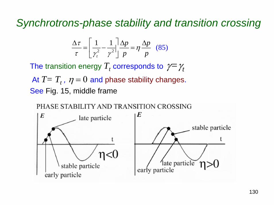
Synchrotrons-phase stability and transition crossing
The transition energy Tt corresponds to γ=γtAt T= Tt , η = 0 and phase stability changes.
See Fig. 15, middle frame
2 2
1 1 5 (8 )t
p pp p
τ ητ γ γ
⎡ ⎤Δ Δ Δ= − =⎢ ⎥
⎣ ⎦

131
Synchrotrons-phase stability and transition crossing
• Below transition, a particle with Δp/p >0 has greater speed, gets around quicker the next time
• Above transition, a particle with Δp/p >0 takes a longer path, takes longer to get around.
• Phenomena is due to special relativity; β =1• At transition
τ is independent of momentum– All particles are isochronous (same lap times!)– There is no phase stability. (bad news-beam losses! )

132
Synchrotrons-phase stability and transition crossing
• Accomplishing transition crossing cleanly is important at most proton synchrotrons
(All electron synchrotons operate above transition, no problem)• Done by inducing change in RF phase at transition, usually quickly
• Examples at Fermilab
– Fermilab Booster (T=0.4-8 GeV, R=74.47 m) γt =5.45 (T=4.17 GeV)
– Fermilab Main Injector (T=8-150 GeV, R=528.3 m) γt =20.4 (T=18.2 GeV).
– Superconducting Tevatron (T=150-980 GeV, R=1000 m) γt =18.7 (T=16.6 GeV). The Tevatron always operates above transition.

133
Synchrotrons-phase stability and transition crossing
• In linacs, η < 0 since path length is same for all particles so transition crossing is not an issue
• From this perspective, an isochronous cyclotron operates at transition.

134
Synchrotrons-longitudinal emittance
• The confinement of particle beams in RF bunches in synchrotrons needs quantification.
• Consider a 2-dimensional phase space– Variables are time t and kinetic energy T– Phase space area is defined by ΔtΔT
• Acceptance A is the bucket “area” available to “hold” the beam
• If Ts is the kinetic energy of the ideal particle (MeV) and Vs is the gap voltage (MV),
• Vs typically has values of a few MV
(86162
) s
RF
qVTAh
βω π η
=

135
Synchrotrons-longitudinal emittance
• If Δξ (radians) is the maximum of small oscillations in phase angle at injection or maximum energy (non-accelerating conditions), the longitudinal emittance of the beam is
• For accelerating conditions– Bucket area shrinks to zero as ξ−>π/2– Must have A > S to keep the particles– Otherwise, the particles are lost
• Examples of nominal longitudinal emittances:– Fermilab Booster 0.25 eV s– Fermilab Main Injector: 0.2 eV s– Fermilab Tevatron (collider mode): 3 eV s
( )2
(87) 2
s
RF
qVTSh
πβ ξω π η
Δ=

136
Synchrotrons-harmonic number
Same concept as for cyclotrons & synchrocyclotronsωrfτorbit= h2π is the number of RF cycles per orbith is the harmonic numberτorbit is the orbit periodh is an integer, generally large
The ideal particle will travel around the reference orbit (i.e., through the magnet centers) with frequency
Establishing the closed orbit is important at all synchrotronsRequires correction to offset imperfections, mistunings, etc.Examples of nominal harmonic numbers:
– Fermilab Booster: h = 84– Fermilab Main Injector: h = 588– Fermilab Tevatron (collider mode): h = 1113
(88)1 RForbit
orbit
ffhτ
= =

137
Synchrotrons-betatron oscillations and transverse emittance
• Transverse oscillations about reference orbits in synchrotrons are still called betatron oscillations
• More complex mathematically in synchrotrons, detailed derivations beyond the scope of this lecture
• Only will consider separated function synchrotrons, similar for all strong-focusing machines
• See Fig. 15 (top and bottom frames), define (x,y,s) coordinates
138
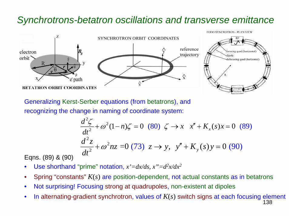
Synchrotrons-betatron oscillations and transverse emittance
Generalizing Kerst-Serber equations (from betatrons), andrecognizing the change in naming of coordinate system:
Eqns. (89) & (90) • Use shorthand “prime” notation, x’=dx/ds, x”=d2x/dx2
• Spring “constants” K(s) are position-dependent, not actual constants as in betatrons• Not surprising! Focusing strong at quadrupoles, non-existent at dipoles• In alternating-gradient synchrotron, values of K(s) switch signs at each focusing element
22
2 (73) =0 , ( ) 0 (90)yd z nz z y y K s ydt
ω ′′+ → + =
22
2 (80) (1 ) 0 ( ) 0 (89)xd n x x K s xdt
ζ ω ζ ζ ′′+ − = → + =

139
Synchrotrons-betatron oscillations and transverse emittance
Eqns. (89) & (90) • Are examples of Hill’s Equation (studied in early 19th century for no practical purpose)• The “forces” or “spring constants”, further, are given by
• These look like quadrupole gradients, as they should.• For completeness have included the centripetal (1/R2) term in Eq. (91) , usually
neglible at large accelerators.• Often represented as constants within a given beam element or drift space between
beam elements.
( ) (90)0 yy K s y′′ + = ( ) 0 (89)xx K s x′′ + =
2 (( )1 1( ) 91)y
x
B sK s
BR x R∂
= +∂
(92)( )1( ) y
y
B sK s
BR x∂
= −∂

140
Synchrotrons-betatron oscillations and transverse emittance
K(s) values are often periodic in a lattice of repeated, identical elements:
Often x- and y-dependencies are similar if not identicalThus, one sometimes just writes down one coordinate to represent bothWith arbitrary integration constants ε and δ, the solution for x(s) is
ε turns out to be the transverse emittance for this type of beam (i.e., in a synchrotron)
( ) (90)0 yy K s y′′ + = ( ) 0 (89)xx K s x′′ + =
( ) ( ) (93 )K s C K s+ =
[ ],,
( ) 1( ) ( ) cos ( ) an (94)d ( )
xx CS x x
CS x
d sx s s sds s
ψε β ψ δβ
= + =

141
Synchrotrons-betatron oscillations and transverse emittance
βCS,x(s) and βCS,x(s) values are E. Courant, photo from BNL website
– Called the amplitude functions or beta functions– One of a set of 3 Courant-Snyder parameters
(The CS subscript is nonstandard, used here to avoid confusion with β=v/c)– Have units of length
• Examples of βCs,x(s) values– Fermilab Booster: horizontal = 34 m, vertical = 21 m– Fermilab Main Injector: both = 58 m– Fermilab Tevatron (collider mode): both = 100 m
[ ],,
( ) 1( ) ( ) cos ( ) an (94)d ( )
xx CS x x
CS x
d sx s s sds s
ψε β ψ δβ
= + =

142
Synchrotrons-betatron oscillations and transverse emittance
• Some number of oscillations in x or y are found in an orbit• As the betatron, this # is generally not an integer and is called the tune:
(95)
• Tune values are managed to achieve desired properties– At injection– At transition– During colliding beams– At extraction
• Examples of tune values– Fermilab Booster: both about 6.7– Fermilab Tevatron (collider mode): both about 19.4

143
Synchrotrons-betatron oscillations and transverse emittance
• The slope, indicative of the mean angular spread in direction is important.• Represented by x’(s)=dx(s)/ds :
• x(s) and x’(s) form the parameters of transverse phase spaceΨ(s), reflective of the focusing strength,will be periodic
• x(s) and x’(s) cycle through sets of values at different locations• Need remaining 2 Courant-Synder parameters (without x and y subscripts)
( ) [ ] [ ],
, ,
( )(96( ) sin ( ) cos ( )
2 ( )) CS x
CS x CS x
sx s s s
s sβε εψ δ ψ δ
β β′⎡ ⎤′ = − + + +⎢ ⎥
⎣ ⎦
(( )( ) 7)2
9CSCS
ss βα′
= −2
( )1 8 9CSCS
CS
αγβ+
=

144
Synchrotrons-betatron oscillations and transverse emittance
• Phase space xx’ in the synchrotron is bounded by the ellipse of Fig. 16 (upper frame)
• Commonly approximate particle distributionsby Gaussian functions, e.g.
• These distributions are considered as stationary in time (i.e., assumes small orbit-to-orbit changes)
2 2 (2 9 9)CS CS CSx xx xε γ α βπ
′ ′= + +
2 2 (10( ) exp / 2 0)2
dxn x dx x σσ π
⎡ ⎤= −⎣ ⎦

145
Synchrotrons-betatron oscillations and transverse emittance
• Connect the standard deviation σ with the emittance ε :
• F is the fraction of particles contained with the ellipse of Eq. (99).• Unfortunately conventions in this are not uniform!
ε=σ2/β (15%) –commonly used at electron acceleratorsε=πσ2/β (39%) –commonly used at proton acceleratorsε=4πσ2/β (87%) –commonly used to characterize “complete” containment of beamε=6πσ2/β (95%) –commonly used to characterize (really) “complete” containment of beam
[ ]22 ln 1 (10 ) 1
CS
Fπσεβ
= − −

146
Synchrotrons-betatron oscillations and transverse emittance
• See Fig. 16 (both frames)• Shows evolution of beam ellipse containing particles during a
segment of the lattice– Maximum displacement is
– Maximum slope (angle) is
,maxmax (102)CSx
εβπ
=
,maxmax (103) CSx
εγπ
′ =

147
Synchrotrons-betatron oscillations and transverse emittance
• For uniform, circular half-aperture of radius a, the admittance is πa2/βCS,max
• During acceleration, emittance shrinks (due to relativity)
• But, normalized transverse emittance εN is invariant• Synchrotron radiation reduces transverse emittance• Transverse emittance is a property of all particle beams
• Examples of εN values– Fermilab Booster: 8 π mm milliradians– Fermilab Main Injector: 30 π mm milliradians– Fermilab Tevatron (collider mode): 24 π mm milliradians
(104)Nε γβε=

148
Synchrotrons - extraction
• Extraction of beam from synchrotrons is done as– single-turn extraction, use “kicker” magnets with fast time
constants matched to the orbit period – resonant extraction, amplitude function is manipulated to get
large beam sizes suitable for splitting by septa.
• Electrostatic septa often followed by magnetic elementsget the beam into the desired extraction channel.

149
Synchrotrons - extraction
• At large accelerators, the magnetic elements may be Lambertson dipoles that follow electrostatic septa– Lambertson magnet has
regular gap plus a field-free hole in its return yoke
– Gap field deflects one beam – Field-free hole in a return
yokes allows passage of the undeflected beam fraction
– Get 2 separated beamsPhoto from Fermilab Report No. G Lambertson, photo from LBNL website

150
Colliding Beams
• Special relativity limits energy available in particle collisions to study fundamental processes
• As energy increases, most goes into increased mass
• Head-on collisions can use all the beam energy• Hence, the prominence of colliding beam experiments at
the energy frontier
2(3
1)o
omm mγ
β= =
−

151
Colliding Beams
• Luminosity is a crucial concept– In beam collisions with solid targets, interaction rates are
proportional to the product of 3 quantitiesDelivery rate of beam particles (i.e., particles s-1)Density of target nuclei ρNA/A (i.e.,nuclei cm-3)
ρ is material density (g cm-3), A is atomic mass number, NA is Avogadro’s Number (6.02 X 10²³ atoms g-mole-1)
Reaction probability (the cross section, here in cm2)– Consider a 1 μA beam, singly-charged beam (6.25 X 10¹² s-1) of
1 cm2 cross-sectional area– Hits a solid target of about 1 cm thickness– Intensity X target nuclei density is of order 1035 cm-2s-1.– Colliding two such 1 μA beams; only get about 4 x 1025 cm-2s-1
– Big Difference! Is this hopeless?

152
Colliding Beams
• Is this hopeless? No!– In circular machine get many orbits of same particles– With linacs or synchrotrons, can squeeze beam spot sizes– Will emphasize synchrotrons
• Working in cgs units as is usual, connect – Average rate of events Revent (s-1) ,
– Luminosity L (cm2s-1)– Reaction cross section of interest σint (cm2)
• If have 2 bunches of beam with n1 and n2 particles colliding at frequency f
int (105) eventR Lσ=
1 2 (10 64
) x y
n nL fπσ σ
=

153
Colliding Beams
• If have 2 bunches of beam with n1 and n2 particles colliding at frequency f
– Where the two beam sizes are explicitly included
– Lattice properties of the 2 beams are identical (i.e., in x and y).
• Taking for this purpose ε=πσ2/β • Denote the value of βCS(s) at the interaction point by β*
• Get largest L by maximizing beam particles and by minimizing εand β*
1 2 (10 64
) x y
n nL fπσ σ
=
1 2
, ,* *
(4
10 7) x CS x y CS y
n nL fε β ε β
=

154
Colliding Beams
• Get largest L by maximizing beam & minimizing ε and β*
• Minimize β* by– Using strong quadrupoles adjacent to interaction regions– Often not used during acceleration, only during collisions
– Accept tradeoff of greater angular divergence since ε conserved– Angular diverence can be focused back on after collisions
• Example: Before 1993, at Fermilab Tevatron β* = 0.5 m was achieved (compared with βCS,max(s) = 100 m in the general lattice. (Ongoing efforts continue to improve this!)
• Can see challenges of single-pass linear colliders!
1 2
, ,* *
(4
10 7) x CS x y CS y
n nL fε β ε β
=

155
Colliding Beams
• Luminosity in a store decays with time– Loss from collisions– Loss due to imperfections (beams are not perfect Gaussians)– Space charge effects – Beam-beam interactions (One beam looks like an electric
current to the other!)
• Integrated luminosity (integral over time) is important– Cross sections can be expressed in units of picobarns (pb) – 1.0 pb=1x10-12x10-24cm2=1x10-36cm2
– Integrated luminosity is expressed in units of inverse picobarns(pb-1)

156
Colliding Beams
• Illustration at Fermilab (980 GeV protons on 980 GeVantiprotons)– Spring 2007, A good store had <L> = 2X1032 cm-2s-1
– Achievement of 1 pb-1 of integrated luminosity requires 5000 s (1.4 h) (Would see on average one event @ 1 pb cross section)
– To accumulate 1 fb-1 (10-15 barns) requires 1400 hours.

157
Colliding Beams
• How to get the 2nd beam?– Two rings of protons, ions, or electrons are used (e.g., RHIC,
below), but expensive– Can use a single ring if one beam is antimatter (e.g., positrons or
antiprotons) or if beams have opposite charges
Photos of Relativistic Heavy Ion Collilder taken from BNL website

158
Colliding Beams• Answers
– Stochastic cooling: store beam in a ring, apply feedback across ring diameter (or chord) to effect corrections
– Electron coolingUse large mass difference between antiprotons and electronsCan travel together since charge the sameMatch velocities (make relativistic parameters β and γ equal)Transverse momentum transferred from antiprotons to electronsElectrons are refrigerant, take “heat” away, hence “cooling”
• Example at Fermilab: – T= 8 GeV (γ=9.53) antiprotons already stochastically cooled
– Cooled further using T=4.36 MeV (γ=9.53) electrons– Done in a unique ring of permanent magnets– Electrons come from a single-stage Pellatron

159
Colliding BeamsFermilab Debuncher (left) and Accumulator (right) Rings
(Home of Stochastic Cooling)
Simon van der Meer, Photo from Nobel Prizes website. Fermilab Rings, Photo from Fermilab website

160
Colliding BeamsFermilab 8 GeV Recycler Ring (Permanent Magnets)
(Home of Electron Cooling)
G. Budker photo from Budker Institute website, other photos from Fermilab website

161
Synchrotrons and storage rings-radiation protection considerations
• All considerations pertaining to HV and RFEmittance (both longitudinal and transverse) and Courant-Synder parameters are important
• Gaussian functions may not adequately describe tails of beams
• Duty factor is a consideration– Instrument response questions– Safety interlock considerations

162
Synchrotrons and storage rings-radiation protection considerations
• Single-turn and resonant extraction pose different challenges– Single turn extraction may happen too fast for some
corrective measures– Resonant extraction can, by design, produce large
beams with increased beam loss• Centering of beam is often important
– To avoid scraping– To avoid quadrupole steering
• Long term storage of beam in storage rings

163
Synchrotrons and storage rings-radiation protection considerations
• Need to understand feasible and non-feasible beam losses– Can the entire beam be lost at a point?– Can this happen repeatedly?– Can the beam really be lost in a localized region in a
circular machine if in a closed orbit?Injected, non-circulating beam is different.Extracted, non-circulating beam likewise is different.Time constants for magnets likely long compared with orbit periodsNeed input from accelerator physicists!

164
Future possibilities• General techniques for accelerating/handing
beams– Originated decades ago– Rely on macroscopic static & dymanic
electromagnetic fields– Use special relativity, but have no direct connection
with quantum world• Phase velocity considerations do not allow free
electromagnetic waves to accelerate particles– Energetic particles outrun the group velocity of waves– Accelerating E fields in free waves are transverse to
energy flow, not longitudinal

165
Future possibilities• Use of lasers is tempting
– Conservation of momentum & energy precludes transfer of all energy from individual photon to a particle.
– But, can use photons collectively• New development: laser-wakefield acceleration
– Lasers are used to generate plasma waves– Waves drag particles along (like waves behind a
boat)– E fields in 10-100 GV m-1 range.

166
Future possibilities• New development: laser-wakefield acceleration
– DifficultiesMaintaining laser intensity over distances neededLarge spreads in accelerated particle energies
Slippage between velocity of relativistic particles (β=1) and velocity of the wake (β<1)
– Breakthrough example at LBNL• Acceleration of 1.0 GeV electrons• In a distance of 0.033 m
– There are other recent successes• There are other techniques

167
Future possibilities• Working at the quantum level
– Interatomic electromagnetic and nuclear forces are much stronger than seen macroscopically.
– Difficult to exploitAvailable only over short distancesOften hidden as binding energy
– Channeling by particles in a crystal (Fermilab example) • 900 GeV protons deflected by angle of 0.64 milliradians• Silicon crystal 0.039 m (long) X 0.003 m (high) X 0.009 m
(wide), mechanically bent to achieve deflection• Bend achieved by same deflection in same length would need
Static field of E = 14.8 GV m-1 (Eq. 17)
Static field of B = 49.3 T (Eq. (20)

168
Conclusion• Accelerator physicist needs to understand
rudiments of operation of his/her particular installation
• Several read this material and offered comments– Dr. Michael Syphers - Fermilab accelerator physicist– Dr. Kamran Vaziri - Fermilab radiation physicist– Dr. Alex Elwyn - Fermilab radiation physicist (retired)
• Support was provided by– Mr. William Griffing, Fermilab ES&H Director, who
encouraged my participation– My Fermilab co-workers who sat through a dry run.– My wife, Claudia, who allowed much work at home