140

Acceptance Sampling by Variables

Advantages of Variables Sampling

o Smaller sample sizes are required

o Measurement data usually provide more information about

the manufacturing process

o When AQLs are very small, the sample sizes required by

attributes sampling plans are very large.

Disadvantages of Variables Sampling

o The distribution of the quality characteristic must be known

o A separate sampling plan must be employed for each quality

characteristic that is being inspected.

o It is possible that the use of a variables sampling plan will

lead to rejection of a lot even though the actual sample

inspected does not contain any defective items.

Two types of variables sampling procedures

1. Plans that control the lot or process fraction defective (or

nonconforming). [Procedure 1]

Take a random sample of n units. Calculate:

LSLx

ZLSL

If kZLSL , accept the lot, otherwise, reject it. The value of k, a critical

distance can be found from the requirement of the plan.

2. Plans that control a lot or process parameter (usually the mean).

141

[Procedure 2]

Take a random sample of n units. Calculate:

LSLx

ZLSL

Use LSLZ or )1( nnZQ LSLLSL to estimate p̂ of the process. If

Mp ˆ , accept the lot, otherwise, reject the lot. M is a specified

value.

Both procedures can be used when an upper specification limit is given.

The variable then is

xUSL

ZUSL

When both upper and lower specifications are given, the second

procedure should be used.

If the standard deviation is not given, then sample standard deviations

will be used to replace the in the above equations.

Caution in the use of variables sampling

o The distribution of the quality characteristic must be known

o The usual assumption is that the parameter of interest follows

the normal distribution. This is a critical assumption.

o If the normality assumption is not satisfied, then estimates of

the fraction defective based on the sample mean and standard

142

deviation will not be the same as if the parameter were

normally distributed

o It is possible to use variables sampling plans when the

parameter of interest does not have a normal distribution. We

then need to know the distribution the parameter follows and

develop a corresponding procedure.

Design a variable sampling plan for Procedure 1.

o Similar to the plan for attribute sampling, based on the OC

curve with 1 for lots with fraction defective 1p , for lots

with fraction defective 2p .

o We can use the nomograph in Figure 16.2 to find the

required values of the sampling plan.

Example 16.1. For a given process, the given lower specification is 225. If 1p =0.01, 1 =0.95 and 2p =0.06, =0.10, we can find that, when the process is unknown, n=40 and k=1.9 from the nomograph,. When the process is known, then the sample size would be 15, from the same nomograph. Assume that a sample with n=40 is taken and we have

255x and 15s , then,

215

225255

s

LSLxZLSL

Since 9.12 kZ LSL , we accept the lot.

143

We can also use the same nomograph for designing a variables sampling

plan using Procedure 2. An additional chart is needed to determine the

big M used in this procedure. After the n and k are determined using the

nomograph, the chart in Fig 16-3 should be used to find the big M. It is

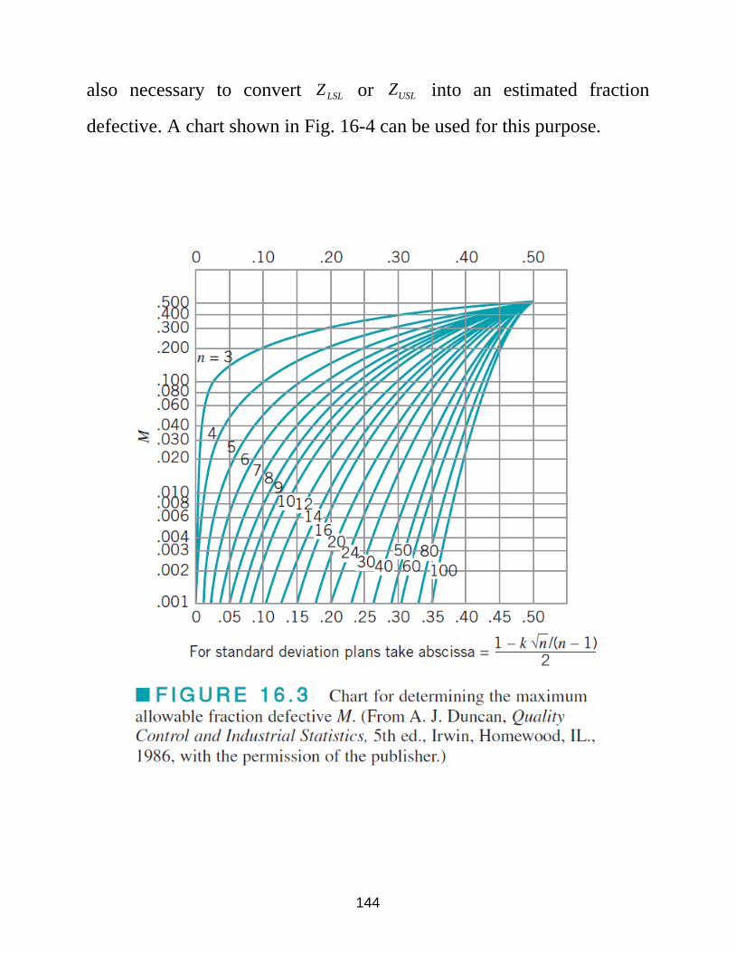
144

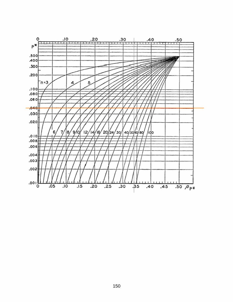
also necessary to convert LSLZ or USLZ into an estimated fraction

defective. A chart shown in Fig. 16-4 can be used for this purpose.

145

Example 16-2

Continue from Example 16-1. If the process is unknown, we have

n=40, k=1.9. From Fig.16-3, we use the abscissa equation

abscissa = 2

1 1 nnk

to get the abscissa value

35.02

1

2

1 140409.1

1

n

nk

146

Then from the nomograph in Figure 16.3, we read that M=0.030 from

the intersection of the curve for sample size 40 and the 0.35 vertical line.

If we use the same sample of 40 units (n=40) to find that 255x and

15s , then as calculated before, we have,

215

225255

s

LSLxZLSL

From Figure 16-4, we read Mp 030.0020.0ˆ and the lot will be

accepted.

147

When we have double-specification limits, Procedure 2 can also be used

to decide if a lot can be accepted. We can start in the same way to get

sample size n and the critical value k as we did in a single limit plan to

have the same values of 1p , 2p and as the desired double-

specification-limit plan. Then we can find the value of M from Fig 16-3.

We then compute the values of LSLZ and USLZ . We then use Fig. 16-4 to

find the corresponding fraction defective estimates LSLp̂ and USLp̂ . If

Mpp USLLSL ˆˆ , the lot is accepted; otherwise, it will be rejected.

148

Example

For a plan with process unknown and with 1p =0.014, =0.95,

2p =0.09 and =0.10, we can see from the nomograph in Fig. 16-2 that

k=1.7 and n=29. Use the abscissa calculation in Fig.16-3, we can

calculate the abscissa value:

abscissa = 34.02

1

2

1 28297.1

1

n

nk

From the nomograph shown in page 150 (same but more precise than

that in Fig.16-3), we can find that M=0.040. Assume for this example,

that LSL=550 and USL=700. Also assume that we take a sample of 29

and find that the mean of this sample is 570 and the sample standard

deviation s is 40, we then calculate:

75.140

500570

s

LSLxZLSL

25.340

570700

s

xUSLZUSL

From the chart in page 151 (same but more precise than that in Fig. 16-

4), we can read that 037.0ˆ LSLp and 0004.0ˆ USLp . Since

040.00374.00004.0037.0ˆˆ Mpp USLLSL , we accept the lot.

149

150

151

Military Standard MIL STD 414 (ANSI/ASQC Z1.9)

MIL STD 414 is a lot-by-lot acceptance-sampling plan for variables

introduced in 1957.

Sample size code letters are used as in MIL STD 105E, but the same

code letter does not imply the same sample size in both standards.

Sample sizes are a function of the lot size and the inspection level.

All sampling plans assume the quality characteristic of interest is

normally distributed.

MIL STD 414 is divided into four sections:

152

o A: general description of the sampling plans including

definitions, sample size code letters, and OC curves for the

plans.

o B: variables sampling plans based on the sample standard

deviation for the case in which the process or lot variability

is unknown.

o C: variables sampling plans based on the sample range

method

o D: variables sampling plans for the case where the process

standard deviation is known.

ANSI/ASQC Z1.9 is the civilian counterpart of MIL STD 414.

Differences and revisions

1. Lot size ranges were adjusted to correspond to MIL STD 105D

2. Code letters assigned to the various lot size ranges were arranged

to make protection equal to that of MIL STD 105E

3. AQLs of 0.04, 0.065, and 15 were deleted

4. Original inspection levels I, II, III, IV, and V were relabeled S3,

S4, I, II, III, respectively.

5. Original switching rules were replaced by those of MIL STD

105E, with slight revisions.

153

Table for the sample size code of the standard

154

Example.16-3

Assume that for a quality characteristic of interest, the lower

specification limit is 225 psi. The AQL at this specification limit is 1%.

Assume that the lot size is 100,000. We use Procedure 1 from MIL

STD414 for the testing. Lot standard deviation is unknown.

From Table 16-1, if inspection level is IV, the sample size letter is O.

Then from Table 16-2, we read that n=100. For the acceptable quality

level of 1%, on normal inspection, the k value is 2.00. On tightened

inspection, k is 2.14.

The standard has rules to shift to tightened or reduced inspection based

on the process average.

MIL STD414 and ANSI/ASQC Z1.9

The standard becomes similar to that in MIL STD105E such as the rule

of switching from tightened to normal and so on. Please refer to the text

book in Section 16-3.3.

155