acceptance sampling for attributes via hypothesis testing ... · acceptance sampling for attributes...
TRANSCRIPT
ORIGINAL RESEARCH
Acceptance sampling for attributes via hypothesis testingand the hypergeometric distribution
Robert Wayne Samohyl1
Received: 13 March 2017 / Accepted: 13 September 2017 / Published online: 7 October 2017
� The Author(s) 2017. This article is an open access publication
Abstract This paper questions some aspects of attribute
acceptance sampling in light of the original concepts of
hypothesis testing from Neyman and Pearson (NP). Attri-
bute acceptance sampling in industry, as developed by
Dodge and Romig (DR), generally follows the international
standards of ISO 2859, and similarly the Brazilian stan-
dards NBR 5425 to NBR 5427 and the United States
Standards ANSI/ASQC Z1.4. The paper evaluates and
extends the area of acceptance sampling in two directions.
First, by suggesting the use of the hypergeometric distri-
bution to calculate the parameters of sampling plans
avoiding the unnecessary use of approximations such as the
binomial or Poisson distributions. We show that, under
usual conditions, discrepancies can be large. The conclu-
sion is that the hypergeometric distribution, ubiquitously
available in commonly used software, is more appropriate
than other distributions for acceptance sampling. Second,
and more importantly, we elaborate the theory of accep-
tance sampling in terms of hypothesis testing rigorously
following the original concepts of NP. By offering a
common theoretical structure, hypothesis testing from NP
can produce a better understanding of applications even
beyond the usual areas of industry and commerce such as
public health and political polling. With the new proce-
dures, both sample size and sample error can be reduced.
What is unclear in traditional acceptance sampling is the
necessity of linking the acceptable quality limit (AQL)
exclusively to the producer and the lot quality percent
defective (LTPD) exclusively to the consumer. In reality,
the consumer should also be preoccupied with a value of
AQL, as should the producer with LTPD. Furthermore, we
can also question why type I error is always uniquely
associated with the producer as producer risk, and likewise,
the same question arises with consumer risk which is
necessarily associated with type II error. The resolution of
these questions is new to the literature. The article presents
R code throughout.
Keywords Acceptance sampling � Lot quality assurance
sampling (LQAS) � Hypergeometric � Operatingcharacteristic curve (OCC) � Receiver operatingcharacteristic (ROC) Curve � Hypothesis test � R CRAN
When acceptance sampling is presented as a collection of tables in
step-by-step recipes, practitioners can learn enough in a few hours to
set up sampling plans, and filter out some of the non-conforming
product in large lots. This, however, is not enough to negotiate
agreements over the long run especially among international
businesses. This review of acceptance sampling results from a
consultant’s need to go beyond the table-and-recipe stage of
introductory training, and advance to a level of understanding
compatible with the formation of international contracts. We dedicate
this work to all those practitioners (especially Elton Thiesen and
Carlos Reich) who successfully (and quickly) acquired sufficient
knowledge of sampling standards to apply sampling plans on the shop
floor but confronted a consultant/professor whose toolkit lacked an
intuitive approach compatible with the shop floor environment.
Thanks to Jan van Lohuizen, Armin Koenig and Osiris Turnes who
carefully read the first rough draft and offered insightful practical
comments. Special thanks to Galit Shmueli who kindly encouraged
this project and made some initial corrections in personal
correspondence. If merit exists, it belongs to everyone; errors are
mine.
Robert Wayne Samohyl retired from the Nucleo de Normalizacao e
Qualimetria (NNQ).
& Robert Wayne Samohyl
1 Federal University of Santa Catarina, Florianopolis, Brazil
123
J Ind Eng Int (2018) 14:395–414
https://doi.org/10.1007/s40092-017-0231-9
Introduction
In commerce, any negotiation puts buyer and supplier in
direct conflict.1 Although the exchange of products and
services can take place either with legal contracts or as
informal agreements promoting the welfare of all partici-
pants, the main characteristic of negotiation is the attempt
of one adversary to gain more. Even in honest and open
negotiations with a relatively free flow of well-defined
objectives among all participants, there are still differences
between the antagonisms of buyers and sellers. Each
adversary is an independent decision maker at least in
theory, capable of assuming responsibility for her own
decisions. In the commerce of large lots of standardized
goods, statistical modeling and the concepts of probability
can distinguish between different points of view, recog-
nizing and revealing the conflicts inherent in negotiations.
Consequently, to ensure the quality of large lots, each party
may require different contractual sampling plans which
specify lot size (N), sample size (n) and the maximum
number of defective parts (c) in the sample that still allows
for lot acceptance, the formal symbols are PL(N, n, c).
The main objective of this paper is to discuss the rela-
tionship between acceptance sampling and formal
hypothesis tests as developed by NP. Considering that the
pioneering work of Dodge and Romig (DR) (1929) in
acceptance sampling, which has survived decades of aca-
demic debate and practice, arrived before the formalization
of hypothesis testing by NP, the question is why bring
hypothesis testing into the discussion at all. Throughout the
rest of this paper, we will attempt to show that, if used
appropriately, hypothesis testing offers a more logically
complete structure to decision-making and therefore to
better decisions.
It is common in the literature (for example, Shmueli
2011; Hund 2014), but not in the original pioneering work
of DR, to associate consumer and producer2 risk with the
concepts of the probability of type II and type I error,
respectively. In our approach, we shall go further and
develop the generalization that both consumer and pro-
ducer feel the cost of both errors. In other words, we shall
explicitly allow for two type I errors and two type II errors
depending on the perspective of the consumer or the
producer. We will show that the decision-making process
may be compromised by the commonly used simplification
that type I error is felt only by the producer and in like
manner type II error is inclusive only to the consumer.
Hypothesis testing from NP, by offering a common theo-
retical structure, can produce a better understanding of the
application of sampling procedures and their results.3 In a
series of examples, we show that measures of risk will be
more reliable and risk itself lowered.
Deming (1986) was opposed to acceptance sampling. He
argued that inspection by sampling leads to the erroneous
acceptance of bad product as a natural and inevitable result
of any commercial process, which in turn leads to the
abandonment of continuous process improvement at the
heart of the organization. Deming’s position that inspection
should be either abandoned altogether or applied with
100% intensity has been debated in the literature (see Chyu
and Yu 2006, for review and a Bayesian approach to the
question), and his position is supported by some. Even
though acceptance sampling is only a simple counting
exercise with no analysis for uncovering the causes of non-
conforming quality,4 our position is that acceptance sam-
pling should be an integral part of the commercial–indus-
trial process and, even when perfect confidence reigns
between buyer and seller, but sampling itself should never
be abandoned. Deming (1975), however, was very much in
accord with statistical studies by random sampling that are
restricted to inferring well-defined characteristics of large
populations, just not as a procedure for continuous quality
improvement.
In the next section, we discuss traditional acceptance
sampling emphasizing those concepts modified in the rest
of the text. Sections ‘‘Lot tolerance percent defective
(LTPD) in consumer risk’’ and ‘‘Acceptable quality limit
(AQL) in producer risk’’ will present the traditional rela-
tionships between AQL and producer risk, and LTPD and
consumer risk. Section ‘‘A unique sampling plan for both
parties—DR tradition’’ closes the discussion of traditional
acceptance sampling offering the possibilities of con-
structing sampling plans that are unique for both producer
and consumer. In section ‘‘Acceptance sampling via
hypothesis tests’’, we will lay out our interpretation of NP
hypothesis testing and its connection to acceptance sam-
pling. The next two sections will attempt a synthesis of
basic concepts in NP hypothesis testing and acceptance
sampling. We then propose new procedures for the solution
to unique sampling plans that simultaneously satisfy pro-
ducer and consumer. Finally, the last two sections present
1 The specific area of applied statistics elaborated here possesses at
least three different names. In industrial settings and in this article, the
name is Acceptance Sampling. When DR first introduced this
statistical application, the name was Inspection Sampling. In
medicine and public health, the name is Lot Quality Assurance
Sampling (LQAS). See, for example, Biedron et al. (2010). A very
popular textbook discussion is Shmueli (2011), Schilling and
Neubauer (2009) and NIST/SEMATECH (2012).2 Consumer and producer are the names used in the original work of
DR. Sometimes we will use similar terms like buyer and seller
without causing confusion.
3 The author has applied the basic ideas in this article to the polling
of public opinion and public health (Samohyl 2015, 2016).4 See Samohyl (2013) for a causal analysis of quality via logistic
regression.
396 J Ind Eng Int (2018) 14:395–414
123

conclusions and ideas for future work in the area. A series
of appendices offer review material for statistical concepts
frequently used in acceptance sampling, including R
snippets that give a brief description of the R code used in
figures and tables.
Traditional acceptance sampling
Considering that the pioneering work of DR comes earlier
than the formalization of hypothesis testing by NP, the
question is why acceptance sampling should integrate
hypothesis testing at all. We will show that hypothesis
testing can offer a common structure that generalizes and
clarifies some issues in the application of acceptance
sampling.
DR formally introduced inspection sampling in 1929
and in fact only from the viewpoint of the consumer. The
priority given to the consumer will be an important
ingredient for the discussion of hypothesis testing in this
paper. They mention producer risk only marginally. In
1944, they emphasize even more clearly their position that
consumer risk is their first priority (Dodge and Romig
1944).
The first requirement for the method will, therefore,
be in the form of a definite assurance against passing
any unsatisfactory lot that is submitted for inspection.
[…] For the first requirement, there must be specified
at the outset a value for the lot tolerance percent
defective (LTPD) as well as a limit to the probability
of accepting any submitted lot of unsatisfactory
quality. The latter has, for convenience, been termed
the Consumer’s Risk….
Both consumer and producer are concerned with the
quality of the lot measured by the percentage (p = X/N) of
defective items. Values of p close to zero indicate that the
lot is high quality. In traditional acceptance sampling, it is
natural to assume that the producer requires a relatively
low maximum value for p to guarantee that the lot is, in
fact, acceptable to the consumer. The producer calls this
limiting value for p the acceptable quality level (AQL).
Even though management and business strategy determine
the value of AQL, it should reflect the actual value of
quality reached by the producer. A value of AQL lower
than the dictates of the production line will lead to
sequential rejections. On the other hand, the consumer in
question will allow for a limiting value of p that is a
maximum value for defining the defective rate tolerable to
the consumer who calls this value the LTPD.5 Any value of
p greater than LTPD signifies that the consumer will reject
the lot as low quality. Both producer and consumer know
that AQL should be substantially lower than LTPD; this
signifies that lots have relatively high quality when they
leave the producer and avoid rejection by the buyer.
The classification rule in traditional acceptance sampling
is relatively simple: a lot is acceptable if in a sample of size
n the number of defective parts x is less than or equal to a
predetermined cutoff value c. The inequality x B c identi-
fying a high quality sample signifies that it is very likely that
the lot also possesses an acceptable level of quality. On the
other hand, if x is greater than c (x[ c), identifying a low-
quality sample, then it is likely that the lot is also of low
quality. The practice of acceptance sampling determines the
values of c and n that reduce to an acceptable level the
probability of error. In other words, the intention of accep-
tance sampling is to minimize the probability of wrongly
classifying the lot. Equation (1) represents the conditional
probability of the sample indicating unacceptable low
quality x[ c when, in fact, the lot is high quality p�AQL,
a false positive (FP).6 The cost of rejecting good lots falls
heavily on the producer, more than the consumer.
P x[ c=p�AQLð Þ ¼ P FPð Þ¼ probability of a false positive FPð Þ
ð1Þ
The equation illustrates that the frequency of FPs de-
pends on the chosen values of c and AQL. For example, if
they were chosen to result in P(FP) = 5%, then, in the
universe of high-quality lots, 5% of all samples would
indicate in error that the lot was unacceptable. DR label
Eq. (1) as producer risk. The producer who rejects a good
product is creating a problem that in fact does not exist,
perhaps even stopping the assembly line to find solutions to
difficulties only imagined. Traditional acceptance sampling
refers to Eq. (1), the probability of type 1 error, as a. We
emphasize that DR never associated producer and con-
sumer risk to type I and type II error.
When the sample includes a small number of defective
items (x B c), this indicates to the buyer that the lot is high
quality. Equation (2) represents the conditional probability
of the sample indicating high quality when, in fact, the lot
is unacceptable (p[LTPD). This condition represents a
false negative (FN).
P x� c=p[LTPDð Þ ¼ P FNð Þ¼ probability of a false negative FNð Þ
ð2Þ
5 Also called limiting quality and consumer’s risk quality in ISO
(1999, 1985).
6 The use of the concepts of positive and negative are common in the
medical and data science literature, for instance, Provost and Fawcett
(2013, chap. 7). Sensitivity of a test to recognize true positives (TP/
(all positives)). Specificity is the capacity to recognize true negatives
(TN/(all negatives)).
J Ind Eng Int (2018) 14:395–414 397
123

DR labeled Eq. (2) as consumer risk since acquiring bad
product would harm assembly lines or retail with low-
quality inputs and merchandise. In traditional acceptance
sampling, the probability of type 2 error (Eq. (2)) takes the
name of b. In the application of acceptance sampling, the
producer and consumer predetermine the acceptable values
for P(FN) and P(FP) along with LTPD and AQL. The
solution for n and c called a sampling plan (or sample
design) PL(n, c) is mathematically determined from the
binomial or Poisson distribution. All of this information is
summarized Table 1.
The application of acceptance sampling procedures fall
into three simple steps:
1. Determine the values for the size of the sample n and
the cutoff limit c.
2. Draw the sample and count the number of defective
items c in it.
3. a. If x B c then accept the lot as likely high quality, but
this may be wrong for b percent of bad lots.
b. If x[ c then reject the lot as likely low unaccept-
able quality, but this may be wrong for a percent of goodlots.
Later on, our considerations on hypothesis testing will
require modifications in the above steps. Appendix
‘‘Operating characteristic curve (OCC)’’ presents the
operating characteristic curve (OCC). The curve is a
standard statistical tool for understanding and constructing
sampling plans and appears several times in this article.
Lot tolerance percent defective (LTPD)in consumer risk
The consumer defines the LTPD as the maximum accept-
able rate of poor quality. The sampling plan, if well thought
out, possesses values for n and c that indicate little chance
of acceptance if p is greater than the LTPD tolerated by the
consumer. Specifically, this means that the probability of
error P(x B c/p C LTPD) = b is very small. In other
words, the consumer protects herself against poor quality
by choosing an adequate sampling plan that keeps her risk
at a low and tolerable level for undesirable levels of p.
In Fig. 1 the sampling plan is PL(3000, 200, 0),
remembering that it is generally beneficial to the buyer to
have a very small c. In this example, LTPD is 1%. With
p equal to 1% or greater (quality worse), there is a prob-
ability of still accepting the lot equal to 0.125 or less.
Depending upon the necessities and market power of the
buyer, consumer risk of less than 12.5% may be required. It
is important to emphasize that the sampling plans analyzed
in this section follow the cumulative hypergeometric dis-
tribution (Appendix ‘‘Hypergeometric distribution’’).
Along the OCC, the pair of values LTPD and P(LTPD)
signifies a single point. There are several configurations of
PL(N, n, c) compatible with a given pair of values for LTPD,
P(LTPD), eachconfigurationproducingdifferent shapes for the
OCC.The choice of configuration, in practice, is not as free as it
seems. Technology and the commercial terms of the negotia-
tion usually impose lot size N. The value of c usually does not
flee too far from zero. In the end, only sample size n remains
unknown. We discuss this question further in what follows.
Table 2 shows new calculations for consumer sampling
plans defined by P(LTPD) and LTPD. The columns labeled
letter, N, n, and c are common to most sampling standards.
Shmueli (2011) uses ANSI/ASQC Z1.4 and ISO 2859
(1999, 1985) extensively. Note that in the table adequate
sampling plans for the consumer are not abundant. There
are few plans that produce a risk factor less than 10%. They
appear mostly in the last three lines of the table. Table 3
produces comparable results for producer risk. This exer-
cise in comparing consumer and producer risk serves to
demonstrate the difficulty for two bargaining parties to find
one unique plan that would satisfy the minimum risk
requirements of both simultaneously. We will return to this
topic after the discussion of producer risk.
Acceptable quality limit (AQL) in producer risk
Producer error comes from the idea that the producer suf-
fers more from the rejection of good lots than the accep-
tance of bad ones. To calculate producer risk, the producer
Table 1 Traditional lot
classification in acceptance
sampling with sample results
compared to the real state
Real states of population Sample results
x B c x[ c
p B AQL P(x B c/p B AQL)
P(TN)
P(x[ c/p B AQL) = a
P(FP) error (Eq. 1)
PP = 1
p C LTPD P(x B c/p C LTPD) = b
P(FN) error (Eq. 2)
P(x[ c/p C LTPD) = 1 - b
P(TP)
PP = 1
TN true negative, TP true positive, FP false positive, FN false negative
398 J Ind Eng Int (2018) 14:395–414
123

Fig. 1 Hypergeometric
sampling plan as OCC for
PL(3000, 200, 0) and
LTPD = 0.01
Table 2 Traditional consumer sampling plans and consumer risk with the hypergeometric distribution
CONSUMER common standards, single sample normal, level II—hypergeometric distribution
Letter N LTPD = 0.65% Consumer risk LTPD = 1.0% Consumer risk LTPD = 1.5% Consumer risk
n c n c n c
J 1200 80 0 .575 80 0 .435 80 0 .286
K 1201 125 0 .414 125 0 .266 125 0 .136
K 3200 125 0 .432 125 0 .278 125 0 .146
L 3201 200 0 .257 200 0 .126 200 1 .188
L 10,000 200 0 .268 200 0 .131 200 1 .194
M 10,001 315 0 .124 315 1 .172 315 2 .144
M 35,000 315 0 126 315 1 .175 315 2 .147
N 35,001 500 1 161 500 2 .122 500 4 .128
N 150,000 500 1 .163 500 2 .123 500 4 .130
P 150,001 800 2 .107 800 4 .098 800 7 .087
P 500,000 800 2 .108 800 4 0.098 800 7 .088
Q 500,001? 1250 4 .092 1250 8 0.123 1250 13 .106
Table 3 Traditional producer sampling plans and producer risk with the hypergeometric distribution; Appendix ‘‘Producer sampling plans
recalculated with the hypergeometric distribution’’ has a complete table of producer risk
PRODUCER Common standards, single sample normal, level II hypergeometric distribution
Letter N AQL = 0.65% Producer risk AQL = 1.0% Producer risk AQL = 1.5% Producer risk PRODUCER risk
n c n c n c c
J 1200 80 0 .425 80 0 .565 80 0 .714 5 .001
K 1201 125 0 .586 125 0 .734 125 0 .864 5 .007
K 3200 125 0 .568 125 0 .722 125 0 .854 5 .010
L 3201 200 0 .743 200 0 .874 200 1 .812 6 .028
L 10,000 200 0 .732 200 0 .869 200 1 .806 6 .031
M 10,001 315 0 .876 315 1 .828 315 2 .856 7 .101
M 35,000 315 0 .874 315 1 .825 315 2 .853 7 .104
N 35,001 500 1 .839 500 2 .878 500 4 .872 9 .221
N 150,000 500 1 .837 500 2 .877 500 4 .870 9 .222
P 150,001 800 2 .893 800 4 .902 800 7 .913 12 .424
P 500,000 800 2 .892 800 4 .902 800 7 .912 12 .424
Q 500,001? 1250 4 .906 1250 8 .877 1250 13 .894 18 .508
J Ind Eng Int (2018) 14:395–414 399
123
must decide upon the value of AQL. If p B AQL, then the
batch is defined as good, and likewise, if p[AQL lots are
considered non-compliant. Well-chosen AQL and corre-
sponding sampling plans reduce producer risk and there-
fore increase the probability of not rejecting good lots. The
producer should offer items that bring high levels of sat-
isfaction to the consumer and consequently renewed con-
tracts. This means that AQL should always be less than
LTPD.
In Fig. 2, the sampling plan is PL(3000, 10, 0), and AQL
is 0.5%. For p equal to 0.5%, the probability of accepting
the lot is equal to P(AQL) = 0.951. Since the sum of the
probabilities of accepting the good lot and rejecting the
good lot is equal to unity (see the definition of a in
Table 1), the probability of rejection of the good lot is
0.049 (= 1 - 0.951). If p is less than the AQL of 0.5%,
high quality is present; the producer is more likely to
accept the lot. Remember that the probability of rejecting
good lots is producer risk. In Fig. 2, the horizontal line
P(AQL) divides the vertical axis at 0.951, and the part
above that point up to the limit of one is the producer risk
0.049. In industry, a producer risk 1 - P(AQL) below 5%
is very attractive and usual for acceptance sampling.
The pair AQL and P(AQL) may correspond to several
sampling plans and, consequently, several OCCs. In the
next section, we will investigate the difficulties in finding a
single sampling plan that would allow for both producer
and consumer to possess their own distinct values of AQL
and LTPD, and the risk factors P(LTPD) and
{1 - P(AQL)} all for one unique sampling plan, PL(N, n,
c). If such a plan exists, one unique inspection somewhere
between producer and consumer would satisfy all parties
and inspection costs reduced.
Table 3 has the same sampling plans as Table 2 but
from the point of view of the producer. The table has an
additional set of sampling plans in the last columns where
c has comparatively larger values than c in the other col-
umns. Only in the last column of the table are there sam-
pling plans that would satisfy the requirements of the
producer. Plans where c = 5 or 6 have risk factors that are
less than 10%, even though in practice a risk limit of 5%
for the producer is much more common.
Recognizing that the points of view of the producer or
consumer come from different perspectives, the value
chosen for c is of pivotal importance. The producer will
want a c that is relatively large, admitting the possibility of
accepting bad lots so that there is no rejection of good lots.
The consumer, on the other hand, will desire a low value
for c, consequently rejecting some good lots but better
guaranteeing the acceptance of only good lots. Therefore, it
will be difficult if not impossible to find values for c that
will serve the desires of both adversaries.
A unique sampling plan for both parties—DRtradition
A solution for a unique sampling plan for buyer and seller
might be determined based on five predetermined param-
eters and the search for appropriate values for n and c. The
five predetermined parameters are:
LTPD e P(LTPD), desired values for the consumer,
AQL e [1 - P(AQL)], desired values for the producer,
and
N lot size (same for both parties), necessary as a
parameter of the hypergeometric probability function
H{}.
Following Eq. 6 in the appendix,
Fig. 2 Hypergeometric
sampling plan with the OCC for
PL(3000, 10, 0) and
AQL = 0,005
400 J Ind Eng Int (2018) 14:395–414
123
Consumer risk ¼ PðLTPDÞ ¼ H PL N; n; cð Þ;LTPDf gð3Þ
Producer risk ¼ 1� PðAQLÞ¼ 1� H PLðN; n; cÞ; AQLf g ð4Þ
It is common practice in all standards for commerce and
industry to work with consumer and producer risks at
maximum values of either 5 or 10%. The common risk
percentages produce four cases illustrated in Table 4.
In case 5–5, both producer risk [1 - P(AQL)] and con-
sumer riskP(LTPD) are 5%. In Fig. 3 AQL and LTPD are set
at 0.005 and 0.01, respectively. We have drawn the corre-
sponding ROC curve (see Appendix ‘‘The receiver operating
characteristics (ROC) curve’’) using the hypergeometric
function for c = 10, 11, 12, 13. The plan PL(3000, 1600, 11)
satisfies the risk conditions specified by buyer and seller, that
both risks be less than 5%. Because of the discreteness of the
probability function, consumer risk is 4.9% and producer risk
is 3.2% at c = 11. Along the ROC curve, the value of
c changes and accordingly the values of a and b. For example,
the plan PL(3000, 1600, 12) is supported by a = 0.7% and
b = 9.9%. This last plan is much better for the producer and
much worse for the consumer. The higher ROC curve origi-
nates from the binomial distribution with the same sampling
plan; nevertheless, due to the mathematics of the binomial,
consumer and supplier risks result in much larger values,
greater than 10%. The binomial deceives the decision makers
into seeing almost double the risk where it does not exist.
Case 5–10, illustrated in Fig. 4, is the most encountered
in practice: consumer risk at 10% and producer risk 5%.
Buyers (who are disinterested or ignorant to the disad-
vantages) apply sampling plans that follow these risk levels
even though they are prejudicial to the buyer himself. For
AQL and LTPD at 0.005 and 0.01, respectively, the plan
PL(3000, 1400, 10) satisfies the risk conditions specified.
Buyer risk is 0.098 and producer risk is 0.034. This plan is
slightly easier to apply than case 5–5, given the smaller
sample n and acceptance number c.
Case 10–5 in Fig. 5, represents a sampling plan that
pleases the buyer and demonstrates his market power by
putting the seller at a disadvantage. This case is actually
quite frequent when the seller is a small or medium sized
establishment and the buyer is a large retailing or manu-
facturing firm; producer risk [1 - P(AQLp)] has been
placed at 10% while consumer risk P(LTPDc) remains at
5%. AQL continues to be 0.005. The resulting unique
sampling plan is PL(3000, 1400, 9). The buyer should be
very pleased with this plan represented by a risk factor of
4.7%, while on the other side, the supplier finds his position
weakened, as he is obligated to produce at a relatively
high-quality rate AQL of 0.005 and must confront a risk
factor of 9.7%. Once again, the difference is large between
the outcomes of the hypergeometric and the binomial
probability functions.
The last case in Table 4, where both consumer and
producer risks are 10%, is not analyzed due to its very rare
occurrence.
What is unclear in traditional acceptance sampling is the
necessity of linking AQL exclusively to the producer and
LTPD exclusively to the consumer. In reality, the con-
sumer should also be preoccupied with a value of AQL, as
should the producer with LTPD. We also question why
type I error is always associated with the producer as
producer risk, and likewise, the same question arises with
consumer risk which is necessarily associated with type II
error. The resolution of these questions is new to the lit-
erature and the remainder of this article will elaborate a
response. In the next sections, we show that hypothesis test
concepts from NP are relevant to practical applications of
acceptance sampling, but only if the specific nature of the
decision maker is taken into account.
Acceptance sampling via hypothesis tests
Historically, the work of Dodge and Romig (1929)
appeared before the concepts of hypothesis testing received
wide acceptance in practice. Their work depends exclu-
sively on probability functions, and the probabilistic
interpretation of the concepts of producer and consumer
risk some years before Neyman and Pearson (1933) offered
their seminal interpretation of type I and type II error.
DR worked in industry and commerce and, subse-
quently, the design of acceptance sampling they developed,
because of the innate conflict between buyers and sellers,
was strictly applicable to this environment. Our review of
hypothesis testing is at most a simple skeleton of the rel-
evant area of scientific methodology, better elaborated in
works like Rice (1995, chapter 9) and the original work of
Neyman and Pearson (1933). Nevertheless, our interpre-
tation of acceptance sampling in light of hypothesis testing
is new to the literature. First, we will concentrate on the
nature and definition of the null hypothesis.
Simply stated, a hypothesis is a clear statement of a
characteristic of a population and usually its numerical
Table 4 Common risk settings for maximum permissible values for
consumer and producer risk
Risk settings Consumer risk P(LTPD)
5% 10%
Producer risk 1 - P(AQL)
5% 5–5 5–10
10% 10–5 10–10
J Ind Eng Int (2018) 14:395–414 401
123

Fig. 3 ROC curve
hypergeometric and binomial
sampling plan PL(3000, 1600,
c) for Case 5-5 from Table 4.
AQL = 0.5% and
LTPD = 1.0%
Fig. 4 ROC curve
hypergeometric and binomial
sampling plans PL(3000, 1400,
c): case 5-10 from Table 4
AQL = 0.5% and
LTPD = 1.0%
Fig. 5 ROC curve
hypergeometric and binomial
sampling plans PL(3000, 1400,
c): advantageous to the
consumer Case 10-5
AQL = 0.5% and
LTPD = 1.0%
402 J Ind Eng Int (2018) 14:395–414
123
value, or of a relationship among characteristics (some-
thing happens associated with something else), that may or
may not be true. It carries with itself a doubt that calls for
evaluation. Hypotheses are not unique but come in pairs (or
multiples not reviewed here) of exclusive statements in the
sense that if one statement is true then the other statement
is false. When the decision maker judges one of the
hypotheses as true, he necessarily judges the other as false.
The lot is conforming or non-conforming. Vaccination
drives reached the target population or not. Your candidate
is winning the election campaign or is not winning. The
accused is either innocent or guilty.
From the viewpoint of the decision maker, the conse-
quences of incorrectly rejecting one of the hypotheses are
usually more severe than those of incorrectly rejecting the
other. As we have seen above, lots are either conforming or
non-conforming, and for the consumer for instance,
incorrectly accepting the non-conforming lot committing
the false negative can be disastrous. In such a case, the null
hypothesis is the statement that costs the most when
wrongly judged (Rice 1995). This nomenclature serves to
organize relevant social or industrial questions or labora-
tory experiments. The null carries the symbol Ho, the
alternative hypothesis Ha. From the consumer’s point of
view, therefore, the null hypothesis is that the lot is non-
conforming. Rejecting this null when it is true incurs
extremely high costs for the consumer. In similar fashion
but from the producer point of view, the null hypothesis is
that the lot is conforming, because as mentioned already,
rejecting this null has extremely high costs for the pro-
ducer. We illustrate these differences in Table 5.
The hypothesis test attempts to classify the lot by
accepting or rejecting the null usually by examining a
small random sample. In Table 5, the decision maker
indicates states of the null by examining a small sample of
the population and consequently accepting or rejecting the
null hypothesis. For the purpose of this article, we follow
statistical methodology; a random sample from the relevant
population indicates the state of the null. However, other
methods are available outside the realm of Statistics, like
flipping a coin or throwing seashells in a basket. In the
population itself, the null is, in reality, either true or false,
even though this condition in the population is unknown to
the decision maker, and continues to be unknown even
after the sampling procedure. As shown in Table 6, the
result of the acceptance sampling procedure can have one
of four possible results.
Two quadrants are labeled as correct, and the other two
as errors. In general, we would like to maximize the
probability of falling into the correct boxes and minimize
the probability of error. Following NP, accepting as true
the false null is a type II error, whereas rejecting a true null
is type I error. The exact definition of the null hypothesis is
crucial, and as stated above should be defined as the con-
dition that incurs the highest cost if chosen in error. The
choice of which of the two hypotheses is to be the null
depends, therefore, on the decision maker, and how he
perceives the distinctive costs of the two errors.
In acceptance sampling, the statistical test of the validity
of the null hypothesis is based on the relationship between
x and c, given the value of n. When the null hypothesis
suffers rejection, the researcher makes an inference as
inference as to the population value of the characteristic in
the hypothesis test. However, the value of the characteristic
is not a point estimate but rather only a probabilistic gen-
eralization of a region of values inferred from x and c. In
other words, the rejection of the null does not imply any-
thing about the point value of p itself other than its role in
determining the conformance of the lot. Even the con-
struction of confidence intervals do not supply isolated
point estimates of the population parameters but rather an
interval of probable variation around the point estimate.
We have assumed in the discussion above that the null
for the producer is that the lot is conforming, or analo-
gously the production line is stable producing a good
product. The engineer who tries to correct problems that do
not exist (he rejects the null when it is true) is wasting
precious time in worthless activities. This is a type I error,
the basis of the p value7 to the statistician and equivalent to
producer risk for the industrial engineer. Increasing the
value of the cutoff c will decrease the probability of type I
error by making rejection of the lot more difficult. How-
ever, increasing the value of c makes acceptance easier and
therefore will increase the probability of type II error, bp.Considering that type II error is relatively less important
for the producer, the tradeoff tends to be attractive for the
producer. From the consumer’s side of the story and con-
trary to the producer, the null should be that the lot is non-
conforming, in other words, that the consumer should
naturally distrust the quality of the lot or process.
In traditional acceptance sampling, consumer risk has
been exclusively the subject of the consumer, and producer
risk the subject of the producer. Nonetheless, there is no
Table 5 Hypotheses and the decision maker
Consumer Producer
Ho: null hypothesis Low-quality
unacceptable lot
High-quality
acceptable lot
Ha: alternative
hypothesis
High-quality
acceptable lot
Low-quality
unacceptable lot
7 Recently much controversy has surrounded the concept of the
p value, specifically its incorrect use in published works. See Gelman
(2013) for clarification of the problem.
J Ind Eng Int (2018) 14:395–414 403
123
conceptual reason to restrict each risk factor to only one
adversary in the negotiation process. Logically, there is no
reason why the producer should not recognize and react to
the probability of accepting the bad lot what has been
called up to now consumer risk. Accepting the bad lot is
certainly a problem for the producer, however, as described
earlier a problem of secondary intensity. Likewise, reject-
ing the good lot and committing a false positive is also a
problem for the consumer but of only moderate intensity.
From the viewpoint of the consumer we have, LTPDc and
P(LTPDc) and furthermore AQLc and P(AQLc).8 Here the
consumer feels both risks, primarily the probability of
accepting bad lots P(LTPDc), and less intensely the prob-
ability of rejecting good lots [1 - P(AQLc)]. The con-
sumer can and should construct his sampling plan using
both risks recognizing that less consumer risk should be his
objective since its repercussions are more costly, while he
tolerates more secondary risk. Specifically, the consumer,
for example, could use a P(LTPDc) of 3% and a
[1 - P(AQLc)] of 10%.
The producer could follow analogous procedures. The
producer will apply not only the risk pair AQLp and
[1 - P(AQLp)] as would be traditional, but also the risk
pair LTPDp and P(LTPDp) recognizing that the producer
suffers from his own secondary risk even though by a lesser
degree. For example, the producer could set
[1 - P(AQLp)] to 1% and P(LTPDp) 10%.
The correct routine for hypothesis testing is that first, we
elaborate the hypothesis by conceptualizing an important
characteristic of the population, and only then, in a second
step, are the relevant probabilities of the resulting sampled
data calculated. More importantly, the state of the
hypothesis in the population is usually unknown, and will
remain that way forever. Of course, one day in the future,
end users will know the quality of the lot with certainty,
depending upon the availability of all appropriate data.
Nevertheless, even after ample time has passed, lot quality
will remain elusive.
This section has been a first attempt at generalizing risk
factors to both players. We have allowed consumers to
recognize producer risk and producers may now
acknowledge consumer risk. However, we have kept the
two decision makers each as a self-determining unit. In
later sections, we attempt to generalize acceptance sam-
pling to the case of both risks applying to both producer
and consumer simultaneously.
Acceptance sampling from the viewpointof the decision maker
As seen above, the definition of the null depends on point
of view. The producer must decide on a limiting value for
AQLp above which the lot is unacceptable. In other words,
if the fraction defective p is less than AQLp (p B AQLp),
then the lot is defined by the producer as conforming. On
the other hand, for the consumer, (p B LTPDc) defines the
conforming lot. Under no circumstances should we assume
that the values of AQLp and LTPDc are equal, nor should
they be, given that they come from distinct decision makers
on opposite sides of the negotiation.
Each decision maker should weigh the importance of
two risks when constructing his own sampling plan: a
primary risk based on his own null hypothesis and a sec-
ondary risk based on his own alternative hypothesis. For
the consumer, the relation p�AQLC defines secondary
risk. Likewise, p[LTPDp defines the secondary risk for
the producer. Consequently, Eq. (1) and (2) can be
rewritten as the following, featuring either the viewpoint of
the producer emphasizing AQLp and LTPDp, or the con-
sumer emphasizing LTPDc and AQLc, respectively.9
P x[ c=p�AQLPð Þ ¼ P FPð Þ ¼ aP ð1aÞP x� c=p[LTPDPð Þ ¼ P FNð Þ ¼ bP ð2aÞP x� c=p[LTPDCð Þ ¼ P FNð Þ ¼ aC ð1bÞP x[ c=p�AQLCð Þ ¼ P FPð Þ ¼ bC ð2bÞ
The probability of type I errors (aP and aC) called pri-
mary risks is given in Eqs. (1a) and (1b). Both equations
represent the rejection of the respective null when it is true.
Similarly, the probability of type II errors (bP and bC) herecalled secondary risks is given in Eqs. (2a) and (2b). These
four equations can be collapsed back to the original
Eqs. (1) and (2) by assuming unique values of c and n and
assuming AQLp = AQLc and LTPDc = LTPDp. Conse-
quently, aP = bC and aC = bP. Considering that the pro-
ducer and the consumer are independent decision makers,
there is no reason to expect these equalities in the real
world. It is essential for the logic of this paper to under-
stand the relative importance of FP and FN for the decision
makers. For producers, FPs are more important, and for
Table 6 Occurrences for hypothesis tests of the consumer, and
Table 8 that of the producer
Real states of the null
hypothesis Ho in
the population
Decision maker chooses between
states of the null hypothesis Ho
Accept Ho Reject Ho
True Ho Correct Type I error
False Ho Type II error Correct
8 Subscripts P for producer and C for consumer.
9 We have not used subscripts for all the parameters, hopefully
without loss of clarity.
404 J Ind Eng Int (2018) 14:395–414
123

consumers, FNs are more important as illustrated in the
next tables. One further equation completes the concepts
for hypothesis testing: a\ b, reflecting the higher costs of
type I error. Table 7 elaborates the point of view of the
consumer, and Table 8 that of the producer. At the buyer’s
warehouse, the inspection will indicate the high or low
quality of the lot. In some very rare cases, the buyer accepts
the lot without inspection implying total confidence
between buyer and seller, but considering the rarity of
mutual confidence in the marketplace, the buyer usually
undertakes some kind of inspection. The desire of the buyer
at the moment of inspection is to maximize the probability
of accepting good lots, a true negative (TN), or rejecting
bad ones, a true positive (TP). There is a tradeoff between
the probability of erroneously accepting the bad lot, a false
negative (FN), and the probability of erroneously rejecting
the good lot, a false positive (FP). An appropriate proba-
bility function can measure these probabilities and form the
basis for the construction of sampling plans.
For the consumer, FN is an error of disastrous pro-
portions, and as stated above, DR calls the probability of
this occurrence consumer risk. Accepting the defective
lot means placing inadequate material on the assembly
line or on the store shelves. On the other hand, the
consumer who rejects good lots commits FP, a lesser
error, even though the result may be costly in terms of
unnecessary replacement costs and delays. DR and all
posterior literature in acceptance sampling assume that
the risk of rejecting acceptable lots has no relevance to
the consumer. Even though this assumption may have
been necessary to simplify the probability calculations in
the early 1900s, today’s calculators have made this
assumption reasonably gratuitous. Logically, the sam-
pling plan that satisfies the consumer will have as a
sample cutoff a very small number of defective items
c and a relatively large sample size n, facilitating
rejection. This means that some good lots will be judged
guilty as non-conforming and rejected, but this conse-
quence is less troublesome to the consumer. For
instance, when a multinational makes purchases from a
small supplier, the multinational sets c at zero, com-
pelling the small supplier to rectify some lots unjustly
rejected (Squeglia 1994). Logically, since its repercus-
sions are more severe, the decision maker should hold
primary risk to lower levels when compared to sec-
ondary risk.
Table 8 describes the point of view of the producer. The
null for the producer is that the lot is conforming. In this
case, type I error means that the lot is actually conforming
but has been rejected by the producer. As always and by
definition, type I error is more costly than type II error.
Immediately after the fabrication of the lot, but before
expediting the lot to the consumer, an inspection should
occur to verify its quality level p. The interest of the pro-
ducer is to expedite lots with acceptable quality to assure
customer satisfaction and future transactions. When an
inspection by the producer results in rejected lots, the
common practice is to apply universal 100% inspection to
the rejected lot still in the factory replacing all bad parts.
From the producer point of view, the major worry is the
probability of the rejection of good lots P(x[ c/
p B AQLp), which are false positives FP known as pro-
ducer risk, a false alarm calling the producer to action
where action is not necessary. The producer priority is to
avoid the rejection of good lots, and, consequently, the
sampling plan includes relatively large c. Clearly, with
c large, the producer judges some bad lots as conforming,
but as emphasized above this error is less troublesome for
the producer.
Calculating the unique plan that satisfiesboth parties, all risks
This section illustrates what happens when taking into
account both consumer and producer simultaneously, and
assumes that each adversary worries about both kinds of
risk, the probability of accepting the bad lot and the
probability of rejecting the good lot. Moreover, each
adversary will prioritize one of the two risks and down-
grade the importance of the other. In other words, we
should select only those sampling plans where a\b. Thisgeneralization of acceptance sampling is not present in the
literature.
Table 7 Alternative occurrences for consumer
Reality of null Ho in the population:
lot is non-conforming
Consumer chooses between states of the null hypothesis Ho: lot is non-conforming
Accept Ho x[ c Reject Ho x B c
True Ho
p[LTPDc
P(TP)
P(x[ c/p[LTPDc)
aC = P(FN) type I error
P(x B c/p[LTPDc)
PP = 1
True Ha
p B AQLc
bC = P(FP) type II error
P(x[ c/p B AQLc)
P(TN) = 1 - bCP(x B c/p B AQLc)
PP = 1
FN false negative, FP false positive, TP true positive, TN true negative
J Ind Eng Int (2018) 14:395–414 405
123

As stated earlier the possibility of letting bad product pass
through undetected is only a minor nuisance for the producer
and so he tolerates this error at higher levels of risk. In
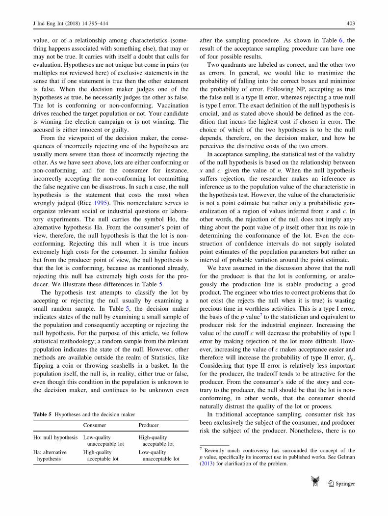
Table 9, we allow the values of a and b to vary and revised
plans are reported. Sample size shows itself to be very
sensitive to b risk. When allowing for higher values of
secondary b risk, these new configurations can greatly
reduce the cost of sampling. A small secondary risk of 5%
requires a sample size of 1600, whereas allowing for more
secondary risk brings sample size down to 1000. The
hypergeometric distribution is the basis of all of the calcu-
lations in Table 9, with two exceptions commented on later.
Producer and consumer fix primary risks at less than 5% and
secondary risks vary. Lot size is 3000 units. LTPD is 1% and
AQL is 0.5%.10 The sampling plan PL(N, n, c) should satisfy
these five parameters. The resulting sample sizes are much
smaller than lot size 3000. We have devoted two lines in
Table 9 to the binomial distribution to illustrate its inaccu-
racy. In the first line, the sample size is equal to the size of
the lot, an illogical result since sampling by definition
requires samples smaller than the population. 100%
inspection is not sampling and therefore there is no need to
specify a value for c. This illogical result is due to the large
variance formed by the binomial distribution explained in
Appendix ‘‘Hypergeometric distribution’’. Generally, the
binomial yields pessimistic results; measures of risk and
dispersion are overestimated. Surely, such pessimism could
lead to discouragement for sampling procedures and even
the abandonment of sampling programs.
Figure 6 shows the appropriate ROC curves for the
consumer sampling plan PL(3000, 1400, c) and PL(3000,
1400, c) for the producer. The dialog between the two
parties, in this case, is not so difficult since the two plans
are very similar. The two parties could use the same sample
of 1400 and proceed with the counting of defective items.
The sampling procedure would be inconclusive in only one
case when x = 10. The cutoff value for the producer is the
value of 10 (x B 10) meaning that the producer will see the
lot as good quality, whereas the consumer will see this
value of x as demonstrating the low quality of the lot
(x[ 9). The appearance of exactly 10 defective items in
the sample will occur in only 5% of the lots and therefore
should not cause extreme conflict between parties.
The examples above have all used N = 3000 for illus-
trative purposes for didactic reasons only. In Table 10, we
have collected results that permit population size to vary.
Noteworthy in the table is the similarity for plans among
the last three population sizes of 20,000, 30,000, and
40,000. Sample size and cutoff values are all the same
PL(n, 3000, c = 20, 21) but risk factors are not, as popu-
lation size increases risk factors also increase, once again
showing the necessity of using the hypergeometric distri-
bution for obtaining more accurate results even with rela-
tively large populations.
Conclusions
The paper has shown that sampling plans should be true to
the data and the situation they represent. When lot sizes are
finite, statistical approximations may lead to serious esti-
mation errors. Since the process of sampling is inherently
error prone, the sampling process should employ only the
most accurate data available, including lot size. The pri-
ority for researchers in any area should be the utilization of
the most appropriate formulations, like the hypergeometric
distribution in sampling plans, so that unnecessary addi-
tions to inherent errors do not occur.
There are several directions for advancing this research,
for example, the important area of Bayesian statistics not
mentioned in the paper. This was not because we wanted to
devalue its appropriateness for sampling plans, but rather
because its contribution would be doubtful to the questions
of this paper, based entirely on traditional frequentist
statistics. Bayesian approaches will be an important part of
future research. The work of Suresh and Sangeetha (2011)
is especially interesting in this regard. Finally, we suggest
that the application of the R package Shiny (shiny.rstu-
dio.com, RSTUDIO 2013) could facilitate the day-to-day
operation of the approach proposed here. Contributions to
the literature have already gone in this direction (Hund
2014).
Table 8 Alternative occurrences for producer
Reality of null Ho: lot is conforming Producer chooses between states of the null hypothesis Ho: lot is conforming
Accept Ho x B c Reject Ho x[ c
True Ho p B AQLp P(TN) P(x B c/p B AQLp) P(FP) type I error: ap = P(x[ c/
p B AQLp)
PP = 1
True Ha p[LTPDp P(FN) type II error: bp = P(x B c/
p[LTPDp)
P(TP) P(x[ c/p[LTPDp)P
P = 1
FN false negative, FP false positive, TP true positive, TN true negative
10 Factories and consumers will have independent values for LTPD
and AQL. The values in this example are arbitrary but originate from
the experience of the author.
406 J Ind Eng Int (2018) 14:395–414
123
We intend to expand this research into the areas of
public health and political polling. Public health has seen
extensive applications of traditional acceptance sampling
in lot quality assurance sampling (LQAS), but in our view,
this area would benefit greatly from the reformulation
following a careful reassessment of NP. The public health
literature for LQAS is ambiguous on the issue of defining
the null hypothesis, depending on the author and the area
under scrutiny (Biedron, et al. 2010; Rhoda et al. 2010;
Pagano and Valadez 2010). We suggest that the sampling
Fig. 6 ROC curve sampling
plans for producer PL(3000,
1400, 10) and consumer
PL(3000, 1400, 9)
Table 9 Hypergeometric sampling plans PL(3000, n, c) for several values of a and b, N = 3000, LTPDp is 1%; AQLp is 0.5%
Consumer Secondary Producer Secondary Sampling plan
aC = P(LTPDc) bc = 1 - P(AQLc) ap = 1 - P(AQLp) bp = P(LTPDp) n c c/n
Binomial approximation .032 .08 3000 22 .007
… … .032 .049 1600 11 .007
.049 .059 … … 1500 10 .007
… … .017 .099 1500 11 .007
.047 .097 … … 1400 9 .006
… … .034 .098 1400 10 .007
.043 .213 … … 1200 7 .007
… … .033 .175 1200 9 .008
.039 .29 … … 1100 6 .005
… … .018 .288 1100 9 .008
.035 .381 … … 1000 5 .005
… … .03 .285 1000 8 .008
Binomial approximation .031 .457 1000 9 .009
Table 10 Hypergeometric
sampling plans PL(N, n, c) for
several lot sizes given LTPDp is
1%; AQLp is 0.5%
Consumer Secondary Producer Secondary Sampling plan
aC = P(LTPDc) bc = 1 - P(AQLc) ap = 1 - P(AQLp) bp = P(LTPDp) N n c
.049 .059 … … 3000 1500 10
… … .017 .099 3000 1500 11
.015 .054 … … 5000 2300 15
… … .022 .031 5000 2300 16
.035 .071 … … 10,000 2400 16
… … .038 .059 10,000 2400 17
.025 .066 … … 20,000 3000 20
… … .039 .041 20,000 3000 21
.028 .072 … … 30,000 3000 20
… … .044 .045 30,000 3000 21
.03 .074 … … 40,000 3000 20
… … .046 .047 40,000 3000 21
J Ind Eng Int (2018) 14:395–414 407
123

plans should recognize and emphasize the viewpoint of the
target population as Rhoda et al. (2010) argues. For
example in the case of a vaccination campaign where
coverage is of major interest, the population (analogous to
the consumer) should suggest a null that would define the
cutoff where coverage is inadequate. A sample that indi-
cates the target population is receiving adequate levels of
coverage, when in fact coverage is inadequate, is a very
serious error indeed.
For political polling, the decision makers perspective
can come from the candidate (consumer of consulting
services) or from the pollster (supplier, producer). The null
for the candidate is that his adversary is winning the
political campaign, analogous to the null of the buyer that
lots are of bad quality. If in fact, the adversary is winning
but the candidate believes that his own campaign is win-
ning, the result for the candidate could be very costly.
Falsely believing his campaign is ahead; he may diminish
his efforts and consequently fall behind even more. This is
type I error for the candidate. Public health and polling
have already seen some progress in applying the new
methods proposed here (Samohyl 2015, 2016).
Open Access This article is distributed under the terms of the
Creative Commons Attribution 4.0 International License (http://crea
tivecommons.org/licenses/by/4.0/), which permits unrestricted use,
distribution, and reproduction in any medium, provided you give
appropriate credit to the original author(s) and the source, provide a
link to the Creative Commons license, and indicate if changes were
made.
Appendix
Hypergeometric distribution
The most relevant characteristic of the hypergeometric dis-
tribution is that population size N enters directly into its for-
mulation contrary to other distributions like the binomial and
Poisson. The hypergeometric mass function produces an
estimate of the probability of x defectives appearing in the
sample, depending on lot quality p = X/N and the sample size
n.Note that the number of good parts in the lot is (N - X), and
the number of good parts in the sample is (n - x). See Gonin
(1936) for the development of the equation.
Ph ¼X!
x! X�xð Þ! þN�Xð Þ!
n�xð Þ! N�Xð Þ� n�xð Þð Þ!N!
n! N�nð Þ!¼
X
x
� �
þN � X
n� x
� �
N
n
� �
¼pNð Þ!
x! pN�Xð Þ! þ1�pð ÞNð Þ!
n�xð Þ! 1�pð ÞNð Þ� n�Xð Þð Þ!N!
n! N�nð Þ!
ð5Þ
To simplify, we rewrite the hypergeometric mass func-
tion h to emphasize dependence on the defective rate p.
Ph pð Þ ¼ h N; n; x; pf g
Supplying numbers to N, n, x, we draw Fig. 7 to
demonstrate this dependence graphically. As p gets closer
to zero, the probability of finding samples with x = 0
becomes more likely, Ph(p) approaches one. The step for-
mat for N = 500 is due to the discrete nature of this non-
continuous distribution. Allowing N to approach infinity in
the hypergeometric distribution will result in the binomial
distribution. Guttman et al. (1982, p. 30) demonstrates this
theorem.
For acceptance sampling, the probability of accepting
the lot is a cumulative sum containing x = 0, 1, 2, …, c, in
the framework of the cumulative probability distribution.
Specifically, in a sample of size n, from a population of size
N, a lot is acceptable even though the sample may contain
up to c defective items. Consequently, with H representing
the cumulative hypergeometric distribution:
PH cð Þ ¼ H PL N; n; cð Þ; pf g ð6Þ
The hypergeometric is more comprehensive and precise
than the binomial and the Poisson. Even though the means
are identical for all three distributions (np), the binomial
variance varb(x) and the hypergeometric variance varh(x)
have distinct values, but varb(x) is always greater than
varh(x)
varb xð Þ ¼ np 1� pð Þ;varh xð Þ ¼ varb xð Þ � N � nð Þ= N � 1ð Þ
The Poisson variance varp(x) is simply np, equal to its
mean and, consequently, when p is very small approaching
zero, then varb(x) & varp(x).The advantage of the hyper-
geometric is that its variance is smaller, and furthermore,
much smaller when N and n are proximate values. The
vertical axis in the next figure is the ratio
varh(x)/varb(x) which varies from 0.0 to 1.0. The x- and y-
axes at the base are sample size n and population size
N. The figure shows that when N is large and n small, there
is practically no difference between the two variances.
However, when N and n have similar values, the result is a
value of varh(x)/varb(x) that approximates zero, the
hypergeometric variance being much smaller than the
binomial as seen in Fig. 8. Even when population size N is
40,000, and when sample size n is relatively large, the
difference between the two variances can be relevant.
Considering the fact that the hypergeometric distribution is
more general and more accurate than both the binomial and
the Poisson, the question arises why do many applied areas
of research continue to ignore the hypergeometric
distribution?
408 J Ind Eng Int (2018) 14:395–414
123

Producer sampling plans recalculated
with the hypergeometric distribution
For the industrial practitioner who needs to use a sampling
plan from the producer point of view right now urgently, go
directly to Table 11 for producer sampling plans using the
hypergeometric distribution. This table incorporates the
most popular plans found in current standards for the
producer, but risk factors come from the hypergeometric
distribution. It is common in practice to use sampling plan
tables without a careful understanding of the concepts that
generate the numerical entries and may result in poor
decision-making. Moreover, this may be the reason for
disregarding the hypergeometric distribution as the proper
base of the calculations.
Single sampling plans are ubiquitous in practically all
industries and are the focus of this article. Double and
multiple stage sampling plans may be less risky in a the-
oretical sense showing a lower probability of sampling
error, however, applications on the shop floor require
intensive training and the learning curve is uncomfortably
steep. Single sampling plans, on the other hand, will reduce
costs significantly and even bring a new dynamic to the
factory. The elimination of costly 100% total inspection
will enhance the adoption of modern management tech-
niques in general, and help to make negotiations between
buyers and sellers more transparent and organized. Our
intention is to show how to improve standard sampling
plans like the ISO standards (1999, 1985) by recalculating
tables with the hypergeometric distribution, and more
importantly taking into account the correct usage of
hypothesis testing. All major and most emerging econo-
mies have similar standards. Table 11 for producer sam-
pling plans, the most utilized on a worldwide scale (but not
always coherently), previews some important results from
this paper. This table combines several tables of popular
national and international sampling plans.
How to use Table 11 step-by-step
1. Choose the size of the lot N from the second column.
2. The third column gives the sample size n.
3. Choose the worst level of quality permitted by the
producer—acceptance quality level AQL. The
table contains only four levels: 0.04, 0.065, 0.65, 1%,
reflecting the very strict industry standards of modern
manufacturing.
4. Column c presents the cutoff number of failed parts
in the sample that still allow for the acceptance of
the lot as conforming. Consequently, if c ? 1 bad
parts are found in the sample, this means the lot is
rejected as non-conforming. To economize on
resources and make the process even faster, sam-
pling could be sequential and decisions taken even
before all n items pass through inspection. c ? 1 bad
parts may be found before the total sample n is taken
and rejection may already occur. Alternatively,
n - c parts could be sequentially sampled with no
bad parts found, meaning that the lot should be
accepted immediately.
Fig. 7 Mass hypergeometric
distribution Ph(p) = h{N, 300,
0, p}
Fig. 8 Comparing hypergeometric and binomial variances
J Ind Eng Int (2018) 14:395–414 409
123
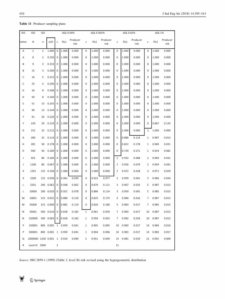
Table 11 Producer sampling plans
Source: ISO 2859-1 (1999) (Table 2, level II) risk revised using the hypergeometric distribution
410 J Ind Eng Int (2018) 14:395–414
123

5. Finally, in the appropriate column check for producer
risk.
Comments on Table 11
Following, are some comments about the revised numbers
in the table.
• The column n/N emphasizes the varying nature of the
relative size of the sample compared to lot size. Large
lots usually require proportionately smaller samples.
• Up to the letter F, N = 91 and n = 20, all plans use
c = 0 and therefore are extremely easy to apply on the
shop floor. The advantage of these plans is that once a
defective item appears sampling can stop given that the
minimum condition for accepting the lot has been
violated (Squeglia 1994).
• Popular thought has it that producer risk is constant
throughout the standard tables, however when risk is
recalculated using the hypergeometric distribution a
notable dispersion of values is apparent. For example,
for the 1% column (the last column of the table)
producer risk varies from 0.0 to 13.3%. Furthermore,
note that there are many plans with zero risk for the
producer.
Operating characteristic curve (OCC)
In this article, we suggest the use of the hypergeometric
distribution as the basis for constructing sampling plans
and not the approximations following the binomial and
Poisson distributions. In all standard sampling plans
including ISO (1999, 1985) and the Brazilian standards
ABNT-NBR (1989a, b), graphical analysis of the rela-
tionship of P() to several of its numerical characteristics is
always included in the documentation, such as the form
and functional relationship of P() with lot quality p. The
graphical representation of P() and p is known as the
operating characteristic curve (OCC).11 Along the curve,
the parameters of the sampling plan PL(N, n, c) are con-
stant (Eq. 6). As the quality of the lot deteriorates with
p increasing, the probability of getting a high-quality
sample P(x B c) diminishes, or inversely, the probability
of getting a low-quality sample 1 - P(x B c) increases. In
Fig. 9, we illustrate three different plans for lot size
N = 10,000. All plans are almost identical for high-quality
lots up to p = 0.007. After this point, the three plans begin
to diverge. The plan with the largest sample size n = 300
dominates the others from the consumer point of view
since the probability of accepting lots decreases faster as
the lot deteriorates in terms of p. The shape of the OCC has
been extensively analyzed for acceptance sampling in for
example Mittag and Rinne (1993, pp. 139–142). Sampling
plans that are more favorable either to the consumer or to
the producer are constructed altering the values of n and c,
and if possible the size of the lot N. Later in the article, we
lay out a procedure for optimizing sampling plans.
Table 12 PL(10,000, 100, c); AQL = 0.005 and LTPD = 0.010
c a producer risk b consumer risk
9 .305 .003
10 .148 .008
11 .055 .021
12 .015 .048
13 .002 .098
14 .000 .177
15 .000 .288
Fig. 9 OCC for
P(p) PL(10,000, n, d)
11 See Shmueli (2011, chap. 2) for a revision of the OCC in
acceptance sampling.
J Ind Eng Int (2018) 14:395–414 411
123
The receiver operating characteristics (ROC) curve
Another useful way of viewing the intricate relationships
within the hypergeometric distribution in the context of
acceptance sampling is in light of the receiver operating
characteristics (ROC) curve, a standard tool in the area of
data mining and other computationally intense procedures
(Provost and Fawcett 2013, chap. 8). The construction of
sampling plans with the help of ROC curves will be very
useful for the new procedures suggested later on.
Considering all other variables constant, the ROC
curve represents the relationship between a and b as the
cutoff c assumes different values.12 The central question
is at what rate risk measures change as c changes in a
given sampling plan. As cutoff c increases, it becomes
more and more difficult to reject lots and therefore
producer risk will decrease, but consumer risk increases
as more and more lots are accepted. The ROC curve is a
quick way of ascertaining this trade off. Table 12 and
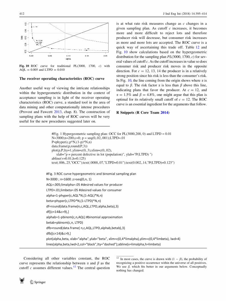
Fig. 10 show calculations based on the hypergeometric
distribution for the sampling plan PL(3000, 1700, c) for sev-
eral values of cutoff c. As the cutoff increases in value so does
consumer risk and producer risk moves in the opposite
direction. For c = 12, 13, 14 the producer is in a relatively
strong position since his risk is less than the consumer’s risk.
In Fig. 10, the line coming from the origin shows where a is
equal to b. The risk factor a is less than b above this line,
indicating plans that favor the producer. At c = 12, and
a = 1.5% and b = 4.8%, one might argue that this plan is
optimal for its relatively small cutoff of c = 12. The ROC
curve is an essential ingredient for the arguments that follow.
R Snippets (R Core Team 2014)
Fig. 10 ROC curve for traditional PL(3000, 1700, c) with
AQL = 0.005 and LTPD = 0.010
12 In most cases, the curve is drawn with (1 - b), the probability of
recognizing a positive occurrence within the universe of all positives.
We use b, which fits better in our arguments below. Conceptually
nothing has changed.
412 J Ind Eng Int (2018) 14:395–414
123
J Ind Eng Int (2018) 14:395–414 413
123

References
Associacao Brasileira De Normas Tecnicas (1989) Planos de
amostragem e procedimentos na inspecao por atributos - ABNT
NBR 5426:1985, Versao Corrigida (corrected version)
Associacao Brasileira De Normas Tecnicas (1989) Guia para
utilizacao da norma ABNT NBR 5426 - ABNT NBR
5427:1985 Versao Corrigida (corrected version)
Biedron C, Pagano M, Hedt BL, Kilian A, Ratcliffe A, Mabunda S,
Valadez JJ (2010) An assessment of Lot Quality Assurance
Sampling to evaluate malaria outcome indicators: extending
malaria indicator surveys. Int J Epidemiol 39(1):72–79
Chyu C-C, Yu I-C (2006) A bayesian analysis of the deming cost
model with normally distributed sampling data. Qual Eng
18:107–116. doi:10.1080/08982110600567442
Deming WE (1975) On probability as a basis for action. Am Stat
29(4):146–152
Deming WE (1986) Out of the crisis. MIT Press, Cambridge
Dodge HF, Romig HG (1929) Sampling inspection. Bell Syst Tech J
8(4):613–631
Dodge HF, Romig HG (1944) Sampling inspection tables. Wiley,
New York
Gelman A (2013) P values and statistical practice. Epidemiology
24(1):69–72. doi:10.1097/EDE.0b013e31827886f7
Gonin HT (1936) The use of factorial moments in the treatment of the
hypergeometric distribution and in tests for regression. Philos
Mag 7 21:215–226
Guttman I, Wilks SS, Hunter JS (1982) Introductory engineering
statistics. Wiley, New York
http://www.pubmedcentral.nih.gov/articlerender.fcgi?artid=2710509
&tool=pmcentrez&rendertype=abstract
Hund L (2014) New tools for evaluating LQAS survey designs.
Emerg Themes Epidemiol 11:2. doi:10.1186/1742-7622-11-2
Iso-International Standard 2859-1 (1999) Sampling procedures for
inspection by attributes—Part 1: sampling schemes indexed by
acceptance quality limit (AQL) for lot-by-lot inspection, 2nd edn
Iso-International Standard 2859-2 (1985) Sampling procedures for
inspection by attributes—Part 2: sampling plans indexed by
limiting quality (LQ) for isolated lot inspection, 1st edn
Mittag HJ, Rinne H (1993) Statistical methods of quality assurance,
3rd edn. Chapman & Hall, New York
Neyman J, Pearson E (1933) On the problem of the most efficient
tests of statistical hypotheses. Philos Trans R Soc A Math Phys
Eng Sci 231:694–706
NIST/SEMATECH (2012) e-handbook of statistical methods. http://
www.itl.nist.gov/div898/handbook/
Pagano M, Valadez JJ (2010) Commentary: understanding practical
lot quality assurance sampling. Int J Epidemiol 39(1):69–71.
doi:10.1093/ije/dyp406
Provost F, Fawcett T (2013) Data science and business. O’Reilly,
Cambridge
R Core Team (2014) R: a language and environment for statistical
computing. R Foundation for Statistical Computing, Vienna,
Austria. http://www.R-project.org/
Rhoda DA, Fernandez SA, Fitch DJ, Lemeshow S (2010) LQAS: user
beware. Int J Epidemiol 39(1):60–68. doi:10.1093/ije/dyn366
Rice J (1995) Mathematical statistics and data analysis, 2nd edn.
Duxbury Press, Belmont
Rstudio Inc (2013) shiny: web application, framework for R. R
package [Version 0.5.0]. http://CRAN.R-project.org/package=
shiny
Samohyl R (2013) Audits and logistic regression, deciding what
really matters in service processes. A case study of a government
funding agency for research grants. In: Proceedings of the Fourth
International Workshop on knowledge discovery, knowledge
management, and decision support. doi:10.2991/.2013.33
Samohyl R (2015) An acceptance sampling approach to polling
public opinion. https://www.researchgate.net/publication/
295919947
Samohyl R (2016) Lot quality assurance sampling (LQAS) from a
Neyman–Pearson perspective https://www.researchgate.net/pub
lication/305334204
Schilling EG, Neubauer DV (2009) Acceptance sampling in quality
control, 2nd edn. CRC Press, Boca Raton
Shmueli G (2011) Practical acceptance sampling, 2nd ed. CreateS-
pace Independent Publishing Platform
Squeglia NL (1994) Zero acceptance number sampling plans. ASQ
Quality Press, Milwaukee
Suresh K, Sangeetha V (2011) Construction and selection of bayesian
chain sampling plan (BChSP-1) using quality regions. Modern
Appl Sci 5(2):226–234. doi:10.5539/mas.v5n2p226
414 J Ind Eng Int (2018) 14:395–414
123