access point/qos tradeoff in multihop cellular networks ... · pdf filemultihop cellular...

RADIO COMMUNICATION SYSTEMS LABORATORY

Access Point/QoS Tradeoff inMultihop Cellular NetworksUsing Spatial Reuse TDMA

ERIK WALLIN

RADIO COMMUNICATION SYSTEMS LABORATORYDEPARTMENT OF SIGNALS, SENSORS AND SYSTEMS

Access Point/QoS Tradeoff inMultihop Cellular NetworksUsing Spatial Reuse TDMA

ERIK WALLIN

Master Thesis

September 2003

TRITA—S3—RST—0314ISSN 1400—9137ISRN KTH/RST/R--03/14--SE

Abstract

Higher profit and better quality of the communication systems, these are the re-quirements for a telecom company of today. This master thesis has investigatedthe possibility to construct cheaper wireless cellular networks while maintainingsatisfactory performance. It is possible to make every part of a communicationsystem more efficient and consequently more profitable. This thesis has studieda multihop technique which extends coverage as its primary benefit. Multi-hopping is, as the word implies, the use of other mobile devices, e.g. cellulartelephones and laptops, as relays in order to transport a message between anaccess point and a mobile device. To implement this system, the mobile devicesmust be smarter and must have more functionality, e.g. routing. The multihoptechnique affects system performance in other ways, rather than just increasingcoverage. This master thesis has studied two of those affected performances,delay and power consumption. Delay is important for realtime applications andthe power consumption is important for the battery duration. The behaviour,i.e. the gradient, of the curves was studied and hypothetical formulas were sug-gested. The first performance measure used was the average delay per packetbetween a mobile station and the access point it is connected to. This measurewas proposed to be proportional to the mobile station density and proportionalto the reciprocal of the access point density raised to 1.5. With respect to theaccess point density, this was found out to be an upper bound of the delay.The second performance measure used was the average used transmitted powerper packet and two hypothetical boundary equations were proposed. Simula-tions were performed and showed similarities and deviations compared to thehypothetical formulas. Despite certain deviations, the results and the discussionaround them are valuable for network designers in the sense of deeper under-standing of the principles behind these performance measures.

iii

Acknowledgements

This master thesis has been done for Wireless@KTH and their project Affordable

Wireless Services and Infrastructure (AWSI) and I would like to thank thepersons involved in the project, especially project manager Jens Zander andwork packet leader Tim Giles, for the opportunity to write about this interestingtopic and their feedback from the project. Tim has also been my supervisor andhe gave me assistance in the beginning when there were too many directions totake. Pietro Lungaro was another student involved in the AWSI project and wehave had many fruitful discussions about the subject along the way. Last butnot least I would like to thank my girlfriend Arune Luksaite for being supportivewith some advice involving the non-technical parts of the thesis and for givingme extra motivation.

v

Contents

1 Introduction 1

1.1 Background and Usability . . . . . . . . . . . . . . . . . . . . . . 11.2 Previous Research . . . . . . . . . . . . . . . . . . . . . . . . . . 3

1.2.1 Purpose of Study . . . . . . . . . . . . . . . . . . . . . . . 31.3 Thesis Outline . . . . . . . . . . . . . . . . . . . . . . . . . . . . 3

2 System Model 5

2.1 Delimitation . . . . . . . . . . . . . . . . . . . . . . . . . . . . . . 52.2 Simulation Model . . . . . . . . . . . . . . . . . . . . . . . . . . . 6

2.2.1 Propagation Model . . . . . . . . . . . . . . . . . . . . . . 62.2.2 Link Model . . . . . . . . . . . . . . . . . . . . . . . . . . 92.2.3 Connectivity . . . . . . . . . . . . . . . . . . . . . . . . . 112.2.4 Traffic Model . . . . . . . . . . . . . . . . . . . . . . . . . 112.2.5 Routing . . . . . . . . . . . . . . . . . . . . . . . . . . . . 122.2.6 STDMA . . . . . . . . . . . . . . . . . . . . . . . . . . . . 12

2.3 Variables . . . . . . . . . . . . . . . . . . . . . . . . . . . . . . . 162.3.1 AP Density . . . . . . . . . . . . . . . . . . . . . . . . . . 162.3.2 MS density . . . . . . . . . . . . . . . . . . . . . . . . . . 16

2.4 Performance Measures . . . . . . . . . . . . . . . . . . . . . . . . 162.4.1 Average Used Transmitted Power per Packet . . . . . . . 172.4.2 Average Delay per Packet . . . . . . . . . . . . . . . . . . 17

2.5 Simulation . . . . . . . . . . . . . . . . . . . . . . . . . . . . . . . 18

3 System Hypothesis 21

3.1 Average Delay per Packet . . . . . . . . . . . . . . . . . . . . . . 213.1.1 MS Density . . . . . . . . . . . . . . . . . . . . . . . . . . 213.1.2 AP Density . . . . . . . . . . . . . . . . . . . . . . . . . . 22

3.2 Average Used Transmitted Power per Packet . . . . . . . . . . . 233.2.1 MS Density . . . . . . . . . . . . . . . . . . . . . . . . . . 233.2.2 AP Density . . . . . . . . . . . . . . . . . . . . . . . . . . 24

4 Results and Discussion 27

4.1 Delay . . . . . . . . . . . . . . . . . . . . . . . . . . . . . . . . . 274.1.1 Single Cell Environment . . . . . . . . . . . . . . . . . . . 274.1.2 Multiple Cells Environment . . . . . . . . . . . . . . . . . 30

4.2 Used Power . . . . . . . . . . . . . . . . . . . . . . . . . . . . . . 314.2.1 Single Cell Environment . . . . . . . . . . . . . . . . . . . 344.2.2 Multiple Cells Environment . . . . . . . . . . . . . . . . . 34

vii

viii Contents

5 Conclusions 37

5.1 Summary . . . . . . . . . . . . . . . . . . . . . . . . . . . . . . . 375.2 Future Work . . . . . . . . . . . . . . . . . . . . . . . . . . . . . 37

5.2.1 Use of STDMA . . . . . . . . . . . . . . . . . . . . . . . . 385.2.2 Fairness in Delay . . . . . . . . . . . . . . . . . . . . . . . 385.2.3 Fairness in Used Power per Node . . . . . . . . . . . . . . 38

References 39

List of Abbreviations

AP Access PointFIFO First In First OutGSM Global System for Mobile CommunicationsLAN Local Area NetworkLoS Line of SightMHA Minimum Hop AlgorithmMS Mobile StationPRN Packet Radio NetworkQoS Quality of ServiceSINR Signal to Interference and Noise RatioSIR Signal to Interference RatioSMS Short Message ServiceSTDMA Spatial Reuse Time Division Multiple AccessTDMA Time Division Multiple AccessWAN Wide Areal Network

ix

Chapter 1

Introduction

This thesis has investigated performance measures in a cellular packet radio net-

work (PRN) using a multihop technique. Multihopping is a technique where apacket can be relayed by mobile stations (MSs), for example a cellular telephoneor a laptop, in order to reach its destination. Figure 1.1 illustrates the use ofmultihopping in a cellular system. One of the first experiments that used PRNwas ALOHANET[1] on Hawaii. A similar strategy with intelligent relaying hasbeen successfully implemented in the Internet, but there most of the links arewired.

1.1 Background and Usability

The cost of a commercial communication system, e.g. GSM, contains many fac-tors. Nowadays, marketing, billing and administration constitute a very highcost for a wireless operator, while equipment costs tend to be a smaller part.The rent for places where the Access Points (APs), i.e. base stations, are posi-tioned is a cost that could be reduced with a multihop technique due to extendedcoverage. The economic situation for the telecom companies makes it importantfor them to investigate where they can cut down the infrastructure costs in newnetworks at a relative low loss in performance. A network with multihopping isone possibility to increase the coverage from an AP but this would of course alsodecrease the Quality of Service (QoS) of the system. QoS in a PRN includesmaximum throughput, delay and power consumption, or combinations of them1.A potential increase in coverage due to relaying could be cost efficient for ruralareas where the amount of users is lower and thereby also the income of theoperators. The multihop technique is not only suited for commercial purposes.If the network is also adhoc2, the network could, for example, be well suitedfor the military and for rescue actions. An adoc solution for these scenarios isattractive because of the fast and simple installation and management of suchnetworks. This is of course also valid for all other communication systems, es-pecially private wireless local area networks (LANs). A general vision of thefuture commercial wireless communication systems is that there will be severaldifferent wireless systems, connected together via the wired backbone. Differ-

1Example: Throughput per used power as in [2].2An adhoc network is selfmanaging and selfconfiguring.

1

2 Chapter 1. Introduction

Figure 1.1: Example of a multihop system

ent communication systems have different advantages and disadvantages and areason why wireless networks are increasingly common is the possibility of usermobility. Wired networks on the other hand are and will always be superiorin data rates. Coverage against capacity and data rates is a design problemin wireless networks. A possible and economic solution would therefore be touse satellite communication in rural areas and cellular networks in urban areas.Extra capacity in for example airports and shopping malls, i.e. hot spots, couldbe covered with wireless LANs (WLANs). For areas where the need for datarates is higher than rural areas and lower than urban areas a multihop techniquecould with advantage be used. The leading motive for all these systems is afterall an economical aspect. All these wireless networks together could then extendthe Internet to (almost) the whole earth. A possibility is then that a MS couldhave more than one interface and then connect to the most appropriate networkdependent on the service which is used. With such a device, travel could be pos-sible between different areas without problems. An interesting point is also thatif the placement of APs in a multihop network is close enough, it will be thesame system as a non-multihop network. If the multihop system is adhoc, anetwork with low density of APs could first be built and new APs could easilybe placed where the need for capacity tends to be higher.

1.2. Previous Research 3

1.2 Previous Research

The concept of multihopping has been discussed for a long time. However, veryfew implementations have actually used the technique. T.J. Harrold and A.R.Nix in [3] investigated this concept and had power reduction3 and coverageextension as benefits of this. Harrold and Nix in [4] continued their work byinvestigating the capacity enhancement as a function of the number of relayingusers and found an enhancement if compared to a usual architecture withoutmultihopping. H-Y. Hsieh and R. Sivakumar in [2] obtained some interesting re-sults after comparing the decrease in throughput in a multihop cellular networkin relation to a non-multihop cellular network. This is due to the bottleneckat the AP. However when they compared the throughput with respect to theused power, the multihop technique appeared to be much more efficient. Allthese studies above compared the benefits and shortcomings between systemsthat either use or do not use multihopping.With the introduction of multihopping, new features have to be added to thenetwork. Routing and scheduling are two features that are added or changed insuch a network. Many studies have compared different routing and schedulingalgorithms for different scenarios with different results. A study carried out byJ. Gronkvist ([5]) constitutes the scheduling method used in this thesis. Differ-ent assignment methods were investigated both with analysis and simulationsfor two different traffic models, broadcast and unicast traffic. The studied sce-nario was a communication system which used Spatial Reuse TDMA (STDMA).The results were expressed in delay and throughput.

1.2.1 Purpose of Study

A missing part in the previous studies is an investigation of QoS for differentcell sizes in cellular multihop networks. An economic motivation to manipulatewith this parameter, i.e. the AP density, was briefly discussed in section 1.1and is hence the purpose to this thesis. The density of mobile devices is also ofinterest. To be able to serve more MSs in a cell is logically more economic andthe MS density was therefore also a parameter to be studied.

1.3 Thesis Outline

The simulation model is presented in chapter 2. Section 2.2.1 to 2.2.6 describesthe network model while the definition of the problem formulation can be foundin section 2.4. Definitions of performance measures and variables will also bedescribed here. This chapter is followed by analysis in chapter 3 where approxi-mations of the perfromance measures are derived. These expressions are some ofthe the main contributions from this thesis. Except analysis of the problem, thethesis also contains simulations. The simulation results are together with theapproximated expressions from chapter 3 presented in graphs and discussed inchapter 4. Finally, chapter 5 concludes the results from chapter 4 and proposesa few new areas of research closely related to this thesis.

3Only the transmitted powers was included in the measure.

Chapter 2

System Model

This chapter first describes the system model used for the performance evalua-tion in the desired scenarios. This is followed by the definitions of the perfor-mance measures and the variables to be used. With these parameters described,a more exact problem formulation can be defined. Last in this chapter, there isan explanation of how the simulation of the networks was implemented.

2.1 Delimitation

The thesis had the following requirements on the system model.

• The network should be cellular.

• The network should use a multihop technique.

• The general design of the network should be feasible to implement.

This description of the network is very general. Certain design parameters arethus necessary to decide. Designing a multihopping cellular network involveschoosing algorithms and parameters for each protocol layer. The number offeasible combination is huge. It is impractical to examine them all, so a limitedset of algorithms and parameters was chosen. However, all these algorithmsand techniques should be feasible to implement. The most important choiceof parameters for the network is the choice of STDMA as the medium access

control (MAC) protocol. The reason to choose a deterministic MAC protocol isthe need of a more efficient use of the frequency spectrum. Radio communicationcan not compete with wires where the data rates of today could be gigabits persecond. That would mean that a radio link should need a frequency spectrumover 1 GHz. That is of course not possible for this thesis’ scenarios describedin section 5.2. However, the need for higher data rates is still there and aneffective use of the bandwidth will probably be much cheaper than buying morebandwidth. The frequency band for these kinds of networks is hard to predict.The choice is here to simulate an outdoor environment with a frequency band of100 MHz around 2 GHz. This frequency range is roughly the one used for 3G,which makes new types of networks not implementable in this frequency range.A positive consequence, and a reason for choosing this frequencies, is that thisfrequency range is well documented. If the central frequency was different, some

5

6 Chapter 2. System Model

constants in the propagation model would change, and the average number ofneighbours for a node would change. This could either affect the coverage orthe spatial reuse. Routing is also a feature that has to be implemented in amultihop network. Unfortunately, different routing algorithms could change theperformance drastically. Minimum Hop Algorithm, MHA has been used in thisthesis due to the delay performance in low trafficed networks and stability1.

2.2 Simulation Model

The simulation environment to be implemented and analysed is presented indetail in this section.

2.2.1 Propagation Model

The propagation for a signal is an important part of a radio network. A linkfrom node i to node j, denoted (i, j) has a pathgain, denoted Gij , which isan important part and decides the range of a reliable transmission. This isexplained in section 2.2.3. An assumption that a link’s pathgain is equal inboth directions, i.e. Gij = Gji is made. The model, used to determine thepathgain, is taken from [12] and [13]. The pathgain model can be divided intotwo parts, one deterministic and one stochastic due to fading.

Gij = Gd(dij) + Gf (2.1)

where Gd is a deterministic pathgain as a function of the distance dij and Gf

is shadow fading, everything expressed in dB.

Distance dependent gain

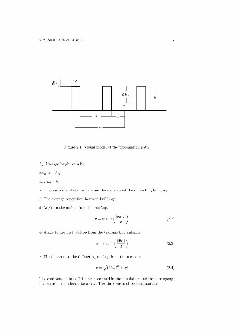
The value of Gd in a normal cellular system without multihopping has beenmodelled for many existing systems like the first and second generation mobiletelephony. A problem that arises when multihopping is added to a cellularsystem is that a different propagation model is required. This is due to differenttypes of links, not only MS to/from AP communication. Models have beendeveloped by Xia in [12] and figure 2.1 shows the visual model. This was furtherdescribed in [13] and the straight forward models from those papers will be usedhere. Three different models are needed to model three identified situations thatcan occur with access points and mobile users. The expressions can be dividedinto three parts. Free space pathloss (Lfs), diffraction from a rooftop down to areceiving mobile (Lrtm) and a multiple screen diffraction loss due to propagationpast rows of buildings (Lmsd).

The following parameters from the figure will be used in the pathloss ex-pressions

R The horizontal distance between transmitter and receiver.

h Average height on buildings.

hm Average height of MSs.

1Less MSs are involved in the routes

2.2. Simulation Model 7

Figure 2.1: Visual model of the propagation path.

hb Average height of APs.

δhm h− hm

δhb hb − h

x The horizontal distance between the mobile and the diffracting building.

d The average separation between buildings.

θ Angle to the mobile from the rooftop.

θ = tan−1

( |δhm|x

)

(2.2)

φ Angle to the first rooftop from the transmitting antenna.

φ = tan−1

( |δhb|d

)

(2.3)

r The distance to the diffracting rooftop from the receiver.

r =

√

(δhm)2

+ x2 (2.4)

The constants in table 2.1 have been used in the simulation and the correspong-ing environment should be a city. The three cases of propagation are


1. AP to/from MS

GAP−MS = 10 log10

(

λ

4πR

)2

+10 log10

[

λ

2π2r

(

1

θ− 1

2π + θ

)2]

+10 log10

(

d

R

)2

(2.5)

2. MS to MS

GMS−MS = 10 log10

(

λ

4πR

)2

+ 10 log10

[

λ

2π2r

(

1

θ− 1

2π + θ

)2]

+

+ 10 log10

(

d

2πR

)2λ

√

(δhm)2

+ d2

(

1

φ− 1

2π + φ

)2

(2.6)

3. AP to AP

GAP−AP = 10 log10

(

λ

4πR

)2

+ 10 log10

(

d

R

)2

(2.7)

These models are assumed to be valid at non line of sight (LoS) propagation.At LoS, a free space model is deployed as follows.

GLoS = 10 log10

(

λ

4πR

)2

(2.8)

The probability of LoS (pLoS(R)) then also has to be expressed. For AP to APtransmission, LoS is assumed not to occur. LoS is not desired due to increasedinterference between the APs. The APs can probably be placed in a way so LoSdoes not occur. For AP to MS and MS to AP transmission, this is assumed tobe as follows2.

pAP−MSLoS (R) =

{

1 R < d

0 R ≥ d(2.9)

Finally, in case of MS-MS the LoS is calculated as follows.

1. Place one MS at a random position between two buildings with a separa-tion of d meter.

2The MS is not allowed to be further away from the AP than d (the next building).

Parameter valueh 15 mhm 1.5 mhb 5 mx 50 md 100 m

Table 2.1: Simulation parameters used in propagation model.


2. Place the other MS at distance R meters away from the first MS. This isdone randomly, either to the left or to the right of the first MS.

3. If there is no building between the MSs, LoS occurs, otherwise not.

Notably, this simple model does not cause any correlation in pLoS betweendifferent links in the pathgain matrix.

Shadow Fading

A log-normal shadow fading, Gf will be added to the system in order to modelvariations in the environment. This is expressed, in dB, as

Gf ∈ N(0, σ) (2.10)

where σ is assumed to change depending on the path. N(m,σ) is a gaussiandistribution with m as expected value and σ2 as variance. Assumptions for thethree cases are presented in table 2.2

Propagation Type σ (dB)AP - AP 6AP - MS 8MS - MS 10

Table 2.2: Variation of σ depending on propagation type

These values of σ vary in different environments, but a common value ina city for AP to MS propagation should be around 8 dB and the rougher ter-rain, the higher value of σ should be used. [18] used σAP−MS = 10dB andσMS−MS = 12dB, but their city environment contained more buildings withjust streets as separation3. From these values it is reasonable to assume theapproximative values in table 2.2. For more accurate fading, correlation shouldalso be included. If a MS is in a shadow, e.g. a basement or tunnel, the proba-bility of shadow in a near position would increase compared to the average case.However if the MS is behind a building, the result are not the same. This partis not included in the thesis because of simplicity.

2.2.2 Link Model

Assume that N nodes exist in a network numbered from 1 to N. A pathgainmatrix G can be defined as follows.

G =

G11 G12 . . . G1N

G21 G22 . . . G2N

......

. . ....

GN1 GN2 . . . GNN

Gij is the pathgain of (i,j) as described in section 2.2.1. In order to receive apacket correctly, the SINR at node j, which is denoted as γj must be above a

3Their street width, i.e. d, was 15 meters.


certain threshold γ0. For a transmitting node i, γj for a given timeslot can beexpressed as follows.

γj =GijG

ai Ga

j Pi∑

k 6=i XkGkjGakGa

j Pk + Pnoise

≥ γ0 (2.11)

Xk is a boolean parameter which has value one if node k transmits at the sametime instant and zero otherwise. Ga

i is the antenna gain from node i. Theantennas are chosen to be omnidirectional for simplicity and the values of theantenna gains are 8.2 dBi4 for an AP antenna and 2.2 dBi for a MS antenna([17], [13]). Pi is the transmitted power from node i. The main noise whichoccurs around 2 GHz is thermal noise which can be approximated to be whitegaussian. The noise power will therefore be

Pnoise = kT0BFsys (2.12)

where k = 1.3810−23 J/K is Bolzmans constant, T0 = 290 K, Fsys is the receivernoise factor and B the noise bandwidth which is 100 MHz in the frequency bandthat will be used. A value used in [12] of the noise factor was 9 dB and this valuewas also used in this thesis. This is the exact expression of the SINR, but whensimulating a wide area network, N will be very large and an approximation isneeded. The STDMA algorithm, used in this thesis5 creates a schedule for eachcell and a logical approximation would therefore be to approximate the outercell interference to node j as a constant Io

i (j). N will then be reduced to thenumber of nodes in the cell. Equation 2.11 is then replaced with the followingequation, where i, k, j are nodes in the cell.

γj =GijG

ai Ga

j Pi∑

k 6=i XkjGkjGakGa

j Pk + Ioj + Pnoise

≥ γ0 (2.13)

Ioj is thus the outer cell interference to node j and this is the term to approx-

imate. One way is to do simulation, but in this thesis a simple approximationwill be employed which uses the fact that pathgains to any receiver from a APare much higher than if the transmitter was a MS. Furthermore, the fact thatthe APs are not transmitting all the time is also considered. According to [15],the total interference could be considered as the first ring of interferers (6 APs)multiplied by a constant depending on the propagation coefficient, which in thisthesis case is set to 4. The total number of interferers could then instead beconsidered as 7.2, all positioned on the first tier. Io

j results in the followingexpression.

Ioj =

7.2bGijGaj Ga

i Pmax

b + 1(2.14)

Pmax is the maximum transmitted power by the transmitter, i.e. node i, andb

b+1 is the relation in traffic load between downlink and uplink. As stated above,this is an approximation made for a wide area network. For a single cell networklike WLAN, Io

j = 0.

4dBi is the gain compared to an isotropic antenna. (0dB = 0dBi)5See section 2.2.6


2.2.3 Connectivity

Depending on the pathloss of (i,j), a transmission on this link is either possibleor not. A connectivity matrix C with N nodes is expressed as:

C =

C11 C12 . . . C1N

C21 C22 . . . C2N

......

. . ....

CN1 CN2 . . . CNN

(2.15)

Cij is a boolean variable which takes the value one if a transmission on (i,j) ispossible and thus could be part of a route. Such a link is also called a feasi-

ble link. The link’s feasibility depends on multiple parameters. Intra-cell andinter-cell interference (Io

i ) and noise decrease the quality of the signal. Inter-cell interference and noise will always be present while the intra-cell interferencedepends on the medium access scheme, which in this thesis is STDMA. The re-quirement to transmit with less than the allowed maximum transmitting powerand still be above the target SINR at the receiver plus a margin, γm, gives thefollowing expression on the minimum allowed pathgain on (i,j), expressed in dB.

Gij ≥ Gthreshold = γtarget + Pnoise + Ioi − Pmax (2.16)

γtarget is γ0 + γm and the value of γm is important. If there does not exist anymargin, it would mean that an active link with a pathgain of Gthreshold must begiven an own timeslot and only that link in the whole network can be activatedduring that timeslot. This means that no reuse is possible, not even in a wide

area network (WAN). A too high margin implies that the nodes in average havefewer neighbours and therefore in case of low MS density, a risk of not connectednodes arises. This margin also protects some against mobility, i.e. changes inthe pathgain matrix6. In this thesis, a margin of 1 dB will be used. Pmax is 0dBW for both APs and MSs.

2.2.4 Traffic Model

It is very difficult to predict the traffic model for future communication system.In order to design a system in a good manner, certain predictions of the existingtypes of traffic and their amount must be done. Different types could be voicecalls, messages, video conferences, web browsing etc. A more advanced trafficmodel could contain these different services with different probabilities for eachservice. The model would however, probably not correspond to reality. Whothought, for example, that SMS in GSM should be such a success? Therefore,a Poisson generation of packets is chosen with equal data rate demands for ev-ery MS. A system contains active and passive MSs. Active MSs have packetsto transmit while passive MSs are silent. A Poisson arrival of λi packets pertimeslot from each active MS i will be considered with the closest AP as desti-nation. When the packet arrives at an AP, an answer will be generated. Thisanswer is modelled as b packets. The value of b depends on the application. Forvoice calls, b should be equal to 1 because talking and listening exist at aboutthe same amount. This was the value applied for this thesis simulation model.

6Higher mobility will of course change G faster and errors will occur more often


Notable here is that the parameter b is part of equation 2.14. In a multihopsystem there is a possibility to be able to communicate to nearby situated MSswithout relaying through an AP. This kind of local traffic is however assumed tobe very small in a cellular network and is not taken into account in this thesis.This should be almost true for WANs, but also LANs, if the applications arenot of a type that implies communication between the local nodes.

2.2.5 Routing

A route consists of a number of feasible links. The connectivity matrix, C, showsthose links and is therefore used for the routing purpose. Many researchers havestudied different routing algorithms and the resulting behaviour on a multihopsystem. The design of the algorithms could for example be to select the routewith the lowest pathloss. Consequently, the nodes can transmit with a lowerpower and thus the interference caused will decrease. Another alternative is toselect the route with the least number of hops to the destination. This one iscalled Minimum Hop Algorithm (MHA). An advantage with this algorithm isa decrease of the delay for low traffic loads. Another advantage is that a routemade by MHA will always involve less or equal number of relays than any otherroute which is preferable from a stability point of view. The chance that somerelaying MS disconnects from the network decreases. However, changes in theconnectivity matrix due to mobility will cause some trouble to MHA. MHA willbe used here and the exact algorithm in the system model is as follows.

1. For each nodes i and j, identify the routes that minimize the number ofrelays and put them in a array.

2. Select from the array the routes that would cause the minumum transmit-ted power.

The second step in the algorithm could be chosen in other ways, for example justto pick a random route from the array. Selecting the route from the relay thatminimizes the transmitted powers is assumed to be more effective and thereforechosen. Suppose that a network contains both active and passive nodes asassumed in section 2.2.4. The STDMA algorithm needs the whole pathgainmatrix, G, for making the schedule. It could be simplified by just taking activeusers into account. This simplification is probably a ”must” for a STDMAnetwork because signaling about the pathgains is probably the weakest pointin the system. The signaling of pathgains would decrease significantly withthis decision, but the available relays would also decrease which could affectthe coverage. An alternative is to set up stations with relaying as their onlytask. However, this will also be an infrastructure cost and therefore it is notconsidered.

2.2.6 STDMA

The MAC layer is very important for the network’s behavior and a layer thateasily can be choosen and designed to optimize the system for a certain aspect.The reason to choose STDMA was the more effective behavior in loaded systemsas mentioned in section 2.1. The assumption from section 2.2.4 was that unicasttraffic should be used. A previous study [5] concerning the different types of


traffic found that link assignment increased the maximal throughput in thesystem, which is assumed to be important. The STDMA algorithm, whichcan be found from the same reference will be used in this thesis. The mainidea behind the algorithm is to create a short schedule where every link willbe assigned at least the relative number of timeslots required for that link.The APs have the responsibility to create the schedule, i.e. that scheduling iscentralized. If the scheduling would have been decentralized, every node mustknow the pathgain matrix. This would have caused more signalling about thepathgain matrix, which consumes bandwidth. Therefore, centralized schedulingwould logically be used in cellular networks. The traffic in the cell has to becalculated in the algorithm. For a small cell in the network it will in the uplinkcase resemble figure 2.2. The roman numbers are the relative number of packetsfor each link. The downlinks will then contain the same values multiplied bythe constant b, which was described in section 2.2.4.

Figure 2.2: Relative traffic in an uplink case

An example on the frame and the assignment of its own timeslot and therelaying of other packets can be seen in figure 2.3. In the following STDMAalgorithm, xi denotes a a feasible link where some packets will be routed. Λx

i

denotes the relative traffic on a link xi. The priority between the link sets is setto τiΛi

x, where τi is the number of time slots since the link’s last transmission.If the link has not transmitted yet in the schedule, τi is the number of timeslotsfrom the beginning of the frame. For each t from 1 to T, the resulting schedule,


Figure 2.3: Example of a STDMA frame

Yt, consists of the links that will be transmitted simultaneously at the time t.T is the length of the frame, measured in timeslots.

STDMA algorithm

1. Initialize:

(a) Enumerate the links.

(b) Create a list, A, containing all of the links and an empty list B.

(c) Set t to zero.

(d) Calculate the number of time slots each link is to be guaranteed andset hi = Λx

i .

(e) Reorder list A according to Λxi , highest priority first.

(f) Set τi to zero for all links.

2. Repeat until list A is empty:

(a) Set t← t + 1 and Yt ← ∅(b) For each link xi in list A:

i. Set Yt ← Yt ∪ xi

ii. If the links in Yt can transmit simultaneously

• If hi = 1, remove the link from list A and add to list B

• Set hi ← hi − 1, and set τi to zero

iii. If the links in Yt cannot transmit simultaneously, set Yt ← Yt\xi.Set τi ← τi + 1.

(c) For each link xi in list B but not in Yt:

i. Set Yt ← Yt ∪ xi

ii. If the links in Yt can transmit simultaneously, set τi to zero.

iii. If the links in Yt cannot transmit simultaneously, set Yt ← Yt\xi.Set τi ← τi + 1.

(d) Reorder lists A and B according to the link priority, τiΛix, highest

priority first.

Step 2.b.ii and 2.c.ii require a method to check whether the links can transmitat the same timeslot or not. This is achieved by SIR balancing([14], pp 155-163)and with that method the intial transmitted power of each active link is set andlater collected as results. This is done at the AP which should have the neededpathgain matrix for the cell. In reality this power should change via iterative


power control([14], pp 172-173) because of changes in the pathgain matrix. Thismethod is optimal in the sense that the minimum SINR of the receivers withinthe cell is maximized. These transmitting powers is the powers that mostlyiterative power control algorithms also converge to, which motivates the use ofSIR balancing. The result of this method is thus that iterative power controldoes not have to be taken into account in the simulation program which will besatisfactory since only snapshots will be examined.

Problems with schedule length and errors

A problem arises in the STDMA algorithm when there are more than one typeof service. According to this algorithm each link should get the proportionalnumber of timeslots compared to the other users. The larger least common de-nominator, the longer STDMA schedule, which implies longer time to calculatethe schedule. A network that has to recalculate the schedule often will then, ofcourse, not be efficient. Enough computing power is also needed at the AP. Ifthe schedule has to be updated frequently, communication could still be donewithin the cell. The schedule has to be remade at a time when the first erroroccurs which is not possible to fix with power control. This probably concernsonly one timeslot while the rest of the timeslots in the schedule will work satis-factory. Then a method could be to remove links from the ”damaged” timeslot7

while the AP calculates a new schedule and when it is ready distributes the MSsthe new and valid schedule.

STDMA in WAN, Implementation Aspects

The STDMA algorithm causes certain problems when designing a network. Thealgorithm makes it possible to have error free communication and this is becausethe algorithm estimates the SINR at the receivers in advance. To do that, allpathgains have to be calculated and distributed over the whole network. Thiswill cause much signaling in a WAN. In case of mobility, which a network ofmobile devices, of course, is supposed to manage, the refreshing rate of thepathgain matrix (G) has to be considered. Many MSs means lots of signalingat every update of G and fast moving MSs implies more frequent updates.Therefore, normal STDMA is not such a good choice for fast moving units in abig network. However, if the bandwidth used for collecting the pathgain matrixdata to the AP and the distribution of a new schedule is small compared to thetotal bandwidth, the problem with big networks will be reduced significantly.A solution to this problem is to divide the WAN into smaller parts and makean own schedule in each part. A natural choice will be to divide the WANinto the already existing cells, defined as the AP and the MSs connected to it8.A consequence of this partitioning of the network is not to allow a cell to usethe same frequency as its neighbours because the STDMA algorithm would notwork satisfactory then. A technique with frequency reuse in different cells mustthus be considered. This technique has been used for example in many systemsand can be found in [14] (section 4.2). The whole idea with spatial reuse is abit of a waste, why optimize and try to reuse frequency within the cell when theneighbor cell will not use the same frequency? To give each cell maximimum

7Priority could be given to the real time packets.8This is done with help of the routing algorithm in section 2.2.5.


bandwidth, the choice of the cluster size will be the smallest possible, i.e. 3. Thisis done with the requirement that the outer interference, Io, is acceptable9. Onemore thing to know for making the schedule is to calculate, measure or estimatethe outer interference, Io. From section 2.2.1 it is found that MSs and APs havedifferent Io depending on the propagation model which differs in the two cases.In a real system it should probably be better to measure the interference, buthere the estimation from equation 2.14 will be used. The distance to the firstring of interferers, di, will be three multiplied with the cell radius ([14], pg 77)or as follows, where Rcell is the cell radius.

di = 3Rcell (2.17)

2.3 Variables

Many parameters can of course be varied in the system. The aim of this thesisis to investigate the following variables.

2.3.1 AP Density

APs are placed in the system area, each in the middle of a geometric cell, whichhas the shape of a hexagon. The AP density parameter, ρAP , will therefore be

ρAP =1

3√

3R2

cell

2

(2.18)

where Rcell is the big radius of the hexagon.

2.3.2 MS density

In the whole system area, MSs are placed randomly according to a poissonprocess. The MS density parameter, ρMS , will therefore equal the expectedvalue of the total number of users in one cell, E(MS), divided by the cell area.

ρMS =E(MS)3√

3R2

cell

2

(2.19)

2.4 Performance Measures

One can identify many QoS parameters in a communication system. The pur-pose of this thesis was to investigate delay and power consumption. The delayis important for certain realtime services and this is a parameter that could beaffected negatively with bigger cells that use multihopping. Almost all commer-cial networks have such services and it is therefore important to investigate. Thepower consumption is important for mobile users since the battery life is impor-tant. [3] showed that multihopping could reduce the used transmitted powers.The power consumption does not only consist of the transmitted power. Threedifferent sorts of powers are identified as follows.

9Fewer neighbours of each node is the effect of higher outer interference. A clustersize of3 does not affect this too much and is therefore choosen

2.4. Performance Measures 17

1. Power used when transmittingThis power will probably not be changed so much in future systems. Bettercoding and antennas are though possible. This implies lower requirementon the SINR and hence the transmitted power could be lowered.

2. Power used when receivingThis power is assumed to be constant and is device specific.

3. OtherPower is also consumed to run applications. The power that a device usewhen being idle and sleeping is also in this part included. This part is alsomuch dependent on the device.

What can be seen from these three types of power is the dependency on thedevice, i.e. the MS’s hardware and complexity. The ideas behind this thesislead to a system that does not exist today, but is possible to implement inthe future. What then can be assumed is great improvements of the hardware.However, the batteries will also be improved and maybe the power consumptionwill not be a problem in the future. The transmitted power of a device causesbig debates about eventual health problems due to the radiation. It is also thepart of power consumption that is not so device dependent and is therefore themeasure to be investigated. When more knowledge about devices is achieved,the power used when receiving must also be investigated. A reason for this isthat this power will increase and be proportional to the number of receivingnodes in a route.An example of a device with TDMA equipment is the GSM mobile telephoneNokia 6220, which has a battery which holds for ”up to 8 days”([16]) in standbystate (sleeping) and ”up to 2-4 hours”([16]) when talking. The important fac-tor here is the limit in talk time, which consists of idle time and transmit-ting/receiving time. The devices in this thesis are not defined, but there will besome type of TDMA equipment, e.g. like in a cellular telephone using GSM.

2.4.1 Average Used Transmitted Power per Packet

Let Pk,l be the power needed to transmit a packet between the neighbour nodesk and l. The measure is then the sum of all transmitted powers during a packet’sroute from the source i to the destination j and can be expressed as

Pij =∑

(k,l)∈route(i,j)

Pk,l (2.20)

where route(i, j) contains all the links needed to route a packet from node i

to j. The average of Pij for all source nodes i, denoted P is the performancemeasure that is investigated.

2.4.2 Average Delay per Packet

Delay is defined as the number of timeslots it takes between the arrival of apacket to the source’s buffer and the arrival to the packet’s destination. Thedelay from node i to j, Dij , for a route can then be expressed as


Dij =∑

(k,l)∈route(i,j)

Dk,l (2.21)

The average of Dij for all source nodes i, denoted D is the performance measurethat is investigated.

2.5 Simulation

When a problem becomes very complex, analysis and approximation are verydifficult and a simulation is more suitable. Analysis could be too difficult andapproximations have to be verified somehow. This is the case in this thesis anda simulation is thus needed to get the results. It should be very easy if therealready existed a free-to-use network simulator suitable for this thesis systemmodel. There exist some programs, for example ns-2 [10] and GloMoSim [11].However, to build a special program for this thesis was thought to be easier sincethe propagation model and other special algorithms were not implemented inthese programs. The simulation program uses snapshots of different networksand transmits packets for a small time. The network contains 5x5 hexagon cells,but the performance measures was only collected from the inner 3x3 cells. Thisis to prevent boundary effects from the routing. A MS that is closer to oneAP does not necessarily have to be connected to it. The main steps in eachsnapshot are as follows.

1. Put an AP in the middle of each hexagon and place a poisson number ofMSs in the network area. The radius of the cell and the expected numberof MSs depends on ρAP and ρMS .

2. Calculate the gain matrix, G, according to the propagation model and theshadow fading in section 2.2.1.

3. Make a routing table according to the MHA algorithm that was describedin section 2.2.5.

4. Calculate the STDMA schedule according to the definition in section 2.2.6

5. Generate packets at the MSs and transmit according to the schedule for anumber of timeslots. When the startup time is exceeded10, values of delayand power consumption are stored during the routes. This is repeateduntil sufficient data to the performance measures described in section 2.4is collected11.

6. Collect the performance measures and go back to 1 and iterate for differentnetworks until the performance measures for all networks has converged12

7. Go back to 1 and simulate different ρAP and ρMS .

10The startup time in the simulation was set to 10 times the length of the STDMA schedule.At this time, the number of packets in the network had converged (found visually).

11The number of timeslots for the performance measures for a specific network to convergewas also found visually. 100 times the length of the STDMA schedule was the time used inthe simulation

12100 iterations was used for the measure to converge. Again, this number was foundvisually

2.5. Simulation 19

What could be added to this is what different values of ρAP and ρMS to simulate.One requirement is that the coverage should be maintained with very highprobability since it is not the scope of this thesis to investigate coverage. Thismeans that all nodes would be connected to the network and it implies that ρMS

and ρAP should not be too low. From the traffic assumption in section 2.2.4, allMSs have the same traffic demands. This value is set to a constant. If the totalamount of traffic in a cell is more than the maximum capacity allows, it willcause overflow in the buffers at the relaying MSs and at the AP. Investigation ofthe maximum capacity is not the scope of this thesis. This gives upper boundson ρAP and ρMS . Trial and error is used to find these situations which set theboundaries of ρAP and ρMS .

Chapter 3

System Hypothesis

The main purpose of this thesis is to investigate the performance measuresdescribed in section 2.4. This chapter tries to propose relationships between theperformance measures and the variables. What is needed is thus a formula forthe average delay per packet as follows.

D ∝ fD(ρAP )gD(ρMS) (3.1)

fD and gD are functions dependent on ρAP and ρMS respectively. Similar, aformula for the average used transmitted power per packet is as follows.

P ∝ fP (ρAP )gP (ρMS) (3.2)

fP and gP are functions dependent on ρAP and ρMS respectively. The functionsfD, gD, fP and gP are hence necessary to propose hypothetical formulas for.

3.1 Average Delay per Packet

The delay of a packet depends on the queueing time at the transmitter andeach relay during the route as described in equation 2.21. The STDMA algo-rithm is traffic based and a certain number of timeslots are given to each linkrelatively. Therefore, the service rate at each transmitter could be modelledas deterministic. The arrival rate is more difficult to model. When there arepackets in the MS before in the route, the arrival rate could also be modelledas deterministic, otherwise it is simply zero. In which state the arrival rate isdepends on the generation of packets. The generation is Poisson distributedwhich makes this approach rather difficult. However, further analysis with helpof queueing theory would be good if the purpose was to investigate a specificnetwork configuration. But since the measure of the delay in this thesis is theaverage of the delay per packet, a more general approach is presented below.This approach assumes that the generated traffic load to the network is not toohigh and causes overflow in the buffer.

3.1.1 MS Density

The MS density is proportional to the expected number of users in the cell.Therefore it is also proportional to the generated traffic to the cell which is ap-proximately proportional to the length of the STDMA schedule. An assumption

21

22 Chapter 3. System Hypothesis

that the average delay per packet is proportional to the schedule length is nowmade. This is logical for a circuit switched network with fixed data rates whereeach transmission from a node belongs to a certain node, either itself or anothernode. This prevents the nodes from larger queues. A Poisson generation ofpackets with FIFO queues as it is in this thesis is more difficult to do analysison, but it is still assumed to be proportional to the scheule length which isproportional to ρMS . One can imagine that a higher user density could give ahigher possibility of reuse within the cell, but this will probably be neglectible.This should at least be true for the used values of ρMS . fD in equation 3.1 willtherefore be as follows.

fD ∝ ρMS (3.3)

3.1.2 AP Density

The effect to the delay from the AP density is harder to predict and varies fromcase to case. Similar to the fD, one part of gD is also proportional to the ex-pected number of users and the generated traffic, ( 1

ρAP). The average number

of hops in the route increases with bigger radius of the cell approximately assketched in figure 3.1. This figure is approximated further so that the aver-

Figure 3.1: The average number of hops as a function of distance

age number of hops at a certain distance is proportional to the distance, i.e.#hops ∝ distance. Integration over the cell area of the new function multipliedby the probability density function for a MS, gives the result of the averagenumber of hops for all MSs, H, as follows.

H ∝ 1√ρAP

(3.4)

3.2. Average Used Transmitted Power per Packet 23

An argument for the approximation is that it is much more probable for a MS tobe on x+∆x meters away from the AP then x meters, due to the cell geometry.The simplification should be more valid for more hops away between the APand the outer MSs according to the curve’s appearance, which in fact is notthe case for the boundaries in this thesis of ρAP . Equation 3.4 will still beused because better possibilities to compare the approximation for D with thesimulation results will occur. A positive consequence of an increased cell area isthat the reuse will increase, but this is, of course, much less than the impact ofthe increased average number of hops. For smaller cells with very seldom threehops between a MS and an AP, this will make even smaller impact becausereuse of timeslots occurs at quite a few slots. The conclusion of gD from thesearguments is as follows.

gD ∝ ρ− 3

2

AP (3.5)

The reuse is better for bigger cells and a simulation would therefore probablymean a positive deviation compared to equation 3.5. It is also notable thatthe routing algorithm has a big effect on gD. The formula above is howevergeneral for all routing algorithms but different algorithms can drasticly changethe constants. If one would have used a minimum pathloss algorithm, theaverage number of hops would have increased but the reuse within the cellwould also be much better since every link would use less power.

3.2 Average Used Transmitted Power per Packet

The behavior of P is affected by the variables from section 2.3. But in oppositeto the delay, P is not affected by the traffic model. The power control algorithmis, however, more important. The intra cell interference is affecting the SINRmost if it exists, i.e. reuse of a timeslot within the cell is performed. If justone packet in the cell can transmit at a timeslot, it will therefore with higherprobability be assigned a lower power with SIR balancing. This means that thevariation of the result will also for P be very wide, but that is not so importantsince only the average value is of more importance. A MS will probably moveaway from that position sooner or later.

3.2.1 MS Density

This section would have looked different with another routing algorithm thanMHA. Adding MSs to an existing cell could give three effects.

1. The new node could act as a relay and reduce the number of hops fromthe AP to a communicating node. In that case, more power is probablyneeded since a reduced number of hops probably would mean that eachhop is longer.

2. The new node replaces a relay but the number of hops remains the same.This could happen because of MHA.

3. The new node does not affect the route.

The third alternative is most common for all cells and with the AP densities thisthesis will use1, alternative two is more common than alternative one. What

1Dense placement where one and two hops for a route are most common.

24 Chapter 3. System Hypothesis

these three alternatives give to the result is that a higher MS density could givea slightly lower average power per packet. The impact is however small and thefollowing hypothesis is instead used for fP .

fP ∝ 1 (3.6)

3.2.2 AP Density

From the equations for non LoS propagation in section 2.2.1, the signal atten-uation for a link is proportional to the distance between the transmitter andreceiver raised to four. However, there is a constant pathgain in dB which ismuch larger when an AP station is part of the transmission and this will ofcourse affect the results. The results also depend on the routing algorithm andthe power control algorithm that are used. In a cell without multihopping, theused power per packet should follow the inverse of the propagation model, i.e.in this case proportional to the radius raised to four. However, with a multihoptechnique, the total distance between an AP and a MS is divided into smallerdistances2 and another propagation model, which is linear instead of propor-tional to the distance raised to four, can be assumed. Figure 3.2 shows the used

Figure 3.2: The used transmitted power per packet when using multihopping

transmitted power per packet as a function of the distance for both models. The

2The routing algorithm has significant influence here.

3.2. Average Used Transmitted Power per Packet 25

distance, R, is mapped to the AP density as follows.

R ∝ 1√ρAP

(3.7)

This approach requires a number of hops and is hence not the best approxima-tion for this thesis where three hops very seldom occurs. On the same way asfor the delay, the average value for P is calculated by integrating the functionover the cell area. This is done for both curves in figure 3.2 and it gives thatthe approximations should be somewhere in between the following functions.

gdistance4

p ∝ 1

ρ2AP

(3.8)

glinearp ∝ 1√

ρAP

(3.9)

Chapter 4

Results and Discussion

Simulation was made according to the algorithm in section 2.5. In this chapter,these results are presented and compared with the approximations in chapter 3.

4.1 Delay

The approximation of the delay was not about finding absolute numbers of thedelay, but more about finding the typical characteristics of the curve, i.e. thegradient. The following sections show the relation between the approximationsand the simulation results. The following formula was assumed for D.

D ∝ ρMSy

ρAPx

(4.1)

4.1.1 Single Cell Environment

From chapter 3, the value of y was 1 and 32 for x. Specific for this environment

is the absence of outer interference which is what can be assumed in a LAN. Infigure 4.1, the average delay per packet is compared to the approximation fromequation 4.1. What can be seen from the comparison is that the simulationcurves roughly resemble the approximated curves. The gradient is slightly dif-ferent, which is probably a result from the reuse. Slightly lower delays comparedto the approximation curve are experienced for bigger cells, i.e. lower values ofρAP . Figures 4.21 and 4.32 show that for this simulation, a value of x would bearound 1.2 instead. One reason is the actual time spent at a relaying MS. Thehypothesis assumed that the time was equal at every node, which would havebeen the case for streaming traffic. However, if a packet arrives at a relayingMS with an empty queue, the time spent at the relaying MS would then just beuntil the next timeslot the relaying MS is allowed to transmit on the next link.A relaying MS has more than one timeslot per schedule and the packet couldthen ”steal” a timeslot which was not intended for the packet itself. This will,of course, cause lower delays for the system, especially in bigger cells where theaverage number of hops between a MS and the AP is bigger. This discussionmakes the hypothetical curve to constitute an upper bound on the delay for

1The lowest simulation curve in figure 4.1.2The highest simulation curve in figure 4.1.

27

28 Chapter 4. Results and Discussion

1 1.2 1.4 1.6 1.8

x 10−5

0

10

20

30

40

50

60

70

80~50 MSs in the smallest cell~40 MSs in the smallest cell~30 MSs in the smallest cell

Ave

rage

del

ay p

er p

acke

t (in

tim

eslo

ts)

AP density (1/m2)

Thin lines: approximation Thick lines: simulation

Figure 4.1: Average delay per packet in a LAN

1 1.2 1.4 1.6 1.8

x 10−5

20

25

30

35

40

AP density (1/m2)

Ave

rage

del

ay p

er p

acke

t (in

tim

eslo

ts) Simulation

x = 1x = 3/2x = 6/5

Figure 4.2: Hypothesis test of x in a LAN

an expansion in the coverage3 of an existing multihop STDMA network. Thesimulation curves of D seem to be slightly more than proportional to the MS

3This means bigger cells.

4.1. Delay 29

1 1.2 1.4 1.6 1.8

x 10−5

40

45

50

55

60

65

70

75Simulationx = 3/2x = 1x = 6/5

Ave

rage

del

ay p

er p

acke

t (in

tim

eslo

ts)

AP density (1/m2)

Figure 4.3: Hypothesis test of x in a LAN

density. A reason to this observation could be that high variations have a nega-tive effect on the delay. Namely, queues in the nodes buffers have very negativeimpact on D. Higher variations exist in a cell with more MSs because queueswill with higher propability occur. Whether Poisson traffic is a good model forthe hypothesis could then be questioned. Figure 4.4 shows that a more rea-sonable value for this simulation environment to assume is around 1.25 for y.If the network was able to manage realtime services like streaming media withhigh demands on low delay, this delay measure would perhaps not be the bestone to investigate. Figure 4.5 shows big variances between different networks.The reason to this is different number of MSs in a cell4 and different networkconfigurations with different number of average hops for a MS to the AP.

What really matters, in fact, is not the average delay per packet for a specificnetwork, but the average delay and variance for a single packet. This dependson, besides the number of MSs in the cell, the number of hops between the MSand the AP. Poisson generation of packets does, of course, also matter for thevariance. A traffic model with Poisson arrival is however not a good model forstreaming media, where the generation of packets is deterministic. Priority inthe buffers could be a solution to this problem and this is briefly explained morein a proposal to future research in section 5.2.2.

4The number of MSs in a cell is a random variable as described in 2.2.4.


1 1.2 1.4 1.6 1.8

x 10−5

20

30

40

50

60

70

80

AP density (1/m2)

Ave

rage

del

ay p

er p

acke

t (in

tim

eslo

ts) Thick lines: Simulation

Thin lines: y = 1.5 Dashed lines: y = 1.25 Dash−dotted lines: y = 1

Figure 4.4: Hypothesis test of y in a LAN when x = 1.2

1 1.2 1.4 1.6 1.8

x 10−5

0

20

40

60

80

100

Ave

rage

del

ay p

er p

acke

t (in

tim

eslo

ts)

AP density (1/m2)

Figure 4.5: Variance of average delay per packet in a LAN

4.1.2 Multiple Cells Environment

The arguments from section 4.1.1 explains the results for D also in this WANenvironment. The only difference is the presence of outer interference which

4.2. Used Power 31

causes shorter maximum distance in the feasible links. This implies other valuesfor ρAP in equation 3.1. Despite smaller cells, the MSs in the WAN scenario inthis simulation experienced higher average number of hops to the AP due to theshorter distances of feasible links. The results of the simulation compared toequation 4.1 are shown in figure 4.6. Again, the gradient is affected by the reuse

2 2.2 2.4 2.6 2.8 3 3.2

x 10−5

0

20

40

60

80

100

120

AP density (1/m2)

Ave

rage

del

ay p

er p

acke

t (in

tim

eslo

ts) ~50 MSs in the smallest cell

~40 MSs in the smallest cell~30 MSs in the smallest cell

Thin lines: approximation Thick lines: simulation

Figure 4.6: Average delay per packet in a WAN

within the cell. The impact of the reuse is bigger in this WAN scenario andthe reuse and the result of stealing timeslots, which was discussed in section4.1.1, is something that really has to be taken into account. The effect of”stealing” timeslots should be bigger for this WAN scenario due to a highervalue of average number of hops. Figures 4.75 and 4.86 show that for thissimulation, a value of x would be around 1 instead. Similarly as in section4.1.1, the parameter y is tested. Figure 4.9 shows that 2

3 < y < 1 for thisscenario. It appears to be rather strange that the value of y is below 1 becausethe opposite was experienced in the LAN scenario. The same argument used inthat section(4.1.1) would then contradict this result. The explanation for thiscase is that the effect of ”stealing” timeslots would increase and be dominant,which seems logical. The variation of the result is presented in figure 4.10 anda big variation for the different networks is also here experienced.

4.2 Used Power

The transmitted powers was on the same method as for the delay collected andaveraged. The approximation part of gP for P in section 3.2 did not come up

5The lowest simulation curve in figure 4.66The highest simulation curve in figure 4.6


2 2.2 2.4 2.6 2.8 3 3.2

x 10−5

40

45

50

55

60

65

70

75

80

AP density (1/m2)

Ave

rage

del

ay p

er p

acke

t (in

tim

eslo

ts) Simulation

x = 3/2x = 1/2x = 1

Figure 4.7: Hypothesis test of x in a WAN.

2 2.2 2.4 2.6 2.8 3 3.2

x 10−5

70

80

90

100

110

120

130

AP density (1/m2)

Ave

rage

del

ay p

er p

acke

t (in

tim

eslo

ts) Simulationx = 3/2x = 1/2x = 1

Figure 4.8: Hypothesis test of x in a WAN.

with one formula. Instead, two equations were presented. The approximation

4.2. Used Power 33

2 2.2 2.4 2.6 2.8 3 3.2

x 10−5

70

80

90

100

110

120

130

AP density (1/m2)

Ave

rage

del

ay p

er p

acke

t (in

tim

eslo

ts) Simulation

x = 3/2x = 1/2x = 1

Figure 4.9: Hypothesis test of y in a WAN with x = 1.

2 2.2 2.4 2.6 2.8 3 3.2

x 10−5

0

20

40

60

80

100

120

140

160

180

AP density (1/m2)

Ave

rage

del

ay p

er p

acke

t (in

tim

eslo

ts)

Figure 4.10: Variance of average delay per packet in a WAN


for P will be the same since fP ∝ 1.

Pdistance4

∝ 1

ρ2AP

(4.2)

Plinear ∝ 1√

ρAP

(4.3)

4.2.1 Single Cell Environment

The simulation result of a single cell environment is presented in figure 4.11.What can be conducted from this figure is a very small separation between

1 1.2 1.4 1.6 1.8

x 10−5

0

0.02

0.04

0.06

0.08

0.1

0.12

0.14

0.16~50 MSs in the smallest cell~40 MSs in the smallest cell~30 MSs in the smallest cell

AP density (1/m2)

Ave

rage

use

d po

wer

per

pac

ket (

W)

Thin lines: simulation Thick Lines: approximation

Figure 4.11: Average used transmitted power per packet in a LAN

the different user densities, which confirms the discussion in section 3.2.1. Thegradient of the simulation curve in the figure lies within the boundariy equationsdescribed in section 3.2.2. A big variance of P was expected and is shownin figure 4.12. The impact from different network configurations is thus alsosignificant here. The number of users was assumed not to change the result,but the MSs positions in the cell cause a problem in a multihop network becauserelaying MSs use their battery much more than other not-relaying MSs whichis not fair. This is briefly discussed in section 5.2.3 and could be solved bysensitive routing algorithms and/or economic compensation.

4.2.2 Multiple Cells Environment

The only difference from a single cell scenario and a multiple cell scenario isthe presence of outer interference. The transmitting power of a single active

4.2. Used Power 35

1 1.2 1.4 1.6 1.8

x 10−5

0

0.05

0.1

0.15

0.2

0.25

AP density (1/m2)

Ave

rage

use

d po

wer

per

pac

ket (

W)

Figure 4.12: Variance of average used transmitted power per packet in a LAN

link in the STDMA schedule will therefore increase significantly. The smallercell in the simulation and, therefore, closer distances do not counteract this somuch. Figure 4.13 shows that the simulation curves also here lies within thehypothetical curves. For this WAN scenario, the curve is closer to the upper

approximation curve (Pdistance4

) which indicates that the average number ofhops is more for this scenario. The absolute values of the powers are here higherthan for the LAN scenario, which is a result of existing outer interference. Thevariance of P is also here big as shown in figure 4.14. The reasons are the sameas in the single cell environment.


2 2.2 2.4 2.6 2.8 3 3.2

x 10−5

0

0.1

0.2

0.3

0.4

0.5

~50 MSs in the smallest cell~40 MSs in the smallest cell~30 MSs in the smallest cell

AP density (1/m2)

Ave

rage

use

d po

wer

per

pac

ket (

W)

Thin lines: simulation Thick Lines: approximation

Figure 4.13: Average used transmitted power per packet in a WAN

2 2.2 2.4 2.6 2.8 3 3.2

x 10−5

0

0.1

0.2

0.3

0.4

0.5

0.6

0.7

0.8

0.9

Ave

rage

use

d po

wer

per

pac

ket (

W)

AP density (1/m2)

Figure 4.14: Variance of average used transmitted power per packet in a WAN

Chapter 5

Conclusions

This final chapter first gives a summary of the thesis and then follows threedifferent brief proposals to future research.

5.1 Summary

This thesis has investigated how delay and power consumption are affectedin a cellular multihop network using STDMA and MHA. Both single cell andmultiple cells scenarios were investigated. Average values of the delay per packetand used transmitted power per packet in the route between a MS and anAP were investigated and the characteristics of the curves were approximated.Simulations were also done and comparisions with the hypothetical formulasgave both similarities and deviations. This was shown in the figures 4.1, 4.6,4.11 and 4.13. The hypothetical curve for the delay was found to constitute anupper bound on delay on bigger networks which could be valuable knowledgefor network designers before an expansion of an existing multihop network isrealized. The power was difficult to model due to the network topology. Twohypothetical formulas were proposed and constituted boundary equations forthe measure. These measures varied significantly which could cause troubleto realtime applications. Figures 4.5, 4.10, 4.12 and 4.14 showed this and thereason to this was different network configurations, e.g. different number ofMSs and their placement in the cell for example. This is more critical for thedelay than the used power and could partly be solved by giving higher priorityto packets with a source or destination of MSs outside the relaying MSs as isproposed in section 5.2.2. The problem that some relaying stations consumemore power than others could be solved with a different routing algorithm oreconomic compensation as proposed in section 5.2.3. When deciding the systemmodel, some weaknesses of STDMA were also suspected. The use of STDMAcould be limited to small systems (e.g. WLANs) with low mobility due to theneed of the pathgain matrix. This is further discussed in section 5.2.1.

5.2 Future Work

During the decision of the system model and the analysis of the results, somecritical points were observed, which would be interesting for further research.

37

38 Chapter 5. Conclusions

5.2.1 Use of STDMA

STDMA was investigated in this thesis and has, of course, major influenceon the results. What could be worth considering is the use of STDMA. Theexcellent theoretical results are not taking into account the amount of signalingof the pathgain matrix. Both bigger networks and high mobility require moresignaling and the loss in bandwidth due to the signaling compared to the totalbandwidth must be considered. The mobility also requires low delays of thesignaling. Relatively small networks are therefore maybe a demand for STDMAif it should be used effectively. Communication systems like 3G where MSs cantravel in cars could therefore be avoided. Small cellular networks, e.g. WLANs,could be interesting to investigate further, especially if the amount of local trafficis small because the traffic based algorithm effectively prevent the bottleneckthat otherwise occurs at the links closest to the AP. Before any implementationof a network that uses STDMA, the signaling of the pathgain matrix must beinvestigated further.

5.2.2 Fairness in Delay

MSs with more hops away from the AP will experience longer delays. This isnot fair to those MSs, especially if the wanted service requires a low delay. Suchservices are the ones that require a two-way communication, e.g. telephonecalls and some games. A possible solution to this problem is to give real timepackets from outer regions higher priority in the relays buffers. A timestampcould with advantage be added to the packet when the packet is transmittedfrom the destination. Packets that has spent more time in the system couldthen get higher priority. After a realistic algorithm for this is implemented,the variance of this thesis measure, D, will then be much smaller. With a morerealistic traffic model for realtime services, the maximum delay per packet couldbe an interesting topic.

5.2.3 Fairness in Used Power per Node

The impact from different network configurations has significant influence onwhich MSs are required to use their battery power to relay other MSs’ packets.A MS will probably move around and therefore the same MS does not alwayshave to relay other MSs packets. A study of this could be done with a modelfor mobility among the MSs. If the study for that mobility model will showthat this spreads the power almost equally among the MSs, then the problemdissappears and does not have to be solved. If the result’s outcome is negative, aneed for a solution arises. Routing algorithms, which are sensitive to the amountof energy left in the MSs batteries could be possible and research have been donewithin this area. Algorithms, which spread the traffic so more MSs have to relaypackets. However, in realtime services, it is sometimes practical with a circuit.Another approach is to compensate the relaying MSs economically.

References

[1] N. Abramson ”The ALOHA System - Another Alternative for ComputerCommunications”, 1970 Fall Comput. Conf. AFIPS Conf. Proc., vol. 37Montval, NJ : AFIPS Press, 1970, pp. 181-285.

[2] H-Y. Hsieh, R. Sivakumar. ”On Using the Ad-hoc Network Model in Cel-lular Packet Data Networks.” Mobihoc’02 pp. 36-47, Lausanne, June 2002.

[3] T.J. Harrold, A.R. Nix ”Intelligent Relaying for Future Personal Commu-nication Systems.” IEE Colloquium on Capacity and Range Enhancement

Techniques for the third Generation Mobile Communications and Beyond,February 2000.

[4] T.J. Harrold, A.R. Nix ”Capacity Enhancement Using Intelligent Relayingfor Future Personal Communication Systems.” in Proceedings of VTC-2000Fall, pp 2115-2120.

[5] J. Gronkvist. ”Assignment Strategies for Spatial Reuse TDMA.” LicenciateThesis, Radio Communication Systems, Department of S3. Royal Instituteof Technology, Stockholm, Sweden, April 2002.

[6] T. Rouse, S. McLaughlin, H. Haas ”Coverage-Capacity Analysis of Oppor-tunity Driven Multiple Access (ODMA) in Utra TDD.” 3G 2001 MobileCommunications Technologies, IEE Conference Publication 477, pp. 252-256, March 2001.

[7] T. Rouse, I. Band, S. McLaughlin ”Capacity and Power Investigation ofOpportunity Driven Multiple Access (ODMA) Networks in TDD-CDMABased Systems.” IEEE International Conference on Communications, NewYork, 2002

[8] M. Sanchez. ”Multiple Access Protocols with Smart Antennas in MultihopAd Hoc Rural-Area Networks.” Licenciate Thesis, Radio CommunicationSystems, Department of S3. Royal Institute of Technology, Stockholm, Swe-den, June 2002.

[9] O. Sommariba. ”Multihop Packet Radio Systems in Rough Terrain.” Li-cenciate Thesis, Radio Communication Systems, Department of S3. RoyalInstitute of Technology, Stockholm, Sweden, October 1995.

[10] The Network Simulator - ns-2. http://www.isi.edu/nsnam/ns/, August2002.

39

40 References

[11] GloMoSim. http://pcl.cs.ucla.edu/projects/glomosim/, August 2002..

[12] H. H. Xia. ”A Simplified Analytical Model for Predicting Path Loss in Ur-ban and Suburban Environments” IEEE Transactions on vehicular tech-nonogy, vol. 46, no. 4. pp. 1040-1046. November 1997.

[13] M. Qingyu, W. Wenbo, Y Dacheng, W. Daqing. ”An investigation of in-terference between UTRA-TDD and FDD system” Communications Tech-nology Proceedings, 2000. WCC - ICCT 2000. International Conference,Volume 1, pp 339-346 vol. 1.

[14] J. Zander, S-L Kim. ”Radio Resource Management for Wireless Networks”.Artech House, Boston, 2001.

[15] Lecture notes available at: http://www.s3.kth.se/radio/COURSES/-/WNETWORKS 2E1512 2002/Slides/WN02chap4 part1.pdf as for 03-03-03.

[16] Brief techniqual information for Nokia 6220 available athttp://www.nokia.com/nokia/0,5184,5880,00.html as for 03-04-05.

[17] Sami Tabbane ”Handbook of Mobile Radio Networks.” Artech House Mo-bile Communications Library, 2000.

[18] 3rd Generation Partnership Project. ”Radio Frequency (RF) system sce-narios” (TR 25.942 V6.0.0.). 2002.

TRITA—S3—RST—0314ISSN 1400—9137

ISRN KTH/RST/R--03/14--SE

Radio Communication Systems Lab.Dept. of Signals, Sensors and SystemsRoyal Institute of TechnologyS–100 44 STOCKHOLMSWEDEN

ERIK WALLIN Access Point/QoS Tradeoff in Multihop Cellular Networks Using Spatial Reuse TDMA

access point/qos tradeoff in multihop cellular networks ... · pdf filemultihop cellular...

Documents