accomplishment of vacsy experimental set-up and its ... · accomplishment of vacsy experimental...
TRANSCRIPT
ACCOMPLISHMENT OF VACSY EXPERIMENTAL SET-UP
AND ITS APPLICATION TO INVESTIGATE MOLECULAR
ORIENTATION DISTRIBUTION OF SOLID-STATE
POLYMERS
Dissertation
zur Erlangung des akademischen Grades doktor rerum naturalium
(Dr. rer. nat.)
vorgelegt der
Mathematisch-Naturwissenschaftlich-Technischen Fakultät
der Martin-Luther-Universität Halle-Wittenberg
von Herrn Zhanjun Fang
geb. am: 20. 03. 1965 in Beijing, China
Gutachter:
1. Prof. Dr. H. Schneider (FB Physik/Universität Halle)
2. Prof. Dr. Ch. Jäger (IOQ/HF/Universität Jena)
3. Doz. Dr. S. Grande (Inst. F. Exp. Physik/Universität Leipzig)
Halle (Saale), den 30.11.1999

L
Abstract
Accomplishment of VACSY experimental set-up and Its Application to Investigate Molecular
Orientation Distribution of Solid-State Polymers
by Zhanjun Fang
The macroscopic characteristics of polymer materials, especially liquid crystalline polymer
materials, depend significantly on their molecular orientation distribution. Mainly three methods,
X-ray diffraction, neutron scattering and NMR, are used to investigate molecular orientation
distribution in polymer materials. While X-ray diffraction is suitable for studying the orientation
distribution of samples in crystalline state, neutron scattering and NMR are two widely adopted
methods for samples in amorphous state. NMR’s unprecedented selectivity makes it the unique
experimental tool to investigate the orientation distribution of individual segments in a long
molecular chain. Along with the advancements of solid-state NMR technology during the last
twenty years, a number of NMR approaches become available to study molecular orientation
distribution of solid-state polymers. 2H NMR with line-shape analysis is the most popularly used
method, this is mainly due to its good S/N ratio and its simplicity of data analysis. However, this
method requires very expensive and time consuming isotope labelling. 1H wide-line NMR and
moment analysis approach has also been widely used for studying orientation distribution of
weakly order polymer samples, but this method can hardly provide us the orientation
information of a specific segment in a long molecular chain. Several 13C NMR approaches,
which utilise the orientation dependent chemical shift anisotropy and correlate them with their
structural related chemical shift isotropy, have the greatest advantage to investigate the
orientation distribution of individual segments in a long molecular chain of un-labelled polymer
materials.
VACSY as a promising method to re-introduce the Chemical Shift Anisotropy (CSA)
under the condition of fast variable angle sample spinning and separate them by their
corresponding Chemical Shift Isotropy (CSI) in the second dimension of a 2D NMR correlation
spectrum has been selected by us to study the orientation distribution of liquid crystal polymers
(LCPs). In this work, a probehead specially designed for the implementation of VACSY
experiment is constructed from scratches. On top of other functionalities of a normal CPMAS
double resonance probe, the VACSY probe adds the capability for the accurate controlling of the
angle between the sample spinning axis and the external magnetic field B0 direction. Much
effort has been paid to optimise the double resonance RF circuit for maximum efficiency and the
angle control system to achieve an accuracy better than 0.25o. A computer program for VACSY
spectra simulation in the case of slow sample spinning is created and successfully applied to
simulate the influences on the final CSA line-shape due to insufficient sample spinning speed,
the angle mis-setting (between the sample spinning axis and the external

LL
magnetic field B0 direction), the number of angle sampling steps, etc. The VACSY simulation
result proves to be very useful in selecting the correct experimental parameters. To reduce the
phase artefacts due to an incomplete time domain data sampling which are inherent to VACSY
experiment, two new VACSY data processing approaches are proposed and successfully applied
to process our VACSY experimental data. Comparing with the normal interpolation approach
published by Frydman et al, these two new proposals allow the final VACSY spectra to be
displayed in phase sensitive mode and the interpolation noise is also reduced to some degree.
The VACSY experimental set-up and its corresponding processing software are firstly
applied to measure the values of chemical shift tensor elements for well known samples such as
Glycine, DMS, HMB and Durene, the measurement results are in good agreement with
published values. Then, this VACSY experimental set-up is applied to investigate the orientation
distribution behaviour of two polymer liquid crystalline samples: hexa-hexyloxytriphenylene
and polyacrylates. The procedure for creating certain orientation distribution in LC samples is:
heat the sample over its clearing temperature (Tc) while it is put inside a strong magnetic field
(9.4T), wait for equilibrium and then slowly cool it down below its glass transition temperature
(Tg) to freeze the orientation distribution within the sample. From 13C VACSY spectra of the LC
samples in both isotropic state and oriented state, the orientation distribution is analysed by the
method of CSA line-shape fitting approach. For a reliable extraction of orientation distribution
through an accurate line-shape analysis approach, fast sample spinning relative to the chemical
shift anisotropy is highly desirable. For the hexa-hexyloxytriphenylene sample, the result is
compared with the result of 2H NMR line splitting measurements published by D. Goldfarb and
Z. Luz. Suggestions for further improvements of VACSY as a method for the study of
orientation distribution of solid-state polymers are also given.
i
Zusammenfassung
Aufbau eines VACSY-NMR Experiments und seine Anwendung zur Untersuchung der molekularen
Orientierungsverteilung in festen Polymeren
von Zhanjun Fang
Die makroskopischen Eigenschaften von polymeren Materialien, besonders von
flüssigkristallinen Polymeren, hängen stark von der molekularen Orientierung ab. Im wesentlichen
existieren drei Methoden (Röntgen-Beugung, Neutronenstreuung und NMR), um die molekulare
Orientierung und deren Verteilung in polymeren Materialien zu untersuchen. Während die Röntgen-
Beugung für das Studium der Orientierungsverteilung im kristallinen Zustand geeignet ist, sind
Neutronenstreuung und NMR weit verbreitete Methoden für Proben im amorphen Zustand. Die
unübertroffene Selektivität der NMR macht sie zu einem einmaligen Werkzeug für die Untersuchung
der Orientierungsverteilung von verschiedenen molekularen Einheiten in einer langen Molekülekette.
In Verbindung mit den Fortschritten der Festkörper-NMR-Technologie der letzten 20 Jahre wurden
eine Reihe von NMR-Zugängen für die Untersuchung der molekularen Orientierungsverteilung in
festen Polymeren möglich. Dabei ist die 2H-NMR-Linenformanalyse die am häufigsten verwendeten
Methode, vor allem durch das gute Signal-Rausch-Verhältnis und die einfache Analyse der Daten.
Allerdings erfordert diese Methode die teure und zeitaufwendige Isotopenmarkierung. Die 1H-
Breitlinien-NMR und Momentenanalyse wird ebenfalls häufig zum Studium der
Orientierungsverteilung in schwach geordneten Polymeren angewendet, allerdings kann diese
Methode die Orientierungsinformation über ein spezielles Segment einer langen Molekülkette nicht
liefern. Verschiedene 13C-NMR-Zugänge, welche die orientierungsabhängige anisotrope Chemische
Verschiebung (ACV) ausnutzt und sie mit der strukturabhängigen isotropen Chemischen
Verschiebung (ICV) korreliert, sind für die Untersuchung der Orientierungsverteilung von
individuellen Segmenten in einer langen Molekülkette in nicht-isotopenmarkierten Polymeren am
erfolgversprechendsten.
VASCY ist eine erfolgversprechende Methode zur Wiedereinführung der Anisotropie der
Chemischen Verschiebung unter den Bedingungen des schnellen Variable-Angle Spinning und ihrer
Trennung durch die entsprechend Isotrope Chemische Verschiebung in der zweiten Dimension eines
2D-NMR-Korellationspektrums. Diese Methode wurde von uns zur Untersuchung der
Orientierungsverteilung von flüssigkristallinen Polymeren ausgewählt. In der vorliegenden Arbeit
wurde ein NMR-Probenkopf für die speziellen Anforderungen des VACSY-Experiments gebaut.
Außer den NMR-Funktionen eines gewöhnlichen CPMAS-Doppelresonanz-Probenkopfes mußte die

ii
Fähigkeit für die exakte Einstellung und Änderung des Winkel zwischen der MAS-Rotorachse und
dem externe Magnetfeld geschaffen werden. Großer Wert wurde auf die Optimierung des
Doppelresonanz-HF-Kreises auf maximale Effizienz und auf eine Genauigkeit von besser als 0.25°
für die Winkeleinstellung gelegt. Ein Computerprogramm für die Simulation von VACSY-Spektren
bei endlicher Rotationsfrequenz und deren Einfluß auf die 2D-VACSY-Spektren, des Einflusses von
nicht-exakten Winkeleinstellungen, die Abhängigkeit der Spektren von der Anzahl der
Winkelinkremente usw. wurde erstellt. Die Simulationsrechnungen haben sich als sehr wertvoll für
die Auswahl optimaler experimenteller Parameter erwiesen. Zur Verminderung von Phasen-
Artefakten, bedingt durch den eingeschränkten experimentell zugänglichen Wertebereich im
VACSY-Experiment, wurden zwei neuartige Verarbeitungsroutinen für VACSY-Datensätze
vorgeschlagen. Verglichen mit der originalen Verarbeitungsprozedur verbessert sich die Qualität der
2D-VACSY-Spektren durch die Möglichkeit der Darstellung in phase-sensitive mode und durch den
Wegfall der Dateninterpolation.
Das VACSY-NMR-Experiment und seine Verarbeitungs-Software wurden angewendet zur
Bestimmung der Parameter der ACV für wohl bekannte Modellsubstanzen wie Glyzin,
Dimethylsulfon (DMS), Hexamethylbenzen (HMB) und 1,2,4,5-Tetramethylbenzen (Durene). Die
Ergebnisse stimmen mit den bekannten Werten überein und bestätigen die korrekte Arbeitsweise der
VACSY-hard- und Software. Im weiterem wurden VACSY-Experimente an zwei flüssigkriattlinen
Substanzen durchgeführt: Hexahexyloxytriphennylen (HHOTP) und einen flüssigkristallinen
Polymer auf Polyakrylatbasis. Zur Schaffung eines orientierten Zustandes wurde folgende Prozedur
angewendet: Aufheizen der Probe in einem starken Magnetfeld (9,4T) bis über die Klärtemperatur
(TC), abwarten bis zur Einstellung eines Gleichgewichtszustandes und anschließende langsame
Abkühlung bis unterhalb der Glastemperatur (Tg) zum Einfrieren des orientierten Zustandes. Die
VACSY-Spektren des flüssigkristallinen Proben wurden sowohl im isotropen als auch im
orientierten Zustand mittels NMR-Linienformanaylse der ACV analysiert. Für HHOTP wurden die
Ergebnisse mit früheren Experimenten anderer Autoren verglichen. Vorschläge für die weitere
Verbesserung der Methode werden gegeben.

TABLE OF CONTENTS
Chapter 1. Introduction 1
1.1 Motivation 1
�����Scope of thesis 3
Chapter 2. NMR and molecular orientation distribution 5
2.1 Important NMR interactions in solid materials 5
�����Co-ordinates system 7
�����Dependence of NMR frequency on molecular segmental orientation 9
�������Chemical shift interaction - static case 9
�������Chemical shift interaction - macroscopic sample rotation 12
�����Study of orientation distribution from anisotropic NMR interactions 15
�������The anisotropy of dipole-dipole interaction 15
�������The anisotropy of quadrupolar interaction 16
�������The anisotropy of chemical shift interaction 17
�����Procedures to extract orientation distribution from CSA line-shape 18
�������Direct reconstruction procedure 18
�������Moment analysis procedure 20
Chapter 3. NMR methods to measure chemical shift anisotropy 25
�����Introduction 25
�����Methods to retrieve anisotropic CSA patterns 26
�������Stop-and-go 26
�������Magic-Angle-Hopping, Magic-Angle-Turning (MAT) 27
�������Fast flipping between MAS and OMAS 28
�������Tycko’s 4-S-pulses method 29
�������RF field modulation 30
�������VACSY 31
Chapter 4. VACSY and interpolation of experimental data 32
�����Introduction 32
�����Theory of VACSY 33
�����Methods to implement interpolation or extrapolation 35
�������Normal interpolation - Frydmann procedure 35
�������Normal interpolation and Linear Prediction 37

�������Non-orthogonal interpolation 43
�������VACSY transformation with eigen-coordinates 48
Chapter 5. Simulation 51
�����Introduction 51
�����Simulation program 52
�������Stepwise procedure 53
�������Conroy procedure 53
5.3 Simulation results 55
�������Influence of sample spinning speed on CSA line-shape 56
�������Influence of angle E mis-setting on CSA line-shape 59
�������Influence of angle E sampling range on CSA line-shape 61
�������Influence of angle E sampling numbers on CSA line-shape 63
�������Influence of fluctuation in sample spinning speed on CSA line-shape 64
Chapter 6. Construction of a VACSY probe 67
�����Introduction 67
�����Basics of radio frequency engineering 68
�������Capacitance 68
�������Inductance 69
�������O/4 wavelength cable 70
�������Single resonance circuit 71
�������Matching 72
�������Double resonance circuit 73
6.3 RF design in VACSY probe 75
6.4 VACSY RF circuit optimisation 76
6.5 Angle control 77
Chapter 7. Experimental results and discussion 80
�����Introduction 80
�����VACSY to measure CS tensor elements 80
7.2.1 1D VAS experiment to measure CS tensor elements of glycine 80
�������VACSY experiment to measure CS tensor elements of HMB and DMS 82
�������VACSY experiment to measure CS tensor elements of Durene 84
�����Liquid crystal phase and polymer liquid crystal materials 85
�������Liquid crystal phase 85

�������Polymer liquid crystal materials 88
�����VACSY to study orientation distribution of hexa-hexyloxytriphenylene 88
�����VACSY to study orientation distribution of polyacrylates (LCSPs) 93
�����Summary 102
References
Acknowledgements
Erklärung
Curriculum Vitae
�
c h a p t e r 1
INTRODUCTION
1.1 Motivation
In material science, the relationship between macroscopic properties and microscopic
structures is crucial for scientists to improve known and design new materials. This is particular
important for the case of synthetic polymers, where material properties depend strongly on both
the molecular structure and the organisation of macromolecules in solid state: their phase
structure, morphology, molecular order, molecular dynamics, etc. [Flory 1953; Kroschwitz
1990]. Different methods have been developed to study these aspects respectively. In general,
information about structure and order are frequently studied through X-ray scattering, neutron
scattering and various kinds of microscopy methods. Information about dynamics are mainly
obtained from relaxation experiments [McCrum et al., 1967].
Nuclear Magnetic Resonance (NMR) [Abragam, 1961; Slichter, 1980] is well established
in structural characterisation of liquids or compounds in solution, but much less in solids [Fyfe,
1983; Bovey, 1988]. However, in solid state, due to the presence of angular dependent NMR
anisotropic interactions and its unprecedented selectivity, NMR serves as a unique method for
studying molecular orientation distribution of weakly ordered solid state polymers.
It is well known that: in both natural and synthetic materials, the orientation distribution of
the molecular chains directly influence their properties, some examples of these materials are:
�� High modulus polymer fibres, such as KELVAR, they consist of strongly elongated
macromolecules which lead to extremely high strength. The higher the molecular order,
the bigger the modulus of the fiber.
�� Natural materials, like wood and human bones, they also show up a high degree of
molecular orientation.
�� Liquid Crystal materials. Their main applications as electrically driven optical devices
are based on the ability of the molecules to orient themselves with respect to
neighbouring molecules or with respect to external magnetic/electric field.

�
Preferred orientation can arise, either accidentally or purposely, when polymers are subjected to
particular fabrication procedures [Ward, 1982, 1985]. The complete description of the
orientation order of polymer materials requires a specification of the orientation distribution
function of every relevant molecular moiety, which is usually given in terms of three angles that
describe the segment orientation with respect to the macroscopic sample direction. Where the
macroscopic sample direction often means the drawn direction or the direction of plane normal
for thin film samples. However, in many practical cases the characterisation of orientation
distribution can be simplified. For example, in the case of the sample has macroscopic uniaxial
symmetry, the number of relevant angles is reduced to one, the theoretical calculation is then
greatly simplified. Additionally, in many polymers some or all segments are fixed relative to one
another by intra- or intermolecular forces, so that the whole sample can be characterised by the
orientation distribution of chain axes in amorphous materials or by unit cell in crystalline
materials. In the case of very broad orientation, it is often enough to describe the orientation
distribution in terms of a few order parameters [Schmidt-Rohr and Spiess, 1994].
In practice, a variety of techniques to study the orientation distribution are available.
Several of them, for example birefringence measurements, however, can only determine one or a
few order parameters. This means the resolution of these methods is restricted, because quite
different orientation distributions can have identical second moments. Also, in these methods it
is very difficult to correlate the orientation of individual molecular units to their corresponding
experimental data [Schmidt-Rohr and Spiess, 1994]. Wide Angle X-ray (WAX) scattering are
popularly used to fully determine the orientation distribution of crystalline samples by means of
„pole figure analysis“ [Balta-Calleja and Vonk, 1989], but this method is not suitable for
studying amorphous materials. Due to its intrinsic supreme selectivity, NMR does not have any
difficulty to correlate the orientation of individual molecular units to their corresponding
experimental data, neither does it pose any restrictions for being used to study amorphous
materials. This makes NMR one of the most important method for studying molecular
orientation distribution of weakly ordered solid polymers.
However, What NMR can directly measure is the orientation distribution of chemical shift
tensor in Principal Axis System (PAS) with respect to external magnetic field B0 instead of the
orientation distribution of molecular chain axes, many complications will arise when the latter
distribution is derived from the directly measured chemical shift tensor distribution.
�
1.2 Scope of thesis
In this work, our primary interest is to study the orientation distribution behaviour of liquid
crystal side-chain polymers by the method of NMR, chemical shift anisotropic interaction is
selected as the experimental tool. To obtain the necessary CSA patterns and separate them by
their corresponding chemical shift isotropic values of different in-equivalent nuclear sites, a
special 2D NMR correlation method - Variable Angle Correlation Spectroscopy (VACSY) is
applied [Frydman et al, 1994].
Chapter 2 is the theoretical basis for this work. Firstly, all NMR interactions in solid
materials are listed and briefly discussed. Only those angular-dependent anisotropic interactions
can give us information about molecular orientation distribution. Then, for the convenience of
mathematical handling, several NMR relevant co-ordinates systems are discussed. Different
systems are connected to each other through Euler transformations. In section 2.3, a typical
example of the NMR anisotropic interactions - chemical shift anisotropic interaction and the
dependence of resonance frequency on molecular orientation is thoroughly discussed for the
cases of both static and macroscopic sample spinning. In section 2.4, the availability of
orientation distribution information and the corresponding possible implementation procedures
for different NMR anisotropic interactions, namely: dipolar interaction, quadrupolar interaction,
and chemical shift interaction are discussed. In section 2.5, different approaches to extract out
the orientation distribution information from CSA patterns are discussed.
Based on the discussion in chapter 2, it becomes clear that the most important step in our
procedure for obtaining orientation distribution information is to get non-distorted CSA patterns.
Chapter 3 gives a general discussion about the most popularly applied approaches to obtain CSA
patterns, their advantages and limitations are also discussed. Due to its simplicity in mechanic
aspect and its better performance comparing with multiple RF pulses approaches, VACSY is
selected by us as the method to study the orientation distribution behaviour of liquid crystal
polymer samples. Chapter 4 gives the theoretical background of VACSY, also described here are
the necessary implementation procedures such as data interpolation in time domain, removal of
phase artefacts, etc.
While VACSY needs a special probe to be performed, there are some problems which
would not be met in normal 2D NMR experiments. Computer simulation can answer some
special questions related to VACSY, such as: how much a spinning speed is necessary with
respect the CSA value of a specified sample in order to neglect line-shape distortion? How many
angle sampling steps are necessary to minimise the data interpolation error? Chapter 5

�
introduces a VACSY simulation program and gives all the simulation results. Only recently,
VACSY probe is commercially available. In chapter 6, the necessary knowledge for constructing
a VACSY probe is presented, such as: the basic theory of radio frequency engineering, single
resonance and double resonance RF circuits, impedance matching, accurate angle control, etc.
Chapter 7 presents the experimental results of the application of VACSY to various
samples. It is shown that VACSY can be used to reliably measure chemical shift principal
values, such as in the case of glycine, dimethylsulfon (DMS), hexamethylbenzene (HMB). It is
also shown that VACSY can be used to separate two very close spectral lines and measure the
values of their chemical shift tensor elements respectively, such as in the case of Durene. Finally,
the result of the application of VACSY to study the orientation distribution of two liquid crystal
samples, hexa-hxyloxytriphenylene and LCSP polyacrylates, are discussed.
�
c h a p t e r 2
NMR AND MOLECULAR ORIENTATION DISTRIBUTION
2.1 Important NMR interactions in solid materials
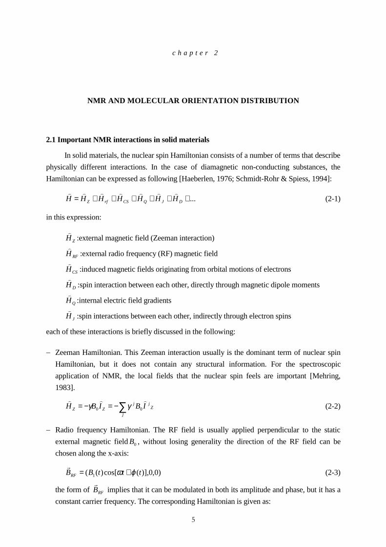
In solid materials, the nuclear spin Hamiltonian consists of a number of terms that describe
physically different interactions. In the case of diamagnetic non-conducting substances, the
Hamiltonian can be expressed as following [Haeberlen, 1976; Schmidt-Rohr & Spiess, 1994]:
...++++++= DJQCSrfZ HHHHHHH�������
(2-1)
in this expression:
ZH�
:external magnetic field (Zeeman interaction)
RFH�
:external radio frequency (RF) magnetic field
CSH�
:induced magnetic fields originating from orbital motions of electrons
DH�
:spin interaction between each other, directly through magnetic dipole moments
QH�
:internal electric field gradients
JH�
:spin interactions between each other, indirectly through electron spins
each of these interactions is briefly discussed in the following:
�� Zeeman Hamiltonian. This Zeeman interaction usually is the dominant term of nuclear spin
Hamiltonian, but it does not contain any structural information. For the spectroscopic
application of NMR, the local fields that the nuclear spin feels are important [Mehring,
1983].
Zj
j
jZZ IBIBH
���
∑−=−= 00 γγ (2-2)
�� Radio frequency Hamiltonian. The RF field is usually applied perpendicular to the static
external magnetic field0B , without losing generality the direction of the RF field can be
chosen along the x-axis:
)0,0)],(cos[)(( 1 tttBBRF ϕω +=G
(2-3)
� the form of RFBG
implies that it can be modulated in both its amplitude and phase, but it has a
constant carrier frequency. The corresponding Hamiltonian is given as:

�
∑+=j
xjj
RF ItttBH��
γϕω )](cos[)(1 (2-4)
� In multiple resonance experiments RFBG
consists of a sum of fields that differ, in particular, in
their carrier frequencies.
�� Chemical Shift interaction Hamiltonian. Under the influence of the 0B field, the electron
cloud generates also an additional field SB which in diamagnetic materials scales with the
field 0B according to:
0BBS
GGσ= (2-5)
� so that the Hamiltonian for the chemical shift interaction of nuclear spins is given:
00 )( BIIIBIH zzLF
zyzLF
yxzLF
xj j
jjjjCS σσσγσγ
���G�G�++=⋅⋅= ∑ ∑ (2-6)
� here, αβσ LF are the elements of the laboratory frame representation of the chemical shift
tensor.
�� Dipolar interaction Hamiltonian. The Hamiltonian of dipolar interactions between nuclear
spins is given as:
∑<
⋅−⋅⋅−=
kj jk
kjjkjk
kjkjk
j
kjD r
IIrrIrrIH
30
)(
)/)(/(3
4
�G�GG�GG
�G
=�
γγπ
µ(2-7)
� where jkrG
defines the vector from nucleus j to nucleus k and jkjk rrG=
�� Quadrupolar interaction Hamiltonian. The Hamiltonian can be written in the form:
i
i
iiii
i
iii
i
iiiii
i
Q
IVIII
eQ
IIIIIVII
eQH
�G�G
�G�����
∑
∑ ∑
⋅⋅−
=
−+−
==
)12(6
])()([)12(6
23
1,23
αβαββα
βααβ δ(2-8)
� where ieQ and iI are the nuclear quadruple moment and the nuclear spin quantum number of
the i th nucleus. αβiV is the second (D, E) derivative of the electric potential at the site of i th
nucleus.
�� Indirect spin-spin coupling Hamiltonian. This term is popularly referenced as J coupling and
it plays a crucial role in solution NMR. It may be expressed as:
∑<
⋅⋅=ki
kikiJ IJIH
�G�G�(2-9)
� where ikJ is also a tensor of rank two.

�
Two properties of the NMR Hamiltonian are emphasised here: firstly, in most cases, the
Zeeman interaction is the dominant term, all local fields experienced by these frequently
investigated nuclei: 1H, 2H, 13C, 15N, 19F, 29Si , 31P are smaller, so that: the energy shifts
originated by these terms can be treated with first-order perturbation theory; Secondly, only
those ‘secular’ parts of the local field terms which commute with zI�
are relevant for the
calculation of energy shifts. After this ‘truncation’, the Hamiltonian for different local field
interactions are given as:
�� chemical shift interaction
∑ ⋅⋅=i
zzLFii
zi
CS BIH 0σγ��
(2-10)
�� hetero-nuclear dipolar coupling
)3)(1cos3(4
221
30 ∑∑ −−=
<j
zk
zj
jkkj jk
SI
DIS II
rH
��=
�θγγ
πµ
(2-11)
�� homo-nuclear dipolar coupling
)3)(1cos3()(
42
21
3
20 k
j
jz
kz
jjk
kj jk
I
DII IIII
rH
�G�G��=
�
∑∑ ⋅−−−=<
θγπ
µ(2-12)
�� quadrupolar interaction
)3()()12(2 2
1 iiz
iz
iLFzz
i
iii
i
Q IIIIVII
eQH
�G�G��
=
�⋅−
−= ∑ (2-13)
2.2 Co-ordinates system
The characterisation of orientation distribution can be performed in terms of various
angles and reference systems, all of them are interrelated to each other. However, some of them
are adequate for the NMR spectroscopy, while others directly describe the distribution of the
structural axes in the sample [Schmidt-Rohr & Spiess]. For the convenience of later discussion,
the definitions of all these angles and co-ordinates systems are described in the following
diagram of fig2-1. Here, we follow Schmidt Rohr & Spiess’s conventions.
�� Laboratory frame, LF. The z axis LZG
of the laboratory frame is defined as the external
magnetic field 0BG
.
�� Sample-fixed Director frame, DF. The primary order direction of the sample is denoted
as the sample director and is usually chosen as the z axis DZG
of the director frame.
�� Molecular frame, MF. Molecular frame is fixed relative to the molecular repeat unit,
usually the local chain axis is chosen as the z axis MZG
of the molecular frame. The three
Euler angles ( MMM ΦΘΨ ,, ) describe the orientation of a given molecular frame in the
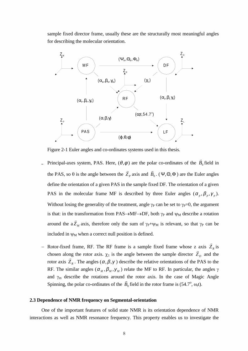
�
sample fixed director frame, usually these are the structurally most meaningful angles
for describing the molecular orientation.
PAS
M F
R F
D F
LF( , , )ϕ θ φ
( , , )Ψ Θ ΦM M M
( , , )α β γP P P
( , , )α β γ( 54.7 )oωrt,
( , , )α β γM M M( )χ1
Z P
Z M
Z L
Z D
Z R
( , )α β γ0 0, 0
� Figure 2-1 Euler angles and co-ordinates systems used in this thesis.
�
Principal-axes system, PAS. Here, (φθ , ) are the polar co-ordinates of the 0BG
field in
the PAS, so T is the angle between the PZG
axis and 0BG
. ( ΦΘΨ ,, ) are the Euler angles
define the orientation of a given PAS in the sample fixed DF. The orientation of a given
PAS in the molecular frame MF is described by three Euler angles ( ppp γβα ,, ).
Without losing the generality of the treatment, angle JP can be set to JP=0, the argument
is that: in the transformation from PASoMFoDF, both JP and \M describe a rotation
around the a MZG
axis, therefore only the sum of JP+\M is relevant, so that JP can be
included in \M when a correct null position is defined.
�� Rotor-fixed frame, RF. The RF frame is a sample fixed frame whose z axis RZG
is
chosen along the rotor axis. F1 is the angle between the sample director DZG
and the
rotor axis RZG
. The angles ( γβα ,, ) describe the relative orientations of the PAS to the
RF. The similar angles ( MMM γβα ,, ) relate the MF to RF. In particular, the angles J
and Jm describe the rotations around the rotor axis. In the case of Magic Angle
Spinning, the polar co-ordinates of the 0BG
field in the rotor frame is (54.7o, Zrt).
2.3 Dependence of NMR frequency on Segmental-orientation
One of the important features of solid state NMR is its orientation dependence of NMR
interactions as well as NMR resonance frequency. This property enables us to investigate the

�
molecular orientation and re-orientation of individual segments. The origin of this angular
dependence lies in the tensorial nature of these interactions [Schmidt-Rohr & Spiess].
In this section, the relationship between the NMR resonant frequency and segmental-
orientations will be derived for the typical case of chemical shift interaction.
2.3.1 chemical shift interaction - static case
If only Zeeman interaction and chemical shift interaction are considered, according to
equation (2-2), (2-5) and using 00 Bγω −= , the Hamiltonian of a specified nuclear spin is:
zzzLF
CSz IHH���
)1(0 σω −=+ (2-14)
this leads to a slow precession of the magnetisation with a frequency:
zzLF
CS σωω 0−= (2-15)
relative to the Larmor frequency 0ω of the unshielded spin. zzLFσ is the z element of the
shielding tensor expressed in the laboratory frame, which depends on the orientation of the
molecular segment relative to 0BG
field. Assume that: )1,0,0(00 BB =G
, the unit vector is
000 / BBbGG
= , then zzLFσ can be written as:
( ) 00
1
0
0
100 sssLFzz
LF bbGG
σσσ =
= (2-16)
this relation is valid with both 0bG
and σ expressed in any co-ordinates system S, since the
bilinear form of the above equation is co-ordinates independent [Schmidt-Rohr & Spiess].
Similarly, CSω can be written as:
PASPASPASsssCS bbbb 000000
GGGGσωσωω −=−= (2-17)
in the last part of equation (2-17), both 0BG
field direction 0bG
and tensor σ are expressed in their
principal value systems (PAS). 0bG
can be described by its polar co-ordinates ),( φθ in the PAS,
PASxxσ , PAS
yyσ , PASzzσ are the principal values of tensor σ . Then, CSω can be further expressed
as:
))(cos)sin(sin)sin(cos(
)()(
2220
000
θσθφσθφσω
σωωα
αααα
PASzz
PASyy
PASxx
PASPASPASCS bb
++=
−= ∑(2-18)

��
if we define the isotropic chemical shift as:
)(31 PAS
zzPAS
yyPAS
xxiso σσσσ ++= (2-19)
then subtract this isotropic chemical shift from each principal values and define:
isoPAS
xxx σσσ −=:
isoPAS
yyy σσσ −=: (2-20)
isoPAS
zzz σσσ −=:
the formula for calculation the resonance frequency can be further simplified, here two cases
with different tensor symmetry are discussed:
�� Case 1: Tensor has axial symmetry with respect to its principal z axis. So that, yx σσ = and
yxz σσσ 22 −=−= , the frequency formula is given as:
)1cos3( 221
0, −−= θσωω zanisoCS (2-21)
� due to this dependence of resonance frequency on molecular segment orientation, in a powder
sample a specific powder line-shape will be observed. In solid NMR, powder means a
isotropic sample of sufficiently rigid materials.
For the case of axial symmetric tensor, the calculation of the powder spectrum is relatively
easy because of the angle φ independence. The principle is that: the integral intensity of
corresponding interval in T and Z is equal:
θθωθω dPdS )())(( = (2-22)
� divided both sides by θd , and re-arrange:
θθδθθωθθω cossin3/)(//)())(( PddPS == (2-23)
for powder samples, )(θP is solely decided by the size of the surface element, θθ sin)( =P
and it is normalised according to ∫ =o
o
dP90
0
1)( θθ . This leads to:
θδθω
cos3
1))(( =powderS , 2
1/3
2cos += δωθ (2-24)
� finally, it is given as:
δωδθω
21
1
6
1))((
+=powderS , δωδ ≤≤−
2(2-25)

��
� the shape of this powder spectrum is shown in fig2-2, it was firstly calculated by
Bloembergen and Rowland in 1953 [Bloembergen and Rowland, 1953]. The centre of the
range covered by this powder spectrum is at 4/)45( δω =o , the centre of gravity is at
0)74.54( =oω .
� Figure 2-2: Powder spectrum for chemical shift tensor with axial symmetry.
�� Case 2: Tensor has no symmetry. In this case, it is useful to introduce two popularly
referenced parameters:
� asymmetry parameter: z
xy
σσσ
η−
=: (2-26)
� anisotropy parameter: zσωδ 0−= (2-27)
� the frequency formula is then given as:
))2cos(sin1cos3(),( 2221 φθηθδφθω −−= (2-28)
when 0=η it is the case of tensor with axial symmetry. The Euler angles ),( φθ of the 0BG
field in PAS are also the Euler angles ),,( arbitaryφθ specifies the Euler transformation from
PAS into laboratory frame. The third Euler angle, corresponding to a rotation around the 0BG
axis is not relevant for the frequency, since the secular interactions are invariant under a
rotation around 0BG
.
The calculation of the powder spectrum for the general case of 0≠η is much more
complicated, it has been treated by Bloembergen and Rowland (1953). Here only the result is
given as shown in fig2-3. The resulting spectra span the range between )1(21 ηδ +− and δ+ .
At yσ the spectrum has maximum intensity which decreases with increasing η .
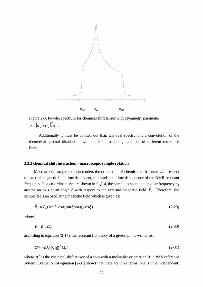
��
Figure 2-3: Powder spectrum for chemical shift tensor with asymmetry parameter
( ) zxy σσση −= .
Additionally it must be pointed out that: any real spectrum is a convolution of the
theoretical spectral distribution with the line-broadening functions of different resonance
lines.
2.3.2 chemical shift interaction - macroscopic sample rotation
Macroscopic sample rotation renders the orientation of chemical shift tensor with respect
to external magnetic field time dependent, this leads to a time dependence of the NMR resonant
frequency. In a co-ordinate system shown in fig2-4, the sample is spun at a angular frequency Zr
around an axis at an angle [ with respect to the external magnetic field 0BG
. Therefore, the
sample feels an oscillating magnetic field which is given as:
)cos,sinsin,cos(sin00 ξϕξϕξBB =G
(2-29)
where
trωϕϕ += (2-30)
according to equation (2-17), the resonant frequency of a given spin is written as:
)( 000 bbB R�G�G
⋅⋅−= σγω (2-31)
where Rσ is the chemical shift tensor of a spin with a molecular orientation R in PAS reference
system. Evaluation of equation [2-31] shows that there are three terms: one is time independent,

��
one oscillates with frequency Zr, and one oscillates with frequency 2Zr [Herzfeld and Berger,
1980].
Z R
Y R
X R
+� ϕ
Figure 2-4: The co-ordinate system with the rotor as the frame of reference. The ZR is the axis of
rotation of the sample. H0 is a unit vector in the direction of the applied magnetic field
( ) ( )( )[ ] ( ) ( )[{( )] [ ]}ϕσϕσξξϕσ
ϕσσξσσξσγξγβαω
sincoscossin22sin
2cossin1cos3,,,,
231312
2211212
332
21
0
RRR
RRRBt
+++
−+−−+−=(2-32)
where σ is the isotropic chemical shift
( ) ( )zzyyxxRRR σσσσσσσ ++=++=
3
1
3
1332211 (2-33)
Rσ depends on the relative orientation of the molecular segment R with respect to PAS system
according to the following expression:
( ) ( )γβασ
σσ
γβασ ,,
00
00
00
,, 1−
= RR
zz
yy
xxR (2-34)
where ( )γβα ,,R is the rotation matrix for the Euler angles γβα ,, describing the orientation of
the molecule segment relative to principal value system in which the chemical shift tensor is
diagonal:
−
−
−=
100
0cossin
0sincos
cos0sin
010
sin0cos
100
0cossin
0sincos
αααα
ββ
ββγγγγ
R (2-35)

��
for further simplification, two general cases are considered:
�� Case 1: 4454 ′′°=ξ , sample is spun at the magic angle position
when 4454 ′′°=ξ the frequency formula of equation [2-32] is simplified to:
[ ] [ ]{ })sin()cos(2)22sin()22cos( 1132
2232
0 rBABAB ++++++++−= ϕγϕγϕγϕσγω (2-36)
where the coefficients are:
[ ]
)(coscossin
)(sincossin
))(sincos(cos))(sincos(cos
)(sin)(coscossin
1
1
22221222
21
2
221
yyxx
yyxx
zzyyzzxx
xxyyzzxx
B
B
A
A
σσβαασσβαα
σσααβσσααβ
σσασσαββ
−−=
−−=
−−+−−=
−+−=
(2-37)
for a powder sample, the free induction decay of the whole sample is given by:
( ) ( )∫ ∫ ∫ ∫
⋅=
− π π πγββαγβαω
πξ
2
0 0
2
0 02 sin,,,exp8
1, 2 ddddttietg
tT
t
(2-38)
where T2 is the transverse relaxation time. The Fourier transform of the free induction decay
consists of a central resonance at the isotropic chemical shift position and a series of spinning
side bands spaced Zr apart from each other. The principal values of the chemical shift anisotropy
can be recovered from the relative intensities of the spinning side bands [Herzfeld and Berger,
1980]. When the spinning speed of the sample Zr is larger comparing with the anisotropy G of
chemical shift interaction of a particular spin, the intensities of the spinning side bands become
non-significant and only the central resonance is reserved. This is the case of high resolution
solid state NMR.
�� Case 2: 4454 ′′°≠ξ , sample is spun at the Off Magic Angle position
In this case, the general frequency formula of equation [2-32] is not easy to be further
analytically simplified. However, in the special case of fast sample spinning: Zr >> G, all
spinning side bands will disappear and the frequency formula is simply given as:
( ) ( )( )[ ]σσξσγξω −−+−= RBt 332
21
0 1cos3, (2-39)
the final spectrum consists of one single anisotropic line located at the isotropic chemical shift
position, its shape resembles the powder line shape. However, the chemical shift anisotropy of
this line is scaled down to ( )( )σσξ −− R33
2 1cos32
1.

��
2.4 Study of orientation distribution from anisotropic NMR interactions
To study the orientation distribution of partially ordered polymer materials by the method
of NMR, an angular-dependent anisotropic interaction of the interested nuclear spins must be
investigated. A number of studies have been reported for partly drawn polymers, in which the
constituent chains are preferentially but not fully oriented [McBrierty, V. J., et al, 1968, 1971,
1973; Kashiwagi, M., et al, 1971,1972,1973]. Three possible NMR anisotropic interactions are
discussed in the following:
2.4.1 The anisotropy of dipole-dipole interaction
By means of the anisotropy of direct dipole-dipole interaction, the most often used nucleus
is 1H. In this case, the dependence of resonance frequency on the orientation of inter-nuclear
vector is given as (for the case of homonuclear interaction):
)1cos3(8
3)1cos3( 2
2,13
210221 −=−= θγγ
πµθδω
r= (2-40)
here T is the angle between the external magnetic field 0BG
and the inter-nuclear vector
connecting nucleus 1 and nucleus 2, r1.2 is the distance between them. The advantage of this
method is its large S/N ratio in the case of 1H & 13F nuclei and correspondingly a very short
measuring time. The main disadvantage is that: overlapping of many dipolar pair-interactions
normally make the resonance line featureless, therefore well defined line-splitting can only be
observed in some special samples. Experimentally, there are several procedures to implement his
strategy:
�� Obtain <P2> from line splitting. But, in practice, well defined line splitting is hardly available
in polymer materials which consist of complicated macromolecules. Due to many possible
structural conformations and motional averaging, usually the final 1H spectrum is a
featureless broad line.
�� Line-shape analysis. In theory, if the exact relative positions of all surrounding spins within
the molecule are known, it is possible to calculate the theoretical line-shape due to dipole-
dipole interactions [Hentschel, Schlitter, Sillescu, Spiess, 1977]. Then, orientation
distribution can be deduced out by a comparison between theoretical and experimental line-
shape. But, because the complicated structural conformations in macromolecular polymers,
the position information of the surrounding spins are hardly possible to be obtained.
�� Moment analysis of the wide-line spectra. This is the classical and the most successful
method which is popularly applied in the case of proton NMR [Van Vleck, 1948; McBrierty,
1993]. The dependence of second and fourth moments of dipolar broadened lines on sample
orientations relative to B0 is a direct reflection of molecular orientations in partially ordered
��
polymers. In principle, it is possible to determine all moments; in practice, constraints arise
from experimental factors such as signal-to-noise ratio. Arbitrary number of experiments for
different sample orientations relative to B0 over-determine the accessible moments [McCall
and Hamming, 1959]. Practically, lower order moments of the distribution are evaluated first
and these are used in fitting of the experimental data to determine moments of higher order.
2.4.2 The anisotropy of quadrupolar interaction
The most popular nucleus used in this scope is duterium 2H, this method is also referenced
as 2H NMR [Spiess, 1984, 1985]. In this case, the spectra are dominated by intramolecular
quadruple interaction between the quadruple moment and the electric field gradient (EFG) tensor
[Hentschel, 1979; Spiess, 1980]. The dependence of resonance frequency on the molecular
segment orientation is given as [Schmidt-Rohr and Spiess, 1994]:
))2cos(sin1cos3(4
3
))2cos(sin1cos3(
2221
2221
φθηθ
φθηθδω
Q
Q
eQeq −−⋅⋅=
−−=
=
(2-41)
here Q is the quadrupolar moment. In aliphatic C-2H bond the asymmetry parameter KQ of the
electric field gradient tensor is negligible ( 0≅Qη ) due to the approximately uniaxiality of the
electron density in this bond [Hentschel, et al., 1976]. This symmetry also causes the unique z
axis of the PAS of the electric gradient tensor to coincide with the C-2H bond direction. This
well defined tensor orientation is of great value in the interpretation of 2H NMR spectra
[Hentschel, 1981].
The advantage of this method is a very clean spectrum with good S/N, almost without any
influence coming from other kinds of spin interactions. The disadvantage is: because the natural
abundance of 2H is very low, usually selective deuteration of the sample is necessary and this
procedure is very expensive as well as very time consuming.
2.4.3 The anisotropy of Chemical Shift interaction
To study the orientation dependence of the chemical shift tensor in terms of structural unit
distributions it is necessary to get (i) undistorted spectra and (ii) tensors are well defined in the
molecular fixed system. Ideally, Chemical shifts which cover a wide range and exhibit
appreciable anisotropies are preferred [McBrierty, 1993]. For this purpose, nucleus 13C and 29Si
are frequently used. With these two nuclei, it is also possible to make Chemical Shift interaction
the dominant term by suppressing all other spin interactions through various ingenious NMR
methods such as dipolar de-coupling, multi-pulse sequence, etc. Several procedures are available
to implement this strategy.

��
�� Direct line-shape analysis. In this approach, the orientation distribution of structural units is
obtained by a direct comparison of the experimental spectrum from the sample in oriented
state and a theoretical powder spectrum. In Principle, this method can characterise the
complete orientation distribution. However, due to the generally existing overlap of different
lines and the „round off“ of spectral line features, it is not adequate for most complicated
macromolecular polymers.
�� Moment analysis. This approach is very similar as the moment analysis of 1H spectra
dominated by dipolar-dipolar interactions. With this method, the orientation degrees (up to
several orders) are directly available. Due to noise in the spectrum, difficulty will arise for the
analysis of higher order moments.
�� Synchronised - MAS 2D procedure: site-resolved orientation measurement [Harbison, 1987].
This experiment is conducted under magic angle spinning and rotor synchronised phase
delays. In the direct dimension, due to slow sample spinning the anisotropic chemical shift
interaction shows up as a number of spinning side bands. Therefore, it leads to a better
resolved, high resolution like spectra. In the indirect dimension, orientation information can
be obtained from the side band patterns.
�� 3D ORDER procedure [Titman et al., 1993]. This is the 3D extension of Harbinson’s 2D
method. In Harbison’s 2D approach, there are apparent overlap of various sideband patterns
although the differences in their isotropic chemical shifts are appreciable. In polymer systems
where the sidebands are broadened by conformational and packing effects, the overlapping is
particular serious. Therefore, a 3D experiment which separate spinning sidebands of different
order according to their isotropic chemical shifts is desirable. In principle this 3D approach
gives a better resolution, but at the expense of long experimental time.
�� DECODER (Direction Exchange with Correlation for Orientation Distribution Evaluation
and Reconstruction) procedure. In this method, the orientation dependent frequency for each
individual segment is measured two or three times by means of 2D or 3D NMR spectroscopy
with a sample flip between the evolution and detection periods [Henrichs, 1987]. In principle,
full orientation distribution can be obtained through the final 2D or 3D correlation spectra
[Schmidt-Rohr et al., 1992; Chmelka et al., 1993], However, in 2D cases overlapping often
impedes the further orientation distribution analysis.
�� VACSY procedure, this is the method we selected for the investigation of molecular
orientation distribution of liquid crystal polymers in solid state. In this method, the separation
& correlation of isotropic and anisotropic interactions is achieved through a number of
independent variable-angle-spinning (VAS) experiments [Frydman et al., 1992]. In the direct
direction, there is no overlapping and all spectral lines are separated according to their

��
Chemical Shift isotropic values; In the indirect direction, the complete orientation distribution
can be derived from the CSA line-shape at different isotropic positions.
2.5 Procedures to extract orientation distribution from NMR line-shape of chemical shift
interaction
There are several procedures available to extract the information about orientation
distribution of chemical shift tensors from the NMR line-shape of chemical shift anisotropic
interaction. Two most popularly applied methods are discussed in the following:
�� direct reconstruction
�� moment analysis
2.5.1 Direct reconstruction procedure
Direct reconstruction is the most direct and most convincing method to obtain the
orientation distribution. In this approach, the orientation distribution of chemical shift tensors is
obtained by a direct comparison of the experimental spectrum from the sample in oriented state
and a theoretical powder spectrum [Hempel G., 1982]
D
E F
G
Figure 2-5: Simulation result of the direct reconstruction approach, the chemical shift tensor
elements used are ( zyx σσσ ,, ) = (100, 100, -100) (ppm). (a) spectrum of isotropic powder. (b)
spectrum with an orientation distribution of Gaussian f unction centred at 30o , hwhm is 23o. (d)
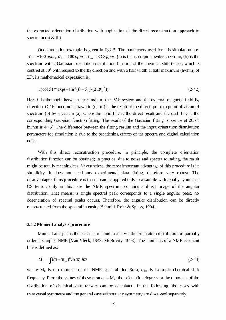
��
the extracted orientation distribution with application of the direct reconstruction approach to
spectra in (a) & (b)
One simulation example is given in fig2-5. The parameters used for this simulation are:
ppm100|| −=σ , ppm100=⊥σ , ppmiso 3.33=σ . (a) is the isotropic powder spectrum, (b) is the
spectrum with a Gaussian orientation distribution function of the chemical shift tensor, which is
centred at 30o with respect to the B0 direction and with a half width at half maximum (hwhm) of
23o, its mathematical expression is:
))2/()(sinexp()(cos 20
2θσθθθ ⋅−−=u (2-42)
Here T is the angle between the z axis of the PAS system and the external magnetic field B0
direction. ODF function is drawn in (c). (d) is the result of the direct ‘point to point’ division of
spectrum (b) by spectrum (a), where the solid line is the direct result and the dash line is the
corresponding Gaussian function fitting. The result of the Gaussian fitting is: centre at 26.7o,
hwhm is 44.5o. The difference between the fitting results and the input orientation distribution
parameters for simulation is due to the broadening effects of the spectra and digital calculation
noise.
With this direct reconstruction procedure, in principle, the complete orientation
distribution function can be obtained; in practice, due to noise and spectra rounding, the result
might be totally meaningless. Nevertheless, the most important advantage of this procedure is its
simplicity. It does not need any experimental data fitting, therefore very robust. The
disadvantage of this procedure is that: it can be applied only to a sample with axially symmetric
CS tensor, only in this case the NMR spectrum contains a direct image of the angular
distribution. That means: a single spectral peak corresponds to a single angular peak, no
degeneration of spectral peaks occurs. Therefore, the angular distribution can be directly
reconstructed from the spectral intensity [Schmidt Rohr & Spiess, 1994].
2.5.2 Moment analysis procedure
Moment analysis is the classical method to analyse the orientation distribution of partially
ordered samples NMR [Van Vleck, 1948; McBrierty, 1993]. The moments of a NMR resonant
line is defined as:
∫ −= ωωωω dSM nison )()( (2-43)
where Mn is nth moment of the NMR spectral line S(Z), Ziso is isotropic chemical shift
frequency. From the values of these moments Mn, the orientation degrees or the moments of the
distribution of chemical shift tensors can be calculated. In the following, the cases with
transversal symmetry and the general case without any symmetry are discussed separately.

��
2.5.2.1 Moment Analysis for a uniaxial system
Here, we assume that the investigated sample exhibits transverse symmetry, both
macroscopically and microscopically. So that the orientation distribution can be described by a
single angle θ which specifies the tensor symmetry axis direction PZG
relative to the external
magnetic field direction LZG
. This distribution function )(θR can be expanded in terms of
Legendre polynomials )(cosθLP , which form a complete set of orthogonal basis functions for
θcos over the interval [0...1].
∑ ><+=L
LL PPLR )(cos)12()( θθ (2-44)
the range 1cos0 ≤≤ θ corresponds to the angle range °≤≤ 900 θ which is sufficient for the
analysis of NMR second-rank tensor orientations [Schmidt-Rohr & Spiess, 1994]. The
coefficients <PL> in (2-44) are often referenced as orientation degrees. Because )(cosθLP
functions are orthogonal, <PL> can be easily calculated as:
θθθ cos)(cos)(1
0
dPRP LL ∫>=< (2-45)
the distribution function is normalised according to:
1sin)(cos)(90
0
1
0
0 ==>=< ∫∫ θθθθθ dRdRP
o
o
(2-46)
<P0> is considered as representing the isotropic part of the distribution. The orientation degrees
<PL> for L>0 contain the information about orientation distribution. Particularly, if the
orientation is centred around o0=θ , <P2> characterise the width of the distribution: the smaller
the <P2>, the larger the width of the orientation distribution )(θR . However, if the distribution
contains isolated G functions which means very sharp peaks, the Legendre Polynomial expansion
is not convergent. For example, if the distribution is ( )θδ , all the orientation degrees <PL> = 1
for L > 1.
For the convenience of data analysis, a few basic properties of the orientation degrees in
the Legendre polynomial expansions and several representative orientation cases are
summarised in the following.
�� if normalisation condition <P0> = 1, all other orientation degrees are in the range [1,-0.5]
�� if all orientation degrees <PL> = 0 when L > 0, then )(θR is isotropic.
�� if all orientation degrees <PL> = 1, the distribution is perfect uniaxial with )(θR = ( )θδ

��
Usually, Gaussian distribution function is used to approximate a real distribution:
)2/sinexp()( 22θσθθ −= NR (2-47)
for Gaussian distribution, all orientation degrees are positive as can be easily proved by actually
evaluating the integrals of equation (2-45). The values of the orientation degrees decrease
monotonically with increasing order L. The orientation degrees of Gaussian distributions as a
function of θσ is shown in fig2-6:
�3 �FRV �!/
θ
σθ
�
�
�
�
�
��
Figure 2-6: dependence of order parameters on the width θσ of a Gaussian orientation
distribution. For this specific type of distribution, the order parameters decrease with increasing
L. For comparing widths of distributions as given in different publications, it may be important
to remember that the full width at half maximum of the Gaussian is 2.35θσ .
For the convenience of later analysis, the values of second order orientation degree <P2> for
some θσ values of a Gaussian orientation distribution are given in table2-1:
acos(VT) 5o 10o 15o 20o 23o 25o 30o 35o 40o
<P2> 0.98 0.91 0.77 0.57 0.45 0.39 0.27 0.20 0.15
From the theory of spectral line-shape analysis for partially ordered polymers developed
by Hentschel et al. [Hentschel, 1978; McBrierty, 1993], assume the sample has (i) fibre
symmetry and the structural units are also transversely isotropic (ii) axially symmetric coupling
tensors, the relationship between the moments nM of NMR line-shape and orientation degree
LP is derived in the following [Hempel, 1998]. The number of tensors which have their

��
symmetry axes in the interval [ ])(coscos,cos θθθ d+ is given as ( ) )(coscos θθ dR , they
contribute to NMR line-shape in the resonant frequency region [ ]ωωω d+, with relative
intensity ωω dS )( . That is:
ωωθθ dSdR )()(cos)(cos = (2-48)
replacing the integrand of equation (2-43) with equations (2-48) and (2-21), we get:
nn
n PM 23
2
∆= σ (2-49)
define:
( )n
nn
n PM
m 2
32
=∆
=σ
and by expanding the powers of 2P into linear sum of Legendre polynomials, for some n values
we get:
"
cscscscs
cscscs
cs
PPPPm
PPPm
Pm
02463
0242
21
35
2
7
3
385
108
77
185
1
7
2
35
18
+++=
><+><+><=
>=<
(2-50)
therefore, the steps to reconstruct the orientation distribution function are:
�� calculate out Mn according to equation [2-43]
�� calculate out <PL> according to equation [2-50]
�� reconstruct orientation distribution according to equation [2-44]
2.5.2.2 Full expansion for non-axial systems
Until now we have restricted our discussion to the case of uniaxial samples with transverse
symmetry in coupling tensors, then the orientation distribution can be expanded in terms of the
Legendre polynomials )(cosθLP . The general case is based on the same principle but more
complicated. In this case, three Euler angles ( )φθϕ ,, are necessary to describe the relative
orientation of chemical shift tensors with respect to LF reference system.
For the general case, the suitable set of basis functions are the Winger functions, the
expansion is given as:

��
),,(),,(0
φθϕφθϕ ∑ ∑ ∑∞
= −= −=
=L
L
Lm
L
Ln
mnL
LmnDPR (2-51)
the Winger functions are orthogonal and the orientation degrees LmnP are the averages of the
orientation-distribution function weighted with the mnLD .
φθϕφθϕφθϕπ
π πdddDR
lP nm
lLmn )(cos),,(),,(
8
12 2
0
1
1
2
0
*,2 ∫ ∫ ∫−
+= (2-52)
),,( φθϕR is normalised according to:
∫ ∫ ∫−=
π πφθϕφθϕ
2
0
1
1
2
01)(cos),,( dddR (2-53)
then, similar steps as in the case of samples and coupling tensors with transverse symmetry
could be used to reconstruct the orientation distribution function.
As mentioned at the beginning of this section, moment analysis is the most frequently
applied procedure to obtain ODF information from 1H NMR spectra. The advantage of this
method is that it is not sensitive to noise. However, when comes to higher moments, the
influence of the noise is drastically enlarged by the term niso)( ωω − in the definition formula of
the moments.
%�
WHQVRU D[LV
PROHFXODU D[LV
GLUHFWRU D[LV
Figure 2-7: The angles used to describe the sample’s orientation distribution. T describes the
angle of chemical shift tensor symmetry axis with respect to external magnetic field B0. G
describes the angle of the sample director direction with respect to the external magnetic field
B0. H is the angle describes the orientation of chemical shift tensor symmetry axis relative to
molecular segment. E is the most important angle which describes the orientation distribution of
molecular segments with respect to the sample director direction.

��
Until now we are only talking about the orientation distribution of chemical shift tensors,
this is the information which can be directly obtained from the NMR spectra under some
reasonable assumptions. However, this orientation distribution information does not have too
much practical meaning, what most interesting to material scientists is the orientation
distribution of molecular segments (MF reference system) with respect to sample director
direction (DF reference system). In order to get molecular segment orientation distribution, some
additional information, such as the angle ε between the tensor symmetry axis PzG
and the
molecular symmetry axis MzG
as indicated in fig2-7, must be available.

��
c h a p t e r 3
NMR METHODS TO MEASURE CHEMICAL SHIFT ANISOTROPY
3.1 Introduction
Cross-Polarisation-magic-angle-spinning (CPMAS) with high-power proton decoupling
[Schaefer, 1976] has been widely applied to obtain high resolution NMR spectra of dilute spin-
1/2 in solids. This method averages out all anisotropic NMR interactions which transform as
second-rank tensors, such as chemical shift anisotropical interactions. However, the principal
elements of chemical shift anisotropy tensor contain useful information on structure, dynamics
and orientation of molecular segments. Attempts to recover these CSA parameters in high
resolution solid-state NMR appeared almost at the same time with the introduction of CPMAS
technique [Lipmaa, 1976; Stejskal, 1977].
Among the different CSA reconstruction schemes, except for the most simplest materials,
overlap of patterns from different groups prevents the valuable information from being extracted
out from one dimensional spectra. Therefore, a variety of two dimensional separation methods
have been proposed to resolve anisotropic line-shapes according to the isotropic frequencies of
individual sites. Some of these techniques rely on static or quasi-static detection and generate the
isotropic evolution by mechanical sample motions, such as: stop-and-go [Zeigler et al., 1988],
magic-angle hopping during evolution [Bax et al., 1983a], flipping of sample rotation axis from
MAS to OMAS [Bax et al., 1983b; Terao et al., 1984; Maciel et al., 1985], variable-angle
correlation spectroscopy (VACSY) [Frydman et al, 1992a, 1992b, 1993, 1994; Lee et al., 1994;
Sachleben, 1997], ultra slow MAS with three periods of evolution [Gan, 1882; Harper et al.,
1998; Hu et al., 1994; McGorge et al., 199], etc. The reliability and good resolution of the quasi-
static spectrum obtained by using these methods are very important. Except the recently
introduced ultra-slow MAS approach, all the techniques mentioned above can not be performed
on standard MAS equipment.
Another category of methods that are based on re-introducing the anisotropic interaction
by 180o pulses synchronised with sample spinning at magic angle position are developed to
avoid the severe requirements on hardware equipment. These pulses usually involve the
evolution period of the experiments, while the detection period acquires the normal MAS signal.
In general, due to the multiple 180o pulses applied during the evolution, these techniques are
very sensitive to experimental imperfections, which can severely distort the powder patterns; the
resolution is also reduced compared with the methods of static detection.
��
In order to explain why we choose VACSY for this work, some of the above mentioned
methods are briefly discussed in the following.
3.2 Methods to retrieve CSA patterns
3.2.1 Stop-and-go
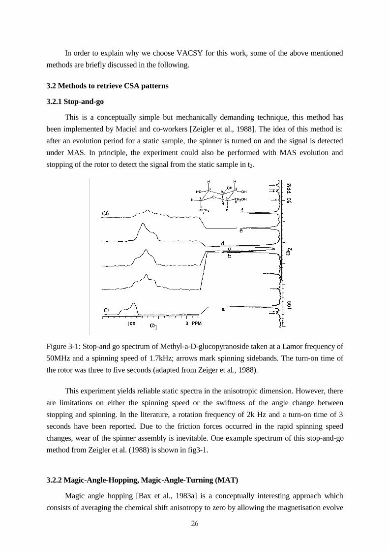
This is a conceptually simple but mechanically demanding technique, this method has
been implemented by Maciel and co-workers [Zeigler et al., 1988]. The idea of this method is:
after an evolution period for a static sample, the spinner is turned on and the signal is detected
under MAS. In principle, the experiment could also be performed with MAS evolution and
stopping of the rotor to detect the signal from the static sample in t2.
Figure 3-1: Stop-and go spectrum of Methyl-a-D-glucopyranoside taken at a Lamor frequency of
50MHz and a spinning speed of 1.7kHz; arrows mark spinning sidebands. The turn-on time of
the rotor was three to five seconds (adapted from Zeiger et al., 1988).
This experiment yields reliable static spectra in the anisotropic dimension. However, there
are limitations on either the spinning speed or the swiftness of the angle change between
stopping and spinning. In the literature, a rotation frequency of 2k Hz and a turn-on time of 3
seconds have been reported. Due to the friction forces occurred in the rapid spinning speed
changes, wear of the spinner assembly is inevitable. One example spectrum of this stop-and-go
method from Zeigler et al. (1988) is shown in fig3-1.
3.2.2 Magic-Angle-Hopping, Magic-Angle-Turning (MAT)
Magic angle hopping [Bax et al., 1983a] is a conceptually interesting approach which
consists of averaging the chemical shift anisotropy to zero by allowing the magnetisation evolve
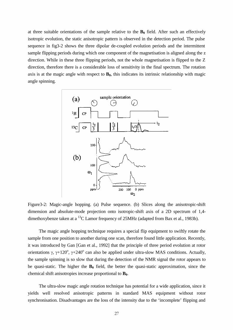
��
at three suitable orientations of the sample relative to the B0 field. After such an effectively
isotropic evolution, the static anisotropic pattern is observed in the detection period. The pulse
sequence in fig3-2 shows the three dipolar de-coupled evolution periods and the intermittent
sample flipping periods during which one component of the magnetisation is aligned along the z
direction. While in these three flipping periods, not the whole magnetisation is flipped to the Z
direction, therefore there is a considerable loss of sensitivity in the final spectrum. The rotation
axis is at the magic angle with respect to B0, this indicates its intrinsic relationship with magic
angle spinning.
Figure3-2: Magic-angle hopping. (a) Pulse sequence. (b) Slices along the anisotropic-shift
dimension and absolute-mode projection onto isotropic-shift axis of a 2D spectrum of 1,4-
dimethoxybenze taken at a 13C Lamor frequency of 25MHz (adapted from Bax et al., 1983b).
The magic angle hopping technique requires a special flip equipment to swiftly rotate the
sample from one position to another during one scan, therefore found little application. Recently,
it was introduced by Gan [Gan et al., 1992] that the principle of three period evolution at rotor
orientations J, J+120o, J+240o can also be applied under ultra-slow MAS conditions. Actually,
the sample spinning is so slow that during the detection of the NMR signal the rotor appears to
be quasi-static. The higher the B0 field, the better the quasi-static approximation, since the
chemical shift anisotropies increase proportional to B0.
The ultra-slow magic angle rotation technique has potential for a wide application, since it
yields well resolved anisotropic patterns in standard MAS equipment without rotor
synchronisation. Disadvantages are the loss of the intensity due to the ‘incomplete’ flipping and

��
the relaxation of the transverse magnetisation components in the storage periods of the
evolution.
3.2.3 Fast flipping between MAS and Off-MAS
From the discussion in section 2.3, it is not difficult to understand that quasi-static
chemical shift anisotropy spectra can be obtained in rotating samples if the sample is spun off
the magic angle. This suggests a switching angle sample spinning (SASS) 2D experiment with
OMAS evolution, flip of the sample spinning axis to the magic angle, and MAS detection. The
magnetisation is stored along the z axis during the sample flip, producing an ( )11cos tϖ or
( )11sin tϖ amplitude modulation of the magnetisation detected during t2. With an angle T
between the rotation axis and B0, the OMAS spectrum corresponds to the static spectrum scaled
by )1cos3( 221 −θ , if the signal is sampled at multiples of the rotor period, that means tdw=tr.
However, if the signal is not sampled at multiples of the rotor period and the sample spinning
speed is smaller than the anisotropy parameters, spinning sidebands appear in both direct and
indirect dimensions. Moreover, the line-shape of the central band or any arbitrary sideband is not
the same as its corresponding static CSA line-shape [Tekely, 1998].
The anisotropic spectrum can always be fitted into the restricted spectral range of 1/tr by
choosing a sufficient small OMAS scaling factor, typically used is Tr=Tm+4o. This is actually
very convenient in practice, since it involves only small flip angles. If the isotropic shift is
outside the 1/tr range, the spectrum is aliased, but the information is not lost. Through re-
arranging the Z1 data cyclically, the standard representation can be recovered. The pulse
sequence for implementing this MAS and OMAS fast flipping method is shown in fig 3-3.
Figure 3-3: Sequence applied in 2D NMR approach for obtaining 13C CSA powder patterns
identifiable with individual isotropic chemical-shift averages (adapted from Gary E. Maciel,
1985).
The disadvantages of this method are twofold: (i) it requires a special equipment which
can realise the swift MAS-OMAS flipping and make sample spinning stable within one scan,

��
this is technically very demanding. (ii) the loss of magnetisation by flipping only one component
of magnetisation onto z axis and by relaxation during the storage time of the magnetisation.
3.2.4 Tycko’s 4-S-pulses method
Even under the conditions of fast magic angle spinning, the complete anisotropic
information is possible to be reintroduced by one or several pairs of rotor-synchronised 180o
pulses per rotation period. For this category of methods, the sample spins at the magic angle at
all times, the signals acquired during the detection period t2 are modulated by spin precession
during the evolution period t1, in which rf pulses are applied in synchrony with the sample
rotation [Tycko et al., 1989]. The RF pulses prevent sample spinning from averaging out the
CSA during t1. Fourier transformation with respect to t1 and t2 yields a two dimensional
spectrum with CSA patterns along one axis and isotropic chemical shift along the other. The
CSA patterns of in-equivalent nuclei are resolved in the two dimensional spectrum as long as the
in-equivalent nuclei have resolved isotropic shifts in the one dimensional MAS spectrum.
Several versions of this two dimensional „MAS/CSA“ technique have been proposed,
differing in the details of the rf pulses applied during t1[Alla et al., 1978; Yarim-Agaev et al.,
1982; Bax et al., 1983c]. A common feature of these versions of the MAS/CSA technique is the
fact that the CSA patterns in the two dimensional spectrum do not, in general, have the same
shapes as do one dimensional CSA patterns of stationary sample. In a recently introduced
approach from Tycko et al. [Tycko et al., 1989], it is demonstrate that: such distortions can be
avoided. The minimum number of 180o pulses required is four. The pulse sequence used in
Tycko’s MAS/CSA approach is shown in fig 3-4:
Figure 3-4: Pulse sequence for two-dimensional MAs/CSA experiment. The sample spins at the
magic angle with rotation period t. During the t1 interval, which is incremented in units of t, a
sequence of p pulses (in this case, four per rotation period) applied to 13C nuclei prevents the
chemical-shift anisotropy from being averaged out by magic-angle spinning. If the p pulses are

��
given at properly chosen times within the rotation period, chemical-shift-anisotropy powder
patterns with the same line-shapes as are observed in stationary samples are obtained in the t1
dimension of the two-dimensional spectrum. The p/2 pulse at the end of t1 allows purely
absorptive spectra to be obtained (adapted from Tycko, 1989).
This multi-180o pulse MAS method has the important practical advantage that it can be
performed on a standard MAS equipment and it can be applied to samples with short T1
relaxation times. The disadvantages are: firstly, the rotational resonance of 1H dipolar interaction
seriously broadens the CSA line-shape. Secondly, when comes to high speed rotation regime,
the approximation: ' (width of 180o pulse) is much smaller comparing with the rotation period tr
is not valid any more, serious CSA line-shape distortion will show up.
3.2.5 RF field modulation
A unique advantage of NMR is that nuclear spin Hamiltonian can be easily manipulated
and modified to severe special purposes, such as the removal of an internal interaction for the
spectral simplification and resolution enhancement, or the recovery of an anisotropic interaction
in solid state MAS NMR by applying proper rf field perturbations [Ernst et al., 1987]. The
predominant advantage of Hamiltonian manipulations by rf modulations is that it does not
require critical adjustments of the experimental parameters like pulse width [Ishii et al., 1998].
Until now, the profiles of most rf modulations for Hamiltonian manipulations are
relatively simple for the ease of the theoretical treatments, such as: switching between a small
number of amplitudes, phases, frequencies and simple continuos modulation fields [Bennett et
al., 1995; Hediger et al., 1997]. More general modulations will certainly provide more flexible
and efficient manipulations without lengthening the cycle times. However, these more
complicated rf fields can not easily be treated theoretically, nor prediction of the response is easy
available. In a publication from Ishii and Terao [Ishii et al., 1998], a general procedure is
proposed to design rf modulations which realise a desirable Hamiltonian manipulation. This
approach provides general solutions, the wave forms of modulations are not always simple. They
have a infinite number of freely adjustable parameters. By properly adjusting such parameters,
the performance of Hamiltonian manipulations can be improved without lengthening the cycle
time.
One example about the application of an amplitude modulation field using Ishii and
Terao’s approach is demonstrated in fig 3-5 to restore chemical shift anisotropy under fast MAS.
While the multiple pulses method proposed by Tycko et al. [Tycko et al., 1989] for recovering
CSA patterns under MAS failed at a spinning speed of 10KHz, this approach of amplitude-
modulated rf field works without any difficulty.
The disadvantages of this method are: firstly, it is quite difficult to design the efficient RF
modulation field for a desired hamiltonian manipulation. Secondly, the manipulation effect of

��
the modulated RF field is sensitive to resonant offset, that is: the difference between the carrier
frequency of the RF field and the isotropic chemical shift frequencies. This makes the method
not adequate for samples which have many resonant lines distributed in a big frequency range.
Figure 3-5: 2D pulse sequences for observation of (a) 13C chemical shift anisotropy and (b)
13C-15N dipolar powder patterns under MAS. After cross polarisation, in (a) the modulated rf
field is applied in the t 1 period to 13C spins to recover the chemical shift anisotropy under
MAS, while it is applied to 15N to recouple the 13C-15N dipolar interaction in (b)(adapted from
Ishii, 1998).
3.2.6 VACSY
Frydman et al [Frydman et al., 1992] introduced that the separation of isotropic and
anisotropic Chemical shift interactions could also be achieved in an effective variable angle
spinning approach. This method is termed as VACSY (Variable Angle Correlation
SpectroscopY). VACSY is the selected method in this work to recover the CSA patterns of solid
state liquid crystal samples in both isotropic state and oriented state. ODF information for
different molecular segments can then be extracted out from these CSA patterns. The theory and
implementation procedure of VACSY are described in chapter 4.
��
c h a p t e r 4
VACSY AND INTERPOLATION OF EXPERIMENTAL DATA
4.1 Introduction
From the discussion in chapter 3, we know that two categories of methods are available to
recover CSA powder patterns: group one - incomplete isotropic averaging is achieved by
spinning fast but off the magic angle, by spinning slowly at the magic angle or by not spinning at
all. This class of techniques requires both swift mechanical motions and storage of the evolving
magnetisation, they are not suitable for samples with a relatively short T1 relaxation time. Group
2 - these approaches rely on the synchronisation of magic angle spinning and radio frequency
pulses. Therefore they are very sensitive to experimental imperfections such as pulse width and
imperfect experimental parameters cause distortions in the final CSA powder patterns.
The effort to search for better methods which can obtain undistorted CSA line-shapes has
never ended. In 1992, a new method, termed as VACSY - Variable Angle correlation
SpectroscopY, was introduced by Frydman et al [Frydman et al., 1992] for correlating
anisotropic and isotropic chemical shifts of in-equivalent nuclei in solid state samples.
A unique feature of this method is that the final spectra are obtained by processing signals
arising from a spinning sample, acquired in independent experiments as a function of the angle
between the axis of macroscopic sample rotation and the external magnetic field direction. This
is in contrast to previously proposed techniques, which are based on either sudden mechanical
sample flipping or multi-pulse sequences. Time evolution of the variable angle spinning signals
is determined by a distribution of resonant frequencies relating the isotropic frequencies of the
spins with their corresponding chemical shift anisotropies. Fourier transformation of this data
results in a two-dimensional NMR spectrum. The pulse sequence of VACSY experiment is
shown in fig4-1.
In VACSY, the change of the sample spinning angle is completed between two
independent experiments. So, it does not put a strict limitation on the T1 relaxation time of the
investigated sample and the requirements for the mechanical performance of the probe are also
relaxed. These are the predominant advantages of VACSY comparing with other approaches.

��
1.0
-0.5
1H
13C
P (cos )2 θ
Figure 4-1: Pulse sequence of VACSY experiment. In the direct dimension: cross polarisation
between 1H and 13C, data is acquired under 1H high power decoupling. In indirect dimension,
angle T can be sampled in an range corresponding to a range of [-0.5,1.0] for P2(cosT).
4.2 Theory of VACSY
Suppose that one wishes to obtain a 2D NMR spectrum of a sample, in which unscaled
isotropic chemical shifts of different sites are correlated with their corresponding full CSA
powder patterns. The usual 2D NMR approach suggests that the spins are allowed to evolve
during a time ta under the exclusive effects of anisotropic interactions, followed by a time ti in
which the spins only process at their isotropic chemical shift frequencies. Regardless of the way
in which these two interactions are separated, this acquisition scheme creates a time domain
space S(ta, ti), associated with independent anisotropic and isotropic evolution frequencies.
If the time domain data S(ta, ti) is sampled properly, the final correlation spectrum I(Za, Zi)
can be calculated as:
( ) ( ) ( )[ ] iaiiaaiaia dtdtttittSI ∫∫ ⋅+⋅−= ωωωω exp,, (4-1)
This Fourier transformation provides a 2D NMR spectrum in which slices parallel to the Za axis
at the isotropic frequencies of the resolved sites show CSA powder patterns.
A NMR experiment like this, which can realise complete separation of unscaled isotropic
and anisotropic interactions, are highly impossible in practical cases. However, it is possible and
relatively simple to measure the time domain signals by acquiring a set of independent Variable-
Angle-Spinning (VAS) NMR signals as indicated by the pulse sequence in fig4-1. This is the
initial idea of VACSY.
Let us consider a system composed of isolated spin ½ nuclei, the dependence of resonance
frequency on CS tensor orientation is given as:
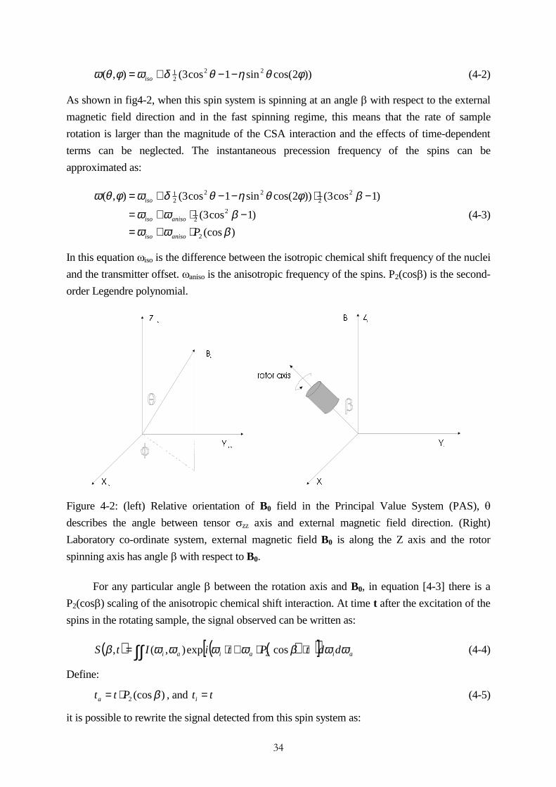
��
))2cos(sin1cos3(),( 2221 φθηθδωφθω −−+= iso (4-2)
As shown in fig4-2, when this spin system is spinning at an angle E with respect to the external
magnetic field direction and in the fast spinning regime, this means that the rate of sample
rotation is larger than the magnitude of the CSA interaction and the effects of time-dependent
terms can be neglected. The instantaneous precession frequency of the spins can be
approximated as:
)(cos
)1cos3(
)1cos3())2cos(sin1cos3(),(
2
221
22122
21
βωωβωω
βφθηθδωφθω
Panisoiso
anisoiso
iso
⋅+=−⋅+=
−⋅−−+=
(4-3)
In this equation Ziso is the difference between the isotropic chemical shift frequency of the nuclei
and the transmitter offset. Zaniso is the anisotropic frequency of the spins. P2(cosE) is the second-
order Legendre polynomial.
=3 $ 6
;3 $ 6
<3 $ 6
%�
%�
=�
;�
<�
URWRU D[LV
Figure 4-2: (left) Relative orientation of B0 field in the Principal Value System (PAS), T
describes the angle between tensor Vzz axis and external magnetic field direction. (Right)
Laboratory co-ordinate system, external magnetic field B0 is along the Z axis and the rotor
spinning axis has angle E with respect to B0.
For any particular angle E between the rotation axis and B0, in equation [4-3] there is a
P2(cosE) scaling of the anisotropic chemical shift interaction. At time t after the excitation of the
spins in the rotating sample, the signal observed can be written as:
( ) ( )( )[ ] aiaiai ddtPtiItS ωωβωωωωβ ∫∫ ⋅⋅+⋅= cosexp),(, 2 (4-4)
Define:
)(cos2 βPtta ⋅= , and tti = (4-5)
it is possible to rewrite the signal detected from this spin system as:
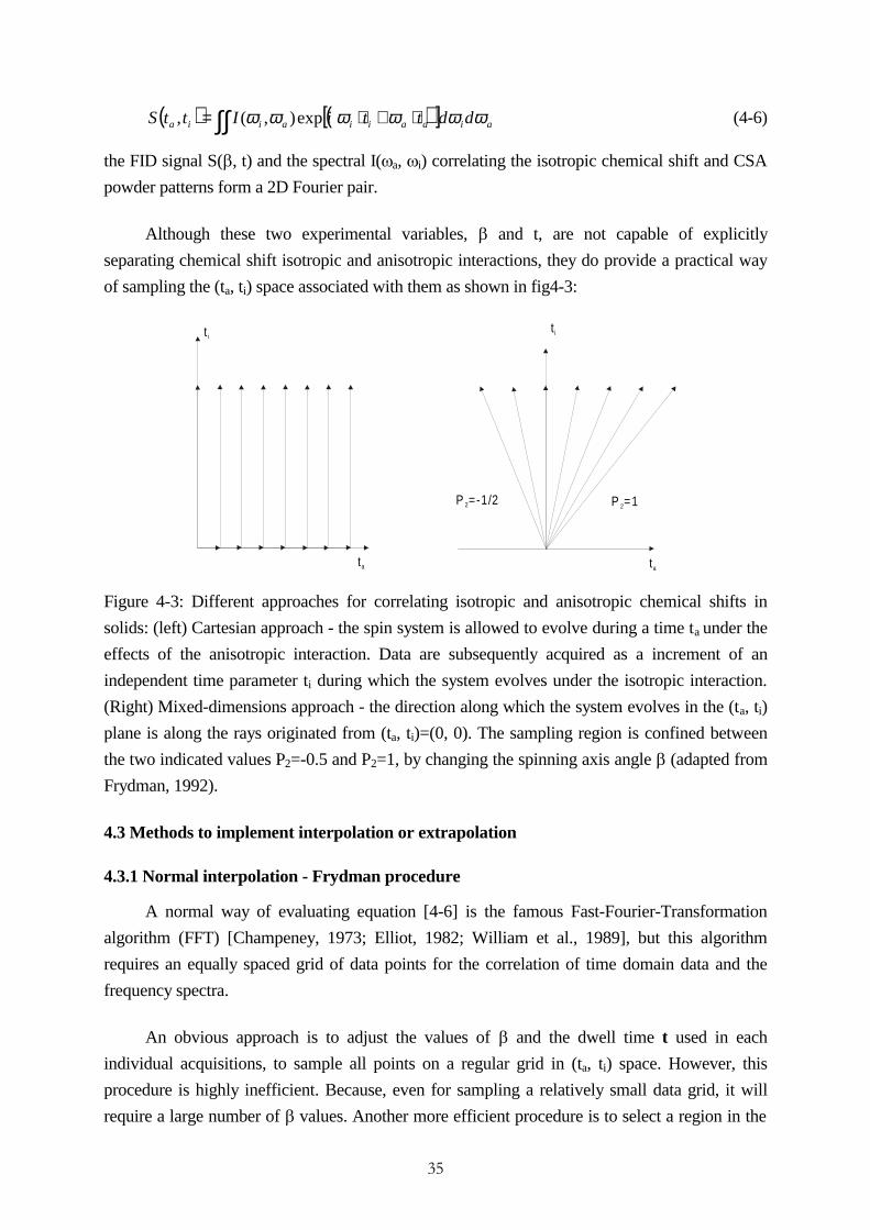
��
( ) ( )[ ] aiaaiiaiia ddttiIttS ωωωωωω∫∫ ⋅+⋅= exp),(, (4-6)
the FID signal S(E, t) and the spectral I(Za, Zi) correlating the isotropic chemical shift and CSA
powder patterns form a 2D Fourier pair.
Although these two experimental variables, E and t, are not capable of explicitly
separating chemical shift isotropic and anisotropic interactions, they do provide a practical way
of sampling the (ta, ti) space associated with them as shown in fig4-3:
ta
P =-1/22 P =12
tit i
ta
Figure 4-3: Different approaches for correlating isotropic and anisotropic chemical shifts in
solids: (left) Cartesian approach - the spin system is allowed to evolve during a time ta under the
effects of the anisotropic interaction. Data are subsequently acquired as a increment of an
independent time parameter ti during which the system evolves under the isotropic interaction.
(Right) Mixed-dimensions approach - the direction along which the system evolves in the (ta, ti)
plane is along the rays originated from (ta, ti)=(0, 0). The sampling region is confined between
the two indicated values P2=-0.5 and P2=1, by changing the spinning axis angle E (adapted from
Frydman, 1992).
4.3 Methods to implement interpolation or extrapolation
4.3.1 Normal interpolation - Frydman procedure
A normal way of evaluating equation [4-6] is the famous Fast-Fourier-Transformation
algorithm (FFT) [Champeney, 1973; Elliot, 1982; William et al., 1989], but this algorithm
requires an equally spaced grid of data points for the correlation of time domain data and the
frequency spectra.
An obvious approach is to adjust the values of E and the dwell time t used in each
individual acquisitions, to sample all points on a regular grid in (ta, ti) space. However, this
procedure is highly inefficient. Because, even for sampling a relatively small data grid, it will
require a large number of E values. Another more efficient procedure is to select a region in the
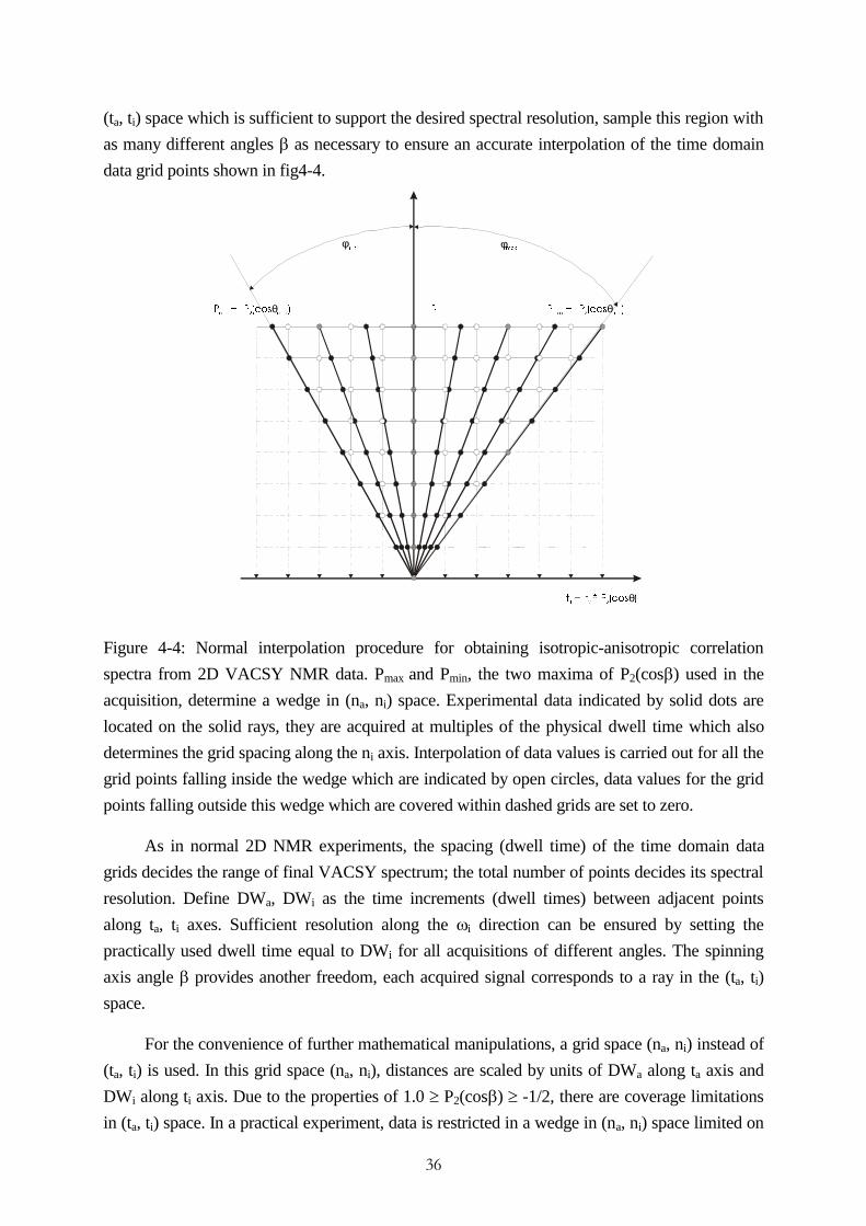
��
(ta, ti) space which is sufficient to support the desired spectral resolution, sample this region with
as many different angles E as necessary to ensure an accurate interpolation of the time domain
data grid points shown in fig4-4.
W W 3 �FRV �� � �
θ
3 3 �FRV �PD[ � PLQ
θW�
φPLQ
φPD[
3 3 �FRV �PLQ � PD[
θ
Figure 4-4: Normal interpolation procedure for obtaining isotropic-anisotropic correlation
spectra from 2D VACSY NMR data. Pmax and Pmin, the two maxima of P2(cosE) used in the
acquisition, determine a wedge in (na, ni) space. Experimental data indicated by solid dots are
located on the solid rays, they are acquired at multiples of the physical dwell time which also
determines the grid spacing along the ni axis. Interpolation of data values is carried out for all the
grid points falling inside the wedge which are indicated by open circles, data values for the grid
points falling outside this wedge which are covered within dashed grids are set to zero.
As in normal 2D NMR experiments, the spacing (dwell time) of the time domain data
grids decides the range of final VACSY spectrum; the total number of points decides its spectral
resolution. Define DWa, DWi as the time increments (dwell times) between adjacent points
along ta, ti axes. Sufficient resolution along the Zi direction can be ensured by setting the
practically used dwell time equal to DWi for all acquisitions of different angles. The spinning
axis angle E provides another freedom, each acquired signal corresponds to a ray in the (ta, ti)
space.
For the convenience of further mathematical manipulations, a grid space (na, ni) instead of
(ta, ti) is used. In this grid space (na, ni), distances are scaled by units of DWa along ta axis and
DWi along ti axis. Due to the properties of 1.0 t P2(cosE) t -1/2, there are coverage limitations
in (ta, ti) space. In a practical experiment, data is restricted in a wedge in (na, ni) space limited on

��
the sides with the highest and lowest P2(cosE) values used, P2max and P2min. The angles Imax and
Imin in (na, ni) corresponding to P2max and P2min with respect to the isotropic axis are given as:
ai
ai
DWDWP
DWDWP
/)tan(
/)tan(
min2min
max2max
⋅=⋅=
φφ
(4-7)
if N independent variable angle spinning experiments are carried out, the angles Ii which consist
of a uniform sampling of the (na, ni) space are given as:
1
1)( minmaxmin −
−⋅−+=N
ii φφφφ , Ni ,...,2,1= (4-8)
from this set of the angles {Ii} the actual values of the angles {Ei} used in N independent
variable angle spinning experiments are given as:
21
3
1/)tan(2cos 1
+⋅⋅= − iia
i
DWDW φβ (4-9)
.,...,2,1 Ni =
experimental experience shows that in the range of 0.5 t P2(cosE) t -0.5, with the total number
of independent VAS experiments less than 30, satisfactory spectra can be obtained. This is due
to the fact that: in the range of 1.0 t P2(cosE) t 0.5, the angle E is small and the coil is
approximately in parallel to the external magnetic field direction, therefore its efficiency to
detect NMR signal is drastically reduced. Therefore, the signal intensity of the VAS experiments
corresponding to the angles in this range is reduced and therefore non-significant for data
interpolation.
After the finish of N independent VAS experiments, the acquired data are used to
interpolate a regular 2D array in the region between Imax and Imin in (na, ni) space. Because
signals corresponding to different spinning angles are digitised using an equal dwell time DWi,
on the grid, the positions to be interpolated are always flanked by two data points along ta axis.
These two points are used to linearly interpolate the intermediate positions on the regular grid
until a regular 2D NMR array is generated. The total number of points interpolated along the two
dimensions of the grid are somehow arbitrary. The only requirement is that it should be large
enough to allow the signal decay to zero to obtain maximum resolution.
4.3.2 Normal interpolation plus Linear Prediction
One disadvantage of the conventional 2D VACSY interpolation approach is that it is not
possible to obtain pure-absorption-mode spectra because of phase-twist artefacts which are
inherent to the experiment as shown in fig4-7. The resulting loss of resolution and line-shape
distortions may impede analysis of the experimental spectra.

��
In 2D VACSY experiment, a series of variable angle spinning free-induction decays are
acquired and placed at angles:
[ ])(costan 21 βφ RP−= (4-10)
in (ta, ti) space as shown in fig4-4. Here, ta, ti define the anisotropic and isotropic time axes,
P2(cosE) is the second-order Legendre polynomial, E is the angle of the rotation axis with
respect to the static field direction, R is the ratio of the anisotropic to isotropic spectral width.
Typically, P2 ranges from -0.5 to +0.5, so the signal partially spans two of the quadrants in the
Fourier space. Once the FIDs are acquired and positioned in (ta, ti) space, the grid positions
within this region can be interpolated from the experimental data points. The rest of the (ta, ti)
space is set to zero. The phase artefacts inherent to the 2D VACSY spectrum are due to the
incomplete sampling in these two quadrants.
In general, phase artefacts in an NMR spectrum are due to the incomplete sampling of the
time-domain Fourier space. Many procedures have been developed to do zero order and first
order phase corrections [Wachter et al., 1989; Montigy et al., 1990; Van Vaals et al., 1990]. In
the case of one-dimensional NMR signal:
[ ]∫∞
∞−
= ωωω dtiItS exp)()( (4-11)
the spectral intensity distribution I(Z) and the FID signal S(t) form a Fourier pair. However, the
final experimental spectrum )(ωI ′ must take into account line broadening and truncation of the
signal. Assume that all spectral components have the same Lorentzian line broadening, )(ωI ′ is
the convolution of I(Z) with a Lorentzian-point-spread function (PSF), P(Z) [Lee et al., 1995]:
)(*)()( ωωω PII =′ (4-12)
if the signal covers the full Fourier space for positive and negative time, P(Z) is an absorption
Lorentzian line-shape. )(ωI ′ is then simply the broadened form of I(Z). If the signal spans only
half of the Fourier space for positive time, P(Z) is complex valued function:
2222
)()()(
λωω
λωλ
ωωω
++
+=
+=
i
iDAP(4-13)
here A(Z) and D(Z) are the absorption and dispersion Lorentzian line-shapes, O is the
exponential relaxation factor. In both cases the real part of P(Z) has the same line-shape, the
same spectral information is available from covering either all or just half of the time-domain
Fourier space as shown in fig4-5.

��
Figure 4-5: One-dimensional Lorentzian point-spread function (PSF), P(w). (a) Complete signal
acquired for positive and negative time; P(w) is then a real Lorentzian line-shape. (b) Signal
acquired only for t>0. The real component is an Lorentzian line-shape, while the imaginary
component becomes a dispersion line-shape (adapted from Y. K. Lee, 1995).
The same principle applies to higher dimensions. In the case of two-dimensional NMR
signal:
[ ]∫ ∫∞
∞−
∞
∞−
+= 2122112121 )(2exp),(),( ωωωωωω ddttiIttS (4-14)
the experimental spectrum ),( 21 ωωI ′ is a two-dimensional convolution of the spectral density
distribution I(Z1,Z2) with the 2D PSF function P(Z1,Z2). If there is no truncation and the signal
spans the complete Fourier space, P(Z1,Z2) is a 2D pure absorption Lorentzian line-shape. If
only half the Fourier space is acquired by truncating the signal for t2<0, P(Z1,Z2) is complex
valued function:
[ ][ ])()()()(2
)()()(2),(
22112211
22221121
ωωωωωωωωω
DiAAA
iDAAP
+=+=
(4-15)
where A1(Z1) is the absorptive component in Z1, A2(Z2) and D2(Z2) are absorptive and
dispersive components in Z2. The pure-absorptive line-shape A1(Z1)A2(Z2) can be obtained by
sampling only half of the full Fourier space. Obviously, similar results will be obtained by
truncating the signal along t1 dimension rather than t2 dimension.
In the case of both t1 and t2 dimensions are truncated, that is: only one quadrant in the
Fourier space is acquired, then both the real and imaginary parts of P(Z1,Z2) show positive and
negative lobes due to the mixing of the absorptive and dispersive components.

��
[ ] [ ][ ] [ ])()()()()()()()(
)()()()(),(
2211221122112211
2222111121
ωωωωωωωωωωωωωω
ADDAiDDAA
iDAiDAP
++−=+⋅+=
(4-16)
and pure absorption line-shapes are no longer possible as shown in fig4-6 [Lee et al., 1995].
Figure 4-6: Two-dimensional Lorentzian PSF, P(w1,w2), in conventional 2D NMR experiments.
(a) P(w1,w2) for signal acquired in all four quadrants of the time-domain, P(w1,w2) is a real 2D
Lorentzian line-shape. (b) P(w1,w2) for signal acquired in two of the four quadrants. The real
component of P(w1,w2) remains a 2D absorption Lorentzian line-shape, a1(w1)a2(w2), while the
imaginary component is a mixture of absorptive and dispersive terms. (c) P(w1,w2) for signal
acquired in only one quadrant. P(w1,w2) contains a mixture of absorptive and dispersive terms in
both the real and imaginary components (adapted from Y. K. Lee, 1994)
Back to the case of VACSY, consider the PSF function P(Za, Zi) for the case of R=2 and
+0.5 t P2 t -0.5. Since I ranges form -45o to +45o, the total area of the Fourier space covered by
the VACSY signal is equivalent to one quadrant, so P(Za, Zi) is similar in form to P(Z1,Z2) in
fig4-6. The artefact ridges become less intense when R increases and a larger area of the Fourier
space contains experimental data. Unfortunately this is achieved at the cost of spectral resolution
in the anisotropic dimension and increased interpolation error.
The spectral artefacts shown in Figure 4-7 are special to 2D VACSY experiments due to
the unconventional truncation and interpolation of time domain data. Often these artefacts may
be ignored, particularly when the spectrum is dominated by broad anisotropic patterns. Because
the artefacts are also broadened, then the interference between different sites becomes

��
negligible. This explains the success of 2D VACSY despite the artefacts inherent to the
technique. However, these artefacts can become a serious problem when the spectrum contains
closely spaced isotropic shifts with small anisotropies. The ridge artefacts emerging from a
narrow site may interfere with the anisotropic patterns of neighbouring sites, causing serious
line-shape distortions. The removal of such artefacts becomes especially important when there
are partially overlapping or a continuos distribution of isotropic shifts, or when accurate line-
shape analysis is required as in the study of partial molecular ordering in this work.
Artefacts in 2D VACSY spectra can be reduced if the missing data points in the signal
Fourier space (ta, ti) can be extrapolated using the experimental data [Lee et al., 1995]. However,
due to the large number of missing data points, the extrapolation technique must maintain
accuracy over several periods of the signal. Linear prediction with singular-value decomposition
LPSVD is one such technique which has been used for extrapolation and spectral estimation in
NMR [Rutledge (Ed.), 1996; Barkhuijsen et al., 1985; Stephenson, 1988; Kumaresan et al.,
1982, Kay, 1988].
The LPSVD method assumes the signal to be a time series represented by a sum of
decaying exponentials with additional white Gaussian noise:
[ ]∑=
++−=M
mdmmmn nwntiay
1
)()()(exp δλω (4-17)
1,,2,1 −= Nn "
where am, Zm, Om are the complex amplitude, frequency and damping factor of each exponential
term, respectively. M is the total number of exponential components, td is the dwell time of the
time series signal, N is the total number of points in the time series, G is an integer that specifies
the shift from the time origin to the first sample data point.
The general procedure of LPSVD computation is outlined briefly in the following. A set of
linear prediction equations in the backward prediction mode is given as:
−=
⋅
−−−++−−
+
1
1
0
1
1
0
11
132
21
LNLNLNLN
L
L
y
y
y
b
b
b
yyy
yyy
yyy
##
"
#%##
"
"
(4-18)
or in a compact form as:
hAb −= (4-19)

��
where b is the vector of the backward LP coefficients, A is the (N-L)uL data matrix, h is the data
vector with N-L components. The number of LP coefficients (prediction order), L, is bounded by
N-M t L t M, typically is set to 0.75N [Kumaresan et al., 1982].
The singular-value-decomposition (SVD) of the matrix A is written as a product of three
matrices [Kay, 1988]:
+
= V
O
SUA (4-20)
where V+ denotes Hermitian conjugate; U and V are orthogonal matrices of dimensions (N-L)
u(N-L) and LuL respectively. S is a diagonal matrix with the singular values as its diagonal
elements ( ){ }LNLkk −= ,min,,2,1, "σ . O is a null matrix. Denoting the column vectors of the
matrices U and V by { }LNuuu −"21 and { }Lvvv "21 , the backward linear
prediction coefficients are computed as:
∑=
+−=M
mmm
m
Vhub1
)(1
σ(4-21)
where the summation limit M truncates the SVD solution for b. For low noise data, M is simply
the total number of peaks in the spectrum; However, if the data contains significant noise, M
becomes an adjustable parameter [De Beer et al.,, 1988; Lin et al., 1993]. Once the backward LP
coefficients have been calculated, the missing data points in the time series can be extrapolated
as:
∑=
+−=L
kknkn yby
1
, ( )δ−−−= ,,2,1 "n (4-22)
where n=-G defines the data point at the time origin. To take advantage of the signal-to-noise
ratio improvements in LPSVD, the entire time series should be reconstructed by calculating out
the spectral parameters associated with the data set. The parameters, Zm and Dm can be obtained
by constructing a polynomial:
LL zbzbzbzP −−− ++++= *2*
21*
11)( " (4-23)
which has roots at [ ]mmm iz αω += exp . The complex amplitude am can then be obtained by
substituting Zm and Dm into equation [4-17]. Fig4-7 shows an example of the LPSVD procedure
applied to a 2D VACSY simulation spectrum, the improvement in spectral resolution is
significant.

��
Figure 4-7: Simulation of 2D VACSY spectra. The simulations are using R=2, td=200 us, and
three sites with chemical shift tensors: (Vxx, Vyy, Vzz) = (0.3, 1.0, 2.3), (-0.5, -0.5, -1.5), (-2.5, -
2.0, -1.0)(kHz). (a) Normal phased 2D VACSY spectrum obtaining using +0.5tP2t-0.5 and
R=2. The area of Fourier space outside of the shaded region is set to zero. The 2D spectrum
reveals the phase artefacts inherent to the normal 2D VACSY experiment. The projection onto
the Za axis yields a constant function, whereas the projection onto the Zi axis yields the pure
absorption isotropic spectrum. (b) 2D VACSY spectrum after extrapolation using LPSVD. The
area set to zero in (a) is extrapolated from the interpolated simulation data in the shaded region.
LPSVD is used to extrapolate the data in each slice, parallel to the ta axis, to the ti=0 point. the
phase artefacts are eliminated from the 2D spectrum. The projection onto the Za axis yields the
overlap of the different traceless anisotropic powder patterns, while the projection onto the Zi
axis again yields the isotropic MAS spectrum.
4.3.3 Non-orthogonal interpolation
The interpolation procedure introduced in section 4.3.1 can not obtain pure-absorptive 2D
VACSY spectrum, distortions of CSA line-shape patterns due to phase artefacts are impossible
to be eliminated. The LPSVD procedure introduced in section 4.3.2 is capable to extrapolate the
missing data points and obtain a clean pure-absorptive VACSY spectrum. However, if the
experimental data contains significant noise this procedure may fail or give apparently incorrect
results.
Here, a new interpolation procedure, termed as non-orthogonal interpolation, is proposed
by G. Hempel and successfully implemented by us. In this procedure, the experimental data are
interpolated to a non-regular grid based on two axes z1, z2:
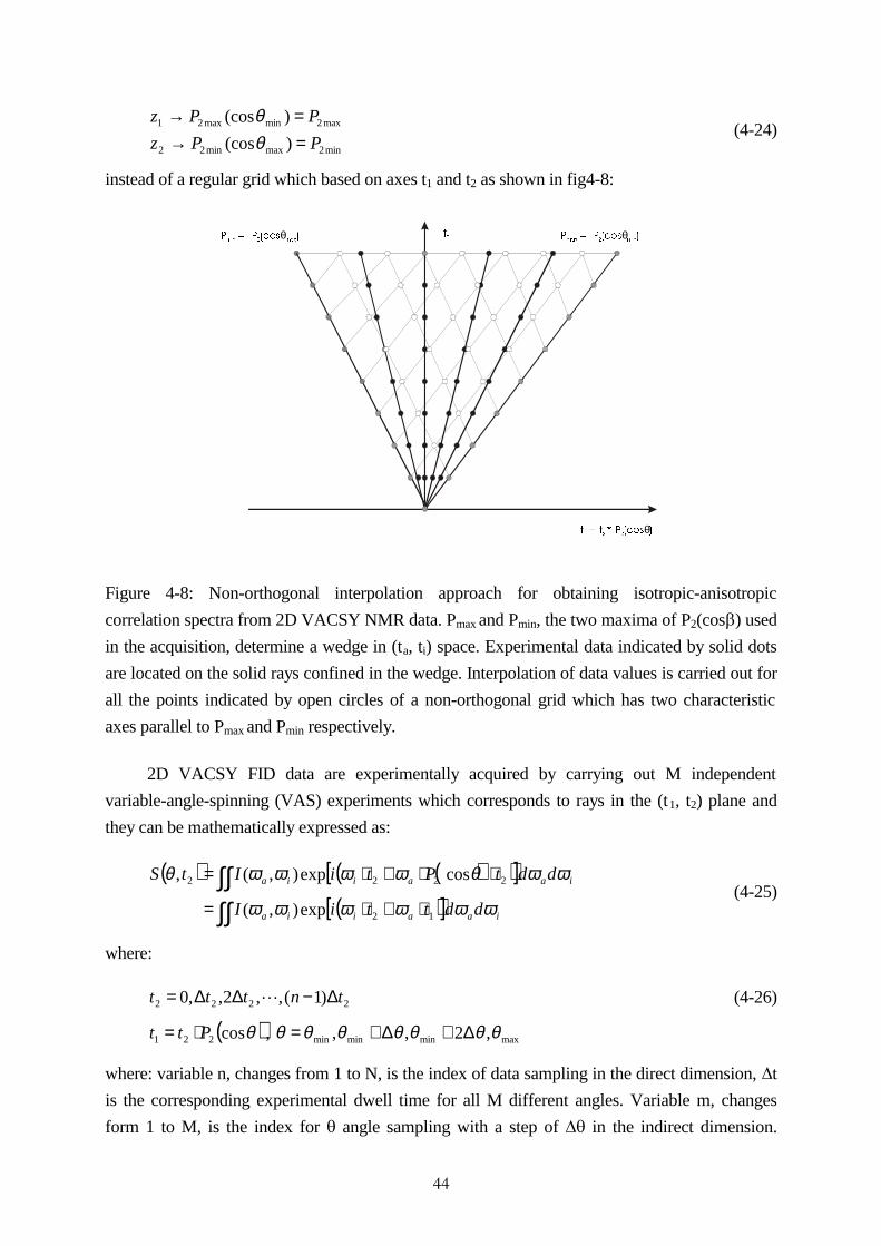
��
min2maxmin22
max2minmax21
)(cos
)(cos
PPz
PPz
=→=→
θθ
(4-24)
instead of a regular grid which based on axes t1 and t2 as shown in fig4-8:
W W 3 �FRV �� � �
θ
3 3 �FRV �PLQ � PD[
θ 3 3 �FRV �PD[ � PLQ
θW�
Figure 4-8: Non-orthogonal interpolation approach for obtaining isotropic-anisotropic
correlation spectra from 2D VACSY NMR data. Pmax and Pmin, the two maxima of P2(cosE) used
in the acquisition, determine a wedge in (ta, ti) space. Experimental data indicated by solid dots
are located on the solid rays confined in the wedge. Interpolation of data values is carried out for
all the points indicated by open circles of a non-orthogonal grid which has two characteristic
axes parallel to Pmax and Pmin respectively.
2D VACSY FID data are experimentally acquired by carrying out M independent
variable-angle-spinning (VAS) experiments which corresponds to rays in the (t1, t2) plane and
they can be mathematically expressed as:
( ) ( )( )[ ]( )[ ]∫∫
∫∫⋅+⋅=
⋅⋅+⋅=
iaaiia
iaaiia
ddttiI
ddtPtiItS
ωωωωωω
ωωθωωωωθ
12
2222
exp),(
cosexp),(,(4-25)
where:
2222 )1(,,2,,0 tnttt ∆−∆∆= " (4-26)
( )θcos221 Ptt ⋅= , maxminminmin ,2,, θθθθθθθ ∆+∆+=
where: variable n, changes from 1 to N, is the index of data sampling in the direct dimension, 't
is the corresponding experimental dwell time for all M different angles. Variable m, changes
form 1 to M, is the index for T angle sampling with a step of 'T in the indirect dimension.

��
Directly after signal acquisition, an arbitrary VACSY FID data point of the mth independent
experiment at time tn ∆⋅ in co-ordinates system { }t t1 2, is expressed as:
( ) ( )( )[ ]
⇒
∆⋅⋅∆+⋅+∆⋅⋅= ∫∫
n
nP
ddtnmPtniInmFID
m
iaaiiat ωωθθωωωω 2min22 )cos(exp),(,
(4-27)
and:
( )( )θθ ∆+= mPPm min2 cos (4-28)
In the following discussion, the co-ordinate of this data point in co-ordinates system { }t t1 2, is
denoted as: { }nP nm,
Now we change the co-ordinates system from { }t t1 2, to { }z z1 2, , where: z1 is along max2P
direction and z2 along min2P direction, they are the two base vectors of co-ordinates system
{ }z z1 2, . In co-ordinates system { }t t1 2, , z1 and z2 can be expressed as following:
=
1max2
1
Pz� ,
=
1min2
1
Pz� (4-29)
therefore, the transformation matrix from co-ordinates system { }z z1 2, to { }t t1 2, is given as:
=
2
1min2max2
2
1
11 z
zPP
t
t(4-30)
Because the data set tnmFID ),( obtained directly form VAS acquisitions do not fulfil the 2D FT
requirements, they must be interpolated to the new data set zjiFID ),( on the non-regular grid
points.
In co-ordinates system { }z z1 2, , that is: in the non-regular grid space, if we focus on an
arbitrary data point zjiFID ),( , it should have a co-ordinate (i, j)z. Using the transformation
matrix in equation (4-30), the co-ordinate of the same data point in co-ordinates system { }t t1 2,
can be written as:
( ) ( ) ( )( )
+
−++=
+
⋅+⋅=
=
+
ji
PPPji
ji
PjPi
j
iPP
j
iji
j
zt
max2min2max2min2max2min2max2
11(4-31)
from a direct comparison of equation (4-27) and (4-30), it is easy to get that: in co-ordinates
system { }z z1 2, , an arbitrary data point zjiFID ),( has the following co-ordinate in system
{ }t t1 2, :
��
( ) )( max2min2max2' PPji
jPP
jin
m −+
+=
+=(4-32)
So, in { }t t1 2, space, the two nearest data points relative to this one have co-ordinates:
=+
= +
n
nPnmFID
n
nPnmFID m
tm
t1),1(,),( (4-33)
where:
1' +≤≤+=
mmm PPP
jin(4-34)
In space { }z z1 2, , the value of this arbitrary data point zjiFID ),( can then be interpolated
through these two nearby data points tnmFID ),( and tnmFID ),1( + in space { }t t1 2, by the
following equation:
( ) ( ) ( )tmm
mmt
mm
mmz nmFID
PP
PPnmFID
PP
PPjiFID ,1,,
1
1
1
''
+−−
+−−
=+
+
+
(4-35)
In fig4-8, data points indicated by solid circles which are lying on rays originated from (0, 0) are
acquired by M independent VAS experiments, this 2D data array does not fulfil FFT
requirements. Data points which are indicated by open circles form a non-orthogonal grids and
fulfil 2D FFT conditions, these are the data points which should be interpolated from
experimental data by using equation (4-34).
After normal 2D FT evaluation, a non-orthogonal 2D VACSY spectrum is obtained. Due
to a rotation of co-ordinate system { }z z1 2, relative to { }t t1 2, for an angle which is decided by
max2P and min2P as shown in fig4-8, in the final VACSY spectrum the CSA powder patterns are
rotated for the same angle with respect to the VACSY spectrum obtained by the normal
interpolation procedure as shown in fig4-9c. CSI and CSA projections can not be directly taken
from the VACSY spectrum obtained with this non-orthogonal approach, a reverse version of this
non-orthogonal interpolation procedure for the VACSY spectral data is required to rotate the
final spectrum to normal direction, that is: CSI and CSA are parallel to Z1, Z2 directions
respectively. A „four points“ interpolation formula is used to accomplish this smooth reverse
interpolation as shown in fig4-9d, and in the anisotropic direction the final spectrum is scaled for
a known factor comparing with the spectrum in fig4-9c.
A direct comparison of the results of these two interpolation approaches to a simulated
VACSY data is presented in fig4-9. Fig4-9b shows that due to the incomplete data sampling in
(t1, t2) space, the VACSY spectrum obtained from the normal interpolation procedure can not be
displayed in phase sensitive mode. A well accepted fact is that the resolution of a spectrum
displayed in magnitude mode (absolute value mode) or power mode is lower than the same

��
spectrum displayed in phase sensitive mode when its imaginary part in not zero like in the case
of VACSY, and moreover the correct line-shape of a spectrum is also changed when it is
displayed in magnitude mode or power mode. In some cases when good spectral resolution is
highly desirable as in the case of closely spaced isotropic chemical shifts or when accurate line-
shape analysis is required as in the investigation of partial molecular ordering, it is highly
desirable that the spectra can be displayed in phase sensitive mode.
F1 (ppm)-200-150-100-50050100150200
F2(ppm)
-50
0
50
100
150
200
250
300
Figure 4-9a: VACSY simulation spectrum processed by normal interpolation procedure and
displayed in absolute value mode, chemical shift tensor used (Vxx, Vyy, Vzz)=(100, 100, -100)
(ppm).
F1 (ppm)-200-150-100-50050100150200
F2(ppm)
-50
0
50
100
150
200
250
300
Figure 4-9b: VACSY simulation spectrum processed by normal interpolation procedure and
displayed in phase sensitive mode, chemical shift tensor used (Vxx, Vyy, Vzz)=(100, 100, -100)
(ppm).

��
F1 (ppm)-200-150-100-50050100150200
F2(ppm)
-50
0
50
100
150
200
250
300
Figure 4-9c: VACSY simulation spectrum processed by non-orthogonal interpolation procedure
and displayed in phase sensitive mode, chemical shift tensor used (Vxx, Vyy, Vzz)=(100, 100, -
100) (ppm).
Figure 4-9d: A four-points reverse interpolation approach to rotate the spectrum in fig4-9c into
normal directions, displayed in phase sensitive mode, chemical shift tensor used (Vxx, Vyy, Vzz) =
(100, 100, -100) (ppm).
The advantages of the this non-orthogonal interpolation method is that: (i) the CSA line-
shape distortions are somewhat less comparing with the normal interpolation procedure; (ii) the
final 2D VACSY spectrum is possible to be displayed in phase sensitive mode; (iii) comparing
with the LPSVD method, this method can not completely remove phase artefacts as LPSVD
does, but it can be successfully used to process noisy data.

��
4.3.4 VACSY transformation with eigen-coordinates
In all three above mentioned VACSY data processing methods: interpolation,
interpolation plus Linear Prediction and non-orthogonal interpolation methods, the data value of
the desired position in the (t1, t2) space is calculated from experimentally acquired data values by
using various interpolation or extrapolation algorithms. From the principle of interpolation
calculation, it is easy to understand that a difference always exists between the interpolation
result and the theoretical magnetisation evolution. Especially when the direct digitisation index n
[1,...,N] goes to bigger value, where the data point to be interpolated is quite far apart from two
adjacent acquired data points, the error of interpolation becomes bigger. A good interpolation
algorithm can greatly reduce this error, but it can not totally remove this deviation.
In order to reduce the interpolation error as much as possible, G. Hempel proposed another
VACSY data processing approach which obtains the final 2D VACSY correlation spectrum by
directly transforming the experimentally acquired data set without doing any interpolation or
extrapolation. This proposal has been successfully applied to process VACSY
simulation/experimental data by me and it gives satisfied results. The procedure is termed as:
VACSY transformation with eigen-coordinates.
From the mathematical expression of VACSY fid data in equation (4-25), the
corresponding VACSY spectrum can be expressed as:
( ) ( )( )[ ]∫∫ ⋅⋅+⋅= 22222222 cosexp,),( dtdpttPtitPSI aiia θωωωω (4-36)
denote: p=P2(cosT), we have:
( )∫∫ ⋅⋅⋅= dpttpidttitpSI aiia 22222 )exp()exp(,),( ωωωω (4-37)
this is not a normal Fourier transformation. Here, the first time variable is t2, it correlates to Zi in
frequency domain; the second time variable is p multiplies t2, it correlates to Za in frequency
domain. In order to be calculated by computer, the analytical equation (4-36) has to be converted
into its corresponding digital form. The digitisation relation between time variables and
frequency variables are given in the following:
kaa ⋅∆⇒ ωω ; 2222 )(cos tpmPttp m ⋅=∆⋅+⋅⇒⋅ θθ ; knZtpS ⇒),( 2 ;
lii ⋅∆⇒ ωω ; ntt ⋅∆⇒2 ; klkn IZ ⇒ ; (4-38)
The complete transformation is divided into two steps, integration for p�t2 and for t2 respectively.
(i) step one: the integration (this corresponds to summation in digital form) for variable p�t2, the
intermediate result is denoted as Zkn:

��
[ ]
)]exp()exp([2
1
)exp(
maxmax0
1
1
pntkiSpntkiS
pntkiSZ
aMnan
M
mmamnkn
⋅⋅∆⋅⋅∆+⋅⋅∆⋅⋅∆+
⋅⋅∆⋅⋅∆= ∑−
=
ωω
ω(4-39)
a special computer program written in C by us is required to realise this part of data calculation.
The calculation result is stored in VNMR fid data format which can be directly used by VNMR
software for next step processing. (ii) step two: the intermediate result of step one Zkn is firstly
multiplied by ntt ⋅∆=2 , then a normal 1D Fourier transformation is performed. VNMR
software is used for the calculation in this step and all later graphic manipulations. The result
VACSY spectrum processed by this new approach for the same simulation data as in fig4-9 is
shown in fig4-10:
From a direct comparison of fig4-10, fig4-9a, fig4-9b, fig4-9c, fig4-9d, the advantages of
this ‘VACSY transformation with eigen-coordinates’ are: (i) in fig4-10, the projection onto the
isotropic axis is somewhat narrower and the singularities of the projection onto the anisotropic
axis are sharper comparing with the corresponding spectra of fig4-9a. This is because: fig4-10 is
displayed in phase sensitive mode while fig4-9a in absolute value mode. (ii) in fig4-10 the 2D
VACSY spectrum is not rotated like in fig4-9c, this makes the isotropic and anisotropic
projections directly possible. (iii) in fig4-10, outside the region where spectra feature is the
signal intensities are very low comparing with both fig4-9a and fig4-9d. This is due to the fact
that in ‘VACSY transformation with eigen-coordiantes’, there are no interpolation errors.
However, the butter-fly-like phase artefacts surrounding the spectral feature in fig4-10 are still
present. This is due to the incomplete sampling of (t1, t2) space as discussed in section4.3.2, until
now the only available way to remove them is by performing Linear Prediction.
Figure 4-10: VACSY simulation spectrum processed by ‘VACSY transformation with eigen-
coordinates’ procedure and displayed in phase sensitive mode, chemical shift tensor used (Vxx,
Vyy, Vzz)=(100, 100, -100) (ppm).

��
c h a p t e r 5
SIMULATION
5.1 Introduction
VACSY is a method to reintroduce CSA patterns in one dimension and correlate them
with their chemical shift isotropic values in another dimension of a 2D NMR spectrum. In
chapter 2 it has been shown that: from the NMR line-shape of chemical shift anisotropy, the
complete orientation distribution function of partially ordered solid state polymer samples can be
extracted out by various procedures. In all these procedures, an accurate analysis of the CSA
line-shape is required. So, for a successful orientation distribution investigation the most
important step is to obtain a non-distorted CSA patterns of the sample in both isotropic state and
oriented state.
In practical cases, the spectra may have imperfections which originate from:
�� noise
�� phase artefacts arising from in-complete data sampling
�� broadening caused by certain distribution of chemical shift values corresponding to
different structural conformations, residual dipolar interaction from incomplete de-
coupling, etc.
then, many difficulties may arise in the forth-coming orientation distribution analysis. In extreme
cases, some procedures may become not valid any more.
The deterioration of NMR spectra by noise, FT artefacts and broadening is common to all
NMR methods. In general, noise can be reduced by improvement of the RF circuits in the probe
and by using coherent addition of a large number of transitions; FT artefacts can be removed by
careful zero order and first order phase corrections, linear prediction, etc; Line broadening can be
relieved by optimising dipolar decoupling efficiency and by doing experiments in low
temperature region. Many work have been done in this area to solve these problems, now for
most samples a satisfied spectrum can be obtained.
VACSY experiments need a dedicated probe to be implemented, except the reasons
mentioned above there are some special factors which might cause distortions of the CSA line-
shapes if they are not correctly chosen, such as the control accuracy of the angle E which is the
angle between the rotation axis and the external magnetic field direction B0; the deviation of

��
spinning speed from setting value while the rotor is flipped from one angle to another, etc. Even
if the necessary hardware equipment and interpolation software are ready, before a VACSY
experiment is started several important questions special for VACSY have to be understood, for
example:
�� How much a spinning speed is necessary with respect to the CSA value of the
investigated sample to neglect the CSA line-shape distortion of the central spinning
band?
�� How much a control accuracy is necessary to neglect the CSA line-shape distortion due
to the angle E mis-setting?
�� How much a sampling range of the angle E is necessary for the acquisition of a non-
distorted CSA line-shape?
�� How many independent VAS experiments should be carried out for a non-distorted
CSA line-shape?
�� How much a fluctuation in spinning speed is tolerable to achieve a non-distorted CSA
line-shape?
�� etc.
Of course, these answers can be found through many times of try and error experiments. But,
this will be an extremely inefficient way and it also does not guarantee that the optimised
parameters will be fund. A more efficient approach for answering these questions is by using
computer simulation. Computer simulation provides an excellent way to deeply understand the
influence on the final CSA patterns from each individual parameter of a VACSY experiment
5.2 Simulation Program
The dependence of NMR resonance frequency on molecular segmental orientations in the
case of macroscopic sample spinning has been discussed in chapter 2 and the corresponding
equations are given in equations (2-32) - (2-35). For a powder sample, the free induction decay
of the whole sample is given by:
( ) ( )∫ ∫ ∫ ∫
⋅=
− π π πγββαγβαω
πξ
2
0 0
2
0 02 sin,,,exp8
1, 2 ddddttietg
tT
t
(5-1)
where T2 is the transverse relaxation time, (D, E, J) are the three Euler angles which describe the
orientation of PAS system relative to rotor system RF as illustrated in fig2-1. All the simulation
calculations in this thesis are based on equation (5-1) and its corresponding angle definitions

��
given here. For all simulations, FID data are firstly calculated according to equation (5-1), then
Frydman’s normal interpolation procedure and VNMR software from VARIAN are used to get
the final spectra through fast Fourier transformation. The calculation result of ( )tg ,ξ from
equation (5-1) corresponds to the experimental VAS acquisition where the sample spinning axis
has an angle equal to [. A total number of M calculations of ( )tg ,ξ corresponding to the angle [
in a range ([min, [max) form a complete simulation VACSY fid data set.
Equation (5-1) shows that: in order to get the free induction decay of the whole sample
corresponding to one specified angle [ position, three integrals (powder averaging) with respect
to the three Euler angles D, E, J have to be evaluated. If the corresponding part of the simulation
program for this powder averaging is not correctly optimised, the whole VACSY simulation
might be extremely time consuming [Conroy, 1967; Eden et al., 1998; Maricq et al, 1979]]. Two
available procedures to implement this powder averaging are described in the following.
5.2.1 Stepwise procedure
An obvious approach for evaluating the three powder averaging integrals is a step-wise
procedure. This procedure is demonstrated as following:
( ) ( )γ
γ
β
β
α
α
β
βππ π ππππ
γβαγββαγβαα
α
β
β
γ
γN
n
N
n
N
n
N
nfdddf
N
n
N
n
N
n
222)
2sin(,,sin,,
2
0 0
2
0 1 1 1
⋅⋅
⋅⋅⋅⋅
⇒∫ ∫ ∫ ∑∑∑= = =
(5-2)
the three integrals with respect to D, E, J are converted to three summations for the convenience
of digital calculation by computer. D is digitised for ND steps in the range (0, 2S), E is digitised
for NE steps in the range (0, S), J is digitised for NJ steps in the range (0, 2S). The selected values
for ND, NE, NJ depend on the values of the CSA tensor elements of the investigated sample.
Take the case of COO- group in glycine for example, the three principal values of
chemical shift are: 238 ppm, 178ppm and 108ppm. ND=100 NE=100 NJ=30 are normally
necessary for simulation to give a smooth CSA line-shape.
If the numbers of steps ND, NE, NJ are relative large, the total number of calculations
necessary for a smooth simulation of CSA line-shape is NDuNEuNJ. Then, this process might
become very time consuming. On a SUN Sparc workstation, a VACSY simulation with 200
angle [ steps, chemical shift tensor elements: 238 ppm, 178ppm and 108ppm, digitisation
numbers: ND=100 NE=100 NJ=30, takes more than 4 days!

��
5.2.2 CONROY procedure
Harold Conroy proposed a new general method for the numerical integration of functions
with many independent variables [Conroy, 1967]. Apply this procedure to perform powder
averaging, the calculation time is drastically reduced.
In this new method the sample points are distributed systematically rather than at random.
The ensemble of points forms a unique, closed, symmetrical pattern, which effectively fill the
space of the multidimensional integration as shown in fig5-1. This method employs certain
rational constants which control the arrangement of sample points. A table of the constants for
the case of three independent integration variables is given in table 5-1.
0 1 2 3 4 5 6 70,0
0,5
1,0
1,5
2,0
2,5
3,0
3,5 stepwise methodNo. for α: 60, No. for β: 60
β (0
- π)
in 6
0 st
eps
α (0-2π) in 60 steps
0 1 2 3 4 5 6 70,0
0,5
1,0
1,5
2,0
2,5
3,0
3,5
Conroy method, overall number 52number for α: 25, number for β: 15
β (0
- π)
α (0-2π)
Figure 5-1: Comparison between stepwise approach and Conroy approach. (left) Stepwise
approach - random distribution of calculation data points for the case 2D powder averaging, D
from 0 to 2S, E from 0 to S. (Right) Conroy approach - symmetric distribution of calculation
data points for the case of 2D powder averaging, D from 0 to 2S, E from 0 to S.
According to Conroy’s procedure, instead of three integration/summation loops as in the
step-wise procedure, only one integration/summation loop is required. In this single loop,
integration/ summation is calculated form 1 to the selected general integration constant Const0.
D is sampled in the range (0, 2S) with an increment of 2S/Const1. If 0tD or Dt2S then D is
mirrored back to the range of (0, 2S) by using relations -D or 4S-D. Angle E and J are handled
similarly as D but with Connst2 and Const3 respectively.
Const0 Const1 Const2 Const3 52 5 7 11 538 115 241 251 1154 11 369 569 3722 653 1005 1483 6044 595 1359 1865
Table 5-1: Conroy rational constants for the calculation of powder averaging. Const0- overall
rational constant; (Const1, Const2, Const3) - rational constants for angles (D, E, J)

��
Two computer programs for VACSY spectrum simulation are written in C language, one
uses step-wise approach, another one uses Conroy’s method. A comparison of the necessary
calculation time between these two methods is presented in fig5-2. With visually the same
simulation result, the calculation time used by the step-wise approach is about 1000 times of the
time used by Conroy’s method!
Figure5-2: Comparison of calculation time between stepwise approach and Conroy approach.
(left) Stepwise method - total number of integral summation, and number of steps for each angle
are given in inserted text boxes. (right) Conroy method - total number of integral summation,
and number of rational constants used for each angle are also given in text boxes.
With Conroy’s method for powder averaging, on a SUN Sparc workstation, the same
VACSY simulation with 200 angle [ steps, chemical shift tensor elements: 238 ppm, 178ppm
and 108ppm, Conroy number used: 3722, takes less than 2 hours.
5.3 Simulation results
The VACSY simulation program using Conroy’s powder averaging method is used to
perform all the following simulation calculations. The global parameters used for these
simulations are: Lamor frequency: 100.53MHz for 13C (corresponding to 400MHz for 1H);
��
spectral width for both direct and indirect dimensions are equal to 49875.3 Hz; number of points
used in the direct dimension is 512; Except for the case of 1D VAS simulation to show the
influence of insufficient spinning speed on the CSA line-shape, three principal values of HMB’s
chemical shift tensor: 12.5ppm, 185.5ppm, 185.5ppm are used. For all 2D VACSY simulations,
Frydman’s normal interpolation procedure is used to interpolate the data to ni=256 steps in the
indirect direction.
5.3.1 How much a spinning speed is necessary with respect to the CSA value of the
investigated sample to neglect the CSA line-shape distortion of the central spinning band?
In the case of macroscopic sample spinning, when the spinning frequency is less than the
width of the chemical shift anisotropy, spinning sidebands appear. One well accepted fact is that
the centre-band and each spinning sideband contain all contributions from different parts of the
static powder pattern. According to this argument, except for a scaling factor the CSA line-
shapes of the centre-band and all sidebands should be exactly the same as the static CSA line-
shape.
However, numerical simulation shows that, in slow spinning regime, due to the destructive
interference of the magnetisation of different crystallites, their contribution to the centre-band
and to each spinning sideband is strongly different. Therefore, under the condition of off-magic-
angle spinning, different line-shapes will appear for the centre-band and for each spinning
sideband [Tekely, 1998]. This indicates that: some crystallite orientations may not show up in
the CSA line-shape of the centre-band or any spinning sideband of a slow spinning sample,
therefore impede the correct characterisation of orientation distribution through the line-shape
analysis procedure. In order to solve this problem, the distortion of the CSA line-shape from its
corresponding static state due to a not enough spinning speed has to be minimised. Two
approaches can be used: (i) increase spinning speed to remove all sidebands (ii) do experiments
in a lower B0 field, because chemical shift interaction is proportional to the B0 field.
Therefore, for VACSY experiment a simulation program becomes useful to find out how
much a minimum spinning speed with respect to the CSA value of the investigated sample is
necessary to neglect the distortion of the line-shape. The simulation results using the indicated
CSA parameters for 1D and 2D slow sample spinning cases are shown in fig5-3 and fig5-4
respectively. With these CSA parameters, the line-shape distortion at a spinning speed bigger
than 6.0 kHz can be neglected.
�� 1D simulation

��
ppm-40-20020406080100120140160180200
Figure 5-3a: Influence of sample spinning speed on CSA line-shape at E=600. Spinning speed:
3.0kHz. CSA tensor elements used (Vxx, Vyy, Vzz)=(160, 75 ,0) (ppm).
ppm-40-20020406080100120140160180200
Figure 5-3b: Influence of sample spinning speed on CSA line-shape at E=600. Spinning speed:
6.0kHz. CSA tensor elements used (Vxx, Vyy, Vzz)=(160, 75 ,0) (ppm).
ppm-40-20020406080100120140160180200
Figure 5-3c: Influence of sample spinning speed on CSA line-shape at E=600. Spinning speed:
35.0kHz. CSA tensor elements used (Vxx, Vyy, Vzz)=(160, 75 ,0) (ppm).

��
�� 2D VACSY simulation
F1 (ppm)-200-150-100-50050100150200
F2(ppm)
-50
0
50
100
150
200
250
300
Figure 5-4a: Influence of sample spinning speed on CSA line-shape. VACSY simulation with:
angle E sampling range: 35o - 90o in 120 experimental steps; CSA tensor elements used (Vxx, Vyy,
Vzz) = (185.5, 185.5, 12.5) (ppm); spinning speed: 2.0kHz.
F1 (ppm)-200-150-100-50050100150200
F2(ppm)
-50
0
50
100
150
200
250
300
Figure 5-4b: Influence of sample spinning speed on CSA line-shape. VACSY simulation with:
angle E sampling range: 35o - 90o in 120 experimental steps; CSA tensor elements used (Vxx, Vyy,
Vzz) = (185.5, 185.5, 12.5) (ppm); spinning speed: 6.0kHz.

��
F1 (ppm)-200-150-100-50050100150200
F2(ppm)
-50
0
50
100
150
200
250
300
Figure 5-4c: Influence of sample spinning speed on CSA line-shape. VACSY simulation with:
angle E sampling range: 35o - 90o in 120 experimental steps; CSA tensor elements used (Vxx, Vyy,
Vzz) = (185.5, 185.5, 12.5) (ppm); spinning speed: 15.0kHz.
5.3.2 How much a control accuracy is necessary to neglect the CSA line-shape distortion
due to the angle E mis-setting?
The simulation result of the CSA line-shape distortion due to the mis-setting of the sample
spinning axis E is shown in fig5-5. With the indicated CSA parameters, if the uncertainty of
angle E is bigger than 0.5o, significant line-shape distortion appears. Here, the angle uncertainty
is randomly generated within the indicated range for VACSY data acquisitions at different angle
E positions .
In our VACSY probe, the mechanical system used to control angle E includes a step
motor, an angle encoder, a pulley and string. The motion is generated by the stepmotor located
about 25cm aside from the main magnet. The stepmotor can also be put directly under the main
magnet. Nevertheless, due to the magnetic property of the stepmotor a safe distance from the
main magnet to the stepmotor has to be found and maintained. The motion is then coupled
upwards to the sample housing through a pulley and string, where the main uncertainty in angle
E control originates. Firstly, the tension of the connection string should be adjusted according to
the torque of the stepmotor and the friction force existed between different moving parts of this
angle E control system; Secondly, the backlash in the pulley and string system, which happens
when the moving direction is reversed, has to be accurately measured and compensated in the
stepmotor control program. The current angle is monitored through a angle encoder attached
together with the stepmotor.
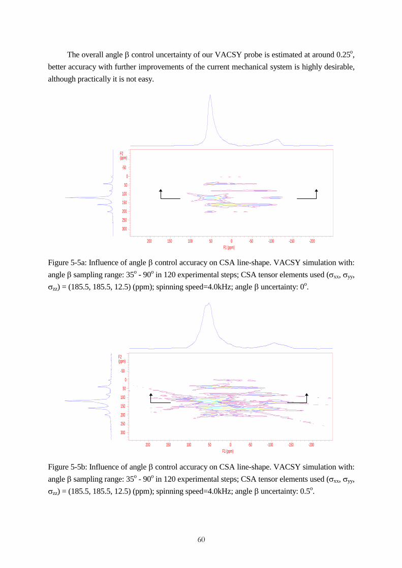
��
The overall angle E control uncertainty of our VACSY probe is estimated at around 0.25o,
better accuracy with further improvements of the current mechanical system is highly desirable,
although practically it is not easy.
F1 (ppm)-200-150-100-50050100150200
F2(ppm)
-50
0
50
100
150
200
250
300
Figure 5-5a: Influence of angle E control accuracy on CSA line-shape. VACSY simulation with:
angle E sampling range: 35o - 90o in 120 experimental steps; CSA tensor elements used (Vxx, Vyy,
Vzz) = (185.5, 185.5, 12.5) (ppm); spinning speed=4.0kHz; angle E uncertainty: 0o.
F1 (ppm)-200-150-100-50050100150200
F2(ppm)
-50
0
50
100
150
200
250
300
Figure 5-5b: Influence of angle E control accuracy on CSA line-shape. VACSY simulation with:
angle E sampling range: 35o - 90o in 120 experimental steps; CSA tensor elements used (Vxx, Vyy,
Vzz) = (185.5, 185.5, 12.5) (ppm); spinning speed=4.0kHz; angle E uncertainty: 0.5o.

��
F1 (ppm)-200-150-100-50050100150200
F2(ppm)
-50
0
50
100
150
200
250
300
Figure 5-5c: Influence of angle E control accuracy on CSA line-shape. VACSY simulation with:
angle E sampling range: 35o - 90o in 120 experimental steps; CSA tensor elements used (Vxx, Vyy,
Vzz) = (185.5, 185.5, 12.5) (ppm); spinning speed=4.0kHz; angle E uncertainty: 2.0o.
5.3.3 How much a range of the angle E is necessary for the acquisition of a non-distorted
CSA line-shape?
F1 (ppm)-200-150-100-50050100150200
F2(ppm)
-50
0
50
100
150
200
250
300
Figure 5-6a: Influence of angle E sampling range on CSA line-shape. VACSY simulation with:
CSA tensor elements used (Vxx, Vyy, Vzz)=(185.5, 185.5, 12.5) (ppm); spinning speed=4.0kHz;
Angle E sampling range of 45 - 63o in 40 experimental steps;

��
F1 (ppm)-200-150-100-50050100150200
F2(ppm)
-50
0
50
100
150
200
250
300
Figure 5-6b: Influence of angle E sampling range on CSA line-shape. VACSY simulation with:
CSA tensor elements used (Vxx, Vyy, Vzz)=(185.5, 185.5, 12.5) (ppm); spinning speed=4.0kHz;
Angle E sampling range of 36 - 72o in 80 experimental steps;
F1 (ppm)-200-150-100-50050100150200
F2(ppm)
-50
0
50
100
150
200
250
300
Figure 5-6c: Influence of angle E sampling range on CSA line-shape. VACSY simulation with:
CSA tensor elements used (Vxx, Vyy, Vzz)=(185.5, 185.5, 12.5) (ppm); spinning speed=4.0kHz;
Angle E sampling range of 27 - 81o in 120 experimental steps.
The simulation result of the CSA line-shape distortion due to a not sufficient sampling
rang of angle E is shown in fig5-6. With the indicated CSA parameters, if sampling range of
angle E is smaller than 20o, for example from 45o - 63o, some line-shape distortion begins to
appear. This is due to a insufficient data sampling area in space (ta, ti) for the interpolation step
as described in chapter 4, therefore phase artefacts and increasing interpolation error cause the
resulted CSA line-shape distortion

��
5.3.4 How many independent VAS experiments should be carried out for a non-distorted
line-shape?
The simulation result of the CSA line-shape distortion due to a not sufficient sampling
numbers of angle E in a sufficient angle range is shown in fig5-7. With the indicated CSA
parameters and a sufficient angle range for data acquisition 35o - 90o, if the sampling numbers of
angle E is less than 30, again some line-shape distortion begins to appear. The reason is the
insufficient sampling number of the data area in space (ta, ti) corresponding to an angle range of
35o - 90o in real space, this leads to increasing interpolation error and the resulted distortion in
the final spectrum.
F1 (ppm)-200-150-100-50050100150200
F2(ppm)
-50
0
50
100
150
200
250
300
Figure 5-7a: Influence of angle E sampling number on CSA line-shape. VACSY simulation
with: Angle E sampling range of 35 - 90o; CSA tensor elements used (Vxx, Vyy, Vzz)=(185.5,
185.5, 12.5) (ppm); spinning speed=4.0kHz; angle E sampling numbers: 60

��
F1 (ppm)-200-150-100-50050100150200
F2(ppm)
-50
0
50
100
150
200
250
300
Figure 5-7b: Influence of angle E sampling number on CSA line-shape. VACSY simulation
with: Angle E sampling range of 35 - 90o; CSA tensor elements used (Vxx, Vyy, Vzz)=(185.5,
185.5, 12.5) (ppm); spinning speed=4.0kHz; angle E sampling numbers: 120
F1 (ppm)-200-150-100-50050100150200
F2(ppm)
-50
0
50
100
150
200
250
300
Figure 5-7c: Influence of angle E sampling number on CSA line-shape. VACSY simulation
with: Angle E sampling range of 35 - 90o; CSA tensor elements used (Vxx, Vyy, Vzz)=(185.5,
185.5, 12.5) (ppm); spinning speed=4.0kHz; angle E sampling numbers: 240
5.3.5 How much a fluctuation in spinning speed is tolerable to achieve a non-distorted CSA
line-shape?
The simulation result of the CSA line-shape distortion due to the fluctuation in sample
spinning speed is shown in fig5-8. With the indicated CSA parameters, if the fluctuation of the

��
sampling spinning speed is bigger than 500Hz, significant line-shape distortion appears. Here,
fluctuation in sample spinning speed is randomly generated within the indicated range for
VACSY data acquisitions at different angle E positions.
In our VACSY probe, the tribo-electric antenna design is adapted to detect the sample
spinning speed while it can easily follow the movement of the whole sample housing when the
experiment is swept through a certain angle range. There are two problems here (i) when the
sample housing changes from angle E to another, with a constant air supply the sample spinning
speed changes in the range of 0 - 500Hz. In principle, automatic spinning speed regulation can
adjust it back to the setting speed. However, (ii) with the tribo-electric spinning speed detection
design, there is strong interference in the spinning speed control signal when rf pulses are in
action. This interference can destroy the automatic spinning speed regulation control loop and in
the worst cases stop the spinning.
Recently, the spinning speed detection scheme of our VACSY probe is changed to fibber
optic spinning speed detector with some careful mechanic design to allow the rigid fibber follow
the movements of the sample housing. Now, during the whole VACSY experiment the spinning
speed can be regulated to the setting value within an error of 10Hz. So, the line-shape distortion
due to this reason is removed.
F1 (ppm)-200-150-100-50050100150200
F2(ppm)
-50
0
50
100
150
200
250
300
Figure 5-8a: Influence of fluctuation in spinning speed on CSA line-shape. VACSY simulation
with: angle E sampling range of 35 - 90o in 120 steps; CSA tensor elements used (Vxx, Vyy, Vzz)
=(185.5, 185.5, 12.5) (ppm); spinning speed=4.0kHz; fluctuation in spinning speed: 0.0Hz

��
F1 (ppm)-200-150-100-50050100150200
F2(ppm)
-50
0
50
100
150
200
250
300
Figure 5-8b: Influence of fluctuation in spinning speed on CSA line-shape. VACSY simulation
with: angle E sampling range of 35 - 90o in 120 steps; CSA tensor elements used (Vxx, Vyy,
Vzz)=(185.5, 185.5, 12.5) (ppm); spinning speed=4.0kHz; fluctuation in spinning speed: 100.0Hz
F1 (ppm)-200-150-100-50050100150200
F2(ppm)
-50
0
50
100
150
200
250
300
Figure 5-8c: Influence of fluctuation in spinning speed on CSA line-shape. VACSY simulation
with: angle E sampling range of 35 - 90o in 120 steps; CSA tensor elements used (Vxx, Vyy,
Vzz)=(185.5, 185.5, 12.5) (ppm); spinning speed=4.0kHz; fluctuation in spinning speed: 500.0Hz
��
c h a p t e r 6
CONSTRUCTION OF A VACSY PROBE
6.1 Introduction
The word probe or probe-head is used to refer to the complete piece of equipment
intimately associated with the sample. For the simplest experiments, the probe consists of the
mechanical structure required to hold the sample in the homogeneous spot of the magnet, a coil
surrounding the sample, a tuning capacitor and a rf transmission line. However, most NMR
problems of interest require control over the sample environment, such as: temperature,
electromagnetic irradiation, pressure, orientation, rotation and etc, apparatus associated with
these functions also become parts of the NMR probe.
The modern NMR probe is a complex apparatus which is designed to accommodate all of
the environmental requirements of the NMR experiment. The radio-frequency (rf) section often
includes (a) an rf observe channel optimised for highest signal-to-noise ratio (SNR or S/N) at the
X nucleus frequency, (b) a less efficient rf channel for hetero-nuclear decoupling (usually 1H),
(c) another low-efficiency channel for magnetic field lock (usually 2H). Variable temperature
(VT) control is achieved through a resistive heater in a gas stream that flows over the sample. In
high resolution liquid probes, slow sample spinning (100-200Hz) about the external magnetic
field B0 direction is required to average out azimuthal inhomogeneity. In solid state probes, high
speed sample spinning (200-36000Hz) is required to average out chemical shift anisotropy
and/or dipolar interactions [Doty, 1996a].
Due to the absence of molecular tumbling in solids to average out line-broadening
interactions, the requirements for solid probes are more demanding than for liquid probes. Solid
probes require much greater bandwidths [Hartmann et al., 1962; Mansfield et al., 1963;
Vaughan, 1978]. A wide-line probe usually has spectral excitation bandwidth greater than
80KHz, that is equal to be able to generate 90o pulses less than 3Ps. To do this, it normally must
withstand peak rf voltages in excess of 3 KV [Doty, F. D., 1996b]. Often wide-line probes are
double tuned (DT) to allow cross polarisation (CP) and high power decoupling for increased
sensitivity and resolution. If S/2 pulse length below 2Ps can be generated, multiple pulse line-
narrowing techniques may be applied to remove dipolar broadening, but this is generally only
useful in single resonance probes.

��
Addressing the often conflicting requirements of high sensitivity, high resolution, large
spectral bandwidth, low background signals, wide VT range, high speed sample spinning,
intense irradiation, and uniform field gradients require careful attention to a number of problems
in material science, physics, electrical engineering, and mechanical engineering [Doty, F. D.,
1996a]. These efforts make a NMR probe very expensive.
The most common solid probe is the cross polarisation/magic angle spinning (CPMAS)
probe, which adds high-speed sample spinning at the magic angle to the other capabilities of a
DT wide-line probe for effective averaging of the chemical shift anisotropy and possibly dipolar
interactions at very high speed, therefore the spectral resolution for spin-1/2 nuclei is greatly
improved. Single resonance MAS probes can generate the short pulses needed for the combined
rotation and multiple pulse spectroscopy (CRAMPS) line-narrowing technique for 1H and 19F.
Large volume MAS rotors can achieve stable rotational spin rate which is necessary for slow
MAS, where pulses are applied in precise synchronisation with rotor orientation to average out
anisotropic chemical shift interactions as with high speed MAS. Extended variable temperature
(X-VT) CPMAS probes allow experiments from 35K to more than 500oC [Doty, 1996b]
6.2 Basics of radio frequency engineering
For the design and construction of a NMR probe, basic understanding of rf engineering
and electromagnetic field theory is necessary [Gordan, R. E., 1985; Tranficante, D. D., 1989;
Jackson, 1975]. NMR signal detection is different from antenna theory and is simpler. Antennas
are designed to receive electromagnetic waves in the far-field limit whereas NMR probes are
designed to sense magnetic fields in the near-field limit [Hoult, D. I., 1989]. A number of
articles [Hoult and Richards, 1976; Hoult, 1978; Schneider and Dullenkopf, 1977; Doty et al.,
1981; Hayes et al., 1985; Doty et al., 1988; Carlson, 1988; Crozier et al, 1995] and a text book
[Chen and Hoult, 1989; Fukushima and Roeder, 1996] have presented excellent discussions of
general NMR probe design problems.
6.2.1 Capacitance
Capacitance (farads) is defined as electric charge per volt (V), and capacitive energy is
equal to CV2/2. Stray capacitance can often be estimated to sufficient accuracy from the
expression for parallel plate capacitor Cp of area A (m2), separation d (m), and dielectric constant
Nd:
d
AkC d
p0ε= (6-1)

��
or from the expression for the low-frequency capacitance of a coaxial capacitor [Doty et al.,
1981] of length h, dielectric o.d. d0, and dielectric i.d. di:
)/ln(
)(2 0
io
odc dd
dhkC
+= επ(6-2)
where H0 is the permittivity of free space - 8.84 pFm-1. Parallel capacitors add algebraically
...321 +++= CCCCsum , while series capacitors add reciprocally ...CCCC 33
12
11
1sum +++= −−−− .
6.2.2 Inductance
The definition of inductance L (henrys) is given by Farady’s law - the induced voltage
divided by the rate of change in current di/dt. The inductive energy is equal to 2/2LiT . The
inductance of the finite, multiturn, single layer rf solenoid in fig6-1 with a constant pitch, an
integral number of turns, and a high surface coverage is given in nH, for dimensions in mm, by
the following expression:
9.0
22
2.1
)/2.01(4
rh
nrnLs +
−= (6-3)
Figure 6-1: a five-turn solenoid (adapted from Doty, 1994).
where n is the number of turns (fig6-1 has five turns), h is the overall axial length, and r is the
effective inside radius, which for round wire is approximately equal to the inside coil radius plus
20% of the wire radius. The last term in the numerator corrects for the fact that the helix makes
the effective coil length a little less that the overall length. This expression is correct to within
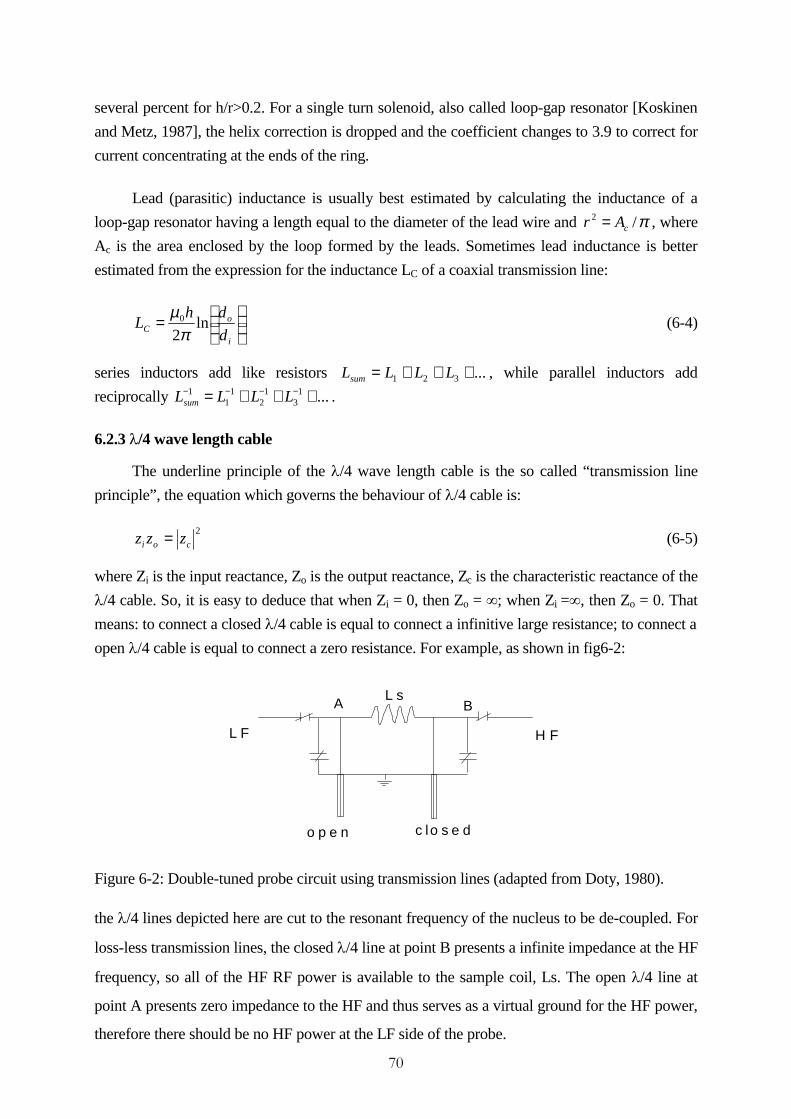
��
several percent for h/r>0.2. For a single turn solenoid, also called loop-gap resonator [Koskinen
and Metz, 1987], the helix correction is dropped and the coefficient changes to 3.9 to correct for
current concentrating at the ends of the ring.
Lead (parasitic) inductance is usually best estimated by calculating the inductance of a
loop-gap resonator having a length equal to the diameter of the lead wire and π/2cAr = , where
Ac is the area enclosed by the loop formed by the leads. Sometimes lead inductance is better
estimated from the expression for the inductance LC of a coaxial transmission line:
=
i
oC d
dhL ln
20
πµ
(6-4)
series inductors add like resistors ...321 +++= LLLLsum , while parallel inductors add
reciprocally ...13
12
11
1 +++= −−−− LLLLsum .
6.2.3 O/4 wave length cable
The underline principle of the O/4 wave length cable is the so called “transmission line
principle”, the equation which governs the behaviour of O/4 cable is:
2
coi zzz = (6-5)
where Zi is the input reactance, Zo is the output reactance, Zc is the characteristic reactance of the
O/4 cable. So, it is easy to deduce that when Zi = 0, then Zo = f; when Zi =f, then Zo = 0. That
means: to connect a closed O/4 cable is equal to connect a infinitive large resistance; to connect a
open O/4 cable is equal to connect a zero resistance. For example, as shown in fig6-2:
L F H F
c lo s e do p e n
L sA B
Figure 6-2: Double-tuned probe circuit using transmission lines (adapted from Doty, 1980).
the O/4 lines depicted here are cut to the resonant frequency of the nucleus to be de-coupled. For
loss-less transmission lines, the closed O/4 line at point B presents a infinite impedance at the HF
frequency, so all of the HF RF power is available to the sample coil, Ls. The open O/4 line at
point A presents zero impedance to the HF and thus serves as a virtual ground for the HF power,
therefore there should be no HF power at the LF side of the probe.

��
However, when losses are introduced into the O/4 lines, the situation is different. At point
A the impedance is usually large enough to limit the HF rejection to less than 20 dB on the LF
side of the probe. The even more serious problem is the finite impedance presented by the closed
O/4 line at point B, in it there is a dramatic loss in the HF efficiency [Doty, 1981].
A alternative for the ¼ O cable is to employ a series - parallel reduction scheme on the
equivalent circuit using lumped elements as demonstrated in fig6-3 [Doty, 1981].
HFLF
A B
CA
LA
RA
LB
CB
RB
CH
CH'
CL
CL'
Figure 6-3: Lumped-element equivalent of figure 6-2 (adapted from Doty, 1980).
6.2.4 Single resonance circuit
Fig6-4 shows the basic RLC series and parallel circuits, respectively. The losses in the
series RLC circuit are best represented by the total effective series resistance Rs (from the coil,
capacitor, leads, etc). For the parallel circuit, the losses may be represented more conveniently
by a total effective parallel resistor Rp.
/ & /
&
Figure 6-4: Principle of RF resonant circuits. (left) parallel resonant circuit; (right) serial
resonant circuit.
In both cases, the basic equations from ac circuits apply for rms power P and peak power
Pp.
p
psPP
R
VRiPP
222
22
=== (6-6)
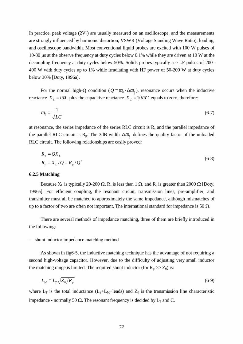
��
In practice, peak voltage (2Vp) are usually measured on an oscilloscope, and the measurements
are strongly influenced by harmonic distortion, VSWR (Voltage Standing Wave Ratio), loading,
and oscilloscope bandwidth. Most conventional liquid probes are excited with 100 W pulses of
10-80 Ps at the observe frequency at duty cycles below 0.1� while they are driven at 10 W at the
decoupling frequency at duty cycles below 50%. Solids probes typically see LF pulses of 200-
400 W with duty cycles up to 1% while irradiating with HF power of 50-200 W at duty cycles
below 30% [Doty, 1996a].
For the normal high-Q condition (21/0 ωω ∆=Q ), resonance occurs when the inductive
reactance LiXL ω= plus the capacitive reactance CiXC ω1= equals to zero, therefore:
LC
10 =ω (6-7)
at resonance, the series impedance of the series RLC circuit is Rs and the parallel impedance of
the parallel RLC circuit is Rp. The 3dB width 21ω∆ defines the quality factor of the unloaded
RLC circuit. The following relationships are easily proved:
2// QRQXR
QXR
pLs
Lp
==
=(6-8)
6.2.5 Matching
Because XL is typically 20-200 :, Rs is less than 1 :, and Rp is greater than 2000 : [Doty,
1996a]. For efficient coupling, the resonant circuit, transmission lines, pre-amplifier, and
transmitter must all be matched to approximately the same impedance, although mismatches of
up to a factor of two are often not important. The international standard for impedance is 50 :.
There are several methods of impedance matching, three of them are briefly introduced in
the following:
�� shunt inductor impedance matching method
As shown in fig6-5, the inductive matching technique has the advantage of not requiring a
second high-voltage capacitor. However, due to the difficulty of adjusting very small inductor
the matching range is limited. The required shunt inductor (for Rp >> Z0) is:
pTM RZLL 0= (6-9)
where LT is the total inductance (LS+LM+leads) and Z0 is the transmission line characteristic
impedance - normally 50 :. The resonant frequency is decided by LT and C.

��
&
/0/ / &
&0
Figure 6-5: (left)shunt inductive impedance matching circuit; (right) series capacitive impedance
matching circuit (adapted from Doty, 1994).
�� series capacitor impedance matching
As high voltage capacitors are now readily available, capacitive matching circuit as shown
in fig6-5 is popularly used. The required match capacitance (again, for Rp >> Z0) is given as:
0ZRX PCM = (6-10)
�� parallel capacitor impedance matching
The series resonant circuit is most often used in NMR with the addition of a capacitor in
parallel for impedance matching as shown in fig6-6. If Cc >> C the resonance condition remains
close to 12 =LCω and the impedance at resonance is 22 )/( CCLCQ ′+ω .Take an example of
Lamor frequency at 100MHz, if r=0.1:, the Cc | 0.005 PF for the coil to be matched to 50 :
impedance. The resonance condition should be fulfilled with the largest possible L and the
smallest C to achieve the highest Q and also maintain the condition Cc >> C at the same time.
&0
/
&
Figure 6-6: Parallel capacitive impedance matching circuit (adapted from Fukushima and
Roeder, 1998).
6.2.6 Double resonance circuit
Two saddle coils, rotated 90o about the B0 axis provide a convenient method of doing
double resonance NMR with good isolation. However, with this design only the inner coil can
have the optimum filling factor, and sometimes it is required to have the same spatial

��
distribution of the two rf fields B1 and B2. Also, triple- or quadruple-resonance NMR
experiments are often required. Therefore it is often desirable to double-tune or triple-tune a
single sample coil [Doty, 1996a].
Fig6-7 shows an example DT RF circuit which is used in Doty’s NMR goniometer probe.
Where, the 73nH coil is the sample coil. The 1.2PF capacitor is used to bring the resonance
frequency down to the desired range. 27PF capacitor together with the second sample coil 6nH
form the series ‘frequency trap’ for HF, that is to bypass all the HF leakage which passes through
the sample coil and prevent it to reach the observe detector. Some people like to use series
frequency trap, while others like to use parallel frequency trap. With respect to prevent the HF
leakage, they have the same function. However, they may produce different effects on tuning
and matching conditions of the LF side.
73nH
1.2PF
6nH
HFLF1.5-45PF
1-10PF
1.5-45PF
1-10PF
1.4PF
27PF
Figure 6-7: Double resonance circuit used in Doty’s goniometer probe.
Another DT RF circuit example which is shown in fig6-8 is the circuit used in the NMR
group of Uni. Jena. Where, two unique features are:
�� Variable inductor: In Jena’s design, variable inductors are used to replace variable capacitors.
Comparing with variable capacitors, variable inductors have the advantages of (i)higher
voltage tolerance (ii)easily adjustable in a bigger range (iii)cheaper (home made).
�� a “Rod-Ring” capacitor: To give a reference ground for the HF de-coupling power, at the
immediate end of the sample coil in LF side, a very small capacitor (home made and called
“Rod-Ring”) is added. The typical capacitance value for this capacitor is around 1 PF. It
provides low impedance (good grounding) for the HF frequency.
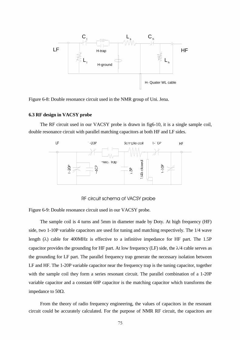
��
HFLF
Ls
Lh
Ll
Cl
Ch
H-trap
H-ground
H- Quater WL cable
Figure 6-8: Double resonance circuit used in the NMR group of Uni. Jena.
6.3 RF design in VACSY probe
The RF circuit used in our VACSY probe is drawn in fig6-10, it is a single sample coil,
double resonance circuit with parallel matching capacitors at both HF and LF sides.
/) +)����3
����3
a��3
)UHT� 7UDS
6DPSOH FRLO ����3���
FORVH
G��3
����3
5)�FLUFXLW�VFKHPD�RI�9$&6<�SUREH
Figure 6-9: Double resonance circuit used in our VACSY probe.
The sample coil is 4 turns and 5mm in diameter made by Doty. At high frequency (HF)
side, two 1-10P variable capacitors are used for tuning and matching respectively. The 1/4 wave
length (O) cable for 400MHz is effective to a infinitive impedance for HF part. The 1.5P
capacitor provides the grounding for HF part. At low frequency (LF) side, the O/4 cable serves as
the grounding for LF part. The parallel frequency trap generate the necessary isolation between
LF and HF. The 1-20P variable capacitor near the frequency trap is the tuning capacitor, together
with the sample coil they form a series resonant circuit. The parallel combination of a 1-20P
variable capacitor and a constant 60P capacitor is the matching capacitor which transforms the
impedance to 50:.
From the theory of radio frequency engineering, the values of capacitors in the resonant
circuit could be accurately calculated. For the purpose of NMR RF circuit, the capacitors are

��
normally in the range of 1a100PF, inductance in the range of 1a200nH. However, the parasic
distributive capacitance and inductance existed between different components are in the same
range, and they are dependent on many practical factors such as circuit layout, connection wires
and etc. In most cases, these distributive parameters are not possible to be accurately calculated
except some approximate estimations. So, in general the resonant condition is hardly possible to
be accurately calculated. The effective way to find out the correct capacitance and inductance
values is a procedure of repeatedly ‘try and error’.
VACSY experiment needs a special probe to be performed. A VACSY probe adds the
ability of accurate control over the angle between sample spinning axis and external magnetic
field direction B0 to an ordinary double tune CPMAS probe. The general diagram of a VACSY
experiment set-up is shown in fig6-9.
681�63$5&ZRUNVWDWLRQ
,129$����0+]
9$5,$1
VWHSPRWRU FRQWUROOHU
DQJOH GLVSDO\
LQVWUXPHQWDO VHWXS RI D 9$&6< H[SHULPHQW
a
c
b
b
ed
a: D oty ro to rb: R F- double re son an ce c ircu itc : pu lley - s tring d: stepm otore: angle encoder/d isp lay

��
Figure 6-10: Diagram of the overall VACSY experimental set-up.
6.4 VACSY RF circuit optimisation
During the optimisation of our VACSY RF circuit, much attention has been paid to the
following things:
�� Arrangement of the circuit components. A good RF circuit layout can minimise the
distributive capacitance and inductance, as well as minimise noise and unwanted resonant
peaks. There is no universal rule for how a good RF circuit layout should be, but experience
proves that: a good RF circuit layout is the one which has fewer wire connections between
individual components and fewer inner loops.
�� Connection points and connection wires. For all solid NMR probes, good sensitivity (S/N -
signal to noise ratio) is highly desirable, while poor S/N normally means longer experimental
time or simply make some experiments not feasible. Many factors influence the S/N of a final
NMR probe, such as Q values of components used (capacitors and inductors), soldering
junctions, connection wires used and etc. Today, the Q values of components higher than 200
are commercially available. From our experience, the crucial connections in the circuit should
use 2mm in diameter silver coated copper wire; the soldering should be performed with
extreme care for a nice round shape by using soldering material with highest conductivity.
�� Arching problem. The electrical theory tells us that arching most possibly happens when the
gap between the positive electrode and the negative electrode (ground) is too small. To
prevent arching or to remove arching: firstly, the components on the PCB should be arranged
to have as large a spacing as possible, especially between different capacitors. Secondly,
when arching exists in the circuit, experience proves that: wrapping the suspicious
components using Teflon tape is quite successful to remove arching in some NMR probes.
Thirdly, when arching is caused by a defected component and very strong, it can be located
easily by direct vision: Take out the probe from the magnet, remove cover, perform tuning
and matching as normal, then apply normal NMR de-coupling pulse sequence. In a dark
room, if arching is strong ‘flashing’ near that point should be seen by eye.
6.5 Angle control
As described in chapter 5, in VACSY accurate control of the angle between the sample
spinning axis and the external magnetic field direction B0 is very important. VACSY simulation
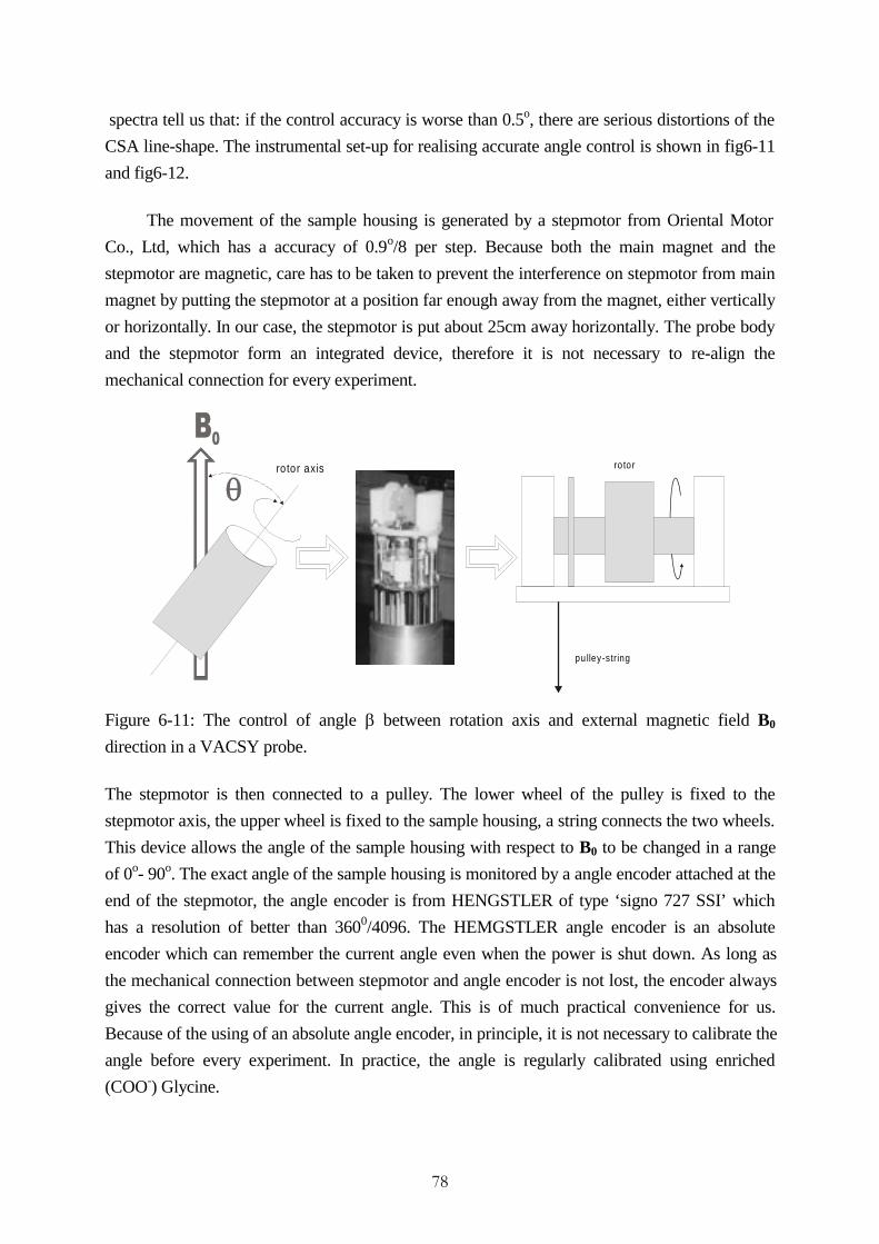
��
spectra tell us that: if the control accuracy is worse than 0.5o, there are serious distortions of the
CSA line-shape. The instrumental set-up for realising accurate angle control is shown in fig6-11
and fig6-12.
The movement of the sample housing is generated by a stepmotor from Oriental Motor
Co., Ltd, which has a accuracy of 0.9o/8 per step. Because both the main magnet and the
stepmotor are magnetic, care has to be taken to prevent the interference on stepmotor from main
magnet by putting the stepmotor at a position far enough away from the magnet, either vertically
or horizontally. In our case, the stepmotor is put about 25cm away horizontally. The probe body
and the stepmotor form an integrated device, therefore it is not necessary to re-align the
mechanical connection for every experiment.
rotor axis ro tor
pu lley-string
Figure 6-11: The control of angle E between rotation axis and external magnetic field B0
direction in a VACSY probe.
The stepmotor is then connected to a pulley. The lower wheel of the pulley is fixed to the
stepmotor axis, the upper wheel is fixed to the sample housing, a string connects the two wheels.
This device allows the angle of the sample housing with respect to B0 to be changed in a range
of 0o- 90o. The exact angle of the sample housing is monitored by a angle encoder attached at the
end of the stepmotor, the angle encoder is from HENGSTLER of type ‘signo 727 SSI’ which
has a resolution of better than 3600/4096. The HEMGSTLER angle encoder is an absolute
encoder which can remember the current angle even when the power is shut down. As long as
the mechanical connection between stepmotor and angle encoder is not lost, the encoder always
gives the correct value for the current angle. This is of much practical convenience for us.
Because of the using of an absolute angle encoder, in principle, it is not necessary to calibrate the
angle before every experiment. In practice, the angle is regularly calibrated using enriched
(COO-) Glycine.

��
Figure 6-12: General diagram of a VACSY probe with stepmotor and angle-encoder.
The final angle control accuracy is decided by several factors, to improve the accuracy the
following steps have been undertaken:
�� check the location of the stepmotor to make sure that there is no interference of the
main magnet on the stepmotor.
�� the tension of the connection string is carefully adjusted by a very sensitive optical
method. When the tension is too high, there occurs slippery and some stepmotor steps
would be missed. On the other hand, when the tension is too low, due to the problem of
backlash a number of starting steps will generate no motion of the sample housing .
�� minimise friction between different parts in the sample housing by replacing direct
contact bearing with micro glass ball bearing form MMB Bearing Co.
The final angle control accuracy is estimated to be better than 0.25o by comparing the
results of line width measurements of enriched (COO-) Glycine using VACSY probe and
VARIAN 7mm MAS probe. Other basic specifications of my VACSY probe are: 1H channel
tuning range 390 MHz - 460 MHz, 13C channel tuning range 97.5 MHz - 110M Hz; 1H S/2 pulse
with a RF output power of 360 Watt is 2.5 Ps (100 kHz), 13C S/2 pulse with a RF output power
of 61 Watt is 4.0 Ps (63kHz); Angle of rotation axis can be changed from 0o-90o, angle control
accuracy is less than 0.25o (estimated from experiment performance).

��
c h a p t e r 7
EXPERIMENTAL RESULTS AND DISCUSSION
7.1 Introduction
All following experiments are carried out on a VARIAN 400 MHz INOVA spectrometer
with 1KW linear high powder amplifier for solid-state applications. The VACSY probe is a self
built double resonance probe. It uses a standard Doty 5 mm sample spinning module, the
maximum spinning speed can reach about 7.0 kHz. The change of the angle between the sample
spinning axis and the external magnetic field is realised through a stepmotor and pulley-string
mechanism. The accuracy of angle control is estimated at 0.25 degree. All VACSY experimental
data are interpolated to ni=250 steps in the indirect direction by using Frydman’s normal
interpolation procedure and then transformed by VNMR’s FFT software to get the final spectra.
7.2 VACSY to measure chemical shift tensor elements
VACSY is a promising method to correlate the chemical shift anisotropies with their
corresponding chemical shift isotropic values. So, one of the basic applications of VACSY
would be to measure the values of chemical shift tensor elements, for example the values of 13C
chemical shift tensor elements. If the sample has only one in-equivalent 13C nuclei, the values of
chemical shift tensor elements can be easily measured by a simple static dipolar decoupling(DD)
cross-polarisation(CP) experiment. Another popular method for measuring values of chemical
shift tensor elements is to carry out a CPMAS experiment with dipolar decoupling, when the
sample spinning speed is smaller than the anisotropic value of the chemical shift tensor, a series
of spinning sidebands will appear. From the relative intensities of these spinning sidebands with
respect to the central band, the values of chemical shift tensor elements can be obtained by
applying the Herzfeld-Berger procedure. However, if there are more than one in-equivalent 13C
nucleus in the sample and their chemical shift anisotropies overlap each other, both methods
become inadequate. In these cases, alternatives which can separate lines according to their
isotropic chemical shift values and correlate each with their corresponding chemical shift
anisotropies must be selected.
7.2.1 1D VAS experiment to measure CS tensor elements of glycine
The first alternative is 1D VAS experiment: the sample is spinning at an off-magic angle
position and the spinning speed is larger than the biggest chemical shift anisotropic value of all
spectral lines, FID data acquisition is carried out under CP and DD. From chapter 3 we know,

��
when the sample is in fast spinning at an off-magic angle position the chemical shift anisotropic
value is scaled down according to the second Legendre polynomial of the angle T between
rotation axis and the external magnetic field direction:
( ) ( )[ ]1cos3 221
0 −+−= θσσγθω aiB (7-1)
The measured chemical shift anisotropic value aσ ′ and the theoretical chemical shift anisotropic
value aσ is related by the following equation:
))1cos3(/( 221 −′= θσσ aa (7-2)
An example is given in fig7-1 of enriched (COO-) glycine measured at angle equal to 80.26o for
the spinning axis relative to the external magnetic field direction. The scaled anisotropic
chemical shift value measured at 80.26o is aσ ′ = 65.5 ppm, the calculated full anisotropic
chemical shift value is aσ =143.3 ppm. In fig7-1 there is an apparent deviation from the
theoretical CSA line-shape, this is due to an insufficient sample spinning speed and two weak
spinning sidebands are also visible at each side of the centre band in fig7-1.
ppm50100150200250300
Figure 7-1: VAS 13C (100 MHz) NMR spectrum of enriched (COO-) Glycine, measured at an
angle E=80.26o between the sample rotation axis and B0 direction, spinning speed used is 6.0
kHz.
Because the angle between sample rotation axis and B0 field direction is controlled better
than 0.25 degree, we have reasons to believe that this method is more reliable than the normally
applied Herzfeld-Berg method. However, VAS 1D method can only partially relieve the
overlapping problem due to the scaling of chemical shift anisotropy at off-magic -angle position.
In most practical cases, overlapping from lines with slightly different isotropic values still
restrain this procedure to be successfully applied to more complicated polymer samples.

��
7.2.2 VACSY experiment to measure CS tensor of HMB and DMS
The second alternative for measuring the values of chemical shift tensor elements is a
complete VACSY experiment. In the 2D VACSY spectrum, the projection along the isotropic
dimension gives a high resolution CPMAS spectrum, all lines are separated according to their
individual isotropic chemical shift values; their chemical shift anisotropic patterns are given in
the projections from the slices along the anisotropic dimension. An example of VACSY used to
measure values of chemical shift tensor elements in enriched Glycine is demonstrated in fig7-2
F1 (ppm)-200-150-100-50050100150200
F2(ppm)
-50
0
50
100
150
200
250
300
Figure 7-2: VACSY 13C (100 MHz) NMR spectrum of enriched (COO-) glycine, data acquired
for angle E sampling angle of 35o-90o in 120 steps, sample spinning speed is 6.0 kHz.
Because the 13C nuclei of carbonyl group has a very large chemical shift anisotropy, the
spinning speed used to acquire the corresponding VACSY spectrum is 6.0 kHz (still smaller
than the anisotropic chemical shift value), so the spectrum of the sky-line projection along the
isotropic dimension includes the isotropic line and two higher order spinning sidebands. The
spectrum along the anisotropic dimension is the sky-line projection of the central spinning
sideband. The anisotropic chemical shift value is directly measured from the singularities of this
projection spectrum: 145.0 ppm. This result agrees very well with the result obtained from 1D
VAS measurement. The 3D plot of the above analysed glycine VACSY spectrum is given in
fig7-3, it demonstrates more clearly the correlation of chemical shift isotropy and anisotropy.

��
Figure 7-3: 3D plot with projections of the VACSY 13C spectrum in figure 7-2. The (sky-line)
projection onto the anisotropic axis is from the slice at central spinning band (isotropic chemical
shift position). The (sky-line) projection onto the isotropic axis is the same as 1D CPMAS
spectrum.
Two more measurement examples are given for HMB in fig7-4 and DMS in fig7-5. The
measurement result of anisotropic chemical shift value of HMB is: 161.2 ppm. The spin rate
used to get this VACSY spectrum is 3.9 kHz and is much smaller than the chemical shift
anisotropic value of the aromatic carbons in HMB. So, the line-shape of the central spinning
sideband is strongly distorted and two higher order spinning sidebands appear in the spectrum at
each side of the centre band. For the methyl carbons, due to its strong intensity and the smaller
chemical shift anisotropic value, serious artefacts show up as explained in section 4.3.2.
F1 (ppm)-200-150-100-50050100150200
F2(ppm)
-50
0
50
100
150
200
250
300

��
Figure 7-4: VACSY 13C (100 MHz) NMR spectrum of Hexamethyl Benzene (HMB), data
acquired for angle E sampling range of 38o-80o in 180 steps, sample spinning speed is 3900 Hz.
The measurement result of the chemical shift anisotropy of DMS is 52.5 ppm, the spin rate
used is 3.9 kHz and it is comparable with DMS’s chemical shift anisotropic value. So, only a
very weak spinning sideband is visible here. Due to thermal motions with a rate comparable with13C NMR frequency present in DMS sample around room temperature, this VACSY experiment
is carried out at a temperature below 0oC with the help of a special cooling device. Otherwise,
there is very strong spectral rounding at the two singularity frequency positions.
F1 (ppm)-80-60-40-20020406080
F2(ppm)
0
20
40
60
80
100
120
140
Figure 7-5: VACSY 13C (100 MHz) NMR spectrum of dimethylsulfon (DMS), data acquired for
angle E sampling range of 27o-81o in 240 steps, sample spinning speed is 3900 Hz.
7.2.3 VACSY experiment to measure CS tensors of Durene
All three above measured samples: glycine, HMB and DMS are relatively simple
substances from the NMR point of view. They have only one resonant line in the aromatic
region, the overlapping problem does not exist. In these cases, 1D NMR methods such as static,
CPMAS and VAS are enough to measure the values of chemical shift tensor elements. However,
if two or more resonant lines have very close isotropic chemical shift values their anisotropic
chemical shift patterns will overlap each other, then all 1D methods become not adequate. In
these cases, special designed 2D correlation methods such as VACSY have to be applied. An
example of VACSY used to measure the chemical shift tensor elements of two very closely
located resonant lines in Durene is shown in fig7-6. The experiment is performed with a
spinning speed of 3.5 kHz, the angle between the spinning axis and the external magnetic field is
sampled in a range of 35o - 90o with 120 steps. Four spinning sidebands for each isotropic line
show up due to the apparently not sufficient spinning speed comparing with their anisotropic
chemical shift values.
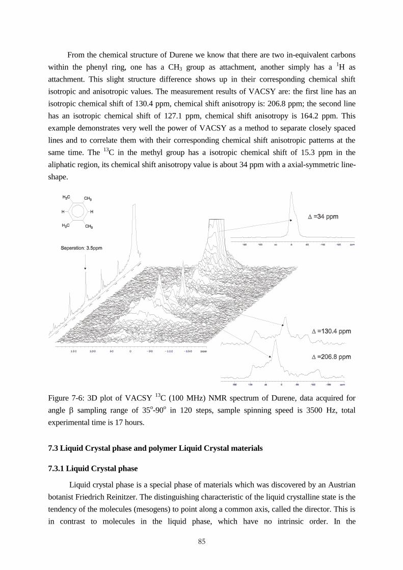
��
From the chemical structure of Durene we know that there are two in-equivalent carbons
within the phenyl ring, one has a CH3 group as attachment, another simply has a 1H as
attachment. This slight structure difference shows up in their corresponding chemical shift
isotropic and anisotropic values. The measurement results of VACSY are: the first line has an
isotropic chemical shift of 130.4 ppm, chemical shift anisotropy is: 206.8 ppm; the second line
has an isotropic chemical shift of 127.1 ppm, chemical shift anisotropy is 164.2 ppm. This
example demonstrates very well the power of VACSY as a method to separate closely spaced
lines and to correlate them with their corresponding chemical shift anisotropic patterns at the
same time. The 13C in the methyl group has a isotropic chemical shift of 15.3 ppm in the
aliphatic region, its chemical shift anisotropy value is about 34 ppm with a axial-symmetric line-
shape.
Figure 7-6: 3D plot of VACSY 13C (100 MHz) NMR spectrum of Durene, data acquired for
angle E sampling range of 35o-90o in 120 steps, sample spinning speed is 3500 Hz, total
experimental time is 17 hours.
7.3 Liquid Crystal phase and polymer Liquid Crystal materials
7.3.1 Liquid Crystal phase
Liquid crystal phase is a special phase of materials which was discovered by an Austrian
botanist Friedrich Reinitzer. The distinguishing characteristic of the liquid crystalline state is the
tendency of the molecules (mesogens) to point along a common axis, called the director. This is
in contrast to molecules in the liquid phase, which have no intrinsic order. In the
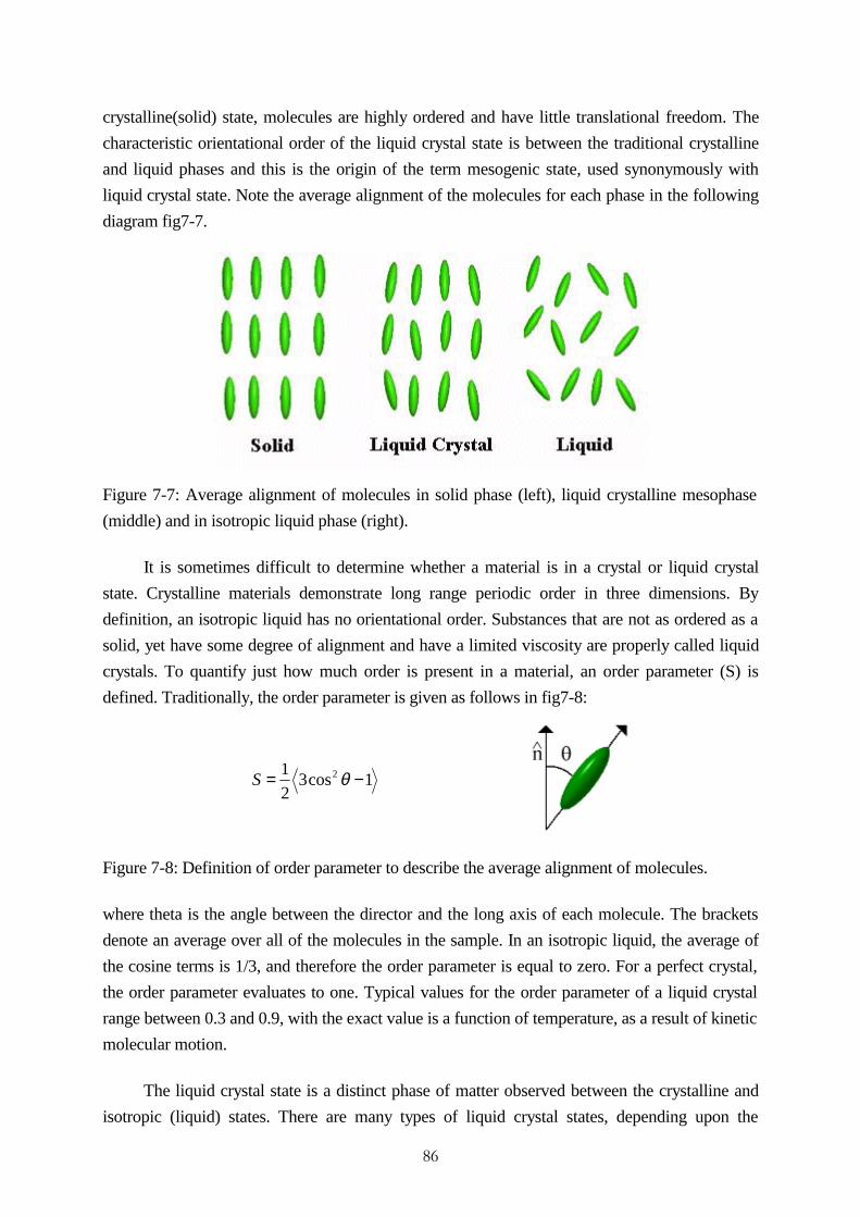
��
crystalline(solid) state, molecules are highly ordered and have little translational freedom. The
characteristic orientational order of the liquid crystal state is between the traditional crystalline
and liquid phases and this is the origin of the term mesogenic state, used synonymously with
liquid crystal state. Note the average alignment of the molecules for each phase in the following
diagram fig7-7.
Figure 7-7: Average alignment of molecules in solid phase (left), liquid crystalline mesophase
(middle) and in isotropic liquid phase (right).
It is sometimes difficult to determine whether a material is in a crystal or liquid crystal
state. Crystalline materials demonstrate long range periodic order in three dimensions. By
definition, an isotropic liquid has no orientational order. Substances that are not as ordered as a
solid, yet have some degree of alignment and have a limited viscosity are properly called liquid
crystals. To quantify just how much order is present in a material, an order parameter (S) is
defined. Traditionally, the order parameter is given as follows in fig7-8:
Figure 7-8: Definition of order parameter to describe the average alignment of molecules.
where theta is the angle between the director and the long axis of each molecule. The brackets
denote an average over all of the molecules in the sample. In an isotropic liquid, the average of
the cosine terms is 1/3, and therefore the order parameter is equal to zero. For a perfect crystal,
the order parameter evaluates to one. Typical values for the order parameter of a liquid crystal
range between 0.3 and 0.9, with the exact value is a function of temperature, as a result of kinetic
molecular motion.
The liquid crystal state is a distinct phase of matter observed between the crystalline and
isotropic (liquid) states. There are many types of liquid crystal states, depending upon the
1cos32
1 2 −= θS

��
amount of order in the material. Two of them are most often observed: nematic phase and
smectic phase:
x� Nematic Phases
The nematic liquid crystal phase is characterised by molecules that have no positional
order but tend to point in the same direction (along the director). In the following diagram fig7-
9, notice that the molecules point vertically but are arranged with no particular order.
Figure 7-9: Liquid crystalline nematic phase.
Liquid crystals are anisotropic materials, and the physical properties of the system vary
with the average alignment with the director. If the alignment is large, the material is very
anisotropic. Similarly, if the alignment is small, the material is almost isotropic.
x� Smectic Phases
The smectic state is another distinct mesophase of liquid crystal substances. Molecules in
this phase show a degree of translational order not present in the nematic. In the smectic state,
the molecules maintain the general orientational order of nematics, but also tend to align
themselves in layers or planes. Motion is restricted to within these planes and separate planes are
observed to flow past each other. The increased order means that the smectic state is more
"solid-like" than the nematic. This is shown in fig7-10.
Figure 7-10: Liquid crystalline smectic phase. (left) smectic A phase; (right) smectic C phase.

��
7.3.2 Polymer Liquid Crystal materials
Polymer liquid crystals (PLCs) are a class of materials that combine the properties of
polymers with those of liquid crystals. These "hybrids" show the same mesophases characteristic
of ordinary liquid crystals, yet retain many of the useful and versatile properties of polymers.
In order for normally flexible polymers to display liquid crystal characteristics, rod-like or
disk-like elements (called mesogens) must be incorporated into their chains. The placement of
the mesogens plays a large role in determining the type of PLC that is formed. Main-chain
polymer liquid crystals or MC-PLCs are formed when the mesogens are themselves part of the
main chain of a polymer. Conversely, side chain polymer liquid crystals or SC-PLCs are formed
when the mesogens are connected as side chains to the polymer by a flexible "bridge" (called the
spacer.) as shown in fig7-11
Figure 7-11: Two common polymer liquid crystalline material: main-chain polymer liquid
crystal and side-chain polymer liquid crystal.
7.4 VACSY to study orientation distribution of PLC sample - hexa-hexyloxytriphenylene
The existence of a new type of liquid crystalline phase in compounds composed of disc-
like molecules was reported by Chandrasekhar et al. In 1977 [Chandrasekhar, 1997] and Billard
et al. in 1978 [Billard, 1978]. They observed liquid crystalline mesophases on derivatives of
triphenylene. In their work, the discotic phase of p-n-hexa-hexyloxytriphenylene, R=OC6H13, as
illustrated in fig7-12 is studied, its phase diagram is also given here:
S olid68 Co 99 Co
Iso tropicD isco tic

��
R
R
R
R
R
R
1
11
1
11
23
3
2
2
33
2
23
32
R
R
R
R
R
R
Figures 7-12: (top) phase diagram of p-n-hexa-hexyloxytriphenylene; (bottom) Chemical
formula of p-n-hexa-hexyloxytriphenylene, R=OC6H13.
here Isotropic stands for isotropic liquid and Discotic stands for discotic mesophases. The 13C
1D CPMAS spectrum is shown in fig 7-13, the spinning speed used here is 6.0 kHz. There are
three 13C lines in the aromatic region which have isotropic chemical shifts values: 143.7ppm,
117.9ppm, 99.1ppm respectively and a number of 13C lines in the aliphatic region which are not
well resolved. The assignment result of some resonant lines is given in fig7-13. The assignment
is achieved through a comparison of two CPMAS experiments with 4.2 kHz and 6.1 kHz
spinning speed receptively. In fig7-13 letters with stars, a*, b*, c*, denote their corresponding
spinning sidebands of resonate lines a, b, c.
a (1/2/3) - 143.7ppm d (-O-C- in R) - 62.8ppm
b (1/2/3) - 117.9ppm e (-CH3 in R) - 10.3ppm
c (1/2/3) - 99.1ppm

��
Figure 7-13: CPMAS 13C (100 MHz) NMR spectrum of p-n-hexa-hexyloxytriphenylene sample
in isotropic powder state, sample spinning speed used is 6.0 kHz.
In the following orientation distribution study, we focus on the 13C line with the isotropic
chemical shift of 143.7ppm which has the biggest spectral intensity. The procedure for creating
certain orientation distribution in sample p-n-hexa-hexyloxytriphenylene is that: (i) insert the
rotor with sample into the main magnet of our VARIAN INOVA 400 MHz spectrometer (9.4T),
the rotor axis direction is set parallel to the magnetic field direction. (ii) heat the sample up to
10oC over its clearing temperature Tc and wait for about 20 minutes for equilibrium. (iii) at a
temperature rate of 1K/min, slowly cool down the sample till below the phase transition
temperature from liquid crystalline mesophase to solid phase. NMR measurements for the
oriented samples are carried out at room temperature. Two VACSY experiments are conducted,
one for the sample in isotropic powder state, another for the sample in oriented state, the
corresponding 2D spectra with skyline projections from the indicated slices are shown in fig 7-
14. The VACSY experiments are conducted with 5.0 kHz spinning speed, in a angle range of
35o - 90o with 60 steps. The final VACSY spectra are obtained by firstly interpolating the
experimental data to 256 points in the anisotropic dimension by using Frydman’s normal
interpolation procedure and then normal 2D FT.
F1 (ppm)-200-150-100-50050100150
F2(ppm)
20
40
60
80
100
120
140
160
180
200
Figure 7-14a: VACSY 13C (100 MHz) NMR spectrum of p-n-hexa-hexyloxytriphenylene
sample in isotropic powder state, data is acquired for angle E sampling range of 35o-90o in 60
steps, sample spinning speed used is 5.0 kHz

��
F1 (ppm)-200-150-100-50050100150
F2(ppm)
20
40
60
80
100
120
140
160
180
200
Figure 7-14b: VACSY 13C (100 MHz) NMR spectrum of p-n-hexa-hexyloxytriphenylene
sample in oriented state with the orientation procedure described in the text, data is acquired for
angle E sampling range of 35o-90o in 60 steps, sample spinning speed used is 5.0 kHz
From the known magnetic susceptibility tensor of the aromatic rings it is expected that the
mesophase molecules prefer an orientation in which the molecular rigid planes lie parallel to the
magnetic field, and the director perpendicular to it. Since all perpendicular orientations are
equally probable, it is reasonable to assume that the discotic phase is broken up into many
domains with their directors normal to the external field and a random azimuthal distribution
[Goldfarb, 1981] as is shown in fig7-15:
σ]]
σ[[
σ\\
Figure 7-15: (left) Schematic diagram of the domain distribution in sample hexa-
hexyloxytriphenylene by slowly cooling of the discotic mesogens in a magnetic field. The discs
represent the liquid crystalline molecule and the n is the direction of the domain. (adapted from

��
D. Goldfarb and Z. Luz, 1981). (right) the geometric orientation of aromatic 13C chemical shift
tensor relative to phenyl-ring plane
D. Goldfarb, Z. Luz and H. Zimmermann have studied the orientation behaviour of the same
sample in mesophase by using 2H NMR, the procedure which we used to create certain
orientation in the sample is similar to their procedure except that they used a lower magnetic
field of 6.3T. Their 2H NMR study results show surprisingly the relative high value of order
parameter S (0.90 - 0.95) and its very weak temperature dependence even close to the clearing
temperature.
To evaluate the orientation distribution of p-n-hexa-hexyloxytriphenylene from VACSY
spectra, the CSA line-shape simulation approach is adapted to find out the orientation
distribution existed in oriented state p-n-hexa-hexyloxytriphenylene sample. The projections
from slices at isotropic chemical shift position 143ppm in both isotropic state and oriented state
are shown in fig7-16. For the simulation, an simple Gaussian distribution function is assumed:
)2/)(sinexp()( 22σθθθθ refNU −−= (7-3)
Here T is the angle between the z axis of the principal value system (PAS) and the z axis of the
rotor frame (RF), Tref is the centre and 1.17TV is the half width at half maximum value of the
Gaussian distribution. In the particular case of p-n-hexa-hexyloxytriphenylene oriented by the
above described procedure, the rigid phenyl-ring plane is parallel to the rotor’s rotation axis,
therefore the Vzz element of the aromatic 13C chemical shift tensor is in perpendicular to the
rotor’s rotation axis.

��
Figure 7-16: Analysis of orientation distribution in hexa-hexyloxytriphenylene by the method of
line-shape fitting from VACSY spectra of sample in isotropic state and oriented state, chemical
shit tensor used for simulation is (Vxx, Vyy, Vzz)=(203, 158, 70) (ppm) (a) projection of
experimental VACSY spectrum of sample in isotropic powder state. (b) projection of
experimental VACSY spectrum of sample in oriented state. (c) simulated CSA spectra of
sample in oriented state for different orientation distributions. Comparing the spectra in (b) and
in (c), the orientation distribution for the best fitting is Tref = 90o and TV # 20o, corresponding to
an order parameter of S=0.55r0.1.
In order to take into account the influence of a non-sufficient spinning speed on the final
CSA patterns, complete VACSY simulations with exactly the same experimental sample
spinning speed, instead of simple 1D simulations, are conducted. The chemical shift tensor
elements used for the simulation are obtained from the VACSY measurement of the sample in
isotropic powder state and they are: ppmiso 6.143=σ , ppmxx 3.203=σ , ppmyy 8.157=σ ,
ppmiso 6.69=σ . The simulation result gives the orientation distribution function as: the Vzz
element of the aromatic 13C chemical shift tensor has a Gaussian orientation distribution
function with the centre at 900 relative to the rotor’s ration axis, the hwhm is about 23o. Due to
the fixed geometrical relationship between the Vzz element of the chemical shift tensor for 13C in
a phenyl ring as shown in fig7-15, this is equal to say that: the rigid phenyl-ring planes have a
Gaussian orientation distribution function with the centre parallel to the rotor’s ration axis, the
hwhm is about 23o. This distribution corresponds to an order parameter of S = 0.55r0.1.
��
The difference of the order parameter S obtained by Goldfarb et al. using 2H NMR and by
us using VACSY may come from (i) Goldfarb and Luz’s 2H investigation was conducted for
sample in mesophase, but our VACSY investigation was carried out for sample in solid state.
Differences in molecular structure as well as molecular orientation distribution very likely exist
between these two state. (ii) in our line-shape fitting approach the selected Gaussian distribution
model is too coarse. (iii) some other NMR interactions have to be considered, the strong
rounding of the VACSY spectrum for sample in isotropic powder state comparing with the
theoretical powder line-shape is a strong evidence of this.
7.5 VACSY to study orientation distribution of LCSP polyacrylates
The main interest of our work is to study the orientation behaviour of a special type of
side-chain polymer liquid crystal materials, namely polyacrylates. The phase diagram of these
polyacrylates is given in fig7-17:
so lid
25~35 Co 102~111 Co64~75 Co
nem aticsm ectic Iso trop ic
Figure 7-17: Phase diagram of polyacrylates - side-chain polymer liquid crystal samples
here smectic stands for liquid crystalline smectic phase, nematic stands for liquid crystalline
nematic phase and isotropic stands for isotropic liquid phase. Its chemical formula, 1D CPMAS
spectra and resonant line assignments are shown in the fig7-18.
C H3 C
C
C
O(C H2)5 O
O
C
C C
C
CC
CO
O
C
C C
C
CC
O C H3()
n
1 2
3
4
O
O(5 1 0) O 11
1 2 1 3
1 4
1 31 2
1 5
O
O
16
1 7 18
19
181 7
O 2 0
)( n
po lyacrylate
Figure 7-18a: Chemical molecular structure of polyacrylates - side-chain polymer liquid crystals

��
D
E
FG
H
IJ
MLN
O
K
Figure 7-18b: CPMAS 13C (100 MHz) NMR spectrum of polyacrylates (LCSPs), sample
spinning speed used is 10.0 kHz with VARIAN 7mm MAS probe
The assignment result of the resonant lines in the 13C CPMAS spectrum of figure 7-18b is
given in the following:
a(1): 17.1ppm g (17): 122.2 ppm
b(6-9): 27.3ppm h (13): 132.5 ppm
c(2): 45.2ppm i (19): 145.5 ppm
d(20): 55.6ppm j (16): 157.5 ppm
e(5): 65.9ppm k (11): 164.2 ppm
f(12/18): 114.3ppm l (4): 177.7ppm
In the 1D CPMAS spectrum, which is acquired under a spinning speed of 10.0 kHz with
VARIAN 5 mm MAS probe, there are five spectral lines in the aliphatic area mainly from the
main chain and seven lines in the aromatic area from side chain (mesogens). In principle, from
one VACSY experiment the orientation distribution of each molecular segment in both main
chain and side chain can be analysed simultaneously. However, due to the problem of not
sufficient signal to noise ratio of natural abundance polymer liquid crystal substances, not all
anisotropic chemical shift patterns are well resolved in a VACSY spectrum.

��
VA C S Y spec trum of po lyacry la te (LC SP s) in o rien ted s ta te
Figure 7-19a: 3D plot of VACSY 13C (100 MHz) NMR spectrum of polyacrylates (LCSPs) in
oriented state with the orientation procedure described in the text. Data is acquired for angle E
sampling range of 35o-90o in 30 steps, sample spinning speed used is 5.0 kHz
VAC SY spectrum of po lyacry la te (LC S Ps) in iso tropic s ta te
Figure 7-19b: 3D plot of VACSY 13C (100 MHz) NMR spectrum of polyacrylates (LCSPs) in
isotropic powder state. Data is acquired for angle E sampling range of 35o-90o in 30 steps,
sample spinning speed used is 5.0 kHz

��
In fig7-19 the 3D VACSY spectra of LCSP polyacrylates in isotropic state and oriented
state are shown. The VACSY experiments are conducted with 4.0 kHz spinning speed, in a
angle range of 35o-90o with 30 steps. Final VACSY spectra are obtained by firstly interpolating
the experimental data to 256 points in the anisotropic dimension using Frydman’s normal
interpolation procedure and then normal 2D FT. The procedure to create certain orientation
distribution in LCSP polyacrylates is similar to the procedure applied to p-n-hexa-
hexyloxyphenylene sample, that is (i) insert the rotor with sample into the main magnet of our
VARIAN INOVA 400 MHz spectrometer(9.4T), the rotor axis direction is set parallel to the
magnetic field direction. (ii) heat the sample up to 125oC and wait for about 20 minutes for
equilibrium. (iii) at a temperature rate of 1K/min, slowly cool down the sample till below the
phase transition temperature of liquid crystalline mesophase to solid phase. NMR measurements
for the oriented samples are conducted at room temperature.
With the same arguments stated in section 7.4 for p-n-hexa-hexyloxyphenylene sample,
we expect the mesogens of polyacrylates in liquid crystalline phase prefer an orientation in
which the molecular rigid planes lie parallel to the rotor axis direction (external magnetic field
direction), and the director perpendicular to it. Since all perpendicular orientations are equally
probable, the directors are expected to distribute randomly in the radial plane.
The main characteristics of the orientation distribution created by the above described
procedure is clearly seen from the changes of 13C anisotropy chemical shift patterns of 13C from
aromatic area in the VACSY spectra: (i) the VACSY spectrum of the sample in isotropic state
shows broad CSA patterns, this corresponds to a randomly distributed mesogens, although there
are strong deviation from theoretical CSA powder patterns due to line broadening and poor S/N
ratio. On another hand, the VACSY spectrum of the sample in oriented state shows strongly
enhanced features and all the enhanced features are confined in a smaller spectral range relative
to their CSA powder patterns, this indicates a narrower segmental/tensor orientation distribution
range. (ii) comparing the VACSY spectrum of polyacrylates in oriented state with the VACSY
spectrum of p-n-hexa-hexyloxytriphenylene in oriented state, it is not difficult to find that both
of them are enhanced in the region between line-shape singularities xxσ and yyσ and strongly
reduced in the region between yyσ and zzσ . This indicates that the orientation procedure has
successfully changed the rigid planes of mesogens from an random orientation distribution to a
preferred parallel orientation with respect to the rotor axis direction (external magnetic field
direction). This conclusion is in good agreement with our theoretical analysis as well as the
results from 1H NMR experiments.
The projections from the slices parallel to the anisotropic dimension at each well resolved
isotropic site are given in fig7-20, fig7-21 and fig7-22. The above stated CSA pattern changes
between isotropic state and oriented state from 13C in aromatic region at positions (f), (g), (i), (j),
(k) can be seen more clearly.

��
In principle, the CSA patterns at each well resolved isotropic site can be taken for
orientation distribution analysis. In this way, the full orientation distribution function for each
individual molecular segment, either in main chain or in mesogenic groups, can be obtained
separately. However, as can be seen from fig7-20: firstly, the CSA patterns of aliphatic 13C at
position (b), (c), (d) do not show a significant change; secondly, due to their relative smaller
CSA values and strong intensities, strong phase artefacts show up nearby as described in chapter
4. These two bad factors make the 13C in aliphatic region (mainly from main chain) not suitable
for orientation distribution study by the method of VACSY. Even in aromatic 13C region, at
some positions when the spectral intensity is very small like position (L), it is difficult to get any
meaningful orientation information.
Lines at positions (f), (g), (i), (j), (k) show the same general orientation features, this is
because that all these 13C are from the mesogenic group and the mesogenic group which
contains several phenyl rings from a quite rigid molecular segment, therefore they maintain a
general orientation.

��
a
L
k
j
i
g
f
d
c
b
d (o re n )
b(iso )
d(iso )
b ( o r e n )
c(iso)
c(oren)
Figure 7-20: (Sky-line) Projections from slices of VACSY spectra in both isotropic state and
oriented state onto the anisotropic axis at isotropic line positions of (b), (c), (d) in aliphatic
region.
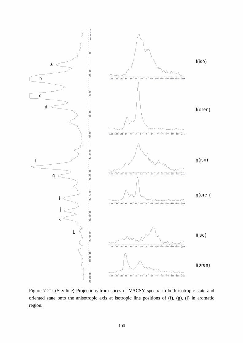
���
a
L
k
j
i
g
f
d
c
b
f(oren)
g(oren)
i(o ren)
f(iso)
g(iso)
i(iso)
Figure 7-21: (Sky-line) Projections from slices of VACSY spectra in both isotropic state and
oriented state onto the anisotropic axis at isotropic line positions of (f), (g), (i) in aromatic
region.

���
a
L
k
j
i
g
f
d
c
b
k(iso)
k (o ren)
L(iso)
L(oren)
j(o ren)
j(iso)
Figure 7-22: (Sky-line) Projections from slices of VACSY spectra in both isotropic state and
oriented state onto the anisotropic axis at isotropic line positions of (j), (k), (l) in aromatic
region.
To make a quantitative analysis of the orientation distribution of the mesogenic groups of
this LCSP polyacrylate sample, we chose the 13C line at position (f) and apply the line-shape

���
fitting procedure. Again, the simple Gaussian distribution function as defined in equation (7-3)
is selected. Because the spinning speed used to acquired the VACSY spectrum is only 3.5 kHz,
the line-shape distortion due to a non-sufficient spinning speed has to be taken into account as
described in chapter 5. Here, complete VACSY simulations with exactly the same experimental
sample spinning speed are carried out, the result is shown in fig7-23.
Figure 7-23: Analysis of orientation distribution in LCSPs - polyacrylates by the method of line-
shape fitting from VACSY spectra of sample in isotropic state and oriented state, chemical shit
tensor used for simulation is (Vxx, Vyy, Vzz)=(207, 148, 18) (ppm). (a) projection of experimental
VACSY spectrum of sample in isotropic powder state. (b) projection of experimental VACSY
spectrum of sample in oriented state. (c) simulated CSA spectra of sample in oriented state for
different orientation distributions. Comparing the spectra in (b) and in (c), the orientation
distribution for the best fitting is Tref = 90o and TV # 18o, corresponding to an order parameter of
S=0.65r0.1.
The simulation result shows an orientation distribution of the mesogens in the investigated
polyacrylate LCSP as: the Vzz element of the chemical shift tensor for aromatic 13C at position (f)
from the mesogenic groups has a Gaussian orientation distribution function with the centre at
90o relative to the rotor axis direction, the hwhm is about 20o. With the same arguments as the
discussion for p-n-hexa-hexyloxytriphenylene in section 7-4, it is equal to state that: the rigid
mesogenic planes are highly oriented parallel to the rotor axis direction, the distribution function
is described as an Gaussian function with an hwhm angle of about 20o which corresponds to an
order parameter S = 0.65 r 0.1.

���
Comparing the experimental CSA patterns with the simulated CSA patterns in both
isotropic powder state and oriented state, there are some degree of deviations. Especially for the
experimental CSA pattern of the LCSP polyacrylate sample in powder state, where a theory-like
powder line-shape as well as the three singularities could not be clearly identified. These
deformation of CSA patterns are quite often met in macromolecular samples. In our opinion,
these are due to (i) complicated structural conformations existed in polymer samples. (ii)
possible anisotropic thermal motions although experiments are conducted under a temperature
well below sample’s Glass transition temperature Tg. (iii) not sufficient dipolar decoupling.
7.6 Summary
The following conclusions might be drawn from this work:
(1) VACSY is practically one of most promising methods to obtain the correlation
between chemical shift isotropy and chemical shift anisotropy. Firstly, it is not very
sensitive to errors in experimental parameters like various methods of multi-pulses with
MAS rotor synchronisation. Secondly, it does not require a very swift mechanical
change of the rotor status like in the methods of stop-and-go, MAS-OMAS, Magic
Angle Hopping.
(2) VACSY can be used reliably to measure the values of chemical shift tensor elements.
In the case of simple substance with few non-overlapping lines, CSA tensor elements
can be easily measured by 1D VAS experiment with a better accuracy comparing with
the popularly applied Hertzfeld-Berger approach. In the case of multiple lines with
overlapped CSA tensors, VACSY can successfully separate them according to their
isotropic chemical shift values and then measure their CSA tensor elements
respectively.
(3) VACSY is a promising alternative for the study of orientation distribution in polymer
samples. Due to its ability to correlate each CSA patterns with their corresponding
chemical shift isotropic values, when S/N ratio is high enough, VACSY is possible to
obtain the complete orientation distribution of each individual molecular segments with
one experiment, for example main-chain and side-chain orientation distribution or
orientation distribution at different positions inside the side-chain of LCSPs.
(4) An accurate orientation distribution analysis by the method of VACSY requires the
sample spinning reaches a certain minimum speed with regard to the chemical shift
anisotropy of the investigated sample. Otherwise, the distortion of CSA pattern due to a
slow spinning speed may invalidate the results. Two solutions are suggested: (i) higher
spinning speed. (ii) lower Bo field. The (i) is the best solution, because it does not

���
sacrifice the sensitivity which is also a big trouble when macromolecular samples are
studied.
(5) In the case of nucleus with relative smaller anisotropic chemical shift values and
bigger spectral intensities, like the aliphatic 13C in our polyacrylate LCSPs, serious
phase artefacts prevent an accurate orientation distribution analysis. In this case, Linear
Prediction should be applied to relieve the phase artefacts.

,
REFERENCES
1. Abragam, A. (1961). The Principles of nuclear Magnetism. Oxford University Press,
London
2. Alla, M. A., Kundla, E. I. and Lippmaa, E. T. (1978). JETP Lett., 27, 194
3. Balta-Calleja, F. J. and Vonk, C. G. (1989). X-ray Scattering of Synthetic Polymers.
Elsevier, Amsterdam
4. Barkhuijsen, R. de B., Bovee, W. M. M. J. and Van Ormondt, D.(1985). Retrieval of
frequencies, amplitudes, damping factors and phases for time-domain signals using linear
least-squares procedure, J. Magn. Reson. 61, 465
5. Bax, A., Szeverenyi, N. M. and Maciel, G. E. (1983a). Isotropic Shifts and CSAs: 2D
Magic-Angle Hopping NMR. J. Magn. Reson., 52, 147
6. Bax, A., Szeverenyi, N. M. and Maciel, G. E. (1983b). CS Anisotropy of Powders: 2D
NMR with Flip of Spinning Axis. J. Magn. Reson., 55, 494
7. Bax, A., Szeverenyi, N. M. and Maciel, G. E. (1983c). CS Anisotropy in Powders Studied
by 2D CP/MAS NMR. J. Magn. Reson., 51, 400
8. Bennett, A. E. Rienstra, C. M., Auger, M., Lakshmi, K. V and Griffin, R. G. (1995). J.
Chem. Phys., 103, 6951
9. Bloembergen, N. and Rowland, J. A. (1953). Acta Met.,1, 731
10. Bovey, F. A. (1988). Nuclear Magnetic Resonance Spectroscopy. Academic Press, San
Diego
11. Carlson, J. W. (1988). J. Magn. Reson. 78, 563
12. Champeney, D. C. (1973). Fourier Transforms and Their Physical Applications.
Academic Press, New York
13. Chen, C.-N. and Hoult, D. I. (1989). Biomedical Magnetic Resonance Technology, Adam
Hilgar, New York
14. Chmelka, B. F., Schmidt-Rohr, K. and Spiess, H. W. (1993). Orientation Distributions in
PET Films and Fibers from DECODER NMR. Macromolecules, 26, 2282
,,
15. Conroy, H. (1967). Molecular Scrödinger Equation. VII. A New Method for the Evaluation
of Multidimensional Integration, J. Chem. Phys., 47(12)
16. Crozier, S., Luescher, K., Forbes, L. K. and Doddrell, D. M. (1995). J. Magn. Reson. 109,
1
17. De Beer, R., Van Ormondt, D., Pijnappel, W. W. F. and Van Der Veen, J. W. C. (1988)
Isr. J. Chem. 28, 249
18. Doty, F. D. (1996a). Probe Design and Construction. Encyclopedia of NMR, 1996, Vol.
6, 3573
19. Doty, F. D. (1996b). Solid Sate Probe Design. Encyclopedia of NMR, 1996, Vol.7, 4475
20. Doty, F. D., Inners, R. R. and Ellis, P. D. (1981). J. Magn. Reson. 43, 399
21. Doty, F. D., Connick, T. J., Ni, X. Z. and Clingan, M. N. (1988). J. Magn. Reson. 77, 536
22. Eden, M. and Levitt, M. H. (1998). Computation of Orientational Averages in Solid-State
NMR by Gaussian Spherical Quadrature. J. Magn. Reson. 132, 220
23. Ernst, R. R., BodenHausen, G. and Wokaun, A. (1987). Principles of Nuclear Magnetic
Resonance in One and Two Dimensions. Oxford Univeresity Press, Oxford
24. Elliott, D. F. and Rao, K. R. (1982). Fast Transforms: Algorithms, Analyses, Applications.
Academic Press, New York
25. Flory, J. (1953). Principles of Polymer Chemistry, Cornell University Press, Ithaca
26. Frydmann, L., Chingas, G. C., ..., Pines, A. (1992a). Variable Angle Correlation
Spectroscopy in Solid-State Nuclear Magnetic Resonance, J. Chem. Phys. 97(7), 4800,
Oct. 1992
27. Frydmann, L., Chingas, G. C., ..., Pines, A. (1992b). Correlation of Isotropic Chemical
Shifts in Solids by Two-Dimensional Variable-Angle-Spinning NMR. Israel Journal of
Chemistry, 32, 161
28. Frydmann, L., Lee, Y. K., Emsley, L., Chingas, G. C. and Pines, A. (1993). Variable
Angle Three-Dimensional Exchange NMR for the Study of Molecular Motion in Complex
Solids. J. Am. Chem. Soc., 115(11) 4826
29. Frydman, L., Lee, Y. K., Emsley, L. (1994). Solid-State Dynamic Processes in Complex
Systems Analyzed by Two-Dimensional Isotropic-Anisotropic Correlation Nuclear
Magnetic Resonance. J. Chem. Phys., 101(1), 111

,,,
30. Fukushima, E. and Roeder, S. B. W. (1996). Experimental Pulse NMR - A Nuts and Bolts
Approach. Addison-Welsley Publishing Company
31. Fyfe, C. A. (1983). Solid State NMR for Chemists. C.F.C Press, Guelph
32. Gan, Z. (1992). High-Resolution-Shift and CSA Correlation by Slow MAS. J. Am. Chem.
Soc., 114, 8307
33. Gordan, R. E. (1985). Phys. Med. Biol. 30(8), 741
34. Haeberlen, U. (1976). High Resolution NMR in Solids - Selective Averaging, Academic
Press, San Diego
35. Harbison, G. S., Vogt, V.-D. and Spiess, H. W. (1987). Partially Orieted Solids:
Characterisation by 2D MAS NMR. J. Chem. Phys., 86, 1206
36. Harper, J. K., McGeorge, G. and Grant, D. M. (1998). Solid-State 13C Chemical Shift
Tensors in Terpenes. Magnetic Resonance in Chemistry, 36, 135
37. Hartmann, S. R. and Hahn, E. L. (1962) Phys. Rev. 128, 2042
38. Hayes, C., Edelstein, W., Schenck, J. Mueller, O. M. and Eash, M. (1985). J. Magn.
Reson. 63, 622
39. Hediger, S., Singer, P., Tomaselli, M., Ernst, R. R. and Meier, B. H. (1997). J. Magn.
Reson., 125, 291
40. Hempel, G., Schneider, H. (1982). Pure and Appl. Chem. 54, 635-646
41. Hempel, G., Jacobi, A. et al. (1999). Macromol. Chem. Phys. 2000, 1608
42. Hentschel, R., et al. (1976). Magn. Reson. Relat. Phenom., 19th Proc. Congr.Ampere,
1976, 381
43. Hentschel, R., Schlitter, J., Sillescu, H. and Spiess, H. W. (1978). J. Chem. Phys., 68(1),
56, Jan 1978
44. Hentschel, R. and Spiess, H. W. (1979). J. Magn. Reson., 1979, 35, 157
45. Hentschel, R., Sillescu, H. and Spiess, H. W. (1980). Polymer, 22, 1516, Nov. 1981
,9
46. Henrichs, P. M. (1987). Molecular Orientation and Structure with 13C NMR: A Study of
Biaxial Films of PET. Macromolecules, 20, 2099
47. Herzfeld, J. and Berger, A. E. (1980) Sideband intensities in NMR spectra of samples
spinning at the magic angle, J. of Chem. Phys. 73(121), 6021-6030, 15 Dec. 1980
48. Hoult, D. I. (1989). Concepts Magn. Reson. 1, 1
49. Hoult, D. I. and Richards, R. E. (1976). J. Magn. Reson. 24, 71
50. Hoult, D. I. (1978). Prog. NMR Spectrosc., 12, 41
51. Hu, J. Z., Wang, W., ..., Grant, D. M. (1995). Magic-Angle-Turning Experiments for
Measuring Chemical-Shift-Tensor Principal Values in Powdered Solids. J. Magn. Reson.,
113, 210
52. Ishii, Y. and Terao, T. (1998). Manipulation of Nuclear Spin Hamiltonians by rf-Field
modulations and Application to Observation of Powder Patterns under Magic-Angle
Spinning. J. Chem. Phys., 109, 1
53. Jackson, J. D. (1975). Classical Electrodynamics. Wiely, New York
54. Kashiwagi, M., Folkes, M. J. and Ward, I. M (1971). Polymer, 12, 697
55. Kashiwagi, M. and Ward, I. M. (1972). Polymer, 13, 145
56. Kasiwagi, M., Cunningham, A., Manuel, A. J. and Ward, I. M. (1973). Polymer , 14, 111
57. Kay, S. M. (1988). Modern Spectral Estimation theory and Application, Prentice-Hall,
Englewood Cliffs, New Jersey
58. Kolbert, A. C. and Griffin, R. G. (1990). 2D Resolution of Isotropic and Anisotropic
Chemical Shifts in MAS NMR. Chem. Phys. Lett., 166, 87
59. Koskinen, M. F. and Metz, K. R. (1992). J. Magn. Reson. 98, 576
60. Kroschwitz, I. Ed. (1990). Concise Encyclopedia of Polymer Science and Technology,
Wiley, New York
61. Kumaresan, R. and Tufts, D. W. (1982). IEEE Trans. Acoust. Speech Signal Process.
ASSP-30, 833

9
62. Lee, Y. K., Emsley, L., ..., Pines, A. (1994). Three-Dimensional Variable-Angle Nuclear
Resonance Exchange Spectroscopy without Rotor Axis Hopping. J. Chem. Phys., 101(3),
1852
63. Lee, Y. K., Vold, R. L., Hoatson, G. L., Lin, Y.-Y. and Pines, A. (1995). Linear Prediction
with Singular-Value Decomposition for Removing Phase Artifacts in 2D VACSY Spectra.
J. Magn. Rson., 112, 117
64. Lin, Y.-Y., Ge, N.-H and Hwang, L.-P (1993). J. Magn. Reson. A 105, 65
65. Lpmaa, E. Alla, M. and Turherm, T. (1976). Proceedings of the 19th Congress Ampere,
Heiderberg, 1976, 241
66. Maciel, G. E., Szeverenyi, N. M. and Sardashti, M. (1985). CSA Powder Patterns: 2D
Angle Flipping Effects of Crystallite Packing. J. Magn. Reson., 64, 365
67. Mansfiled, P. and Powles, J. G. (1963). J. Sci. Instrum. 40, 232
68. Maricq, M. M. and Waugh, J. S. (1979). NMR in rotating solids, J. Chem. Phys. 70(7)
69. McBrierty, V. J. and Ward, I. M. (1968). Journal of Physics, 1, 1529
70. McBrierty, V. J., McDonald, I. R. and Ward, I. M. (1971). Journal of Physics, 4, 88
71. McBrierty, V. J. and McDonald, I. R. (1973). Journal of Physics, 4, 88
72. McBrierty, V. J. (1974). Polymer, 15, 503
73. McBrierty, V. J. and Packer, K. J. (1993). Nuclear Magnetic Resonance in Solid
Polymers, Cambridge Uni. Press, New York
74. McCall, D. W. and Hanmming, R. W. (1959). Acta Cryst., 12, 81
75. McCrum, N. G., Read, B. E. and Williams, G. (1967). Anelastic and Dielectric Effects in
Polymeric Solids, Dover, New York
76. McGeorge, G., Alderman, D. W. and Grant, D. M. (1999). Resolution Enchancement in13C and 15N Magic-Angle Turning Experiments with TPPM Decoupling. J. Magn. Reson.,
137, 138
77. Mehring, M. (1983). High Resolution NMR Spectroscopy in Solids, Springer-Verlag,
Berlin

9,
78. Montigny, F., elbayed, K., Brondeau, J. and Canet, D. (1990) Automatic Phase Correction
of Fourier Transform Nuclear Magnetic Resonance Spectroscopy Data and Estimation of
Peak Area by Fitting to a Lorentzian Shape", Analytical Chemistry, 62 (8), 15 April 1990
79. Pines, A., Gibby, M. G. and Waugh, J. S. (1973). J. Chem. Phys., 59, 569
80. Rutledge, D. N. (Ed.) (1996) Signal treatment and signal analysis in NMR, Elsevier
81. Sachleben, J. R. and Frydman, L. (1997). Orientational Alignment in Solids from
Bidimensional Isotropic-Anisotropic Nuclear Resonance Spectroscopy: Applications to
the Analysis of Aramide Fibers. Solid State Nuclear Magnetic Resonance , 7, 301
82. Schaefer, J. and Stejskal, E. O. (1976). J. Am. Chem. Soc., 98, 1031
83. Schmidt-Rohr, K., Spiess, H. W. (1994). Multidimensional Solid-state NMR and
Polymers, Academic Press, San Diego
84. Schmidt-Rohr, K., Wilhelm, M., Johansson, A. and Spiess, H. W. (1993). Shift Tnsors in
Methlene Groups. Magn. Reson. in Chem., 31, 352
85. Schneider, H. J. and Dullenkopf, P. (1977). Rev. Sci. Instrum. 48, 68
86. Slichter, C. P. (1980). Principles of Magnetic Resonance. Springer-Verlag, Berlin
87. Spiess, H. W. (1980). J. Chem. Phys., 1980, 72, 6755
88. Spiess, H. W. (1984). NMR in Oriented Polymers, In I. M. Ward (ed.), Decelopments in
Oriented Polymers. Applied Science Publishers, London
89. Spiess, H. W. (1985). 2H NMR for Studying Mobility and Orientation in Polymers. Adv.
Polym. Sci., 66, 23
90. Stejskal, E. O., Schaefer, J. and Mckay, R. A. (1977). J. Magn. Reson., 25, 569
91. Stephenson, D. S. (1988) Linear Prediction and Maximum Entropy Methods in NMR
Spectroscopy. Prog. NMR Spectrosc. 20, 515
92. Tekely, P.(1998). To What Extent the Centralband and Each Spinning Sideband Contain
Contributions from Different Parts of the Static Powder Pattern?, Solid Sate NMR 14,
33-41, 1999

9,,
93. Terao, T., Fujii, T., Onodera, T. and Saika, A. (1984). Switching-Angle Spinning NMR:
Powder- Pattern-Resolved 2D Spectra. Chem. Phys. Lett., 107, 145
94. Titman, J. J., Feaux de Lacronix, S. and Spiess, H. W. (1993). Structure and Order in
Solids by 3D MAS NMR. J. Chem. Phys., 98, 3816
95. Traficante, D. D. (1989). Concepts Magn. Reson. 1, 73
96. Tycko, R., Dabbagh, G. and Mirau, P. A. (1989). Determination of Chemical-Shift-
Aniostropy Lineshapes in a Two-Dimensional Magic-Angle-Spinning NMR Experiment. J.
Magn. Reson., 85, 265
97. Wachter, E.A., Sidky, E.Y. and Farrar, T.C. (1989). Calculation of Phase-Correction
Constants Using the DISPA Phase Angle Estimation Technique, J. Magn. Reson., 82, 239
98. Van Vaals, J.J. and Van Gerwen, P. H. J. (1990). Novel Methods for Automatic Phase
Correlation of NMR Spectra, J. Magn. Reson. 86, 127-147
99. Van Vleck, J. H. (1948). Phys. Rev., 74, 1168
100. Vaughan, R. W. (1978). Annu. Rev. Phys. Chem. 29, 397
101. Ward, I. M., Ed. (1982). Developments in Oriented Polymers, Applied Science Publishers,
London
102. Ward, I. M. (1985). In Characterisation of Polymers in the Solid State I: Part A: NMR and
other Spectroscopic Methods, Kausch, H. H. and Zachmann, H. G. (eds.), Springer-
Verlag, Berlin
103. William H. P., Brian P. F., Teukolsky, S. A., Vetterling, W. T. (1989). Numerical Recipes,
Cambridge University Press, London
104. Yarim-Agaev, Y., Tutunjian, P. N. and Waugh, J. S. (1982). J. Magn. Reson., 47, 51
105. Zeigler, R. C., Wind, R. A. and Maciel, G. E. (1988). Stop-and-Go Spinning in MAS, J.
Magn. Reson., 79, 299

Erklärung
Ich erkläre hiermit, dass die Dissertation selbständig verfasst wurde und nur die
angegebenen Hilfsmittel benutzt wurden. Die Dissertation wurde noch an keiner anderen
Universität oder Hochschule eingereicht.
Halle, den 20. 09. 1999
(Zhanjun Fang)

ACKNOWLEDGMENTS
I would like to thank all the people who have helped me in any respect for the realisation
of this thesis. In particular, I want to thank:
Prof. Dr. H. Schneider for accepting me as a Ph. D. student and advising me through
three years of Ph. D. study.
Dr. D. Reichert for introducing me all the secrets/tricks of experimental NMR
and for having a lot of patience with me when I had various
problems about probe, spectrometer, with mechanic
workshop, even with immigration office.
Dr. G. Hempel for excellently explaining all the basic NMR theories to me,
answering my questions in physics, chemistry, mathematics
and for his talented suggestions to solve problems occurred in
this project.
Dr. M. Braun for his kind help in the construction of the RF circuit of my
VACSY probe.
all other members of Prof. Dr. Schneider’s group for the pleasant atmosphere during
work as well as in coffee breaks.

Curriculum Vitae
20. 03. 1965 Born in Beijing, P. R. China
1982 - 1987 Department of Electronic Engineering, Tsinghua University
Beijing, 100084, P. R. China
B. S. in Electronic Engineering
Title of Diploma work: ‘Fabrication of Single Transverse Mode
InGaAsP/InP Semiconductor Laser by Liquid Epitaxy’
1987 - 1990 Department of Electronic Engineering, Tsinghua University
Beijing, 100084, P. R. China
M. S. in Electron Physics and Devices
Title of Master degree work: ‘Characteristics of the All Optic
Switching Network in Time Domain Optic Fibre Communication
System’
1990 - 1995 Division of Length Metrology, National Institute of Metrology
Beijing, 100013, P. R. China
Research Scientist
Research area: ‘Small Scale Length Metrology’
1995 - 1996 Danish Institute of Fundamental Metrology
Lyngby, DK-2800, Denmark
Fellowship Research Scientist
Research area: ‘Application of Scanning Tunnelling Microscope in
Surface Roughness Metrology'
1996 - 1999 FB Physik, Martin-Luther-Universität, Halle-Wittenberg
D-06108, Halle/Saale, Germany
Ph.D. study in Physics
PhD thesis title: ‘Accomplishment of VACSY Experimental Set-up
and its Application to Investigate Molecular Orientation Distribution
of Solid-State Polymer’
Halle, den 20. 09. 1999,
Zhanjun Fang