Accounting Conservatism, the Quality of Earnings,and Stock Returns

Stephen H. PenmanGraduate School of Business

Columbia University

and

Xiao-Jun ZhangHaas School of Business

University of California, Berkeley

December, 1999

The comments of participants in workshops at Columbia University, Cornell Universityand the University of Minnesota are appreciated, particularly those of Tom Dyckman andJohn Elliott.

1

Accounting Conservatism, the Quality of Earnings, and Stock Returns

It is often claimed that the practice of conservatism in accounting produces higher quality

earnings. Conservatism yields lower earnings, it is said, and so prima facie these “conservative”

earnings are higher quality. In this paper we show, empirically, that conservative accounting can

yield lower quality earnings. And we show that the stock market does not appear to price the

lower quality earnings appropriately.

The term “quality of earnings” is vague and has been used with different interpretations

in mind. We examine the issue from the point of view of an analyst wishing to forecast future

earnings. We interpret the term to mean that reported earnings, purged of transparently

extraordinary items, is of good quality if it is a good indicator of future earnings. Thus we have

in mind the notion of “sustainable earnings” that is often referred to in financial analysis. We

also view earnings forecasts as an input to equity valuation. So we interpret the market as

misinterpreting the quality of earnings (in pricing firms) if it fails, given wider interpretive

information available, to see that reported earnings is not sustainable in the future. This view of

market inefficiency has been referred to in the past as “fixation” on reported earnings, so, in

those terms, we examine whether the market is "fixated" on reported earnings, unaware that they

may be of doubtful quality because of conservative accounting practices.

By conservatism we mean accounting practice, consistently applied, that keeps the book

values of net assets relatively low. So LIFO accounting for inventories is conservative relative to

FIFO (if inventory costs are increasing); expensing research and development (R&D)

expenditures rather than capitalizing and amortizing them is conservative; accelerated

depreciation methods and/or using short estimated asset lives are conservative; and policies that

2

consistently estimate high allowances for doubtful accounts, sales returns or warranty liabilities

are conservative.

Conservative accounting raises questions about the quality of the balance sheet. But the

accounting for book values also affects the earnings calculation (of course). Earnings quality

questions arise with conservative accounting because, with growth in investment, earnings are

indeed lower than otherwise. But these lower earnings create “hidden reserves.” Hidden

reserves can be increased, reducing earnings, by increasing investment. And hidden reserves can

be reduced, creating earnings, by reducing investment or reducing the rate of growth in

investment. If the change in investment is temporary, the induced change in earnings is also

temporary and not indicative of subsequent earnings.

The literature on earnings quality is extensive, typically focusing on manipulation of

accounting principles or accounting estimates to manage reported earnings. (For a recent review,

see Healy and Wahlen (1998)). So, for example, to inflate earnings temporarily, estimates of the

valuation reserve for deferred tax assets, or of doubtful accounts, are temporarily lowered. Or, to

reduce earnings temporarily (and to bleed them back in the future) a restructuring charge is

overestimated. The earnings quality we have in mind is driven instead by real activity.

Accounting methods and estimates are not changed. Rather, given a (conservative) accounting

policy consistently applied over time, earnings is temporarily affected by (real) investment.

Manipulation and earnings management may or may not be intended by management but, if

intended, the effect is achieved by an understanding of the joint effect of real activity and

accounting policy. The effect is perverse: reducing investment reduces future earnings from

investments but, with conservative accounting, reducing investment increases current earnings,

making them a poor indicator of future earnings.

3

We have two research questions. First, are temporary changes in earnings associated

with conservative accounting indeed observed? And, second, does the stock market price these

temporary earnings as if they are indeed unsustainable? The answer to the first question appears

to be yes. The answer to the second is no. In carrying out the analysis we also develop indexes

that indicate the quality of earnings. These indexes, in themselves, are an aid to financial

analysis and research.

Anticipated future earnings differ from current earnings with changes in investment. So,

to examine the sustainability of earnings, we focus on accounting rates of return, that is, earnings

relative to net assets, that deflates earnings for new net investment. The rate of return also

captures the effect of conservatism on both earnings and book values. And this focus serves our

purpose of analyzing the pricing of earnings of varying quality. Accrual-accounting residual

income valuation models dictate that forecasted earnings can be interpreted for valuation

purposes only with reference to the book values that generate them, so describe intrinsic equity

values as being determined by anticipated accounting rates of return and growth in the book

value of net assets. So pricing errors can occur if the market, relying on the current rate of

return, forecasts future rates of returns incorrectly.

The paper is organized as follows. As a background to the analysis, the next section

outlines the effects of conservative accounting and investment growth on accounting rates of

return. Section 2 develops indexes for scoring firms on their conservative accounting and the

quality of their earnings, and also describes the data. Sections 3 and 4 address the two research

questions. Section 3 investigates whether the sustainability of accounting rates of return is

diagnosed with the quality scores. Section 4 documents returns to taking positions in stocks on

the basis of the quality diagnosis. A summary of the conclusion is in Section 5.

4

1. Conservatism, Investment, Accounting Rates of Return, and the Quality of Earnings

Researchers have introduced a variety of definitions of conservative accounting. Some,

like Basu (1997), define conservatism as the practice of reducing earnings (and writing down net

assets) in response to "bad news" but not increasing earnings (and writing up net assets) in

response to "good news." In the accounting-based valuation literature, researchers often refer to

Feltham and Ohlson (1995) who characterize conservative or "biased" accounting as an

expectation that reported net assets will be less than market value in the long run. That definition

classifies the accounting for anticipated positive net-present-value investments at historical cost

as conservative accounting, because those investments are expected to be carried at less than

their value. Others, like Gjesdal (1999), distinguish "economic profitability" from accounting

profitability such that the accounting for anticipated investments is conservative if it gives them a

carrying value that yields an accounting rate of return greater than the internal rate of return on

their cost. So, for example, conservative accounting follows the practice of carrying an asset

whose value is equal to its historical cost (a zero net present value investment) at less than

historical cost.

Our notion of conservatism follows the latter definition; that is, it concerns biased

application of historical cost accounting. But, for our purposes, we do not have to establish

unbiased historical-cost carrying values of investments or unbiased allocations of investment

cost to match against revenues. Rather, we examine conservatism in a relative sense such that

one practice (for example, accelerated depreciation) is considered more conservative relative to

another if the accumulated amortizations it yields are greater than those for the other (and

consequently the carrying value it yields is always less).

5

The interaction between conservative accounting, investment and earnings is best

explained for the case of LIFO accounting for inventories because, for that case, the dollar effect

of the interaction is transparent in the LIFO reserve disclosure in footnotes to U.S. financial

statements. LIFO accounting carries inventories on the balance sheet at lower amounts than

FIFO or average cost methods if inventory prices have risen in the past. It is, then, more

conservative than the alternatives under conditions of rising inventory prices. Earnings are not

affected by LIFO if dollar inventories are unchanged for the earnings period: cost of goods sold

is equal to purchases for the period, as it is with FIFO. Accordingly the LIFO reserve, the

accumulated difference between FIFO and LIFO earnings is unaffected.1 But, if dollar

inventories increase, either through physical inventory growth or inventory price changes,

earnings are lower under LIFO. Accordingly, the LIFO reserve increases. And, if dollar

inventories decline (so lower LIFO inventory costs are brought into cost of goods sold), earnings

are higher under LIFO. Accordingly, the LIFO reserve decreases -- and earnings -- are increased

as the result of a real phenomenon, a decline in inventory.

The LIFO reserve is a case of a “hidden reserve” that results from conservative

accounting, but one that is made manifest by the LIFO reserve disclosure requirement. The

buildup of the LIFO reserve is a case of creating hidden reserves and the decline in the LIFO

reserve -- known as LIFO dipping -- is a case of liquidation of hidden reserves.

The same phenomena are produced -- less transparently -- by all forms of conservative

accounting. “Accelerated” depreciation (that reports lower net asset values) has no affect on

earnings if tangible assets are not growing, but reduces earnings (and creates hidden reserves) if

investment in the assets increase, ceteris paribus. (It is the growth case that people must have in

mind when they assert that conservative accounting reports lower earnings). If investments

6

decline, accelerated depreciation creates earnings through the liquidation of hidden reserves.

Immediate expensing of R&D expenditures and advertising is conservative (setting “knowledge

assets” and “brand assets” to zero on the balance sheet), but has no affect on earnings relative to

capitalizing and amortizing the expenditures if the expenditures are not growing. However,

increasing R&D investments and advertising with immediate expensing “depresses” earnings,

and slowing them increases earnings.

The effect of conservative accounting on accounting rates of return is, strangely enough,

to present a picture of profitability that is other than conservative. With lower net asset values

and no effect on earnings, return on net assets is higher under conservative accounting if assets

are not changing (see Feltham and Ohlson (1995)). Growth in assets reduces return on net assets

below the no-growth level with conservative accounting, but induces an expected growth in

earnings and residual earnings. Decreases in the rate of growth in investment increase return on

net assets above its previous level and declines in investment (negative growth) increase return

on net assets above the no-growth level. This is modeled in Zhang (1998) and is laid out, with

examples, in Penman (2000).

Quality of earnings issues arise, then, if a change in a reported accounting rate of return

that is induced by a change in investment is temporary. If an analyst accepts the current book

rate of return as an indicator of future rates of return, he or she will be misled if the reported rate

of return is temporarily affected by the joint effect of conservative accounting and investment

activity. But, if the analyst penetrates the joint effect, he or she will discover the reported

number to be a poor quality indicator of long-run “sustainable” profitability. And "quality of

valuation" issues also arise if valuations are made from forecasts of earnings. This follows

directly, if an investor follows the prescription of residual earnings valuation models and so

7

forecasts future book rates of return to value firms. But cash-flow valuations usually forecast

earnings also, in order to predict future cash-flow.

Our empirical analysis, then, documents the incidence of these temporary effects on

accounting rates of return, and asks whether the market pricing of stocks is consistent with

investors appreciating the quality of earnings in valuing stocks.

2. Indexes of Conservatism and Earnings Quality

The empirical analysis uses two indexes. The first scores the degree of application of

conservative accounting by firms. The second scores the quality of earnings that results from the

joint effect of conservatism and investment activity. The sample of firms used in the analysis are

NYSE and AMEX non-financial firms on the combined COMPUSTAT Annual Industrial and

Research files (which include nonsurvivors) for 1975-1997. Monthly stock returns up to

December, 1997 were obtained from 1997 CRSP files. Our sample period begins in 1975

because, prior to that year, accounting data to construct the indexes were missing for a

significant number of firms on COMPUSTAT.

2.1 Conservatism Index (C-score)

The C-score that was developed in Penman and Zhang (1999) measures the effect of the

application of conservative accounting on the balance sheet by the level of hidden reserves that

are created by conservatism relative to net operating assets:

it

itit NOA

reservehiddenEstimatedC = ,

where i indicates firms and t indicates balance sheet dates. Net operating assets, NOA, is the

book value of operating assets minus operating liabilities, as defined in Nissim and Penman

(1999). NOA excludes financial assets and liabilities from total net assets (shareholders’ equity)

8

as these financial items typically are at, or close to, market value on the balance sheet and so are

not affected by conservative accounting.2

A complete C-score calculates hidden reserves created by all operating items in the

balance sheet -- including bad-debt allowances, depreciation allowances, valuation allowances,

deferred revenue, pension liabilities and other estimated liabilities. For the purpose here, we

wish to distinguish earnings quality issues that arise from changes in estimates -- accounting

manipulation -- from quality issues that arise from permanent accounting policy and changes in

investment. An allowance for bad debts, for example, might be “high” because of a permanent

policy of carrying net receivables at a conservative level or because of a temporary increase in

the estimate of bad debts to “bleed” income to the future. Unable to distinguish the two effects

for balance sheet items subject to estimates, we construct a C-score based only on the accounting

treatment of inventories, R&D and advertising expenditures; the accounting for these items is

driven by mandates from accounting regulators or (in the case of LIFO) by an accounting choice

that (usually) cannot change from period to period. So

itresit

resit

resitit NOA/)ADVRDINV(C ++= ,

where the three reserve components are calculated as follows:

− Inventory hidden reserve ( )resitINV equals the LIFO reserve reported in footnotes.

Its value is zero for non-LIFO firms.

− R&D hidden reserve ( )resitRD is calculated as estimated R&D assets. We use the

coefficients estimated by Lev and Sougiannis (1996) to capitalize and amortizeR&D, and so construct a book value without immediate expensing.

− Advertising expenses are capitalized and amortized using an ad hoc acceleratedmethod over two years. (Bublitz and Ettredge (1989) and Hall (1993) indicate ashort useful life for advertising, typically one to two years).

9

Each component of the reserve can be used to calculate a sub-score, the hidden reserve

component relative to NOA. We conduct our analysis using sub-scores as well to see if any

particular activity drives the results.

Of the 46,955 firms with share price, shares outstanding, and book value of common

equity on COMPUSTAT from 1975-97, NOA could be calculated for 46,854 of them. Of these,

46,122 had positive NOA, and C-scores could be calculated for 38,540 of them. Firm-years

were deleted if none of the three sub-scores could be calculated from the COMPUSTAT data.

When only some of the sub-scores were missing, we used industry median sub-scores (for 2-digit

SIC industry groups) as substitutes to calculate the overall C-score for that firm-year. The

38,540 firm-years were made up as follows:

Firm-years with 1 sub-score 8,285

Firm-years with 2 sub-scores 19,258

Firm-years with 3 sub-scores 10,997

Total firm-years 38,540

Of these 38,540 firm-years, the LIFO reserve was available for 36,244 of them, 13,931

cases of firms on LIFO and 22,313 non-LIFO cases (where the reserve is zero). The R&D

reserve could be calculated for 25,357 firm-years and the advertising reserve could be calculated

for 18,191 firm-years.

Table 1 summarizes the distribution of C-scores over firm-years. The median of 0.114

indicates how much higher NOA would have been for the typical firm if hidden reserves had not

been created by the accounting treatment of the three items. The mean of 0.31, relative to the

median and upper percentile scores, indicates that scores are particularly large for a relatively

small number of firms.

10

2.2 Earnings Quality Indicator (Q-score)

While the C-score measures the effect of conservative accounting on the balance sheet,

the Q-score measures the effect of conservative accounting on earnings in the income statement.

One measure is calculated as

1it

1it

it

itAit NOA

ER

NOA

ERQ

−

−−= ,

where ER indicates estimated hidden reserves. That is, AitQ is the change in Cit. So a firm’s QA

score is “high” if it builds up its hidden reserve at a faster rate than the growth in NOA, and

“low” if it decreases its reserve at a slower rate. A second measure compares a firm’s hidden

reserve to the median for its SIC two-digit industry:

−=

it

it

it

itBit NOA

ERmedianIndustry

NOA

ERQ .

If BitQ is large in absolute value it might indicate that hidden reserves are temporary (and will

revert to industry norms).

The Q-score combines these two measures:

( ) ( )Bit

Aitit Qx5.0Qx5.0Q +=

The relative weights are arbitrary; they are changed to (1,0) and (0,1) in a sensitivity analysis.

Q-scores could be calculated for 32,343 firm-years. To ensure that the Q-scores capture

changes in the growth of firms' investment activities, we delete 2,547 firm-years where the firms

have missing R&D and missing advertising expenditures on COMPUSTAT and they use non-

LIFO inventory methods. Table 1 gives the distribution of the final sample of 29,796 Q-scores

over firm-years. The median is close to zero. The scores for the upper percentiles indicate a

considerable amount of hidden reserves were created annually for a considerable percentage of

11

firms (during this period of considerable asset growth). Low Q-scores are lower in absolute

values than high scores, but 40% of cases reported liquidations of reserves.

3. Analysis of the Quality of Book Rates of Return

We examine how Q-scores predict changes in core RNOA. Core RNOA (core return on

net operating assets) is calculated as

Core RNOAit = [Core operating incomeit x (1 − marginal tax rateit)]/average NOAit.

Core operating income is operating income before interest, special items, and extraordinary items

and discontinued operations, so excludes items that are transparently indicated in the income

statement as (presumably) temporary components of earnings, along with interest expense,

which is not generated by operations, and which is not affected by conservative accounting.

Thus, we identify reported income that the investor might identify as sustainable income from

operations in the future. After-tax core operating income is measured with no allocation of taxes

between operating and financing activities. Any deviation of effective tax rates on operating

income from marginal rates (calculated as the Federal statutory rate + 2%) is deemed temporary.

To conduct the analysis, firms were sorted in each year of the period, 1976-96, and within

each 2-digit SIC industry, into 10 equal-sized groups based on the core RNOA they reported for

the year. This grouping controls for the type of operations, so accounting differences are

observed for firms with similar operations. The grouping also controls for the mean reversion in

RNOA documented in Nissim and Penman (1999), so that RNOA behavior identified with Q-

scores does not just reflect this typical behavior. Only RNOA groups with at least three firms

were retained. Then, within each RNOA group, firms were further divided into three equal-sized

groups based on their Q-scores. We refer to these as high, median and low Q-score groups.

12

Figure 1a tracks Q scores for the high and low Q-groups for five years before the year of

the grouping, Year 0, to five years after. The plots are means of group medians over the 21 years

for which the grouping was done. Mean Q-scores for low-Q groups deteriorate up to and

including Year 0, but subsequently recover; those for high-Q groups increase up to Year 0, to

reverse later. Accordingly, the quality change in Year 0 appears to be temporary. Figures 1b

and 1c indicate that most of the reversion from abnormal quality in Year 0 is due to the QA

component of the quality index. Mean QA for the low-Q groups is above zero prior to Year 0,

drops below zero in Year 0, and is again above zero in years after Year 0.

Panel A of Table 2 reports median core RNOA for the three Q-score groups and for all

firms together. The median RNOA are tracked from 5 years before and after the year of the

grouping, Year 0. As in Figure 1, the numbers in the panel are means of medians over the 21

years for which the grouping was done. Figure 2a tracks the means for the high and low Q-score

groups diagrammatically. Figure 2b tracks the same means, but with an adjustment of the

RNOAs in each year for the median RNOA for all firms in that year; this adjusts for trends in

median RNOA over time.

The results indicate that, on average, Q-scores do discriminate on the future path of

RNOA. The RNOA for high Q groups are declining prior to Year 0, consistent with increasing

hidden reserves depressing earnings. The mean RNOA for these groups continue at about the

same level, or slightly higher, subsequent to Year 0. The low-Q groups report lower mean

RNOA than the high groups prior to Year 0 but by Year 0 their mean RNOA are approximately

the same as that for the high group. But subsequently the mean RNOA for the low-Q groups

deteriorates.

13

Accordingly the low-Q groups are identified ex post as those with lower quality RNOA

in Year 0. More importantly for practical quality analysis, they are identified ex ante as firms

with low quality RNOA by the Q-score. Significantly, the liquidation of the hidden reserves

gives them an RNOA in Year 0 that is indistinguishable, on average, from that of the high group

and all firms as a whole. But the Q-score diagnostic indicates that this creation of earnings is

temporary. An investor forecasting future RNOA based on current RNOA would do well to

investigate its quality.

Figure 3 depicts the relationship between Q-scores and changes in core RNOA between

Year 0 and Year +1. It divides firms classified as high-Q and low-Q into those that had increases

in core RNOA in Year 1 and those that had decreases. The relative frequency of increases in

RNOA is higher for the high-Q firms and the relative frequency of decreases in RNOA is higher

for the low-Q firms. The Chi-square statistic (with one degree of freedom) for a test of

independence between Q group and change in RNOA in Year 1 is 73.9, with a probability given

no relationship of less than 0.001.

Further significance tests are given in Panel A of Table 2. For these tests, differences in

median core RNOA between Year 0 and each of the five years prior to and subsequent to Year 0

were calculated for both high-Q and low-Q groups for each of the 21 years that firms were sorted

on Q-scores. Then the difference between the RNOA changes for high and low groups were

calculated. Table 2 gives the mean differences over the 21 years, along with a t-statistic on those

mean differences (based on a standard error of the mean estimated from the time series of mean

differences). The t-statistics indicate that the differences in RNOA changes for the low-Q groups

in the five years subsequent to Year 0 are statistically significantly less than those for the high-Q

groups. The size of the differences -- over 1% -- indicate that they are also economically

14

significant.3 Of the firms with low-Q that survived through Year +1, 44.2% had increasing

RNOA in Year +1, compared to 52.5% for high-Q firms. Panels B - D of Table 2 repeat the

analysis in Panel A for three subperiods. The findings are robust over the three periods.

Non-surviving firms are included for years +1 to +5 only if they survive to the respective

years. The number of firms included in the analysis from 1976 to 1996 is given in Panel A of

Table 2.4 But, as the sample period ends in 1996, firms in the Year 0 sample after 1991 could

not have their RNOA observed for at least one year subsequent to Year 0. So, to give a better

indication of the survivorship rate, only firms in the analysis for 1976 to 1991 are included in the

firm count at the bottom of Panel A. There is not much difference in survivorship rates over the

three Q-groups. Further analysis revealed that, of the non-surviving firms, low-Q groups had a

higher proportion of firms that were liquidated or delisted and high-Q groups had a higher

proportion of firms involved in mergers and acquisitions.

We have attempted to control for the typical mean reversion of RNOA. But some of the

differential behavior of RNOA across Q-score groups might be attributable to differential

behavior of different levels of RNOA if Q-scores are strongly correlated with RNOA (and thus

the ranking on Q-scores is effectively a ranking on RNOA). The median Spearman correlation

between Q-scores and RNOA within RNOA groups is 0.00, and the mean correlation is 0.10.

The 75th percentile of rank correlation is 0.42. In any case, the analysis in Table 2 was repeated

with a ranking on RNOA within each RNOA group, then splitting into three RNOA groups

rather than on Q-scores. There was little difference in the RNOA dynamics for groups. The

RNOA for high RNOA groups, trend-adjusted, declined slightly and those for low RNOA

increased slightly, consistent with the normal mean reversion in RNOA. But, given the low on-

15

average correlation between RNOA and Q-scores, the behavior of RNOA for Q groups cannot be

attributed to this phenomenon.

3.1 Analyzing the RNOA Changes

Core RNOA equals core profit margin (core operating income/sales) multiplied by asset

turnover (sales/net operating assets). Figures 4a and 4b plot profit margins for the five years

before and after Year 0 for high and low Q groups, respectively. As the accounting for

inventories, R&D and advertising does not affect depreciation and amortization, profit margins

are before these items. It is clear from Figure 4 that profit margins in Year 0 are of poor quality

(as a predictor of subsequent margins) for the low-Q groups while those for the high-Q groups

are a reasonably good indicator of subsequent margins, on average. Of the firms that survived

through Year +1, 49.8% of low-Q firms had increasing profit margins in Year +1 compared to

55.1% of high-Q firms.

Figure 5 plots asset turnovers. LIFO dipping does not affect sales, the numerator of the

asset turnover, but reduces inventory in net operating assets in the denominator. So LIFO

dipping increases the asset turnover, holding sales constant. R&D and advertising expenditures

have no effect on the asset turnover. But the average asset turnover for low-Q groups in Figure 5

decline in Year 0. Thus it appears that the core RNOA created by low-Q firms in Year 0 is a

profit margin effect. Asset turnovers for high-Q groups increase in Year 0. So changes in

turnover are related to earnings quality, as in Fairfield and Yohn (1998) (where accounting

manipulation is conjectured), but for different reasons.

Given the effect of LIFO dipping and R&D and advertising on net operating assets, the

decline in asset turnovers for low-Q firms in Year 0 is driven by a decline in sales. So it appears

that the low-Q firms are increasing profit margins and maintaining core RNOA at the level of

16

high-Q firms, on average, even though sales are declining. To investigate this conjecture, we

examined sales growth rates for high and low Q groups. These growth rates were actually higher

in Year 0 for low-Q groups, an average of 8.5% for low-Q groups and 6.8% for high-Q groups.

The fall in asset turnovers for low-Q firms were due to increases in net operating assets other

than inventories. But, of the low-Q firms, 55.2% had decreasing sales relative to net operating

assets other than inventory and 44.8% had increases.

To understand why firms with both increasing sales and decreasing sales (relative to

NOA) might have low-Q scores, we split both high-Q and low-Q firms into those with increases

and decreases in sales relative to net operating assets in Year 0 and examined their sales growth

in the following year, Year +1. Table 3 reports the findings. The table shows that low-Q firms

with decreasing sales are identified as "low quality" because they are more likely to have sales

decreases in the following year -- 35.64% of them have sales increases in Year 1, compared to

41.74% for high-Q firms with a decrease in sales relative to net operating assets other than

inventory. On the other hand, low-Q firms with increasing sales are identified as "low quality"

because their future sales are more likely to decrease -- 51.64 % of them have sales increases in

Year 1, compared to 60.32% for high-Q firms with increasing sales relative to net operating

assets before inventory.

Thus the low-Q group includes two types of firms. One has decreasing sales, currently

and in the future, and tend to reduce R&D, advertising and inventory spending with the effect of

temporarily sustaining the profit margin. The other has increasing sales that are not as

sustainable as those for high-Q firms (possibly because of a decrease in expenditures in R&D,

advertising and inventory).

17

3.2 Tracking Investment

To corroborate that changes in Q are indeed due to changes in investment, we track the

investment in inventory, R&D and advertising. For these three items, hidden reserves results

from changes in dollar investment. So, to track investment, Figure 6 plots average cumulative

(compounded) growth rates of hidden reserves for high and low Q groups for years −5 to +5.

Growth in hidden reserves is calculated as

Growth in ER = 1t

1itit

ER

ERER

−

−−.

Figure 6a depicts a slowing of growth rates for the low-Q groups up to and including Year 0, but

a convergence towards the high-Q growth rates subsequently. Figure 6b plots the difference in

average cumulative growth rates between high and low Q groups, showing that, on average, low-

Q firms have higher growth in estimated reserves subsequent to Year 0. The recovery of growth

rates after Year 0 for the low-Q firms indicates that the slowing of investment growth up to Year

0 was indeed temporary, increasing earnings, profit margins and RNOA temporarily.5

To check whether the patterns we have observed are attributable to only one component

of our C-score index, Figure 7 repeats Figure 2a with the C-score (and consequently, the Q-

score) calculated from sub-scores for inventory accounting, R&D accounting and advertising.

Results for each are similar to that for the overall C-score.

There is one qualification to our interpretation of the results. Firms that reduce

investment or the rate of growth in investment can do so in anticipation of lower profitability of

new projects. Therefore the lower RNOA subsequent to year 0 for low-Q firms may reflect

lower project profitability. The indications in Figure 6 that the decline in investment is

temporary, argue against this interpretation. So does Figure 1 where the abnormal Q score in

Year 0 is temporary. And the conservatism effect is at work, ceteris paribus, by the construction

18

of the accounting. In any case, an anticipated change in profitability from current profitability

for any reason is a quality of earnings issue, and the results indicate the Q-score discriminates on

quality (for any reason).

4. The Returns to Quality Analysis

We now investigate whether the stock market prices stocks as if it appreciates the

differential quality of earnings that is indicated by our Q-score. To conduct this investigation,

we take investment positions in stocks in the sample period based on their Q-scores and observe

whether these positions earn differential returns, adjusting for conjectured risk differentials.

Table 4 gives raw returns and size-adjusted returns to the investment position. In each

year from 1976-95, and within each 2-digit SIC industry, firms are ranked and placed in 10

equal-sized portfolios based on their Q-scores. The year that portfolios are formed is denoted as

Year 0. Mean buy-and-hold returns are then calculated for each portfolio for each year, −2 to +5.

The table reports mean raw returns and size-adjusted returns over the 20 years that the positions

were taken.

The grouping within industry controls for operating risk (to some degree) and the size

adjustment controls for the “size effect” in stock returns that has been conjectured as a premium

for risk. Size-adjusted returns are computed by subtracting the raw (buy-and-hold) return on a

matched, value-weighted portfolio formed from size-decile groupings supplied by CRSP. The

return accumulation begins three months after fiscal-year end, by which time annual reports are

required to be filed with the SEC.

The mean returns for years +1 to +5 in Table 3 are positively related to Q. The difference

between the mean returns for the highest Q and lowest Q portfolios in Year +1 is 9.03%, or

8.95% on a size-adjusted basis. This is a return to a zero-net-investment strategy with canceling

19

long and short positions in the highest and lowest Q portfolios. The statistical significance of

these returns was assessed by randomly assigning firms to Q portfolios in 5,000 replications of

the zero-net-investment strategy. The numbers reported for the significance test are the relative

frequencies of observing the actual mean differences, or higher, in these replications. It appears

that most of the return from going long on high-Q stocks and shorting low-Q stocks would have

been earned in the first year after Year 0. Figure 8 indicates that a positive return would have

been earned from this strategy every year except 1990.

Not only are the returns to the zero-net-investment strategy positive subsequent to Year 0,

they are also negative prior to Year 0. The picture that the return reversals present is one of a

market accepting the reported earnings of firms uncritically in Years −2 to 0, but reversing its

mistake in subsequent years. The market fails, in part at least, to penetrate the earnings quality

due to changes in hidden reserves.

The trading strategy, as implemented in Table 4, suffers from a “peeking-ahead” bias.

We used Lev and Sougiannis (1996) estimated coefficients to capitalize and amortize R&D and

these estimates use data from dates after positions are taken in stocks here, at least for some

years. We substituted industry medians when certain sub-scores were missing in calculating the

C-score, but median data are sometimes not be available at the ranking date due to different

fiscal year ends. The Q-score also involves an industry comparison.

Accordingly, we scrutinized the reported returns in Table 4 for these possible biases. We

used an ad hoc method for capitalizing R&D, using a sum-of-the-year’s digits method over five

years to amortize capitalized expenditures. We used the prior year’s industry median for

calculating C-scores and, when forming portfolios, we compared Q-scores with those of firms

with the same fiscal-year end. With these accommodations, the difference in size-adjusted

20

returns between high and low Q portfolios in Year +1 was 7.63% (and 3.36%, 2.97%, 0.36% and

3.92% for years +2 to +5) for the 58.8% of cases with December 31 fiscal-year ends. A

calculation was also made for all firms by forming portfolios every month based on firms with

fiscal-year ends three months before, and then weighting the monthly portfolios equally

(investing $1 each month) and, alternatively, weighing them according to the number of firms in

each month’s ranking. The mean, size-adjusted return difference for high and low Q portfolios

in Year +1 was 15.27% using equal weights (and 6.34%, 7.27%, -0.20% and 5.79% in Years +2

to +5). The mean size-adjusted return difference using the weighted calculation was 9.86% in

Year +1 (and 6.22%, 4.02%, 1.26% and 4.59% in years +2 to +5).

One always suspects risk explanations for predictable abnormal returns. The documented

return differences over high-Q and low-Q groups are short-lived, not the permanent difference

that one would expect if the differences were due to risk. The specification and measurement of

risk premiums is elusive. Our control for industry and size attempts to deal with the

identification problem. Further investigation revealed that high-Q firms tended to be larger, with

lower book-to-market ratios and leverage, than low-Q firms. Common conjectures about the

relationship between these attributes and average returns suggest that high-Q firms should have

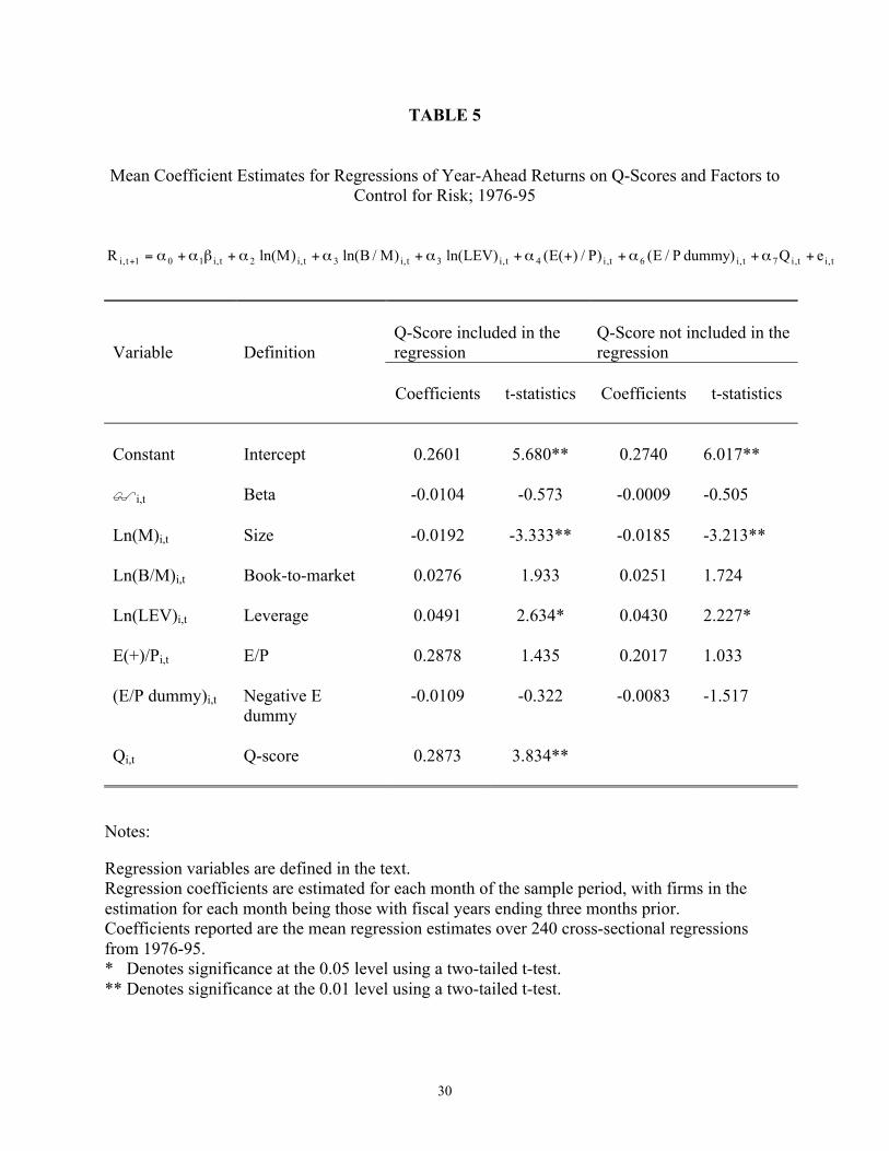
lower returns. In Table 5 we report the results of estimating Fama and MacBeth-type cross-

sectional regressions, using individual stocks, with a control for factors that have been nominated

as risk factors (by Fama and French (1992), for example):

Ri,t+1 = α0+ α1βi,t+ α2 ln (M)i,t+ α2 1n(B/M)i,t+ α3 1n(LEV)i,t+ α4 (E(+)/P)i,t+ α6 (E/P dummy)i,t+ α7Qi,t+ ei,t

Where

Ri,t+1 = annual return in Year +1 after the Q scoring; The year begins three months after fiscal-year end.

Bi,t = CAPM beta;

21

Mi,t = market value;

(B/M)i,t = book-to-market ratio;

(LEV)i,t = leverage, calculated as book value of total assets to book value of equity;

(E(+)/P)i,t = earnings-to-price ratio, positive earnings only;

(E/P dummy)i,t = negative earnings dummy: 1 if earnings are negative, 0 otherwise;

Qi,t = Q score in year t.

The mean coefficients from estimating the coefficients of this regression for each of the

240 months, t, from 1976 to 1995 are given in Table 5. Results are given with and without the Q

score in the regression. The mean estimated coefficient on Q is positive and significantly

different from zero. We conclude that Q-scores forecast returns in excess of those expected from

risk factors commonly identified with firms. If one interprets the coefficients on the variables as

abnormal returns to investing, it is concluded that Q-scores generate abnormal returns over those

identified with those variables.

In further sensitivity analysis, we repeated the return tests with Q-scores calculated from

C sub-scores for inventory accounting, R&D and advertising, and for the QA and QB scores. The

results were quite similar, in each case, to those for the composite score. The mean, size-

adjusted return for the zero-net-investment strategy in Year +1 for the R&D subscore was 7.33%

(significance level 0.000), 5.22% (0.000) for the inventory subscore, and 4.24% (0.000) for the

advertising subscore.

5. Conclusion

Conservative accounting with investment growth depresses earnings and accounting rates

of return, and creates hidden reserves. Slowing of investment releases hidden reserves, and

creates earnings and higher rates of return. If a change in investment is temporary, the effects on

22

earnings and rates of return are temporary, calling into question the quality -- or sustainability --

of earnings.

Using a constructed conservative accounting index and a quality of earnings index, this

paper diagnoses poor-quality earnings that result from changes in investment with conservative

accounting. The quality index forecasts changes, from current levels, of future core return on net

operating assets, so ex ante is an analysis tool to discover earnings of low quality.

The paper also shows that quality scores predict stock returns (in the sample period) over

those forecasted using measures commonly conjectured as risk proxies. The indications are that

the stock market did not penetrate the quality of earnings of firms with conservative accounting

during the sample period. Accordingly there were rewards to a quality analysis along the lines in

the paper.

23

FOOTNOTES

1. The Securities and Exchange Commission (SEC) requires the LIFO reserve to be calculatedas the accumulated excess of the current cost of inventories over LIFO cost. But, with rapidinventory turnover, FIFO cost approximates current cost, so most firms use FIFO cost.

2. A C-score might also be calculated as estimated hidden reserve relative to net operatingassets plus the estimated hidden reserve. Then the estimated reserve would be expressed as apercentage of net operating assets that would have been reported had conservative accountingnot been practiced. But in this paper we wish to compare the effect of changes hiddenreserves on return on net operating assets, and this return is, of course, denominated in netoperating assets.

3. Using the residual income valuation formula, a revision of forecasted RNOA of 1.3% peryear for five years has considerable effect on the calculated value.

4. The numbers of firms in the three Q groups in Year 0 are not the same because the totalnumber of firms assigned to groups is not always divisible by three.

5. The increasing estimated reserves for low-Q firms (relative to the high-Q firms) might alsobe due to a higher rate of non-surviving firms affecting the mean growth rate.

24

REFERENCES

Basu, S. "The Conservatism Principle and the Asymmetric Timeliness of Earnings." Journal ofAccounting and Economics 24 (1997): 3-37.

Bublitz, B., and M. Ettredge. “The Information in Discretionary Outlays: Advertising, Research,and Development.” Accounting Review 64 (1989): 108-124.

Fama, E., and K. French. “The Cross-section of Expected Stock Returns.” Journal of Finance47 (1992): 427-465.

Fairfield, P., and T. Yohn. “Changes in Asset Turnover Signal Changes in Profitability.”Working Paper, Georgetown University, 1998.

Feltham, J., and J. Ohlson. “ Valuation and Clean Surplus Accounting for Operating andFinancial Activities.” Contemporary Accounting Research 11 (1995): 689-731.

Gjesdal, F. "A Steady State Growth Valuation Model: A Note on Accounting and Valuation."Working paper, Norwegian School of Economics, 1999.

Hall, B. New Evidence on the Impacts of Research and Development. University of California,Berkeley, 1993.

Healy, P., and J. Wahlen. “A Review of the Earnings Management Literature and ItsImplications for Standard Setting.” Working Paper, Harvard University and IndianaUniversity, 1998.

Lev, B., and T. Sougiannis. “The Capitalization, Amortization, and Value-Relevance of R&D.”Journal of Accounting and Economics 21 (1996): 107-138.

Nissim, D., and S. Penman. “Ratio Analysis and Equity Valuation.” Working paper,University of California at Berkeley and Columbia University, 1998.

Penman, S. Financial Statement Analysis and Security Valuation. To be published by Irwin/McGraw-Hill, 2000.

Penman, S., and X-J. Zhang. “Conservatism, Growth and Accounting Rates of Return: AnEmpirical Analysis.” Working Paper, University of California, Berkeley, 1999.

Zhang, X-J. “Earnings Forecasting and Equity Valuation under Conservative Accounting.”Ph.D. Dissertation, Columbia University, 1998.

25

TABLE 1

Distribution of C-scores and Q-scores over Firm Years; 1975-97

C-Score Q-Score

No. of Firm-Years 38,540 29,796

Mean 0.313 0.099

Percentiles:

95 0.576 0.219

90 0.413 0.139

75 0.236 0.059

60 0.153 0.025

Median 0.114 0.009

40 0.084 0.000

25 0.048 -0.010

10 0.014 -0.046

5 0.004 -0.075

Notes:

C-score and Q-score calculations are described in the text.

26

TABLE 2

Patterns of Median Core Return on Net Operating Assets (Core RNOA) for Groups withDifferent Q-Scores; 1976-96

Year-5 -4 -3 -2 -1 0 1 2 3 4 5

Panel A: All YearsCore RNOA: High Q .1231 .1214 .1179 .1143 .1116 .1107 .1147 .1122 .1090 .1088 .1065 Medium Q .1165 .1153 .1136 .1116 .1097 .1090 .1075 .1054 .1026 .1005 .1013 Low Q .1113 .1108 .1094 .1092 .1110 .1094 .1002 .0976 .0950 .0939 .0930 All firms .1173 .1159 .1135 .1117 .1107 .1096 .1077 .1052 .1023 .1012 .1006

Differences in changes inCore RNOA from Year 0:High Q – Low Q

.0104 .0092 .0071 .0038 -.001 0 .0131 .0132 .0126 .0136 .0121

T-statistic on meandifferences in changes inCore RNOA

5.650 4.324 4.092 1.950 −.051 7.379 7.172 6.477 5.256 3.835

No. of Firms (1976-1996): High Q 4184 4324 4486 4683 4897 5193 4928 4475 4094 3728 3398 Medium Q 6153 6353 6527 6697 6939 7178 6816 6197 5711 5198 4731 Low Q 5168 5291 5419 5574 5719 5925 5595 5087 4679 4258 3876 All firms 15505 15968 16432 16954 17555 18296 17339 15759 14484 13184 12005

No. of Firms (1976-1991): High Q 3486 3612 3734 3883 4027 4240 4032 3850 3687 3543 3398 Medium Q 5102 5260 5411 5533 5697 5865 5584 5334 5134 4935 4731 Low Q 4247 4349 4447 4567 4670 4804 4543 4344 4176 4032 3876 All firms 12835 13221 13592 13983 14394 14909 14159 13528 12997 12510 12005

27

Table 2 continued

Year-5 -4 -3 -2- -1 0 1 2 3 4 5

Panel B: 1976-82Core RNOA: High Q .1448 .1544 .1511 .1433 .1354 .1284 .1243 .1156 .1052 .1007 .0945 Medium Q .1346 .1463 .1456 .1425 .1348 .1270 .1182 .1103 .0994 .0925 .0896 Low Q .1315 .1404 .1407 .1376 .1366 .1274 .1120 .1046 .0947 .0906 .0858 All firms .1373 .1469 .1458 .1411 .1356 .1276 .1186 .1105 .0992 .0940 .0902

Panel C: 1983-89Core RNOA: High Q .1204 .1060 .0995 .0947 .0954 .0990 .1045 .1036 .1032 .1044 .1069 Medium Q .1152 .1019 .0956 .0915 .0927 .0966 .0985 .0973 .0967 .0965 .1026 Low Q .1119 .0986 .0928 .0900 .0944 .0964 .0915 .0890 .0908 .0904 .0948 All firms .1156 .1020 .0957 .0922 .0942 .0970 .0979 .0960 .0968 .0974 .1017

Panel D: 1990-96Core RNOA: High Q .1042 .1036 .1031 .1049 .1039 .1047 .1152 .1183 .1223 .1309 .1334 Medium Q .0997 .0978 .0995 .1006 .1017 .1033 .1064 .1089 .1155 .1214 .1256 Low Q .0906 .0933 .0946 .0999 .1020 .1043 .0970 .0994 .1012 .1056 .1055 All firms .0989 .0988 .0990 .1018 .1022 .1041 .1066 .1099 .1142 .1202 .1225

Notes:

Year 0 is the year that Q-scores are calculated; years – 5 to –1 are the five years preceding year 0and years +1 to +5 are the five years subsequent to year 0. The Q-score groups are based on aranking of firms each year on Q-scores within industry and RNOA groups. The RNOA numbersin the table are means of median RNOA for each group.

28

TABLE 3

Percentage of Firms with Sales Increases and Decreases in Year +1, for High-Q andLow-Q Groups with Increases and Decreases in Sales Relative to Net Operating Assets BeforeInventory (NOABI) in Year 0.

Sales (relative to NOABI) at Year 0Increase Decrease

High Q 60.32% 41.74%

Low Q 51.64% 35.64%

Note:

For firms with Sales Increases (Decreases) relative to NOABI in year 0, the Chi-square statistic(with one degree of freedom) for a test of independence between Q group and sales changes inYear 1 is 34.3 (20.1) with a probability given no relationship of less than 0.001.

29

TABLE 4

Mean Percentage Stock Returns for Portfolios Formed on Q-Scores; 1976-95

Q Portfolios Year-2 Year-1 Year 0 Year+1 Year+2 Year+3 Year+4 Year+5

Panel A: Raw returns

Lowest Q 26.67 28.19 26.39 17.03 22.51 20.81 22.58 19.122 21.27 22.25 19.51 19.02 20.36 21.20 18.70 17.153 22.56 20.75 21.16 21.39 20.90 20.68 18.94 20.264 23.25 24.39 21.01 19.63 22.85 20.35 24.13 18.215 21.30 23.44 19.81 20.87 21.73 20.75 22.19 17.526 20.87 22.37 19.56 20.97 20.94 20.15 21.44 19.807 20.32 21.58 20.15 22.64 21.47 20.77 20.55 18.248 20.57 22.39 21.20 21.19 21.05 21.41 19.39 17.849 19.66 18.50 21.94 21.20 21.64 19.84 19.70 18.88

Highest Q 18.25 20.64 23.33 26.06 23.53 22.78 22.12 20.93

High - Low -8.41 -7.55 -3.06 9.03 1.02 1.98 -0.46 1.80Significance 0.000 0.265 0.091 0.616 0.136

Panel B: Size-adjusted returns

Lowest Q 3.39 5.40 4.21 -3.17 -0.26 -0.09 -0.24 -0.062 0.08 0.72 -0.57 -0.66 0.48 1.58 -1.29 -0.223 2.33 0.72 1.21 1.72 1.35 1.05 -0.47 3.904 2.97 3.27 1.56 0.12 2.58 1.09 5.34 1.995 1.32 2.68 0.54 1.51 1.46 2.15 2.23 0.656 1.07 2.20 0.27 1.06 1.78 1.59 3.47 2.867 1.34 2.41 0.87 2.85 2.12 1.99 2.09 1.798 2.61 1.23 3.14 2.91 1.44 3.05 0.80 1.299 0.79 -0.12 2.10 2.76 2.40 1.02 0.39 2.06

Highest Q -0.42 0.19 2.34 5.78 1.80 2.38 2.63 2.90

High - Low -3.81 -5.21 -1.87 8.95 2.05 2.46 2.86 2.96Significance 0.000 0.070 0.036 0.024 0.031

Notes:

Mean buy-and-hold returns are calculated for each Q-score portfolio for each year, -2 to +5. Themean returns over the 20 years are reported in Panel A. Panel B reports the mean of size-adjusted returns which are computed by subtracting the raw (buy-and-hold) return on a size-matched, value-weighted portfolio formed from size-decile groupings supplied by CRSP.The high-low return is the return from investing long in the highest Q portfolio and investing thesame dollar amount short in the lowest Q portfolios for zero net investment.Significance tests are based on 5,000 replications of randomly assigning firms to Q portfolios.The significance numbers are the frequency of observing returns equal to the return on the high-low investment strategy, or higher, in the 5,000 replications.

30

TABLE 5

Mean Coefficient Estimates for Regressions of Year-Ahead Returns on Q-Scores and Factors toControl for Risk; 1976-95

t,it,i7t,i6t,i4t,i3t,i3t,i2t,i101t,i eQ)dummyP/E()P/)(E()LEVln()M/Bln()Mln(R +α+α++α+α+α+α+βα+α=+

Variable DefinitionQ-Score included in theregression

Q-Score not included in theregression

Coefficients t-statistics Coefficients t-statistics

Constant Intercept 0.2601 5.680** 0.2740 6.017**

i,t Beta -0.0104 -0.573 -0.0009 -0.505

Ln(M)i,t Size -0.0192 -3.333** -0.0185 -3.213**

Ln(B/M)i,t Book-to-market 0.0276 1.933 0.0251 1.724

Ln(LEV)i,t Leverage 0.0491 2.634* 0.0430 2.227*

E(+)/Pi,t E/P 0.2878 1.435 0.2017 1.033

(E/P dummy)i,t Negative Edummy

-0.0109 -0.322 -0.0083 -1.517

Qi,t Q-score 0.2873 3.834**

Notes:

Regression variables are defined in the text.Regression coefficients are estimated for each month of the sample period, with firms in theestimation for each month being those with fiscal years ending three months prior.Coefficients reported are the mean regression estimates over 240 cross-sectional regressionsfrom 1976-95.* Denotes significance at the 0.05 level using a two-tailed t-test.** Denotes significance at the 0.01 level using a two-tailed t-test.

31

FIGURE 1a

FIGURE 1b

FIGURE 1c

Figure 1. The behavior of mean Q-score for high and low Q-score groups. Figure 1a tracks Q-scores; Figure 1b tracks the QA component of the Q-score; Figure 1c tracks the QB componentof the Q-score.

Q

-0.1

-0.05

0

0.05

0.1

0.15

-5 -4 -3 -2 -1 0 1 2 3 4 5

Year

High Q

Low Q

QA

-0.025

0

0.025

0.05

-5 -4 -3 -2 -1 0 1 2 3 4 5

Year

High Q

Low Q

QB

-0.2

-0.1

0

0.1

0.2

0.3

-5 -4 -3 -2 -1 0 1 2 3 4 5

Year

High Q

Low Q

32

FIGURE 2a

FIGURE 2b

Figure 2. The behavior of mean core RNOA for high and low Q-score groups. Figure 2a trackscore RNOA; Figure 2b tracks RNOA adjusted for median RNOA for all firms in the relevantyear.

Core RNOA

8.00%

9.00%

10.00%

11.00%

12.00%

13.00%

-5 -4 -3 -2 -1 0 1 2 3 4 5

Year

High Q

Low Q

Relative Core RNOA - median subtracted to take out the trend

-2.00%

-1.00%

0.00%

1.00%

2.00%

-5 -4 -3 -2 -1 0 1 2 3 4 5

Year

High Q

Low Q

33

FIGURE 3

Figure 3. Relative frequency of firms with increasing core RNOA in the year subsequent to theQ-score calculation, for high-Q and low-Q firms.

DecreasingRNOA Increasing

RNOA

Low Q

High Q

0

5

10

15

20

25

30

Frequency (%)

34

FIGURE 4a

FIGURE 4b

Figure 4. The behavior of mean core profit margin before depreciation and amortization forhigh-Q groups (Figure 4a) and low-Q groups (Figure 4b).

Core profit margin before depreciation and amortization High Q group

0.1

0.11

0.12

0.13

-5 -4 -3 -2 -1 0 1 2 3 4 5

Year

Core profit margin before depreciation and amortization Low Q group

0.1

0.11

0.12

0.13

-5 -4 -3 -2 -1 0 1 2 3 4 5

Year

35

FIGURE 5

Figure 5. The behavior of mean asset turnovers for high and low Q-score groups.

Asset Turnover

1.9

2

2.1

2.2

2.3

2.4

2.5

-5 -4 -3 -2 -1 0 1 2 3 4 5

Year

High Q

Low Q

36

FIGURE 6a

FIGURE 6b

Figure 6. Cumulative average growth rates in estimated hidden reserves from year –5 to +5 forhigh and low Q groups (Figure 6a) and differences in cumulative average growth rates betweenhigh and low groups (Figure 6b).

Cumulative Average Growth Rates of Estimated Reserve

0.00%

50.00%

100.00%

150.00%

200.00%

250.00%

-5 -4 -3 -2 -1 0 1 2 3 4 5

Year

Low Q

High Q

Difference in Cumulative Average Growth Rates of Estimated Reserves (High-Low)

0.00%

5.00%

10.00%

15.00%

20.00%

25.00%

30.00%

35.00%

-5 -4 -3 -2 -1 0 1 2 3 4 5

Year

37

FIGURE 7a

FIGURE 7b

FIGURE 7c

Figure 7. The behavior of mean core RNOA for high and low Q-scores, for Q-score constructedonly for changes in the inventory reserve sub-score (Figure 7a), the advertising reserve sub-score(Figure 7b), and the R&D reserve sub-score (Figure 7c).

Core RNOAinventory reserve sub-score

9%

10%

11%

12%

13%

-5 -4 -3 -2 -1 0 1 2 3 4 5

Year

High Q

Low Q

Core RNOAadvertising reserve sub-score

9%

10%

11%

12%

13%

14%

-5 -4 -3 -2 -1 0 1 2 3 4 5

Year

High Q

Low Q

Core RNOAR&D reserve sub-score

9%

10%

11%

12%

13%

-5 -4 -3 -2 -1 0 1 2 3 4 5

Year

High Q

Low Q

38

FIGURE 8

Figure 8. Mean size-adjusted return differences between high-Q and low-Q portfolios in the yearfollowing the Q scoring (year t+1), for each year, 1976-95.

Mean Size-adjust Return

-0.1

0

0.1

0.2

0.319

76

1977

1978

1979

1980

1981

1982

1983

1984

1985

1986

1987

1988

1989

1990

1991

1992

1993

1994

1995

Year

Siz

e-ad

just

ed R

etu

rn