IZA DP No. 2554

Accounting for Intergenerational Income Persistence:Noncognitive Skills, Ability and Education

Jo BlandenPaul GreggLindsey Macmillan

DI

SC

US

SI

ON

PA

PE

R S

ER

IE

S

Forschungsinstitutzur Zukunft der ArbeitInstitute for the Studyof Labor

January 2007

Accounting for Intergenerational

Income Persistence: Noncognitive Skills, Ability and Education

Jo Blanden University of Surrey, LSE and IZA

Paul Gregg

University of Bristol and LSE

Lindsey Macmillan CMPO, University of Bristol

Discussion Paper No. 2554 January 2007

IZA

P.O. Box 7240 53072 Bonn

Germany

Phone: +49-228-3894-0 Fax: +49-228-3894-180

E-mail: iza@iza.org

Any opinions expressed here are those of the author(s) and not those of the institute. Research disseminated by IZA may include views on policy, but the institute itself takes no institutional policy positions. The Institute for the Study of Labor (IZA) in Bonn is a local and virtual international research center and a place of communication between science, politics and business. IZA is an independent nonprofit company supported by Deutsche Post World Net. The center is associated with the University of Bonn and offers a stimulating research environment through its research networks, research support, and visitors and doctoral programs. IZA engages in (i) original and internationally competitive research in all fields of labor economics, (ii) development of policy concepts, and (iii) dissemination of research results and concepts to the interested public. IZA Discussion Papers often represent preliminary work and are circulated to encourage discussion. Citation of such a paper should account for its provisional character. A revised version may be available directly from the author.

IZA Discussion Paper No. 2554 January 2007

ABSTRACT

Accounting for Intergenerational Income Persistence: Noncognitive Skills, Ability and Education*

We analyse in detail the factors that lead to intergenerational persistence among sons, where this is measured as the association between childhood family income and later adult earnings. We seek to account for the level of income persistence in the 1970 BCS cohort and also to explore the decline in mobility in the UK between the 1958 NCDS cohort and the 1970 cohort. The mediating factors considered are cognitive skills, noncognitive traits, educational attainment and labour market attachment. Changes in the relationships between these variables, parental income and earnings are able to explain over 80% of the rise in intergenerational persistence across the cohorts. JEL Classification: J62, J13, J31 Keywords: intergenerational mobility, children, skills Corresponding author: Jo Blanden Department of Economics University of Surrey Guildford Surrey GU2 7XH United Kingdom E-mail: j.blanden@surrey.ac.uk

* This work was funded by the Department for Education and Skills through the Centre for the Economics of Education. We are grateful for helpful comments from three referees.

Executive Summary

Intergenerational persistence is the association between the socio-economic outcomes

of parents and their children as adults. Recent evidence suggests that mobility in the

UK is low by international standards (Jantti et al, 2006) and that mobility fell when

the 1958 and 1970 cohorts are compared (Blanden et al, 2004).

This paper seeks to understand the level and change in the intergenerational

persistence of sons by exploring the contribution made by noncognitive skills,

cognitive ability and education as transmission mechanisms. In order to explain

intergenerational persistence these factors must be correlated with family income and

have an influence on labour market earnings in the early 30s (our measure of adult

outcomes).

There has been considerable research considering the relationship between

educational outcomes and family income (e.g. Blanden and Machin, 2004), and

numerous studies document the positive returns to education in the labour market.

Educational attainment is therefore an obvious transmission mechanism. Similarly we

would expect children of better off parents to have higher cognitive skills that

improve their chances in the labour market, in part by helping them to achieve more

in the education system. Labour market experience is also explored as early

unemployment has been shown to have a negative effect on later earnings (Gregg and

Tominey, 2005).

The consideration of non-cognitive skills as an intergenerational transmission

mechanism is a new contribution made in this paper. Bowles et al (2001) provide an

interesting review of how personality influences wages. James Heckman and co-

authors have produced a number of papers which emphasise the importance of

noncognitive skills in determining educational outcomes and later earnings. Heckman

and Rubinstein (2001) first identified the importance of noncognitive skill with their

observation that high school equivalency recipients earn less than high school

graduate despite being smarter. They attribute this to the negative noncognitive

attributes of those who drop out. In the most recent paper in this series Heckman,

Stixrud and Urzua (2006) model the influence of young people’s cognitive and non-

2

cognitive skills on schooling and earnings. They find that better noncognitive skills

lead to more schooling, but also have an earnings return over and above this. Carneiro

et al (2006) find noncognitive skills measured in childhood to have similar effects in

the British 1958 National Child Development Study1. If parental income is correlated

with noncognitive skills then these could be another important factor driving

intergenerational persistence.

In the first part of this paper we assess the ability of our chosen transmission

mechanisms to account for the elasticity between earnings at age 30 and parental

income averaged at age 10 and 16 for the cohort of sons born in 1970. We find that

our most detailed model is able to account for 0.17 of the 0.32 elasticity we observe

(54%). Of this, the greater part (0.10) is contributed by education, although early

labour market experience also has a role (0.03). The contribution of cognitive and

noncognitive variables is also sizeable but largely occurs through their role in

improving education outcomes. The most important of the noncognitive variables are

the child’s (self-reported) personal efficacy and his level of application (reported by

his teacher at age 10).

The latter half of the paper is concerned with understanding the role these mediating

variables play in the fall in intergenerational mobility between the 1958 and 1970

cohorts. One striking change is that the noncognitive variables are strongly associated

with parental variables in the second cohort, but not in the first. There is also greater

inequality in educational outcomes by parental income in the second cohort. Overall

intergenerational mobility increases from an elasticity of 0.205 to 0.291, an increase

of 0.086, of this over 80% can be explained by our model (the part that is accounted

for has increased by 0.07). The largest contributors to this change are increasingly

unequal educational attainment at age 16 and access to higher education.

Noncognitive traits also have a role, but affect intergenerational persistence through

their impact on educational attainments; this is in contrast to the results found by

Heckman, Stixrud and Urzua (2006) reported above. Cognitive ability makes no

substantive contribution to the change in mobility.

1 Note these studies have concerned non-cognitive characteristics as a dimension of skill; this is separate from exploring the impact of social capital.

3

Our findings highlight, once again, the importance of improving the educational

attainment and opportunities of children from poorer backgrounds for increasing

social mobility. Moreover, they provide suggestive evidence that that policies

focusing on noncognitive skills such as self-esteem and application may be effective

in achieving these goals.

4

1. Introduction

Intergenerational mobility is the degree of fluidity between the socio-economic status

of parents (usually measured by income or social class) and the socio-economic

outcomes of their children as adults. A strong association between incomes across

generations indicates weak intergenerational income mobility, and may mean that

those born to poorer parents have restricted life chances and do not achieve their

economic potential.

Recent innovations in research on intergenerational mobility have been

concentrated on improving the measurement of the extent of intergenerational

mobility, and making comparisons across time and between nations. The evidence

suggests that the level of mobility in the UK is low by international standards (Jantti

et al., 2006, Corak, 2006 and Solon, 2002). Comparing the 1958 and 1970 cohorts

indicates that mobility has declined in the UK (see Blanden et al. 2004).

This paper takes this research a stage further by focusing on transmission

mechanisms; those variables that are related to family incomes and that have a return

in the labour market. First we evaluate the relative importance of education, ability,

noncognitive (or ‘soft’) skills and labour market experience in generating the extent of

intergenerational persistence in the UK among the 1970 cohort. In the second part of

the paper we seek to appreciate how these factors have contributed to the observed

decline in mobility in the UK. We focus here on men for reasons of brevity.

Education is the most obvious of these transmission mechanisms. It is well

established that richer children obtain better educational outcomes, and that those with

higher educational levels earn more. Education is therefore a prime candidate to

explain mobility and changes in it. Indeed, Blanden et al. (2004) find that a

strengthening relationship between family income and participation in post

compulsory schooling across cohorts can help to explain part of the fall in

intergenerational mobility they observe.

Cognitive ability determines both educational attainment and later earnings,

making it another likely contributor to intergenerational persistence. We might expect

a strong link between parental income and measured ability, both because of

biologically inherited intelligence and due to the investments that better educated

parents can make in their children. We seek to understand the extent to which

differing achievements on childhood tests across income groups can explain

5

differences in earnings, both directly, and through their relationship with final

educational attainment. Galindo-Rueda and Vignoles (2005) demonstrate that the role

of cognitive test scores in determining educational attainment has declined between

these two cohorts.

A growing literature highlights that noncognitive personality traits and

personal characteristics earn rewards in the labour market and influence educational

attainment and choices (see Feinstein, 2000, Heckman et al., 2006, Bowles et al.,

2001 and Carneiro et al., 2006). If these traits are related to family background then

this provides yet another mechanism driving intergenerational persistence. Osborne-

Groves (2005) considers this possibility explicitly and finds that 11% of the father-son

correlation in earnings can be explained by the link between personalities alone;

where personality is measured only by personal efficacy.

Finally, labour market experience and employment interruptions have long

been found to influence earnings (see Stevens 1997). Gregg and Tominey (2005)

highlight, in particular, the negative impacts of spells of unemployment as young

adults; we therefore analyse labour market attachment as another way in which family

background might influence earnings.

In the next section we lay out our modelling approach in more detail. Section 3

discusses our data. Section 4 presents our results on accounting for the level of

intergenerational mobility while Section 5 describes our attempt to understand the

change. Section 6 offers conclusions.

2. Modelling Approach

In economics, the empirical work on intergenerational mobility is generally concerned

with the estimation of β in the following regression;

ln lnchildren parentsi iY Y iα β ε= + + (1)

where is the log of some measure of earnings or income for adult children,

and is the log of income for parents, i identifies the family to which parents

and children belong and

ln childreniY

ln parentsiY

iε is an error term. β is therefore the elasticity of children’s

income with respect to their parents’ income and (1- β ) can be thought of as

measuring intergenerational mobility.

6

Conceptually, we are interested in the link between the permanent incomes of

parents and children across generations. However, the measures of income available

in longitudinal datasets are likely to refer to current income in a period. In some

datasets multiple measures of current income can be averaged for parents and

children, moving the measure somewhat closer to permanent income. Additionally it

is usual to control for the ages of both generations.1 In the cohort datasets we use,

substantial measurement error is likely to remain, meaning that our estimates will be

biased downwards as measures of intergenerational persistence. The issue of

measurement error becomes particularly important when considering the changes in

mobility across cohorts and this will be returned to when discussing our findings.

We report the intergenerational partial correlation r, alongside β because

differences in the variance of ln between generations will distort the Y β coefficient.

This is obtained simply by scaling β by the ratio of the standard deviation of parents’

income to the standard deviation of sons’ income, as shown below.

parents son

ln

lnY , lnY ln = Corr ( )

parents

son

Y

Y

SDrSD

β= (2)

The main objective in this paper is to move beyond the measurement of β

and r, and to understand the pathways through which parental income affects

children’s earnings. The role of noncognitive skills can be used as an example,

assuming for the moment that these are measured as a single index. We can measure

the extent to which these skills are related to parental

income , and estimate their pay-offs in the labour

market

iparents

ii YNoncog 11 ln ελα ++=

iichild

i uNoncogInY 11 ++= ρϖ

This means that the overall intergenerational elasticity can be decomposed into

the return to noncognitive skills multiplied by the relationship between parental

income and these skills, plus the unexplained persistence in income that is not

transmitted through noncognitive traits.

)(ln)ln,( 1

parentsi

parentsii

YVarYuCov

+= ρλβ (3)

In our analysis we consider noncognitive skills among several other mediating factors:

cognitive test scores, educational performance and early labour market attachment.

7

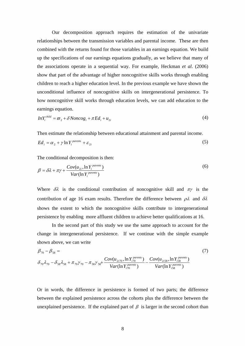
Our decomposition approach requires the estimation of the univariate

relationships between the transmission variables and parental income. These are then

combined with the returns found for those variables in an earnings equation. We build

up the specifications of our earnings equations gradually, as we believe that many of

the associations operate in a sequential way. For example, Heckman et al. (2006)

show that part of the advantage of higher noncognitive skills works through enabling

children to reach a higher education level. In the previous example we have shown the

unconditional influence of noncognitive skills on intergenerational persistence. To

how noncognitive skill works through education levels, we can add education to the

earnings equation.

2 2child

i i i iInY Noncog Ed uϖ δ π= + + + (4)

Then estimate the relationship between educational attainment and parental income.

iparents

ii YEd 22 ln εγα ++= (5)

The conditional decomposition is then:

)(ln)ln,( 2

parentsi

parentsii

YVarYuCov

++= πγδλβ (6)

Where δλ is the conditional contribution of noncognitive skill and πγ is the

contribution of age 16 exam results. Therefore the difference between ρλ and δλ

shows the extent to which the noncognitive skills contribute to intergenerational

persistence by enabling more affluent children to achieve better qualifications at 16.

In the second part of this study we use the same approach to account for the

change in intergenerational persistence. If we continue with the simple example

shown above, we can write

)(ln)ln,(

)(ln)ln,(

58

58582

70

707025858707058587070

5870

parentsi

parentsii

parentsi

parentsii

YVarYuCov

YVarYuCov

−+−+−

=−

γπγπλδλδ

ββ

(7)

Or in words, the difference in persistence is formed of two parts; the difference

between the explained persistence across the cohorts plus the difference between the

unexplained persistence. If the explained part of β is larger in the second cohort than

8

in the first then this indicates that the factors we explore are responsible for part of the

increase in intergenerational persistence.

3. Data

We use information from the two mature publicly accessible British cohort studies,

the British Cohort Study of those born in 1970 and the National Child Development

Study of those born in 1958. Both cohorts began with around 9000 baby boys,

although as we shall see our final samples are considerably smaller than this. We shall

first provide a discussion of how we use the 1970 cohort, before considering how the

data are used in the comparative section of the paper.

British Cohort Study

The BCS originally included all those born in Great Britain between 4th and 11th April

1970. Information was obtained about the sample members and their families at birth

and at ages 5, 10, 16 and 30. We use the earnings information obtained at age 30 as

the dependent variable in our intergenerational models. Employees are asked to

provide information on their usual pay and pay period. Data quality issues mean we

must drop the self-employed. Parental income is derived from information obtained at

age 10 and 16; where parents are asked to place their usual total income into the

appropriate band (there were seven options at age 10 and eleven at age 16). We

generate continuous income variables at each age by fitting a Singh-Maddala

distribution to the data using maximum likelihood estimation. This is particularly

helpful in allocating an expected value for those in the open top category.2 We adjust

the variables to net measures and impute child benefit for all families.3 The

explanatory variable used in the first part of the paper is the average of income over

ages 10 and 16.

In the childhood surveys parents, teachers and the children themselves are

asked to report on the child’s behaviour and attitudes. These responses are combined

to form the noncognitive measures as described in Box 1. Information on cognitive

skills is obtained at age 5 from the English Picture Vocabulary test (EPVT) and a

copying test. At age 10 the child took part in a reading test, maths test and British

Ability Scale test (close to an IQ test). Exam results at age 16 were obtained from

information given in the age 30 sample. This includes detailed information on the

number of exams passed (both GCE O level and CSE). Information on educational

9

achievements beyond age 16 is also available from the age 30 sample, as is

information on all periods of labour market and educational activity from age 16 to

30. This information is used to generate the measure of labour market attachment

which is the proportion of months from age 16 to 30 when the individual is out of

education and not in employment.

Comparative Data on the Two Cohorts

Some modifications must be made to the variables used when comparing the BCS

with the earlier National Child Development Study (NCDS). The NCDS obtains data

at birth and ages 7, 11, 16, 23, 33 and 42 for children born in a week in March 1958.

Parental income data is available only at age 16, meaning that the comparative

analysis of this data is based only on income at this age. The questions that ask about

parental income in the two cohorts are not identical and adjustments must be made to

account for differences in the way income is measured (see Blanden, Chapter 4 for

full details). Intergenerational parameters for the NCDS are obtained by regressing

earnings at age 33 on this parental income measure. Comparative results for the BCS

are generated by regressing earnings at 30 on parental income at age 16.

Careful consideration is needed when using the noncognitive variables to

make comparisons across the cohorts. In both cohorts, mothers are asked a number of

items from the Rutter A scale (this is the version of the Rutter behaviour scale which

is asked of parents, see Rutter et al. 1970). Indicators of internalising behaviour from

the Ruttter scale included in both cohorts are headaches, stomach aches, sleeping

difficulties, worried and fearful, at ages 11/10. Externalising behaviours are fidget,

destructive, fights, irritable and disobedient at the same age. Principal components

analysis is used to form these variables into two scales, we refer to these as the Rutter

externalising and Rutter internalising scales.5

The teacher-reported variables in the NCDS are from the Bristol Social

Adjustment Guide (Stott, 1966, 1971). The teacher was given a series of phrases and

asked to underline those that he/she thought applied to the child. The phrases were

grouped into 11 different behavioural “syndromes”. We have investigated the extent

to which these syndromes are comparable with the scales derived from the teacher

measures in the BCS, and our strict comparability criteria mean that we can only use

some of the information available in each cohort. Together with the internalising and

externalising Rutter scales, we use BCS hyperactivity as comparable with the NCDS

10

restless subscale and application (BCS) matched with inconsequential behaviour

(NCDS). These measures are based on similar questions and the pairs of non-

cognitive measures have very similar correlations with mother’s smoking and adult

health measures. Full details of our methods for choosing comparable variables can

be found in Appendix A.

For cognitive skills; reading, maths and general ability scores at age 11 are

broadly comparable with the reading, maths and British ability scale scores in the

BCS. These variables were also used on a comparative basis by Galindo-Rueda and

Vignoles (2005). Information on exam results at 16 and 18 is obtained from a survey

of all schools attended by the cohort members carried out in 1978. As less detail is

given concerning the grades obtained in individual subjects than is available for the

BCS cohort, O level or CSE points for Maths and English are added together as the

measure of exam success at age 16 (i.e. a grade A is allocated five points, a B four

points etc). Information on later education attainments is derived from the age 23 and

33 surveys for the NCDS, and the data on labour market attachment is taken from the

work history information collected in the age 33 and 42 surveys. It refers to the

period between ages 16 and 33.

4. Accounting for Intergenerational Persistence

Estimates of Intergenerational Persistence

Table 1 details the estimates of intergenerational mobility that we attempt to

understand in the first part of this paper, providing the intergenerational coefficient

and the intergenerational partial correlation. The estimates presented are based on the

average of age 10 and age 16 parental income and are conditional on average parental

age and age-squared. The coefficient is 0.32 while the partial correlation is a little

smaller at 0.27. This estimate is slightly higher than those obtained when using

income data from a single period (see Table 4) but is still likely to understate the level

of persistence compared to using many years of parental income (as in Mazumder,

2001) or by predicting permanent income (as in Dearden et al., 1997). This, however,

is the best estimate from this data that is suitable for decomposition.

Decomposing Intergenerational Persistence

The first stage in understanding which factors mediate intergenerational persistence is

to review which of them has a relationship with parental income, as without this link

11

they cannot play a role in our explanation. The first column of Table 2 provides the

results from regressions of each variable6 on parental income, conditional on parental

age, as in the intergenerational regression. With the exception of the mother’s neurotic

rating at age 5 all the variables we have chosen as possible mediating factors are

strongly related to parental income. Better off children have better noncognitive traits,

and perform better in all cognitive tests. As they grow up they achieve more at all

levels of education and have greater labour market attachment in their teens and 20s.

Our results show that the cognitive variables have stronger associations with

parental income than the noncognitive variables. The noncognitive and cognitive

variables have all been scaled to have a mean of 0 and a standard deviation of 1 the

coefficients therefore indicate the proportionate standard deviation change associated

with a 100% increase in family income. Application and locus of control have the

strongest association with parental income among the noncognitive variables, and for

these variables the magnitude of this association, at 0.3, is similar to the 0.3-0.5

coefficients found for the cognitive variables.

For any factor to be influential in describing intergenerational correlations, it

must be both related to family background and have significant rewards in the labour

market. The remainder of Table 2 builds up the sequential earnings equations; these

show how the early measures of cognitive and noncognitive skill impact on earnings

and how these relationships operate though education and labour market attachment.

Columns [1] and [2] compare the predictive power of the cognitive test variables with

those for noncognitive indices. The explanatory power of these two specifications is

very close with an R-squared of 0.09 for the noncognitive variables and 0.10 for the

cognitive variables. When both sets of variables are included in regression [3] the

explanatory power of the model increases only marginally, implying that the two sets

of variables are predicting the same earnings variation across individuals.

The strongest association with earnings among the cognitive variables are for

copying at age 5 and maths at age 10. The results suggest that, conditional on the

other noncognitive and cognitive scales, a standard deviation increase in the copying

score at age 5 is associated with 4.6% increase in earnings, whilst for the maths score

this is 5.4%. The application and locus of control scores at age 10 and anxiety at age

16 have the largest earnings returns among the noncognitive variables, with 4.7%,

3.1% and -3.3% extra earnings associated with a one standard deviation increase

respectively.7 Specification [4] adds the number of O-levels at grades A-C (or

12

equivalent) obtained at age 16 to the regression. As would be expected the number of

O-levels is a strong predictor of earnings, with each O-level associated with a 3.6%

increase in earnings. Introducing the O-levels variable reduces the strength of the

coefficients for the noncognitive variables. This suggests that these noncognitive

skills are affecting earnings by helping children achieve more at age 16. The most

strongly affected term is the application score; this becomes insignificant. However,

the locus of control, clumsiness, anxiety and extrovert scores remain significant

predictors of earnings. As we might expect, the importance of the early cognitive

variables also diminishes as education variables are introduced.

Specification [5] introduces further educational attainment measures;

participation beyond ages 16 and 18, the number of A-levels achieved and whether or

not a degree is obtained. When these variables are added, the coefficient for the

number of O-levels is reduced by around a half, demonstrating that a large part of the

return to O-levels is due to opening up access to these higher levels of education. The

return to having a degree is 15% (given the number of O- and A-levels achieved). The

measures capturing post-16 education make only a marginal further difference to the

estimated impact of both the cognitive and noncognitive scores. This implies that

these scores do not predict the likelihood of pursuing A-levels or a degree given age

16 attainment.

Column [6] adds measures of labour market attachment. These variables are

clearly explaining a significant part of the variation in earnings at age 30, with all

coefficients significant and large in magnitude. Just under a quarter of the sample

experiences some unemployment and this group spend around 10% (19 months) of

the time between leaving full-time education and age 30 in unemployment. These men

have on average 12% lower wages when compared to those with no unemployment. It

is interesting to note that labour market attachment is not strongly related to the

cognitive and noncognitive variables, given education attainment, as there is little

change in the coefficients on these variables when the labour market attachment

variables are introduced.

Table 2 has shown that the cognitive, noncognitive, education and labour

market variables all have significant relationships with parental income. These

variables also have an important relationship with earnings, either directly or through

education. Table 3 decomposes the overall persistence of income into the contribution

13

of each factor by multiplying each variable’s coefficient in the earnings equation by

its relationship with family income (from column 1). We summarise this for groups of

variables to show the amount of persistence accounted for by the different

transmission mechanisms. In addition, the correlation between the residual of the

earnings equations and family income is described as the unexplained component.

Specifications [1] and [2] show that the noncognitive variables can account for

0.06 points of the 0.32 intergenerational coefficient (19%) and the cognitive variables

account for 0.09 (27%). When the cognitive and noncognitive variables are included

together in specification [3], the total amount accounted for increases by very little, as

we would expect from the earnings regressions.

The education variables account for a large part of intergenerational

persistence, with the introduction of these variables bringing the persistence

accounted for to nearly 46%. The introduction of the labour market attachment

variables means that over half (54%) of β is accounted for. Noncognitive and

cognitive measures are responsible for just 6% and 7% respectively of the

intergenerational persistence given education and labour market attachment. The

decline in the importance of these terms as we introduce measures of attainment

reflects that the cognitive and noncognitive scores mostly affect earnings because of

their influence on education.

5. Accounting for the Decline in Intergenerational Mobility

Estimates of the Change in Intergenerational Mobility

Table 4 provides estimates of the change in intergenerational mobility for sons

between the 1958 and 1970 cohorts. For sons born in 1958, the elasticity of own

earnings with respect to parental income at age 16 was 0.205; for sons born in 1970

the elasticity was 0.291. This is a clear and statistically significant growth in the

relationship between economic status across generations. For the correlation

estimates, the fall in mobility is even more pronounced. The correlation for the 1958

cohort is 0.166 compared with 0.286 for the 1970 cohort. The correlation is lower

than the elasticity for the 1958 cohort because of the particularly strong growth in

income inequality between when the parental income and sons’ earnings data was

collected; parental income was collected in 1974 whereas sons’ earnings were

measured in 1991.

14

The fall in mobility that we observe is a striking result, and before proceeding

to decompose this change, we shall consider its robustness and discuss how our

finding fits with the other literature on changes in intergenerational mobility for the

UK. The main concern is that the difference in the results between the two cohorts are

a consequence of greater downward bias due to measurement error in the NCDS data

compared with the BCS. However, there is no reason to suspect that this is the case.

Grawe (2004) demonstrates that the income information was not affected by the

coincidence of the 1974 survey and the temporary reduction of the working week to

three days. Blanden et al. (2004) show that realistic assumptions about the extent of

measurement error lead to no change in the basic finding that mobility has declined.

Another worry is that the results are being affected by attrition and item non-

response. Both cohorts began with around 9000 sons but attrition and missing

information on parental income and adult earnings means that only around 2000 sons

are available for each cohort in the comparative analysis. If the losses in sample are

purely random then we need not be concerned, however systematic attrition and non-

response can lead to biased coefficients, and if it varies, potentially misleading results

on changes across the cohorts. Blanden (2005, Appendix) considers the issue of

sample selection in the data used here. For the BCS in particular, it appears that the

selections made result in a sample that has higher parental status and better child

outcomes than the full sample. However, there is no evidence to suggest that this is

artificially generating the increase in coefficients across the cohorts.

The results presented in Table 4 are consistent with other estimates using the

same data and other UK studies of changes in income mobility. Dearden et al. (1997)

consider intergenerational earnings persistence for the NCDS cohort and report a

higher β of 0.24. A key difference between this result and ours is that they use

fathers’ earnings rather than parental income. The impact of using parental income

rather than father’s earnings is explored in Blanden et al. (2004) by comparing across

cohorts for those families where only the father is in work, this reduces the rise in

intergenerational persistence by a small amount, indicating that the changing

influence of mothers’ earnings or welfare transfers partly explain these differences.

Ermisch and Francesconi (2004) and Ermisch and Nicoletti (2005) have

explored the change in intergenerational mobility using the British Household Panel

Survey (BHPS). The main difficulty with using the BHPS to measure

15

intergenerational mobility is that data collection only began in 1991. Consequently

there are few individuals who are observed in the family home and then as mature

members of the labour market. Ermisch and Nicoletti (2005) overcome this problem

by using a two-sample two-stage least squares approach to impute father’s earnings

using sons’ recollections of fathers’ occupation and education. They find no

significant change in mobility between the 1950 and 1972 cohorts, although their

findings are consistent with an increase in intergenerational persistence between 1960

and 1971, which would be coincident with the results shown here.

Accounting for the Change in Mobility

As before, the first stage in explaining mobility is to consider the relationships

between family income and the mediating variables. These relationships are explored

in column 1 of Table 5 for the NCDS and column 1 of Table 6 for the BCS. There are

no significant relationships between family income and the noncognitive scales in the

earlier cohort and the relationships between family income and educational attainment

are also weaker. Our results also show an increasing negative association between

parental income and the amount of time spent in unemployment.8 The relationships

between childhood test scores and parental income are also slightly larger in the

second cohort.

The first column of the two tables suggests that the strengthening influence of

family income on noncognitive traits, education and labour market attachment may

account for the fall in mobility shown in Table 4. To confirm this we must also look at

the relationship with earnings; a fall in the earnings return to these variables could

counteract the stronger relationships with incomes. The second columns of the Tables

show that the explanatory power of the noncognitive and cognitive variables on

earnings is slightly higher in the NCDS than the BCS, with an R-squared of 0.12

compared with 0.09, (note that the R-squared is markedly lower than for the expanded

BCS specification in Table 2). The stronger predictive power of the application and

hyperactive BCS variables compared to restless and inconsequential behaviour in the

NCDS is more than offset by the greater predictive power of the cognitive test scores

in the NCDS. This replicates the results of Galindo-Rueda and Vignoles (2005) who

find that ability has declined in its importance in determining children’s outcomes.

16

The education variables reveal a mixed picture, with an increase in the impact

on earnings of exams at age 16 and of degree holding (this is in line with the analysis

of the returns to education in Machin, 2003), but a sharp fall in the return to staying

on beyond age 16. There is no change in the influence of labour market attachment on

earnings. The impact of the combination of the changes in family income

relationships and the change in returns for mobility is not immediately obvious from

Tables 5 and 6, and we shall need to turn to the decomposition to show them more

clearly.

Table 7 provides a detailed breakdown of the contributions made by the

different variables for each cohort. The Table makes it very clear that our mediating

variables are doing a good job of accounting for the change in intergenerational

mobility. While persistence has increased by 0.086 from 0.205 to 0.291 the part that

is accounted for has risen by 0.07 from 0.109 to 0.179: over 80% of the change can be

accounted for. Three factors contribute the bulk of the rise in intergenerational

mobility: access to higher education (mainly through a strengthening of the

relationship with family income), 0.025 or 29%; labour market attachment (entirely

through the strength of the relationship with family income), 0.015 or 19%; and

attainment at age 16, 0.03 or 34%. Noncognitive traits are also increasingly important

(again through the strengthening of the relationship with family background) but they

operate mainly through educational attainment. This can be seen by comparing

columns [1] and [2] for the two cohorts in Table 7. The role of cognitive ability makes

no substantive contribution to changing mobility.

6. Conclusion

This paper has explored the role of education, ability, noncognitive skills and labour

market experience in generating intergenerational persistence in the UK. These

variables are successful in providing suggestive evidence of how parents with more

income produce higher earning sons. The first part of this paper shows that they

account for half of the association between parental income and children’s earnings

for the 1970 cohort. It is clear that inequalities in achievements at age 16 and in post-

compulsory education by family background are extremely important in determining

the level of intergenerational mobility. The dominant role of education disguises an

important role for cognitive and noncognitive skills in generating persistence. These

variables both work indirectly through influencing the level of education obtained, but

17

are nonetheless important, with the cognitive variables accounting for 20% of

intergenerational persistence and noncognitive variables accounting for 10%.

Attachment to the labour market after leaving full-time education is also a substantive

driver of intergenerational persistence.

The second aim of the paper is to use these variables to understand why

mobility has declined between the 1958 and 1970 cohorts. We are able to account for

over 80% of the rise in the intergenerational coefficient, with the increased

relationship of family income with education and labour market attachment

explaining a large part of the change. The growing imbalance in access to higher

education by family background as HE expanded has been noted in a number of other

papers, (e.g. Blanden and Machin, 2004 and Glennester, 2002) and here we provide

powerful evidence that this imbalance is partly driving the decline in intergenerational

mobility in the UK.

Once again though, the role of noncognitive variables is important. There are

clear indications of a strengthening of the relationship between family income and

behavioural traits that affect children’s educational attainment. However, cognitive

ability offers no substantive contribution to changes in mobility; implying that

genetically transmitted intelligence is unlikely to be a substantive driver.

If policy makers seek to raise mobility then this research suggests some key

areas of intervention, starting with the strengthening relationship between family

background and educational attainment. This suggests a need for resources to be

directed at programmes to improve the outcomes of those from derived backgrounds.

This can be done either by universal interventions that are more effective for poor

children, for example high quality pre-school childcare (Currie, 2001) and the UK

literacy hour (Machin and McNally, 2004), or by directing resources exclusively at

poorer schools or communities. The results above suggest that these programmes

should not be exclusively on cognitive abilities but also towards self-esteem, personal

efficacy and concentration. The results also suggest an urgent need to address the

problem of youths who are not in education, employment or training (NEETs), owing

to the strong link between parental income, early unemployment and future earnings.

Notes

1. Solon (1999) provides a review of the evolution of the intergenerational mobility literature. 2. Singh and Maddala (1976). Many thanks to Christopher Crowe for providing his stata

program smint.ado which fits Singh-Maddala distributions to interval data.

18

3. The distribution of the income variables obtained compares reassuringly with incomes for similarly defined families in the same years of the Family Expenditure Surveys, figures showing this are available from the authors on request.

4. Osborn and Milbank (1987) include two further scales; peer relations and conduct disorder, but we do not include these in our analysis as we find they have no relationship with earnings.

5. The NCDS variables in this section are coded into three categories ‘never, sometimes, frequently’ while the BCS variables are coded as a continuous scale. We therefore recode the BCS variables as three categories based on the assumption that the proportion in the each category is the same as in the earlier cohort.

6. Descriptive statistics for the all the variables will are included in Appendix B. 7. We have experimented with non-linear functions of the noncognitive scales, but found that

using these did not improve the fit of the model. 8. Table 5 shows a small positive association between parental income and time of the labour

force for the NCDS cohort. However, this was a very rare labour market state for the men in this cohort.

19

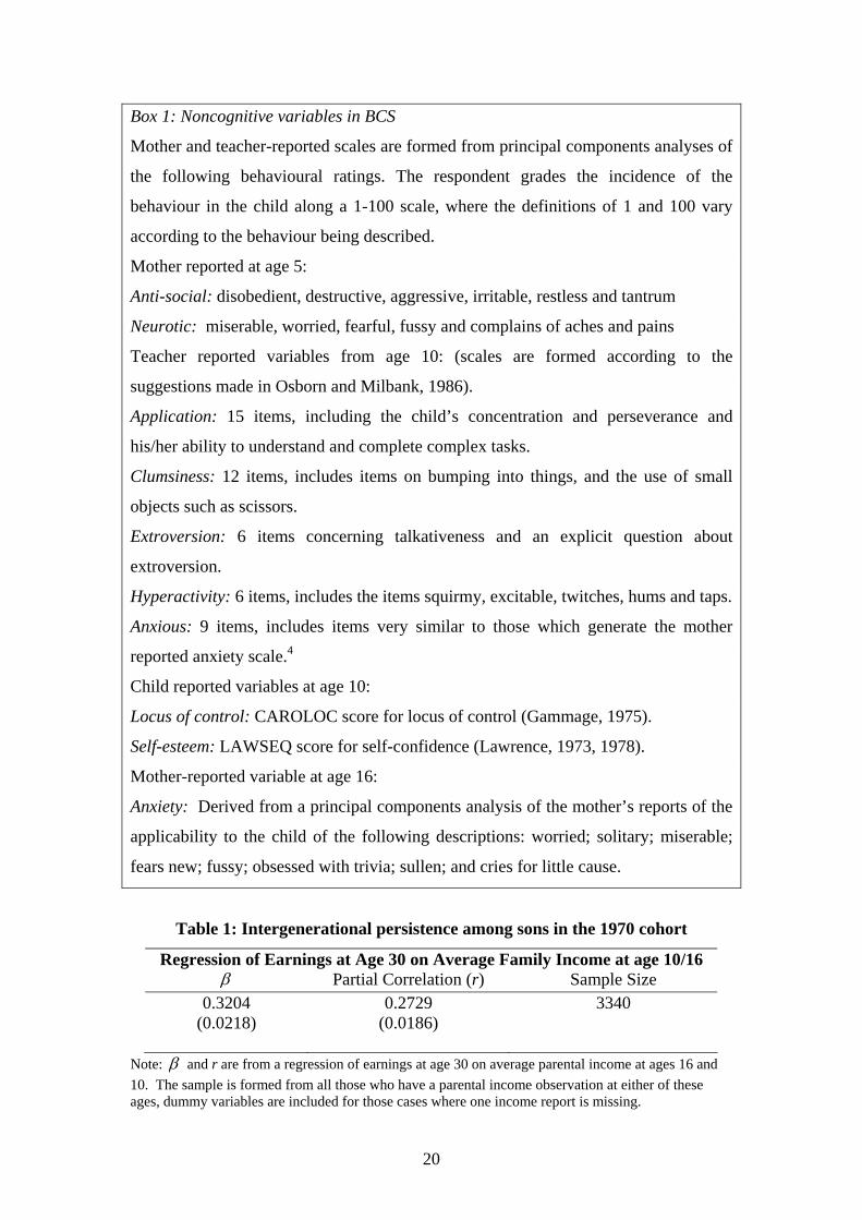
Box 1: Noncognitive variables in BCS

Mother and teacher-reported scales are formed from principal components analyses of

the following behavioural ratings. The respondent grades the incidence of the

behaviour in the child along a 1-100 scale, where the definitions of 1 and 100 vary

according to the behaviour being described.

Mother reported at age 5:

Anti-social: disobedient, destructive, aggressive, irritable, restless and tantrum

Neurotic: miserable, worried, fearful, fussy and complains of aches and pains

Teacher reported variables from age 10: (scales are formed according to the

suggestions made in Osborn and Milbank, 1986).

Application: 15 items, including the child’s concentration and perseverance and

his/her ability to understand and complete complex tasks.

Clumsiness: 12 items, includes items on bumping into things, and the use of small

objects such as scissors.

Extroversion: 6 items concerning talkativeness and an explicit question about

extroversion.

Hyperactivity: 6 items, includes the items squirmy, excitable, twitches, hums and taps.

Anxious: 9 items, includes items very similar to those which generate the mother

reported anxiety scale.4

Child reported variables at age 10:

Locus of control: CAROLOC score for locus of control (Gammage, 1975).

Self-esteem: LAWSEQ score for self-confidence (Lawrence, 1973, 1978).

Mother-reported variable at age 16:

Anxiety: Derived from a principal components analysis of the mother’s reports of the

applicability to the child of the following descriptions: worried; solitary; miserable;

fears new; fussy; obsessed with trivia; sullen; and cries for little cause.

Table 1: Intergenerational persistence among sons in the 1970 cohort

Regression of Earnings at Age 30 on Average Family Income at age 10/16 β Partial Correlation (r) Sample Size

0.3204 0.2729 3340 (0.0218) (0.0186)

Note: β and r are from a regression of earnings at age 30 on average parental income at ages 16 and 10. The sample is formed from all those who have a parental income observation at either of these ages, dummy variables are included for those cases where one income report is missing.

20

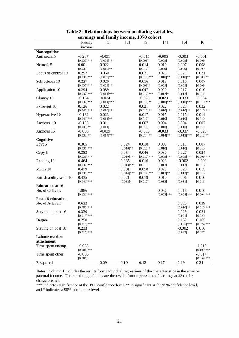
Table 2: Relationships between mediating variables, earnings and family income, 1970 cohort

Family income

[1] [2] [3] [4] [5] [6]

Noncognitive Anti social5 -0.237

[0.037]*** -0.031 [0.009]***

-0.015 [0.009]

-0.005 [0.009]

-0.003 [0.009]

-0.001 [0.009]

Neurotic5 0.001 [0.035]

0.022 [0.010]**

0.014 [0.010]

0.010 [0.009]

0.007 [0.009]

0.008 [0.009]

Locus of control 10 0.297 [0.038]***

0.060 [0.009]***

0.031 [0.010]***

0.021 [0.010]**

0.021 [0.010]**

0.021 [0.009]**

Self esteem 10 0.227 [0.037]***

0.020 [0.009]**

0.016 [0.009]*

0.013 [0.009]

0.010 [0.009]

0.007 [0.009]

Application 10 0.294 [0.037]***

0.089 [0.011]***

0.047 [0.012]***

0.020 [0.012]*

0.017 [0.012]

0.010 [0.011]

Clumsy 10 -0.154 [0.037]***

-0.034 [0.011]***

-0.023 [0.010]**

-0.029 [0.010]***

-0.033 [0.010]***

-0.034 [0.010]***

Extrovert 10 0.126 [0.040]***

0.022 [0.010]**

0.021 [0.010]**

0.022 [0.010]**

0.023 [0.010]**

0.022 [0.010]**

Hyperactive 10 -0.132 [0.041]***

0.023 [0.011]**

0.017 [0.010]

0.015 [0.010]

0.015 [0.010]

0.014 [0.010]

Anxious 10 -0.103 [0.039]**

0.011 [0.011]

0.007 [0.010]

0.004 [0.010]

0.004 [0.010]

0.002 [0.010]

Anxious 16 -0.066 [0.033]**

-0.039 [0.014]***

-0.033 [0.014]**

-0.033 [0.014]**

-0.037 [0.013]***

-0.028 [0.013]**

Cognitive

Epvt 5 0.365 [0.036]***

0.024 [0.010]**

0.018 [0.010]*

0.009 [0.010]

0.011 [0.010]

0.007 [0.010]

Copy 5 0.383 [0.036]***

0.054 [0.010]***

0.046 [0.010]***

0.030 [0.009]***

0.027 [0.009]***

0.024 [0.009]***

Reading 10 0.464 [0.037]***

0.035 [0.013]***

0.016 [0.013]

0.023 [0.013]

-0.002 [0.013]

-0.000 [0.013]

Maths 10 0.479 [0.036]***

0.081 [0.014]***

0.058 [0.014]***

0.029 [0.013]**

0.023 [0.013]*

0.015 [0.013]

British ability scale 10 0.435 [0.041]***

0.021 [0.012]*

0.019 [0.012]

0.010 [0.012]

0.006 [0.011]

0.010 [0.011]

Education at 16 No. of O-levels 1.886

[0.121]*** 0.036

[0.003]*** 0.018 [0.004]***

0.016 [0.004]***

Post-16 education

No. of A-levels 0.622 [0.052]***

0.025 [0.010]**

0.029 [0.010]***

Staying on post 16 0.330 [0.019]***

0.029 [0.021]

0.021 [0.020]

Degree 0.250 [0.018]***

0.152 [0.025]***

0.165 [0.024]***

Staying on post 18 0.233 [0.017]***

-0.002 [0.027]

0.016 [0.027]

Labour market attachment

Time spent unemp -0.023 [0.004]***

-1.215 [0.109]***

Time spent other -0.006 [0.006]

-0.314 [0.059]***

R-squared 0.09 0.10 0.12 0.17 0.19 0.24 Notes: Column 1 includes the results from individual regressions of the characteristics in the rows on parental income. The remaining columns are the results from regressions of earnings at 33 on the characteristics. *** Indicates significance at the 99% confidence level, ** is significant at the 95% confidence level, and * indicates a 90% confidence level.

21

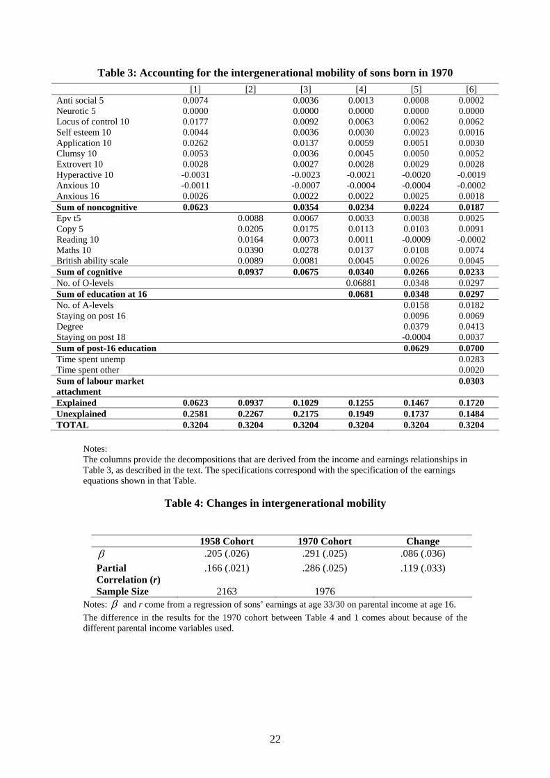
Table 3: Accounting for the intergenerational mobility of sons born in 1970

[1] [2] [3] [4] [5] [6] Anti social 5 0.0074 0.0036 0.0013 0.0008 0.0002 Neurotic 5 0.0000 0.0000 0.0000 0.0000 0.0000 Locus of control 10 0.0177 0.0092 0.0063 0.0062 0.0062 Self esteem 10 0.0044 0.0036 0.0030 0.0023 0.0016 Application 10 0.0262 0.0137 0.0059 0.0051 0.0030 Clumsy 10 0.0053 0.0036 0.0045 0.0050 0.0052 Extrovert 10 0.0028 0.0027 0.0028 0.0029 0.0028 Hyperactive 10 -0.0031 -0.0023 -0.0021 -0.0020 -0.0019 Anxious 10 -0.0011 -0.0007 -0.0004 -0.0004 -0.0002 Anxious 16 0.0026 0.0022 0.0022 0.0025 0.0018 Sum of noncognitive 0.0623 0.0354 0.0234 0.0224 0.0187 Epv t5 0.0088 0.0067 0.0033 0.0038 0.0025 Copy 5 0.0205 0.0175 0.0113 0.0103 0.0091 Reading 10 0.0164 0.0073 0.0011 -0.0009 -0.0002 Maths 10 0.0390 0.0278 0.0137 0.0108 0.0074 British ability scale 0.0089 0.0081 0.0045 0.0026 0.0045 Sum of cognitive 0.0937 0.0675 0.0340 0.0266 0.0233 No. of O-levels 0.06881 0.0348 0.0297 Sum of education at 16 0.0681 0.0348 0.0297 No. of A-levels 0.0158 0.0182 Staying on post 16 0.0096 0.0069 Degree 0.0379 0.0413 Staying on post 18 -0.0004 0.0037 Sum of post-16 education 0.0629 0.0700 Time spent unemp 0.0283 Time spent other 0.0020 Sum of labour market attachment

0.0303

Explained 0.0623 0.0937 0.1029 0.1255 0.1467 0.1720 Unexplained 0.2581 0.2267 0.2175 0.1949 0.1737 0.1484 TOTAL 0.3204 0.3204 0.3204 0.3204 0.3204 0.3204

Notes: The columns provide the decompositions that are derived from the income and earnings relationships in Table 3, as described in the text. The specifications correspond with the specification of the earnings equations shown in that Table.

Table 4: Changes in intergenerational mobility

1958 Cohort 1970 Cohort Change β .205 (.026) .291 (.025) .086 (.036) Partial Correlation (r)

.166 (.021) .286 (.025) .119 (.033)

Sample Size 2163 1976 Notes: β and r come from a regression of sons’ earnings at age 33/30 on parental income at age 16. The difference in the results for the 1970 cohort between Table 4 and 1 comes about because of the different parental income variables used.

22

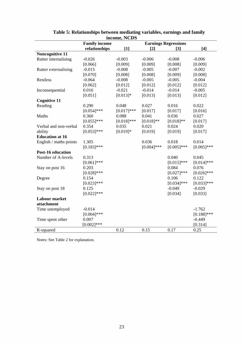
Table 5: Relationships between mediating variables, earnings and family income, NCDS

Family income Earnings Regressions relationships [1] [2] [3] [4] Noncognitive 11 Rutter internalising -0.026

[0.066] -0.003 [0.009]

-0.006 [0.009]

-0.008 [0.008]

-0.006 [0.009]

Rutter externalising -0.015 [0.070]

-0.008 [0.008]

-0.005 [0.008]

-0.007 [0.009]

-0.002 [0.008]

Restless -0.064 [0.062]

-0.008 [0.012]

-0.005 [0.012]

-0.005 [0.012]

-0.004 [0.012]

Inconsequential 0.016 [0.051]

-0.021 [0.013]*

-0.014 [0.013]

-0.014 [0.013]

-0.005 [0.012]

Cognitive 11 Reading 0.290

[0.054]*** 0.048 [0.017]***

0.027 [0.017]

0.016 [0.017]

0.022 [0.016]

Maths 0.360 [0.055]***

0.088 [0.018]***

0.041 [0.018]**

0.036 [0.018]**

0.027 [0.017]

Verbal and non-verbal ability

0.354 [0.053]***

0.035 [0.019]*

0.021 [0.019]

0.024 [0.019]

0.020 [0.017]

Education at 16 English / maths points 1.305

[0.183]*** 0.036

[0.004]*** 0.018 [0.005]***

0.014 [0.005]***

Post-16 education Number of A-levels 0.313

[0.061]*** 0.040

[0.015]*** 0.045 [0.014]***

Stay on post 16 0.203 [0.028]***

0.084 [0.027]***

0.076 [0.026]***

Degree 0.154 [0.023]***

0.106 [0.034]***

0.122 [0.033]***

Stay on post 18 0.125 [0.022]***

-0.049 [0.034]

-0.029 [0.033]

Labour market attachment

Time unemployed -0.014 [0.004]***

-1.762 [0.188]***

Time spent other 0.007 [0.002]***

-0.449 [0.314]

R-squared 0.12 0.15 0.17 0.25 Notes: See Table 2 for explanation.

23

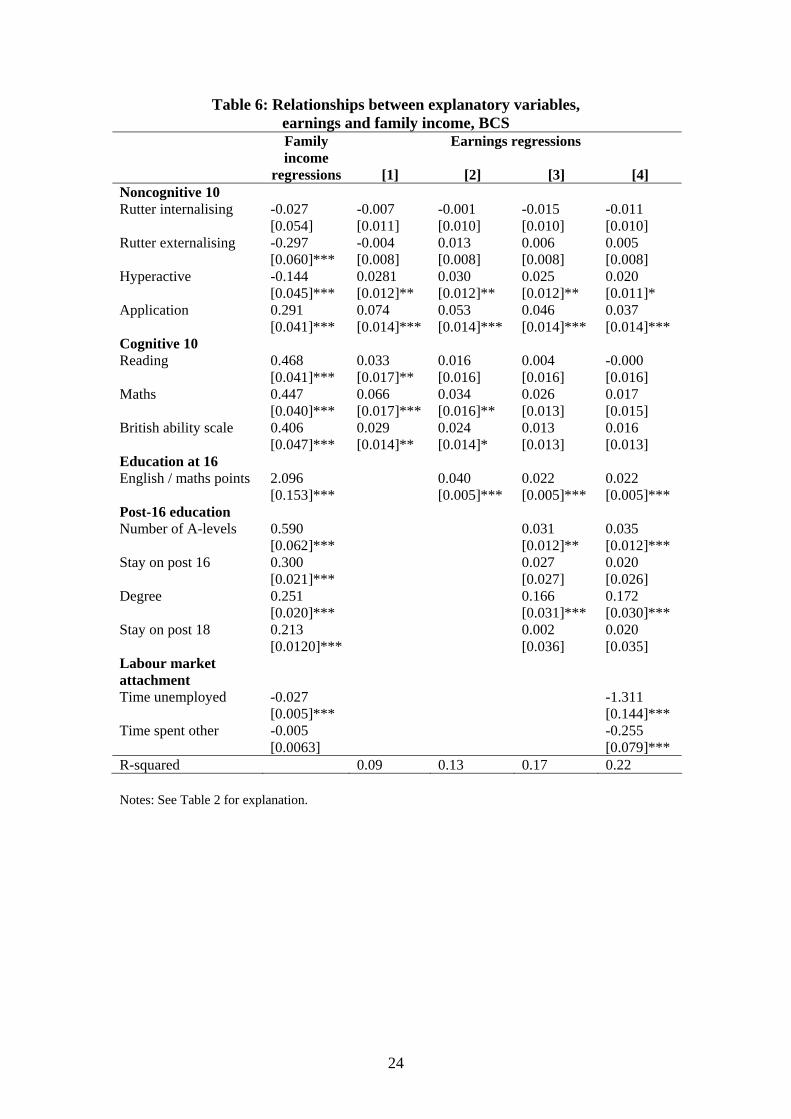
Table 6: Relationships between explanatory variables, earnings and family income, BCS

Family income

Earnings regressions

regressions [1] [2] [3] [4] Noncognitive 10 Rutter internalising -0.027

[0.054] -0.007 [0.011]

-0.001 [0.010]

-0.015 [0.010]

-0.011 [0.010]

Rutter externalising -0.297 [0.060]***

-0.004 [0.008]

0.013 [0.008]

0.006 [0.008]

0.005 [0.008]

Hyperactive -0.144 [0.045]***

0.0281 [0.012]**

0.030 [0.012]**

0.025 [0.012]**

0.020 [0.011]*

Application 0.291 [0.041]***

0.074 [0.014]***

0.053 [0.014]***

0.046 [0.014]***

0.037 [0.014]***

Cognitive 10 Reading 0.468

[0.041]*** 0.033 [0.017]**

0.016 [0.016]

0.004 [0.016]

-0.000 [0.016]

Maths 0.447 [0.040]***

0.066 [0.017]***

0.034 [0.016]**

0.026 [0.013]

0.017 [0.015]

British ability scale 0.406 [0.047]***

0.029 [0.014]**

0.024 [0.014]*

0.013 [0.013]

0.016 [0.013]

Education at 16 English / maths points 2.096

[0.153]*** 0.040

[0.005]*** 0.022 [0.005]***

0.022 [0.005]***

Post-16 education Number of A-levels 0.590

[0.062]*** 0.031

[0.012]** 0.035 [0.012]***

Stay on post 16 0.300 [0.021]***

0.027 [0.027]

0.020 [0.026]

Degree 0.251 [0.020]***

0.166 [0.031]***

0.172 [0.030]***

Stay on post 18 0.213 [0.0120]***

0.002 [0.036]

0.020 [0.035]

Labour market attachment

Time unemployed -0.027 [0.005]***

-1.311 [0.144]***

Time spent other -0.005 [0.0063]

-0.255 [0.079]***

R-squared 0.09 0.13 0.17 0.22 Notes: See Table 2 for explanation.

24

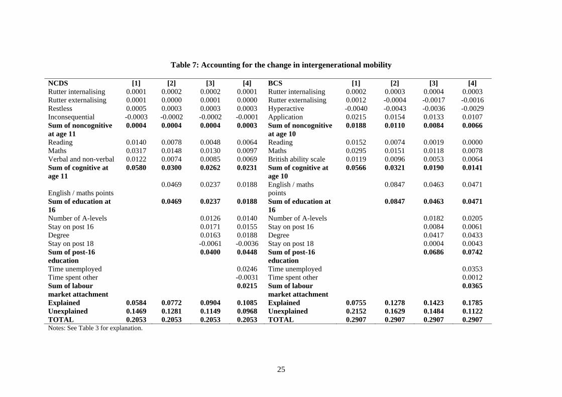
Table 7: Accounting for the change in intergenerational mobility NCDS [1] [2] [3] [4] BCS [1] [2] [3] [4]Rutter internalising 0.0001 0.0002 0.0002 0.0001 Rutter internalising

0.0002 0.0003 0.0004 0.0003Rutter externalising

0.0001 0.0000 0.0001 0.0000 Rutter externalising

0.0012 -0.0004 -0.0017 -0.0016

Restless 0.0005 0.0003 0.0003 0.0003 Hyperactive -0.0040 -0.0043 -0.0036 -0.0029Inconsequential -0.0003 -0.0002 -0.0002 -0.0001 Application 0.0215 0.0154 0.0133 0.0107Sum of noncognitive at age 11

0.0004 0.0004 0.0004 0.0003 Sum of noncognitive at age 10

0.0188 0.0110 0.0084 0.0066

Reading

0.0140 0.0078 0.0048 0.0064 Reading

0.0152 0.0074 0.0019 0.0000Maths 0.0317 0.0148 0.0130 0.0097 Maths 0.0295 0.0151 0.0118 0.0078Verbal and non-verbal 0.0122 0.0074 0.0085 0.0069 British ability scale 0.0119 0.0096 0.0053 0.0064Sum of cognitive at age 11

0.0580 0.0300 0.0262 0.0231 Sum of cognitive at age 10

0.0566 0.0321 0.0190 0.0141

English / maths points 0.0469 0.0237 0.0188 English / maths

points 0.0847 0.0463 0.0471

Sum of education at 16

0.0469 0.0237 0.0188 Sum of education at 16

0.0847 0.0463 0.0471

Number of A-levels 0.0126 0.0140 Number of A-levels 0.0182 0.0205 Stay on post 16 0.0171 0.0155 Stay on post 16 0.0084 0.0061 Degree 0.0163 0.0188 Degree 0.0417 0.0433Stay on post 18 -0.0061 -0.0036 Stay on post 18 0.0004 0.0043 Sum of post-16 education

0.0400 0.0448 Sum of post-16 education

0.0686 0.0742

Time unemployed 0.0246 Time unemployed 0.0353 Time spent other -0.0031 Time spent other 0.0012 Sum of labour market attachment

0.0215 Sum of labour market attachment

0.0365

Explained 0.0584 0.0772 0.0904 0.1085 Explained 0.0755 0.1278 0.1423 0.1785Unexplained

0.1469 0.1281 0.1149 0.0968 Unexplained

0.2152 0.1629 0.1484 0.1122

TOTAL 0.2053 0.2053 0.2053 0.2053 TOTAL 0.2907 0.2907 0.2907 0.2907Notes: See Table 3 for explanation.

25

References

Blanden, J. (2005) Essays on Intergenerational Mobility and its Variation over Time, Place and Family Structure, PhD Thesis, London: University College.

Blanden, J, Goodman, A., Gregg, P. and Machin, S. (2004) ‘Changes in intergenerational mobility in Britain’, in M. Corak, ed. Generational Income Mobility in North America and Europe, Cambridge: Cambridge University Press.

Blanden, J. and Machin, S. (2004) ‘Educational inequality and the expansion of UK higher education’, Scottish Journal of Political Economy, vol. 51(2), pp. 230-249.

Bowles, S., Gintis, H. and Osborne, M. (2001) ‘The determinants of earnings: a behavioural approach’, Journal of Economic Literature, vol. 39(4) pp. 1137-1176.

Carneiro, P., Crawford C. and Goodman, A. (2006) ‘Which skills matter?’, Unpublished, Institute for Fiscal Studies.

Corak, M. (2006) ‘Do poor children become poor adults? Lessons from a cross country comparison of generational earnings mobility’, IZA Discussion Paper No. 1993.

Currie, J. (2001) ‘Early childhood education programs’, Journal of Economic Perspectives, vol. 15(2) pp. 213-238.

Dearden, L., Machin, S. and Reed, H. (1997) ‘Intergenerational mobility in Britain’, ECONOMIC JOURNAL, vol. 107(440), pp. 47-64.

Ermisch, J and Francesconi, M. (2004) ‘Intergenerational mobility in Britain : new evidence from the BHPS’ in M. Corak, (ed) Generational Income Mobility in North America and Europe, Cambridge: Cambridge University Press.

Ermisch, J. and Nicoletti, C. (2005) ‘Intergenerational earnings mobility: changes across cohorts in Britain’, ISER Working Paper 2005-19. Colchester, University of Essex.

Feinstein, L. (2000) ‘The relative economic importance of academic, psychological and behavioural attributes developed in childhood’ CEP Discussion Paper No. 443.

Galindo-Rueda, F. and Vignoles, A. (2005) ‘The declining relative importance of ability in predicting educational attainment’, Journal of Human Resources vol. 40(2) pp. 335-353.

Gammage, P (1975) Socialisation, Schooling and Locus of Control, PhD Thesis, Bristol University.

Glennester, H. (2002) ‘United Kingdom Education 1997-2001’, Oxford Review of Economic Policy, vol. 18(2), pp.120-136.

Grawe, N. (2004) ‘The 3-day week of 1974 and earnings data reliability in the Family Expenditure Survey and the National Child Development Survey’, Oxford Bulletin of Economics and Statistics, vol. 66(3), 567-579.

Gregg, P and Tominey, E. (2005) ‘The wage scar from youth unemployment’, Labour Economics, vol. 12(4), 487-509.

Jäntti, M., Bratsberg, B., Røed, K., Raaum, O., Naylor, R., Osterbacka, E., Bjorklund A., and Eriksson, T., (2006) ‘American exceptionalism in a new light: a comparison of intergenerational earnings mobility in the Nordic countries, the United Kingdom and the United States’ IZA Discussion Paper No. 1938.

Lawrence, D. (1975) Improved Reading Through Counselling, London: Ward Lock.

26

Machin, S. (2003) ‘Wage inequality since 1975’ in P. Gregg and J. Wadsworth (eds.) The Labour Market Under New Labour: The State of Working Britain London: Palgrave Macmillan.

Machin, S. and McNally, S. (2004) ‘The Literacy Hour’ IZA Discussion Paper No. 105. Mazumder, B. (2001) ‘Earnings mobility in the US: a new look at intergenerational

mobility’ Unpublished, Federal Reserve Bank of Chicago. Osborn, A. and Milbank, J (1987) The effects of early education: a report from the Child

Health and Education Study, London: Ward Lock. Osborne-Groves, M. (2005) ‘Personality and the intergenerational transmission of

earnings’ in S. Bowles, H. Gintis and M. Osborne Groves, (eds), Unequal Chances: Family Background and Economic Success, Princeton: Princeton University Press.

Rutter, M., Tizard, J. and Whitmore, K. (1970) Education, Health and Behvaiour, London: Longman.

Singh, S. and Maddala, G. (1976) ‘A Function for Size Distribution of Incomes’ Econometrica, Vol. 44(2), pp. 963-970.

Solon, G. (1999) ‘Intergenerational mobility in the labor market’ in O. Ashenfelter and D. Card (eds.), Handbook of Labour Economics, Volume 3A, Amsterdam: North Holland.

Solon, G. (2002) ‘Cross-Country Differences in Intergenerational Earnings Mobility’, Journal of Economic Perspectives, Vol. 16(3), pp. 59-66.

Stevens, A. H. (1997). ‘Persistent effects of job displacement: the importance of multiple job losses’, Journal of Labor Economics, vol. 15(1), pp. 165-88.

Stott, D.H. (1966) The Social Adjustment of Children; Bristol Social Adjustment Guides Manual (3rd edition), University of London Press.

Stott, D.H. (1971) The Social Adjustment of Children; Bristol Social Adjustment Guides Manual (4th edition), University of London Press.

27

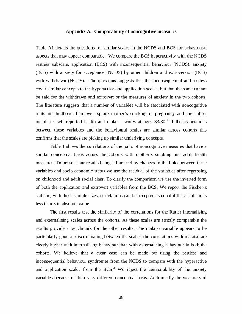
Appendix A: Comparability of noncognitive measures

Table A1 details the questions for similar scales in the NCDS and BCS for behavioural

aspects that may appear comparable. We compare the BCS hyperactivity with the NCDS

restless subscale, application (BCS) with inconsequential behaviour (NCDS), anxiety

(BCS) with anxiety for acceptance (NCDS) by other children and extroversion (BCS)

with withdrawn (NCDS). The questions suggests that the inconsequential and restless

cover similar concepts to the hyperactive and application scales, but that the same cannot

be said for the withdrawn and extrovert or the measures of anxiety in the two cohorts.

The literature suggests that a number of variables will be associated with noncognitive

traits in childhood, here we explore mother’s smoking in pregnancy and the cohort

member’s self reported health and malaise scores at ages 33/30.1 If the associations

between these variables and the behavioural scales are similar across cohorts this

confirms that the scales are picking up similar underlying concepts.

Table 1 shows the correlations of the pairs of noncognitive measures that have a

similar conceptual basis across the cohorts with mother’s smoking and adult health

measures. To prevent our results being influenced by changes in the links between these

variables and socio-economic status we use the residual of the variables after regressing

on childhood and adult social class. To clarify the comparison we use the inverted form

of both the application and extrovert variables from the BCS. We report the Fischer-z

statistic; with these sample sizes, correlations can be accepted as equal if the z-statistic is

less than 3 in absolute value.

The first results test the similarity of the correlations for the Rutter internalising

and externalising scales across the cohorts. As these scales are strictly comparable the

results provide a benchmark for the other results. The malaise variable appears to be

particularly good at discriminating between the scales; the correlations with malaise are

clearly higher with internalising behaviour than with externalising behaviour in both the

cohorts. We believe that a clear case can be made for using the restless and

inconsequential behaviour syndromes from the NCDS to compare with the hyperactive

and application scales from the BCS.2 We reject the comparability of the anxiety

variables because of their very different conceptual basis. Additionally the weakness of

28

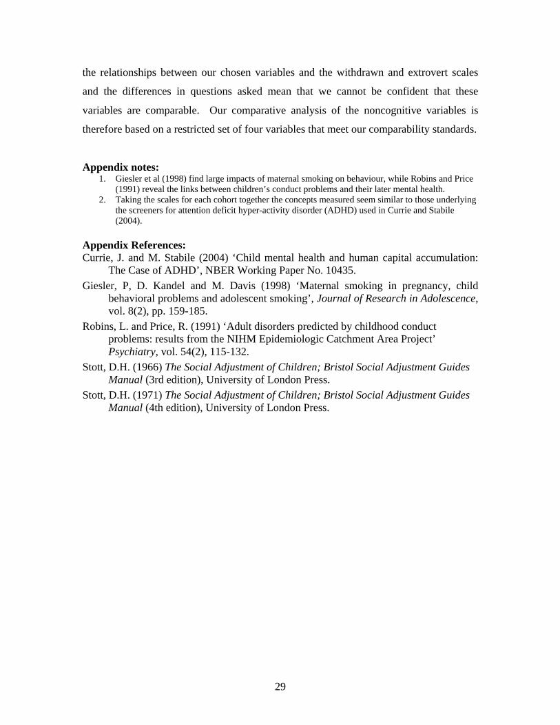
the relationships between our chosen variables and the withdrawn and extrovert scales

and the differences in questions asked mean that we cannot be confident that these

variables are comparable. Our comparative analysis of the noncognitive variables is

therefore based on a restricted set of four variables that meet our comparability standards.

Appendix notes: 1. Giesler et al (1998) find large impacts of maternal smoking on behaviour, while Robins and Price

(1991) reveal the links between children’s conduct problems and their later mental health. 2. Taking the scales for each cohort together the concepts measured seem similar to those underlying

the screeners for attention deficit hyper-activity disorder (ADHD) used in Currie and Stabile (2004).

Appendix References: Currie, J. and M. Stabile (2004) ‘Child mental health and human capital accumulation:

The Case of ADHD’, NBER Working Paper No. 10435. Giesler, P, D. Kandel and M. Davis (1998) ‘Maternal smoking in pregnancy, child

behavioral problems and adolescent smoking’, Journal of Research in Adolescence, vol. 8(2), pp. 159-185.

Robins, L. and Price, R. (1991) ‘Adult disorders predicted by childhood conduct problems: results from the NIHM Epidemiologic Catchment Area Project’ Psychiatry, vol. 54(2), 115-132.

Stott, D.H. (1966) The Social Adjustment of Children; Bristol Social Adjustment Guides Manual (3rd edition), University of London Press.

Stott, D.H. (1971) The Social Adjustment of Children; Bristol Social Adjustment Guides Manual (4th edition), University of London Press.

29

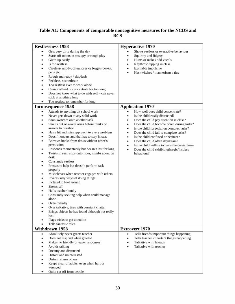
Table A1: Components of comparable noncognitive measures for the NCDS and BCS

Restlessness 1958 Hyperactive 1970

• Gets very dirty during the day • Starts off others in scrappy or rough play • Gives up easily • Is too restless • Careless/ untidy, often loses or forgets books,

pens etc. • Rough and ready / slapdash • Feckless, scatterbrain • Too restless ever to work alone • Cannot attend or concentrate for too long. • Does not know what to do with self – can never

stick at anything long • Too restless to remember for long.

• Shows restless or overactive behaviour • Squirmy and fidgety • Hums or makes odd vocals • Rhythmic tapping in class • Excitable impulsive • Has twitches / mannerisms / tics

Inconsequence 1958 Application 1970 • Attends to anything bit school work • Never gets down to any solid work • Soon switches onto another task • Shouts out or waves arms before thinks of

answer to question • Has a hit and miss approach to every problem • Doesn’t understand that has to stay in seat • Borrows books from desks without other’s

permission • Responds momentarily but doesn’t last for long • Twists in seat, slips onto floor, climbs about on

desk • Constantly restless • Presses to help but doesn’t perform task

properly • Misbehaves when teacher engages with others • Invents silly ways of doing things • Inclined to fool around • Shows off • Hails teacher loudly • Constantly seeking help when could manage

alone • Over-friendly • Over talkative, tires with constant chatter • Brings objects he has found although not really

lost • Plays tricks to get attention • Tells fantastic tales.

• How well does child concentrate? • Is the child easily distracted? • Does the child pay attention in class? • Does the child become bored during tasks? • Is the child forgetful on complex tasks? • Does the child fail to complete tasks? • Is the child confused or hesitant? • Does the child often daydream? • Is the child willing to learn the curriculum? • Does the child exhibit lethargic/ listless

behaviour?

Withdrawn 1958 Extrovert 1970 • Absolutely never greets teacher • Does not respond when greeted • Makes no friendly or eager responses • Avoids talking • Dreamy and distracted • Distant and uninterested • Distant, shuns others • Keeps clear of adults, even when hurt or

wronged • Quite cut off from people

• Tells friends important things happening • Tells teacher important things happening • Talkative with friends • Talkative with teacher

30

• Unresponsive • Incoherent rambling chatter • Like a suspicious animal

Anxious for acceptance from children 1958

Anxious 1970

• Plays the hero • Can’t resist playing to the crowd • Inclined to fool around • Over brave • Over-anxious to be in with the gang • Likes to be the centre of attention • Plays only or mainly with older children • Strikes brave attitude but funks • Brags to other children • Shows off • Misbehaves when teacher is out of the room • Spivvish dress, hairstyle, overdoes dress, make

up. • Damage to public property etc • Foolish pranks when with a gang • Follower in mischief.

• Behaves nervously • Relations with others unhappy / tearful • Obsessional about unimportant tasks • Afraid of new things / situations • Fussy or over particular • Cries for little reason • Fearful in movements • Truants from school

Note: NCDS questions are obtained from Stott (1966 and 1971)

31

Table A2: Choosing comparable noncognitive variables: Correlations with health measures net of social class 1958 Cohort

Rutter Internalising

1970 Cohort Rutter

Internalising

1958 Cohort Rutter

Externalising

1970 Cohort Rutter

Externalising

1958 Cohort BSAS Restless

1970 Cohort Hyperactive

Mother smoked during pregnancy

ρ=0.0171 N=7850

ρ=-0.0246** N=6435

ρ=0.0565*** N=8094

ρ=0.0431*** N=6821

ρ=0.0291*** N=8388

ρ=0.0577*** N=6297

Z=2.4796

Z=2.4796 Z=0.8171 Z=0.8171 Z=-1.7182 Z=-1.7182Self reported health in early 30s

ρ=0.0586*** N=7827

ρ=0.0497*** N=6429

ρ=0.0579*** N=8071

ρ=0.0434*** N=6814

ρ=0.0380*** N=8364

ρ=0.0392** N=6294

Z=0.5302 Z=0.5302 Z=0.8835 Z=0.8835 Z=-0.0720 Z=-0.0720Malaise score in early 30s

ρ=0.1162*** N=7886

ρ=0.1122*** N=6381

ρ=0.0726*** N=8131

ρ=0.0464*** N=6764

ρ=0.0507*** N=8430

ρ=0.0161 N=6247

Z=0.2406 Z=0.2406 Z=1.5975 Z=1.5975 Z=2.0746 Z=2.07461958 Cohort

BSAS Inconsequential

Behaviour

1970 Cohort Inverted

Application

1958 Cohort Withdrawn

1970 Cohort Inverted

Extrovert

1958 Cohort Anxious for

Acceptance by other Children

1970 Cohort Anxious

Mother smoked during pregnancy

ρ=0.0340** N=8388

ρ=0.0569*** N=5642

ρ=0.0042 N=8388

ρ=-0.0042 N=6209

ρ=0.0319 ** N=8388

ρ=0.0070 N=6318

Z=-1.3325 Z=-1.3325 Z=0.5016 Z=0.5016 Z=1.4951 Z=1.4951Self reported health in early 30s

ρ=0.0759*** N=8364

ρ=0.0638*** N=5639

ρ=0.0219** N=8364

ρ=0.0031 N=6207

ρ=0.0232** N=8364

ρ=0.0239** N=6315

Z=0.7055 Z=0.7055 Z=1.1221 Z=1.1221 Z=-0.0420 Z=-0.0420Malaise score in early 30s

ρ=0.0730*** N=8430

ρ=0.0627*** N=5599

ρ=0.0450*** N=8430

ρ=0.0279** N=6161

ρ=0.0381*** N=8430

ρ=0.0661*** N=6269

Z=0.6000 Z=0.6000 Z=1.0214 Z=1.0214 Z=--1.6832 Z=-1.6832Note: ρ is the correlation coefficient, N is the number of observations used to calculate the coefficient and Z is the Fischer z statistic. *** Indicates a correlation is significantly different from zero at the 99% confidence level, ** is significant at the 95% confidence level, and * indicates a 90% confidence level. The smoking and health variables have been purged of their association with socio-economic status by regressing them on the social class of the father and son, the variables used here are the residuals from these equations.

32

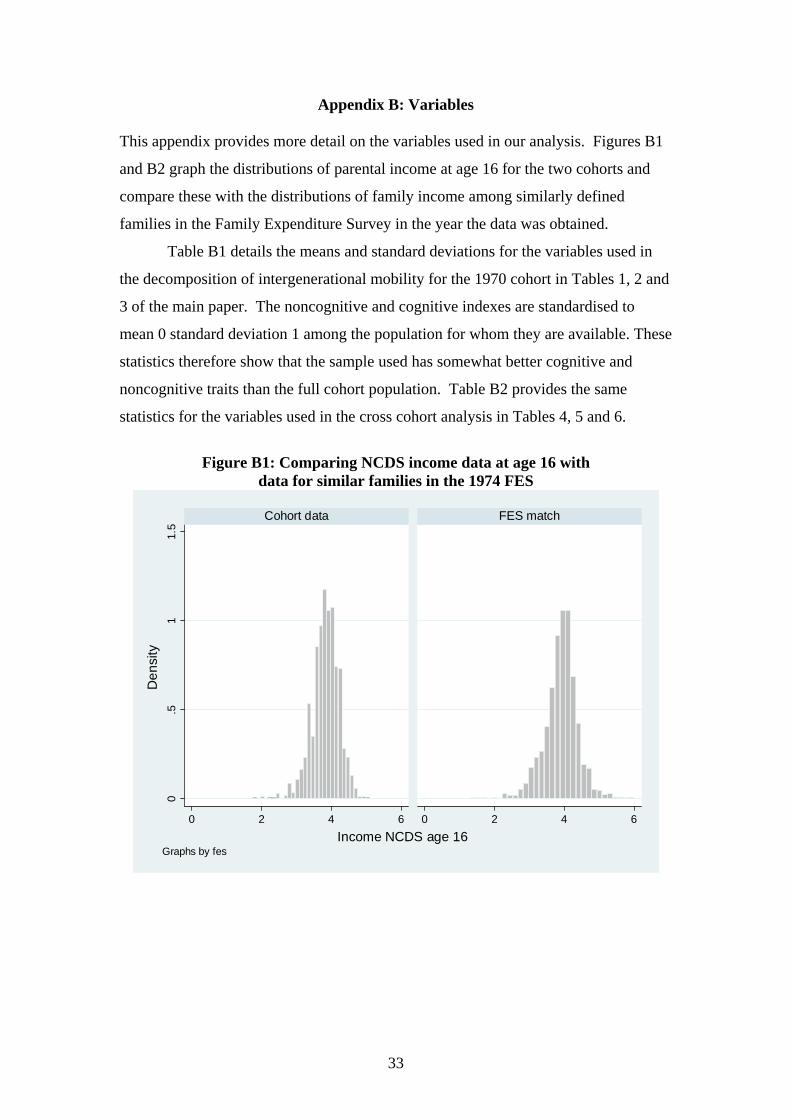
Appendix B: Variables This appendix provides more detail on the variables used in our analysis. Figures B1

and B2 graph the distributions of parental income at age 16 for the two cohorts and

compare these with the distributions of family income among similarly defined

families in the Family Expenditure Survey in the year the data was obtained.

Table B1 details the means and standard deviations for the variables used in

the decomposition of intergenerational mobility for the 1970 cohort in Tables 1, 2 and

3 of the main paper. The noncognitive and cognitive indexes are standardised to

mean 0 standard deviation 1 among the population for whom they are available. These

statistics therefore show that the sample used has somewhat better cognitive and

noncognitive traits than the full cohort population. Table B2 provides the same

statistics for the variables used in the cross cohort analysis in Tables 4, 5 and 6.

Figure B1: Comparing NCDS income data at age 16 with

data for similar families in the 1974 FES

0.5

11.

5

0 2 4 6 0 2 4 6

Cohort data FES match

Den

sity

Income NCDS age 16Graphs by fes

33

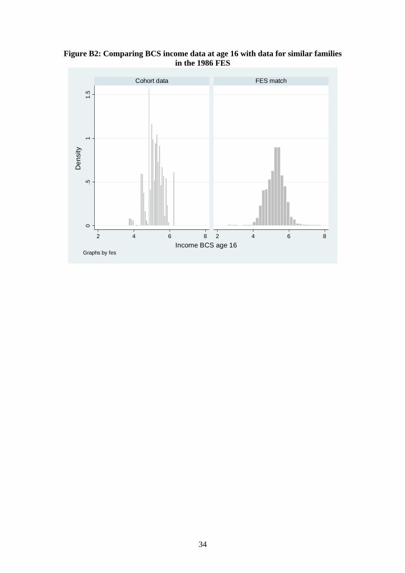
Figure B2: Comparing BCS income data at age 16 with data for similar families in the 1986 FES

0.5

11.

5

2 4 6 8 2 4 6 8

Cohort data FES matchD

ensi

ty

Income BCS age 16Graphs by fes

34

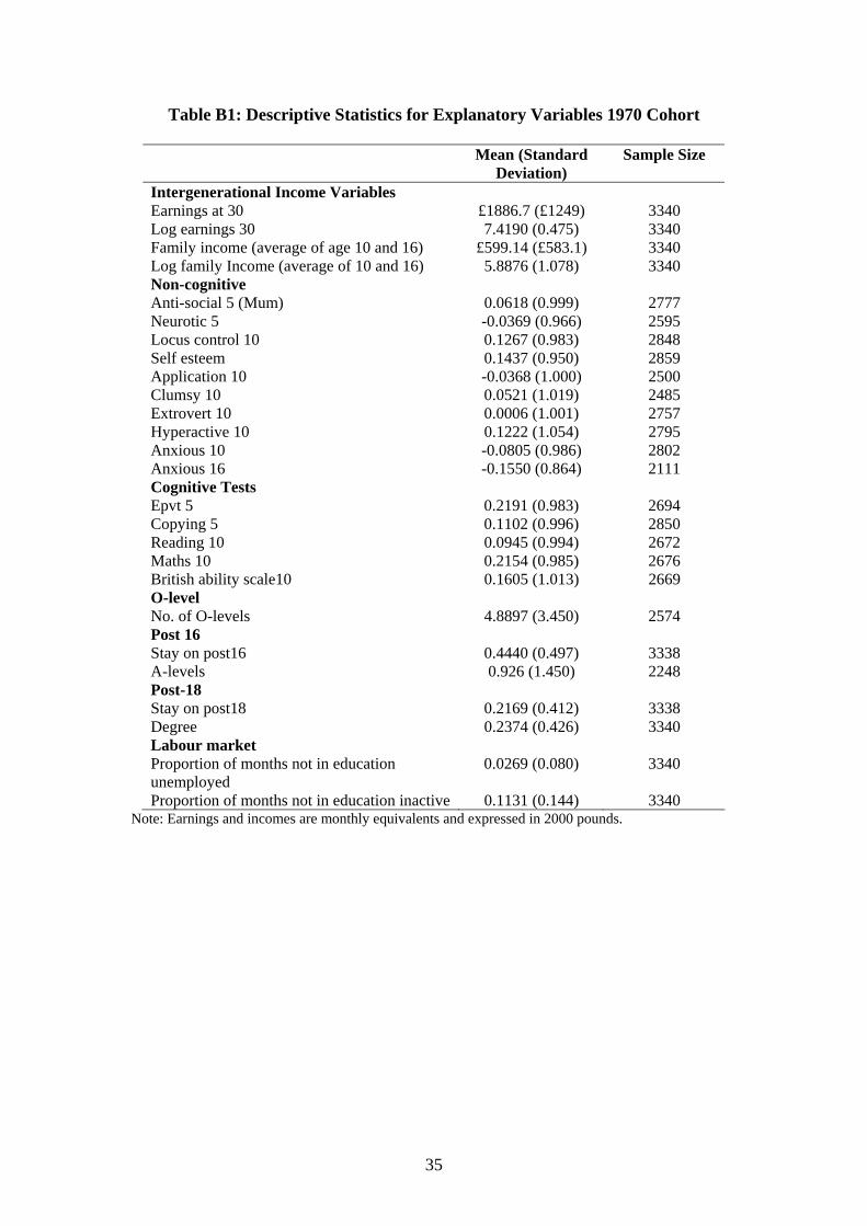
Table B1: Descriptive Statistics for Explanatory Variables 1970 Cohort

Mean (Standard Deviation)

Sample Size

Intergenerational Income Variables Earnings at 30 £1886.7 (£1249) 3340 Log earnings 30 7.4190 (0.475) 3340 Family income (average of age 10 and 16) £599.14 (£583.1) 3340 Log family Income (average of 10 and 16) 5.8876 (1.078) 3340 Non-cognitive Anti-social 5 (Mum) 0.0618 (0.999) 2777 Neurotic 5 -0.0369 (0.966) 2595 Locus control 10 0.1267 (0.983) 2848 Self esteem 0.1437 (0.950) 2859 Application 10 -0.0368 (1.000) 2500 Clumsy 10 0.0521 (1.019) 2485 Extrovert 10 0.0006 (1.001) 2757 Hyperactive 10 0.1222 (1.054) 2795 Anxious 10 -0.0805 (0.986) 2802 Anxious 16 -0.1550 (0.864) 2111 Cognitive Tests Epvt 5 0.2191 (0.983) 2694 Copying 5 0.1102 (0.996) 2850 Reading 10 0.0945 (0.994) 2672 Maths 10 0.2154 (0.985) 2676 British ability scale10 0.1605 (1.013) 2669 O-level No. of O-levels 4.8897 (3.450) 2574 Post 16 Stay on post16 0.4440 (0.497) 3338 A-levels 0.926 (1.450) 2248 Post-18 Stay on post18 0.2169 (0.412) 3338 Degree 0.2374 (0.426) 3340 Labour market Proportion of months not in education unemployed

0.0269 (0.080) 3340

Proportion of months not in education inactive 0.1131 (0.144) 3340 Note: Earnings and incomes are monthly equivalents and expressed in 2000 pounds.

35

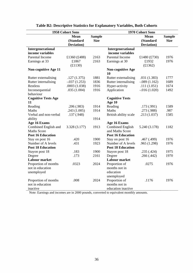
Table B2: Descriptive Statistics for Explanatory Variables, Both Cohorts

1958 Cohort Sons 1970 Cohort Sons Mean

(Standard Deviation)

Sample Size

Mean (Standard Deviation)

Sample Size

Intergenerational income variables

Intergenerational income variables

Parental Income £1360 (£488) 2163 Parental Income £1480 (£730) 1976 Earnings at 33 £1867

(£1130) 2163 Earnings at 30 £1932

(£1362) 1976

Non-cognitive Age 11 Non-cognitive Age 10

Rutter externalising .127 (1.375) 1881 Rutter externalising .031 (1.383) 1777 Rutter internalising -.037 (1.253) 1836 Rutter internalising -.089 (1.162) 1689 Restless .0003 (1.038) 1916 Hyper-activity .111 (1.051) 1674 Inconsequential behaviour

.035 (1.004) 1916 Application -.016 (1.020) 1492

Cognitive Tests Age 11

Cognitive Tests Age 10

Reading .206 (.983) 1914 Reading .173 (.991) 1589 Maths .243 (1.005) 1914 Maths .273 (.988) .987 Verbal and non-verbal ability

.137 (.948) 1914

British ability scale .213 (1.037) 1585

Age 16 Exams Age 16 Exams Combined English and Maths Score

3.328 (3.177) 1913 Combined English and Maths Score

5.240 (3.178) 1182

Post 16 Education Post 16 Education Stay on post 16 .420 1900 Stay on post 16 .467 (.499) 1976 Number of A levels .431 1923 Number of A levels .965 (1.298) 1976 Post 18 Education Post 18 Education Stayon post 18 .183 1900 Stayon post 18 .235 (.424) 1975 Degree .173 2161 Degree .266 (.442) 1970 Labour market Labour market Proportion of months not in education unemployed

.0323 2024 Proportion of months not in education unemployed

.0275 1976

Proportion of months not in education inactive

.008 2024 Proportion of months not in education inactive

.1176 1976

Note: Earnings and incomes are in 2000 pounds, converted to equivalent monthly amounts.

36