accounting for linkage disequilibrium in genome-wide … · 2013-09-25 · accounting for linkage...
TRANSCRIPT
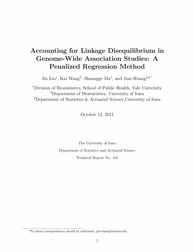
Accounting for Linkage Disequilibrium inGenome-Wide Association Studies: A
Penalized Regression Method
Jin Liu1, Kai Wang2, Shuangge Ma1, and Jian Huang2,3 ∗
1Division of Biostatistics, School of Public Health, Yale University2Department of Biostatistics, University of Iowa
3Department of Statistics & Actuarial Science,University of Iowa
October 13, 2011
The University of Iowa
Department of Statistics and Actuarial Science
Technical Report No. 410
∗To whom correspondence should be addressed. [email protected]
1

Accounting for Linkage Disequilibrium in Genome-Wide
Association Studies: A Penalized Regression Method
Jin Liu1, Kai Wang2, Shuangge Ma1 and Jian Huang2,3
1Division of Biostatistics, School of Public Health, Yale University
2Department of Biostatistics, University of Iowa
2,3Department of Statistics & Actuarial Science,University of Iowa
Abstract
Penalized regression methods are becoming increasingly popular in genome-wideassociation studies (GWAS) for identifying genetic markers associated with disease.However, standard penalized methods such as the LASSO do not take into accountthe possible linkage disequilibrium between adjacent markers. We propose a novelpenalized approach for GWAS using a dense set of single nucleotide polymorphisms(SNPs). The proposed method uses the minimax concave penalty (MCP) for markerselection and incorporates linkage disequilibrium (LD) information by penalizing thedifference of the genetic effects at adjacent SNPs with high correlation. A coordinatedescent algorithm is derived to implement the proposed method. This algorithm isefficient in dealing with a large number of SNPs. A multi-split method is used to cal-culate the p-values of the selected SNPs for assessing their significance. We refer to theproposed penalty function as the smoothed MCP and the proposed approach as theSMCP method. Performance of the proposed SMCP method and its comparison witha LASSO approach are evaluated through simulation studies, which demonstrate thatthe proposed method is more accurate in selecting associated SNPs. Its applicabilityto real data is illustrated using data from a study on rheumatoid arthritis.
Keywords: Genetic association, Feature selection, Linkage disequilibrium, Penalizedregression, Single nucleotide polymorphism.
1 Introduction
With the rapid development of modern genotyping technology, genome-wide association
studies (GWAS) have become an important tool for identifying genetic factors underlying
complex traits. From a statistical standpoint, identifying SNPs associated with a trait can
be formulated as a variable selection problem in sparse, high-dimensional models. The
2
traditional multivariate regression methods are not directly applicable to GWAS because
the number of SNPs in an association study is usually much larger than the sample size.
The LASSO (least absolute shrinkage and selection operator) provides a computationally
feasible way for variable selection in high-dimensional settings Tibshirani [1996]. Recently,
this approach has been applied to GWAS for selecting associated SNPs Wu et al. [2009]. It
has been shown that the LASSO is selection consistent if and only if the predictors meet the
irrepresentable condition Zhao and Yu [2006]. This condition is stringent and there is no
known mechanism to verify it in GWAS. Zhang and Huang Zhang and Huang [2008] studied
the sparsity and the bias of the LASSO in high-dimensional linear regression models. It is
shown that under reasonable conditions, the LASSO selects a model of the correct order of
dimensionality. However, the LASSO tends to overselect unimportant variables. Therefore,
direct application of the LASSO to GWAS tends to generate findings with high false positive
rates. Another limitation of the LASSO is that, if there is a group of variables among which
the pairwise correlations are high, then the LASSO tends to select only one variable from
the group and does not care which one is selected Zou and Hastie [2005].
Several methods that attempt to improve the performance of the LASSO have been
proposed. The adaptive LASSO Zou [2006] uses adaptive weights on each penalty so that
the oracle properties hold under some mild regularity conditions. In the case that the
number of predictors is much larger than sample size, adaptive weights cannot be initiated
easily. Elastic net method Zou and Hastie [2005] can effectively deal with certain correlation
structures in the predictors by using a combination of ridge and LASSO penalties. Fan and
Li Fan and Li [2001] introduced a smoothly clipped absolute deviation (SCAD) method.
Zhang Zhang [2010] proposed a flexible minmax concave penalty (MCP) which attenuates
the effect of shrinkage that leads to bias. Both the SCAD and MCP belong to the same
family of quadratic spline penalties and both lead to oracle selection results Zhang [2010].
3
The MCP has a simpler form and requires weaker conditions for the oracle property. We
refer to Zhang [2010] and Mazumder et al. [2011] for detailed discussion.
However, the existing penalized methods for variable selection do not take into account
the specifics of SNP data. SNPs are naturally ordered along the genome with respect to
their physical positions. In the presence of linkage disequilibrium (LD), adjacent SNPs
are expected to show similar strength of association. Making use of LD information from
adjacent SNPs is highly desirable as it should help to better delineate association signals
while reducing randomness seen in single SNP analysis. Fused LASSO Tibshirani et al. [2005]
is not appropriate for this purpose, since the effect of association for a SNP (as measured
by its regression coefficient) is only identifiable up to its absolute value – a homozygous
genotype can be equivalently coded as either 0 or 2 depending on the choice of the reference
allele.
We propose a new penalized regression method for identifying associated SNPs in GWAS.
The proposed method uses a novel penalty, which we shall refer to as the smoothed minimax
concave penalty, or SMCP, for sparsity and smoothness in absolute values. The SMCP is a
combination of the MCP and a penalty consisting of the squared differences of the absolute
effects of adjacent markers. The MCP promotes sparsity in the model and does automatic
selection of associated SNPs. The penalty for squared differences of the absolute effects
takes into account the natural ordering of SNPs and adaptively incorporates possible LD
information between adjacent SNPs. It explicitly uses correlation between adjacent markers
and penalizes the differences of the genetic effects at adjacent SNPs with high correlation.
We derive a coordinate descent algorithm for implementing the SMCP method. We use
a resampling method for computing p-values of the selected SNPs in order to assess their
significance.
The rest of the paper is organized as follows. Section 2 introduces the proposed SMCP
4

method. Section 3 presents a genome-wide screening incorporating the proposed SMCP
method. Section 4 describes a coordinate descent algorithm for estimating model parame-
ters and discusses selection of the values of the tuning parameters and p-value calculation.
Section 5 evaluates the proposed method and a LASSO method using simulated data. Sec-
tion 6 applies the proposed method to a GWAS on rheumatoid arthritis. Finally, Section 7
provides a summary and discusses some related issues.
2 The SMCP method
Let p be the number of SNPs included in the study, and let βj denote the effect of the jth SNP
in a working model that describes the relationship between phenotype and markers. Here we
assume that the SNPs are ordered according to their physical locations on the chromosomes.
Adjacent SNPs in high LD are expected to have similar strength of association with the
phenotype. To adaptively incorporating LD information, we propose the following penalty
that encourages smoothness in |β|s at neighboring SNPs:
λ22
p−1∑j=1
ζj(|βj| − |βj+1|)2, (1)
where the weight ζj is a measure of LD between SNP j and SNP (j+1). This penalty
encourages |βj| and |βj+1| to be similar to an extent inversely proportional to the LD strength
between the two corresponding SNPs. Adjacent SNPs in weak LD are allowed to have larger
difference in their |β|s than if they are in stronger LD. The effect of this penalty is to
encourage smoothness in |β|s for SNPs in strong LD. By using this penalty, we expect a
better delineation of the association pattern in LD blocks that harbor disease variants while
reducing randomness in |β|s in LD blocks that do not. We note that there is no monotone
relationship between ζ and the physical distance between two SNPs. While it is possible
to use other LD measures, we choose ζj to be the absolute value of lag one autocorrelation
5

coefficient between the genotype scores of SNP j and SNP (j+1). The values of ζj for
rheumatoid arthritis data used by Genetic Analysis Workshop 16, the data set to be used
in our simulation study and empirical study, are plotted for chromosome 6 (Fig. 1(a)). The
proportion that ζj > 0.5 over non-overlapping 100-SNP windows is also plotted (Fig. 1(b)).
[Figure 1 about here.]
For the purpose of SNP selection, we use the MCP, which is defined as
ρ(t;λ1, γ) = λ1
∫ |t|0
(1− x/(γλ1))+dx,
where λ1 is a penalty parameter and γ is a regularization parameter that controls the con-
cavity of ρ. Here x+ is the nonnegative part of x, i.e., x+ = x1{x≥0}. The MCP can be easily
understood by considering its derivative, which is
ρ(t;λ1, γ) = λ1(1− |t|/(γλ1)
)+
sgn(t),
where sgn(t) = −1, 0, or 1 if t < 0,= 0, or > 0, respectively. As |t| increases from 0,
MCP begins by applying the same rate of penalization as the LASSO, but continuously
relaxes that penalization until |t| > γλ1, a condition under which the rate of penalization
drops to 0. It provides a continuum of penalties where the LASSO penalty corresponds to
γ = ∞ and the hard-thresholding penalty corresponds to γ → 1+. We note that other
penalties, such as the LASSO penalty or SCAD penalty, can also be used to replace MCP.
We choose MCP because it possesses all the basic desired properties of a penalty function
and is computationally simple Mazumder et al. [2011], Zhang [2010].
Given the parameter vector β = (β1, . . . , βp)′ and a loss function g(β) based on a working
model for the relationship between the phenotype and markers, the SMCP in a working model
can be expressed as minimizing the criterion
Ln(β) = g(β) +
p∑j=1
ρ(|βj|;λ1, γ) +λ22
p−1∑j=1
ζj(|βj| − |βj+1|)2. (2)
6

We minimize this objective function with respect to β, while using a bisection method to
determine the regularization parameters (λ1, λ2). SNPs corresponding to βj 6= 0 are selected
as being potentially associated with disease. These selected SNPs will be subject to further
analysis using a multi-split sampling method to determine their statistical significance, as
described later.
3 Genome-wide screening incorporating LD
A basic method for GWAS is to conduct genome-wide screening of a large number of dense
SNPs individually and look for those with significant association with phenotype. Although
several important considerations, such as adjustment for multiple comparisons and possible
population stratification, need to be taken into account in the analysis, the essence of the
existing genome-wide screening approach is single-marker based analysis without considering
the structure of SNP data. In particular, the possible LD between two adjacent SNPs are
not incorporated in the analysis.
Our proposed SMCP method can be used for screening a dense set of SNPs incorporating
LD information in a natural way. To be specific, here we consider the standard case-control
design for identifying SNPs that potentially associated with disease. Let the phenotype be
scored as 1 for cases and −1 for controls. Let nj be the number of subjects whose genotypes
are non-missing at SNP j. The standardized phenotype of the ith subject with non-missing
genotype at SNP j is denoted by yij. The genotype at SNP j is scored as 0, 1, or 2 depending
on the number of copies of a reference allele in a subject. Let xij denote the standardized
genotype score satisfying∑
i xij = 0 and∑nj
i=1 x2ij = nj.
Consider the penalized criterion
Ln(β) =1
2
p∑j=1
1
nj
nj∑i=1
(yij − xijβj)2 +
p∑j=1
ρ(|βj|;λ1, γ)
7

+λ22
p−1∑j=1
ζj(|βj| − |βj+1|)2. (3)
Here the loss function is
g(β) =1
2
p∑j=1
1
nj
nj∑i=1
(yij − xijβj)2. (4)
We note that switching the reference allele used for scoring the genotypes changes the sign
of βj but |βj| remains the same. It may be counter-intuitive to use a quadratic loss in (4) for
case-control designs. We now show that this is appropriate. Regardless how the phenotype
is scored, the least squares regression slope of the phenotype over the genotype score at SNP
j (i.e., a regular single SNP analysis) equals
nj∑i=1
yijxij/
nj∑i=1
x2ij = 2(p1j − p2j)/φj(1− φj),
where φj is the proportion of cases out of total subjects computed from the subjects with
non-missing genotype and p1j and p2j are allele frequencies of the SNP j in cases and controls,
respectively. This shows that the βj in the squared loss function (4) can be interpreted as
the effect size of SNP j. In the classification literature, quadratic loss has also been used for
indicator response variables Hastie et al. [2009].
An alternative loss function for binary phenotype would be the sum of negative marginal
log-likelihood based on a working logistic regression model. We have found that the selection
results using this loss function are in general similar to those based on (4). In addition, the
computational implementation of the coordinate descent algorithm described in the next
subsection using the loss function (4) is much more stable and efficient and can easily handle
tens of thousands SNPs.
8
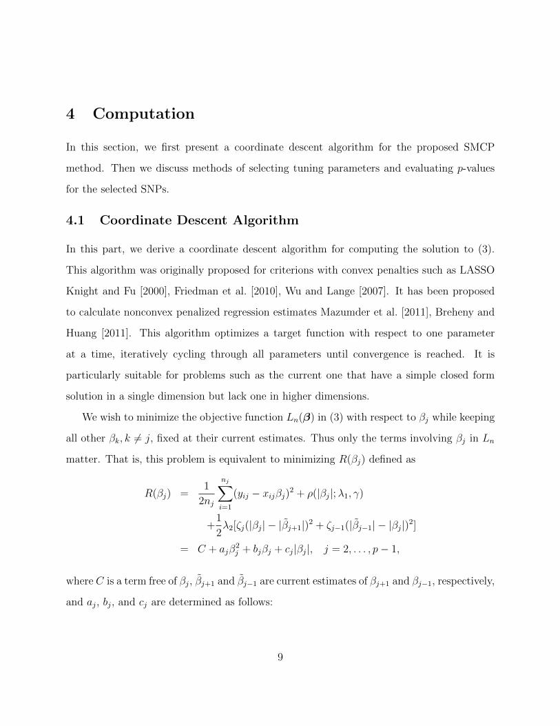
4 Computation
In this section, we first present a coordinate descent algorithm for the proposed SMCP
method. Then we discuss methods of selecting tuning parameters and evaluating p-values
for the selected SNPs.
4.1 Coordinate Descent Algorithm
In this part, we derive a coordinate descent algorithm for computing the solution to (3).
This algorithm was originally proposed for criterions with convex penalties such as LASSO
Knight and Fu [2000], Friedman et al. [2010], Wu and Lange [2007]. It has been proposed
to calculate nonconvex penalized regression estimates Mazumder et al. [2011], Breheny and
Huang [2011]. This algorithm optimizes a target function with respect to one parameter
at a time, iteratively cycling through all parameters until convergence is reached. It is
particularly suitable for problems such as the current one that have a simple closed form
solution in a single dimension but lack one in higher dimensions.
We wish to minimize the objective function Ln(β) in (3) with respect to βj while keeping
all other βk, k 6= j, fixed at their current estimates. Thus only the terms involving βj in Ln
matter. That is, this problem is equivalent to minimizing R(βj) defined as
R(βj) =1
2nj
nj∑i=1
(yij − xijβj)2 + ρ(|βj|;λ1, γ)
+1
2λ2[ζj(|βj| − |βj+1|)2 + ζj−1(|βj−1| − |βj|)2]
= C + ajβ2j + bjβj + cj|βj|, j = 2, . . . , p− 1,
where C is a term free of βj, βj+1 and βj−1 are current estimates of βj+1 and βj−1, respectively,
and aj, bj, and cj are determined as follows:
9

• For |βj| < γλ1,
aj =1
2
(1
nj
nj∑i=1
x2ij + λ2(ζj−1 + ζj)−1
γ
),
bj = − 1
nj
nj∑i=1
xijyij,
and
cj = λ1 − λ2(|βj+1|ζj + |βj−1|ζj−1). (5)
• For |βj| ≥ γλ1,
aj =1
2
(1
nj
nj∑i=1
x2ij + λ2(ζj−1 + ζj)
),
cj = −λ2(|βj+1|ζj + |βj−1|ζj−1), (6)
while bj remains the same as in the previous situation.
Note that function R(βj) is defined for j 6= 1, p. It can be defined for j = 1 by setting
βj−1 = 0 and for j = p by setting βj+1 = 0 in the above two situations.
Minimizing R(βj) with respect to βj is equivalent to minimizing ajβ2j + bjβj + cj|βj|, or
equivalently,
aj
(βj +
bj2aj
)2
+ cj|βj|. (7)
The first term is convex in βj if aj > 0. In the case |βj| ≥ γλ1, aj > 0 is trivially true. In
the case |βj| < γλ1, aj > 0 holds when γ > 1.
Let βj denote the minimizer of R(βj). It has the following explicit expression:
βj = −sign(bj) ·(|bj| − cj)+
2aj. (8)
This is because if cj > 0, minimizing (7) becomes a regular one dimensional LASSO problem.
βj is the soft-threshold operator. If cj < 0, it can be shown that βj and bj are of opposite
10

sign. If bj ≥ 0, expression (7) becomes
aj
(βj +
bj2aj
)2
− cjβj.
Hence βj = −(bj − cj)/2aj < 0. If bj < 0, then |βj| = βj and βj = −(bj + cj)/2aj > 0. In
summary, expression (8) holds in all situations.
The novel penalty (1) affects both aj and cj. Both 2aj and cj are linear in λ2. As λ2
increases, 2aj increases at rate ∂(2aj)/∂λ2 = ζj−1 + ζj while cj decreases at rate ∂cj/∂λ2 =
|βj+1|ζj + |βj−1|ζj−1. In the case of |bj|− cj ≥ 0, these are the rates of change for the denom-
inator and the numerator of |βj| = (|bj| − cj)+/(2aj). The change in |βj| more complicated
as it involves the intercepts of its numerator and denominator. In terms of |βj+1| and |βj−1|,
βj is larger when these two values are larger. Since bj does not depend on λ2, more SNPs
will satisfy |bj| − cj ≥ 0 and thus be selected as λ2 increases.
We note that aj and bj do not depend on any βj. They only need to be computed once
for each SNP. Only cj needs to be updated after all βjs are updated. In the special case
of λ2 = 0, the SMCP method becomes the MCP method. Even cj no longer depends on
βj−1 and βj+1: cj = λ1 if |βj| < γλ1 and cj = 0 otherwise. Expression (8) gives the explicit
solution for βj.
Generally, an iterative algorithm is required to estimate these parameters. Let β(0)
=
(β(0)1 , . . . , β
(0)p )′ be the initial value of the estimate of β. The proposed coordinate descent
algorithm proceeds as follows:
1. Compute aj and bj for j = 1, . . . , p.
2. Set s = 0.
3. For j = 1, . . . , p,
(a) Compute cj according to expressions (5) or (6).
11

(b) Update β(s+1)j according to expression (8).
4. Update s← s+ 1.
5. Repeat steps (3) and (4) until the estimate of β converges.
In practice, the initial values β(0)j , j = 1, . . . , p are set to 0. Each βj is then updated
in turn using the coordinate descent algorithm described above. One iteration completes
when all βjs are updated. In our experience, convergence is typically reached after about 30
iterations for the SMCP method.
The convergence of this algorithm follows from Theorem 4.1(c) of Tseng [2001]. This
can be shown as follows. The objective function of SGL can be written as f(β) = f0(β) +∑Jj=1 fj(βj) where
f0(β) =1
2
p∑j=1
1
nj
nj∑i=1
(yij − xijβj)2 +λ22
p−1∑j=1
ζj(|βj| − |βj+1|)2,
and fj(βj) = ρ(|βj|;λ1, γ). Since f is regular in the sense of (5) in Tseng (2001) and∑Jj=1 fj(βj) is separable , the GCD solutions converge to a coordinatewise minimum point
of f , which is also a stationary point of f .
For now, the property of the second penalty is discussed. We assume that currently, λ1
and λ2 are fixed and we want to solve the objective function (2). Suppose that in the most
recent step (s − 1), βj−1 was updated and compare the value of estimates under adjacent
steps, δ = |β(s)j−1|−|β
(s−1)j−1 |.We further assume that at the most recent step (s−1), only β
(s−1)j−1
is non-zero and δ is usually positive. We now go into the step s to update βj.
• If corr(xj, xj−1) > 0, then ζj−1 = corr(xj, xj−1). We have c(s)j = c
(s−1)j − λ2δζj−1. Note
that c(s)j < c
(s−1)j , since ζj−1 > 0. From expressions(8), we know that β
(s)j will be non-
zero if cj is less than |bj|. One can see that with stronger correlation (i.e. ζj−1 is larger)
12

and/or λ2 is larger, c(s)j is smaller. Consequently, β
(s)j is more likely to be non-zero.
The sign of βj is also positive if it is not zero. It makes sense that the correlation
between (j − 1)th and jth predictors is assumed to be positive.
• It is similar when corr(xj, xj−1) < 0.
Thus, incorporating the second penalty increases the chance that adjacent SNPs with
high correlation to be selected together.
4.2 Tuning parameter selection
Selecting appropriate values for tuning parameters is important. It affects not only the
number of selected variables but also the estimates of model parameters and the selection
consistency. There are various methods that can be applied, which include AIC Akaike
[1974], BIC Schwarz [1978], Chen and Chen [2008], cross-validation and generalized cross-
validation. However, they are all based upon the the performance of prediction error. In
GWAS, disease markers may not be in the set of SNP markers. Practically it is rare that
disease markers are part of SNPs data, which consequently results in non-true model for
SNPs data. Hence, the methods mentioned above may be inadequate in GWAS. Wu et
al. Wu et al. [2009] used a predetermined number of predictors to select the tuning parameter
and implement a combination of bracketing and bisection to search for the optimal tuning
parameter. We adopt Wu et al. [2009] method to select tuning parameters. For this purpose,
tuning parameters λ1 and λ2 are re-parameterized through τ=λ1+λ2 and η=λ1/τ . The value
of η is fixed beforehand. When η = 1, the SMCP method becomes the MCP method.
The optimal value of τ that selects the predetermined number of predictors is determined
through bisection as follows. Let r(τ) denote the number of predictors selected under τ . Let
τmax be the smallest value for which all coefficients are 0. τmax is the upper bound for τ . From
13

(5), τmax = maxj |∑nj
i=1 xijyij|/(njη). To avoid undefined saturated linear models, τ can not
be 0 or close to 0. Its lower bound, denoted by τmin, is set at τmin = ετmax for preselected
ε. Setting ε = 0.1 seems to work well with the SMCP method. Initially, we set τl = τmin
and τu = τmax. If r(τu) < s < r(τl), then we employ bisection. This involves testing the
midpoint τm = 12(τl + τu). If r(τm) < s, we replace τu by τm. If r(τm) > s, we replace τl by
τm. This process repeats until r(τm) = s. From simulation study, we find that regularization
parameter γ also has an important impact on the analysis. Based on our experience, γ = 6
is a reasonable choice for the SMCP method.
4.3 P -values for the selected SNPs
The use of p-value is a traditional way to evaluate the significance of estimates. However,
there are no straightforward ways to compute standard error of penalized linear regression
estimates. Wu et al. Wu et al. [2009] proposed a leave-one-out approach for computing p-
values by assessing the correlations among the selected SNPs in the reduced model. We use
the multi-split method proposed by Meinshausen et al. [2009] to obtain reproducible p-values.
This is a simulation-based method that automatically adjusts for multiple comparisons.
In each iteration, the multi-split method proceeds as follows:
1. Randomly split the data into two disjoint sets of equal size: Din and Dout. The
case:control ratio in each set is the same as in the original data.
2. Fit the SMCP method with data in Din. Denote the set of selected SNPs by S.
3. Assign a p-value Pj to SNP j in the following way:
(a) If SNP j is in set S, set Pj to be its p-value on Dout in the regular linear
regression where SNP j is the only predictor.
14

(b) If SNP j is not in set S, set Pj = 1.
4. Define adjusted p-value by Pj = min{Pj|S|, 1}, j = 1, . . . , p, where |S| is the size
of set S.
This procedure is repeated B times for each SNP. Let P(b)j denote the adjusted p-value for
SNP j in the bth iteration. For π ∈ (0, 1), let qπ be the π-quantile on {P (b)j /π; b = 1, . . . , B}.
Define Qj(π) = min{1, qπ}. Meinshausen et al. [2009] proved that Qj(π) is an asymptotically
correct p-value, adjusted for multiplicity. They also proposed an adaptive version that selects
a suitable value of quantile based on the data:
Qj = min{1, (1− log π0) infπ∈(π0,1)
Qj(π)},
where π0 is chosen to be 0.05. It was shown that Qj, j = 1, . . . , p, can be used for both
FWER (family-wise error rate) and FDR control Meinshausen et al. [2009].
5 Simulation studies
To make the LD structure as realistic as possible, genotypes are obtained from a rheumatoid
arthritis (RA) study provided by the Genetic Analysis Workshop (GAW) 16. This study
involves 2062 individuals. Four hundred of them are randomly chosen. Five thousand SNPs
are selected from chromosome 6. For individual i, its phenotype yi is generated as follows:
yi = x′iβ + εi, i = 1, . . . , 400,
where xi (a vector of length 5000) represents the genotype data of individual i, β is the vector
of genetic effect whose elements are all 0 except that (β2287, . . . , β2298) = (0.1, 0.2,−0.1, 0.2, 1,
−0.1,−1, 0.1,−1, 0.1,−0.6, 0.2) and (β2300, . . . , β2318) = (0.1,−0.6, 0.2, 0.3,−0.1, 0.3, 0.4,−1.2,
0.1, 0.3,−0.7, 0.1, 1, 0.2,−0.4, 0.1, 0.5,−0.2, 0.1). εi is the residual sampled from a normal
15

distribution with mean 0 and standard deviation 1.5. The loss function g(β) is given in
expression (4).
To evaluate the performance of SMCP, we use false discovery rate (FDR) and false
negative rate (FNR) which are defined as follows. Let βj denote the estimated value of βj,
FDR =# of SNPs with βj 6= 0 but βj = 0
# of SNPs with β 6= 0
and
FNR =# of SNPs with βj = 0 but βj 6= 0
# of SNPs with β 6= 0.
[Table 1 about here.]
The mean and the standard deviation of the number of true positives, FDR and FNR for
various values of η for the SMCP method and a LASSO method over 100 replications are
reported in Table 1. In each replication, 50 SNPs are selected. It can be seen that for different
value of η, FDR and FNR change in the same direction, since the number of the selected
SNPs is fixed. As the number of true positives increases, the number of false negatives and
the number of false positives decrease. Overall, the SMCP method outperforms the LASSO
in terms of true positives and FDR.
[Table 2 about here.]
To investigate further the performance of the SMCP method and the LASSO method, we
look into a particular simulated data set. The 50 SNPs selected by the SMCP method and
their p-values obtained using the multi-split method are reported in Table 2. It is apparent
that the number of true positives is much higher for the SMCP method than for the LASSO
method. SMCP selects 25 out of 31 true disease associated SNPs while LASSO selects 21.
Note that multi-split method can effectively assign p-values for the selected SNPs: All the
non-disease associated SNPs are insignificant for the SMCP method. In conparison, two
SNPs (SNP 2320 and SNP 2321) are significant for the LASSO method.
16

6 Application to Rheumatoid Arthritis Data
Rheumatoid arthritis (RA) is a complex human disorder with a prevalence ranging from
around 0.8% in Caucasians to 10% in some native American groups Amos et al. [2009]. Its
risk is generally higher in females than in males. Some studies have identified smoking as a
risk factor. Genetic factors underlying RA have been mapped to the HLA region on region
6p21 Newton et al. [2004], PTPN22 locus at 1p13 Begovich et al. [2004], and the CTLA4
locus at 2q33 Plenge et al. [2005]. There are some other loci reported. These loci are at 6q
(TNFAIP3), 9p13 (CCL21), 10p15 (PRKCQ), and 20q13 (CD40) and seem to be of weaker
effects Amos et al. [2009].
GAW 16 RA data is from the North American Rheumatoid Arthritis Consortium (NARAC).
It is the initial batch of whole genome association data for the NARAC cases (N=868) and
controls (N=1194) after removing duplicated and contaminated samples. The total sample
size is 2062. After quality control and removing SNPs with low minor allele frequency, there
are 475672 SNPs over 22 autosomes, of which 31670 are on chromosome 6.
The SNPs on the whole genome are analyzed simultaneously. By using different numbers
for predetermined number of SNPs, we found that 800 SNPs along the genome are appro-
priate for the GAW 16 RA dataset. For the SMCP method, the optimal value for tuning
parameter τ corresponding to this setting is 1.861 with η = 0.05. p-values of the selected
SNPs are computed using multi-split method. The majority of the SNPs (539 out of 800)
selected by the SMCP method are on chromosome 6, 293 of which are significant at signif-
icance level 0.05. The plot of − log10(p-value) for the selected SNPs against their physical
positions is shown in Fig. 2(a) for chromosome 6.
For the LASSO method (i.e., η = 1 and γ = ∞), the same procedure is implemented
to select 800 SNPs across the genome. The optimal value for tuning parameter τ is 0.091.
17
There are 537 SNPs selected on chromosome 6 and 280 of them are significant with multi-
split p-value less than 0.05. The plot of − log10(p-value) for chromosome 6 is shown in Fig.
2(b).
We also analyzed the data using the MCP method (i.e., η = 1). It selects the same
set of SNPs as the LASSO method. The difference of the LASSO and the MCP lies in the
magnitude of estimates, since the MCP is unbiased under proper choice of γ but the LASSO
is always biased. Two sets of SNPs selected by the SMCP and the LASSO, respectively,
on chromosome 6 are both in the region of HLA-DRB1 gene that has been found to be
associated with RA Newton et al. [2004].
There are SNPs on other chromosomes that are significant or close to be significant (Ta-
ble 3). Particularly, association to rheumatoid arthritis at SNP rs2476601 in gene PTPN22
has been reported previously Begovich et al. [2004]. Other noteworthy SNPs include SNP
rs512244 in RAB28 region, 4 SNPs in TRAF1 region, SNP rs12926841 in CA5A region,
SNP rs3213728 in RNF126P1 region, and SNP rs1182531 in PHACTR3 region. On chromo-
some 9, 4 SNPs in the region of TRAF1 gene are identified by the SMCP method and the
LASSO method. The estimates of βs obtained from SMCP, MCP, LASSO and the regular
single-SNP linear regression analysis are presented in Fig. 3. One can see from Fig. 3, the
MCP method produce larger estimates than the LASSO method, but the estimates from the
SMCP method are smaller than those from the LASSO. This is caused by the (side) shrink-
age effect of the proposed smoothing penalty. In terms of model selection, SMCP tends to
select more adjacent SNPs that are in high LD.
[Figure 2 about here.]
[Figure 3 about here.]
[Table 3 about here.]
18
7 Discussion
Penalized method is a modern variable selection approach developed to handle “large p,
small n” problems. Application of this approach to GWAS is highly anticipated. Compared
to traditional GWAS where each SNP is analyzed one at a time, penalized method is able
to handle a collection of SNPs at the same time. We have proposed a novel SMCP penalty
and introduced a penalized regression method suited to GWAS. A salient feature of this
method is that it takes into account the LD among SNPs in order to reduce the randomness
often seen in the traditional one-SNP-at-a-time analysis. We developed a coordinate descent
algorithm to implement the proposed SMCP method. Also, we applied a multi-split method
to compute p-values which can be used to assess the significance of selected SNPs.
The proposed SMCP method is different from the fused LASSO. The objective function
for fused LASSO can be written
g(β) + λ1
p∑j=1
|βj|+ λ2
p−1∑j=1
|βj+1 − βj|.
One apparent difference between SMCP and fused LASSO is in the second penalty. SMCP
uses a L2 penalty on the absolute difference which makes soft smoothing. In comparison
fused LASSO uses L1 for the smoothing penalty. Hence, it will put adjacent parameters
to be exactly the same. Second, SMCP is not affected by the choice of reference allele for
genotype scoring. Third, SMCP explicitly incorporate a measure of LD of adjacent SNPs to
only encourage smoothness of the effects of those with high LD. This feature of the penalty
is particularly suitable for GWAS. Fourth, SMCP is computationally efficient as it has an
explicit solution when updating βj. In comparison, no such explicit solution exists for fused
LASSO. Its computation is not as efficient as SMCP even using the method proposed by
Friedman et al. [2007].
A thorny issue in handling large number of SNPs simultaneously is computation. We used
19

several measures to tackle this issue. We introduced explicit expressions for implementing the
coordinate descent algorithm. This algorithm is stable and efficient in our simulation studies
and data example. For a dichotomous phenotype, we showed that a marginal quadratic loss
function yields correct estimate of the effect of a SNP. Two important advantages in using
the marginal loss (4) instead of a joint loss are its convenience in computing over genome
and handling missing genotypes, a phenomenon common in high-throughput genotype data.
As the expression (5) indicates, only cj needs to be updated for each iteration. Thus, there is
no need to read all the data on 22 chromosomes in a computer. The inner products between
standardized phenotypes and genotypes are all needed. It makes computing for all SNPs over
genome possible. Second, joint loss function does not allow any missing genotypes. Missing
genotypes have to be imputed upfront, incurring extra computation time and uncertainty in
imputed genotypes. In contrast, the marginal loss function (4) is not impeded by missing
genotypes.
Compared with the LASSO, the proposed SMCP method is able to incorporate the
consecutive absolute difference to the penalty. Simulation studies show that the SMCP
method is superior to LASSO in the context of GWAS in terms of model size and false
negative rate.
We have focused on the case of a dichotomous phenotype in GWAS. The basic idea of
our method can be applied to the analysis of quantitative traits, based on a linear regres-
sion model and a least squares loss function. Furthermore, covariates and environmental
factors, including those derived from principal components analysis based on marker data
for adjusting population stratification, can be incorporated in the SMCP analysis. Specifi-
cally, we can consider a loss function that includes the effects of the SNPs and the covariate
effects based on an appropriate working regression model, then use the SMCP penalty on
the coefficients of the SNPs. The coordinate descent algorithm for the SMCP method and
20
the multi-split method for assessing statistical significance can be used in such settings with
some modifications.
Acknowledgements
The rheumatoid arthritis data was made available through the Genetic Analysis Workshop
16 with support from NIH grant R01-GM031575. The data collection was supported by
grants from the National Institutes of Health (N01-AR-2-2263 and R01-AR-44422), and the
National Arthritis Foundation. The work of Liu and Huang is partially supported by NIH
grant R01CA120988 and NSF grant DMS 0805670. The work of Ma is partially supported
by NIH grants R01CA120988, R03LM009754 and R03LM009828.
References
H. Akaike. A new look at the statistical model identification. IEEE Trans. Automat. Control,
19(6):716–723, 1974.
C. Amos, W. Chen, M. Seldin, E. Remmers, K. Taylor, L. Criswell, A. Lee, R. Plenge,
D. Kastner, and P. Gregersen. Data for genetic analysis workshop 16 problem 1, association
analysis of rheumatoid arthritis data. BMC Proceedings, 3:S2, 2009.
A. Begovich, V. Carlton, L. Honigberg, S. Schrodi, A. Chokkalingam, H. Alexander,
K. Ardlie, Q. Huang, A. Smith, J. Spoerke, M. Conn, M. Chang, S. Chang, R. Saiki,
J. Catanese, D. Leong, V. Garcia, L. Mcallister, D. Jeffery, A. Lee, F. Batliwalla, E. Rem-
mers, L. Criswell, M. Seldin, D. Kastner, C. Amos, J. Sninsky, and P. Gregersen. A mis-
sense single-nucleotide polymorphism in a gene encoding a protein tyrosine phosphatase
(PTPN22) is associated with rheumatoid arthritis. Am. J. Hum. Genet., 75:330–337, 2004.
21
P. Breheny and J. Huang. Coordinate descent algorithms for nonconvex penalized regression
methods. Ann. Appl. Statist., 5(1):232–253, 2011.
J. Chen and Z. Chen. Extended Bayesian information criteria for model selection with large
model spaces. Biometrika, 95(3):759–771, 2008.
J. Fan and R. Li. Variable selection via nonconcave penalized likelihood and its oracle
properties. J. Am. Stat. Assoc., 96(456):1348–1360, 2001.
J. Friedman, T. Hastie, and H. Hofling. Pathwise coordinate optimization. Ann. Appl.
Statist., 1(2):302–332, 2007.
J. Friedman, T. Hastie, and R. Tibshirani. Regularized paths for generalized linear models
via coordinate descent. J. Stat. Softw., 33(1):1–22, 2010.
T. Hastie, R. Tishirani, and J.H. Friedman. The elements of statistical learning:data mining,
inference, and prediction. Springer-Verlag New York,LLC, second edition, 2009.
K. Knight and W. Fu. Asymptotics for LASSO-type estimators. Ann. Statist., 28(5):1356–
1378, 2000.
R. Mazumder, J. Friedman, and T. Hastie. SparseNet:Coordinate descent with non-convex
penalties. J. Am. Stat. Assoc., page doi:10.1198/jasa.2011.tm09738., 2011.
N. Meinshausen, L. Meier, and P. Buhlmann. P -values for high-dimensional regression. J.
Am. Stat. Assoc., 104(488):1671–1681, 2009.
J. Newton, S. Harney, B. Wordsworth, and M. Brown. A review of the MHC genetics of
rheumatoid arthritis. Genes Immun., 5(3):151–157, 2004.
22
R. Plenge, L. Padyukov, E. Remmers, S. Purcell, A. Lee, E. Karlson, F. Wolfe, D. Kastner,
L. Alfredsson, D. Altshulder, P. Gregersen, L. Klareskog, and J. Rioux. Better subset
regression using the nonnegative garrote. Am. J. Hum. Genet., 77:1044–1060, 2005.
G. Schwarz. Estimating the dimension of a model. Ann. Statist., 6(2):461–464, 1978.
R. Tibshirani. Regression shrinkage and selection via the LASSO. J. R. Stat. Soc. Ser. B,
58(1):267–288, 1996.
R. Tibshirani, S. Rosset, J. Zhu, and K. Knight. Sparsity and smoothness via the fused
LASSO. J. R. Stat. Soc. Ser. B, 67(1):91–108, 2005.
P. Tseng. Convergence of a block coordinate descent method for nondifferentiable minimiza-
tion. J. Optimiz. Theory App., 109:475–494, 2001.
T. Wu and K. Lange. Coordinate descent procedures for LASSO penalized regression. Ann.
Appl. Statist., 2(1):224–244, 2007.
T. Wu, Y. Chen, T. Hastie, E. Sobel, and K. Lange. Genomewide association analysis by
LASSO penalized logistic regression. Bioinformatics, 25(6):714–721, 2009.
C.-H. Zhang. Nearly unbiased variable selection under minimax concave penalty. Ann.
Statist., 38(2):894–942, 2010.
C.-H. Zhang and J. Huang. The sparsity and bias of the LASSO selection in high-dimensional
linear regression. Ann. Statist., 36(4):1567–1594, 2008.
P. Zhao and B. Yu. On model selection consistency of LASSO. J. Mach. Learn. Res., 7(12):
2541–2563, 2006.
H. Zou. The adaptive LASSO and its oracle properties. J. Am. Stat. Assoc., 101(476):
1418–1429, 2006.
23

H. Zou and T. Hastie. Regularization and variable selection via the elastic net. J. R. Stat.
Soc. Ser. B, 67(2):301–320, 2005.
24

(a) Absolute lag-one autocorrelation ζj
(b) Absolute lag-one autocorrelation coefficients larger than0.5 averaged within non-overlapping 100-SNPs windows.
Figure 1: Plots of absolute lag-one autocorrelation ζj on Chromosome 6 from Genetic Anal-ysis Workshop 16 Rheumatoid Arthritis data.
25

(a) SMCP (b) LASSO
Figure 2: Plot of − log10(p-value) for SNPs on chromosome 6 selected by (a) the SMCPmethod and (b) the LASSO method for the rheumatoid arthritis data. These p-values aregenerated using the multi-split method. The horizontal line corresponds to significance level0.05.
26

(a) SMCP
(b) MCP
(c) LASSO
(d) Regular Single-SNP Linear Regression
Figure 3: Genome-wide plot of |β| estimates.27

Table 1: Mean and standard error (in parentheses) of the number of true positive, falsediscovery rate (FDR) and false negative rate (FNR) over 100 simulation replications. Thereare 31 associated SNPs.
Method η True Positive FDR FNRSMCP 0.05 29.12(0.78) 0.418(0.016) 0.061(0.025)
0.06 28.75(0.87) 0.425(0.017) 0.073(0.028)0.08 28.24(0.81) 0.435(0.016) 0.089(0.026)0.1 27.87(0.75) 0.443(0.015) 0.101(0.024)0.2 27.02(0.67) 0.460(0.013) 0.128(0.021)0.3 26.14(0.45) 0.477(0.009) 0.157(0.015)0.4 25.97(0.36) 0.481(0.007) 0.162(0.012)0.5 25.71(0.61) 0.486(0.012) 0.171(0.020)0.6 25.42(0.61) 0.492(0.012) 0.180(0.020)0.7 25.15(0.56) 0.497(0.011) 0.189(0.018)0.8 24.82(0.55) 0.504(0.012) 0.199(0.018)0.9 24.66(0.65) 0.507(0.013) 0.205(0.021)1 24.20(0.84) 0.516(0.017) 0.219(0.027)
LASSO — 24.31(0.83) 0.514(0.016) 0.216(0.027)
28

Table 2: List of SNPs selected by the SMCP and the LASSO method for a simulated dataset. Recall that the 31 disease-associated SNPs are 2287 – 2298 and 2300 – 2318.
SMCP LASSO Regression
SNP |β| p-value∗ |β| p-value∗ |β| p-value∗∗
2110 -0.042 1 -0.944 4.4e-042112 0.042 1 0.944 4.4e-042118 -0.001 1 -0.077 1 -0.925 2.5e-042120 0.002 1 0.071 1 0.920 2.7e-042181 -0.002 1 -0.080 1 -1.037 2.7e-042240 0.045 1 0.241 1 1.103 1.6e-052241 0.059 1 0.251 1 1.175 1.8e-052242 0.046 1 0.158 1 1.103 8.6e-052247 -0.010 1 -0.101 1 -0.941 1.7e-042269 -0.059 1 -0.481 1 -1.627 1.6e-062270 0.034 1 1.136 0.0022272 -0.003 1 -0.089 1 -0.979 2.2e-042279 -0.019 1 -0.181 1 -1.506 1.3e-042281 -0.037 1 -1.145 5.2e-042284 -0.037 1 -1.310 5.5e-042286 -0.167 1 -0.163 1 -1.165 9.1e-052287 0.621 0.006 0.816 0.008 1.642 9.5e-122288 0.618 0.006 0.812 0.008 1.640 1.2e-112289 -0.896 0.324 -0.890 0.191 -2.223 1.5e-082290 0.467 0.002 1.040 5.1e-04 1.884 1.2e-142291 0.068 1 0.569 0.3832293 0.108 0.012 0.808 0.003 1.625 9.1e-122294 0.083 1 0.815 0.0022295 -0.061 0.660 -0.413 0.405 -1.299 7.0e-072299 -0.132 1 -0.079 0.8152300 0.580 0.003 1.004 0.002 1.836 2.6e-142301 -0.782 0.003 -1.084 0.015 -2.086 8.5e-132302 0.687 2.7e-04 1.205 6.3e-05 2.039 1.7e-172303 1.221 1 0.722 1.9e-012304 -0.856 0.001 -1.089 1.92e-04 -1.933 2.3e-152305 -0.892 8.2e-06 -1.395 1.19e-05 -2.239 1.2e-202306 0.824 0.030 0.724 0.014 1.527 8.1e-112307 -0.914 0.159 -0.684 0.203 -1.709 1.5e-082308 0.740 1 0.429 0.705 1.328 5.7e-072309 0.738 1.1e-04 1.321 1.51e-05 2.182 8.3e-192310 -0.910 0.252 -0.853 0.133 -2.139 1.6e-082311 0.477 1 0.1554 0.6422312 0.717 9.4e-04 1.390 6.30e-05 2.412 2.6e-162313 1.029 1 0.036 1 1.525 5.8e-042314 -0.762 0.019 -0.916 0.004 -1.776 1.3e-122315 0.786 0.019 0.916 0.004 1.776 1.3e-122316 -0.831 0.006 -0.960 0.006 -1.853 9.8e-132317 -0.757 0.251 -0.458 0.161 -1.285 1.4e-072318 0.986 0.001 1.393 1.03e-04 2.442 7.0e-162319 9.3e-05 1 0.348 0.1982320 0.399 0.073 0.928 0.014 2.031 3.2e-102321 -0.388 0.066 -0.911 0.017 -2.016 4.9e-102332 -0.010 1 -0.133 1 -1.046 1.2e-042337 -0.049 1 -0.439 1 -1.733 6.1e-062343 0.007 1 0.133 1 1.009 1.1e-042346 -0.033 1 -0.310 1 -1.414 1.6e-052360 -0.015 1 -1.052 6.6e-042363 -0.020 1 -0.273 1 -1.127 8.4e-062371 -3.2e-04 1 -0.059 1 -0.916 3.3e-042772 0.035 1 0.872 4.6e-044421 -0.001 1 -0.077 1 -1.109 3.0e-044628 -4.15e-04 1 -1.013 7.8e-04∗ Computed using the multi-split method.∗∗ Single SNP analysis, not corrected for multiple testing.∗∗∗ Empty cells stand for SNPs that are not identified from the model
29
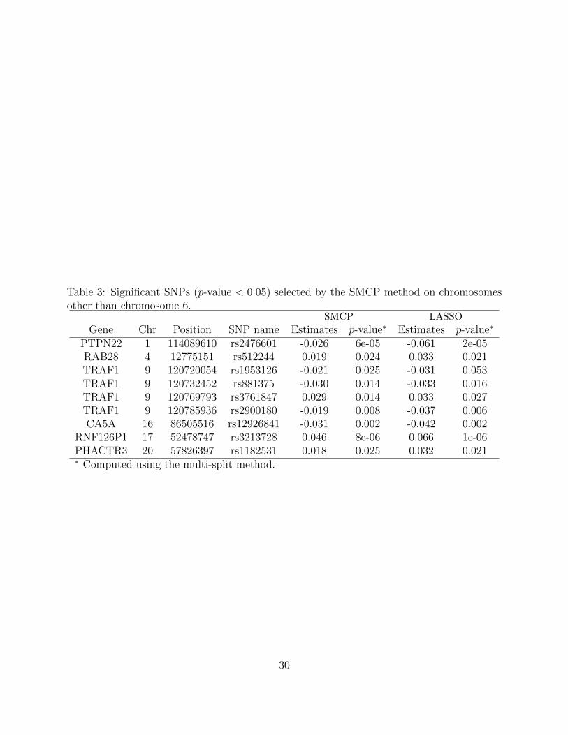
Table 3: Significant SNPs (p-value < 0.05) selected by the SMCP method on chromosomesother than chromosome 6.
SMCP LASSO
Gene Chr Position SNP name Estimates p-value∗ Estimates p-value∗
PTPN22 1 114089610 rs2476601 -0.026 6e-05 -0.061 2e-05RAB28 4 12775151 rs512244 0.019 0.024 0.033 0.021TRAF1 9 120720054 rs1953126 -0.021 0.025 -0.031 0.053TRAF1 9 120732452 rs881375 -0.030 0.014 -0.033 0.016TRAF1 9 120769793 rs3761847 0.029 0.014 0.033 0.027TRAF1 9 120785936 rs2900180 -0.019 0.008 -0.037 0.006CA5A 16 86505516 rs12926841 -0.031 0.002 -0.042 0.002
RNF126P1 17 52478747 rs3213728 0.046 8e-06 0.066 1e-06PHACTR3 20 57826397 rs1182531 0.018 0.025 0.032 0.021∗ Computed using the multi-split method.
30