accuracy of the lightning mapping array - ua hydrology...

Accuracy of the Lightning Mapping Array

Ronald J. Thomas,1 Paul R. Krehbiel,2 William Rison,1 Steven J. Hunyady,3

William P. Winn,3 Timothy Hamlin,2 and Jeremiah Harlin2

Received 16 January 2004; revised 26 April 2004; accepted 18 May 2004; published 29 July 2004.

[1] The location accuracy of the New Mexico Tech Lightning Mapping Array (LMA) hasbeen investigated experimentally using sounding balloon measurements, airplane tracks,and observations of distant storms. We have also developed simple geometric models forestimating the location uncertainty of sources both over and outside the network. Themodel results are found to be a good estimator of the observed errors and also agree withcovariance estimates of the location uncertainties obtained from the least squaressolution technique. Sources over the network are located with an uncertainty of 6–12 mrms in the horizontal and 20–30 m rms in the vertical. This corresponds well withthe uncertainties of the arrival time measurements, determined from the distribution ofchi-square values to be 40–50 ns rms.Outside the network the location uncertainties increasewith distance. The geometric model shows that the range and altitude errors increase as therange squared, r2,while the azimuthal error increases linearlywith r. For the 13 station, 70 kmdiameter network deployed during STEPS the range and height errors of distant sourceswere comparable to each other, while the azimuthal errors weremuch smaller. The differencein the range and azimuth errors causes distant storms to be elongated radially in plan views ofthe observations. The overall results are shown to agree well with hyperbolic formulationsof time of arrival measurements [e.g., Proctor, 1971]. Two appendices describe (1) thebasic operation of the LMAand the detailedmanner inwhich itsmeasurements are processedand (2) the effect of systematic errors on lightning observations. The latter provides analternative explanation for the systematic height errors found by Boccippio et al. [2001] indistant storm data from the Lightning Detection and Ranging system at Kennedy SpaceCenter. INDEX TERMS: 3304 Meteorology and Atmospheric Dynamics: Atmospheric electricity; 3324

Meteorology and Atmospheric Dynamics: Lightning; 3360 Meteorology and Atmospheric Dynamics: Remote

sensing; 3394 Meteorology and Atmospheric Dynamics: Instruments and techniques; 6969 Radio Science:

Remote sensing; KEYWORDS: lightning, thunderstorms, aircraft sparking, radio frequency tracking and location,

data telemetry

Citation: Thomas, R. J., P. R. Krehbiel, W. Rison, S. J. Hunyady, W. P. Winn, T. Hamlin, and J. Harlin (2004), Accuracy of the

Lightning Mapping Array, J. Geophys. Res., 109, D14207, doi:10.1029/2004JD004549.

1. Introduction

[2] The New Mexico Tech Lightning Mapping Array(LMA) locates the sources of impulsive radio frequencyradiation produced by lightning flashes in three spatialdimensions and time [Rison et al., 1999; Krehbiel et al.,2000]. It does so by accurately measuring the arrival times ofradiation events at a network of ground-based measurementstations spread over an area typically 60 km in diameter.The signals are received in an unused very high frequency(VHF) television band, usually channel 3 (60–66 MHz).The accuracy of the locations depends on the uncertainty ofthe arrival time measurements and on the number and

positions of the stations used to obtain each solution. Thearrival times are measured independently at each stationusing an accurate time base provided by a GPS receiver.In this paper we investigate the accuracy of the sourcelocations both experimentally and theoretically and showhow the experimentally observed errors are explained by thetiming uncertainties and array geometry. The results can beused to design and optimize an array that meets a given setof requirements.[3] The use of time of arrival (TOA) measurements in

lightning studies was pioneered by D. E. Proctor in SouthAfrica [e.g., Proctor, 1971, 1981; Proctor et al., 1988].Proctor utilized a network of five stations arrayed along twonearly perpendicular baselines to study the detailed break-down of individual lightning discharges. The network, inthe approximate form of a cross, was about 30 km in east–west (E–W) extent and 40 km in north–south (N–S)extent. The analog receiver outputs from each of theoutlying stations were telemetered to the central station,where they were recorded and manually processed to

JOURNAL OF GEOPHYSICAL RESEARCH, VOL. 109, D14207, doi:10.1029/2004JD004549, 2004

1Electrical Engineering Department, New Mexico Tech, Socorro, NewMexico, USA.

2Physics Department, New Mexico Tech, Socorro, New Mexico, USA.3Langmuir Laboratory, Geophysical Research Center, New Mexico

Tech, Socorro, New Mexico, USA.

Copyright 2004 by the American Geophysical Union.0148-0227/04/2004JD004549$09.00

D14207 1 of 34

identify the times of common events. The arrival timedifferences were analyzed using hyperbolic formulationsto obtain the source locations. In his initial paper on thesystem, Proctor [1971] discussed the geometric interpreta-tion of the solutions and the effect of the network geometryon the location accuracy. The TOA measurements weremade with 5 MHz bandwidth receivers at a center frequencyof 300 MHz and had estimated timing errors Dt of about70 ns rms. From this the horizontal location accuracy wasestimated by Proctor to be about cDt ’ 20 m for sourceswithin the boundaries of the network. Owing to the way inwhich the hyperbolic surfaces intersected, the vertical errorswere larger and were estimated to vary from 100 m up toseveral hundred meters or a kilometer, depending on thealtitude and horizontal location of the source relative to themeasurement stations.[4] Using Proctor’s approach, Lennon [1975] imple-

mented a seven station network for monitoring lightningover and around Kennedy Space Center (KSC), Florida.Called the Lightning Detection and Ranging (LDAR) sys-tem, the network consisted of an approximately circulararray of six measurement stations about 16 km in diameterconcentric with a central seventh station. Conceptually andfor processing purposes, the network was considered toconsist of two Y-shaped arrays, one upright and the otherupside down, each consisting of three outlying stations andthe central station. Logarithmically detected RF signalsfrom the outlying stations were telemetered in analog formto the central station, as in Proctor’s system, but were thendigitized with 50 ns time resolution and were automaticallyprocessed to obtain the lightning sources in real time. Thesystem typically located several tens of events per lightningflash [e.g., Krehbiel, 1981]. In addition to being importantfor operations at Kennedy Space Center (KSC) and theCape Canaveral Air Force Station, the LDAR systemprovided valuable information on the storms during theThunderstorm Research International Program (TRIP 76–78) [e.g., Lhermitte and Krehbiel, 1979].[5] The accuracy of the LDAR system was studied by

Poehler [1977], who estimated the location uncertaintiesover the network from geometric dilution of precisionformulations for an ideal Y-shaped array and performedMonte Carlo simulations of the location accuracy outsidethe network. Assuming 20 ns rms timing errors, theresults indicated 7–11 m rms uncertainties in plan locationsover the network and an order of magnitude larger (72–100 m rms) errors in the vertical for sources at 8 kmaltitude. Outside the network the location uncertainties werefound to be much greater in range than in azimuth; thelocation uncertainties were considered to be acceptable to32 km range (500 m rms error in range and 250 m error inaltitude). Poehler confirmed the error results by analyzingthe scatter in an airplane track that (for then unknownreasons) was detected by the LDAR system and by analyzingsystem calibration data provided by spark generators locatedon the top of two buildings at KSC.[6] An improved, second-generation version of the

LDAR system was developed by Lennon and coworkersat Kennedy Space Center in the early 1990s [Maier et al.,1995]. Observations from the new LDAR systemwere studied statistically by Boccippio et al. [2001] for a19 month period during 1997–1998, including the two

summer convective seasons. The distribution of locatedlightning sources was determined as a function of heightand range out to 300 km distance from the network. Theareal density of sources was found to decrease exponentiallywith range, inconsistent with and more rapidly than wouldbe predicted by signal detectability (i.e., signal-to-noiseratio) considerations. Also, the height of the maximumlightning activity was found to increase systematically withrange, from a physically correct value of 9 km altitude overand close to the network to a physically incorrect valueof about 20 km altitude at 300 km range. The authorssummarized results from other TOA systems, includingearly results from the Lightning Mapping Array, whichindicated that the range errors outside the network increasedas the range squared (r2). From a Monte Carlo analysis oftheir analytic formulations, Boccippio et al. inferred that thesystematic height increase with distance resulted from thesystem having unexpectedly large range errors at largedistances. The sources at large range were thought to bedominated by overranged sources in storms at intermediateranges, which would appear to be at higher altitudes.[7] The problem of retrieving source locations from TOA

measurements has also been studied by Koshak andSolakiewicz [1996] (hereinafter referred to as KS96) andby Koshak et al. [2004]. KS96 developed an alternativeformulation to the nonlinear hyperbolic equations used byProctor and Lennon for retrieving the source locations.Their formulation recast the TOA equations in a linear formand enabled solutions and error analyses to be obtainedanalytically. Koshak et al. [2004] applied the results ofKS96 to develop a more complete source retrieval algorithmand used it in a theoretical study of the errors in an LMAbeing operated in north Alabama [e.g., Goodman, 2003].The retrieval algorithm is basically the same as that devel-oped to process LMA observations (Appendix A).[8] In the present study we examine the accuracy of the

Lightning Mapping Array both experimentally and theoret-ically. We separate the problem into two regimes byinvestigating the location uncertainties first over or nearthe array and then outside the array. In each regime wedevelop simple geometric models which describe the basicway in which the measurements determine the sourcelocations and give the functional behavior of the locationaccuracies. The model results are compared with experi-mentally observed errors from a sounding balloon and fromaircraft tracks and with the results of linearized covarianceanalyses from the solution technique. The results confirmand extend many of the findings of the previous studies,correct some other findings, and elaborate on severalpractical aspects of the observations. The models providesimple analytic formulations for the errors that are in goodagreement with the experimental results and show, forexample, why the range errors increase as r2. The effectof systematic errors is discussed in Appendix B, whichincludes an alternative explanation for the systematic heightincrease found by Boccippio et al. [2001] in the LDARobservations.[9] The data of this study were obtained while the LMA

was being operated in the Severe Thunderstorm Electrifi-cation and Precipitation Study (STEPS 2000) in northwest-ern Kansas and eastern Colorado [Lang et al., 2004; W. D.Rust et al., Inverted-polarity electrical structures in thunder-

D14207 THOMAS ET AL.: LMA ACCURACY

2 of 34

D14207

storms in the Severe Thunderstorm Electrification andPrecipitation Study (STEPS), submitted to AtmosphericResearch, 2003]. A brief description of the mapping systemand of the processing approach used to obtain the sourcelocations is given in Appendix A.

2. Lightning Example

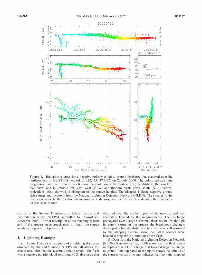
[10] Figure 1 shows an example of a lightning dischargeobserved by the LMA during STEPS that illustrates thespatial resolution that the system is able to obtain. The flashwas a negative polarity cloud-to-ground (CG) discharge that

occurred over the northern part of the network and wasaccurately located by the measurements. The dischargepropagated over a large horizontal distance (40 km) throughits parent storm; in the process the breakdown channelsdeveloped a fine dendritic structure that was well resolvedby the mapping system. More than 5000 sources werelocated during the 2 s duration of the flash.[11] Data from the National Lightning Detection Network

(NLDN) [Cummins et al., 1998] show that the flash was amultiple-stroke CG discharge that lowered negative chargeto ground. The top panel of the figure shows the altitude ofthe sources versus time and indicates that the initial stepped

Figure 1. Radiation sources for a negative polarity cloud-to-ground discharge that occurred over thenorthern end of the STEPS network at 2223:35–37 UTC on 22 July 2000. The colors indicate timeprogression, and the different panels show the evolution of the flash in (top) height-time, (bottom left)plan view, and in (middle left) east–west (E–W) and (bottom right) north–south (N–S) verticalprojections. Also shown is a histogram of the source heights. The triangles indicate negative groundstrike times and locations from the National Lightning Detection Network (NLDN). The squares in theplan view indicate the location of measurement stations, and the vertical line denotes the Colorado-Kansas state border.


3 of 34

D14207

leader initiated between 8 and 9 km altitude, after about50 ms of preliminary breakdown, and required about 60 msto reach ground. (All altitudes in this study are GPSaltitudes, which are within about 10 m of mean sea level.)The NLDN observed the initial stroke and two subsequentstrokes at the times and locations indicated by the trianglesin the figure. Similar but less extensive horizontal flasheswere studied by Krehbiel et al. [1979], who showed thatsources of charge for successive strokes developed horizon-tally away from the flash initiation region.[12] The colors of the sources indicate time progression;

when viewed in time animation, the flash steadily devel-oped outward along the various branches, with multiplebranches extending simultaneously in time. The TOAtechnique and the processing are readily able to sort outthe resulting ‘‘back and forth’’ activity of the differentbranches. The subsequent strokes were initiated by fast dartleaders, for which only a few sources were located by themapping system. Such leaders typically last only a fewhundred microseconds and therefore are not well sampledby the 80 or 100 ms measurement windows with which theLMA usually operates. The lack of a second stepped leaderin the LMA data indicates that all strokes went down asingle channel to ground. A final breakdown event at 37.4 snear the end of the flash (shown in red) traversed thecomplete horizontal extent of the discharge and progresseddownward toward ground. It would appear to have initiatedanother stroke but most likely was an attempted leader ofthe type reported by Shao et al. [1995].[13] Figure 2 shows an expanded view of a 10-km-wide

section of the channels to indicate their detailed structure.The dots used in Figure 2 have a size of about 100 m,which, as will be seen, is comparable to or larger than the

plan location accuracy with which the system is able tolocate impulsive events. While many of the individualchannels are well resolved, the lateral spread of the sourcesalong the channels is comparable to or slightly larger thanthe dot sizes. This is indicative of unresolved additionalstructure in the breakdown channels and/or of locationuncertainties introduced by the sources not being completelyimpulsive. The late-stage breakdown (red sources) retracedthe earlier channels with good accuracy.[14] In addition to fine-scale ‘‘noisiness’’ in the channel

structure, a relatively small number of sources have kilo-meter or larger errors. These are seen in the verticalprojection panels of Figure 1 as outlying points both aboveand below the horizontal channels and alongside the chan-nel to ground. The outlying points can be identified as beingincorrect because of the limited vertical extent of the in-cloud breakdown and the relatively localized and un-branched initial leader channel. As discussed in section 3,the outlying points result from the occasional incorporationof random local noise events at a station into the set of datavalues used to obtain the solutions. For analyses of indi-vidual flashes, outlying points can be removed by manuallyediting the observations and/or by tightening goodness of fitrestrictions. Sections 3–6 present detailed analyses of theaccuracy of the mapping system for sources over andoutside the network.

3. Location Accuracy Over the Network

[15] We first investigate the location errors for sourcesover or near the network of measurement stations. Theerrors were determined experimentally by using the map-ping array to locate a sounding balloon that carried a GPSreceiver and a VHF transmitter. The results are found to bein good agreement with error estimates from a simplegeometric model and with linearized estimates of thelocation uncertainties obtained from the least squares solu-tion technique.[16] Several experiments were conducted during STEPS

in which the LMA was used to track sounding balloonscarrying a pulsed VHF transmitter. The transmitter broad-cast short-duration (125 ns) pulses of 63 MHz radiation,which were located by the LMA as the balloon ascended.One sounding balloon carried a handheld GPS receiver(Magellan GPS 310) that determined the balloon locationevery second. A serial bit stream containing the GPSlocation data was transmitted to the ground by modulatingthe time between transmitted pulses. The pulse transmissionrate averaged about 140 s�1, and more than 500,000 pulseswere located during the �1 hour flight. Details of themodulation and decoding technique are presented inAppendix D.[17] Figure 3 shows the flight path of the GPS sounding

balloon as determined by the mapping system. Figure 3 alsoshows the network of measurement stations used duringSTEPS. Thirteen stations were deployed over an area about80 km in E–W extent and 60 km in N–S extent. Theballoon was launched near the center of the network andascended to about 24 km altitude. In the process it driftedeastward to slightly beyond the network’s northeasternedge. The rubber balloon burst at 24 km altitude, afterwhich the instrument rapidly descended to about 19 km

Figure 2. Expanded plan view of the dendritic structure ofthe flash of Figure 1, showing the level of detail in theobservations and the accuracy with which several break-down events near the end of the flash retrace the earlierchannels (red sources).


4 of 34

D14207

altitude before the transmitter ceased functioning. The flighttook place between 1800 and 1900 LT on 9 July in clear-weather conditions with no nearby storms.[18] Figure 4 shows successively expanded views of the

LMA balloon track (red dots) and the onboard GPSlocations (central black line). The data are shown in E–W vertical projection. The expanded view in the lowerright panel shows that most of the LMA source locationswere within ±50 m of the GPS track. The location differ-ences were determined by fitting the GPS track with asequence of third-order polynomials over consecutive 10 stime intervals. The GPS locations were then interpolated tothe time of each transmitted pulse, and the mean and

standard deviation of the difference values were evaluatedover each kilometer interval along the track. The meandifference in each interval was typically about 15 m andcould have resulted from uncertainty in the onboard GPSlocation itself. Histograms of the difference values showthat >99% of the locations were normally distributed aboutthe mean, with standard deviations between 10 and 30 m(an example is shown in Figure 8). About 1% of thelocated sources exhibited larger errors, up to severalkilometers, and correspond to the outlying points inFigure 4. The periodic fluctuations of the source heightsseen in the lower right panel are due to small systematictiming errors, discussed in Appendix B. As required by

Figure 3. Trajectory of the balloon flight as located by the Lightning Mapping Array (LMA) relative tothe network of 13 mapping stations (green squares). The (lower left) plan view and (middle right) altitudeprojections show that the balloon drifted eastward as it ascended, crossing from Colorado into Kansasshortly after launch. The balloon rose for about an hour, encountering easterly winds above 19 kmaltitude and (top) bursting at 23.5 km. Only events located by at least eight stations are displayed. Thecoordinate origin was near the center of the network at the location of a lightning interferometer andelectric field change sensor.


5 of 34

D14207

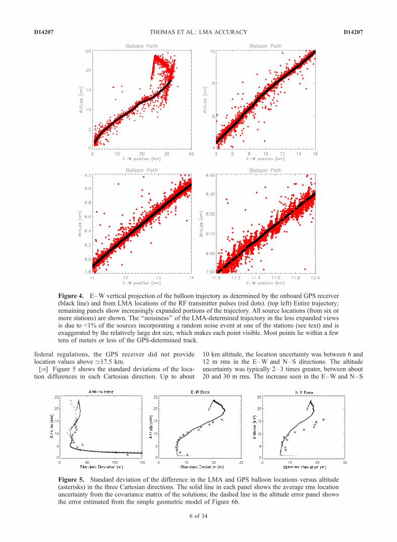
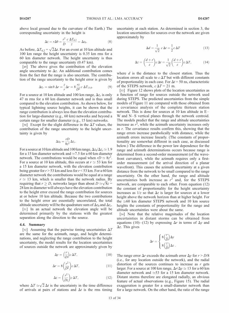
federal regulations, the GPS receiver did not providelocation values above ’17.5 km.[19] Figure 5 shows the standard deviations of the loca-

tion differences in each Cartesian direction. Up to about

10 km altitude, the location uncertainty was between 6 and12 m rms in the E–W and N–S directions. The altitudeuncertainty was typically 2–3 times greater, between about20 and 30 m rms. The increase seen in the E–W and N–S

Figure 4. E–W vertical projection of the balloon trajectory as determined by the onboard GPS receiver(black line) and from LMA locations of the RF transmitter pulses (red dots). (top left) Entire trajectory;remaining panels show increasingly expanded portions of the trajectory. All source locations (from six ormore stations) are shown. The ‘‘noisiness’’ of the LMA-determined trajectory in the less expanded viewsis due to <1% of the sources incorporating a random noise event at one of the stations (see text) and isexaggerated by the relatively large dot size, which makes each point visible. Most points lie within a fewtens of meters or less of the GPS-determined track.

Figure 5. Standard deviation of the difference in the LMA and GPS balloon locations versus altitude(asterisks) in the three Cartesian directions. The solid line in each panel shows the average rms locationuncertainty from the covariance matrix of the solutions; the dashed line in the altitude error panel showsthe error estimated from the simple geometric model of Figure 6b.


6 of 34

D14207

errors above 7 km altitude occurred as the balloon driftedtoward and outside the northeastern boundary of thenetwork. Below about 3 km altitude (2 km above groundlevel) the altitude uncertainty rapidly increased to more than100 m rms.[20] The expected values of the location errors can be

estimated from simple geometric considerations, as indicatedin Figure 6. The horizontal uncertainty is determinedprimarily by distant stations (Figure 6a). The plan locationis constrained by the measurements at each station to bewithin a radial distance Dd ’ ±cDt from its actual location,where Dt is the rms timing uncertainty. Measurements indifferent directions from the source therefore restrict theplan location to an approximate circle of diameter 2Dd =2cDt. For an assumed error Dt ’ 40 ns, Dd ’ 12 m. Thissimple model, also used by Proctor [1971] and Poehler[1977], slightly overestimates the measured errors, whichare between 6 and 12 m rms (Figure 5).[21] The above model represents the solution as the

intersection of circles concentric with each station andimplicitly assumes that the source time is known. The modelcan be refined by noting that although the source time is notknown, when the source is situated along the baselinebetween two measurement stations, the location accuracy

corresponds to half the uncertainty in the difference in arrivaltimes. Because the errors are uncorrelated at the two stations,the rms error in the arrival time difference is

ffiffiffi2

pDt. Thus

Dd = (1/2) cffiffiffi2

pDt = (1/

ffiffiffi2

p) cDt = 8.5 m. Since sources over

the central part of the network are effectively surrounded,the refined result is the appropriate one and is in goodagreement with the observed errors. To the extent thatmultiple sets of stations are involved in the horizontallocations, the error can be somewhat smaller, as observed.[22] The altitude of the source is determined primarily by

the arrival time at the closest station (Figure 6b). Thealtitude has the smallest uncertainty when the source isdirectly above a station and increases for sources that aredisplaced horizontally away from the station. The uncer-tainty in the radial distance r from the close station is thesame as the horizontal uncertainty for distant stations,namely ±cDt. From the geometry of the resulting parallel-ogram the rms error in the height z is given by

Dz ’ c Dtd þ r

z

� �; ð1Þ

where d is the horizontal distance of the source from theclose station. When the source is directly above the station,d = 0 and r = z, giving that Dz ’ cDt, as expected. For thegeneral case in which d 6¼ 0 the vertical uncertainty isgreater than the horizontal by a factor of Dz/Dd ’ (d + r)/z >1. This is also seen in the experimental results. For sourceheights equal to half the distance between stations (in ourcase, z = 5–10 km above ground level), dmax ’ z andr ’

ffiffiffi2

pz, so the ratio of the vertical to horizontal errors is

Dz/Dd ’ 1 +ffiffiffi2

p= 2.4. This is in good agreement with the

observations that the vertical errors were 2–3 timesthe horizontal errors. For z small compared to d and r thevertical error becomes increasingly large.[23] The estimate of the height uncertainty from

equation (1) is shown by the dashed curve in the left panelof Figure 5, assuming Dt = 40 ns. The curve was determinedusing the actual distance of the balloon from the neareststation. The separate minima at 5 km and 10 km altitudecorrespond to the balloon passing nearly over two stationsas it ascended. The minima correspond to relative maximain the measured errors, however, because of signal dropoutswhen the balloon was above or nearly above a station. (Thedropouts are more clearly evident in the data of Figure 7,discussed below, and are due to the vertical dipolar antennasof both the transmitting and receiving antennas pointingtoward each other, i.e., being close to or in the nulls oftheir antenna patterns.) The model results are otherwise ingood agreement with the measured errors.[24] The geometric interpretations of the simple error

models are compared with those obtained from the hyper-bolic approach used by Proctor [1971] in section 6 of thispaper.[25] The location uncertainties can also be determined

from an error analysis of the equations used to obtain thesolutions. As discussed in Appendix A, the source locationsare obtained using a standard iterative least squares proce-dure (the Levenburg-Marquardt algorithm) to solve thenonlinear TOA equations [e.g., Bevington, 1969]. Thealgorithm linearizes the equations around successive trialsolutions, and the linearization for the final solution gives a

Figure 6. Simple geometric models for the locationuncertainty of sources over the network. (a) Plan viewindicating how distant stations constrain the plan location toan approximate circle of radius Dd = cDt. (b) Vertical crosssection indicating how a close station enables the altitude ofthe source to be determined.


7 of 34

D14207

covariance matrix describing the location uncertainties.The linearized error estimates are a good approximation tothe actual uncertainties if the measurement errors aresufficiently small. The validity of the covariance errorestimates was checked using a Monte Carlo simulation,which showed that the uncertainties are well approximatedby the linearized equations and that normally distributedtiming uncertainties give normally distributed positionuncertainties. (Koshak et al. [2004] made a detailed com-parison of the linearized covariance error estimates withMonte Carlo simulations; they found that both approachesgave similar horizontal errors but that the linearizationapproximation gave slightly larger vertical errors than theMonte Carlo simulation for sources outside the network.)[26] The covariance-estimated errors for the balloon

measurements are shown by the solid curve in each of thepanels of Figure 5. The rms timing uncertainty was againassumed to be Dt = 40 ns, and the closest nine stations wereused for determining the covariances. The results are ingood agreement with the observations. The increase withaltitude of the measured E–W and N–S errors is due to theballoon drifting outside the northeast periphery of thenetwork. The increase is well matched by the covarianceresults in the E–W direction but is underestimated in theN–S direction. The cause of the latter difference is notunderstood. The altitude uncertainties from the covarianceanalysis agree well both with the measured errors and withthe estimates from the simple geometric model.

[27] Figure 7 shows a scatter diagram of the covariance-estimated height uncertainty for each RF pulse during theballoon flight. In this case the covariance values correspondto the actual stations used to locate each event. The differentfamilies of curves correspond to different sets of stationsbeing used to locate the events, with the larger uncertaintiescorresponding to less favorable combinations or numbers ofstations. The missing solutions near 11 km altitude in theleftmost set of curves occurred while the balloon was abovethe northeast station and resulted from signal dropouts atthat station, discussed above. The leftmost family of co-variance values (constituting most of the points in the plot)are in good agreement with the measured values of Figure 5(left).[28] Figure 8 shows a histogram of the vertical location

errors for sources between 10 and 11 km altitude. Thecentral part of the distribution is well fit by a normaldistribution whose mean is 10 m and standard deviation is23 m. This corresponds to >99% of the data points andincludes most of the points in this altitude range fromFigure 7. The tails of the distribution are not well fittedby the normal distribution and reflect a relatively smallnumber of solutions having significantly larger errors, up to1 km or larger. These ‘‘bad’’ points most likely result fromthe inclusion of an incorrect TOA value (or values) in thedata used to obtain the solutions.[29] Incorrect TOA values are produced when the signal

of interest is overridden by randomly timed, larger-ampli-tude signals from local noise sources at one or morestations. Local noise signals are produced by corona fromnearby transformers and power lines (or in storm conditions,from elevated objects exposed to strong electric fields) and,at lower VHF frequencies, are always present in the datafrom each station. A variety of other man-made signalscan also contribute to local site noise. As discussed inAppendix A, only the strongest event in successive 100 or80 ms time windows has its time recorded; it is not

Figure 7. Covariance estimates of the altitude uncertaintyfor each transmitted pulse during the balloon flight. Theresults group into curves associated with different combina-tions of stations being used to locate the pulses. Sets ofcurves having larger uncertainty correspond to less favor-able sets of stations participating in the solution. Theblanked out sources around 11 km altitude in the leftmostset of curves resulted from signal dropouts as the balloonpassed directly above the northeast station (Figure 3).

Figure 8. Histogram of the difference between the LMAand GPS location values between 10 and 11 km altitude.The solid line shows a normal distribution fitted to the data;the distribution has a mean value of 10 m and a standarddeviation of 23 m and fits over 99% of the data points.


8 of 34

D14207

uncommon for a local noise signal to be stronger than andpreempt distant lightning signals in a given time window.[30] Almost all local noise events are rejected by the data

processing because only events with correlated sets ofarrival times at the different stations correspond to acommon source. To aid in the rejection, we require that aminimum of six stations participate in the solution for thefour unknowns (x, y, z, and t) of each event, providing atleast two redundant measurements (degrees of freedom) as acheck on the validity of the solution. However, local noiseevents are unavoidably incorporated into some solutions.This is also evidenced by the outlying points along theballoon trajectory in the different panels of Figure 4. Theoutlying points can be reduced by increasing the minimumnumber of stations required to participate in the solutions.Figure 3 shows only the sources located by eight stations,which eliminated all outlying points.[31] To test that the outlying locations were caused by the

incorporation of noise signals, we performed a six stationMonte Carlo simulation in which normally distributed errorswith a standard deviation of 70 ns were added to the arrivaltimes at the different stations of a simulated event. For onestation chosen at random, an additional error uniformlydistributed over ±7 ms was added. (The value of 7 mscorresponded to the time window of acceptance over whichthe data from a given station could be used in a solution.)Solutions were occasionally obtained that had goodness offit values low enough to be considered a valid solution (andtherefore would have been included in the data points ofFigures 7 and 8) but whose location was substantiallydisplaced from the correct one and therefore would havebeen in the ‘‘bad’’ point tail of the distribution in Figure 8.For simulated solutions having reasonable goodness of fitvalues it was not possible to identify which station contrib-uted the bad data point from the residues of the least squaresfit. Similarly, we have not been able to identify bad datapoints in nonsimulated solutions having reasonable good-ness of fit values.

3.1. Chi-Square Distributions

[32] Excluding bad data points, the above mentionedresults indicate that the effective timing errors of the LMAsystem were about 40 ns rms for the balloon soundingdata. The timing errors can be more precisely determinedby examining the goodness of fit values of the solutions.(The goodness of fit is given by the reduced chi-squarevalue cn

2 of the solution, discussed in Appendix A.) Inparticular, one can compare the distribution of reducedchi-square values for the solutions with the theoreticaldistributions. The theoretical distributions are given byBevington [1969] and assume the measurement errors areGaussian distributed.[33] Figure 9 shows the observed and theoretical distri-

butions of the reduced chi-square values. Separate compar-isons are made for different values of the number of degreesof freedom, i.e., for solutions obtained from differentnumbers of stations. The solutions were obtained assuminga nominal 70 ns rms timing error at each station, but the chi-square values are readily scaled to an rms error of any Dt bymultiplying by a factor (70 ns/Dt)2. The reduced chi-squarevalues shown in Figure 9 have been adjusted to correspondto an rms error Dt = 43 ns and are in good agreement with

the theoretical distributions. This refines the value of thetiming uncertainty and demonstrates that the timing errorsare Gaussian distributed.[34] The timing uncertainty is slightly larger when fewer

stations participated in the solutions than when morestations participated. For 10 station solutions (the mostnumerous) the best fit corresponds to Dt = 43 ns, whilefor six station solutions the best fit corresponds to Dt =48 ns. Assuming that the six station solutions correspondedto weaker signals on average, the increase in the timingerrors is likely caused by the receiver signal-to-noise ratiobeing smaller for weaker signals.[35] Figure 10 shows the same type of analysis for actual

lightning data. The timing error is slightly larger for thelightning signals and was about 50 ns rms. Again, the rmserror increases as the number of stations participating in thesolutions decreased, from about 46 ns for 10 stationsolutions to 53 ns for six station solutions. In contrast withthe balloon data, however, the number of located sourcesdoes not go to zero with increasing chi-square but hasa ‘‘tail’’ of approximately constant number density foradjusted chi-square values greater than about 2. The tailindicates the presence of non-Gaussian errors, for example,from the inclusion of local noise events as discussedin section 3 or from some lightning signals being non-impulsive, having their peak amplitudes at slightly differenttimes at the different stations.[36] Whereas Figure 9 shows that the balloon transmit-

ter pulses were most often located by 10 stations, thelightning events were most often located by only six orseven stations. Of 1.3 million events located during the10 min time interval of the lightning data, 60% werelocated by only six stations, 81% were located by six orseven stations, and 92% were located by eight stations orless. This behavior is typical and reflects the increase inthe number of lightning sources with decreasing power.From the study by Thomas et al. [2001], the number oflocated sources typically varies as 1/P, where P is theestimated source power. As the source power approachesthe network’s minimum detectable level, located eventswill tend to be detected by the minimum number ofstations.

3.2. Summary

[37] The effective timing errors of the LMA system arefound to be about 43 ns rms for the deterministic trans-mitter pulses (i.e., pulses having a well-defined shape) andabout 50 ns rms for lightning signals. The 50 ns uncer-tainty for lightning is found to vary somewhat with thenumber of stations participating in the solutions and alsofor different storms or time intervals but is representativeof the STEPS data. For sources between about 6 and12 km altitude over the central part of the network, thelocation accuracies are 6–12 m rms in horizontal positionand 20–30 m rms in the vertical. The location accuraciesare degraded somewhat for events over or outside theperiphery of the network.

4. Location Accuracy Outside the Network

[38] Outside the mapping network the location uncer-tainties increase with distance from the array. In this


9 of 34

D14207

section we present a simple geometric model that showsthe basic way a TOA network locates distant events. Themodel provides analytic formulations for the source loca-tions that enable the increase of the location uncertaintieswith distance to be expressed analytically as well. Themodel-predicted errors are verified by comparing themwith covariance results for the location uncertainties and,in section 5.1, with observations of aircraft tracks anddistant storms.[39] Consider a five station network in the form of a

cross- or plus-shaped array, as shown in Figure 11a. Thesource to be located is assumed to be situated a relativelylarge distance to the right (east) of the network, approxi-mately off the end of the E–W (x) baseline. Conceptually,the network is considered to consist of stations S2 and S4along the x baseline, called the longitudinal baseline, andstations S0, S1, and S3 along the N–S or y baseline, calledthe transverse baseline. For simplicity the network isassumed to have the same extent D in both the E–W andN–S directions. For an actual network, D would correspondto the network diameter.

[40] The network locates distant events by determiningthe range, azimuth, and elevation angles of a source fromthe center of the array. In other words, the measurementsdetermine the spherical coordinates (r, q, f) of the sourcerelative to the network. Referring to Figure 11, the radiusr of a source (also referred to as the slant range) isdetermined from the curvature of the wavefront, primar-ily as it arrives at the transverse stations (S0, S1, S3).The azimuth angle f is determined primarily from thedifference in the arrival times at the two ends of thetransverse baseline (S1 and S3). The elevation angle q isdetermined primarily by the arrival times at the longitu-dinal stations (S2 and S4). To keep the formulationssimple, no attempt is made to incorporate redundantmeasurements into the model; the redundancies slightlyreduce the timing uncertainties but do not otherwiseaffect the basic results.[41] The conceptual array is essentially the same as the

five station network used by Proctor [1971]. Networks withgreater redundancy consist of 7 to 10 or more stationsdeployed over an approximately circular area so that there

Figure 9. Distribution of reduced chi-square (cn2) values during the balloon sounding for different

number of degrees of freedom n = N � 4. The cn2 values have been adjusted to correspond to an rms

timing error Dtrms = 43 ns, which gives good agreement with the theoretical distribution (solid lines). Theeffective timing uncertainty varied slightly with the number of stations N that participated in thesolutions, ranging from 43 ns for ten station solutions (the most numerous) to 48 ns for six stationsolutions.


10 of 34

D14207

will always tend to be stations located transverse to andalong the arrival direction.

4.1. Azimuthal Position

[42] For determining the azimuthal position of the source,one can assume to first order that the wavefront fromthe distant source is planar. Referring to Figure 11b, theazimuth angle f is determined by the arrival times at thetwo ends of the transverse baseline, namely at stations S1and S3. From the right triangle in the figure, one has that

D sinf ¼ c T3;1; ð2Þ

where T3,1 = T3 � T1 is the difference in the arrival times atS3 and S1. For small f the rms uncertainty in the azimuthangle is related to the rms uncertainty in the arrival timedifference T3,1 by Df = (1/D)cDT3,1. The resultinguncertainty in the y direction is therefore

Dy ¼ r Df ¼ r

D

� �c DT3;1: ð3Þ

For equal timing uncertainties Dt at each station the rmsuncertainty DT3,1 =

ffiffiffi2

pDt. For Dt = 50 ns, cDT3,1 = 21 m.

At a range of 100 km the azimuth uncertainty is 35 m rmsfor a 60 km diameter network typical of the LMA. Theazimuth position is therefore well determined.[43] In an actual network the azimuth angle will be found

from the difference of the arrival times at a number of pairsof stations. However, the accuracy of f will be determinedprimarily by stations having the greatest separation trans-verse to the incident signal.

4.2. Range Determination

[44] The range is obtained from the curvature of thewavefront reaching the network (Figure 11c). Closerevents will have greater curvature; more distant eventswill have less curvature. To determine the curvature, wecan assume to first order that the source lies on or abovethe x axis so that the wavefront reaches S1 and S3 at thesame time. In addition, S0 is assumed to be halfwaybetween S1 and S3. The difference T13,0 between thearrival time at S1 and S3 and at S0 is a measure of thecurvature and thus of the distance to the source.

Figure 10. Same as Figure 9, except for 10 min of lightning data over the network on 11 June 2000. Thetiming uncertainty was slightly larger than for the deterministic balloon pulses, having an average valueDtrms = 50 ns and varying from 53 ns for six station solutions, which are the most numerous for lightningsources, to 46 ns for ten station solutions. In addition, the distributions have an enhanced ‘‘tail’’ at largerchi-square values. The exact timing uncertainties vary somewhat from storm to storm and during a storm.


11 of 34

D14207

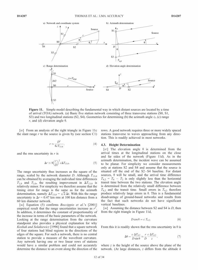
[45] From an analysis of the right triangle in Figure 11cthe slant range r to the source is given by (see section C1)

r ’ D2

8cT13;0; ð4Þ

and the rms uncertainty in r is

Dr ’ 8r

D

� �2

cDT13;0: ð5Þ

The range uncertainty thus increases as the square of therange, scaled by the network diameter D. Although T13,0can be obtained by averaging the individual time differencesT1,0 and T3,0, the resulting improvement in DT13,0 isrelatively minor. For simplicity we therefore assume that thetiming error for range is the same as for the azimuthdetermination, namely DT13,0 =

ffiffiffi2

pDt. With this the range

uncertainty is Dr = 0.47 km rms at 100 km distance from a60 km diameter network.[46] Equation (5) confirms Boccippio et al.’s [2001]

empirical result that the range uncertainties increase as r2.In addition, it determines the constant of proportionality ofthe increase in terms of the basic parameters of the network.Looking at the range determination from the curvaturestandpoint also provides a physical explanation for whyKoshak and Solakiewicz [1996] found that a square networkof four stations had blind regions in the directions of theedges of the square. For such a network, there is no centralstation to provide a measure of the wavefront curvature.Any network having one or two linear rows of stationswould have a similar problem and could not accuratelydetermine the distance to an event along the direction of the

rows. A good network requires three or more widely spacedstations transverse to waves approaching from any direc-tion. This is readily achieved in most networks.

4.3. Height Determination

[47] The elevation angle q is determined from thearrival times at the longitudinal stations on the closeand far sides of the network (Figure 11d). As in theazimuth determination, the incident wave can be assumedto be planar. For simplicity we consider measurementsonly at stations S2 and S4 and assume that the source issituated off the end of the S2–S4 baseline. For distantsources, q will be small, and the arrival time differenceT4,2 = T4 � T2 is only slightly less than the horizontaltransit time between the two stations. The elevation angleis determined from the relatively small difference betweenT4,2 and the transit time. Small errors in T4,2 thereforeproduce relatively large errors in q. This is a fundamentaldisadvantage of ground-based networks and results fromthe fact that such networks do not have significantvertical baselines.[48] Assuming the distance between S2 and S4 is D, then

from the right triangle in Figure 11d,

D cos q ¼ c T4;2: ð6Þ

From this it is readily shown that the rms uncertainty in q is

Dq ¼ c DT4;2

D sin q’ r

D

c DT4;2

z; ð7Þ

where z is the height of the source above the plane of thenetwork. (At large distances, z differs from the altitude h

Figure 11. Simple model describing the fundamental way in which distant sources are located by a timeof arrival (TOA) network. (a) Basic five station network consisting of three transverse stations (S0, S1,S3) and two longitudinal stations (S2, S4). Geometries for determining (b) the azimuth angle f, (c) ranger, and (d) elevation angle q.


12 of 34

D14207

above local ground due to the curvature of the Earth.) Thecorresponding uncertainty in the height is

Dz ¼ rDq ¼ r2

D

c DT4;2

z¼ Dzq: ð8Þ

As before, DT4,2 =ffiffiffi2

pDt. For an event at 10 km altitude and

100 km range the height uncertainty is 0.35 km rms for a60 km diameter network. The height uncertainty is thuscomparable to the range uncertainty (0.47 km).[49] The above gives the contribution of the elevation

angle uncertainty to Dz. An additional contribution comesfrom the fact that the range is also uncertain. The contribu-tion of the range uncertainty to the height error is given by

Dzr ¼ sin q Dr ¼ z

rDr ¼ 8

rz

D2c DT13;0: ð9Þ

For a source at 10 km altitude and 100 km range, Dzr is only47 m rms for a 60 km diameter network and is thus smallcompared to the elevation contribution. As shown below, fortypical lightning source heights, it can be shown that therange contribution is always less than the elevation contribu-tion for large-diameter (e.g., 60 km) networks and beyond acertain range for smaller diameter (e.g., 15 km) networks.[50] Except for the slight difference in the DT values, the

contribution of the range uncertainty to the height uncer-tainty is given by

Dzq ¼rD

8z2Dzr:

For a source at 10 kmaltitude and 100km range,Dzq/Dzr’1.9for a 15 km diameter network and’7.5 for a 60 km diameternetwork. The contributions would be equal when rD ’ 8z2.For a source at 10 km altitude, this occurs at r ’ 53 km fora 15 km diameter network, with the elevation contributionbeing greater for r > 53 km and less for r < 53 km. For a 60 kmdiameter network the contributions would be equal at a ranger ’ 13 km, which is smaller than the network radius. Byrequiring that r D, networks larger than about D ’

ffiffiffi8

pz =

28 km in diameter will always have the elevation contributionto the height error exceed the range contribution for sourcesat or below 10 km altitude. Because the two contributionsto the height error are essentially uncorrelated, the totalaltitude uncertainty will be the quadrature sum ofDzq andDzr.[51] In an actual network the elevation angle will be

determined primarily by the stations with the greatestseparation along the direction to the source.

4.4. Summary

[52] Assuming that the pairwise timing uncertainties DTare the same for the azimuth, range, and height determi-nations, and neglecting the range contribution to the heightuncertainty, the model results for the location uncertaintiesof sources outside the network are approximately given by

Dy ¼ r

D

� �cDT ; ð10Þ

Dr ¼ 8r2

D2

� �cDT ; ð11Þ

Dz ¼ r2

Dz

� �cDT ; ð12Þ

where DT ’ffiffiffi2

pDt is the uncertainty in the time difference

of arrivals at pairs of stations and Dt is the rms timing

uncertainty at each station. As determined in section 3, thelocation uncertainties for sources over the network are givenapproximately by

Dd ¼ 1ffiffiffi2

p cDt ¼ 1

2cDT ð13Þ

Dz ¼ d þ r

z

� �cDt ¼ 1ffiffiffi

2p d þ r

z

� �cDT ; ð14Þ

where d is the distance to the closest station. Thus thelocation errors all scale to cDT but with different constantsof proportionality in each case. For Dt = 50 ns, characteristicof the STEPS network, cDT = 21 m.[53] Figure 12 shows plots of the location uncertainties as

a function of range for sources outside the network usedduring STEPS. The predicted uncertainties from the simplemodels of Figure 11 are compared with those obtained froma covariance analysis of the complete thirteen stationnetwork. This is done for sources at 10 km altitude in E–W and N–S vertical planes through the network centroid.The models predict that the range and altitude uncertaintiesincrease as r2, while the azimuth uncertainty increases onlyas r. The covariance results confirm this, showing that therange errors increase parabolically with distance, while theazimuth errors increase linearly. (The constants of propor-tionality are somewhat different in each case, as discussedbelow.) The difference in the power law dependence for therange and azimuth determinations occurs because range isdetermined from a second-order measurement (of the wave-front curvature), while the azimuth requires only a first-order measurement (of the arrival direction of a planarwavefront). This causes the azimuth uncertainty at a givendistance from the network to be small compared to the rangeuncertainty. On the other hand, the range and altitudeuncertainties both increase as r2 and, for the STEPSnetwork, are comparable to each other. From equation (12)the constant of proportionality for the height uncertaintyincreases as 1/z so that Dz is larger for sources at a lowerheight above the network horizon than at higher height. Forthe ’60 km diameter STEPS network and 10 km sourceheights the constants of proportionality for the range andaltitude uncertainties were about the same.[54] Note that the relative magnitudes of the location

uncertainties in distant storms can be obtained fromequations (10)–(12) by expressing Dr in terms of Dy andDz. This gives

Dr ¼8

r

D

� �Dy

8z

D

� �Dz :

8><>:

The range error Dr exceeds the azimuth error Dy for r > D/8(i.e., for any location outside the network), and the radialdistortion of the sources continues to increase as r getslarger. For a source at 100 km range, Dr/Dy’ 13 for a 60 kmdiameter network and ’53 for a 15 km diameter network.Distant storms therefore are elongated radially, an obviousfeature of actual observations (e.g., Figure 15). The radialexaggeration is greater for a small-diameter network thanfor a large network. On the other hand, the ratio of the range


13 of 34

D14207

and height errors is 8z/D and depends on the source heightand not on range. The STEPS network was 60–80 km indiameter so that sources at z = 7.5–10 km altitude wouldhave approximately equal range and height uncertainties.[55] The STEPS network had a larger extent in the E–

W direction than in the N–S direction, with the N–Sextent being 57.2 km and the E–W extent being 76.6 km.Since the range and azimuth errors depend on the trans-verse extent, while the altitude error depends on thelongitudinal extent, the range and azimuth uncertaintiesin Figure 12 are greater for sources in the E–W plane(black) than for sources in the N–S plane (red). Theinverse is true for the altitude uncertainty. In all casesthe covariance errors are less than those predicted by thesimple model, assuming that D corresponds to the physicalextent of the network in the appropriate direction. Thisreflects the effect of averaging the results of a number ofbaselines when data from all stations are used to locate anevent. Stated another way, fully overdetermined solutionscorrespond to an effective network diameter larger than thephysical diameter. By matching the model predictions tothe covariance results, the effective size of the thirteenstation network was D = 78 km in the N–S direction and100 km in the E–W direction. The effective dimensions of

the complete STEPS network were therefore 36% and31% greater than its physical dimensions. (Another inter-esting feature of the Figure 12 results is that the differencebetween the model- and covariance-predicted errors is lessfor the altitude determination than for the range andazimuth locations. This indicates that the altitude determi-nation is less affected by averaging and therefore that it isdetermined primarily by the closest and most distantstations of the network (or of the set of stations thatparticipate in a given solution).)[56] Rather than being located by all stations of a net-

work, radiation events are invariably located by only asubset of stations (e.g., Figures 9 and 10). This counteractsthe tendency of the network to be oversized by multiple-station averaging. The net effect is that the effectivediameter might be comparable to (or smaller than) theactual diameter, making the simple model estimates approx-imately correct when the actual diameter is assumed.

5. Further Comparison With ExperimentalObservations

[57] In this section we use observations of aircraft tracksand of distant storms to gain additional insights into the

Figure 12. (top right) Range, (bottom left) azimuth, and (bottom right) altitude uncertainties of (top left)the STEPS network for sources at 10 km altitude in E–W (black) and N–S (red) vertical planes throughthe network centroid. The plus symbols show the covariance error estimates for the complete 13 stationnetwork, assuming a timing uncertainty of 50 ns rms. The solid lines show the error estimates from thesimple model of Figure 11 for 50 ns timing error and network sizes D = 78 km and 57 km in the E–Wand N–S directions, respectively. The model-predicted errors are larger than the covariance values due toaveraging effects when all stations are assumed to participate in the solutions (see text). The contributionof the elevation angle and range uncertainties to the altitude error are shown separately in the altitudepanel. The approximate network centroid was determined by minimizing the azimuthal error for sourcesin the E–W and N–S directions and was at (x, y) = (�6, 0) km relative to the coordinate origin.


14 of 34

D14207

performance of the mapping network and to test the validityof the error models.

5.1. Aircraft Tracks

[58] On a number of occasions during STEPS the mappingarray located aircraft flying over or near the project area.Visual observations showed that the aircraft were detectedwhen ice crystal clouds (cirrus clouds or storm anvils) werepresent over or around the network. From this, it was evidentthat the LMAwas locating small sparks caused by collisionalcharging from the planes as they flew through the ice clouds.

That such charging occurs is well known [e.g., Gunn et al.,1946; Illingworth and Marsh, 1986; Jones, 1990]. Sparkinghas also been detected by the LDAR system from aircraftflying through cirrus clouds [e.g., Maier et al., 1995].Because airplanes fly along straight paths, the tracks canbe used to investigate the location uncertainties by measur-ing the scatter of the sources along the track. This approachwas used to determine the errors of the original LDARsystem, as discussed in section 1.[59] Figure 13 shows an example of an aircraft track

observed on 25 May 2000. Only 10 stations were operating

Figure 13. Aircraft track over Kansas and Colorado on 25 May 2000. The plane was flying from east towest at about 9 km altitude (29.5 left) and vectored between two electrically active storms. The airplanewas tracked by the LMA because it was flying through an ice crystal cloud downwind of the storms thatcaused it to become charged and give off a steady stream of small sparks. The plane was tracked for13 min over a 170 km distance and was presumably a commercial aircraft. Two other aircraft were moreweakly detected over the center and to the south of the mapping network. The squares indicate theoperational stations on this day; only sources located by seven or more stations are shown. The trianglesindicate the location of negative polarity ground discharges. The distance scales are in latitude andlongitude in the plan view and in kilometer units in the vertical projections.


15 of 34

D14207

on this day, which was the first day data were recordedduring STEPS. The airplane was flying from east to westdownwind of a line of thunderstorms in eastern Colorado.The speed (245 m s�1 or 550 mph) and altitude of thetrack are typical of a commercial airliner. As it flewwestward, the aircraft gradually ascended from 8.5 km to9.0 km altitude (28–29.5 left) and vectored through thegap between two thunderstorms. After passing between thestorms the track ended as the plane presumably emergedinto cloud-free air. More than 300,000 sparks were locatedover the 800 s (13 min) duration of the track. Two weakertracks are also seen in Figure 13, south of and over thecenter of the network.[60] Figure 14 shows the standard deviation of the

scatter about the mean track and compares the scatter withthe covariance estimates of the location uncertainties.Separate plots are shown for the E–W, N–S, and altitudeerrors. The standard deviation of the scatter (red plusses)was determined relative to a cubic spline fit to the trackand is smoothed by a 13 s (3.2 km) running average. Theblack dots indicate the covariance values for the individualevents, assuming 50 ns rms timing errors. As in Figure 7,the dots group into multiple sets of curves correspondingto different sets of stations being involved in the solutions.The average of the covariance results is shown by the setof green dots and should correspond to the observedscatter. The two are often in good agreement, but thescatter is sometimes larger than would be predicted by theaverage covariance value. The set of orange points atthe bottom of each plot is the covariance error if allstations contributed to the solutions and should representthe lower limit of the location uncertainty. This is indeedthe case: Some station combinations come close to achiev-ing the lower limit, and the measured scatter sometimesachieves it as well.[61] In the first half of the track the airplane flew toward,

over, and past the southern part of the network. During thistime the E–W error decreased from 200 m rms to almost10 m and then increased again (Figure 14 (top)). Theminimum error occurred at 320 s; at this time the airplanewas at x = �2 km, i.e., almost due south of the coordinateorigin near the center of the network. (The minimumtransverse error location provides a means of defining thecentroid of the network in a given direction. The covarianceanalyses of Figure 12 showed that when all stations wereincorporated into the calculations, the network centroid wasat x, y = (�6, 0) km relative to the coordinate origin. TheFigure 14 results for the 25 May airplane track indicate thatthe network centroid was at about (�2, 0) km for the10 stations that were operational on that day.) The E–Wscatter agreed well with the predicted covariance values upthrough the time of the minimum but became more erraticfor about 300 s afterward.[62] The N–S error (Figure 14 (middle)) had a

broader and shallower minimum at about 575 s as theairplane passed due west of the coordinate origin. Thecovariance minimum was only partially reflected inthe observed scatter, probably because the sparks wereweak and even dropped out during this time (shownlater in Figure 17).[63] The altitude uncertainty (Figure 14 (bottom))

showed two local minima as the airplane passed over

the southern edge of the network. The first minimum, atabout 200 s in Figure 14, occurred as the airplaneapproached station ‘‘J’’ on the southeast edge of thenetwork. The second minimum (at 400 s) occurred as theairplane passed over the southwestern station ‘‘G.’’The airplane passed within 14 km horizontal distance ofstation J and 2 km horizontal distance of G. The altitudescatter agreed reasonably well with the predicted covari-ance values while approaching and passing J but did notagree very well with the covariance values during theG overpass. Rather, during the G overpass the scatterexhibited large fluctuations and even had a relative max-imum at the time of the covariance minimum. The lattermay have been caused by decreases in the signal strengthas the plane passed close to the null of station G’sreceiving antenna. (The first minimum in the altitude erroralong the 25 May airplane track occurred not at the time ofclosest approach to Station J, which was at x = +12 km inFigure 13, but earlier, when the plane was at x ’ +25 km.At this time the plane was off the end of the baselinebetween J and the network centroid. From the results foraltitude determination (Figures 11d and 22b) the networkhad the greatest longitudinal (as opposed to transverse)extent at the time of the minimum altitude error. Thisis consistent with a visual inspection of the network inFigure 13 and with the position of the airplane at the time ofthe minimum.)[64] During the final part of the track, from 600 s on,

the observed scatter (red) and average covariance values(green) agreed well in each direction. The individualcovariance values for the E–W and N–S errors showeda bimodal distribution, with one of the modes givingclose to the optimal accuracy and the other mode havingerrors that were 2–5 times larger. The average covariancevalues and the scatter tracked the mode having the largererrors, indicating that most of the sparks during this timewere located by a less than optimal set (or sets) ofstations. The bimodal behavior was not present in thevertical errors, indicating that the bimodality resulted frominclusion or loss of stations along transverse (N–S)baselines.[65] Figures 15 and 16 show data for another track, in

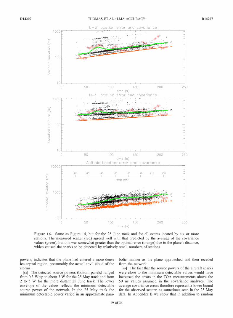
this case, for an aircraft flying from west to east at 10–11 km altitude (33–36 left), 85–120 km northeast ofthe network. Good agreement is obtained between theobserved scatter and the covariance error results. At100 km range, approximately in the middle of the track,the observed height scatter was between 400 and 500 mrms, slightly less than the average covariance result (greendots) and slightly greater than the optimal, all-stationcovariance prediction (of about 300 m). (At 100 km rangethe model-predicted uncertainty is about 370 m rms.) Therange errors are discussed later and also agree with themodel prediction.[66] Note that comparing Figures 14 and 16 for the

two aircraft tracks shows that while the optimal covari-ance-predicted uncertainties (orange dots) varied in asteady manner with time in both cases, the individualand average covariance values (black and green dots) aswell as the measured scatter of the source locationsfluctuated considerably during the 25 May track. Fur-ther examination of the observations indicates that this


16 of 34

D14207

resulted from 25 May being the first day data wererecorded during STEPS and from relatively large differ-ences in the threshold values for recording data at eachstation (Appendix A). The remaining stations of the

network and the communications links between stationswere still being set up on 25 May, and we had not yetstarted monitoring and adjusting or equalizing the thresh-old values. The performance difference is also seen in

Figure 14. Measured and predicted rms scatter of the radiation sources in three Cartesian directionsabout the mean of the 25 May aircraft track. Shown are the standard deviation of the observed scatter(red), the covariance error estimates for each individual spark (black dots, assuming 50 ns rms timinguncertainty), and a running average of the covariance values (green), for all events located by six or morestations. The orange dots show the covariance values if all 10 stations operational on that day had locatedthe events and represent the optimal error. The individual covariances group into sets of curvescorresponding to different combinations of stations, as in Figure 7, some of which approach the optimalerror. The predicted error in altitude shows two minima as the plane passed over or close to the twosouthern stations of the network. The x and y errors have minima due south and west of the networkcenter, respectively.


17 of 34

D14207

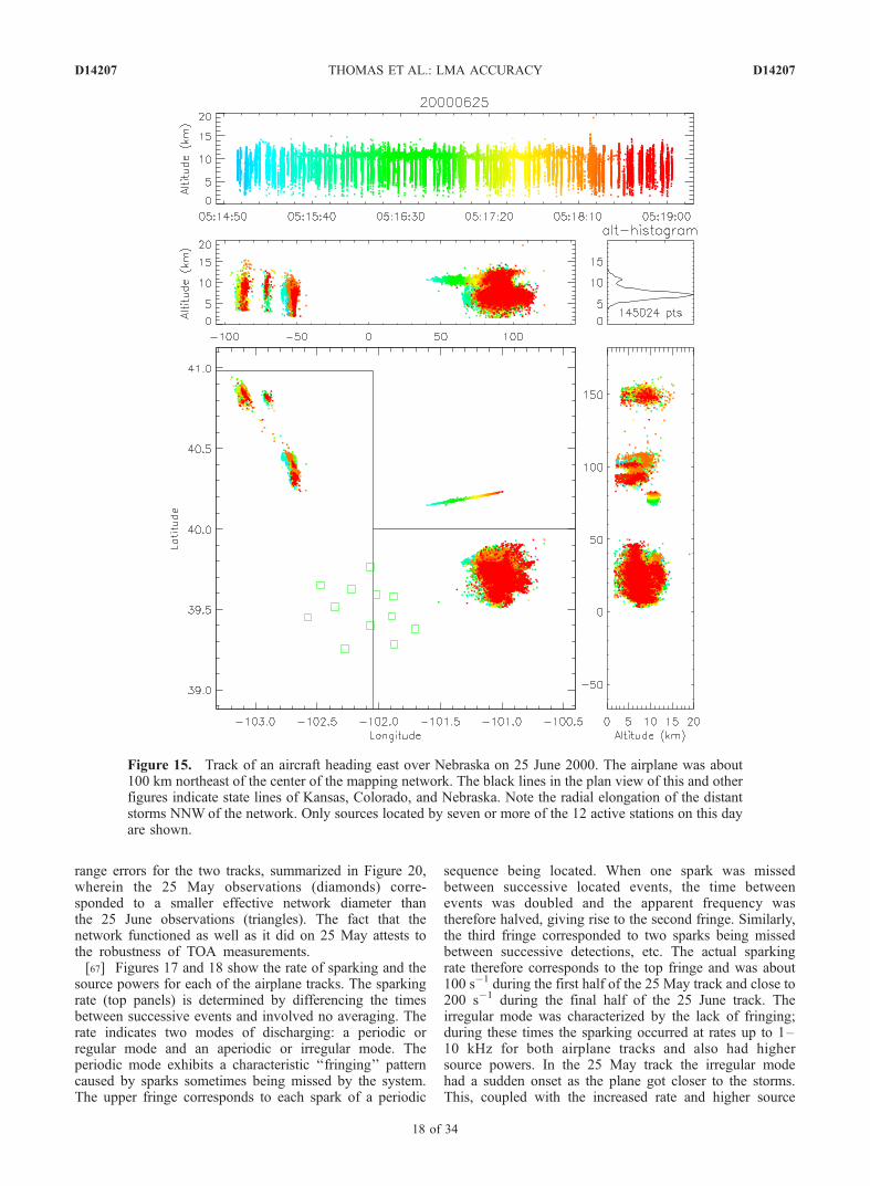
range errors for the two tracks, summarized in Figure 20,wherein the 25 May observations (diamonds) corre-sponded to a smaller effective network diameter thanthe 25 June observations (triangles). The fact that thenetwork functioned as well as it did on 25 May attests tothe robustness of TOA measurements.[67] Figures 17 and 18 show the rate of sparking and the

source powers for each of the airplane tracks. The sparkingrate (top panels) is determined by differencing the timesbetween successive events and involved no averaging. Therate indicates two modes of discharging: a periodic orregular mode and an aperiodic or irregular mode. Theperiodic mode exhibits a characteristic ‘‘fringing’’ patterncaused by sparks sometimes being missed by the system.The upper fringe corresponds to each spark of a periodic

sequence being located. When one spark was missedbetween successive located events, the time betweenevents was doubled and the apparent frequency wastherefore halved, giving rise to the second fringe. Similarly,the third fringe corresponded to two sparks being missedbetween successive detections, etc. The actual sparkingrate therefore corresponds to the top fringe and was about100 s�1 during the first half of the 25 May track and close to200 s�1 during the final half of the 25 June track. Theirregular mode was characterized by the lack of fringing;during these times the sparking occurred at rates up to 1–10 kHz for both airplane tracks and also had highersource powers. In the 25 May track the irregular modehad a sudden onset as the plane got closer to the storms.This, coupled with the increased rate and higher source

Figure 15. Track of an aircraft heading east over Nebraska on 25 June 2000. The airplane was about100 km northeast of the center of the mapping network. The black lines in the plan view of this and otherfigures indicate state lines of Kansas, Colorado, and Nebraska. Note the radial elongation of the distantstorms NNW of the network. Only sources located by seven or more of the 12 active stations on this dayare shown.


18 of 34

D14207

powers, indicates that the plane had entered a more denseice crystal region, presumably the actual anvil cloud of thestorms.[68] The detected source powers (bottom panels) ranged

from 0.3 W up to about 3 W for the 25 May track and from2 to 5 W for the more distant 25 June track. The lowerenvelope of the values reflects the minimum detectablesource power of the network. In the 25 May track theminimum detectable power varied in an approximate para-

bolic manner as the plane approached and then recededfrom the network.[69] The fact that the source powers of the aircraft sparks

were close to the minimum detectable values would haveincreased the errors in the TOA measurements above the50 ns values assumed in the covariance analyses. Theaverage covariance errors therefore represent a lower boundfor the observed scatter, as sometimes seen in the 25 Maydata. In Appendix B we show that in addition to random

Figure 16. Same as Figure 14, but for the 25 June track and for all events located by six or morestations. The measured scatter (red) agreed well with that predicted by the average of the covariancevalues (green), but this was somewhat greater than the optimal error (orange) due to the plane’s distance,which caused the sparks to be detected by relatively small numbers of stations.


19 of 34

D14207

errors, the airplane tracks had systematic sawtooth errors(Figure B1) that would have been partially responsible forthe fluctuations in the scatter about the mean track.

5.2. Distant Storm Observations

[70] Observations of distant localized storms provideanother way of estimating the range errors of the system.As seen in Figure 15, the extent of the lightning sourcesin distant storms is elongated radially relative to theirazimuthal extent. The radial spread of the sources can bemeasured relative to their azimuthal spread to estimate therange uncertainty. Similar measurements were used byBoccippio et al. [2001] to estimate the range error of theLDAR system.[71] An analysis of the radial and azimuthal variances of

the sources due both to the storm size itself and to thelocation errors (see section C2) shows that if the parentstorm itself is circular or nearly circular,

s2range ’ s2radial � s2transverse: ð15Þ

In other words, the inferred variance of the range errors,srange2 , is the measured radial variance of the sources, sradial

2 ,reduced by the measured azimuthal (transverse) variance ofthe storm, stransverse

2 .

[72] The result assumes that the azimuthal errors are smallcompared to the range errors, which is true for distantstorms. If it cannot be assumed that the storms are circular(which is often or even usually the case), the result willapply to averages over a number of storms:

hs2rangei ’ hs2radiali � hs2transversei : ð16Þ

The assumption here is that there is no systematicdependence of storm orientation in the set of storms beingaveraged.[73] Observations of 60 localized storms at ranges greater

than about 100 km have been used to estimate the rms rangeerror srange. Figure 19 shows the measured radial andtransverse spreads for each storm and the correspondingrange error from equation (15). Seven out of 20 stormsbetween 100 and 170 km range had negative apparentvalues of srange; since this is impossible, the storms inquestion could not have had a circular shape. At thesedistances the model-predicted range error is <1.5 km rmsand does not significantly distort the storm so that noncir-cular shapes can easily dominate the results. Accordingly(and somewhat arbitrarily), we limited the analyses to the40 storms beyond 170 km range and used equation (16) toestimate srange. The averaging was done over eight groupsof four to six storms in each range bin, with the storms in

Figure 17. (top) Rate of detected sparks and (bottom)radiated source power as a function of time during the25 May airplane track. The fringing pattern in the rate plotresults from some sparks of a periodic sequence not beinglocated by the system (see text).

Figure 18. Same as Figure 17, except for the 25 Juneairplane track.


20 of 34

D14207

each group being in different directions from the network.The results are presented in section 5.3.

5.3. Summary of Range Errors

[74] Figure 20 summarizes the estimated range errors andcompares the results with the simple model predictions fordistant storms. The graph is presented in the same log-logform as Figure 6 of Boccippio et al. [2001] (hereinafterreferred to as B2001) for comparison with their results. Thestraight lines in the figure correspond to the r2 rangedependence predicted by the simple model. The bottomtwo lines show the model-predicted range errors fromequation (5) for network diameters D = 45 km and 70 kmand for 50 ns rms timing errors, representative of the STEPSnetwork. The estimated range errors from the distant stormanalyses are shown by the square symbols and the estimatederrors from the two aircraft tracks are shown by thediamond and triangle symbols. The data points typicallylie between the two lines, indicating that the effectivenetwork diameter was between 45 and 70 km. The effectivediameter corresponds to the transverse extent of the networkand is reduced from the actual diameter by the fact that mostradiation sources were located by only six or seven stationsof the thirteen station array. The distant 25 June airplanetrack (triangles) corresponded to the largest effective diam-eter of about 70 km. The slightly larger uncertainties and

smaller inferred network diameter for the 25 May airplanetrack (diamonds) likely resulted from the network not beingfully operational on that day.[75] The upper three lines and the plus symbols in

Figure 20 are from Figure 6 of B2001 and describe theinferred range errors for the 16-km-diameter LDAR networkat Kennedy Space Center. The dashed line is the rms errorinferred by B2001 from aircraft measurements presentedby Maier et al. [1995]. The aircraft data were obtained outto about 35 km range, mostly off scale to the left inFigure 20. B2001 characterized the range error by its rmsvalue at 100 km distance; extrapolated to this distance, therange error from the aircraft data was s100 = 3.6 km. (Forcomparison, s100 = 0.35 km and 0.84 km for 70 km and45 km effective diameters of the STEPS network, respec-tively.) Letting D = 16 km in equation (5), s100 = 3.6 kmgives DT13,0 = 38 ns for the rms timing error of the LDARsystem. (Maier et al. [1995] reported that the aircraft locationerrors were consistent with 50 ns rms timing uncertainty; therange errors inferred by B2001 refine this result.) Forcomparison, the equivalent timing uncertainty of the LMAfor deterministic transmitter pulses was Dt = 43 ns rms at a

Figure 19. (top) Standard deviation of the lightningsources in distant localized storms in the radial andtransverse directions and (bottom) the inferred rms radialrange error. The negative range errors at <175 km range arenot physically possible and indicate that the storms hadunequal transverse and radial extents.

Figure 20. Standard deviation of the range error versusrange outside the measurement network, showing themodel-estimated performance of 70 km and 45 km diameternetworks (two bottom lines), the errors estimated fromlocalized storms at distances >150 km from the networkcenter (open squares, representing averages over four or fivestorms grouped in range), and error estimates from theaircraft tracks of Figures 14 and 16 (diamonds and triangles,respectively). The top three lines and the data pointsdenoted by the plus symbols are from Boccippio et al.[2001] and describe the inferred performance of the LDARsystem at Kennedy Space Center (see text).


21 of 34

D14207

given station and DT =ffiffiffi2

pDt = 61 ns for time differences of

arrival. Because the LDAR system digitized all the signalsat the central station in exact time synchronization, it wouldbe expected to have smaller relative timing errors thanindependent digitizing of the LMA. Despite its relativelysmall size, the LDAR network provided reasonably accuraterange determinations out to at least 35 km range and, byextrapolation, to more than 100 km range.[76] At distances greater than about 70 km, however,

B2001 inferred that the range errors of the LDAR systemwere significantly larger than would be expected from theaircraft measurements. This was determined from the radialspread of sources in storms beyond 75 km range, indicatedby the plus symbols in Figure 20. B2001’s estimates did notattempt to account for storm size, however, and thereforeoverestimated the actual range errors by an unknownamount. The dotted lines in the upper part of Figure 20 arethe range errors that B2001 determined would be needed toexplain the systematic increase in the height of sources withdistance from the LDAR network. The range errors inferredfrom the analysis had s100 values of 22 and 28 km rms, afactor of 6–8 larger than expected from the aircraft measure-ments and somewhat larger than the distant storm values.From equation (4), in order to explain a s100 value of 22 km,the rms timing uncertainty would have had to increase by afactor of 6, to 230 ns rms. Alternatively, the transversediameter of the network would have had to be decreasedby a factor of

ffiffiffi6

p= 2.45 to an effective value of D = 6.5 km.

[77] Appendix B describes the effect of systematic errorsupon the location accuracy and performance of the LMA.This analysis provides a simpler explanation for the sys-tematic height errors of the LDAR data as being due torelatively small, systematic errors in the elevation angledetermination rather than to overly large range errors.

6. Comparison to Hyperbolic Geometry

[78] In this section we relate the simple geometric modelsof this study to the geometry of hyperbolic formulations forTOA measurements. The formulations themselves are de-scribed by Proctor [1971] and are not repeated here. Asdiscussed by Proctor and briefly described in Appendix A,the time differences of arrival (TDOA) at pairs of stationsconstrain the source to lie on hyperboloids of revolutionabout the baselines between pairs of stations. The three-dimensional location of the source is determined from theintersection of three or more such hyperboloids obtainedfrom four or more stations.[79] Figure 21a illustrates how stations locate the plan

position of a source over the network. A cross-shaped

network is used to do this. Four sets of hyperbolae areshown to indicate how the time differences of arrival atdifferent pairs of stations determine the source locationand the uncertainty in the location. For each station pair(e.g., 2–3), two hyperbolae are shown which indicate the

Figure 21. Manner in which the hyperbolae correspond-ing to arrival time differences at pairs of stations constrainthe location and accuracy of sources situated over or near aTOA network. The sets of hyperbolae for the differentstation pairs indicate the effect of timing uncertainties atthose stations on the location. For example, the ‘‘2–4’’hyperbolae denote the uncertainty in the location frommeasurements made at stations S2 and S4 (see text). Theinscribed parallelogram in Figure 21b is from the simplemodel of Figure 6b and assumes the same errors used togenerate the sets of hyperbolae.


22 of 34

D14207

effect of the uncertainty in the TDOA values at the stations.The magnitude of the errors is greatly exaggerated forpurposes of illustration. As can be seen, when the sourcehas stations in different directions, its location is constrainedto be in an enclosed region that is approximately circular.This is the fundamental basis of the horizontal error modelin Figure 6a for sources over the network. Hyperbolae areshown only for pairs of outlying stations (S1–S4) and notfor the central station.[80] Figure 21b illustrates how the hyperbolae associated

with the close station (S0) defines the altitude of the source,in comparison with the simple geometric model of Figure 6b.Three sets of hyperbolae are shown, corresponding to thetime differences of the ‘‘inner’’ station pairs (2–0 and 4–0)and the ‘‘outer’’ station pair (2–4). Examination of thehyperbolae shows that height is most constrained by theinner pair off to the side of the source, i.e., by the 4–0 pair.The 2–0 and 2–4 differences primarily restrict the hori-zontal position because the stations are on both sideof the source. The inscribed parallelogram is the simplemodelresult corresponding to the same timing errors; it providesa good estimate of the horizontal uncertainty (even thoughthe source is well above the plane of the network) and slightlyunderestimates the height uncertainty.[81] Figure 21c shows how the uncertainty of the plan

location increases for a source just outside the periphery ofthe network. The uncertainty has become primarily radialrelative to azimuthal uncertainty. The source still hasstations in opposite directions in the azimuthal directionbut not in the radial direction. The radial error was theprimary cause of the increased E–W and N–S errors seenduring the balloon flight as the balloon drifted outside thenetwork (Figure 5).[82] Figure 22 shows the hyperbolic geometries for

locating a source outside the network. As in the modelformulations of Figure 11 the source is assumed to be eastof the network to illustrate the effect of the transverse andlongitudinal stations in determining the location. The planview of Figure 22a shows how the hyperbolae associatedwith the transverse stations (S0, S1, S3) locate the sourceazimuth and range. The combination of the inner arrivaltime differences 3–0 and 1–0 determine the range of thesource, consistent with the model idea that these timedifferences determine the curvature of the wavefront. Whilethe same time differences also constrain the source in theazimuthal direction, the greatest constraint is provided bythe outermost stations, 3–1, as in the model. Also, the rangeuncertainty has become relatively larger than the azimuthaluncertainty. Note that the projection can be in any planepassing through the transverse stations and thus gives thethree-dimensional radius or ‘‘slant range’’ to the source.[83] The vertical projection of Figure 22b illustrates how

the longitudinal stations determine the elevation angle of thesource. The elevation angle, in combination with the rangefrom the transverse stations, determines the height of thesource. The most distant station pair, 4–0, least restricts theelevation angle. Both the close inner pair (2–0) and the outerpair (2–4) restrict the elevation angle by about similaramounts, with the outer pair being somewhat better owingto the larger distance between the stations. (The 2–4 pairwould become increasingly better for more distant sources.)None of the longitudinal station pairs serve to constrain the

range of the source, which is determined by the transversestations. In the example shown the altitude uncertainty ismostly due to the range error and to a lesser degree to theelevation angle error. However, for more distant sources atthe same altitude the elevation uncertainty would dominatethe height uncertainty, again as indicated by the model.[84] In summary, the results of the simple geometric

models are fully consistent with those of the more rigoroushyperbolic formulations. The advantage of the geometricmodels is that they provide first-order analytical estimatesof the location uncertainties.

7. Summary and Further Discussion

[85] Time of arrival systems such as the Lightning Map-ping Array constitute a highly accurate and discriminatoryspace-time correlation filter. Noise signals that do not arrive‘‘at the right place at the right time’’ are mostly excludedfrom solutions, whereas signals emanating from a commonsource can be accurately located. The basic unit of locationaccuracy is cDt, where Dt is the rms uncertainty in the TOAmeasurements at each location. The value of Dt is bestdetermined from the distribution of goodness of fit values(Figures 9 and 10). For the STEPS network, Dt was

Figure 22. Same as Figure 21, but for sources outside thenetwork. (a) The top projection shows how the transversestations (S1, S0, S3) determine the range and azimuthalposition of the source and apply in the slanted plane passingthrough the through the transverse stations and the source.(b) The vertical projection shows how the longitudinalstations (S2, S0, S4) determine the elevation direction of thesource which, in conjunction with the range, gives thesource altitude (see text). The dotted lines provide ageometrical construction for incorporating the slant rangeinformation into the determination of the source height.


23 of 34

D14207

determined to be 43 ns rms for deterministic pulses from aballoon-borne transmitter and about 50 ns rms for typicallightning observations. These are overall values that includethe effect of the various different sources of error or uncer-tainty, including small systematic timing andpositional errors,and are representative of the performance of the STEPSnetwork. For 50 ns errors, cDt = 15 m; the location uncertain-ties are proportional to cDt and scale upward or downwarddepending on the source location relative to the network andthe direction in which the uncertainty is being evaluated.[86] With the above accuracy, impulsive events over the

central part of the network are located with an uncertainty assmall as 6–12 m rms in the horizontal and 20–30 m rms inthe vertical. The uncertainty gradually increases with dis-tance away from the central part of the network. For sourcesoutside the network the range and altitude uncertaintiesincrease as the square of the range, r2, while the azimuthaluncertainty increases linearly with r. The difference in the rdependence causes the range uncertainty to dominate overthe azimuthal uncertainty so that plan views of distantstorms are radially elongated. For large-diameter networkssuch as the one used during STEPS (D ’ 70 km) the rangeand altitude uncertainties are comparable to each other forsources at typical lightning altitudes (z ’ 5–10 km). Forsmaller diameter networks the range uncertainty exceeds thealtitude uncertainty, for example, by about a factor of 5 forthe 16-km-diameter LDAR network.[87] The location accuracy outside the network also

depends on the network diameter and is convenientlyexpressed in terms of the rms uncertainties at 100 km range.For the 70 km diameter network operated during STEPS therange uncertainty at 100 km range was found experimen-tally from aircraft tracks to be 300–600 m rms. The altitudeuncertainty was comparable in magnitude. The measurederrors were somewhat larger than the optimal uncertainties,which from covariance error analyses were ’200–300 mrms for range and altitude, assuming all stations participatedin the solutions. The uncertainty in azimuthal position wasan order of magnitude smaller, being 20–30 m rms for all-station solutions.[88] The difference between the observed and optimal

errors is that all stations usually do not participate insolutions. Spark-type discharges such as those produced bylightning or aircraft are most often located by the minimumallowed number of stations, which is N = 6 for the LMAprocessing (Figure 10). One reason for this is that the radiatedsource powers P of natural lightning have an approximate1/P distribution [Thomas et al., 2001] so that most locatedsources are low-power events that will tend to be detected bya minimal number of stations (often but not necessarily theclosest stations). A typical LMA network has 10–12 mea-surement stations; the larger number of stations increases thelikelihood that events will be located by more than theminimum number. Empirically, however, the primary advan-tage of increasing the number of stations is that more sourcesare located during a given lightning discharge.[89] The effective timing uncertainty as determined from

the distribution of goodness of fit values varies somewhatwith the number of stations participating in the solutionsand also from one data set to another. These effects are thesubject of continued study; they can be caused, for example,by different stations being operational on a given day or

during a given storm, by temporal variations in the back-ground noise levels at the stations, differences in stormlocation, and possibly even by differences in the nature ofthe lightning activity itself. For the STEPS observations theeffective rms timing uncertainty Dt has been found to varyfrom 43 to 55 ns for lightning solutions involving seven ormore stations. The most recent LMA network, the Univer-sity of Oklahoma/National Severe Storms Laboratory sys-tem in central Oklahoma, has smaller effective timinguncertainties, ranging from 38 to 45 ns rms for lightningsources located at six or more stations. The improvementlikely results from the use of newer and more identicalstations and electronics configurations and more accuratedeterminations of the positions and time delay values for theindividual stations.[90] As discussed in Appendix A, locally generated noise

is always present in the data from each station. Local noiseevents impact the observations and the location uncertain-ties in several ways. First, the noise limits the stationsensitivity by increasing the level above which lightningevents can be detected. If a local noise event is stronger thanthe lightning event to be located and occurs within the samemeasurement time window, it prevents that station fromparticipating in the solution for the lightning source. Bychance, a small fraction of local noise events happen to lieclose enough in time to the lightning event and are incor-porated into the set of arrival times used to locate its source.In the latter case the data are ‘‘contaminated,’’ and thesource location is in error by some amount. Some of thecontaminated source locations are obviously in error, butthe contamination is not always obvious, nor can contam-inated sources be identified objectively on the basis ofresiduals or goodness of fit values.[91] The balloon sounding data indicate that noise-con-

taminated solutions typically comprise <1% of the locatedsources. Obviously contaminated locations can be substan-tially reduced or eliminated by restricting the sources tothose located by N = 7 stations or more. This eliminates asignificant number of valid solutions but can be useful whenlooking at the overall lightning activity in a storm or inother situations where there are a large number of sources(e.g., Figures 3, 13, and 15). A good compromise forlightning measurements that maximizes the number of validsolutions while keeping contaminated events at an accept-able level is to have the minimum number of participatingstations be N = 6 and to vary the goodness of fit value belowwhich the data points are utilized for anaylsis. Empirically,for the LMA observations, this occurs for goodness of fitvalues cn

2 2 (see section A2).[92] Other factors that degrade the location accuracy are

more difficult to quantify and usually cannot be controlled.For example, if the emitting region is larger than the radiofrequency wavelength (’5 m), or if the radiated signal isnot impulsive, the source may be timed differently at eachstation. The result will be a poorer fit to the arrival times anda more uncertain location. Similarly, continuous radiationevents such as stepped or dart leaders that have weak ormultiple embedded impulsive events can give incorrect ornoisy locations. Observations of such events are substan-tially improved by decreasing the width of the measurementtime windows. The LMA is typically operated either with80 or 100 ms time windows or in high-resolution mode with


24 of 34

D14207

10 ms time windows. With 10 ms windows the observationsare best made with small-diameter networks and can beused for detailed studies of individual lightning discharges[Rison et al., 2000; Behnke et al., 2003]. A compact array ofmapping stations is currently being operated in 10 ms modeat New Mexico Tech’s Langmuir Laboratory for Atmo-spheric Research. Eight stations are deployed within a 4 kmdiameter area, and four outlying stations over a 60 kmdiameter area, for detailed studies of lightning over themountaintop laboratory.[93] The LMA is able to monitor lightning activity over a

relatively large geographical area compared to the dimen-sions of the network itself. Observations during STEPSshowed that lightning-producing storms can be monitoredout to 200–300 km range, namely over an area 400–600 km(250–375 miles) in diameter. Such monitoring is nowroutinely conducted by the North Alabama LMA beingoperated by NASA’s National Space Science and Technol-ogy Center (NSSTC) [Goodman, 2003; Koshak et al., 2004](http://branch.nsstc.nasa.gov). The NSSTC group processesthe data in real time and supplies the resulting ‘‘totallightning’’ observations to the National Weather Serviceoffice in Huntsville, who are evaluating its usefulness innowcasting severe weather [Darden et al., 2003]. Real-timeprocessing and display has recently been developed for anLMA being operated in central Oklahoma by OU/NSSL(see http://lightning.nmt.edu/oklma). A third LMA systemis currently being installed for weather monitoring andnowcasting studies at White Sands Missile Range in centralNew Mexico. Finally, a similar, commercial version ofthe mapping system, called LDAR-II, is being operatedin the Dallas-Fort Worth metropolitan area by Vaisala,Incorporated [Demetriades et al., 2004; L. D. Carey et al.,Lightning location relative to storm structure in a leading-line, trailing-stratiform mesoscale convective system,submitted to Journal of Geophysical Research, 2004], anda second LDAR-II system is soon to be set up in theHouston, Texas, area as part of the Houston EnvironmentalAerosol Thunderstorm (HEAT) project planned during 2005.[94] In addition to making lightning observations, the

mapping system is able to detect and track aircraft flyingthrough ice crystal clouds over or near the network. Theaircraft emit a steady sequence of sparks as a result ofcollisional charging with the ice crystals, and the sparks areoften strong enough to be located. The source powers of theaircraft sparks are just above the minimum detectable valuesof the LMA, and the ability to detect such tracks is a goodindication of the network sensitivity. Since most locatedlightning events also have source powers near the minimumvalue, such lightning events are energetically similar to theaircraft discharges.[95] The sounding balloon measurements show that air-

borne instruments or aircraft can be accurately tracked in thevicinity of a network by having the platforms carry a pulsedtransmitter whose frequency is in the passband of themapping system. The transmitter can be compact andlightweight and can operate with a low duty cycle forextended time periods from a small battery. Limitedamounts of data can be transmitted to ground by modulatingthe time between transmitted pulses (Appendix D).[96] Finally, the TOA mapping technique can be used for

other kinds of applications. Examples include the detection

and monitoring of faults on power transmission lines,tracking of ground-based equipment or personnel carryingpulsed transmitters, and studies of radio frequency interfer-ence from buildings and other installations. A set oflightweight, compact, and readily deployable mapping sta-tions is currently being constructed to be used use both forlightning studies and other applications. The system will beportable and can be operated from automotive batteries andwill enable observations to be made in locations andsituations where they would otherwise not be feasible.

Appendix A: The Lightning Mapping Array

[97] In this appendix we describe the basic way in whichthe LMA operates and the manner in which its data areprocessed. Figure A1 shows the basic geometry of the TOAtechnique. An impulsive radiation event occurring at (x, y, z)and time t is received at a number of measurement locationson the ground. At location (xi, yi, zi) the arrival time is ti,according to

c t � tið Þ ¼ffiffiffiffiffiffiffiffiffiffiffiffiffiffiffiffiffiffiffiffiffiffiffiffiffiffiffiffiffiffiffiffiffiffiffiffiffiffiffiffiffiffiffiffiffiffiffiffiffiffiffiffiffiffiffiffiffiffiffiffiffiffiffiffiffiffiffix� xið Þ2 þ y� yið Þ2 þ z� zið Þ2Þ

q; ðA1Þ

where c is the propagation speed of the signals. Measure-ments of ti at N 4 locations can be used to determine thefour unknowns (x, y, z, t). The mapping network deployedduring STEPS consisted of 13 stations spread over a 60 �80 km area in northwestern Kansas and eastern Colorado(Figures 3, 13, and 15). Other LMA networks in Alabamaand Oklahoma consist of 10–12 stations spread over similaror slightly smaller areas. The stations are spaced typically15–20 km apart and are connected by wireless commu-nication links into a central location. The communicationsenable the station operation to be monitored and controlledand also enable real-time processing and display of the data.[98] Each LMA station receives the lightning signals in a

locally unused television channel in the lower VHF band(usually TV channel 3, 60–66 MHz). The radio signals arelogarithmically received over a large (80 dB) dynamicrange, and the detected signals are digitized using a spe-cially designed data acquisition and processing card (theLMA card) interfaced to a standard PC. The LMA carddigitizes the signals at a 25 MHz rate and determines thearrival times of the peak events in successive 80 ms timeintervals, or ‘‘windows.’’ (The initial version of the LMAcards digitized the receiver output at a 20 MHz rate and had100 ms time windows. The STEPS network consisted ofboth types of stations.) Events are captured only when their

Figure A1. Basic TOA technique. Measurements of thearrival times ti at N 4 locations are used to determine thelocation and time of the source event (x, y, z, t).


25 of 34

D14207

peak amplitude exceeds a threshold value which can beremotely or automatically adjusted at each station. Typicalthreshold values correspond to received power levels of�70 to �80 dBm at the antenna output, depending on localsite noise. Sites have to be specially tested and selected toprovide this level of sensitivity and are usually situated inremote locations. Typical threshold values enable the arrayto detect radiated source powers down to a few tenths of awatt in the receiver passband for events over or near thenetwork (Figure 17).[99] The above operation enables each station to detect up

to 12,500 events, or ‘‘triggers,’’ per second, correspondingto the number of 80 ms intervals in 1 s (10,000 events s�1

for systems having 100 ms windows). The threshold valuesare typically adjusted to produce ’100–1000 triggers s�1 inthe absence of lightning. The background trigger rate iscaused by local corona and radio frequency interference ateach station, which varies with time, sometimes substan-tially and even over relatively short (second) time intervals.Anomalous propagation or variable reception of distanttelevision stations in the receiving channel can also interferewith the operation of the network. The composite video ofan interfering television signal will trigger the system at thefull rate so that the threshold needs to be adjusted to beabove the peak of any interfering television signal level.[100] The data stream from the LMA card is assembled

into a sequence of 10 Mb or larger files and recorded locallyon disk. Decimated data are communicated to a centrallocation for real-time processing and display. The decima-tion typically selects the strongest radiation event in fivesuccessive windows, namely in a 400 ms time window. Thedata stream includes the arrival time of the peak event (withthe 40 ns time resolution of the digitization) as well as thepeak signal amplitude (with 0.5 dB resolution). A header isplaced in the data stream at the beginning of each second,which contains time information for the current second andrelated diagnostic information.[101] The overall data rate is 73 kb s�1 when the system is

triggering at full rate and 4–8 kb s�1 for 5–10% triggerrates. At the latter rates and depending on storm activity a40 Gb disk can record the data at each station for up to 60–120 days. The decimated data rates are proportionally lowerand can be communicated over the wireless links for real-time processing. In current systems the primary data re-cording is on hard disk at each station, with the disks beingswapped out as they become full and their data transferredto RAID drives for postprocessing as desired. Disklessoperation is possible when fast communication links areavailable into a central location.[102] The stations can also be operated in high-rate mode.

This mode, used for detailed lightning studies, determinesthe peak radiation event in successive 10 ms windows andcan be initiated remotely by uploading different firmwareinto the LMA card.

A1. Timing Considerations

[103] A fundamental difference between the LMA and thecurrent and early LDAR systems at Kennedy Space Centeris that the TOA values are measured independently at eachstation rather than at a central site. The independent timingwas made possible by the availability of inexpensive,compact GPS receivers capable of providing an accurate

time base at each station. It has the substantial advantage ofsignificantly reducing the data rate needed to communicatethe measurements to a central location for real-time pro-cessing. In turn, this allows the communications links to bedigital for increased reliability and noise immunity. Theindependent timing also enables the stations to be operatedindependently of each other, without communications links,allowing a network to be deployed and operated in situa-tions where measurements would otherwise not be possible.The GPS receivers at each station output a 1 pulse s�1

signal whose timing is accurate to a few tens of nano-seconds rms. The signal is used to control the frequency of amaster 25 MHz oscillator on the LMA card. The oscillatorfrequency is controlled within a few counts per second of anexact 25 MHz rate, and the difference from the exact countis recorded in the data stream and used to compensate thearrival times during the data processing.[104] The fact that the arrival times are quantized in 40 ns

increments causes a random timing error, whose rms valueis 40/

ffiffiffiffiffi12

p’ 12 ns [e.g., De Fatta et al., 1988]. The

quantization error adds in quadrature to the other errorsand contributes in a minor way to the overall timinguncertainty of ’50 ns rms. A related error arises from thefact that the receiver output is quantized in amplitude aswell, introducing an additional uncertainty in the time of thesignal peak. The effect of the amplitude quantization isreduced by using 12 bit bipolar (11 bit unipolar) digitizationrather than the 8 bit digitization available for the earlierLDAR system. Short-duration radiation events impulsivelyexcite the receiver, causing its output to oscillate, or ‘‘ring,’’with the impulse response of the receiver bandpass. The3 dB width of the ringing amplitude is approximately 1/B ’170 ns, where B = 6 MHz is the filter bandwidth. At the0.06 dB level corresponding to the 11 bit digitization theresponse width is about 22 ns. This somewhat increases40 ns quantization of the temporal sampling.[105] The deterministic pulses of the sounding balloon

measurements are indicative of the magnitude of the sys-tem-related errors. The pulses were 125 ns in duration,corresponding to ’8 cycles of 63 MHz radiation. The finiteduration of the pulses somewhat broadens the width of thereceiver response relative to impulsive inputs, and theoverall timing errors for the pulses were about 43 ns rms(Figure 9). Except for the broadening, the 43 ns valuerepresented the combined effects of clock uncertaintiesassociated with the independent timing measurements, sig-nal quantization, and receiver signal-to-noise effects, whichcause weak signals to be timed less accurately than strongsignals. It also includes additional uncertainties such asthose associated with the exact position of the receivingantenna and the time delay from the antenna into the LMAcard. The peak power of the balloon transmitter wasrelatively low, on the order a few watts, but with a dutycycle of about 10�5, resulting in the average power beingminimal. In some respects, the transmitter pulses are similarto lightning signals, most of which have low power levels inthe receiver passband and are often broadened as well.[106] The rms timing errors of lightning signals for the

STEPS observations were somewhat larger, ’50 ns rms, butnot substantially larger. The increase in the timing errorindicates that the lightning signals themselves introduced anadditional uncertainty of about

ffiffiffiffiffiffiffiffiffiffiffiffiffiffiffiffiffiffiffiffi502 � 432

p= 25 ns to the


26 of 34

D14207

measurements. This represents the effects of the nondeter-ministic nature of the lightning signals, such as not beingimpulsive in time and/or localized in space.

A2. Solution Technique

[107] The data processing solves the TOA equation (A1)to determine the source location and time from the mea-sured arrival times. For the LMA data, this is done on asecond-by-second basis using the nonlinear least squaresMarquardt algorithm. The algorithm minimizes the chi-square goodness of fit value

c2 ¼XNi¼1

t obsi � t fiti

� 2Dt 2rms

; ðA2Þ

where tiobs is the measured arrival time at the ith station, ti

fit

is the predicted arrival time from equation (A1) for eachtrial solution, and N is the number of stations participatingin the solution. Dtrms is the uncertainty of the timingmeasurements, assumed to be a constant and the same forall stations. The Marquardt algorithm minimizes c2 in aniterative manner by linearizing the TOA equations for eachstation around successive trial solutions and by solving thelinearized equations to obtain the next trial solution. Asdiscussed by Bevington [1969], the linearized curvaturematrix used to obtain the solution can be inverted to obtainthe covariance matrix describing the uncertainties of the(x, y, z, t) values [see also Koshak et al., 2004]. Finally,because the value of the timing uncertainty Dtrms is notnecessarily known a priori, a nominal value of 70 ns isassumed in the processing. The resulting c2 values arereadily scaled to any constant rms error, however, bymultiplying by (70 ns/Dtactual)

2.[108] The goodness of fit values are normalized relative to

the number of measurements N by determining the reducedchi-square value, cn

2 = c2/n, where n = (N � 4) is thenumber of degrees of freedom (i.e., the number of redun-dant measurements) for the solution. The cn

2 values have aknown statistical distribution when the measurement errorsare Gaussian distributed, which depends only on n. Asdiscussed in section 3.1, the distribution of measured cn

2

values for different degrees of freedom provides the mostaccurate way of estimating the overall errors of the system.[109] In processing the LMA data, we require that a

minimum of N = 6 stations participate in a solution,providing two or more redundant measurements as a checkon the solution’s validity. Most lightning sources are locatedby the minimum number of stations, whereas the determin-istic pulses from the balloon-borne transmitter were mostoften located by measurements at 10 stations. The fact thatthere is good agreement between the observed and theoret-ical distribution of cn

2 values indicates that most of themeasurement errors are Gaussian distributed. The nonzerotail seen in the distributions for the lightning sources inFigure 10 is indicative of an additional, uniform errorcontribution, presumably due to the lightning events beingnonimpulsive.[110] From the statistical distribution of goodness of fit

values in the presence of Gaussian errors (e.g., Figures 9and 10) the restriction cn

2 2 passes about 90% of validdata points. This applies to actual chi-square values,

namely those adjusted to take into account the differencebetween the actual and assumed rms timing errors, asdescribed in connection with equation (A2). Thus for50 ns actual errors an actual chi-square value of 2 corre-sponds to an unadjusted value of 2/(70/50)2 ’ 1.0. Whilethis restriction is often used in displaying and analyzinglightning observations, the processing typically acceptssolutions having larger unadjusted values so as to not missenergetic radiation events.[111] The solution calculations are performed in a Carte-

sian coordinate system tangent to the reference surface ofthe Earth at the coordinate origin for the network. The GPS-derived latitude, longitude, and altitude of the stationlocations are converted into the Cartesian frame using theWGS-84 ellipsoidal model for the Earth’s surface (i.e., thesame model used by the GPS), and the (x, y, z) sourcelocations are converted back to geocentric coordinates andGPS altitude in the final output. GPS altitude differs frommean sea level by on the order of 10 m, depending onlocation. As noted by Koshak et al. [2004], the solutions canbe obtained directly in geocentric coordinates, but the formof the TOA equation (A1) makes it convenient to work in aCartesian system.[112] One advantage of working in a Cartesian frame is

that equation (A1) can be cast as a set of linear equations in(x, y, z, t), which are useful in obtaining the solutions. Thisis done by squaring both sides of equation (A1) andsubtracting the equations for N 5 stations from eachother to obtain (N � 1) difference equations [Koshak andSolakiewicz, 1996; Koshak et al., 2004]. In the process thequadratic terms in (x, y, z, t) cancel, leaving only termslinear in the unknowns. In particular, differencing theequations for stations i and j gives

xij xþ yij yþ zij z� c2tij t ¼ kij; ðA3Þ

where xij = (xi � xj), etc., kij = (1/2)[(ri2 � rj

2) � c2(ti2 � tj

2)],and ri

2 = xi2 + yi

2 + zi2. Equation (A3) defines a plane in four-

dimensional (x, y, z, t) hyperspace, and the solution is theintersection of four or more such hyperplanes. The arrivaltime values are incorporated in both the tij and kij terms. Theadvantage of the hyperplane approach is that the equationscan be solved analytically for any set of five or moremeasurements to obtain (x, y, z, t). The disadvantage is that zis poorly determined for networks that are close to planarbut not quite planar. The x, y, t values are adversely affectedas well. Since actual networks are nearly but not quiteplanar, the hyperplane approach gives an approximatesolution that can be used as the starting estimate for a moreaccurate least squares solution.[113] To understand why the hyperplane approach does

not give accurate solutions for near-planar arrays, it ishelpful first to consider the hyperbolic approach to solvingequation (A1). The hyperbolic approach differencesequation (A1) for N 4 stations directly, without firstsquaring each equation. This eliminates t as a variable in theequations, giving three or more equations in (x, y, z) only.The equations depend only on the time differences of arrival(TDOA) rather than on the individual arrival times them-selves. As discussed by Proctor [1971], measurements ofthe TDOA for a given pair of stations define a hyperboloid


27 of 34

D14207

of revolution about the baseline between the stations. Thesource must lie on the hyperboloid. The solution for (x, y, z)corresponds to the intersection of the hyperboloids fromthree or more baselines, and the solution for t is thenobtained from one or more of the original equations.Although the hyperbolic approach is conceptually usefulin understanding the solution (e.g., Figures 21 and 22), theformulations are complex and analytically intractable for allbut a few ideal network configurations.[114] The differencing used in the hyperplane formula-

tions does not eliminate t as a variable, only the quadraticterms in (x, y, z, t). Consequently, a minimum of fivemeasurements are needed to obtain four difference equa-tions to determine the unknowns, in effect discarding oneredundant measurement in the process. For the special casein which the network is exactly planar (in the x-y plane, forexample), z is eliminated as a variable due to the zij = zi � zjcoefficients being identically zero. This would allow theequations for only four stations to be differenced to deter-mine (x, y, t). The height z would then be determined fromone or more of the original equations. An analytic, linearleast squares version of this approach was proposed byKoshak and Solakiewicz [1996] as a means of obtainingsolutions for planar networks, instead of the iterative leastsquares approach.[115] When the network is not quite planar, the arrival

times at the stations are altered from what they would be for aplanar network, and one must retain the terms in z in thehyperplane equations. However, the zij coefficients tend to berelatively small, causing the determinant of the coefficientsto be somewhat ill conditioned. The z value is particularlynot well determined, and the (x, y, t) values are affected aswell. Thus the linear hyperplane approach by itself givesonly an approximate solution, as found by Koshak et al.[2004]. The hyperplane solution is highly useful as a startingpoint for the nonlinear least squares procedure, however, andthe LMA processing takes advantage of this.[116] A major issue in processing actual observations is

identifying sets of arrival times that correspond to eachother and discriminating against events that do not socorrespond. This presents a computational challenge requir-ing that all possible combinations of arrival times beexamined to determine which values correspond to commonevents. The amount of processing needed to do this issubstantially increased by the presence of local noise inthe data from each station, which cannot be identified assuch in advance and which have to be treated as potentiallylocatable events. The number of events that have to beexamined is determined from the physical constraints im-posed by the transit time between individual pairs ofstations and by the requirement that a minimum of sixmeasurements be available for solutions.[117] The LMA processing is done in 1 s segments and

begins by combining the arrival times at all stations into asingle one-dimensional array sorted sequentially by time.(Among other things, this allows data to be combined fromstations having different measurement time windows, as, forexample, in the STEPS network.) The array contains thearrival times in increasing time order but not in anyparticular station order, which is identified in a parallelarray. The sequential sorting scheme greatly simplifies thesearch procedure for valid data combinations; by starting at

the beginning and going point by point through the array, itis necessary only to look forward from a given data pointfor candidate sets of arrival times and still explore allpossible combinations. The basic assumption is that eacharrival time value is the initial event of a locatable source; ifit isn’t the initial event, it should have been included in anearlier solution, or it is a noise event. The assumptionis tested by searching forward in time for six stationcombinations of data values that satisfy the transit timeconstraints. The first five arrival times of each such com-bination would be from stations closest in space to thepossible event and are used to obtain the hyperplanesolution. To guard against height errors in the hyperplanesolutions, physically unreasonable z values are replaced bya nominal, physically reasonable value. In turn, the hyper-plane solution is used to predict the approximate arrivaltimes at the other stations, and it is determined if eventswere detected at the other stations near the predicted times.If six or more stations have possible data, the values areanalyzed with the iterative least squares algorithm to obtaina trial solution. This procedure is repeated for all possiblesix station combinations having the same initial point; thetrial solution having the lowest reduced chi-square value(below a specified maximum value) and smallest locationuncertainty (from the trace of the covariance matrix) isconsidered to be the valid result. The metric used is theproduct of cn

2 and the trace. (If cn2 is less than unity, it is

assumed to be unity for the purposes of computing themetric.) The data values that participated in the solution areflagged to delete them from further consideration, and theprocedure continues to sequence through the array one datavalue at a time.[118] A useful option in the processing procedure is to

generate a ‘‘template’’ of arrival time differences whenevera valid solution is found. The template is used to searchthrough the full array of arrival times for additional eventsemanating from sources close to the template solution. Also,two or more combination search passes can be madethrough the array, first with a low cn

2 cutoff value (e.g., 2or 5), and then with a higher value (e.g., cn

2 = 500). Thelatter is useful for capturing energetic lightning events thathave large cn

2 values owing to the source being spatially ortemporally extensive.[119] The overall number of combinations that need to be

tested increases rapidly with the total number of stations andwith the trigger rates at each station, and this can substan-tially slow the processing. For the situation in which allstations of a 13 station, 70 km diameter network aretriggering at the maximum rate, on the order of 400,000six station combinations need to be examined by theforward search procedure per starting event. (It was notunusual for full trigger rates to be produced by severestorms during STEPS.) At lesser trigger rates the numberof combinations is substantially reduced, and many combi-nations can be eliminated immediately by the transit timeconstraints. With current processor speeds and memorycapacity, active storms can be processed at rates rangingfrom faster than real time to factors of 20–50 slower thanreal time, depending on the number of stations, trigger rates,and the amount of lightning activity. Data decimated to400 ms sampling windows can be processed faster than realtime, even at full data rates. In highly active storm situa-


28 of 34

D14207

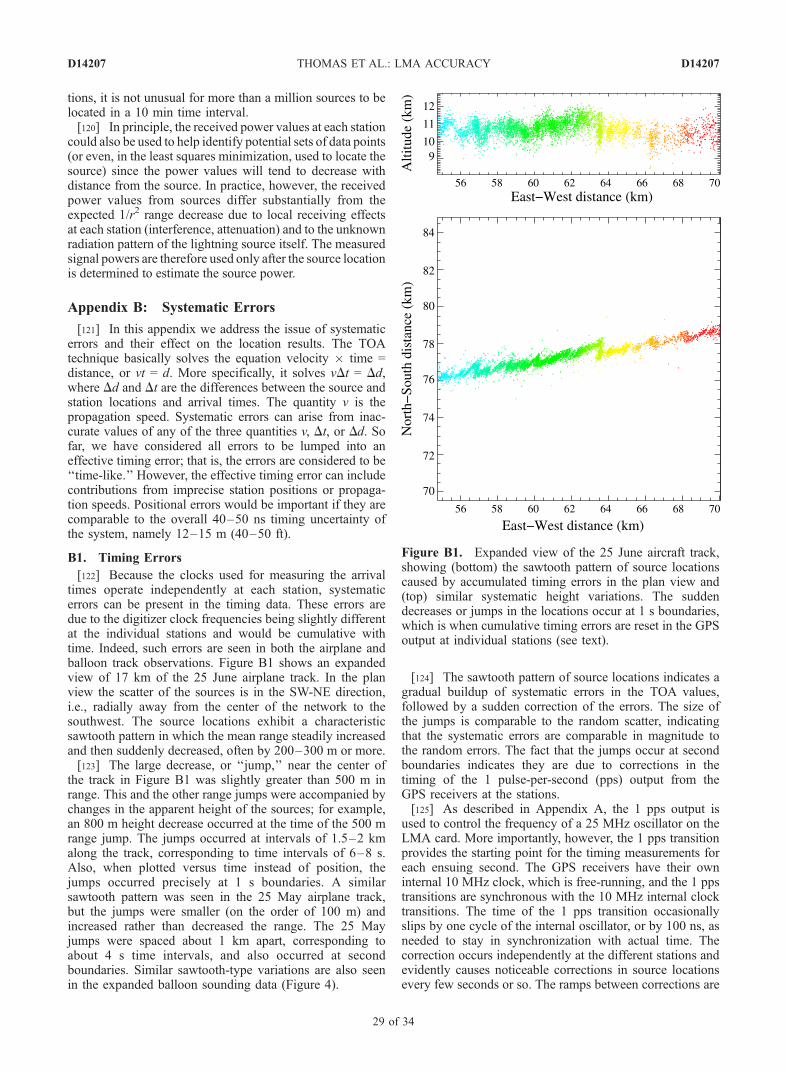
tions, it is not unusual for more than a million sources to belocated in a 10 min time interval.[120] In principle, the received power values at each station

could also be used to help identify potential sets of data points(or even, in the least squares minimization, used to locate thesource) since the power values will tend to decrease withdistance from the source. In practice, however, the receivedpower values from sources differ substantially from theexpected 1/r2 range decrease due to local receiving effectsat each station (interference, attenuation) and to the unknownradiation pattern of the lightning source itself. The measuredsignal powers are therefore used only after the source locationis determined to estimate the source power.

Appendix B: Systematic Errors

[121] In this appendix we address the issue of systematicerrors and their effect on the location results. The TOAtechnique basically solves the equation velocity � time =distance, or vt = d. More specifically, it solves vDt = Dd,where Dd and Dt are the differences between the source andstation locations and arrival times. The quantity v is thepropagation speed. Systematic errors can arise from inac-curate values of any of the three quantities v, Dt, or Dd. Sofar, we have considered all errors to be lumped into aneffective timing error; that is, the errors are considered to be‘‘time-like.’’ However, the effective timing error can includecontributions from imprecise station positions or propaga-tion speeds. Positional errors would be important if they arecomparable to the overall 40–50 ns timing uncertainty ofthe system, namely 12–15 m (40–50 ft).

B1. Timing Errors

[122] Because the clocks used for measuring the arrivaltimes operate independently at each station, systematicerrors can be present in the timing data. These errors aredue to the digitizer clock frequencies being slightly differentat the individual stations and would be cumulative withtime. Indeed, such errors are seen in both the airplane andballoon track observations. Figure B1 shows an expandedview of 17 km of the 25 June airplane track. In the planview the scatter of the sources is in the SW-NE direction,i.e., radially away from the center of the network to thesouthwest. The source locations exhibit a characteristicsawtooth pattern in which the mean range steadily increasedand then suddenly decreased, often by 200–300 m or more.[123] The large decrease, or ‘‘jump,’’ near the center of

the track in Figure B1 was slightly greater than 500 m inrange. This and the other range jumps were accompanied bychanges in the apparent height of the sources; for example,an 800 m height decrease occurred at the time of the 500 mrange jump. The jumps occurred at intervals of 1.5–2 kmalong the track, corresponding to time intervals of 6–8 s.Also, when plotted versus time instead of position, thejumps occurred precisely at 1 s boundaries. A similarsawtooth pattern was seen in the 25 May airplane track,but the jumps were smaller (on the order of 100 m) andincreased rather than decreased the range. The 25 Mayjumps were spaced about 1 km apart, corresponding toabout 4 s time intervals, and also occurred at secondboundaries. Similar sawtooth-type variations are also seenin the expanded balloon sounding data (Figure 4).

[124] The sawtooth pattern of source locations indicates agradual buildup of systematic errors in the TOA values,followed by a sudden correction of the errors. The size ofthe jumps is comparable to the random scatter, indicatingthat the systematic errors are comparable in magnitude tothe random errors. The fact that the jumps occur at secondboundaries indicates they are due to corrections in thetiming of the 1 pulse-per-second (pps) output from theGPS receivers at the stations.[125] As described in Appendix A, the 1 pps output is

used to control the frequency of a 25 MHz oscillator on theLMA card. More importantly, however, the 1 pps transitionprovides the starting point for the timing measurements foreach ensuing second. The GPS receivers have their owninternal 10 MHz clock, which is free-running, and the 1 ppstransitions are synchronous with the 10 MHz internal clocktransitions. The time of the 1 pps transition occasionallyslips by one cycle of the internal oscillator, or by 100 ns, asneeded to stay in synchronization with actual time. Thecorrection occurs independently at the different stations andevidently causes noticeable corrections in source locationsevery few seconds or so. The ramps between corrections are

Figure B1. Expanded view of the 25 June aircraft track,showing (bottom) the sawtooth pattern of source locationscaused by accumulated timing errors in the plan view and(top) similar systematic height variations. The suddendecreases or jumps in the locations occur at 1 s boundaries,which is when cumulative timing errors are reset in the GPSoutput at individual stations (see text).


29 of 34

D14207

caused by the 25 MHz clocks at each station not beingprecisely adjusted. This results in the gradual accumulationof small timing errors during each second. The data streamcontains information used to compensate for this effect inthe processing, but residual effects remain.[126] The magnitude of the time corrections can be

estimated from the size of the jumps and from the modelformulations of section 4. The 500 m range decrease inFigure B1 occurred at a distance close to r = 100 km andtherefore corresponded to a fractional change of �0.005 inrange. In the context of the simple model the range isdetermined by the difference T13,0 in the arrival time at theouter transverse stations relative to the central station(Figure 11c). From equation (4), T13,0 = 20 ms for a stormat 100 km range. Also, a �0.005 fractional range changewould have corresponded to a +0.005 fractional change inT13,0. The sudden jump in T13,0 would thus have been+0.005 � 20 ms, or 100 ns. This is the value that wouldbe expected from the 1 pps signal slipping by one 10 MHzclock cycle. Either a single station was primarily responsi-ble for determining the range, or the timing was fortuitouslycorrected at the same second at two or more stations thatwere determining the range. The fact that most jumps weresmaller than 500 m indicates that the timing correctionswere at stations that had less influence on the range value.[127] The sawtooth variations make a significant contri-

bution to the rms scatter about the aircraft tracks, compa-rable to the random errors. Both the systematic and randomerrors are accounted for in the overall timing uncertainties,however, and therefore in the covariance- and model-predicted location uncertainties as well. GPS receiverscurrently provide additional information on the offset ofthe 1 pps transition from true time; use of this informationshould enable the sawtooth errors to be reduced belowdetectable levels in future versions of the LMA.[128] Systematic timing errors also arise if the time delays

between the VHF antennas and the digitizer at each stationare imprecisely known. The delays are on the order ofseveral hundred ns and differ from station to station due todifferent cable lengths and any differences in the receivercomponents. Examination of the residuals of data solutionsat each station provides a way of detecting and correctinglarge (’40 ns) systematic errors, but usually not smallererrors.

B2. Spatial Errors

[129] Systematic spatial errors can result from imprecisevalues of the station locations. The station positions aredetermined by averaging the output of each station’s GPSreceiver for a few hours to a day or more. Tests indicate thata few-hour average determines the GPS antenna position towithin about 1–3 m in the horizontal and 2–7 m in thevertical. These results are obtained in the absence ofselective availability (the purposeful introduction of errorsinto the GPS transmissions), which was turned off on 2 May2000, just prior to the STEPS field observations. Thelocation information required in the processing are thepositions of the VHF antenna at each station, which istypically located 30 m or so away from the station elec-tronics and GPS receiver. (This is done to reduce radiofrequency interference from the electronics below detectablelevels at the antenna. In some networks and sites, it is also

needed for the VHF antenna to be clear of local obstruc-tions.) With some care, the x, y, z offsets between the GPSand VHF antennas can be measured to ’1 m or so andshould not contribute significantly to the overall error.[130] Station location errors have the greatest effect on the

height of sources in distant storms. The height of distantsources depends on the elevation angle of arrival, q, and therange r. As discussed in connection with Figure 11d, q isdetermined primarily from the arrival times at the close andfar stations along the arrival direction. For distant sources, qis small, and the arrival times differ only by a small amountfrom the transit time between the stations. Relatively smallerrors in the presumed station locations (or in the measuredTOA values) cause errors in q whose effect is magnified fordistant events. This is illustrated in section B3.

B3. LDAR Height Errors

[131] As discussed in sections 1 and 5.2, B2001 found asystematic increase in the height of the maximum lightningactivity with distance from the LDAR network. The max-imum lightning activity occurred at 9 km altitude in stormsover and close to the network but artificially increased up to20 km altitude at 300 km range. B2001 explained the heightincrease as being due to larger than expected range errorsand to a consequent tendency for located events at largedistances to be dominated by overranged events fromintermediate-distance storms. Assuming a constant eleva-tion angle, the overranging increased the apparent altitudeof the sources. The range errors appeared to be large fromobservations of distant storms in the LDAR data, asdiscussed in section 5.2. In turn, the explanation of thesystematic height increase supported the idea of larger thanexpected range errors.[132] Figure B2 illustrates how TOA networks will tend

to overrange sources outside the network. If the measure-ment errors are sufficiently small, the location uncertaintiesare symmetric about the source location. However, if theerrors are not sufficiently small (or even for small measure-ment errors, at sufficiently large range), nonlinear effectscause the uncertainties to be asymmetric and the average

Figure B2. Hyperbolic geometry for the plan location of adistant source, illustrating how measurement errors causeasymmetric location errors and bias the source locationoutward in range.


30 of 34

D14207

location to be biased outward in range. The bias occurs evenin the absence of systematic measurement errors and can beseen from the hyperbolic geometry of how distant sourcesare located. The bias is exacerbated when the errors arelarge, due either to the range itself being large and/or tolarge errors in the measurements themselves.[133] B2001 showed that overranging of sources at inter-

mediate distances (due both to random errors and biasing ofthe range values) provided a possible explanation of thesystematic height increase with distance. However, therange errors needed to do this were an order of magnitudelarger than those that were expected from aircraft measure-ments. They were also larger than would be expectedfrom the size of the LDAR network and its timing errors(section 5.3). B2001 assumed that elevation errors were nota significant factor in the height increase, but this was anincorrect assumption which, when taken into account,provides a simple and better explanation of the systematicheight increase.[134] Figure B3 shows the effect of a systematic baseline

or timing error on the apparent height of sources versusrange from the LDAR network. The results are overlaid onthe source density contours from Figure 7 of B2001. Thecomparison shows that the observed height increase isperfectly fitted if the baselines between opposite sides ofthe network were systematically overestimated by 15 m(triangles). Equivalently, the time differences of arrival atopposite sides of the network were systematically under-estimated by 50 ns. The height values were determinedusing the model result equation (6) for the elevation angle ofdistant sources in the presence of the systematic errors.When correct baseline and timing values are used, the

model slightly overestimates the 9 km height of sourceswithin 30–50 km range of the network but accuratelyestimates the source heights at larger ranges (circles). Thecalculations assume that the effect of the range error uponthe source height was small compared to the elevation error,as shown in section 4. Biased and random range errorswould still have an effect, but this will be small incomparison to the elevation errors. Whatever the rangeerrors of the LDAR system may have been at largedistances, the uncertainty in the elevation angle is thedominant factor in the source height values, and overlylarge range errors are not necessary to explain the system-atic height increase.[135] It is not possible to determine the detailed cause of

the height error without knowing the specifics of the LDARoperation and processing. However, the above results indi-cate that it was due to a systematic baseline or timing error.A 15 m baseline overestimate corresponds to a 0.1%fractional error in the 16 km baseline length D. Systematicbaseline errors will occur if imprecise values are used forthe local radius of curvature of the Earth, namely if theWGS-84 model is not used to convert station latitude andlongitude values to Cartesian coordinates in the data pro-cessing. The mean radius of the Earth is 6370 km but variesfrom 6378 km at the equator to 6357 km at the poles. A0.1% or 6.4 km overestimate of the assumed radii ofcurvature would give the observed results. Systematicheight errors in distant storms have been obtained in theLMA processing, both from not using the WGS-84 conver-sion and by processing data with purposely incorrect stationlocations. The accuracy of the TOA technique is such thatthe results are sensitive to the shape of the Earth.[136] Alternatively, from equation (6), the same system-

atic height error would be produced if the arrival timedifferences T4,2 at the close and far stations were under-estimated by 0.1% (or if the propagation speed was under-estimated by the same amount). For a 16 km baseline, T4,2 ’53.3 ms for distant sources. Systematically underestimatingthe arrival time differences by about 50 ns therefore wouldgive the same height errors, as indicated in Figure B3. Sucha systematic timing error would tend to average to zero inthe azimuthally integrated data of B2001, but land-seaasymmetries in the amount of lightning activity aroundthe LDAR network could allow a bias not to average tozero. (Systematic timing errors of 50 ns should also bedetected in the pulser data used to calibrate and monitor theLDAR’s operation.) From the subsequent discussion onpropagation speeds, absent an artificial error, it would bedifficult to underestimate the propagation speed by 0.1%.[137] The effect of overestimating the baseline lengths is to

increase the apparent height of distant sources. Conversely,underestimating the baseline lengths would decrease theapparent heights. For sources below some altitude z1 themeasured time delay value T4,2 will exceed the assumedtransit time, making the hypotenuse shorter than the adjacentside in the right triangle of Figure 11d and cosq > 1. Sourcesjust above or at z1 will appear to be on the network horizon,while sources below z1 will be rejected, as if they have‘‘disappeared’’ below the horizon. (Alternatively, if thecosq value is set to unity by the processing program, thesources will accumulate on the network horizon. This lattereffect was noticed in initial processing of LMA observations

Figure B3. Predicted height increase with range forsources at 9 km altitude if the baseline distances of the16-km-diameter LDAR network were overestimated by0.1% (15 m) (triangles) or, equivalently, if the arrival timedifferences at close and far stations were underestimated by50 ns (solid curve). The results are overlaid on observationsof the systematic height increase found by Boccippio et al.[2001] (contours); all heights are above the local Earth (seetext).


31 of 34

D14207

from Oklahoma in 1998.) For sources over or near thenetwork the effect of small positional errors in the stationlocations is primarily to increase the chi-square values of theleast squares solutions and does not significantly affect thesource locations.

B4. Propagation Speed

[138] The propagation speed is a function of the dielectricconstant of the Earth’s atmosphere, which, in the VHFrange, depends on altitude and water content. From Doviakand Zrnic [1993] the speed of radio waves is typicallyreduced from its free space value by 0.03% at sea level andby about 0.02% at 600 mbar pressure. Thus the propagationspeed varies slightly with altitude, causing the signals tobe refracted somewhat from their true location andarrival direction. Refraction has a significant effect onlyon distant storm observations, however, which are alreadysubstantially affected by the random measurement errors.Consequently, we have not attempted to include refractioneffects in the present study; it usually suffices to use anaverage propagation speed.[139] The LMA processing currently uses the 600 mbar

speed, namely 0.02% less than the free space value c �299,792,458 m s�1. In other words, the propagation speed isassumed to be v = c/1.0002. 600 mbar pressure correspondsto about 4.5 km altitude in the atmosphere, so the 600 mbarvalue would represent the average speed for sources at’9 km altitude. The average speed would be slightlyoverestimated for sources at higher altitude and slightlyunderestimated for sources at lower altitude. At most, thisincurs an error of <0.01%. The effect of a 0.01% propaga-tion speed error would be to alter the distance r between agiven station and the source by (0.01%)r or by 1 m forsources at 10 km range, 5 m at 50 km range, and 30 m at300 km range. Such errors are small in comparison to therandom timing errors.[140] The above expresses the effect of propagation speed

on the range to the source. The analysis can be made morespecific by noting that, from equation (4), the range r of adistant source is inversely proportional to the propagationspeed c. In finite difference form the differential expressionfor r is therefore

Dr

r¼ �Dc

c; ðB1Þ

where Dc is the error in c. Thus the fractional error in r isthe negative of the fractional error in c. Overestimating c by0.01% would underestimate r by the same fractionalamount. At 100 km range the systematic error in r wouldbe Drc = �r(Dc/c) = �10 m, as above. From equation (5)the random range error for a 70 km diameter networkhaving 50 ns rms timing uncertainty is Drt ’ 350 m rms.Therefore the systematic range error is 3% of the randomerror. At close ranges the speed error increases relative tothe timing error but remains small in absolute terms (e.g.,’1 m at 10 km distance).[141] The effect of a propagation speed error is magnified

in directions transverse to r and for distant storms, canbecome comparable to the uncertainty due to timing errors.The magnification effect on height can be seen from thedifferential of z = r sinq, where q is the elevation angle to the

source. For distant storms, q is determined from equation (6),and the differential for z gives

Dz

z¼ � cos2 q

r

z

� �2 Dc

c’ � r

z

� �2 Dc

c: ðB2Þ

For sources at 10 km height and 100 km range the error in zis magnified by a factor of (10)2 = 100 relative to the errorfor r. A 0.01% speed overestimate would therefore under-estimate the apparent height of the source by 100 m. Thisresult has been verified by processing data for the 25 Juneaircraft track with different values of the propagation speed.Such an error would still be less than that due to randomtiming errors, which is 300 m rms for a 70 km diameternetwork having 50 ns timing uncertainties.[142] As seen for the other errors, it is the height of distant

sources that is most affected by propagation speed errorsrather than the range. Interestingly, use of the 600 mbarpropagation speed guarantees a small systematic heighterror for distant storms. This is because the elevation angledepends on the time difference of arrival at the close and farstations along the direction of arrival, which for lowelevation angle sources is determined by the propagationspeed immediately above the Earth’s surface. The 600 mbarvalue overestimates this speed by up to 0.01% and poten-tially by more if ground effects further slow the wave.

Appendix C: Range Uncertainties Outside theNetwork

C1. Simple Model Formulation

[143] The range of a source outside the network isdetermined from the curvature of the wavefront at stationstransverse to the arrival direction, as indicated in Figure 11c.From the right triangle in Figure 11c, one has that

D=2ð Þ2þ r2 ¼ r þ cT13;0� 2

:

Simplifying and noting that cT13,0�D/2 for sources at largeranges gives

r ¼ D2

8cT13;0� cT13;0

2’ D2

8cT13;0: ðC1Þ

The differential of this gives

dr ¼ � D2

8cT 213;0

dT13;0 ¼ � 8r2

D2cdT13;0;

so that the rms uncertainty in r is

Dr ¼ 8r

D

� �2

cDT13;0: ðC2Þ

The uncertainty in the range r is thus proportional to thearrival time uncertainty DT13,0 and increases as r2, scaled bythe network diameter D.

C2. Distant Storm Observations

[144] For distant storms, the experimentally observedvariance of the lightning sources is the sum of the variancesdue to the storm size and to the measurement uncertainties.Denoting the standard deviation of the locations in the radial


32 of 34

D14207

and azimuthal directions as srange and sazim, respectively,the total variances are given by

s2radial ¼ s2kstorm þ s2range

and

s2transverse ¼ s2?storm þ s2azim ;

where skstorm and s?storm are the standard deviationsassociated with the size of the storm itself in the radialand transverse directions, respectively. Assuming the stormextents are related by skstorm = f � s?storm, where f is a shapefactor that can be greater or less than unity, the standarddeviation of the range error is given by

s2range ¼ s2radial � f 2 s2transverse � s2azim� �

:

If f is not substantially different from unity, the effect of theazimuthal error sazim can be neglected in comparison to therange error srange, giving

s2range ’ s2radial � f 2 � s2transverse: ðC3Þ

Finally, if the storms are circular or nearly circular, ( f ’ 1)so that

s2range ’ s2radial � s2transverse: ðC4Þ

Alternatively, if f is not close to unity, one can average theresults over a number of storms in different directions fromthe network. Denoting the average by angle brackets, onehas that h f 2i ’ 1 if there is no systematic dependence off on the direction of the storm or from storm to storm. Thusfrom equation (24),

hs2rangei ¼ hs2radiali � h f 2 � s2transversei¼ hs2radiali � hf 2ih�s2transversei’ hs2radiali � hs2transversei: ðC5Þ

This result is the same as equation (C4) but applies toaverages rather than individual storm values.

Appendix D: Pulse Transmitter and DataEncoder

[145] The pivotal component of the balloon-borne pulsetransmitter is an integrated circuit oscillator in the frequencyband (60–66 MHz) of the LMA. The oscillator (Fox,Incorporated KF090AT) has a control pin for turning onand off the 63 MHz oscillator with a digital logic level of 0or 5 V. In our pulse transmitter the digital logic signal comesfrom one of the output pins of a microcontroller (Motorola68HC12), which has special circuits for producing pulseswith precise frequency and duration.[146] The 63 MHz signal from the integrated circuit

oscillator is amplified in two stages with GaAs powertransistors (Motorola MRF136 and MRF171A). In orderto reduce power consumption, the amplification of thepower transistors is held at a low level by the microcon-troller until just before the oscillator’s 63 MHz pulse isgated out. The pulse duration was 125 ns (eight cycles of63 MHz), which is the minimum width that could beproduced by the microcontroller. The power emitted duringthe pulse was estimated to be about 60 W into a matchedload. However, the source powers estimated by the LMAwere only 1–2 W. The difference is presumed to be due to a

mismatch between the transmitter and the wire antenna onthe balloon package and to gain losses associated with thepatterns of the transmitting and receiving antennas.[147] The microcontroller (1) searched for the appropriate

serial string of position and time information from a globalpositioning system (GPS) receiver (Magellan GPS 310),(2) converted each character in the string to a time intervalcorresponding to the numerical equivalent of the character,and (3) gated the oscillator to produce pulses after each timeinterval.[148] Each LMA receiver recorded the time each pulse

was received with an uncertainty of about 40 ns. From thecollection of times recorded at each receiver the position ofthe pulse transmitter and the time it emitted the pulse couldbe determined as if it were a pulse of radiation fromlightning. In addition, by differencing the times of succes-sive pulses, the numerical equivalent of each character inthe string from the GPS receiver on the balloon could berecovered, thus providing a direct measure of the position ofthe balloon-borne instrument. Figure D1 shows the timeinterval between pulses from a single LMA station during a2 s interval just after 0000 UTC. The time interval includestwo strings from the GPS receiver. Some of the characterscorresponding to the time intervals are shown in the figure,and the two character strings are given in the figure caption.[149] In other applications the time intervals between

pulses would not need to correspond to characters. Instead,

Figure D1. Time intervals between pulses as a function oftime. Some of the corresponding characters are labeled. Thecharacter at 9.5 ms is an underscore, which filled intervalswhen the balloon-borne GPS receiver was not sendingcharacters to the microcontroller. The cluster of charactersbetween 4.2 and 5.7 ms are the numbers 0 to 9, commas,asterisks, and decimal points. The two strings shown inthe figure are GPGGA,000129.51,3933.9830,N,10159.1883,W,1,09,0.9,06496, M,,,,*36 and GPGGA,000130.44,3933.9813,N,10159.1803, W,1,09,0.9,06500,M,,,,*3D.The first string gives the position of the balloon-bornereceiver at 0001:29.51 UTC; the position was 39�33.98300N latitude, 101� 59.18830W longitude and 6496 mabove a reference surface. Nine satellites were being usedby the GPS receiver.


33 of 34

D14207

they could, for example, correspond to the numbers derivedfrom a sensor or sensors attached to a computer via ananalog-to-digital converter. In this case, the position of theinstrument would be determined in only one way: bylocating the sources of the pulses as the LMA does forlightning. The pulse transmitter/microcontroller combinationallows the LMA to be used as a telemetry receiver that alsogives the location of the transmitting instrument. Severalidentical instruments could be transmitting simultaneously,in which case the times to be subtracted to give time intervalswould be selected to come from nearly the same locations;the instruments would be distinguished by their locationsrather than by transmitting on separate frequencies.[150] It is interesting to calculate the bit rate that can be

transmitted by this unusual method of telemetry. The LMAitself establishes a minimum time interval between pulsesbecause it records the time for only the largest amplitudepulse in successive time windows that are typically 80 or100 ms in duration (but which can be reduced to 10 ms). Inaddition, if the Lightning Mapping Array is also being usedto study lightning, most of the windows would probably bereserved to receive pulses from lightning. Thus the conver-sion from the value of a datum to a time interval betweenpulses could be a linear transformation such as

dt ¼ dtmin þ dtbit D; ðD1Þ

where dtmin is the minimum desired time interval betweenpulses, dtbit is the time interval increment corresponding toan increase of 1 in a data word, and D is the data value. Thetime interval increment, dtbit, must be greater than theuncertainty in the difference between the arrival timesrecorded by the LMA receivers, which is about 60 ns. If N isthe word length, then the information content of each timeinterval between pulses is N bits, and the bit rate is

B ¼ N=dt ¼ N= dtmin þ dtbit Dð Þ: ðD2Þ

Thus for this method of telemetry the bit rate depends onthe data values. With a minimum interval between pulsesof 1 ms and dtbit = 120 ns the average bit rate is about104 bits s�1, with 10 bit words.[151] In the situation in which the Lightning Mapping

Array was used only as a telemetry receiver (in the absenceof lightning) the bit rate could be increased by reducing theminimum duration between pulses.

[152] Acknowledgments. This work was supported by the U.S.National Science Foundation under grants ATM-9912073, ATM-0070934,and ATM-9601652. We thank David Proctor, Ken Cummins, and athird reviewer for their constructive comments and suggestions on themanuscript.

ReferencesBehnke, S. A., R. J. Thomas, P. Krehbiel, and W. Rison (2003), Propagationspeeds of lightning leaders throughout an entire flash using 10 ms timeresolution 3D mapping data, Eos Trans. AGU, 84(46), Fall Meet. Suppl.,Abstract AE21A-1103.

Bevington, P. R. (1969), Data Reduction and Error Analysis for thePhysical Sciences, McGraw-Hill, New York.

Boccippio, D. J., S. Heckman, and S. J. Goodman (2001), A diagnosticanalysis of the Kennedy Space Center LDAR network: 1. Data charac-teristics, J. Geophys. Res., 106, 4769–4786.

Cummins, K. L., M. J. Murphy, E. A. Bardo, W. L. Hiscox, R. B. Pyle, andA. E. Pifer (1998), A combined TOA/MDF technology upgrade of theU.S. National Lightning Detection Network, J. Geophys. Res., 103,9035–9044.

Darden, C., J. Burks, T. Bradshaw, D. Boccippio, S. Goodman,R. Blakeslee, E. McCaul, D. Buechler, J. Hall, and J. Bailey (2003),The integration of total lightning information into National WeatherService operations, Eos Trans. AGU, 84(46), Fall Meet. Suppl., AbstractAE31B-03.

De Fatta, D. J., J. G. Lucas, and W. S. Hodgkiss (1988), Digital SignalProcessing: A System Design Approach, 661 pp., John Wiley, Hoboken,N. J.

Demetriades, N. W. S., M. J. Murphy, and R. L. Holle (2004), The im-portance of total lightning in the future of weather nowcasting, paperpresented at the Symposium on Planning, Nowcasting, and Forecastingin the Urban Zone, Am. Meteorol. Soc., Seattle, Wash., 11–15 Jan.

Doviak, R. J., and D. S. Zrnic (1993), Doppler Radar and Weather RadarObservations, 562 pp., Academic, San Diego, Calif.

Goodman, S. (2003), Atmospheric electrical activity and the prospects forimproving short-term weather forecasting, paper presented at the 12thInternational Conference on Atmospheric Electricity, Int. Comm. onAtmos. Electr., Versailles, France, 9–13 June.

Gunn, R., W. C. Hall, and G. D. Kinzer (1946), Part I—The precipitation-static interference problem and methods for its investigation, Proc. IRE,34, 156–161.

Illingworth, A. J., and S. J. Marsh (1986), Static charging of aircraft bycollisions with ice crystals, Rev. Phys. Appl., 12, 803–808.

Jones, J. J. (1990), Electric charge acquired by airplanes penetrating thun-derstorms, J. Geophys. Res., 95, 16,589–16,600.

Koshak, W. J., and R. J. Solakiewicz (1996), On the retrieval of lightningradio sources from the time-of-arrival data, J. Geophys. Res., 101,26,631–26,639.

Koshak, W. J., et al. (2004), North Alabama Lightning Mapping Array(LMA): VHF source retrieval algorithm and error analyses, J. Atmos.Oceanic Technol., 21, 543–558.

Krehbiel, P. R. (1981), An analysis of the electric field change produced bylightning, Ph.D. dissertation, Univ. of Manchester Inst. of Sci. and Tech-nol., U. K.

Krehbiel, P. R., M. Brook, and R. A. McCrory (1979), An analysis of thecharge structure of lightning discharges to ground, J. Geophys. Res., 84,2432–2456.

Krehbiel, P. R., R. J. Thomas, W. Rison, T. Hamlin, J. Harlin, and M. Davis(2000), Lightning mapping observations in central Oklahoma, Eos Trans.AGU, 81(3), 21–25.

Lang, T. J., et al. (2004), The Severe Thunderstorm Electrification andPrecipitation Study (STEPS), Bull. Am. Meteorol. Soc., in press.

Lennon, C. L. (1975), LDAR: New lightning detection and ranging system,Eos Trans. AGU, 56(12), 991.

Lhermitte, R., and P. R. Krehbiel (1979), Doppler radar and radio observa-tions of thunderstorms, IEEE Trans. Geosci. Electron., GE-17, 162–171.

Maier, L., C. Lennon, T. Britt, and S. Schaefer (1995), LDAR systemperformance and analysis, paper presented at the 6th Conference onAviation Weather Systems, Am. Meteorol. Soc., Boston, Mass.

Poehler, H. A. (1977), An accuracy analysis of the LDAR system, NASAContract. Rep., CR-154631, 83 pp.

Proctor, D. E. (1971), A hyperbolic system for obtaining VHF radiopictures of lightning, J. Geophys. Res., 76, 1478–1489.

Proctor, D. E. (1981), VHF radio pictures of cloud flashes, J. Geophys.Res., 86, 4041–4071.

Proctor, D. E., R. Uytenbogaardt, and B. M. Meredith (1988), VHF radiopictures of lightning flashes to ground, J. Geophys. Res., 93, 12,683–12,727.

Rison, W., R. J. Thomas, P. R. Krehbiel, T. Hamlin, and J. Harlin (1999), AGPS-based three-dimensional lightning mapping system: Initial observa-tions in central New Mexico, Geophys. Res. Lett., 26, 3573–3576.

Rison, W., P. Krehbiel, R. Thomas, T. Hamlin, and J. Harlin (2000), A time-of-arrival lightning mapping system with high time resolution, Eos Trans.AGU, 81(48), Fall Meet. Suppl., Abstract A52C-01.

Shao, X. M., P. R. Krehbiel, R. J. Thomas, and W. Rison (1995), Radiointerferometric observations of cloud-to-ground lightning phenomena inFlorida, J. Geophys. Res., 100, 2749–2783.

Thomas, R. J., P. R. Krehbiel, W. Rison, T. Hamlin, J. Harlin, andD. Shown (2001), Observations of VHF source powers radiated bylightning, Geophys. Res. Lett., 28, 143–146.

��T. Hamlin, J. Harlin, and P. R. Krehbiel, Physics Department, New

Mexico Tech, Socorro, NM 87801, USA. ([email protected]; [email protected]; [email protected])S. J. Hunyady and W. P. Winn, Langmuir Laboratory, Geophysical

Research Center, New Mexico Tech, Socorro, NM 87801, USA.([email protected]; [email protected])W. Rison and R. J. Thomas, Electrical Engineering Department, New

Mexico Tech, Socorro, NM 87801, USA. ([email protected]; [email protected])


34 of 34

D14207

accuracy of the lightning mapping array - ua hydrology...

Documents