achieving robust self management for large scale distributed
TRANSCRIPT

Master of Science ThesisStockholm, Sweden 2010
TRITA-ICT-EX-2010:99
M U H A M M A D A S I F F A Y Y A Z
Achieving Robust Self Management forLarge Scale Distributed Applications
using Management Elements
K T H I n f o r m a t i o n a n d
C o m m u n i c a t i o n T e c h n o l o g y


The Royal Institute of TechnologySchool of Information and Communication Technology
Muhammad Asif Fayyaz
Achieving Robust Self Management for Large ScaleDistributed Applications using Management Elements
Master’s ThesisStockholm, 2010-5-26
Examiner: Vladimir Vlassov,The Royal Institute of Technology (KTH), Sweden
Supervisors: Konstantin Popov and Ahmad Al-Shishtawy,Swedish Institute of Computer Sciences, Sweden


This work is dedicated to my family who has always prayed for my success


Abstract
Autonomic computing is an approach proposed by IBM that enables a
system to self-configure, self-heal, self-optimize, and self-protect itself,
usually referred to as self-* or self-management. Humans should only
specify higher level policies to guide the self-* behavior of the system.
Self-Management is achieved using control feedback loops that consist of
four stages: monitor, analyze, plan, and execute.
Management is more challenging in dynamic distributed environments
where resources can join, leave, and fail. To address this problem a
Distributed Component Management System (DCMS), a.k.a Niche, is
being developed at KTH and SICS (Swedish Institute of Computer
Science). DCMS provides abstractions that enable the construction of
distributed control feedback loops. Each loop consists of a number of
management elements (MEs) that do one or more of the four stages of a
control loop mentioned above.
The current implementation of DCMS assumes that management
elements (MEs) are deployed on stable nodes that do not fail. This
assumption is difficult to guarantee in many environments and application
scenarios. One solution to this limitation is to replicate MEs so that if one
fails other MEs can continue working and restore the failed one. The
problem is that MEs are stateful. We need to keep the state consistent
among replicas. We also want to be sure that all events are processed
(nothing is lost) and all actions are applied exactly once.
This report explains a proposal for the replication of stateful MEs
under DCMS framework. For improved scalability, load-balancing and
fault-tolerance, different breakthroughs in the field of replicated state
machine has been taken into account and discussed in this report. Chord
has been used as an underlying structured overlay network (SON). This
report also describes a prototype implementation of this proposal and
discusses the results.
i


Acknowledgements
All praises to my GOD whose blessings on me are limitless.
It is a pleasure to thank those who guided me and helped me out to fulfill
my thesis project. I am deeply indebted to my supervisor Konstantin
Popov from Swedish Institute of Technology (SICS), whose
encouragement, guidance and support helped me to developed an
understanding of the subject. He was always there to help me and direct
me in every aspect of my work.
I would like to express my sincere gratitude to my co-supervisor Ahmad
Al-Shishtawy whose help enabled me to successfully develop the prototype
implementation of our proposal. He made his support available in every
aspect of this thesis and his motivation and approach toward a problem
always proved an inspiration for my work. Working with him was a great
learning experience and it will help me a lot in further my career.
I would also like to thank my examinor Vladmir Vlassov for his careful
inspection and review of my work. I deeply appreciate his help, not only
technically, but also in resolving many management issues. Without his
help, it would not have been possible to present my thesis this month.
I am thankful to Cosmin Arad from SiCS for his help regarding kompics
and Dr. Seif Haridi from KTH, who taught me the basic and advanced
level courses on Distributed Systems.
Last but not the least, I would like to thank my family who has always
helped me to find confidence in myself and has always prayed for my success.
Stockholm, 2010-5-26
Muhammad Asif Fayyaz
iii

Contents
Contents iv
List of Figures vii
List of Symbols and Abbreviations ix
1 Introduction 1
1.1 Motivation . . . . . . . . . . . . . . . . . . . . . . . . . . . . 1
1.2 Problem Statement . . . . . . . . . . . . . . . . . . . . . . . 2
1.3 Research Questions . . . . . . . . . . . . . . . . . . . . . . . 3
1.4 Note About Team Work . . . . . . . . . . . . . . . . . . . . 4
1.5 Thesis Outline . . . . . . . . . . . . . . . . . . . . . . . . . . 5
2 Background 7
2.1 Niche Platform . . . . . . . . . . . . . . . . . . . . . . . . . 7
2.1.1 Niche in Grid4All . . . . . . . . . . . . . . . . . . . . 7
2.1.2 Self-Managing Applications with Niche . . . . . . . . 8
2.1.3 Niche Runtime Environment . . . . . . . . . . . . . . 10
2.2 Structured Overlay Networks . . . . . . . . . . . . . . . . . 11
2.3 Paxos . . . . . . . . . . . . . . . . . . . . . . . . . . . . . . 12
2.3.1 Basic Protocol . . . . . . . . . . . . . . . . . . . . . . 12
2.3.2 3-PHASE PAXOS . . . . . . . . . . . . . . . . . . . 13
2.3.3 Multi-Paxos Optimization . . . . . . . . . . . . . . . 14
2.4 Replicated Stateful Serivces . . . . . . . . . . . . . . . . . . 15
2.4.1 System Model . . . . . . . . . . . . . . . . . . . . . . 15
2.4.2 Maintaining Global Order Using Virtual Slots . . . . 16
2.4.3 Request Handling Using PAXOS . . . . . . . . . . . 17
2.4.4 Leader Replica Failure . . . . . . . . . . . . . . . . . 17
2.4.5 Flow Control . . . . . . . . . . . . . . . . . . . . . . 18
2.5 Leader Election and Stability without Eventual Timely Links 18
iv

v
2.5.1 Eventual Leader Election (Ω) . . . . . . . . . . . . . 19
2.5.2 Ω with ♦f-Accessibility . . . . . . . . . . . . . . . . 19
2.5.3 Protocol Specification . . . . . . . . . . . . . . . . . 20
2.6 Migration of Replicated Stateful Services . . . . . . . . . . . 21
2.7 KOMPICS . . . . . . . . . . . . . . . . . . . . . . . . . . . . 22
2.7.1 Chord Overlay Using Kompics . . . . . . . . . . . . . 23
2.7.2 REAL-TIME NETWORK SIMULATION . . . . . . 25
3 Proposed Solution for Robust Management Elements 27
3.1 Configurations and Replica Placement Schemes . . . . . . . 29
3.2 State Machine Architecture . . . . . . . . . . . . . . . . . . 32
3.3 Replicated State Machine Maintenance . . . . . . . . . . . . 33
3.3.1 State Machine Creation . . . . . . . . . . . . . . . . 33
3.3.2 Client Interactions . . . . . . . . . . . . . . . . . . . 34
3.3.3 Handling Lost Messages . . . . . . . . . . . . . . . . 35
3.3.4 Request Execution . . . . . . . . . . . . . . . . . . . 36
3.3.5 Handling Churn . . . . . . . . . . . . . . . . . . . . . 37
3.3.6 Handling Multiple Configuration Change . . . . . . . 39
3.3.7 Reducing Migration Time . . . . . . . . . . . . . . . 39
3.4 Applying Robust Management Elements In Niche . . . . . . 41
4 Implementation Details 43
4.1 Underlying Assumptions . . . . . . . . . . . . . . . . . . . . 43
4.2 Basic Underlying Architecture . . . . . . . . . . . . . . . . . 44
4.2.1 Data structures . . . . . . . . . . . . . . . . . . . . . 44
4.2.2 Robust Management Element Components . . . . . . 45
4.3 Node Join and Failures using Kompics . . . . . . . . . . . . 48
4.4 System Startup . . . . . . . . . . . . . . . . . . . . . . . . . 48
4.5 Churn Model . . . . . . . . . . . . . . . . . . . . . . . . . . 49
4.6 Client Request Model . . . . . . . . . . . . . . . . . . . . . . 51
5 Analysis and Results 53
5.1 Testbed Environment . . . . . . . . . . . . . . . . . . . . . . 53
5.2 Methodology . . . . . . . . . . . . . . . . . . . . . . . . . . 54
5.3 Experiments and Performance Evaluations . . . . . . . . . . 55
5.3.1 Request Timeline . . . . . . . . . . . . . . . . . . . . 55
5.3.2 Effect of Churn on RSM Performance . . . . . . . . . 57
5.3.3 Effect of Replication Degree on RSM Performance . . 58
5.3.4 Optimization using Fault Tolerance (Failure Tolerance) 63

vi CONTENTS
5.3.5 Effect of Overlay Node Count on RSM Performance . 63
5.3.6 Effect of Request Frequency on RSM Performance . . 64
5.4 Summary of Evaluation . . . . . . . . . . . . . . . . . . . . . 67
5.4.1 Request Critical Path . . . . . . . . . . . . . . . . . . 68
5.4.2 Fault Recovery . . . . . . . . . . . . . . . . . . . . . 68
5.4.3 Other Overheads . . . . . . . . . . . . . . . . . . . . 69
6 Conclusion 71
6.1 Answers to Research Questions . . . . . . . . . . . . . . . . 71
6.2 Summary and future work . . . . . . . . . . . . . . . . . . . 75
Bibliography 77
A How to use our Prototype 83
A.1 Package Contents . . . . . . . . . . . . . . . . . . . . . . . . 83
A.2 Defining Experiments . . . . . . . . . . . . . . . . . . . . . . 83
A.3 Defining Log Levels . . . . . . . . . . . . . . . . . . . . . . . 85
A.4 Running Experiments . . . . . . . . . . . . . . . . . . . . . . 86
A.5 Collecting Results . . . . . . . . . . . . . . . . . . . . . . . . 86
B Experiment Result Data 89
B.1 Variable Replication Degree . . . . . . . . . . . . . . . . . . 89

List of Figures
2.1 Niche in Grid4All Architecture Stack [6] . . . . . . . . . . . . . 8
2.2 Application Architecture with Niche . . . . . . . . . . . . . . . 9
2.3 Niche container processes on Overlay network . . . . . . . . . . 10
2.4 Basic Paxos 2-Phase Protocol . . . . . . . . . . . . . . . . . . . 14
2.5 Basic Paxos 3-Phase Protocol . . . . . . . . . . . . . . . . . . . 15
2.6 3-Phase Paxos Protocol with stable leader . . . . . . . . . . . . 15
2.7 Virtual Slots in Replicated State Machine . . . . . . . . . . . . 16
2.8 Kompics simulation architecture [23] . . . . . . . . . . . . . . . 24
2.9 Architecture of Chord Implementation as developed by Kompics
[23] . . . . . . . . . . . . . . . . . . . . . . . . . . . . . . . . . . 24
3.1 Replica Placement Example . . . . . . . . . . . . . . . . . . . . 29
3.2 State Machine Architecture . . . . . . . . . . . . . . . . . . . . 31
4.1 Robust Management Element components inside Kompics . . . 45
4.2 ChordPeer architecture with RME . . . . . . . . . . . . . . . . 47
4.3 ChordPeer architecture with new components . . . . . . . . . . 47
4.4 A simple non-optimized system startup . . . . . . . . . . . . . . 49
4.5 Lifetime model with average lifetime=30 and alpha=2 . . . . . 50
5.1 Effect of additional network delay on the latency . . . . . . . . 56
5.2 Effect of additional network delay on the latency . . . . . . . . 56
5.3 Request latency for a single client (high churn) . . . . . . . . . 57
5.4 Effect of Replication Degree on request latency . . . . . . . . . 58
5.5 Single Request timeline . . . . . . . . . . . . . . . . . . . . . . . 59
5.6 Effect of Replication Degree on Average Replica Failures . . . . 60
5.7 Effect of Replication Degree on Leader Replica Failures . . . . . 60
5.8 Effect of Replication Degree on Leader Election Messages . . . . 61
5.9 Effect of Replication Degree on Recovery Delay . . . . . . . . . 62
5.10 Effect of Replication Degree on Recovery Message Overhead . . 62
vii

viii LIST OF FIGURES
5.11 Effect of Fault Tolerance on Message Overhead (replication
degree = 25) . . . . . . . . . . . . . . . . . . . . . . . . . . . . 64
5.12 Request latency for variable Overlay Node Count . . . . . . . . 65
5.13 Message overhead for variable Overlay Node Count . . . . . . . 65
5.14 Request Latency for variable request frequency . . . . . . . . . 66
5.15 Recovery Message Overhead for variable request frequency . . . 67

List of Symbols
and Abbreviations
DCMS Distributed Component Management System
SON Structured Overlay Network
YASS Yet Another Storage System
ME Management Element
RSM Replicated State Machine
RME Robust Management Element
RSMID Robust State Machine Identifier
RMEI Robust Management Element Identifier
RMERI Robust Management Element Replica Identifier
MEI Management Element Identifier
MERI Management Element Replica Identifier
ACK Acknowledgement
IP Internet Protocol
Node Physical Machine (Computer, Mobile etc.)
ACK Acknowledgement
IP Internet Protocol
VO Virtual Organization
QoS Quality of Services
ix


Chapter 1
Introduction
Autonomic computing [1] is an attractive paradigm to tackle management
overhead of complex applications by making them self-managing.
Self-management, namely self-configuration, self-optimization, self-healing,
and self-protection, is achieved through autonomic managers [2], which
continuously monitor hardware and/or software resources and act
accordingly. Autonomic computing is particularly attractive for large-scale
and/or dynamic distributed systems where direct human management
might not be feasible.
Niche [3, 4] is a distributed component management system that
facilitates to build self-managing large-scale distributed systems.
Autonomic managers play a major rule in designing self-managing
systems [5]. An autonomic manager in Niche consists of a network of
management elements (MEs). Each ME is responsible for one or more
roles in the construction of Autonomic Manager. These roles are:
Monitor, Analyze, Plan, and Execute (the MAPE loop [2]). In Niche, MEs
are distributed and interact with each other through events (messages) to
form control loops.
1.1 Motivation
Niche intends to work in a highly dynamic environment with
heterogeneous, poorly managed computing resources [6]. A notable
example of such environments is community-based Grids where individuals
and small organizations create ad-hoc Grid virtual organizations (VOs)
1

2 CHAPTER 1. INTRODUCTION
that utilize unused computing resources. Community-based grids are
meant to provide “best-effort“ services to their participants, but because
of the nature of their resources, it cannot provide more strict
quality-of-service (QoS) guarantees [6].
In such a dynamic environment, constructing autonomic managers is
challenging as MEs need to be restored with minimal disruption to the
autonomic manager whenever the resource where MEs execute leaves or
fails. A common way to make a service tolerate machine failures is to
replicate it on several machines. However, replication can only mask a
limited number of failures, and the longer the service runs, the more likely
the failure count will exceed this number [7]. In addition to that, it is easy
to achieve consistency in a replicated service with no changing states. MEs
are stateful entities and they must keep their state consistent with other
replicas. For the sake of this report, we will use the term configuration as
a set of replicated MEs, while a migration is a change in this configuration.
This change can be due to replacing failed machines with the new one or
adding new machines into the system for load-balancing.
1.2 Problem Statement
Niche management elements should : 1) be replicated to ensure
fault-tolerance; 2) survive continuous resource failures by automatically
restoring failed replicas on other nodes; 3) maintain its state consistent
among replicas; 4) provide its service with minimal disruption in spite of
resource join/leave/fail (high availability). 5) be location transparent (i.e.
clients of the RME should be able to communicate with it regardless of its
current location). Because we are targeting large-scale distributed
environments with no central control, such as P2P networks, all
algorithms should be decentralized.
For implementing replication of MEs, we have decided to use
SMART [8] which not only replaces failed machines by the new ones, but
also adds new machines into the system using configuration change
(migration) protocol. Although SMART claims to fulfill many of the
limitations that other approaches have for migrating replicated state
machines [8], yet there are some areas where the information is still very
limited. SMART has been described and tested in an environment with
100 Mb/s Ethernet LAN as the underlying network. This is not enough

1.3. RESEARCH QUESTIONS 3
when analyzing the behavior of such a system in larger and dynamic
networks e.g. DHT, CHORD. In addition to that, the experiments
conducted by SMART used few nodes/machines in the system and the
behavior of the protocol with large number of nodes is still unclear. Only
one pseudo-code has been provided with the paper which proved to be
much less information than for implementing a whole system.
Furthermore, there is no practical implementation information available
regarding the underlying protocol including Paxos [9] in such kind of
migration scenarios. Last but not the least, the most important aspect of
such a system is it’s behavior in extreme conditions and high churn
scenarios where multiple nodes can fail at the same time. There is no
information about the behavior of the given system in such kind of
environments.
1.3 Research Questions
Based on the problem statement in the previous section, here are some
Research Questions (RQ) that this thesis work must attempt to address.
RQ-01 : Replication by itself is not enough to guarantee long
running services in the presence of continuous churn.
This is because the number of failed nodes hosting
ME replicas will increase with time. Eventually this
will cause the service to stop. Therefore, we use
service migration [8] to enable the reconfiguration of
the set of nodes hosting ME replicas. However, all this
process should be self-automated. How to automate
re-configuration of replica set in order to tolerate
continuous churn?
RQ-02 : Reconfiguration or migration of MEs will cause extra
delay in request processing. How to minimize this effect?
RQ-03 : Replication of MEs will result in extra overhead on the
performance of the system. How to control this extra
overhead?

4 CHAPTER 1. INTRODUCTION
RQ-04 : When a migration request is submitted and decided,
according to SMART, on excution of migrate request,
leader in the configuration will assign its LastSlot, send
JOIN message to host machines in the NextConf and will
propose null requests for all the remaining unproposed
slots until the LastSlot. However, the solution is
unclear if another configuration change request has
already been proposed. It might happen, due to
high churn rate, that multiple configuration change
requests are submitted to the leader at the same time.
If two configuration change will be executed by the
same configuration, it could result in having multiple
NextConf with the same ConfID i.e. duplicate and
redundant configuratons. How to avoid this scenario?
RQ-05 : How to make the system scalable i.e. how to control the
system performance when it is overloaded and churn rate
is high?
RQ-06 : How overlay node count effects the performance of
replicated MEs?
RQ-07 : We have assumed a fair-loss model of message dilvery.
That means, some messages can be lost even when
sending them to alive replicas. How to handle these
lost messages.
RQ-08 : What are the factors other than replication and request
frequency that can influence the performance of a
replicated state machine?
1.4 Note About Team Work
The research presented in this thesis is not a product of the individual effort
of the author of this thesis but rather a joint effort of a team of researchers
from the Swedish Institute of Computer Science (SICS) and KTH the Royal
Institute of Technology Sweden. In addition to thesis author, the team

1.5. THESIS OUTLINE 5
includes Ahmad Al-Shishtawy, Konstantin Popov from SICS and Vladimir
Vlassov from KTH. Most of the parts of this report has been taken from the
paper [10], which includes the contribution from all the above mentioned
authors. The main responsibility of this report’s author was the prototype
implementation, conducting experiments and evaluating results, however he
was also part of other activities as well.
1.5 Thesis Outline
This report explains a generic approach and an associated algorithm to
achieve long-living fault-tolerant services in a structured P2P
environments.It also describes the implementation details and the results
of the simulations conducted to evaluate the proposed algorithms.
The rest of this report is organized as follows: chapter 2 presents the
necessary background required to understand the proposed algorithm. In
chapter 3, we describe our proposed decentralized algorithm to automate
the migration process. Followed by applying the algorithm to the Niche
platform to achieve RMEs in chapter 3.4. In chapter 4 we describes our
prototype implementation of the proposed system and discusses our
experimental results in chapter 5. Finally, Section 6 presents conclusions
and the future work.


Chapter 2
Background
2.1 Niche Platform
Niche [6, 3] is a distributed component management system (DCMS) that
implements the autonomic computing architecture [2]. Niche includes a
programming model, APIs, and a runtime system including deployment
service. DCMS intends to reduce the cost of deployment and run-time
management of applications by allowing developers to program application
self-* behaviors that do not require intervention by a human operator.
Niche has been derived from Fractal Component Model [11] and provides
a mechanism for defining the structure and deployment of the distributed
application using Architecture Description Language (ADL).
2.1.1 Niche in Grid4All
Niche has been developed as part of Grid4ALL project that aims to
prototype Grid software building blocks that can be used by non-expert
users in dynamic Grid environments such as community-based Grids. In
these environments, computing resources are volatile, and possibly of
low-quality and poorly managed. Because of the dynamic nature and
ad-hoc, peer-to-peer styles of creating virtual organizations in
community-based Grids, availability and consumption of computing
resources cannot be coordinated. For achieving this vision, both the
applications and the Grid must automatically adjust themselves to
available resources and load demands that change over time, self-repair
itself after hardware and software failures, protect themselves from
7

8 CHAPTER 2. BACKGROUND
Figure 2.1: Niche in Grid4All Architecture Stack [6]
security threats, and at the same time be reasonably efficient with
resource consumption [6].
2.1.2 Self-Managing Applications with Niche
Niche is a runtime system that seperates application’s functional code
from its non-functional (self-*) code. An application in the framework
consists of a component-based implementation of the applications
functional specification (the lower part of 2.2), and a component-based
implementation of the applications self-* behaviors (the upper part).
Niche provides functionality for component management and
communication which is used by applications, in particular by user-written
implementation of self-* behaviors. Niche implements a run-time
infrastructure that aggregates computing resources on the network used to
host and execute application components.
A self-* code in Niche framework is organized as a network of
management elements (MEs) interacting through events. MEs are stateful
entities that subscribe to and receive events from sensors, and other MEs.

2.1. NICHE PLATFORM 9
Figure 2.2: Application Architecture with Niche
This enables the construction of distributed control loops [12]. The self-*
code senses changes in the environment and can affect changes in the
architecture – add, remove and reconfigure components and bindings
between them.
According to Niche framework specification [6], MEs funtionality is
subdivided into watchers (W1,W2 ... on 2.2), aggregators (Aggr1) and
managers (Mgr1). Watchers are meant to monitor the status of individual
components and groups in the system. They usually recieves events from
sensors but can also watch other management elements as well. On the
other hand, an agreegator is subscribed to several watchers and maintains
partial information about the application status at a more course-grained
level. Agreegators can also analyze symptoms and issue change requests to
managers. Managers use the information recieved from different watchers
and aggregators to decide and execute the changes in the infrastructure.
Managers are meant to posess enough information about the status of the
applications architecture as a whole in order to be able to maintain it. In
this sense managers are different from watchers and aggregators where the
information is though more detailed but limited to some parts, properties
and/or aspects of the architecture. For example, in a storage application

10 CHAPTER 2. BACKGROUND
Figure 2.3: Niche container processes on Overlay network
the manager needs to know the current capacity, the desing capacity and
the number of online users in order to meet a decision whether additional
storage elements should be allocated, while the storage capacity
aggregator knows only the current capacity of every storage element.
2.1.3 Niche Runtime Environment
The Niche runtime system consists of a set of distributed container
processes, on several physical nodes, that can host components (MEs and
application components). As shown in figure 2.3, the distributed
containers are connected together through an overlay network. Niche relies
on overlay network for scalable, self-* address lookup and message delivery
services. It also uses overlay to implement bindings between components,
message passing between MEs, storage of architecture representation and
failure sensing. On each physical node, there is a local Niche process that
provides the Niche API to applications, as shown in figure 2.3 . The

2.2. STRUCTURED OVERLAY NETWORKS 11
overlay allows to locate entities stored on nodes of the overlay. On the
overlay, entities are assigned unique overlay identifiers and for each overlay
identifier, there is a physical node hosting the identified element. Such a
node is usually refered as “responsible“ node for the identifier.
Responsible nodes for overlay entities can change upon churn. Every
physical node on the overlay and thus in Niche also has an overlay
identifier, and can be located and contacted using that identifier.
Niche maintains several types of entities, in particular components of
the application architecture and internal Niche entities maintaining
representation of the application’s architecture. Niche entities are
distributed on the overlay. Functional components are situated on the
specified physical nodes, while MEs and entities representing the
architecture might be moved upon churn between physical nodes.
2.2 Structured Overlay Networks
Structured Overlay Networks, SONs, are known for their self-organising
features and resilience under churn[13]. We assume the following model of
SONs and their APIs. We believe, this model is representative, and in
particular it matches the Chord [14] SON. In the model, SON provides the
operation to locate items on the network. For example, items can be data
items for DHTs, or some compute facilities that are hosted on individual
nodes in a SON. We say that the node hosting or providing access to an
item is responsible for that item. Both items and nodes posses unique
SON identifiers that are assigned from the same name space. The SON
automatically and dynamically divides the responsibility between nodes
such that there is always a responsible node for every SON identifier. SON
provides a ’lookup’ operation that returns the address of a node
responsible for a given SON identifier. Because of churn, node
responsibilities change over time and, thus, ’lookup’ can return over time
different nodes for the same item. In practical SONs the ’lookup’
operation can also occasionally return wrong (inconsistent) results.
Further more, SON can notify application software running on a node
when the responsibility range of the node changes. When responsibility
changes, items need to be moved between nodes accordingly. In Chord-like
SONs the identifier space is circular, and nodes are responsible for items
with identifiers in the range between the node’s identifier and the identifier

12 CHAPTER 2. BACKGROUND
of the predecessor node. Finally, a SON with a circular identifier space
naturally provides for symmetric replication of items on the SON - where
replica IDs are placed symmetrically around the identifier space circle.
Symmetric Replication [15] is a scheme used to determine replica
placement in SONs. Given an item ID i and a replication degree f ,
symmetric replication is used to calculate the IDs of the item’s replicas.
The ID of the x-th (1 ≤ x ≤ f) replica of the item i is computed as
follows:
r(i, x) = (i+ (x− 1)N/f) mod N (2.1)
where N is the size of the identifier space.
The IDs of replicas are independent from the nodes present in the system.
A lookup is used to find the node responsible for hosting an ID. For the
symmetry requirement to always be true, it is required that the replication
factor f divides the size of the identifier space N .
2.3 Paxos
Paxos [9] is a well known consensus protocol for dynamic distributed
environments. Consensus can be either about agreeing on a set of values
to commit or to make a course of actions or decisions. Paxos, as
standalone protocol is easy to understand, but in real-life scenarios, a
variant of the original protocol is usually used.
2.3.1 Basic Protocol
Paxos describes the actions of the process, involved in the consensus phase,
by their roles in the protocol. These are Client, Acceptor, Proposer, Learner
and Leader. Each process or node can play multiple of these roles at the
same time.
Client: The Client issues a request to the proposer and waits for the
response.
Acceptor: Used to choose a single value
Proposer: On client request, propose a value to be chosen by
Acceptors.

2.3. PAXOS 13
Learner: Learn what value has been chosen.
Leader: Paxos requires a distinguished Proposer (called the leader)
to make progress.
In this paper, every process or node in the system is assumed to be
playing the role of Acceptor, Proposer and Learner at the same time. For
the sake of simplicity, let us assume that one of the processes has been
chosen as the leader and only leader can propose.
There are two phases of the Paxos protocol, as describes by Leslie
Lamport [9] and that works as below:
Phase 1 (Prepare Phase) 1. A proposer selects a proposal number n
and sends a prepare request with number n to a majority of
acceptors.
2. If an acceptor receives a prepare request with number n greater
than that of any prepare request to which it has already
responded, then it responds to the request with a promise not
to accept any more proposals numbered less than n and with
the highest-numbered proposal (if any) that it has accepted.
Phase 2 (Propose Phase) 1. If the proposer receives a response to
its prepare requests (numbered n) from a majority of acceptors,
then it sends an accept request to each of those acceptors for a
proposal numbered n with a value v, where v is the value of the
highest-numbered proposal among the responses, or is any
value if the responses reported no proposals.
2. a)If an acceptor receives an accept request for a proposal
numbered n, it accepts the proposal unless it has already
responded to a prepare request having a number greater than n.
Paxos fulfils Safety property at all time while liveness requirement asserts
that if there are enough non-faulty process are available for a long enough
time, then some value is eventually chosen [16].
2.3.2 3-PHASE PAXOS
There is a variant of basic paxos that reduces the total number of messages
being sent in phase 2 of the protocol. In phase 2, all the processes, rather

14 CHAPTER 2. BACKGROUND
Figure 2.4: Basic Paxos 2-Phase Protocol
than sending the messages to every other process, sends the message only
to the leader. When leader will receives 2b messages from quorum, it will
start phase 3 of the Paxos protocol and inform other processes about the
decision by sending the DECIDE message. This type of Paxos protocol has
fewer number of messages at the cost of two one more message delay.
2.3.3 Multi-Paxos Optimization
In a replicated state machine scenario, a Paxos consensus is required for
every action to be taken by each replicated state machine. As described
above, every consensus has an overhead of at least four message delays. If
a complete Paxos instances will be executed for every action that is to be
taken by each replica, it will be a significant amount of overhead on the
system.
If the leader is relatively stable, phase-1 can be skipped for future
instances of the protocol with the same leader [17]. When a process
becomes a leader, it executes phase-I to get the latest state and to get the
promise for all the future consensus instances until a new leader is
selected. In this way, phase-1 will be executed only once and every time,
when the leader receives a request from the client, it only executes the rest
of the protocol as shown below.

2.4. REPLICATED STATEFUL SERIVCES 15
Figure 2.5: Basic Paxos 3-Phase Protocol
Figure 2.6: 3-Phase Paxos Protocol with stable leader
2.4 Replicated Stateful Serivces
2.4.1 System Model
State machine replication [9, 18, 19] approach is a renown method for
implementing fault-tolerant and consistent distributed services. In this
approach, a copy of the service a.k.a. replica, runs on each machine.
These replicas communicate by passing messages in a communication

16 CHAPTER 2. BACKGROUND
Figure 2.7: Virtual Slots in Replicated State Machine
network. Communication is asynchronous and unreliable where messages
can be duplicated, lost or can take an arbitrarily long time to arrive. But
messages which arrive on the destination machines are not corrupted.
These replicas should be deterministic and their states should only
depend upon the previous states and their inputs. They all begin in the
same initial state. A replica moves from one state to the next by
applying/executing an update/request to its state machine. The next
state is completely being determined by the current state and the update
being executed.
Clients send/request updates to the replicas. Each update is
distinguished by the identifier of the sender client and a client-based
monotonically increasing sequence number. The State Machine
Replication by Paxos for System Builders assumes that each client has at
most one outstanding update at one time.
Replicas use PAXOS protocol to globally order all the clients requests
and execute these requests in the same order. So, every replica should have
the same state after executing the same number of requests.
2.4.2 Maintaining Global Order Using Virtual Slots
To globally order all client requests, every replica has maintained in itself a
list of virtual slots and assigns each clients update/request to one of these
slots. These slots are numbered incrementally and the assigned requests
will be executed in the same order e.g. If request X is assigned to slot 50
and request Y is assigned to slot 51, then first X will be executed and then
Y. To assign requests to a slot, one of the replicas becomes the leader using
some leader election algorithm.

2.4. REPLICATED STATEFUL SERIVCES 17
2.4.3 Request Handling Using PAXOS
A simple sequence of handling of client’s request can be explained as follows:
the client sends a request to the replica group. All replicas, on receiving
this request, will store this message into their pending list. When the leader
replica receives the client request, it will choose the next available virtual
slot and will send the proposal to other replicas. This proposal will be
a tentative suggestion that the given client’s request should occupy the
proposed slot. Each replica, on receiving this proposal, will log it (write it to
some stable storage) and then sends the leader a confirmation message. On
receiving the confirmation message from the quorum, the leader announces
that the proposal has been decided by sending the DECIDE message to
all the replicas. Each replica, receiving the DECIDE message will set the
status of the request slot to ready to be executed. Once all requests with
lower slot numbers are executed, the replicas will execute the request and
send the reply to the client. The client will receive multiple confirmations
for the give request, but will just ignore the additional confirmations for the
same request.
2.4.4 Leader Replica Failure
Replicated state machines are using multi-paxos protocol, in which the
phase-1 (Prepare phase) is only executed once the leader changes. When a
leader fails, other replicas select a new leader using a leader election
algorithm. The newly elected leader will run the Prepare phase for all
future instances of the Paxos protocol (i.e. for all sequence numbers) that
will run until the leader is changed again.
The leader replica will send PREPARE message to start the prepare
phase. The prepare message will contain the last slot number the sender
has executed update till. In the group with newly elected leader, the leader
will make the proposal above that slot number. So this message is to learn
about any accepted proposals for the next slots.
Upon receiving the PREPARE message, a replica will send back a
promise message that contains information about each slot after the last
leader given slot. For each slot, the replica will send the LOGGED
proposals and DECISIONS (if any).
Leader, on receiving the promise messages from quorum, will first update
its status from the DECISIONS and will propose messages that it got as

18 CHAPTER 2. BACKGROUND
part of the Promise messages. After that, leader will be ready to propose
new messages.
2.4.5 Flow Control
As suggested by Lamport [9], to avoid having too much undecided proposals
at one time, our implementation also has a sliding window mechanism for
proposing requests. The size of this sliding window is usually referred to as
a. So, the leader can propose updates from i to i+a after updates 1 through
i are decided.
2.5 Leader Election and Stability without
Eventual Timely Links
In a replicated state machine, the leader replica can fail. So, each replica
uses a HEARTBEAT mechanism to learn if the other replica is still alive. If
the leader fails, other replicas will start a protocol to choose the new leader.
In this section, we will discuss about two of the most well known leader
election algorithms in distributed dynamic environment.
Let us define two important properties of a coordination protocol like
Paxos in a distributed system.
Safety
Non-triviality: No value is chosen unless it is first proposed.
Consistency: No two distinct values are both chosen. (two
different learners cannot learn different values).
Liveness
Termination: We’d like the protocol to eventually terminate.
Paxos safety property must be preserved at all times while its liveness
property depends on the selection of a single leader.

2.5. LEADER ELECTION AND STABILITY WITHOUT EVENTUAL TIMELY LINKS19
2.5.1 Eventual Leader Election (Ω)
Eventual Leader Election (Ω) abstraction encapsulates a leader election
algorithm which ensures that eventually the correct processes will elect the
same/single correct process as their leader [20]. It has the following
properties.
Eventual Accuracy: There is a time after which every correct
process trusts some correct process.
Eventual Agreement: There is a time after which no two correct
processes trust different correct processes.
While Ω captures the abstract properties needed to provide liveness, it
does not provide much concrete information about system conditions under
which progress can be guaranteed. So we use leader election as described in
2.5.2 Ω with ♦f-Accessibility
Ω has been described with more precise requirements in paper “Ω Meets
Paxos: Leader Election and Stability without Eventual Timely Links“ [21].
It requires ♦f-Accessibility for this protocol to work, which is defined by
this paper as follows:
Timely Link : A link between two processes is timely at time t if the
sender receives the response within d time.
f-accessibility : A process p is said to be f-accessible at time t if there
exist f other processes q such that the link between p and q are timely
at t.
f-accessibility : There is a time t and a process p such that for all t‘ ≥t, p is f-accessible at t‘.
In this paper, from now on, we will refer to this algorithm as
♦f-Accessible Leader Election .
There are two major contributions that are made by this algorithm:

20 CHAPTER 2. BACKGROUND
♦f-Accessible Leader Election [21] algorithm formulates more
precisely the synchrony conditions required to achieve leader
election. It guarantees to elect a leader without having eventual
timely links. Progress is guaranteed in the following surprisingly
weak settings: Eventually one process can send messages such that
every message obtains f timely responses, where f is a resilience
bound. Such a process is named as ♦f-accessible. These f responders
need not be fixed and may change from one message to another.
This condition is very much according to the workings of Paxos,
whose safety does not necessitate that the f processes with which a
leader interacts be fixed [21].
The second contribution provided by this algorithm [21] is leader
stability. In Paxos, change of leader is a costly operation as it
necessitates the execution of a prepare phase by the new leader.
This improvement suggests that a qualified leader (a leader which
remains capable of having proposals committed in a timely fashion)
should not be demoted.
In our model for replication of management elements, we have
implemented ♦F-Accessible leader election without the optimization of
leader stability. The optimization for leader stability will be implemented
in future.
2.5.3 Protocol Specification
In this protocol [21], every process maintains for itself a state that
comprises of a non-decreasing epochNum and an epoch freshness counter.
An epochNum is a pair of serialNum and processId that can be null as
well. States are ordered lexicographically i.e. First by epochNum and then
by processId (epochNum is internally ordered first by serialNum and then
by processId. In addition to that each process maintains a copy of registry,
which is a collection of states of all processes in the group. A process
updates the state of another process when it handles REFRESH message
from that process.
There are three timers that are being used in this algorithm. These are
refreshTimer with length ∆ time units, roundtripTimer with δ time unit
and readTimer with (∆+ δ) time units. On expiration of refreshTimer
each process will send a refresh message containing its state to all other

2.6. MIGRATION OF REPLICATED STATEFUL SERVICES 21
processes and will start the roundtripTimer with d time units timeout.
When a process receives this request, it updates the sender process state
in its own replica of registry and sends response with a refreshack message.
If the process is able to receive the refreshack messages from f+1 processes
before roundtripTimer expires, the process will be sure that it has timely
links with at least f+1 processes and hence it will increment its freshness
count in its registry. On the other hand, if a process is not able to receive
refreshack messages from f+1 processes, it will increase its serialNum in its
epoch inside the registry.
In addition to registry, every process also records the states of all other
processes in a vector named views. The views vector also contains an expiry
bit for every process in addition to that processs state. The expiry bit is
to indicate whether that processs state has been continuously refreshed or
not. To assess whether a process state (epoch number) has expired, every
process updates its view by periodically reading the entire registry vector
from n-f processes. We have taken n as the total number of processes and f
as n/2. The full specification of the algorithm can be read from the original
paper [21].
2.6 Migration of Replicated Stateful
Services
SMART [8] is a technique for changing the set of nodes where a replicated
state machine runs, i.e. migrate the service. The fixed set of nodes, where
a replicated state machine runs, is called a configuration. Adding and/or
removing nodes (replicas) in a configuration will result in a new
configuration.
SMART is built on the migration technique outlined in [22]. The idea
is to have the current configuration as a part of the service state. The
migration to a new configuration proceeds by executing a special request
that causes the current configuration to change. This request is like any
other request that can modify the state. The change does not happen
immediately but is scheduled to take effect after α slots.This gives the leader
the flexibility to safely propose requests to α slots concurrently, without
worrying about configuration change. This technique of proposing multiple
concurrent requests is also known as pipelining.

22 CHAPTER 2. BACKGROUND
The main advantage of SMART over other migration technique is that
it allows to replace non-failed nodes. This enables SMART to rely on an
automated service (that may use imperfect failure detector) to maintain the
configuration by adding new nodes and removing suspected ones.
An important feature of SMART is the use of configuration-specific
replicas. The service migrates from conf1 to conf2 by creating a new
independent set of replicas in conf2 that run in parallel with replicas in
conf1. The replicas in conf1 are kept long enough to ensure that conf2 is
established. This simplifies the migration process and help SMART to
overcome problems and limitations of other techniques. This approach can
possibly result in many replicas from different configurations to run on the
same node. To improve performance, SMART uses a shared execution
module that holds the state and which is shared among replicas on the
same node. The execution module is responsible for modifying the state
by executing assigned requests sequentially and producing output. Other
than that each configuration runs its own instance of the Paxos and leader
election algorithm independently without any sharing. This makes it, from
the point of view of the replicated state machine instance, look like as if
the Paxos algorithm is running on a static configuration. Conflicts
between configurations are avoided by assigning a non-overlapping range
of slots [FirstSlot, LastSlot] to each configuration. The FirstSlot for conf1
is set to 1. When a configuration change request appears at slot n this will
result in setting LastSlot of current configuration to n + α − 1 and setting
the FirstSlot of the next configuration to n+ α.
Before a new replica in a new configuration can start working it must
acquire a state from another replica that is at least FirstSlot-1. This can be
achieved by copying the state from a replica from the previous configuration
that has executed LastSlot or from a replica from the current configuration.
The replicas from the previous configuration are kept until a majority of
the new configuration have initialised their state.
2.7 KOMPICS
Kompics [23] is a reactive component model that is used for programming,
configuring and executing distributed protocols as software components
that interact asynchronously using data-carrying events [24, 25, 26].
Kompics is similar to Fractal component model which is a modular,

2.7. KOMPICS 23
extensible and programming language agnostic component model that can
be used to design, implement, deploy and reconfigure systems and
applications, from operating systems to middleware platforms and to
graphical user interfaces [11]. As DCMS has been derived from Fractal
Component Model [11], so to mimic the fractal programming model and
to ease the development, we have used Kompics [25] framework to
implement our prototype.
Kompics components are reactive, concurrent and they can be
composed into complexed architecture of composite components. These
components are safely configurable at runtime and allow for sharing of
common subcomponents at various levels in the component hierarchy [26].
Components communicate by passing data-carying events through typed
bidirectional ports connected by channels. Ports are event-based
component interfaces and they represent a service or protocol abstraction.
There are two directions of port i.e. + and -. A + event will go to + side of
the port and - event will go to - side. A component either provides + or
requires - as port [23].
Kompics has developed a set of utility components and methodology
for building and evaluating P2P systems. The framework provides many
reusable components e.g. bootstrap service, failure detectors, network and
timers. Kompics has developed and evaluated a Chord overlay to
demonstrate the practicality of Kompics framework.
2.7.1 Chord Overlay Using Kompics
Kompics has developed and evaluated a Chord overlay to demonstrate the
practicality of Kompics P2P framework [23]. It also has provided a
simulation environment where the whole Chord overlay system can be
executed. The Chord simulation architecture is as shown in figure 2.8.
The simulation environment is a single process running all the peers,
bootstrap and monitor server within the same process.
ChordSimulationMain is executed using a single-thread simulator
scheduler for deterministic replay and simulated time advancement.
P2pOrchestrator is a generic component that interprets experiment
scenarios and sends the scenario events e.g. chordJoin, chordLookup to
the ChordSimulator. P2pOrchestrator also provides a network abstraction
and can be configured with a specific latency and bandwidth model.

24 CHAPTER 2. BACKGROUND
Figure 2.8: Kompics simulation architecture [23]
Figure 2.9: Architecture of Chord Implementation as developed by Kompics[23]
P2pSimulator and P2pOrchestrator can be replaced with each other, but
P2pOrchestrator simulate everything in real time. It uses
KingLatencyMap[12] to simulate a real-life overlay network. The detail of
KingLatencyMap will be discussed in section “Real-Time Network
Simulation“.
ChordSimulator in Kompics simulation environment consist of all
ChordPeers in the overlay. A ChordPeer simulate a node abstraction in
Chord overlay. A detail architecture of ChordPeer is shown in figure 2.9
ChordPeerPort is used to pass all events to ChordPeer including
ChordLookup and ChordJoin. The Network and Timer abstractions are

2.7. KOMPICS 25
provided by the MinaNetwork [27] and JavaTimer component. The
ChordMonitorClient periodically check the Chord status and send it to
the ChordMonitorServer, as shown in figure 7.1. For detail about working
of the Chord, please refer to Building and Evaluating P2P Systems using
the Kompics Component Framework [23]
2.7.2 REAL-TIME NETWORK SIMULATION
In Kompics, as described above, P2pOrchestrator provides a real-time
network abstraction for applications working in wide area networks. To
provide such an abstraction, P2pOrchestrator uses KingLatencyMap [28].
KingLatencyMap is used to estimate latency between any two Internet
hosts, from any other Internet host. The accuracy of this estimation can
be further verified from King: Estimating Latency between Arbitrary
Internet End Hosts [28].


Chapter 3
Proposed Solution for Robust
Management Elements
In this section we present our approach and associated algorithm to
achieve robust services. Our algorithm automates the process of selecting
a replica set (configuration) and the decision of migrating to a new
configuration in order to tolerate resource churn. This approach, which
includes our algorithm combined with the replicated state machine
technique and migration support, will provide a robust service that can
tolerate continuous resource churn and run for long period of time without
the need of human intervention.
Our approach was mainly designed to provide Robust Management
Elements (RMEs) abstraction that is used to achieve robust
self-management. An example is our platform Niche [3, 4] where this
technique is applied directly and RMEs are used to build robust
autonomic managers. However, we believe that our approach is generic
enough and can be used to achieve other robust services. In particular, we
believe that our approach is suitable for structured P2P applications that
require highly available robust services.
We assume that the environment that will host the Replicated State
Machines (RSMs) consists of a number of nodes (resources) that form
together a Structured Overlay Network (SON). The SON may host
multiple RSMs. Each RSM is identified by a constant ID drawn from the
SON identifier space, which we denote as RSMID in the following. RSMID
permanently identifies an RSMs regardless of the number of nodes in the
system and node churn that causes reconfiguration of set of replicas in an
27

28CHAPTER 3. PROPOSED SOLUTION FOR ROBUST MANAGEMENT ELEMENTS
RSM. Given an RSMID and the replication degree, symmetric replication
scheme is used to calculate the SON ID of each replica. The replica SON
ID is used to assign a responsible node to host each replica in a similar
way as in Distributed Hash Tables (DHTs). This responsibility, unlike the
replica ID, is not fixed and changes overtime because of node churn.
Clients that send requests to RSM need to know only its RSMID and
replication degree. With this information clients can calculate identities of
individual replicas according to the symmetric replication scheme, and
locate the nodes currently responsible for the replicas using the lookup
operation provided by the SON. Most of the nodes found in this way will
indeed host up-to-date RSM replicas - but not necessarily all of them
because of lookup inconsistency and node churn.
Fault-tolerant consensus algorithms like Paxos require a fixed set of
known replicas that we call configuration. Some of replicas, though, can
be temporarily unreachable or down (the crash-recovery model). The
SMART protocol extends the Paxos algorithm to enable explicit
reconfiguration of replica sets. Note that RSMIDs cannot be used for
neither of the algorithms because the lookup operation can return over
time different sets of nodes. In the algorithm we contribute for
management of replica sets, individual RSM replicas are mutually
identified by their addresses which in particular do not change under
churn. Every single replica in a RSM configuration knows addresses of all
other replicas in the RSM.
The RSM, its clients and the replica set management algorithm work
roughly as follows. A dedicated initiator chooses RSMID, performs lookups
of nodes responsible for individual replicas and sends to them a request to
create RSM replicas. Note the request contains RSMID, replication degree,
and the configuration consisting of all replica addresses, thus newly created
replicas perceive each other as a group and can communicate with each
other directly withoud relying on the SON. RSMID is also distributed to
future RSM clients.
Because of churn, the set of nodes responsible for individual RSM
replicas changes over time. In response, our distributed configuration
management algorithm creates new replicas on nodes that become
responsible for RSM replicas, and eventually deletes unused ones. The
algorithm consists of tow main parts. The first part runs on all nodes of
the overlay and is responsible for monitoring and detecting changes in the
replica set caused by churn. This part uses several sources of events and

3.1. CONFIGURATIONS AND REPLICA PLACEMENT SCHEMES 29
0 12
3
4
5
6
7
8
9
10
11
12
13
14151617
1819
20
21
22
23
24
25
26
27
28
29
3031
SM r1
SM r2
SM r3
SM r4
RSM ID = 10, f=4, N=32Replica IDs = 10, 18, 26, 2
Responsible Node IDs = 14, 20, 29, 7
Ref(14) Ref(20) Ref(29) Ref(7) 1 2 3 4
Configuration =
Figure 3.1: Replica Placement Example: Replicas are selected according tothe symmetric replication scheme. A Replica is hosted (executed) by thenode responsible for its ID (shown by the arrows). A configuration is afixed set of direct references (IP address and port) to nodes that hosted thereplicas at the time of configuration creation. The RSM ID and ReplicaIDs are fixed and do not change for the entire life time of the service. TheHosted Node IDs and Configuration are only fixed for a single configuration.Black circles represent physical nodes in the system.
information, including SON node failure notifications, SON notifications
about change of responsibility, and requests from clients that indicates the
absence of a replica. Changes in the replica set (e.g. failure of a node that
hosted a replica) will result in a configuration change request that is sent
to the corresponding RSM. The second part is a special module, called the
management module, that is dedicated to receive and process monitoring
information (the configuration change requests). The module use this
information to construct a configuration and also to decide when it is time
to migrate (after a predefined amount of changes in the configuration).
We discuss the algorithm in greater detail in the following.
3.1 Configurations and Replica Placement
Schemes
All nodes in the system are part of SON as shown in Fig. 3.1. The Replicated
State Machine that represents the service is assigned an RSMID from

30CHAPTER 3. PROPOSED SOLUTION FOR ROBUST MANAGEMENT ELEMENTS
Algorithm 1: Helper Procedures
1: procedure GetConf(RSMID)2: ids[ ]← GetReplicaIDs(RSMID) . Replica Item IDs3: for i← 1, f do refs[i]← Lookup(ids[i])4: end for5: return refs[ ]6: end procedure
7: procedure GetReplicaIDs(RSMID)8: for x← 1, f do ids[x]← r(RSMID, x) . See equation 2.19: end for10: return ids[ ]11: end procedure
the SON identifier space of size N . The set of nodes that will form a
configuration are selected using the symmetric replication technique [15].
The symmetric replication, given the replication factor f and the RSMID,
is used to calculate the Replica IDs according to equation 2.1. Using the
lookup() operation, provided by the SON, we can obtain the IDs and direct
references (IP address and port) of the responsible nodes. These operations
are shown in Algorithm 1. The rank of a replica is the parameter x in
equation 2.1. A configuration is represented by an array of size f . The
array holds direct references (IP and port) to the nodes that form the
configuration. The array is indexed from 1 to f and each element contains
the reference to the replica with the corresponding rank.
The use of direct references, instead of using lookup operations, as the
configuration is important for our approach to work for two reasons. First
reason is that we can not rely on the lookup operation because of the
lookup inconsistency problem. The lookup operation, used to find the
node responsible for an ID, may return incorrect references. These
incorrect references will have the same effect in the replicatino algorithm
as node failures even though the nodes might be alive. Thus the incorrect
references will reduce the fault tolerance of the replication service. Second
reason is that the migration algorithm requires that both the new and the
previous configurations coexist until the new configuration is established.
Relying on lookup operation for replica IDs may not be possible. For
example, in Figure 3.1, when a node with ID = 5 joins the overlay it
becomes responsible for the replica SM r4 with ID = 2. A correct
lookup(2) will always return 5. Because of this, the node 7, from the
previous configuration, will never be reached using the lookup operation.
This can also reduce the fault tolerance of the service and prevent the
migration in the case of large number of joins.

3.1. CONFIGURATIONS AND REPLICA PLACEMENT SCHEMES 31
Shared Execution Module
Paxos 1 Paxos 2 Paxos 3
1 2 3 ... ... ...
ServiceState
Conf 1Conf 2Conf 3
assignrequeststo slots
State
Slots
sequentiallyexecute requests
R1FirstSlot
R1LastSlot
R3FirstSlot
R2FirstSlot
R2LastSlot
Input
Output
Paxos,Leader Election, andMigration Messages
Service Specific Module Management Module
Figure 3.2: State Machine Architecture: Each machine can participate inmore than one configuration. A new replica instance is assigned to eachconfiguration. Each configuration is responsible for assigning requests toa none overlapping range of slot. The execution module executes requestssequentially that can change the state and/or produce output.
Nodes in the system may join, leave, or fail at any time (churn).
According to the Paxos constraints, a configuration can survive the failure
of less than half of the nodes in the configuration. In other words, f/2 + 1
nodes must be alive for the algorithm to work. This must hold
independently for each configuration. New configuration, on receiving
JOIN messages will reply with READY messages. Once a configuration
receives READY messages from more than half the replicas in new
configuration, it considers the new configuration as established and can
destroy itself. The detail of this process is explained in SMART [8].
Due to churn, the responsible node for a certain replica may change.
For example in Fig.3.1 if node 20 fails then node 22 will become
responsible for identifier 18 and should host SM r2. Our algorithm,
described in the remainder of this section, will automate migration process
by detecting the change and triggering a ConfChange requests when churn
changes responsibilities. The ConfChange requests will be handled by the
state machine and will eventually cause it to migrate to a new
configuration.

32CHAPTER 3. PROPOSED SOLUTION FOR ROBUST MANAGEMENT ELEMENTS
3.2 State Machine Architecture
The replicated state machine (RSM) consists of a set of replicas, which
forms a configuration. Migration techniques can be used to change the
configuration (the replica set). The architecture of a replica is shown in
Fig. 3.2. The architecture uses the shared execution module optimization
presented in [8]. This optimization is useful when the same replica
participate in multiple configurations. The execution module executes
requests. The execution of a request may result in state change, producing
output, or both. The execution module should be a deterministic
program. Its outputs and states must depend only on the sequence of
input and the initial state. The execution module is also required to
support checkpointing. That is the state can be externally saved and
restored. This enables us to transfer states between replicas.
The execution module is divided into two parts: the service specific
module and the management module. The service specific module
captures the logic of the service and executes all requests except the
ConfChange request which is handled by the management module. The
management module maintains a next configuration array that it uses to
store ConfChange requests in the element with the corresponding rank.
After a predefined threshold of the number and type (join/leave/failure) of
changes. The management module decides that it is time to migrate. It
uses the next configuration array to update the current configuration
array resulting in a new configuration. After that the management module
passes the new configuration to the migration protocol to actually preform
the migration. The reason to split the state in two parts is because the
management module is generic and independent of the service and can be
reused with different services. This simplifies the development of the
service specific module and makes it independent from the replication
technique. In this way legacy services, that are already developed, can be
replicated without modification given that they satisfy execution module
constraints (determinism and checkpointing).
In a corresponding way, the state of a replica consists of two parts: The
first part is internal state of the service specific module which is application
specific; The second part consists of the configurations.
The remaining parts of the replica, other than the execution module,
are responsible to run the replicated state machine algorithms (Paxos and
Leader Election) and the migration algorithm (SMART). As described in

3.3. REPLICATED STATE MACHINE MAINTENANCE 33
the previous section, each configuration is assigned a separate instance of
the replicated state machine algorithms. The migration algorithm is
responsible for specifying the FirstSlot and LastSlot for each
configuration, starting new configurations, and destroying old
configurations after the new configuration is established.
The Paxos algorithm guarantees liveness when a single node acts as a
leader, thus it relies on a fault-tolerant leader election algorithm. Our
system uses the algorithm described in[21]. This algorithm guarantees
progress as long as one of the participating processes can send messages
such that every message obtains f timely (i.e. with a pre-defined timeout)
responses, where f is a algorithm’s constant parameter specifying how
many processes are allowed to fail. Note that the f responders may
change from one algorithm round to another. This is exactly the same
condition on the underlying network that a leader in the Paxos itself relies
on for reaching timely consensus. Furthermore, the aforementioned work
proposes an extension of the protocol aiming to improve leader stability so
that qualified leaders are not arbitrarily demoted which causes significant
performance penalty for the Paxos protocol.
3.3 Replicated State Machine Maintenance
This section will describe the algorithms used to create a replicated state
machine and to automate the migration process in order to survive resource
churn.
3.3.1 State Machine Creation
A new RSM can be created by any node in the SON by calling CreateRSM
shown in Algorithm 2. The creating node construct the configuration
using symmetric replication and lookup operations. The node then sends
an InitSM message to all nodes in the configuration. Any node that
receives an Init SM message (Algorithm 6) will start a state machine
(SM) regardless of its responsibility. Note that the initial configuration,
due to lookup inconsistency, may contain some incorrect nodes. This does
not cause problems for the replication algorithm. Using migration, the
configuration will eventually be corrected.

34CHAPTER 3. PROPOSED SOLUTION FOR ROBUST MANAGEMENT ELEMENTS
Algorithm 2: Replicated State Machine API
1: procedure CreateRSM(RSMID). Creates a new replicated state machine
2: Conf [ ]← GetConf(RSMID). Hosting Node REFs
3: for i← 1, f do4: sendto Conf [i] : InitSM(RSMID, i, Conf)5: end for6: end procedure
7: procedure JoinRSM(RSMID, rank)8: SubmitReq(RSMID,ConfChange(rank,MyRef))
. The new configuration will be submitted and assigned a slot to be executed9: end procedure
10: procedure SubmitReq(RSMID, req). Used by clients to submit requests
11: Conf [ ]← GetConf(RSMID). Conf is from the view of the requesting node
12: for i← 1, f do13: sendto Conf [i] : Submit(RSMID, i, Req)14: end for15: end procedure
3.3.2 Client Interactions
A client can be any node in the system that requires the service provided
by the RSM. The client need only to know the RSMID and the replication
degree to be able to send requests to the service. Knowing the RSMID, the
client can calculate the current configuration using equation 2.1 and lookup
operations (See Algorithm 1). This way we avoid the need for an external
configuration repository that points to nodes hosting the replicas in the
current configuration. The client submits requests by calling SubmitReq
as shown in Algorithm 2. The method simply sends the request to all
replicas in the current configuration. Due to lookup inconsistency, that can
happen either at the client side or the RSM side, the client’s view of the
configuration and the actual configuration may differ. We assume that the
client’s view overlaps, at least at one node, with the actual configuration
for the client to be able to submit requests. Otherwise, the request will fail
and the client need to try again later after the system heals itself. We also
assume that each request is uniquely stamped and that duplicate requests
are filtered. In the current algorithm the client submits the request to
all nodes in the configuration for efficiency. It is possible to optimise the
number of messages by submitting the request only to one node in the
configuration that will forward it to the current leader. The trade off is
that sending to all nodes increases the probability of the request reaching

3.3. REPLICATED STATE MACHINE MAINTENANCE 35
Algorithm 3: Execution
1: receipt of Submit(RSMID, rank,Req) from m at n2: SM ← SMs[RSMID][rank]3: if SM 6= φ then4: if SM.leader = n then SM.schedule(Req) . Paxos schedule it5: else . forward the request to the leader6: sendto SM.leader : Submit(RSMID, rank,Req)7: end if8: else9: if r(RSMID, rank) ∈]n.predecessor, n] then . I’m responsible10: JoinRSM(RSMID, rank) . Fix the configuration11: else12: DoNothing . This is probably due to lookup inconsistency13: end if14: end if15: end receipt
16: procedure ExecuteSlot(req) . The Execution Module17: if req.type = ConfChange then . The Management Module18: nextConf [req.rank]← req.id
. Update the candidate for the next configuration19: if nextConf.changes = threshold then20: newConf ← Update(CurrentConf,NextConf)21: SM.migrate(newConf)
. SMART will set LastSlot and start new configuration22: end if23: else . The Service Specific Module handles all other requests24: ServiceSpecificModule.Execute(req)25: end if26: end procedure
the RSM . This reduces the negative effects of lookup inconsistencies and
churn on the availability of the service. Clients may also cache the reference
to the current leader and use it directly until the leader changes.
3.3.3 Handling Lost Messages
We have assumed a fair-loss model of message dilvery. That means, some
messages can be lost even when sending them to alive replicas. To increase
the probability of handling every message sent by the clients every client
submits the requests to each replica in a RSM. Each non-leader replica
will forward the message to the leader replica, which will ignore duplicate
messages. This approach might result in overloading leader with too many
messages, especially when the degree of replication is large. To avoid this
situation, there is another mechanism that has been tested. Each recieved
message should be tagged with the recieved timestamp and should be stored
by each replica in a pending requests queue. Periodically, every repica
checks the pending requests queue and if a request has been in the pending

36CHAPTER 3. PROPOSED SOLUTION FOR ROBUST MANAGEMENT ELEMENTS
Algorithm 4: Lost Message Handling
1: receipt of Submit(RSMID, rank,Req) from m at n2: SM ← SMs[RSMID][rank]3: if SM 6= φ then4: if SM.leader = n then SM.schedule(Req) . Paxos schedule it5: else . tag and save request in pending list6:7: Req.rcvdts← currts . tag recieved Request8: store pendingReqs : Store(RSMID,Req)9: end if10: else11: if r(RSMID, rank) ∈]n.predecessor, n] then . I’m responsible12: JoinRSM(RSMID, rank) . Fix the configuration13: else14: DoNothing . This is probably due to lookup inconsistency15: end if16: end if17: end receipt
18: procedure CheckExpiredRequest(RSMID, rank) .19: SM ← SMs[RSMID]20: for i← 1, sizeof(SM.pendingReqs) do . check every request in pending list21: if (currts− SM.PendingReqs[req].rcvdts) > threshold then22:23: SM.PendingReqs[req].rcvdts← currts . reset timestamp24: sendto SM.leader : Submit(RSMID, rank, SM.PendingReqs[req]) . forward
the request to the leader25: end if26: end for27: end procedure
28: procedure DecideSlot(RSMID, req) . The Execution Module29: SM ← SMs[RSMID]30: SM.PendingReqs[req].remove() . Remove request from pending list31: ExecuteSlot(req)32: end procedure
list for a long time, it is retransmitted to the leader. Algorithm 3 Submit
method can be modified as shown in Algorith 4. Once the request is decided,
it is removed from the pending list.
3.3.4 Request Execution
The execution of client requests is initiated by receiving a submit request
from a client and consists of three phases. Checking if the node is responsible
for the request, scheduling the request and then execute it.
When a node receives a request from a client it will first check, using
the RSMID in the request, if it is hosting the replica to which the request
is directed to. If this is the case, then the node will submit the request to
that replica. The replica will try to schedule the request for execution if the

3.3. REPLICATED STATE MACHINE MAINTENANCE 37
Algorithm 5: Churn Handling
1: procedure NodeJoin . Called by SON after the node joined the overlay2: sendto successor : PullSMs(]predecessor,myId])3: end procedure
4: procedure NodeLeavesendto successor : NewSMs(SMs) . Transfer all hosted SMs to Successor
5: end procedure
6: procedure NodeFailure(newPred, oldPred). Called by SON when the predecessor fails
7: I ←Sf
x=2 ]r(newPred, x), r(oldPred, x)]8: multicast I : PullSMs(I)9: end procedure
replica believes that it is the leader. Otherwise the replica will forward the
request to the leader.
On the other hand, if the node is not hosting a replica with the
corresponding RSMID, it will proceed with one of the following two
scenarios: In the first scenario, It may happen due to lookup inconsistency
that the configuration calculated by the client contains some incorrect
references. In this case, a incorrectly referenced node ignores client
requests (Algorithm 3 line 12) when it finds out that it is not responsible
for the target RSM. In the second scenario, it is possible that the client is
correct but the current replica configuration contains some incorrect
references. In this case, the node that discovers through the client request
that it was supposed to be hosting a replica will attempt to correct the
current configuration by sending a ConfChange request replacing the
incorrect reference with the reference to itself (Algorithm 3 line 10). The
scheduling is done by assigning the request to a slot that is agreed upon
among all replicas in the configuration (using the Paxos algorithm).
Meanwhile, scheduled requests are executed sequentially in the order of
their slot numbers. These steps are shown in Algorithm 3. At execution
time, the execution module will direct all requests except the ConfChange
request to the service specific module for execution. The ConfChange will
be directed to the management module for processing.
3.3.5 Handling Churn
Algorithm 5 shows how to maintain the replicated state machine in case
of node join/leave/failure. When any of these cases happen, a new node
may become responsible for hosting a replica. In case of node join, the

38CHAPTER 3. PROPOSED SOLUTION FOR ROBUST MANAGEMENT ELEMENTS
Algorithm 6: SM maintenance (handled by the container)
1: receipt of InitSM(RSMID,Rank,Conf) from m at n2: new SM . Creates a new replica of the state machine3: SM.ID ← RSMID4: SM.Rank ← Rank . 1 ≤ Rank ≤ f5: SMs[RSMID][Rank]← SM . SMs stores all SM that node n is hosting6: SM.Start(Conf) .7: end receipt
8: receipt of PullSMs(Intervals) from m at n9: for each SM in SMs do10: if r(SM.id, SM.rank) ∈ I then11: newSMs.add(SM)12: end if13: end for14: sendto m : NewSMs(newSMs)15: end receipt
16: receipt of NewSMs(NewSMs) from m at n17: for each SM in NewSMs do18: JoinRSM(SM.id, SM.rank)19: end for20: end receipt
new node will send a message to its successor to get information (RSMID
and replication degree) about any replicas that the new node should be
responsible for. In case of leave, the leaving node will send a message to its
successor containing information about all replicas that it was hosting.
In the case of failure, the successor of the failed node needs to discover
if the failed node was hosting any replicas. This can be done in a proactive
way by checking all intervals (line 7) that are symmetric to the interval that
the failed node was responsible for. One way to achieve this is by using
interval-cast that can be efficiently implemented on SONs e.g. using bulk
operations [15]. The discovery can also be done lazily using client requests
as described in the previous section and Algorithm 3 line 10. The advantage
of using lazy apprpoach reduces message burden on the system. However, in
the proactive way, the system does not have to depend on the client’s request
frequency and in this way, it could be more robust. Both of these approached
could be used together to make the system more fault-tolerant. All newly
discovered replicas are handled by NewSMs (Algorithm 6). The node will
request a configuration change by joining the corresponding RSM for each
new replica. Note that the configuration size is fixed to f . A configuration
change means replacing reference at position r in the configuration array
with the reference of the node requesting the change.

3.3. REPLICATED STATE MACHINE MAINTENANCE 39
3.3.6 Handling Multiple Configuration Change
When a migration request is submitted and decided, SMART [8] protocol
is used to migrate a SM from one configuration to another. According to
SMART, on excution of migrate request, leader in the configuration will
assign its LastSlot, send JOIN message to host machines in the NextConf
and will propose null requests for all the remaining unproposed slots until
the LastSlot. However, the situation is unclear if another ConfChange
request has already been proposed. It might happen, due to high churn
rate, that multiple ConfChange requests are submitted to the leader at the
same time. If two ConfChange will be executed by the same configuration,
it could result in having multiple NextConf with the same ConfID. To avoid
having this situation, as shown in algorithm 3, everytime a ConfChange
request is executed, it will replace at position r in the configuration array
with the reference of the node who requested this change. This way, only
one NextConf will be created. This will make sure to avoid any conflicts due
to multiple configurations with the same ConfId and also to have redundant
configurations.
There can be different scenarios with multiple ConfChange. In one
scenario, replicas placed on different nodes fails at the same time, the
successors of all these nodes will get infomation from the ME group as
explained before and will request for replacing the failed replicas with the
newly created replicas. On the other hand, there can be a situation where
multiple replicas are hosted on the same node in the overlay. This could
happen due to high churn rate and less number of nodes available in the
overlay. If that node fails, the successor of that node will pull all failed
replicas, will create these replicas on its own node and will request for
multiple ConfChange requests. To optimize this situation, the new node
can also send a single ConfChange request with a list of new replicas to be
replaced.
3.3.7 Reducing Migration Time
The system can become unresponsive during the migration time i.e. when
NextConf is created and until it recieves the FINISH message and a new
leader is elected. This duration is very crutial for scalability and
responsiveness of the system. In case of high-churn scenarios, there can be
many migrations during a short span of time. An optimization, which is

40CHAPTER 3. PROPOSED SOLUTION FOR ROBUST MANAGEMENT ELEMENTS
Algorithm 7: SM maintenance (handled by RSM replica)
1: receipt of Join(RSMID,Rank,Conf,ConfId) from m at n2: SM ← SMs[RSMID][rank]3: if SM [ConfId].Started = false then . If Replica is not started yet4: SM [ConfId].leader = Conf [0] . Choosing lowest rank replica as leader5: StartFeld(()RSMID,Rank,Conf,ConfId) . Starting FELD6: if SM [ConfId].leader = n then StartPromisePhase(()ConfId) . Paxos start
promise phase7: end if8: end if9: end receipt
10: receipt of Elect(RSMID,Leader, Conf,ConfId) from m at n11: SM ← SMs[RSMID][rank]12: if SM [ConfId].leader = n then StartPromisePhase(()ConfId) . Paxos start
promise phase13: end if14: end receipt
already proposed, is to wait for a certain number of replica failures in a
RSM before deciding to migrate. This is also shown in figure 3 line 19 and
will be referred as replica Fault-Tolerance. However, this does not
reduce the time of migration when it happens. Migration time depends
mainly on the time to detect failure and the leader election algorithm.
To handle this situation and to further optimize our algorithm, we have
modified the startup of an RSM as shown in Algorithm 7. Our implemented
♦f-Accessible Leader Election is choosing the lowest ranked most responsive
replica as the leader. On joining an RSM, every SM will choose replica with
lowest rank as the default leader before starting the leader election. Most
of the time all the replicas in an RSM are alive and responsive. This would
mean that, when a replica node will join the RSM it will assume replica with
lowest rank as the default leader. This will reduce the migration time as
replicas will start their Paxos’s first phase without waiting for the leader
election to finish.
In worst scenarios, if the lowest ranked replica is faulty (not working
properly), then eventually a new leader will be chosen by the leader election
and the leader then will start proposing the requests from pending request
queue.

3.4. APPLYING ROBUST MANAGEMENT ELEMENTS IN NICHE 41
3.4 Applying Robust Management
Elements In Niche
The autonomic manager in Niche is constructed from a set of management
elements. To achieve robustness and high availability of Autonomic
Managers, in spite of churn, we will apply the algorithm described in the
previous section to management elements. Replicating management
elements and automatically maintaining them will result in what we call
Robust Management Element (RME). An RME will:
be replicated to ensure fault-tolerance. This is achieved by replicating
the service using the replicated state machine algorithm.
survive continuous resource failures by automatically restoring failed
replicas on other nodes. This is achieved using our proposed approach
that will automatically migrate the RME replicas to new nods when
needed.
maintain its state consistent among replicas. This is guaranteed by
the replicated state machine algorithm and the migration mechanism
used.
provide its service with minimal disruption in spite of resource
join/leave/fail (high availability). This is due to replication. In case
of churn, remaining replicas can still provide the service.
be location transparent (i.e. clients of the RME should be able to
communicate with it regardless of its current location). The clients
need only to know the RME ID to be able to use an RME regardless of
the location of individual replicas.
The RMEs are implemented by wrapping ordinary MEs inside a state
machine. The ME will serve as the service specific module shown in
Figure 3.2. However, to be able to use this approach, the ME must follow
the same constraints as the execution module. That is the ME must be
deterministic and provide checkpointing.
Typically, in replicated state machine approach, a client sends a request
that is executed by the replicated state machine and gets a result back. In
our case, to implement feedback loops, we have two kinds of clients from
the point of view of an RMS. A set of sending client Cs that submit requests

42CHAPTER 3. PROPOSED SOLUTION FOR ROBUST MANAGEMENT ELEMENTS
to the RME and a set of receiving clients Cr that receive results from the
RME. The Cs includes sensors and/or other (R)MEs and the Cr includes
actuators and/or other (R)MEs.
To simplify the creation of control loops, that are formed in Niche by
connecting RMEs together, we use a publish/subscribe mechanism. The
publish/subscribe system delivers requests/responses to link different stages
(RMEs) together to form a control loop.

Chapter 4
Implementation Details
To evaluate the performance of our approach and to show the practicality
of our algorithms, we built a prototype implementation of Robust
Management Elements using the Kompics [29] component model. As
described before, Kompics is a framework for building and evaluating
distributed systems in simulation, local execution and distributed
deployments. For the underlying SON, we used Chord implementation
that is provided by Kompics. This Chord implementation provides the
functionality to resolve a SON Id to an address of the node responsible for
it. Nodes are able to directly communicate with each other using this
address. Every physical node know the range of SON Id:s it is currently
responsible for. We use lookup and failure detection facilities from this
implementation.
4.1 Underlying Assumptions
A fail-stop model has been assumed i.e. nodes can fail only by
stopping. Other models including byzantine failures will be handled
in future.
Messages are delivered fair-loss to alive replicas i.e. some messages
can be lost.
All assumption for Paxos and Replicated State Machine should hold
e.g. Less than half of the nodes can fail. Majority of the nodes or
quorum should stay alive.
43

44 CHAPTER 4. IMPLEMENTATION DETAILS
4.2 Basic Underlying Architecture
4.2.1 Data structures
Slots Every request recieved by RMEs is being
assigned to virtual slots. This is used to
ensure the order of requests execution by the
RMEs. An RME can execute request from
slot n+1 only if it had already executed input
from slot n.
FirstSlot The starting slot number for a configuration
to which the client requests can be assigned.
LastSlot The last slot for a configuration to assign a
request.
ServiceState This is use to abstract the state of a
replica. As described before, it consists
of internal state of the service specific
module, configurations (current and next
configuration) and Paxos and SMART
specific state information. The migration
algorithm is responsible for specifying
the FirstSlot and LastSlot for each
configuration.
PendingRequests Clients are sending requests to each replica
in a configuration. Each replica, on
recieving the requests, stores the requests
in a PendingRequests list. If a request
remains in the pending list for more than the
allowed time, it is considered as expired and
is resubmitted to the leader.

4.2. BASIC UNDERLYING ARCHITECTURE 45
Figure 4.1: Robust Management Element components inside Kompics
MERI Used to uniquely identify a replica in an
RSM. It Contains replica number (rank),
SON ID, IP and address information of a
particular replica in the configuration.
MEI Contains RSMID and replication degree.
RSMID uniquly identifies an RSM and
is used, together with replication degree,
to find the replica IDs as specified in
Algorithm 1.
4.2.2 Robust Management Element Components
The basic entities of the implmented protype are MEInitiator,
MEMonitor, MEContainer, MEReplica, MESensor and FELD. These
entities are implemented as Kompics components and are shown in dark
colors in the component diagrams below.
46 CHAPTER 4. IMPLEMENTATION DETAILS
MEInitiator MEInitiator is responsible for initializing
the system and starting up the RME
configuration. It is implemented as
a Kompics component and lies outside
the structured overlay network (SON)
component i.e. Chord in our case. It is
shown in figure 4.1.
MEMonitor MEMonitor is used for evaluating system
performance. It gathers all the data
needed for calculating the latency and
message overhead due to robust management
elements. Just like MEInitiator, MEMonitor
also lies outside of the structured overlay
network.
MEContainer The DCMS runtime system consists of a set
of distributed container processes on several
physical nodes for hosting components (MEs
and application components). MEContainer
is an abstraction of these DCMS containers.
Every node in structured overlay network
will host a Container. A Container is
responsible for getting requests from the
Initiator for creating and starting a replica.
When a predecessor of a ChordPeer fails,
this information is also indicated to the
MEContainer, which will then start the
process to find and replace the failed ME.
A Container can host multiple replicas
which are uniquely identified by their MERI.
Changes in the successors and predecessors
of a node in the overlay are being informed
to the Container. Container can also request
the ME group to replace a replica with a new
replica.

4.2. BASIC UNDERLYING ARCHITECTURE 47
Figure 4.2: ChordPeer architecture with RME
Figure 4.3: ChordPeer architecture with new components
MEReplica This is the main component entity
responsible for implementing all the
functionalities of a RME replica. When a
replica is started, it is provided with its
unique MERI in addition to RSMID and the
replication degree. MERI uniquely identifies
a MEReplica and consists of information
including its SON ID, IP address and the
physical node address. This can be used
to directly communicate with a specific
MEReplica. It is also provided the MERIs
of all replicas that are part of the same
configuration. MEReplica implements the
SMART protocol for migration in addition
to Paxos for deciding and executing client’s
requests.

48 CHAPTER 4. IMPLEMENTATION DETAILS
FELD This component is used to implement
the functionality of ♦f-Accessible Leader
Election [21]. When a MEReplica is
started, it starts its FELD and provides the
configuration Id and MERI of replicas which
are part of the same configuration.
MESensor This entity is used to capture the
abstraction of Sensors inside Niche
framework. MESensors will generate
requests periodically to RSM without waiting
for the reply.
4.3 Node Join and Failures using Kompics
To fail a node, Kompics Chord framework provide a special message
ChordPeerFail that can be used to fail a specific node in the overlay. It
takes the overlay id of the node as part of the input message and will
destroy the ChordPeer, along with all the components inside that
ChordPeer. The failure of the node will be indicated to the successor
ChordPeer and ultimately to its MEContainer.
To create a node in the Kompics Chord overlay, there is a special message
ChordPeerJoin that can be used. It takes as input the SON ID of the node,
creates a node and will try to join this node into an existing SON. If there
is no already created SON, then it will create one and will make the node
part of this SON. Every node has a MEContainer that is also created as
part of the initialization.
4.4 System Startup
System starts when the MEInitiator gets a request to start an RSM. The
system assumes that underlying SON is already initialized and contains
some valid physical nodes. The request also contains a MEI with RSMID
and replication degree for the RSM. The Initiator, on receiving this message,
creates MERI for each replica by first calculating the symmetric Son Id and
then getting the node address for this SON Id from the Chord overlay as

4.5. CHURN MODEL 49
Figure 4.4: A simple non-optimized system startup
described in section 3. A simple scenario of system startup is shown in
figure 4.4.
However, with the optimization as proposed in section 3.3.7, the replicas
will choose the lowest ranked replica as the leader and the leader will start
the promise phase, without waiting for the leader election.
4.5 Churn Model
The most important aspect of evaluating our algorithms is to verify its
behavior in extreme churn scenarios. SMART has shown its experiments
with a very basic and simple setup which is enough to understand the
working of the SMART yet may not be enough to understand the scalability
of a system. On the other hand, although Paxos for System builders [19]
has shown paxos with respect to extreme scenario, but they did not involve
failure of nodes in their tests, which is also very important to learn the
scalability of the system.
To experiment the performance of our algorithms in various churn
scenarios, we have used the lifetime-based node failure model [13, 30] with
shifted Pareto lifetime Distribution. The sample java code of this model is
shown below while a sample output of this algorithm is shown in
Figure 4.5.

50 CHAPTER 4. IMPLEMENTATION DETAILS
0
100
200
300
400
500
600
700
800
900
0 100 200 300 400 500 600 700 800 900 1000
Life
time
(min
utes
)
Life Number
Lifetime-based churn model
Figure 4.5: Lifetime model with average lifetime=30 and alpha=2
double rand = randomGenerator.nextDouble();
double avgLifeTimeInMinutes = 30;
double alpha = 2;
double beta = avgLifeTimeInMinutes * (alpha - 1);
double base = 1 - rand;
double power = -(1/alpha);
double powerResult = Math.pow(base, power);
double lifetime = beta * (powerResult - 1);
As you can see in figure 4.5, there are very few nodes with longer
life-time, most of the nodes have very short life-time near to 0. Java
Random() function is used to generate uniform random numbers. These
random number are used to calculate lifetime.
The intensity of Churn depends on averageLifeTimeInMinutes
variable. For high churn we used 30 and for low churn we used 150
minutes as its value.

4.6. CLIENT REQUEST MODEL 51
When a node lifetime is finished, it is removed from the Chord and at
the same time another node with a random Overlay Id is added into the
system. This is to make sure that nodes will go up and down, but the mean
number of nodes will be the same.
4.6 Client Request Model
In the experiments that we conducted, clients (sensors) are making
requests to RSM. For the sake of simplicity, an integer data value is being
replicated over RSM. Every sensor is issuing command to add or subtract
some number from that stored data value. We have chosen this model to
make the execution of the request as quickly as possible while still be able
to watch the consistency of the replicated data.
In our experiments, we have tried to replicate the behaviour of a failure
detector Sensor/Client inside Niche platform. Sensors are generating
request with a modeled request frequency based on lifetime-based node
failure model. This is to abstract the behaviour that Sensors are generting
requests whenever there is some node failure detected. The algorithm of
this model is similar to the one mentioned above for churn. Sample java
code of Sensor’s functionality is shown below:
1. Generate a random request.
2. Sleep for Pareto time, calucated as below:
double rand = randomGenerator.nextDouble();
int avgLifetimeInMs = nicheConfig.getSensorRequestAvgIntervalInMs();
double avgLifeTimeInSec = ((double)avgLifetimeInMs)/1000.0;
double alpha = 2;
double beta = avgLifeTimeInSec * (alpha - 1);
double base = 1 - rand;
double power = -(1/alpha);
double powerResult = Math.pow(base, power);
double finalResult = beta * (powerResult - 1);
int sleepTime = (int)(finalResult * 1000.00);
3. Wake up. Go to step 1.


Chapter 5
Analysis and Results
To evaluate the performance of our proposed model and to show the
practicality of our algorithms, we built a prototype implementation of
Robust Management Elements using the Kompics [29] component model.
In this section we describe our experiments, the methodology of our
experiments and the analysis of the results.
5.1 Testbed Environment
We used Kompics as an underlying framework to develop our prototype and
conduct our experiments. More explanation about compics is described in
section 2.7. Kompics provides an implementation of Chord that we used as
our underlying structured overlay network. It provides lookup and failure
detection facilities and also a unique id for each node including an IP address
and port. This unique id can be used for direct communication with the
destination node.
In order to make network simulation more realistic, we used King
latency dataset, available at [31], that measures the latencies between DNS
servers using the King [32] technique. To experiment the performance of
our algorithms in various churn scenarios, we have used the lifetime-based
node failure model [13, 30] with shifted Pareto lifetime Distribution.
53

54 CHAPTER 5. ANALYSIS AND RESULTS
5.2 Methodology
There are various factors in a dynamic distribution environment that can
influence the performance of our approach. Input parameters include
Numeric (architectural) parameters:
– Number of RSM: 1
– Number of clients: 4
– Overlay size (the number of nodes) in the rage 200 to 600
– Replication degree which varies from 1 to 25. 1 means no
replication (base-line case).
– Fault Tolerance: this is the number of failures that will cause the
RSM to migrate. This can range from 1 to strictly less than half
of the number of replicas.
Timing (operational) parameters
– Pareto distribution of requests with a specified mean time
between consecutive requests from a client to the RSM. It
ranges from 500ms to 4 seconds.
– Pareto distribution of churn events (joins and failures) with a
specified mean time between consecutive churn events of 30
minutes (high churn rate), 90 minutes (medium churn rate),
150 minutes (high churn rate)
Clients send requests to the RSM that receives the requests, handles
them (i.e. performs all the actions related to replicated state machine and
makes a state transition) and finally replies to requesters. In our tests,
we have enabled pipelining of requests as suggested by SMART. We are
using alpha value equal to 10 i.e there can be 10 requests being handled
by manager in parallel. In all plots, unless otherwise stated, we simulated
8 hours. The plot is the average of 10 independent runs with standard
deviation bars.
We estimate performance of the manager as a request latency which is
a time between sending a request to the manager and receiving a response
from it. We also measure the complexity of the replication (including leader
election and Paxos) and migration (including SMART and our algorithm)

5.3. EXPERIMENTS AND PERFORMANCE EVALUATIONS 55
caused by churn. We estimate the complexity as the number of messages
due to replication and churn.
The base line in our evaluation is the system with no replication and
no churn. We expect that the base-line system has highest performance
compare to performance of a system with replication and with/without
churn, because the replication mechanism as well as churn (migration
caused by it) introduce performance overhead to maintain replication and
to tolerate churn (to migrate SMs).
The difference in performance of the base-line system and a system with
replication indicates the replication overhead and the overhead caused by
churn (if any). There are three kinds of overhead in the system. (i) Paxos
(which happens on arrival of requests to RSM), (ii) SM migration (which
happens on churn), and (iii) leader election (which happens all the time).
All the overheads cause increase in the number of messages and may cause
performance degradation, i.e. increase of the request latency.
5.3 Experiments and Performance
Evaluations
5.3.1 Request Timeline
we conducted our first experiment to present the timeline of a single
request with constant link latency of 1ms. This test setup has a single
RSM with a replication degree 10 and overlay node size 200. Although in
later experiments, the underlying network delay is using King latency
map, yet the idea of this experiment is to show the validity of the
implemented system and a very basic idea about a single request handling.
As shown in figure 5.1, the processing time on each SM is almost zero.
Similar to the above experiment, we conducted another experiment to
show the effect of network delay on the client’s request latency. As shown in
figure 5.2, the request latency increases in propotion to the network delay.
Here also, the network delay is constant and is not based on King Latency
Map [32]

56 CHAPTER 5. ANALYSIS AND RESULTS
Figure 5.1: Effect of additional network delay on the latency
0
20
40
60
80
100
120
140
160
0 5 10 15 20 25 30 35 40
Req
uest
Lat
ency
(m
s)
Link Latency (ms)
Link Latency Vs. Request Latency
Figure 5.2: Effect of additional network delay on the latency

5.3. EXPERIMENTS AND PERFORMANCE EVALUATIONS 57
5.3.2 Effect of Churn on RSM Performance
To get the effect of churn on the performance of robust management
elements, we conducted experiment as shown in figure 5.3 . This figure
depicts all requests latency for a single client during 8 hours of high churn
rate. Every other parameter was kept constant as described before.
Fault-Tolerance was set to 1 i.e. system will migrate after any replica
failure. The replication degree was set to 10 in this experiment. During
these 8 hours, around 100 replica failure happened. However, the effect of
a non-leader replica failure is minimal and this is because of the
optimization that we did for leader selection during migration. This is
described in section 3.3.7.
0
1000
2000
3000
4000
5000
6000
7000
8000
0 1000 2000 3000 4000 5000 6000 7000
Req
uest
Lat
ency
(m
s)
Request Number
Figure 5.3: Request latency for a single client (high churn)
Out of more than 7000 requests only less that 20 requests were severely
affected. The spike happened when the leader in Paxos algorithm fails.
This is because Paxos can not proceed (assign the request to a slot) until
a new leader is elected. This delay is around 6 seconds on average, and

58 CHAPTER 5. ANALYSIS AND RESULTS
mainly depends on the time taken to detect the failure of the current leader
and electing a new leader according to the leader election parameters used
in the simulations. During this time any request that arrive at the RSM
will be delayed. Non-leader failure does not seems to pose much impact on
the performance. In this experiment, a migration due to non-leader replica
takes on average around 300 milliseconds to complete.
5.3.3 Effect of Replication Degree on RSM
Performance
To check the performance overhead due to replication degree, we conducted
various experiments while keeping all the parameters fixed and varying the
replication degree. We changed replication degree from 1 to 25 while keeping
the overlay node size 500, client request frequency as 4 seconds and number
of clients as 4. The effect of replication degree on the client request latency
is shown in figure 5.4. Experiments result data is written in appendix B
0
100
200
300
400
500
600
700
800
0 5 10 15 20 25 30
Req
uest
Lat
ency
(m
s)
Replication Degree
Variable Replication Vs. Request Latency
average(highchurn)std div(highchurn)
average(mediumchurn)std div(mediumchurn)
average(lowchurn)std div(lowchurn)
average(nochurn)std div(nochurn)
average(noReplication)
Figure 5.4: Effect of Replication Degree on request latency

5.3. EXPERIMENTS AND PERFORMANCE EVALUATIONS 59
From the figure 5.4, we can see that the replication degree does
increase the request latency if we compare it with the non-replicated
system. However, the situation does not become worse if the replication
degree is increased. Infact, increasing replication degree does not seem to
have any impact over the request latency. This is due to the fact that
processing time on a single replica is almost equivalent to zero. That
means sending a message to one replica or multiple replicas takes the same
amount of time. To further verify this conclusion and keeping in view our
previous experiment about churn effect on the performance, we concluded
that churn (node failures) effect happens severely when a leader replica
fails. So, we performed more experiments with variable replication degree
and calculated the failure count of Leader Replicas. These experiments
were conducted with different churn rates as shown in figure 5.7.
Figure 5.7 shows churn rate has an obvious impact on the leader replica
failures i.e. the higher the churn rate, the more leader replicas will fail.
However, the replication degree does not seems to have much relation with
the leader replica failures.
100
150
200
250
300
350
400
450
500
0 5 10 15 20 25 30
Mes
sage
Ove
rhea
d pe
r R
eplic
a P
er M
inut
e
Replication Degree
Variable Replication Vs. Message Overhead Per Minute
average(highchurn)std div(highchurn)
average(mediumchurn)std div(mediumchurn)
average(lowchurn)std div(lowchurn)
average(nochurn)std div(nochurn)
average(nochurn)
Figure 5.5: Single Request timeline

60 CHAPTER 5. ANALYSIS AND RESULTS
0
50
100
150
200
250
300
0 5 10 15 20 25 30
Num
ber
of R
eplic
a F
ailu
res
Replication Degree
Variable Replication Vs. Number of Replica Failure
average(highchurn)std div(highchurn)
average(mediumchurn)std div(mediumchurn)
average(lowchurn)std div(lowchurn)
average(nochurn)std div(nochurn)
Figure 5.6: Effect of Replication Degree on Average Replica Failures
0
5
10
15
20
25
30
0 5 10 15 20 25 30
Num
ber
of L
eade
r R
eplic
a F
ailu
res
Replication Degree
Variable Replication Vs. Number of Leader Replica Failures
average(highchurn)std div(highchurn)
average(mediumchurn)std div(mediumchurn)
average(lowchurn)std div(lowchurn)
average(nochurn)std div(nochurn)
Figure 5.7: Effect of Replication Degree on Leader Replica Failures

5.3. EXPERIMENTS AND PERFORMANCE EVALUATIONS 61
To check the impact of replication degree over message overhead we
conducted further experiments. As shown in figure 5.5 replication degree
does increase the message overhead two to three times compared to no
replication. This increase is mainly due to Paxos messages for every
request. These messages further increases if we increase the replication
degree. However, if we compare the message overhead per replica per
minute, then this difference becomes negligible as shown in figure 5.5.
Although, there is still a slight increase in message overhead while
increasing the replication degree. This is because, when the replication
degree is high, there are more replica failures. This is also shown in
figure 5.6. And in addition to that, when the replication degree is high,
there are more messages for migration. However, as shown in 5.6, there
are 50 replica failures for replication degree 5 during 8 hours of simulation
and 100 replica failures for replication degree 10. These are quite low
compared to the Paxos messages due to large number of requests from the
client. So, SMART or migration messages are not putting much impact on
the curve in figure 5.5.
0
500
1000
1500
2000
2500
3000
3500
4000
0 5 10 15 20 25
ELD
Msg
Ove
rhea
d pe
r R
eplic
a P
er M
inut
e
Replication Degree
average(highchurn)std div(highchurn)
average(mediumchurn)std div(mediumchurn)
average(lowchurn)std div(lowchurn)
average(nochurn)std div(nochurn)
Figure 5.8: Effect of Replication Degree on Leader Election Messages
The effect of replication degree over leader election messages is shown

62 CHAPTER 5. ANALYSIS AND RESULTS
200
300
400
500
600
700
800
900
1000
0 5 10 15 20 25
Nic
he D
elay
in m
s
Replication Degree
average(highchurn)std div(highchurn)
average(mediumchurn)std div(mediumchurn)
average(lowchurn)std div(lowchurn)
average(nochurn)std div(nochurn)
Figure 5.9: Effect of Replication Degree on Recovery Delay
0
2
4
6
8
10
12
14
0 5 10 15 20 25
Nic
he O
verh
ead
per
Rep
lica
Per
Min
ute
Replication Degree
average(highchurn)std div(highchurn)
average(mediumchurn)std div(mediumchurn)
average(lowchurn)std div(lowchurn)
average(nochurn)std div(nochurn)
Figure 5.10: Effect of Replication Degree on Recovery Message Overhead

5.3. EXPERIMENTS AND PERFORMANCE EVALUATIONS 63
in figure 5.8. As expected, the leader election message increases with
increase in replication degree. In other experiments, the effect of
replication degree on discovery messages and delay is shown in figure 5.9
and figure 5.10. In these figures, Recovery Messages are referred to as
Niche Overhead and similarly Recovery Delay is referred to as Niche
Delay. Recovery messages are those messages that are used to discover a
failed replica due to churn. Whereas, Recovery Delay is the time to
discover a failed replica. The discovery delay decreases with more replicas.
This is because discovering one replica is sufficient and with more replicas
the higher probability to find a close replica (in terms of link latency).
More detail about Recovery Messages and Recovery Delay are
explained in section 5.4.2.
5.3.4 Optimization using Fault Tolerance (Failure
Tolerance)
As shown in figures 5.5, figure 5.8 and figure 5.10, replication degree does
have an influence over the message overhead. The more replication degree
the more number of messages in the system. To reduce these messages and
to further optimize our solution, we did further experiments while increasing
fault tolerance. This optimizaton is discussed in more detail in section 3.3.7.
The result of these experiments is shown in figure 5.11. Fault tolerance of
1 means that the RSM will migrate immediately after a failure while fault
tolerance of 10 means that the RSM will wait for 10 replica failures before
migrating. For making the results more obvious and easy to understand,
we set the request frequency of four clients to 1000ms for this experiment
and used replication degree as 25.
From this figure 5.11, it is clear that increase in failure-tolerance does
decrease the number of messages (Paxos and Migration). This optimization
is important for making our proposal suitable in scenarios with high churn
rate.
5.3.5 Effect of Overlay Node Count on RSM
Performance
In another set of experiments, we tested the effect of overlay node count on
the RSM performance. We kept the replication degree to 10 and the sensor

64 CHAPTER 5. ANALYSIS AND RESULTS
1080
1100
1120
1140
1160
1180
1200
1220
1240
1260
0 2 4 6 8 10 12 14
Mes
sage
Ove
rhea
d pe
r R
eplic
a P
er M
inut
e
Failure Tolerance
average(highchurn)std div(highchurn)
average(mediumchurn)std div(mediumchurn)
average(lowchurn)std div(lowchurn)
Figure 5.11: Effect of Fault Tolerance on Message Overhead (replicationdegree = 25)
count to 4 for these experiments. The sensors were making requests with
mean average interval of 4 seconds. The results of these experiments are
shown in figure 5.12 and figure 5.13.
As shown in figure 5.13, overlay node count does not have any impact
over message overhead (SMART+Paxos). However, according to
figure 5.12 increase in overlay node count is slightly increasing the client
request latency. This is due to the fact that if there are more nodes in the
overlay, the replicas will be more widely dispersed inside SON. As we are
using King Latency Map for network delay, so the more dispersed the
replicas are the more time it will take for communicating with each other
i.e. more time for request handling.
5.3.6 Effect of Request Frequency on RSM
Performance
In addition to the above experiments, we conducted another series of
experiments in which we tested the performance of RSM with different

5.3. EXPERIMENTS AND PERFORMANCE EVALUATIONS 65
100
150
200
250
300
350
400
450
100 200 300 400 500 600 700
Req
uest
Lat
ency
in m
s
Overlay Nodes Count
Overlay Nodes Count Vs. Request Latency
average(highchurn)std div(highchurn)
average(mediumchurn)std div(mediumchurn)
average(lowchurn)std div(lowchurn)
Figure 5.12: Request latency for variable Overlay Node Count
68
70
72
74
76
78
80
82
84
86
88
90
100 200 300 400 500 600 700
Mes
sage
Ove
rhea
d pe
r R
eplic
a P
er M
inut
e
Overlay Nodes Count
Overlay Nodes Count Vs. Message Overhead Per Minute
average(highchurn)std div(highchurn)
average(mediumchurn)std div(mediumchurn)
average(nochurn)std div(nochurn)
Figure 5.13: Message overhead for variable Overlay Node Count

66 CHAPTER 5. ANALYSIS AND RESULTS
client’s request frequencies. Normally, in previous experiments,
clients/sensors were making requests to RSM with a mean average request
frequency of 4 seconds. As there were 4 sensors that were making the
requests, so in effect the mean average request frequency was 1 second.
However, in these experiments, the request frequency is changed from
500ms to 2500ms. These settings are made to be sure to overload the
RSMs and get some impact due to request frequency. The result of these
experiments are shown in figures 5.14 and 5.15. We only performed
relevant experiments under this category i.e. Request Frequency Vs.
Leader Election Messages does not make any sense as ELD messages
are higly unlikely to be effected by an increase in request frequency.
150
200
250
300
350
400
450
500
550
0 500 1000 1500 2000 2500 3000
Req
uest
Lat
ency
in m
s
Mean Request Frequency
Mean Request Frequency Vs. Request Latency
average(highchurn)std div(highchurn)
average(mediumchurn)std div(mediumchurn)
average(lowchurn)std div(lowchurn)
Figure 5.14: Request Latency for variable request frequency
Figure 5.14 shows that when request frequency is around 500ms and 4
sesors are making continous requests based on client request frequency
model 5.3.6, then higher churn has more impact on latency over lower
churns. This is because of the fact that RSM is constantly overloaded by
pending messages and the more the RSM has to migrate, the longer will
be these pending message queue. However, this difference reduces when we
decrease the request frequency to 1000 or beyond. When analyzing these

5.4. SUMMARY OF EVALUATION 67
400
600
800
1000
1200
1400
1600
1800
2000
2200
2400
0 500 1000 1500 2000 2500 3000
Mes
sage
Ove
rhea
d pe
r R
eplic
a P
er M
inut
e
Mean Request Frequency
Mean Request Frequency Vs. Message Overhead Per Minute
average(highchurn)std div(highchurn)
average(mediumchurn)std div(mediumchurn)
average(lowchurn)std div(lowchurn)
average(nochurn)std div(nochurn)
Figure 5.15: Recovery Message Overhead for variable request frequency
results, the reader should also take into account the fact that migration
time heavily depends on failure detection and leader election time.
If we analyze the effect of request frequency over message overhead
(SMART+Paxos), it is clearly obvious from figure 5.15 that the higher the
request frequency, the more will be the messages. The shape of the curve
is also due to the frequency request model that clients are using to
generate requests. The detail of this request model is explained in section .
5.4 Summary of Evaluation
In evaluating the performance we are mainly interested in measuring the
message complexity and the time complexity of our approach. The
evaluation is divided in three main categories: critical path evaluation,
failure recovery evaluation, and periodic maintenance of the SON and
leader election.

68 CHAPTER 5. ANALYSIS AND RESULTS
5.4.1 Request Critical Path
In this category, we studied the input parameters that has impact on the
time and message complexity related to handling client requests. This
does not include the lookup preformed by clients to discover the replica
set (configuration). This is because it is not on the critical path. Clients
may cache the configuration or periodically update it. For this reason the
performance is not affected by the overlay size because all critical
messages (Paxos and Migration) involve direct links that do not use the
overlay. Leader election messages are also not included for the same
reason and this issue is discussed below.
The effect of churn on performance (request latency) is minimal unless
the system is overloaded with pending messages. As discussed in
section 5.3.2 and shown in Figure 5.3, out of more than 7000 requests only
less that 20 requests where severely affected. The spike is due to leader
replica failure.
The number of critical messages (Paxos and Migration) is affected by
the replication degree. This is because of the Paxos algorithm that
requires more messages to reach consensus with higher number of replicas.
However, as shown in Figure 5.5 if we calculate the message overhead per
replica per minute, difference in message overhead per replica becomes
neglegible for different replication degrees. Only Migration messages then
remains the obvious influencing factor. On the other hand, as shown in
figure 5.4, request latency is not affected due to increase in replication
degree because Paxos requires two phases regardless of the number of
messages. The number of messages is also affected by churn because the
higher the churn the more migration is required.
The number of critical messages is also affected by the fault tolerance
parameter. Higher fault tolerance means that the RSM waits more before
it decides to migrate and thus requires less messages. Figure 5.11 shows the
message overhead for an RSM with 25 replicas and variable fault tolerance.
5.4.2 Fault Recovery
When an overlay node fails another node (the successor) becomes
responsible for any replicas on the failed node. The successor node need to
discover if any replicas where hosted on the failed mode. In the simulation
experiments we used overlay range cast to do the discovery. This process
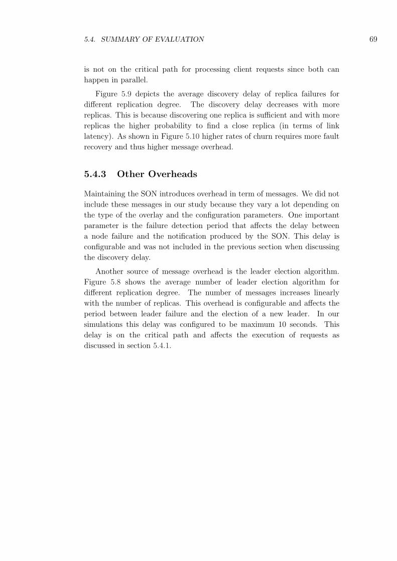
5.4. SUMMARY OF EVALUATION 69
is not on the critical path for processing client requests since both can
happen in parallel.
Figure 5.9 depicts the average discovery delay of replica failures for
different replication degree. The discovery delay decreases with more
replicas. This is because discovering one replica is sufficient and with more
replicas the higher probability to find a close replica (in terms of link
latency). As shown in Figure 5.10 higher rates of churn requires more fault
recovery and thus higher message overhead.
5.4.3 Other Overheads
Maintaining the SON introduces overhead in term of messages. We did not
include these messages in our study because they vary a lot depending on
the type of the overlay and the configuration parameters. One important
parameter is the failure detection period that affects the delay between
a node failure and the notification produced by the SON. This delay is
configurable and was not included in the previous section when discussing
the discovery delay.
Another source of message overhead is the leader election algorithm.
Figure 5.8 shows the average number of leader election algorithm for
different replication degree. The number of messages increases linearly
with the number of replicas. This overhead is configurable and affects the
period between leader failure and the election of a new leader. In our
simulations this delay was configured to be maximum 10 seconds. This
delay is on the critical path and affects the execution of requests as
discussed in section 5.4.1.


Chapter 6
Conclusion
In this report, we presented an approach to achieve robust management
elements that will simplify the construction of autonomic managers. The
approach uses replicated state machines and relies on our proposed
algorithm to automate replicated state machine migration in order to
tolerate churn. The algorithm uses symmetric replication, which is a
replication scheme used in structured overlay networks, to decide on the
placement of replicas and to monitor them. The replicated state machine
is used, beside its main purpose of providing the service, to process
monitoring information and to decide when to migrate. Although in this
paper we discussed the use of our approach to achieve robust management
elements, we believe that this approach might be used to replicate other
services in structured overlay networks in general.
6.1 Answers to Research Questions
Let us now address those research questions that I mentioned in the
introduction of this report:
71

72 CHAPTER 6. CONCLUSION
RQ-01 : Replication by itself is not enough to guarantee long
running services in the presence of continuous churn. This
is because the number of failed nodes hosting ME replicas
will increase with time. Eventually this will cause the
service to stop. Therefore, we use service migration [8]
to enable the reconfiguration of the set of nodes hosting
ME replicas. However, all this process should be self-
automated. How to automate re-configuration of replica
set in order to tolerate continuous churn?
Findings This report proposed a decentralized algorithm 5 that
will use migration to automatically reconfigure the set of
nodes hosting ME replicas. It contains a special module
called Container that exist on all nodes of the overlay
and is responsible for monitoring and detecting changes in
the replica set caused by churn. More detail is given in
section sec:handlingchurn.
RQ-02 : Reconfiguration or migration of MEs will cause extra delay
in request processing. How to minimize this effect?
Findings As described in section 3.3.7, we proposed to reduce
migration time by letting all replicas in a configuration
to choose a common leader before starting the leader-
election process. For example, every replica when starts
choose replica with lowest rank as the default leader. This
would mean to start the prepare face immidiately without
waiting for leader-election to choose a leader. In addition
to that, number of migrations can be controlled using
Fault-Tolerance as described in section 3.3.7.
RQ-03 : Replication of MEs will result in extra overhead on the
performance of the system. How to control this extra
overhead?
Findings Replication of MEs does have an impact on the request
latency if we compare it with a non-replicated ME.
However, in a RSM, increasing this replication degree
further does not increase the request latency as shown in
figure 5.4. This is with the assumption that processing
time of messages on any replica is zero. On the other
hand, SMART and failure replica discovery messsages does
increase due to increase in replication degree. This can be
further controlled and optimized using Fault-Tolerance
as described in section 3.3.7.

6.1. ANSWERS TO RESEARCH QUESTIONS 73
RQ-04 : When a migration request is submitted and decided,
according to SMART, on excution of migrate request,
leader in the configuration will assign its LastSlot, send
JOIN message to host machines in the NextConf and will
propose null requests for all the remaining unproposed
slots until the LastSlot. However, the solution is unclear
if another configuration change request has already been
proposed. It might happen, due to high churn rate, that
multiple configuration change requests are submitted to
the leader at the same time. If two configuration change
will be executed by the same configuration, it could result
in having multiple NextConf with the same ConfID i.e.
duplicate and redundant configuratons. How to avoid this
scenario?
Findings To avoid having this situation, as shown in algorithm 3
and described in section 3.3.6 , everytime a ConfChange
request is executed, it will replace at position r in the
configuration array with the reference of the node who
requested this change. This way, only one NextConf will
be created. This will make sure to avoid any conflicts due
to multiple configurations with the same ConfId and also
to have redundant configurations.
RQ-05 : How to make the system scalable i.e. how to control the
system performance when it is overloaded and churn rate
is high?
Findings When the system is overloaded with client’s requests,
the performance of the system can be optimized by
incrementing the pipeline i.e. the number of requests being
handled in parallel. However, in overloaded scenarios,
the churn or migration effect can become obvious. The
maximum impact of Churn or Migration happens when a
leader replica fails. As shown in figure 5.11, churn effect can
be further controlled using Fault-Tolerance i.e. waiting
for a certain number of replica failures before deciding to
migrate.

74 CHAPTER 6. CONCLUSION
RQ-06 : How overlay node count effects the performance of
replicated MEs?
Findings As shown in figure 5.5, overlay node count does
not seems to have any impact over message overhead
(SMART+Paxos). However, increase in overlay node count
is slighly increasing the client request latency. This is due
to the fact that if there are more nodes in the overlay,
the replicas will be more widely dispersed inside SON. As
we are using King Latency Map for network delay, so the
more replicas will be dispersed, the more time it will take
for communication with each other.
RQ-07 : We have assumed a fair-loss model of message dilvery. That
means, some messages can be lost even when sending them
to alive replicas. How to handle these lost messages.
Findings To increase the probability of handling every message sent
by the clients, every client will submit the requests to each
replica in a RSM. Each non-leader replica, on recieving the
message, will forward the message to the leader replica,
which will ignore duplicate messages. This approach
might result in overloading leader with too many messages,
especially when the degree of replication is large. To avoid
this situation, there is another mechanism that has been
tested. Each recieved message should be tagged with the
recieved timestamp and should be stored by each replica
in a pending requests queue. Periodically, every repica
checks the pending requests queue and if a request has
been in the pending list for a long time, it is retransmitted
to the leader. More detail is described in section 3.3.3 and
algorithm 4. Once the request is decided, it is removed
from the pending list.
RQ-08 : What are the factors other than replication and request
frequency that can influence the performance of a
replicated state machine?
Findings There are many other factors that can influence the
performance of RME system. Most important of these are:
failure detection time (the time to detect a failure), leader
election time, churn rate and the fault-tolerance factor.
If the failure detection and leader election time is short,
it will reduce discovery delay, however, it will put an
extra burden of running these protocol too often i.e. more
messages. So these parameters should be chosen carefully.

6.2. SUMMARY AND FUTURE WORK 75
6.2 Summary and future work
In order to validate and evaluate our approach, we have implemented a
prototype that includes the proposed algorithms. We conducted various
simulation tests that validated our approach and showed its performance
in various scenarios. In our future work, we will integrate the implemented
prototype with the Niche platform to support robust management elements
in self-managing distributed applications. We also intend to optimise the
algorithm in order to reduce the amount of messages and we will investigate
the effect of the publish/subscribe system used to construct control loops
and try to optimise it. In addition to that, we will verify how our proposal
works in overlays other than Chord. This will give us good understanding
of how generic our approach is. Finally, we will try to apply our approach
to other problems in the field of distributed computing.


Bibliography
[1] P. Horn. Autonomic computing: IBM’s perspective on the state of
information technology, October 15 2001. [cited at p. 1]
[2] IBM. An architectural blueprint for autonomic computing,
4th edition. http://www-03.ibm.com/autonomic/pdfs/
AC Blueprint White Paper 4th.pdf, June 2006. [cited at p. 1, 7]
[3] Ahmad Al-Shishtawy, Joel Hoglund, Konstantin Popov, Nikos
Parlavantzas, Vladimir Vlassov, and Per Brand. Enabling self-
management of component based distributed applications. In
Thierry Priol and Marco Vanneschi, editors, From Grids to Service
and Pervasive Computing, pages 163–174. Springer US, July 2008.
[cited at p. 1, 7, 27]
[4] Niche homepage. [cited at p. 1, 27]
[5] Ahmad Al-Shishtawy, Vladimir Vlassov, Per Brand, and Seif Haridi. A
design methodology for self-management in distributed environments.
In Computational Science and Engineering, 2009. CSE ’09. IEEE
International Conference on, volume 1, pages 430–436, Vancouver, BC,
Canada, August 2009. IEEE Computer Society. [cited at p. 1]
[6] Konstatin Popov. D1.5 full specification and final prototypes of overlay
services. Technical report, European Commission. [cited at p. vii, 1, 2, 7,
8, 9]
[7] Jacob R. Lorchand Atul Adyaand William J. Boloskyand Ronnie
Chaikenand John R. Douceur and Jon Howell. The smart way to
migrate replicated stateful services. In Proceedings of the 2006 EuroSys
Conference, Leuven, Belgium, April 2006. ACM. [cited at p. 2]
[8] Jacob R. Lorch, Atul Adya, William J. Bolosky, Ronnie Chaiken,
John R. Douceur, and Jon Howell. The SMART way to migrate
77

78 BIBLIOGRAPHY
replicated stateful services. SIGOPS Oper. Syst. Rev., 40(4):103–115,
2006. [cited at p. 2, 3, 21, 31, 32, 39, 72]
[9] L. Lamport. Paxos made simple. In ACM SIGACT News 32, 2001.
[cited at p. 3, 12, 13, 15, 18]
[10] Ahmad Al-Shishtawy, Muhammad Asif Fayyaz, Konstantin Popov, and
Vladimir Vlassov. Achieving robust self-management for large-scale
distributed applications. [cited at p. 5]
[11] E. Bruneton, T. Coupaye, and J.B. Stefani. The fractal component
model. Technical report, France Telecom R&D and INRIA, 2004.
[cited at p. 7, 23]
[12] Distributed Control Loop Patterns for Managing Distributed
Applications, 2008. [cited at p. 9]
[13] Joseph S. Kong, Jesse S. Bridgewater, and Vwani P. Roychowdhury.
Resilience of structured p2p systems under churn: The reachable
component method. Computer Communications, 31(10):2109–2123,
June 2008. [cited at p. 11, 49, 53, 85, 87]
[14] I. Stoica, R. Morris, D. Karger, M.F. Kaashoek, and H. Balakrishnan.
Chord: A scalable peer-to-peer lookup service for internet applications.
In Proceedings of the ACM SIGCOMM ’01 Conference, pages 149–160,
San Diego, California, August 2001. [cited at p. 11]
[15] Ali Ghodsi. Distributed k-ary System: Algorithms for Distributed
Hash Tables. PhD thesis, Royal Institute of Technology (KTH), 2006.
[cited at p. 12, 30, 38]
[16] Jim Gray and Leslie Lamport. Consensus on transaction commit. ACM
Trans. Database Syst. 31(1): 133-160, 2006. [cited at p. 13]
[17] Paxos algorithm. [cited at p. 14]
[18] Fred B. Schneider. Implementing fault-tolerant services using the state
machine approach : A tutorial. ACM Computing Surveys, Vol. 22, No.
4, 1990. [cited at p. 15]
[19] Yair Amir and Jonathan Kirsch. Paxos for system builders. In
Proceedings of the 2008 Workshop on Large-Scale Distributed Systems
and Middleware (LADIS 2008), Yorktown, NY, September 2008.
[cited at p. 15, 49]

79
[20] Rachid Guerraoui and Lus Rodrigues. Introduction to Reliable
Distributed Programming. Springer Berlin Heidelberg New York.
[cited at p. 19]
[21] F. Oprea D. Malkhi and L. Zhou. Omega meets paxos: Leader election
and stability without eventual timely links. In Proceedings of 19th
International Conference on Distributed Computing (DISC’05), pages
199–213, December 2005. [cited at p. 19, 20, 21, 33, 48]
[22] Leslie Lamport. Paxos made simple. SIGACT News, 32(4):51–58,
December 2001. [cited at p. 21]
[23] Cosmin Arad, Jim Dowling, and Seif Haridi. Building and evaluating
p2p systems using the kompics component framework. In IEEE P2P
2009. [cited at p. vii, 22, 23, 24, 25]
[24] Cosmin Arad, Jim Dowling, and Seif Haridi. Developing, simulating,
and deploying peer-to-peer systems using the kompics component
model. In Proceedings of the Fourth International ICST Conference on
COMmunication System softWAre and middlewaRE table of contents
Dublin, Ireland. [cited at p. 22]
[25] Kompics. [cited at p. 22, 23]
[26] Cosmin Arad and Seif Haridi. Practical protocol composition,
encapsulation and sharing in kompics. [cited at p. 22, 23]
[27] Apache mina. [cited at p. 25]
[28] Krishna P. Gummadi, Stefan Saroiu, and Steven D. Gribble. King:
Estimating latency between arbitrary internet end hosts. In To
appear in the Proceedings of SIGCOMM IMW 2002, November 2002,
Marseille, France. [cited at p. 25]
[29] C. Arad, J. Dowling, and S. Haridi. Building and evaluating p2p
systems using the kompics component framework. In Peer-to-Peer
Computing, 2009. P2P ’09. IEEE Ninth International Conference on,
pages 93 –94, sept. 2009. [cited at p. 43, 53]
[30] D. Leonard, Zhongmei Yao, V. Rai, and D. Loguinov. On lifetime-
based node failure and stochastic resilience of decentralized peer-to-
peer networks. Networking, IEEE/ACM Transactions on, 15(3):644
–656, june 2007. [cited at p. 49, 53, 85, 87]

80 BIBLIOGRAPHY
[31] Meridian: A lighweight approach to network positioning. http://www.
cs.cornell.edu/People/egs/meridian. [cited at p. 53]
[32] Krishna P. Gummadi, Stefan Saroiu, and Steven D. Gribble.
King: estimating latency between arbitrary internet end hosts. In
IMW ’02: Proceedings of the 2nd ACM SIGCOMM Workshop on
Internet measurment, pages 5–18, New York, NY, USA, 2002. ACM.
[cited at p. 53, 55, 85, 88]

Appendices
81


Appendix A
How to use our Prototype
We have made a prototype implementation of our proposed model using
kompics framework. A framework for testing has also been implemented
where user can define tests in a file and can run the tests for a longer
duration of time. In this chapter, we will describe how the user can use this
test framework. The package can be provided to the user on request.
A.1 Package Contents
The provided package will contain the follwing important files:
niche.jar Protype implementation of our proposed model.
log4j.properties For defining log level.
tests.in Fefined experiments.
NicheExperiments.class Experiment test framework main class.
Stats.class Class to calcualte the result statistics.
TestResult.class Class to process the results.
A.2 Defining Experiments
A test framework is provided with our protype that can be used to run a
batch of experiments. These experiments are defines in file tests.in. The
83

84 APPENDIX A. HOW TO USE OUR PROTOTYPE
sytax to define tests is as follows:
TestCycles
OverlayNodeCount
ReplicationDegree
TolerateFailures
SensorCount
SensorStartDelayInMin
SensorRequestAvgIntervalInMs
TestDurationInMin
nodeAverageLifeTime
linkLatency
seed
F-ReplicaNumber-Interval
Here is the decription of the parameters;
TestCycles Number of cycles for a particular test.
OverlayNodeCount These number of nodes will be created in Kompics
Chord overlay before starting the experiment.
ReplicationDegree Number of RMEs in an RSM.
TolerateFailures This will instruct the experiment to weight for give
number of failure of replicas in an RSM before deciding to migrate.
SensorCount Number of clients/sensors making the requests to the RSM.
SensorStartDelayInMin Delay for the sensors before starting the
requests. Sensors should be started after enough time e.g. 60
minutes, for the system to initialize itself properly.
SensorRequestAvgIntervalInMs Sensor request frequency depends
upon this parameter. This specifies the mean average interval
between two requests of the sensor. The sensor request model is
defined using life-base model with shifted pareto distribution.
TestDurationInMin Test Duration in Minutes. Test duration starts after
the sensors start making the requests.

A.3. DEFINING LOG LEVELS 85
nodeAverageLifeTime This is an alpha value for lifetime-based node
failure model [13, 30] with shifted Pareto lifetime Distribution. Used
to generate Churn in the system. A zero value means no churn.
linkLatency Should be set to 0. 0 means the King [32] technique.
Otherwise the specified value will be used as latency for every link in
the system.
seed A random value for the initialization of the system.
F-ReplicaNumber-Interval should be set to NoExplicitFailure.
A test file tests.in is provided with the package and it already has
some sample defined experiments. A chunk of experiments, from this file, is
shown below. In these experiments, we are testing the effect of replication
degree on the system. The replication degree varies from 1 to 25 while 1
means no replication.
1 500 1 1 4 60 4000 480 0 0 0 NoExplicitFailure
1 500 5 1 4 60 4000 480 0 0 0 NoExplicitFailure
1 500 10 1 4 60 4000 480 0 0 0 NoExplicitFailure
1 500 15 1 4 60 4000 480 0 0 0 NoExplicitFailure
1 500 20 1 4 60 4000 480 0 0 0 NoExplicitFailure
1 500 25 1 4 60 4000 480 0 0 0 NoExplicitFailure
A.3 Defining Log Levels
User can define log levels for the experiment inside log4j.properties
file. This file is provided as part of the package. The main module of the
experiments is log4j.logger.se.kth.niche whos level is set to OFF.
The user can increase the loglevel by changing its value. The available log
levels are: TRACE, DEBUG, INFO, WARN, ERROR, FATAL.
When the tests are executed, the results and logs will be generated in a
folder named “Log“. This Log folder will be created in the same directory
as the executable jar file. Some of the important log files are:
smart.log This will log information about the migrations and replica
failures happening inside the system.

86 APPENDIX A. HOW TO USE OUR PROTOTYPE
niche.log General logging of the system
nichedelay.log Logging recovery delay for each replica failure.
sensorXXX.log Information about sensor requests and the latency of each
request is logged here.
Once a test is complete, a subdirectory inside Log will be created and
these log files will be moved to that directory.
A.4 Running Experiments
After defining the experiments, the user can start the tests using the
following command.
>>java -jar NicheExperiments tests.in
If the tests has been defined in a file different than tests.in, provide
the name of that test file instead of tests.in above.
A.5 Collecting Results
All the defined tests in the file are executed in sequence. If any of the test
is complete, it’s result will be logged in file Tests.result with its unique
testId. The result of an experiment is a single line and consists of following
values in the sequence described:
TestCycles
OverlayNodeCount
ReplicationDegree
TolerateFailures
SensorCount
SensorStartDelayInMin
SensorRequestAvgIntervalInMs
TestDurationInMin
nodeAverageLifeTime
linkLatency

A.5. COLLECTING RESULTS 87
seed
totalSensorRequest
averageRequestLatency
averageLinkDelay
averageNicheDelay
nicheMsgCountPerReplicaPerMinute (Paxos+SMART)
nicheEldMsgCountPerReplicaPerMinute
nicheRecoveryMsgCountPerReplicaPerMinute
leaderReplicaFailureCount
nonLeaderReplicaFailureCount
unknownReplicaFailureCount
Decription of these results values are:
TestCycles Number of cycles for a particular test.
OverlayNodeCount These number of nodes will be created in Kompics
Chord overlay before starting the experiment.
ReplicationDegree Number of RMEs in an RSM.
TolerateFailures This will instruct the experiment to weight for give
number of failure of replicas in an RSM before deciding to migrate.
SensorCount Number of clients/sensors making the requests to the RSM.
SensorStartDelayInMin Delay for the sensors before starting the
requests. Sensors should be started after enough time e.g. 60
minutes, for the system to initialize itself properly.
SensorRequestAvgIntervalInMs Sensor request frequency depends
upon this parameter. This specifies the mean average interval
between two requests of the sensor. The sensor request model is
defined using life-base model with shifted pareto distribution.
TestDurationInMin Test Duration in Minutes. Test duration starts after
the sensors start making the requests.
nodeAverageLifeTime This is an alpha value for lifetime-based node
failure model [13, 30] with shifted Pareto lifetime Distribution. Used
to generate Churn in the system. A zero value means no churn.
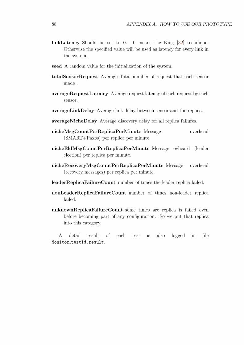
88 APPENDIX A. HOW TO USE OUR PROTOTYPE
linkLatency Should be set to 0. 0 means the King [32] technique.
Otherwise the specified value will be used as latency for every link in
the system.
seed A random value for the initialization of the system.
totalSensorRequest Average Total number of request that each sensor
made .
averageRequestLatency Average request latency of each request by each
sensor.
averageLinkDelay Average link delay between sensor and the replica.
averageNicheDelay Average discovery delay for all replica failures.
nicheMsgCountPerReplicaPerMinute Message overhead
(SMART+Paxos) per replica per minute.
nicheEldMsgCountPerReplicaPerMinute Message ovheard (leader
election) per replica per minute.
nicheRecoveryMsgCountPerReplicaPerMinute Message overhead
(recovery messages) per replica per minute.
leaderReplicaFailureCount number of times the leader replica failed.
nonLeaderReplicaFailureCount number of times non-leader replica
failed.
unknownReplicaFailureCount some times are replica is failed even
before becoming part of any configuration. So we put that replica
into this category.
A detail result of each test is also logged in file
Monitor testId.result.

Appendix B
Experiment Result Data
B.1 Variable Replication Degree
Fixed Test Parameters:
Replication Degree = 500, Fault-Tolerance = 1, Sensor Count = 4, Sensor
Request Frequency = 4000, Test Duration = 8 hours.
Table columns:
Replication Degree, Churn Rate, Total Client Requests, Avg Request
Latency, Avg Discovery Delay, Avg Msg Overhead, Avg Leader Election
Msg Overhead, Avg Discvoery Msg Overhead, Avg Leader Replica Failure,
Avg Replica Failure
1 0 29067 134.27 0 121.11 0 0 0 0
5 0 28729 276.92 0 287.3 432.49 0 0 0
10 0 28357 303.97 0 289.48 928.71 0 0 0
15 0 28612 295.44 0 294.08 1420.96 0 0 0
20 0 28407 284.56 0 292.95 1911.99 0 0 0
25 0 28654 272.31 0 296.1 2399.4 0 0 0
5 30 28548 258.09 626.73 285.27 410.45 1.99 11.9 45.2
10 30 28761 349.97 619.28 297.17 849 5.53 10.15 97.85
15 30 28864 298.94 465.96 301.14 1207.29 6.05 10.43 138.43
20 30 28649 363.11 530.36 309.99 1621.92 9.53 8.64 194.82
25 30 28761 380.41 451.87 320.46 1975.36 11.07 13.25 236.85
89

90 APPENDIX B. EXPERIMENT RESULT DATA
5 90 28801 264.11 616.96 288.72 427.06 0.81 6.67 20.67
10 90 28773 339.12 560.82 294.96 881.63 2.04 4.79 46.43
15 90 28589 306.34 435.02 299.38 1356.73 2.65 4.64 70.86
20 90 28874 319.9 478.15 309.84 1842.23 4.5 6.21 97.43
25 90 28801 283.09 397.43 314.9 2268.62 4.95 5.27 122.88
5 150 28528 256.04 666.33 286.36 434.09 0.52 3.29 13.36
10 150 28529 299.67 628.73 293.34 911.23 1.96 3.21 31.71
15 150 28523 272.06 437.79 298.26 1385.97 1.86 4.21 51.5
20 150 28362 284.76 486.28 302.39 1876.76 3.09 3 71.79
25 150 28531 306.95 394.85 307.99 2342.49 3.11 3.92 81.15


www.kth.se
TRITA-ICT-EX-2010:99