achieving sub-pixel geolocation accuracy in support of ... · achieving sub-pixel geolocation...

Achieving sub-pixel geolocation accuracy in support of MODIS

land science

Robert E. Wolfe a,b,*, Masahiro Nishihama a,b, Albert J. Fleig a,c, James A. Kuyper a,d,David P. Roy a,e, James C. Storey b,f, Fred S. Patt g,h

aLaboratory for Terrestrial Physics (Code 922), NASA Goddard Space Flight Center, Greenbelt, MD 20771, USAbRaytheon ITSS, 4400 Forbes Blvd., Lanham, MD 20706, USA

cPITA Analytic Sciences, 8705 Burning Tree Rd, Bethesda, MD 20817, USAdSAIC GSC, Seabrook, MD 20706, USA

eDepartment of Geography, 1113 LeFrak Hall, University of Maryland, College Park, MD 20742, USAfUnited States Geological Survey, EROS Data Center, Sioux Falls, SD 57198, USA

gLaboratory for Hydrospheric Processes (Code 970.2), NASA Goddard Space Flight Center, Greenbelt, MD 20771, USAhSAIC GSC, Beltsville, MD 20705, USA

Received 19 May 2001; received in revised form 24 February 2002; accepted 6 March 2002

Abstract

The Moderate Resolution Imaging Spectroradiometer (MODIS) was launched in December 1999 on the polar orbiting Terra spacecraft and

since February 2000 has been acquiring daily global data in 36 spectral bands—29 with 1 km, five with 500 m, and two with 250 m nadir pixel

dimensions. The Terra satellite has on-board exterior orientation (position and attitude) measurement systems designed to enable geolocation

of MODIS data to approximately 150 m (1r) at nadir. A global network of ground control points is being used to determine biases and trends in

the sensor orientation. Biases have been removed by updating models of the spacecraft and instrument orientation in the MODIS geolocation

software several times since launch and have improved the MODIS geolocation to approximately 50 m (1r) at nadir. This paper overviews thegeolocation approach, summarizes the first year of geolocation analysis, and overviews future work. The approach allows an operational

characterization of the MODIS geolocation errors and enables individual MODIS observations to be geolocated to the sub-pixel accuracies

required for terrestrial global change applications.

D 2002 Elsevier Science Inc. All rights reserved.

1. Introduction

The Moderate Resolution Imaging Spectroradiometer

(MODIS) science team has developed remote sensing

algorithms for deriving global time-series data products

on various geophysical parameters that are used by the

Earth science community (Salomonson, Barnes, Maymon,

Montgomery, & Ostrow, 1989). Accurate operational geo-

location is required to generate these products; in particular,

to generate the temporally composited MODIS products

and to support MODIS change detection and retrieval of

biophysical parameters over heterogeneous land surfaces

(Justice et al., 1998; Roy, 2000; Townshend, Justice,

Gurney, & McManus, 1992). The MODIS Land Science

Team requires the geolocation accuracy to be 150 m (1r),with an operational goal of 50 m (1r) at nadir (Nishihama et

al., 1997). This accuracy requirement and goal guides the

design of the MODIS geolocation algorithm and error

analysis approach.

Satellite data production systems operationally register

different orbits of data by geometric correction of each orbit

into a common Earth-based coordinate system. Geometric

correction is necessary to remove distortions introduced by

the instrument sensing geometry, the curvature of the Earth,

surface relief, and perturbations in the motion of the sensor

relative to the surface. Geometric correction can be consid-

ered a two-stage process: first the sensed observations are

geolocated, and then they are gridded into a predefined

georeferenced grid. The geometric distortions present in

satellite data may be categorized into system-dependent and

system-independent distortions. System-dependent geomet-

ric distortions are introduced by the sensor. System-inde-

0034-4257/02/$ - see front matter D 2002 Elsevier Science Inc. All rights reserved.

PII: S0034 -4257 (02 )00085 -8

* Corresponding author. Laboratory for Terrestrial Physics (Code 922),

NASA Goddard Space Flight Center, Greenbelt, MD 20771, USA.

E-mail address: [email protected] (R.E. Wolfe).

www.elsevier.com/locate/rse

Remote Sensing of Environment 83 (2002) 31–49

pendent distortions are introduced by the motion of the

sensor, oblateness and rotation of the Earth, and surface

relief. Correction for these distortions can be performed

using parametric and/or nonparametric approaches. Non-

parametric approaches require the identification of distinct

features that have known locations, usually termed ground

control points (GCPs), to model the spatial relationship

between the sensed data and an Earth based coordinate

system. The spatial relationships are assumed to be repre-

sentative of the geometric distortions and are used to

calculate mapping functions, for example polynomial func-

tions (Bernstein, 1983). Nonparametric approaches can

correct all types of geometric distortion (Roy, Devereux,

Grainger, & White, 1997). However, nonparametric

approaches are not suitable for the operational correction

of satellite data because accurate GCPs are expensive to

collect and may not be available over homogeneous,

unstructured, and cloudy scenes. In addition, the sun–

target–sensor geometry, used in the generation of many of

the MODIS land products (e.g., Schaaf et al., 2002, this

issue; Vermote, El Saleous, & Justice, 2002, this issue), must

be estimated when nonparametric approaches are used (Roy

& Singh, 1994). Parametric approaches require information

concerning the sensing geometry (interior orientation) and

the sensor attitude and position (exterior orientation), which

describe the circumstances that produced the sensed image.

GCPs may be used to correct errors in the sensor interior and

exterior orientation knowledge (Emery & Ikeda, 1989;

Moreno & Melia, 1993; Rosborough, Baldwin, & Emery,

1994). Relief information is required to remove relief dis-

tortion effects that are dependent upon the sensing altitude,

the terrain height, and the distance of the terrain from nadir

(Schowengerdt, 1997).

MODIS is on board the Terra, and planned Aqua, satellite

which benefits from accurate and rapid measurement of the

satellite exterior orientation. Consequently, the MODIS geo-

location is performed using a parametric approach with GCPs

only used to remove orientation biases and trends. The Terra

exterior orientation is measured in real time by sensors on

board the satellite. The attitude is measured by on-board

inertial gyro and star-tracking sensors and the position is

measured by the Tracking Data Relay Satellite System

(TDRSS) On-board Navigation System (TONS) (Folta,

Elrod, Lorenz, & Kapoor, 1993; Teles, Samii, & Doll,

1995). The MODIS and Terra interior orientation parameters

are characterized prior to launch (Barnes, Pagano, & Salo-

monson, 1998; Silverman & Linder, 1992). A global digital

elevation model (DEM) (Logan, 1999) is used to model and

remove relief distortion effects. The MODIS geolocation

product defines the geodetic latitude and longitude (WGS-

84), sensor and solar geometry, slant range, and terrain height

of the sensed MODIS 1 km observations. These data are

subsequently used to spatially resample and temporally

composite MODIS products into georeferenced grids.

Improvements to the MODIS geolocation accuracy are

made by the adjustment of the sensor interior parameters

with future planned work to remove systematic exterior

orientation measurement errors. The information required

to perform these improvements is derived by an error

analysis and reduction methodology based on comparison

of sensed MODIS data with a global distribution of GCPs. At

the time of writing three adjustments have been made since

launch. This paper overviews the geolocation approach,

summarizes the first year of geolocation analysis, and over-

views future work.

2. MODIS instrument geometry

The Terra, and planned Aqua, spacecraft orbit the Earth

at an altitude of 705 km in a near polar orbit with an

inclination of 98.2j and a mean period of 98.9 min

(Salomonson et al., 1989). Terra’s sun-synchronous orbit

has a dayside equatorial 10:30 am local crossing time and a

16-day repeat cycle. MODIS has a 110j across-track field ofview and senses the entire equator every 2 days with full

daily global coverage above approximately 30j latitude

(Wolfe, Roy, & Vermote, 1998). MODIS senses in 36

spectral bands from the visible to the thermal infrared—29

with 1 km (at nadir) pixel dimensions, five with 500 m

pixels, and two with 250 m pixels (Barnes et al., 1998;

SBRC, 1992). MODIS is a paddle broom (sometimes called

a whiskbroom) electro-optical instrument that uses the

forward motion of the satellite to provide the along-track

direction of scan (Fig. 1). The electromagnetic radiation

(EMR) reflected or emitted from the Earth is reflected into

the instrument telescope by a rotating two-sided scan mirror.

One-half revolution of the scan mirror takes approximately

1.477 s and produces the across-track scanning motion. The

EMR is then focused onto separate calibrated radiation

detectors covered by narrow spectral band-pass filters.

MODIS simultaneously senses, in each band, 10 rows of

1 km detector pixels, 20 rows of 500 m detector pixels, and

40 rows of 250 m detector pixels. Each row corresponds to a

single scan line of MODIS data that is nominally composed

of 1354 1 km, 2708 500 m, and 5416 250 m observations.

The MODIS detectors are grouped on four focal planes—

Long Wave Infrared (LWIR), Short/Medium Wave Infrared

(SWIR/MWIR), Near Infrared (NIR), and Visible (VIS)

(Salomonson et al., 1989). Detectors for each band are laid

out on the focal planes in the along-scan direction (Figs. 1

and 2) causing the same Earth location to be sampled at

different times by different bands. The times that the

MODIS scan mirror passes each of 24 encoder positions

during the Earth-view portion of the scan is measured

electro-optically. These timing data are subsequently used

to compute the scan angle of the MODIS observations. Each

1 km, 500 m, and 250 m observation is sampled in 333.333,

166.667, and 83.333 As, respectively. To allow for detector

readout, the detector integration time is 10 As less than the

data-sampling rate at each of the three MODIS resolutions.

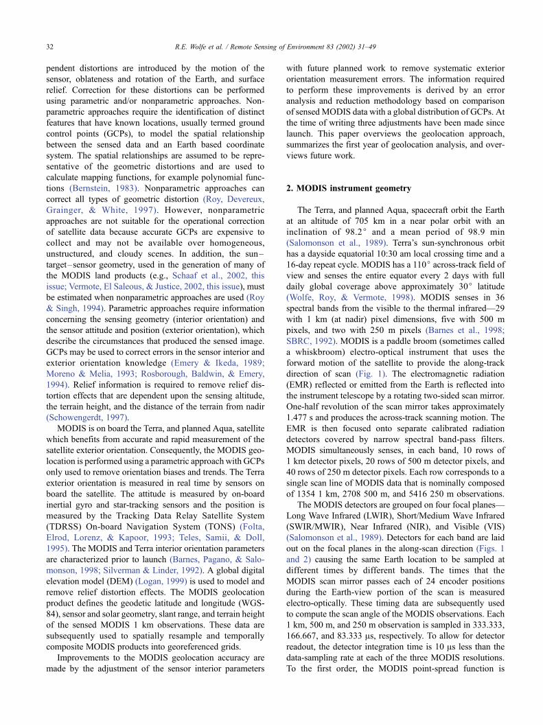
To the first order, the MODIS point-spread function is

R.E. Wolfe et al. / Remote Sensing of Environment 83 (2002) 31–4932

triangular in the scan direction (Fig. 3). The centers of the

integration areas of the first observation in each scan are

aligned, in a ‘‘peak-to-peak’’ alignment (Fig. 3). In the track

direction, the point-spread function is rectangular and the

observations at the different resolutions are nested, allowing

four rows of 250 m observations and two rows of 500 m

Fig. 2. Along-scan layout of the MODIS focal planes showing the detector locations with respect to the reference optical axis. Vertically (not shown) are 10

addition sets of detectors for a total of 10, 20 and 40 detectors for each of the 1 km (bands 8–36), 500 m (bands 3–7), and 250 m (bands 1 and 2) bands,

respectively, that make up a single MODIS scan. Band 0 is a hypothetical band used in the geolocation calculations.

Fig. 1. Overview of MODIS sensing geometry. A scan of MODIS data is sensed over a half revolution of the MODIS double-sided scan mirror and is focused

onto four focal planes containing a total of 310, 100, and 80 detectors that sense the 1 km, 500 m, and 250 m bands, respectively (36 bands). The instantaneous

sensing of the four co-registered focal planes is shown, illustrating the MODIS ‘‘paddle broom’’ sensing geometry.

R.E. Wolfe et al. / Remote Sensing of Environment 83 (2002) 31–49 33

observations to cover the same area as one row of 1 km

observations.

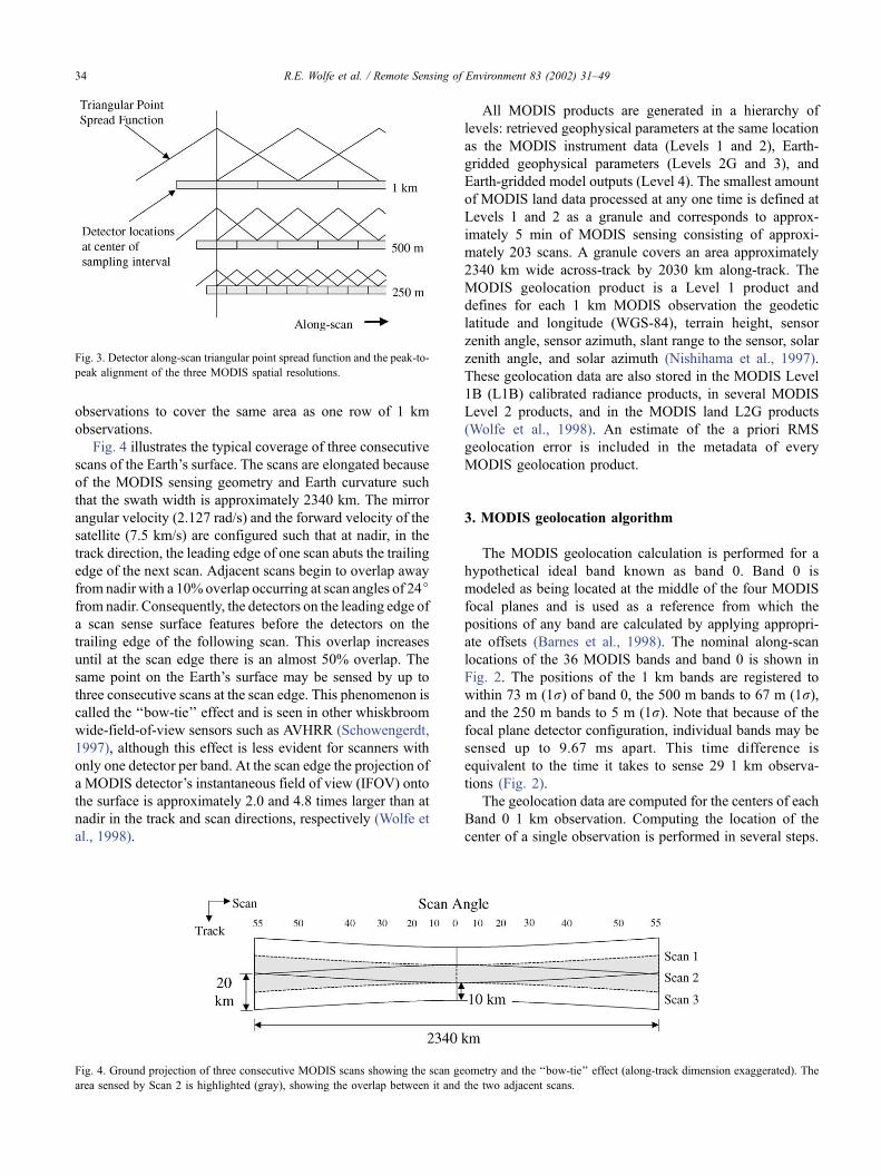
Fig. 4 illustrates the typical coverage of three consecutive

scans of the Earth’s surface. The scans are elongated because

of the MODIS sensing geometry and Earth curvature such

that the swath width is approximately 2340 km. The mirror

angular velocity (2.127 rad/s) and the forward velocity of the

satellite (7.5 km/s) are configured such that at nadir, in the

track direction, the leading edge of one scan abuts the trailing

edge of the next scan. Adjacent scans begin to overlap away

from nadir with a 10% overlap occurring at scan angles of 24jfrom nadir. Consequently, the detectors on the leading edge of

a scan sense surface features before the detectors on the

trailing edge of the following scan. This overlap increases

until at the scan edge there is an almost 50% overlap. The

same point on the Earth’s surface may be sensed by up to

three consecutive scans at the scan edge. This phenomenon is

called the ‘‘bow-tie’’ effect and is seen in other whiskbroom

wide-field-of-view sensors such as AVHRR (Schowengerdt,

1997), although this effect is less evident for scanners with

only one detector per band. At the scan edge the projection of

a MODIS detector’s instantaneous field of view (IFOV) onto

the surface is approximately 2.0 and 4.8 times larger than at

nadir in the track and scan directions, respectively (Wolfe et

al., 1998).

All MODIS products are generated in a hierarchy of

levels: retrieved geophysical parameters at the same location

as the MODIS instrument data (Levels 1 and 2), Earth-

gridded geophysical parameters (Levels 2G and 3), and

Earth-gridded model outputs (Level 4). The smallest amount

of MODIS land data processed at any one time is defined at

Levels 1 and 2 as a granule and corresponds to approx-

imately 5 min of MODIS sensing consisting of approxi-

mately 203 scans. A granule covers an area approximately

2340 km wide across-track by 2030 km along-track. The

MODIS geolocation product is a Level 1 product and

defines for each 1 km MODIS observation the geodetic

latitude and longitude (WGS-84), terrain height, sensor

zenith angle, sensor azimuth, slant range to the sensor, solar

zenith angle, and solar azimuth (Nishihama et al., 1997).

These geolocation data are also stored in the MODIS Level

1B (L1B) calibrated radiance products, in several MODIS

Level 2 products, and in the MODIS land L2G products

(Wolfe et al., 1998). An estimate of the a priori RMS

geolocation error is included in the metadata of every

MODIS geolocation product.

3. MODIS geolocation algorithm

The MODIS geolocation calculation is performed for a

hypothetical ideal band known as band 0. Band 0 is

modeled as being located at the middle of the four MODIS

focal planes and is used as a reference from which the

positions of any band are calculated by applying appropri-

ate offsets (Barnes et al., 1998). The nominal along-scan

locations of the 36 MODIS bands and band 0 is shown in

Fig. 2. The positions of the 1 km bands are registered to

within 73 m (1r) of band 0, the 500 m bands to 67 m (1r),and the 250 m bands to 5 m (1r). Note that because of the

focal plane detector configuration, individual bands may be

sensed up to 9.67 ms apart. This time difference is

equivalent to the time it takes to sense 29 1 km observa-

tions (Fig. 2).

The geolocation data are computed for the centers of each

Band 0 1 km observation. Computing the location of the

center of a single observation is performed in several steps.

Fig. 4. Ground projection of three consecutive MODIS scans showing the scan geometry and the ‘‘bow-tie’’ effect (along-track dimension exaggerated). The

area sensed by Scan 2 is highlighted (gray), showing the overlap between it and the two adjacent scans.

Fig. 3. Detector along-scan triangular point spread function and the peak-to-

peak alignment of the three MODIS spatial resolutions.


First, the line-of-sight ufoc from each detector of a band is

generated in the focal plane coordinate system:

ufoc ¼ ðx; y; f Þ

where (x, y) are the positions of the detector focal plane

coordinates and f is the focal length (bold is used to denote

matrices throughout this paper). The line-of-sight is then

rotated from the focal plane (foc) to the telescope (tel)

coordinate system and then to the instrument (inst) coordinate

system:

uimg ¼ Tinst=telTtel=focufoc

(In this paper we use the symbolTsys2/sys1 to represent a 3 by 3

transformation matrix that rotates a 3-vector from coordinate

system sys1 to sys2. For instance, Tinst/tel rotates a vector

from the telescope to the instrument coordinate system.) The

Tinst/tel rotation matrix includes a rotation of the focal planes

by � 0.129j about the center of the telescope reference

optical axis (bore-sight) to compensate for the along-track

movement of 65.2 m during the 9.67 ms elapsed time

between the sensing of the detectors located at the leading

and trailing edges of the focal plane (Fig. 2).

One of the key elements of the MODIS geometric model

is the mirror model. Because it is impossible to manufacture

a two-sided mirror with perfectly parallel sides and align the

mirror perfectly with the mirror rotation axis, three angles are

used to characterize the mirror surfaces and to construct the

normal to the mirror surfaces (Fig. 5). The normal for each

mirror side are:

nside1 ¼

�sinb2þ c

� �

sina2

� �cos

b2þ c

� �

cosa2

� �cos

b2þ c

� �

266666664

377777775

ð1Þ

nside2 ¼

�sinb2� c

� �

sina2

� �cos

b2� c

� �

�cosa2

� �cos

b2� c

� �

266666664

377777775

where a, b, and c are shown in Fig. 5.

Using the time of the observation, t, the angle of rotation

of the scan mirror h is determined and the normal to the

rotating scan mirror nsidei for mirror side i is constructed in

the scan mirror (mirr) coordinate system. The mirror normal

is rotated to the instrument reference frame:

ninst ¼ Tinst=mirrTðhÞrotnsidei

A Chebyshev polynomial interpolation technique is used

to interpolate between the encoder times (Preus, Flannery,

Teukolsky, & Vetterling, 1988) to obtain the scan mirror

angle h at observation time t. The line-of-sight vector is

reflected by the scan mirror, computed by:

uinst ¼ uimg � 2ninstðuimg � ninstÞ

The satellite position peci and velocity veci are defined in

the Earth Centered Inertial (ECI) coordinate system and the

satellite attitude (nr, np, ny) is defined in the spacecraft

reference frame. At time t a composite transformation

matrix is constructed to rotate from the instrument coordi-

nate system, through the spacecraft (sc), orbital (orb), and

ECI coordinate systems, to the Earth Centered Rotating

(ECR) coordinate system:

Tecr=inst ¼ TðtÞecr=eciTðpeci; veciÞeci=orb

� Tðnr; np; nyÞorb=scTsc=inst ð2Þ

The line-of-sight and the satellite position are then

rotated to ECR coordinates:

uecr ¼ Tecr=instuinst

pecr ¼ TðtÞecr=ecipeci

The intersection of the line-of-sight with the WGS-84

ellipsoid (DMA, 1987) xellip is then calculated as:

xellip ¼ pecr þ duecr

The ellipsoid intersection is calculated by turning the

problem into a unit sphere intersection problem (by inde-

pendently rescaling the components of each vector by the

inverse of the length of the corresponding ellipsoid axis) and

is trigonometrically solved for the slant range d.

An iterative search process is used to follow the line-of-

sight from the instrument to the intersection of the terrain

surface represented by a DEM. Complex relief does not

Fig. 5. Three angles (wedge angles a and b, and axis error c) used to

characterize the two surfaces of the MODIS scan mirror. Angle d is not

used in the described error analysis because it does not have a significant

geometric impact.


confuse this technique because the search is in a downward

direction. The search begins by computing the angle v

between the line-of-sight unit vector uecr and ellipsoid

normal n computed at the ellipsoid intersection:

cosv ¼ uecr � n

Using a precompiled maximum local terrain height,

Hmax, the ECR coordinates of the search starting point

xmax are:

xmax ¼ xellip þHmax

cosvuecr

Starting at xmax, the ith iteration of the search is per-

formed by computing the ECR coordinates of the search

point:

xi ¼ xmax þ idsuecr

where ds is the step size. The DEM height at the latitude and

longitude of each search point is calculated using bilinear

interpolation. The search stops when the DEM height is

higher than the search point height. The terrain intersection

is then linearly interpolated from the point at which the

search stopped xk and the previous search point xk� 1.

The height, geodetic latitude and longitude at the inter-

section are stored in the geolocation product. Subsequently,

the slant range to the sensor, sensor zenith angle, and sensor

azimuth are computed and stored for each intersection. In

addition, the solar zenith and azimuth are computed from

the observation time and geodetic latitude and longitude

using standard astronomical models (Standish, Newhall,

Williams, & Yeomans, 1992).

4. Error sources

The Terra exterior orientation is estimated from star

tracker, inertial gyro and TONS navigation data streams

that are combined using a Kalman filter (Folta et al., 1993).

The interior orientation parameters are characterized prior to

launch by the instrument and spacecraft builders (Barnes

et al., 1998; Silverman & Linder, 1992). A number of error

sources are anticipated that include errors in the exterior and

interior orientation, digital elevation model errors, and errors

due to refraction and aberration.

Errors in sensor attitude (due to exterior or interior

orientation errors) will induce geolocation displacements

that are directly proportional to the attitude error, the sensor

altitude, local Earth curvature (ignoring terrain effects), and

the scan angle (Nishihama et al., 1997). Roll attitude errors

cause along-scan geolocation displacements that are asym-

metric over the sensor field of view and increase from

minimum displacements at nadir to maximum displace-

ments at large scan angles. Yaw and pitch errors cause very

small along-scan geolocation displacements that increase in

a symmetrical nonlinear manner, from zero displacement at

nadir to larger displacements for scan angles further off

nadir. In the track direction, pitch errors cause displacements

that are almost constant over the sensor field of view, roll

errors cause no displacement, and yaw errors cause dis-

placements that behave in a similar manner to the along-

scan yaw displacements but are larger. Roll and pitch

attitude errors cause the greatest geolocation displacements

at nadir in the scan and track direction, respectively. For

example, a 10 arc-sec error in roll causes an along-scan 34

m displacement at nadir and a 165 m error at the edge of the

scan (at 55j scan angle). The same error in pitch causes a 34

m and 39 m along-track displacement at nadir and at the

edge of the scan, respectively. Yaw displacements, for a 10

arc-sec error, increase from zero at nadir to 56 m in the track

direction at the edge of the scan. Along and across-track

sensor position measurement errors will cause directly

proportional displacements in the planimetric geolocation

position. Altitude position measurement errors will cause

along-scan displacements that are proportional to the alti-

tude error and increase with scan angles further from nadir.

Tables 1 and 2 summarize error estimates of the interior

orientation and the exterior attitude orientation, expressed as

roll, pitch, and yaw errors. These errors are broken down

into dynamic and static components (Fleig, Hubanks,

Storey, & Carpenter, 1993). They include errors expected

Table 1

MODIS interior orientation knowledge

Roll Pitch Yaw

Dynamic terms

Bearings 0 3.3 6.5

Mirror control system 12.4 0 0

Scan angle measurement 3.7 0 0

Neighboring EOS instrument dynamics 6.7 6.7 6.7

Scan mirror assembly to spacecraft interface

thermal and structural distortion

1.7 1.7 1.7

Optical bench assembly to spacecraft interface


1.7 1.7 1.7

Optical bench assembly distortion

(including telescope)

1.7 1.7 1.7

Other dynamic errors 3.3 3.3 3.3

Total Dynamic (RSS) 15.2 8.6 10.3

Static Terms

Scan mirror assembly to spacecraft interface


6.7 6.7 6.7

Optical bench assembly to spacecraft interface


6.7 6.7 6.7

Optical bench assembly distortion

(including telescope)

5 5 5

Spectral band registration error 2.4 2.4 2.4

Instrument and spacecraft mate errors 5 5 5

Scan mirror assembly to optical

bench measurement error

1.7 1.7 1.7

Alignment cube angle measurement error 1.7 1.7 1.7

Cooler launch errors 2.4 2.4 0

Scan axis to mounting feet alignment 3.3 3.3 3.3

Other static errors 3.3 3.3 3.3

Total Static (RSS) 13.4 13.4 13.1

All errors expressed as roll, pitch and yaw errors (1r, arc-seconds).


as a result of satellite launch and on-orbit errors due to

thermal and structural distortions. It is expected that the

errors summarized in Tables 1 and 2 contribute approxi-

mately 117 m (1r) to the total geolocation error at nadir,

increasing to 385 m (1r) at 55j scan angle. In addition to

these, TONS planimetric position measurement errors are

expected to introduce approximately 20 m (1r) along-trackand 11 m (1r) along-scan displacements for all scan angles.

TONS position altitude measurement errors (4 m, 1r) areexpected to cause along-scan geolocation displacements

from zero at nadir to 7 m (1r) at 55j scan angle. The ratio

of the dynamic and static components of these errors are

estimated to be 59:41. Fig. 6 illustrates geolocation dis-

placement error ellipses at nadir (solid lines) and at the scan

edge (dotted lines) for all the error components (i.e., Tables

1 and 2, and the TONS position errors). Both the static and

dynamic error components are illustrated. The along-scan

component is 41% larger than the along-track component at

nadir, and 249% larger at 55j scan angle. If the static errors

are removed, the total remaining error is expected to be 47

m (1r) at nadir and 166 m (1r) at 55j scan angle.

Although the DEM is used to remove relief effects,

residual geolocation errors may be introduced because of

errors in the DEM, errors introduced by interpolating the

line-of-sight intersection in the DEM, and high frequency

relief variations occurring within each IFOV. The MODIS

DEM is defined with a 30 arc-sec pixel dimension (0.925

km at the equator) and is derived from a number of different

data sources including aggregated data from the National

Imaging and Mapping Agency (NIMA) and Digital Chart of

the World data (Gesch, Verdin, & Greenlee, 1999; Logan,

1999). The NIMA data, which covers 73% of the land

surface, has a 59 m (RMSE) height error (Gesch, 1998) with

other areas less accurate. DEM elevation errors will induce

geolocation displacements that are proportional to the sens-

ing altitude, the terrain height, and the distance of the terrain

from nadir. For example, a 59 m DEM elevation error will

cause a 129 m geolocation displacement at 55j scan angle

in the scan direction, and negligible displacement ( < 4 m) in

the track direction. Line-of-sight intersection interpolation

errors, DEM resolution issues, and the variable MODIS

IFOV dimensions combine to introduce complex unmod-

eled location errors. More study is needed to understand the

nature and magnitude of these errors and the impact they

may have on MODIS geolocation, particularly in areas of

high spatial frequency relief.

The geolocation algorithm does not model refraction or

aberration. For nominal atmospheric conditions, the refrac-

tion of visible light at 55j scan angle is equivalent to an 11 mlocation displacement toward nadir in the scan direction

(Noerdlinger & Klein, 1995). We consider this error to be

negligible compared to the increase in the along-scan pro-

jected IFOV surface dimensions with scan angle. At nadir,

light takes 2.3 ms to travel from the surface to the MODIS

sensor. In this period, MODIS travels 17 m in the track

direction, an effect similar to a small pitch bias of 5 arc-sec.

Since we do not model refraction and aberration effects, they

will appear as small biases in the geolocation error analysis.

5. Ground control points

The MODIS operational geolocation error analysis and

reduction methodology uses a global distribution of land

GCPs to characterize and then remove some of the error

components discussed above. The MODIS geolocation

group has collaborated with the Terra and Landsat-7 instru-

ment teams to develop a library of land GCPs (Bailey et al.,

1997). A global distribution of 121 Landsat-4 and Landsat-5

Table 2

Terra interior (z) and exterior (*) orientation knowledge

Roll Pitch Yaw

Dynamic terms

Attitude determination * 3.2 3.9 2.4

Ephemeris error * 0.4 1 0.4

Structure dynamicsz 1 2 1.7

Thermal distortionz 4.3 4.2 2.1

Total dynamic (RSS) 5.5 6.1 3.6

Static Terms

Thermal distortionz 9.1 13.1 2.9

Moisture distortionz 5.9 4.6 1.5

Measurement errorz 5 5 5

Gravity effectsz 2.5 12.9 4.9

Launch shiftz 8 7.7 10.5

Star position knowledge * 1 1 1

Total static (RSS) 14.7 21.1 13.1

All errors expressed as roll, pitch and yaw errors (1r, arc-seconds). Inaddition to these, planimetric position measurement errors are expected to

be 20 m (1r) along-track and 11 m (1r) along-scan for all scan angles and

with altitude position measurement errors expected to be 4 m (1r).

Fig. 6. Geolocation displacement error ellipses at nadir (solid lines) and at

55j scan angles (dotted lines) for two cases: when both the static and

dynamic error components are considered, and when only the dynamic

components errors are considered. Errors are shown at the (1r) level andillustrate all the known expected error components (see Tables 1 and 2, and

the TONS position errors described in the text).


Fig. 7. Global distribution of 420 land ground control points (GCPs) extracted from 110 Landsat-4 and Landsat-5 TM scenes.

R.E.Wolfe

etal./Rem

ote

Sensin

gofEnviro

nment83(2002)31–49

38

precision geolocated terrain corrected TM scenes has been

obtained. Approximately five cloud-free GCPs are selected

from each TM scene to give a total of 605 land GCPs. The

latitude, longitude, and height of the GCPs are known to 15

m (1r). A 24 km2 image ‘‘chip’’, including the terrain height

at each 30 m TM pixel, is extracted around the GCP location

and stored in a GCP library. TM bands 3 (0.66 Am) and 4

(0.83 Am), comparable to the two MODIS 250 m bands 1

(0.645 Am) and 2 (0.859 Am), are stored. The locations of

the land GCPs are illustrated in Fig. 7. Approximately 50%

of the TM scenes are located along US coastlines, 25%

along a corridor from the Kara Sea in Russia to the southern

tip of Africa, and the remainder are distributed over South

America and Australia.

The Landsat GCPs are located in the sensed MODIS L1B

data by area-based matching. GCPs sensed by MODIS at

view zenith angles greater than 45j are not used as the

surface area sensed by the MODIS IFOV increases rapidly

above this zenith angle (Wolfe et al., 1998). Residual errors

between the known GCP locations and the corresponding

locations in the MODIS data are used in the geolocation

error and reduction analyses. GCP residuals are also used to

quantify the impact of changes to the interior orientation

parameters and exterior orientation biases. For this latter

purpose, the GCP residuals are normalized by dividing by

the dimension of the local MODIS observation IFOV in the

along-scan and along-track dimensions. In this way, the

GCP residuals are meaningfully expressed in nadir pixel

dimensions or equivalently in meters at nadir.

The GCP matching process is performed in several steps.

Spatially coincident MODIS L1B data, from one of the two

250 m bands, are compared with the corresponding 24 km2

TM GCP chip. The MODIS line-of-sight is initially com-

puted for the GCP location assuming perfect MODIS geo-

location. The TM chip is then spatially degraded to 250 m

using a MODIS point spread function (Barnes et al., 1998)

defined by the sensing geometry of each MODIS 250 m

observation intersecting the chip area. An area-based corre-

lation is computed between the MODIS 250 m and the TM

degraded data using a normalized gray-level correlation

technique (Pratt, 1991). This process is repeated; translating

the MODIS data over a regular grid of locations centered on

the line-of-sight initially computed assuming perfect MODIS

geolocation. The size and resolution of the grid are defined in

MODIS along-scan and across-scan angular space. The grid

point where the maximum correlation occurs defines the final

‘‘true’’ MODIS geolocation. The difference between the true

location and the initial location computed, assuming perfect

MODIS geolocation, defines the geolocation residual error.

In order to remove poorly matched GCPs, only those with

maximum correlation coefficients greater than 0.6 are con-

sidered. In this way inaccurate, out-of-date and out-of-season

GCPs, and GCPs contaminated by cloud and aerosols, are

less likely to be used.

Initially, after MODIS launch, the angular equivalent of

an at-nadir 2 km2 grid with a 50-m sampling interval was

used to perform the land GCP matching. After two updates

to the MODIS interior orientation parameters, the grid size

was reduced to an at-nadir equivalent of 400 m2 with a 25-m

sampling interval. This changed the best possible matching

precision, equal to one-half the step size, from 25 to 12.5 m.

6. Geolocation error analysis and reduction methodology

A deterministic least squares (minimum variance) esti-

mation is used to compute the sensor orientation parameters

that best fit the GCP data. Models of the interior and exterior

orientation parameters are described by linearized collinear-

ity equations, building on the mathematical foundation

described by Konecny (1976). These equations are used to

compute the along-track, across-track and radial position,

roll, pitch and yaw attitude angles, and mirror parameters,

and their rates of change (Nishihama et al., 1997). In this

process, all errors are assumed to be randomly distributed

with a mean of zero. Details of the method are given in

Appendix A. Initially after launch, it is not possible to

uniquely differentiate between attitude and position induced

geolocation errors. Consequently, the error analysis (Appen-

dix A) is initially performed holding certain parameters

fixed. Updates to the interior orientation parameters are

performed by modifying look-up-tables in the geolocation

software that define the transformation matrix elements used

by Eqs. (1) and (2). Reliable numerical solution of the

linearized collinearity equations without holding certain

parameters fixed may only be performed after initial updates

have been made.

Corrections of any systematic exterior orientation meas-

urement errors can only be performed after the sensor

interior orientation parameters are well defined. To date,

no explicit corrections of these measurement errors have

been performed, though implicit corrections may have been

made when the sensor interior orientation parameters were

updated. Similarly, updates of dynamic interior orientation

parameters (for example, associated with day-side/night-

side thermal flexing) will be performed. These updates will

either necessitate temporally parameterized adjustments to

the transformation matrix elements, or matrix elements

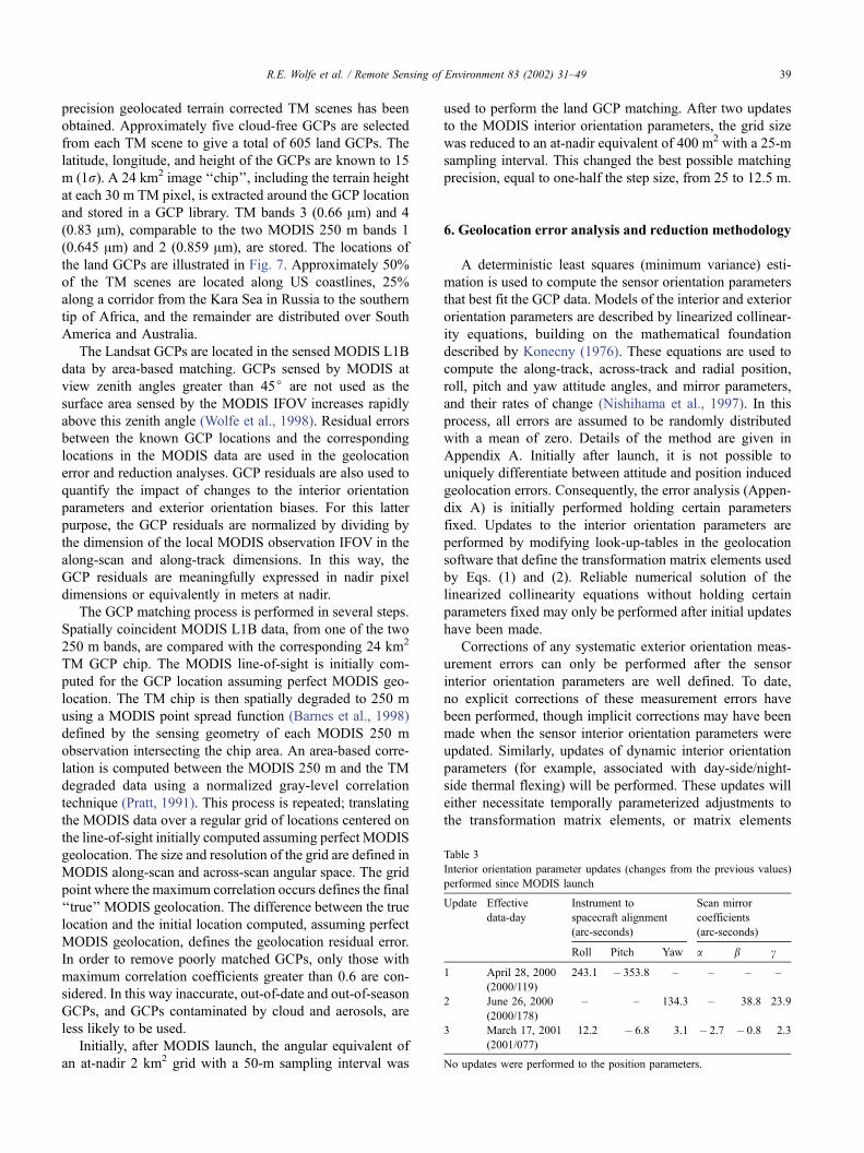
Table 3

Interior orientation parameter updates (changes from the previous values)

performed since MODIS launch

Update Effective

data-day

Instrument to

spacecraft alignment

(arc-seconds)

Scan mirror

coefficients

(arc-seconds)

Roll Pitch Yaw a b c

1 April 28, 2000

(2000/119)

243.1 � 353.8 – – – –

2 June 26, 2000

(2000/178)

– – 134.3 – 38.8 23.9

3 March 17, 2001

(2001/077)

12.2 � 6.8 3.1 � 2.7 � 0.8 2.3

No updates were performed to the position parameters.


parameterized with respect to the on-board instrument

engineering data stream (for example, on-board temper-

ature). Long-term changes will necessarily be removed only

after sufficient time-series analysis.

7. Results

This paper was written a little over one year after first

light from the MODIS instrument. At the time of writing

three updates have been made to the interior orientation

parameters describing the MODIS to Terra alignment and

the MODIS scan mirror alignment. These updates are

summarized in Table 3 and their impact on the MODIS

geolocation, summarized in Table 4 and illustrated in Fig. 8.

The results of these three updates are described in more

detail below.

In this paper geolocation errors are adjusted for scan

angle and expressed in nadir equivalent units. This indicates

the minimum error in meters over the MODIS field of view,

i.e., as if the data were sensed at nadir. The adjustments are

made by multiplying the geolocation error by the observa-

tion dimension at the scan angle and dividing by the

Table 4

Ground control point (GCP) residuals measured before and after updates to

the sensor interior orientation parameters (Table 3)

Update Number of

GCP residuals

Along-track

residuals (m)

Along-scan

residuals (m)

Mean Std.

Dev.

Mean Std.

Dev.

Measured

before Update 1

126 1273 281 1041 386

Measured

after Update 1

258 116 383 19 146

Measured

after Update 2

13,879 27 51 25 53

Measured

after Update 3

414 18 38 4 40

These results are adjusted for scan angle and shown in nadir equivalent

units.

Fig. 8. GCP residuals found immediately after launch (Table 4) and after

three interior orientation updates performed in the first year of MODIS

operations (Table 3). One standard deviation (1r) error bars about the mean

error are shown. These results are adjusted for scan angle and are shown in

nadir equivalent units. The 150 m (1r) geolocation accuracy specification

and 50 m (1r) operational goal are shown for comparative purposes.

Fig. 9. False color images illustrating at-launch MODIS geolocation (a),

and the geolocation after the first update to the MODIS interior orientation

was performed (b), for a 60 km2 area over the Gulf of Mexico coastline,

northwest Florida. MODIS Band 1 (0.645 Am) shown as red and spatially

degraded TM Band 4 (0.66 Am) shown as blue, with green set to zero. The

MODIS data were sensed on February 24, 2000, and the TM data were

sensed on October 3, 1993.


observation dimension at nadir. An approximation of the

geolocation error at any scan angle can be calculated by

multiplying the nadir equivalent error by the inverse of this

observation dimension ratio. However, such estimates will

only be representative of a large collection of MODIS data

and not of individual MODIS observations.

7.1. Initial analyses and first update

Immediately after first Earth-view data became available,

the geolocation accuracy was quantified by examination of

126 GCP residuals. This analysis gave a geolocation error

estimate of 1.3 km (0.3 km, 1r) and 1.0 km (0.4 km, 1r) atnadir in the track and scan directions, respectively (Table 4).

These geolocation errors were significantly greater than the

MODIS at-launch specification and were found to be

systematically mislocated. A unique solution of the linear-

ized collinearity equations (Appendix A) based on more

than a few parameters was not available. Consequently, as

roll and pitch attitude errors cause the greatest geolocation

displacements in the scan and track directions (at nadir),

respectively, a unique solution for adjustments to just these

two parameters was found by holding sensor yaw, scan

mirror, and spacecraft position parameters constant (Table

3). Fig. 9 illustrates the at-launch MODIS geolocation (a),

and the geolocation after this first update to the MODIS

interior orientation was performed (b). The figure shows

false color Landsat-5 TM data and MODIS 250 m data for a

60 km2 area of the Florida coastline. The MODIS data are

shown in red and the TM data are shown in blue. The TM

data were spatially degraded to 250 m using the MODIS

point spread function defined for the sensing geometry of

each MODIS 250 m observation. The MODIS at-launch

data (Fig. 9a) clearly exhibit along-track and smaller along-

scan displacements relative to the TM data. Some isolated

differences are also due to differences in the cloud cover and

Fig. 10. GCP residuals found after the first update to the interior orientation parameters (Table 3) plotted as a function of scan angle in the track (a) and scan (b)

directions. The 258 residuals are plotted to show the MODIS mirror sides used in the GCP matching process. These results are adjusted for scan angle and

shown in nadir equivalent units.


land-cover change that may have occurred between the

acquisitions of these data. Fig. 9b shows the impact of the

first update. The images are well matched and differences at

the 250 m resolution are difficult to discern visually.

An analysis of 258 GCP residuals, computed after the first

update was performed, indicated that the update reduced the

geolocation error substantially to a mean of 116 m along-

track with a standard deviation of 383 m, and 19 m (146 m,

1r) along-scan (Table 4). Fig. 10 shows along-track and

along-scan GCP residuals plotted as a function of scan angle.

The mirror side used to sense the L1B data containing the

matched GCP location is also shown, indicating geolocation

displacements that are strongly correlated with the mirror

side. In the track direction (Fig. 10a), the differences between

the two mirror sides are significant and the residuals are

asymmetrically distributed for scan angles either side of

nadir. In the scan direction (Fig. 10b), both the differences

between the mirror sides and the asymmetric distributions

either side of nadir are less apparent. These distributions are

most likely explained by remaining yaw attitude and scan

mirror coefficient errors.

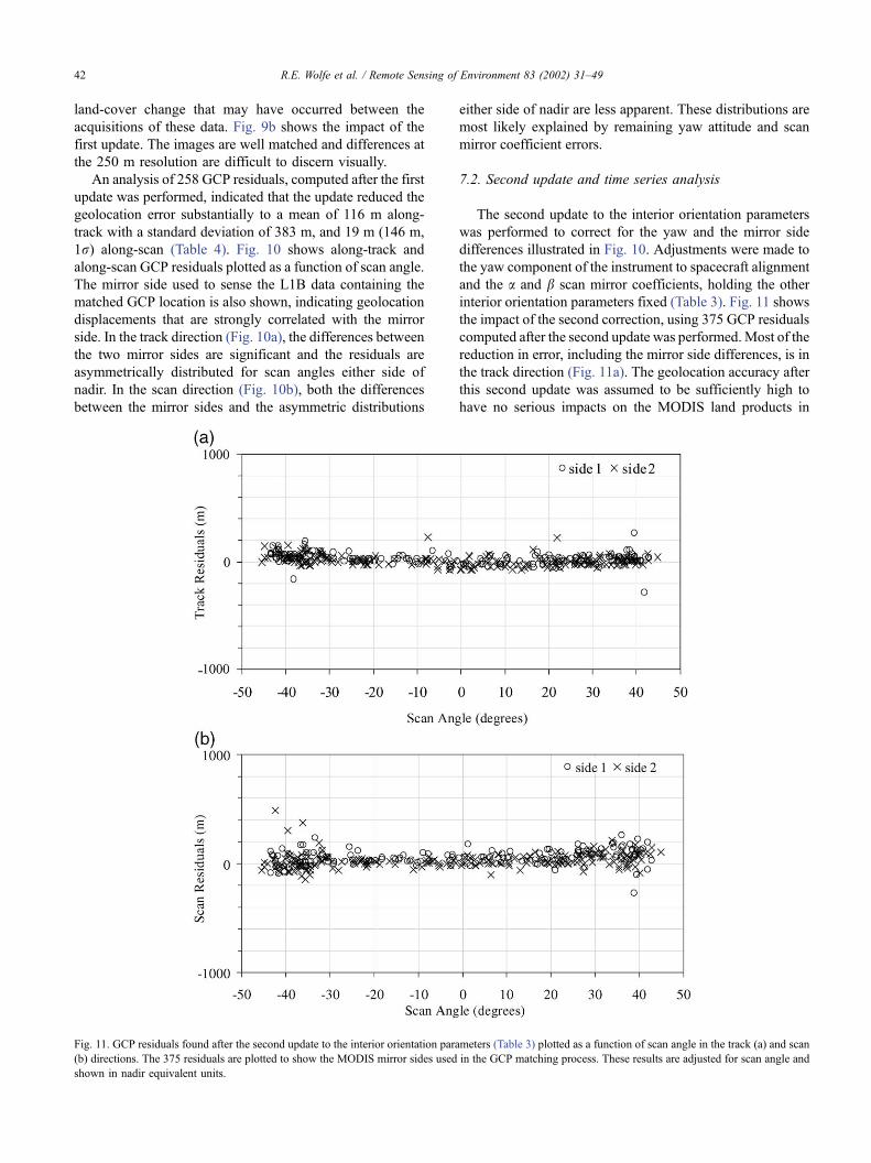
7.2. Second update and time series analysis

The second update to the interior orientation parameters

was performed to correct for the yaw and the mirror side

differences illustrated in Fig. 10. Adjustments were made to

the yaw component of the instrument to spacecraft alignment

and the a and b scan mirror coefficients, holding the other

interior orientation parameters fixed (Table 3). Fig. 11 shows

the impact of the second correction, using 375 GCP residuals

computed after the second update was performed. Most of the

reduction in error, including the mirror side differences, is in

the track direction (Fig. 11a). The geolocation accuracy after

this second update was assumed to be sufficiently high to

have no serious impacts on the MODIS land products in

Fig. 11. GCP residuals found after the second update to the interior orientation parameters (Table 3) plotted as a function of scan angle in the track (a) and scan

(b) directions. The 375 residuals are plotted to show the MODIS mirror sides used in the GCP matching process. These results are adjusted for scan angle and

shown in nadir equivalent units.


production at that time. Consequently, the interior orientation

parameters were not subsequently updated for a substantial

period to allow a long time-series of data to be analyzed.

Figs. 12–14 show GCP residuals computed fromMODIS

data sensed from data-days 2000/201 (July 19, 2000) to 2001/

031 (January 31, 2001). Note that data losses occurred from

data-days 2000/218 to 2000/232 when no useful calibrated

MODIS sensor data were available due to a problem with the

MODIS on-board data formatter. Analysis of 13,879 GCP

residuals collected over this period indicate that the second

update reduced the along-track and along-scan geolocation

mean error to 27 m (51 m, 1r) and 25 m (53 m, 1r),respectively (Table 4). These results are described in more

detail below.

Fig. 12 illustrates the overall mean and standard deviation

of the GCP residuals in the scan and track directions, as well

as the errors separately for each mirror side. The mirror side

biases appear to be approximately F 15 m in the scan and

F 10 m in the track direction and most likely correspond to

residual errors in the a, b, and c scan mirror coefficients (Fig.

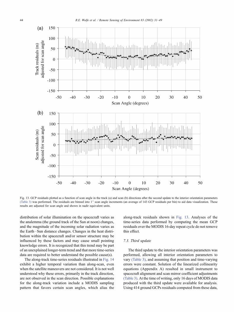
5). Fig. 13 illustrates the GCP residuals plotted as a function

of scan angle in the track (a) and scan (b) directions. To aid

visualization, the residuals are binned into 1j scan angle

increments. In the track direction the residuals increase from a

mean of 10 m at nadir to up to approximately 50 m at 45j offnadir. The magnitude of the along-track displacement toward

the scan edge is much larger than expected due to, for

example, a pitch bias. A better explanation for the cause of

this distribution may be a systematic error in the sensor

exterior orientation parameter timing in combination with

interior orientation biases. In the scan direction, the residuals

are distributed with a mean offset of approximately 25 m. A

small residual asymmetry as a function of scan angle is

evident, with an approximately 10-m difference from one

side of the scan to the other.

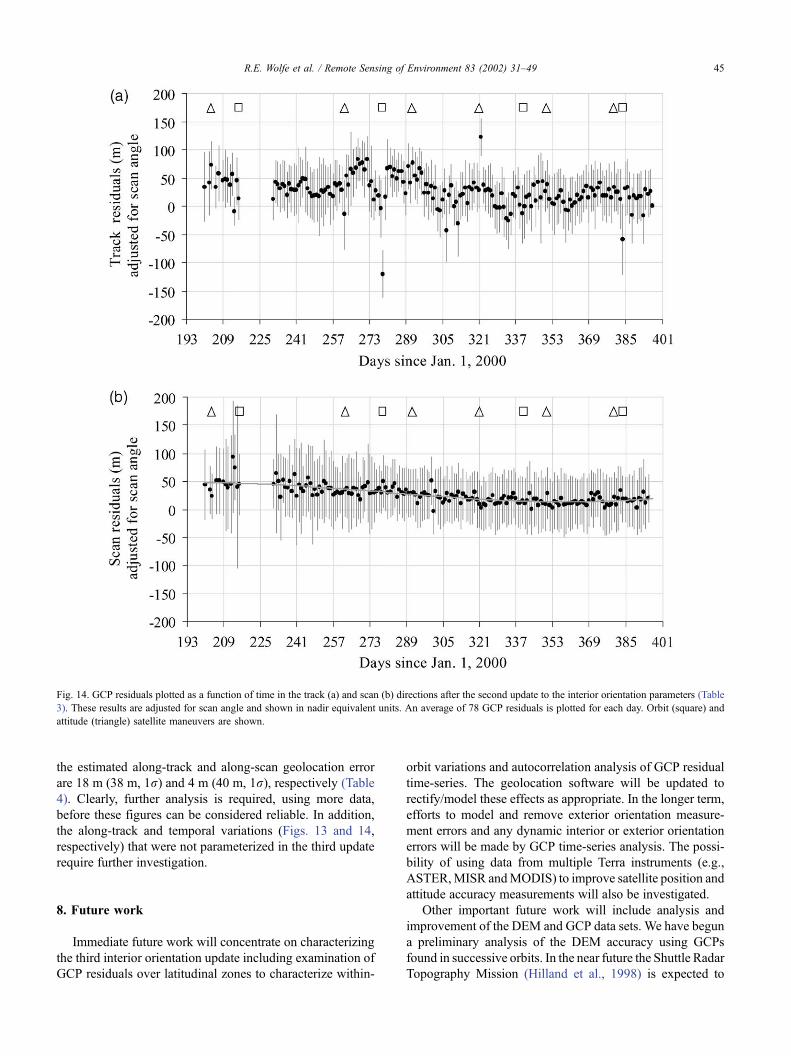
A time-series analysis of the GCP residuals was performed

to characterize any time-varying errors in the sensor interior

orientation parameters and exterior orientation measure-

ments. Fig. 14 shows the mean and the standard deviation

of the GCP residuals computed for each data-day plotted as a

function of time in the track (a) and scan (b) directions. The

daily standard deviations of the residuals are approximately

50 m in both the scan and the track directions. This indicates

that on a daily basis, the geolocation accuracy will fall within

the operational MODIS geolocation goal if the mean errors

can be removed. Note that the GCP matching grid resolution

changed on data-day 2001/276, improving the best possible

GCP matching precision from 25 to 12.5 m, which is

observed in the smaller error bars in Fig. 14b after this date.

Satellite maneuvers that occurred on data-days 2000/279,

2000/322, and 2000/384 (i.e., 2001/018) are clearly evident

in the along-track residuals shown in Fig. 14. Satellite orbit

maneuvers, mainly dragmakeup, but occasionally inclination

adjustment maneuvers, have been performed every 2 to 3

months since launch to maintain the Terra 16-day repeat

cycle. Satellite attitude roll maneuvers up to 20j have been

performed approximately once a month to allow MODIS to

view the moon near the scan edge for calibration and

characterization purposes. About 1 h before any maneuver,

the satellite attitude control system stops using star tracker

data and uses the less accurate on-board gyro data. The TONS

position data stream is not used during orbit maneuvers and

satellite position is determined from less accurate predicted

ephemeris data. After attitudemaneuvers, the satellite attitude

measurements take up to 1 h to return to their nominal

accuracy. After orbit (position) maneuvers, the TONS navi-

gation algorithms are re-initialized and the return to nominal

position accuracy takes more than 1 h. During any type of

maneuver, GCPs may fall outside the MODIS search grid

because of imprecision in the sensor exterior orientation

knowledge, so that no matches are found. At the beginning

and end of a maneuver, matches are more likely to be found

than during the maneuver, but with inflated residuals propor-

tionally related to the imprecision in the sensor exterior

orientation knowledge. Operational science algorithms that

rely on accurate geolocation should not use data sensed

during maneuvers. All GCP residuals collected during

maneuvers are excluded from the geolocation error analysis.

The time-series results shown in Fig. 14 exhibit a notice-

able temporal trend. In the scan direction (Fig. 14b), the mean

geolocation error is approximately 50 m at the beginning of

the time series (data-day 2000/201), and systematically

reduces to approximately 15 m by data-day 2000/362. This

trend also appears in the track direction (Fig. 14a) although it

is not as apparent because of high frequency residual varia-

tions. Currently, we are hypothesizing that this trend may be

related to the yearly solar cycle. During this cycle, the mean

Fig. 12. Mean GCP residuals (with 1r error bars) in the track and scan

directions after the second update to the interior orientation parameters

(Table 3) was performed. The 13,879 residuals are plotted to show the

MODIS mirror sides used in the GCP matching process. These results are

adjusted for scan angle and shown in nadir equivalent units.


distribution of solar illumination on the spacecraft varies as

the analemma (the ground track of the Sun at noon) changes,

and the magnitude of the incoming solar radiation varies as

the Earth–Sun distance changes. Changes in the heat distri-

bution within the spacecraft and/or sensor structure may be

influenced by these factors and may cause small pointing

knowledge errors. It is recognized that this trend may be part

of an unexplained longer-term trend and that more time-series

data are required to better understand the possible cause(s).

The along-track time-series residuals illustrated in Fig. 14

exhibit a higher temporal variation than along-scan, even

when the satellite maneuvers are not considered. It is not well

understood why these errors, primarily in the track direction,

are not observed in the scan direction. Possible explanations

for the along-track variation include a MODIS sampling

pattern that favors certain scan angles, which alias the

along-track residuals shown in Fig. 13. Analyses of the

time-series data performed by computing the mean GCP

residuals over the MODIS 16-day repeat cycle do not remove

this effect.

7.3. Third update

The third update to the interior orientation parameters was

performed, allowing all interior orientation parameters to

vary (Table 3), and assuming that position and time-varying

errors were constant. Solution of the linearized collinearity

equations (Appendix A) resulted in small instrument to

spacecraft alignment and scan mirror coefficient adjustments

(Table 3). At the time of writing, only 16 days ofMODIS data

produced with the third update were available for analysis.

Using 414 ground GCPs residuals computed from these data,

Fig. 13. GCP residuals plotted as a function of scan angle in the track (a) and scan (b) directions after the second update to the interior orientation parameters

(Table 3) was performed. The residuals are binned into 1j scan angle increments (an average of 143 GCP residuals per bin) to aid data visualization. These

results are adjusted for scan angle and shown in nadir equivalent units.


the estimated along-track and along-scan geolocation error

are 18 m (38 m, 1r) and 4 m (40 m, 1r), respectively (Table

4). Clearly, further analysis is required, using more data,

before these figures can be considered reliable. In addition,

the along-track and temporal variations (Figs. 13 and 14,

respectively) that were not parameterized in the third update

require further investigation.

8. Future work

Immediate future work will concentrate on characterizing

the third interior orientation update including examination of

GCP residuals over latitudinal zones to characterize within-

orbit variations and autocorrelation analysis of GCP residual

time-series. The geolocation software will be updated to

rectify/model these effects as appropriate. In the longer term,

efforts to model and remove exterior orientation measure-

ment errors and any dynamic interior or exterior orientation

errors will be made by GCP time-series analysis. The possi-

bility of using data from multiple Terra instruments (e.g.,

ASTER,MISR andMODIS) to improve satellite position and

attitude accuracy measurements will also be investigated.

Other important future work will include analysis and

improvement of the DEM and GCP data sets. We have begun

a preliminary analysis of the DEM accuracy using GCPs

found in successive orbits. In the near future the Shuttle Radar

Topography Mission (Hilland et al., 1998) is expected to

Fig. 14. GCP residuals plotted as a function of time in the track (a) and scan (b) directions after the second update to the interior orientation parameters (Table

3). These results are adjusted for scan angle and shown in nadir equivalent units. An average of 78 GCP residuals is plotted for each day. Orbit (square) and

attitude (triangle) satellite maneuvers are shown.


generate a more accurate and consistent DEM of most of the

land surface. We plan to incorporate these data once they

become available. We will clean the land GCP library,

looking for obvious biases in GCPs or GCPs that have

features that do not correlate consistently with MODIS data.

Some effort will be made to incorporate additional land GCPs

and refresh GCPs where necessary using Landsat-7 ETM+

data. In addition, we plan to use a global set of 6501 island

GCPs originally developed for the geolocation of SeaWIFS

data (Patt, Woodward, & Gregg, 1997). These island GCPs

are defined as the centroid of World Vector Shoreline (WVS)

island vectors with a location error of 250 m (1r). The islandGCPs will be located in the sensed MODIS L1B data by

feature extraction techniques.We expect that the global island

GCP library will be particularly useful in identifying and

characterizing anomalous cases during maneuvers and in

finding possible within-orbit variations.

MODIS data will be reprocessed several times over the

mission lifetime. During each of these reprocessing activities,

the most up-to-date geolocation parameters will be used to

ensure that the most accurate geolocation is produced. We

plan to use the same geolocation error analysis approach to

support the MODIS instrument on the Aqua spacecraft,

currently scheduled for launch in April 2002. The MODIS/

Aqua error reduction will be performed synergistically with

MODIS/Terra data and we expect the error reduction to be

achieved more rapidly.

9. Conclusion

The MODIS geolocation effort has successfully met its

initial objectives. We are able to provide MODIS Earth

location data to sub-pixel accuracy, approaching the opera-

tional MODIS geolocation goal of 50 m (1r) at nadir. Threeupdates to the parameters that define the Terra/MODIS

sensing geometry have been performed in the first year since

Terra launch. Provisional analysis of GCPs residuals com-

puted after the most recent update indicates a mean geo-

location error of 18 m across-track and 4 m along-scan, with

standard deviations of 38 and 40 m, respectively. There are

five factors that have contributed to this success. First, the

Terra spacecraft was built to provide a stable platform with

highly precise external orientation knowledge and very little

high frequency jitter. Second, the MODIS instrument was

built to provide a stable instrument with little random noise

and with precise interior orientation knowledge. Third, accu-

rate global DEM and GCP data sets were available. Fourth,

GCP matching was used to determine biases in the sensor

orientation. Finally, this bias information was used to provide

improved processing constants for subsequent geolocation

processing.

The sub-pixel accuracy provided by the MODIS geo-

location product is sufficient to allow the MODIS land

science team to create and analyze their science products

without incurring the delay and cost associated with improv-

ing the geolocation accuracy of individual data granules. In

coming years, we will look for any degradation in MODIS

geolocation accuracy and attempt to eliminate seasonal

variations or annual trend changes in the data to hold the

geolocation accuracy within the desired range. We believe

that this approach for obtaining accurate geolocation can be

applied operationally to other moderate spatial resolution

instruments on future missions such as the National Polar-

orbiting Operational Environmental Satellite System (NPO-

ESS) and the NPOESS Preparatory Project (NPP).

Acknowledgements

Accurate satellite geolocation requires contributions from

a large number of specialized groups. We would like to

recognize the contributions of the MODIS calibration and

characterization team; the GSFC Flight Dynamics, Attitude

Control, Terra Flight Operations and TONS groups; space-

craft builder Lockheed-Martin; instrument builder SBRS;

EOS SDP toolkit engineers; and the MODIS flight

operations team. The EOS DEM and GCP Science Working

Groups, the EROS Data Center, the MISR and ASTER

instrument teams, and the Landsat-7 project made additional

contributions. We would also like to thank Bert Guindon,

Hugh Kiefer, Chuck Wivell, Veljko Jovanovic, Alan

Strahler, and Peter Noerdlinger for many useful suggestions

in the original review of the MODIS geolocation approach.

This work was performed under the direction of the MODIS

Science Data Support Team and MODIS land science team

in the Terrestrial Information Systems Branch (Code 922) of

the Laboratory of Terrestrial Physics (Code 900) at NASA

GSFC. The work was funded under NASA GSFC contracts

NAS5-32350, NAS5-99085, NAS5-32373, and NASA

grant NCC5449-C.

Appendix A. Numerical error analysis

This appendix describes the observation equations solved

using a set of linearized collinearity equations to estimate

correction biases for the satellite position, attitude, and/or

scan mirror coefficients. The error analysis uses the GCP

residuals expressed as the view vector shift from the

observed to the true location. More details are described

in Nishihama et al. (1997) and USGS (1997).

A.1. Least squares method

All estimates are performed in the orbital coordinate

system. The error analysis is undertaken in the following

steps: (1) define the view vector as a function of the desired

parameters, (2) linearize the system and differentiate with

respect to the parameters, (3) define observation equations

using changes in view vectors to the ground, and (4) solve

the observation equations with the least squared method.


In the least squares method, the given observations Y and

the partial derivative coefficient matrix H are related to the

residual errors in the parameters X by:

Y ¼ HX ðA1ÞBy the least squared method, we estimate the residual

errors in the parameters as:

X ¼ ðHTHÞ�1ðHTYÞThe vector Y is made up of n 3-vectors Yi=(dy1,i, dy2,i,

dy3,i), each containing the difference between the true and

observed location in the orbital reference frame from GCP

residual i. The vectorX contains the corrections dxj to each of

m parameters xj. The coefficient matrix H contains 3n rows

and m columns. For each GCP residual i, the 3 row by m

column sub-matrix Hi contains a row for each of the three

components k of the observation. The row is made up of the

partial derivatives dyk,i/dxj of the component with respect to

each parameter being estimated.

This method can be used to solve for all parameters

simultaneously or for a subset of the parameters, holding the

reminder fixed. The following sections describe derivation

of the observation equations for the scan mirror coefficients,

satellite position, and satellite attitude. Derivations for rates

of change in these parameters are solved analytically in a

similar fashion (Nishihama et al., 1997).

A.2. Scan mirror wedge angles b and c, and axis angle acorrections

The normal to each mirror side are described in Eq. (1).

Let d be one of:

d1 ¼ b2þ c or d2 ¼ b

2� c ðA2Þ

The normal vector in Eq. (1) containing a small change ddin d from an initial value dd0 can be approximated for mirror

side 1 as:

n1 ¼ n1ðd0 þ ddÞc

�ðsind0 þ cosðd0ÞddÞ

sina2

� �ðcosd0 � sinðd0ÞddÞ

cosa2

� �ðcosd0 � sinðd0ÞddÞ

266664

377775

n1c

�sind0

sina2

� �cosd0

cosa2

� �cosd0

266664

377775þ

�cosðd0Þ

�sina2

� �sinðd0Þ

�cosa2

� �sinðd0Þ

266664

377775dd ðA3Þ

The normal vector for the mirror side 2 can be expressed

similarly. The view vector in the orbital coordinate system

uorb can be expressed as:

uorb ¼ Torb=scTsc=instuinst ¼ Torb=scTsc=instðuimg � 2ðBnÞ�ðuimg � BnÞÞ ðA4Þ

where uimg is the view vector in the instrument coordinate

system transformed from the line-of-sight vector from a

detector in a focal plane, and n is the normal vector to the

mirror surface as a function of d (Eq. (A3)), and:

B ¼ Tinst=mirrTðhÞrot

where h is the mirror scan angle. Differentiating Eq. (A4) as

function of d at the initial value d0, we have:

duorb ¼ Ddd

where D is a partial derivative matrix evaluated at d0.Replacing the above notations duorb and D with Yi and

Hi, respectively, for ith GCP residual, we have:

Yi ¼ Hidd Z Y ¼ Hdd Z dd ¼ ðHTHÞ�1ðHTYÞ

After using Eq. (A1) to separately estimate dd for each

mirror side (dd1, dd2), we derive db and dc from relation-

ships in Eq. (A2). Note that in Eq. (A1), HTH and HTY are

both scalar when estimating a single parameter. The deri-

vation for a follows a similar process.

A.3. Satellite position and attitude corrections

Let xcp=(xcp, ycp, zcp) be the true location of the GCP in

ECR coordinates, and p, v be the satellite ephemeris in ECR

coordinates. Define a view vector uecr from sensor to the

control point by:

uecr ¼xcp � p

jxcp � pj

Convert all the coordinates in ECR to the orbital coor-

dinates:

p ! ð0; 0; 0Þ; xcp ! x0 ¼ ðx0; y0; z0Þ and

uecr ! uorb ¼x0

jx0j

In terms of satellite position and attitude changes, the

difference between the view vector to the true GCP location

ucp and view vector to the observed control point uobsrv can

be expressed as sum of two parts by:

ucp � uobsrv ¼ ðucp � uobsrvÞposition þ ðucp � uobsrvÞattitude

A.3.1. Satellite position

Let x, y, and z be shifts in the satellite position in the

orbital coordinate system. A view vector to the GCP is given

by:

u ¼ ðx0 � x; y0 � y; z0 � zÞffiffiffiffiffiffiffiffiffiffiffiffiffiffiffiffiffiffiffiffiffiffiffiffiffiffiffiffiffiffiffiffiffiffiffiffiffiffiffiffiffiffiffiffiffiffiffiffiffiffiffiffiffiffiffiffiffiffiffiffiffiffiffiffiðx0 � xÞ2 þ ðy0 � yÞ2 þ ðz0 � zÞ2

q ¼ ðux; uy; uzÞ


By differentiating u with respect to x, y and z changes in

u can be approximated by:

ðucp � uobsrvÞposition ¼ �Q

dx

dy

dz

266664

377775

where Q is the partial derivative matrix. In Eq. (A1), for the

ith GCP residual, the above notations (ucp� uobsrv)positionand matrix Q are replaced with Yi and Hi, respectively.

A.3.2. Satellite attitude

Let uorb, usc, and uinst be a view vector in the orbital,

spacecraft, and instrument coordinate systems, respectively.

Then:

usc ¼ Tsc=instuinst

uorb ¼ Torb=scusc ¼ Fðnr; np; nyÞusc

where nr, np, and ny are attitude parameters for roll, pitch,

and yaw, respectively.

Let

X1 ¼ nr ¼ x01 þ x1; X2 ¼ np ¼ x02 þ x2;

X3 ¼ ny ¼ x03 þ x3

and

Torb=sc ¼

cosX3cosX2 � sinX3sinX1sinX2 �sinX3cosX1 cosX3sinX2 þ sinX3sinX1cosX2

sinX3cosX2 þ cosX3sinX1sinX2 cosX3cosX1 sinX3sinX2 � cosX3sinX1cosX2

�cosX1sinX2 sinX1 cosX1cosX2

266664

377775

Since xj are small angles we can use the approximation:

Torb=sccF0 þ F1x1 þ F2x2 þ F3x3

where Fj are 3� 3 partial derivate matrices with respect to

each parameter. So

uorb ¼ ðF0 þ F1x1 þ F2x2 þ F3x3ÞuscThe observation equation can then be written as:

ðucp � uobsrvÞattitude ¼ ½F1usc F2usc F3usc�

dx1

dx2

dx3

266664

377775

In Eq. (A1), for ith GCP residual the above notations

(ucp� uobsrv)attitude and [F1usc F2usc F3usc] are replaced with

Yi and Hi, respectively.

References

Bailey, G. B., Carneggie, D., Kieffer, H., Storey, J. C., Jovanovic, V. M., &

Wolfe, R. E. (1997). Ground Control Points for Calibration and Cor-

rection of EOS ASTER, MODIS, MISR and Landsat 7 ETM+ Data,

SWAMP GCP Working Group Final Report, USGS, EROS Data Cen-

ter, Sioux Falls, SD.

Barnes, W. L., Pagano, T. S., & Salomonson, V. V. (1998). Pre-launch

characteristics of Moderate Resolution Imaging Spectroradiometer

(MODIS) on EOS-AM1. IEEE Transactions on Geoscience and Remote

Sensing, 36, 1088–1100.

Bernstein, R. (1983). Image geometry and rectification. In R. N. Colwell

(Ed.),Manual of remote sensing (2nd ed.) (pp. 873–922). Falls Church,

VA: American Society of Photogrammetry.

DMA (1987). Defense Mapping Agency (DMA) Technical Report (TR),

Supplement to Department of Defense World Geodetic System 1984

(WGS84) Technical Report, TR 8350.2-A, prepared by the DMA

WGS84 Development Committee.

Emery, W. J., & Ikeda, M. (1989). AVHRR image navigation: summary and

review. Canadian Journal of Remote Sensing, 10, 46–56.

Fleig, A. J., Hubanks, P. A., Storey, J. C., & Carpenter, L. (1993). An

analysis of MODIS Earth Location Error, Version 2.0. Greenbelt,

MD: NASA Goddard Space Flight Center.

Folta, D. C., Elrod, B., Lorenz, M., & Kapoor, A. (1993). Precise naviga-

tion for the Earth Observing System (EOS)-AM1 spacecraft using the

TDRSS onboard navigation system (TONS). Advances in the astrono-

nautical sciences 84(1), ( pp. 103–123). San Diego, CA: Univelt.

Gesch, D. B. (1998). Accuracy assessment of a global elevation model using

Shuttle laser altimeter data. Proceedings, 1998 International Geosci.

and Remote Sensing Symposium, Seattle, Washington, ( pp. 840–842).

Gesch, D. B., Verdin, K. L., & Greenlee, S. K. (1999). New land surface

digital elevation model covers the Earth. Eos Transactions, American

Geophysical Union, 80(6), 69–70.

Hilland, J. E., Stuhr, F. V., Freedman, A., Imel, D., Shen, Y., Jordan, R., &

Caro, E. (1998). Future NASA Spaceborne SAR Missions. IEEE Aero-

space and Electronic Systems Magazine, (November 9–16).

Justice, C. O., Vermote, E., Townshend, J. R. G., Defries, R., Roy, D. P.,

Hall, D. K., Salomonson, V. V., Privette, J. L., Riggs, G., Strahler, A.,

Lucht, W., Myneni, R. B., Knyazikhin, Y., Running, S. W., Nemani,

R. R., Wan, Z., Huete, A. R., van Leeuwen, W., Wolfe, R. E., Giglio, L.,

Muller, J.-P., Lewis, P., & Barnsley, M. J. (1998). The Moderate Res-

olution Imaging Spectroradiometer (MODIS): land remote sensing for

global change research. IEEE Transactions on Geoscience and Remote

Sensing, 36, 1228–1249.

Konecny, G. (1976). Mathematical models and procedures for the geomet-

ric registration of remote sensing imagery. International Archives of

Photogrammetry and Remote Sensing, 21(3), 1–33.

Logan, T. L. (1999). EOS/AM-1 Digital Elevation Model (DEM) Data Sets:

DEM and DEM Auxiliary Datasets in Support of the EOS/Terra Plat-

form, JPL D-013508. Pasadena, CA: Jet Propulsion Laboratory, Cali-

fornia Institute of Technology.

Moreno, J. F., & Melia, J. (1993). A method for accurate geometric cor-

rection of NOAA AVHRR HRPT data. IEEE Transactions on Geosci-

ence and Remote Sensing, 31(1), 204–226.

Nishihama, M., Wolfe, R. E., Solomon, D., Patt, F. S., Blanchette, J., Fleig,

A. J., & Masuoka, E. (1997). MODIS Level 1A Earth Location Algo-

rithm Theoretical Basis Document Version 3.0, SDST-092, Lab. Terres-

trial Phys. Greenbelt, MD: NASA Goddard Space Flight Center.

Noerdlinger, P. D., & Klein, L. (1995). Theoretical Basis of the SDP Toolkit

Geolocation Package for the ECS Project, Technical Paper 445-TP-002-

002, EOSDIS Core System Project. Landover, MD: Hughes Applied

Information Systems.

Patt, F. S., Woodward, R., & Gregg, W. (1997). An automated method for

navigation assessment for Earth survey sensors using island targets.

International Journal of Remote Sensing, 18, 3311–3336.

Pratt, W. K. (1991). Digital image processing (2nd ed.) ( p. 663). New York:

John Wiley and Sons.

Preus, W., Flannery, B., Teukolsky, S., & Vetterling, W. (1988). Numerical

recipes in C. ( pp. 158–162). Cambridge, NY: Cambridge Univ. Press.

Rosborough, G. W., Baldwin, D. G., & Emery, W. J. (1994). Precise

AVHRR image navigation. IEEE Transactions on Geoscience and Re-

mote Sensing, 32(3), 644–657.


Roy, D. P. (2000). The impact of misregistration upon composited wide

field of view satellite data and implications for change detection. IEEE

Transactions on Geoscience and Remote Sensing, 38, 2017–2032.

Roy, D. P., Devereux, B., Grainger, B., & White, S. (1997). Parametric

geometric correction of airborne thematic mapper imagery. Internation-

al Journal of Remote Sensing, 18, 1865–1887.

Roy, D. P., & Singh, S. (1994). The importance of instrument pointing

accuracy for surface bidirectional reflectance distribution mapping. In-

ternational Journal of Remote Sensing, 15, 1091–1099.

Salomonson, V. V., Barnes, W. L., Maymon, P. W., Montgomery, H. E., &

Ostrow, H. (1989). MODIS: advanced facility instrument for studies of

the earth as a system. IEEE Transactions on Geoscience and Remote

Sensing, 27, 145–153.

SBRC (1992). The MODIS Technical Description Document (Preliminary),

document number DM VJ50-0073, prepared for National Aeronautics

and Space Administration (NASA) Goddard Space Flight Center

(GSFC) by Hughes Santa Barbara Research Center (SBRC), Santa

Barbara, CA.

Schaaf, C. B., Gao, F., Strahler, A. H., Lucht, W., Li, X., Tsang, T.,

Strugnell, N., Zhang, X., Jin, Y., Muller, J.-P., Lewis, P., Barnsley,

M., Hobson, P., Disney, M., Roberts, G., Dunderdale, M., d’Entremont,

R. P., Hu, B., Liang, S., Privette, J., & Roy, D. (2002). First Operational

BRDF, albedo and nadir reflectance products from MODIS. Remote

Sensing of Environment, 83, 135–148 (this issue).

Schowengerdt, R. A. (1997). Remote sensing models and methods for image

processing (2nd ed.) (pp. 100–109). San Diego: Academic Press.

Silverman, H., & Linder, D. (1992). Pointing and orbit study update, EOS-

AM, EOS-DN-SE&I-037. Valley Forge, PA: GE Astro-space Division.

Standish, E. M., Newhall, X. X., Williams, J. G., & Yeomans, D. K.

(1992). Orbital ephemerides of the sun, moon and planets. In P. K.

Seidelmann (Ed.), Explanatory supplement to the astronomical alma-

nac ( pp. 279–374). Mill Valley, CA: University Books.

Teles, J., Samii, M. V., & Doll, C. E. (1995). Overview of TDRSS.

Advances in Space Research, 16, 1267–1276.

Townshend, J. R. G., Justice, C. O., Gurney, C., & McManus, J. (1992).

The impact of misregistration on change detection. IEEE Transactions

on Geoscience and Remote Sensing, 30, 1054–1060.

USGS (1997). In J. C. Storey (Ed.), Landsat 7 Image Assessment System

Geometric Algorithm Theoretical Basis Document, Version 2, USGS

EROS Data Center.

Vermote, E. F., El Saleous, N. Z., & Justice, C. O. (2002). Atmospheric

correction of MODIS data in the visible to middle infrared: first results.

Remote Sensing of Environment, 83, 97–111 (this issue).

Wolfe, R. E., Roy, D. P., & Vermote, E. (1998). MODIS land data storage,

gridding and compositing methodology: Level 2 Grid. IEEE Transac-

tions on Geoscience and Remote Sensing, 36, 1324–1338.


achieving sub-pixel geolocation accuracy in support of ... · achieving sub-pixel geolocation...

Documents