2

3

Acknowledgements First  and  foremost,  we  would  like  to  thank  our  Final  Year  Project  (FYP) supervisor,  Professor  Mohammad  Adnan  Al‐Alaoui.,  for  his  support  and assistance in guiding us throughout the project.  In addition, we would like to thank Mr. Khaled Joujou for his valuable help in installing and running the database software.    We would like to thank the coordinator of the FYPs, Professor Jean Saade, for his  time  in organizing and coordinating  the projects. We are also grateful  to the Department of Electrical and Computer Engineering for making this FYP possible.   

4

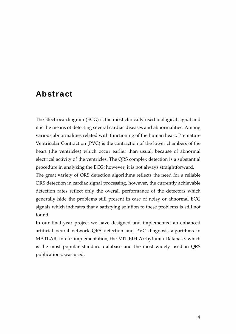
Abstract The Electrocardiogram (ECG) is the most clinically used biological signal and it is the means of detecting several cardiac diseases and abnormalities. Among various abnormalities related with functioning of the human heart, Premature Ventricular Contraction (PVC) is the contraction of the lower chambers of the heart  (the  ventricles) which  occur  earlier  than  usual,  because  of  abnormal electrical activity of the ventricles. The QRS complex detection is a substantial procedure in analyzing the ECG; however, it is not always straightforward.  The great variety of QRS detection algorithms reflects the need for a reliable QRS detection in cardiac signal processing, however, the currently achievable detection  rates  reflect  only  the  overall  performance  of  the  detectors which generally hide  the problems  still present  in  case of noisy or abnormal ECG signals which indicates that a satisfying solution to these problems is still not found.  In  our  final  year  project we  have  designed  and  implemented  an  enhanced artificial  neural  network  QRS  detection  and  PVC  diagnosis  algorithms  in MATLAB. In our implementation, the MIT‐BIH Arrhythmia Database, which is  the most  popular  standard  database  and  the most widely  used  in QRS publications, was used.  

5

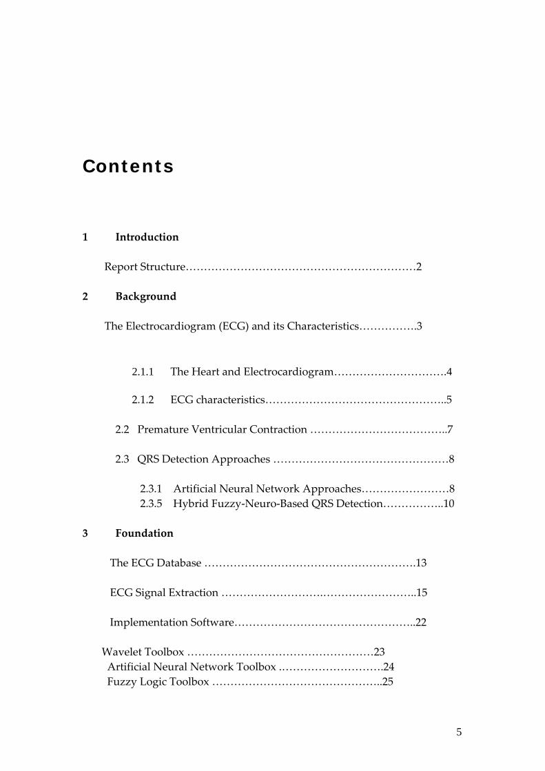
Contents  1 Introduction     Report Structure………………………………………………………2 

 2 Background      The Electrocardiogram (ECG) and its Characteristics…………….3 

 

2.1.1 The Heart and Electrocardiogram………………………….4

2.1.2      ECG characteristics…………………………………………..5  

2.2   Premature Ventricular Contraction ………………………………..7  

2.3   QRS Detection Approaches …………………………………………8  

2.3.1    Artificial Neural Network Approaches……………………8 2.3.5    Hybrid Fuzzy‐Neuro‐Based QRS Detection……………..10     

3 Foundation  

    The ECG Database ………………………………………………….13       ECG Signal Extraction ……………………….……………………..15       Implementation Software…………………………………………..22 

   Wavelet Toolbox ……………………………………………23     Artificial Neural Network Toolbox .……………………….24     Fuzzy Logic Toolbox ………………………………………..25 

 

6

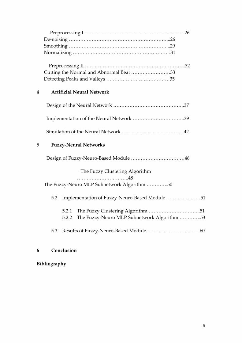
     Preprocessing I ……………………………………………………..26  De‐noising ……………………………………………………...26  Smoothing ……………………………………………………...29  Normalizing ……………………………………………………31 

      Preprocessing II ……………………………………………………..32  Cutting the Normal and Abnormal Beat ……………………33  Detecting Peaks and Valleys …………………………………35  4 Artificial Neural Network   

  Design of the Neural Network ……………………………………..37  

  Implementation of the Neural Network …………………………..39     Simulation of the Neural Network ………………………………...42  5 Fuzzy‐Neural Networks  

    Design of Fuzzy‐Neuro‐Based Module ……………………………46  

The Fuzzy Clustering Algorithm …………………………..48 

The Fuzzy‐Neuro MLP Subnetwork Algorithm ………….50  

5.2 Implementation of Fuzzy‐Neuro‐Based Module …………………51  

5.2.1    The Fuzzy Clustering Algorithm …………………………..51 5.2.2 The Fuzzy‐Neuro MLP Subnetwork Algorithm ………….53 

   5.3    Results of Fuzzy‐Neuro‐Based Module ……………………...……60 

  

6 Conclusion  Bibliography      

7

List of Figures

2.1   The objective of electrocardiography ……………………………. 4 2.2  Clinical ECG tracing of patients……………………………………4 2.3  The standard 12‐lead set of ECG…………………………………...5 2.4  The three limb leads…………………………………………………5 2.5  The three augmented leads…………………………………………6 2.6  The six referenced leads   …………………………………………..6 2.7  The ECG signal and its different components……………………7 2.8  Normal ECG recording……………………………………………..8 2.9  ECG of an LVH patient……………………………………………11 2.10  Common Structure of the QRS detectors………………………..12 2.11  The relation between the convolution integral of the wavelet               function multiplied by a uniform wave and the appearance of a               local maxima in the WT…………………………………………..15  2.12  Functional Blocks of a Fuzzy Inference System…………………17 2.13  Block diagram of FIS for ECG interpretation and LVH diagnosis             ……………………………………………………………………… 19 2.14  The membership functions of the FIS………………………...….19 2.15  Functional Description of a Single Neuron……………………...21 2.16  A 3‐2‐2 configured multilayer perceptron with direct connection             between input and output ………………………………………..21 2.17  A single layer ANN with 202 inputs and 3 outputs employing 

the batch mode of the Al‐Alaoui Algorithm, Form I…………...23 2.18  An MLP ANN with 202 inputs and 3 outputs employing the             error backpropagation………………………………………….....24 2.19  An MLP ANN structure…………………………………………..26 3.1  The plots in time of the pure surface and the filtrated ECG             signals………………………………………………………………33 3.2  The plots of the power spectrum of the pure ECG and the one  

8

            filtered at 20 Hz……………………………………………………33 3.3  The first module of the ANN MLP Approach 1 for QRS complex              detection and beat classification………………………………...34 3.4  The second module of the ANN MLP Approach 1 for LVH               diagnosis…………………………………………………………..35 3.5  The structure of a hybrid fuzzy‐neuro‐based network……….37 3.6  The performance of the G‐K algorithm of the self‐organization             to the recognition of clusters…………………………………….40  4.1  The MIT‐BIH Arrhythmia Database…………………………....44  4.2  The available ECG files on the database site…………………..45 4.3  Sample Record of the MIT‐BIH Database………………….......46  4.4  MATLAB Signal Processing Toolbox…………………………..47 4.5  SPTool GUI……………………………………………………..…48 4.6  MATLAB Fuzzy Logic Toolbox…………………………….…..48 4.7  ANFIS Editor GUI…………………………………………….….49 4.8  MATLAB Neural Network Toolbox………………………..…..50 4.9  The Neural Network Tool………………………………….……50

9

Chapter 1 Introduction   The past few decades have witnessed an outstanding pace of clinical, surgical, and  technological developments. Since  then great efforts have been made  to benefit from the technological advances and use of computers in the medical field.  Since  the  electro  cardiogram  (ECG)  is  used  for  analyzing  the  clinical conditions of the heart, the most vital organ in the human body, it is of great important to cardiologists to perform ECG analysis with maximum accuracy. Much  research  has  been  done  in  the  field  of  ECG  analysis,  all  aiming  at performing automatic  signal detection with near perfect detection  rates. For thirty years now, efforts have been oriented to the modeling of the expertise of  cardiologists  and  specialists  through  computers.  This  issue  has  been tackled by many  researchers who have  come up with a variety of different ECG  recognition  and  QRS  detection  algorithms  that  have  become  widely known  in  the  literature.  Among  the  numerous  studied  and  evaluated methods,  artificial  neural  network  methods  have  taken  special  attention because their properties such as non‐linearity, learning ability, and universal approximation allow  them  to  solve  complicated  signal processing problems like QRS detection and PVC diagnosis.  In  this  report, we will present our  final year project work which consists of designing  and  implementing  enhanced  artificial  neural  and  hybrid  fuzzy neural networks for QRS detection and PVC diagnosis. In our work, we have used  the  standard MIT‐BIH  Arrhythmia  database  as  our  ECG  source  and MATLAB 7.0.1 as our implementation and testing environment.    

10

1.1 Report Structure This final report presents our work throughout the fall and spring semesters of  academic  year  2005  –  2006 while  emphasizing  on  the work  performed during  the  spring  term. The  report  is divided  into  six  chapters where  each chapter covers a substantial portion of the project. In chapter 2, Background, we  tackle  the  basics  of  this  project while  elaborating  about  the  heart  and electrocardiogram,  the Premature Ventricular Contraction  abnormality,  and an overview of  the  two QRS detection approaches we have  followed  in  the project, artificial neural networks and hybrid fuzzy‐ neural networks. Chapter 3,  Foundation,  discusses  all  what  have  been  done  before  the  actual implementation  of  the  two modules.  It  involves  an  explanation  about  the standard ECG database used  in this project and how we managed to extract the signals from it, and then moves to introduce the MATLAB software tools we  have  used  for  preprocessing  and  implementation.  Finally,  the  chapter covers  thoroughly each of  the preprocessing steps  that are divided  into  two main stages. Chapter 4, Artificial Neural Network, covers the ANN module in details while  presenting  the  design,  implementation,  and  simulation  of  the module. Similarly, chapter 5 presents the same sections on the second module which  is  fuzzy‐neural networks. Both chapters 5 and 6 compare  the module results with  international  results  from  the  literature.  Finally,  we  conclude with chapter 6 which wraps up  the project and presents a section on ethical considerations.  

11

Chapter 2 Background The objective of  this chapter  is  to  introduce  the ECG signal  that  is  the main subject of  the project. The electrocardiogram  is very helpful  in  the diagnosis of  cardiac  diseases  since  they  often  result  in  ECG  abnormalities.  To  detect such abnormalities as PVC  (Premature Ventricular Contraction), a variety of methods have been used  in the  literature. In this section, we will review the methods  that we have  implemented  in  our project, namely  artificial neural networks and hybrid fuzzy‐neuro networks.   2.1 The Electrocardiogram and Its

Characteristics

The heart is the most vital organ of the human body since it acts as a pump  that pushes oxygen‐rich blood  to  the organs,  cells, and tissues of the body. Every heart beat is caused by electrical impulses from the heart muscle that cause the atria and then the ventricles to contract and consequently pump blood to the lungs and  the  rest of  the body. This electrical activity of  the heart  is measured by the electrocardiogram which serves as a means to detect for irregular heart conditions and possibly heart diseases. Electrocardiography  has  evolved  over  time  and  is  becoming more  accurate  as  it  is  being  automated  by making  use  of  the several software QRS detection techniques available. 

12

2.1.1 The Heart and Electrocardiogram

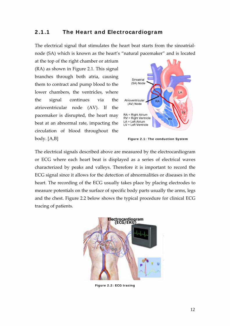
The electrical signal  that stimulates  the heart beat starts  from  the sinoatrial‐node (SA) which is known as the heart’s “natural pacemaker” and is located at the top of the right chamber or atrium (RA) as shown in Figure 2.1. This signal branches  through  both  atria,  causing them to contract and pump blood to the lower  chambers,  the  ventricles,  where the  signal  continues  via  the atrioventricular  node  (AV).  If  the pacemaker  is  disrupted,  the  heart may beat at an abnormal rate,  impacting  the circulation  of  blood  throughout  the body. [A,B]                                                            Figure 2.1: The conduction System                    

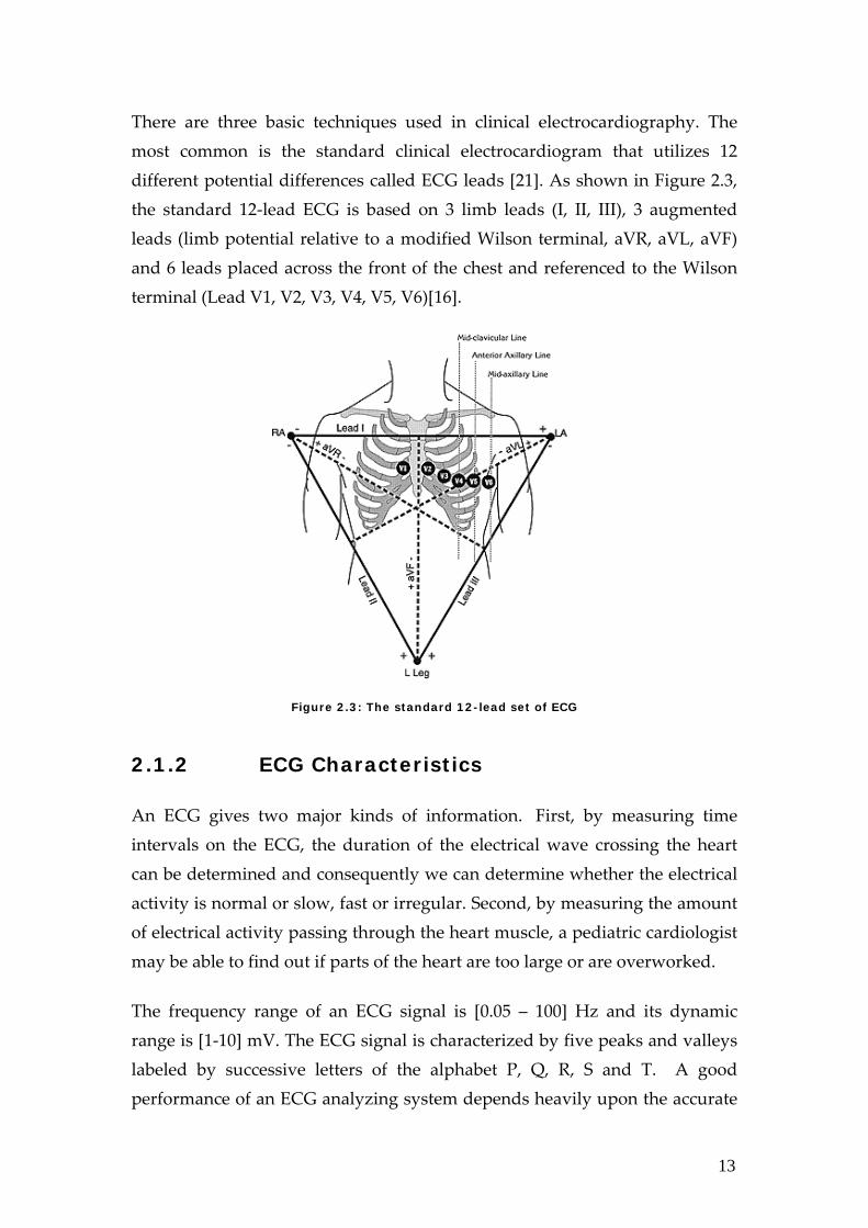
The electrical signals described above are measured by the electrocardiogram or  ECG where  each  heart  beat  is  displayed  as  a  series  of  electrical waves characterized  by peaks  and  valleys. Therefore  it  is  important  to  record  the ECG signal since it allows for the detection of abnormalities or diseases in the heart. The recording of the ECG usually takes place by placing electrodes to measure potentials on the surface of specific body parts usually the arms, legs and the chest. Figure 2.2 below shows the typical procedure for clinical ECG tracing of patients. 

 

 

 

 

 

Figure 2.2: ECG tracing

13

There  are  three  basic  techniques  used  in  clinical  electrocardiography.  The most  common  is  the  standard  clinical  electrocardiogram  that  utilizes  12 different potential differences called ECG leads [21]. As shown in Figure 2.3, the  standard  12‐lead ECG  is based  on  3  limb  leads  (I,  II,  III),  3  augmented leads (limb potential relative to a modified Wilson terminal, aVR, aVL, aVF) and 6 leads placed across the front of the chest and referenced to the Wilson terminal (Lead V1, V2, V3, V4, V5, V6)[16].  

Figure 2.3: The standard 12-lead set of ECG

2.1.2 ECG Characteristics

An  ECG  gives  two major  kinds  of  information.   First,  by measuring  time intervals on  the ECG,  the duration of  the  electrical wave  crossing  the heart can be determined and consequently we can determine whether the electrical activity is normal or slow, fast or irregular. Second, by measuring the amount of electrical activity passing through the heart muscle, a pediatric cardiologist may be able to find out if parts of the heart are too large or are overworked.  

The  frequency  range  of  an  ECG  signal  is  [0.05  –  100] Hz  and  its  dynamic range is [1‐10] mV. The ECG signal is characterized by five peaks and valleys labeled  by  successive  letters  of  the  alphabet  P,  Q,  R,  S  and  T.    A  good performance of an ECG analyzing system depends heavily upon the accurate 

14

and reliable detection of the QRS complex, as well as the T and P waves [11]. The P wave represents the activation of the upper chambers of the heart, the atria while the QRS wave (or complex) and T wave represent the excitation of the ventricles or  the  lower  chambers of  the heart. The detection of  the QRS complex  is  the most  important  task  in automatic ECG  signal analysis. Once the QRS  complex has been  identified,  a more detailed  examination of ECG signal, including the heart rate, the ST segment, etc., can be performed. Figure 2.4 shows the ECG signal with  its different elements as well as the time and amplitude characteristics of the paper that the ECG is usually recorded on.        

Figure 2.4: The ECG signal and its different components

In the normal Sinus rhythm i.e. the normal state of the heart, the P‐R interval is  in  the  range  of  0.12  to  0.2  seconds,  the QRS  interval  from  0.04  to  0.12 seconds, the Q‐T interval is less than 0.42 seconds, and the normal rate of the heart  is from 60 to 100 beats per minute [2]. From the recorded shape of the ECG,  cardiologists  can  usually  tell  whether  the  patient’s  heart  activity  is normal or abnormal. Figure 2.5 shows a typical normal ECG signal.           

Figure 2.5: Normal ECG recording [6]

 

15

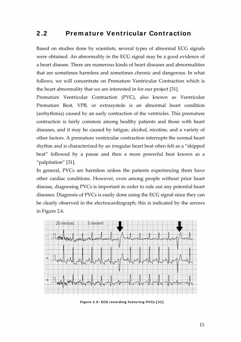
2.2 Premature Ventricular Contraction   Based on  studies done by  scientists,  several  types of abnormal ECG  signals were obtained. An abnormality in the ECG signal may be a good evidence of a heart disease. There are numerous kinds of heart diseases and abnormalities that are sometimes harmless and sometimes chronic and dangerous. In what follows, we will  concentrate on Premature Ventricular Contraction which  is the heart abnormality that we are interested in for our project [31].  Premature  Ventricular  Contraction  (PVC),  also  known  as  Ventricular Premature  Beat,  VPB,  or  extrasystole  is  an  abnormal  heart  condition (arrhythmia) caused by an early contraction of the ventricles. This premature contraction  is  fairly  common  among  healthy  patients  and  those with  heart diseases, and  it may be caused by  fatigue, alcohol, nicotine, and a variety of other factors. A premature ventricular contraction interrupts the normal heart rhythm and is characterized by an irregular heart beat often felt as a “skipped beat”  followed  by  a  pause  and  then  a  more  powerful  beat  known  as  a “palpitation” [31].   In  general,  PVCs  are  harmless  unless  the  patients  experiencing  them  have other  cardiac  conditions. However,  even  among people without prior heart disease, diagnosing PVCs is important in order to rule out any potential heart diseases. Diagnosis of PVCs is easily done using the ECG signal since they can be clearly observed in the electrocardiograph; this is indicated by the arrows in Figure 2.6.  

Figure 2.6: ECG recording featuring PVCs [32]

16

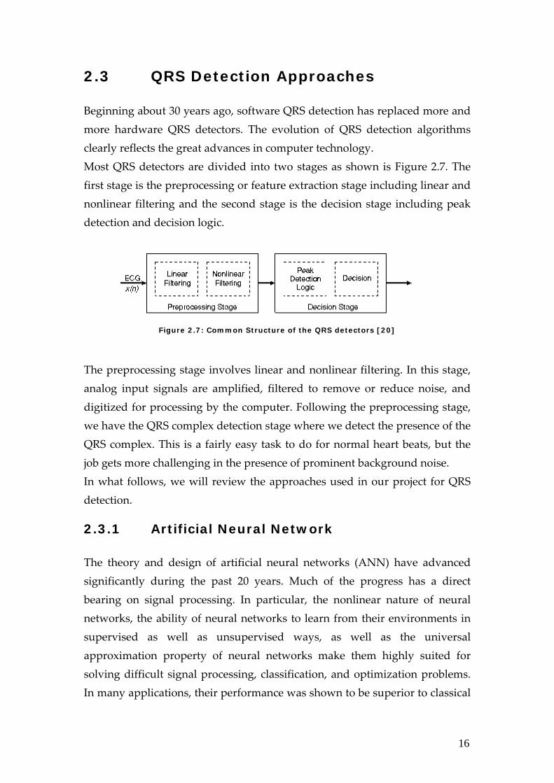
2.3 QRS Detection Approaches Beginning about 30 years ago, software QRS detection has replaced more and more  hardware QRS  detectors.  The  evolution  of QRS  detection  algorithms clearly reflects the great advances in computer technology.  Most QRS detectors are divided  into  two stages as shown  is Figure 2.7. The first stage is the preprocessing or feature extraction stage including linear and nonlinear  filtering and  the second stage  is  the decision stage  including peak detection and decision logic.  

Figure 2.7: Common Structure of the QRS detectors [20]

 The preprocessing stage  involves  linear and nonlinear filtering. In this stage, analog  input  signals  are  amplified,  filtered  to  remove  or  reduce noise,  and digitized for processing by the computer. Following the preprocessing stage, we have the QRS complex detection stage where we detect the presence of the QRS complex. This  is a fairly easy task to do for normal heart beats, but the job gets more challenging in the presence of prominent background noise.  In what  follows, we will review  the approaches used  in our project  for QRS detection.   2.3.1 Artificial Neural Network  The  theory  and  design  of  artificial  neural  networks  (ANN)  have  advanced significantly  during  the  past  20  years. Much  of  the  progress  has  a  direct bearing  on  signal  processing.  In  particular,  the  nonlinear  nature  of  neural networks,  the ability of neural networks to  learn from their environments  in supervised  as  well  as  unsupervised  ways,  as  well  as  the  universal approximation  property  of  neural  networks  make  them  highly  suited  for solving difficult signal processing, classification, and optimization problems. In many applications, their performance was shown to be superior to classical 

17

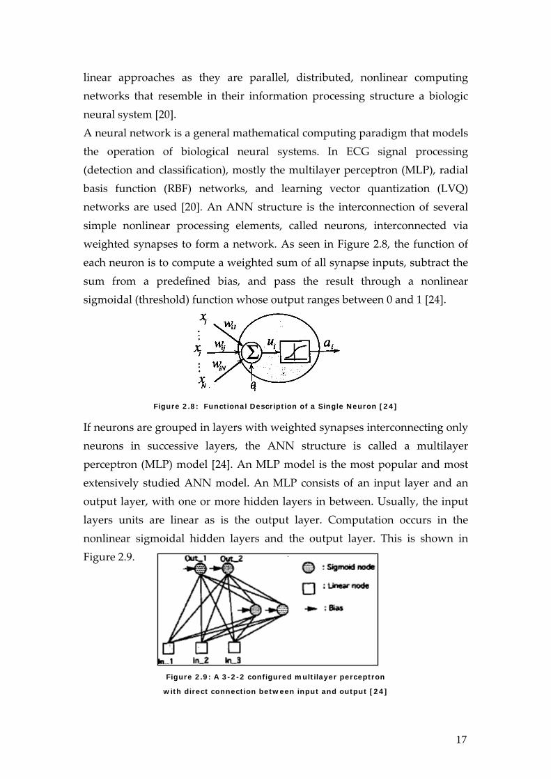
linear  approaches  as  they  are  parallel,  distributed,  nonlinear  computing networks  that  resemble  in  their  information processing  structure  a  biologic neural system [20].  A neural network is a general mathematical computing paradigm that models the  operation  of  biological  neural  systems.  In  ECG  signal  processing (detection and classification), mostly the multilayer perceptron (MLP), radial basis  function  (RBF)  networks,  and  learning  vector  quantization  (LVQ) networks are used  [20]. An ANN  structure  is  the  interconnection of  several simple  nonlinear  processing  elements,  called  neurons,  interconnected  via weighted synapses  to  form a network. As seen  in Figure 2.8,  the  function of each neuron is to compute a weighted sum of all synapse inputs, subtract the sum  from  a  predefined  bias,  and  pass  the  result  through  a  nonlinear sigmoidal (threshold) function whose output ranges between 0 and 1 [24].      

Figure 2.8: Functional Description of a Single Neuron [24]

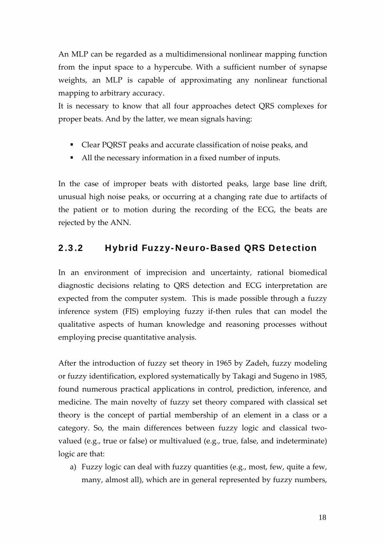
If neurons are grouped in layers with weighted synapses interconnecting only neurons  in  successive  layers,  the  ANN  structure  is  called  a  multilayer perceptron  (MLP) model  [24]. An MLP model  is  the most popular and most extensively studied ANN model. An MLP consists of an  input  layer and an output  layer, with one or more hidden  layers  in between. Usually, the  input layers  units  are  linear  as  is  the  output  layer.  Computation  occurs  in  the nonlinear  sigmoidal  hidden  layers  and  the  output  layer.  This  is  shown  in Figure 2.9.  

 

Figure 2.9: A 3-2-2 configured multilayer perceptron

with direct connection between input and output [24]

18

An MLP can be regarded as a multidimensional nonlinear mapping function from  the  input  space  to  a  hypercube. With  a  sufficient  number  of  synapse weights,  an  MLP  is  capable  of  approximating  any  nonlinear  functional mapping to arbitrary accuracy.    It  is  necessary  to  know  that  all  four  approaches  detect QRS  complexes  for proper beats. And by the latter, we mean signals having:   

Clear PQRST peaks and accurate classification of noise peaks, and   All the necessary information in a fixed number of inputs.   

In  the  case  of  improper  beats  with  distorted  peaks,  large  base  line  drift, unusual high noise peaks, or occurring at a changing rate due  to artifacts of the  patient  or  to  motion  during  the  recording  of  the  ECG,  the  beats  are rejected by the ANN.  

2.3.2 Hybrid Fuzzy-Neuro-Based QRS Detection In  an  environment  of  imprecision  and  uncertainty,  rational  biomedical diagnostic  decisions  relating  to QRS  detection  and  ECG  interpretation  are expected  from  the computer system.   This  is made possible  through a  fuzzy inference  system  (FIS)  employing  fuzzy  if‐then  rules  that  can  model  the qualitative  aspects  of  human  knowledge  and  reasoning  processes without employing precise quantitative analysis.   After the  introduction of fuzzy set theory  in 1965 by Zadeh, fuzzy modeling or fuzzy identification, explored systematically by Takagi and Sugeno in 1985, found numerous practical applications  in  control, prediction,  inference, and medicine. The main novelty of  fuzzy  set  theory compared with classical  set theory  is  the  concept  of  partial membership  of  an  element  in  a  class  or  a category.  So,  the main  differences  between  fuzzy  logic  and  classical  two‐valued (e.g., true or false) or multivalued (e.g., true, false, and indeterminate) logic are that: 

a) Fuzzy logic can deal with fuzzy quantities (e.g., most, few, quite a few, many, almost all), which are in general represented by fuzzy numbers, 

19

fuzzy  predicates  (e.g.,  expensive,  rare),  and  fuzzy  modifiers  (e.g., extremely, unlikely). 

b) The notions of truth and false are both allowed to be fuzzy using fuzzy true/false values (e.g., very true, mostly false). Then, the ultimate goal of fuzzy logic is to provide foundations for approximate reasoning.  

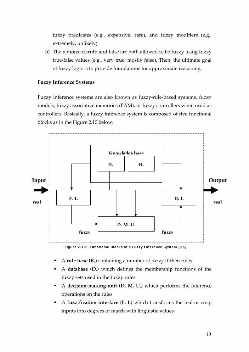
 Fuzzy Inference Systems    Fuzzy  inference  systems are also known as  fuzzy‐rule‐based systems,  fuzzy models, fuzzy associative memories (FAM), or fuzzy controllers when used as controllers. Basically, a fuzzy inference system is composed of five functional blocks as in the Figure 2.10 below.            

        

Figure 2.10: Functional Blocks of a Fuzzy Inference System [25]

  A rule base (R.) containing a number of fuzzy if‐then rules   A  database  (D.) which  defines  the membership  functions  of  the fuzzy sets used in the fuzzy rules 

A decision‐making‐unit  (D. M. U.) which performs  the  inference operations on the rules 

A fuzzification interface (F. I.) which transforms the real or crisp inputs into degrees of match with linguistic values 

F. I. D. I.

D. M. U.

D. R.

Knowledge base

fuzzyfuzzy

Input Output

real real

20

A  Defuzzification  interface  (D.  I.)  which  transforms  the  fuzzy results of the inference into a crisp output 

 Usually  the  rule  base  and  the database  are  jointly  referred  to  as  the knowledge base. 

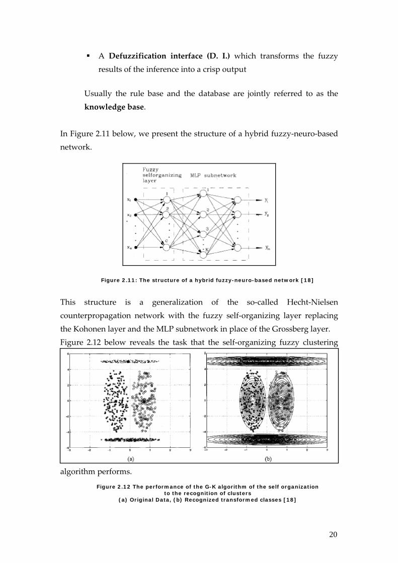
 In Figure 2.11 below, we present the structure of a hybrid fuzzy‐neuro‐based network.   

  

Figure 2.11: The structure of a hybrid fuzzy-neuro-based network [18]

 This  structure  is  a  generalization  of  the  so‐called  Hecht‐Nielsen counterpropagation  network with  the  fuzzy  self‐organizing  layer  replacing the Kohonen layer and the MLP subnetwork in place of the Grossberg layer. Figure  2.12  below  reveals  the  task  that  the  self‐organizing  fuzzy  clustering 

algorithm performs.  

Figure 2.12 The performance of the G-K algorithm of the self organization to the recognition of clusters

(a) Original Data, (b) Recognized transformed classes [18] 

21

Chapter 3 Foundation In this chapter we cover all the steps that preceded project implementation. A major element of the foundation stage was the extraction of ECG signals from the standard database  that we have chosen  for our project. After extraction, the signals were subject to preprocessing using several tools available by the MATLAB  software,  the  primary  implementation  software  of  our  final  year project.    3.1 The ECG Database

The  role  of  a  standard  database  is  very  important  in  evaluating  the performance  of  QRS  detection  algorithms.  A  standard  or  a  benchmark database is a well annotated and validated database that is made available for academic and industrial groups for testing and result‐comparison in different applications.  ECG  databases  have  been  present  for  a  long  time  now  and because they contain a  large number of signals that are representative of the large variety of ECGs as well as  the rarely observed but clinically  important signals,  they  have  been  used  throughout  the  literature  of  QRS  detection algorithms in producing and comparing results. It is easy to obtain and make use  of  ECG  data  from  local  hospitals  to  base work  on  them;  however  any results obtained using  such data  can not be  evaluated  fairly because of  the lack  of  approved  works  that  use  the  same  data.  This  is  why  it  is  very important to us to select a standard ECG database to base our work on. For  a  number  of  years,  researchers  worldwide  have  been  investigating methods  for  real‐time  ECG  rhythm  analysis  and  for  that  sake  standard 

22

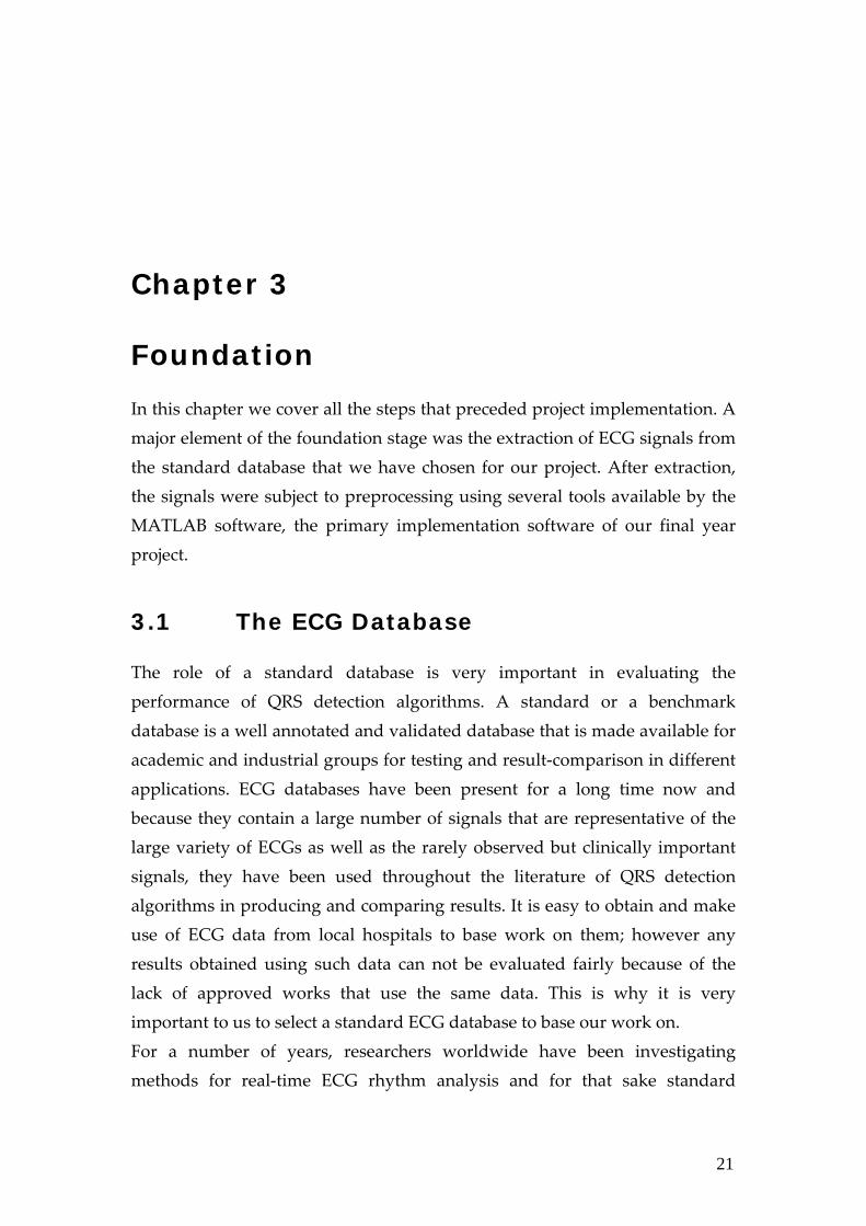
databases  and  especially  the MIT‐BIH Arrhythmia Database  have  been  an enormous help for the development and evaluation of ECG classification and detection  algorithms. We  have  selected  the MIT‐BIH  database  to  base  our work on because it is available online where the ECG files are easily accessible and because many important works in the literature have based their work on this database and have  reported  their  results and  findings  in published and widely acknowledged papers.  

Figure 3.1: The MIT-BIH Arrhythmia Database [1]

The MIT‐BIH database  is  a very popular database  that  is provided by MIT and  Boston’s  Beth  Israel  Hospital.  It  consists  of  ten  databases  that  serve different  test  purposes  and  the most  frequently  used  database  among  the others  is  the Arrhythmia Database  that  contains  48  half‐hour  recordings  of two‐channel ambulatory ECG  [20]. These  recordings were obtained  from 47 subjects studied between 1975 and 1979 by the BIH Arrhythmia Laboratory.  Out  of  the  48  recordings,  25 were  chosen  from  numerous  ambulatory  ECG recordings whereas the rest was randomly selected from a mixed population of patients varying between inpatients (60%) and outpatients (40%) [1]. There are more  than  a  hundred  thousand  QRS  complexes  in  this  database  and  the detection of these complexes varies from straight‐forward to difficult according to  the  different  levels  of  abnormality,  noise  and  artifacts.  The  data  of  the 

23

database  consists  of  annotated ECG  sampled  at  a  rate  of  360 Hz with  11‐bit resolution  over  a  10  mV  range  [1].  Included  with  the  database  is  the annotations reference which explains approximately 110,000 annotations [1,20]. 

The  data  gathering  of  the MIT‐BIH Arrhythmia Database  has  started  since 1975  but  the  first  distribution  has  taken  place  only  in  1980. Only  recently, February 2005, the full data became available online on PhysioNet’s webpage www.physionet.org as one of physiobank’s databases.  3.2 ECG Signal Extraction

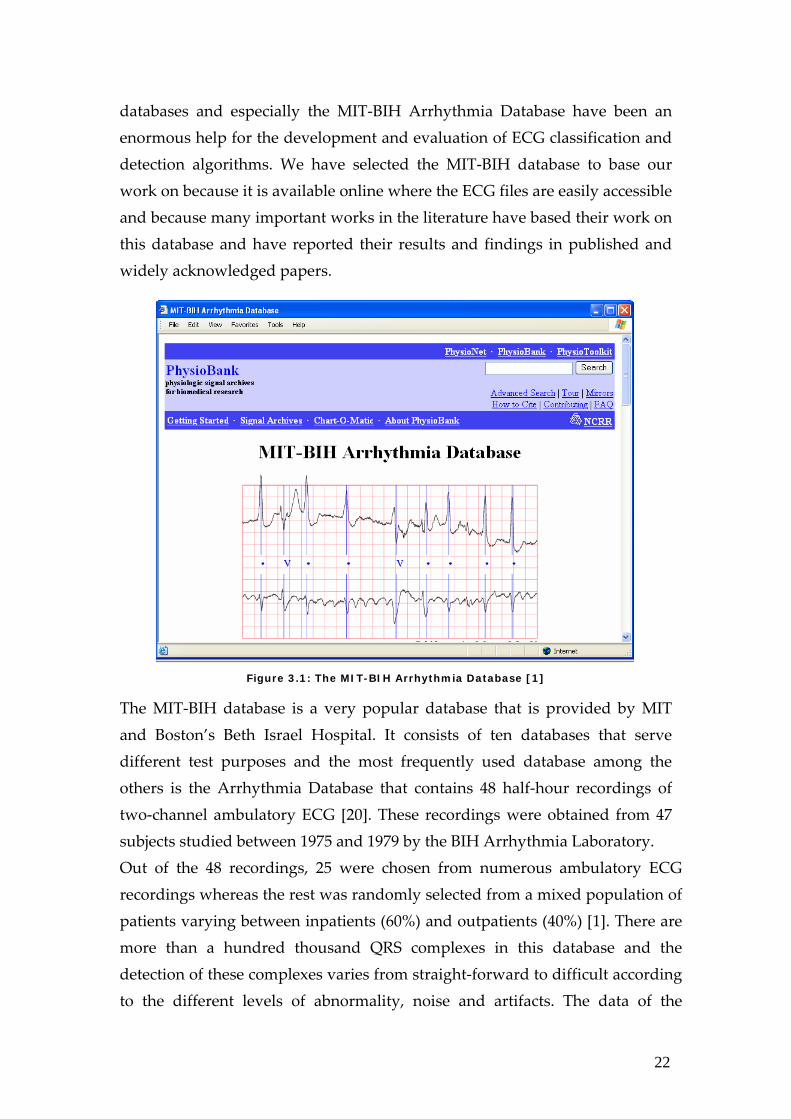
As  can  be  seen  in  Figure  3.2,  the MIT‐BIH Arrhythmia Database  provides three set of  files  to be downloaded  for each record. The  .dat  files are binary signal  files  and  contain  the  actual data  like  the  number  of  sample  and  the amplitude  of  the  signal  at  that  sample  point.  The  .hea  files  are  short  text “header” files used to determine the location and format of the signal files by the software that reads them. Finally, the  .atr files are binary files containing annotations or labels pointing to specific locations within the signals.

Figure 3.2: The MIT-BIH Arrhythmia Database Records [1]

 

24

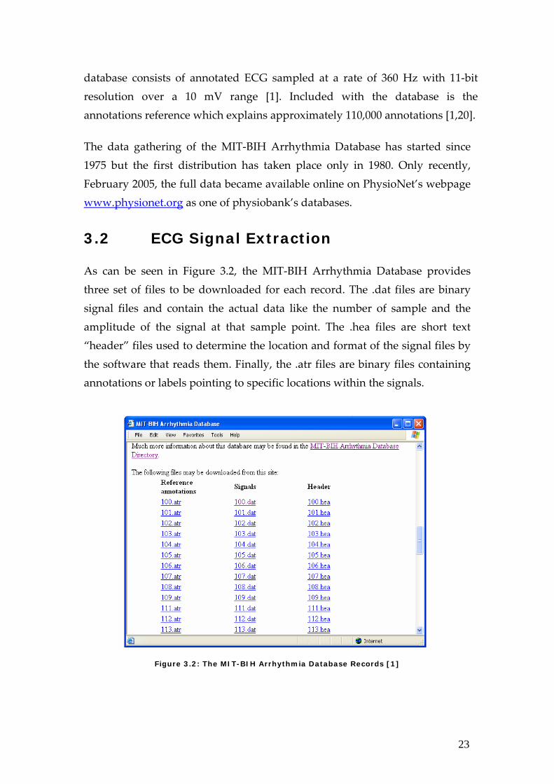
It is clearly stated at the PhysioBank that simply saving the .dat, .hea, and .atr of each record would not enable the user to view the signals and process them further.  Instead, there is a list of steps that one must engage in according to the running operating system in order to fully use the PhysioBank data. The series of steps include installing several software packages, provided as open source software by PhysioNet, and are indicated on the main page of the PhysiToolkit shown in Figure 3.3.  

Figure 3.3: PhysiToolkit main page

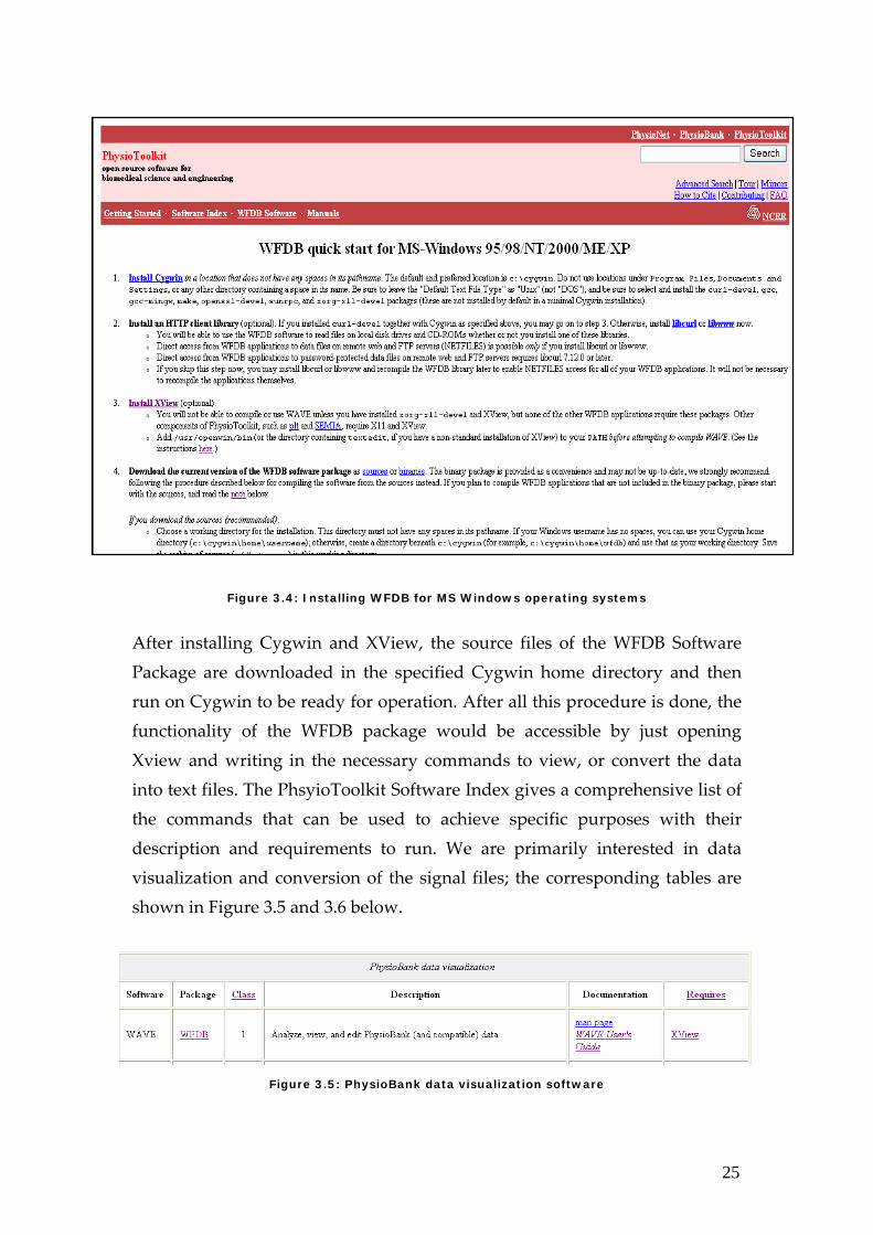
 The primary  software  is  the WFDB  Software Package which  contains  all  the functions  needed  to  extract  the  data  from  the  signal  files  and  study  the physiological signals. Installing the WFDB software package and library is not a straightforward task on MS Windows as it involves numerous steps that are sometimes ambiguously explained on the PhysiToolkit page in concern, shown in Figure 3.4. As  seen  in  the  figure,  the  first  step  for acquiring  the necessary packages  is  to  install  Cygwin  which  is  a  Unix  environment  emulator  on windows. Cygwin enables us to compile and run the binary files needed for the complete  installation  of  the  software  packages.  The  second  step  is  to  install XView  which  is  required  to  run WAVE,  the  software  which  enables  us  to visualize  the  signals with  their  annotations  and  time  series  and  allows us  to manipulate the signals for our own processing purposes.  

25

Figure 3.4: Installing WFDB for MS Windows operating systems

After  installing Cygwin  and XView,  the  source  files of  the WFDB Software Package  are downloaded  in  the  specified Cygwin home directory  and  then run on Cygwin to be ready for operation. After all this procedure is done, the functionality  of  the  WFDB  package  would  be  accessible  by  just  opening Xview and writing  in  the necessary commands  to view, or convert  the data into text files. The PhsyioToolkit Software Index gives a comprehensive list of the  commands  that  can  be  used  to  achieve  specific  purposes  with  their description  and  requirements  to  run. We  are  primarily  interested  in  data visualization and conversion of  the signal  files;  the corresponding  tables are shown in Figure 3.5 and 3.6 below.  

Figure 3.5: PhysioBank data visualization software

26

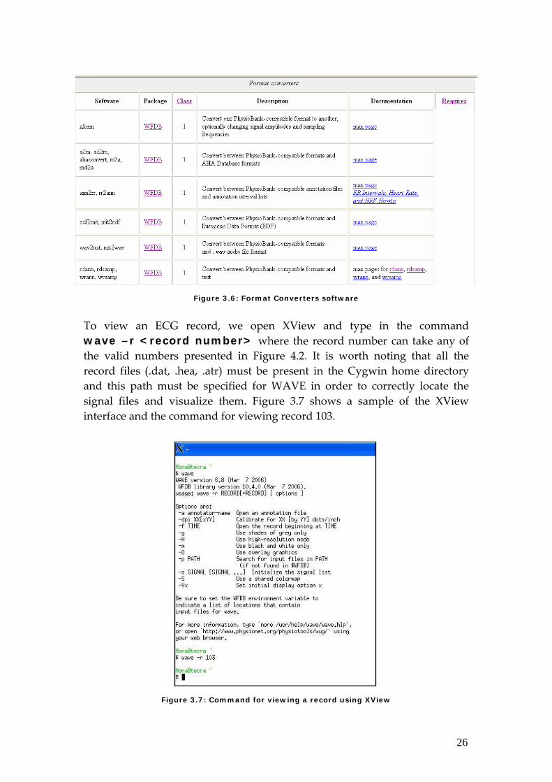
Figure 3.6: Format Converters software

To  view  an  ECG  record,  we  open  XView  and  type  in  the  command  wave –r <record number> where  the record number can  take any of the  valid  numbers  presented  in  Figure  4.2.  It  is worth  noting  that  all  the record  files  (.dat,  .hea,  .atr) must be present  in  the Cygwin home directory and  this  path must  be  specified  for WAVE  in  order  to  correctly  locate  the signal  files  and  visualize  them.  Figure  3.7  shows  a  sample  of  the  XView interface and the command for viewing record 103. 

Figure 3.7: Command for viewing a record using XView

27

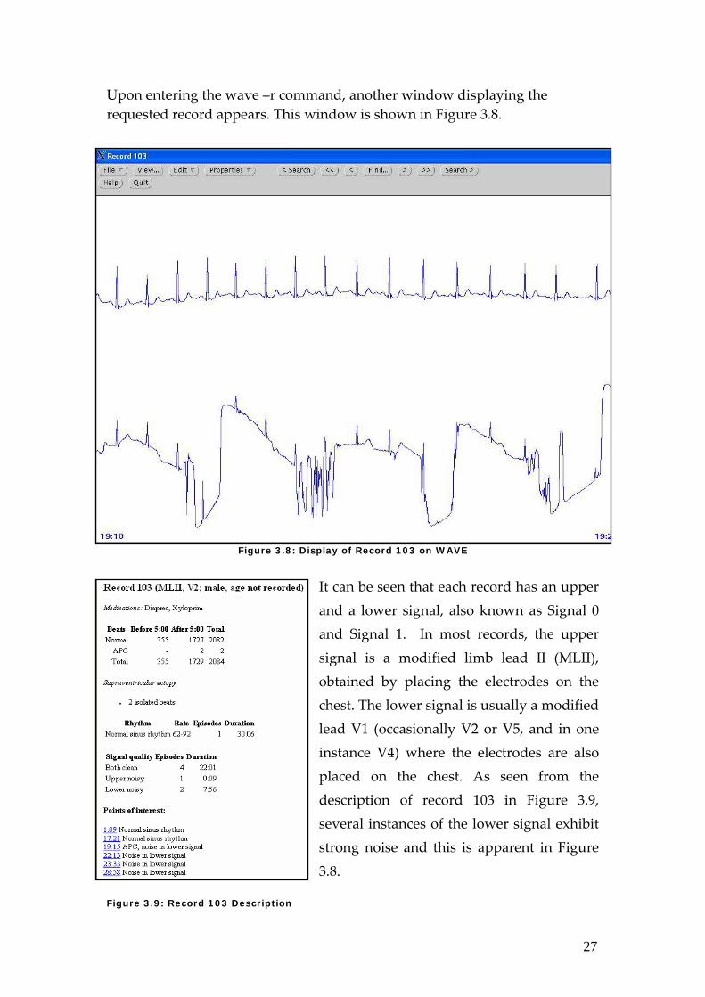
Upon entering the wave –r command, another window displaying the requested record appears. This window is shown in Figure 3.8.  

Figure 3.8: Display of Record 103 on WAVE

It can be seen that each record has an upper and a  lower  signal, also known as Signal 0 and  Signal  1.    In most  records,  the  upper signal  is  a  modified  limb  lead  II  (MLII), obtained  by  placing  the  electrodes  on  the chest. The lower signal is usually a modified lead V1  (occasionally V2 or V5, and  in one instance V4) where  the  electrodes  are  also placed  on  the  chest.  As  seen  from  the description  of  record  103  in  Figure  3.9, several instances of the lower signal exhibit strong noise and  this  is apparent  in Figure 3.8. 

Figure 3.9: Record 103 Description

28

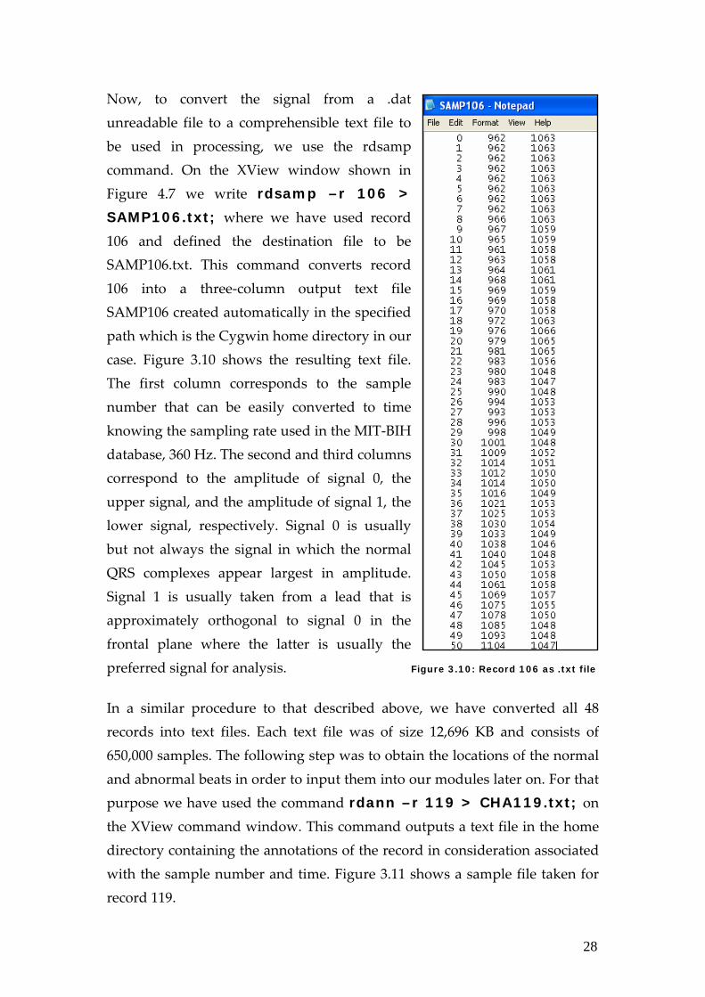
Now,  to  convert  the  signal  from  a  .dat unreadable  file  to a  comprehensible  text  file  to be  used  in  processing,  we  use  the  rdsamp command.  On  the  XView  window  shown  in Figure  4.7  we  write rdsamp –r 106 >

SAMP106.txt; where we  have  used  record 106  and  defined  the  destination  file  to  be SAMP106.txt.  This  command  converts  record 106  into  a  three‐column  output  text  file SAMP106 created automatically in the specified path which is the Cygwin home directory in our case.  Figure  3.10  shows  the  resulting  text  file. The  first  column  corresponds  to  the  sample number  that  can  be  easily  converted  to  time knowing the sampling rate used in the MIT‐BIH database, 360 Hz. The second and third columns correspond  to  the  amplitude  of  signal  0,  the upper signal, and the amplitude of signal 1, the lower  signal,  respectively.  Signal  0  is  usually but not always  the  signal  in which  the normal QRS  complexes  appear  largest  in  amplitude. Signal  1  is  usually  taken  from  a  lead  that  is approximately  orthogonal  to  signal  0  in  the frontal  plane  where  the  latter  is  usually  the preferred signal for analysis.                                   Figure 3.10: Record 106 as .txt file

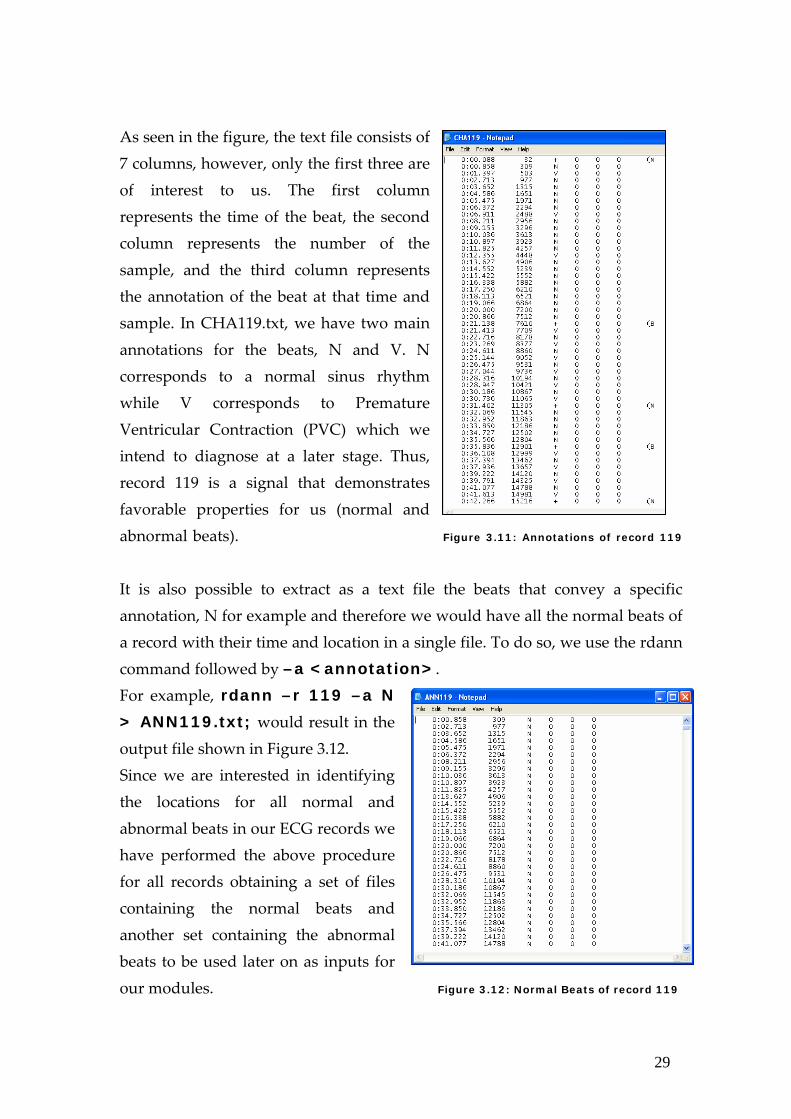
In  a  similar  procedure  to  that  described  above, we  have  converted  all  48 records  into  text  files.  Each  text  file was  of  size  12,696 KB  and  consists  of 650,000 samples. The following step was to obtain the locations of the normal and abnormal beats in order to input them into our modules later on. For that purpose we have used the command rdann –r 119 > CHA119.txt; on the XView command window. This command outputs a text file in the home directory containing the annotations of the record in consideration associated with the sample number and time. Figure 3.11 shows a sample file taken for record 119.  

29

As seen in the figure, the text file consists of 7 columns, however, only the first three are of  interest  to  us.  The  first  column represents  the  time of  the beat,  the second column  represents  the  number  of  the sample,  and  the  third  column  represents the annotation of  the beat at  that  time and sample.  In CHA119.txt, we have  two main annotations  for  the  beats,  N  and  V.  N corresponds  to  a  normal  sinus  rhythm while  V  corresponds  to  Premature Ventricular  Contraction  (PVC)  which  we intend  to  diagnose  at  a  later  stage.  Thus, record  119  is  a  signal  that  demonstrates favorable  properties  for  us  (normal  and abnormal beats).                                                                           Figure 3.11: Annotations of record 119

It  is  also  possible  to  extract  as  a  text  file  the  beats  that  convey  a  specific annotation, N for example and therefore we would have all the normal beats of a record with their time and location in a single file. To do so, we use the rdann command followed by –a <annotation>.  For  example,  rdann –r 119 –a N

> ANN119.txt; would result in the output file shown in Figure 3.12.  Since we  are  interested  in  identifying the  locations  for  all  normal  and abnormal beats in our ECG records we have  performed  the  above  procedure for  all  records  obtaining  a  set  of  files containing  the  normal  beats  and another  set  containing  the  abnormal beats  to be used  later on as  inputs  for our modules.                                                 Figure 3.12: Normal Beats of record 119

30

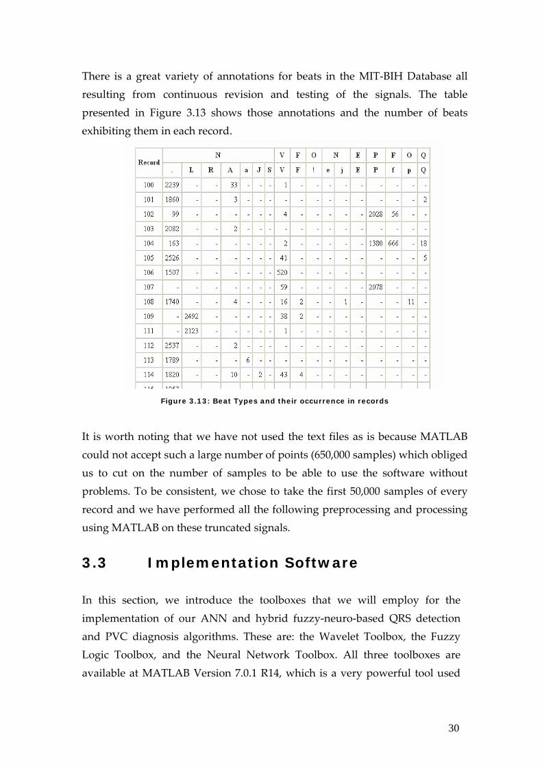
There  is a great variety of annotations  for beats  in  the MIT‐BIH Database all resulting  from  continuous  revision  and  testing  of  the  signals.  The  table presented  in  Figure  3.13  shows  those  annotations  and  the  number  of  beats exhibiting them in each record.  

Figure 3.13: Beat Types and their occurrence in records

 

It  is worth noting  that we have not used  the  text  files as  is because MATLAB could not accept such a large number of points (650,000 samples) which obliged us  to  cut  on  the  number  of  samples  to  be  able  to  use  the  software without problems. To be consistent, we chose  to  take  the  first 50,000 samples of every record and we have performed all the following preprocessing and processing using MATLAB on these truncated signals.  3.3 Implementation Software  In  this  section,  we  introduce  the  toolboxes  that  we  will  employ  for  the implementation  of  our ANN  and  hybrid  fuzzy‐neuro‐based QRS  detection and  PVC  diagnosis  algorithms.  These  are:  the Wavelet  Toolbox,  the  Fuzzy Logic  Toolbox,  and  the  Neural  Network  Toolbox.  All  three  toolboxes  are available at MATLAB Version 7.0.1 R14, which  is a very powerful  tool used 

31

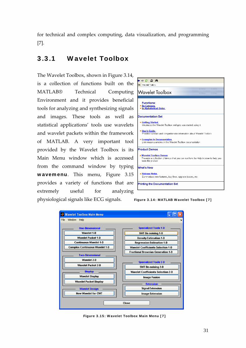
for  technical and  complex  computing, data visualization, and programming [7].  3.3.1 Wavelet Toolbox The Wavelet Toolbox, shown in Figure 3.14, is  a  collection  of  functions  built  on  the MATLAB®  Technical  Computing Environment  and  it  provides  beneficial tools for analyzing and synthesizing signals and  images.  These  tools  as  well  as statistical  applications’  tools  use  wavelets and wavelet packets within the framework of  MATLAB.  A  very  important  tool provided  by  the  Wavelet  Toolbox  is  its Main  Menu  window  which  is  accessed from  the  command  window  by  typing wavemenu.  This  menu,  Figure  3.15 provides  a  variety  of  functions  that  are extremely  useful  for  analyzing physiological signals like ECG signals.          Figure 3.14: MATLAB Wavelet Toolbox [7]   

Figure 3.15: Wavelet Toolbox Main Menu [7]

32

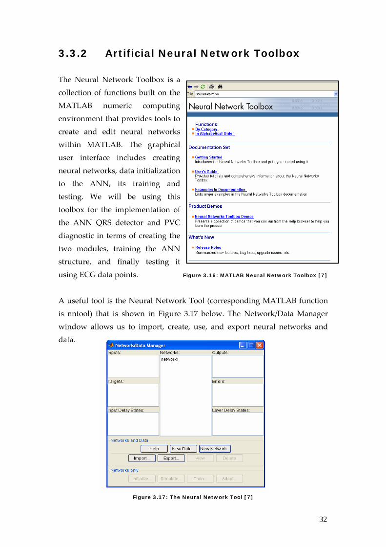
3.3.2 Artificial Neural Network Toolbox The Neural Network Toolbox  is  a collection of  functions built on  the MATLAB  numeric  computing environment that provides tools to create  and  edit  neural  networks within  MATLAB.  The  graphical user  interface  includes  creating neural networks, data initialization to  the  ANN,  its  training  and testing.  We  will  be  using  this toolbox  for  the  implementation  of the  ANN  QRS  detector  and  PVC diagnostic  in  terms of creating  the two  modules,  training  the  ANN structure,  and  finally  testing  it using ECG data points.                       Figure 3.16: MATLAB Neural Network Toolbox [7]

 A useful tool  is the Neural Network Tool (corresponding MATLAB function is  nntool)  that  is  shown  in  Figure  3.17  below.  The Network/Data Manager window  allows  us  to  import,  create,  use,  and  export  neural  networks  and data.

Figure 3.17: The Neural Network Tool [7]

33

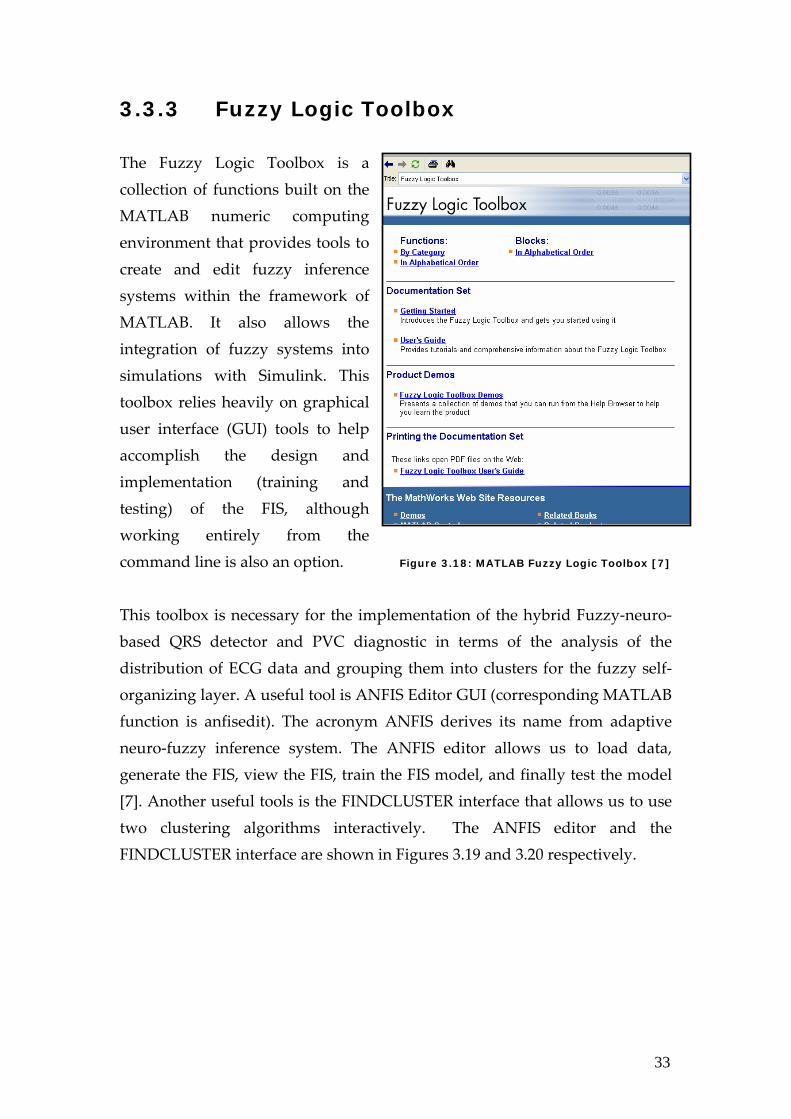
3.3.3 Fuzzy Logic Toolbox The  Fuzzy  Logic  Toolbox  is  a collection of  functions built on  the MATLAB  numeric  computing environment that provides tools to create  and  edit  fuzzy  inference systems  within  the  framework  of MATLAB.  It  also  allows  the integration  of  fuzzy  systems  into simulations  with  Simulink.  This toolbox relies heavily on graphical user  interface  (GUI)  tools  to  help accomplish  the  design  and implementation  (training  and testing)  of  the  FIS,  although working  entirely  from  the command line is also an option.              Figure 3.18: MATLAB Fuzzy Logic Toolbox [7]

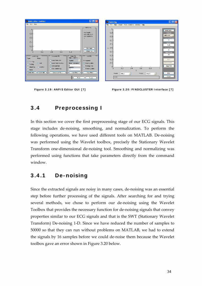
 This toolbox  is necessary for the  implementation of the hybrid Fuzzy‐neuro‐based  QRS  detector  and  PVC  diagnostic  in  terms  of  the  analysis  of  the distribution of ECG data and grouping  them  into clusters  for  the  fuzzy self‐organizing layer. A useful tool is ANFIS Editor GUI (corresponding MATLAB function  is  anfisedit).  The  acronym ANFIS  derives  its  name  from  adaptive neuro‐fuzzy  inference  system.  The  ANFIS  editor  allows  us  to  load  data, generate the FIS, view the FIS, train the FIS model, and finally test the model [7]. Another useful tools is the FINDCLUSTER interface that allows us to use two  clustering  algorithms  interactively.    The  ANFIS  editor  and  the FINDCLUSTER interface are shown in Figures 3.19 and 3.20 respectively. 

34

Figure 3.19: ANFIS Editor GUI [7] Figure 3.20: FINDCLUSTER Interface [7]

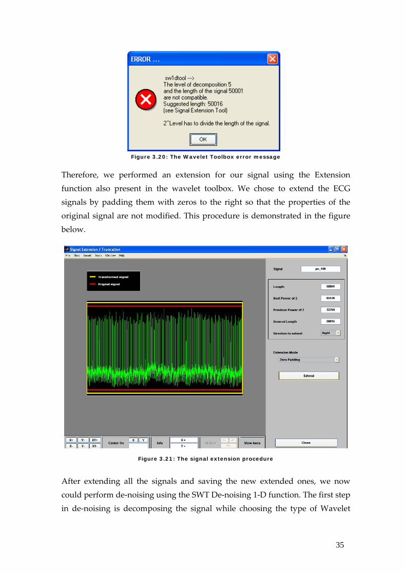
3.4 Preprocessing I In this section we cover the first preprocessing stage of our ECG signals. This stage  includes  de‐noising,  smoothing,  and  normalization.  To  perform  the following  operations, we  have  used  different  tools  on MATLAB. De‐noising was  performed  using  the Wavelet  toolbox,  precisely  the  Stationary Wavelet Transform one‐dimensional de‐noising  tool. Smoothing  and normalizing was performed  using  functions  that  take  parameters  directly  from  the  command window. 3.4.1 De-noising Since the extracted signals are noisy in many cases, de‐noising was an essential step  before  further  processing  of  the  signals. After  searching  for  and  trying several  methods,  we  chose  to  perform  our  de‐noising  using  the  Wavelet Toolbox that provides the necessary function for de‐noising signals that convey properties similar to our ECG signals and that is the SWT (Stationary Wavelet Transform) De‐noising 1‐D. Since we have reduced  the number of samples  to 50000 so  that  they can run without problems on MATLAB, we had  to extend the signals by 16 samples before we could de‐noise them because the Wavelet toolbox gave an error shown in Figure 3.20 below.  

35

Figure 3.20: The Wavelet Toolbox error message

Therefore,  we  performed  an  extension  for  our  signal  using  the  Extension function  also  present  in  the wavelet  toolbox. We  chose  to  extend  the  ECG signals by padding  them with zeros  to  the  right  so  that  the properties of  the original signal are not modified. This procedure  is demonstrated  in the figure below.  

Figure 3.21: The signal extension procedure

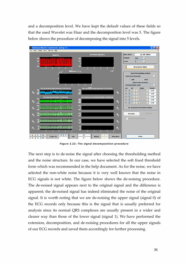
 After  extending  all  the  signals  and  saving  the  new  extended  ones, we  now could perform de‐noising using the SWT De‐noising 1‐D function. The first step in de‐noising  is decomposing  the  signal while  choosing  the  type  of Wavelet 

36

and a decomposition  level. We have kept  the default values of  these  fields so that the used Wavelet was Haar and the decomposition level was 5. The figure below shows the procedure of decomposing the signal into 5 levels.   

Figure 3.22: The signal decomposition procedure

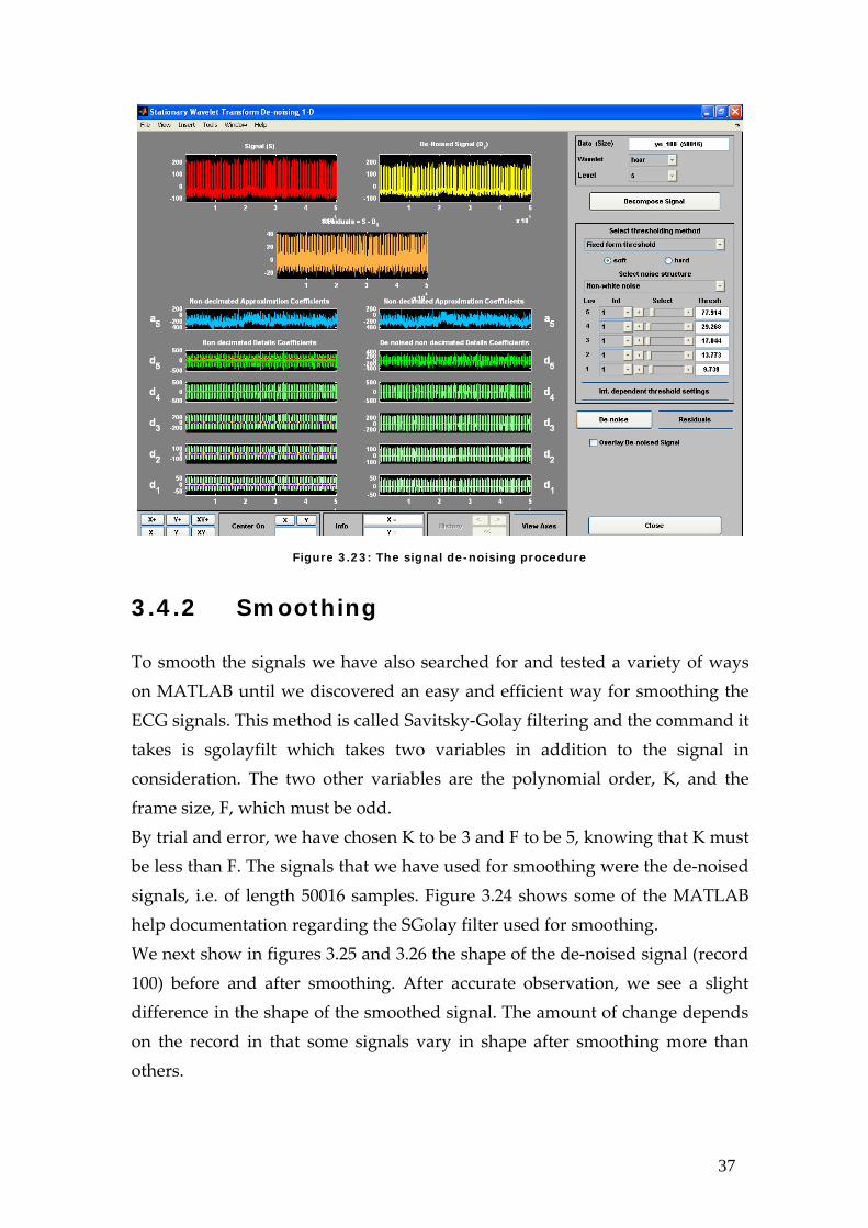
 The next step is to de‐noise the signal after choosing the thresholding method and  the noise structure.  In our case, we have selected  the soft  fixed  threshold form which was recommended in the help document. As for the noise, we have selected  the non‐white noise because  it  is very well known  that  the noise  in ECG  signals  is not white. The  figure below  shows  the de‐noising procedure. The de‐noised  signal appears next  to  the original  signal and  the difference  is apparent;  the de‐noised signal has  indeed eliminated  the noise of  the original signal. It  is worth noting  that we are de‐noising  the upper signal  (signal 0) of the ECG  records  only  because  this  is  the  signal  that  is usually preferred  for analysis  since  its normal QRS  complexes  are usually present  in  a wider  and clearer way  than  those of  the  lower signal  (signal 1). We have performed  the extension, decomposition, and de‐noising procedures for all the upper signals of our ECG records and saved them accordingly for further processing. 

37

Figure 3.23: The signal de-noising procedure

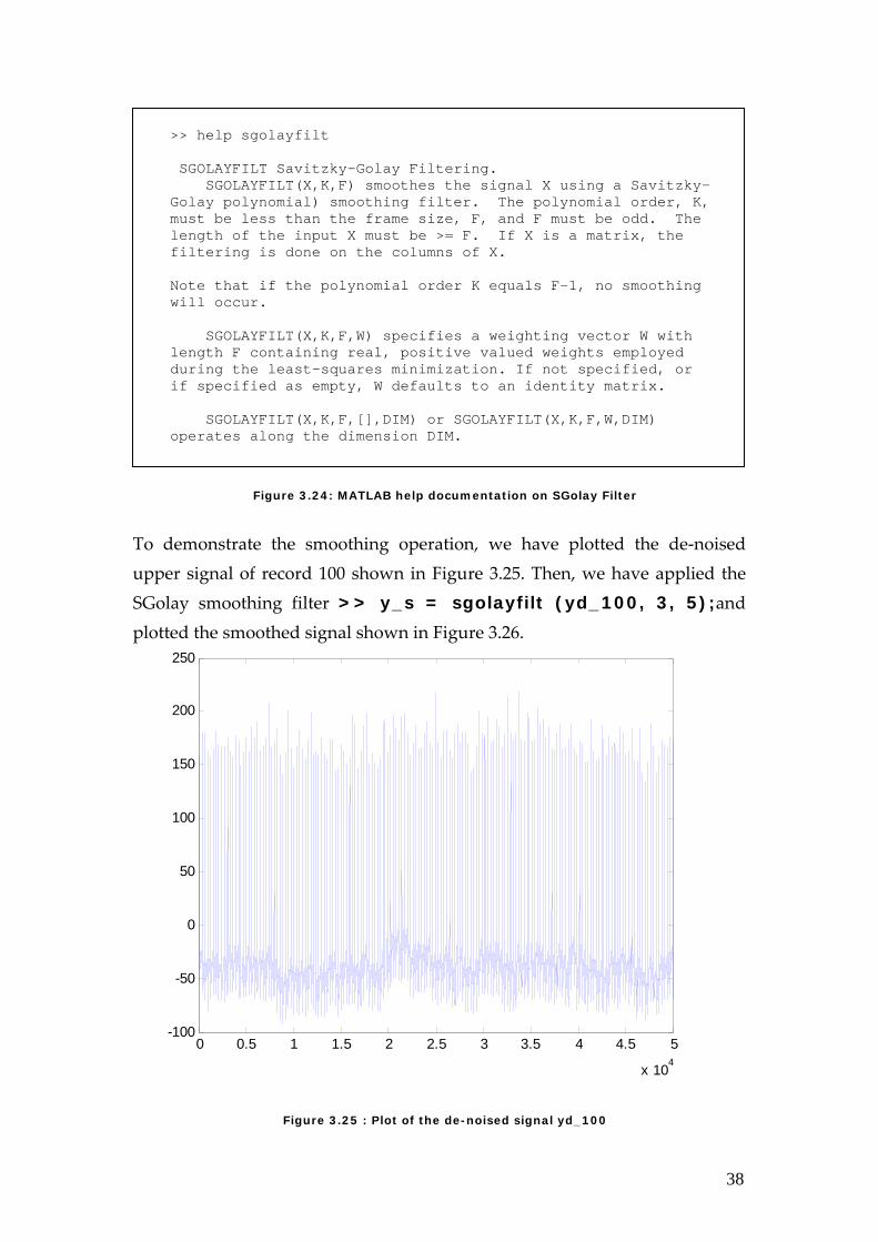
3.4.2 Smoothing  To smooth the signals we have also searched for and tested a variety of ways on MATLAB until we discovered an easy and efficient way for smoothing the ECG signals. This method is called Savitsky‐Golay filtering and the command it takes  is  sgolayfilt  which  takes  two  variables  in  addition  to  the  signal  in consideration. The  two  other  variables  are  the polynomial  order, K,  and  the frame size, F, which must be odd.  By trial and error, we have chosen K to be 3 and F to be 5, knowing that K must be less than F. The signals that we have used for smoothing were the de‐noised signals,  i.e. of  length 50016 samples. Figure 3.24 shows some of  the MATLAB help documentation regarding the SGolay filter used for smoothing.  We next show in figures 3.25 and 3.26 the shape of the de‐noised signal (record 100)  before  and  after  smoothing. After  accurate  observation, we  see  a  slight difference in the shape of the smoothed signal. The amount of change depends on  the  record  in  that  some  signals vary  in  shape  after  smoothing more  than others.  

38

                

Figure 3.24: MATLAB help documentation on SGolay Filter

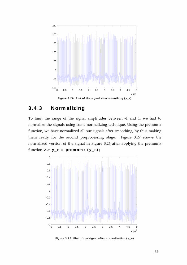
 To  demonstrate  the  smoothing  operation,  we  have  plotted  the  de‐noised upper signal of record 100 shown  in Figure 3.25. Then, we have applied  the SGolay  smoothing  filter  >> y_s = sgolayfilt (yd_100, 3, 5);and plotted the smoothed signal shown in Figure 3.26.  

 Figure 3.25 : Plot of the de-noised signal yd_100 

>> help sgolayfilt SGOLAYFILT Savitzky-Golay Filtering. SGOLAYFILT(X,K,F) smoothes the signal X using a Savitzky-Golay polynomial) smoothing filter. The polynomial order, K, must be less than the frame size, F, and F must be odd. The length of the input X must be >= F. If X is a matrix, the filtering is done on the columns of X. Note that if the polynomial order K equals F-1, no smoothing will occur. SGOLAYFILT(X,K,F,W) specifies a weighting vector W with length F containing real, positive valued weights employed during the least-squares minimization. If not specified, or if specified as empty, W defaults to an identity matrix. SGOLAYFILT(X,K,F,[],DIM) or SGOLAYFILT(X,K,F,W,DIM) operates along the dimension DIM.

0 0.5 1 1.5 2 2.5 3 3.5 4 4.5 5

x 104

-100

-50

0

50

100

150

200

250

39

0 0.5 1 1.5 2 2.5 3 3.5 4 4.5 5

x 104

-100

-50

0

50

100

150

200

250

 Figure 3.26: Plot of the signal after smoothing (y_s)

 3.4.3 Normalizing

To  limit  the  range  of  the  signal  amplitudes  between  ‐1  and  1,  we  had  to normalize  the signals using some normalizing  technique. Using  the premnmx function, we have normalized all our signals after smoothing, by thus making them  ready  for  the  second  preprocessing  stage.    Figure  3.27  shows  the normalized  version  of  the  signal  in  Figure  3.26  after  applying  the premnmx function. >> y_n = premnmx (y_s);

Figure 3.26: Plot of the signal after normalization (y_n)

0 0.5 1 1.5 2 2.5 3 3.5 4 4.5 5

x 104

-1

-0.8

-0.6

-0.4

-0.2

0

0.2

0.4

0.6

0.8

1

40

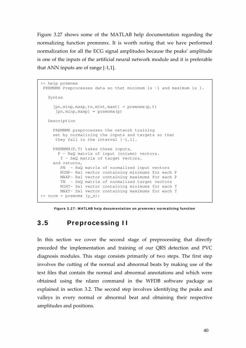
Figure  3.27  shows  some  of  the MATLAB  help  documentation  regarding  the normalizing  function  premnmx.  It  is worth  noting  that we  have  performed normalization for all the ECG signal amplitudes because the peaks’ amplitude is one of the inputs of the artificial neural network module and it is preferable that ANN inputs are of range [‐1,1].    

Figure 3.27: MATLAB help documentation on premnmx normalizing function

3.5 Preprocessing II In  this  section  we  cover  the  second  stage  of  preprocessing  that  directly preceded  the  implementation  and  training  of  our  QRS  detection  and  PVC diagnosis modules. This  stage  consists primarily  of  two  steps. The  first  step involves  the  cutting of  the normal and abnormal beats by making use of  the text  files  that  contain  the normal  and  abnormal  annotations  and which were obtained  using  the  rdann  command  in  the  WFDB  software  package  as explained  in  section  3.2. The  second  step  involves  identifying  the peaks  and valleys  in  every  normal  or  abnormal  beat  and  obtaining  their  respective amplitudes and positions. 

>> help premnmx PREMNMX Preprocesses data so that minimum is -1 and maximum is 1. Syntax [pn,minp,maxp,tn,mint,maxt] = premnmx(p,t) [pn,minp,maxp] = premnmx(p) Description PREMNMX preprocesses the network training set by normalizing the inputs and targets so that they fall in the interval [-1,1]. PREMNMX(P,T) takes these inputs, P - RxQ matrix of input (column) vectors. T - SxQ matrix of target vectors. and returns, PN - RxQ matrix of normalized input vectors MINP- Rx1 vector containing minimums for each P MAXP- Rx1 vector containing maximums for each P TN - SxQ matrix of normalized target vectors MINT- Sx1 vector containing minimums for each T MAXT- Sx1 vector containing maximums for each T >> norm = premnmx (y_s);

41

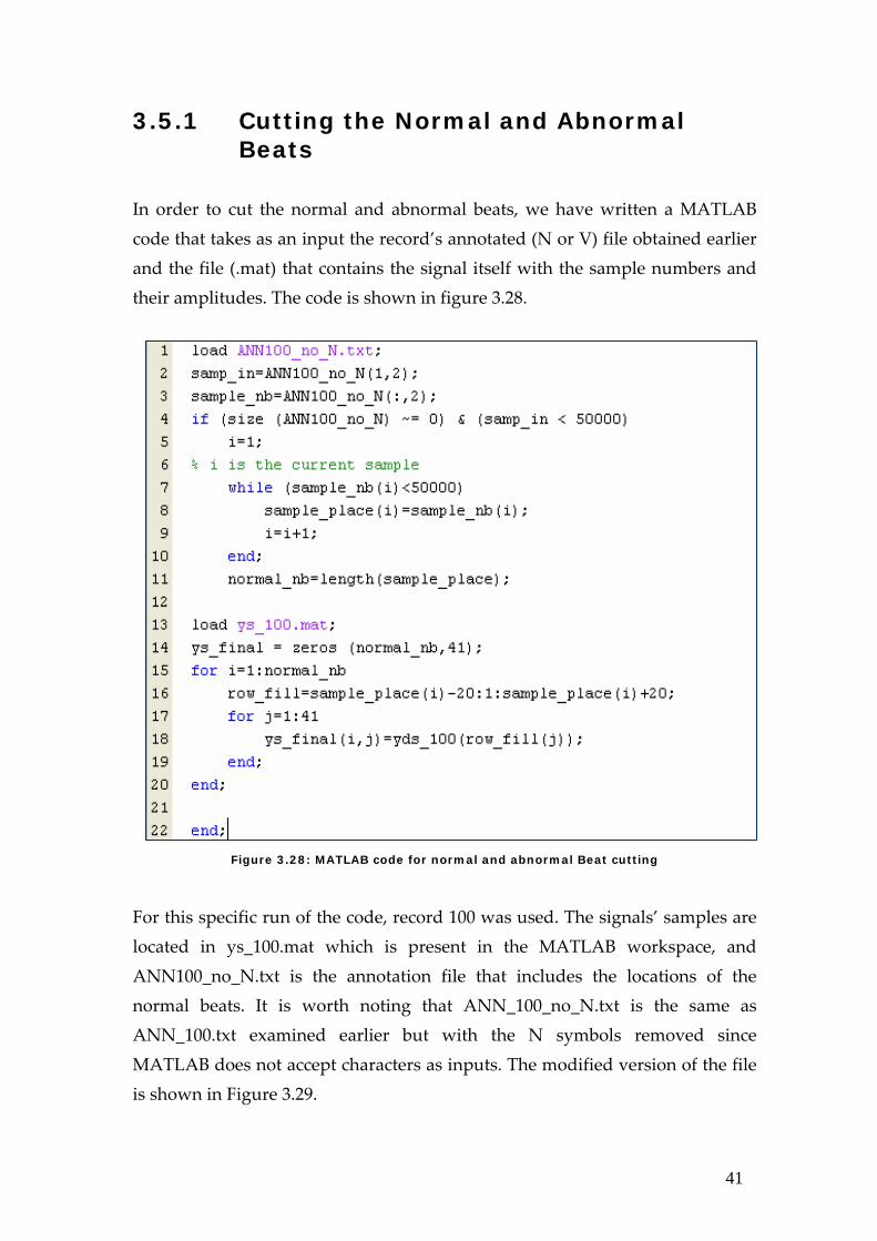
3.5.1 Cutting the Normal and Abnormal Beats

In order  to  cut  the normal and abnormal beats, we have written a MATLAB code that takes as an input the record’s annotated (N or V) file obtained earlier and the file (.mat) that contains the signal  itself with the sample numbers and their amplitudes. The code is shown in figure 3.28.   

Figure 3.28: MATLAB code for normal and abnormal Beat cutting

 For this specific run of the code, record 100 was used. The signals’ samples are located  in  ys_100.mat  which  is  present  in  the  MATLAB  workspace,  and ANN100_no_N.txt  is  the  annotation  file  that  includes  the  locations  of  the normal  beats.  It  is  worth  noting  that  ANN_100_no_N.txt  is  the  same  as ANN_100.txt  examined  earlier  but  with  the  N  symbols  removed  since MATLAB does not accept characters as inputs. The modified version of the file is shown in Figure 3.29. 

42

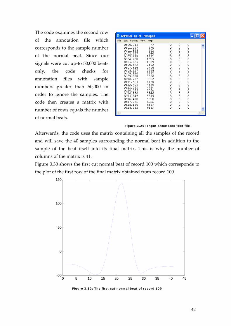
The code examines the second row of  the  annotation  file  which corresponds to the sample number of  the  normal  beat.  Since  our signals were cut up‐to 50,000 beats only,  the  code  checks  for annotation  files  with  sample numbers  greater  than  50,000  in order  to  ignore  the  samples.  The code  then  creates  a  matrix  with number of rows equals the number of normal beats.  

                  Figure 3.29: Input annotated text file

Afterwards,  the code uses  the matrix containing all  the samples of  the record and will  save  the 40  samples  surrounding  the normal beat  in addition  to  the sample  of  the  beat  itself  into  its  final  matrix.  This  is  why  the  number  of columns of the matrix is 41.   Figure 3.30 shows the first cut normal beat of record 100 which corresponds to the plot of the first row of the final matrix obtained from record 100.                

Figure 3.30: The first cut normal beat of record 100

0 5 10 15 20 25 30 35 40 45-50

0

50

100

150

43

Similarly, we cut the normal beats of all signals. We cut the abnormal beats too in the same fashion and with the same code using the PVC annotated files. 

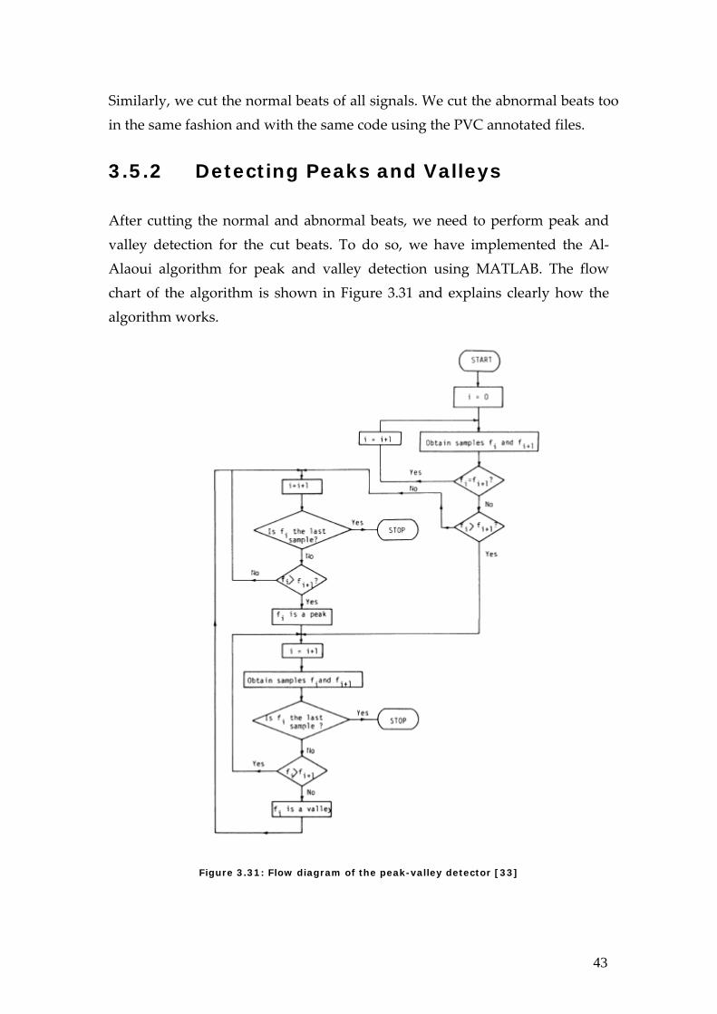
3.5.2 Detecting Peaks and Valleys  After cutting  the normal and abnormal beats, we need  to perform peak and valley detection  for  the  cut  beats. To do  so, we  have  implemented  the Al‐Alaoui  algorithm  for  peak  and  valley  detection  using MATLAB.  The  flow chart of  the algorithm  is shown  in Figure 3.31 and explains clearly how  the algorithm works.  

                      

Figure 3.31: Flow diagram of the peak-valley detector [33]

 

44

The peak and valley detector  correctly detects  the P, Q, R, S, and T waves. Our code also identifies whether one of these waves is missing by replacing it by a zero ‘0’ since not all beats, especially abnormal ones, are characterized by the  standard PQRST waves. Therefore, at  this  stage we performed  the peak and  valley  detection  and  consequently  QRS  detection  since  we  could determine the position and amplitudes of the Q, R, and S waves.  The  code used at  this  stage  results  in  five outputs which are  the amplitude and position of each of the P, Q, R, S, and T waves. These 10 outputs are used in the processing stage as inputs for the ANN module and the hybrid fuzzy‐neuro module. 

 

45

Chapter 4 Artificial Neural Network A neural network  is a connection of parallel operating simple elements  that are inspired by biological nervous systems. The neural network can be trained to perform a particular function by adjusting the values of the connections (or weights) between these elements. In this chapter, we will start by introducing the  design  method  of  the  neural  network. We  will  then  move  on  to  the implementation stages involving both the training and testing parts; the latter also known as the simulation. Finally, we will tabulate the computed results and compare those to others achieved by systems in the literature.     

4.1 Design of the Neural Network

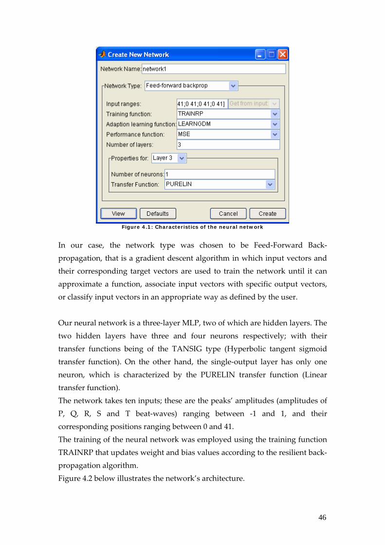
The Neural Network  Toolbox  is  a  useful  tool  for  industry,  education  and research. It explains procedures, applies them, and shows their successes and failures; thus, helping in the development of neural networks.   The NNtool in the Neural Network Toolbox was previously shown in Figure 3.17 Within  the  Network/Data  Manager  in  the  NNTool  window,  the  New Network  button  is  used  for  creating  a  neural  network which  can  also  be imported  from  the  Matlab  workspace.  Once  we  choose  creating  a  new network, a window illustrating the network’s desired characteristics pops up as given by Figure 4.1. 

46

Figure 4.1: Characteristics of the neural network

In  our  case,  the  network  type  was  chosen  to  be  Feed‐Forward  Back‐propagation, that is a gradient descent algorithm in which input vectors and their corresponding  target vectors are used  to  train  the network until  it can approximate a  function, associate  input vectors with specific output vectors, or classify input vectors in an appropriate way as defined by the user.  Our neural network is a three‐layer MLP, two of which are hidden layers. The two  hidden  layers  have  three  and  four  neurons  respectively;  with  their transfer  functions  being  of  the  TANSIG  type  (Hyperbolic  tangent  sigmoid transfer  function). On  the  other hand,  the  single‐output  layer has  only  one neuron, which  is  characterized  by  the  PURELIN  transfer  function  (Linear transfer function). The network takes ten inputs; these are the peaks’ amplitudes (amplitudes of P,  Q,  R,  S  and  T  beat‐waves)  ranging  between  ‐1  and  1,  and  their corresponding positions ranging between 0 and 41. The training of the neural network was employed using the training function TRAINRP that updates weight and bias values according to the resilient back‐propagation algorithm. Figure 4.2 below illustrates the network’s architecture. 

47

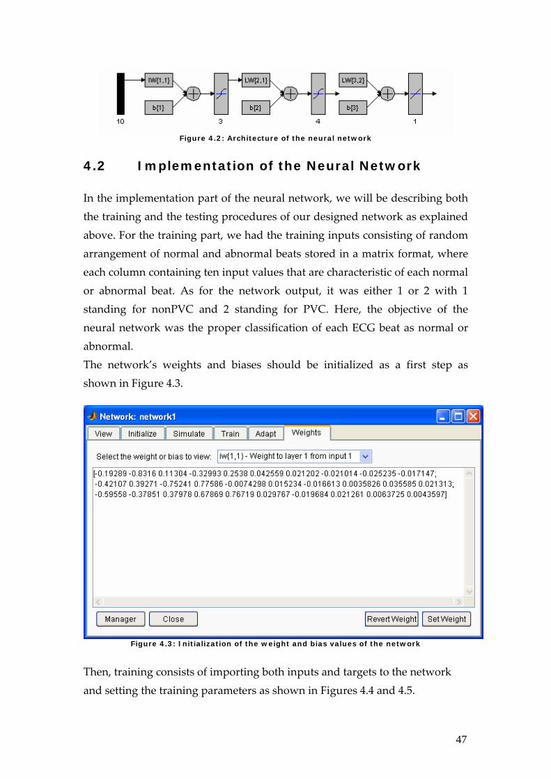
 Figure 4.2: Architecture of the neural network

4.2 Implementation of the Neural Network

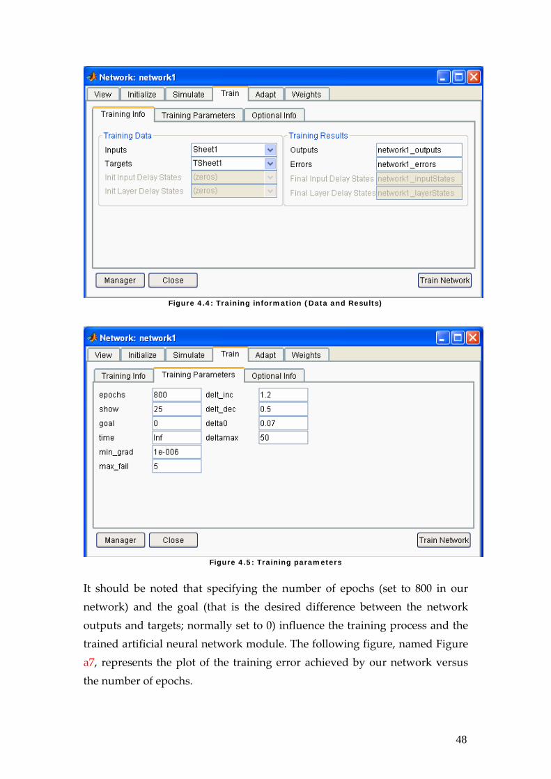
In the implementation part of the neural network, we will be describing both the training and the testing procedures of our designed network as explained above. For the training part, we had the training inputs consisting of random arrangement of normal and abnormal beats stored in a matrix format, where each column containing ten input values that are characteristic of each normal or  abnormal  beat. As  for  the  network  output,  it was  either  1  or  2 with  1 standing  for  nonPVC  and  2  standing  for  PVC.  Here,  the  objective  of  the neural network was  the proper classification of each ECG beat as normal or abnormal. The  network’s  weights  and  biases  should  be  initialized  as  a  first  step  as shown in Figure 4.3.   

Figure 4.3: Initialization of the weight and bias values of the network

Then, training consists of importing both inputs and targets to the network and setting the training parameters as shown in Figures 4.4 and 4.5. 

48

Figure 4.4: Training information (Data and Results)

Figure 4.5: Training parameters

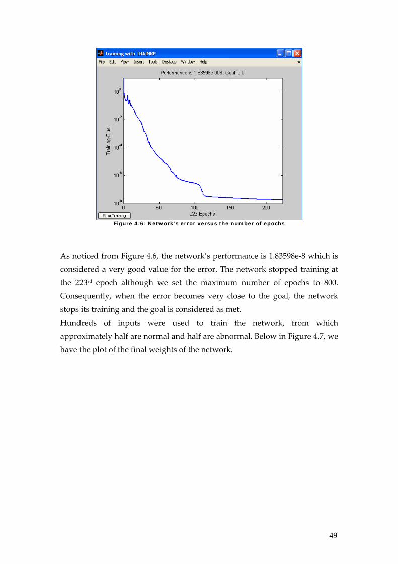
It  should be noted  that  specifying  the number  of  epochs  (set  to  800  in  our network)  and  the  goal  (that  is  the  desired  difference  between  the  network outputs and targets; normally set to 0) influence the training process and the trained artificial neural network module. The following figure, named Figure a7,  represents  the plot of  the  training error achieved by our network versus the number of epochs. 

 

49

 Figure 4.6: Network’s error versus the number of epochs

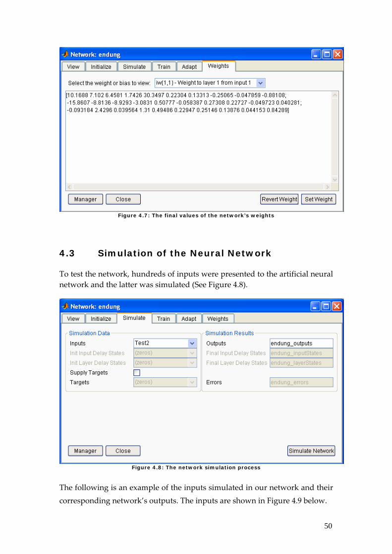
 As noticed from Figure 4.6, the network’s performance is 1.83598e‐8 which is considered a very good value for the error. The network stopped training at the  223rd  epoch  although we  set  the maximum  number  of  epochs  to  800. Consequently, when  the  error  becomes  very  close  to  the  goal,  the  network stops its training and the goal is considered as met. Hundreds  of  inputs  were  used  to  train  the  network,  from  which approximately half are normal and half are abnormal. Below in Figure 4.7, we have the plot of the final weights of the network.  

50

 Figure 4.7: The final values of the network’s weights

4.3 Simulation of the Neural Network

To test the network, hundreds of inputs were presented to the artificial neural network and the latter was simulated (See Figure 4.8). 

Figure 4.8: The network simulation process

The following is an example of the inputs simulated in our network and their corresponding network’s outputs. The inputs are shown in Figure 4.9 below. 

51

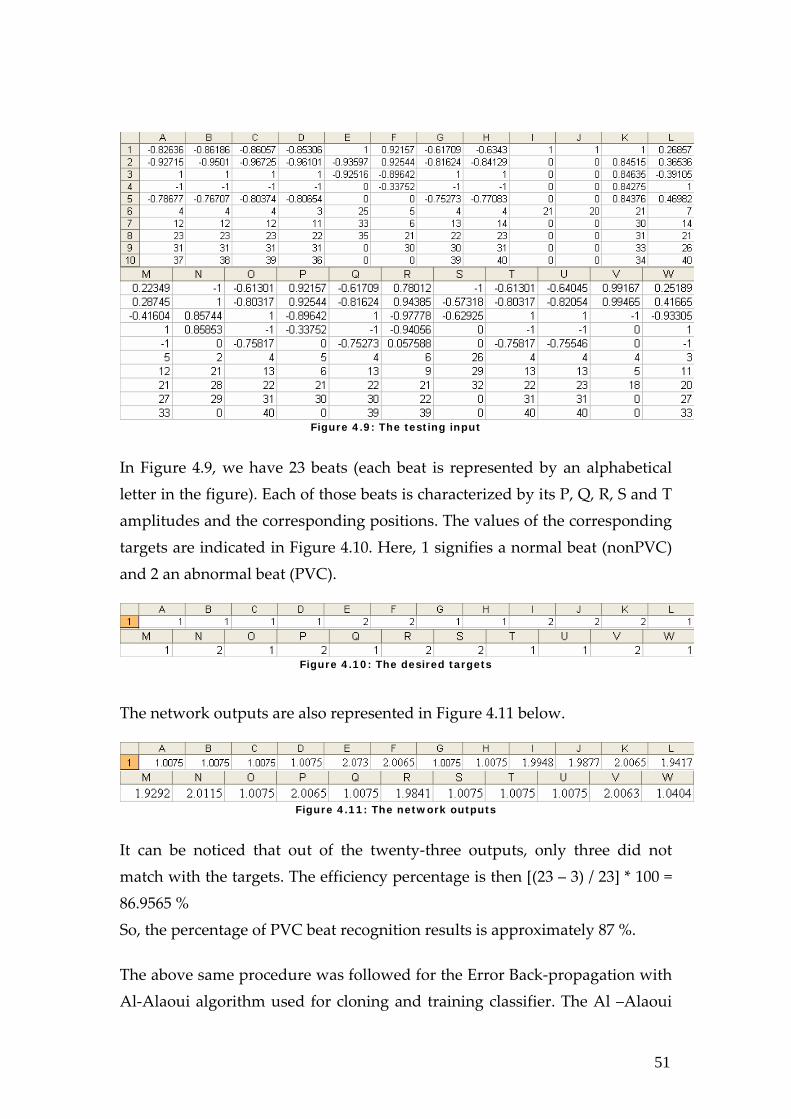
Figure 4.9: The testing input

In Figure 4.9, we have 23 beats  (each beat  is  represented by an alphabetical letter in the figure). Each of those beats is characterized by its P, Q, R, S and T amplitudes and the corresponding positions. The values of the corresponding targets are indicated in Figure 4.10. Here, 1 signifies a normal beat (nonPVC) and 2 an abnormal beat (PVC). 

Figure 4.10: The desired targets

 The network outputs are also represented in Figure 4.11 below.

Figure 4.11: The network outputs

It  can  be  noticed  that  out  of  the  twenty‐three  outputs,  only  three  did  not match with the targets. The efficiency percentage is then [(23 – 3) / 23] * 100 = 86.9565 %  So, the percentage of PVC beat recognition results is approximately 87 %.   The above same procedure was followed for the Error Back‐propagation with Al‐Alaoui algorithm used  for cloning and  training classifier. The Al –Alaoui 

52

0 5 10 15 20 251

1.2

1.4

1.6

1.8

2

2.2

2.4

0 5 10 15 20 250.8

1

1.2

1.4

1.6

1.8

2

2.2

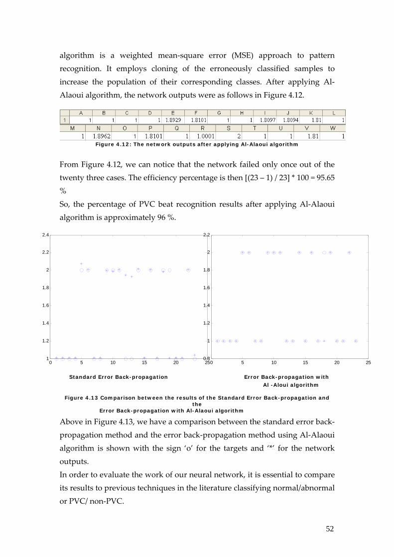
algorithm  is  a  weighted  mean‐square  error  (MSE)  approach  to  pattern recognition.  It  employs  cloning  of  the  erroneously  classified  samples  to increase  the  population  of  their  corresponding  classes.  After  applying  Al‐Alaoui algorithm, the network outputs were as follows in Figure 4.12. 

Figure 4.12: The network outputs after applying Al-Alaoui algorithm

From Figure 4.12, we can notice that the network failed only once out of the twenty three cases. The efficiency percentage is then [(23 – 1) / 23] * 100 = 95.65 %  So,  the percentage of PVC beat  recognition  results after applying Al‐Alaoui algorithm is approximately 96 %.  

     Standard Error Back-propagation Error Back-propagation with   Al -Aloui algorithm

Figure 4.13 Comparison between the results of the Standard Error Back-propagation and the

Error Back-propagation with Al-Alaoui algorithm

Above in Figure 4.13, we have a comparison between the standard error back‐propagation method and the error back‐propagation method using Al‐Alaoui algorithm  is  shown with  the  sign  ‘o’  for  the  targets and  ‘*’  for  the network outputs.  In order to evaluate the work of our neural network, it is essential to compare its results to previous techniques in the literature classifying normal/abnormal or PVC/ non‐PVC.  

53

 Comparing  two  existing  QRS  enhancement  methods,  the  linear  adaptive filtering  method  and  the  band‐pass  filtering  method  to  the  Error  Back‐propagation  method,  using  Record  108  of  the  MIT/BIH  Database,  the following results were obtained and summarized in Table 4.1.  

Table 4.1: Comparison between the efficiency of different techniques for QRS Detection

The failed detection rate (given in %) of our designed and implemented error backpropagation  artificial neural network being  0.8 %  is  comparable  to  the best system out of the three  indicated above; and these relate to well‐known international published papers.  

54

       

Chapter 5 Fuzzy-Neural Networks  We have presented in Chapter 4 the first module for QRS detection and PVC diagnosis, using the Artificial Neural Networks Method.  We have described the  design  steps  and  the  implementation  stages  of  this  method  from  the creation of the artificial neural network system to  its training and finally the testing with  standard  database  records.  In  addition, we  have  provided  an improvement  to  this method using  the Al‐Alaoui Algorithm and  compared both  techniques  in  neural  networks  in  terms  of  rate  of misclassification  to other well‐published  and  recognized  systems  in  the  literature.  This  section will be discussing  the second module dedicated  for QRS detection and PVC diagnosis, which is the Fuzzy‐Neuro‐Based Module, from the design process to the implementation stages and the results obtained.    5.1 Design of Fuzzy-Neuro-Based Module  Design Criteria: 

QRS detection and PVC diagnosis   Real‐time implementation

 Proposed Solution:   ANFIS  system  that  can  be  trained  using  desired  input‐output (amplitude/position‐class) ECG  signals and  is able  to adapt  to any patientʹs cardiac signal generating its proper diagnosis, either PVC or nonPVC.

55

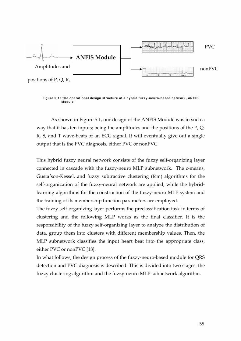
Figure 5.1: The operational design structure of a hybrid fuzzy-neuro-based network, ANFIS Module

As shown in Figure 5.1, our design of the ANFIS Module was in such a way that it has ten inputs; being the amplitudes and the positions of the P, Q, R, S, and T wave‐beats of an ECG signal. It will eventually give out a single output that is the PVC diagnosis, either PVC or nonPVC.      This hybrid  fuzzy neural network consists of  the  fuzzy self‐organizing  layer connected  in cascade with  the  fuzzy‐neuro MLP subnetwork.   The c‐means, Gustafson‐Kessel,  and  fuzzy  subtractive  clustering  (fcm)  algorithms  for  the self‐organization of  the  fuzzy‐neural network are applied, while  the hybrid‐learning algorithms for the construction of the fuzzy‐neuro MLP system and the training of its membership function parameters are employed.  The fuzzy self‐organizing layer performs the preclassification task in terms of clustering  and  the  following  MLP  works  as  the  final  classifier.  It  is  the responsibility of the fuzzy self‐organizing layer to analyze the distribution of data, group  them  into  clusters with different membership values. Then,  the MLP  subnetwork  classifies  the  input  heart  beat  into  the  appropriate  class, either PVC or nonPVC [18]. In what follows, the design process of the fuzzy‐neuro‐based module for QRS detection and PVC diagnosis is described. This is divided into two stages: the fuzzy clustering algorithm and the fuzzy‐neuro MLP subnetwork algorithm.    

ANFIS Module

PVC  

nonPVC  Amplitudes and 

positions of P, Q, R, 

56

5.1.1 The Fuzzy Clustering Algorithm  This algorithm is a data clustering technique where each data point belongs to a  cluster  to  some degree  that  is  specified by a membership grade.  It  shows how  to group data points that populate some multidimensional space  into a specific number of different clusters.  The inputs to this fuzzy clustering algorithm are the ten values corresponding to  the  amplitudes  and  the  positions  of  the  P, Q,  R,  S,  and  T  beats  in  the processed ECG signal recording under classification denoted by vectors xk = [xk1  , xk2  , …, xkN]T for k = 1, 2,…p.   The classification of these vectors xk into c clusters, with each cluster having a center vector ci = [ci1, ci2, …, ciN]T for i = 1, 2,…c,  results  in  the partitioning of  the  inputs  in  the data space according  to given membership  functions. The  fuzzy clustering algorithms search  for  the partition  matrix  and  cluster  centers  such  that  the  objective  function  E  is minimized.  

1

),(

1

1 1

2

=

=

∑

∑∑

=

= =

c

i

mji

c

i

p

jij

mji

u

cxduE 

 where the parameter m controls the fuzziness of the clusters; its typical value is  2,  the  function  ),( ij cxd measures  the  distance  between  the  input  vector 

jx and the center  ic , and the partition matrix U of the elements  jiu  represents the membership function degrees of the data vector  jx .   The  distance  ),( ij cxd   of  the  G‐K  algorithm  uses  the  scaled  metric  norm having  

)()(),(2iji

Tijij cxMcxcxd −−=   

with  iM being a positive definite matrix adjusted  to  the actual  shape of  the cluster and it is defined as follows  

1)det( −= iN

ii FFM   

 

57

And 

 ∑

∑

=

=

−−= p

j

mji

p

jij

Tij

mji

i

u

cxcxuF

1

1)()( 

being the cluster covariance matrix.    The  training  of  the  fuzzy  clustering  self‐organizing  layer  is done using  the fuzzy competition. It searches for the cluster centers and the partition matrix elements. And  its objective  is  to  find  the optimal number of  cluster  centers needed  for  the  input‐output  data‐pair  modeling  as  well  as  the  optimal influence ranges of each of these cluster centers defined by the cluster center radius. Below, we have the different steps in the design process of the fuzzy subtractive algorithm; these are:   

1. Choose the number of clusters c and the weighting coefficients m. 2. Initialize the  termination  tolerance  ε and  the partition matrix U  such 

that  11

=∑=

c

i

mjiu .  

3. Start  iterating. Determine  the  clusters  ci  =  [ci1,  ci2, …,  ciN]T  for  i  =  1, 2,…c,where 

 

∑

∑

=

== p

j

mji

p

jj

mji

i

u

xuc

1

1  

 4. Calculate the matrices  iF ( i =1, 2,.. c) 5. Compute  the  distances  cid ji ...,,2,1(2 = and  )...,,2,1 pj = between  the 

input vector and the cluster centers. 6. Update the partition matrix   jiu  entries  ci ...,,2,1( = and  )...,,2,1 pj =    

 

∑=

−

=c

k

m

jk

jiji

dd

u

1

)1/(2)(

1  

 If  0=jid for some i = I, take  =jIu 1 and  =jiu 0 for i ≠ I. Iterate until 

ε≤− − |||| 1ll UU for two succeeding iterations [18].  

58

It should be noted that the most important stage of the design is the choice of the number of clusters and  the cluster radius centers  (the  influence range of each cluster center on the data samples nearby belonging to a given cluster by a  specified  grade  of membership);  as  this will  affect  the  complexity  of  the whole system in terms of its set of rules as well as the number of membership function  for each of  the  ten  inputs and  single output when  the  fuzzy‐neuro system  is generated after  the  second algorithm described  later on.  It would also  affect  the  reduction  rate  of  the  error  function  and  the  generalization ability of the network. This can be recognized by the following:  If  the  number  of  clusters  chosen  is  too  small,  i.e.  the  values  of  the  cluster radius centers are too large with respect to the training data samples, then, the number  of membership  function  for  the  inputs  and  the  output will be  low yielding  lower  complexity  of  the whole  fuzzy‐neuro  system. Nevertheless, this will prevent the reduction of the error function from reaching a very low level.  From  a  different  perspective,  if  it  is  too  high,  this will  destroy  the generalization ability of the network.      5.1.2 The Fuzzy-Neuro MLP Subnetwork

Algorithm  The  fuzzy‐neuro  MLP  subnetwork  classifies  the  applied  input  vector, representing the heart beat to the appropriate class, PVC or nonPVC. This  is attained by applying  the output of  the self‐organizing  fuzzy clustering  layer to the input layer of the MLP subnetwork structure.  Now  for  the generation of  the  fuzzy‐neuro system, we will create a Sugeno‐type ANFIS,  the  fuzzy‐neuro system, with a knowledge of  the  training data pairs composed of the ten  inputs and the desired class output as well as the optimal  cluster  radius  center. This  is achieved by extracting  the  set of  rules that model  the data behaviour by  first determining  the number of rules and antecedent  membership  functions  and  then  using  linear  least‐squares estimation to determine each ruleʹs consequent equations.  As for the further learning of the fuzzy‐neuro MLP subnetwork, we will use a hybrid‐learning algorithm to identify the membership function parameters of the single‐output ANFIS. It will adapt the membership function parameters of 

59

the  ANFIS  using  a  combination  of  the  least‐squares  and  backpropagation gradient  descent methods. After  the  training  procedure  is  over,  the  cluster centers  and  the  scaling matrices  of  the  self‐organizing  layer  as well  as  the generated adaptive membership function parameters of the fuzzy‐neuro MLP subnetwork  are  frozen  and  ready  for  use  in  the  retrieval mode, when  the hybrid  fuzzy‐neuro‐based  QRS  detector  and  PVC  diagnostic  approach  is tested with ECG signals.

 5.3 Implementation of Fuzzy-Neuro-Based Module  The ANFIS Module  or  the Hybrid  Fuzzy‐Neuro Module was  implemented using  the  Graphical  Interfaces ANFIS  Editor  GUI  and  the  FINDCLUSTER GUI  of  the  Fuzzy  Logic  Toolbox  of MATLAB  Version  7.0  R14.  The  basic structure  of  our  Sugeno‐type  inference  system  is  a model  that maps  input characteristics to input membership functions, input membership functions to rules, rules  to a set of output characteristics, output characteristics  to output membership  functions,  and  the  output membership  functions  to  a  single‐valued output or a decision associated with the output. Let us start by giving the whole picture of the ANFIS module implementation divided into the two basic algorithms implemented and described previously.  

  5.2.1 The Fuzzy Clustering Algorithm  This algorithm estimates the number of clusters and cluster centers in a set of data.  So,  it  starts  with  an  initial  guess  of  the  cluster  centers,  which  are intended to spot the mean location of each cluster. In most cases, these initial estimates or guesses are  incorrect.  It also assigns every data  sample point a membership grade  for each cluster;  i.e. a measure  to how much  the specific data  point  follows  or  agrees  with  the  property  described  by  each  cluster defined  by  the  cluster  center.  By  iteratively  updating  the  values  of  these cluster  centers  and  the  membership  grades,  also  known  as  the  partition matrix elements, for each data sample of the training data, the cluster centers 

60

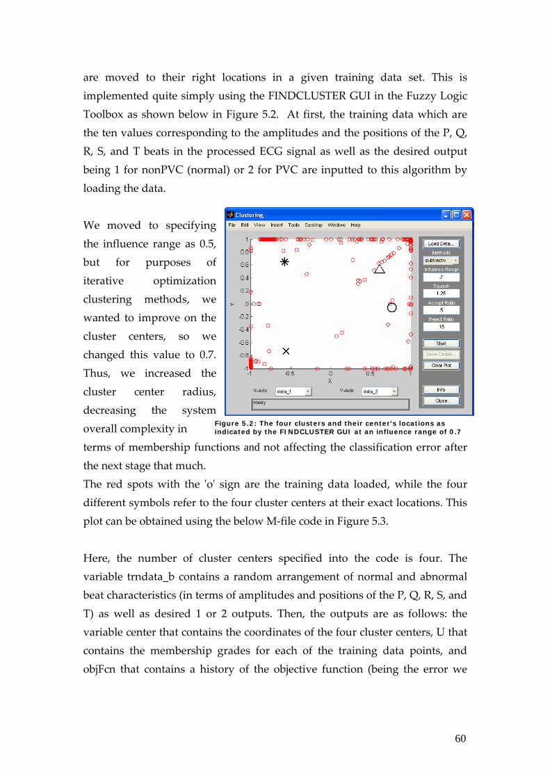
are  moved  to  their  right  locations  in  a  given  training  data  set.  This  is implemented quite simply using the FINDCLUSTER GUI in the Fuzzy Logic Toolbox as shown below  in Figure 5.2.   At  first,  the  training data which are the ten values corresponding to the amplitudes and the positions of the P, Q, R, S, and T beats  in  the processed ECG signal as well as  the desired output being 1 for nonPVC (normal) or 2 for PVC are  inputted to this algorithm by loading the data.  

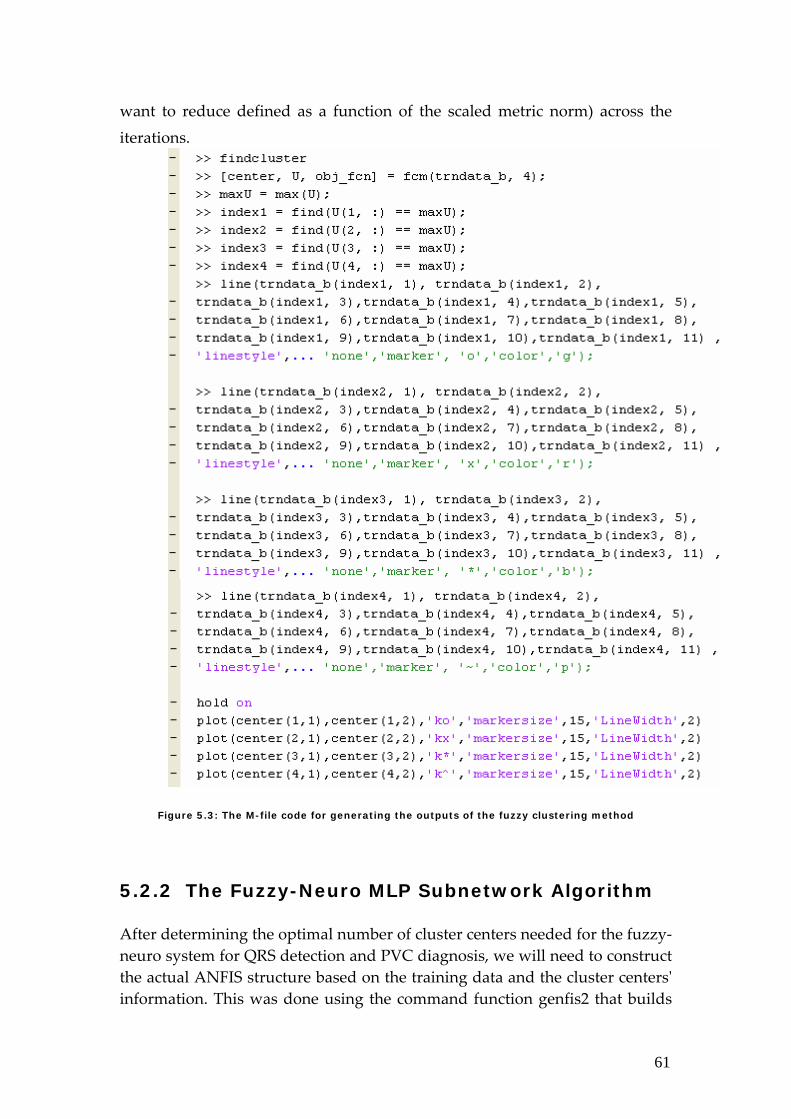
We  moved  to  specifying the  influence  range as 0.5, but  for  purposes  of iterative  optimization clustering  methods,  we wanted  to  improve on  the cluster  centers,  so we changed  this  value  to  0.7. Thus,  we  increased  the cluster  center  radius, decreasing  the  system overall complexity in terms of membership functions and not affecting the classification error after the next stage that much.  The  red  spots with  the  ʹoʹ  sign  are  the  training data  loaded, while  the  four different symbols refer to the four cluster centers at their exact locations. This plot can be obtained using the below M‐file code in Figure 5.3.   Here,  the  number  of  cluster  centers  specified  into  the  code  is  four.  The variable  trndata_b contains a  random arrangement of normal and abnormal beat characteristics (in terms of amplitudes and positions of the P, Q, R, S, and T)  as well  as  desired  1  or  2  outputs.  Then,  the  outputs  are  as  follows:  the variable center that contains the coordinates of the four cluster centers, U that contains  the membership  grades  for  each  of  the  training  data  points,  and objFcn  that  contains  a history  of  the  objective  function  (being  the  error we 

Figure 5.2: The four clusters and their center's locations as indicated by the FINDCLUSTER GUI at an influence range of 0.7

61

want  to  reduce defined  as  a  function of  the  scaled metric norm)  across  the iterations.    

S

H

e

Figure 5.3: The M-file code for generating the outputs of the fuzzy clustering method

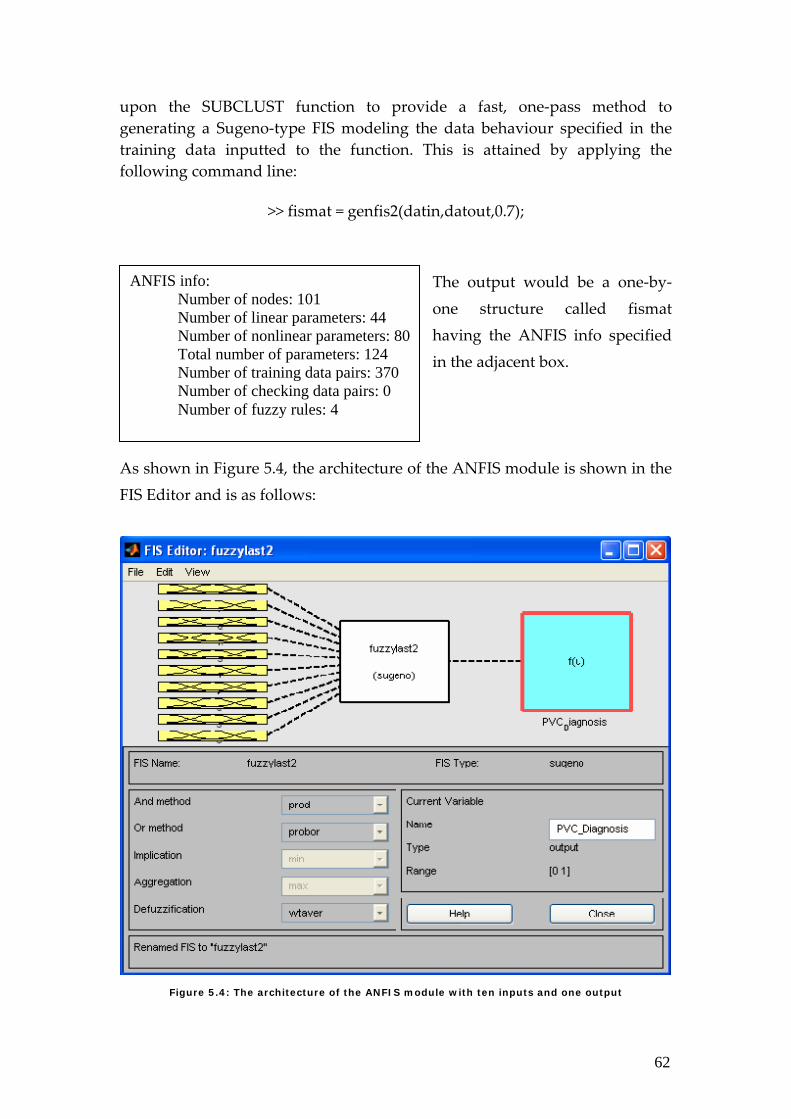
5.2.2 The Fuzzy-Neuro MLP Subnetwork Algorithm  After determining the optimal number of cluster centers needed for the fuzzy‐neuro system for QRS detection and PVC diagnosis, we will need to construct the actual ANFIS structure based on the training data and the cluster centersʹ information. This was done using  the command  function genfis2  that builds 

62

upon  the  SUBCLUST  function  to  provide  a  fast,  one‐pass  method  to generating  a  Sugeno‐type FIS modeling  the data behaviour  specified  in  the training  data  inputted  to  the  function.  This  is  attained  by  applying  the following command line: 

>> fismat = genfis2(datin,datout,0.7);

The  output  would  be  a  one‐by‐one  structure  called  fismat having  the ANFIS  info  specified in the adjacent box.  

As shown in Figure 5.4, the architecture of the ANFIS module is shown in the FIS Editor and is as follows:  

Figure 5.4: The architecture of the ANFIS module with ten inputs and one output

ANFIS info: Number of nodes: 101 Number of linear parameters: 44 Number of nonlinear parameters: 80 Total number of parameters: 124 Number of training data pairs: 370 Number of checking data pairs: 0 Number of fuzzy rules: 4

63

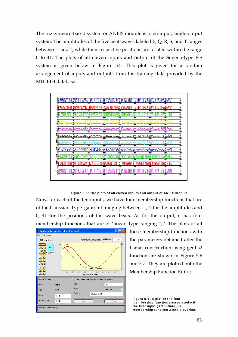
The fuzzy‐neuro‐based system or ANFIS module is a ten‐input, single‐output system. The amplitudes of the five beat‐waves labeled P, Q, R, S, and T ranges between ‐1 and 1, while their respective positions are located within the range 0  to  41.  The  plots  of  all  eleven  inputs  and  output  of  the  Sugeno‐type  FIS system  is  given  below  in  Figure  5.5.  This  plot  is  given  for  a  random arrangement  of  inputs  and outputs  from  the  training data provided by  the MIT‐BIH database.      

Figure 5.5: The plots of all eleven inputs and output of ANFIS module

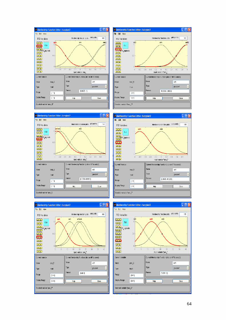
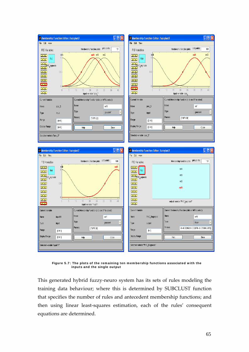
Now, for each of the ten inputs, we have four membership functions that are of the Gaussian Type ʹgaussmfʹ ranging between ‐1, 1 for the amplitudes and 0,  41  for  the  positions  of  the  wave  beats.  As  for  the  output,  it  has  four membership  functions  that  are  of  ‘linear’  type  ranging  1,2. The plots  of  all 

these membership  functions with the parameters obtained after  the fismat  construction using genfis2 function  are  shown  in Figure  5.6 and 5.7. They are plotted onto the Membership Function Editor. 

Figure 5.6: A plot of the four membership functions associated with the first input (amplitude_P). Membership function 3 and 4 overlap.

64

65

This generated hybrid  fuzzy‐neuro system has  its sets of rules modeling  the training  data  behaviour; where  this  is  determined  by  SUBCLUST  function that specifies the number of rules and antecedent membership functions; and then  using  linear  least‐squares  estimation,  each  of  the  rules’  consequent equations are determined. 

Figure 5.7: The plots of the remaining ten membership functions associated with the inputs and the single output

66

       

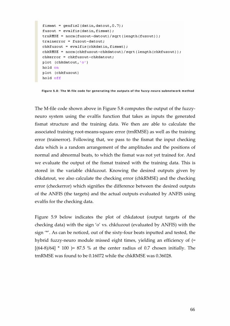
Figure 5.8: The M-file code for generating the outputs of the fuzzy-neuro subnetwork method

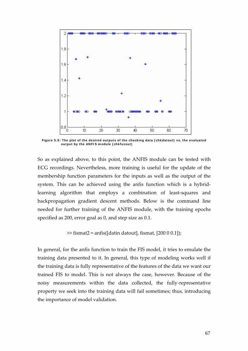
 The M‐file code shown above in Figure 5.8 computes the output of the fuzzy‐neuro  system  using  the  evalfis  function  that  takes  as  inputs  the  generated fismat  structure  and  the  training  data. We  then  are  able  to  calculate  the associated training root‐means‐square error (trnRMSE) as well as the training error  (trainerror).  Following  that, we pass  to  the  fismat  the  input  checking data which  is a random arrangement of  the amplitudes and  the positions of normal and abnormal beats, to which the fismat was not yet trained for. And we  evaluate  the output of  the  fismat  trained with  the  training data. This  is stored  in  the  variable  chkfuzout.  Knowing  the  desired  outputs  given  by chkdatout, we also calculate the checking error (chkRMSE) and the checking error (checkerror) which signifies the difference between the desired outputs of the ANFIS (the targets) and the actual outputs evaluated by ANFIS using evalfis for the checking data.   Figure  5.9  below  indicates  the  plot  of  chkdatout  (output  targets  of  the checking data) with the sign ‘o’ vs. chkfuzout (evaluated by ANFIS) with the sign ‘*’. As can be noticed, out of the sixty‐four beats inputted and tested, the hybrid  fuzzy‐neuro module missed  eight  times, yielding  an  efficiency of  (= [(64‐8)/64]  *  100  )=  87.5 %  at  the  center  radius  of  0.7  chosen  initially.  The trnRMSE was found to be 0.16072 while the chkRMSE was 0.36028.      

67

             

Figure 5.9: The plot of the desired outputs of the checking data (chkdatout) vs. the evaluated output by the ANFIS module (chkfuzout)  So as  explained above,  to  this point,  the ANFIS module  can be  tested with ECG  recordings. Nevertheless, more  training  is useful  for  the update of  the membership  function parameters  for  the  inputs as well as  the output of  the system.  This  can  be  achieved  using  the  anfis  function which  is  a  hybrid‐learning  algorithm  that  employs  a  combination  of  least‐squares  and backpropagation  gradient  descent  methods.  Below  is  the  command  line needed  for  further  training of  the ANFIS module, with  the  training  epochs specified as 200, error goal as 0, and step size as 0.1.   

>> fismat2 = anfis([datin datout], fismat, [200 0 0.1]);  In general, for the anfis function to train the FIS model, it tries to emulate the training data presented  to  it.  In general,  this  type of modeling works well  if the training data is fully representative of the features of the data we want our trained  FIS  to model. This  is not  always  the  case, however. Because  of  the noisy  measurements  within  the  data  collected,  the  fully‐representative property we seek into the training data will fail sometimes; thus, introducing the importance of model validation.   

68

Model  Validation  is  the  process  of  presenting  input/output  data  pairs  to which  the ANFIS module was not  trained  for, and realizing how well  is  the ANFIS model predicting  the  corresponding data  set output values. Here,  it should be noted  that  increasing  the number of  epochs  to which  the ANFIS module  is  trained  for  can  be  troublesome  in  the  sense  that  it  can  create  a problem of the system overfitting the data to which it is being trained for. So, we need to be very careful in choosing the number of training epochs, and it is significant for the model validation not becoming trivial to have a large set of  data  from which we  are  choosing  randomly  our  training  and  checking data.    

It should be mentioned that the implementation was carried out on an IBM‐PC (Intel/3.2 GHz with 2 GB of RAM), using MATLAB (Mathworks Inc., Natick, Massachusetts).   

5.4 Results of Fuzzy-Neuro-Based Module  

To compare our hybrid fuzzy‐neuro module with other approaches used for QRS detection and ECG beat recognition, specifically  for  the PVC diagnosis, we  have  used  the  record  108  out  of  the MIT‐BIH  standard  database.  The comparison was made to the following beat recognition systems, reported in the  international  journals:  hybrid  fuzzy  neural  network  (FHyb‐HOSA)[18], multistage  systems using MLP  (MLP1)  [24]; multistage  systems using MLP (MLP2)  [28];  expert  system using Kohonen and SVD  (SOM‐SVD)  [29]; LVQ and autoregression AR MLP  (MLP‐LVQ)  [30]; and Fourier and MLP  (MLP‐Fourier) [31].  The  tables Table 5.1 and Table 5.2 shown below summarize respectively  the comparative  results  of  the  rate  of  misclassification  (given  in  %)  and  the efficiency  (given  in %  as well)  of  premature  ventricular  contraction  beats, labeled as ‘V’ in the database, using the systems presented above.  

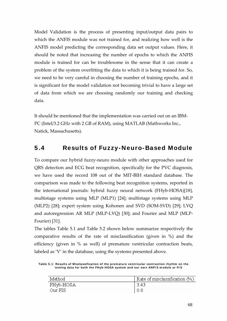
Table 5.1: Results of Misclassification of the premature ventricular contraction rhythm on the testing data for both the FHyb-HOSA system and our own ANFIS module or FIS 

69

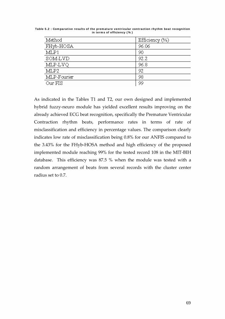
Table 5.2 : Comparative results of the premature ventricular contraction rhythm beat recognition in terms of efficiency (%) 

As  indicated  in  the Tables T1 and T2, our own designed  and  implemented hybrid  fuzzy‐neuro module  has  yielded  excellent  results  improving  on  the already achieved ECG beat recognition, specifically the Premature Ventricular Contraction  rhythm  beats,  performance  rates  in  terms  of  rate  of misclassification and efficiency  in percentage values. The comparison clearly indicates low rate of misclassification being 0.8% for our ANFIS compared to the 3.43%  for  the FHyb‐HOSA method and high  efficiency of  the proposed implemented module reaching 99% for the tested record 108 in the MIT‐BIH database.    This  efficiency was  87.5 % when  the module was  tested with  a random  arrangement  of  beats  from  several  records with  the  cluster  center radius set to 0.7.  

70

Chapter 6 Conclusion The great variety of QRS detection and PVC diagnostic algorithms reflect the need  for a  reliable method  for QRS detection and PVC diagnosis  in  cardiac signal  processing.  The  currently  achievable  detection  rates  reflect  only  the overall performance of  the detectors. These numbers hide  the problems  that are  still  present  in  case  of  noisy  or  abnormal  ECG  signals.  A  satisfying solution to these problems is still not found.   In  our  final  year  project,  we  have  chosen  to  design  and  implement  two techniques by which QRS detection and PVC diagnosis are achieved. These are:   

1. Artificial Neural Network 2. Hybrid Fuzzy‐neuro Network 

 We have  implemented both  techniques  in MATLAB using  three  specialized toolboxes  that we  have described  in  the  report. The modules  implemented aim  at  performing  two  tasks: QRS  complex  detection  and  PVC  diagnosis. These modules managed to perform reliable QRS complex detection and PVC diagnosis in an enhanced and efficient manner. At the end of our fyp work, it is notable  to  state  that our work exhibited good  results as we have aspired and hopefully we have made a valuable  contribution  to  the  field of  cardiac signal processing. 

71

6.1 ABET Considerations  In the process of design and implementation of any system or process, there are  in  fact several  issues  that we need  to  take  into consideration  in  terms of realistic  constraints  or  boundaries  imposed.  These  can  be  economic, environmental,  social, political,  ethical, health  and  safety, manufacturability and sustainability issues. In our case, we have implemented two modules, the Artificial Neural Network Module and  the Hybrid Fuzzy‐Neuro Module  in MATLAB  using  three  specialized  toolboxes.  The  two  modules  aim  at performing two tasks: QRS complex detection and PVC diagnosis.  In what  follows, we will  be  discussing  how  the  above  constraints  can  be related or realized in our two modules or systems.   1. Economic:  In  terms  of  economy,  our  two  systems  are  software‐integrated implemented  on  MATLAB.  So,  in  terms  of  actual  cost  or  budget constraints  set  by  us,  there  was  none  due  to  the  lack  of  the  need. Nevertheless, for our systems to be later used in hospitals and clinics, both private and public, for real‐time QRS detection and PVC diagnosis, there will be this economical consideration in terms of the need for the hospital or the clinic to acquire MATLAB and buy its license. This can be avoided if we later on consider writing the two systems, starting from the MATLAB work we have done, in another language that can be less expensive to the hospital or the clinic making use of the systems.      2. Environmental:  As  for  the  environmental  considerations,  these  are  significant  for  any responsible person  let alone an  engineer  involved  in providing practical solutions  to  real‐life problems.  In our case, given  that we have designed two modules but our  implementation was software‐oriented, we did not have that concern much. It would have been the case if we had considered actual hardware implementation or even FPGA realization.   

72

3. Social:  Given that the ultimate goal of our final year project is to be allocated into health services and used among cardiologists and doctors  in hospitals or clinics, there exist some social issues here. We need to make the simulation of the two implemented modules, the artificial neural network one and the hybrid  fuzzy‐neuro  one,  as  user‐friendly  as  possible,  because  software manipulation may not be the expertise of the one handling the simulation run. So, in this case, we need to set out a clear set of instructions or module tutorial which we somehow did in the implementation section in Chapters 4 and 5 in our report. This will really facilitate the job of the person using our  systems.  Other  issues  in  question  can  be  both  socially  and economically  realized.  They  have  economic  roots  or  origins  but  they appear more socially related.   These are the  issues on how to make these services accessible to all classes in the society, especially keeping in mind that  this  is a new  technology employed and not available at all hospitals and clinics. In that case, as hospitals or clinics will be charged for buying the modules first from us and then getting MATLAB, the running software for now, as well as  its  license,  this will  incur high  charges on people  in need of ECG beat interpretation. And here we need to address these issues with scrutiny and delicate care.   4. Political:  This does not quite fit our final year project because it is simply not related in any way.   5. Ethical:  In  terms  of  ethics  and morality,  these  are  of high  significance  of  course because  in  the  end we  are  aiming  onto providing  systems handling  the health benefit of people, which is quite a responsibility. So, we need to be as responsible and humanistic in terms of incorporating all ethical worries in  our  handling  of  all  stages  of  the  work:  design,  implementation, 

73

development and marketing later on. We have always taken seriously the honesty  factor  in  all  of  these  stages,  especially when  it  comes  to  result reporting and work documentation. We have also worked hard to obtain the  best  possible  results  for  the  modules  we  have  designed  and implemented,  comparing  our  results  at  every  step  of  the way  to  other systemsʹ results provided in the literature.     6. Health and Safety:  When  it  comes  to  health  and  safety,  a  flag  is  raised.  This  is  one  of  the priorities  that we  have  set  in  handling  issues  related  to  the  final  year project.  Our  fyp,  being  of  a  biomedical  application,  it  serves  a  health‐related purpose. And  to  this, we have performed  reliable QRS detection and PVC diagnosis in an enhanced and highly‐efficient way in an attempt to make ECG abnormalitiesʹ diagnosis stretch to a  larger dimension from the smaller one, which is the need of expertise of cardiologists, which can be complementary and informative to our workʹs diagnosis.  7. Manufacturability and Sustainability:  Speaking of any system or process  implies having manufacturability and sustainability  concerns.  As  for  the  first,  this  is  conceivable  in  our implementation  later on when we make  it  integrated  into hardware;  for instance as part or option of an existing ECG machine in a hospital or even a  separate QRS detection and PVC diagnostic machine. And here  comes the  issues we have  spoken earlier on  in  the economic,  social and ethical points  stated  above.  When  it  comes  to  the  second  concern,  the sustainability  issue,  we  need  to  thoroughly  examine  the  proper  time schedule for software maintenance and later hardware check. This should be  made  with  cooperation  of  the  modulesʹ  acquiring  party  (hospital, clinics, private ownership by individual, etc…), the MATLAB or any other language  if  the  work  were  to  be  revised  later  on  programmers  and software specialists, and the Ministry of Health Services if seen needed.   

74

The  above  stated  seven  points  are  to  be  considered  realistically  when dealing with any  system or process. This  is why we have  taken what  is related  in them and  incorporated that  into the considerations of our final year project.    

75

Bibliography

1. “PhysioBank MIT‐BIH Database”,         http://www.physionet.org/physiobank/database.   2. Bin  Ramli,  and  P.  Aidawati  Ahmad,  « Correlation  analysis  for 

abnormal ECG signal features extraction, » Proceedings of the 4th National Conference  on Telecommunication Technology Proceedings,  IEEE, pp. 232‐237, 2003. 

3. E. J. Berbari, Bioelectric Phenomena: Principles of Electrocardiography. Chap. 13: CRC Press LLC, 1995.  

4. E. Karam and G. M. Drzewiecki, « Modeling of hypertension‐induced Left Ventricular Hypertrophy, » Proceedings of the 7th Annual Northeast Bioengineering Conference, 1991.  

5. F.  U.  Humez  and  P. W. Macfarlane,  « Assessment  of  selected  ECG voltage  criteria  for  abnormality  in  eccentric  and  concentric  Left Ventricular Hypertrophy, » Computers  in Cardiology, vol. 30, pp. 57‐59, 2003.  

6. F.G, Yanowitz, M.D., The Alan E. Lindsay ECG Learning Center in Cyberspace, University of Utah School of Medicine. Online: http://medstat.med.utah.edu/kw/ecg/index.html. 

7. Full Help of Fuzzy Logic Tool Box of MATLAB Version 7.0.1 R14. 8. G. McDarby, B.G. Celler, N. H. Lovell, Characterising the Discrete Wavelet Transform of an ECG Signal with Simple Parameters for use in Automated Diagnosis, 2nd International Conference on Bioelectromagnetism, February 1998, Melbourne Australia. 

9. K. Englehart, P. Parker, B. Hudgins, Chapter eight: Wavelet methods in biomedical signal processing, Handbook of Neuroprosthetic Methods (Biomedical Engineering), Book, CRC Press LLC, 2003. Available Online: http://www.neurosciencenetbase.com/ejournals/books. 

10. K.Wachtell, J. N. Bella, P. R. Liebson, E. Gerdts, B. Dahlöf, T. Aalto, M. 

76

J. Roman, V. Papademetriou, H. Ibsen, J. Rokkedal, and R. B. Devereux, « Impact of different partition values on prevalences of Left Ventricular Hypertrophy  and  concentric  geometry  in  a  large  hypertensive population, » The American Heart Association, Inc. , vol. 35, no. 6 , 2000. 

11. Li, C. Zheng, C. Tai, Detection of ECG Characteristic Points Using Wavelet Transforms, IEEE Transactions on Biomedical Engineering, Vol. 42 No. 1, January 1995. 

12. M. A. Al‐Alaoui,  « A unified  analog  and digital design  to peak  and valley detector, window peak and valley detectors, and zero crossing detectors, » IEEE Trans. on Instrumentation and Measurement, vol. 35, pp. 304‐307, 1986. 

13. M. A. Al‐Alaoui, J. El Achkar, M. Hijazi, T. Zeineddine, and M. Khuri, «Application of artificial neural networks  to QRS detection and LVH diagnosis,» Proceedings of ICECSʹ 95, December 1995.  

14. M.  Kundu,  M.  Nasipuri,  and  D.  K.  Basu,  «A  knowledge‐based approach  to     ECG  interpretation using  fuzzy  logic, »  IEEE Trans.  on Syst., Man, and Cybern., vol. 28, no. 2, pp. 237‐243, April 1998.  

15. M.J. Vaessen, A QRS detection method using analog wavelet transform in ECG analysis, June 20, 2005. Available: Online http://www.fdaw.unimaas.nl/education/bachelor/conference/7.pdf. 

16. N.A. Mark Estes  III, M. S. Link, M. Homoud, and P.  J. Wang, « ECG findings  in  active patients, » The Physician  and Sportsmedicine, vol.  29, no. 3, March 2001.  

17. P. M. Okin, M.  J.  Roman,  R.  B. Devereux,  and  P. Kligfield,  « Time‐voltage  area  of  the  QRS  for  the  identification  of  Left  Ventricular Hypertrophy, » The American Heart Association,  Inc.  , vol.  27, pp.  251‐258, 1996. 

18. S. Osowski,  and Tran Hoai Linh,  «ECG beat  recognition using  fuzzy hybrid neural network, » IEEE Trans. Biomed. Eng., vol. 48, no. 11, pp. 1265‐1271, November 2001.  

19. S.M. Szilagi, Comparison of The Neural_network‐based Adaptive Filtering and Wavelet Transform for R, T and P Waves Detection, Technical University of Budapest, 1997. 

20. U. Köhler, C. Hennig, and R. Orglmeister, « The principles of software 

77

QRS  detection, »  IEEE  Trans.  Biomed.  Eng.,  vol.  2,  pp.  42‐57,  January 2002. 

21. W.J. Tompkins, Biomedical Digital Signal Processing, Prentice Hall, New Jersey, 1993. 

22. Y. Deng, W. Wolf, R. Schnell  and U. Appel, « New aspects  to  event‐synchronous  cancellation  of  ECG  interference:  an  application  of  the method in diaphragmatic EMG signals, » IEEE Trans. Biomed. Eng., vol. 47, no. 9, pp. 1177‐1184, September 2000. 

23. Y. Hen Hu, and J. N. Hwang, Neural Networks HandBook: Introduction to Neural Networks for Signal Processing. Chap. 1: CRC Press LLC, 2002.  

24. Y.  Hen  Hu,  W.  J.  Tompkins,  J.  L.  Urrusti,  and  V.  X.  Afonso, «Applications  of  artificial  neural  networks  for  ECG  signal  detection and  classification, »  Journal  of Electrocardiography, vol. 26  supplement,  pp. 66‐73, 1993.  

25.  N.  Shublaq,  «A  fuzzy  rule‐based  system  for  real‐time  filtration  of contaminated  EMGdi  signals,  »  Summer  Training  Report  at  Ecole Polytechnique de Montreal, 2005.  

26. PhysioBank Fantasia Database”,       http://www.physionet.org/physiobank/database/fantasia/ 27. N.  Izeboudjen,  and  A.  Farah,  «A  new  neural  network  system  for 

arrhythmiaʹs classification, » Proc. Neural Networks Conference, Vienna, Austria, pp. 208‐216, 1998. 

 28. Y. Hen Hu,  S. Palreddy,  and W.  J. Tompkins,  «A patient  adaptable ECG beat classifier using a mixture of experts approach, » IEEE Trans. Biomed. Eng., vol. 44, pp. 891‐900, September 1997. 

29. G. E. Oien, N. A. Bertelsen, T. Eftestol, and J. H. Husoy, «ECG rhythm classification using artificial neural networks, » Proc. 1996 IEEE Digital Signal Processing Workshop, pp. 514‐517, 1996. 

30. K. Minami, H. Nakajima, and T. Toyoshima, «Real‐time discrimination of ventricular tachyarrhythmia with Fourier‐transform neural network, IEEE Trans. Biomed. Eng., vol. 46, pp. 179‐185, February 1999. 

31.Premature  Ventricular  Contractions,  Available  Online: http://heart.healthcentersonline.com/arrhythmia/pvc.cfm 

32. “Premature Ventricular Contraction”, Wikepedia the Free       Encyclopedia, Available Online: 

http://en.wikipedia.org/wiki/Premature_ventricular_contraction 

78

33. M. A. Al‐Alaoui,  « A unified  analog  and digital design  to peak  and valley detector, window peak and valley detectors, and zero crossing detectors, » IEEE Trans. on Instrumentation and Measurement, vol. 35, pp. 304‐307, 1986.