acoustic emission methods in fatigue testing -...

1

Acoustic emission methods

in fatigue testing

Axel Lison Almkvist

Master of Science Thesis

Stockholm, Sweden 2015

3


in fatigue testing

Axel Lison Almkvist

Master of Science Thesis MMK 2015:8 MKN 127

KTH Industrial Engineering and Management

Machine Design

SE-100 44 STOCKHOLM

0 5 10 15 20 25 30 35-0.2

-0.15

-0.1

-0.05

0

0.05

0.1

0.15Signal against hydraulic noise

Time (ms)

Hydraulic noise

Signal

5

Examensarbete MMK 2015:8 MKN 127

Akustisk emission i utmattningsprovning

Axel Lison Almkvist

Godkänt

2015-02-19

Examinator

Ulf Sellgren

Handledare

Stefan Björklund

Uppdragsgivare

Scania CV AB

Kontaktperson

Daniel Bäckström

Sammanfattning

Nyckelord: Akustisk emission, AE, gråjärn, CFRP

Akustisk emission är små elastiska vågor som bland annat kommer från processer i ett material,

såsom spricktillväxt. Akustisk emission (AE) är namnet på den testmetod där dessa vibrationer

registreras och analyseras. Metoden används i materialprovning och för att testa och inspektera

komponenter, såsom tryckkärl. På Scania, en stor tillverkare av lastbilar och bussar, har tidigare

undersökningar för att implementera denna teknik på utmattning inte lyckats. Anledningen ligger

i att de hydrauliska riggarna som testningen vanligtvis sker i, typiskt sett genererar ett

bakgrundsljud som skymmer den intressanta signalen från materialet.

I detta examensarbete testades två typer av material, gråjärn och en kolfiberarmerad komposit, i

en hydraulisk rigg på Scania. Eftersom de akustiska emissionerna från materialet gömdes i

bakgrunden användes metoden att spara ner hela vågformen för signalen, vilket är ovanligt

eftersom detta innebär att mycket stora mängder data måste sparas. Det visade sig genom

frekvensanalys vara möjligt att extrahera de akustiska emissionerna från materialet, trots det

hydrauliska bruset. Det faktum att det är möjligt att följa de processerna inuti materialet, som

föregår brottet, öppnar upp nya intressanta möjligheter för materialprovning på Scania.

7

Master of Science Thesis MMK 2015:8 MKN 127


in fatigue testing

Axel Lison Almkvist

Approved

2015-02-19

Examiner

Ulf Sellgren

Supervisor

Stefan Björklund

Commissioner

Scania CV AB

Contact person

Daniel Bäckström

Abstract

Keywords: Acoustic emission, AE, grey iron, CFRP

Acoustic emissions are small vibration pulses, elastic waves, emitted from damage processes

such as crack growth inside a material. Acoustic emission (AE) is also the name of the test

method in which theses emissions are recorded and analysed and the method is used in materials

research and the testing and inspection of structures. At Scania, a large manufacturer of trucks

and buses, previous attempts to implement this technique has been unsuccessful due to the fact

that the hydraulic rigs in which the material typically is tested, produce a high background noise

level, that covers the interesting emissions from the material.

In this thesis two materials, a grey iron and a carbon fiber reinforced polymer were tested in a

hydraulic rig at Scania. Since the material signal was buried in the noise, the entire waveform

was recorded, which is an unusual approach, since it generates large amounts of data. It was

shown that using frequency analysis, it is possible to extract the material emissions in spite of the

hydraulic noise. That fact makes it possible to follow the internal processes of the material

leading up to failure, which means new interesting opportunities in materials testing at Scania.

9

Acknowledgement First of all, I would like to thank my supervisor Daniel Bäckström, for his support, guidance and

interesting discussions throughout the project.

Further thanks go to Torsten Sjögren from Statens Provningsanstalt, who made the tests at Scania

and provided me with valuable advice about acoustic emission during the project.

I would also like to also express my gratitude to all those at Scania who have helped me with my

project, but especially to Peter Skoglund, Peter Nerman, Joakim Voltaire, Anna Andersson and

Lennart Persson.

Axel Lison Almkvist

Södertälje, February 2015

11

Table of contents

1 INTRODUCTION 13

1.1 Background 13

1.2 Purpose 15

1.3 Research questions 15

1.4 Delimitations 15

1.5 Research methodology 15

2 FRAME OF REFERENCE 18

2.1 Acoustic emission basics and history 18

2.2 Applications 18

2.3 Equipment and data analysis 18

2.4 Acoustic emission sources and wave propagation 20

2.5 Noise and existing noise reduction methods 22

3 METHOD 24

3.1 Tests carried out at Scania 24

3.2 Rigs 24

3.3 Specimens 24

3.4 Equipment 25

3.5 Procedure 26

3.6 Tensile tests 27

3.7 Stepwise tensile test with off-loading 28

3.8 Hydropulse noise test 29

3.9 Attenuation tests 29

3.10 Composites subjected to corrosive environment 31

3.11 Specimens analysed with non-linear ultrasound by Acoustic Agree 31

3.12 Data conversion 32

3.13 Data analysis 32

4 RESULTS AND ANALYSIS 36

12

4.1 Time analysis of signal and noise 36

4.2 Time-frequency analysis of individual events 38

4.3 Noise in fatigue test rig 40

4.4 Cumulative emissions over the tests 41

4.5 Stepwise tensile testing 45

4.6 Composite specimens subjected to a corrosive environment 46

4.7 Attenuation in composite and steel beam 47

4.8 Noise from the hydropulse rig 50

4.9 Results from Acoustic Agree 51

5 DISCUSSION AND CONCLUSIONS 54

5.1 Discussion 54

5.2 Conclusions 59

6 RECOMMENDATIONS AND FUTURE WORK 60

6.1 Recommendations 60

6.2 Future work 60

7 REFERENCES 61

13

1 Introduction

This chapter provides an introduction to why acoustic emission has a potential in materials

testing at Scania along with the scope of this thesis.

1.1 Background Scania is a manufacturer of trucks and buses. Facing increasing demands on these products there

is a need for better materials that can meet the increasing requirements. For example, higher

combustion temperatures and pressures, driven by a desire to reduce fuel consumption, require a

material capable of withstanding the combined effect of thermal and mechanical stress. Another

interesting opportunity is to make some structural parts out of composites to reduce the total

vehicle weight, to make it possible increase the working load. To allow for the introduction of

new materials or the introduction of known materials in more demanding applications, a very

precise knowledge about their properties is needed, a knowledge which is usually gathered

through extensive testing. Furthermore, it also vital to verify the strength of these components

that have been made out of these materials. This is also done through testing.

Current test methods provide ways to verify these properties. However, there are some

limitations, which call for the continuous development of test methods, which is the reason why

resources are devoted to this at UTM, the materials technology section, at Scania. Consider for

example the fatigue test of a metal specimen. The output from this test is basically binary, either

it has been stressed enough cycles to reach failure or not. The specimen is either broken or it is

not. The reason for that is that we are only considering the macroscopic consequence of the

damage to the material, which is whether or not it has reached failure. What we are not

considering is the microscopic events, such as crack growth, which is the actual damage that has

occurred to the material. The process in which cracks form and grow that ultimately leads to the

failure of the material is known to start long before the failure actually occurs. Having a method

to follow this process as it happens would make it possible to determine not only that the

specimen has failed but how close it is to fail. In other words it would be possible to determine

how much of the life that is spent. Being able to determine this would be of great value when

testing. Furthermore, in some types of testing, for example the hydropulse testing of engine

blocks where engine blocks are subjected to repeated hydraulic pulses meant to simulate the

combustion pressure, there is no satisfactory way of determining when the life of the block is

spent. The predominant method to evaluate the blocks is to cut them and look for cracks. The

hydropulse testing is an example of a kind of test where the possibility to “peak inside” the

material, without stopping the test and cut the specimen into pieces, would be very useful.

So the question is, how can we follow these microscopic events inside the material, when the

only thing the material tells us is the macroscopic result of these microscopic events, i. e. the

failure? To state that the material does not tell us anything until the failure is not correct. In fact,

it is the direct opposite of silent. The process of breaking for example a piece of wood is in fact a

very audible process. And the sound generated when doing so starts long before the piece breaks.

The same is true for breaking a piece of metal, but in this case, the vibrations from the crack

growth are of a too high frequency to be audible for the human ear.

In other words, we can follow the microscopic process that lead to the failure of a material by

recording the vibrations generated by the crack growth process. The emitted energy is called

acoustic emissions which also is the name of the test method where these vibrations are recorded

using piezoelectric sensors attached to the specimen (1). Acoustic emission, AE, has been used

as a technique to listen to crack growth and other material processes since the 1960s (2).

14

Applications include materials research, regular inspection of structures and continuous

monitoring of structures. For example, American Airlines has developed a way of AE-testing

containers of fire extinguisher gas (3). Some concrete bridges are continuously monitored with

AE-sensors to detect growing cracks (4). Using multiple sensors it is possible to determine the

location of the source of the acoustic emission, in other words, find out where the growing crack

is located. This is based on the difference of the arrival time of the signal between the sensors, in

the same way as GPS works. Nivesrangsan et. al. (5) managed to locate simulated sources in a

diesel engine with an accuracy of 20-30 mm.

Given the possibility to actually listen and find out what is going on inside the material, why has

not this method gained more widespread use than it has? The reason is that there are a number of

obstacles that have not yet been overcome. First of all, it is difficult to translate the parameters of

the recorded AE-signal into more exact information about the event that caused the emission,

which in practice makes the interpretation of AE data from a test a more qualitative rather than

quantitative matter (1). Furthermore, there are other processes that can create signals that make it

difficult to know what is coming from the material, and what is not. In other words, there is noise

that has to be filtered out. There are different types of noise, including friction noise, electrical

and hydraulic (6).

This work focuses on the last source of noise, hydraulic noise. The hydraulic noise can be

significant from pumps and servo valves in hydraulically actuated test rigs (6). The aim is to

make AE a useable technique in spite of these high noise levels. Previous attempts of

implementing AE in test rigs at Scania did not reach success, and the hydraulic noise was

identified as the major obstacle that had to be overcome to make AE usable. Furthermore, the

application of acoustic emission equipment in hydraulic rigs is not actively encouraged by

retailers of AE-systems (7).

As stated above, it is the noise in hydraulically actuated test rigs that are problematic. Given this

background one might ask why hydraulic rigs are used when there are other types available, such

as electrical rigs, which are not noisy from an AE perspective. The answer lies in the fact that a

large part of the testing done at Scania is fatigue testing, which to make testing times reasonable

a high load frequency is required that cannot be achieved by electrical rigs. If electrically

actuated rigs were used instead, the test time would increase ~tenfold.

Another promising method for measuring the degree of damage in a specimen is the non-linear

ultrasonic method developed by the Swedish company Acoustic Agree (8). This method is an

active method, which means that a signal is sent into the material, as opposed to AE, where it is

the material itself that produces the emissions. The reflection of this signal is than analysed and

conclusions about how damaged the material is can be made. The company claims that looking

at the non-linear terms gives several advantages over conventional ultrasonic testing, such being

less sensitive to holes in the structure. Non-linear terms refers to how the reflected wave differs

from a purely sinusoidal wave.

As stated in the very beginning of the introduction, there is a desire to reduce weight by

introducing some composite parts in some places in the truck. This master thesis was a part of a

larger project about composite applications in trucks and buses. With this background, it is

necessary to know how composites are affected by a corrosive environment, which is an

environment that the material must be able to withstand in certain potential applications.

15

1.2 Purpose The purpose of this master thesis was to by means of practical tests of the AE technique,

evaluate whether or not acoustic emission is a technique that has further potential in materials

testing at Scania. If that is the case, Scania will have improved possibilities to understand the

process that leads to the failure of the specimen during fatigue testing. This will be of great

benefit in various applications. The focus area was to extract useful information from the AE-

signal in spite of the high noise level.

Furthermore, the method developed by the company Acoustic Agree (8) was evaluated to see

how accurate it is in determining how much damage that has been done to a specimen. In

addition, a purpose was to find out how composites are affected by a corrosive environment.

1.3 Research questions There are six research questions that were intended to be answered in this master thesis.

What characterizes the acoustic emission signals from grey iron and a carbon fiber

reinforced polymer when undergoing a tensile test?

What characterizes the noise from a hydraulic rig, including the hydropulse rig?

Given the answers to the two questions above, how is the signal best separated from the

noise?

Can such filtering be made fast enough so that it can be carried out continuously during a

fatigue test making it possible to save only the desired data, as opposed to the entire

signal?

How accurately can the method developed by the company Acoustic Agree determine

how damaged a cast iron and composite specimen are?

How are composites affected by a corrosive environment?

1.4 Delimitations The scope of the thesis is limited by the following:

The investigated materials will be limited to a carbon fiber composite and grey iron, no

components or other materials will be tested

Due to practical limitations of data storage no real fatigue test will be done

The investigations will be limited to two tensile testing rigs, a hydraulic fatigue rig and

an electrical rig. A hydropulse rig will also be studied.

1.5 Research methodology As stated previously, the method to answer the research questions was to evaluate the use of AE

by conducting tests at the rigs at Scania followed by filtering. In addition to doing tests in a noisy

hydraulic test rig, the exact same tests were done in an electric rig, as a reference. Doing this

served two purposes. First, it aids in the separation of the noise from the acoustic emission from

material processes. Since the electric rig can be considered not noisy, at least compared to the

hydraulic, the information gathered from the electric rig is exactly what to look for among the

noise from the hydraulic rig. Secondly, the approach with two rigs provides proof that what is

considered acoustic emissions from the material actually is this and not something else. What is

only found in the hydraulic rig is considered noise and what is present when testing in both rigs,

must be emissions from the material since that is the only thing that is in place both times.

Since Scania did not possess acoustic emission equipment, the actual physical testing at the test

rigs at Scania were performed together with an external company, Statens provningsanstalt in

16

Borås. Two different materials were tested, grey iron as well as a carbon reinforced polymer.

Both kinds of materials were stressed to their ultimate strength with increasing stress over a

period of approximately one minute.

In this thesis, an unusual approach was taken where the entire signal sent from the sensor was

recorded, as opposed to only information from the times when actual acoustic emission takes

place. Why this is unusual is explained by the fact that AE generates huge amounts of data very

quickly. The relevant frequency span for AE is 20-1000 kHz (2), which means that a very high

sampling rate is necessary to capture the waveform. For example, if the sampling rate were to be

ten times higher than for example a 500 kHz wave, 5 million samples per second are necessary.

At least 16-bit resolution is needed to achieve a satisfactory degree of resolution for the

amplitude, which means that the data rate is 80 Mbit/s, comparable to a high speed broadband.

With 8 bits per byte this means that 0.6 GB of data is generated each minute, an amount of data

which is impractical to record and store with even with the computers of today, let alone

imaginable to record and store in the 1960s when AE was first developed. But storing

information only from the moments when acoustic emission takes place, requires a method of

identifying these moments. With a noise level lower than the amplitude of the acoustic

emissions, this is a task without any difficulty, a threshold is put just above the noise level and

the moments when acoustic emission takes place, are easily identified as the times when the

amplitude of the signal exceeds the threshold level, as illustrated in Figure 1 below. Another

name for the acoustic emission events are “hits”.

Figure 1 With low noise levels, the hits are easily defined as the times when the amplitude crosses the

threshold, which is set just above the noise level.

However, when the noise level is equal or larger than the amplitude of the hits, as can be the case

in hydraulic test rigs, the technique with a threshold cannot successfully be implemented to find

the hits, simply because the hits are superimposed on the noise rather than sticking out above it.

1 2 3 4 5 6 7 8 9

-0.04

-0.03

-0.02

-0.01

0

0.01

0.02

0.03

0.04

Tid [ms]

Threshold

Am

plit

ude

[V

]

17

Therefore, in order to find the hits, it is necessary to capture the entire signal from the sensor and

then find them, by some other means. If the length of test is kept at no more than a couple of

minutes, given the data rates described earlier, the file sizes are no larger than 1-2 GB. This is

something which with today’s computers is at least manageable to store and analyse. However,

in fatigue testing, with test time sometimes reaching a week or even more, storing the entire

waveform is practically impossible, since this would result in several terabytes of data.

For this reason, an application of AE in fatigue testing, which is the ultimate aim of this work,

requires a method of filtering that is sufficiently fast to work in real time. This is the reason why

this requirement is put on the filtering algorithm in the research questions. It is also the reason

why a delimitation of this thesis is not to include a fatigue test.

The analysis of the data gathered from the test was done MATLAB (9) with a focus on spectral

analysis using the Fourier transform. The analysis followed three steps, characterisation of the

useful signal from the quiet electric rig, characterisation of the noise in the hydraulic rig and

finally separation of the useful signal from the noise. Furthermore, the characteristics of what

was considered signal from the material was compared to what was find in the literature study

regarding the nature of these emissions. The large files sizes were many times challenging,

requiring the data to be read in chunks rather than as a whole.

The active method developed by the company Acoustic Agree (8) was evaluated by letting them

analyse a number of specimens, stressed to various levels of their ultimate strength. To evaluate

how composites are affected by a corrosive environment, a number of specimens were put in a

special chamber. The chamber simulates a corrosive environment according to a standard in the

automobile industry. The stress-strain curves of these specimens as well as the acoustic emission

were then compared to those that have not been in the chamber, in order to see the effect of the

treatment.

18

2 Frame of reference

In this section the basic principles of acoustic emission testing are explained.

2.1 Acoustic emission basics and history As stated in the introduction it is a well-known phenomenon, that many materials such as rock

and wood etc. emit sounds when breaking. The first documented practical use of AE is pottery

makers listening for cracks, during the drying process (10). The major source of acoustic

emission is the growth of cracks in materials (2). The crack growth means a release of stress

energy that is turned into an elastic wave, that propagates throughout the material. However,

acoustic emission is not just limited to crack growth. Other phenomena such as friction and leaks

in hydraulic systems such as pipes and valves, will produce similar sounds in the same frequency

range as AE.

The development of modern acoustic emission started with the Ph. D. thesis of J. Kaiser in 1950

at the University of Munich (“Untersuchung über das Auftreten von Geräuschen beim

Zugversuch”). Source location based on time of arrival difference was soon developed in the

1960s (11). Parallel development of acoustic emission took place in the Soviet Union (2). At

present, AE is used in a number of industries and applications to locate potential defects.

However, it is difficult to make more exact conclusions about a defect given the AE information.

The reason for this is that the signal will be affected by the frequency transfers functions of the

source, medium, sensor and electronics before it can analysed (12). In other words, to tell more

precisely what has happened at the source, one has to have knowledge of all of these transfer

functions. Kanji has pointed out in that the next step in characterizing AE sources is to use FE-

modelling (12).

2.2 Applications The usage of AE can be divided into a few different areas: materials research, inspection and

testing of components and structures, continuous monitoring of structures and production quality

control. In materials research AE has been used to study twining, martensitic phase

transformation, stress corrosion cracking, distinction between intra- and intergranular cracking

etc. (12). For inspection and testing, typical applications include pressure vessels, storage tanks

and aerospace structures (10). As mentioned above, leaks create emissions (2) that make them

detectable by AE, which is the reason why AE is used in the oil and gas as well as in the nuclear

industry. AE can also be used to ensure the quality of welds. In that case, sensors are attached

close to the weld to detect if any cracks will develop in the weld, after the weld has been

completed (10). At Scania AE is used to ensure that the straitening of pinions (13) and

crankshafts (7) after the hardening process does not induce cracks. In the case of continuous

monitoring of structures, AE has been applied to for example prestressed concrete bridges (4).

A number of standards have been written about the use of acoustic emission. At present there are

more than 20 such ASTM standards, which include standards for mounting of sensors,

calibration of sensors, leak detection, weld monitoring, testing of different types of storage and

pressure vessels (14).

2.3 Equipment and data analysis The most vital part of the AE-system is of course the sensor. The sensor is in turn connected to

the data acquisition system, which is described in more detail below. The function of the sensor

is to convert the mechanical motion of the surface of the test specimen into an electrical signal

that can be recorded and analysed. The sensor uses the phenomenon called piezoelectric effect.

19

Some materials, when subjected to a force, will redistribute the charges in the material, such that

it will result in voltage across the material (15). By connecting the sides of the material to an

electrical system, this voltage can be measured. This means that the acceleration of the material,

which will result in a certain force, can be turned into an electrical signal. If the frequency of the

force is close to the eigenfrequency of the piezoelectric crystal, resonance will occur and the

motion will be amplified. On the other hand, if the frequency is well below the eigenfrequency,

no such effect will be present. This is illustrated in Figure 2.

Figure 2 The frequency response of a piezoelectric crystal. A wideband sensor uses the yellow area where the

response is linear, whereas a resonance sensor uses the peak around its resonance frequency. (16)

As illustrated in Figure 2, there are two different regions. These two different regions gives rise

to two different types of sensors: wideband-sensors that have a flat frequency response and

resonance type sensors that operate around their resonance frequency. Wide-band sensors are

utilized, when one wishes to study the AE-waveform, which is typically in research applications.

Resonance sensors have a higher sensitivity and are used in practical applications, such as testing

of components. The higher sensitivity comes at the cost of only being able to listen to a more

limited frequency band. To ensure a good transmission of waves between the material and the

sensor, a couplant, typically some kind of grease, is put in between. The couplant fills out the

unevenness of the surfaces of the material and the sensor. To verify that the sensor is in good

contact with the material, a so called lead-break test is done. In this test a 0.5 mm lead pencil tip

is broken by pushing it diagonally against the material. This breaking produces a relatively

consistent source that will give an amplitude of approximately 100 dB, if the sensor has been

attached properly (see below for the definition of decibel in the context of acoustic emission).

Lead-breaks can also be used to study the attenuation in materials. In this case lead-breaks are

made further away from the sensor, and one studies how the amplitude decreases with distance.

To reduce electrical interference the sensor is connected to a preamplifier, typically with 40 dB

gain (2). Some sensors are equipped with integral preamplifiers. After the amplifier, the signal

goes through a band-pass filter, that lets through the relevant frequency range for acoustic

emission, which is around 20 -1000 kHz (2). The filter passes the signal on to an analog-digital

converter and a hit detection system (10). A hit is another name for an acoustic emission event.

The hit detection system is in turn connected to a computer in which parameters of the hits are

calculated and plotted against each other. The detection of hits is done using a threshold, as

described in the introduction. The most common parameters are shown in Figure 3.

20

Figure 3 The most common parameters that are extracted from an acoustic emission event.

The most important parameter is the amplitude which is expressed in decibel and calculated

using the peak amplitude of the hit. The calculation is shown in the equation

eamplifier

ref

GainV

VDecibel Pr10 )(log20 ,

where V is the voltage recorded, Vref the reference voltage (1 µV ) and Gainpreamplifier is the

preamplifier gain (typically, and also used in this thesis 40 dB). With this definition, a 6 dB

increase is equivalent to a two-fold increase in voltage amplitude. MARSE in Figure 3 is the

blue area under the signal envelope. Based on the duration and number of counts, the average

frequency, abbreviated AF, can be calculated. It is also common to record the waveform of the

hit and make an analysis using frequency spectrums and wavelet transforms. However,

waveform gathering in this case, for example by Beattie (11) and Huang (1) refers only to the

recording of the hit, not the entire signal that passes through the sensor.

As stated in the introduction, by using multiple sensors, source location can be done, i. e. finding

the position of the growing defect. Using a known wave velocity and the difference in arrival

time between the sensors, one will be able to calculate the position of the source. For location on

a line two sensors are necessary and on a plane three are necessary. Since the strength of the

signal decreases over distance, the amplitude can also be used to determine the position of the

source (5).

2.4 Acoustic emission sources and wave propagation The waves recorded in acoustic emission are waves that depend on the density and other

properties of the material through which it travels. When the wave travels through a solid the

wave is called a bulk wave. Two types of bulk waves exist, longitudinal waves, where the

particle motion is parallel to the velocity of the wave, and shear waves, where the direction of the

particle motion is perpendicular to the velocity of the wave. However, real structures have

boundaries, and eventually the waves will reach these boundaries, which will give rise to surface

21

waves. Surface waves can be divided into Rayleigh waves and Love waves, where the particle

motion is perpendicular and parallel to the surface, respectively (11).

As waves, acoustic emission waves will undergo phenomena such as diffraction, dispersion,

reflection and attenuation (2). In reality, a recorded signal will be a superposition of different

waves and their reflections. It is due to all of these phenomena that it is extremely difficult to

make useful interpretations of the AE waveforms, in other words make conclusions about the

source, given what the wave looks like (1).

When using acoustic emission on test rods, the AE-sensor can be put right above the source of

acoustic emission, but this is not the case for structures, where one instead has to rely on the fact

that the wave will travel through the structure to the sensor. During this propagation, the wave

will be subject to attenuation, which makes this phenomenon very important. The fact that the

amplitude of the signal decreases with increasing distance from the sensor means that the sensors

have to be spaced properly. Attenuation is due to three reasons. First, the amplitude will decrease

as the wave front takes up a larger and larger area the further out in the material it reaches. In a

solid, the energy will decrease proportional to the square of the distance and in a plate

proportional to the distance. Secondly, the internal material damping (hysteresis) will decrease

the amplitude and, thirdly wave scattering at inclusions and other internal defects will also

reduce the amplitude (10). The material damping is different for different frequencies, with

typically increased damping for higher frequencies (11).

The two studied materials in this thesis was a carbon reinforced polymer and a grey iron. For this

reason, some information about acoustic emission in these two materials is presented below.

Starting with grey iron, very few articles are available. Morgner and Heyse (17) found acoustic

emissions from the very beginning of a tensile test. Sjögren (18) also found emissions at 40 dB

early in the test, as did Shen et. al (19). Morgner and Heyse divided the process into three stages:

plastic deformation, microcracking and macrocracking. They attributed emissions of around 40

dB to microcracks and emissions of around 50-80 dB to macrocracks. Shen et al. made the same

division of the process into three stages, with a rapid increase in emissions in the last 10 % of a

test. At loads corresponding to 60 % of the ultimate load and above Morgner and Heyse reported

emissions at load hold. Regarding frequencies Shen et. al. (19) reported signals between 50-500

kHz using a broadband sensor, but there were also energy up to 800 kHz and even above. Little

information is published about the attenuation of AE signal in grey iron structures. Nivesrangsan

et. al. found a mere 6 dB decrease when the emissions of a simulated source went from the first

to the fourth cylinder of a 74 kW diesel engine (5). When investigated at previous measurements

at Scania the maximum attenuation from the inside of the cylinder to the nearest available

possible sensor location was found to be 10 dB (20).

For composites, there are a large number of articles available (21) (22) (23), since a lot more

research has been done. Generally, the emissions from composites are much louder. There are

also a larger number of processes that will generate AE, including matrix cracking, fiber-matrix

debonding, fiber break and crack propagation (11). Using a combination of energy and frequency

one should be able to tell if the signal comes from matrix cracking or fiber-break, according to

Gorman (21). Matrix cracking is more energetic and results in higher amplitudes since larger

volumes are involved. Frequencies are below 50 kHz and might also be in the audible range (<20

kHz) (21) (23). For fiber break, reported frequencies are 200-300 kHz (21) (23).

Regarding attenuation, signals in composites will be attenuated to a much higher degree than in

metals (11) and this is one of the difficulties when using AE on composites (23). Different

22

authors have investigated the attenuation in composites. For example attenuation was found to be

10 dB per 0.5 m for one composite plate (22). Especially, higher frequencies are subject to high

attenuation with signals above 300 kHz being attenuated to the background noise level at 0.5 – 1

m (23). An important phenomenon in AE is the so called Kaiser effect (10), named after its

discoverer Kaiser. If a material is stressed to a certain point and that stress produces acoustic

emissions, then typically if the load were to be lowered to zero again and then raised again, no

emission will occur until the previously maximum applied load has been reached again. The

Kaiser effect is reasonably valid for most metals, but less valid for composites (11). In the tests

done in this thesis among other things the Kaiser effect was studied.

If new acoustic emission occurs during reloading before the previous maximum load has been

reached, this is called the felicity effect (10). The quotient of the load at which AE starts again

and the previous maximum load, is called the felicity ratio. A too low felicity ratio indicates that

damage has been done to the material, which is used in some non-destructive testing with AE

(11). Morgner and Heyse found the Kaiser effect to be present up 90 % of the ultimate load in

grey iron. The reason why the Kaiser effect exists is because AE is an irreversible process. Once

the emission has occurred, it will not happen again, unless the defect has been “repaired” in

some way (11).

2.5 Noise and existing noise reduction methods In this part noise and reduction methods for are discussed. Noise reduction is indeed one of the

big challenges in AE, and one that has to be dealt with in the future (1). Noise can be either

continuous or of burst type (24). Fang and Berkovits (6) list four main noise sources in fatigue

testing in hydraulic test rigs (6). These are electrical noise, friction in the load train, crack face

friction (friction between crack surfaces during the part of the load cycle where the force is

decreased, in a fatigue test) and hydraulic noise coming from servo-valves and hydraulic pumps.

The electrical noise is said to reach levels of around 20 dB and the hydraulic can reach

“significant levels”. Fang and Berkovits list three noise reduction methods. First, if the noise is

continuous but varying in amplitude, an adaptive threshold can be applied that varies with the

amplitude of the noise. This is illustrated in Figure 4. Barat et. al (24) looked at a more advanced

way of calculating this threshold.

23

Figure 4 The basic concept of an adaptive threshold that varies with the background noise level. In this case

the background is pulsating, with two pulses shown in the figure.

Secondly, if multiple sensors are used, signals can be filtered out based on their spatial origin, for

example if they originated outside of the test rod. This is done by comparing the arrival times to

the different sensors. If the difference in arrival time for a hit is approximately equal to the wave

velocity times the distance between the sensors, the hit probably comes from outside of the test

rod. Thirdly, filtering can done based on the hit-parameters (such as those shown in Figure 3).

For example one could choose to disregard hits below a certain number of counts.

Barsoum et. al. (25) encountered a high hydraulic background with noise up to 40 dB using a

MTS-rig. This noise was filtered out by putting the threshold at 40 dB and by removing the rest

(higher amplitude, but burst type) by using hit parameter-filtering. Hits with an average

frequency below 15 kHz, were disregarded. As stated in introduction, retailers of AE-systems do

not recommended the use of AE on hydraulic rigs for this reason.

In 2012 a master thesis was done at Scania where the use of AE in a hydropulse rig was tested.

However, since the noise level was 80-90 dB it was hard to detect any cracks. A 100 kHz high-

pass filter was introduced in an attempt to reduce the noise, but this turned out to be unsuccessful

(20).

0 200 400 600 800 1000 1200 1400 1600 1800-0.8

-0.6

-0.4

-0.2

0

0.2

0.4

0.6

0.8Adaptive filter example

Time (ms)

Background noise

Adaptive thresholdA

mp

litud

e (

V)

24

3 Method

In this section, the method used to evaluate AE for use at Scania, is described.

3.1 Tests carried out at Scania The tests at the rigs at Scania were carried out by an external company, SP (Statens

provningsanstalt). Two rigs were used: a noisy hydraulic and a quiet electric. The specimens (a

composite and grey iron) were tested in two different ways: a standard tensile test until failure

and a stepwise tensile test where the specimen is stressed to the ultimate load in steps, with off-

loading in-between.

3.2 Rigs The electric rig was manufactured Galdabini by and the hydraulic rig by MTS. These rigs were

capable of forces of 600 kN and 250 kN respectively. In the electric rig, the force is generated by

an electromagnetic actuator and in the hydraulic rig via a hydraulic cylinder, the pressure to

which is supplied from a central hydraulic system in the building, which is shared by a vast array

of hydraulic rigs. The rigs can be seen in Figure 5 below.

Figure 5 The two rigs used for the tensile testing of composite and grey iron. The quiet electric rig is to the

left and the noisy hydraulic is to the right.

3.3 Specimens Two different materials were used in the testing, a carbon-reinforced polymer, with a vinyl ester

matrix, and a grey iron. The specimens had cross sections of 20x6 mm and 10x15 mm, resulting

in cross-section areas of 120 mm2 and 148 mm

2, respectively (taking the 1 mm chamfer of the

grey iron specimen into account). The specimens are shown in Figure 6.

25

Figure 6 The grey iron (top) and composite specimens (bottom) used in the testing.

3.4 Equipment The tests were carried out with a wideband sensor, “WSα”, manufactured by the “Physical

Acoustic Corporation” (26). A wideband sensor was used, since studying the different

frequencies of the signal and the noise was the major approach to separate the signal from the

noise. The frequency response of the sensor is shown in Figure 7.

Figure 7 The figure shows the frequency response of the sensor that was used. The different curves represent

different calibration standards.

The cable from the sensor connects to a preamplifier that in these experiments were put at 40 dB.

The preamplifier has an integral band pass-filter, that passes signals from 20 kHz to 1.2 MHz.

The preamplifier is shown in Figure 8.

200 mm

26

Figure 8 The preamplifier used in the experiments. In the lower left corner of the figure, a sensor can be seen.

The preamplifier was in turn connected to the data acquisition card of the specially designated

AE-computer. The computer was equipped with the AE software “AEwin”, that can analyse the

data and generate a large variety of different plots. Instead of that, in these experiments, the

built-in function to store the entire signal was used. The setup can be seen in Figure 9. The

equipment used in this testing, cost approximately 300 000 SEK (27).

Figure 9 The different parts of the AE-system that recorded the signal.

3.5 Procedure After setting up the equipment, the sensors were attached to the specimens with electric tape. As

described in the frame-of-reference of this thesis, a couplant is needed to ensure adequate

transmission of the waves from the investigated material to the sensor. The couplant used in

these experiments was a stopcock grease. Due to the uneven surface of the composite,

considerable more grease was needed to ensure a good contact, compared to the grey iron.

To verify that a good connection had indeed been achieved, the standard test of breaking a pencil

lead tip, immediately next to the sensor, was done (0.5 mm, 2H). A recorded amplitude level

equal to or above 97 dB from the lead break was accepted, otherwise the sensor was reattached.

For the composite specimens, the sensor was attached right at the center of the test rod, as can be

seen in Figure 10. For the cast iron specimens, the sensor was attached approximately 2 cm from

the center point, since the width of the specimen at the center was smaller than the diameter of

the sensor, as seen in Figure 11. After the attachment of the sensor the specimen was put into the

grips of the rig. Care was taken to ensure a vertical alignment. After the insertion of the

27

specimens, the test procedure programmed was started, at the same time as the AE waveform-

gathering was started. The two different types of tests are described below.

Figure 10 A composite specimen with a sensor attached.

Figure 11 Since the width of the grey iron specimen at the narrowest point, was smaller than the diameter of

the sensor, the sensor was attached a little to the side. The red circle indicates the position of the sensor.

The procedure for each test is summarized in the list below.

1. Application of couplant on sensor and twisting against the specimen to ensure a good

bond.

2. Attachment using tape.

3. Verification of connection using lead-break test.

4. Insertion of the specimen into the rig.

5. Starting of the test program and the AE-signal recording at the same time.

6. Test rig executes test program

7. End of test

3.6 Tensile tests In these tests both materials were subjected to a deformation that was set to increase linearly.

The intention was to keep the time to failure at somewhere around a minute to make the amount

of data manageable to handle, but still make the test slow enough to prevent the individual hits

from overlapping each other. Starting with composites, for the electric rig, a deformation speed

of 5 mm/min gave a time to failure of 90 s. However, when switching to the hydraulic rig, due to

different machines stiffnesses, this deformation speed gave a too fast test. Therefore the

deformation speed was decreased. The deformation speeds and their resulting times to failure are

summarized in Table 1.

28

Table 1 The deformation speeds and their resulting times to failure.

Deformation speed Test time (approximately)

Electric rig

Composite 5 mm/min 90 s

Grey iron 1 mm/min 90 s

Hydraulic rig

Composite 1.6 mm/min 90 s

Grey iron 1 mm/min 40 s

The intention was to make the force increase linearly. However, when studying the actual force

curves it was found that the force increased quicker in the hydraulic rig, which was something

that had to be taken into account in the analysis. The actual response is shown in Figure 12.

Figure 12 The different the ways in which the hydraulic and electric rig reaches the maximum force.

3.7 Stepwise tensile test with off-loading In addition to the tensile test, another type of test was done. In the grey iron the force was raised

to 25 % and 55 % of the ultimate force with off-loading in-between. For composites it was 33 %

and 67 %. The force-time curve can be seen in Figure 13. The force was not lowered to zero in

the off-loading, but rather kept above by a small amount (too small to be noticeable in Figure

13). The reason for doing these stepwise tensile tests was a desire to study the Kaiser-effect (10)

and also a possible Felicity effect (11).

0 10 20 30 40 50 60 70 80 90 1000

10

20

30

40

50

60

70

80

90

100

110

Time (percentage of maximum)

Forc

e (

perc

enta

ge o

f m

axim

um

)

Electric rig

Hydraulic rig

29

Figure 13 The force-time curve of the stepwise tensile test. The curve shown is for grey iron.

3.8 Hydropulse noise test As mentioned earlier in the report, one potential application of AE could be the hydropulse test

rigs used for testing engine blocks with pulses of oil. For this reason, a noise test was done where

noise was sampled. During the test an engine block was subjected to a pressure fluctuating

between 5 and 327 bar at a frequency of 13 Hz. Due to the casting process, most of the engine

block has an uneven surface unsuitable for the attachment of an AE-sensor. However, some

surfaces are machined and the sensor was attached to such a surface. The noise from the

hydropulse rig was sampled for approximately one minute.

3.9 Attenuation tests As stated in the introduction, the hope is that AE is a technique that can be employed not only

when testing materials but also components. When testing materials, the sensor can be placed

immediately above the spot where the cracks form, but when testing components one has to rely

on the ability of the wave to propagate throughout the structure, during which it undergoes

attenuation. Literature gives some numbers that can be used for estimation of the attenuation. In

the following experiments, tests were done of the attenuation in actual structures that could be of

interest at Scania to test with AE. The chosen structures were a part of the steel frame of the

truck and a composite beam. These structures can be seen in Figure 14 and Figure 15. The sensor

was attached at the beams and sources were simulated using pencil lead breaks (0.5 mm, 2H).

The distances to the sensor are shown in Table 2 and Table 3. Please note that the surfaces of the

simulated sources were chosen to include surfaces both parallel and perpendicular to the surface

that the sensor was attached to. Three lead breaks were made at all positions.

0 10 20 30 40 50 60 70 80 90 100 1100

10

20

30

40

50

60

70

80

90

100

Time

Forc

e (

perc

enta

ge o

f m

axim

um

)

30

Figure 14 The steel beam with the locations of the sensor and the numbers of the simulated sources. The

location of the sensor was to the left of the pieces of tape.

Table 2 The table shows the distances to the sensor for the different locations of the lead-breaks on the steel

beam. The distances are the shortest distance along the surface the beam from the sensor to the position of

the lead-break.

Steel beam sensor positions

Postion Distance to sensor

1 32 cm

2 55 cm

3 55 cm

4 74 cm

5 74 cm

6 98 cm

7 98 cm

Sensor

6 4 2

1

3 5 7

31

Figure 15 The composite beam with the locations of the sensor and the numbers of the simulated sources. The

location of the sensor was to the left of the pieces of tape.

Table 3 The distances to the sensor for the different locations of the lead-breaks on the composite beam. The

distances are the shortest distance along the surface the beam from the sensor to the position of the lead-

break.

Composite beam sensor positions

Postion Distance to sensor

1 20 cm

2 40 cm

3 50 cm

4 69 cm

5 88 cm

6 109 cm

7 100 cm

8 78 cm

9 42 cm

3.10 Composites subjected to corrosive environment To study the effect of a corrosive environment on the composites, they were put in a special

chamber (28) where they were subjected to cycles of temperature and humidity, according to the

standard nVDA (29) . According to the standard the treatment should last 12 weeks, but due to

practical limitations on when it was possible to do the testing, the composite specimens could

only be treated for 11 weeks. Unfortunately, the cycle was also subjected to a disturbance, due to

a problem with the chamber. The temperature failed to reach the required level of – 15°C for the

2nd

, 5th

to 8th

and 10th

and 11th

of these weeks. During these weeks, the temperature reached only

+3 °C instead. The specimens were tested using a tensile test, as described above. The specimens

were tested approximately two hours after they had been taken out of the chamber. During this

time, they were stored in room temperature. At the time they were tested they had partially dried

up.

3.11 Specimens analysed with non-linear ultrasound by Acoustic Agree The method was evaluated by sending the company a couple of specimens, stressed to various

levels of their ultimate strength. One specimen that had not been subjected to any load at all, was

Sensor 1

7 8

6 5 4 2

9

3

32

also included, as a reference. The composite had a strength of approximately 80 kN, and

therefore the chosen load levels were 0, 5, 20, 40 and 60 kN. Five corresponding specimens that

had been subjected to the corrosive treatment were also analysed by AA. The grey iron

specimens had a strength of about 37 kN and the specimens sent to Acoustic Agree (8) were

stressed to 10, 20 and 36 kN. The specimens were analysed using two different methods, which

are called P-NAW and I-NAW by the company.

3.12 Data conversion The AE-program saves the waveform data in binary format, which means that conversion is

necessary before the data can be analysed in Matlab. A conversion program, that came from a

supplier of AE-system were supposed to achieve this, but failed to do so, which required

modifications to the program.

With 16-bit resolution and 5 million samples per second a 90 second long test generates a file of

approximately 1 gigabyte. This was small enough to be converted in one piece, i. e. the RAM-

could store the entire variable at once. However, the files of the stepwise tensile tests were

considerably larger, with some approaching 3 GB. These files were too big to fit in the RAM-

memory at once. Therefore, they had to be converted in chunks, i. e. only a part of the signal was

converted and then stored on the hard drive, to make it possible to clear the RAM-memory so

that the next chunk could be converted. The data was after the conversion stored in “.mat”-files

which are convenient since they allow loading of only a part of a variable as opposed to the

entire variable at once. Doing so requires v7.3 matfiles, available from Matlab R2006b (30).

3.13 Data analysis The nature of the signals, where the longest of the tests exceeded a billion data points, makes

them nearly impossible to get any overview of, if one were to look just at the time signal. Even if

one would look at 10000 data points at once, it would be very hard to go through it all.

Furthermore, it is also very hard to find any hits if the amplitude of the noise is larger than the

amplitude of the hits.

For these two reasons, the time signal was studied using spectrograms (31). Studying a signal

using its frequency spectrum is very common. In a frequency spectrum, the energy or amplitude

content for each frequency is plotted. The frequency resolution, is determined by how long

signal that the frequency spectrum is based on. A longer signal means better resolution. When a

very long signal is available, as in this case, it is possible get a sufficient frequency resolution

using only a portion of the time signal. By generating the frequency spectrum for several such

portions after each other and putting these next to each other, one has generated a two-

dimensional representation of the data that includes both a dimension of frequency and time. The

difference between a frequency spectrum and a spectrogram is illustrated in Figure 16 and

Figure 17.

33

Figure 16 A 5 Hz sine wave, corrupted with noise and its frequency spectrum. Notice the peak at 5 Hz. The

frequency spectrum does not capture any change over time.

Figure 17 A spectrogram of a time-signal. The spectrogram has been made by putting frequency for

consecutive time periods after each other, which means that it shows how the frequency content of the signal

0 100 200 300 400 500 600 700 800 900 1000-20

-10

0

10

20Signal corrupted with random Noise

Time (ms)

0 5 10 15 20 25 30 35 40 45 500

2

4

6Frequency spectrum of y(t)

Frequency (Hz)

|Y(f

)|

Fre

qu

ency

[kH

z]

Time [ms]

34

changes over time. The different amplitudes are shown using different colors. As can be seen the signal

consists of two frequency bands, present for the whole duration of the spectrogram, but in the middle, there is

a short burst of a higher frequency.

As described above the spectrograms were made for two reasons, to be able to identify the hits

and to make it possible to look at a larger portion of the signal. Looking at a larger portion of the

signal becomes easier since the data is made two dimensional. Compare for example looking at a

time signal 1 million data points long, to looking at a one megapixel picture.

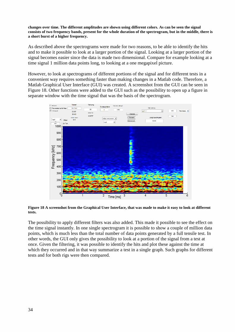
However, to look at spectrograms of different portions of the signal and for different tests in a

convenient way requires something faster than making changes in a Matlab code. Therefore, a

Matlab Graphical User Interface (GUI) was created. A screenshot from the GUI can be seen in

Figure 18. Other functions were added to the GUI such as the possibility to open up a figure in

separate window with the time signal that was the basis of the spectrogram.

Figure 18 A screenshot from the Graphical User Interface, that was made to make it easy to look at different

tests.

The possibility to apply different filters was also added. This made it possible to see the effect on

the time signal instantly. In one single spectrogram it is possible to show a couple of million data

points, which is much less than the total number of data points generated by a full tensile test. In

other words, the GUI only gives the possibility to look at a portion of the signal from a test at

once. Given the filtering, it was possible to identify the hits and plot these against the time at

which they occurred and in that way summarize a test in a single graph. Such graphs for different

tests and for both rigs were then compared.

Fre

que

ncy

[kH

z]

Time [ms]

36

4 Results and analysis

In this section the results from the tests using acoustic emission made during this thesis, are

presented.

4.1 Time analysis of signal and noise To start with, an acoustic emission event, from the silent electric test rig is compared with the

noise background from the hydraulic rig. This is shown in Figure 19. The acoustic emission

event is from a grey iron test rod.

Figure 19 An acoustic emission event compared to the hydraulic background. It would be hard to detect the

signal since the amplitude of the noise is higher than the signal.

Please note the timescale, the signal decays in a very short time.

As can be seen, the amplitude of the noise background is much larger than the signal that we

want to detect. However, zooming in on the acoustic emission event in Figure 19, illustrates how

the problem of noise can be solved. If we look at the zoomed-in picture Figure 20, we can notice

that there is a difference in frequency between the signal and the noise, with the signal having a

higher frequency. It can be noted that the noise consists of a low frequency dominating the

spectrum, as well as a higher frequency component.

0 5 10 15 20 25 30 35-0.2

-0.15

-0.1

-0.05

0

0.05

0.1

0.15Signal against hydraulic noise

Time (ms)

Hydraulic noise

Signal

Am

plit

ude

(V

)

37

Figure 20 A zoomed-in picture of the acoustic emission event against hydraulic background from Figure 19.

The fact that there is frequency difference between the noise and the acoustic emission event

would make it possible to, using frequency analysis, detect the signal if it was superimposed on

the noise. An example of this is shown in Figure 21. In this case we can see that in the beginning

there is only hydraulic background noise present and the signal is dominated by a relatively low

frequency. However, at around 0.025 ms there is a much higher frequency component present,

which is a material signal. Over time this signal decays, which is typical of acoustic emission

events.

0 0.02 0.04 0.06 0.08 0.1 0.12 0.14 0.16 0.18 0.2-0.1

-0.05

0

0.05

0.1

0.15Signal against hydraulic noise (zoomed in)

Time (ms)

Hydraulic noise

Signal

Am

plit

ude

(V

)

38

Figure 21 An acoustic emission event corrupted with lower-frequency noise. The acoustic emission event

starts at around 0.025 ms.

4.2 Time-frequency analysis of individual events As stated in 3.13 Data analysis, the acoustic emission events were studied using spectrograms, in

which one can see both the dimension of time and frequency. In Figure 22 we can see the

spectrogram of a typical hit from grey iron recorded in the electric quiet rig.

Figure 22 A spectrogram of an acoustic emission event from grey iron in the silent electric rig. Please note

how the axis are oriented. As can be seen the hit is a rapid broadband event.

0 0.01 0.02 0.03 0.04 0.05 0.06 0.07-0.06

-0.04

-0.02

0

0.02

0.04

0.06

0.08Signal corrupted with noise

Time (ms)

Time [ms] Frequency

[kHz]

Am

plit

ude

(V

)

Amplitude

[V/kHz]

39

As seen in the Figure 22, the hit is a broadband event with energy covering almost all of the AE

frequency range (20 kHz -1.2 MHz). Here the hit extends a little higher up in the frequency-

plane but is otherwise consistent with the findings about frequency of others (19).

The noise in the hydraulic fatigue rig will be described in more detail later in the report, but for

purposes of comparison, some noise recorded in the hydraulic rig is shown in Figure 23.

Figure 23 A spectrogram of noise in the hydraulic rig. The noise is limited to lower frequencies.

As can be seen the amplitude of the noise is very large compared to the emission shown in

Figure 22. An event recorded in the hydraulic rig is shown in Figure 24.

Figure 24 An acoustic emission event, recorded in the hydraulic rig.

Figure 24 illustrates the fact that the hydraulic noise covers the lower frequencies of the acoustic

emission event, however if one only looks at the higher frequency components, there is no doubt

that one would be able to detect the acoustic emission event. A 500 kHz high-pass filter was

applied to this signal. It should be pointed out that the filtered signal was generated in Matlab at

Time [ms]

Time [ms]

Frequency

[kHz]

Frequency

[kHz]

Amplitude

[V/kHz]

Amplitude

[V/kHz]

40

a speed that was approximately a tenth of the time that the signal was recorded, in other words,

filtering can be achieved in real time.

So far, all of the spectrograms shown above have been from the grey iron. Below a spectrogram

of a signal recorded from a composite test is shown (Figure 25). This signal has been recorded in

the hydraulic rig. Please notice the scale on the z-axis has changed, the picture is zoomed out,

compared to the spectrograms of the grey iron. The composite material emits considerable higher

levels than the grey iron, both in terms of occurrence and amplitude. During the 20 ms many

emissions take place which is not the case for grey iron. Also in the composites there are some

low frequency signals that are higher than the noise level, which makes it possible to detect them

without using any kind of filtering. As seen in the figure there is a presence of both this low-

frequency, high-amplitude signal as well as higher frequency signal, stretching up to 600 kHz. It

is possible that these signals can be attributed to matrix cracking and fiber break respectively as

reported by (21) (23).

Figure 25 A spectrogram of signal from a composite test, recorded in the hydraulic rig. Please note that the

spectrogram is zoomed-out compared to the previous. As can be seen, apart from the emissions in 200-600

kHz range, there are also some low frequency emission, with an amplitude high enough to break through the

noise barrier.

The noise will be described in more detail below, but in Figure 25 above one can notice that the

noise is not going up to 400 kHz but rather is constrained to a much lower frequency range as

opposed to the spectrograms presented earlier.

4.3 Noise in fatigue test rig By studying spectrograms two types of noise were identified. A narrow band noise from around

20-50 kHz and a more broadband noise from around 75 kHz to 400 kHz, with a center around

150 kHz. Sometimes both types of noise were present and sometimes only one of the types, but

there was no time when none of the types were present. The two types of noise are presented in

Figure 26. It can also be seen in the figure that both types of noise are continuous rather than of

burst type. If the low frequency noise was present, the typical overall noise level was up to 70

dB.

Frequency

[kHz] Time [ms]

Amplitude

[V/kHz]

41

Figure 26 Noise in the hydraulic rig. There is high amplitude noise at a low frequency, and there is also noise

centered around 150 kHz.

A closer look at the lower frequency noise in Figure 27, shows that this noise is centred around

20 kHz, which was the lower frequency limit of the band-pass filter (integral to the preamplifier)

used in the tests, as described in 3.4 Equipment. Therefore, this noise is placed right in the

transition band of the filter and there is probably a lot more high amplitude noise below 20 kHz,

that is not recorded thanks to the band-pass filter.

Figure 27 A closer look at the low frequency noise in Figure 26.

4.4 Cumulative emissions over the tests So far, all of the spectrograms that have been shown have only been of a short portion of a test,

20 ms, compared to about a minute, which was a typical duration for a test. The reason for that is

simply that there is a limit to how long signal that can fit into a single spectrogram. A way to

summarize all the emissions for a test is needed. This was done using accumulated amplitude.

This takes into account both the number and strength of the emissions. This is shown for the grey

iron test rods in Figure 28. Accumulated amplitude means that at a given percentage of the

ultimate load the sum of the amplitude (voltage not decibel) of all hits so far is summed up, as

seen in Figure 28.

Time [ms]

Frequency

[kHz]

Time

[ms]

Frequency [kHz]

Amplitude

[V/kHz]

Amplitude

[V/kHz]

42

Figure 28 Accumulated emissions for grey iron.

As can be seen the curves were generated from tests done both in the noisy and the non-noisy

rig, and both were generated using 500 kHz high-pass filtering. Hits below 35 dB were

disregarded. It should be pointed out that these curves were generated in Matlab (9) in a time that

was much shorter than the time it took to do the tests, in other words, the filtering could have

been done in real time. In these curves, we can notice a couple of things. We can see that AE

starts very early in the test and that there is a rapid increase in the last 10 % of the test, as

reported by others (19). It is also seen that the curves form two groups, the noisy and non-noisy

rig, with less variation within the latter group.

For the composites, as described above, there were two types of signals, a high frequency signal

and a lower frequency signal with an amplitude high enough to be above the noise level. For all

three tests done with composites, the higher frequency component of noise was not present. For

this reason, it was determined that 70 kHz high-pass filtering would be sufficient, as opposed to

500 kHz. Accumulated emissions for the high frequency signal and the lower frequency signal

are shown in Figure 29 and Figure 30, respectively.

0 10 20 30 40 50 60 70 80 90 100 1100

2

4

6

8

10

12

14

16Accumulated amplitude grey iron (>35 dB)

Force [percentage of ultimate strength]

Accum

ula

ted a

mplit

ude g

rey iro

n

Non-noisy rig, test rod 1



Noisy rig, test rod 1



Acc

um

ula

ted

am

plit

ude

[V

]

43

Figure 29 Accumulated emissions for composites after 70 kHz high-pass filtering.

Figure 30 Accumulated emissions for composites direct on the signal, i. e. without any filtering. ,

By studying Figure 29 and Figure 30 it is possible to see that these curves also form two groups.

Compared to grey iron there is a more distinct moment, around half-way through the test, at

which the emissions start. However, for one of the test rods, the unfiltered signal deviates from

0 10 20 30 40 50 60 70 80 90 100 1100

500

1000

1500

2000

2500

3000

3500

4000

4500

5000Accumulated amplitude composite (>40 dB)


Accum

ula

ted a

mplit

ude c

om

posite







0 10 20 30 40 50 60 70 80 90 100 1100

1000

2000

3000

4000

5000

6000

7000

8000

9000Accumulated amplitude composite (>65 dB)


Accum

ula

ted a

mplit

ude c

om

posite







Acc

um

ula

ted

am

plit

ude

[V

] A

ccu

mu

late

d a

mp

litu

de [

V]

44

the others. As mentioned earlier the composite emits considerable more than the grey iron. This

can be seen by comparing the z-axis scale in Figure 28, to those in Figure 29 and Figure 30.

For the grey iron the reason for difference between the curves were investigated using scatter

plots, which are shown in Figure 31. In these plots the amplitude of the hits (in decibel) are

plotted against the force at which they occurred. As can be seen in the figure, there are a lot more

hits at lower decibel levels, present early in the tests made in the non-noisy rig. However, in both

rigs 40 dB levels hits are present early, as reported by others (19) (18). Also at the ends of the

tests (>80 %) the scatter plots look more similar.

Figure 31 Scatter plots for the grey iron tests. The tests from the non-noisy rig are shown to the left and those

from the noisy, after filtering is shown to the right. The decibel-value of the hits are plotted against

normalized force.

0 10 20 30 40 50 60 70 80 90 100

40

50

60

70

80

90


Accum

ula

ted a

mplit

ude


0 10 20 30 40 50 60 70 80 90 100

40

50

60

70

80

90


Accum

ula

ted a

mplit

ude


0 10 20 30 40 50 60 70 80 90 100

40

50

60

70

80

90


Accum

ula

ted a

mplit

ude


0 10 20 30 40 50 60 70 80 90 100

40

50

60

70

80

90


Accum

ula

ted a

mplit

ude


0 10 20 30 40 50 60 70 80 90 100

40

50

60

70

80

90


Accum

ula

ted a

mplit

ude


0 10 20 30 40 50 60 70 80 90 100

40

50

60

70

80

90


Accum

ula

ted a

mplit

ude


Am

plit

ude

(dB

)

Am

plit

ude

(dB

) A

mp

litu

de (

dB)

Am

plit

ude

(dB

)

Am

plit

ude

(dB

)

Am

plit

ude

(dB

)

45

4.5 Stepwise tensile testing The result from the stepwise tensile testing is presented below. Starting with the grey iron the

result is shown in Figure 32.

Figure 32 The acoustic emission events and the force during the stepwise tensile testing of grey iron. The vast

majority of the emissions take place during three time periods, which stop when the force starts to decrease

and start when the previously maximum applied load has been reached again.

Plotted in the figure is the voltage of the emissions and the time of the test. The amplitude has

been scaled for comparison with the force curve. As showed in the figure the emissions take

place basically during three periods. Although it is true that there are some emissions in between

these periods, the vast majority takes place during these periods. What is interesting is when the

emissions start and stop. The Kaiser effect says that emissions will start again when the

previously maximum load has been reached (10). For the first period they start from the very

beginning of the test and they stop almost at the same time that the force starts to decrease. The

same is true for the second period, the emissions stop almost at the same time that the force starts

to decrease. What however is more interesting is when the emissions start again in period two

and three. This occurs at the second times that the force reaches 25 % and 55 % of the maximum

load the. This is the same time that the maximum previously applied load has been reached

again, as the Kaiser effect predicts. Testing by others (17) found felicity effect starting at 90 %,

However, in this thesis no felicity effect was observed, which might have to do with the fact the

last load step only was 55 % of maximum load. The equivalent result for the composite test rods

is shown in Figure 33. Apparently the Kaiser effect was also present in the composite.

0 10 20 30 40 50 60 70 80 90 100 1100

10

20

30

40

50

60

70

80

90

100Stepwise tensile testing grey iron (>30 dB)

Time (percentage of test duration)

Forc

e (

perc

enta

ge o

f ultim

ate

load)

Amplitude of emission

Force

46

Figure 33 The acoustic emission events and the force during the stepwise tensile testing of the composite

material. Just as for the grey iron, the vast majority of the emissions take place during three time periods,

which stop when the force starts to decrease and start when the previously maximum applied load has been

reached again.

4.6 Composite specimens subjected to a corrosive environment When testing the treated composite specimens no significant difference was noticed against the

untreated specimens in terms of acoustic emission. However, by looking at the force-time curve,

there was a significant decrease in stiffness, but no change in rupture strength. The result is

shown in Figure 34. The values are shown Table 4.

0 10 20 30 40 50 60 70 80 90 100 1100

10

20

30

40

50

60

70

80

90

100Stepwise tensile testing composite (>30 dB)

Time (percentage of test duration)

Forc

e (

perc

enta

ge o

f ultim

ate

load)

Amplitude of emission

Force

47

Figure 34 There was a significant decrease in stiffness from the corrosive treatment to the composite test

rods. However, there was no change in rupture strength.

Table 4 The different times to failure for treated and untreated composite.

Decrease in time to failure

Test rod number Untreated Treated

1 85,8 (s) 115,9 (s)

2 94,7 (s) 112,1 (s)

3 92,3 (s) 116 (s)

Average 90,9 (s) 114,7 (s)

Percentage stiffness decrease 26%

4.7 Attenuation in composite and steel beam The result from the attenuation tests in the steel and composite beam are shown in Figure 35 and

Figure 36, respectively. For the composite beam, recorded amplitudes spanned several orders of

magnitude, and therefore the result is presented in a logarithmic scale, but for the steel beam

attenuation was much lower and therefore the scale is linear. The values presented are an average

of the three lead-breaks made at each position. For some reason the lead break at position 5 in

the composite beam, did not give any useful result. As can be seen in the figures, the attenuation

is much higher in the composite than in the steel beam. For the steel beam one can clearly see

that the lead breaks made on a surface parallel to the sensor produced higher amplitudes

compared to those perpendicular, even though the distance was the same. The values for the steel

beam and the composite beam are also shown in Table 5 and Table 6. If one studies Table 6 with

the composite beam, one sees that the results are in the same range as the 20 dB/m attenuation

reported in (22).

0 20 40 60 80 100 1200

10

20

30

40

50

60

70

80

90Treated and untreated composites

Time (s)

Forc

e (

kN

)

Untreated 1

Untreated 2

Untreated 3

Treated 1

Treated 2

Treated 3

48

Figure 35 The amplitudes of the lead breaks made on the steel beam. A can be seen the amplitude does not

decrease much with distance.

Table 5 Attenuation in the steel beam.

Position Distance to sensor (mm) Voltage value Decibel value

1 320

0,048 53,6

2 550

0,052 54,3

3 550

0,046 53,3

4 740

0,041 52,3

5 740

0,033 50,4

6 980

0,042 52,5

7 980

0,037 51,4

49

Figure 36 The amplitudes of the lead breaks made on the composite beam. A can be seen the amplitude does

decrease much with distance. Please note that the logarithmic scale.

Table 6 Attenuation in the composite beam.

Position Distance to sensor (mm) Voltage value Decibel value

1 200 1,513 83,6

2 400 0,354 71,0

3 500 0,060 55,6

4 690 0,035 50,9

5 880 - -

6 1090 0,018 45,1

7 1000 0,017 44,6

8 780 0,048 53,6

9 420 0,042 52,5

50

4.8 Noise from the hydropulse rig By looking at the time signal of noise in the hydropulse rig, Figure 37 below, a cyclic behaviour

can be seen, consistent with the pump frequency at 13 Hz. The maximum amplitude of the noise

during this time period was 0.7 V, equivalent to 77 dB.

- Figure 37 Time signal of the hydropulse noise test. In the figure, seven “bumps” can be seen, consistent with

the frequency of the hydraulic pump at 13 Hz.

The worst case, both in terms of amplitude and frequency is at the peak of those “bumps” shown

in Figure 37. For this reason, the part was studied using spectrograms. See Figure 38.

Figure 38 Noise in the hydropulse rig.

Frequency

[kHz]

Time [ms]

Amplitude

[V/kHz]

Am

plit

ude

(V

)

51

As shown Figure 38, the noise stretches higher up in the frequency plane the compared to the

fatigue test rig seen in Figure 26. When applying a 700 kHz high pass filter it was possible to

reduce the noise level dramatically. As could be seen in Figure 22, a grey iron acoustic emission

event contains energy also above 700 kHz. After this had been done it could be concluded that

the high amplitudes came from a low number of single-point spikes. Since the single-point

spikes would cross a threshold only once, they can be distinguished from real hits, which cross

the threshold several times. This is called hit-parameter based filtering (the hit must have a

certain number of counts to be regarded as a hit). Considering the amplitude of the noise that was

not these spikes implementing this kind of filtering would give a noise level of 30 dB.

4.9 Results from Acoustic Agree The results from the testing done by the non-linear ultrasound method of the company Acoustic

Agree (8), is presented below. The company used two different methods, called I-NAW and P-

NAW and gave a damage value for each specimen with the damage value 100 given to the

reference (undamaged) specimens. Three groups of test rods were analysed: grey iron, composite

and the corrosively treated composite. The results are shown in Figure 39, Figure 40 and Figure

41, respectively.

Figure 39 The damage value for the grey iron specimens from the non-linear ultrasound method by the

company acoustic agree. P-NAW and I-NAW refers to the two slightly different methods used by the

company. The ultimate load was approximately 37 kN for these specimens.

0

100

200

300

400

500

600

700

Reference 0 kN 10 kN 20 kN 36 kN

Grey iron damage value

P-NAW

I-NAW

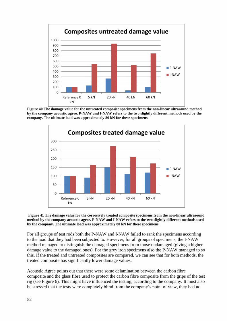
52

Figure 40 The damage value for the untreated composite specimens from the non-linear ultrasound method

by the company acoustic agree. P-NAW and I-NAW refers to the two slightly different methods used by the

company. The ultimate load was approximately 80 kN for these specimens.

Figure 41 The damage value for the corrosively treated composite specimens from the non-linear ultrasound

method by the company acoustic agree. P-NAW and I-NAW refers to the two slightly different methods used

by the company. The ultimate load was approximately 80 kN for these specimens.

For all groups of test rods both the P-NAW and I-NAW failed to rank the specimens according

to the load that they had been subjected to. However, for all groups of specimens, the I-NAW

method managed to distinguish the damaged specimens from those undamaged (giving a higher

damage value to the damaged ones). For the grey iron specimens also the P-NAW managed to so

this. If the treated and untreated composites are compared, we can see that for both methods, the

treated composite has significantly lower damage values.

Acoustic Agree points out that there were some delamination between the carbon fibre

composite and the glass fibre used to protect the carbon fibre composite from the grips of the test

rig (see Figure 6). This might have influenced the testing, according to the company. It must also

be stressed that the tests were completely blind from the company’s point of view, they had no

0

100

200

300

400

500

600

700

800

900

1000

Reference 0kN

5 kN 20 kN 40 kN 60 kN

Composites untreated damage value

P-NAW

I-NAW

0

50

100

150

200

250

300

Reference 0kN

5 kN 20 kN 40 kN 60 kN

Composites treated damage value

P-NAW

I-NAW

53

additional information except for the fact that one specimen was undamaged and should be

assigned the value 100.

54

5 Discussion and conclusions

This section contains the discussion and conclusions.

5.1 Discussion As discussed in the introduction, increasing demands such as the need to reduce fuel

consumption calls for the development of new materials and components. This development

requires considerable amounts of testing. At Scania, due to the nature of what the material will

have to go through in the finished product, the testing will typically be fatigue testing. In this

kind of testing, it would be of great benefit, to have a non-destructive way of extracting

information continuously during the test, as opposed to just looking at the number of cycles

needed for failure. Such a non-destructive test method would make it possible to get a whole new

dimension data of what is going on inside the material without increasing the number of

specimens used and without increasing the cycle time in the rigs. It would allow test engineers to

follow the microscopic processes inside the material and not just look at the macroscopic

consequence of these processes, i. e. failure.

Acoustic emission is considered a technique that can provide such additional information, but the

hydraulic noise has been considered a challenge (20). In this thesis, it was shown that the

acoustic emission events can be extracted from the data set even though it is hidden behind the

noise. Furthermore, it was shown that the filtering algorithm was fast enough to be carried out in

real time. This means that is not necessary to store the entire data set, which for a fatigue test

lasting several weeks, would be to large amounts of data to be able to handle.

To answer these questions, a number of objectives were set up. The first objective was to

characterize the signal from grey iron and a carbon fibre composite. For the grey iron, the signal

covered almost the frequency range of AE (20 kHz – 1.2 MHz), consistent with the findings of

others (19). At a sampling rate of 5 Mhz and for example a wave at 500 kHz, there will only be

10 samples per wave, which is not very much to get a really good description of the wave. Please

note that the 10 samples per wave are meant to get a description of the wave, not just say that

those frequencies are there. In that case the Nyqvist criterion says the two samples per wave are

sufficient. To get a better a resolution, the sampling rate could be increased. For the composites,

the situation turned out to be more complicated with different types of signals, that possible

could be attributed to different material processes, as proposed in 4.2 Time-frequency analysis of

individual events.

The second objective was to characterize the noise. The characterisation is very important since

it influences the choice of filtering method. First of all, it was not of burst type, i. e. the noise

were not spikes that could be mistaken for hits. If that would have been the case, some kind of

hit-parameter based method would have been suitable. Rather, the noise identified in this thesis

was continuous and limited to certain frequency bands, which made frequency filtering the most

suitable method. Two types of noise were found and sometimes only one of the types was

present. The reason behind that is unknown. The noise is assumed to come from the hydraulic

system of the rig, including the pump, valves etc. but its more exact origin is not known.

However, to find out that was not the focus of this thesis, but rather to find out if the signal could

be separated from the noise, which was the third objective. For these reasons, frequency filtering

turned out to be the most suitable method, based on the findings that the material signal and

hydraulic noise did not occupy identical parts of the frequency spectrum.

55

The fourth objective, how to achieve filtering in real-time, requires a little more discussion. The

real-time filtering is necessary to avoid storing the entire data set which would produce too large

amounts of data if all data from a fatigue test were to be stored. In this thesis it was shown that

the filtering could be performed in real time in Matlab. The assumption is made that a personal

computer will be available to filter and store the filtered information, when doing the testing.

In practice, however, the same kind of filtering could be achieved using analog filters. It is also

possible that a resonance sensor with appropriate characteristic could have picked up the higher

frequencies and rejected the lower. However, this kind of sensor would never achieve the

optimal signal-to-noise ratio. The reason for that is it is not designed to fit the particular noise

and signal that is present and because of that it will always reject some signal and pass some

noise, lowering the signal-to-noise-ratio. As described above, there were two types of noise, with

sometimes only one type present. If the filtering were made digitally it would be possible to

adapt the filtering to those circumstances, manually or automatically, and in doing so achieving

the best possible signal-to-noise ratio. For this reason, it is the view of the author that digital

filtering e.g. in Matlab should be preferred to analog filters. Another way of filtering tested in

this thesis was to multiply the signal with a wave of a certain frequency. This sliding

multiplication is a very fast and simple method of finding parts of the signal that is similar to the

wave. When the wave is multiplied with noise or other structures of the signal, which are not

very similar to the wave, the product will not become very large. However, when the wave

reaches a part of the signal that is similar to the wave, the product of the multiplication will raise

significantly.

It is important to point out that no real-time filtering was actually done in this thesis, rather it was

shown that it could be done in real-time on an already recorded signal. When this will actually be

implemented, there has to be a practical solution. One way would be to modify the software

“AEwin” such that it will produce a buffer file with the recorded waveform for example over the

last minute. Then a Matlab (9)-program could read the file continuously, filter the data and store

any possible information in a separate mat-file.

In this thesis, the active ultrasonic method developed by the company Acoustic Agree (8), was

also investigated, by analysing the result of the testing of some test rods. None of their methods

succeeded in ranking the test rods according to their damage, but the I-NAW method managed to

identify all the damaged test rods, which makes the method interesting and something that

deserves a closer look. The fact that the corrosively treated composites all got a lower damage

value is also an interesting. Being an active method also brings some advantages, for example

the ability to do the test several times on the same specimen, something that is not possible with

acoustic emission. In AE the test can only be done once and only at the exact time when the

damage happens.

In this thesis the method chosen was to store the entire waveform and then analysing the data

afterwards. Dealing with that large amount of data sometimes caused problems and required

routines where the data is analysed in chunks because of the limited RAM-memory available.

Even though the final application will be one where real-time filtering will be employed, further

investigations, for example studying the noise from other rigs, would typically include complete

waveform gathering, as well. In those applications one has to keep in mind the fact that the large

file sizes make it necessary to have routines that analyse the data in chunks. Designing these

routines takes a lot more effort than designing routines where the entire data set is dealt with at

once. Talking about data amounts, an interesting question is, how many years back in time was

an ordinary personal computer able to deal with the data amounts dealt with in this thesis? On

the other hand, how fast will the development of computing power and data storage be in the

56

future? “Moore’s law” (32) states that there has been an exponential increase in computing

power. Of course, this development will not go on forever, but with increasing computing power

more complex filtering algorithms can be used in real-time. There has also been an increase in

the availability of data storage. Even though this development in not quite as fast the

development of computing power it cannot be excluded that at some point in the future, it will be

possible to store the entire waveform also for a fatigue test. This means that an optimal filtering

method can be chosen afterwards, as opposed beforehand.

The chosen method in this thesis was to do just that, to store the entire waveform. So, could the

same result have been achieved using some other method? One view could be that the same kind

of result could have been achieved by using a bunch of high-pass filters, such a 100 kHz, 200

kHz and so on, and then looked at the test that achieved the best signal-noise-ratio. However, this

is based on the fact that the noise is limited to some range of lower frequencies, something that

was not known beforehand. The result from the hydropulse noise test shows that the noise can

very well be distributed over several frequency bands. Such an approach with filters could also

not have answered the three first research questions individually. Furthermore, it would have a

been a lot more difficult to find out the more exact nature of the noise in the hydraulic fatigue

rig, such as the fact that it consisted of two types, with sometimes only one type present.

The purpose of this thesis was to investigate the possible use of AE, primarily for fatigue testing.

However, the chosen method, to store the entire wave made it not practical to study a fatigue

test. Rather, tensile tests were done instead, which means that the results here only represent

what the signal and noise looks like during the conditions of a tensile test. However, it is

reasonable to assume the results also will be valid for a fatigue test.

When looking at the curves of accumulated acoustic emission in Figure 28, the curves form two

groups, one for the test rods tested in the noisy rig and one for those tested in the non-noisy. A

closer look at scatter plots in Figure 31, reveals that the difference to a large degree is owing to a

number of low amplitude hits present in the non-noisy but not the noisy rig. However, even

though there was a difference between the groups, the similarity within each group was

significant, which demonstrates AE:s usability as a tool to follow the damage process leading up

to failure. Looking at Figure 28, one can see that for each group separately, once passing

approximately 80 % of the failure load, one would be able to predict the failure, relatively well.

As discussed earlier in the report, it would be beneficial to be able to use AE not only for the

testing of materials but also to test components, for example engine blocks, which are being

tested in a hydropulse rig. It was demonstrated that using high-pass filtering at 700 kHz and

some hit-parameter based filtering, it was possible to reduce the noise-level to 30 dB. Does this

mean that hits above 30 dB from Figure 31, can be detected against the background that has been

reduced to 30 dB? Before such conclusion can be made, two other phenomena have to be taken

into account. Both these phenomena will raise the threshold of the size of hits, which can

actually be detected. The increase in threshold will be by a certain factor, but since the factors

will be expressed in decibel, the final threshold can be calculated by adding the decibel values,

thanks to the properties of the logarithm. The first phenomena is the attenuation. As the waves

travel from the location of the crack to the nearest sensor the amplitude of the waves will

decrease. This is due to a number of reasons, as discussed in the frame-of-reference. During

previous investigations at Scania this was found to be 10 dB at maximum for cylinder heads.

This raises the threshold of what size of hits that can be detected, up to 40 dB. The second factor

that has to be taken into account is the fact that when the filtering is done at 700 kHz, as opposed

to 500 kHz, more energy will be removed from the hit, decreasing its amplitude. As could be

seen in Figure 22, an acoustic emission event contains energy over a wide range of frequencies.

57

If one assumes that the energy is distributed equally up to the cut-off frequency of the high-pass

filter used (1.2 MHz), this loss can be estimated. Under this assumption the width of the

frequency band decreases by 30 % (from 500 KHz – 1.2 MHz to 700 KHz – 1.2 MHz), which is

equal to 1.5 dB. The phenomenon is illustrated in Figure 42.

Figure 42 Comparison of different filter cut-off frequencies.

If these 1.5 dB also were to be taken into account, one would get a 41.5 dB threshold. Hits of

that size are present well in advance of the failure of the grey iron test rods, as can be seen in

Figure 31. However, the argument has some flaws. For example, the assumption that the energy

is equally distributed probably would not be correct. Furthermore, the 10 dB reported from

previous investigations at Scania was for pencil-lead breaks, which contain a wide range of

frequencies. For frequencies above 700 kHz the attenuation will typically be higher. On the other

hand, as seen in Figure 38, there is a relatively silent band around 500 kHz that could be used to

improve the signal-to-noise-ratio. In other words one would look for a pattern of frequencies

rather than a single band. To summarize, although the argument does not provide any proof that

it would be able to follow the crack growth, it is far from proving the contrary, which makes it

promising that it indeed would be possible. It should also be pointed out that more advanced

signal processing could be used to study the hits once they have been identified.

Testing components, such as an engine block, would typically involve the use of several sensors.

In doing so, one would receive more information about each single acoustic emission event than

what could be gathered using only a single sensor. With multiple sensors, some way of analysing

this multivariate data is necessary. Furthermore, in this thesis the traditional hit-parameters

presented in Figure 3 were not studied. Including these in the analysis would probably be

beneficial but also raise the complexity of the data that has to be analysed.

Testing the components in research and development is certainly an interesting application of

AE. Acoustic emission is used to continuously monitor concrete bridges, which means that the

technique is utilized to detect cracks in a component that is in use. Could the same application be

made also in the heavy vehicle industry? In other words could AE be used to monitor for

example the steel frame or an axle on a truck? If possible, an early warning of failure would

mean the possibility to pull off the road and go to a workshop instead of experiencing a

catastrophic failure. A deeper analysis of this possibility is beyond the scope of this thesis, but an

interesting thought.

58

The purpose of this thesis was to see if the problem of hydraulic noise in a test rig could be

overcome and the results show that, this seems to be the case. This is something which hopefully

opens up a few more applications for acoustic emission.

59

5.2 Conclusions The conclusions based on the research questions are presented below.

Acoustic emission (AE) can be used to follow the process inside a material leading up to

failure. The material signal from grey iron was very broad-band. The composite emitted

two types of signals.

The hydraulic noise was primarily constrained to lower frequencies.

It was possible to filter out the signal from the noise in a hydraulic test rig. The noise was

previously thought to be an obstacle that could not be overcome.

The filtering can be made fast enough to be executed in real-time. This makes an

application to fatigue testing possible, where post-processing as opposed to real-time

filtering would have meant that an unreasonable amount of data had to be stored.

The method developed by the company Acoustic Agree could indicate the presence of

damage but could not distinguish between different amounts of damage.

The corrosive treatment of the composite specimens resulted in a significant decrease in

stiffness.

60

6 Recommendations and future work

In this section, recommendations and future work is presented.

6.1 Recommendations Acquire acoustic emission equipment (~300 kkr).

Employ real-time filtering for fatigue testing.

Investigate further possibilities of using acoustic emission for the testing of components.

6.2 Future work Implement the practical possibility to filter the data from the AE-data acquisition in real-

time.

Use a higher sampling rate to get a better description of the high-frequency waveforms.

Include all the different hit-parameters in a multivariate analysis.

61

7 References 1. Huang, M. JOM vol. 50, no. 11, November 1998. [Online] [Cited: Februari 1, 2015.]

http://www.tms.org/pubs/journals/JOM/9811/Huang/Huang-9811.html.

2. Muravin, Boris. [Online] [Cited: Februari 1, 2015.]

http://www.muravin.com/downloads/Muravin%20-

%20Acoustic%20Emission%20Science%20and%20Technology.pdf.

3. The Acoustic Emission halon 1301 fire extinguisher. Beattie, A. G. and Thornthon, D. D.

Chicago : Journal of Acoustic Emission, 2005, Vol. 23.

4. Acoustic Emission as a monitoring metod in prestressed concrete bridges health condition.

Kalicka, M. Chicago : Journal of Acoustic Amission, 2009, Vol. 27.

5. Source location of acoustic emission in diesel engines. Nivesransan, P et. al. s.l. : Mechanical

Systems and Signal Processing, 2007, Vol. 21.

6. Fatigue Design Model Based on Damage Mechanisms Revealed by Acoustic Emission

Measurements. Fang, D and Berkovits, A. 2, s.l. : Journal of Engineering Materials and

Technology, 1995, Journal of Engineering Materials and Technology, Vol. 117, pp. 200-208.

7. Bäckström, D. Scania, Personal communication. September 15, 2014.

8. Acoustic Agree. Metallgatan 1, 372 38 Ronneby : s.n.

9. MATLAB R2013b_64bit, The MathWorks, Inc., Natick, Massachusetts, United States : s.n.

10. NDT Resource Center. [Online] [Cited: Februari 1, 2015.] https://www.nde-

ed.org/EducationResources/CommunityCollege/Other%20Methods/AE/AE_Index.htm.

11. Beattie, Alan G. [Online] [Cited: Februari 1, 2015.] http://energy.sandia.gov/wp/wp-

content/gallery/uploads/SAND2013-7779BeattieAE-NDTmonograph1.pdf.

12. Acoustic Emission in materials research – a review. Ono, Kanji. s.l. : Journal of Acoustic

Emission, 2011, Vol. 29.

13. Bagge, M. Scania, Personal communication. September 05, 2014.

14. Overview of current and developing ASTM Acoustic Emission standards. Carlos, M. F.


15. [Online] [Cited: February 02, 2015.] http://en.wikipedia.org/wiki/Piezoelectricity.

16. [Online] February 2, 2015. http://en.wikipedia.org/wiki/Piezoelectric_sensor.

17. Uncommon Cries of Cast Iron Elucidated by Acoustic Emission Analysis. Morgner, W and

H, Heyse. Chicago : Journal of acoustic emission, 1986, Vol. 5.

18. International Journal of Cast Metals Research. Sjögren, T and Svensson, I. L. 4, s.l. :

International Journal of Cast Metals Research,, 2005, Vol. 18.

19. Study on the Characteristics of Acoustic Emission for Grey Cast Iron. Shen, G et. al. s.l. :

30th European Conference on Acoustic Emission Testing, 2012. 30th European Conference on

Acoustic Emission Testing.

20. Bäcklin, Annika. Internal Scania report, "Using acoustic emission measurements to detect

fatigue cracks in cast iron components", Diploma work. 2012.

21. Modal AE Analysis of Fracture and Failure in Composite Materials, and the Quality and

Life of High Pressure Composite Pressure Vessels. Gorman, M. R. Chicago : Journal of

Acoustic Emission, 2011, Vol. 29.

62

22. Advanced AE Techniques in Composite Materials. Prosser and P., H. Chicago : Journal of

Acoustic Emission, 1996, Vol. 14.

23. Research and Applications of AE on Advanced Composites. Ono, Kanji and Gallego, A.


24. Intelligent AE signal filtering methods. Barat, V et. al. Chicago : Journal of Acoustic

Emission, 2010, Vol. 28.

25. Neural network fatigue life prediction in notched bridge steel I-beams from acoustic

emission amplitude data. Barsoum, F F, et. al. Chicago : Journal of Acoustic Emission, 2011,

Vol. 29.

26. Physical Acoustics Corporation (PAC). 195 Clarksville Road · Princeton Jct, NJ 08550 ·

USA : s.n.

27. Sjögren, Torsten. Statens Proveningsanstalt (SP), Personal communication. November 26,

2014.

28. Climate chamber. s.l. : Manufactured by “Control Art”, “Hönö, Sweden” Model: Control art

climate chamber type 2.

29. Verband der Automobilindustrie VDA 232-102, Zyklische Korrosionsprüfung von

Werkstoffen und Bauteilen im Automobilbau.

30. [Online] [Cited: February 1, 2015.] http://se.mathworks.com/help/matlab/import_export/mat-

file-versions.html.

31. [Online] February 1, 2015. http://en.wikipedia.org/wiki/Spectrogram.

32. [Online] [Cited: February 2, 2015.] http://en.wikipedia.org/wiki/Moore%27s_law.

acoustic emission methods in fatigue testing -...

Documents