acoustic modeling for speech recognition under … modeling for speech recognition under limited...
TRANSCRIPT

Acoustic Modeling for SpeechRecognition under Limited Training Data
Conditions
A thesis submitted to the School of Computer Engineeringin partial fulfillment of the requirement for
the degree of Doctor of Philosophy
by
DO VAN HAI
August 26, 2015

Abstract
The development of a speech recognition system requires at least three resources: a large
labeled speech corpus to build the acoustic model, a pronunciation lexicon to map words
to phone sequences, and a large text corpus to build the language model. For many
languages such as dialects or minority languages, these resources are limited or even
unavailable - we label these languages as under-resourced. In this thesis, the focus is
to develop reliable acoustic models for under-resourced languages. The following three
works have been proposed.
In the first work, reliable acoustic models are built by transferring acoustic infor-
mation from well-resourced languages (source) to under-resourced languages (target).
Specifically, the phone models of the source language are reused to form the phone mod-
els of the target language. This is motivated by the fact that all human languages share a
similar acoustic space, and hence some acoustic units e.g. phones, of two languages may
have high correspondence and therefore allows the mapping of phones between languages.
Unlike previous studies which examined only context-independent phone mapping, the
thesis extends the studies to use context-dependent triphone states as the units to achieve
higher acoustic resolution. In addition, linear and nonlinear mapping models with dif-
ferent training algorithms are also investigated. The results show that the nonlinear
mapping with discriminative training criterion achieves the best performance in the pro-
posed work.
In the second work, rather than increasing the mapping resolution, the focus is to
improve the quality of the cross-lingual feature used for mapping. Two approaches based
on deep neural networks (DNNs) are examined. First, DNNs are used as the source
language acoustic model to generate posterior features for phone mapping. Second,
DNNs are used to replace multilayer perceptrons (MLPs) to realize the phone mapping.
i

Experimental results show that better phone posteriors generated from the source DNNs
result in a significant improvement in cross-lingual phone mapping, while deep structures
for phone mapping are only useful when sufficient target language training data are
available.
The third work focuses on building a robust acoustic model using the exemplar-based
modeling technique. Exemplar-based model is non-parametric and uses the training
samples directly during recognition without training model parameters. This study uses
a specific exemplar-based model, called kernel density, to estimate the likelihood of target
language triphone states. To improve performance for under-resourced languages, cross-
lingual bottleneck feature is used. In the exemplar-based technique, the major design
consideration is the choice of distance function used to measure the similarity of a test
sample and a training sample. This work proposed a Mahalanobis distance based metric
optimized by minimizing the classification error rate on the training data. Results show
that the proposed distance produces better results than the Euclidean distance. In
addition, a discriminative score tuning network, using the same principle of minimizing
training classification error, is also proposed.
ii

Acknowledgments
I would like to express my sincere thanks and appreciation to my supervisor, Dr. Chng
Eng Siong (NTU), and co-supervisor, Dr. Li Haizhou (I2R) for their invaluable guidance,
support and suggestions. Their encouragement also helps me to overcome the difficulties
encountered in my research. My thanks also go to Dr. Xiao Xiong (NTU) for his help,
discussions during my PhD study time.
My thanks also go to my colleagues in the speech group of the International Com-
puter Science Institute (ICSI) including Prof. Nelson Morgan, Dr. Steven Wegmann,
Dr. Adam Janin, Arlo Faria for their generous help and fruitful discussions during my
internship at ICSI.
I also want to thank my colleagues in the speech group in NTU, for their help. I am
very comfortable to collaborate with my team mates Guangpu, Ha, Haihua, Hy, Nga,
Steven, Thanh, Tung, Tze Yuang and Zhizheng. My life is much more colorful and
comfortable with their friendship.
Last but not least, I would like to thank my family in Vietnam, for their constant
love and encouragement.
iii

Contents
Abstract . . . . . . . . . . . . . . . . . . . . . . . . . . . . . . . . . . . . . . i
Acknowledgments . . . . . . . . . . . . . . . . . . . . . . . . . . . . . . . . iii
List of Publications vii
List of Figures . . . . . . . . . . . . . . . . . . . . . . . . . . . . . . . . . . ix
List of Tables . . . . . . . . . . . . . . . . . . . . . . . . . . . . . . . . . . . xii
List of Abbreviations . . . . . . . . . . . . . . . . . . . . . . . . . . . . . . xv
1 Introduction 1
1.1 Contributions . . . . . . . . . . . . . . . . . . . . . . . . . . . . . . . . . 3
1.2 Thesis Outline . . . . . . . . . . . . . . . . . . . . . . . . . . . . . . . . . 5
2 Fundamentals and Previous Works 7
2.1 Typical Speech Recognition System . . . . . . . . . . . . . . . . . . . . . 7
2.1.1 Feature extraction . . . . . . . . . . . . . . . . . . . . . . . . . . 8
2.1.2 Acoustic model . . . . . . . . . . . . . . . . . . . . . . . . . . . . 8
2.1.3 Language model and word lexicon . . . . . . . . . . . . . . . . . . 11
2.1.4 Decoding . . . . . . . . . . . . . . . . . . . . . . . . . . . . . . . 11
2.2 Acoustic Modeling for Under-resourced Languages . . . . . . . . . . . . . 12
2.2.1 Universal phone set method . . . . . . . . . . . . . . . . . . . . . 14
2.2.2 Cross-lingual subspace GMM (SGMM) . . . . . . . . . . . . . . . 19
2.2.3 Source language models act as a feature extractor . . . . . . . . . 22
2.3 Summary . . . . . . . . . . . . . . . . . . . . . . . . . . . . . . . . . . . 33
iv

3 Cross-lingual Phone Mapping 35
3.1 Tasks and Databases . . . . . . . . . . . . . . . . . . . . . . . . . . . . . 36
3.2 Cross-lingual Linear Acoustic Model Combination . . . . . . . . . . . . . 37
3.2.1 One-to-one phone mapping . . . . . . . . . . . . . . . . . . . . . . 37
3.2.2 Many-to-one phone mapping . . . . . . . . . . . . . . . . . . . . . 39
3.3 Cross-lingual Nonlinear Context-dependent Phone Mapping . . . . . . . 44
3.3.1 Context-independent phone mapping . . . . . . . . . . . . . . . . 45
3.3.2 Context-dependent phone mapping . . . . . . . . . . . . . . . . . 46
3.3.3 Combination of different input types for phone mapping . . . . . 49
3.3.4 Experiments . . . . . . . . . . . . . . . . . . . . . . . . . . . . . . 50
3.4 Conclusion . . . . . . . . . . . . . . . . . . . . . . . . . . . . . . . . . . . 65
4 Deep Neural Networks for Cross-lingual Phone Mapping Framework 67
4.1 Deep Neural Network Introduction . . . . . . . . . . . . . . . . . . . . . 68
4.1.1 Deep architectures . . . . . . . . . . . . . . . . . . . . . . . . . . 68
4.1.2 Restricted Boltzmann machines . . . . . . . . . . . . . . . . . . . 69
4.1.3 Deep neural networks for speech recognition . . . . . . . . . . . . 71
4.1.4 Experiments of using DNNs for monolingual speech recognition . 73
4.1.5 Conclusion . . . . . . . . . . . . . . . . . . . . . . . . . . . . . . . 78
4.2 Deep Neural Networks for Cross-lingual Phone Mapping . . . . . . . . . 79
4.2.1 Three setups using DNNs for cross-lingual phone mapping . . . . 80
4.2.2 Experiments . . . . . . . . . . . . . . . . . . . . . . . . . . . . . . 83
4.3 Conclusion . . . . . . . . . . . . . . . . . . . . . . . . . . . . . . . . . . . 88
5 Exemplar-based Acoustic Models for Limited Training Data Conditions 90
5.1 Introduction . . . . . . . . . . . . . . . . . . . . . . . . . . . . . . . . . . 91
5.2 Kernel Density Model for Acoustic Modeling . . . . . . . . . . . . . . . . 93
5.3 Distance Metric Learning . . . . . . . . . . . . . . . . . . . . . . . . . . . 95
5.4 Discriminative Score Tuning . . . . . . . . . . . . . . . . . . . . . . . . . 97
5.5 Experiments . . . . . . . . . . . . . . . . . . . . . . . . . . . . . . . . . . 98
5.5.1 Experimental procedures . . . . . . . . . . . . . . . . . . . . . . . 98
v

5.5.2 Using MFCC and cross-lingual bottleneck feature as the acoustic
feature . . . . . . . . . . . . . . . . . . . . . . . . . . . . . . . . . 99
5.5.3 Distance metric learning for kernel density model . . . . . . . . . 101
5.5.4 Discriminative score tuning . . . . . . . . . . . . . . . . . . . . . 103
5.6 Conclusion . . . . . . . . . . . . . . . . . . . . . . . . . . . . . . . . . . . 107
6 Conclusion and Future Works 108
6.1 Contributions . . . . . . . . . . . . . . . . . . . . . . . . . . . . . . . . . 108
6.1.1 Context-dependent phone mapping . . . . . . . . . . . . . . . . . 108
6.1.2 Deep neural networks for phone mapping . . . . . . . . . . . . . . 109
6.1.3 Exemplar-based acoustic model . . . . . . . . . . . . . . . . . . . 110
6.2 Future Directions . . . . . . . . . . . . . . . . . . . . . . . . . . . . . . . 110
A Appendix 112
A.1 Derivation for Distance Metric Learning . . . . . . . . . . . . . . . . . . 112
References 116
vi

List of Publications
Journals
(i) Van Hai Do, Xiong Xiao, Eng Siong Chng, and Haizhou Li, “Context-dependent
Phone Mapping for Acoustic Modeling of Under-resourced Languages,” Interna-
tional Journal of Asian Language Processing, vol. 23, no. 1, pp. 21-33, 2015.
(ii) Van Hai Do, Xiong Xiao, Eng Siong Chng, and Haizhou Li, “Cross-lingual Phone
Mapping for Large Vocabulary Speech Recognition of Under-resourced Languages,”
IEICE Transactions on Information and Systems, vol. E97-D, no. 2, pp. 285-295,
2014.
Conferences
(iii) Van Hai Do, Xiong Xiao, Eng Siong Chng, and Haizhou Li, “Kernel Density-
based Acoustic Model with Cross-lingual Bottleneck Features for Resource Limited
LVCSR,” in Proceedings of Annual Conference of the International Speech Com-
munication Association (INTERSPEECH), pp. 6-10, 2014.
(iv) Van Hai Do, Xiong Xiao, Eng Siong Chng, and Haizhou Li, “Context-dependent
Phone Mapping for LVCSR of Under-resourced Languages,” in Proceedings of An-
nual Conference of the International Speech Communication Association (INTER-
SPEECH), pp. 500-504, 2013.
(v) Van Hai Do, Xiong Xiao, Eng Siong Chng, and Haizhou Li, “Context Dependant
Phone Mapping for Cross-Lingual Acoustic Modeling,” in Proceedings of Interna-
tional Symposium on Chinese Spoken Language Processing (ISCSLP), pp. 16-20,
2012.
vii

(vi) Van Hai Do, Xiong Xiao, Eng Siong Chng, and Haizhou Li, “A Phone Mapping
Technique for Acoustic Modeling of Under-resourced Languages,” in Proceedings
of International Conference on Asian Language Processing (IALP), pp. 233-236,
2012.
(vii) Van Hai Do, Xiong Xiao, and Eng Siong Chng, “Comparison and Combination
of Multilayer Perceptrons and Deep Belief Networks in Hybrid Automatic Speech
Recognition Systems”, in Proceedings of Asia-Pacific Signal and Information Pro-
cessing Association Annual Summit and Conference (APSIPA ASC), 2011.
(viii) Van Hai Do, Xiong Xiao, Ville Hautamaki, and Eng Siong Chng, “Speech At-
tribute Recognition using Context-Dependent Modeling”, in Proceedings of Asia-
Pacific Signal and Information Processing Association Annual Summit and Con-
ference (APSIPA ASC), 2011.
(ix) Haihua Xu,Van Hai Do, Xiong Xiao, and Eng Siong Chng, “A Comparative Study
of BNF and DNN Multilingual Training on Cross-lingual Low-resource Speech
Recognition,” in Proceedings of Annual Conference of the International Speech
Communication Association (INTERSPEECH), 2015.
(x) Mirco Ravanelli, Van Hai Do, and Adam Janin “TANDEM-Bottleneck Feature
Combination using Hierarchical Deep Neural Networks,” in Proceedings of Interna-
tional Symposium on Chinese Spoken Language Processing (ISCSLP), pp. 113-117,
2014.
(xi) Korbinian Riedhammer, Van Hai Do, and Jim Hieronymus, “A Study on LVCSR
and Keyword Search for Tagalog,” in Proceedings of Annual Conference of the
International Speech Communication Association (INTERSPEECH), pp. 2529-
2533, 2013.
viii
List of Figures
2.1 Block diagram of a typical speech recognition system. . . . . . . . . . . . 8
2.2 A left-to-right HMM model with three true states. . . . . . . . . . . . . . 9
2.3 Phonetic-acoustic modeling [1]. . . . . . . . . . . . . . . . . . . . . . . . 10
2.4 An example of the universal phone set approach. . . . . . . . . . . . . . . 13
2.5 Illustration of the cross-lingual subspace Gaussian mixture model (SGMM)
approach. . . . . . . . . . . . . . . . . . . . . . . . . . . . . . . . . . . . 14
2.6 Source acoustic models act as a feature extractor. . . . . . . . . . . . . . 14
2.7 Phones of Spanish and Japanese are expressed in the IPA format [2]. . . 15
2.8 Cross-lingual tandem approach. . . . . . . . . . . . . . . . . . . . . . . . 24
2.9 Automatic speech attribute transcription (ASAT) framework for cross-
lingual speech recognition. . . . . . . . . . . . . . . . . . . . . . . . . . . 25
2.10 Probabilistic sequence-based phone mapping model. . . . . . . . . . . . . 30
3.1 Differences between feature distributions of three HMM states for a same
IPA phone across three languages [3]. . . . . . . . . . . . . . . . . . . . . 40
3.2 Combination weights for the proposed many-to-one phone mapping. . . . 42
3.3 Combination weights for phone “sh” and “th” in English. . . . . . . . . . 43
3.4 Posterior-based phone mapping. NS and NT are the numbers of phones in
the source and target languages, respectively. . . . . . . . . . . . . . . . . 45
3.5 A diagram of the training process for the context-dependent cross-lingual
phone-mapping. . . . . . . . . . . . . . . . . . . . . . . . . . . . . . . . . 48
3.6 A diagram of the decoding process for the context-dependent cross-lingual
phone mapping. . . . . . . . . . . . . . . . . . . . . . . . . . . . . . . . . 49
ix

3.7 Feature combination in the cross-lingual phone mappping where NS1, NS2
are the numbers of tied-states in the source language acoustic model 1 and
2, respectively. . . . . . . . . . . . . . . . . . . . . . . . . . . . . . . . . . 50
3.8 Probability combination in the cross-lingual phone mappping. . . . . . . 50
3.9 Cross-lingual tandem system for Malay (source language) and English
(target language). . . . . . . . . . . . . . . . . . . . . . . . . . . . . . . . 55
3.10 The WER (%) of different acoustic models with different amounts of target
training data. . . . . . . . . . . . . . . . . . . . . . . . . . . . . . . . . . 61
3.11 The WER (%) of individual and combined phone mapping models. . . . 62
3.12 The WER (%) of the phone mapping model for two source languages with
three different amounts of target training data. . . . . . . . . . . . . . . . 64
4.1 A DNN (b) is composed by a stack of RBMs (a). . . . . . . . . . . . . . 69
4.2 Four steps in training a DNN for speech recognition. . . . . . . . . . . . 73
4.3 Phone error rate (PER) on the training and test sets of the HMM/GMM
model with different model complexities. . . . . . . . . . . . . . . . . . . 75
4.4 Performance of the HMM/DNN acoustic model for the two initialization
schemes and the combined models with different numbers of layers. . . . 76
4.5 Comparison of HMM/MLP and HMM/DNN on an LVCSR task for dif-
ferent training data sizes. . . . . . . . . . . . . . . . . . . . . . . . . . . . 78
4.6 Illustration of using DNN as the source language acoustic model to gen-
erate cross-lingual posterior feature for phone mapping (Setup A). . . . . 81
4.7 Illustration of using DNN to extract cross-lingual bottleneck feature for
target language acoustic models (Setup B). . . . . . . . . . . . . . . . . . 81
4.8 Illustration of using DNNs for both the source acoustic model and the
phone mapping (Setup C ). . . . . . . . . . . . . . . . . . . . . . . . . . . 82
4.9 WER (%) of the cross-lingual phone mapping using deep source acoustic
model versus the phone mapping using shallow source acoustic model and
the monolingual model. . . . . . . . . . . . . . . . . . . . . . . . . . . . . 86
4.10 WER (%) of the two cross-lingual models using bottleneck feature gen-
erated by the deep source bottleneck network (Setup B). The last column
shows the WER given by the phone mapping model in Setup A for com-
parison. . . . . . . . . . . . . . . . . . . . . . . . . . . . . . . . . . . . . 86
x
4.11 Comparison of the cross-lingual phone mapping using shallow and deep
structures for phone mapping. . . . . . . . . . . . . . . . . . . . . . . . . 88
5.1 Kernel density estimation for acoustic modeling of an LVCSR system. . . 94
5.2 The proposed discriminative score tuning. . . . . . . . . . . . . . . . . . 97
5.3 Illustration of the linear feature transformation matrices. BN stands for
cross-lingual bottleneck features, DML stands for distance metric learning.
The MFCC feature vectors are ordered as [c1,...,c12,c0], and their delta
and acceleration versions. . . . . . . . . . . . . . . . . . . . . . . . . . . 102
5.4 Frame error rate (%) obtained by the kernel density model with two ini-
tialization schemes for transformation Q. . . . . . . . . . . . . . . . . . . 104
5.5 The weight matrix of the 2-layer neural network score tuning. . . . . . . 105
5.6 Performance in WER(%) of the proposed kernel density model using dif-
ferent score tuning neural network architectures. . . . . . . . . . . . . . . 106
xi

List of Tables
2.1 Performance and model complexity of GMM and SGMM models in a
monolingual task [4]. . . . . . . . . . . . . . . . . . . . . . . . . . . . . . 21
2.2 Different cross-lingual methods using the source acoustic models as a fea-
ture extractor. . . . . . . . . . . . . . . . . . . . . . . . . . . . . . . . . . 23
2.3 Speech attribute subsets [5]. . . . . . . . . . . . . . . . . . . . . . . . . . 25
3.1 One-to-one phone mapping from Malay to English generated by the data-
driven method using 7 minutes of English training data. . . . . . . . . . 38
3.2 Word error rate (WER) (%) of the one-to-one phone mapping for cross-
lingual acoustic models. . . . . . . . . . . . . . . . . . . . . . . . . . . . 39
3.3 Word error rate (WER) (%) of many-to-one phone mapping for cross-
lingual acoustic models with 7 minutes of target training data. . . . . . . 43
3.4 Word error rate (WER) (%) of the monolingual monophone and triphone
baseline HMM/GMMmodels for 16 minutes of training data with different
model complexities. . . . . . . . . . . . . . . . . . . . . . . . . . . . . . . 54
3.5 The WER (%) of different monolingual and cross-lingual acoustic models
with 16 minutes of English training data. . . . . . . . . . . . . . . . . . . 56
3.6 The WER (%) of different mapping architectures with 16 minutes of target
English training data (the target acoustic model is triphone). Number in
(.) in the first and the last column indicates the number of inputs and
number of hidden units, respectively. Number in (.) of the third column
represents relative improvement over the corresponding 2-layer NN in the
second column. . . . . . . . . . . . . . . . . . . . . . . . . . . . . . . . . 59
xii

5.1 WER (%) obtained by various models at four different training data sizes.
Row 1-6 are results obtained by using MFCC feature. Row 7-11 show
results obtained by using cross-lingual bottleneck feature. KD stands for
kernel density used for acoustic modeling. . . . . . . . . . . . . . . . . . 100
5.2 WER (%) obtained by the kernel density model using MFCC feature with
two initialization schemes for transformation Q. . . . . . . . . . . . . . 104
xiii

xiv

List of Abbreviations
ASAT Automatic Speech Attribute Transcription systemASR Automatic Speech RecognitionBN-DNN Deep Neural Network to generate cross-lingual BottleNeck featureDML Distance Metric LearningDNN Deep Neural NetworkEM Expectation MaximizationFER Frame Error RateGMM Gaussian Mixture ModelHLDA Hetroscedastic Linear Discriminant AnalysisHMM Hidden Markov ModelHMM/DNN Hidden Markov Model / Deep Neural NetworkHMM/GMM Hidden Markov Model / Gaussian Mixture ModelHMM/MLP Hidden Markov Model / Multi-Layer PerceptronHMM/KD Hidden Markov Model / Kernel Density ModelIPA International Phonetic AlphabetKD Kernel Density ModelKL-HMM Kullback-Leibler based Hidden Markov Modelk-NN k-Nearest NeighborsLDA Linear Discriminant AnalysisLVCSR Large-Vocabulary Continuous Speech RecognitionMFCC Mel Frequency Cesptral CoefficientsMAP Maximum A PosterioriMLE Maximum Likelihood EstimationMLLR Maximum Likelihood Linear RegressionMLP Multi-Layer PerceptronMMI Maximum Mutual InformationMVN Mean and Variance NormalizationNN Neural NetworkPCA Principal Component AnalysisPER Phone Error RatePOS-DNN Deep Neural Network to generate cross-lingual POSterior featureRBM Restricted Boltzmann MachineSA Speech AtributeSGMM Subspace Gaussian Mixture ModelWER Word Error RateWSJ Wall Street Journal speech corpus
xv

Chapter 1
Introduction
Speech is the most common and effective form of human communication. Much research
in the last few decades has focused on improving speech recognition systems to robustly
convert speech into text automatically [6]. Unfortunately, speech researchers have only
focused on dozens out of the thousands of spoken languages in the world [7]. To build a
large-vocabulary continuous speech recognition (LVCSR) system, at least three resources
are required: a large labeled speech corpus to build the acoustic model, a pronunciation
lexicon to map words to phone sequences, and a large text corpus to build the language
model. For many languages such as dialects or minority languages, these resources are
limited or even unavailable, they are called under-resourced languages for LVCSR re-
search. The scope of the thesis is to examine the development of reliable acoustic models
for under-resourced languages.
One major obstacle to build an acoustic model for a new language is that it is very
expensive to acquire a large amount of labeled speech data. Usually tens to hundreds of
hours of training data are required to build a reasonable acoustic model for an LVCSR
system, while commercial systems normally use thousands of hours of training data.
This large resource requirement limits the development of a full fledged acoustic model
for under-resourced languages.
The above challenge motivates researchers to examine cross-lingual techniques to
transfer knowledge from acoustic models of well-resourced (source) languages to under-
resourced (target) languages. Various methods have been proposed for cross-lingual
acoustic modeling which can be classified into three main categories.
1

Chapter 1. Introduction
The first category is based on an universal phone set [7–10] that is generated by
merging phone sets of different languages according to the international phonetic alphabet
(IPA) scheme. A multilingual acoustic model can therefore be trained for all languages
using the common phone set. An initial acoustic model for a new target language can
be obtained by mapping from the multilingual acoustic model. To improve performance
on the target language, this initial acoustic model is refined using adaptation data of the
target language. One disadvantage of this approach is that phones in different languages
can be similar, they are unlikely to be identical. Hence, it can be hard to merge different
phone sets appropriately.
In the second category, the idea is to create an acoustic model that can be effectively
broken down into two parts in which the major part captures language-independent statis-
tics and the other part captures language specific statistics. For cross-lingual acoustic
modeling, the language-independent part of a well-trained acoustic model of the source
language is borrowed by the acoustic model of the target language to reduce the target
language training data requirement. A typical example in this approach is the cross-
lingual subspace Gaussian mixture models (SGMMs) [4, 11, 12]. In SGMMs, the model
parameters are separated into the subspace parameters that are language-independent,
and phone state specific parameters that are language-dependent. With such a model,
the well-trained subspace parameters from the source language are captured and speech
data of the target language are applied to adapt the target language phone state spe-
cific parameters. As those parameters only account for a small proportion of the overall
model, they could be reliably trained with a small amount of training data. The dis-
advantage of this approach is that it requires the source and target models to have the
similar structures. This limits the flexibility of the approach for different cross-lingual
tasks.
In the third category, which is also the most popular approach, the source acoustic
model acts as a feature extractor to generate cross-lingual features such as source language
phone posteriors for the target language speech data. As these features are higher-level
features as compared to conventional features such as MFCCs, they enable the use of
simpler models trained with a small amount of training data to model the target acoustic
space. In this category, various cross-lingual methods have been proposed using various
types of cross-lingual features and target acoustic models as detailed below.
2

Chapter 1. Introduction
• Cross-lingual tandem: phone posteriors [13–15] generated by source language mul-
tilayer perceptron neural networks (MLPs) or bottleneck features [16, 17] generated
by source language bottleneck networks are used as the input feature for a target
language HMM/GMM acoustic model.
• Automatic speech attribute transcription (ASAT) [18–20]: speech attribute poste-
riors generated by the source language speech attribute detectors are used as the
input features for a target language MLP.
• Cross-lingual Kullback-Leibler based HMM (KL-HMM) [21, 22]: each state in the
KL-HMM is modeled by a discrete distribution to measure the KL-divergence be-
tween the state model and a source language phone posterior input.
• Sequence-based phone mapping [23, 24]: a source language phone sequence decoded
by the source language phone recognizer is mapped to the target language phone
sequence using a target language discrete HMM.
• Posterior-based phone mapping [25]: source language phone posteriors generated
by the source language MLP are mapped to the target language phone posteriors
using a target language MLP.
Although, the above methods offer some solutions to the under-resourced acoustic
model development, this area of research remains active as building reliable acoustic
models with limited training data has not been fully achieved. The objective of this
thesis is to further investigate novel and efficient acoustic modeling techniques to improve
performance of speech recognition for under-resourced languages.
1.1 Contributions
This thesis focuses on the third category of cross-lingual acoustic modeling which uses
source acoustic models to generate cross-lingual features for the target language speech
data. The reason is that it is a flexible approach which allows to use different architectures
for source and target acoustic models. Three novel methods are proposed.
3

Chapter 1. Introduction
The first method is called the context-dependent phone mapping. This method is
motivated by the fact that all human languages share similar acoustic space and there-
fore most sound units such as phones may be shared by different languages. Hence,
a target language acoustic model can be mapped from acoustic models of other lan-
guages for the speech recognition purpose. Specifically, the source acoustic models are
used as feature extractors to generate the source language phone posterior or likelihood
scores. These scores are then mapped to the phones of the target language. Differ-
ent to previous works which used context-independent monophone mapping, this work
proposes context-dependent triphone states as the acoustic units to achieve higher map-
ping resolution. Experimental results in the Wall Street Journal (WSJ) corpus show that
the proposed context-dependent phone mapping outperforms context-independent mono-
phone mapping significantly, even in the case of very limited training data. In this study,
two mapping functions, including simple linear mapping and nonlinear mapping with
different training algorithms, are investigated. The results show that using the nonlinear
mapping with the discriminative training criterion achieves the best performance.
While the first work focuses on improving the mapping resolution by using context
information, the second work focuses on improving the cross-lingual features used for
mapping, e.g. source language posterior feature using deep models. In this work, two
approaches using deep neural networks (DNNs) are studied. In the first approach, DNNs
are used as the acoustic model of the source language. It is hypothesized that DNNs
can model the source language better than shallow models such as MLPs or GMMs, and
the features generated by DNNs can produce better performance for phone mapping.
In the second approach, DNNs are used to realize the phone mapping as opposed to
the conventional MLP approach. Experimental results show that using DNN source
acoustic models produce better results than shallow source acoustic models for cross-
lingual phone mapping. Differently, using deep structures for phone mapping is only
useful when a sufficient amount of target language training data is available.
The third contribution of the thesis is to apply exemplar-based model for acous-
tic modeling under limited training data conditions. Exemplar-based model is non-
parametric and uses the training samples directly without estimating model parameters.
This makes the approach attractive when training data are limited. In this study, a
4

Chapter 1. Introduction
specific exemplar-based model, called kernel density model, is used as the target lan-
guage acoustic model. Specifically, the kernel density model uses cross-lingual bottleneck
feature generated by the source language bottleneck DNN to estimate the likelihood
probability of target language triphone states. In the kernel density model, the major
design consideration is the choice of a distance function used to measure the similarity of
a test sample and a training sample. In this work, a novel Mahalanobis-based distance
metric learnt by minimizing the classification error rate on the training data is proposed.
Experimental results show that the proposed distance produces significant improvements
over the Euclidean distance metric. Another issue of the kernel density model is that it
tries to estimate the distribution of the classes rather than optimal decision boundary
between classes. Hence, its performance is not optimal in terms of speech recognition
accuracy. To address this, a discriminative score tuning is introduced to improve the
likelihood scores generated by the kernel density model. In the proposed score tuning, a
mapping from the target language triphones to themselves is realized with the criterion
of using the same principle of minimizing the training classification error.
The work on context-dependent phone mapping is published in the journal: IEICE
Transactions on Information and Systems [26], and in the two conferences: IALP 2012
[27] and ISCSLP 2012 [28]. The work on applying deep neural networks on monolingual
speech recognition and cross-lingual phone mapping is published in the two conferences:
APSIPA ASC 2011 [29] and INTERSPEECH 2013 [30]. The work on the exemplar-based
acoustic model is published the conference: INTERSPEECH 2014 [31].
1.2 Thesis Outline
This thesis is organized as follows:
In Chapter 2, the background information of statistical automatic speech recognition
research is provided, followed by a review of the current state-of-the-art techniques for
cross-lingual acoustic modeling.
In Chapter 3, a linear phone mapping is proposed for cross-lingual speech recognition
where the target language phone model is formed as a linear combination of the source
language phone models. To improve performance, a non-linear phone mapping realized by
5

Chapter 1. Introduction
a MLP is then applied. Finally, context-dependent phone mapping is proposed to achieve
higher acoustic resolution as compared to the context-independent phone mapping for
cross-lingual acoustic modeling.
In Chapter 4, deep neural networks (DNNs) are first investigated in monolingual
speech recognition tasks. DNNs are then proposed to use for the cross-lingual phone
mapping framework to improve the cross-lingual phone posteriors used for the mapping.
In addition, DNNs are also investigated to realize the phone mapping function.
In Chapter 5, a non-parametric acoustic model, called exemplar-based model, is ap-
plied for speech recognition under limited training data conditions. To improve per-
formance of the model, a novel Mahalanobis-based distance metric is then proposed.
Finally, a score tuning is introduced at the top of the model to improve likelihood scores
for decoding.
Finally, the thesis concludes in Chapter 6 with a summary of the contributions and
several possible future research directions.
6

Chapter 2
Fundamentals and Previous Works
In this chapter, a brief introduction to typical speech recognition systems is provided,
followed by a review of the current state-of-the-art techniques for cross-lingual acoustic
modeling. The cross-lingual acoustic modeling techniques are grouped in three categories,
i.e. universal phone set, subspace GMM, and using source language acoustic models as
a feature extractor. The techniques in each category and sub-category will be reviewed
individually.
As the review provided in the chapter is relatively extensive covering many tech-
niques, to make it easier to appreciate the relationship between thesis’s contributions to
the existing techniques, it is necessary here to point out which techniques that are closely
related to our study. The first contribution presented in Chapter 3 and second contribu-
tion presented Chapter 4 of the thesis are context-dependent phone mapping. The related
techniques include posterior-based phone mapping (Section 2.2.3.4) and cross-lingual tan-
dem (Section 2.2.3.1). The third contribution presented in Chapter 5 is exemplar-based
acoustic modeling. The related literature is the exemplar-based method (Section 2.2.3.5).
2.1 Typical Speech Recognition System
Before examining different approaches in cross-lingual speech recognition, this section
presents a brief introduction of the conventional ASR system. Fig. 2.1 shows the block
diagram of a typical speech recognition system. It consists of five modules: feature
extraction, acoustic model, language model, word lexicon, and decoding. These modules
will be described in details in the next subsections.
7

Chapter 2. Fundamentals and Previous Works
Word
Lexicon
Language
Model
Acoustic
Model
“hello world”
Decoding s
X={x} p(X|W)
p(W)
Feature
Extraction
Speech
waveform
Figure 2.1: Block diagram of a typical speech recognition system.
2.1.1 Feature extraction
The feature extraction module is used to generate speech feature vectors X = {x} fromthe waveform speech signal s. The module’s aim is to extract useful information and
remove irrelevant information such as noise from the speech signal. The features are
commonly computed on a frame-by-frame basis for every 10ms with a frame duration of
25ms. In such short frame duration, speech can be assumed to be stationary. Currently,
the most popular features for ASR are Mel filterbank cepstral coefficients (MFCC) [32]
and perceptual linear prediction (PLP) [33]. Normally, 39 dimensional MFCC or PLP
feature vectors are used, consisting of 12 static features plus an energy feature, and the
first and second time derivatives of the static features. The derivatives are included to
capture the temporal information. A detailed discussion of features for ASR can be found
in [34].
2.1.2 Acoustic model
The acoustic model is used to model the statistics of speech features for each speech
unit such as a phone or a word. The Hidden Markov Model (HMM) [35] is the de facto
standard used in the state-of-the-art acoustic models. It is a powerful statistical method
to model the observed data in a discrete-time series.
An HMM is a structure formed by a group of states connected by transitions. Each
transition is specified by its transition probability. The word hidden in HMMs is used to
8

Chapter 2. Fundamentals and Previous Works
indicate that the assumed state sequence generating the output symbols is unknown. In
speech recognition, state transitions are usually constrained to be from left to right or
self repetition, called the left-to-right model as shown in Fig. 2.2.
S1 S2 S3 Stop Start
Figure 2.2: A left-to-right HMM model with three true states.
Each state of the HMM is usually represented by a Gaussian Mixture Model (GMM)
to model the distribution of feature vectors for the given state. A GMM is a weighted
sum of M component Gaussian densities and is described by Eq. (2.1).
p(x|λ) =M∑i=1
wig(x|µi,Σi) (2.1)
where p(x|λ) is the likelihood of a D-dimensional continuous-valued feature vector
x, given the model parameters λ = {wi,µi,Σi}, where wi is the mixture weight which
satisfies the constraint ΣMi wi = 1, µi ∈ RD is the mean vector, and Σi ∈ RD×D is the
covariance matrix of the ith Gaussian function g(x|µi,Σi) defined by
g(x|µi,Σi) =1
(2π)D/2 |Σi|1/2exp
(−1
2(x− µi)
TΣ−1i (x− µi)
). (2.2)
The parameters of HMM/GMM acoustic models are usually estimated using the max-
imum likelihood (ML) criterion in speech recognition [35]. In ML, acoustic model param-
eters are estimated to maximize the likelihood of the training data given their correct
word sequence. A comprehensive review of parameter estimation of the HMM/GMM
model can be found in [35].
9
Chapter 2. Fundamentals and Previous Works
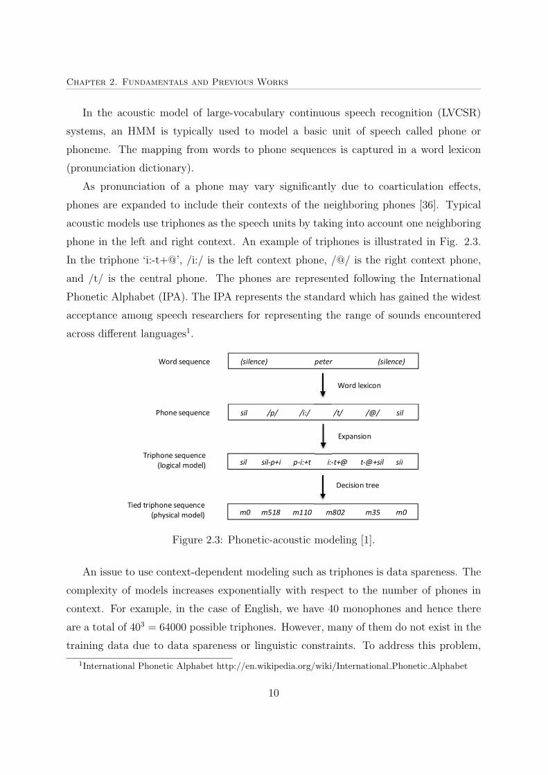
In the acoustic model of large-vocabulary continuous speech recognition (LVCSR)
systems, an HMM is typically used to model a basic unit of speech called phone or
phoneme. The mapping from words to phone sequences is captured in a word lexicon
(pronunciation dictionary).
As pronunciation of a phone may vary significantly due to coarticulation effects,
phones are expanded to include their contexts of the neighboring phones [36]. Typical
acoustic models use triphones as the speech units by taking into account one neighboring
phone in the left and right context. An example of triphones is illustrated in Fig. 2.3.
In the triphone ‘i:-t+@’, /i:/ is the left context phone, /@/ is the right context phone,
and /t/ is the central phone. The phones are represented following the International
Phonetic Alphabet (IPA). The IPA represents the standard which has gained the widest
acceptance among speech researchers for representing the range of sounds encountered
across different languages1.
(silence) peter (silence)
sil /p/ /i:/ /t/ /@/ sil
sil sil-p+i p-i:+t i:-t+@ t-@+sil sil
m0 m518 m110 m802 m35 m0
Word sequence
Phone sequence
Triphone sequence
(logical model)
Tied triphone sequence
(physical model)
Word lexicon
Expansion
Decision tree
Figure 2.3: Phonetic-acoustic modeling [1].
An issue to use context-dependent modeling such as triphones is data spareness. The
complexity of models increases exponentially with respect to the number of phones in
context. For example, in the case of English, we have 40 monophones and hence there
are a total of 403 = 64000 possible triphones. However, many of them do not exist in the
training data due to data spareness or linguistic constraints. To address this problem,
1International Phonetic Alphabet http://en.wikipedia.org/wiki/International Phonetic Alphabet
10

Chapter 2. Fundamentals and Previous Works
the decision tree-based clustering was investigated to tie triphones into physical models
[36]. With this approach, the number of models is reduced and model parameters can be
estimated robustly.
The latest state-of-the-art acoustic models have moved from HMM/GMM to HMM/DNN
(Deep Neural Network) architecture [37–41]. DNNs were recently introduced as a power-
ful machine learning technique [42] and have been applied widely for acoustic modeling
of speech recognition from small [37, 39] to very large tasks [40, 41] with a good success.
In this thesis, application of DNNs for cross-lingual speech recognition is presented in
Chapter 4.
2.1.3 Language model and word lexicon
While the acoustic model is used to score acoustic input feature, the language model
assigns a probability to each hypothesized word sequence during decoding to include
language information to improve ASR performance. For example, the word sequence “we
are” should be assigned a higher probability than the sequence “we is” for an English
language model. The typical language model is “N -gram” [43]. In an N -gram language
model, the probability of a word in a sentence is conditioned on the previous N−1 words.If N is equal to 2 or 3, we have “bigram” or “trigram” language model, respectively. The
paper [43] presents an excellent overview of recent statistical language models.
A word lexicon bridges the acoustic and language models. For instance, if an ASR
system uses a phone acoustic model and a word language model, then the word lexicon
defines the mapping between the words and the phone set. If a word acoustic model is
used, the word lexicon is simply a one-to-one trivial mapping.
2.1.4 Decoding
The decoding block, which is also known as the search block, decodes the sequence of
feature vectors into a symbolic representation. This block uses the acoustic model and
the word lexicon to provide an acoustic score for each hypothesis word sequence W .
The language model is simultaneously applied to compute the language model score for
each hypothesized word sequence. The task of the decoder is to determine the best
hypothesized word sequence that can then be selected based on the combined score
11
Chapter 2. Fundamentals and Previous Works
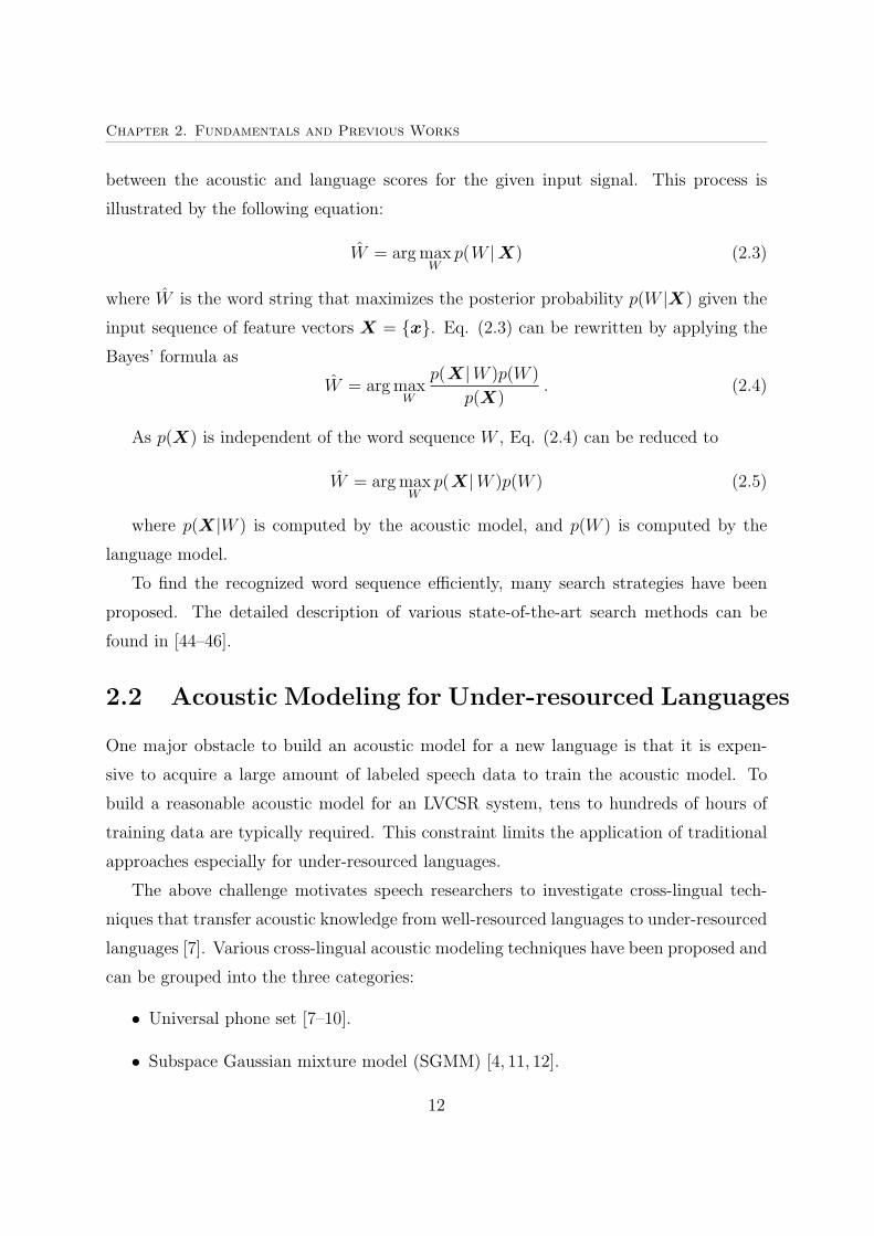
between the acoustic and language scores for the given input signal. This process is
illustrated by the following equation:
W = argmaxW
p(W |X) (2.3)
where W is the word string that maximizes the posterior probability p(W |X) given the
input sequence of feature vectors X = {x}. Eq. (2.3) can be rewritten by applying the
Bayes’ formula as
W = argmaxW
p(X|W )p(W )
p(X). (2.4)
As p(X) is independent of the word sequence W , Eq. (2.4) can be reduced to
W = argmaxW
p(X|W )p(W ) (2.5)
where p(X|W ) is computed by the acoustic model, and p(W ) is computed by the
language model.
To find the recognized word sequence efficiently, many search strategies have been
proposed. The detailed description of various state-of-the-art search methods can be
found in [44–46].
2.2 Acoustic Modeling for Under-resourced Languages
One major obstacle to build an acoustic model for a new language is that it is expen-
sive to acquire a large amount of labeled speech data to train the acoustic model. To
build a reasonable acoustic model for an LVCSR system, tens to hundreds of hours of
training data are typically required. This constraint limits the application of traditional
approaches especially for under-resourced languages.
The above challenge motivates speech researchers to investigate cross-lingual tech-
niques that transfer acoustic knowledge from well-resourced languages to under-resourced
languages [7]. Various cross-lingual acoustic modeling techniques have been proposed and
can be grouped into the three categories:
• Universal phone set [7–10].
• Subspace Gaussian mixture model (SGMM) [4, 11, 12].
12

Chapter 2. Fundamentals and Previous Works
• Source language models act as a feature extractor [13–18, 20–25, 31].
The first category is referred to as universal phone set [7–10]. It generates a common
phone set by pooling the phone sets of different languages (Fig. 2.4). A multilingual
acoustic model can therefore be trained by using this common phone set. In general,
with this approach, an initial acoustic model for a new language Y can be obtained by
mapping from the multilingual acoustic model. Also, to improve performance on the
target language, the initial acoustic model is refined using adaptation data of the target
language.
Y
(initial target model)
Source language X1
Multilingual acoustic model
Mapping
Y
(Refined target model)
Model
Refinement
Adaptation data of target language
Source language X2
Source language X3
Figure 2.4: An example of the universal phone set approach.
The second category is the cross-lingual subspace Gaussian mixture model (SGMM)
[4, 11, 12]. As shown in Fig. 2.5, in the SGMM acoustic model, the model parameters are
separated into two classes, i.e. language-independent parameters and language-dependent
parameters. With such a model, the language-independent parameters from a well-
resourced (source) language can be reused and the language-dependent parameters are
trained with speech data from the target language. As language-dependent parameters
only account for a small proportion of the overall parameters, they could be reliably
trained with a small amount of training data. Hence the SGMM is a possible approach
to supporting speech recognition development of under-resourced languages.
In the third category, which is also the most popular approach, the source acoustic
model is used as a feature extractor to generate cross-lingual features for target language
13

Chapter 2. Fundamentals and Previous Works
Copy
Well-resourced (source) language acoustic model
Under-resourced (target)
language acoustic model
Trained by source language data
Trained by
target language data
Language-dependent
Language-independent
Language-dependent
Language-independent
Figure 2.5: Illustration of the cross-lingual subspace Gaussian mixture model (SGMM)approach.
speech data (Fig. 2.6). As these cross-lingual features are higher-level and more mean-
ingful features as compared to conventional features such as MFCCs, they allow the use
of a simpler model that could be trained using only a small amount of training data for
target acoustic model development.
Cross-lingual feature
- Phone posterior - Speech attribute posterior
- Bottleneck feature
Well-resourced (source) language acoustic model
- HMM/MLP - Speech attribute detector - Bottleneck network
Under-resourced (target)
language acoustic model
- HMM/GMM - HMM/MLP - KL-HMM - Exemplar-based model
Target language
acoustic score
Target language
speech data
Figure 2.6: Source acoustic models act as a feature extractor.
In the next subsections, the above cross-lingual techniques will be reviewed in details.
2.2.1 Universal phone set method
In this approach, a common phone set is generated by pooling the phone sets of different
languages to train a multilingual acoustic model [7, 8]. This allows the model to be shared
by various languages and hence reduces the complexity and number of parameters for
the multilingual LVCSR system. The acoustic model for a new language can be achieved
by mapping from the multilingual acoustic model. Also, to improve performance, this
initial model is then bootstrapped using the new language training data.
The rest of the section is organized as follows. Subsection 2.2.1.1 presents the one-to-
one phone mapping techniques to map the phone sets of different languages. Subsection
2.2.1.2 discusses about building a multilingual acoustic model. Subsection 2.2.1.3 presents
recent techniques for acoustic model refinement.
14
Chapter 2. Fundamentals and Previous Works
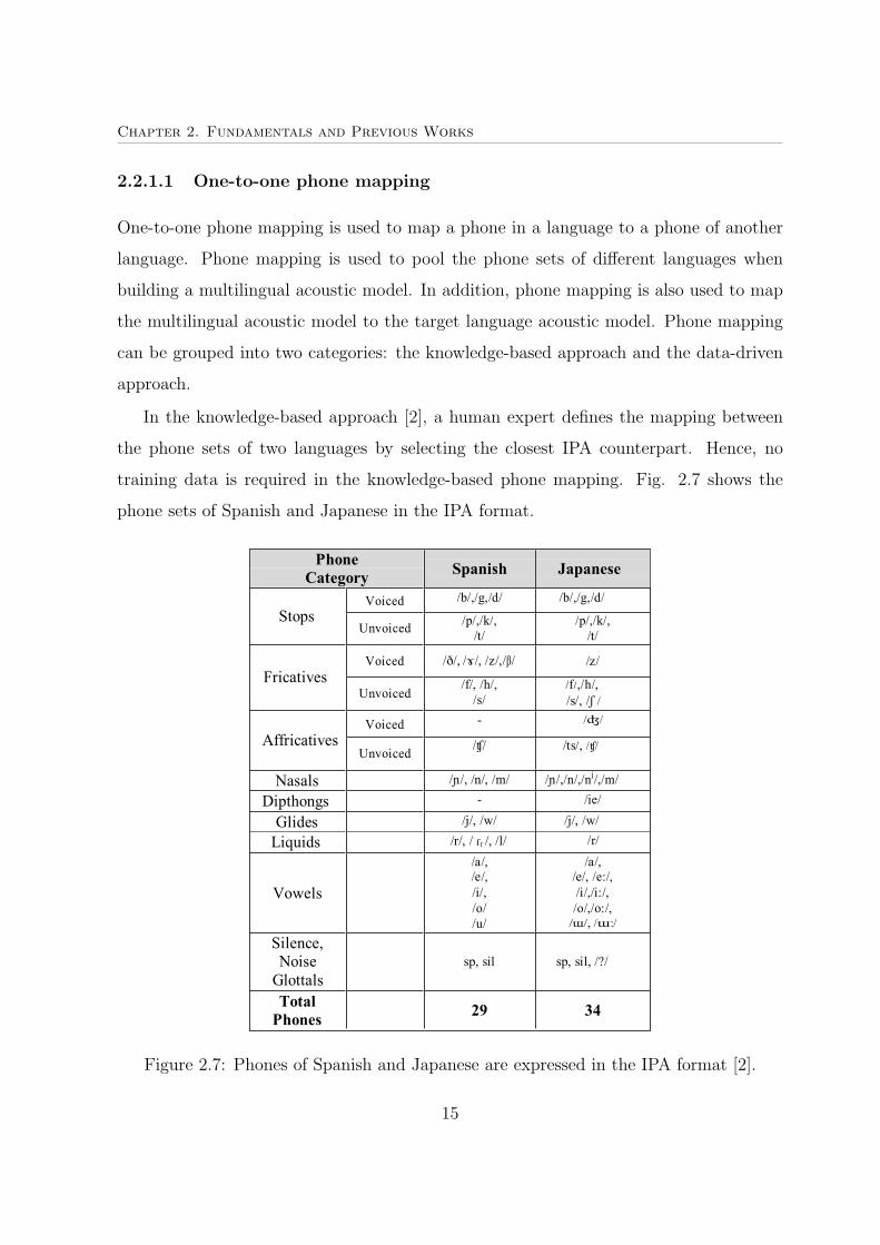
2.2.1.1 One-to-one phone mapping
One-to-one phone mapping is used to map a phone in a language to a phone of another
language. Phone mapping is used to pool the phone sets of different languages when
building a multilingual acoustic model. In addition, phone mapping is also used to map
the multilingual acoustic model to the target language acoustic model. Phone mapping
can be grouped into two categories: the knowledge-based approach and the data-driven
approach.
In the knowledge-based approach [2], a human expert defines the mapping between
the phone sets of two languages by selecting the closest IPA counterpart. Hence, no
training data is required in the knowledge-based phone mapping. Fig. 2.7 shows the
phone sets of Spanish and Japanese in the IPA format.
Phone Category
Spanish
Japanese
Stops
Voiced /b/,/g,/d/ /b/,/g,/d/
Unvoiced /p/,/k/,
/t/
/p/,/k/,
/t/
Fricatives
Voiced /ð/, / /, /z/,/ / /z/
Unvoiced /f/, /h/,
/s/
/f/,/h/,
/s/, / /
Affricatives
Voiced - / /
Unvoiced / / /ts/, / /
Nasals / /, /n/, /m/ / /,/n/,/nj/,/m/
Dipthongs - /ie/
Glides /j/, /w/ /j/, /w/
Liquids /r/, / r /, /l/ /r/
Vowels
/a/, /e/,
/i/,
/o/
/u/
/a/, /e/, /e:/,
/i/,/i:/,
/o/,/o:/, / /, / :/
Silence, Noise
Glottals
sp, sil
sp, sil, /?/
Total
Phones
29
34
Figure 2.7: Phones of Spanish and Japanese are expressed in the IPA format [2].
15

Chapter 2. Fundamentals and Previous Works
In data-driven mapping approach, a mathematically tractable, predetermined perfor-
mance measure is used to determine the similarity between acoustic models from different
languages [2]. The two popular performance measures are used: confusion-based matrices
and distance-based measures [47, 48].
The confusion matrix technique involves the use of a grammar-free phone recognizer of
the source language to decode the target speech. The hypothesized transcription is then
cross compared with the target language reference transcription. Based on the frequency
of co-occurrence between the phones in the source and target inventories, a confusion
matrix is generated. The one-to-one phone mapping to a target phone is derived by
picking the hypothesized phone which has the highest normalized confusion score.
An alternative data-driven method is to estimate the difference between phone models
using the model parameters directly. The distance metrics between phone models which
have been used include Mahalanobis, KullBack-Liebler and Bhattacharya [49].
Experiments on the Global Phone corpus in [2] showed that in most cases, the two
data-driven mapping techniques produce similar mappings. Comparing to the knowledge-
based phone mapping, the two data-driven techniques provide a modest improvement
when mapping is conducted for the matched conditions. However, the result showed that
knowledge-based mapping is superior when mappings are required in the mismatched
conditions.
2.2.1.2 Multilingual acoustic models
In [8], the multilingual acoustic model is built based on the assumption that the articu-
latory representations of phones are similar across languages and phones are considered
as language-independent units. This allows the model to be shared by various languages
and hence reduces the complexity and number of parameters for the multilingual LVCSR
system. Two combination methods ML-mix and ML-tag are proposed to combine the
acoustic models of different languages [8].
Denote p(x|si) to be the emission probability for feature vector x of state si,
p (x|si) =Ki∑k=1
csi,kN(x|µsi,k
,Σsi,k
)(2.6)
16

Chapter 2. Fundamentals and Previous Works
where si is a state of a phone in a specific language, N(x|µsi,k
,Σsi,k
)is the normal
distribution with mean vector µsi,kand covariance matrix Σsi,k. csi,k is the mixture
weight for mixture k, Ki is the number of mixtures for state si.
In the ML-mix combination, the training data are shared across different languages
to estimate the acoustic model’s parameters. The phones in different languages which
have the same IPA unit are merged and the training data of languages belonging to the
same IPA unit are used to train this universal phone, i.e. during the training process,
no language information is preserved. The ML-mix model combination method can be
described by:
ML - mix :
csi,k = csj ,k,∀i, j : IPA(si) = IPA(sj),µsi,k
= µsj ,k,∀i, j : IPA(si) = IPA(sj),
Σsi,k = Σsj ,k,∀i, j : IPA(si) = IPA(sj),
Different to the above method, the ML-tag combination method preserves each phone’s
language tag. Similar to ML-mix, all the training data and the same clustering proce-
dure are used. However, only the Gaussian component parameters are shared across
languages, the mixture weights are different. This approach can be described by:
ML - tag :
csi,k = csj ,k,∀i = j,µsi,k
= µsj ,k,∀i, j : IPA(si) = IPA(sj),
Σsi,k = Σsj ,k,∀i, j : IPA(si) = IPA(sj),
Experiments were conducted in [9] to evaluate the usefulness of two above approaches.
Five languages were used, Croatian, Japanese, Korean, Spanish, and Turkish. In this
work, the authors concentrated on recognizing these five languages simultaneously which
are involved for training the multilingual acoustic models. The ML-tag combination
method outperforms ML-mix in all languages. In addition, the ML-tag model reduces
40% number of parameters as compared to the monolingual systems. Although the ML-
tag model performs slightly worse than the language dependent acoustic models, such
model can be used to rapidly build an acoustic model for a new language [9, 10] using
different model refinement techniques which will be discussed in the next section.
2.2.1.3 Cross-lingual model refinement
To build a new language acoustic model from the pre-trained multilingual acoustic model,
a phone mapping from the given multilingual model phone set to the new language phone
17

Chapter 2. Fundamentals and Previous Works
set is first identified. After that the initial acoustic model of the target language is
generated by copying the required phone models from the multilingual acoustic model.
The performance of such initial model is usually very poor. To improve, the initial target
model is adapted using target language speech data. The rest of this section discusses
two popular methods for cross-lingual model refinement: model bootstrapping and model
adaptation.
Model bootstrapping is the simplest cross-lingual model refinement approach [8, 50,
51]. Bootstrapping simply means that the model is completely re-trained with the target
language training data using the initial acoustic model. Although experimental results
have shown that there is no significant improvement over monolingual training of the
target language, there is a significant improvement in convergence speed of the training
process [8, 50, 51]
When the amount of target training data is scarce, the traditional model adaptation
techniques can be applied to the initial acoustic model. Model adaptation techniques
can be grouped into two main categories: direct and indirect adaptation. In direct
adaptation, the model parameters are re-estimated given the adaptation data. Bayesian
learning, in the form of maximum a posteriori (MAP) adaptation [52, 53], forms the
mathematical framework for this task. In contrast, the indirect adaptation approach
avoids the direct re-estimation of the model parameters. Mathematical transformations
are built to convert the parameters of the initial model to the target conditions. The most
popular representative of this group is maximum likelihood linear regression (MLLR) [54]
which transforms the input features to maximize the likelihood of the acoustic model.
The first study using model adaptation scheme for cross-lingual model refinement was
reported in [55]. In that study, online MAP adaptation was used to adapt monolingual
and multilingual German, US-English, US-Spanish acoustic models to Slovenian. Only
the means of the Gaussians were adapted resulting in an absolute gain in WER up to
10% for a digit recognition task.
Methods using offline MAP adaptation were reported in [56, 57]. Multilingual English-
Italian-French-Portuguese-Spanish models were transformed to German in [56]. An im-
provements up to 5% in WER over mapped, non-adapted models was achieved on a
isolated word recognition task. In [57], the language transfer was applied from English to
18

Chapter 2. Fundamentals and Previous Works
Mandarin. In these experiments the phone recognition could be improved by 10% using
MAP adaption.
In [47], Czech was used as the target language while Mandarin, Spanish, Russian, and
English were the source languages. Adaptation to Czech was performed by concatenating
MLLR and MAP. Although significant improvements were achieved over the non-adapted
models, the performance of a pure Czech triphone system trained with the adaptation
data was not reached.
To sum up, the universal phone mapping is an intuitive approach for cross-lingual
acoustic modeling which is based on the assumption that phones can be shared in different
languages. In this approach, a multilingual acoustic model is built by pooling the phone
sets of different languages to train a multilingual acoustic model. The acoustic model for
a new language is achieved by using a one-to-one phone mapping from the multilingual
acoustic model. However, phones in different languages can be similar, they are unlikely
to be identical. Hence, the one-to-one phone mapping may cause the poor performance
of the initial cross-lingual acoustic model. In Chapter 3, we propose a novel many-to-one
phone mapping to improve speech recognition of under-resourced languages.
2.2.2 Cross-lingual subspace GMM (SGMM)
Unlike the universal phone set approach, in the subspace GMM (SGMM) approach, a
novel model structure is proposed to reduce the amount of required training data. In this
approach [4, 12], the model parameters are separated into two classes, i.e. the subspace
parameters that are almost language independent, and phone state specific parameters
that are language dependent. As well-resourced languages can first be used to train
the subspace parameters and the limited target language data used to train phone state
parameters. As phone state parameters only account for a small proportion of the overall
model, they could be reliably trained using a limited amount of target training data.
Similar to the conventional GMM model, the SGMM also uses mixtures of Gaussians
as the underlying state distribution, however, parameters in the SGMM are shared be-
tween states. Sharing is justified by the high correlation between states distributions
since the variety of sounds that the human articulatory tract can produce is limited [58].
19

Chapter 2. Fundamentals and Previous Works
In the SGMM model [58], the distribution of the features in HMM state j is a mixture
of Gaussians:
p(x|j) =K∑i=1
wjiN(x|µji,Σi) (2.7)
where, there are K full-covariance Gaussians shared between all states. Unlike the
conventional GMM, in the SGMM, the state dependent mean vector µji and mixture
weight wji are not directly estimated as parameters of the model. Instead, µji of state j
is a projection into the ith subspace defined by a linear subspace projection matrix M i,
µji = M ivj (2.8)
where vj is the state projection vector for state j and a language-dependent parameter.
The subspace projection matrix M i is shared across state distribution and language-
independent which has the dimension of D×S where D is the dimension of input feature
vector x, S is the dimension of the state projection vector vj. The mixture weight wji
in Eq. (2.7) is derived from the state projection vector vj using a log-linear model,
wji =exp (qT
i vj)K∑
i′=1
exp(qTi′vj)
(2.9)
with a globally shared parameter qi determining the mapping.
To have more flexibility for the SGMM model, the concept of substates is adopted for
state modeling. Specifically, the distribution of a state j can be represented by more than
one vector vjm, in this case, m is the substate index. Similar to the state distribution in
Eq. (2.7), substate distribution is again a mixture of Gaussians. The state distribution
is then a mixture of substate distributions,
p(x|j) =Mj∑m=1
cjm
K∑i=1
wjmiN(x|µjmi,Σi) (2.10)
µjmi = M ivjm (2.11)
wjmi =exp (qT
i vjm)K∑
i′=1
exp(qTi′vjm)
(2.12)
20

Chapter 2. Fundamentals and Previous Works
Table 2.1: Performance and model complexity of GMM and SGMM models in a mono-lingual task [4].
Model Number of Sub-statesNumber of parameters
WER(%)State-independent State-specific
GMM n.a 0 2427k 52.5SGMM 1.9k 952k 77k 48.9SGMM 12k 952k 492k 47.5
where cjm is the relative weight of substate m in state j.
Table 2.1 shows the number of parameters and word error rate (WER) for GMM and
SGMMmodels in a monolingual task [4]. In the conventional GMMmodel, all parameters
are state-dependent. In contrast, a significant amount of parameters are shared between
states in the SGMM models. The number of state-dependent parameters in SGMMs
varies following the number of sub-states. Although, in this case, the SGMM models
have a smaller number of total parameters as compared to the GMM model, the WERs
in both the SGMM models are significantly better.
With its special architecture, the SGMM can be very naturally applied for cross-
lingual speech recognition. The state independent SGMM parameters, Σi, M i, qi can
be trained from well-resourced languages while the state dependent parameters vjm, cjm
are trained from limited training data of the under-resourced language.
Study in [4] is the first work applying SGMM for cross-lingual speech recognition.
In that work, the SGMM shared parameters are trained from 31 hours of Spanish and
German while the state-specific parameters are trained on 1 hour of English which is
randomly extracted from the Callhome corpus. With this approach, the cross-lingual
SGMM model achieves 11% absolute improvement over the conventional monolingual
GMM system. The idea of SGMM is further developed using the regularized SGMM
estimation approach [59]. The experimental result on the GlobalPhone corpus showed
that regularizing cross-lingual SGMM systems (using the ℓ1-norm) results in a reduced
WER.
One issue when using multiple languages to estimate the shared parameters in the
SGMM is the potential mismatch of the source languages with the target language, e.g.
the differences in phonetic characteristics, corpus recording conditions, and speaking
styles. To address this, maximum a posteriori (MAP) adaptation can be used [12]. In
21

Chapter 2. Fundamentals and Previous Works
particular, the target language model can be trained by MAP adaptation on the phonetic
subspace parameters. This solution results in a consistent reduction in word error rate
on the GlobalPhone corpus [12].
In conclusion, in the SGMM approach, a novel acoustic model structure is proposed to
reduce the amount of training data required for acoustic model training. In the SGMM,
model parameters are separated into two classes: language-dependent and language-
independent. With such a model, language-independent parameters can be borrowed
from the well-resourced language and the limited target language data are used to train
the language-dependent parameters. Although, the SGMM approach can provide signif-
icant improvements over the monolingual models, this approach requires the source and
target models to have the similar structures. This limits the flexibility of the approach for
different cross-lingual tasks. In the next section, a more flexible cross-lingual framework
will be discussed.
2.2.3 Source language models act as a feature extractor
This section discusses about the third category which is also currently the most popular
approach. In this approach, the idea is to use source language acoustic models as a
feature extractor to generate high-level, meaningful features to support under-resourced
acoustic model development. As listed in Table 2.2, various cross-lingual methods have
been proposed using different types of target acoustic models and different types of cross-
lingual features. These methods will be presented in details in the following subsections.
The proposed works in this thesis belong to this category. The works in Chapter 3 and
Chapter 4 are cross-lingual phone mapping. The related techniques include posterior-
based phone mapping (Subsection 2.2.3.4) and cross-lingual tandem (Subsection 2.2.3.1).
The works in Chapter 5 are exemplar-based acoustic modeling. The related literature is
the exemplar-based method (Subsection 2.2.3.5).
2.2.3.1 Cross-lingual tandem approach
The tandem approach was proposed by Hermansky et al. in 2000 for monolingual speech
recognition. In this approach, a neural network is used to generate phone posterior feature
for an HMM/GMM acoustic model. This feature takes advantages of the discriminative
22

Chapter 2. Fundamentals and Previous Works
Table 2.2: Different cross-lingual methods using the source acoustic models as a featureextractor.
Method Cross-lingual feature Target acoustic modelCross-lingual tandem Phone posteriors [13–15] HMM/GMM
Bottleneck feature [16, 17]ASAT [18–20] Speech attribute posteriors HMM/MLPCross-lingual KL-HMM [21, 22] Phone posteriors KL-HMMSequence-based phone mapping [23, 24] Phone sequences Discrete HMMPosterior-based phone mapping [25] Phone posteriors HMM/MLPCross-lingual exemplar-based Bottleneck features Exemplar-based modelmodel [31]
ability of neural networks while retaining the benefit of conventional HMM/GMMmodels
such as model adaptation.
The tandem approach was recently applied for cross-lingual tasks [13–17]. As shown
in Fig. 2.8, in the cross-lingual tandem approach, the source language data are used to
train an MLP. This MLP is then used to generate source language phone posteriors for
the target language data. These posterior scores are passed to a log function. Taking log
renders the feature distribution to appear more Gaussian [60]. As the posterior features
are of high dimension, they are not suitable for the HMM/GMM modeling. To reduce
the dimensionality of the feature, a dimensionality reduction such as PCA (Principal
Component Analysis) or HLDA (Hetroscedastic Linear Discriminant Analysis) is applied.
To further improve performance, these features are concatenated with low level spectral
features such as MFCCs or PLPs to create the final feature vector which is modeled by
the target language’s HMM/GMM.
The main disadvantage of the tandem approach comes from its dimensionality reduc-
tion process as it results in information loss. This effect will be investigated in Chapter
3, and Chapter 4 of this thesis.
A variation of the tandem approach is the bottleneck feature approach [61]. The
bottleneck feature is generated using an MLP with several hidden layers where the size
of the middle hidden layer, i.e. bottleneck layer is set to be small. With this structure,
an arbitrary feature size can be obtained without using dimensionality reduction step
and is independent to the MLP training targets. The bottleneck feature has been used
widely in speech recognition and provides a consistent improvement over conventional
23

Chapter 2. Fundamentals and Previous Works
Feature
extraction
MFCCs,
PLPs
Concatenate
Recognized
results HMM/GMM
Phone
posteriors Trained by target
language data
Speech
signal
MLP Log & PCA
Recognized
results
Trained by source
language data
(Target
language)
Figure 2.8: Cross-lingual tandem approach.
features such as MFCCs, PLPs and posterior features as well. In [16, 17], bottleneck
feature has been applied for cross-lingual ASR by using a bottleneck MLP trained for
source languages to generate the bottleneck features for a target language HMM/GMM
model. Their results showed a potential ability to use bottleneck feature in cross-lingual
speech recognition. In Chapter 4 and Chapter 5 of this thesis, cross-lingual bottleneck
feature will be used in the proposed cross-lingual framework.
2.2.3.2 Automatic speech attribute transcription (ASAT)
Automatic speech attribute transcription (ASAT) proposed by Lee et al [19] is a novel
framework for acoustic modeling that uses a different type of speech units called speech
attributes. Speech attributes (SAs) such as voicing, nasal, dental, describe how speech is
articulated. They are also called phonological features, articulatory features, or linguistic
features. SAs have been shown to be more language universal than phones and hence
may be used as speech units and be adapted to a new language more easily [62, 63].
The set of SAs can be divided into subsets as illustrated in Table 2.3 [5]. SAs in each
subset can then be classified by an MLP to estimate posterior probability p(ai|x), where aidenotes the ith SA in that subset, and x is the input vector at time t. Experimental results
with monolingual speech recognition in [5] showed that SAs help to improve performance
of a continuous numbers recognition task under clean, reverberant and noisy conditions.
In the ASAT framework [19], SA posteriors generated by various detectors are merged
to estimate higher level speech units such as phones or words to improve decoding.
The framework exploits language-independent features by directly integrating linguistic
24

Chapter 2. Fundamentals and Previous Works
Table 2.3: Speech attribute subsets [5].Attribute subset Possible output value
Voicing +voice, -voice, silenceManner stop, vowel, fricative, approximant, nasal, lateral, silencePlace dental, labial, coronal, palatal, velar, glottal, high, mid, low, silence
Front-Back front, back, nil, silenceLip Rounding +round, -round, nil, silence
knowledge carried by SAs into the ASR design process. This approach allows to build
a speech recognition system for a new target language with a small amount of training
data.
Fig. 2.9 shows the ASAT framework for cross-lingual speech recognition. SA detectors
are used to generate SA posterior probability p(ai|x). An event merger is then used to
combine these posteriors to generate target phone posterior probability p(pj|x). Finally,these phone posteriors are used by a decoder (evidence verifier) as in the hybrid ASR
approach [64].
p([aa]|x)
p([ow]|x)
p([sil]|x)
p(vowel|x)
Detectors
Vowel
Nasal
Silence
Event
Merger p(nasal|x)
p(sil|x)
Evidence
Verifier p([uw]|x)
(Target
language)
Speech
feature (x)
Recognized
results
.
.
.
.
.
.
Posteriors of SAs given
speech feature
Posteriors of target phones
given speech feature
Trained by source
language data
Trained by target
language data
Figure 2.9: Automatic speech attribute transcription (ASAT) framework for cross-lingualspeech recognition.
In our recent work [65], the experiments also showed the usefulness of SAs in a cross-
lingual ASR framework. Specifically, SA posterior probabilities estimated by the SA
25

Chapter 2. Fundamentals and Previous Works
detectors are mapped to context-dependent tied states of the target language by an MLP.
The results showed that using SAs alone provides lower performance over the phone-based
approach, however, when SA posteriors are concatenated with phone likelihood scores
generated by the source HMM/GMM model, consistent improvements are observed over
both the individual systems. This shows that SAs provide complementary information
to phone-based scores for cross-lingual modeling.
In [66], we proposed a method to recognize SAs more accurately by considering the
left or the right context of SAs called bi-SAs. Our results on the TIMIT database
showed that the higher resolution SA can help to improve SA and phone recognition
performance significantly. The idea of context-dependent bi-SAs was then applied on
cross-lingual ASR tasks [65]. Specifically, four bi-SA detectors: left-bi-manner, right-bi-
manner, left-bi-place and right-bi-place are trained with source language data. Given a
target language speech frame, each detector then generates posterior probabilities for each
class of bi-SAs. These posteriors are further combined and mapped into target triphone
states. Experimental results showed that context-dependent SAs perform better over
context-independent SAs in cross-lingual tasks.
2.2.3.3 Kullback-Leibler based HMM (KL-HMM)
In this subsection, the KL-HMM, a special type of HMM based on the Kullback-Leibler
divergence is presented [21, 22, 67, 68]. Similar to the tandem approach, the KL-HMM
uses phone posteriors generated by the source language MLP as the input feature. How-
ever, while the tandem approach uses a mixture of Gaussians to model the statistics of
the feature, the KL-HMM has a simpler architecture with less parameters and hence can
be estimated more robustly in the case of limited training data.
In the KL-HMM, state emission probability p(zt|sd) of state sd for feature zt ∈ RK
is simply modeled by a categorical distribution2 yd =[y1d, ..., y
Kd
]T, d ∈ {1, ..., D}, where
K is the dimensionality of the input feature and D is the number of states in KL-HMM.
The input feature vector zt =[z1t , ..., z
Kt
]Tis the phone posterior probability generated
by an MLP and satisfies the constraint:
2a categorical distribution is a probability distribution that describes the result of a random eventthat can take on one of K possible outcomes, with the probability of each outcome separately specified.
26

Chapter 2. Fundamentals and Previous Works
K∑i=1
zit = 1. (2.13)
The posterior vector zt is modeled as a discrete probability distribution on the HMM
state space. For each state sd and each feature vector zt, a dissimilarity measurement
between the two discrete distributions yd and zt can be measured by their KL-divergence
KL(yd||zt) =K∑k=1
ykd logykdzkt
. (2.14)
In the conventional HMM/GMM model, if we ignore the effect of state transition
probabilities and language model factor, the cost function during decoding to find the
optimum word sequence W can be expressed by
JW (X) = minΦW
T∑t=1
−log p(sΦt |xt) (2.15)
where ΦW represents all possible state sequences of length T allowed by W , X = {xt}is the sequence of the input feature vectors. If we use the KL divergence approach as in
Eq. (2.14), we can rewrite Eq. (2.15) as
JW (X) = minΦW
T∑t=1
KL(yΦt||zt). (2.16)
The model described by Eq. (2.16) can be interpreted as a finite state machine where
each state has an associated cost given by the KL-divergence between its corresponding
target distribution, yd and the posterior vector, zt [68]. Hence, the parameters of the
KL-HMM are simply the D state distributions {yd}Dd=1. The number of parameters in
this model is very small as compared to the HMM/GMM model and hence the KL-HMM
is a good option for acoustic modeling under limited training data conditions.
In the training process, the arithmetic mean of all the posterior features associated
with KL-HMM state sd forms state categorical distribution yd.
yd =1
Nd
Nd∑i=1
zi (2.17)
27
Chapter 2. Fundamentals and Previous Works
where Nd is the number of training samples zi which are associated with state sd.
Experiments for the monolingual tasks conducted in [67] indicated that the KL-HMM
outperforms the tandem method for a small task with limited training data. However,
one weak point of the KL-HMM approach is that the model is too simple, i.e. it has
very few parameters and hence could not achieve better performance when more training
data become available. This observation was seen in [68] where Aradilla et al. applied
the KL-HMM to large vocabulary for the WSJ corpus. Experimental results showed that
KL-HMM performs slightly worse than the tandem approach.
In [21, 22], Imseng et al. applied the KL-HMM approach for cross-lingual tasks.
Similar to the cross-lingual tandem [13–15] and posterior-based phone mapping [25] ap-
proaches, an MLP well-trained by a source language is used to generate phone posterior
probabilities for speech data of the target language. These posteriors are then used as
the input feature for the target language acoustic model such as HMM/GMM (tandem),
HMM/MLP (phone mapping) or KL-HMM. Experiments in [21] indicated that the cross-
lingual KL-HMM achieves better performance than the cross-lingual tandem model if less
than 4 hours of target data are used. However, when more training data became avail-
able, the cross-lingual KL-HMM does not continue to improve, and is even worse than
the monolingual HMM/GMM model. This phenomenon is also repeated in [22], when
more than 1 hour of target language training data are used, the KL-HMM performes
worse than other models such as cross-lingual SGMM or HMM/GMM.
In conclusion, the KL-HMM approach has advantages such as its simple architecture
with a small number of parameters. Consequently, it also means that it is useful only
for limited training data conditions. The followings summarize the disadvantages of the
KL-HMM approach.
• Lack of flexibility: the number of parameters in KL-HMM depends only on the
number of outputs of the source language MLP and number of states in the target
language. Normally, when the amount of target training data changes, the com-
plexity of the target model should be changed accordingly. However, as the number
of states in the target language is constraint by the limited target training data
while a change in the number of the MLP outputs results in re-training the source
MLP.
28
Chapter 2. Fundamentals and Previous Works
• The KL-HMM modeling does not allow easy implementation for additional features
such as non-probabilistic features. In addition, as the input feature of KL-HMM
depends directly on the MLP, if the MLP is not well-trained, the KL-HMM will
not work well.
2.2.3.4 Sequence-based and posterior-based phone mapping
In the phone mapping approach, the speech data of the target language are first rec-
ognized as phone sequences [23] or phone posteriors [25] of a source language. These
phone sequences or posteriors are then mapped to the corresponding phone sequences or
posteriors of the target language followed by the standard decoding process.
The cross-lingual phone recognition process can be formulated as follows [23, 24, 69]:
Y = argmaxY
{p (Y |O,X ,Y , θ(X ))} = argmaxY
{∑X
pM (Y |X) p (X|O,X , θ(X ))
}(2.18)
where O is the observation sequence, X and Y are the source and target phone sets,
respectively, θ(X ) denotes an acoustic model for X and pM (Y |X) is the probability of
mapping from phone sequence X to phone sequence Y . This can be approximated as a
two-stage process:
X = argmaxX
{p (X|O,X , θ(X ))} (2.19)
Y ≈ argmaxY
{pM
(Y |X
)}(2.20)
The first stage is simply the decoding process using the source phone recognizer, θ(X )to obtain the best source phone sequence X given O. Then, in the second stage, the
mapping between the source language phone sequence, X to the target language phone
sequence, Y is implement by a mappingM: X → Y .In [23], Sim and Li proposed a novel sequence-based phone mapping method where
the mapping function M is modeled as a probabilistic model. The mapping model is
estimated as follows:
M = argmaxM
{∑Y ∈Ψ
p (Y |X,O,M)
}(2.21)
29

Chapter 2. Fundamentals and Previous Works
where Ψ denotes the target language training set, X and Y are the pair of phone
sequences for the speech utterance, O. In [23, 24] the mapping between two phone se-
quences is implemented as a discrete HMM where each state in the HMM model repre-
sents a phone in the target language while the phone sequence generated by the source
phone recognizer X is used as the input for the discrete HMM. The HMM can be trained
using a maximum likelihood criterion. However, in the generative HMM model, it is
required |X| ≥ |Y | where |X|, |Y | are the length of the two phone sequences X, Y , re-
spectively. To satisfy this condition, in [23, 24], Sim and Li expanded the original phone
sequence X into smaller “frames” based on the duration of each phone in X. This process
is illustrated in Fig. 2.10.
a b c d
a a a a b b b c c c c c d d d
Discrete HMM
Source phone
recognizer
A B C
Source phone sequence
Target speech
Expanded source phone sequence
Target phone sequence
Figure 2.10: Probabilistic sequence-based phone mapping model.
The experiments conducted in the SpeechDat-E and TIMIT databases [23, 24] indi-
cated that the probabilistic sequence-based phone mapping model can be trained with
a small amount of training data due to the small number of parameters in the discrete
HMM.
A main limitation of the sequence-based phone mapping system is that only the 1-
best phone sequence X given by the source phone recognizer is used Eq. (2.19, 2.20) as
the input for mapping. That means that other possibilities in the decoding are ignored.
This can be interpreted as information loss by “quantization effect” during the decoding
30

Chapter 2. Fundamentals and Previous Works
process. To address this, in [25], the author suggested that the mapping between the
source and target phone sets can be implemented before the decoding stage, i.e. at the
probability level. Specifically, the source phone posteriors generated by the source MLP
acoustic model are used as the input for the mapping to the target phone posteriors. The
mapping is implemented using a product-of-expert method where either the experts or
their weights are modeled as functions of the posterior probabilities of the source phones,
generated by the source phone MLP. Experimental results on the NTIMIT database
showed that using only 15.6 minutes of training data to train the posterior-based phone
mapping achieves a cross-lingual phone recognition errors of 46.0% while the monolingual
phone recognizer trained on the same amount of data obtained 53.4% phone error rate.
Based on the spirit of this approach, the thesis proposes an extension called “context-
dependent phone mapping” and applies it for large vocabulary word recognition tasks.
The result will be presented in Chapter 3.
2.2.3.5 Exemplar-based approach
While the above methods use parametric models such as GMM, MLP, KL-HMM, or
discrete HMM for the target acoustic modeling, this section introduces the use of non-
parametric models called exemplar-based model that can use the training samples di-
rectly. Unlike parametric methods, exemplar-based methods, such as k-nearest neighbors
(k-NN) [70] for classification and kernel density (or Parzen window) [70] for density esti-
mation, do not assume a parametric form for the discriminant or density functions. This
makes them attractive when the functional form or the distribution of decision boundary
is unknown or difficult to learn and especially when training data are limited.
In the machine learning community, two broad categories of approaches for modeling
the observed data are suggested [70]. The first category is referred to as eager (offline)
learning that uses all the available training data to build a model before the test sample
is seen. The second category is referred to as lazy (exemplar-based) learning that selects
a subset of exemplars from the training data to build a local model for each test sam-
ple. Although exemplar-based methods have been popular in many tasks such as face
recognition [71], object recognition [72], audio classification [73], they are only recently
applied for speech recognition [74–76].
31

Chapter 2. Fundamentals and Previous Works
An exemplar-based speech recognition system typically contains three stages: exem-
plar selection, instance modeling, and decoding [77].
In the exemplar selection stage, the process identifies the most relevant training in-
stances to each test instance using a distance metric. Given a suitable distance metric,
different types of exemplars can be used e.g. individual frames [74], or segmental level
such as fixed-length sequences of multiple frames [78] or variable length segments [79].
In the instance modeling stage, the training exemplars identified via the first stage
as most relevant for the test instance are used to model the test instance. For instance
modeling, each training exemplar is associated with a class label that can range from
HMM-states on individual frame [74], to word labels for word segments [79]. For example,
in the k-nearest neighbor (k-NN) method, the class posterior of class qi given test instance
xt can be estimated as
p(qi|xt) =Nit
Nt
(2.22)
where Nt is the total number of the most relevant training exemplars for test instance
xt, Nit is the number of the most relevant training exemplars belong to class qi.
The third stage is to perform decoding to recognize the test utterance. Specifically,
given the observation X = {xt}, the instance models from the previous stage, and a
set of subword units U , an acoustic score p(X|U) is computed directly for the segmental
approaches. For the frame-based techniques, class posterior p(qi|xt) needs to be converted
to the frame-based observation likelihood to compute acoustic score p(X|U) of the whole
utterance.
Recently, several studies have successfully applied the exemplar-based approach for
acoustic modeling [74–76]. In [74], the authors proposed to use a nearest neighbor clas-
sifier at the frame level in a speech recognition system. Specifically, the kernel density
estimation [80] is used to replace GMM in the HMM/GMM model for state likelihood
estimation as:
p(xt|qi) =1
Nit
Nit∑j=1
exp(− ||xt − eij||2
σ
)(2.23)
32

Chapter 2. Fundamentals and Previous Works
where xt is the test feature vector at frame t, eij is the jth exemplar of class qi, ||xt−eij||2
denotes the distance between xt and eij, Nit is the number of the most relevant exemplars
to xt that belong to class qi, σ is a scaling factor.
Experimental results in [74] for the English EPPS large vocabulary task showed that
the kernel density approach produces a consistently better result than the conventional
GMM when less than 3 hours of speech training data are available.
The k-NN method is also used in [76] where the authors proposed a method for learn-
ing label embeddings to model the similarity between labels within a nearest neighbor
framework. These estimates were then applied to acoustic modeling for speech recogni-
tion. Experimental results showed that significant improvements in terms of word error
rate (WER) are achieved on a lecture recognition task over a state-of-the-art baseline
GMM model.
One major issue in an exemplar-based system for speech recognition is its high com-
putational cost during decoding. To address this, in [75], two methods were proposed.
The first method was proposed to quickly select a subset of informative exemplars among
millions of training examples. The second method makes approximations to the sparse
representation computation such that a matrix-matrix multiplication is reduced to a
matrix-vector product. Experiments conducted in four large vocabulary tasks indicated
improvements in speedup by a factor of four relative to the original method as well as
improvements in WER in combination with a baseline HMM system.
Our recent work [31] is the first study that applies the exemplar-based approach for
cross-lingual acoustic modeling. Specifically, cross-lingual bottleneck feature generated
by a source language bottleneck DNN is used as the input feature for an exemplar-based
acoustic model of the target language. Chapter 5 of the thesis will present the proposed
cross-lingual exemplar-based acoustic model in details.
2.3 Summary
In this chapter, a conventional speech recognition system is first presented followed by
a review of the state-of-the-art cross-lingual acoustic modeling techniques. Among these
techniques, the cross-lingual phone mapping and the exemplar-based approaches are ones
33

Chapter 2. Fundamentals and Previous Works
of this thesis’s focuses. In next three chapters, the proposed methods will be presented.
Chapter 3 presents the context-dependent phone mapping approach. Chapter 4 examines
the use of deep neural networks in the cross-lingual phone mapping. Chapter 5 proposes
an exemplar-based acoustic model for limited training data conditions.
34

Chapter 3
Cross-lingual Phone Mapping
This chapter presents a novel phone mapping technique for large vocabulary automatic
speech recognition of under-resourced languages by leveraging well-trained acoustic mod-
els of other languages (source languages). This strategy is based on the linguistic knowl-
edge that speech units such as phones in different languages may be similar and hence
acoustic information of some well-trained models can be mapped to a new target lan-
guage. However, phones for different languages would not be identical and hence “hard
mapping” may not be appropriate. If the target speech unit has an overlapping distri-
bution with speech units from the source language, then a “soft mapping” may be more
appropriate.
In the first part of the chapter, a cross-lingual linear combination method is pro-
posed. Specifically, the target language’s phone model is generated as a weighted sum of
the source language’s phone models optimized by the maximum likelihood criterion. In
the second part, a nonlinear phone mapping architecture is introduced to improve perfor-
mance. The nonlinear mapping is used to convert likelihood or posterior scores generated
by the source acoustic model to target phone posteriors. Unlike previous studies which
used context-independent phone mapping strategy, the thesis proposes a novel extension
to use context-dependent triphone states as the acoustic units to achieve higher acoustic
resolution.
The results in this chapter have been published in: IEICE Transactions on Informa-
tion and Systems [26], IALP 2012 [27], and ISCSLP 2012 [28].
The chapter is organized as follows: Section 3.1 presents the detailed setup of cross-
lingual phone mapping and databases to be used in the chapter. In Section 3.2, the
35

Chapter 3. Cross-lingual Phone Mapping
cross-lingual linear acoustic model combination method is described. In Section 3.3, a
discussion of context-dependent nonlinear phone mapping is presented.
3.1 Tasks and Databases
Databases: To evaluate the performance of the proposed cross-lingual phone mapping
method, the Malay language is used as the source language and the English language
(WSJ0 task1) used as the taget under-resourced language. The WSJ0 English corpus
has been chosen as the under-resourced language as the effect of sufficient training data
for it is well known. Hence we can focus on the proposed work under the reduced
training corpus. In addition, Hungarian is also used as the source language to verify the
effectiveness of multiple source languages.
In the WSJ0 corpus, there are 7138 clean training sentences, or roughly 15 hours of
speech data. To simulate under-resourced conditions, sentences from the 7138 sentences
are randomly selected to generate smaller training sets. For testing, the clean test set is
used consisting of 166 sentences, or 20 minutes of speech. In this work, the focus is on
acoustic model training and it is assumed that the language model and pronunciation
dictionary of the target language are available. In addition, the source language acoustic
model is well trained using 100 hours of the Malay read speech corpus [81].
Language model and dictionary: The standard Wall Street Journal English bi-
gram language model is used in word recognition experiments. The test set contains
a vocabulary of 5k words. The CMU dictionary is used which consists of 40 phones,
including the silence phone.
Features: The features used in this study are the conventional 12th-order Mel fre-
quency cepstral coefficients (MFCCs) and C0 energy, along with their first and second
temporal derivatives. The frame length is 25ms and the shift is 10ms. To reduce record-
ing mismatch between the source and target corpora, utterance-based mean and variance
normalization (MVN) is applied to both training features of Malay and training and test-
ing features of English.
1The Aurora-4 corpus with clean training and test setting is actually used in this study. The Aurora-4clean data are a filtered version of the WSJ0 SI84 training data and Nov92 test data. The Aurora 4corpus with 16kHz sampling rate version is used.
36

Chapter 3. Cross-lingual Phone Mapping
3.2 Cross-lingual Linear Acoustic Model Combina-
tion
This section first discusses the use of one-to-one phone mapping (hard-mapping) to gen-
erate an acoustic model of a desired target language from a well-trained acoustic model of
another language denoted here as the source language. The one-to-one phone mapping
performance is then improved using adaptation techniques. After that, the proposed
method based on many-to-one phone mapping is presented. In the proposed method, the
model of a target speech unit is built as a linear combination of models from the source
speech units.
3.2.1 One-to-one phone mapping
To perform one-to-one phone mapping, two approaches can be used: knowledge-based
[82] and data-driven methods [8].
In the knowledge-based approach [82], a human expert defines the mapping between
phone set of the two languages by selecting the closest IPA counterpart. Hence, no
training data is required in this method. However, one difficulty of this approach is that
expert knowledge is required to formulate the linguistic relationships between languages.
Although linguistic experts might in theory be able to define relations according to pho-
netic dictionaries, the IPA system suffers from inconsistencies caused by the principles of
phonological contrast and is thus error prone [1]. To overcome this challenge, this section
focuses on the data-driven approach to perform one-to-one phone mapping from Malay
to English.
When training data are available, a data-driven approach [8] to find the phone map-
ping between the two languages is an option. In our case, the English target language
phone recognizer trained with limited English training data is first used to perform forced
alignment on the English training utterances. These English training utterances are then
decoded by the source Malay language acoustic model into Malay phone sequences. To
find the relationship between the English and Malay phones, a confusion matrix between
the two phone sets is computed by a frame-wise comparison of the alignments, normalized
by the summed frequency of the hypothesized phone [8]. The one-to-one phone mapping
37

Chapter 3. Cross-lingual Phone Mapping
Table 3.1: One-to-one phone mapping from Malay to English generated by the data-driven method using 7 minutes of English training data.No English phone Malay phone No English phone Malay phone
(Target language) (Source language) (Target language) (Source language)1 ah @ 21 l o2 aa aw 22 m m3 ae a 23 n n4 ao o 24 ng ng5 aw aw 25 ow o6 ay aj 26 oy w7 b b 27 p p8 ch ts 28 r r9 d d 29 s s10 dh t 30 sh ss11 eh a 31 zh z12 er r 32 t ts13 ey e 33 th f14 f f 34 uh j15 g g 35 uw u16 hh h 36 v v17 ih e 37 w w18 iy i 38 y nj19 jh dz 39 z z20 k k 40 sil sil
is then derived by picking the hypothesized phone which has the highest normalized
confusion score.
Table 3.1 shows the one-to-one phone mapping from Malay to English using data-
driven method with 7 minutes of English training data. Since the number of phones in
English is 40 while Malay has only 34 phones, some of the English phones are mapped
to the same Malay phone. There are several surprising phone mappings such as English
phone dh is mapped to Malay phone t or English phone uh is mapped to Malay phone
j. There are two main reasons for these poor mappings. Firstly, the performance of the
English phone recognizer is poor due to it is trained using only 7 minutes of English
data. Secondly, the English phones such as dh and uh are not present in Malay and
hence they are poorly recognized and result in mapping errors. To address this problem,
in [57], linguistic knowledge can be applied to refine the initial mapping generated by the
38

Chapter 3. Cross-lingual Phone Mapping
Table 3.2: Word error rate (WER) (%) of the one-to-one phone mapping for cross-lingualacoustic models.
Method Amount of adaptation data (minutes)0 1 7
One-to-one mapping 69.3 - -MLLR adaptation
1-class-MLLR - 65.8 64.08-class-MLLR - - 54.316-class-MLLR - - 52.232-class-MLLR - - 50.964-class-MLLR - - 50.1
data-driven phone mapping. This approach however only results in a small improvement
in cross-lingual phone recognition.
Given the one-to-one phone mapping, an initial acoustic model for each phone in the
target language can be obtained by copying the corresponding phone acoustic model of
the source language. As illustrated in the first row of Table 3.2, for the no adaptation
data condition, the one-to-one phone mapping achieves the poor word error rate (WER)
of 69.3%.
If target language training data are available, they can be used to adapt the initial
target acoustic model. In our experiment, maximum likelihood linear regression (MLLR)
[83] is applied for adaptation. The second row of Table 3.2 shows the WER achieved
when 1 and 7 minutes of adaptation data are used. Comparing to the result in the first
row, an improvement in WER is observed. However, using 7 minutes of adaptation data
just provides a small improvement over the case of using 1 minute. To benefit from
larger amounts of target adaptation data, multi-class MLLR is applied [83]. The results
for multi-class MLLR using 7 minutes of adaptation data are shown in the last four
rows in Table 3.2. Significant improvements are observed as compared to the case of the
single-class MLLR in the second row.
3.2.2 Many-to-one phone mapping
As discussed in the previous section, the one-to-one phone mapping can be used to
build an acoustic model for the target language by copying phone models from a well-
trained source acoustic model. This approach however results in a high word error rate
39
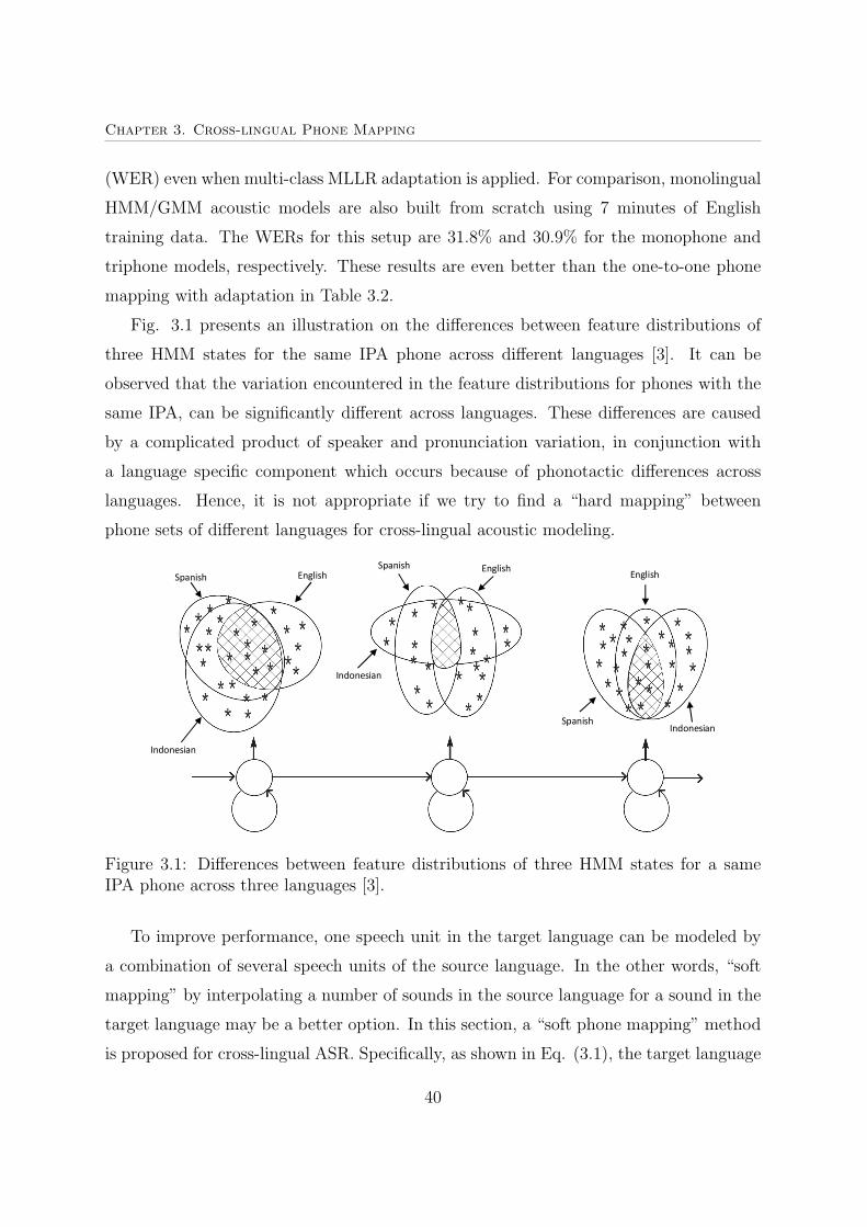
Chapter 3. Cross-lingual Phone Mapping
(WER) even when multi-class MLLR adaptation is applied. For comparison, monolingual
HMM/GMM acoustic models are also built from scratch using 7 minutes of English
training data. The WERs for this setup are 31.8% and 30.9% for the monophone and
triphone models, respectively. These results are even better than the one-to-one phone
mapping with adaptation in Table 3.2.
Fig. 3.1 presents an illustration on the differences between feature distributions of
three HMM states for the same IPA phone across different languages [3]. It can be
observed that the variation encountered in the feature distributions for phones with the
same IPA, can be significantly different across languages. These differences are caused
by a complicated product of speaker and pronunciation variation, in conjunction with
a language specific component which occurs because of phonotactic differences across
languages. Hence, it is not appropriate if we try to find a “hard mapping” between
phone sets of different languages for cross-lingual acoustic modeling.
Indonesian
Spanish English
Indonesian
Spanish English English
Indonesian Spanish
Figure 3.1: Differences between feature distributions of three HMM states for a sameIPA phone across three languages [3].
To improve performance, one speech unit in the target language can be modeled by
a combination of several speech units of the source language. In the other words, “soft
mapping” by interpolating a number of sounds in the source language for a sound in the
target language may be a better option. In this section, a “soft phone mapping” method
is proposed for cross-lingual ASR. Specifically, as shown in Eq. (3.1), the target language
40

Chapter 3. Cross-lingual Phone Mapping
phone model is formed as a linear combination of the source language phone models,
p(ot|sTj ) =NS∑i=1
cijp(ot|sSi ) (3.1)
where ot is the input feature vector of the target language, sSi is the ith phone in the
source language, sTj is the jth phone in the target language, NS is the number of phones in
the source language, cij is the combination weight for phone pair (sSi , sTj ) which satisfies
the constraints:
NS∑i=1
cij = 1; ∀j (3.2)
cij ≥ 0;∀i, j. (3.3)
In Eq. (3.1), p(ot|sSi ) can be modeled by any type of source acoustic models such as
HMM/GMM or HMM/MLP. In this study, the conventional HMM/GMM is used as the
source acoustic model and hence Eq. (3.1) becomes:
p(ot|sTj ) =NS∑i=1
cij
MSi∑
k=1
wSikg(ot|µS
ik,∑S
ik) (3.4)
where MSi , w
Sik, µ
Sik,∑S
ik are parameters of the source HMM/GMM acoustic model.
MSi is the number of Gaussian mixtures for phone sSi , w
Sik is the mixture weight, µS
ik is the
mean vector and∑S
ik is the covariance matrix of the kth Gaussian function g(ot|µSik,∑S
ik).
In the training process of the many-to-one phone mapping, only the combination
weight cij is estimated using the expectation maximization (EM) algorithm [35], the
other parameters MSi , w
Sik, µ
Sik,∑S
ik given by the source acoustic model are not modified.
Table 3.3 shows the WER of the proposed many-to-one phone mapping method. In
the first experiment using 7 minutes of target training data, 40 phones in the target
English are mapped from 34 phones in Malay using Eq. (3.4). With this “soft-mapping”
technique, 53.3%WER is obtained. This result is much better than 69.3%WER obtained
by the “hard-mapping” approach without adaptation, and only slightly worse than the
systems that use multi-class MLLR adaptation in Table 3.2. However the performance
is still poorer than the monolingual model.
41

Chapter 3. Cross-lingual Phone Mapping
Fig. 3.2 illustrates the combination weight matrix, {cij} for this mapping where the
x-axis is the English phones, the y-axis is the Malay phones. It can be seen that the
target English phones have high value of {cij} with not one but several source Malay
phones. This re-confirms the hypothesis that it is more appropriate to use the many-
to-one scheme for phone mapping. Fig. 3.3 shows the combination weights for two
English phones sh and th. The results show that phone sh has a strong relevance with
Malay phone ss, but phone th has no clear relevance with any source Malay phone. One
explanation for this phenomenon is that English consonant th has no overlap with any
phone in the Malay phone set2 and hence several Malay phones are utilized to perform
this mapping.
5 10 15 20 25 30 35 40
5
10
15
20
25
30
0.1
0.2
0.3
0.4
0.5
0.6
0.7
0.8
0.9
aa ae ah ao aw ay b ch d dh eh er ey f g hh ih iy jh k l m n ng ow oy p r s sh t th uh uw v w y z zh sil
@ a aj
aw b d
dz
e
f g
gg h
i j k
kk
l
m n
ng nj
o p r s
ss
t ts u v
w x z
sil
English (target)
Ma
lay
(so
urc
e)
Figure 3.2: Combination weights for the proposed many-to-one phone mapping.
To improve the performance of the many-to-one phone mapping, the resolution of the
mapping input and output is increased from phones to states. HMM-states are used to
replace phones as the speech units for mapping. Increasing acoustic unit resolution is a
common method in ASR where 3-state-HMM is used to model a phone. As shown in the
2Malay phonology http://en.wikipedia.org/wiki/Malay phonology
42

Chapter 3. Cross-lingual Phone Mapping
0
0.1
0.2
0.3
0.4
0.5
0.6
0.7
0.8
@ a ajaw b d dz e f g gg h i j k kk l m n ng nj o p r s ss t ts u v w x z sil
sh
th
Source phone (Malay)
Co
mb
inti
on w
eig
ht
Figure 3.3: Combination weights for phone “sh” and “th” in English.
Table 3.3: Word error rate (WER) (%) of many-to-one phone mapping for cross-lingualacoustic models with 7 minutes of target training data.No Mapping #Source units #Target units WER (%)
Context-independent mapping1 Monophone to Monophone 34 40 53.52 Monophone state to Monophone 102 (34x3) 40 47.93 Monophone state to Monophone state 102 (34x3) 120 (40x3) 39.7
Context-dependent mapping4 Monophone state to Triphone state 102 243 36.35 Triphone state to Triphone state 498 243 27.46 Triphone state to Triphone state 1010 243 26.57 Triphone state to Triphone state 1592 243 26.38 Triphone state to Triphone state 5000 243 26.8
second and third rows of Table 3.3, using HMM-states as the speech units for mapping
gives a significant improvement over using phones as in Experiment 1. To get even
higher resolution for mapping, triphone tied-states are proposed to used as the speech
unit for mapping. Specifically, each target triphone tied-state model is formed as a linear
combination of the source triphone tied-state models. While the number of tied-states
of the target acoustic model is kept to be 243 due to the limited 7 minutes of English
training data, the number of tied-states in the source acoustic model is allowed to vary
from 102 to 5000 in the experiments of the last five rows in Table 3.3.
As shown in rows 4-8 of Table 3.3, using context-dependent triphone tied-states in
43

Chapter 3. Cross-lingual Phone Mapping
both the source and target language acoustic models can improve the mapping perfor-
mance significantly. Using 1592 tied states in the source acoustic model achieves the best
WER at 26.3%, this result is better than 30.9% WER obtained by the monolingual model
and better than 50.1% WER obtained by the one-to-one phone mapping with multi-class
MLLR in Table 3.2. However, a small increase in WER is observed when using more
states in the source language acoustic model. It can be explained that when too many
source language states are used, the limited training data in the target language may not
be sufficient to estimate the large number of combination weights robustly.
3.3 Cross-lingual Nonlinear Context-dependent Phone
Mapping
The previous section showed that the proposed many-to-one phone mapping can achieve
significant improvement over the one-to-one mapping approach. The proposed mapping
is however based on linear combination. To improve performance, a more powerful non-
linear phone mapping approach is examined in this section.
Nonlinear phone mapping was first used in [25]. In this approach, the MLP source
language acoustic model is used to generate phone posterior probabilities for the target
language speech data. These posteriors are then mapped to the phone posteriors of
the target language by a nonlinear mapping, e.g. an MLP. Experimental results showed
promising improvements for the target language speech recognition under limited training
data conditions.
Applying the idea of nonlinear phone mapping in [25], this section proposes a novel
phone mapping method called cross-lingual nonlinear context-dependent phone mapping.
The phone mapping framework in [25] is extended with three major improvements.
The first improvement is to use the sharper acoustic resolution by mapping triphone
states as opposed to only mapping monophone states. The use of triphone mapping has
been shown to be more advantageous over monophone mapping in Section 3.2.
The second improvement examines the use of source language’s likelihood scores gen-
erated by a conventional HMM/GMM model for the mapping as opposed to posterior
scores generated by a hybrid HMM/MLP model. The use of likelihood scores easily allows
44

Chapter 3. Cross-lingual Phone Mapping
Acoustic model
(Source language)
Speech data(target language) Phone Mapping
f:ot
Phone posterior(source language)
vt=[p(si|ot)] ut=[p(qj|vt)]=f(vt)
Phone posterior(target language)
TimeTime
Phone
ID(s
ourc
ela
ngu
age)
Phone
ID(t
arg
et
langu
ag
e)
Figure 3.4: Posterior-based phone mapping. NS and NT are the numbers of phones inthe source and target languages, respectively.
different types of source acoustic models to be utilized. For example, if the HMM/GMM
model is used as the source language model, many acoustic modeling techniques, such as
model adaptation, can be easily applied as opposed to the source language hybrid model.
Thirdly, the use of multiple source acoustic models in the cross-lingual phone mapping
framework is examined. In one scenario, two source models trained from the same source
language are used together to generate scores for cross-lingual phone mapping. In another
scenario, two source models from two different source languages are used. In both cases,
significant improvements to word error rate (WER) are achieved.
The following subsections are organized as follows. In Subsection 3.3.1, the descrip-
tion of context-independent phone mapping in [25] is presented. In Subsection 3.3.2,
the proposed context-dependent phone mapping is described in details. Subsection 3.3.3
discusses about combination of different types of input features for phone mapping. Sub-
section 3.3.4 presents the experimental setup, results, and discussions.
3.3.1 Context-independent phone mapping
This section describes the posterior-based context-independent cross-lingual phone map-
ping proposed in [25]. This method is shown in Fig. 3.4.
The first process is to use the source language acoustic model to convert the target
language speech data to the source language phone posteriors p(si|ot) for each target
45

Chapter 3. Cross-lingual Phone Mapping
speech feature frame ot and each source language phone si. The source language posterior
vector at time t is denoted as vt = [p(s1|ot), ..., p(sNS|ot)], where NS is the number of
phones in the source language.
In the second process of phone mapping, the representation vt is then mapped to the
phone posterior vector of the target language as:
ut = f(vt) (3.5)
where ut = [p(q1|vt), ..., p(qNT|vt)] is the phone posterior vector of the target language,
qj with j ∈ {1, ..., NT} is the jth phone of the target language, NT is the number of target
phones, f(·) is a mapping function to be learned.
In the previous study of cross-lingual phone mapping [25], monophones or monophone
states are used as the class units in both the source and target language acoustic models.
As a result, the acoustic resolution of the system is low and hence limits the performance
of the cross-lingual system. The experimental results in Section 3.2 showed that sig-
nificant improvements can be achieved by using context-dependent triphone tied-states
instead of monophones as the speech units for the proposed linear phone mapping.
In the next subsection, a context-dependent phone mapping method is proposed. In
addition, multi-stream phone mapping using different source language acoustic models is
also investigated. Unlike the technique proposed in Section 3.2 where the Expectation-
Maximization (EM) algorithm is used to estimate the linear combination weights, in this
study, a neural network, a nonlinear mapping is used to discriminatively map source
acoustic scores to the target speech units. The detailed explanation will be presented in
the following subsections.
3.3.2 Context-dependent phone mapping
To build a high resolution acoustic model for the target language, the input represen-
tation of the acoustic space should be as detailed as possible. It is well known that
monophones are just a coarse representation of the acoustic space. In comparison, a
triphone acoustic model has sharper acoustic resolution and has been widely used in
HMM/GMM-based LVCSR systems [6, 84, 85]. Following this, the proposal to extend
monophone mapping to triphone mapping between the source and target languages is
46

Chapter 3. Cross-lingual Phone Mapping
examined. There are several advantages of using triphone states for phone mapping. For
instance, one obvious advantage is that the mainstream acoustic modeling technology for
LVCSR is based on triphone modeling and hence well-trained triphone acoustic models
of many popular languages can be easily obtained. In addition, in this study, we propose
to use HMM/GMM as opposed to hybrid HMM/MLP architecture as in [25] for the
source language acoustic modeling. With this approach, many techniques such as model
adaptation for robust performance can be applied. Hence, cross-lingual phone mapping
may potentially benefit from these existing techniques.
In the proposed context-dependent cross-lingual phone mapping, a target language
feature frame ot is encoded into a vector of source language acoustic scores, vt, which
can be source likelihoods generated by source language HMM/GMM:
vt = [p(ot|s1), ..., p(ot|sNS)] (3.6)
or source posteriors generated by source language HMM/MLP:
vt = [p(s1|ot), ..., p(sNS|ot)] (3.7)
where NS is the number of tied-states in the source language acoustic model, si in
Eq. (3.6), (3.7) is the ith tied-state in the source language acoustic model. Similar to
the monophone mapping, the source language triphone acoustic scores vt are mapped
to the target language triphone tied-state posterior vector ut using Eq. (3.5) where
ut = [p(q1|vt), ..., p(qNT|vt)], qj with j ∈ {1, ..., NT} is now the jth tied-state of the
target language acoustic model, NT is the number of target tied-states, f(·) is a mapping
function to be learned. In this study, the mapping function f is implemented by a 3-layer
MLP. The choice of the 3-layer architecture will be discussed in Section 3.3.4.5.
The training process of the proposed cross-lingual triphone mapping is illustrated in
Fig. 3.5 and summarized in the following steps:
Step 1 Build the target language’s conventional HMM/GMM acoustic model from the
limited target training data. Use decision tree to tie the triphone states to a
predefined number. Generate the triphone state label for each frame of the training
data using forced alignment.
47

Chapter 3. Cross-lingual Phone Mapping
Training of the target language
monolingual HMM/GMM
Forced
alignment
Triphone state frame label(target language)
ot
Acoustic score generation
Acoustic model
(source language)
Training speech data
(target language) MLP mappingTraining of
MLP mapping
Figure 3.5: A diagram of the training process for the context-dependent cross-lingualphone-mapping.
Step 2 Evaluate feature vector ot of the target language training data on the source
acoustic model to generate the acoustic score vector vt as in Eq. (3.6) or Eq. (3.7).
Step 3 Train the mapping MLP, f(.) of Eq. (3.5). Use vt as the input and the triphone
state label generated in Step 1 as the target class of the mapping.
Fig. 3.6 illustrates the decoding process with a cross-lingual phone mapping acoustic
model for LVCSR. The steps are as follows:
Step 1 Generate the source acoustic score vector vt for each input frame ot of the test
utterances as in Step 2 of the training procedure.
Step 2 Use the trained phone mapping f(.) to map vt to the target language tied-state
posterior vector ut.
Step 3 Convert the target tied-state posterior vector to scaled likelihood vector lt =
[p(vt|q1), ..., p(vt|qNT)] by normalizing them with their corresponding priors [p(q1), .., p(qNT
)].
The priors are obtained from the target training label.
Step 4 Use the scaled state likelihoods, together with the language model and lexicon
of the target language for decoding.
48

Chapter 3. Cross-lingual Phone Mapping
Conversion to
likelihood (Bayes)
Decoding
Recognized word
sequences
State priors
(target language)
Lexicon(target language)
Language model(target language)
Trained MLP
mappingSource acoustic
model
Acoustic score
generation
MappingSpeech data ot
(target language)
Figure 3.6: A diagram of the decoding process for the context-dependent cross-lingualphone mapping.
3.3.3 Combination of different input types for phone mapping
As shown in Section 3.3.2, the proposed phone mapping can handle different types of
source acoustic models and different source languages to generate acoustic scores, and
hence an improvement may be obtained by combining these input streams if they provide
complementary information. In this study, two levels of combination are investigated:
feature combination and probability combination [5, 86–88].
The feature combination scheme is a simple and straightforward approach. As shown
in Fig. 3.7, in this approach, different cross-lingual features are concatenated to form
the input of the mapping. For example, in the case when we use two types of source
acoustic models, e.g. HMM/GMM and HMM/MLP, likelihood scores generated by the
source HMM/GMM and posterior scores generated by the source HMM/MLP models
are concatenated to form the input of the mapping.
The probability combination method is illustrated in Fig. 3.8. In this study, mul-
tiple target language state posterior vectors are combined at the target language prob-
ability level using the unweighted sum rule [5]. In the case of two streams are used,
combined posterior probability vector uCt = [p(q1|v1
t ,v2t ), ..., p(qNT
|v1t ,v
2t )] of the target
49

Chapter 3. Cross-lingual Phone Mapping
Acoustic score
generation
Trained MLP
mapping
Acoustic model 1(source language)
Speech data
(target speech)
ot
1 2
Mapping
Acoustic score
generation
Acoustic model 2(source language)
Con
cate
nati
on
Figure 3.7: Feature combination in the cross-lingual phone mappping where NS1, NS2
are the numbers of tied-states in the source language acoustic model 1 and 2, respectively.
Co
mbin
ati
on
Acoustic score
generation
Trained MLP
mapping 1Source acoustic
model 1
Target speech
ot1
Mapping
Acoustic score
generation
Source acoustic
model 2
2
Mapping
Trained MLP
mapping 2
Figure 3.8: Probability combination in the cross-lingual phone mappping.
language is computed by taking the average value of the two target state posterior vectors
u1t = [p(q1|v1
t ), ..., p(qNT|v1
t ] and u2t = [p(q1|v2
t ), ..., p(qNT|v2
t ] estimated by the two phone
mappings as illustrated in Eq. (3.8),
uCt =
u1t + u2
t
2. (3.8)
3.3.4 Experiments
3.3.4.1 Experimental setup
Tasks: To verify the performance the proposed cross-lingual phone mapping method,
similar to Section 3.2, Malay is used as the source language and English as the presumed
50

Chapter 3. Cross-lingual Phone Mapping
under-resourced language. Sentences are randomly selected from the 15 hours of the
clean training set in WSJ0 to generate the training sets of sizes of 7 minutes, 16 minutes,
and 55 minutes. In addition, Hungarian is also used as a source language to investigate
the effect of multiple source languages in phone mapping.
Source acoustic models: Two different Malay source acoustic models are evalu-
ated: conventional HMM/GMM model and hybrid HMM/MLP model. Both the models
are trained from 100 hours of Malay read speech data [81]. In the HMM/GMM model,
triphone HMMs are used and the triphone states are clustered to 1592 tied-states by using
decision tree based clustering. The emission probability distribution of each tied-state is
represented by a GMM with 32 Gaussian mixtures. The hybrid HMM/MLP model uses
the same HMM structure as the HMM/GMM model, and state posterior probabilities
are estimated by a 3-layer-MLP with 2000 hidden units. The hybrid HMM/MLP model
uses input feature vectors concatenated from 9 frames of MFCC features. Both the
HMM/GMM and the HMM/MLP source acoustic models have about 4 million free pa-
rameters. Two monophone based HMM/GMM and HMM/MLP source language acoustic
models with 102 monophone states are also trained for comparison purpose.
Besides experiments with Malay source models, experiments with Hungarian HMM/MLP
monophone model are also conducted.
MLP network training: To train MLP neural networks for the phone mapping
model and the monolingual hybrid baseline models, the limited target training set is
separated into two parts randomly. The first part is used as the training data to update
network weights and contains around 90% of the training set. The rest is used as the
development set to prevent the network from over-fitting. The cross-entropy criterion is
used to train the network discriminatively. In all experiments, 3-layer MLPs with 500
hidden units are used. Experiments show that the performance of the phone mapping is
quite stable when 500 or more hidden units are used. Although the amount of parameters
in the phone mapping neural network is quite large, the use of early stopping criterion
prevents overtraining effectively.
Transition probabilities in HMM model: In the cross-lingual and hybrid baseline
acoustic models, for each HMM state, the probability of jumping to the next state is
simply set to 0.5. The probability of remaining in the state is hence also 0.5.
51

Chapter 3. Cross-lingual Phone Mapping
3.3.4.2 Experimental organization
Section 3.3.4 conducts a relatively large number of experiments with different aspects of
phone mapping. This subsection presents the outline of the experiments conducted in
this part.
• 3.3.4.3 Baseline acoustic models : This subsection describes three baseline systems.
Two of the systems are based on HMM/GMM and HMM/MLP monolingual acous-
tic models which are trained directly from 16 minutes of English training data to
examine how the performance of conventional acoustic modeling is affected by in-
sufficient training data. The third system is a cross-lingual tandem acoustic model
chosen as a competing system to compare against the proposed cross-lingual phone
mapping system.
• 3.3.4.4 Cross-lingual phone mapping acoustic models : This subsection reports the
experimental results of the proposed cross-lingual phone mapping discussed in Sec-
tion 3.3.2 trained on the same 16 minutes of English training data. Various phone
mapping schemes are investigated e.g. using source language HMM/GMM and
HMM/MLP models, using monophone and triphone mapping schemes. The result
in this section will show the advantage of the proposed phone mapping approach
over the monolingual and cross-lingual tandem models in Subsection 3.3.4.3.
• 3.3.4.5 Discussion on mapping structure: The previous subsection uses 3-layer neu-
ral network as the phone mapping from the source language to the target language.
This subsection will show that using 3-layer neural network is more advantageous
over 2-layer neural network even both the two architectures use the same number
of parameters.
• 3.3.4.6 Effect of training data size: In all experiments conducted in the previous
subsections, we assumed that only 16 minutes of target training data are available.
This subsection examines the performance of the proposed cross-lingual phone map-
ping when less and more target training data are used. In this section, we also
compare the experimental result of the phone mapping method with the result of
the linear acoustic model combination proposed in Section 3.2.
52

Chapter 3. Cross-lingual Phone Mapping
• 3.3.4.7 Combination of different types of source language acoustic models : Since
the proposed phone mapping method can handle various types of source acoustic
models to generate acoustic scores, an improvement can be obtained by combining
them. This subsection conducts the combination at different levels of the two phone
mappings which use the source language acoustic model HMM/GMM to generate
source language likelihoods and HMM/MLP to generate source language posteriors.
• 3.3.4.8 Using multiple source languages : This subsection investigates the perfor-
mance of the proposed phone mapping method with different source languages. In
addition, we show that combination of different source languages can give a better
acoustic coverage and results in a significant improvement for phone mapping.
3.3.4.3 Baseline acoustic models
In this section, two baseline monolingual acoustic models for English, i.e. the HMM/GMM
model and the HMM/MLP model are first described. The experiments are conducted to
examine how the performance of conventional acoustic modeling is affected by insufficient
training data. In addition, a cross-lingual tandem acoustic model is conducted for the
comparison purpose.
a. Monolingual HMM/GMM acoustic models
Two baseline HMM/GMM acoustic models are built using 16 minutes of English
training data, one is a monophone model and the other is a context-dependent triphone
model. In the monophone model, there are 120 states (i.e. 40 phones x 3 states/phone);
while in the triphone model, there are 243 tied-states.
Table 3.4 shows the performance of the monophone and triphone models with different
model complexities. It is observed that the best triphone model (4 Gaussian mixtures /
state) outperforms the best monophone model (8 Gaussian mixtures / state), although
the two acoustic models contain comparable total number of parameters. It is also
consistent to experiments in Section 3.2, the results show that triphone model is more
robust than monophone model even when only a very limited amount of training data is
available. The best WER obtained by triphone model is 23.1%. We also built a triphone
HMM/GMM model with the full 15 hours of English training data and achieved 7.9%
53

Chapter 3. Cross-lingual Phone Mapping
Table 3.4: Word error rate (WER) (%) of the monolingual monophone and triphonebaseline HMM/GMM models for 16 minutes of training data with different model com-plexities.
Number of Monophone TriphoneGaussian mixtures / state Model Model
2 36.2 26.64 29.9 23.18 24.9 24.216 25.0 -
WER. This shows that conventional HMM/GMM system does not perform well under
very small training size scenarios.
b. Monolingual hybrid HMM/MLP acoustic models
Two English monolingual hybrid HMM/MLP models [64] are also trained using the
same 16 minutes of training data to compare against the two HMM/GMM models. Hy-
brid HMM/MLP acoustic models offer several advantages over the HMM/GMM approach
such as: MLPs are discriminative as compared to GMMs. Furthermore, HMM/MLP does
not make parametric assumption about the distribution of inputs. The HMM/MLP ap-
proach has been applied successfully for phone recognition [89] and recently for word
recognition [90].
In this experiment, MLPs are used to predict the posterior probabilities of the mono-
phone states and triphone tied-states. First, 1 frame of MFCC is used to form the input
for the MLP. The frame-level state labels used for MLP training are obtained from the
above HMM/GMM baseline models. The WER for the hybrid monophone and triphone
models are 22.8% and 20.5% (the second row of Table 3.5), respectively. These results
show a significant improvement over the best corresponding HMM/GMM models.
Now, more frames are used as the input for MLP as suggested in recent studies in
hybrid systems [37–41]. Specifically, 9 frames of MFCC are used to form the input for
the MLP. Surprisingly, with this configuration, we obtain a worse result, 24.6% WER for
the monophone model and 22.5% WER for the triphone model. It may be due to that
using more input frames can cause over-fitting for the MLP when an extremely small
training size is used. Our Interspeech 2013 paper [30] also confirmed that using single
frame as the input for the hybrid HMM/MLP model is a better choice when less than 55
minutes of training data are used.
54

Chapter 3. Cross-lingual Phone Mapping
Feature
extraction
MFCC
Concatenation
Recognized
resultsHMM/GMM- monophone
- triphone
State
posteriors (vt)Trained by 16 minutes of
English dataR102: monophone
R1592
: triphone
Speech
signal MLP- monophone
- triphone
Log &
PCA
Trained by 100 hours of
Malay data
(English)
Figure 3.9: Cross-lingual tandem system for Malay (source language) and English (targetlanguage).
c. Cross-lingual tandem baseline
In this study, cross-lingual tandem systems, which were proposed for under-resourced
acoustic modeling, are also investigated. In the cross-lingual tandem approach [13–15],
the source MLP acoustic model is used to generate phone or state posterior scores for
the target speech. These scores are then used as the feature for the target language
HMM/GMM.
As shown in Fig. 3.9, the Malay MLP is used to generate state posterior probabil-
ity vector vt. The natural logarithm is applied on the posteriors to make them closer
to the Gaussian distribution. As the dimensionality of posterior vector vt is usually
high, principal component analysis (PCA) is used to project the log posterior vectors
to 39-dimensional feature vectors v′t. After that, v
′t is augmented with 39-dimensional
MFCCs to form 78-dimensional vectors v′′t which are used as the input feature for a
target language HMM/GMM model.
In this study, two types of source language MLPs are used, i.e. monophone and tri-
phone networks which have 102 and 1592 outputs, respectively. The results of the tandem
approach with the two different types of source MLPs are shown in the third and forth
rows of Table 3.5. It can be seen that both the two cross-lingual tandem models outper-
form the monolingual HMM/GMM and HMM/MLP models (the first two rows). These
results demonstrate the benefit of using acoustic scores of a well-trained source acoustic
model. However, using the source triphone MLP to generate tandem feature resulted in
slightly worse WER than using the source monophone MLP. This can be explained as
55
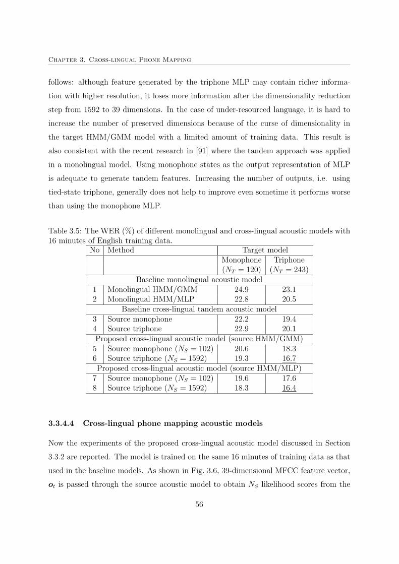
Chapter 3. Cross-lingual Phone Mapping
follows: although feature generated by the triphone MLP may contain richer informa-
tion with higher resolution, it loses more information after the dimensionality reduction
step from 1592 to 39 dimensions. In the case of under-resourced language, it is hard to
increase the number of preserved dimensions because of the curse of dimensionality in
the target HMM/GMM model with a limited amount of training data. This result is
also consistent with the recent research in [91] where the tandem approach was applied
in a monolingual model. Using monophone states as the output representation of MLP
is adequate to generate tandem features. Increasing the number of outputs, i.e. using
tied-state triphone, generally does not help to improve even sometime it performs worse
than using the monophone MLP.
Table 3.5: The WER (%) of different monolingual and cross-lingual acoustic models with16 minutes of English training data.
No Method Target modelMonophone Triphone(NT = 120) (NT = 243)
Baseline monolingual acoustic model1 Monolingual HMM/GMM 24.9 23.12 Monolingual HMM/MLP 22.8 20.5
Baseline cross-lingual tandem acoustic model3 Source monophone 22.2 19.44 Source triphone 22.9 20.1Proposed cross-lingual acoustic model (source HMM/GMM)5 Source monophone (NS = 102) 20.6 18.36 Source triphone (NS = 1592) 19.3 16.7Proposed cross-lingual acoustic model (source HMM/MLP)
7 Source monophone (NS = 102) 19.6 17.68 Source triphone (NS = 1592) 18.3 16.4
3.3.4.4 Cross-lingual phone mapping acoustic models
Now the experiments of the proposed cross-lingual acoustic model discussed in Section
3.3.2 are reported. The model is trained on the same 16 minutes of training data as that
used in the baseline models. As shown in Fig. 3.6, 39-dimensional MFCC feature vector,
ot is passed through the source acoustic model to obtain NS likelihood scores from the
56

Chapter 3. Cross-lingual Phone Mapping
source HMM/GMM model or NS posteriors from the HMM/MLP model. In this study,
both context-independent and context-dependent source acoustic models are examined:
(i) The Malay monophone acoustic model with 102 states.
(ii) The Malay triphone acoustic model with 1592 tied-states.
These NS scores are mapped to NT states of the target language. NT can be 120 states
for the English monophone model or 243 tied-states for the English triphone model.
The last four rows of Table 3.5 represent the results for the proposed cross-lingual
acoustic models which use the HMM/GMM and hybrid HMM/MLP source models. From
the table, four major observations can be seen.
First, all proposed cross-lingual phone mappings outperform the monolingual baseline
models significantly. The WERs obtained by the proposed method are also considerably
better than the cross-lingual tandem approach although both approaches use source
acoustic scores as the input feature. This shows that the phone mapping approach is
more advantageous than the tandem approach which models the source acoustic scores
by Gaussian distributions.
Second, by comparing the last four rows of Table 3.5, it is clear that using source
triphone as the input of the cross-lingual phone mapping produces better results than
using source monophone. This is due to the fact that the source triphone states provide
more detailed representation of the target speech than the source monophone states.
This result is contrary to the result on the cross-lingual tandem approach (row 3, 4).
It can be explained that MLP phone mapping can handle all inputs and does not lose
information via the dimensionality reduction step as in the tandem approach and hence
can take advantage of higher resolution feature generated by the source language context-
dependent model. This is explored further in Section 3.3.4.5.
Third, by comparing the last two columns of the table, it is observed that using target
language triphone states as the label of the phone mapping consistently outperforms using
target language monophone states. The best performance of the cross-lingual phone
mapping is WER=16.7% and 16.4% for the source HMM/GMM and source HMM/MLP,
respectively. These results are obtained by using triphone representation in both the
source and target language acoustic models.
57

Chapter 3. Cross-lingual Phone Mapping
Fourth, using the source hybrid HMM/MLP can produce a small improvement over
the source conventional HMM/GMM. However, with the best configuration (i.e. triphone-
to-triphone mapping), the performance of the two systems is almost the same.
In summary, the results in Table 3.5 show that the cross-lingual phone mapping out-
performs the monolingual acoustic models as well as the cross-lingual tandem model.
In addition, the proposed context-dependent cross-lingual phone mapping produces sig-
nificantly better results than the context-independent cross-lingual phone mapping in
[25].
3.3.4.5 Discussion on mapping structure
The previous subsection showed that for the case of limited training data, the proposed
phone mapping method using MLPs is much more effective than the tandem approach
which tries to model source acoustic scores using Gaussian distributions. It demonstrates
that choosing an appropriate model to relate the source acoustic scores to target phone
states is important. In the experiments discussed in Subsection 3.3.4.4, 3-layer MLPs
were used as the phone mapping from the source language to the target language. In
this subsection, the reason for selecting this MLP topology is presented.
As stated in the previous subsections, source acoustic scores, i.e. posteriors, likeli-
hoods can be considered as higher level features as compared to conventional features
such as MFCCs for speech recognition. This raises the question of whether we can use
a simpler mapping to perform this task. To answer this question, experiments are con-
ducted using 2-layer neural networks (NN) (i.e. with no hidden layer). In the case of
monolingual hybrid HMM/MLP, the MLP can be considered as a mapping from the
input cepstral feature, i.e. MFCCs to HMM states.
Table 3.6 shows the phone mapping results with different inputs and different NN
architectures for 16 minutes of target English training data. Three different types of
input are:
• MFCCs with 39 inputs (i.e. 1 frame of 39-dimensional MFCC vector)
• Source monophone likelihoods with 102 inputs
• Source triphone likelihoods with 1592 inputs
58

Chapter 3. Cross-lingual Phone Mapping
Table 3.6: The WER (%) of different mapping architectures with 16 minutes of targetEnglish training data (the target acoustic model is triphone). Number in (.) in thefirst and the last column indicates the number of inputs and number of hidden units,respectively. Number in (.) of the third column represents relative improvement over thecorresponding 2-layer NN in the second column.
Input Mapping architecture2-layer NN 3-layer NN 3-layer NN
(500HUs) (*)MFCC (39) 30.6 20.5 (33.0%) 24.5 (34HUs)Source monophone (102) 21.6 18.3 (15.3%) 20.3 (72HUs)Source triphone (1592) 17.6 16.7 (5.0%) 16.9 (211HUs)
243 outputs are used to model 243 tied states in the target context-dependent acoustic
model. The second column represents WER of using 2-layer NN. The third column is the
result using 3-layer NN with 500 neurons in the hidden layer presented in the previous
section. The number in (.) represents relative improvement over 2-layer NN mapping.
By comparing these two columns of Table 3.6, it is observed that in all three cases, 3-
layer NN outperforms corresponding 2-layer NN significantly, especially for the case of
MFCC input. The results show that for low level MFCC features, 3-layer MLP performs
much better than 2-layer NN due to that the system needs to be powerful enough to
accurately map MFCC to states of the target language. For high level features such as
source triphone scores, although the difference between the 2-layer and 3-layer networks
is smaller, a more flexible 3-layer network is still preferred. This result is also consistent
with the result reported in [25] where the posterior weighted product-of-expert approach
realized by a 3-layer NN outperformed the product-of-posterior model realized by a 2-
layer NN in a cross-lingual phone recognition task.
Now we investigate whether the improvement of 3-layer NNs over 2-layer NNs comes
from larger number of parameters or their 3-layer architecture. The result shown in the
last column of Table 3.6 is obtained using 3-layer NNs those have the same number of
parameters as the corresponding 2-layer NNs. Number in (.) represents number of hidden
units in the 3-layer NN. It is observed that although the performance deteriorates when
smaller hidden layers are used, 3-layer NNs perform better than 2-layer NNs even with
the same number of parameters. One advantage of using 3-layer NNs is that while it
is impossible to change number of parameters in 2-layer NNs, it is very easy to select a
59

Chapter 3. Cross-lingual Phone Mapping
suitable model complexity for different phone mapping problems by changing number of
hidden units in 3-layer NNs. Note that in all of mapping experiments in this study, 3-layer
NNs with 500 hidden units are simply chosen. It is believed that further improvement
can be obtained if this parameter is chosen carefully for each experiment. From the
finding in this subsection, in all next experiments, 3-layer MLP will be used to realize
phone mapping.
3.3.4.6 Effect of training data size
In all previous experiments, we assumed that only 16 minutes of target English training
data are available. In this section, we examine the effect of different training data sizes
on the performance of the cross-lingual phone mapping acoustic model. Three training
data sizes are used in our study, i.e. 7 minutes, 16 minutes, and 55 minutes of English
target data which are randomly selected from 15 hours training data of the WSJ0 corpus.
The experiments in Section 3.3.4.4 showed that using context-dependent triphone at
both the source and target language acoustic models can improve the phone mapping
performance significantly. Therefore, in this section, both the source and target language
acoustic model are context-dependent triphone. The source language acoustic model
consists of 1592 tied-states. For the target language acoustic model, with each training
data size, the training steps are followed the procedure in Section 3.3.2 to build the phone
mapping. The number of tied states in the target acoustic model is optimized to achieve
the best performance for the monolingual HMM/GMM model. This number varies for
different amounts of available target training data. Specifically, 243, 243 and 501 triphone
tied states are used for the cases of 7, 16, 55 minutes of training data, respectively.
As opposed to the phone mapping model, in the cross-lingual tandem model, the
source language MLP is monophone while the target language acoustic model is triphone.
The reason has been shown in Section 3.3.4.3 that using source language triphone MLP
results in a poor performance due to information lost during the dimensionality reduction
step.
Fig. 3.10 shows the performance of five different acoustic models in WER with three
different amounts of training data. The first three columns represent the performance of
the three baseline models which include monolingual models: HMM/GMM, HMM/MLP
60
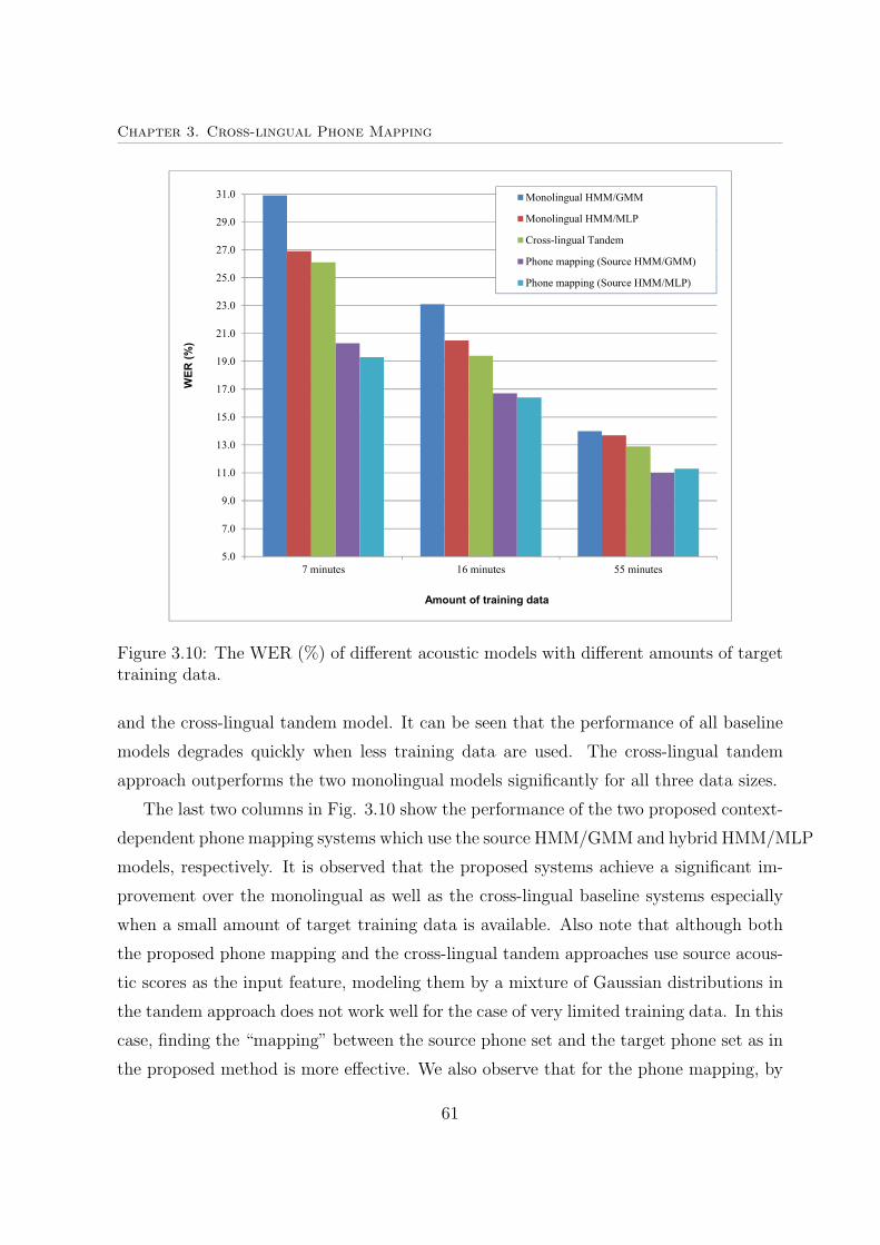
Chapter 3. Cross-lingual Phone Mapping
5.0
7.0
9.0
11.0
13.0
15.0
17.0
19.0
21.0
23.0
25.0
27.0
29.0
31.0
7 minutes 16 minutes 55 minutes
Monolingual HMM/GMM
Monolingual HMM/MLP
Cross-lingual Tandem
Phone mapping (Source HMM/GMM)
Phone mapping (Source HMM/MLP)
Amount of training data
WE
R (
%)
Figure 3.10: The WER (%) of different acoustic models with different amounts of targettraining data.
and the cross-lingual tandem model. It can be seen that the performance of all baseline
models degrades quickly when less training data are used. The cross-lingual tandem
approach outperforms the two monolingual models significantly for all three data sizes.
The last two columns in Fig. 3.10 show the performance of the two proposed context-
dependent phone mapping systems which use the source HMM/GMM and hybrid HMM/MLP
models, respectively. It is observed that the proposed systems achieve a significant im-
provement over the monolingual as well as the cross-lingual baseline systems especially
when a small amount of target training data is available. Also note that although both
the proposed phone mapping and the cross-lingual tandem approaches use source acous-
tic scores as the input feature, modeling them by a mixture of Gaussian distributions in
the tandem approach does not work well for the case of very limited training data. In this
case, finding the “mapping” between the source phone set and the target phone set as in
the proposed method is more effective. We also observe that for the phone mapping, by
61
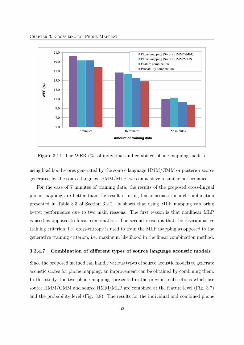
Chapter 3. Cross-lingual Phone Mapping
5.0
7.0
9.0
11.0
13.0
15.0
17.0
19.0
21.0
7 minutes 16 minutes 55 minutes
Phone mapping (Source HMM/GMM)
Phone mapping (Source HMM/MLP)
Feature combination
Probability combination
Amount of training data
WE
R(%
)
Figure 3.11: The WER (%) of individual and combined phone mapping models.
using likelihood scores generated by the source language HMM/GMM or posterior scores
generated by the source language HMM/MLP, we can achieve a similar performance.
For the case of 7 minutes of training data, the results of the proposed cross-lingual
phone mapping are better than the result of using linear acoustic model combination
presented in Table 3.3 of Section 3.2.2. It shows that using MLP mapping can bring
better performance due to two main reasons. The first reason is that nonlinear MLP
is used as opposed to linear combination. The second reason is that the discriminative
training criterion, i.e. cross-entropy is used to train the MLP mapping as opposed to the
generative training criterion, i.e. maximum likelihood in the linear combination method.
3.3.4.7 Combination of different types of source language acoustic models
Since the proposed method can handle various types of source acoustic models to generate
acoustic scores for phone mapping, an improvement can be obtained by combining them.
In this study, the two phone mappings presented in the previous subsections which use
source HMM/GMM and source HMM/MLP are combined at the feature level (Fig. 3.7)
and the probability level (Fig. 3.8). The results for the individual and combined phone
62

Chapter 3. Cross-lingual Phone Mapping
mapping models are shown in the Fig. 3.11. It is clearly shown that the combined
systems outperform both the individual phone mappings consistently. Although the two
source acoustic models are trained with the same data from the same language, the
different model structures and different training criteria make information generated by
the two acoustic models complementary. While the source language HMM/GMM is
trained on a maximum likelihood criterion, the source language HMM/MLP models use
a discriminative criterion to optimize the model parameters.
There is also a difference between the two combination methods. Combination at
the probability level gives a better performance over combination at the feature level
especially when a very small amount of training data is available. It can be explained
that although the feature combination approach seems to be a better choice for multi-
stream input for the MLP mapping, it may suffer from overfitting when a very small
amount of training data is available. Especially, when source triphone models are used,
the number of inputs for the mapping is large if we concatenate multi-streams at input
level. In this case, the probability combination method can be a better option.
3.3.4.8 Using multiple source languages
In all previous experiments, only Malay is used as the source language. This subsec-
tion investigates the performance of the proposed phone mapping method with different
source languages. A well-trained monophone hybrid MLP Hungarian phone recognizer
from Brno University of Technology (BUT)3 [92] is used. Given English speech data,
the Hungarian recognizer produces 186 monophone state posterior probabilities for each
speech frame. These probabilities are mapped to English tied-states as in the Malay-to-
English case. Note that BUT Hungarian recognizer uses 8-kHz sampling waveform as the
input while our target English corpus (i.e. WSJ0) is 16-kHz. We need to down-sample
the target corpus to 8-kHz before applying the Hungarian recognizer.
Fig. 3.12 shows the results of the two phone mapping models with the two source
languages. The first column is WER of the phone mapping with the source language
Malay reported in the previous sections. In this case source acoustic scores are generated
by the Malay triphone HMM/GMMmodel. The result for Hungarian-to-English mapping
3http://speech.fit.vutbr.cz/software/phoneme-recognizer-based-long-temporal-context
63

Chapter 3. Cross-lingual Phone Mapping
5.0
7.0
9.0
11.0
13.0
15.0
17.0
19.0
21.0
7 minutes 16 minutes 55 minutes
Malay-to-English
Hungarian-to-English
Feature combination
Probability combination
WE
R(%
)
Amount of training data
Figure 3.12: The WER (%) of the phone mapping model for two source languages withthree different amounts of target training data.
is shown in the second column. It can be seen that when a very small amount of target
training data is available (i.e. 7 and 16 minutes) using the Hungarian source acoustic
model provides better performance than using the Malay model. One possible reason is
that Hungarian language and English language are more similar than the Malay-English
pair. As a result, the Hungarian-to-English phone mapping can be implemented easier
and hence provides better performance even with an extremely small amount of target
training data. However, when more training data are available, using the source Malay
model achieves better performance. This can be explained as the BUT Hungarian MLP is
a monophone recognizer while the Malay HMM/GMM model is a triphone model which
provides higher resolution feature input for phone mapping. This will be useful when we
have more target data to train the mapping.
The last two columns of Fig. 3.12 show the results when Malay-to-English and
Hungarian-to-English mappings are combined at the feature and probability levels. In-
terestingly, the combined models provide a big improvement over both the individual
mappings. It demonstrates that the two acoustic models of the two source languages
provide complementary information. In other words, combination of different source lan-
64

Chapter 3. Cross-lingual Phone Mapping
guages can give a better acoustic coverage for phone mapping. It is also noted that with
55 minutes of English training data, the best combined phone mapping can give 9.0%
WER which is close to 7.9% WER of the monolingual HMM/GMM model trained with
the whole 15 hours of English training data.
There is a also a slight difference between the two combination approaches. While
probability combination outperforms feature combination for the case of 7 minutes of
training data, with bigger amounts of training data, i.e. 16 and 55 minutes, feature
combination is a better choice. Note that the dimension of posterior vectors generated
by the Hungarian phone recognizer is only 186, which is much lower than the number of
tied states in the Malay triphone model (1592 tied states). Hence, it is less likely to have
overtraining problem when 16 minutes or more English training data are available. This
may explain why in this case, feature combination is better than probability combination
in Fig. 3.12 and vice versa in Fig. 3.11 (the last two columns).
3.4 Conclusion
This chapter presented two novel phone mapping techniques for large vocabulary auto-
matic speech recognition of under-resourced languages by leveraging well-trained acoustic
models of other languages. In the first part of the chapter, a cross-lingual linear acous-
tic model combination method was presented. Specifically, phone model of the target
language is assumed to be a weighted sum of all phone models in the source language
acoustic model. In the second part, a nonlinear phone mapping architecture was pre-
sented. In this mapping, the source acoustic model is used to generate likelihood or
posterior scores, these scores are then mapped to target phone posteriors using a nonlin-
ear mapping, e.g. MLP. Experimental results verified the effectiveness of the proposed
phone mapping technique for building LVCSR models under limited training data condi-
tions. There are two advantages in the proposed methods, i.e. the use of triphone states
for improved acoustic resolution of both the source and target models and the ability to
apply various types of source acoustic models which results in an additional improvement
when combining them even they are trained from the same data. The experimental re-
sults indicated that using nonlinear phone mapping with discriminative training criterion
65

Chapter 3. Cross-lingual Phone Mapping
(cross-entropy) achieves better performance than using linear combination with genera-
tive training criterion (maximum likelihood). In addition, the combination of different
source languages can significantly improve the performance of phone mapping as we may
have a better acoustic coverage for the target language.
This chapter showed that using 3-layer neural networks as the mapping can achieve
better results over simpler 2-layer mapping networks. In the next chapter, the proposed
phone mapping will be investigated using deeper structures for the source and target
language acoustic models.
66

Chapter 4
Deep Neural Networks forCross-lingual Phone MappingFramework
In the previous chapter, the focus was to increase the mapping resolution by using context
information. In this chapter, the focus is shifted to improve the quality of cross-lingual
features used for mapping by using deeper structures such as Deep Neural Networks
(DNNs). DNNs proposed by Hinton et al. in 2006 [42] is a new powerful machine
learning technique with multiple nonlinear layers. They have been used effectively for
handwriting recognition [42], 3-D object recognition [93], dimensionality reduction [94]
and recently in speech recognition from small [37, 39] to very large tasks [40, 41].
In this chapter, two approaches are investigated to improve the cross-lingual phone
mapping using DNNs. In the first approach, DNNs are used as the source language
acoustic model. This is motivated by the fact that if DNNs can model the source language
better than shallow models, the source language posterior features generated from DNNs
will also be better and should result in better performance of phone mapping. In the
second approach, DNNs are used to replace 3-layer MLPs to realize the phone mapping
function. The results presented in this chapter have been published in APSIPA ASC
2011 [29] and INTERSPEECH 2013 [30].
The chapter is organized as follows. Section 4.1 introduces DNNs and their application
for monolingual speech recognition. Section 4.2 applies DNNs to improve cross-lingual
phone mapping. Section 4.3 concludes the chapter.
67

Chapter 4. Deep Neural Networks for Cross-lingual Phone Mapping Framework
4.1 Deep Neural Network Introduction
In this section, the concept of deep learning and DNNs is introduced in details. Subsection
4.1.1 provides an introduction to deep architectures and their advantages over shallow
architectures. Subsection 4.1.2 introduces a basic block of DNNs called Restricted Boltz-
mann Machines (RBMs). Subsection 4.1.3 presents the applications of DNNs for speech
recognition. Subsection 4.1.4 shows experimental results of using DNNs for monolingual
speech recognition.
4.1.1 Deep architectures
Deep learning is a relatively new area of machine learning first proposed by Hinton et
al. in 2006 [42]. It has been effectively used for handwriting recognition [42], 3-D object
recognition [93], dimensionality reduction [94] as well as speech recognition tasks [37–41].
The concept of deep structures is defined from neural networks. A multilayer percep-
tron neural network (MLP) with many hidden layers is an example of deep architecture
models. The complexity theory of circuits [95] strongly suggests that deep architectures
are much more efficient in terms of required computational elements than shallow ar-
chitectures such as hidden Markov models, neural networks with only one hidden layer,
conditional random fields, kernel regression, support vector machines, and many others.
Deep architecture models have many levels of non-linearities which allow them to
compactly represent highly nonlinear functions. Unfortunately, such deep networks are
hard to train. In general, since models with deep architectures consist of several nonlin-
ear layers, the associated loss functions are almost always non-convex. If the weights of
the networks are initialized randomly, then the local gradient-based optimization algo-
rithms such as backpropagation will often be trapped in poor local optima. To overcome
this, Hinton et al. [42] introduced a moderately fast, unsupervised learning procedure for
deep generative models called Deep Neural Networks (DNNs). The greedy layer-by-layer
training is the key feature of this algorithm in order to efficiently learn a deep, hierar-
chical probabilistic model. This learning algorithm can optimize the network weights at
time complexity linear to the size and depth of the network. There are several distinct
characteristics of the algorithm [96]:
68

Chapter 4. Deep Neural Networks for Cross-lingual Phone Mapping Framework
• The greedy layer-by-layer learning algorithm has been shown to be able to find a
good set of model parameters even for very large models containing many nonlinear
layers with millions of parameters.
• The algorithm can efficiently use unlabeled data for the unsupervised pre-training
process. Labeled data are only used at the final step to train the network weights
for classification.
The next section will introduce a basic block of DNNs called Restricted Boltzmann
Machines (RBMs).
4.1.2 Restricted Boltzmann machines
A DNN is made by stacking several bipartite undirected graphical models called restricted
Boltzmann machines (RBMs). A RBM is a realization of Markov random fields with a
two-layer architecture as illustrated in Fig. 4.1(a). There are two types of units in the
architecture, they are: visible (typically Bernoulli or Gaussian) stochastic units v are
connected to hidden (typically Bernoulli) stochastic units h. Normally, all the visible
h
v
(a) RBM (b) DNN
Figure 4.1: A DNN (b) is composed by a stack of RBMs (a).
units are connected to all the hidden units and there is no visible to visible or hidden to
hidden unit connection. The weights of the connections and the biases of the individual
units form a joint probability distribution p(v,h|θ) over v and h given model parameters
θ. This distribution is defined in terms of an energy function E(v,h|θ) [96] as
p(v,h|θ) = exp(−E(v,h|θ))Z(θ)
(4.1)
69

Chapter 4. Deep Neural Networks for Cross-lingual Phone Mapping Framework
where Z(θ) is known as the normalizing constant
Z(θ) =∑v
∑h
exp(−E(v,h|θ)). (4.2)
The marginal probability that the model assigns to a visible vector v is
p(v|θ) =
∑h
exp(−E(v,h|θ))
Z(θ). (4.3)
With different types of visible and hidden units, different energy functions are defined.
In the case when both the visible and the hidden units are Bernoulli stochastic units, the
energy function is defined [96] as
E(v,h|θ) = −V∑i=1
H∑j=1
wijvihj −V∑i=1
bivi −H∑j=1
ajhj (4.4)
where model parameters θ = {w, b,a}, wij is the weight between visible unit i and
hidden unit j; bi and aj are biases for visible unit i and hidden unit j, respectively; V ,
H are the number of visible units and hidden units, respectively.
Since there is no visible-visible connection, all of the visible units become independent
given the hidden units, and vice versa. The conditional distributions, when both the
visible and hidden units are Bernoulli stochastic units, can be effectively derived [96] as
p(hj = 1|v, θ) = σ
(V∑i=1
wijvi + aj
)(4.5)
p(vi = 1|h, θ) = σ
(H∑j=1
wijhj + bi
)(4.6)
where σ(x) = 1/(1 + exp(−x)) is the sigmoidal function.
For the case when the visible and hidden units are Gaussian and Bernoulli stochastic
units respectively, the energy function is defined as
E(v,h|θ) = −V∑i=1
H∑j=1
wijvihj +1
2
V∑i=1
(vi − bi)2 −
H∑j=1
ajhj (4.7)
and the conditional probabilities of hidden unit hj and visible unit vi are
70
Chapter 4. Deep Neural Networks for Cross-lingual Phone Mapping Framework
p(hj = 1|v, θ) = σ
(V∑i=1
wijvi + aj
)(4.8)
p(vi|h, θ) = N
(H∑j=1
wijhj + bi, 1
)(4.9)
where vi is a real number which follows a Gaussian distribution N (.) with the meanH∑j=1
wijhj + bi and unit variance.
The Gaussian-Bernoulli RBMs are normally used to convert real-valued stochastic
visible units to binary stochastic variables and so that they can be further processed by
other Bernoulli-Bernoulli RBMs.
Eq. (4.5), (4.8) allow the use of RBM weights to initialize an MLP with sigmoidal
hidden units because we can equate the inference for RBM hidden units with forward
propagation in a neural network.
The goal of learning in a RBM is to change the model parameters θ to maximize the
probability of the data p(v|θ). The training process can be done effectively by a procedure
called “Contrastive Divergence” [97]. After training the RBMs, they are stacked to build
the DNN. In the next section, the application of DNNs for speech recognition will be
presented.
4.1.3 Deep neural networks for speech recognition
The recent success of DNNs for various problems has interested speech researchers to
apply them for ASR tasks. Mohamed and Hinton [38] used interpolating conditional
RBMs (ICRBMs) for phone recognition on the TIMIT corpus. A good accuracy was
achieved using a simple one layer RBMs. In another work [37], a four-layer DNN was used
to estimate the 183 state posteriors of 61 monophone for 3-state-HMM models. Although
monophone models were used, the hybrid HMM/DNN system provided a competitive
phone error rate on the TIMIT corpus. However, when more layers were added to the
DNN, no significant improvement was observed. In [41], DNNs were combined with
conditional random fields (CRFs) instead of HMMs to model the sequential information.
In this research, the DNN weights as well as the state-to-state transition parameters
71

Chapter 4. Deep Neural Networks for Cross-lingual Phone Mapping Framework
and language model scores were optimized by using a sequential discriminative training
criterion. A higher accuracy was achieved over the HMM/DNN model with the frame
discriminative training criterion on the TIMIT corpus.
In the Gaussian-Bernoulli RBM architecture, the inputs are conditionally independent
given the hidden unit activations. This assumption is inappropriate for speech data when
many frames are concatenated to form an input vector. To relax this assumption, in
[98], mean-covariance RBMs (mcRBMs) were proposed and Dahl et al. [39] applied the
mcRBM for ASR tasks and achieved a very low phone error rate of 20.5% on the TIMIT
corpus.
The success of HMM/DNN on phone recognition tasks motivated speech researchers
to apply deep structures to LVCSR with much larger vocabularies and more varied speak-
ing styles. The first successful use of HMM/DNN acoustic models for a large vocabulary
task used data collected from the Bing mobile voice search application. The results
reported in [99] showed that using HMM/DNN acoustic model with context-dependent
states achieves 69.6% sentence accuracy on the test set, compared with 63.8% for a strong,
minimum phone error (MPE)-trained HMM/GMM baseline. The HMM/DNN training
recipe developed for the Bing voice search data was applied to the Switchboard speech
recognition task [40]. A DNN with 7 hidden layers and 2,048 units in each layer and
full connectivity between adjacent layers are used to replace the GMM in the acoustic
model. Experimental results showed that using DNNs reduced the word error rate to
18.5% which is significantly better than 27.4% of the baseline HMM/GMM.
Now, we discuss in details about how to build a DNN for speech recognition. Basically,
as shown in Fig. 4.2, four main steps are required to train a DNN.
Step 1: The pre-training procedure is conducted for the first RBM [97], and then the
activation probabilities of the first RBM’s hidden units are used as the visible data
for the second RBM. This process is then repeated to train upper RBMs.
Step 2: After nth RBMs are trained, the final layer is added to represent the desired
outputs such as HMM-states.
Step 3: The class training labels are provided for each frame in the training set. These
labels can be obtained from other acoustic models such as HMM/GMM.
72

Chapter 4. Deep Neural Networks for Cross-lingual Phone Mapping Framework
1st RBM (Visible layer: Gaussian)
2nd RBM (Visible layer: Bernoulli)
1st RBM (Hidden layer: Bernoulli)
3rd RBM (Visible layer: Bernoulli)
2nd RBM (Hidden layer: Bernoulli)
1st RBM
2nd RBM
nth RBM (Hidden layer: Bernoulli)
.
.
.
Output
nth RBM
nth RBM (Visible layer: Bernoulli)
(n-1)th RBM (Hidden layer: Bernoulli)
Speech feature
State posteriors
Layer-by-layer pre-training
(unsupervised)
Training labels provided
Backpropagation
(supervised)
Output layer
added
1
2
3
4
DNN:
Output layer
DNN:
nth hidden layer
DNN:
(n-1)th hidden layer
DNN:
2nd hidden layer
DNN:
1st hidden layer
DNN:
Input layer
Figure 4.2: Four steps in training a DNN for speech recognition.
Step 4: A discriminative learning procedure such as back-propagation is used to fine-
tune all the network weights jointly using the labeled training data.
In the decoding process, the DNN is treated as a conventional neural network with
the same architecture. The next section will present the application of the above DNNs
for two monolingual speech recognition tasks.
4.1.4 Experiments of using DNNs for monolingual speech recog-nition
In this section, the performance of the hybrid HMM/DNNmodel is investigated for mono-
lingual tasks. Its performance is compared with shallow models such as HMM/GMM and
HMM/MLP models. This section also investigates the advantages of RBM pre-training
73

Chapter 4. Deep Neural Networks for Cross-lingual Phone Mapping Framework
for DNN weight initialization over the random weight initialization scheme. Two speech
recognition experiments are conducted. The first experiment is phone recognition on the
TIMIT database1. The second experiment evaluates the HMM/DNN acoustic model in
an LVCSR task under limited training data conditions on the WSJ0 corpus.
4.1.4.1 HMM/DNN acoustic model for phone recognition
a. Experimental setup
The phone recognition performance of different acoustic models is evaluated on the
TIMIT speech database. The training set consists of 3696 utterances from 462 speakers
which is around 3 hours. A small subset of speakers is extracted from the training set
(50 speakers) and used as the development set. The complete test data set contains 1344
utterances from 168 speakers. No language model is used. Our APSIPA 2011 paper [29]
gives the explicit experimental setup details.
b. Shallow baseline acoustic models
Before examining the HMM/DNN model, we first present the recognition results given
by two conventional shallow models: HMM/GMM and HMM/MLP.
Fig. 4.3 illustrates the phone error rate (PER) on the training and test sets provided
by the HMM/GMM model with different model complexities. It is observed that the
PER in both the training and test sets reduces consistently when the model complexity
increases from 1 to 128 Gaussian mixtures per state. Over-fitting occurs when higher
complexity models are used, i.e. while the PER in the training set drops rapidly, the
PER in the test set rises. This shows that with the HMM/GMM model adding more
parameters does not always bring more benefit when there is insufficient amount of
training data. The best PER in the test set obtained by the conventional HMM/GMM
system is 33.6% when the number of Gaussian mixtures per state is 128.
Another shallow acoustic model is the hybrid HMM/MLP [64]. In this case, the MLP
replaces the GMM of the HMM/GMM model to produce the state likelihood score. A
3-layer MLP with 1024 hidden units is selected. To train the MLP, each frame in the
training data is assigned a state label. This label is generated using forced alignment
1http://www.ldc.upenn.edu/Catalog/CatalogEntry.jsp?catalogId=LDC93S1
74

Chapter 4. Deep Neural Networks for Cross-lingual Phone Mapping Framework
Figure 4.3: Phone error rate (PER) on the training and test sets of the HMM/GMMmodel with different model complexities.
with the above HMM/GMM model. The hybrid HMM/MLP achieves 27.3% PER which
is much better than 33.6% from the HMM/GMM model.
c. Deep acoustic models
The previous part examined the two shallow acoustic models i.e. HMM/GMM and
HMM/MLP. In this part, we investigate deep acoustic models to answer two questions:
(i) can improvement be achieved using deeper structure of DNN? (ii) for DNN models,
would RBM pre-training initialization help to improve performance over random weight
initialization?. To answer these questions, experiments will be conducted to evaluate
DNNs with the number of layers from 3 to 8 and with both the RBM pre-training
initialization and the random weight initialization schemes. In this experiment, the
number of hidden units in each hidden layer is 1024.
Fig. 4.4 presents the PER of the HMM/DNN models. The x-axis shows the num-
ber of layers i.e. how deep is the network, and the y-axis shows the phone error rate.
Performances of the HMM/DNN models using the two initialization schemes are shown
as the green and blue lines. Note that when 3-layer architecture with random weight
initialization is used, DNN becomes conventional MLP in the previous experiment. In
75

Chapter 4. Deep Neural Networks for Cross-lingual Phone Mapping Framework
24
24.5
25
25.5
26
26.5
27
27.5
28
28.5
1 2 3 4 5 6
M LP
DBN
Sum rule
Productrule
Number of layers
Ph
on
ee
rro
rra
te(%
)
Random weight initialization
RBM-pretraining initialization
Combined model (sum rule)
Combined model (prod rule)
3 4 5 6 7 8
3-layer MLP
Figure 4.4: Performance of the HMM/DNN acoustic model for the two initializationschemes and the combined models with different numbers of layers.
this case, the results show that even shallow network can benefit from using RBM pre-
training. Adding the second hidden layer gives better performance for DNN with the two
initialization schemes. However, with deeper architectures, the DNN with random ini-
tialization does not achieve further improvement, and its performance even deteriorates
when number of layers is larger than 6. This shows empirically that the back propaga-
tion algorithm cannot handle well for deep structures with random weight initialization.
Whereas the performance of the DNN with RBM pre-training initialization shows that
using more hidden layers can improve performance of the model.
Now, we investigate the combination of the DNN models with the two initialization
schemes above. Combination of information from different ASR systems generally im-
proves speech recognition accuracy [5, 86–88]. The work in Chapter 3 (Section 3.3.4.7)
showed that combination of different phone mapping systems can give a consistent im-
provement over the individual systems. The reason for this advantage is that different
systems often provide different errors. In this experiment, the combination of the above
two DNN models is examined i.e. combination of the DNN with RBM pre-training ini-
tialization and the DNN with random weight initialization. The PER of the combined
76

Chapter 4. Deep Neural Networks for Cross-lingual Phone Mapping Framework
models is shown in Fig. 4.4 (red and purple lines) when the two DNN models are com-
bined at the probability level using either the product or sum rules [29] (more details can
be found in our APSIPA ASC 2011 paper [29]). Interestingly, significant improvements
are achieved over both the two individual systems. Although the two models have an
identical structure and training data, the different weight initialization schemes make
information generated by the two DNNs is complementary.
4.1.4.2 HMM/DNN acoustic model for LVCSR under limited training dataconditions
The previous subsection showed that using the HMM/DNN acoustic model achieves
a significant improvement over shallow models on a phone recognition task. In this
subsection, we investigate the HMM/DNN model under limited training data conditions
for an LVCSR task.
a. Experimental setup
Training data are randomly extracted from the WSJ0 corpus to generate four subsets
with 7, 15, 55 and 220 minutes of training data. The number of tied states is optimized
to achieve the best performance for the HMM/GMM model. This number varies for
different amounts of available target training data. Specifically, 243, 243, 501 and 1005
triphone tied-states are used for the cases of 7, 16, 55 and 220 minutes of training data,
respectively.
Since the amount of training data is small, small-scaled neural networks with 500
units for each hidden layer are used. Four acoustic models are examined:
• HMM/GMM baseline model.
• HMM/MLP model with random weight initialization: MLP with 3-layer architec-
ture.
• HMM/DNN model with random weight initialization: DNN with 5-layer architec-
ture.
• HMM/DNN model with RBM pre-training initialization: DNN with 5-layer archi-
tecture.
77

Chapter 4. Deep Neural Networks for Cross-lingual Phone Mapping Framework
5.0
7.0
9.0
11.0
13.0
15.0
17.0
19.0
21.0
23.0
25.0
27.0
29.0
31.0
7 minutes 16 minutes 55 minutes 220 minutes
HMM/GMM model
HMM/MLP model with random weight initialization
HMM/DNN model with random weight initialization
HMM/DNN model with RBM-pretraining initialization
Amount of training data
WE
R (
%)
Figure 4.5: Comparison of HMM/MLP and HMM/DNN on an LVCSR task for differenttraining data sizes.
b. Experimental results
Fig. 4.5 shows the performance of above four models under four limited training data
sizes. It is observed that the performance of all four models drops quickly when limited
training data are used and three hybrid models outperform significantly the HMM/GMM
baseline model. We also see that using HMM/DNN (third column) achieves a signifi-
cant improvement over the two shallow models i.e. HMM/GMM (first column) and
HMM/MLP (second column) even under very limited training data conditions. Now, we
investigate the effect of the RBM pre-training initialization over random initialization
for DNN. As shown in the fourth column, using the RBM pre-training scheme achieves
a consistent improvement over random weight initialization except the case of 7 minutes
of training data.
4.1.5 Conclusion
This section introduced the deep architectures and their advantages over the shallow
architectures for speech recognition. The advantages of DNNs were then verified by ex-
78

Chapter 4. Deep Neural Networks for Cross-lingual Phone Mapping Framework
periments conducted on a monolingual phone recognition task and a monolingual LVCSR
task under limited training data conditions. The next section will present the work of
applying DNNs to improve the proposed cross-lingual phone mapping method.
4.2 Deep Neural Networks for Cross-lingual Phone
Mapping
In the proposed work of cross-lingual phone mapping presented in Chapter 3, both the
source acoustic model and phone mapping function were implemented using shallow
models, i.e. HMM/GMM, HMM/MLP were used as the source models and MLPs were
used for the phone mapping function. Section 4.1.4 has shown the advantages of deep
models over shallow models for monolingual speech recognition tasks. The aim of this
section is to investigate the use of DNNs for cross-lingual phone mapping.
In this section, two approaches to use DNNs for the cross-lingual phone mapping
are examined. The first approach is to use DNNs as the acoustic model of the source
language. It is hypothesized that if DNNs can model the source language better than
shallow models such as MLPs or GMMs, source language posterior feature generated from
DNNs will also be better and will result in better performance for the phone mapping
task. For comparison, source language bottleneck DNN [61] is also used to generate
cross-lingual bottleneck feature for the target acoustic models. In the second approach,
DNNs are used to replace the MLPs to realize the phone mapping function. Again, this
is motivated by the fact that DNNs may have better mapping capability than shallow
models such as MLPs. These two approaches result in three experimental setups:
• Setup A: using DNNs as the source language acoustic model to generate cross-
lingual posterior feature for phone mapping.
• Setup B: using DNNs to extract cross-lingual bottleneck feature for target lan-
guage acoustic models (used as a baseline to compare to Setup A).
• Setup C: using DNNs to implement the phone mapping function.
These three setups will be presented in the next subsection.
79

Chapter 4. Deep Neural Networks for Cross-lingual Phone Mapping Framework
4.2.1 Three setups using DNNs for cross-lingual phone map-ping
4.2.1.1 Setup A: using DNNs as the source language acoustic model to gen-erate cross-lingual posterior feature for phone mapping
Section 4.1.4 showed that using DNNs for acoustic models achieves a significant improve-
ment over shallow models for both monolingual phone recognition and word recognition.
It is interesting to investigate whether the benefit of DNN-based source language acous-
tic models will also propagate to the target language after cross-lingual phone mapping.
The using of DNN-based source acoustic models in phone mapping is straightforward
and shown in Fig. 4.6. The shaded steps represent the source DNN acoustic model
(called POS-DNN where POS stands for posterior feature) to generate posterior feature.
The output layer presents monophone or triphone states of the source language acoustic
model. The output from source DNN model is fed into the phone mapping neural network
to map to target language state posteriors. If we view the phone mapping module as a
conventional hybrid system, the DNN source acoustic model acts as a feature extractor
that is well-trained from a large amount of data in the source language. In this approach,
the cross-lingual phone mapping is able to benefit from recent progress in DNN-based
acoustic modeling techniques [100]. It is expected that a sharper DNN source language
acoustic model is able to describe the target language speech data better, hence making
the cross-lingual phone mapping be an easier task.
4.2.1.2 Setup B: using DNNs to extract cross-lingual bottleneck feature fortarget language acoustic models
This setup is conducted as a baseline to compare to our phone mapping approach in
Setup A where DNNs are used as the source language acoustic model. Using DNNs to
extract bottleneck feature is also a popular way to utilize the capability of DNNs to
improve speech recognition performance. There are also several studies that investigate
the portability of bottleneck feature trained from one language to use as the feature for
acoustic models of another language [16, 17]. This approach is illustrated in Fig. 4.7. In
the bottleneck network (called BN-DNN where BN stands for bottleneck feature), there
is a bottleneck layer that is usually 30 to 40 nodes. The purpose of using such bottleneck
80

Chapter 4. Deep Neural Networks for Cross-lingual Phone Mapping Framework
DNN-based source language
acoustic model
(POS-DNN)
MLP-based Cross-lingual
phone mapping
Input layer
Multiple hidden
layers
Source language
output layer
(generate source
posterior feature)
Single hidden
layers
Target language
output layer
Figure 4.6: Illustration of using DNN as the source language acoustic model to generatecross-lingual posterior feature for phone mapping (Setup A).
Target language
acoustic model
- HMM/GMM
- HMM/DNN
DNN-based source language
bottleneck features extractor
(BN-DNN)
Input layer
Hidden layers
Source language
output layer
Bottleneck
layer
Figure 4.7: Illustration of using DNN to extract cross-lingual bottleneck feature fortarget language acoustic models (Setup B).
81
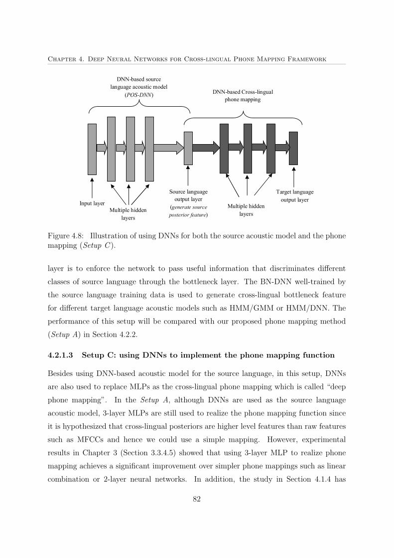
Chapter 4. Deep Neural Networks for Cross-lingual Phone Mapping Framework
DNN-based source
language acoustic model
(POS-DNN) DNN-based Cross-lingual
phone mapping
Input layer
Source language
output layer
(generate source
posterior feature)
Multiple hidden
layers
Target language
output layer
Multiple hidden
layers
Figure 4.8: Illustration of using DNNs for both the source acoustic model and the phonemapping (Setup C ).
layer is to enforce the network to pass useful information that discriminates different
classes of source language through the bottleneck layer. The BN-DNN well-trained by
the source language training data is used to generate cross-lingual bottleneck feature
for different target language acoustic models such as HMM/GMM or HMM/DNN. The
performance of this setup will be compared with our proposed phone mapping method
(Setup A) in Section 4.2.2.
4.2.1.3 Setup C: using DNNs to implement the phone mapping function
Besides using DNN-based acoustic model for the source language, in this setup, DNNs
are also used to replace MLPs as the cross-lingual phone mapping which is called “deep
phone mapping”. In the Setup A, although DNNs are used as the source language
acoustic model, 3-layer MLPs are still used to realize the phone mapping function since
it is hypothesized that cross-lingual posteriors are higher level features than raw features
such as MFCCs and hence we could use a simple mapping. However, experimental
results in Chapter 3 (Section 3.3.4.5) showed that using 3-layer MLP to realize phone
mapping achieves a significant improvement over simpler phone mappings such as linear
combination or 2-layer neural networks. In addition, the study in Section 4.1.4 has
82

Chapter 4. Deep Neural Networks for Cross-lingual Phone Mapping Framework
shown that using deep structures can help to consistently improve performance of the
DNN acoustic model for monolingual tasks even under limited training data conditions.
In this setup, we will answer an important question, how much target language training
data are required for effective training of a deep phone mapping. The combination of
the DNN-based source acoustic model in Setup A and the DNN-based phone mapping is
shown in Fig. 4.8. From the figure, it is shown that there are two DNNs, the output of
the source language DNN acoustic model is directly fed into the input of the DNN phone
mapping.
4.2.2 Experiments
In this section, experiments for the above three setups are conducted. The section is or-
ganized as follows. Subsection 4.2.2.1 introduces databases, neural network architectures
and other experimental setup. Subsection 4.2.2.2 presents the experimental results using
deep source acoustic model in phone mapping (Setup A). Subsection 4.2.2.3 conducts
cross-lingual acoustic models using bottleneck feature generated by the source language
bottleneck network (Setup B) for comparison purpose. Subsection 4.2.2.4 presents the ex-
perimental results when deep structures are applied for both the source language acoustic
model and the phone mapping (Setup C ).
4.2.2.1 Experimental setup
Task and Databases:
All experiments in this chapter use the same databases as in Chapter 3. Specifically,
Malay is used as the source language and English is the target language. The experiments
are to measure the word error rate (WER) on the target language using three setups. In
addition to three limited training data sizes i.e. 7, 15, 55 minutes of the target language
as in Chapter 3, we also generate a 220 minute data set to examine whether we can
benefit from cross-lingual phone mapping when even more training data are available.
Neural networks:
Two 5-layer DNNs i.e. POS-DNN in Setup A and BN-DNN in Setup B are used as
the source language acoustic models to generate cross-lingual posterior and bottleneck
features, respectively. The input of each DNN is formed by concatenating 9 frames of
83

Chapter 4. Deep Neural Networks for Cross-lingual Phone Mapping Framework
39-dimensional MFCCs. Each hidden layer of both the DNNs consists of 2000 hidden
units except the middle hidden layer of the BN-DNN i.e. the bottleneck layer has 39
units. Chapter 3 has shown that using context-dependent triphone in the source lan-
guage acoustic models results in better phone mapping performance. Hence, the source
POS-DNN in this case is also a context-dependent DNN i.e. it consists of 1592 out-
puts to represent 1592 tied-states in the source acoustic model. While using source
language context-dependent POS-DNN for phone mapping (Setup A,C ) achieve a bet-
ter performance, our experiments indicated that using context-dependent BN-DNN does
not achieve any improvement over context-independent BN-DNN for cross-lingual speech
recognition (Setup B). Hence, for the source language BN-DNN, 102 outputs are used to
represent 102 monophone states in the Malay source acoustic model.
Both the POS-DNN and BN-DNN are first initialized by RBM pre-training [42]. For
the first RBM (i.e. Gaussian-Bernoulli), a learning rate of 0.005 is used with 10 pre-
training epochs. The rest RBMs (i.e. Bernoulli-Bernoulli), a learning rate of 0.05 is used
with 5 pre-training epochs. After that the DNNs are fine tuned by the back-propagation
algorithm. The “newbob”2 procedure is used with the initial learning rate of 0.008.
For the target language neural networks, since the target training data are limited,
small-scaled neural networks are used with 500 units for each hidden layer. 3-layer
architecture, i.e. with 1 hidden layer, is used for the case of shallow networks and 5-layer
architecture, i.e. with 3 hidden layers, is used for the case of deep networks.
4.2.2.2 Setup A: using DNNs as the source language acoustic model to gen-erate cross-lingual posterior feature for phone mapping
Fig. 4.9 shows the WER given by three models for four different amounts of target
training data where the two first models are used as the baselines for comparison:
(i) Monolingual HMM/DNN model with MFCC feature (presented in Section 4.1.4.2).
(ii) Cross-lingual phone mapping using shallow source language MLP acoustic model
(proposed in Chapter 3, Section 3.3.4.6).
2http://www1.icsi.berkeley.edu/Speech/faq/nn-train.html
84

Chapter 4. Deep Neural Networks for Cross-lingual Phone Mapping Framework
(iii) Cross-lingual phone mapping using deep source language DNN acoustic model
(Setup A).
It is observed that using DNN as the source acoustic model can improve significantly
the performance of phone mapping over using shallow models. It shows that DNN can
model the source language better than shallow models, and hence posteriors generated
from DNN are better and then result in better performance of phone mapping. It is
also seen that both the two cross-lingual phone mappings significantly outperform the
monolingual model for limited training data conditions. This gain however reduces when
more target training data are available. For the case of 220 minutes, cross-lingual phone
mapping with shallow source acoustic model even achieves a worse WER than the mono-
lingual HMM/DNN model while cross-lingual phone mapping using deep source acoustic
model still obtains slightly better performance than the baseline monolingual HMM/DNN
model (7.5% versus 7.8% WER). It shows that when more target language training data
are available, if the source language model is not strong enough (i.e. shallow), it can
result in the poor performance of phone mapping.
4.2.2.3 Setup B: using DNNs to extract cross-lingual bottleneck feature fortarget language acoustic models
As shown in Fig. 4.7, cross-lingual bottleneck feature generated by the source language
bottleneck network can be used for various target language acoustic models such as
HMM/GMM or HMM/DNN. Unlike the cross-lingual tandem approach presented in
Section 3.3.4.3.c in Chapter 3, using bottleneck feature with the target HMM/GMM
model, we do not need to perform dimensionality reduction such as PCA since bottleneck
feature is low dimensional features which can fit well to the HMM/GMM model.
Fig. 4.10 shows the WER of the two cross-lingual models using bottleneck feature
generated by the source language bottleneck network (BN-DNN). The first and second
columns represent the WER given by the two cross-lingual systems which use target
language HMM/GMM and HMM/DNN models, respectively. It is observed that using
target HMM/DNN acoustic model results in a significantly better performance over using
target HMM/GMM model especially under limited training data conditions. However,
both of the cross-lingual models using source bottleneck feature are outperformed by the
85

Chapter 4. Deep Neural Networks for Cross-lingual Phone Mapping Framework
5.0
7.0
9.0
11.0
13.0
15.0
17.0
19.0
21.0
23.0
25.0
7 minutes 16 minutes 55 minutes 220 minutes
Monolingual HMM/DNN model (Section 4.1.4.2)
Phone mapping using shallow source model (Section 3.3.4.6)
Phone mapping using deep source model (Setup A)
Amount of training data
WE
R (
%)
Figure 4.9: WER (%) of the cross-lingual phone mapping using deep source acousticmodel versus the phone mapping using shallow source acoustic model and the monolin-gual model.
5.0
7.0
9.0
11.0
13.0
15.0
17.0
19.0
21.0
23.0
25.0
7 minutes 16 minutes 55 minutes 220 minutes
Cross-lingual bottleneck feature with target HMM/GMM model (Setup B)
Cross-lingual bottleneck feature with target HMM/DNN model (Setup B)
Phone mapping using deep source model (Setup A)
Amount of training data
WE
R (
%)
Figure 4.10: WER (%) of the two cross-lingual models using bottleneck feature generatedby the deep source bottleneck network (Setup B). The last column shows the WER givenby the phone mapping model in Setup A for comparison.
86
Chapter 4. Deep Neural Networks for Cross-lingual Phone Mapping Framework
proposed phone mapping (Setup A) in the last column. The reason can be explained that
placing a bottleneck layer before the output layer can reduce performance of the neural
network [101]. Our recent study [30] also confirmed that using bottleneck neural network
(BN-DNN) can reduce the frame accuracy at the output layer over the conventional DNN
(POS-DNN) for both the training and development set. This may cause a performance
degradation in cross-lingual models.
4.2.2.4 Setup C: using DNNs to implement the phone mapping function
The experiment in this section is conducted to answer two questions: (i) can improvement
be achieved using a deep phone mapping? (ii) would RBM pre-training initialization help
to improve over random weight initialization for the deep phone mapping?. Hence, three
different configurations for phone mapping are conducted:
• Shallow phone mapping: MLP with random weight initialization (Setup A).
• Deep phone mapping (rand): DNN with random weight initialization (Setup C ).
• Deep phone mapping (RBM): DNN with RBM pre-training initialization (Setup
C ).
The comparison result of using the above three different configurations is showed
in Fig. 4.11. We can see that using deep structures for phone mapping is only useful if
sufficient training data are available i.e. 55 and 220 minutes. There is no different between
random weight initialization and RBM pre-training initialization in this case. We also
find that if keeping the amount of training data for back-propagation i.e. supervised
training fixed, using more training data for unsupervised RBM pre-training, no further
improvement is observed. This observation is contrary to the result in Section 4.1.4.2
where DNNs were superior to MLPs for a monolingual task even under very limited
training data conditions. It can be explained that the mapping from source language
posterior feature to the target phone states is easier to implement than the mapping
from low-level feature MFCC to the target phone states as in the monolingual model.
Hence, under limited training data conditions, it does not require deep structures or
RBM pre-training for cross-lingual phone mapping.
87

Chapter 4. Deep Neural Networks for Cross-lingual Phone Mapping Framework
5.0
7.0
9.0
11.0
13.0
15.0
17.0
19.0
21.0
23.0
25.0
7 minutes 16 minutes 55 minutes 220 minutes
Shallow phone mapping with random weight initialization (Setup A)
Deep phone mapping with random weight initialization (Setup C)
Deep phone mapping with RBM pre-training initialization (Setup C)
Amount of training data
WE
R (
%)
Figure 4.11: Comparison of the cross-lingual phone mapping using shallow and deepstructures for phone mapping.
4.3 Conclusion
This chapter improved the phone mapping framework proposed in Chapter 3 by using
deep neural networks (DNNs). Two approaches have been investigated. In the first
approach, DNNs are used as the source language acoustic model. The experimental
results showed that using DNN source language acoustic models produced significantly
better results than using shallow source language acoustic models in the proposed cross-
lingual phone mapping framework. This suggests that cross-lingual posteriors generated
from deep models are of higher quality than those generated from shallow models. In
addition, we also found that using cross-lingual posteriors as in the phone mapping
method is a better choice than using cross-lingual bottleneck feature for cross-lingual
speech recognition. In the second approach, DNNs are used to realize the phone mapping
function in place of shallow MLPs. Unlike the first approach, using DNNs for phone
mapping is only useful when sufficient target training data are available. In this approach,
no improvement is found by using RBM pre-training initialization over random weight
initialization even more training data are used for unsupervised pre-training of the phone
mapping.
88

Chapter 4. Deep Neural Networks for Cross-lingual Phone Mapping Framework
In conclusion, in the phone mapping framework, we need a strong source language
acoustic model to generate better cross-lingual posterior features for the target language
speech data. However, the mapping from source posteriors to the target posteriors is a
simple task, it can be implemented using a shallow network under limited training data
conditions.
89

Chapter 5
Exemplar-based Acoustic Models forLimited Training Data Conditions
This chapter focuses on building a robust acoustic model using exemplar-based modeling
technique under limited training data conditions. Unlike conventional acoustic models
presented in the previous chapters, such as GMM or DNN, exemplar-based model is non-
parametric and uses the training samples directly to form the model parameters. Hence,
the approach does not assume a parametric form for the density or discriminant functions
and is an attractive method when the functional form or the distribution of decision
boundary is unknown or difficult to estimate under limited training data conditions [70].
In this chapter, a specific exemplar-based model, called kernel density estimation is
used to generate the likelihood of target language triphone states. However, we found
that simply using MFCC feature for the kernel density model results in a poor speech
recognition performance [31]. This is because the distance between test MFCC feature
vectors and exemplar vectors is simply the Euclidean distance, which is not robust to the
variations of low-level features such as MFCC. To address this, three approaches are pro-
posed. Firstly, the higher level cross-lingual bottleneck feature is used as the input for the
kernel density model. Secondly, a novel Mahalanobis distance based metric, optimized
by minimizing the classification error rate on the training data, is proposed. Thirdly, a
discriminative score tuning network to fine tune the likelihood scores by also minimizing
training classification error is suggested. Experimental results on the Wall Street Journal
(WSJ) corpus show that the proposed kernel density model achieves improved perfor-
mance and performs even better than the DNN acoustic model under limited training
data conditions.
90

Chapter 5. Exemplar-based Acoustic Models for Limited Training Data Conditions
The work in this chapter is published in INTERSPEECH 2014 [31].
5.1 Introduction
This section provides a brief introduction of the exemplar-based model and its application
for speech recognition. In addition, the three proposed approaches to improve exemplar-
based acoustic model for limited training data conditions are also discussed.
Unlike the parametric methods for acoustic modeling such as GMM or DNN, exemplar-
based method is a non-parametric model that uses the training samples directly to form
the model e.g. the k-nearest neighbors (k-NN) method [70] for classification and kernel
density (or Parzen window) [70] for density estimation are well known examples. Al-
though exemplar-based methods such as k-NN are very simple and easy to implement,
they are often among the best performing techniques in many machine learning tasks
[73]. Exemplar-based methods have been popular in many tasks such as face recognition
[71], object recognition [72] and audio classification [102].
Recently, several studies have applied exemplar-based methods for acoustic modeling
[74–77]. In [76], the authors proposed a method to learn class label embeddings to model
the similarity between labels within a nearest neighbor framework. They applied these
estimates to acoustic modeling for speech recognition. Experimental results showed that
significant improvements in terms of word error rate (WER) are achieved on a lecture
recognition task over a state-of-the-art baseline GMM model. In [74], the authors re-
ported that using kernel density estimation can achieve promising results under limited
training data conditions. The k-NN method was also used in [76], a consistent improve-
ment is achieved when applying smoothing across frames. Such results motivated us to
apply exemplar-based methods to resource-limited LVCSR task, where the amount of
training data is very little.
This chapter applies the exemplar-based approach at the frame-level for acoustic
modeling of resource-limited speech recognition. Specifically, we apply kernel density
estimation [74, 80] to replace GMM of the HMM/GMMmodel or DNN of the HMM/DNN
model to estimate the state likelihood probability. This approach is selected since it fits
in the current LVSCR system with modest changes. In our experiments, we however
91

Chapter 5. Exemplar-based Acoustic Models for Limited Training Data Conditions
found that simply using the kernel density model with conventional MFCC feature yields
worse results than GMM [31]. We suggest that the simple Euclidean distance used in
kernel density estimation is not robust against MFCC feature variations. To address
this, three approaches are proposed: using cross-lingual bottleneck feature in place of
MFCC, applying distance metric learning in place of the Euclidean distance and using
discriminative score tuning.
(i) In the first approach, cross-lingual bottleneck feature generated by a bottleneck
neural network trained by a source language [16, 17, 30, 61] is used as the acoustic
feature for the kernel density model of the target language. Cross-lingual bottleneck
feature has been used effectively for HMM/GMM models [16], hybrid HMM/MLP
[30] as well as in our recent kernel density model [31]. Our results show that when
the target language training data are limited, the kernel density model using cross-
lingual bottleneck feature achieves a significant improvement over the conventional
features such as MFCC.
(ii) In the second approach, distance metric learning is applied to learn the distance
metric between a test vector and a training exemplar to improve speech recognition
performance. In other words, a transformation is applied to transform input feature
to a new space where the Euclidean distance can be performed well [103]. Specif-
ically, a Mahanalobis based distance is learnt in an iterative manner to improve
the frame classification accuracy on the training set by maximizing the mutual
information criterion (MMI) [104].
(iii) In the third approach, we address a limitation of the kernel density method that it
tries to estimate the distribution of the speech classes rather than optimal decision
boundary between classes e.g. HMM states. Hence, its performance is not optimal
in terms of speech recognition accuracy. To solve this, we introduce a discriminative
score tuning module on the top of the kernel density estimation and the speech
recognition performance is consistently improved.
The rest of this chapter is organized as follows: Section 5.2 presents the kernel density
acoustic model framework using the Euclidean distance. Section 5.3 describes the pro-
posed distance metric learning method. Section 5.4 shows the proposed discriminative
92

Chapter 5. Exemplar-based Acoustic Models for Limited Training Data Conditions
score tuning module. Section 5.5 presents the experimental settings and results. Finally,
we conclude in Section 5.6.
5.2 Kernel Density Model for Acoustic Modeling
In this study, instead of using a GMM to model the feature distribution for a triphone
tied-state as in the conventional HMM/GMM acoustic model, the kernel density model
similar to the one used in [31, 74] is applied. Specifically, the likelihood of a feature
vector, ot for a speech class, sj, i.e. a tied-state is estimated as follows:
p(ot|sj) =1
ZNj
Nj∑i=1
exp(− ||ot − eij||2
σ
)(5.1)
where eij is the ith exemplar of class j, ||ot − eij||2 is the Euclidean distance between
ot and eij, σ is a scale variable, Nj is the number of exemplars in class j, and Z is a
normalization term to make Eq. (5.1) be a valid distribution.
From Eq. (5.1), the likelihood function is mathematically similar to a GMM with a
shared scalar variance for all dimensions. Effectively, Eq. (5.1) puts a Gaussian-shaped
function at each training exemplar and sums all these Gaussians with a normalization
factor to the likelihood function. The likelihood function in Eq. (5.1) is a non-parametric
way to estimate the distribution of the features, i.e. we do not assume any structure for
the density and the model size grows with the training data. However, the limitation of
the kernel density estimation approach as compared to the GMM approach is its high
computational cost in the decoding process as it requires computation of the distance
between every testing frame with all frames in the training set. As this thesis focuses on
building the kernel density model with limited training data, the computational cost will
not be a big problem. However, when training data increase, pruning techniques should
be considered to accelerate the decoding process.
As shown in Fig 5.1, there are four main steps to build an LVCSR system with the
kernel density acoustic model [31]:
Step 1 Build a triphone-based HMM/GMM acoustic model.
93

Chapter 5. Exemplar-based Acoustic Models for Limited Training Data Conditions
Kernel density
estimation
Decoding
Language model
xt
Speech
signalState frame label
p(ot|sj)
ot
sj
Recognized words
Feature
extraction
Lexicon
HMM/GMM
Forced alignment
Figure 5.1: Kernel density estimation for acoustic modeling of an LVCSR system.
Step 2 Generate state label for each frame (exemplar) of training data using forced
alignment. The training exemplars are then grouped based on their state label.
Step 3 Use kernel density model to estimate HMM state emission probability p(ot|sj)as in Eq. (5.1)1.
Step 4 Plug the state emission probability into a standard decoder such as Viterbi
decoder for decoding.
In our preliminary experiments, we found that using MFCC as the input feature on
the kernel density model results in worse performance than the HMM/GMM baseline
[31]. This could be due to the fact that the kernel density model of Eq. (5.1) uses the
Euclidean distance with global scale variable σ to measure distance between test features
and exemplars. This distance metric may not handle well the MFCC feature variations.
To address this, we use cross-lingual bottleneck feature which can be considered as a
1In fact, scaled likelihood is used since the normalization term, Z in Eq. (5.1) is the same for allclasses and never needs to be computed [31].
94

Chapter 5. Exemplar-based Acoustic Models for Limited Training Data Conditions
high-level discriminative feature for the kernel density model. Our experiments achieved
promising performance under limited training data conditions [31]. This issue will be
investigated in details in Section 5.5.2.
Another issue of the kernel density acoustic model in Fig. 5.1 is that it uses the
Euclidean distance which treats all feature dimensions equally and ignores the correlation
between feature dimensions. Hence our second extension discussed below is to use a more
meaningful distance metric in the kernel density model to address this problem.
5.3 Distance Metric Learning
Several distance metric learning approaches have been proposed for different applications.
For example, the large margin nearest neighbors (LMNN) algorithm [105] is a supervised
approach to learning Mahalanobis distance metric. LMNN seeks a linear feature trans-
formation such that, in the transformed space, the k nearest exemplars from the correct
class and exemplars from other classes become separated by a larger margin. Another
metric learning technique is the locality preserving projections (LPP) algorithm [106].
LLP learns a linear transformation Q : Rd 7→ Rp where (p ≤ d) that aims to preserve
the neighborhood structure of the data. In this study, we apply metric learning to ker-
nel density based acoustic model and learn a Mahalanobis based distance metric that
is optimized for speech recognition. A Mahalanobis based distance, which is equivalent
to a full rank linear feature transformation, is learnt to optimize the frame classification
accuracy on the training.
A Mahalanobis based distance is defined as [103]:
d(ot, eij) = (ot − eij)TM (ot − eij) (5.2)
where d(ot, eij) is the Mahalanobis based distance between input feature vector ot and
exemplar eij, M is a matrix to be learnt. Since M is a symmetric positive semi-definite
matrix, it can be factored as: M = QTQ. Hence Eq. (5.2) can be rewritten as
d(ot, eij) = (Qot −Qeij)T (Qot −Qeij). (5.3)
95

Chapter 5. Exemplar-based Acoustic Models for Limited Training Data Conditions
This implies the Mahalanobis based distance can be interpreted as the Euclidean dis-
tance in a transformed space, ot → Qot [103]. The purpose of this work is to learn
transformation Q to transform the input space to a new space where the kernel density
model can perform better.
The proposed method learns a Mahanalobis based distance in Eq. (5.3) to optimize
the frame accuracy on the training set by maximizing posterior probability p(sC |ot) of
the correct HMM state sC for each input feature ot. In this work, for each ot, the cost
function f , which is a function of transformation Q, is defined as the MMI (Maximum
Mutual Information) criterion as follows:
f(Q) = log (p(sC |ot)) = log
p(ot|sC)p(sC)J∑
j=1
p(ot|sj)p(sj)
(5.4)
where J is the number of states, sC is the correct state label for input vector ot, p(sj)
is the state prior estimated from training data, p(ot|sj) is the likelihood probability
estimated by the kernel density model as in Eq. (5.5) for input feature ot and state sj,
p(ot|sj)=1
ZNj
Nj∑i=1
exp(−(Qot −Qeij)
T (Qot −Qeij)). (5.5)
Eq. (5.5) is derived from Eq. (5.1) by using the Mahalanobis based distance defined
in Eq. (5.3) and the scaling factor σ is set to 1.
The goal is to find Q to maximize f(Q). In this study, the gradient descent algorithm
is applied to update Q iteratively. The proposed distance metric learning procedure is
described as follows:
Step 1 Initialize transformation Q ∈ RD×D as an identity matrix where D is the di-
mension of the input feature, ot.
Step 2 Compute the derivative of f with respect to Q, ∂f∂Q
. The detailed derivation is
presented at Appendix A.1.
Step 3 Update Q using the gradient descent method: Qnew ← Qold + α ∂f∂Q
, where α is
the learning rate.
96

Chapter 5. Exemplar-based Acoustic Models for Limited Training Data Conditions
p(ot|sj) p(sj|ot) p’(s
j|o
t) p’(o
t|s
j)
Convert to
posteriors Tune posteriors
(Neural network)
Convert to
likelihoods
Figure 5.2: The proposed discriminative score tuning.
Step 4 Estimate the likelihood scores of all samples in the development set using Eq.
(5.5). Convert these scores into state posteriors to compute the frame accuracy in
the next step.
Step 5 The recognized state label for each sample (frame) in the development set is
determined by picking the state label of the highest posterior score in that frame.
Compute the frame accuracy in the development set by comparing the recognized
state label and the ground truth, i.e. state label provided by forced alignment in
the development set. If the frame accuracy still significantly increases go back Step
2, otherwise, we quit the learning procedure.
5.4 Discriminative Score Tuning
The class likelihood function in Eq. (5.5) has two limitations when it is used for speech
recognition. Although the likelihood function asymptotically approaches the true density
when infinite training data are available, in the case of very few training data, it may not
lead to good recognition performance as the density estimate is not robust. Secondly, the
dynamic range of the log likelihood generated by Eq. (5.5) may be very different from
the conventional GMM system, making it necessary to carefully re-tune the language
model scale and beam width. Such tuning process is tedious and may not produce the
best results. In this section, we propose a discriminative score tuning step to address
these two limitations.
A neural network can be used to tune the likelihood scores with the criterion of frame
classification accuracy. The proposed discriminative tuning module is illustrated in Fig.
5.2. The figure shows that state likelihood score p(ot|sj) generated by the kernel density
model is first converted to state posterior score p(sj|ot) using the Bayes rule:
p(sj|ot) =p(ot|sj)p(sj)
J∑j′=1
p(ot|sj′)p(sj′). (5.6)
97

Chapter 5. Exemplar-based Acoustic Models for Limited Training Data Conditions
where state prior p(sj) is estimated from training data, J is the number of HMM
tied-states. Posterior score p(sj|ot) is then fine tuned by a neural network. The number
of inputs and outputs of the neural network is the same, and is equal to the number
of HMM tied-states, J . The goal of the neural network is to estimate a new posterior
p′(sj|ot) such that it maximizes the frame classification accuracy.
Since the standard decoder uses state likelihood scores in the decoding process, state
posteriors after tuning must be converted back to likelihood scores. In practice, scaled
likelihoods are used as in Eq. (5.7) since the scaling factor p(ot) is constant for all states
and does not affect the classification decision.
p′(ot|sj) =p′(sj|ot)p(ot)
p(sj)∝ p′(sj|ot)
p(sj). (5.7)
5.5 Experiments
5.5.1 Experimental procedures
Similar to Chapter 3 and Chapter 4, we evaluate the performance of the proposed method
on the WSJ0 task. Four different training data sizes are used in this study. For each
training size, an HMM/GMM system is first built with a different number of tied-states.
This number is determined empirically. Specifically, we use 243, 243, 501 and 1005 tri-
phone tied-states for the cases of 7, 16, 55 and 220 minutes of training data, respectively.
For each data size, we randomly extract around 10% amount of data from the train-
ing set to build the development set. The rest is used to train the models. The baseline
HMM/GMMmodel provides both the state-tying decision tree and frame level state label
for the building of the hybrid HMM/DNN and the kernel density (HMM/KD) models.
Since the training data sizes are small, a small-scaled DNN architecture with 5-layer
structure and 500 neurons in each hidden layer serving as a competitive baseline model
is built. The DNNs are initialized using RBM pre-training [42]. The test data are 166
clean utterances, or about 20 minutes of speech.
Similar to Chapter 4, two types of feature are investigated in this chapter. The first
feature is 39 dimensional MFCC, including 13 static features and its time derivatives.
The second feature is the chapter’s first approach to use cross-lingual bottleneck feature
98

Chapter 5. Exemplar-based Acoustic Models for Limited Training Data Conditions
for the kernel density model. Bottleneck feature is generated by a bottleneck DNN which
is well-trained using Malay speech corpus. More detailed setup can be found in Section
4.2.1.2 of Chapter 4 (Setup B).
In this work, the focus is on acoustic model training with limited training data hence
we assumed that the language model and pronunciation dictionary are available. The
standard WSJ bigram LM and the 5k vocabulary are used in decoding. In the hybrid
model (HMM/DNN) and the kernel density model (HMM/KD), for each HMM state,
the probability of jumping to the next state is simply set to 0.5.
5.5.2 Using MFCC and cross-lingual bottleneck feature as theacoustic feature
This section reports the performance of the first approach of using cross-lingual feature
for the kernel density model. The results in word error rate (WER) obtained by various
models using MFCC and cross-lingual bottleneck features with four different amounts of
training data are presented in Table 5.1.
The first and second rows show the result of the two baseline models i.e. conventional
HMM/GMM and hybrid HMM/DNN using MFCC features (reported in Section 4.1.4.2
of Chapter 4). As expected, the WER gets worse when less training data are used. The
HMM/DNN model outperforms the HMM/GMM model significantly for all training data
sizes.
The third row of Table 5.1 shows the results obtained by using MFCC feature with the
plain HMM/KD model presented in Section 5.2, i.e. without distance metric learning and
score tuning. In this experiment, scaling factor σ in Eq. (5.1) is set to 1. Unfortunately,
the kernel density model produces worse results than the HMM/GMM baseline. As
discussed in Section 5.2, the reason is that the Euclidean distance is not robust to feature
variation of MFCC.
Next, let’s examine the results obtained by using the cross-lingual bottleneck fea-
ture. In Table 5.1, row 7 and 8 show the WER of the two baseline HMM/GMM and
HMM/DNN models using cross-lingual bottleneck feature (reported in Section 4.2.2.3 of
Chapter 4). It is observed that using cross-lingual bottleneck feature significantly im-
proves both the HMM/GMM and HMM/DNN models especially for the case of very lim-
ited target language training data. These results show the benefit of using cross-lingual
99

Chapter 5. Exemplar-based Acoustic Models for Limited Training Data Conditions
Table 5.1: WER (%) obtained by various models at four different training data sizes.Row 1-6 are results obtained by using MFCC feature. Row 7-11 show results obtainedby using cross-lingual bottleneck feature. KD stands for kernel density used for acousticmodeling.
No Acoustic modelTraining data (minutes)7 16 55 220
Monolingual model (MFCC feature)1 HMM/GMM baseline model 30.9 23.1 14.0 9.12 HMM/DNN baseline model 24.1 17.9 11.3 7.83 Plain HMM/KD 33.7 26.2 15.5 11.54 HMM/KD+LDA 33.3 25.6 15.1 11.05 HMM/KD+distance metric learning (DML)(approach 2 ) 25.6 19.5 11.5 8.36 HMM/KD+DML+score tuning (approach 2+3 ) 23.3 17.1 9.7 7.0
Cross-lingual model (cross-lingual bottleneck feature) (approach 1 )7 HMM/GMM baseline model 24.6 18.5 11.3 10.18 HMM/DNN baseline model 17.5 15.3 10.3 8.59 Plain HMM/KD (approach 1 ) 18.8 15.8 10.6 8.210 HMM/KD+distance metric learning (DML)(approach 1+2 ) 18.4 15.6 10.3 8.011 HMM/KD+DML+score tuning (approach 1+2+3 ) 15.7 13.1 9.8 7.6
Phone mapping using deep source acoustic model (Setup A - Section 4.2.2.2)12 Phone mapping using deep source acoustic model 16.3 13.9 8.9 7.5
features generated by the well-resourced language models. Note that at 220 minutes,
the HMM/GMM and HMM/DNN with cross-lingual bottleneck feature actually perform
worse than those models with MFCC feature. This could be due to that the gain of
cross-lingual bottleneck feature is offset by the loss due to the mismatch between the
two corpora i.e the source language and the target language. Now, we focus on row 9
of Table 5.1 when the cross-lingual bottleneck feature is used for the HMM/KD model.
A large improvement is observed over the result in row 3 where MFCC feature is used.
Moreover, in the case of using the cross-lingual bottleneck feature, the HMM/KD model
outperforms the HMM/GMM model in row 7 significantly and even approaches to the
HMM/DNN model in row 8. This shows that the HMM/KD model can be well employed
when good input features are used.
100

Chapter 5. Exemplar-based Acoustic Models for Limited Training Data Conditions
5.5.3 Distance metric learning for kernel density model
5.5.3.1 Experimental results
The experiments in Section 5.5.2 indicated that the plain kernel density model with
the Euclidean distance is outperformed by the conventional HMM/GMM model when
MFCC is used as the input feature. However, using cross-lingual bottleneck feature, the
kernel density model achieves a significantly better performance than the HMM/GMM
model. To improve the kernel density model with MFCC feature, the Euclidean distance
is replaced by the Mahalanobis based distance metric as in Eq. (5.3). Transformation
matrix Q is trained following the procedure in Section 5.3. We use the mini-batch mode
update strategy with the mini-batch size of 50, i.e. Q is updated after every 50 frames
using accumulative gradient. The learning rate, α is set to 0.0002.
The result of the kernel density model with the distance metric learning for MFCC
feature is listed in row 5 of Table 5.1. A large improvement is achieved over the plain
kernel density model in row 3. This improvement remains stable over different training
data sizes i.e. from 24% to 28% relative. The result in row 5 is also significantly better
than the HMM/GMMmodel in row 1 and approaches the performance of the HMM/DNN
model in row 2.
For comparison, we also apply Linear Discriminant Analysis (LDA) which uses the
label of training data to linearly separate classes. In this experiment, MFCC is ap-
plied LDA to keep all 39 dimensions before used as the input for the conventional kernel
density model. As shown in row 4 of Table 5.1, using LDA just results in a small im-
provement in WER over the plain kernel density model with MFCC in row 3. The study
in [107] indicated that LDA suffers from a small sample size problem when dealing with
high-dimensional data. Our experimental results show that LDA can give 4.3% relative
improvement for the case of 220 minutes, this improvement drops to 1.2% when 7 min-
utes of training data are used. In another experiment, we use the standard Mahalanobis
distance as in Eq. (5.2) where M = S−1 with S is the covariance matrix of input feature
ot. However, the result is even not as good as using the Euclidean distance and hence is
not reported here.
We also apply the proposed distance metric learning for cross-lingual bottleneck fea-
ture, the result is shown in row 10 of Table 5.1. Unlike to the case of MFCC feature,
101

Chapter 5. Exemplar-based Acoustic Models for Limited Training Data Conditions
5 10 15 20 25 30 35
5
10
15
20
25
30
35
−1
−0.5
0
0.5
1
1.5
2
(a) MFCC + LDA
5 10 15 20 25 30 35
5
10
15
20
25
30
350
0.2
0.4
0.6
0.8
1
1.2
1.4
1.6
(b) MFCC + DML
5 10 15 20 25 30 35
5
10
15
20
25
30
35 0
0.2
0.4
0.6
0.8
1
(c) BN + DML
Figure 5.3: Illustration of the linear feature transformation matrices. BN stands forcross-lingual bottleneck features, DML stands for distance metric learning. The MFCCfeature vectors are ordered as [c1,...,c12,c0], and their delta and acceleration versions.
applying distance metric learning for bottleneck feature achieves only a small improve-
ment over the plain kernel density model in row 9. It indicates that distance metric
learning is more important when low level features such as MFCC are used as the input
of the kernel density model.
5.5.3.2 Distance metric learning illustration
To give an insight to why the proposed distance metric learning approach can improve
performance of the kernel density acoustic model, we compare the feature transforma-
tions learnt by LDA, and distance metric learning on MFCC and cross-lingual bottleneck
features. The MFCC feature transformation learnt by LDA is shown in Fig. 5.3(a). For
comparison, the MFCC feature transformation learnt by the proposed distance metric
learning is shown in Fig. 5.3(b). It can be observed that the transformation learnt
by distance metric learning has an obvious diagonal structure. From the values of the
diagonal elements, the weights of MFCC features c0-c12 are almost monotonically de-
creasing, meaning that in the kernel density model, lower order MFCC features are more
important than higher order MFCC features for frame classification. It is also observed
that there are two off diagonal bars in the transformation, which model the correlation
between static and corresponding acceleration features. On the other hand, there is no
clear structure in the LDA-derived transformation matrix.
The learnt transformation matrix for cross-lingual bottleneck feature is shown in Fig.
5.3(c). It is observed that the transformation matrix for the bottleneck feature is closer
102

Chapter 5. Exemplar-based Acoustic Models for Limited Training Data Conditions
to the identity matrix than the MFCC transformation matrix, although both are learnt
by the distance metric learning method. The diagonal values of the transformation for
bottleneck feature are similar to each other, meaning that all dimensions of bottleneck
feature contribute similarly to the kernel density model and hence speech recognition. In
addition, there is no clear off-diagonal structure, this may indicate that there is no obvious
correlation between dimensions of bottleneck feature that can be modeled for better
frame classification performance. The above observations are reasonable considering that
cross-lingual bottleneck feature is extracted by a deep neural network that is trained to
discriminate sound classes. Hence there is less gain to apply the distance metric learning
method on bottleneck feature than on MFCC feature.
5.5.3.3 Effects of Q initialization
In the previous distance metric learning experiments, the transformation matrix Q is
initialized as an identity matrix. Now we examine how the initialization procedure can
affect the performance. In this experiment, Q is initialized randomly. Specifically, each
value of Q is set to a small random value. The result of the kernel density model using
MFCC feature with two initialization schemes for Q is listed in Table 5.2. We can see
that there is almost no difference for the two initialization schemes in term of speech
recognition performance. However, the difference comes from the number of required
iterations to train Q. Fig. 5.4 shows the frame error rate (FER) of tied-states for the
development set given by the kernel density model over the training process of Q for the
case of 16 minutes training data. We can see that finally both of the two initialization
schemes provide a similar FER. However, by using an identity matrix as the initialization
forQ, we can obtainQ just after few iterations. Note that the training process of distance
metric learning is very time consuming hence all next experiments will use an identity
matrix for Q initialization.
5.5.4 Discriminative score tuning
The likelihood scores generated by the kernel density model are further refined by the
score tuning module as described in Section 5.4. Specifically, a 2-layer neural network
is placed on the top of the kernel density model to fine tune the likelihood scores. This
103

Chapter 5. Exemplar-based Acoustic Models for Limited Training Data Conditions
Table 5.2: WER (%) obtained by the kernel density model using MFCC feature with twoinitialization schemes for transformation Q.
No InitializationTraining data (minutes)7 16 55 220
1 Identity matrix (row 5 of Table 5.1) 25.6 19.5 11.5 8.32 Random-weight-matrix 25.5 19.6 11.7 8.2
45
50
55
60
65
70
75
80
1 2 3 4 5 6 7 8 9 10 11 12 13 14 15 16 17 18 19 20
Initialization as a random-weight-matrix
Initialization as an identity matrix
Iteration
Fra
me
err
or
rate
(%)
Figure 5.4: Frame error rate (%) obtained by the kernel density model with two initial-ization schemes for transformation Q.
neural network is trained with the cross-entropy criterion to minimize the training frame
classification error. While the distance metric learning makes more discriminative feature
for the kernel density model, score tuning aims to fine tune the likelihood scores in a
discriminative manner. The results of the kernel density model with distance learning
and score tuning are shown in row 6 of Table 5.1 for the case of MFCC input and
row 11 for the case of cross-lingual bottleneck feature input. It can be seen that using
the discriminative score tuning can significantly improve the performance of the kernel
density model for both the cases when MFCC and bottleneck features are used. The
kernel density model with distance metric learning and score tuning provides the best
performance over the GMM and even the DNN models for all four training data sizes.
The experimental results also show that when training data are more than 55 minutes,
the proposed kernel density model with MFCC feature achieves better results than with
104

Chapter 5. Exemplar-based Acoustic Models for Limited Training Data Conditions
Output
Inpu
t
50 100 150 200
50
100
150
200
−2
0
2
4
6
8
10
Figure 5.5: The weight matrix of the 2-layer neural network score tuning.
cross-lingual bottleneck feature.
Row 12 of Table 5.1 shows the result of the phone mapping approach using deep mod-
els in Chapter 4 for comparison purpose. It can be seen that under very limited training
data conditions i.e. 7 and 16 minutes, the cross-lingual exemplar-based method in row
11 consistently outperforms the phone mapping method. However, when more target
training data are available the exemplar-based is outperformed by the phone mapping
approach. Also note that this is not a really fair comparison since the phone mapping
uses cross-lingual posterior feature while the exemplar-based model uses cross-lingual
bottleneck feature. In the future work, cross-lingual posterior feature will be considered
as the input feature to the exemplar-based system.
Fig. 5.5 illustrates the input to output weight matrix of the 2-layer-neural network
score tuning in the case of using 16 minutes of training data. In this case the acoustic
model contains 243 tied-states. We can see diagonal elements have much larger values
than the off-diagonal elements. This shows that the neural network just slightly tunes
the posterior scores and the output scores have very high correlation with the input
posteriors. This is reasonable as the input and output are the posteriors of the same
classes.
105

Chapter 5. Exemplar-based Acoustic Models for Limited Training Data Conditions
5.0
7.0
9.0
11.0
13.0
15.0
17.0
19.0
21.0
23.0
25.0
7 minutes 16 minutes 55 minutes 220 minutes 7 minutes 16 minutes 55 minutes 220 minutes
MFCC feature Cross-lingual bottleneck feature
No score tuningScore tuning using 2 layer NNScore tuning using 3 layer NNScore tuning using 5 layer NN
Amount of training data and input feature
WE
R (
%)
Figure 5.6: Performance in WER(%) of the proposed kernel density model using differentscore tuning neural network architectures.
Now, we examine whether we can benefit from using more complicated neural network
architectures for score tuning. To do this, a 3-layer neural network (i.e. 1 hidden layer)
and a 5-layer neural network (i.e. 3 hidden layers) are used for score tuning. Each hidden
layer contains 500 neurons. Fig. 5.6 illustrates the WER obtained by the proposed kernel
density model with and without score tuning for two different input feature i.e. MFCC
and cross-lingual bottleneck features. The first column is the WER provided by the
kernel density model without score tuning (shown in row 5 and row 10 of Table 5.1). The
second column shows the WER of the kernel density model with 2-layer neural network
score tuning (shown in row 6 and row 11 of Table 5.1). Column 3 and 4 present the
WER of the kernel density model using 3- and 5-layer neural network architectures for
score tuning, respectively. It can be seen that different neural network architectures for
score tuning provide a similar performance for the kernel density model.
106

Chapter 5. Exemplar-based Acoustic Models for Limited Training Data Conditions
5.6 Conclusion
This chapter studied the development of an acoustic model for resource limited LVCSR
using kernel density model. Three approaches to improve performance have been pro-
posed. First, the cross-lingual bottleneck was used to replace MFCC as the input for
the kernel density model. Second, a Mahanalobis-based distance metric to replace the
Euclidean distance was explored. Third, a score tuning method was applied to fine tune
the likelihood scores using a discriminative criterion. With these three approaches, the
performance of the kernel density model is improved. The experimental results on the
WSJ corpus showed that the proposed model produces consistently better results than
both the HMM/GMM and HMM/DNN models, up to 220 minutes of training data.
One issue of using the kernel density model is its high computational cost for decoding
especially when training data increase. To reduce the decoding time, pruning techniques
will be investigated in the future works.
107

Chapter 6
Conclusion and Future Works
This thesis has focused on the challenges of acoustic modeling for under-resourced lan-
guages. In particular, three novel methods were proposed to improve speech recog-
nition performance under limited training data conditions. The methods are: context-
dependent phone mapping, deep neural networks for phone mapping, and exemplar-based
acoustic modeling. Experimental results showed that these three methods can work ef-
fectively. The contributions of the thesis and possible future research directions will be
presented in the following sections.
6.1 Contributions
6.1.1 Context-dependent phone mapping
In chapter 3, a study on the application of cross-lingual phone mapping for under-
resourced acoustic modeling using well-trained acoustic models of other languages was
presented. This method is motivated by the fact that all human languages share similar
acoustic space and therefore most sound units such as phones may be shared by differ-
ent languages. In our experiments, the source acoustic models were used as a feature
extractor to generate cross-lingual features such as source language phone posterior or
likelihood scores. These scores were then mapped to the phones of the target language.
Different to previous works which used context-independent monophone mapping, this
thesis proposed higher mapping resolution by using context-dependent triphone states
as the acoustic units for mapping. Experiments conducted in the Wall Street Journal
108

Chapter 6. Conclusion and Future Works
(WSJ0) corpus verified the effectiveness of the proposed context-dependent phone map-
ping for building LVCSR models. There are two advantages in the proposed methods, i.e.
the use of triphone states to improve acoustic resolution of both source and target models,
and the ability to apply different types of source acoustic models. In addition, we found
that using nonlinear phone mapping with discriminative training criterion achieves better
performance than using linear combination with generative training criterion. The work
also showed that the use of different source languages in combination can significantly
improve the performance of phone mapping. This work has been published in the journal:
IEICE Transactions on Information and Systems [26], and in the two conferences: IALP
2012 [27] and ISCSLP 2012 [28].
6.1.2 Deep neural networks for phone mapping
In the second work described in Chapter 4, the focus was to improve the cross-lingual
feature used for mapping, i.e. source language posteriors using deep neural networks
(DNNs). Two approaches were investigated. In the first approach, DNNs were used as
the source language acoustic model. This was motivated by the fact that DNNs have been
shown to have better acoustic modeling than shallow models such as MLPs or GMMs and
hence we expected better performance for the phone mapping. The experimental results
on the WSJ0 corpus verified that using DNN source language acoustic models produced
significantly better results than using shallow source language acoustic models in the
cross-lingual phone mapping task. This suggests that the posteriors generated from deep
models are of better quality than those generated from shallow models. In addition, we
also found that using cross-lingual posteriors as in the phone mapping method is a better
choice than using cross-lingual bottleneck feature for the target language acoustic models.
In the second approach, DNNs were used to realize the phone mapping as opposed to
the conventional MLP approach. Unlike the first approach, using DNNs for the phone
mapping is only useful when sufficient target training data are available. This work has
been published in the two conferences: APSIPA ASC 2011 [29] and INTERSPEECH
2013 [30].
109

Chapter 6. Conclusion and Future Works
6.1.3 Exemplar-based acoustic model
The third contribution presented in Chapter 5 proposed a novel exemplar-based acous-
tic model for limited training data conditions. Exemplar-based model is non-parametric
and uses the training samples directly without estimating model parameters. This makes
the approach attractive under limited training data conditions. In this study, a specific
exemplar-based model called kernel density is used for acoustic modeling. To improve
performance of the kernel density acoustic model under limited training data conditions,
three approaches have been proposed. In the first approach, a robust cross-lingual bot-
tleneck feature generated by a source language bottleneck neural network was used as the
acoustic feature in place of MFCC for the kernel density model of the target language.
In the second approach, distance metric learning was applied to learn the distance metric
between a test vector and a training exemplar to improve speech recognition performance.
Specifically, a Mahanalobis based distance is learnt in an iterative manner to optimize
the frame classification accuracy on the training set by maximizing the mutual informa-
tion criterion (MMI). In the third approach, we proposed a discriminative score tuning
module on the top of the kernel density model to fine tune the likelihood scores generated
by the kernel density model with a discriminative criterion. Experiments conducted in
the WSJ0 corpus showed that with three proposed approaches, performance of the kernel
density model is significantly improved and outperforms other acoustic models such as
HMM/GMM and even HMM/DNN for limited training data conditions. This work has
been published in the conference: INTERSPEECH 2014 [31].
6.2 Future Directions
The objective of the thesis has been to develop novel algorithms to improve speech
recognition performance under limited training data conditions. This has resulted in the
development of several techniques to address this issue. However, the proposed techniques
have several constraints e.g. both training and test data are in clean condition. To
generalize the proposed algorithms, the following future research directions are proposed:
Cross-lingual adaptation techniques for phone mapping: Experiments con-
ducted in this thesis used both the training and test sets in clean condition. Our pre-
110

Chapter 6. Conclusion and Future Works
liminary experiments showed that cross-lingual phone mapping performance drop signif-
icantly if there is a mismatch between training and test conditions or between the source
language corpus and the target language corpus. To solve this, adaptation techniques
can be applied.
Measure the similarity between the source and target acoustic spaces: In
this thesis, Malay and Hungarian were used as the source languages to map to English
target language. Experimental results showed that different source languages have dif-
ferent effects on phone mapping performance. Hence, in the case that multiple source
languages are available, the selection of appropriate source languages to map to the tar-
get language is an important question. For the future work, we suggest to find a measure
to determine the similarity between two languages’ acoustic spaces and discuss how it
can affect cross-lingual phone mapping performance. This is not an easy task since not
only phonetic overlap between the source and target languages need to be considered but
other factors such as corpus recording condition, speaking style, corpus size should also
need to be taken into consideration.
Using wider context input: In this thesis, the phone mapping and exemplar mod-
els used only one frame of cross-lingual posteriors or bottleneck feature as the input.
Recently, with the development of DNN acoustic models, using multi-frames as the in-
put feature to capture broader context is a preferred choice and results in a significant
improvement. However, under limited training data conditions, it is not easy to apply
this technique since using wider contexts also means increasing the input feature size for
target acoustic models. One direction for future work is to find a robust way to use wider
contexts while preventing the model from over-fitting.
Pruning in the exemplar-based model: One issue of using the kernel density
model is its high computational cost in the proposed distance metric learning and the
decoding phases especially when training data increase. To reduce the training and
decoding time, pruning techniques will be investigated in the future works.
Using a real under-resourced corpus: In this thesis, English corpus has been
chosen as the under-resourced language as the effect of sufficient training data for it is
well known. Hence we can focus on the proposed work under the reduced training corpus.
In the future, a real under-resourced language should be considered.
111

Appendix A
Appendix
A.1 Derivation for Distance Metric Learning
In this work, for each input feature ot, the cost function f which is a function of trans-
formation matrix Q is defined as the MMI (Maximum Mutual Information) criterion as
follows:
f(Q) = log (p(sC |ot)) = log
p(ot|sC)p(sC)J∑
j=1
p(ot|sj)p(sj)
(A.1)
where J is the number of states, sC is the correct state label for input vector ot,
p(sC), p(sj) are the state prior estimated from training data, p(ot|sk) with ∀k ∈ {i, C}is the likelihood probability estimated by the kernel density model as in Eq. (A.2) for
input feature ot and state sk.
p(ot|sk) =1
NkZ
Nk∑i=1
exp(− (Qot −Qeik)
T (Qot −Qeik))
(A.2)
where eik is the ith exemplar of class k, Nk is the number of exemplars in class k,
and Z, which is a function of Q, is a normalization term to make Eq. (A.2) be a valid
distribution.
Denote
gik = exp(−(Q(ot − eik)
)T (Q(ot − eik)
))(A.3)
112

Chapter A. Appendix
we then have
p(ot|sk) =1
NkZ
Nk∑i=1
gik. (A.4)
The goal of distance metric learning is to find transformation Q to maximize f . In
this study, the gradient descent method is used. From Eq. (A.1), the derivative of f
with respect to Q is derived as
∂f
∂Q=
∂ log(p(ot|sC)p(sC)
)∂Q
− ∂
∂Qlog
J∑j=1
(p(ot|sj)p(sj)
)(A.5)
=∂ log
(p(ot|sC)p(sC)
)∂Q
− 1J∑
j′=1
(p(ot|sj′)p(sj′))
J∑j=1
∂(p(ot|sj)p(sj)
)∂Q
(A.6)
=∂ log
(p(ot|sC)
)∂Q
− 1J∑
j′=1
(p(ot|sj′)p(sj′)
) J∑j=1
(p(ot|sj)p(sj)
∂log(p(ot|sj)p(sj)
)∂Q
)
(A.7)
=∂ log
(p(ot|sC)
)∂Q
−J∑
j=1
p(ot|sj)p(sj)J∑
j′=1
(p(ot|sj′)p(sj′)
) ∂log(p(ot|sj)
)∂Q
(A.8)
=∂ log
(p(ot|sC)
)∂Q
−J∑
j=1
(p(sj |ot)
∂log(p(ot|sj)
)∂Q
)(A.9)
where p(sj |ot) is the state posterior.
As p(ot|sk) is defined in Eq. (A.4), we then have
∂log (p(ot|sk))∂Q
=∂
∂Q
(− log (Nk)− log (Z) + log
( Nk∑i=1
gik
))(A.10)
= − ∂
∂Qlog (Z) +
∂
∂Qlog( Nk∑
i=1
gik
). (A.11)
113

Chapter A. Appendix
By substituting Eq. (A.11) into Eq. (A.9) with k ∈ {i, C}, we obtain
∂f
∂Q=− ∂
∂Qlog (Z) +
∂
∂Qlog( NC∑
i=1
giC
)
−J∑
j=1
p(sj |ot)
(− ∂
∂Qlog (Z) +
∂
∂Qlog( Nj∑
i=1
gij
)) (A.12)
∂f
∂Q=− ∂
∂Qlog (Z) +
∂
∂Qlog( NC∑
i=1
giC
)+( J∑
j=1
p(sj |ot)) ∂
∂Qlog (Z)−
J∑j=1
(p(sj |ot)
∂
∂Qlog( Nj∑
i=1
gij
)).
(A.13)
Note that the sum of state posteriors for all states:J∑
j=1
p(sj |ot) = 1, and hence
normalization term Z in Eq. (A.13) is eliminated. Thus, Eq. (A.13) becomes:
∂f
∂Q=
∂
∂Qlog( NC∑
i=1
giC
)−
J∑j=1
(p(sj |ot)
∂
∂Qlog( Nj∑
i=1
gij
)). (A.14)
Recall that gik is defined as in Eq. (A.3) with k ∈ {i, C}, we then have
∂
∂Qlog( Nk∑
i=1
gik
)=
1Nk∑i′=1
gi′k
Nk∑i=1
∂gik∂Q
(A.15)
=1
Nk∑i′=1
gi′k
Nk∑i=1
(gik
∂(− (ot − eik)
TQTQ(ot − eik))
∂Q
)(A.16)
= − 1Nk∑i′=1
gi′k
Nk∑i=1
(2gikQ (ot − eik) (ot − eik)
T)
(A.17)
= −2QNk∑i=1
(gik
Nk∑i′=1
gi′k
(ot − eik) (ot − eik)T
)(A.18)
= −2QNk∑i=1
(pk(i|ot) (ot − eik) (ot − eik)
T)
(A.19)
114

Chapter A. Appendix
where pk(i|ot) = gik/Nk∑i′=1
gi′k. If we consider feature distribution p(ot|sk) estimated by
the kernel density as a GMM with Nk number of mixtures, pk(i|ot) is then the posterior
probability of mixture ith given feature vector ot and state sk.
In summary,
∂f
∂Q=2Q
J∑j=1
(p(sj |ot)
Nj∑i=1
(pj(i|ot)(ot−eij)(ot−eij)
T))−
NC∑i=1
(pC(i|ot)(ot−eiC)(ot−eiC)
T)(A.20)
where with ∀k ∈ {i, C}
pk(i|ot) =gik
Nk∑i′=1
gi′k
(A.21)
gik = exp(−(Q(ot − eik)
)T (Q(ot − eik)
))(A.22)
p(sj |ot) =p(ot|sj)p(sj)
J∑j′=1
(p(ot|sj′)p(sj′)
) (A.23)
with
p(ot|sj) =1
NjZ
Nj∑i=1
gij. (A.24)
Note that we do not need to compute Z in Eq. (A.24) as after substituting p(ot|sj) fromEq. (A.24) into Eq. (A.23), Z is eliminated.
115

References
[1] F. Diehl, Multilingual and crosslingual acoustic modelling for automatic speech
recognition. PhD thesis, Universitat Politecnica de Catalunya, 2007.
[2] T. L. Martin, Towards improved speech recognition for resource poor languages.
PhD thesis, Queensland University of Technology, 2006.
[3] J. Kohler, “Multilingual phone models for vocabulary-independent speech recogni-
tion tasks,” Speech Communication, vol. 35, no. 1, pp. 21–30, 2001.
[4] L. Burget, P. Schwarz, M. Agarwal, P. Akyazi, K. Feng, A. Ghoshal, O. Glembek,
N. Goel, M. Karafiat, and D. Povey, “Multilingual acoustic modeling for speech
recognition based on subspace Gaussian mixture models,” in Proc. International
Conference on Acoustics, Speech and Signal Processing (ICASSP), pp. 4334–4337,
2010.
[5] K. Kirchhoff, “Combining articulatory and acoustic information for speech recog-
nition in noisy and reverberant environments,” in Proc. International Conference
on Spoken Language Processing (ICSLP), 1998.
[6] X. Huang, A. Acero, and H.-W. Hon, Spoken language processing: a guide to theory,
algorithm, and system development. Prentice Hall, 2001.
[7] T. Schultz and K. Kirchhoff, Multilingual speech processing. Elsevier, Academic
Press, 2006.
[8] T. Schultz and A. Waibel, “Experiments on cross-language acoustic modeling,”
in Proc. European Conference on Speech Communication and Technology (EU-
ROSPEECH), pp. 2721–2724, 2001.
116

REFERENCES
[9] T. Schultz and A. Waibel, “Language-independent and language-adaptive acoustic
modeling for speech recognition,” Speech Communication, vol. 35, no. 1, pp. 31–51,
2007.
[10] T. Niesler, “Language-dependent state clustering for multilingual acoustic mod-
elling,” Speech Communication, vol. 49, no. 6, pp. 453–463, 2007.
[11] L. Lu, A. Ghoshal, and S. Renals, “Regularized subspace Gausian mixture models
for speech recognition,” IEEE Signal Processing Letters, vol. 18.7, pp. 419–422,
2011.
[12] L. Lu, A. Ghoshal, and S. Renals, “Maximum a posteriori adaptation of subspace
Gaussian mixture models for cross-lingual speech recognition,” in Proc. Interna-
tional Conference on Acoustics, Speech and Signal Processing (ICASSP), pp. 4877–
4880, 2012.
[13] A. Stolcke, F. Grezl, M. Hwang, X. Lei, N. Morgan, and D. Vergyri, “Cross-domain
and cross-language portability of acoustic features estimated by multilayer percep-
trons,” in Proc. International Conference on Acoustics, Speech and Signal Process-
ing (ICASSP), pp. 321–324, 2006.
[14] S. Thomas, S. Ganapathy, and H. Hermansky, “Cross-lingual and multistream
posterior features for low resource LVCSR systems,” in Proc. Annual Conference of
the International Speech Communication Association (INTERSPEECH), pp. 877–
880, 2010.
[15] P. Lal, Cross-lingual Automatic Speech Recognition using Tandem Features. PhD
thesis, The University of Edinburgh, 2011.
[16] K. Vesely, M. Karafiat, F. Grezl, M. Janda, and E. Egorova, “The language-
independent bottleneck features,” in Proc. Spoken Language Technology Workshop
(SLT), pp. 336–341, 2012.
[17] N. T. Vu, F. Metze, and T. Schultz, “Multilingual bottle-neck features and its
application for under-resourced languages,” in Proc. International Workshop on
117

REFERENCES
Spoken Languages Technologies for Under-resourced Languages (SLTU), pp. 90–
93, 2012.
[18] C.-H. Lee, “From knowledge-ignorant to knowledge-rich modeling: a new speech
research paradigm for next generation automatic speech recognition,” in Proc. In-
ternational Conference on Spoken Language Processing (ICSLP), 2004.
[19] C.-H. Lee, M. A. Clements, S. Dusan, E. Fosler-Lussier, K. Johnson, B. Juang,
and L. R. Rabiner, “An overview on Automatic Speech Attribute Transcription
(ASAT),” in Proc. Annual Conference of the International Speech Communication
Association (INTERSPEECH), pp. 513–516, 2007.
[20] S. Siniscalchi and C.-H. Lee, “A study on integrating acoustic-phonetic information
into lattice rescoring for automatic speech recognition,” Speech Communication,
vol. 51, no. 11, pp. 1139–1153, 2009.
[21] D. Imseng, H. Bourlard, and P. N. Garner, “Using KL-divergence and multilingual
information to improve ASR for under-resourced languages,” in Proc. International
Conference on Acoustics, Speech and Signal Processing (ICASSP), pp. 4869–4872,
2012.
[22] P. N. Garner, D. Imseng, J. Dines, H. Bourlard, and P. Motlicek, “Comparing differ-
ent acoustic modeling techniques for multilingual boosting,” in Proc. Annual Con-
ference of the International Speech Communication Association (INTERSPEECH),
2012.
[23] K. C. Sim and H. Li, “Context sensitive probabilistic phone mapping model for
cross-lingual speech recognition,” in Proc. Annual Conference of the International
Speech Communication Association (INTERSPEECH), pp. 2715–2718, 2008.
[24] K. C. Sim and H. Li, “Stream-based context-sensitive phone mapping for cross-
lingual speech recognition,” in Proc. Annual Conference of the International Speech
Communication Association (INTERSPEECH), pp. 3019–3022, 2009.
118

REFERENCES
[25] K. C. Sim, “Discriminative product-of-expert acoustic mapping for crosslingual
phone recognition,” in Proc. IEEE Workshop on Automatic Speech Recognition
and Understanding (ASRU), pp. 546–551, 2009.
[26] V. H. Do, X. Xiao, E. S. Chng, and H. Li, “Cross-lingual phone mapping for large
vocabulary speech recognition of under-resourced languages,” IEICE Transactions
on Information and Systems, vol. E97-D, no. 2, pp. 285–295, 2014.
[27] V. H. Do, X. Xiao, E. S. Chng, and H. Li, “A phone mapping technique for acous-
tic modeling of under-resourced languages,” in Proc. International Conference on
Asian Language Processing (IALP), pp. 233–236, 2012.
[28] V. H. Do, X. Xiao, E. S. Chng, and H. Li, “Context dependant phone mapping
for cross-lingual acoustic modeling,” in Proc. International Symposium on Chinese
Spoken Language Processing (ISCSLP), pp. 16–20, 2012.
[29] V. H. Do, X. Xiao, and E. S. Chng, “Comparison and combination of multilayer
perceptrons and deep belief networks in hybrid automatic speech recognition sys-
tems,” in Proc. Asia-Pacific Signal and Information Processing Association Annual
Summit and Conference (APSIPA ASC), 2011.
[30] V. H. Do, X. Xiao, E. S. Chng, and H. Li, “Context-dependent phone mapping
for LVCSR of under-resourced languages,” in Proc. Annual Conference of the In-
ternational Speech Communication Association (INTERSPEECH), pp. 500–504,
2013.
[31] V. H. Do, X. Xiao, E. S. Chng, and H. Li, “Kernel density-based acoustic model
with cross-lingual bottleneck features for resource limited LVCSR,” in Proc. An-
nual Conference of the International Speech Communication Association (INTER-
SPEECH), pp. 6–10, 2014.
[32] S. Davis and P. Mermelstein, “Comparison of parametric representations for mono-
syllabic word recognition in continuously spoken sentences,” IEEE Transactions on
Acoustics, Speech and Signal Processing, vol. 28, no. 4, pp. 357–366, 1980.
119

REFERENCES
[33] H. Hermansky, “Perceptual linear predictive (PLP) analysis of speech,” Journal of
the Acoustical Society of America, vol. 87, no. 4, pp. 1738–1752, 1990.
[34] L. R. Rabiner and R. Schafer, Introduction to digital speech processing. Foundations
and Trends in Signal Processing, 2007.
[35] L. Rabiner, “A tutorial on hidden Markov models and selected applications in
speech recognition,” Proceedings of the IEEE, vol. 77, no. 2, pp. 257–286, 1989.
[36] S. Young, “The HTK Book (for HTK Version 3.3),” Cambridge University Press,
Cambridge, UK, 2005.
[37] A. Mohamed, G. Dahl, and G. Hinton, “Deep belief networks for phone recog-
nition,” in Proc. NIPS Workshop on Deep Learning for Speech Recognition and
Related Applications, 2009.
[38] A. Mohamed and G. Hinton, “Phone recognition using restricted Boltzmann ma-
chines,” in Proc. International Conference on Acoustics, Speech and Signal Pro-
cessing (ICASSP), pp. 4354–4357, 2010.
[39] G. Dahl, A.-r. Mohamed, and G. E. Hinton, “Phone recognition with the mean-
covariance restricted Boltzmann machine,” pp. 469–477, 2010.
[40] F. Seide, G. Li, X. Chen, and D. Yu, “Feature engineering in context-dependent
deep neural networks for conversational speech transcription,” in Proc. IEEE Work-
shop on Automatic Speech Recognition and Understanding (ASRU), pp. 24–29,
2011.
[41] A. Mohamed, D. Yu, and L. Deng, “Investigation of full-sequence training of deep
belief networks for speech recognition,” in Proc. Annual Conference of the Inter-
national Speech Communication Association (INTERSPEECH), 2010.
[42] G. Hinton, S. Osindero, and Y. Teh, “A fast learning algorithm for deep belief
nets,” Neural computation, vol. 18, no. 7, pp. 1527–1554, 2006.
[43] R. Rosenfeld, “Two decades of statistical language modeling: where do we go from
here?,” Proceedings of the IEEE, vol. 88, pp. 1270–1278, Aug. 2000.
120

REFERENCES
[44] H. Ney and S. Ortmanns, “Progress in dynamic programming search for LVCSR,”
Proceedings of the IEEE, vol. 88, pp. 1224–1240, Aug. 2000.
[45] X. L. Aubert, “An overview of decoding techniques for large vocabulary continuous
speech recognition,” Computer Speech & Language, vol. 16, no. 1, pp. 89–114, 2002.
[46] M. Mohri, F. Pereira, and M. Riley, “Weighted finite-state transducers in speech
recognition,” Computer Speech & Language, vol. 16, no. 1, pp. 69–88, 2002.
[47] W. Byrne, P. Beyerlein, J. M. Huerta, S. Khudanpur, B. Marthi, J. Morgan, N. Pe-
terek, J. Picone, D. Vergyri, and T. Wang, “Towards language independent acoustic
modeling,” in Proc. International Conference on Acoustics, Speech and Signal Pro-
cessing (ICASSP), vol. 2, pp. 1029–1032, 2000.
[48] N. Srinivasamurthy and S. Narayanan, “Language-adaptive Persian speech recog-
nition,” in Proc. Annual Conference of the International Speech Communication
Association (INTERSPEECH), 2003.
[49] J. J. Sooful and E. C. Botha, “An acoustic distance measure for automatic cross-
language phoneme mapping,” in Proc. PRASA, 2001.
[50] B. Wheatley, K. Kondo, W. Anderson, and T. Muthusamy, “An evaluation of cross-
language adaptation for rapid HMM development in a new language,” in Proc.
International Conference on Acoustics, Speech and Signal Processing (ICASSP),
pp. 237–240, 1994.
[51] T. Schultz and A. Waibel, “Fast bootstrapping of LVCSR systems with multilin-
gual phoneme sets,” in Proc. European Conference on Speech Communication and
Technology (EUROSPEECH), pp. 371–374, 1997.
[52] J. L. Gauvain and C. H. Lee, “Maximum a posteriori estimation for multivariate
Gaussian mixture observations of Markov chains,” IEEE Transactions on Speech
and Audio Processing, vol. 2, no. 2, pp. 291–298, 1994.
[53] Q. Huo, C. Chan, and C. H. Lee, “Bayesian adaptive learning of the parameters of
hidden Markov model for speech recognition,” IEEE Transactions on Speech and
Audio Processing, vol. 3, no. 5, pp. 334–345, 1995.
121

REFERENCES
[54] C. J. Leggetter and P. C. Woodland, “Flexible speaker adaptation for large vocabu-
lary speech recognition,” Computer Speech and Language, vol. 9, no. 2, pp. 171–185,
1995.
[55] U. Bub, J. Kohler, and B. Imperl, “In-service adaptation of multilingual hidden-
Markov-models,” in Proc. International Conference on Acoustics, Speech and Signal
Processing (ICASSP), pp. 1451–1454, 1997.
[56] J. Kohler, “Language adaptation of multilingual phone models for vocabulary inde-
pendent speech recognition tasks,” in Proc. International Conference on Acoustics,
Speech and Signal Processing (ICASSP), pp. 417–420, 1998.
[57] P. Fung, C. Y. Ma, and W. K. Liu, “Map-based cross-language adaptation aug-
mented by linguistic knowledge: from English to Chinese,” in Proc. European Con-
ference on Speech Communication and Technology (EUROSPEECH), pp. 871–874,
1999.
[58] D. Povey, L. Burget, M. Agarwal, P. Akyazi, F. Kai, A. Ghoshal, O. Glembek,
N. Goel, M. Karafiat, and A. Rastrow, “The subspace Gaussian mixture model: a
structured model for speech recognition,” Computer Speech & Language, vol. 25,
no. 2, pp. 404–439, 2011.
[59] L. Lu, A. Ghoshal, and S. Renals, “Regularized subspace Gaussian mixture models
for cross-lingual speech recognition,” in Proc. IEEE Workshop on Automatic Speech
Recognition and Understanding (ASRU), pp. 365–370, 2011.
[60] H. Hermansky, D. Ellis, and S. Sharma, “Tandem connectionist feature extraction
for conventional HMM systems,” in Proc. International Conference on Acoustics,
Speech and Signal Processing (ICASSP), pp. 1635–1638, 2000.
[61] F. Grezl, M. Karafiat, S. Kontar, and J. Cernock, “Probabilistic and bottleneck
features for LVCSR of meetings,” in Proc. International Conference on Acoustics,
Speech and Signal Processing (ICASSP), pp. 757–760, 2007.
122

REFERENCES
[62] D.-C. Lyu, S. M. Siniscalchi, T.-Y. Kim, and C.-H. Lee, “Continuous phone recogni-
tion without target language training data.,” in Proc. Annual Conference of the In-
ternational Speech Communication Association (INTERSPEECH), pp. 2687–2690,
2008.
[63] S. M. Siniscalchi, D.-C. Lyu, T. Svendsen, and C.-H. Lee, “Experiments on cross-
language attribute detection and phone recognition with minimal target-specific
training data,” IEEE Transactions on Audio, Speech, and Language Processing,
vol. 20, no. 3, pp. 875–887, 2012.
[64] H. Bourlard and N. Morgan, “Continuous speech recognition by connectionist sta-
tistical methods,” IEEE Transactions on Neural Networks, vol. 4, pp. 893–909,
1993.
[65] V. H. Do, X. Xiao, E. S. Chng, and H. Li, “Context-dependent phone mapping for
acoustic modeling of under-resourced languages,” International Journal of Asian
Language Processing, vol. 23, no. 1, pp. 21–33, 2015.
[66] V. H. Do, X. Xiao, and E. S. Chng, “Speech attribute recognition using context-
dependent modeling,” in Proc. Asia-Pacific Signal and Information Processing As-
sociation Annual Summit and Conference (APSIPA ASC), 2011.
[67] G. Aradilla, J. Vepa, and H. Bourlard, “An acoustic model based on Kullback-
Leibler divergence for posterior features,” in Proc. International Conference on
Acoustics, Speech and Signal Processing (ICASSP), 2007.
[68] G. Aradilla, H. Bourlard, and M. Magimai-Doss, “Using KL-based acoustic models
in a large vocabulary recognition task,” in Proc. Annual Conference of the Interna-
tional Speech Communication Association (INTERSPEECH), pp. 928–931, 2008.
[69] K. C. Sim and H. Li, “Robust phone set mapping using decision tree clustering for
cross-lingual phone recognition,” in Proc. International Conference on Acoustics,
Speech and Signal Processing (ICASSP), pp. 4309–4312, 2008.
[70] R. O. Duda, P. E. Hart, and D. G. Stork, Pattern classification. John Wiley &
Sons, 2000.
123

REFERENCES
[71] R. Brunelli and T. Poggio, “Face recognition: Features versus templates,” IEEE
Transactions on pattern analysis and machine intelligence, vol. 15, no. 10, pp. 1042–
1052, 1993.
[72] H. Zhang, A. C. Berg, M. Maire, and J. Malik, “SVM-KNN: Discriminative nearest
neighbor classification for visual category recognition,” in Proc. IEEE Computer
Society Conference on Computer Vision and Pattern Recognition, vol. 2, pp. 2126–
2136, 2006.
[73] K. Q. Weinberger, J. Blitzer, and L. K. Saul, “Distance metric learning for large
margin nearest neighbor classification,” in Proc. Advances in Neural Information
Processing Systems (NIPS), pp. 1473–1480, 2005.
[74] T. Deselaers, G. Heigold, and H. Ney, “Speech recognition with state-based near-
est neighbour classifiers,” in Proc. Annual Conference of the International Speech
Communication Association (INTERSPEECH), pp. 2093–2096, 2007.
[75] J. Labiak and K. Livescu, “Nearest neighbor classifiers with learned distances for
phonetic frame classification,” in Proc. Annual Conference of the International
Speech Communication Association (INTERSPEECH), pp. 2337–2340, 2011.
[76] N. Singh-Miller and M. Collins, “Learning label embeddings for nearest-neighbor
multi-class classification with an application to speech recognition,” in Proc. Ad-
vances in Neural Information Processing Systems (NIPS), pp. 1678–1686, 2009.
[77] T. N. Sainath, B. Ramabhadran, D. Nahamoo, D. Kanevsky, D. Van Compernolle,
K. Demuynck, J. F. Gemmeke, J. R. Bellegarda, and S. Sundaram, “Exemplar-
based processing for speech recognition: An overview,” IEEE Signal Processing
Magazine, vol. 29, no. 6, pp. 98–113, 2012.
[78] J. F. Gemmeke, L. Ten Bosch, L. Boves, and B. Cranen, “Using sparse represen-
tations for exemplar based continuous digit recognition,” in EUSIPCO, pp. 1755–
1759, 2009.
124

REFERENCES
[79] K. Demuynck, D. Seppi, D. Van Compernolle, P. Nguyen, and G. Zweig, “Inte-
grating meta-information into exemplar-based speech recognition with segmental
conditional random fields,” in Proc. International Conference on Acoustics, Speech
and Signal Processing (ICASSP), pp. 5048–5051, 2011.
[80] B. W. Silverman, Density Estimation for Statistics and Data Analysis. Chapman
and Hall, New York, 1986.
[81] X. Xiao, E. S. Chng, T. P. Tan, and H. Li, “Development of a Malay LVCSR
System,” in Proc. Oriental COCOSDA, pp. 25–30, 2010.
[82] V.-B. Le and L. Besacier, “Automatic speech recognition for under-resourced
languages: Application to Vietnamese language,” IEEE Transactions on Audio,
Speech, and Language Processing, vol. 17, no. 8, pp. 1471–1482, 2009.
[83] M. J. Gales, “Maximum likelihood linear transformations for HMM-based speech
recognition,” Computer speech & language, vol. 12, no. 2, pp. 75–98, 1998.
[84] M.-Y. Hwang and X. Huang, “Shared-distribution hidden markov models for speech
recognition,” Speech and Audio Processing, IEEE Transactions on, vol. 1, no. 4,
pp. 414–420, 1993.
[85] G. E. Dahl, D. Yu, L. Deng, and A. Acero, “Context-dependent pre-trained deep
neural networks for large-vocabulary speech recognition,” Audio, Speech, and Lan-
guage Processing, IEEE Transactions on, vol. 20, no. 1, pp. 30–42, 2012.
[86] X. Li, Combination and generation of parallel feature streams for improved speech
recognition. PhD thesis, Carnegie Mellon University, 2005.
[87] X. Cui, J. Xue, B. Xiang, and B. Zhou, “A study of bootstrapping with multiple
acoustic features for improved automatic speech recognition,” in Proc. Annual Con-
ference of the International Speech Communication Association (INTERSPEECH),
2009.
125

REFERENCES
[88] C. Ma, H.-K. Kuo, H. Soltau, X. Cui, U. Chaudhari, L. Mangu, and C.-H. Lee, “A
comparative study on system combination schemes for LVCSR,” in Proc. Interna-
tional Conference on Acoustics, Speech and Signal Processing (ICASSP), pp. 4394–
4397, 2010.
[89] P. Matejka, P. Schwarz, and J. Cernocky, “Towards lower error rates in phoneme
recognition,” in TSD, Brno, Czech Republic, 2004.
[90] A. Abad, T. Pellegrini, I. Trancoso, and J. Neto, “Context dependent modelling
approaches for hybrid speech recognizers,” in Proc. Annual Conference of the In-
ternational Speech Communication Association (INTERSPEECH), pp. 2950–2953,
2010.
[91] Z. Tuske, M. Sundermeyer, R. Schluter, and H. Ney, “Context-dependent MLPs for
LVCSR: Tandem, hybrid or both?,” in Proc. Annual Conference of the International
Speech Communication Association (INTERSPEECH), 2012.
[92] P. Schwarz, P. Matejka, and J. Cernocky, “Hierarchical structures of neural net-
works for phoneme recognition,” in Proc. International Conference on Acoustics,
Speech and Signal Processing (ICASSP), vol. 1, pp. 1520–6149, 2006.
[93] V. Nair and G. Hinton, “3-D object recognition with deep belief nets.,” Advances
in Neural Information Processing Systems, no. 22, 2009.
[94] G. Hinton and R. Salakhutdinov, “Reducing the dimensionality of data with neural
networks,” Science, vol. 313, no. 5786, 2006.
[95] Y. Bengio, P. Lamblin, D. Popovici, and H. Larochelle, “Greedy layer-wise training
of deep networks,” Advances in neural information processing systems, vol. 19,
p. 153, 2007.
[96] R. Salakhutdinov, Learning deep generative models. PhD thesis, University of
Toronto, 2009.
[97] G. E. Hinton, “Training products of experts by minimizing contrastive divergence,”
Neural computation, vol. 14, no. 8, pp. 1771–1800, 2002.
126

REFERENCES
[98] M. Ranzato and G. Hinton, “Modeling pixel means and covariances using fac-
torized third-order boltzmann machines,” in Proc. Computer Vision and Pattern
Recognition (CVPR), pp. 2551–2558, IEEE, 2010.
[99] G. E. Dahl, D. Yu, L. Deng, and A. Acero, “Context-dependent pre-trained deep
neural networks for large-vocabulary speech recognition,” Audio, Speech, and Lan-
guage Processing, IEEE Transactions on, vol. 20, no. 1, pp. 30–42, 2012.
[100] G. Hinton, L. Deng, D. Yu, G. E. Dahl, A.-r. Mohamed, N. Jaitly, A. Senior,
V. Vanhoucke, P. Nguyen, and T. N. Sainath, “Deep neural networks for acoustic
modeling in speech recognition: The shared views of four research groups,” IEEE
Signal Processing Magazine, vol. 29, no. 6, pp. 82–97, 2012.
[101] T. N. Sainath, B. Kingsbury, and B. Ramabhadran, “Auto-encoder bottleneck fea-
tures using deep belief networks,” in Proc. International Conference on Acoustics,
Speech and Signal Processing (ICASSP), pp. 4153–4156, 2012.
[102] S. Z. Li, “Content-based audio classification and retrieval using the nearest feature
line method,” IEEE Transactions on Speech and Audio Processing, vol. 8, no. 5,
pp. 619–625, 2000.
[103] J. Goldberger, S. Roweis, G. Hinton, and R. Salakhutdinov, “Neighbourhood com-
ponents analysis,” in Proc. Advances in Neural Information Processing Systems
(NIPS), pp. 513–520, 2005.
[104] D. Povey, Discriminative training for large vocabulary speech recognition. PhD
thesis, Cambridge University, 2004.
[105] K. Q. Weinberger and L. K. Saul, “Distance metric learning for large margin nearest
neighbor classification,” Journal of Machine Learning Research, vol. 10, pp. 207–
244, 2009.
[106] X. He and P. Niyogi, “Locality preserving projections,” in Proc. Advances in Neural
Information Processing Systems (NIPS), 2003.
127
REFERENCES
[107] L.-F. Chen, H.-Y. M. Liao, M.-T. Ko, J.-C. Lin, and G.-J. Yu, “A new LDA-based
face recognition system which can solve the small sample size problem,” Pattern
recognition, vol. 33, no. 10, pp. 1713–1726, 2000.
128