acoustics module · areas of acoustics engineering simulation. ... the models also illustrate the...

Acoustics MODULE

V E R S I O N 3 . 5

MODEL LIBRARY

COMSOL Multiphysics

How to contact COMSOL:

BeneluxCOMSOL BV Röntgenlaan 19 2719 DX Zoetermeer The Netherlands Phone: +31 (0) 79 363 4230 Fax: +31 (0) 79 361 4212 [email protected] www.comsol.nl

DenmarkCOMSOL A/S Diplomvej 376 2800 Kgs. Lyngby Phone: +45 88 70 82 00 Fax: +45 88 70 80 90 [email protected] www.comsol.dk

FinlandCOMSOL OY Arabianranta 6 FIN-00560 Helsinki Phone: +358 9 2510 400 Fax: +358 9 2510 4010 [email protected] www.comsol.fi

FranceCOMSOL France WTC, 5 pl. Robert Schuman F-38000 Grenoble Phone: +33 (0)4 76 46 49 01 Fax: +33 (0)4 76 46 07 42 [email protected] www.comsol.fr

GermanyCOMSOL Multiphysics GmbH Berliner Str. 4 D-37073 Göttingen Phone: +49-551-99721-0 Fax: +49-551-99721-29 [email protected] www.comsol.de

ItalyCOMSOL S.r.l. Via Vittorio Emanuele II, 22 25122 Brescia Phone: +39-030-3793800 Fax: +39-030-3793899 [email protected] www.it.comsol.com

NorwayCOMSOL AS Søndre gate 7 NO-7485 Trondheim Phone: +47 73 84 24 00 Fax: +47 73 84 24 01 [email protected] www.comsol.no

SwedenCOMSOL AB Tegnérgatan 23 SE-111 40 Stockholm Phone: +46 8 412 95 00 Fax: +46 8 412 95 10 [email protected] www.comsol.se

SwitzerlandFEMLAB GmbH Technoparkstrasse 1 CH-8005 Zürich Phone: +41 (0)44 445 2140 Fax: +41 (0)44 445 2141 [email protected] www.femlab.ch

United KingdomCOMSOL Ltd. UH Innovation Centre College Lane Hatfield Hertfordshire AL10 9AB Phone:+44-(0)-1707 636020 Fax: +44-(0)-1707 284746 [email protected] www.uk.comsol.com

United States COMSOL, Inc. 1 New England Executive Park Suite 350 Burlington, MA 01803 Phone: +1-781-273-3322 Fax: +1-781-273-6603

COMSOL, Inc. 10850 Wilshire Boulevard Suite 800 Los Angeles, CA 90024 Phone: +1-310-441-4800 Fax: +1-310-441-0868

COMSOL, Inc. 744 Cowper Street Palo Alto, CA 94301 Phone: +1-650-324-9935 Fax: +1-650-324-9936

[email protected] www.comsol.com

For a complete list of international representatives, visit www.comsol.com/contact

Company home pagewww.comsol.com

COMSOL user forumswww.comsol.com/support/forums

Acoustics Module Model Library © COPYRIGHT 1994–2008 by COMSOL AB. All rights reserved

Patent pending

The software described in this document is furnished under a license agreement. The software may be used or copied only under the terms of the license agreement. No part of this manual may be photocopied or reproduced in any form without prior written consent from COMSOL AB.

COMSOL, COMSOL Multiphysics, COMSOL Script, COMSOL Reaction Engineering Lab, and FEMLAB are registered trademarks of COMSOL AB.

Other product or brand names are trademarks or registered trademarks of their respective holders.

Version: September 2008 COMSOL 3.5

Part number: CM020202

C O N T E N T S

C h a p t e r 1 : I n t r o d u c t i o nModel Library Guide . . . . . . . . . . . . . . . . . . . . . 2

Typographical Conventions . . . . . . . . . . . . . . . . . . . 5

C h a p t e r 2 : T u t o r i a l M o d e l s

Bessel Panel 8

Introduction . . . . . . . . . . . . . . . . . . . . . . . . 8

Model Definition . . . . . . . . . . . . . . . . . . . . . . . 8

Results and Discussion. . . . . . . . . . . . . . . . . . . . . 10

Modeling in COMSOL Multiphysics . . . . . . . . . . . . . . . . 13

Reference . . . . . . . . . . . . . . . . . . . . . . . . . 13

Modeling Using the Graphical User Interface . . . . . . . . . . . . 14

Hollow Cylinder 19

Introduction . . . . . . . . . . . . . . . . . . . . . . . . 19


Results. . . . . . . . . . . . . . . . . . . . . . . . . . . 23



Point-Source Version . . . . . . . . . . . . . . . . . . . . . 29

Optimizing the Shape of a Horn 34

Introduction . . . . . . . . . . . . . . . . . . . . . . . . 34




Reference . . . . . . . . . . . . . . . . . . . . . . . . . 40


Jet Pipe 48

Introduction . . . . . . . . . . . . . . . . . . . . . . . . 48

C O N T E N T S | i

ii | C O N T E N T S



Reference . . . . . . . . . . . . . . . . . . . . . . . . . 52


Piezoacoustic Transducer 59

Introduction . . . . . . . . . . . . . . . . . . . . . . . . 59




Transient Gaussian Explosion 69

Introduction . . . . . . . . . . . . . . . . . . . . . . . . 69




References . . . . . . . . . . . . . . . . . . . . . . . . . 74


Ultrasound Scattering Off a Cylinder 78

Introduction . . . . . . . . . . . . . . . . . . . . . . . . 78



Reference . . . . . . . . . . . . . . . . . . . . . . . . . 81


C h a p t e r 3 : I n d u s t r i a l M o d e l s

Absorptive Muffler 88

Introduction . . . . . . . . . . . . . . . . . . . . . . . . 88




References . . . . . . . . . . . . . . . . . . . . . . . . . 94

Modeling Using the Graphical User Interface—Rigid Walls . . . . . . . 94

Absorptive Muffler—Absorbing Walls . . . . . . . . . . . . . . . 99

Absorptive Muffler—Propagating Mode Analysis . . . . . . . . . . 100

Car Interior 104

Introduction . . . . . . . . . . . . . . . . . . . . . . . 104

Model Definition . . . . . . . . . . . . . . . . . . . . . . 104

Results and Discussion. . . . . . . . . . . . . . . . . . . . 106

Modeling in COMSOL Multiphysics . . . . . . . . . . . . . . . 108

References . . . . . . . . . . . . . . . . . . . . . . . . 109

Modeling Using the Graphical User Interface . . . . . . . . . . . 109

Flow Duct 115

Introduction . . . . . . . . . . . . . . . . . . . . . . . 115




References . . . . . . . . . . . . . . . . . . . . . . . . 124


Initial Stage—Geometry, Mesh, and Common Settings . . . . . . . 125

Stage I—The Background Flow . . . . . . . . . . . . . . . . 131

Stage II—The Boundary Source Mode . . . . . . . . . . . . . 133

Stage III—The Acoustic Field . . . . . . . . . . . . . . . . . 135

The Case Without a Background Flow . . . . . . . . . . . . . 140

Loudspeaker Driver 145

Introduction . . . . . . . . . . . . . . . . . . . . . . . 145




Modeling Using the Graphical User Interface—Force Factor . . . . . 156

Modeling Using the Graphical User Interface—Blocked Impedance . . . 160

Modeling Using the Graphical User Interface—Acoustics. . . . . . . 163

Preparing for the Vented Loudspeaker Enclosure Model . . . . . . . 170

Loudspeaker Driver in a Vented Enclosure 175

Introduction . . . . . . . . . . . . . . . . . . . . . . . 175




C O N T E N T S | iii

iv | C O N T E N T S


Muffler with Perforates 193

Introduction . . . . . . . . . . . . . . . . . . . . . . . 193



References . . . . . . . . . . . . . . . . . . . . . . . . 199


Postprocessing with COMSOL Script/MATLAB . . . . . . . . . . 208

SAW Gas Sensor 210

Introduction . . . . . . . . . . . . . . . . . . . . . . . 210


Results. . . . . . . . . . . . . . . . . . . . . . . . . . 214

References . . . . . . . . . . . . . . . . . . . . . . . . 216


Sensor without Gas Exposure . . . . . . . . . . . . . . . . . 221

Sensor with Gas Exposure . . . . . . . . . . . . . . . . . . 223

C h a p t e r 4 : B e n c h m a r k M o d e l s

Vibrations of a Disk Backed by an Air-Filled Cylinder 226

Introduction . . . . . . . . . . . . . . . . . . . . . . . 226



Reference . . . . . . . . . . . . . . . . . . . . . . . . 228


Adding the 3D Pressure Acoustics Application Mode . . . . . . . . 231

Coupling the Equations . . . . . . . . . . . . . . . . . . . 233

Open Pipe 238

Introduction . . . . . . . . . . . . . . . . . . . . . . . 238




Reference . . . . . . . . . . . . . . . . . . . . . . . . 244


Lumped Impedance Version . . . . . . . . . . . . . . . . . . 249

Scattering from a Plate with Ribs 252

Introduction . . . . . . . . . . . . . . . . . . . . . . . 252




Reference . . . . . . . . . . . . . . . . . . . . . . . . 257


INDEX 265

C O N T E N T S | v

vi | C O N T E N T S

1

I n t r o d u c t i o n

The Acoustics Module Model Library consists of a set of models from various areas of acoustics engineering simulation. Its purpose is to assist you in learning, by example, how to model sophisticated acoustics systems and effects. Through the library models, you can tap the expertise of the top researchers in the field, examining how they approach some of the most difficult modeling problems you might encounter. You can thus get a feel for the power that COMSOL Multiphysics offers as a modeling tool. In addition to serving as references, the models can give you a head start if you are developing a model of a similar nature.

We have divided the models into three groups:

• Benchmark models—this category consists of models for which you can compare the COMSOL Multiphysics solution with either an analytical solution or some reference numerical solution

• Industrial models—these are models in applied fields of acoustics with direct industrial relevance

• Tutorial models—the models in this group are deemed particularly suitable for learning how to model with the Acoustics Module

The models also illustrate the use of the various acoustics-specific application modes from which we built them. These specialized modes are not available in the

1

2 | C H A P T E R 1

base COMSOL Multiphysics package, and they come with their own graphical user interfaces that make it quick and easy to access their power. You can even modify them for custom requirements. COMSOL Multiphysics itself is very powerful, and with sufficient expertise in a given field you could certainly develop these modes by yourself. But why spend the hundreds or thousands of hours that would be necessary when our team of experts has already done the work for you?

Note that the model descriptions in this book do not contain every detail on how to carry out every step in the modeling process. Before tackling these in-depth models, we urge you to first read the second book in the Acoustics Module documentation set. Titled the Acoustics Module User’s Guide, it introduces you to the basic functionality in the module, covers basic modeling techniques, and includes reference material of interest to those working in acoustics. For more information on how to work with the COMSOL Multiphysics graphical user interface, please refer to the COMSOL Multiphysics User’s Guide or the COMSOL Multiphysics Quick Start manual. An explanation of how to model with a programming language is available in yet another book, the COMSOL Multiphysics Scripting Guide.

The book in your hands, the Acoustics Module Model Library, provides details about a large number of ready-to-run models that illustrate real-world uses of the module. Each entry comes with theoretical background as well as instructions illustrating how to set it up. They were written by our staff engineers who have years of experience in acoustics; they are your peers, using the language and terminology needed to get across the sophisticated concepts in these advanced topics.

Finally, note that we supply these models as COMSOL Multiphysics Model MPH-files so that you can import them into COMSOL Multiphysics for immediate execution.

Model Library Guide

The table below summarizes key information about the entries in the Acoustics Module Model Library. A series of columns states the application mode (such as Pressure Acoustics) used to solve the corresponding model. The solution time is the elapsed time measured on a machine running Windows Vista with a 2.6 GHz AMD Athlon X2 Dual Core 500 CPU and 2 GB of RAM. For models with a sequential solution strategy, the Solution Time column shows the total combined solution time for all solution steps. Additional columns point out the modeling features that a given

: I N T R O D U C T I O N

PA

RA

ME

TR

IC S

TU

DY

√

√

example highlights. The categories here include the type of analysis (such as time harmonic or transient) and whether multiphysics or parametric studies are included.

TABLE 1-1: ACOUSTICS MODULE MODEL LIBRARY

MODEL PAGE APPLICATION MODES

SOLUTION TIME

ST

AT

ION

AR

Y

TIM

E-H

AR

MO

NIC

TR

AN

SIE

NT

EIG

EN

FR

EQ

UE

NC

Y/E

IGE

NM

OD

E

SE

NS

ITIV

ITY

/OP

TIM

IZA

TIO

N

MU

LT

IPH

YS

ICS

TUTORIAL MODELS

Bessel Panel 8 Pressure Acoustics

2 min √

Doppler Shift 136* Aeroacoustics 2 s √

Hollow Cylinder 19 Solid, Stress-Strain; Pressure Acoustics

41 s √ √

Optimizing the Shape of a Horn¤

34 Pressure Acoustics, Moving Mesh (ALE) Optimization

42 s √ √

Jet Pipe 48 Aeroacoustics (acae, acab)

12 s √

Piezoacoustic Transducer 59 Piezo; Pressure Acoustics

1 s √ √ √

Cylindrical Subwoofer 14* Pressure Acoustics

21 s √

Transient Gaussian Explosion

69 Pressure Acoustics

3 min √

Ultrasound Scattering Off a Cylinder

78 Pressure Acoustics, UWVF

9 s √

INDUSTRIAL MODELS

Absorptive Muffler 88 Pressure Acoustics (acpr, acbm)

8 min √ √

| 3

4 | C H A P T E R 1

√

√

√

PA

RA

ME

TR

IC S

TU

DY

Car Interior 104 Pressure Acoustics

88 min √

Flow Duct 115 Compressible Potential Flow, Aeroacoustics (acae, acab)

32 s √ √ √ √

Loudspeaker Driver† 145 Pressure Acoustics; AC Power Electromagnetics; Axial Symmetry, Stress-Strain

15 min √ √

Loudspeaker Suspension† 145 (Pressure Acoustics; AC Power Electromagnetics) Axial Symmetry, Stress-Strain

57 s √ √

Loudspeaker Driver in a Vented Enclosure


35 min

Muffler with Perforates 193 Pressure Acoustics

27 min √

SAW Gas Sensor 210 Piezo Plane Strain 42 s √ √BENCHMARK MODELS

Vibrations of a Disk Backed by an Air-Filled Cylinder‡

226 Pressure Acoustics, Mindlin Plate

12 s √ √



SOLUTION TIME

ST

AT

ION

AR

Y

TIM

E-H

AR

MO

NIC

TR

AN

SIE

NT

EIG

EN

FR

EQ

UE

NC

Y/E

IGE

NM

OD

E

SE

NS

ITIV

ITY

/OP

TIM

IZA

TIO

N

MU

LT

IPH

YS

ICS


√

√

PA

RA

ME

TR

IC S

TU

DY

* This page number refers to the Acoustics Module User’s Guide. ¤ This model requires the Optimization Lab. † This model requires the AC/DC Module. ‡ This model requires the COMSOL Multiphysics Structural Mechanics Module.

Typographical Conventions

All COMSOL manuals use a set of consistent typographical conventions that should make it easy for you to follow the discussion, realize what you can expect to see on the screen, and know which data you must enter into various data-entry fields. In particular, you should be aware of these conventions:

• A boldface font of the shown size and style indicates that the given word(s) appear exactly that way on the COMSOL graphical user interface (for toolbar buttons in the corresponding tooltip). For instance, we often refer to the Model Navigator, which is the window that appears when you start a new modeling session in COMSOL; the corresponding window on the screen has the title Model Navigator. As another example, the instructions might say to click the Multiphysics button, and the boldface font indicates that you can expect to see a button with that exact label on the COMSOL user interface.

• The names of other items on the graphical user interface that do not have direct labels contain a leading uppercase letter. For instance, we often refer to the Draw toolbar; this vertical bar containing many icons appears on the left side of the user interface during geometry modeling. However, nowhere on the screen will you see

Open Pipe 238 Pressure Acoustics

22 s √

Scattering from a Plate with Ribs


5 min √



SOLUTION TIME

ST

AT

ION

AR

Y

TIM

E-H

AR

MO

NIC

TR

AN

SIE

NT

EIG

EN

FR

EQ

UE

NC

Y/E

IGE

NM

OD

E

SE

NS

ITIV

ITY

/OP

TIM

IZA

TIO

N

MU

LT

IPH

YS

ICS

| 5

6 | C H A P T E R 1

the term “Draw” referring to this toolbar (if it were on the screen, we would print it in this manual as the Draw menu).

• The symbol > indicates a menu item or an item in a folder in the Model Navigator. For example, Physics>Equation System>Subdomain Settings is equivalent to: On the Physics menu, point to Equation System and then click Subdomain Settings. COMSOL Multiphysics>Heat Transfer>Conduction means: Open the COMSOL

Multiphysics folder, open the Heat Transfer folder, and select Conduction.

• A Code (monospace) font indicates keyboard entries in the user interface. You might see an instruction such as “Type 1.25 in the Current density edit field.” The monospace font also indicates COMSOL Script codes.

• An italic font indicates the introduction of important terminology. Expect to find an explanation in the same paragraph or in the Glossary. The names of books in the COMSOL documentation set also appear using an italic font.


2

T u t o r i a l M o d e l s

In this chapter you can find a selection of tutorial models that show how to use the features in the Acoustics Module to solve common acoustics problems.

7

8 | C H A P T E R

Be s s e l P an e l

Introduction

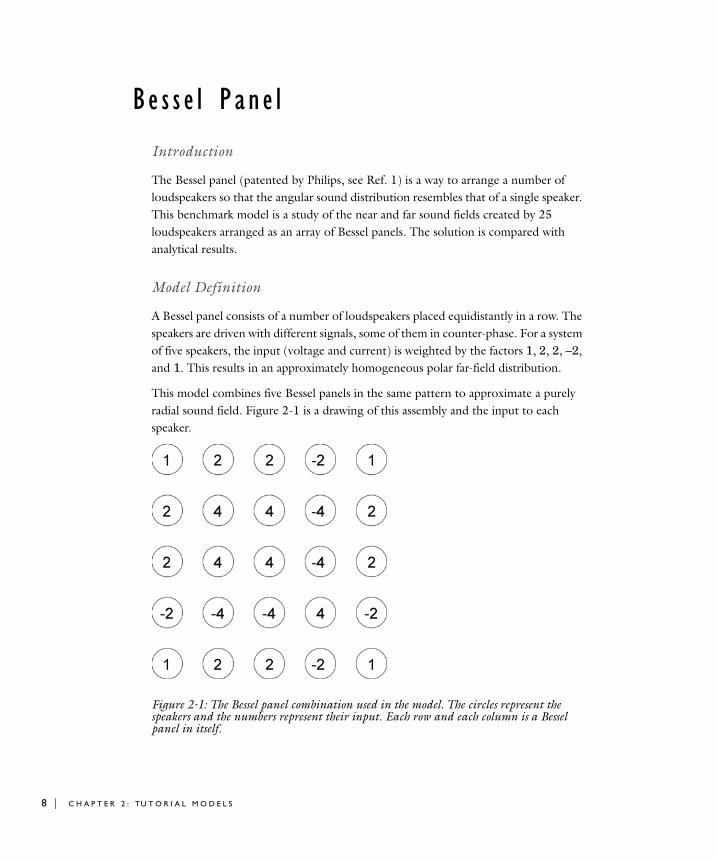
The Bessel panel (patented by Philips, see Ref. 1) is a way to arrange a number of loudspeakers so that the angular sound distribution resembles that of a single speaker. This benchmark model is a study of the near and far sound fields created by 25 loudspeakers arranged as an array of Bessel panels. The solution is compared with analytical results.

Model Definition

A Bessel panel consists of a number of loudspeakers placed equidistantly in a row. The speakers are driven with different signals, some of them in counter-phase. For a system of five speakers, the input (voltage and current) is weighted by the factors 1, 2, 2, −2, and 1. This results in an approximately homogeneous polar far-field distribution.

This model combines five Bessel panels in the same pattern to approximate a purely radial sound field. Figure 2-1 is a drawing of this assembly and the input to each speaker.

Figure 2-1: The Bessel panel combination used in the model. The circles represent the speakers and the numbers represent their input. Each row and each column is a Bessel panel in itself.

2 : TU T O R I A L M O D E L S

For the harmonic sound waves of acoustic pressure that you study in this model, the following frequency-domain Helmholtz equation applies for p(x):

Here ρ0 is the density of the medium (kg/m3), ω = 2π f denotes the angular frequency (rad/s), cs refers to the speed of sound (m/s), and QL (1/s2) is a monopole source representing a loudspeaker.

For air, ρ0 = 1.25 kg/m3 and cs = 343 m/s. For the frequency use f = 100 Hz. Each loudspeaker, L, is represented by a point source emitting a flow of strength SL = 10−2 nL m3/s, where nL is the weight factor shown in Figure 2-1. It holds that

where δ(3) refers to the 3D Dirac delta function and RL is the location of the speaker L.

See Figure 2-2 for the model geometry. The distance between two neighboring loudspeakers is 0.5 m. A sphere of radius of 5 m represents an infinite air domain surrounding the loudspeakers.

Figure 2-2: The model geometry.

p x t,( ) p x( )eiωt=

∇ 1ρ0------– ∇p⎝ ⎠

⎛ ⎞⋅ ω2p

ρ0 cs2

--------------– QL

L∑=

QL ωSL δ 3( ) R RL–( )=

B E S S E L P A N E L | 9

10 | C H A P T E R

The predefined radiation condition within the spherical wave option minimizes reflections on the exterior boundaries of the air sphere. This boundary condition allows a spherical wave to travel out of the system while generating only minimal reflections for the wave’s non-spherical components. The radiation boundary condition is useful when the surroundings are simply a continuation of the domain.

For mathematical details on the radiation boundary condition, see the description under the heading “Radiation Boundary Condition” on page 79 of the Acoustics Module User’s Guide.

Results and Discussion

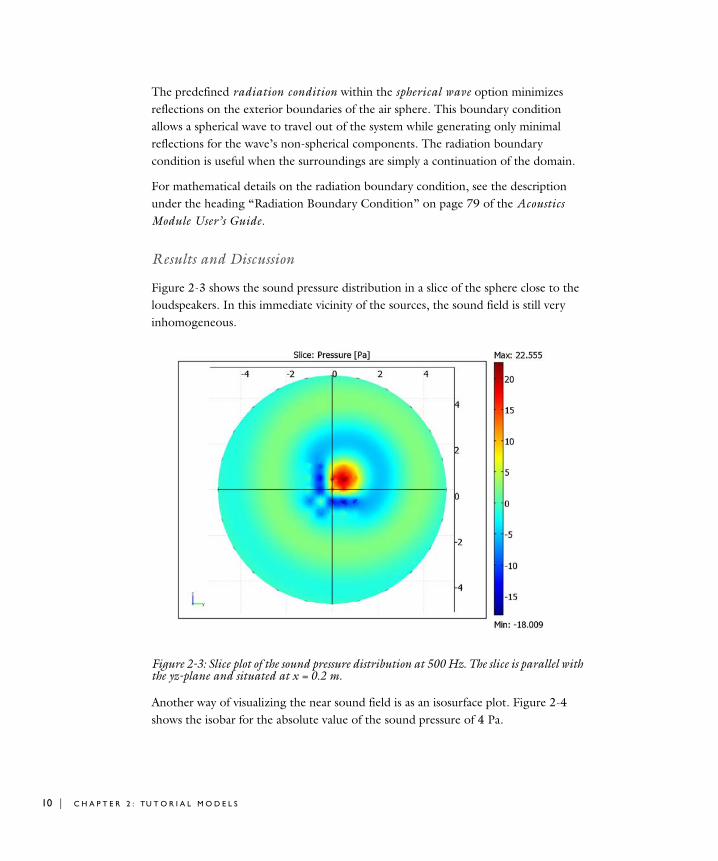
Figure 2-3 shows the sound pressure distribution in a slice of the sphere close to the loudspeakers. In this immediate vicinity of the sources, the sound field is still very inhomogeneous.

Figure 2-3: Slice plot of the sound pressure distribution at 500 Hz. The slice is parallel with the yz-plane and situated at x = 0.2 m.

Another way of visualizing the near sound field is as an isosurface plot. Figure 2-4 shows the isobar for the absolute value of the sound pressure of 4 Pa.


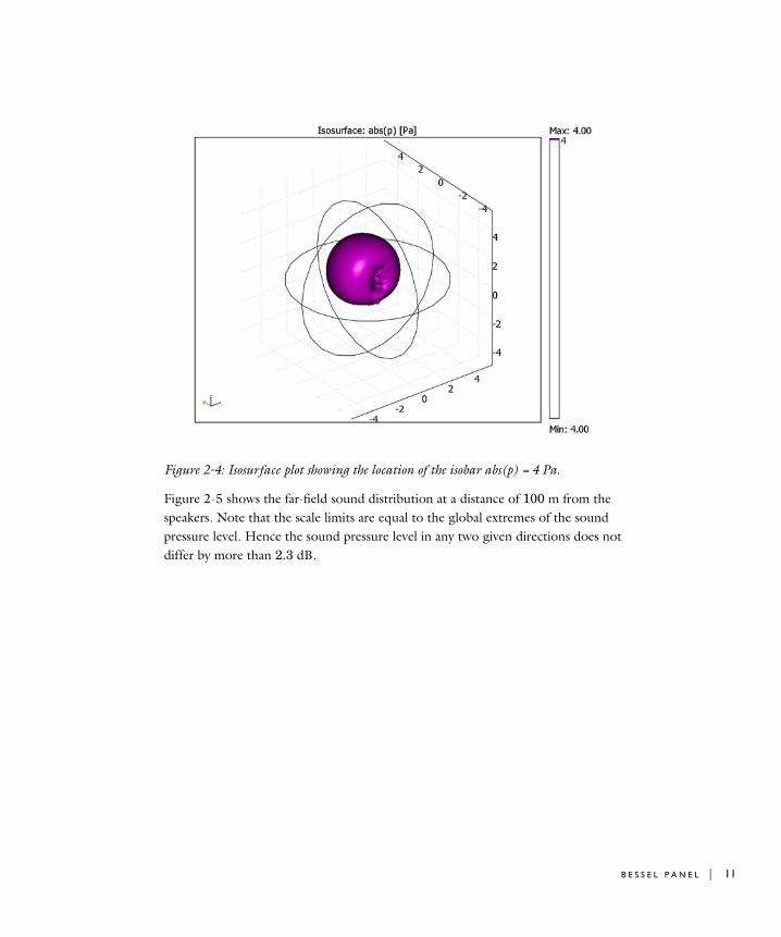
Figure 2-4: Isosurface plot showing the location of the isobar abs(p) = 4 Pa.

Figure 2-5 shows the far-field sound distribution at a distance of 100 m from the speakers. Note that the scale limits are equal to the global extremes of the sound pressure level. Hence the sound pressure level in any two given directions does not differ by more than 2.3 dB.


12 | C H A P T E R

Figure 2-5: Sound pressure level (dB) at a distance of 100 m from the loudspeakers.

Figure 2-6 plots the computed far-field pressure at a radial distance of 100 m versus polar angle in the positive xz-plane and compares it to the analytical solution. As the plot shows, the computed solution is close to the analytical solution. Besides refining the mesh, you can refine the accuracy by adding perfectly matched layers outside the computational domain; for more information see page 73 of the Acoustics Module


User’s Guide. Finally, the accuracy is bounded by the far-field transformation itself: the longer the distance from the sources, the better the accuracy.

Figure 2-6: Sound pressure level (dB) at a radial distance of 100 m in the xz-plane (zero azimuthal angle) as a function of the polar angle from the xy-plane. The solid line represents the computed solution and the dashed line the analytical solution.

Modeling in COMSOL Multiphysics

Use the Pressure Acoustics application mode of the Acoustics Module to set up the model of the Bessel panel. The GMRES solver with the Geometric multigrid preconditioner ensures low memory consumption at a high mesh resolution. In an optional exercise that requires COMSOL Script or MATLAB, you run a script to calculate the analytical solution for comparison.

Reference

1. “Bessel panels—high-power speaker systems with radial sound distribution,” Technical publication 091, Philips Export BV, 1983.


14 | C H A P T E R

Model Library path: Acoustics_Module/Tutorial_Models/bessel_panel

Modeling Using the Graphical User Interface

M O D E L N A V I G A T O R

1 In the Model Navigator select 3D from the Space dimension list.

2 From the list of application modes select Acoustics Module>Pressure Acoustics>Time-harmonic analysis.

3 Click OK to close the Model Navigator.

G E O M E T R Y M O D E L I N G

1 Choose Draw>Sphere. In the Radius edit field type 5, then click OK.

2 Choose Draw>Point. Add a point to the geometry by typing the following values in the Coordinates edit fields, then click OK.

3 With the point selected, choose Draw>Modify>Array. Enter the following data, then click OK.

O P T I O N S A N D S E T T I N G S

Choose Options>Constants and define the following constant.

Coordinates x 0

Coordinates y -1

Coordinates z -1

Displacement x 0

Displacement y 0.5

Displacement z 0.5

Array size x 1

Array size y 5

Array size z 5

NAME EXPRESSION DESCRIPTION

S 0.01[m^3/s] Flow source


P H Y S I C S S E T T I N G S

Subdomain SettingsThe Bessel loudspeaker array is modeled in air. Because this is the default medium no changes are needed.

Boundary Conditions1 Choose Physics>Boundary Settings.

2 Select all the boundaries, then select Radiation condition from the Boundary condition list.

3 From the Wave type list select Spherical wave.

In preparation for studying the far field, you must supply a postprocessing variable. Plotting on boundaries gives you the far field for all angles. When plotting on edges you are limited to fixed azimuthal or polar angles, but as there is a lower number of computations involved these plots display much faster.

4 Go to the Far-Field page.

5 Select Boundaries 5–8.

6 In the top Name edit field type farp. When you select the next edit field in the table the default values for the field and the normal derivative appears.

7 Select the Symmetry planes: x=0 check box. Keep the default Symmetric pressure.

8 Click OK to close the dialog box.

Point Settings1 Choose Physics>Point Settings.

2 For all points, select Flow from the Type of source list. Assign the values of the flow according to the table below.

The minus signs correspond to sources with the opposite phase.


G E N E R A T I N G T H E M E S H

1 From the Mesh menu open the Free Mesh Parameters dialog box. On the Global page, select Custom mesh size and type 0.85 in the Maximum element size edit field.

2 Click Remesh, then click OK.

SETTINGS POINTS 3, 7, 25, 29

POINTS 4, 8, 12, 26

POINTS 5, 6, 14, 18, 20, 24, 27, 28

POINTS 9, 16, 17, 22, 23

POINTS 10, 11, 15, 21

iS S -2*S 2*S 4*S -4*S


16 | C H A P T E R

C O M P U T I N G T H E S O L U T I O N

1 Choose Solve>Solver Parameters or click the corresponding button on the Main toolbar to open the Solver Parameters dialog box.

2 From the Linear system solver list select GMRES, and from the Preconditioner list select Geometric multigrid.

3 Click the Settings button. In the dialog box that appears click Preconditioner, then select Refine mesh from the Hierarchy generation method list.

4 Click OK twice to close both the Linear System Solver Settings dialog box and the Solver Parameters dialog box. Click the Solve button on the Main toolbar.

PO S T P R O C E S S I N G A N D V I S U A L I Z A T I O N

The default plot shows the acoustic pressure on five equidistant slices along the x-axis. The central slice comprises the point sources, resulting in singular pressure values. For a better view of the local pressure distribution close to the sources, try a single slice offset by a small distance from the sources.

1 Choose Postprocessing>Plot Parameters or click the corresponding button on the Main toolbar.

2 On the Slice page find the Slice positioning area. Click the Vector with coordinates option button for the x levels entry and type 0.2 in the corresponding edit field.

3 Click OK to generate the plot.

4 Click the Go to YZ View button. The plot should now resemble the one in Figure 2-3.

The near-field radiation pattern is well represented by an isosurface plot of the absolute value of the sound pressure.

1 Click the Go to Default 3D View button.

2 Return to the Plot Parameters dialog box and click the General tab. Clear the Slice check box and select the Isosurface check box.

3 On the Isosurface page, type abs(p) in the Expression edit field on the Isosurface Data page.

4 Select the Vector with isolevels option button and type 4 in the corresponding edit field.

5 Select the Uniform color option button. Click the Color button, select a violet hue and click OK.


6 Click OK to generate the plot, then click the Headlight button on the Camera toolbar to get a clearer view.

The far-field pressure farp is normalized to give the pressure at a distance of 1 m from the source. The sound intensity, I, is proportional to p2, and the total power radiated, P = 4π Ir2, is independent of the distance, r, from the source. It then follows that p scales as r−1. Thus, to get the sound pressure level in dB at a distance of 100 m from the panel, proceed as follows.

1 Choose Postprocessing>Domain Plot Parameters and click the Line/Extrusion tab.

2 Select Edge 11 and type 10*log10(1/100^2*0.5*abs(farp)^2/abs(p_ref_acpr)^2) in the Expression edit field in the y-axis data area.

3 Click the Expression option button and then click the Expression button in the x-axis data area.

4 In the dialog box that appears, type atan2(z,x) in the Expression edit field and select the degree sign (°) from the Unit list.

5 Click OK twice to see the plot.

What you see now is the sound pressure level at a distance of 100 m from the panel as a function of the polar angle at zero azimuthal angle. This plot should resemble the solid line in Figure 2-6.

You can visualize the far field in all possible directions using the boundaries of the sphere. Please note that it takes approximately 30 minutes before this plot shows. If you do not want to see the far field on the boundaries, skip the next two steps.

1 In the Plot Parameters dialog box click the Boundary tab. In the Expression edit field type 10*log10(1/100^2*0.5*abs(farp)^2/abs(p_ref_acpr)^2).

2 Select the Boundary plot check box, then click OK to see the plot.

When the far-field boundary plot eventually shows up, the values should vary between 68.7 dB and 71.0 dB.

The plot that appears when you open this model in the Model Library is a combination of the isosurface plot that you already have and a surface plot of the local sound pressure level:

1 Choose Options>Suppress>Suppress Boundaries. In the dialog box that appears, select Boundary 2 and click OK.

2 In the Plot Parameters dialog box click the Boundary tab. Select Sound pressure level from the Predefined quantities list and click OK.


18 | C H A P T E R

PO S T P R O C E S S I N G W I T H C O M S O L S C R I P T

If you have access to COMSOL Script or MATLAB, you can easily compare the results from your simulation with the analytical solution. The bessel_pressure script returns the pressure at the coordinates (xin, yin, zin). The script is stored in the multiphysics folder as bessel_pressure.m.

To compare the simulation results with the analytical solution as in Figure 2-6, follow these steps:

1 Choose Options>Functions.

2 Click the New button. In the Function name edit field type bessel_pressure, then click OK to return to the Functions dialog box.

3 In the Arguments edit field type x, y, z, and in the Expression edit field type bessel_pressure(x,y,z).

4 Select the May produce complex output for real arguments check box.


6 Choose Solve>Update Model.

7 Choose Postprocessing>Domain Plot Parameters.

8 If you have closed the far-field plot, recreate it by selecting Edge 11 on the Line/

Extrusion tab and then clicking Apply.

9 On the General page select the Keep current plot check box and click the Title/Axis button.

10 In the Title/Axis Settings dialog box go to the Title edit field and type Computed (solid) and analytic (dashed) far-field pressure, then in the Second axis

label edit field type Sound pressure level (dB). Click OK to close the dialog box.

The radius of the model geometry is 5 m. To get the sound level at a distance of 100 m from the source, you therefore must multiply the input coordinates with a factor of 20.

11 Go to the Line/Extrusion page of the Domain Plot Parameters dialog box.

12 In the Expression edit field type 10*log10(0.5*abs(bessel_pressure(20*x,20*y,20*z))^2/

abs(p_ref_acpr)^2).

13 Click the Line Settings button. From the Line style list select Dashed line, then click OK.

14 Click OK to see the plot, which should resemble the one in Figure 2-6.


Ho l l ow C y l i n d e r

Introduction

Fluid acoustics coupled to structural objects, such as membranes or plates, represents an important application area in many engineering fields. Some examples are:

• Loudspeakers

• Acoustic sensors

• Nondestructive impedance testing

• Medical ultrasound diagnostics of the human body

Model Definition

This model provides a general demonstration of an acoustic fluid phenomenon in 3D coupled to a solid object. In this study, the solid object is a capped, hollow aluminum cylinder filled with and immersed in water.

The acoustic waves created by a source inside the cylinder impact on the cylinder walls. In the model, you first calculate the frequency response from the solid object and then feed the information back to the acoustics domain so that you can analyze the wave pattern.

H O L L O W C Y L I N D E R | 19

20 | C H A P T E R

Figure 2-7: A hollow aluminum cylinder is immersed in water. The white line inside the cylinder indicates the line source, and the tiny sphere next to the line shows the position of the point source. The simulation domain is bounded by a large sphere.

Figure 2-7 illustrates the aluminum cylinder immersed in water. The cylinder is 2 cm in height and has an outer diameter of 1 cm. The thickness of its walls is 1.5 mm.

The water-filled acoustic domain outside the cylinder is truncated to a sphere with a reasonably large diameter. In two different versions of the model, the system is driven either by a line source coinciding with the axis of the cylinder and located entirely within the cylinder, or by a point source in the interior of the cylinder. The frequency is 60 kHz, that is, in the ultrasound region. The harmonic acoustic pressure in the water at the surface of the cylinder acts as a boundary load on the 3D solid to ensure continuity in pressure. In solving the model, the harmonic displacements and stresses in the solid cylinder are calculated, using the normal acceleration of the solid surface at the acoustics domain boundary to ensure continuity in acceleration.

D O M A I N E Q U A T I O N S

Water SubdomainFor harmonic sound waves we use the frequency-domain Helmholtz equation for sound pressure:


Here, the acoustic pressure is a harmonic quantity, (N/m2), ρ0 is the density of the medium (kg/m3), q is an optional dipole source (N/m3), ω is the angular frequency (rad/s), and cs is the speed of sound (m/s). In the present model, no dipole source is included.

In the above table, pwref denotes the standard reference pressure used when defining the sound pressure level in water; its value differs from that of air, which is the default setting in COMSOL Multiphysics.

Solid SubdomainYou calculate the harmonic stresses and strains inside the solid cylinder walls using a frequency response analysis in the 3D Solid, Stress-Strain application mode. The material data comes from the built-in database for Aluminum 3003-H18.

B O U N D A R Y C O N D I T I O N S

Outer PerimeterOn the outer spherical perimeter of the water domain (Figure 2-7), use the predefined Radiation condition with the Spherical wave option. This boundary condition allows a spherical wave to travel out of the system, giving only minimal reflections for the non-spherical components of the wave. The radiation boundary condition is useful when the surroundings are only a continuation of the domain.

For mathematical details on the radiation boundary condition, see the subsection “Radiation Boundary Conditions” on page 79 of the Acoustics Module User’s Guide.

Cylinder-Water InterfaceTo couple the acoustic pressure wave to the solid cylinder, set the boundary load F (force/unit area) on the cylinder to

TABLE 2-1: ACOUSTICS DOMAIN DATA

QUANTITY VALUE DESCRIPTION

ρ0 997 kg/m3 Density

cs 1500 m/s Speed of sound

pwref 10-6 Pa Reference sound pressure

f = ω/2π 60,000 Hz Frequency

∇ 1ρ0------– ∇p q–( )⎝ ⎠

⎛ ⎞⋅ ω2p

ρ0 cs2

--------------– 0=

p p0eiωt=

F ns– p=


22 | C H A P T E R

where ns is the outward-pointing unit normal vector seen from inside the solid domain.

To couple the frequency response of the solid back to the acoustics problem, use the boundary condition that the normal acceleration

equal that of the solid structure. Here, na is the outward-pointing unit normal vector seen from inside the acoustics domain.

These boundary conditions are available as boundary groups using the Acoustic-Structure Interaction predefined multiphysics coupling.

E D G E A N D P O I N T S E T T I N G S

In the two cases considered, the sound waves are generated by either a point source or a line source. A line source along the z-axis is defined as follows:

Here P is the power per unit length of an infinitely long line source placed in a homogeneous medium extending to infinity. Furthermore, δ(2)(r) is the Dirac delta function in two dimensions, r denoting the projection of the position vector onto the xy-plane.

For a point source of power P located at the point R = R0 in an infinite homogeneous space, the definition is

where δ(3)(R) is the Dirac delta function in three dimensions. Any type of confinement will result in higher power usage.

an na–1ρ0------– ∇p q–( )⎝ ⎠

⎛ ⎞⋅=

∇ 1ρ0------ ∇p–⎝ ⎠

⎛ ⎞⋅ 2 P ωρ0

---------- δ 2( ) r( )=

∇ 1ρ0------ ∇p–⎝ ⎠

⎛ ⎞⋅ 2πP cs

ρ0-------------- δ 3( ) R R0–( )=


Results

Figure 2-8: Sound-pressure plot (dB) of the acoustic waves in the coupled problem, using a point source inside the cylinder. The surfaces of the cylinder show its deformation (m). Some of the surfaces are hidden to reveal the pressure distribution inside the cylinder.

Figure 2-8 shows the sound pressure in the near field as a slice plot, for the case of an off-center point source. Far-field results are shown in the “Postprocessing and Visualization” section of the step-by-step instructions.


The implementation of this model does not require any special tricks, but relies on standard equations and conditions in COMSOL Multiphysics and the Acoustics Module. Thanks to an internal scaling of the equations, the system of equations is symmetric. This means that you can use a solver designed for problems that generate symmetric stiffness matrices, thereby saving a considerable amount of system memory and shortening the calculation time.

Model Library path: Acoustics_Module/Tutorial_Models/hollow_cylinder


24 | C H A P T E R



1 Start COMSOL Multiphysics.

2 In the Model Navigator, select 3D from the Space dimension list.

3 Select Acoustics Module>Acoustic-Structure Interaction from the list of application modes.

4 Click OK.

O P T I O N S

1 Open the Constants dialog box from the Options menu and enter the following values (the descriptions are optional):

2 Click OK.

3 Choose Physics>Scalar Variables and enter the following values:

4 Click OK.


All the buttons used in creating the geometry of this model are located in the leftmost of the vertical toolbars.


Freq 60[kHz] Frequency

rhow 997[kg/m^3] Water density

cw 1500[m/s] Speed of sound in water

pw_ref 1[uPa] Reference sound pressure in water

R 3[cm] Radius of modeling domain

edgeL 1.7[cm] Length of line source


freq_acsld Freq Excitation frequency

freq_acpr Freq Excitation frequency

p_ref_acpr pw_ref Pressure reference


1 Click the Cylinder button. In the dialog box that appears, enter property values according to the following table:

Let all other entries retain their default values. Click OK to close the dialog box.

2 Click the Cylinder button once more and create a cylinder with the following specifications; when done, click OK.

3 Click the Line button. Create a line with the following endpoints; when done, click OK.

4 Click the Point button. Create a point located at the following coordinate; when done, click OK.

5 Click the Sphere button. In the dialog box that appears, type 0.03 in the Radius edit field, and let the other entries retain their default values. Click OK to close the dialog box.

6 Click the Zoom Extents button on the Main toolbar.

PROPERTY VALUE

Radius 0.005

Height 0.02

Axis base point, z -0.01

PROPERTY VALUE

Radius 0.0035

Height 0.017

Axis base point, z -0.0085

PROPERTY VALUE

x 0 0

y 0 0

z -0.0085 0.0085

PROPERTY VALUE

x 0.001

y 0.002

z 0.005


26 | C H A P T E R


Subdomain Settings—Solid1 From the Multiphysics menu, select Solid, Stress-Strain (acsld).

2 From the Physics menu, select Subdomain Settings. Select Subdomains 1 and 3, then select Fluid domain from the Group list.

3 Select Subdomain 2, then select Solid domain from the Group list.

4 On the Material page, click Load. Select Aluminum 3003-H18 under the Basic Material

Properties entry in the Materials list. Click OK.

5 Click the Damping tab, then select No damping from the Damping model list.

6 Click OK.

Boundary Conditions—Solid1 In the Boundary Settings dialog box select all the exterior boundaries (5–12, 15–16,

and 19–20).

2 From the Group list, select Fluid load.

The variables nx_acpr, ny_acpr, and nz_acpr in the predefined face load components are the Cartesian components of the normal vector directed outward from the subdomains where the Pressure Acoustics (acpr) application mode is active.

3 Click OK.

Subdomain Settings—Pressure Acoustics1 From the Multiphysics menu, select Pressure Acoustics (acpr).

2 Choose Physics>Subdomain Settings.

3 Select Subdomain 2 and then select Solid domain from the Group list.

4 Select Subdomains 1 and 3 and then select Fluid domain from the Group list. Enter the following data for the density and the speed of sound:

5 Click OK.

Boundary Conditions—Pressure Acoustics1 Select Physics>Boundary Settings. Hold down the Ctrl key and select Boundaries 1–

4, 13–14, and 17–18. Select Radiation condition from the Boundary condition list, and choose Spherical wave as the wave type.

QUANTITY VALUE/EXPRESSION

ρ0 rhow

cs cw


2 Select the Select by group check box, then select Boundary 5 to get a group selection of all the remaining boundaries.

3 From the Group list, select Structural acceleration.

4 Click OK.

The variables u_tt_acsld, v_tt_acsld, and w_tt_acsld in the predefined setting for the normal acceleration are the acceleration components from the Solid,

Stress-Strain (acsld) application mode.

Edge Settings—Pressure Acoustics1 Select Physics>Edge Settings.

2 In the dialog box that appears, select Edge 26.

3 Select Power in the Type of source list, then set P to 1/edgeL.

4 Click OK.

Note that the presence of a Dirac delta function is not explicitly indicated on the right-hand side of the equation in the Equation area; instead, the localization of the source to the selected edge is implicitly understood.


1 From the Mesh menu open the Free Mesh Parameters dialog box. On the Global page select Custom mesh size and type 0.005 in the Maximum element size edit field.

This value corresponds to 0.2 L, where L = cs/f is the wavelength of the sound waves in the acoustics domain. Combined with the (default) choice of second-order elements, it follows that the rule-of-thumb minimum of ten to twelve degrees of freedom per wavelength for the solution to be reliable is satisfied.

2 Click the Subdomain tab. Select Subdomain 2 and set the Maximum element size to 0.002.

3 Click Remesh, then click OK to close the dialog box.


1 Select Solve>Solver Parameters.

2 From the Solver list, select Stationary.

3 From the Linear system solver list, select GMRES.

The GMRES solver by default uses the geometric multigrid preconditioner to solve the system in two iterations: first with 1st-order elements and then with 2nd-order elements. In solving the present model, GMRES is faster and requires less memory (about 400 MB versus 900 MB) than the SPOOLES linear solver.


28 | C H A P T E R

4 Click OK.

5 Click the Solve button on the Main toolbar.


Figure 2-9: The sound pressure level (dB) inside and outside the cylinder, and the deformations (m) of the cylinder when using a line pressure source along the axis of the cylinder.

The default plot is a slice plot of the von Mises stress. There is much more information hidden in the solution, and there is a lot you can do to improve the result’s readability and enhance its looks. For example, to arrive at the plot in Figure 2-9, do as follows:

1 Choose Options>Suppress>Suppress Boundaries.

2 Select Boundaries 5–6 and 9–10 from the list. Click OK.

3 Choose Postprocessing>Plot Parameters. On the General page, select the check boxes for Slice, Boundary, and Deformed shape in the Plot type area. Leave all the other check boxes cleared.

4 Click the Slice tab, then select Pressure Acoustics (acpr)>Sound pressure level among the Predefined quantities. In the Slice positioning area type 0 in all three Number of

levels edit fields. On the y levels line, click the Vector with coordinates button, then type 0.002 in the corresponding edit field.


5 Click the Boundary tab and select Solid, Stress-Strain (acsld)>Total displacement in the list of Predefined quantities. Click the Colormap button and select hsv from the corresponding list.

6 Click the Deform tab. In the Domain types to deform area, make sure that only the Boundary check box is selected. Click the Boundary Data tab, and verify that the selection in the Predefined quantities list is Displacement.

7 Click OK.

To refine the visual quality of the model, do as follows:

1 Click both the Headlight button and the Scene Light button on the Main toolbar.

2 Choose Options>Visualization/Selection Settings.

3 On the Camera page click the Perspective button in the Projection area.

4 Click the Lighting tab. In the Scene light area click all four light sources and clear the Enabled check box on each one of them.

5 Click the New button. Select Spot in the Type list. Click OK.

6 Specify the light source as in the following table, then click OK.

You can experiment with the viewing angle by clicking the Zoom and Dolly In/Out buttons on the Plot toolbar and clicking and dragging the geometry.

Point-Source Version

Once you are done solving and postprocessing the line-source version of this model, save it and proceed to set up a point-source version. Whereas the line source gives an axially symmetric pressure field, the point source is displaced from the origin and thus motivates a 3D model. Starting from your line source model, do the following to shift to a point source version.

PROPERTY VALUE

Position -0.01 -0.01 0

Direction 0 1 0

Spread angle 90

Concentration 0.05


30 | C H A P T E R


Point Settings—Pressure AcousticsChoose Physics>Point Settings. In the dialog box that appears select Point 20. In the Type of source list select Power and set P to 1 W.

Edge Settings—Pressure AcousticsTo turn off the line source choose Physics>Edge Settings. In the dialog box that appears select Edge 26 and set P to 0.


Click the Solve button on the Main toolbar.


The location of the slice plot now coincides with the point source, where the pressure field is singular. You get a nicer plot if you move the slice away from the source:

1 In the Plot Parameters dialog box, click the Slice tab.

2 In the y levels edit field, type 0 in the Vector with coordinates column.

3 Click OK.

Your plot should now resemble Figure 2-8 on page 23.

Far-Field Postprocessing1 Choose Physics>Boundary Settings and go to the Far-Field page.

2 Select Boundaries 1–4, 13–14, and 17–18.

3 Define a variable with the Name pfar.



You can now plot the far pressure field in the direction from the origin towards any point To see, for instance, the field as a function of the elevation angle along Edge 16, do the following:


7 On the Line/Extrusion page, select Edge 16.

8 From the Predefined quantities list, select Pressure Acoustics (acpr)>Sound pressure

level for pfar.


9 For the x-axis data click the Expression button and specify the expression atan2(-y,z). Click OK to close the dialog box and then click OK again to see the plot. Verify that it looks similar to Figure 2-10.

Figure 2-10: The far-field sound pressure level in dB as a function of the polar angle from 0 to π/2 at the fixed azimuthal angle of −π and a distance of 1 m from the source.

If you are patient and have some spare time, you can try to plot the far-field radiation pattern at all possible angles around the sphere. This is typically done as a deformed surface plot. Because postprocessing the far field is computationally heavy this might take several minutes.

1 Choose Options>Constants. Add the following constants; when done, click OK.

2 Choose Options>Expressions>Boundary Expressions.

3 On Boundaries 1–4, 13–14, and 17–18, define the variable deformation as (Lpfar_acpr-Lpfarmax)/(Lpfarmax-Lpfarmin).

4 Click OK.


Lpfarmin 122 Min sound pressure level (dB)

Lpfarmax 163 Max sound pressure level (dB)


32 | C H A P T E R


6 Open the Plot Parameters dialog box. On the General page, select the check boxes for Boundary and Deformed shape only.

7 Click the Boundary tab. From the Predefined quantities list, select Pressure Acoustics

(acpr)>Sound pressure level for pfar.

8 Click the Deform tab, then click the Boundary Data tab. In the Domain types to deform area select the Boundary check box only. Enter the following Boundary Data:

9 Click OK and wait for a few minutes to see the plot.

10 Rotate the plot to explore the directional dependence of the pressure in the far-field region. If you prefer, you can manually enter settings from Options>Visualization/

Selection Settings. For a nice view, click the Camera tab and enter the following data:

x component deformation*x

y component deformation*y

z component deformation*z

PROPERTY VALUE

Camera position 0.18 0.39 0.29

Camera target 0 0 0

Camera up vector 0.11 0.55 -0.83

Camera view angle 11.6


Figure 2-11 shows a zoom in of the resulting radiation pattern.

Figure 2-11: Radiation pattern of the far-field sound pressure level at a distance of 1 m from the source. The lower the pressure, the larger the inward deformation from the original spherical boundary.

This plot gives a useful overview of the far-field sound pressure level. The first thing to notice is that the plot has a mirror symmetry with respect to the plane spanned by the z-axis and the point of excitation. This may be easier to verify by inspection if you turn off the light sources. Furthermore, there are two distinct maxima, above and below the end caps of the cylinder, respectively. The minima approximately correspond to nodes in the structural deformation.


34 | C H A P T E R

Op t im i z i n g t h e S h ap e o f a Ho r n

Introduction

This model shows how to apply boundary shape optimization to a simple axisymmetric horn. For the sake of simplicity, the far-field sound pressure level is maximized for a single frequency and in a single direction. The focus is on the optimization procedure, which involves parametrization of the geometry, choice of objective function and optimization solver settings.

The model was inspired by the work of Erik Bängtsson, Daniel Noreland, Martin Berggren, and others (Ref. 1).

Note: This model requires the Optimization Lab.

Model Definition

A plane-wave mode feeds an axisymmetric horn radiating from an infinite baffle towards an open half space. The radius of the feeding waveguide is assumed to be fixed, as well as the depth of the horn and the size of the hole where the horn is attached to


the baffle. By varying the curvature of the initially conical surface of the horn, its directivity and impedance can be changed.

Figure 2-12: The initial configuration is a simple cone.

The surface is parameterized by assuming that the radius of the horn (as function of the distance from the baffle) deviates from the simple cone by a function of the form

(2-1)

where s is a parameter varying between 0 and 1 along the edge of the cone, di are scale factors and the qi are the optimization variables to be optimized. Note that dr(0) = dr(1) = 0, and that the function is smooth. The number of optimization variables can be varied; using more variables gives more freedom and potentially a better final value of the objective function, but will also make the optimization process more sensitive and may generate a shape which is less suitable for production.

Optimization can only be applied to real-valued functions, because the minimum of a complex-valued function is not well-defined. But the raw result from a frequency-domain acoustics simulation is a complex-valued pressure field. From this

dr qidi iπs( )sin

i 1=

N

∑=

O P T I M I Z I N G T H E S H A P E O F A H O R N | 35

36 | C H A P T E R

you will have to generate a scalar, real-valued quantity to be used as objective function in the optimization process. However, any operation which converts a complex number to a real value is necessarily non-analytical, which means that its derivative is not uniquely defined.

The gradient-based optimization solver in COMSOL’s Optimization Lab by default evaluates derivatives of the objective function via the solution of an adjoint equation. This procedure requires that the symbolic derivative of any non-analytic function is selected in a special way. The default behavior of the composite functions abs(z) and conj(z), which are most commonly used to obtain a real-valued objective function, is to return a derivative parallel to the real axis. However, this behavior is not appropriate for the adjoint method, where you instead need the definitions

(2-2)

It is indeed possible to redefine the symbolic derivatives of built-in functions in COMSOL Multiphysics, but in this case it is more convenient to use the special function realdot(z1, z2), which evaluates as real(z1·conj(z2)) but differentiates according to Equation 2-2. In particular, as a measure of the transmission properties of the horn, you will use a an expression of the form realdot(pm, pm)/p0

2, where pm is the pressure measured at a specific point in front of the horn and p0 is the (real-valued and constant) amplitude of the incoming wave.

If you choose to evaluate pm in the near-field, or can afford to include a sufficiently large domain in front of the horn to effectively measure a far-field value at a point in the model, you can simply measure pm as the local pressure in a geometry vertex. However, in order to optimize the far-field directivity pattern in an efficient way, pm should be defined using an integral representation of the far-field pressure as function of the angle from the axis.

COMSOL Multiphysics contains optimized code for evaluating such far-field integrals. This is, however, a pure post-processing feature which does not support the automatic differentiation required by the adjoint method. Therefore, you will have to return to the definition of the Helmholtz-Kirchhoff integral as given in its asymptotic axisymmetric form by Equation 3-5 on page 33 in the Acoustics Module User’s Guide:

zdd z z

z-----=

z1dd z1z2( ) z2=

z2dd z1z2( ) z1=


(2-3)

If the infinite baffle is placed at z = 0, its effect is the same as if adding a mirror image of the horn and at the same time removing the baffle. If, in addition, the integration surface is taken to be the wide end of the horn, in the plane of the baffle, most of the terms in Equation 2-3 cancel out, and all that is left is

(2-4)

where J0 is the Bessel function of the first kind of order 0, and the angle Θ from the axis has been introduced as a parameter. This integral is easily implemented in COMSOL Multiphysics as an integration coupling variable.

Optimization as a rule implies many evaluations of the model for different designs, which may be very time consuming. In addition, the solver can be asked to evaluate each design at a number of frequencies and optimize with respect to the sum of the objective function evaluated for each frequency. In this tutorial, a single frequency of 4000 Hz has been selected in order to make it possible to experiment with other aspects of the model. For example, changing the parameter Θ, you can easily study the effect on the horn shape of optimizing the output at a specified angle from the axis.

pfar R( ) 12---– re

ik zZR-------

J[ 0krRR

-----------⎝ ⎠⎛ ⎞ p r( )∇ n⋅ –

S∫≅

ikp r( )R

----------------- inr RJ1krRR

-----------⎝ ⎠⎛ ⎞ nzZJ0

krRR

-----------⎝ ⎠⎛ ⎞+⎝ ⎠

⎛ ⎞ dS

pm Θ( ) rJ0 kr θ( )sin( )z∂

∂p rdS∫=


38 | C H A P T E R


By changing the shape of the horn within the limits of the selected parametrization, the on-axis sound pressure level can be raised by about 1 dB compared to the simple cone in Figure 2-12.

Figure 2-13: The final shape of the horn, optimized for on-axis SPL at 5000 Hz.


The improvement is rather small, because also the initial configuration shows a marked directivity, as can be seen from Figure 2-14. Obviously, the optimal shape with respect to on-axis SPL leads to deep undesirable minima in other directions.

Figure 2-14: Far-field patterns for the original (solid blue) and final (dashed red) designs.

Optimizing with respect to a slight off-axis direction can give you a more uniform far-field pattern, but may also result in a deep minimum on the axis. Try for example to set the off-axis angle Θ to 22°.

To search for a stable and practically useful horn design, you might instead create a composite objective function as a weighted sum of transmission values evaluated for a number of discrete directions, or choose to minimize the deviation from the mean SPL over a range of angles. In addition, you would also want to optimize with respect to more than one frequency, and experiment with different parameterizations.


COMSOL Multiphysics implements the parametrization as a prescribed boundary displacement in a Moving Mesh application mode. The mesh is allowed to move freely in the conical part of the horn, but otherwise kept fix. Some measures must be taken


40 | C H A P T E R

to avoid inverted elements when the shape of the cone is changed. Firstly, a quad mesh will be used, since quads are less likely to become inverted, compared to triangles.

Secondly, the amplitude of the boundary displacement is restricted by limits on the optimization variables. These artificial constraints are intended to keep the mesh element volumes positive at all times and must not be active at the optimum point. You will perform this sanity check as a final postprocessing step.

A time-harmonic Pressure Acoustics application mode solves for the pressure field inside the horn and in a small spherical domain surrounding its opening. The air domain is terminated by a spherical PML layer which absorbs outgoing waves in such a way that the artificial termination of the domain has no influence on the near-field. An accurate near-field is sufficient, since the far-field result is based on an integral representation evaluated in the plane of the baffle. A matched boundary condition on the waveguide attached to the narrow end feeds the horn with a plane wave of amplitude p0.

An Optimization application mode adds five scalar optimization variables, q1 to q5, which are constrained to vary in the interval [−1, 1]. The maximum effect of each variable on the boundary displacement is controlled by the scale factors di in Equation 2-1. The pressure measured by an integration coupling variable according to Equation 2-4 is inserted into a scalar objective function contribution equal to the negative of the SPL value, or −10·log10(0.5·realdot(pm, pm)/(20·10−6)2).

Reference

1. E. Bängtsson, D. Noreland, and M. Berggren, Shape Optimization of an acoustic horn, Technical report 2002-019, Department of Information Technology, Uppsala University, May 2002.

Model Library path: Acoustics_Module/Tutorial_Models/horn_shape_optimization




1 In the Model Navigator, select Axial Symmetry (2D) from the Space dimension list, then go to the list of application modes and select COMSOL Multiphysics>Deformed

Mesh>Moving Mesh (ALE).

2 Click the Multiphysics button, then click Add.

3 Select Acoustics Module>Pressure Acoustics from the application mode list, then click Add.

4 Select COMSOL Multiphysics>Optimization and Sensitivity>Optimization, then click Add.



1 Shift-click the Rectangle/Square button on the Draw toolbar. In the dialog box that appears, change the following settings; when done, click OK.

2 Create another rectangle with the following changes compared to the defaults:

3 Zoom in to the geometry by clicking the Zoom Extents button on the Main toolbar.

4 Click the Ellipse/Circle (Centered) button on the Draw toolbar. Right-click at the origin and drag to create a circle of radius 0.3.

5 Draw another circle of radius 0.2 inside the first one.

6 Shift-click to select both circles, then click the Union button on the Draw toolbar.

7 Select the joined circles together with the larger of the rectangles (R2), then click the Intersection button.

8 To draw the actual horn, click the Line button on the Draw toolbar; click consecutively at (0, 0), (0.1, 0), (0.025, -0.15), (0, -0.15), and (0, 0); and finally right-click once anywhere in the geometry to close the curve and turn it into a solid object.

Size Width 0.025

Height 0.025

Position z -0.2

Size Width 0.3

Height 0.3


42 | C H A P T E R


1 Choose Options>Constants.

2 Define the following constants; when finished, click OK.

3 Choose Options>Expressions>Global Expressions and add the expression for the radial displacement of the horn surface:

4 Choose Options>Integration Coupling Variables>Boundary Variables.

5 Select Boundary 6 and create a variable with the following properties:

6 Click OK.


Subdomain Settings—Moving Mesh (ALE)1 From the Multiphysics menu, select the Moving Mesh (ALE) application mode.

2 Choose Physics>Subdomain Settings to open the Subdomain Settings dialog box.

3 Select Subdomains 1, 3, and 4, click the No displacement button, and then click OK.

Boundary Conditions—Moving Mesh (ALE)4 From the Physics menu, open the Boundary Settings dialog box.


r0 0.025[m] Radius of waveguide

p0 1[Pa] Incident pressure amplitude

theta 0[deg] Polar angle

d1 0.02[m] Scale factor






dr q1*d1*sin(1*pi*s)+q2*d2*sin(2*pi*s)+ q3*d3*sin(3*pi*s)+q4*d4*sin(4*pi*s)+ q5*d5*sin(5*pi*s)

Radial displacement

NAME EXPRESSION INTEGRATION ORDER

FRAME GLOBAL DESTINATION

pm r*besselj(0,k_acpr*r* sin(theta))*pz

4 ref yes


5 Select Boundaries 3, 4, and 6.

6 Select the dr and dz check boxes to lock these boundaries at their initial positions.

7 Select Boundary 9, again select the dr and dz check boxes, and enter dr in the Mesh

displacement, r direction edit field.


Subdomain Settings—Pressure AcousticsThe default medium in the Pressure acoustics application mode is air, so the only thing you have to do is activate the PML domain.

1 From the Multiphysics menu, choose the Pressure Acoustics application mode.

2 From the Physics menu, open the Subdomain Settings dialog box.

3 Select Subdomain 4 and click the PML tab.

4 From the Type of PML list, choose Spherical.

5 Select the Absorbing in radial dir. check box, then click OK to close the dialog box.

Boundary Conditions—Pressure AcousticsThe default boundary condition is sound hard, which is appropriate for the horn surface and the baffle, and does no harm on the outside of the PML or on the axis. Therefore, only the waveguide port requires the boundary condition to be changed. In addition, far-field postprocessing variables must also be defined in Boundary Settings.

1 Choose Physics>Boundary Settings.

2 Select Boundary 2. From the Boundary condition list, choose Matched boundary and set the Pressure source field to p0.

3 Click the Interior boundaries check box, then select Boundary 6.

4 On the Far-Field page, type pf in the first row of the Name column.

5 Press Tab to automatically fill in the remaining columns.

6 Select the z=0 check box under Symmetry planes but leave the list box at Symmetric

Pressure. This procedure accounts for the infinite baffle.


Scalar Settings—OptimizationIn the Optimization application mode, you define the objective function, declare optimization variables, and constraints.

8 Activate the Optimization application mode by selecting it from the Multiphysics menu or in the Model Tree.


44 | C H A P T E R

9 Choose Physics>Scalar Settings to open the Scalar Settings dialog box.

10 In the Scalar contribution field on the Objective page, enter -2*pi*realdot(pm,pm)/(pi*r0^2*p0^2).

11 Click the Variables tab. Enter Variable names q1, q2, q3, q4, and q5 on separate lines in the table, all with Init value 0.

12 Click the Scalar Constraints tab and limit the allowed value of each of the optimization variables to the range [−1, 1]. When you are done, the Scalar constraints table should look as follows:



The model will be run at a frequency of 5000 Hz, corresponding to a wavelength of just under 7 cm. Using the standard at-least-six-elements-per-wavelength rule, a maximum element size of 1 cm seems like a good choice. A quad mesh is in general more resistant to element warping when the mesh is deformed. Therefore, use an unstructured quad mesh everywhere except in the PMLs, which perform better with a mapped mesh aligned with the radial and tangential directions.

1 Choose Mesh>Free Mesh Parameters.

2 Click the Custom mesh size option button, type 0.01 in the Maximum element size edit field, and then click OK to close the dialog box.

3 Go to Subdomain Mode by clicking the corresponding button on the main toolbar.

4 Select all subdomains except the PML, then click the Mesh Selected (Free, Quad) button on the Mesh toolbar.

5 To set the number of mesh layers in the PML, begin by selecting Mapped Mesh Parameters from the Mesh menu.

6 On the Boundary page, select Boundary 7 and then select the Constrained edge

element distribution check box.

7 Set the Number of edge elements to 8, then click OK.

LB EXPRESSION UB

-1 q1 1

-1 q2 1

-1 q3 1

-1 q4 1

-1 q5 1


8 Click the Mesh Remaining (Mapped) button on the Mesh toolbar to complete the mesh.


Before starting the actual optimization solver it is good practice to check the model set-up by running the sensitivity solver once. This way, you can also study the reference state on which you intend to improve.


2 Select Parametric from the Solver list and select the Optimization/Sensitivity check box.

3 In the Parameter Names field, enter the name of the frequency variable: freq_acpr.

4 As Parameter values, enter just 5000.

5 Click the Optimization/Sensitivity tab and verify that the Analysis is set to Sensitivity rather than Optimization.

6 Click Apply in the dialog box, then click the Solve button on the Main toolbar.


The default plot in the main window shows the mesh displacement in the Moving Mesh application mode. Because the initial optimization variable values are zero, so is the displacement. The acoustical quantities are far more interesting for visualization, but for clarity, the PML zone should not be included in the plot.

1 Click the Plot Parameters button on the Main toolbar to open the dialog box with that name.

2 On the Surface page, select Pressure Acoustics (acpr)>Sound pressure level from the list of Predefined quantities.

3 Click OK to close the dialog box and display the SPL value.

4 Go to Subdomain Mode by clicking the corresponding button on the Main toolbar.

5 Select the PML domain, then click Hide Selected Objects.


46 | C H A P T E R

6 Return to Postprocessing Mode using the button on the Main toolbar.

7 To see the far-field SPL pattern, first choose Postprocessing>Domain Plot Parameters.

8 On the Line/Extrusion page, select Boundary 12 and find Pressure Acoustics

(acpr)>Sound pressure level for pf in the list of Predefined quantities.

9 Click the lower option button in the x-axis data area, then click the Expression button to open the X-Axis Data dialog box.

10 Type atan2(r,z) in the Expression field, press Tab, and select the degree sign from the Unit list.

11 Click OK to close the dialog box, then click Apply in the Domain Plot Parameters dialog box to display the far-field pattern.


Now return to solving the actual optimization problem. In this tutorial, the optimization is performed only for a single frequency. This can also be seen as a preparation step before starting a time-consuming optimization over a frequency range.

1 Return to the Optimization/Sensitivity page in the Solver Settings dialog box and change the Analysis type to Optimization.


2 Increase the Optimality tolerance to 1e-4, which is still stricter than the accuracy of this low-resolution finite element model.

3 Optionally, to follow the optimization solver’s progress, select the Plot while solving check box. When you run the optimization, the software then plots the SPL field (according to the current settings in the Plot Parameters dialog box) in a separate figure window and updates it after each model evaluation.

4 Click OK to close the dialog box, then click the Solve button on the Main toolbar.

The solution requires about 20 model evaluations, which should not take more than a minute on a modern computer. You can follow the


When the solution is ready, you can immediately study the optimal (within the constraints imposed by the parametrization) shape of the horn. To see a direct comparison of the far-field pattern before and after optimization (Figure 2-14) do the following:

1 Return to the Domain Plot Parameters dialog box, select again Boundary 12 on the Line/Extrusion page, and click the Line Settings button.

2 In the Line Settings dialog box, select Color from the Line color list. Click OK.

3 Click the General tab. Select the Keep current plot check box, then click Apply.

The solution returned by the optimization solver is only guaranteed to be a local optimum within the given constraints. It is good practice to check whether any constraints imposed to keep the problem well posed (in this case avoid inverted mesh elements) are active at the optimum point. If some artificial constraint is active, try to relax it a little and restart the solution.

4 Choose Postprocessing>Data Display>Global.

5 From the Predefined quantities list, select Optimization (opt)>q1.

6 Click Apply and check that the value lies inside the specified range −1 < q1 < 1.

7 Check q2, q3, q4, and q5 in the same way.

8 When done, click OK.

Because none of the parameters take on a limiting value, the obtained solution can be assumed independent of the artificial bounds.


48 | C H A P T E R

J e t P i p e

Introduction

This example models the radiation of fan noise from the annular duct of a turbofan aeroengine. When the jet stream exits the duct, a vortex sheet appears along the extension of the duct wall. In the model you calculate the near field on both sides of the vortex sheet.

Model Definition

The model is axisymmetric with the symmetry axis coinciding with the engine’s centerline. The flows both inside and outside the duct are uniform mean flows, but because the flow velocities differ, a vortex sheet separates them.

The Aeroacoustics application mode in the Acoustics Module describes acoustic waves in a moving fluid with the potential, , for the local particle velocity as the basic dependent variable; see the chapter “Aeroacoustics” on page 107 of the Acoustics Module User’s Guide for further details. However, the field equation is only valid when the velocity field is irrotational, a condition that is not satisfied across a vortex sheet. As a consequence, the velocity potential is discontinuous across this sheet. To model this discontinuity you use assemblies that are connected through pairs. The following boundary condition on the pair models the vortex sheet:

z

r

φ


In these equations, ω is the angular velocity, V is the mean flow velocity, w is the normal displacement, is the velocity potential, and p is the pressure. The subscripts 1 and 2 refer to the two sides of the boundary.

The velocity normal to the vortex sheet is zero, which implies that the last term in the condition vanishes. In the model the variables are made dimensionless. The velocities are divided by the speed of sound in air and the densities are divided by the density for air. For example the model uses the Mach number M = V/c0 as the mean flow velocity. This leads to the boundary conditions

where M denotes the transverse Mach number.

The duct has a hard wall, which you also model using a boundary condition on a pair.

The acoustic field inside the duct can be described as a sum of eigenmodes propagating in the duct and then radiating in the free space. This is discussed in section 2.1 in Ref. 1. In this example you study the radiated acoustic waves produced by a single eigenmode at a time. First you calculate the eigenmodes with the circumferential mode order 4 on the inlet boundary. From these eigenmodes, the one with radial mode order 0 is used as incident wave. You then calculate the velocity fields with circumferential mode numbers, m = 17 and 24 and with radial mode order, n = 0.


The boundary mode analysis made with the circumferential wave number m = 4, 17, and 24 gives several eigenmodes corresponding to different radial mode numbers. This

ρ iω M1∇T+( ) w n– ρ∇φ1V

c2-----ρ iω φ1 ∇φ1 V⋅( )+( )–⎝ ⎠

⎛ ⎞⋅=

ρ iω M2∇T+( ) w n– ρ∇φ2V

c2-----ρ iω φ2 ∇φ2 V⋅( )+( )–⎝ ⎠

⎛ ⎞⋅=

p1 p2=

φ

iω M1∇T+( ) wn∂

∂φ1=

iω M2∇T+( ) wn∂

∂φ2=

p1 p2=

J E T P I P E | 49

50 | C H A P T E R

example, as well as in Ref. 1, uses the following eigenmodes as incident waves in the duct.

Figure 2-15: (a) Mode shape for m = 4, n = 0; (b) Mode shape for m = 17, n = 1; (c) Mode shape for m = 24, n = 1.

The near field around the duct obtained by COMSOL Multiphysics can be compared to the results for the near field in Ref. 1. Figure 2-16 to Figure 2-18 show the near-field solution for a Mach number equal to 0.45 in the pipe and 0.25 on the outside. The figures show the field for the different eigenmodes shown in Figure 2-15.

(a) (b)

(c)


Figure 2-16: The near-field solution for m = 4 and n = 0.


J E T P I P E | 51

52 | C H A P T E R


Reference

1. G. Gabard and R.J. Astley, “Theoretical model for sound radiations from annular jet pipes: far- and near-field solution,” J. Fluid Mech., vol. 549, pp. 315–341, 2006.

Model Library path: Acoustics_Module/Tutorial_Models/jet_pipe



1 In the Model Navigator go to the Space dimension list and select Axial symmetry (2D), then click the Multiphysics button.

2 From the list of application modes select Acoustics Module>Aeroacoustics>Boundary

modal analysis. In the Dependent variables edit field type phi_b. Click Add.


3 From the list of application modes select Acoustics Module>Aeroacoustics>Time-harmonic analysis. Click Add.

4 Click OK.


1 From the Draw menu select Specify Objects>Rectangle.

2 Specify the following rectangles, all with Corner as the Position Base.

3 Click the Zoom Extents button.

4 Select R1, R2, and R3, then click the Union button on the Draw toolbar.

5 Select R4, R5, R6, and R7, then click the Union button.

6 Select CO1 and CO2, then click the Create Pairs and Imprints button.

This completes the geometry-modeling state. The geometry in the drawing area of the user interface on your screen should now like that in the figure below.

RECTANGLE WIDTH HEIGHT R Z

R1 0.25 0.5 0.75 -0.5

R2 0.25 1 0.75 0

R3 0.25 0.2 0.75 1

R4 1 1.5 1 -0.5

R5 1.2 0.2 1 -0.7

R6 0.2 1.9 2 -0.7

R7 1.2 0.2 1 1

J E T P I P E | 53

54 | C H A P T E R


Enter the following constants in the Constants dialog that you open from the Options menu. When finished, click OK.


Units1 From the Physics menu, select Model Settings.

2 Set the Base unit system to None.

3 Click OK.

Identity Pairs1 From the Physics menu, select Identity Pairs>Identity Boundary Pairs.

2 Click New and check Boundary 8 as source boundary and Boundary 13 as destination boundary.

3 Select Pair 1 and clear the check boxes for Boundaries 8 and 13 that you selected in the previous step.

4 Click OK.

Subdomain Settings1 From the Physics menu, open the Subdomain Settings dialog box.

2 Select Subdomains 1–3. Set Vz to M1, and both cs and ρ to 1.

3 Select Subdomains 4–9. Set Vz to M0, and both cs and ρ to 1.

4 Go to the PML page.

5 Select Subdomains 3, 4, 6, 7, and 9. Set Type of PML to Cylindrical and select the Absorbing in z direction check box.

6 Select Subdomains 7–9.

The settings that differ between the subdomains are now highlighted in yellow; these settings will not be affected unless you explicitly change them.

7 From the Type of PML list, select Cylindrical; this changes the setting for Subdomain 8. Select the Absorbing in r direction check box.

8 Click OK.

NAME VALUE DESCRIPTION

M0 0.25 Mach number outside the duct

M1 0.45 Mach number inside the duct

m 4 Circumferential wave number


Boundary Conditions1 From the Multiphysics menu, select Aeroacoustics, Boundary Modal Analysis (acab).

2 From the Physics menu, open the Boundary Settings dialog box.

3 Select all boundaries and clear the Active in this domain check box.

4 Select Boundary 2 only, then select the Active in this domain check box.

5 Set Vz to M1 and both cs and ρ to 1.

6 Click OK.

Application Scalar Variables1 From the Physics menu, select Scalar Variables.

2 Set the Excitation frequency to 30/(2*pi) and the Circumferential wave number to m.

3 Click OK.


1 From the Mesh menu, select Mapped Mesh Parameters.

2 From the Predefined mesh sizes list, select Extremely fine. Click Remesh.

3 When the mesh is finished, click OK to close the dialog box.


1 From the Solve menu, open the Solver Parameters dialog box.

2 Set Desired number of propagation constants to 10.

3 Click OK.

4 From the Solve menu, open the Solver Manager.

5 On the Solve For page, select Aeroacoustics, Boundary Modal Analysis (acab).

6 Click Apply, then click Solve.

7 On the Initial Value page click the Store Solution button and click OK in the dialog box that appears to store all solutions.

8 Click OK in the Solver Manager dialog box to close it.


1 From the Postprocessing menu, select Domain Plot Parameters.

2 On the Line/Extrusion page select Boundary 2 and make sure the Expression is phi_b.

J E T P I P E | 55

56 | C H A P T E R

3 On the General page select the value with the highest real part in the Solutions to use list. Click Apply.

The figure that appears is the same as in Figure 2-15 (a). This corresponds to the lowest radial mode (n = 0).

4 You can look at higher modes by selecting values with lower real part in the Solution

to use list.

When you solve for m = 17 or 24 you can generate Figure 2-15 (b) or (c) by selecting the value with the second highest real part, n = 1.

5 Click OK to close the dialog when you are ready.


Boundary Conditions1 From the Multiphysics menu select Aeroacoustics(acae).

2 Select Boundary 2. Set the Boundary condition to Velocity potential and 0 to phi_b.

3 Go to the Pairs page and select Pair 1. Set the Boundary condition to Vortex sheet.

4 Select Pair 2 and set the Boundary condition to Sound hard boundary (wall).

5 Click OK.


1 From the Solve menu, open the Solver Manager.

2 Set the Initial value to Stored solution and the Propagation constant to the one with highest real part to get the lowest radial mode.

3 On the Solve For page, select Aeroacoustics (acae).

4 Click OK.

5 Open the Solver Parameters dialog and set the solver to Stationary. Click OK.



Follow these steps to generate Figure 2-16 on page 51.

1 From the Postprocessing menu, open the Plot Parameters dialog box.

2 On the Surface page, select the Surface plot check box, then set the Colormap to gray.

3 On the General page, set the Solution at angle (phase) to 180.

4 Clear the Boundary check box in the Plot type area.

5 Click OK.

φ


6 From the Options menu, choose Suppress>Suppress Subdomains.

7 Select Subdomains 3, 4, and 6–9, then click OK.

8 Click first the Postprocessing Mode button and then the Zoom Extents button.

You have now solved the example for the eigenmode m = 4 and n = 0. To generate Figure 2-17 on page 51 you need to solve the example with m = 17 and n = 1 and to generate Figure 2-18 you need to use m = 24 and n = 1. To solve the example again with a different eigenmode you can follow these steps.

1 From the Options menu, open the Constants dialog box.

2 Change the value of m to 17 to generate Figure 2-17 or 24 to generate Figure 2-18 in the Constants dialog. Click OK.

3 From the Physics menu, select Boundary Settings.

4 Select Boundary 2 and set 0 to 0, then click OK.

Go through the steps to solve the model once again with the new value of the circumferential mode number. Start from the section “Computing the Solution” on page 55.

When choosing the eigenmode to use as incident wave you need to take the one with second highest real part to get the radial mode number n equal to 1.

Finally, the image you see when opening this model from the Acoustics Module model library is produced from the last obtained solution (m = 24, n = 1) with the following steps:

1 Click the Plot Parameters button on the Main toolbar.

2 On the General page, select the Contour check box and clear the one for Geometry

edges.

3 Click the Surface tab.

4 From the Predefined quantities list on the Surface Data page, select Aeroacoustics (acae)>Sound pressure level.

5 From the Colormap list inside the Surface color area select jet.

6 On the Height Data page, select the Height data check box.

7 From the Predefined quantities list select Aeroacoustics (acae)>Sound pressure level.

8 Click the Contour tab.

9 From the Predefined quantities list on the Contour Data page select Aeroacoustics (acae)>Sound pressure level.

φ

J E T P I P E | 57

58 | C H A P T E R

10 Inside the Contour levels area, select the option button next to the Vector with

isolevels edit field. Type linspace(60,125,66) in this edit field to obtain a contour-line distance of 1 dB.

11 Clear the Color scale check box inside the Contour color area.


13 From the Predefined quantities list, select Aeroacoustics (acae)>Sound pressure level.

14 Go to the General page and click the Title button.

15 Select the option button next to the edit field and enter the title Sound pressure level (dB), then click OK to close the Title dialog box.

16 Click OK to generate the plot and close the Plot Parameters dialog box.

17 Click both the Scene Light button and the Perspective Projection button on the Camera toolbar to the left of the drawing area.

18 Double-click to clear the AXIS and CSYS buttons on the status bar at the bottom of the user interface.


After rotating the view by clicking and dragging in the drawing area you should see a plot similar to that in the figure below.


P i e z o a c ou s t i c T r a n s du c e r

Introduction

A piezoelectric transducer can be used either to transform an electric current to an acoustic pressure field or, the opposite, to produce an electric current from an acoustic field. These devices are generally useful for applications that require the generation of sound in air and liquids. Examples of such applications include phased array microphones, ultrasound equipment, inkjet droplet actuators, drug discovery, sonar transducers, bioimaging, and acousto-biotherapeutics.

Model Definition

In a phased-array microphone, the piezoelectric crystal plate fits into the structure through a series of stacked layers that are divided into rows. The space between these layers is referred to as the kerf , and the rows are repeated with a periodicity, or pitch.

This model simulates a single crystal plate in such a structure. The element is rotationally symmetric, making it possible to use an axisymmetric 2D application mode in COMSOL Multiphysics.

P I E Z O A C O U S T I C TR A N S D U C E R | 59

60 | C H A P T E R

Figure 2-19: The model geometry.

In the air domain, the wave equation describes the pressure distribution:

(2-5)

For this model, assume that the pressure varies harmonically in time as

Hence Equation 2-5 simplifies to

(2-6)

Because there are no sources present, Equation 2-6 simplifies further to

1

ρ0 cs2

--------------t2

2

∂

∂ p ∇ 1ρ0------– ∇p q–( )⎝ ⎠

⎛ ⎞⋅+ Q=

p x t,( ) p x( ) eiωt=

∇ 1ρ0------– ∇p q–( )⎝ ⎠

⎛ ⎞⋅ ω2p

ρ0 cs2

--------------– Q=

∇ 1ρ0------– ∇p( )⎝ ⎠

⎛ ⎞⋅ ω2p

ρ0 cs2

--------------– 0=


The piezoelectric domain is made of the crystal PZT5-H, which is a common material in piezoelectric transducers. The structural analysis is also time harmonic although, for historical reasons, in structural-mechanics terminology it is a frequency response analysis.

The frequency is set to 300 kHz, which is in the ultrasonic range (dolphins and bats, for example, communicate in the range of 20 Hz to 150 kHz, while humans can only hear frequencies in the range 20 Hz to 20 kHz).


A voltage of 100 V is applied to the upper part of the transducer, while the bottom part is grounded. At the interface between the air and solid domain, the boundary condition for the acoustics application mode is that the pressure is equal to the normal acceleration of the solid domain

where an is the normal acceleration.

This drives the pressure in the air domain. The solid domain is on the other hand subjected to the acoustic pressure changes in the air domain. Because of the high voltage applied to the transducer, this load is probably negligible in comparison. Yet because the model is in 2D, it is possible to include this load and solve the full model simultaneously on any computer.


Figure 2-20 shows the pressure distribution in the air domain. This plot clearly shows how the PML (perfectly matched layer) absorbs the wave effectively.

n 1ρ0------ ∇p( )⎝ ⎠⎛ ⎞⋅ an=


62 | C H A P T E R

Figure 2-20: Surface and height plot of the pressure distribution.

Figure 2-21 shows the pressure distribution along the air-solid interface. The acoustic pressure load is small in comparison to the electrical load, which is plotted in Figure 2-22 on page 63.


Figure 2-21: Acoustic pressure at the air-solid interface.

Figure 2-22: von Mises Stress along the air-solid interface.

The results from a far-field analysis appear in Figure 2-23 on page 64. This figure shows that the sound pressure level reaches a maximum right in front of the transducer. This result also shows that the sound pressure level is fairly low. Although humans cannot hear these high frequencies, it can be mentioned for comparison that 15 dB is about the same sound pressure level as rustling leaves. On the other hand, because this is just one element in an array of elements, a more detailed study is necessary in order to draw further conclusions.


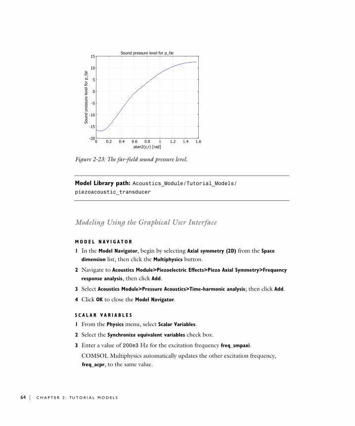
64 | C H A P T E R

Figure 2-23: The far-field sound pressure level.

Model Library path: Acoustics_Module/Tutorial_Models/piezoacoustic_transducer



1 In the Model Navigator, begin by selecting Axial symmetry (2D) from the Space

dimension list, then click the Multiphysics button.

2 Navigate to Acoustics Module>Piezoelectric Effects>Piezo Axial Symmetry>Frequency

response analysis, then click Add.

3 Select Acoustics Module>Pressure Acoustics>Time-harmonic analysis; then click Add.


S C A L A R V A R I A B L E S

1 From the Physics menu, select Scalar Variables.

2 Select the Synchronize equivalent variables check box.

3 Enter a value of 200e3 Hz for the excitation frequency freq_smpaxi.

COMSOL Multiphysics automatically updates the other excitation frequency, freq_acpr, to the same value.


4 Click OK.


1 Draw a rectangle, R1, by first selecting Draw>Specify Objects>Rectangle and then specifying the following properties; when done, click OK.

2 Click the Zoom Extents button on the Main toolbar to automatically fit the geometry to your window.

The geometry for the transducer is now complete. Continue by creating the acoustics domain, which consists of two domains: one air domain and one PML domain.

3 Choose Draw>Specify Objects>Circle. Specify a Radius of 4e-3, then click OK.

4 Choose Draw>Specify Objects>Square. Specify a Width of 4e-3, then click OK.


6 Select the circle and the square, then click the Intersection button on the Draw toolbar.

7 Select the geometry object CO1. Press Ctrl+C to copy it, then press Ctrl+V and click OK in the dialog box that opens to paste the copy with no displacement.

8 Select the geometry object CO2, then click the Scale button. In the Scale factor area, type 1.5 in both the r and the z edit field. (You can select the geometry objects from a list in the Create Composite Objects dialog box.) Click OK.

9 Once again, click the Zoom Extents button on the Main toolbar to automatically fit the geometry to your window.

S U B D O M A I N S E T T I N G S — P I E Z O A X I A L S Y M M E T R Y

1 Select the Piezo Axial Symmetry (smpaxi) application mode from the Model Tree or from the Multiphysics menu.

2 From the Physics menu, choose Subdomain Settings.

3 Select Subdomains 2 and 3, then clear the Active in this domain check box.

PROPERTY VALUE

Width 1e-3

Height 0.5e-3

Position, base Corner

Position, r 0

Position, z -0.5e-3


66 | C H A P T E R

4 Select Subdomain 1, then click the Load button.

5 From the Basic Material Properties library, select Lead Zirconate Titanate (PZT-5H).

In the Piezoelectric Material Properties library, you find more than 20 additional piezoelectric materials.

6 Click OK to close the Materials/Coefficients Library dialog box.

Note: For a piezoelectric material, you can specify an orientation and a coordinate system. In this model, use the default settings: the xz-plane in the global coordinate system.

7 Click OK to close the Subdomain Settings dialog box.

B O U N D A R Y C O N D I T I O N S — P I E Z O A X I A L S Y M M E T R Y

1 From the Physics menu, choose Boundary Settings.

2 On the Constraint page, enter the following structural boundary conditions:

3 Click the Electric BC tab, and set the electric boundary condition as follows:

4 Select Boundary 4.

5 On the Load page, type -p in the Fz edit field to specify the acoustic pressure load, and then click OK. p is the name of the dependent variable for pressure in the Pressure Acoustics application mode. The pressure acts from the air toward the piezo domain (in the negative z direction), which explains the minus sign in front of p. Click OK to close the dialog box.

S U B D O M A I N S E T T I N G S — P R E S S U R E A C O U S T I C S

1 Select the Pressure Acoustics (acpr) application mode from the Model Tree or from the Multiphysics menu.

2 From the Physics menu, select Subdomain Settings.

SETTINGS BOUNDARY 1 BOUNDARY 2

Constraint condition Symmetry plane Roller

SETTINGS BOUNDARY 1 BOUNDARY 2 BOUNDARY 4 BOUNDARY 6

Boundary condition

Axial symmetry Ground Electric potential Zero charge/Symmetry

V0 100


3 Select Subdomain 1, then clear the Active in this domain check box.

4 Select Subdomain 3.

5 On the PML page, select Spherical from the Type of PML list.

6 Select the Absorbing in radial dir. check box, then enter a value of 2e-3. This value corresponds to the PML’s extension in the radial direction.

7 Set the inner PML radius, R0, to 4e-3.


Because the default values correspond to the properties of air, you do not have to specify the subdomain settings for Subdomain 2.

B O U N D A R Y C O N D I T I O N S — P R E S S U R E A C O U S T I C S


2 Select Boundary 4, then select Normal acceleration as the boundary condition.

3 Set the value of the inward acceleration, an, to w_tt_smpaxi (this is the second-order time derivative of the structural displacement).

4 Click OK.

M E S H G E N E R A T I O N

1 From the Mesh menu, choose Free Mesh Parameters.

2 On the Global page, click the Custom mesh size option button.

3 Specify a Maximum element size of (343/200e3)/5. This value corresponds to 1/5th of the acoustic wavelength. For wave models it is important to use a mesh size sufficiently small to properly resolve the wavelength.

4 Click Remesh. When the mesher has finished, click OK to close the dialog box.


1 Click the Solver Parameters button on the Main toolbar.

2 From the Solver list, select Stationary.


4 Click the Solve button from the Main toolbar.


To reproduce the plot in Figure 2-20, proceed as follows:



68 | C H A P T E R

2 Click the Surface tab.

3 On the Surface Data page, select Pressure Acoustics (acpr)>Pressure from the Predefined quantities list .


5 From the Predefined quantities list, select Pressure Acoustics (acpr)>Pressure.


7 Click the Headlight button on the Camera toolbar for clearer visualization.

To create Figure 2-21 and Figure 2-22 do the following:

1 Open the Domain Plot Parameters dialog box from the Postprocessing menu.

2 Go to the Line/Extrusion page.

3 In the Expression edit field, enter p.

4 From the Boundary selection list, select boundary 4 and then click on Apply.

5 To plot von Mises stress along the same boundary (Figure 2-22), enter mises_smpaxi in the Expression edit field, and then click OK.

To create Figure 2-23, you need to define a far-field variable.

1 Assure that the Pressure Acoustics (acpr) is selected from the Model Tree, then open the Boundary Settings dialog box.

2 Select Boundary 10, then click the Far-Field tab.

3 Type p_far in the Name edit field, then click OK.

4 From the Solve menu, choose Update Model.

5 From the Postprocessing menu, open the Domain Plot Parameters dialog box.

6 Go to the Line/Extrusion page. Select Boundary 10.

7 From the Predefined quantities list, select Pressure Acoustics (acpr)>Sound pressure

level for p_far.

8 Click the Expression button in the x-axis data area, then click the Expression button.

9 In the Expression edit field, type atan2(z,r). Click OK.

10 Click OK to create Figure 2-23.


T r a n s i e n t Gau s s i a n Exp l o s i o n

Introduction

This model introduces some important concepts to have in mind when solving transient problems. In particular, it examines the relationship between the frequency content in the sources driving the model, the mesh resolution, and the time step.

Model Definition

An ellipse with sound-hard walls has the interesting property that an acoustic signal emanating from one of the foci refocuses at the other focal point b/c seconds later, where b (in meters) is the major axis length and c (m/s) is the speed of sound.

Inspired by Ref. 1 and Ref. 2, this model involves a Gaussian explosion at one focus of an ellipse to illustrate some properties of time-dependent acoustic problems. The major and minor axis lengths are 10 m and 8 m, respectively. The major axis coincides with the x-axis and the foci are located at x = −3 m and x = 3 m. Because of symmetry the model can be limited to the upper half-plane.

Denoting the fluid density by ρ and the speed of sound by cs, the acoustic pressure field, p(x, t), inside the elliptical chamber is governed by the wave equation

1

ρ cs2

---------t2

2

∂∂ p ∇ 1

ρ--- p∇–⎝ ⎠

⎛ ⎞⋅+ S x t,( )=

TR A N S I E N T G A U S S I A N E X P L O S I O N | 69

70 | C H A P T E R

where the point-source term on the right-hand side is given by

The time dependence of the explosion is determined by the cutoff Gaussian pulse

describing the rate of air flow (measured in m2/s) away from the source, located at x = x0. The parameter f0, which is proportional to the pulse bandwidth, is chosen as f0 = c/(Nh), where h is a typical mesh-element size, and N is the number of elements per wavelength required to resolve a harmonic wave with some accuracy. The following discussion uses N = 6, but N = 4 should be acceptable for many purposes.

As the following plots show, by taking τ = 1/f0 the pulse very closely approximates a full Gaussian, the effect of the cutoff tails being numerically insignificant.

Figure 2-24: Normalized Gaussian pulse and its derivative.

A particularly interesting property of the Gaussian function is that its Fourier transform is equally simple (neglect cutoff effects):

where ω0 = 2π f0. The magnitude of the Fourier transform falls off quickly for increasing angular frequencies, ω. Practically all the energy in the signal is contained in the frequency band −2ω0 < ω < 2ω0 with most of it concentrated between −ω0 and ω0.

S x t,( )td

dg t( ) δ 2( ) x x0–( )=

g t( ) A eπ2f0

2 t τ–( )2– 0 t 2τ< <0 otherwise

⎩⎪⎨⎪⎧

=

G ω( ) g t( ) e iωt– td

∞–

∞

∫≡ 2A πω0

--------------- e

ω2

ω02

------– iωt0–

=


Therefore, when using a forcing function of this type, it is enough to resolve wavelengths corresponding to the angular frequency, ω0, which in turn corresponds to the frequency f0. The frequency was chosen on the basis of mesh-element size and resolving power of the spatial discretization, so, in practice, the pulse shape is a function of the mesh resolution. The important point is that there is little to gain in prescribing a forcing function that contains frequencies that the mesh cannot resolve.

In addition to controlling the pulse shape and the amount of time the solver needs to take a single time step, the mesh resolution imposes a restriction on the time step size. The relationship between mesh size and time-step size is closely related to the CFL number (Ref. 3), which is defined as

This nondimensional number can be interpreted as the fraction of an element the wave travels in a single time step. A CFL number around 1 would correspond to the same resolution in space and time if the discretization errors were of the same size; however, that is normally not the case.

COMSOL Multiphysics uses by default the implicit second-order accurate method generalized-α to solve transient acoustics problems (see the section “The Time-Dependent Solver” on page 391 of the COMSOL Multiphysics User’s Guide for more details) and in space the default is 2nd-order elements. Generalized-α introduces some numerical damping of high frequencies, but much less than the BDF method.

The temporal discretization errors for generalized-α are thus larger than the spatial discretization errors when 2nd-order elements are used in space. The limiting step size, where the errors are of roughly the same size, can be found somewhere at CFL < 0.2. You can get away with a longer time step if the forcing does not make full use of the mesh resolution, that is, if high frequencies are absent from the outset.

When the excitation contains all the frequencies the mesh can resolve, there is no point in using the automatic time-step control provided by the time-dependent solver. The tolerances in the automatic error control are difficult to tune when there is weak but important high-frequency content. Instead, you can use your knowledge of the typical mesh size, speed of sound, and CFL number to calculate and prescribe a fixed time step. To check that the accuracy is acceptable, it is recommended that you run a short sequence of typical excitations with progressively smaller time steps and check the convergence.

CFL c∆ th

---------=


72 | C H A P T E R


Using the properties of air for the medium and selecting a mesh density based on the parameters h = 0.15 m and N = 6 gives a pulse half-width of t0 = 2.624 ms. To be on the safe side, requiring CFL < 0.05 gives a fixed time step of 0.02 ms. The model runs for 0.035 s so that you can study the refocusing at the right-hand focus point at roughly 0.0315 s.

Figure 2-25: The refocusing occurs at roughly 0.0315 s. An animation gives a better feeling for the process.

For the selected combination of mesh size, pulse shape, and time step, the solution can be shown to be both smooth and accurate. Selecting a smaller value for N leads to oscillations if the CFL number is small enough, while selecting a higher CFL number (and consequentially a larger time step) leads to an inaccurate solution.

The next figure shows the pressure along the left-hand part of the major axis at t = 9 ms—right after the wave is reflected from the apex at x = −5 m—for four


different CFL numbers: 0.2, 0.1, 0.05, and 0.025. The difference between the last two is small enough to call the solution practically converged.

Figure 2-26: The CFL number has a pronounced effect on the accuracy of the final solution. The difference is marked between CFL = 0.2 (dash-dot), CFL = 0.1(dotted), and CFL = 0.05 (dashed), but essentially indiscernible between the latter time and CFL = 0.025 (solid line).

To get a better view of the graphs in Figure 2-26, go to the COMSOL Help Desk and open the PDF version of the Acoustics Module Model Library. At a magnification of 300% the lines are readily distinguishable.


You set up this tutorial model using the transient analysis type in the Pressure Acoustics application mode of the Acoustics Module. For material properties and boundary conditions use the default settings, which correspond to an air-filled chamber with sound-hard walls.

The modeling instructions are written for a parameter set that gives a converged and stable solution. You are encouraged to experiment with the resolution number, N, the CFL number, and other parameters to see their effects on the result.


74 | C H A P T E R

References

1. B. Yue and M.N. Guddati, “Dispersion-reducing finite elements for transient acoustics,” J. Acoust. Soc. Am., vol. 118, no. 4, 2005.

2. H.-O. Kreiss, N.A. Peterson, and J. Yström, “Difference approximations for the second order wave equation,” SIAM J. Numer. Anal., vol. 40, no. 5, 2002.

3. R. Courant, K.O. Friedrichs, and H. Lewy, “On the partial difference equations of mathematical physics,” IBM Journal, vol. 11, pp. 215–234, 1956.

Model Library path: Acoustics_Module/Tutorial_Models/gaussian_explosion



1 In the Model Navigator, select 2D from the Space dimension list, then go to the list of application modes and select Acoustics Module>Pressure Acoustics>Transient analysis.



1 Shift-click the Rectangle/Square button on the Draw toolbar. In the dialog box that appears, change the following settings, then click OK.

2 Zoom out by clicking the Zoom Extents button on the Main toolbar.

3 Shift-click the Ellipse/Circle button on the Draw toolbar. Modify the following entries, then click OK.

4 Press Ctrl+A to select both objects, then click the Intersection button.

Size Width 10

Height 4

Position x -5

A-semiaxes 5

B-semiaxes 4


5 Click the Point button, then draw a point at the coordinates (−3, 0).

The completed geometry in the drawing area should look like that in the figure below.


Choose Options>Constants and define the following constants; when finished, click OK.

Note the value of roughly 2·10−5 s for the maximum time step; you will use this result at the solving stage.



2 Select Point 2, then select Gaussian pulse from the Type of source list.


c_air 343[m/s] Speed of sound in air

h_max 0.15[m] Typical element size

N 6 Points per wavelength

A 4[m^2/s] Point-source amplitude

f0 c_air/(h_max*N) Frequency bandwidth

t0 1/f0 Pulse half width

CFL 0.05 CFL number

t_step CFL*h_max/c_air Maximum time step


76 | C H A P T E R

3 In the A edit field type A and in the f0 edit field type f0.

4 Click OK.


With the choice of a typical mesh size of h = 0.15, the mesh must be made as isotropic as possible. You can accomplish this by setting the maximum mesh size explicitly while keeping the other mesh parameters relaxed.


2 Click the Custom mesh size option button and type 0.15 in the Maximum element

size edit field.

3 Click the Remesh button, then click OK.



2 Specify the output Times in the Time stepping frame as 0:0.0005:0.035.

3 Click the Time Stepping tab and set Time step taken by solver to Manual.

4 Set the time step to the value calculated from the chosen mesh density and the CFL number by typing 2e-5 in the Time step edit field. Click OK to close the dialog box.

5 Click the Solve button on the Main toolbar to start solving.

To compare the effect of different choices of CFL number and resolution parameter, N, do the following:

6 Open the Constants dialog box, change N or CFL to some other interesting value, then click Apply.


7 If you changed the CFL number, check the new value of t_step and transfer it to the Time step edit field on the Time Stepping page in the Solver Parameters dialog box.

8 Solve again by clicking the Solve button.


The default plot shows the pressure at the final time.

1 For a more attractive plot, click first the 3D Surface Plot button and then the Headlight button on the Plot toolbar.

2 To see the solution close to the refocusing moment, click the Plot Parameters button on the Main toolbar, select 0.0315 from the Solution at time list, then click OK. The result should look like that in Figure 2-25 on page 72.

3 It is illustrative to animate transient problems in general and wave propagation in particular; you can do this by clicking the Animate button on the Plot toolbar.


78 | C H A P T E R

U l t r a s o und S c a t t e r i n g O f f a C y l i n d e r

Introduction

This model, which is inspired by a benchmark problem discussed in Ref. 1, exemplifies ultrasound acoustics modeling with the ultraweak variational formulation (UWVF) in a simple setting. The main advantage of the UWVF for modeling high-frequency acoustic phenomena is its economy with regards to computational complexity compared to low-order finite element analysis. This advantage stems from the property of the UWVF’s elements containing information about the solution to the Helmholtz scalar wave equation in free space.

Model Definition

The modeling domain, depicted in Figure 2-27, consists of a circle of radius 5 cm surrounded by a concentric annulus of outer radius 10 cm. In the circle domain, representing an obstacle, the speed of sound is co = 3000 m/s and the density ρo = 2000 kg/m3. Outside the circular obstacle, the speed of sound is cs = 1500 m/s and the density ρo = 1000 kg/m3. From a location 1 cm outside the outer boundary of the annulus, a sound source emits cylindrical ultrasound waves of frequency f0 = 250 kHz, corresponding to wavelengths in the two domains of λo ≡ co/f0 = 1.2 cm and λs ≡ cs/f0 = 0.6 cm, respectively. On the outer annulus boundary, you impose a radiation boundary condition that absorbs outgoing cylindrical waves. This boundary condition also allows you to model the incoming waves.

Figure 2-27: Modeling domain.

sound sourcelocation

acousticobstacle

co, ρo

surroundingmedium

cs, ρs

radiation bc



Figure 2-28 shows the acoustic pressure field, p, using the wave colormap. The difference in wavelength between the two subdomains is clearly visible, as is the interference pattern between the incident and scattered waves. Notice also how no artificial distortion of the waves leaving the modeling domain can be discerned.

Figure 2-28: The acoustic pressure field. The wavelength inside the obstacle is twice that in the surrounding medium. A radiation boundary condition on the modeling domain’s outer boundary both specifies the source and absorbs outgoing waves.

The incoming and scattered waves are most easily distinguishable in the grayscale plots in Figure 2-29 of the pressure field’s real (left) and imaginary (right) parts. (Because COMSOL Multiphysics by default plots the real part of a time-harmonic variable such as , the plots in Figure 2-28 and the left panel of Figure 2-29 depict the same quantity.


U L T R A S O U N D S C A T T E R I N G O F F A C Y L I N D E R | 79

80 | C H A P T E R

Figure 2-29: Real (left) and imaginary (right) parts of the acoustic pressure field.

You solve this problem using a mesh with 822 elements, shown in Figure 2-30. With the default Ultraweak Helmholtz elements of order 20, the resulting number of DOFs is 16,440. The solution time with the default UMFPACK solver is about 8.6 s with a peak memory usage of 481 MB on a machine running Windows Vista with a 2.6 GHz AMD Athlon X2 Dual Core 500 CPU and 2 GB of RAM. (Using the SPOOLES solver, the solution time is doubled but peak memory usage is reduced to 322 MB.)

Solving the same problem with the same resolution using 2nd-order Lagrange elements requires about 220,000 DOFs (the maximum element size set equal to 1/6th of a wavelength), and takes about five times longer and consumes roughly 75% more memory. In this simple comparison, the UWVF thus shows its strengths.

Figure 2-30: The mesh used in the model for computing the solution for the pressure field. The maximum element size in both domains is specified as twice the wavelength.


Reference

1. T. Huttunen, The ultra weak variational formulation for ultrasound transmission problems, doctoral dissertation, Kuopio University Publications C, Natural and Environmental Sciences 168, 2004.

Model Library path: Acoustics_Module/Tutorial_Models/ultrasound_scattering




2 From the list of application modes, select Acoustics Module>Pressure Acoustics>Time-harmonic analysis with UWVF.



1 Shift-click the Ellipse/Circle (Centered) button on the Draw toolbar.

2 Specify a Radius of 0.1, then click OK.


4 Repeat Steps 1–2 to add a second, concentric, circle, of radius 0.05.

5 Click in the drawing area and press Ctrl+A to select both circles.

6 Click the Create Composite Object button on the Draw toolbar. In the dialog box that appears, click OK to accept the default settings.


82 | C H A P T E R

The finished geometry in the drawing area should look like that in the following figure.

O P T I O N S

Constants1 From the Options menu, select Constants.

2 Enter the following names, expressions, and descriptions (the descriptions are optional); when done, click OK.

Note the values of the wavelengths, λo = 12 mm and λs = 6 mm, which are important for determining an appropriate mesh element size.

Scalar Expressions1 From the Options menu, point to Expressions, and then select Scalar Expressions.


c_o 3000[m/s] Speed of sound in obstacle

c_s 1500[m/s] Speed of sound in surrounding medium

rho_o 2000[kg/m^3] Density in obstacle

rho_s 1000[kg/m^3] Density in surrounding medium

f0 250[kHz] Sound frequency

lda_o c_o/f0 Wavelength in obstacle

lda_s c_s/f0 Wavelength in surrounding medium

k_s 2*pi[rad]/lda_s Wave number in surrounding medium


2 Define the following constants; when done, click OK.

The point-source expression, p_in, representing the incoming wave is proportional to the 0th-order Hankel function of the 2nd kind:

where is the distance from the source location (x0, y0).


Subdomain Settings1 From the Physics menu, choose Subdomain Settings.

2 Enter settings according to the following table; when done, click OK.

Boundary Conditions1 From the Physics menu, choose Boundary Settings.

2 Select Boundaries 1, 2, 5, and 8 (all segments of the outer boundary).

3 From the Boundary condition list, select Radiation condition.

4 For the outgoing wave, select Cylindrical wave from the Wave type list.


R sqrt((x+0.11[m])^2+y^2) Distance from source

p_in (i/4)*(besselj(0,k_s*R)-i*bessely(0,k_s*R)) Incoming wave

SETTINGS SUBDOMAIN 1 SUBDOMAIN 2

ρ0 rho_s rho_o

cs c_s c_o

pini4---H0

2( ) ksR( ) i4--- J0 ksR( ) iY0 ksR( )–( )= =

R x x0–( )2 y y0–( )2+≡


84 | C H A P T E R

5 Click the p0 = pi option button to use the application mode variable p_in_acpr for the incoming wave.

6 Click OK.

Scalar Variables1 From the Physics menu, choose Scalar Variables.

2 Set the excitation frequency by changing the expression for freq_acpr to f0.

3 Specify the incoming wave by changing the expression for p_i_acpr to p_in.

4 Click OK.


To give acceptable accuracy, the Acoustics Module’s ultraweak variational formulation needs a relatively uniform mesh, governed by the maximum element size parameter, hmax, rather than by sharp geometry details. As a rule of thumb, when using the default UWVF settings, specifying an hmax equal to or slightly larger than 2λ gives a good balance between convergence and accuracy.

Because the wavelength differs between the two subdomains in this model, specify hmax at the subdomain level in the Free Mesh Parameters dialog box:

1 From the Mesh menu, select Free Mesh Parameters.

2 Click the Subdomain tab.


3 Specify the maximum element sizes in the two subdomains as follows:

4 Click the Remesh button.

5 Click OK.




The default plot, shown in the following figure, displays the acoustic pressure field, p—or, more precisely, the real part of the complex quantity | p | ei arg(p). The coarse appearance is a consequence of the ultraweak variational formulation’s high element order. Moreover, the jet colormap is not ideally suited for visualizing the wave pattern.

To modify the settings for element refinement and colormap, follow these steps:


2 On the General page, clear the Auto check box for Element refinement and type 20 in the associated element field (the order of the default Ultraweak Helmholtz elements).

3 On the Surface page, find the Surface color area. From the Colormap list, select wave.

4 Click Apply.

The wave colormap is ideally suited for visualizing waves, because of its clear distinction between the low and high ends of the scale. For optimal effect, the range

SETTING SUBDOMAIN 1 SUBDOMAIN 2

Maximum element size 0.012 0.024


86 | C H A P T E R

should be symmetric around zero, which then is rendered white. To ensure this feature for the current plot, you need to adjust the range slightly.

5 Click the Range button. Clear the Auto check box, then set Min to -0.0725 and Max to 0.0725 (these limits are sufficient for all phases of the pressure field). Click OK.

6 Click Apply to generate the plot in Figure 2-28.

Proceed to generate the plots in Figure 2-29 with the following steps:

7 In the Expression edit field on the Surface Data page, type real(p). Because COMSOL Multiphysics plots the real part of a complex quantity by default, this setting only affects the plot title.

8 Change the Colormap to gray (or grayprint, if you want to print the plot on paper).

9 Click Apply to generate the plot in the left panel of Figure 2-29.

10 Change the entry in the Expression edit field to imag(p).

11 Click Apply to generate the plot in the right panel.

12 Change the Expression to p and the Colormap to wave, then click OK to close the Plot

Parameters dialog box with the plot you see when you open the model in the drawing area.


3

I n d u s t r i a l M o d e l s

This chapter contains a selection of models from the automotive and aerospace industries as well as a model of a loudspeaker.

87

88 | C H A P T E R

Ab s o r p t i v e Mu f f l e r

Introduction

This model describes the pressure-wave propagation in a muffler for an internal combustion engine. The approach is generally applicable to analyzing the damping of propagation of harmonic pressure waves.

The model’s purpose is to show how to analyze both inductive and resistive damping in pressure acoustics. In addition to a 3D model in two versions—with and without resistive damping—this example includes a 2D analysis of propagation modes in the muffler chamber. It then calculates the transmission loss for the frequency range 50 Hz–1500 Hz.

Model Definition

The muffler—schematically depicted in Figure 3-1—consists of a 24-liter resonator chamber with a section of the centered exhaust pipe included at each end. In the first version of the model the chamber is empty. In the second version it is lined with 15 mm of absorbing glass wool.

Figure 3-1: Geometry of the lined muffler with the upper half removed. The exhaust fumes enter through the left pipe and exit through the right pipe.


This model solves the problem in the frequency domain using the time-harmonic Pressure Acoustics application mode. The model equation is a slightly modified version of the Helmholtz equation for the acoustic pressure, p:

3 : I N D U S T R I A L M O D E L S

where ρ is the density, cs equals the speed of sound, and ω gives the angular frequency.

In the absorbing glass wool, the damping enters the equation as a complex speed of sound, cc = ω/kc, and a complex density, ρc = kc Zc/ω, where kc is the complex wave number and Zc equals the complex impedance.

For a highly porous material with a rigid skeleton, the well-known model of Delany and Bazley estimates these parameters as functions of frequency and flow resistivity. Using the original coefficients of Delany and Bazley (Ref. 1), the expressions are

where Rf is the flow resistivity, and where ka = ω/ca and Za = ρa ca are the free-space wave number and impedance of air, respectively. You can find flow resistivities in tables. For glass-wool-like materials, Bies and Hansen (Ref. 2) give an empirical correlation

where ρap is the material’s apparent density and dav is the mean fiber diameter. This model uses a rather lightweight glass wool with ρap = 12 kg/m3 and dav = 10 µm.


The boundary conditions are of three types.

• At the solid boundaries, which are the outer walls of the resonator chamber and the pipes, the model uses sound hard (wall) boundary conditions:

• The boundary condition at the inlet involves a combination of incoming and outgoing plane waves:

∇ p∇ρ

-------–⎝ ⎠⎛ ⎞ ω2p

cs2ρ

----------–⋅ 0=

kc ka 1 0.098ρa fRf

---------⎝ ⎠⎛ ⎞

0.7–⋅ i 0.189

ρa fRf

---------⎝ ⎠⎛ ⎞

0.595–⋅ ⋅–+⎝ ⎠

⎛ ⎞⋅=

Zc Za 1 0.057ρa fRf

---------⎝ ⎠⎛ ⎞

0.734⋅ i 0.087

ρa fRf

---------⎝ ⎠⎛ ⎞

0.732–⋅ ⋅–+⎝ ⎠

⎛ ⎞⋅=

Rf3.18 10 9– ρap

1.53⋅ ⋅dav

2---------------------------------------------=

p∇ρ

-------–⎝ ⎠⎛ ⎞ n⋅ 0=

A B S O R P T I V E M U F F L E R | 89

90 | C H A P T E R

In this equation, p0 represents the applied outer pressure, ∆T is the boundary tangential Laplace operator, and i equals the imaginary unit (see Ref. 3). This boundary condition is valid as long as the frequency is kept below the cutoff frequency for the second propagating mode in the tube.

• At the outlet boundary, the model specifies an outgoing plane wave:

The wave numbers and mode shapes through a cross section of the chamber are found as the solution of a related eigenvalue problem:

For a given angular frequency ω = 2π f, only modes such that κx2 is positive can

propagate. The cutoff frequency of each mode is calculated as


The following equation defines the attenuation (in dB) of the acoustic energy, dw:

Here wo and wi denote the outgoing power at the outlet and the incoming power at the inlet, respectively. You can calculate each of these quantities as an integral over the corresponding surface:

n 1ρ0------ p∇⋅ ik p

ρ0------ i

2k-------∆T p+ +

i2k------- ∆T p0 1 k n⋅( )–( ) ik

p0ρ0------+⎝ ⎠

⎛ ⎞ eik k r⋅( )–

=

n 1ρ0------ p∇⋅ i k

ρ0------ p i

2k-------∆T p+ + 0=

∇ p y z,( )∇ρ0

---------------------–⎝ ⎠⎛ ⎞⋅ ω2

ρ0c2------------

κx2

ρ0------–

⎝ ⎠⎜ ⎟⎛ ⎞

p y z,( )– 0=

fjω2 c2κx

2–

2π-----------------------------=

dw 10wowi-------⎝ ⎠

⎛ ⎞log=

wop 2

2ρcs------------ Ad

∂Ω∫=


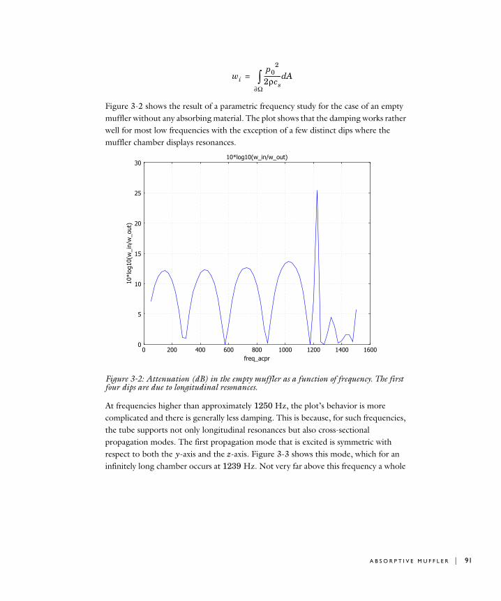
Figure 3-2 shows the result of a parametric frequency study for the case of an empty muffler without any absorbing material. The plot shows that the damping works rather well for most low frequencies with the exception of a few distinct dips where the muffler chamber displays resonances.

Figure 3-2: Attenuation (dB) in the empty muffler as a function of frequency. The first four dips are due to longitudinal resonances.

At frequencies higher than approximately 1250 Hz, the plot’s behavior is more complicated and there is generally less damping. This is because, for such frequencies, the tube supports not only longitudinal resonances but also cross-sectional propagation modes. The first propagation mode that is excited is symmetric with respect to both the y-axis and the z-axis. Figure 3-3 shows this mode, which for an infinitely long chamber occurs at 1239 Hz. Not very far above this frequency a whole

wip0

2

2ρcs------------ Ad

∂Ω∫=


92 | C H A P T E R

range of modes that are combinations of this propagation mode and the longitudinal modes participate, making the damping properties increasingly unpredictable.

Figure 3-3: The chamber’s first symmetric propagation mode. The plot shows the absolute value of the pressure.


The glass-wool lining improves attenuation at higher frequencies. Figure 3-4 shows the attenuation with a layer of lining on the chamber’s upper and lower walls.

Figure 3-4: Attenuation (dB) in the absorbing muffler as a function of frequency (Hz). The dips are still present, but the general trend is that the higher the frequency, the better the damping.


Setting up this model in COMSOL Multiphysics requires the Acoustics Module. You employ two application modes: Pressure Acoustics for the full 3D model, and Boundary Modal Analysis for the propagating mode analysis.

The software has predefined expressions for the Delany-Bazley coefficients, so the only damping parameter you must supply is the flow resistivity.

The parametric solver provides results for a range of frequencies. The software computes integrals in the power expressions using boundary integration coupling variables, and it plots the resulting attenuation versus frequency.


94 | C H A P T E R

References

1. M. A. Delany and E. N. Bazley, “Acoustic properties of fibrous absorbent materials,” Appl. Acoust., vol. 3, pp. 105–116, 1970.

2. D. A. Bies and C. H. Hansen, “Acoustical properties of fibrous absorbent materials,” Appl. Acoust., vol. 14, pp. 357–391, 1980.

3. D. Givoli and B. Neta, “High-order non-reflecting boundary scheme for time-dependent waves,” J. Comp. Phys., vol. 186, pp. 24–46, 2003.

Model Library path: Acoustics_Module/Industrial_Models/absorptive_muffler

Modeling Using the Graphical User Interface—Rigid Walls


1 In the Model Navigator find the Space dimension list and select 3D.

2 In the list of application modes select Acoustics Module>Pressure Acoustics>Time-harmonic analysis.



Choose Options>Constants and enter the data in this table (the descriptions are optional); when finished, click OK.


1 Choose Draw>Work-Plane Settings. Go to the Quick page and select the y-z option button, then in the x edit field type 0. Click OK.


c_air 343[m/s] Speed of sound in air

p0 1[Pa] Amplitude of incoming pressure wave


2 Create four circles with the specifications in the following table. Use the Circle dialog box, which you open by shift-clicking the Ellipse/Circle (Centered) button on the Draw toolbar; after specifying each cylinder, click OK.

3 Shift-click the Rectangle/Square button on the Draw toolbar. Create two rectangles with the following specifications; after each rectangle, click OK.

4 Choose Draw>Create Composite Object. In the dialog box that appears, enter the Set formula as C1+C2+R1. Clear the Keep interior boundaries check box, then click Apply to create a union of these objects.

5 In the same dialog box, enter the Set formula as C3+C4+R2. Click OK to create the union and close the dialog box.

6 Choose Draw>Extrude. Select both objects, type 0.6 in the Distance edit field, and click OK.

7 Shift-click the Cylinder button on the Draw toolbar. Specify properties according to the first line in the following table, then click OK to create the cylinder.

8 Repeat the previous step but enter the properties on the second table row.


RADIUS BASE CENTER

X Y

0.075 -0.075 0

0.075 0.075 0

0.06 -0.075 0

0.06 0.075 0

WIDTH HEIGHT BASE CENTER

X Y

0.15 0.15 0 0

0.15 0.12 0 0

RADIUS HEIGHT AXIS BASE POINT AXIS DIRECTION VECTOR

X Y Z X Y Z

0.04 0.15 -0.15 0 0 1 0 0

0.04 0.15 0.6 0 0 1 0 0


96 | C H A P T E R

If you select all the objects, the geometry should now look like that in Figure 3-5.

Figure 3-5: The muffler geometry.


Subdomain SettingsIn the second version of this model you insert a lining in Subdomain 2. For now, however, the muffler is completely hollow. Leave all subdomain settings at their default values, which represent air.


2 Go to the Boundary list and Ctrl-click to select Boundaries 1 and 28.

3 From the Boundary condition list select Radiation condition. Leave the Wave type at the corresponding default selection, which is Plane wave.

4 Select Boundary 1 only, and in the p0 edit field type p0.

This setting results in a pressure source value of p0 on Boundary 1, and a setting of 0 on Boundary 28. On all other boundaries use the default condition, Sound hard boundary (wall).

5 Click OK to confirm the settings and close the dialog box.


Coupling Variables1 Choose Options>Integration Coupling Variables>Boundary Variables.

2 In the Boundary Integration Variables dialog box select Boundary 1, then create a boundary integration variable with the Name w_in and defined by the Expression p0^2/(2*rho_acpr*cs_acpr).

3 Select Boundary 28 and create a second boundary integration variable. To do so, add it to the second row of the table with the Name w_out and define it by the Expression abs(p)^2/(2*rho_acpr*cs_acpr).

4 Click OK.


1 From the Mesh menu open the Free Mesh Parameters dialog box.

2 From the Predefined mesh sizes list select Coarse.

3 Click the Custom element size button and type 1.2 in the Resolution of narrow regions edit field.

4 On the Advanced page go to the x-direction scale factor edit field and type 0.25.

5 Click OK.

6 Click the Initialize Mesh button on the Main toolbar to generate the mesh.


1 From the Solve menu open the Solver Parameters dialog box.

2 In the Solver list select Parametric.

3 In the Parameter name edit field type freq_acpr, and in the Parameter values edit field type 50:25:1500. This setting computes the solution for frequencies from 50 Hz to 1500 Hz in steps of 25 Hz.

Note: The solution process as set up here takes approximately 10 minutes. If you want to run a faster but less detailed analysis, try a frequency range of 100 Hz to 1500 Hz with a step of 50 Hz; to do so, type 100:50:1500 in the Parameter values edit field.

4 Click OK.

5 Click the Solve button on the Main toolbar to compute the solution.


98 | C H A P T E R


The default plot shows the pressure on five equidistant slices of the geometry at 1500 Hz, the last frequency in the frequency sweep. To get a better view of what goes on inside the muffler, you might want to look at other slices.

1 From the Postprocessing menu open the Plot Parameters dialog box.

2 On the Slice page set the Number of levels to 1 along all three coordinate directions.

3 Click Apply to generate the plot.

4 On the General page go to the Solution to use area, where you can select which frequency to look at among the entries in the Parameter value list. Try, for example, 1250 Hz, which is just where the damping becomes less efficient.

5 Click the Slice tab and type abs(p) in the Expression edit field.

6 Click Apply to generate the new plot.

As you can see, the pressure field varies primarily with the y-coordinate, while it is nearly constant in the z direction. The reason is that 1250 Hz is just higher than the cutoff frequency for the first symmetric propagating mode, which is excited by the incoming wave. You can get an indication of the mode’s shape by looking at a cross section of the chamber:

7 Click the Go to YZ View button on the Camera toolbar to the left of the drawing area. Take a quick glance at Figure 3-3, which shows the true shape of the corresponding eigenmode for an infinite tube with the same cross section as the chamber; this should resemble what you have. In the last exercise for this model you reproduce the eigenmode calculation.

As an alternative way of visualizing the pressure, try an isosurface plot.

1 Click the Go to Default 3D View button on the Camera toolbar.

2 In the Plot Parameters dialog box, go to the General page. Clear the Slice check box and select the Isosurface check box.

3 On the Isosurface page, enter 15 for the Number of levels.

4 On the General page, select 1400 from the Parameter value list.

5 Click OK to close the dialog box and generate the plot.


6 Click the Scene Light button on the Camera toolbar to make the pressure field look even nicer.

Figure 3-6: The pressure field in the muffler for a frequency of 1400 Hz.

To study the attenuation as a function of frequency, plot some global variables.

1 Choose Postprocessing>Global Variables Plot.

2 In the Expression edit field type 10*log10(w_in/w_out). Click the > button next to the edit field to copy your expression to the Quantities to plot list.

3 Click OK to see the plot, which should look like the one in Figure 3-2.

Absorptive Muffler—Absorbing Walls

In this, the second version of the model, you line the muffler with a layer of absorptive glass wool. Continue working from where you left off with the model developed thus far and make the following changes and additions.


100 | C H A P T E R


1 Choose Options>Constants. In the resulting dialog box, retain the existing constants and add new ones according to the following table; when done, click OK.


Subdomain SettingsChoose Physics>Subdomain Settings. In the resulting dialog box select Subdomain 2 and change its settings according to the following table; when done, click OK.


Click the Solve button on the Main toolbar to compute the solution.


Looking at the pressure field at a selection of frequencies, it is clear that the damping is now better than before, especially at higher frequencies. To see the attenuation and reproduce Figure 3-4, return to the Global Variables Plot dialog box and again plot 10*log10(w_in/w_out).

Absorptive Muffler—Propagating Mode Analysis

As an additional exercise, use a 2D perpendicular boundary mode analysis to calculate the chamber’s propagating eigenmodes.

Model Library path: Acoustics_Module/Industrial_Models/muffler_eigenmodes


rho_ap 12 Apparent density of glass wool (kg/m^3)

d_av 10e-6[m] Mean fiber diameter

R_f 3.18e-9[N*s/m^4]* rho_ap^1.53/d_av^2

Flow resistivity (Ns/m^4)

SETTINGS SUBDOMAIN 2

Type of damping Delany-Bazley

Rf R_f


M O D E L S E T T I N G S

1 Choose Multiphysics>Model Navigator.

2 From the list of application modes select Acoustics Module>Pressure Acoustics>Boundary modal analysis, then click Add.

3 From the Ruling application mode list select Pressure Acoustics, Boundary Modal

Analysis (acbm).

4 Click OK.


Boundary ConditionsThe model performs a boundary-mode analysis on a cross section of the muffler, so you should deactivate it elsewhere. Keep the default boundary conditions for air and the wall-edge conditions.


2 Select all boundaries and clear the Active in this domain check box.

3 Select Boundaries 6, 9, and 16, then select the Active in this domain check box.

4 Click OK to confirm and close the dialog box.

Scalar Variables1 Choose Physics>Scalar Variables and set the value of freq_acbm to 1500. This means

that the software looks for propagating modes with cutoff frequencies as high as 1500 Hz.

2 Click OK to close the Application Scalar Variables dialog box.


1 Open the Solver Manager dialog box either by clicking the corresponding button on the Main toolbar or from the Solve menu.

2 On the Solve For page instruct the software to solve only for p2, then click OK.

3 Open the Solver Parameters dialog box.

4 From the Solver list select Eigenvalue.

5 On the General page go to the Propagation constant area. In the Desired number of propagation constants edit field type 8, and in the Search for propagation constants around edit field type 20.

6 Click OK.



102 | C H A P T E R

You should expect to find the free-space propagation mode with a propagation constant equal to ω/cs = 27.5 rad/m, along with all other propagating modes—the higher the mode, the lower the propagation constant. In this case there are five propagating modes all together. However, the solver does not stop at zero but instead moves on to find three damped modes with imaginary propagation constants.


Visualize the boundary eigenmodes as follows:

1 Open the Plot Parameters dialog box.

2 On the General page clear the Isosurface check box and select the Boundary check box.

3 Click the Boundary tab and type p2 in the Expression edit field.

4 Return to the General page and study the propagating modes by selecting, in turn, the real-valued entries in the Propagation constant list, then clicking Apply to generate each plot.

Next calculate the cutoff frequencies for the five propagating modes.

1 Choose Postprocessing>Data Display>Global. In the Expression edit field type sqrt(omega_acbm^2-kz_acbm^2*c_air^2)/(2*pi).

2 Select a real-valued entry in the Propagation constant list, then click Apply to evaluate the corresponding cutoff frequency.

The following is a list of the cutoff frequencies that you should obtain when repeating the last step for all five propagating modes, together with their symmetry properties:

Finally, to reproduce the plot in Figure 3-3 for the symmetric propagating mode, follow these steps:

CUTOFF FREQUENCY (HZ) CHARACTERISTICS

0 Plane wave

635 Antisymmetric with respect to y, symmetric with respect to z

1209 Symmetric with respect to y, antisymmetric with respect to z

1239 Symmetric with respect to y and z

1466 Antisymmetric with respect to y and z


1 In the Plot Parameters dialog box go to the General page and select the symmetric mode (propagation constant equal to 15.5 m−1).

2 Click the Boundary tab and type abs(p2) in the Expression edit field.


The mode shape you see should resemble the profile of the propagating-wave solution at 1250 Hz derived in the time-harmonic 3D analysis of the model.


104 | C H A P T E R

C a r I n t e r i o r

Introduction

In this model, a point source generates a pressure wave in the Sound Brick, a test bench car interior (Ref. 1). The sound level is measured at another point and at a range of frequencies high enough that a good mesh resolution is required to properly resolve the wave. To get an idea of the accuracy of the model, the sound level is studied using a couple of different resolutions.

Model Definition

The geometrical and material parameters in this model come from Ref. 2. For the dimensions of the Sound Brick see Figure 3-7.

For the harmonic sound waves of acoustic pressure, , that you study in this model, the following frequency-domain Helmholtz equation applies for p(x):

Here ρ0 is the density (kg/m3), ω = 2π f denotes the angular frequency (rad/s), cs refers to the speed of sound (m/s), and Q (1/s2) is a monopole source.

A point source flow of strength S = 10−5 m3/s located at the point R0 = (0.21, 0, 1.28) drives the system, so that

where δ(3)(R) is the 3D Dirac delta function. Assume, furthermore, that the walls of the Sound Brick are perfectly reflecting.

The sound level is measured at the point R1 = (1.34, 1.22, 0.8) at a range of frequencies from 490 Hz to 500 Hz.


∇ 1ρ0------– ∇p⎝ ⎠

⎛ ⎞⋅ ω2p

ρ0 cs2

--------------– Q=

Q ωS δ 3( ) R R0–( )=


Figure 3-7: The geometry of the car interior. The dimensions are length × height × depth = 3.0 m × 1.4 m × 1.7 m. The windshield has its lower end 0.8 m above the floor and with an inclination such that the entire volume of the geometry is 6.5 m3.

C A R I N T E R I O R | 105

106 | C H A P T E R


Figure 3-8 shows the sound pressure distribution in the car interior at 500 Hz.

Figure 3-8: Slice plot of the sound pressure distribution at 500 Hz.

A direct comparison of the computational results with those published in Ref. 2 is difficult for two reasons:

• The sampling frequency is too small to resolve some of the resonances at the higher frequencies

• The amplitude for the point source is not given

Nevertheless, it is possible to examine the accuracy of the results by studying how they converge when using successively greater mesh resolutions.

Table 3-1 shows how the number of wavelengths per element (first column) and the resulting number of degrees of freedom (second column) affect the memory usage (third column) and the time needed to solve for each frequency (fourth column). The fifth column indicates the line style used in Figure 3-9. The numbers were measured


while solving on a workstation running Windows Vista with a 2.6 GHz AMD Athlon X2 Dual Core 500 CPU and 2 GB of RAM.

To provide an idea of the accuracy of the various solutions, Figure 3-9 shows the measured sound level between 490 Hz and 500 Hz, computed at 0.1 Hz intervals for the listed mesh resolutions. As you can see in the plot, all the curves follow each other closely except at the dips and peaks, where the curves for the two coarsest meshes are off somewhat in frequency and substantially in amplitude. The two finest meshes agree very well on the location of the resonances but differ regarding the amplitude. This is because without energy losses in the system, the resonances are singular. A perfect resolution in space and time would result in infinite sound levels in the peaks and absolutely no sound in the dips. In real-life applications, the extremes would be much less pronounced than in the plot because the sound sources are rarely point-like and

TABLE 3-1: MEMORY AND TIME USAGE FOR DIFFERENT MESH RESOLUTIONS

ELEMENTS PER WAVELENGTH

DOFS MEMORY (MB)

SOLUTION TIME PER FREQUENCY (S)

LINE STYLE

5.6 85,733 300 5 Dotted

6.4 125,413 360 8 Dash-dot

7.2 179,335 520 12 Dashed

8.0 248,791 720 20 Solid


108 | C H A P T E R

the walls are usually not perfectly reflecting. In such cases, you can expect a similar solution accuracy at the peaks and the dips as in between them.

Figure 3-9: Sound pressure level (dB) at the point of measurement as a function of frequency for a few different mesh densities. For a legend see Table 3-1.


You set up the Sound Brick model using the Acoustics Module’s Pressure Acoustics application mode. The GMRES solver with the Geometric Multigrid preconditioner ensures low memory consumption at a high mesh resolution.

The preconditioner operates on two meshes:

• An initial mesh that you specify, on which a coarse approximation to the solution is computed.

• An automatically generated mesh, finer than the initial one, on which the final solution is obtained.

In the case treated in the step-by-step instructions, you generate the initial mesh by specifying a maximum element size of L/3.2, where L = cs/f is the free-space wavelength of the sound waves at 500 Hz. The maximum element size that the


preconditioner can handle for 2nd-order Lagrange elements is just less than L/2, as given by the Nyquist criterion. However, using such a coarse mesh would give an ill-conditioned problem, resulting in higher memory usage and a longer solution time.

During the solution procedure, COMSOL Multiphysics automatically generates a finer mesh from the coarse one using a regular refinement method where every element is split into eight identical smaller elements. The maximum element size is hence smaller by a factor of two compared to the original mesh. It follows that the rule-of-thumb minimum of ten to twelve degrees of freedom per wavelength for the solution to be reliable is fulfilled.

For a detailed description of the geometric multigrid technique and its use in modeling, see the section “The Geometric Multigrid Solver/Preconditioner” on page 555 of the COMSOL Multiphysics Reference Guide.

References

1. The Sound Brick is located in Acoustic Competence Centre, Inffeldgasse 25, A-8010 Graz, Austria. Web site: http://www.accgraz.com

2. Hepberger and others, “Application of the Wave Based Method for the Steady-state Acoustic Response Prediction of a Car Cavity in the Mid-frequency Range,” Proceedings of the International Conference on Noise and Vibration Engineering, ISMA2002, Leuven, Belgium 2002, 887-884.

Model Library path: Acoustics_Module/Industrial_Models/car_interior




2 From the list of application modes select Acoustics Module>Pressure Acoustics>Time-harmonic analysis.



4 Choose Draw>Work-Plane Settings. On the Quick tab select z-x y: 0, then click OK.


110 | C H A P T E R

5 Choose Draw>Specify Objects>Line. In the dialog box that appears, make the following entries; when done, click OK.

6 Choose Draw>Extrude. Make sure the object you just created (CO1) is selected, then type 1.7 in the Distance edit field. Click OK to extrude CO1 and close the dialog box.

7 Choose Draw>Point. In the dialog box that appears, make the following entries:



Choose Options>Constants and define the following constants (the descriptions are optional). When done, click OK.


Subdomain Settings1 Choose Physics>Subdomain Settings.

2 Select Subdomain 1, then in the Fluid density edit field type rho and in the Speed of

sound edit field type cs.


Boundary ConditionsUse the default Sound hard boundary (wall) condition for all boundaries.


Coordinates x 0 1.4 1.4 0.8 0

Coordinates y 0 0 1.7451 3 3

Style Closed polyline (solid)

Coordinates x 0.21 1.34

Coordinates y 0 1.22

Coordinates z 1.28 0.8


rho 1.2[kg/m^3] Air density

cs 343.8[m/s] Speed of sound

S 1e-5[m^3/s] Flow source strength


2 Select Point 5, then type S in the Flow out from source edit field.



1 From the Mesh menu open the Free Mesh Parameters dialog box.

2 On the Global page, select Custom mesh size and type 343.8/500/3.2 in the Maximum element size edit field.

3 Click Remesh, then click OK.



2 From the Solver list, select Parametric.

3 In the Parameter name edit field type freq_acpr, and in the Parameter values edit field type linspace(490,500,11).

4 Select GMRES from the Linear system solver list, then select Geometric multigrid from the Preconditioner list.

5 Click the Settings button. In the dialog box that appears select Preconditioner from the Linear system solver tree, and then select Refine mesh from the Hierarchy

generation method list.

These settings implement the solution procedure described in the subsection “Modeling in COMSOL Multiphysics” on page 108. In particular, the choice of hierarchy-generation method ensures that the automatically generated mesh satisfies the Nyquist criterion.

6 Click OK twice to close first the Linear System Solver Settings dialog box and then the Solver Parameters dialog box.



The default plot shows the acoustic pressure on five equidistant slices along the x-axis. As a first postprocessing step, generate a couple of more informative plots.


2 On the Slice page find the Number of levels edit fields. Enter 4, 1, and 1 for the x levels, y levels, and z levels, respectively.


112 | C H A P T E R

3 Click Apply to see the plot, which should resemble the one in Figure 3-8.

To get an idea of the location of the resonances, try an isosurface plot of the sound pressure level.

4 Return to the Plot Parameters dialog box and click the General tab.

5 Clear the Slice check box and select the Isosurface check box.

6 Clear the Element refinement: Auto check box and type 1 in the corresponding edit field. At the cost of a less refined plot, this setting is done to avoid running out of graphics memory.

7 On the Isosurface page select Sound pressure level from the Predefined quantities list.

8 Select the Vector with isolevels option button and type 50 60 70 80 in the corresponding edit field.

9 Click OK to generate the plot, then click the Headlight button on the Camera toolbar to get a clearer view. The plot should resemble that in Figure 3-10.

Figure 3-10: Isosurface plot of the sound pressure level in dB at 500 Hz.

Finally, display the sound pressure level at the point of measurement as a function of frequency:



11 On the General page, select the Keep current plot check box.

12 On the Point page, select Point 6. In the Expression field, type Lp_acpr.

13 Click OK to close the dialog box and generate the plot.

If you want to compare the results from this solution with a finer mesh resolution, take the following steps:

1 Choose Mesh>Mesh Cases.

2 From the Mesh cases list select 1, then click the Delete button.



5 Enter a different value for the Maximum element size. For example, 343.8/500/3.6 gives 3.6 elements per wavelength in the coarse mesh and 7.2 elements per wavelength in the solution mesh. Make sure that you check with Table 3-1 for an estimate of the time and memory consumption before solving.

6 Click the Remesh button, then click OK.

7 In the Solver Parameters dialog box, click the Settings button.

8 In the Linear System Solver Settings dialog box, select Preconditioner from the Linear

system solver tree to the left. From the Hierarchy generation method list, select Refine

mesh. Click OK twice to close the dialog boxes.

9 Click the Solve button.

10 Open the Domain Plot Parameters dialog box.

11 On the Point page, click the Line Settings button. Select a different Line color, Line

style, or Line marker to separate the new solution from the previous one. Click OK to close the Line Settings dialog box.

12 Click OK.

A new plot should now appear in the same figure as the old one.

13 Start over with another mesh resolution if desired.

Figure 3-11 shows the measured sound pressure level as a function of frequency for a four different meshes and with a frequency pitch of 1 Hz. To reproduce Figure 3-9 with a pitch of 0.1 Hz, open the Solver Parameters dialog box and edit the entry in the Parameter values edit field to read linspace(490,500,101) before going through the solution procedure again. Note, however, that such a detailed frequency sweep takes a few hours of computing time even on a comparatively powerful workstation.


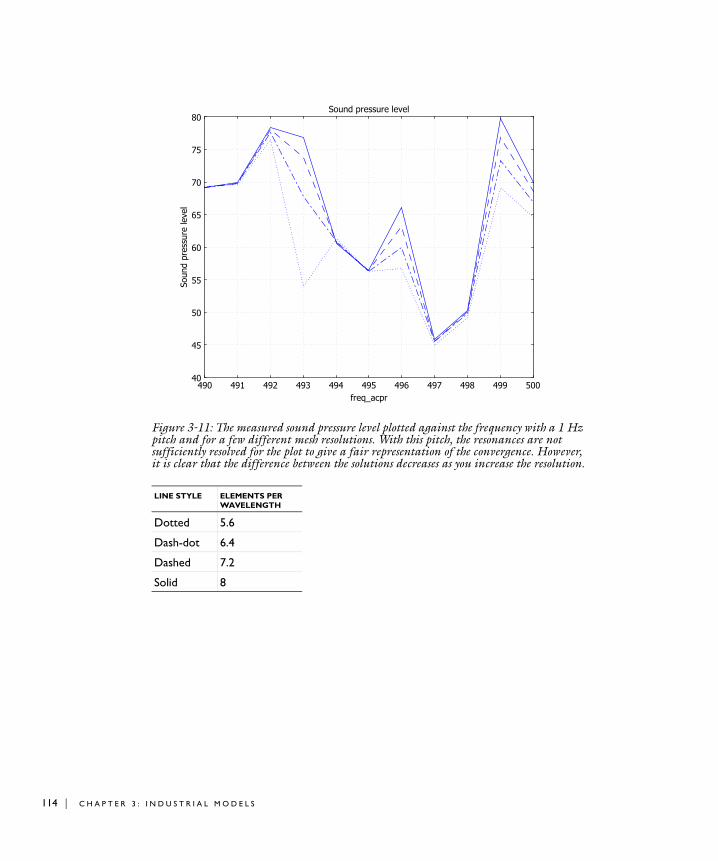
114 | C H A P T E R

Figure 3-11: The measured sound pressure level plotted against the frequency with a 1 Hz pitch and for a few different mesh resolutions. With this pitch, the resonances are not sufficiently resolved for the plot to give a fair representation of the convergence. However, it is clear that the difference between the solutions decreases as you increase the resolution.

LINE STYLE ELEMENTS PER WAVELENGTH

Dotted 5.6

Dash-dot 6.4

Dashed 7.2

Solid 8


F l ow Du c t

Introduction

The modeling of aircraft-engine noise is a central problem in the field of computational aeroacoustics. In this example you simulate the harmonically time-varying acoustic field from a turbofan engine under various conditions and calculate the attenuation of the acoustic noise made possible by introducing a layer of lining inside the engine duct.

Model Definition

Assume that the flow in the axisymmetric duct is compressible, inviscid, perfectly isentropic, and irrotational. In terms of variables made dimensionless by division by suitable combinations of a reference duct radius, , a reference speed of sound, , and a reference density, , it is described by

Here is the density, equals the velocity, denotes the pressure, equals the speed of sound, and γ is the constant ratio of the specific heats at constant pressure and volume.

Because the flow is irrotational, you can describe the velocity field, , in terms of a potential, , defined by the equation . The basic time- and space-dependent variables describing the flow are then the velocity potential and the density, . These variables (and the velocity field itself) are split into a stationary mean-flow part and a harmonically time-varying acoustic part:

Also assume that the amplitudes of the acoustic variables are small compared to the corresponding mean-flow quantities. This allows for a linearization of the equations of

R∞ c∞ρ∞

ρ∂t∂

------ ∇ ρv( )⋅+ 0=

ρ v∂t∂

------ v ∇v⋅+⎝ ⎠⎛ ⎞ ∇p+ 0=

γp ργ

= c2 pd

ρd------- ρ

γ 1–= =

ρ v p c

v v r z t, ,( )=

φ v ∇φ=

ρ

φ Φ φeiωt+= v V v eiωt

+= ρ ρ ρ aeiωt+=

F L O W D U C T | 115

116 | C H A P T E R

motion and the equation of state, and it extends the mean-flow + acoustic split to the pressure:

In particular, the linearized equations for the acoustic variables are

The duct geometry used in this model, depicted in Figure 3-12, is taken from Ref. 1. It is an approximate model of the inlet section of a turbofan engine in the very common CFM56 series.

Figure 3-12: The duct geometry.

The spinner and duct-wall profiles are given, respectively, by the equations

where , and L = 1.86393 is the duct length. A noise source is imposed at z' = 0, henceforth referred to as the source plane. This is where the fan would be located in the actual engine geometry. The plane z = L corresponds to the fore end of the engine and is referred to as the inlet plane.

p P p eiωt+=

iωρa ∇ ρ φ∇– ρaV+( )⋅+ 0=

ρ iωφ V φ∇⋅+( ) p=

p C2ρa=

R1 z′( ) max 0 0.64212 0.04777 0.98234 z′2+( )1 2⁄

–,[ ]=

R2 z′( ) 1 0.18453 z′2– 0.10158 e 11 1 z ′–( )– e 11––

1 e 11––

------------------------------------------+=

0 z' z L⁄ 1≤=≤


For the reference quantities in this model, choose the duct radius, the mean-flow speed of sound, and the mean-flow density at the source plane. Hence, all three of these quantities take the value 1.

To facilitate the COMSOL Multiphysics modeling, add a set of auxiliary domains to the geometry:

• A cylindrical domain—adjoined at the inlet plane and extending to the terminal plane, z = 2.86393—extends the modeling domain into a region where you can consider the mean flow as being uniform. This allows you to impose the simple boundary condition of a constant velocity potential and a vanishing tangential velocity for the background flow at the terminal plane.

• PML domains, adjoined at the source and terminal planes, allow you to conveniently implement non-reflecting boundary conditions for the aeroacoustic field. At the source plane, the PML domain is split into three annular sections with the innermost and outermost sections damping both in the axial and radial directions, while the central one is damping only in the axial direction.

The remaining boundary conditions for the mean flow consist of a natural boundary condition specifying the mass-flow rate through the source plane via the normal velocity and the density; slip conditions (vanishing tangential velocity) at the duct wall and at the spinner; and axial symmetry at r = 0.

For the aeroacoustic field, the model considers two different boundary conditions at the duct wall:

• Sound hard—the normal component of the acoustic particle velocity vanishes at the boundary.

• Impedance—the normal component of the acoustic particle velocity is related to the particle displacement through the equation

where Z is the impedance. This boundary condition, first derived by Myers (Ref. 2), was later recast in a weak form by Eversman (Ref. 3); it is this weak version, which is directly suitable for finite element modeling, that is implemented in the Aeroacoustics application mode of the COMSOL Multiphysics Acoustics Module. The impedance boundary condition represents a lined duct wall. In this model, following Ref. 1, the impedance is taken to be Z = 2 − i.

The spinner, in contrast, is always assumed to be acoustically hard.

iω v n⋅( ) iω V ∇⋅ n n V∇⋅( )⋅( )–+[ ] pZ----⎝ ⎠⎛ ⎞=

F L O W D U C T | 117

118 | C H A P T E R

This study examines two cases for the mean-flow normal velocity component at the source plane, Vz, which (owing to the choice of reference speed) alternatively can be referred to as the source-plane axial Mach number, M: M = − 0.5, approximately representative of a passenger aircraft at cruising speed, and M = 0.

The dimensionless angular frequency (nondimensionalized through division by ) is ω = 16, and the circumferential mode number is m = 10. If you want to

obtain a deeper understanding of the duct’s aeroacoustic characteristics, you can, of course, perform a systematic exploration of parameter space by varying these quantities independently.


T H E M E A N - F L OW F I E L D

For the nontrivial case of a source-plane axial Mach number of M = −0.5, the resulting mean-flow field appears in Figure 3-13. Note, in particular, that the velocity potential is uniform well beyond the terminal plane, thus justifying the boundary condition imposed there. Furthermore, as could be expected, deviations from the mean density

R∞ c∞⁄


value appear primarily near the nonuniformities of the duct geometry, such as at the tip of the spinner.

Figure 3-13: Mean-flow velocity potential and density for source-plane Mach number M = −0.5.

As a complement, a more quantitative picture of the variations of the mean-flow velocity and density profiles along the axial direction appear in the cross-section plots in Figure 3-14.

F L O W D U C T | 119

120 | C H A P T E R

Figure 3-14: Mean-flow cross-section plot at a sample radius of 0.8.

T H E N O I S E S O U R C E

With the solution for the mean-flow field at hand, it is possible to calculate the corresponding eigenmodes for the acoustic field at the source plane. Figure 3-15 shows the resulting velocity-potential profile for the lowest mode. This is the boundary mode used as the source of the acoustic noise field in the duct for the case M = −0.5.


Figure 3-15: The first axial boundary mode at the source plane (z = 0) for the case of a background flow with Mach number M = −0.5.

T H E A E R O A C O U S T I C F I E L D

The pressure fields for the case without a background mean flow, depicted in Figure 3-16, very closely match those for the corresponding FEM solutions presented in Figure 6 of Ref. 1. Similarly, the results for the attenuation between the source and

F L O W D U C T | 121

122 | C H A P T E R

inlet planes in the lined-wall case are in good agreement: 50.3 dB for the COMSOL Multiphysics solution versus 51.6 dB for the FEM solution in Ref. 1.

Figure 3-16: Acoustic pressure field for the cases of hard (top) and lined (bottom) duct wall with no mean flow and at circumferential mode number m = 10 and angular frequency ω = 16.

Turning to the case with a mean flow, the pressure field for the hard-wall case in the upper image of Figure 3-17 closely resembles the FEM solution obtained by Rienstra and Eversman in Ref. 1. For the lined-wall case in the lower image, although the agreement is still quite good, you can note some differences, especially near the source plane. This observation extends to the attenuation, for which the calculated value of 22.0 dB differs significantly from the value of 27.2 dB obtained in Ref. 1.


Figure 3-17: Acoustic pressure distribution for the cases of hard (top) and lined (bottom) duct wall with mean flow (M = −0.5) and at circumferential mode number m = 10 and angular frequency ω = 16.

However, these discrepancies have a natural explanation: the source mode in the COMSOL Multiphysics calculation was derived for the case of a hard duct wall, whereas Rienstra and Eversman used a noise source adapted to the acoustic lining. The lowest mode for the lined-wall case is a linear combination of the two forward-propagating hard-wall modes. Thus, the noise source term used to obtain the FEM solution in the lower half of Figure 3-17 is not optimally adapted to the duct, and it is consequently not maximally attenuated.

F L O W D U C T | 123

124 | C H A P T E R


The model involves three application modes, the last of which is used twice:

• Compressible Potential Flow (acpf)—for modeling the mean-flow velocity field

• Aeroacoustics, Boundary modal analysis (acab)—for calculating the boundary eigenmode to be used as the source of the acoustic noise in the mean-flow background

• Aeroacoustics, Time-harmonic analysis (acae, acae2)—for modeling the acoustic field above and below the source plane

After an initial modeling stage—consisting of creating the geometry and the mesh, then defining expressions and variables—you proceed by solving the model of the aero-engine duct in a mean-flow background in three steps. Thereafter you repeat part of the procedure in order to derive the corresponding solution in the absence of a background flow.

References

1. S.W. Rienstra and W. Eversman, “A Numerical Comparison Between the Multiple-Scales and Finite-Element Solution for Sound Propagation in Lined Flow Ducts,” J. Fluid Mech., vol. 437, pp. 367–384, 2001.

2. M.K. Myers, “On the Acoustic Boundary Condition in the Presence of Flow,” J. Sound Vib., vol. 71, pp. 429–434, 1980.

3. W. Eversman, “The Boundary Condition at an Impedance Wall in a Non-Uniform Duct with Potential Mean Flow,” J. Sound Vib., vol. 246, pp. 63–69, 2001. Errata: ibid, vol. 258, pp. 791–792, 2002.

Model Library path: Acoustics_Module/Industrial_Models/flow_duct



Initial Stage—Geometry, Mesh, and Common Settings


1 In the Model Navigator go to the Space dimension list and select Axial symmetry (2D), then click Multiphysics.

2 From list of application modes select Acoustics Module>Aeroacoustics>Boundary modal analysis. In the Dependent variables edit field type phi_b, then click Add.

3 From the list of application modes select Acoustics Module>Aeroacoustics with flow, then click Add.

4 From the list of application modes select Acoustics Module>Aeroacoustics>Time-harmonic analysis. In the Dependent variables edit field type phi2, then click Add.



First import the duct geometry, which is supplied in the form of an mphbin file:

1 Choose File>Import>CAD Data From File, browse to the folder Acoustics Module/Industrial Models, select the file flow_duct.mphbin, and click Import.

Next attach rectangles at the inlet and outlet. These are not part of the duct but allow you to implement the appropriate boundary conditions using perfectly matched layers (PMLs).

2 If the SNAP field on the Status bar at the bottom of the workspace is not already selected, double-click to select it.

3 Choose Draw>Draw Objects>Rectangle/Square or click the corresponding button at the top of the Draw toolbar. In the drawing area click at the top right corner of the duct and drag to the point (r = 0, z = 3).

4 With the rectangle (R1) that you just created still selected, choose Draw>Object Properties to open the Rectangle dialog box. In the Height edit field type 0.2, then click OK.

5 Click the Rectangle/Square button on the Draw toolbar. In the drawing area click at the bottom left corner of the duct and drag to the point (r = 1, z = −0.5).

F L O W D U C T | 125

126 | C H A P T E R

6 With the rectangle (R2) that you just created still selected, choose Draw>Object Properties. In the Height edit field type 0.2, and in the z edit field type -0.2. Click OK.

7 Click the Rectangle/Square button on the Draw toolbar. In the drawing area click at the bottom left corner of rectangle R2 and drag to the origin (r = 0, z = 0).

8 With the rectangle (R3) that you just created still selected choose Draw>Object Properties. In the Width edit field type 0.2, and in the r edit field type 0.223557. Click OK.

9 Click the Rectangle/Square button on the Draw toolbar. In the drawing area click at the bottom right corner of rectangle R2 and drag to the point (r = 1.5, z = 0).

10 With the rectangle (R4) that you just created still selected, choose Draw>Object Properties. In the Width edit field type 0.2. Click OK.

11 Click the Zoom Extents button on the Main toolbar to get a proper overview of the duct geometry, which should look like the one in Figure 3-18.

Figure 3-18: The axisymmetric duct geometry with auxiliary PML domains (R1–R4).


1 Choose Mesh>Mapped Mesh Parameters, then in the resulting dialog box go to the Boundary page.


2 Select Boundary 7. Select the Constrained edge element distribution check box, and in the Number of edge elements edit field type 40.

3 Repeat the procedure in Step 2 using the data in the following table:


5 Click the Mesh All (Mapped) button on the Mesh toolbar to generate the mesh. The result should look like that in Figure 3-19.

Figure 3-19:The meshed geometry.

Note that the mesh you just created is significantly denser than required to accurately model the background flow. However, in order to resolve the acoustic perturbations—which appear on a smaller scale—it is necessary to use a fine mesh.

BOUNDARIES NUMBER OF EDGE ELEMENTS

22, 61, 98, 99 18

60 60

1 39

2 1

44–59, 62–65 2

8–19, 23–39, 66–94 3

40, 95 5

F L O W D U C T | 127

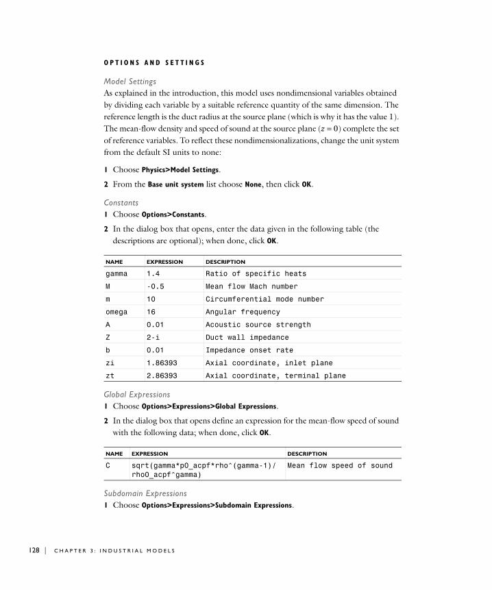
128 | C H A P T E R


Model SettingsAs explained in the introduction, this model uses nondimensional variables obtained by dividing each variable by a suitable reference quantity of the same dimension. The reference length is the duct radius at the source plane (which is why it has the value 1). The mean-flow density and speed of sound at the source plane (z = 0) complete the set of reference variables. To reflect these nondimensionalizations, change the unit system from the default SI units to none:

1 Choose Physics>Model Settings.

2 From the Base unit system list choose None, then click OK.

Constants1 Choose Options>Constants.

2 In the dialog box that opens, enter the data given in the following table (the descriptions are optional); when done, click OK.

Global Expressions1 Choose Options>Expressions>Global Expressions.

2 In the dialog box that opens define an expression for the mean-flow speed of sound with the following data; when done, click OK.

Subdomain Expressions1 Choose Options>Expressions>Subdomain Expressions.


gamma 1.4 Ratio of specific heats

M -0.5 Mean flow Mach number

m 10 Circumferential mode number

omega 16 Angular frequency

A 0.01 Acoustic source strength

Z 2-i Duct wall impedance

b 0.01 Impedance onset rate

zi 1.86393 Axial coordinate, inlet plane

zt 2.86393 Axial coordinate, terminal plane


C sqrt(gamma*p0_acpf*rho^(gamma-1)/ rho0_acpf^gamma)

Mean flow speed of sound


2 Define variables with the scope, name, and expressions from the following table; when done, click OK.

Boundary Expressions1 Choose Options>Expressions>Boundary Expressions.

2 Select Boundary 43, then define an expression for the source mode’s intensity component normal to the source boundary according to the following table:

This expression is the acab application mode’s equivalent of Iz in Table 6-3 on page 121 of the Acoustics Module User’s Guide. The expression involves a constant kz for the out-of-plane wave number that you specify later. It is convenient to introduce this constant here instead of using the application scalar variable ikz_acab set equal to i*kz. This is because ikz_acab must take its default value -lambda when you solve for the boundary mode, and you would therefore have to change its value back and forth repeatedly between the various modeling stages.

3 Click OK to close the Boundary Expressions dialog box.

Because the definition of the boundary mode’s acoustic pressure variable, p_acab, involves ikz_acab, you must additionally modify its expression as follows:

4 From the Physics menu, choose Equation System>Boundary Settings.

5 In the Boundary Settings - Equation System dialog box, click the Variables tab.

6 With Boundary 43 still selected, edit the Expression for p_acab by replacing ikz_acab with i*kz.

7 Click OK to close the Equation System>Boundary Settings dialog box.

Note that p_acab is just a postprocessing variable, so changing its expression does not affect the solution.

Boundary VariablesDefine some expressions that you later use to extend the mean-flow density and velocity variables to the upper PML domain by means of extrusion from the terminal plane at z = 2.86393. Do so by executing the following instructions:

SUBDOMAINS NAME EXPRESSION

4–6 rho rho0_acpf

5 V M

NAME EXPRESSION

Iz_source A^2*0.5*real((p_acab/rho0_acpf+Vr_acab*vr_acab-Vz_acab *i*kz*phi_b)*conj(rho*Vz_acab-rho0_acpf*i*kz*phi_b))

F L O W D U C T | 129

130 | C H A P T E R

1 Choose Options>Extrusion Coupling Variables>Boundary Variables.

2 Go to the Source page. Select Boundary 6, then define variables with the following data:

3 Click the Destination tab.

4 In the Level list select Subdomain, and in the Variable list select V.

5 In the Subdomain selection list select the check box next to Subdomain 3. The Use selected subdomains as destination check box is then automatically selected.

6 From the Variable list select rho, then select the Use selected subdomains as

destination check box.

7 Click OK.

Next define two integration coupling variables that evaluate to the input acoustic power produced by the noise source and the power through the inlet plane.


2 Enter the data given in the following table below, leaving the Global destination check box selected (the default) for both variables; when done, click OK.

Scalar Expressions1 Choose Options>Expressions>Scalar Expressions.

2 In the dialog box that opens define an expression for the acoustic attenuation with the following data; when done, click OK.


Application Mode Properties1 Choose Physics>Scalar Variables to open the Application Scalar Variables dialog box.

NAME EXPRESSION TRANSFORMATION

V vz_acpf General

rho rho General

BOUNDARY NAME EXPRESSION

43 w_source Iz_source

4 w_inlet Iz_acae


dw 10*log10(w_source/w_inlet) Acoustic attenuation (dB)


2 With the Synchronize equivalent variables check box selected, modify the variables according to the following table; when done, click OK.

Stage I—The Background FlowIn this modeling stage you derive the stationary background on which propagate the time-harmonic acoustic perturbations that you model in Stage III. You calculate this flow field using the Compressible Potential Flow application mode defined on the duct geometry proper (Subdomain 1) and on the auxiliary region (Subdomain 2) appended at the inlet plane (z = 1.86393), and subsequently extend the flow to the PML domains by continuity. A mass-flow boundary condition is imposed at the source plane, and a Dirichlet condition for the velocity potential is applied at the terminal plane (z = 2.86393). The duct wall and the spinner are both impervious to the flow.


Subdomain Settings1 In the Multiphysics menu select Compressible Potential Flow (acpf).


3 In the Subdomain selection list select Subdomains 1–2, then type gamma in the γ edit field.

4 In the Subdomain selection list select Subdomains 3–6, then clear the Active in this domain check box.

5 Click OK.


2 In the Boundary selection list select Boundaries 1 and 3.

3 From the Boundary condition list choose Axial symmetry.

4 Select Boundary 6 (the terminal plane), and as the Boundary condition select Normal flow.

NAME EXPRESSION

freq_acab omega/(2*pi)

m_acab 10

p0_acpf rho0_acpf^gamma/gamma

rho0_acpf 1

v0_acpf M

F L O W D U C T | 131

132 | C H A P T E R

5 Select Boundary 43 (the source plane), and as the Boundary condition select Mass flow. Leave the Normal velocity and Fluid density edit fields at their default values.

6 Click OK.


1 Choose Solve>Solver Manager or click the corresponding button on the Main toolbar. Either action opens the Solver Manager dialog box.

2 Click the Solve For tab.

3 In the Solve for variables list select Compressible Potential Flow (acpf), then click Apply.

4 Choose Solve>Solver Parameters (or click the corresponding button on the Main toolbar) to open the Solver Parameters dialog box.

5 From the Solver list select Stationary, then click OK.

6 Return to the Solver Manager dialog box and click Solve.

7 On the Initial Value page, click the Store Solution button.

8 Click OK.


First zoom in on the interesting part of the geometry.

1 Choose Options>Suppress>Suppress Subdomains.

2 From the Subdomain selection list select Subdomains 3–6, then click OK.


Next visualize the mean-flow field.


2 On the General page, go to the Plot type area and select only the Surface, Contour, and Geometry edges check boxes.

3 On the Surface page go to the Predefined quantities list and select Compressible

Potential Flow (acpf)>Density (alternatively, type rho in the Expression edit field).

4 On the Contour page go to the Predefined quantities list and select Compressible Potential Flow (acpf)>Velocity potential.

5 On the General page click the Title button.

6 Click the option button next to the edit field and enter the title Surface: density Contour: velocity potential (M=-0.5).


7 Click OK to close the Title dialog box, then click OK to close the Plot Parameters dialog box and generate the plot presented in Figure 3-13 on page 119.

To get a detailed view of the density and velocity profiles along the length of the duct, proceed as follows:

1 Choose Postprocessing>Cross-Section Plot Parameters.

2 On the General page select the Keep current plot check box and clear the Display cross-section in main axes check box

3 Click the Line/Extrusion tab.

4 In the y-axis data area, find the Expression edit field and enter rho.

5 In the x-axis data area, select z from the list next to the upper option button.

6 In the Cross-section line data area, modify the coordinate values according to the following table; when done, click Apply.

7 In the y-axis data area, go to the Expression edit field and type -vz_acpf.

8 Click the Line Settings button.

9 From the Line color list, select Color, then in the Line style list select Dashed line. Click OK to close the Line Settings dialog box.

10 In the Cross-Section Plot Parameters dialog box, click the General tab.

11 Click the Title/Axis button to open the Title/Axis Settings dialog box.

12 Click the option button next to the Title edit field and enter the text Mean flow cross-section plots at r=0.8.

13 Click the option button next to the Second axis label edit field and enter the text Density (solid) axial Mach number (dashed).

14 Click OK to close the Title/Axis Settings dialog box, then click OK to close the Cross-Section Plot Parameters dialog box. Doing so generates the graphs in Figure 3-14 on page 120.

Stage II—The Boundary Source ModeAs the source generating the acoustic field in the duct, use a single boundary mode imposed at z = 0. More specifically, take this mode to be the lowest propagating axial mode in the duct computed in the background flow field from the previous stage of

r0, r1 0.8

z1 1.86393

F L O W D U C T | 133

134 | C H A P T E R

the modeling process. The subsequent instructions demonstrate how to derive this boundary mode.


Boundary Conditions1 In the Multiphysics menu select Aeroacoustics, Boundary Modal Analysis (acab).


3 In the Boundary selection list select Boundary 43.

4 In the left and right parts of the V edit field type vr_acpf and vz_acpf, respectively.

5 In the cs edit field type C, and in the ρ edit field type rho.

6 Select Boundary 40, then select the Select by group check box and clear the Active in this domain check box.

7 Click OK.


1 Click the Solver Manager button on the Main toolbar to open the Solver Manager dialog box.

2 On the Initial Value page select the Stored solution option button in both the Initial

value area and the Values of variables not solved for and linearization point area.


4 In the Solve for variables list select Aeroacoustics, Boundary Modal Analysis (acab), then click Apply.

5 Click the Solver Parameters button on the Main toolbar to open the Solver

Parameters dialog box.

6 From the Solver list select Eigenvalue.

7 In the Desired number of propagation constants edit field type 8, and in the Search for

propagation constants around edit field type 10.

8 Click OK to close the Solver Parameters dialog box.

9 Return to the Solver Manager dialog box and click Solve.

10 Go to the Initial Value page and click the Store Solution button to open the Store

Solution dialog box.

Inspect the Propagation constant list and notice that there are four solutions with a purely real propagation constant, three of them positive and one negative. In other words, there are four propagating waves, three of which propagate in the positive


z direction and one in the opposite direction. The strong background flow has shifted the propagation constants, which in the absence of a mean flow would be symmetrically distributed around zero.

In the subsequent modeling stage, you will use the value of the largest positive propagation constant (≈27.12) and the absolute value of the single negative propagation constant (≈5.778); these propagation constants correspond to the lowest forward-propagating and backward-propagating modes, respectively.

11 Select the last entry from the Propagation constant list to store the solution corresponding to the lowest forward-propagating mode. Click OK.

12 Choose Options>Constants and add the following entries to the list of constants:

(In the expression column, preferably use the exact values you obtained for the propagation constants, although they should be quite close to those displayed here.)

13 Click OK to close the Solver Manager dialog box.


To verify that you have found the lowest axial mode, plot the boundary mode velocity potential as follows:


2 On the General page select the last entry in the Solutions to use list.

3 From the Plot in list select New figure, then select the Keep current plot check box.

4 Click the Title/Axis button, then select the option button next to the Title edit field. Enter the text First axial mode at source plane (z=0). Click OK.

5 On the Line/Extrusion page go to the Boundary selection list and select Boundary 43.

6 In the x-axis data area select r from the list next to the upper option button. In the y-axis data area keep the default variable choice, phi_b.

7 Click OK to close the dialog box and generate the plot in Figure 3-15 on page 121.

Stage III—The Acoustic FieldEquipped with the solution derived in the two previous stages, you can now go on to simulate the acoustic field. You model the noise source through the judicious choices


kz 27.123744 Axial propagation constant

kzr 5.778166 Axial propagation constant, reflected mode

F L O W D U C T | 135

136 | C H A P T E R

of boundary conditions at the source plane (z = 0) for the two time-harmonic Aeroacoustics application modes. Furthermore, implement non-reflecting boundary conditions at both ends of the duct geometry by using the auxiliary PML domains that you added to the model earlier in the geometry creation steps.

Here are the detailed instructions for the procedure.



2 Add a constant with the name pmax defined by the expression 1.500211.

3 Click OK.


Subdomain Settings—Aeroacoustics (acae)1 In the Multiphysics menu select Aeroacoustics (acae).


3 In the Subdomain selection list select Subdomains 4–6, then clear the Active in this domain check box.

4 Select Subdomains 1–3, then in the cs edit field type C.

5 Select Subdomain 3 only.

6 In the left part of the V edit field type 0, and in the right part type V.

7 Click the PML tab.

8 In the Type of PML list select Cylindrical.

9 Select the Absorbing in z direction check box. Specify the PML width in this direction by typing 0.2 in the corresponding edit field.

10 In the Lz edit field type 2*pi/kz to specify the scaled PML length.

11 Click OK.

Subdomain Settings—Aeroacoustics (acae2)1 In the Multiphysics menu select Aeroacoustics (acae2).


3 Select Subdomains 1–3, then clear the Active in this domain check box.

4 Select Subdomains 4–6.

5 In the cs edit field type C, and in the ρ edit field type rho.


6 Select Subdomain 5 by itself.

7 In the right-hand part of the V edit field type V, and in the left-hand part leave the default value, 0.

8 Click the PML tab.

9 In the Type of PML list select Cylindrical.

10 Select the Absorbing in z direction check box and type 0.2 in the corresponding edit field.

11 In the Lz edit field type 2*pi/kzr.

12 Select the two Subdomains 4 and 6.

13 From the Type of PML list select Cylindrical.

14 Select both the Absorbing in r direction and the Absorbing in z direction check boxes, then type 0.2 in the corresponding edit fields.

15 In both the Lr and Lz edit fields enter 2*pi/kzr.

16 Select Subdomain 4 only, then in the R0 edit field type 0.223557.

17 Click OK.


2 Select Boundary 43.

3 In the Boundary condition list select Velocity potential.

4 In the 0 edit field type phi-A*phi_b, then click OK.

5 Choose Physics>Properties to open the Application Mode Properties dialog box.

6 In the Weak constraints list select On, then click OK.

7 In the Multiphysics menu select Aeroacoustics (acae).


9 With Boundary 43 still selected, go to the Boundary condition list and select Normal mass flow. Then in the mn edit field type rho*(-i*kz*A*phi_b).

10 Select Boundaries 1, 3, and 5, then in the Boundary condition list select Axial symmetry.

11 Click OK.


1 Click the Solver Manager button on the Main toolbar.


φ

F L O W D U C T | 137

138 | C H A P T E R

3 In the Solve for variables list select both Aeroacoustics (acae) and Aeroacoustics

(acae2), then click OK.





Zoom in on the duct geometry proper, that is, Subdomain 1.


2 Select Subdomains 2–6, then click OK.


Next visualize the aeroacoustic field.


2 On the General page clear the Surface check box.


4 In the Expression edit field type p_acae/pmax.

5 Select the Vector with isolevels option button, then type the following vector in the corresponding edit field: 0.0001 0.001 0.01 0.02 0.04 0.06 0.1 0.2 0.3 0.4 0.5 0.6 0.7 0.8 0.9.

6 In the Colormap list select hsv, then click Apply.

7 Click the General tab.

8 Select the Keep current plot check box, and then return to the Contour page.

9 In the Colormap list select jet.

10 Select the Filled check box, then click Apply.


12 Select the check box next to the edit field and enter the title Hard wall, flow.

13 Click OK to close the Title dialog box, then click OK to close the Plot Parameters dialog box.

In the drawing area of the COMSOL Multiphysics user interface you should now see the upper image in Figure 3-17 on page 123, which shows the acoustic field in a mean-flow field of axial Mach number −0.5 for the case of a hard duct wall.


Next change the model to that of a duct with a lined wall by implementing an impedance boundary condition. Begin by adjusting the value of pmax so as to obtain a normalized plot.



2 Change the value of pmax to 1.718862, then click OK.



2 Select Boundaries 44–59 and 62–95.

3 From the Boundary condition list select Impedance boundary condition.

4 In the Z edit field type Z/flc2hs(z/zi,b).

5 Select Boundary 60 by itself, then from the Boundary condition list select Impedance

boundary condition.

6 In the Z edit field type Z/flc2hs((zt-z)/(zt-zi),b), then click OK.

The reason behind using the smoothed Heaviside function flc2hs in Steps 4 and 6 above is to make the impedance a continuous (albeit abruptly changing) function across the interfaces between regions with and without an acoustic lining. This is a condition required for the equivalence of Myers’s original impedance boundary condition and its weak reformulation due to Eversman used here to hold (see Ref. 3).





2 On the General page clear the Keep current plot check box.


4 In the Colormap list select hsv.

5 Clear the Filled check box, then click Apply.


F L O W D U C T | 139

140 | C H A P T E R

7 Select the Keep current plot check box, then return to the Contour page.




11 Change the text in the title edit field to Lined wall, flow, then click OK to close the Title dialog box.

12 Click OK to close the Plot Parameters dialog box.

The plot in the main window should now closely resemble the lower image in Figure 3-17.

With a lined duct wall, the acoustic perturbations emanating from the noise source no longer propagate without loss. To display the acoustic attenuation between the source plane and the inlet plane at z = 1.86393, execute the following commands:


2 In the Expression edit field type dw, then click OK.

The value for the current solution of this previously defined expression—approximately 22.0 dB—now appears in the Message log at the bottom of the COMSOL Multiphysics user interface.

Note: The source mode used in these calculations was derived for the case of a hard duct wall, whereas the lowest mode for the lined-wall case would be a linear combination of the two forward-propagating hard-wall modes. For this reason, the noise source is not an eigenmode and is, consequently, not maximally attenuated. This observation is borne out by a comparison of the calculated attenuation of 22.0 dB with the corresponding quantity calculated in Ref. 1, where a value of approximately 27 dB was obtained.

The Case Without a Background FlowFollow these instructions to repeat the calculations for the case when no background mean-flow field is present.



ConstantsChoose Options>Constants. Change the value of M to 0, then click OK.



2 On the Solve For page go to the Solve for variables list and select Compressible

Potential Flow (acpf).

3 Click the Initial Value tab.

4 In the Initial value area select the Initial value expression option button.

5 In the Values of variables not solved for and linearization point area, select the Use selection from Initial value frame option button.

6 Click the Solve button, then click the Store Solution button.

7 Select the Stored solution option button in both the Initial value area and the Values of variables not solved for and linearization point area.

8 Go back to the Solve For page and select Aeroacoustics, Boundary Modal Analysis

(acab), then click Apply.

9 Click the Solver Parameters button, select Eigenvalue from the Solver list, then click OK to close the Solver Parameters dialog box.

10 Return to the Solver Manager dialog box and click the Solve button.

11 Go to the Initial Value page and click the Store Solution button.

12 Return to the main user interface and from the Options menu open the Constants dialog box.

13 Change the expressions for both kz and kzr to the value of the last entry in the Propagation constant list, which should be approximately 10.83. Click OK.

14 Return to the Store Solution dialog box and from the Propagation constant list select the last entry (with a value of the propagation constant approximately equal to 10.83). Click OK.

15 Click OK to close the Solver Manager dialog box.

Having computed and saved the mean-flow-free background and boundary mode solution, turn next to the calculation of the acoustic field.

F L O W D U C T | 141

142 | C H A P T E R






2 From the Boundary selection list select Boundary 44.

3 Select the Select by group check box, then in the Boundary condition list select Sound hard boundary (wall).

4 Select Boundary 60, then in the Boundary condition list select Sound hard boundary

(wall).

5 Click OK.



2 On the Solve For page go to the Solve for variables list and select both Aeroacoustics

(acae) and Aeroacoustics (acae2). Click OK.






2 On the General page clear the Surface check box.










11 Select the check box next to the edit field and enter the title Hard wall, no flow.

12 Click OK to close the Title dialog box, then click OK to close the Plot Parameters dialog box.

A plot similar to the one in the upper half of Figure 3-16 on page 122 should now appear in the drawing area. It depicts the acoustic field in the duct in the absence of a background mean flow and for the case of a hard duct wall.

As the fourth and final case of study, consider a lined duct wall in the absence of a background flow.






2 Select Boundaries 44–59 and 62–95, then in the Boundary condition list select Impedance boundary condition.

The expression Z/flc2hs(z/zi,b) should appear in the Z edit field.

3 Select Boundary 60, then in the Boundary condition list select Impedance boundary

condition.

Now the expression in the Z edit field should read Z/flc2hs((zt-z)/(zt-zi),b).

4 Click OK.





2 On the General page clear the Keep current plot check box.



F L O W D U C T | 143

144 | C H A P T E R







11 Change the text in the edit field to Lined wall, flow, then click OK to close the Title dialog box.

12 Click OK.

The plot in the main window should now closely resemble the lower one in Figure 3-16.

Finally display the value of the acoustic attenuation. To do so, choose Postprocessing>Data Display>Global, then click OK.

The value of dw—for this case approximately 50.3 dB—should appear in the Message log at the bottom of the user interface.

Note: In contrast to the attenuation calculated for the case of a mean-flow background in the first part of this exercise, the latest value is quite close to that in Ref. 1 (51.6 dB). The reason is that both use the same source mode as a result of the fact that there is a single forward-propagating mode in the flow-free case, thus making the two calculations directly comparable.


L oud s p e ak e r D r i v e r

Introduction

This is a model of a loudspeaker of the dynamic cone driver type, common for low and medium frequencies. The instructions walk you through modeling its electromagnetic, structural, and acoustic properties. The output from the model includes the total electric impedance and the on-axis sound pressure level at a nominal driving voltage, as functions of the frequency.

When performing the acoustic measurements in this model, the driver is set up in an infinite baffle—a wide reflective surface acting to shut out the sound produced on the backside of the cone. An extended 3D version of the model, “Loudspeaker Driver in a Vented Enclosure” on page 175, uses the electromechanical properties modeled here and adds a vented enclosure.

The model starts out with the Small-Signal analysis from the AC/DC Module to compute the driving force and the blocked voice coil impedance. It then uses these results and adds application modes from the Acoustics Module for the acoustic-structure analysis. As an optional final modeling step, you can choose to extract and export the data needed for the 3D model.

Model Definition

Figure 3-20 shows the geometry of the baffled driver with its functional parts. The field from the magnet is supported and focused by the iron pole piece and top plate to the thin gap where the voice coil is wound around a former extending from the apex of the cone. Although the voice coil consists of many turns of wire, it is for simplicity modeled as a homogenized domain. When a driving AC voltage is applied to the voice coil, the resulting force causes it to vibrate, and the cone to create sound.

The dust cap protects the magnetic motor. In this design, it is made of the same stiff and light composite material as the cone and also contributes to the sound. A centered hole in the pole piece counteracts pressure buildup beneath the dust cap. The suspension, consisting of the surround, made of a light foam material, and the spider, a flexible cloth, keep the cone in place and provide damping and spring forces.

The outer perimeters of the magnet and suspension are normally attached to a basket, a hollow supporting metal structure. The basked is not included in this model, but the

L O U D S P E A K E R D R I V E R | 145

146 | C H A P T E R

magnet assembly and outer rims of the spider and surround are considered to be fixed. The omission of the basket means that the considered geometry is rotationally symmetric and can be modeled in the rz-plane.

Figure 3-20: Geometry of the modeled loudspeaker driver.

The loudspeaker is driven by a time-harmonic voltage, V = V0exp(iωt), applied to the voice coil. The following theory section first describes the electromagnetic analysis of the current in the voice coil and the driving force that this current gives rise to. Once the relation between the driving voltage and the force is established, the force is applied in an acoustic-structure interaction analysis set up to compute the sound production.

The force on a wire of length L and with the current I in a magnetic flux density B perpendicular to the wire is given by F = IBL. The voice coil consists of N = 100 turns of thin copper wire and occupies a cross-sectional area A in the rz-plane. The total force Fe from the current on the coil hence becomes

(3-1)

where the integral is taken over the coil domain.

The current through the voice coil relates to the applied voltage as

Magnet

Pole piece

Top plate

Voice coil

Spider

Baffle

SurroundDust capCone

Fe I–2πN

A------------ rBr Ad∫=


, (3-2)

where Zb is the blocked electric impedance (the electric impedance of the voice coil measured while the speaker’s moving parts are stationary) and −Vbe denotes the back EMF (the voltage induced in the coil due to its motion through the permanent magnetic field in the gap).

To evaluate the back EMF, consider the same wire of length L in the magnetic flux density B, but now traveling at a velocity v perpendicular to the wire. The wire gets an induced back EMF equal to vBL. The total back EMF in the coil becomes

(3-3)

The common factor in Fe and Vbe is known in the loudspeaker community as the force factor, “BL”:

. (3-4)

To find the blocked coil impedance, an external current density corresponding to a time-harmonic loop voltage of (V0 + Vi)/N is applied to the domain of the still stationary coil. The induced voltage Vi is computed as the calculated induced azimuthal electric field in the coil times the length of the wire. The blocked coil impedance, finally, is obtained as Zb = V0/Ib, where Ib is the current through the blocked coil.

With the constant BL and the frequency-dependent Zb now both known, Equations 3-1 to 3-4 can be rearranged to form the sought relationship between V0 and Fe:

(3-5)

Note the dependence of the driving force on the velocity of the moving coil, which is unknown prior to the acoustic-structure interaction computation.

In computing the acoustic-structure interaction, Fe is applied to the voice coil domain. A structural equation is solved in the moving parts of the driver, and a pressure acoustics equation in the surrounding air. The pressure acoustics equation uses a normal acceleration boundary condition for the structural vibrations to propagate into the air. Conversely, the acoustic pressure is applied as a boundary load on the structure.

I V0 Vbe+( ) Zb⁄=

V– be v–2πN

A------------ rBr Ad∫=

BL 2πNA

------------– rBr Ad∫=

Fe BLV0 BLv–

Zb-------------------------=


148 | C H A P T E R

The air domains and the baffle should ideally extend to infinity. To avoid unphysical reflections where you truncate the geometry, you will use Perfectly Matched Layers (PMLs), as seen in Figure 3-21. For more information, see “Perfectly Matched Layers (PMLs)” on page 37 in the Acoustics Module User’s Guide.

Figure 3-21: Overview of the model geometry with the structures in pink.

Although the modeled air domain has a radius of only 0.12 m, the local acoustic pressure can be extracted anywhere thanks to COMSOL’s functionality for far-field pressure computation. The sensitivity is calculated as the sound pressure level on the axis at 1 m, for the applied voltage V0 = 4 V.

As a final modeling step, results are extracted from this model for use as lumped parameters in the Vented Loudspeaker Enclosure. The documentation to that example contains a circuit representation of the force balance on the cone.


The magnetic flux density in and around the voice coil appears in Figure 3-22. The maximum flux density in the air arises in the gap between the pole piece and the top

Air

Air

PML

PML


plate. Performing the integral in Equation 3-4 over the voice coil domain gives a force factor BL = 7.55 N/A.

Figure 3-22: Magnetic flux density near the voice coil.

The iron in the pole piece and top plate is modeled as a nonlinear magnetic material, with the relationship between the B and H fields described by interpolation from measured data. Figure 3-23 shows the local effective relative permeability µr = B/(µ0H). The plot shows that the iron is close to saturation in the center of the pole piece, but remains in the linear regime above and below the magnet. This indicates that if you want to use less material, you can likely decrease the radius of the pole piece and top plate with very little effect on the magnetic field in the gap.


150 | C H A P T E R

Figure 3-23: The local relative permeability in the pole piece and top plate, when subjected to the field from the magnet.

In computing the blocked coil impedance, the AC equation is linearized around the local permeability resulting from the static solution. Figure 3-24 shows the induced currents at two different frequencies.

Figure 3-24: Induced currents in the pole piece and top plate, at 52 Hz (left) and 905 Hz (right).


At the higher frequency, the skin effect brings the currents closer to the surfaces. This causes the inductance as well as the resistive part of the impedance to change with the frequency. Figure 3-25 shows a plot of the blocked coil inductance versus frequency.

Figure 3-25: The inductance of the blocked coil as a function of frequency.

From the acoustic-structure interaction analysis, Figure 3-26 shows the sound pressure level distribution at 3500 Hz. A minimum has formed in a direction about 45 degrees above the baffle. At lower frequencies, the sound pressure level is rather evenly distributed but peaks in the on-axis direction.


152 | C H A P T E R

Figure 3-26: Sound pressure level distribution in dB at 3500 Hz.

Figure 3-27 presents the loudspeaker’s sensitivity. The preferred operating range is where the response is rather even, that is, roughly in the range 100 Hz–1500 Hz. A vented enclosure can extend the range to lower frequencies, as shown in the Vented Loudspeaker Enclosure model.


Figure 3-27: Loudspeaker sensitivity, measured as the on-axis sound pressure level (dB) at a distance of 1 m from the unit. The pressure is evaluated using an input signal of 4 V, or 2.83 V RMS, which corresponds to a power of 1 W at an 8 Ω. nominal impedance. Note the logarithmic frequency scale.

The total electrical impedance, defined as Z = V0/I, appears in Figure 3-28. The features of this plot are very characteristic of loudspeaker drivers. The peak at approximately 40 Hz coincides with the mechanical resonance; at this frequency the reactive part of the impedance switches sign from inductive to capacitive. In most of the operational range the impedance is largely resistive. Between 100 Hz and 1 kHz it varies only between 6.1 Ω and 8.3 Ω. These are typical values for speakers with a nominal impedance of 8 Ω, as the nominal impedance is usually taken to represent a mean value over the usable frequency range, which for this driver extends between somewhat below 100 Hz and above 1 kHz. At frequencies higher than 1 kHz, the impedance continues to increase as the inductance of the voice coil starts playing a more important part.


154 | C H A P T E R

Figure 3-28: Electrical impedance (Ω) of the loudspeaker as a function of frequency (Hz).


The step-by-step instructions takes you through the following steps:

• Perform a static analysis of the magnetic field distribution to evaluate the force factor, BL.

• Sweep the frequency in an AC analysis where you apply a time-harmonic voltage to the voice coil, to compute the blocked coil impedance, Zb.

• Use BL and Zb in an acoustic-structure interaction analysis computing the sound pressure level and total electrical impedance of the driver as functions of the frequency.

• (Optional): Prepare for the Vented Loudspeaker Enclosure model by performing a separate mechanical analysis of the suspension, exporting its frequency-dependent resistance and compliance as well as Zb.

The static magnetic field computation and the AC analysis use the Small-Signal Analysis multiphysics node available in COMSOL’s AC/DC Module. This node contains two application modes. First, the field from the magnet is computed in a static


application mode. The iron used in the pole piece and top plate is a nonlinear magnetic material, with interpolation data describing the relationship between the B and H fields. After solving this step of the model, you can evaluate BL by integrating the magnetic flux density over the voice coil domain.

The time-harmonic application mode in the small-signal analysis inherits the permeability distribution from the static application mode. For the time-harmonic assumption to be strictly valid, the applied AC voltage must be so small that the resulting current creates a magnetic field which does not significantly alter this permeability. Even though this is hardly the situation here, linearizing around a local biased permeability should still be a better approximation than assuming a constant permeability. The very most accurate way to compute the impedance would be in a fully transient analysis, which is outside the scope of this model.

The Acoustic-Structure Interaction multiphysics node features a structural Stress-Strain application mode for the moving structures and a Pressure Acoustics application mode for the air. It also provides the boundary conditions for the two-way acoustic coupling between the air and the structures.

In most loudspeaker specifications, the suspension is characterized by a mechanical compliance Cs and resistance Rs. In order to keep the resistance constant over a range of frequencies, the material needs to have a damping factor that increases linearly with the frequency or, equivalently, Rayleigh damping with and a constant βdK = η0/ω0, where η0 is the loss factor measured at the angular frequency ω0. In this model, the frequency where the loss factor is measured is chosen to be near the lowest mechanical resonance of the driver.

Model Library path: Acoustics_Module/Industrial_Models/loudspeaker_driver

Model Library path: Acoustics_Module/Industrial_Models/loudspeaker_suspension

αδM 0=


156 | C H A P T E R

Modeling Using the Graphical User Interface—Force Factor


1 In the Model Navigator go to the Space dimension list and select Axial symmetry (2D).

2 In the list of application modes select AC/DC Module>Quasi-Statics,

Magnetic>Azimuthal Induction Currents, Vector Potential>Small-signal analysis.

3 Click OK.

Selecting the Small-signal analysis makes two Azimuthal Induction Currents, Vector

Potential application modes appear in the Multiphysics menu. They are named emqa and emqa2. The emqa application mode is for computing the static magnetic field. The time-harmonic emqa2 application mode uses the static field solution in evaluating the permeability in the partially saturated iron core.


Choose Options>Constants. Enter the data given in this table (the descriptions are optional); when done, click OK.


The geometry in this model can be created with COMSOL’s drawing tools, but to save time, you will import it from a prepared file.

1 Choose File>Import>CAD Data From File.

2 Browse to the file loudspeaker_driver.mphbin, which is located in your COMSOL Multiphysics installation folder under models/Acoustics_Module/Industrial_Models.


Subdomain SettingsIn order to evaluate the loudspeaker’s force factor you need to compute the magnetic flux density in the voice coil’s air gap. This simulation is made with the emqa application mode.

1 In the Multiphysics menu, select the first one of the two application modes, named emqa.


N 100 Number of turns in coil

B0 0.4[T] Remanent flux density in magnet


The field from the static magnet is mostly contained in the magnetic motor of the driver, and decreases the further out you get from it. To minimize the computational effort, it makes sense to deactivate those subdomains where you can expect the field to be negligible.


3 Select Subdomains 1, 3–5, 10, and 13. Clear the Active in this domain check box.

Next, apply a magnetization to the magnet.

4 Select Subdomain 12. For the Constitutive relation pick B = µ0µrH + Br, then type B0 in the right-most of the two edit fields for remanent flux density. This gives a remanent flux density equal to 0.4 T in the z direction.

The pole piece and top plate will take their nonlinear B-H relation from the Material Library. The electric conductivity is also assigned and will be used in the subsequent impedance computation.

5 Select Subdomains 6 and 11. Click the Load button, then in the Electric (AC/DC)

Material Properties list select Soft Iron (with losses) and click OK.

The cone apex, the voice coil, and the spider are not magnetic. Therefore, as for the surrounding air, these parts will use the default value for the relative permittivity, µr = 1.



2 Select Boundary 2, then in the Boundary condition list select Axial symmetry.

Of the boundaries along the z-axis, Boundary 2 is the only one that is active in the magnetic model. All other exterior boundaries use the default Magnetic insulation, which is reasonable where the field is small.


Coupling Variables1 Choose Options>Integration Coupling Variables>Subdomain Variables.

2 In the Subdomain Integration Variables dialog box select the voice coil (Subdomain 8) and create the following subdomain integration variables:

NAME EXPRESSION

A 1

BL -N*Br_emqa*2*pi*r/A


158 | C H A P T E R

(Use the default settings for Integration order and Global destination.) The Expression field contains the integrand to be integrated over the voice coil subdomain. A will hence evaluate to the cross-sectional area of the voice coil, making the force factor BL roughly equal to the number of windings times the mean flux density in the voice coil.


To optimize the accuracy of the force factor and prepare for the impedance computation, you need a dense mesh throughout the magnetic motor. The voice coil, where your integration coupling variable evaluates the force factor, is so thin that the default settings automatically will give a sufficient resolution.

1 Choose Mesh>Free Mesh Parameters and click the Subdomain tab.

2 Press Ctrl+A to select all subdomains, then set the Method to Triangle.

3 Select only Subdomains 6, 11, and 12, then set the Maximum element size to 1e-3.


5 When the mesher has finished, click OK to close the Free Mesh Parameters dialog box.


1 Choose Solve>Solver Manager.

2 On the Solve For page, select only the first application mode, solving for Aphi.

3 Click OK, then the Solve button on the Main toolbar to compute the solution.


The default plot shows the magnetic flux density. You can use the Zoom Window button to zoom in on the magnetic motor. If you keep only the air subdomain visible and suppress all others from the view, it will become apparent that the gap acts to focus the flux.


2 Select Subdomain 2, then click Apply.

3 Click the Invert Suppression button, then click OK.

4 Click the Postprocessing Mode button on the Main toolbar.

Proceed to visualize the direction and relative magnitude of the flux with an arrow plot.

1 Choose Postprocessing>Plot Parameters and click the Arrow tab.

2 On the Arrow page, select the Arrow plot check box.


3 From the list of Predefined quantities, select Azimuthal Induction Currents, Vector

Potential (emqa)>Magnetic flux density.

4 Under Number of points, enter 60 both for r points and z points.

5 Click OK to see the plot and reproduce Figure 3-22.

The force factor should ideally be independent of the momentary location of the voice coil in the air gap. For this to happen, the flux density should be nearly constant in the air gap and close to zero outside of it. Proceed to visualize the flux density as a function of the z-coordinate along the voice coil.


2 On the Line/Extrusion page select Boundary 29 and type normB_emqa in the Expression edit field. Click OK to generate the new plot, which should resemble that in Figure 3-29.

Figure 3-29: Magnetic flux density along the voice coil.

Next, find out the value of the force factor.


2 In the Expression edit field type BL. Click OK.


160 | C H A P T E R

The force factor evaluates to 7.55 (N/A). As a final postprocessing step on the static solution, make a plot of the relative permeability.


2 Click the Suppress None button, then OK.

3 In the Plot Parameters dialog box, go to the Arrow page and clear the Arrow plot check box.

4 Go to the Surface page. From the list of Predefined quantities, select Azimuthal

Induction Currents, Vector Potential (emqa)>Relative permeability.

5 Click OK to see the plot and reproduce Figure 3-23.

Modeling Using the Graphical User Interface—Blocked Impedance


Choose Options>Constants and add the following constants to the list. The descriptions are optional.

The peak driving voltage of 4 V corresponds to an RMS level of 2.83 V. Defining freq, which you will use as the solver parameter, as a constant is not necessary However, it gives you the option of verifying that your model setup is complete by solving for a single frequency with the stationary solver before doing the full frequency sweep.


2 In the Subdomain Integration Variables dialog box select the voice coil (Subdomain 8) and add the following subdomain integration variables:

You have now defined Vi, the induced voltage in the blocked voice coil, as the mean induced azimuthal electric field in the coil subdomain times the total wire length.


V0 4[V] Peak driving voltage

R0 5.6[ohm] DC resistance of coil

freq 100[Hz] Sample driving frequency

NAME EXPRESSION

Vi N*Ephi_emqa2*2*pi*r/A

Ib Jphi_emqa2/N


Ib, the current through the blocked coil, is the total current through the subdomain divided by the number of turns.

3 Choose Options>Expressions>Global Expressions. In the resulting dialog box enter the following expressions and descriptions; when done, click OK.

The blocked coil impedance and inductance are now defined in terms of the applied voltage and the yet-to-be-computed current through the blocked coil. Note that because they are functions of coupling variables, which do not support units, these expressions have undefined units in the COMSOL user interface.


Subdomain Settings1 In the Multiphysics menu, select the second one of the two application modes,

named emqa2.


3 Select the same subdomains that you deactivated in the emqa application mode (Subdomains 1, 3–5, 10, and 13). Clear the Active in this domain check box.

4 Select Subdomain 8 and set the External current density to N*(V0+Vi)/R0/A.

The current through each of the N turns of the coil is now equal to the sum of the applied voltage and the negative induced voltage, divided by the resistance of the coil. The emqa2 application mode inherits the conductivity and the computed relative permeability from the emqa application mode, so there is no need to reapply any material settings.

Note: Normally, the Loop potential edit field is the most convenient way to apply a voltage. The reason you used an equivalent external current density instead is that with a loop potential, you would also need to supply a nonzero Electric conductivity to describe the material in the coil. This would result in the induced current being inhomogeneously distributed over the coil domain, as if it were a continuous metal


Zb V0/Ib Blocked coil impedance (ohm)

Lb imag(Zb)/(2*pi*freq) Blocked coil inductance (H)


162 | C H A P T E R

cylinder. In contrast, setting the conductivity to zero and letting the coil resistance appear in the external current density means that the induced current density is forced to be constant over the coil domain. Since the current in each turn of the coil wire by necessity is the same, this is the desired homogenization of the coil.


2 Select Boundary 2, then in the Boundary condition list select Axial symmetry.



The mesh used in computing the impedance needs to resolve the induced eddy currents in the pole piece and top plate. For the results to be accurate, the skin depth needs to be resolved by at least 1, preferably 2 quadratic elements.

With a conductivity of 1.17·107 S/m and a peak relative permeability of 1200, the skin depth in the iron at the maximum frequency of 3.5 kHz does not go below 0.07 mm. In practice, most of the induced currents will run in regions of the pole piece where the biased relative permeability is much less than 1200, which makes the skin depth greater. In this model, it is therefore sufficient to use a mesh size of 0.1 mm along the iron surfaces that are closest to the voice coil. To apply this fine mesh mostly where it is needed, you will at the same time increase the global mesh growth rate.


2 On the Global page click the Custom mesh size button and set the Element growth

rate to 2.

3 On the Boundary page select Boundaries 8, 9, 11, 12, 30–32, and 37. Set the Maximum element size to 1e-4.


5 When the mesher has finished, click OK.



2 On the Initial Value page, click the Store Solution button and set Value of variables

not solved for and linearization point to Stored solution.

3 On the Solve For page, select only the second application mode, solving for Aphi2.



By setting the Value of variables not solved for to Stored solution, you have now told the software to use the static magnetic field solution when doing the impedance computation.

5 Choose Physics>Scalar Variables. In the dialog box that appears, find the frequency nu_emqa2 and type freq in the Expression edit field; click OK to close the dialog box.

6 From the Solve menu open the Solver Parameters dialog box.

7 From the Solver list, select Parametric.

8 In the Parameter names edit field, type freq.

9 In the Parameter values edit field type logspace(1,log10(3500),40). This will generate 40 logarithmically-spaced frequencies between 10 Hz and 3.5 kHz.

10 Click OK, then click the Solve button on the Main toolbar to compute the solution.


The plot still shows the relative permeability. Zoom in on the iron core and study the induced currents for a couple of frequencies.

1 From the Postprocessing menu select the Plot Parameters dialog box. Go to the Surface page and from the list of Predefined quantities select Azimuthal Induction

Currents, Vector Potential (emqa2)>Induced current density, phi component.

2 On the General page, set the Element refinement to 3 and try a few different frequencies from the Parameter value list. Verify that the current extends further into the core at lower frequencies.

You can also plot the blocked coil impedance and inductance as functions of the frequency.


4 From the Predefined quantities list, select the Blocked coil inductance.

5 Click first the > button and then OK to see a plot of the blocked coil inductance versus frequency. It decreases from near 1.2 mH at 10 Hz to just below 0.6 mH at 3.5 kHz.

Modeling Using the Graphical User Interface—Acoustics

Now knowing the constant force factor and the blocked impedance versus the frequency, it is time to set up the mechanical and the acoustic parts of the loudspeaker model.


164 | C H A P T E R

1 Choose Multiphysics>Model Navigator.

2 In the list of application modes select Acoustics Module>Acoustic-Structure

Interaction>Frequency response analysis. Click Add.

3 Click OK.

Selecting Acoustic-Structure Interaction gives you an Axial Symmetry, Stress-Strain application mode for the moving parts in the driver and a Pressure Acoustics application mode for the acoustic pressure wave in the air.


ConstantsChoose Options>Constants and add the following constants to the existing list; when done, click OK.


2 In the Subdomain Integration Variables dialog box select the voice coil (Subdomain 8) and add the following subdomain integration variable:

The expression w_t_acaxi is the local z-velocity of the voice coil. You can find the definition of this and other application mode-specific variables from Physics>Equation System>Subdomain Settings, on the Variables page. Integrating over Subdomain 8 and dividing by its area means that the variable v will now contain the average z-velocity of the voice coil. The expression Vol will evaluate to the volume of the coil.


f0 40[Hz] Frequency where loss factor is given

omega0 2*pi*f0 Angular frequency where loss factor is given

NAME EXPRESSION

v w_t_acaxi/A

Vol 2*pi*r


Global ExpressionsChoose Options>Expressions>Global Expressions. Add the following scalar expressions; when done, click OK.

You have now defined the current and the electric impedance of the voice coil in motion, as well as the electric force driving the coil. Note that in the case of zero velocity, both the current and the impedance reduce to their blocked coil counterparts, Ib and Zb.

Application Scalar Variables1 Choose Physics>Scalar Variables.

2 Make sure that the Synchronize equivalent variables check box is checked, then in the Expression field for freq_acaxi enter freq.

Note that because the Synchronize equivalent variables check box is selected, freq_acpr will automatically change and become freq.

3 Click OK.


Subdomain Settings—Stress-Strain1 Choose Multiphysics>Axial Symmetry, Stress-Strain (acaxi).


3 Select all subdomains that represent air: 1, 2, 4, and 5.

4 From the Group list (not the Groups tab), select Fluid domain.

The subdomains that you have made fluid domains will be deactivated from the solid equation. The magnet assembly will not move or deform in this simulation, and should therefore also be deactivated.

5 Select Subdomains 6, 11, and 12, then clear the Active in this domain check box.


I (V0-BL*v)/Zb Total current (A)

Z V0/I Total electrical impedance (ohm)

Fe BL*I Total electric force (N)


166 | C H A P T E R

13

a0

6 The active subdomains need material properties. Assign properties according to the table below. The damping parameters are located on the Damping page.

The material properties used in this model are partly made up, but aim to resemble those used in a real driver. The diaphragm and dust cap both consist of a HexaCone®-like material; a light and very stiff composite. The apex has properties representative of glass fibre materials. The spider, acting as a spring, is made of a phenolic cloth with a much lower stiffness. The surround, finally, is a light resistive foam.

7 Select Subdomain 8 and click the Load tab. In the Fz edit field, type Fe/Vol to apply the electric force to the voice coil.

8 Click OK.

Boundary Conditions—Stress-StrainExcept for the symmetry boundary and those where the spider and the surround are attached to the case, all boundaries experience the pressure load from the surrounding air.


2 Press Ctrl+A to select all active boundaries.

3 In the Group list, select Fluid load.

4 Select Boundaries 58 and 62.

5 Set the Constraint condition to Fixed, then on the Load page change the load to 0 in both directions.

6 Select Boundary 3 and change the load to 0 in both directions.

7 Click OK.

SETTINGS SUBDOMAINS 3, 10 SUBDOMAIN 7 SUBDOMAIN 8 SUBDOMAIN 9 SUBDOMAIN

E 140e9 70e9 110e9 0.48e9 1.6e6

ν 0.42 0.33 0.35 0.3 0.4

ρ 720 2e3 8.7e3 650 67

Damping: loss factor

0.04 0.04 - - -

Damping: Rayleigh, αdM

- - - 0 0

Damping: Rayleigh, βdK

- - - 0.14/omega0 0.46/omeg


Subdomain Settings—Pressure AcousticsIn the Pressure Acoustics application mode, only the air subdomains should be active. There is no need to set any material properties, since the defaults are those for air.

1 Choose Multiphysics>Pressure Acoustics (acpr).


3 Select all the solid subdomains: 3 and 6–13.

4 From the Group list (not the Groups page), select Solid domain.

The subdomains that you have turned into solid domains will be deactivated from the pressure acoustics equation.

5 Select Subdomains 1 and 5. On the PML page, set the Type of PML to Spherical and select the Absorbing in radial direction check box.

6 Click OK.

Boundary Conditions—Pressure AcousticsThe same boundaries as experienced a pressure load in the Stress-Strain application mode should create a pressure wave due to the structural vibrations. The easiest way to select those boundaries is to briefly return to the Stress-Strain application mode and select them as a group.

1 Choose Multiphysics>Axial Symmetry, Stress-Strain (acaxi).


3 Click the Groups tab and select the Fluid load group.

4 Click Cancel to leave the dialog box.

5 Without clicking in the geometry, choose Multiphysics>Pressure Acoustics.


7 With the same boundaries still selected, set the Group drop-list to Structural

acceleration.

8 Select the active boundaries along the symmetry axis: 1, 2, 4, and 5, then in the Boundary condition list select Axial symmetry.

All remaining exterior boundaries will use the default condition, Sound hard

boundary (wall). In order to compute the far-field sound pressure, you will also need a source boundary.

9 Select the Interior boundaries check box.

10 Select Boundary 70 and click the Far-Field tab.

11 Enter a new far-field variable with the Name pfar.


168 | C H A P T E R

12 Click in the Field edit field, and the Field and Normal derivative entries will automatically be filled in.

13 Select the z=0: Symmetric pressure check box and click the Full integral radio button.

14 Click OK.

You have now supplied a source boundary encompassing all local sound sources and applied a symmetry plane to account for the infinite baffle. After computing the solution, you can evaluate the pressure in a point (r, z) by entering pfar(r,z). To facilitate extraction of the sensitivity, define a new expression for the on-axis sound pressure level at a 1 m distance:

15 Choose Options>Expressions>Scalar Expressions.

16 Define a new variable with the Name SPL and the Expression 10*log10(0.5*pfar(0,1)*conj(pfar(0,1))/p_ref_acpr^2).


In this computation, the air domain and the thin moving structures need to be well resolved.


2 On the Global page, click the Reset to Defaults button, then in the Predefined mesh

sizes list select Extra fine.

3 Click the Custom mesh size button. Set both the Element growth rate and the Resolution of narrow regions to 2.

4 Click the Subdomain tab. Press Ctrl+A to select all subdomains, then set the Method to Triangle.


6 When the mesher has finished, click OK.


1 From the Solve menu select the Solver Manager.

2 On the Initial Value page, click the Store Solution button.

3 In the dialog box that appears, all parameter values should be selected. Click OK to store all solutions.

4 In the Values of variables not solved for and linearization point area, select All from the Parameter value list.

5 On the Solve For page select Axial Symmetry, Stress-Strain (acaxi) and Pressure

Acoustics (acpr).


6 Click OK to close the Solver Manager.

7 Click the Solve button on the Main menu to compute the solution.


The plot still shows the induced currents, but now on a mesh that is not optimized for this analysis. Proceed to visualize the acoustic pressure field in the air.

1 Choose Options>Suppress>Suppress Subdomains. Select the PML subdomains (number 1 and number 5), then click OK.

2 Choose Postprocessing>Plot Parameters.

3 Click the Surface tab, and in the Predefined quantities list select Pressure Acoustics (acpr)>Pressure, or Pressure Acoustics (acpr)>Sound pressure level

if you want to see the sound pressure measured in dB.

4 On the General page, use the Parameter value list to plot the pressure field for a few different frequencies; click Apply after making each selection to generate the plot. Figure 3-26 shows the sound pressure level at 3500 Hz.

5 When finished, click OK.

To view the sensitivity as a function of the pressure, execute the following instructions:

1 Choose Postprocessing>Domain Plot Parameters. On the General page click the Title/Axis button and select to use a Log scale for the First axis.

2 On the Point page select an arbitrary point, then in the Expression edit field enter SPL.

Being defined as a scalar expression, the sensitivity needs to be evaluated somewhere in the geometry. No matter which point you choose, the result will still be that at a 1 m on-axis distance.

3 Click Apply to see the plot. You should see something similar to the image in Figure 3-27.

4 To see the total electric impedance, type abs(Z) in the Expression edit field and then click Apply again to reproduce Figure 3-28.

The impedance could also have been shown as a global plot.


170 | C H A P T E R

Preparing for the Vented Loudspeaker Enclosure Model

The model “Vented Loudspeaker Enclosure” is an extension of the model that you are currently working on. It investigates how the sensitivity of this driver is affected by placing it in a bass-reflex enclosure. Because this by necessity becomes a large 3D model, it is important to consider the time and memory required to solve it, and, if needed, reduce them. The Vented Loudspeaker Enclosure model does this by modeling only the pressure acoustics. Its electromagnetic and mechanical properties are modeled as lumped parameters exported from this model. To extract these data, proceed as follows:

B L O C K E D C O I L I M P E D A N C E


2 Select all entries in the Quantities to plot list, then click the < button.

3 From the Predefined quantities list, select Blocked coil impedance (ohm).

4 Click the > button, then click Apply.

The plot that appears shows the real (resistive) part of the blocked coil impedance.

5 In the figure window, click the ASCII button to export the plot data.

6 Use the Browse button, select a suitable folder, and save the plot as Rb.txt.

7 Repeat the procedure to save the Blocked coil inductance (H) as Lb.txt.

Figure 3-30 shows the results.

Figure 3-30: Blocked coil resistance (Ω)and blocked coil inductance vs. frequency (Hz).

M E C H A N I C A L S U S P E N S I O N I M P E D A N C E

The mechanical suspension impedance is an idealized way of describing the suspension’s mechanical behavior. It is defined as the complex-valued ratio between a force applied where the suspension would otherwise connect to the cone and the


velocity at the same place. To isolate the mechanical suspension from the rest of the model, run a structural simulation of only the spider and the surround.



2 Add the following constant to the existing list; when done, click OK.


Subdomain Settings1 Choose Multiphysics>Axial Symmetry, Stress-Strain (acaxi).

2 Choose Physics>Subdomain Settings and select the solid subdomains that now should be excluded from the simulation: 3, 7, 8, and 10.

3 Clear the Active in this domain check box, then click Apply.

4 In the list of subdomains, verify that 9 and 13 are the only ones not grayed out, then click OK to close the dialog box.

Boundary Settings1 Choose Physics>Boundary Settings and select the boundaries where the suspension

connects to the cone, Boundaries 22 and 59.

2 In the Constraint condition list, select Prescribed velocity.

3 Select the Vr and Vz check boxes. For Velocity r dir., keep the default 0. For Velocity

z dir., enter v0.


From the earlier simulation, the outer perimeter of the suspension is still fixed.



2 On the Solve For page, select to solve only for Axial Symmetry, Stress-Strain (acaxi).

3 On the Initial Value page, set Values of variables not solved for and linearization point to Zero.

Setting the value of the variables not solved for to zero means that you can keep the fluid load boundary condition and still not have any forces from the previous pressure acoustics solution acting on the suspension.


v0 1[m/s] Velocity for suspension impedance simulation


172 | C H A P T E R


5 Click the Solve button on the Main menu to compute the solution.


The plot now shows zero acoustic pressure everywhere. Follow the instructions below to show the suspension’s deformation.

1 Choose Postprocessing>Plot Parameters, then click the Surface tab.

2 From the Predefined quantities list on the Surface Data page, choose Axial Symmetry,

Stress-Strain (acaxi)>Total displacement. From the Unit list, choose µm.

3 Click the Deform tab, then select the Deformed shape plot check box.

4 From the Predefined quantities list, choose Axial Symmetry, Stress-Strain

(acaxi)>Displacement.

5 On the General page, type 90 in the Solution at angle (phase) edit field.

6 Click OK to see the plot, which now shows the shape of the suspension at the time of maximal displacement (90° out of phase with the applied velocity). The plot should look like that in the picture below.

Figure 3-31: The deformed suspension at 3500 Hz.

Proceed to view and store the suspension resistance and compliance.


7 Choose Postprocessing>Boundary Integration.

8 In the Expression to integrate area, select Axial Symmetry, Stress-Strain

(acaxi)>Reaction Force, z-dir. from the Predefined quantities list; the expression RFz_acaxi then appears in the Expression edit field with the unit N for newton displayed in the Unit of integral list.

The predefined boundary variables RFr_acaxi and RFz_acaxi provide a convenient way to compute accurate reaction forces. They are only defined in the node points of the finite element mesh and specifically designed to be used for postprocessing in the Boundary Integration dialog box.

9 Edit the Expression to read real(RFz_acaxi/v0). This is the suspension’s resistance. Verify that its unit is kg/s, which is the same as Ns/m.

10 Select the Compute surface integral (for axisymmetric modes) check box.

11 Click Plot to plot the resistance vs. frequency.

12 To obtain a logarithmic frequency scale, click the X log button in the figure window’s toolbar.

Figure 3-32 shows the resulting plot. The title and axis labels in this figure have been modified in the Edit Plot dialog box, which you open by clicking the figure-window toolbar button with the same name.

Figure 3-32: Suspension resistance (Ns/m) vs. frequency (Hz).

13 In the figure window, click the ASCII button to export the plot data.

14 In the Save Current Plot in ASCII File dialog box, click the Browse button.

15 In the Save Data As dialog box, select a suitable location, enter the File name Rs.txt, and then click Save.


174 | C H A P T E R

16 Back in the Save Current Plot in ASCII File dialog box, the full file path now appears in the Export to file edit field. Click OK to export the plot in the default format, which gives a text file with a header followed by frequencies and the corresponding resistance values in two separate columns.

17 Return to the Boundary Integration dialog box, and change the Expression to -1/(2*pi*freq*imag(RFz_acaxi/v0)). This is the suspension’s compliance with unit kg2/m or, equivalently, m/N.

18 Click Plot to plot the compliance vs. frequency. Compare your result to Figure 3-33 (again, a logarithmic frequency scale, has been used).

19 Repeat Steps 13 through 16 to store the plot data in a text file, but this time use the file name Cs.txt.

Figure 3-33: Suspension compliance (m/N) vs. frequency (Hz).


L oud s p e ak e r D r i v e r i n a V en t e d En c l o s u r e

Introduction

This example models the acoustic behavior of a loudspeaker driver mounted in a bass reflex enclosure.

One of the most important design parameters for a loudspeaker driver is its sensitivity as a function of the frequency. The sensitivity is commonly defined as the on-axis sound pressure level, measured at a 1 m distance, as the driver is loaded by an AC voltage of 4 V. To isolate the driver’s performance from that of the environment it usually operates in, the driver is often set directly in an infinite baffle. This approach is used in another example model in the Acoustics Module Model Library, called Loudspeaker Driver. This model borrows the electromechanical parameters from that example and shows how the enclosure affects the sensitivity.

The model uses the time-harmonic Pressure Acoustics application mode, available in the Acoustics Module, and a Global Equation connecting the driving voltage with the motion of the cone.

Model Definition

Figure 3-34 shows the geometry of the considered driver as modeled in the Loudspeaker Driver example. In the model described here, the driver is set in a frame and placed in a bass reflex enclosure (Figure 3-35). The defining feature of this enclosure type is the vent, which in a properly designed enclosure acts to boost the sound at low frequencies.

As seen in Figure 3-36, the infinite baffle is now flush with the front wall of the enclosure. Figure 3-37 shows the complete model geometry, which includes a spherical domain for the air outside the enclosure. The concentric spherical mantle that envelopes the air domain is a perfectly matched layer (PML), acting to absorb the outgoing waves with a minimum of reflections.

L O U D S P E A K E R D R I V E R I N A V E N T E D E N C L O S U R E | 175

176 | C H A P T E R

Figure 3-34: The driver, here set in an infinite baffle as in the Loudspeaker Driver model.

Figure 3-35: The frame and the vented enclosure.

Magnet

Pole Piece

Top Plate

Voice Coil

Spider

Baffle

SurroundDust CapCone


Figure 3-36: The geometry of the loudspeaker. The black half circle represents the baffle, which, in the model, forms a full half-plane extending to infinity.

Figure 3-37: The complete model geometry. Thanks to the symmetry with respect to the xz-plane, the model consists of only one half of the speaker and the outside air.


178 | C H A P T E R

The motion and deformation of the cone and the suspension as they interact with the sound pressure waves in the air should ideally be set up as a complete acoustic-structure interaction analysis, with the structural deformations computed locally. This approach is demonstrated in a number of models in the Model Library of COMSOL’s Acoustics Module, including the Loudspeaker Driver.

This model however makes the assumption that the cone operates in piston-mode (that is as a perfectly rigid object). Furthermore, it approximates the motion of the spider and the surround by linear functions decreasing with the distance from where they attach to the cone, to where they are fixed to the immobile frame. These simplifications mean that the motion of all deforming parts can be described by just one scalar, here chosen to be the z-directed acceleration applied to the cone, a.

The equation of motion for the cone then reads:

, (3-6)

where m is the mass of the cone, Fe is the electric driving force, Fs is the reacting mechanical force from the suspension and spider, and Fa is the acoustic pressure force from the air. The forces are defined as follows:

(3-7)

Here, ω is the angular velocity and v = a/(jω) is the cone velocity. BL is known as the force factor of the voice coil and Zb is its blocked impedance; the electric impedance as measured when the coil is at stand-still. These parameters, as well as the mechanical resistance Rs and compliance Cs, forming the impedance Zs, are imported from the Loudspeaker Driver model. While the impedances have been computed as complex-valued functions of the frequency, BL is a constant equal to 7.55 N/A. The documentation to the Loudspeaker Driver model (“Loudspeaker Driver” on page 145) contains a discussion of the terms in the expression for the electric force.

In the definition of Fa, the surface integral of the pressure, p, times the z-component of the normal (pointing outwards from the acoustics domain), is taken over both sides of the surface of the cone and suspension. The reason the suspension is included in the

ma Fe Fs Fa+ +=

FeBLV0

Zb---------------- v BL( )2

Zb----------------–=

Fs vZs– v Rs1

jωCs-------------+⎝ ⎠

⎛ ⎞–= =

Fa 2 pnz sdS∫°=


domain is that the suspension impedance was modeled in vacuum. The factor 2 accounts for the fact that only half of the total geometry is included in the model.

V0, finally, is the driving voltage. The definition of sensitivity assumes a driving power that equals 1 W when the total impedance of the loudspeaker is at its nominal value. The modeled driver has a nominal impedance of 8 Ω, which translates to a driving voltage of V = V0 exp( i ω t ) with the amplitude V0 = 4 V.

The model defines a in terms of the forces and V0 as a function of Fe. It then solves a scalar equation adapting a so that V0 = 4 V is fulfilled.

For an alternative view of the force balance on the cone, see the circuit model in Figure 3-38.

Figure 3-38: Circuit model of equations 3-6 and 3-7.


The model produces a sound pressure distribution inside and outside the enclosure for all frequencies solved for. As one example of how you can visualize the solution, see Figure 3-39, which shows the pressure at 1052 Hz as an isosurface plot. An alternative option is shown in Figure 3-40, where the sound pressure level in dB is plotted on a slice near the symmetry plane.

BLV0Zb

----------------

m

RsBL( )2

Zb----------------

1Cs------

v

p∫°


180 | C H A P T E R

Figure 3-39: Isosurface plot of the sound pressure at 1052 Hz.

Figure 3-40: Slice plot of the sound pressure level at 1052 Hz.


Thanks to COMSOL’s full integral far-field evaluation, you can evaluate the pressure not only inside the computational domain, but also anywhere outside the domain. This allows you to for instance plot the sound pressure level versus the elevation angle, or evaluate the directivity. The step-by-step instructions to this model show you how to plot the sensitivity (Figure ).

Figure 3-41: Loudspeaker sensitivity measured as the on-axis sound pressure level (dB) at a distance of 1 m from the unit. The pressure is evaluated using an RMS input signal of 2.83 V, corresponding to a power of 1 W at 8 Ω. Note the logarithmic scale for the frequency.

Compared to the sensitivity of the baffled driver in the Loudspeaker Driver model (Figure 3-27 on page 153), adding the enclosure clearly results in a “boost” for the lower frequencies, roughly the range between 30 and 100 Hz. On the flip side, it also causes an undesired peak at approximately 700 Hz, due to a resonance forming in the box. While you cannot completely avoid such resonances, loudspeaker manufacturers typically make them less prominent by careful positioning of the driver and the vent, as well as shaping of the vent and the enclosure. It is also common to line or partly stuff the enclosure with damping materials.


182 | C H A P T E R


This model requires the Acoustics Module and uses the time-harmonic version of the Pressure Acoustics application mode to solve for the acoustic pressure distribution. The frequency-dependent data from the Loudspeaker Driver model is imported by interpolation functions reading from text files.

Figure 3-42: Cross-sectional view of the driver and vent. The parts, shown by numbers, are separated by black boundaries, representing pressure discontinuities, and gray identity pairs, across which the pressure is continuous.

In order to simplify the geometry, the cone and suspension are represented as boundaries. To allow for a discontinuous pressure across these boundaries, each boundary needs to constitute a border between two parts of an assembly (see “Using Assemblies” on page 413 in the COMSOL Multiphysics Modeling Guide). As shown in Figure 3-42, this implies that a total of 3 parts is required. The parts are joined with identity boundaries at the locations marked with arrows in the same figure, to make the pressure continuous in the air domains.

The model uses the parametric solver to sweep the frequency through a logarithmically spaced range of values from 10 Hz to 3.5 kHz.

Model Library path: Acoustics_Module/Industrial_Models/vented_loudspeaker_enclosure

1

3

2

1

3

Identity pairs




1 In the Model Navigator go to the Space dimension list and select 3D.

2 In the list of application modes select Acoustics Module>Pressure Acoustics.

3 Click OK.


The geometry in this model can be created with COMSOL’s drawing tools, but to save time, you will import it from a prepared file.

1 Choose File>Import>CAD Data From File.

2 Browse to the file vented_loudspeaker_enclosure.mphbin, which is located in your COMSOL Multiphysics installation folder under models/Acoustics_Module/Industrial_Models.

3 Click Import to import the geometry.

If you zoom in on the driver and click in the geometry, you will find that as depicted in Figure 3-42, it consists of three objects: one beneath the dustcap (CO2), one between the cone and the spider (CO3), and one for the rest of the geometry (CO1). The solid domains are part of CO1, but do not participate in the simulation and could in principle be excluded. In this model, they are kept in order to enable visualization of all parts of the speaker.

4 Choose Draw>Use Assembly.

You have now told the software to disconnect the solution between the objects. Proceed to create pairs reconnecting the objects only where the boundaries between them are not meant to represent physical barriers. Start with the boundaries between CO1 and CO2 (Pair 1 in Figure 3-43):

5 Choose Physics>Identity Pairs>Identity Boundary Pairs.

6 Click the New button. In the Source boundaries list, select the check boxes for Boundaries 99 and 118.

7 In the Destination boundaries list, select the check boxes for Boundaries 238 and 252.

Define Pair 2 between CO1 and CO2:

8 Click the New button. In the Source boundaries list, select the check boxes for Boundaries 108 and 110.


184 | C H A P T E R

9 In the Destination boundaries list, select the check boxes for Boundaries 246 and 247.

Finally, create Pair 3 between CO1 and CO3:

10 Click the New button. In the Source boundaries list, select the check boxes for Boundaries 42, 53, 162, and 178.

11 In the Destination boundaries list, select the check boxes for Boundaries 186, 196, 227, and 233.


Figure 3-43: The pair boundaries.


1 Choose Options>Constants. Enter the data given in this table (the descriptions are optional); when done, click OK.

The force factor is the one computed in the Loudspeaker Driver model. You will use the measures of the spider and surround in defining the linear decrease of the acceleration from their inner to their outer radii.

2 Choose Physics>Scalar Variables.


BL 7.55[N/A] Force factor

m 0.017[kg] Cone mass

su_a 66[mm] Inner radius of surround

su_b 82[mm] Outer radius of surround

sp_a 18.4[mm] Inner radius of spider

sp_b 66[mm] Outer radius of spider

Pair 1

Pair 2

Pair 3


)

3 For the Excitation frequency, type freq in the Expression edit field; click OK to close the dialog box.

The following steps take you through importing the electric impedance of the blocked voice coil and the mechanical impedance of the suspension, both of them as computed for a range of frequencies in the Loudspeaker Driver model. Since you cannot interpolate from complex-valued data, you will import the real and imaginary constituents separately.

4 Choose Options>Functions. Click the New button.

5 In the Function name edit field, type Rb.

6 Click the Interpolation button and select to Use data from File.

7 Click the Browse button, browse to Rb.txt (in your COMSOL installation folder under models/Acoustics_Module/Industrial_Models) and click Open.

8 Click OK, then the New button; repeat the procedure for Lb, Rs, and Cs.


10 Choose Options>Expressions>Global Expressions. Enter the data given in this table (the descriptions are optional); when done, click OK.

The expressions for Zb and Zs reconstruct the blocked coil and suspension impedances by calling the interpolation functions containing your imported data. The velocity, force, and voltage expressions define the relation between the cone acceleration a and the driving voltage V0, as described in the Model Definition. Note that Fa, the acoustic pressure force on the cone and suspension, is yet to be defined. The acceleration scaling expressions evaluate to 1 on the inner perimeters of the surround and spider, and decrease linearly to 0 on their outer perimeters.


omega 2*pi*freq Angular frequency (rad/s)

Zb Rb(freq)+j*omega*Lb(freq) Blocked coil impedance (ohm)

Zs Rs(freq)+1/(j*omega*Cs(freq)) Suspension impedance (Ns/m)

v a/(j*omega) Cone velocity (m/s)

Fs -v*Zs Force from suspension (N)

Fe m*a-(Fs+Fa) Driving electric force (N)

V0 Fe*Zb/BL+v*BL Driving voltage (V)

r sqrt(x^2+y^2) Radial coordinate for scaling (m

surround (r-su_b)/(su_a-su_b) Acceleration scaling on surround

spider (r-sp_b)/(sp_a-sp_b) Acceleration scaling on spider


186 | C H A P T E R


Global Equations1 Choose Physics>Global Equations.

2 Create a new equation with the Name a and the Expression V0-4.

The equation you just entered means “adapt a so that V0 − 4 V = 0 can be fulfilled.”

Subdomain Settings1 Choose Physics>Subdomain Settings.

2 Select the solid subdomains, that is Subdomains 2 and 4–9. Clear the Active in this

domain check box.

3 Select Subdomain 1 and click the PML tab.

4 From the Type of PML list, select Spherical.

5 Select the Absorbing in r direction check box.

6 For the PML center point, set x0 to -0.07.

7 Set the PML scaling exponent to 2.


The PML center point is set to coincide with the geometric center point of the PML domain. A scaling exponent of 2 means that the damping increases the further into the PML you go. This lowers the risk that any internal reflections due to insufficient mesh resolution substantially affect the solution.

Boundary ConditionsThe first boundary setting you will apply is the acceleration condition on the spider. Start by selecting the boundaries constituting the spider:

1 Click the Boundary Mode button on the Main toolbar.

1 Click the Go to YZ View button on the Camera toolbar.

2 Click to deselect the Orbit/Pan/Zoom button on the Camera toolbar.


3 Use the Zoom Window button on the Main toolbar to zoom in on the driver; then draw a box to select the spider boundaries, as in Figure 3-44, which also shows an isometric view of the same selected boundaries.

Figure 3-44: The spider boundaries, in the yz plane and in the default 3D view.


If you want to verify that you selected the right boundaries, you can scroll through the Boundary selection list. The selected boundaries should be 59, 66, 67, 75, 85, 88, 91, 92, 96, 122, 127, 131, 132, 134, 135, 141, 145, 146, 197, 200–207, 211, and 213–220. Note that because the spider constitutes the border between two parts of an assembly, it consists of two layers of boundaries, one for each part.

5 From the Boundary condition list, select Normal acceleration.

6 In the Inward acceleration text field, type -a*nz*spider.

The term “inward” here refers to the direction of a normal vector pointing from the boundary into its assembly part. The acceleration you applied is equal to the factor governing the linear decrease multiplied by −a⋅n, where a = aez. and n is the normal vector pointing outward from each part of the assembly.

7 By clicking in the geometry or picking from the Boundary selection list, select the boundaries on both sides of the surround: Boundaries 46, 48, 148, 150, 190, 192, 222, and 223. See Figure 3-45.


9 In the Inward acceleration text field, type -a*nz*surround.


188 | C H A P T E R

10 By clicking in the geometry or picking from the Boundary selection list, select the boundaries on both sides of the cone and dust cap: Boundaries 61, 100, 111, 123, 198, 212, 240, and 248. See Figure 3-45.

Figure 3-45: The boundaries of the surround (left) and cone and dust cap (right).


12 In the Inward acceleration edit field, type -a*nz.

The remaining boundaries will use the default Sound hard boundary (wall) condition. Proceed to specify the source boundaries for the far-field pressure computation.


14 Select Boundaries 16 and 55, then click the Far-Field tab.

15 Enter a new far-field variable with the Name pfar.

16 Click in the Field edit field, and the Field and Normal derivative entries will automatically be filled in.

17 Click the Full integral button.

18 Select the y=0: Symmetric pressure and z=0: Symmetric pressure check boxes.

19 Click OK.

You have now supplied a source boundary encompassing all local sound sources and applied symmetry planes to account for the infinite baffle and the geometric symmetry. After computing the solution, you can evaluate the pressure in a point (x, y, z) by entering pfar(x,y,z). To facilitate extraction of the sensitivity, define a new expression for the on-axis sound pressure level at a 1 m distance:

20 Choose Options>Expressions>Scalar Expressions.

Define a new variable with the Name SPL and the Expression 10*log10(0.5*pfar(0,0,1)*conj(pfar(0,0,1))/p_ref_acpr^2), then click OK.


The variable p_ref_acpr is a reference level, defined from Physics>Scalar Variables. Per default, it is set to 20 µPa, which is the most commonly used value for air.

The z-component of the pressure force on the moving parts is given by an integral on all the moving boundaries. Now that you have applied the acceleration boundary conditions, it is easy to select these boundaries.

1 Open the Boundary Settings dialog box again, from Physics>Boundary Settings.

2 Click the Groups tab and select the groups where you have applied an acceleration; these groups are unnamed3, unnamed4, and unnamed5.

3 Click Cancel to close the dialog box without applying any further settings.

4 With the boundaries still selected, choose Options>Integration Coupling

Variables>Boundary Variables.

5 Create a new boundary integration variable with the Name Fa and the Expression 2*p*nz.

6 Click OK.


For the solution to properly connect across the identity pairs, the mesh on the destination boundary cannot be coarser than that on the source boundary. The optimal way to mesh an identity pair is to use the Copy mesh feature to get an identical mesh on both boundaries. This can only be done sequentially, two boundaries at a time. The effort pays off however, as the result is a mesh that allows an iterative solver to converge. Compared to a direct solver, the iterative solver operates slightly faster and uses much less memory.

The other thing to keep in mind when you mesh this model is that you need to resolve the wave at all frequencies, with at least 5 to 6 elements per wavelength to obtain a good accuracy. The highest frequency you will solve for is 3.5 kHz.


2 In the Predefined mesh sizes list select Coarse, then click the Custom mesh size button.

3 In the Maximum element size edit field, type 343/3500/4.5. The next step in the instruction will guide you through creating the boundary mesh, so make sure to keep the dialog box open and do not generate the mesh just yet.

This setting will give you a mesh size less than or equal to the wavelength at 3.5 kHz divided by 4.5. Due to the exact definition of mesh size and the way the mesh elements are distributed, you will in practice get around 6 mesh elements per wavelength at this frequency.


190 | C H A P T E R

Note: With the maximum element size that you just applied, the solution process will use roughly 1 GB of memory.

4 On the Boundary page, select all source boundaries in the Boundary selection list: Boundaries 42, 53, 99, 108, 110, 118, 162, and 178.

5 Click the Mesh Selected button.

6 In the Boundary selection list, select only Boundaries 42 and 186.

7 With the Free Mesh Parameters dialog box still open, click the Copy Mesh button on the Mesh toolbar.

8 Repeat the procedure for the following pairs of boundaries: 53 and 196, 99 and 238, 108 and 246, 110 and 247, 118 and 252, 162 and 227, 178 and 233.

9 Click OK, then click the Mesh remaining (free) button on the Mesh toolbar to generate the mesh.


1 From the Solve menu choose Solver Parameters.

2 In the Solver list, select Parametric.

3 In the Parameter names edit field, type freq.

4 In the Parameter values field, type logspace(1,log10(3500),40).

This gives you a logarithmically spaced list of 40 frequencies between 10 Hz and 3.5 kHz.

Note: Depending on the specifications of your computer, the solution may take up to a few minutes per frequency. If you want to save time, you can choose to solve for fewer frequencies by entering a number less than 40.

5 From the Linear system solver list, select GMRES.

6 From the Preconditioner list, select Geometric multigrid.

7 Click the Settings button.

8 In the tree structure, select Coarse solver.

9 From the Coarse solver list, select PARDISO.

10 Click OK twice to close both open dialog boxes.




The default plot shows the pressure distribution on five equidistant slices parallel with the yz-plane, at 3500 Hz. To get a better view, try excluding the PML and plotting the sound pressure level on a slice near the symmetry boundary:


2 Select Subdomain 1 and click OK.

3 Choose Postprocessing>Plot Parameters and click the Slice tab.

4 From the list of Predefined quantities select Sound pressure level.

5 Under Slice positioning, set Number of x levels to 0.

6 For y levels, click the option button under Vector with coordinates and enter 1e-3.

7 Click OK to see the plot, which should look like Figure 3-46.

Figure 3-46: Sound pressure level (dB) at 3500 Hz.

8 To study the sensitivity, choose Postprocessing>Domain Plot Parameters and click the Point tab.

9 In the Expression edit field, enter SPL.


192 | C H A P T E R

10 Select Point 1 and click OK.

11 Click the x log button to get logarithmically spaced frequencies and reproduce Figure 3-41.

Note: If you would like to compare the sensitivity in this model with that of the driver in an infinite baffle, keep the figure window open while opening the Loudspeaker Driver model from the Model Library. On the General page of the Domain Plot Parameters dialog box in that model, select to Keep current plot and Plot

in Figure 1 before plotting SPL. Now both sensitivity plots will appear.

Figure 3-39 shows the pressure distribution as isosurfaces at 1052 Hz. The boundaries are yellow on the driver and vent, red on the enclosure, and black on the infinite baffle. To find out which plot parameters were used in creating this plot, you can open the model from the Model Library and choose Postprocessing>Plot Parameters. Note that the expression bndcol, which is used on the Boundary page, was defined from Physics>Expressions>Boundary Expressions to take on different values on the different boundaries. Note also that certain edges have been suppressed, using Options>Suppress>Suppress Edges.


Mu f f l e r w i t h P e r f o r a t e s

The original version of this model was developed by Dr. Sabry Allam and Prof. Mats Åbom at the Marcus Wallenberg Laboratory for Sound and Vibration Research, Royal Institute of Technology, Stockholm, Sweden. Dr. Allam and Prof. Åbom also provided the experimental data used in the model.

Introduction

There are two basic types of mufflers:

• Reflective (or reactive) mufflers—those that reflect acoustic waves by abrupt area expansions or changes of impedance.

• Dissipative mufflers—mufflers based on dissipation of acoustic energy into heat through viscous losses in fibrous materials or flow-related (resistive) losses in perforated pipes.

Reflective mufflers are best suited for the low frequency range where only plane waves can propagate in the system, while dissipative mufflers with fibers are efficient in the mid-to-high frequency range. Dissipative mufflers based on flow losses, on the other hand, work also at low frequencies. A typical automotive exhaust system is a hybrid construction consisting of a combination of reflective and dissipative muffler elements. The reflective parts are normally tuned to remove dominating low-frequency engine harmonics while the dissipative parts are designed to take care of higher-frequency noise.

In the industry, exhaust systems are typically analyzed with nonlinear 1D gas-dynamics codes. Such codes, however, do not capture 3D acoustic effects such as higher-order duct modes, and the modeling of fibrous materials is not satisfactory. In practice, there is therefore a need to use linear acoustic models of exhaust and intake systems to enable detailed modeling and optimization of the acoustic response, at the cost of neglecting nonlinear effects.

Model Definition

The muffler you analyze in this model is an example of a complex hybrid muffler in which the dissipative element is created completely by flow through perforated pipes

M U F F L E R W I T H P E R F O R A T E S | 193

194 | C H A P T E R

and plates. When designing a model for a muffler without fibrous materials you need to consider the following aspects:

• Geometry—The design for this model is based on a modular muffler developed for research purposes. It closely resembles commercially available automotive mufflers, and was used as a test case for muffler modeling in a recent EC-project (ARTEMIS).

• Mean flow distribution—The Mach number in an exhaust system is normally less than 0.3. This means that in mufflers with flow expansions the average Mach number is quite small (less than 0.1). For such cases you can neglect the convective flow effects, and the only important effect of the mean flow is its influence on the impedance of perforated pipes/plates. This model treats the case where there is no mean flow in the muffler.

• Temperature distribution—In a running engine, the air temperature inside the muffler is typically in the range 300–400 °C. There is also a temperature gradient through the muffler. However, the acoustic effect of this gradient is small and the average temperature is normally used to calculate the speed of sound. In this case, the experiments were performed at room temperature (20 °C). The model therefore assumes the temperature in the muffler to be constant and uses the default values for air density and speed of sound.

A schematic cross-section of the muffler geometry is depicted in Figure 3-47.

Figure 3-47: Muffler geometry cross section.

The detailed design and dimensions of the outlet pipe and the four baffles (as seen from the right in Figure 3-47) are given in Figure 3-48 through Figure 3-51.

outlet

baffle 1 baffle 4

pipe perforate 1with sleeve

pipe perforate 2

pipe perforate 3

baffle 3

baffle 2

inlet


Figure 3-48: Outlet pipe. A stainless steel sleeve is located above the left perforated section with 288 holes. The other two pipe perforates contain 144 holes each.

Figure 3-49: Baffle number 1, outlet side to the left and inlet side to the right.

Figure 3-50: Baffles number 2 and 3.


196 | C H A P T E R

Figure 3-51: Baffle number 4.

The model geometry is supplied as a CAD file. To reduce computation time only the upper half of the muffler is included; imposing the homogeneous Neumann sound-hard boundary condition at z = 0 accounts for the reflection symmetry in the central horizontal plane through the muffler. (A careful inspection of the drawings in Figure 3-49–Figure 3-51 shows that the reflection symmetry is not perfect for the perforates on the outlet side. However, the asymmetry is so minor that it is safe to neglect its effects.)

In the CAD geometry, the perforated regions are outlined by edges drawn on the corresponding boundaries. This is illustrated for baffle number 1 in Figure 3-52 where the perforated regions have been shaded for emphasis.

Figure 3-52: Perforated regions of baffle number 1.

outlet side inlet side


You model the acoustic effects of the perforates by applying the Acoustics Module’s lumped perforated-plate impedance pair boundary condition on these regions. The semiempirical expression for the impedance, Z, then reads (Refs 1–2):

Here σ denotes the area porosity, that is, the fraction of a model-geometry perforate region that is covered by holes in the real muffler geometry. Furthermore, θ is the specific resistance and χ the specific reactance, given by

where µ is the dynamic viscosity, k is the wave number, ρ is the density, cs the speed of sound, tp is the plate thickness, dh is the hole diameter, and δh is the end correction. The default expression for the end correction is 0.25 dh.

Finally, the term θf allows you to specify additional contributions to the specific impedance, for example the resistance caused by a mean flow in the muffler. Different models have been proposed for such a flow resistance; for a discussion and further references, see Refs 3–4. In this model, you use θf to include the effects of the metallic sleeve above pipe perforate number 1.

The relevant input parameters for the model are listed in Table 3-2. The porosity values were obtained by dividing the total area of the holes in each perforate with the area of the corresponding region in the CAD geometry. The resistance of the metallic sleeve was experimentally measured.

TABLE 3-2: MODEL INPUT PARAMETERS

PROPERTY VALUE DESCRIPTION

tp 1.5 mm Plate thickness

dh 5 mm Hole diameter in perforates

σp 0.22 Porosity, pipe perforates

σbi 0.46 Porosity, baffle perforates on inlet side

σbo 0.30 Porosity, baffle perforates on outlet side

θsleeve 1 Specific resistance, metallic sleeve

ρ 1.25 kg/m3 Density of air

cs 343 m/s Speed of sound

µ 1.8·10-5 Pa·s Dynamic viscosity

Zρcs--------- 1

σ--- θ iχ+( ) θf+=

θ 8µkρcs---------- 1

tpdh------+⎝ ⎠

⎛ ⎞ and χ k tp δh+( )= =


198 | C H A P T E R

The wave number, k, is given by 2π f/cs where f denotes the frequency. You run the simulation for a range of frequencies between 20 Hz and 600 Hz.


The transmission loss in the muffler is defined as

(3-8)

where Pin and Pout denote the total acoustic power at the inlet and the outlet, respectively. Figure 3-53 displays the Acoustics Module modeling results for the transmission loss as a function of sound frequency together with experimentally measured data.

Figure 3-53: Transmission loss versus frequency.

As the figure shows, the agreement is excellent except in the range 170–300 Hz. The deviation here is presumably related to some coupled shell vibration that modifies the interior acoustic field.

TL 10log10PinPout-----------⎝ ⎠⎛ ⎞=


You can get a better sense of the results by studying the sound pressure level field inside the muffler for selected frequencies. The plots in Figure 3-54 display this field for the frequencies 530 Hz and 555 Hz, respectively; as Figure 3-53 shows, the former frequency corresponds to a local maximum for the transmission loss whereas the latter gives a local minimum. In Figure 3-54 you can see these how these properties are related to the sound pressure level distributions near the muffler inlet and outlet.

Figure 3-54: Sound pressure level distributions at 530 Hz (top) and 555 Hz.

References

1. A. Bauer, “Impedance Theory and Measurements on Porous Acoustic Liners,” Journal of Aircraft, vol. 14, no. 8, pp. 720–728, 1977.

2. E.J. Rice, “A theoretical study of the acoustic impedance of orifices in the presence of a steady grazing flow,” NASA report TM X-71903, 1976.


200 | C H A P T E R

3. T. Elnady, Modelling and Characterization of Perforates in Lined Ducts and Mufflers, doctoral dissertation, Dept. Aeronautical and Vehicle Eng., Royal Institute of Technology, Stockholm, 2004.

4. R. Kirby, “Transmission loss predictions for dissipative silencers of arbitrary cross section in the presence of mean flow,” J. Aoust. Soc. Am., vol. 114, pp. 200–209, 2003.

Model Library path: Acoustics_Module/Industrial_Models/perforated_muffler




2 From the list of application modes select Acoustics Module>Pressure

Acoustics>Time-harmonic analysis.

3 Click OK.


A horizontal symmetry plane through the muffler means that it is sufficient to model only half of the geometry. This geometry is available as a CAD file that comes with the Acoustics Module. To import the geometry, perform the following steps:

1 From the File menu select Import>CAD Data From File.

2 Browse to the folder Models>Acoustics Module>Industrial Models.

3 Select the file perforated_muffler.mphbin, then click Import.

When the import procedure has finished, you should see the upper half of a muffler in the drawing area. At this point, the geometry consists of a number of composite objects; to allow you to impose the appropriate boundary conditions on the baffles and the interior parts of the pipes, you need to turn it into an assembly and create boundary pairs.

4 From the Draw menu, select Use Assembly.

5 Select all objects in the drawing area by pressing Ctrl+A, then click the Create Pairs

and Imprints button on the Draw toolbar.


This completes the geometry-modeling stage. After repeated clicks on the Increase

Transparency button on the Camera toolbar, the geometry in the drawing area of the user interface on your screen should look like that in the Figure 3-55. (To return to the return to the default visualization settings, click the Decrease Transparency button an equal number of times.

Figure 3-55: The muffler geometry as an assembly.


Constants1 From the Options menu choose Constants.

2 Enter the names, values, and descriptions listed in the table. When finished, click OK.

The frequency value in this table is the initial frequency in the range of 20–600 Hz for which you later solve the model using the parametric solver.

Integration Coupling VariablesTo determine the transmission loss in the muffler you first need to calculate the total acoustic power at the inlet and at the outlet. To this end, define two integration coupling variables as follows:

NAME VALUE DESCRIPTION

p0 1[Pa] Inlet pressure

t_w 1.5[mm] Wall thickness

d_h 5[mm] Hole diameter

sigma_p 0.24 Porosity, pipe perforates

sigma_bi 0.35 Porosity, baffle panels on inlet side

sigma_bo 0.30 Porosity, baffle panels on outlet side

freq 20[Hz] Frequency


202 | C H A P T E R


2 On the Source page, select Boundary 8 (the inlet).

3 Define the surface integral

as an integration coupling variable by typing P_in in the Name edit field and 2*p0^2/(2*rho_acpr*cs_acpr) in the Expression edit field of the first row of the table. Leave the default settings for the Integration order and the Global destination.

4 Select Boundary 1 (the outlet).

5 Now define the integral

by typing P_out in the Name edit field and 2*p*conj(p)/(2*rho_acpr*cs_acpr) in the Expression edit field of the second row of the table. As above, leave the Integration order and Global destination settings at their default values.

Global ExpressionsNext, make the transmission loss (see Equation 3-8) available at the postprocessing stage as a global expression:

1 Choose Options>Expressions>Global Expressions.

2 Define a global expression by the Name TL and the Expression 10*log10(P_in/P_out).

3 Click OK.


Identity PairsBefore applying the boundary conditions, you need to create separate pairs for the perforated regions of the baffles.

1 Choose Physics>Identity Pairs>Identity Boundary Pairs.

2 In the Identity pairs list select Pair 8.

3 In the Source boundaries list, clear the check boxes for Boundaries 32 and 33.

4 With the check box for Boundary 31 still selected click the Select Source button.

Pin 2p0

2

2 ρcs------------

S5

∫=

Pout 2 p 2

2 ρcs-------------

S1

∫=


5 In the Destination boundaries list, clear the check boxes for Boundaries 51 and 56.

6 With the check box for Boundary 48 still selected click the Select Destination button.

7 Click the New button.

In the Name edit field it now reads Pair 26; keep this entry as it is.

8 In the Source boundaries list select Boundary 32, then click the Check Selected button below the list. (Alternatively, select the check box for Boundary 32 directly.)

9 Click the Select Source button.

10 In the Destination boundaries list select Boundary 51, then click the Check Selected button below the list.

11 Click the Select Destination button.

12 Define Pair 27 by repeating Steps 7 through 11, but use Boundary 33 as the source and Boundary 56 as the destination.

13 Repeat this procedure (Steps 2–12) for the remaining baffles and the inner ends of the pipes using the data in the table below; already existing pairs (to be modified in analogy with Pair 8 above) are marked with an asterisk. When done, click OK.

Boundary Conditions1 From the Physics menu select Boundary Settings.

2 Select Boundary 8 (the inlet). From the Boundary condition list select Radiation

condition. In the Pressure source edit field type p0.

PAIR SOURCE BOUNDARIES

BOUNDARIES TO CLEAR

DESTINATION BOUNDARY

BOUNDARIES TO CLEAR

*15 64 65, 66 83 86, 91

28 65 86

29 66 91

*22 99 100, 101 114 117, 121

30 100 117

31 101 121

*25 126 127 128 131

32 127 131

*24 111, 112 113 118, 119 125

33 113 125

*19 80, 81 82 133, 134 135

34 82 135


204 | C H A P T E R

3 Select Boundary 1 (the outlet). From the Boundary condition list select Radiation

condition. For this boundary, keep the default value (0) in the Pressure source edit field.

4 Click the Pairs tab.

5 Define boundary conditions for the pairs according to the following table (for pairs and parameters not explicitly mentioned, leave the default settings):

The setting θf = 1 for Pair 6 represents the impedance contribution ρ cs from the metallic sleeve outside the perforated pipe section closest to the outlet.

6 Click OK.

A P P L I C A T I O N S C A L A R V A R I A B L E S

1 From the Physics menu select Scalar Variables.

SETTINGS PAIRS 1, 3, 4, 7, 8, 10, 11, 14, 15, 17–19, 21, 22, 24, 25

PAIR 6 PAIRS 13, 20 PAIRS 26, 28, 30, 32 PAIRS 27, 29, 31

Type Sound hard boundary (wall)

Impedance boundary condition, Perforated plate

σ sigma_p sigma_p sigma_bo sigma_bi

θf 1

tp t_w t_w t_w t_w

dh d_h d_h d_h d_h


2 In the Expression edit field for freq_acpr type freq.

3 Click OK.


Because boundary conditions are defined on the destination boundary in a pair, you obtain the best numerical result if the mesh on the destination boundary is finer than that on the source boundary. With the following steps you specify a finer mesh on the destination boundaries for pairs with an impedance boundary condition. For the pairs using the sound-hard boundary condition there is no connection between the parts. Therefore, there is no reason to use different mesh sizes on the two parts of those pairs.

1 From the Mesh menu select Free Mesh Parameters.

2 Go to the Boundary page and select Boundaries 35, 37, 51, 56, 68, 70, 86, 91, 103, 105, 117, 121, and 131. Set the Maximum element size to 0.012.

3 Click OK.

4 Click the Initialize Mesh button on the Main toolbar.

For this model, the limiting factor when determining the mesh size is resolving the geometry details—not the smallest wave length, which is roughly 57 cm.



2 In the Solver list select Parametric.

3 In the Parameter area on the General page, type freq in the Parameter name edit field and type 20:5:600 in the Parameter values edit field.

This setting gives a frequency sweep from 20 Hz to 600 Hz in steps of 5 Hz. This suffices to resolve the main features in the muffler’s frequency response. However, it leads to a solution time on the order of 100 minutes. If you want to reduce the solution time you can either reduce the range or increase the step size.

4 Click OK.



The default plot is a slice plot of the acoustic pressure field for the final frequency in the sweep. For many purposes, visualizing the sound pressure level field is more informative.



206 | C H A P T E R

2 Click the Slice tab. From the Predefined quantities list, select Sound pressure level.

3 In the Slice positioning area, type 0 in the Number of levels edit fields for x levels and y levels. For z levels, click the option button next to the Vector with coordinates edit field and enter the level 1e-4.

4 Click Apply to generate a plot of the sound pressure level distribution near the muffler’s symmetry plane.

To include information about the sound pressure level away from this symmetry plane, add some isolevel curves:

5 On the Isosurface page, select the Isosurface plot check box.

6 On the Isosurface Data page, select Sound pressure level from the Predefined

quantities list.

7 In the Isosurface levels area, type 25 in the Number of levels edit field.

8 In the Isosurface color area, clear the Color scale check box.

9 Click Apply.

After clicking the Headlight button on the Camera toolbar, the plot in the drawing area should resemble that in the figure below.


To generate the plot of transmission loss vs. frequency displayed by the solid blue line in Figure 3-53, follow these instructions:

1 From the Postprocessing menu select Cross-Section Plot Parameters.

2 Click the Point tab, then in the Expression edit field type TL.

Because you are plotting a global expression, the choice of point is irrelevant. Therefore, leave the default plot-point coordinates.

3 Click OK to generate the graph displayed in the following figure.

The plots in Figure 3-54, comparing the sound pressure level fields for the local transmission-loss maximum near 530 Hz and the corresponding local minimum near 555 Hz, are obtained as follows:

1 Click the General tab in the Plot Parameters dialog box.

2 In the Plot type area, clear the Isosurface check box.

3 In the Solution to use area, select 530 from the Parameter value list.

4 Click Apply to generate the upper plot in Figure 3-54 in the drawing area.

The contrast in color near the inlet and outlet reflects the high transmission-loss value. Compare this plot to the corresponding one at the frequency 555 Hz:


208 | C H A P T E R

5 In the Solution to use area, select 555 from the Parameter value list.

6 To keep the previous plot for comparison, select New figure from the Plot in list.

7 Click Apply to generate the lower plot in Figure 3-54.

In this case, the color contrast between inlet and outlet is significantly less marked. Indeed, as the transmission loss vs. frequency curve shows, the transmission loss at 555 Hz is below 10 dB compared to roughly 48 dB at 530 Hz.

The plot displayed in the drawing area when you open the model is generated with the following commands:

1 On the General page of the Plot Parameters dialog box, select 600 from the Parameter

value list.

2 In the Plot type area, select the Streamline check box, then click the Streamline tab.

3 From the Predefined quantities list inside the Streamline data area, select Intensity.

4 From the Streamline plot type list, select Magnitude controlled.

5 On the Density page, set the Min distance to 0.03 and the Max distance to 0.04.

6 On the Line Color page, select the Uniform color option button, then click the Color button.

7 From the palette, select a yellow color, then click OK.

8 From the Line type list select Tube, then click the Tube Radius button.

9 Clear the Auto check box for the Radius scale factor, then type 0.3 in the associated edit field. Click OK to close the Tube Radius Parameters dialog box.

10 From the Tube resolution list, select Low.

11 Click OK to generate the plot and close the Plot Parameters dialog box.

Postprocessing with COMSOL Script/MATLAB

The experimental data visualized with red rings in Figure 3-53 is included with the Acoustics Module. If you have a license for COMSOL Script or MATLAB, you can add these data to the transmission-loss plot, thereby completing the reproduction of Figure 3-53, as follows.

1 First, if you are running COMSOL via a server, choose File>Client/Server/

MATLAB>Disconnect from Server/MATLAB. Click Yes to confirm the closure of the server connection. This step allows you to open COMSOL Script on your local desktop.


2 Choose File>COMSOL Script (or File>Client/Server/MATLAB>Connect to MATLAB).

Next, import the data:

3 In the COMSOL Script window that opens, use the commands pwd and cd to navigate to the root directory of your COMSOL installation and from there to the directory models/Acoustics_Module/Industrial_Models.

4 At the command-line prompt, type perforated_muffler_exp_data to load the data.

5 Type who to inspect the variables in your COMSOL Script workspace.

The list displayed should include the variable TLexp. This is a 296-by-2 matrix whose first and second columns contain a set of frequencies in the range 20–600 Hz and the corresponding transmission-loss measurements, respectively.

6 Finally, plot the data in the open figure window by executing the following commands:

hold onplot(TLexp(:,1),TLexp(:,2),'linestyle','none',... 'marker','o','color','r')


210 | C H A P T E R

S AW Ga s S e n s o r

Introduction

A surface acoustic wave (SAW) is an acoustic wave propagating along the surface of a solid material. Its amplitude decays rapidly, often exponentially, with the depth of the material. SAWs are featured in many kinds of electronic components, including filters, oscillators, and sensors. SAW devices typically use electrodes on a piezoelectric material to convert an electric signal to a SAW, and back again.

In this model, you investigate the resonance frequencies of a SAW gas sensor. The sensor consists of an interdigitated transducer (IDT) etched onto a piezoelectric LiNbO3 (lithium niobate) substrate and covered with a thin polyisobutylene (PIB) film. The mass of the PIB film increases as PIB selectively adsorbs CH2Cl2 (dichloromethane, DCM) in air. This causes a shift in resonance to a slightly lower frequency.

Model Definition

Figure 3-56 shows a conceptual view of the gas sensor in this model. IDTs used in SAW devices may have hundreds of identical electrodes, and each electrode can be about 100 times longer than it is wide. You can therefore neglect the edge effects and reduce the model geometry to the periodic unit cell shown in Figure 3-57. The height of this cell does not have to extend all the way to the bottom of the substrate but only a few wavelengths down, so that the SAW has almost died out at the lower boundary. In the model, this boundary is fixed to a zero displacement.


Figure 3-56: Conceptual view of the SAW gas sensor, showing the IDT electrodes (in black), the thin PIB film (light gray), and the LiNbO3 substrate (dark gray). For the sake of clarity, the dimensions are not to scale and the IDT has fewer electrodes than in common devices. A slice of the geometry is removed to reveal the modeled unit cell (in white).

S A W G A S S E N S O R | 211

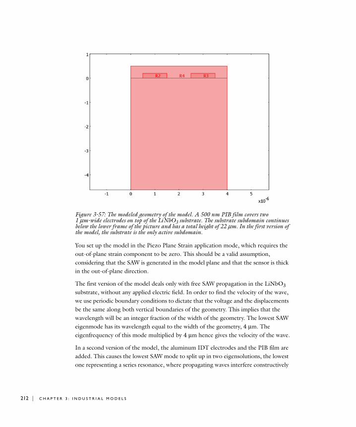
212 | C H A P T E R

Figure 3-57: The modeled geometry of the model. A 500 nm PIB film covers two 1 µm-wide electrodes on top of the LiNbO3 substrate. The substrate subdomain continues below the lower frame of the picture and has a total height of 22 µm. In the first version of the model, the substrate is the only active subdomain.

You set up the model in the Piezo Plane Strain application mode, which requires the out-of-plane strain component to be zero. This should be a valid assumption, considering that the SAW is generated in the model plane and that the sensor is thick in the out-of-plane direction.

The first version of the model deals only with free SAW propagation in the LiNbO3 substrate, without any applied electric field. In order to find the velocity of the wave, we use periodic boundary conditions to dictate that the voltage and the displacements be the same along both vertical boundaries of the geometry. This implies that the wavelength will be an integer fraction of the width of the geometry. The lowest SAW eigenmode has its wavelength equal to the width of the geometry, 4 µm. The eigenfrequency of this mode multiplied by 4 µm hence gives the velocity of the wave.

In a second version of the model, the aluminum IDT electrodes and the PIB film are added. This causes the lowest SAW mode to split up in two eigensolutions, the lowest one representing a series resonance, where propagating waves interfere constructively


and the other one a parallel (“anti-”) resonance, where they interfere destructively. These two frequencies constitute the edges of the stopband, within which no waves can propagate through the IDT.

The adsorption of DCM gas is represented as a slight increase of the density of the PIB film. In the third and final version of the model, the sensor is exposed to 100 ppm of DCM in air at atmospheric pressure and room temperature. The “partial density” of DCM in the PIB film is then calculated as

,

where K = 10l.4821 (Ref. 1) is the air/PIB partition coefficient for DCM, M is its molar mass, and

is its concentration in air.

The substrate used in the simulation is YZ-cut LiNbO3 with properties cited in Ref. 2. The density of the PIB film is from Ref. 1. The Poisson’s ratio is taken to be 0.48, which corresponds to a rather rubbery material. The Young’s modulus is set to 10 GPa. Even at the comparatively high frequencies considered in this model, this is likely an overestimation. However, a much lower value would result in a multitude of eigenmodes located inside the film. While those may be important to consider in designing a SAW sensor, the focus in this model is on the SAW modes. Also, any effects of the DCM adsorption on other material properties than the density are neglected.

ρDCM PIB, KMc=

c 100 10 6– p RT( )⁄⋅ ⋅=


214 | C H A P T E R

Results

Figure 3-58 shows the SAW as it propagates along the surface of the piezoelectric substrate. The frequency corresponding to a 4 µm wavelength computes to 870 MHz, giving a phase velocity of 3479 m/s.

Figure 3-58: Deformed shape plot of a freely propagating SAW in the substrate. The color scale shows the magnitude of the displacements.

In the full model with the periodic IDT and the thin film included, the resonance and anti-resonance frequencies evaluate to 841 MHz and 850 MHz, respectively. Figure 3-59 and Figure 3-60 show the electric potential distribution characteristics for these solutions.


Figure 3-59: Electric potential distribution and deformations at resonance, 841 MHz. The potential is symmetric with respect to the center of each electrode.

Exposing the sensor to a 100 ppm concentration of DCM in air leads to a resonance frequency shift of 227 Hz downwards. This is computed by evaluating the resonance frequency before and after increasing the density of adsorbed DCM to that of the PIB domain.

Note that the computational mesh is identical in both these solutions. This implies that the relative error of the frequency shift is similar to that of the resonance frequency itself. Thus the shift is accurately evaluated despite being a few magnitudes smaller than the absolute error of the resonance frequency.

In a real setup, the drift is often measured by mixing the signal from a sensor exposed to a gas with a reference signal from one protected from the gas. The beat frequency then gives the shift.


216 | C H A P T E R

Figure 3-60: Electric potential distribution and deformations at antiresonance, 851 MHz. The potential is antisymmetric with respect to the center of the electrodes.

References

1. K. Ho and others, “Development of a Surface Acoustic Wave Sensor for In-Situ Monitoring of Volatile Organic Compounds”, Sensors vol. 3, pp. 236–247, 2003.

2. Ahmadi and others, “Characterization of multi- and single-layer structure SAW sensor”, Sensors 2004, Proceedings of IEEE, vol. 3, pp. 1129–1132, 2004.

Model Library path: Acoustics_Module/Industrial_Models/SAW_gas_sensor



1 Open the Model Navigator and click the New tab.


2 From the Space dimension list, select 2D.

3 In the list of application modes, select Acoustics Module>Piezo Plane

Strain>Eigenfrequency analysis.

4 Click OK.


1 Create the following rectangles by repeatedly using Draw>Specify Objects>Rectangle. Click OK after specifying the data for each rectangle.

2 Select all objects and choose Draw>Modify>Scale. In the dialog box that appears, enter 1e-6 for both scale factors; then click OK.

3 Click the Zoom Extents button on the Main toolbar to zoom in on the now micron-sized geometry.



2 Define the following constant names, expressions, and (optionally) descriptions:

WIDTH HEIGHT BASES: CORNER X BASE: CORNER Y

4 22 0 -22

1 0.2 0.5 0

1 0.2 2.5 0

4 0.5 0 0


p 101.325[kPa] Air pressure

T 25[degC] Air temperature

R 8.3145[Pa*m^3/(K*mol)] Gas constant

c_DCM_air 100e-6*p/(R*T) DCM concentration in air

M_DCM 84.93[g/mol] Molar mass of DCM

K 10^1.4821 PIB/air partition constant for DCM

rho_DCM_PIB K*M_DCM*c_DCM_air Mass concentration of DCM in PIB

rho_PIB 0.918[g/cm^3] Density of PIB

E_PIB 10[GPa] Young’s modulus of PIB

nu_PIB 0.48 Poisson’s ratio of PIB

eps_PIB 2.2 Relative permittivity of PIB


218 | C H A P T E R

3 Click OK.


In the first version of the model, you compute the velocity for SAW propagation in a homogenous, electrically insulated LiNbO3 substrate. The supplied material data are with reference to the xy-plane.


2 Select Subdomains 2–4, then clear the Active in this domain check box.

3 Select Subdomain 1, then select xy plane from the Material orientation list.

4 Click the Edit button associated with cE. Enter the following values in the Elasticity

matrix dialog box; when finished, click OK.

5 Click the Edit button associated with e. Enter the following values in the Coupling

matrix dialog box; when finished, click OK.

6 Click the Edit button associated with εrS. Enter the following values in the Relative

permittivity dialog box; when finished, click OK.

7 in the Density edit field, type 4647.



2 Select Boundary 2, then set the Constraint condition to Fixed.

3 Select all exterior boundaries (Boundaries 1, 2, 4, 7, 10, 12, 15, and 16).

2.424e11 0.752e11 0.752e11 0 0 02.03e11 0.573e11 0 0.085e11 0

2.03e11 0 0.085e– 11 00.752e11 0 0.085e11

0.595e11 00.595e11

1.33 0.23 0.23 0 0 00 0 0 2.5– 0 3.70 2.5– 2.5 0 3.7 0

28.7 0 085.2 0

85.2


4 On the Electric BC page, set the Boundary condition to Zero charge/Symmetry.

5 Click OK.

6 Choose Physics>Periodic Conditions>Periodic Boundary Conditions.

7 On the Source page, select Boundary 1. On the first row in the Expression column, type u, then press Enter; the software automatically adds the corresponding Constraint name pconstr1 to the table.

8 On the Destination page, check Boundary 16 and type u in the Expression edit field.

9 On the Source Vertices page, Ctrl-click to select Vertices 1 and 2, then click the >> button.

10 On the Destination Vertices page, Ctrl-click to select Vertices 12 and 13, then click the >> button.

11 Repeat Steps 7 through 10 to define the expressions v and V in an analogous fashion, starting by entering them in the Expression edit field on the Source page, on the 2nd and 3rd row, respectively.

12 When done, click OK to close the Periodic Boundary Conditions dialog box.



2 From the Predefined mesh sizes list, choose Extremely fine.

3 On the Subdomain page, select all subdomains and set the Method to Quad.

4 On the Boundary page, select the upper boundaries of the substrate (Boundaries 4, 7, 10, 12, and 15) and set the Maximum element size to 0.05e-6.

5 Click Remesh, then click OK. When done, a zoom-in on the upper part of the geometry should look like Figure 3-61.


220 | C H A P T E R

Figure 3-61: The meshed geometry.


1 From the Solve menu, open the Solver Parameters dialog box.

2 Enter 850e6 in the Search for eigenfrequencies around edit field, then click OK.



The solver returns 6 eigensolutions with eigenfrequencies in the vicinity of 850 MHz. At 869.8 MHz, two of them are—within the numerical accuracy—the same. These show the shape and the frequency for a SAW with wavelength equal to the width of the geometry.


2 On the General page, select one of the eigenfrequencies equal to 869.8 MHz.

3 On the Deform page, select the Deformed shape plot check box. Clear the Auto check box and type 400 in the Scale factor edit field.


4 Click OK to close the dialog box and see a plot of the total displacement. If you want to, you can repeat the procedure with the other solution to verify that they are the same, only shifted by 90 degrees. One of the solutions look like that in Figure 3-58.

5 To evaluate the velocity, choose Postprocessing>Data Display>Global.

6 In the Expression edit field, type eigfreq_smppn*4[um].

7 In the Eigenfrequency list, select one of the 869.8 MHz entries.

8 Click OK to see the value of the velocity in the message log. It evaluates to approximately 3479 m/s.

This concludes the first part of the model. Proceed to find out how the electrodes and the PIB film affect the behavior of the SAW.

Sensor without Gas Exposure


2 Select Subdomains 2–4, then select the Active in this domain check box.

3 From the Material model list, select Decoupled, isotropic.

4 Select only Subdomain 2.

5 On the Structural page, enter E_PIB for the Young’s modulus, nu_PIB for the Poisson’s ratio, and rho_PIB for the Density.

6 On the Electrical page, select the Enable electrical equation check box and enter eps_PIB in the Relative permittivity edit field.

7 Select Subdomains 3 and 4, then click the Load button.

8 In the Materials/Coefficients Library dialog box, select Basic Material

Properties>Aluminum and click OK.




3 Select Boundaries 6–9 and 11–14. On the Electric BC page, set the condition to Electric potential. Keep the default zero potential.

4 Select Boundaries 3, 5, and 17, and set the condition to Zero charge/Symmetry.



222 | C H A P T E R

Note: The eigenfrequencies and hence the stopband do not depend on the values of the potentials. In fact, for linear eigenfrequency problems, they are automatically set to zero at the electrodes, regardless of the applied value. You can solve the corresponding driven problem by switching to a frequency response analysis and applying different potentials to the electrodes.

6 Choose Physics>Periodic Conditions>Periodic Boundary Conditions.

7 On the Source page, select Boundary 3. Enter u in the first Expression edit field and v in the row below, and V in the third row.


9 From the Constraint name list, select pconstr1; check Boundary 17 (in addition to the already selected Boundary 16); and type u in the Expression edit field.

10 From the Constraint name list, select pconstr2; check Boundary 17; and type v in the Expression edit field.

11 From the Constraint name list, select pconstr3; check Boundary 17; and type V in the Expression edit field.


You have now established the periodicity in the PIB film.




If you are still using the manual scaling of the deformations from the previous exercise, the plot that appears after solving will look rather distorted. Proceed as follows to find the SAW modes and use more suitable plot parameters:


2 On the General page, select the 850 MHz eigenfrequency.

3 On the Deform page, type 40 in the Scale factor edit field.

4 Click Apply to view a plot of the total displacement at anti-resonance.

5 On the General page, select the 841 MHz eigenfrequency, then click Apply to see the deformations at resonance. This plot should look like Figure 3-62.


Figure 3-62: Deformations at resonance.

A plot of the electric potential shows a qualitative difference between the two solutions.

6 On the Surface page, select Piezo Plane Strain (smppn)>Electric potential from the Predefined quantities list.

7 Click Apply to see the potential distribution at resonance, as shown in Figure 3-59 on page 215. Notice that it is symmetric with respect to each individual electrode.

8 On the General page, select the 850 MHz eigenfrequency and click OK to see the potential distribution at anti-resonance, as in Figure 3-60 on page 216. This time, it is antisymmetric.

Sensor with Gas Exposure

In the final version of this model, you expose the sensor to DCM gas. The eigenfrequencies then shift by a very small amount. To see the shift, you need to include more digits in the output.



224 | C H A P T E R

2 Enter the expression eigfreq_smppn and select the 841 MHz eigenfrequency.

3 Select the Display result in full precision check box, then click OK.

The message log now shows all computed digits of the eigenfrequency.

Subdomain Settings1 From the Physics menu, select Subdomain Settings.

2 Select Subdomain 2. On the Structural page, change the Density so that it reads rho_PIB+rho_DCM_PIB.



Click the Solve button.



2 Make sure that the expression still says eigfreq_smppn and select the 841 MHz eigenfrequency.

3 Click OK.

The first 6 digits of the eigenfrequency are the same as before. Subtracting the new value from the previous value (which is most easily done by copying and pasting the results from the message log) shows that the eigenfrequency with gas exposure is lower by 227 Hz.


4

B e n c h m a r k M o d e l s

This chapter covers benchmarks models solving acoustics problems with an established or analytic solution. The benchmark data provide the possibility to validate results obtained with the Acoustics Module.

225

226 | C H A P T E R

V i b r a t i o n s o f a D i s k Ba c k ed b y an A i r - F i l l e d C y l i n d e r

Introduction

The vibration modes of a thin or thick circular disk are well known, and it is possible to compute the corresponding eigenfrequencies to arbitrary precision from a series solution. The same is true for the acoustic modes of an air-filled cylinder with perfectly rigid walls. A more interesting question to ask is: What happens if the cylinder is sealed in one end not by a rigid wall but by a thin disk? This is the question you address in this model.

Note: This model requires the Acoustics Module and the Structural Mechanics Module.

Model Definition

In COMSOL Multiphysics you can model an air-filled cylinder sealed by a thin disk in one end using at least two different approaches. You describe the pressure in the cavity with a Pressure Acoustics application mode, while the model of the disk can be either a thin shell in 3D, using shell elements, or a 2D plate. The latter approach to modeling this acoustic-structure interaction is possible thanks to nonlocal couplings and COMSOL Multiphysics’ ability to model in different numbers of space dimensions at the same time—extended multiphysics.

In Ref. 1, D. G. Gorman and others have thoroughly investigated the model at hand, and they have developed a semi-analytical solution verified by experiments and simulations. The geometry is a rigid steel cylinder with a height of 255 mm and a radius of 38 mm. One end is welded to a heavy slab, while the other is sealed with a steel disk only 0.38 mm thick. Some of the theoretical eigenfrequencies of a thin disk

4 : B E N C H M A R K M O D E L S

in vacuum and of a rigidly sealed chamber are given in the following table (according to Ref. 1).

Here you model the coupled system using the extended multiphysics approach. This means that you draw the disk in a 2D geometry and model it with Mindlin-theory DRM-plate elements, while you draw the cylinder in a separate 3D geometry. The acoustics in the cylinder is described in terms of the acoustic (differential) pressure. The eigenvalue equation for the pressure is

where c is the speed of sound and ω = 2π f defines the eigenfrequency, f.

A first step is to calculate the eigenfrequencies for the disk and the cylinder separately and compare them with the theoretical values in Table 4-1. This way you can verify the basic components of the model and assess the accuracy of the FEM solution before modeling the coupled system.


Most of the modes show rather weak coupling between the structural bending of the disk and the pressure field in the cylinder. It is, however, interesting to note that some of the uncoupled modes have been split into one co-vibrating and one contra-vibrating mode with distinct eigenfrequencies. This is the case for modes 1 and 2 and for modes 9 and 12 in the FEM solution. The table below shows a comparison of the eigenfrequencies from the COMSOL Multiphysics analysis with the semi-analytical and experimental frequencies reported by D. G. Gorman and others in Ref. 1. The

TABLE 4-1: BENCHMARK VALUES FOR EIGENFREQUENCIES OF THE DISK AND THE CYLINDER

NUMBER CLAMPED DISK IN VACUUM (HZ) RIGIDLY SEALED CYLINDER (HZ)

1 671.8 672.5

2 1398 1345

3 2293 2018

4 2615 2645

5 3356 2690

6 4000 4387

∆ p–ω2

c2------ p=

V I B R A T I O N S O F A D I S K B A C K E D B Y A N A I R - F I L L E D C Y L I N D E R | 227

228 | C H A P T E R

table also states whether the modes are structurally dominated (str), acoustically dominated (ac), or tightly coupled (str/ac).

As the table shows, the FEM solution is in good agreement with both the theoretical predictions and the experimentally measured values for the eigenfrequencies. As you might expect from the evaluation of the accuracies for the uncoupled problems, the precision is generally better for the acoustics-dominated modes.

Reference

1. D. G. Gorman, J. M. Reese, J. Horacek, and D. Dedouch: “Vibration analysis of a circular disk backed by a cylindrical cavity,” Proc. Instn. Mech. Engrs., vol. 215, Part C, 2001.

Model Library path: Acoustics_Module/Benchmark_Models/coupled_vibration



1 Select 2D from the Space dimension list.

TABLE 4-2: RESULTS FROM SEMI-ANALYTICAL AND COMSOL MULTIPHYSICS ANALYSES AND EXPERIMENTAL DATA

TYPE SEMI-ANALYTICAL (HZ) COMSOL MULTIPHYSICS (HZ) EXPERIMENTAL (HZ)

str/ac 636.9 637.2 630

str/ac 707.7 707.7 685

ac 1347 1347.4 1348

str 1394 1395.3 1376

ac 2018 2018.6 2040

str 2289 2293.1 2170

str/ac 2607 2612.1 2596

ac 2645 2646.3 –

str/ac 2697 2697.1 2689

ac 2730 2730.9 2756

ac 2968 2969.3 2971


2 In the list of application modes, select Structural Mechanics Module>Mindlin Plate>Eigenfrequency analysis.

3 Click OK.


The geometry of the disk is a solid circle. Its location does not really matter because you embed it in 3D using coupling variables, but the transformations are trivial if you center the disk at the origin:

1 Press the Shift key and click the Ellipse/Circle (Centered) button.

2 In the Circle dialog box, type 0.038 in the Radius edit field and click OK to create a circle of radius 0.038 m, centered at the origin.



Boundary ConditionsThe edges of the disk are welded to the cylinder and can therefore be described as rigidly clamped or fixed.


2 Select one of the boundaries and then press Ctrl+A to select all boundaries.

3 Make sure that you have selected Tangent and normal coord. sys. (t,n) in the Coordinate system list.

4 Select Fixed in the Condition list.

5 Click OK.

Subdomain Settings—Material PropertiesThe steel disk has the following material properties (in the default SI units):

• Young’s modulus, E = 2.1·1011

• Poisson’s ratio, ν = 0.3

• Density, ρ = 7800

1 From the Physics menu, choose Subdomain Settings.



230 | C H A P T E R

3 Enter material data according to the following table:

4 Click OK.


To obtain accurate values of the eigenfrequencies of the disk, you need a mesh that is finer than the one produced with the default settings.

1 Open the Free Mesh Parameters dialog box from the Mesh menu.

2 Click the Custom mesh size option button and type 0.002 in the Maximum element

size edit field.

3 Click the Remesh button and then click OK.


When solving for the eigenfrequencies of the disk in vacuum, only the frequency interval between 500 Hz and 3250 Hz is of interest. Start by searching for the 20 first eigenfrequencies (some of these are almost identical and come from double eigenvalues) and make the solver start its search around 500 Hz:

1 From the Solve menu, choose Solver Parameters.

2 Type 20 in the Desired number of eigenfrequencies edit field.

3 Type 500 in the Search for eigenfrequencies around edit field.

4 Click OK.



1 Click the 3D Surface Plot button to see the deflection of the disk.

Next, try looking at some of the eigenmodes.

2 From the Postprocessing menu, choose Plot Parameters.

3 On the General page, choose an eigenfrequency from the Eigenfrequency list in the Solution to use area; click Apply to generate the corresponding plot.

MATERIAL PROPERTY VALUE

E 2.1e11

ν 0.3

ρ 7800

thickness 0.00038


4 When done, click Cancel or OK to close the Plot Parameters dialog box.

The eigenmode associated with the eigenfrequency around 3360 Hz.

You can now compare the eigenfrequencies with the theoretical values for a thin disk. The discrepancy is below 2% for all eigenmodes in the interval, so the conclusion is that the mesh resolution is sufficient.

Adding the 3D Pressure Acoustics Application Mode

Now add a second geometry that will contain the cylinder and the acoustic pressure variable using a 3D Pressure Acoustics application mode.

1 From the Multiphysics menu, choose Model Navigator.

2 Click the Add Geometry button to add a second geometry.

3 In the Add Geometry dialog box, select 3D from the Space dimension list.

4 Click OK.

5 In the list of application modes, select Acoustics Module>Pressure Acoustics>Eigenfrequency analysis.

6 Click Add.


232 | C H A P T E R

7 Click OK.


1 Click the Cylinder toolbar button.

2 Type 0.038 in the Radius edit field and 0.255 in the Height edit field.

3 Click OK.



Boundary ConditionsFor the moment, assume that all boundaries are perfect hard walls, which is the default boundary condition.

Subdomain Settings1 From the Physics menu, choose Subdomain Settings.


3 Type 1.2 in the Fluid density (ρ0) edit field. Leave the other properties at their default value.

4 Click OK.


Click the Initialize Mesh button to create a mesh using the default parameters.


To solve for the acoustic modes only, you must deactivate the Mindlin Plate application mode during the solution. If the plate is not deactivated, COMSOL Multiphysics solves the two eigenvalue problems simultaneously but independently of one another.

1 From the Solve menu, choose Solver Manager.


3 Ctrl-click on the Mindlin Plate (smdrm) folder to clear that application mode’s variables from the list of variables to solve for, then click OK.




2 On the General page, clear the Slice check box and select the Isosurface check box.


3 In the Solution to use area, select one of the solutions near 2730 Hz from the Eigenfrequency list.

4 Click the Isosurface tab. In the edit field for isosurface levels under Number of levels, type 10. From the Colormap list select hot, then click Apply.

5 Click the Headlight button on the Camera toolbar.

6 Return to the General page and try a few different eigenmodes by selecting the corresponding eigenfrequencies, clicking Apply to generate each plot.

Pressure isosurfaces for one of two eigenmodes associated with an eigenfrequency near 2969 Hz.

You can also compare these eigenfrequencies with the theoretical values in Table 4-2 on page 228. This time, the relative error seems to be much smaller than for the disk, which means that any additional mesh refinement should be done on the plate part.

Coupling the Equations

The first step in the process of coupling the Mindlin plate elements to the acoustic equation is to create the nonlocal couplings; use coupling variables to make the pressure available as a load on the plate and the out-of-plane displacement of the plate a valid parameter in the coefficients for the acoustic equation.


234 | C H A P T E R

O P T I O N S A N D S E T T I N G S — C O U P L I N G V A R I A B L E S

First define a coupling variable for the acoustic pressure from the top face of the cylinder to the disk (Mindlin plate):

1 On the Options menu, point to Extrusion Coupling Variables and then click Boundary

Variables.

2 In the Boundary Extrusion Variables dialog box, select Boundary 4 (the top face) of the cylinder.

3 Type p in the top row under both Name and Expression.


5 Select Geom1 in the Geometry list, then select Subdomain 1 (the disk) in the 2D geometry.

6 Click the Source Vertices tab.

7 In the Vertex selection list, select Vertices 2, 4, and 8. Click the >> button.

8 Click the Destination Vertices tab.


10 Click OK.

Now define a coupling variable for the out-of-plane displacement, w, from the disk to the top face of the cylinder. Also the acceleration, wtt, is needed.

1 If you are in the Pressure Acoustics application mode, switch to the Mindlin Plate application mode by choosing Geom1: Mindlin Plate (smdrm) from the Multiphysics menu.

2 On the Options menu, point to Extrusion Coupling Variables and then click Subdomain

Variables.

3 In the Subdomain Extrusion Variables dialog box, select Subdomain 1.

4 Type w in the top row under both Name and Expression. Type wtt in the second row under both Name and Expression.


6 Select w from the Variable list.

7 Select Geom2 in the Geometry list, then select the check box next to Boundary 4.







13 Select wtt from the Variable list.

14 Select Geom2 in the Geometry list, then select the check box next to Boundary 4.





19 Click OK.


Boundary ConditionsThe sound-hard boundary condition for a rigid wall is that the normal acceleration vanishes. For a moving wall, such as the thin disk that now seals the cylinder, the appropriate condition is instead

where a is the normal acceleration of the wall.

1 If the Mindlin Plate application mode is selected, switch to the Pressure Acoustics application mode by choosing 2 Geom2: Pressure Acoustics (acpr) from the Multiphysics menu.


3 Select the top of the cylinder where the plate is located, that is, Boundary 4.


5 In the an edit field, type -wtt (the structural acceleration in the negative z direction).

6 Click OK.

Subdomain SettingsThe acoustic pressure acting as a normal load constitutes the coupling in the opposite direction.

1 From the Multiphysics menu, choose 1 Geom1: Mindlin Plate (smdrm).

2 Open the Subdomain Settings dialog box.

3 Click the Load tab.

n ∇p⋅ρa

---------------- a–=


236 | C H A P T E R


5 In the Fz edit field, type p to specify the pressure as a surface load on the disk.

6 Click OK.

7 Switch back to the 3D geometry by choosing 2 Geom2: Pressure Acoustics (acpr) from the Multiphysics menu.


1 From the Solve menu, choose Solver Manager.

2 In the Solver Manager dialog box, click the Solve For tab.

3 Reactivate the Mindlin Plate application mode by selecting both Geom1 (2D) and Geom2 (3D) and all corresponding variables in the Solve for list.

4 Click the Solve button to compute the solution. When done, click OK.


1 Open the Plot Parameters dialog box.

2 On the General page, add boundary and deformed shape plots to the isosurface plot by selecting the Boundary and Deformed shape check boxes in the Plot type area.

3 Click the Boundary tab.

4 In the Boundary data area, enter the Expression lambda^2*w, that is, the normal acceleration of the disk. On the other boundaries, w is not defined so those boundaries are invisible.

5 Click the Deform tab and select the Boundary check box only in the Domain types to

deform area.

6 In the Deformation data area, click the Boundary Data tab and type 0, 0, and w in the x component, y component, and z component edit field, respectively.


8 Select an entry from the Eigenfrequency list, then click Apply to examine the corresponding eigenmode.

9 When finished, click Cancel or OK to close the Plot Parameters dialog box.


One of the two eigenmodes with an eigenfrequency near 2730 Hz.


238 | C H A P T E R

Open P i p e

Introduction

If you plan on setting up a large, complicated acoustics model, it can be useful to break it up in smaller, simpler problems. In this example, a vibrating piston is mounted inside one end of a cylindrical pipe. The other end is open and set in a plane baffle. A first version of the model studies the air outside the baffle as a PML (perfectly matched layer) region. A second version measures and then uses the impedance load on the piston, where it replaces the air region with an impedance boundary condition applied to the tube’s open end. The impedance boundary condition uses a radiation impedance given as a function of the measured impedance at the piston. You can employ the technique of measuring impedances and reusing them in impedance boundary conditions to handle arbitrary kinds of pipe openings.

Model Definition

Figure 4-1: Pipe geometry. The flange is cut off in the illustration but is assumed to extend to infinity. The piston makes up the bottom of the pipe.


Figure 4-1 shows the geometry simulated in this model. A pipe of length L = 1.5 m and radius a = 0.25 m has a driving piston at one end. The other end is open and flush with the infinite hard wall in which it is set. The piston vibrates harmonically with a velocity where v0 = 1 m/s, and ω = 2π f is the angular frequency (rad/s). The model sweeps the frequency, f, through a range of values between 10 Hz and 700 Hz. The acoustic medium is air with a density of 1.25 kg/m3 and a speed of sound of 343 m/s.

The axial symmetry of the geometry and the physics makes it natural to set the model up in a 2D axisymmetric application mode. Two cylindrical PMLs represent the air outside the pipe as shown in Figure 4-2.

Figure 4-2: Model geometry. PML 1 is damping only in the z direction, while PML 2 is damping in both the r direction and the z direction.

The PMLs serve to absorb the outgoing waves so that the nonphysical reflections at their exterior boundaries have a minimal influence on the pressure field inside the pipe. PMLs require the tangential component of the damping to be continuous across a

v v0eiωt=

O P E N P I P E | 239

240 | C H A P T E R

boundary. Hence the PML just above the pipe is damping only in the z direction, while the one outside the pipe is damping both in the r direction and the z direction. For further details about the PML implementation in the Acoustics Module, please refer to “Perfectly Matched Layers (PMLs)” on page 37 in the Acoustics Module User’s Guide.


For harmonic sound waves this model uses the frequency-domain Helmholtz equation for sound pressure:

Here the acoustic pressure is a harmonic quantity, (N/m2), ρ0 is the density (kg/m3), q denotes an optional dipole source (N /m3), and cs is the speed of sound (m/s). The model under study includes no dipole source.


The first version of the model uses two distinct boundary conditions. First, it represents the hard walls of the pipe and the flange by the equation

where n is the outward-pointing unit normal vector seen from inside the acoustics domain. The model also uses this condition at the exterior boundaries of the PMLs. Second, the piston is modeled with a normal acceleration condition:

where the normal acceleration, an, is defined as iω v0.

The second version of the model replaces the PML domains with an impedance boundary condition at the opening of the pipe:

The impedance Z is a function of the frequency obtained by measuring and transforming the radiation load on the piston. Given a piston impedance Z0 = p/v evaluated at the piston, introduce the quantities α0 and β0 such that

∇ 1ρ0------– ∇p q–( )⎝ ⎠

⎛ ⎞⋅ ω2p

ρ0 cs2

--------------– 0=

p p0eiωt=

n 1ρ0------ ∇p qs–( )⎝ ⎠⎛ ⎞⋅ 0=

n 1ρ0------ ∇p qs–( )⎝ ⎠⎛ ⎞⋅ an=

n–1ρ0------ ∇p qs–( )⎝ ⎠⎛ ⎞⋅ iωp

Z----------=


(4-1)

With αL = α0 and βL = β0 − kL/π, where k = ω/cs, define

(4-2)

This transformation is derived in Ref. 1 as a valid approximation in the long-wavelength limit where only plane waves can propagate inside the tube. Note that this reference uses the definition , which makes the formulas look slightly different. Because Z corresponds to the radiation impedance of a membrane set in an infinite hard wall plane, it is possible to analytically derive values for αL and βL; these values appear in Ref. 1.


Figure 4-3: Acoustic pressure field in the pipe at 700 Hz.

The pressure field in the pipe at 700 Hz (Figure 4-3) is dominated by an outgoing and a reflected plane wave except close to the opening.

Z0 ρ0cs π α0 iβ0+( )tanh=

Z ZL ρ0cs π αL iβL+( )tanh= =

p p0eiωt=

O P E N P I P E | 241

242 | C H A P T E R

Figure 4-4 shows the reactance measured at the piston. The zero crossings of the reactance plot occur at the acoustic eigenfrequencies of the tube and the outside air. Comparing these to the simple analytic case of zero pressure at the open end, the eigenfrequencies of the open tube are consistently lower. This is to be expected because the computed eigenmodes are not restrained to the inside of the pipe but can spill out into the open.

Figure 4-4: The reactance at the piston as a function of frequency.

The analytical eigenfrequencies are given by the expression

The accuracy of the computed eigenfrequencies is limited by the pitch of the frequency sweep. The following table is based on a pitch of 1 Hz.

TABLE 4-3: COMPUTED AND SIMPLIFIED ANALYTIC FREQUENCIES IN THE OPEN PIPE

COMPUTED (HZ) SIMPLIFIED ANALYTIC (HZ)

50.4 57.2

101.8 114.3

154.2 171.5

fnncs4L--------=


Using values for αL and βL from Ref. 1 in Equation 4-1 and Equation 4-2 lets you calculate semi-analytical values for the piston impedance, Z0. Figure 4-5 compares this impedance with the computed impedance.

Figure 4-5: Measured (solid) and semi-analytical (dashed) impedance at the piston. Because the fit is so good that it is difficult to tell the curves apart, the figure zooms in on the frequency range from 100 to 300 Hz.

207.5 228.7

261.6 285.8

316.3 343.0

371.4 400.2

426.8 457.3

482.7 514.5

538.9 571.7

595.6 628.8

652.8 686.0

TABLE 4-3: COMPUTED AND SIMPLIFIED ANALYTIC FREQUENCIES IN THE OPEN PIPE

COMPUTED (HZ) SIMPLIFIED ANALYTIC (HZ)

O P E N P I P E | 243

244 | C H A P T E R


This model is set up in 2D axisymmetry using the Pressure Acoustics application mode of the Acoustics Module. This application mode has automated support for PMLs, making it a straightforward task to set up the model. Using the Solver Manager, you store the PML solution for reuse in the impedance boundary condition of the second version of the model.

Reference

1. P.M. Morse and K.U. Ingard, Theoretical Acoustics, Princeton Univ. Press, 1986.

Model Library path: Acoustics_Module/Benchmark_Models/open_pipe



1 Start COMSOL Multiphysics.

2 In the Model Navigator, select Axial symmetry (2D) from the Space dimension list.

3 From the list of application modes select Acoustics Module>Pressure

Acoustics>Time-harmonic analysis.

4 Click OK.

O P T I O N S

1 Open the Constants dialog box from the Options menu and enter the values in the following table (the descriptions are optional); when done, click OK.

2 Choose Options>Expressions>Scalar Expressions and enter the expressions in the following table. Alternatively, to avoid entering the expressions, click the


v0 1[m/s] Maximum piston velocity

a 0.25[m] Pipe radius

L 1.5[m] Pipe length

rho_air 1.25[kg/m^3] Air density

cs_air 343[m/s] Speed of sound in air


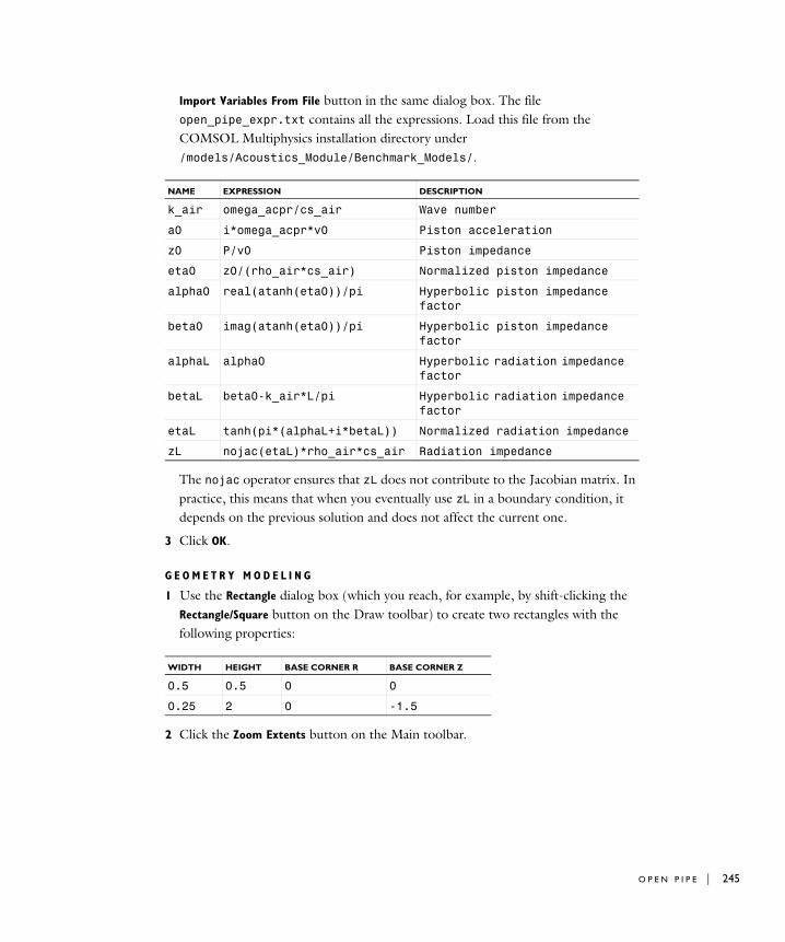
Import Variables From File button in the same dialog box. The file open_pipe_expr.txt contains all the expressions. Load this file from the COMSOL Multiphysics installation directory under /models/Acoustics_Module/Benchmark_Models/.

The nojac operator ensures that zL does not contribute to the Jacobian matrix. In practice, this means that when you eventually use zL in a boundary condition, it depends on the previous solution and does not affect the current one.

3 Click OK.


1 Use the Rectangle dialog box (which you reach, for example, by shift-clicking the Rectangle/Square button on the Draw toolbar) to create two rectangles with the following properties:



k_air omega_acpr/cs_air Wave number

a0 i*omega_acpr*v0 Piston acceleration

z0 P/v0 Piston impedance

eta0 z0/(rho_air*cs_air) Normalized piston impedance

alpha0 real(atanh(eta0))/pi Hyperbolic piston impedance factor

beta0 imag(atanh(eta0))/pi Hyperbolic piston impedance factor

alphaL alpha0 Hyperbolic radiation impedance factor

betaL beta0-k_air*L/pi Hyperbolic radiation impedance factor

etaL tanh(pi*(alphaL+i*betaL)) Normalized radiation impedance

zL nojac(etaL)*rho_air*cs_air Radiation impedance

WIDTH HEIGHT BASE CORNER R BASE CORNER Z

0.5 0.5 0 0

0.25 2 0 -1.5

O P E N P I P E | 245

246 | C H A P T E R


Subdomain SettingsChoose Physics>Subdomain Settings and apply the following settings; when done, click OK.

Boundary ConditionsChoose Physics>Boundary Settings and apply the following boundary conditions; when done, click OK.

Boundary Integration VariablesChoose Options>Integration Coupling Variables>Boundary Variables. Select boundary 2 and define the following boundary integration coupling variable; when done, click OK.

This variable represents the mean value of the pressure over the piston.



2 On the Global page, click the Custom mesh size button and in the Maximum element

size edit field type 0.04.

3 Click the Boundary tab and select Boundaries 2 and 4. In the Maximum element size edit field type 0.02.

4 Click OK.

SETTINGS SUBDOMAIN 1 SUBDOMAIN 2 SUBDOMAIN 3

ρ0 rho_air rho_air rho_air

cs cs_air cs_air cs_air

Type of PML None Cylindrical Cylindrical

Absorbing in r direction - unchecked 0.25

Absorbing in z direction - 0.5 0.5

R0 - - 0.25

SETTINGS BOUNDARIES 1, 3 BOUNDARY 2 BOUNDARIES 5, 6, 8–10

Axial symmetry Normal acceleration

Sound hard boundary (wall)

an - a0 -

NAME EXPRESSION

P 2*r*p/a^2


5 Click the Initialize Mesh button on the Main toolbar to create the mesh.


1 Choose Solve>Solver Parameters.

2 From the Solver list select Parametric.

3 In the Parameter name edit field type freq_acpr, and in the Parameter values edit field type 10:10:700.

4 Click the Stationary tab, then select Linear from the Linearity list to ensure that the parametric sweep uses the linear solver.

5 Click OK.



Figure 4-6: The acoustic pressure in the tube and in the PMLs at 700 Hz.

The default plot should look like Figure 4-6. It displays the acoustic pressure in the tube at the final frequency of the sweep, 700 Hz. It also shows that the damping is efficient in the PML regions.

To get a better view of the damping, try plotting the sound level in dB:

O P E N P I P E | 247

248 | C H A P T E R

1 Choose Postprocessing>Plot Parameters.

2 On the Surface page choose Pressure Acoustics (acpr)>Sound pressure level from the Predefined quantities list. Click OK.

With a visual inspection you can see that the pressure drop from the open end of the tube to the top boundary of the PML region that makes up the air domain is roughly 50 dB. This means that the part of the wave that is reflected at this boundary experiences a total of 100 dB damping before it returns to the tube. This is more than enough for all practical purposes.

From now on suppress the PMLs and look exclusively at the physical pressure field inside the tube.


2 Select Subdomains 2 and 3, then click OK.

3 Open the Plot Parameters dialog box again and click the Surface tab.

4 From the Predefined quantities list choose Pressure Acoustics (acpr)>Pressure. Click OK.

Note how the pressure field deviates from the simple plane wave behavior in the vicinity of the open end of the tube. Now examine the impedance at the piston.

5 Choose Postprocessing>Domain Plot Parameters and click the Point tab.

6 Select an arbitrary point in the Point selection list. In the Expression field, type real(z0), then click Apply to see the plot.

You are now looking at the acoustic resistance as a function of frequency. The peaks show the resonance frequencies for the semi-open tube with a resolution given by the pitch of the frequency sweep.

You can get the same resonance frequencies with the accuracy improved by the linear interpolation between neighboring frequencies if you instead study the zeros of the reactance plot.

7 Remaining on the Point page, enter imag(z0) in the Expression field and click Apply to see the plot.

By zooming in on the zeros in this plot, you should find frequencies similar to those in Table 4-3. To get the same accuracy as in this table, though, you would have to resolve the model with a frequency pitch of 1 Hz.

Finally, plot the real and the imaginary parts of the radiation impedance:

1 Still on the Point page, type real(zL) in the Expression field and click Apply.


2 On the General page select the Keep current plot check box.

3 Click the Title/Axis button. In the Title edit field type Radiation resistance (solid) and reactance (dashed), and in the Second axis label edit field type (ohm). Click OK.

4 On the Point page click the Line Settings button. Set the Line style to Dashed line. Click OK.

5 In the Expression field type imag(zL), then click OK to reproduce the plot in Figure 4-7.

Figure 4-7: Radiation resistance and reactance at the opening of the pipe.

Lumped Impedance Version

In this version of the model, replace the PMLs with an impedance boundary condition using the radiation impedance that you have already calculated.

S U B D O M A I N S E T T I N G S

From the Physics menu open the Subdomain Settings dialog box. Select Subdomains 2 and 3, clear the Active in this domain check box, and then click OK.

O P E N P I P E | 249

250 | C H A P T E R


From the Physics menu open the Boundary Settings dialog box. Select Boundary 4. In the Boundary condition list select Impedance boundary condition. Enter zL for the Input impedance, then click OK.



2 Click the Store Solution button. In the dialog box that appears, make sure that all frequencies are selected, then click OK.

3 In the Values of variables not solved for and linearization point list select Stored solution.

4 From the Parameter value list select All.

5 Click OK.



The pressure field is now everywhere independent of the r coordinate. The impedance boundary condition still leaves the piston impedance unchanged.

1 Choose Postprocessing>Domain Plot Parameters and click the General tab.

2 Clear the Keep current plot check box. Click the Title/Axis button. Select the Auto buttons for all options, then click OK to close the Title/Axis dialog box.

3 On the Point page, click Line Settings. Set the Line style to Solid line, then click OK.

4 In the Expression edit field type real(z0). Click Apply to see the plot.

5 Enter imag(z0) in the Expression edit field. Click OK to see the plot.

The resistance and reactance plots appear to be virtually identical to those from the solution using PMLs. If you want to compare these results to the analytical solution, follow these steps:

1 Choose Options>Functions.

2 In the Functions dialog box, click the New button.

3 In the New Function dialog box, enter the Function name alphaL_ana.

4 Click the Interpolation button. In the Use data from list, select File.

5 Browse to find the file alpha.txt, which is located in the COMSOL Multiphysics installation directory under /models/Acoustics_Module/Benchmark_Models/. Click Open, then click OK to close the New Function dialog box.


or

or

.

6 Repeat Steps 2 through 5 to create another interpolation function, but this time use the function name betaL_ana and the data file beta.txt, which you find in the same folder as alpha.txt.

7 Click OK to close the Functions dialog box dialog box.

8 If you previously entered the scalar expressions manually, now choose Options>Expressions>Scalar Expressions and add the following scalar expressions; when done, click OK.



11 Click the Point tab. In the Expression edit field type abs(z0), then click Apply.

12 On the General page select the Keep current plot check box.

13 Click the Title/Axis button. In the Title edit field type Analytical (dashed) and computed (solid) piston impedance, and in the Second axis label edit field type (ohm). Click OK.

14 On the Point page click the Line Settings button. Set the Line style to Dashed line, then click OK.

15 In the Expression field type abs(z0_ana), then click OK to generate the plot.

If you zoom in on the range between 100 Hz and 300 Hz, what you get should look like the image in Figure 4-5.


alpha0_ana alphaL_ana(k_air*a) Hyp. piston imp. fact

beta0_ana betaL_ana(k_air*a)+k_air*L/pi Hyp. piston imp. fact

eta0_ana tanh(pi*(alpha0_ana+i*beta0_ana)) Normalized piston imp

z0_ana eta0_ana*rho_air*cs_air Piston impedance

O P E N P I P E | 251

252 | C H A P T E R

S c a t t e r i n g f r om a P l a t e w i t h R i b s

Introduction

The following model has been suggested as a benchmark for acoustic scattering from a thin 3D structure (Ref. 1). Problems of this kind have traditionally been the domain of boundary element (BEM) codes, and the test case was designed with such solvers in mind. The purpose of the present model is to show that scattering problems can be handled very well also by a finite element software like COMSOL Multiphysics, using the built-in PML functionality to reduce the model domain to a minimum.

There is no closed-form reference solution to this benchmark problem, but the presented results correlate very well with the boundary element solutions reported in Ref. 1.


Model Definition

The test geometry consists of a quadratic plate with a pair of stiffening ribs welded on top along the two lines of symmetry. The side length is 60 cm and the ribs are 15 cm high.

Figure 4-8: Target geometry and surface mesh.

All parts are assumed to have negligible thickness and to be perfectly rigid. You can therefore model the entire structure as boundaries with sound-hard surfaces on both sides. To be able to set separate boundary conditions on the two sides of a boundary, you must create the geometry as an assembly and disconnect the boundaries representing the structure.

Scattering problems are best modeled using the scattered-field formulation. This means that you write the acoustic pressure as the sum of a known incident field, pi, and an unknown scattered field, ps. Inserting this sum in the standard acoustic Helmholtz equation and assuming that the incident field by itself is a solution to the same equation, you are left with an equation for the scattered field:

S C A T T E R I N G F R O M A P L A T E W I T H R I B S | 253

254 | C H A P T E R

Here ρ0 is the equilibrium density (kg/m3), ω = 2π f denotes the angular frequency (rad/s), and cs refers to the speed of sound (m/s). The incident field does not appear in the equation but it modifies the boundary conditions.

The benchmark case specifies the material properties of air as ρ0 = 1.225 kg/m3 and cs = 340 m/s. Two frequencies are used in the test: 1000 Hz and 1500 Hz. In each case, a plane wave with an intensity of 100 dB SPL is travelling in the (1,−1,−1) direction.

To avoid the scattered waves spuriously reflecting back from the model boundaries onto the target structure, the latter can be padded tightly in PMLs. In this case, it is easiest to define axis-parallel PMLs outside the minimal box around the structure. Note that this means you have a PML directly on the bottom target surface, with no air domain in between, and that there is no reason not to build the model in this way. The PMLs are set to be just one half wavelength thick and three quadratic elements across, which is by far enough to match the accuracy in the reference solutions. For an introduction to using PMLs when modeling with the Acoustics Module, see “Perfectly Matched Layers (PMLs)” on page 73 of the Acoustics Module User’s Guide.

The entire model can be constructed as a six-by-six-by-three grid of identical cubes. This gives you more subdomains than strictly necessary, but it greatly simplifies the process of creating a structured hexahedral mesh. The final geometry consists of an assembly of six separate parts, which are joined with identity pairs on all internal boundaries that are not part of the target structure. (For an explanation of the terminology concerning assemblies, refer to the section “The Object Properties dialog box for a 3D solid object.” on page 76 of the COMSOL Multiphysics User’s Guide.)


Of the 108 domains making up the geometry, 92 are PMLs. The pressure solution inside the PMLs has very little to do with the true scattered field. In the 16 domains

∇ 1ρ0------– ∇ps⎝ ⎠

⎛ ⎞⋅ω2ps

ρ0 cs2

--------------– 0=


representing the actual geometry, the pressure field is correct to the extent the discretization allows.

The reference solutions are given as SPL values along a vertical line from Z = −2 to Z = 2 situated at X = 1, Y = −1. Producing these values at an intermediate distance from the target is easy for a boundary element code. However, while solving this benchmark problem in the presented way is straightforward, obtaining numbers comparable to the reference solutions requires some additional work.

The easiest way to evaluate the pressure at an intermediate distance from a radiating object is by using the Helmholtz-Kirchhoff integral representation formula. For the particular case of a thin scatterer this formula simplifies to

(4-3)

where k is the wave number, n is the outward-facing normal vector, and the integral is taken over the target surface, S. Note that the two sides of a thin structure are separate surfaces in the integral, with opposite normal directions. The far-field feature in the Acoustics Module allows you to solve the above integral.

ps R( ) 14π------ e ik r R––

r R–----------------------- p

sr( ) 1 ik r R–+( )

r R– 2------------------------------------- n r R–( )⋅( ) vd

S∫=


256 | C H A P T E R

Knowing the scattered pressure field at the probe positions, the total sound pressure level can be calculated as

where the reference pressure for air is taken to be pref = 2 ·10−5 Pa. The results are presented in Table 4-4.

The obtained values are indistinguishable from one of the reference solutions in Ref. 1, with the other being slightly off.


You set up this benchmark model using the scattered-field formulation in the Pressure Acoustics application mode. Perfectly matched layers (PMLs) allow you to truncate the domain close to the target geometry. To further reduce memory requirements, you can use a multigrid solver, although direct solvers are faster when applicable. With the far-field variable for the scattered pressure field at the probe positions you can extract the benchmark results.

TABLE 4-4: TOTAL SOUND PRESSURE LEVEL FOR VARYING Z AT X=1, Y=-1

Z COORDINATE 1000 HZ 1500 HZ

-2.0 99.2 101.4

-1.6 97.6 96.3

-1.2 100.1 100.0

-0.8 100.3 100.4

-0.4 96.7 97.6

0.0 101.7 98.7

0.4 99.2 99.7

0.8 98.8 101.6

1.2 101.6 102.4

1.6 98.4 100.3

2.0 101.4 99.5

Lp R( ) 10pi R( ) ps R( )+ 2

2pref2

-------------------------------------------⎝ ⎠⎜ ⎟⎛ ⎞

log=


Reference

1. A.J.Svobodnik, G.Hofstetter & O. von Estorff, “Benchmarks for Radiation and Scattering of Sound,” NAFEMS Ref. -R0083, 2003.

Model Library path: Acoustics_Module/Benchmark_Models/plate_with_ribs




2 From the Application Modes tree select Acoustics Module>Pressure Acoustics>Time-harmonic analysis, scattered wave.



The geometry consists of 108 identical cubes. You start by creating one such cube and thereafter, step by step, duplicate and copy this single cube until the final geometry is obtained.

1 Choose Draw>Use Assembly to put COMSOL Multiphysics in assembly mode.

2 Choose Draw>Block. In the dialog box that appears, modify the following entries; when finished, click OK.

3 With the single cube selected, choose Edit>Copy or press Ctrl+C to put a copy of the cube on the clipboard.

4 Choose Edit>Paste or press Ctrl+V to paste a copy of the cube into the drawing area. Enter the following information into the Paste dialog box; when finished click OK.

Length X 0.15

Y 0.15

Z 0.15

Displacement x -0.3


258 | C H A P T E R

5 Repeat Step 4 to paste a second copy in the same position.

6 Paste one more copy, specifying:

7 Now select the first block, BLK1, and choose Draw>Modify>Array or press the Array button on the Draw toolbar. Enter the following data; when finished, click OK.

8 Select the original block together with the newly created three, then press the Union button on the Draw toolbar.

9 With the new composite object still selected, again open the Array dialog box and set the following values; when finished, click OK.

10 Return to the second cube created, BLK2, select it and open the Array dialog box. Enter the following data; when finished, click OK.

y -0.3

z -0.15

Displacement x -0.45

y -0.45

z -0.15

Displacement x 0.15

y 0.15

z 0

Array size x 2

y 2

z 1

Displacement x -0.3

y -0.3

z 0

Array size x 2

y 2

z 1

Displacement x 0.15

y 0.15

z 0


11 Join the original and the 15 new copies in a single object by selecting them and then clicking the Union button.

12 Return to the Array dialog box, but with the cube BLK3 as selected source object. Create copies as follows; when finished, click OK.

13 Select the new copies together with BLK3, then click the Union button.

14 Select the last of the original four cubes, BLK4, and for the final time open the Array dialog box. This time you will create 107 copies.

15 Add the original cube BLK4 to the selection and click the Union button.

16 Finally, add the composite object CO6 to the selection and click the Difference button on the Draw toolbar.

17 Before leaving draw mode you must create identity pairs on the objects’ common surfaces. Do this by selecting all objects and clicking the Create Pairs button.

Array size x 4

y 4

z 1

Displacement x 0.15

y 0.15

z 0.15

Array size x 4

y 4

z 2

Displacement x 0.15

y 0.15

z 0.15

Array size x 6

y 6

z 3


260 | C H A P T E R


1 Choose Options>Constants and create the following constants; when done, click OK.


Subdomain SettingsThe material properties are the same in all domains, those of air, while the PMLs have different settings depending on in which directions they are absorbing. It is easiest to set the same PML parameters everywhere first, and then disable the damping in directions where it is not needed.


2 Select all domains by pressing Ctrl+A. In the Fluid density edit field type 1.225 and in the Speed of sound edit field type 340.

3 With all domains still selected, go to the PML page and select Cartesian from the Type

of PML list.

4 For all three directions, select the check box for absorption and change the corresponding Scaled PML width to 0.5*cs_acpr/freq_acpr, which is half the default value. When combined with a radiation boundary condition applied on the outer PML boundary, this setting typically results in sufficient damping while requiring half the number of mesh layers in the PML to resolve the acoustic waves.

5 Now select all subdomains which do not have a boundary face at x = −0.45 or at x = 0.45 and clear the Absorbing in x direction check box. You do this most easily by clicking the Go to XY view toolbar button for a top view, then clicking the Orbit/Pan/

Zoom button to clear it, and finally drawing a rubber-band box around all domains except the leftmost and rightmost columns.


Lp_i 100 Incident wave sound pressure level

p0 sqrt(2*2e-5^2* 10^(Lp_i/10))

Incident wave amplitude (Pa)

kx 1/sqrt(3) Incident wave direction, x component

ky -1/sqrt(3) Incident wave direction, y component

kz -1/sqrt(3) Incident wave direction, z component

X 1 Probe x coordinate

Y -1 Probe y coordinate

Z 0 Probe z coordinate


6 Repeat Step 5 for the y direction, that is, clear the Absorbing in y direction check box for all domains which do not have a boundary at y = −0.45 or y = 0.45.

7 Click the Go to YZ view toolbar button, use a rubber band to select the middle row of domains and clear the Absorbing in z direction check box.


Boundary ConditionsTo define the scattering structure, use the sound-hard boundary condition on the pairs, which sets sound-hard boundary conditions on all boundaries in each pair. Also define the far-field variable for the scattered field at the probe positions (p_s_probe).


2 Select Boundary 1, then double-click the Select by group check box to select all exterior boundaries. From the Boundary condition list, select Radiation condition. The PMLs work best with a radiation condition on the outside.

3 Click the Pairs tab to enable pair selection. Select Pairs 6–13 and Sound hard

boundary (wall) from the Boundary condition list.

4 Click the Boundaries tab, then go to the Far-Field page.

5 Type p_s_probe in the Name column of the first table row. When moving to the next cell in the table default values appear in the Field and Normal derivative columns.

All the selected boundaries have a sound-hard boundary condition. This means that the normal derivative of the total pressure, pt, is zero. Because you use the scattered field formulation, the normal derivative for the pressure variable, p = pt − pi, is equal to . The accuracy of the far-field calculation increases if you enter this expression as the normal derivative. However, because the scatterer is thin, you can simplify the problem further by noting that the normal derivative of the incident pressure, pi, is equal in magnitude but of opposite signs for two points on opposite sides of the thin scatterer surface. Therefore, as is expressed in Equation 4-3, the corresponding contributions to the Helmholtz-Kirchhoff integral cancel.

6 In view of the preceding discussion, set the Normal derivative to 0.

7 Set the Type of integral to Full integral.


Application Scalar VariablesThe incident wave field is a global quantity defined in the Application Scalar Variables dialog box.

1 Choose Physics>Scalar Variables.

n– pi∇⋅


262 | C H A P T E R

2 Set the incident pressure wave to p0*exp(-i*k_acpr*(kx*x+ky*y+kz*z)).



1 Click the Boundary Mode button on the Main toolbar, then click the Decrease Mesh

Size button on the Mesh toolbar twice to set the mesh size to Finer.

2 Press Ctrl+A to select all boundaries, then click the Mesh Selected (Mapped) button to mesh all boundary faces with regular quadrilateral elements.

3 Click the Subdomain Mode button on the Main toolbar, then select all subdomains.

4 Click the Mesh Remaining (Swept) button to mesh the interior of the model with solid hexahedra.

5 Choose Mesh>Mesh Statistics and verify that you have 64,854 degrees of freedom and 6912 hexahedral elements. When done, click OK.


On many computers, you can solve the model directly with the default SPOOLES direct symmetric solver. When memory is not a limiting factor, a direct solver is usually the fastest option, but for the sake of illustration, the following steps describe a possible set of iterative solver settings:


2 Select the Parametric solver, set Parameter name to freq_acpr and set the Parameter values to 1000 1500. If you want to use the default direct solver, you can now jump directly to Step 12.

3 Click the Settings button in the Linear system solver area to open the Linear System

Solver Settings dialog box.

4 Select Geometric multigrid as Linear system solver. New nodes labeled Presmoother, Postsmoother, and Coarse solver appear in the tree to the left. Leave the geometric multigrid settings as they are to create a coarse level by reducing the element order only.

5 Select the Presmoother node in the tree and select GMRES from the Presmoother list.

6 Keep the Number of iterations at 2 but change the Number of iterations before restart to 2.

7 Expand the Presmoother tree node by clicking the plus sign to its left and select the Preconditioner node.


8 Select SSOR as Preconditioner for the GMRES presmoother.

9 Repeat the presmoother settings in Steps 5–8 for the Postsmoother node, that is, select GMRES with two iterations before restart as smoother and SSOR as preconditioner for the smoother.

10 The Coarse solver setting can be left at the default choice. Using SPOOLES would save some memory by exploiting the matrix symmetries but UMFPACK is faster for small problems.

11 Click OK to close the Linear System Solver Settings dialog box.

12 Click OK to close the Solver Parameters dialog box, then click the Solve button on the Main toolbar to compute the solution.


The default plot shows the scattered wave pressure on five equidistant slices along the x-axis. To get a better view of the wave pattern, you can change the slice positions:


2 Clear the Element refinement: Auto check box and type 3 or 4 in the edit field.

3 On the Slice page, select the three option buttons next to the Vector with coordinates edit fields in the Slice positioning area, then make the following entries:

4 Select which quantity to visualize among the Predefined quantities, for example Sound pressure level.

5 Click OK to see the plot.

6 For better visibility, turn on some light by pressing the Headlight button on the Camera toolbar.

To extract the values in Table 4-4 do the following steps:

The line along which you want the values is not a part of the geometry. Therefore use the line x = 0, y = 0, . In the expression you use X = x + 1, Y = y − 1, Z = 20 z.

1 Choose Postprocessing>Data Display>Subdomain to open the Data Display dialog box.

FIELD VALUE

x levels -0.01 0.01

y levels -0.01 0.01

z levels -0.01 0.01

0.1 z 0.1≤ ≤–


264 | C H A P T E R

2 In the Expression field, type 10*log10(0.5*abs(p_s_probe(1,-1,20*z)+

p0*exp(-i*k_acpr*(kx-ky+kz*20*z)))^2/2e-5^2).

3 In the z edit field type -2/20:0.4/20:2/20, select an entry from the Parameter

value list, and click Apply.


I N D E X

A absorptive muffler 88

acoustically-dominated modes 228

acoustics of a muffler 88

acoustic-structure interaction 226

aeroacoustics 115

aircraft-engine noise modeling 115

area porosity, for perforated plate 197

B Bessel panel 8

boundary conditions, for perforated

plate 197

C car interior 104

CFL number 71

contra-vibrating mode 227

D damping

Delany-Bazley 89

inductive 88

resistive 88

Delany-Bazley damping 89

dissipative muffler 193

E end correction, for perforated plate 197

extended multiphysics 226

F far-field plots 31

flow duct 115

G Gaussian explosion 69

H Helmholtz-Kirchhoff integral 255

I interdigitated transducer 210

irrotational velocity field 48

K kerf 59

M models, overview of 2

muffler

acoustics model of 88

dissipative 193

reflective 193

muffler with perforates 193

N numerical damping 71

P perfectly matched layers 117, 238, 252

perforated plate

impedance boundary condition for 197

piezoelectric transducer 59

piezoelectricity models

piezoacoustic transducer 59

SAW gas sensor 210

pitch 59

porosity, for perforated plate 197

R radiation condition 10, 21

radiation patterns 31

reflective muffler 193

S SAW gas sensor 210

scattering problems 252

Sound Brick 104

structurally-dominated modes 228

surface acoustic waves 210

T tightly coupled modes 228

transmission 88

transmission loss 88

typographical conventions 5

U ultrasound diagnostics 19

ultrasound scattering 78

UWVF, tutorial model for 78

V verification, of experiments 226

vortex sheet 48

W water acoustics 19

I N D E X | 265

266 | I N D E X

acoustics module · areas of acoustics engineering simulation. ... the models also illustrate the...

Documents