AcousticsProfessor Nachiketa Tiwari

Department of Mechanical EngineeringIndian Institute of Technology, Kanpur

Lecture 5Module 2

Examples of 1-D Waves in Tubes, Short tubes, Kundt’s Tube

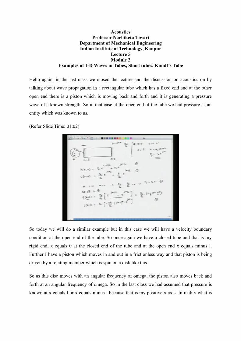
Hello again, in the last class we closed the lecture and the discussion on acoustics on by

talking about wave propagation in a rectangular tube which has a fixed end and at the other

open end there is a piston which is moving back and forth and it is generating a pressure

wave of a known strength. So in that case at the open end of the tube we had pressure as an

entity which was known to us.

(Refer Slide Time: 01:02)

So today we will do a similar example but in this case we will have a velocity boundary

condition at the open end of the tube. So once again we have a closed tube and that is my

rigid end, x equals 0 at the closed end of the tube and at the open end x equals minus l.

Further I have a piston which moves in and out in a frictionless way and that piston is being

driven by a rotating member which is spin on a disk like this.

So as this disc moves with an angular frequency of omega, the piston also moves back and

forth at an angular frequency of omega. So in the last class we had assumed that pressure is

known at x equals l or x equals minus l because that is my positive x axis. In reality what is

happening is that we actually know the velocity boundary condition at x equals minus l

because we know the displacement of the piston exactly.

Now so the question here is that if I know the displacement of the piston at x equals minus l

then how is the pressure profile inside the closed tube. So we will begin by writing down the

boundary conditions, so at x equals 0, u equals 0 that is velocity is 0 and at x equals minus l,

velocity equals a constant Us times cosine of omega t. So let this t in lowercase Us cosine of

omega t. So I can rewrite this as Us and here Us upper case equals Us e j omega t and if I take

the real value, real component of upper case Us then I get.

So just for clarity purposes I will, so I get same thing as Us cosine omega t, so please note

here that the velocity of the piston is not influenced by waves in the tube because it is moving

by whatever amount is dictated by the motion of this rotating disk. So with this understanding

of the boundary conditions we now proceed to write down transmission line equations as they

apply to this particular tube.

So P x omega equals P plus now once again P plus is the strength of forward travelling wave

and it could in general depend on frequency. In this case it is independent of frequency

because there is only one frequency which is being generated here but in general P plus and P

minus both could depend on frequency. So it is P plus e minus j omega x over c and then

there is a reflected component P minus e j omega x over c.

Similarly velocity which depends on x and omega equals P plus by all over characteristic

impedance times e minus j omega x over c plus P minus over Z not excuse me there should

be a negative sign here e j omega x over c. Now once we impose the boundary condition that

at x equals to 0, u is 0 what we get is, because at x equals 0, u equals 0 we get P plus over Z

not minus P minus over Z not equals 0 which gives me P plus equals P minus.

Now I use this relationship, so let us number our equations 1, 2 and 3 and if I put 3 in 2, I get

U x of omega equals P plus over Z not and because P plus is and P plus equals P minus, I

replace P minus by P plus and since this is a common term I take it out of parenthesis and I

get e minus j omega x over c minus e j omega x over c and I know that this term is nothing

but 2 times sine of omega x over c times j.

So I can rewrite this as P plus over Z not times 2 j sine omega x over c, so actually there

should be a negative sign here, so if I have to write U as a function of x and t earlier I was

just writing down the complex amplitude part, so now I know that complex velocity depends

on x and time, so that equals real of minus 2 P plus over Z not times j sin omega x over c

times e j omega t.

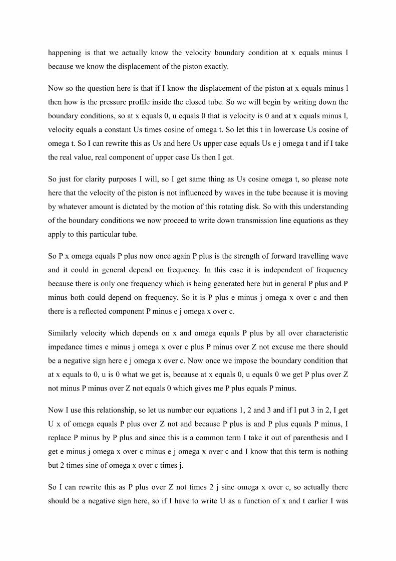
So now we know, so we have applied the first boundary condition and then use that condition

for the velocity equation. Now I am going to determine P plus by utilizing the second

boundary condition that is Us equals Us e j omega t.

(Refer Slide Time: 08:02)

So we know that at x equals minus l, Us equals a magnitude part Us excuse me this is

velocity equals magnitude of it times cosine of omega t and so again just to be consistent this

is lowercase and I know that magnitude of upper case Us is lowercase Us. So now I use this,

impose this boundary condition on equation 4. So I put this equation, so put this in 4 we get

Us equals U of minus l times j omega and that gives us Us equals minus 2 P plus over Z not

sine omega x over c and this whole thing has to be evaluated x equals minus l and then I take

its magnitude.

So from this I get u s that is lowercase u s because that is the magnitude and that equals 2 P

plus over Z not sine of omega l over c and because x equals minus l, so this term becomes

negative omega l over c and the magnitude of this or I can write this as P plus the magnitude

of P plus equals Us over times Z not. So we are taking it out from the magnitude side because

Z not is a pure number and it is a positive entity.

And then the denominator I get 2 sine omega l over c and there is a negative sign before

omega l over c. So that is my P plus, so I know now I have calculated P plus I know that P

negative is same as P positive, so I know that entire solution for pressure and also for velocity

and if I take the real components I can find the actual values for pressure and velocity. Now

once we have developed this equation for P positive, we see that at l equals n lambda over 2

or let us do it slightly differently.

That the condition for P positive to be a maxima would be when the denominator here is

exactly 0. So when denominator is 0 then P plus equals infinite and the condition for that is

when sine omega l over c equals 0. Now sine omega l over c is going to be 0 when omega l

over c equals n times pi and n is an integer it could start from 0 and it could go up to infinity

which means l equals c times n pi over omega.

Now I know that omega is 2 pi times frequency, so l equals c over 2 pi f times n pi and we

know that c over f is nothing but the wavelength of the wave. So that is lambda over 2 and

then pi gets cancelled from numerator and denominator. So I am left with n lambda over 2.

So the condition for maximum pressure is that, so maximum pressure happens at a place at a

location l when l equals n lambda over 2.

So at l equals n lambda over 2, P is maximized and actually in an ideal case as we are seeing

its value actually shoots up to infinite or infinity. Now in reality that may not necessarily

happen because there are damping effects possible and because of that there will be P which

will be at its peak value but it will not be necessarily infinity.

The other way to look at this statement is that if I am placing this vibrating piston at a

location such that this value of l corresponds to n times half the wavelength as long as this

value of l is an integer multiple of half the wavelength of the pressure wave going into the

tube, I would be having a situation where the magnitude of the pressure wave positive

pressure wave would be at its maximum.

(Refer Slide Time: 14:36)

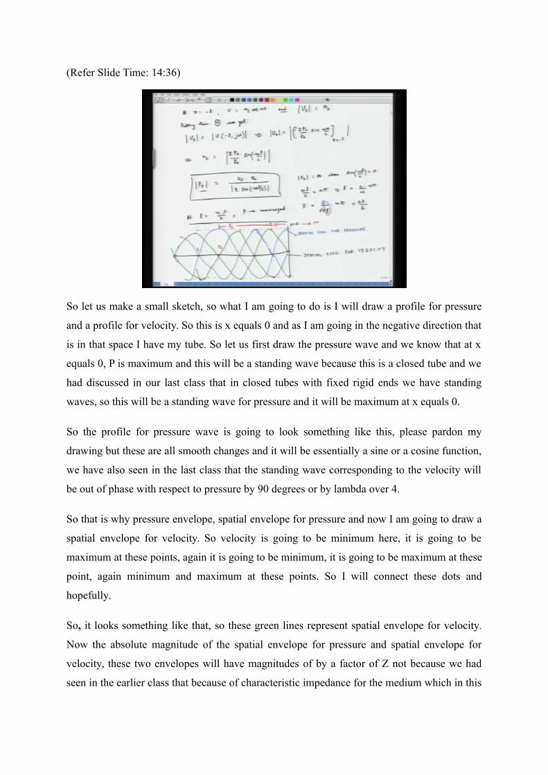
So let us make a small sketch, so what I am going to do is I will draw a profile for pressure

and a profile for velocity. So this is x equals 0 and as I am going in the negative direction that

is in that space I have my tube. So let us first draw the pressure wave and we know that at x

equals 0, P is maximum and this will be a standing wave because this is a closed tube and we

had discussed in our last class that in closed tubes with fixed rigid ends we have standing

waves, so this will be a standing wave for pressure and it will be maximum at x equals 0.

So the profile for pressure wave is going to look something like this, please pardon my

drawing but these are all smooth changes and it will be essentially a sine or a cosine function,

we have also seen in the last class that the standing wave corresponding to the velocity will

be out of phase with respect to pressure by 90 degrees or by lambda over 4.

So that is why pressure envelope, spatial envelope for pressure and now I am going to draw a

spatial envelope for velocity. So velocity is going to be minimum here, it is going to be

maximum at these points, again it is going to be minimum, it is going to be maximum at these

point, again minimum and maximum at these points. So I will connect these dots and

hopefully.

So, it looks something like that, so these green lines represent spatial envelope for velocity.

Now the absolute magnitude of the spatial envelope for pressure and spatial envelope for

velocity, these two envelopes will have magnitudes of by a factor of Z not because we had

seen in the earlier class that because of characteristic impedance for the medium which in this

case is air, the magnitude of velocity’s spatial envelope is P plus over Z not times a constant

while the same for pressure is just P plus times a constant which is 2.

So here I have assumed that the picture shows that they have the same magnitude but in

reality they are off by a factor of Z not but anyway the point what I am trying to make here

by drawing this picture is that if my length of the tube which is, so this is my negative x

direction and this is positive x direction. So if the length of the tube is such that my system is

located at this point or the other case could be that the piston is located at point P2 and here it

is located at point P1.

Now if my piston is located at point P2 in this case the length of the tube is L2, in this case

the piston has to move theoretically by a distance of 0 the amplitude of piston’s motion has to

be theoretically 0 to excite pressure wave which has this non-zero spatial envelope, okay.

However if the location of the piston is at point P1 then no matter how much the piston

moves by it because it will not generate a pressure wave which will have this spatial

envelope.

So these statements are being made in the context of an assumption which we have made that

there is no damping in the system. So if there is no damping in the system and if I place the

piston at location P2 then it has to move by very amount, very small amount of a distance, the

amplitude of its motion has to be very small and that small amplitude of motion would be

sufficient enough to excite a pressure wave whose spatial envelope is depicted here in blue

colour.

Another way to look at it is that if I have a room and if I place a transducer or a loudspeaker

at a corner point in a room then even if that transducer moves by small amount of distance

then assuming that there is no damping effect in the room that small amount of displacement

of the transducer would be, so that is the discussion which I wanted to have in context of

standing waves as they develop in a closed tube at one end and an open tube where the

excitation is being driven by, is being generated by a piston which moves by a known

velocity.

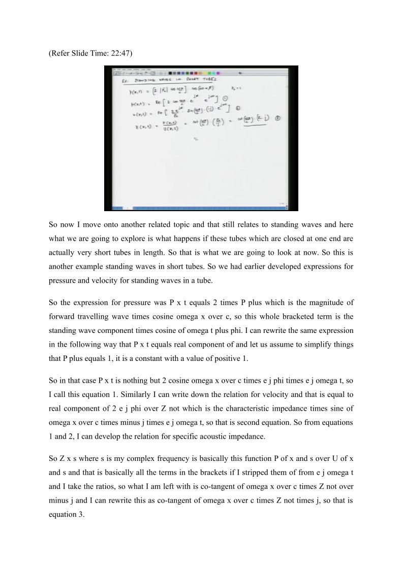
(Refer Slide Time: 22:47)

So now I move onto another related topic and that still relates to standing waves and here

what we are going to explore is what happens if these tubes which are closed at one end are

actually very short tubes in length. So that is what we are going to look at now. So this is

another example standing waves in short tubes. So we had earlier developed expressions for

pressure and velocity for standing waves in a tube.

So the expression for pressure was P x t equals 2 times P plus which is the magnitude of

forward travelling wave times cosine omega x over c, so this whole bracketed term is the

standing wave component times cosine of omega t plus phi. I can rewrite the same expression

in the following way that P x t equals real component of and let us assume to simplify things

that P plus equals 1, it is a constant with a value of positive 1.

So in that case P x t is nothing but 2 cosine omega x over c times e j phi times e j omega t, so

I call this equation 1. Similarly I can write down the relation for velocity and that is equal to

real component of 2 e j phi over Z not which is the characteristic impedance times sine of

omega x over c times minus j times e j omega t, so that is second equation. So from equations

1 and 2, I can develop the relation for specific acoustic impedance.

So Z x s where s is my complex frequency is basically this function P of x and s over U of x

and s and that is basically all the terms in the brackets if I stripped them of from e j omega t

and I take the ratios, so what I am left with is co-tangent of omega x over c times Z not over

minus j and I can rewrite this as co-tangent of omega x over c times Z not times j, so that is

equation 3.

Now this expression for specific impedance for a tube is a very general expression and it is

valid for all tubes as long as they have uniform cross-sections and as long as they are closed

at one end. So now we make an approximation that what happens if this tube has a very small

length. So what if tube is short? So short tube, so that is something we are going to develop.

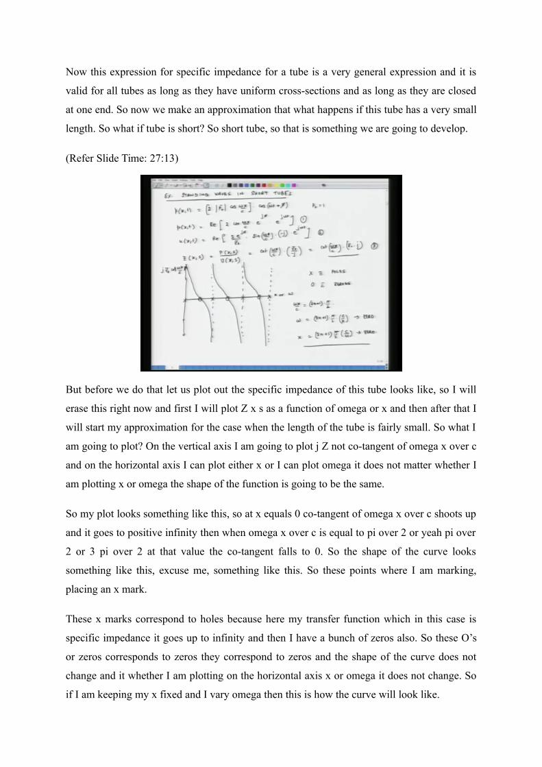
(Refer Slide Time: 27:13)

But before we do that let us plot out the specific impedance of this tube looks like, so I will

erase this right now and first I will plot Z x s as a function of omega or x and then after that I

will start my approximation for the case when the length of the tube is fairly small. So what I

am going to plot? On the vertical axis I am going to plot j Z not co-tangent of omega x over c

and on the horizontal axis I can plot either x or I can plot omega it does not matter whether I

am plotting x or omega the shape of the function is going to be the same.

So my plot looks something like this, so at x equals 0 co-tangent of omega x over c shoots up

and it goes to positive infinity then when omega x over c is equal to pi over 2 or yeah pi over

2 or 3 pi over 2 at that value the co-tangent falls to 0. So the shape of the curve looks

something like this, excuse me, something like this. So these points where I am marking,

placing an x mark.

These x marks correspond to holes because here my transfer function which in this case is

specific impedance it goes up to infinity and then I have a bunch of zeros also. So these O’s

or zeros corresponds to zeros they correspond to zeros and the shape of the curve does not

change and it whether I am plotting on the horizontal axis x or omega it does not change. So

if I am keeping my x fixed and I vary omega then this is how the curve will look like.

Or if I am keeping omega fixed and keep on increasing, changing the value of x the shape of

the transfer function will look to be the same, the condition for zeros is when omega x over c

equals 2n plus 1 times pi over 2. So if I am keeping my x fixed then if x is fixed then when

omega equals 2n plus 1 times pi over 2 times c over x then I get a 0 or if I am keeping omega

fixed then again the condition would be 2n plus 1 pi over 2 times c over omega, this is the

condition for a 0.

The condition for a pole would be that this term omega x over c has to be an integral multiple

of pi, so it could be 0, pi, 2 pi, 3 pi and so on and so forth. So now with this understanding we

move onto the next step and we ask the question that what if my tube is small in length? So I

have a short tube.

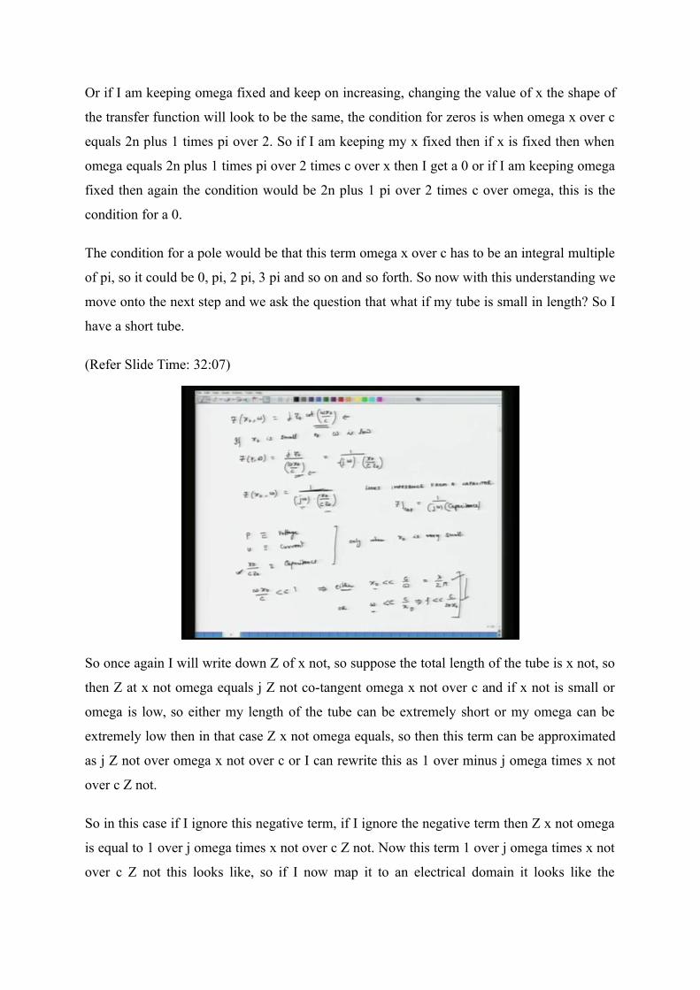
(Refer Slide Time: 32:07)

So once again I will write down Z of x not, so suppose the total length of the tube is x not, so

then Z at x not omega equals j Z not co-tangent omega x not over c and if x not is small or

omega is low, so either my length of the tube can be extremely short or my omega can be

extremely low then in that case Z x not omega equals, so then this term can be approximated

as j Z not over omega x not over c or I can rewrite this as 1 over minus j omega times x not

over c Z not.

So in this case if I ignore this negative term, if I ignore the negative term then Z x not omega

is equal to 1 over j omega times x not over c Z not. Now this term 1 over j omega times x not

over c Z not this looks like, so if I now map it to an electrical domain it looks like the

impedance from a capacitor, looks like impedance because for a capacitor Z capacitor equals

1 over j omega times capacitance, looks like 1 over j omega times capacitance.

So a short tube behaves something like similar to a capacitor where the impedance is x not

over c which is velocity of sound divided by Z not and of course the impedance is this term

multiplied by j omega and the whole thing they can inverse of, so again now if I draw

analogies, if pressure corresponds to voltage and u corresponds to which is velocity

corresponds to current then x not over c Z not corresponds to capacitance, it corresponds to

capacitance.

Now we have assumed, now this is valid only when x not is very small. So then the question

is how small is small? So that is something we are going to now qualify. So from this point to

this point we made this jump because we assumed that x not is small and that jump would

have been possible only if omega x not over c was extremely small compared to 1 which

means that either x not is extremely small compared to c over omega which in turn equals

lambda over 2 pi or omega is extremely small to c over x.

So if these, either of these conditions are satisfied, so the condition that a tube could behave

something similar like a capacitor which has a capacitance value of x not over or equivalent

capacitance value of x not over c Z not valid, if either the length of the tube is extremely

small compared to one sixth lambda over 2 pi which is approximately equal to one sixth of

wavelength.

Or the angular frequency is such that it is extremely small compared to c over x not that is f is

frequency is extremely small compared to 2 pi c over 2 pi x not, so once again if this

condition holds true or the second condition holds true then a short tube or then a tube would

behave as a lumped, it would behave same thing similar like a lumped capacitive element in

the context that if pressure is analogous to voltage, velocity is analogous to current then the

impedance, specific impedance offered by the tube at its free end would be something of this

value. So then now we move onto the next step and we see that how we could, if we have a

long transmission line then how could we have propagation of a wave, a sound wave, an

acoustic wave in a transmission line using a lumped parameter model.

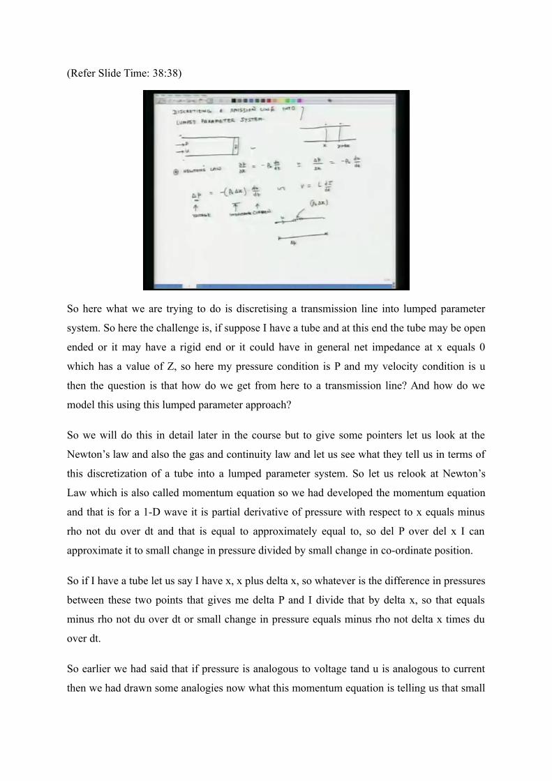
(Refer Slide Time: 38:38)

So here what we are trying to do is discretising a transmission line into lumped parameter

system. So here the challenge is, if suppose I have a tube and at this end the tube may be open

ended or it may have a rigid end or it could have in general net impedance at x equals 0

which has a value of Z, so here my pressure condition is P and my velocity condition is u

then the question is that how do we get from here to a transmission line? And how do we

model this using this lumped parameter approach?

So we will do this in detail later in the course but to give some pointers let us look at the

Newton’s law and also the gas and continuity law and let us see what they tell us in terms of

this discretization of a tube into a lumped parameter system. So let us relook at Newton’s

Law which is also called momentum equation so we had developed the momentum equation

and that is for a 1-D wave it is partial derivative of pressure with respect to x equals minus

rho not du over dt and that is equal to approximately equal to, so del P over del x I can

approximate it to small change in pressure divided by small change in co-ordinate position.

So if I have a tube let us say I have x, x plus delta x, so whatever is the difference in pressures

between these two points that gives me delta P and I divide that by delta x, so that equals

minus rho not du over dt or small change in pressure equals minus rho not delta x times du

over dt.

So earlier we had said that if pressure is analogous to voltage tand u is analogous to current

then we had drawn some analogies now what this momentum equation is telling us that small

change in pressure is equal to a constant which is rho not times delta x times the differential

of velocity with respect to time.

So this is analogous to voltage equals L dI over dt, so this if I say that small change in

pressure is corresponds to voltage and this corresponds to current, u corresponds to current

then this corresponds to inductance, so the Newton Law essentially captures the inductive

part of an acoustic circuit.

So here my approximation could be something like this so I have an across variable delta p

and if the current or analogous to current I have velocity flowing through this element then

the inductance of this value is rho not del x, of course ignoring the negative term. So what

Newton’s Law tells us is it essentially captures the inductive processes happening in a system

in the context that when I equate pressure to voltage and I consider current or velocity

analogous to current.

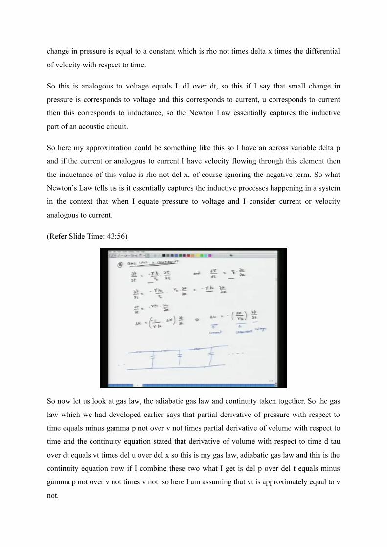
(Refer Slide Time: 43:56)

So now let us look at gas law, the adiabatic gas law and continuity taken together. So the gas

law which we had developed earlier says that partial derivative of pressure with respect to

time equals minus gamma p not over v not times partial derivative of volume with respect to

time and the continuity equation stated that derivative of volume with respect to time d tau

over dt equals vt times del u over del x so this is my gas law, adiabatic gas law and this is the

continuity equation now if I combine these two what I get is del p over del t equals minus

gamma p not over v not times v not, so here I am assuming that vt is approximately equal to v

not.

So v not times del u over del x equals minus gamma so, excuse me so this should be actually

p not, so this del p over del t I can write this as gamma p not over v not in the numerator and

denominator cancel out each other so times del u over del x so just to rewrite this again I get

del p over del t equals minus gamma p not times del u over del x and again as I made

approximation earlier where I am approximating partial derivatives as ratios of small

differences so I can rewrite this whole equation as small change in u equals, so I am

reframing del u over del x.

So small change in u equals 1 over gamma p not times small change in x and of course this a

negative sign times partial derivative of pressure with respect to time. So again to rewrite this

change in velocity equals negative of delta x over gamma p not times partial derivative of

pressure with respect to time. So now if I look at this equation, let us look at these three terms

and what we see is that if we maintain our previous analogies that is U is analogous to current

and P which is pressure is analogous to voltage.

So this analogous to change in current, this is analogous to rate of change of voltage, so then

this it looks like a capacitive term. So essentially when we try to when we synthesize gas law,

continuity and pressure in all into one equation. The gas law and continuity when they are

combined these two laws they essentially try to capture quote unquote the capacitive nature

of an acoustics circuit and the Newton's Law captures the inductive nature of an acoustic

circuit if I am having a lumped parameter model.

So using this approaches and we will see that later we can develop, elaborate transmission

line models which could look something like this. So once again as we will move later into

the course we will see that we will be discretising acoustics circuits and of course also the

mechanical and electrical circuits into lumped parameter systems.

But the basis due to which acoustics circuit could be parameterized as small lumps is two-

fold, the first part is that wherever we will see inductive type of elements in the context of

pressure being analogous to voltage and current being analogous to velocity in that context

the inductive part will be coming from the momentum equation, while the capacitive part will

be attributable to the gas law and the continuity equation. It will be combined effect of gas

law and continuity equation.

(Refer Slide Time: 50:22)

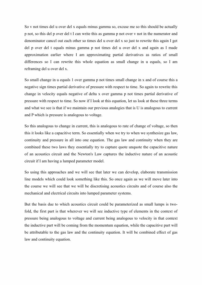
Our final topic for today will be a device called a Kundt’s tube, so here again we will have a

long tube, it will be fixed, it will have a termination at an extreme end but this termination

may or may not be rigid in nature. So this is the tube and let us assume that the termination at

this end is such that the impedance at x equals 0 is ZL, it is ZL.

So here the question is that if I can measure pressure and velocity in the tube at a large

number of points, can I from that data calculate the value of ZL. Now the ZL will depend on

the type of material which is there at the end of the tube so if I have to characterize a

particular material in terms of its acoustic properties I can do that using a Kundt’s tube.

So what we will be doing in next 20-30 minutes is developing an approach through which we

will relate pressure and velocity to ZL and then we will develop a mechanism or a

methodology through which the data from this pressure and velocity field could be used to

extract ZL, the value of ZL. So the transmission line equation is P x omega equals P plus e

minus j omega x over c plus P negative e j omega x over c and then U, which is complex

velocity, amplitude is equal to P plus.

Or instead of P plus I will just right now write it as U plus e minus j omega x over c plus U

minus e j omega x over c and earlier we had seen and this we can further write in terms of

pressure as P plus e minus j omega x over c minus P minus e j omega x over c and then of

course I divide here by characteristic impedance.

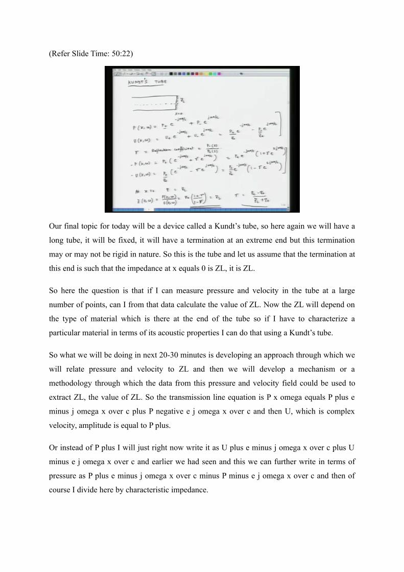
Now at this point I introduce a number gamma and gamma could itself depend on angular

frequency or frequency so like P plus, P negative, U positive and U negative, gamma also

depends on angular frequency and that is defined as it is called as reflection co-efficient and

that is defined as P negative over P positive and both these terms depend on frequency.

Introducing gamma into the relation for pressure and velocity I rewrite these two equations,

so what I get is P x of omega equals P plus e minus j omega x over c plus gamma e j omega x

over c and then U of x omega equals P plus e and then there is a Z not in the numerator e

minus j omega x over c minus gamma e j omega x over c.

So now I take e minus j omega x over c out, so I further rewrite this as P plus e minus j

omega x over c times 1 plus gamma e 2 j omega x over c and here I get P plus over Z not e

minus j omega x over c and then in the parenthesis I get 1 minus gamma e 2 j omega x over c.

So this is my second set of equations.

So now we know that the boundary condition at x equals 0, Z equals ZL and ZL could depend

on frequency because these specific materials have their damping properties varying with

respect to frequency so at x equals 0, Z equals ZL and that means Z 0 omega equals P 0

omega over U 0 omega and that is equal to, so now I plug x equals 0 in relation for pressure

and velocity and what I get is Z not 1 plus gamma over 1 minus gamma and this is equal to

ZL.

Or I can re-express gamma from here as gamma equals ZL minus Z not over ZL plus Z not so

basically I am rewriting this relation as this relation, so now the question is, so I started my

journey with the expectation that I have to figure out what is the value of ZL, now if I can

determine gamma then using this relation if I can find ZL, I can find gamma or if I can find

gamma I can find ZL.

(Refer Slide Time: 57:49)

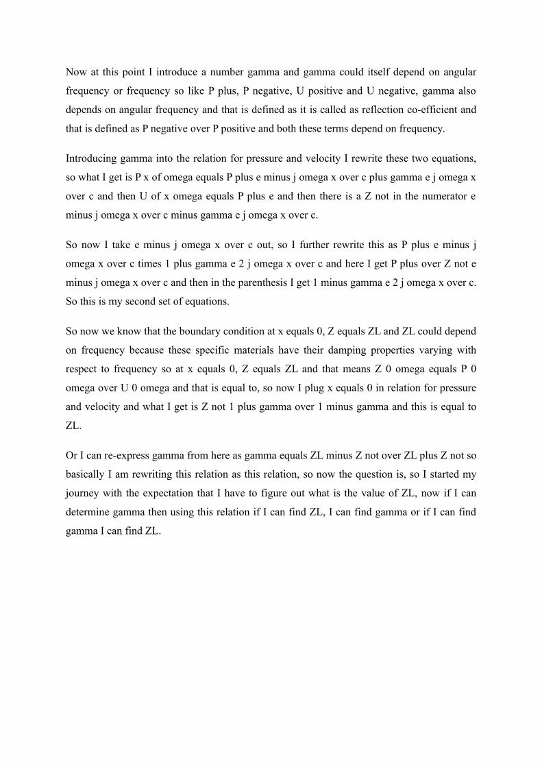
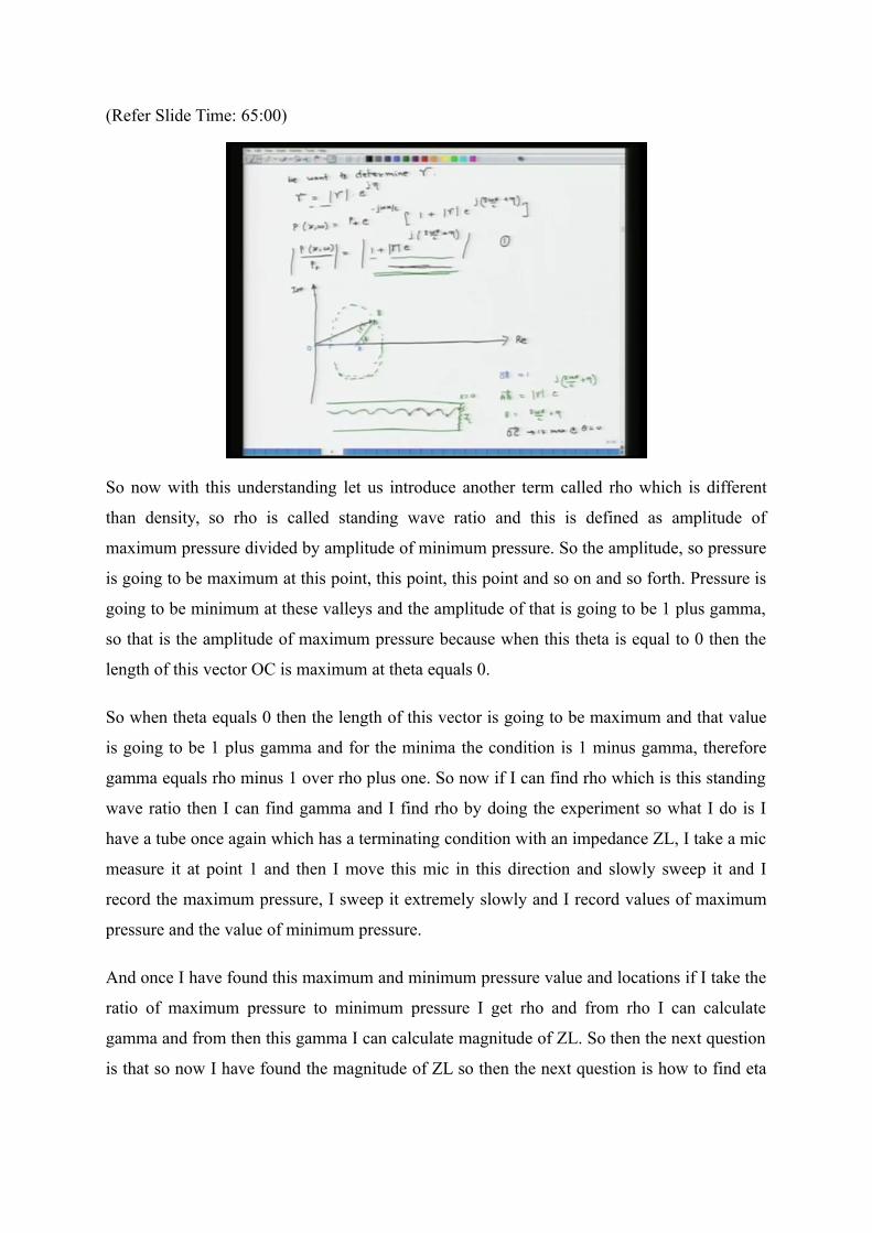
So then my question is that how do we find gamma? So that is what we do now. So here the

endeavour is we want to determine gamma, so we assume a form for gamma. Gamma is a

pure number and it can change with frequency for a specific frequency let us say gamma

equals a magnitude part times e to the power of j eta and eta is a real number so P of x omega

is P positive so now I plug this in these relations for P and U.

So what I get is P x omega equals P positive e minus j omega x over c times 1 plus the

magnitude of gamma times e j 2 omega x over c plus theta or P x omega over P plus equals

and if I take its magnitude then what I get is 1 plus gamma magnitude of it e j times 2 omega

x over c plus eta and I take the magnitude of this whole entire thing. So let us call this

equation 1.

So the ratio of pressure, complex amplitude of the pressure with respect to P positive is this

term. So now what we do is we will plot it graphically and let us see what it means. So we are

plotting this term under right side. So this is the imaginary axis, this is real axis, so the first

term here is 1. So I plot a line whose length is 1 and it is a pure real number so it is co

incident with the real axis.

So vector OA equals 1, the second vector is the term in green, underlined in green. The

magnitude of this term is gamma and the angle, the phase of this thing is 2 omega x plus eta

so as x increases, the angle keeps on changing so with A as the centre I draw a circle, so this

is, so let us assume for a moment this is circle and I draw another vector B where vector AB

equals gamma so the magnitude of this is the radius of this circle is absolute value of gamma

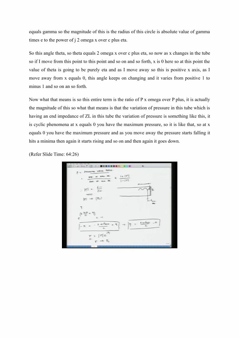
times e to the power of j 2 omega x over c plus eta.

So this angle theta, so theta equals 2 omega x over c plus eta, so now as x changes in the tube

so if I move from this point to this point and so on and so forth, x is 0 here so at this point the

value of theta is going to be purely eta and as I move away so this is positive x axis, as I

move away from x equals 0, this angle keeps on changing and it varies from positive 1 to

minus 1 and so on an so forth.

Now what that means is so this entire term is the ratio of P x omega over P plus, it is actually

the magnitude of this so what that means is that the variation of pressure in this tube which is

having an end impedance of ZL in this tube the variation of pressure is something like this, it

is cyclic phenomena at x equals 0 you have the maximum pressure, so it is like that, so at x

equals 0 you have the maximum pressure and as you move away the pressure starts falling it

hits a minima then again it starts rising and so on and then again it goes down.

(Refer Slide Time: 64:26)

(Refer Slide Time: 65:00)

So now with this understanding let us introduce another term called rho which is different

than density, so rho is called standing wave ratio and this is defined as amplitude of

maximum pressure divided by amplitude of minimum pressure. So the amplitude, so pressure

is going to be maximum at this point, this point, this point and so on and so forth. Pressure is

going to be minimum at these valleys and the amplitude of that is going to be 1 plus gamma,

so that is the amplitude of maximum pressure because when this theta is equal to 0 then the

length of this vector OC is maximum at theta equals 0.

So when theta equals 0 then the length of this vector is going to be maximum and that value

is going to be 1 plus gamma and for the minima the condition is 1 minus gamma, therefore

gamma equals rho minus 1 over rho plus one. So now if I can find rho which is this standing

wave ratio then I can find gamma and I find rho by doing the experiment so what I do is I

have a tube once again which has a terminating condition with an impedance ZL, I take a mic

measure it at point 1 and then I move this mic in this direction and slowly sweep it and I

record the maximum pressure, I sweep it extremely slowly and I record values of maximum

pressure and the value of minimum pressure.

And once I have found this maximum and minimum pressure value and locations if I take the

ratio of maximum pressure to minimum pressure I get rho and from rho I can calculate

gamma and from then this gamma I can calculate magnitude of ZL. So then the next question

is that so now I have found the magnitude of ZL so then the next question is how to find eta

because that will help us in determining the phase of ZL so for doing that we have to find the

location of the first minima.

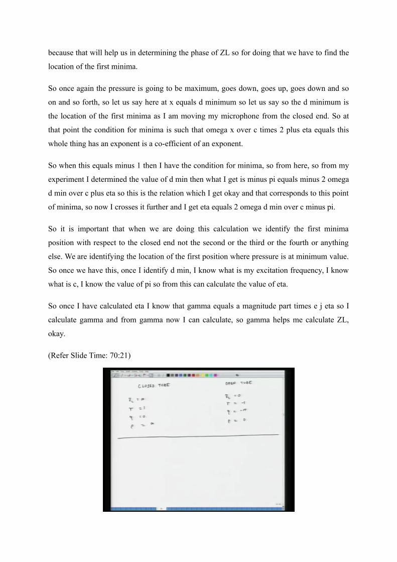
So once again the pressure is going to be maximum, goes down, goes up, goes down and so

on and so forth, so let us say here at x equals d minimum so let us say so the d minimum is

the location of the first minima as I am moving my microphone from the closed end. So at

that point the condition for minima is such that omega x over c times 2 plus eta equals this

whole thing has an exponent is a co-efficient of an exponent.

So when this equals minus 1 then I have the condition for minima, so from here, so from my

experiment I determined the value of d min then what I get is minus pi equals minus 2 omega

d min over c plus eta so this is the relation which I get okay and that corresponds to this point

of minima, so now I crosses it further and I get eta equals 2 omega d min over c minus pi.

So it is important that when we are doing this calculation we identify the first minima

position with respect to the closed end not the second or the third or the fourth or anything

else. We are identifying the location of the first position where pressure is at minimum value.

So once we have this, once I identify d min, I know what is my excitation frequency, I know

what is c, I know the value of pi so from this can calculate the value of eta.

So once I have calculated eta I know that gamma equals a magnitude part times e j eta so I

calculate gamma and from gamma now I can calculate, so gamma helps me calculate ZL,

okay.

(Refer Slide Time: 70:21)

Let us look at two extreme scenarios, I could have a closed tube and I could have an open

tube, so these are extreme conditions, for a closed tube ZL equals infinity and for an open

tube ZL equals 0. For closed tube gamma equals 1, for an open tube gamma equals negative 1

because P plus equals negative of P1. For closed tube eta equals 0 and here eta equals

negative of pi and finally for a closed tube rho equals which is the standing wave ratio is

infinity and here rho standing wave ratio because there are no standing waves it is 0.

So with this we end today’s class and we will in the next class start talking about something

more about transmission of waves through ducts. Thank you.