acta universitatis upsaliensis uppsala dissertations from...
TRANSCRIPT

ACTA UNIVERSITATIS UPSALIENSISUppsala Dissertations from
the Faculty of Science and Technology59


EMAD ABD-ELRADY
Nonlinear Approaches to Periodic
Signal Modeling

Dissertation for the Degree of Doctor of Philosophy in Electrical Engineering withspecialization in Signal Processing presented at Uppsala University 2005.
ABSTRACT
Abd-Elrady, E. 2005: Nonlinear Approaches to Periodic Signal Modeling. Written inEnglish. Acta Universitatis Upsaliensis. Uppsala Dissertations from the Faculty
of Science and Technology 59. 231 pp. Uppsala, Sweden. ISBN 91-554-6079-8
Periodic signal modeling plays an important role in different fields since manyphysical signals can be considered to be approximately periodic. Examples includespeech, musical waveforms, acoustic waves, signals recorded during patient monitoringand outputs of possibly nonlinear systems excited by a sinusoidal input.
The unifying theme of this thesis is using nonlinear techniques to model periodicsignals. The suggested techniques utilize the user pre-knowledge about the signalwaveform. This gives the suggested techniques an advantage, provided that the as-sumed model structure is suitable, as compared to other approaches that do notconsider such priors.
The suggested technique of the first part of this thesis relies on the fact that a sinewave that is passed through a static nonlinear function produces a harmonic spectrumof overtones. Consequently, the estimated signal model can be parameterized as aknown periodic function (with unknown frequency) in cascade with an unknown staticnonlinearity. The unknown frequency and the parameters of the static nonlinearity(chosen as the nonlinear function values in a set of fixed grid points) are estimatedsimultaneously using the recursive prediction error method (RPEM).
A complete treatment of the local convergence properties of the suggested RPEMalgorithm is provided. Also, an adaptive grid point algorithm is introduced to estimatethe unknown frequency and the parameters of the static nonlinearity in a number ofadaptively estimated grid points. This gives the RPEM method more freedom toselect the grid points and hence reduces modeling errors.
Limit cycle oscillations problem are encountered in many applications. Therefore,mathematical modeling of limit cycles becomes an essential topic that helps to betterunderstand and/or to avoid limit cycle oscillations in different fields.
In the second part of this thesis, a second-order nonlinear ODE model is usedto model the periodic signal as a limit cycle oscillation. The right hand side of thesuggested ODE model is parameterized using a polynomial function in the states,and then discretized to allow for the implementation of different identification algo-rithms. Hence, it is possible to obtain highly accurate models by only estimating afew parameters. Also, this is conditioned on the fact that the signal model is suitable.
In the third part, different user aspects for the two nonlinear approaches of thethesis are discussed. Also, some comments on other approaches to the problem ofmodeling periodic signals are given. Finally, topics for future research are presented.
Keywords: Cramer-Rao bounds; frequency estimation; identification; limit cycle; non-linear systems, periodic signals; Wiener model structure.
Emad Abd-Elrady, Uppsala University, Department of Information Technology, Divi-
sion of Systems and Control, P. O. Box 337, SE-751 05 Uppsala, Sweden.
c© Emad Abd-Elrady 2005
ISSN 1104-2516ISBN 91-554-6079-8.urn:nbn:se:uu:diva-4644 (http://urn.kb.se/resolve?urn=urn:nbn:se:uu:diva-4644)
Printed in Sweden by Elanders Gotab, Stockholm 2005
Distributor: Uppsala University Library, Box 510, SE-751 20 Uppsala, Sweden

To my family


“All praise is due to Allah, the Lord of the Worlds”
Acknowledgements
First of all I would like to express my deep and sincere gratitude to my supervi-sors Prof. Torsten Soderstrom and Prof. Torbjorn Wigren for their unlimitedsupport, excellent guidance and for sharing their profound knowledge in systemidentification. I am also grateful to them for valuable comments and sugges-tions on the manuscript of this thesis.
I am indebted to Prof. Johan Schoukens for valuable discussions and pleas-ant collaboration.
I am thankful to Ms. Ingegerd Wass for her patience and understandingwhile helping with all administrative issues.
I wish also to thank all my colleagues at Systems and Control group forcreating such a pleasant work environment, stimulating discussions and fortheir great tendency to help. I am indebted to Mats Ekman for interestingdiscussions and for his useful comments on the manuscript of this thesis. Also,I am thankful to Peter Naucler and Agnes Runqvist for providing the Swedishtranslation of the thesis summary.
I am thankful to Prof. Jonas Sjoberg for serving as my faculty opponent.Thanks are due to Prof. Irene Gu, Prof. Xiaoming Hu and Assoc. Prof. PeterHandel for being the members of my thesis committee.
I am grateful to Prof. Atef Bassiouney and Prof. Eweda Eweda for theirsupport and encouragement during my master study in Egypt. I would likealso to thank my colleagues at the Higher Technological Institute for their helpand friendship.
Also, my friends in Uppsala deserve a special thank for their support andfriendship. I am indebted to Usama Hegazy, Mohamed Issa, Dr. Idress Atti-talla, and their families for the nice time that we spent together.
My parents, my sisters and their families, and my wife’s family have beenalways encouraging me during my study. My wife Riham has been alwaysunderstanding and supportive. This thesis would not exist without her loveand patience. Finally, I am grateful to my kids, Hadil and Omar, for adding abig smile to my life.


Contents
Glossary xiii
1 Introduction 1
1.1 Periodic Signals . . . . . . . . . . . . . . . . . . . . . . . . . . . 1
1.1.1 Fourier Series Representation . . . . . . . . . . . . . . . 1
1.1.2 Importance of Periodic Signal Modeling . . . . . . . . . 3
1.1.3 Introductory Examples . . . . . . . . . . . . . . . . . . . 4
1.2 Modeling of Periodic Signals . . . . . . . . . . . . . . . . . . . . 6
1.2.1 System Identification . . . . . . . . . . . . . . . . . . . . 6
1.2.2 The Scope of the Thesis . . . . . . . . . . . . . . . . . . 7
1.3 Previous Approaches to Periodic Signal Modeling . . . . . . . . 7
1.3.1 The Periodogram . . . . . . . . . . . . . . . . . . . . . . 7
1.3.2 Modeling of Line-Spectra . . . . . . . . . . . . . . . . . 8
1.3.3 The Adaptive Comb Filter . . . . . . . . . . . . . . . . 10
1.4 Periodic Signal Modeling Based on the Wiener Model Structure 12
1.4.1 Block-Structured Models . . . . . . . . . . . . . . . . . 12
1.4.2 The Adaptive Nonlinear Modeler . . . . . . . . . . . . . 17
1.4.3 The Periodic Signal Modeling Approach Based on theWiener Model . . . . . . . . . . . . . . . . . . . . . . . . 18
1.5 Periodic Signal Modeling Using Orbits of Second-Order Nonlin-ear ODE’s . . . . . . . . . . . . . . . . . . . . . . . . . . . . . . 19
1.5.1 Dynamical Systems . . . . . . . . . . . . . . . . . . . . . 20
1.5.2 Nonlinear Models of Dynamical Systems . . . . . . . . . 20
1.5.3 Solutions of Ordinary Differential Equations . . . . . . . 21
1.5.4 Second-Order Autonomous Systems . . . . . . . . . . . 22
1.5.5 Limit Cycles . . . . . . . . . . . . . . . . . . . . . . . . 22
1.5.6 Stability of Periodic Solutions . . . . . . . . . . . . . . . 23
1.5.7 The Periodic Signal Modeling Approach Using PeriodicOrbits . . . . . . . . . . . . . . . . . . . . . . . . . . . . 24
1.6 Why and When to Use the Proposed Methods in this Thesis? . 26
1.7 Thesis Outline and Contributions . . . . . . . . . . . . . . . . . 30
vii

viii CONTENTS
I Periodic Signal Modeling Based on the WienerModel Structure 35
2 Periodic Signal Modeling Using Adaptive Nonlinear Function
Estimation 37
2.1 Introduction . . . . . . . . . . . . . . . . . . . . . . . . . . . . . 37
2.2 Review of the Algorithm of [121] . . . . . . . . . . . . . . . . . 38
2.3 Piecewise Quadratic Approximation . . . . . . . . . . . . . . . 40
2.4 Numerical Examples . . . . . . . . . . . . . . . . . . . . . . . . 42
2.5 Conclusions . . . . . . . . . . . . . . . . . . . . . . . . . . . . . 46
3 A Modified Nonlinear Approach to Periodic Signal Modeling 47
3.1 Introduction . . . . . . . . . . . . . . . . . . . . . . . . . . . . . 47
3.2 The Modified Algorithm . . . . . . . . . . . . . . . . . . . . . . 47
3.3 Local Convergence . . . . . . . . . . . . . . . . . . . . . . . . . 51
3.3.1 The Associated ODE Approach . . . . . . . . . . . . . . 51
3.3.2 Analysis Details . . . . . . . . . . . . . . . . . . . . . . 53
3.3.3 Discussion . . . . . . . . . . . . . . . . . . . . . . . . . . 56
3.4 The Cramer-Rao Bound . . . . . . . . . . . . . . . . . . . . . . 58
3.5 Numerical Examples . . . . . . . . . . . . . . . . . . . . . . . . 60
3.6 Conclusions . . . . . . . . . . . . . . . . . . . . . . . . . . . . . 64
3.A Proof of Lemma 3.2 . . . . . . . . . . . . . . . . . . . . . . . . 67
3.B Proof of Lemma 3.3 . . . . . . . . . . . . . . . . . . . . . . . . 70
3.C Proof of Theorem 3.2 . . . . . . . . . . . . . . . . . . . . . . . . 73
4 An Adaptive Grid Point Algorithm for Periodic Signal Mod-
eling 79
4.1 Introduction . . . . . . . . . . . . . . . . . . . . . . . . . . . . . 79
4.2 The Suggested Algorithm . . . . . . . . . . . . . . . . . . . . . 79
4.3 The Cramer-Rao Bound . . . . . . . . . . . . . . . . . . . . . . 83
4.4 Numerical Examples . . . . . . . . . . . . . . . . . . . . . . . . 85
4.5 Conclusions . . . . . . . . . . . . . . . . . . . . . . . . . . . . . 92
4.A Proof of Theorem 4.1 . . . . . . . . . . . . . . . . . . . . . . . . 92
II Periodic Signal Modeling Using Orbits of Second-Order Nonlinear ODE’s 101
5 The Second-Order Nonlinear ODE Model 103
5.1 Introduction . . . . . . . . . . . . . . . . . . . . . . . . . . . . . 103
5.2 Examples . . . . . . . . . . . . . . . . . . . . . . . . . . . . . . 104

CONTENTS ix
5.3 Modeled Signal and Measurements . . . . . . . . . . . . . . . . 107
5.4 Model Structures . . . . . . . . . . . . . . . . . . . . . . . . . . 107
5.5 Parameterization . . . . . . . . . . . . . . . . . . . . . . . . . . 109
5.6 Discretization . . . . . . . . . . . . . . . . . . . . . . . . . . . . 110
6 Sufficiency of Second-Order Nonlinear ODE for Modeling Pe-
riodic Signals 111
6.1 Introduction . . . . . . . . . . . . . . . . . . . . . . . . . . . . . 111
6.2 General Assumptions on the Modeled signal . . . . . . . . . . . 112
6.3 Smoothness of the Modeled Orbit . . . . . . . . . . . . . . . . . 112
6.4 Conditions on y(t) to Be a Solution . . . . . . . . . . . . . . . 113
6.5 Uniqueness of the Solution . . . . . . . . . . . . . . . . . . . . . 116
6.6 When a Second-Order ODE Model Is Insufficient . . . . . . . . 117
6.7 Conclusions . . . . . . . . . . . . . . . . . . . . . . . . . . . . . 118
7 Least Squares and Markov Estimation of Periodic Signals 119
7.1 Introduction . . . . . . . . . . . . . . . . . . . . . . . . . . . . . 119
7.2 The Least Squares Algorithm . . . . . . . . . . . . . . . . . . . 120
7.3 The Markov Estimate . . . . . . . . . . . . . . . . . . . . . . . 122
7.4 Numerical Examples . . . . . . . . . . . . . . . . . . . . . . . . 124
7.4.1 The LS Algorithm Simulation Study . . . . . . . . . . . 125
7.4.2 The Markov Estimate Compared to the LS Estimate . . 127
7.5 Conclusions . . . . . . . . . . . . . . . . . . . . . . . . . . . . . 130
8 Periodic Signal Modeling with Kalman Filters 131
8.1 Introduction . . . . . . . . . . . . . . . . . . . . . . . . . . . . . 131
8.2 The Kalman Filter (KF) . . . . . . . . . . . . . . . . . . . . . . 132
8.3 The Extended Kalman Filter (EKF) . . . . . . . . . . . . . . . 134
8.4 Simulation Study . . . . . . . . . . . . . . . . . . . . . . . . . . 134
8.5 Conclusions . . . . . . . . . . . . . . . . . . . . . . . . . . . . . 138
9 Maximum Likelihood Estimation of Periodic Signals 139
9.1 Introduction . . . . . . . . . . . . . . . . . . . . . . . . . . . . . 139
9.2 The ODE models . . . . . . . . . . . . . . . . . . . . . . . . . . 139
9.3 The Maximum Likelihood Method . . . . . . . . . . . . . . . . 141
9.4 The Cramer-Rao Bound . . . . . . . . . . . . . . . . . . . . . . 143
9.5 Simulation Study . . . . . . . . . . . . . . . . . . . . . . . . . . 144
9.6 Conclusions . . . . . . . . . . . . . . . . . . . . . . . . . . . . . 149
9.A Derivation of the Details of the CRB . . . . . . . . . . . . . . . 149

x CONTENTS
10 Periodic Signal Modeling Based on Fully Automated Spectral
Analysis 153
10.1 Introduction . . . . . . . . . . . . . . . . . . . . . . . . . . . . . 153
10.2 The Least Squares Estimate . . . . . . . . . . . . . . . . . . . . 154
10.3 The Fully Automated Spectral Analysis Technique . . . . . . . 154
10.3.1 Initial Estimate T0 . . . . . . . . . . . . . . . . . . . . . 155
10.3.2 Improved Estimate of the Period Length . . . . . . . . . 156
10.3.3 Estimation of the Fourier Coefficients and their Variance 157
10.3.4 Estimation of x1(t), x2(t) and x2(t) . . . . . . . . . . . 157
10.4 Simulation Study . . . . . . . . . . . . . . . . . . . . . . . . . . 158
10.5 Conclusions . . . . . . . . . . . . . . . . . . . . . . . . . . . . . 159
11 Periodic Signal Modeling Based on Lienard’s Equation 163
11.1 Introduction . . . . . . . . . . . . . . . . . . . . . . . . . . . . . 163
11.2 The ODE Model Based on Lienard’s Equation . . . . . . . . . 164
11.2.1 Model Structures . . . . . . . . . . . . . . . . . . . . . . 164
11.2.2 Discretization . . . . . . . . . . . . . . . . . . . . . . . . 164
11.2.3 Algorithms . . . . . . . . . . . . . . . . . . . . . . . . . 165
11.3 Model Parameterization Using Lienard’s Theorem . . . . . . . 166
11.4 Numerical Examples . . . . . . . . . . . . . . . . . . . . . . . . 169
11.5 Conclusions . . . . . . . . . . . . . . . . . . . . . . . . . . . . . 175
11.A Proof of Theorem 11.2 . . . . . . . . . . . . . . . . . . . . . . . 175
12 Bias Analysis in LS Estimation of Periodic Signals 177
12.1 Introduction . . . . . . . . . . . . . . . . . . . . . . . . . . . . . 177
12.2 Estimation Errors . . . . . . . . . . . . . . . . . . . . . . . . . 178
12.3 Explicit Analysis for Simple Systems . . . . . . . . . . . . . . . 181
12.3.1 Random noise errors . . . . . . . . . . . . . . . . . . . . 181
12.3.2 Discretization errors . . . . . . . . . . . . . . . . . . . . 185
12.4 Numerical Study . . . . . . . . . . . . . . . . . . . . . . . . . . 190
12.5 Conclusions . . . . . . . . . . . . . . . . . . . . . . . . . . . . . 196
12.A Asymptotic Random Noise Bias for S2 Using A3 . . . . . . . . 197
12.B Discretization Error Contributions to x2(kh) and x2(kh) . . . . 199
12.C Discretization Error of Order O(h3) for S1 . . . . . . . . . . . 200
12.D Results of Table 12.2 and Table 12.3 . . . . . . . . . . . . . . . 201
12.E Asymptotic Discretization Bias for S2 Using A3 . . . . . . . . 202

CONTENTS xi
III User Aspects and Future Research 205
13 User Aspects 207
13.1 Introduction . . . . . . . . . . . . . . . . . . . . . . . . . . . . . 207
13.2 User Aspects for the Approach of Part I . . . . . . . . . . . . . 207
13.2.1 Modeled Signal . . . . . . . . . . . . . . . . . . . . . . . 207
13.2.2 Choice of the Algorithm . . . . . . . . . . . . . . . . . . 207
13.2.3 Grid Points . . . . . . . . . . . . . . . . . . . . . . . . . 208
13.2.4 Nonlinear Modeler . . . . . . . . . . . . . . . . . . . . . 208
13.2.5 Additive Noise . . . . . . . . . . . . . . . . . . . . . . . 209
13.2.6 Local Minima . . . . . . . . . . . . . . . . . . . . . . . . 209
13.2.7 Design Variables . . . . . . . . . . . . . . . . . . . . . . 209
13.2.8 Computational Complexity . . . . . . . . . . . . . . . . 210
13.3 User Aspects for the Approach of Part II . . . . . . . . . . . . 210
13.3.1 Modeled Signal . . . . . . . . . . . . . . . . . . . . . . . 210
13.3.2 Choice of the Algorithm . . . . . . . . . . . . . . . . . . 210
13.3.3 Sampling Period . . . . . . . . . . . . . . . . . . . . . . 211
13.3.4 Additive Noise . . . . . . . . . . . . . . . . . . . . . . . 211
13.3.5 Design Variables . . . . . . . . . . . . . . . . . . . . . . 211
13.3.6 Polynomial Degrees . . . . . . . . . . . . . . . . . . . . 211
13.3.7 Computational Complexity . . . . . . . . . . . . . . . . 212
14 Conclusions and Future Research 215
14.1 Conclusions . . . . . . . . . . . . . . . . . . . . . . . . . . . . . 215
14.2 Topics for Future Research . . . . . . . . . . . . . . . . . . . . 216
Svensk Sammanfattning 221
Bibliography 223


Glossary
The following lists of notations and abbreviations are intended to introducesymbols that are frequently used in the thesis. The notational convention usedis that matrices are written with bold face, upper case, for example, R andthat vectors are written with bold face, lower case, for example, r. Note thatthe same symbol may occasionally be used for a different purpose.
Notations
col R a column vector created by stacking the columns of thematrix R on top of each other
D differentiation operatorDM set of parameter vectors describing the model setE expectation operatore(kh) discrete-time white noisee(t) continuous-time white noisef frequencyfs sampling frequencyh sampling intervalI identity matrixinf the infimum, the greatest lower boundmaxθ maximization with respect to θminθ minimization with respect to θN number of measurementsN set of positive integersN (0, σ2) normal distribution with zero mean and variance σ2
O(h) ∆ = O(h) ⇒ ∆/h is bounded when h→ 0p(x) probability density function of xq forward-shift operator (qy(kh) = y(kh+ h))q−1 backward-shift operator (q−1y(kh) = y(kh− h))R set of real numbersRn the n-dimensional Euclidean spaceRi×j a matrix of i rows and j columns
RT transpose of the matrix R
R† pseudoinverse of the matrix Rsup the supremum, the least upper boundT time periodx time derivative of x(t)x estimate of x|x| absolute value of x
xiii

xiv GLOSSARY
‖x‖ the L2 norm of the vector x (‖x‖2 = xTx)Z set of all integersZN set of measurementsδk,s Kronecker delta (= 1 if k = s, otherwise = 0)δ(τ) Dirac’s δ-functionω angular frequency (ω = 2π
T )∅ empty set∈ belongs to⊂ subset∩ intersection∪ union
, equal by definition6= not equal≈ approximately equal⇒ implies∃ exists∀ for all
Abbreviations
AR autoregressiveARMA autoregressive moving averageASA automated spectral analysisBLUE best linear unbiased estimatecf. confere, compareCRB Cramer-Rao bounddB decibelDFT discrete Fourier transformEB Euler backward approximationEC Euler center approximationEF Euler forward approximatione.g. exempli gratia, for the sake of exampleEKF extended Kalman filterEIV error in variablesESPRIT estimation of signal parameters by rotational invariance
techniquesFFT fast Fourier transformFIR finite impulse responsei.e. id est, that isIIR infinite impulse responseKF Kalman filterLHP left half planeLS least squaresMISO multiple input, single output

GLOSSARY xv
ML maximum likelihoodMSE mean squared errorMUSIC multiple signal classificationODE ordinary differential equationpdf probability density functionPSD power spectral densityRHP right half planeRLS recursive least squaresRPEACF recursive prediction error adaptive comb filterRPEM recursive prediction error methodSISO single input, single outputSNR signal to noise ratioTLS total least squaresWELS weighted extended least squaresw.r.t. with respect to


Chapter 1
Introduction
1.1 Periodic Signals
NATURE is full of systems which return periodically to the same initialstate, passing through the same sequence of intermediate states every
period. Everyday life is more or less built up around such phenomena, fromnight and day to the rise and fall of the tides, the phases of the moon, and theannual cycle of the seasons.
A signal fp(t) is said to be periodic if there is a positive real number Tosuch that for all times t,
fp(t) = fp(t+ To). (1.1)
The smallest value of To that achieves (1.1) is called the period of fp(t). Someexamples of periodic signals are shown in Fig. 1.1.
Many physical signals can be considered to be approximately periodic. Ex-amples include speech, musical waveforms, acoustic waves generated by he-licopters and boats, and outputs of possibly nonlinear systems excited by asinusoidal input, see [75, 121].
In biomedicine, several signals recorded during patient monitoring are ap-proximately periodic, e.g. heart rhythm, cardiograms and pneumograms, see[1]. In repetitive control applications, e.g. doing some repetitive jobs usingrobotic manipulators, periodic signals can be used as a reference control signal,see [64, 100]. In mechanical engineering, periodic signals can be used in the de-tection and estimation of machine vibration, see [124]. In signal processing, theproblem of extracting signals that contain (almost) periodic components fromthe noise corrupted observations arises in radar, sonar, and communicationswhere it is important to estimate the parameters of these periodic components,see [102].
1.1.1 Fourier Series Representation
There is one sort of periodic behaviour that can be regarded as the basis fordescribing more general cases. This is the “sinusoidal” waveform shown inFig. 1.1(a), so called because one realization is the sine function, sin(t).
General periodic signals can be represented by a sum of sinusoidal waveswhose frequencies are integral multiples of the lowest frequency (the so-called
1

2 1. Introduction
0 10 20 30 40 50 60−2
−1.5
−1
−0.5
0
0.5
1
1.5
2
Time [seconds]
To
(a) Sinusoidal wave
0 10 20 30 40 50 60 70−2
−1.5
−1
−0.5
0
0.5
1
1.5
2
Time [seconds]
To
(b) Square wave
0 10 20 30 40 500
0.5
1
1.5
2
2.5
3
Time [seconds]
To
(c) Saw-tooth wave
0 50 100 150−1
−0.8
−0.6
−0.4
−0.2
0
0.2
0.4
0.6
0.8
1
Time [seconds]
To
(d) Sum of sinusoidal waves
F i gur e 1.1: Examp les of p er io d ic s ign als .
fundamental frequency). This representation is known as a Fourier series, seee.g. [81], and it is given by
fp(t) = C0 +
∞∑
k=1
Ck sin(kωot+ φk), (1.2)
where C0 is the mean value of the periodic signal, ωo = 2π/To is the funda-mental angular frequency, Ck and φk are the amplitude and phase of the kthharmonic component of fp(t), respectively. For example, a square wave, seeFig. 1.1(b), can be approximated by
s(t) =
∞∑
k=1,3,5,..
1
ksin(kωot). (1.3)
The approximated square wave is shown in Fig. 1.2 using 3 and 8 harmonics.

1.1. Periodic Signals 3
0 10 20 30 40 50−1
−0.8
−0.6
−0.4
−0.2
0
0.2
0.4
0.6
0.8
1
Time [seconds]
(a) 3 harmonics
0 10 20 30 40 50−1
−0.8
−0.6
−0.4
−0.2
0
0.2
0.4
0.6
0.8
1
Time [seconds]
(b) 8 harmonics
Figure 1.2: Approximating a square wave with a sum of sinusoidal components.
1.1.2 Importance of Periodic Signal Modeling
Periodic signal modeling plays an important role in many fields, e.g., for thefollowing reasons:
• Tracking of time-varying parameters of sinusoids in additive noise is ofgreat importance in many engineering applications such as radar, com-munications, control, biomedical engineering and others, see e.g. [34, 42,43, 68, 106, 115].
• In many applications of signal processing as in sonar, radar and commu-nications, it is desirable to eliminate or extract sine waves from observeddata or to estimate their unknown frequencies, amplitudes and phases,see e.g. [33, 46, 48, 49, 102].
• In numerous practical applications there is a need to enhance or eliminatesignals locally modeled as a finite or infinite sum of harmonics. Theseinclude enhancement of noisy biological signals, such as voiced speechand heart waveforms. When the parameters of the signal are unknownor possibly time-varying a natural approach is to use an adaptive filter toenhance/eliminate the signal or to estimate its parameters, see e.g. [20,51, 75].
• The design of power systems is complicated in the presence of harmonics.Presence of harmonics can lead to unpredicted interaction between com-ponents in power networks, which in the worst case can lead to instability,see e.g. [3, 73].
• Periodic signal models have been found to be very good candidates foruse in speech synthesis systems or in speech production machines. Text-to-speech (TTS) systems are used for voice delivery of text messages and

4 1. Introduction
1 365 730 10954
6
8
10
12
14
16
18
20
t [days]
N(t
) [h
ou
rs]
Figure 1.3: Number of daylight hours in Stockholm.
e-mail, reading books and voice response to database inquires, see e.g.[32, 79].
1.1.3 Introductory Examples
Example 1.1. Number of hours of daylight.
Many important periodic phenomena abound in the real world. The numberof hours of daylight on a given day of the year at any particular location onearth is a periodic function of time. It can be modeled by (see [36])
N (t) = no + σ sin
(2π(t− tno
)
To
), (1.4)
where
• t is the number of days from January 1 of any given year,
• no is the average number of hours of daylight (12 hours),
• σ is the maximum variation above (in summer) and below (in winter) no.This means that the longest day is no + σ hours and the shortest day isno − σ hours,
• tnois the number of the day when exactly no hours of daylight occur,
• To is the period of the periodic function N (t) which in this case equalsthe number of days in a year (365 days).
Once the function (1.4) is available, it is possible to answer a variety of questionssuch as: How many hours of daylight would be expected on a particular date?When will there be a specific number of hours of daylight? For example, theplot of the function N (t) is given in Fig. 1.3 for Stockholm.

1.1. Periodic Signals 5
0 500 1000 1500 2000−2.5
−2
−1.5
−1
−0.5
0
0.5
1
1.5
2
2.5
Time [samples]
x
(a) Muscle fiber length vs. time
0 500 1000 1500 2000−0.8
−0.6
−0.4
−0.2
0
0.2
0.4
0.6
0.8
Time [samples]
v(b) Stimulus vs. time
−1 −0.5 0 0.5 1−3
−2
−1
0
1
2
3
v
x
diastole
systole
(c) Muscle fiber length vs. stimulus
Figure 1.4: The pumping heart signals.
Example 1.2. The pumping heart.
The human heart, a pump which takes re-oxygenated blood from the lungs andpumps it out to the rest of the body, may be modeled as an oscillator. Thesystem oscillates between two states: diastole, or relaxed state, and systole, orcontracted state. An electro-chemical stimulus causes the heart muscle con-traction and transition from diastole to systole states. A simplified model ofthis process is the modified Van der Pol oscillator, see [14]:
x = µ
[−v −
(x3
3− αx
)],
v =x− x0
µ,
(1.5)
where x(t) is the muscle fiber length in the heart, v(t) is the stimulus,µ > 0 and α are parameters. The model (1.5) has an equilibrium point at

6 1. Introduction
(x v)T
=(x0 − x3
0
3 + αx0
)T. Equation (1.5) is solved numerically using
the Matlab function ode45 for µ = 10, α = 1 and x0 = 0, i.e. the equilibriumpoint is shifted at the origin. The muscle fiber length x(t) and the stimu-lus v(t) are plotted in Figures 1.4(a)-1.4(b) versus time. Also, x(t) is plottedversus v(t) in Fig. 1.4(c). Figures 1.4(a)-1.4(b) show that x(t) and v(t) areperiodic with time and Fig. 1.4(c) shows that in the transition from diastole(long fibers) to systole (short fibers), the contraction happens slowly at first(this ensures no blood backflow which could damage the heart) but that at highenough stimulus the fibers contract suddenly to push the blood all throughoutthe body.
1.2 Modeling of Periodic Signals
1.2.1 System Identification
System identification is the field of mathematical modeling of dynamic systemsand of signal characteristics using experimental data. Many applications can befound in technical and non-technical areas. In control and system engineering,system identification methods are used to estimate suitable models for designof regulators, a prediction algorithm, or for simulation. In signal processingapplications such as communications, geophysical engineering and mechani-cal engineering, models obtained by system identification are used for spectralanalysis, fault detection, linear prediction and other purposes. In non-technicalareas such as biology, environmental sciences and econometrics, system iden-tification is used to develop models for increasing knowledge of the identifiedobject, or for prediction and control.
System identification can be divided into two categories: off-line identifica-tion or batch identification, and on-line identification or recursive identification.Off-line identification means that a batch of data are collected from the systemand subsequently - as a separate procedure - this batch of data are used toconstruct a model. On the other hand, in case the model is needed to sup-port decisions that should be taken during the operation of the system, i.e.“on-line”, it is necessary to infer the model at the same time as the data arecollected. The model is then “updated” at each time instant some new databecome available. This means that if there is an estimate γ(t − 1) based ondata up to time t− 1, then γ(t) is computed by some modification of γ(t− 1)when the new data becomes available.
Nowadays, there is a quite substantial literature on recursive identificationsee e.g. [51, 59, 65, 66, 69]. Different recursive algorithms have been suggestedand analyzed to find conditions necessary for the recursive algorithm to performwell. Recursive identification methods have the following general features:
• They are the main part of adaptive systems where the action is takenbased on the most recent model.
• They do not occupy much memory space, since not all data are stored.

1.3. Previous Approaches to Periodic Signal Modeling 7
• They can be easily modified to track time-varying parameters.
• They can be used as a first step in a fault detection algorithm, see [13,35], which is used to find out if the system characteristics have changedsignificantly.
1.2.2 The Scope of the Thesis
The study and the analysis of periodic signals is broadly important. Veryoften, transient changes in these signals carry important information aboutthe system. Many modeling schemes are used in this analysis. Some of theseschemes may be constrained by the fact that no prior knowledge about theperiodic signal is available. Other schemes, like the ones used in this thesis,can benefit from prior knowledge about the signal waveform. In real-time, afrequency estimation algorithm must be able to detect, estimate and track thechanging dynamics of either single or multiple periodic signals. This estimationprocess may be constrained by the level and type of noise.
The study in this thesis concerns modeling of real-valued periodic signalsusing nonlinear techniques. The suggested nonlinear techniques in this thesisbenefit from prior information about the periodic signal such as being generatedfrom nonlinear ordinary differential equation (ODE) or that its shape resemblesknown waveforms. Hence, an improvement in the performance of these methodsis expected as compared to other methods that do not make use of any priors.This is provided that the assumed model structure is suitable for these periodicsignals.
1.3 Previous Approaches to Periodic Signal Modeling
The problem of periodic signal modeling has been approached from many di-rections. Each one of these approaches has its advantages and disadvantages.In this section, some of these earlier approaches will be discussed. More specif-ically, periodograms, modeling of line-spectra and adaptive comb filtering willbe described. New approaches to the problem of modeling periodic signals willbe presented in Sections 1.4-1.5.
1.3.1 The Periodogram
The periodogram should be considered as the first method used to determinepossible hidden periodicities in time series. For N samples of a signal y(t), theperiodogram is defined as
φp(ω) =1
N
∣∣∣∣∣
N∑
t=1
y(t) e−iωt
∣∣∣∣∣
2
. (1.6)
Practically, it is not possible to evaluate φp(ω) over a continuum of frequencies.Hence, the frequency variable must be sampled for the purpose of computing

8 1. Introduction
φp(ω). The following sampling scheme is most commonly used:
ωk =2π
Nk , k = 0, · · · , N − 1. (1.7)
A direct evaluation of (1.6) requires about N2 complex multiplications andadditions (N2 flops), which may be a heavy computational burden for largevalues of N . For this reason, the Fast Fourier Transform (FFT) algorithm, seee.g. [87, 88], is used as a standard technique. The FFT algorithm requires onlyO(N logN) flops.
The periodogram is simple and easy to apply but it has sometimes a poorperformance for estimation of the power spectral density (PSD). The followingreasons contribute to this fact:
• It is an asymptotically unbiased spectral estimator. In practice, the usermay need to increase the number of samples N too much to reduce thebias significantly.
• It is an inconsistent spectral estimator, i.e. it continues to fluctuatearound the true PSD with nonzero variance even if N is increased withoutbound.
• It is suffering from a leakage problem or transferring of power from thefrequency bands that contain most of the power to bands that containless or no power. This may give an incorrect indication of the existenceof harmonic overtones.
The high variance of the periodogram method motivates the development ofmodified methods that have lower variance, at a cost of reduced resolution.All the refining periodogram methods, like the Blackman-Tukey method, theBartlett method, the Welch method and the Daniell method are seeking toreduce the variance of the periodogram by smoothing or averaging the peri-odogram estimates in some way. The problem with these modified methods isthat they increase the bias, see [102] for more details.
1.3.2 Modeling of Line-Spectra
In many applications, particularly in communications, radar and sonar, signalscan be described as
y(t) = x(t) + e(t),
x(t) =
n∑
k=1
αk ei(ωkt+φk),
(1.8)
where x(t) is the noise free complex-valued sinusoidal signal and {αk}, {ωk}and {φk} are its amplitudes, frequencies and phases, respectively. The followingassumptions are mathematically convenient:
• αk > 0 for ωk ∈ [−π, π] to prevent model ambiguities.

1.3. Previous Approaches to Periodic Signal Modeling 9
• {φk} are independent random variables, uniformly distributed on [−π, π].
• e(t) is circular white noise with variance σ2, i.e.
E{e(t) e∗(s)} = σ2δt,s,
E{e(t) e(s)} = 0,(1.9)
where E is the expectation operator.
The covariance function and the PSD of the noisy sinusoidal signal y(t) can becalculated under the previous assumptions. It follows that
E{eiφp e−iφj} = δp,j . (1.10)
Now, letxp(t) = αp e
i(ωpt+φp), (1.11)
denote the pth sine wave in (1.8). It follows from (1.10) that
E{xp(t) x∗j (t− k)} = α2p e
iωpkδp,j . (1.12)
Thus the covariance function of y(t) is
r(k) = E{y(t) y∗(t− k)} =n∑
p=1
α2p e
iωpk + σ2δk,0. (1.13)
The PSD of y(t) is given by the Discrete Time Fourier Transform (DFT) of{r(k)}, which is
φ(ω) = 2π
n∑
p=1
α2p δ(ω − ωp) + σ2, (1.14)
where δ(ω−ωp) is the Dirac function. The PSD of y(t) is called a line spectrumbecause it consists of a constant level equal to the noise power σ2 with nvertical lines or impulses located at the sinusoidal frequencies {ωk} and havingamplitudes of {2πα2
k}.In many applications, the parameters of major interest are the locations
of the spectral lines or the sinusoidal frequencies. Once {ωk} are determined,{α2
k} can be obtained by a least squares method from (see [99])
r(k) =
n∑
p=1
α2p e
iωpk + residuals, (1.15)
or both {αk} and {φk} can be derived by a least squares method from
y(t) =
n∑
k=1
βk eiωkt + residuals, (1.16)
whereβk = αk e
iφk . (1.17)

10 1. Introduction
Many methods has been suggested for solving this frequency estimation prob-lem, for example the nonlinear least squares method, the high order Yule-Walker method, the Min-Norm method, the MUSIC method and the ESPRITmethod, see e.g. [102].
The main advantages of the line-spectra approach is that it can be usedfor high resolution applications as in radar and sonar, where it gives accuratefrequency estimates. On the other hand, line-spectra methods usually requirea higher computational burden than the refining periodogram methods.
1.3.3 The Adaptive Comb Filter
A comb filter is a filter that has a comb-like frequency response, see [49, 54,75, 87]. The adaptive comb filtering technique suggested in [75] for model-ing periodic signals consists of two cascaded infinite impulse response (IIR)sections. These two sections are only parameterized by the estimated funda-mental frequency of the periodic signal. The first section is used to estimate thefundamental frequency and enhance the periodic signal. Given the estimatedfundamental frequency, the harmonic amplitudes and phases are estimated sep-arately in the second section.
In order to describe the algorithm presented in [75], let x(t) be the periodicsignal whose parameters are to be estimated. Thus
x(t) =
n∑
k=1
Ck sin(kωot+ φk), (1.18)
where ωo is the fundamental frequency, Ck and φk are the amplitude andphase of the kth harmonic component of x(t), respectively. The number n isthe assumed number of truncated harmonics in x(t). In practice, n is chosen sothat the energy in the remaining harmonics is sufficiently small. The remainingharmonics are considered as part of the noise. Hence, the measured signal attime t is assumed to be
y(t) = x(t) + v(t),
=
n∑
k=1
Ck sin(kωot+ φk) + v(t), (1.19)
where v(t) is zero-mean white noise with variance σ2.
The adaptive comb filtering approach is based on using an IIR whiteningfilter for y(t), i.e. the filter that produces “approximately” a white noise ifits input is y(t). For a sum of n sine waves (not necessarily harmonics) withadditive white noise, y(t) can be shown to satisfy the following autoregressivemoving-average (ARMA) model (see [102]);
L(q−1) y(t) = L(q−1) v(t), (1.20)
where L(q−1) is the 2nth-order polynomial in the unit delay operator q−1,whose zeros are on the unit circle at the sine wave frequencies. Since the nulls

1.3. Previous Approaches to Periodic Signal Modeling 11
RLSRPEACFy(t) x(t)
ωo(t)
{Ck(t)}
{φk(t)}
Figure 1.5: Block diagram of the adaptive comb filtering approach.
of L(q−1) are at the sine wave frequencies, it does not follow from (1.20) thaty(t) = v(t). Note that the cancellation of L(q−1) in (1.20) is not allowedbecause the zeros of L(q−1) are on the unit circle.
Since in this special case, the zeros of L(q−1) are at integral multiples ofωo, L(q−1) can be written as
L(q−1) =n∏
k=1
(1 + αkq−1 + q−2), (1.21)
whereαk = −2 cos(kωo). (1.22)
Due to the symmetry of L(q−1),
L(q−1) = 1 + l1q−1 + · · · + lnq
−n + · · · + l1q−2n+1 + q−2n. (1.23)
The whitening filter of y(t) can be approximated by
H(q−1) =L(q−1)
L(ρq−1)=
∏nk=1(1 + αkq
−1 + q−2)∏nk=1(1 + ραkq−1 + ρ2q−2)
. (1.24)
From (1.24), the whitening filter is stable when ρ < 1. It is characterizedby 2n zeros on the unit circle at {e±jkωo , 1 ≤ k ≤ n} and 2n poles at{ρe±jkωo , 1 ≤ k ≤ n}. The parameter ρ is chosen by the user; typical valuesare 0.95 − 0.995.
It can be easily observed from (1.20), (1.21) and (1.24) that the error signal
ε(t) = H(q−1) y(t), (1.25)
approximates the noise v(t) when ρ is sufficiently close to one and αk satisfies(1.22).
The unknown parameter vector is given by
θ =(ωo C1 . . . Cn φ1 . . . φn
)T. (1.26)
A maximum likelihood estimation algorithm of θ would require a nonlinearsearch for 2n + 1 parameters. For simplicity, the algorithm is divided intotwo cascaded parts, as is illustrated in Fig. 1.5. As shown in the figure, thefirst part of the algorithm is the recursive prediction error adaptive comb filter(RPEACF), which estimates the fundamental frequency ωo and enhances theperiodic signal x(t). The second part, based on ωo and x(t), estimates theamplitudes {Ck} and the phases {φk}, after parameter transformation, usinga linear recursive least squares (RLS) algorithm, see [75, 99].

12 1. Introduction
The adaptive comb filtering approach has the following advantages:
• It does not need any stability monitoring as do other RPE algorithms,cf. [75].
• It estimates also the amplitudes and the phases of the harmonics.
On the other hand, it misses the following:
• It does not give any information on the underlying nonlinearity or non-linear dynamics (in cases where a nonlinearity causes the harmonic spec-trum).
• It does not benefit from any prior information about the waveform, otherthan the fact that it is harmonic.
• It is essential for the approach to find a good estimate for the harmonicsnumber n. The use of an underestimated n usually adds a distortion tothe filtered signal. The use of an overestimated n adds some noise to theoutput.
The study of this thesis concentrates on nonlinear techniques for the peri-odic signal modeling problem, namely: periodic signal modeling based on theWiener model structure and periodic signal modeling using orbits of second-order nonlinear ordinary differential equations (ODE’s). An introduction tothese approaches are given in the following sections.
1.4 Periodic Signal Modeling Based on the Wiener ModelStructure
Over the years considerable attention has been given to the identification of lin-ear systems, see e.g. [51, 59, 67, 69, 99]. Linear systems have proven their use-fulness in numerous engineering applications, and many theoretical results havebeen derived for the identification and control of these systems. However, manyreal-life systems inherently show nonlinear dynamic behavior. Consequently,the use of linear models has its limitations. When performance requirementsare high, the linear model may not be accurate enough, and nonlinear modelsmay have to be used. Recently, the field of identifying nonlinear systems hasattracted an increaing number of researchers.
Next, an introduction to some block-structured models used in nonlinearsystem identification is given. Also, the original adaptive nonlinear modeler,which introduced the piecewise linear parametrization of static nonlinearitiesin system identification, is discussed.
1.4.1 Block-Structured Models
Block-structured models are used to model nonlinear systems that can berepresented by interconnections of linear dynamics and static nonlinear ele-

1.4. Periodic Signal Modeling Based on the Wiener Model Structure 13
dynamic
systemnonlinearity
Linear Static ynyu
Figure 1.6: The Wiener model structure.
ments. There are four commonly used block-structured models in the litera-ture, namely: the Wiener model [11, 53, 77, 83, 117-119], the Hammersteinmodel [9, 12, 103, 109, 112, 113, 129], the Wiener-Hammerstein cascade model[15, 16, 18, 19, 21, 93] and the Hammerstein-Wiener cascade model [7, 8, 130].For these nonlinear models, it is assumed that only the input and the outputsignals of the model are measurable. In the following, the mentioned block-structured models are discussed individually.
The Wiener Model Structure
The Wiener model structure consists of a linear dynamic system followed bya static nonlinearity, as shown in Fig. 1.6. The input and output of the totalsystem can be measured, possibly with noise, but not the intermediate signal.Wiener models arise in practice whenever a measurement device has a nonlinearcharacteristic, see [17, 19, 37, 44, 60, 76, 82].
Consider the following parameteric description for the linear dynamics andthe static nonlinearity. Assume that the intermediate signal y(t) is related tothe input signal by
y(t) =B(q−1)
A(q−1)u(t), (1.27)
where A(q−1) and B(q−1) are polynomials in the delay operator q−1, given by
A(q−1) = 1 + a1q−1 + · · · + ana
q−na ,
B(q−1) = bo + b1q−1 + · · · + bnb
q−nb .(1.28)
Also, let the output of the Wiener model yn(t) be defined as
yn(t) = f(y(t)
), (1.29)
where f(·) is the function of the static nonlinearity. Hence,
yn(t) = f
(B(q−1)
A(q−1)u(t)
). (1.30)
It is not possible to identify the linear dynamics independently of the staticnonlinearity. Independent parameterization of the two blocks requires main-taining the static gain to be constant in one of the blocks, see [118, 119]. Thisis due to the fact that the total input-output static gain of the Wiener modelis the product of the static gains of the two cascaded blocks. Also, it is impor-tant in what way disturbances enter to the system, see e.g. [119]. As shown in

14 1. Introduction
dynamic
systemnonlinearity
Linear Static
Linear
dynamic
system nonlinearity
Static
yn
yn
y
yu
u
w
w
∑
∑
Figure 1.7: Two possible cases for a disturbance w to enter a Wiener type system.
Fig. 1.7, in the upper figure w is considered as a measurement noise but in thelower figure w is considered as a disturbance entering into the system.
Using a parametric description for the linear dynamic block and the staticnonlinearity, a prediction error criterion, see [99], can be used to estimate theparameters of the Wiener model. Due to complexity of the prediction errorcriterion, it is usually minimized numerically, e.g. by Gauss-Newton method.Starting with a good initial estimate, the numerical search can be designed toguarantee convergence to a local minimum of the criterion function.
Also, nonparametric approaches have been used to identify the Wienermodel in [11, 37]. In [37], the static nonlinearity was assumed to be invert-ible. Hence, the inverse of the static nonlinearity was expressed as a regressionfunction and a nonparametric regression estimation technique was developed.Also, a method for recovering the impulse response of the linear block waspresented. In [11], a nonstandard basis of the Fourier series representation wasused as an input to the Wiener model. Then, the relationship between thephase of the linear block and the output was exploited. Hence, the phase ofthe linear block was extracted based on the discrete Fourier transform (DFT)of the output measurements. Following that step, the static nonlinearity aswell as the gain of the linear block was estimated.
Static
nonlinearity
Linear
system
dynamicynyu
Figure 1.8: The Hammerstein model structure.
The Hammerstein Model Structure
The Hammerstein model consists of a static nonlinearity followed by a lineardynamic system, as shown in Fig. 1.8. The Hammerstein model is consideredas the easiest nonlinear model to use for identification purposes compared to

1.4. Periodic Signal Modeling Based on the Wiener Model Structure 15
other nonlinear model structures. To explain this, assume that the outputsignal yn(t) is given by
yn(t) =B(q−1)
A(q−1)y(t), (1.31)
where A(q−1) and B(q−1) are given by (1.28). Also, in this case the output ofthe static nonlinearity y(t) is given by
y(t) = f(u(t)
), (1.32)
where f(·) is the function of the unknown static nonlinearity. Approximatingy(t) as
y(t) =n∑
i=1
βifi(u(t)
)(1.33)
where {βi}ni=1 are unknown constants and {fi(·)}ni=1 are suitable and knownbasis functions. In this case, it is possible to use independent parameterizationof the two blocks by redefining the input as
u(t) =(f1(u(t)
)f2(u(t)
)· · · fn
(u(t)
)), (1.34)
i.e. transforming the Hammerstein model to a linear MISO model. This trans-formation allows for the identification of Hammerstein models using linear tech-niques such as the least squares (LS) algorithm.
One can find a quite substantial literature dealing with the identification ofHammerstein models. Generally speaking, existing identification methods forHammerstein models can be divided into iterative methods, see e.g. [101, 112,113], over-parameterization methods, see e.g. [22], stochastic methods, see e.g.[16, 38], separable least squares methods, see e.g. [9, 116], blind identificationmethods, see e.g. [12] and frequency domain methods, see e.g. [10].
Linear
dynamic
system
Static
nonlinearity
Linear
dynamic
system
yny1 y2u
Figure 1.9: The Wiener-Hammerstein cascade model.
The Wiener-Hammerstein Model Structure
Identification of the Wiener-Hammerstein model structure is a more difficultproblem compared to identifying the Wiener and the Hammerstein models. Togive an idea about the difficulty of identifying the Wiener-Hammerstein model,assume that the output signal yn(t) is given by (see Fig. 1.9)
yn(t) =B(q−1)
A(q−1)y2(t), (1.35)
where A(q−1) and B(q−1) are given by (1.28), and
y2(t) = f(y1(t)
). (1.36)

16 1. Introduction
Also, assume
y1(t) =D(q−1)
C(q−1)u(t), (1.37)
where
C(q−1) = 1 + c1q−1 + · · · + cnc
q−nc ,
D(q−1) = do + d1q−1 + · · · + dnd
q−nd .(1.38)
Now, the output of the Wiener-Hammerstein model is
yn(t) =B(q−1)
A(q−1)f
(D(q−1)
C(q−1)u(t)
). (1.39)
In this case, it is more difficult, compared to the Wiener and the Hammer-stein models, to obtain an efficient algorithm to estimate the two linear dy-namic blocks and the static nonlinearity simultaneously. In [16, 18, 19] correla-tion methods were used in order to identify systems described by the Wiener-Hammerstein model. Another approach for the identification of the Wiener-Hammerstein model was suggested in [126]. It consists of estimating, in theSISO case, impulse responses of the linear subsystems and the parametersof the nonlinear element. In [21], a technique for recursive identification ofWiener-Hammerstein model with extension to the MISO case was presented.The technique uses a transformation which leads to a unique and equivalentrealization of the equations (1.35)-(1.38). After that, a weighted extended leastsquares (WELS) method, see [69], was employed to estimate recursively andseparately the parameters of the linear subsystems and the static nonlinearelement.
Linear
system
dynamicStatic
nonlinearity
Static
nonlinearity
yny1 y2u
Figure 1.10: The Hammerstein-Wiener cascade model.
The Hammerstein-Wiener Model Structure
Recently, the problem of identifying the Hammerstein-Wiener model was con-sidered, see [7, 8, 130]. The Hammerstein-Wiener model consists of a linearblock embedded between two static nonlinear blocks, see Fig. 1.10. In pro-cess control environments, the Hammerstein-Wiener model can be motivatedby considering the input nonlinear block as the actuator nonlinearity and theoutput nonlinear block as the process nonlinearity. The Hammerstein-Wienermodel structure can be considered as a Wiener model structure with an artifi-cial input u(t), see Eqs. (1.33)-(1.34).
In [7], an over-parameterization method was introduced. The method of [7]suggests a two-stage identification scheme based on the assumption that thetwo nonlinear blocks are a priori known smooth nonlinear functions. In [8],

1.4. Periodic Signal Modeling Based on the Wiener Model Structure 17
the previous assumption was relaxed and a blind identification technique wasintroduced to estimate the linear block and the two unknown static nonlinear-ities. In [130], a relaxation algorithm which is numerically simpler and morereliable than general nonlinear search algorithms was presented.
1.4.2 The Adaptive Nonlinear Modeler
One of the main objectives in identification of block-structured models is toidentify the static nonlinearity simultaneously with the linear dynamics. Inorder to overcome the problem that the static nonlinearity is totally unknown,a parameterization of the static nonlinearity is needed. Many different possi-bilities have been suggested for this purpose, see [44, 95]:
• Power series [30].
• Chebyshev polynomials [30].
• Splines or piecewise polynomials [4, 31, 91, 117].
• Neural networks [50, 52].
• Hinging hyperplanes [23, 89].
• Wavelets [28, 71].
In this thesis, the static nonlinearity is parameterized by piecewise polynomialsand assumed to be single-valued on each interval where the slope of the drivingsignal has a constant sign. Situations that include multi-valued static nonlin-earities, like hysteresis and backlash, will not be considered. The parameters ofthe piecewise polynomials are chosen as the values of the estimated nonlinearoutput in some user chosen grid points exactly as done in [4, 117].
The static nonlinearity output y is modeled as
y = f(x), (1.40)
where x is the input. The model is parameterized in terms of the values of thefunction f in some user chosen grid points x1, · · · , xn, see Fig. 1.11. Differentkinds of interpolation can be used to evaluate the nonlinear function values atintermediate points. Thus, the parameter vector of the static nonlinearity ishere defined as
θ =(f(x1) f(x2) · · · f(xn)
)T. (1.41)
Assuming linear interpolation, the static nonlinearity model becomes (in[xk, xk+1])
f(x) =xk+1 − x
xk+1 − xkf(xk) +
x− xkxk+1 − xk
f(xk+1). (1.42)
Also, a quadratic interpolation can be used by introducing a third grid pointassumed to be in the middle of each two grid points. In this case, the model

18 1. Introduction
y
xx1 x2 x3 x4 xn−2 xn−1 xn
f(x1)
f(x2)
f(x3)f(x4)
f(xn−2)
f(xn−1)f(xn)
Figure 1.11: The adaptive nonlinear modeler.
of the static nonlinearity becomes (in [xk, xk+1])
f(x) = f(xk+ 12) +
f(xk+1) − f(xk)
(xk+1 − xk)(x− xk+ 1
2) +
2(f(xk+1) − 2f(xk+ 1
2) + f(xk)
)
(xk+1 − xk)2(x− xk+ 1
2)2.
(1.43)
1.4.3 The Periodic Signal Modeling Approach Based on the WienerModel
The approach of periodic signal modeling based on the Wiener model structureis the main theme of the first part of this thesis. The approach was introducedin [121]. Also, an on-line tracking scheme based on this approach was presentedin [47].
The suggested method relies on the fact that a sine wave that is passedthrough a static nonlinear function produces a harmonic spectrum of over-tones. Consequently, the estimated signal model can be parameterized as adriving periodic wave with unknown period in cascade with a piecewise linearfunction. The driving wave can be chosen depending on any prior knowledge.If, for example, the signal is known to be close to a triangle wave, this can bereadily exploited by the proposed method. The driving frequency and the pa-rameters of the nonlinear output function are estimated simultaneously. Hence,a periodic wave with unknown fundamental frequency in cascade with a pa-rameterized and unknown nonlinear function can be used as a signal model foran arbitrary periodic signal, as shown in Fig. 1.12.
A recursive prediction error (RPE) algorithm is used to estimate recursivelythe periodic function frequency, which represents the fundamental frequency of

1.5. Periodic Signal Modeling Using Orbits of Second-Order Nonlinear ODE’s 19
Periodic function
Periodic function Piecewise static
nonlinearitygenerator
RPEM
Algorithm
−+
channel
Nonlinear distortion
Noise
ε
y
u
u y ∑
∑
Figure 1.12: The approach to periodic signal modeling based on the Wiener modelstructure. Note that the signal generation within the dashed frame may also be based onother structures. As long as the measured signal y is periodic, the method of the thesisapplies.
the true periodic wave. The algorithm estimates, simultaneously with the fun-damental frequency, the static nonlinearity parameterized in some grid pointschosen by the user.
1.5 Periodic Signal Modeling Using Orbits of Second-OrderNonlinear ODE’s
The study of limit cycle oscillations is an important topic in the engineeringfield. Limit cycle oscillations problem encountered in many applications suchas aerodynamics, see [6], combustion systems, see [26], relay feedback systems,see [56], reaction kinetics, queuing systems and oscillating chemical reactions,see [14]. Hence, mathematical modeling of limit cycles becomes an essentialtopic that helps to better understand and/or to avoid limit cycle oscillationsin different fields.

20 1. Introduction
The second major nonlinear technique presented in this thesis for modelingperiodic signals is based on using orbits of second-order nonlinear ODE’s. Inthis section a background for this approach is given.
1.5.1 Dynamical Systems
The dynamics of any situation refers to how the situation changes over thecourse of time. A dynamical system is a mathematical description for howthe system setting changes or evolves from one moment of time to the next.Examples of dynamic systems include:
• The solar system.
• The weather.
• The economy.
• The human body (heart, brain, lungs, ...).
• Ecology (plant and animal populations).
• Chemical reactions.
• The electrical power grid.
• The internet.
1.5.2 Nonlinear Models of Dynamical Systems
Large classes of dynamical systems can be modeled by a finite number of cou-pled first-order ordinary differential equations, see [40, 57, 84, 131],
x1 = f1(t, x1, · · · , xn, u1, · · · , up),x2 = f2(t, x1, · · · , xn, u1, · · · , up),...
... (1.44)
xn = fn(t, x1, · · · , xn, u1, · · · , up),
where x1, x2, · · · , xn are the state variables which represent the memory thatthe dynamical system has of its past. In (1.44) xi denotes the derivative of xiand u1, u2, · · · , up are the inputs to the dynamical system.
A vector notation is usually used to write (1.44) in a compact form. To doso, define
x =(x1 x2 · · · xn
)T,
u =(u1 u2 · · · up
)T,
f(t,x,u) =(f1(t,x,u) f2(t,x,u) · · · fn(t,x,u)
)T.

1.5. Periodic Signal Modeling Using Orbits of Second-Order Nonlinear ODE’s 21
Now, the n first-order differential equations (1.44) can be rewritten as onen-dimensional first-order vector differential equation
x = f(t,x,u). (1.45)
Equation (1.45) is called the state equation referring to x as the state and uas the input. Sometimes, Eq. (1.45) is associated with the following outputequation
y = h(t,x,u). (1.46)
Equation (1.46) defines a q-dimensional output vector y that comprises vari-ables of particular interest of the analysis of the dynamical system, e.g. vari-ables that can be physically measured or variables that are required to behavein a specific manner. It is usually referred to (1.45) and (1.46) together as thestate-space model.
In many situations the analysis of dynamical systems deals with the stateequation without explicit presence of an input u. In this case the state equationbecomes
x = f(t,x). (1.47)
Equation (1.47) is called an unforced state equation. Working with unforcedstate equations does not necessarily mean that the input to the system is zero.It could be that the input has been specified as a given function of time, agiven feedback function of the state, or both.
A special case of (1.47) arises when the function f does not depend explicitlyon t, i.e.
x = f(x). (1.48)
In this case the system is said to be autonomous or time-invariant. The be-havior of an autonomous system is invariant to shifts in the time origin, sincechanging the time variable from t to τ = t−△t does not change the right-handside of the state equation. If the system is not autonomous, then it is callednon-autonomous or time-varying.
1.5.3 Solutions of Ordinary Differential Equations
In order to use the state equation defined by (1.47) as a useful mathematicalmodel of different physical systems, a solution for Eq. (1.47) must exist. Also,Eq. (1.47) must be able to predict the future state of the system from its currentstate at t0. This means that the initial-value problem
x = f(t,x), x(t0) = x0, (1.49)
must have a unique solution. It is shown in the literature, see e.g [62, 92], thatexistence and uniqueness of solutions to Eq. (1.49) can be ensured by imposingsome constraints on the right hand side function f(t,x). These constraints are:
• The function f(t,x) is piecewise continuous in time t.

22 1. Introduction
• There is a constant L ≥ 0 such that the function f(t,x) satisfy theLipschitz condition given by
‖f(t,x) − f(t,y)‖ ≤ L‖x− y‖, (1.50)
for all x and y in some neighborhood of (t0,x0).
1.5.4 Second-Order Autonomous Systems
Second-order autonomous systems occupy an important place in the study ofnonlinear systems because solution trajectories can be represented by curves inthe plane, see [62, 92, 111]. This allows for easy visualization of the qualitativebehavior of the system. A second-order autonomous systems are representedby two scalar differential equations
x1 = f1(x1, x2),
x2 = f2(x1, x2),(1.51)
or in a more compact form as given in (1.48), where
x(t) =(x1(t) x2(t)
)T,
f(x) =(f1(x1, x2) f2(x1, x2)
)T.
(1.52)
Let x(t) =(x1(t) x2(t)
)Tbe the solution of (1.51) that starts at a certain
initial state x0 =(x10 x20
)T. The locus in the x1-x2 plane of the solution
x(t), for all t ≥ 0, is a curve that passes through the point x0. This curve iscalled a trajectory or orbit. The x1-x2 plane is usually called state plane orphase plane.
1.5.5 Limit Cycles
Oscillation is one of the most important phenomena that occur in dynamicalsystems. In linear systems, sustained oscillations result from oscillatory inputsand their amplitude and frequency are uniquely dependent on initial conditionsof the states of the system. For nonlinear systems, periodic oscillations mayarise from non-oscillatory inputs. There are nonlinear systems that can go intoan oscillation of fixed amplitude and frequency, irrespective of the initial state.Sustained periodic oscillations in nonlinear systems are called limit cycles, see[41, 45, 104, 125, 128].
A system oscillates when it has a nontrivial periodic solution
x(t+ T ) = x(t), ∀ t ≥ 0,
for some T > 0. The word “nontrivial” is used to exclude constant solutionscorresponding to equilibrium points. The image of the periodic solution in thephase plane is a closed trajectory, which is usually called a periodic orbit.

1.5. Periodic Signal Modeling Using Orbits of Second-Order Nonlinear ODE’s 23
1.5.6 Stability of Periodic Solutions
A periodic solution is (asymptotically) stable if its associated periodic orbit isalso (asymptotically) stable. The stability of a periodic orbit can be exploitedfrom the concept of stability of invariant sets. This is because the periodic orbitis considered as a special case of invariant sets. The issue of stability of periodicorbits is discussed in detail in [62]. A brief discussion is only introduced in thissection.
Let M be a closed invariant set of the second-order autonomous system(1.51). Define an ǫ-neighborhood of M by
Vǫ = {x ∈ R2 | dist(x,M) < ǫ}, (1.53)
where dist(x,M) is the minimum distance from x to a point in M, i.e.
dist(x,M) = infy∈M
‖x− y‖. (1.54)
Hence, the closed invariant set M of (1.51) is
• stable if, for each ǫ > 0, there is δ > 0 such that
x(0) ∈ Vδ ⇒ x(t) ∈ Vǫ, ∀t ≥ 0. (1.55)
• asymptotically stable if its is stable and δ can be chosen such that
x(0) ∈ Vδ ⇒ limt→∞
dist(x,M) = 0. (1.56)
Example 1.3. A periodic orbit.Consider the following second-order nonlinear system
x1 = x2,
x2 = −x1 + (1 − x21 − x2
2)x2.(1.57)
By inspection, it is seen that (1.57) admits a periodic solution
up(t) :
{x1 = sin t
x2 = cos t, t ∈ [0, 2π].(1.58)
The phase portrait of this periodic solution for different initial states is givenin Fig. 1.13.
The associated periodic orbit with up(t) is defined by
γp = {x ∈ R2 | r = 1}, where r =√x2
1 + x22.
The Vǫ neighborhood of γp is defined in this case by the annular region
Vǫ = {x ∈ R2 | 1 − ǫ < r < 1 + ǫ}.

24 1. Introduction
−6 −4 −2 0 2 4 6−6
−4
−2
0
2
4
6
x1
x 2
Figure 1.13: The periodic orbit generated by (1.57).
Thus, it can be noticed that given ǫ > 0, we can choose a value for δ such thatconditions (1.55)-(1.56) are satisfied. This means that any solution starting inthe Vδ neighborhood will asymptotically go to γp which can be noticed fromFig. 1.13, i.e. γp is asymptotically stable.
The previous conclusion can be also investigated in the sense of Lyapunovstability, see [62]. Consider the Lyapunov function
V (x) = (1 − x21 − x2
2)2, x2
1 + x22 6= 1. (1.59)
Differentiating both sides of (1.59) w.r.t. time t and using (1.57) give
V (x) = −4(1 − x21 − x2
2)[x1x1 + x2x2
]
= −4x22(1 − x2
1 − x22)
2 ≤ 0. (1.60)
Also, using LaSalle’s theorem, see [62], V (x) = 0 only at the origin (forx2
1 + x22 6= 1). Hence, the periodic solution of (1.57) is asymptotically stable.
1.5.7 The Periodic Signal Modeling Approach Using Periodic Orbits
Many systems that generate periodic signals can be described by second-ordernonlinear ODE’s with polynomial right hand sides. Examples include tunneldiodes, pendulums, negative-resistance oscillators and biochemical reactors, see[57, 62]. Therefore, by using a second-order nonlinear ODE model for theperiodic signal, it can be expected that there are good opportunities to obtainhighly accurate models by only estimating a few parameters.
It is proved in [122, 123] that a second-order nonlinear ODE is sufficientto model a large class of periodic signals provided that the phase plane plot

1.5. Periodic Signal Modeling Using Orbits of Second-Order Nonlinear ODE’s 25
that is constructed from the periodic signal and its first derivative lacks anyintersections or limiting cases such as corners, stops and cusps. Intersectedphase plots need higher order nonlinear ODE’s to be modeled accurately. Theresults of [122, 123] are discussed in more details in Chapter 6.
The idea of the suggested approach for modeling periodic signals usingsecond-order nonlinear ODE model is based on the following steps:
• Model structure:The periodic signal is modeled as a function of the state of the followingsecond-order nonlinear ODE
y(t) = f(y(t), y(t),θ
), (1.61)
where θ is an unknown parameter vector to be determined. Hence, choos-ing (
x1
x2
)=
(y(t)y(t)
), (1.62)
the model given in (1.61) is now transfered to the following state spacemodel
(x1
x2
)=
(x2(t)
f(x1(t), x2(t),θ
)),
y(t) =(
1 0)( x1(t)
x2(t)
).
(1.63)
• Model parameterization:The function of the right hand side of the second state equation of (1.63),is then parameterized by expanding it in terms of truncated basis func-tions selected by the user. In case polynomial basis are considered, asin this thesis, the right hand side of the second state equation of (1.63)becomes
f(x1(t), x2(t),θ
)=
L∑
l=0
M∑
m=0
θl,mxl1(t)x
m2 (t). (1.64)
In this case, the parameter vector θ takes the form
θ =(θ0,0 · · · θ0,M · · · θL,0 · · · θL,M
)T. (1.65)
• Model discretization:The ODE model is then discretized in time to allow implementation ofdifferent algorithms.
• Parameter vector estimation:Different statistical algorithms are then developed to estimate the param-eter vector θ.

26 1. Introduction
−−1 0−0.3 −0.15 0.15 0.3 1
0.3
0.8
0.5
−0.3
−0.5
−0.8
fj(u)
Iou
f1(u)f2(u)
Figure 1.14: The static nonlinearities used for the generation of the data of Example 1.4.
1.6 Why and When to Use the Proposed Methods in thisThesis?
A direct and important question that may arise in the mind of the reader ofthis thesis is: why and when to use the approaches introduced in this thesis?The following two examples aim at answering that question. More detailedanswers will follow in Part III of this thesis.
Example 1.4. Comparison between some existing methods for modeling peri-odic signals and the approach of Part I.
In order to compare the performance of the approach of modeling periodic sig-nals based on the Wiener model structure with the periodogram approach andthe line-spectra approach, the following simulations were performed.
The data were generated according to the following description: the driv-
ing wave was given by u(t,θol ) = Xo sinωot where θol ,(Xo ωo
)T=
(1 2π × 0.05
)T. Two static nonlinearities were used as shown in Fig. 1.14.
The grid points and the parameters of the static nonlinearities were:
g1 =(−1 −0.3 −0.15 0.15 0.3 1
)T,
g2 =(−1 −0.3 0.3 1
)T,
θo1 =(−0.8 −0.3 0.3 0.8
)T, u(t,θol ) ∈ I1,
θo2 =(−0.8 −0.5 0.5 0.8
)T, u(t,θol ) ∈ I2.
(1.66)
where u(t,θol ) ∈ I1 for positive slopes and u(t,θol ) ∈ I2 for negative slopes,

1.6. Why and When to Use the Proposed Methods in this Thesis? 27
0 80 160 240 320−1
−0.8
−0.6
−0.4
−0.2
0
0.2
0.4
0.6
0.8
1
Time [samples]
Figure 1.15: The simulated data for Example 1.4.
respectively. The reason for using two static nonlinearities is to generate un-symmetric nonlinear distorted periodic signal which is a common situation inpractice, see Remark 2.1 for details. The generated data are shown in Fig. 1.15.
The fixed grid point algorithm of Chapter 3, the ESPRIT method, see [102],and the periodogram method, see Section 1.3.1, were used to model the data.The model from the ESPRIT method was evaluated by estimating 12 frequencycomponents and the amplitudes and the phases of these components were esti-mated using the linear least squares method. The model from the periodogrammethod was evaluated by the extraction of the 12 most powerful frequencybins and neglecting the rest that consequently represent the model error. Theidea is thus to compare the methods using a fixed number of parameters. Themean square error (MSE) was calculated as the average value of the squaredmodeling error. The results for different number of samples and for differentsignal to noise ratios (SNRs) are plotted in Fig. 1.16.
It can be concluded from Fig. 1.16 that the fixed grid point algorithm givesthe lowest MSE for different SNRs. The periodogram method gives a consider-ably lower MSE than the ESPRIT method for high SNR and a large number ofsamples. Also, it can be concluded from the results that the ESPRIT methodmay not be suitable for the case of modeling a large number of overtones. Thereason for this worse performance of the ESPRIT method may be caused byadding the rest of the overtones to the white noise. Since the model of all theline-spectra methods are based on assuming an additive white noise, this willnot be satisfied in this case. To support this claim, the results obtained by theESPRIT method from the original data were compared to the results obtainedby the ESPRIT method from 12 pure sinusoids in additive white noise. The12 sinusoids were estimated from the original data. The results for both casesare given in Fig. 1.17. As shown in Fig. 1.17, the MSE for the case obeyingthe model assumption is decreasing as the number of samples increases.
The simulation results and the previous discussion indicate that the pro-posed method is a good choice to be used in cases when the data generationresembles the imposed model structure.

28 1. Introduction
0.2 0.4 0.6 0.8 1 1.2 1.4 1.6 1.8 2
x 104
−45
−40
−35
−30
−25
−20
−15
−10
−5
0
Number of samples
MS
E [d
B]
(a) SNR = 60 dB
0.2 0.4 0.6 0.8 1 1.2 1.4 1.6 1.8 2
x 104
−45
−40
−35
−30
−25
−20
−15
−10
−5
Number of samples
MS
E [d
B]
(b) SNR = 40 dB
0.2 0.4 0.6 0.8 1 1.2 1.4 1.6 1.8 2
x 104
−40
−35
−30
−25
−20
−15
−10
−5
Number of samples
MS
E [d
B]
(c) SNR = 20 dB
0.2 0.4 0.6 0.8 1 1.2 1.4 1.6 1.8 2
x 104
−25
−20
−15
−10
−5
0
Number of samples
MS
E [d
B]
(d) SNR = 0 dB
Figure 1.16: The fixed grid point algorithm (solid), the ESPRIT method (dash-dot) andthe periodogram (dashed).
Example 1.5. Comparison between some existing methods for modeling peri-odic signals and the approach of Part II.
Similarly to Example 1.4, the approach of periodic signal modeling usingsecond-order nonlinear ODE’s is compared in this example with the peri-odogram and the ESPRIT method. The data were generated from the Vander Pol oscillator, see [62], given by
x1 = x2,
x2 = −x1 + 2(1 − x21)x2.
(1.67)
The Matlab routine ode45 was used to solve (1.67). The initial state of (1.67)
was selected as(x1(0) x2(0)
)T= (2 0)T . The measured signal was in all
examples selected as the first state with white Gaussian noise added. A data

1.6. Why and When to Use the Proposed Methods in this Thesis? 29
0.2 0.4 0.6 0.8 1 1.2 1.4 1.6 1.8 2
x 104
−29
−28
−27
−26
−25
−24
−23
−22
−21
Number of data samples
MS
E [d
B]
Figure 1.17: The ESPRIT method for the real data (dash-dot) and for 12 pure sinusoids(solid) [ SNR = 40 dB ].
0 50 100 150 200−2.5
−2
−1.5
−1
−0.5
0
0.5
1
1.5
2
2.5
Time [samples]
Figure 1.18: The data generated from the Van der Pol oscillator of Eq. (1.67).
length of 104 samples was generated from (1.67) with a sampling period h = 0.1second, see Fig. 1.18. The period of the generated signal was approximately7.5 seconds. The least squares algorithm using the automated spectral anlysistechnique (LS-ASA) of Chapter 10 was used to estimate the parameters of thesecond-order ODE model with second-degree polynomials (L = M = 2).
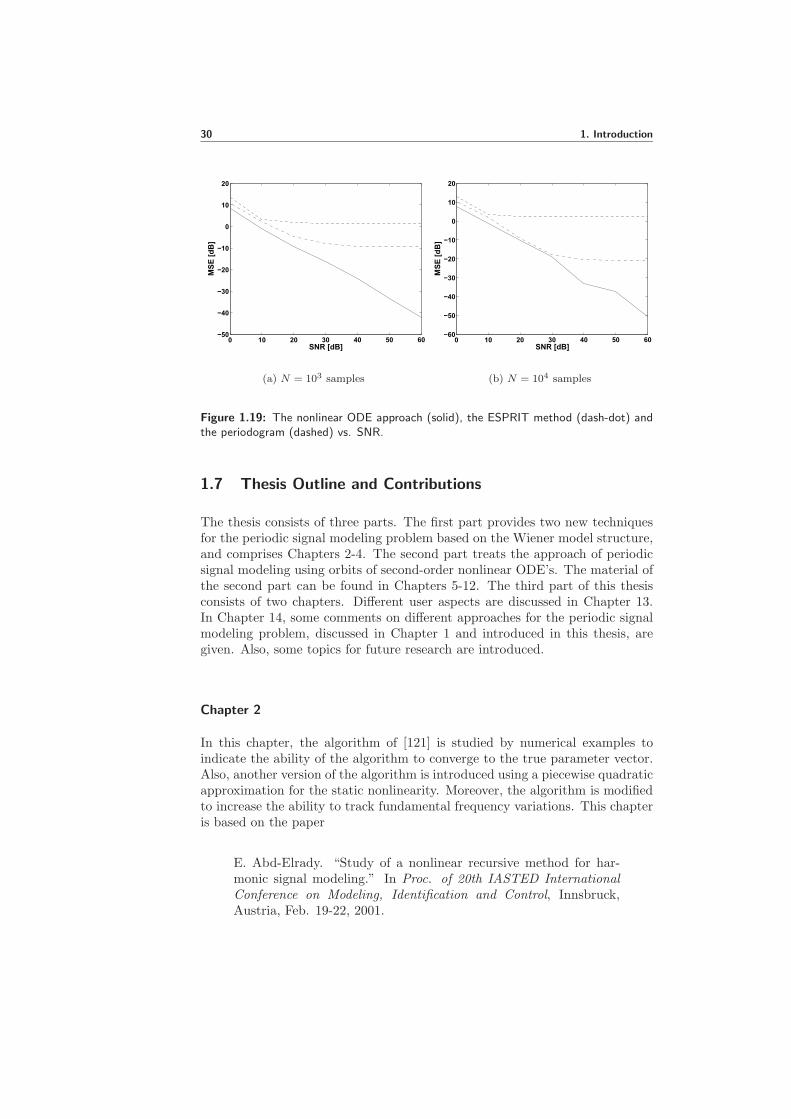
As done in Example 1.4, the model from the ESPRIT method was evaluatedby estimating 10 frequency components and the amplitudes and the phases ofthese components were estimated using the linear least squares method. Themodel from the periodogram method was evaluated by the extraction of the10 most powerful frequency bins and neglecting the rest that consequentlyrepresent the model error. The MSE was calculated as the average value of thesquared modeling error for the three approaches. The results for data lengthsof 103 and 104 samples and for different SNRs are plotted in Fig. 1.19.
It can be concluded from Fig. 1.19 that the approach of second-order non-linear ODE’s gives a more accurate signal model compared to the periodogramand the ESPRIT method especially at moderate and high SNRs.
30 1. Introduction
0 10 20 30 40 50 60−50
−40
−30
−20
−10
0
10
20
SNR [dB]
MS
E [
dB
]
(a) N = 103 samples
0 10 20 30 40 50 60−60
−50
−40
−30
−20
−10
0
10
20
SNR [dB]
MS
E [
dB
]
(b) N = 104 samples
Figure 1.19: The nonlinear ODE approach (solid), the ESPRIT method (dash-dot) andthe periodogram (dashed) vs. SNR.
1.7 Thesis Outline and Contributions
The thesis consists of three parts. The first part provides two new techniquesfor the periodic signal modeling problem based on the Wiener model structure,and comprises Chapters 2-4. The second part treats the approach of periodicsignal modeling using orbits of second-order nonlinear ODE’s. The material ofthe second part can be found in Chapters 5-12. The third part of this thesisconsists of two chapters. Different user aspects are discussed in Chapter 13.In Chapter 14, some comments on different approaches for the periodic signalmodeling problem, discussed in Chapter 1 and introduced in this thesis, aregiven. Also, some topics for future research are introduced.
Chapter 2
In this chapter, the algorithm of [121] is studied by numerical examples toindicate the ability of the algorithm to converge to the true parameter vector.Also, another version of the algorithm is introduced using a piecewise quadraticapproximation for the static nonlinearity. Moreover, the algorithm is modifiedto increase the ability to track fundamental frequency variations. This chapteris based on the paper
E. Abd-Elrady. “Study of a nonlinear recursive method for har-monic signal modeling.” In Proc. of 20th IASTED InternationalConference on Modeling, Identification and Control, Innsbruck,Austria, Feb. 19-22, 2001.
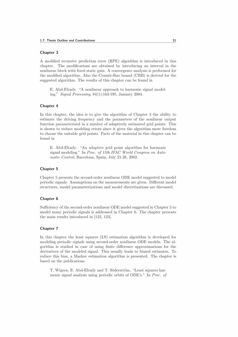
1.7. Thesis Outline and Contributions 31
Chapter 3
A modified recursive prediction error (RPE) algorithm is introduced in thischapter. The modifications are obtained by introducing an interval in thenonlinear block with fixed static gain. A convergence analysis is performed forthe modified algorithm. Also the Cramer-Rao bound (CRB) is derived for thesuggested algorithm. The results of this chapter can be found in
E. Abd-Elrady. “A nonlinear approach to harmonic signal model-ing.” Signal Processing, 84(1):163-195, January 2004.
Chapter 4
In this chapter, the idea is to give the algorithm of Chapter 3 the ability toestimate the driving frequency and the parameters of the nonlinear outputfunction parameterized in a number of adaptively estimated grid points. Thisis shown to reduce modeling errors since it gives the algorithm more freedomto choose the suitable grid points. Parts of the material in this chapter can befound in
E. Abd-Elrady. “An adaptive grid point algorithm for harmonicsignal modeling.” In Proc. of 15th IFAC World Congress on Auto-matic Control, Barcelona, Spain, July 21-26, 2002.
Chapter 5
Chapter 5 presents the second-order nonlinear ODE model suggested to modelperiodic signals. Assumptions on the measurements are given. Different modelstructures, model parameterizations and model discretizations are discussed.
Chapter 6
Sufficiency of the second-order nonlinear ODE model suggested in Chapter 5 tomodel many periodic signals is addressed in Chapter 6. The chapter presentsthe main results introduced in [122, 123].
Chapter 7
In this chapter the least squares (LS) estimation algorithm is developed formodeling periodic signals using second-order nonlinear ODE models. The al-gorithm is studied in case of using finite difference approximations for thederivatives of the modeled signal. This usually leads to biased estimates. Toreduce this bias, a Markov estimation algorithm is presented. The chapter isbased on the publications
T. Wigren, E. Abd-Elrady and T. Soderstrom. “Least squares har-monic signal analysis using periodic orbits of ODE’s.” In Proc. of

32 1. Introduction
13th IFAC Symposium on System Identification (SYSID 03), Rot-terdam, The Netherlands, August 27-29, 2003.
E. Abd-Elrady, T. Soderstrom and T. Wigren. “Periodic signalanalysis using periodic orbits of nonlinear ODE’s based on theMarkov estimate.” In Proc. of 2nd IFAC Workshop on PeriodicControl Systems (PSYCO 04), Yokohama, Japan, Aug. 30 - Sep. 1,2004.
Chapter 8
Chapter 8 introduces two recursive algorithms based on the Kalman filter (KF)and the extended Kalman filter (EKF). The Kalman filter estimate is biasedbut can be used to generate initial conditions for more elaborate nonlineartechniques such as the EKF. The EKF algorithm shows a superior performancethan the KF algorithm. This chapter is based on the paper
T. Wigren, E. Abd-Elrady and T. Soderstrom. “Harmonic sig-nal analysis with Kalman filters using periodic orbits of nonlinearODE’s.” In Proc. of IEEE International Conference on Acous-tics, Speech, and Signal Processing (ICASSP 03), Hong Kong,April 6-10, 2003.
Chapter 9
In this chapter, a maximum likelihood (ML) algorithm is developed for estimat-ing the parameter vector responsible for the generation of the modeled signal.The ML estimates are compared statistically to the Cramer-Rao bound, whichis also derived for the nonlinear ODE model in this chapter. The results of thischapter can be found in
T. Soderstrom, T. Wigren and E. Abd-Elrady. “Periodic signalanalysis by maximum likelihood modeling of orbits of nonlinearODE’s.” To appear in Automatica.
Chapter 10
In this chapter the spectral analysis technique introduced in [94] is used toestimate the period of the modeled signal in addition to some basic Fourierseries coefficients. This allows an evaluation of more accurate estimate forthe modeled signal and its derivatives needed to find a LS estimate for theODE model. The spectral analysis technique of [94] improves the LS estimatessignificantly. This chapter is based on the publications
E. Abd-Elrady and J. Schoukens. “Least squares periodic signalmodeling using orbits of nonlinear ODE’s and fully automated spec-tral analysis.” To appear in Automatica.

1.7. Thesis Outline and Contributions 33
E. Abd-Elrady and J. Schoukens. “Least squares periodic signalmodeling using orbits of nonlinear ODE’s and fully automated spec-tral analysis.” In Proc. of 6th IFAC Symposium on Nonlinear Con-trol Systems (NOLCOS 04), Stuttgart, Germany, September 1-3,2004.
Chapter 11
In this chapter Lienard’s equation, which has been used to describe a number ofoscillating electrical and mechanical systems, is used as the generating modelfor the periodic signal. The parameterization in this case makes use of theappropriate conditions imposed on the polynomials of Lienard’s equation toguarantee the existence of a unique and stable periodic orbit. Chapter 11 isbased on the paper
E. Abd-Elrady, T. Soderstrom and T. Wigren. “Periodic signalmodeling based on Lienard’s equation.” IEEE Transaction on Au-tomatic Control, 49(10):1773-1778, October 2004.
Chapter 12
In this chapter a bias analysis for the LS algorithm developed in Chapter 7 ispresented. Also, discretization errors are evaluated using Taylor series expan-sions. Chapter 12 is based on the publications
E. Abd-Elrady and T. Soderstrom. “Bias analysis in least squaresestimation of periodic signals using nonlinear ODE’s.” Submittedto International Journal of Control.
E. Abd-Elrady and T. Soderstrom. “Bias analysis in periodic sig-nals modeling using nonlinear ODE’s.” Submitted to 16th IFACWorld Congress on Automatic Control, Prague, Czech Republic,July 3-8, 2005
Chapter 13
Different user aspects for the two suggested approaches in this thesis for mod-eling periodic signals are given in this chapter.
Chapter 14
Comments on different approaches to the periodic signal modeling problem andsome topics for future research are given in this chapter.


Part I
Periodic Signal Modeling Based on the
Wiener Model Structure
35


Chapter 2
Periodic Signal Modeling Using Adaptive NonlinearFunction Estimation
2.1 Introduction
THE problem of modeling periodic signals has received a great deal of at-tention in the literature, see e.g. [49, 75]. The algorithm of [121], that is
studied here, has the property to give information on the underlying nonlin-earity, in cases where the overtones are generated by nonlinear imperfectionsin the system. In some cases it may also be known that the modeled signal iscloser to other signals than to sine waves. This fact can be exploited in theapproach of [121]. Therefore, the algorithm of [121] may then be more efficientthan methods such as [49, 75] that do not consider such priors.
The method of [121] is based on the fact that a sine wave passing througha static nonlinear function produces a harmonic spectrum of overtones. Hence,the Wiener model structure, cf. Section 1.4.1, is used as a signal model for anarbitrary periodic signal, as shown in Fig. 1.12. The linear block of the Wienermodel is a periodic function generator with a tunable fundamental frequency.The periodic function generator is cascaded by a parameterized and unknownstatic nonlinearity which consists the nonlinear block of the Wiener model.
In this chapter, the nonlinearity is chosen to be piecewise linear exactly as in[121], with the estimated parameters being the function values in a set of userchosen grid points. Also, the nonlinearity can be parameterized in terms of apiecewise quadratic function. In this case, slight modifications in the algorithmof [121] are needed.
The performance of the proposed recursive Gauss-Newton prediction errormethod (RPEM) for joint estimation of the driving frequency and the param-eters of the nonlinear output function is studied by numerical examples. Fur-thermore, modifications that improve the tracking performance are suggested.
The chapter is organized as follows. In Section 2.2, a review of the algo-rithm introduced in [121] is given. A parameterization of the nonlinearity as apiecewise quadratic function is presented in Section 2.3. Numerical examplesand conclusions are given in Section 2.4 and Section 2.5, respectively.
37

38 2. Periodic Signal Modeling Using Adaptive Nonlinear Function Estimation
2.2 Review of the Algorithm of [121]
The method of [121] utilizes a known periodic function as an input to an un-known static nonlinearity. The chosen periodic signal reflects any prior knowl-edge that is available about the modeled signal. Hence, let the driving inputsignal u(t, ω) to be defined as
u(t, ω) = Λ(ωt), (2.1)
where t is discrete time and ω is the unknown normalized angular frequency.The fact that Λ(·) is periodic means
Assumption 2.1. Λ(ω(t+ 2kπ
ω ))
= Λ(ωt), k ∈ Z.
The method of [121] proceeds by dividing one complete period of Λ(ωt)into L disjoint intervals Ij , j = 1, · · · , L; where Λ(ωt) satisfies the followingcondition
Assumption 2.2. Λ(ωt) is a monotone function of ωt on each Ij , j = 1, · · · , L.
Similarly, the static nonlinear block is divided into L static nonlinearities{fj(θj ,Λ(ωt)
)}Lj=1 that correspond to these L disjoint intervals Ij . Hence,
the model output is defined as
y(t, ω,θn) = fj(θj ,Λ(ωt)
), Λ(ωt) ∈ Ij , j = 1, · · · , L
θn =(θT1 · · · θTL
)T.
(2.2)
Remark 2.1. Assumption 2.2 is introduced in [121] to make the suggestedmodeling approach more general. This can be explained here as done in[121] by assuming that one static nonlinearity is considered and the drivinginput periodic function Λ(ωt) is chosen to be a sinusoid with amplitude α, i.e.Λ(ωt) = α sin(ωt). In this case, y(t, ω,θ1) = f1
(θ1, α sin(ωt)
). If the unknown
parameter vector θ1 of the static nonlinearity converged to a fixed parame-
ter vector θo1, it follows that f1
(θo1, α sin
(ω(π/ω − t)
))= f1
(θo1, α sin(ωt)
)∀ t.
This means that the model output signal in half of the time period, i.e. π/ω,will be given by the model output signal in the second half. In this case, theapproach will only be suitable for modeling periodic signals with a symmetricnonlinear distortion.
Remark 2.2. Note that the notation Λ(ωt) ∈ Ij - which is used all over Part Iof the thesis - means that the phase ωt of the periodic function Λ(ωt) is suchthat Ij is in effect. This notation is used intentionally to highlight the switchingbetween static nonlinearities in different intervals.
Considering the use of a piecewise linear model for the parameterization offj(θj ,Λ(ωt)
), cf. [4, 118, 119, 121], a set of grid points are defined as follows:
gTj =(uj1 uj2 · · · ujkj
), j = 1, · · · , L
uj1 = infγ∈Ij
γ,
ujkj= supγ∈Ij
γ.
(2.3)

2.2. Review of the Algorithm of [121] 39
PSfrag
f j(u
)
uuj1 uj2 uj3 uj4 ujkj−2 u
jkj−1 ujkj
f j1
f j2
f j3f j4
f jkj−2
f jkj−1f jkj
Figure 2.1: Grids points, parameters and resulting piecewise linear model.
Then by choosing the parameter vectors θj as the values of fj(θj , u(t, ω)
)in
the grid points, i.e.
θj =(f j1 f j2 · · · f jkj
)T, j = 1, · · · , L
fj(θj , uji ) = f ji , i = 1, · · · , kj
(2.4)
a piecewise linear function of u(t, ω) can be constructed from the linear seg-ments with end points in (uji−1, f
ji−1) and (uji , f
ji ) as shown in Fig. 2.1.
A recursive Gauss-Newton RPEM then follows by a minimization of thecost function
V (ω,θn) = limN→∞
1
N
N∑
t=1
E[ε2(t, ω,θn)
], (2.5)
where ε(t, ω,θn) is the prediction error defined as
ε(t, ω,θn) = y(t) − y(t, ω,θn), (2.6)
and y(t) is the measured signal.
In order to formulate the RPEM algorithm, the negative gradient ofy(t, ω,θn) is needed. It is given by (for u(t, ω) ∈ Ij , j = 1, . . . , L)
ψ(t, ω,θn) =
(∂fj
(θj ,u(t,ω)
)
∂u ψl(t) 0 · · · 0 ∂fj
(θj ,u(t,ω)
)
∂θj
0 · · · 0)T
, (2.7)
where
ψl(t) = tdΛ(φ)
dφ
∣∣φ=ωt
. (2.8)
The RPEM that appears in [121] was derived as in [69, 119]. It is given by

40 2. Periodic Signal Modeling Using Adaptive Nonlinear Function Estimation
ε(t) = y(t) − y(t)
λ(t) = λoλ(t− 1) + 1 − λo
S(t) = ψT (t)P (t− 1)ψ(t) + λ(t)
P (t) =(P (t− 1) − P (t− 1)ψ(t)S−1(t)ψT (t)P (t− 1)
)/λ(t)
(ω(t)
θn(t)
)=
[(ω(t− 1)
θn(t− 1)
)+ P (t)ψ(t)ε(t)
]
DM
(2.9)
u(t+ 1) = Λ(φ) |φ=ω(t)(t+1)
ψl(t+ 1) = (t+ 1)dΛ(φ)
dφ
∣∣φ=ω(t)(t+1)
when u(t+ 1) ∈ Ij , j = 1, · · · , Lwhen u(t+ 1) ∈ [uji , u
ji+1], i = 1, · · · , kj − 1
y(t+ 1) =f ji (t)u
ji+1 − f ji+1(t)u
ji
uji+1 − uji+f ji+1(t) − f ji (t)
uji+1 − ujiu(t+ 1)
∂fj(·)∂u
=f ji+1(t) − f ji (t)
uji+1 − uji
∂fj(·)∂f ji
=uji+1 − u(t+ 1)
uji+1 − uji
∂fj(·)∂f ji+1
=u(t+ 1) − ujiuji+1 − uji
∂fj(·)∂f jl
= 0, l 6= i, i+ 1
end
∂fj(·)∂θj
=
(∂fj(·)∂f j1
· · · ∂fj(·)∂f jkj
)
ψ(t+ 1) =
(∂fj(·)∂u
ψl(t+ 1) 0 · · · 0 ∂fj(·)∂θj
0 · · · 0)T
end
where DM indicates that the projection algorithms described in [69] are usedto keep the estimator in the model set.
It was shown in [121] that the minimum of V (ω,θn) is unaffected by coloredmeasurement disturbances. Also, the Cramer-Rao bound (CRB) for (ω θTn )T
was derived in this paper.
2.3 Piecewise Quadratic Approximation
The static nonlinearity can also be modeled as a piecewise quadratic function.Since a quadratic curve is uniquely determined by its values in three points,

2.3. Piecewise Quadratic Approximation 41
the following grid points are introduced
gj =(uj1 uj3
2
uj2 · · · ujkj− 1
2
ujkj
)T, j = 1, · · · , L. (2.10)
The additional grid points are assumed to be located in the middle of theintervals [uji , u
ji+1], i = 1, · · · , kj − 1. The corresponding parameter vector,
describing the static nonlinearity is then
θj =(f j1 f j3
2
f j2 · · · f jkj− 1
2
f jkj
)T, j = 1, · · · , L. (2.11)
The RPEM algorithm introduced in (2.9) then requires the following modifica-tions in the nonlinear output and gradient calculations:
when u(t+ 1) ∈ Ij , j = 1, · · · , Lwhen u(t+ 1) ∈ [uji , u
ji+1], i = 1, · · · , kj − 1
y(t+ 1) = f ji+ 1
2
(t) +f ji+1(t) − f ji (t)
uji+1 − uji
(u(t+ 1) − uj
i+ 12
)+
2(f ji+1(t) − 2f j
i+ 12
(t) + f ji (t))
(uji+1 − uji )2
(u(t+ 1) − uj
i+ 12
)2
∂fj(·)∂u
=f ji+1(t) − f ji (t)
uji+1 − uji+
4(f ji+1(t) − 2f j
i+ 12
(t) + f ji (t))
(uji+1 − uji )2
(u(t+ 1) − uj
i+ 12
)
∂fj(·)∂f ji
=uji+ 1
2
− u(t+ 1)
uji+1 − uji+
2(u(t+ 1) − uj
i+ 12
)2
(uji+1 − uji )2
∂fj(·)∂f j
i+ 12
= 1 −4(u(t+ 1) − uj
i+ 12
)2
(uji+1 − uji )2
∂fj(·)∂f ji+1
=u(t+ 1) − uj
i+ 12
uji+1 − uji+
2(u(t+ 1) − uj
i+ 12
)2
(uji+1 − uji )2
∂fj(·)∂f jl
= 0 , l 6= i, i+1
2, i+ 1
end
∂fj(·)∂θj
=
∂fj(·)∂f j1
∂fj(·)∂f j3
2
· · · ∂fj(·)∂f j
kj− 12
∂fj(·)∂f jkj
ψ(t+1) =
(∂fj(·)∂u
ψl(t+ 1) 0 · · · 0 ∂fj(·)∂θj
0 . . . 0
)T
end.
(2.12)

42 2. Periodic Signal Modeling Using Adaptive Nonlinear Function Estimation
−−1 0−0.3 0.3 1
0.3
0.8
0.5
−0.3
−0.5
−0.8
fj(u)
u
f1(u)f2(u)
Figure 2.2: The static nonlinearities of Example 2.1.
2.4 Numerical Examples
In order to study the performance of the RPEM algorithm suggested for jointestimation of the driving frequency and the parameters of the nonlinear outputfunction, the following simulations were performed.
Example 2.1. Convergence to the true parameter vector using Algorithm (2.9).
The data were generated as follows. The driving wave was given byu(t, ωo) = sinωot where ωo = 2π × 0.05. Two static nonlinearities (L = 2)were used as shown in Fig. 2.2 and defined by
gj =(−1 −0.3 0 0.3 1
)T, j = 1, 2
θo1 =(−0.8 −0.3 0 0.3 0.8
)T, u ∈ I1
θo2 =(−0.8 −0.5 0 0.5 0.8
)T, u ∈ I2.
(2.13)
where u(t, ω) ∈ I1 for positive slopes and u(t, ω) ∈ I2 for negative slopes, re-spectively. The additive noise was white zero-mean Gaussian with varianceσ2 = 0.01. Algorithm (2.9) was initialized with λ(0) = 0.95, λo = 0.99,P (0) = 0.01I and ω(0) = 2π × 0.02. Further, the grid points in (2.13) wereused, and the initial values for the nonlinearities were given by straight lineswith unity slope.
The modeled signal and the estimated signal are given in Fig. 2.3(a). Also,the estimate of the driving frequency and the parameter estimates are given inFigures 2.3(b)-2.3(d).

2.4. Numerical Examples 43
(a) The true signal (dashed) and the
model output (solid)
0 500 1000 15000.12
0.15
0.18
0.21
0.24
0.27
0.3
0.33
Driv
ing
freq
uenc
y [r
ad]
Time [samples]
EstimateTrue
(b) Convergence of the driving frequency
0 500 1000 1500
−1
−0.5
0
0.5
1
Par
amet
er e
stim
ates
(θ1)
Time [samples]
(c) Convergence of θ1
0 500 1000 1500
−1
−0.5
0
0.5
1
Par
amet
er e
stim
ates
(θ2)
Time [samples]
(d) Convergence of θ2
Figure 2.3: Convergence using Algorithm (2.9).
After 1500 samples the following estimates were obtained;
ω = 0.3140,
θ1 =(−0.784 −0.284 −0.037 0.326 0.796
)T,
θ2 =(−0.802 −0.515 −0.085 0.486 0.796
)T.
Hence, it can be concluded that convergence to the true parameter vector istaking place.
Example 2.2. Convergence to the true parameter vector using Algorithm(2.12).
In this example the data were generated and Algorithm (2.12) was initialized

44 2. Periodic Signal Modeling Using Adaptive Nonlinear Function Estimation
0 500 1000 15000.12
0.15
0.18
0.21
0.24
0.27
0.3
0.33
Driv
ing
freq
uenc
y [r
ad]
Time [samples]
EstimateTrue
Figure 2.4: Convergence of the driving frequency using Algorithm (2.12).
as in Example 2.1. The grid points in this case were
gj =(−1 −0.5 0 0.5 1
)T, j = 1, 2
θo1 =(−0.8 −0.5 0 0.5 0.8
)T, u ∈ I1
θo2 =(−0.8 −0.6 0 0.6 0.8
)T, u ∈ I2.
(2.14)
The estimated fundamental frequency is given in Fig. 2.4. After 1500 samplesthe following estimates were obtained;
ω = 0.3143,
θ1 =(−0.804 −0.536 −0.069 0.470 0.796
)T,
θ2 =(−0.835 −0.575 0.066 0.613 0.823
)T.
Also here it can be concluded that the convergence to the true parameter vectoris taking place.
Example 2.3. Tracking fundamental frequency variations.
To improve the ability of Algorithm (2.9) to track fundamental frequency vari-ations, it can be modified as follows.
ε(t) = y(t) − y(t)
S(t) = ψT (t)P (t− 1)ψ(t) + r2(t)
P (t) = P (t− 1) − P (t− 1)ψ(t)S−1(t)ψT (t)P (t− 1) +R1(t)(ω(t)
θn(t)
)=
[(ω(t− 1)
θn(t− 1)
)+ P (t)ψ(t)ε(t)
]
DM
(2.15)
where R1(t) and r2(t) are the gain design variables (see [69] page 273). Thismodification transforms the problem into an extended Kalman filter (EKF)formulation. For more literature on tracking, see [34, 42, 43, 115].

2.4. Numerical Examples 45
0 500 1000 1500 20000.1
0.15
0.2
0.25
0.3
0.35
0.4
0.45
0.5
Driv
ing
freq
uenc
y [r
ad]
Time [samples]
True Estimate
Figure 2.5: Tracking the fundamental frequency using Algorithm (2.15).
The data were generated as in Example 2.1 and Algorithm (2.15) was ini-tialized with P (0) = 0.01I and ω(0) = 2π × 0.02. The design variables wereR1(t) = 10−4I and r2(t) = 0.2. Also, the grid points in (2.13) were used, andthe initial values for the nonlinearities were given by straight lines with unityslope.
The true and the estimated fundamental frequency are given in Fig. 2.5.After 2400 samples the following estimates were obtained;
ω = 0.3479,
θ1 =(−0.817 −0.259 0.020 0.342 0.800
)T,
θ2 =(−0.799 −0.487 −0.091 0.378 0.839
)T,
and it can be concluded that Algorithm (2.15) has the ability to track thefundamental frequency variations.
Example 2.4. Statistical results for the fundamental frequency estimate.
In order to compare the performance of the RPEM algorithm given in (2.9) withthe derived Cramer-Rao bound (CRB) in [121] for the fundamental frequencyestimation, 100 Monte-Carlo simulation experiments were performed.
The data were generated and the algorithm was initialized as in Example 2.1with ω(0) = 2π×0.03. The statistics is based on excluding simulations that didnot satisfy a margin of 5 standard deviations (as predicted by the CRB) fromthe true fundamental frequency. Both the CRB of the fundamental frequencyestimate and the mean square error (MSE) value were evaluated for differentsignal to noise ratios (SNRs). The data length was 2000 samples. The numberof excluded simulations did not exceed 15 experiments. The statistical resultsare plotted in Fig. 2.6. The results show that the RPEM algorithm gives anaccurate estimate of the fundamental frequency at moderate and high SNRs.

46 2. Periodic Signal Modeling Using Adaptive Nonlinear Function Estimation
0 5 10 15 20 25 3010
−10
10−9
10−8
10−7
10−6
SNR
C
RB
, M
SE
CRBMSE
Figure 2.6: The CRB and the MSE of the fundamental frequency estimate using Algo-rithm (2.9).
2.5 Conclusions
The recursive periodic signal estimation approach introduced in [121] has beenstudied by numerical examples to investigate the convergence to the true pa-rameter vector and the ability of tracking fundamental frequency variations.Modifications that improve the latter property were suggested. Also, the ap-proximation of the static nonlinearity by a piecewise quadratic parameteri-zation was introduced. Moreover, Monte-Carlo experiments show that themethod gives good results, in particular for moderate values of the signal tonoise ratio.

Chapter 3
A Modified Nonlinear Approach to Periodic SignalModeling
3.1 Introduction
THE periodic signal modeling technique introduced in Chapter 2 is mod-ified in this chapter. The difference between the technique described in
Chapter 2 and the one given here is that in [121] the differential static gain wasfixed in the linear block. Here, however, the differential static gain is fixed inthe nonlinear block. This requires a slight modification of the parameterizationof the static nonlinearity.
The modifications in the proposed RPEM are obtained by introducing aninterval in the nonlinear block with fixed gain. The modification in the con-vergence analysis is, however, substantial and allows a treatment of the localconvergence properties of the algorithm. This is the main reason for the modifi-cation. The convergence analysis is based on Ljung’s method with an associatedordinary differential equation (ODE), see [65, 66, 69].
The contributions of this chapter can hence be summarized as follows. Con-ditions for local convergence to the true parameter vector are derived with av-eraging theory for the suggested method. Furthermore, the Cramer-Rao bound(CRB) is calculated. Finally, the performance for joint estimation of the driv-ing frequency and the parameters of the nonlinear output function is studiedby numerical examples.
The chapter is organized as follows. Modifications in the algorithm of [121]are discussed in Section 3.2. A local convergence analysis is presented in Sec-tion 3.3. Section 3.4 presents the derivation of the CRB for the modifiedalgorithm. In Section 3.5, some numerical examples are given. Conclusions aregiven in Section 3.6.
3.2 The Modified Algorithm
Since the model is a cascade of two blocks, the differential static gain of themodel will be a factor of two free parameters. It is nevertheless necessary forthe algorithm to have information about where the static gain is located, orthe criterion function may have an infinite number of minima. In this case,
47

48 3. A Modified Nonlinear Approach to Periodic Signal Modeling
the RPEM algorithm will be sliding around in a valley of the criterion functionresulting in numerical problems. Therefore, one of the parameters need to befixed, cf. [118]. In [121], this was done in the driving signal block. Here,however, the opposite situation will be investigated.
In order to fix the static gain in an amplitude subinterval Io contained inexactly one of the L disjoint intervals Ij , j = 1, · · · , L; the driving input signalof the modified method is modeled as
u(t,θl) = XΛ(ωt),
θl =(X ω
)T,
(3.1)
where X is a (possibly time varying) parameter recursively estimated to allowthe linear block of the model to adapt its static gain so that the data in Io can beexplained. Choosing Io to be contained in the first interval I1, f1
(θ1, u(t,θl)
)
is defined as in [118] to become
f1(fo,θ1, u(t,θl)
)= Ko u(t,θl) + fo, u(t,θl) ∈ Io ⊂ I1, (3.2)
so∂f1(fo,θ1, u(t,θl)
)
∂u= Ko, u(t,θl) ∈ Io. (3.3)
Here Ko is a user chosen constant. The grid points now become [118]
gTj =
{ (u1−k−1
u1−k−1 +1
· · · uo− uo+ · · · u1k+1 −1
u1k+1
), j = 1
(uj−k−j
uj−k−j +1· · · uj−1 uj1 · · · uj
k+j −1
ujk+
j
), j = 2, · · · , L.
(3.4)Hence, the parameters θj are defined by
θj =(f j−k−j
· · · f j−1 f j1 · · · f jk+
j
)T, j = 1, · · · , L
fj(θj , uji ) =
{Kou(t,θl) + fo, u(t,θl) ∈ Io, j = 1
f ji , i = −k−j , · · · ,−1, 1, · · · , k+j , j = 1, · · · , L.
(3.5)
Note that there are no parameters corresponding to the grids uo− and uo+ ,since
f1(fo,θ1, uo−) = Kouo− + fo,
f1(fo,θ1, uo+) = Kouo+ + fo.(3.6)
The parameter vector then takes the form, with θl defined by (3.1)
θ =(θTl θTn
)T,
θn =(fo θ
T
n
)T,
θn =(θT1 · · · θTL
)T,
θj =(f j−k−j
· · · f j−1 f j1 · · · f jk+
j
)T, j = 1, · · · , L.
(3.7)

3.2. The Modified Algorithm 49
Taking into account that ψl(t) in this case is given by
ψl(t) =(
Λ(φ) |φ=ωt XtdΛ(φ)dφ
∣∣φ=ωt
)T, (3.8)
the recursive prediction error algorithm of Chapter 2 is modified to become
ε(t) = y(t) − y(t)
λ(t) = λoλ(t− 1) + 1 − λo
S(t) = ψT (t)P (t− 1)ψ(t) + λ(t)
P (t) =(P (t− 1) − P (t− 1)ψ(t)S−1(t)ψT (t)P (t− 1)
)/λ(t)
(θl(t)
θn(t)
)=
[(θl(t− 1)
θn(t− 1)
)+ P (t)ψ(t)ε(t)
]
DM
(3.9)
u(t+ 1) = X(t)Λ(φ) |φ=ω(t)(t+1)
ψl(t+ 1) =(
Λ(φ) |φ=ω(t)(t+1) X(t)(t+ 1)dΛ(φ)dφ
∣∣φ=ω(t)(t+1)
)T
when u(t+ 1) ∈ I1
when u(t+ 1) ∈ [u1−1, uo− ]
y(t+ 1) =f1−1(t)uo− −
(Kouo− + fo(t)
)u1−1
uo− − u1−1
+Kouo− + fo(t) − f1
−1(t)
uo− − u1−1
u(t+ 1)
∂f1(·)∂u
=Kouo− + fo(t) − f1
−1(t)
uo− − u1−1
∂f1(·)∂f1
−1
=uo− − u(t+ 1)
uo− − u1−1
∂f1(·)∂fo
=u(t+ 1) − u1
−1
uo− − u1−1
∂f1(·)∂f1
l
= 0, l 6= −1, 0
end
when u(t+ 1) ∈ [uo− , uo+ ]
y(t+ 1) = Kou(t+ 1) + fo(t)
∂f1(·)∂u
= Ko
∂f1(·)∂fo
= 1
∂f1(·)∂f1
l
= 0, l 6= 0
end

50 3. A Modified Nonlinear Approach to Periodic Signal Modeling
when u(t+ 1) ∈ [uo+ , u11]
y(t+ 1) =
(Kouo+ + fo(t)
)u1
1 − f11 (t)uo+
u11 − uo+
+f11 (t) −Kouo+ − fo(t)
u11 − uo+
u(t+ 1)
∂f1(·)∂u
=f11 (t) −Kouo+ − fo(t)
u11 − uo+
∂f1(·)∂fo
=u1
1 − u(t+ 1)
u11 − uo+
∂f1(·)∂f1
1
=u(t+ 1) − uo+
u11 − uo+
∂f1(·)∂f1
l
= 0, l 6= 0, 1
end
when u(t+ 1) ∈ Ij , j = 1, · · · , L
when u(t+ 1) ∈ [uji , uji+1] ∀i =
{ −k−1 , ..,−2, 1, .., k+1 − 1, j = 1
−k−j , · · · , k+j − 1, j = 2, · · · , L.
y(t+ 1) =f ji (t)u
ji+1 − f ji+1(t)u
ji
uji+1 − uji+f ji+1(t) − f ji (t)
uji+1 − ujiu(t+ 1)
∂fj(·)∂u
=f ji+1(t) − f ji (t)
uji+1 − uji
∂fj(·)∂f ji
=uji+1 − u(t+ 1)
uji+1 − uji
∂fj(·)∂f ji+1
=u(t+ 1) − ujiuji+1 − uji
∂fj(·)∂fo
= 0
∂fj(·)∂f jl
= 0, l 6= i, i+ 1
end
∂fj(·)∂θj
=
(∂fj(·)∂fj
−k−
j
· · · ∂fj(·)∂fj
−1
∂fj(·)∂fj
1
· · · ∂fj(·)∂fj
k+j
)
ψ(t+ 1) =(
∂fj(·)∂u ψTl (t+ 1)
∂fj(·)∂fo
0 · · · 0 ∂fj(·)∂θj
0 · · · 0)T
end.
In this chapter the nonlinearity is chosen to be piecewise linear with the esti-mated parameters being the function values in a fixed set of grid points resultingin a fixed grid point adaptation. These grid points are chosen by the user de-pending on any prior information about the wave form. For example the peakto peak value of the wave form helps to determine the grids range for each in-

3.3. Local Convergence 51
terval. Intervals with distorted amplitude (as the amplitude range [-0.06,0.06]in Example 3.5, cf. Fig. 3.4(a) and Eq. (3.51)) require a higher number of gridpoints to identify all the details of the static nonlinearity. The possibility toestimate the grid points recursively in addition to the driving frequency andthe parameters of the nonlinear output function resulting in an adaptive gridpoint algorithm will be studied in Chapter 4.
3.3 Local Convergence
As mentioned above, one major reason for the modification of the originalmethod of [121], was to perform a convergence analysis. Local convergence ofthe RPEM to the true parameter vector is analyzed here with the linearized,associated ordinary differential equation (ODE), see e.g. [69, 118]. First, a briefintroduction to the associated ODE approach is given. Second, the detailsof the local convergence analysis are presented. Finally, a discussion on thetechnical conditions needed to guarantee local convergence is given.
3.3.1 The Associated ODE Approach
The associated ODE approach was used in [69] to perform the convergenceanalysis of a basic structure of recursive algorithms related to quadratic criteriasuch as (2.5). This section reviews the relevant parts of the presentation of [69].The basic structure of [69] is
ε(t) = y(t) − y(t) (3.10)
R(t) = R(t− 1) + γ(t)[η(t)Λ−1(t)ηT (t) −R(t− 1)
](3.11)
θ(t) = θ(t− 1) + γ(t)R−1(t)η(t)Λ−1(t)ε(t) (3.12)
ξ(t+ 1) = A(θ(t)
)ξ(t) +B
(θ(t)
)z(t) (3.13)
(y(t+ 1)
col η(t+ 1)
)= C
(θ(t)
)ξ(t+ 1) (3.14)
where R(t) is the Hessian approximation in the Gauss-Newton algorithm, γ(t)is the adaptation gain (γ(t) → 0 as t → ∞), η(t) is a vector that is related
to the gradient of the prediction y(t) w.r.t θ, Λ(t) is the covariance matrix
of prediction errors, {z(t)} is the data set, A(θ(t)
), B(θ(t)
)and C
(θ(t)
)are
extended state space matrices that result from merging two finite-dimensionallinear filters which produce the output y(t) and the gradients η(t). ξ(t) denotesthe states of this extended state space model.
Now, the performance of the recursive algorithm (3.10)-(3.14) is investigated
for sufficiently large t. This means that γ(t) will be small, the estimates {θ(t)}will change slowly and closely to some value θ, and R(t) will be close to somevalue R. In this case, Eqs. (3.11)-(3.12) can be modified to
θ(t) ≈ θ(t− 1) + γ(t)R−1η(t, θ)Λ−1ε(t, θ), (3.15)
R(t) ≈ R(t− 1) + γ(t)[η(t, θ)Λ−1ηT (t, θ) − R
]. (3.16)

52 3. A Modified Nonlinear Approach to Periodic Signal Modeling
Introducing the following average updating directions:
f(θ) , E[η(t, θ)Λ−1ε(t, θ)
], (3.17)
G(θ) , E[η(t, θ)Λ−1ηT (t, θ)
], (3.18)
equations (3.15)-(3.16) can be written in the form
θ(t) ≈ θ(t− 1) + γ(t)R−1f(θ) + γ(t)v1(t), (3.19)
R(t) ≈ R(t− 1) + γ(t)[G(θ) − R
]+ γ(t)v2(t), (3.20)
where v1(t) and v2(t) are zero-mean random variables.
The analysis of [69] proceeds by defining times t and t such that
t∑
k=t
γ(k) = △τ (3.21)
where △τ is a small number. This follows since t was assumed to be sufficientlylarge and γ(t) is arbitrarily small. Hence, if θ(t) = θ andR(t) = R, Eqs. (3.19)-(3.20) can be written in the form
θ(t) ≈ θ + △τR−1f(θ) +
t∑
k=t
γ(k)v1(k)
≈ θ + △τR−1f(θ) (3.22)
R(t) ≈ R+ △τ[G(θ) − R
]+
t∑
k=t
γ(k)v2(k)
≈ R+ △τ[G(θ) − R
](3.23)
since∑tk=t γ(k)v1(k) ≪ △τR−1
f(θ) and∑tk=t γ(k)v2(k) ≪ △τ
[G(θ) − R
].
Now by changing the time scale such that t↔ τ and t↔ τ+△τ , Eqs. (3.22)-(3.23) can be regarded as a numerical scheme to solve the following ODE:
θ = R−1f(θ)
R = G(θ) −R(3.24)
where θ is a fixed vector belonging to DM , the set of parameter vectors de-scribing the model set.
Finally, the analysis of [69] linked the stability properties of the solution
x ,
(θ
col R
)(3.25)
of the associated ODE (3.24) to the convergence of the recursive algorithm(3.10)-(3.14). In brief, if the ODE is globally or locally stable, the recursivealgorithm will be globally or locally convergent, respectively.

3.3. Local Convergence 53
3.3.2 Analysis Details
The convergence analysis of the RPEM algorithm (3.9) proceeds along thefollowing lines. First, it is investigated when the true parameter vector is astationary point to the differential equation associated with (3.9). The localstability of this point is then studied. The analysis relies on the fact thatLjung’s original method of analysis is also applicable to the Wiener modelstructure. This was shown formally in [119]. However, here the driving linearblock is slightly different from [119].
The celebrated analysis of [65] relies on the assumption that the parame-ters of the model should be constrained to the set DM , where strict asymptoticstability holds. This can not be achieved in the present case, since the periodicdriving function is only BIBO-stable (when modeled as a filter). Therefore,a completely stringent treatment of the local convergence properties of thepresent algorithm, requires modifications of the approach of [65]. This will notbe undertaken here, since the periodic function can be treated as a superposi-tion of sine waves. Since any sine wave can be represented with an AR-modelwith separate poles on the unit-circle, the present case can thus be thoughtas a limiting case of [65]. Because of the simplicity of the model (the staticapproach), this heuristic argument is believed to be sufficient to motivate thefollowing calculations.
The local convergence analysis of Algorithm (3.9) begins by calculating theaverage updating directions (3.17)-(3.18) that define the associated ODE fromthe model and gradient relations. The calculations consider using a fixed pa-
rameter vector θ ∈ DM and a fixed R (where P (t) =(tR(t)
)−1) as mentioned
in Section 3.3.1. When Algorithm (3.9) is compared to the algorithm of [118],it is found that the average updating directions are
f(θ) = limt→∞
E ψ(t,θ)ε(t,θ)
= limt→∞
E
(∂fj(·)∂u ψl(t,θ)ε(t,θ)∂fj(·)∂θn
Tε(t,θ)
), (3.26)
F (R,θ) = G(θ) −R, (3.27)
G(θ) = limt→∞
E ψ(t,θ)ψT (t,θ)
= limt→∞
E
[∂fj(·)
∂u
]2ψlψ
Tl
∂fj(·)
∂uψl
∂fj(·)
∂fo
∂fj(·)
∂uψl
∂fj(·)
∂θn∂fj(·)
∂fo
∂fj(·)
∂uψT
l
∂fj(·)
∂fo
∂fj(·)
∂fo
∂fj(·)
∂fo
∂fj(·)
∂θn
∂fj(·)
∂θn
T ∂fj(·)
∂uψT
l
∂fj(·)
∂θn
T ∂fj(·)
∂fo
∂fj(·)
∂θn
T ∂fj(·)
∂θn
. (3.28)
Proceeding with the analysis, the following condition is introduced;
Assumption 3.1. The linear block and the static nonlinearity of the systemare contained in the model set.
Noticing that the model output is given by
y(t,θ) = fj(θn, u(t,θl)
), u(t,θl) ∈ Ij , j = 1, . . . , L (3.29)

54 3. A Modified Nonlinear Approach to Periodic Signal Modeling
then there is a vector θo such that the output of the static nonlinearity of thesystem is described by
y(t) = fj(θon, u(t,θ
ol ))
+ w(t), u(t,θol ) ∈ Ij , j = 1, . . . , L. (3.30)
where w(t) is the disturbance which satisfies the following condition;(cf. [69, 118])
Assumption 3.2. w(t) is a bounded, strictly stationary, zero mean stochasticprocess that fulfills
E |w(t) − wos(t)|4 ≤ c λt−s, c <∞, |λ| < 1.
Remark 3.1. wos(t) denotes a random variable that belongs to the σ-algebragenerated by {w(t)}t1,∀ t ≥ s but independent of {w(t)}s1. This is simply meansthat wos(t) is a very good approximation of w(t) during the time interval [s, t].See [69] for more details.
Since there is no use of w(t) in the input signal generation, the following con-dition is also satisfied;
Assumption 3.3. ψl(t,θo) and w(t) are independent.
By choosing θ = θo, it is concluded from (3.9) that
ε(t,θo) = y(t) − y(t,θo) = w(t). (3.31)
When this is inserted into (3.26) the result f(θo) = 0 is obtained by Assump-tion 3.3. Assumption 3.2, together with (3.27) then implies that the ODE(3.24) associated with (3.9) has a stationary point described by
x∗ ,
(θo
col G(θo)
). (3.32)
Following [69, 118], the local stability of the stationary point (3.32) need to bechecked. This can be done by studying the eigenvalues of the matrix
A ,∂
∂x
(R−1f(θ)
col(G(θ) −R
)) ∣∣∣
x=x∗
=
(G−1(θo)df(θ)
dθ
∣∣θ=θo 0
ddθ col
(G(θ) −R
)∣∣θ=θo −I
). (3.33)
Hence, x∗ is locally stable provided that all the eigenvalues of A are inthe LHP. This means that it is necessary to prove that the eigenvalues of
G−1(θo)df(θ)dθ
∣∣θ=θo are in the LHP. The derivative of f(θ) w.r.t. θ can be
evaluated from (3.26) by straightforward calculations. When θ is replaced byθo in the resulting expression, Eq. (3.28) together with Assumption 3.3 gives
G−1(θo)df(θ)
dθ
∣∣∣θ=θo
= −I. (3.34)

3.3. Local Convergence 55
Equation (3.34) is valid provided that the inverse of the matrix G(θo) exists.Taking into account that G(θo) is at least positive semidefinite by construc-tion, the goal of the next analysis is to find conditions that imply the positivedefiniteness of G(θo).
In order to achieve the previous goal, it is convenient, as done in [117], tostudy the contribution to G(θo) from the mid-subinterval Io. Introducing thegate function for this purpose, where
gate(u(t,θol )
)=
{1, u(t,θol ) ∈ Io ⊂ I10, otherwise.
(3.35)
Again, by u(t,θol ) ∈ Io it is meant that the phase ωt is such that I0 is in effect.Thus G(θo) can then be expressed as
G(θo) = limt→∞
E(1 − gate(u)
)ψ(t,θ)ψT (t,θ) + lim
t→∞E gate(u)ψ(t,θ)ψT (t,θ),
=
(A B
BT C
)+
(A 0
0 0
), (3.36)
where (cf. Eq. (3.28))
A = limt→∞
E gate(u)
(K2oψlψ
Tl Koψl
KoψTl 1
)
|θl=θol
, (3.37)
C = limt→∞
E(1 − gate(u)
)∂fj(·)∂θn
T∂fj(·)∂θn
∣∣∣θn=θ
o
n
= limt→∞
E(1 − gate(u)
)
∂f1(·)∂θ1
T ∂f1(·)∂θ1
...∂f1(·)
∂θ1
T ∂fL(·)
∂θL
.... . .
...∂fL(·)
∂θL
T ∂f1(·)∂θ1
...∂fL(·)
∂θL
T ∂fL(·)
∂θL
|θn=θ
on
(3.38)
Now Lemma 2 of [118] will be useful. This result can be formulated as follows.
Lemma 3.1. Consider the block-matrix decomposition
G =
(A B
BT C
)+
(A 0
0 0
),
where both terms on the right-hand side are symmetric. Assume that the firstterm of G is positive semidefinite and that A and C are positive definite. ThenG is also positive definite.
Proof. See [118].
The following two lemmas give the conditions necessary to satisfy that Aand C are positive definite. The notation intentionally follows [117, 118].

56 3. A Modified Nonlinear Approach to Periodic Signal Modeling
Lemma 3.2. Assume that the following conditions hold for the RPEM:
Assumption 3.4. αo = limt→∞ E gate(u) > 0.
Assumption 3.5. limt→∞ E gate(u)△ψl△ψTl ≥ δ limt→∞ E △ψl△ψ
Tl ,
δ > 0, where ψl = 1αoψol + △ψl and ψol = limt→∞ E gate(u)ψl.
Assumption 3.6. |Ko| > 0.
Assumption 3.7. ψl is unbiased, i.e. limt→∞ E ψl = 0.
Assumption 3.8. Λ(φ) is continuous, three times differentiable where
|Λ(φo)| ≥ ǫ1 > 0,∣∣∣d
2Λ(φ)dφ2
∣∣∣φ=φo
≥ ǫ2 > 0, and has at least one minimum or
one maximum point at φo.
Assumption 3.9. φ = ωt has a continuous probability density function (pdf).
Then A > 0.
Proof. See Appendix 3.A.
Lemma 3.3. Assume that the following condition is satisfied for the model;
Assumption 3.10. The probability density function hu(u) of u(t,θol ) fulfillshu(u) ≥ δ1 > 0 in at least one nonzero interval [aji , b
ji ] ⊂ Iji =
(uji−1, u
ji
)for all
i = −k−j + 1, . . . , k+j , j = 1, . . . , L.
Then C > 0.
Proof. See Appendix 3.B.
The fact that A and C are positive definite now implies the positive defi-niteness of G(θo) using Lemma 3.1. This completes the proof of the followingtheorem:
Theorem 3.1. Under Assumptions 2.1-2.2 and Assumptions 3.1-3.10, theRPEM algorithm given in (3.9) converges locally to
(θolθon
)∈ DM .
3.3.3 Discussion
The conditions of Lemma 3.2 and Lemma 3.3, except Assumptions 3.7-3.9, aresimilar to the corresponding ones of [118]. Assumptions 3.4-3.6 are necessary toindicate that there is a sufficient amount of signal energy in the mid-subintervalIo. Assumption 3.10 means that there should be signal energy somewhere inevery subinterval of the piecewise linear model of the static nonlinearity.

3.3. Local Convergence 57
The analysis of Appendix 3.A leads to the inequality
limt→∞
E △ψl△ψT
l > 0, (3.40)
where △ψl = △ψol + △ψl and △ψol = limt→∞ E △ψl, cf. Appendix 3.A.The inequality (3.40) can not be satisfied for all driving signals as shown inthe following two examples.
Example 3.1. Consider the following
u(t,θol ) = XoΛ(φ) |φ=ωot,
Λ(φ) = sin(φ), (3.41)
and assume that the phase ωot is uniformly distributed in the interval [0, 2π].In this case △ψl = ψl , because there is no bias in ψl. Thus
E △ψl△ψT
l = E
(Λ2(φ) Xo
ωo φ Λ(φ)dΛ(φ)dφ
Xo
ωo φ Λ(φ)dΛ(φ)dφ [X
o
ωo ]2 φ2 [dΛ(φ)dφ ]2
)
φ=ωot
. (3.42)
Straightforward calculations give
E △ψl△ψT
l =1
2π
∫ 2π
0
△ψl△ψT
l dφ
=
(12
−Xo
4ωo
−Xo
4ωo [Xo
ωo ]2 ( 2π2
3 + 14 )
), (3.43)
which is a positive definite matrix. Thus (3.40) is a valid inequality in thiscase.
Example 3.2. Consider the following
u(t,θol ) = XoΛ(φ) |φ=ωot,
Λ(φ) =1
2π
(φ− π
), 0 ≤ φ < 2π
Λ(φ) = Λ(φ+ 2kπ), k ∈ Z.
(3.44)
In this case, straightforward calculations give
E △ψl△ψT
l =
(112
Xo
12ωo
Xo
12ωo [Xo
ωo ]2 112
), (3.45)
which is singular. Thus (3.40) is not valid in this case.
Example 3.1 and Example 3.2 give an indication about the need for furtherconditions to guarantee the inequality (3.40).

58 3. A Modified Nonlinear Approach to Periodic Signal Modeling
Assumptions 3.7-3.9 give sufficient requirements on the driving signal toguarantee (3.40). Assumption 3.7 is needed to simplify the analysis of Ap-pendix 3.A. It simply means removing the bias from the periodic signal beforeapplying the RPEM algorithm. Assumption 3.8 means that the periodic sig-nal must be continuous and have a smooth curvature at the minimum or themaximum point of the signal. This assumption is needed to be able to use aTaylor series expansion around this minimum or maximum point. It can benoticed that Assumption 3.8 is not fulfilled for the periodic signal of Exam-ple 3.2. Assumption 3.9 is needed to evaluate the expectation in the inequality(3.40).
Remark 3.2. Note that in the rest of the analysis in this chapter, all thequantities given are evaluated at the true parameter vector θo even when thisis not stated explicitly. Hence, for notational convenience θ is used instead ofθo.
3.4 The Cramer-Rao Bound
In this section the CRB of the proposed parameterization is calculated. Intro-duce the following conditions:
Assumption 3.11. E [w(t)w(s)] = σ2δt,s and w(t) is Gaussian.
Assumption 3.12. N > No such that there exist a time instant t < No whereu ∈ Ij and u ∈ [uji , u
ji+1] ∀i, j ∈ {i = −k−j , . . . , k+
j − 1, j = 1, . . . , L}.Remark 3.3. Assumption 3.12 means that there is signal energy in each subin-terval of the model, cf. [121] and Assumption 3.10.
Then the following theorem holds for the signal model of Assumption 3.1:
Theorem 3.2. Under Assumptions 2.1-2.2 and Assumptions 3.1-3.12, the CRBfor (θTl θ
Tn )T is given by
CRB(θ) = σ2
(N∑
t=1
I(t)
)−1
, (3.46)
where
I(t) =
IX,X IX,ω IX,fo 0 ··· 0 IX,f
ji
IX,f
ji+1
0 ··· 0
Iω,X Iω,ω Iω,fo 0 ··· 0 Iω,f
ji
Iω,f
ji+1
0 ··· 0
Ifo,X Ifo,ω Ifo,fo 0 ··· 0 Ifo,f
ji
Ifo,f
ji+1
0 ··· 0
0 0 0 0 0...
......
......
0 0 0 0 0I
fji
,XI
fji
,ωI
fji
,fo0 ··· 0 I
fji
,fji
If
ji
,fji+1
0 ··· 0
If
ji+1
,XI
fji+1
,ωI
fji+1
,fo0 ··· 0 I
fji+1
,fji
If
ji+1
,fji+1
0 ··· 0
0 0 0 0 0...
......
......
0 0 0 0 0
, (3.47)

3.4. The Cramer-Rao Bound 59
u(t,θl) ∈ [uji , uji+1] ∈ Ij , i = −k−j , . . . , k+
j − 1, j = 1, . . . , L;
IX,X =
[∂fj(·)∂u
]2Λ2(φ) |φ=ωt,
Iω,ω =
[∂fj(·)∂u
]2X2t2
[dΛ(φ)
dφ
∣∣∣φ=ωt
]2,
Ifo,fo=
[∂fj(·)∂fo
]2,
IX,ω =
[∂fj(·)∂u
]2Xt Λ(φ)
dΛ(φ)
dφ
∣∣∣φ=ωt
,
IX,fo=∂fj(·)∂u
∂fj(·)∂fo
Λ(φ) |φ=ωt,
Iω,fo=∂fj(·)∂u
∂fj(·)∂fo
XtdΛ(φ)
dφ
∣∣∣φ=ωt
,
IX,fji
=∂fj(·)∂u
∂fj(·)∂f ji
Λ(φ) |φ=ωt,
IX,fji+1
=∂fj(·)∂u
∂fj(·)∂f ji+1
Λ(φ) |φ=ωt, (3.48)
Iω,fji
=∂fj(·)∂u
∂fj(·)∂f ji
XtdΛ(φ)
dφ
∣∣∣φ=ωt
,
Iω,fji+1
=∂fj(·)∂u
∂fj(·)∂f ji+1
XtdΛ(φ)
dφ
∣∣∣φ=ωt
,
Ifo,fji
=∂fj(·)∂fo
∂fj(·)∂f ji
,
Ifo,fji+1
=∂fj(·)∂fo
∂fj(·)∂f ji+1
,
Ifji ,f
ji
=
[∂fj(·)∂f ji
]2
,
Ifji+1,f
ji+1
=
[∂fj(·)∂f ji+1
]2
,
Ifji ,f
ji+1
=∂fj(·)∂f ji
∂fj(·)∂f ji+1
.
Proof. See Appendix 3.C.
Remark 3.4. The details of the proof follow [121] closely.
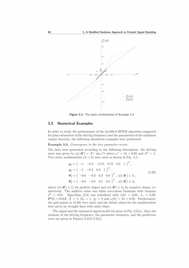
60 3. A Modified Nonlinear Approach to Periodic Signal Modeling
−−1 0−0.3 −0.15 0.15 0.3 1
0.3
0.8
0.5
−0.3
−0.5
−0.8
fj(u)
Iou
f1(u)f2(u)
Figure 3.1: The static nonlinearities of Example 3.3.
3.5 Numerical Examples
In order to study the performance of the modified RPEM algorithm suggestedfor joint estimation of the driving frequency and the parameters of the nonlinearoutput function, the following simulation examples were performed.
Example 3.3. Convergence to the true parameter vector.
The data were generated according to the following description: the drivingwave was given by u(t,θol ) = Xo sinωot where ωo = 2π × 0.05 and Xo = 1.Two static nonlinearities (L = 2) were used as shown in Fig. 3.1;
g1 =(−1 −0.3 −0.15 0.15 0.3 1
)T,
g2 =(−1 −0.3 0.3 1
)T,
θo1 =(−0.8 −0.3 0.3 0.8
)T, u(t,θol ) ∈ I1,
θo2 =(−0.8 −0.5 0.5 0.8
)T, u(t,θol ) ∈ I2.
(3.49)
where u(t,θol ) ∈ I1 for positive slopes and u(t,θol ) ∈ I2 for negative slopes, re-spectively. The additive noise was white zero-mean Gaussian with varianceσ2 = 0.01. Algorithm (3.9) was initialized with λ(0) = 0.95, λo = 0.99,P (0) = 0.01I, X = 1, K0 = 1, f0 = 0 and ω(0) = 2π × 0.02. Furthermore,the grid points in (3.49) were used, and the initial values for the nonlinearitieswere given by straight lines with unity slope.
The signal and the estimated signal model are given in Fig. 3.2(a). Also, theestimate of the driving frequency, the parameter estimates, and the predictionerror are given in Figures 3.2(b)-3.2(e).

3.5. Numerical Examples 61
0 200 400 600 800 1000−1.5
−1
−0.5
0
0.5
1
1.5
Time [samples]
(a) The signal (dashed) and the esti-
mated signal model (solid)
0 200 400 600 800 10000.1
0.15
0.2
0.25
0.3
0.35
Driv
ing
freq
uenc
y [r
ad]
Time [samples]
EstimateTrue
(b) Convergence of the fundamental fre-quency
0 200 400 600 800 1000
−1
−0.5
0
0.5
1
Par
amet
er e
stim
ates
(θ1 ,
f o)
Time [samples]
(c) Convergence of θ1 and fo
0 200 400 600 800 1000
−1
−0.5
0
0.5
1
Par
amet
er e
stim
ates
(θ2)
Time [samples]
(d) Convergence of θ2
0 200 400 600 800 1000−0.6
−0.4
−0.2
0
0.2
0.4
0.6
Pre
dict
ion
erro
r
Time [samples]
(e) Prediction error ε
Figure 3.2: Convergence to the true parameter vector using Algorithm (3.9).

62 3. A Modified Nonlinear Approach to Periodic Signal Modeling
After 1000 samples the following estimates were obtained;
X = 0.95, ω = 0.3141, fo = −0.0094,
θ1 =(−0.8705 −0.2869 0.3024 0.8625
)T,
θ2 =(−0.8214 −0.4910 0.5087 0.8280
)T.
It can be concluded that the convergence to the true parameter vector is takingplace.
Example 3.4. Tracking fundamental frequency variations.
As in Chapter 2, to improve the ability of the modified algorithm to trackfundamental frequency variations, Algorithm (3.9) is modified to
ε(t) = y(t) − y(t)
S(t) = ψT (t)P (t− 1)ψ(t) + r2(t)
P (t) = P (t− 1) − P (t− 1)ψ(t)S−1(t)ψT (t)P (t− 1) +R1(t)(θl(t)
θn(t)
)=
[(θl(t− 1)
θn(t− 1)
)+ P (t)ψ(t)ε(t)
]
DM
(3.50)
where R1(t) and r2(t) are the gain design variables.
The data were generated as in Example 3.3 and Algorithm (3.50) was ini-tialized with P (0) = 10−3I, X = 1, K0 = 1, f0 = 0 and ω(0) = 2π × 0.02.The design variables were R1 = 10−4I and r2 = 0.25. Also, the grid pointsin (3.49) were used, and the initial values for the nonlinearities were given bystraight lines with unity slope.
The signal and the estimated signal model are given in Fig. 3.3(a). Also,the true and estimated fundamental frequency are shown in Fig. 3.3(b). Theparameter estimates and the prediction error are given in Figures 3.3(c)-3.3(e).After 2400 samples the following estimates were obtained;
X = 0.8432, ω = 0.3474, fo = −0.0499,
θ1 =(−0.9169 −0.2709 0.3477 0.9313
)T,
θ2 =(−0.8897 −0.5422 0.4102 0.9036
)T,
and it can be concluded that Algorithm (3.50) has the ability to track thefundamental frequency variations.
Example 3.5. Modeling and tracking of flute music.
In this example, a piece of flute music is modeled using Algorithm (3.50). Thesignal was extracted from a CD in .wav format with a sampling frequency of22.05 kHz. The algorithm was initialized with P (0) = 500I, X = 1, K0 = 1,f0 = 0 and ω(0) = 2π × 348 rad/sec. The design variables were R1 = 0.01Iexcept that R1(2, 2) = 0.05 to speed up frequency convergence. r2 = 1 wasused.

3.5. Numerical Examples 63
0 500 1000 1500 2000−1.5
−1
−0.5
0
0.5
1
1.5
Time [samples]
(a) The signal (dashed) and the esti-
mated signal model (solid)
0 500 1000 1500 20000.1
0.15
0.2
0.25
0.3
0.35
0.4
0.45
0.5
Driv
ing
freq
uenc
y [r
ad]
Time [samples]
True Estimate
(b) Tracking the fundamental frequency
0 500 1000 1500 2000
−1
−0.5
0
0.5
1
Par
amet
er e
stim
ates
(θ1 ,
f o)
Time [samples]
(c) Parameter estimates θ1 and fo
0 500 1000 1500 2000
−1
−0.5
0
0.5
1
Par
amet
er e
stim
ates
(θ2)
Time [samples]
(d) Parameter estimates θ2
0 500 1000 1500 2000−1
−0.5
0
0.5
Pre
dict
ion
erro
r
Time [samples]
(e) Prediction error ε
Figure 3.3: Tracking the fundamental frequency of a sinusoid using Algorithm (3.50).

64 3. A Modified Nonlinear Approach to Periodic Signal Modeling
The grid points used for this example were
g1 =(− 0.12 − 0.06 − 0.03 − 0.015 − 0.0075 0.0075 0.015 0.03 0.06 0.12
)T,
g2 =(− 0.12 − 0.06 − 0.03 − 0.015 0.015 0.03 0.06 0.12
)T.
(3.51)The results are given in Fig. 3.4. After 1000 samples the following estimateswere obtained;
X = 0.1097, ω = 2π(349.4114), fo = 0.0096,
θ1 =(− 0.1509 0.0144 0.0255 0.0155 0.0008 0.0057 0.0349 0.1156
)T,
θ2 =(− 0.147 − 0.0266 − 0.028 − 0.0443 − 0.0368 − 0.0174 0.05 0.0964
)T.
The plot of the estimated static nonlinearity is given in Fig. 3.5. Also, the com-parison between the Hamming windowed periodogram with window width 400samples for the data and the model for different number of the true parametersis given in Fig. 3.6. The results show that the method gives good results fordifferent parameter vector sizes.
Example 3.6. Performance of the RPE algorithm as compared to the CRB.
In order to allow for comparison, the setup of this example closely resemblesthe numerical example of [121] and Example 2.4. In this example, 100 Monte-Carlo simulations were performed with different noise realizations to comparethe performance of the modified algorithm (3.9) with the derived CRB for thefundamental frequency estimate. The data were generated and the algorithmwas initialized as in Example 3.3. The statistics is based on excluding simu-lations that did not satisfy a margin of 5 standard deviations from the truefundamental frequency. Both the CRB for the fundamental frequency estimateand the MSE value were evaluated for data length of 2000 samples and fordifferent SNR. The number of excluded simulations did not exceed 15 exper-iments. The statistical results are plotted in Fig. 3.7 which shows that thealgorithm gives good statistical results.
3.6 Conclusions
The recursive periodic signal estimation algorithm of Chapter 2 has been mod-ified by introducing an interval in the nonlinear block with fixed static gain.This modification allows a treatment of local convergence properties of themodified algorithm. It was proven that the algorithm is locally convergentto the true parameter vector by using the associated ODE approach. Thenthe modified algorithm was studied by numerical examples and it was shownthat it can be easily modified to track fundamental frequency variations. Also,the CRB was calculated for the modified algorithm. Monte-Carlo experimentsshow that the modified algorithm gives good statistical results.

3.6. Conclusions 65
0 200 400 600 800 1000
−0.1
−0.05
0
0.05
0.1
0.15
Time [samples]
(a) The flute music (dashed) and the
model output (solid)
0 200 400 600 800 10002186
2188
2190
2192
2194
2196
2198
Driv
ing
freq
uenc
y [r
ad/s
ec]
Time [samples]
(b) Tracking the fundamental frequencyof the flute music
0 200 400 600 800 1000−0.2
−0.15
−0.1
−0.05
0
0.05
0.1
0.15
Par
amet
er e
stim
ates
(θ1 ,
f o)
Time [samples]
(c) Parameter estimates θ1 and fo
0 200 400 600 800 1000−0.15
−0.1
−0.05
0
0.05
0.1
0.15
0.2
Par
amet
er e
stim
ates
(θ2)
Time [samples]
(d) Parameter estimates θ2
0 200 400 600 800 10000
0.2
0.4
0.6
0.8
1
Est
imat
e of
X
Time [samples]
(e) Gain adaptation
0 200 400 600 800 1000−0.2
−0.15
−0.1
−0.05
0
0.05
0.1
0.15
0.2
Pre
dict
ion
erro
r
Time [samples]
(f) Prediction error ε
Figure 3.4: Modeling and tracking of the flute music using Algorithm (3.50).

66 3. A Modified Nonlinear Approach to Periodic Signal Modeling
−0.1 −0.05 0 0.05 0.1 0.15−0.2
−0.15
−0.1
−0.05
0
0.05
0.1
0.15
0.2
f j(u
)
u
Figure 3.5: Estimated static nonlinearity of the flute music. f1(u) (solid) and f2(u)(dashed).
0 500 1000 1500 2000 2500 3000−80
−70
−60
−50
−40
−30
−20
−10
0
Frequency [Hz]
Pow
er [d
B]
(a) 11 parameters
0 500 1000 1500 2000 2500 3000−80
−70
−60
−50
−40
−30
−20
−10
0
Frequency [Hz]
Pow
er [d
B]
(b) 15 parameters
0 500 1000 1500 2000 2500 3000−80
−70
−60
−50
−40
−30
−20
−10
0
Frequency [Hz]
Pow
er [d
B]
(c) 19 parameters
0 500 1000 1500 2000 2500 3000−80
−70
−60
−50
−40
−30
−20
−10
0
Frequency [Hz]
Pow
er [d
B]
(d) 23 parameters
Figure 3.6: The windowed periodogram for the flute music (solid) and the model(dashed).
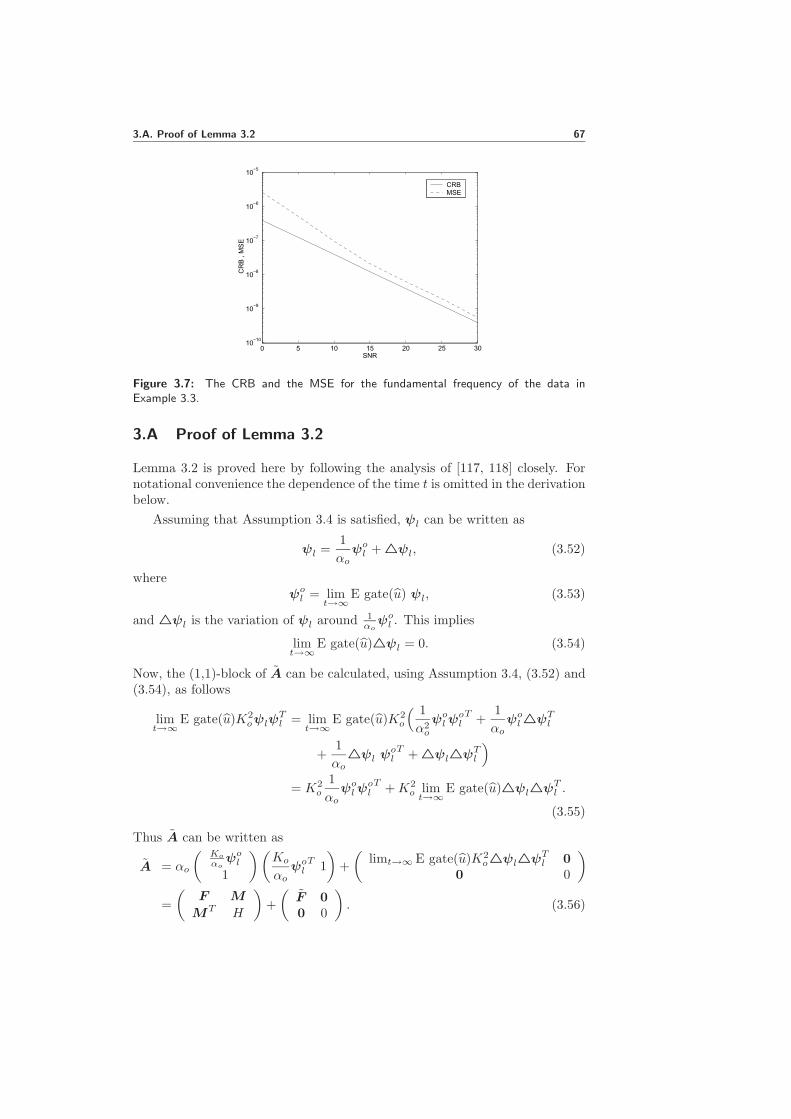
3.A. Proof of Lemma 3.2 67
0 5 10 15 20 25 3010
−10
10−9
10−8
10−7
10−6
10−5
SNR
CR
B ,
MS
E
CRBMSE
Figure 3.7: The CRB and the MSE for the fundamental frequency of the data inExample 3.3.
3.A Proof of Lemma 3.2
Lemma 3.2 is proved here by following the analysis of [117, 118] closely. Fornotational convenience the dependence of the time t is omitted in the derivationbelow.
Assuming that Assumption 3.4 is satisfied, ψl can be written as
ψl =1
αoψol + △ψl, (3.52)
whereψol = lim
t→∞E gate(u) ψl, (3.53)
and △ψl is the variation of ψl around 1αoψol . This implies
limt→∞
E gate(u)△ψl = 0. (3.54)
Now, the (1,1)-block of A can be calculated, using Assumption 3.4, (3.52) and(3.54), as follows
limt→∞
E gate(u)K2oψlψ
Tl = lim
t→∞E gate(u)K2
o
( 1
α2o
ψolψolT
+1
αoψol△ψ
Tl
+1
αo△ψl ψ
olT
+ △ψl△ψTl
)
= K2o
1
αoψolψ
olT
+K2o limt→∞
E gate(u)△ψl△ψTl .
(3.55)
Thus A can be written as
A = αo
(Ko
αoψol1
)(Ko
αoψol
T1
)+
(limt→∞ E gate(u)K2
o△ψl△ψTl 0
0 0
)
=
(F M
MT H
)+
(F 0
0 0
). (3.56)

68 3. A Modified Nonlinear Approach to Periodic Signal Modeling
Applying Lemma 3.1 again and taking into account that H = αo > 0 byAssumption 3.4, positive definiteness of A follows, if
F = limt→∞
E gate(u)K2o△ψl△ψ
Tl > 0.
In order to proceed, it is necessary to consider Assumption 3.5. This con-dition means that the contribution to the expectation from Io, should not benegligible as compared to the whole contribution to the expectation. It is acondition on the amplitude distribution of the driving signal, i.e. the drivingsignal should be such that a sufficient amount of signal energy is located in themid-subinterval Io. Taking into account that |Ko| > 0 by Assumption 3.6, itremains to study when
limt→∞
E △ψl△ψTl > 0
is satisfied. Since Eq. (3.54) does not imply that △ψl has zero mean, △ψl iswritten as
△ψl = △ψol + △ψl,
where△ψol = lim
t→∞E △ψl.
Then △ψl has zero mean, and
limt→∞
E △ψl△ψTl = △ψol△ψ
olT
+ limt→∞
E △ψl△ψT
l ≥ limt→∞
E △ψl△ψT
l .
Therefore, (3.40) is introduced. Since △ψl has zero mean, and
ψl =1
αoψol + △ψol + △ψl,
by introducing Assumption 3.7, it follows that
ψl = △ψl.
Hence it is possible to analyze ψl directly since for δ > 0 it follows that
F = K2o limt→∞
E gate(u)△ψl△ψTl
≥ δK2o limt→∞
E △ψl△ψTl
≥ δK2o limt→∞
E △ψl△ψT
l
= δK2o limt→∞
E ψlψTl . (3.57)
So far, the treatment parallels that of [118]. However, from now on thedifference of the linear block needs to be exploited, and the analysis becomesdifferent from [118]. To find the conditions that guarantee (3.40), F must be
proved to be positive definite. It is suitable to expand Λ(φ) and dΛ(φ)dφ around
φo, where φo is a maximum or a minimum point for Λ(φ). This requires

3.A. Proof of Lemma 3.2 69
the introduction of Assumption 3.8. The expansion, using properties of themaximum or minimum point, is
Λ(φ) = Λ(φo) +1
2
d2Λ(φ)
dφ2
∣∣∣φ=φo
(φ− φo)2 + O
((φ− φo)
3),
dΛ(φ)
dφ=d2Λ(φ)
dφ2
∣∣∣φ=φo
(φ− φo) + O((φ− φo)
2),
(3.58)
where O denotes the ordo concept. It follows that, around this point
Λ2(φ) =[Λ(φo)
]2+ Λ(φo)
d2Λ(φ)
dφ2
∣∣∣φ=φo
(φ− φo)2 + O
((φ− φo)
3),
(3.59)[dΛ(φ)
dφ
]2=
[d2Λ(φ)
dφ2
∣∣∣φ=φo
]2(φ− φo)
2 + O((φ− φo)
3), (3.60)
Λ(φ)dΛ(φ)
dφ= Λ(φo)
d2Λ(φ)
dφ2
∣∣∣φ=φo
(φ− φo) + O((φ− φo)
2). (3.61)
To guarantee that F > 0, it is required that (cf. Eq. (3.57))
F , limt→∞
E ψlψTl
= limt→∞
E
(Λ2(φ) Xo
ωo φ Λ(φ)dΛ(φ)dφ
Xo
ωo φ Λ(φ)dΛ(φ)dφ [X
o
ωo ]2 φ2 [dΛ(φ)dφ ]2
)> 0. (3.62)
Now
limt→∞
E(·) =1
2π
∫ 2π
0
(·) hφ dφ ≥ 1
2π
∫ φo+α
φo−α(·) hφ dφ , lim
t→∞Eα(·)
for all positive semidefinite integrands. Restricting the consideration to thesmall interval [φo − α, φo + α], α arbitrary small, it follows that
F ≥ limt→∞
Eα
(Λ2(φ) Xo
ωo φ Λ(φ)dΛ(φ)dφ
Xo
ωo φ Λ(φ)dΛ(φ)dφ [X
o
ωo ]2 φ2 [dΛ(φ)dφ ]2
). (3.63)
Hence, it turns out that F > 0 if the right hand matrix of (3.63) is positivedefinite. Substituting by Eqs. (3.59)-(3.61) in Eq. (3.63), the minors of thismatrix must satisfy the following inequalities
[Λ(φo)
]2+ Λ(φo)
d2Λ(φ)
dφ2
∣∣∣φ=φo
Eα[(φ− φo)
2]> 0, (3.64)
[Xo
ωo
]2 [d2Λ(φ)
dφ2
∣∣∣φ=φo
]2Eα[φ2(φ− φo)
2]> 0, (3.65)
[[Λ(φo)
]2+ Λ(φo)
d2Λ(φ)
dφ2
∣∣∣φ=φo
Eα[(φ− φo)
2]]
Eα[φ2(φ− φo)
2]>
[Λ(φo)
]2[Eα[φ(φ− φo)
]]2. (3.66)

70 3. A Modified Nonlinear Approach to Periodic Signal Modeling
Straightforward calculations for Eα[(φ − φo)
2],Eα
[φ2(φ − φo)
2]
and
Eα[φ(φ− φo)
]through the interval
[φo − α, φo + α
](where α is a very small
positive number) using Assumption 3.9 (which guarantees that the pdf of φ is“almost” constant in the interval under consideration) give
Eα[(φ− φo)
2]
=1
π
α3
3+ O(α4), (3.67)
Eα[φ2(φ− φo)
2]
=1
π
(α5
5+α3
3φ2o
)+ O(α6), (3.68)
Eα[φ(φ− φo)
]=
1
π
α3
3+ O(α4), (3.69)
Substituting by (3.67)-(3.68) in (3.64)-(3.66), respectively, and selecting α ar-bitrary small (neglecting O(α4) etc.), it follows that
[Λ(φo)
]2+ Λ(φo)
d2Λ(φ)
dφ2
∣∣∣φ=φo
1
π
α3
3> 0, (3.70)
[Xo
ωo
]2 [d2Λ(φ)
dφ2
∣∣∣φ=φo
]21
π
α3
3φ2o > 0, (3.71)
[[Λ(φo)
]2+ Λ(φo)
d2Λ(φ)
dφ2
∣∣∣φ=φo
1
π
α3
3
][1
π
α3
3φ2o
]> 0, (3.72)
provided that
|Λ(φo)| ≥ ǫ1 > 0,∣∣∣d2Λ(φ)
dφ2
∣∣∣φ=φo
≥ ǫ2 > 0,
φo 6= 0
(3.73)
Note that φo = ωot can not be equal to zero since ωo 6= 0 and time t isarbitrary chosen. Thus (3.62) is guaranteed for any continuous periodic signalwith a minimum or a maximum point. The result follows.
3.B Proof of Lemma 3.3
Following [117, 118], Lemma 3.2 can be proved as follows.
Recalling that the matrix C is defined as
C = limt→∞
E(1 − gate(u)
)
∂f1(·)∂θ1
T ∂f1(·)∂θ1
...∂f1(·)
∂θ1
T ∂fL(·)
∂θL
.... . .
...∂fL(·)
∂θL
T ∂f1(·)∂θ1
...∂fL(·)
∂θL
T ∂fL(·)
∂θL
, (3.74)
and noticing that
∂fm(·)∂θm
∂fn(·)∂θn
T
= 0 if n 6= m (3.75)

3.B. Proof of Lemma 3.3 71
C can be written as
C = limt→∞
E(1 − gate(u)
)
∂f1(·)∂θ1
T ∂f1(·)∂θ1
... 0
.... . .
...
0 ...∂fL(·)
∂θL
T ∂fL(·)
∂θL
. (3.76)
Since∂fj(·)∂θj
= 0, u(t,θol ) ∈ Io (3.77)
it follows that
limt→∞
E(1 − gate(u)
) ∂fj(·)∂θj
T∂fj(·)∂θj
= limt→∞
E∂fj(·)∂θj
T∂fj(·)∂θj
. (3.78)
Hence
C = limt→∞
E
∂f1(·)∂θ1
T ∂f1(·)∂θ1
... 0
.... . .
...
0 ...∂fL(·)
∂θL
T ∂fL(·)
∂θL
. (3.79)
Also it can be noticed from the RPEM algorithm (3.9) that the (j,j)-block(Cjj) of the matrix C can be written as
Cjj =(C
jj−0
0 Cjj+
), (3.80)
where Cjj− and Cjj+ are band-matrices given by
Cjj− = limt→∞
E
∂fj
∂fj
−k−
j
∂fj
∂fj
−k−
j
∂fj
∂fj
−k−
j
∂fj
∂fj
−k−
j+1
0 ... 0
∂fj
∂fj
−k−
j+1
∂fj
∂fj
−k−
j
. . ....
0. . .
.... . . 0
∂fj
∂fj−2
∂fj
∂fj−1
0 ... 0∂fj
∂fj−1
∂fj
∂fj−2
∂fj
∂fj−1
∂fj
∂fj−1
,
(3.81)
Cjj+ = limt→∞
E
∂fj
∂fj1
∂fj
∂fj1
∂fj
∂fj1
∂fj
∂fj2
0 ... 0
∂fj
∂fj2
∂fj
∂fj1
. . ....
0. . .
.... . . 0
∂fj
∂fj
k+j
−1
∂fj
∂fj
k+j
0 ... 0∂fj
∂fj
k+j
∂fj
∂fj
k+j
−1
∂fj
∂fj
k+j
∂fj
∂fj
k+j
. (3.82)
If these two matrices are positive definite then alsoCjj is positive definite. Pos-itive definiteness of Cjj consequently proves positive definiteness of C. Since

72 3. A Modified Nonlinear Approach to Periodic Signal Modeling
Cjj− and Cjj+ have similar structure, it is sufficient to investigate one of themas done in [117, 118].
Investigate, for example, Cjj+ . Since Cjj+ is positive semidefinite by con-struction, positive definiteness of Cjj+ can be proved if
dT Cjj+ d = 0 =⇒ d = 0 (3.83)
where d is an arbitrary vector. Using Eq. (3.82) gives
dT Cjj+ d = limt→∞
E
k+
j∑
m=1
dm∂fj
∂f jm
2
, (3.84)
where dm, m = 1, · · · , k+j are the components of the vector d. Let the function
fCjj+
(d, u) be given by
fCjj+
(d, u) ,
k+j∑
m=1
dm∂fj
∂f jm6= 0, ∀ u ∈
[uj1, u
j
k+j
]. (3.85)
This function represents a piecewise linear curve (see [118]) and its values inthe grid points uji , i = 1, . . . , k+
j are dm, m = 1, · · · , k+j , i.e.
fCjj+
(d, uji ) = di , i = 1, . . . , k+j . (3.86)
This is because when u ∈[uji , u
ji+1
], i = 1, . . . , k+
j −1, the function fCjj+
(d, u)can be written as
fCjj+
(d, u) = diuji+1 − u
uji+1 − uji+ di+1
u− ujiuji+1 − uji
which is a linear function of u that satisfies
fCjj+
(d, uji ) = di,
fCjj+
(d, uji+1) = di+1.
Using Assumption 3.10, Eq. (3.84) can be written as
dT Cjj+ d = limt→∞
E[fC
jj+(d, u)
]2
=
∫ uj
k+j
uj1
[fC
jj+(d, u)
]2hu(u)du. (3.87)
Now, conditions that imply (3.83) can be investigated. These conditions canbe found by equating (3.87) to zero. Let Iji =
(uji−1, u
ji
), i = −k−j + 1, . . . , k+
j ,j = 1, . . . , L denote the (open) subintervals of the piecewise linear model of thestatic nonlinearity including Io. Since by Assumption 3.10
hu(u) ≥ δ1 > 0 (3.88)

3.C. Proof of Theorem 3.2 73
in at least one nonzero interval [aji , bji ] ⊂ Iji . Since
[fC
jj+(d, u)
]2is nonnega-
tive and continuous on[uj1, u
j
k+j
], it follows from equation (3.87) and Assump-
tion 3.10 that
fCjj+
(d, u) = 0 , u ∈ [ai, bi] ⊂ Iji , i = 1, . . . , k+j , j = 1, . . . , L.
Thus fCjj+
(d, u) is analytic in Iji and equals zero in nonzero intervals
[ai, bi] ⊂ Iji . Hence, it follows from the properties of analytic functions (seee.g. [27]) that
fCjj+
(d, u) = 0 , u ∈ Iji , i = 1, . . . , k+j , j = 1, . . . , L.
Since the function fCjj+
(d, u) is continuous, Eq. (3.86) finally gives
fCjj+
(d, uji ) = di = 0 , i = 1, . . . , k+j .
This means that (3.83) is satisfied for all driving signals that fulfill Assump-tion 3.10.
The previous analysis proves positive definiteness of Cjj+ . Since Cjj− hassimilar structure as Cjj+ , Cjj is also positive definite. This consequently leadsto the positive definiteness of C.
3.C Proof of Theorem 3.2
The proof of Theorem 3.2 follows the main lines of a similar result in [121].The log-likelihood function l(θ) of the RPEM algorithm (3.9) is given by
l(θ) = constant − 1
2σ2
N∑
t=1
(y(t) − y(t,θ)
)2, (3.89)
Hence, the gradient of the log-likelihood function is defined as (cf. Eqs. (3.1)and (3.7))
∂l(θ)
∂θ=
(∂l(θ)
∂θl
∂l(θ)
∂θn
), (3.90)
where
∂l(θ)
∂θl=
(∂l(θ)
∂X
∂l(θ)
∂ω
),
∂l(θ)
∂θn=
(∂l(θ)
∂fo
∂l(θ)
∂θ1· · · ∂l(θ)
∂θL
), (3.91)
∂l(θ)
∂θj=
∂l(θ)
∂f j−k−j
· · · ∂l(θ)∂f j−1
∂l(θ)
∂f j1· · · ∂l(θ)
∂f jk+
j
.

74 3. A Modified Nonlinear Approach to Periodic Signal Modeling
In this case, the Fisher information matrix [99] can be written as
J = −E∂l(θ)
∂θ
T∂l(θ)
∂θ= −E
∂l(θ)∂θl
T ∂l(θ)∂θl
∂l(θ)∂θl
T ∂l(θ)∂θn
∂l(θ)∂θn
T ∂l(θ)∂θl
∂l(θ)∂θn
T ∂l(θ)∂θn
. (3.92)
In order to calculate the blocks of the matrix J , the following relations areneeded
∂l(θ)
∂X=
1
σ2
N∑
t=1
(y(t) − y(t,θ)
)∂y(t,θ)∂X
,
∂l(θ)
∂ω=
1
σ2
N∑
t=1
(y(t) − y(t,θ)
)∂y(t,θ)∂ω
,
∂l(θ)
∂fo=
1
σ2
N∑
t=1
(y(t) − y(t,θ)
)∂fj(·)∂fo
, (3.93)
∂l(θ)
∂f ji=
1
σ2
N∑
t=1
(y(t) − y(t,θ)
)∂fj(·)∂f ji
,
∂l(θ)
∂f ji+1
=1
σ2
N∑
t=1
(y(t) − y(t,θ)
)∂fj(·)∂f ji+1
,
where
∂y(t,θ)
∂X=∂fj(·)∂u
Λ(φ) |φ=ωt,
∂y(t,θ)
∂ω=∂fj(·)∂u
XtdΛ(φ)
dφ
∣∣∣φ=ωt
,
(3.94)
for u(t,θl) ∈ [uji , uji+1] ∈ Ij , i = −k−j , . . . , k+
j − 1, j = 1, . . . , L. Thus usingAssumption 3.1 and Assumption 3.11, it follows that
E
[∂2l(θ)
∂X2
]= − 1
σ2
N∑
t=1
[∂fj(·)∂u
]2Λ2(φ) |φ=ωt,
E
[∂2l(θ)
∂ω2
]= − 1
σ2
N∑
t=1
[∂fj(·)∂u
]2X2t2
[dΛ(φ)
dφ
∣∣∣φ=ωt
]2,
E
[∂2l(θ)
∂f2o
]= − 1
σ2
N∑
t=1
[∂fj(·)∂fo
]2,
E
[∂2l(θ)
∂X∂ω
]= − 1
σ2
N∑
t=1
[∂fj(·)∂u
]2Xt Λ(φ)
dΛ(φ)
dφ
∣∣∣φ=ωt
,
E
[∂2l(θ)
∂X∂fo
]= − 1
σ2
N∑
t=1
∂fj(·)∂u
∂fj(·)∂fo
Λ(φ)∣∣∣φ=ωt
,
E
[∂2l(θ)
∂ω∂fo
]= − 1
σ2
N∑
t=1
∂fj(·)∂u
∂fj(·)∂fo
XtdΛ(φ)
dφ
∣∣∣φ=ωt
,

3.C. Proof of Theorem 3.2 75
E
[∂2l(θ)
∂X∂f ji
]= − 1
σ2
N∑
t=1
∂fj(·)∂u
∂fj(·)∂f ji
Λ(φ) |φ=ωt,
E
[∂2l(θ)
∂X∂f ji+1
]= − 1
σ2
N∑
t=1
∂fj(·)∂u
∂fj(·)∂f ji+1
Λ(φ) |φ=ωt, (3.95)
E
[∂2l(θ)
∂ω∂f ji
]= − 1
σ2
N∑
t=1
∂fj(·)∂u
∂fj(·)∂f ji
XtdΛ(φ)
dφ
∣∣∣φ=ωt
,
E
[∂2l(θ)
∂ω∂f ji+1
]= − 1
σ2
N∑
t=1
∂fj(·)∂u
∂fj(·)∂f ji+1
XtdΛ(φ)
dφ
∣∣∣φ=ωt
,
E
[∂2l(θ)
∂fo∂fji
]= − 1
σ2
N∑
t=1
∂fj(·)∂fo
∂fj(·)∂f ji
,
E
[∂2l(θ)
∂fo∂fji+1
]= − 1
σ2
N∑
t=1
∂fj(·)∂fo
∂fj(·)∂f ji+1
,
E
[∂2l(θ)
∂f ji ∂fji
]= − 1
σ2
N∑
t=1
∂fj(·)∂f ji
∂fj(·)∂f ji
,
E
[∂2l(θ)
∂f ji+1∂fji+1
]= − 1
σ2
N∑
t=1
∂fj(·)∂f ji+1
∂fj(·)∂f ji+1
,
E
[∂2l(θ)
∂f ji ∂fji+1
]= − 1
σ2
N∑
t=1
∂fj(·)∂f ji
∂fj(·)∂f ji+1
.
Taking into account that ∂2l(θ)∂θm∂θn
= 0 for m 6= n. Introducing the notation in
(3.48) and noticing that J = 1/σ2∑Nt=1 I(t), Eq. (3.46) directly follows from
Assumption 3.12.
Remark 3.5.∂fj(·)∂u ,
∂fj(·)∂fo
,∂fj(·)∂fj
i
and∂fj(·)∂fj
i+1
can be calculated for different
subintervals using (3.9). Thus the matrix I(t) takes the following forms:
(i) When u(t,θl) ∈ [uji , uji+1] ∀i =
{ −k−1 , . . . ,−2, 1, . . . , k+1 − 1, j = 1
−k−j , . . . , k+j − 1, j = 2, . . . , L.
I(t) =
IX,X IX,ω 0 ··· 0 IX,f
ji
IX,f
ji+1
0 ··· 0
Iω,X Iω,ω 0 ··· 0 Iω,f
ji
Iω,f
ji+1
0 ··· 0
0 0 0 0...
......
...
0 0 0 0I
fji
,XI
fji
,ω0 ··· 0 I
fji
,fji
If
ji
,fji+1
0 ··· 0
If
ji+1
,XI
fji+1
,ω0 ··· 0 I
fji+1
,fji
If
ji+1
,fji+1
0 ··· 0
0 0 0 0...
......
...
0 0 0 0
, (3.96)

76 3. A Modified Nonlinear Approach to Periodic Signal Modeling
where
IX,X =
[f ji+1 − f ji
uji+1 − uji
]2
Λ2(φ) |φ=ωt,
Iω,ω =
[f ji+1 − f ji
uji+1 − uji
]2
X2t2[dΛ(φ)
dφ
∣∣∣φ=ωt
]2,
IX,ω =
[f ji+1 − f ji
uji+1 − uji
]2
Xt Λ(φ)dΛ(φ)
dφ
∣∣∣φ=ωt
,
IX,fji
=f ji+1 − f ji
uji+1 − uji
uji+1 − u(t,θl)
uji+1 − ujiΛ(φ) |φ=ωt,
IX,fji+1
=f ji+1 − f ji
uji+1 − uji
u(t,θl) − ujiuji+1 − uji
Λ(φ) |φ=ωt, (3.97)
Iω,fji
=f ji+1 − f ji
uji+1 − uji
uji+1 − u(t,θl)
uji+1 − ujiXt
dΛ(φ)
dφ
∣∣∣φ=ωt
,
Iω,fji+1
=f ji+1 − f ji
uji+1 − uji
u(t,θl) − ujiuji+1 − uji
XtdΛ(φ)
dφ
∣∣∣φ=ωt
,
Ifji ,f
ji
=
[uji+1 − u(t,θl)
uji+1 − uji
]2
,
Ifji+1,f
ji+1
=
[u(t,θl) − ujiuji+1 − uji
]2
,
Ifji ,f
ji+1
=uji+1 − u(t,θl)
uji+1 − uji
u(t,θl) − ujiuji+1 − uji
.
(ii) When u(t,θl) ∈ [u1−1, uo− ] ⊂ I1;
I(t) =
IX,X IX,w IX,fo 0 ··· 0 IX,f1
−10 ··· 0
Iω,X Iω,ω Iω,fo 0 ··· 0 Iω,f1
−10 ··· 0
Ifo,X Ifo,ω Ifo,fo 0 ··· 0 Ifo,f1
−10 ··· 0
0 0 0 0...
......
...
0 0 0 0I
f1−1
,XI
f1−1
,ωI
f1−1
,fo0 ··· 0 I
f1−1
,f1−1
0 ··· 0
0 0 0 0...
......
...
0 0 0 0
, (3.98)
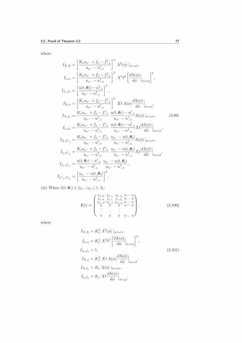
3.C. Proof of Theorem 3.2 77
where
IX,X =
[Kouo− + fo − f1
−1
uo− − u1−1
]2Λ2(φ) |φ=ωt,
Iω,ω =
[Kouo− + fo − f1
−1
uo− − u1−1
]2X2t2
[dΛ(φ)
dφ
∣∣∣φ=ωt
]2,
Ifo,fo=
[u(t,θl) − u1
−1
uo− − u1−1
]2,
IX,ω =
[Kouo− + fo − f1
−1
uo− − u1−1
]2Xt Λ(φ)
dΛ(φ)
dφ
∣∣∣φ=ωt
,
IX,fo=Kouo− + fo − f1
−1
uo− − u1−1
u(t,θl) − u1−1
uo− − u1−1
Λ(φ) |φ=ωt, (3.99)
Iω,fo=Kouo− + fo − f1
−1
uo− − u1−1
u(t,θl) − u1−1
uo− − u1−1
XtdΛ(φ)
dφ
∣∣∣φ=ωt
,
IX,f1−1
=Kouo− + fo − f1
−1
uo− − u1−1
uo− − u(t,θl)
uo− − u1−1
Λ(φ) |φ=ωt,
Iω,f1−1
=Kouo− + fo − f1
−1
uo− − u1−1
uo− − u(t,θl)
uo− − u1−1
XtdΛ(φ)
dφ
∣∣∣φ=ωt
,
Ifo,f1−1
=u(t,θl) − u1
−1
uo− − u1−1
uo− − u(t,θl)
uo− − u1−1
,
If1−1,f
1−1
=
[uo− − u(t,θl)
uo− − u1−1
]2.
(iii) When u(t,θl) ∈ [uo− , uo+ ] ⊂ I1;
I(t) =
IX,X IX,ω IX,fo 0 ··· 0Iω,X Iω,ω Iω,fo 0 ··· 0Ifo,X Ifo,ω Ifo,fo 0 ··· 0
0 0 0 0 ··· 0...
......
0 0 0 0 ··· 0
, (3.100)
where
IX,X = K2o Λ2(φ) |φ=ωt,
Iω,ω = K2o X
2t2[dΛ(φ)
dφ
∣∣∣φ=ωt
]2,
Ifo,fo= 1, (3.101)
IX,ω = K2o Xt Λ(φ)
dΛ(φ)
dφ
∣∣∣φ=ωt
,
IX,fo= Ko Λ(φ) |φ=ωt,
Iω,fo= Ko Xt
dΛ(φ)
dφ
∣∣∣φ=ωt
.

78 3. A Modified Nonlinear Approach to Periodic Signal Modeling
(iv) When u(t,θl) ∈ [uo+ , u11] ⊂ I1;
I(t) =
IX,X IX,ω IX,fo 0 ··· 0 IX,f1
10 ··· 0
Iω,X Iω,ω Iω,fo 0 ··· 0 Iω,f1
10 ··· 0
Ifo,X Ifo,ω Ifo,fo 0 ··· 0 Ifo,f1
10 ··· 0
0 0 0 0...
......
...
0 0 0 0I
f11 ,X
If11 ,ω
If11 ,fo
0 ··· 0 If11 ,f1
10 ··· 0
0 0 0 0...
......
...
0 0 0 0
, (3.102)
where
IX,X =
[f11 −Kouo+ − fou1
1 − uo+
]2Λ2(φ) |φ=ωt,
Iω,ω =
[f11 −Kouo+ − fou1
1 − uo+
]2X2t2
[dΛ(φ)
dφ
∣∣∣φ=ωt
]2,
Ifo,fo=
[u1
1 − u(t,θl)
u11 − uo+
]2,
IX,ω =
[f11 −Kouo+ − fou1
1 − uo+
]2Xt Λ(φ)
dΛ(φ)
dφ
∣∣∣φ=ωt
,
IX,fo=f11 −Kouo+ − fou1
1 − uo+
u11 − u(t,θl)
u11 − uo+
Λ(φ) |φ=ωt, (3.103)
Iω,fo=f11 −Kouo+ − fou1
1 − uo+
u11 − u(t,θl)
u11 − uo+
XtdΛ(φ)
dφ
∣∣∣φ=ωt
,
IX,f11
=f11 −Kouo+ − fou1
1 − uo+
u(t,θl) − uo+
u11 − uo+
Λ(φ) |φ=ωt,
Iω,f11
=f11 −Kouo+ − fou1
1 − uo+
u(t,θl) − uo+
u11 − uo+
XtdΛ(φ)
dφ
∣∣∣φ=ωt
,
Ifo,f11
=u1
1 − u(t,θl)
u11 − uo+
u(t,θl) − uo+
u11 − uo+
,
If11 ,f
11
=
[u(t,θl) − uo+
u11 − uo+
]2.

Chapter 4
An Adaptive Grid Point Algorithm for PeriodicSignal Modeling
4.1 Introduction
IN the previous two chapters the nonlinearity was chosen to be piecewiselinear with the estimated parameters being the function values in a fixed set
of grid points, resulting in fixed grid point adaptation. In this chapter, theRPEM algorithm introduced in Chapter 3 is modified to enable the algorithmto estimate the grid points as well as the driving frequency and the parametersof the nonlinear output function, resulting in automatic grid point adaptation.This is expected to reduce the modeling errors since it gives the algorithm morefreedom to choose the suitable grid points.
The contributions of this chapter can hence be summarized as follows. Thealgorithm (3.9) is modified to adaptively estimate the grid points. Also, theCRB is derived for the suggested method. Furthermore, the performance forjoint estimation of the driving frequency, the parameters of the nonlinear outputfunction as well as the grid points, is studied by numerical examples. Thepurpose is to investigate convergence to the true parameter vector, the abilityto track both the fundamental frequency and the amplitude variations, and theperformance as compared to the fixed grid point algorithm.
The chapter is organized as follows. In Section 4.2, the suggested algorithmis introduced. The derivation of the CRB for the suggested algorithm is pre-sented in Section 4.3. Finally, Numerical examples and conclusions are givenin Section 4.4 and Section 4.5, respectively.
4.2 The Suggested Algorithm
Similarly as done in Chapter 3 the driving input signal u(t,θl) is modeled as
u(t,θl) = XΛ(ωt),
θl =(X ω
)T,
(4.1)
where t denotes discrete time, ω ∈ [0, π] denotes the unknown normalizedangular frequency: ω = 2πf/fs where f is the frequency, and fs is the samplingfrequency. X is a possibly time-varying parameter.
79

80 4. An Adaptive Grid Point Algorithm for Periodic Signal Modeling
The piecewise linear model discussed in Chapter 3 is used also here for theparameterization of the nonlinearity. Choosing Io to be contained in the firstinterval I1, the grid points are defined as
gTj =
{ (u1−k−1
u1−k−1 +1
· · · uo− uo+ · · · u1k+1 −1
u1k+1
), j = 1
(uj−k−j
uj−k−j +1· · · uj−1 uj1 · · · uj
k+j −1
ujk+
j
), j = 2, · · · , L.
(4.2)Then with fj
(θj , gj , u(t,θl)
)denoting the nonlinearity to be used in Ij , the
parameters θj are chosen as the values of fj(θj , gj , u(t,θl)
)in the grid points,
i.e.
θj =(f j−k−j
· · · f j−1 f j1 · · · f jk+
j
)T, j = 1, · · · , L
fj(θj , gj , uji ) =
{Kou(t,θl) + fo , u(t,θl) ∈ Io , j = 1
f ji , i = −k−j , · · · ,−1, 1, · · · , k+j , j = 1, · · · , L.
(4.3)
Also, here Ko is a constant static gain chosen by the user and there are noparameters corresponding to uo− and uo+ (cf. Eq. (3.6)). Therefore the modeloutput becomes
y(t,θ) = fj(θj , gj , u(t,θl)
), u(t,θl) ∈ Ij , j = 1, · · · , L
θ =(θTl θTn θTg
)T,
θl =(X ω
)T,
θn =(fo θ
T
n
)T,
θn =(θT1 · · · θTL
)T,
θg =(gT1 · · · gTL
)T.
(4.4)
Hence, similarly as done in the previous two chapter, a recursive Gauss-NewtonPEM follows by the minimization of the following cost function
V (θ) = limN→∞
1
N
N∑
t=1
E[ε2(t,θ)
]. (4.5)
The objective of this chapter is, as stated in the introduction, to esti-mate the grid points recursively in addition to the estimation of the funda-mental frequency and the parameters of the nonlinear output function. Thiswill give the algorithm more freedom to choose the grid points and achieve abetter performance. In this case, the negative gradient of y(t,θ) is given by(for u(t,θl) ∈ Ij , j = 1, · · · , L)
ψ(t,θ) =(
∂fj(·)∂u ψl(t)
∂fj(·)∂fo
0 · · · 0 ∂fj(·)∂θj
0 · · · 0 ∂fj(·)∂gj
0 · · · 0)T
,
(4.6)where
ψl(t) =(
Λ(φ) |φ=ωt XtdΛ(φ)dφ
∣∣∣φ=ωt
)T. (4.7)

4.2. The Suggested Algorithm 81
Thus the RPEM algorithm becomes
ε(t) = y(t) − y(t)
λ(t) = λoλ(t− 1) + 1 − λo
S(t) = ψT (t)P (t− 1)ψ(t) + λ(t)
P (t) =(P (t− 1) − P (t− 1)ψ(t)S−1(t)ψT (t)P (t− 1)
)/λ(t)
θl(t)
θn(t)
θg(t)
=
θl(t− 1)
θn(t− 1)
θg(t− 1)
+ P (t)ψ(t)ε(t)
DM
(4.8)
u(t+ 1) = X(t)Λ(φ) |φ=ω(t)(t+1)
ψl(t+ 1) =
(Λ(φ) |φ=ω(t)(t+1) X(t)(t+ 1)dΛ(φ)
dφ
∣∣∣φ=ω(t)(t+1)
)T
when u(t+ 1) ∈ I1
when u(t+ 1) ∈ [u1−1, uo− ]
y(t+ 1) =f1−1uo− − (Kouo− + fo)u
1−1
uo− − u1−1
+Kouo− + fo − f1
−1
uo− − u1−1
u(t+ 1)
∂f1(·)∂u1
−1
=(f1
−1 −Kouo− − fo)uo−
(uo− − u1−1)
2+Kouo− + fo − f1
−1
(uo− − u1−1)
2u(t+ 1)
∂f1(·)∂u
=Kouo− + fo − f1
−1
uo− − u1−1
∂f1(·)∂f1
−1
=uo− − u(t+ 1)
uo− − u1−1
∂f1(·)∂fo
=u(t+ 1) − u1
−1
uo− − u1−1
∂f1(·)∂u1
l
= 0 , l 6= −1
∂f1(·)∂f1
l
= 0 , l 6= −1, 0
end
when u(t+ 1) ∈ [uo− , uo+ ]
y(t+ 1) = Kou(t+ 1) + fo
∂f1(·)∂u
= Ko
∂f1(·)∂fo
= 1
∂f1(·)∂f1
l
= 0 , l 6= 0
∂f1(·)∂u1
l
= 0 , ∀ l
end

82 4. An Adaptive Grid Point Algorithm for Periodic Signal Modeling
when u(t+ 1) ∈ [uo+ , u11]
y(t+ 1) =(Kouo+ + fo)u
11 − f1
1uo+
u11 − uo+
+f11 −Kouo+ − fou1
1 − uo+u(t+ 1)
∂f1(·)∂u1
1
=(f1
1 −Kouo+ − fo)uo+
(u11 − uo+)2
− f11 −Kouo+ − fo(u1
1 − uo+)2u(t+ 1)
∂f1(·)∂u
=f11 −Kouo+ − fou1
1 − uo+
∂f1(·)∂fo
=u1
1 − u(t+ 1)
u11 − uo+
∂f1(·)∂f1
1
=u(t+ 1) − uo+
u11 − uo+
∂f1(·)∂u1
l
= 0 , l 6= 1
∂f1(·)∂f1
l
= 0 , l 6= 0, 1
end
when u(t+ 1) ∈ Ij , j = 1, · · · , L
when u(t+ 1) ∈ [uji , uji+1] ∀i =
{ −k−1 , ..,−2, 1, .., k+1 − 1, j = 1,
−k−j , · · · , k+j − 1, j = 2, · · · , L.
y(t+ 1) =f ji u
ji+1 − f ji+1u
ji
uji+1 − uji+f ji+1 − f ji
uji+1 − ujiu(t+ 1)
∂fj(·)∂uji
=(f ji − f ji+1)u
ji+1
(uji+1 − uji )2
+f ji+1 − f ji
(uji+1 − uji )2u(t+ 1)
∂fj(·)∂uji+1
=(f ji+1 − f ji )u
ji
(uji+1 − uji )2
− f ji+1 − f ji
(uji+1 − uji )2u(t+ 1)
∂fj(·)∂u
=f ji+1 − f ji
uji+1 − uji
∂fj(·)∂f ji
=uji+1 − u(t+ 1)
uji+1 − uji
∂fj(·)∂f ji+1
=u(t+ 1) − ujiuji+1 − uji
∂fj(·)∂ujl
= 0 , l 6= i, i+ 1
∂fj(·)∂fo
= 0
∂fj(·)∂f jl
= 0 , l 6= i, i+ 1
end

4.3. The Cramer-Rao Bound 83
∂fj(·)∂θj
=
(∂fj(·)∂fj
−k−
j
· · · ∂fj(·)∂fj
−1
∂fj(·)∂fj
1
· · · ∂fj(·)∂fj
k+j
)
∂fj(·)∂gj
=
(∂fj(·)∂uj
−k−
j
· · · ∂fj(·)∂uj
−1
∂fj(·)∂uj
1
· · · ∂fj(·)∂uj
k+j
)
ψ(t+ 1) =(
∂fj(·)∂u ψTl (t+ 1)
∂fj(·)∂fo
0 · · · 0 ∂fj(·)∂θj
0 · · · 0 ∂fj(·)∂gj
0 · · · 0)T
end.
Remark 4.1. It is assumed here that some precautions are taken to preventgrid miss ordering during the estimation process. This is stated as
Assumption 4.1. Grid ordering is included in the definition of the model set.
4.3 The Cramer-Rao Bound
Theorem 4.1. Under Assumptions 2.1-2.2, Assumption 3.1, Assump-
tions 3.11-3.12 and Assumption 4.1, the CRB for(θTl θ
Tn θ
Tg
)Tis given by
CRB(θ) = σ2
(N∑
t=1
I(t)
)−1
, (4.9)
where
I(t) =
IX,X IX,ω IX,fo 0 ··· 0 IX,f
ji
IX,f
ji+1
0 ··· 0 IX,u
ji
IX,u
ji+1
0 ··· 0
Iω,X Iω,ω Iω,fo 0 ··· 0 Iω,f
ji
Iω,f
ji+1
0 ··· 0 Iω,u
ji
Iω,u
ji+1
0 ··· 0
Ifo,X Ifo,ω Ifo,fo 0 ··· 0 Ifo,f
ji
Ifo,f
ji+1
0 ··· 0 Ifo,u
ji
Ifo,u
ji+1
0 ··· 0
0 0 0 0 0 0 0...
......
......
......
0 0 0 0 0 0 0I
fji
,XI
fji
,ωI
fji
,fo0 ··· 0 I
fji
,fji
If
ji
,fji+1
0 ··· 0 If
ji
,uji
If
ji
,uji+1
0 ··· 0
If
ji+1
,XI
fji+1
,ωI
fji+1
,fo0 ··· 0 I
fji+1
,fji
If
ji+1
,fji+1
0 ··· 0 If
ji+1
,uji
If
ji+1
,uji+1
0 ··· 0
0 0 0 0 0 0 0...
......
......
......
0 0 0 0 0 0 0I
uji
,XI
uji
,ωI
uji
,fo0 ··· 0 I
uji
,fji
Iu
ji
,fji+1
0 ··· 0 Iu
ji
,uji
Iu
ji
,uji+1
0 ··· 0
Iu
ji+1
,XI
uji+1
,ωI
uji+1
,fo0 ··· 0 I
uji+1
,fji
Iu
ji+1
,fji+1
0 ··· 0 Iu
ji+1
,uji
Iu
ji+1
,uji+1
0 ··· 0
0 0 0 0 0 0 0...
......
......
......
0 0 0 0 0 0 0
,
(4.10)
u(t,θl) ∈[uji , u
ji+1
]∈ Ij , i = −k−j , . . . , k+
j − 1, j = 1, . . . , L.

84 4. An Adaptive Grid Point Algorithm for Periodic Signal Modeling
IX,X =
[∂fj(·)∂u
]2Λ2(φ) |φ=ωt,
Iω,ω =
[∂fj(·)∂u
]2X2t2
[dΛ(φ)
dφ
∣∣∣φ=ωt
]2,
Ifo,fo=
[∂fj(·)∂fo
]2,
IX,ω =
[∂fj(·)∂u
]2Xt Λ(φ)
dΛ(φ)
dφ
∣∣∣φ=ωt
,
IX,fo=∂fj(·)∂u
∂fj(·)∂fo
Λ(φ) |φ=ωt,
Iω,fo=∂fj(·)∂u
∂fj(·)∂fo
XtdΛ(φ)
dφ
∣∣∣φ=ωt
,
IX,fji
=∂fj(·)∂u
∂fj(·)∂f ji
Λ(φ) |φ=ωt,
IX,fji+1
=∂fj(·)∂u
∂fj(·)∂f ji+1
Λ(φ) |φ=ωt,
IX,uji
=∂fj(·)∂u
∂fj(·)∂uji
Λ(φ) |φ=ωt,
IX,uji+1
=∂fj(·)∂u
∂fj(·)∂uji+1
Λ(φ) |φ=ωt,
Iω,fji
=∂fj(·)∂u
∂fj(·)∂f ji
XtdΛ(φ)
dφ
∣∣∣φ=ωt
,
Iω,fji+1
=∂fj(·)∂u
∂fj(·)∂f ji+1
XtdΛ(φ)
dφ
∣∣∣φ=ωt
,
Iω,uji
=∂fj(·)∂u
∂fj(·)∂uji
XtdΛ(φ)
dφ
∣∣∣φ=ωt
,
Iω,uji+1
=∂fj(·)∂u
∂fj(·)∂uji+1
XtdΛ(φ)
dφ
∣∣∣φ=ωt
, (4.11)
Ifo,fji
=∂fj(·)∂fo
∂fj(·)∂f ji
,
Ifo,fji+1
=∂fj(·)∂fo
∂fj(·)∂f ji+1
,
Ifo,uji
=∂fj(·)∂fo
∂fj(·)∂uji
,
Ifo,uji+1
=∂fj(·)∂fo
∂fj(·)∂uji+1
,

4.4. Numerical Examples 85
Ifji ,f
ji
=
[∂fj(·)∂f ji
]2
,
Ifji+1,f
ji+1
=
[∂fj(·)∂f ji+1
]2
,
Ifji ,f
ji+1
=∂fj(·)∂f ji
∂fj(·)∂f ji+1
,
Iuji ,u
ji
=
[∂fj(·)∂uji
]2
,
Iuji+1,u
ji+1
=
[∂fj(·)∂uji+1
]2
,
Iuji ,u
ji+1
=∂fj(·)∂uji
∂fj(·)∂uji+1
,
Ifji ,u
ji
=∂fj(·)∂f ji
∂fj(·)∂uji
,
Ifji ,u
ji+1
=∂fj(·)∂f ji
∂fj(·)∂uji+1
,
Ifji+1,u
ji
=∂fj(·)∂f ji+1
∂fj(·)∂uji
,
Ifji+1,u
ji+1
=∂fj(·)∂f ji+1
∂fj(·)∂uji+1
.
Proof. See Appendix 4.A.
4.4 Numerical Examples
In order to study the performance of the RPEM algorithm suggested for jointestimation of the driving frequency and the parameters of the nonlinear outputfunction in a set of grid points estimated recursively, the following simulationexamples were performed.
Example 4.1. Convergence of the adaptive grid point algorithm.
The data were generated according to the following description: the drivingwave was given by u(t,θol ) = sinωot where ωo = 2π × 0.05. The static nonlin-earity was chosen as
f(u) =
(5/3)u2 + 0.15 , u ≥ 0.3u , −0.3 ≤ u < 0.3
−(5/3)u2 − 0.15 , u < −0.3(4.12)
Note that this means the system is not in the model set, i.e. undermodelingeffects are at hand.
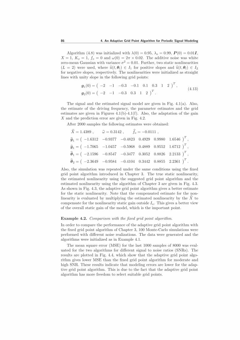
86 4. An Adaptive Grid Point Algorithm for Periodic Signal Modeling
Algorithm (4.8) was initialized with λ(0) = 0.95, λo = 0.99, P (0) = 0.01I,X = 1, Ko = 1, fo = 0 and ω(0) = 2π × 0.02. The additive noise was whitezero-mean Gaussian with variance σ2 = 0.01. Further, two static nonlinearities(L = 2) were used, where u(t,θl) ∈ I1 for positive slopes and u(t,θl) ∈ I2for negative slopes, respectively. The nonlinearities were initialized as straightlines with unity slope in the following grid points:
g1(0) =(−2 −1 −0.3 −0.1 0.1 0.3 1 2
)T,
g2(0) =(−2 −1 −0.3 0.3 1 2
)T.
(4.13)
The signal and the estimated signal model are given in Fig. 4.1(a). Also,the estimate of the driving frequency, the parameter estimates and the gridestimates are given in Figures 4.1(b)-4.1(f). Also, the adaptation of the gainX and the prediction error are given in Fig. 4.2.
After 2000 samples the following estimates were obtained:
X = 1.4389 , ω = 0.3142 , fo = −0.0111 ,
g1 =(−1.6312 −0.9377 −0.4823 0.4929 0.9980 1.6546
)T,
g1 =(−1.7065 −1.0457 −0.5968 0.4889 0.9552 1.6712
)T,
θ1 =(−2.1596 −0.8547 −0.3477 0.3052 0.8826 2.2133
)T,
θ2 =(−2.3649 −0.9584 −0.4104 0.3442 0.8855 2.2361
)T.
Also, the simulation was repeated under the same conditions using the fixedgrid point algorithm introduced in Chapter 3. The true static nonlinearity,the estimated nonlinearity using the suggested grid point algorithm and theestimated nonlinearity using the algorithm of Chapter 3 are given in Fig. 4.3.As shown in Fig. 4.3, the adaptive grid point algorithm gives a better estimatefor the static nonlinearity. Note that the compensated estimate for the non-linearity is evaluated by multiplying the estimated nonlinearity by the X tocompensate for the nonlinearity static gain outside Io. This gives a better viewof the overall static gain of the model, which is the important point.
Example 4.2. Comparison with the fixed grid point algorithm.
In order to compare the performance of the adaptive grid point algorithm withthe fixed grid point algorithm of Chapter 3, 100 Monte-Carlo simulations wereperformed with different noise realizations. The data were generated and thealgorithms were initialized as in Example 4.1.
The mean square error (MSE) for the last 1000 samples of 8000 was eval-uated for the two algorithms for different signal to noise ratios (SNRs). Theresults are plotted in Fig. 4.4, which show that the adaptive grid point algo-rithm gives lower MSE than the fixed grid point algorithm for moderate andhigh SNR. These results indicate that modeling errors are lower for the adap-tive grid point algorithm. This is due to the fact that the adaptive grid pointalgorithm has more freedom to select suitable grid points.

4.4. Numerical Examples 87
0 500 1000 1500 2000−2.5
−2
−1.5
−1
−0.5
0
0.5
1
1.5
2
2.5
Time [samples]
(a) The signal (dashed) and the esti-
mated signal model (solid)
0 500 1000 1500 20000.1
0.15
0.2
0.25
0.3
0.35
Driv
ing
freq
uenc
y [r
ad]
Time [samples]
EstimateTrue
(b) Convergence of the fundamental fre-quency
0 500 1000 1500 2000−2.5
−2
−1.5
−1
−0.5
0
0.5
1
1.5
2
2.5
Par
amet
er e
stim
ates
(θ1 ,
f o)
Time [samples]
fo
f1−1
f1−2
f1−3
f11
f12
f13
(c) Convergence of θ1
0 500 1000 1500 2000−2.5
−2
−1.5
−1
−0.5
0
0.5
1
1.5
2
2.5
Par
amet
er e
stim
ates
(θ2)
Time [samples]
f2−3
f2−2
f2−1
f21
f22
f23
(d) Convergence of θ2
0 500 1000 1500 2000−2.5
−2
−1.5
−1
−0.5
0
0.5
1
1.5
2
2.5
Grid
est
imat
es (
g 1)
Time [samples]
u1−1
u1−2
u1−3
u11
u12
u13
(e) Convergence of g1
0 500 1000 1500 2000−2.5
−2
−1.5
−1
−0.5
0
0.5
1
1.5
2
2.5
Grid
est
imat
es (
g 2)
Time [samples]
u2−3
u2−2
u2−1
u21
u22
u23
(f) Convergence of g2
Figure 4.1: Convergence to the true parameter vector using Algorithm (4.8).

88 4. An Adaptive Grid Point Algorithm for Periodic Signal Modeling
0 500 1000 1500 20000.9
1
1.1
1.2
1.3
1.4
1.5
Est
imat
e of
X
Time [samples]
(a) Adaptation of X
0 500 1000 1500 2000−1
−0.8
−0.6
−0.4
−0.2
0
0.2
0.4
0.6
0.8
1
Pre
dict
ion
erro
r
Time [samples]
(b) Prediction error
Figure 4.2: Convergence of X and the prediction error ε for Example 4.1.
−2 −1.5 −1 −0.5 0 0.5 1 1.5 2−4
−3
−2
−1
0
1
2
3
4
Input
Out
put
True static nonlinearity (solid)Estimate with adaptive grid alg. (dashed)Estimate with fixed grid alg. (dash−dot)
Figure 4.3: The compensated estimates of the static nonlinearity.
20 25 30 35 40 45 50 55 60−38
−36
−34
−32
−30
−28
−26
−24
−22
−20
−18
SNR [dB]
MS
E [d
B]
The adaptive grid Alg.The fixed grid Alg.
Figure 4.4: The MSE results.

4.4. Numerical Examples 89
0 400 800 1200 1600 2000 2400−1
−0.5
0
0.5
1
Time [samples]
(a) The signal (dashed) and the esti-
mated signal model (solid)
0 400 800 1200 1600 2000 24000.1
0.15
0.2
0.25
0.3
0.35
0.4
0.45
0.5
Driv
ing
freq
uenc
y [r
ad]
Time [samples]
EstimateTrue
(b) Tracking the fundamental frequencyvariations
Figure 4.5: Tracking the fundamental frequency using Algorithm (4.14).
Example 4.3. Tracking the fundamental frequency variations.
As mentioned in Chapter 3, to improve the ability of the suggested algorithmto track fundamental frequency variations, Algorithm (4.8) is modified to
ε(t) = y(t) − y(t)
S(t) = ψT (t)P (t− 1)ψ(t) + r2(t)
P (t) = P (t− 1) − P (t− 1)ψ(t)S−1(t)ψT (t)P (t− 1) +R1(t)
θl(t)
θn(t)
θg(t)
=
θl(t− 1)
θn(t− 1)
θg(t− 1)
+ P (t)ψ(t)ε(t)
DM
(4.14)
where R1(t) and r2(t) are the gain design variables. The data were generatedas in Example 4.1 with
go1 =(−1 −0.3 −0.15 0.15 0.3 1
)T,
go2 =(−1 −0.3 0.3 1
)T,
θo1 =(−0.8 −0.3 0.3 0.8
)T, u(t,θol ) ∈ I1
θo2 =(−0.8 −0.5 0.5 0.8
)T, u(t,θol ) ∈ I2.
(4.15)
Also, Algorithm (4.14) was initialized as in Example 4.1. The design variableswere R1(t) = 10−6I except that R1(2, 2) = 5×10⁻⁵ to speed up the frequencytracking and r2(t) = 0.2. Also, the grid points in (4.15) were used, and theinitial values for the nonlinearities were given by straight lines with unity slope.The signal and the estimated signal model are given in Fig. 4.5(a). Also, thetrue and estimated fundamental frequency are shown in Fig. 4.5(b). It can beconcluded from the results that Algorithm (4.14) has the ability to track thefundamental frequency variations.

90 4. An Adaptive Grid Point Algorithm for Periodic Signal Modeling
0 200 400 600 800 1000 1200−1
−0.8
−0.6
−0.4
−0.2
0
0.2
0.4
0.6
0.8
1
Time [samples]
(a) The signal (dashed) and the esti-
mated signal model (solid)
0 200 400 600 800 1000 12000.1
0.15
0.2
0.25
0.3
0.35
0.4
0.45
Driv
ing
freq
uenc
y [r
ad]
Time [samples]
EstimateTrue
(b) Tracking the fundamental frequencyvariations
0 200 400 600 800 1000 12000
0.2
0.4
0.6
0.8
1
1.2
1.4
X
Time [samples]
EstimateTrue
(c) Tracking the damped amplitude
Figure 4.6: Modeling a damped sinusoid using Algorithm (4.14).
Example 4.4. Tracking the damped amplitude and the fundamental frequencyvariations.
In this example the driving wave of the system was given byu(t,θol ) = e(−t/τ) sinωot where ωo = 2π × 0.05 and τ = 100. Two staticnonlinearities were used;
go1 =(−1 −0.3 −0.15 0.15 0.3 1
)T,
go2 =(−1 −0.3 0.3 1
)T,
θo1 =(−0.8 −0.3 0.3 0.8
)T, u(t,θol ) ∈ I1
θo2 =(−0.8 −0.2 0.2 0.8
)T, u(t,θol ) ∈ I2.
(4.16)
Algorithm (4.14) was initialized with P (0) = 0.01I, X = 1, Ko = 1, fo = 0and ω(0) = 2π × 0.02. Furthermore, the design variables were r2(t) = 0.1 and

4.4. Numerical Examples 91
0 0.05 0.1 0.15 0.2 0.25 0.3 0.35 0.4 0.45 0.5−80
−70
−60
−50
−40
−30
−20
−10
0
10
20
Normalized frequency
Pow
er [d
B]
(a) 19 parameters
0 0.05 0.1 0.15 0.2 0.25 0.3 0.35 0.4 0.45 0.5−80
−70
−60
−50
−40
−30
−20
−10
0
10
20
Normalized frequency
Pow
er [d
B]
(b) 27 parameters
Figure 4.7: The windowed periodogram for the data (solid) and the model (dashed).
R1(t) = 10−5I except that R1(1, 1) = 5 × 10⁻³ and R1(2, 2) = 5 × 10⁻⁵ inorder to speed up both the amplitude and the fundamental frequency tracking.The additive noise was white zero-mean Gaussian with variance σ2 = 0.005.
The damped wave and the estimated signal are shown in Fig. 4.6(a). Theestimate for the fundamental frequency variations and the damped amplitudeare shown in Fig. 4.6(b) and Fig. 4.6(c), respectively. The results show thatthe algorithm has the ability to track both the damped amplitude and thefundamental frequency variations.
Example 4.5. Signal modeling with different true parameter vector sizes.
In this example the data were generated and Algorithm (4.8) was initialized asin Example 4.1. The Hamming windowed periodogram with window width of400 samples for the data and the model for two different numbers of the trueparameters were also evaluated. The results are given in Fig. 4.7. The resultsshow that the adaptive grid point algorithm gives good results for differentparameter vector sizes.
Example 4.6. Performance of the adaptive grid point algorithm as comparedto the CRB.
In order to compare the performance of Algorithm (4.8) with the derivedCRB for the fundamental frequency estimation, 100 Monte-Carlo simulationsof 2000 samples were performed with different noise realizations. The datawere generated and the algorithm was initialized as in Example 4.3 except thatP (0) = 10−4I. The statistics is based on excluding simulations that did notsatisfy a margin of 5 standard deviations from the true fundamental frequency.Both the CRB for the fundamental frequency estimate and the mean squareerror (MSE) value were evaluated for different SNRs. The number of excludedsimulations did not exceed 10 experiments. The results are plotted in Fig. 4.8,which show that the adaptive grid point algorithm gives good statistical results.
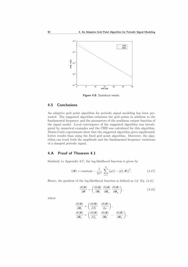
92 4. An Adaptive Grid Point Algorithm for Periodic Signal Modeling
0 5 10 15 20 25 3010
−10
10−9
10−8
10−7
10−6
SNR [dB]
CR
B ,
MS
E
CRBMSE
Figure 4.8: Statistical results.
4.5 Conclusions
An adaptive grid point algorithm for periodic signal modeling has been pre-sented. The suggested algorithm estimates the grid points in addition to thefundamental frequency and the parameters of the nonlinear output function ofthe signal model. Local convergence of the suggested algorithm was investi-gated by numerical examples and the CRB was calculated for this algorithm.Monte-Carlo experiments show that the suggested algorithm gives significantlybetter results than using the fixed grid point algorithm. Moreover, the algo-rithm can track both the amplitude and the fundamental frequency variationsof a damped periodic signal.
4.A Proof of Theorem 4.1
Similarly to Appendix 3.C, the log-likelihood function is given by
l(θ) = constant − 1
2σ2
N∑
t=1
(y(t) − y(t,θ)
)2, (4.17)
Hence, the gradient of the log-likelihood function is defined as (cf. Eq. (4.4))
∂l(θ)
∂θ=
(∂l(θ)
∂θl
∂l(θ)
∂θn
∂l(θ)
∂θg
), (4.18)
where
∂l(θ)
∂θl=
(∂l(θ)
∂X
∂l(θ)
∂ω
),
∂l(θ)
∂θn=
(∂l(θ)
∂fo
∂l(θ)
∂θ1· · · ∂l(θ)
∂θL
),

4.A. Proof of Theorem 4.1 93
∂l(θ)
∂θj=
∂l(θ)
∂f j−k−j
· · · ∂l(θ)∂f j−1
∂l(θ)
∂f j1· · · ∂l(θ)
∂f jk+
j
, (4.19)
∂l(θ)
∂θg=
(∂l(θ)
∂g1
∂l(θ)
∂g2
· · · ∂l(θ)∂gL
),
∂l(θ)
∂gj=
∂l(θ)
∂uj−k−j
· · · ∂l(θ)∂uj−1
∂l(θ)
∂uj1· · · ∂l(θ)
∂ujk+
j
.
In this case, the Fisher information matrix [99] can be written as
J = −E∂l(θ)
∂θ
T∂l(θ)
∂θ
= −E
∂l(θ)∂θl
T ∂l(θ)∂θl
∂l(θ)∂θl
T ∂l(θ)∂θn
∂l(θ)∂θl
T ∂l(θ)∂θg
∂l(θ)∂θn
T ∂l(θ)∂θl
∂l(θ)∂θn
T ∂l(θ)∂θn
∂l(θ)∂θn
T ∂l(θ)∂θg
∂l(θ)∂θg
T ∂l(θ)∂θl
∂l(θ)∂θg
T ∂l(θ)∂θn
∂l(θ)∂θg
T ∂l(θ)∂θg
. (4.20)
In order to calculate the blocks of the matrix J , the following relations areneeded
∂l(θ)
∂X=
1
σ2
N∑
t=1
(y(t) − y(t,θ)
)∂y(t,θ)∂X
,
∂l(θ)
∂ω=
1
σ2
N∑
t=1
(y(t) − y(t,θ)
)∂y(t,θ)∂ω
,
∂l(θ)
∂fo=
1
σ2
N∑
t=1
(y(t) − y(t,θ)
)∂fj(·)∂fo
,
∂l(θ)
∂f ji=
1
σ2
N∑
t=1
(y(t) − y(t,θ)
)∂fj(·)∂f ji
, (4.21)
∂l(θ)
∂f ji+1
=1
σ2
N∑
t=1
(y(t) − y(t,θ)
)∂fj(·)∂f ji+1
,
∂l(θ)
∂uji=
1
σ2
N∑
t=1
(y(t) − y(t,θ)
)∂fj(·)∂uji
,
∂l(θ)
∂uji+1
=1
σ2
N∑
t=1
(y(t) − y(t,θ)
)∂fj(·)∂uji+1
,
where
∂y(t,θ)
∂X=∂fj(·)∂u
Λ(φ) |φ=ωt,
∂y(t,θ)
∂ω=∂fj(·)∂u
XtdΛ(φ)
dφ
∣∣∣φ=ωt
,
(4.22)

94 4. An Adaptive Grid Point Algorithm for Periodic Signal Modeling
for u(t,θl) ∈[uji , u
ji+1
]∈ Ij , i = −k−j , . . . , k+
j − 1, j = 1, . . . , L. Thus usingAssumption 3.1 and Assumption 3.11, it follows that
E
[∂2l(θ)
∂X2
]= − 1
σ2
N∑
t=1
[∂fj(·)∂u
]2Λ2(φ) |φ=ωt,
E
[∂2l(θ)
∂ω2
]= − 1
σ2
N∑
t=1
[∂fj(·)∂u
]2X2t2
[dΛ(φ)
dφ
∣∣∣φ=ωt
]2,
E
[∂2l(θ)
∂f2o
]= − 1
σ2
N∑
t=1
[∂fj(·)∂fo
]2,
E
[∂2l(θ)
∂X∂ω
]= − 1
σ2
N∑
t=1
[∂fj(·)∂u
]2Xt Λ(φ)
dΛ(φ)
dφ
∣∣∣φ=ωt
,
E
[∂2l(θ)
∂X∂fo
]= − 1
σ2
N∑
t=1
∂fj(·)∂u
∂fj(·)∂fo
Λ(φ) |φ=ωt,
E
[∂2l(θ)
∂ω∂fo
]= − 1
σ2
N∑
t=1
∂fj(·)∂u
∂fj(·)∂fo
XtdΛ(φ)
dφ
∣∣∣φ=ωt
,
E
[∂2l(θ)
∂X∂f ji
]= − 1
σ2
N∑
t=1
∂fj(·)∂u
∂fj(·)∂f ji
Λ(φ) |φ=ωt,
E
[∂2l(θ)
∂X∂f ji+1
]= − 1
σ2
N∑
t=1
∂fj(·)∂u
∂fj(·)∂f ji+1
Λ(φ) |φ=ωt,
E
[∂2l(θ)
∂X∂uji
]= − 1
σ2
N∑
t=1
∂fj(·)∂u
∂fj(·)∂uji
Λ(φ) |φ=ωt,
E
[∂2l(θ)
∂X∂uji+1
]= − 1
σ2
N∑
t=1
∂fj(·)∂u
∂fj(·)∂uji+1
Λ(φ) |φ=ωt,
E
[∂2l(θ)
∂ω∂f ji
]= − 1
σ2
N∑
t=1
∂fj(·)∂u
∂fj(·)∂f ji
XtdΛ(φ)
dφ
∣∣∣φ=ωt
,
E
[∂2l(θ)
∂ω∂f ji+1
]= − 1
σ2
N∑
t=1
∂fj(·)∂u
∂fj(·)∂f ji+1
XtdΛ(φ)
dφ
∣∣∣φ=ωt
,
E
[∂2l(θ)
∂ω∂uji
]= − 1
σ2
N∑
t=1
∂fj(·)∂u
∂fj(·)∂uji
XtdΛ(φ)
dφ
∣∣∣φ=ωt
,
E
[∂2l(θ)
∂ω∂uji+1
]= − 1
σ2
N∑
t=1
∂fj(·)∂u
∂fj(·)∂uji+1
XtdΛ(φ)
dφ
∣∣∣φ=ωt
, (4.23)
E
[∂2l(θ)
∂fo∂fji
]= − 1
σ2
N∑
t=1
∂fj(·)∂fo
∂fj(·)∂f ji
,

4.A. Proof of Theorem 4.1 95
E
[∂2l(θ)
∂fo∂fji+1
]= − 1
σ2
N∑
t=1
∂fj(·)∂fo
∂fj(·)∂f ji+1
,
E
[∂2l(θ)
∂fo∂uji
]= − 1
σ2
N∑
t=1
∂fj(·)∂fo
∂fj(·)∂uji
,
E
[∂2l(θ)
∂fo∂uji+1
]= − 1
σ2
N∑
t=1
∂fj(·)∂fo
∂fj(·)∂uji+1
,
E
[∂2l(θ)
∂f ji ∂fji
]= − 1
σ2
N∑
t=1
[∂fj(·)∂f ji
]2
,
E
[∂2l(θ)
∂f ji+1∂fji+1
]= − 1
σ2
N∑
t=1
[∂fj(·)∂f ji+1
]2
,
E
[∂2l(θ)
∂f ji ∂fji+1
]= − 1
σ2
N∑
t=1
∂fj(·)∂f ji
∂fj(·)∂f ji+1
,
E
[∂2l(θ)
∂uji∂uji
]= − 1
σ2
N∑
t=1
[∂fj(·)∂uji
]2
,
E
[∂2l(θ)
∂uji+1∂uji+1
]= − 1
σ2
N∑
t=1
[∂fj(·)∂uji+1
]2
,
E
[∂2l(θ)
∂uji∂uji+1
]= − 1
σ2
N∑
t=1
∂fj(·)∂uji
∂fj(·)∂uji+1
,
E
[∂2l(θ)
∂f ji ∂uji
]= − 1
σ2
N∑
t=1
∂fj(·)∂f ji
∂fj(·)∂uji
,
E
[∂2l(θ)
∂f ji ∂uji+1
]= − 1
σ2
N∑
t=1
∂fj(·)∂f ji
∂fj(·)∂uji+1
,
E
[∂2l(θ)
∂f ji+1∂uji
]= − 1
σ2
N∑
t=1
∂fj(·)∂f ji+1
∂fj(·)∂uji
,
E
[∂2l(θ)
∂f ji+1∂uji+1
]= − 1
σ2
N∑
t=1
∂fj(·)∂f ji+1
∂fj(·)∂uji+1
.
Taking into account that ∂2l(θ)∂θm∂θn
= 0 and ∂2l(θ)∂gm∂gn
= 0 for m 6= n. Introducing
the notation in (4.11) and noticing that J = 1/σ2∑Nt=1 I(t), Eq. (4.9) directly
follows from Assumption 3.12.
Remark 4.2.∂fj(·)∂u ,
∂fj(·)∂fo
,∂fj(·)∂fj
i
,∂fj(·)∂fj
i+1
,∂fj(·)∂uj
i
and∂fj(·)∂uj
i+1
can be calculated for
different subintervals using (4.8). Thus the matrix I(t) takes the followingforms:

96 4. An Adaptive Grid Point Algorithm for Periodic Signal Modeling
(i) When u(t,θl) ∈ [uji , uji+1] ∀i =
{ −k−1 , . . . ,−2, 1, . . . , k+1 − 1, j = 1,
−k−j , . . . , k+j − 1, j = 2, . . . , L.
I(t) =
IX,X IX,ω 0 ··· 0 IX,f
ji
IX,f
ji+1
0 ··· 0 IX,u
ji
IX,u
ji+1
0 ··· 0
Iω,X Iω,ω 0 ··· 0 Iω,f
ji
Iω,f
ji+1
0 ··· 0 Iω,u
ji
Iω,u
ji+1
0 ··· 0
0 0 0 0 0 0...
......
......
...
0 0 0 0 0 0I
fji
,XI
fji
,ω0 ··· 0 I
fji
,fji
If
ji
,fji+1
0 ··· 0 If
ji
,uji
If
ji
,uji+1
0 ··· 0
If
ji+1
,XI
fji+1
,ω0 ··· 0 I
fji+1
,fji
If
ji+1
,fji+1
0 ··· 0 If
ji+1
,uji
If
ji+1
,uji+1
0 ··· 0
0 0 0 0 0 0...
......
......
...
0 0 0 0 0 0I
uji
,XI
uji
,ω0 ··· 0 I
uji
,fji
Iu
ji
,fji+1
0 ··· 0 Iu
ji
,uji
Iu
ji
,uji+1
0 ··· 0
Iu
ji+1
,XI
uji+1
,ω0 ··· 0 I
uji+1
,fji
Iu
ji+1
,fji+1
0 ··· 0 Iu
ji+1
,uji
Iu
ji+1
,uji+1
0 ··· 0
0 0 0 0 0 0...
......
......
...
0 0 0 0 0 0
,
(4.24)where
IX,X =
[f ji+1 − f ji
uji+1 − uji
]2
Λ2(φ) |φ=ωt,
Iω,ω =
[f ji+1 − f ji
uji+1 − uji
]2
X2t2[dΛ(φ)
dφ
∣∣∣φ=ωt
]2,
IX,ω =
[f ji+1 − f ji
uji+1 − uji
]2
Xt Λ(φ)dΛ(φ)
dφ
∣∣∣φ=ωt
,
IX,fji
=f ji+1 − f ji
uji+1 − uji
uji+1 − u(t,θl)
uji+1 − ujiΛ(φ) |φ=ωt,
IX,fji+1
=f ji+1 − f ji
uji+1 − uji
u(t,θl) − ujiuji+1 − uji
Λ(φ) |φ=ωt,
IX,uji
=f ji+1 − f ji
uji+1 − uji
[(f ji − f ji+1)u
ji+1
(uji+1 − uji )2
+f ji+1 − f ji
(uji+1 − uji )2u(t,θl)
]Λ(φ) |φ=ωt,
IX,uji+1
=f ji+1 − f ji
uji+1 − uji
[(f ji+1 − f ji )u
ji
(uji+1 − uji )2
− f ji+1 − f ji
(uji+1 − uji )2u(t,θl)
]Λ(φ) |φ=ωt,
Iω,fji
=f ji+1 − f ji
uji+1 − uji
uji+1 − u(t,θl)
uji+1 − ujiXt
dΛ(φ)
dφ
∣∣∣φ=ωt
,
Iω,fji+1
=f ji+1 − f ji
uji+1 − uji
u(t,θl) − ujiuji+1 − uji
XtdΛ(φ)
dφ
∣∣∣φ=ωt
,

4.A. Proof of Theorem 4.1 97
Iω,uji
=f ji+1 − f ji
uji+1 − uji
[(f ji − f ji+1)u
ji+1
(uji+1 − uji )2
+f ji+1 − f ji
(uji+1 − uji )2u(t,θl)
]Xt
dΛ(φ)
dφ
∣∣∣φ=ωt
,
Iω,uji+1
=f ji+1 − f ji
uji+1 − uji
[(f ji+1 − f ji )u
ji
(uji+1 − uji )2
− f ji+1 − f ji
(uji+1 − uji )2u(t,θl)
]Xt
dΛ(φ)
dφ
∣∣∣φ=ωt
,
Ifji ,f
ji
=
[uji+1 − u(t,θl)
uji+1 − uji
]2
, (4.25)
Ifji+1,f
ji+1
=
[u(t,θl) − ujiuji+1 − uji
]2
,
Ifji ,f
ji+1
=uji+1 − u(t,θl)
uji+1 − uji
u(t,θl) − ujiuji+1 − uji
,
Iuji ,u
ji
=
[(f ji − f ji+1)u
ji+1
(uji+1 − uji )2
+f ji+1 − f ji
(uji+1 − uji )2u(t,θl)
]2
,
Iuji+1,u
ji+1
=
[(f ji+1 − f ji )u
ji
(uji+1 − uji )2
− f ji+1 − f ji
(uji+1 − uji )2u(t,θl)
]2
,
Iuji ,u
ji+1
=
[(f ji − f ji+1)u
ji+1
(uji+1 − uji )2
+f ji+1 − f ji
(uji+1 − uji )2u(t,θl)
]×
[(f ji+1 − f ji )u
ji
(uji+1 − uji )2
− f ji+1 − f ji
(uji+1 − uji )2u(t,θl)
],
Ifji ,u
ji
=uji+1 − u(t,θl)
uji+1 − uji
[(f ji − f ji+1)u
ji+1
(uji+1 − uji )2
+f ji+1 − f ji
(uji+1 − uji )2u(t,θl)
],
Ifji ,u
ji+1
=uji+1 − u(t,θl)
uji+1 − uji
[(f ji+1 − f ji )u
ji
(uji+1 − uji )2
− f ji+1 − f ji
(uji+1 − uji )2u(t,θl)
],
Ifji+1,u
ji
=u(t,θl) − ujiuji+1 − uji
[(f ji − f ji+1)u
ji+1
(uji+1 − uji )2
+f ji+1 − f ji
(uji+1 − uji )2u(t,θl)
],
Ifji+1,u
ji+1
=u(t,θl) − ujiuji+1 − uji
[(f ji+1 − f ji )u
ji
(uji+1 − uji )2
− f ji+1 − f ji
(uji+1 − uji )2u(t,θl)
].

98 4. An Adaptive Grid Point Algorithm for Periodic Signal Modeling
(ii) When u(t,θl) ∈ [u1−1, uo− ] ⊂ I1;
I(t) =
IX,X IX,ω IX,fo 0 ··· 0 IX,f1
−10 ··· 0 I
X,u1−1
0 ··· 0
Iω,X Iω,ω Iω,fo 0 ··· 0 Iω,f1
−10 ··· 0 I
ω,u1−1
0 ··· 0
Ifo,X Ifo,w Ifo,fo 0 ··· 0 Ifo,f1
−10 ··· 0 I
fo,u1−1
0 ··· 0
0 0 0 0 0...
......
......
0 0 0 0 0I
f1−1
,XI
f1−1
,ωI
f1−1
,fo0 ··· 0 I
f1−1
,f1−1
0 ··· 0 If1−1
,u1−1
0 ··· 0
0 0 0 0 0...
......
......
0 0 0 0 0I
u1−1
,XI
u1−1
,ωI
u1−1
,fo0 ··· 0 I
u1−1
,f1−1
0 ··· 0 Iu1−1
,u1−1
0 ··· 0
0 0 0 0 0...
......
......
0 0 0 0 0
, (4.26)
where
IX,X =
[Kouo− + fo − f1
−1
uo− − u1−1
]2Λ2(φ) |φ=ωt,
Iω,ω =
[Kouo− + fo − f1
−1
uo− − u1−1
]2X2t2
[dΛ(φ)
dφ
∣∣∣φ=ωt
]2,
Ifo,fo=
[u(t,θl) − u1
−1
uo− − u1−1
]2,
IX,ω =
[Kouo− + fo − f1
−1
uo− − u1−1
]2Xt Λ(φ)
dΛ(φ)
dφ
∣∣∣φ=ωt
,
IX,fo=Kouo− + fo − f1
−1
uo− − u1−1
u(t,θl) − u1−1
uo− − u1−1
Λ(φ) |φ=ωt,
Iω,fo=Kouo− + fo − f1
−1
uo− − u1−1
u(t,θl) − u1−1
uo− − u1−1
XtdΛ(φ)
dφ
∣∣∣φ=ωt
,
IX,f1−1
=Kouo− + fo − f1
−1
uo− − u1−1
uo− − u(t,θl)
uo− − u1−1
Λ(φ) |φ=ωt,
IX,u1−1
=Kouo− + fo − f1
−1
uo− − u1−1
×[(f1
−1 −Kouo− − fo)uo−
(uo− − u1−1)
2+Kouo− + fo − f1
−1
(uo− − u1−1)
2u(t,θl)
]Λ(φ) |φ=ωt,
Iω,f1−1
=Kouo− + fo − f1
−1
uo− − u1−1
uo− − u(t,θl)
uo− − u1−1
XtdΛ(φ)
dφ
∣∣∣φ=ωt
, (4.27)
Iω,u1−1
=Kouo− + fo − f1
−1
uo− − u1−1
×[(f1
−1 −Kouo− − fo)uo−
(uo− − u1−1)
2+Kouo− + fo − f1
−1
(uo− − u1−1)
2u(t,θl)
]Xt
dΛ(φ)
dφ
∣∣∣φ=ωt
,

4.A. Proof of Theorem 4.1 99
Ifo,f1−1
=u(t,θl) − u1
−1
uo− − u1−1
uo− − u(t,θl)
uo− − u1−1
,
Ifo,u1−1
=u(t,θl) − u1
−1
uo− − u1−1
[(f1
−1 −Kouo− − fo)uo−
(uo− − u1−1)
2+Kouo− + fo − f1
−1
(uo− − u1−1)
2u(t,θl)
],
If1−1,f
1−1
=
[uo− − u(t,θl)
uo− − u1−1
]2,
Iu1−1,u
1−1
=
[(f1
−1 −Kouo− − fo)uo−
(uo− − u1−1)
2+Kouo− + fo − f1
−1
(uo− − u1−1)
2u(t,θl)
]2,
If1−1,u
1−1
=uo− − u(t,θl)
uo− − u1−1
[(f1
−1 −Kouo− − fo)uo−
(uo− − u1−1)
2+Kouo− + fo − f1
−1
(uo− − u1−1)
2u(t,θl)
].
(iii) When u(t,θl) ∈ [uo− , uo+ ] ⊂ I1;
I(t) =
IX,X IX,ω IX,fo 0 ··· 0Iω,X Iω,ω Iω,fo 0 ··· 0Ifo,X Ifo,ω Ifo,fo 0 ··· 0
0 0 0 0 ··· 0...
......
0 0 0 0 ··· 0
, (4.28)
where
IX,X = K2o Λ2(φ) |φ=ωt,
Iω,ω = K2o X
2t2[dΛ(φ)
dφ
∣∣∣φ=ωt
]2,
Ifo,fo= 1, (4.29)
IX,ω = K2o Xt Λ(φ)
dΛ(φ)
dφ
∣∣∣φ=ωt
,
IX,fo= Ko Λ(φ) |φ=ωt,
Iω,fo= Ko Xt
dΛ(φ)
dφ
∣∣∣φ=ωt
.
(iv) When u(t,θl) ∈ [uo+ , u11] ⊂ I1;
I(t) =
IX,X IX,ω IX,fo 0 ··· 0 IX,f1
10 ··· 0 I
X,u11
0 ··· 0
Iω,X Iω,ω Iω,fo 0 ··· 0 Iω,f1
10 ··· 0 I
ω,u11
0 ··· 0
Ifo,X Ifo,ω Ifo,fo 0 ··· 0 Ifo,f1
10 ··· 0 I
fo,u11
0 ··· 0
0 0 0 0 0...
......
......
0 0 0 0 0I
f11 ,X
If11 ,ω
If11 ,fo
0 ··· 0 If11 ,f1
10 ··· 0 I
f11 ,u1
10 ··· 0
0 0 0 0 0...
......
......
0 0 0 0 0I
u11,X
Iu11,ω
Iu11,fo
0 ··· 0 Iu11,f1
10 ··· 0 I
u11,u1
10 ··· 0
0 0 0 0 0...
......
......
0 0 0 0 0
, (4.30)

100 4. An Adaptive Grid Point Algorithm for Periodic Signal Modeling
where
IX,X =
[f11 −Kouo+ − fou1
1 − uo+
]2Λ2(φ) |φ=ωt,
Iω,ω =
[f11 −Kouo+ − fou1
1 − uo+
]2X2t2
[dΛ(φ)
dφ
∣∣∣φ=ωt
]2,
Ifo,fo=
[u1
1 − u(t,θl)
u11 − uo+
]2,
IX,ω =
[f11 −Kouo+ − fou1
1 − uo+
]2Xt Λ(φ)
dΛ(φ)
dφ
∣∣∣φ=ωt
,
IX,fo=f11 −Kouo+ − fou1
1 − uo+
u11 − u(t,θl)
u11 − uo+
Λ(φ) |φ=ωt,
Iω,fo=f11 −Kouo+ − fou1
1 − uo+
u11 − u(t,θl)
u11 − uo+
XtdΛ(φ)
dφ
∣∣∣φ=ωt
,
IX,f11
=f11 −Kouo+ − fou1
1 − uo+
u(t,θl) − uo+
u11 − uo+
Λ(φ) |φ=ωt, (4.31)
IX,u11
=f11 −Kouo+ − fou1
1 − uo+×
[(f1
1 −Kouo+ − fo)uo+
(u11 − uo+)2
− f11 −Kouo+ − fo(u1
1 − uo+)2u(t,θl)
]Λ(φ) |φ=ωt,
Iω,f11
=f11 −Kouo+ − fou1
1 − uo+
u(t,θl) − uo+
u11 − uo+
XtdΛ(φ)
dφ
∣∣∣φ=ωt
,
Iω,u11
=f11 −Kouo+ − fou1
1 − uo+×
[(f1
1 −Kouo+ − fo)uo+
(u11 − uo+)2
− f11 −Kouo+ − fo(u1
1 − uo+)2u(t,θl)
]Xt
dΛ(φ)
dφ
∣∣∣φ=ωt
,
Ifo,f11
=u1
1 − u(t,θl)
u11 − uo+
u(t,θl) − uo+
u11 − uo+
,
Ifo,u11
=u1
1 − u(t,θl)
u11 − uo+
[(f1
1 −Kouo+ − fo)uo+
(u11 − uo+)2
− f11 −Kouo+ − fo(u1
1 − uo+)2u(t,θl)
],
If11 ,f
11
=
[u(t,θl) − uo+
u11 − uo+
]2,
Iu11,u
11
=
[(f1
1 −Kouo+ − fo)uo+
(u11 − uo+)2
− f11 −Kouo+ − fo(u1
1 − uo+)2u(t,θl)
]2,
If11 ,u
11
=u(t,θl) − uo+
u11 − uo+
[(f1
1 −Kouo+ − fo)uo+
(u11 − uo+)2
− f11 −Kouo+ − fo(u1
1 − uo+)2u(t,θl)
].

Part II
Periodic Signal Modeling Using Orbits of
Second-Order Nonlinear ODE’s
101


Chapter 5
The Second-Order Nonlinear ODE Model
5.1 Introduction
THE work of this part of the thesis is inspired by one possible model forthe generation of periodic signals, namely nonlinear ordinary differential
equations (ODE’s). There is a rich theory on the subject as outlined in, e.g.,[62, 84, 92, 104, 105, 111, 125, 128]. The focus here will be on periodic orbitsand their properties. Some of the strongest results of the theory concern ODE’swith two state variables. The reason is that closed periodic orbits, in case theydo not intersect themselves, divide the space into one part interior to the orbitand one part exterior to the orbit. The mathematical consequence is thatthere are several powerful theorems on the existence of periodic solutions toODE’s, and hence it seems to be advantageous to base estimation algorithmson second-order ODE’s.
Many systems that generate periodic signals can be described by nonlinearODE’s. Examples include tunnel diodes, pendulums, biological predator-preysystems and radio frequency synthesizers, see [62]. Many of these systemsare described by second-order ODE’s with polynomial right hand sides. Itcan therefore be expected that there are good opportunities to obtain highlyaccurate models by estimating only a few parameters. The parsimony principle,see e.g. [99], suggests that the achievable accuracy would be improved by theproposed methods, as compared, e.g., to the periodogram and other methodsthat do not impose the same amount of prior information on the solution.
The specific signal model of this part is therefore obtained by introducinga polynomial parameterization of the right hand side of a general second-ordernonlinear ODE, and by defining the periodic signal to be modeled as a functionof the states of this ODE.
The chapter is organized as follows. Some motivation examples are givenin Section 5.2. Section 5.3 introduces the the assumptions on the modeledsignal and the measurement noise. Section 5.4 discusses different model struc-tures. Section 5.5 presents the polynomial parameterization of the ODE model.Discretization of the parameterized ODE model is introduced in Section 5.6.
103

104 5. The Second-Order Nonlinear ODE Model
λ
θ
mg
Figure 5.1: The simple pendulum.
5.2 Examples
In this section two examples for oscillating systems that can be described bysecond-order nonlinear ODE’s are given. The examples are taken from [62]with some changes.
Example 5.1. The simple pendulum.
Consider the simple pendulum shown in Fig. 5.1. The simple pendulum consistsof a mass m hanging from a string of length λ and fixed at a pivot point. Whendisplaced to an initial angle and released, the pendulum will swing back andforth with periodic motion. By applying Newton’s second law of motion, theequation of motion in the tangential direction can be written as
mλθ = −mg sin θ − ξλθ, (5.1)
where g is the acceleration due to gravity and ξ is the coefficient of friction.
Choosing the state variables as
(x1
x2
)=
(θ
θ
), (5.2)
the state equations of the simple pendulum are
x1 = x2,
x2 = − gλ
sinx1 −ξ
mx2.
(5.3)
In case of no friction, the state equations become
x1 = x2,
x2 = − gλ
sinx1.(5.4)
These two state equations were numerically solved for g = 9.81 m/s2 andλ = 1 m. The sampling period was selected as h = 0.01 s. The pendulum was

5.2. Examples 105
0 200 400 600 800 1000−2
−1.5
−1
−0.5
0
0.5
1
1.5
2
Time [samples]
θ
(a) The angle θ vs. time
−2 −1 0 1 2−5
−4
−3
−2
−1
0
1
2
3
4
5
x1
x 2
(b) θ vs. θ
Figure 5.2: Oscillations of the simple pendulum.
+
−
Element
Resistive
iLiC
C L
i
v
n
Figure 5.3: The negative resistance oscillator.
initiated at rest with a 90 degree angle with the vertical. The results are plottedin Fig. 5.2. Figure 5.2(a) shows that the angle θ is oscillating with time andFig. 5.2(b) shows that plotting x2 = θ vs. x1 = θ represents a periodic orbit.
Example 5.2. The negative resistance oscillator.
The negative resistance oscillator of Fig. (5.3) consists of an inductor L, acapacitor C and a resistive element. The resistive element has the following i-vcharacteristic:
i = h(v), (5.5)

106 5. The Second-Order Nonlinear ODE Model
0 500 1000 1500 2000−2.5
−2
−1.5
−1
−0.5
0
0.5
1
1.5
2
2.5
Time [samples]
v
(a) The voltage v vs. time
−3 −2 −1 0 1 2 3−3
−2
−1
0
1
2
3
x1
x 2
(b) v vs. v
Figure 5.4: Oscillations of the negative resistance oscillator.
where h(·) satisfies the following conditions:
h(0) = 0,dh(·)dv
∣∣∣v=0
< 0,
h(v) → ∞ as v → ∞,
h(v) → −∞ as v → −∞.
Applying Kirchhoff’s current law at node n
iC + iL + i = 0. (5.6)
Substituting by Eq. (5.5) and expressing the currents iC and iL as a functionof the voltage v, Eq. (5.6) becomes
Cdv
dt+
1
L
∫ t
−∞v(t)dt+ h(v) = 0. (5.7)
Differentiating Eq. (5.7) with respect to time t and multiplying the result byL, results in
CLd2v
dt2+ v + L
dh(v)
dt= 0. (5.8)
Now, changing the time variable from t to τ = t√CL
transforms Eq. (5.8) to
v + εdh(v)
dvv + v = 0, (5.9)
where v and v denote the first and second derivatives with respect to τ , respec-tively, and ε =
√L/C.
Choosing the state variables as(x1
x2
)=
(vv
), (5.10)

5.3. Modeled Signal and Measurements 107
the state equations representing the negative resistance oscillator become
x1 = x2,
x2 = −x1 − εdh(x1)
dx1x2.
(5.11)
These two state equations were numerically solved for h(x1) = −x1 + 13x
31 (the
Van der Pol oscillator) and ε = 1. The results are given in Fig. (5.4).
The previous two examples show some practical oscillating systems thatcan be described by second-order nonlinear ODE’s. In case it is required tomodel the oscillations generated by these systems, a second-order nonlinearODE model is a good match. Hence, an estimation technique for modelingor identifying the right hand sides of Eq. (5.4) and Eq. (5.11) is needed. Inthis case, the accuracy of the obtained ODE model is expected to exceed theaccuracy of other models that do not make use of such priors. In the restof this chapter, the second-order ODE model suggested for modeling periodicsignals as being an oscillations such as the ones given in Fig. 5.2 and Fig. 5.4is described.
5.3 Modeled Signal and Measurements
The starting point is the discrete time measured signal z(kh), where
z(kh) = y(kh) + e(kh), k = 1, · · · , N. (5.12)
Here
• y(t) is the continuous time signal to be modeled;
• h is the sampling interval;
• y(kh) is the sampled value of y(t);
• e(kh) is the discrete time measurement noise.
It is assumed that y(t) is periodic, i.e.
Assumption 5.1. y(t+ T ) = y(t), ∀t ∈ R, 0 < T < ∞, where T denotes theperiod.
Furthermore, e(kh) is assumed to be zero-mean Gaussian white noise, i.e.
Assumption 5.2. e(kh) ∈ N (0, σ2), E[e(kh)e(kh+ jh)
]= δj,0σ
2.
5.4 Model Structures
As stated above, the main idea of the work in Part II of this thesis is to modelthe generation of the signal y(t) by means of an unknown parameter vector θ

108 5. The Second-Order Nonlinear ODE Model
and a nonlinear ODE, i.e.
x = f(x,θ
),
y = h(x).(5.13)
Considering the use of second-order ODE’s, Eq. (5.13) is modified to
(x1
x2
)=
(f1(x1(t), x2(t),θ1
)
f2(x1(t), x2(t),θ2
)),
y(t) =(c1 c2
)( x1(t)x2(t)
).
(5.14)
Hereθ =
(θT1 θT2
)T, (5.15)
where the vectors θ1 and θ2 are unknown parameter vectors and(c1 c2
)
contains the selected output weighting factors.
At this point it is highly relevant to pose the question whether the model(5.14) may be too general. In [122, 123], it is proved that it can often beassumed that the second order ODE
y(t) = f(y(t), y(t),θ
), (5.16)
generates the periodic signal that is measured provided that the following con-dition holds:
Assumption 5.3. The phase plane plot that is constructed from the periodicsignal y(t) and its first derivative y(t) lacks any intersections or limiting casessuch as corners, stops and cusps.
Remark 5.1. Assumption 5.3 is needed to exclude signal classes that haveintersected phase plane plots since these classes need higher order ODE’s to bemodeled accurately, see Chapter 6 and [122, 123] for more details.
Thus choosing the state variables as follows
(x1
x2
)=
(y(t)y(t)
), (5.17)
the model given in (5.14) is reduced to
(x1
x2
)=
(x2(t)
f(x1(t), x2(t),θ
)),
y(t) =(
1 0)( x1(t)
x2(t)
).
(5.18)
This model depends only on the parameters of the right hand side function ofthe second state equation of (5.18), a fact that should be advantageous from acomputational and performance point of view. The obvious question is then -are there other facts that could motivate the use of (5.14) instead of (5.18)?

5.5. Parameterization 109
One key to the answer of this question is the output equations of (5.14) and(5.18). Physically, it may very well be the case that the system is governedby (5.16), but the generated periodic signal may be a nonlinear function of yand y. It could also be the case that this function is not well known and/ornoninvertible, and the question is then what can be done in such situations?One idea would be to reuse the output relation of (5.18) and try to find arepresentation of the state space ODE such that the first state equals thesought output. In order to study the implications of this idea, the followingsystem is studied
y(t) = f(y(t), y(t),θ
), (5.19)
z = g(y(t), y(t)
). (5.20)
With the states chosen as(x1
x2
)=
(zy(t)
), (5.21)
it follows by differentiation that
x1 =∂g(y, x2)
∂yx2 +
∂g(y, x2)
∂x2f(y(t), x2,θ
), (5.22)
x2 = f(y(t), x2,θ
). (5.23)
It remains to find an expression for y as a function of x1 and x2. This followsfrom Eqs. (5.19)-(5.21), since under mild regularity conditions [62] the inversefunction theorem allows at least a local solution of the output equation withrespect to y, i.e.
x1 = g(y, x2) ⇒ y = h(x1, x2). (5.24)
When (5.24) is inserted in (5.22) and (5.23), it is clear that the result fits intothe structure (5.14), with the weight of the output equation being equal tothose of (5.18). The conclusion is that the model structure (5.14) may extendthe validity of the proposed periodic signal modeling approach, beyond that of(5.18). Despite this fact, the study in this thesis will concentrate on the modelstructure (5.18) since the analysis of Chapter 6 proves that (5.18) is sufficientto model periodic signals that satisfy Assumption 5.3.
5.5 Parameterization
A natural approach is now to expand the right hand side of the second stateequation of (5.18) in terms of known basis functions
{bk(x1(t), x2(t)
)}∞k=0
,modeling the right hand side as a truncated superposition of these functions.In case of a polynomial model, a suitable parameterization is
f(x1(t), x2(t),θ
)=
L∑
l=0
M∑
m=0
θl,mxl1(t)x
m2 (t), (5.25)
θ =(θ0,0 · · · θ0,M · · · θL,0 · · · θL,M
)T. (5.26)

110 5. The Second-Order Nonlinear ODE Model
Remark 5.2. No scale factor problems are expected with this parameteriza-tion. The reason is that the transformation
y = ky, (5.27)
transforms (5.16) to
¨y(t) = kf(1
ky(t),
1
k˙y(t),θ
). (5.28)
Since the polynomial model is a general function expansion, the function of(5.28) can be modeled equally well as the function of (5.16).
5.6 Discretization
In order to formulate complete discrete time models, the continuous time ODEmodel (5.18) needs to be discretized. This can be done, for example, by exploit-ing Euler numerical integration schemes. The discretization interval is selectedto be equal to the sampling period h. The numerical integration schemes con-sidered in this thesis and its corresponding discrete models are:
• Euler backward approximation (EB):
x1(kh) = x1(kh− h) + hx2(kh), (5.29)
x2(kh) = x2(kh− h) + h
L∑
l=0
M∑
m=0
θl,mxl1(kh)x
m2 (kh). (5.30)
• Euler forward approximation (EF):
x1(kh+ h) = x1(kh) + hx2(kh), (5.31)
x2(kh+ h) = x2(kh) + h
L∑
l=0
M∑
m=0
θl,mxl1(kh)x
m2 (kh). (5.32)
• Euler center approximation (EC):
x1(kh+ h) = x1(kh− h) + 2hx2(kh), (5.33)
x2(kh+ h) = x2(kh− h) + 2h
L∑
l=0
M∑
m=0
θl,mxl1(kh)x
m2 (kh). (5.34)
Remark 5.3. For simplicity the discretization interval is selected to be equalto the sampling interval h. Otherwise, it would be a multiple of h.
Remark 5.4. Using (5.30), in which x2(kh) = g(x1(kh), x2(kh)
), does not
lead to any numerical problems since (5.30) will not be solved for x2(kh). Aswill be shown in Chapter 7, x1(kh) and x2(kh) will be replaced by quantitiesevaluated from the measured data.
Now the discretized model can be used to implement different off-line andon-line algorithms to estimate the parameter vector θ. This is the main themeof Chapters 7-12. In the next chapter, the sufficiency of the second-order ODEmodel described by Eq. (5.18) to model many periodic signals is studied.

Chapter 6
Sufficiency of Second-Order Nonlinear ODE forModeling Periodic Signals
6.1 Introduction
IN the previous chapter the second-order nonlinear ODE model described by(5.18) was suggested to model periodic signals. A natural questions that
follow directly: “When it is sufficient to use second-order ODE model?” or“What types of periodic signals can be modeled by (5.18)?”. These questionswere addressed in [122, 123] and detailed answers were provided. In this chaptera brief review of the main results of [122, 123] is given.
It is stressed that the contents of this chapter is not a contribution of theauthor. It is included to provide the reader with a complete picture of theproblem treated in Part II of the thesis.
The work done in [122, 123] proceeds as follows. First, some assumptionsof general validity on the modeled signal and its derivatives are given. Thensmoothness conditions are introduced to guarantee that the phasor constructedfrom the periodic signal y(t) and its first derivative y(t), where t denotes con-tinuous time, i.e
y(t) =
(y(t)y(t)
)∈ R2, (6.1)
represents a periodic orbit without any intersections. It is then proved thatthere exists an ODE that has the given signal as one solution. The providedconditions are emphasized by a phase plane geometrical intuition. Finally, theuniqueness of the solution of the ODE model is treated.
The chapter is organized as follows. General assumptions on the periodicsignal are introduced in Section 6.2. Section 6.3 presents the smoothness con-ditions necessary to guarantee that the periodic orbit does not contain anyintersections. In Section 6.4, necessary conditions on y(t) to be a solutionof the second-order ODE model are given. Uniqueness of the solution of thesecond-order ODE model is addressed in Section 6.5. Section 6.6 discusses theissue of insufficiency of the second-order ODE model. Finally, conclusions aregiven in Section 6.7.
111

112 6. Sufficiency of Second-Order Nonlinear ODE for Modeling Periodic Signals
−2 −1.5 −1 −0.5 0 0.5 1 1.5−3
−2
−1
0
1
2
3
y
dy/d
t
. PI
Figure 6.1: A periodic orbit with an intersection at PI .
6.2 General Assumptions on the Modeled signal
The work of [122, 123] begins by assuming some conditions on the modeledsignal that can be satisfied for many signals. It is assumed that the periodicsignal y(t) fulfills Assumption 5.1 and the following assumptions:
Assumption 6.1. The signal y(t) is not corrupted by any disturbance.
Assumption 6.2. The signal y(t) is twice continuously differentiable.
It follows from Assumption 6.2 that y(t + T ) = y(t), ∀t ∈ R, where Tdenotes the period. Hence, the signal y(t) can be represented as the firstcoordinate of the closed curve generated by y(t).
6.3 Smoothness of the Modeled Orbit
As mentioned in the introduction of this chapter, the objective is to constructan autonomous second-order ODE system such that y(t) is a solution of thisODE system. Hence, the selected state vector of the ODE model must containsall necessary informations to construct the closed orbit representing the signaly(t). This means that the generated closed orbit by y(t) should not containany intersections such as the intersection at point PI in Fig. 6.1. In such cases,the evolution of the orbit after the point PI will depend on the evolution beforePI . Then, the further evolution of y(t) can not be determined uniquely fromone single point in R2.
A condition that excludes situations where periodic orbit y(t) intersectsitself is given in [122, 123] as follows:
Assumption 6.3. For all y(t) ∈ S ⊂ R2:
•(y(t1)y(t1)
)=
(y(t2)y(t2)
)⇒ t1 = t2 + kT, k ∈ Z
6.4. Conditions on y(t) to Be a Solution 113
where Z denotes the set of all integers.
• ∃ δ, L1, L2, δ > 0, 0 < L1 ≤ L2 <∞ such that
|t1 − t2| < δ ⇒ L1|t1 − t2| ≤∣∣∣∣
∣∣∣∣
(y(t1)y(t1)
)−(y(t2)y(t2)
)∣∣∣∣
∣∣∣∣ ≤ L2|t1 − t2|.
The smoothness Assumption 6.3 ensures the exclusion of signals that con-struct intersected phase planes and any other degenerate cases such as cusps,corners and stops. This was given in implicit way in Assumption 5.3. Also, thefollowing lemma was proved in [122, 123].
Lemma 6.1. Under Assumptions 6.2-6.3, the curve y(t) ∈ R2 is smooth and
without self-intersections. Further, the speed√yT (t)y(t) of the curve y(t) is
strictly positive for all t and satisfy the following relation
0 < L1 ≤√yT (t)y(t) ≤ L2 <∞.
Proof. See [122, 123].
Since the speed of the curve y(t) is proved to be positive and finite inLemma 6.1, it follows that the velocity vector y(t) which is tangent to y(t)varies smoothly and no jump phenomena can take place.
6.4 Conditions on y(t) to Be a Solution
The next step is to find the conditions necessary for y(t) to be a solution forthe second-order ODE model. Selecting the state vector to be
(x1
x2
)=
(y(t)y(t)
), (6.4)
and differentiating (6.4) with respect to time t, cf. Assumption 6.2, gives(x1
x2
)=
(x2
y(t)
). (6.5)
This equation represents the second-order nonlinear ODE system suggested tomodel the periodic signal. This system is autonomous only if the second righthand side function y(t) can be expressed in terms of the states x1 and x2. Thiscan be done by solving (6.4) w.r.t. the time t. The implicit function theorem,see [62] page 651, is useful in this case. The theorem is stated as follows.
Theorem 6.1. Assume that f : Rn ×Rm → Rn is continuously differentiableat each point (x, z) of an open set P ⊂ Rn ×Rm. Let (x0, z0) be a point in Pfor which f(x0, z0) = 0 and for which the Jacobian matrix [∂f/∂x](x0, z0) isnonsingular. Then there exist neighborhoods U ⊂ Rn of x0 and V ⊂ Rm of z0such that for each z ∈ V the equation f(x, z) = 0 has a unique solution x ∈ U .Moreover, this solution can be given as x = g(z), where g is continuouslydifferentiable at z = z0.

114 6. Sufficiency of Second-Order Nonlinear ODE for Modeling Periodic Signals
−1.5 −1 −0.5 0 0.5 1 1.5−2.5
−2
−1.5
−1
−0.5
0
0.5
1
1.5
2
2.5
x1
x 2
o x x x x x x x
+
Figure 6.2: Solving for the time in the phase plane plot. The point marked by ‘o’corresponds to the point where solution is performed while points marked by ‘x’ and ‘+’corresponds to alternative points with same x2,0 and x1,0, respectively.
Proof. See [2, 63].
Now consider a closed orbit like the one shown in Fig. 6.2 and a point
x0 =(x1,0 x2,0
)Ton this orbit (marked by ‘o’). The intention now is to solve
at x0 to find t as a function in x1,0 and/or x2,0. The state equation (6.4) canbe written in the form
(f1(x1, t)f2(x2, t)
)=
(x1 − y(t)x2 − y(t)
)=
(00
). (6.6)
Solving the first equation of (6.6) in the point x0 gives the times t1,i,i = 1, · · · , I (marked by ‘+’ in Fig. 6.2). Similarly, solving the second equationof (6.6) in the same point gives the times t2,j , j = 1, · · · , J (marked by ‘x’ inFig. 6.2). Furthermore, differentiating (6.6) with respect to time t, it followsthat (cf. Assumption 6.2 and Lemma 6.1)
∂f1(x1,0, t1,i)
∂t= −y(t1,i) 6= 0, (6.7)
∂f2(x2,0, t2,j)
∂t= −y(t2,j) 6= 0. (6.8)
Therefore, it can be concluded that for all t1,i and t2,j that fulfill (6.7) and (6.8),respectively, there are continuously differentiable functions h1,i, i = 1, · · · , Iand h2,j , j = 1, · · · , J such that
t = h1,i(x1), t ∈ U1,i, x1 ∈ V1,i, i = 1, · · · , I (6.9)
t = h2,j(x2), t ∈ U2,j , x2 ∈ V2,j , j = 1, · · · , J (6.10)
where U1,i, V1,i, U2,j , V2,j are the corresponding neighborhoods of t1,i, x1,0,t2,j , x2,0, respectively. Since any intersection possibility in the periodic orbit

6.4. Conditions on y(t) to Be a Solution 115
was excluded by Assumption 6.3, there is only one i = i1 and one j = j1 suchthat t1,i1 = t2,j1 within the same period.
Remark 6.1. Note that by Lemma 6.1√y2(t) + y2(t) ≥ L1 > 0. Hence
Eq. (6.7) and/or Eq. (6.8) always holds. In this case, the valid equation(s) canbe used to solve for t.
The analysis done in [122, 123] proceeds by selecting a number of points{(x1,k x2,k
)T}Kk=1
∈ S, ordered clockwise or counterclockwise around the
curve y(t), such that the resulting overlapped neighborhoods covers one com-plete period. Then the times {tk}Kk=1 corresponding to these points are com-puted. This procedure was formulated in [122, 123] by the following assump-tions:
Assumption 6.4. Ik ≤ I < ∞, Jk ≤ J < ∞, ∀(x1,k x2,k
)T ∈ S,k = 1, · · · ,K.
Assumption 6.5. Uρ(k),k ∩ Uρ(k+1),k+1 6= ∅, k = 1, · · · ,K − 1 and
Uρ(K),K ∩(Uρ(1),1 + T
)6= ∅.
Assumption 6.6.⋃Kk=1 Uρ(k),k ⊃ [t, t+ T ] for an appropriately selected t.
Here the quantities Ik and Jk corresponds to quantities I and J for x0.
Also,{Uρ(k),k
}Kk=1
and{Vρ(k),k
}Kk=1
are the neighbourhoods around the points{(x1,k x2,k
)T}Kk=1
, where
ρ(k) =
{1 if Eq. (6.7) is used
2 if Eq. (6.8) is used.
Hence, it is concluded in [122, 123] from Assumptions 6.4-6.6 that there existsneighborhoods Uρ(k),k ⊂ Uρ(k),k and Vρ(k),k ⊂ Vρ(k),k such that
Uρ(k),k ∩ Uρ(k+1),k+1 = ∅, k = 1, · · · ,K − 1 (6.11)
Uρ(K),K ∩(Uρ(1),1 + T
)= ∅, (6.12)
K⋃
k=1
Uρ(k),k = [t, t+ T ], (6.13)
hperiod(x1, x2) , t =
{hk1,i1(k)(x1), x1 ∈ V1,k, ρ(k) = 1
hk2,j1(k)(x2), x2 ∈ V2,k, ρ(k) = 2.(6.14)
Remark 6.2. The object of defining the neighborhoods Uρ(k),k and Vρ(k),k isto remove the overlapping region between the underlying neighborhoods. Thisis because the solution around the underlying points must be the same in theoverlapping region.
Now substituting by expression (6.14) in Eq. (6.5) leads in [122, 123] to thefollowing theorem:

116 6. Sufficiency of Second-Order Nonlinear ODE for Modeling Periodic Signals
Theorem 6.2. Consider the periodic signal y(t). Under Assumption 5.1 andAssumptions 6.1-6.6, there exists a function hperiod(x1, x2) and a second-orderordinary differential equation
(x1
x2
)=
(x2
y(hperiod(x1, x2)
)), (6.15)
that has a solution given by(x1 x2
)T=(y(t) y(t)
)T.
6.5 Uniqueness of the Solution
The solution provided by Theorem 6.2 may not be unique. Uniqueness ofthe solution follows in case hperiod(x1, x2) is Lipschitz, cf. Section 1.5.3. Thefollowing two corollaries were concluded in [122, 123] from [62]:
Corollary 6.3. Assume that the conditions of Theorem 6.2 hold. Assume inaddition that there are constants L3 and L4 such that
∣∣∣y(hperiod(x1, x2)
)− y(hperiod(z1, z2)
)∣∣∣ ≤ L3
∣∣∣∣
∣∣∣∣
(x1
x2
)−(z1z2
)∣∣∣∣
∣∣∣∣ ,∣∣∣y(hperiod(x0
1, x02))∣∣∣ ≤ L4,
(6.16)
∀(x1 x2)T , (z1 z2)
T ∈ R2 and ∀t ∈ [t0, t1]. Then there is a second-orderODE
(x1
x2
)=
(x2
y(hperiod(x1, x2)
)),
(x1(t0)x2(t0)
)=
(x0
1
x02
)∈ S,
that has the unique solution(x1 x2
)T=(y(t) y(t)
)T, t ∈ [t0, t1].
Corollary 6.4. Assume that the conditions of Theorem 6.2 hold. Assume inaddition that there is a constant L5 such that
∣∣∣y(hperiod(x1, x2)
)− y(hperiod(z1, z2)
)∣∣∣ ≤ L5
∣∣∣∣
∣∣∣∣
(x1
x2
)−(z1z2
)∣∣∣∣
∣∣∣∣ ,
∀(x1 x2)T , (z1 z2)
T ∈ D ⊂ R2 and ∀t ≥ t0. Let W be a compact subsetof the domain D, (x0
1 x02)T ∈ W , and suppose that it is known that every
solution of
(x1
x2
)=
(x2
y(hperiod(x1, x2)
)),
(x1(t0)x2(t0)
)=
(x0
1
x02
)∈ S,
(which exists) lies entirely in W . Then this second-order ODE has the unique
solution(x1 x2
)T=(y(t) y(t)
)T, t ∈ [t0, t1].

6.6. When a Second-Order ODE Model Is Insufficient 117
6.6 When a Second-Order ODE Model Is Insufficient
From the previous discussion, it can be noticed that higher order ODE modelsare needed in case the periodic orbit intersect itself in R2. The work of [122,123] suggested to increase the order of the ODE in steps (one order more in eachstep). In this case, the extra state is selected as the next higher derivative ofthe periodic signal. For example, in case of extension from second-order ODE,the state variable x3 = y(t) is added. If the phase plot in R3 still containsintersections, a fourth state x4 = d3y(t)/dt3 is added and this procedure isrepeated until all intersections disappear.
The analysis done in Section 6.3 and Section 6.4 was repeated for the generalorder case in [122, 123] and the following theorem was proved.
Theorem 6.5. Consider a periodic signal y(t). Under Assumption 5.1, As-sumption 6.2, Assumptions 6.5-6.6 and the following assumptions:
Assumption 6.7. The signal y(t) is n+ 1 times continuously differentiable.
Assumption 6.8. For all
y...
y(n)
∈ Sn+1 ⊂ Rn+1:
•
y(t1)...
y(n)(t1)
=
y(t2)...
y(n)(t2)
⇒ t1 = t2 + kT, k ∈ Z.
• ∃ δ, L1, L2, δ > 0, 0 < L1 ≤ L2 <∞ such that
|t1−t2| < δ ⇒ L1|t1−t2| ≤
∣∣∣∣∣∣∣
∣∣∣∣∣∣∣
y(t1)...
y(n)(t1)
−
y(t2)...
y(n)(t2)
∣∣∣∣∣∣∣
∣∣∣∣∣∣∣≤ L2|t1−t2|.
Assumption 6.9. Im,k ≤ I < ∞, ∀(x1,k · · · xn+1,k
)T ∈ Sn+1,m = 1, · · · , n+ 1, k = 1, · · · ,K.
there exists a function hperiod(x1, · · · , xn+1) and an n+ 1 : th order ODE
x1
x2
...xnxn+1
=
x2
x3
...xn+1
x(n)(hperiod(x1, · · · , xn+1)
)
,
that has a solution given by(x1 · · ·xn+1
)T=(y(t) · · · y(n)(t)
)T.
Proof. See [122, 123].

118 6. Sufficiency of Second-Order Nonlinear ODE for Modeling Periodic Signals
6.7 Conclusions
The main results of the work done in [122, 123] have been introduced in thischapter. The results show that the approach of modeling periodic signals usingsecond-order nonlinear ODE model is sufficient to model many periodic signalsprovided that the phase plot generated from the modeled signal and its firstderivative does not contain any intersections. In case that the mentioned phaseplot contains any intersections, a higher order ODE model is necessary toaccurately model the periodic signal. The new ODE model is constructed byadding extra states to the original state vector. The extra states are chosen tobe equal to the higher order derivatives of the modeled signal.
Chapter 7
Least Squares and Markov Estimation of PeriodicSignals
7.1 Introduction
THE linear regression model is a very common concept in statistics. It isthe simplest type of parametric models. The linear regression model can
be written asY(t) = φT (t) θ, (7.1)
where Y(t) is a measurable quantity, φ(t) is an n-vector of known quantitiesand θ is an n-vector of unknown parameters to be estimated. The elementsof the vector φ(t) are often called regressors while Y(t) is called the regressedvariable.
Introducing the equation errors as
ε(t) = Y(t) − φT (t) θ, (7.2)
the least squares (LS) estimate of the unknown vector θ (often called the pa-
rameter vector) is defined as the vector θLS
N that minimize the loss function
V (θ) =1
2
N∑
t=1
ε2(t), (7.3)
where N is the number of available measurements. The LS estimate θLS
N isgiven by (see [99])
θLS
N =
[ N∑
t=1
φ(t)φT (t)
]−1[ N∑
t=1
φ(t)Y(t)
]. (7.4)
This estimate is expected to be consistent (unbiased) provided that the equa-tion errors, ε(t), are zero-mean white.
In this chapter, an LS estimation algorithm is developed for the problemof modeling periodic signals using second-order nonlinear ODE’s. As will beshown, the developed LS algorithm gives biased estimates, especially at low sig-nal to noise ratios (SNRs). One of the reasons that contribute to this bias is theinvalidity of the whiteness assumption on the equation errors ε(t). Therefore,
119

120 7. Least Squares and Markov Estimation of Periodic Signals
a Markov estimation algorithm is introduced to compensate for this bias byusing an estimate for the covariance matrix of the residuals. The performanceof the two algorithms are illustrated in a simulation study.
The chapter is organized as follows. Section 7.2 discusses the LS estimationalgorithm. The Markov estimation algorithm is introduced in Section 7.3.Section 7.4 presents a simulation study for the LS and the Markov estimationalgorithms. Conclusions appear in Section 7.5.
7.2 The Least Squares Algorithm
A number of different algorithms can now be derived from the second-orderODE model of Chapter 5. In order to formulate the model in a linear regressionform, two approximations are needed, cf. Eq. (5.17).
1. As x1 = y(t) is not known, use the estimate
x1(kh) = z(kh). (7.5)
2. As x2 = y(t) is not known, use the estimate
x2(kh) = z(kh) =z(kh) − z(kh− h)
h. (7.6)
Remark 7.1. More general differentiating filters than (7.6) can be used. Rea-sonable differentiating filters are of the form
H(q) =(1 − q−1)
hH(q), (7.7)
with H a low pass filter (q−1z(kh) = z(kh − h)) of unity static gain. In thiscase (7.6) is replaced by
xd(kh+ h) = K xd(kh) +L z(kh),
x2(kh) = M xd(kh) + d z(kh).(7.8)
Note that the filter output in (7.8) is only an estimate of x2(kh) since it is con-structed from a measured signal. See [25] for more details about differentiatingfilters. In particular, the choice K = 0, L = 1/h, M = −1/h, d = 1/h givesthe estimate (7.6).
Remark 7.2. In the following, for notational convenience the dependence onh is omitted assuming h equals one unit time. This means that an integer kcan be used as time variable.
To proceed, note that Eqs. (5.29)-(5.30) result in the model
x1(k) − x1(k − 1) = x2(k), (7.9)
x2(k) − x2(k − 1) = φT(x1(k), x2(k)
)θ, (7.10)

7.2. The Least Squares Algorithm 121
where
φT(x1(k), x2(k)
)=(
1 · · · xM2 (k) · · · xL1 (k) · · · xL1 (k)xM2 (k)), (7.11)
θ =(θ0,0 · · · θ0,M · · · θL,0 · · · θL,M
)T. (7.12)
By replacing the states of Eqs. (7.9)-(7.10) with the estimates given in (7.5)and (7.6), the second state equation (7.10) results in
x2(k) = x2(k) − x2(k − 1)
= φT(x1(k), x2(k)
)θ + ε(k).
(7.13)
The first state equation (7.9) is not needed. The expression (7.13) fol-lows by performing a Taylor series expansion of φT
(x1(k), x2(k)
)around
(x1(k) x2(k)
)T. In (7.13) the combined regression error, ε(k), has been intro-
duced. It can not be expected to be white since the Taylor series expansion in(7.13) produces a sum of noise samples that are delayed with a varying numberof sampling periods. This means that the least squares estimator will, in theend, be biased. However, for relatively high signal to noise ratios the accuracycould still be good. Note that (7.13) is a linear regression with the parametervector θ as unknown.
Assuming that data are available at times k − N, · · · , k and defining thevectors and matrices
ZN =( x2(k) · · · x2(k −N + 1)
)T, (7.14)
ΦN =
φT(x1(k), x2(k)
)
...
φT(x1(k −N + 1), x2(k −N + 1)
)
, (7.15)
εN =(ε(k) · · · ε(k −N + 1)
)T, (7.16)
the following regression equation results
ZN = ΦN θ + εN . (7.17)
Hence the LS estimate θLS
N is given by (see [99])
θLS
N =(ΦTNΦN
)−1ΦTN ZN . (7.18)
Note that it is not numerically sound to solve the least squares problem di-rectly using the normal equations that appear implicitly in (7.18). Instead aformulation as an over-determined system of equations should be used, see [99]for more details.
Remark 7.3. The LS estimate in (7.18) is expected to give considerably accu-rate models at high signal to noise ratios (SNRs) and further research is neededto extend the operating region toward low SNRs. Realizing that Eq. (7.17) is

122 7. Least Squares and Markov Estimation of Periodic Signals
an error-in-variables (EIV) problem since both ZN and the columns of ΦN hasnoise contributions, the possibility of using the total least squares (TLS), see[107, 108], has been studied. The idea was to calculate the standard deviationof the noise disturbance on each column of the data matrix [ZN ΦN ] and todesign a weighting matrixG to have similar noise contributions on the columnsof the data matrix. In this case, Eq. (7.17) becomes
ZN ≈ (ΦN G) θ, (7.19)
where θ is a weighted parameter vector and the estimate of the true parametervector follows as
θ = G θTLS
. (7.20)
Using the weighted TLS did not lead to improvements compared to the LSestimate at moderate SNR. Hence, it is relevant to neglect noise effects and usethe LS type of solution.
7.3 The Markov Estimate
The least squares estimate θLS
N given in (7.18) is expected to be approximatelyunbiased in case the regression error vector εN is white, i.e. its covariancematrix has the form σ2I. This is not the case here due to the Taylor seriesexpansion of (7.13). If the covariance matrix
RN = E[εN εTN
](7.21)
is known, the Markov estimate, also known as the BLUE (best linear unbiasedestimate) will satisfy [99]
θMarkov
N =(ΦTN R−1
N ΦN
)−1
ΦTN R−1
N ZN . (7.22)
This estimator rests on the assumption that the mean of the noise is zero andthat the system is in the model set. The above is not exactly true here, but theestimator can of course be applied anyway. Note that stationarity is assumedin the computation of RN in order to avoid a dependence on k.
Using Eqs. (5.12), (7.5)-(7.6), the left hand side of Eq. (7.13) can be writtenas
x2(k) = x2(k) − x2(k − 1)
= z(k) − 2z(k − 1) + z(k − 2)
= y(k) − 2y(k − 1) + y(k − 2) + e(k) − 2e(k − 1) + e(k − 2)
= y(k) − y(k − 1) + e(k) − e(k − 1). (7.23)
Hence Eq. (7.13) becomes
y(k) − y(k − 1) + e(k) − e(k − 1) = φT(x1(k), x2(k)
)θ + ε(k). (7.24)
In the following, it will be shown how an approximate value of RN can becomputed under the following assumption:

7.3. The Markov Estimate 123
Assumption 7.1. The contributions to ε(k) from the regressor vectorφT(x1(k), x2(k)
)do not dominate over the noise that enter linearly in (7.24),
i.e. the equation error ε(k) fulfills
ε(k) ≈ e(k) − e(k − 1),
where e(k) is the white noise in Eq. (5.12).
The idea is then to neglect the regressor vector contribution and only use theparts of the noise that enter linearly. Therefore based on Assumption 7.1,(7.16) becomes
εN =
e(k) − e(k − 1)...
e(k −N + 1) − e(k −N)
. (7.25)
Now, an extended state space model can be constructed for the regressionerror vector εN using the differentiating filter (7.8) and time delays. Considerthe following state vector
X(k) =(XT
1 (k) XT2 (k)
)T, (7.26)
whereX1(k) = xd(k), (7.27)
X2(k) =( e(k − 1) · · · e(k −N)
)T. (7.28)
Then, under Assumption 7.1, the matrix RN can be computed from the fol-lowing asymptotically stable stochastic discrete time system
X(k + 1) = A X(k) +B e(k),
εN (k) = D X(k) +E e(k).(7.29)
Remark 7.4. The system (7.29) is intended to model the correlation propertiesof the noise that appears in the computation of the matrixRN . For this reason,the superposition principle is used to subtract the signal from the input to thedifferentiator filter so that only the noise remains as an input. Note thatthe dynamics of the system (7.29) need to account for the dynamics of thedifferentiating filter, and the delays of the states needed in order to generatethe vector εN given by (7.25).
Let nd denote the order of the differentiating filter (7.8). Then, the blockmatrices of (7.29) are given by
A =
(K 0nd×ND1 SN
), (7.30)
B =
L
d0(N−1)×1
, (7.31)

124 7. Least Squares and Markov Estimation of Periodic Signals
D =(D1 D2
), (7.32)
E =
(d
0(N−1)×1
), (7.33)
where 0i×j denotes an empty matrix of i rows and j columns. Also, the N ×Ndimensional shift-matrix
SN =
0 · · · 01 0
0 1 0...
.... . .
. . .. . .
0 · · · 0 1 0
, (7.34)
generates (N − 1) delayed states. The N × (N +nd) matrix D is built up fromthe blocks
D1 =
(M
0(N−1)×nd
), (7.35)
D2 =
−1 0 0 · · · 0 01 −1 0 · · · 0 00 1 −1 · · · 0 0...
. . .. . .
......
0 0 0 · · · 1 −1
. (7.36)
It is now straightforward to compute RN . First the stationary state covariancematrix of (7.29), i.e.
PN = E[X(k)XT (k)
](7.37)
is computed as the unique positive definite symmetric solution of the stationaryLyapunov equation (see e.g. [55])
PN = A PN AT + σ2 B BT . (7.38)
Then, from (7.29)RN ≈D PN DT + σ2 E ET . (7.39)
Remark 7.5. In case the residual covariance matrix RN is singular or ill-conditioned, the matrix RN + ΦNΦT
N may be better conditioned to inversionthan RN . The following (theoretically equivalent) formula can be used insteadof (7.22) (see [99]);
θMarkov
N =
[ΦTN
(RN + ΦNΦT
N
)†ΦN
]−1
ΦTN
(RN + ΦNΦT
N
)†ZN , (7.40)
where Y † denotes the pseudoinverse of the matrix Y .
7.4 Numerical Examples
In the following two sections a detailed simulation study for the LS algorithmand the Markov estimation algorithm is given.

7.4. Numerical Examples 125
0 1000 2000 3000−2.5
−2
−1.5
−1
−0.5
0
0.5
1
1.5
2
2.5
Time [sample]
x 1
0 1000 2000 3000−4
−3
−2
−1
0
1
2
3
4
Time [samples]x 2
Figure 7.1: The generated Van der Pol signals.
7.4.1 The LS Algorithm Simulation Study
The Van der Pol oscillator [62] was selected as the underlying system in Ex-amples 7.1-7.3 of this simulation study. The oscillator was described by
(x1
x2
)=
(x2
−x1 + 2(1 − x21)x2
). (7.41)
The Matlab routine ode45 was used to solve (7.41). The initial state of (7.41)
was selected as(x1(0) x2(0)
)T= (0 1)T . All results below are based on
data runs of length N = 104. The measured signal was in all examples se-lected as the first state with white Gaussian noise added. The differentiatedsignal was obtained by applying a simple first order difference (Euler forwardapproximation). The signals generated from (7.41) with h = 0.01 s are shownin Fig. 7.1.
Example 7.1. The effect of the sampling period on the LS algorithm.
The noise level was selected in this example so that a SNR of 60 dB wasobtained. The estimated model used third-degree polynomials, i.e. L = M = 3.The LS algorithm was run for different sampling periods. As a measure ofperformance,
V =‖θN − θo‖2
‖θo‖2(7.42)
was computed and plotted as a function of h in Fig. 7.2. In (7.42), θo denotesthe true parameter vector.
The minimum of the plot can be explained as follows. For small values ofh, the numerical differentiation results in a large noise amplification. The errorcaused by the regression vector then becomes dominant. For large values of hthe most pronounced effect is instead modeling errors introduced by the Eulerforward numerical discretization scheme. The former error decreases with hwhile the latter error in general increases with h, and hence an optimal h may

126 7. Least Squares and Markov Estimation of Periodic Signals
0.05 0.075 0.1 0.125 0.150
0.5
1
1.5
2
h
V
Figure 7.2: The effect of the choice of sam-pling period.
20 30 40 50 60−4
−2
0
2
4
6
8
10
12
SNR [dB]
V [
dB
]
Figure 7.3: The variation of the perfor-mance with the SNR for h = 0.075 s(dashed), h = 0.1 s (dotted) and h = 0.2 s(solid).
−3 −2 −1 0 1 2 3−4
−3
−2
−1
0
1
2
3
4
x1
x 2
0 1 2 3 4 5−70
−50
−30
−10
10
30
Frequency [Hz]
Po
wer
[d
B]
Figure 7.4: Phase plane plot (left) and periodogram (right) obtained with SNR=50 dB.System (solid) and identified model (dashed).
exist. A more detailed study for the effect of the choice of sampling interval onthe performance of the LS algorithm is given in Chapter 12.
Example 7.2. The effect of the SNR on the LS algorithm.
In this example the setup was the same as in Example 7.1, with the exceptionsthat the SNR was varied and that L = M = 2. The sampling periods wereselected to be h = 0.075 s, h = 0.1 s and h = 0.2 s. The performance measure(7.42) was plotted for the three cases in Fig. 7.3. As a further illustrationa phase plane plot and a periodogram appear in Fig. 7.4. Figure 7.4 wasgenerated using h = 0.075 s.
The plots of the performance measure (7.42) in Fig. 7.3 are consistent withthe explanation given in response to Fig. 7.2. It is clear from Fig. 7.3 that theLS algorithm provides good estimates only at high SNR. Also the minimumof the plots can be similarly explained as in Example 7.1 by the fact that thetotal bias is a contribution of discretization errors and random noise errors,

7.4. Numerical Examples 127
2 3 4 50
0.5
1
1.5
2
2.5
3
3.5
4
Polynomial degree
V
Figure 7.5: The effect of the polynomial degree on the performance of the LS algorithm.
cf. Chapter 12. Hence, there is an optimal value for the SNR (when h is fixed)that achieves the minimal total estimation error.
Example 7.3. The effect of over-parameterization on the LS algorithm.
Simulations were run for the polynomial degrees 2, 3, 4 and 5 using SNR=60 dBand h = 0.1 s. The performance as expressed by (7.42) is illustrated in Fig. 7.5.The result indicates that the LS algorithm can cope with degrees that areincorrect with at least one unit.
Example 7.4. The effect of under-modeling on the LS algorithm.
In order to study the effect of under-modeling the LS algorithm was used toidentify the undamped physical pendulum system
y = − gλ
sin(y). (7.43)
Here g = 9.81 m/s2 and λ = 1 m. The sampling time was selected as h = 0.01 s.The system was initiated at rest with a 90 degree angle with the vertical.All simulations used SNR=50 dB. The system was identified with polynomialdegrees ranging from 2 to 7 as illustrated in Fig. 7.6. The results of Fig. 7.6show that the accuracy of the obtained model improves as the polynomialdegree increases. This is consistent with the fact that the accuracy of thepolynomial approximation of sin(y) increases with the polynomial degree.
7.4.2 The Markov Estimate Compared to the LS Estimate
The Van der Pol oscillator given in Eq. (7.41) was selected also as the underlyingsystem in Examples 7.5-7.6 of this simulation study. 1000 data samples weregenerated with h = 0.03 s. The differentiated signal was obtained in thissimulation by applying the fourth order low-pass Butterworth filter [86]
H(q−1) =0.662 + 2.648q−1 + 3.972q−2 + 2.648q−3 + 0.662q−4
1 + 3.181q−1 + 3.861q−2 + 2.112q−3 + 0.4383q−4, (7.44)

128 7. Least Squares and Markov Estimation of Periodic Signals
−2 −1 0 1 2−5
−4
−3
−2
−1
0
1
2
3
4
5
x1
x 2
−2 −1 0 1 2−5
−4
−3
−2
−1
0
1
2
3
4
5
x1
x 2
(a) Polynomial degrees 2 (left) and 3 (right)
−2 −1 0 1 2−5
−4
−3
−2
−1
0
1
2
3
4
5
x1
x 2
−2 −1 0 1 2−5
−4
−3
−2
−1
0
1
2
3
4
5
x1
x 2
(b) Polynomial degrees 4 (left) and 5 (right)
−2 −1 0 1 2−5
−4
−3
−2
−1
0
1
2
3
4
5
x1
x 2
−2 −1 0 1 2−5
−4
−3
−2
−1
0
1
2
3
4
5
x1
x 2
(c) Polynomial degrees 6 (left) and 7 (right)
Figure 7.6: Phase plane plot for different polynomial degrees. System (solid) and iden-tified model (dashed).

7.4. Numerical Examples 129
100
101
102
0
10
20
30
40
50
Mag
nitu
de (
dB)
Frequency (rad/sec)
Figure 7.7: The Bode plot of the differenti-ation filter.
0 10 20 30 40 50 60 70 80−15
−10
−5
0
5
10
15
20
SNR [dB]
V [
dB
]
LS Markov
Figure 7.8: Comparison between Markovestimates and LS estimates for differentSNRs.
−3 −2 −1 0 1 2 3−5
−4
−3
−2
−1
0
1
2
3
4
5
x1
x 2
−3 −2 −1 0 1 2 3−5
−4
−3
−2
−1
0
1
2
3
4
5
x1
x 2
Figure 7.9: True (solid) and estimated (dashed) phase plots. LS estimator (left) andMarkov estimator (right).
with a bandwidth (0.9π/h) rad/sec on the signal generated from a simple firstorder difference (Euler backward approximation). The Bode plot of the differ-entiation filter is shown in Fig. 7.7.
Example 7.5. This example illustrates the superior performance of theMarkov algorithm as compared to the LS algorithm. In this example the es-timated model used second-degree polynomials. Both algorithms were run fordifferent SNRs. As a measure of performance, Eq. (7.42) was computed andplotted as a function of the SNR in Fig. 7.8. Also, the phase plots for theestimated models at a SNR of 60 dB and the true system are given in Fig. 7.9.
It can be noticed from Fig. 7.8 that even the Markov estimation algorithmgives significantly better estimates than the LS algorithm, the Markov estimatesat low and moderate SNR are practically not useful since V ≈ 1. This is due tothe fact that only 1000 data samples were used and further increase in the datalength was not possible due to high computational complexity of the algorithm(cf. Chapter 13).

130 7. Least Squares and Markov Estimation of Periodic Signals
2 3 4 5−15
−10
−5
0
5
10
15
Polynomial degree
V [
dB
]
LS Markov
Figure 7.10: Comparison between Markov estimates and LS estimates for different poly-nomial degrees.
Example 7.6. This example illustrates the effect of over-parameterization onthe performance of the Markov estimation algorithm as compared to the LSalgorithm. Simulations were run for the polynomial degrees 2, 3, 4 and 5 usinga SNR of 50 dB. The performance as expressed by Eq. (7.42) is illustrated inFig. 7.10. The results indicate that the Markov estimator is less sensitive toover-parameterization than the LS estimator.
7.5 Conclusions
The main idea of this chapter is to model periodic signals as being generated bysecond-order nonlinear ODE’s. A linear in the parameters polynomial modelwas used in order to derive a least squares algorithm. This algorithm was testedin a simulation study and was shown to work well for high signal to noise ratios.Robustness with respect to over- and under-modeling was also demonstrated.The sampling period was found to be an important tuning parameter.
It is concluded from the simulation study of the LS algorithm that furtherresearch is needed to extend the operating region towards lower signal to noiseratios and to get ride of the bias. For this reason, a Markov estimation algo-rithm was developed in this chapter. An extended state space representationwas used in order to derive an estimate of the noise correlation properties of therequired prefiltering. The suggested algorithm results in improved parameterestimates as compared to the LS estimation algorithm. However, the Markovestimation algorithm is computationally demanding. From a practical pointof view, both the LS and the Markov algorithms are more suitable for highSNR cases. This is due to the fact that the accuracy of the finite differenceapproximations used is degraded significantly at low SNR.

Chapter 8
Periodic Signal Modeling with Kalman Filters
8.1 Introduction
IN Chapter 7 the least squares and the Markov estimation algorithms wereintroduced for the approach of modeling periodic signals using second-order
nonlinear ODE’s. These algorithms are off-line or batch identification algo-rithms, i.e. data were assumed to be collected and available before identifi-cation process starts. In the identification process, the batch data availableare used to find a second-order ODE model that resembles the periodic signalgeneration. Needless to say that the LS algorithm can easily be written as arecursive algorithm, see [99] for details.
In 1960, R. E. Kalman published his celebrated paper [61] describing arecursive solution to the discrete-data linear filtering problem. Since that time,the Kalman filter has been used in many applications such as aerospace, targettracking, marine and satellite navigation, see e.g. [24, 39, 127].
Kalman’s solution, known as the Kalman filter (KF), is a set of mathe-matical equations that provide an efficient computational (recursive) means toestimate the state of a process that is governed by a linear stochastic differenceequation, in a way that minimizes the mean of the squared error. The filter isvery powerful since it supports estimations of the system (past, present, andfuture) states even when the precise nature of the modeled system is unknown.
In practice, it is very often the case that the process to be estimated and/orthe measurement relationship to the process are non-linear. Then it is appro-priate to use the extended Kalman filter (EKF), that linearizes around theprevious state, instead of the KF. The EKF approach is to apply the stan-dard KF (for linear systems) to nonlinear systems with additive white noise bycontinually updating this linearization, starting with an initial guess. In otherwords, a linear Taylor approximation of the system function is only consid-ered at the previous state estimate and that of the observation function at thecorresponding predicted position. This approach gives a simple and efficientalgorithm to handle nonlinear models. However, convergence to the true statesmay not be obtained if the initial guess is poor or if the disturbances are solarge that the linearization is inadequate to describe the system.
In this chapter, recursive identification (on-line) algorithms, such as theKalman filter and the extended Kalman filter are developed. In this case the
131

132 8. Periodic Signal Modeling with Kalman Filters
second-order ODE model of the periodic signal is updated at each time instancesome new data sample becomes available. In practice, recursive algorithms mayalso be used for a batch of data as done in this chapter.
The chapter is organized as follows. The KF algorithm is presented inSection 8.2. Section 8.3 introduces the EKF algorithm. In Section 8.4, asimulation study is presented. Finally, conclusions follow in Section 8.5.
8.2 The Kalman Filter (KF)
Similarly to Chapters 5-7, the following ODE model is assumed to generate theperiodic signal.
(x1
x2
)=
(x2(t)
φT(x1(t), x2(t)
)θ
),
y(t) =(
1 0)( x1(t)
x2(t)
).
(8.1)
Here, the vectors φT(x1(t), x2(t)
)and θ are given by
φT(x1(t), x2(t)
)=(
1 · · · xM2 (t) · · · xL1 (t) · · · xL1 (t)xM2 (t)), (8.2)
θ =(θ0,0 · · · θ0,M · · · θL,0 · · · θL,M
)T. (8.3)
The model (8.1) is discretized to allow for the implementation of recursive algo-rithms. In the recursive case the Euler forward numerical integration scheme,cf. Section 5.6, is used and the discretized model becomes
x1(kh+ h) = x1(kh) + hx2(kh),
x2(kh+ h) = x2(kh) + hφT(x1(kh), x2(kh)
)θ. (8.4)
The Kalman filter is obtained by introduction of the parameters as states,using a random walk assumption, see [96]. Other alternatives than a ran-dom walk assumption are possible. However, the choice used here is stan-dard in the literature. Note that the construction of the regression vectorφT(x1(kh), x2(kh)
)of (8.2) is based on the exact states, which are not available
in practice. These quantities must therefore be approximated in all practicalalgorithms. This procedure differs between the KF and the EKF algorithms,treated in this chapter.
The idea of the Kalman filter algorithm is to replace the first state appearingin the regression vector by the measured output signal, z(kh), a choice thatfollows from the definition of the output vector in Eq. (8.1). Due to the selectedstructure, the second state is replaced by an estimate of the derivative of themeasured output signal. This latter signal, denoted z(kh), is obtained from adifferentiating filter, cf. Eqs. (7.5)-(7.6) and Remark 7.1.
The state vector of the Kalman filter is now augmented with the estimatedparameter vector as follows
x(kh) =(x1(kh) x2(kh) θT
)T. (8.5)

8.2. The Kalman Filter (KF) 133
Hence, using equations (8.1), (8.4) and (8.5) result in an extended state spacemodel given by
x(kh+ h) = F(h, z(kh), z(kh)
)x(kh) +w(kh),
z(kh) = Hx(kh) + e(kh),(8.6)
where
F(h, z(kh), z(kh)
)=
1 h 0
0 1 h φT(z(kh), z(kh)
)
0 0 I(M+1)(L+1)
, (8.7)
H =(
1 0 0). (8.8)
In order to complete the Kalman filter description, noise properties andinitial values need to be set. The measurement noise properties follow from As-sumption 5.2. Because of the nonlinear data dependence in φT
(z(kh), z(kh)
),
the system noise is not Gaussian. However, the Kalman filter can be appliedanyway. The performance of the algorithm can be expected to be close to thatof an exact Kalman filter, provided that the following conditions hold with asufficient accuracy.
Assumption 8.1. The process noise vector satisfy the following:
w(kh) =(w1(kh) w2(kh) wθ
T (kh))T ∈ N (0,R1),
E[w(kh)wT (kh+ jh)
]= δj,0R1.
Assumption 8.2. The initial values
x(t0|t0 − h) = E[x(t0)|x(t0 − h)
],
P (t0|t0 − h) = E[(x(t0) − x(t0|t0 − h)
)(x(t0) − x(t0|t0 − h)
)T ],
define a Gaussian distribution of the prior state.
Now, the Kalman filter is given by, see [96];
K(kh) = P (kh|kh− h)HT(HP (kh|kh− h)HT + r2
)−1
x(kh|kh) = x(kh|kh− h) +K(kh)(z(kh) −Hx(kh|kh− h)
)
P (kh|kh) = P (kh|kh− h) − P (kh|kh− h)HT
×(HP (kh|kh− h)HT + r2
)−1
HP (kh|kh− h) (8.9)
x(kh+ h|kh) = F(h, z(kh), z(kh)
)x(kh|kh)
P (kh+ h|kh) = F(h, z(kh), z(kh)
)P (kh|kh)F T
(h, z(kh), z(kh)
)+R1.

134 8. Periodic Signal Modeling with Kalman Filters
8.3 The Extended Kalman Filter (EKF)
The extended Kalman filter differs from the Kalman filter in one crucial point- the state propagation matrix is built up from the recursively estimated statesrather than directly from measured data, i.e. Eqs. (8.6)-(8.7) are replaced by
x(kh+ h) = F(h, x1(kh), x2(kh)
)x(kh) +w(kh),
z(kh) = Hx(kh) + e(kh),(8.10)
F(h, x1(kh), x2(kh)
)=
1 h 0
0 1 hφT(x1(kh), x2(kh)
)
0 0 I(M+1)(L+1)
. (8.11)
Following [96], the extended Kalman filter recursions are now given by
K(kh) = P (kh|kh− h)HT(HP (kh|kh− h)HT + r2
)−1
x(kh|kh) = x(kh|kh− h) +K(kh)(z(kh) −Hx(kh|kh− h)
)
P (kh|kh) = P (kh|kh− h) − P (kh|kh− h)HT
×(HP (kh|kh− h)HT + r2
)−1
HP (kh|kh− h) (8.12)
x(kh+ h|kh) = F(h, x(kh|kh)
)x(kh|kh)
F (kh) =∂(F (h,x)x
)
∂x|x=x(kh|kh)
P (kh+ h|kh) = F (kh)P (kh|kh)F T (kh) +R1.
Remark 8.1. The modifications as compared to the Kalman filter may seemminor. However, it is stressed that they are not. First, since there are nononlinear transformations of noisy measurements, Assumption 8.1 can nowbe expected to hold exactly, and no significant bias problems are expected.Secondly, the dynamics of Eqs. (8.10)-(8.11) is highly nonlinear. It is in factpolynomial. Hence instability phenomena and even finite escape time effectsmay come into play. See [62] for further details.
8.4 Simulation Study
The proposed algorithms were tested with data generated by a Van der Poloscillator as described in [62]. This system can here be described by the ODE
(x1
x2
)=
(x2
−x1 + 2(1 − x21)x2
). (8.13)
Data sets of length 3 × 10⁴ samples were generated by solving (8.13) withthe Matlab routine ode45, using h = 0.01 s. Initial states were chosen as(x1(0) x2(0)
)T= (0 1)T . In the KF estimation algorithm, z(kh) was ob-
tained using the Euler center approximation, see Section 5.6.

8.4. Simulation Study 135
0 0.5 1 1.5 2 2.5 3
x 104
−3
−2
−1
0
1
2
Time [samples]
Par
amet
er e
stim
ates
(a) Using the KF algorithm
0 0.5 1 1.5 2 2.5 3
x 104
−2.5
−2
−1.5
−1
−0.5
0
0.5
1
1.5
2
2.5
Time [samples]
Par
amet
er e
stim
ates
(b) Using the EKF algorithm
Figure 8.1: Parameter convergence.
Example 8.1. Bias properties of the KF and the EKF algorithms.
In this example the bias properties of the KF and the EKF are inves-tigated. White Gaussian noise was added to obtain data with a sig-nal to noise ratio (SNR) of 15 dB. The algorithms were initialized with(x1(0) x2(0) θ
T(0))T
= (−0.5 0.5 0)T and the remaining parameterswere selected as P (0| − h) = 10I, R1 = 10−5I and r2 = 1. The parametervector was selected according to Eq. (8.3) with L = M = 2. The simulation re-sults are available in Figures 8.1-8.3, where the Kalman filter and the extendedKalman filter are compared.
−4 −2 0 2 4−4
−3
−2
−1
0
1
2
3
4
x1
x 2
−4 −2 0 2 4−4
−3
−2
−1
0
1
2
3
4
x1
x 2
Figure 8.2: True (solid) and estimated (dashed) phase plane plots. The KF (left) andthe EKF (right) [SNR=15dB].

136 8. Periodic Signal Modeling with Kalman Filters
0 1 2 3 4 5−50
−40
−30
−20
−10
0
10
20
30
Frequency [Hz]
Po
wer
[d
B]
0 1 2 3 4 5−50
−40
−30
−20
−10
0
10
20
30
Frequency [Hz]
Po
wer
[d
B]
Figure 8.3: True (solid) and estimated (dashed) spectra. The KF (left) and the EKF(right) [SNR=15dB].
It can be concluded from Figures 8.1-8.3 that the EKF algorithm has asuperior performance. It appears to be unbiased, which is not true for the KFalgorithm. However, note that when a polynomial degree of three was tried atthis low SNR, the EKF became unstable, while the KF still delivered usableresults. This is in line with the predictions of Remark 8.1.
Example 8.2. The effect of the SNR on the KF and the EKF algorithms.
In this example the performance of the KF and the EKF is studied as the SNRchanges. The goal is to see the effect of the SNR on the KF bias encounteredin Example 8.1. As a measure of performance,
V =‖θN − θo‖2
‖θo‖2(8.14)
was computed and plotted as a function of the SNR in Fig. 8.4.
The results of Fig. 8.4 indicate that the bias of the KF estimates decreasesas the SNR increases. It can be concluded that the performance of the KFalgorithm is quite close to the performance of the EKF algorithm for moderateand high SNRs. Also, Fig. 8.4 shows that the EKF is more suitable for lowSNR cases than the LS and the Markov algorithms, see Figures 7.3 and 7.8.The phase plots for the true and estimated phase plots at SNR = 40 dB aregiven in Fig. 8.5.

8.4. Simulation Study 137
0 10 20 30 40 50 60−20
−15
−10
−5
0
5
10
15
SNR [dB]
V [
dB
]
KFEKF
Figure 8.4: The effect of the SNR on the performance of the KF and the EKF algorithms.
−4 −2 0 2 4−4
−3
−2
−1
0
1
2
3
4
x1
x 2
−4 −2 0 2 4−4
−3
−2
−1
0
1
2
3
4
x1
x 2
Figure 8.5: True (solid) and estimated (dashed) phase plane plots. The KF (left) andthe EKF (right) [SNR=40dB].

138 8. Periodic Signal Modeling with Kalman Filters
2 3 40
0.1
0.2
0.3
0.4
0.5
0.6
0.7
Polynomial degree
V
KFEKF
Figure 8.6: The effect of the polynomial degree on the performance of the KF and theEKF algorithms.
Example 8.3. The effect of over-parameterization on the KF and the EKFalgorithms.
To study the effect of the polynomial degree on the performance of the KF andthe EKF algorithms, simulations were run for the polynomial degrees 2, 3 and4 using SNR=50 dB. The performance as expressed by (8.14) is illustrated inFig. 8.6.
The results indicate that the KF algorithm appears to be slightly morerobust against over-parameterization than the EKF algorithm. Also, when apolynomial degree of 5 was tried, the EKF algorithm became unstable.
8.5 Conclusions
In this chapter, two recursive algorithms, namely the Kalman filter algorithmand the extended Kalman filter algorithm, were developed for modeling periodicsignals using second-order nonlinear ODE’s. The KF, although biased at lowsignal to noise ratios, performed robustly and can be recommended, e.g., forinitial value generation for the EKF. The latter algorithm showed a performancethat was superior to the KF especially for low SNRs. On the other hand,the EKF algorithm is more sensitive to over-parameterization than the KFalgorithm and instability problems are encountered at high polynomial degrees.
Also, the EKF is found to be more suitable for low SNRs cases than theLS and the Markov algorithms of Chapter 7. This is due to the fact thatin the EKF algorithm the states are estimated recursively and simultaneouslywith the parameter vector instead of using the noisy measured signal and itsderivatives.

Chapter 9
Maximum Likelihood Estimation of Periodic Signals
9.1 Introduction
LET X denote the vector of observations of a stochastic variable and letp(X ,θ) denote the probability density function (pdf) of X . The form of
p(X ,θ) is assumed to be known. The parameter vector θ, which completelydescribes the pdf, is to be estimated. The maximum likelihood (ML) estimateof θ is defined by
θML = arg maxθ
p(X ,θ). (9.1)
Thus with the ML approach the value of θ is chosen which makes the datamost plausible as measured by the likelihood function p(X ,θ).
In practice, it is often impossible to find an analytical solution for (9.1).This is due to the fact that the model is complex and involves many parame-ters and/or complex probability functions. Hence, Eq. (9.1) is usually solvednumerically using an optimization (or minimization) algorithm. Another com-mon practical problem when implementing the ML estimation algorithm is theexistence of local minima. Hence, it is very important to have a good ini-tial condition for the minimization algorithm to avoid convergence to a localminimum instead of the true (global) minimum.
In this chapter a ML algorithm is developed for periodic signal estimationusing second-order nonlinear ODE’s. The approach is analyzed by derivationand solution of a system of ODE’s that describes the evolution of the Cramer-Rao bound (CRB) over time. This allows the theoretically achievable accuracyof the proposed method to be assessed in the ideal case where the signals canbe exactly described by the imposed model.
The chapter is organized as follows. Section 9.2 discusses the details on theODE models including a definition of the parameterization. Section 9.3 intro-duces the ML algorithm, while Section 9.4 presents the CRB. The chapter endswith a simulation study and conclusions in Sections 9.5 and 9.6, respectively.
9.2 The ODE models
In order to model the periodic signal y(t) that is defined in Section 5.3, thefollowing two models are considered.
139

140 9. Maximum Likelihood Estimation of Periodic Signals
• Model I: (x1
x2
)=
(f1(x1(t), x2(t),θ1
)
f2(x1(t), x2(t),θ2
)),
z(t) =(c1 c2
)( x1(t)x2(t)
)+ e(t),
(9.2)
where(x1(t) x2(t)
)Tis the state vector and
(c1 c2
)is the vector
containing the selected output weighting factors that generate y(t) whenmultiplied with the state vector. Furthermore
θ =(θT1 θT2
)T, (9.3)
is the unknown parameter vector.
• Model II: (x1
x2
)=
(x2(t)
f2(x1(t), x2(t),θ2
)),
z(t) =(
1 0)( x1(t)
x2(t)
)+ e(t).
(9.4)
As mentioned in Chapter 5, Model II is considered more restrictive than Model Isince Model II depends only on the parameters of the second right hand sidefunction f2
(x1(t), x2(t),θ2
). The analysis of Chapter 6 also suggests that one
right hand function is sufficient. However, this choice of model structure isby no means a necessity. Future developments may very well result in furthermotivation for the use of Model I. In order to obtain results of a general validity,the treatment of this chapter will therefore deal with the two models.
Expanding the right hand side of the state equations of (9.2) as well as thesecond state equation of (9.4) in terms of a polynomial model and discretiz-ing the two models using the Euler forward approximation (cf. Section 5.6),Model I and Model II become (for t = kh)
• Model I:
x1(t+ h) = x1(t) + φT1(x1(t), x2(t), h
)θ1,
x2(t+ h) = x2(t) + φT2(x1(t), x2(t), h
)θ2, (9.5)
z(t) = c1x1(t) + c2x2(t) + e(t).
• Model II:
x1(t+ h) = x1(t) + hx2(t),
x2(t+ h) = x2(t) + φT2(x1(t), x2(t), h
)θ2, (9.6)
z(t) = x1(t) + e(t).
Here
φ1
(x1(t), x2(t), h
)= h
(1 · · · xM1
2 (t) · · · xL11 (t) · · · xL1
1 (k)xM12 (t)
)T,
φ2
(x1(t), x2(t), h
)= h
(1 · · · xM2
2 (t) · · · xL21 (t) · · · xL2
1 (k)xM22 (t)
)T,
(9.7)

9.3. The Maximum Likelihood Method 141
θ1 =(θ1,0,0 · · · θ1,0,M1
· · · θ1,L1,0 · · · θ1,L1,M1
)T,
θ2 =(θ2,0,0 · · · θ2,0,M2
· · · θ2,L2,0 · · · θ2,L2,M2
)T.
(9.8)
Remark 9.1. Note that the difference between Model I and Model II is notvery important as such. The complexity and obtainable accuracy dependsmore on the number of parameters used for modeling, than on the modelsthemselves. The two models thus offer two possibilities for signal modelingand the required number of parameters for each structure can be expected todepend on the application. Also, note that L2 and M2 are not necessarily thesame for Model I and Model II.
9.3 The Maximum Likelihood Method
Before proceeding with the development of the criterion function, it is notedthat equations (9.5) and (9.6) can be simultaneously treated by a use of themodel
x(t+ h) = Fx(t) + Φ(x(t), h
)θ, x(t0) = xt0 ,
z(t) = Hx(t) + e(t),(9.9)
where x =(x1(t) x2(t)
)T. This follows by the selections
F =
(1 00 1
),
Φ(x(t), h
)=
(φT1(x(t), h
)0
0 φT2(x(t), h
)),
θ =(θT1 θT2
)T,
H =(c1 c2
),
(9.10)
and
F =
(1 h0 1
),
Φ(x(t), h
)=
(0
φT2(x(t), h
)),
θ = θ2,
H =(1 0
),
(9.11)
where (9.10) and (9.11) correspond to Model I and Model II, respectively.
Proceeding with the statement of the maximum likelihood criterion it isobserved that the measurement disturbance in Eq. (9.9) is assumed to be Gaus-sian, i.e. Assumption 5.2 is assumed to hold. Note also that the initial valuesxt0 = x(t0) of the states need to be non-stochastic and estimated together withthe unknown non-stochastic parameter vector for the problem to be meaningful

142 9. Maximum Likelihood Estimation of Periodic Signals
with Gaussian distributions. It follows that the likelihood function equals
p(ZN ,θ,xt0
)=
1√2πσ
exp
[−(z(t0) −Hxt0
)2
2σ2
]×
1
(2π)N/2σN
N∏
k=1
exp
[−(z(t0 + kh) −Hx(t0 + kh,θ,xt0)
)2
2σ2
],
(9.12)
where ZN denotes the set of all measurements and N denotes the numberof measurements. The dependence on the parameter vector and the initialvalue enter implicitly in Eq. (9.12) via the modeled states x(t0 + kh,θ,xt0)at the sampling instances. The generation of the model states is perhaps bestunderstood by referring to the criterion minimization strategy that is outlinedin the end of this section. There the model (9.9) is iterated to generate acomplete state trajectory (of model states). This is done for the fixed set ofinitial values xt0 and parameters θ, that correspond to one specific iteration ofthe criterion minimization procedure.
Taking logarithms, scaling and changing signs, it is straightforward to seethat the maximization of (9.12) is equivalent to the following minimizationproblem;
(θT
ML xTt0
)T= arg min
θ,xt0
L(θ,xt0), (9.13)
where
L(θ,xt0) =(z(t0)−Hxt0
)2+
N∑
k=1
(z(t0 + kh)−Hx(t0 + kh,θ,xt0)
)2. (9.14)
Typically, the minimization of the criterion L(θ,xt0) has to be carried out inseveral steps since (9.13) seldom has a unique minimum point and since a densegrid search in a high dimensional parameter space is generally not feasible. Notethat if a grid search would be applied, the model (9.9) would have to be iteratedfrom t0 to t0 + Nh once for each grid point, using the parameters and initialvalues defined by the grid point.
One tentative multistep criterion minimization procedure could follow thesteps:
1. Use any of the low complexity algorithms such as the LS method ofChapter 7 or the KF of Chapter 8, possibly followed by the EKF, tocompute initial estimates of θ and xt0 .
2. Possibly perform a grid search around this initial estimate in order torefine it further.
3. Perform a final gradient or Gauss-Newton iterative search, using the re-fined initial estimate as initial values to the iteration.

9.4. The Cramer-Rao Bound 143
Obviously, there are many ways to vary this theme. It is, e.g., possible tocompute gradients by forming differences numerically between two trajectoriesof (9.9). Alternatively, sensitivity derivatives could be computed analyticallyand integrated.
9.4 The Cramer-Rao Bound
The accuracy of the maximum likelihood estimates obtained will depend on theevolution of the trajectories of the nonlinear ODE that describes the system.The observability of the parameters will vary with the state of the ODE duringthe orbit. The approach taken to compute the CRB in this chapter allowsfor handling of orbits that are only asymptotically periodic, a situation thatnaturally arises because of transient phenomena. These effects are modeled bythe inclusion of the initial values of the ODE in the CRB computation.
Remark 9.2. It should be noted that the CRB is limited to a study of accuracyin the ideal case where the system (or signal) can be exactly described by theimposed model, by at least one value of the parameter vector. The CRB hencecovers one aspect of the analysis of the performance of the proposed method, byassessment of the theoretically achievable accuracy. One inevitable consequenceof the selected model structure is that the accuracy study by means of the CRBis not being made against the conventional parameters like frequency, phase andamplitude, rather the accuracy of the parameters of the polynomial expansionof the model is studied.
Remark 9.3. The “unbiased” CRB is used in the computations below. Theestimates for the initial values may however be biased - no proof of the oppositehas been provided. However, the part of the CRB that describes the parametervector should not be affected by this. The reason is that the transient effectsof the initial values fade away and hence the asymptotic estimates can notbe affected. This means that the unbiased CRB is useful for studying theaccuracy of the asymptotic estimates, possibly excluding the estimates of theinitial values. See [99, 110] for more details on the biased CRB.
The model used in the CRB computation is selected as the most general ofthe models used for estimation, i.e. Model I described by (9.2) in combinationwith (9.3). The CRB for Model II described by (9.4) follows by exclusion ofthe relevant matrix blocks of the obtained result for Model I. The model usedfor the development of the CRB is hence
(x1(t,θ,ψ)x2(t,θ,ψ)
)=
(f1(x1(t,θ,ψ), x2(t,θ,ψ),θ1
)
f2(x1(t,θ,ψ), x2(t,θ,ψ),θ2
)),
z(t,θ,ψ) =(c1 c2
)( x1(t,θ,ψ)x2(t,θ,ψ)
)+ e(t),
(9.15)
with the initial values(x1(t0)x2(t0)
)=
(ψ1
ψ2
)= ψ. (9.16)

144 9. Maximum Likelihood Estimation of Periodic Signals
The measurements are assumed to be discrete time and available at timest1 + h, · · · , t1 +Nh. The objective is now to compute (see e.g. [99])
CRB−1 = E[LT (t,θ,ψ)L(t,θ,ψ)
], (9.17)
where
L(t,θ,ψ) =(
(logL)θ1 (logL)θ2 (logL)ψ1(logL)ψ2
). (9.18)
As usual, the CRB is evaluated for the true parameter vector. The subscriptsare used to denote partial differentiation. Since the measurement noise is Gaus-sian by Assumption 5.2, the likelihood function, L(θ,ψ), is up to a constantgiven by
−logL(θ,ψ) =1
2σ2
N∑
k=1
(z(t1 +kh)− c1x1(t1 +kh,θ,ψ)− c2x2(t1 +kh,θ,ψ)
)2.
(9.19)The expectation of (9.17) can then be evaluated, by exploiting that for the trueparameter vector, the output error is white Gaussian noise. The componentsof the expectation of (9.17) depend on the partial derivatives of the states withrespect to the unknowns (the sensitivity derivatives). This follows directlyfrom (9.17). The computation of the sensitivity derivatives can be performedby partial differentiation of both sides of the original differential equation (9.15)with respect to the unknowns. The result is a new set of ODE’s that need to beintegrated together with the model (9.15), in order to compute the quantitiesneeded in the computation of the components of (9.17). The initial valuesneeded for the solution follow by partial differentiation of Eq. (9.16). Thecalculations are straightforward but tedious. The results are displayed in detailin Appendix 9.A.
The calculation of the CRB can now be summarized as follows:
1. Solve the system of differential equations given by (9.15) together with(9.33)-(9.40), using the initial conditions (9.16) and (9.41). This system iscomplete and can be solved with any high accuracy numerical routine forsolving ODE’s. The solution is computed on [t0, tend] ⊇ [t1 + h, t1 +Nh].
2. Compute the elements of the Fisher information matrix (9.23)-(9.32) fromthe computed trajectories.
3. Invert (9.17) to finalize the computation.
9.5 Simulation Study
The focus of this simulation study is on accuracy. Thus, other importantissues like convergence, local minima and the use of multiple algorithms forinitialization purposes (outlined in Section 9.3) are not covered. The two mainpurposes are to study the theoretical accuracies achievable by means of the

9.5. Simulation Study 145
CRB and to compare the maximum likelihood method performance to thisbound.
The following model of the Van der Pol oscillator was considered in thisstudy (
x1
x2
)=
(x2
−x1 + 2(1 − x21)x2
). (9.20)
The model structure given by (9.4) was used, and the parameters θ0,1, θ1,0 andθ2,1 were estimated, together with the initial values. The remaining parame-ters were fixed to 0. This means that 3 parameters plus 2 initial values areestimated by the maximum likelihood algorithm and are also included in theCRB calculation. The reason for restricting the number of parameters was aneed to restrict the run time of the simulations since convergence of the steep-est descent algorithm (9.21) required more than 2000 iterations (this is not anuncommon number in practice, see [70]). The components corresponding toθ1 in (9.17) disappear since here the CRB was computed from the restrictedmodel, i.e. Model II. The state initial values were x1(0) = x2(0) = 0.5. Thesampling period in all experiments was h = 0.01 s.
The maximum likelihood criterion (9.13) was minimized with the followingsteepest descent algorithm
(θn+1
xt0,n+1
)=
(θnxt0,n
)
−(△L(θn,xt0,n)
)T (△L(θn,xt0,n))
(△L(θn,xt0,n)
)TH(θn,xt0,n)
(△L(θn,xt0,n)
)△L(θn,xt0,n).
(9.21)
Here H(θn,xt0,n) denotes the Hessian of L(θn,xt0,n) and △L(θn,xt0,n) is thegradient of L(θn,xt0,n). The reader is referred to [70], page 150 and page 154for further details. As stated above, the focus is on accuracy. Hence, to avoidproblems with local minima of the criterion function, the algorithm was initi-
ated close to the true parameter vector(
[θo]T [xot0 ]T)T
.
Example 9.1. The signal to noise ratio study.
This example evaluates the CRB and the performance of the maximum like-lihood method as a function of the SNR of the data. To evaluate the perfor-mance, 50 Monte-Carlo experiments, each using a data length of 2000 samples,were conducted for a number of different SNRs. The algorithm (9.21) wasinitiated according to
(θ
xt0
)=
(θo
xot0
)− 5σ(SNR, N), (9.22)
where σ(SNR, N) is the standard deviation as predicted by the CRB evaluatedat specific SNR and data length N . Note again that each iteration of (9.21)requires a solution of the ODE and the corresponding sensitivity derivativesthat appear in Appendix 9.A.

146 9. Maximum Likelihood Estimation of Periodic Signals
0 10 20 30 40 50 60−80
−70
−60
−50
−40
−30
−20
−10
0
CR
B a
nd
MS
E f
or
θ 0,1 [
dB
]
SNR [dB]
(a) θ0,1
0 10 20 30 40 50 60−90
−80
−70
−60
−50
−40
−30
−20
−10
0
CR
B a
nd
MS
E f
or
θ 1,0 [
dB
]
SNR [dB]
(b) θ1,0
0 10 20 30 40 50 60−80
−70
−60
−50
−40
−30
−20
−10
0
CR
B a
nd
MS
E f
or
θ 2,1 [
dB
]
SNR [dB]
(c) θ2,1
0 10 20 30 40 50 60−90
−80
−70
−60
−50
−40
−30
−20
−10C
RB
an
d M
SE
fo
r x 1(0
) [d
B]
SNR [dB]
(d) x1(0)
0 10 20 30 40 50 60−90
−80
−70
−60
−50
−40
−30
−20
−10
CR
B a
nd
MS
E f
or
x 2(0)
[dB
]
SNR [dB]
(e) x2(0)
Figure 9.1: Performance of the ML method vs. SNR. CRB (solid), MSE (dashed) andthe Monte-Carlo 95% confidence interval (dotted).

9.5. Simulation Study 147
The results of the evaluation appear in Fig. 9.1. The CRB is plotted solidwhile the performance of the maximum likelihood method is plotted dashed.The 95% confidence interval, see [99] page 579, of 50 Monte-Carlo experimentsis plotted dotted. It can be seen that the (relevant) parameters are estimatedwith accuracies that are close to the CRB. This is to be expected, consideringthe fact that the maximum likelihood method is known to reach the CRBasymptotically under mild conditions. It can also be observed that the closenessto the CRB begins to deteriorate below SNRs of 10 dB. Finally, the CRBs rolloff linearly with the SNR in a log-log plot. This is consistent with the fact thatthe standard deviation enters as a factor in the CRB.
Example 9.2. The data length study.
This example evaluates the CRB and the performance of the maximum likeli-hood method as a function of the number of samples available for estimation.As compared to Example 9.1, the following differences apply. First, all resultsare evaluated for a fixed SNR of 30 dB. Secondly, the data lengths were cho-sen so as to include an integer number of complete periods. The reason forthis is to provide estimates that are balanced with respect to the state spacesignal energy available for estimation. Unless this would be the case, the max-imum likelihood method can be expected to be biased for finite data sets, thusdistorting the intended accuracy assessment.
The results of the evaluation appear in Fig. 9.2. It can be observed thatthe accuracy of the estimated parameters of the ODE model approaches theCRB when the available amount of data increases. This is consistent with theconjecture that the maximum likelihood method in this case should approachthe CRB. The performance for the initial values is worse, cf. Remark 9.3. Itcan even be observed that the accuracy of the algorithm for the initial valuesgets worse when the data set is increased above a certain number of samples.This is believed to be a result of the fact that the effect of the initial values onthe signals decay with time - hence the signal energy available for estimationof the initial values are located at the beginning of the data set. Thereforethe overall signal to noise ratio for the estimation of these parameters starts todecrease after a certain period of time since only noise enters the estimationalgorithm as far as the initial values are concerned. The result could then bea drift of these parameters. Note also that the initial values are not expectedto be unbiased since the signal energy related to the initial values is finite,even when the data length turns to infinity. Hence, efficiency of the maximumlikelihood method for these parameters cannot be expected.
Some further comments related to the simulations are in order. First, it isvery important to apply the ODE solvers in a correct manner. One problemencountered was the fact that the inaccuracy of the Matlab ODE solvers in-creased when the high order ODE’s related to the model and the sensitivityderivatives were solved. Numerical instability was another problem. The prob-lems were solved by explicit control of the required inaccuracy, and by the useof different ODE solvers for the estimated model and the gradient calculations.See Section 13.3.7 for details.

148 9. Maximum Likelihood Estimation of Periodic Signals
500 1000 1500 2000 2500 3000 3500 4000 45000
0.5
1
1.5
2
2.5x 10
−4
CR
B a
nd
MS
E f
or
θ 0,1
N [samples]
(a) θ0,1
500 1000 1500 2000 2500 3000 3500 4000 45000
0.2
0.4
0.6
0.8
1
1.2
1.4
1.6
1.8
2x 10
−5
CR
B a
nd
MS
E f
or
θ 1,0
N [samples]
(b) θ1,0
500 1000 1500 2000 2500 3000 3500 4000 45000
0.5
1
1.5
2
2.5
3
3.5x 10
−4
CR
B a
nd
MS
E f
or
θ 2,1
N [samples]
(c) θ2,1
500 1000 1500 2000 2500 3000 3500 4000 45000.2
0.4
0.6
0.8
1
1.2
1.4
1.6
1.8
2x 10
−5
CR
B a
nd
MS
E f
or
x 1(0)
N [samples]
(d) x1(0)
500 1000 1500 2000 2500 3000 3500 4000 45000.5
1
1.5
2
2.5
3
3.5
4
4.5
5x 10
−5
CR
B a
nd
MS
E f
or
x 2(0)
N [samples]
(e) x2(0)
Figure 9.2: Performance of the ML method vs. data length. CRB (solid), MSE (dashed)and the Monte-Carlo 95% confidence interval (dotted).

9.6. Conclusions 149
9.6 Conclusions
Based on the second-order nonlinear ODE model for modeling periodic signals,a maximum likelihood (ML) method and the Cramer-Rao bound (CRB) forthe selected model structure have been derived in this chapter. The CRB iscomputed via the solution of a large system of ordinary differential equations.The ML algorithm was tested in a simulation study and a comparison to theCRB was performed. The ML algorithm seems to give a performance very closeto the CRB, approaching the CRB when the number of samples increases.
9.A Derivation of the Details of the CRB
The elements of the CRB are first evaluated, exploiting the symmetry of (9.17).The elements become, using the whiteness of the noise
E[(
(logL)θ1
)T ((logL)θ1
)]=
1
σ2
N∑
k=1
( (x1(t1 + kh,θ,ψ)
)θ1(
x2(t1 + kh,θ,ψ))θ1
)T (c1c2
)(c1c2
)T ( (x1(t1 + kh,θ,ψ)
)θ1(
x2(t1 + kh,θ,ψ))θ1
),
(9.23)
E[(
(logL)θ2
)T ((logL)θ1
)]=
1
σ2
N∑
k=1
( (x1(t1 + kh,θ,ψ)
)θ2(
x2(t1 + kh,θ,ψ))θ2
)T (c1c2
)(c1c2
)T ( (x1(t1 + kh,θ,ψ)
)θ1(
x2(t1 + kh,θ,ψ))θ1
),
(9.24)
E[(
(logL)ψ1
)T ((logL)θ1
)]=
1
σ2
N∑
k=1
( (x1(t1 + kh,θ,ψ)
)ψ1(
x2(t1 + kh,θ,ψ))ψ1
)T (c1c2
)(c1c2
)T ( (x1(t1 + kh,θ,ψ)
)θ1(
x2(t1 + kh,θ,ψ))θ1
),
(9.25)
E[(
(logL)ψ2
)T ((logL)θ1
)]=
1
σ2
N∑
k=1
( (x1(t1 + kh,θ,ψ)
)ψ2(
x2(t1 + kh,θ,ψ))ψ2
)T (c1c2
)(c1c2
)T ( (x1(t1 + kh,θ,ψ)
)θ1(
x2(t1 + kh,θ,ψ))θ1
),
(9.26)
E[(
(logL)θ2
)T ((logL)θ2
)]=
1
σ2
N∑
k=1
( (x1(t1 + kh,θ,ψ)
)θ2(
x2(t1 + kh,θ,ψ))θ2
)T (c1c2
)(c1c2
)T ( (x1(t1 + kh,θ,ψ)
)θ2(
x2(t1 + kh,θ,ψ))θ2
),
(9.27)

150 9. Maximum Likelihood Estimation of Periodic Signals
E[(
(logL)ψ1
)T ((logL)θ2
)]=
1
σ2
N∑
k=1
( (x1(t1 + kh,θ,ψ)
)ψ1(
x2(t1 + kh,θ,ψ))ψ1
)T (c1c2
)(c1c2
)T ( (x1(t1 + kh,θ,ψ)
)θ2(
x2(t1 + kh,θ,ψ))θ2
),
(9.28)
E[(
(logL)ψ2
)T ((logL)θ2
)]=
1
σ2
N∑
k=1
( (x1(t1 + kh,θ,ψ)
)ψ2(
x2(t1 + kh,θ,ψ))ψ2
)T (c1c2
)(c1c2
)T ( (x1(t1 + kh,θ,ψ)
)θ2(
x2(t1 + kh,θ,ψ))θ2
),
(9.29)
E[(
(logL)ψ1
)T ((logL)ψ1
)]=
1
σ2
N∑
k=1
( (x1(t1 + kh,θ,ψ)
)ψ1(
x2(t1 + kh,θ,ψ))ψ1
)T (c1c2
)(c1c2
)T ( (x1(t1 + kh,θ,ψ)
)ψ1(
x2(t1 + kh,θ,ψ))ψ1
),
(9.30)
E[(
(logL)ψ2
)T ((logL)ψ1
)]=
1
σ2
N∑
k=1
( (x1(t1 + kh,θ,ψ)
)ψ2(
x2(t1 + kh,θ,ψ))ψ2
)T (c1c2
)(c1c2
)T ( (x1(t1 + kh,θ,ψ)
)ψ1(
x2(t1 + kh,θ,ψ))ψ1
),
(9.31)
E[(
(logL)ψ2
)T ((logL)ψ2
)]=
1
σ2
N∑
k=1
( (x1(t1 + kh,θ,ψ)
)ψ2(
x2(t1 + kh,θ,ψ))ψ2
)T (c1c2
)(c1c2
)T ( (x1(t1 + kh,θ,ψ)
)ψ2(
x2(t1 + kh,θ,ψ))ψ2
).
(9.32)
This completes the derivation of the different elements of the Fisher informationmatrix. It remains to compute the partial derivatives of the states with respectto the unknowns, i.e. the sensitivity derivatives. Towards this end, it is notedthat a straightforward partial differentiation of (9.15) results in:
d(x1(t,θ,ψ)
)θ1
dt=(f1 (x1, x2,θ1)
)x1
(x1(t,θ,ψ)
)θ1
+(f1 (x1, x2,θ1)
)x2
(x2(t,θ,ψ)
)θ1
+(f1 (x1, x2,θ1)
)θ1.
(9.33)
d(x1(t,θ,ψ)
)θ2
dt=(f1 (x1, x2,θ1)
)x1
(x1(t,θ,ψ)
)θ2
+(f1 (x1, x2,θ1)
)x2
(x2(t,θ,ψ)
)θ2. (9.34)

9.A. Derivation of the Details of the CRB 151
d(x2(t,θ,ψ)
)θ1
dt=(f2 (x1, x2,θ2)
)x1
(x1(t,θ,ψ)
)θ1
+(f2 (x1, x2,θ2)
)x2
(x2(t,θ,ψ)
)θ1. (9.35)
d(x2(t,θ,ψ)
)θ2
dt=(f2 (x1, x2,θ2)
)x1
(x1(t,θ,ψ)
)θ2
+(f2 (x1, x2,θ2)
)x2
(x2(t,θ,ψ)
)θ2
+(f2 (x1, x2,θ2)
)θ2.
(9.36)
d(x1(t,θ,ψ)
)ψ1
dt=(f1 (x1, x2,θ1)
)x1
(x1(t,θ,ψ)
)ψ1
+(f1 (x1, x2,θ1)
)x2
(x2(t,θ,ψ)
)ψ1. (9.37)
d(x1(t,θ,ψ)
)ψ2
dt=(f1 (x1, x2,θ1)
)x1
(x1(t,θ,ψ)
)ψ2
+(f1 (x1, x2,θ1)
)x2
(x2(t,θ,ψ)
)ψ2. (9.38)
d(x2(t,θ,ψ)
)ψ1
dt=(f2 (x1, x2,θ2)
)x1
(x1(t,θ,ψ)
)ψ1
+(f2 (x1, x2,θ2)
)x2
(x2(t,θ,ψ)
)ψ1. (9.39)
d(x2(t,θ,ψ)
)ψ2
dt=(f2 (x1, x2,θ2)
)x1
(x1(t,θ,ψ)
)ψ2
+(f2 (x1, x2,θ2)
)x2
(x2(t,θ,ψ)
)ψ2. (9.40)
The initial conditions to these equations follow by differentiation of (9.16).
(x1(t0)
)θ1
=(x2(t0)
)θ1
= 0,(x1(t0)
)θ2
=(x2(t0)
)θ2
= 0,(x1(t0)
)ψ1
=(x2(t0)
)ψ2
= 1,(x1(t0)
)ψ2
=(x2(t0)
)ψ1
= 0.
(9.41)
This completes the derivation of the CRB.


Chapter 10
Periodic Signal Modeling Based on FullyAutomated Spectral Analysis
10.1 Introduction
IT was shown in Chapters 5-9 that periodic signals can be modeled by meansof second-order nonlinear ordinary differential equations (ODE’s). The right
hand side function of the ODE model is parameterized in terms of knownbasis functions. The least squares (LS) algorithm developed in Chapter 7for estimating the coefficients of these basis functions gives biased estimates,especially at low signal to noise ratios (SNRs).
The bias encountered in the least squares estimate is due to two reasons.First, the assumption on the residuals in the linear regression equation (7.13)to be white is not valid. In Chapter 7 this problem was addressed by estimat-ing the noise covariance matrix and implementing a Markov estimate basedalgorithm. Second, derivatives of the modeled signal evaluated using finitedifference approximations are highly contaminated with noise. Hence, the re-gressors and the regressed variable of the linear regression equation are alsocontaminated with noise, and the problem becomes an error-in-variables (EIV)problem, see [107, 108]. However, for good estimates of the derivatives of themodeled signal and/or relatively high SNRs the accuracy is good.
In this chapter a fully automated spectral analysis (ASA) technique, see[85, 94], is used to eliminate the noise contributions on the modeled signal andits derivatives. The ASA technique estimates the period length and the funda-mental Fourier coefficients of the modeled signal. This allows an evaluation ofaccurate estimates for the derivatives of the modeled signal. This is expectedto avoid noise amplification in the differentiation phase extending the operatingregion of the LS estimation algorithm toward low SNRs.
The chapter is organized as follows. Section 10.2 discusses the least squaresestimate. The fully automated spectral analysis (ASA) technique is presentedin Section 10.3. Section 10.4 gives a comparative simulation study betweenthe least squares algorithm using the ASA technique (LS-ASA) and the leastsquares (LS) algorithm using finite difference approximation. Conclusions ap-pear in Section 10.5.
153

154 10. Periodic Signal Modeling Based on Fully Automated Spectral Analysis
10.2 The Least Squares Estimate
In Chapter 7 the second state equation of the ODE model (5.18) was formulatedin the following linear regression form
x2(t) = φT(x1(t), x2(t)
)θ, (10.1)
where
φT(x1(t), x2(t)
)=(
1 · · · xM2 (t) · · · xL1 (t) · · · xL1 (t)xM2 (t)), (10.2)
θ =(θ0,0 · · · θ0,M · · · θL,0 · · · θL,M
)T. (10.3)
To estimate the parameter vector θ from (10.1), some approximations forx1(t), x2(t) and x2(t) were needed. Replacing these states by their estimates,Eq. (10.1) resulted in (at t = kh)
x2(kh) = φT(x1(kh), x2(kh)
)θ + ε(kh). (10.4)
The expression (10.4) followed by performing a Taylor series expansion of the
regression vector φT(x1(kh), x2(kh)
)around
(x1(kh) x2(kh)
)T. Since the
Taylor series expansion in (10.4) produces sums of noise samples that are de-layed with a varying number of sampling periods, the combined regression error,ε(kh), is not white.
The LS estimate (7.18) has been studied in Chapter 7 using
x1(kh) = z(kh) = y(kh) + e(kh) (10.5)
in addition to x2(kh) and x2(kh) evaluated using finite difference approxima-tion. It is shown in Chapter 7 that the LS algorithm gives accurate modelsat high SNRs and further research is needed to extend the operating regiontoward low SNRs. This is due to amplifying the measurement noise duringdifferentiating the measured signal. In this chapter the ASA technique [94] isused to find more accurate estimates for the noise free periodic signal x1(t) andits derivatives, x2(t) and x2(t). An accurate estimate x1(t) is found by elimi-nating noise corruption on the modeled signal. Also, more accurate estimatesx2(t) and x2(t) are found by differentiating x1(t) in the frequency domain. TheASA technique is discussed in the next section.
10.3 The Fully Automated Spectral Analysis Technique
The aim of the automated spectral analysis (ASA) algorithm is to estimate thespectrum of a periodic signal without requiring that:
• an integer number of periods is measured;
• the signal period equals an integer number of samples.
On the other hand the following properties are desired:

10.3. The Fully Automated Spectral Analysis Technique 155
• eliminating user choices: in other words, no user interaction is needed sothat a fully automated procedure is available;
• the calculation time grows slowly with the record length(in the order
of O(N logN))
and this holds independent on the number of estimatedharmonics.
In order to reach the previous goals the data record should contain at least2 full periods + 48 samples (The 48 samples are needed to account for theshift in the FIR filter used in the algorithm). The spectrum of the signal iscalculated up to 0.4fs (fs = 1/h) with a relative error smaller than 10−5 of thepeak value of the spectrum. The algorithm is explained in all details in [94].Here only a brief introduction is given.
Remark 10.1. The reason for choosing the order of the FIR to be 48 is that itis the lowest order that achieves a systematic errors of 100 dB below the signallevel in a frequency band up to 0.4fs, see [94].
Consider the periodic signal z(t) given in (10.5) with basic frequencyf0 = 1/T :
z(t) =
F∑
r=−FZr ej2πrf0t (10.6)
sampled at the time instances t = kh, with f0F ≤ 0.4fs, Zr = Z−r is theFourier coefficient of the rth component (where . denotes the complex conju-gate). Note that T/h is not required to be a rational number. N equidistantmeasurements of z(kh) are made over more than 2 periods once the transientsdisappeared (the steady state solution is reached). Under these conditions the
ASA technique allows to obtain estimates Zr of the Fourier coefficients Zr,together with an estimate of the variance
σ2Z(r) = E
[(Zr − E[Zr])(Zr − E[Zr])
]. (10.7)
Remark 10.2. Note that F is chosen such that f0F ≤ 0.4fs is fulfilled. Thismeans that the bandwidth of the sampled data is restricted to 80% of theNyquist frequency to allow upsampling and interpolation in the ASA techniquewithout aliasing, see [85].
The procedure consists of two parts. In a first step, an initial estimate T0 ofthe period length T is made using correlation methods. In a second step this ini-tial estimate is improved by minimizing a cost function V (T ) (cf. Eq. (10.10)),and eventually the corresponding Fourier coefficients are calculated using thefast Fourier transform (FFT).
10.3.1 Initial Estimate T0
The initial estimate of the period length is based on the autocorrelation Rzz(τ)of z(t). The basic idea is to detect the distance between successive peaks in

156 10. Periodic Signal Modeling Based on Fully Automated Spectral Analysis
Rzz(τ). If a wide band signal with a flat amplitude spectrum is analyzed, thissimple method gives a good estimate. However it fails in practice for a numberof special cases. Since the method should be robust, it is refined in [94] to dealalso with special signals like:
• z(t) is a beat signal (a narrow band signal) resulting in an strongly oscil-lating behaviour of Rzz(τ) (instead of estimating the correct period, theperiod of this oscillation would be detected).
• z(t) is a beat signal with a strongly odd behaviour. These signals have aparasitic peak at half the period length.
10.3.2 Improved Estimate of the Period Length
The improved period will be obtained by minimizing a cost function V (T ), thatis defined below step by step.
1- Assume that the period of the signal is T (to be estimated). From the ini-tial estimate it is known that the measurements cover more than M ∈ N
periods of the signal.
2- In the next step, the samples are interpolated with an equidistant gridwith L samples per period, such that ML = 2n points result in theprocessed record (fast FFT calculations). The number of data points isalso chosen high enough to avoid aliasing, L > 2.5F . The interpolatedsignal
u(q, T ), q = 0, · · · ,ML− 1 (10.8)
is an estimate of z(qT/L). It is calculated starting from the measure-ments z(kh) using classical upsampling [29] and interpolation techniques[90]. The upsampling factor used is 6, an FIR filter of 48 × 6 taps isused internally (designed with the Remez exchange procedure, pass bandto 0.35fs, stopband from 0.6fs). A cubic interpolation is made on theupsampled data. Using these choices, the systematic errors are 100 dBbelow the signal level up to 0.4fs.
3- Calculate the DFT spectrum (using the FFT)
U(s, T ) =1
MLML−1∑
q=0
u(q, T ) e−j2πsq
ML . (10.9)
Note that the choice of L allows a fast calculation of the DFT using theFFT.
4- Define the cost function
V (T ) =
∑Ls=1
(|U(Ms+ 1, T )|2 + |U(Ms− 1, T )|2
)
∑Ls=1 |U(Ms, T )|2
. (10.10)
This can be interpreted as the ratio of the power on the nonexcited fre-quency lines to that on the excited lines.
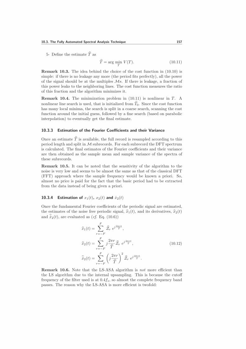
10.3. The Fully Automated Spectral Analysis Technique 157
5- Define the estimate T as
T = arg minT
V (T ). (10.11)
Remark 10.3. The idea behind the choice of the cost function in (10.10) issimple: if there is no leakage any more (the period fits perfectly), all the powerof the signal should be at the multiples Ms. If there is leakage, a fraction ofthis power leaks to the neighboring lines. The cost function measures the ratioof this fraction and the algorithm minimizes it.
Remark 10.4. The minimization problem in (10.11) is nonlinear in T . A
nonlinear line search is used, that is initialized from T0. Since the cost functionhas many local minima, the search is split in a coarse search, scanning the costfunction around the initial guess, followed by a fine search (based on parabolicinterpolation) to eventually get the final estimate.
10.3.3 Estimation of the Fourier Coefficients and their Variance
Once an estimate T is available, the full record is resampled according to thisperiod length and split in M subrecords. For each subrecord the DFT spectrumis calculated. The final estimates of the Fourier coefficients and their varianceare then obtained as the sample mean and sample variance of the spectra ofthese subrecords.
Remark 10.5. It can be noted that the sensitivity of the algorithm to thenoise is very low and seems to be almost the same as that of the classical DFT(FFT) approach where the sample frequency would be known a priori. So,almost no price is paid for the fact that the basic period had to be extractedfrom the data instead of being given a priori.
10.3.4 Estimation of x1(t), x2(t) and x2(t)
Once the fundamental Fourier coefficients of the periodic signal are estimated,the estimates of the noise free periodic signal, x1(t), and its derivatives, x2(t)
and x2(t), are evaluated as (cf. Eq. (10.6))
x1(t) =
F∑
r=−FZr ej
2πrt
T ,
x2(t) =F∑
r=−Fj2πr
TZr ej
2πrt
T ,
x2(t) =
F∑
r=−F
(j2πr
T
)2
Zr ej2πrt
T .
(10.12)
Remark 10.6. Note that the LS-ASA algorithm is not more efficient thanthe LS algorithm due to the internal upsampling. This is because the cutofffrequency of the filter used is at 0.4fs, so almost the complete frequency bandpasses. The reason why the LS-ASA is more efficient is twofold:

158 10. Periodic Signal Modeling Based on Fully Automated Spectral Analysis
0 10 20 30 40 50 60 70 80−50
−40
−30
−20
−10
0
10
SNR [dB]
V [
dB
]
LS LS−ASA
Figure 10.1: Comparison between the LS-ASA estimates and the LS estimatesfor different SNRs.
• Only one frequency line in M lines is used, the others are put to zeros(M periods measured). This leads to a reduction of the noise power byM.
• Only the significant Fourier coefficients are used in the estimates x1(t),
x2(t) and x2(t). Hence, an enormous noise reduction is obtained.
10.4 Simulation Study
The Van der Pol oscillator [62] was selected as the underlying system in thisexample. The oscillator is described by
(x1
x2
)=
(x2
−x1 + ε(1 − x21)x2
). (10.13)
The Matlab routine ode45 was used to solve (10.13) for ε = 2. The initial
state of (10.13) was selected as(x1(0) x2(0)
)T= (0 1)T . All results below
are based on data runs of length N = 104 with a sampling period h = 0.1 s.The measured signal z(t) selected as the first state with white noise added.
The differentiated signals x2(t) and x2(t) for the LS estimation algorithmwere obtained using first order difference (Euler center approximation) withx1(t) = z(t). On the other hand, these signals were evaluated using (10.12) forthe LS-ASA estimation algorithm.
In this example the estimated model used second-degree polynomials(L = M = 2). Both the LS and the LS-ASA algorithms were run for differ-ent SNRs. As a measure of performance,
V =‖θN − θo‖2
‖θo‖2(10.14)

10.5. Conclusions 159
−4 −2 0 2 4−5
−3
−1
1
3
5
x1
x 2
−4 −2 0 2 4−5
−3
−1
1
3
5
x1
x 2
Figure 10.2: True (solid) and estimated (dashed) phase plots. LS estimate (left)and LS-ASA estimate (right) [SNR=20 dB].
was computed and plotted as a function of the SNR in Fig. 10.1. In (10.14),θo denotes the true parameter vector. The phase plots for the estimated mod-els at SNR of 20 dB and 60 dB in addition to the true system are given inFigures 10.2-10.3. Also, the estimated periodic signals at SNR of 20 dB and60 dB compared to the true signal are given in Figures 10.4-10.5. The LS al-gorithm using the Euler center approximation did not give stable limit cyclesfor SNRs below 20 dB. The LS-ASA algorithm still gives good models for lowSNRs as shown in Figures 10.6-10.7.
It can be concluded from Figures 10.1-10.7 that the LS-ASA algorithmgives significantly better estimates than the LS algorithm using finite differenceapproximation. Also, the LS-ASA algorithm gives more accurate estimatesthan the Markov estimation algorithm of Chapter 7, see Fig. (7.8). Moreover,the computational complexity of the LS-ASA algorithm is much lower than theMarkov estimation algorithm and the MLE algorithm of Chapter 9.
10.5 Conclusions
A least squares estimation algorithm based on fully automated spectral analysis(ASA) technique has been introduced for the modeling of periodic signals usinga second-order nonlinear ODE model. The ASA technique reduces the noisecontributions on the modeled signal and its derivatives significantly. The sug-gested algorithm results in a much better performance as compared to the LSestimation algorithm using finite difference approximation. Also, the LS-ASAalgorithm is computationally less demanding as compared to the Markov esti-mation algorithm and the MLE algorithm.

160 10. Periodic Signal Modeling Based on Fully Automated Spectral Analysis
−4 −2 0 2 4−4
−3
−2
−1
0
1
2
3
4
x1
x 2
−4 −2 0 2 4−4
−3
−2
−1
0
1
2
3
4
x1
x 2
Figure 10.3: True (solid) and estimated (dashed) phase plots. LS estimate (left)and LS-ASA estimate (right) [SNR=60 dB].
0 1000 2000 3000−2.5
−2
−1.5
−1
−0.5
0
0.5
1
1.5
2
2.5
Time [samples]
0 1000 2000 3000−2.5
−2
−1.5
−1
−0.5
0
0.5
1
1.5
2
2.5
Time [samples]
Figure 10.4: True (solid) and estimated (dashed) signals. LS estimate (left) andLS-ASA estimate (right) [SNR=20 dB].

10.5. Conclusions 161
0 1000 2000 3000−2.5
−2
−1.5
−1
−0.5
0
0.5
1
1.5
2
2.5
Time [samples]0 1000 2000 3000
−2.5
−2
−1.5
−1
−0.5
0
0.5
1
1.5
2
2.5
Time [samples]
Figure 10.5: True (solid) and estimated (dashed) signals. LS estimate (left) andLS-ASA estimate (right) [SNR=60 dB].
−4 −2 0 2 4−5
−3
−1
1
3
5
x1
x 2
−4 −2 0 2 4−5
−3
−1
1
3
5
x1
x 2
Figure 10.6: True (solid) and estimated LS-ASA (dashed) phase plots. 0 dB(left) and 10 dB (right).

162 10. Periodic Signal Modeling Based on Fully Automated Spectral Analysis
0 1000 2000 3000−2.5
−2
−1.5
−1
−0.5
0
0.5
1
1.5
2
2.5
Time [samples]0 1000 2000 3000
−2.5
−2
−1.5
−1
−0.5
0
0.5
1
1.5
2
2.5
Time [samples]
Figure 10.7: True (solid) and estimated LS-ASA (dashed) signals. 0 dB (left)and 10 dB (right).

Chapter 11
Periodic Signal Modeling Based on Lienard’sEquation
11.1 Introduction
IN the early days of nonlinear dynamics, it was found that many oscillatingcircuits can be modeled by the following second-order differential equation
known as Lienard’s equation, see [125, 128],
y + f(y)y + g(y) = 0. (11.1)
Lienard’s equation can be interpreted mechanically as the equation of motionfor a unit mass subject to a nonlinear damping force −f(y)y and a nonlinearrestoring force −g(y). Applications of Lienard’s equation can be found in manyimportant examples. Examples include chemical reactions, growth of a singlespecies, predator-prey systems and vibration analysis, see [74].
Choosing the state variables as x1 = y(t) and x2 = y(t), Lienard’s equationis equivalent to the system
x1 = x2,
x2 = −g(x1) − f(x1)x2,(11.2)
which is known as the Lienard’s system.
In this chapter Lienard’s equation is used to model periodic signals followingthe approach introduced in Chapter 5. The conditions that guarantee theexistence of periodic orbits for Lienard systems, see [57, 104], are used to reducethe number of parameters required to model periodic signals. This is expectedto give significantly better parameter accuracy as compared to the approachused in Chapter 5 in case the modeled signal fulfills Lienard’s equation. Anotheradvantage is that it can easily be checked if the estimated model will generatea stable periodic orbit.
The chapter is organized as follows. Section 11.2 introduces the details onthe model based on Lienard’s equation. Section 11.3 analyzes the conditionsimposed on the model to achieve the reduction in the parameters to be es-timated. Section 11.4 presents a comparative simulation study between theapproach taken in this chapter and the approach of Chapter 5. Conclusionsappear in Section 11.5.
163

164 11. Periodic Signal Modeling Based on Lienard’s Equation
11.2 The ODE Model Based on Lienard’s Equation
11.2.1 Model Structures
The work done in Chapter 5 is based on modeling the signal y(t) by means ofan unknown parameter vector θ and an ODE of order two, i.e.
(x1
x2
)=
(x2(t)
f(x1(t), x2(t), θ
)),
y(t) =(
1 0)( x1(t)
x2(t)
).
(11.3)
The right hand side of the second state equation of (11.3) was expanded in termsof a truncated superposition of polynomial basis. Hence f
(x1(t), x2(t), θ
)was
parameterized as
f(x1(t), x2(t), θ
)=
L∑
l=0
M∑
m=0
θl,mxl1(t)x
m2 (t),
θ =(θ0,0 · · · θ0,M θ1,0 · · · θ1,M · · · θL,0 · · · θL,M
)T.
(11.4)
In this chapter a Lienard model (11.2) is used for modeling periodic signals.Then the state space model (11.3) becomes
(x1
x2
)=
(x2(t)
−g(x1(t),θ1
)− f
(x1(t),θ2
)x2(t)
),
y(t) =(
1 0)( x1(t)
x2(t)
),
(11.5)
θ =(θ1
T θ2T)T. (11.6)
Also here g(x1(t),θ1
)and f
(x1(t),θ2
)are parameterized using (scalar) poly-
nomial models
g(x1(t),θ1
)=
L1∑
l1=1
θ1,l1xl11 (t),
f(x1(t),θ2
)=
L2∑
l2=0
θ2,l2xl21 (t).
(11.7)
Needless to say, the model (11.5) can be seen as a special case of the generalcase (11.3).
11.2.2 Discretization
Similarly to Chapter 5, the continuous time ODE model (11.5) is discretized inorder to formulate complete discrete models. This is done here by exploiting

11.2. The ODE Model Based on Lienard’s Equation 165
an Euler forward numerical integration scheme. Selecting the discretizationinterval to be equal to the sampling period h, results in
x1(kh+ h) = x1(kh) + hx2(kh),
x2(kh+ h) = x2(kh) − h
L1∑
l1=1
θ1,l1xl11 (kh) − h
(L2∑
l2=0
θ2,l2xl21 (kh)
)x2(kh).
(11.8)
Remark 11.1. In the following, for notational convenience the dependence onh is omitted assuming that h is equal to one time unit. This means that aninteger k can be used as the time variable.
The model (11.8) can then be compactly written in the linear regressionform as
x1(k + 1) − x1(k) = x2(k),
x2(k + 1) − x2(k) = − φT(x1(k), x2(k)
)θ,
(11.9)
where
φT(x1(k), x2(k)
)=(x1(k) · · · xL1
1 (k) x2(k) · · · xL21 (k)x2(k)
),
θ =(θ1,1 · · · θ1,L1
θ2,0 · · · θ2,L2
)T.
(11.10)For comparison, discretizing the second state equation of (11.3) results in
x2(k + 1) − x2(k) = φT (x1(k), x2(k)
)θ, (11.11)
where
φT (x1(k), x2(k)
)=
(1 x2(k) · · ·xM2 (k) x1(k) · · ·x1(k)x
M2 (k) · · · xL1 (k) · · ·xL1 (k)xM2 (k)
),
(11.12)
and the parameter vector θ is given by (11.4).
11.2.3 Algorithms
In order to derive different estimation schemes based on the model (11.9) thereare at least three choices. The first choice is to formulate the model in a linearregression form using the measured data (cf. Section 5.3) and the approxima-tions x1(k) = z(k) and x2(k) = z(k + 1)− z(k). Once the model is formulatedin the linear regression form, a number of different estimation algorithms basedon the least squares estimate, the Markov estimate (cf. Chapter 7), the Kalmanfilter (cf. Chapter 8) and the maximum likelihood estimate (cf. Chapter 9)can be developed from the model (11.9).
Another choice is to estimate the states x1(k) and x2(k) in addition to theparameter vector θ using the EKF as done in Chapter 8. In this case the

166 11. Periodic Signal Modeling Based on Lienard’s Equation
regression vector φT(x1(k), x2(k)
)is built up from the estimated states x1(k)
and x2(k) rather than directly from measured data.
The third choice is to use algorithms based on the automated spectral anal-ysis technique of Chapter 10 which finds more accurate estimates for the noisefree periodic signal, x1(k), and its time derivatives, x2(k) and x2(k).
11.3 Model Parameterization Using Lienard’s Theorem
In this section the model assumptions introduced in Lienard’s theorem [57, 104]are considered and exploited. The theorem reads as follows.
Theorem 11.1. (Lienard’s theorem) Suppose that f(y) and g(y) satisfy thefollowing conditions:
Assumption 11.1. f(y) and g(y) are continuously differentiable for all y;
Assumption 11.2. g(−y) = −g(y) ∀ y (i.e. g(y) is an odd function);
Assumption 11.3. g(y) > 0 for y > 0;
Assumption 11.4. f(−y) = f(y) ∀ y (i.e. f(y) is an even function);
Assumption 11.5. The odd function F (y) =∫ y0f(u)du has exactly one pos-
itive zero at y = a, is negative for 0 < y < a, is positive and nondecreasing fory > a, and F (y) → ∞ as y → ∞.
Then the system (11.2) has a unique, stable limit cycle surrounding the originin the phase plane.
Proof. See [57].
Remark 11.2. The assumptions on g(y) mean that the restoring force acts likean ordinary spring and tends to reduce any displacement. Also the assumptionson f(y) imply that the damping is negative at small |y| and positive at large|y|. Since small oscillations are amplified and large oscillations are damped,the system tends to settle into a self-sustained oscillation of some intermediateamplitude.
Applying Assumption 11.2 and Assumption 11.4, the models (11.7) takethe form
g(x1(t), θ1
)=
L1∑
l1=0
θ1,l1x2l1+11 (t),
f(x1(t), θ2
)=
L2∑
l2=0
θ2,l2x2l21 (t),
(11.13)
θ =(θT1 θ
T2
)T=(θ1,0 · · · θ1,L1
θ2,0 · · · θ2,L2
)T, (11.14)
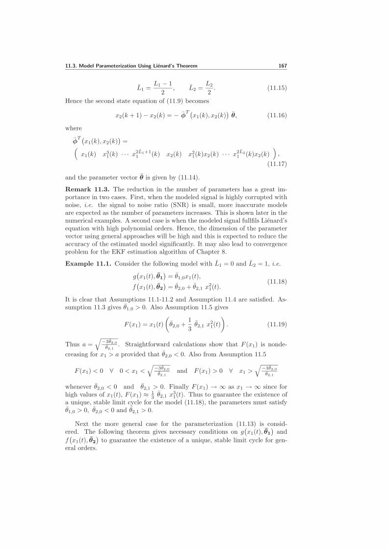
11.3. Model Parameterization Using Lienard’s Theorem 167
L1 =L1 − 1
2, L2 =
L2
2. (11.15)
Hence the second state equation of (11.9) becomes
x2(k + 1) − x2(k) = − φT (x1(k), x2(k)
)θ, (11.16)
where
φT (x1(k), x2(k)
)=
(x1(k) x3
1(k) · · · x2L1+11 (k) x2(k) x2
1(k)x2(k) · · · x2L21 (k)x2(k)
),
(11.17)
and the parameter vector θ is given by (11.14).
Remark 11.3. The reduction in the number of parameters has a great im-portance in two cases. First, when the modeled signal is highly corrupted withnoise, i.e. the signal to noise ratio (SNR) is small, more inaccurate modelsare expected as the number of parameters increases. This is shown later in thenumerical examples. A second case is when the modeled signal fullfils Lienard’sequation with high polynomial orders. Hence, the dimension of the parametervector using general approaches will be high and this is expected to reduce theaccuracy of the estimated model significantly. It may also lead to convergenceproblem for the EKF estimation algorithm of Chapter 8.
Example 11.1. Consider the following model with L1 = 0 and L2 = 1, i.e.
g(x1(t), θ1
)= θ1,0x1(t),
f(x1(t), θ2
)= θ2,0 + θ2,1 x
21(t).
(11.18)
It is clear that Assumptions 11.1-11.2 and Assumption 11.4 are satisfied. As-sumption 11.3 gives θ1,0 > 0. Also Assumption 11.5 gives
F (x1) = x1(t)
(θ2,0 +
1
3θ2,1 x
21(t)
). (11.19)
Thus a =√
−3θ2,0
θ2,1. Straightforward calculations show that F (x1) is nonde-
creasing for x1 > a provided that θ2,0 < 0. Also from Assumption 11.5
F (x1) < 0 ∀ 0 < x1 <√
−3θ2,0
θ2,1and F (x1) > 0 ∀ x1 >
√−3θ2,0
θ2,1
whenever θ2,0 < 0 and θ2,1 > 0. Finally F (x1) → ∞ as x1 → ∞ since forhigh values of x1(t), F (x1) ≈ 1
3 θ2,1 x31(t). Thus to guarantee the existence of
a unique, stable limit cycle for the model (11.18), the parameters must satisfyθ1,0 > 0, θ2,0 < 0 and θ2,1 > 0.
Next the more general case for the parameterization (11.13) is consid-ered. The following theorem gives necessary conditions on g
(x1(t), θ1
)and
f(x1(t), θ2
)to guarantee the existence of a unique, stable limit cycle for gen-
eral orders.

168 11. Periodic Signal Modeling Based on Lienard’s Equation
Theorem 11.2. Assume that the Lienard’s system is given by(x1
x2
)=
(x2(t)
−g(x1(t), θ1
)− f
(x1(t), θ2
)x2(t)
),
y(t) =(
1 0)( x1(t)
x2(t)
),
(11.20)
where the odd function g(x1, θ1) and the even function f(x1, θ2) are continu-ously differentiable polynomials given by
g(x1, θ1) = θ1,0x1 + θ1,1x31 + · · · + θ1,L1
x2L1+11 ,
f(x1, θ2) = θ2,0 + θ2,1x21 + · · · + θ2,L2
x2L21 .
(11.21)
Then this system has a unique, stable limit cycle encircling the origin in thephase plane if
Assumption 11.6. All zeros of the polynomial
A(s) = θ1,0 + θ1,1 s+ θ1,2 s2 + · · · + θ1,L1
sL1 (11.22)
are in the LHP.
Assumption 11.7. The polynomial
B(s) = θ2,0 +θ2,13
s+θ2,25
s2 + · · · + θ2,L2
2L2 + 1sL2 (11.23)
has exactly one positive real zero (say at a2) and θ2,0 < 0.
Assumption 11.8. f(x1, θ2) ≥ 0 ∀ x1 > a.
Proof. See Appendix 11.A
Remark 11.4. From Routh’s stability criterion for continuous systems,see [80], all zeros of A(s) are in the LHP if there are no sign changes in theleft-most column of the Routh array. A necessary but not sufficient conditionfor this to happen is θ1,i > 0 for i = 0, · · · , L1. Also from Descarte’s ruleof sign [58], the number of positive real roots of B(s) is either equal to thenumber of variations of sign between successive terms in B(s) when arrangedin descending powers of s or less than that number by an even integer. ThusB(s) should have an odd number of sign variations.
In addition to the reduction achieved in the number of estimated parame-ters, another advantage of the approach used in this chapter can be concluded.Since Theorem 11.2 gives more specific conditions on the parameters, theseconditions can be used as a detection method for the existence of a unique,stable periodic orbit that models the periodic signal. Once the parameter vec-tor θ is estimated, the polynomials A(s) and B(s) can be constructed and theconditions of Theorem 11.2 can be examined.
Remark 11.5. Note that there may be unique periodic solutions even in caseswhere the parameter constraints are not fulfilled. This is because the conditionsof Theorem 11.1 are only sufficient for general periodic signals.

11.4. Numerical Examples 169
11.4 Numerical Examples
In this section a comparative simulation study for the two modeling approachesdescribed by (11.3) and (11.5) is presented.
Example 11.2. In this example the data were generated using the followingLienard’s system
(x1
x2
)=
(x2
−x1 + (1 − 2 x41) x2
)(11.24)
which satisfies the conditions of Theorem 11.1. The Matlab routine ode45
was used to solve (11.24). The initial states of (11.24) were selected as(x1(0) x2(0)
)T= (1 0)T . All results below are based on data runs of length
N = 3 × 10⁴ samples with a sampling period h = 0.01 s. The period of thesolution of (11.24) was approximately 7 seconds. The measured signal was se-lected as the first state with white Gaussian noise added to obtain data with aSNR of 30 dB.
The model (11.3) was compared with the model (11.5) by modeling theperiodic signal generated by (11.24) using the EKF estimation algorithm in-troduced in Chapter 8. The two EKF algorithms were initialized with
(x1(0) x2(0)
θT
(0))T
= (−0.5 0.5 0)T ,
(x1(0) x2(0) θ
T
(0))T
= (−0.5 0.5 0)T .
The remaining parameters were selected as P (0) = 10I, R1 = 0.001I andr2 = 1. The orders of the models were chosen as L = 4, M = 1, L1 = 0 andL2 = 2. The number of estimated parameters was (L+ 1)(M + 1) = 10 for themodel (11.3) and L1 + L2 + 2 = 4 for the model (11.5).
After 3 × 10⁴ samples the parameter estimates were as follows:
θT
=(0.005, 1.021,−1.149,−0.009, 0.008,−0.235, 0.086, 0.020,−0.011,−1.908
)
θT
=(1.036,−0.990, 0.040, 2.102
).
Note the negative sign difference betweenθ and θ, cf. Eq. (11.11) and
Eq. (11.16). Comparing the estimated parameter vector θ with the resultsof Theorem 11.2 gives θ1,0 = 1.036 > 0, θ2,0 = −0.99 < 0 and θ2,2 = 2.102.Thus A(s) = 1.036 and B(s) = −0.99 + 2.102
5 s2. It is clear that A(s) doesnot have zeros in the RHP and B(s) has one positive zero at 1.535. Alsof(x1, θ2) = 2.102x4
1 − 0.99 > 0 ∀x1 >√
1.535. This shows that the estimatedmodel represents a unique, stable periodic orbit surrounding the origin in thephase plane.
The parameter estimates and phase plots for the system (11.24) and theestimated models are shown in Figures 11.1-11.2. The results indicate that

170 11. Periodic Signal Modeling Based on Lienard’s Equation
0 0.5 1 1.5 2 2.5 3
x 104
−2.5
−2
−1.5
−1
−0.5
0
0.5
1
1.5
Time [samples]
Par
amet
er e
stim
ates
(a) Using the model (11.5)
0 0.5 1 1.5 2 2.5 3
x 104
−2.5
−2
−1.5
−1
−0.5
0
0.5
1
1.5
Time [samples]
Par
amet
er e
stim
ates
(b) Using the model (11.3)
Figure 11.1: Parameter convergence.
−2 −1 0 1 2−2.5
−1.5
−0.5
0.5
1.5
2.5
x1
x 2
−2 −1 0 1 2−2.5
−1.5
−0.5
0.5
1.5
2.5
x1
x 2
Figure 11.2: True (solid) and estimated (dashed) phase plane plots for system (11.24).The model (11.5) left and the model (11.3) right. The models are initialized as
x1(0) = −0.5, x2(0) = 0.5 and the final parameter vector estimate θ orθ, respectively,
is applied.
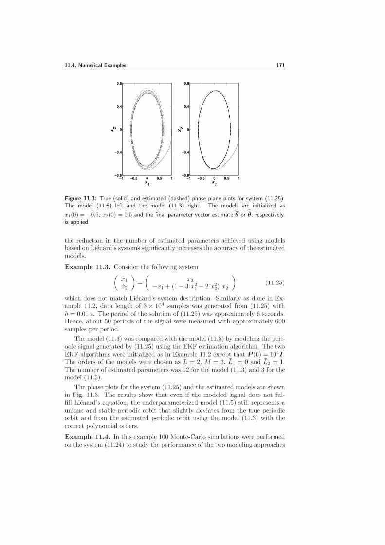
11.4. Numerical Examples 171
−1 −0.5 0 0.5 1−0.8
−0.4
0
0.4
0.8
x1
x 2
−1 −0.5 0 0.5 1−0.8
−0.4
0
0.4
0.8
x1
x 2
Figure 11.3: True (solid) and estimated (dashed) phase plane plots for system (11.25).The model (11.5) left and the model (11.3) right. The models are initialized as
x1(0) = −0.5, x2(0) = 0.5 and the final parameter vector estimate θ orθ, respectively,
is applied.
the reduction in the number of estimated parameters achieved using modelsbased on Lienard’s systems significantly increases the accuracy of the estimatedmodels.
Example 11.3. Consider the following system(x1
x2
)=
(x2
−x1 + (1 − 3 x21 − 2 x2
2) x2
)(11.25)
which does not match Lienard’s system description. Similarly as done in Ex-ample 11.2, data length of 3 × 10⁴ samples was generated from (11.25) withh = 0.01 s. The period of the solution of (11.25) was approximately 6 seconds.Hence, about 50 periods of the signal were measured with approximately 600samples per period.
The model (11.3) was compared with the model (11.5) by modeling the peri-odic signal generated by (11.25) using the EKF estimation algorithm. The twoEKF algorithms were initialized as in Example 11.2 except that P (0) = 104I.The orders of the models were chosen as L = 2, M = 3, L1 = 0 and L2 = 1.The number of estimated parameters was 12 for the model (11.3) and 3 for themodel (11.5).
The phase plots for the system (11.25) and the estimated models are shownin Fig. 11.3. The results show that even if the modeled signal does not ful-fill Lienard’s equation, the underparameterized model (11.5) still represents aunique and stable periodic orbit that slightly deviates from the true periodicorbit and from the estimated periodic orbit using the model (11.3) with thecorrect polynomial orders.
Example 11.4. In this example 100 Monte-Carlo simulations were performedon the system (11.24) to study the performance of the two modeling approaches

172 11. Periodic Signal Modeling Based on Lienard’s Equation
described by (11.3) and (11.5) compared to the Cramer-Rao bound (CRB) de-rived in Chapter 9 with different noise realizations. The data were generated asin Example 11.2. The two EKF algorithms were initialized with P (0) = 10−4I,R1 = 10−6I, r2 = 1 and
(x1(0) x2(0)
θT
(0))T
=(− 0.5 0.5 θo + σ(SNR, N)
)T,
(x1(0) x2(0) θ
T
(0))T
=(− 0.5 0.5 θo + σ(SNR, N)
)T.
where θo and θo are the true parameter vectors, σ(SNR, N) and σ(SNR, N)are the standard deviations as predicted by the CRB evaluated at specific SNRand data length N . The orders of the models were chosen as in Example 11.2.
The mean square error (MSE) and the CRB were evaluated for N = 3×10⁴
samples with different SNRs. The results are shown in Figures 11.4(a)-11.4(c).Also as a measure of performance,
V1 =1
n
n∑
1
‖θN − θo‖2,
V2 =1
n
n∑
1
‖θN − θo‖2
(11.26)
were computed and plotted as a function of the SNR in Fig. 11.4(d) (n isthe number of experiments in which convergence to the true parameter vectoris achieved). Also, the Monte-Carlo experiments were repeated for differentdata lengths with SNR=10 dB. The initial values of P and R1 were chosenas P (0) = 10I, R1 = 10−5I. The results are plotted in Fig. 11.5. The resultsof Figures 11.4-11.5 show that the approach of this chapter gives significantlybetter parameter estimates compared to the approach described by (11.3) es-pecially for small SNR.
Example 11.5. In this example the suggested approach of this chapter is usedto model a piece of a bell sound extracted from a CD in .wav format with asampling frequency of 22.05 kHz. The least squares algorithm of Chapter 7was applied to model 200 samples of the acoustic signal, see Fig 11.6(a). Themodel (11.5) with different combinations of L1 and L2 was used. It was noticedthat the parameters of θ2 were very small compared to the parameters of θ1.Hence, θ2 was excluded from the model (11.5). Finally, the following modelwas obtained: (
x1
x2
)=
(x2
−7.22 × 107x1 + 1.14 × 109x31
). (11.27)
The real data, the model output, the true and the estimated phase plots aregiven in Fig. 11.6. Note that the model obtained does not satisfy the conditionsof Theorem 11.2. Specifically, the polynomial A(s) has a zero in the RHP (ats = 0.06). Hence, there is a possibility that multi limit cycles could exist.
Therefore, the model was initialized at(x1(0) x2(0)
)T= (−0.08 0)T , i.e.
close to the true limit cycle.

11.4. Numerical Examples 173
0 10 20 30 40 50−90
−80
−70
−60
−50
−40
−30
−20
−10
0
CR
B a
nd
MS
E [
dB
]
SNR [dB]
(a) MSE(θ1,0 (dashed), θ1,0 (solid)
)and
CRB(θ1,0 (dot-o), θ1,0 (dot-x)
)
0 10 20 30 40 50−70
−60
−50
−40
−30
−20
−10
0
CR
B a
nd
MS
E [
dB
]
SNR [dB]
(b) MSE(θ0,1 (dashed), θ2,0 (solid)
)and
CRB(θ0,1 (dot-o), θ2,0 (dot-x)
)
0 10 20 30 40 50−60
−50
−40
−30
−20
−10
0
CR
B a
nd
MS
E [
dB
]
SNR [dB]
(c) MSE(θ4,1 (dashed), θ2,2 (solid)
)and
CRB(θ4,1 (dot-o), θ2,2 (dot-x)
)
0 10 20 30 40 50−16
−14
−12
−10
−8
−6
−4
−2
0
2
4
SNR [dB]
V1 a
nd
V2 [
dB
]
(d) V1 (dashed) and V2 (solid)
Figure 11.4: Statistical results vs. signal to noise ratio.

174 11. Periodic Signal Modeling Based on Lienard’s Equation
5000 10000 15000 20000 25000 30000−50
−45
−40
−35
−30
−25
−20
−15
−10
−5
CR
B a
nd
MS
E [
dB
]
N [samples]
(a) MSE(θ1,0 (dashed), θ1,0 (solid)
)and
CRB(θ1,0 (dot-o), θ1,0 (dot-x)
)
5000 10000 15000 20000 25000 30000−35
−30
−25
−20
−15
−10
−5
CR
B a
nd
MS
E [
dB
]
N [samples]
(b) MSE(θ0,1 (dashed), θ2,0 (solid)
)and
CRB(θ0,1 (dot-o), θ2,0 (dot-x)
)
5000 10000 15000 20000 25000 30000−20
−15
−10
−5
0
5
CR
B a
nd
MS
E [
dB
]
N [samples]
(c) MSE(θ4,1 (dashed), θ2,2 (solid)
)and
CRB(θ4,1 (dot-o), θ2,2 (dot-x)
)
5000 10000 15000 20000 25000 30000−5
−4
−3
−2
−1
0
1
2
3
4
5
V1 a
nd
V2 [
dB
]
N [samples]
(d) V1 (dashed) and V2 (solid)
Figure 11.5: Statistical results vs. data length.

11.5. Conclusions 175
0 50 100 150 200−0.1
−0.05
0
0.05
0.1
Time [samples]
(a) Signals
−0.1 −0.05 0 0.05 0.1−800
−600
−400
−200
0
200
400
600
800
x1
x 2(b) Phase plots
Figure 11.6: Real data (solid) and estimated model (dashed) of a bell sound.
11.5 Conclusions
The modeling of periodic signals using Lienard’s equation has been studied.The approach of this chapter is based on using the appropriate assumptionsimposed in Lienard’s theorem to guarantee the existence of a unique and stableperiodic orbit in the phase plane surrounding the origin. Using these conditionsleads to a reduction in the ODE model parameters. This reduction not onlyreduces the computational load but also significantly increases the accuracy ofthe model in case the periodic signal does fulfill Lienard’s equation descriptioncompared to more general approaches. Moreover, the approach can be usedfor modeling signals that do not fulfill Lienard’s equation with only a smalldegradation in the accuracy of the estimated models.
11.A Proof of Theorem 11.2
First note that Assumptions 11.1-11.2 and Assumption 11.4 are true by con-struction. It remains to verify Assumption 11.3 and Assumption 11.5. Begin-ning with Assumption 11.3, the odd function g(x1, θ1) can be written as
g(x1, θ1) = x1 A(x21).
Choosing s = x21 gives Eq. (11.22). Further
g(x1) > 0 ∀ x1 > 0 if A(x21) > 0.
The latter is the case if all zeros of A(s) are in the LHP, since for negative zerosA(s) takes the form
A(s) =
L1∏
i=1
(s+ zi) for zi > 0,

176 11. Periodic Signal Modeling Based on Lienard’s Equation
where −zi, i = 1, · · · , L1 are the zeros of A(s). Thus Assumption 11.6 impliesAssumption 11.3.
Remark 11.6. Note that in case zi is complex, i.e. zi = zir + jzic and itscomplex conjugate is given as zi = zir − jzic, it follows that
(s+ zi)(s+ zi) = s2 + 2zirs+ z2ir + z2
ic > 0.
This means that A(x21) > 0 for complex roots and Assumption 11.6 still implies
Assumption 11.3.
Proceeding with Assumption 11.5, since f(x1, θ2) is an even function
F (x1) = x1 B(x21).
To satisfy Assumption 11.5, B(x21) should have exactly one positive zero at
x1 = a, be negative for 0 < x1 < a, be positive and nondecreasing for x1 > a,and F (x1) → ∞ as x1 → ∞. This means θ2,0 should be negative (for F (x1)to be negative for small x1) and B(s) given by (11.23) should have exactly onepositive real zero. The nondecreasing condition on F (x1) for x1 > a means
dF
dx1≥ 0 for x1 > a.
Since
F (x1) =
∫ x1
0
f(u)du,
differentiating both sides gives
dF
dx1= f(x1, θ2).
Thus F (x1) is a nondecreasing function if Assumption 11.8 satisfied. HenceAssumption 11.7 and Assumption 11.8 together imply Assumption 11.5.

Chapter 12
Bias Analysis in LS Estimation of Periodic Signals
12.1 Introduction
AS mentioned in Chapter 7, the Least squares (LS) estimator gives biasedestimates at low signal to noise ratios (SNRs). The major reasons for
this bias are the noise contamination of the derivatives of the modeled sig-nal evaluated using Euler approximations, as well as discretization errors. InChapter 10 the automated spectral analysis (ASA) technique was used to findmore accurate estimates for the noise free periodic signal, x1(t), and its timederivatives, x2(t) and x2(t). Although the approach of Chapter 10 shows asignificant improvement in the performance compared to using finite differenceapproximations, it is still interesting to study the bias in the LS estimationalgorithm of Chapter 7 which is based on finite difference approximations.
The LS algorithm of Chapter 7 uses the linear regression equation
x2(t) = φT(x1(t), x2(t)
)θ + ε(t) (12.1)
for estimating the parameter vector θ. Here
φT(x1(t), x2(t)
)=(
1 · · · xM2 (t) · · · xL1 (t) · · · xL1 (t)xM2 (t)), (12.2)
θ =(θ0,0 · · · θ0,M · · · θL,0 · · · θL,M
)T. (12.3)
The estimate x1(kh) of x1(kh) is chosen to be equal to the modeled data(cf. Eq. (5.12)), i.e.
x1(t) = z(t) = y(t) + e(t), (12.4)
where y(t) is the continuous time periodic signal and e(t) is a zero-mean white
Gaussian noise. Also, x2(t) and x2(t) are the estimates of the first and secondderivatives of the modeled signal, respectively, evaluated using finite differenceapproximation, and ε(t) is a regression error.
In this chapter, an analysis of the bias in the LS estimate of two periodicnonlinear systems is given. The goal is to study the effect of the samplingperiod, the signal to noise ratio and the system parameters on the estimationbias.
The chapter is organized as follows. Different estimation errors are dis-cussed in Section 12.2. In Section 12.3, bias analysis and discretization errors
177

178 12. Bias Analysis in LS Estimation of Periodic Signals
for some simple periodic systems are evaluated. Section 12.4 gives a compara-tive numerical study between three different Euler approximation techniques.Conclusions appear in Section 12.5.
12.2 Estimation Errors
In order to estimate the parameter vector θ from the linear regression equation(12.1), some estimates of the modeled signal x1(kh), its first derivative x2(kh)and second derivative x2(kh) are needed. Estimating these quantities usingfinite difference approximations from the measured data leads to some estima-tion errors. It is expected that the LS estimates will suffer from two estimationerrors, namely: random noise errors and discretization errors. Random noiseerrors result due to differentiating additive measurement noise. On the otherhand, discretization errors are caused by approximating the signal derivativesusing finite difference schemes.
To investigate how the estimate θLS
N behaves when the data length N be-comes large, consider the following:
R = E[φ(x1(t), x2(t)
)φT(x1(t), x2(t)
)], (12.5)
r = E[φ(x1(t), x2(t)
) x2(t)], (12.6)
where
φT(x1(t), x2(t)
)=(
1 · · · xM2 (t) · · · xL1 (t) · · · xL1 (t)xM2 (t)), (12.7)
and
Ef(t) = limN→∞
1
N
N∑
t=1
Ef(t). (12.8)
Remark 12.1. E is used instead of the ordinary expectation E to account fornoise-free signals. For fully random signals E = E.
In this case the asymptotic parameter vector estimate θ is given by
θ = R−1 r = θ0 + θb, (12.9)
where θ0 is the true parameter vector and θb is the bias vector. Similarly
R = R0 + Rb, (12.10)
r = r0 + rb, (12.11)
where
R0 = E[φ(x1(t), x2(t)
)φT(x1(t), x2(t)
)],
r0 = E[φ(x1(t), x2(t)
)x2(t)
], (12.12)

12.2. Estimation Errors 179
and Rb and rb are the bias contributions to R0 and r0, respectively, due tousing estimated states x1(t) and x2(t) instead of the true states.
Now using (12.9)-(12.11) gives
θ = (R0 + Rb)−1 (r0 + rb)
= R−10 r0︸ ︷︷ ︸θ0
+(R0 + Rb)−1(rb − Rbθ0)︸ ︷︷ ︸θb
. (12.13)
Remark 12.2. The bias vector θb is a contribution of random noise errors anddiscretization errors. The contributions of random noise errors and discretiza-tion errors are denoted in this chapter by θn and θd, respectively. Hence
θb = θn + θd, (12.14)
where
θn = (R0 + Rn)−1(rn − Rnθ0), (12.15)
θd = (R0 + Rd)−1(rd − Rdθ0). (12.16)
Also, here Rn and rn are the bias contributions to R0 and r0, respectively,due to random noise errors; Rd and rd are the bias contributions to R0 andr0, respectively, due to discretization errors.
The bias vector θb will depend on the sampling period h and the derivativeapproximations. Derivative approximations can always be chosen by the user.A general approximation for the derivatives of the modeled signal is [97]
Dnf(t) =1
hn
∑
j
Γn,jf(t+ jh), (12.17)
which has to satisfy the following conditions
∑
j
Γn,jjv =
{0 v = 0, · · · , n− 1n! v = n.
(12.18)
The frequency function of the differentiator (12.17) then satisfies
Dn(ejω) = (jω)n + O(|ω|n+1), (12.19)
where O(.) denotes the ordo concept. This means that the low-frequencyasymptote of the differentiator frequency function is (jω)n. See [97, 98] formore details.
Remark 12.3. As can be noticed from (12.18), the minimal number of termsin (12.17) is n+1. In such a case Dn will be a high-pass filter. If the number ofcoefficients is increased, the gained degree of freedom can be used to decreasethe high frequency gain to avoid differentiating the noise as much as possible.See [25] for more details about design of differentiating filters.

180 12. Bias Analysis in LS Estimation of Periodic Signals
In this chapter the estimation of the parameter vector will be considered forthe following three simple finite difference approximations of x2(kh) and x2(kh)which are special cases from (12.17) (in all approximations, x1(kh) = z(kh) waschosen):
• A1: Euler backward approx. (EB)
x2(kh) =1
h
0∑
j=−1
Γ1,j x1(kh+ jh), Γ1,−1 = −1 and Γ1,0 = 1,
x2(kh) =1
h2
0∑
j=−2
Γ2,j x1(kh+ jh), Γ2,−2 = 1, Γ2,−1 = −2 and Γ2,0 = 1.
(12.20)
• A2: Euler forward approx. (EF)
x2(kh) =1
h
1∑
j=0
Γ1,j x1(kh+ jh), Γ1,0 = −1 and Γ1,1 = 1,
x2(kh) =1
h2
2∑
j=0
Γ2,j x1(kh+ jh), Γ2,0 = 1, Γ2,1 = −2 and Γ2,2 = 1.
(12.21)
• A3: Euler center approx. (EC)
x2(kh) =1
h
1∑
j=−1
Γ1,j x1(kh+ jh), Γ1,−1 = −1
2, Γ1,0 = 0 and Γ1,1 =
1
2,
x2(kh) =1
h2
2∑
j=−2
Γ2,j x1(kh+ jh), Γ2,−2 =1
4, Γ2,−1 = 0, Γ2,0 = −1
2,
Γ2,1 = 0, and Γ2,2 =1
4.
(12.22)
Remark 12.4. A1-A3 are chosen as examples for finite difference approxima-tion. Many other different approximations can be considered. For example,one can think about evaluating x2(kh) and x2(kh) using two different finitedifference approximations.
It is well known from the numerical analysis literature that EC approxima-tion gives lower discretization error compared to EB and EF approximations.This is because EC approximation gives a higher order (in h) remainder termwhen a Taylor series expansion is performed. Hence the EC approximationprovides smaller remainder term (for small h) than the EB and EF approxi-mations. Also, the discretization error in this case is expected to decrease as hdecreases. On the other hand, random noise error gives both bias and variance
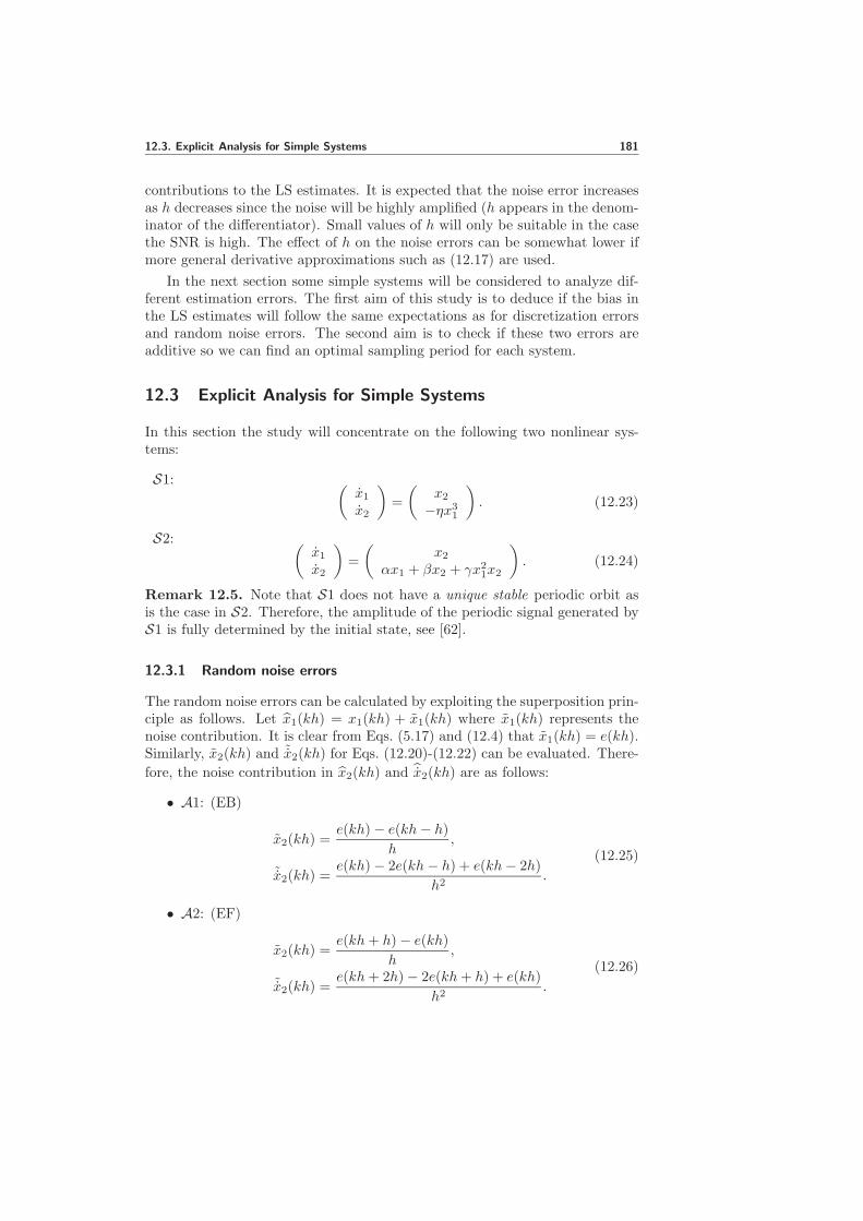
12.3. Explicit Analysis for Simple Systems 181
contributions to the LS estimates. It is expected that the noise error increasesas h decreases since the noise will be highly amplified (h appears in the denom-inator of the differentiator). Small values of h will only be suitable in the casethe SNR is high. The effect of h on the noise errors can be somewhat lower ifmore general derivative approximations such as (12.17) are used.
In the next section some simple systems will be considered to analyze dif-ferent estimation errors. The first aim of this study is to deduce if the bias inthe LS estimates will follow the same expectations as for discretization errorsand random noise errors. The second aim is to check if these two errors areadditive so we can find an optimal sampling period for each system.
12.3 Explicit Analysis for Simple Systems
In this section the study will concentrate on the following two nonlinear sys-tems:
S1: (x1
x2
)=
(x2
−ηx31
). (12.23)
S2: (x1
x2
)=
(x2
αx1 + βx2 + γx21x2
). (12.24)
Remark 12.5. Note that S1 does not have a unique stable periodic orbit asis the case in S2. Therefore, the amplitude of the periodic signal generated byS1 is fully determined by the initial state, see [62].
12.3.1 Random noise errors
The random noise errors can be calculated by exploiting the superposition prin-ciple as follows. Let x1(kh) = x1(kh) + x1(kh) where x1(kh) represents thenoise contribution. It is clear from Eqs. (5.17) and (12.4) that x1(kh) = e(kh).Similarly, x2(kh) and ˜x2(kh) for Eqs. (12.20)-(12.22) can be evaluated. There-
fore, the noise contribution in x2(kh) and x2(kh) are as follows:
• A1: (EB)
x2(kh) =e(kh) − e(kh− h)
h,
˜x2(kh) =e(kh) − 2e(kh− h) + e(kh− 2h)
h2.
(12.25)
• A2: (EF)
x2(kh) =e(kh+ h) − e(kh)
h,
˜x2(kh) =e(kh+ 2h) − 2e(kh+ h) + e(kh)
h2.
(12.26)

182 12. Bias Analysis in LS Estimation of Periodic Signals
• A3: (EC)
x2(kh) =e(kh+ h) − e(kh− h)
2h,
˜x2(kh) =e(kh+ 2h) − 2e(kh) + e(kh− 2h)
4h2.
(12.27)
Remark 12.6. Note that by Assumption 5.2, E(xi1) = 0,∀i odd, E(x21) = σ2,
E(x41) = 3σ4, and E(x6
1) = 15σ6.
Remark 12.7. Note that for noise-free periodic data
E(xi1x2) =1
T
∫ T
0
xi1(t)x2(t)dt =1
T
∫ T
0
xi1(t)x1(t)dt
=1
T (i+ 1)
[xi+1
1 (T ) − xi+11 (0)
]= 0, ∀ i.
(12.28)
Similarly, E(xi2x2) = 0, ∀ i.
In the following two examples, the bias contribution due to random noiseerrors is analyzed for S1 and S2 .
Example 12.1. Random noise errors of S1.
Here φ = −x31. Thus R = E(x6
1) and r = E(−x31x2). Straightforward calcula-
tions give
R = E(x1 + x1)6
= E(x61)︸ ︷︷ ︸
R0
+15σ2E(x41) + 45σ4E(x2
1) + 15σ6
︸ ︷︷ ︸Rn
. (12.29)
Similarly,
r = E[− (x1 + x1)
3(x2 + ˜x2)]
= −E(x31x2) − 3E(x2
1)E(x1˜x2) − 3σ2E(x1x2) − E(x3
1˜x2)
= ηE(x61)︸ ︷︷ ︸
r0
−3E(x21)E(x1
˜x2) + 3σ2ηE(x41) − E(x3
1˜x2)︸ ︷︷ ︸
rn
.(12.30)
Since R and r are scalars in this case, Eq. (12.15) gives
θ =r0
R0︸︷︷︸η
+rnR0 − r0Rn
R0R︸ ︷︷ ︸θn
. (12.31)
Thus it follows that
θn =rn − ηRn
R. (12.32)
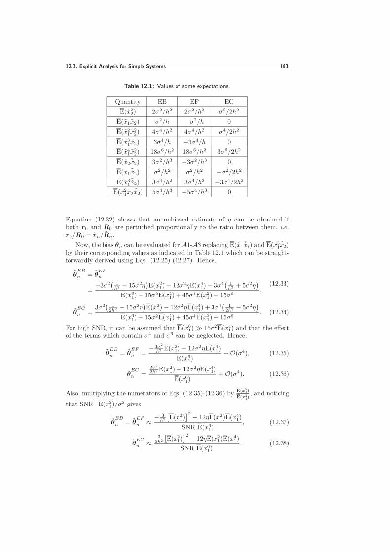
12.3. Explicit Analysis for Simple Systems 183
Table 12.1: Values of some expectations.
Quantity EB EF EC
E(x22) 2σ2/h2 2σ2/h2 σ2/2h2
E(x1x2) σ2/h −σ2/h 0
E(x21x
22) 4σ4/h2 4σ4/h2 σ4/2h2
E(x31x2) 3σ4/h −3σ4/h 0
E(x41x
22) 18σ6/h2 18σ6/h2 3σ6/2h2
E(x2˜x2) 3σ2/h3 −3σ2/h3 0
E(x1˜x2) σ2/h2 σ2/h2 −σ2/2h2
E(x31˜x2) 3σ4/h2 3σ4/h2 −3σ4/2h2
E(x21x2
˜x2) 5σ4/h3 −5σ4/h3 0
Equation (12.32) shows that an unbiased estimate of η can be obtained ifboth r0 and R0 are perturbed proportionally to the ratio between them, i.e.r0/R0 = rn/Rn.
Now, the bias θn can be evaluated for A1-A3 replacing E(x1˜x2) and E(x3
1˜x2)
by their corresponding values as indicated in Table 12.1 which can be straight-forwardly derived using Eqs. (12.25)-(12.27). Hence,
θEB
n = θEF
n
=−3σ2
(1h2 − 15σ2η
)E(x2
1) − 12σ2ηE(x41) − 3σ4
(1h2 + 5σ2η
)
E(x61) + 15σ2E(x4
1) + 45σ4E(x21) + 15σ6
,(12.33)
θEC
n =3σ2(
12h2 − 15σ2η
)E(x2
1) − 12σ2ηE(x41) + 3σ4
(1
2h2 − 5σ2η)
E(x61) + 15σ2E(x4
1) + 45σ4E(x21) + 15σ6
. (12.34)
For high SNR, it can be assumed that E(x61) ≫ 15σ2E(x4
1) and that the effectof the terms which contain σ4 and σ6 can be neglected. Hence,
θEB
n = θEF
n =− 3σ2
h2 E(x21) − 12σ2ηE(x4
1)
E(x61)
+ O(σ4), (12.35)
θEC
n =3σ2
2h2 E(x21) − 12σ2ηE(x4
1)
E(x61)
+ O(σ4). (12.36)
Also, multiplying the numerators of Eqs. (12.35)-(12.36) byE(x2
1)
E(x21)
, and noticing
that SNR=E(x21)/σ
2 gives
θEB
n = θEF
n ≈ − 3h2
[E(x2
1)]2 − 12ηE(x2
1)E(x41)
SNR E(x61)
, (12.37)
θEC
n ≈3
2h2
[E(x2
1)]2 − 12ηE(x2
1)E(x41)
SNR E(x61)
. (12.38)

184 12. Bias Analysis in LS Estimation of Periodic Signals
Therefore, θn satisfies the following relations for high SNR and for small h;
θn ∝ 1
SNR, (12.39)
θn ∝ 1
h2. (12.40)
Example 12.2. Random noise errors of S2.
In this case, φT =(x2 x1 x2
1x2
)and θ = (β α γ)T . Therefore
R = E(φφT ) = E
x2
2 x1x2 x21x
22
x1x2 x21 x3
1x2
x21x
22 x3
1x2 x41x
22
, (12.41)
and
r = E(φx2) = E
x2x2
x1x2
x21x2x2
. (12.42)
Similarly as done in Example 12.1, replacing x1, x2 and x2 by (x1+x1), (x2+x2)and (x2 + ˜x2), it follows that
R(1, 1) = E(x22) + E(x2
2), (12.43)
R(1, 2) = E(x1x2), (12.44)
R(1, 3) = E(x21x
22) + σ2E(x2
2) + E(x21)E(x2
2) + E(x21x
22), (12.45)
R(2, 2) = E(x21) + σ2, (12.46)
R(2, 3) = 3E(x21)E(x1x2) + E(x3
1x2), (12.47)
R(3, 3) = E(x41x
22) + 6σ2E(x2
1x22) + 3σ4E(x2
2)
+ E(x41)E(x2
2) + 6E(x21)E(x2
1x22) + E(x4
1x22), (12.48)
r(1) = E(x2˜x2), (12.49)
r(2) = αE(x21) + E(x1
˜x2), (12.50)
r(3) = βE(x21x
22) + γE(x4
1x22) + 2αE(x2
1)E(x1x2)
+ E(x21)E(x2
˜x2) + E(x21x2
˜x2). (12.51)
Hence, using Eq. (12.15) and Table 12.1, θn can be evaluated numerically forA1-A3.
Asymptotic expressions for the random noise bias on the parameters β,α and γ (denoted as βn, αn and γn, respectively) can be evaluated usingEq. (12.15), Table 12.1, and Eqs. (12.43)-(12.51). Straightforward calculationsassuming high SNR and small h for A3, see Appendix 12.A, give
βn ≈ E(x21)
2h2SNR×
β(E(x2
1)E(x21x
22) − E(x4
1x22))
+ γ(E(x4
1)E(x21x
22) − E(x2
1)E(x41x
22))
(E(x2
2)E(x41x
22) −
[E(x2
1x22)]2) ,
(12.52)

12.3. Explicit Analysis for Simple Systems 185
αn ≈ −1
2h2SNR, (12.53)
γn ≈ E(x21)
2h2SNR×
β(E(x2
1x22) − E(x2
1)E(x22))
+ γ(E(x2
1)E(x21x
22) − E(x4
1)E(x22))
(E(x2
2)E(x41x
22) −
[E(x2
1x22)]2) . (12.54)
Also, for β = −γ = ε, ‖θn‖ can be approximated as
‖θn‖ ≈ ε
2h2SNR
√L2 +Q2 +
1
ε2(12.55)
where
L = E(x21)(E(x2
1)E(x21x
22) + E(x2
1)E(x41x
22) − E(x4
1x22) − E(x4
1)E(x21x
22)),
(12.56)
Q = E(x21)(E(x2
1x22) + E(x4
1)E(x22) − E(x2
1)E(x22) − E(x2
1)E(x21x
22)). (12.57)
Hence
‖θn‖ ∝ 1
SNR, (12.58)
‖θn‖ ∝ 1
h2. (12.59)
12.3.2 Discretization errors
In this section the evaluation of discretization errors is considered. The data areassumed to be noise-free (i.e. x1(kh) = x1(kh)) and the estimates x2(kh) andx2(kh) are chosen as one of A1-A3. The discretization error contributions to
x2(kh) and x2(kh) can be evaluated using a Taylor series expansion assuming:
Assumption 12.1. The solution to the ODE model described by Eq. (5.18)is sufficiently differentiable.
The discretization errors for A1-A3 can be summarized as follows, see Ap-pendix 12.B:
• A1: (EB)
x2(kh) = −h2D2x1(kh) +
h2
6D3x1(kh) −
h3
24D4x1(kh) + O(h4),
˜x2(kh) = −hD2x2(kh) +7h2
12D3x2(kh) + O(h3).
(12.60)

186 12. Bias Analysis in LS Estimation of Periodic Signals
• A2: (EF)
x2(kh) =h
2D2x1(kh) +
h2
6D3x1(kh) +
h3
24D4x1(kh) + O(h4),
˜x2(kh) = hD2x2(kh) +7h2
12D3x2(kh) + O(h3).
(12.61)
• A3: (EC)
x2(kh) =h2
6D3x1(kh) +
h4
120D5x1(kh) + O(h6),
˜x2(kh) =h2
3D3x2(kh) + O(h4).
(12.62)
In the next two examples, discretization errors of S1 and S2 are evaluated.
Example 12.3. Discretization errors of S1.
Here φ = −x31. Thus R = E(x6
1) and r = E(−x31x2). Equation (12.9) gives
θ =E(−x3
1x2)
E(x61)
=E(−x3
1x2)
E(x61)︸ ︷︷ ︸
η
+E(−x3
1˜x2)
E(x61)︸ ︷︷ ︸
θd
. (12.63)
Noticing that (cf. Remark 12.7)
E(x31D
2x2) = E(x31Dx2) = E
(x3
1D[−ηx3
1
] )= −3ηE(x5
1x1) = 0, (12.64)
and using Eqs. (12.60)-(12.62), it follows that
θEB
d = θEF
d = −7h2
12
E(x31D
3x2)
E(x61)
+ O(h3), (12.65)
θEC
d = −h2
3
E(x31D
3x2)
E(x61)
+ O(h4). (12.66)
It also holds that x31D
3x2 = −6ηx41x
22 + 3η2x8
1. Therefore Eqs. (12.65)-(12.66)can alternatively be written as
θEB
d = θEF
d =7h2η
4
E(2x41x
22 − ηx8
1)
E(x61)
+ O(h3), (12.67)
θEC
d = h2ηE(2x4
1x22 − ηx8
1)
E(x61)
+ O(h4). (12.68)
The discretization errors of S1 can be reduced to be of O(h3) by consideringthe general differentiator form given in (12.17), see Appendix 12.C. Also, it isconcluded from Eqs. (12.67)-(12.68) that
θd ∝ h2. (12.69)

12.3. Explicit Analysis for Simple Systems 187
Now the total estimation bias θ can be found for S1 by the addition ofEqs. (12.67)-(12.68) and Eqs. (12.37)-(12.38), respectively. Thus
θEB
= θEF ≈ 7h2η
4
E(2x41x
22 − ηx8
1)
E(x61)
+− 3h2 [E(x2
1)]2 − 12ηE(x2
1)E(x41)
SNR E(x61)
,
(12.70)
θEC ≈ h2η
E(2x41x
22 − ηx8
1)
E(x61)
+3
2h2 [E(x21)]
2 − 12ηE(x21)E(x4
1)
SNR E(x61)
. (12.71)
Differentiating |θ|2 using Eqs. (12.70)-(12.71) w.r.t. the sampling period h tofind the optimal sampling period value that minimize the norm of the totalbias θ gives
hEBopt = hEFopt ≈∣∣∣∣
6[E(x21)]
2
7η SNR E(2x41x
22 − ηx8
1)
∣∣∣∣
14
, (12.72)
hECopt ≈[
6E(x21)E(x4
1)
SNR E(2x41x
22 − ηx8
1)
(1 −
√
1 − SNR E(2x41x
22 − ηx8
1)
24η[E(x41)]
2
)] 12
. (12.73)
Remark 12.8. Differentiating |θ|2 for S1 means solving 2θ dθdh = 0. Since
θEB
= 0 does not have any real roots, expression (12.72) was found by solvingdθ
EB
dh = 0. Expression (12.73) was found by solving θEC
= 0 for positive realroots.
Example 12.4. Discretization errors of S2.
In this case, φT =(x2 x1 x2
1x2
). Therefore
R = E(φφT )
= E
x2
2 x1x2 x21x
22
x1x2 x21 x3
1x2
x21x
22 x3
1x2 x41x
22
, (12.74)
and
r = E(φx2)
= E
x2x2
x1x2
x21x2x2
. (12.75)
Now using Eqs. (12.60)-(12.62), discretization errors on each component of Rand r can be computed. The results are given in Table 12.2, see Appendix 12.D.Also, discretization errors can be evaluated as a function of α, β and γ by usingDx2 = αx1 + βx2 + γx2
1x2. The results in this case are given in Table 12.3,see Appendix 12.D. Finally θd can be evaluated numerically for different Eulerapproximations using Eq. (12.16).

188 12. Bias Analysis in LS Estimation of Periodic Signals
Table
12.2
:D
iscretization
errorsofS
2.
Quan
tityE
BE
FE
C
Rd (1,1)
h23E
(x2 D
2x2 )
+h24E
(Dx
2 )2
h23E
(x2 D
2x2 )
+h24E
(Dx
2 )2
h23E
(x2 D
2x2 )
+O
(h4)
+O
(h3)
+O
(h3)
Rd (1,2)
−h2E
(x1 D
x2 )
+O
(h2)
h2E
(x1 D
x2 )
+O
(h2)
h26E
(x1 D
2x2 )
+O
(h4)
Rd (1,3
)−hE
(x21 x
2 Dx
2 )+O
(h2)
hE
(x21 x
2 Dx
2 )+O
(h2)
h23E
(x21 x
2 D2x
2 )+O
(h4)
Rd (2,2)
00
0
Rd (2,3)
−h2E
(x31 D
x2 )
+O
(h2)
h2E
(x31 D
x2 )
+O
(h2)
h26E
(x31 D
2x2 )
+O
(h4)
Rd (3,3
)−hE
(x41 x
2 Dx
2 )+O
(h2)
hE
(x41 x
2 Dx
2 )+O
(h2)
h23E
(x41 x
2 D2x
2 )+O
(h4)
rd (1
)−hE [x
2 D2x
2+
12(Dx
2 )2 ]
hE [x
2 D2x
2+
12(Dx
2 )2 ]
h2E [
16Dx
2 D2x
2+
13x
2 D3x
2 ]
+O
(h2)
+O
(h2)
+O
(h4)
rd (2)
−hE
(x1 D
2x2 )
+O
(h2)
hE
(x1 D
2x2 )
+O
(h2)
h23E
(x1 D
3x2 )
+O
(h4)
rd (3
)−hE [x
21 x2 D
2x2
+12x
21 (Dx
2 )2 ]
hE [x
21 x2 D
2x2
+12x
21 (Dx
2 )2 ]
h2E [
16x
21 Dx
2 D2x
2+
13x
21 x2 D
3x2 ]
+O
(h2)
+O
(h2)
+O
(h4)

12.3. Explicit Analysis for Simple Systems 189
Table
12.3
:D
iscr
etiz
atio
ner
rors
ofS
2as
afu
nct
ion
ofth
esy
stem
par
amet
ers.
Quantity
EB
EF
EC
Rd(1
,1)
h2
[ (α 3
+7β2
12
) E(x
2 2)+
α2
4E
(x2 1)
h2
[ (α 3
+7β2
12
) E(x
2 2)+
α2
4E
(x2 1)
h2 3
[ (α+
β2) E
(x2 2)+
2βγE
(x2 1x2 2)
+7β
γ6
E(x
2 1x2 2)+
2γ 3E
(x1x3 2)
+7β
γ6
E(x
2 1x2 2)+
2γ 3E
(x1x3 2)
+2γE
(x1x3 2)+
γ2E
(x4 1x2 2)]
+O
(h4)
+7γ2
12
E(x
4 1x2 2)]
+O
(h3)
+7γ2
12
E(x
4 1x2 2)]
+O
(h3)
Rd(1
,2)
−h 2
αE
(x2 1)+
O(h
2)
h 2αE
(x2 1)+
O(h
2)
h2 6
[ αβE
(x2 1)+
2γE
(x2 1x2 2)+
αγE
(x4 1)]
+O
(h4)
Rd(1
,3)
−h[ β
E(x
2 1x2 2)+
γE
(x4 1x2 2)]
+O
(h2)
h[ β
E(x
2 1x2 2)+
γE
(x4 1x2 2)]
+O
(h2)
h2 3
[ (α+
β2) E
(x2 1x2 2)+
2βγE
(x4 1x2 2)
+2γE
(x3 1x3 2)+
γ2E
(x6 1x2 2)]
+O
(h4)
Rd(2
,2)
00
0
Rd(2
,3)
−h 2
αE
(x4 1)+
O(h
2)
h 2αE
(x4 1)+
O(h
2)
h2 6
[ αβE
(x4 1)+
2γE
(x4 1x2 2)+
αγE
(x6 1)]
+O
(h4)
Rd(3
,3)
−h[ β
E(x
4 1x2 2)+
γE
(x6 1x2 2)]
+O
(h2)
h[ β
E(x
4 1x2 2)+
γE
(x6 1x2 2)]
+O
(h2)
h2 3
[ (α+
β2) E
(x4 1x2 2)+
2βγE
(x6 1x2 2)
+2γE
(x5 1x3 2)+
γ2E
(x8 1x2 2)]
+O
(h4)
rd(1
)−
h[ (
α+
3β2
2
) E(x
2 2)+
α2
2E
(x2 1)
h[ (
α+
3β2
2
) E(x
2 2)+
α2
2E
(x2 1)
h2
[ α2β
6E
(x2 1)+
γ( 1
9α
6+
3β2
2
) E(x
2 1x2 2)+
α2γ
6E
(x4 1)
+3βγE
(x2 1x2 2)+
2γE
(x1x3 2)
+3βγE
(x2 1x2 2)+
2γE
(x1x3 2)
+β( 5
α 6+
β2
2
) E(x
2 2)+
3βγE
(x1x3 2)+
3β
γ2
2E
(x4 1x2 2)
+3γ2
2E
(x4 1x2 2)]
+O
(h2)
+3γ2
2E
(x4 1x2 2)]
+O
(h2)
+3γ2E
(x3 1x3 2)+
γ3 2E
(x6 1x2 2)+
2γ 3E
(x4 2)]
+O
(h4)
rd(2
)−
h[ α
βE
(x2 1)+
2γE
(x2 1x2 2)+
αγE
(x4 1)]
h[ α
βE
(x2 1)+
2γE
(x2 1x2 2)+
αγE
(x4 1)]
h2 3
[ α(α
+β
2) E
(x2 1)+
2α
βγE
(x4 1)+
8βγE
(x2 1x2 2)
+O
(h2)
+O
(h2)
+2γE
(x1x3 2)+
8γ2E
(x4 1x2 2)+
αγ2E
(x6 1)]
+O
(h4)
rd(3
)−
h[ (
α+
3β2
2
) E(x
2 1x2 2)+
α2
2E
(x4 1)
h[ (
α+
3β2
2
) E(x
2 1x2 2)+
α2
2E
(x4 1)
h2
[ α2β
6E
(x4 1)+
γ( 1
9α
6+
3β2
2
) E(x
4 1x2 2)+
α2γ
6E
(x6 1)
+3βγE
(x4 1x2 2)+
2γE
(x3 1x3 2)
+3βγE
(x4 1x2 2)+
2γE
(x3 1x3 2)
+β( 5
α 6+
β2
2
) E(x
2 1x2 2)+
3βγE
(x3 1x3 2)+
3β
γ2
2E
(x6 1x2 2)
+3γ2
2E
(x6 1x2 2)]
+O
(h2)
+3γ2
2E
(x6 1x2 2)]
+O
(h2)
+3γ2E
(x5 1x3 2)+
γ3 2E
(x8 1x2 2)+
2γ 3E
(x2 1x4 2)]
+O
(h4)

190 12. Bias Analysis in LS Estimation of Periodic Signals
In Appendix 12.E, asymptotic expressions for the discretization bias on theparameters β, α and γ (denoted as βd, αd and γd, respectively) using A3 arederived at high SNR and it is proved that
‖θd‖ ∝ h2. (12.76)
Now using Eqs. (12.52)-(12.54) and Eqs. (12.129)-(12.131) the norm of the totalestimation bias is given by
‖θ‖ ≈√
(βn + βd)2 + (αn + αd)2 + (γn + γd)2. (12.77)
Differentiating ‖θ‖2 w.r.t. the sampling period h gives (for β = −γ = ε)
hECopt ≈
∣∣∣∣∣∣9
(SNR)2×
|R0|2[E(x2
1)]2
+ ε2[E(x21)]
2(T 21 + T 2
5 )
4|R0|2[E(x2
1)]4T 2
4 + 4(T 22 + T 2
6 ) + ε2(T 23 + T 2
7 ) + 4ε(T2T3 + T6T7)
∣∣∣∣∣∣
18
(12.78)where
T1 =E(x21)E(x2
1x22) − E(x4
1x22) − E(x4
1)E(x21x
22) + E(x2
1)E(x41x
22), (12.79)
T2 =E(x41x
22)E(x2D
3x2) − E(x21x
22)E(x2
1x2D3x2), (12.80)
T3 =E(x21x
22)E(x2
1x2D2x2) − E(x4
1x22)E(x2D
2x2)
− E(x21x
22)E(x4
1x2D2x2) + E(x4
1x22)E(x2
1x2D2x2), (12.81)
T4 =E(x1D3x2) −
ε
2E(x1D
2x2) +ε
2E(x3
1D2x2), (12.82)
T5 =E(x21x
22) − E(x2
1)E(x22) − E(x2
1)E(x21x
22) + E(x4
1)E(x22), (12.83)
T6 =E(x22)E(x2
1x2D3x2) − E(x2
1x22)E(x2D
3x2), (12.84)
T7 =E(x21x
22)E(x2D
2x2) − E(x22)E(x2
1x2D2x2)
− E(x21x
22)E(x2
1x2D2x2) + E(x2
2)E(x41x2D
2x2). (12.85)
Similarly, analytical expressions for hEBopt and hEFopt can be derived by repeatingthe analysis of Appendix 12.A and Appendix 12.E for A1 and A2, respectively.
12.4 Numerical Study
In this section a numerical study of the estimation errors of S1 and S2 usingA1-A3 is given. The study is based on numerical evaluation of the truncatedanalytical expressions derived in Section 12.3. In the numerical calculation ofthe derived expressions, E(f(t)) was approximated by 1
N
∑Nt=1 f(t).

12.4. Numerical Study 191
0 10 20 30 40 50 60 70 80−60
−50
−40
−30
−20
−10
0
10
20
30
SNR [dB]
|Bia
s| [
dB
]
EB & EFEC
Figure 12.1: |θn| vs. SNR for S1 [η = 2, h = 0.05 s].
0 10 20 30 40 50 60 70 80−50
−40
−30
−20
−10
0
10
20
30
SNR [dB]
No
rm o
f th
e b
ias
vect
or
[dB
]
EBEFEC
Figure 12.2: ‖θn‖ vs. SNR for S2 [α = −1, β = −γ = 2, h = 0.05 s].
Example 12.5. Random noise error study.
In this example 104 data samples were generated from S1 and S2 using theMatlab routine ode45 for η = 2, α = −1, β = 2 and γ = −2. The ini-
tial states of S1 and S2 were selected as(x1(0) x2(0)
)T=(0 1
)Tand
(x1(0) x2(0)
)T=(2 0
)T, respectively. These initial states were chosen so
that transient effects can be neglected. First, the bias error for these systemswas studied at different SNRs with a sampling period h = 0.05 s. Second, thebias was studied at different sampling periods. In this case, the SNR was 50 dBfor S1 and 60 dB for S2. Finally, the bias was studied for different values ofthe system parameters. The results are shown in Figures 12.1-12.6.
As it is shown in the log-log scale Figures 12.1-12.2, log ‖θn‖ using A1-A3 isproportional to
(− log(SNR) + constant
)for moderate and high SNR. Also, it

192 12. Bias Analysis in LS Estimation of Periodic Signals
−3 −2.8 −2.6 −2.4 −2.2 −2 −1.8 −1.6 −1.4 −1.2 −1−30
−25
−20
−15
−10
−5
0
5
10
15
20
log10
(h)
|Bia
s| [
dB
]
EB & EFEC
Figure 12.3: |θn| vs. h for S1 [η = 2, SNR = 50 dB].
−3 −2.8 −2.6 −2.4 −2.2 −2 −1.8 −1.6 −1.4 −1.2 −1−40
−30
−20
−10
0
10
20
30
log10
(h)
No
rm o
f th
e b
ias
vect
or
[dB
]
EBEFEC
Figure 12.4: ‖θn‖ vs. h for S2 [α = −1, β = −γ = 2, SNR = 60 dB].
can be concluded from the log-log scale Figures 12.3-12.4 that log ‖θn‖ is pro-portional to
(− log(h) + constant
). These results match the derived asymp-
totic results in Eqs. (12.39)-(12.40) and Eqs. (12.58)-(12.59), and the earlierexpectation that random noise errors and its corresponding bias θn can bereduced by increasing the sampling period h or using smaller h whenever theSNR is high. Also, it can be noticed that A3 gives the lowest bias as expected.
Figures 12.5-12.6 show that the random noise bias increases as the valueof η in S1 and ε in S2 (β = ε, γ = −ε) is increased. This is so because thenonlinear dynamics of the systems S1 and S2 become more effective as η and ε,respectively, increases. Hence, the signals generated by S1 and S2 become morenonlinearly distorted and the accuracy of the finite difference approximationsdecreases.
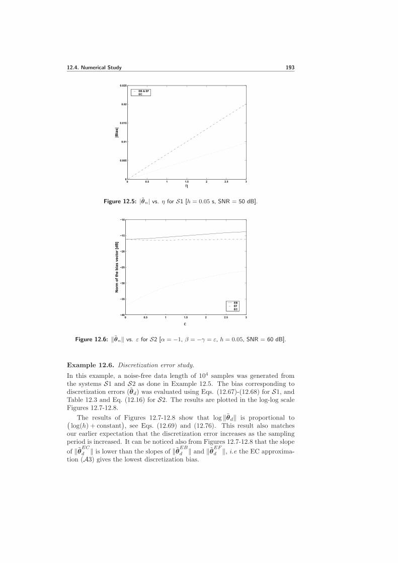
12.4. Numerical Study 193
0 0.5 1 1.5 2 2.5 30
0.005
0.01
0.015
0.02
0.025
η
|Bia
s|
EB & EFEC
Figure 12.5: |θn| vs. η for S1 [h = 0.05 s, SNR = 50 dB].
0 0.5 1 1.5 2 2.5 3−40
−35
−30
−25
−20
−15
−10
ε
No
rm o
f th
e b
ias
vect
or
[dB
]
EBEFEC
Figure 12.6: ‖θn‖ vs. ε for S2 [α = −1, β = −γ = ε, h = 0.05, SNR = 60 dB].
Example 12.6. Discretization error study.
In this example, a noise-free data length of 104 samples was generated fromthe systems S1 and S2 as done in Example 12.5. The bias corresponding todiscretization errors (θd) was evaluated using Eqs. (12.67)-(12.68) for S1, andTable 12.3 and Eq. (12.16) for S2. The results are plotted in the log-log scaleFigures 12.7-12.8.
The results of Figures 12.7-12.8 show that log ‖θd‖ is proportional to(log(h) + constant
), see Eqs. (12.69) and (12.76). This result also matches
our earlier expectation that the discretization error increases as the samplingperiod is increased. It can be noticed also from Figures 12.7-12.8 that the slope
of ‖θECd ‖ is lower than the slopes of ‖θEBd ‖ and ‖θEFd ‖, i.e the EC approxima-tion (A3) gives the lowest discretization bias.

194 12. Bias Analysis in LS Estimation of Periodic Signals
−2.6 −2.4 −2.2 −2 −1.8 −1.6 −1.4 −1.2 −1−5
−4.5
−4
−3.5
−3
−2.5
−2
−1.5
−1
log10
(h)
|Bia
s| [
dB
]
EB & EFEC
Figure 12.7: θd vs. h for S1 [η = 2].
−2.6 −2.4 −2.2 −2 −1.8 −1.6 −1.4 −1.2 −1−40
−35
−30
−25
−20
−15
−10
−5
0
log10
(h)
No
rm o
f th
e b
ias
vect
or
[dB
]
EBEFEC
Figure 12.8: ‖θd‖ vs. h for S2 [α = −1, β = −γ = 2].
Also, θd can be evaluated for different system parameters. The results areshown in Figures 12.9-12.10. These figures show that ‖θd‖ increases as thevalue of η in S1 and ε in S2 is increased. This behaviour can be explainedhere, as done in Example 12.5, by the accuracy reduction of the derivativeapproximations due to increasing the nonlinear dynamics of the two systems.
It can be concluded from Example 12.5 and Example 12.6 that there are twocontradicting requirements to obtain an accurate estimate for the parametervector θ using the least squares estimation algorithm. A small sampling periodh is needed to reduce the bias contribution due to discretization errors θd, anda large h is required to reduce the bias contribution due to random noise errorsθn. Therefore, it is expected that there is an optimal sampling period hopt thatachieves minimum total estimation bias. This hopt can be easily determined by

12.4. Numerical Study 195
0 0.5 1 1.5 2 2.5 30
0.002
0.004
0.006
0.008
0.01
0.012
0.014
0.016
0.018
η
|Bia
s|
EB & EFEC
Figure 12.9: |θd| vs. η for S1 [h = 0.05 s].
0 0.5 1 1.5 2 2.5 30
0.1
0.2
0.3
0.4
0.5
0.6
0.7
ε
No
rm o
f th
e b
ias
vect
or
EBEFEC
Figure 12.10: ‖θd‖ vs. ε for S2 [α = −1, β = −γ = ε, h = 0.05 s].
adding the two bias contributions and plotting the results versus h as shownin Figures 12.11-12.12. Figure 12.11 shows that hopt = 0.052 s gives minimumestimation bias for S1. The evaluation of the approximate analytical values ofhEBopt (= hEFopt ) and hECopt , see Eqs. (12.72)-(12.73), gives 0.0425 s and 0.0490 s,respectively. Figure 12.12 shows that hopt = 0.03 s for S2 in case EB or EFapproximations are used. On the other hand, if EC approximation is used, theoptimal sampling period is hopt = 0.02 s. The expression of hECopt in Eq. (12.78)gives 0.0190 s.
The difference between the value of hopt concluded from Fig. 12.11 and thederived analytical expressions for S1 is expected to be reduced as the SNRincreases. This is due to the fact that the analytical expressions are derivedfor high SNR values. In order to verify this expectation, the total estimationbias was re-evaluted for SNR=70 dB. The results in this case are given in

196 12. Bias Analysis in LS Estimation of Periodic Signals
0 0.01 0.02 0.03 0.04 0.05 0.06 0.07 0.08 0.09 0.1−120
−100
−80
−60
−40
−20
0
20
h
To
tal e
stim
atio
n b
ias
[dB
]
EB & EFEC
Figure 12.11: |θ| vs. h for S1 [η = 2, SNR=50 dB].
0 0.01 0.02 0.03 0.04 0.05 0.06 0.07 0.08 0.09 0.1−20
−15
−10
−5
0
5
10
15
20
25
30
h
No
rm o
f to
tal e
stim
atio
n b
ias
vect
or
[dB
]
EBEFEC
Figure 12.12: ‖θ‖ vs. h for S2 [α = −1, β = −γ = 2, SNR=60 dB].
Fig. 12.13. Figure 12.13 shows that hopt = 0.016 s. The evaluation of theapproximate analytical values of hEBopt and hECopt in this case gives 0.0133 s and0.0153 s, respectively.
12.5 Conclusions
Estimation errors in the LS modeling of periodic signals using second-order non-linear ODE have been studied in this chapter. The estimation of the parametersof two nonlinear systems were considered using different Euler approximationtechniques. The analysis shows that the sampling period (h) plays a criticalrole in the performance of the LS estimation algorithm. Asymptotic analyticalexpressions show that
‖θn‖ ∝ 1h2SNR , ‖θd‖ ∝ h2

12.A. Asymptotic Random Noise Bias for S2 Using A3 197
0 0.005 0.01 0.015 0.02 0.025 0.03 0.035−110
−100
−90
−80
−70
−60
−50
−40
−30
−20
h
To
tal e
stim
atio
n b
ias
[dB
]
EB & EFEC
Figure 12.13: |θ| vs. h for S1 [η = 2, SNR=70 dB].
and that the estimation bias increases whenever the nonlinear dynamics becomemore effective. Hence, the existence of an optimal sampling period hopt thatachieves the lowest estimation bias is expected. It is shown in the chapter howan analytical expression for hopt can be derived in a systematic way for differentperiodic nonlinear systems.
12.A Asymptotic Random Noise Bias for S2 Using A3
Using Table 12.1 and Eqs. (12.43)-(12.51), it follows that (neglecting σ4 andσ6 terms)
R(1, 1) = E(x22) +
σ2
2h2, (12.86)
R(1, 2) = 0, (12.87)
R(1, 3) = E(x21x
22) + σ2E(x2
2) +σ2
2h2E(x2
1), (12.88)
R(2, 2) = E(x21) + σ2, (12.89)
R(2, 3) = 0, (12.90)
R(3, 3) = E(x41x
22) + 6σ2E(x2
1x22) +
σ2
2h2E(x4
1), (12.91)
r(1) = 0, (12.92)
r(2) = αE(x21) −
σ2
2h2, (12.93)
r(3) = βE(x21x
22) + γE(x4
1x22). (12.94)
Hence
rn = σ2(
0 − 12h2 0
)T+ O(σ4), (12.95)

198 12. Bias Analysis in LS Estimation of Periodic Signals
and
Rn = σ2
1
2h2 0 E(x22) + 1
2h2 E(x21)
0 1 0E(x2
2) + 12h2 E(x2
1) 0 6E(x21x
22) + 1
2h2 E(x41)
+O(σ4). (12.96)
Substituting by Eqs. (12.86)-(12.96) in Eq. (12.15) after evaluating R−1 gives
βn =βσ2
D
(E(x2
2)E(x21x
22) +
1
2h2E(x2
1)E(x21x
22) −
1
2h2E(x4
1x22)
)+γσ2
D ×(
1
2h2E(x4
1)E(x21x
22) + 6
[E(x2
1x22)]2 − 1
2h2E(x2
1)E(x41x
22) − E(x2
2)E(x41x
22)
)
+ O(σ4), (12.97)
αn =−σ2
(1
2h2 + α)
E(x21)
+ O(σ4), (12.98)
γn =βσ2
D
(1
2h2E(x2
1x22) − [E(x2
2)]2 − 1
2h2E(x2
1)E(x22)
)+γσ2
D ×(
1
2h2E(x2
1)E(x21x
22) − 5E(x2
2)E(x21x
22) −
1
2h2E(x4
1)E(x22)
)+ O(σ4),
(12.99)
where
D = E(x22)E(x4
1x22) −
[E(x2
1x22)]2
+ O(σ2). (12.100)
Multiplying the numerators and denominators of Eqs. (12.97)-(12.99) by
2h2 E(x21)
σ2 gives
βn ≈βE(x21)
D(2h2E(x2
2)E(x21x
22) + E(x2
1)E(x21x
22) − E(x4
1x22))
+γE(x2
1)
D ×(2h2(6[E(x2
1x22)]
2 − E(x22)E(x4
1x22))
+ E(x41)E(x2
1x22) − E(x2
1)E(x41x
22)),
(12.101)
αn ≈ −(1 + 2h2α)
D ×(E(x2
2)E(x41x
22) −
[E(x2
1x22)]2)
, (12.102)
γn ≈βE(x21)
D(− 2h2
[E(x2
2)]2
+ E(x21x
22) − E(x2
1)E(x22))
+γE(x2
1)
D ×(− 10h2E(x2
2)E(x21x
22) + E(x2
1)E(x21x
22) − E(x4
1)E(x22)), (12.103)
where
D ≈ 2h2SNR(E(x2
2)E(x41x
22) −
[E(x2
1x22)]2)
. (12.104)
Substituting by (12.104) in Eqs. (12.101)-(12.103) gives Eqs. (12.52)-(12.54).
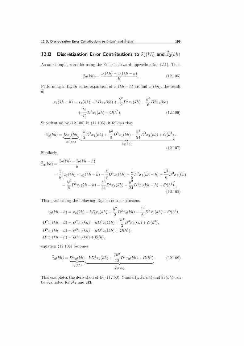
12.B. Discretization Error Contributions to x2(kh) and x2(kh) 199
12.B Discretization Error Contributions to x2(kh) and x2(kh)
As an example, consider using the Euler backward approximation (A1). Then
x2(kh) =x1(kh) − x1(kh− h)
h. (12.105)
Performing a Taylor series expansion of x1(kh − h) around x1(kh), the resultis
x1(kh− h) = x1(kh) − hDx1(kh) +h2
2D2x1(kh) −
h3
6D3x1(kh)
+h4
24D4x1(kh) + O(h5). (12.106)
Substituting by (12.106) in (12.105), it follows that
x2(kh) = Dx1(kh)︸ ︷︷ ︸x2(kh)
−h2D2x1(kh) +
h2
6D3x1(kh) −
h3
24D4x1(kh) + O(h4)
︸ ︷︷ ︸x2(kh)
.
(12.107)Similarly,
x2(kh) =x2(kh) − x2(kh− h)
h
=1
h
[x2(kh) − x2(kh− h) − h
2D2x1(kh) +
h
2D2x1(kh− h) +
h2
6D3x1(kh)
− h2
6D3x1(kh− h) − h3
24D4x1(kh) +
h3
24D4x1(kh− h) + O(h4)
].
(12.108)
Thus performing the following Taylor series expansions
x2(kh− h) = x2(kh) − hDx2(kh) +h2
2D2x2(kh) −
h3
6D3x2(kh) + O(h4),
D2x1(kh− h) = D2x1(kh) − hD3x1(kh) +h2
2D4x1(kh) + O(h3),
D3x1(kh− h) = D3x1(kh) − hD4x1(kh) + O(h2),
D4x1(kh− h) = D4x1(kh) + O(h),
equation (12.108) becomes
x2(kh) = Dx2(kh)︸ ︷︷ ︸x2(kh)
−hD2x2(kh) +7h2
12D3x2(kh) + O(h3)
︸ ︷︷ ︸˜x2(kh)
. (12.109)
This completes the derivation of Eq. (12.60). Similarly, x2(kh) and x2(kh) canbe evaluated for A2 and A3.

200 12. Bias Analysis in LS Estimation of Periodic Signals
12.C Discretization Error of Order O(h3) for S1
For S1
E(x61)η = −E(x1x
31)
= −E
1
h2
∑
j
Γ2,jx1(kh+ jh) × x31(kh)
= − 1
h2
∑
j
Γ2,jE
[ ∞∑
v=0
1
v!(jh)vDvx1 × x3
1
]
= − 1
h2
∞∑
v=0
1
v!hv(∑
j
Γ2,jjv
)E(Dvx1 × x3
1
).
(12.110)
Now using (12.18) and noticing that E(x31D
3x1) = E(x31D
2x2) = 0 from (12.64),straightforward calculations give
η = η − 1
E(x61)
∞∑
v=4
1
v!hv−2
(∑
j
Γ2,jjv
)E(Dvx1 × x3
1
)
= η + η2h2 + η3h
3 + · · ·︸ ︷︷ ︸η
(12.111)
In order to have discretization errors of O(h3), η2 should hence be equal to 0.Since
η2 = − 1
4!E(x61)
(∑
j
Γ2,jj4
)E(D4x1 × x3
1
), (12.112)
η2 = 0 if ∑
j
Γ2,jj4 = 0.
One can design the differentiation filter so that∑j Γ2,jj
4 = 0. For example,consider using a filter with 5 coefficients based on EF and EB approximationsand including low pass filter effects with unity static gain, i.e.
H(q) =(q − ρ)
(1 − ρ)(q − 1)(1 − q−1)
(ρ− q−1)
(ρ− 1), (12.113)
where ρ is a free parameter to be determined to achieve that∑2j=−2 Γ2,jj
4 = 0.In this case it holds that
Γ2,0 = −2(1 + ρ+ ρ2)
(1 − ρ)2,
Γ2,1 = Γ2,−1 =(1 + ρ)2
(1 − ρ)2,
Γ2,2 = Γ2,−2 = − ρ
(1 − ρ)2.
(12.114)

12.D. Results of Table 12.2 and Table 12.3 201
Thus
2∑
j=−2
Γ2,jj4 =
1
(1 − ρ)2[−2ρ(2)4 + 2(1 + ρ)2(1)4 − 2(1 + ρ+ ρ2)(0)4
]
=2
(1 − ρ)2(ρ2 − 14ρ+ 1
).
(12.115)
It follows that∑2j=−2 Γ2,jj
4 = 0 for ρ = 7 ± 4√
3. Therefore, choosing
ρ = 7 − 4√
3 or ρ = 7 + 4√
3 gives
η = η3h3 + O(h4)
= −h3E(x3
1D4x2
)
5!(1 − ρ)2[−2ρ(2)5 + 2(1 + ρ)2
]+ O(h4)
= −h3
15E(x3
1D4x2
)+ O(h4).
(12.116)
12.D Results of Table 12.2 and Table 12.3
Consider the first element in Table 12.2, i.e. Rd(1, 1) in the EB approximation.Using Eqs. (12.74) and (12.107), it follows that
R(1, 1) = E{x22}
= E{x2 −h
2Dx2 +
h2
6D2x2 + O(h3)}2
= E(x22)︸ ︷︷ ︸
R0(1,1)
−hE(x2Dx2) +h2
3E(x2D
2x2) +h2
4E(Dx2)
2 + O(h3)︸ ︷︷ ︸
Rd(1,1)
.
(12.117)
Taking into account that E(x2Dx2) = 0, cf. Remark 12.7, it follows that
Rd(1, 1) =h2
3E(x2D
2x2) +h2
4E(Dx2)
2 + O(h3). (12.118)
Similarly, the remaining elements of Table 12.2 can be systematically evaluated.
In Table 12.3, Rd(1, 1) can be also expressed as a function of the systemparameters exploiting the fact that
Dx2 = αx1 + βx2 + γx21x2. (12.119)
Hence
D2x2 = D(αx1 + βx2 + γx21x2)
= αx2 + βDx2 + γ(2x1x22 + x2
1Dx2). (12.120)

202 12. Bias Analysis in LS Estimation of Periodic Signals
Now reusing Dx2 = αx1 + βx2 + γx21x2 in (12.120) and substituting in
(12.118), it follows that
Rd(1, 1) = h2
[(α
3+
7β2
12
)E(x2
2) +α2
4E(x2
1) +7βγ
6E(x2
1x22)
+2γ
3E(x1x
32) +
7γ2
12E(x4
1x22)
]. (12.121)
Following the same procedure, the remaining terms of Table 12.3 can be eval-uated.
12.E Asymptotic Discretization Bias for S2 Using A3
From Table 12.2
rd − Rdθ0 =
h2
13E(x2D
3x2) − β6 E(x2D
2x2) − γ6 E(x2
1x2D2x2)
13E(x1D
3x2) − β6 E(x1D
2x2) − γ6 E(x3
1D2x2)
13E(x2
1x2D3x2) − β
6 E(x21x2D
2x2) − γ6 E(x4
1x2D2x2)
+ O(h4),
(12.122)
R =
E(x2
2) + h2
3 E(x2D2x2)
h2
6 E(x1D2x2) E(x2
1x22) + h2
3 E(x21x2D
2x2)h2
6 E(x1D2x2) E(x2
1)h2
6 E(x31D
2x2)
E(x21x
22) + h2
3 E(x21x2D
2x2)h2
6 E(x31D
2x2) E(x41x
22) + h2
3 E(x41x2D
2x2)
+ O(h4). (12.123)
Inverting R and substituting in (12.16) gives (neglecting h4 terms)
βd ≈h2E(x2
1)
3|R|
[(E(x4
1x22)E(x2D
3x2) − E(x21x
22)E(x2
1x2D3x2)
)
+β
2
(E(x2
1x22)E(x2
1x2D2x2) − E(x4
1x22)E(x2D
2x2))
+γ
2
(E(x2
1x22)E(x4
1x2D2x2) − E(x4
1x22)E(x2
1x2D2x2)
)],
(12.124)
αd ≈h2
3|R|
[(E(x2
2)E(x41x
22) −
[E(x2
1x22)]2)×
(E(x1D
3x2) −β
2E(x1D
2x2) −γ
2E(x3
1D2x2)
)], (12.125)

12.E. Asymptotic Discretization Bias for S2 Using A3 203
γd ≈h2E(x2
1)
3|R|
[(E(x2
2)E(x21x2D
3x2) − E(x21x
22)E(x2D
3x2))
+β
2
(E(x2
1x22)E(x2D
2x2) − E(x22)E(x2
1x2D2x2)
)
+γ
2
(E(x2
1x22)E(x2
1x2D2x2) − E(x2
2)E(x41x2D
2x2))], (12.126)
where
|R| = E(x21)(E(x2
2)E(x41x
22) − [E(x2
1x22)]
2)
+ O(h2). (12.127)
For a small sampling period, |R| can be approximated again to be
|R| ≈ E(x21)(E(x2
2)E(x41x
22) − [E(x2
1x22)]
2)
= |R0|. (12.128)
Substituting by (12.128) in Eqs. (12.124)-(12.126), results in
βd ≈h2E(x2
1)
3|R0|
[(E(x4
1x22)E(x2D
3x2) − E(x21x
22)E(x2
1x2D3x2)
)
+β
2
(E(x2
1x22)E(x2
1x2D2x2) − E(x4
1x22)E(x2D
2x2))
+γ
2
(E(x2
1x22)E(x4
1x2D2x2) − E(x4
1x22)E(x2
1x2D2x2)
)],
(12.129)
αd ≈h2
3E(x21)
(E(x1D
3x2) −β
2E(x1D
2x2) −γ
2E(x3
1D2x2)
), (12.130)
γd ≈h2E(x2
1)
3|R0|
[(E(x2
2)E(x21x2D
3x2) − E(x21x
22)E(x2D
3x2))
+β
2
(E(x2
1x22)E(x2D
2x2) − E(x22)E(x2
1x2D2x2)
)
+γ
2
(E(x2
1x22)E(x2
1x2D2x2) − E(x2
2)E(x41x2D
2x2))]. (12.131)
Hence, Eq. (12.76) is concluded from Eqs. (12.129)-(12.131).


Part III
User Aspects and Future Research
205


Chapter 13
User Aspects
13.1 Introduction
TWO nonlinear approaches for modeling periodic signals were suggested inPart I and Part II of this thesis. Also, a review of the existing approaches
to the same problem was given in Chapter 1. In this chapter, different useraspects for the two suggested approaches are discussed. In the next chaptersome comments on the different approaches to the problem of modeling periodicsignals are given, and some topics for future research are presented.
13.2 User Aspects for the Approach of Part I
In this section, different user aspects for the approach of modeling periodicsignals based on the Wiener model structure are presented. The approach wasstudied in Chapters 2-4.
13.2.1 Modeled Signal
The approach of Part I can deal with a wide class of periodic signals. Itis suitable for the cases where the modeled signal is affected particularly byunderlying static nonlinear distortion. In this case, the approach can provideestimates for the fundamental frequency and the static nonlinearity. Also, theapproach can track frequency and amplitude variations in the periodic signal,see Examples 2.3, 3.4, 4.3-4.4.
13.2.2 Choice of the Algorithm
Three algorithms were introduced in Part I, namely: Algorithm (2.9), Algo-rithm (3.9) and Algorithm (4.8). Algorithm (2.9) was introduced in [121] forjoint estimation of the fundamental frequency of the periodic signal and theparameters of the output nonlinear function, cf. Chapter 2. In order to obtaina treatment of the local convergence properties of the RPEM of Chapter 2,the static gain of the Wiener model structure was fixed in a subinterval Io inthe static block instead of being fixed in the linear block. This modification
207

208 13. User Aspects
resulted in Algorithm (3.9), cf. Chapter 3. The adaptive grid algorithm (Algo-rithm (4.8)) was introduced in Chapter 4 to recursively estimate the grid pointsin addition to the fundamental frequency and the parameters of the static non-linearity. It was shown that Algorithm (4.8) gives more accurate estimatesthan Algorithm (3.9), cf. Fig. 4.4. This is due to the fact that Algorithm (4.8)has more freedom to select the grid points and hence a reduction of modelingerrors is achieved.
13.2.3 Grid Points
The choice of the grid points for the approach of Part I is essential to obtaina good model accuracy, especially for Algorithm (2.9) and Algorithm (3.9).These grid points are chosen by the user depending on any prior informationabout the modeled signal. For example the peak to peak value of the wave formhelps to determine the grids range for each interval. Intervals with distortedamplitude such as the case of the flute data in Example 3.5, see Fig. 3.4(a) andEq. (3.51), require a higher number of grid points to identify all the details ofthe static nonlinearity.
Estimating the grid points recursively in addition to the driving frequencyand the parameters of the nonlinear output function was considered in Algo-rithm (4.8) resulting in an automatic grid point adaptation. One advantage isthat less effort need to be spent on the selection of the grid points. Note that aninitial value of the grid points need to be provided though. The improvementin the accuracy obtained in Example 4.2 by using Algorithm (4.8) instead ofAlgorithm (3.9), see Fig 4.4, indicates the importance of a good selection forthe grid points.
Also, the performance of the algorithms was studied in Chapters 3-4 withthe number of grid points, see Figures 3.6, 4.7. It can be concluded that theperformance improves as the number of grid points increases to some extent.Beyond this extent, further increase of the grid points does not improve theperformance. On the contrary, an unnecessary increase of the grid points maylead to a reduction of the accuracy due to over-parameterization.
13.2.4 Nonlinear Modeler
One of the main objectives of the approach of Part I is to estimate the staticnonlinearity. Since the static nonlinearity is unknown, a nonlinear modeleris needed. In Section 1.4.2 different possibilities to parameterize the staticnonlinearity were suggested.
In this thesis piecewise linear and piecewise quadratic polynomials wereconsidered. It is expected that a piecewise polynomial is sufficient to obtainaccurate models in case an enough number of grid points are considered. In thecase of using a small number of grid points, it is more proper to consider higherorder polynomials to reduce modeling errors. Needless to say considering otherpossibilities to parameterize the static nonlinearity, see Section 1.4.2, requiresmodification of the gradient calculations of the algorithms of Part I.

13.2. User Aspects for the Approach of Part I 209
13.2.5 Additive Noise
The approach of Part I can handle - with good efficiency - periodic signalswith low signal to noise ratio (SNR). This can be noticed from the results ofFig. 1.16(d). Also, note that this noise can be colored, see [121]. Further, sincean output error approach is used, the sensitivity to high frequency modelingerrors can be expected to be better than, e.g., LS methods, see [114].
13.2.6 Local Minima
Due to the complexity of the prediction error criterion (2.5), it is minimizedby a Gauss-Newton method in this thesis. Hence, starting with good initialestimates is essential for the approach to guarantee convergence of the Gauss-Newton method to a local minimum of the criterion function. This was takeninto consideration for example when the flute data were modeled in Exam-ple 3.5. Therefore, a good initial value of the fundamental frequency was ob-tained using the periodogram. Note that convergence to false local minima isa general problem when output error techniques are used.
13.2.7 Design Variables
The algorithms introduced in Part I require initialization of P (t), R1(t), r2(t)and the forgetting factor λ(t). The guidelines for choosing these quantities arediscussed in detail in Chapter 5 of [69]. In general, the choice of these initialvalues follows the lines:
• P (0) is usually chosen as P (0) = ρI. A large value of ρ makes the
initial value of the parameter vector θ(0) only marginally important.The parameter estimates in this case will change quickly in the transientperiod. A small value of ρ means that much confidence is put in the priorknowledge of θ(0). In this case θ(t) will converge slowly.
• R1(t) should be chosen constant and diagonal, i.e. R1(t) = r1I if nodetailed knowledge about the system dynamics is at hand. Note alsothat only the ratio r1/r2 will influence the parameter estimates. In casethere is a need to speed up the convergence or the tracking of someparameters, the diagonal weights of the matrix R1(t) corresponding tothese parameters are given higher values, cf. Examples 2.3, 3.4, 4.3-4.4.
• λ(t) is very often chosen to grow exponentially using the relation
λ(t) = λoλ(t− 1) + 1 − λo.
This choice was suggested to achieve optimal asymptotic accuracy forreasonably long data sequences, see [69]. The values λ(0) = 0.95 andλo = 0.99 have been proved to be useful in many cases.

210 13. User Aspects
13.2.8 Computational Complexity
In general, the complexity of the algorithms (2.9), (3.9) and (4.8) of Part Iis low. More specifically, it is monotonically increasing from Algorithm (2.9)to Algorithm (4.8). This follows as a consequence of increasing the size ofthe parameter vector. Also, the computational complexity of each individualalgorithm increases as the number of grid points chosen by the user is increased.
13.3 User Aspects for the Approach of Part II
Different user aspects for the approach of modeling periodic signals using orbitsof second-order nonlinear ODE’s are presented in this section. The approachwas studied in detail in Chapters 5-12.
13.3.1 Modeled Signal
The approach of modeling periodic signals using a second-order nonlinear ODEmodel is suitable for periodic signals that have phase plots that lack any selfintersections. As was discussed in Chapter 6, intersected periodic orbits in R2
needs higher order ODE’s to be modeled accurately. Also, the approach ofPart II is (so far) not suitable for signals that are almost periodic, i.e. thatcontain amplitude or frequency variations. This is so since these signals donot represent stable periodic orbits. In this case the suggested nonlinear ODEmodel needs to be modified to track amplitude and frequency variations.
13.3.2 Choice of the Algorithm
Different off-line algorithms (the LS, the Markov, the ML and the LS-ASA)and on-line algorithms (the KF and the EKF) were introduced in Part II. Thechoice of the algorithm depends on some factors such as the SNR, polynomialdegrees and the computational complexity. See Sections 13.3.4, 13.3.6, 13.3.7for details.
In general, the LS-ASA algorithm (cf. Chapter 10) has the best performanceas compared to other off-line algorithms. It also does not require initialization.The EKF algorithm can be recommended for on-line applications. Here it maybe necessary to initialize the algorithm with parameters from an initial run of,e.g., the KF algorithm. The LS-ASA and the EKF algorithms can be used tomodel highly noise contaminated periodic signals. On the other hand, the restof the algorithms introduced in Part II are more suitable for high SNR cases.
If possible, the Lienard model (cf. Chapter 11) is preferred as comparedto the general signal model of Chapter 5. Apart from the reduction of thenumber of parameters, it allows for checking the existence of the periodic orbitgenerated by the model.

13.3. User Aspects for the Approach of Part II 211
13.3.3 Sampling Period
The sampling period is a critical parameter for the approach of Part II. Aswas indicated in Chapter 12, the total estimation bias in the LS algorithm is acombination of random noise errors (θn) and discretization errors (θd). Also,it is proved in Chapter 12 that
θn ∝ 1/h2 and θd ∝ h2.
Hence, there is an optimal sampling period that achieves the lowest estimationerrors. Therefore, the sampling period must be chosen carefully. This can bedone for example by plotting the mean square error of the modeling errors,i.e the difference between the true signal and the model output, for differentselections of the sampling period. A suitable sampling period can then bechosen as the value that achieves lowest mean square errors.
13.3.4 Additive Noise
The construction of the LS, the Markov and the KF algorithms introduced inPart II is based on the true states x1(t), x2(t) and x2(t). Since these states areunknown, they are replaced by their estimates. The estimates x1(t), x2(t) andx2(t) were evaluated using finite difference approximations in Chapters 7-8.Therefore, due to the differentiation of the noise, these algorithms were biasedfor low and moderate SNRs. The situation was much better when the EKFalgorithm was used in Chapter 8 since the states x1(t) and x2(t) were estimatedrecursively in addition to the parameters of the ODE model, cf. Fig. 8.3.
The automated spectral analysis (ASA) technique of Chapter 10 was in-troduced to extend the operating region of the off-line algorithms of Part IItowards low SNRs. This was done by differentiating the signal - after elimi-nating the noise - in the frequency domain. This leads to much better results,cf. Fig. 10.1. Therefore, the user is advised to use finite difference approxima-tions only for high SNR scenarios. In case of low SNR, the EKF or algorithmsbased on the ASA technique such as the LS-ASA of Chapter 10 are good can-didates.
13.3.5 Design Variables
The design variables P (t), R1(t) and r2(t) are also needed for the implemen-tation of the KF and the EKF algorithms. See Section 13.2.7 for details.
13.3.6 Polynomial Degrees
The approach of Part II is based on modeling the right hand side function of thesecond-order nonlinear ODE model using basis functions. In this thesis, the useof a polynomial basis was considered. The selection of the polynomial degreesL and M , cf. Eqs. (5.25)-(5.26), is one of the major choices. Undermodelingand overparameterization lead to modeling errors and/or numerical problems.

212 13. User Aspects
This issue was addressed in Examples 7.3-7.4, 7.6, 8.3, see Figures 7.5-7.6, 7.10,8.6.
Using too many parameters (overparameterization) normally means thatthe obtained accuracy is reduced. However, the effect of overparameteriza-tion becomes more severe in cases where the underlying optimization problembecomes singular because of an excessive number of parameters. In such situ-ations algorithms such as the EKF algorithm may fail completely, which is areason why a detailed understanding of overparameterization is central. Sucha detailed analysis is a topic for future research, cf. Section 14.2.
In practical situations, the main problem is most often undermodeling, i.e.the imposed model is not capable of describing the system (signal) completely.For example, Fig. 6.2 was generated from a Lienard system with L = 14 andM = 1. Since the size of the parameter vector θ is a function in L and M ,it is not appropriate to use high polynomial degrees especially at low SNR.For this reason, the ODE model based on Lienard’s equation was suggested inChapter 11.
In this thesis, two methods for model order selection were capable of han-dling undermodeling effects. The most straightforward method to select modelorder is perhaps to exploit plots of the measured signal together with simulatedsignals obtained by the estimated model. In this particular setting it is par-ticularly suitable to use phase plane plots or periodograms to assess frequencydomain properties, see Figures 8.2-8.3, 10.2-10.7.
The second useful method used in this thesis is to calculate the sum of thesquared prediction errors for different selections of the model order. When thisperformance measure is plotted against the model order a suitable model ordercan often be selected where the performance measure levels out, or where itstarts to increase, see Figures 7.5, 7.10.
Still another method could be to apply the mean residual analysis methodof [120] for model order selection. That method assesses the amplitude errorof the output signal.
The selection of the polynomial orders is a critical point in the approachof Part II. Hence, some of the topics for future research are to find a suitablemodel reduction technique or making use of other kinds of basis functions, seeSection 14.2 for further details.
13.3.7 Computational Complexity
Most of the algorithms suggested in Part II such as the LS, the KF and theEKF algorithms have low computational complexities. On the other hand, theMarkov and the ML algorithms have a quite high computational complexity.Due to the fact that the Markov estimation algorithm needs a matrix inversionand solution of a Lyapunov equation, see Eqs. (7.22), (7.38) and Example 7.5,it was difficult to extend the data length to 2000 samples or more to increasethe accuracy of the estimated model.

13.3. User Aspects for the Approach of Part II 213
On the other hand, the implementation of the ML estimation algorithmsuffered from a lot of numerical difficulties. These difficulties prevented anincrease of the number of Monte-Carlo simulations over 50 experiments in Ex-amples 9.1-9.2. In order to obtain good accuracies for the estimated parameters(as compared to the CRB), see Examples 9.1-9.2 and Figures 9.1-9.2, the useris advised to follow the following recipe:
1. The sampling period should be as small as possible since this will reducethe errors in the ODE solver. Hence, a large data length is necessary tohave a clear periodic oscillation.
2. There are some options that can be imposed on the Matlab ODE solversto control the error tolerance such as “RelTol”, see e.g. ode45 help inMatlab.
3. The accuracy of the estimated signal is much better if “two” ODEsolvers are considered. One for the estimated model and the second forEqs. (9.33)-(9.40) which are used to calculate the sensitivity derivativesnecessary to evaluate the gradient and the Hessian, cf. Eq. (9.21). Thisis because the accuracy of the ODE solver decreases when the dimensionof the system of ODE’s is increased. Degradation in the accuracy of theODE solver could lead to an oscillatory gradient instead of a decreasingone.
4. The parameter vector should contain only the effective parameters.Hence, 5 parameters only were considered in the simulation study ofChapter 9 instead of 11 parameters. This gives an indication of the im-portance to apply some model reduction techniques on the approach ofPart II.
5. In order to study the performance of the ML algorithm versus the avail-able data length, it is appropriate to use a complete number of periods.This is to provide estimates that are balanced with respect to the statespace signal energy available for estimation. Otherwise, the ML methodcan be expected to be biased for finite data sets.
6. The gradient algorithm (9.21) needs a high number of iterations to con-verge as the data length increases.


Chapter 14
Conclusions and Future Research
14.1 Conclusions
The selection of a suitable method for modeling periodic signals is anapplication-dependent choice. Some applications require a complete or partialknowledge about amplitudes, frequencies and phases of the harmonic compo-nents. Some other applications require estimation of underlying nonlinearitiesor a mathematical model for the periodic signal.
Different approaches to periodic signal modeling were introduced and dis-cussed in the previous chapters of this thesis. As was mentioned, the peri-odogram (cf. Section 1.3.1) is a fast but sometimes a poor estimator due to,e.g., bias, high variance, leakage and low spectral resolution. The modifiedperiodogram methods have a medium resolution but this improvement is ob-tained on the expense of an increased bias. The periodogram can be used, asis done in Example 3.5, as an initial step to give a good initial estimate for thefundamental frequency of the measured data.
Line-spectra methods (cf. Section 1.3.2) such as the ESPRIT and the MU-SIC algorithms give estimates with high accuracy on the account of the com-putational burden. Also, it is crucial to estimate the number of the sinusoidalcomponents in these methods. Line-spectra methods are typically used in ap-plications where sine waves in noise need to be detected and estimated. Someexamples can be found in array signal processing, sonar and radar. It is crucialthat the noise is white when these methods are applied, cf. Example 1.4.
Adaptive comb filtering techniques (cf. Section 1.3.3) can be used also forperiodic signal modeling. Even if it is considered the most common approachto be used in many applications, it lacks the ability to give information on anyunderlying nonlinearities.
The nonlinear approach based on the Wiener model structure has two ad-ditional properties compared to other approaches. First, it gives informationon the underlying nonlinearity, in cases where the overtones are generated bynonlinear imperfections in the system. The estimation of the underlying non-linearity is an important issue in some applications of signal processing. Forexample, high-speed wireless communication channels often need a nonlinearequalizer for acceptable performance, see [72]. Secondly in some cases it maybe known that the modeled signal closely resembles some other signal than a
215

216 14. Conclusions and Future Research
sine wave, e.g. a square wave or a sawtooth wave. In this case prior informationabout the waveform can be used to increase the efficiency of the algorithm andthe suggested method may then be more efficient than others.
On the other hand, the nonlinear approach based on the Wiener modelstructure lacks the ability to directly estimate the amplitudes and phases of theharmonic components. Also, as was mentioned in Chapter 1, the predictionerror criterion used in this approach often has several local minima. Thus, itis important to choose good initial conditions to guarantee that the algorithmwill converge to the true parameter vector.
The second nonlinear approach for periodic signal modeling of this thesiswas introduced in Part II. The approach is based on using orbits of second-ordernonlinear ODE’s. The motivation of suggesting this approach is the existenceof many periodic systems that can be described by second-order nonlinearODE’s. Moreover, many of these systems are described by polynomial righthand sides. Hence, polynomial basis functions were used to approximate theright hand function of the suggested nonlinear ODE model. By using theapproach of Part II, a good opportunity exists to obtain highly accurate modelsby estimating only a few parameters.
On the other hand, the nonlinear approach of Part II lacks the ability todirectly estimate the amplitudes and phases of the harmonic components. Thetechnique is most suitable for periodic signals that do not intersect themselvesin the R2 phase plane. Also, the phase of the generated periodic signal from theODE model is highly dependent on the accuracy of the estimated parameters.This means that small drifts from the true parameters cause a phase shiftbetween the true and the model output signals even when the model signalresembles the true signal very well, cf. Fig. 10.7.
14.2 Topics for Future Research
There are several possibilities for further research that can be pursued withinthe framework provided by this thesis. Some of the possible extensions areshortly described below:
• It would be interesting to perform a convergence analysis of the adaptivegrid point algorithm introduced in Chapter 4. The analysis would followthe main lines of the analysis of Chapter 3.
• The use of finite difference approximations in the LS estimation algorithmof Chapter 7 leads to biased estimates. This is because the regressors andthe regressed variable of the linear regression equation are contaminatedwith noise, and the problem becomes an error-in-variables (EIV) prob-lem, see [107]. It would be interesting to study different EIV techniques,especially the total least squares (TLS) [108] method, to find a suitableapproach to get ride of this bias when a finite difference approximationis used.

14.2. Topics for Future Research 217
• It would be interesting to check the possibility of using model reductiontechniques, see [78], to reduce the size of the parameter vector to beestimated for the nonlinear ODE model. This is expected to increase theaccuracy of the estimated model, and reduce the risk of divergence incase of using, e.g., the EKF algorithm.
• It is also interesting to search for a statistical method to detect the ex-istence of the periodic orbit from the estimated parameter vector. Thismethod can be used instead of only plotting the phase portrait of thesolution of the estimated ODE model and comparing it to the phase plotof the true data. Extensions on the results based on Lienard’s equationmay provide useful ideas.
• The approach of Part II uses polynomial basis functions to parameterizethe right hand side of the second-order nonlinear ODE model. An in-teresting topic for future research is to study the possibility to use otherkinds of basis functions, such as orthogonal functions or sinusoids. Thegoal will be to check if such basis functions would be better than the poly-nomial basis regarding stability of algorithms and numerical accuracy ofthe estimated model.
• The practically very important issue of model order selection in the ap-proach using second-order nonlinear ODE model seems to require furtherresearch on identifiability properties to find the conditions that may resultin an overparameterized model.
• Another interesting problem is to derive a convergence analysis for theODE approach of Part II. An idea to do this is to perform an averaginganalysis, see [5], for the suggested ODE model. Averaging is expectedto simplify the convergence analysis considerably by assuming that theparameter vector is changing much more slowly than the states of theODE model.
• It is of interest to modify the ODE approach to track amplitude andfrequency variations in the modeled periodic signal. This will allow tomodel quasi periodic signals.


Svensk Sammanfattning
Var omvarld ar full av system som periodiskt atervander till samma ini-tialtillstand, efter att ha passerat samma sekvens av mellantillstand varje pe-riod. Vardagslivet ar mer eller mindre uppbyggt av sadana fenomen; skift-ningarna mellan natt och dag, tidvattnets ebb och flod, manens olika faser ocharstidernas arliga cykler.
En signal fp(t) kallas periodisk om det for alla tidpunkter t finns ett positivtreellt tal To sa att
fp(t) = fp(t+ To).
Det minsta vardet pa To sa att relationen ar uppfylld ar periodtiden for signalenfp(t).
Manga fysikaliska signaler kan approximativt betraktas som periodiska. Ex-empel pa detta ar tal, musikaliska vagformer, akustiska vagor genererade avhelikoptrar och batar, och utsignaler fran mojligtvis olinjara system som ex-citeras av en sinusformad insignal. Vid patientovervakning ar manga signalersom spelas in approximativt periodiska, t.ex. hjartrytm, kardiogram och pneu-mogram.
Inom repetitiva reglertekniktillampningar, t.ex. utforande av nagot repeti-tivt arbete m.h.a. robotmanipulatorer, kan periodiska signaler anvandas somreferenssignal till regulatorn. Periodiska signaler kan aven anvandas for attdetektera och skatta vibrationer i maskiner inom maskinteknik. Inom signalbe-handling uppstar problemet att fran brusforvanskade matningar extrahera sig-naler som innehaller (nastan) periodiska komponenter. Typiska tillampningarfinns inom radar, sonar och telekommunikation. Dar ar det viktigt att skattaparametrar for dessa periodiska komponenter.
Modellering av periodiska signaler ar ett problem som angripits fran mangahall. Varje angreppsatt har sina for- och nackdelar. Nagra av dessa tidigaremetoder diskuteras i borjan av avhandlingen. Mer precist beskrivs periodogram,modellering av linjespekrum och adaptiva kamfilter.
Den roda traden i avhandlingen handlar om att anvanda olinjara teknikerfor att modellera periodiska signaler. De foreslagna metoderna utnyttjaranvandarens a priori-kunskaper om signalens vagform. Forutsatt att den an-tagna modellstrukturen ar lamplig ger detta teknikerna i denna avhandling enfordel gentemot andra angreppsatt, som inte forutsatter sadan kunskap.
I Del I vilar den foreslagna tekniken pa det faktum att en sinusvag sompasserar genom en statisk olinjar funktion genererar ett harmoniskt spektrumav overtoner. Den skattade signalen kan foljaktligen parametriseras som enkand periodisk funktion (med okand frekvens) i kaskad med en okand statiskolinjaritet. Den okanda frekvensen och den statiska olinjaritetens parametrar
219

220 SVENSK SAMMANFATTNING
(som valjs som den statiska olinjaritetens varde i en uppsattning av fixa nat-punkter) skattas samtidigt genom att anvanda rekursiva prediktionsfelsmeto-den (RPEM).
Iden bakom de tekniker som foreslas i forsta delen kan sammanfattas somfoljer. Lat den drivande insignalen u(t, ω) definieras som
u(t, ω) = Λ(ωt),
dar t ar diskret tid och ω ∈ [0, π] ar den okanda, normaliserade vinkel-frekvensen. Dela sedan upp en hel period av Λ(ωt) i L disjunkta intervall,Ij , j = 1, ..., L. Om vi later fj
(θj ,Λ(ωt)
)ange den statiska olinjaritet som
anvands i intervall Ij , sa kan modellens utsignal beskrivas som
y(t, ω,θn) = fj(θj ,Λ(ωt)
), Λ(ωt) ∈ Ij , j = 1, · · · , L
θn =(θT1 θT2 · · · θTL
)T.
Om en styckvis linjar modell for parametrisering av fj(θj ,Λ(ωt)
)anvands,
definieras ett antal nat-punkter och elementen i parametervektorerna θj valjssom vardena av fj
(θj , u(t, ω)
)i dessa punkter.
En rekursiv Gauss-Newton-skattare erhalls sedan genom att minimera kost-nadsfunktionen
V (ω,θn) = limN→∞
1
N
N∑
t=1
E[y(t) − y(t, ω,θn)
]2,
dar y(t) ar den uppmatta signalen som skall modelleras.
En fullstandig behandling av de lokala konvergensegenskaperna hos denforeslagna RPEM-algoritmen ingar i Del I. Dessutom presenteras en adaptivnat-punktsalgoritm for att estimera den okanda frekvensen samt parametrarnai de statiska olinjariteterna for ett antal adaptivt estimerade natpunkter. Dettager RPEM-metoden storre frihet att valja punkter i natet och reducerar darformodelleringsfelet.
I Del II anvands en andra ordningens icke-linjar ODE for att modelleraden periodiska sigenalen som en sjalvsvangning, “limit cycle oscillation”. Idenbakom denna metod ar baserad pa foljande punkter:
• Modellstruktur :Den periodiska signalen modelleras som en funktion av tillstanden av enandra ordningens olinjar ODE
y(t) = f(y(t), y(t),θ
),
dar θ ar en okand parametervektor som skall bestammas.
• Parametrisering av modellen:Funktionen f
(y(t), y(t),θ
)kan da parametriseras genom att skrivas som
en summa av trunkerade polynom.

SVENSK SAMMANFATTNING 221
• Diskretisering av modellen av modellen:For att kunna implementera de olika algoritmerna diskretiseras ODE-modellen i tiden.
• Estimering av parametervektorn:Olika statistiskt baserade metoder for att estimera parametervektorn θutvecklas.
I Del III diskuteras olika anvandaraspekter hos de tva olinjara metodernai denna avhandling. Dessutom kommenteras ytterligare metoder for att mod-ellera periodiska signaler. Som avslutning ges exempel pa framtida forskning-somraden.


Bibliography
[1] M. Akay. Nonlinear Biomedical Signal Processing: Dynamic Analysisand Modeling, volume 2 of IEEE Press Series on Biomedical Engineering.John Wiley & Sons Inc, 2000.
[2] T. M. Apostol. Mathematical Analysis. Addison-Wesley, Reading, Mas-sachusetts, 1957.
[3] J. Arrillaga, B. C. Smith, and N. R. Watson. Power System HarmonicAnalysis. John Wiley & Sons, Canada, 1999.
[4] K. J. Astrom. The adaptive nonlinear modeler. Technical Report TFRT-3178, Lund Institute of Technology, Lund, Sweden, 1985.
[5] K. J. Astrom and B. Wittenmark. Adaptive Control. Addison-Wesley,MA, USA, 1989.
[6] J. S. Bae and I. Lee. Limit cycle oscillation of missile control fin withstructural non-linearity. Journal of Sound and Vibration, 269(3-5):669–687, 2004.
[7] E. Bai. An optimal two-stage identification algorithm for Hammerstein-Wiener nonlinear systems. Automatica, 34(3):333–338, 1998.
[8] E. Bai. A blind approach to the Hammerstein-Wiener model identifica-tion. Automatica, 38:967–979, 2002.
[9] E. Bai. Identification of linear systems with hard input nonlinearities ofknown structure. Automatica, 38:853–860, 2002.
[10] E. Bai. Frequency domain identification of Hammerstein models. IEEETransactions on Automatic Control, 48:530–542, 2003.
[11] E. Bai. Frequency domain identification of Wiener models. Automatica,39:1521–1530, 2003.
[12] E. Bai and M. Fu. A blind approach to Hammerstein model identification.IEEE Transactions on Signal Processing, 50(7):1610–1619, July 2002.
[13] M. Basseville and I. V. Nikiforov. Detection of Abrupt Changes - Theoryand Application. Prentice-Hall, Englewood Cliffs, NJ, USA, 1993.
[14] E. Beltrami. Mathematics for Dynamic Modeling. Prentice Hall, secondedition, 1998.
223

224 BIBLIOGRAPHY
[15] S. A. Billings. Identification of nonlinear systems - a survey. IEE Pro-ceedings, 127(6):272–285, 1980.
[16] S. A. Billings and S. Y. Fakhouri. Identification of a class of nonlin-ear systems using correlation analysis. IEE Proceedings, 125(7):691–697,1978.
[17] S. A. Billings and S. Y. Fakhouri. Identification of nonlinear systemsusing the Wiener model. Electronics Letters, 13(17):502–504, 1978.
[18] S. A. Billings and S. Y. Fakhouri. Theory of separable processes withapplications to the identification of nonlinear systems. IEE Proceedings,125(9):1051–1058, 1978.
[19] S. A. Billings and S. Y. Fakhouri. Identification of systems containinglinear dynamics and static nonlinear elements. Automatica, 18(1):15–26,1982.
[20] B. F. Boroujeny. Adaptive Filters: Theory and Applications. John Wiley& Sons, Chichester, UK, 1998.
[21] M. Boutayeb and M. Darouach. Recursive identification method forMISO Wiener-Hammerstein model. IEEE Transactions on AutomaticControl, 44(11):2145–2149, 1999.
[22] M. Boutayeb, H. Rafaralahy, and M. Darouach. A robust and recursiveidentification method for Hammerstein model. In Proc. of IFAC WorldCongress, pages 447–452, San Francisco, CA, USA, 1996.
[23] L. Breiman. Hinging hyperplanes for regression, classification andfunction approximation. IEEE Transactions on Information Theory,39(3):999–1012, 1993.
[24] R. G. Brown and P. Y. C. Hwang. Introduction to Random Signals andApplied Kalman Filtering. John Wiley & Sons Inc, second edition, 1992.
[25] B. Carlsson. Digital Differentiating Filters and Model Based Fault De-tection. Ph.D. thesis, Department of Technology, Uppsala University,Uppsala, Sweden, 1989.
[26] R. A. Casas, R. R. Bitmead, C. A. Jacobson, and C. R. Johanson Jr.Prediction error methods for limit cycle data. Automatica, 38:1753–1760,2002.
[27] R. V. Churchill, J. W. Brown, and R. F. Verhy. Complex Variables andApplications. McGraw-Hill International, Auckland, New Zealand, thirdedition, 1974.
[28] D. Coca and S. A. Billings. Nonlinear system identification using waveletmultiresolution models. International Journal of Control, 74(18):1718–1736, 2001.

BIBLIOGRAPHY 225
[29] R. E. Crochiere and L. R. Rabiner. Multirate digital signal processing.Prentice-Hall, Englewood Cliffs, NJ, USA, 1983.
[30] G. Dahlquist and A. Bjork. Numerical Methods. Prentice-Hall, Engle-wood Cliffs, New Jersey, USA, 1974.
[31] C. de Boor. A Practical Guide to Splines. Applied Mathematical Science.Springer-Verlag, New York, USA, 1978.
[32] T. Dutoit. An Introduction to Text-To-Speech Synthesis. Kluwer Aca-demic, 1997.
[33] M. P. Fitz. Further results in the fast estimation of a single fre-quency. IEEE Transactions on Communications, 42(2/3/4):862–864,February/March/April 1981.
[34] T. R. Fortescue, L. S. Kershenbaum, and B. E. Ydstie. Implementa-tion of self-tuning regulators with variable forgetting factor. Automatica,17(6):831–835, 1981.
[35] J. Gertler. Fault Detection and Diagnosis in Engineering Systems. MarcelDekker, NY, USA, 1998.
[36] S. P. Gordon. Functioning in the Real World: A Precalculus Experience.Addison-Wesley, 1997.
[37] W. Greblicki. Nonparametric identification of Wiener systems. IEEETransaction on Information Theory, 38:1487–1493, 1992.
[38] W. Greblicki. Nonlinearity estimation in Hammerstein systems based onordered observations. IEEE Transaction on Signal Processing, 44:1224–1233, 1996.
[39] M. S. Grewal and A. P. Andrews. Kalman Filtering: Theory and PracticeUsing MATLAB. John Wiley & Sons Inc, second edition, 2001.
[40] R. Grimshaw. Nonlinear Ordinary Differential Equations. Blackwell,Oxford, UK, 1990.
[41] J. Guckenheimer and P. Holmes. Nonlinear Oscillations, Dynamical Sys-tems, and Bifurcations of vector fields. Springer-Verlag, NY, USA, 1997.
[42] L. Guo and L. Ljung. Exponential stability of general tracking algorithms.IEEE Transactions on Automatic Control, 40:1376–1387, 1995.
[43] L. Guo and L. Ljung. Performance analysis of general tracking algo-rithms. IEEE Transactions on Automatic Control, 40:1388–1402, 1995.
[44] A. Hagenblad. Aspects of the Identification of Wiener Models. Licenti-ate thesis, Department of Electrical Engineering, Linkoping University,Linkoping, Sweden, 1999.

226 BIBLIOGRAPHY
[45] J. K. Hale and K. Kocak. Dynamics and Bifurcations. Texts in AppliedMathematics. Springer-Verlag, NY, USA, 1996.
[46] P. Handel. Estimation Methods For Narrow-Band Signals. Ph.D. thesis,Department of Technology, Uppsala University, Uppsala, Sweden, 1993.
[47] P. Handel. Adaptive nonlinear modeling of periodic signals. In Proc.of 1st European Conference on Signal Analysis and Prediction, Prague,Czech Republic, June, 24–27 1997.
[48] P. Handel, A. Eriksson, and T. Wigren. Performance analysis of a correla-tion based single tone frequency estimator. Signal Processing, 44:223–231,1995.
[49] P. Handel and P. Tichavsky. Adaptive estimation for periodic signalenhancement and tracking. International Journal of Adaptive Controland Signal Processing, 8:447–456, 1994.
[50] S. Haykin. Neural Networks: A Comprehensive Foundation. Macmilan,New York, USA, 1994.
[51] S. Haykin. Adaptive Filter Theory. Prentice-Hall, Upper Saddle River,NJ, USA, third edition, 1996.
[52] J. Hu, K. Kumamaru, and K. Hirasawa. A quasi-ARMAX approachto modeling of nonlinear systems. International Journal of Control,74(18):1754–1766, 2001.
[53] O. L. R. Jacobs. Gaussian approximation in recursive estimation of mul-tiple states of nonlinear Wiener systems. Automatica, 24(2):243–247,1988.
[54] Y. K. Jang and J. F. Chicaro. Adaptive IIR comb filter for harmonic sig-nal cancellation. International Journal of Electronics, 75:241–250, 1993.
[55] A. H. Jazwinsky. Stochastic Processes and Filtering Theory. AcademicPress, New York, USA, 1970.
[56] K. H. Johansson, A. E. Barabanov, and K. J. Astrom. Limit cycles withchattering in relay feedback systems. IEEE Transactions on AutomaticControl, 47(9):1414 – 1423, Sep. 2002.
[57] D. W. Jordan and P. Smith. Nonlinear Ordinary Differential Equations:An Introduction to Dynamical Systems. Oxford University Press, Oxford,UK, third edition, 1999.
[58] E. I. Jury. Inners and Stability of Dynamic Systems. Wiley-Interscience,1974.
[59] T. Kailath, A. H. Sayed, and B. Hassibi. Linear Estimation. Prentice-Hall, Upper Saddle River, NJ, USA, 2000.

BIBLIOGRAPHY 227
[60] A. Kalafatis, N. Arifin, L. Wang, and W. R. Cluett. A new approach tothe identification of pH processes based on the Wiener model. ChemicalEngineering Science, 50(23):3693–3701, 1995.
[61] R. E. Kalman. A new approach to linear filtering and prediction prob-lems. Transactions of the ASME–Journal of Basic Engineering, 82(SeriesD):35–45, 1960.
[62] H. K. Khalil. Nonlinear Systems. Prentice-Hall, Upper Saddle River, NJ,USA, third edition, 2002.
[63] S. G. Krantz and H. R. Parks. The Implicit Function Theorem: History,Theory, and Applications. Birkhauser Boston, 2002.
[64] A. Langari and B. A. Francis. Sampled-data repetitive control systems.In Proc. of American Control Conference, volume 3, pages 3234 –3235,Baltimore, Maryland, USA, June 1994.
[65] L. Ljung. Analysis of recursive stochastic algorithms. IEEE Transactionson Automatic Control, AC-22:551–575, 1977.
[66] L. Ljung. Strong convergence of a stochastic approximation algorithm.Annals of Statistics, 6:680–696, 1978.
[67] L. Ljung. System Identification - Theory for the User. Prentice-Hall,Upper Saddle River, NJ, USA, second edition, 1999.
[68] L. Ljung and S. Gunnarsson. Adaptation and tracking in system identi-fication - a survey. Automatica, 26(1):7–22, 1990.
[69] L. Ljung and T. Soderstrom. Theory and Practice of Recursive Identifi-cation. M.I.T. Press, Cambridge, MA, USA, 1983.
[70] D. G. Luenberger. Introduction to Linear and Nonlinear Programming.Addison-Wesley, Reading, Massachusetts, 1973.
[71] S. Mallat. A Wavelet Tour of Signal Processing. Academic Press, SanDiego, USA, 1998.
[72] M. B. Matthews and G. S. Moschytz. The identification of nonlineardiscrete-time-fading-memory systems using neural network models. IEEETransactions on Circuits and Systems II, 41:740–751, 1994.
[73] E. Mollerstedt. Dynamic Analysis of Harmonics in Electrical Systems.Ph.D. thesis, Department of Automatic Control, Lund Institute of Tech-nology, Lund, Sweden, 2000.
[74] H. N. Moreira. Lienard-type equations and the epidemiology of malaria.Ecological Modelling, 60:139–150, 1992.
[75] A. Nehorai and B. Porat. Adaptive comb filtering for harmonic signalenhancement. IEEE Transactions on Acoustics, Speech, and Signal Pro-cessing, ASSP-34:1124–1138, 1986.

228 BIBLIOGRAPHY
[76] A. Nordsjo. Studies on Identification of Time-Invariant and Time-Varying Nonlinear Systems. Ph.D. thesis, Department of Signals, Sensorsand Systems, Royal Institute of Technology, Stockholm, Sweden, 1998.
[77] A. Nordsjo and L. Zetterberg. Identification of certain time-varying non-linear Wiener and Hammerstein systems. IEEE Transactions on SignalProcessing, 49(3):577–592, 2001.
[78] G. Obinata and B. D. O. Anderson. Model Reduction for Control Sys-tem Design. Communications and Control Engineering. Springer-Verlag,London, UK, 2000.
[79] D. O’Brien and A. I. C. Monaghan. Concatenative synthesis based onharmonic model. IEEE Transactions on Speech and Audio Processing,9(1):11–20, 2001.
[80] K. Ogata. Modern Control Engineering. Prentice Hall, Upper SaddleRiver, NJ, USA, fourth edition, 2002.
[81] A. V. Oppenheim, A. S. Willsky, and S. Hamid. Signals and Systems.Prentice Hall, second edition, 1997.
[82] P. J. Orava and A. J. Niemi. State model and stability analysis of a pHcontrol process. International Journal of Control, 20:557–567, 1974.
[83] G. Pajunen. Adaptive control of Wiener type nonlinear systems. Auto-matica, 28(4):781–785, 1992.
[84] L. Perko. Differential Equations and Dynamical Systems. Texts in Ap-plied Mathematics. Springer-Verlag, NY, USA, 1991.
[85] R. Pintelon and J. Schoukens. Identification of Linear Syatems. A fre-quency domain approach. IEEE Press, Picataway, 2001.
[86] B. Porat. A Course in Digital Signal Processing. John Wiley, NY, USA,1997.
[87] J. G. Proakis and D. G. Manolakis. Digital Signal Processing: Principles,Algorithms and Applications. Prentice-Hall, Upper Saddle River, NJ,USA, third edition, 1996.
[88] J. G. Proakis, C. M. Rader, F. Ling, and C. L. Nikias. Advanced DigitalSignal Processing. Macmillan, NY, USA, 1992.
[89] P. Pucar and J. Sjoberg. On the hinge-finding algorithm for hinginghyperplanes. IEEE Transactions on Information Theory, 44(3):1310–1319, May 1996.
[90] Y. Rolain, J. Schoukens, and G. Vandersteen. Signal reconstruction fornon-equidistant finite length sample sets: A KIS approach. IEEE Trans.on Instrumentation and Measurement, 47(5):1046–1052, 1998.

BIBLIOGRAPHY 229
[91] W. Rudin. Principles of Mathematical Analysis. McGraw-Hill, thirdedition, 1976.
[92] S. Sastry. Nonlinear Systems - Analysis, Stability, and Control. Interdis-ciplinary Applied Mathematics. Springer-Verlag, NY, USA, 1999.
[93] J. Schoukens, J. G. Nemeth, P. Crama, Y. Rolain, and R. Pintelon. Fastapproximate identification of nonlinear systems. Automatica, 39:1267–1274, 2003.
[94] J. Schoukens, Y. Rolain, G. Simon, and R. Pintelon. Fully automatedspectral analysis of periodic signals. IEEE Trans. on Instrumentationand Measurement, 52(4):1021–1024, 2003.
[95] J. Sjoberg, Q. Zhang, L. Ljung, A. Benveniste, B. Delyon, P. Glorennec,H. Hjalmarsson, and A. Juditsky. Nonlinear black-box modeling in systemidentification: a unified overview. Automatica, 31(12):1691–1724, 1995.
[96] T. Soderstrom. Discrete-Time Stochastic Systems - Estimation and Con-trol. Springer-Verlag, London, UK, second edition, 2002.
[97] T. Soderstrom, H. Fan, B. Carlsson, and S. Bigi. Least squares parameterestimation of continuous time ARX models from discrete-time data. IEEETrans. on Automatic Control, 42(5):659–673, May 1997.
[98] T. Soderstrom and M. Mossberg. Performance evaluation of methodsfor identifying continuous-time autoregressive processes. Automatica,36(1):53–59, January 2000.
[99] T. Soderstrom and P. Stoica. System Identification. Prentice-Hall Inter-national, Hemel Hempstead, United Kingdom, 1989.
[100] M. Steinbuch. Repetitive control for systems with uncertain period-time.Automatica, 38(12):2103–2109, 2002.
[101] P. Stoica. On the convergence of an iterative algorithm used for Ham-merstein system identification. IEEE Transaction on Automatic Control,26:967–969, 1981.
[102] P. Stoica and R. Moses. Introduction to Spectral Analysis. Prentice-Hall,Upper Saddle River, NJ, USA, 1997.
[103] P. Stoica and T. Soderstrom. Instrumental-variable methods for iden-tification of Hammerstein systems. International Journal of Control,35(3):459–476, 1982.
[104] S. H. Strogatz. Nonlinear Dynamics and Chaos: With Applications toPhysics, Biology, Chemistry, and Engineering. Addison-Wesley, 1994.
[105] V. Szebehely. Theory of Orbits. Academic Press, New York, USA, 1967.

230 BIBLIOGRAPHY
[106] P. Tichavsky and P. Handel. Recursive estimation of frequencies andfrequency rates of multiple cisoids in noise. Signal Processing, 58:117–129, 1997.
[107] S. Van Huffel and P. Lemmerling. Total Least Squares Problem andErrors-in-Variables Modeling: Analysis, Algorithms and Applications.Kluwer Academic Publishers, Dordrecht, The Netherlands, 2002.
[108] S. Van Huffel and J. Vandewalle. The Total Least Squares Problem:Computational Aspects and Analysis. Frontiers in Applied Mathematicsseries. SIAM, Philadelphia, Pennsylvania, USA, 1991.
[109] T. H. Van Pelt and D. S. Bernstein. Nonlinear system identification usingHammerstein and nonlinear feedback models with piecewise linear staticmaps. International Journal of Control, 74(18):1807–1823, 2001.
[110] H. L. Van Trees. Detection, Estimation, and Modulation Theory. Wiley,New York, USA, 1968.
[111] M. Vidyasagar. Nonlinear Systems Analysis. Prentice Hall, EnglewoodCliffs, NJ, USA, second edition, 1993.
[112] J. Voros. Parameter identification of discontinuous Hammerstein sys-tems. Automatica, 33(6):1141–1146, 1997.
[113] J. Voros. Iterative algorithm for parameter identification of Hammer-stein systems with two-segment nonlinearities. IEEE Transactions onAutomatic Control, 44(11):2145–2149, 1999.
[114] B. Wahlberg and L. Ljung. Design variables for bias distribution intransfer function estimation. IEEE Transactions on Automatic Control,AC-31(2):134–144, 1986.
[115] P. E. Wellstead and S. P. Sanoff. Extended self-tuning algorithm. Inter-national Journal of Control, 34(3):433–455, 1981.
[116] D. Westwick and R. Kearney. Seperable least squares identification ofnonlinear Hammerstein models: application to stretch reflex dynamics.Annals of Biomedical Engineering, 29:707–718, 2001.
[117] T. Wigren. Recursive Identification Based on the Nonlinear WienerModel. Ph.D. thesis, Department of Technology, Uppsala University, Up-psala, Sweden, 1990.
[118] T. Wigren. Recursive prediction error identification using the nonlinearWiener model. Automatica, 29:1011–1025, 1993.
[119] T. Wigren. Convergence analysis of recursive identification algorithmsbased on the nonlinear Wiener model. IEEE Transactions on AutomaticControl, AC-39:2191–2206, 1994.
BIBLIOGRAPHY 231
[120] T. Wigren. User choices and model validation in system identificationusing nonlinear Wiener models. In Proc. of 13th IFAC Symposium onSystem Identification, Rotterdam, The Netherlands, August, 27–29 2003.
[121] T. Wigren and P. Handel. Harmonic signal modeling using adaptivenonlinear function estimation. In Proc. of IEEE International Conferenceon Acoustics, Speech and Signal Processing, Atlanta, GA, May, 7–10 1996.
[122] T. Wigren and T. Soderstrom. Second order ODEs are sufficent for mod-eling of many periodic signals. Technical Report 2003-025, Dept. of In-formation Technology, Uppsala University, Uppsala, Sweden, 2003.
[123] T. Wigren and T. Soderstrom. A second order ODE is sufficent formodeling of many periodic signals. Submitted to International Journal ofControl, 2004.
[124] V. Wowk. Machinery Vibration: Measurement and Analysis. McGraw-Hill, USA, 1991.
[125] Y. Ye. Theory of limit cycles. Translation of Mathematical Monographs.American Mathematical Society, Providence, Rhode Island, USA, 1986.
[126] K. Yoshine and N. Ishii. Nonlinear analysis of a linear-nonlinear system.International Journal of Systems Science, 23(4):623–630, 1992.
[127] P. Zarchan and H. Musoff. Fundamentals of Kalman Filtering: A Prac-tical Approach, volume 190 of Progress in Astronautics and AeronauticsSeries. American Institute of Aeronautics and Astronautics (AIAA),2000.
[128] Z. Zhi-fen, D. Tong-ren, H. Wen-zao, and D. Zhen-xi. Qualitative The-ory of Differential Equations. Translation of Mathematical Monographs.American Mathematical Society, Providence, Rhode Island, USA, 1992.
[129] Y. Zhu. Identification of Hammerstein models for control using ASYM.International Journal of Control, 73(18):1692–1702, 2000.
[130] Y. Zhu. Estimation of an N-L-N Hammerstein-Wiener model. Automat-ica, 38:1607–1614, 2002.
[131] D. Zwillinger. Handbook of Differential Equations. Academic Press, SanDiego, CA, USA, 1989.