actafutura - esa.int · actafutura issue8 gtoc5: ... consult the gtoc portal at ... d. di lorenzo,...
TRANSCRIPT

Acta FuturaIssue 8
GTOC5: results andmethods
Advanced Concepts Teamhttp://www.esa.int/act


Publication: Acta Futura, Issue 8 (2014)
Editor-in-chief: Duncan James Barker
Associate editors: Dario IzzoJose M. Llorens MontolioPacôme DelvaFrancesco BiscaniCamilla PandolfiGuido de CroonLuís F. SimõesDaniel Hennes
Editorial assistant: Zivile Dalikaite
Published and distributed by: Advanced Concepts TeamESTEC, European Space Research and Technology Centre2201 AZ, NoordwijkThe Netherlandswww.esa.int/actafuturaFax: +31 71 565 8018
Cover image: solution submitted by The University of Texas at Austin team
ISSN: 2309-1940D.O.I.:10.2420/ACT-BOK-AF
Copyright ©2014- ESA Advanced Concepts Team
Typeset with X ETEX


Contents
Foreword to the special issue on the GTOC5 competition 7Dario Izzo and Luís F. Simões
GTOC5: Problem statement and notes on solution verification 9Ilia S. Grigoriev and Maxim P. Zapletin
GTOC5: Results from the Jet Propulsion Laboratory 21Anastassios E. Petropoulos, Eugene P. Bonfiglio, Daniel J. Grebow, Try Lam, Jeffrey S. Parker, Juan Arrieta, Damon F.Landau, Rodney L. Anderson, Eric D. Gustafson, Gregory J. Whiffen, Paul A. Finlayson, Jon A. Sims
GTOC5: Results from the Politecnico di Torino and Università di Roma Sapienza 29Lorenzo Casalino, Dario Pastrone, Francesco Simeoni, Guido Colasurdo and Alessandro Zavoli
GTOC5: Results from the Tsinghua University 37Fanghua Jiang, Yang Chen, Yuechong Liu, Hexi Baoyin and Junfeng Li
GTOC5: Results from the European Space Agency and University of Florence 45Dario Izzo, Luís F. Simões, Chit Hong Yam, Francesco Biscani, David Di Lorenzo, Bernardetta Addis and Andrea Cassioli
GTOC5: Results from the National University of Defense Technology 57Xiao-yong Jiang, Zong-fu Luo, Yi-jun Lian and G.Tang
5

6

Acta Futura 8 (2014) 7-8DOI: 10.2420/AF08.2014.7
ActaFutura
Foreword to the special issue on the GTOC5 competitionDario Izzo *, Luís F. Simões
The Global Trajectory Optimization Competition(GTOC) is an event taking place every one or two years,over roughly a one month period, during which some ofthe best aerospace engineers andmathematicians world-wide challenge themselves to solve a “nearly-impossible”problem of interplanetary trajectory design. The prob-lem is released by the winning team of the previousedition and needs to be related to interplanetary tra-jectory design and its complexity high enough to en-sure a clear competition winner. Over time, the variousproblem statements and solutions returned will form aformidable database of experiences, solutions and chal-lenges for the scientific community.The fifth edition of GTOC was organised by Ilia S.
Grigoriev andMaxim P. Zapletin from the LomonosovMoscow State University, Faculty of Mechanics andMathematics, in 2010. The problem statement was re-leased to the community on the 4th of October 2010.The whole competition (GTOC5) was dedicated to the80th anniversary of Vladimir Vasilievich Beletskij, a So-viet and Russian scientist, corresponding member ofthe Russian Academy of Sciences, professor at MoscowState University, and a prominent expert in celestial me-chanics and spaceflight theory. The “nearly-impossible”problem the 38 teams who registered for the event hadto solve was that of delivering a scientific payload to agroup of asteroids, via multiple rendezvous, with eachrendezvous being followed at some later stage by a fly-by of the same asteroid to deploy a penetrator [1] ¹. The
*Corresponding author. E-mail: [email protected]¹For additional information, consult the GTOC Portal at
objective function rewarded the numbers of visits andpenetrators deployed, with extra points being awardedfor visits to the Beletskij asteroid. A secondary perfor-mance index, the total time of flight, was used as a tiebreaker. The competition was won by the team from theJet Propulsion Laboratory [2].This special issue of Acta Futura includes only papers
written by the competition organizers and participants,and received contributions from the top four rankedteams [2, 3, 4, 5], as well as the 13th ranked [6]. Theydescribe the methods used to solve this complex inter-planetary trajectory optimization problem. The very na-ture of the special issue encouraged us to accept pa-pers with different style and logic than that commonlyadopted in peer-reviewed journals.Research into the GTOC5 problem was, however,
not confined to the competition itself. In the interven-ing years, a growing body of work has revisited the chal-lenges it put forth, and helped carry its legacy into thefuture. We present here a sample, in purely chronolog-ical order, of papers which either addressed the sameproblem, outside the scope of the competition, extendedwork carried out during the competition, or simply tookelements of the GTOC5 problem as a basis for researchinto different problems. In [7], Shen et al. presenta full solution to the GTOC5 problem, which in theofficial competition would have ranked 9th place. In[8], Gao et al. report on the preliminary design of anextended mission for Chang’e 2, China’s second lunarprobe. The GTOC5 dataset of 7075 asteroids’ Keple-
http://sophia.estec.esa.int/gtoc_portal
7

Acta Futura 8 (2014) / 7-8 Izzo et Simões
rian orbital elements was used to identify possible aster-oid encounters. Such results were however discarded, infavor of the more accurate asteroid approach predictionsfrom the International Astronomical Union. Chang’e 2would eventually fly-by the asteroid 4179 Toutatis onDecember 13 2012, making China’s CNSA the fourthspace agency to directly explore an asteroid. In [9],Gustafson et al. present what can be seen as a com-plement, or follow-up, to [2], the description of JPL’swinning solution to GTOC5. Specifically, [9] presentsfour clustering algorithms for the automatic grouping ofcelestial body orbits in terms of their navigation proxim-ity. The GTOC5 asteroids dataset features prominentlythroughout the paper, as the main application test case.More recently, in [10], Gatto and Casalino also madeuse of the GTOC5 asteroids dataset, as well as space-craft specification, to evaluate a proposed method thatquickly computes quasi-optimal transfers between low-eccentricity orbits with small changes of orbital ele-ments.The months following the end of GTOC5 also saw
the publication of two PhD theses, bymembers of teamsnot otherwise featured in this issue. In [11], Lantoine,from the Georgia Institute of Technology (5th place inthe competition), uses the GTOC5 problem as a testcase for evaluating the developed optimization frame-work. In [12], Gad, from the Michigan Technologi-cal University (not ranked in the competition), applies a“hidden genes genetic algorithm” to generate an initialimpulsive trajectory for the GTOC5 problem.With the publication of this special issue we would
like to help the GTOCs to achieve a greater impact onthe scientific literature than they already have. We infact feel that all the efforts put into solving these hardproblems result in a great treasure trove for the scientificcommunity in general, and are thus worth to be pre-served and transmitted to future generations.
References
[1] I. S. Grigoriev and M. P. Zapletin, “GTOC5:Problem statement and notes on solution verifica-tion,” Acta Futura, vol. 8, pp. 9–19, 2014.
[2] A. E. Petropoulos, E. P. Bonfiglio, D. J. Grebow,T. Lam, J. S. Parker, J. Arrieta, D. F. Landau, R. L.Anderson, E. D. Gustafson, G. J. Whiffen, P. A.Finlayson, and J. A. Sims, “GTOC5: Results fromthe Jet Propulsion Laboratory,” Acta Futura, vol. 8,pp. 21–27, 2014.
[3] L. Casalino, D. Pastrone, F. Simeoni, G. Cola-surdo, and A. Zavoli, “GTOC5: Results fromthe Politecnico di Torino and Università di RomaSapienza,” Acta Futura, vol. 8, pp. 29–36, 2014.
[4] F. Jiang, Y. Chen, Y. Liu, H. Baoyin, and J. Li,“GTOC5: Results from the Tsinghua University,”Acta Futura, vol. 8, pp. 37–44, 2014.
[5] D. Izzo, L. F. Simões, C. H. Yam, F. Bis-cani, D. Di Lorenzo, B. Addis, and A. Cassi-oli, “GTOC5: Results from the European SpaceAgency and University of Florence,” Acta Futura,vol. 8, pp. 45–55, 2014.
[6] X. Jiang, Z. Luo, Y. Lian, andG. Tang, “GTOC5:Results from the National University of DefenseTechnology,” Acta Futura, vol. 8, pp. 57–65, 2014.
[7] H. Shen, J. Zhou, Q. Peng, Y. Luo, and H. Li,“Low-thrust trajectory optimization for multipletarget bodies tour mission,” Theoretical and Ap-plied Mechanics Letters, vol. 1, no. 5, pp. –, 2011.053001.
[8] Y. Gao, H.-N. Li, and S.-M.He, “First-round de-sign of the flight scenario for Chang’e-2’s extendedmission: takeoff from lunar orbit,” Acta MechanicaSinica, vol. 28, no. 5, pp. 1466–1478, 2012.
[9] E. D. Gustafson, J. J. Arrieta-Camacho, and A. E.Petropoulos, “Orbit clustering based on transfercost,” in Spaceflight Mechanics 2013: Proceedings ofthe 23rd AAS/AIAA Space FlightMechanicsMeeting(February 10-14, 2013, Kauai, Hawaii), vol. 148of Advances in the Astronautical Sciences, pp. 1395–1411, 2013. AAS 13-297.
[10] G. Gatto and L. Casalino, “Fast evaluation andoptimization of low-thrust transfers to multi-ple targets,” in AIAA/AAS Astrodynamics SpecialistConference (August 4-7, 2014, San Diego, Califor-nia), 2014. AIAA 2014-4113.
[11] G. Lantoine, A methodology for robust optimiza-tion of low-thrust trajectories in multi-body environ-ments. PhD thesis, Georgia Institute of Technol-ogy, Dec. 2010.
[12] A. H. Gad, Space trajectories optimization us-ing variable-chromosome-length genetic algorithms.PhD thesis, Michigan Technological University,2011. UMI 3474596.
8 DOI: 10.2420/AF08.2014.7

Acta Futura 8 (2014) 9-19DOI: 10.2420/AF08.2014.9
ActaFutura
GTOC5: Problem statement and notes on solution verificationIlia S. Grigoriev *, and Maxim P. Zapletin
Lomonosov Moscow State University, Faculty of Mechanics and Mathematics
Abstract. The Global Trajectory Optimiza-tion Competition was initiated in 2005 by the Ad-vanced Concepts Team of the European SpaceAgency. The Outer Planets Mission AnalysisGroup of the Jet Propulsion Laboratory, winner ofGTOC1, organized the following edition in 2006.All the following editions were organized by thewinners of the previous competition edition: theAerospace Propulsion Group of the Dipartimentodi Energetica of the Politecnico di Torino, then theInterplanetary Mission Analysis team of the Cen-tre National d’Etudes Spatieles de Toulouse. Fi-nally, the team of Faculty of Mechanics andMath-ematics of Lomonosov Moscow State University,winner of the GTOC4, was very pleased to orga-nize the fifth edition of the GTOC. In these noteswe describe the problem we chose to release andsome of the work done to verify the results returnedby the various teams.
1 Introduction
Traditionally, the GTOC problems are kinds of globaloptimization problems, that is to say complex optimiza-tion problems characterized by a large number of localoptima. Such problems can be solved either by means oflocal or global optimizationmethods. GTOC5 problemis a global optimization problem and aims at fulfillingthe following criteria:
• the design space is large and leads to a great number*Corresponding author. E-mail: [email protected]
of local optima,
• the problem is complex but in any case it can besolved within the 4-weeks period allowed for thecompetition,
• its formulation is simple enough so that it can besolved by researchers not experienced in astrody-namics,
• even if some registered teams have already devel-oped their own optimization tools for interplane-tarymissions, the problem specificities make it newto all the teams,
• problem solutions can be easily verified.
2 ProblemDescription
Generalities
The mission proposed for the 5th edition of the GlobalTrajectory Optimization Competition may be entitled:“How to visit the greatest number of asteroids with re-visiting”. The spacecraft starts from the Earth. Thestarting epoch should be chosen within an assigned in-terval of allowed launch epochs. The spacecraft is al-lowed to visit only asteroids from a list made availableto all participants. For the first visit to a particular as-teroid, the spacecraft has to perform a rendezvous. Asuccessive flyby is allowedwith the spacecraft relative ve-locity at encounter constrained by a minimum set min-imum value. The first rendezvous with an asteroid cor-
9

Acta Futura 8 (2014) / 9-19 Grigoriev et Zapletin
responds to the delivery of a scientific equipment. Theweight of such a scientific equipment is set to be 40 kgat each asteroid. The second asteroid encounter (fly-by)corresponds to the delivery of a 1 kg penetrator. Eachmission is assigned a score according to the cumula-tive number of points: 0.2 for delivery of the scientificequipment and 0.8 for the penetrator. The spacecraft isequipped with a jet engine with low thrust. Durationof mission and final weight of the spacecraft is limited.In honor of V. Beletskij 80th anniversary, a trajectoryvisiting the Beletskij asteroid adds bonus points.
Dynamical model
TheEarth and asteroids are assumed to followKeplerianorbits around the Sun. The only forces acting on thespacecraft are the Sun’s gravity and the thrust producedby the engine (when this last one is on). The asteroid’sKeplerian orbital parameters in the J2000 heliocentricecliptic frame are provided in an ASCII–formatted file¹that gives:
1. t0 — epoch in modified Julian date (MJD),
2. a — semi major axis in AU,
3. e — eccentricity,
4. i — inclination in deg.,
5. ω — argument of periapsis in deg.,
6. Ω — longitude of the ascending node in deg.,
7. M0 — mean anomaly at epoch in deg..
8. j — asteroid number,
9. asteroid name
Earth’s orbital elements are given in the J2000 helio-centric ecliptic frame and are detailed in Table 1. Otherrequired constants are given in Table 2.
Spacecraft and Trajectory Constraints
The spacecraft is launched from the Earth, with a hy-perbolic excess velocity vector v∞, |v∞| ⩽ 5 km/s andof unconstrained direction. The year of launch must liein the range 2015 to 2025, inclusive: 57023 MJD ⩽ts ⩽ 61041 MJD.
¹In total, the file contains 7075 records about asteroids, and isavailable athttp://sophia.estec.esa.int/gtoc_portal
t0, MJD 54000a, AU 0.999988049532578e, 1.67168116316 · 10−2
i, deg. 8.854353079654 · 10−4
ω, deg. 287.61577546182Ω,, deg. 175.40647696473M0, deg. 257.60683707535µ, km3/ s2 398601.19
Table . The Earth Keplerian orbital parameters.
The spacecraft has a constant specific impulse Isp =3000 s and its thrust level T is bounded. The thrust levelcan be modulated at will, that means that T can take anyvalue between 0 and Tmax: 0 ⩽ T ⩽ Tmax = 0.3 N.This maximum value Tmax is constant and so does notdepended on the distance between the spacecraft andthe Sun. In addition, there is no constraint on thethrust direction. The spacecraft mass only varies dur-ing thrusting periods and is constant when the engineis off (coast periods). The spacecraft has a fixed initialmass, i.e. wet mass, mi = 4000 kg (that is not af-fected by the launch v∞). The spacecraft dry mass ismd ⩾ 500 kg, the propellant mass mp and the scien-tific payload mass ms, so that mi = md +mp +ms.The scientific payload massms consists of the scientificequipment mass and the penetrators mass. For exam-ple, if the mission trajectory contains k rendezvous andl flybys, ms = k · (40kg) + l · (1kg).
After launch, the spacecraft must provide a maximumnumber of asteroid missions. Asteroid mission meansan asteroid rendezvous at first and then the same flybyasteroid with a velocity not less than ∆VA
min = 0.4 km/s.Especially we notice that penetration before delivery ofthe scientific equipment is not considered and is nottaken into account in the performance index. A ren-dezvous requires the spacecraft position and velocity tobe the same as those of the target asteroid. A flyby re-quires concurrence of position of spacecraft and a tar-get asteroid. Velocity of spacecraft relating an asteroidshould exceed the set minimum value ∆VA
min.The choice of asteroids is part of the optimization
process. In addition, each asteroid’s mission must berealized only once during the trajectories.
The flight time, measured from start to the end mustnot exceed 15 years:
T = tf − ts ⩽ 5478.75 days. (1)
10 DOI: 10.2420/AF08.2014.9

GTOC5: Problem statement and notes on solution verification
Sun’s gravitational parameter µS, km3/s2 1.32712440018 · 1011
Astronomical Unit AU, km 1.49597870691 · 108
Standard acceleration due to gravity, gE, m/s2 9.80665Day, s 86400Year, days 365.2500:00 01 January 2015, MJD 5702324:00 31 December 2025, MJD 61041
Table . Constants and conversion.
Performance index
The performance index J is used to evaluate and rankall trajectories. J is computed as follows: an asteroidrendezvous and delivery of the scientific block is valued0.2 points, and a subsequent delivery of a penetrator 0.8points. In case of an asteroid mission on the Beletskijasteroid these numbers are raised 1.5 times: 0.3 for theunloading of the scientific block and 1.2 for the subse-quent penetration.When two solutions yield the same value of J, we con-
sider the following secondary performance index:
T = tf − ts → min,
where T denotes the time of flight that has to satisfy theimportant constraint in Eq.(1).
Solution format
Each team returning a solution was required to submittwo files². The first file was required to contain:
• a short description of the method used,
• a summary of the best solution found, in particu-lar at least: GTOC5 names of the visited asteroids,launch date, launch v∞, date and spacecraft massat each flyby, date of the final rendezvous, thrustdurations, total flight time T, value of the perfor-mance index J, value of the final mass mf,
• a visual representation of the trajectory, such as aprojection of the trajectory onto the ecliptic plane.
The second file had to contain the data necessary to ver-ify the solution returned. It had to provide informationline by line in the following format: time t, spacecraftposition components x, y, z, spacecraft velocity com-ponents vx, vy, vz, mass of spacecraftm, thrust Tx, Ty,
²All files received are available athttp://sophia.estec.esa.int/gtoc_portal
Tz. Trajectory data had to be provided at increments(not exceeding one day) for each inter-body phase of thetrajectory. In addition, trajectory data were requestedto be provided at each time corresponding either to arendezvous, flyby or discontinuity on the thrust. Alldata had to be returned in the J2000 heliocentric eclipticframe.
3 Problem formalization
In this section we provide the formal description of allequations describing the dynamics relevant to the prob-lem along with other relevant background information.
Position and velocity in Keplerian orbits
The motion of the Earth and asteroids around the Sunis governed by the following equations:
xj = vjx, yj = vjy, zj = vjz,
vjx = −µSx
j
(rj)3 , vjy = −µSy
j
(rj)3 , vjz = −µSz
j
(rj)3 ,
where j is either the asteroid number or the symbolE in case we are referring to the Earth. xj, yj, zjare the components of the spacecraft position vector,rj =
√(xj)2 + (yj)2 + (zj)2 is distance from the Sun
and vjx, vjy, vjz are the spacecraft velocity vector compo-nents.The position and velocity at a specified epoch t can be
determined from the Keplerian orbital parameters a, e,i,ω,Ω,M0 (M0 being the mean anomaly at epoch t0)using the following relations:
n =õS/a3,
p = a(1 − e2),
with the definition of mean anomaly M:
M = n(t− t0) +M0,
DOI: 10.2420/AF08.2014.9 11

Acta Futura 8 (2014) / 9-19 Grigoriev et Zapletin
M→ (−π,π], π ≈ 3.141592653589793238;
and Kepler’s equation:
E− e sinE = M,
The true anomaly θ is then:
θ
2=
√(1 + e
1 − e
)E
2,
and,r =
p
1 + e cos θ,
vr =
õ
pe sinθ, vn =
õ
p(1 + e cos θ).
Finally:
x = r[cos(θ+ω) cosΩ− sin(θ+ω) cos i sinΩ],y = r[cos(θ+ω) sinΩ+ sin(θ+ω) cos i cosΩ],z = r sin(θ+ω) sin i,vx =
x
rvr+
+(− sin(θ+ω) cosΩ− cos(θ+ω) cos i sinΩ)vn,
vy =y
rvr+
+(− sin(θ+ω) sinΩ+ cos(θ+ω) cos i cosΩ)vn,
vz =z
rvr + cos(θ+ω) sin i · vn,
Optimization problem
Themotion of the spacecraft around the Sun is governedby the following equations:
x = vx, y = vy, z = vz, m = −T/c,
vx = −µSx
r3 +Tx
m= Fx, vy = −
µSy
r3 +Ty
m= Fy,
vz = −µSz
r3 +Tz
m= Fz,
T ≡√T 2x + T 2
y + T 2z ⩽ Tmax = 0.3 N.
where x, y, z is the spacecraft position components, vx,vy, vz the spacecraft velocity components, T the thrustmagnitude of the engine, gE = 9.80665 m/s2 the stan-dard acceleration due to gravity on the Earth surface,Isp = 3000 s the specific impulse of the engine, c =
Isp · gE the exhaust velocity and r =√
x2 + y2 + z2
the distance from the Sun.
The following constraints prescribe an Earth depar-ture:
m(ts) = mi, x(ts) − xE(ts) = 0,
y(ts) − yE(ts) = 0, z(ts) − zE(ts) = 0,
(vx(ts) − vEx(ts))2 + (vy(ts) − vEy(ts))
2+
+ (vz(ts) − vEz (ts))2 ⩽ v2∞,
57023.0 MJD ⩽ ts ⩽ 61041.0 MJD;
wheremi = 4000 kg— initial mass of spacecraft, v∞ ⩽5 km/s — hyperbolic excess velocity.
The delivery of the scientific block at the j-asteroid is,instead, prescribed by the following conditions:
m(tj−) −m(tj+) = 40 kg,
x(tj) − xj(tj) = 0, y(tj) − yj(tj) = 0,
z(tj) − zj(tj) = 0, vx(tj) − vjx(t
j) = 0,
vy(tjf) − vjy(t
j) = 0, vz(tj) − vjz(t
j) = 0,
where tj is the epoch of rendezvous at the j-asteroid.Finally, the delivery of the penetrator (i.e. at an aster-
oid fly-by) follows from the following constraints :
x(tjp) − xj(tjp) = 0, y(tjp) − yj(tjp) = 0,
z(tjp) − zj(tjp) = 0,
m(tj−p ) −m(tj+p ) = 1 kg,
(vx(tjp) − vjx(t
jp))
2 + (vy(tjp) − vjy(t
jp))
2+
+ (vz(tjp) − vjz(t
jp))
2 ⩾ ∆VAmin
2,
tjp > tj.
It is worth underlying how the delivery of the pen-etrator payload may take place only after the deliveryof a scientific block, but it can be done any time after.The distance between the spacecraft and the asteroid attimes tj and t
jp should not exceed 1000 km. Relative
velocity at time tj should not exceed 1 m/c in case of arendezvous transfer and should be not less than 0.4 km/sin case of penetration.The performance index may be described in exact
mathematical terms as follows:
J =32(α1 + β1) +
n∑j=2
(αj + βj)
12 DOI: 10.2420/AF08.2014.9

GTOC5: Problem statement and notes on solution verification
where n is the total number of asteroids in the list andwhere αj ∈ 0, 0.2, βj ∈ 0, 0.8:
αj =
0.2, — if rendezvous was fulfilled,0, else.
βj =
0.8, αj > 0 and ∃tjp ∈ (tj, tf]
tj— moments of j-asteroid rendezvoustjp— moments of j-asteroid flyby
0, else.
The final epoch of the mission is considered to be theepoch of the last action, that is rendezvous or penetra-tion:
tf = max∃tjp,∃tj
(tjp, tj),
T = tf − ts ⩽ 5478.75 ED, m(tf) ⩾ 500 kg.
Themathematical expression of the secondary perfor-mance index used to break ties, is:
T = tf − ts → min .
4 Trajectories Verification
All trajectories returned before the competition dead-line were tested by substitution. The solution returned,when inserted into the equations, should return zero.However, due to the approximate calculations carriedout, one can obtain some small value instead of zero.We will not dwell on the verification of the point-wiseconditions at departure from Earth and of the encoun-ters with the asteroids (rendezvous and flyby), and in-stead focus on the analysis of the trajectory itself. Thisis done separately for the thrust arcs (active legs) and forthe ballistic arcs (inactive legs)
4.1 Inactive Legs Verification
When checking an inactive leg, the epoch, position andvelocity of the spacecraft at the beginning and at theend of the inactive leg were used. According to thesevalues the parameters of the Keplerian ellipse were de-termined: a — semi-major axis , e — eccentricity, i —orbital inclination, Ω — longitude of ascending node,ω — pericenter’s argument, M0 — mean anomaly in achosen epoch. The difference between the parametersof the two ellipses corresponding to the initial and finalpositions on the leg were calculated. If these obtaineddifferences were less than a prescribed value, then the
corresponding leg was considered as verified. The fol-lowing values were used as the acceptable differences fora tight verification:
∆amax = 10−13 AU, ∆emax = 10−13,∆imax = 10−13 deg, ∆Ωmax = 10−13 deg,∆ωmax = 10−11 deg, ∆M0 max = 10−8 deg.
(2)
while we also considered a “slack verification” defined bythe following values:
∆amax = 10−8 AU, ∆emax = 10−8,∆imax = 10−5 deg, ∆Ωmax = 10−5 deg,∆ωmax = 10−5 deg, ∆M0 max = 10−5 deg.
4.2 Active Legs Verification
In the case of active legs, the main problem was associ-ated with the satisfaction of the constraints on the valueof the maximum thrust and on the accurate satisfactionof the differential constraints.The following model was used to verify all the active
legs of submitted trajectories.
x = vx, y = vy, z = vz, m = −T/c,
vx = −µSx
r3 +T
mex, vy = −
µSy
r3 +T
mey,
vz = −µSz
r3 +T
mez, (3)
ex = ωyez −ωzey, ey = ωzex −ωxez,
ez = ωxey −ωyex,
T = Q,
where x, y, z are the spacecraft coordinates, vx, vy, vzits velocity components, m its mass, T the thrust value,ex, ey, ez the unit vector components of the thrust di-rection, µS is the Sun’s gravity parameter, c = IspgE
the exhaust velocity and ωx, ωy, ωz, Q interpolationconstants described later in further details.It is assumed that the following conditions are satis-
fied:T(t1) ⩽ Tmax, T(t2) ⩽ Tmax,
|e| =√e2x + e2
y + e2z = 1.
It has to be noted how the thrust value T and the com-ponents of the thrust direction unit vector ex, ey, ez areconsidered as state variables and not control variables forverification purposes. The calculation of ex(t1), ey(t1),
DOI: 10.2420/AF08.2014.9 13

Acta Futura 8 (2014) / 9-19 Grigoriev et Zapletin
ez(t1), T(t1) and ωx, ωy, ωz, Q, the numerical inte-gration of a Cauchy problem deriving from the systemof differential equations Eq.(3) and the comparison ofthe obtained values with the ones reported in the sub-mitted solution file was made for every successive pairsof lines in an active leg. Let there be two rows of re-sults:t1, x(t1), y(t1), z(t1), vx(t1), vy(t1), vz(t1), m(t1),Tx(t1), Ty(t1), Tz(t1)t2, x(t2), y(t2), z(t2), vx(t2), vy(t2), vz(t2), m(t2),Tx(t2), Ty(t2), Tz(t2)The values t1, x(t1), y(t1), z(t1), vx(t1), vy(t1),
vz(t1),m(t1) determine the starting epoch and the first7 initial values to be used in the Cauchy problem solu-tion. The initial value for T(t1) is determined from theformula:
T(t1) =√T 2x(t1) + T 2
y(t1) + T 2z(t1), (4)
The constant value Q is defined by:
Q = (T(t2) − T(t1))/(t2 − t1), (5)
where
T(t2) =√T 2x(t2) + T 2
y(t2) + T 2z(t2). (6)
The values ex(t1), ey(t1), ez(t1) were defined by:
ex(t1) = Tx(t1)/T(t1), ey(t1) = Ty(t1)/T(t1),ez(t1) = Tz(t1)/T(t1).
(7)Note that the above formulas in case of a maximumthrust subarc give: T(t1) = T(t2) = Tmax, Q = 0.With the aim of determining constants ωx, ωy, ωz
the following formulas were used :
ωx = ey(t1)ez(t2) − ez(t1)ey(t2),ωy = ez(t1)ex(t2) − ex(t1)ez(t2),ωz = ex(t1)ey(t2) − ey(t1)ex(t2),
sinα =√ω2
x + ω2y + ω2
z,cosα = ex(t1)ex(t2) + ey(t1)ey(t2) + ez(t1)ez(t2),ωx = ωx
sinαα
(t2−t1), ωy =
ωy
sinαα
(t2−t1),
ωz = ωz
sinαα
(t2−t1).
(8)Such a choice of ω corresponds to a uniform transitionof the vector e in the direction of the shortest geodesicon the unit sphere from e(t1) to e(t2)³.
³This can be proved rigorously, but it is not in the scope of thispaper to do so.
Formulas (7)–(8) are well behaved if the thrust islarger than zero and α = 0. If α = 0, by continuity:
ωx = 0, ωy = 0, ωz = 0. (9)
TheCauchy problem solution from t1 to t2 was foundby means of a Dormand-Prince 7(8) method with theremainder error set to 10−12 [1]. The reasons for choos-ing this method are related, firstly, to a comparison ofseveral methods of the numerical solutions to the as-trodynamics problems carried out in the book [1] and,secondly, to personal experience (nothing more appro-priate is known to these authors at this time).
The values x(t2), y(t2), z(t2), vx(t2), vy(t2), vz(t2),m(t2) calculated as a result of the Cauchy problem so-lution from t = t1 to t = t2 were compared with thesubmitted values (i.e. the following line of the solutionfile) x(t2), y(t2), z(t2), vx(t2), vy(t2), vz(t2), m(t2)and the following errors were computed:
∆R =√∆x2 + ∆y2 + ∆z2,
∆V =√∆v2
x + ∆v2y + ∆v2
z, ∆m = |m(t2)−m(t2)|,
where
∆x = x(t2) − x(t2), ∆y = y(t2) − y(t2),∆z = z(t2) − z(t2), ∆vx = vx(t2) − vx(t2),∆vy = vy(t2) − vy(t2), ∆vz = vz(t2) − vz(t2).
The trajectory was considered verified if, for all thesteps in the active leg of the trajectory: ∆R ⩽ ∆Rmax,∆V ⩽ ∆Vmax, ∆m ⩽ ∆mmax.
For normal verification of the maximum thrust legwith 1 day average step the following values were used(this turns out to be important in terms of checking theconstraint on the value of thrust):
∆Rmax = 10−9 AU, ∆Vmax = 10−9 AU/day,
∆mmax = 10−11 kg, (10)
For normal verification of the intermediate (not maxi-mum) thrust leg with 1 day average step the followingvalues were used:
∆Rmax ⩽ 10−8 AU, ∆Vmax ⩽ 2 · 10−8 AU/day,
∆mmax ⩽ 1 g. (11)
In case of a slack verification the value of the time stepdecreased, and the constraints slightly increased
14 DOI: 10.2420/AF08.2014.9

GTOC5: Problem statement and notes on solution verification
Table . GTOC5— Ranking
Rank Team Team name J T , day1 29 Jet Propulsion Laboratory (USA) 18 5459.292 13 Politecnico di Torino, Universita’ di Roma (Italy) 17 5201.583 20 Tsinghua University, Beijing (China) 17 5277.864 5 ESA-ACT and Global Optimization Laboratory 16 5181.815 14 Georgia Institute of Technology (USA) 16 5420.166 1 The University of Texas at Austin,
Odyssey Space Research, ERC Incorporated (USA) 15 5394.167 2 DLR, Institute of Space Systems (Germany) 14 5438.008 35 Analytical Mechanics Associates, Inc. (USA) 13 5144.649 18 Aerospace Corporation (USA) 12.2 5472.0810 4 VEGA Deutschland (Germany) 12 4873.9911 16 University of Strathclyde,
University of Glasgow (Scotland) 12 5241.9012 21 ”Mathematical Optimization”
at Friedrich-Schiller-University, Jena (Germany) 11 5475.5513 26 College of Aerospace and Material Engineering,
National University Of Defense Technology (China) 8 4819.1014 33 University of Missouri-Columbia (USA) 1.8 4705.3315 23 InTrance - DLR / FH Aachen / EADS (Germany) 1.2 1271.0
Late solution− 3 University of Trento (Italy) 10 5241.82− 17 College of Aerospace and Material Engineering,
National University of Defense Technology (China) 13 5343.31Major constraints violation, solution not ranked
− 28 AEVO-UPC (Germany/Spain) 6.4 5290.0− 30 Michigan Technological University,
The University of Alabama (USA) 4.2 4215.45
Moreover, the values ex(t2), ey(t2), ez(t2), P(t2)calculated as a result of the Cauchy problem solution,were compared to the reference values ex(t2), ey(t2),ez(t2), P(t2). If their difference on any leg exceeded10−14 the need of a more precise trajectory definitionwas inferred.
4.3 Preliminary Testing
The choice of the values ∆amax, ∆emax, ∆imax, ∆Ωmax,∆ωmax, ∆M0 max to be used in the verification of theinactive legs and ∆Rmax, ∆Vmax, ∆mmax for the verifica-tion of active legs was made empirically based on theanalysis of several Cauchy problems’ solutions. First,the trajectories returned as solutions at previous GTOCwere analyzed. In addition to these “reference” trajecto-ries some trajectories with ad-hoc generated errors wereused.
Inactive Legs Testing
Inactive legs testing (performed over Pontryagin’sextremals, which our team submitted as GTOC2,
GTOC3 solutions) showed that the maximum differ-ence between the parameters reaches the values:
maxt ∆a = 2 · 10−15 AU,maxt ∆e = 6 · 10−16,maxt ∆i = 2 · 10−15 deg,maxt ∆Ω = 5 · 10−14 deg,maxt ∆ω = 9.1 · 10−13 deg,maxt ∆M0 = 2 · 10−10 deg.
Therefore, the satisfaction of the weaker constraintsin Eq.(2) seemed not to be difficult for us. However,also the slack validation values, leading to a differencein a few kilometers between positions at the beginningand at the end, seemed quite acceptable. Looking back,we note how testing of inactive legs was rather easy andall submitted solutions passed this test quite easily.
MaximumThrust Legs Testing
Maximum thrust legs testing was also tuned againstthe Pontryagin extrema of our team’s solutions to theGTOC2 and GTOC3 editions. According to such legs
DOI: 10.2420/AF08.2014.9 15

Acta Futura 8 (2014) / 9-19 Grigoriev et Zapletin
the maximum values of errors achieved was:
maxt ∆R < 2 · 10−10 AU,maxt ∆V < 2 · 10−10 AU/day,maxt ∆m < 4 · 10−12 kg.
We note that the solutions testing of Team 18 fromAerospace Corporation gave almost identical results.Since that particular solution had been submitted as oneof the first, it strongly encouraged us increasing our con-fidence in the verification method we devised.
IntermediateThrust Legs Testing
Preliminary analysis of intermediate thrust legs wasperformed on the trajectories our team submitted asGTOC4 solution. We then computed the followingmaximum errors:
maxt ∆R < 6 · 10−9 AU,maxt ∆V < 1.5 · 10−8 AU/day,maxt ∆m < 0.6 g.
Tipically, the maximum errors were achieved in corre-spondence to high thrust variations. It is important tonote that in the neighborhood of the maximum valueof thrust, very close to the boundary of admissible con-trols, errors were smaller. The increase in the values for∆Rmax,∆Vmax,∆mmax found for the intermediate thrustlegs, with respect to the values found for the maximumthrust legs, is probably due to the errors in approxi-mating the thrust value. An improved approximationmethod, possibly, could reduce that difference.
Testing of active legs with ad-hoc generated errors
Asmentioned, we tested our verificationmethod also ontrajectories where we knowingly inserted errors and un-feasibilities. Trajectories with faulty thrust values weregenerated first: we used a thrust value 2% and 5% higherwith respect to the maximum allowed. This excess isa crucial point. According to our experience duringGTOC4, we found how an increase in thrust of 2 % onthe constructed solution could result on one more pointto be added to the final objective function (i.e. the num-ber of flybys). This type of error is quite possible and acommon source is the conversion between the unit sys-tem used by the team carrying out the computations andthe unit system required in the solution format.Such an error was easily caught with a help of ∆m
value. More precisely, the thrust value was calculated
using the valuesm(t1),m(t2) and the times t1, t2 statedin the solution file. To this aim, the differential equation
m = −T/c
was used where T was assumed as constant:m(t2) −m(t1) = −Tconst/c(t2 − t1),Tconst =
m(t1)−m(t2)t2−t1
c.
If a maximum thrust leg was being been consideredthe problem would immediately became apparent asTconst > Tmax. For intermediate thrust legs, thethrust excess used in the equations was not necessarilyimplying an unfeasible trajectory, if it did not exceed agiven tolerance Pmax. In both cases, this situation wasdiagnosed.
Secondly, trajectories were generated with the incor-rect thrust value only in the differential equations for thevelocity. The value of thrust considered was also higherthan the one stated by 2% and 5%. In this case, our pro-gram diagnosed the emergence of significant errors ∆R,∆V in the solution at all steps of integration. The ∆Verrors exceeded errors in ∆R (and that is quite naturally,in general). In this case, errors in the mass fitted intothe normal ranges.
For maximum thrust legs it was found that themaximum velocity error was very close to the valuemaxt ∆V ≈ 1 · 10−7 AU/day, in the case of exceed-ing stated thrust on 2 %, and in case of exceedingstated thrust on 5% — to the value maxt ∆V ≈ 2.5 ·10−7 AU/day. For intermediate thrust legs maximumvelocity error was very close to the value maxt ∆V ≈2 · 10−7 AU/day, in the case of exceeding stated thruston 2 %, and in case of exceeding stated thrust on 5%—to the value maxt ∆V ≈ 5 · 10−7 AU/day.
All in all, these tests led to our final choice for the tol-erances used (10), (11). Let us note another importantproperty of these errors: with a decrease in the step ofdata presentation they decreased linearly.
4.4 Testing
As solutions came in and we tried to verify them, it be-came immediately clear how the devised method wastoo strict to cope with good trajectories that were foundusing a low order of approximation and / or the use oflow accuracy requirements.
Illustration
One of the main causes of failure of our automatedmeans of verification was connected to the fact that
16 DOI: 10.2420/AF08.2014.9

GTOC5: Problem statement and notes on solution verification
# t (MJD) Thrust_x (N) Thrust_y (N) Thrust_z (N)60090.0 -0.26094494E-02 0.27197042E-02 -0.12774956E+0060091.0 -0.26094494E-02 0.27197042E-02 -0.12774956E+0060092.0 -0.26094494E-02 0.27197042E-02 -0.12774956E+0060093.0 -0.26094494E-02 0.27197042E-02 -0.12774956E+0060094.0 -0.26094494E-02 0.27197042E-02 -0.12774956E+0060095.0 -0.26094494E-02 0.27197042E-02 -0.12774956E+0060096.0 0.89636482E-03 -0.92208983E-03 0.10697305E+0060097.0 0.89636482E-03 -0.92208983E-03 0.10697305E+0060098.0 0.89636482E-03 -0.92208983E-03 0.10697305E+0060099.0 0.89636482E-03 -0.92208983E-03 0.10697305E+0060100.0 0.89636482E-03 -0.92208983E-03 0.10697305E+00
Table . Example data set from one of the solutions.
some teams used a piecewise continuous control, but didnot use (or report), in their time grid, the discontinuitypoint. As an example, consider the data set from one ofthe solutions detailed in Table 4.The values of the coordinates, velocities and masses,
which are not important for our analysis, don’t takeplace in the solution above. It is seen that betweent = 60095.0 and 60096.0 control varies greatly. Thismay hint to the fact that a switching point of controlis present at this leg of the final trajectory. In such aswitching point functions of the coordinates, velocitiesandmasses are continuous (left and right limits exist andcoincide) but the left and right limits of the thrust com-ponents exist and differ. A “qualified” solution is alsoreported in Table 5 and strengthens the confidence inthe fact that this leg does have a switching point (pointof discontinuity) of control. In Figure 1, for clarity, wereport the time dependences of the thrust vector com-ponents in both cases.An attempt to integrate directly these data points
leads to a failure of the verification as it introduces a(small) error which invalidates the whole trajectory. Theisolation of the switching point, as requested by the tem-plate file, with solutions described in terms of joiningactive and inactive legs (two consecutive lines with thesame time, same values of the coordinates, velocities,and SC mass and differing controls, separated by oneor more lines of comments) can completely solve theproblem of automated test of trajectories. Unfortunatelysome teams did not comply to this directive.
End of Testing
Two teams submitted trajectories that did not pass ourautomated testing, but at the same time were sufficiently
accurate to treat them seriously. These two trajectorieswere checked as follows. For each trajectory phase, theproblem of minimizing the mass for a given flight timewas solved starting from the reported initial position ofthe spacecraft (flying away from Earth or from the as-teroid at a given point in time with a certain speed) andthe final position of the spacecraft (approaching the as-teroid at a given moment of time with a certain speed).This produced what we called a “qualified” trajectory.The qualified trajectory was built either on the basis ofthe Pontryagin maximum principle, or on the basis ofa simplified pseudo-optimal approach. If the cost ofmass did not exceed the value claimed by the authors(for Pontryagin extrema) or were not significantly su-perior to it (within ∼ 0.5 kg in the pseudo-optimal ap-proach), such a leg was considered as validated. In thecase of one leg, the solution could not be constructed us-ing the maximum thrust constraint, but it could be stillvalidated with a thrust value exceeding of 0.0075% theprescribed one. Such a leg was also considered as valid.The reconstruction of qualified legs really convinced us,that the trajectory proposed by the authors exist. At thesame time, in those cases in which we were not able toconstruct a trajectory on some leg, this would not beused as proof of the non-existence of the authors’ tra-jectory. Such a test was carried out, nevertheless, andextended the testing time of one week while providinguseful insights. We did not want to use such an ap-proach for all trajectories. While optimal control prob-lems can be solved quite effectively the full automationof such a procedure is still problematic and it often re-quires considerable effort. For all the other trajectories,the method explained above and based on a direct nu-merical integration was then preferred.
DOI: 10.2420/AF08.2014.9 17

Acta Futura 8 (2014) / 9-19 Grigoriev et Zapletin
# t (MJD) Thrust_x (N) Thrust_y (N) Thrust_z (N)60094.0 -0.26094494E-02 0.27197042E-02 -0.12774956E+0060094.1 -0.26094494E-02 0.27197042E-02 -0.12774956E+0060094.2 -0.26094494E-02 0.27197042E-02 -0.12774956E+0060094.3 -0.26094494E-02 0.27197042E-02 -0.12774956E+0060094.4 -0.26094494E-02 0.27197042E-02 -0.12774956E+0060094.5 -0.26094494E-02 0.27197042E-02 -0.12774956E+0060094.6 -0.26094494E-02 0.27197042E-02 -0.12774956E+0060094.7 -0.26094494E-02 0.27197042E-02 -0.12774956E+0060094.8 -0.26094494E-02 0.27197042E-02 -0.12774956E+0060094.9 -0.26094494E-02 0.27197042E-02 -0.12774956E+0060095.0 -0.26094494E-02 0.27197042E-02 -0.12774956E+0060095.1 -0.26094494E-02 0.27197042E-02 -0.12774956E+0060095.2 -0.26094494E-02 0.27197042E-02 -0.12774956E+0060095.3 -0.26094494E-02 0.27197042E-02 -0.12774956E+0060095.4 0.89636482E-03 -0.92208983E-03 0.10697305E+0060095.5 0.89636482E-03 -0.92208983E-03 0.10697305E+0060095.6 0.89636482E-03 -0.92208983E-03 0.10697305E+0060095.7 0.89636482E-03 -0.92208983E-03 0.10697305E+0060095.8 0.89636482E-03 -0.92208983E-03 0.10697305E+0060095.9 0.89636482E-03 -0.92208983E-03 0.10697305E+0060096.0 0.89636482E-03 -0.92208983E-03 0.10697305E+00
Table . Corresponding qualified solution.
Figure . Fig. 1 Time dependences of the thrust vector components in Tables 4 and 5
18 DOI: 10.2420/AF08.2014.9

GTOC5: Problem statement and notes on solution verification
-2 10 8-10 8
010 8
2 10 8-2 10 8
-10 8
0
10 8
2 10 8
-10 7
-5 10 6
0
5 10 6
10 7
Figure . Visualization of the winning trajectory, from the JPL Team.
5 Results
38 teams representing 11 countries registered in theGTOC5 competition — China, Colombia, Germany,Greece, Italy, The Netherlands, Kazakhstan, Portugal,Scotland, Spain, USA. 17 teams provided solutions thatcould be checked – achieved results are presented in Ta-ble 3. In the first part of the table teams are sorted by thevalues of the first and second functional, in the secondpart by the delivered solution time (after the competi-tion), in the third part teams are not sorted.
The Jet Propulsion Laboratory (USA) team, earlierwinner in GTOC1, won the first place. Second was theteam from Politecnico di Torino, Universita’ di Roma(Italy), which won the first place in GTOC2. TheESA-ACT and Global Optimization Laboratory teamranked fourth: it is composed of theGTOC1 organizersand ideological inspirers of the competition in general.The great progress of our Chinese colleagues from Bei-jing has to be be noted. Tsinghua University team tookthe place of honor among the leaders. We would alsolike to note the achievement of the team from Univer-sity from Missouri-Columbia (USA): it is not easy forone person, especially for a graduate student, to bringthe problem to an end. The experience matured duringsuch a competition is certainly very important and wewish him further success.
References
[1] E. Hairer, S. Nørsett, and G. Wanner, Solving or-dinary differential equations. Springer, 2006.
DOI: 10.2420/AF08.2014.9 19

20

Acta Futura 8 (2014) 21-27DOI: 10.2420/AF08.2014.21
ActaFutura
GTOC5: Results from the Jet Propulsion LaboratoryAnastassios E. Petropoulos*, Eugene P. Bonfiglio, Daniel J. Grebow, Try Lam,
Jeffrey S. Parker, Juan Arrieta, Damon F. Landau, Rodney L. Anderson, Eric D. Gustafson,Gregory J. Whiffen, Paul A. Finlayson, Jon A. Sims
Mission Design and Navigation Section, Jet Propulsion Laboratory, California Institute of Technology, 4800 Oak Grove Drive, Pasadena, CA 91109, U.S.A.
Abstract. We present the methods and re-sults of the Jet Propulsion Laboratory team inthe 5th Global Trajectory Optimization Compe-tition. Our broad-search strategy utilized severalrecently developed phase-free metrics for rapidlynarrowing the search options. Two different, adap-tive, branch-and-prune strategies were employedto build up asteroid sequences using a rendezvous-flyby-rendezvous building block, with a robust lo-cal optimizer in the loop. The best of these se-quences were refined end-to-end using the samedirect optimizer, to yield the winning 18-point,18-asteroid solution.
1 Introduction
Several features of the GTOC5 problem make ituniquely challenging. In addition to the customary largetimespan permitted for launch, there is a large numberof asteroids (7075) to choose from, which makes theproblem combinatorially challenging. Furthermore, asecond combinatorial layer arises from the freedom tovisit an arbitrary number of asteroids before returningto an asteroid for the impactor part.Given the vast option space, it is necessary to use
very rapid metrics for conducting a broad search. Thebroad search was conducted primarily using a branch-
*Corresponding author. E-mail: [email protected]
and-prune approach, where trajectories were built upchronologically by adding on new legs to trajectoriesin an initial set of single-leg trajectories. The ques-tion of which asteroids to consider for the new legs wasaddressed using phase-free metrics of the difficulty toreach a candidate asteroid’s orbit. Using a local opti-mizer, MALTO, legs to each of the candidate asteroidswere optimized individually for a combination of flighttime and propellant usage. In the final step, the trajec-tories were optimized end-to-end, and then refined “byhand.”The final optimization included looking at shifting
the flybys to occur at different parts of the trajectory inorder to decrease the propellant mass consumed. In thismanner, a trajectory was found which performed a ren-dezvous and subsequent flyby with eighteen asteroids,yielding an eighteen-point trajectory whose flight timewas minimized by using all the available propellant asexpeditiously as possible.
2 Broad Search
The primary broad search method was a chronologi-cal tree search in the branch-and-prune style. We didalso briefly consider using a graph search over asteroidsat discrete times, however it would have been difficultto incorporate the flyby requirement into our graph-search strategies. In the chronological tree search, it
21

Acta Futura 8 (2014) / 21-27 Petropoulos et al.
Table . List of the eight lowest flight time Earth-asteroid legs,optimized for a weighted sum on flight time and propellant mass.
AstID TOF C3 Mf Date of Launch(days) km2/s2 (kg) ( JD)
1712 53.9 6.3 3952.5 2459127.70645029 66.5 21.0 3941.4 2460657.09706259 67.2 25.0 3940.8 2460176.58485264 74.5 9.3 3934.4 2457396.44435778 76.2 21.6 3932.8 2458090.72225159 81.1 17.2 3928.5 2460853.91466112 89.7 13.1 3921.0 2460971.46924374 99.0 25.0 3912.8 2458107.7060
was quickly decided that a sufficiently simple, yet ade-quately representative, building block after launch fromEarth would be a rendezvous-flyby-rendezvous (RFR)sequence, that is, flying by an asteroid (to drop the im-pactor) right after completing the rendezvous with thatsame asteroid and before proceeding to a rendezvouswith the next asteroid. We termed this a return depth ofzero for the flyby asteroid. Having a return depth of oneor more, i.e. performing a rendezvous of one or more as-teroids between the asteroid’s rendezvous and flyby, wasdeemed too difficult to study in any depth, and so wasrelegated as an option to be used during the final solu-tion refinement.The first step, then, in the chronological tree search
was to determine a good set of initial legs, fromEarth toasteroid rendezvous, upon which RFR blocks could beadded. This problem was sufficiently small as to be doneexhaustively using the optimizer MALTO (describedbelow). All possible launch dates and flight times (usinga discretized grid) and all asteroids were considered. Theoptimization objective was to minimize a linear combi-nation of propellant mass consumed on the leg and legflight time. The weighting in the combination was cho-sen so that the estimated expiration of the flight timeand propellant mass would be simultaneous once all thebuilding blocks had been added on.The Earth-asteroid (EA) legs were sorted by increas-
ing flight time. The top eight legs are shown in Table 1.For the branch-and-prune process, up to the top twohundred legs were considered for the next stage. It isworth noting that some initial experiments suggestedthat the extra points allocated in the problem statementto asteroid Beletskij were not worth the added propel-lant and flight time needed to undertake the excursionto such a large semi-major axis and eccentricity, either atthe start of the trajectory or at the end. Hence, asteroidBeletskij was not explicitly added either to the candidate
Figure . Global- and local-rank pruning, left and right, respec-tively.
EA legs or to the subsequent RFR sequences.Now the question arises of how to select the second
asteroid for each of the EA legs in order to build up thetrajectory to a sequence of Earth - asteroid 1 rendezvous- asteroid 1 flyby - asteroid 2 rendezvous. The candidatesecond asteroids were taken as the ones “closest” to theorbit of the first asteroid, as measured by the candidateLyapunov functionQ [1]. Q, called the proximity quo-tient, is also the basis of the Q-law feedback algorithmfor phase-free, low-thrust orbit transfers— it is a highlynon-linear, scaled function that may be thought of asthe square of the “best-case” time-to-go. Other metricsof closeness were briefly considered, including a binningbased on classical orbital elements, and a function of theangular momentum and eccentricity vectors. This setof candidate second asteroids, typically containing 600-1200 asteroids depending on the current stage in thetrajectory build up, would be passed on to MALTO tooptimize the candidate RFR blocks, again with a tunedlinear combination of flight time and mass.
Once a set of optimized RFR blocks was obtained forappending to each trajectory, two different pruning ap-proaches were taken before proceeding to tack on thenext RFR block. Pruning was necessary because therewere far too many optimized RFR blocks to carry for-ward. The two pruning strategies are depicted pictoriallyin Figure 1. In the “global-rank pruning,” the trajec-tories with their newly added RFR blocks were rankedbased on propellant mass and flight time; the top 100or 200 new trajectories would be carried forward. In“local-rank pruning”, the top few RFR block additionsfor each trajectory would be taken, up to a maximum of100 or 200 new trajectories. In both cases, various di-
22 DOI: 10.2420/AF08.2014.21

GTOC5: Results from the Jet Propulsion Laboratory
versity preservation methods were used, for example, inlocal-rank pruning, only up to ten RFRs were permittedfor each trajectory, so no single trajectory could hog thelimelight in the next generation.The pruning factors, diversity preservation strategies
and the weighting factors in the optimisation were allchanged adaptively after each generation (i.e., RFR ad-dition). This was not done automatically, but by makingcareful projections of how much longer the flight timeand propellant mass might last and by examining the di-versity characteristics of each generation before pruning.
3 Local Optimisation
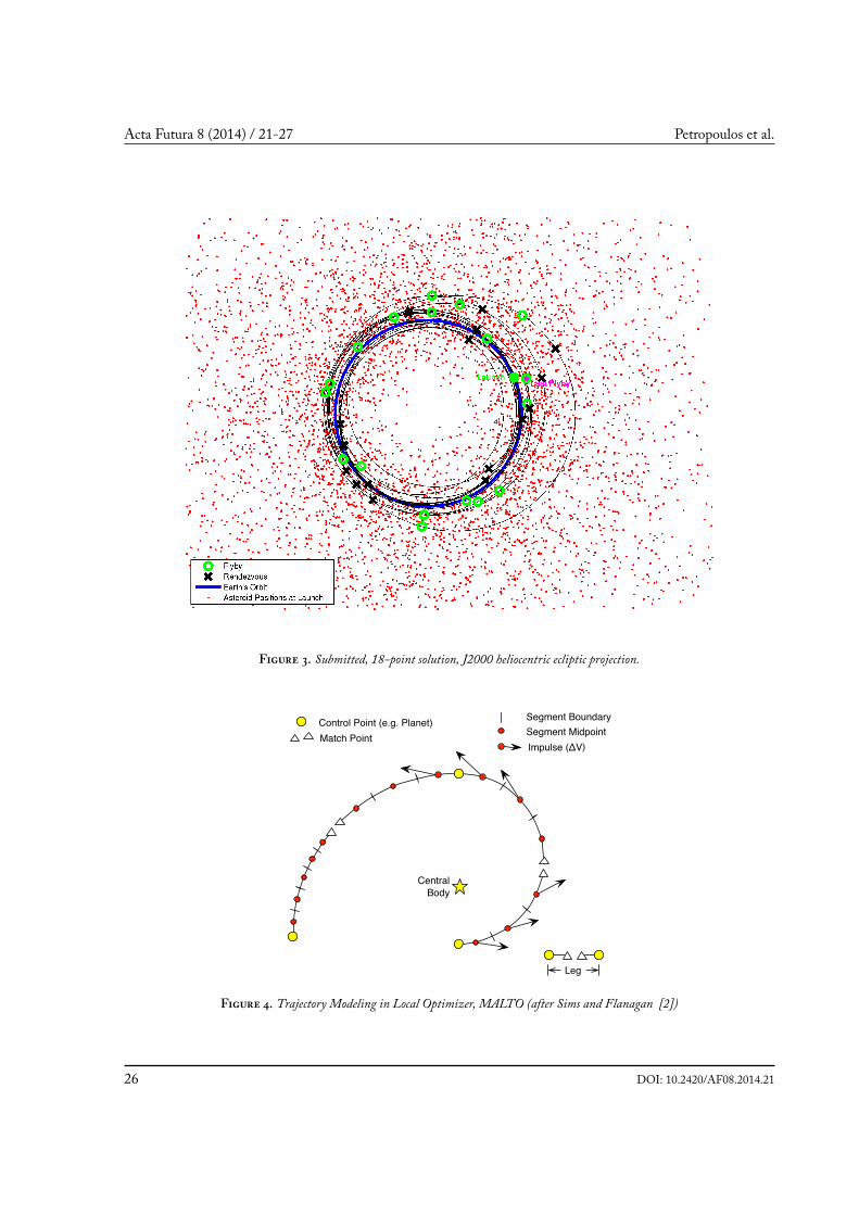
The local optimization program, MALTO, also used inprevious GTOCs, is based on the algorithm formulatedby Sims and Flanagan [2]. In this formulation, the low-thrust arcs are modelled as a series of impulsive velocityincrements (∆Vs). Each leg (i.e., from one flyby body orcontrol point to the next one in time) is split into a num-ber of segments, as shown in Fig. 4. Targeting is done bymeans of a match point, which occurs after a specifiednumber of segments from the first control point. Thetrajectory is propagated forward in time from the firstcontrol point to the match point, and backwards in timefrom the next control point to the match point. Trajec-tory propagation is conic, except that at the temporalmidpoint of the segments a discontinuity in the velocity(∆V) is allowed. The maximummagnitude of the ∆V isequal to the available thrust acceleration multiplied bythe duration of the segment. From the rocket equation,the mass drop corresponding to the ∆V is computed.When a sufficient number of segments is used (for near-circular orbits, 20 to 30 segments per revolution is nor-mally sufficient), this formulation provides an excellentapproximation to an actual low-thrust arc. Other con-straints, such as flyby altitude constraints, are applied asneeded.The optimisation variables are the magnitude and di-
rection of the impulses; the launch, flyby and arrivaltimes; the incoming and outgoing v∞ vectors at theflyby bodies; the outgoing/incoming v∞ vectors at thelaunch/arrival body; and also the initial spacecraft mass(for the outside chance that the benefit of increasedthrust acceleration could outweigh the penalty of re-duced mass; initial mass would be reduced by dumpingsome propellant instantaneously). The optimisation en-gine used is SNOPT [3], which is based on the sequen-tial quadratic programming method. SNOPT finds lo-
cally optimal solutions which satisfy the non-linear con-straints. Appropriate scaling is used for the variablesand analytic derivatives are used.While the replacement of the low-thrust arcs with
a series of impulsive ∆Vs is a reasonable approxima-tion, the question arises of how to obtain a smoothlyvarying state for the spacecraft which adequately repre-sents the motion the spacecraft would have under lowthrust. The approach taken here is simple. Essentially,a weighted average state is computed for intermediatetimes on any given segment. The known spacecraft stateat the start of the segment is propagated forward coni-cally up to the end time of the segment, and the knownspacecraft state at the end of the segment is propagatedconically backwards up to the start time of the segment.At any interior time point on the segment, a linearlyweighted average is taken of the states at that time pointas taken from the forward-propagated state history andthe backwards-propagated state history. The directionof the thrust vector is taken as inertially fixed for the du-ration of the segment and equal to the direction of theimpulsive ∆V on that segment. The magnitude of thethrust is taken as that magnitude which yields a charac-teristic velocity (from the rocket equation) equal to theimpulsive ∆V . At higher acceleration levels, this ap-proximation becomes less accurate. To overcome thiseffect, more segments can be used. For the submittedsolution, around 100 segments were used per revolutionat the end of the trajectory when the thrust accelerationhad gotten substantially higher.
4 Results
The global-rank pruning and the local-rank pruningwere yielding comparable results up to about the 15-asteroid mark, that is, 15 consecutive rendezvous-flyby-rendezvous blocks. Beyond that, the local-rank prun-ing method started out-pacing the global-rank method.Both approaches reached 17 asteroids, however, onlythe trajectories from the local-rank method had suffi-cient flight time and propellant left to reach an 18th as-teroid. All of the 18-asteroid solutions we obtained hap-pened to share the same itinerary up to the 17th aster-oid, indicating that the number of possible 18-asteroidsolutions is probably rather limited, and far smaller thanthe number of 17- asteroid possibilities. Table 3 lists thefirst asteroids in all of the trajectories we found with 16or more asteroids.
DOI: 10.2420/AF08.2014.21 23

Acta Futura 8 (2014) / 21-27 Petropoulos et al.
Figure . Submitted, 18-point solution, J2000 heliocentric ecliptic frame.
24 DOI: 10.2420/AF08.2014.21

GTOC5: Results from the Jet Propulsion Laboratory
Table . Submitted, 18-point solution.Enc AstSeqN GTOC5 name Encounter Date TOF from TOF from s/c Mass Drop v∞# (yyyy.mm.dd) launch last Enc before drop mass (km/s)
(days) (days) (kg) (kg)1 - Earth 2020.10.15 0.00 0.00 4000.00 0.00 3.2312 1712 (2001 GP2) 2021.01.12 88.84 88.84 3951.33 40.00 0.0003 1712 (2001 GP2) 2021.05.22 218.29 129.45 3823.08 1.00 0.4004 4893 (2007 UN12) 2021.12.13 424.02 205.73 3670.91 40.00 0.0005 4893 (2007 UN12) 2022.04.20 551.35 127.33 3553.32 1.00 0.4006 4028 (2006 JY26) 2023.02.16 853.72 302.38 3405.66 40.00 0.0007 6939 (2010 JR34) 2023.12.10 1150.21 296.49 3146.84 40.00 0.0008 6939 (2010 JR34) 2024.03.27 1258.97 108.76 3035.81 1.00 0.4009 5884 (2009 BD) 2025.04.30 1657.39 398.42 2744.99 40.00 0.00010 5416 (2008 JL24) 2026.05.06 2028.32 370.93 2533.23 40.01 0.00011 5416 (2008 JL24) 2026.08.11 2125.37 97.05 2435.77 1.00 0.40012 5884 (2009 BD) 2026.12.09 2245.41 120.05 2402.63 1.00 1.97213 1600 (2000 SG344) 2027.04.25 2382.60 137.19 2323.82 40.00 0.00014 1600 (2000 SG344) 2027.07.30 2478.87 96.27 2239.36 1.00 0.40015 4165 (2006 RH120) 2028.09.18 2894.91 416.03 2151.60 40.00 0.00016 4165 (2006 RH120) 2029.02.13 3042.33 147.42 2079.32 1.00 0.40017 5711 (2008 UA202) 2029.08.11 3221.29 178.96 2016.40 40.00 0.00018 5711 (2008 UA202) 2029.12.26 3358.63 137.34 1945.74 1.00 0.40019 5174 (2008 CX118) 2030.06.27 3541.30 182.67 1824.74 40.00 0.00020 5174 (2008 CX118) 2030.09.08 3614.81 73.51 1746.25 1.00 0.40021 4028 (2006 JY26) 2031.03.25 3812.19 197.38 1675.47 1.00 1.79422 1059 (1993 HD) 2031.07.20 3929.83 117.64 1616.19 40.00 0.00023 1059 (1993 HD) 2031.09.18 3989.53 59.70 1536.86 1.00 0.40024 5945 (2009 CV) 2032.02.14 4138.55 149.02 1438.30 40.00 0.00025 5945 (2009 CV) 2032.05.10 4224.29 85.75 1373.16 1.00 0.40026 5894 (2009 BK2) 2032.12.08 4437.11 212.82 1214.14 40.00 0.00027 5894 (2009 BK2) 2033.01.24 4483.52 46.41 1145.08 1.00 0.40028 401 (2001 CC21) 2033.04.15 4565.03 81.51 1072.27 40.00 0.00029 401 (2001 CC21) 2033.05.27 4606.91 41.88 1007.93 1.00 0.40030 505 (2001 WC47) 2033.11.08 4771.64 164.73 867.08 40.00 0.00031 505 (2001 WC47) 2033.12.27 4820.55 48.91 812.03 1.00 0.40032 3779 (2005 YA37) 2034.08.25 5061.75 241.20 782.74 40.00 0.00033 3779 (2005 YA37) 2034.10.04 5101.33 39.58 728.31 1.00 0.40034 3878 (2006 BZ147) 2035.03.27 5275.62 174.28 651.01 40.00 0.00035 3878 (2006 BZ147) 2035.04.23 5302.33 26.71 597.32 1.00 0.40036 1788 (2001 QJ142) 2035.09.09 5441.56 139.23 553.70 40.00 0.00037 1788 (2001 QJ142) 2035.09.29 5461.82 20.27 501.00 1.00 0.400
DOI: 10.2420/AF08.2014.21 25
Acta Futura 8 (2014) / 21-27 Petropoulos et al.
Figure . Submitted, 18-point solution, J2000 heliocentric ecliptic projection.
Control Point (e.g. Planet)
Match PointSegment Midpoint
Segment Boundary
Impulse (ΔV)
Leg
Central
Body
Figure . Trajectory Modeling in Local Optimizer, MALTO (after Sims and Flanagan [2])
26 DOI: 10.2420/AF08.2014.21

GTOC5: Results from the Jet Propulsion Laboratory
Table . List of first asteroids visited for solutions found with 16 or more asteroidsAstID AstName a e i ω Ω Max J
(AU) (deg.) (deg.) (deg.)1043 (1991 VG) 1.027 0.049 1.45 24.5 74.0 161712 (2001 GP2) 1.038 0.074 1.28 111.3 196.9 182679 (2003 WT153) 0.894 0.178 0.37 148.5 56.0 165249 (2008 EA9) 1.059 0.080 0.42 335.9 129.4 175416 (2008 JL24) 1.038 0.107 0.55 281.9 225.8 175884 (2009 BD) 1.002 0.047 0.38 100.2 53.1 165945 (2009 CV) 1.112 0.150 0.96 178.9 24.1 176112 (2009 HC) 1.039 0.126 3.78 269.8 203.8 166979 (2010 KV7) 1.215 0.219 0.31 36.9 255.9 16
4.1 Submitted solution
The best of the 18-asteroid solutions was further refinedsystematically. First, we attempted to add a rendezvousof a new asteroid, anywhere along the trajectory, bylooking for close, low-speed approaches with any of theasteroids that were not already on the itinerary. Neithersufficient propellant nor sufficient flight time remainedto realize this option. Second, we tried to minimize theflight time by trying to beneficially increase the returndepth for some asteroids and by consuming all the avail-able propellant. The return-depth increase was foundby looking for close approaches at later times. Two in-creases in return depth were made: Asteroid 4028 wentto a return depth of 7, and asteroid 5884 to 1.The final, submitted 18-asteroid solution, since it
performs a rendezvous and subsequent flyby with eachasteroid, has a performance index of J = 18. Theflight time is 5461.82 days. The thruster is “on” for3134.95 days, and the final spacecraft mass is 500 kg(after the impactor mass of 1 kg is released at the finalasteroid). Our submitted solution is shown in Table 2and in Figures 3 and 2.
5 Acknowledgements
This research was carried out at the Jet Propulsion Labo-ratory, California Institute of Technology, under a con-tract with the National Aeronautics and Space Admin-istration.Copyright 2014 California Institute of Technology.
U.S. Government sponsorship acknowledged.
6 Conclusions
Having a good local optimizer was essential in our ef-fort, both in terms of speed and of robustness. Also, theQ-law screening metric was indispensable for trimmingdown the number of candidates passed to the optimizer.The local-rank-pruning strategy appeared considerablybetter than the global-rank-pruning strategy, however,this may simply have been due to not preserving enoughdiversity in the latter. Lastly, the adaptive tuning of theoptimizer weightings and branch-and-prune parame-ters was found to be very important as trajectories werebuilt up.
References
[1] A. Petropoulos, “Refinements to the Q-law forLow-Thrust Orbit Transfers,” in AASPaper 05-162,AAS Space Flight Mechanics Meeting, Copper Moun-tain, Colorado, Jan. 2005.
[2] J. A. Sims and S. N. Flanagan, “Preliminary De-sign of Low-Thrust Interplanetary Missions,” inAAS/AIAA Astrodynamics Specialist Conference, Aug.1999.
[3] P. E. Gill, W. Murray, and M. A. Saunders, “User’sguide for snopt version 7: Software for large-scalenonlinear programming,” 2006.
DOI: 10.2420/AF08.2014.21 27

28

Acta Futura 8 (2014) 29-36DOI: 10.2420/AF08.2014.29
ActaFutura
GTOC5: Results from the Politecnico di Torino and Universitàdi Roma Sapienza
Lorenzo Casalino *, Dario Pastrone, Francesco SimeoniDipartimento di Ingegneria Meccanica e Aerospaziale, Politecnico di Torino, corso Duca degli Abruzzi 24, 10129 Torino (Italy)
Guido Colasurdo, and Alessandro ZavoliDipartimento di Ingegneria Meccanica e Aerospaziale, Università di Roma “Sapienza”, via Eudossiana 18, 00184 Roma (Italy)
Abstract. Problems that concern a large numberof possible targets, such as those typical of GlobalTrajectory Optimization Competitions (GTOC),require a global search for the optimal solution anda local refinement. During the 5th edition of theGlobal Trajectory Optimization Competition, weused different approximated techniques to performa global search of suitable asteroid sequences; a lo-cal optimization method based on an indirect ap-proach was then used to verify the feasibility ofthe suggested legs and perform the optimizationof multi-leg sequences. All the tools used by ourteam are presented in this paper. The best solutionfound is described and discussed.
1 Introduction
The problem proposed by GTOC5 organizers is quitechallenging. Relevant trajectories encounter a greatnumber of asteroids (18 in the best solution) selectedfrom a very large list (7075 elements). The number ofpossible sequences is incredibly huge and it is necessaryto individuate candidate solutions on the basis of a roughevaluation of the maneuvers that efficiently move thespacecraft from an asteroid to the following one. This
*Corresponding author. E-mail: [email protected]
approximate process aims at locating the global opti-mum region in the solution space.The globally-optimal maneuver will be very close to
running out of time and propellant. In particular, ac-cording to GTOC5 rules, more asteroids are reached,less propellant is available for the whole mission, dueto the mass that is discharged at each rendezvous/flyby.The global searchmust be backed by a refinement, whichimproves the trajectory looking for the local optimumthat spares either time or propellant (hopefully both).The local optimization is periodically carried out dur-ing the global search, in order to verify the feasibilityof the suggested legs and to assess the spacecraft mass,which is quite important to define the available thrust-acceleration.Validation of the most promising legs and improve-
ment of assessed sequences were carried out by means ofan indirect optimization method, based on the theory ofoptimal control. The time limits for the overall missionmake a fast transfer (between an asteroid and the fol-lowing one) really attractive. On the other hand, theavailable propellant is scarce, in particular when manyasteroids appear in the sequence; mass can be saved atthe expense of time, by introducing coast arcs. An opti-mal balance must be sought, and, in building the trajec-tory, both minimum-fuel legs (with fixed time of flight)
29

Acta Futura 8 (2014) / 29-36 Casalino et al.
and minimum-time legs were evaluated, according tothe event sequence suggested by the global search meth-ods.Legs were periodically joined to perform a multi-leg
optimization (up to five legs were considered) and de-termine the optimal intermediate times. The joined op-timization of multi-leg segments is very important, asthe previous propellant consumption determines space-craft mass and available thrust-acceleration during thefollowing legs. In comparison to the result of optimiz-ing single legs, a greater propellant consumption is usu-ally preferred in the initial legs, and coast arcs are pushedtowards the final part of the segment. In this way, solu-tions up to 17 asteroids were found. On the competitionlast day, the fastest trajectory intercepting 17 asteroidshas been searched for, in order to improve the secondaryperformance index.
2 Global Search and Asteroid Selection
A wise choice of the target asteroids and a control law,which guarantees a good balance between propellantconsumption and flight time, are required to reach alarge number of asteroids. Even though the latter taskis mandatory, the former one is a necessary prelimi-nary step; the decision on the next target is a complexproblem as it requires, as in a chess match, to foreseesome of the following targets in order to avoid to enter adead end. Only some “global” or “synthetic” features ofeach transfer (i.e., estimated duration∆t and propulsivecost ∆V) are necessary to try a prediction of suitable se-quences of asteroids. The global search is hence focusedon finding a way to produce good estimates for possiblemaneuvers and on assembling sequences of maneuversthat could be useful to the maximization of the meritindex.
2.1 Edelbaum approximation and sequential strategy
A way to estimate the cost of a maneuver is based on anelaboration of Edelbaum’s formulas [1], which, undersuitable hypotheses, permit to calculate the required∆Vto transfer a spacecraft between two orbits (subscripts 1and 2); the flyby cost is neglected. The following rela-tionship
∆V =√(ka∆a)2 + (ke∆e)2 + (ki∆i)2 (1)
considers the efforts to change the spacecraft energy (ex-pressed by the semi-major axis change ∆a), to modify
shape and orientation of the ellipse (∆e), and to rotatethe orbit plane (∆i); they are summed up taking intoaccount the benefit of combining the three maneuvers.One has
∆a = a2 − a1 (2)
∆e =√(ep2 − ep1)2 + (eq2 − eq1)2 (3)
∆i =√(hx2 − hx1)2 + (hy2 − hy1)2 + (hz2 − hz1)2 (4)
where components of eccentricity vector in the perifocalsystem and direction cosines of angular momentum inthe heliocentric ecliptic system are used
ep = e cos(Ω+ω) (5)eq = e sin(Ω+ω) (6)
hx = sin i sinΩ (7)hy = − sin i cosΩ (8)
hz = cos i (9)
The cost coefficients
ka =V0
2a0(10)
ke = 0.649V0 (11)ki =
π
2V0 (12)
are obtained by averaging on a complete revolution thedifferential equations that relate the variations of orbitalparameters to the propulsive effort, while using meanvalues for the spacecraft orbit
a0 = (a1 + a2)/2 (13)V0 =
õ/a0 (14)
The phase of the two asteroids is not directly takeninto account, even though it has a major impact on theactual ∆V . However, given a departure date ti and theestimated∆V , the associated flight time∆t can be easilycalculated from the propellant mass flow rate mp:
∆t = ∆m/mp + ∆tfb (15)
where the first term is related to the estimated ∆V
∆m = mi
(1 − e−∆V/c
)(16)
30 DOI: 10.2420/AF08.2014.29

GTOC5: Results from the Politecnico di Torino and Università di Roma Sapienza
and the second term is a time penalty ∆tfb = 2mi
which considers the time necessary to perform theflyby; this relationship between non-dimensional vari-ables (see section 3) was empirically obtained from sev-eral test cases. The penalty diminishes with the space-craft mass to reflect the thrust-acceleration increase.Note that flyby influence on ∆V is instead neglected.The final position of the spacecraft is estimated as
ϑf = ϑ1 + ϑ0∆t, assuming a constant angular veloc-ity ϑ0 =
õ/a3
0. It corresponds to the desired positionof the target asteroid, which is compared to its actualposition at tf; the difference is a measure of the correctphasing between the relevant asteroids.This procedure to estimate transfer cost and asteroid
phasing constitutes the core of the sequential strategy:assigned an asteroid, the time of its rendezvous is as-sumed as initial time; transfers to all the others aster-oids, sorted on the basis of the estimated ∆V , accord-ing to Edelbaum’s formulas, are analyzed. The maneu-vers that have the target asteroid well phased, are opti-mized to verify their feasibility and actual cost, whichdepends also on the phase characteristics. A tree is cre-ated by propagating the trajectory up to five rendezvousby means of the same technique. Predictions are quiteaccurate for transfers with up to three rendezvous andbecome less reliable for longer sequences. Unfortunatelythe number of analyzed branches is limited by the com-putation capabilities and the necessity of verifying eachleg. More branches are added only if this limited searchdoes not produce interesting continuation.This way of facing the global search is probably the
most intuitive; however, it has some drawbacks: sincethe phase analysis depends on the initial time, in somecases a departure delay could avoid the discharge of aninteresting branch. Moreover, less promising maneu-vers are not examined, but their high cost might be off-set by a very favorable continuation.
2.2 Chain strategy
The chain strategy assumes that the transfer betweentwo asteroids is carried out in proximity of the most fa-vorable position; all the opportunities that present ade-quate phasing are found in the whole allowed time do-main. The features of each transfer, comprising esti-mated departure and arrival times, are recorded and con-stitute a catalog of elementary legs. Tentative chains arethen created by connecting legs that present acceptablegaps (or overlaps) between estimated arrival and depar-
ture times.The choice of the best position for themaneuver is the
crucial point; experience acquired in GTOC2 suggeststhat a good transfer occurs where the asteroid orbits areclose to tangency; therefore the nominal point of themaneuver is arbitrarily located at the orbit intersections(if any) or at the point of minimum distance, makingreference to the orbit projections on the ecliptic plane.If the minimum distance overcomes an assigned value,maneuvers between the two asteroids are not consideredworth of attention.The cost in terms of ∆V is evaluated on the basis of
an impulsive maneuver
∆V = ∆Vip + ∆Vop (17)
which is sum of the in-plane maneuver
∆Vip =√(Vr2 − Vr1)2 + (Vt2 − Vt1)2 (18)
and the out-of-plane maneuver
∆Vop = ∆i(Vt1 + Vt2)/2 (19)
with radial and tangential velocity components given by
Vr =√µ/p e sinν (20)
Vt =√µ/p(1 + e cosν) (21)
The impulsive approximation does not hold if the im-pulsive ∆V is beyond a threshold related to the avail-able thrust-acceleration; in these circumstances ∆V isevaluated using Edelbaum’s formulae, presented in theprevious subsection.The impulsive approximation requires that the ma-
neuver point is close to the line of nodes between theorbit planes of the relevant asteroids. The maneuverpoint is rejected if its angular distance from either nodeis greater than
∆ϑmax = tan−1(0.2/√∆i) (22)
This dependence on∆iwas introduced tomake the con-dition tight when the plane rotation is large, and, onthe contrary, weak in the case of almost coplanar orbits.This condition does not apply to Edelbaum’s approxi-mation.To ensure a proper phasing between the two aster-
oids, for each passage of the departure asteroid at thenominal point during the competition window, the ac-tual angular distance between the asteroids is considered
DOI: 10.2420/AF08.2014.29 31

Acta Futura 8 (2014) / 29-36 Casalino et al.
and a maneuver opportunity only occurs if the phaseangle is less than a prescribed value (difference above4 or 8 degrees are not accepted in the case of impul-sive or Edelbaum approximation, respectively). Startand end times of the maneuver are evaluated by split-ting the time-length, evaluated using the required veloc-ity change and the available thrust magnitude, symmet-rically around the orbit intersection or the minimum-distance point (i.e., the nominal point of the maneuver).A reduced set of asteroids (containing about one
thousand elements) has been considered by dischargingthe asteroids with eccentricity larger than 0.4 and in-clination greater than 10 degrees. Using the previousapproximations, a database of estimated usable maneu-vers has been created. It collects a list of favorable trans-fers for the whole range of permitted dates. A transferis described by initial date, final date, propellant con-sumption. The maneuvers are aggregated to form a se-ries of possible sequences. The time between arrival toand departure from the same asteroid cannot be smalleror greater than assigned quantities; in the former case(small overlap) the maneuver probably could not be car-ried out; in the latter (large gap) the sequence wouldwaste too much time.In the last days of GTOC5 the procedure has
been improved by creating different databases for suit-able mass values from the initial to the final one, asthe leg time-lengths depend on the available thrust-acceleration and therefore the current mass. Additionaldatabases were created using the samemass for up to fivelegs; eventually, a different value was adopted for eachleg.
2.3 First asteroid
The mission departs from the Earth, and an extensivesearch of the solution space must be performed to iden-tify a suitable first asteroid for the sequence. Asteroidswith semimajor axis close to 1 AU, small eccentricityand inclination were selected; among them preferencewas given to the asteroids well phased for a ballisticmission that left the Earth from the line of nodes andreached the target in correspondence of perihelion oraphelion. A local optimization of the rendezvous mis-sion to these asteroids was carried out assuming opti-mal phasing: free hyperbolic excess velocity was initiallyconsidered, but the relevant constraint was introducedwhen required. Comparison of actual and required as-teroid positions on the possible arrival dates allowedto find favorable legs to a set of first asteroids, which
were used as starting points for the sequential strategyand whose presence in the chain strategy database waschecked. This strategy proved to be very efficient asgood initial sequences (comprising the one of the bestsolution found by this team) were found. On the con-trary, a reverse strategy, which tried to find suitable legsfrom Earth to the initial asteroid of long chains sug-gested by the chain strategy, did not provide good re-sults.
3 Indirect Optimization
Accurate integration and adequate optimization to as-sure actual feasibility with suitable values of propellantconsumption and time-of-flight are required for eachtrajectory leg, which joins two consecutive asteroids.The authors have been applying indirect optimizationto space trajectories for a long time. Their indirect ap-proach is based on the split of the trajectory into arcs,which join at relevant points. An almost mechanical ap-plication of optimal control theory (OCT) determinesthe boundary conditions for optimality at the arc junc-tions. This modular approach is very useful for thepresent problem, as the trajectory is made of similar re-peating legs.
Preliminary analysis showed that performing theflyby immediately after the rendezvous of the same as-teroid is, in general, not very expensive; this event se-quence has been assumed to limit the search space, eventhough some interesting opportunities may be missed.Therefore, the basic maneuver consists of a transferbetween two asteroids (rendezvous conditions are en-forced) with intermediate flyby of the departure one; inaddition, the prescribed minimum velocity at flyby mustbe enforced.
Position r, velocity v and mass m of the spacecraftare the problem state variables. They are made non-dimensional by using the radius of Earth’s orbit, the cor-responding circular velocity and the spacecraft mass atthe start of the whole mission (4000 kg) as referencevalues. The spacecraft state is described by differentialequations
dr/dt = v (23)dv/dt = −r/r3 + T/m+ ap (24)
dm/dt = −T/c (25)
The trajectory is controlled by the thrust vector T (ef-fective exhaust velocity c is constant).
32 DOI: 10.2420/AF08.2014.29

GTOC5: Results from the Politecnico di Torino and Università di Roma Sapienza
At departure from asteroid A1 (subscript 0) one has
r0 = rA1(t0) (26)v0 = vA1(t0) (27)
m0 = k (28)
where k is a fixed value, which derives from the previousmaneuvers. At flyby of A1 (subscripts 1- and 1+ denotevalues just before and after the flyby)
r1+ = r1− = rA1(t1) (29)m1+ = m1− − ∆mFB (30)t1+ = t1− (31)v1+ = v1− (32)
[v1− − vA1(t1)]2 = v2∞ (33)
and at rendezvous with asteroid A2 (subscript 2)
r2 = rA2(tf) (34)v2 = vA2(tf) (35)
The adjoint variables are introduced and the Hamil-tonian is defined as
H = λTrV + λT
v (g+ T/m) − λmT/c (36)
OCT provides the Euler-Lagrange equations for theadjoint variables
dλr
dt= −
[∂g
∂r
]Tλv (37)
dλv
dt= −λr (38)
dλmdt
=λvT
m2 (39)
Thrust magnitude and direction are the problem controlvariables. According to Pontryagin’s Maximum princi-ple (PMP), thrust must be parallel to the velocity adjointvector λv, i.e., the primer vector [2]. The Hamiltonianbecomes
H = λTrV + λT
vg+ TSF (40)
where the switching function SF = λv/m − λm/c isintroduced. Thrust has its maximum value when SF >
0, whereas it is zero when SF < 0, in agreement withPMP.The boundary conditions for optimality of the base-
line leg derive from a general formulation of OCT[3, 4], which is omitted for the sake of conciseness. If
the initial time is free and the final mass m2 is maxi-mized, the transversality condition at departure is
SF0 = 0 (41)
At flyby, the position adjoint vector has a free discon-tinuity, the primer vector is continuous and parallel torelative velocity
λv1+ = λv1− =
= [v1− − vA1(t1)]λv1−/v∞ (42)
and the transversality condition is[λTr (v− vA1) + TSF
]1+ =
=[λTr (v− vA1) + TSF
]1− (43)
One also has λm2 = 1 and SF2 = 0 at the final point.Departure time may be specified (e.g., forcing an im-
mediate departure after the asteroid has been reached),replacing Eq. 41. Minimum-time legs have also beenconsidered; the boundary conditions at the final pointbecome λm2 = 0 and H2 = 1. The first leg departingfrom Earth is different; v∞ is not zero and subsequentEarth flyby is not required. Either optimal or maximumv∞ departures are considered, and slightly different setsof boundary conditions pertain to the first leg.Several baseline legs are joined together to optimize
a multi-rendezvous, multi-flyby trajectory. Boundaryconditions for optimality are slightly modified at inter-mediate rendezvous, where time continuity and massdiscontinuity (∆mRV ) are enforced. When multiplelegs are joined, an improved accuracy is required to ob-tain convergence; in these cases, instead of deciding thethrust magnitude according to SF during integration,the trajectory is split into burn and coast arcs on the ba-sis of the single-leg solutions; SF = 0 is imposed wherethe engine is switched on or off, in order to determinethe corresponding times.From the numerical point of view, the optimization
problem is transformed into a multi-point boundaryvalue problem (MPBVP). An iterative procedure [5]based on Newton’s method is employed to solve theMPBVP.
4 Results
Both global search strategies have been used by Team13and both suggested useful legs and favorable asteroid se-quences. With some exceptions, sequential strategy and
DOI: 10.2420/AF08.2014.29 33

Acta Futura 8 (2014) / 29-36 Casalino et al.
Table . Trajectory events
Event Date, MJD Body mass, kg v∞, km/sdeparture 59029.82 Earth 4000.00 1.92rendezvous 59182.60 2007 UN12 3959.66 0.00
flyby 59325.80 2007 UN12 3843.12 0.40rendezvous 59564.06 2001 GP2 3718.02 0.00
flyby 59696.06 2001 GP2 3593.18 0.40rendezvous 59967.18 2006 JY26 3377.17 0.00
flyby 60076.73 2006 JY26 3249.29 0.40rendezvous 60288.52 2010 JR34 3076.33 0.00
flyby 60398.01 2010 JR34 2969.70 0.40rendezvous 60856.82 2009 BD 2688.00 0.00
flyby 60982.30 2009 BD 2602.32 0.40rendezvous 61403.94 2008 JL24 2492.96 0.00
flyby 61494.29 2008 JL24 2401.14 0.40rendezvous 61704.81 2000 SG344 2318.36 0.00
flyby 61797.21 2000 SG344 2234.24 0.40rendezvous 62036.91 2008 UA202 2091.41 0.00
flyby 62174.34 2008 UA202 2019.10 0.40rendezvous 62357.31 2006 RH120 1958.36 0.00
flyby 62440.89 2006 RH120 1877.76 0.40rendezvous 62699.23 2004 QA22 1712.13 0.00
flyby 62762.93 2004 QA22 1631.45 0.40rendezvous 62891.52 2003 WT153 1562.39 0.00
flyby 62978.70 2003 WT153 1490.33 0.40rendezvous 63174.77 2006 BZ147 1366.50 0.00
flyby 63234.79 2006 BZ147 1296.01 0.40rendezvous 63422.79 2009 YR 1192.48 0.00
flyby 63464.58 2009 YR 1119.60 0.40rendezvous 63681.18 2006 WB 975.84 0.00
flyby 63723.64 2006 WB 915.42 0.40rendezvous 63867.61 1991 VG 787.57 0.00
flyby 63903.95 1991 VG 732.34 0.40rendezvous 63999.76 1993 HD 700.25 0.00
flyby 64028.08 1993 HD 645.33 0.40rendezvous 64211.06 2009 CV 553.95 0.00
flyby 64231.41 2009 CV 501.34 0.40
Edelbaum’s approximation, due to its continuous-thrustnature, proved more reliable for the initial legs of thetrajectory, when the large spacecraft mass causes a smallacceleration. On the contrary, impulsive approximationand chain strategy were more reliable in the mission fi-nal phases, which exhibit shorter burn times due to thelarger thrust-acceleration. The chain search strategy canupdate its database by including legs between asteroidsthat have already been verified and optimized. It proveduseful in the final days of the competition, suggestingalternative sequences in replacement of segments of thebase trajectory.
Many sequences of several asteroids have been sug-gested by the global search and analyzed by means oflocal optimization. In the last week of competition, at-tention was exclusively dedicated to the most promisingtrajectory, with adjustments and asteroid replacementsto improve the solution, which eventually reached 17 as-teroids. On the competition last day, efforts were madeto find the fastest 17-asteroid mission, which is the bestsolution found by this team and summarized hereafter:
• departure on June 19, 2020 (59029.82 MJD),v∞ = 1.92 km/s;
34 DOI: 10.2420/AF08.2014.29

GTOC5: Results from the Politecnico di Torino and Università di Roma Sapienza
• arrival (flyby of asteroid 2009 CV) on Sept. 26,2034 (64231.41 MJD);
• final mass after release of penetrator mass 500.34kg;
• total time of flight tf − t0 = 5201.58 days;
• performance index J = 17 (17 rendezvous and 17penetrations).
Details of the event sequence are given in Table 1; agraphical representation is shown in Fig. 1.
0.60
0.75
0.90
1.05
1.20
1.35
59000 61000 63000 65000
EarthRendezvousFlyby
Time, MJD
Rad
ius,
AU
Figure . Graphical representation of the solution.
A typical leg between two asteroids is presented inFig. 2; one should note that the maneuver from flyby torendezvous occurs where the orbits are almost tangent.Positions of both asteroids at initial, flyby, and final timeare shown: requirements in terms of phasing appear verytight to perform an efficient rendezvous. In unfavorablecircumstances, thrust is used to move the spacecraft in-ward to increase its angular velocity and reach a leadingasteroid. The opposite maneuver is performed to waitfor a trailing one.Table 2 presents the actual ∆V to perform each leg
of the final trajectory; it includes the flyby cost (veloc-ity change from asteroid departure to its flyby), whichresults to be almost the same for all the legs. The esti-mated∆V is also shown; usually it has been provided byEdelbaum’s formulas (Eq. 1); in two occurrences (de-noted by asterisks) the leg was suggested by the impul-sive approximation, and the corresponding∆V (Eq. 17)is shown. The former approximation overvalues the pro-pellant consumption, whereas the latter underestimatesthe needed ∆V , but it is more effective in positioningthe maneuver and analyzing the asteroid phasing. As a
-1.0
-0.5
0.5
-0.5 0.5 -1.0
Y
X
rendezvous1993 HD
flyby1991 VG
rendezvous1991 VG
1993 HD
1991 VG
Figure . Leg from asteroid 1991 VG to asteroid 1993 HD.
matter of fact, Edelbaum’s formulas give a reliable guessof the overall ∆V needed for the entire leg: differencesare quite low, usually ranging from −18% to +7%, asthe benefit of the synergistic use of propulsion offsetsthe flyby cost. Noticeable exceptions concern the legdeparting from 2006 BZ147 and the last leg from 1993HD. These transfers are very fast and Edelbaum’s ap-proximation is less reliable; moreover the flyby cost be-comes significant for low-∆V transfers.Estimation of transfer times is more complex, also be-
cause coast arcs are introduced to reduce the propellantconsumption but cannot be foreseen. Results prove thatthe relationship providing the flyby penalty is accurate,even though a 25% greater coefficient appears more ap-propriate. Table 2 shows that Eq. 15, which includesthe flyby maneuver, is in substantial agreement with theleg actual time-length. This kind of analysis is howeverdifficult and, at a certain extent, questionable. Accord-ing to the global strategy of the mission, some legs areflown to reach the asteroid as soon as possible withoutcoast arcs; other legs have plenty of available time whichis exploited to reduce the propellant consumption.Adjustments have been tried to increase the accuracy
of the estimations obtained by means of Edelbaum’sapproximation, which assumes almost circular orbits,whereas orbit eccentricities are often not negligible. Inparticular, tangential thrust has effects on both energyand eccentricity; when the transfer is short (less thanone revolution), performance depends on the spacecraftposition along its orbit. In a favorable position (e.g.,close to the perihelion if both energy and eccentricitymust be increased), the actual ∆V may be lower thanthe value provided by Edelbaum’s approximation; unfa-
DOI: 10.2420/AF08.2014.29 35

Acta Futura 8 (2014) / 29-36 Casalino et al.
Table . Leg actual and estimated characteristics
Whole Leg Flyby Estimation RatioDeparture ∆V ∆t ∆Vfb ∆tfb ∆Vest ∆test ∆tfb
∆Vest
∆V∆test∆t
Asteroid km/s days km/s days km/s days days2007 UN12 1.547 381 0.580 143 1.290 306 115 0.83 0.802001 GP2 2.503 403 0.687 132 2.200 409 118 0.88 1.012006 JY26 2.386 321 0.785 110 2.067 355 98 0.87 1.112010 JR34 3.576 568 0.653 109 3.772 504 89 1.05 0.892009 BD 1.764 547 0.512 125 1.468 224 78 0.83 0.412008 JL24 1.649 301 0.628 90 1.672 226 72 1.01 0.752000 SG344 2.507 332 0.576 92 2.640 289 67 1.05 0.87∗2008 UA202 1.352 320 0.467 137 2.249 232 61 1.66 0.722006 RH120 3.331 342 0.629 84 3.142 277 57 0.94 0.812004 QA22 1.980 192 0.725 64 1.636 152 50 0.83 0.792003 WT153 3.160 283 0.626 87 3.149 221 45 1.00 0.782006 BZ147 3.112 248 0.684 60 1.719 125 40 0.55 0.502009 YR 4.870 258 0.852 42 4.322 213 35 0.89 0.83
∗2006 WB 5.044 186 0.649 42 4.202 170 28 0.83 0.911991 VG 1.884 132 0.606 36 2.025 79 22 1.07 0.601993 HD 5.121 211 0.673 28 2.210 75 20 0.43 0.35
vorable situations may also arise. Moreover, the actualangular velocity may exhibit relevant changes with re-spect to the average value ϑ0, modifying the final lon-gitude ϑf. Some improvements have been investigated,for instance, by considering the maneuver actual radius,but insufficient time precluded a complete and success-ful analysis.
5 Conclusion
Team13 employed a set of tools which were sufficientto find a good solution to GTOC5 problem. The use offormulas based on Edelbaum’s approximation permitteda satisfactory reduction of the options to be analyzed bythe indirect optimization code, which was used to as-sess the actual feasibility of the trajectory legs. An es-timation based on impulsive approximation suggestedsome additional legs, that were actually included in thefinal trajectory. The chain strategy supported the searchfor improvements to the provisional solution. A majorenhancement would have been a technique which pro-vided an affordable estimate of the cost related to incor-rect phasing between asteroids. Finally, Team13 did notconsider the possibility of delayed flybys and this pointmay have been crucial for the victory.
References
[1] T. N. Edelbaum, “Propulsion requirements for con-trollable satellites,” ARS Journal, vol. 31, no. 8,pp. 1079–1089, 1961.
[2] D. F. Lawden, Optimal Trajectories for Space Navi-gation. London: Butterworths, 1963.
[3] A. E. Bryson and Y.-C. Ho, Applied Optimal Con-trol. New York, NY: Hemisphere, 1975. Revisedprinting.
[4] L. Casalino, G. Colasurdo, and D. Pastrone, “Op-timal low-thrust escape trajectories using gravityassist,” Journal of Guidance, Control, and Dynam-ics, vol. 22, no. 5, pp. 637–642, 1999. doi:10.2514/2.4451.
[5] G. Colasurdo and D. Pastrone, “Indirect optimiza-tion method for impulsive transfer,” paper AIAA-94-3762, AIAA, 1994.
36 DOI: 10.2420/AF08.2014.29

Acta Futura 8 (2014) 37-44DOI: 10.2420/AF08.2014.37
ActaFutura
GTOC5: Results from the Tsinghua UniversityFanghua Jiang *, Yang Chen, Yuecong Liu, Hexi Baoyin and Junfeng Li
School of Aerospace Engineering, Tsinghua University, Beijing, 100084, China
Abstract. The Lab of Aerospace Dynamics atTsinghua University ranked three in the 5th globaltrajectory optimization competition. The resultsfound are presented and the methods used are de-scribed briefly. The search for the greatest num-ber of asteroids that must be visited first by ren-dezvous and possibly revisited thereafter by flyby isperformed in two steps. The first step is a roughglobal search on the reduced candidate space thatrepresents 1000 asteroids with orbit energies dif-fering smallest from the Earth. The launch win-dow and flight time of each leg are discretized withadmissible time step, and then series of Lambertproblems are solved. Branch, bound and prune al-gorithms are used to advance the achievable im-pulsive trajectories. The second step involves localoptimization of the impulsive trajectories by indi-rect method combined with homotopic approach.The techniques of normalization of the unknownmultipliers and a fixed step Runge-Kutta integratorwith switching function detection are significantlyexploited to solve series of multi-point boundaryvalue problems The best trajectory of 17 asteroidrendezvous and successive flybys, and especially offully bang-bang control, is obtained.
1 Introduction
TheLab of Aerospace Dynamics at Tsinghua University(THU LAD) has taken part in all five trajectory opti-mization competitions but did not obtain top-level re-
*Corresponding author. E-mail: [email protected]
sults until this competition. It should be realized that toobtain somewhat wonderful results for this kind of com-plex optimization problem, the strategy of first roughglobal search and then local optimization, which wasnot well performed in previous competition resolutionof this group, is crucial. The global search requiresthe low-thrust trajectories to be approximated simplyenough to carry out large amount of time saving exhaus-tive search methods. Ballistic approximation to eachleg, which results in bi-impulse transfer, is much sim-pler than shape-based methods [1]. Fortunately, forthis competition problem, within admissible 15 yearsof mission time, the number of candidate asteroids are7075. This implies that the flight time of each leg con-necting two targets may be short enough to not exceedone revolution, so that ballistic approximation is some-what competent. After rough search in the large solu-tion space, lots of impulsive sequences are determined.Though bounded and pruned carefully, some sequencescannot be transferred into low-thrust trajectories. Re-cently, this group devotes more time to indirect methodcombined with homotopic approach [2] for low-thrusttrajectory optimization. Some practical techniques [3]are used to transfer the local optimization problem fromimpulsive propulsion to low-thrust one, so that eventu-ally the competition result is obtained, more techniquesdetails cloud be found in reference [3].
37

Acta Futura 8 (2014) / 37-44 Jiang et al.
Figure . Distribution of orbit energy differences between asteroids and the Earth.
2 General description of the method
2.1 Preliminary consideration
Before solving this problem, the first conceptualproblem one should consider is the upper bound theperformance index may reach. Though reasonableestimation mainly depends on experience and intuition,the upper bound may be 20, which means at least 20asteroid first rendezvous and successive flybys. Becausethe initial mass is 4000 kg, the dry mass is at least 500kg, one rendezvous loses 40 kg equipment, one flybyloses 1 kg penetrator, and the thruster parameters givethat one year of full thrust consumes about 322 kg fuel,it can be evaluated that the accumulative time of fullthrust is about (4000−500−20×40−20×1)/322=8.3years, a little larger than half of the maximum missiontime. The index of 20 requires at least 40 legs of tra-jectories, which means the average flight time of eachleg is 4.5 months, somewhat urgent for a rendezvousmission. So the index 20 is regarded as the upperbound.The average leg flight time not more than half
year implies the trajectories from one asteroids to thesuccessive are generally not longer than one revolution,thus ballistic approximation for each leg is somewhatcompetent. A series of Lambert problems will berapidly solved, whereas, the number of 7075 asteroidsgiven by the organizer is still over-burdensome forperforming exhaustive search methods. Since thespacecraft must be launched from the Earth andrendezvous is necessary to score one point, reserving a
certain number of asteroids with smallest orbit energydifferences from the Earth may be a good trade-off.Here the expressions presented by Izzo et al. [4]are used to evaluate orbit energy differences. Thedistribution of orbit energy differences is plot by Fig. 1,which shows that most asteroids are of the values [7.5,10] km/s. The Beletskij asteroid with bonus point is notincluded because its orbit energy difference is 10.246km/s, too high order.
2.2 Global search in the reduced search space
The global search in the reduced search space of 1000asteroids applies the branch, bound and prunes algo-rithms. Brand, bound and prune algorithm is a generalalgorithm for finding optimal solutions of optimizationproblems, especially in discrete and combinatorial op-timization. The branch, bound and prune method isadopted as global optimization method by most of theparticipating teams in previous competitions.
The launch window and flight time of each leg arediscretized. The steps for grid search of launch date andflight time of each leg are varied from 0.05 years to 0.01years. The flight time of each leg of trajectory is boundby the upper and lower limits, which are set to be 0.8years and 0.2 years, respectively. The state at each tar-get asteroid is regarded as the start point of the next legof trajectory. And the end point of each leg is deter-mined by selecting the candidate target. Then, seriesof Lambert problems are solved to determine the ren-dezvous or flyby objects. Four types of transfer legs are
38 DOI: 10.2420/AF08.2014.37

GTOC5: Results from the Tsinghua University
Figure . Searching procedure of the branch, bound and prunealgorithm.
distinguished: rendezvous to rendezvous, rendezvous toflyby, flyby to rendezvous and flyby to flyby. ∆V of eachtrajectory leg can be obtained from the computation re-sults of Lambert problem. The prune criterion is set tobe that the total∆V of each leg should be not more thanw×T×∆t/m, where, T is the maximal thrust,∆t is theflight time, m is the mass of the spacecraft, and impor-tantly w is a factor that usually we set it with 0.5. Thepossible sequences are propagated with up to millionseach time. When the number of reserved sequences istoo less, the factor or the upper bound of flight time iseither enlarged. When the cumulate ∆V is up to about40 km/s or the total flight time is up to 15 years, thepropagation is ended. Fig. 2 shows the searching proce-dure.
2.3 Local optimization by indirect method
Indirect method combined with homotopic approach
The dynamic equations of the spacecraft subject only tothe central force of Sun’s gravity and the thrust of itsown electric propulsion system are
r = v, v = −µ
r3 r +Tmaxu
mα, m = −
Tmaxu
Ispg0(1)
where r and v denote the state of spacecraft in theheliocentric ecliptic reference frame (HERF), m is theinstantaneous mass, Tmax is the maximal thrust magni-
tude, α is the unit thrust direction vector, u ∈ [0, 1]is the engine thrust ratio, Isp is the thruster specificimpulse, g0 is the standard acceleration of gravity atsea level, and µ is the Sun’s gravitational constant.For computing convenience, the quantities aboutlength, time, and mass are made non-dimensional byastronomical unit (AU, 149597870.66 km), year (yr,365.25 × 86400 s), and spacecraft initial mass, respec-tively. Under model (1), it can be deduced throughusing minimum principle to optimal control theorythat for fuel-optimal problem, the optimal control isbang-bang control, and for time-optimal problem, theoptimal thrust magnitude is always maximal.Due to the discontinuous bang-bang control, thefuel-optimal problem is very difficult to solve. To over-come the difficulty, homotopic approach is introducedto solve the fuel-optimal problem by modifying theperformance index as
J = λ0
tf∫t0
L (x,u, t)dt
= λ0Tmax
Ispg0
tf∫t0
[u− εu (1 − u)]dt
(2)
where λ0 is a positive numerical factor introduced tomake multiplier normalization, and the homotopy pa-rameter ε ∈ [0, 1] connects the fuel-optimal problem(ε = 0) with the energy-optimal problem (ε = 1). Forthe modified performance index, the Hamiltonian is
H = λr · v + λv ·(−µ
r3 r +Tmaxu
mα
)− λm
Tmax
Ispg0u+ λ0
Tmax
Ispg0[u− εu (1 − u)]
(3)
where λr, λv , and λm are the co-state variables, alsoknown as functional Lagrange multipliers.According to the minimum principle, the optimalcontrol that minimizes the Hamiltonian holds theforms
α = −λv
∥λv∥(4)
u = 0 if ρ > ε
u = 1 if ρ < −ε
u = 12 − ρ
2ε if |ρ| ⩽ ε
(5)
where the switching function (SF) is of the form
ρ = 1 −Ispg0 ∥λv∥
λ0m−
λm
λ0(6)
DOI: 10.2420/AF08.2014.37 39

Acta Futura 8 (2014) / 37-44 Jiang et al.
The Euler-Lagrange equations are given as
λr =µ
r3 λv −3µr · λv
r5 r,
λv = −λr, λm = −Tmaxu
m2 ∥λv∥(7)
Expression (5) shows that the optimal thrust ratio isalways continuous and sometimes even differentiableunless SF equals to zeros. This attribute causes theoptimal control problem, especially the energy-optimalproblem, greatly easy to be solved.Denote the spacecraft state [r, v, m] by x, and cor-
responding co-state by λ. Consider general boundaryand inner (termed an event) constraints combined bythe p-D equality constraint
ψ(x (t0) ,x (tf) ,x
(t−m
),x
(t+m
), t0, tf, t−m, t+m
)= 0(8)
and the q-D inequality constraint
σ(x (t0) ,x (tf) ,x
(t−m
),x
(t+m
), t0, tf, t−m, t+m
)⩽ 0(9)
where - and + denote the date just before and after theevent m, respectively. Then, under the index (2), byintroducing p- and q-D numerical multiplier vectors χand κ, the first-order necessary conditions are derivedto include the transversality conditions
λ (t0) = −χ · ∂ψ∂x (t0)
−κ · ∂σ∂x (t0)
,
λ (tf) =χ · ∂ψ∂x (tf)
+κ · ∂σ∂x (tf)
(10)
λ(t−m
)=χ · ∂ψ∂x (t−m)
+κ · ∂σ∂x (t−m)
,
λ(t+m
)= −
χ · ∂ψ∂x (t+m)
−κ · ∂σ∂x (t+m)
(11)
and the stationary conditions
H (t0) =χ · ∂ψ∂t0
+κ · ∂σ∂t0
,
H (tf) = −χ · ∂ψ∂tf
−−κ · ∂σ∂tf
(12)
H(t−m
)= −
χ · ∂ψ∂t−m
−κ · ∂σ∂t−m
,
H(t+m
)=χ · ∂ψ∂t+m
+κ · ∂σ∂t+m
(13)
For the caset−m = t+m = tm , the stationary conditionscan be combined to be
H(t+m
)−H
(t−m
)=χ · ∂ψ∂tm
+κ · ∂σ∂tm
(14)
where the Hamiltonian at t−m differs from its value att+m because the costate and state may both be differentat the date just before and after the event. Besides, thecomplementary slackness conditions
κjσj = 0, j = 1,2, · · · ,q (15)
and the nonnegativity conditions
λ0 > 0,κj ⩾ 0, j = 1,2, · · · ,q (16)
should be satisfied at the same time. For a gen-eral optimal control problem with both boundaryand inner constraints, the calculus of variations andminimum principle can transfer it to a boundaryvalue problem. The unknowns are chosen to bex (t0) ,x (t+m) , t0, t−m, t+m, tf,χ,κ,λ0. The statesx (t−m) and x (tf) are obtained through integratingthe dynamic equations (1). λ (t0) and λ (t+m) aredetermined by the first parts of Eq. (10) and (11),and then they are used as the initial value to integrateco-state equations (7) to obtain λ (t−m) and λ (tf),which should satisfy the second parts of Eq. (10) and(11). The optimal datas [t0, t−m, t+m, tf] are determinedby the stationary conditions (12)-(13), and numericalmultipliers [χ , κ] by the constraints (8) and thecomplementary slackness conditions (15). Note thatthe non negativity conditions (16) are just used tocheck the validity of the obtained multipliers λ0 and κ.Except the positive factor λ0, the number of unknowns,however they are chosen, is always equal to that ofequations.
An interesting attribute is that when regarding thefunctional co-states λ (t), numerical multipliers [χ, κ], and numerical factor λ0 together as combinedmultipliers, then all the equations needed to solvethe boundary value problem are homogeneous to thecombined multipliers. Therefore, they can be scaledarbitrarily. One way, for example, is dividing them bythe Euclidian norm of the combined vector[λ0,χ,κ] sothat these unknown multipliers satisfy√
λ20 + χ · χ+ κ · κ = 1 (17)
Note that when the chosen unknowns includes theboundary co-state values, the normalization conditionshould also take them into account. The normalization
40 DOI: 10.2420/AF08.2014.37

GTOC5: Results from the Tsinghua University
will constraint the solution space of unknown multipli-ers and greatly increase the possibility to find the solu-tions.To solve the nonlinear equations including integral,MinPack-1 [5], a program package implements a mod-ification of Powell’s hybrid algorithm [6] that is a com-bination of Newton’s method and the method of gra-dient, is used. With the application of homotopic ap-proach, the fuel-optimal problem is solved by startingfrom the energy-optimal problem (ε = 1). The param-eter ε is decreased slowly and successive related problemis solved by using the preceding solution as the initialguess of the following resolution. When the parameterε is not close to zero, integrators such as Runge-Kuttamethods with adaptive step size are competent to en-sure the integration accuracy because the optimal thrustvaries not too rapidly. when the parameter ε of ho-motopic problem is close to zero, Runge-Kutta methodwith adaptive step size is not able to insure the inte-gration accuracy because the right-hand sides of ODEsvary rapidly around switching points. Here the fourth-order Runge-Kutta algorithmwith fixed step size (RK4)combined with switching detection will be considered toovercome this problem.If the fixed step size h is small enough, the value
of SF at the (k+1)-th iteration can be approximatelyexamined by the value at the k-th iteration through
ρk+1 = ρk + ρkh+12ρkh
2 (18)
where the first and second derivatives of SF with respectto time both exist
ρ = Ispg01λ0
λv · λr
m ∥λv∥(19)
ρ = Ispg01λ0
[−λr · λr
m ∥λv∥+
µ
r3
∥λv∥m
−3µr5
∥λv · r∥2
m ∥λv∥+
+Tmaxu
Ispg0m2
λv · λr
∥λv∥+
(λv · λr)2
m∥λv∥3
](20)
Dividing the range of SF into three intervals:(−∞,−ε), (−∞,−ε), and [−ε, ε], the iterationfrom xk to xk+1 is carried out by first examining whichintervals the values of ρk and ρk+1 respectively fallinto. There are nine cases with respect to the values ofρk and ρk+1. The details about the switching detectiontechnique and integration strategy can be found inpublished work [3].
The first-order necessary conditions for competitionproblem
The events of launch from the Earth with limitedhyperbolic excess velocity, rendezvous with asteroids,and flyby with asteroids with lower bound relativevelocity are thoroughly considered as constraints andthe corresponding quantities are determined throughsolving the consequent first-order necessary conditions(FONCs). Set the lower bound of launch window57023 MJD as the reference date, and all quantities arenon-dimensional. For the launch from the Earth, theequality and inequality constraints are
ψ =
r (t0) − rE (t0)m (t0) − 1
= 0 (21)
σ = vrel − 1.0547 ⩽ 0 (22)
where vrel denotes the magnitude of relative velocityvrel = v (t0) − vE (t0), and rE and vE denote theposition and velocity of the Earth, and 1.0547 AU/yr is
equal to 5 km/s. The FONCs are derived as
λr (t0) = −χ1:3,λv (t0) = −κvrelvrel
, λm (t0) = −χ4
H (t0) + χ1:3 · vE + κvrel · aE (t0) = 0(23)
where χi:j denotes the i-th to j-th components of thevector χ, and aE is the acceleration vector of the Earth.For an intermediate rendezvous at date tm with an
asteroid, the constraints are
ψ =
r (tm) − ra (tm)v (tm) − va (tm)
m (t−m) −m (t+m) − 0.01
= 0 (24)
where non-dimensional mass 0.01 equals to 40 kg,and subscript a denotes the asteroid. The FONCs arederived as
DOI: 10.2420/AF08.2014.37 41

Acta Futura 8 (2014) / 37-44 Jiang et al.
Table . Competition design resultsAsteroid name Date (MJD) Event Mass (kg)Earth 58684.8875 Launch 4000.0002009BD 58995.6407 Rendezvous 3902.27532009BD 59132.1819 Flyby 3786.70792008EA9 59468.8073 Rendezvous 3623.22402008EA9 59589.7345 Flyby 3503.05381991VG 59674.6080 Rendezvous 3427.27731991VG 59803.9887 Flyby 3320.74072000SG344 60033.4813 Rendezvous 3212.49102000SG344 60155.9597 Flyby 3112.22272007UN12 60513.4954 Rendezvous 2903.57422007UN12 60618.0116 Flyby 2800.46302008KT 60902.0098 Rendezvous 2664.32182008KT 60993.2060 Flyby 2559.61912001GP2 61322.5804 Rendezvous 2383.03772001GP2 61401.5696 Flyby 2279.21832007VU6 61720.5920 Rendezvous 2121.07742007VU6 61799.6402 Flyby 2034.89212009YR 62005.2438 Rendezvous 1903.67092009YR 62072.3511 Flyby 1817.64822004QA22 62360.9638 Rendezvous 1714.33672004QA22 62427.6511 Flyby 1625.42052006RH120 62664.1824 Rendezvous 1441.75542006RH120 62715.2479 Flyby 1362.92801993HD 62937.4473 Rendezvous 1260.49561993HD 62993.2455 Flyby 1195.47982006JY26 63204.8926 Rendezvous 1118.98272006JY26 63255.4615 Flyby 1056.96352007YF 63376.8418 Rendezvous 992.44072007YF 63432.1415 Flyby 935.32412008UA202 63609.9229 Rendezvous 849.75472008UA202 63642.3136 Flyby 790.30122009WR52 63821.1021 Rendezvous 679.22052009WR52 63846.0501 Flyby 623.12932003WE 63943.4974 Rendezvous 563.04692003WE 63962.7500 Flyby 508.0949
λr
(t+m
)− λr
(t−m
)+ χ1:3 = 0,
λv
(t+m
)− λv
(t−m
)+ χ4:6 = 0
λm(t−m
)= λm
(t+m
)= χ7,
H(t−m
)−H
(t+m
)− χ1:3 · va (tm)
− χ4:6 · aa (tm) = 0
(25)
where aa is the acceleration vector of the asteroid.For an intermediate flyby at date tm with an asteroid,
the constraints are
ψ =
r (tm) − ra (tm)
m (t−m) −m (t+m) − 0.00025
= 0 (26)
σ = 0.0844 − vrel ⩽ 0 (27)
where vrel denotes the magnitude of relative velocityvrel = v (tm) − va (tm), and nondimensional mass0.00025 and velocity 0.0844 equal to 1 kg and 400 m/s,respectively. The FONCs are derived as
42 DOI: 10.2420/AF08.2014.37
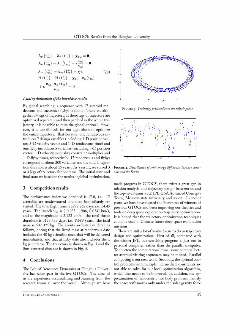
GTOC5: Results from the Tsinghua University
λr
(t+m
)− λr
(t−m
)+ χ1:3 = 0,
λv
(t+m
)− λv
(t−m
)− κ
vrelvrel
= 0
λm(t−m
)= λm
(t+m
)= χ7,
H(t−m
)−H
(t+m
)− χ1:3 · va (tm)
+ κvrel · aa (tm)
vrel= 0
(28)
Local optimization of the impulsive results
By global searching, a sequence with 17 asteroid ren-dezvous and successive flybys is found. There are alto-gether 34 legs of trajectory. If these legs of trajectory areoptimized separately and then patched as the whole tra-jectory, it is possible to miss the global optimal. How-ever, it is too difficult for our algorithms to optimizethe entire trajectory. That because, one rendezvous in-troduces 7 design variables (including 3-D position vec-tor, 3-D velocity vector and 1-D rendezvous time) andone flyby introduces 5 variables (including 3-D positionvector, 1-D velocity inequality constraint multiplier and1-D flyby time), respectively. 17 rendezvous and flybyscorrespond to about 200 variables and the total integra-tion duration is about 15 years. As a result, we solved 3or 4 legs of trajectory for one time. The initial state andfinal state are based on the results of global optimization.
3 Competition results
The performance index we obtained is 17.0, i.e. 17asteroids are rendezvoused and then immediately re-visited. The total flight time is 5277.862 days, i.e. 14.45years. The launch v∞ is [-0.935, 1.906, 0.034] km/s,and so the magnitude is 2.123 km/s. The total thrustdurations is 3173.433 days, i.e. 8.689 years. The finalmass is 507.095 kg. The events are listed in detail asfollows, noting that the listed mass at rendezvous dateincludes the 40 kg scientific mass that will be deliveredimmediately, and that at flyby date also includes the 1kg penetrator. The trajectory is shown in Fig. 3 and theSun-centered distance is shown in Fig. 4.
4 Conclusions
The Lab of Aerospace Dynamics at Tsinghua Univer-sity has taken part in the five GTOCs. The aims ofus are experience accumulating and learning from theresearch teams all over the world. Although we have
Figure . Trajectory projected onto the ecliptic plane
Figure . Distribution of orbit energy differences between aster-oids and the Earth.
made progress in GTOC5, there exists a great gap inmission analysis and trajectory design between us andthe top-level teams, such JPL, ESAAdvancedConceptsTeam, Moscow state university and so on. In recentyears, we have investigated the literatures of winners ofprevious GTOCs and been improving our theories andtools on deep space exploration trajectory optimization.It is hoped that the trajectory optimization techniquescould be used in Chinese future deep space explorationmissions.There are still a lot of works for us to do in trajectory
design and optimization. First of all, compared withthe winner JPL, our searching program is just run inpersonal computer, rather than the parallel computer.To shorten the computational time, some potential bet-ter asteroid-visiting sequences may be missed. Parallelcomputing is our next work. Secondly, the optimal con-trol problems with multiple intermediate constraints arenot able to solve for our local optimization algorithm,which also needs to be improved. In addition, the ap-proximation of heliocentric two body problem, namelythe spacecraft moves only under the solar gravity force
DOI: 10.2420/AF08.2014.37 43

Acta Futura 8 (2014) / 37-44 Jiang et al.
and the thrust of on-board propulsion system, is em-ployed for all the five GTOCs. And the simplified con-straints are considered. For example, the details of howthe rendezvous or flyby would occur are not addressed.The gravity assists are approximated to the impulsivemodel. That is, only the preliminary mission designproblems are concerned about in GTOCs. However,in practical engineering, an accurate dynamical model,which includes the perturbation forces of third bod-ies and solar radiation pressure, should be used. Andthe gravity assist should be studied in a full ephemerismodel. The trajectory optimization problem in an accu-rate dynamical model is expected to be investigated.
5 Acknowledgments
This work was supported by the National Natural Sci-ence Foundation of China (Grant No. 11302112) andthe Tsinghua University Initiative Scientific ResearchProgram (Grant No. 20131089268)
References
[1] A. E. Petropoulos and J. M. Longuski, “Shape-based algorithm for automated design of low-thrust, gravity-assist trajectories,” Journal of Space-craft and Rockets, vol. 41, no. 5, pp. 787–796, 2004.
[2] T.Haberkorn, P.Martinon, J. Gergaud, et al., “Lowthrust minimum-fuel orbital transfer: a homotopicapproach,” Journal of Guidance, Control, and Dy-namics, vol. 27, no. 6, pp. 1046–1060, 2004.
[3] F. Jiang, H. Baoyin, and J. Li, “Practical techniquesfor low-thrust trajectory optimization with homo-topic approach,” Journal of guidance, control, and dy-namics, vol. 35, no. 1, pp. 245–258, 2012.
[4] D. Izzo, T. Vinko, C. Bombardelli, et al., “GTOC2Activities and results of ESA advanced conceptsTeam.” February 2007.
[5] J. J. Moré, B. S. Garbow, and K. E. Hillstrom, Userguide for MINPACK-1. Argonne National Labora-tory Argonne, IL, 1980.
[6] M. J. Powell, “A hybrid method for nonlinearequations,”Numerical methods for nonlinear algebraicequations, vol. 7, pp. 87–114, 1970.
44 DOI: 10.2420/AF08.2014.37

Acta Futura 8 (2014) 45-55DOI: 10.2420/AF08.2014.45
ActaFutura
GTOC5: Results from the European Space Agency andUniversity of Florence
Dario Izzo *, Luís F. Simões, Chit Hong Yam, Francesco BiscaniEuropean Space Agency, Advanced Concepts Team
David Di Lorenzo, Bernardetta Addis, Andrea CassioliUniversity of Florence, Global Optimization Laboratory
Abstract. This paper describes the methodolo-gies used to tackle the problem of the 5th GlobalTrajectory Optimization Competition within theteam composed by the Advanced Concepts Teamof the European Space Agency and theGlobal Op-timization Laboratory of the University of Flo-rence. The method pursued is powered by two in-novative approaches: a linearized model of the ‘selffly-by’ aiding a first broad tree search of chemi-cal propulsion options and the use of global opti-mization techniques (Monotonic Basin Hopping,in this case) applied directly to the low-thrust tra-jectory model.
1 Preliminaries
In the context of the Global Trajectory OptimizationCompetitions we consider the problem of the fifth edi-tion (GTOC5), released by Moscow State Universityscientists, winners of the 4th GTOC edition. The exactmathematical formulation of the problem is describedin [1] and we will assume the reader is familiar with it.In short, starting from the Earth, a spacecraft equippedwith low-thrust propulsion capable of delivering a con-stant thrust of 0.5 N, needs to visit as many asteroids
*Corresponding author. E-mail: [email protected]
as possible from a given list of N = 7075 possible tar-gets. Each visit is a rendezvous. After an asteroid hasbeen visited, an optional fly-by can be attempted (atany time) to deliver a penetrator to the asteroid surface,and thus increase the mission value. The primary mis-sion objective is thus to visit (and revisit) as many as-teroids as possible within the mission constraints. Asimple calculation shows the complexity of the prob-lem. The possible asteroid sequences (considering onlysubsequent rendezvous) is N!
(N−n)! , where n is the se-quence length. As soon as n grows larger, the prob-lem complexity grows and soon a simple grid search be-comes unsuitable. The situation is actually much worseas asteroid re-visits are also possible. As the problemcomplexity is overwhelming we start by introducing onesimplifying assumption in the attempt to map the prob-lem into an easier case. We assume that the spacecraftperforms a fly-by delivering the penetrator immediatelyafter each asteroid rendezvous. Under this assumption
45

Acta Futura 8 (2014) / 45-55 Izzo et al.
we may state the GTOC5 problem as
find: seq ⊆ An, mjd ∈ Rn+1
to maximize: n = cardinality of seqsubject to: mf(seq, mjd) ⩾ 500 kg
mjdn+1 −mjd1 ⩽ 15 yearsmjdi+1 > mjdi i ∈ 1, . . . ,n57023 < mjd1 < 61041Ai = Aj i = j i ∈ 1, . . . ,n
(1)where A is the set of all 7075 asteroids, mjd is a vec-tor containing the launch epoch and all the rendezvousepochs (dimensionn+1) and seq = [A1,A2,A3, ..,An]is a vector containing the asteroid encounter sequence.The functionmf is the result of a global low-thrust op-timization where the spacecraft dynamics is accountedfor. We assume here that infeasible choices of (mjd,seq)(from the dynamical point of view, e.g. trajectories thatcannot perform the requested rendezvous/fly-bys in theselected epochs) result inmf < 500 kg. In order to solvethe problem stated in (1) we follow a two step approachwhich is common in trajectory design and that provedquite valuable to tackle problems in previous editions ofthe GTOC (see for example [2, 3]). We first computemf(seq, mjd) assuming the spacecraft equipped witha chemical engine capable of delivering instantaneous∆V changes. This allows to compute mf with a greatlyreduced computational effort, and thus to explore thesearch space exhaustively. In a second step, we map thesolutions found in this “chemical version” of the prob-lem back to the original one. The rest of the paper isorganized as follows: in Section 2 we study the first tra-jectory leg (i.e. Earth-Asteroid transfer) for all possibleasteroids, in Section 3 we explore the structure of low-thrust self-fly-by trajectories and we propose a simplechemical approximation for such legs. Exploiting theseresults we are able to define, in Section 4, the chem-ical version of our search problem and to propose, inSection 5 a few techniques to explore the vast solutionspace. In Section 6 we map the solutions obtained backto the full low-thrust problem. Finally, in Section 7 wediscuss the experience we gained from the applicationof the proposed methods.
2 The first low-thrust leg
Any trajectory that is a solution to the problem statedin (1) needs to start with an Earth-Asteroid leg. Thus,we study, separately, the optimal control problem for thefirst leg with the intention to further simplify the overall
problem. In particular, we study the low-thrust transferfrom the Earth to a generic asteroid A1 ∈ A allowing(from the GTOC5 problem description) as a startingrange 57023 < mjdE < 61041 and constraining thestarting velocity gain delivered by the launcher to∆V ⩽5. Because of the launch window width, more than timeone launch possibility for any considered asteroid is to beexpected. In order to locate them efficiently, we use, di-rectly on the low-thrust model, the global optimizationapproach described in Yam et al. [4]. In short, we tran-scribe the Optimal Control Problem (OCP) into a NonLinear Programming Problem (NLP) using a methodsimilar to the Sims-Flanagan transcription [5] and wethen consider the resulting NLP as a global non-linearlyconstrained optimization problem which we solve us-ing the Monotonic Basin Hopping (MBH) technique[6, 7]. This procedure allows us to find good launch pos-sibilities in a reasonably short time, since we are ableto compute good launch possibilities to all asteroids,first with time as objective function and then with mass.Overall we are able to solve, for two different objectives,a total of 70,750 non linearly constrained global opti-mization problems (ten per asteroid) determining goodlaunch opportunities to reach the asteroids in the list.We denote the best launch window for each asteroidA1in the sequence with mjdE(A1). It is to be noted thatthis first optimization was run in parallel over 16 CPUsand completed overnight (the open-source PaGMOop-timization library was used for this purpose [8]). As theamount of results from this optimization effort is huge,in Table 1 we report, as an example, only some of thebest launch possibilities found for both minimal timeand minimal mass ranked with respect to the objectivefunction. Launch occasions used in later optimizationruns (of the full trajectory) are also included. Note thatout of the 7075 asteroids, roughly 3000 result into un-feasible trajectories (for the considered constraints), andthus are not selected in the following searches as start-ing asteroids. To allow for greater speed, a rather coarsemesh grid was used as a precise computation of each op-timal trajectory was, at this point of our solution strat-egy, not a priority.
3 The self-fly-by
To formalize the GTOC5 problem in the form givenby (1), we assumed that the spacecraft always revisitsan asteroid immediately after it has performed the ren-dezvous with. This creates a trajectory leg (or phase)
46 DOI: 10.2420/AF08.2014.45

GTOC5: Results from the European Space Agency and University of Florence
Time optimal Mass optimalRank Asteroid m [kg] t [days] Rank Asteroid m [kg] t [days]1. 2001 GP2 87.47 53.88 1. 2009 QR 41.56 700.952. 2007 XB23 98.54 66.44 2. 2006 QV89 47.15 907.443. 2009 QR 99.24 67.24 3. 2006 XY 48.76 711.62... ... ... .... ... ... ... ...8. 2006 XY 127.14 98.91 6. 2007 UN12 51.13 942.1915. 2006 QV89 138.39 111.67 50. 2007 XB23 77.18 771.57]20. 2007 UN12 146.89 121.32 103. 2008 JL24 93.08 1009.81]43. 1991 VG 175.33 153.60 105. 2001 GP2 94.11 918.56]50. 2008 ST 179.92 158.81 110. 1991 VG 95.61 1079.69113. 2008 JL24 216.41 200.22 129. 2008 ST 101.32 827.77
Table . Some opportunities found with the global optimization of the first trajectory leg
having some unusual boundary conditions, namely azero departure relative velocity ∆Vdep = 0 and an ar-rival relative velocity ∆Varr ⩾ V = 0.4 km/s, with thearrival and departure object being the same (i.e. the as-teroid). We call this leg a self-fly-by leg. Representingsuch a leg as a ballistic arc, for each given transfer time,there exists a Lambert solution (the one that matchesexactly the asteroid orbit). Following this representa-tion we could estimate the total ∆V as the velocity mis-match at arrival between the Lambert solution (i.e. theasteroid orbit) and the next phase (i.e. ∆V = V = 0.4km/s) but we would have no indication on the necessarytransfer time as such a ∆V does not depend on it. Wethus develop an alternative simplified model for this pe-culiar leg by considering, in one dimension, the motionof a point mass subject to an external acceleration. Thepoint mass position will be indicated by s, its velocity byv and its acceleration by a. We assume that the pointmass (our spacecraft) will accelerate at its maximum ca-pability a = Tmax/m0 away from the origin (asteroid)for a time t1 and then it will accelerate back towards theorigin for a time t2. Starting from s = 0 and v = 0 weget:
s(t1 + t2) =
12at
21 + at1t2 −
12at
22
v(t1 + t2) = a(t1 − t2)
if we also require that s(t1+t2) = 0 and v(t1+t2) = V
(which accounts for the terminal boundary conditions atthe fly-by) we conclude: t1 = 2√
2Va
t2 = Va
(√2
2 + 1)
hence, ∆Tsfb = t1 + t2 = m0V
Tmax
(1 +√
2)
∆Vsfb = a∆T = V(
1 +√
2) (2)
This crude model of a low-thrust self-fly-by leg is validunder the assumption of an infinite specific impulse (thishypothesis can be removed by propagating also the massequation, leading to more complex algebraic formulas)and can be considered as a zero-th order approximationof the spacecraft motion relative to the asteroid. The ad-vantage is that, by using (2), we can put a quick estimateon the propellant consumption and on the time of flightfor such a leg. In particular, for the specificmission data,the∆Vsfb is estimated to be equal to∆Vsfb = 960 m/sfor all self fly-by legs, while the time of flight varies from∆Tsfb ≈ 150 days, at the beginning when the spacecraftweights 4000 kg, to ∆Tsfb ≈ 18 days at the end whenthe spacecraft weights only 500 kg. In order to test thevalidity of such a model in the context of the GTOC5problem, we performed the global low-thrust optimiza-tion of self fly-by legs selecting at random 10% of theasteroid population and letting the starting epoch freein the initial launch window. We used an initial massof m0 = 4000 kg and we let the velocity direction ofthe spacecraft relative to the asteroid free at the fly-by.By doing so, we let the optimizer select the best startingorbital anomalies to take advantage of orbital mechanicseffects in order to shorten the self fly-by duration.The results are shown in Figure 2. We plotted the∆Tsfband ∆Vsfb resulting from the low-thrust global opti-mization against semi-major axis and eccentricity of thetarget asteroid. We observe how the predictions comingfrom (2) are quite crude, still they represent an improve-
DOI: 10.2420/AF08.2014.45 47

Acta Futura 8 (2014) / 45-55 Izzo et al.
t = 0 t = t t = t +t1 2 1
Figure . Visualization of the simple model for the low-thrust, self-fly-by leg
ment with respect to a simpler purely ballistic approx-imation, furthermore they systematically overestimatethe values resulting from the solution of the time op-timal self fly-by problem. We also see that only a weakcorrelation exists between the asteroid semi-major axisand eccentricity and the accuracy of the prediction.
4 The chemical problem
Using the results derived in Sections 2-3 we transformthe problem stated in (1) into a simpler one where thespacecraft trajectory is built by putting together Lam-bert arcs, self fly-by arcs (described by (2)) and the firstleg resulting from the global optimization described inSection 2. We state the following new problem, whichwe refer to as the chemical version of the full-problem:
find: seq ⊆ An
to maximize: n = cardinality of seqsubject to: m∗
f(seq) ⩾ 500 kgT∗f = mjdn −mjdE ⩽ 15 yearsAi = Aj
(3)Formally, the difference with respect to (1), is that thecontinuous part of the decision vector (i.e. the modifiedJulian dates) has disappeared as it now depends, via theLambert solution, solely on the asteroids selected. Thefinal mass constraint takes a different form (this reflectsthe change in the trajectory model) and the startingepoch is not in the decision vector as it depends only onthe choice of the first asteroid A1 (for each asteroid weconsidered the best launch opportunity found. In latersearches we also considered the second and third bestsin an attempt to make our search less greedy). Note thata number of different options can actually be consideredwhen computing m∗
f(seq) (e.g., number of revolutions
in the Lambert solution, or Lambert arc duration). Inthese cases, we always perform an inner search to greed-ily select the best option.
4.1 Computingm∗f(seq)
Consider seq = [A1,A2, ...,An]. We denote the epochand the spacecraft mass at the i-th asteroid with re-spectively tAi
and mAi. Consider now the transfer
Aifb−→ Ai
rndv−−−→ Ai+1: an asteroid to asteroid ren-dezvous with self fly-by. We estimate its costs using theexpressions:
mAi+1 +mpld =
=[mAi
exp(−∆Vsfb
Ispg0
)−mp
]exp
(−
∆Vi(i+1)
Ispg0
)tAi+1 = tAi
+ ∆Tsfb + ∆Ti(i+1)(4)
where ∆Vi(i+1) and ∆Ti(i+1) are the estimates of theAi
rndv−−−→ Ai+1 leg,mp is the penetratormass left at thefly-by and mpld is the payload mass delivered at eachasteroid. Starting frommA1 and tA1 as returned by theglobal optimization of the first leg, wemay use the aboveequation to sequentially to obtainm∗
f = m∗An
and T∗f =
tAn− tE. The estimates for ∆Vi(i+1) and ∆Ti(i+1) are
the only data needed. In order to compute them, weconsider all the multiple revolution Lambert’s problemsolutions for the transfer fromAi toAi+1 at time tAi
+∆Tfsb for different values of the transfer times∆Ti(i+1)(we consider all values in [100,700] days with bins of10 days) and we select the best one in terms of minimalvelocity change (evaluated as the mismatches with theasteroid velocities, after having subtracted V).
48 DOI: 10.2420/AF08.2014.45

GTOC5: Results from the European Space Agency and University of Florence
Figure . ∆Tsfb and ∆Vsfb distributions for the time optimal self fly-by legs. The zero-th order approximation has ∆Tsfb = 150days and ∆Vsfb = 960 m/s, and can thus be considered an upper bound.
5 The tree search
Let us now consider problem (3). The non linear con-straints m∗
f and T∗f share a monotonicity property with
respect to n. Given an allowed sequence seq ⊂ An
of cardinality n, and a possible new asteroid, the newallowed sequence seq ′ ⊆ An+1 of cardinality n + 1,obtained by adding such asteroid, satisfies
m∗f(seq) ⩽ m∗
f(seq ′)T∗f (seq) ⩾ T∗
f (seq ′)
This property, specific of the given problem, allows usto explore the search space of feasible sequences in-crementally, starting from short length sequences andadding asteroids when possible. We implemented twoapproaches that exploit such a structure, a branch aprune recursive tree search, and an order based GeneticAlgorithm using hidden genes.
5.1 Branch and prune
The branch and prune algorithmwe developed is, essen-tially, a recursive search over the tree of possible chemi-cal representations of the full trajectory. The algorithmis built around the basic recursive function described inAlgorithm 1.
The choices of the pruning criteria and the list of as-teroid candidates to consider at each step are crucial fora successful application of such an algorithm. A badselection of these functions can result in pruning goodbranches. Within the context of the GTOC competi-tion there is no way of knowing how to choose thesefunctions, nor of studying the impact of a certain choiceon the resulting trajectories. So expert knowledge is
Algorithm 1 Recursive procedure for the Branch andPrunebp_step([A1,A2, ...,An],mAn
, tAn])
A← list of possible candidates for the next asteroidfor An+1 in A doCompute mAn+1 , tAn+1 using (4)if prune( N,mAn+1 , tAn+1 ) then
log and continueelse
call bp_step([A1, ...,An+1],mAn+1 , tAn+1 ])end if
end for
necessary and discriminates success from failure. Thelist of possible candidates considered as reachable froma given asteroid is formed by considering the first 512out of the 7075 asteroids ranked using the simple Edel-baum approximation [9]. We list below the pruning cri-teria we used:
1. At each recursive step we defineamax = ηTmax/mAn
and we prune if∆Vn(n+1)/∆Tn(n+1) ⩾ amax. The coeffi-cient η is set to 0.9;
2. We prune if mAn+1 ⩽ 400 kg;
3. We prune if TAn+1 ⩾ 16 years;
4. At each recursive step, we define a tolerated varia-tion on the mass as dmtol = 600−200(n+1)/Nt
kg, where nt is the maximum length found so farfor a feasible sequence plus one. We then prune if[4000 − 3500(n+ 1)/nt] −mAn+1 ⩽ dmtol;
DOI: 10.2420/AF08.2014.45 49

Acta Futura 8 (2014) / 45-55 Izzo et al.
A1 A2 A3 . . .
ast2
ast1
×nnnnnn
66nnnnnn
× //
×PPP
PPP
((PPPPP
P
ast3
ast1 ast4
... ast1
E
""
===
====
====
====
====
88qqqqqqqqqqqqqqq× //
==
×
AA
''OOOOO
OOOOOO
OO ast2 ast3 ast1
ast2
×~~~~~~~~~
??~~~~~~~~~
×nnnnnn
66nnnnnn
// ast4
×nnnnnn
66nnnnnn
× //
×OOO
OOO
''OOOOO
O
>>>
>>>>
>>>>
>>>>
>>>>
>
444
4444
4444
4444
4444
4444
4444
ast3
... astk ast5
astj
×pppppp
77pppppp
× //
×NNN
NNN
''NNNNN
N
astl ast6
... astm...
Figure . Visualization of the branch and prune process over a small part of the search tree. Starting from the Earth (left) only the firstthree asteroid selections are shown and only a subsets of the transfer opportunities between asteroids are considered. Most branches arehere pruned helping the visualization.
50 DOI: 10.2420/AF08.2014.45

GTOC5: Results from the European Space Agency and University of Florence
5. At each recursive step, we define a tolerated delayon the time as dttol = 1000 − 500(n + 1)/Nt
days, where Nt is the maximum length found sofar for a feasible sequence plus one. We then pruneif (tAn+1 − tE) − 15(n+ 1)/nt ⩽ dttol.
The last two pruning criteria are used to prune trajec-tories that accumulate too much delay (either in mass ortime) with respect to a nominal linear schedule bringingin nt + 1 encounters the mass from 4000 kg to 500 kgand the time from 0 years to 15 years. A visualizationof the resulting search process is shown in Figure 3. Werun such an algorithm starting from all launch opportu-nities found performing the global optimization of thefirst Earth-Asteroid leg (see 2). The algorithm, run inparallel over 8 CPUs, completed the entire tree search inroughly a week, returning millions of asteroid sequencesand their encounter dates. Remarkably, in all the com-puted sequences longer than 16, the first asteroidA1 wasone of 1991 VG, 2007 UN12, 2008 JL24 and 2008 ST.We found several sequences of length n = 17 (whichwe later could not transform into a feasible low-thrusttrajectory), but no solution was found with a sequencelength n = 18.
5.2 Order-based Genetic Algorithm
The main risk with a branch and prune approach lies inthe fact that in order to obtain a tractable search space,strict pruning criteria need to be enforced, so as to dis-card vast swaths of the full search space. Branching andpruning criteria are greedy, in the sense that they de-mand performance to be above certain thresholds at ev-ery step, and their enforcement thus prevents the iden-tification of solutions that, in order to reach excellentperformance levels at some point in the future, first needto “pay” high costs.
The second approach followed for the identificationof good asteroid sequences used an order based GeneticAlgorithm (GA), in which a population of completecandidate solutions (chromosomes) is evolved towardsmaximization of a given fitness function. Chromosomesare here ordered subsets of the set of asteroids availablefor the mission, and crossover and mutation operationsare defined on them, that always generate valid permu-tations. The goal with pursuing this second approachwas to conduct an exploration on the much larger searchspace resulting from a relaxation of the pruning criteriaused in the branch and prune tree searches. Exhaus-tive enumeration of the possible solutions was then no
longer feasible, but we assumed this approach could suc-ceed in identifying good solutions possibly discarded bythe branch and prune’s greedier approach.A population of 5000 chromosomes was used. Each
chromosome in the initial population was randomlygenerated by uniform sampling without replacement of20 asteroids from the full set of 7075 asteroids. Notransition constraints were imposed on the asteroid se-quences (by contrast with the branch and prune ap-proach, where an asteroid branches only into the 512asteroids expected to represent the best transfers). Theonly imposed positional constraint was that, as men-tioned in Section 4.1, A1 had to be one of the aster-oids for which a good launch possibility had previouslybeen identified in the global optimization of the first leg.After generating a random sample of asteroids, the se-quence would then be rotated until one of those aster-oids would occupy A1. This constraint is preserved bythe crossover and mutation operators described below.Given a sequence of asteroids in a chromosome, a tra-
jectory is built by sequentially expressing the encodedasteroids, up to the transfer that breaks one of the con-straints: mAn+1 ⩾ 500 kg, and TAn+1 ⩽ 15 years.The remaining asteroids in the chromosome are not ex-pressed in the trajectory, and do not therefore contributeto the chromosome’s fitness.The costs of transfers between asteroids in a chromo-
some were determined as described in Section 4.1, withthe difference that the transfer time ∆Ti(i+1) was cho-sen from amongst the 156 values in the range of 1 to 776days (approximately 2.1 years), in bins of 5 days, andwas the one with minimal velocity change that did notcause the maximum acceleration amax to be exceeded(being amax determined using a coefficient η of 1.0 –see Section 5.1, pruning criterion 1). By comparisonwith the branch and prune tree searches, these changesenlarge the search space with a great number of trajec-tories containing legs that take too long to complete orrequire greater accelerations. Doing so in the context ofthe Genetic Algorithm, however, increases the rate ofdiscovery of good relative orderings between asteroids,that can then be used as building blocks in the construc-tion of better trajectories.Fitness assignment takes into account a chromo-
some’s trajectory score, as well as the resources (massand time) needed in order to achieve it. The best of twochromosomes is defined as being the one with greatestscore. In case of a tie, it is then the one with greatestresource savings rating r(x). A generalized mixture op-erator [10] aggregates the attribute vector x = [(m∗
f -
DOI: 10.2420/AF08.2014.45 51

Acta Futura 8 (2014) / 45-55 Izzo et al.
500)/3500, (15 - T∗f )/15], in which the final amounts
of mass and time are transformed into the ratios of theavailable budgets for the mission left unused by the tra-jectory:
r(x) =∑n
i=1 wi(x)xiwi(x) = 1 − xi∑n
j=1 xj
The linear weight generating function wi(x) dynami-cally adjusts the weights assigned to each attribute, asa function of the degree to which each is being satis-fied. Specifically, it implements a preference for trajec-tories that allocate more evenly the mission’s resources.As both mass and time are critical resources that needto be made available for additional asteroids to becomereachable,wi(x) favors improvements to the least avail-able resource.A steady-state population update scheme was used,
which alternates between steps of parent selection, mat-ing, and insertion of the generated offspring back intothe population. Tournament selection, with a tour-nament size of 2, is used for selecting 2 parents forreproduction. The selected parents always undergo acrossover operation, in which a single offspring is gener-ated. That offspring then undergoes mutation. Finally,the offspring replaces the worst solution in the popula-tion, if it has a better fitness, otherwise it is discarded.A uniform scanning adjacency-based crossover oper-
ator was implemented. It is a variation on the operatorsin [11]. One offspring chromosome is sequentially con-structed, by selecting asteroids from parents, in a waythat explores variations on the relative orderings theyencode. Throughout the construction, one index is keptper parent, pointing to the asteroid in its chromosomevector that the parent advocates as being the adequatechoice to follow up from the asteroid last added to theoffspring sequence. At every step, the offspring ran-domly selects one of the parents, and takes the asteroid itis currently pointing to. Initially, those indexes point tothe first asteroid in each parent. Whenever one asteroidis added to the offspring sequence, each parent updatesits index, so as to point in its chromosome to the posi-tionally nearest asteroid to the one just added, that is notyet present on the offspring sequence. Example: consid-ering asteroid 2 was just now added to the offspring, theparent [3, 7, 2, 6, 5, 1, 4] would set its position marker tothe first asteroid in the following sequence, that is notalready part of the offspring: [6, 7], [5, 3], 1, 4 (scanningforward and back from asteroid 2, with no wrapping;should two asteroids at the same distance from 2, suchas 6 and 7, be viable choices, one of them is chosen at
0 1 2 3 4 5trajectory evaluations ×105
0
2
4
6
8
10
12
14
16
18
Sco
re
bestaverageworst
0 1 2 3 4 5trajectory evaluations ×105
0
50
100
150
200
250
300
dis
tinct
ast
ero
ids
expre
ssed a
t posi
tion
position in trajectory
1234567
891011121314
Figure . Performance of the order-based Genetic Algorithm:scores (top) and diversity (bottom) of asteroid sequences in popula-tions throughout the optimization (values averaged over 30 runs).
random). Should an added asteroid not occur in one ofthe parents, that parent keeps its position marker at itsprevious state.
The implemented mutation operator swaps two con-secutive asteroids, chosen uniformly at random fromamong the 19 pairs in the sequence. Should the firstpair be chosen, the second asteroid only takes the placeof the first if it too is a valid starting asteroid.
Figure 4 shows the typical performance of a GA run(averaged over 30 independent runs) searching amongthe complete set of available asteroids, for a sequencewith maximal score. Figure 4(top) shows the progressin the population’s scores throughout the search. Theaverage score of the best found asteroid sequence in arun was 12.7 (st. dev.: 0.6), with the best score achievedwith this setup being 14.2. As individual GA runs com-pleted on average in approximately 17 hours (runningin a single processor), the GA achieved on average 75%of the quality of solutions identified in the branch and
52 DOI: 10.2420/AF08.2014.45

GTOC5: Results from the European Space Agency and University of Florence
prune tree search (where sequences of length 17 werefound), in roughly 1.3% of the CPU time, while search-ing in a much larger search space.Figure 4(bottom) shows the number of distinct as-
teroids being expressed at each position Ai across thepopulation’s 5000 trajectories. We can observe that, fol-lowing the appearance of chromosomes in the popula-tion which are able to express a greater number of aster-oids (increase the score), over what had previously beenidentified, there is an explosion in the number of as-teroids being identified as viable choices for those legs.At the same time, the gradual identification of the bestasteroids for a given position continually pushes for aconvergence on the set of asteroids that are deemed ap-propriate choices at the preceding positions. As thecrossover and mutation operators only make use of theasteroids contained in parents’ chromosomes, it is fromchromosomes’ non-expressed genes that novel combi-nations are generated. Though non-expressed genes donot contribute to an individual chromosome’s fitness,the crossover operator is able to use it as a “geneticmemory” of good relative orderings that were expressedat some point in the chromosome’s ancestors. Non-expressed genes are therefore equally undergoing evo-lution, increasing the likelihood of successful transfersbeing generated.
6 Back to the low-thrust world
The results from the tree search come in the form ofpairs [seq, mjd] containing asteroid sequences and theirencounter dates. The large number of returned trajec-tories is prohibitive to perform a full optimization forall of them. Thus, we further screen the solutions. Thisis done considering the global optimization for singleasteroid-to-asteroid legs with self fly-by and trying totransform incrementally the trajectory returned by thechemical search into a real low-thrust trajectory. Dur-ing the optimization, an upper bound on the arrival timeof a given leg is set to the departure time of the next legto ensure the ’continuity’ of the whole trajectory. Afterthis preliminary screening process, we obtained a list offeasible low-thrust trajectories, ranked by the number ofasteroid encounters, flight time, and final mass.Next, we attempt to optimize selected sequences as
a whole trajectory by removing the bounds on the ar-rival and departure times. Due to the complexity of theproblem, the optimizer has problems in converging ina reasonable amount of time if we optimize the whole
trajectory from start. Instead we try to assemble a few(two or three) asteroid to asteroid legs at a time by re-moving the bounds on the middle times but keeping thebounds at the start and the end.In the last step the full trajectory is considered as
one single nonlinear programming problem. We usea low-thrust trajectory model similar to that describedin [5] which is the basis of the widely used GAL-LOP/MALTO trajectory optimization tool [12]. Inour own implementation (available in the open sourcepython library called PyKEP), the possibility of switch-ing between Keplerian and low-thrust propagation ispresent, so we first use a Keplerian propagator to exploitits speed. Only at the endwe switch to a low-thrust Tay-lor propagation [13], roughly 5 times slower than theKeplerian, where the whole trajectory is numerically in-tegrated to satisfy all the constraints up to the requestedaccuracy. In Table 2 we report a summary of the besttrajectory found.
7 Lessons Learnt
The trajectory summarized in Table 2 ranked as fourthin the GTOC5 competition, a result one can be veryproud of, but that has to be analyzed in the context ofthe overall methodology used. In particular we must re-mark that solutions with N = 17 and N = 18 exist forthis problem, as proved by the other solutions returnedby other teams, but were not found by our methodol-ogy. While we did find solutions with N = 17 dur-ing the chemical tree search, we were not able to trans-form them into low-thrust solutions. No solutions withN = 18 was found by our branch and prune exhaustivetree search. While it is difficult to say exactly what partof our methodologies failed, we may look to them crit-ically as to locate their main limitations and determinegood research directions.
1. The assumption that a chemical trajectory can ap-proximate a low-thrust one is very strong and,whenever possible, should be avoided. This re-quires the development of more and more efficienttools for low-thrust optimization, but also a cor-rect choice for the solution strategy, i.e. one thatdoes require only the strictly necessary amount oftrajectory legs to be computed. In the case of theGTOC5 problem, this was probably a main fac-tor to our algorithm failure in finding any n = 18solution.
DOI: 10.2420/AF08.2014.45 53

Acta Futura 8 (2014) / 45-55 Izzo et al.phase
startasteroidend
asteroidstartm
assend
mass
startepochend
epochleg
toftottof
thrustduration1
Earth
(2007UN12)
4000.003874.24
59062.8159241.23
178.430.49
1402
(2007UN12)
(2007UN12)
3834.243736.18
59241.2359366.70
125.470.83
1253
(2007UN12)
(2006JY26)
3735.183487.07
59366.7059718.72
352.021.80
2804
(2006JY26)
(2006JY26)
3447.073360.45
59718.7259827.12
108.412.09
1085
(2006JY26)
(2001GP2)
3359.453122.40
59827.1260120.57
293.452.90
2936
(2001GP2)
(2001GP2)
3082.403005.40
60120.5760222.60
102.033.18
1027
(2001GP2)
225312(1996
XB27)
3004.402706.22
60222.6060645.66
423.064.33
3378
225312(1996
XB27)
225312(1996
XB27)
2666.222610.63
60645.6660768.01
122.354.67
709
225312(1996
XB27)
(2003SM
84)2609.63
2491.0560768.01
61044.11276.10
5.42162
10(2003
SM84)
(2003SM
84)2451.05
2391.0361044.11
61135.7191.60
5.6871
11(2003
SM84)
(2006HE2)
2390.032227.29
61135.7161410.80
275.096.43
21812
(2006HE2)
(2006HE2)
2187.292132.20
61410.8061490.44
79.646.65
6213
(2006HE2)
(2007HC)
2131.202006.92
61490.4461679.56
189.127.16
15014
(2007HC)
(2007HC)
1966.921916.45
61679.5661753.71
74.157.37
5815
(2007HC)
(1998KY26)
1915.451734.75
61753.7162127.99
374.288.39
37416
(1998KY26)
(1998KY26)
1694.751649.67
62127.9962192.70
64.718.57
5017
(1998KY26)
(2009TD17)
1648.671552.93
62192.7062383.79
191.109.09
11118
(2009TD17)
(2009TD17)
1512.931473.12
62383.7962440.28
56.499.25
4319
(2009TD17)
(2007YF)
1472.121345.03
62440.2862647.84
207.569.82
16420
(2007YF)
(2007YF)
1305.031271.97
62647.8462697.49
49.659.95
3721
(2007YF)
(1999AO10)
1270.971190.78
62697.4962949.99
252.5010.64
14422
(1999AO10)
(1999AO10)
1150.781127.17
62949.9963002.23
52.2310.79
2423
(1999AO10)
(2006RH
120)1126.17
1027.1163002.23
63303.21300.99
11.61140
24(2006
RH120)
(2006RH
120)987.11
964.0063303.21
63344.0940.88
11.7222
25(2006
RH120)
(2008UA202)
963.00926.63
63344.0963481.71
137.6212.10
3226
(2008UA202)
(2008UA202)
886.63867.50
63481.7163522.77
41.0612.21
1727
(2008UA202)
(2008HU4)
866.50770.33
63522.7763874.80
352.0313.17
16728
(2008HU4)
(2008HU4)
730.33713.20
63874.8063905.35
30.5513.26
1529
(2008HU4)
(2004VJ1)
712.20657.25
63905.3564061.71
156.3613.69
5430
(2004VJ1)
(2004VJ1)
617.25603.89
64061.7164090.16
28.4513.76
1231
(2004VJ1)
(2003W
T153)
602.89554.57
64090.1664225.14
134.9914.13
5932
(2003W
T153)
(2003W
T153)
514.57501.00
64225.1464244.62
19.4714.19
13
Table.Sum
maryofthebesttrajectoryfound
afterthefulllow-thrustoptim
ization
54 DOI: 10.2420/AF08.2014.45

GTOC5: Results from the European Space Agency and University of Florence
2. Traversing the search tree using a branch and prunealgorithm, implemented as a depth-first search, isnot necessarily a good idea. While depth firstsearch has the advantage of delivering immedi-ately some solutions one can work with (a veryimportant property in the context of the GTOCcompetitions), its complexity grows exponentiallyand thus encourages the introduction of moreand more arbitrary pruning criteria that eventu-ally risk to make the search too greedy. Strategiessuch as breadth first search or A∗ algorithm vari-ants should also be considered and when possibleadopted. It is likely that our strict pruning crite-ria, necessary for the depth first search to finish ina reasonable amount of time, did not allow us tofind better solutions.
3. The use of evolutionary techniques, such as theorder based genetic algorithm here used, to per-form a trajectory search for a multiple asteroid ren-dezvous mission, while not competitive with otherapproaches for the considered problem, showed in-teresting results and it is considered as a very inter-esting research topic.
4. Monotonic Basin Hopping, in connection to theSims-Flanagan trajectory model may help to avoidthe need for an initial trajectory guess, resulting inan unbiased exploration of the low-thrust solutionspace.
References
[1] I. S. Grigoriev and M. P. Zapletin, “Problemdescription for the 5th global trajectories opti-mization competition,” tech. rep., LomonosovMoscow State University, Faculty of Mechanicsand Mathematics, October 2010.
[2] M. Belló Mora and J. Cano, “1st ACT global tra-jectory optimisation competition: Results found atDEIMOSSpace,” Acta Astronautica, vol. 61, no. 9,pp. 794–805, 2007.
[3] A. Petropoulos, T. Kowalkowski, M. Vavrina,D. Parcher, P. Finlayson, G.Whiffen, and J. Sims,“1st ACT global trajectory optimisation competi-tion: Results found at the Jet Propulsion Labora-tory,” Acta Astronautica, vol. 61, no. 9, pp. 806–815, 2007.
[4] C. H. Yam, D. di Lorenzo, and D. Izzo, “Low-thrust trajectory design as a constrained globaloptimization problem,” Journal of Aerospace Engi-neering, vol. 225, no. 11, pp. 1243–1251, 2011.
[5] J. A. Sims and S. N. Flanagan, “PreliminaryDesign of Low-Thrust Interplanetary Missions,”in AAS/AIAA Astrodynamics Specialist Conference,Aug. 1999.
[6] D. J. Wales and J. P. K. Doye, “Global opti-mization by basin-hopping and the lowest energystructures of Lennard–Jones clusters containingup to 110 atoms,” Journal of Physical Chemistry A,vol. 101, no. 28, pp. 5111–5116, 1997.
[7] B. Addis, A. Cassioli, M. Locatelli, andF. Schoen, “A global optimization methodfor the design of space trajectories,” Computa-tional Optimization and Applications, vol. online,june 2009.
[8] F. Biscani, D. Izzo, and C. H. Yam, “AGlobal Optimisation Toolbox for Massively Par-allel Engineering Optimisation,” in 4th Interna-tional Conference on Astrodynamics Tools and Tech-niques (ICATT 2010), May 2010.
[9] T. Edelbaum, “Propulsion requirements for con-trollable satellites,” ARS (Am. Rocket Soc.) J.,vol. 31, 1961.
[10] R. A. M. Pereira and R. A. Ribeiro, “Aggregationwith generalized mixture operators using weight-ing functions,” Fuzzy Sets and Systems, vol. 137,no. 1, pp. 43–58, 2003.
[11] A. E. Eiben, P.-E. Raué, and Z. Ruttkay, “Geneticalgorithms with multi-parent recombination,” inParallel Problem Solving from Nature – PPSN III(Y. Davidor, H.-P. Schwefel, and R. Männer,eds.), vol. 866 of Lecture Notes in Computer Science,pp. 78–87, Springer Berlin / Heidelberg, 1994.
[12] C. H. Yam, D. Izzo, and F. Biscani, “Towardsa High Fidelity Direct Transcription Method forOptimisation of Low-Thrust Trajectories,” in 4thInternational Conference on Astrodynamics Tools andTechniques (ICATT 2010), May 2010.
[13] A. Jorba and M. Zou, “A Software Package forthe Numerical Integration of ODEs by Meansof High-Order Taylor Methods,” Experiment.Math., vol. 14, pp. 99–117, 2005.
DOI: 10.2420/AF08.2014.45 55

56

Acta Futura 8 (2014) 57-65DOI: 10.2420/AF08.2014.57
ActaFutura
GTOC5: Results from the National University of DefenseTechnology
Xiaoyong Jiang *, Zongfu Luo, Yijun Lian, Guojian TangCollege of Aerospace and Materials Engineering, National University of Defense Technology, 410073 Changsha (China)
Abstract. We propose a general scheme to solvethe 5th Global Trajectory Optimization Compe-tition problem, summarize the methods we em-ployed and present the results we obtained. Thegeneral scheme contains four relatively indepen-dent parts, among which the global optimizationand local optimization are key components. Inglobal optimization, we mainly attempted threemethods to obtain the asteroid sequence, and paidspecial attention to the last asteroid. In local opti-mization, we applied a direct shooting method tothe low-thrust trajectory design. The final trajec-tory launches at 58956 MJD, and revisits 8 aster-oids (the Beletskij asteroid is not included). Therank of the competition shows that our result is dis-tant from the global optimum, which suggests thatour global optimization method is premature dueto inefficient loop operations.
1 Introduction
The problem proposed in GTOC5 is “to visit the great-est number of asteroids with revisiting”. In the prob-lem description, three points of practical interest can befound: (1) Asteroid exploration mission: it draws moreand more interests for science in the 21st century. Basedon its observation and analysis, many significant sci-entific questions, such as the solar system’s origin, the
*Corresponding author. E-mail: [email protected]
planetary evolution mechanism, etc., may be unveiled.Since the Galileo spacecraft, which had visited two as-teroids, Gaspra and Ida, in 1991 and 1993, nine space-crafts have already explored asteroids. (2) Low-thrustpropulsion: its momentum transfer per kilogram of pro-pellant is 10 to 20 times greater than that of chemicalpropulsion [1]. Since 1998, NASA’s Deep Space 1 andDawn mission, JAXA’s Hayabusa and ESA’s SMART1 all use the low-thrust propulsion for deep space ma-neuvers. (3) Multiple deep space exploration missions:by proper design, it will increase the scientific rewardsenormously.From a competition point of view, the three points ofinterest mentioned above produces three characteristics:(1) The asteroid gravity can be neglected in the pre-liminary design. Thus the dynamical model is simpleand suitable for a competition. (2) The trajectory isperturbed by low-thrust almost throughout the time offlight, accordingly should be calculated by numerical in-tegration. In this case, mission design and optimizationcan be considered as a complex constrained continuousoptimal control problem. (3) Multiple missions bringeven more complexity to the problem. So more atten-tion should be paid to global optimization and solutionspace pruning.Comparing with former GTOCs¹, the problem pro-
¹For additional information about GTOCs, consult the GTOCPortal at http://sophia.estec.esa.int/gtoc_portal
57

Acta Futura 8 (2014) / 57-65 Jiang et al.
posed in GTOC5 has three differences: (1) The search-ing space is so large (7075 candidate asteroids in thelist) that it is almost impossible to find the global op-timization solution. (2) Two maneuvers (rendezvousand flyby) should be applied to each target in order. (3)The spacecraft needs to deliver some mass for each en-counter.This paper gives a preliminary analysis of the prob-
lem, summarizes the methods we employed to solve it,and presents and discusses the results found by Team26 from National University of Defense Technology(NUDT).
2 Preliminary Analysis
Preliminary Analysis of the Index
The first performance index of the problem is to maxi-mize the number of asteroids with revisiting. We giveit a preliminary assessment firstly. After revisiting anasteroid, the spacecraft delivers a scientific equipment(40kg) and a penetrator (1kg), which means that itsmass decreases 41kg. Suppose conservatively that thelow-thrust propulsion burns more than 100days at itshighest level during a revisiting, the propellant con-sumption is:
∆m =F
Ispg0t = 88.10kg (1)
where ∆m is the propellant consumption, F is the low-thrust magnitude, Ispis the specific impulse, g0 is thesea level gravitational acceleration, and t is the low-thrust active duration.Therefore, the greatest number of asteroids with revisit-ing within its 3500kg consumable mass is less than
350041 + 88.10
= 27.11 (2)
On the other hand, if we estimate conservatively thetime of flight of revisiting an asteroid to be more than200 days, the greatest number of asteroids with revisit-ing within its 15 years transfer time is less than 5478.75
200 =27.39.So it is reasonable to assume that the first perfor-
mance index is no more than 27.
Preliminary Filtration of Asteroids
There are 7075 candidate asteroids in the list; there-fore, it is infeasible to traverse each of them when se-
1 1.5 2 2.50
1
2
3
4
5
6
7
a [AU]
i [de
g]
Beletskij
Figure . Distribution of semimajor axis and inclination ofBeletskij asteroid and others.
lecting the next visiting asteroid during global optimiza-tion. There are several methods to reduce the searchingspace, such as orbit elements filtration, orbital energyfiltration, nearest plane to asteroids filtration, etc. It iseffective and simple to filter asteroids by the orbit el-ements. If the orbit elements of an objective body aremore different from those of another, it needs more en-ergy to transfer from the one to the other. We screenasteroids by:
a ∈ [0.95, 1.20]AU, i ∈ [0, 2]deg, e ∈ [0, 0.3] (3)
where a is semi-major axis, i is inclination, and e iseccentricity.After this screening, almost 99% of candidate asteroidsare excluded, and only 73 asteroids are reserved. Thesearching space reduces sharply.
Evaluate the Feasibility of Visiting Beletskij Asteroid
In honor of V. Beletskij 80th anniversary, mission toBeletskij asteroid adds bonus points. For it, the estima-tion raises 1.5 times. But as showed in Fig.1, its semi-major axis is more than 2.6AU, and its inclination ismore than 6.0deg. It means that more propellant shouldbe consumed to transfer to Beletskij asteroid than thatto near-Earth asteroids. It is safe to conclude that in theinitial phases, the spacecraft is capable of revisiting twomore near-Earth asteroids (the first performance indexadds 2+) if it can revisit Beletskij asteroid. Therefore,during global optimization, we do not take the missionto Beletskij asteroid into account.
58 DOI: 10.2420/AF08.2014.57

GTOC5: Results from the National University of Defense Technology
Figure . General scheme of multiple asteroids tour with low-thrust propulsion.
Figure . Sketch of Flux Tube Pruning Method.
Asteroid Exploration Strategy
For this specific GTOC5 problem, there is a strategyto explore asteroids: to flyby an asteroid directly afterrendezvousing with it. Since the minimum velocity toflyby an asteroid is 0.4km/s, there is rarely another as-teroid mission which consumes less propellant than thatof flyby after a rendezvous with an asteroid. Adoptingthis strategy, the efficiency of global optimization willpromote considerable, and rare global optimization so-lutions are excluded. During the competition, we realizethis strategy later but do not have enough time to pro-gram it. Based on some simulation, in our opinion, ifthe minimum velocity to flyby an asteroid is increasedto 1.0km/s, the strategy would be invalid and the prob-lem would be more competitive.
3 Methodology
General Scheme
Following the analysis of literature [2, 3, 4], we deriveda general scheme to deal with the GTOC5 problem.As showed in Fig.2, there are four parts in the gen-eral scheme: the initialization, global optimization, lo-cal optimization, and data verification. In the initial-ization part, asteroids in database were screened by or-bit elements, and lots of them were excluded. In theglobal optimization, the low-thrust trajectory was re-placed by a bi-impulse trajectory to estimate the transfer
energy. And a Lambert solver was applied to get the re-quired velocity. By minimizing the total required veloc-ity ∆Vsum, a primary asteroids sequence was obtained.In the local optimization part, the sequence was imple-mented based on low-thrust propulsion. If the imple-mentation was not realizable or lead to high energy con-sumption, the solution would be refined, and gave theformer part feedback to reselect the asteroid sequence.In the data verification part, we checked the results toinsure that all constraints were fulfilled, and outputtedorbit results as required.
Global Optimization
In this part, we mainly attempted three methods to ob-tain the asteroid sequence, termed Flux Tube PruningMethod (FTPM), Ecliptic Projection Method (EPM)and Branch–Bound Method (BBM), and special atten-tion was paid to BBM.
Flux Tube PruningMethod
The essence of the Flux Tube PruningMethod is to pro-duce a flux tube centered by the position of spacecraftwhen it is in motion. If an asteroid appears in the tubetwice or more, it will be reserved. Otherwise it will beexcluded. Reserved asteroids are sequenced in time or-der, which form the primary exploration sequence. It isshowed in Fig.3.
DOI: 10.2420/AF08.2014.57 59

Acta Futura 8 (2014) / 57-65 Jiang et al.
Firstly, consider hyperbolic excess velocity from theEarth, the launch time and the first target asteroid,which were selected individually. An enumeration algo-rithm was introduced to search them at the range from2015 to 2025 with an interval of 100days. Then, a fluxtube centered at the nominal trajectory propagated fromthe first asteroid was applied. And the flux tube also hada 0.05 AU threshold radius. Some asteroids would beinvolved in the flux tube and sequenced by time. Sincethere were many combinations of the launch time andthe first target asteroid, a variety of asteroids sequencewould be found.FTPM decreases the complexity of asteroids select-
ing and avoids massive iterative calculation; thereby itsimplifies global optimization considerably. However,often there are few asteroids satisfy the flux tube con-straint. And what makes it worse, the velocity of the re-served asteroids does not take into account, so the low-thrust trajectory implementation is not realizable occa-sionally.
Ecliptic ProjectionMethod
The essence of the Ecliptic ProjectionMethod is to con-sider the ecliptic as a reference projection plane, and torestrict rendezvous and flybys in it. An asteroid is repre-sented by the two nodes at which its orbit intersects theecliptic. Select an asteroid is to estimate whether one ofits nodes is nearest to the current orbit at a given time.Firstly we selected the first asteroid. Considering 5.0km/s escape velocity from the Earth, we restricted it by:
∆t ∈ [20, 400]days∆ϕ ∈ [0, 350]deg∆a ∈ [0, 0.2]AU
(4)
where a is the semimajor axis difference.By the same method, we obtained a series of aster-
oids. Combining them with the first one, we got theprimary asteroid sequence, as is shown in Fig.4.
EPM reduces three-dimensional global optimiza-tion to two dimensions by means of ecliptic projection,but it also excludes many feasible solutions out of theecliptic. Moreover, since the orbit inclination is nottaken into account, there are some differences betweenthe velocity of node in ecliptic and in three dimensionsspace, which causes the asteroids sequence cannotcompletely implement by low-thrust.
Figure . Sketch of selecting the first asteroids by Ecliptic Projec-tion Method.
Branch–BoundMethod
The Branch–Bound Method, which is first proposed byA. H. Land and A. G. Doig [5], is a general method tosolve various optimization problems. It enumerates allcandidate solutions systematically, where large subsetsof unfeasible candidates are discarded by using upperand lower bounds of the quantity being optimized.We apply this method to global trajectories optimiza-tion, and the outline of BPM is summarized by thepseudo-codes in the following.
1. input an initial departure time ti;
2. for i = 1 : N, select the first candidate aster-oid A1 ∈ Nand the arrival date t1, and solvethe Lambert problem to obtain required velocity∆v = ∆v1 + ∆v2, where
∆v1 =
∆v1 − 5, if ∆v1 > 50 if ∆v1 ⩽ 5
3. For j = 1 : N, branch: choose the second aster-oid and solve Lambert problem for each possibletransfer;
4. If an encounter happens for the first time, mark itas a rendezvous case (∆v = ∆v1+∆v2); otherwise,a flyby case (∆v = ∆v1);
5. Convert ∆v to equivalent mass consumptionby Tsiolkovsky formula ∆mk = mk0(1 −exp(−∆v
c));
60 DOI: 10.2420/AF08.2014.57

GTOC5: Results from the National University of Defense Technology
6. Compute maximal potential fuel for low-thrustpropulsion by ∆mL = (Tmax
c)∆T ;
7. Define feasibility ratio η, usually 0.6 for rendezvousand 0.7 for flyby;
8. Bound: accept or refuse by inequality ∆mL ⩽η∆mk, save the accepted asteroid; update N , elsego to step 3;
9. Termination: TOF > 15 years or m(tf) < 500 kgor no feasible asteroid, save J and TOF.
The main advantages of BBM are:(1) It does not simplify the global trajectories op-
timization, except that the low-thrust trajectory is re-placed by the bi-impulse trajectory. Therefore, the so-lution is global optimum.(2) Since the bi-impulse solutions are weighted by ra-
tio, most of the low-thrust implementation is feasible inlocal optimization.Themain disadvantage is thatmassive loop operations
should be taken, or even worse, an infinite loop may beproduced in the proceeding. It will cause the global op-timization procedure inefficient.Considering the global optimality and feasibility, we
finally apply BBM to search for the asteroid sequencefor local optimization.
Low-thrust trajectory design
Methods for low-thrust trajectory design can be cate-gorized as indirect, direct and hybrid methods. Indirectmethods are the original approach for orbit transfer op-timization. They are based on the optimal control the-ory and the calculus of variations (COV).The two-pointboundary value problem (TPBVP) is established fromthe first order necessary optimality condition [6]. Thedifficulty of indirect methods is that the initial co-statevariables of the TPBVP are unknown and further thatthe nonlinearity of the problem means that the vectorflow is very sensitive to some or all of these initial co-state variables [7]. Direct methods disperse the orbittransfer into several segments. In each segment, the arccan be determined by several control parameters. Solv-ing the problem is to adjust a series of control parametersto optimize an objective function and satisfy constraints.The problem is thus converted into a nonlinear pro-gramming (NLP) problem, and can be solved by NLPproblem solvers, such as genetic algorithms (GA), parti-cle swarm optimizer (PSO), evolutionary neurocontrol
Figure . Sketch map of direct shooting method.
(EN), etc. The advantages of direct methods are: (1)need not to apply optimal control theory and co-statevariables, (2) it is not sensitive to initial guess, and (3)it is robust to get a near-optimal result. The disadvan-tages are that the result is not global optimal and theyneed quite a long CPU time for numerical integratinglots of orbit transfers. Hybrid methods utilize the op-timal control steering of the TPBVP, and also convertthe optimal control problem into a NLP problem [6].They can be considered as the compromise of indirectmethod and direct methods.Since direct methods are insensitive to initial guess
and easy for programming, we introduce a direct shoot-ing method for GTOC5 problem. The sketch mapof the direct shooting method is presented in Fig.5.The horizontal axis represents transfer time, the verti-cal axis represents state variables, and the curve repre-sents the orbit transfer. The orbit transfer is averagedinto n segments. In segment i(i = 1, 2, . . . ,n), theterminal state Xi(ri, vi,mi) is numerically integratedvia the initial state Xi−1 and the constant control vectorui(Ti,αi,βi). Therefore, given the initial state X0 andconstant control vectors u1,u2, . . . ,un, the orbit trans-fer is determined.The objective function is to minimize propellant con-sumption, namely:
J = −
∫tft0
mdt (5)
which can be rewritten as follows:
J = J(X(t0), tf,αvinf ,βvinf , T1,α1,β1, . . . , Tn,αn,βn)(6)
where J is the objective function, t0 and tf are departuretime and arrival time, respectively, αvinf
and βvinfare
DOI: 10.2420/AF08.2014.57 61

Acta Futura 8 (2014) / 57-65 Jiang et al.
the horizon angle and elevation angle of escape velocityvinf, respectively.Besides, the orbit transfer should satisfy the terminalstate constraints:
Ψ[X(tf), tf] =
[rsc(tf) − rM(tf)
vsc(tf) − vM(tf)
]= 0 (7)
where rsc and vsc are the position vector and thevelocity vector of probe, respectively, rM and vM arethe position vector and the velocity vector of Mars,respectively.Hence the formulation is in an NLP problem form,and can be solved by NLP problem solvers.
4 Results
As mentioned in Sect. 2, only 73 near-Earth asteroidsare reserved after orbit elements filtration. Fig.6 andFig.7 present asteroids distribution with respect toeccentricity and ascend node distance, respectively.The vertical axis represents the number of near-Earthasteroids. The horizontal axes represent eccentricity andascend node distance, respectively. As showed in Fig.6,the asteroids are somewhat distributed uniformly.Whereas the ascend node distance of asteroids arefocused in [0.8, 1.2] AU, as showed in Fig.7.
0 0.1 0.2 0.30
1
2
3
4
5
eccentricity
Num
. of N
EA
Figure . Near-Earth asteroids distribution with respect to ec-centricity.
Based on the reserved asteroids, a systematic searchwas performed over the launch window, and hundredsof solutions were found by BBM. The boundary andstep of searching parameters used in BBM are reported
0.8 1 1.2 1.4 1.60
1
2
3
4
5
6
7
8
9
rAN
[AU]
Num
. of N
EA
Figure . Near-Earth asteroids distribution with respect to as-cend node distance.
in Table 1.
The solutions are summarized in Fig.9. Each dot rep-resents an asteroid sequence, and the points in the bluerectangle are candidates for low-thrust trajectory de-sign. As showed in Fig.9, six sequences with high per-formance indexes were provided by Lambert bi-impulsetrajectory approximation. In order to evaluate the per-formance of asteroids sequences, we defined a complexindex δv including the performance index, total requiredvelocity ∆vsum and time of flight(TOF), which wasgiven by:
δv = a1J
∆vsum
+ a2J
TOF(8)
where a1 and a2 are the penalty coefficient of ∆vsum
and TOF, respectively.In competition duration, only solution d with the
Figure . Sketch map of direct shooting method.
highest δv was selected to implement by low-thrust.
62 DOI: 10.2420/AF08.2014.57
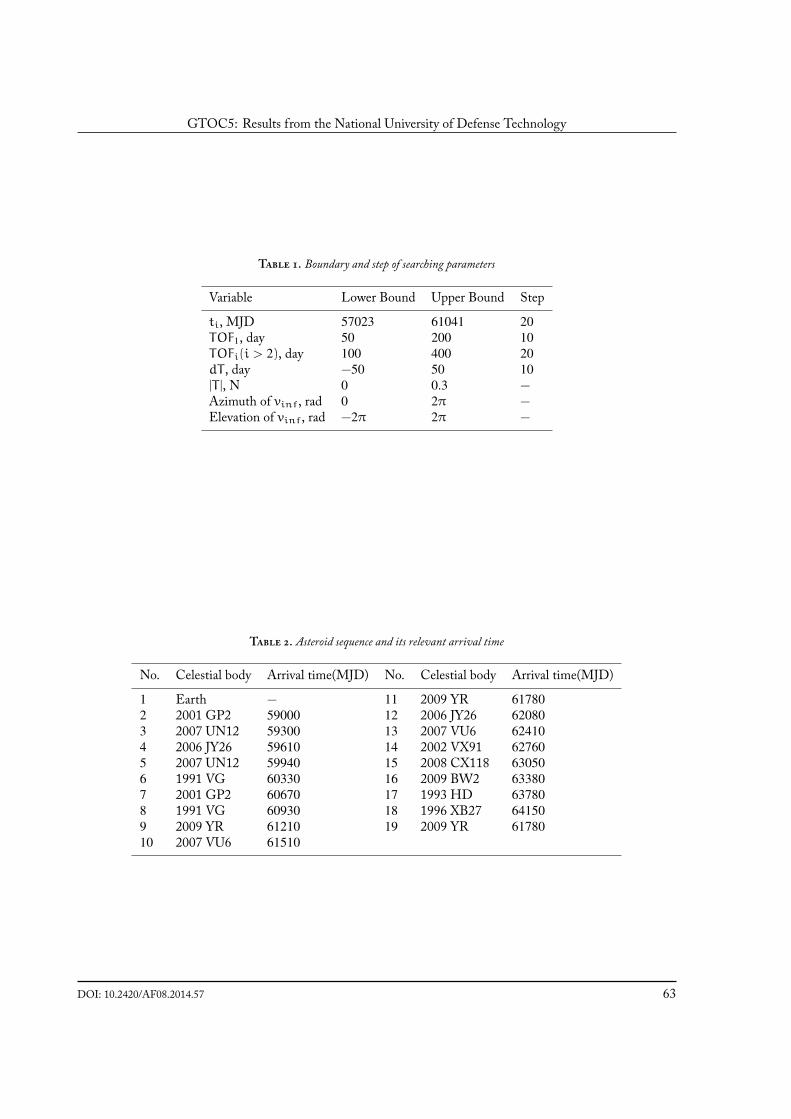
GTOC5: Results from the National University of Defense Technology
Table . Boundary and step of searching parameters
Variable Lower Bound Upper Bound Step
ti, MJD 57023 61041 20TOF1, day 50 200 10TOFi(i > 2), day 100 400 20dT , day −50 50 10|T |, N 0 0.3 −Azimuth of vinf, rad 0 2π −Elevation of vinf, rad −2π 2π −
Table . Asteroid sequence and its relevant arrival time
No. Celestial body Arrival time(MJD) No. Celestial body Arrival time(MJD)
1 Earth − 11 2009 YR 617802 2001 GP2 59000 12 2006 JY26 620803 2007 UN12 59300 13 2007 VU6 624104 2006 JY26 59610 14 2002 VX91 627605 2007 UN12 59940 15 2008 CX118 630506 1991 VG 60330 16 2009 BW2 633807 2001 GP2 60670 17 1993 HD 637808 1991 VG 60930 18 1996 XB27 641509 2009 YR 61210 19 2009 YR 6178010 2007 VU6 61510
DOI: 10.2420/AF08.2014.57 63

Acta Futura 8 (2014) / 57-65 Jiang et al.
Figure . Spacecraft-Sun distance during the found trajectory.
And it is detailed in Table 2.
During the process of low-thrust trajectory genera-tion, we found that few of the impulse phases could notbe achieved due to the accelerative capability of low-thrust propulsion system; hence, two approaches are ap-plied. Firstly, some refinements with the dates of theEarth and asteroids were made to minimize ∆vsum ;secondly, the candidate asteroid database was enlarged.Finally, a set of asteroids is derived, as showed in thefollowing Fig. 10.Table 3 summarizes the main parameters of the final
solution including the escape velocity of initial date aswell as two angles of direction in J2000 ecliptic frame.The total time of flight and mass after revisiting 8 aster-oids are also given.
The spacecraft’s distance to the Sun is illustrated inFig.8. As is shown, the last several segments behavepoor due to the troubles in the transformation from thebi-impulse trajectory to the low-thrust trajectory. Insummary, the problem of multiple asteroids encounterwith fixed dates (as solved by a Lambert model)can only a preliminary scenario that must be furtheranalysied including the low-thrust dynamics.
−2 −1 0 1 2
x 108
−1.5
−1
−0.5
0
0.5
1
1.5
x 108
x (km,J2000 ecliptic frame)
y (k
m,J
2000
ecl
iptic
fram
e)
2007 VU6 flyby(27/06/2033)
Sun
Asteroid
Earthdepart(17/04/2020)
Low−thrust trajectory
Figure . Sketch map of direct shooting method.
5 Conclusions
We have presented the methods and results obtainedat NUDT for GTOC5. Although our result is distantfrom the global optimum, there are valuable experi-ences gained from the extremely interesting challengeof GTOC5. They may be summarized as:
(1) The key technique to solve the problem is to finda reliable global optimization. Referring to results andworkshop of GTOC5, we find that almost all of theranking teams have ripe methods for the low-thrust
64 DOI: 10.2420/AF08.2014.57

GTOC5: Results from the National University of Defense Technology
Table . Final optimization solution parameters
Launch date 58956 MJDLaunch vinf 881.9 m/sAzimuth 48.6 degElevation 61.5 degTime of flight 4819.1 days (13.2 years)Final mass 626.3 kgPerformance index 8.0
trajectory design. But their global optimization meth-ods are of a wide variety, and this is the primary factorto influence the performance index.(2) A suitable method should be taken to estimate the
low-thrust trajectory energy. In global optimization, itis unpractical to search all low-thrust trajectories to as-teroids. The low-thrust trajectory energy is commonlyestimated by the Lambert bi-impulse trajectory. Butin practice, we find the bi-impulse trajectory cannotconvert to the low-thrust trajectory occasionally. Theydo not correspond one-to-one.(3) There should be a reasonable schedule for the
competition. During the competition, we spend lotsof time to program our routines and obtain a viableasteroid sequence. And no sufficient time left forsearching the global optimum.However, this is the first time our team participates
in the competition. We do not have an extravaganthope to get the global optimum. Our main purposeis to follow the state-of-the-art techniques in globaltrajectory optimization and to form our own methodsand routines to solve the problem. From this point ofview, we have achieved our competition objective.
References
[1] S. Lee, P. von Allmen, and W. Fink, “Comparisonof multi-objective genetic algorithms in optimizingq-law low-thrust orbit transfers,” in GECCO 2005,Washington, DC, June 2005.
[2] A. Dias and J. de Vasconcelos, “Multi-objective ge-netic algorithms applied to solve optimization prob-lems,” IEEE Trans. Magn., vol. 38, pp. 1133–1136,2002.
[3] A. E. Petropoulos, T. T. McConaghy, and T. J.Debban, “Design and optimization of low-thrusttrajectories with gravity assists,” Journal of Spacecraftand Rockets, vol. 40, pp. 380–387, 2003.
[4] J. Dankanich, “Low-thrust propulsion technolo-gies, mission design, and application,” Aerospacetechnologies advancements, pp. 219––240, 2010.
[5] A. H. Land and A. Doig, “An automatic methodof solving discrete programming problems,” Econo-matrica, vol. 28, pp. 497–520, 1960.
[6] G. Yang, Advances in low-thrust trajectory optimiza-tion and flight mechanics. Columbia, Missouri: Uni-versity of Missouri, 2003.
[7] B. Conway, Spacecraft Trajectory Optimization. Uni-versity of Illinois: Cambridge University Press,2010.
DOI: 10.2420/AF08.2014.57 65

66