active control of an aeroelastic structure

Copyright ©1997, American Institute of Aeronautics and Astronautics, Inc.

AIAA Meeting Papers on Disc, January 1997A9715114, AIAA Paper 97-0016

Active control of an aeroelastic structure

Jeffry BlockTexas A & M Univ., College Station

Heather GilliattTexas A & M Univ., College Station

AIAA, Aerospace Sciences Meeting & Exhibit, 35th, Reno, NV, Jan. 6-9, 1997

Linear and nonlinear aeroelastic response is modeled with a unique experiment that allows for prescribed plunge and pitchmotion of a wing. The addition of a control surface, combined with a PC-based active control system, extends the stableflight region. Aerodynamics are modeled with an approximation to Theodorsen's (1935) classical unsteady theory.Incorporated with a full-state feedback control law, an optimal observer is developed to stabilize the system above the openloop flutter velocity. Coulomb damping and pitch hardening are included to examine nonlinear control behavior. Thenonlinear model is tested using the control laws developed from linear theory. Each theoretical model is simulated usingMatlab and the experimental model of the active control system. An excellent correlation between theory and experiment isachieved for the models. Using an optimal observer and full-state feedback, the linear and nonlinear systems are stabilized atvelocities which are over twice the open loop flutter velocity. A limited amount of control is achieved when the system isundergoing limit cycle oscillations. (Author)

AIAA-97-0016

ACTIVE CONTROL OF AN AEROELASTIC STRUCTUREJeffry Block and Heather Gilliatt

Texas A&M UniversityCollege Station, Texas 77843-3141

ABSTRACT

Linear and nonlinear aeroelastic response ismodeled with a unique experiment that allows forprescribed plunge and pitch motion of a wing. Theaddition of a control surface, combined with a personal-computer based active control system, extends thestable flight region. Aerodynamics are modeled withan approximation to Theodorsen's classical unsteadytheory. Incorporated with a full-state feedback controllaw, an optimal observer is developed to stabilize thesystem above the open loop flutter velocity. Coulombdamping and pitch hardening are included to examinenonlinear control behavior. The nonlinear model istested using the control laws developed from lineartheory. Each theoretical model is simulated usingMatlab® and the experimental model of the activecontrol system. An excellent correlation betweentheory and experiment is achieved for the models.Using an optimal observer and full-state feedback, thelinear and nonlinear systems are stabilized at velocitieswhich are over twice the open loop flutter velocity. Alimited amount of control is achieved when the systemis undergoing limit cycle oscillations.

NOMENCLATURE

a = nondimensional distance from midchord toelastic axis

b = semichordof wingc = nondimensional distance from midchord to

control surface hingeC(k) = Theodorsen's functionca = pitch d.o.f. structural damping coefficientch = plunge d.o.f. structural damping coefficiente = nondimensional distance from midchord to

control surface leading edgeg = acceleration due to gravityh = plunge displacement coordinateIa = mass moment of inertia of wing about elastic

axisK = full-state feedback gainsk = reduced frequency (bco/u)ka = pitch d.o.f. structural spring constant

* Graduate Research Assistant, Department ofAerospace Engineering, Member AIAA

Copyright © 1996 by J. Block and H. Gilliatt. Published by theAmerican Institute of Aeronautics and Astronautics, Inc. withpermission.

kh = plunge d.o.f. structural spring constantL = estimator gainsL(t) = lift of wing about aerodynamic centerM(t) = moment of wing about aerodynamic centerMf = friction moment caused by Coulomb dampingm = mass of the wingQ = state weighting matrixQ = process noise covarianceR = control weighting matrixR = measurement noise covarianceu = free stream velocityxa = nondimensional distance between elastic axis

and center of massa = pitch displacement coordinateP = control surface deflection coordinateAA = difference in peak ampitudes of free vibrationu,h = static coefficient of friction in plunge directionHa = static coefficient of friction in pitch directionp = density of airco = frequency of motion

INTRODUCTION

Aeroelasticity is the interaction of structural,inertial and aerodynamic forces. Combined, theseforces may cause an aircraft or structure to becomeunstable or "flutter". Flutter is an oscillatory instabilitythat occurs when the structural damping transitionsfrom positive to negative due to the presence ofaerodynamic forces. During this transition, two modesof vibration coalesce to the same frequency and achievean aeroelastic resonance. Bending and torsion are thetwo most common vibration modes of a wing whichcoalesce to flutter. A literature review gives severalexamples of flutter analysis and control, as well asnonlinear aeroelastic analysis. Following, anexperiment will be presented which will combineflutter control with nonlinear aeroelasticity.

Theodorsen1 was an original investigator ofthe flutter phenomenon. He developed an unsteadyaerodynamic model which led to the popularTheodorsen's function. The function takes into accountthe lag effects of the unsteady aerodynamics at differentvalues of the reduced frequency, k. Theodorsen andGarrick2 used this method to compare the theoreticalpredictions of flutter velocity and frequency with

1American Institute of Aeronautics and Astronautics

experimental results. The method assumes oscillatorymotion of the wing and provides an excellent means forpredicting the flutter velocity and frequency. Wagnerand R. T. Jones3 approximated Theodorsen's functionto simulate a wing in unsteady aerodynamic flow. Withthese approximations, the equations of motion can beintegrated and solved to show the response of a two orthree dimensional wing.

Since the developments by Wagner and Jones,several authors have attempted to further understandthe unsteady motion of an airfoil. Lyons, et al.simplified the equations to be more applicable tocontrol law development by converting Jones'approximation into the Laplace domain andaugmenting the states of the system to account for thelag terms in the aerodynamics. To describe Wagner'sfunction and Theodorsen's function in the frequencydomain, Vepa5 developed a Fade approximationtechnique valuable for arbitrary small motions of a thinwing. Edwards, et al.6 contributed to the developmentby dividing the circulatory terms of the lift into"rational" and "nonrational" portions. The"nonrational" part was separated because it can not bewritten as a ratio of polynomials. Edward's methodapplied to arbitrary small motion of a wing and reducedthe number of augmented states previously required tomodel the unsteady aerodynamics.

Many control strategies have been applied tothe problem of delaying flutter or controlling unstablewing motion. Lyons, et al.4, investigated full-statefeedback with a Kalman estimator for the purpose offlutter suppression. Their theoretical model was fairlysimple and required only eight states. This controlsystem implemented estimators to describe unmeasuredstates and state feedback as the control method.Karpel7 compared the aerodynamic descriptions ofLyons, et al., Vepa, and Edwards to develop partial-state feedback controllers. He used pole placementtechniques to develop the control laws for fluttersuppression and gust alleviation.

A recent investigation of flutter control byHeeg8 increased the flutter velocity by 20%. The workinvolved a small wing model mounted on spring tinesto simulate the bending and torsion modes.Piezoelectric plates were mounted to the bending tine tocontrol that mode. Heeg's analysis employs a classicapproach for control, by using root locus plots to deriveproportional gain, feedback control laws.

All of the researchers have shown that lineartheory is often applicable for elaborate control systems.Unfortunately, as the current military and civilianaircraft are becoming increasingly complicated, so arethe needs for more sophisticated aeroelastic models.Most systems contain nonlinearities which are either

neglected by the designer or linearized within theequations of motion. As a result, researchers have putforth a great effort to understand the nonlinearitiesinherent in structural models.

Before describing these research efforts, it isimportant to understand some common nonlinearitesand where they may occur in aeroelastic systems. Forexample, saturation occurs when an increasing inputinto a system will no longer increase the output of thesystem. This nonlinearity occurs in most motorcontrollers when their operational limits are exceeded.Free play, or dead zone nonlinearity, is often seen incontrol surface linkages or hinges when the surface willnot move until the magnitude of the input exceeds acertain value. Hysteresis is described by a systemmoving along a cyclic path. When friction affectslinkage dynamics or when rivets are slipping on a wing,this may occur. A nonlinear stiffness may also be seenin many aerodynamic structures. For instance,nonlinear stiffness may be observed in the largebending of wings and rotor blades, or in control sticksthat become increasingly harder to deflect as they aremoved further from the neutral position.

Breitbach9 stated that a poor agreementbetween theory and experiment in flutter is most likelydue to nonlinear structural stiffness in structuralmodels. He also presented a detailed examination ofmany types of nonlinearities that may affect aeroelasticsystems. Woolston, et al.10, investigated nonlinearitiesin structural stiffness and control surface linkages.They created a model with torsional free play,hysteresis, cubic-hardening and cubic-softeningnonlinearities. For general wing motion, they observedthat the flutter velocity lowered as the initialdisturbance grew and that the stability of the systemwas highly dependent on the magnitude of the initialcondition. A cubic-softening spring stiffness in thetorsional degree of freedom lowered the flutter velocityas well. They also noted that cubic hardening causedstable limit cycle oscillations, rather than divergentflutter, at velocities above the open loop fluttervelocity.

Lee and LeBlanc" performed a numericalanalysis of a nonlinear wing model using a timemarching scheme that simulated the motion withrespect to tune. Soft and hard cubic springs wereexamined by varying different physical parameters.For the soft spring case, unstable motion wasencountered below the linear flutter speed for nearlyevery parameter; however, increasing the nonlinearityand increasing the mass ratio tended to make thesystem more unstable at lower velocities. For the hardspring case, limit cycle oscillations were always presentinstead of divergent flutter. Varying the parameters of

~ 2 ~American Institute of Aeronautics and Astronautics

the hard spring case had differing effects on theamplitudes of the limit cycles.

These researchers have developed models forexploring nonlinear aeroelasticity. However, there hasnot been a connection between nonlinear aeroelasticityand active control strategies. The model currentlybeing tested at Texas A&M University may be alteredto prescribe a linear or nonlinear structural stiffness.With the nonlinear structural stiffness, the model hasbeen shown to exhibit limit cycle oscillations12.Various full-state feedback control laws may be testedon the structure with the addition of a control surface.An unsteady aerodynamic model is developed with anapproximation to Theodorsen's function, and anobserver, based upon the Kalman estimator, will beused to estimate the augmented state system.Following tests of the linear structural model,nonlinearities are introduced and control is attemptedusing the linear controller. The work presented hereinwill, therefore, begin the process of combining activeflutter control with nonlinear aeroelasticity.

THEORY

The wing is free to plunge (h) and pitch (a)about the elastic axis as shown in Fig. 1. The lift andmoment are assumed to act at the quarter chord of thewhig. The mass, inertia, damping, stiffness andaerodynamics are per unit span. The control surfacehinge is located at the leading edge of the controlsurface, thus "e" is equal to "c" in all derivations whichfollow. The motion of the system, without controlsurface dynamics, may be described by

kh 0m mxabl I £1 .k OK„.__, u T n •• ( « - i •mxab Ia I a

where the terms are defined in the Nomenclature.(1)

To properly model the aeroelastic wing,unsteady aerodynamics must be incorporated.Unsteady aerodynamics assume that all of the flowfield variables change with position, velocity,acceleration and tune. These aerodynamics alsoincorporate both non-circulatory and circulatory flowabout the airfoil. Theodorsen1 derived the lift per unitspan and moment per unit span with unsteadyaerodynamics, assuming harmonic motion of theairfoil. They are of the form,

-L(t) = -pb2(umx + Tth - Ttbad - uT4(3 - T,bp) - 27rpubC(k)(2)- . o u

) = -pb2[ Jt(i - a)ub<i + jib2(l + a2)a + (T4 + T]0)u2P

+ (T, - T8 - (c - a)T4 + IT, ,)ubp - (T7 + (c- a)T,)b2p- ajcbiil + 2pub27t(-i + a)C(k) {ua + h + b(i - a)(i+ L T u + b a T j . (3)

The lift and moment equations describe howthe accelerations, velocities and positions of the wingand control surface affect the plunging and pitchingmotion of the airfoil. The 'T' constants areTheodorsen's T-functions and are functions of theelastic axis location and the control surface hingelocation.

To implement the control surface dynamicswith the plunging and pitching equations of motion, Eq.(1), the dynamics are assumed to be that of a secondorder system with eigenvalues far to the left of thestructural model. By choosing where the eigenvalueswill be, the control surface dynamics will not affect thecoupling of the plunging and pitching motion. Thesedynamics are therefore represented by the second ordertransfer function,

(4)

in the Laplace domain, and in the time domain,

P + 50p + 2500p = 2500pcon, . (5)The Pcom term is the control variable for the system.The function C(k) is Theodorsen's function,compromised of real and imaginary terms of the form,C(k) = F(k) + iG(kX where F(k) and G(k) are Besselfunction equations, and k is the reduced frequencydefined by k=bo>/u. Jones developed an approximationto Theodorsen's function, which simplifiesmathematical calculations3. The approximation, whichcan also be represented in the Laplace domain withs=ia>, is described by,

Fig. 1 Aeroelastic system modelC(k) = l-- .165 .335

1- .04551 (6)


To incorporate this approximation into the lift andmoment equations, six new states must be added to thesystem. The new states account for the aerodynamiclag due to the second and third terms of Eq. (6). Afterexpanding and converting to the time domain, theresulting equations are,

X-X+.0455-X = 0 andb

(7)

Substitution of the numerators in Eq. (6) are made forC(k) in the equations of motion and are applied to thenew states, X(s)andX(s) . The equations of motion, withunsteady aerodynamics, are represented by

(8)

with the DI matrix defined by [0 0 2500]T and theyinclude the dynamics of the control surface as well asthe plunging and pitching motion. The six additionalequations from (7) are added to Eq. (8) and placed intostate-space form such that

(9)

(10)

with the output equations

{Y}=[I2X2 02xlo]{X}=[Z]{X}.

The system consists of twelve states, of which onlyplunge and pitch are measured. The remaining tenstates need to be determined with a state estimator.

Since the system is stabilizable, a full-statefeedback control law can be derived to place theeigenvalues of the closed loop system into desiredlocations in the left half complex plane13. The left-halfcomplex plane defines the stable region for the system.With full-state feedback, the motion of the system canbe driven to a desired final state by choosing particularfeedback gains, [K]. This type of feedback requires thatall of the states be measured and used in the controllaw, {U} = -[K]{X}. The states are multiplied by thegains and used as the control surface input.

The feedback gains can be determined using apole-placement technique, which would place theclosed loop eigenvalues where the designer chooses, orby optimizing a performance index with a LinearQuadratic Regulator. The Linear Quadratic Regulator(LQR) approach minimizes the performance index,

(11)

There are many variations of this performance index; itis the designer's task to choose one that will define theconstraints such as position, velocity or boundaryconditions on the system. The performance index is

minimized by first solving the algebraic Ricattiequation defined by,

ATP + PA-R-'PBBTP + Q = 0. (12)

After the equation is solved for [P], the optimal gainmatrix may be determined by, K=R"'BTP. By mini-mizing the performance index, the optimal values of[K] in the control law are determined. A suitableperformance index for our aeroelastic model is

J = (13)

This particular index normalizes the maximum valuesof the states and inputs. After choosing the state andcontrol weighting matrices that describe theperformance index, Matlab® or other suitable code canfind the optimal feedback gains. The chosenperformance index is only a first approximation for theweighting, however, and the system should be tested tosee how well the gains work for various conditions.The weightings must be varied until a truly suitable setof feedback gains are determined.

The complete system consists of twelve states,one input and two outputs. It would be ideal to useonly a full-state feedback control scheme; but, since allof the states are not measurable, this is not feasible.Instead, a state observer will be created to estimatethose states which are not measurable. The observer isa modified set of equations which describe the motionof the system. A set of feedback gains, [L], are chosento make the dynamics of the observer 3-4 times fasterthan the dynamics of the original system. In so doing,the observer corrects for any error between its initialcondition and the actual states. The observer feedbackgains, [L], are multiplied by the difference between theoutput of the original system and the output of theobserver, as stated in the following equation,

L[Y-Y] . (14)

This equation is similar to the state-space equationspreviously discussed; however, the new equations arenow functions of the estimated states, {X}. Figure 2shows a complete diagram of an observer with full-statefeedback control.

To derive the observer feedback gains, [L], asimilar approach to the full-state feedback gains isnecessary. A performance index is used to weight theeffects of process and measurement noise, rather thanthe state and control cost used to calculate full-statefeedback gains. The equations of motion have assumedthese noises to be negligible. The process noise, [w],takes into account errors or nonlinearities within theequations of motion. The measurement noise, [v],takes into account the largest possible error of each


sensor. The process and measurement noise areassumed to be zero mean with covariance given byE{wwT} = Q, E{wT} = R, and E{wvT> = 0. By weightingthe measurement noise and sensor noise, theperformance index allows the designer to optimallychoose between speed of reconstruction and protectionagainst measurement noise. The state-space equationswith noise included are of the form,

[W] (15)(16)

The noise values need to be suitably chosen to modelany equation uncertainties.

Fig. 2 Block diagram of observer based full-state feedback

Although the derived estimator gains areoptimal for the given weightings, they may not beoptimal for the system. The control system is based onthe measurements from the sensors and the integrationof the estimator equations of motion. If the model ofthe system is not accurate, then as the actual states tendtowards one solution, the estimated states couldpotentially do the opposite. Therefore, it is importantthat the system model is accurate and that substantialtesting of the estimator is completed prior to finalbuilding of the aeroelastic control system.

In order to better describe the model andphysical structural response, two nonlinearities aredescribed. First, Coulomb damping is apparent in theresponse of the plunge and pitch motion for certaincases; therefore, it is implemented in the predictions.A more detailed description of the application of theCoulomb damping will be presented in theExperimental Setup section. The second nonlinearity, apolynomial pitch hardening, may be introduced into theequations of motion by replacing the linear stiffness,k0= 3.43 N-m/rad, with the nonlinear stiffness, ka=2.82(1 - 22.1a + 1315.5a2 - 8580a3 + 17289.7a4) N-m/rad. This polynomial stiffness term was derived byO'Neil12 and is a function of the experimental structure.An advantage of the experimental apparatus permits asimple change between a linear or nonlinear pitchstiffness.

PREDICTIONS

For purposes of control, the system is neithercompletely controllable nor completely observable.Therefore, the lesser conditions of stabilizable anddetectable are examined. Figure 3 shows theeigenvalues of the system as the velocity is raised to20.0 m/s. The plot shows the system eigenvalues at 0.5m/s increments of velocity for the elastic axis locationof a = -.8424. The pitch mode, which is directlymeasured, is known to go unstable; the remainingmodes are stable and permit the requirements ofstabilizable and detectable. Since the only unstablemode is the pitch mode, LQR theory is used to derivecontroller gains for full-state feedback.

-O -XDamping

Fig. 3 Unsteady aerodynamic characteristic equation roots

.

DampingFig. 4 Controlled unsteady aerodynamic characteristic eq. roots

Also from Fig. 3, the flutter velocity andfrequency are determined at the point where the pitchmode crosses the zero damping axis. The predictedflutter velocity and frequency are found to be 15.25 m/sand 2.07 Hz, respectively. All control laws are derivedat 19.06 m/s, or 25% above the flutter velocity. Theweightings are chosen to normalize the maximumvalues of the measured variables. However, it is notedthat a quicker response time is achieved by increasingthe plunge weighting. Therefore, a maximumdeflection of 0.005 meters for the plunge is usedinstead of the actual limiting value of 0.04 meters.Noise estimates are created to derive the observer


feedback gains. Process noise is estimated to beproportional to the singular value decomposition of theeigenvalues. Measurement noise is the square of thesmallest possible measurements of the plunge andpitch motion, defined by the resolution of the opticalencoders used in the experiment. To build the observerequations of motions, Eq. (14), the observer feedbackgains and the full-state feedback gains are combined.

Time (seconds)Fig. 5 Predicted plunge motion at 16.0 ni/s:

— controlled, - - - uncontrolled,- • • - ideal estimated

0 0,5 1 _ 15 , 2 2.5 3Time (seconds)Fig. 6 Predicted pitch motion at 16.0 m/s:

— controlled, ---uncontrolled, • • • • ideal estimated

With the observer and full-state feedback, thesystem should be stabilized well above the fluttervelocity. Figure 4 shows the controlled eigenvalues ofthe system as the velocity is raised to 25.0 m/s. Fromthe plot, it is evident that the pitch mode no longercrosses the zero damping axis and, thus, the systemremains stable. Figures 5 and 6, respectively, show theplunge and pitch motion given a 0.01 meter plungeinitial condition. The response is at 16.0 m/s, which isjust above the flutter velocity. The effects of controlcan clearly be seen, as the motion is stabilized within2.5 seconds. The estimation values, which begin withzero initial conditions, are able to match the dynamicsof the system within 0.1 seconds and are barely visible.The control surface deflection begins at zero and mustaccelerate to meet the required control signal. As thevelocity is raised to higher values, the settling time

improves since the control surface has more authorityover the motion.

A Runge-Kutta integration scheme is used forsimulating the wing motion with the nonlinearities.With Coulomb damping, the predictions for fluttervelocity and frequency are 14.9 m/s and 2.02 Hz,respectively. When the nonlinear pitch stiffness isapplied, the system response does not growexponentially when the flutter velocity is reached.Instead, it is bounded to oscillations of limitedamplitude, commonly referred to as limit cycleoscillations (LCOs). These limit cycles are first evidentat velocities just under the open loop flutter velocityand are dependent upon the initial conditions (ICs).Figure 7 shows the predicted LCOs of the plungedegree of freedom given a 0.01 meter 1C at 13.75 m/s.The frequency of motion for the system is 2.55 Hz.Figure 8 shows the predicted pitch motion due to theplunge input. When the 1C is changed to a = 0.0875radians hi the pitch direction, LCOs are not predicteduntil the velocity reaches 14.5 m/s. The frequency hasalso changed to 2.67 Hz.

O.OM

0.004

•C.CO*

•C-Oofil

Time (seconds)Fig. 7 Predicted plunge LCO at 13.75 m/s

Time (seconds)Fig. 8 Predicted pitch LCO at 13.75 m/s

EXPERIMENTAL SETUP

The aeroelastic model was tested in TexasA&M University's 2x3 foot wind tunnel. This tunnelhas a maximum operating speed of 150 ft/s, or 45 m/s,which is well beyond the flutter region of the model.


The model is mounted vertically in the tunnel so thatonly the wing is within the test section; this permits theassumption of an infinite span wing. Motion in theplunge and pitch directions, which simulates bendingand torsion motion of a wing, is created by a twin-camsystem (Fig. 9). The maximum plunge deflection is at± 0.04 meters and the maximum pitch angle is ±28°.Figure 10 shows the underside of the model with thelinear and nonlinear cams. These cams are mountedadjacent to one another for simple changing betweenthe two cams. The combination of the springs and thecams provides the prescribed linear or nonlinearstiffness. Encoders are mounted on the pitch andplunge cams to measure the plunge and pitch positions.A control surface and motor are designed for easyattachment and removal to permit other research effortsat the same time. The control surface is 20% of thechord and is full-span.

Fixed

Plunge Carnage

Fig. 9 Isometric view of aeroelastic structure

• NoGuncv Csun

Plunge Spring

Fig. 10 Bottom view of aeroelastic structure

The linear structural model for the aeroelasticwing includes a viscous form of structural damping inthe plunge and pitch degrees of freedom, representing alogarithmic decay. Free vibration experiments areinitially undertaken, hi order to quantify these terms.To measure the plunge damping, the pitch degree offreedom is restrained, and to measure the pitchdamping, the plunge degree of freedom is restrained.

With the assumption that the damped free vibration islogarithmic, the log-decrement method is used tocalculate the damping ratio, £, for each degree offreedom.

An alternative to the logarithmic, viscousdamping model is a Coulomb damping model. Thereare many differences between the two types ofdamping. Viscous damping appears as a logarithmicdecay in the free vibration, whereas Coulomb dampingappears as a linear decay. In the equations of motion,viscous damping is represented by a linear termproportional to the velocity, but Coulomb damping isdefined by a force opposing the motion of the system.Once the friction force is greater than the restoringforce, the system motion will stop. These differencesbetween viscous and Coulomb damping are visible inFig. 11, which shows a plunge free vibration at zerowind tunnel velocity. Note that the Coulomb dampingstops as soon as the friction force is greater than therestoring force and the motion does not necessarily stopat the zero position. When applied to the aeroelasticstructural model, the Coulomb equations for the plungeand pitch frictional forces are respectively defined by

and (17)

The frictional moment, Mf, is due to the offset mass ofthe nonlinear pitch cam. To determine the coefficientsof friction, the following general equation is used,

AA , (18)

where AA is the difference in peak amplitudes of thefree vibration. When the nonlinear cams are applied tothe system, the free vibration contains more Coulombdamping than viscous damping. For mis reason, theCoulomb damping predicts the nonlinear responsemore accurately than the viscous damping. With mis inmind, the viscous damping is always used in the linearcontrol development, and the Coulomb damping isalways used for the nonlinear LCO predictions.

Fig. 11 Viscous and Coulomb damping:—damping, — Coulomb damping


The aerodynamic loads on the control surfacerequire that a high torque motor be used. Also, sincethe motor is placed externally on the wing, a minimalsize is desired. The Futaba FPS-134 servomotor ischosen to meet all of the requirements. It is small insize, can deliver up to 112.6 oz-in of torque and has anembedded controller board, which directs its motion.The maximum control surface deflection is set to ± 32°and the minimum possible motor increment is 0.016°.The dynamics of the motor are neglected, and it isassumed that the motor reacts exactly as specified, aslong as the maximum velocity of 4.75 rad/s is notreached. By placing the motor external to the wing, theaerodynamics are slightly affected; the positive stallangle has been reduced from 16° to 13°, and thenegative stall angle has been lowered from 16° to 15°.

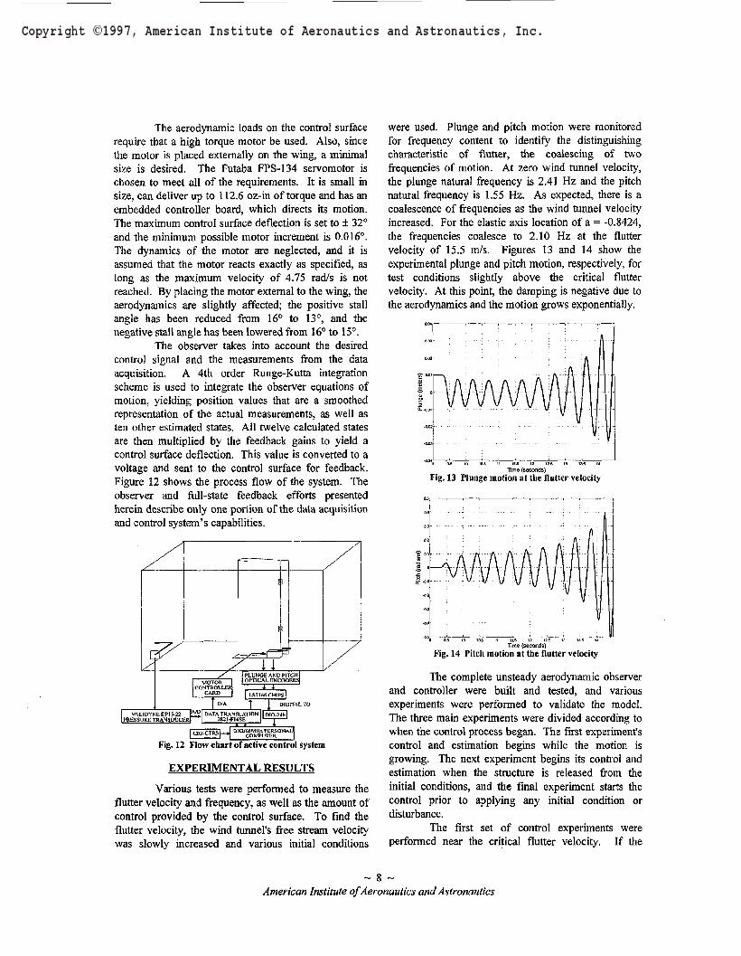
The observer takes into account the desiredcontrol signal and the measurements from the dataacquisition. A 4th order Runge-Kutta integrationscheme is used to integrate the observer equations ofmotion, yielding position values that are a smoothedrepresentation of the actual measurements, as well asten other estimated states. All twelve calculated statesare then multiplied by the feedback gains to yield acontrol surface deflection. This value is converted to avoltage and sent to the control surface for feedback.Figure 12 shows the process flow of the system. Theobserver and full-state feedback efforts presentedherein describe only one portion of the data acquisitionand control system's capabilities.

Fig. 12 Flow chart of active control system

EXPERIMENTAL RESULTS

Various tests were performed to measure theflutter velocity and frequency, as well as the amount ofcontrol provided by the control surface. To find theflutter velocity, the wind tunnel's free stream velocitywas slowly increased and various initial conditions

were used. Plunge and pitch motion were monitoredfor frequency content to identify the distinguishingcharacteristic of flutter, the coalescing of twofrequencies of motion. At zero wind tunnel velocity,the plunge natural frequency is 2.41 Hz and the pitchnatural frequency is 1.55 Hz. As expected, there is acoalescence of frequencies as the wind tunnel velocityincreased. For the elastic axis location of a = -0.8424,the frequencies coalesce to 2.10 Hz at the fluttervelocity of 15.5 m/s. Figures 13 and 14 show theexperimental plunge and pitch motion, respectively, fortest conditions slightly above the critical fluttervelocity. At this point, the damping is negative due tothe aerodynamics and the motion grows exponentially.

Time (seconds)Fig. 13 Plunge motion at the flutter velocity

Time (seconds)Fig. 14 Pitch motion at the flutter velocity

The complete unsteady aerodynamic observerand controller were built and tested, and variousexperiments were performed to validate the model.The three main experiments were divided according towhen the control process began. The first experiment'scontrol and estimation begins while the motion isgrowing. The next experiment begins its control andestimation when the structure is released from theinitial conditions, and the final experiment starts thecontrol prior to applying any initial condition ordisturbance.

The first set of control experiments wereperformed near the critical flutter velocity. If the

American Institute of Aeronautics and Astronautics

velocity is much higher, the motion grows too rapidlyto physically decide when the control should begin.The results of this experiment are very positive. Aslong as the system motion does not exceed the limitingstall angle of positive 13° prior to starting the control,the system is always controlled. Figures 15 and 16show the plunge and pitch motion, respectively, for thistype of experiment, with the velocity at the fluttervelocity of 15.5 m/s. The motion is excited by a pitch1C and continues to grow until the control system isturned on at approximately 12 seconds. The maximumcontrol surface deflection is 10°. The estimated valuesare, in essence, a smoothed output of the actualmeasurements. When the controller is turned on, theestimated states start from zero initial conditions andrapidly converge to the actual values. Since thefeedback gains are derived at 19.06 m/s, the systemdoes not stabilize as fast as it possibly could. If,however, the feedback gains had been derived at 15.5m/s, the system would have stabilized more rapidly.

Time (seconds)Fig. 15 Controlled plunge motion at 15.5 m/s:

— estimated plunge motion, — actual measurements

e (seconds)Fig. 16 Controlled Pitch motion at 15.5 m/s:

— estimated plunge motion,— actual measurements

Less control surface motion is required atvelocities above the flutter velocity. This was shownthrough the second type of experiment. For thisexperiment, the velocity is set to a constant value andan 1C is set in the pitch or plunge position. Thecontroller is started at the same time the system is

released from the initial conditions and performsextremely well for velocities up to 31.4 m/s. Thesystem is not tested at higher velocities to avoidexceeding the limitations of the servomotor. Figures 17and 18 show the plunge and pitch measurements andestimated values from the controller for one test at thisvelocity. A pitch input of -0.0875 radians and aplunge input of-0.007 meters are used for the ICs. Themaximum required control surface deflection is 5° forthis case. Initiating control when the system is releasedfrom initial conditions provides an excellent means ofcontrol. The system is shown to stabilize at velocitiesover 100% above the open loop flutter velocity.

9 0,5 10

Fig. 17 Controlled plunge motion at 31.4 m/s:— estimated motion,—actual measurements

Time (seconds!Fig. 18 Controlled pitch motion at 31.4 m/s:

— estimated motion,—actual measurements

The system is extremely stable when control isstarted prior to giving an 1C. Except for inputs thatcause the system to encounter stall, nearly every initialcondition, including impulses, is stabilized. The systemis again tested up to 31.4 m/s and shows even morerapid settling times than those shown in Figs. 17 and18. When the system is released from an 1C, thecontrol surface is at an ideal position for stabilizing thesystem. However, hi the previous type of experiments,the control surface begins at zero initial condition andhas to catch up to the ideal stabilizing motion.

From the experimental data, the linear controlmodel is shown to be very effective. Prior to testing

American Institute of Aeronautics and Astronautics

this controller on the nonlinear model, LCO boundariesneed to be determined. The LCOs are due to thepolynomial pitch stiffness and are encountered atdifferent velocities depending upon the initialconditions. Two ICs are used for these tests. With a0.01 meter plunge input, limit cycles are firstencountered at approximately 14.25 m/s. Thefrequency of motion of the system is 2.87 Hz. Whenthe input is changed to 0.087 radians in the pitchdirection, the LCOs occur at approximately 15.25 m/sand a frequency of 2.87 Hz. Figures 19 and 20 showthe plunge and pitch LCOs due to the 0.01 meterplunge input at approximately 14.25 m/s.

Time (seconds)Fig. 19 Plunge limit cycle oscillation at 14.25 m/s

TVns (secc-ncs)Fig. 20 Pitch limit cycle oscillation at 14.25 m/s

When the linear controller is applied to thesystem, very similar results to the linear model areachieved. The system is stabilized at velocities up to31.0 m/s for experiments when the controller is startedat the time of release from initial conditions. Plots ofthe system response under control are nearly identicalto those of Figs. 17 and 18. The controller performscorrectly as long as the system does not enter intoLCOs prior to starting the control. This is similar to thelimit of control on the linear system, in that there is nocontrol after the system reaches the stall angle of 13°.

When the nonlinear system is experiencinglimit cycles, the motion is coupled and the singleactuator controller has a very limited ability to

uncouple the system. During LCO response, the resultof the same linear controller action is a stabilizedplunge motion and a larger amplitude and frequencypitching motion. In order to stabilize the system adifferent control law is required. When the system is inlimit cycle motion, the coupling is opposite to that ofthe linear flutter motion: during flutter, the plunge andpitch motion are 180° out of phase, and during LCOs,the two motions are in phase with each other. A controllaw that will counter this phase difference is necessaryfor LCO control. Experimentally, the only limit cyclecontrol is achieved near the flutter velocity. Figures 21and 22 shows one case of control given LCOs. Athigher velocities, the control surface can not uncouplethe nonlinear system.

Time (seconds)Fig. 21 Controlled plunge limit cycle motion at 16.0 m/s:

— estimated motion, — actual

Time (seconds)Fig. 22 Controlled pitch limit cycle motion at 16.0 m/s:

— estimated motion, — actual

CONCLUSIONS

To accurately describe the flow around theaeroelastic structure, the unsteady aerodynamic model,with the R. T. Jones approximation to Theodorsen'sfunction, is essential. The predictions for the open loopsystem are in excellent agreement with theexperimental values. At the elastic axis location of a =-0.8424, the flutter velocity and frequency are predictedto be 15.25 m/s at 2.07 Hz, respectively, with viscousdamping and 14.9 m/s and 2.02 Hz, respectively, with


Coulomb damping. These numbers compare very wellwith the experimental values of 15.5 m/s and 2.10 Hz.For the linear system, the use of Coulomb dampingdoes not predict the open loop flutter velocity as well asthe viscous damping, since the actual pitch dampingcontains more viscous than Coulomb damping.

A good correlation of theory and experimentfor the nonlinear structural model is also achieved. Byusing a fourth order Runge-Kutta integration of theequations of motion, the limit cycle predictions of13.75 m/s and 2.55 Hz are made for a 0.01 meterplunge input. Experimentally, the values of 14.25 m/sand 2.87 Hz are achieved. The method shows thecorrect trends for a pitch input of 0.0875 radians aswell; theoretically, the limit cycle velocity of 14.5 m/sand frequency of 2.67 Hz are expected and the valuesof 15.25 m/s and 2.87 Hz are achieved. The unsteadyaerodynamic model therefore predicts when the limitcycles should occur, but does not correctly match thelimit cycle frequency. When comparing the amplitudesof the limit cycles between Figs. 7 and 19, and Figs. 8and 20, the theoretical predictions are not veryaccurate. The experimental amplitudes are larger thanpredicted because the servomotor is in the airstreamand has an effect on the flow around the wing. Inaddition, the servomotor carries a larger inertial forcethan is accounted for in the theoretical model. Thisdoes not affect the linear model because when flutteroccurs, the wing's motion grows exponentially inamplitude and the added inertial affects will only causeit to go more unstable. The servomotor does not limitthis growth, but actually drives it more unstable.

The aeroelastic control system developed forthe wind tunnel performs nearly as designed. With theknowledge learned from initial tests, a more completefeedback system is developed based on the unsteadyaerodynamic model. A trailing edge control surface isadded to the existing wing structure and a high torqueservomotor is adapted to drive the surface. The resultis a unique aeroelastic control system that is capable ofstabilizing the structure at velocities over twice theopen loop flutter velocity. In addition, the structuralresponse of the wing can be tailored for a linear ornonlinear response. Whether the linear or nonlinearresponse is present, the controller is capable ofstabilizing the system. When the system is undergoinglimit cycle oscillations, a limited amount of controlmay be achieved by modifying the control law toaccount for phasing.

REFERENCES

'Theodorsen, T., "General Theory ofAerodynamic Instability and the Mechanism of

Flutter," NACA Report 496, 1935, NACA, Hampton,Virginia.

2Theodorsen, T., and Garrick, I. E.,"Mechanism of Flutter: A Theoretical andExperimental Investigation of the Flutter Problem,"NACA Report 685, 1940, NACA, Hampton, Virginia.

3Fung, Y.C., An Introduction to the Theory ofAeroelasticity. John Wiley and Sons, New York, 1955,pp. 207-215.

"Lyons, M. G., Vepa, R., Mclntosh, S. C., andDeBra, D. B, "Control Law Synthesis and SensorDesign for Active Flutter Suppression," Proceedings ofthe AIAA Guidance and Control Conference. AIAAPaper No. 73-832, 1973, pp. 1-29.

5Vepa, R., "On the Use of Pade Approximantsto Represent Unsteady Aerodynamic Loads forArbitrary Small Motions of Wings," AIAA, AIAAPaper No. 76-17, 1976.

'Edwards, J. W. , Ashley, H., and Breakwell,J., "Unsteady Aerodynamic Modeling for ArbitraryMotions," AIAA Journal. Vol. 17, No. 4, April 1979,pp. 365-374.

7Karpel, M., "Design for Active FlutterSuppression and Gust Alleviation Using State-SpaceAeroelastic Modeling," Journal of Aircraft. Vol. 19,No. 3, Mar. 1982, pp. 221-227.

8Heeg, J., "Analytical and ExperimentalInvestigation of Flutter Suppression by PiezoelectricActuation," NASA Technical Paper 3241, 1993,NASA.

9Breitbach, E. J., "Effects of StructuralNonlinearities on Aircraft Vibration and Flutter,"AGARD-R-665, Jan 1978, North Atlantic TreatyOrganization, Neuilly sur Seine, France.

10Woolston, D. S., Runyan, H. L., andAndrews, R. E., "An Investigation of Effects of CertainTypes of Structural Nonlinearities on Wing and ControlSurface Flutter," Journal of Aeronautical Sciences. Vol.24, No. 1, Jan. 1957, pp. 57-63.

"Lee, B. H. K., and LeBlanc, P., "FlutterAnalysis of a Two-Dimensional Airfoil with CubicNonlinear Restoring Force," NAE-AN-36, NRC No.25438, Ottawa, Quebec, Canada, Feb. 1986.

12O'Neil, T., Experimental and AnalyticalInvestigations of an Aeroelastic Structure withContinuous Nonlinear Stiffness. M. S. Thesis, May1996, Texas A&M University.

13O'ReiIly, J.. Observers for Linear Systems.Academic Press, London, 1983.


active control of an aeroelastic structure

Documents