active portfolio management and portfolio construction
TRANSCRIPT

MASTER THESIS, FALL 2012CAND.MERC. APPLIED ECONOMICS AND FINANCE
COPENHAGEN BUSINESS SCHOOL
AUTHOR: JOHAN CHRISTIAN HILSTEDDATE OF SUBMISSION: DECEMBER 14TH 2012
ACTIVE PORTFOLIO MANAGEMENT AND PORTFOLIO CONSTRUCTION
- IMPLEMENTING AN INVESTMENT STRATEGY
SUPERVISOR: JEPPE SCHOENFELDT
NUMBER OF PAGES: 77
NUMBER OF CHARACTERS: 145.260
SIGNATURE:
Active Portfolio Management and Portfolio Construction – Implementing an Investment Strategy
1
Abstract
This thesis aims at creating an investment strategy for active portfolio management to outperform the
MSCI Denmark from 1992 to 2011. The index development of the Danish stock market has been quite
impressive as it has performed remarkably better than other national indices. It is therefore interesting
to investigate whether active portfolio management constitutes a winning strategy superior to investing
in the MSCI Denmark.
There is no generally accepted approach to conduct active portfolio management. This thesis approaches
the subject by comparing two internationally diversified portfolios to the MSCI Denmark as benchmark -
one portfolio submitted to a 20% maximum asset representation restriction, the other portfolio left
unrestricted.
From investment strategy we conclude that combining strategic and tactical asset allocation constitutes
an appropriate investment strategy for active portfolio management, as it limits the long-term portfolio
investment opportunities and allows for short-term portfolio repositioning. The information ratio
constitutes the performance measure of active portfolio management, as it optimizes portfolio
construction by comparing expected returns of portfolio and benchmark – the residual return. The Capital
Assets Pricing Model (CAPM) was utilized for return estimations for both investment opportunities and
benchmark. Mean-variance portfolio construction was conducted based upon investment opportunities
expected to outperform the benchmark.
The MSCI Denmark provides realized average monthly return of 0,65%, while the actively managed
portfolios produce average realized monthly return of 0,34% and 0,37%, respectively. In that regard,
active portfolio management has not outperformed the benchmark, and statistical findings cannot suggest
portfolio timing skill. However, considering the systematic risk adjusted return, both portfolios yield
significant alpha, or value added, with the unrestricted portfolio being the best performing portfolio.
In conclusion, active portfolio management cannot produce higher return than the MSCI Denmark, but has
proven to benefit the investor, as the market risk exposure justifies both inferior and superior portfolio
return to the benchmark.
Active Portfolio Management and Portfolio Construction – Implementing an Investment Strategy
2
Table of Contents
Abstract .......................................................................................................................................... 1
1. Introduction ................................................................................................................................ 4
1.1 Research Objectives ................................................................................................................................... 6
1.1.1 Superior Research Objective ................................................................................................................... 6
1.1.2 Subordinate Research Objectives ........................................................................................................... 6
1.2 Structure of Thesis...................................................................................................................................... 7
1.3 Methodology .............................................................................................................................................. 8
1.3.1 Financial Assets and Risk ......................................................................................................................... 8
1.3.2 Applied Theoretical Approach ............................................................................................................... 10
1.3.3 Interviews .............................................................................................................................................. 11
1.4 Assumptions and limitations .................................................................................................................... 12
1.4.1 Assumptions .......................................................................................................................................... 12
1.4.2 Limitations ............................................................................................................................................. 13
1.5 Data .......................................................................................................................................................... 14
1.5.1 Equity Sector Return Data ..................................................................................................................... 14
2.Investment Strategy ................................................................................................................... 18
2.1 Investment Strategy as the Source of Portfolio Performance ................................................................. 18
2.2 Strategic Asset Allocation ......................................................................................................................... 19
2.2.1 Discussing Empirical Findings and Brinson et.al. ................................................................................... 21
2.3 Tactical Asset Allocation ........................................................................................................................... 23
2.4 Professional Views upon Asset Allocation ............................................................................................... 24
2.5 Benchmark and Investment Opportunities .............................................................................................. 25
2.5.1 Benchmark............................................................................................................................................. 26
2.5.2 Investment Opportunities ..................................................................................................................... 27
2.6 Crafting the Investment Strategy ............................................................................................................. 30
3.Active Portfolio Management ..................................................................................................... 33
3.1 Defining Active Portfolio Management .................................................................................................... 33
3.2 Performance Measure and Portfolio Added Value .................................................................................. 34
3.2.1 Information Ratio .................................................................................................................................. 34
3.2.2 Portfolio Value Added ........................................................................................................................... 35
Active Portfolio Management and Portfolio Construction – Implementing an Investment Strategy
3
4.Risk and Return in Active Portfolio Management ........................................................................ 38
4.1 Expected Return in Active Portfolio Management .................................................................................. 38
4.1.1 Asset Pricing in an Active Setting .......................................................................................................... 38
4.2 Risk Management ..................................................................................................................................... 46
4.2.1 Investor Utility ....................................................................................................................................... 47
4.2.2 Professional Views upon Risk and Risk Management ........................................................................... 47
4.2.3 Risk Management and Risk Factors ....................................................................................................... 48
4.2.4 Financial Risk ......................................................................................................................................... 49
5.Portfolio Construction ................................................................................................................ 51
5.1 Objective of Portfolio Construction ......................................................................................................... 51
5.2 Choice of Portfolio Model ........................................................................................................................ 51
5.3 Mean-Variance Application in an Active Setting ...................................................................................... 52
5.3.1 The Model ............................................................................................................................................. 53
5.3.2 Model Short-Comings ............................................................................................................................ 55
5.3.3 Portfolio Repositioning and Transaction Costs ..................................................................................... 60
5.4 Model Performance ................................................................................................................................. 63
5.4.1 Sector Distribution ................................................................................................................................ 63
6.Performance Evaluation of the Investment Strategy ................................................................... 67
6.1 Return-Based Performance Analysis ........................................................................................................ 67
6.1.1 Cross-Sectional Comparison .................................................................................................................. 67
6.1.2 Market Timing ....................................................................................................................................... 69
6.2 Analysis of Value Added ........................................................................................................................... 71
7.Conclusion ................................................................................................................................. 75
8.References ................................................................................................................................. 78
9.Appendix Overview .................................................................................................................... 81
Appendix 1: Glossary ...................................................................................................................................... 82
Appendix 2: Sector Market Value and Correlation Matrix of Sector Return ................................................. 86
Appendix 3: Interview Guide .......................................................................................................................... 87
Appendix 4: Active Return and Testing for Return Stationarity..................................................................... 89
Appendix 5: Expected Residual Return .......................................................................................................... 95
Appendix 6: Portfolio Positions of Investment Opportunities ....................................................................... 97

Active Portfolio Management and Portfolio Construction – Implementing an Investment Strategy
4
1. Introduction A common objective of the portfolio investor is to achieve a higher portfolio risk adjusted return as
opposed to investment in a single asset. Combining assets into a portfolio carries the opportunity of risk
reduction and at the same time acquiring a higher return compared to single asset investment.
As financial markets experience different phases, different regimes reside in the markets and many
investment portfolios incur both losses and gains if it is not managed in accordance with the investor’s
expectations to future market developments. For long-term investments such as pension investments,
incurring losses in the short term is of little concern as the investment time frame allows for the
opportunity to reduce such losses by gaining future positive returns. However, for some investors, in
practice, this is not a feasible strategy since they are constrained by consumptions and liabilities.
Accordingly, investors need to liquidate some of their investments in order to fulfill financial needs and
obligations. In other words, the investor buys and sells stocks, and the basis of this decision is the
conviction that abnormal investment returns can be gained. However, the efficient market hypothesis,
which can be traced back to Samuelson (1965) and Farma (1970), states that market prices incorporate all
information rationally and instantaneously, eliminating the possibility for the investor to achieve abnormal
returns and should this hypothesis hold in practice, the only optimal portfolio strategy would be to
conduct portfolio investment and hold the portfolio throughout a predetermined time frame1 2.
However, assuming stock markets are not efficient, in terms of market paradigm we turn to the adaptive
market hypothesis by Lo (2004) who acknowledges the problematic issue of the assumption of market
efficiency3. This paradigm carries some implications that necessitate portfolios to be actively managed.
First, a relationship between asset risk and return exists, but is unlikely to be stable over time. Second,
arbitrage opportunities arise over time. A third implication is that investment strategies might not perform
equally well in different economic environments. A fourth implication is survival, which is enabled by
evolving markets and financial technology. This thesis will not seek to investigate the extent of these
implications but yields an important conclusion: a portfolio has to be actively managed. The most
1 Samuelson (1965): p. 43
2 Farma (1970): p. 383
3 Lo (2004): p. 18
Active Portfolio Management and Portfolio Construction – Implementing an Investment Strategy
5
important reasons are the changing market behavior, and the advances in market research which will lead
to improved tools in portfolio management.
Active portfolio management is a widely used concept where investors compare their investment
performance to the market or a benchmark portfolio in order to determine whether their investment
decision has yielded a higher return than either of these. Commonly applied benchmarks in active
portfolio management are large and highly liquid indices such as the S&P 500 or the Dow Jones Index. In
addition, the investment opportunities are usually limited to the underlying stocks of that benchmark
categorized into sectorial based indices. The advantage of this approach is that the benchmarks underlying
indices are likely to follow a somewhat similar return pattern as the overall market, making it less difficult
to allocate portfolio assets. We will in this thesis deviate from this approach, as we apply the MSCI
Denmark as benchmark and ten globally based sectorial indices as investment opportunities subjected to
active portfolio management.
In order to assemble optimal portfolios, Harry Markowitz (1952)4 introduced the concept of efficient
portfolio, which either optimizes the return of an asset or minimizes the risk of the asset for a given level
of return. The concept is realized by diversifying assets in a portfolio, which is achieved by investing in a
variety of different stocks that change differently in relation to each other – stocks with low covariance.
Therefore, as the results of this thesis are of a theoretical nature, the aim is to apply financial modeling of
Markowitz’ modern portfolio theory, in order to solve the optimal portfolio construction problems. With
regards to portfolio optimization another important topic is considered: Portfolio repositioning – the
process of over- and underweighting portfolio assets on a periodic basis.
4 Markowitz (1952): p. 82

Active Portfolio Management and Portfolio Construction – Implementing an Investment Strategy
6
1.1 Research Objectives
The following research questions will be answered in this thesis with regards to active portfolio
management.
1.1.1 Superior Research Objective
The research objective of this thesis is to devise an investment strategy by assembling a diversified
portfolio with the aim of outperforming the MSCI Denmark by altering positions of portfolio assets on a
short-term basis over a 20 year timeframe. The purpose of this investigation is to determine whether
return generated from such strategy is warranted by its systematic market risk. In that regard, the aim is
to determine whether active portfolio management is more attractive than high performing benchmark
investing on a long-term basis.
1.1.2 Subordinate Research Objectives
In order to accommodate the superior research objectives, a portfolio will be constructed, subjected to
active portfolio management and compared to the portfolio’s benchmark – the MSCI Denmark. In order to
provide reliable results to support the conclusion, the following subordinate research questions must be
answered.
1. How does the mean-variance portfolio model conduct asset allocation in the context of active
portfolio management?
2. How does active portfolio management perform compared to MSCI Denmark between 1992 and
2011?
3. Does active portfolio management performance indicate investment skill on the part of the
investor?
4. With regards to portfolio and benchmark systematic risk, does active portfolio management add
value to the investor?
Active Portfolio Management and Portfolio Construction – Implementing an Investment Strategy
7
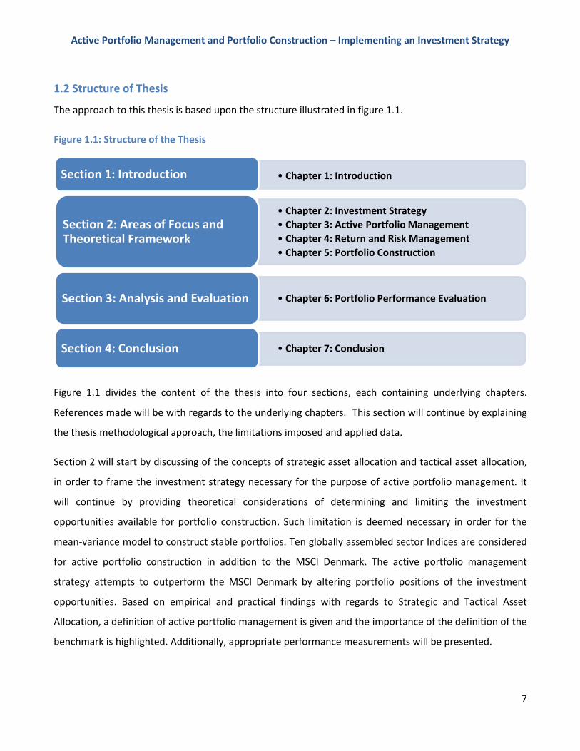
1.2 Structure of Thesis
The approach to this thesis is based upon the structure illustrated in figure 1.1.
Figure 1.1: Structure of the Thesis
Figure 1.1 divides the content of the thesis into four sections, each containing underlying chapters.
References made will be with regards to the underlying chapters. This section will continue by explaining
the thesis methodological approach, the limitations imposed and applied data.
Section 2 will start by discussing of the concepts of strategic asset allocation and tactical asset allocation,
in order to frame the investment strategy necessary for the purpose of active portfolio management. It
will continue by providing theoretical considerations of determining and limiting the investment
opportunities available for portfolio construction. Such limitation is deemed necessary in order for the
mean-variance model to construct stable portfolios. Ten globally assembled sector Indices are considered
for active portfolio construction in addition to the MSCI Denmark. The active portfolio management
strategy attempts to outperform the MSCI Denmark by altering portfolio positions of the investment
opportunities. Based on empirical and practical findings with regards to Strategic and Tactical Asset
Allocation, a definition of active portfolio management is given and the importance of the definition of the
benchmark is highlighted. Additionally, appropriate performance measurements will be presented.
• Chapter 1: Introduction Section 1: Introduction
• Chapter 2: Investment Strategy
• Chapter 3: Active Portfolio Management
• Chapter 4: Return and Risk Management
• Chapter 5: Portfolio Construction
Section 2: Areas of Focus and Theoretical Framework
• Chapter 6: Portfolio Performance Evaluation Section 3: Analysis and Evaluation
• Chapter 7: Conclusion Section 4: Conclusion
Active Portfolio Management and Portfolio Construction – Implementing an Investment Strategy
8
The section continues by providing return estimates as input variables for portfolio construction. Based on
theoretical and practical findings, issues regarding the risk active portfolio management are exposed to
will be analyzed and evaluated. The section then concludes by applying the Markowitz mean-variance
portfolio model for portfolio construction. Implementation possibilities with regards to portfolio
repositioning are additionally presented and briefly discussed. The performance of the mean-variance
model in the context of active portfolio management will then be examined. First in terms of asset
allocation, i.e. whether the model has produced stable portfolios during portfolio repositioning. Second,
return estimates will indicate whether outperformance is present on a long-term basis.
Section 3 will present the results of the active portfolio management process. From the portfolio strategy,
the portfolio model presented in section 2 will have assembled portfolios based on the provided risk and
return estimates. This section therefore answers the questions of whether active portfolio management
has added value to the investment and whether these results are due to skill rather than luck.
Section 4 concludes by summarizing the answers to the research questions.
1.3 Methodology
1.3.1 Financial Assets and Risk
An enduring element regarding portfolio performance concerns the relationship between risk and return
on investments. A financial investment, in contrast to a real investment, which involves tangible assets
such as land and production facilities, is an allocation of money whose value is supposed to increase over
time. Therefore a security is a contract to receive prospective benefits under stated conditions like stocks
and bonds.
The two main attributes that distinguish securities are time and risk. Usually the interest rate or rate of
return (depending on whether the security is a bond or stock) is defined as the gain or loss of the
investment relative to the initial value of the investment. An investment always contains some sort of risk,
categorized into two types – systematic and unsystematic risk, and the higher such risks the higher return
is demanded by investors.
Active Portfolio Management and Portfolio Construction – Implementing an Investment Strategy
9
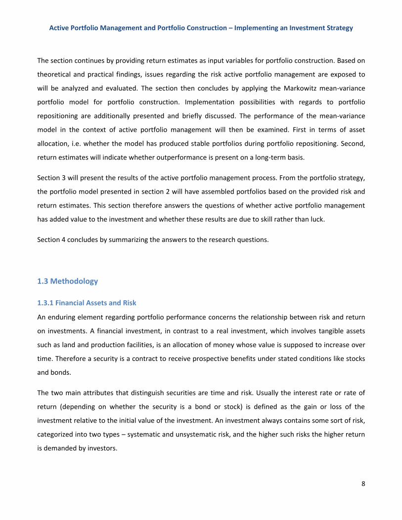
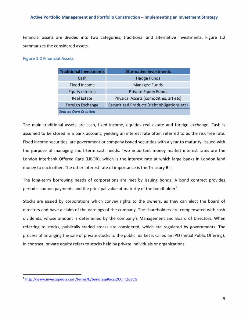
Financial assets are divided into two categories; traditional and alternative investments. Figure 1.2
summarizes the considered assets.
Figure 1.2 Financial Assets
The main traditional assets are cash, fixed income, equities real estate and foreign exchange. Cash is
assumed to be stored in a bank account, yielding an interest rate often referred to as the risk free rate.
Fixed income securities, are government or company issued securities with a year to maturity, issued with
the purpose of managing short-term cash needs. Two important money market interest rates are the
London Interbank Offered Rate (LIBOR), which is the interest rate at which large banks in London lend
money to each other. The other interest rate of importance is the Treasury Bill.
The long-term borrowing needs of corporations are met by issuing bonds. A bond contract provides
periodic coupon payments and the principal value at maturity of the bondholder5.
Stocks are issued by corporations which convey rights to the owners, as they can elect the board of
directors and have a claim of the earnings of the company. The shareholders are compensated with cash
dividends, whose amount is determined by the company’s Management and Board of Directors. When
referring to stocks, publically traded stocks are considered, which are regulated by governments. The
process of arranging the sale of private stocks to the public market is called an IPO (Initial Public Offering).
In contrast, private equity refers to stocks held by private individuals or organizations.
5 http://www.investopedia.com/terms/b/bond.asp#axzz2CCmQC8CG
Traditional Investments Alternative Investments
Cash Hedge Funds
Fixed Income Managed Funds
Equity (stocks) Private Equity Funds
Real Estate Physical Assets (comodities, art etc)
Foreign Exchange Securitized Products (debt obligations etc)
Source: Own Creation
Active Portfolio Management and Portfolio Construction – Implementing an Investment Strategy
10
Real estate investments and foreign exchange derivatives are also found in portfolios, the latter for
hedging against currency risks. Alternative investments emphasize the widening spectrum of investment.
These types of investment are beyond the scope of this thesis.
Risk and return obviously depends upon the type of investment. In order to measure investment return on
a frequent basis we turn to equities, or stocks, as return can be realized at any point in time, preferable for
an investor who favors frequent trading. The risk of such investment is presented when positive or
negative return is realized upon trading. Hence, emphasis on risk and return is important to consider,
particularly in the context of active portfolio management, as the investor takes on the risk of frequently
realizing positive and negative returns.
The emphasis of the relationship between risk and return is reflected in the applied theoretical models.
These models are described below. As the research objective is based upon a practical exercise it
important to also include real-life methods and applications with regards to investment strategies.
Therefore, the methods and information provided by selected theoretical concepts applied is
supplemented by the input of two investment professionals. Their contribution to this thesis is described
subsequently to the applied theoretical approach.
1.3.2 Applied Theoretical Approach
Throughout the analysis the following theories will assist in performing active portfolio management.
The framework of the investment strategy will be established by the concepts of strategic and tactical
portfolio management. The investment opportunity set will be limited and the relevance of the
benchmark discussed.
In order to apply the mean-variance portfolio model, expected return estimates and risk measures for
each of the sector Indices suitable for the purpose of active portfolio management will be outlined. The
former will be calculated by use of the Capital Asset Pricing Model (CAPM) model. The advantage of
applying the CAPM model is that we can separate the market risk, beta and expected market return, of
each sector index, and in that manner compare risk and return of sectors and benchmark.
Active Portfolio Management and Portfolio Construction – Implementing an Investment Strategy
11
Portfolio construction will be conducted by Markowitz’ mean-variance portfolio model as it optimizes
asset allocation in Excel based on performance ratios appropriate for the purpose of the investment
strategy6. Thus, optimizing with respect to the information ratio, which indicates relative benchmark
performance with regards to its residual risk, alpha, and residual return, beta, will lead to asset allocations
expected to provide the portfolio with a return superior to the benchmark. The asset allocation will be
conducted as a repetitive process.
1.3.3 Interviews
In order to limit the amount of assumptions made and to provide a practical point of view when
processing empirical data and applying theoretical models, interviews were conducted in order to uncover
relevant areas of study. Also, practical reviews were applied, as some exercised concepts of investment
theory carry universal definitions or conditions for execution.
Empirical and practical data have been obtained through interviews and consultation with two investment
professionals, who provided relevant information, relating to the research objective.
Peter Sjøntoft, Vice President, Global Banking, Citigroup Global Markets Limited, London United
Kingdom
Peter Sjøntoft has provided his personal viewpoints upon issues where elements of investment
theory seem difficult to apply in real-life investment strategies. Furthermore, he has provided
suggestions of where to challenge the application of these theories. He has assisted in adding
practical viewpoints in establishing the framework for active portfolio management, and
discussions regarding the use of investment strategies.
Claus Vorm, Senior Portfolio Manager, Nordea Investment Management, Copenhagen, Denmark
Claus Vorm has been responsible for establishing a team of investment specialists in charge of
managing Nordea’s tactical asset allocation, as well as the banks quantitative products.
Furthermore, he has been responsible for managing various balanced portfolios.
Claus Vorm has contributed with insights into the use of the strategic and tactical asset allocation
processes in Nordea’s investment strategies, which will be included when forming the investment
6 Benninga (2008): p. 338
Active Portfolio Management and Portfolio Construction – Implementing an Investment Strategy
12
strategy for active portfolio management. His contribution also extends to views upon risk
management.
Peter Sjøntoft and Claus Vorm were chosen with the purpose of providing a nuanced representation of
opinions concerning investment decisions, as well as contributing with informational groundwork for the
research objective. Their experiences and information has enabled continuous tightening of the research
objective. The interview with Claus Vorm was recorded and stored on the CD attached. Due to geographic
differences, interviews with Peter Sjøntoft were conducted by phone, so no conversation was recorded,
and therefore no specific citations made. For interview guide, see Appendix 3.
1.4 Assumptions and limitations
In order to maintain a clear focus throughout the thesis it is necessary to define some assumptions and
limitations.
1.4.1 Assumptions
The theoretical discussion and the practical calculations with regards to the portfolio construction, will
take the point view of a Danish investor who has funds available for investments. In that regard
differences between investments by pension funds and private funds, including e.g. tax considerations and
consequences will not be discussed.
All calculations are conducted on the basis of monthly data, stated in US dollars from January 1992 to
December 2011. Data have been extracted from Datastream, MSCI Barra and Statistikbanken. Monthly
observations are opted for as opposed to e.g. daily observations as the former provides clear and
adequate information with regards to the development of the index prices and for sufficient data
management. The time period is considered appropriate as it provides a sufficient amount of data and it
covers significant economic events, affecting the financial markets.
With regards to the issue of transaction costs, we will assume that all transactions have equal expense
over the entire period. In addition, in order to limit the constraints to the mean-variance portfolio model,
Active Portfolio Management and Portfolio Construction – Implementing an Investment Strategy
13
the transaction costs will be deducted from the return on investment subsequent to portfolio
repositioning.
Finally, I will assume that markets are not completely efficient7. However, I will assume that the investor is
rational suggesting that he prefers more to less. Although market efficiency rests on the assumption that
investors are rational, its validity is not undermined by the investor not being rational, given he does not
trade randomly. In addition, all hedging of currency is completed by future contracts, meaning that only
index movement excluding currency behavior is considered. Moreover, the analysis will not incorporate
any tax effects. This is mainly because of the complexities of the Danish tax system. Furthermore, the
introduction of such a system is in conflict with the conditions of portfolio theory that leads to saying that
the investor should buy the market portfolio.
1.4.2 Limitations
1.4.2.1 Theoretical framework
In portfolio theory there are several models and applications appropriate for portfolio construction. Both
Markowitz (1952) and Black Litterman (1992) propose portfolio models applicable for portfolio
construction. The thesis will apply Markowitz’ mean-variance portfolio model, but argumentation and
justification for the choice of model will be provided. The model will be explained superficially, and
derivations will not be included when explaining the model, as I intend to present the model in the most
comprehensive manner possible.
Short sales will not be introduced throughout this thesis. The reason for this is that the mean-variance
model tends to incorporate extreme values in the asset positions when short sales are included providing
portfolios of poor applicability. Another reason is that major stock exchanges have unique short sales
regulations8. Furthermore, financial gearing is prohibited. Both assumptions contribute to portfolio
robustness, meaning altering investment positions are comparable with changes in return and covariance
estimates.
7 Shleifer (2000): p. 3
8 http://www.sec.gov/spotlight/keyregshoissues.htm
Active Portfolio Management and Portfolio Construction – Implementing an Investment Strategy
14
1.4.1.2 Data
In order to construct a globally representative portfolio ten sector indices have been chosen, as they
represent a significant proportion of the world stock market. The indices are presented in chapter 1.5. The
MSCI Denmark and MSCI World Market indices are obtained from MSCI Barra9.
Before selecting the sector Indices I examined their historical returns, variances and covariance along with
the correlation and size of their market capitalization (see Appendix 2). The examination showed a
moderate pattern of a positive risk-return relationship among the sectors. Some of the sectors with the
highest risk-return payoff even had some of the lowest correlations towards other markets. The general
picture, however, showed high correlations among sectors leaving only a few inter-correlations below 0,5
suggesting high integration among sectors (only Technology showed correlation below 0,5). High market
integration is not an attractive property from perspective of investment theory as it constructs portfolios
based upon high return estimations and low covariance, hence low correlations. However, this scenario
highlights whether one major advantage in portfolio management, diversification, can provide the
portfolio with a higher risk adjusted return compared to the benchmark.
1.5 Data
In this chapter the definition and source of the equity sector return applied in the thesis are presented.
1.5.1 Equity Sector Return Data
There is a large industry of providing investors with benchmark data of sectors. They use Global Industry
Classification Standards (GICS) which operates with a ten sector classification (MSCI Barra, 2010): Energy,
Materials, Industrials, Consumer Discretionary, Consumer Staples, Healthcare, Financials, Information
Technology, Telecommunication Services, Utilities. These sector groups can again be classified into 24
industry groups, 68 industries, and 154 sub-industries10.
Equity return data in this thesis is obtained from Datastream and Morgan Stanley Capital International
(MSCI), since they offer data on world sector return covering the needed time periods. With regards to
9 http://www.msci.com/products/indices/country_and_regional/all_country/performance.html
10 MSCI Barra (2010): p. 82
Active Portfolio Management and Portfolio Construction – Implementing an Investment Strategy
15
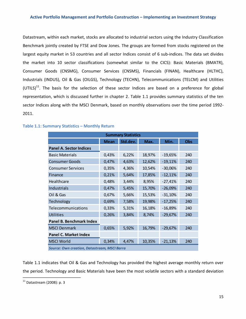
Datastream, within each market, stocks are allocated to industrial sectors using the Industry Classification
Benchmark jointly created by FTSE and Dow Jones. The groups are formed from stocks registered on the
largest equity market in 53 countries and all sector Indices consist of 6 sub-indices. The data set divides
the market into 10 sector classifications (somewhat similar to the CICS): Basic Materials (BMATR),
Consumer Goods (CNSMG), Consumer Services (CNSMS), Financials (FINAN), Healthcare (HLTHC),
Industrials (INDUS), Oil & Gas (OILGS), Technology (TECHN), Telecommunications (TELCM) and Utilities
(UTILS)11. The basis for the selection of these sector Indices are based on a preference for global
representation, which is discussed further in chapter 2. Table 1.1 provides summary statistics of the ten
sector Indices along with the MSCI Denmark, based on monthly observations over the time period 1992-
2011.
Table 1.1: Summary Statistics – Monthly Return
Table 1.1 indicates that Oil & Gas and Technology has provided the highest average monthly return over
the period. Technology and Basic Materials have been the most volatile sectors with a standard deviation
11
Datastream (2008): p. 3
Mean Std.dev. Max. Min. Obs
Panel A. Sector Indices
Basic Materials 0,43% 6,22% 18,97% -19,65% 240
Consumer Goods 0,47% 4,63% 12,62% -19,11% 240
Consumer Services 0,35% 4,36% 10,54% -30,06% 240
Finance 0,21% 5,64% 17,85% -12,11% 240
Healthcare 0,48% 3,44% 8,95% -27,41% 240
Industrials 0,47% 5,45% 15,70% -26,09% 240
Oil & Gas 0,67% 5,66% 15,53% -31,10% 240
Technology 0,69% 7,58% 19,98% -17,25% 240
Telecommunications 0,33% 5,31% 16,18% -16,89% 240
Utilities 0,26% 3,84% 8,74% -29,67% 240
Panel B. Benchmark Index
MSCI Denmark 0,65% 5,92% 16,79% -29,67% 240
Panel C. Market Index
MSCI World 0,34% 4,47% 10,35% -21,13% 240
Summary Statistics
Source: Own creation, Datastream, MSCI Barra
Active Portfolio Management and Portfolio Construction – Implementing an Investment Strategy
16
above 7% and 6%, respectively. Note, that market and benchmark indices are two different indices. When
referring to the benchmark, it is the MSCI Denmark targeted for outperformance, while referring to the
market relates to the MSCI World index. The latter will only be applied for return calculations and
systematic risk estimations. From Appendix 4 all indices are concluded to be stationary indicating that
positive monthly returns are likely to be followed by negative return and vice versa, which in fact
complicates active portfolio management, as it makes the decision of market timing rather difficult. This
problem will be addressed with regards to portfolio construction in chapter 5.
Within the literature of stock returns there is no general convention regarding the use of simple and log-
returns. For example Campbell and Thomson (2008) use the simple mean approach while Benninga (2008)
argues log-returns, which is marginally more precise when modeling assets in Excel1213. Therefore, the
monthly return data is calculated as log-returns, and these returns are applied throughout this thesis. The
simple and log-return methods were tested on a few sector indices and only small differences were found.
Thus, we do not expect the conclusions to be significantly different if simple returns had been used
instead.
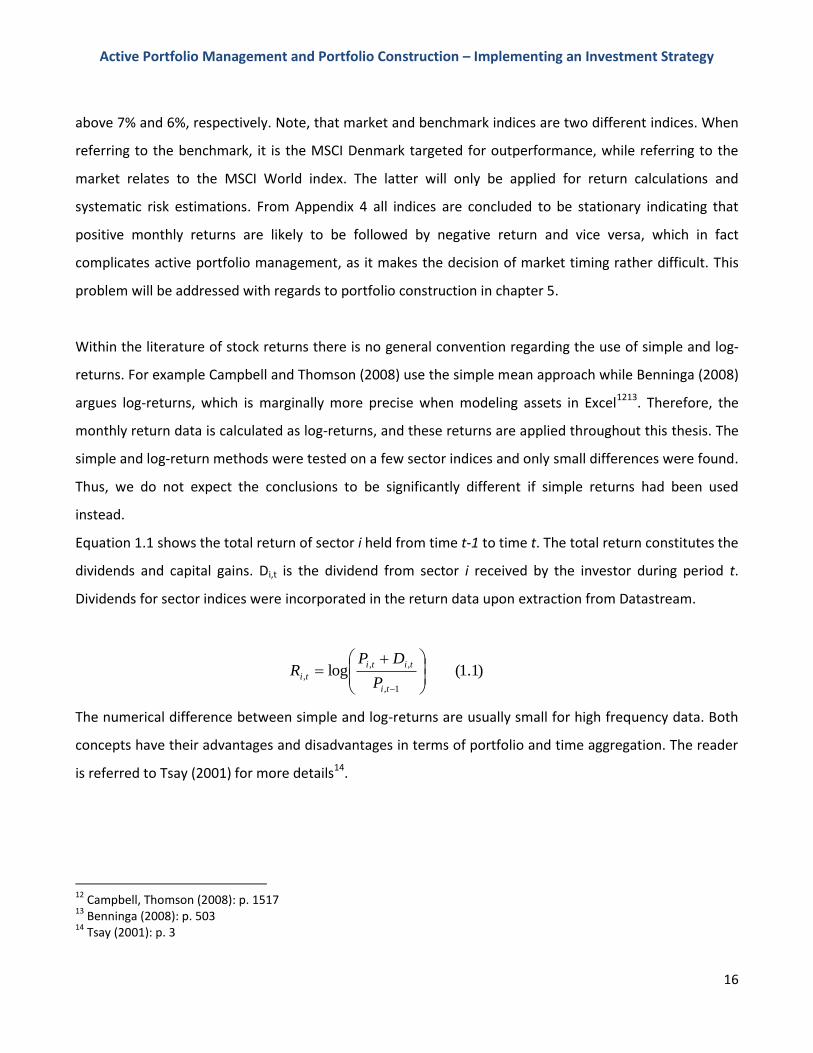
Equation 1.1 shows the total return of sector i held from time t-1 to time t. The total return constitutes the
dividends and capital gains. Di,t is the dividend from sector i received by the investor during period t.
Dividends for sector indices were incorporated in the return data upon extraction from Datastream.
)1.1(log1,
,,
,
ti
titi
tiP
DPR
The numerical difference between simple and log-returns are usually small for high frequency data. Both
concepts have their advantages and disadvantages in terms of portfolio and time aggregation. The reader
is referred to Tsay (2001) for more details14.
12
Campbell, Thomson (2008): p. 1517 13
Benninga (2008): p. 503 14
Tsay (2001): p. 3

Active Portfolio Management and Portfolio Construction – Implementing an Investment Strategy
17
The excess return is defined by the return in excess of the risk free asset.
)2.1(,,, tfti
e
ti RRR
Here, e
tiR , is the monthly excess return of investment i at time t, tiR , is the return of investment i at time t,
and tfR , is the monthly return of the risk free asset at time t.
Active return is defined by the excess return of an asset or portfolio in excess of the benchmark return at
time t.
)3.1(,,, tBtiti RRR
Here, tiR , is the active return and tBR , the benchmark return at time t. Substituting the right hand side of
equation 1.2 into 1.3 and subtracting the risk free rate from the benchmark return yields the following
calculation for active excess return:
tBti
e
t
tftBtfti
e
t
RRR
RRRRR
,,
,,,, )4.1(
From equation 1.4, active return is identical to active excess return.
Active Portfolio Management and Portfolio Construction – Implementing an Investment Strategy
18
1. Investment Strategy
In order to frame the concept of active portfolio management a specified investment strategy is
required. Investors buy and sell stocks based upon individual incentives such as a desire for abnormal
investment returns or because they are constrained by consumption and liabilities. Hence, there is no
single approach defined to actively manage a portfolio as the allocation of assets differs depending
upon the investment objective. Thus, an investment strategy appropriate for answering the research
objective is called for. We will apply the concepts of strategic and tactical asset allocation, two debated
methodologies to portfolio management, in order to establish a framework for such strategy15.
2.1 Investment Strategy as the Source of Portfolio Performance
The accepted advice about spreading investments on several asset classes in order to minimize risk, and
not let emotions or gut feelings control the continuous portfolio allocation process, has become common
knowledge. Nevertheless, the opinions and expectations of the individual investor still dominates the
decision making process when they assemble portfolios16.
According to Peter Sjontoft, identifying an investor who has managed to outperform a benchmark is not
necessarily rare or difficult, when selecting among investors who base their investment decisions on gut
feelings, emotions or even randomly select stocks to invest in. On average, these investors may in fact
outperform a given benchmark, not because they are smart investors with extensive market insights, but
because the stocks they invest in simply happen to perform better than the market over the given
timeframe. Berk (2005) supports this statement, claiming that little evidence of performance persistence
exists – investors that perform well in one year are no more likely to perform as well next year17. One
possible explanation for this is that markets are, as in this case stationary, which opens the possibility for
investor lucky as they happen to buy stocks when markets are down and sell with a positive return. Such
scenario promotes the assumption that investor performance can be due to luck rather than skill and that
active portfolio management could be just as successful as random portfolio management – in an
15
Schneeweis et.al. (2010): p. 91 16
http://www.proinvestor.com/finansnyhed/10294074/Fodboldaktier-koebes-som-legetøj 17
Berk (2005): p. 30
Active Portfolio Management and Portfolio Construction – Implementing an Investment Strategy
19
individual case, not on average. The investor who chose e.g. Novo Nordisk or Apple five years ago would
likely have outperformed most indices18. The question is really if someone who over-performed was lucky
or skilled, i.e. is his chances of repeating the performance next year higher than average? On that basis the
investor’s management skills is put into context as this constitutes the performance difference between
passive and active portfolio management. In that regard active portfolio return stem from the investment
strategy. The investment strategy constitute the process of asset allocation and security selection, as
these determine what to invest in at which point in time in order to generate positive active return.
2.2 Strategic Asset Allocation
Strategic asset allocation is a static approach to asset allocation where the portfolio assets are allocated
based on a long-term return estimate. Asset positions are retained throughout the period, meaning that
as asset returns change their portfolio weights change correspondingly, and the investor then rebalance
the portfolio by adjusting asset weights back to their initial positions19. Once the assets have been
selected for portfolio construction, no other asset will be introduced at any time.
Markowitz’ extensive work on the modern portfolio theory has yielded a dimension to the asset
management theory, i.e. diversification. This reward emerges when assets, which correlate negatively or
independently with each other, are assembled into a portfolio20. Strategic asset allocation sets forth long-
term allocations for assets possessing such characteristics.
The allocation process relies on the assumption that markets are efficient, which makes it impossible to
obtain abnormal return on investments, and therefore makes market timing irrelevant. On the contrary
active trading will increase transaction costs, which reduces the realized return more than expected. In
order to illustrate the argument against market timing, Ibbotson Associates made the following analysis21:
18
http://www.euroinvestor.dk/boerser/nasdaq-omx-copenhagen/novo-nordisk-b/205365 and http://www.euroinvestor.dk/boerser/nasdaq/apple-inc/38687 19
Schneeweis (2010): p. 99 20
Markowitz (1959): p.102 21
Spar Invest (2007): p. 17
Active Portfolio Management and Portfolio Construction – Implementing an Investment Strategy
20
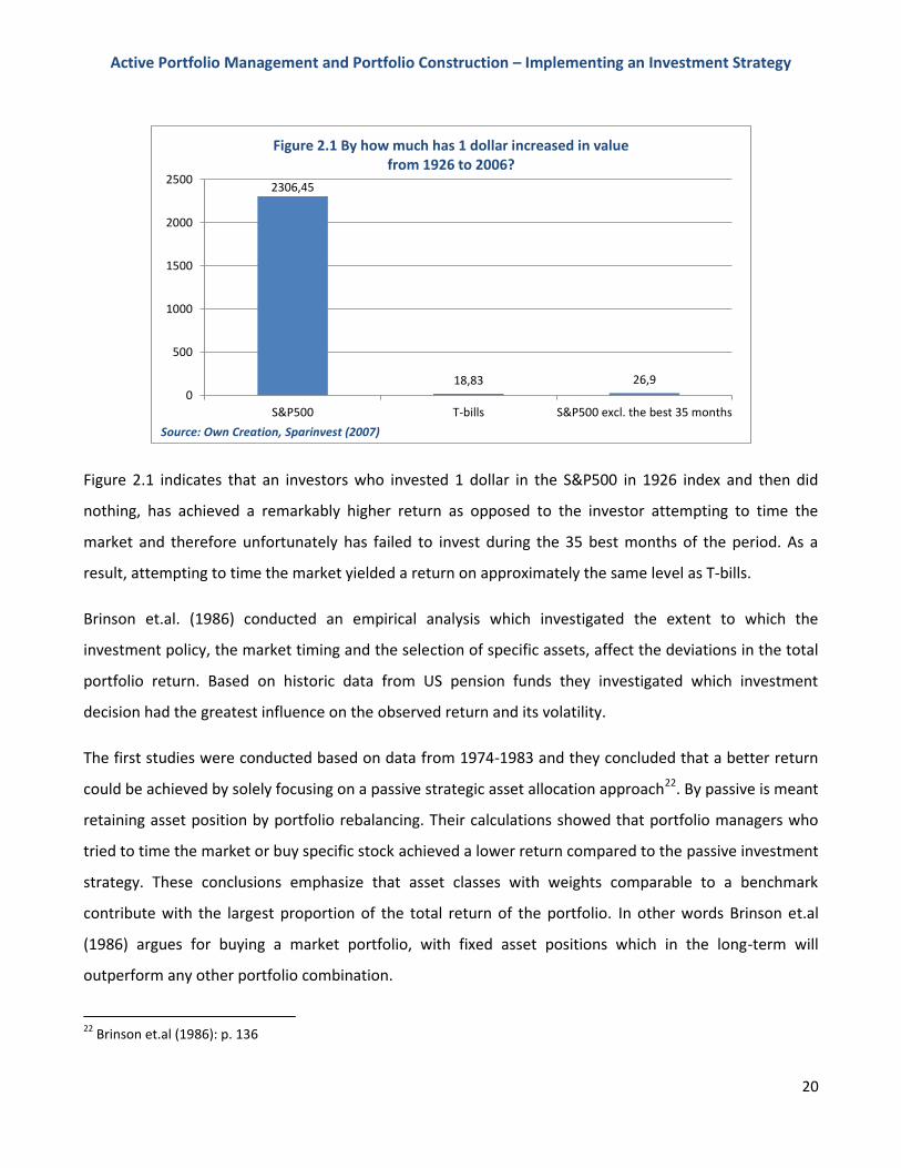
Figure 2.1 indicates that an investors who invested 1 dollar in the S&P500 in 1926 index and then did
nothing, has achieved a remarkably higher return as opposed to the investor attempting to time the
market and therefore unfortunately has failed to invest during the 35 best months of the period. As a
result, attempting to time the market yielded a return on approximately the same level as T-bills.
Brinson et.al. (1986) conducted an empirical analysis which investigated the extent to which the
investment policy, the market timing and the selection of specific assets, affect the deviations in the total
portfolio return. Based on historic data from US pension funds they investigated which investment
decision had the greatest influence on the observed return and its volatility.
The first studies were conducted based on data from 1974-1983 and they concluded that a better return
could be achieved by solely focusing on a passive strategic asset allocation approach22. By passive is meant
retaining asset position by portfolio rebalancing. Their calculations showed that portfolio managers who
tried to time the market or buy specific stock achieved a lower return compared to the passive investment
strategy. These conclusions emphasize that asset classes with weights comparable to a benchmark
contribute with the largest proportion of the total return of the portfolio. In other words Brinson et.al
(1986) argues for buying a market portfolio, with fixed asset positions which in the long-term will
outperform any other portfolio combination.
22
Brinson et.al (1986): p. 136
2306,45
18,83 26,90
500
1000
1500
2000
2500
S&P500 T-bills S&P500 excl. the best 35 months
Figure 2.1 By how much has 1 dollar increased in value from 1926 to 2006?
Source: Own Creation, Sparinvest (2007)
Active Portfolio Management and Portfolio Construction – Implementing an Investment Strategy
21
In addition to providing a better return, 93,6% of the deviations of return can be explained by strategic
asset allocation23. Therefore, as regards to long-term investments, literature has proved that in terms of
returns, the best idea is to conduct portfolio investment, and not try to alter investment positions on a
periodic basis. In addition, resources committed to the investment decision should be concentrated
around the strategic decisions – the determination of the investment opportunity set - since the risk of the
investment can be observed here.
In order to substantiate these results, Brinson et.al. (1991) conducted a new analysis on behalf of US
pension funds during the period 1977-1987. They reached the same results as just discussed. For this
period 91,5% of the standard deviation of return could be explained from strategic asset allocation. Only
1,8% of the return deviations was explained by tactical asset allocation - the process of over- and
underweight portfolio sectors24.
Aside from explaining a majority of return deviations, the strategic approach to asset allocation
contributes to a better risk adjusted return in contrast to attempting to time the market. Such approach
offers investors the possibility of achieving a higher return at a lower risk. This is in accordance with
Markowitz (1952) portfolio theory, as he developed the efficient portfolio based on long-term historical
data.
2.2.1 Discussing Empirical Findings and Brinson et.al.
The findings supporting the strategic asset allocation as the prevailing investment strategy assumes
market efficiency, which makes it impossible to obtain abnormal returns, and thus makes market timing
irrelevant. However, to believe investors have the same information available and that the full use of this
information is reflected in asset prices is a naïve assumption. Empirical findings within the area of
behavioral finance have provided evidence that the assumption of a fully informed rational investor is
rather bold. Grossman and Stiglitz (1980) go even as far as stating that if markets were perfectly efficient
there would be no profit from gathering information, in which case there would be no reason to trade,
leading markets to eventually collapse25. In order to adopt a strategy for active portfolio management,
23
Brinson et.al (1986): p. 137 24
Brinson et.al. (1991): p. 45 25
Grossman and Stiglitz (1980): p. 393
Active Portfolio Management and Portfolio Construction – Implementing an Investment Strategy
22
trading is thus required and although markets are stationary, we can therefore not assume full efficiency
in the market, but refer to the adaptive market hypothesis instead.
Despite their conclusions, Brinson et al. (1986) have, however, received criticism for their analysis. Jahnke
(1997) criticized their use of the variance as risk measurement as opposed to the standard deviation26. If
the variance were to be replaced with the standard deviation, the strategic asset allocation would instead
explain 79% of the return deviations, which is not nearly as seminal as 93,6%.
In addition, the argument that risk of a passive investment strategy can be more easily identified is rather
obsolete. Only if assets expected returns are constant over time, should the asset weights remain
constant. The problem with such assumption is that stocks perform differently over different timeframes
due to their stages in business cycles and changes in macroeconomic developments. Hence, investors
assume changing risk premiums on stocks, leading expectations of asset prices, and as a result, their
portfolio weight to change. On this basis, investors should consider asset allocation as a dynamic process
which allows asset positions to change as their expected premiums change.
Among the critics towards Brinson et.al are also Statman (2000). He concludes that a portfolio manager
who consequently invests in the appropriate asset classes (stocks, bonds and holds cash as well) every
year between 1980 and 1997, achieves a return 8,1% per year in excess of passive strategic approach27. In
addition, 89,4% of the return deviations could be explained by the investment strategy, and the result is
therefore not far from the analysis of Brinson et.al. (1986). His point is that the investor should not only
focus on the strategic approach, but adopt a more active approach as well.
Regardless of whether the investor believes in the conclusions of Brinson et.al or joins the group of critics,
there is no doubt that the opted investment strategy has major influence upon the portfolio return
deviation. Strategic Asset allocation offers an attractive feature in the asset selection. It is fixed, which
means determining a fixed opportunity is supported by literature and carries practical advantage for
portfolio construction as we don’t have to dedicate resources to identifying new opportunities. With
regards to asset allocation we turn to the dynamic approach of tactical asset allocation.
26
Jahnke (1997): p. 2 27
Statman (2000): p. 19

Active Portfolio Management and Portfolio Construction – Implementing an Investment Strategy
23
2.3 Tactical Asset Allocation
Contrary to strategic asset allocation strategy, another practice within asset allocation assumes a more
active approach to asset management. In order to conduct a thorough investigation of whether active
investment management can outperform a benchmark, a different strategy is considered. The main points
of tactical asset allocation are outlined in the following.
Following a strategic asset allocation approach, changes in the portfolio will exclusively occur ex-post,
meaning that the investor will modify his portfolio as a reaction to events occurred, by rebalancing the
asset weight back to their initial target weights. The initial portfolio composition will therefore be altered
as a result of general market developments. In periods of negative returns for some assets the portfolio
must be rebalanced so the optimal proportion of assets is recreated.
However, asset allocation must be based on expectations of short term future returns in order to
continuously ensure positive active return. In 1971 William Fouse launched the first index fund28. His work
made it possible to control different asset classes simultaneously, and this technique has later been
known as tactical asset allocation. On that basis, compared to strategic asset allocation, tactical asset
allocation is on the other hand an ex-ante investment strategy where the investor proactively adjusts his
portfolio based on market historic developments and expectations29. Thus, the dynamic nature of tactical
asset allocation requires active adjustments to the investment opportunities in response to short-term
changes in the economic environment. Its objective is to adjust the allocation in order to take advantages
of temporary pockets of market inefficiency30.
Contrary to Strategic Asset Allocation the investor has not determined an optimal asset distribution, but
adjusts the portfolio in accordance with his expectations to the market development. Therefore, the
essence of tactical asset allocation is to proactively position portfolio assets based upon changes in
expected returns. Thus, assets with high expected returns are favored, as opposed to the remaining
opportunity set, and assets with low expected returns are less desired. The advantage of the tactical asset
28
Lee (2000): p. 12 29
Picerno (2010): p. 153 30
Schneeweis (2010): p. 101
Active Portfolio Management and Portfolio Construction – Implementing an Investment Strategy
24
allocation and the main source of its popularity is that it combines Graham and Dodd’s value investment
strategy together with Markowitz modern portfolio theory31.
The concept of value investing by Graham and Dodd has been an active investment strategy. Investors
seek undervalued stocks with low price-to-earnings ratios. On the other hand, Markowitz considers
investments within a determined timeframe, and hence only the market portfolio can be considered a
risky portfolio. Tactical asset allocation made it possible to combine these two strategies into one, which
enables the possibility of active management and thereby a superior return.
2.4 Professional Views upon Asset Allocation
As described above there is no doubt that strategic asset allocation constitutes a relevant investment
strategy and carries the advantage of a predetermined long-term investment universe. However, from the
viewpoint of the active investor, tactical asset allocation also seems a suitable investment strategy as it
proactively repositions the portfolio on a regular basis in accordance with the investor’s expectations. The
extent to which investors follow the strategic or tactical approach or even both when constructing optimal
portfolios remains unknown. The following will therefore include a review of Claus Vorm’s assessment
upon the process of asset allocation and highlight the way Nordea Investment Management applies
portfolio theory.
In relation to balanced portfolios, the initial asset allocation is based on long-term investment decisions
consistent with strategic asset allocation. The asset allocation process begins by considering levels of
equilibrium for interest rate structures, inflation rates etc. From these estimations Nordea attempts to
determine the long-term risk premium on each selected stock. The equilibrium expectations enables
expected return calculations over a strategic default period, which is within a business cycle of
approximately ten years.
Nordea then starts optimizing, by allocating funds into the stocks which are considered below long-term
equilibrium – undervalued stocks. On that basis it is reasonable to form a strategy that considers the state
of the economy compared to long-term equilibrium. Claus Vorm considers this a strategic analysis,
31
Value investment involves investing in stocks with low P/E ratio
Active Portfolio Management and Portfolio Construction – Implementing an Investment Strategy
25
valuable for creating highly diversified optimal portfolios based on estimated expected return and
covariance among assets. Obviously, as other portfolio models, this method carries pitfalls, but Claus
Vorm believes that the results of these models combined with the investor’s common sense can create
strong diversified portfolios.
On the other hand, Claus Vorm also believes advantages can be utilized in tactical asset allocation. Stocks
may be underpriced as considered in the strategic asset allocation, but they may have to be priced even
lower before returning to equilibrium, hence Nordea will have to purchase the stock e.g. two months
later.
The important conclusion here is that both strategic and tactical asset allocation will not necessarily have
to be present in the same investment strategy. We implement a long-term investment strategy with
changes in short-term portfolio positions, within the boundaries of predetermined risk parameters. This
approach can add value in terms allocating funds on a strategic long-term basis and reposition the
portfolio on a tactical basis. Hence, both the strategic and tactical approach is implemented in a balanced
portfolio, as the portfolio assets are repositioned on a regular basis. Claus Vorm suggests a useful strategy
would be to balance assets within determined boundaries, e.g. portfolio assets can be reweighted ±20% of
their initial portfolio weight each month.
Strategic and tactical asset allocation will both be implemented as part of the investment strategy, in
balanced capacities. Strategic asset allocation offers advantages in terms of limiting the investment
opportunities which combined can be submitted to periodic repositioning in accordance with tactical asset
allocation.
2.5 Benchmark and Investment Opportunities
The choice of benchmark is of significant importance, as its performance obviously plays a key role in
determining the success of the investment strategy. Additionally, the investment opportunities must be
given careful consideration as combining such should constitute a more attractive investment compared
to the benchmark.
Active Portfolio Management and Portfolio Construction – Implementing an Investment Strategy
26
2.5.1 Benchmark
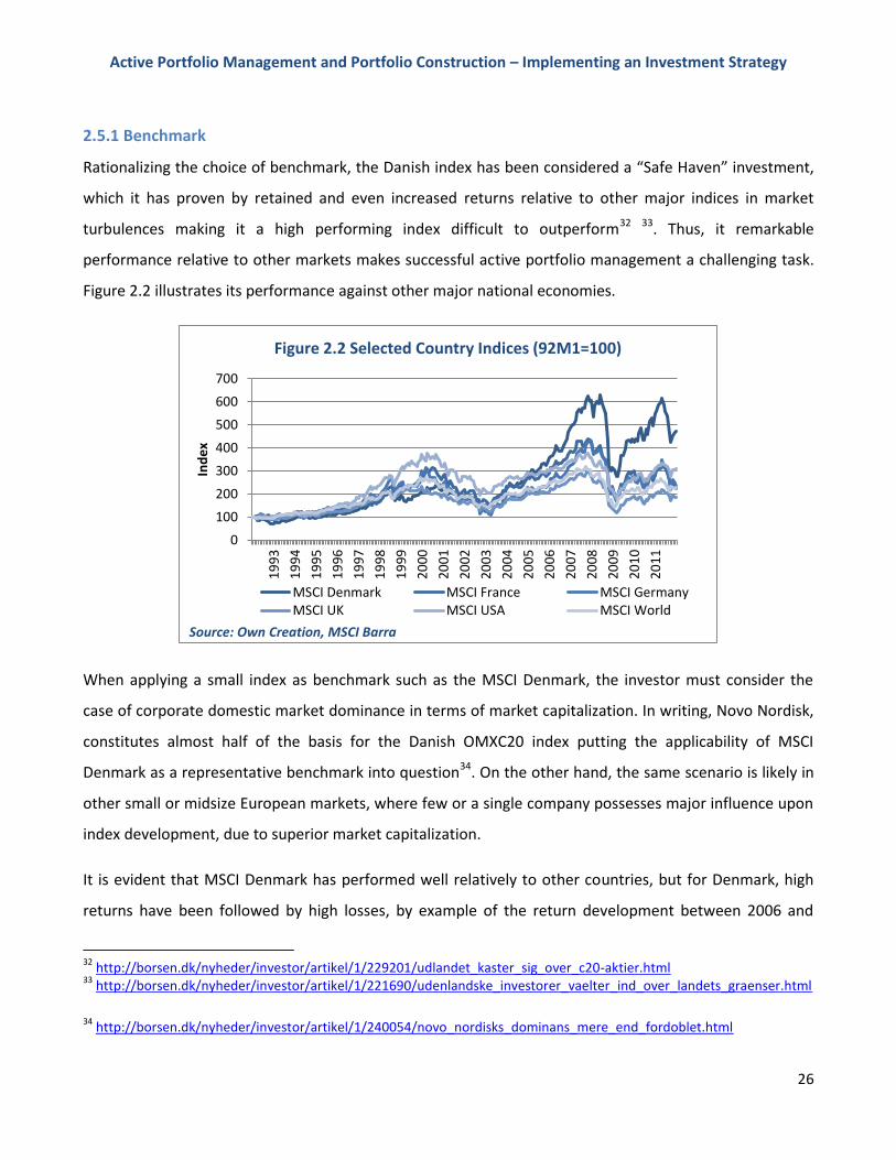
Rationalizing the choice of benchmark, the Danish index has been considered a “Safe Haven” investment,
which it has proven by retained and even increased returns relative to other major indices in market
turbulences making it a high performing index difficult to outperform32 33. Thus, it remarkable
performance relative to other markets makes successful active portfolio management a challenging task.
Figure 2.2 illustrates its performance against other major national economies.
When applying a small index as benchmark such as the MSCI Denmark, the investor must consider the
case of corporate domestic market dominance in terms of market capitalization. In writing, Novo Nordisk,
constitutes almost half of the basis for the Danish OMXC20 index putting the applicability of MSCI
Denmark as a representative benchmark into question34. On the other hand, the same scenario is likely in
other small or midsize European markets, where few or a single company possesses major influence upon
index development, due to superior market capitalization.
It is evident that MSCI Denmark has performed well relatively to other countries, but for Denmark, high
returns have been followed by high losses, by example of the return development between 2006 and
32
http://borsen.dk/nyheder/investor/artikel/1/229201/udlandet_kaster_sig_over_c20-aktier.html 33
http://borsen.dk/nyheder/investor/artikel/1/221690/udenlandske_investorer_vaelter_ind_over_landets_graenser.html
34 http://borsen.dk/nyheder/investor/artikel/1/240054/novo_nordisks_dominans_mere_end_fordoblet.html
0
100
200
300
400
500
600
700
19
93
19
94
19
95
19
96
19
97
19
98
19
99
20
00
20
01
20
02
20
03
20
04
20
05
20
06
20
07
20
08
20
09
20
10
20
11
Ind
ex
Figure 2.2 Selected Country Indices (92M1=100)
MSCI Denmark MSCI France MSCI GermanyMSCI UK MSCI USA MSCI World
Source: Own Creation, MSCI Barra
Active Portfolio Management and Portfolio Construction – Implementing an Investment Strategy
27
2009. Thus, from its historical performance we can expect the index to carry high market risk – beta. Peter
Sjøntoft suggests that investing in high beta stocks is indeed one way to achieve high return, but as these
returns comes with high risk, investing in low beta stocks with low returns is not an unwise investment
decision. The MSCI Denmark appear as a difficult benchmark to outperform in terms of realized return,
but relatively low return on investments therefore constitute an equally successful investment strategy
with regards to adding portfolio value, given the condition that low returns are warranted by
correspondingly low market risk. From Claus Vorms comments with regards to portfolio construction,
value added stem from selecting stocks with different levels of systematic risk, thus different levels of
return, and based upon these input data construct portfolios carrying systematic risk at a level justified by
the realize a return. The stock selection is determined and limited by the investment opportunities.
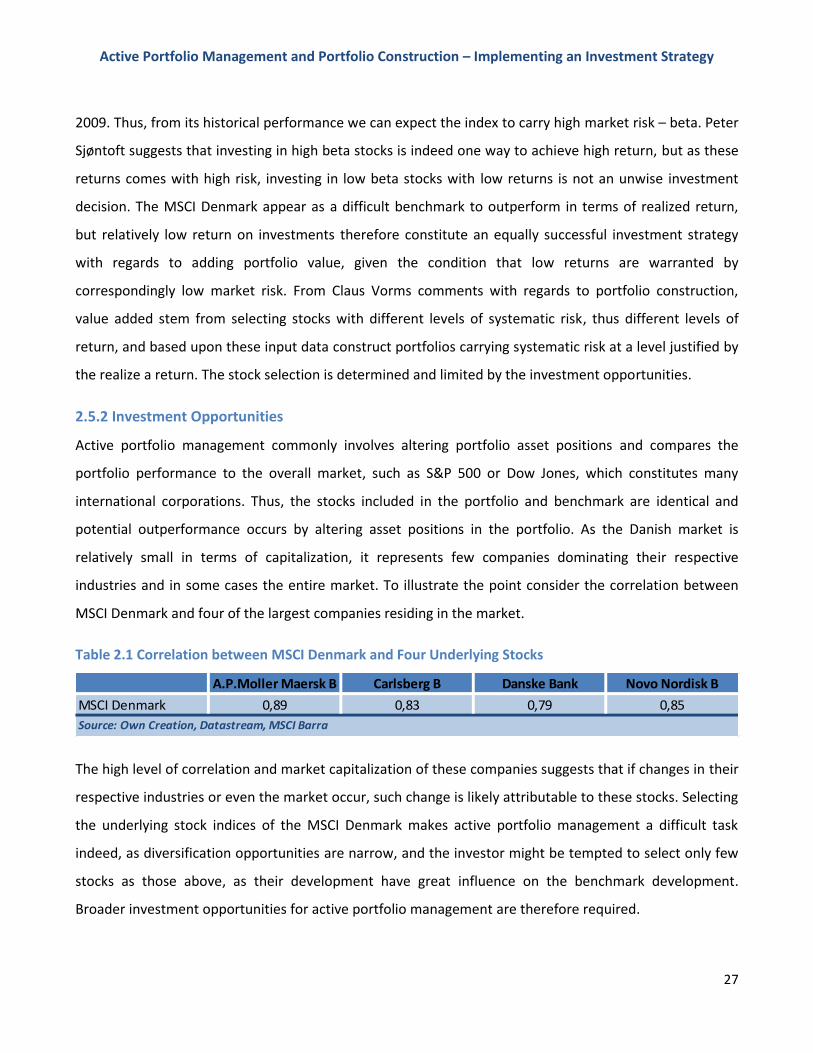
2.5.2 Investment Opportunities
Active portfolio management commonly involves altering portfolio asset positions and compares the
portfolio performance to the overall market, such as S&P 500 or Dow Jones, which constitutes many
international corporations. Thus, the stocks included in the portfolio and benchmark are identical and
potential outperformance occurs by altering asset positions in the portfolio. As the Danish market is
relatively small in terms of capitalization, it represents few companies dominating their respective
industries and in some cases the entire market. To illustrate the point consider the correlation between
MSCI Denmark and four of the largest companies residing in the market.
Table 2.1 Correlation between MSCI Denmark and Four Underlying Stocks
The high level of correlation and market capitalization of these companies suggests that if changes in their
respective industries or even the market occur, such change is likely attributable to these stocks. Selecting
the underlying stock indices of the MSCI Denmark makes active portfolio management a difficult task
indeed, as diversification opportunities are narrow, and the investor might be tempted to select only few
stocks as those above, as their development have great influence on the benchmark development.
Broader investment opportunities for active portfolio management are therefore required.
A.P.Moller Maersk B Carlsberg B Danske Bank Novo Nordisk B
MSCI Denmark 0,89 0,83 0,79 0,85
Source: Own Creation, Datastream, MSCI Barra
Active Portfolio Management and Portfolio Construction – Implementing an Investment Strategy
28
2.5.2.1 Seeking International Opportunities
A variation of different assets will provide the investor with a variability of return in the portfolio and
reduces its risk. In order to achieve portfolio optimization the investor must allocate different asset classes
to the portfolio. According to Litterman (2003), to find independency among assets, and hence reduce the
risk of the portfolio, the investor must consider different markets35. In addition, Markowitz (1959) claims
that in order to achieve optimization at an international level, it is important to consider different types of
sectors and industries36. Hence, the most beneficial way to allocate assets is to invest globally. Portfolio
optimization traditionally requires independency among a diversified selection of assets, thus allocating
assets in different types of sectors and industries seems beneficial to achieve optimization.
When considering an investment in common stock, investors tend to divide the vast universe of stocks
into categories based on general business lines and by industry within these business lines. One way of
dividing this universe of stocks gives classifications for industrial firms, financial institutions and other
industry sectors. An alternative classification scheme separates US and foreign common stocks. I have
avoided the latter division, because the industry breakdown is more useful when constructing the
portfolio of global common stocks. When stocks are sorted by industries rather than geography they
constitute a more comprehensive illustration of company-level performance. It is easier to identify which
stocks are performing better than others as they not only react to global macroeconomic events, but also
individual sectorial events. Therefore, return patterns are assumed to develop somewhat differently,
which enables the identification of diversification opportunities. With a global capital market the focus
should include all the companies in an industry viewed in a global setting. Extensive market integration
advocates for this decision as it has diminished the importance of the geographic location of major
companies, while their sectorial location is better characterized.
2.5.2.2 The Rise of Sector Importance
Obviously, the asset allocation process refers to the decision process of determining the amount of funds
that should be allocated to each financial asset in the existing opportunity set. It is the investor’s objective
to obtain the highest risk adjusted return as possible. Our interpretation from Brinson et. al (1986) showed
that the asset allocation decision is by far the most dominant factor of portfolio performance as it explain
35
Litterman (2003): p. 137 36
Markowitz (1959): p. 89
Active Portfolio Management and Portfolio Construction – Implementing an Investment Strategy
29
more than 91% of the variation in asset returns. Furthermore, Litterman (2003) suggestions that asset
allocation can be divided into two different types of decisions 1) asset allocation between different asset
classes, e.g. stocks and bonds and 2) asset allocation within one asset class, e.g. countries and sectors.
Hopkins and Miller (2001) analyzed these dimensions of global equity portfolios (countries, sectors,
industries and companies). Their analysis concluded that a significant shift seemed to have occurred in the
importance of global sectors and industries at the expense of geography in global investment strategies37.
Although this emphasis is likely to shift through time the reward for global sector allocation, as well as
organizing stock selection on a sectorial basis, seems to justify allocating resources to sector research.
Their tests further suggested that an industry group orientation, rather than a broader sector-level
orientation can add value to asset allocation research. However, in order to maintain track of an
affordable amount of data in addition to a global representation among the investment opportunities,
further investigation of subgroups below the sectorial level will not be considered in this thesis.
Considering the advice of broad diversification from Claus Vorm, this thesis seeks to allocate assets into a
portfolio, which represents a broad global market portfolio, which is solid and easy to measure. Each asset
represents a sector index which embodies a range of industries. As introduced in chapter 1 the further
analysis considers the Datastream World Indices with ten sub-indices, which have been chosen to
represent ten major industry sectors as introduced in chapter 1.5.
2.5.2.3 Market Integration
Only a few decades ago some national markets were considered difficult to gain access to, limiting
investment opportunities to only domestic markets. As globalization has integrated national economies,
companies, consumers and investors now trade across borders, which results in increasing correlation
between markets. Hence, systematic risk arises as economic development in some countries impact that
of others, which to some extend align their return patterns, as they are affected by the same
developments. However, based on historical performance MSCI Denmark stands out as having performed
remarkably better than other major indices. In terms of benchmark comparison, both advantages and
disadvantages for applying the MSCI Denmark as benchmark exist. Table 2.2 shows the correlation
between each sector index, Denmark and four major national economies.
37
Hopkins and Miller (2001): p. 1
Active Portfolio Management and Portfolio Construction – Implementing an Investment Strategy
30
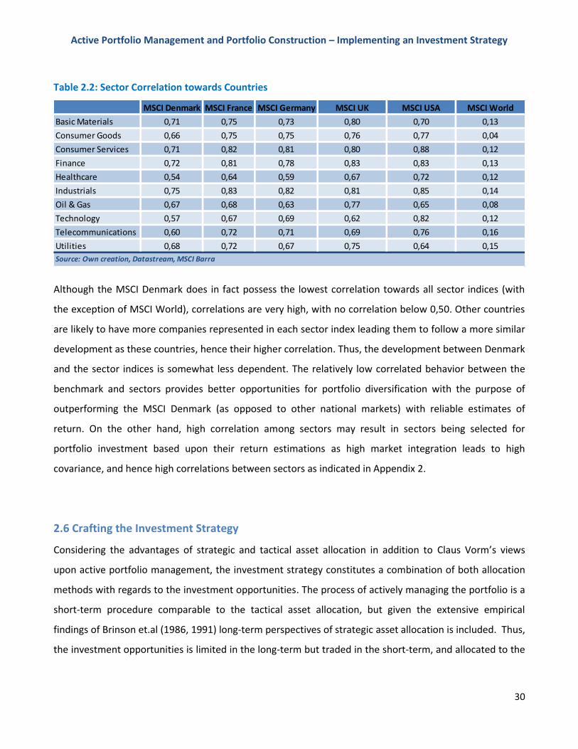
Table 2.2: Sector Correlation towards Countries
Although the MSCI Denmark does in fact possess the lowest correlation towards all sector indices (with
the exception of MSCI World), correlations are very high, with no correlation below 0,50. Other countries
are likely to have more companies represented in each sector index leading them to follow a more similar
development as these countries, hence their higher correlation. Thus, the development between Denmark
and the sector indices is somewhat less dependent. The relatively low correlated behavior between the
benchmark and sectors provides better opportunities for portfolio diversification with the purpose of
outperforming the MSCI Denmark (as opposed to other national markets) with reliable estimates of
return. On the other hand, high correlation among sectors may result in sectors being selected for
portfolio investment based upon their return estimations as high market integration leads to high
covariance, and hence high correlations between sectors as indicated in Appendix 2.
2.6 Crafting the Investment Strategy
Considering the advantages of strategic and tactical asset allocation in addition to Claus Vorm’s views
upon active portfolio management, the investment strategy constitutes a combination of both allocation
methods with regards to the investment opportunities. The process of actively managing the portfolio is a
short-term procedure comparable to the tactical asset allocation, but given the extensive empirical
findings of Brinson et.al (1986, 1991) long-term perspectives of strategic asset allocation is included. Thus,
the investment opportunities is limited in the long-term but traded in the short-term, and allocated to the
MSCI Denmark MSCI France MSCI Germany MSCI UK MSCI USA MSCI World
Basic Materials 0,71 0,75 0,73 0,80 0,70 0,13
Consumer Goods 0,66 0,75 0,75 0,76 0,77 0,04
Consumer Services 0,71 0,82 0,81 0,80 0,88 0,12
Finance 0,72 0,81 0,78 0,83 0,83 0,13
Healthcare 0,54 0,64 0,59 0,67 0,72 0,12
Industrials 0,75 0,83 0,82 0,81 0,85 0,14
Oil & Gas 0,67 0,68 0,63 0,77 0,65 0,08
Technology 0,57 0,67 0,69 0,62 0,82 0,12
Telecommunications 0,60 0,72 0,71 0,69 0,76 0,16
Utilities 0,68 0,72 0,67 0,75 0,64 0,15
Source: Own creation, Datastream, MSCI Barra
Active Portfolio Management and Portfolio Construction – Implementing an Investment Strategy
31
portfolio based upon their expected return and covariance with the other sectors. Figure 2.1 composes
the applied elements of the investment strategy.
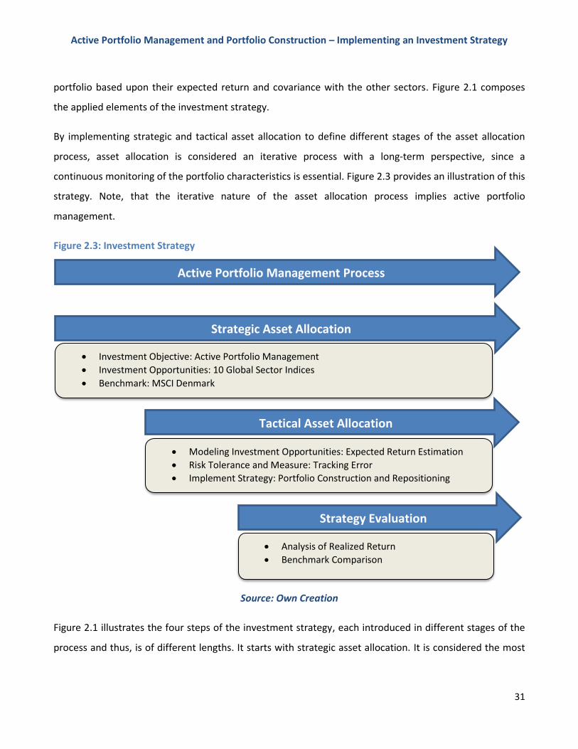
By implementing strategic and tactical asset allocation to define different stages of the asset allocation
process, asset allocation is considered an iterative process with a long-term perspective, since a
continuous monitoring of the portfolio characteristics is essential. Figure 2.3 provides an illustration of this
strategy. Note, that the iterative nature of the asset allocation process implies active portfolio
management.
Figure 2.3: Investment Strategy
Source: Own Creation
Figure 2.1 illustrates the four steps of the investment strategy, each introduced in different stages of the
process and thus, is of different lengths. It starts with strategic asset allocation. It is considered the most
Active Portfolio Management Process
Strategic Asset Allocation
Investment Objective: Active Portfolio Management
Investment Opportunities: 10 Global Sector Indices
Benchmark: MSCI Denmark
Tactical Asset Allocation
Modeling Investment Opportunities: Expected Return Estimation
Risk Tolerance and Measure: Tracking Error
Implement Strategy: Portfolio Construction and Repositioning
Strategy Evaluation
Analysis of Realized Return
Benchmark Comparison
Active Portfolio Management and Portfolio Construction – Implementing an Investment Strategy
32
important part of the success of the investment strategy. It defined the investment objective and the
investment opportunity set. Thus, strategic asset allocation is based on a long-term focus. Therefore, this
part of the strategy has a much lower frequency in terms of asset allocation.
The next step is the modeling of the investment opportunities. For frequent portfolio construction if the
investment opportunities do not comply with the investment objective, i.e. if they are expected to deliver
negative active return, they are excluded from the portfolio at that given time. In that manner, the new
information about the involvement of the prices of the different sectors compared to the benchmark is
incorporated in the optimization problem, i.e. the model parameters are updated and portfolio
repositioning is conducted under the constraints of the investors risk tolerance in addition to the absence
of short sale and financial gearing.
The final step involves the evaluation of the portfolio positions and analysis of its performance in
comparison to the benchmark. No alterations are made from this point as the mean-variance model
ensures no violation of the investment constraints and the portfolio construction is conducted with no
regards to the transaction costs, as they are deducted from the realized portfolio return.
Active Portfolio Management and Portfolio Construction – Implementing an Investment Strategy
33
2. Active Portfolio Management
In the context of this thesis, active portfolio management involves the dynamic nature of tactical asset
allocation which alters portfolio sector index positions of the investment universe in order to provide a
positive active return compared to benchmark investment. This chapter will provide a formal definition
of the concept and identify performance measurement, which serves the purpose of determining
whether active portfolio management has outperformed the benchmark.
3.1 Defining Active Portfolio Management
Active portfolio management means allocation of funds based on expectations of future market
developments. The strategy is performed against the MSCI Denmark as benchmark. This chapter
introduces the main concept of active portfolio management and its instruments. We begin with the
definition of active portfolio management:
Active portfolio management is the implementation of a dynamic investment strategy that over- and
underweights the predefined investment opportunities over a long-term basis, with the single objective of
outperforming the predefined benchmark at a predefined time in order to add value to the portfolio.
From this definition the importance of the benchmark for active portfolio management is evident. In
terms of risk and performance measures, the use of benchmarks is important in order to obtain clear
measurements in accordance with the investment strategy. In order to evaluate the performance of the
investment strategy we will establish appropriate performance measures which aim at capturing the
systematic risk adjusted return of the portfolio in comparison to that of the benchmark – the residual
return – and measure whether it in fact adds value to the investor.
Active Portfolio Management and Portfolio Construction – Implementing an Investment Strategy
34
3.2 Performance Measure and Portfolio Added Value
Several performance measures for portfolio evaluation exist, such as the Sharpe Ratio and Jensen’s Alpha,
and they are selected based on the purpose of portfolio management38. As portfolio performance in this
thesis must be considered relative to the benchmark a relative rather than an absolute performance
measure is required. Thus, we will employ a performance measure that captures the expected excess
return of the portfolio in comparison to the benchmark – the active return. The information ratio provides
such estimation39.
3.2.1 Information Ratio
We denote the active return as the difference between the portfolio returns and the benchmark return,
which is illustrated in the nominator of equation 3.1. The mean of the residual returns is usually called
alpha, and standard deviation the tracking error. The quotient of alpha divided by the tracking error is
called the information ratio:
)1.3()(
BP
BP
S
RRrationInformatio
Where RP is the portfolio return, RB is the benchmark return, thus the numerator is the portfolio active
return. SP-B is the tracking error, or the standard deviation of the residual return, measured as the squared
difference between portfolio and benchmark return. Estimates for each three components are provided in
chapter 4. According to Stotz (2005) with regards to the information ratio, the investment strategy
ultimately seeks to either maximize the expected return of the active portfolio or minimizing the tracking
error40. Since the portfolio is compared to the benchmark, active return determines the comparative
capital gains, while the tracking error indicates how well the portfolio tracks the benchmark. In other
words, active return determines whether the portfolio has outperformed the benchmark and the tracking
error determines whether the information ratio is significant.
38
http://www.investopedia.com/terms/s/sharperatio.asp#axzz2ED7A5ucy http://www.investopedia.com/terms/j/jensensmeasure.asp#axzz2ED7A5ucy 39
http://www.investopedia.com/terms/i/informationratio.asp#axzz24eZnzbHn 40
Stoltz (2005): p. 264
Active Portfolio Management and Portfolio Construction – Implementing an Investment Strategy
35
3.2.2 Portfolio Value Added
Obviously, successful execution of the investment strategy involves over- and underweighting of the
investment opportunities expected to perform well and poorly, respectively. The asset selecting approach
only identifies the forthcoming winners and losers. Correspondingly, as shot selling is not allowed, the
investor can allocate a proportion between 0% and 100% to a single asset. Hence, the amount of capital
allocated to each asset need not be sophisticated, as it could just as well be equally weighted. However, if
the mean of the active return of the portfolio is positive, the investor has actually beaten the benchmark,
and whether the outperformance is significant or not is reflected in the information ratio, which will be
investigated in chapter 6. Therefore, the information ratio should rather be seen as an indicator for the
manager’s skill than a performance measure.
I put the above statement in a more mathematical framework. Considering the information ratio in
equation 3.1 We let the return of the actively managed portfolio, tPR , , and the benchmark tBR , be defined
by the following models:
)2.3(10
1
,,,
n
i
tititP RR
)3.3(,,, titBtB RR
The investment universe consists of n=10 investment opportunities for the active portfolio and tiR ,
denotes the excess return of the i-th investment opportunity. ti , denotes the beta of asset i at time t,
and will be applied on a rolling basis rather than an overall average. Maintaining an average beta over the
period is misleading as the environments in which companies operate change, leading the market risk,
which they are exposed to change over time41. As the benchmark is treated as a single stock it only
consists of n=1 investment opportunity, and will therefore not be submitted to reweighting at any time.
Furthermore, I will impose one constraint:
10
1
, 1n
i
tip leaving the investor the opportunity to invest
in the optimal tangent portfolio or hold cash42. Given the relatively small size of the MSCI Denmark in
41
I will explain the basis for this application thoroughly in chapter 5 42
Borsen interview at time 8:45: http://borsen.dk/nyheder/investor/artikel/1/246033/aktiv_kapitalforvaltning_for_de_tunge_investorer.html
Active Portfolio Management and Portfolio Construction – Implementing an Investment Strategy
36
terms of capitalization, it is neither broad nor representative and hence is not characterized as a market,
as it carries market risk, as well as the sector indices, relative to the global stock market. In addition, the
benchmark does not represent the investment opportunities, meaning they are not indices underlying the
MSCI Denmark, but in fact larger in terms of capitalization, and have developed somewhat
interdependently with regards to the benchmark. Nevertheless, the investor should still have the
opportunity to invest globally within the limits of the investment strategy and opportunity set in order to
provide opportunities for diversification. Hence, the benchmark beta does not represent a weighted
average of the sector’s beta.
We compare active beta and active return as two separate factors in order to measure value added.
Holding high beta investment should only add value to the investor if the return is correspondingly high an
vice versa.
)4.3(*,,
e
ttBtPt Ra
The mechanics of active portfolio management is seen from equation 3.4. It represents a cornerstone for
measuring value added, or residual return, and tracks any value added by active portfolio management.
For the case of a non-negative active return, e
tR ≥0, the exposure of the investor should at least be as big
as the exposure of the portfolio, tBtP ,, in order for active portfolio management to add value on
average. Accordingly, for the case e
tR ≤0, in order to obtain value added tBtP ,, so a positive alpha is
maintained. Thus, the beta adjustments to the excess active return tracks any value added from active
investing. Hence, if a positive alpha is maintained active investing has added value to the investment.
These equations show that security selection and market timing are the same, because in both cases the
investor controls tP, in order to add value to the portfolio.
The beta portfolio is constrained in order to limit the amount of risk the investor can take upon his
investments. Investing in high beta stocks is likely to generate high returns, but its risk deteriorates the
investment value for the investor as well. Pursuing high beta investments, such as the benchmark is a risky
way to generate high returns. Therefore, the crucial point for successful security selection and market
Active Portfolio Management and Portfolio Construction – Implementing an Investment Strategy
37
timing is the correct prediction of the active return, tR , hence estimates for expected return for the
portfolio and the benchmark.
Note from equation 3.3 that the correct prediction of security return is not the only source of alpha. It was
previously argued that the significance of the outperformance of an investment strategy is reflected by
the information ratio. By now we have shown that the information ratio can be increased by better
predictions of security prices, tR . Obviously, the information ratio may also be increased by variances in
residual return, provided that the mean residual return remains the same. Minimizing the residual risk
hence, becomes important as well for maximizing the information ratio.
Treynor and Black (1973), describes systematic active portfolio management approach, coupling the
identification of alpha, and risk management43. Traditional portfolio theory does not distinguish between
active portfolio management and optimal portfolio construction. This thesis will not attempt to fill this
gap, meaning portfolio construction is conducted with the sole purpose of outperforming the benchmark
on a risk adjusted basis. Whether, a deviation from the investment strategy could in some way have
provided the investor with higher residual return than realized remains hypothetical and will not be
investigated. However, what all active portfolio strategies have in common is that outperformance has to
be gained through altering investment positions, which is emphasized in the definition above.
This chapter provided a review of the framework of active portfolio management. The important
takeaway for the pending analysis is the need for expected return estimations and measures for risk. We
will then have the necessary input to conduct portfolio construction.
43
Treynor, Black (1973): p. 69
Active Portfolio Management and Portfolio Construction – Implementing an Investment Strategy
38
4. Risk and Return in Active Portfolio Management
In accordance with the information ratio as the performance measurement of active portfolio
management, emphasis is required on active risk and return. This chapter establishes valid estimates for
expected return and risk measures appropriate for portfolio construction. The investment strategy
requires estimates every time the portfolio is to be reweighted. An exposition of the capital Asset
Pricing Model (CAPM) will provide such estimates. Furthermore, we investigate the risk factors the
investment is exposed to in order to determine risk warranting the return.
4.1 Expected Return in Active Portfolio Management
Based on the assumptions of Markowitz portfolio theory Sharpe (1964), have derived the Capital Asset
Pricing Model (CAPM)44. The importance and relevance to this thesis of the CAPM model is derived from
its terminology, i.e. its use of the Greek letters ɑ and β, which is widely used in the context of portfolio
management today.
The CAPM seems to be an attractive approach to the active portfolio management. It has, however,
received extensive criticism, particularly from Farma and French (2004), arguing against its empirical
foundation implying that most implications of the model are invalid45. Nevertheless, I will in this chapter
set up the CAPM model.
4.1.1 Asset Pricing in an Active Setting
The CAPM model plays an important role when selecting portfolios according to mean-variance
optimization. When using the CAPM forecasts of expected return to construct optimal mean-variance
portfolios, those portfolios will consist simply of positions in the market and the risk free asset. In other
words, optimal portfolios constructed under mean-variance optimization will differ from the market
portfolio and cash if the forecasted excess return differ from the CAPM excess return. As we adopt tactical
asset allocation I add components to the asset pricing model. Thus, the expected return, in this thesis is
built on five factors: the risk free interest rate, the sector specific risk adjustment, the market risk
44
Sharpe (1964): p. 436 45
Farma (2004): p. 26
Active Portfolio Management and Portfolio Construction – Implementing an Investment Strategy
39
premium, a premium for exceptional market return, and an expected residual return. Note, the residual
return is, ai, is a constant.
From these four factors the CAPM in active portfolio management takes the following form:
)1.4(R* ,,
e
tM,,,,,, tititftMtitfti aRRRRE
Here, E(Ri,t) is the expected return of asset i. Rf is the risk free rate, βi,t is the systematic risk of sector i, RM
is the market return. Exceptional market return, ti,
e
tB,R and the expected residual return, ai,t extend
the traditional CAPM model for the investment opportunities only. As the purpose of active portfolio
management is to obtain the highest portfolio residual return possible, the portfolio should not only be
maximized with regards to its own standard deviation, but also with regards to the risk adjusted return of
the benchmark, in order to improve the information ratio. Therefore premiums for selecting the
investment opportunities over the market and benchmark are warranted.
4.1.1.1 The Risk Free Interest Rate
To estimate the risk free rate, Rf, I consider two Danish government default-free bonds. Obviously, no
bonds are default free. However, the selection of the Danish default- free bond is based upon the obvious
reason that the investor is assumed to be Danish and since these bonds are considered safe investments46.
The 10 year government default-free bond rate is commonly used, particularly in valuations as the
maturity of the bond, the market and the forecasting period will be close to each other. Figure 4.1
illustrates the 5 year Danish government bond rate against the 10 year Danish default-free bond rate.
46 http://www.jyskebank.dk/wps/portal/jfo/finansnyt/struktureredeprodukter/danmark2015
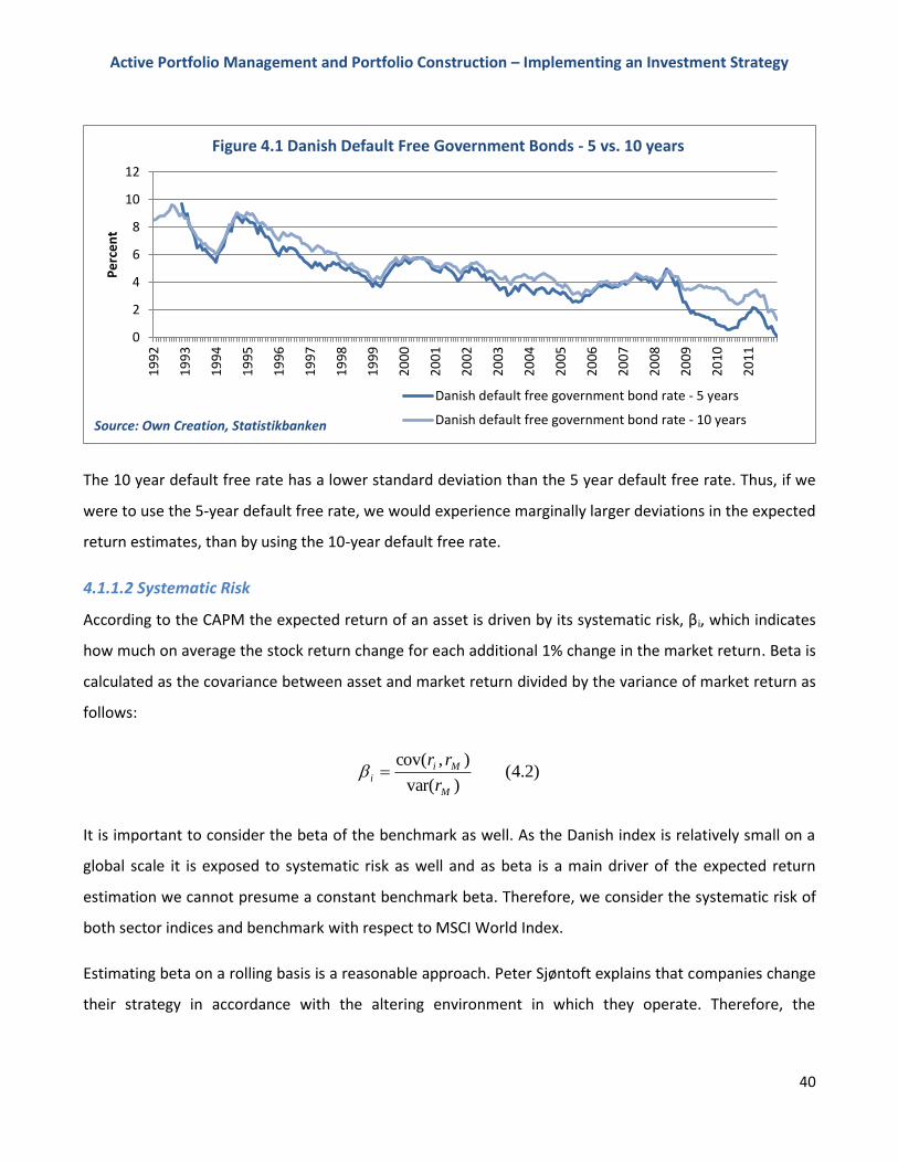
Active Portfolio Management and Portfolio Construction – Implementing an Investment Strategy
40
The 10 year default free rate has a lower standard deviation than the 5 year default free rate. Thus, if we
were to use the 5-year default free rate, we would experience marginally larger deviations in the expected
return estimates, than by using the 10-year default free rate.
4.1.1.2 Systematic Risk
According to the CAPM the expected return of an asset is driven by its systematic risk, βi, which indicates
how much on average the stock return change for each additional 1% change in the market return. Beta is
calculated as the covariance between asset and market return divided by the variance of market return as
follows:
)2.4()var(
),cov(
M
Mi
ir
rr
It is important to consider the beta of the benchmark as well. As the Danish index is relatively small on a
global scale it is exposed to systematic risk as well and as beta is a main driver of the expected return
estimation we cannot presume a constant benchmark beta. Therefore, we consider the systematic risk of
both sector indices and benchmark with respect to MSCI World Index.
Estimating beta on a rolling basis is a reasonable approach. Peter Sjøntoft explains that companies change
their strategy in accordance with the altering environment in which they operate. Therefore, the
0
2
4
6
8
10
12
19
92
19
93
19
94
19
95
19
96
19
97
19
98
19
99
20
00
20
01
20
02
20
03
20
04
20
05
20
06
20
07
20
08
20
09
20
10
20
11
Pe
rce
nt
Figure 4.1 Danish Default Free Government Bonds - 5 vs. 10 years
Danish default free government bond rate - 5 years
Danish default free government bond rate - 10 yearsSource: Own Creation, Statistikbanken
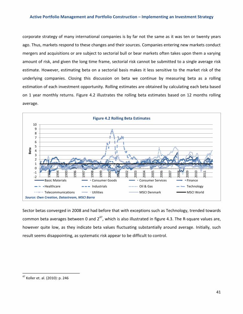
Active Portfolio Management and Portfolio Construction – Implementing an Investment Strategy
41
corporate strategy of many international companies is by far not the same as it was ten or twenty years
ago. Thus, markets respond to these changes and their sources. Companies entering new markets conduct
mergers and acquisitions or are subject to sectorial bull or bear markets often takes upon them a varying
amount of risk, and given the long time frame, sectorial risk cannot be submitted to a single average risk
estimate. However, estimating beta on a sectorial basis makes it less sensitive to the market risk of the
underlying companies. Closing this discussion on beta we continue by measuring beta as a rolling
estimation of each investment opportunity. Rolling estimates are obtained by calculating each beta based
on 1 year monthly returns. Figure 4.2 illustrates the rolling beta estimates based on 12 months rolling
average.
Sector betas converged in 2008 and had before that with exceptions such as Technology, trended towards
common beta averages between 0 and 247, which is also illustrated in figure 4.3. The R-square values are,
however quite low, as they indicate beta values fluctuating substantially around average. Initially, such
result seems disappointing, as systematic risk appear to be difficult to control.
47
Koller et. al. (2010): p. 246
-2-10123456789
10
19
93
19
94
19
95
19
96
19
97
19
98
19
99
20
00
20
01
20
02
20
03
20
04
20
05
20
06
20
07
20
08
20
09
20
10
20
11
Be
ta
Figure 4.2 Rolling Beta Estimates
Basic Materials Consumer Goods Consumer Services Finance
Healthcare Industrials Oil & Gas Technology
Telecommunications Utilities MSCI Denmark MSCI World
Source: Own Creation, Datastream, MSCI Barra
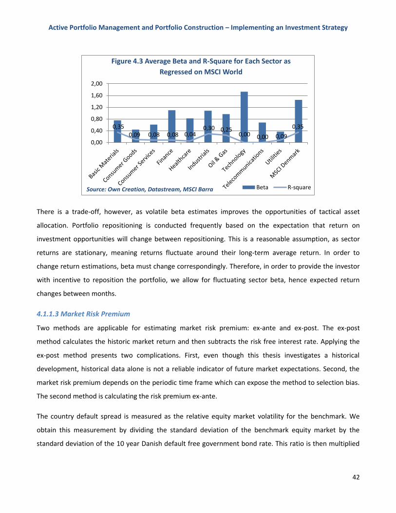
Active Portfolio Management and Portfolio Construction – Implementing an Investment Strategy
42
There is a trade-off, however, as volatile beta estimates improves the opportunities of tactical asset
allocation. Portfolio repositioning is conducted frequently based on the expectation that return on
investment opportunities will change between repositioning. This is a reasonable assumption, as sector
returns are stationary, meaning returns fluctuate around their long-term average return. In order to
change return estimations, beta must change correspondingly. Therefore, in order to provide the investor
with incentive to reposition the portfolio, we allow for fluctuating sector beta, hence expected return
changes between months.
4.1.1.3 Market Risk Premium
Two methods are applicable for estimating market risk premium: ex-ante and ex-post. The ex-post
method calculates the historic market return and then subtracts the risk free interest rate. Applying the
ex-post method presents two complications. First, even though this thesis investigates a historical
development, historical data alone is not a reliable indicator of future market expectations. Second, the
market risk premium depends on the periodic time frame which can expose the method to selection bias.
The second method is calculating the risk premium ex-ante.
The country default spread is measured as the relative equity market volatility for the benchmark. We
obtain this measurement by dividing the standard deviation of the benchmark equity market by the
standard deviation of the 10 year Danish default free government bond rate. This ratio is then multiplied
0,35
0,09 0,08 0,08 0,040,30 0,25
0,00 0,00 0,09
0,35
0,00
0,40
0,80
1,20
1,60
2,00
Figure 4.3 Average Beta and R-Square for Each Sector as
Regressed on MSCI World
Beta R-squareSource: Own Creation, Datastream, MSCI Barra
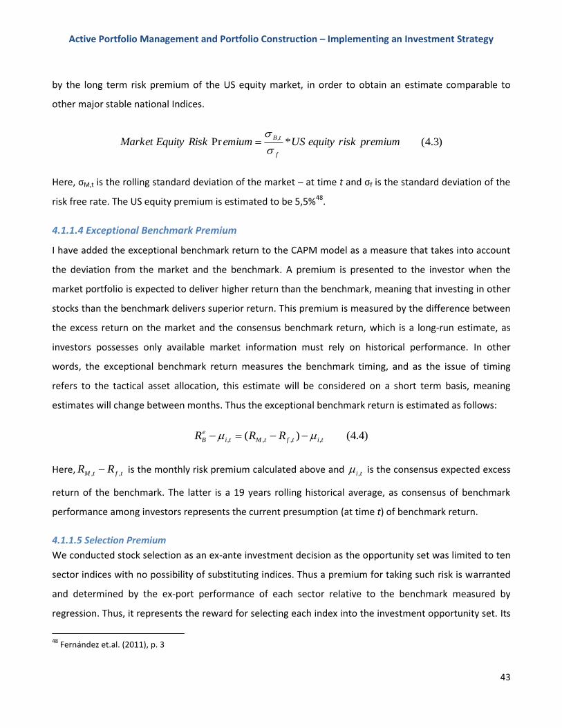
Active Portfolio Management and Portfolio Construction – Implementing an Investment Strategy
43
by the long term risk premium of the US equity market, in order to obtain an estimate comparable to
other major stable national Indices.
)3.4(*Pr,
premiumriskequityUSemiumRiskEquityMarketf
tB
Here, σM,t is the rolling standard deviation of the market – at time t and σf is the standard deviation of the
risk free rate. The US equity premium is estimated to be 5,5%48.
4.1.1.4 Exceptional Benchmark Premium
I have added the exceptional benchmark return to the CAPM model as a measure that takes into account
the deviation from the market and the benchmark. A premium is presented to the investor when the
market portfolio is expected to deliver higher return than the benchmark, meaning that investing in other
stocks than the benchmark delivers superior return. This premium is measured by the difference between
the excess return on the market and the consensus benchmark return, which is a long-run estimate, as
investors possesses only available market information must rely on historical performance. In other
words, the exceptional benchmark return measures the benchmark timing, and as the issue of timing
refers to the tactical asset allocation, this estimate will be considered on a short term basis, meaning
estimates will change between months. Thus the exceptional benchmark return is estimated as follows:
)4.4()( ,,,, titftMti
e
B RRR
Here, tftM RR ,, is the monthly risk premium calculated above and ti , is the consensus expected excess
return of the benchmark. The latter is a 19 years rolling historical average, as consensus of benchmark
performance among investors represents the current presumption (at time t) of benchmark return.
4.1.1.5 Selection Premium
We conducted stock selection as an ex-ante investment decision as the opportunity set was limited to ten
sector indices with no possibility of substituting indices. Thus a premium for taking such risk is warranted
and determined by the ex-port performance of each sector relative to the benchmark measured by
regression. Thus, it represents the reward for selecting each index into the investment opportunity set. Its
48
Fernández et.al. (2011), p. 3
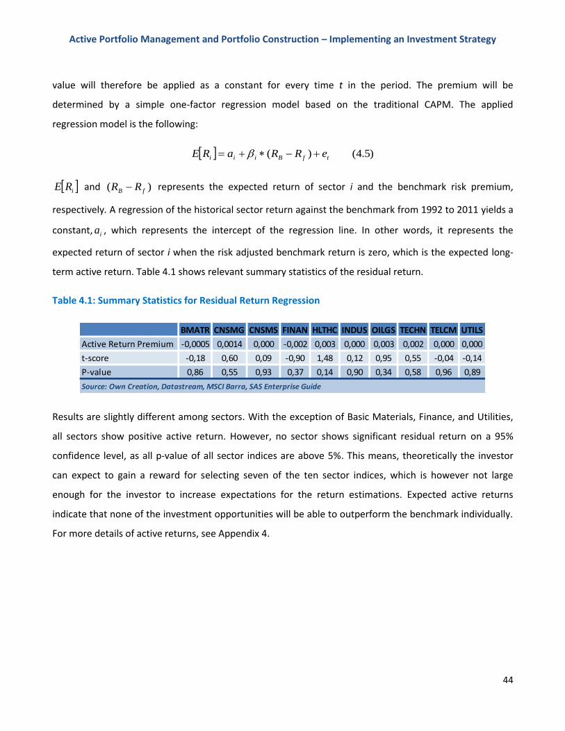
Active Portfolio Management and Portfolio Construction – Implementing an Investment Strategy
44
value will therefore be applied as a constant for every time t in the period. The premium will be
determined by a simple one-factor regression model based on the traditional CAPM. The applied
regression model is the following:
)5.4()( tfBiii eRRaRE
iRE and )( fB RR represents the expected return of sector i and the benchmark risk premium,
respectively. A regression of the historical sector return against the benchmark from 1992 to 2011 yields a
constant, ia , which represents the intercept of the regression line. In other words, it represents the
expected return of sector i when the risk adjusted benchmark return is zero, which is the expected long-
term active return. Table 4.1 shows relevant summary statistics of the residual return.
Table 4.1: Summary Statistics for Residual Return Regression
Results are slightly different among sectors. With the exception of Basic Materials, Finance, and Utilities,
all sectors show positive active return. However, no sector shows significant residual return on a 95%
confidence level, as all p-value of all sector indices are above 5%. This means, theoretically the investor
can expect to gain a reward for selecting seven of the ten sector indices, which is however not large
enough for the investor to increase expectations for the return estimations. Expected active returns
indicate that none of the investment opportunities will be able to outperform the benchmark individually.
For more details of active returns, see Appendix 4.
BMATR CNSMG CNSMS FINAN HLTHC INDUS OILGS TECHN TELCM UTILS
Active Return Premium -0,0005 0,0014 0,000 -0,002 0,003 0,000 0,003 0,002 0,000 0,000
t-score -0,18 0,60 0,09 -0,90 1,48 0,12 0,95 0,55 -0,04 -0,14
P-value 0,86 0,55 0,93 0,37 0,14 0,90 0,34 0,58 0,96 0,89
Source: Own Creation, Datastream, MSCI Barra, SAS Enterprise Guide
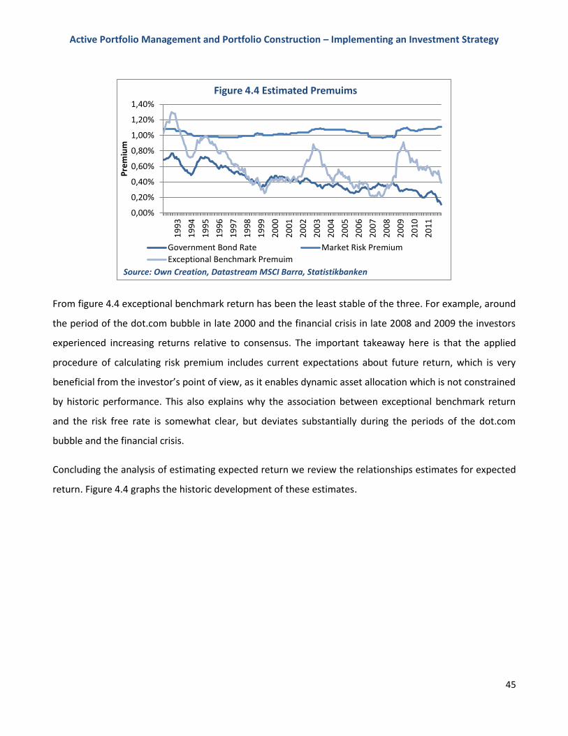
Active Portfolio Management and Portfolio Construction – Implementing an Investment Strategy
45
From figure 4.4 exceptional benchmark return has been the least stable of the three. For example, around
the period of the dot.com bubble in late 2000 and the financial crisis in late 2008 and 2009 the investors
experienced increasing returns relative to consensus. The important takeaway here is that the applied
procedure of calculating risk premium includes current expectations about future return, which is very
beneficial from the investor’s point of view, as it enables dynamic asset allocation which is not constrained
by historic performance. This also explains why the association between exceptional benchmark return
and the risk free rate is somewhat clear, but deviates substantially during the periods of the dot.com
bubble and the financial crisis.
Concluding the analysis of estimating expected return we review the relationships estimates for expected
return. Figure 4.4 graphs the historic development of these estimates.
0,00%
0,20%
0,40%
0,60%
0,80%
1,00%
1,20%
1,40%
19
93
19
94
19
95
19
96
19
97
19
98
19
99
20
00
20
01
20
02
20
03
20
04
20
05
20
06
20
07
20
08
20
09
20
10
20
11
Pre
miu
m
Figure 4.4 Estimated Premuims
Government Bond Rate Market Risk Premium
Exceptional Benchmark Premuim
Source: Own Creation, Datastream MSCI Barra, Statistikbanken
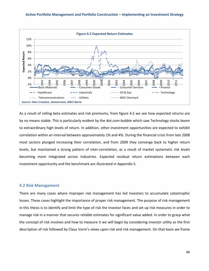
Active Portfolio Management and Portfolio Construction – Implementing an Investment Strategy
46
As a result of rolling beta estimates and risk premiums, from figure 4.5 we see how expected returns are
by no means stable. This is particularly evident by the dot.com-bubble which saw Technology stocks boom
to extraordinary high levels of return. In addition, other investment opportunities are expected to exhibit
correlation within an interval between approximately 1% and 4%. During the financial crisis from late 2008
most sectors plunged increasing their correlation, and from 2009 they converge back to higher return
levels, but maintained a strong pattern of inter-correlation, as a result of market systematic risk levels
becoming more integrated across industries. Expected residual return estimations between each
investment opportunity and the benchmark are illustrated in Appendix 5.
4.2 Risk Management
There are many cases where improper risk management has led investors to accumulate catastrophic
losses. These cases highlight the importance of proper risk management. The purpose of risk management
in this thesis is to identify and limit the type of risk the investor faces and set up risk measures in order to
manage risk in a manner that secures reliable estimates for significant value added. In order to grasp what
the concept of risk involves and how to measure it we will begin by considering investor utility as the first
description of risk followed by Claus Vorm’s views upon risk and risk management. On that basis we frame
-2%
0%
2%
4%
6%
8%
10%
12%1
99
3
19
94
19
95
19
96
19
97
19
98
19
99
20
00
20
01
20
02
20
03
20
04
20
05
20
06
20
07
20
08
20
09
20
10
20
11
Exp
ect
ed
Re
turn
Figure 4.5 Expected Return Estimates
Basic Materials Consumer Goods Consumer Services Finance
Healthcare Industrials Oil & Gas Technology
Telecommunications Utilities MSCI Denmark
Source: Own Creation, Datastream, MSCI Barra
Active Portfolio Management and Portfolio Construction – Implementing an Investment Strategy
47
a definition of risk in order to limit the types of risk factors the portfolio is exposed to, ultimately leading
to identifying a measurement for the tracking error.
4.2.1 Investor Utility
The first systematic description of risk for financial problems is risk aversion, and I will now give a brief
description of how investor’s utility is treated. A variety of different perspectives upon risk resides among
investors and hence their levels of utility differ.
One of the major subjects of investigation is the relationship between risk and return. In contrast to usual
utility evaluation, where individuals choose between two positive goods, in this case I consider return as a
positive good while treating risk as a negative good as increase in the former increases the information
ratio while increases in the latter decreases it. However, risk and return often comes hand in hand. Theory
generalizes three different types of investors by their risk appetite: risk averse, risk seeking, and risk
loving. The difference between investor types is their demand for compensation for taking on new risk.
This rationale is commonly used in practice and is determined to be the general motive for the difference
in investor’s preference when choosing stocks over e.g. bonds.
On the basis of these considerations that the investor regards risk and return as being a negative and
positive good, respectively, diversification is required as a means for risk management. By spreading the
investment into several investment opportunities the investor should be able to claim a higher risk
adjusted return than any of the assets alone. Accordingly, diversification implies that the compensation
for having risk is increased. Thus, there is a positive relationship between portfolio sectors and their
associated return. Markowitz established the mean-variance approach in portfolio context on the basis of
this relationship. We will ensure diversification with regards to portfolio construction with the objective
for the investor to be compensated for any additional risk taken. We will therefore impose a constraint of
maximum 20% portfolio weight to each sector index upon portfolio reweighting (Portfolio construction
without such constraint will also be conducted). Chapter 5 will discuss the details of this constraint.
4.2.2 Professional Views upon Risk and Risk Management
Claus Vorm explained that a vast variety of risk exists, which the investor is exposed to and which
dependents upon the investment objective. Thus, he acknowledges that risk is based on a point of view, as
Active Portfolio Management and Portfolio Construction – Implementing an Investment Strategy
48
is it dependent upon investor perception and the investment mandate the manager is given (being the
investor himself or a professional manager). In that sense, proper risk management involves conducting
investments submitted the constraints and risk preference of the investor. Thus, realized risk is obviously
determined ex-ante and must not be higher than the risk permitted by the mandate.
Accordingly, in terms of measuring risk, measurements again depend upon the investor’s presumption of
risk. Claus Vorm explained the variations of investor’s preference. Whether risk is measured as tracking
error, beta or absolute risk is a question of investment objectives. In terms of active portfolio
management the investor chooses an exposure to stocks and allows for a pre-defined tracking error. In
order to control the tracking error, risk can also be controlled in an absolute sense, by setting specific
boundaries in terms of short fall or volatility. However, actively managed portfolios have proven to deliver
better performance with flexible investment mandates49, meaning providing the investor (or portfolio
manager) with no specific investment constraints with regards to choosing risky investments over less
risky investments. The long investment horizon allows for a flexible mandate as the investor has
substantial opportunities for compensate potential losses incurred by potential gains from investments.
4.2.3 Risk Management and Risk Factors
From the discussion above we conclude there is no universal definition of risk and neither is there any one
generally accepted definition of risk in specific environments. However, it is a common presumption
among investors to link risk with uncertainty. In addition the definition of risk must allow for reasonable
measurements. Therefore, for the purpose of active portfolio management we define risk as follows:
Risk is the exposure to some uncertain future events.
Only an event that has a dependency on the portfolio may influence its risk. In many cases of risk
management, probabilities of possible future events are estimated. We do not presume to know these
probabilities as the referred events may not even be known. We will therefore apply an ex-ante measure
for the tracking error with regards to portfolio optimization, and evaluates portfolio performance by
means of an ex-post measure. The focus in this chapter will be on the ex-post measure, and the ex-ante
tracking error will be highlighted with regards to portfolio optimization in chapter 5.
49
http://www.ft.com/intl/cms/s/0/4657d420-1f0f-11d9-9015-00000e2511c8.html#axzz2B4mrBLDb
Active Portfolio Management and Portfolio Construction – Implementing an Investment Strategy
49
We will refer to ex-post risk management from Claus Vorms statements above. He suggests that risk can
be limited to one or a few measurements, and in that regard we consider risk factors relevant to adding
portfolio value. Based on the fact that the investment universe is limited to stocks, we consider only the
risk within the area of investments. In order to model asset risk, for simplicity, we consider two risk factors
also included in value added:
Systematic risk
Active sector risk to the benchmark.
As a consequence of estimating the tracking error ex-post, the systematic risk is the only risk factor the
investor is able to control. Restricting the portfolio beta to 1, tP provides the option to move from a
portfolio that is fully invested in equities to one that incorporates a proportion of risk equivalent to
holding cash. In a declining market, for example, cash provides a safe haven helping the investor to ride
out a down turn while positioning the portfolio to take advantage of opportunities as they arise. In down
markets high proportions of cash level risk can help the investor to produce milder declines and lower
volatility than the benchmark. In a strong positive market the investor can revert to a more fully invested
portfolio, which will help keep pace and potentially outperform as the benchmark rises.
Estimating the tracking error ex-ante proscribes controlling realized portfolio return deviation from the
benchmark. However, as outlined in chapter 1 the investment opportunities and the benchmark have
shown quite high correlations, and we can therefore expect somewhat similar return development
between the investment opportunities. When returns between investment opportunities and the
benchmark appear to have deviated, the tracking error increases.
4.2.4 Financial Risk
The risk measure with regards to the risk factors and utility seeks to increase risk adjusted return by
diversification. However, we still need a tangible measurement relevant for the investor which
incorporates the risk factors, market risk and idiosyncratic benchmark risk, in order to conduct specific ex-
post estimation of the tracking error. Additionally, it is relevant to adopt a procedure for risk estimation
that reflects the active holding of the investment opportunities. As the portfolio is actively managed, the
investor seeks to acquire residual return and hence also takes active risk upon his investments.
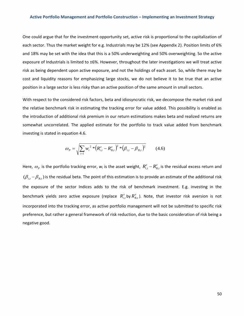
Active Portfolio Management and Portfolio Construction – Implementing an Investment Strategy
50
One could argue that for the investment opportunity set, active risk is proportional to the capitalization of
each sector. Thus the market weight for e.g. Industrials may be 12% (see Appendix 2). Position limits of 6%
and 18% may be set with the idea that this is a 50% underweighting and 50% overweighting. So the active
exposure of Industrials is limited to ±6%. However, throughout the later investigations we will treat active
risk as being dependent upon active exposure, and not the holdings of each asset. So, while there may be
cost and liquidity reasons for emphasizing large stocks, we do not believe it to be true that an active
position in a large sector is less risky than an active position of the same amount in small sectors.
With respect to the considered risk factors, beta and idiosyncratic risk, we decompose the market risk and
the relative benchmark risk in estimating the tracking error for value added. This possibility is enabled as
the introduction of additional risk premium in our return estimations makes beta and realized returns are
somewhat uncorrelated. The applied estimate for the portfolio to track value added from benchmark
investing is stated in equation 4.6.
)6.4(**1
2
,,
2
,,
2
i
tBti
e
tB
e
tiiP RRw
Here, P is the portfolio tracking error, wi is the asset weight, e
tB
e
ti RR ,, is the residual excess return and
)( ,, tBti is the residual beta. The point of this estimation is to provide an estimate of the additional risk
the exposure of the sector Indices adds to the risk of benchmark investment. E.g. investing in the
benchmark yields zero active exposure (replace e
tiR , bye
tBR , ). Note, that investor risk aversion is not
incorporated into the tracking error, as active portfolio management will not be submitted to specific risk
preference, but rather a general framework of risk reduction, due to the basic consideration of risk being a
negative good.
Active Portfolio Management and Portfolio Construction – Implementing an Investment Strategy
51
5. Portfolio Construction Implementing the investment strategy involves portfolio construction and repositioning. This chapter
constitutes the final steps of active portfolio management which enables evaluation of portfolio
performance. The primary focus of portfolio construction concerns the process of determining the
amount of funds allocated to each investment opportunity and that process relies on the applied
portfolio model. The process of repositioning simply comprises the timing of when the model conducts
asset allocation as a repetitive exercise.
5.1 Objective of Portfolio Construction
The objective of portfolio construction is to combine the investment opportunities into portfolios which
provide the investor with positive active return compared to investing in one sector index alone. This is
essential in the context of every portfolio management strategy. Therefore, any sector index estimated to
provide such return at any point of portfolio reweighting should be given a correspondingly large portfolio
weight. Markowitz’ mean-variance portfolio model conducts portfolio composition on such basis. As the
model conducts asset distribution based upon maximization processes of performance measures, it fits
the purpose of active portfolio management, since the information ratio constitutes the performance
indicator of active portfolio management.
5.2 Choice of Portfolio Model
Markowitz (1952) derived mean-variance portfolio theory stating that rational investors should either
maximize expected return for a given level of risk or minimize risk for a given level of return. He
additionally emphasized the importance of the investor to observe the movements among the assets – the
covariance. By constructing a portfolio of assets the investor can generate higher expected return at the
same level of risk as the portfolio not considering the covariance of portfolio assets50. This framework
allows for comparing different portfolios on a risk-return basis, and indicates how to choose the fraction
invested in each asset of the portfolio, so each asset best suits the investor’s risk-return expectations.
50
Markowitz (1952): p. 80
Active Portfolio Management and Portfolio Construction – Implementing an Investment Strategy
52
The mean-variance portfolio model is selected based upon its compatibility with both strategic and tactical
allocation. The classical approach to modern portfolio theory was developed by Harry Markowitz with his
article “Portfolio Selection” in 195251. Subsequent to its development, the model has received criticism,
particularly from Black and Litterman (1992), who introduced the BL-model, with the intention to improve
the deficiencies of Markowitz model52. We apply Markowitz mean-variance model based upon two crucial
criteria.
First, the BL-model presumes to know the investors personal risk preference and conducts asset allocation
in accordance with the market capitalization of the investment opportunities 53. The investor’s risk
preference is considered in this thesis but not specified into a utility function, as the conclusions from
chapter 4 indicated only that diversification is preferred by the investor. In addition, we do not consider
the risk of active holdings dependent on the size of the stocks, but rather the size of the exposure of the
active holdings. Second, the BL-model assumes the investment opportunities of active portfolio
management are underlying indices of the benchmark and that investor utility depends on the active
position and of each portfolio asset54. This is simply not the case in this thesis, as the underlying stocks of
the benchmark and the investment opportunities are two different groups of stocks. The advantage of the
mean-variance model is by treating the benchmark as a single stock, the model conducts tactical asset
allocation based upon optimization of the information ratio by. In other words, based on the return and
covariance estimates, the mean variance model selects stocks from the investment opportunities, on the
basis on the expectation that these opportunities can outperform the benchmark.
5.3 Mean-Variance Application in an Active Setting
In extension to the above, first systematic treatment of the portfolio selection problem is attributed to
Markowitz (1952). It is a popular financial optimization model, although its deficiencies are widely
documented and lacks important properties which are encountered in real-world investment processes.
51
Markowitz (1952): p. 77 52
Litterman (2003): p.76 53
Benninga (2008): p. 357 54
Da Silva et.al. (2009): p. 3-4
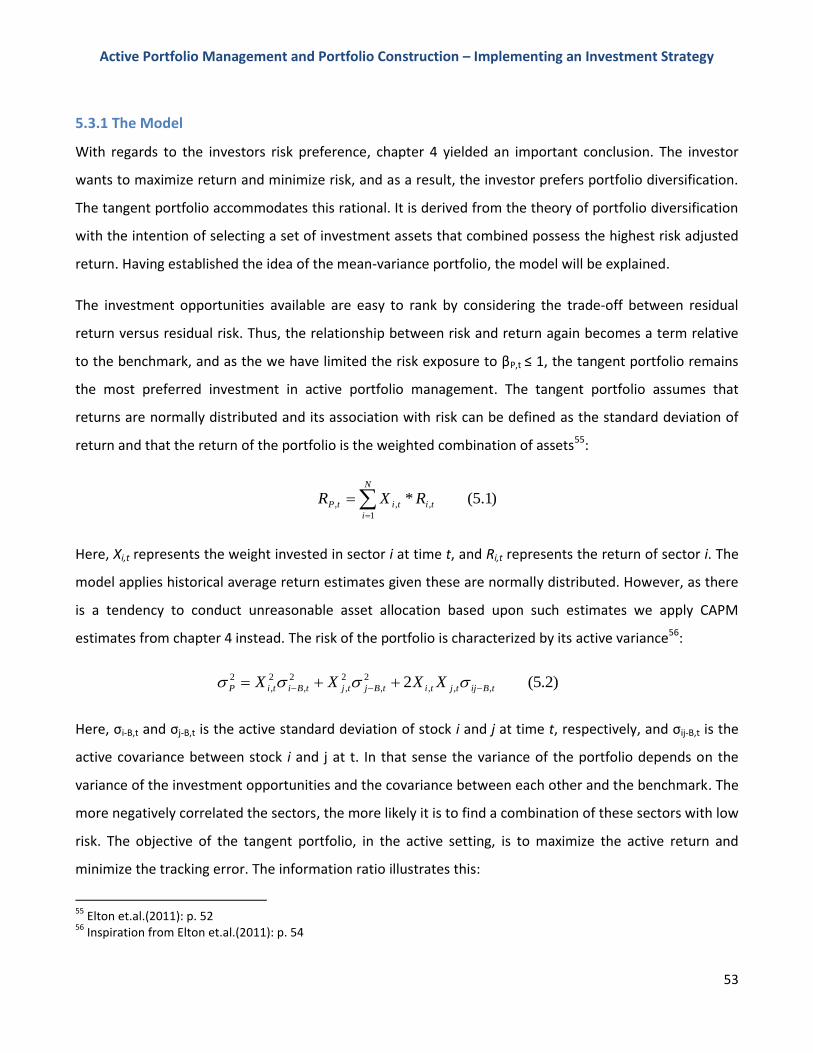
Active Portfolio Management and Portfolio Construction – Implementing an Investment Strategy
53
5.3.1 The Model
With regards to the investors risk preference, chapter 4 yielded an important conclusion. The investor
wants to maximize return and minimize risk, and as a result, the investor prefers portfolio diversification.
The tangent portfolio accommodates this rational. It is derived from the theory of portfolio diversification
with the intention of selecting a set of investment assets that combined possess the highest risk adjusted
return. Having established the idea of the mean-variance portfolio, the model will be explained.
The investment opportunities available are easy to rank by considering the trade-off between residual
return versus residual risk. Thus, the relationship between risk and return again becomes a term relative
to the benchmark, and as the we have limited the risk exposure to βP,t ≤ 1, the tangent portfolio remains
the most preferred investment in active portfolio management. The tangent portfolio assumes that
returns are normally distributed and its association with risk can be defined as the standard deviation of
return and that the return of the portfolio is the weighted combination of assets55:
)1.5(*1
,,,
N
i
tititP RXR
Here, Xi,t represents the weight invested in sector i at time t, and Ri,t represents the return of sector i. The
model applies historical average return estimates given these are normally distributed. However, as there
is a tendency to conduct unreasonable asset allocation based upon such estimates we apply CAPM
estimates from chapter 4 instead. The risk of the portfolio is characterized by its active variance56:
)2.5(2 ,,,
2
,
2
,
2
,
2
,
2
tBijtjtitBjtjtBitiP XXXX
Here, σi-B,t and σj-B,t is the active standard deviation of stock i and j at time t, respectively, and σij-B,t is the
active covariance between stock i and j at t. In that sense the variance of the portfolio depends on the
variance of the investment opportunities and the covariance between each other and the benchmark. The
more negatively correlated the sectors, the more likely it is to find a combination of these sectors with low
risk. The objective of the tangent portfolio, in the active setting, is to maximize the active return and
minimize the tracking error. The information ratio illustrates this:
55
Elton et.al.(2011): p. 52 56
Inspiration from Elton et.al.(2011): p. 54
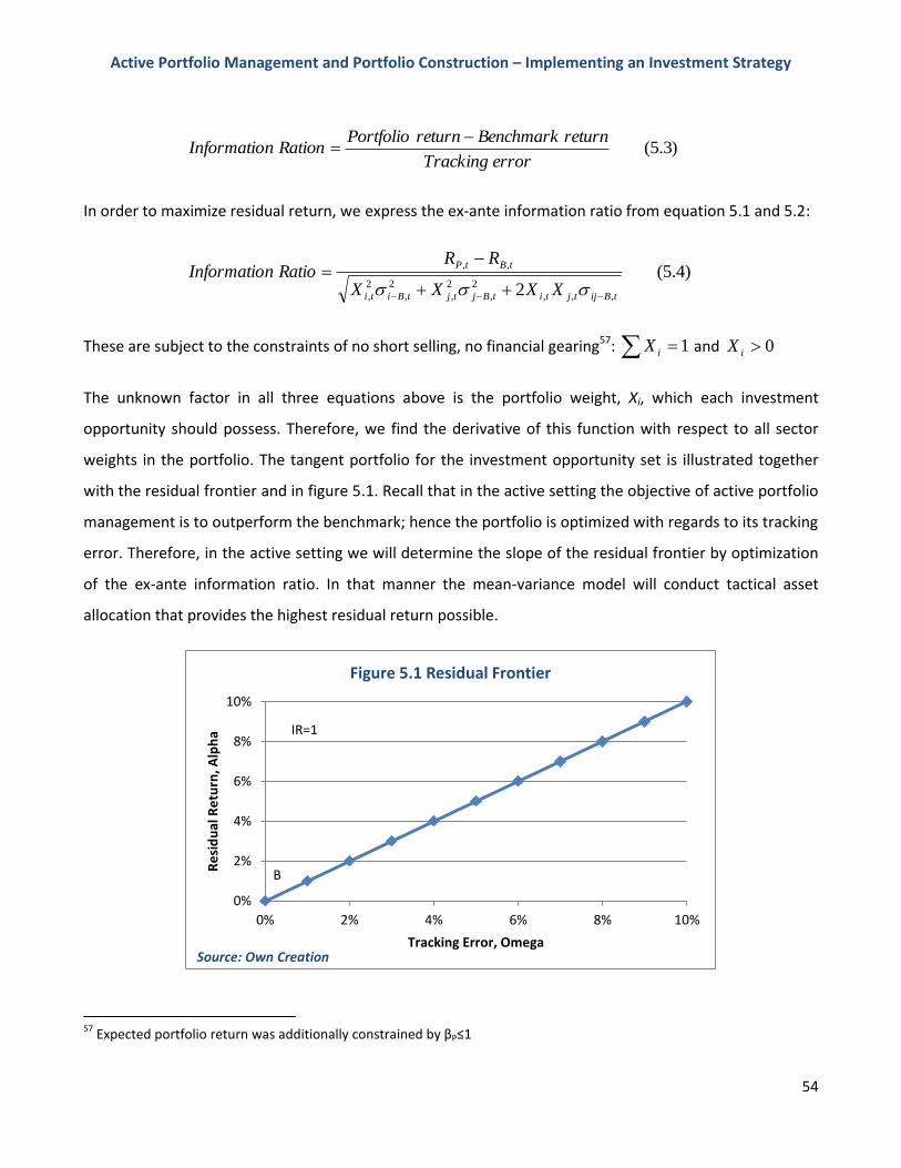
Active Portfolio Management and Portfolio Construction – Implementing an Investment Strategy
54
)3.5(errorTracking
returnBenchmarkreturnPortfolioRationnInformatio
In order to maximize residual return, we express the ex-ante information ratio from equation 5.1 and 5.2:
)4.5(2 ,,,
2
,
2
,
2
,
2
,
,,
tBijtjtitBjtjtBiti
tBtP
XXXX
RRRationInformatio
These are subject to the constraints of no short selling, no financial gearing57: 1iX and 0iX
The unknown factor in all three equations above is the portfolio weight, Xi, which each investment
opportunity should possess. Therefore, we find the derivative of this function with respect to all sector
weights in the portfolio. The tangent portfolio for the investment opportunity set is illustrated together
with the residual frontier and in figure 5.1. Recall that in the active setting the objective of active portfolio
management is to outperform the benchmark; hence the portfolio is optimized with regards to its tracking
error. Therefore, in the active setting we will determine the slope of the residual frontier by optimization
of the ex-ante information ratio. In that manner the mean-variance model will conduct tactical asset
allocation that provides the highest residual return possible.
57
Expected portfolio return was additionally constrained by βP≤1
0%
2%
4%
6%
8%
10%
0% 2% 4% 6% 8% 10%
Re
sid
ual
Re
turn
, Alp
ha
Tracking Error, Omega
Figure 5.1 Residual Frontier
Source: Own Creation
B
IR=1
Active Portfolio Management and Portfolio Construction – Implementing an Investment Strategy
55
The residual frontier plots the expected residual return, alpha, against the residual risk, ωp, and it will
always be a straight line through the origin. Its slope is thus determined by the information ratio and
therefore shows the possible fund allocation which is expected to outperform the benchmark for a
rational investor. The form of a straight line is based upon the assumption that not all investors have equal
market expectations nor the same borrowing and lending rates. Thus, they have different presumptions of
risk and return, but can still hold an optimal portfolio, as the optimal portfolio is situated at any point on
the residual frontier. The investor will, however, hold a portfolio containing no systematic risk above
market level, hence the tangent portfolio, in order to obtain the highest residual return possible. Thus, if
the investor is in the point of the tangency portfolio, on the residual frontier, he has allocated his entire
investment in the portfolio, with βP,t=1. Through portfolio repositioning we maximize the information ratio
in order to keep the portfolio located on the steepest residual frontier possible.
The origin designated B, represents the benchmark portfolio. By definition the benchmark portfolio has no
residual return, in other words both alpha and omega are equal to zero. Obviously, the slope of the
residual frontier represents the performance of the active investor, as a higher information ratio
represents a higher residual return.
5.3.2 Model Short-Comings
Markowitz’ mean-variance model might seem reasonable from a theoretical point of view, as it is easy to
understand and clearly presents the important concepts of risk and return. However, Richard Michaud
(1989) discusses the practical problems in his article The Markowitz Optimization Enigma: Is ‘Optimized’
Optimal?. He claims that that the model often leads to irrelevant optimal portfolios and reviews a number
of disadvantages using the model, which likely appears with the applied data of this thesis, particularly
due to their high correlation. Two of the most important disadvantages are stated and addressed below58.
5.3.2.1 First Disadvantage: Investment Instability
We estimated expected return based on historic data in chapter 4. Regardless of estimation methods,
exact estimates of future returns, variances, or covariance are, however, subject to estimation errors, and
some would even argue they are impossible in the first place. Michaud and Black and Litterman (1992)
58
Michaud (1989): p. 35
Active Portfolio Management and Portfolio Construction – Implementing an Investment Strategy
56
support this claim, stating that the optimization process inherent in the model maximizes errors59. The
mean-variance model overweight assets with high expected return and negative correlation and
underweight those with low expected return and positive correlation60. These assets are according to
Michaud (1989), those that are most prone to be subject to estimation errors.
This argument appears to be somewhat contradictory. The reason for investors to estimate high return on
assets should be that they believe the asset will return well in the future. It then seems reasonable to
appreciate that the model provides an overweight to these assets in the portfolio. The purpose of
repositioning the portfolio is based on the presumption that returns change over time and are therefore
constituted by the CAPM calculated on a monthly basis. Hence, the return estimate applied in the mean-
variance model for e.g. Technology are higher in mid-2002 before the bursting of the dot.com bubble than
in mid-2008 during the financial crisis. Return estimates during the course of dynamic asset allocation thus
change, but investment opportunities display high covariance suggesting they follow similar return
patterns. The mean-variance model will then have difficulties in selecting investment opportunities that
trend differently. Hence, it is more likely to select to select investment opportunities based on return
estimates. These estimates change between months, and so is their portfolio position likely to as well. One
advantage and disadvantage follows. If one investment opportunity possess substantially higher expected
active return than other, the model is likely to provide substantial portfolio weight to that sector, which it
maintains until portfolio reweighting is initiated again. On the other hand, if that sector is indeed the only
investment opportunity expected to outperform the benchmark upon portfolio repositioning the model
should allocate a correspondingly large amount funds to that sector. The only problem with this scenario
is that if the model allocates all or most funds into a single or a few investment opportunities in the first
period the portfolio is likely to sustain losses in the next period as positive returns are likely to be followed
by negative returns as a result of return stationarity among investment opportunities. This issue however,
refers to market timing and should therefore be addressed accordingly.
5.3.2.2 Second Disadvantage: Concentration
A second disadvantage concerns the use of constraints to the portfolio. In order to place all investment
funds in the portfolio we imposed the constraints of no short sales and no financial gearing meaning
59
Black, Litterman (1992): p. 34 60
Michaud (1989): p. 36
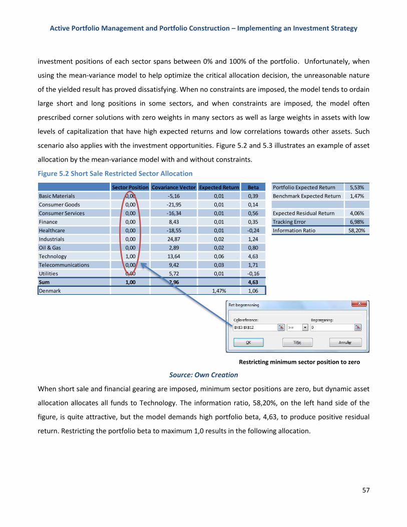
Active Portfolio Management and Portfolio Construction – Implementing an Investment Strategy
57
investment positions of each sector spans between 0% and 100% of the portfolio. Unfortunately, when
using the mean-variance model to help optimize the critical allocation decision, the unreasonable nature
of the yielded result has proved dissatisfying. When no constraints are imposed, the model tends to ordain
large short and long positions in some sectors, and when constraints are imposed, the model often
prescribed corner solutions with zero weights in many sectors as well as large weights in assets with low
levels of capitalization that have high expected returns and low correlations towards other assets. Such
scenario also applies with the investment opportunities. Figure 5.2 and 5.3 illustrates an example of asset
allocation by the mean-variance model with and without constraints.
Figure 5.2 Short Sale Restricted Sector Allocation
Restricting minimum sector position to zero
Source: Own Creation
When short sale and financial gearing are imposed, minimum sector positions are zero, but dynamic asset
allocation allocates all funds to Technology. The information ratio, 58,20%, on the left hand side of the
figure, is quite attractive, but the model demands high portfolio beta, 4,63, to produce positive residual
return. Restricting the portfolio beta to maximum 1,0 results in the following allocation.
Sector Position Covariance Vector Expected Return Beta Portfolio Expected Return 5,53%
Basic Materials 0,00 -5,16 0,01 0,39 Benchmark Expected Return 1,47%
Consumer Goods 0,00 -21,95 0,01 0,14
Consumer Services 0,00 -16,34 0,01 0,56 Expected Residual Return 4,06%
Finance 0,00 8,43 0,01 0,35 Tracking Error 6,98%
Healthcare 0,00 -18,55 0,01 -0,24 Information Ratio 58,20%
Industrials 0,00 24,87 0,02 1,24
Oil & Gas 0,00 2,89 0,02 0,80
Technology 1,00 13,64 0,06 4,63
Telecommunications 0,00 9,42 0,03 1,71
Utilities 0,00 5,72 0,01 -0,16
Sum 1,00 2,96 4,63
Denmark 1,47% 1,06
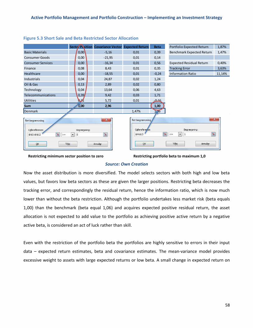
Active Portfolio Management and Portfolio Construction – Implementing an Investment Strategy
58
Figure 5.3 Short Sale and Beta Restricted Sector Allocation
Restricting minimum sector position to zero Restricting portfolio beta to maximum 1,0
Source: Own Creation
Now the asset distribution is more diversified. The model selects sectors with both high and low beta
values, but favors low beta sectors as these are given the larger positions. Restricting beta decreases the
tracking error, and correspondingly the residual return, hence the information ratio, which is now much
lower than without the beta restriction. Although the portfolio undertakes less market risk (beta equals
1,00) than the benchmark (beta equal 1,06) and acquires expected positive residual return, the asset
allocation is not expected to add value to the portfolio as achieving positive active return by a negative
active beta, is considered an act of luck rather than skill.
Even with the restriction of the portfolio beta the portfolios are highly sensitive to errors in their input
data – expected return estimates, beta and covariance estimates. The mean-variance model provides
excessive weight to assets with large expected returns or low beta. A small change in expected return on
Sector Position Covariance Vector Expected Return Beta Portfolio Expected Return 1,87%
Basic Materials 0,00 -5,16 0,01 0,39 Benchmark Expected Return 1,47%
Consumer Goods 0,00 -21,95 0,01 0,14
Consumer Services 0,00 -16,34 0,01 0,56 Expected Residual Return 0,40%
Finance 0,08 8,43 0,01 0,35 Tracking Error 3,63%
Healthcare 0,00 -18,55 0,01 -0,24 Information Ratio 11,14%
Industrials 0,04 24,87 0,02 1,24
Oil & Gas 0,13 2,89 0,02 0,80
Technology 0,04 13,64 0,06 4,63
Telecommunications 0,39 9,42 0,03 1,71
Utilities 0,31 5,72 0,01 -0,16
Sum 1,00 2,96 1,00
Denmark 1,47% 1,06
Active Portfolio Management and Portfolio Construction – Implementing an Investment Strategy
59
one asset might generate a radically different portfolio. According to Michaud this mainly depends on an
ill conditioned covariance matrix, which is exemplified in insufficient historic data61.
An easy but rather primitive approach to avoid portfolio corner solutions and guarantee diversification is
the implementation of the condition of a maximum portfolio sector position. This adjustment carries both
advantages and drawbacks. Assuming that sectors are likely to show realized return fluctuations over
short time periods, and depending on the frequency on portfolio repositioning, the investor may be
unfortunate to conduct reposition during a month where realized returns are low or negative while they
are extraordinary high in both prior and succeeding months. This sector will then accordingly be given zero
or low asset weight during months of high returns and thus bypasses profitable short-term investment
opportunities. This issue concerns market timing and in order to cope with it the investor needs to ensure
that he captures these extraordinary high returns with at least a proportion of his portfolio a limitation of
portfolio proportions is imposed, forcing the mean-variance model to conduct dynamic asset allocation to
a broader number of investment opportunities. However, by ensuring a limited proportion of each
investment opportunity also assumes a high risk as the months between the reweighting months might as
well yield low or negative realized returns. Figure 5.4 extends figure 5.2 and 5.3 by imposing the
restriction maximum 20% portfolio weight. Thus, running the mean-variance model in Excel two different
conditions for the portfolio were tested: a maximum 20% restricted portfolio and an unrestricted
portfolio. The performance of both portfolios is analyzed in the context of active portfolio management in
chapter 6.
61
Michaud (1989): p. 35
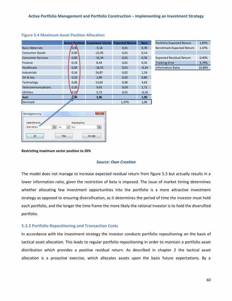
Active Portfolio Management and Portfolio Construction – Implementing an Investment Strategy
60
Figure 5.4 Maximum Asset Position Allocation
Restricting maximum sector position to 20%
Source: Own Creation
The model does not manage to increase expected residual return from figure 5.3 but actually results in a
lower information ratio, given the restriction of beta is imposed. The issue of market timing determines
whether allocating few investment opportunities into the portfolio is a more attractive investment
strategy as opposed to ensuring diversification, as it determines the period of time the investor must hold
each portfolio, and the longer the time frame the more likely the rational investor is to hold the diversified
portfolio.
5.3.3 Portfolio Repositioning and Transaction Costs
In accordance with the investment strategy the investor conducts portfolio repositioning on the basis of
tactical asset allocation. This leads to regular portfolio repositioning in order to maintain a portfolio asset
distribution which provides a positive residual return. As described in chapter 2 the tactical asset
allocation is a proactive exercise, which allocates assets upon the basis future expectations. By a
Sector Position Covariance Vector Expected Return Beta Portfolio Expected Return 1,87%
Basic Materials 0,00 -5,16 0,01 0,39 Benchmark Expected Return 1,47%
Consumer Goods 0,00 -21,95 0,01 0,14
Consumer Services 0,00 -16,34 0,01 0,56 Expected Residual Return 0,40%
Finance 0,19 8,43 0,01 0,35 Tracking Error 3,74%
Healthcare 0,00 -18,55 0,01 -0,24 Information Ratio 10,80%
Industrials 0,16 24,87 0,02 1,24
Oil & Gas 0,20 2,89 0,02 0,80
Technology 0,06 13,64 0,06 4,63
Telecommunications 0,20 9,42 0,03 1,71
Utilities 0,20 5,72 0,01 -0,16
Sum 1,00 2,96 1,00
Denmark 1,47% 1,06
Active Portfolio Management and Portfolio Construction – Implementing an Investment Strategy
61
continuous repositioning process, the investor will sell stocks expected to decrease and acquire stocks
expected to increase in value.
5.3.3.1 Portfolio Repositioning
In order to make the investigation of the research objective more applicable to reality we need to include
an important aspect that is indeed present for the active portfolio investor: transaction costs – the trading
costs associated with both buying and selling stocks during repositioning.
Transaction costs constitute one of the major arguments against active portfolio management, and hence
in order to prove whether if it is in fact possible for active portfolio management to outperform the
benchmark we consider transaction costs with regards to the portfolio repositioning.
In a practical setting there is always a tradeoff between repositioning the portfolio and transaction costs.
If the investor chooses to reposition often, the costs of trading will consume a significant part of the
return. In contrast, too little repositioning may cause the portfolio to deviate from the investor’s goal of
outperforming the benchmark.
We chose to reposition the portfolio every quarter from 1992-2012. The empirical findings of Sun (2006)
suggests high transaction costs for such procedure, and for that reason favors reweighting by dynamic
programming or no repositioning at all62. However, as all investment opportunities display stationary
return patterns, positive returns are likely to be followed by correspondingly high negative returns,
complicating an attempt to identify pockets of market inefficiency where the investor can conduct
portfolio positioning. Thus, the purpose of quarterly repositioning is to acquire a positive average active
return between reweighting. This issue regarding repositioning refers to the timing skill of the investor,
and thus, the next chapter will investigate whether quarterly repositioning does in fact produce superior
active return and whether such return is produced as an act of luck rather than investment skill.
The mean-variance model keeps the asset weights constant in between repositioning. This assumption
under the transaction costs setting is not valid because it causes the transaction costs to be extremely
high. The reason for this is that when one asset moves in one direction the portfolio weight of that asset
moves in the same direction. As a result the goal to keep sector weights constant between all quarters
62
Sun (2006): p. 12
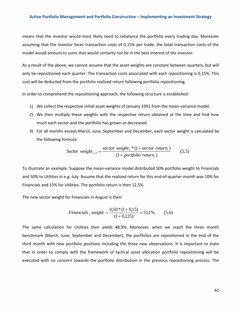
Active Portfolio Management and Portfolio Construction – Implementing an Investment Strategy
62
means that the investor would most likely need to rebalance the portfolio every trading day. Moreover
assuming that the investor faces transaction costs of 0,15% per trade, the total transaction costs of the
model would amount to sums that would certainly not be in the best interest of the investor.
As a result of the above, we cannot assume that the asset weights are constant between quarters, but will
only be repositioned each quarter. The transaction costs associated with each repositioning is 0,15%. This
cost will be deducted from the portfolio realized return following portfolio repositioning.
In order to comprehend the repositioning approach, the following structure is established:
1) We collect the respective initial asset weights of January 1992 from the mean-variance model.
2) We then multiply these weights with the respective return obtained at the time and find how
much each sector and the portfolio has grown or decreased.
3) For all months except March, June, September and December, each sector weight is calculated by
the following formula:
)5.5()1(
)sec1(*sec1
t
tt
treturnportfolio
returntorweighttorweightSector
To illustrate an example: Suppose the mean-variance model distributed 50% portfolio weight to Financials
and 50% to Utilities in e.g. July. Assume that the realized return for this end-of-quarter-month was 10% for
Financials and 15% for Utilities. The portfolio return is then 12,5%.
The new sector weight for Financials in August is then:
)6.5(%1,51)125,01(
)15,01(*50,0,
weightFinancials
The same calculation for Utilities then yields 48,9%. Moreover, when we reach the three month
benchmark (March, June, September and December), the portfolios are repositioned in the end of the
third month with new portfolio positions including the three new observations. It is important to state
that in order to comply with the framework of tactical asset allocation portfolio repositioning will be
executed with no concern towards the portfolio distribution in the previous repositioning process. The
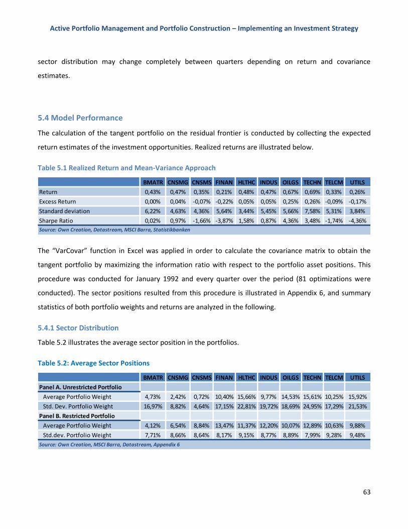
Active Portfolio Management and Portfolio Construction – Implementing an Investment Strategy
63
sector distribution may change completely between quarters depending on return and covariance
estimates.
5.4 Model Performance
The calculation of the tangent portfolio on the residual frontier is conducted by collecting the expected
return estimates of the investment opportunities. Realized returns are illustrated below.
Table 5.1 Realized Return and Mean-Variance Approach
The “VarCovar” function in Excel was applied in order to calculate the covariance matrix to obtain the
tangent portfolio by maximizing the information ratio with respect to the portfolio asset positions. This
procedure was conducted for January 1992 and every quarter over the period (81 optimizations were
conducted). The sector positions resulted from this procedure is illustrated in Appendix 6, and summary
statistics of both portfolio weights and returns are analyzed in the following.
5.4.1 Sector Distribution
Table 5.2 illustrates the average sector position in the portfolios.
Table 5.2: Average Sector Positions
BMATR CNSMG CNSMS FINAN HLTHC INDUS OILGS TECHN TELCM UTILS
0,43% 0,47% 0,35% 0,21% 0,48% 0,47% 0,67% 0,69% 0,33% 0,26%
0,00% 0,04% -0,07% -0,22% 0,05% 0,05% 0,25% 0,26% -0,09% -0,17%
6,22% 4,63% 4,36% 5,64% 3,44% 5,45% 5,66% 7,58% 5,31% 3,84%
0,02% 0,97% -1,66% -3,87% 1,58% 0,87% 4,36% 3,48% -1,74% -4,36%
Source: Own Creation, Datastream, MSCI Barra, Statistikbanken
Return
Excess Return
Standard deviation
Sharpe Ratio
BMATR CNSMG CNSMS FINAN HLTHC INDUS OILGS TECHN TELCM UTILS
4,73% 2,42% 0,72% 10,40% 15,66% 9,77% 14,53% 15,61% 10,25% 15,92%
16,97% 8,82% 4,64% 17,15% 22,81% 19,72% 18,69% 24,95% 17,29% 21,53%
4,12% 6,54% 8,84% 13,47% 11,37% 12,20% 10,07% 12,89% 10,63% 9,88%
7,71% 8,66% 8,64% 8,17% 9,15% 8,77% 8,89% 7,99% 9,28% 9,48%
Average Portfolio Weight
Std. Dev. Portfolio Weight
Source: Own Creation, MSCI Barra, Datastream, Appendix 6
Panel B. Restricted Portfolio
Average Portfolio Weight
Std.dev. Portfolio Weight
Panel A. Unrestricted Portfolio
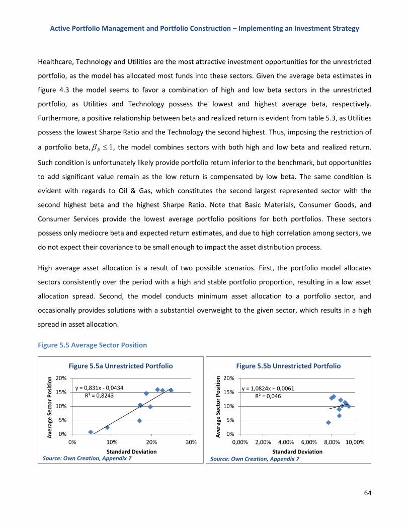
Active Portfolio Management and Portfolio Construction – Implementing an Investment Strategy
64
Healthcare, Technology and Utilities are the most attractive investment opportunities for the unrestricted
portfolio, as the model has allocated most funds into these sectors. Given the average beta estimates in
figure 4.3 the model seems to favor a combination of high and low beta sectors in the unrestricted
portfolio, as Utilities and Technology possess the lowest and highest average beta, respectively.
Furthermore, a positive relationship between beta and realized return is evident from table 5.3, as Utilities
possess the lowest Sharpe Ratio and the Technology the second highest. Thus, imposing the restriction of
a portfolio beta, 1P , the model combines sectors with both high and low beta and realized return.
Such condition is unfortunately likely provide portfolio return inferior to the benchmark, but opportunities
to add significant value remain as the low return is compensated by low beta. The same condition is
evident with regards to Oil & Gas, which constitutes the second largest represented sector with the
second highest beta and the highest Sharpe Ratio. Note that Basic Materials, Consumer Goods, and
Consumer Services provide the lowest average portfolio positions for both portfolios. These sectors
possess only mediocre beta and expected return estimates, and due to high correlation among sectors, we
do not expect their covariance to be small enough to impact the asset distribution process.
High average asset allocation is a result of two possible scenarios. First, the portfolio model allocates
sectors consistently over the period with a high and stable portfolio proportion, resulting in a low asset
allocation spread. Second, the model conducts minimum asset allocation to a portfolio sector, and
occasionally provides solutions with a substantial overweight to the given sector, which results in a high
spread in asset allocation.
Figure 5.5 Average Sector Position
y = 0,831x - 0,0434R² = 0,8243
0%
5%
10%
15%
20%
0% 10% 20% 30%
Ave
rage
Se
cto
r P
osi
tio
n
Standard Deviation
Figure 5.5a Unrestricted Portfolio
Source: Own Creation, Appendix 7
y = 1,0824x + 0,0061R² = 0,046
0%
5%
10%
15%
20%
0,00% 2,00% 4,00% 6,00% 8,00% 10,00%
Ave
rage
Se
cto
r P
osi
tio
n
Standard Deviation
Figure 5.5b Unrestricted Portfolio
Source: Own Creation, Appendix 7
Active Portfolio Management and Portfolio Construction – Implementing an Investment Strategy
65
Figure 5.4 illustrates a positive relationship between average asset allocation and their standard deviation.
The unrestricted portfolio is, however, much more successful in explaining the variation of the
observations. In other words, the regression line for the unrestricted portfolio matches the data points by
83% versus 5% for the restricted portfolio. For the unrestricted portfolio, sectors with high average
weights have constituted portfolio corner solutions, as they carry standard deviations above their average
meaning the position in given periods for these sectors have fluctuated between very high and low values.
Healthcare, Technology and Utilities, possessing the highest average portfolio positions, have either
dominated the portfolio claiming very high portfolio weight (up to more than 90%, respectively) upon
their introduction in some periods or been excluded by the mean-variance model in others.
The distribution pattern is less visible for the restricted portfolio. Imposing a maximum portfolio weight
upon the sectors decreases the standard deviation, resulting in a steeper but much less representable
regression line in figure 5.5. Sector weights therefore fluctuate less in the restricted portfolio, and retains
average values at approximately the same level as the unrestricted portfolio, meaning their distributions
are obviously kept more stable over time as opposed to the unrestricted portfolio.
Note the difference in sector standard deviation. It is not surprisingly higher for the unrestricted portfolio
compared to the restricted portfolio. Any allocation restriction above zero limits the allocation spread,
meaning the lower the restriction of sector distribution the lower the standard deviation is likely to
become. Evidently an equally weighted portfolio would have a zero standard deviation of average
positions63.
Based on the existence of a positive relationship between average portfolio weights and their respective
standard deviation, corner solutions are indeed present in the unrestricted portfolio, which is in fact a
rather disappointing result, given the aim of applying the mean-variance was to secure high risk adjusted
return through diversification. However, tactical asset allocation is based upon expectations of future
return, and estimates showed that benchmark return estimates retained higher levels of return than many
of the investment opportunities. Since the mean-variance model optimizes with regards to which assets
are expected to outperform the benchmark, i.e. the information ratio, only few investment opportunities
might exist, leaving portfolios with only few assets expected to outperform the benchmark.
63
If each sector had a portfolio weight of 10% at all times standard deviations would be zero.
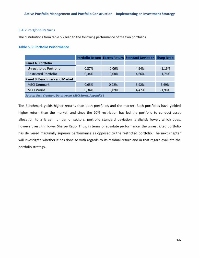
Active Portfolio Management and Portfolio Construction – Implementing an Investment Strategy
66
5.4.2 Portfolio Returns
The distributions from table 5.2 lead to the following performance of the two portfolios.
Table 5.3: Portfolio Performance
The Benchmark yields higher returns than both portfolios and the market. Both portfolios have yielded
higher return than the market, and since the 20% restriction has led the portfolio to conduct asset
allocation to a larger number of sectors, portfolio standard deviation is slightly lower, which does,
however, result in lower Sharpe Ratio. Thus, in terms of absolute performance, the unrestricted portfolio
has delivered marginally superior performance as opposed to the restricted portfolio. The next chapter
will investigate whether it has done so with regards to its residual return and in that regard evaluate the
portfolio strategy.
Portfolio Return Excess Return Standard Deviation Sharp Ratio
Panel A. Portfolio
Unrestricted Portfolio 0,37% -0,06% 4,94% -1,16%
Restricted Portfolio 0,34% -0,08% 4,66% -1,76%
Panel B. Benchmark and Market
MSCI Denmark 0,65% 0,22% 5,92% 3,69%
MSCI World 0,34% -0,09% 4,47% -1,96%
Source: Own Creation, Datastream, MSCI Barra, Appendix 6
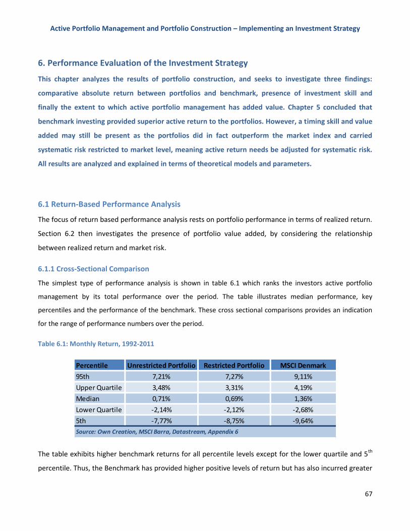
Active Portfolio Management and Portfolio Construction – Implementing an Investment Strategy
67
6. Performance Evaluation of the Investment Strategy
This chapter analyzes the results of portfolio construction, and seeks to investigate three findings:
comparative absolute return between portfolios and benchmark, presence of investment skill and
finally the extent to which active portfolio management has added value. Chapter 5 concluded that
benchmark investing provided superior active return to the portfolios. However, a timing skill and value
added may still be present as the portfolios did in fact outperform the market index and carried
systematic risk restricted to market level, meaning active return needs be adjusted for systematic risk.
All results are analyzed and explained in terms of theoretical models and parameters.
6.1 Return-Based Performance Analysis
The focus of return based performance analysis rests on portfolio performance in terms of realized return.
Section 6.2 then investigates the presence of portfolio value added, by considering the relationship
between realized return and market risk.
6.1.1 Cross-Sectional Comparison
The simplest type of performance analysis is shown in table 6.1 which ranks the investors active portfolio
management by its total performance over the period. The table illustrates median performance, key
percentiles and the performance of the benchmark. These cross sectional comparisons provides an indication
for the range of performance numbers over the period.
Table 6.1: Monthly Return, 1992-2011
The table exhibits higher benchmark returns for all percentile levels except for the lower quartile and 5th
percentile. Thus, the Benchmark has provided higher positive levels of return but has also incurred greater
Percentile Unrestricted Portfolio Restricted Portfolio MSCI Denmark
95th 7,21% 7,27% 9,11%
Upper Quartile 3,48% 3,31% 4,19%
Median 0,71% 0,69% 1,36%
Lower Quartile -2,14% -2,12% -2,68%
5th -7,77% -8,75% -9,64%
Source: Own Creation, MSCI Barra, Datastream, Appendix 6
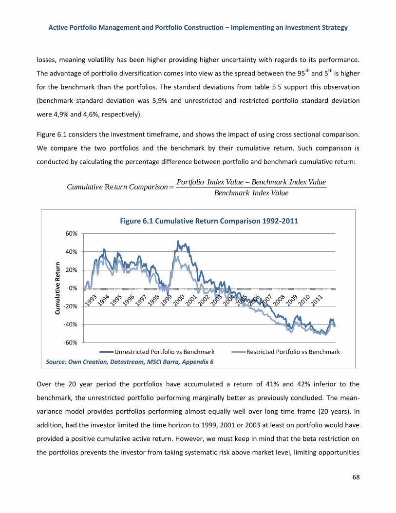
Active Portfolio Management and Portfolio Construction – Implementing an Investment Strategy
68
losses, meaning volatility has been higher providing higher uncertainty with regards to its performance.
The advantage of portfolio diversification comes into view as the spread between the 95th and 5th is higher
for the benchmark than the portfolios. The standard deviations from table 5.5 support this observation
(benchmark standard deviation was 5,9% and unrestricted and restricted portfolio standard deviation
were 4,9% and 4,6%, respectively).
Figure 6.1 considers the investment timeframe, and shows the impact of using cross sectional comparison.
We compare the two portfolios and the benchmark by their cumulative return. Such comparison is
conducted by calculating the percentage difference between portfolio and benchmark cumulative return:
ValueIndexBenchmark
ValueIndexBenchmarkValueIndexPortfolioComparisonturnCumulative
Re
Over the 20 year period the portfolios have accumulated a return of 41% and 42% inferior to the
benchmark, the unrestricted portfolio performing marginally better as previously concluded. The mean-
variance model provides portfolios performing almost equally well over long time frame (20 years). In
addition, had the investor limited the time horizon to 1999, 2001 or 2003 at least on portfolio would have
provided a positive cumulative active return. However, we must keep in mind that the beta restriction on
the portfolios prevents the investor from taking systematic risk above market level, limiting opportunities
-60%
-40%
-20%
0%
20%
40%
60%
Cu
mu
lati
ve R
etu
rn
Figure 6.1 Cumulative Return Comparison 1992-2011
Unrestricted Portfolio vs Benchmark Restricted Portfolio vs Benchmark
Source: Own Creation, Datastream, MSCI Barra, Appendix 6
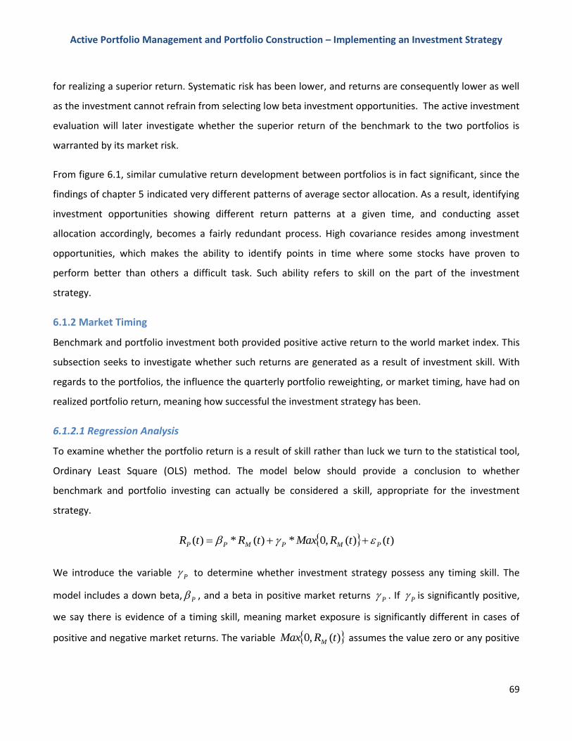
Active Portfolio Management and Portfolio Construction – Implementing an Investment Strategy
69
for realizing a superior return. Systematic risk has been lower, and returns are consequently lower as well
as the investment cannot refrain from selecting low beta investment opportunities. The active investment
evaluation will later investigate whether the superior return of the benchmark to the two portfolios is
warranted by its market risk.
From figure 6.1, similar cumulative return development between portfolios is in fact significant, since the
findings of chapter 5 indicated very different patterns of average sector allocation. As a result, identifying
investment opportunities showing different return patterns at a given time, and conducting asset
allocation accordingly, becomes a fairly redundant process. High covariance resides among investment
opportunities, which makes the ability to identify points in time where some stocks have proven to
perform better than others a difficult task. Such ability refers to skill on the part of the investment
strategy.
6.1.2 Market Timing
Benchmark and portfolio investment both provided positive active return to the world market index. This
subsection seeks to investigate whether such returns are generated as a result of investment skill. With
regards to the portfolios, the influence the quarterly portfolio reweighting, or market timing, have had on
realized portfolio return, meaning how successful the investment strategy has been.
6.1.2.1 Regression Analysis
To examine whether the portfolio return is a result of skill rather than luck we turn to the statistical tool,
Ordinary Least Square (OLS) method. The model below should provide a conclusion to whether
benchmark and portfolio investing can actually be considered a skill, appropriate for the investment
strategy.
)()(,0*)(*)( ttRMaxtRtR PMPMPP
We introduce the variable P to determine whether investment strategy possess any timing skill. The
model includes a down beta, P , and a beta in positive market returns P . If P is significantly positive,
we say there is evidence of a timing skill, meaning market exposure is significantly different in cases of
positive and negative market returns. The variable )(,0 tRMax M assumes the value zero or any positive
Active Portfolio Management and Portfolio Construction – Implementing an Investment Strategy
70
market return at time t. If P is positive and significant there is evidence that quarterly repositioning is a
timing skill, meaning market exposure is significantly different in up and down cases.
With regards to the error term, )(tP , the model’s quality and value depends heavily on the behavior of
the residuals. Consequently, we need to check whether the residuals behave as the OLS assumptions
required.
The error term at different time stages, must be uncorrelated, in order to maintain an unbiased variance
of the betas, ensuring the reliability of the t-tests, which measures parameter significance. Furthermore,
as the regression model contains more than one explanatory variable and these variables have a good
chance of being highly correlated a problem with multicollinerity arises, as we will not be able to separate
the effects of the individual variables64.
The models test hypothesis is stated below:
H0: 0)(,0 tRMax B : Portfolio performance is a result of investment skill
H1: 0)(,0 tRMax B : Portfolio performance is not a result of investment skill
Before testing the hypothesis, we test for autocorrelation in the regression model. Autocorrelation is a
representation of a degree of similarity between the time series, applied in the regression model, and a
lagged version of themselves over successive time intervals65. Testing the model for autocorrelation using
the Maximum Likelihood test with 4 lags, we find that neither portfolios show significant sign of
autocorrelation in the error term. As a result we can draw reliable conclusions from the t-statistics of
significance. We therefore bring to a close that the models do not contain a problem with regards to
autocorrelation, thus conclude that the OLS assumptions are fulfilled. The models results are described in
table 6.1
64
Multicollinearity is present if there is a linear relationship between the explanatory variables: )(,0, tRMax MP 65
Gujarati et.al (2009): p.413
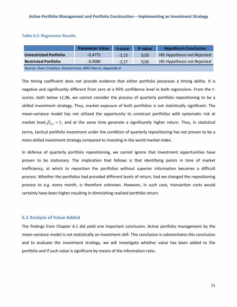
Active Portfolio Management and Portfolio Construction – Implementing an Investment Strategy
71
Table 6.2: Regression Results
The timing coefficient does not provide evidence that either portfolio possesses a timing ability. It is
negative and significantly different from zero at a 95% confidence level in both regressions. From the t-
scores, both below ±1,96, we cannot consider the process of quarterly portfolio repositioning to be a
skilled investment strategy. Thus, market exposure of both portfolios is not statistically significant. The
mean-variance model has not utilized the opportunity to construct portfolios with systematic risk at
market level, 1, tP , and at the same time generate a significantly higher return. Thus, in statistical
terms, tactical portfolio investment under the condition of quarterly repositioning has not proven to be a
more skilled investment strategy compared to investing in the world market index.
In defense of quarterly portfolio repositioning, we cannot ignore that investment opportunities have
proven to be stationary. The implication that follows is that identifying points in time of market
inefficiency, at which to reposition the portfolios without superior information becomes a difficult
process. Whether the portfolios had provided different levels of return, had we changed the repositioning
process to e.g. every month, is therefore unknown. However, in such case, transaction costs would
certainly have been higher resulting in diminishing realized portfolio return.
6.2 Analysis of Value Added
The findings from Chapter 6.1 did yield one important conclusion: Active portfolio management by the
mean-variance model is not statistically an investment skill. This conclusion is substantiates this conclusion
and to evaluate the investment strategy, we will investigate whether value has been added to the
portfolio and if such value is significant by means of the information ratio.
t-score P-value
-2,13 0,03
-2,17 0,03
Source: Own Creation, Datastream, MSCI Barra, Appendix 6
Hypothesis Conclusion
H0: Hypothesis not Rejected
H0: Hypothesis not Rejected
Unrestricted Portfolio
Restricted Portfolio
Parameter Value
-0,4775
-0,4580
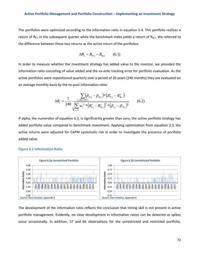
Active Portfolio Management and Portfolio Construction – Implementing an Investment Strategy
72
The portfolios were optimized according to the information ratio in equation 5.4. This portfolio realizes a
return of RP,T in the subsequent quarter while the benchmark index yields a return of RB,T. We referred to
the difference between these two returns as the active return of the portfolios:
)1.6(,, tBtPt RRR
In order to measure whether the investment strategy has added value to the investor, we provided the
information ratio consisting of value added and the ex-ante tracking error for portfolio evaluation. As the
active portfolios were repositioned quarterly over a period of 20 years (240 months) they are evaluated on
an average monthly basis by the ex-post information ratio:
)2.6(
**
*
240
1
1
2
,,
2
,,
2
,,
2011
,,
i
tBti
e
tB
e
tii
e
tB
e
tP
Dect
tBtP
t
RRw
RR
R
If alpha, the numerator of equation 6.2, is significantly greater than zero, the active portfolio strategy has
added portfolio value compared to benchmark investment. Applying optimization from equation 3.3, the
active returns were adjusted for CAPM systematic risk in order to investigate the presence of portfolio
added value.
Figure 6.2 Information Ratio
The development of the information ratio reflects the conclusion that timing skill is not present in active
portfolio management. Evidently, no clear development in information ratios can be detected as spikes
occur occasionally. In addition, 57 and 66 observations for the unrestricted and restricted portfolio,
-0,75
-0,50
-0,25
0,00
0,25
0,50
0,75
1,00
19
93
19
94
19
95
19
96
19
97
19
98
19
99
20
00
20
01
20
02
20
03
20
04
20
05
20
06
20
07
20
08
20
09
20
10
20
11
Info
rmat
ion
Rat
io
Figure 6.2b Unrestricted Portfolio
Source: Own Creation, Appendix 6-3,00
-2,00
-1,00
0,00
1,00
2,00
3,00
4,00
19
93
19
94
19
95
19
96
19
97
19
98
19
99
20
00
20
01
20
02
20
03
20
04
20
05
20
06
20
07
20
08
20
09
20
10
20
11
Info
rmat
ion
Rat
io
Figure 6.2a Unrestricted Portfolio
Source: Own Creation, Appendix 6
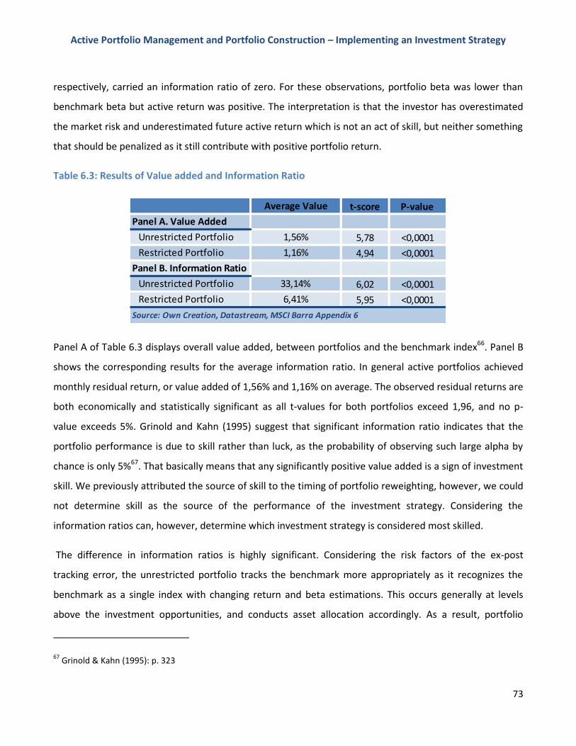
Active Portfolio Management and Portfolio Construction – Implementing an Investment Strategy
73
respectively, carried an information ratio of zero. For these observations, portfolio beta was lower than
benchmark beta but active return was positive. The interpretation is that the investor has overestimated
the market risk and underestimated future active return which is not an act of skill, but neither something
that should be penalized as it still contribute with positive portfolio return.
Table 6.3: Results of Value added and Information Ratio
Panel A of Table 6.3 displays overall value added, between portfolios and the benchmark index66. Panel B
shows the corresponding results for the average information ratio. In general active portfolios achieved
monthly residual return, or value added of 1,56% and 1,16% on average. The observed residual returns are
both economically and statistically significant as all t-values for both portfolios exceed 1,96, and no p-
value exceeds 5%. Grinold and Kahn (1995) suggest that significant information ratio indicates that the
portfolio performance is due to skill rather than luck, as the probability of observing such large alpha by
chance is only 5%67. That basically means that any significantly positive value added is a sign of investment
skill. We previously attributed the source of skill to the timing of portfolio reweighting, however, we could
not determine skill as the source of the performance of the investment strategy. Considering the
information ratios can, however, determine which investment strategy is considered most skilled.
The difference in information ratios is highly significant. Considering the risk factors of the ex-post
tracking error, the unrestricted portfolio tracks the benchmark more appropriately as it recognizes the
benchmark as a single index with changing return and beta estimations. This occurs generally at levels
above the investment opportunities, and conducts asset allocation accordingly. As a result, portfolio
67
Grinold & Kahn (1995): p. 323
t-score P-value
5,78 <0,0001
4,94 <0,0001
6,02 <0,0001
5,95 <0,0001
Source: Own Creation, Datastream, MSCI Barra Appendix 6
Restricted Portfolio
Average Value
1,56%
Panel A. Value Added
Unrestricted Portfolio
Panel B. Information Ratio
Restricted Portfolio
Unrestricted Portfolio
1,16%
33,14%
6,41%
Active Portfolio Management and Portfolio Construction – Implementing an Investment Strategy
74
corner solutions then emerges as the mean-variance model tracks benchmark beta and select the
investment opportunity with the beta best matching benchmark beta. In periods where benchmark beta is
higher than any given investment opportunity, the mean-variance model allocates as much funds as
possible into the investment opportunity which best matches the benchmark beta. However, as portfolio
beta is limited to 1 the mean-variance model cannot allocate 100% funds to one sector index with beta
above 1, but instead distributes the remaining funds into low beta sectors. Restricting maximum portfolio
positions presents a tradeoff. The restricted portfolio cannot eliminate active beta as it can only allocate
20% funds into high beta investment opportunities. Thus the restricted portfolio cannot track benchmark
beta as effectively as the other portfolio. However, diversifying investment positions provides better
conditions for eliminating the other risk factor, active risk, as spreading investments would compensate
losses in some investments by gains in others. As the historic performance of the benchmark has proven
superior to both portfolios, tracking active return is a far more difficult task. Thus, the tracking error is
minimized by eliminating active portfolio beta, and the unrestricted portfolio is more successful in doing
so, making it the most preferred portfolio.
In summary, both portfolios yielded inferior cumulative return compared to the benchmark, and analysis could
not detect any form of investment skill. Investigating whether value was added to the portfolio, we found
that the unrestricted portfolio and the restricted portfolio yielded significant residual returns of 1,56% and
1,16%, respectively. These positive returns add value to the investor, resulting in significant information
ratios of 33% and 6%, respectively. The information ratios are quite different indicating the unrestricted
portfolio tracks the benchmark more successfully than the restricted portfolio.
Active Portfolio Management and Portfolio Construction – Implementing an Investment Strategy
75
7. Conclusion
In this thesis the mechanics of active portfolio management was addressed based upon the motivation
that an investor attempts to outperform a benchmark, the MSCI Denmark. Chapter 1 to 4 established
the investment strategy which involved the determination of a strategic long-term investment
opportunity set and conducting tactical short-term asset allocation by means of Markowitz’ mean-
variance portfolio model. The model was applied each quarter from 1992 to 2011. The asset allocation
was conditional on return and covariance estimations. Two portfolios were constructed: one portfolio
upon which was imposed a restriction of maximum 20% representation of investment opportunities.
The second portfolio was not subject to any constraint with regards to asset allocation.
To answer the superior research objective four sub-questions were identified. Conclusions with respect to
each question and the overall conclusion will be presented in the following based on the findings of
chapter 5 and 6.
How does the mean-variance portfolio model conduct asset allocation in the context of active portfolio
management?
The mean-variance portfolio model was applied for conducting tactical asset allocation in chapter 5. The
model was submitted to three constraints: no short selling, no financial gearing, and a maximum level of
systematic risk constrained to market level, 1, tP . The model conducted asset allocation with regards to
optimization of the information ratio, which measures relative performance of portfolio versus
benchmark. A historical increase in market integration have seen stock markets increase correlation and
hence their covariance towards other markets. Thus, as the investment opportunities display comparable
historical return patterns the mean-variance model primarily selects stocks based upon their expected
return estimates and systematic risk.
Based on the findings in chapter 5, we conclude that optimizing the portfolios against a strong performing
benchmark prescribes concentrated portfolios. In periods of high expected benchmark return, investment
funds need to be allocated to a combination of investment opportunities with both very high and very low
systematic risk, in order to maximize portfolio expected return and retain systematic risk at market level.
Active Portfolio Management and Portfolio Construction – Implementing an Investment Strategy
76
How does active portfolio management perform compared to MSCI Denmark between 1992 and 2011?
Chapter 6 analyzed the results of portfolio construction. By means of tactical asset allocation and the
mean-variance portfolio model the unrestricted and a restricted portfolio provided average monthly
return of 0,37% and 0,34%, respectively. The MSCI Denmark provided an average return of 0,65% per
month. The market return was 0,34%. Neither portfolio outperformed the benchmark, but both
outperformed the market. High covariance and correlation was detected among investment
opportunities, and given different representation of investment opportunities between portfolios,
restricting portfolio representation has not proven to alter portfolio performance.
The choice of time frame is a contributing factor in determining the success of active portfolio
management. Limiting the timeframe to 1999, 2001 and 2003 would have provided cumulative portfolio
return superior to the benchmark, but from 1992 to 2011 cumulative portfolio return was 41% and 42%
below benchmark, respectively.
Based on the findings in chapter 5 and 6, we conclude that MSCI Denmark has provided the investor with
higher realized return as opposed to active portfolio management. This conclusion is based upon respective
performances from 1992 to 2011. Selection of time frame is, however, important to determine the success
of active portfolio management.
Does active portfolio management performance indicate investment skill on the part of the investor?
In order to determine whether the investment strategy indicates investment skill we considered the
timing of portfolio repositioning and turned to the statistical tool Ordinary Least Square. Market return
was regressed on portfolio return and a second explanatory up-market variable containing only positive
market returns was introduced. The purpose of this variable was to determine whether portfolio market
exposure was significantly different in the event of positive and negative market return. The up-market
variable was statistically significant but negative.
Based on the findings with regards to market timing in chapter 6, we conclude that quarterly portfolio
repositioning cannot be attributed as a timing skill. Even though both portfolios provided return superior to
the market index, market exposure of portfolios is not statistically significant.
Active Portfolio Management and Portfolio Construction – Implementing an Investment Strategy
77
With regards to the systematic risk of portfolio and benchmark, does active portfolio management add
value to the investor?
Portfolio value added, or alpha, is present under the condition of positive active beta and positive active
return or vice versa. The rationale behind this condition is that the investor is only rewarded for taking
higher systematic risk than the benchmark if active return is positive. On the other hand, negative active
return still adds value to the portfolios, given the portfolio beta is lower than the benchmark beta. The
unrestricted and restricted portfolio added value by providing monthly average residual return of 1,56%
and 1,16%, respectively. As a result of the unrestricted portfolio possessing concentrated sector positions,
this portfolio was more successful in tracking the benchmark performance resulting in a superior
information ratio of 33% against 6%.
Based on the findings of chapter 6, we conclude that active portfolio management has added significant
value to the investor as opposed to benchmark investment. Restricting the portfolio beta to, 1, tP ,
provides the investor with the ability to control market exposure of the portfolio, leading higher portfolio
systematic risk to be warranted by a higher realized return. On the other hand, leading lower realized
return to be justified by lower systematic risk.
The overall conclusion from this thesis is: the investment strategy of active portfolio management
provides inferior return to investing in the MSCI Denmark. However, maintaining a fixed level of
systematic risk upon portfolio repositioning, portfolio return inferior to the benchmark is justified as the
benchmark demands higher systematic risk in order to generate higher return. In addition, given portfolio
systematic risk exceeds benchmark systematic risk portfolio return is in such case positively significant. In
that regard active portfolio management adds value to the investor.
Active Portfolio Management and Portfolio Construction – Implementing an Investment Strategy
78
8. References
Articles
Berk J. (2005): Five Myths of Active Portfolio Management, The Journal of Portfolio Management,
pp. 27-31
Black F., Litterman R. (1992): Global Portfolio Optimization, Financial Analysis Journal, Vol. 48 No.
5, pp.28-43
Brinson G., Hood L., Beebower G. (1986): Determinants of Portfolio Performance, Financial Analyst
Journal, Vol. 42 No. 4, pp. 133-138
Brinson G., Singer B., Beebower G. (1991): Determinants of Portfolio Performance II: An Update;
Financial Analysts Journal, pp. 40-48
Campbell J., Thomson S. (2008): Predicting Excess Stock Returns Out of Sample: Can Anything Beat
the Historical Average?, The Review of Financial Studies, Vol. 21 No. 4, pp. 1510-1531
Farma E. (1970): Efficient Capital Markets: A Review of Theory and Empirical Work, Vol. 25 No. 2,
The Journal of Finance, pp. 282-417
Farma E., French K. (2004): The Capital Asset Pricing Model: Theory and Evidence, Journal of
Economic Perspectives, Vol. 18, No. 3, pp. 25-46
Grosmann J. and Stiglitz J. (1980): On the Impossibility of Informationally Efficient Markets, Vol. 70,
No. 3, The American Economic Review, pp. 393-408
Jahnke W. (1997): The Asset Allocation Hoax, White Paper, Vol. 1, No. 2, Jahnke & Associates, pp.
1-6
Lo A. (2004): The Adaptive Market Hypothesis: Market Efficiency from an Evolutionary Perspective
Markowitz H. (1952): Portfolio Selection, Journal of Finance, Vol. 7, No. 1, pp. 77-91
Michaud R. (1989): The Markowitz Optimization Enigma: Is ‘Optimized’ Optimal?, Financial Analyst
Journal, Vol. 45 No. 1, pp. 31-42
Samuelson P. (1965): Proof that Properly Anticipated Prices Fluctuate Randomly, Industrial
Management Review 6, 41-50
Sharpe W. (1964): Capital Asset Prices: A theory of Market Equilibrium under Conditions of Risk,
Journal of Finance, Vol. 19, pp. 425-442
Active Portfolio Management and Portfolio Construction – Implementing an Investment Strategy
79
Statman M. (2000): The 93,5% Question of Financial Advisors, The Journal of Investing, pp.16-20
Stoltz (2005): Active Portfolio Management, Implied Expected Returns, and Analyst Optimism,
Swiss Society for Financial Market Research, pp.261-275
Sun W., Fan A., Chen L., Schouwenaars T., Albota M. (2006): Optimal Rebalancing for Institutional
Portfolios, The Journal of Portfolio Management, pp. 33-43
Treynor J., Black F. (1974): How to Use Security Analysis to Improve Portfolio Selection, The Journal
of Business, Vol. 46, No. 1, pp. 66-86
Books
Benninga S. (2008): Financial Modeling, Massachusetts Institute of Technology, Third Edition
Elton E., Gruber M., Brown S., Goetzmann W. (2011): Modern Portfolio Theory and Investment
Analysis, Eighth Edition, John Wiley & Sons Inc.
Grinold R. and Kahn R. (1995): Active Portfolio Management, Irwin Professional Publishing
Gujarati D., Porter D. (2009): Basic Econometrics, Fifth Edition, McGraw Hill
Hopkins P., Miller C. (2001): Country, Sector, and Company Factors in Global Equity Portfolios, The
Research Foundation of AIMR and Blackwell Series in Finance
Koller T., Goedhart M. Wessels D. (2010): Valuation – Measuring the Value of Companies, John
Wiley & Sons Inc.
Litterman R. (2003): Modern Investment Management – An Equilibrium Approach, Goldman Sachs,
John Wiley & Sons Inc.
Markowitz H. (1959): Portfolio Selection – Efficient Diversification of Investments, Second Edition,
Basil Blackwell
Picerno J. (2010): Dynamic Asset Allocation, First Edition, Bloomberg Press, New York
Schleifer A. (2010): Inefficient Markets – An Introduction to Behavioral Finance, Clarendon
Lectures in Economics
Schneeweis T., Crowder G., Kazemi H. (2010): The New Asset Allocation – Risk Management in a
Multi-Asset World, John Wiley & Sons Inc.
Tsay R. (2001): Analysis of Financial Time Series, John Wiley and Sons Inc.
Active Portfolio Management and Portfolio Construction – Implementing an Investment Strategy
80
Databases
Datastream
MSCI Barra
Statistikbanken
Publications
Da Silva A., Lee W., Pornrojnangkool B. (2009): The Black-Litterman Model for Active portfolio
Management, Forthcomming in Journal of Portfolio Management, Winter 2009
Datastream (2008): Global Equity indices, User Guide, Issue 5
Fernández P., Aguirreamalloa J., Corres L. (2011): US Market Risk Premium used in 2011 by
Professors, Analysts and Companies: A Survey with 5731 Answers, Working Paper, IESE Business
School, University of Navarra
Lee W. (2000): Advanced Theory and Methodology of Tactical Asset Allocation
MSCI Barra (2010): MSCI Global Investable Market Indices Methodology; MSCI Barra Index
Methodology
Sparinvest (2007): Strategisk Asset Allocation - kort fortalt, Second Edition
Websites
www.borsen.dk
www.euroinvestor.dk
www.ft.dk
www.investopedia
www.jyskebank.dk
www.msci.com
www.proinvestor.com
www.sec.gov
Active Portfolio Management and Portfolio Construction – Implementing an Investment Strategy
81
9. Appendix Overview
Appendix 1: Glossary
Appendix 2: Sector Market Value and Correlation Matrix of Sector Return
Appendix 3: Interview Guide
Appendix 4: Active Return and Testing for Stationarity
Appendix 5: Expected Residual Sector Return
Appendix 6: Portfolio Positions of Investment Opportunities
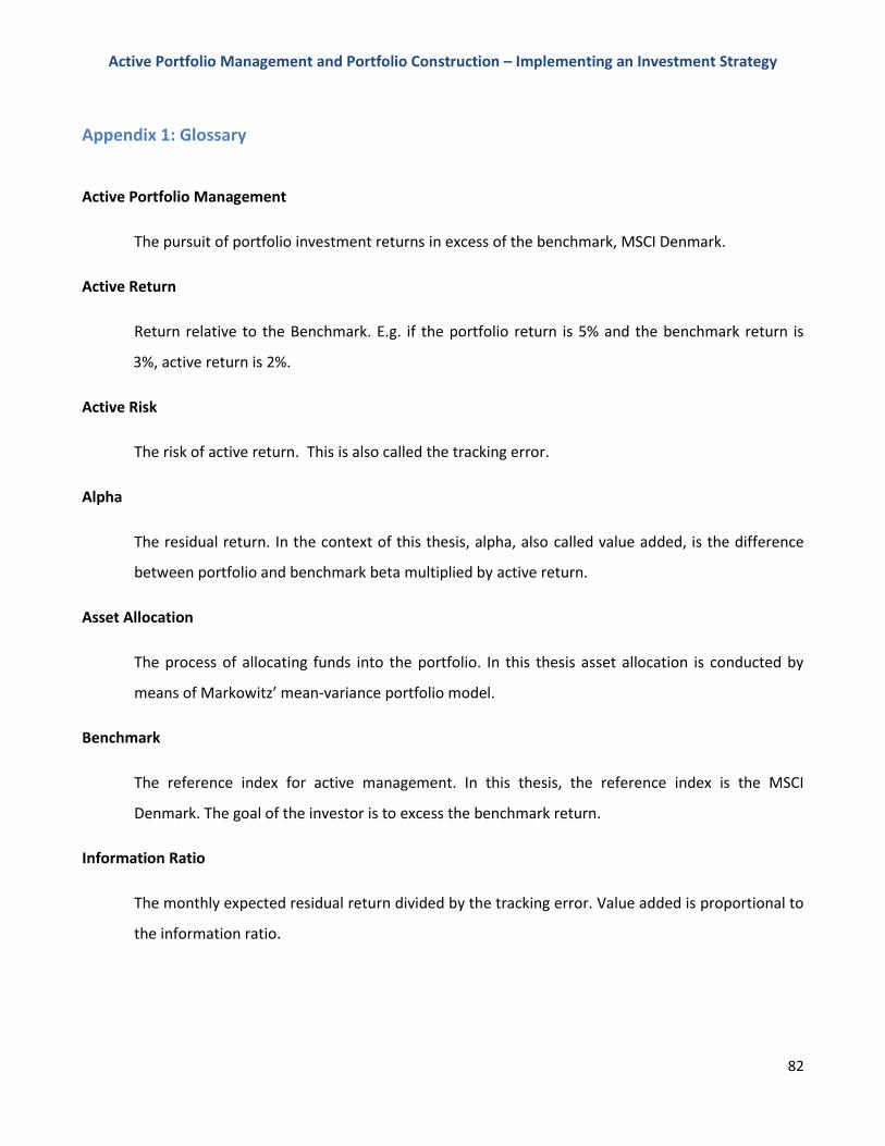
Active Portfolio Management and Portfolio Construction – Implementing an Investment Strategy
82
Appendix 1: Glossary
Active Portfolio Management
The pursuit of portfolio investment returns in excess of the benchmark, MSCI Denmark.
Active Return
Return relative to the Benchmark. E.g. if the portfolio return is 5% and the benchmark return is
3%, active return is 2%.
Active Risk
The risk of active return. This is also called the tracking error.
Alpha
The residual return. In the context of this thesis, alpha, also called value added, is the difference
between portfolio and benchmark beta multiplied by active return.
Asset Allocation
The process of allocating funds into the portfolio. In this thesis asset allocation is conducted by
means of Markowitz’ mean-variance portfolio model.
Benchmark
The reference index for active management. In this thesis, the reference index is the MSCI
Denmark. The goal of the investor is to excess the benchmark return.
Information Ratio
The monthly expected residual return divided by the tracking error. Value added is proportional to
the information ratio.
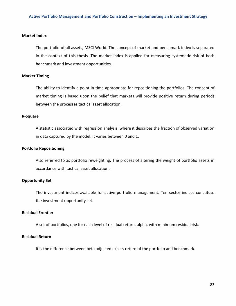
Active Portfolio Management and Portfolio Construction – Implementing an Investment Strategy
83
Market Index
The portfolio of all assets, MSCI World. The concept of market and benchmark index is separated
in the context of this thesis. The market index is applied for measuring systematic risk of both
benchmark and investment opportunities.
Market Timing
The ability to identify a point in time appropriate for repositioning the portfolios. The concept of
market timing is based upon the belief that markets will provide positive return during periods
between the processes tactical asset allocation.
R-Square
A statistic associated with regression analysis, where it describes the fraction of observed variation
in data captured by the model. It varies between 0 and 1.
Portfolio Repositioning
Also referred to as portfolio reweighting. The process of altering the weight of portfolio assets in
accordance with tactical asset allocation.
Opportunity Set
The investment indices available for active portfolio management. Ten sector indices constitute
the investment opportunity set.
Residual Frontier
A set of portfolios, one for each level of residual return, alpha, with minimum residual risk.
Residual Return
It is the difference between beta adjusted excess return of the portfolio and benchmark.
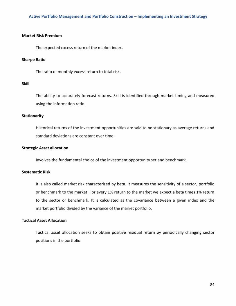
Active Portfolio Management and Portfolio Construction – Implementing an Investment Strategy
84
Market Risk Premium
The expected excess return of the market index.
Sharpe Ratio
The ratio of monthly excess return to total risk.
Skill
The ability to accurately forecast returns. Skill is identified through market timing and measured
using the information ratio.
Stationarity
Historical returns of the investment opportunities are said to be stationary as average returns and
standard deviations are constant over time.
Strategic Asset allocation
Involves the fundamental choice of the investment opportunity set and benchmark.
Systematic Risk
It is also called market risk characterized by beta. It measures the sensitivity of a sector, portfolio
or benchmark to the market. For every 1% return to the market we expect a beta times 1% return
to the sector or benchmark. It is calculated as the covariance between a given index and the
market portfolio divided by the variance of the market portfolio.
Tactical Asset Allocation
Tactical asset allocation seeks to obtain positive residual return by periodically changing sector
positions in the portfolio.
Active Portfolio Management and Portfolio Construction – Implementing an Investment Strategy
85
t-statistic
The t-statistic helps test the hypothesis that a given estimate differs from zero. With some
standard statistical assumptions, the probability that a variable with a true value of zero would
exhibit a t-statistic greater than 1,96 in magnitude is less than 5%.
Tracking Error
See active risk.
Value Added
In the context of this thesis value added is the difference in portfolio and benchmark beta,
multiplied by the active return. Value added depends upon the performance of the investment
strategy.
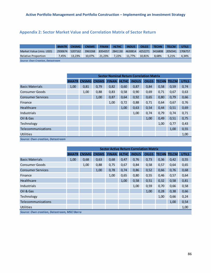
Active Portfolio Management and Portfolio Construction – Implementing an Investment Strategy
86
Appendix 2: Sector Market Value and Correlation Matrix of Sector Return
BMATR CNSMG CNSMS FINAN HLTHC INDUS OILGS TECHN TELCM UTILS
Market Value (mio. USD) 2930674 5207162 3963268 8354357 2841130 4630814 4252271 3416808 2050341 1706757
Relative Proportion 7,45% 13,23% 10,07% 21,23% 7,22% 11,77% 10,81% 8,68% 5,21% 4,34%
Source: Own Creation, Datastream
BMATR CNSMG CNSMS FINAN HLTHC INDUS OILGS TECHN TELCM UTILS
Basic Materials 1,00 0,81 0,79 0,82 0,60 0,87 0,84 0,58 0,59 0,74
Consumer Goods 1,00 0,88 0,83 0,58 0,90 0,69 0,71 0,67 0,63
Consumer Services 1,00 0,87 0,64 0,92 0,65 0,80 0,79 0,66
Finance 1,00 0,72 0,88 0,71 0,64 0,67 0,76
Healthcare 1,00 0,63 0,54 0,44 0,51 0,69
Industrials 1,00 0,74 0,79 0,74 0,71
Oil & Gas 1,00 0,49 0,51 0,75
Technology 1,00 0,77 0,43
Telecommunications 1,00 0,55
Utilities 1,00
Sector Nominal Return Correlation Matrix
Source: Own creation, Datastream
BMATR CNSMG CNSMS FINAN HLTHC INDUS OILGS TECHN TELCM UTILS
Basic Materials 1,00 0,68 0,63 0,68 0,47 0,76 0,73 0,36 0,42 0,55
Consumer Goods 1,00 0,88 0,75 0,67 0,84 0,58 0,57 0,64 0,65
Consumer Services 1,00 0,78 0,74 0,86 0,52 0,66 0,76 0,68
Finance 1,00 0,65 0,80 0,55 0,46 0,57 0,64
Healthcare 1,00 0,58 0,51 0,32 0,58 0,81
Industrials 1,00 0,59 0,70 0,66 0,58
Oil & Gas 1,00 0,28 0,38 0,66
Technology 1,00 0,66 0,24
Telecommunications 1,00 0,54
Utilities 1,00
Source: Own creation, Datastream, MSCI Barra
Sector Active Return Correlation Matrix

Active Portfolio Management and Portfolio Construction – Implementing an Investment Strategy
87
Appendix 3: Interview Guide
First, I would like you to tell me about what you do at Nordea Investment Management. I will afterwards
ask you some questions within the areas of asset allocation and risk management.
Asset Allocation
An area within the literature of finance distinguishes between strategic asset allocation (SAA) and tactical
asset allocation (TAA). SAA accepts that markets are efficient and applies a passive approach to its
investment strategy. On the other hand, TAA is an investment strategy which concerns proactive portfolio
repositioning, based on expectations with regards to the financial markets.
Thus, the difference between TAA and SAA is that TAA does not conduct one long-term based asset
allocation process, but adjusts the portfolio to the market on a periodic basis.
Please provide your assessment upon these two types of asset allocation and you opinion with regards to
the hypothesis of market efficiency?
1) Describe what you consider a good investment strategy with the objective of managing a portfolio
consisting of stocks only.
2) Will you describe this strategy as passive or active portfolio management?
- If passive, is that based on the assumption that it is difficult to produce a return superior to
what the passive market provides, and that opportunities for portfolio diversification are
understated?
- If active, is this based on the conviction that it is in fact possible to outperform the passive
market return?
- Other?
3) Is it your impression that the attempt to time the market by over- and underweighting portfolio
assets based on e.g. sector characteristics, leads to superior return relative to passive investing, or
to transaction costs too high to yield the return your estimations expected?

Active Portfolio Management and Portfolio Construction – Implementing an Investment Strategy
88
Risk Management
Risk is a universal concept, and numerous definitions exist, as investors has different perceptions of risk.
1) Please provide a definition of risk with regards to financial transactions.
2) Describe risk factors which Nordea’s stock portfolios are exposed to in particular.
3) What requirements do you think necessary for the active investor to conduct effective risk
management?
4) How does Nordea Investment Management evaluate risk?
Active Portfolio Management and Portfolio Construction – Implementing an Investment Strategy
89
Appendix 4: Active Return and Testing for Return Stationarity
Important knowledge with regards to timing of portfolio repositioning is whether the investment
opportunities are stationary. Non-stationary investment opportunities make market timing relevant as it
enables the investor to utilize pockets of market inefficiency. Should markets be stationary instead,
positive returns are likely to be followed by negative returns making market timing a difficult process. This
Appendix provides a brief analysis of market stationarity. The figures below illustrate the historical return
development of the investment opportunities and active returns.
To test if the indices are stationary the Argumented Dickey Fuller Test is applied which involves running
the following regression model for each index and test the null hypothesis that 01 and 0 in the
following model68:
ttt YY 11
tY is the difference in index return between time t and t-1 and 1tY is then obviously the index return of
time t-1. The parameter )1( and 11 indicates stationarity. Stationarity is present when
is negative. The null-hypothesis cannot be assessed by standard t-statistic because it does not follow a
standard distribution. Instead the test must be performed using critical values from the Dickey-Fuller
distribution.
68
Gujarati, Porter (2009): p. 755
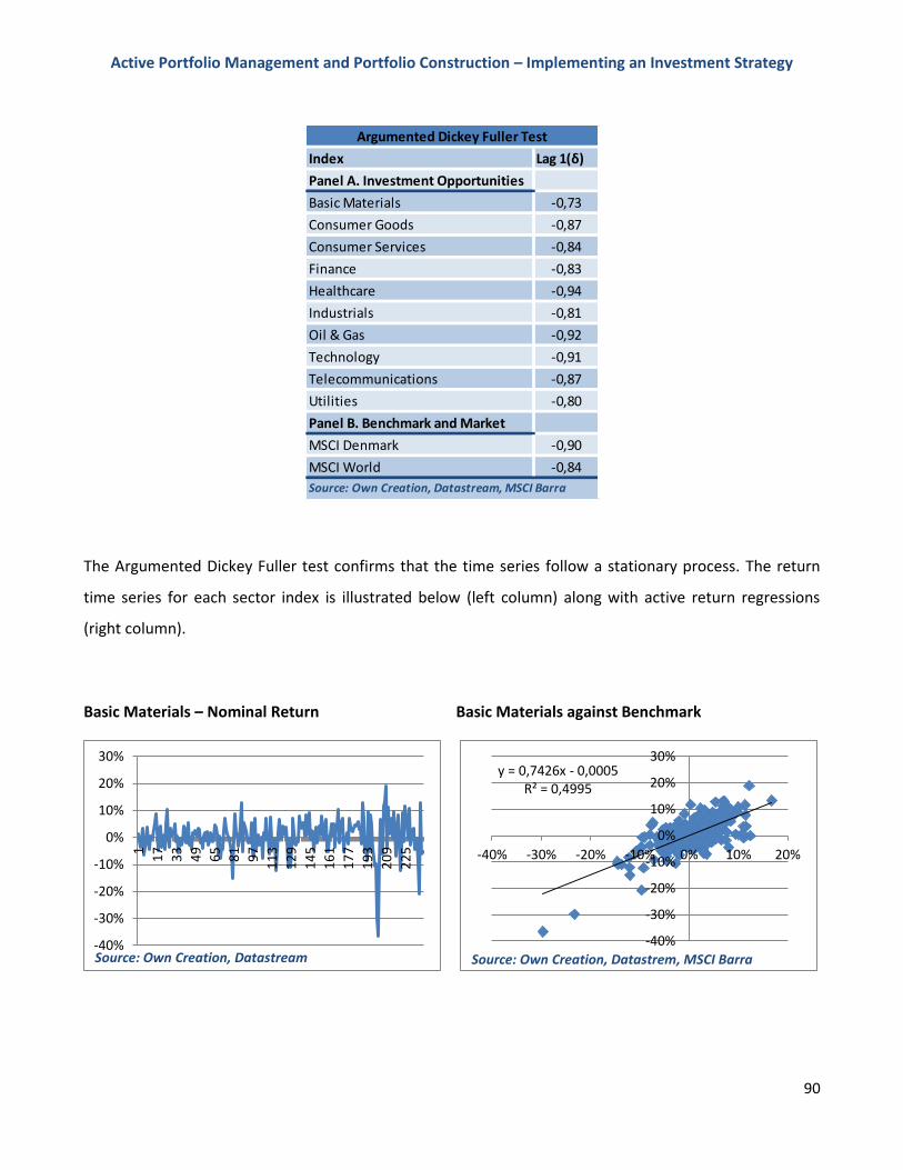
Active Portfolio Management and Portfolio Construction – Implementing an Investment Strategy
90
The Argumented Dickey Fuller test confirms that the time series follow a stationary process. The return
time series for each sector index is illustrated below (left column) along with active return regressions
(right column).
Basic Materials – Nominal Return Basic Materials against Benchmark
Index Lag 1(δ)
Panel A. Investment Opportunities
Basic Materials -0,73
Consumer Goods -0,87
Consumer Services -0,84
Finance -0,83
Healthcare -0,94
Industrials -0,81
Oil & Gas -0,92
Technology -0,91
Telecommunications -0,87
Utilities -0,80
Panel B. Benchmark and Market
MSCI Denmark -0,90
MSCI World -0,84
Argumented Dickey Fuller Test
Source: Own Creation, Datastream, MSCI Barra
y = 0,7426x - 0,0005R² = 0,4995
-40%
-30%
-20%
-10%
0%
10%
20%
30%
-40% -30% -20% -10% 0% 10% 20%
Source: Own Creation, Datastrem, MSCI Barra-40%
-30%
-20%
-10%
0%
10%
20%
30%
1
17
33
49
65
81
97
11
3
12
9
14
5
16
1
17
7
19
3
20
9
22
5
Source: Own Creation, Datastream
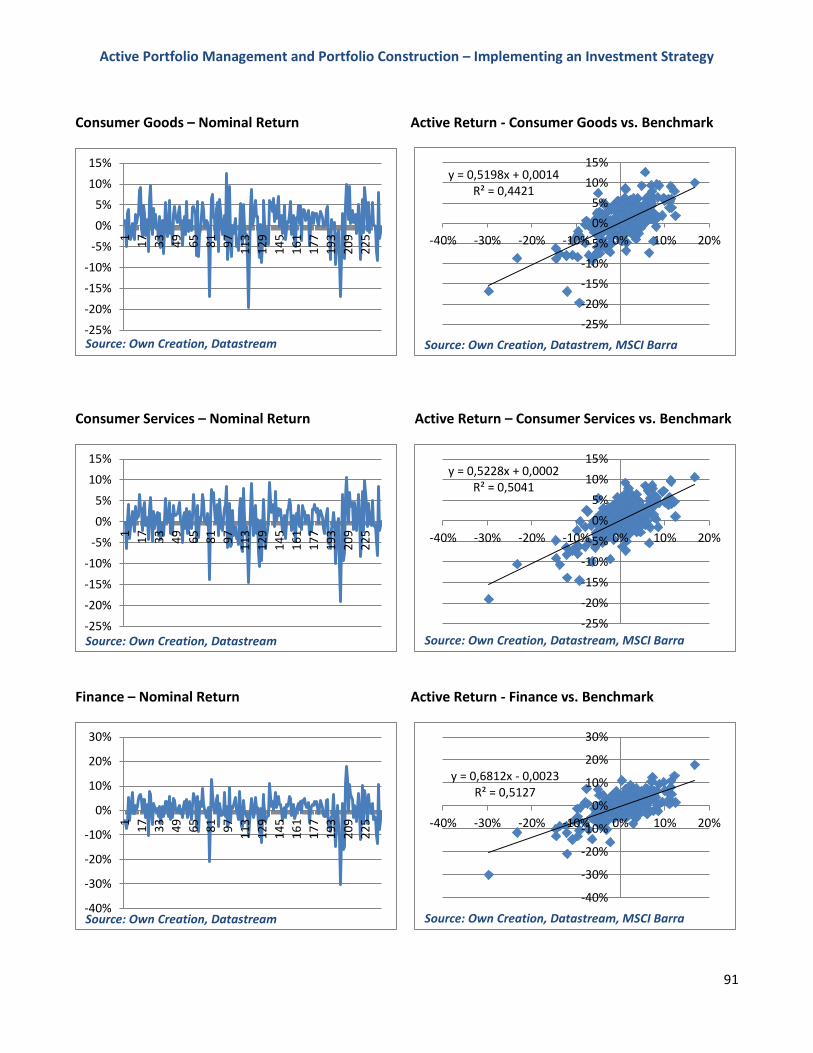
Active Portfolio Management and Portfolio Construction – Implementing an Investment Strategy
91
Consumer Goods – Nominal Return Active Return - Consumer Goods vs. Benchmark
Consumer Services – Nominal Return Active Return – Consumer Services vs. Benchmark
Finance – Nominal Return Active Return - Finance vs. Benchmark
-25%
-20%
-15%
-10%
-5%
0%
5%
10%
15%
1
17
33
49
65
81
97
11
3
12
9
14
5
16
1
17
7
19
3
20
9
22
5
Source: Own Creation, Datastream
y = 0,5198x + 0,0014R² = 0,4421
-25%
-20%
-15%
-10%
-5%
0%
5%
10%
15%
-40% -30% -20% -10% 0% 10% 20%
Source: Own Creation, Datastrem, MSCI Barra
-25%
-20%
-15%
-10%
-5%
0%
5%
10%
15%
1
17
33
49
65
81
97
11
3
12
9
14
5
16
1
17
7
19
3
20
9
22
5
Source: Own Creation, Datastream
y = 0,5228x + 0,0002R² = 0,5041
-25%
-20%
-15%
-10%
-5%
0%
5%
10%
15%
-40% -30% -20% -10% 0% 10% 20%
Source: Own Creation, Datastream, MSCI Barra
-40%
-30%
-20%
-10%
0%
10%
20%
30%
1
17
33
49
65
81
97
11
3
12
9
14
5
16
1
17
7
19
3
20
9
22
5
Source: Own Creation, Datastream
y = 0,6812x - 0,0023R² = 0,5127
-40%
-30%
-20%
-10%
0%
10%
20%
30%
-40% -30% -20% -10% 0% 10% 20%
Source: Own Creation, Datastream, MSCI Barra
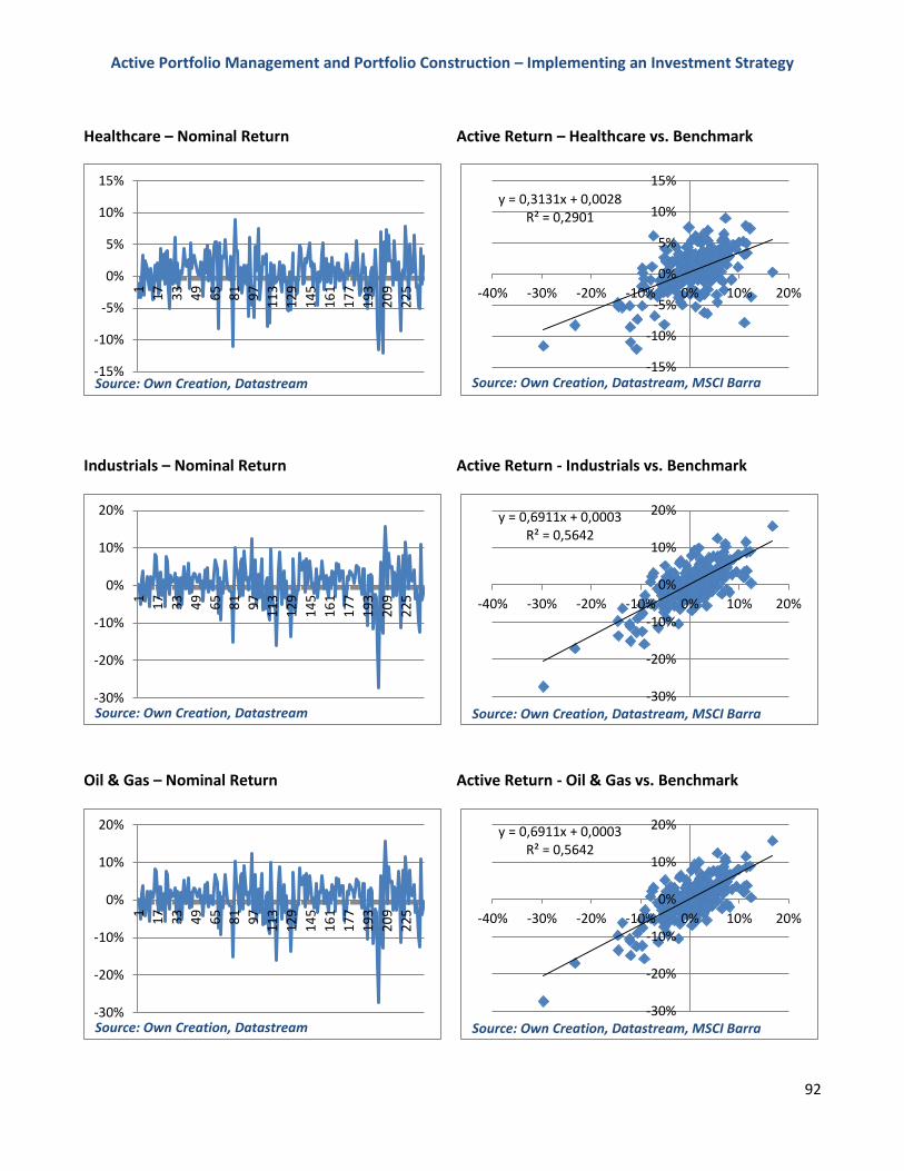
Active Portfolio Management and Portfolio Construction – Implementing an Investment Strategy
92
Healthcare – Nominal Return Active Return – Healthcare vs. Benchmark
Industrials – Nominal Return Active Return - Industrials vs. Benchmark
Oil & Gas – Nominal Return Active Return - Oil & Gas vs. Benchmark
y = 0,3131x + 0,0028R² = 0,2901
-15%
-10%
-5%
0%
5%
10%
15%
-40% -30% -20% -10% 0% 10% 20%
Source: Own Creation, Datastream, MSCI Barra-15%
-10%
-5%
0%
5%
10%
15%
1
17
33
49
65
81
97
11
3
12
9
14
5
16
1
17
7
19
3
20
9
22
5
Source: Own Creation, Datastream
-30%
-20%
-10%
0%
10%
20%
1
17
33
49
65
81
97
11
3
12
9
14
5
16
1
17
7
19
3
20
9
22
5
Source: Own Creation, Datastream
y = 0,6911x + 0,0003R² = 0,5642
-30%
-20%
-10%
0%
10%
20%
-40% -30% -20% -10% 0% 10% 20%
Source: Own Creation, Datastream, MSCI Barra
-30%
-20%
-10%
0%
10%
20%
1
17
33
49
65
81
97
11
3
12
9
14
5
16
1
17
7
19
3
20
9
22
5
Source: Own Creation, Datastream
y = 0,6911x + 0,0003R² = 0,5642
-30%
-20%
-10%
0%
10%
20%
-40% -30% -20% -10% 0% 10% 20%
Source: Own Creation, Datastream, MSCI Barra
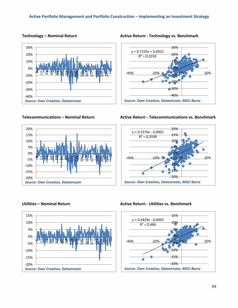
Active Portfolio Management and Portfolio Construction – Implementing an Investment Strategy
93
Technology – Nominal Return Active Return - Technology vs. Benchmark
Telecommunications – Nominal Return Active Return - Telecommunications vs. Benchmark
Utilities – Nominal Return Active Return - Utilities vs. Benchmark
-40%
-30%
-20%
-10%
0%
10%
20%
30%
1
17
33
49
65
81
97
11
3
12
9
14
5
16
1
17
7
19
3
20
9
22
5
Source: Own Creation, Datastream
y = 0,7235x + 0,0022R² = 0,3193
-40%
-30%
-20%
-10%
0%
10%
20%
30%
-40% -20% 0% 20%
Source: Own Creation, Datastream, MSCI Barra
-20%
-15%
-10%
-5%
0%
5%
10%
15%
20%
1
17
33
49
65
81
97
11
3
12
9
14
5
16
1
17
7
19
3
20
9
22
5
Source: Own Creation, Datastream
y = 0,5376x - 0,0001R² = 0,3599
-20%
-15%
-10%
-5%
0%
5%
10%
15%
20%
-40% -20% 0% 20%
Source: Own Creation, Datastream, MSCI Barra
-20%
-15%
-10%
-5%
0%
5%
10%
15%
1
17
33
49
65
81
97
11
3
12
9
14
5
16
1
17
7
19
3
20
9
22
5
Source: Own Creation, Datastream
y = 0,4429x - 0,0003R² = 0,466
-20%
-15%
-10%
-5%
0%
5%
10%
15%
-40% -20% 0% 20%
Source: Own Creation, Datastream, MSCI Barra
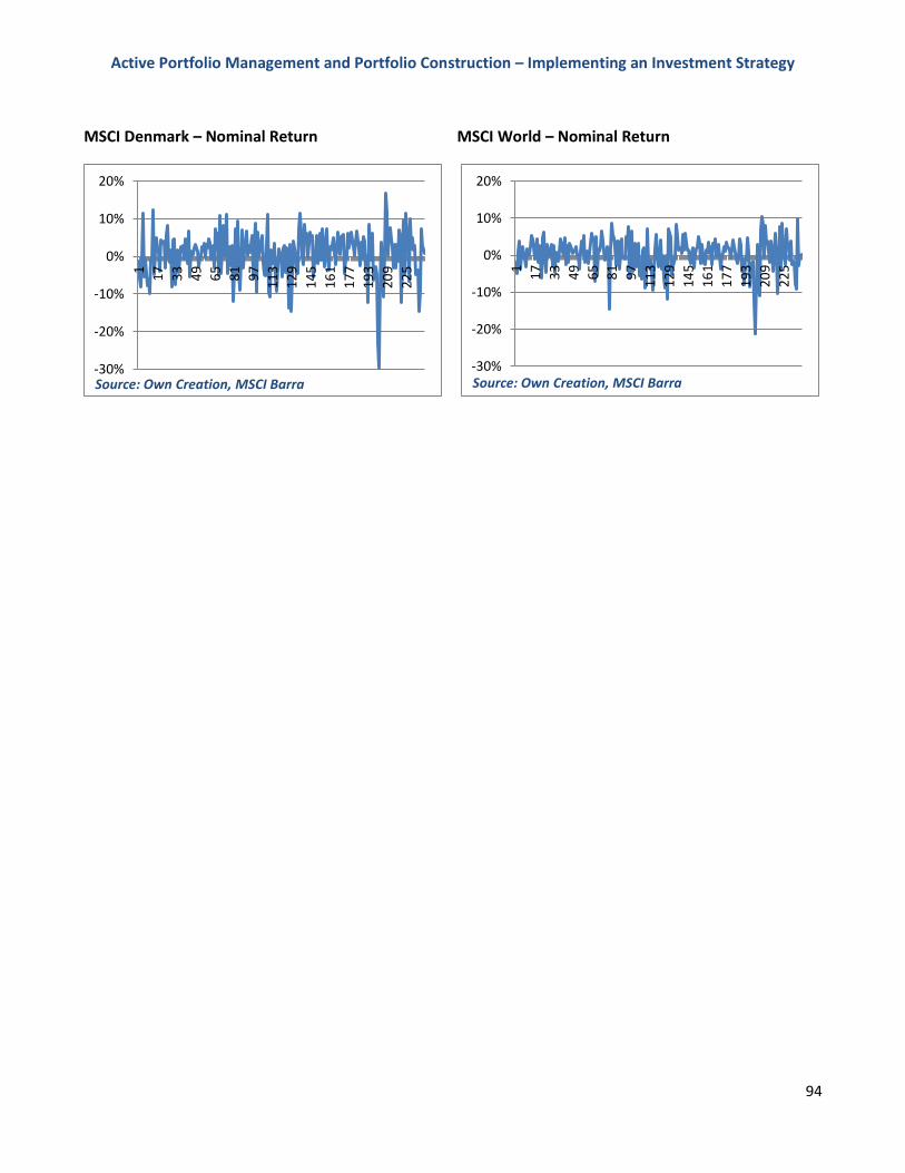
Active Portfolio Management and Portfolio Construction – Implementing an Investment Strategy
94
MSCI Denmark – Nominal Return MSCI World – Nominal Return
-30%
-20%
-10%
0%
10%
20%
1
17
33
49
65
81
97
11
3
12
9
14
5
16
1
17
7
19
3
20
9
22
5
Source: Own Creation, MSCI Barra-30%
-20%
-10%
0%
10%
20%
1
17
33
49
65
81
97
11
3
12
9
14
5
16
1
17
7
19
3
20
9
22
5
Source: Own Creation, MSCI Barra
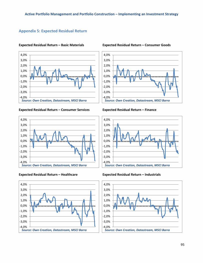
Active Portfolio Management and Portfolio Construction – Implementing an Investment Strategy
95
Appendix 5: Expected Residual Return
Expected Residual Return – Basic Materials Expected Residual Return – Consumer Goods
Expected Residual Return – Consumer Services Expected Residual Return – Finance
Expected Residual Return – Healthcare Expected Residual Return – Industrials
-4,0%
-3,0%
-2,0%
-1,0%
0,0%
1,0%
2,0%
3,0%
4,0%
Source: Own Creation, Datastream, MSCI Barra-4,0%
-3,0%
-2,0%
-1,0%
0,0%
1,0%
2,0%
3,0%
4,0%
Source: Own Creation, Datastream, MSCI Barra
-4,0%
-3,0%
-2,0%
-1,0%
0,0%
1,0%
2,0%
3,0%
4,0%
Source: Own Creation, Datastream, MSCI Barra-4,0%
-3,0%
-2,0%
-1,0%
0,0%
1,0%
2,0%
3,0%
4,0%
Source: Own Creation, Datastream, MSCI Barra
-4,0%
-3,0%
-2,0%
-1,0%
0,0%
1,0%
2,0%
3,0%
4,0%
Source: Own Creation, Datastream, MSCI Barra-4,0%
-3,0%
-2,0%
-1,0%
0,0%
1,0%
2,0%
3,0%
4,0%
Source: Own Creation, Datastream, MSCI Barra
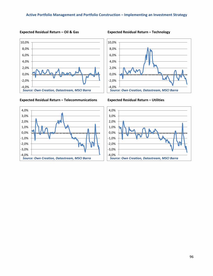
Active Portfolio Management and Portfolio Construction – Implementing an Investment Strategy
96
Expected Residual Return – Oil & Gas Expected Residual Return – Technology
Expected Residual Return – Telecommunications Expected Residual Return – Utilities
-4,0%
-2,0%
0,0%
2,0%
4,0%
6,0%
8,0%
10,0%
Source: Own Creation, Datastream, MSCI Barra-4,0%
-2,0%
0,0%
2,0%
4,0%
6,0%
8,0%
10,0%
Source: Own Creation, Datastream, MSCI Barra
-4,0%
-3,0%
-2,0%
-1,0%
0,0%
1,0%
2,0%
3,0%
4,0%
Source: Own Creation, Datastream, MSCI Barra-4,0%
-3,0%
-2,0%
-1,0%
0,0%
1,0%
2,0%
3,0%
4,0%
Source: Own Creation, Datastream, MSCI Barra
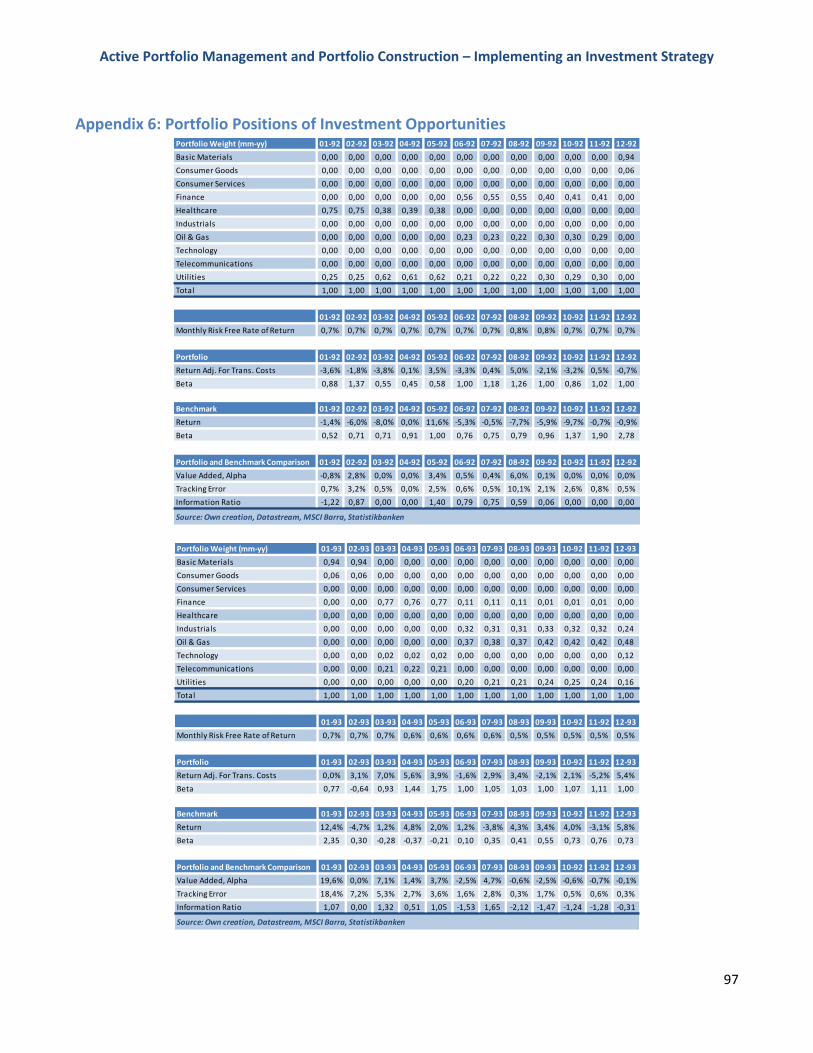
Active Portfolio Management and Portfolio Construction – Implementing an Investment Strategy
97
Appendix 6: Portfolio Positions of Investment Opportunities
Portfolio Weight (mm-yy) 01-92 02-92 03-92 04-92 05-92 06-92 07-92 08-92 09-92 10-92 11-92 12-92
Basic Materials 0,00 0,00 0,00 0,00 0,00 0,00 0,00 0,00 0,00 0,00 0,00 0,94
Consumer Goods 0,00 0,00 0,00 0,00 0,00 0,00 0,00 0,00 0,00 0,00 0,00 0,06
Consumer Services 0,00 0,00 0,00 0,00 0,00 0,00 0,00 0,00 0,00 0,00 0,00 0,00
Finance 0,00 0,00 0,00 0,00 0,00 0,56 0,55 0,55 0,40 0,41 0,41 0,00
Healthcare 0,75 0,75 0,38 0,39 0,38 0,00 0,00 0,00 0,00 0,00 0,00 0,00
Industrials 0,00 0,00 0,00 0,00 0,00 0,00 0,00 0,00 0,00 0,00 0,00 0,00
Oil & Gas 0,00 0,00 0,00 0,00 0,00 0,23 0,23 0,22 0,30 0,30 0,29 0,00
Technology 0,00 0,00 0,00 0,00 0,00 0,00 0,00 0,00 0,00 0,00 0,00 0,00
Telecommunications 0,00 0,00 0,00 0,00 0,00 0,00 0,00 0,00 0,00 0,00 0,00 0,00
Utilities 0,25 0,25 0,62 0,61 0,62 0,21 0,22 0,22 0,30 0,29 0,30 0,00
Total 1,00 1,00 1,00 1,00 1,00 1,00 1,00 1,00 1,00 1,00 1,00 1,00
01-92 02-92 03-92 04-92 05-92 06-92 07-92 08-92 09-92 10-92 11-92 12-92
Monthly Risk Free Rate of Return 0,7% 0,7% 0,7% 0,7% 0,7% 0,7% 0,7% 0,8% 0,8% 0,7% 0,7% 0,7%
Portfolio 01-92 02-92 03-92 04-92 05-92 06-92 07-92 08-92 09-92 10-92 11-92 12-92
Return Adj. For Trans. Costs -3,6% -1,8% -3,8% 0,1% 3,5% -3,3% 0,4% 5,0% -2,1% -3,2% 0,5% -0,7%
Beta 0,88 1,37 0,55 0,45 0,58 1,00 1,18 1,26 1,00 0,86 1,02 1,00
Benchmark 01-92 02-92 03-92 04-92 05-92 06-92 07-92 08-92 09-92 10-92 11-92 12-92
Return -1,4% -6,0% -8,0% 0,0% 11,6% -5,3% -0,5% -7,7% -5,9% -9,7% -0,7% -0,9%
Beta 0,52 0,71 0,71 0,91 1,00 0,76 0,75 0,79 0,96 1,37 1,90 2,78
Portfolio and Benchmark Comparison 01-92 02-92 03-92 04-92 05-92 06-92 07-92 08-92 09-92 10-92 11-92 12-92
Value Added, Alpha -0,8% 2,8% 0,0% 0,0% 3,4% 0,5% 0,4% 6,0% 0,1% 0,0% 0,0% 0,0%
Tracking Error 0,7% 3,2% 0,5% 0,0% 2,5% 0,6% 0,5% 10,1% 2,1% 2,6% 0,8% 0,5%
Information Ratio -1,22 0,87 0,00 0,00 1,40 0,79 0,75 0,59 0,06 0,00 0,00 0,00
Source: Own creation, Datastream, MSCI Barra, Statistikbanken
Portfolio Weight (mm-yy) 01-93 02-93 03-93 04-93 05-93 06-93 07-93 08-93 09-93 10-92 11-92 12-93
Basic Materials 0,94 0,94 0,00 0,00 0,00 0,00 0,00 0,00 0,00 0,00 0,00 0,00
Consumer Goods 0,06 0,06 0,00 0,00 0,00 0,00 0,00 0,00 0,00 0,00 0,00 0,00
Consumer Services 0,00 0,00 0,00 0,00 0,00 0,00 0,00 0,00 0,00 0,00 0,00 0,00
Finance 0,00 0,00 0,77 0,76 0,77 0,11 0,11 0,11 0,01 0,01 0,01 0,00
Healthcare 0,00 0,00 0,00 0,00 0,00 0,00 0,00 0,00 0,00 0,00 0,00 0,00
Industrials 0,00 0,00 0,00 0,00 0,00 0,32 0,31 0,31 0,33 0,32 0,32 0,24
Oil & Gas 0,00 0,00 0,00 0,00 0,00 0,37 0,38 0,37 0,42 0,42 0,42 0,48
Technology 0,00 0,00 0,02 0,02 0,02 0,00 0,00 0,00 0,00 0,00 0,00 0,12
Telecommunications 0,00 0,00 0,21 0,22 0,21 0,00 0,00 0,00 0,00 0,00 0,00 0,00
Utilities 0,00 0,00 0,00 0,00 0,00 0,20 0,21 0,21 0,24 0,25 0,24 0,16
Total 1,00 1,00 1,00 1,00 1,00 1,00 1,00 1,00 1,00 1,00 1,00 1,00
01-93 02-93 03-93 04-93 05-93 06-93 07-93 08-93 09-93 10-92 11-92 12-93
Monthly Risk Free Rate of Return 0,7% 0,7% 0,7% 0,6% 0,6% 0,6% 0,6% 0,5% 0,5% 0,5% 0,5% 0,5%
Portfolio 01-93 02-93 03-93 04-93 05-93 06-93 07-93 08-93 09-93 10-92 11-92 12-93
Return Adj. For Trans. Costs 0,0% 3,1% 7,0% 5,6% 3,9% -1,6% 2,9% 3,4% -2,1% 2,1% -5,2% 5,4%
Beta 0,77 -0,64 0,93 1,44 1,75 1,00 1,05 1,03 1,00 1,07 1,11 1,00
Benchmark 01-93 02-93 03-93 04-93 05-93 06-93 07-93 08-93 09-93 10-92 11-92 12-93
Return 12,4% -4,7% 1,2% 4,8% 2,0% 1,2% -3,8% 4,3% 3,4% 4,0% -3,1% 5,8%
Beta 2,35 0,30 -0,28 -0,37 -0,21 0,10 0,35 0,41 0,55 0,73 0,76 0,73
Portfolio and Benchmark Comparison 01-93 02-93 03-93 04-93 05-93 06-93 07-93 08-93 09-93 10-92 11-92 12-93
Value Added, Alpha 19,6% 0,0% 7,1% 1,4% 3,7% -2,5% 4,7% -0,6% -2,5% -0,6% -0,7% -0,1%
Tracking Error 18,4% 7,2% 5,3% 2,7% 3,6% 1,6% 2,8% 0,3% 1,7% 0,5% 0,6% 0,3%
Information Ratio 1,07 0,00 1,32 0,51 1,05 -1,53 1,65 -2,12 -1,47 -1,24 -1,28 -0,31
Source: Own creation, Datastream, MSCI Barra, Statistikbanken

Active Portfolio Management and Portfolio Construction – Implementing an Investment Strategy
98
Portfolio Weight (mm-yy) 01-94 02-94 03-94 04-94 05-94 06-94 07-94 08-94 09-94 10-94 11-94 12-94
Basic Materials 0,00 0,00 0,00 0,00 0,00 0,00 0,00 0,00 0,00 0,00 0,00 0,00
Consumer Goods 0,00 0,00 0,00 0,00 0,00 0,00 0,00 0,00 0,00 0,00 0,00 0,00
Consumer Services 0,00 0,00 0,00 0,00 0,00 0,00 0,00 0,00 0,00 0,00 0,00 0,00
Finance 0,00 0,00 0,18 0,18 0,18 0,00 0,00 0,00 0,00 0,00 0,00 0,00
Healthcare 0,00 0,00 0,05 0,05 0,05 0,20 0,20 0,20 0,00 0,00 0,00 0,00
Industrials 0,25 0,25 0,34 0,35 0,34 0,64 0,64 0,64 0,58 0,58 0,57 0,33
Oil & Gas 0,48 0,48 0,43 0,43 0,43 0,16 0,16 0,16 0,42 0,42 0,43 0,67
Technology 0,12 0,12 0,00 0,00 0,00 0,00 0,00 0,00 0,00 0,00 0,00 0,00
Telecommunications 0,00 0,00 0,00 0,00 0,00 0,00 0,00 0,00 0,00 0,00 0,00 0,00
Utilities 0,15 0,15 0,00 0,00 0,00 0,00 0,00 0,00 0,00 0,00 0,00 0,00
Total 1,00 1,00 1,00 1,00 1,00 1,00 1,00 1,00 1,00 1,00 1,00 1,00
01-94 02-94 03-94 04-94 05-94 06-94 07-94 08-94 09-94 10-94 11-94 12-94
Monthly Risk Free Rate of Return 0,5% 0,5% 0,5% 0,6% 0,6% 0,7% 0,7% 0,7% 0,7% 0,7% 0,7% 0,7%
Portfolio 01-94 02-94 03-94 04-94 05-94 06-94 07-94 08-94 09-94 10-94 11-94 12-94
Return Adj. For Trans. Costs 5,7% -1,0% -4,1% 3,6% 0,4% 0,2% 1,9% 3,6% -2,9% 3,3% -6,1% 0,0%
Beta 0,90 0,93 1,00 0,77 0,74 1,00 0,91 0,94 1,00 0,95 0,89 0,11
Benchmark 01-94 02-94 03-94 04-94 05-94 06-94 07-94 08-94 09-94 10-94 11-94 12-94
Return 8,2% 0,3% -1,5% 1,6% -8,0% 4,3% 4,7% -7,4% 0,2% 1,8% -4,3% 2,5%
Beta 0,69 1,24 1,36 1,37 1,42 1,35 1,24 1,22 0,92 0,65 0,44 -0,21
Portfolio and Benchmark Comparison 01-94 02-94 03-94 04-94 05-94 06-94 07-94 08-94 09-94 10-94 11-94 12-94
Value Added, Alpha -0,5% 0,4% 1,0% 0,0% 0,0% 1,4% 0,9% 0,0% -0,2% 0,4% -0,8% -0,8%
Tracking Error 0,3% 0,6% 0,8% 1,2% 3,5% 1,0% 0,4% 2,4% 0,9% 0,2% 0,6% 0,8%
Information Ratio -1,78 0,65 1,15 0,00 0,00 1,47 2,18 0,00 -0,25 2,43 -1,30 -1,01
Source: Own creation, Datastream, MSCI Barra, Statistikbanken
Portfolio Weight (mm-yy) 01-95 02-95 03-95 04-95 05-95 06-95 07-95 08-95 09-95 10-95 11-95 12-95
Basic Materials 0,00 0,00 0,50 0,50 0,50 0,00 0,00 0,00 0,00 0,00 0,00 0,00
Consumer Goods 0,00 0,00 0,00 0,00 0,00 0,00 0,00 0,00 0,07 0,07 0,07 0,07
Consumer Services 0,00 0,00 0,00 0,00 0,00 0,00 0,00 0,00 0,00 0,00 0,00 0,00
Finance 0,00 0,00 0,00 0,00 0,00 0,00 0,00 0,00 0,00 0,00 0,00 0,00
Healthcare 0,00 0,00 0,25 0,24 0,24 0,36 0,36 0,35 0,15 0,15 0,16 0,15
Industrials 0,33 0,33 0,12 0,12 0,12 0,00 0,00 0,00 0,00 0,00 0,00 0,00
Oil & Gas 0,67 0,67 0,14 0,14 0,14 0,24 0,23 0,23 0,18 0,18 0,17 0,27
Technology 0,00 0,00 0,00 0,00 0,00 0,27 0,29 0,30 0,30 0,30 0,30 0,25
Telecommunications 0,00 0,00 0,00 0,00 0,00 0,00 0,00 0,00 0,00 0,00 0,00 0,00
Utilities 0,00 0,00 0,00 0,00 0,00 0,14 0,13 0,13 0,29 0,30 0,30 0,26
Total 1,00 1,00 1,00 1,00 1,00 1,00 1,00 1,00 1,00 1,00 1,00 1,00
01-95 02-95 03-95 04-95 05-95 06-95 07-95 08-95 09-95 10-95 11-95 12-95
Monthly Risk Free Rate of Return 0,7% 0,7% 0,7% 0,7% 0,7% 0,7% 0,7% 0,6% 0,6% 0,6% 0,6% 0,6%
Portfolio 01-95 02-95 03-95 04-95 05-95 06-95 07-95 08-95 09-95 10-95 11-95 12-95
Return Adj. For Trans. Costs -3,3% 0,6% 4,2% 3,2% -0,5% 1,8% 3,9% -1,5% 2,3% -0,5% 0,6% 2,0%
Beta 0,41 0,48 0,24 0,25 0,43 1,00 1,03 1,22 1,00 1,06 1,16 1,00
Benchmark 01-95 02-95 03-95 04-95 05-95 06-95 07-95 08-95 09-95 10-95 11-95 12-95
Return 1,3% 2,8% -0,7% 4,6% 4,1% -1,7% 6,7% -5,5% 1,5% 0,1% 0,4% 2,3%
Beta 0,16 0,09 0,59 0,48 0,75 0,94 0,87 1,08 1,00 1,00 0,99 0,82
Portfolio and Benchmark Comparison 01-95 02-95 03-95 04-95 05-95 06-95 07-95 08-95 09-95 10-95 11-95 12-95
Value Added, Alpha -1,2% -0,8% 0,0% 0,3% 1,5% 0,2% -0,5% 0,6% 0,0% 0,0% 0,0% -0,1%
Tracking Error 0,9% 0,6% 0,9% 0,3% 2,0% 1,0% 0,9% 1,7% 0,5% 0,4% 0,9% 2,2%
Information Ratio -1,28 -1,50 0,00 0,96 0,74 0,21 -0,50 0,35 0,00 -0,09 0,05 -0,03
Source: Own creation, Datastream, MSCI Barra, Statistikbanken
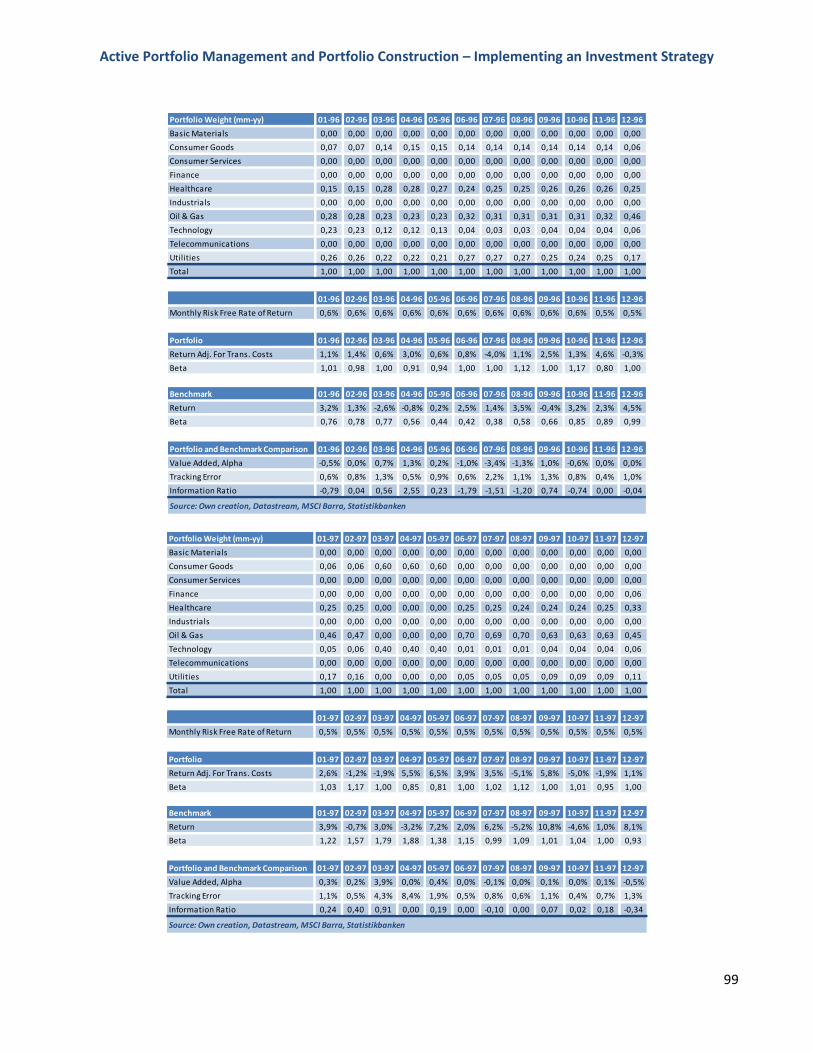
Active Portfolio Management and Portfolio Construction – Implementing an Investment Strategy
99
Portfolio Weight (mm-yy) 01-96 02-96 03-96 04-96 05-96 06-96 07-96 08-96 09-96 10-96 11-96 12-96
Basic Materials 0,00 0,00 0,00 0,00 0,00 0,00 0,00 0,00 0,00 0,00 0,00 0,00
Consumer Goods 0,07 0,07 0,14 0,15 0,15 0,14 0,14 0,14 0,14 0,14 0,14 0,06
Consumer Services 0,00 0,00 0,00 0,00 0,00 0,00 0,00 0,00 0,00 0,00 0,00 0,00
Finance 0,00 0,00 0,00 0,00 0,00 0,00 0,00 0,00 0,00 0,00 0,00 0,00
Healthcare 0,15 0,15 0,28 0,28 0,27 0,24 0,25 0,25 0,26 0,26 0,26 0,25
Industrials 0,00 0,00 0,00 0,00 0,00 0,00 0,00 0,00 0,00 0,00 0,00 0,00
Oil & Gas 0,28 0,28 0,23 0,23 0,23 0,32 0,31 0,31 0,31 0,31 0,32 0,46
Technology 0,23 0,23 0,12 0,12 0,13 0,04 0,03 0,03 0,04 0,04 0,04 0,06
Telecommunications 0,00 0,00 0,00 0,00 0,00 0,00 0,00 0,00 0,00 0,00 0,00 0,00
Utilities 0,26 0,26 0,22 0,22 0,21 0,27 0,27 0,27 0,25 0,24 0,25 0,17
Total 1,00 1,00 1,00 1,00 1,00 1,00 1,00 1,00 1,00 1,00 1,00 1,00
01-96 02-96 03-96 04-96 05-96 06-96 07-96 08-96 09-96 10-96 11-96 12-96
Monthly Risk Free Rate of Return 0,6% 0,6% 0,6% 0,6% 0,6% 0,6% 0,6% 0,6% 0,6% 0,6% 0,5% 0,5%
Portfolio 01-96 02-96 03-96 04-96 05-96 06-96 07-96 08-96 09-96 10-96 11-96 12-96
Return Adj. For Trans. Costs 1,1% 1,4% 0,6% 3,0% 0,6% 0,8% -4,0% 1,1% 2,5% 1,3% 4,6% -0,3%
Beta 1,01 0,98 1,00 0,91 0,94 1,00 1,00 1,12 1,00 1,17 0,80 1,00
Benchmark 01-96 02-96 03-96 04-96 05-96 06-96 07-96 08-96 09-96 10-96 11-96 12-96
Return 3,2% 1,3% -2,6% -0,8% 0,2% 2,5% 1,4% 3,5% -0,4% 3,2% 2,3% 4,5%
Beta 0,76 0,78 0,77 0,56 0,44 0,42 0,38 0,58 0,66 0,85 0,89 0,99
Portfolio and Benchmark Comparison 01-96 02-96 03-96 04-96 05-96 06-96 07-96 08-96 09-96 10-96 11-96 12-96
Value Added, Alpha -0,5% 0,0% 0,7% 1,3% 0,2% -1,0% -3,4% -1,3% 1,0% -0,6% 0,0% 0,0%
Tracking Error 0,6% 0,8% 1,3% 0,5% 0,9% 0,6% 2,2% 1,1% 1,3% 0,8% 0,4% 1,0%
Information Ratio -0,79 0,04 0,56 2,55 0,23 -1,79 -1,51 -1,20 0,74 -0,74 0,00 -0,04
Source: Own creation, Datastream, MSCI Barra, Statistikbanken
Portfolio Weight (mm-yy) 01-97 02-97 03-97 04-97 05-97 06-97 07-97 08-97 09-97 10-97 11-97 12-97
Basic Materials 0,00 0,00 0,00 0,00 0,00 0,00 0,00 0,00 0,00 0,00 0,00 0,00
Consumer Goods 0,06 0,06 0,60 0,60 0,60 0,00 0,00 0,00 0,00 0,00 0,00 0,00
Consumer Services 0,00 0,00 0,00 0,00 0,00 0,00 0,00 0,00 0,00 0,00 0,00 0,00
Finance 0,00 0,00 0,00 0,00 0,00 0,00 0,00 0,00 0,00 0,00 0,00 0,06
Healthcare 0,25 0,25 0,00 0,00 0,00 0,25 0,25 0,24 0,24 0,24 0,25 0,33
Industrials 0,00 0,00 0,00 0,00 0,00 0,00 0,00 0,00 0,00 0,00 0,00 0,00
Oil & Gas 0,46 0,47 0,00 0,00 0,00 0,70 0,69 0,70 0,63 0,63 0,63 0,45
Technology 0,05 0,06 0,40 0,40 0,40 0,01 0,01 0,01 0,04 0,04 0,04 0,06
Telecommunications 0,00 0,00 0,00 0,00 0,00 0,00 0,00 0,00 0,00 0,00 0,00 0,00
Utilities 0,17 0,16 0,00 0,00 0,00 0,05 0,05 0,05 0,09 0,09 0,09 0,11
Total 1,00 1,00 1,00 1,00 1,00 1,00 1,00 1,00 1,00 1,00 1,00 1,00
01-97 02-97 03-97 04-97 05-97 06-97 07-97 08-97 09-97 10-97 11-97 12-97
Monthly Risk Free Rate of Return 0,5% 0,5% 0,5% 0,5% 0,5% 0,5% 0,5% 0,5% 0,5% 0,5% 0,5% 0,5%
Portfolio 01-97 02-97 03-97 04-97 05-97 06-97 07-97 08-97 09-97 10-97 11-97 12-97
Return Adj. For Trans. Costs 2,6% -1,2% -1,9% 5,5% 6,5% 3,9% 3,5% -5,1% 5,8% -5,0% -1,9% 1,1%
Beta 1,03 1,17 1,00 0,85 0,81 1,00 1,02 1,12 1,00 1,01 0,95 1,00
Benchmark 01-97 02-97 03-97 04-97 05-97 06-97 07-97 08-97 09-97 10-97 11-97 12-97
Return 3,9% -0,7% 3,0% -3,2% 7,2% 2,0% 6,2% -5,2% 10,8% -4,6% 1,0% 8,1%
Beta 1,22 1,57 1,79 1,88 1,38 1,15 0,99 1,09 1,01 1,04 1,00 0,93
Portfolio and Benchmark Comparison 01-97 02-97 03-97 04-97 05-97 06-97 07-97 08-97 09-97 10-97 11-97 12-97
Value Added, Alpha 0,3% 0,2% 3,9% 0,0% 0,4% 0,0% -0,1% 0,0% 0,1% 0,0% 0,1% -0,5%
Tracking Error 1,1% 0,5% 4,3% 8,4% 1,9% 0,5% 0,8% 0,6% 1,1% 0,4% 0,7% 1,3%
Information Ratio 0,24 0,40 0,91 0,00 0,19 0,00 -0,10 0,00 0,07 0,02 0,18 -0,34
Source: Own creation, Datastream, MSCI Barra, Statistikbanken
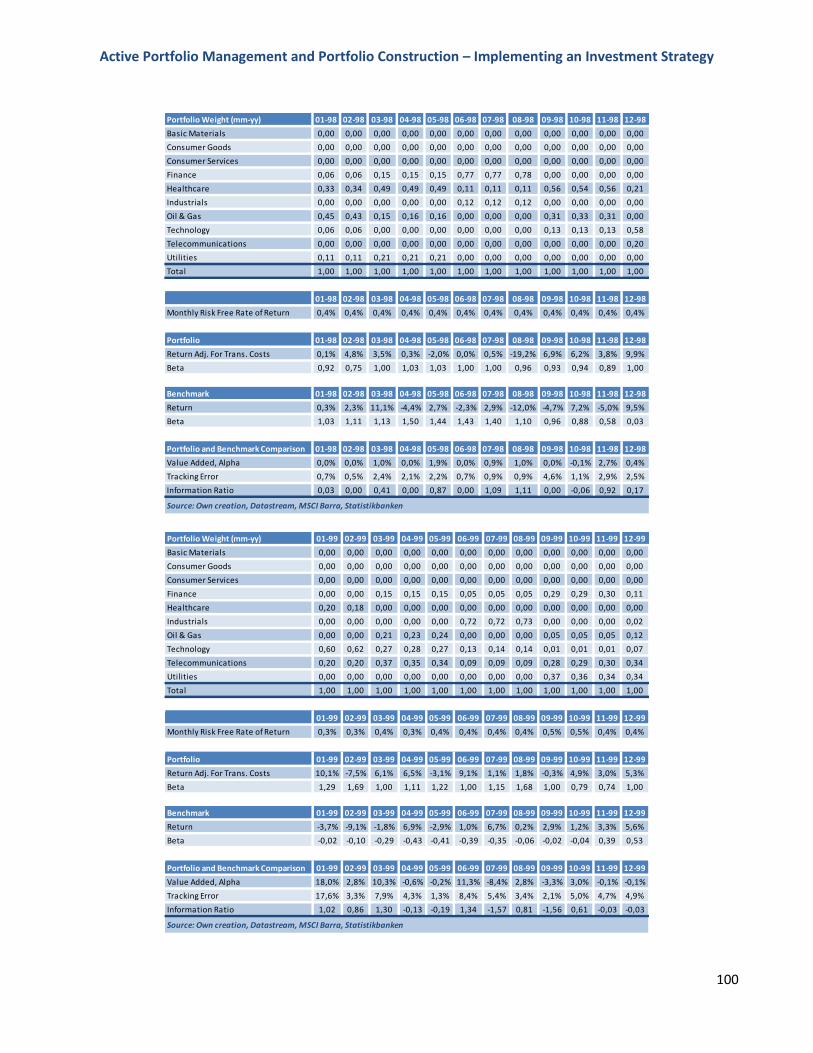
Active Portfolio Management and Portfolio Construction – Implementing an Investment Strategy
100
Portfolio Weight (mm-yy) 01-98 02-98 03-98 04-98 05-98 06-98 07-98 08-98 09-98 10-98 11-98 12-98
Basic Materials 0,00 0,00 0,00 0,00 0,00 0,00 0,00 0,00 0,00 0,00 0,00 0,00
Consumer Goods 0,00 0,00 0,00 0,00 0,00 0,00 0,00 0,00 0,00 0,00 0,00 0,00
Consumer Services 0,00 0,00 0,00 0,00 0,00 0,00 0,00 0,00 0,00 0,00 0,00 0,00
Finance 0,06 0,06 0,15 0,15 0,15 0,77 0,77 0,78 0,00 0,00 0,00 0,00
Healthcare 0,33 0,34 0,49 0,49 0,49 0,11 0,11 0,11 0,56 0,54 0,56 0,21
Industrials 0,00 0,00 0,00 0,00 0,00 0,12 0,12 0,12 0,00 0,00 0,00 0,00
Oil & Gas 0,45 0,43 0,15 0,16 0,16 0,00 0,00 0,00 0,31 0,33 0,31 0,00
Technology 0,06 0,06 0,00 0,00 0,00 0,00 0,00 0,00 0,13 0,13 0,13 0,58
Telecommunications 0,00 0,00 0,00 0,00 0,00 0,00 0,00 0,00 0,00 0,00 0,00 0,20
Utilities 0,11 0,11 0,21 0,21 0,21 0,00 0,00 0,00 0,00 0,00 0,00 0,00
Total 1,00 1,00 1,00 1,00 1,00 1,00 1,00 1,00 1,00 1,00 1,00 1,00
01-98 02-98 03-98 04-98 05-98 06-98 07-98 08-98 09-98 10-98 11-98 12-98
Monthly Risk Free Rate of Return 0,4% 0,4% 0,4% 0,4% 0,4% 0,4% 0,4% 0,4% 0,4% 0,4% 0,4% 0,4%
Portfolio 01-98 02-98 03-98 04-98 05-98 06-98 07-98 08-98 09-98 10-98 11-98 12-98
Return Adj. For Trans. Costs 0,1% 4,8% 3,5% 0,3% -2,0% 0,0% 0,5% -19,2% 6,9% 6,2% 3,8% 9,9%
Beta 0,92 0,75 1,00 1,03 1,03 1,00 1,00 0,96 0,93 0,94 0,89 1,00
Benchmark 01-98 02-98 03-98 04-98 05-98 06-98 07-98 08-98 09-98 10-98 11-98 12-98
Return 0,3% 2,3% 11,1% -4,4% 2,7% -2,3% 2,9% -12,0% -4,7% 7,2% -5,0% 9,5%
Beta 1,03 1,11 1,13 1,50 1,44 1,43 1,40 1,10 0,96 0,88 0,58 0,03
Portfolio and Benchmark Comparison 01-98 02-98 03-98 04-98 05-98 06-98 07-98 08-98 09-98 10-98 11-98 12-98
Value Added, Alpha 0,0% 0,0% 1,0% 0,0% 1,9% 0,0% 0,9% 1,0% 0,0% -0,1% 2,7% 0,4%
Tracking Error 0,7% 0,5% 2,4% 2,1% 2,2% 0,7% 0,9% 0,9% 4,6% 1,1% 2,9% 2,5%
Information Ratio 0,03 0,00 0,41 0,00 0,87 0,00 1,09 1,11 0,00 -0,06 0,92 0,17
Source: Own creation, Datastream, MSCI Barra, Statistikbanken
Portfolio Weight (mm-yy) 01-99 02-99 03-99 04-99 05-99 06-99 07-99 08-99 09-99 10-99 11-99 12-99
Basic Materials 0,00 0,00 0,00 0,00 0,00 0,00 0,00 0,00 0,00 0,00 0,00 0,00
Consumer Goods 0,00 0,00 0,00 0,00 0,00 0,00 0,00 0,00 0,00 0,00 0,00 0,00
Consumer Services 0,00 0,00 0,00 0,00 0,00 0,00 0,00 0,00 0,00 0,00 0,00 0,00
Finance 0,00 0,00 0,15 0,15 0,15 0,05 0,05 0,05 0,29 0,29 0,30 0,11
Healthcare 0,20 0,18 0,00 0,00 0,00 0,00 0,00 0,00 0,00 0,00 0,00 0,00
Industrials 0,00 0,00 0,00 0,00 0,00 0,72 0,72 0,73 0,00 0,00 0,00 0,02
Oil & Gas 0,00 0,00 0,21 0,23 0,24 0,00 0,00 0,00 0,05 0,05 0,05 0,12
Technology 0,60 0,62 0,27 0,28 0,27 0,13 0,14 0,14 0,01 0,01 0,01 0,07
Telecommunications 0,20 0,20 0,37 0,35 0,34 0,09 0,09 0,09 0,28 0,29 0,30 0,34
Utilities 0,00 0,00 0,00 0,00 0,00 0,00 0,00 0,00 0,37 0,36 0,34 0,34
Total 1,00 1,00 1,00 1,00 1,00 1,00 1,00 1,00 1,00 1,00 1,00 1,00
01-99 02-99 03-99 04-99 05-99 06-99 07-99 08-99 09-99 10-99 11-99 12-99
Monthly Risk Free Rate of Return 0,3% 0,3% 0,4% 0,3% 0,4% 0,4% 0,4% 0,4% 0,5% 0,5% 0,4% 0,4%
Portfolio 01-99 02-99 03-99 04-99 05-99 06-99 07-99 08-99 09-99 10-99 11-99 12-99
Return Adj. For Trans. Costs 10,1% -7,5% 6,1% 6,5% -3,1% 9,1% 1,1% 1,8% -0,3% 4,9% 3,0% 5,3%
Beta 1,29 1,69 1,00 1,11 1,22 1,00 1,15 1,68 1,00 0,79 0,74 1,00
Benchmark 01-99 02-99 03-99 04-99 05-99 06-99 07-99 08-99 09-99 10-99 11-99 12-99
Return -3,7% -9,1% -1,8% 6,9% -2,9% 1,0% 6,7% 0,2% 2,9% 1,2% 3,3% 5,6%
Beta -0,02 -0,10 -0,29 -0,43 -0,41 -0,39 -0,35 -0,06 -0,02 -0,04 0,39 0,53
Portfolio and Benchmark Comparison 01-99 02-99 03-99 04-99 05-99 06-99 07-99 08-99 09-99 10-99 11-99 12-99
Value Added, Alpha 18,0% 2,8% 10,3% -0,6% -0,2% 11,3% -8,4% 2,8% -3,3% 3,0% -0,1% -0,1%
Tracking Error 17,6% 3,3% 7,9% 4,3% 1,3% 8,4% 5,4% 3,4% 2,1% 5,0% 4,7% 4,9%
Information Ratio 1,02 0,86 1,30 -0,13 -0,19 1,34 -1,57 0,81 -1,56 0,61 -0,03 -0,03
Source: Own creation, Datastream, MSCI Barra, Statistikbanken
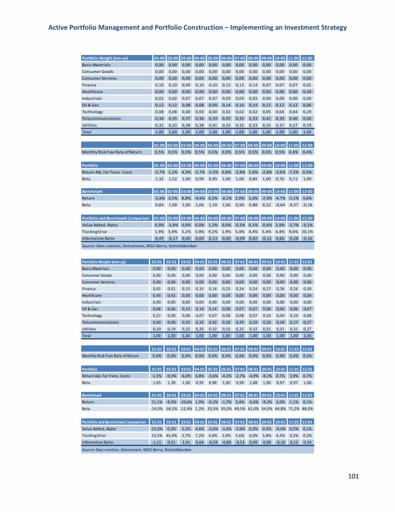
Active Portfolio Management and Portfolio Construction – Implementing an Investment Strategy
101
Portfolio Weight (mm-yy) 01-00 02-00 03-00 04-00 05-00 06-00 07-00 08-00 09-00 10-00 11-00 12-00
Basic Materials 0,00 0,00 0,00 0,00 0,00 0,00 0,00 0,00 0,00 0,00 0,00 0,00
Consumer Goods 0,00 0,00 0,00 0,00 0,00 0,00 0,00 0,00 0,00 0,00 0,00 0,00
Consumer Services 0,00 0,00 0,00 0,00 0,00 0,00 0,00 0,00 0,00 0,00 0,00 0,00
Finance 0,10 0,10 0,09 0,10 0,10 0,13 0,13 0,14 0,07 0,07 0,07 0,01
Healthcare 0,00 0,00 0,00 0,00 0,00 0,00 0,00 0,00 0,00 0,00 0,00 0,44
Industrials 0,02 0,02 0,07 0,07 0,07 0,03 0,03 0,03 0,00 0,00 0,00 0,00
Oil & Gas 0,12 0,12 0,08 0,08 0,09 0,14 0,14 0,14 0,12 0,12 0,12 0,06
Technology 0,08 0,08 0,00 0,00 0,00 0,02 0,02 0,02 0,05 0,04 0,04 0,29
Telecommunications 0,36 0,35 0,37 0,36 0,33 0,35 0,35 0,33 0,41 0,39 0,40 0,00
Utilities 0,32 0,33 0,38 0,38 0,41 0,33 0,32 0,33 0,35 0,37 0,37 0,19
Total 1,00 1,00 1,00 1,00 1,00 1,00 1,00 1,00 1,00 1,00 1,00 1,00
01-00 02-00 03-00 04-00 05-00 06-00 07-00 08-00 09-00 10-00 11-00 12-00
Monthly Risk Free Rate of Return 0,5% 0,5% 0,5% 0,5% 0,5% 0,5% 0,5% 0,5% 0,5% 0,5% 0,4% 0,4%
Portfolio 01-00 02-00 03-00 04-00 05-00 06-00 07-00 08-00 09-00 10-00 11-00 12-00
Return Adj. For Trans. Costs -3,7% 1,2% 4,3% -5,7% -1,5% 0,8% -2,8% 2,4% -2,8% -2,6% -7,2% 0,9%
Beta 1,32 1,52 1,00 0,99 0,95 1,00 1,00 0,85 1,00 0,70 0,71 1,00
Benchmark 01-00 02-00 03-00 04-00 05-00 06-00 07-00 08-00 09-00 10-00 11-00 12-00
Return -5,6% 3,5% 8,8% -9,6% 6,5% -0,2% 2,0% 5,6% -2,0% -4,7% -5,1% 3,6%
Beta 0,84 1,09 1,00 1,06 1,10 1,06 0,90 0,88 0,22 -0,64 -0,57 -0,18
Portfolio and Benchmark Comparison 01-00 02-00 03-00 04-00 05-00 06-00 07-00 08-00 09-00 10-00 11-00 12-00
Value Added, Alpha 0,9% -1,0% 0,0% 0,0% 1,2% 0,0% -0,5% 0,1% -0,6% 2,9% -2,7% -3,1%
Tracking Error 1,9% 5,9% 5,2% 5,9% 9,2% 1,9% 5,4% 4,4% 5,4% 4,4% 9,6% 20,1%
Information Ratio 0,49 -0,17 0,00 0,00 0,13 0,00 -0,09 0,02 -0,12 0,66 -0,28 -0,16
Source: Own creation, Datastream, MSCI Barra, Statistikbanken
Portfolio Weight (mm-yy) 01-01 02-01 03-01 04-01 05-01 06-01 07-01 08-01 09-01 10-01 11-01 12-01
Basic Materials 0,00 0,00 0,00 0,00 0,00 0,00 0,00 0,00 0,00 0,00 0,00 0,00
Consumer Goods 0,00 0,00 0,00 0,00 0,00 0,00 0,00 0,00 0,00 0,00 0,00 0,00
Consumer Services 0,00 0,00 0,00 0,00 0,00 0,00 0,00 0,00 0,00 0,00 0,00 0,00
Finance 0,01 0,01 0,15 0,15 0,14 0,23 0,24 0,24 0,27 0,26 0,26 0,30
Healthcare 0,45 0,42 0,00 0,00 0,00 0,00 0,00 0,00 0,00 0,00 0,00 0,00
Industrials 0,00 0,00 0,00 0,00 0,00 0,00 0,00 0,00 0,00 0,00 0,00 0,00
Oil & Gas 0,06 0,06 0,13 0,14 0,14 0,08 0,07 0,07 0,06 0,06 0,06 0,07
Technology 0,27 0,30 0,08 0,07 0,07 0,08 0,08 0,07 0,10 0,09 0,10 0,08
Telecommunications 0,00 0,00 0,33 0,32 0,32 0,30 0,29 0,29 0,26 0,28 0,27 0,27
Utilities 0,20 0,19 0,32 0,33 0,32 0,32 0,32 0,32 0,31 0,31 0,31 0,27
Total 1,00 1,00 1,00 1,00 1,00 1,00 1,00 1,00 1,00 1,00 1,00 1,00
01-01 02-01 03-01 04-01 05-01 06-01 07-01 08-01 09-01 10-01 11-01 12-01
Monthly Risk Free Rate of Return 0,4% 0,4% 0,4% 0,4% 0,4% 0,4% 0,4% 0,4% 0,4% 0,4% 0,4% 0,4%
Portfolio 01-01 02-01 03-01 04-01 05-01 06-01 07-01 08-01 09-01 10-01 11-01 12-01
Return Adj. For Trans. Costs -1,5% -9,3% -6,0% 6,8% -3,6% -4,2% -2,7% -4,9% -8,2% 0,7% 2,9% 0,7%
Beta 1,05 1,39 1,00 0,95 0,96 1,00 0,99 1,08 1,00 0,97 0,97 1,00
Benchmark 01-01 02-01 03-01 04-01 05-01 06-01 07-01 08-01 09-01 10-01 11-01 12-01
Return 11,1% -9,5% -10,6% 1,9% -0,2% -1,7% 3,4% -5,6% -9,2% 2,0% 1,1% 0,1%
Beta -14,3% -36,5% -12,4% 1,2% 20,3% 35,0% 49,5% 61,0% 54,0% 64,8% 71,2% 88,0%
Portfolio and Benchmark Comparison 01-01 02-01 03-01 04-01 05-01 06-01 07-01 08-01 09-01 10-01 11-01 12-01
Value Added, Alpha -15,0% 0,3% 5,2% 4,6% -2,6% -1,6% -3,0% 0,3% 0,5% -0,4% 0,5% 0,1%
Tracking Error 13,5% 45,4% 2,7% 7,2% 4,4% 2,0% 5,6% 4,0% 5,8% 4,3% 4,2% 0,3%
Information Ratio -1,11 0,01 1,91 0,64 -0,59 -0,80 -0,53 0,09 0,08 -0,10 0,12 0,24
Source: Own creation, Datastream, MSCI Barra, Statistikbanken
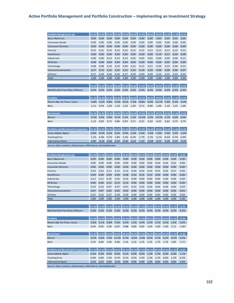
Active Portfolio Management and Portfolio Construction – Implementing an Investment Strategy
102
Portfolio Weight (mm-yy) 01-02 02-02 03-02 04-02 05-02 06-02 07-02 08-02 09-02 10-02 11-02 12-02
Basic Materials 0,00 0,00 0,00 0,00 0,00 0,00 0,00 0,00 0,05 0,05 0,05 0,00
Consumer Goods 0,00 0,00 0,00 0,00 0,00 0,00 0,00 0,00 0,00 0,00 0,00 0,00
Consumer Services 0,00 0,00 0,00 0,00 0,00 0,00 0,00 0,00 0,00 0,00 0,00 0,00
Finance 0,31 0,31 0,22 0,22 0,23 0,15 0,15 0,15 0,12 0,12 0,12 0,33
Healthcare 0,00 0,00 0,00 0,00 0,00 0,00 0,00 0,00 0,19 0,21 0,20 0,08
Industrials 0,00 0,00 0,14 0,14 0,14 0,05 0,05 0,05 0,00 0,00 0,00 0,12
Oil & Gas 0,08 0,08 0,04 0,04 0,04 0,00 0,00 0,00 0,04 0,05 0,04 0,00
Technology 0,08 0,08 0,10 0,10 0,09 0,22 0,21 0,21 0,36 0,33 0,36 0,15
Telecommunications 0,27 0,25 0,25 0,25 0,23 0,20 0,19 0,20 0,00 0,00 0,00 0,07
Utilities 0,27 0,28 0,26 0,26 0,27 0,39 0,40 0,40 0,24 0,25 0,23 0,23
Total 1,00 1,00 1,00 1,00 1,00 1,00 1,00 1,00 1,00 1,00 1,00 1,00
01-02 02-02 03-02 04-02 05-02 06-02 07-02 08-02 09-02 10-02 11-02 12-02
Monthly Risk Free Rate of Return 0,4% 0,4% 0,4% 0,4% 0,4% 0,4% 0,4% 0,4% 0,4% 0,4% 0,4% 0,4%
Portfolio 01-02 02-02 03-02 04-02 05-02 06-02 07-02 08-02 09-02 10-02 11-02 12-02
Return Adj. For Trans. Costs -4,8% -2,2% 4,8% -3,6% -0,5% -7,6% -8,8% 0,9% -12,7% 7,4% 6,1% -4,4%
Beta 1,11 0,93 1,00 1,19 1,10 1,00 0,71 0,80 1,00 1,16 1,35 1,00
Benchmark 01-02 02-02 03-02 04-02 05-02 06-02 07-02 08-02 09-02 10-02 11-02 12-02
Return -5,5% 2,4% 3,0% -4,1% 2,2% 1,2% -13,6% 3,2% -14,5% 2,7% 4,0% 0,4%
Beta 1,13 0,85 0,75 0,86 0,93 0,71 0,21 0,34 0,42 0,65 0,75 0,79
Portfolio and Benchmark Comparison 01-02 02-02 03-02 04-02 05-02 06-02 07-02 08-02 09-02 10-02 11-02 12-02
Value Added, Alpha 0,0% -0,4% 0,5% 0,2% -0,4% -2,6% 2,4% -1,0% 1,0% 2,4% 1,3% -1,0%
Tracking Error 1,2% 2,0% 0,7% 1,8% 1,5% 6,2% 1,7% 2,1% 3,1% 8,5% 6,7% 3,9%
Information Ratio 0,00 -0,18 0,68 0,09 -0,30 -0,42 1,42 -0,48 0,32 0,28 0,19 -0,26
Source: Own creation, Datastream, MSCI Barra, Statistikbanken
Portfolio Weight (mm-yy) 01-03 02-03 03-03 04-03 05-03 06-03 07-03 08-03 09-03 10-03 11-03 12-03
Basic Materials 0,00 0,00 0,00 0,00 0,00 0,00 0,00 0,00 0,00 0,00 0,00 0,00
Consumer Goods 0,00 0,00 0,00 0,00 0,00 0,00 0,00 0,00 0,44 0,44 0,43 0,00
Consumer Services 0,00 0,00 0,00 0,00 0,00 0,00 0,00 0,00 0,00 0,00 0,00 0,00
Finance 0,33 0,33 0,14 0,14 0,14 0,43 0,43 0,43 0,55 0,56 0,57 0,00
Healthcare 0,09 0,09 0,09 0,09 0,08 0,24 0,24 0,23 0,00 0,00 0,00 0,00
Industrials 0,12 0,12 0,26 0,26 0,26 0,00 0,00 0,00 0,00 0,00 0,00 0,00
Oil & Gas 0,00 0,00 0,15 0,15 0,14 0,00 0,00 0,00 0,00 0,00 0,00 0,00
Technology 0,14 0,14 0,07 0,07 0,07 0,33 0,33 0,34 0,00 0,00 0,00 0,39
Telecommunications 0,07 0,07 0,02 0,02 0,02 0,00 0,00 0,00 0,00 0,00 0,00 0,61
Utilities 0,25 0,26 0,27 0,28 0,28 0,00 0,00 0,00 0,00 0,00 0,00 0,00
Total 1,00 1,00 1,00 1,00 1,00 1,00 1,00 1,00 1,00 1,00 1,00 1,00
01-03 02-03 03-03 04-03 05-03 06-03 07-03 08-03 09-03 10-03 11-03 12-03
Monthly Risk Free Rate of Return 0,4% 0,3% 0,3% 0,4% 0,3% 0,3% 0,3% 0,4% 0,4% 0,4% 0,4% 0,4%
Portfolio 01-03 02-03 03-03 04-03 05-03 06-03 07-03 08-03 09-03 10-03 11-03 12-03
Return Adj. For Trans. Costs -2,0% -2,1% -0,8% 7,6% 6,2% 1,5% 3,4% 2,2% 2,1% 6,1% 1,3% 5,0%
Beta 0,94 0,95 1,00 0,97 0,88 0,80 0,85 1,04 1,00 1,00 1,11 1,00
Benchmark 01-03 02-03 03-03 04-03 05-03 06-03 07-03 08-03 09-03 10-03 11-03 12-03
Return -4,5% -4,6% 7,5% 11,5% 6,7% -0,4% -2,0% 8,5% 3,7% 6,2% -0,5% 6,5%
Beta 0,76 0,84 1,00 0,96 1,16 1,22 1,23 1,25 1,79 1,76 1,85 1,71
Portfolio and Benchmark Comparison 01-03 02-03 03-03 04-03 05-03 06-03 07-03 08-03 09-03 10-03 11-03 12-03
Value Added, Alpha 0,4% 0,3% 0,0% 0,0% 0,1% 0,0% 0,0% 1,3% 1,3% 0,0% 0,0% 1,1%
Tracking Error 0,9% 0,8% 1,6% 0,7% 0,1% 0,5% 1,4% 1,3% 1,5% 0,8% 1,2% 0,5%
Information Ratio 0,50 0,33 0,00 -0,05 0,94 0,00 0,00 1,03 0,83 0,05 0,00 2,04
Source: Own creation, Datastream, MSCI Barra, Statistikbanken
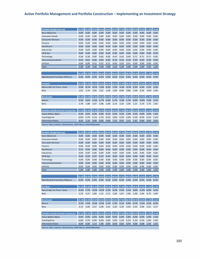
Active Portfolio Management and Portfolio Construction – Implementing an Investment Strategy
103
Portfolio Weight (mm-yy) 01-04 02-04 03-04 04-04 05-04 06-04 07-04 08-04 09-04 10-04 11-04 12-04
Basic Materials 0,00 0,00 0,00 0,00 0,00 0,00 0,00 0,00 0,00 0,00 0,00 0,00
Consumer Goods 0,00 0,00 0,00 0,00 0,00 0,00 0,00 0,00 0,00 0,00 0,00 0,00
Consumer Services 0,00 0,00 0,00 0,00 0,00 0,00 0,00 0,00 0,00 0,00 0,00 0,00
Finance 0,00 0,00 0,00 0,00 0,00 0,00 0,00 0,00 0,00 0,00 0,00 0,00
Healthcare 0,00 0,00 0,48 0,48 0,49 0,00 0,00 0,00 0,00 0,00 0,00 0,50
Industrials 0,00 0,00 0,00 0,00 0,00 0,00 0,00 0,00 0,00 0,00 0,00 0,00
Oil & Gas 0,00 0,00 0,00 0,00 0,00 0,00 0,00 0,00 0,00 0,00 0,00 0,50
Technology 0,38 0,38 0,00 0,00 0,00 0,43 0,43 0,40 0,71 0,71 0,71 0,00
Telecommunications 0,62 0,62 0,00 0,00 0,00 0,18 0,18 0,18 0,29 0,29 0,29 0,00
Utilities 0,00 0,00 0,52 0,52 0,51 0,40 0,39 0,41 0,00 0,00 0,00 0,00
Total 1,00 1,00 1,00 1,00 1,00 1,00 1,00 1,00 1,00 1,00 1,00 1,00
01-04 02-04 03-04 04-04 05-04 06-04 07-04 08-04 09-04 10-04 11-04 12-04
Monthly Risk Free Rate of Return 0,4% 0,4% 0,3% 0,4% 0,4% 0,4% 0,4% 0,4% 0,4% 0,3% 0,3% 0,3%
Portfolio 01-04 02-04 03-04 04-04 05-04 06-04 07-04 08-04 09-04 10-04 11-04 12-04
Return Adj. For Trans. Costs 4,0% -0,1% -0,5% -1,0% 0,3% 1,9% -4,4% -0,3% 2,3% 4,6% 5,2% 2,0%
Beta 1,01 1,10 1,00 1,01 1,06 1,00 0,96 0,86 1,00 0,26 -0,04 1,00
Benchmark 01-04 02-04 03-04 04-04 05-04 06-04 07-04 08-04 09-04 10-04 11-04 12-04
Return 4,5% 5,6% -5,3% -1,7% 0,4% 5,7% -1,9% 1,7% 6,0% -0,9% 7,4% 3,7%
Beta 1,78 1,88 2,07 2,08 2,08 2,16 2,25 2,05 2,21 2,14 1,75 1,82
Portfolio and Benchmark Comparison 01-04 02-04 03-04 04-04 05-04 06-04 07-04 08-04 09-04 10-04 11-04 12-04
Value Added, Alpha 0,3% 4,5% 0,0% 0,0% 0,1% 4,3% 3,2% 2,4% 4,5% 0,0% 3,9% 1,4%
Tracking Error 0,9% 3,7% 5,1% 1,7% 0,2% 2,8% 3,3% 2,0% 3,2% 8,4% 4,2% 1,5%
Information Ratio 0,35 1,20 0,00 0,00 0,64 1,53 0,97 1,21 1,41 0,00 0,93 0,94
Source: Own creation, Datastream, MSCI Barra, Statistikbanken
Portfolio Weight (mm-yy) 01-05 02-05 03-05 04-05 05-05 06-05 07-05 08-05 09-05 10-05 11-05 12-05
Basic Materials 0,00 0,00 0,00 0,00 0,00 0,00 0,00 0,00 0,00 0,00 0,00 0,90
Consumer Goods 0,00 0,00 0,00 0,00 0,00 0,00 0,00 0,00 0,00 0,00 0,00 0,00
Consumer Services 0,00 0,00 0,00 0,00 0,00 0,00 0,00 0,00 0,00 0,00 0,00 0,00
Finance 0,00 0,00 0,00 0,00 0,00 0,00 0,00 0,00 0,00 0,00 0,00 0,00
Healthcare 0,51 0,50 0,00 0,00 0,00 0,00 0,00 0,00 0,04 0,04 0,04 0,00
Industrials 0,00 0,00 0,00 0,00 0,00 0,00 0,00 0,00 0,00 0,00 0,00 0,00
Oil & Gas 0,49 0,50 0,32 0,32 0,32 0,04 0,04 0,04 0,00 0,00 0,00 0,10
Technology 0,00 0,00 0,68 0,68 0,68 0,00 0,00 0,00 0,00 0,00 0,00 0,00
Telecommunications 0,00 0,00 0,00 0,00 0,00 0,00 0,00 0,00 0,00 0,00 0,00 0,00
Utilities 0,00 0,00 0,00 0,00 0,00 0,96 0,96 0,96 0,96 0,96 0,96 0,00
Total 1,00 1,00 1,00 1,00 1,00 1,00 1,00 1,00 1,00 1,00 1,00 1,00
01-05 02-05 03-05 04-05 05-05 06-05 07-05 08-05 09-05 10-05 11-05 12-05
Monthly Risk Free Rate of Return 0,3% 0,3% 0,3% 0,3% 0,3% 0,3% 0,3% 0,3% 0,3% 0,3% 0,3% 0,3%
Portfolio 01-05 02-05 03-05 04-05 05-05 06-05 07-05 08-05 09-05 10-05 11-05 12-05
Return Adj. For Trans. Costs -0,4% 7,7% -3,6% -4,2% 5,3% 3,2% 2,4% 2,1% 3,8% -5,3% 0,9% 4,3%
Beta 1,23 1,27 1,00 1,15 1,11 1,00 1,01 1,06 1,00 1,04 0,75 1,00
Benchmark 01-05 02-05 03-05 04-05 05-05 06-05 07-05 08-05 09-05 10-05 11-05 12-05
Return -2,7% 7,4% -0,3% -3,5% 2,7% 1,7% 3,1% 4,9% 0,7% -2,2% 2,2% 6,3%
Beta 2,15 2,06 2,37 2,48 2,41 2,30 2,39 2,44 2,55 2,99 2,32 2,17
Portfolio and Benchmark Comparison 01-05 02-05 03-05 04-05 05-05 06-05 07-05 08-05 09-05 10-05 11-05 12-05
Value Added, Alpha 0,0% 0,0% 4,5% 0,9% 0,0% 0,0% 0,9% 3,8% 0,0% 6,0% 2,0% 2,4%
Tracking Error 0,6% 3,7% 4,0% 0,6% 5,8% 2,0% 1,1% 4,1% 5,1% 6,1% 1,9% 2,4%
Information Ratio 0,00 0,00 1,13 1,48 0,00 0,00 0,83 0,93 0,00 0,98 1,03 1,02
Source: Own creation, Datastream, MSCI Barra, Statistikbanken
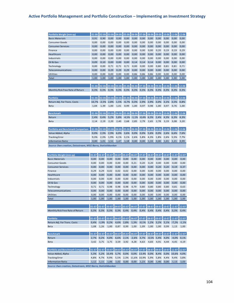
Active Portfolio Management and Portfolio Construction – Implementing an Investment Strategy
104
Portfolio Weight (mm-yy) 01-06 02-06 03-06 04-06 05-06 06-06 07-06 08-06 09-06 10-06 11-06 12-06
Basic Materials 0,91 0,90 0,00 0,00 0,00 0,00 0,00 0,00 0,00 0,00 0,00 0,00
Consumer Goods 0,00 0,00 0,00 0,00 0,00 0,00 0,00 0,00 0,00 0,00 0,00 0,00
Consumer Services 0,00 0,00 0,00 0,00 0,00 0,00 0,00 0,00 0,00 0,00 0,00 0,00
Finance 0,00 0,00 0,00 0,00 0,00 0,00 0,00 0,00 0,20 0,19 0,19 0,29
Healthcare 0,00 0,00 0,00 0,00 0,00 0,00 0,00 0,00 0,00 0,00 0,00 0,00
Industrials 0,00 0,00 0,00 0,00 0,00 0,00 0,00 0,00 0,00 0,00 0,00 0,00
Oil & Gas 0,09 0,10 0,00 0,00 0,00 0,14 0,14 0,14 0,00 0,00 0,00 0,00
Technology 0,00 0,00 0,71 0,71 0,71 0,00 0,00 0,00 0,80 0,81 0,81 0,71
Telecommunications 0,00 0,00 0,29 0,29 0,29 0,00 0,00 0,00 0,00 0,00 0,00 0,00
Utilities 0,00 0,00 0,00 0,00 0,00 0,86 0,86 0,86 0,00 0,00 0,00 0,00
Total 1,00 1,00 1,00 1,00 1,00 1,00 1,00 1,00 1,00 1,00 1,00 1,00
01-06 02-06 03-06 04-06 05-06 06-06 07-06 08-06 09-06 10-06 11-06 12-06
Monthly Risk Free Rate of Return 0,3% 0,3% 0,3% 0,3% 0,3% 0,3% 0,3% 0,3% 0,3% 0,3% 0,3% 0,3%
Portfolio 01-06 02-06 03-06 04-06 05-06 06-06 07-06 08-06 09-06 10-06 11-06 12-06
Return Adj. For Trans. Costs 10,7% -2,5% 2,8% 1,5% -6,7% 0,3% 2,9% 2,9% 3,0% 3,1% 3,5% 0,8%
Beta 1,04 1,39 1,00 1,01 0,99 1,00 0,97 0,98 1,00 0,97 0,76 1,00
Benchmark 01-06 02-06 03-06 04-06 05-06 06-06 07-06 08-06 09-06 10-06 11-06 12-06
Return 2,4% 0,4% 5,2% 5,8% -4,5% -1,1% -0,4% 6,3% 2,4% 4,3% 6,3% 4,3%
Beta 2,14 2,19 2,20 2,40 2,68 2,85 2,79 2,65 2,78 3,19 3,08 3,20
Portfolio and Benchmark Comparison 01-06 02-06 03-06 04-06 05-06 06-06 07-06 08-06 09-06 10-06 11-06 12-06
Value Added, Alpha 0,0% 2,3% 2,9% 6,0% 3,6% 0,0% 0,0% 5,6% 0,0% 2,6% 6,6% 7,6%
Tracking Error 9,3% 2,3% 1,9% 4,1% 3,1% 2,6% 5,8% 4,3% 1,8% 2,6% 5,5% 7,7%
Information Ratio 0,00 1,01 1,51 1,47 1,18 0,00 0,00 1,33 0,00 1,01 1,21 0,99
Source: Own creation, Datastream, MSCI Barra, Statistikbanken
Portfolio Weight (mm-yy) 01-07 02-07 03-07 04-07 05-07 06-07 07-07 08-07 09-07 10-07 11-07 12-07
Basic Materials 0,00 0,00 0,00 0,00 0,00 0,00 0,00 0,00 0,00 0,00 0,00 0,00
Consumer Goods 0,00 0,00 0,00 0,00 0,00 0,21 0,20 0,20 0,00 0,00 0,00 0,00
Consumer Services 0,00 0,00 0,00 0,00 0,00 0,00 0,00 0,00 0,20 0,20 0,19 0,37
Finance 0,29 0,29 0,02 0,02 0,02 0,00 0,00 0,00 0,00 0,00 0,00 0,00
Healthcare 0,00 0,00 0,00 0,00 0,00 0,00 0,00 0,00 0,00 0,00 0,00 0,00
Industrials 0,00 0,00 0,00 0,00 0,00 0,00 0,00 0,00 0,00 0,00 0,00 0,00
Oil & Gas 0,00 0,00 0,00 0,00 0,00 0,00 0,00 0,00 0,00 0,00 0,00 0,00
Technology 0,71 0,71 0,98 0,98 0,98 0,79 0,80 0,80 0,80 0,80 0,81 0,63
Telecommunications 0,00 0,00 0,00 0,00 0,00 0,00 0,00 0,00 0,00 0,00 0,00 0,00
Utilities 0,00 0,00 0,00 0,00 0,00 0,00 0,00 0,00 0,00 0,00 0,00 0,00
Total 1,00 1,00 1,00 1,00 1,00 1,00 1,00 1,00 1,00 1,00 1,00 1,00
01-07 02-07 03-07 04-07 05-07 06-07 07-07 08-07 09-07 10-07 11-07 12-07
Monthly Risk Free Rate of Return 0,3% 0,3% 0,3% 0,3% 0,4% 0,4% 0,4% 0,4% 0,4% 0,4% 0,3% 0,4%
Portfolio 01-07 02-07 03-07 04-07 05-07 06-07 07-07 08-07 09-07 10-07 11-07 12-07
Return Adj. For Trans. Costs 0,4% -1,9% 0,2% 4,6% 2,8% 1,3% -0,1% 1,2% 3,2% 5,1% -7,2% -1,1%
Beta 1,08 1,26 1,00 0,87 0,99 1,00 1,09 1,00 1,00 0,99 1,13 1,00
Benchmark 01-07 02-07 03-07 04-07 05-07 06-07 07-07 08-07 09-07 10-07 11-07 12-07
Return 2,7% 0,2% 4,0% 6,6% 2,1% -2,6% 3,7% -0,5% 5,4% 4,0% -4,0% 0,1%
Beta 3,42 3,75 3,75 3,59 3,92 4,28 4,63 4,83 4,91 4,44 4,45 4,19
Portfolio and Benchmark Comparison 01-07 02-07 03-07 04-07 05-07 06-07 07-07 08-07 09-07 10-07 11-07 12-07
Value Added, Alpha 5,3% 5,2% 10,4% 5,7% 0,0% 0,0% 13,4% 0,0% 8,4% 0,0% 10,6% 4,0%
Tracking Error 4,8% 4,7% 9,9% 5,5% 2,3% 11,6% 10,9% 5,9% 5,8% 4,4% 9,4% 3,8%
Information Ratio 1,12 1,11 1,06 1,02 0,00 0,00 1,23 0,00 1,46 0,00 1,13 1,03
Source: Own creation, Datastream, MSCI Barra, Statistikbanken
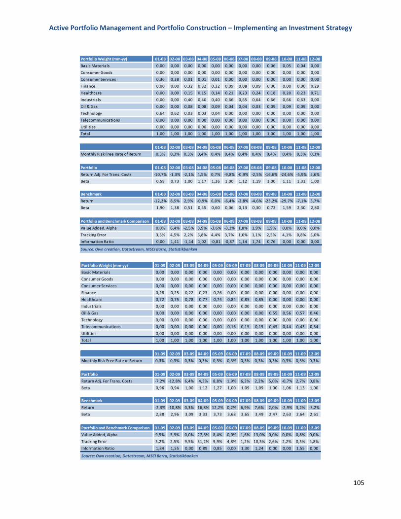
Active Portfolio Management and Portfolio Construction – Implementing an Investment Strategy
105
Portfolio Weight (mm-yy) 01-08 02-08 03-08 04-08 05-08 06-08 07-08 08-08 09-08 10-08 11-08 12-08
Basic Materials 0,00 0,00 0,00 0,00 0,00 0,00 0,00 0,00 0,06 0,05 0,04 0,00
Consumer Goods 0,00 0,00 0,00 0,00 0,00 0,00 0,00 0,00 0,00 0,00 0,00 0,00
Consumer Services 0,36 0,38 0,01 0,01 0,01 0,00 0,00 0,00 0,00 0,00 0,00 0,00
Finance 0,00 0,00 0,32 0,32 0,32 0,09 0,08 0,09 0,00 0,00 0,00 0,29
Healthcare 0,00 0,00 0,15 0,15 0,14 0,21 0,23 0,24 0,18 0,20 0,23 0,71
Industrials 0,00 0,00 0,40 0,40 0,40 0,66 0,65 0,64 0,66 0,66 0,63 0,00
Oil & Gas 0,00 0,00 0,08 0,08 0,09 0,04 0,04 0,03 0,09 0,09 0,09 0,00
Technology 0,64 0,62 0,03 0,03 0,04 0,00 0,00 0,00 0,00 0,00 0,00 0,00
Telecommunications 0,00 0,00 0,00 0,00 0,00 0,00 0,00 0,00 0,00 0,00 0,00 0,00
Utilities 0,00 0,00 0,00 0,00 0,00 0,00 0,00 0,00 0,00 0,00 0,00 0,00
Total 1,00 1,00 1,00 1,00 1,00 1,00 1,00 1,00 1,00 1,00 1,00 1,00
01-08 02-08 03-08 04-08 05-08 06-08 07-08 08-08 09-08 10-08 11-08 12-08
Monthly Risk Free Rate of Return 0,3% 0,3% 0,3% 0,4% 0,4% 0,4% 0,4% 0,4% 0,4% 0,4% 0,3% 0,3%
Portfolio 01-08 02-08 03-08 04-08 05-08 06-08 07-08 08-08 09-08 10-08 11-08 12-08
Return Adj. For Trans. Costs -10,7% -1,3% -2,1% 4,5% 0,7% -9,8% -0,9% -2,5% -16,6% -24,6% -5,9% 5,6%
Beta 0,59 0,73 1,00 1,17 1,26 1,00 1,12 1,19 1,00 1,11 1,31 1,00
Benchmark 01-08 02-08 03-08 04-08 05-08 06-08 07-08 08-08 09-08 10-08 11-08 12-08
Return -12,2% 8,5% 2,9% -0,9% 6,0% -6,4% -2,8% -4,6% -23,2% -29,7% -7,1% 3,7%
Beta 1,90 1,38 0,51 0,45 0,60 0,06 0,13 0,30 0,72 1,59 2,30 2,80
Portfolio and Benchmark Comparison 01-08 02-08 03-08 04-08 05-08 06-08 07-08 08-08 09-08 10-08 11-08 12-08
Value Added, Alpha 0,0% 6,4% -2,5% 3,9% -3,6% -3,2% 1,8% 1,9% 1,9% 0,0% 0,0% 0,0%
Tracking Error 3,3% 4,5% 2,2% 3,8% 4,4% 3,7% 1,6% 1,1% 2,5% 4,1% 0,8% 5,0%
Information Ratio 0,00 1,41 -1,14 1,02 -0,81 -0,87 1,14 1,74 0,76 0,00 0,00 0,00
Source: Own creation, Datastream, MSCI Barra, Statistikbanken
Portfolio Weight (mm-yy) 01-09 02-09 03-09 04-09 05-09 06-09 07-09 08-09 09-09 10-09 11-09 12-09
Basic Materials 0,00 0,00 0,00 0,00 0,00 0,00 0,00 0,00 0,00 0,00 0,00 0,00
Consumer Goods 0,00 0,00 0,00 0,00 0,00 0,00 0,00 0,00 0,00 0,00 0,00 0,00
Consumer Services 0,00 0,00 0,00 0,00 0,00 0,00 0,00 0,00 0,00 0,00 0,00 0,00
Finance 0,28 0,25 0,22 0,23 0,26 0,00 0,00 0,00 0,00 0,00 0,00 0,00
Healthcare 0,72 0,75 0,78 0,77 0,74 0,84 0,85 0,85 0,00 0,00 0,00 0,00
Industrials 0,00 0,00 0,00 0,00 0,00 0,00 0,00 0,00 0,00 0,00 0,00 0,00
Oil & Gas 0,00 0,00 0,00 0,00 0,00 0,00 0,00 0,00 0,55 0,56 0,57 0,46
Technology 0,00 0,00 0,00 0,00 0,00 0,00 0,00 0,00 0,00 0,00 0,00 0,00
Telecommunications 0,00 0,00 0,00 0,00 0,00 0,16 0,15 0,15 0,45 0,44 0,43 0,54
Utilities 0,00 0,00 0,00 0,00 0,00 0,00 0,00 0,00 0,00 0,00 0,00 0,00
Total 1,00 1,00 1,00 1,00 1,00 1,00 1,00 1,00 1,00 1,00 1,00 1,00
01-09 02-09 03-09 04-09 05-09 06-09 07-09 08-09 09-09 10-09 11-09 12-09
Monthly Risk Free Rate of Return 0,3% 0,3% 0,3% 0,3% 0,3% 0,3% 0,3% 0,3% 0,3% 0,3% 0,3% 0,3%
Portfolio 01-09 02-09 03-09 04-09 05-09 06-09 07-09 08-09 09-09 10-09 11-09 12-09
Return Adj. For Trans. Costs -7,2% -12,8% 6,4% 4,3% 8,8% 1,9% 6,3% 2,2% 5,0% -0,7% 2,7% 0,8%
Beta 0,96 0,94 1,00 1,12 1,27 1,00 1,09 1,09 1,00 1,06 1,13 1,00
Benchmark 01-09 02-09 03-09 04-09 05-09 06-09 07-09 08-09 09-09 10-09 11-09 12-09
Return -2,3% -10,8% 0,3% 16,8% 12,2% 0,2% 6,9% 7,6% 2,0% -2,9% 3,2% -3,2%
Beta 2,88 2,96 3,09 3,33 3,73 3,68 3,65 3,49 2,47 2,63 2,64 2,61
Portfolio and Benchmark Comparison 01-09 02-09 03-09 04-09 05-09 06-09 07-09 08-09 09-09 10-09 11-09 12-09
Value Added, Alpha 9,5% 3,9% 0,0% 27,6% 8,4% 0,0% 1,6% 13,0% 0,0% 0,0% 0,8% 0,0%
Tracking Error 5,2% 2,5% 9,5% 31,2% 9,9% 4,8% 1,2% 10,5% 2,6% 2,2% 0,5% 4,8%
Information Ratio 1,84 1,55 0,00 0,89 0,85 0,00 1,30 1,24 0,00 0,00 1,55 0,00
Source: Own creation, Datastream, MSCI Barra, Statistikbanken
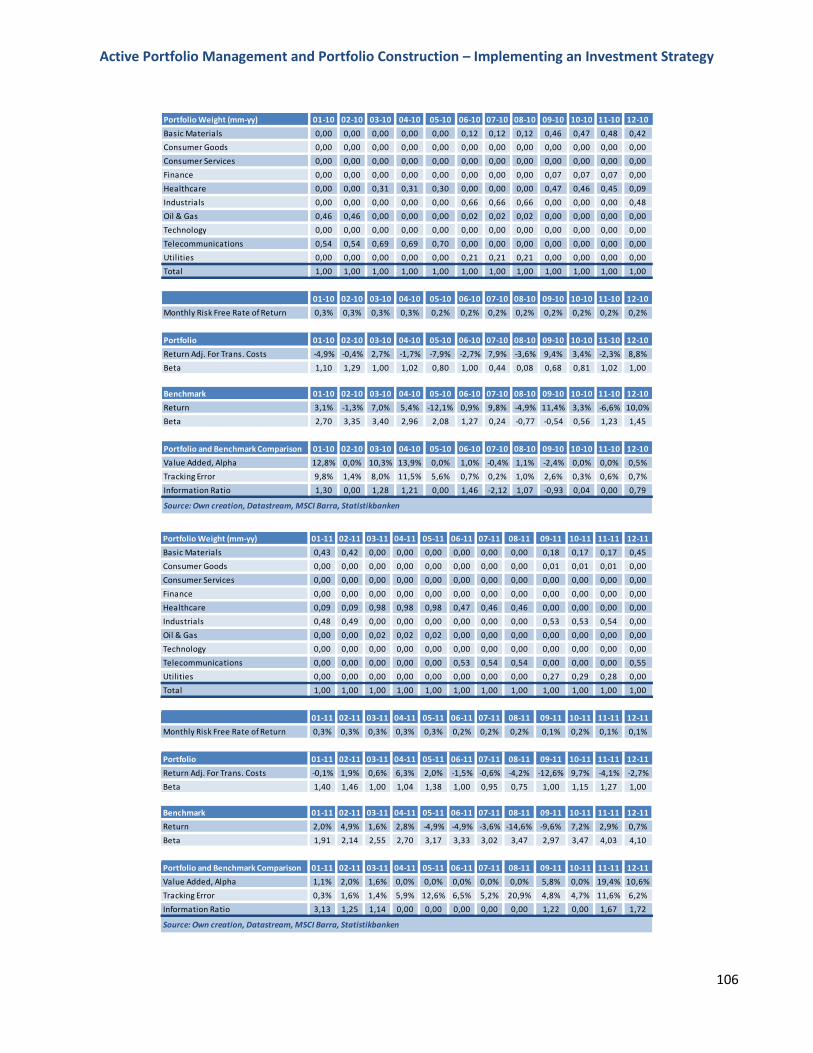
Active Portfolio Management and Portfolio Construction – Implementing an Investment Strategy
106
Portfolio Weight (mm-yy) 01-10 02-10 03-10 04-10 05-10 06-10 07-10 08-10 09-10 10-10 11-10 12-10
Basic Materials 0,00 0,00 0,00 0,00 0,00 0,12 0,12 0,12 0,46 0,47 0,48 0,42
Consumer Goods 0,00 0,00 0,00 0,00 0,00 0,00 0,00 0,00 0,00 0,00 0,00 0,00
Consumer Services 0,00 0,00 0,00 0,00 0,00 0,00 0,00 0,00 0,00 0,00 0,00 0,00
Finance 0,00 0,00 0,00 0,00 0,00 0,00 0,00 0,00 0,07 0,07 0,07 0,00
Healthcare 0,00 0,00 0,31 0,31 0,30 0,00 0,00 0,00 0,47 0,46 0,45 0,09
Industrials 0,00 0,00 0,00 0,00 0,00 0,66 0,66 0,66 0,00 0,00 0,00 0,48
Oil & Gas 0,46 0,46 0,00 0,00 0,00 0,02 0,02 0,02 0,00 0,00 0,00 0,00
Technology 0,00 0,00 0,00 0,00 0,00 0,00 0,00 0,00 0,00 0,00 0,00 0,00
Telecommunications 0,54 0,54 0,69 0,69 0,70 0,00 0,00 0,00 0,00 0,00 0,00 0,00
Utilities 0,00 0,00 0,00 0,00 0,00 0,21 0,21 0,21 0,00 0,00 0,00 0,00
Total 1,00 1,00 1,00 1,00 1,00 1,00 1,00 1,00 1,00 1,00 1,00 1,00
01-10 02-10 03-10 04-10 05-10 06-10 07-10 08-10 09-10 10-10 11-10 12-10
Monthly Risk Free Rate of Return 0,3% 0,3% 0,3% 0,3% 0,2% 0,2% 0,2% 0,2% 0,2% 0,2% 0,2% 0,2%
Portfolio 01-10 02-10 03-10 04-10 05-10 06-10 07-10 08-10 09-10 10-10 11-10 12-10
Return Adj. For Trans. Costs -4,9% -0,4% 2,7% -1,7% -7,9% -2,7% 7,9% -3,6% 9,4% 3,4% -2,3% 8,8%
Beta 1,10 1,29 1,00 1,02 0,80 1,00 0,44 0,08 0,68 0,81 1,02 1,00
Benchmark 01-10 02-10 03-10 04-10 05-10 06-10 07-10 08-10 09-10 10-10 11-10 12-10
Return 3,1% -1,3% 7,0% 5,4% -12,1% 0,9% 9,8% -4,9% 11,4% 3,3% -6,6% 10,0%
Beta 2,70 3,35 3,40 2,96 2,08 1,27 0,24 -0,77 -0,54 0,56 1,23 1,45
Portfolio and Benchmark Comparison 01-10 02-10 03-10 04-10 05-10 06-10 07-10 08-10 09-10 10-10 11-10 12-10
Value Added, Alpha 12,8% 0,0% 10,3% 13,9% 0,0% 1,0% -0,4% 1,1% -2,4% 0,0% 0,0% 0,5%
Tracking Error 9,8% 1,4% 8,0% 11,5% 5,6% 0,7% 0,2% 1,0% 2,6% 0,3% 0,6% 0,7%
Information Ratio 1,30 0,00 1,28 1,21 0,00 1,46 -2,12 1,07 -0,93 0,04 0,00 0,79
Source: Own creation, Datastream, MSCI Barra, Statistikbanken
Portfolio Weight (mm-yy) 01-11 02-11 03-11 04-11 05-11 06-11 07-11 08-11 09-11 10-11 11-11 12-11
Basic Materials 0,43 0,42 0,00 0,00 0,00 0,00 0,00 0,00 0,18 0,17 0,17 0,45
Consumer Goods 0,00 0,00 0,00 0,00 0,00 0,00 0,00 0,00 0,01 0,01 0,01 0,00
Consumer Services 0,00 0,00 0,00 0,00 0,00 0,00 0,00 0,00 0,00 0,00 0,00 0,00
Finance 0,00 0,00 0,00 0,00 0,00 0,00 0,00 0,00 0,00 0,00 0,00 0,00
Healthcare 0,09 0,09 0,98 0,98 0,98 0,47 0,46 0,46 0,00 0,00 0,00 0,00
Industrials 0,48 0,49 0,00 0,00 0,00 0,00 0,00 0,00 0,53 0,53 0,54 0,00
Oil & Gas 0,00 0,00 0,02 0,02 0,02 0,00 0,00 0,00 0,00 0,00 0,00 0,00
Technology 0,00 0,00 0,00 0,00 0,00 0,00 0,00 0,00 0,00 0,00 0,00 0,00
Telecommunications 0,00 0,00 0,00 0,00 0,00 0,53 0,54 0,54 0,00 0,00 0,00 0,55
Utilities 0,00 0,00 0,00 0,00 0,00 0,00 0,00 0,00 0,27 0,29 0,28 0,00
Total 1,00 1,00 1,00 1,00 1,00 1,00 1,00 1,00 1,00 1,00 1,00 1,00
01-11 02-11 03-11 04-11 05-11 06-11 07-11 08-11 09-11 10-11 11-11 12-11
Monthly Risk Free Rate of Return 0,3% 0,3% 0,3% 0,3% 0,3% 0,2% 0,2% 0,2% 0,1% 0,2% 0,1% 0,1%
Portfolio 01-11 02-11 03-11 04-11 05-11 06-11 07-11 08-11 09-11 10-11 11-11 12-11
Return Adj. For Trans. Costs -0,1% 1,9% 0,6% 6,3% 2,0% -1,5% -0,6% -4,2% -12,6% 9,7% -4,1% -2,7%
Beta 1,40 1,46 1,00 1,04 1,38 1,00 0,95 0,75 1,00 1,15 1,27 1,00
Benchmark 01-11 02-11 03-11 04-11 05-11 06-11 07-11 08-11 09-11 10-11 11-11 12-11
Return 2,0% 4,9% 1,6% 2,8% -4,9% -4,9% -3,6% -14,6% -9,6% 7,2% 2,9% 0,7%
Beta 1,91 2,14 2,55 2,70 3,17 3,33 3,02 3,47 2,97 3,47 4,03 4,10
Portfolio and Benchmark Comparison 01-11 02-11 03-11 04-11 05-11 06-11 07-11 08-11 09-11 10-11 11-11 12-11
Value Added, Alpha 1,1% 2,0% 1,6% 0,0% 0,0% 0,0% 0,0% 0,0% 5,8% 0,0% 19,4% 10,6%
Tracking Error 0,3% 1,6% 1,4% 5,9% 12,6% 6,5% 5,2% 20,9% 4,8% 4,7% 11,6% 6,2%
Information Ratio 3,13 1,25 1,14 0,00 0,00 0,00 0,00 0,00 1,22 0,00 1,67 1,72
Source: Own creation, Datastream, MSCI Barra, Statistikbanken
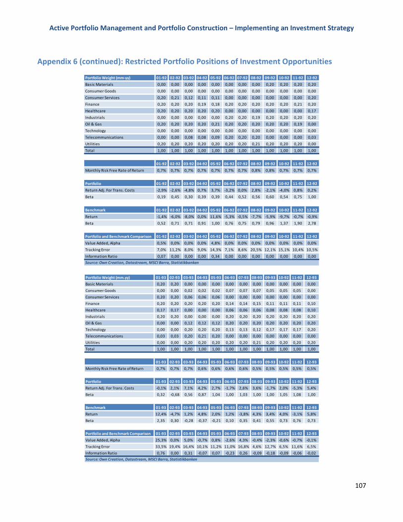
Active Portfolio Management and Portfolio Construction – Implementing an Investment Strategy
107
Appendix 6 (continued): Restricted Portfolio Positions of Investment Opportunities
Portfolio Weight (mm-yy) 01-92 02-92 03-92 04-92 05-92 06-92 07-92 08-92 09-92 10-92 11-92 12-92
Basic Materials 0,00 0,00 0,00 0,00 0,00 0,00 0,00 0,00 0,20 0,20 0,20 0,20
Consumer Goods 0,00 0,00 0,00 0,00 0,00 0,00 0,00 0,00 0,00 0,00 0,00 0,00
Consumer Services 0,20 0,21 0,12 0,11 0,11 0,00 0,00 0,00 0,00 0,00 0,00 0,20
Finance 0,20 0,20 0,20 0,19 0,18 0,20 0,20 0,20 0,20 0,20 0,21 0,20
Healthcare 0,20 0,20 0,20 0,20 0,20 0,00 0,00 0,00 0,00 0,00 0,00 0,17
Industrials 0,00 0,00 0,00 0,00 0,00 0,20 0,20 0,19 0,20 0,20 0,20 0,20
Oil & Gas 0,20 0,20 0,20 0,20 0,21 0,20 0,20 0,20 0,20 0,20 0,19 0,00
Technology 0,00 0,00 0,00 0,00 0,00 0,00 0,00 0,00 0,00 0,00 0,00 0,00
Telecommunications 0,00 0,00 0,08 0,08 0,09 0,20 0,20 0,20 0,00 0,00 0,00 0,03
Utilities 0,20 0,20 0,20 0,20 0,20 0,20 0,20 0,21 0,20 0,20 0,20 0,00
Total 1,00 1,00 1,00 1,00 1,00 1,00 1,00 1,00 1,00 1,00 1,00 1,00
01-92 02-92 03-92 04-92 05-92 06-92 07-92 08-92 09-92 10-92 11-92 12-92
Monthly Risk Free Rate of Return 0,7% 0,7% 0,7% 0,7% 0,7% 0,7% 0,7% 0,8% 0,8% 0,7% 0,7% 0,7%
Portfolio 01-92 02-92 03-92 04-92 05-92 06-92 07-92 08-92 09-92 10-92 11-92 12-92
Return Adj. For Trans. Costs -2,9% -2,6% -4,8% 0,7% 3,7% -3,2% 0,0% 2,8% -2,1% -4,0% 0,8% 0,2%
Beta 0,19 0,45 0,30 0,39 0,39 0,44 0,52 0,56 0,60 0,54 0,75 1,00
Benchmark 01-92 02-92 03-92 04-92 05-92 06-92 07-92 08-92 09-92 10-92 11-92 12-92
Return -1,4% -6,0% -8,0% 0,0% 11,6% -5,3% -0,5% -7,7% -5,9% -9,7% -0,7% -0,9%
Beta 0,52 0,71 0,71 0,91 1,00 0,76 0,75 0,79 0,96 1,37 1,90 2,78
Portfolio and Benchmark Comparison 01-92 02-92 03-92 04-92 05-92 06-92 07-92 08-92 09-92 10-92 11-92 12-92
Value Added, Alpha 0,5% 0,0% 0,0% 0,0% 4,8% 0,0% 0,0% 0,0% 0,0% 0,0% 0,0% 0,0%
Tracking Error 7,0% 11,2% 8,0% 9,0% 14,3% 7,1% 8,6% 20,5% 12,1% 15,1% 10,4% 10,5%
Information Ratio 0,07 0,00 0,00 0,00 0,34 0,00 0,00 0,00 0,00 0,00 0,00 0,00
Source: Own Creation, Datastream, MSCI Barra, Statistikbanken
Portfolio Weight (mm.yy) 01-93 02-93 03-93 04-93 05-93 06-93 07-93 08-93 09-93 10-92 11-92 12-93
Basic Materials 0,20 0,20 0,00 0,00 0,00 0,00 0,00 0,00 0,00 0,00 0,00 0,00
Consumer Goods 0,00 0,00 0,02 0,02 0,02 0,07 0,07 0,07 0,05 0,05 0,05 0,00
Consumer Services 0,20 0,20 0,06 0,06 0,06 0,00 0,00 0,00 0,00 0,00 0,00 0,00
Finance 0,20 0,20 0,20 0,20 0,20 0,14 0,14 0,15 0,11 0,11 0,11 0,10
Healthcare 0,17 0,17 0,00 0,00 0,00 0,06 0,06 0,06 0,08 0,08 0,08 0,10
Industrials 0,20 0,20 0,00 0,00 0,00 0,20 0,20 0,20 0,20 0,20 0,20 0,20
Oil & Gas 0,00 0,00 0,12 0,12 0,12 0,20 0,20 0,20 0,20 0,20 0,20 0,20
Technology 0,00 0,00 0,20 0,20 0,20 0,13 0,13 0,12 0,17 0,17 0,17 0,20
Telecommunications 0,03 0,03 0,20 0,21 0,20 0,00 0,00 0,00 0,00 0,00 0,00 0,00
Utilities 0,00 0,00 0,20 0,20 0,20 0,20 0,20 0,21 0,20 0,20 0,20 0,20
Total 1,00 1,00 1,00 1,00 1,00 1,00 1,00 1,00 1,00 1,00 1,00 1,00
01-93 02-93 03-93 04-93 05-93 06-93 07-93 08-93 09-93 10-92 11-92 12-93
Monthly Risk Free Rate of Return 0,7% 0,7% 0,7% 0,6% 0,6% 0,6% 0,6% 0,5% 0,5% 0,5% 0,5% 0,5%
Portfolio 01-93 02-93 03-93 04-93 05-93 06-93 07-93 08-93 09-93 10-92 11-92 12-93
Return Adj. For Trans. Costs -0,1% 2,1% 7,1% 4,2% 2,7% -1,7% 2,6% 3,6% -1,7% 2,0% -5,3% 5,4%
Beta 0,32 -0,68 0,56 0,87 1,04 1,00 1,03 1,00 1,00 1,05 1,08 1,00
Benchmark 01-93 02-93 03-93 04-93 05-93 06-93 07-93 08-93 09-93 10-92 11-92 12-93
Return 12,4% -4,7% 1,2% 4,8% 2,0% 1,2% -3,8% 4,3% 3,4% 4,0% -3,1% 5,8%
Beta 2,35 0,30 -0,28 -0,37 -0,21 0,10 0,35 0,41 0,55 0,73 0,76 0,73
Portfolio and Benchmark Comparison 01-93 02-93 03-93 04-93 05-93 06-93 07-93 08-93 09-93 10-92 11-92 12-93
Value Added, Alpha 25,3% 0,0% 5,0% -0,7% 0,8% -2,6% 4,3% -0,4% -2,3% -0,6% -0,7% -0,1%
Tracking Error 33,5% 19,4% 16,4% 10,1% 11,2% 11,0% 16,8% 4,6% 12,7% 6,5% 11,6% 6,5%
Information Ratio 0,76 0,00 0,31 -0,07 0,07 -0,23 0,26 -0,09 -0,18 -0,09 -0,06 -0,02
Source: Own Creation, Datastream, MSCI Barra, Statistikbanken
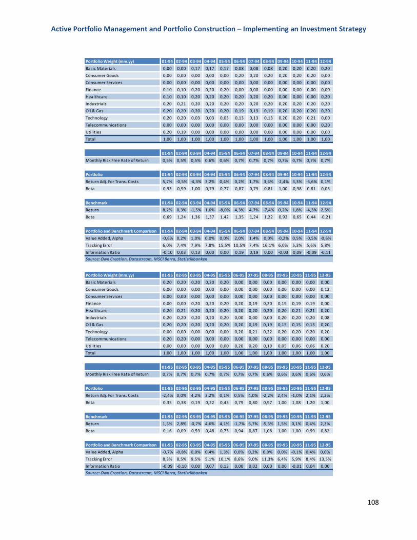
Active Portfolio Management and Portfolio Construction – Implementing an Investment Strategy
108
Portfolio Weight (mm.yy) 01-94 02-94 03-94 04-94 05-94 06-94 07-94 08-94 09-94 10-94 11-94 12-94
Basic Materials 0,00 0,00 0,17 0,17 0,17 0,08 0,08 0,08 0,20 0,20 0,20 0,20
Consumer Goods 0,00 0,00 0,00 0,00 0,00 0,20 0,20 0,20 0,20 0,20 0,20 0,00
Consumer Services 0,00 0,00 0,00 0,00 0,00 0,00 0,00 0,00 0,00 0,00 0,00 0,00
Finance 0,10 0,10 0,20 0,20 0,20 0,00 0,00 0,00 0,00 0,00 0,00 0,00
Healthcare 0,10 0,10 0,20 0,20 0,20 0,20 0,20 0,20 0,00 0,00 0,00 0,20
Industrials 0,20 0,21 0,20 0,20 0,20 0,20 0,20 0,20 0,20 0,20 0,20 0,20
Oil & Gas 0,20 0,20 0,20 0,20 0,20 0,19 0,19 0,19 0,20 0,20 0,20 0,20
Technology 0,20 0,20 0,03 0,03 0,03 0,13 0,13 0,13 0,20 0,20 0,21 0,00
Telecommunications 0,00 0,00 0,00 0,00 0,00 0,00 0,00 0,00 0,00 0,00 0,00 0,20
Utilities 0,20 0,19 0,00 0,00 0,00 0,00 0,00 0,00 0,00 0,00 0,00 0,00
Total 1,00 1,00 1,00 1,00 1,00 1,00 1,00 1,00 1,00 1,00 1,00 1,00
01-94 02-94 03-94 04-94 05-94 06-94 07-94 08-94 09-94 10-94 11-94 12-94
Monthly Risk Free Rate of Return 0,5% 0,5% 0,5% 0,6% 0,6% 0,7% 0,7% 0,7% 0,7% 0,7% 0,7% 0,7%
Portfolio 01-94 02-94 03-94 04-94 05-94 06-94 07-94 08-94 09-94 10-94 11-94 12-94
Return Adj. For Trans. Costs 5,7% -0,5% -4,3% 3,2% 0,4% 0,2% 1,7% 3,4% -2,4% 3,3% -5,6% 0,1%
Beta 0,93 0,99 1,00 0,79 0,77 0,87 0,79 0,81 1,00 0,98 0,81 0,05
Benchmark 01-94 02-94 03-94 04-94 05-94 06-94 07-94 08-94 09-94 10-94 11-94 12-94
Return 8,2% 0,3% -1,5% 1,6% -8,0% 4,3% 4,7% -7,4% 0,2% 1,8% -4,3% 2,5%
Beta 0,69 1,24 1,36 1,37 1,42 1,35 1,24 1,22 0,92 0,65 0,44 -0,21
Portfolio and Benchmark Comparison 01-94 02-94 03-94 04-94 05-94 06-94 07-94 08-94 09-94 10-94 11-94 12-94
Value Added, Alpha -0,6% 0,2% 1,0% 0,0% 0,0% 2,0% 1,4% 0,0% -0,2% 0,5% -0,5% -0,6%
Tracking Error 6,0% 7,4% 7,9% 7,8% 15,5% 10,5% 7,4% 16,1% 6,0% 5,3% 5,6% 5,8%
Information Ratio -0,10 0,03 0,13 0,00 0,00 0,19 0,19 0,00 -0,03 0,09 -0,09 -0,11
Source: Own Creation, Datastream, MSCI Barra, Statistikbanken
Portfolio Weight (mm.yy) 01-95 02-95 03-95 04-95 05-95 06-95 07-95 08-95 09-95 10-95 11-95 12-95
Basic Materials 0,20 0,20 0,20 0,20 0,20 0,00 0,00 0,00 0,00 0,00 0,00 0,00
Consumer Goods 0,00 0,00 0,00 0,00 0,00 0,00 0,00 0,00 0,00 0,00 0,00 0,12
Consumer Services 0,00 0,00 0,00 0,00 0,00 0,00 0,00 0,00 0,00 0,00 0,00 0,00
Finance 0,00 0,00 0,20 0,20 0,20 0,20 0,19 0,20 0,19 0,19 0,19 0,00
Healthcare 0,20 0,21 0,20 0,20 0,20 0,20 0,20 0,20 0,20 0,21 0,21 0,20
Industrials 0,20 0,20 0,20 0,20 0,20 0,00 0,00 0,00 0,20 0,20 0,20 0,08
Oil & Gas 0,20 0,20 0,20 0,20 0,20 0,20 0,19 0,19 0,15 0,15 0,15 0,20
Technology 0,00 0,00 0,00 0,00 0,00 0,20 0,21 0,22 0,20 0,20 0,20 0,20
Telecommunications 0,20 0,20 0,00 0,00 0,00 0,00 0,00 0,00 0,00 0,00 0,00 0,00
Utilities 0,00 0,00 0,00 0,00 0,00 0,20 0,20 0,19 0,05 0,06 0,06 0,20
Total 1,00 1,00 1,00 1,00 1,00 1,00 1,00 1,00 1,00 1,00 1,00 1,00
01-95 02-95 03-95 04-95 05-95 06-95 07-95 08-95 09-95 10-95 11-95 12-95
Monthly Risk Free Rate of Return 0,7% 0,7% 0,7% 0,7% 0,7% 0,7% 0,7% 0,6% 0,6% 0,6% 0,6% 0,6%
Portfolio 01-95 02-95 03-95 04-95 05-95 06-95 07-95 08-95 09-95 10-95 11-95 12-95
Return Adj. For Trans. Costs -2,4% 0,0% 4,2% 3,2% 0,1% 0,5% 4,0% -2,2% 2,4% -1,0% 2,1% 2,2%
Beta 0,35 0,38 0,19 0,22 0,43 0,79 0,80 0,97 1,00 1,08 1,20 1,00
Benchmark 01-95 02-95 03-95 04-95 05-95 06-95 07-95 08-95 09-95 10-95 11-95 12-95
Return 1,3% 2,8% -0,7% 4,6% 4,1% -1,7% 6,7% -5,5% 1,5% 0,1% 0,4% 2,3%
Beta 0,16 0,09 0,59 0,48 0,75 0,94 0,87 1,08 1,00 1,00 0,99 0,82
Portfolio and Benchmark Comparison 01-95 02-95 03-95 04-95 05-95 06-95 07-95 08-95 09-95 10-95 11-95 12-95
Value Added, Alpha -0,7% -0,8% 0,0% 0,4% 1,3% 0,0% 0,2% 0,0% 0,0% -0,1% 0,4% 0,0%
Tracking Error 8,3% 8,5% 9,5% 5,1% 10,1% 8,6% 9,0% 11,3% 6,4% 5,9% 8,4% 13,5%
Information Ratio -0,09 -0,10 0,00 0,07 0,13 0,00 0,02 0,00 0,00 -0,01 0,04 0,00
Source: Own Creation, Datastream, MSCI Barra, Statistikbanken
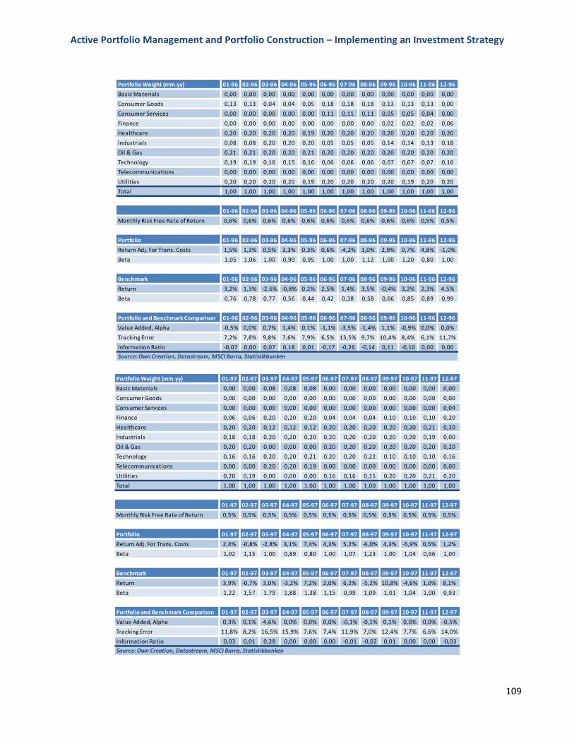
Active Portfolio Management and Portfolio Construction – Implementing an Investment Strategy
109
Portfolio Weight (mm.yy) 01-96 02-96 03-96 04-96 05-96 06-96 07-96 08-96 09-96 10-96 11-96 12-96
Basic Materials 0,00 0,00 0,00 0,00 0,00 0,00 0,00 0,00 0,00 0,00 0,00 0,00
Consumer Goods 0,13 0,13 0,04 0,04 0,05 0,18 0,18 0,18 0,13 0,13 0,13 0,00
Consumer Services 0,00 0,00 0,00 0,00 0,00 0,11 0,11 0,11 0,05 0,05 0,04 0,00
Finance 0,00 0,00 0,00 0,00 0,00 0,00 0,00 0,00 0,02 0,02 0,02 0,06
Healthcare 0,20 0,20 0,20 0,20 0,19 0,20 0,20 0,20 0,20 0,20 0,20 0,20
Industrials 0,08 0,08 0,20 0,20 0,20 0,05 0,05 0,05 0,14 0,14 0,13 0,18
Oil & Gas 0,21 0,21 0,20 0,20 0,21 0,20 0,20 0,20 0,20 0,20 0,20 0,20
Technology 0,19 0,19 0,16 0,15 0,16 0,06 0,06 0,06 0,07 0,07 0,07 0,16
Telecommunications 0,00 0,00 0,00 0,00 0,00 0,00 0,00 0,00 0,00 0,00 0,00 0,00
Utilities 0,20 0,20 0,20 0,20 0,19 0,20 0,20 0,20 0,20 0,19 0,20 0,20
Total 1,00 1,00 1,00 1,00 1,00 1,00 1,00 1,00 1,00 1,00 1,00 1,00
01-96 02-96 03-96 04-96 05-96 06-96 07-96 08-96 09-96 10-96 11-96 12-96
Monthly Risk Free Rate of Return 0,6% 0,6% 0,6% 0,6% 0,6% 0,6% 0,6% 0,6% 0,6% 0,6% 0,5% 0,5%
Portfolio 01-96 02-96 03-96 04-96 05-96 06-96 07-96 08-96 09-96 10-96 11-96 12-96
Return Adj. For Trans. Costs 1,5% 1,3% 0,5% 3,3% 0,3% 0,6% -4,2% 1,0% 2,9% 0,7% 4,8% -1,0%
Beta 1,05 1,06 1,00 0,90 0,95 1,00 1,00 1,12 1,00 1,20 0,80 1,00
Benchmark 01-96 02-96 03-96 04-96 05-96 06-96 07-96 08-96 09-96 10-96 11-96 12-96
Return 3,2% 1,3% -2,6% -0,8% 0,2% 2,5% 1,4% 3,5% -0,4% 3,2% 2,3% 4,5%
Beta 0,76 0,78 0,77 0,56 0,44 0,42 0,38 0,58 0,66 0,85 0,89 0,99
Portfolio and Benchmark Comparison 01-96 02-96 03-96 04-96 05-96 06-96 07-96 08-96 09-96 10-96 11-96 12-96
Value Added, Alpha -0,5% 0,0% 0,7% 1,4% 0,1% -1,1% -3,5% -1,4% 1,1% -0,9% 0,0% 0,0%
Tracking Error 7,2% 7,8% 9,8% 7,6% 7,9% 6,5% 13,5% 9,7% 10,4% 8,4% 6,1% 11,7%
Information Ratio -0,07 0,00 0,07 0,18 0,01 -0,17 -0,26 -0,14 0,11 -0,10 0,00 0,00
Source: Own Creation, Datastream, MSCI Barra, Statistikbanken
Portfolio Weight (mm.yy) 01-97 02-97 03-97 04-97 05-97 06-97 07-97 08-97 09-97 10-97 11-97 12-97
Basic Materials 0,00 0,00 0,08 0,08 0,08 0,00 0,00 0,00 0,00 0,00 0,00 0,00
Consumer Goods 0,00 0,00 0,00 0,00 0,00 0,00 0,00 0,00 0,00 0,00 0,00 0,00
Consumer Services 0,00 0,00 0,00 0,00 0,00 0,00 0,00 0,00 0,00 0,00 0,00 0,04
Finance 0,06 0,06 0,20 0,20 0,20 0,04 0,04 0,04 0,10 0,10 0,10 0,20
Healthcare 0,20 0,20 0,12 0,12 0,12 0,20 0,20 0,20 0,20 0,20 0,21 0,20
Industrials 0,18 0,18 0,20 0,20 0,20 0,20 0,20 0,20 0,20 0,20 0,19 0,00
Oil & Gas 0,20 0,20 0,00 0,00 0,00 0,20 0,20 0,20 0,20 0,20 0,20 0,20
Technology 0,16 0,16 0,20 0,20 0,21 0,20 0,20 0,22 0,10 0,10 0,10 0,16
Telecommunications 0,00 0,00 0,20 0,20 0,19 0,00 0,00 0,00 0,00 0,00 0,00 0,00
Utilities 0,20 0,19 0,00 0,00 0,00 0,16 0,16 0,15 0,20 0,20 0,21 0,20
Total 1,00 1,00 1,00 1,00 1,00 1,00 1,00 1,00 1,00 1,00 1,00 1,00
01-97 02-97 03-97 04-97 05-97 06-97 07-97 08-97 09-97 10-97 11-97 12-97
Monthly Risk Free Rate of Return 0,5% 0,5% 0,5% 0,5% 0,5% 0,5% 0,5% 0,5% 0,5% 0,5% 0,5% 0,5%
Portfolio 01-97 02-97 03-97 04-97 05-97 06-97 07-97 08-97 09-97 10-97 11-97 12-97
Return Adj. For Trans. Costs 2,4% -0,8% -2,8% 3,1% 7,4% 4,3% 5,2% -6,0% 4,3% -5,9% 0,5% 1,2%
Beta 1,02 1,15 1,00 0,89 0,80 1,00 1,07 1,23 1,00 1,04 0,96 1,00
Benchmark 01-97 02-97 03-97 04-97 05-97 06-97 07-97 08-97 09-97 10-97 11-97 12-97
Return 3,9% -0,7% 3,0% -3,2% 7,2% 2,0% 6,2% -5,2% 10,8% -4,6% 1,0% 8,1%
Beta 1,22 1,57 1,79 1,88 1,38 1,15 0,99 1,09 1,01 1,04 1,00 0,93
Portfolio and Benchmark Comparison 01-97 02-97 03-97 04-97 05-97 06-97 07-97 08-97 09-97 10-97 11-97 12-97
Value Added, Alpha 0,3% 0,1% 4,6% 0,0% 0,0% 0,0% -0,1% -0,1% 0,1% 0,0% 0,0% -0,5%
Tracking Error 11,8% 8,2% 16,5% 15,9% 7,6% 7,4% 11,9% 7,0% 12,4% 7,7% 6,6% 14,0%
Information Ratio 0,03 0,01 0,28 0,00 0,00 0,00 -0,01 -0,02 0,01 0,00 0,00 -0,03
Source: Own Creation, Datastream, MSCI Barra, Statistikbanken
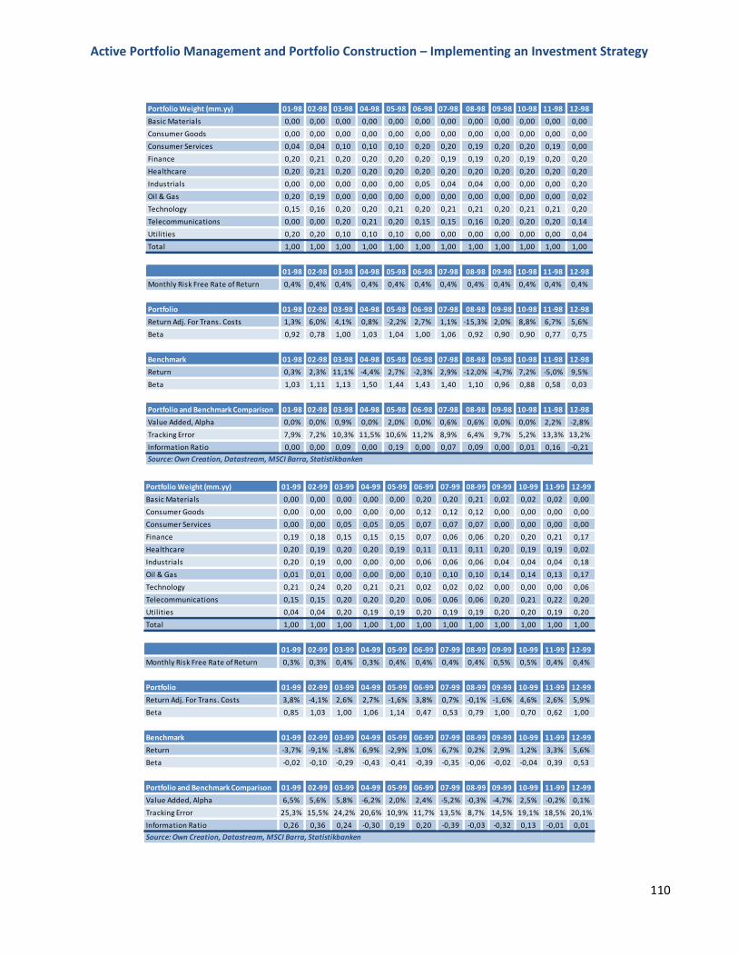
Active Portfolio Management and Portfolio Construction – Implementing an Investment Strategy
110
Portfolio Weight (mm.yy) 01-98 02-98 03-98 04-98 05-98 06-98 07-98 08-98 09-98 10-98 11-98 12-98
Basic Materials 0,00 0,00 0,00 0,00 0,00 0,00 0,00 0,00 0,00 0,00 0,00 0,00
Consumer Goods 0,00 0,00 0,00 0,00 0,00 0,00 0,00 0,00 0,00 0,00 0,00 0,00
Consumer Services 0,04 0,04 0,10 0,10 0,10 0,20 0,20 0,19 0,20 0,20 0,19 0,00
Finance 0,20 0,21 0,20 0,20 0,20 0,20 0,19 0,19 0,20 0,19 0,20 0,20
Healthcare 0,20 0,21 0,20 0,20 0,20 0,20 0,20 0,20 0,20 0,20 0,20 0,20
Industrials 0,00 0,00 0,00 0,00 0,00 0,05 0,04 0,04 0,00 0,00 0,00 0,20
Oil & Gas 0,20 0,19 0,00 0,00 0,00 0,00 0,00 0,00 0,00 0,00 0,00 0,02
Technology 0,15 0,16 0,20 0,20 0,21 0,20 0,21 0,21 0,20 0,21 0,21 0,20
Telecommunications 0,00 0,00 0,20 0,21 0,20 0,15 0,15 0,16 0,20 0,20 0,20 0,14
Utilities 0,20 0,20 0,10 0,10 0,10 0,00 0,00 0,00 0,00 0,00 0,00 0,04
Total 1,00 1,00 1,00 1,00 1,00 1,00 1,00 1,00 1,00 1,00 1,00 1,00
01-98 02-98 03-98 04-98 05-98 06-98 07-98 08-98 09-98 10-98 11-98 12-98
Monthly Risk Free Rate of Return 0,4% 0,4% 0,4% 0,4% 0,4% 0,4% 0,4% 0,4% 0,4% 0,4% 0,4% 0,4%
Portfolio 01-98 02-98 03-98 04-98 05-98 06-98 07-98 08-98 09-98 10-98 11-98 12-98
Return Adj. For Trans. Costs 1,3% 6,0% 4,1% 0,8% -2,2% 2,7% 1,1% -15,3% 2,0% 8,8% 6,7% 5,6%
Beta 0,92 0,78 1,00 1,03 1,04 1,00 1,06 0,92 0,90 0,90 0,77 0,75
Benchmark 01-98 02-98 03-98 04-98 05-98 06-98 07-98 08-98 09-98 10-98 11-98 12-98
Return 0,3% 2,3% 11,1% -4,4% 2,7% -2,3% 2,9% -12,0% -4,7% 7,2% -5,0% 9,5%
Beta 1,03 1,11 1,13 1,50 1,44 1,43 1,40 1,10 0,96 0,88 0,58 0,03
Portfolio and Benchmark Comparison 01-98 02-98 03-98 04-98 05-98 06-98 07-98 08-98 09-98 10-98 11-98 12-98
Value Added, Alpha 0,0% 0,0% 0,9% 0,0% 2,0% 0,0% 0,6% 0,6% 0,0% 0,0% 2,2% -2,8%
Tracking Error 7,9% 7,2% 10,3% 11,5% 10,6% 11,2% 8,9% 6,4% 9,7% 5,2% 13,3% 13,2%
Information Ratio 0,00 0,00 0,09 0,00 0,19 0,00 0,07 0,09 0,00 0,01 0,16 -0,21
Source: Own Creation, Datastream, MSCI Barra, Statistikbanken
Portfolio Weight (mm.yy) 01-99 02-99 03-99 04-99 05-99 06-99 07-99 08-99 09-99 10-99 11-99 12-99
Basic Materials 0,00 0,00 0,00 0,00 0,00 0,20 0,20 0,21 0,02 0,02 0,02 0,00
Consumer Goods 0,00 0,00 0,00 0,00 0,00 0,12 0,12 0,12 0,00 0,00 0,00 0,00
Consumer Services 0,00 0,00 0,05 0,05 0,05 0,07 0,07 0,07 0,00 0,00 0,00 0,00
Finance 0,19 0,18 0,15 0,15 0,15 0,07 0,06 0,06 0,20 0,20 0,21 0,17
Healthcare 0,20 0,19 0,20 0,20 0,19 0,11 0,11 0,11 0,20 0,19 0,19 0,02
Industrials 0,20 0,19 0,00 0,00 0,00 0,06 0,06 0,06 0,04 0,04 0,04 0,18
Oil & Gas 0,01 0,01 0,00 0,00 0,00 0,10 0,10 0,10 0,14 0,14 0,13 0,17
Technology 0,21 0,24 0,20 0,21 0,21 0,02 0,02 0,02 0,00 0,00 0,00 0,06
Telecommunications 0,15 0,15 0,20 0,20 0,20 0,06 0,06 0,06 0,20 0,21 0,22 0,20
Utilities 0,04 0,04 0,20 0,19 0,19 0,20 0,19 0,19 0,20 0,20 0,19 0,20
Total 1,00 1,00 1,00 1,00 1,00 1,00 1,00 1,00 1,00 1,00 1,00 1,00
01-99 02-99 03-99 04-99 05-99 06-99 07-99 08-99 09-99 10-99 11-99 12-99
Monthly Risk Free Rate of Return 0,3% 0,3% 0,4% 0,3% 0,4% 0,4% 0,4% 0,4% 0,5% 0,5% 0,4% 0,4%
Portfolio 01-99 02-99 03-99 04-99 05-99 06-99 07-99 08-99 09-99 10-99 11-99 12-99
Return Adj. For Trans. Costs 3,8% -4,1% 2,6% 2,7% -1,6% 3,8% 0,7% -0,1% -1,6% 4,6% 2,6% 5,9%
Beta 0,85 1,03 1,00 1,06 1,14 0,47 0,53 0,79 1,00 0,70 0,62 1,00
Benchmark 01-99 02-99 03-99 04-99 05-99 06-99 07-99 08-99 09-99 10-99 11-99 12-99
Return -3,7% -9,1% -1,8% 6,9% -2,9% 1,0% 6,7% 0,2% 2,9% 1,2% 3,3% 5,6%
Beta -0,02 -0,10 -0,29 -0,43 -0,41 -0,39 -0,35 -0,06 -0,02 -0,04 0,39 0,53
Portfolio and Benchmark Comparison 01-99 02-99 03-99 04-99 05-99 06-99 07-99 08-99 09-99 10-99 11-99 12-99
Value Added, Alpha 6,5% 5,6% 5,8% -6,2% 2,0% 2,4% -5,2% -0,3% -4,7% 2,5% -0,2% 0,1%
Tracking Error 25,3% 15,5% 24,2% 20,6% 10,9% 11,7% 13,5% 8,7% 14,5% 19,1% 18,5% 20,1%
Information Ratio 0,26 0,36 0,24 -0,30 0,19 0,20 -0,39 -0,03 -0,32 0,13 -0,01 0,01
Source: Own Creation, Datastream, MSCI Barra, Statistikbanken

Active Portfolio Management and Portfolio Construction – Implementing an Investment Strategy
111
Portfolio Weight (mm.yy) 01-00 02-00 03-00 04-00 05-00 06-00 07-00 08-00 09-00 10-00 11-00 12-00
Basic Materials 0,00 0,00 0,00 0,00 0,00 0,00 0,00 0,00 0,00 0,00 0,00 0,00
Consumer Goods 0,00 0,00 0,00 0,00 0,00 0,00 0,00 0,00 0,00 0,00 0,00 0,00
Consumer Services 0,00 0,00 0,04 0,04 0,04 0,07 0,07 0,07 0,00 0,00 0,00 0,00
Finance 0,16 0,16 0,15 0,15 0,15 0,16 0,16 0,17 0,20 0,21 0,21 0,06
Healthcare 0,02 0,02 0,04 0,04 0,04 0,00 0,00 0,00 0,00 0,00 0,00 0,20
Industrials 0,19 0,19 0,20 0,20 0,20 0,20 0,20 0,20 0,05 0,05 0,05 0,20
Oil & Gas 0,17 0,16 0,14 0,14 0,15 0,13 0,13 0,13 0,19 0,19 0,19 0,10
Technology 0,07 0,07 0,03 0,03 0,03 0,03 0,04 0,03 0,17 0,14 0,13 0,20
Telecommunications 0,21 0,21 0,20 0,19 0,17 0,20 0,20 0,19 0,20 0,19 0,20 0,04
Utilities 0,19 0,19 0,20 0,20 0,21 0,20 0,20 0,20 0,20 0,22 0,22 0,20
Total 1,00 1,00 1,00 1,00 1,00 1,00 1,00 1,00 1,00 1,00 1,00 1,00
01-00 02-00 03-00 04-00 05-00 06-00 07-00 08-00 09-00 10-00 11-00 12-00
Monthly Risk Free Rate of Return 0,5% 0,5% 0,5% 0,5% 0,5% 0,5% 0,5% 0,5% 0,5% 0,5% 0,4% 0,4%
Portfolio 01-00 02-00 03-00 04-00 05-00 06-00 07-00 08-00 09-00 10-00 11-00 12-00
Return Adj. For Trans. Costs -4,1% 0,3% 5,7% -5,1% -0,9% 1,4% -2,7% 3,7% -4,3% -3,4% -7,5% 1,4%
Beta 1,27 1,40 1,00 1,01 0,99 1,00 0,99 0,84 1,00 0,31 0,46 1,00
Benchmark 01-00 02-00 03-00 04-00 05-00 06-00 07-00 08-00 09-00 10-00 11-00 12-00
Return -5,6% 3,5% 8,8% -9,6% 6,5% -0,2% 2,0% 5,6% -2,0% -4,7% -5,1% 3,6%
Beta 0,84 1,09 1,00 1,06 1,10 1,06 0,90 0,88 0,22 -0,64 -0,57 -0,18
Portfolio and Benchmark Comparison 01-00 02-00 03-00 04-00 05-00 06-00 07-00 08-00 09-00 10-00 11-00 12-00
Value Added, Alpha 0,7% -1,0% 0,0% 0,0% 0,8% 0,0% -0,4% 0,1% -1,8% 1,2% -2,4% -2,6%
Tracking Error 10,7% 22,3% 17,5% 18,6% 25,8% 16,0% 19,4% 16,5% 33,1% 16,8% 28,8% 37,1%
Information Ratio 0,06 -0,04 0,00 0,00 0,03 0,00 -0,02 0,00 -0,05 0,07 -0,08 -0,07
Source: Own Creation, Datastream, MSCI Barra, Statistikbanken
Portfolio Weight (mm.yy) 01-01 02-01 03-01 04-01 05-01 06-01 07-01 08-01 09-01 10-01 11-01 12-01
Basic Materials 0,00 0,00 0,00 0,00 0,00 0,00 0,00 0,00 0,00 0,00 0,00 0,00
Consumer Goods 0,00 0,00 0,00 0,00 0,00 0,00 0,00 0,00 0,00 0,00 0,00 0,00
Consumer Services 0,00 0,00 0,07 0,07 0,07 0,09 0,09 0,09 0,09 0,09 0,09 0,07
Finance 0,06 0,06 0,20 0,20 0,19 0,20 0,21 0,21 0,20 0,20 0,19 0,20
Healthcare 0,20 0,19 0,00 0,00 0,00 0,00 0,00 0,00 0,01 0,01 0,01 0,00
Industrials 0,20 0,20 0,04 0,03 0,04 0,06 0,06 0,06 0,01 0,01 0,01 0,15
Oil & Gas 0,10 0,10 0,20 0,20 0,21 0,17 0,16 0,17 0,18 0,18 0,18 0,12
Technology 0,18 0,20 0,10 0,09 0,10 0,08 0,08 0,08 0,12 0,10 0,11 0,06
Telecommunications 0,04 0,04 0,20 0,20 0,20 0,20 0,20 0,20 0,20 0,22 0,21 0,20
Utilities 0,21 0,20 0,20 0,21 0,20 0,20 0,20 0,20 0,20 0,20 0,20 0,20
Total 1,00 1,00 1,00 1,00 1,00 1,00 1,00 1,00 1,00 1,00 1,00 1,00
01-01 02-01 03-01 04-01 05-01 06-01 07-01 08-01 09-01 10-01 11-01 12-01
Monthly Risk Free Rate of Return 0,4% 0,4% 0,4% 0,4% 0,4% 0,4% 0,4% 0,4% 0,4% 0,4% 0,4% 0,4%
Portfolio 01-01 02-01 03-01 04-01 05-01 06-01 07-01 08-01 09-01 10-01 11-01 12-01
Return Adj. For Trans. Costs 0,2% -8,8% -6,4% 7,4% -2,4% -4,4% -2,8% -4,8% -9,3% 1,7% 3,3% 1,4%
Beta 1,06 1,21 1,00 0,97 1,00 1,00 0,98 1,07 1,00 0,96 0,97 1,00
Benchmark 01-01 02-01 03-01 04-01 05-01 06-01 07-01 08-01 09-01 10-01 11-01 12-01
Return 11,1% -9,5% -10,6% 1,9% -0,2% -1,7% 3,4% -5,6% -9,2% 2,0% 1,1% 0,1%
Beta -0,14 -0,37 -0,12 0,01 0,20 0,35 0,50 0,61 0,54 0,65 0,71 0,88
Portfolio and Benchmark Comparison 01-01 02-01 03-01 04-01 05-01 06-01 07-01 08-01 09-01 10-01 11-01 12-01
Value Added, Alpha -13,1% 1,0% 4,7% 5,3% -1,8% -1,7% -3,0% 0,4% 0,0% -0,1% 0,6% 0,2%
Tracking Error 25,4% 55,1% 17,0% 29,3% 20,4% 13,1% 24,6% 20,3% 25,7% 22,5% 22,0% 6,3%
Information Ratio -0,52 0,02 0,28 0,18 -0,09 -0,13 -0,12 0,02 0,00 0,00 0,03 0,02
Source: Own Creation, Datastream, MSCI Barra, Statistikbanken
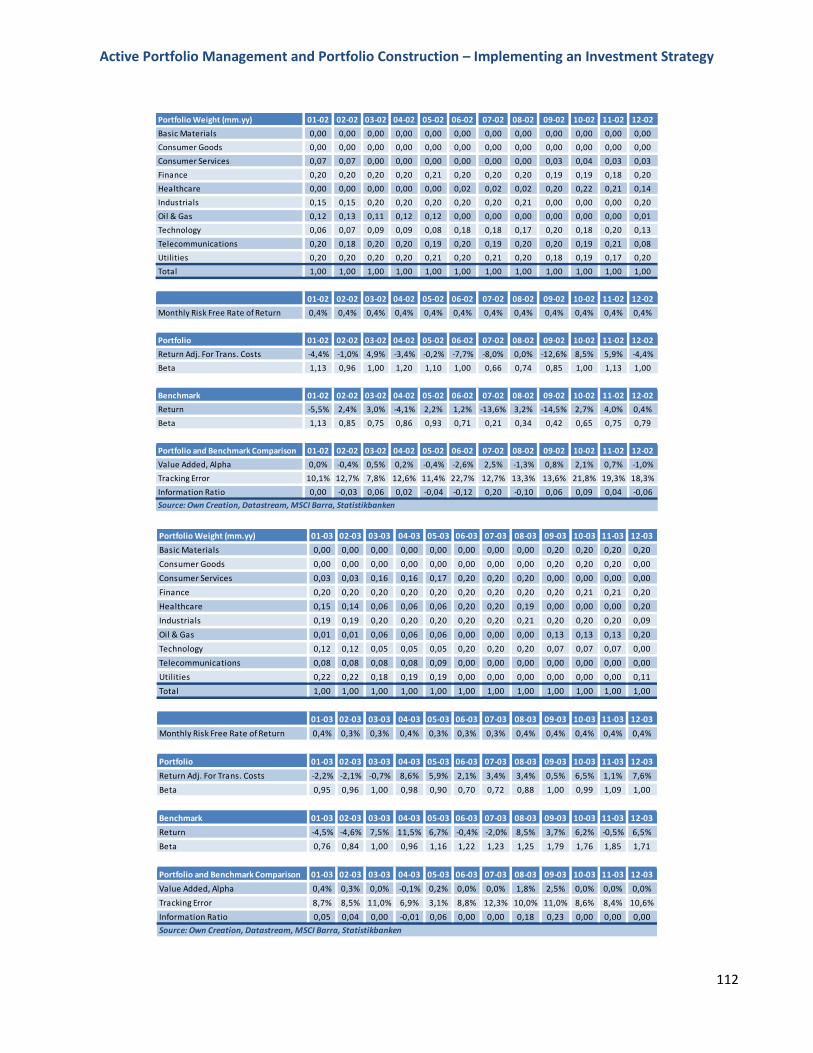
Active Portfolio Management and Portfolio Construction – Implementing an Investment Strategy
112
Portfolio Weight (mm.yy) 01-02 02-02 03-02 04-02 05-02 06-02 07-02 08-02 09-02 10-02 11-02 12-02
Basic Materials 0,00 0,00 0,00 0,00 0,00 0,00 0,00 0,00 0,00 0,00 0,00 0,00
Consumer Goods 0,00 0,00 0,00 0,00 0,00 0,00 0,00 0,00 0,00 0,00 0,00 0,00
Consumer Services 0,07 0,07 0,00 0,00 0,00 0,00 0,00 0,00 0,03 0,04 0,03 0,03
Finance 0,20 0,20 0,20 0,20 0,21 0,20 0,20 0,20 0,19 0,19 0,18 0,20
Healthcare 0,00 0,00 0,00 0,00 0,00 0,02 0,02 0,02 0,20 0,22 0,21 0,14
Industrials 0,15 0,15 0,20 0,20 0,20 0,20 0,20 0,21 0,00 0,00 0,00 0,20
Oil & Gas 0,12 0,13 0,11 0,12 0,12 0,00 0,00 0,00 0,00 0,00 0,00 0,01
Technology 0,06 0,07 0,09 0,09 0,08 0,18 0,18 0,17 0,20 0,18 0,20 0,13
Telecommunications 0,20 0,18 0,20 0,20 0,19 0,20 0,19 0,20 0,20 0,19 0,21 0,08
Utilities 0,20 0,20 0,20 0,20 0,21 0,20 0,21 0,20 0,18 0,19 0,17 0,20
Total 1,00 1,00 1,00 1,00 1,00 1,00 1,00 1,00 1,00 1,00 1,00 1,00
01-02 02-02 03-02 04-02 05-02 06-02 07-02 08-02 09-02 10-02 11-02 12-02
Monthly Risk Free Rate of Return 0,4% 0,4% 0,4% 0,4% 0,4% 0,4% 0,4% 0,4% 0,4% 0,4% 0,4% 0,4%
Portfolio 01-02 02-02 03-02 04-02 05-02 06-02 07-02 08-02 09-02 10-02 11-02 12-02
Return Adj. For Trans. Costs -4,4% -1,0% 4,9% -3,4% -0,2% -7,7% -8,0% 0,0% -12,6% 8,5% 5,9% -4,4%
Beta 1,13 0,96 1,00 1,20 1,10 1,00 0,66 0,74 0,85 1,00 1,13 1,00
Benchmark 01-02 02-02 03-02 04-02 05-02 06-02 07-02 08-02 09-02 10-02 11-02 12-02
Return -5,5% 2,4% 3,0% -4,1% 2,2% 1,2% -13,6% 3,2% -14,5% 2,7% 4,0% 0,4%
Beta 1,13 0,85 0,75 0,86 0,93 0,71 0,21 0,34 0,42 0,65 0,75 0,79
Portfolio and Benchmark Comparison 01-02 02-02 03-02 04-02 05-02 06-02 07-02 08-02 09-02 10-02 11-02 12-02
Value Added, Alpha 0,0% -0,4% 0,5% 0,2% -0,4% -2,6% 2,5% -1,3% 0,8% 2,1% 0,7% -1,0%
Tracking Error 10,1% 12,7% 7,8% 12,6% 11,4% 22,7% 12,7% 13,3% 13,6% 21,8% 19,3% 18,3%
Information Ratio 0,00 -0,03 0,06 0,02 -0,04 -0,12 0,20 -0,10 0,06 0,09 0,04 -0,06
Source: Own Creation, Datastream, MSCI Barra, Statistikbanken
Portfolio Weight (mm.yy) 01-03 02-03 03-03 04-03 05-03 06-03 07-03 08-03 09-03 10-03 11-03 12-03
Basic Materials 0,00 0,00 0,00 0,00 0,00 0,00 0,00 0,00 0,20 0,20 0,20 0,20
Consumer Goods 0,00 0,00 0,00 0,00 0,00 0,00 0,00 0,00 0,20 0,20 0,20 0,00
Consumer Services 0,03 0,03 0,16 0,16 0,17 0,20 0,20 0,20 0,00 0,00 0,00 0,00
Finance 0,20 0,20 0,20 0,20 0,20 0,20 0,20 0,20 0,20 0,21 0,21 0,20
Healthcare 0,15 0,14 0,06 0,06 0,06 0,20 0,20 0,19 0,00 0,00 0,00 0,20
Industrials 0,19 0,19 0,20 0,20 0,20 0,20 0,20 0,21 0,20 0,20 0,20 0,09
Oil & Gas 0,01 0,01 0,06 0,06 0,06 0,00 0,00 0,00 0,13 0,13 0,13 0,20
Technology 0,12 0,12 0,05 0,05 0,05 0,20 0,20 0,20 0,07 0,07 0,07 0,00
Telecommunications 0,08 0,08 0,08 0,08 0,09 0,00 0,00 0,00 0,00 0,00 0,00 0,00
Utilities 0,22 0,22 0,18 0,19 0,19 0,00 0,00 0,00 0,00 0,00 0,00 0,11
Total 1,00 1,00 1,00 1,00 1,00 1,00 1,00 1,00 1,00 1,00 1,00 1,00
01-03 02-03 03-03 04-03 05-03 06-03 07-03 08-03 09-03 10-03 11-03 12-03
Monthly Risk Free Rate of Return 0,4% 0,3% 0,3% 0,4% 0,3% 0,3% 0,3% 0,4% 0,4% 0,4% 0,4% 0,4%
Portfolio 01-03 02-03 03-03 04-03 05-03 06-03 07-03 08-03 09-03 10-03 11-03 12-03
Return Adj. For Trans. Costs -2,2% -2,1% -0,7% 8,6% 5,9% 2,1% 3,4% 3,4% 0,5% 6,5% 1,1% 7,6%
Beta 0,95 0,96 1,00 0,98 0,90 0,70 0,72 0,88 1,00 0,99 1,09 1,00
Benchmark 01-03 02-03 03-03 04-03 05-03 06-03 07-03 08-03 09-03 10-03 11-03 12-03
Return -4,5% -4,6% 7,5% 11,5% 6,7% -0,4% -2,0% 8,5% 3,7% 6,2% -0,5% 6,5%
Beta 0,76 0,84 1,00 0,96 1,16 1,22 1,23 1,25 1,79 1,76 1,85 1,71
Portfolio and Benchmark Comparison 01-03 02-03 03-03 04-03 05-03 06-03 07-03 08-03 09-03 10-03 11-03 12-03
Value Added, Alpha 0,4% 0,3% 0,0% -0,1% 0,2% 0,0% 0,0% 1,8% 2,5% 0,0% 0,0% 0,0%
Tracking Error 8,7% 8,5% 11,0% 6,9% 3,1% 8,8% 12,3% 10,0% 11,0% 8,6% 8,4% 10,6%
Information Ratio 0,05 0,04 0,00 -0,01 0,06 0,00 0,00 0,18 0,23 0,00 0,00 0,00
Source: Own Creation, Datastream, MSCI Barra, Statistikbanken
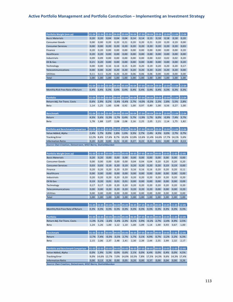
Active Portfolio Management and Portfolio Construction – Implementing an Investment Strategy
113
Portfolio Weight (mm.yy) 01-04 02-04 03-04 04-04 05-04 06-04 07-04 08-04 09-04 10-04 11-04 12-04
Basic Materials 0,20 0,20 0,04 0,04 0,04 0,14 0,14 0,15 0,18 0,18 0,18 0,20
Consumer Goods 0,00 0,00 0,20 0,20 0,21 0,20 0,20 0,21 0,20 0,20 0,19 0,00
Consumer Services 0,00 0,00 0,20 0,20 0,20 0,20 0,20 0,20 0,20 0,20 0,20 0,03
Finance 0,20 0,20 0,00 0,00 0,00 0,00 0,00 0,00 0,00 0,00 0,00 0,20
Healthcare 0,20 0,20 0,00 0,00 0,00 0,00 0,00 0,00 0,00 0,00 0,00 0,00
Industrials 0,09 0,09 0,00 0,00 0,00 0,00 0,00 0,00 0,02 0,02 0,02 0,20
Oil & Gas 0,21 0,20 0,00 0,00 0,00 0,00 0,00 0,00 0,00 0,00 0,00 0,20
Technology 0,00 0,00 0,16 0,16 0,15 0,20 0,20 0,19 0,20 0,20 0,20 0,17
Telecommunications 0,00 0,00 0,20 0,20 0,20 0,20 0,20 0,20 0,20 0,20 0,20 0,00
Utilities 0,11 0,11 0,20 0,20 0,20 0,06 0,06 0,06 0,00 0,00 0,00 0,00
Total 1,00 1,00 1,00 1,00 1,00 1,00 1,00 1,00 1,00 1,00 1,00 1,00
01-04 02-04 03-04 04-04 05-04 06-04 07-04 08-04 09-04 10-04 11-04 12-04
Monthly Risk Free Rate of Return 0,4% 0,4% 0,3% 0,4% 0,4% 0,4% 0,4% 0,4% 0,4% 0,3% 0,3% 0,3%
Portfolio 01-04 02-04 03-04 04-04 05-04 06-04 07-04 08-04 09-04 10-04 11-04 12-04
Return Adj. For Trans. Costs 0,6% 2,9% 0,2% -3,4% -0,4% 2,7% -4,0% -0,3% 2,3% 2,8% 5,5% 2,8%
Beta 1,14 1,25 1,00 0,98 0,92 1,00 0,97 0,89 1,00 0,56 0,27 1,00
Benchmark 01-04 02-04 03-04 04-04 05-04 06-04 07-04 08-04 09-04 10-04 11-04 12-04
Return 4,5% 5,6% -5,3% -1,7% 0,4% 5,7% -1,9% 1,7% 6,0% -0,9% 7,4% 3,7%
Beta 1,78 1,88 2,07 2,08 2,08 2,16 2,25 2,05 2,21 2,14 1,75 1,82
Portfolio and Benchmark Comparison 01-04 02-04 03-04 04-04 05-04 06-04 07-04 08-04 09-04 10-04 11-04 12-04
Value Added, Alpha 2,4% 1,7% 0,0% 1,8% 1,0% 3,5% 2,7% 2,4% 4,5% 0,0% 2,7% 0,7%
Tracking Error 12,2% 8,6% 17,6% 8,7% 10,0% 12,8% 12,6% 11,4% 14,6% 17,7% 14,1% 5,6%
Information Ratio 0,20 0,20 0,00 0,21 0,10 0,27 0,22 0,21 0,31 0,00 0,19 0,13
Source: Own Creation, Datastream, MSCI Barra, Statistikbanken
Portfolio Weight (mm.yy) 01-05 02-05 03-05 04-05 05-05 06-05 07-05 08-05 09-05 10-05 11-05 12-05
Basic Materials 0,20 0,20 0,00 0,00 0,00 0,00 0,00 0,00 0,00 0,00 0,00 0,00
Consumer Goods 0,00 0,00 0,00 0,00 0,00 0,04 0,04 0,04 0,20 0,20 0,20 0,20
Consumer Services 0,03 0,03 0,19 0,20 0,19 0,20 0,20 0,20 0,20 0,19 0,19 0,00
Finance 0,20 0,20 0,20 0,20 0,20 0,16 0,16 0,16 0,20 0,20 0,20 0,11
Healthcare 0,00 0,00 0,00 0,00 0,00 0,00 0,00 0,00 0,00 0,00 0,00 0,00
Industrials 0,20 0,20 0,20 0,20 0,20 0,20 0,20 0,20 0,20 0,20 0,20 0,20
Oil & Gas 0,19 0,20 0,01 0,01 0,01 0,00 0,00 0,00 0,00 0,00 0,00 0,09
Technology 0,17 0,17 0,20 0,20 0,20 0,20 0,20 0,20 0,20 0,20 0,20 0,20
Telecommunications 0,00 0,00 0,20 0,20 0,20 0,20 0,20 0,20 0,00 0,00 0,00 0,20
Utilities 0,00 0,00 0,00 0,00 0,00 0,00 0,00 0,00 0,00 0,00 0,00 0,00
Total 1,00 1,00 1,00 1,00 1,00 1,00 1,00 1,00 1,00 1,00 1,00 1,00
01-05 02-05 03-05 04-05 05-05 06-05 07-05 08-05 09-05 10-05 11-05 12-05
Monthly Risk Free Rate of Return 0,3% 0,3% 0,3% 0,3% 0,3% 0,3% 0,3% 0,3% 0,3% 0,3% 0,3% 0,3%
Portfolio 01-05 02-05 03-05 04-05 05-05 06-05 07-05 08-05 09-05 10-05 11-05 12-05
Return Adj. For Trans. Costs -1,3% 5,1% -2,6% -3,4% 2,3% 0,1% 3,9% -0,1% 2,7% -2,4% 4,9% 2,5%
Beta 1,24 1,26 1,00 1,12 1,10 1,00 1,09 1,14 1,00 0,93 0,67 1,00
Benchmark 01-05 02-05 03-05 04-05 05-05 06-05 07-05 08-05 09-05 10-05 11-05 12-05
Return -2,7% 7,4% -0,3% -3,5% 2,7% 1,7% 3,1% 4,9% 0,7% -2,2% 2,2% 6,3%
Beta 2,15 2,06 2,37 2,48 2,41 2,30 2,39 2,44 2,55 2,99 2,32 2,17
Portfolio and Benchmark Comparison 01-05 02-05 03-05 04-05 05-05 06-05 07-05 08-05 09-05 10-05 11-05 12-05
Value Added, Alpha 0,0% 1,9% 3,3% 0,0% 0,6% 2,1% 0,0% 6,4% 0,0% 0,4% 0,0% 4,5%
Tracking Error 9,0% 14,6% 12,7% 7,0% 14,0% 10,5% 7,8% 17,5% 14,3% 9,6% 14,3% 17,4%
Information Ratio 0,00 0,13 0,26 0,00 0,05 0,20 0,00 0,37 0,00 0,04 0,00 0,26
Source: Own Creation, Datastream, MSCI Barra, Statistikbanken
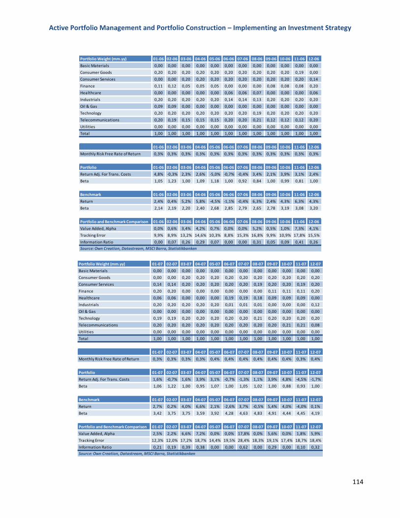
Active Portfolio Management and Portfolio Construction – Implementing an Investment Strategy
114
Portfolio Weight (mm.yy) 01-06 02-06 03-06 04-06 05-06 06-06 07-06 08-06 09-06 10-06 11-06 12-06
Basic Materials 0,00 0,00 0,00 0,00 0,00 0,00 0,00 0,00 0,00 0,00 0,00 0,00
Consumer Goods 0,20 0,20 0,20 0,20 0,20 0,20 0,20 0,20 0,20 0,20 0,19 0,00
Consumer Services 0,00 0,00 0,20 0,20 0,20 0,20 0,20 0,20 0,20 0,20 0,20 0,14
Finance 0,11 0,12 0,05 0,05 0,05 0,00 0,00 0,00 0,08 0,08 0,08 0,20
Healthcare 0,00 0,00 0,00 0,00 0,00 0,06 0,06 0,07 0,00 0,00 0,00 0,06
Industrials 0,20 0,20 0,20 0,20 0,20 0,14 0,14 0,13 0,20 0,20 0,20 0,20
Oil & Gas 0,09 0,09 0,00 0,00 0,00 0,00 0,00 0,00 0,00 0,00 0,00 0,00
Technology 0,20 0,20 0,20 0,20 0,20 0,20 0,20 0,19 0,20 0,20 0,20 0,20
Telecommunications 0,20 0,19 0,15 0,15 0,15 0,20 0,20 0,21 0,12 0,12 0,12 0,20
Utilities 0,00 0,00 0,00 0,00 0,00 0,00 0,00 0,00 0,00 0,00 0,00 0,00
Total 1,00 1,00 1,00 1,00 1,00 1,00 1,00 1,00 1,00 1,00 1,00 1,00
01-06 02-06 03-06 04-06 05-06 06-06 07-06 08-06 09-06 10-06 11-06 12-06
Monthly Risk Free Rate of Return 0,3% 0,3% 0,3% 0,3% 0,3% 0,3% 0,3% 0,3% 0,3% 0,3% 0,3% 0,3%
Portfolio 01-06 02-06 03-06 04-06 05-06 06-06 07-06 08-06 09-06 10-06 11-06 12-06
Return Adj. For Trans. Costs 4,8% -0,3% 2,3% 2,6% -5,0% -0,7% -0,4% 3,4% 2,1% 3,9% 3,1% 2,4%
Beta 1,05 1,23 1,00 1,09 1,18 1,00 0,92 0,84 1,00 0,99 0,81 1,00
Benchmark 01-06 02-06 03-06 04-06 05-06 06-06 07-06 08-06 09-06 10-06 11-06 12-06
Return 2,4% 0,4% 5,2% 5,8% -4,5% -1,1% -0,4% 6,3% 2,4% 4,3% 6,3% 4,3%
Beta 2,14 2,19 2,20 2,40 2,68 2,85 2,79 2,65 2,78 3,19 3,08 3,20
Portfolio and Benchmark Comparison 01-06 02-06 03-06 04-06 05-06 06-06 07-06 08-06 09-06 10-06 11-06 12-06
Value Added, Alpha 0,0% 0,6% 3,4% 4,2% 0,7% 0,0% 0,0% 5,2% 0,5% 1,0% 7,3% 4,1%
Tracking Error 9,9% 8,9% 13,2% 14,6% 10,3% 8,8% 15,3% 16,8% 9,9% 10,9% 17,8% 15,5%
Information Ratio 0,00 0,07 0,26 0,29 0,07 0,00 0,00 0,31 0,05 0,09 0,41 0,26
Source: Own Creation, Datastream, MSCI Barra, Statistikbanken
Portfolio Weight (mm.yy) 01-07 02-07 03-07 04-07 05-07 06-07 07-07 08-07 09-07 10-07 11-07 12-07
Basic Materials 0,00 0,00 0,00 0,00 0,00 0,00 0,00 0,00 0,00 0,00 0,00 0,00
Consumer Goods 0,00 0,00 0,20 0,20 0,20 0,20 0,20 0,20 0,20 0,20 0,20 0,20
Consumer Services 0,14 0,14 0,20 0,20 0,20 0,20 0,20 0,19 0,20 0,20 0,19 0,20
Finance 0,20 0,20 0,00 0,00 0,00 0,00 0,00 0,00 0,11 0,11 0,11 0,20
Healthcare 0,06 0,06 0,00 0,00 0,00 0,19 0,19 0,18 0,09 0,09 0,09 0,00
Industrials 0,20 0,20 0,20 0,20 0,20 0,01 0,01 0,01 0,00 0,00 0,00 0,12
Oil & Gas 0,00 0,00 0,00 0,00 0,00 0,00 0,00 0,00 0,00 0,00 0,00 0,00
Technology 0,19 0,19 0,20 0,20 0,20 0,20 0,20 0,21 0,20 0,20 0,20 0,20
Telecommunications 0,20 0,20 0,20 0,20 0,20 0,20 0,20 0,20 0,20 0,21 0,21 0,08
Utilities 0,00 0,00 0,00 0,00 0,00 0,00 0,00 0,00 0,00 0,00 0,00 0,00
Total 1,00 1,00 1,00 1,00 1,00 1,00 1,00 1,00 1,00 1,00 1,00 1,00
01-07 02-07 03-07 04-07 05-07 06-07 07-07 08-07 09-07 10-07 11-07 12-07
Monthly Risk Free Rate of Return 0,3% 0,3% 0,3% 0,3% 0,4% 0,4% 0,4% 0,4% 0,4% 0,4% 0,3% 0,4%
Portfolio 01-07 02-07 03-07 04-07 05-07 06-07 07-07 08-07 09-07 10-07 11-07 12-07
Return Adj. For Trans. Costs 1,6% -0,7% 1,6% 3,9% 3,1% -0,7% -1,3% 1,1% 3,9% 4,8% -4,5% -1,7%
Beta 1,06 1,22 1,00 0,95 1,07 1,00 1,05 1,02 1,00 0,88 0,93 1,00
Benchmark 01-07 02-07 03-07 04-07 05-07 06-07 07-07 08-07 09-07 10-07 11-07 12-07
Return 2,7% 0,2% 4,0% 6,6% 2,1% -2,6% 3,7% -0,5% 5,4% 4,0% -4,0% 0,1%
Beta 3,42 3,75 3,75 3,59 3,92 4,28 4,63 4,83 4,91 4,44 4,45 4,19
Portfolio and Benchmark Comparison 01-07 02-07 03-07 04-07 05-07 06-07 07-07 08-07 09-07 10-07 11-07 12-07
Value Added, Alpha 2,5% 2,2% 6,6% 7,2% 0,0% 0,0% 17,8% 0,0% 5,6% 0,0% 1,8% 5,9%
Tracking Error 12,3% 12,0% 17,2% 18,7% 14,4% 19,5% 28,4% 18,3% 19,1% 17,4% 18,7% 18,4%
Information Ratio 0,21 0,19 0,39 0,38 0,00 0,00 0,62 0,00 0,29 0,00 0,10 0,32
Source: Own Creation, Datastream, MSCI Barra, Statistikbanken
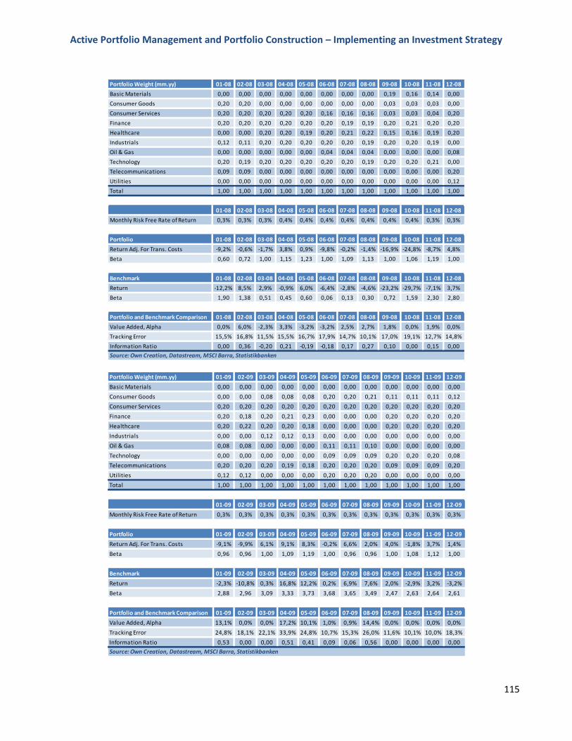
Active Portfolio Management and Portfolio Construction – Implementing an Investment Strategy
115
Portfolio Weight (mm.yy) 01-08 02-08 03-08 04-08 05-08 06-08 07-08 08-08 09-08 10-08 11-08 12-08
Basic Materials 0,00 0,00 0,00 0,00 0,00 0,00 0,00 0,00 0,19 0,16 0,14 0,00
Consumer Goods 0,20 0,20 0,00 0,00 0,00 0,00 0,00 0,00 0,03 0,03 0,03 0,00
Consumer Services 0,20 0,20 0,20 0,20 0,20 0,16 0,16 0,16 0,03 0,03 0,04 0,20
Finance 0,20 0,20 0,20 0,20 0,20 0,20 0,19 0,19 0,20 0,21 0,20 0,20
Healthcare 0,00 0,00 0,20 0,20 0,19 0,20 0,21 0,22 0,15 0,16 0,19 0,20
Industrials 0,12 0,11 0,20 0,20 0,20 0,20 0,20 0,19 0,20 0,20 0,19 0,00
Oil & Gas 0,00 0,00 0,00 0,00 0,00 0,04 0,04 0,04 0,00 0,00 0,00 0,08
Technology 0,20 0,19 0,20 0,20 0,20 0,20 0,20 0,19 0,20 0,20 0,21 0,00
Telecommunications 0,09 0,09 0,00 0,00 0,00 0,00 0,00 0,00 0,00 0,00 0,00 0,20
Utilities 0,00 0,00 0,00 0,00 0,00 0,00 0,00 0,00 0,00 0,00 0,00 0,12
Total 1,00 1,00 1,00 1,00 1,00 1,00 1,00 1,00 1,00 1,00 1,00 1,00
01-08 02-08 03-08 04-08 05-08 06-08 07-08 08-08 09-08 10-08 11-08 12-08
Monthly Risk Free Rate of Return 0,3% 0,3% 0,3% 0,4% 0,4% 0,4% 0,4% 0,4% 0,4% 0,4% 0,3% 0,3%
Portfolio 01-08 02-08 03-08 04-08 05-08 06-08 07-08 08-08 09-08 10-08 11-08 12-08
Return Adj. For Trans. Costs -9,2% -0,6% -1,7% 3,8% 0,9% -9,8% -0,2% -1,4% -16,9% -24,8% -8,7% 4,8%
Beta 0,60 0,72 1,00 1,15 1,23 1,00 1,09 1,13 1,00 1,06 1,19 1,00
Benchmark 01-08 02-08 03-08 04-08 05-08 06-08 07-08 08-08 09-08 10-08 11-08 12-08
Return -12,2% 8,5% 2,9% -0,9% 6,0% -6,4% -2,8% -4,6% -23,2% -29,7% -7,1% 3,7%
Beta 1,90 1,38 0,51 0,45 0,60 0,06 0,13 0,30 0,72 1,59 2,30 2,80
Portfolio and Benchmark Comparison 01-08 02-08 03-08 04-08 05-08 06-08 07-08 08-08 09-08 10-08 11-08 12-08
Value Added, Alpha 0,0% 6,0% -2,3% 3,3% -3,2% -3,2% 2,5% 2,7% 1,8% 0,0% 1,9% 0,0%
Tracking Error 15,5% 16,8% 11,5% 15,5% 16,7% 17,9% 14,7% 10,1% 17,0% 19,1% 12,7% 14,8%
Information Ratio 0,00 0,36 -0,20 0,21 -0,19 -0,18 0,17 0,27 0,10 0,00 0,15 0,00
Source: Own Creation, Datastream, MSCI Barra, Statistikbanken
Portfolio Weight (mm.yy) 01-09 02-09 03-09 04-09 05-09 06-09 07-09 08-09 09-09 10-09 11-09 12-09
Basic Materials 0,00 0,00 0,00 0,00 0,00 0,00 0,00 0,00 0,00 0,00 0,00 0,00
Consumer Goods 0,00 0,00 0,08 0,08 0,08 0,20 0,20 0,21 0,11 0,11 0,11 0,12
Consumer Services 0,20 0,20 0,20 0,20 0,20 0,20 0,20 0,20 0,20 0,20 0,20 0,20
Finance 0,20 0,18 0,20 0,21 0,23 0,00 0,00 0,00 0,20 0,20 0,20 0,20
Healthcare 0,20 0,22 0,20 0,20 0,18 0,00 0,00 0,00 0,20 0,20 0,20 0,20
Industrials 0,00 0,00 0,12 0,12 0,13 0,00 0,00 0,00 0,00 0,00 0,00 0,00
Oil & Gas 0,08 0,08 0,00 0,00 0,00 0,11 0,11 0,10 0,00 0,00 0,00 0,00
Technology 0,00 0,00 0,00 0,00 0,00 0,09 0,09 0,09 0,20 0,20 0,20 0,08
Telecommunications 0,20 0,20 0,20 0,19 0,18 0,20 0,20 0,20 0,09 0,09 0,09 0,20
Utilities 0,12 0,12 0,00 0,00 0,00 0,20 0,20 0,20 0,00 0,00 0,00 0,00
Total 1,00 1,00 1,00 1,00 1,00 1,00 1,00 1,00 1,00 1,00 1,00 1,00
01-09 02-09 03-09 04-09 05-09 06-09 07-09 08-09 09-09 10-09 11-09 12-09
Monthly Risk Free Rate of Return 0,3% 0,3% 0,3% 0,3% 0,3% 0,3% 0,3% 0,3% 0,3% 0,3% 0,3% 0,3%
Portfolio 01-09 02-09 03-09 04-09 05-09 06-09 07-09 08-09 09-09 10-09 11-09 12-09
Return Adj. For Trans. Costs -9,1% -9,9% 6,1% 9,1% 8,3% -0,2% 6,6% 2,0% 4,0% -1,8% 3,7% 1,4%
Beta 0,96 0,96 1,00 1,09 1,19 1,00 0,96 0,96 1,00 1,08 1,12 1,00
Benchmark 01-09 02-09 03-09 04-09 05-09 06-09 07-09 08-09 09-09 10-09 11-09 12-09
Return -2,3% -10,8% 0,3% 16,8% 12,2% 0,2% 6,9% 7,6% 2,0% -2,9% 3,2% -3,2%
Beta 2,88 2,96 3,09 3,33 3,73 3,68 3,65 3,49 2,47 2,63 2,64 2,61
Portfolio and Benchmark Comparison 01-09 02-09 03-09 04-09 05-09 06-09 07-09 08-09 09-09 10-09 11-09 12-09
Value Added, Alpha 13,1% 0,0% 0,0% 17,2% 10,1% 1,0% 0,9% 14,4% 0,0% 0,0% 0,0% 0,0%
Tracking Error 24,8% 18,1% 22,1% 33,9% 24,8% 10,7% 15,3% 26,0% 11,6% 10,1% 10,0% 18,3%
Information Ratio 0,53 0,00 0,00 0,51 0,41 0,09 0,06 0,56 0,00 0,00 0,00 0,00
Source: Own Creation, Datastream, MSCI Barra, Statistikbanken
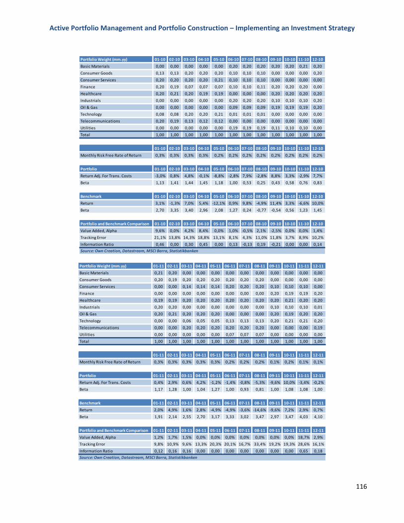
Active Portfolio Management and Portfolio Construction – Implementing an Investment Strategy
116
Portfolio Weight (mm.yy) 01-10 02-10 03-10 04-10 05-10 06-10 07-10 08-10 09-10 10-10 11-10 12-10
Basic Materials 0,00 0,00 0,00 0,00 0,00 0,20 0,20 0,20 0,20 0,20 0,21 0,20
Consumer Goods 0,13 0,13 0,20 0,20 0,20 0,10 0,10 0,10 0,00 0,00 0,00 0,20
Consumer Services 0,20 0,20 0,20 0,20 0,21 0,10 0,10 0,10 0,00 0,00 0,00 0,00
Finance 0,20 0,19 0,07 0,07 0,07 0,10 0,10 0,11 0,20 0,20 0,20 0,00
Healthcare 0,20 0,21 0,20 0,19 0,19 0,00 0,00 0,00 0,20 0,20 0,20 0,20
Industrials 0,00 0,00 0,00 0,00 0,00 0,20 0,20 0,20 0,10 0,10 0,10 0,20
Oil & Gas 0,00 0,00 0,00 0,00 0,00 0,09 0,09 0,09 0,19 0,19 0,19 0,20
Technology 0,08 0,08 0,20 0,20 0,21 0,01 0,01 0,01 0,00 0,00 0,00 0,00
Telecommunications 0,20 0,19 0,13 0,12 0,12 0,00 0,00 0,00 0,00 0,00 0,00 0,00
Utilities 0,00 0,00 0,00 0,00 0,00 0,19 0,19 0,19 0,11 0,10 0,10 0,00
Total 1,00 1,00 1,00 1,00 1,00 1,00 1,00 1,00 1,00 1,00 1,00 1,00
01-10 02-10 03-10 04-10 05-10 06-10 07-10 08-10 09-10 10-10 11-10 12-10
Monthly Risk Free Rate of Return 0,3% 0,3% 0,3% 0,3% 0,2% 0,2% 0,2% 0,2% 0,2% 0,2% 0,2% 0,2%
Portfolio 01-10 02-10 03-10 04-10 05-10 06-10 07-10 08-10 09-10 10-10 11-10 12-10
Return Adj. For Trans. Costs -3,0% 0,8% 4,8% -0,1% -8,8% -2,8% 7,9% -2,8% 8,8% 3,3% -2,9% 7,7%
Beta 1,13 1,41 1,44 1,45 1,18 1,00 0,53 0,25 0,43 0,58 0,76 0,83
Benchmark 01-10 02-10 03-10 04-10 05-10 06-10 07-10 08-10 09-10 10-10 11-10 12-10
Return 3,1% -1,3% 7,0% 5,4% -12,1% 0,9% 9,8% -4,9% 11,4% 3,3% -6,6% 10,0%
Beta 2,70 3,35 3,40 2,96 2,08 1,27 0,24 -0,77 -0,54 0,56 1,23 1,45
Portfolio and Benchmark Comparison 01-10 02-10 03-10 04-10 05-10 06-10 07-10 08-10 09-10 10-10 11-10 12-10
Value Added, Alpha 9,6% 0,0% 4,2% 8,4% 0,0% 1,0% -0,5% 2,1% -2,5% 0,0% 0,0% 1,4%
Tracking Error 21,1% 13,8% 14,3% 18,8% 13,1% 8,1% 4,3% 11,0% 11,8% 3,7% 8,9% 10,2%
Information Ratio 0,46 0,00 0,30 0,45 0,00 0,13 -0,13 0,19 -0,21 0,00 0,00 0,14
Source: Own Creation, Datastream, MSCI Barra, Statistikbanken
Portfolio Weight (mm.yy) 01-11 02-11 03-11 04-11 05-11 06-11 07-11 08-11 09-11 10-11 11-11 12-11
Basic Materials 0,21 0,20 0,00 0,00 0,00 0,00 0,00 0,00 0,00 0,00 0,00 0,00
Consumer Goods 0,20 0,19 0,20 0,20 0,20 0,20 0,20 0,20 0,00 0,00 0,00 0,00
Consumer Services 0,00 0,00 0,14 0,14 0,14 0,20 0,20 0,20 0,10 0,10 0,10 0,00
Finance 0,00 0,00 0,00 0,00 0,00 0,00 0,00 0,00 0,20 0,19 0,19 0,20
Healthcare 0,19 0,19 0,20 0,20 0,20 0,20 0,20 0,20 0,20 0,21 0,20 0,20
Industrials 0,20 0,20 0,00 0,00 0,00 0,00 0,00 0,00 0,10 0,10 0,10 0,01
Oil & Gas 0,20 0,21 0,20 0,20 0,20 0,00 0,00 0,00 0,20 0,19 0,20 0,20
Technology 0,00 0,00 0,06 0,05 0,05 0,13 0,13 0,13 0,20 0,21 0,21 0,20
Telecommunications 0,00 0,00 0,20 0,20 0,20 0,20 0,20 0,20 0,00 0,00 0,00 0,19
Utilities 0,00 0,00 0,00 0,00 0,00 0,07 0,07 0,07 0,00 0,00 0,00 0,00
Total 1,00 1,00 1,00 1,00 1,00 1,00 1,00 1,00 1,00 1,00 1,00 1,00
01-11 02-11 03-11 04-11 05-11 06-11 07-11 08-11 09-11 10-11 11-11 12-11
Monthly Risk Free Rate of Return 0,3% 0,3% 0,3% 0,3% 0,3% 0,2% 0,2% 0,2% 0,1% 0,2% 0,1% 0,1%
Portfolio 01-11 02-11 03-11 04-11 05-11 06-11 07-11 08-11 09-11 10-11 11-11 12-11
Return Adj. For Trans. Costs 0,4% 2,9% 0,6% 4,2% -1,2% -1,4% -0,8% -5,3% -9,6% 10,0% -3,4% -0,2%
Beta 1,17 1,28 1,00 1,04 1,27 1,00 0,93 0,81 1,00 1,08 1,08 1,00
Benchmark 01-11 02-11 03-11 04-11 05-11 06-11 07-11 08-11 09-11 10-11 11-11 12-11
Return 2,0% 4,9% 1,6% 2,8% -4,9% -4,9% -3,6% -14,6% -9,6% 7,2% 2,9% 0,7%
Beta 1,91 2,14 2,55 2,70 3,17 3,33 3,02 3,47 2,97 3,47 4,03 4,10
Portfolio and Benchmark Comparison 01-11 02-11 03-11 04-11 05-11 06-11 07-11 08-11 09-11 10-11 11-11 12-11
Value Added, Alpha 1,2% 1,7% 1,5% 0,0% 0,0% 0,0% 0,0% 0,0% 0,0% 0,0% 18,7% 2,9%
Tracking Error 9,8% 10,9% 9,6% 13,3% 20,3% 20,1% 16,7% 33,4% 19,2% 19,3% 28,6% 16,1%
Information Ratio 0,12 0,16 0,16 0,00 0,00 0,00 0,00 0,00 0,00 0,00 0,65 0,18
Source: Own Creation, Datastream, MSCI Barra, Statistikbanken

Active Portfolio Management and Portfolio Construction – Implementing an Investment Strategy
117