active-set methods for convex quadratic programming

ACTIVE-SET METHODS FOR CONVEX QUADRATICPROGRAMMING

Anders Forsgren∗ Philip E. Gill† Elizabeth Wong†

UCSD Center for Computational MathematicsTechnical Report CCoM-15-02

March 28, 2015

Abstract

Computational methods are proposed for solving a convex quadratic pro-gram (QP). Active-set methods are defined for a particular primal and dualformulation of a QP with general equality constraints and simple lower boundson the variables. In the first part of the paper, two methods are proposed, oneprimal and one dual. These methods generate a sequence of iterates that arefeasible with respect to the equality constraints associated with the optimalityconditions of the primal-dual form. The primal method maintains feasibility ofthe primal inequalities while driving the infeasibilities of the dual inequalities tozero. In contrast, the dual method maintains feasibility of the dual inequalitieswhile moving to satisfy the infeasibilities of the primal inequalities. In each ofthese methods, the search directions satisfy a KKT system of equations formedfrom Hessian and constraint components associated with an appropriate col-umn basis. The composition of the basis is specified by an active-set strategythat guarantees the nonsingularity of each set of KKT equations. Each of theproposed methods is a conventional active-set method in the sense that an ini-tial primal- or dual-feasible point is required. In the second part of the paper,it is shown how the quadratic program may be solved as coupled pair of pri-mal and dual quadratic programs created from the original by simultaneouslyshifting the simple-bound constraints and adding a penalty term to the objec-tive function. Any conventional column basis may be made optimal for sucha primal-dual pair of shifted-penalized problems. The shifts are then updatedusing the solution of either the primal or the dual shifted problem. An obviousapplication of this approach is to solve a shifted dual QP to define an initialfeasible point for the primal (or vice versa). The computational performanceof each of the proposed methods is evaluated on a set of convex problems fromthe CUTEst test collection.

∗Optimization and Systems Theory, Department of Mathematics, Royal Institute of Technology,SE-100 44 Stockholm, Sweden ([email protected]). Research supported by the Swedish ResearchCouncil (VR).†Department of Mathematics, University of California, San Diego, La Jolla, CA 92093-

0112 ([email protected], [email protected]). Research supported in part by Northrop GrummanAerospace Systems, and National Science Foundation grants DMS-1318480 and DMS-1361421.

2 Convex Quadratic Programming

1. Introduction

We consider the formulation and analysis of active-set methods for a convex quadraticprogram (QP) of the form

minimizex∈Rn, y∈Rm

cTx+ 12x

THx+ 12y

TMy

subject to Ax+My = b, x ≥ 0,(1.1)

where A, b, c, H and M are constant, with H and M symmetric positive semidefi-nite. It is assumed throughout that the matrix

(A M

)associated with the equality

constraints has full row rank. (This assumption can be made without loss of gener-ality, as shown in Proposition A.8.)

In order to simplify the theoretical discussion, the inequalities of (1.1) involvenonnegativity constraints only. However, the methods to be described are easilyextended to treat all forms of linear constraints. (Numerical results are given forproblems with constraints in the form xL ≤ x ≤ xU and bL ≤ Ax ≤ bU , for fixedvectors xL, xU , bL and bU .) If M = 0, the QP (1.1) is a conventional convex quadraticprogram with constraints defined in standard form. A regularized quadratic programmay be obtained by defining M = µI for some small positive parameter µ.

Active-set methods for quadratic programming solve a sequence of linear equa-tions that involve the y-variables and a subset of the x-variables. Each set of equa-tions constitutes the optimality conditions associated with an equality-constrainedquadratic subproblem. The goal is to predict the optimal active set, i.e., the set ofconstraints that are satisfied with equality, at the solution of the problem. A conven-tional active-set method has two phases. In the first phase, a feasible point is foundwhile ignoring the objective function; in the second phase, the objective is minimizedwhile feasibility is maintained. A useful feature of active-set methods is that theyare well-suited for “warm starts”, where a good estimate of the optimal active setis used to start the algorithm. This is particularly useful in applications where a se-quence of quadratic programs is solved, e.g., in a sequential quadratic programmingmethod or in an ODE- or PDE-constrained problem with mesh refinement. Otherapplications of active-set methods for quadratic programming include mixed-integernonlinear programming, portfolio analysis, structural analysis, and optimal control.

In Section 2, the primal and dual forms of a convex quadratic program with con-straints in standard form are generalized to include general lower bounds on boththe primal and dual variables. These problems constitute a primal-dual pair thatincludes problem (1.1) and its associated dual as a special case. In Sections 3 and 4,an active-set method is proposed for each of the primal and dual forms associatedwith the generalized problem of Section 2. Both of these methods generate a se-quence of iterates that are feasible with respect to the equality constraints associatedwith the optimality conditions of the primal-dual problem pair. The primal methodmaintains feasibility of the primal inequalities while driving the infeasibilities of thedual inequalities to zero. By contrast, the dual method maintains feasibility of thedual inequalities while moving to satisfy the infeasibilities of the primal inequalities.In each of these methods, the search directions satisfy a KKT system of equationsformed from Hessian and constraint components associated with an appropriate col-

1. Introduction 3

umn basis. The composition of the basis is specified by an active-set strategy thatguarantees the nonsingularity of each set of KKT equations.

The methods formulated in Sections 2–4 define conventional active-set methodsin the sense that an initial feasible point is required. In Section 5, a method isproposed that solves a pair of coupled quadratic programs created from the originalby simultaneously shifting the simple-bound constraints and adding a penalty termto the objective function. Any conventional column basis can be made optimal forsuch a primal-dual pair of shifted-penalized problems. The shifts are then updatedusing the solution of either the primal or the dual shifted problem. An obviousapplication of this idea is to solve a shifted dual QP to define an initial feasiblepoint for the primal, or vice-versa. In addition to the obvious benefit of using theobjective function while getting feasible, this approach provides an effective methodfor finding a dual-feasible point when H is positive semidefinite and M = 0. Findinga dual-feasible point is relatively straightforward for the strictly convex case, i.e.,when H is positive definite. However, in the general case, the dual constraints forthe phase-one linear program involve entries from H as well as A, which complicatesthe formulation of the phase-one method considerably.

Finally, in Section 7 some numerical experiments are presented for a simpleMatlab implementation of the coupled primal-dual method applied to a set ofconvex problems from the CUTEst test collection [33].

There are a number of alternative active-set methods available for solving a QP

with constraints written in the format of problem (1.1). Broadly speaking, thesemethods fall into three classes defined here in the order of increasing generality:(i) methods for strictly convex quadratic programming (H symmetric positive defi-nite) [1,22,31,41,44]; (ii) methods for convex quadratic programming (H symmetricpositive semidefinite) [6, 26, 38, 39, 45]; and (iii) methods for general quadratic pro-gramming (no assumptions on H other than symmetry) [2, 3, 9, 17, 19, 23, 28–30,32,35–37,45]. Of the methods specifically designed for convex quadratic programming,only the methods of Boland [6] and Wong [45, Chapter 4] are dual active-set meth-ods. Some existing active-set quadratic programming solvers include QPOPT [24],QPSchur [1], SQOPT [26], SQIC [30] and QPA (part of the GALAHAD software library) [34].

The primal active-set method proposed in Section 3 is motivated by the methodsof Fletcher [17], Gould [32], and Gill and Wong [30], which may be viewed as methodsthat extend the properties of the simplex method to general quadratic programming.At each iteration, a direction is computed that satisfies a nonsingular system oflinear equations based on an estimate of the active set at a solution. The equationsmay be written in symmetric form and involve both the primal and dual variables.In this context, the purpose of the active-set strategy is not only to obtain a goodestimate of the optimal active set, but also to ensure that the systems of linearequations that must be solved at each iteration are nonsingular. This strategyallows the application of any convenient linear solver for the computation of theiterates. In this paper, these ideas are applied to convex quadratic programming.The resulting sequence of iterates is the same as that generated by an algorithm forgeneral QP, but the structure of the iteration is different, as is the structure of thelinear equations that must be solved. Similar ideas are used to formulate the new


dual active-set method proposed in Sections 4.

The proposed primal, dual, and coupled primal-dual methods use a “conven-tional” active-set approach in the sense that the constraints remain unchanged dur-ing the solution of a given QP. Alternative approaches that use a parametric active-set method have been proposed by Best [4, 5], Ritter [42, 43], Ferreau, Bock andDiehl [16], Potschka et al. [40] and implemented in the qpOASES package by Ferreauet al. [15]. The use of shifts for the bounds have been suggested by Cartis andGould [11] in the context of interior methods for linear programming. Another classof active-set methods that are shown to be convergent for strictly convex quadraticprograms have been considered by Curtis, Han, and Robinson [12].

Notation and terminology. Given vectors a and b with the same dimension,min(a, b) is a vector with components min(ai, bi). The vectors e and ej denote,respectively, the column vector of ones and the jth column of the identity matrixI. The dimensions of e, ei and I are defined by the context. Given vectors x and y,the column vector consisting of the components of x augmented by the componentsof y is denoted by (x, y).

2. Background

Although the purpose of this paper is the solution of quadratic programs of the form(1.1), for reasons that will become evident in Section 5, the analysis will focus onthe properties of a pair of problems that may be interpreted as a primal-dual pairof QPs associated with problem (1.1).

2.1. Formulation of the primal and dual problems

For given constant vectors q and r, consider the pair of convex quadratic programs

(PQPq,r)minimize

x,y

12x

THx+ 12y

TMy + cTx+ rTx

subject to Ax+My = b, x ≥ −q,

and

(DQPq,r)maximize

x,y,z−1

2xTHx− 1

2yTMy + bTy − qTz

subject to −Hx+ATy + z = c, z ≥ −r.

The following result gives joint optimality conditions for the triple (x, y, z) suchthat (x, y) is optimal for (PQPq,r), and (x, y, z) is optimal for (DQPq,r). If q and rare zero, then (PQP0,0) and (DQP0,0) are the primal and dual problems associatedwith (1.1). For arbitrary q and r, (PQPq,r) and (DQPq,r) are essentially the dual ofeach other, the difference is only an additive constant in the value of the objectivefunction.

Proposition 2.1. Let q and r denote constant vectors in Rn. If (x, y, z) is a giventriple in Rn×Rm×Rn, then (x, y) is optimal for (PQPq,r) and (x, y, z) is optimal

2. Background 5

for (DQPq,r) if and only if

Ax+My − b = 0, (2.1a)

Hx+ c−ATy − z = 0, (2.1b)

x+ q ≥ 0, (2.1c)

z + r ≥ 0, (2.1d)

(x+ q)T (z + r) = 0. (2.1e)

In addition, it holds that optval(PQPq,r) − optval(DQPq,r) = −qTr. Finally, (2.1)has a solution if and only if the sets{

(x, y, z) : −Hx+ATy + z = c, z ≥ −r}

and{x : Ax+My = b, x ≥ −q

}are both nonempty.

Proof. Let the vector of Lagrange multipliers for the constraints Ax+My− b = 0be denoted by y. Without loss of generality, the Lagrange multipliers for the boundsx + q ≥ 0 of (PQPq,r) may be written in the form z + r, where r is the given fixedvector r. With these definitions, a Lagrangian function L(x, y, y, z) associated with(PQPq,r) is given by

L(x, y, y, z) = 12x

THx+ (c+ r)Tx+ 12y

TMy − yT(Ax+My − b)− (z + r)T(x+ q),

with z+ r ≥ 0. Stationarity of the Lagrangian with respect to x and y implies that

Hx+ c+ r −ATy − z − r = Hx+ c−ATy − z = 0, (2.2a)

My −My = 0. (2.2b)

The optimality conditions for (PQPq,r) are then given by: (i) the feasibility condi-tions (2.1a) and (2.1c); (ii) the nonnegativity conditions (2.1d) for the multipliersassociated with the bounds x+q ≥ 0; (iii) the stationarity conditions (2.2); and (iv)the complementarity conditions (2.1e). The vector y appears only in the term Myof (2.1a) and (2.2b). In addition, (2.2b) implies that My = My, in which case wemay choose y = y. This common value of y and y must satisfy (2.2a), which is thenequivalent to (2.1b). The optimality conditions (2.1) for (PQPq,r) follow directly.

With the substitution y = y, the expression for the primal Lagrangian may berearranged so that

L(x, y, y, z) = −12x

THx− 12y

TMy + bTy − qTz + (Hx+ c−ATy − z)Tx− qTr. (2.3)

Taking into account (2.2) for y = y, the dual objective is given by (2.3) as −12x

THx−12y

TMy + bTy − qTz − qTr, and the dual constraints are Hx + c − ATy − z = 0 andz + r ≥ 0. It follows that (DQPq,r) is equivalent to the dual of (PQPq,r), the onlydifference is the constant term −qTr in the objective, which is a consequence of theshift z + r in the dual variables. Consequently, strong duality for convex quadraticprogramming implies optval(PQPq,r) − optval(DQPq,r) = −qTr. In addition, the


variables x, y and z satisfying (2.1) are feasible for (PQPq,r) and (DQPq,r) withthe difference in the objective function value being −qTr. It follows that (x, y, z) isoptimal for (DQPq,r) as well as (PQPq,r). Finally, feasibility of both (PQPq,r) and(DQPq,r) is both necessary and sufficient for the existence of optimal solutions.

2.2. Optimality conditions and the KKT equations

The joint optimality conditions (2.1) may be written in terms of the index sets offixed and free primal variables. At an arbitrary point x, consider the index sets

A(x) ={i : xi = −qi

}and F(x) = {1, 2, . . . , n} \ A(x).

The set A(x) is the active set of bound constraints at the point x. The variableswith indices in F(x) are referred to as the free variables. If z is any n-vector, thenF -vector zF and nA-vector zA denote the vectors of components of z associatedwith F(x) and A(x). For the symmetric Hessian H, the matrices HFF and HAA

denote the subset of rows and columns of H associated with the sets F(x) andA(x), respectively. The unsymmetric matrix of components hij with i ∈ F(x) andj ∈ A(x) will be denoted by HFA. Similarly, AF and AA denote the matrices of freeand active columns of A. With these definitions, the joint optimality conditions(2.1) may be written in the form

AFxF +AAxA +My − b = 0, (2.4a)

HFFxF +HFAxA + cF −ATF y − zF = 0, xF + qF ≥ 0, zF + rF = 0, (2.4b)

HTFAxF +HAAxA + cA −ATAy − zA = 0, xA + qA = 0, zA + rA ≥ 0. (2.4c)

Eliminating xA and zF using the equalities zF + rF = 0 and xA + qA = 0 yields theequations

AFxF +My = b+AAqA,

HFFxF −ATF y = HFAqA − cF − rF ,HT

FAxF −ATAy − zA = HAAqA − cA,

which may be expressed in matrix form as(HFF ATFAF −M

)(xF

−y

)=

(HFAqA − cF − rF

AAqA + b

), (2.5)

with zA = HTFAxF + cA −ATAy −HAAqA. If a solution of (PQPq,r) or (DQPq,r) exists,

then the equations (2.5) are compatible, but not necessarily nonsingular.

The proposed methods are based on maintaining index sets B and N that ap-proximate the free and active sets F and A at a solution. The sets B and N definea partition of the index set I = {1, 2, . . . , n}, i.e., I = B ∪ N with B ∩ N = ∅.Following standard terminology, we refer to the subvectors xB and xN associatedwith an arbitrary x as the basic and nonbasic variables, respectively. Let HBB , HNN ,

2. Background 7

HBN , AB, and AN denote submatrices of H and A analogous to HFF , HAA, HFA, AF ,and AA, respectively. The crucial distinction between B and F is that the basic setB is defined in such a way that the KKT matrix

KB =

(HBB ATBAB −M

)is nonsingular (cf. equation (2.5)). As in Gill and Wong [30], any set B such that KB

is nonsingular is referred to as a second-order consistent basis. Methods that imposerestrictions on the eigenvalues of KB are known as inertia-controlling methods. (Fora description of inertia-controlling methods for general quadratic programming, see,e.g., Gill et al. [29], and Gill and Wong [30].) Given a point (x, y, z) satisfying theoptimality conditions (2.4), it is always possible to define a second-order consistentbasis B such that (x, y, z) satisfies the conditions

ABxB +ANxN +My = b, (2.6a)

HBBxB +HBNxN + cB −ATBy − zB = 0, zB + rB = 0, xB + qB ≥ 0, (2.6b)

HTBNxB +HNNxN + cN −ATNy − zN = 0, zN + rN ≥ 0, xN + qN = 0. (2.6c)

(For simplicity, it is assumed that B and N can be defined so that N ⊆ A(x). Inpractice it may be necessary to include indices inN that correspond to variables thatare temporarily fixed at their current values, see, e.g., Gill and Wong [30, Section 6].)Eliminating xN and zB from the equality conditions of (2.6a) and (2.6b) gives (xB,y) as the unique solution of the equations(

HBB ATBAB −M

)(xB

−y

)=

(HBNqN − cB − rB

ANqN + b

). (2.7)

Once xB and y have been defined, the zN -variables may be computed as

zN = HTBNxB −HNNqN + cN −ATNy. (2.8)

The two methods proposed in this paper generate a sequence of iterates that satisfythe equality conditions of (2.6) for some partition B and N . The primal method ofSection 3 imposes the restriction that xB + qB ≥ 0, which implies that the sequenceof iterates is primal feasible. The dual method of Section 4 imposes dual feasibilityvia the bounds zN + rN ≥ 0.

The primal and dual methods are derived in terms of a common framework thatserves to emphasize the similarities in the methods. In particular, the methodsrequire the solution of a common set of equations defined in terms of a partition ofthe index set I = {1, 2, . . . , n}. At the start of each iteration, I is partitioned intodisjoint sets B and N such that B ∪ N = I. This initial partition has the propertythat (x, y, z) is uniquely defined via the equations

Hx+ c−ATy − z = 0,Ax+My − b = 0,

}with xN + qN and zB + rB fixed. (2.9)


During an iteration, xB + qB and zN + rN are free to move. In a primal iteration, xis primal feasible, with xN + qN = 0 and xB + qB ≥ 0. In a dual iteration, z is dualfeasible, with zN + rN ≥ 0 and zB + rB = 0.

An iteration of the primal method begins with the identification of a nonbasicprimal variable xl with an infeasible dual value, i.e., zl + rl < 0. The index l isremoved from the nonbasic set, i.e., N ← N \{l}, and there follows a finite numberof subiterations during which zl + rl is driven to zero from below. During thesesubiterations, the index l remains distinct from B and N while indices are movedfrom B to N in order to maintain primal feasibility. On completion of the finalsubiteration, zl + rl = 0 and the index l is added to the basic set, i.e., B ← B ∪ {l},which defines a conventional partition B ∪N = {1, 2, . . . , n} for the next iteration.An iteration of the dual method is defined in an analogous way. The iteration beginswith the identification of a basic dual variable zl associated with an infeasible primalvariable, i.e., xl + ql < 0. The index l is removed from the basic set, and the dualsubiterations drive xl + ql to zero while maintaining dual feasibility. On completionof the final dual subiteration, xl + ql = 0 and the index l is added to the nonbasicset, giving B ∪N = {1, 2, . . . , n} as in the primal case.

At each subiteration of both the primal and dual methods, an index l and indexsets B and N are known such that B ∪ {l} ∪N = {1, 2, . . . , n}. A search direction(∆x,∆y,∆z) is defined that satisfies the identities

H∆x−AT∆y −∆z = 0, (2.10a)

A∆x+M∆y = 0, (2.10b)

∆xN = 0, (2.10c)

∆zB = 0. (2.10d)

As l 6∈ B and l 6∈ N , these identities allow both ∆xl and ∆zl to be nonzero. Theidentities (2.10) may be expressed in the partitioned matrix form

hll hTBl HT

N l aTl 1hBl HBB HBN ATB Ih

N l HTBN HNN ATN I

al AB AN −MI

I

∆xl∆xB

∆xN

−∆y−∆zl−∆zB−∆zN

=

000000

,

which implies that the quantities ∆xl, ∆xB, ∆y and ∆zl satisfy the homogeneousequations hll hT

Bl aTl 1hBl HBB ATBal AB −M

∆xl∆xB

−∆y−∆zl

=

000

, (2.11a)

with ∆zN given by

∆zN = hN l∆xl +HTBN∆xB −ATN∆y. (2.11b)

2. Background 9

The properties of these equations are established in the next section.

2.3. The linear algebra framework

This section establishes the linear algebra framework that serves to emphasize theunderlying symmetry between the primal and dual methods. It is shown that thesearch direction for the primal and the dual method is a nonzero solution of thehomogeneous equations (2.11a), i.e., every direction is a nontrivial null vector ofthe matrix of (2.11a). In particular, it is shown that the null-space of (2.11a) hasdimension one, which implies that every solution of (2.11a) is unique up to a scalarmultiple. The length of the direction is then completely determined by fixing either∆xl = 1 or ∆zl = 1. The choice of which component to fix depends on whetheror not the corresponding component in a null vector of (2.11a) is nonzero. Theconditions are stated precisely in Propositions 2.3 and 2.4 below.

The first result shows that the components ∆xl and ∆zl of any direction (∆x,∆y, ∆z) satisfying the identities (2.10) must be such that ∆xl∆zl ≥ 0.

Proposition 2.2. If the vector (∆x,∆y,∆z) satisfies the identities

H∆x−AT∆y −∆z = 0,

A∆x+M∆y = 0,

then ∆xT∆z ≥ 0. Moreover, given an index l and index sets B and N such thatB ∪ {l} ∪ N = {1, 2, . . . , n} with ∆xN = 0 and ∆zB = 0, then ∆xl∆zl ≥ 0.

Proof. Premultiplying the first identity by ∆xT and the second by ∆yT gives

∆xTH∆x−∆xTAT∆y −∆xT∆z = 0, and ∆yTA∆x+∆yTM∆y = 0.

Eliminating the term ∆xTAT∆y gives ∆xTH∆x + ∆yTM∆y = ∆xT∆z. By defini-tion, H and M are symmetric positive semidefinite, which gives ∆xT∆z ≥ 0. Inparticular, if B∪{l}∪N = {1, 2, . . . , n}, with ∆xN = 0 and ∆zB = 0, it must holdthat ∆xT∆z = ∆xl∆zl ≥ 0.

The set of vectors (∆xl, ∆xB, −∆y, −∆zl) satisfying the homogeneous equations(2.11a) is completely characterized by the properties of the matrices KB and Kl suchthat

KB =

(HBB ATBAB −M

)and Kl =

hll hTBl aTl

hBl HBB ATBal AB −M

. (2.12)

The properties are summarized by the results of the following two propositions.

Proposition 2.3. If KB is nonsingular, and ∆xl is a given nonnegative scalar,then the quantities ∆xB, ∆y, ∆zl and ∆zN of (2.11) are unique and satisfy the


equations (HBB ATBAB −M

)(∆xB

−∆y

)= −

(hBl

al

)∆xl, (2.13a)

∆zl = hll∆xl + hTBl∆xB − aTl∆y, (2.13b)

∆zN = hN l∆xl +HTBN∆xB −ATN∆y. (2.13c)

If ∆xl = 0, then ∆xB = 0, ∆y = 0, ∆zl = 0 and ∆zN = 0. Otherwise, ∆xl > 0,and either

(i) Kl is nonsingular and ∆zl > 0, or

(ii) Kl is singular and ∆zl = 0, in which case it holds that ∆y = 0, ∆zN = 0,and the multiplicity of the zero eigenvalue of Kl is one, with correspondingeigenvector (∆xl, ∆xB, 0).

Proof. The second and third blocks of the equations (2.11a) imply that(hBl

al

)∆xl +

(HBB ATBAB −M

)(∆xB

−∆y

)=

(00

). (2.14)

As KB is nonsingular by assumption, the vectors ∆xB and ∆y must constitute theunique solution of (2.14) for a given value of ∆xl. Furthermore, given ∆xB and ∆y,the quantities ∆zl and ∆zN of (2.13) are also uniquely defined. The specific value∆xl = 0, gives ∆xB = 0 and ∆y = 0, so that ∆zl = 0 and ∆zN = 0. It followsthat ∆xl must be nonzero for at least one of the vectors ∆xB, ∆y, ∆zl or ∆zN tobe nonzero.

Next it is shown that if ∆xl > 0, then either (i) or (ii) must hold. For (i), itis necessary to show that if ∆xl > 0 and Kl is nonsingular, then ∆zl > 0. If Kl isnonsingular, the homogeneous equations (2.11a) may be written in the formhll hT

Bl aTlhBl HBB ATBal AB −M

∆xl∆xB

−∆y

=

100

∆zl, (2.15)

which implies that ∆xl, ∆xB and ∆y are unique for a given value of ∆zl. Inparticular, if ∆zl = 0 then ∆xl = 0, which would contradict the assumption that∆xl > 0. If follows that ∆zl must be nonzero. Finally, Proposition 2.2 implies thatif ∆zl is nonzero and ∆xl > 0, then ∆zl > 0 as required.

For the first part of (ii), it must be shown that if Kl is singular, then ∆zl = 0.If Kl is singular, it must have a nontrivial null vector (pl, pB, −u). Moreover, everynull vector must have a nonzero pl, because otherwise (pB, −u) would be a nontrivialnull vector of KB, which contradicts the assumption that KB is nonsingular. A fixedvalue of pl uniquely defines pB and u, which indicates that the multiplicity of thezero eigenvalue must be one. A simple substitution shows that (pl, pB, −u, vl) isa nontrivial solution of the homogeneous equation (2.11a) such that vl = 0. Asthe subspace of vectors satisfying (2.11a) is of dimension one, it follows that every

2. Background 11

solution is unique up to a scalar multiple. Given the properties of the known solution(pl, pB, −u, 0), it follows that every solution (∆xl, ∆xB, −∆y, −∆zl) of (2.11a) isan eigenvector associated with the zero eigenvalue of Kl, with ∆zl = 0.

For the second part of (ii), if ∆zl = 0, the homogeneous equations (2.11a) becomehll hTBl aTl


∆xl∆xB

−∆y

=

000

. (2.16)

As Kl is singular in (2.16), Proposition A.1 implies thathll hTBl

hBl HBB

al AB

(∆xl∆xB

)=

000

, and

aTlATB−M

∆y =

000

. (2.17)

The nonsingularity of KB implies that(AB −M

)has full row rank, in which case

the second equation of (2.17) gives ∆y = 0. It follows that every eigenvector of Kl

associated with the zero eigenvalue has the form (∆xl, ∆xB, 0). It remains to showthat ∆zN = 0. If Proposition A.2 is applied to the first equation of (2.17), then itmust hold that hll hT

Bl

hBl HBB

hN l HTBN

(∆xl∆xB

)=

000

.

It follows from (2.13c) that ∆zN = hN l∆xl+H

TBN∆xB−ATN∆y = 0, which completes

the proof.

Proposition 2.4. If Kl is nonsingular, and ∆zl is a given nonnegative scalar, thenthe quantities ∆xl, ∆xB, ∆y and ∆zN of (2.11) are unique and satisfy the equations

hll hTBl aTl


∆xl∆xB

−∆y

=

100

∆zl, (2.18a)

∆zN = HN l∆xl +HTBN∆xB −ATN∆y. (2.18b)

If ∆zl = 0, then ∆xl = 0, ∆xB = 0, ∆y = 0 and ∆zN = 0. Otherwise, ∆zl > 0 andeither

(i) KB is nonsingular and ∆xl > 0, or

(ii) KB is singular and ∆xl = 0, in which case, it holds that ∆xB = 0 and themultiplicity of the zero eigenvalue of KB is one, with corresponding eigenvector(0, ∆y).

Proof. In Proposition 2.2 it is established that ∆xl ≥ 0 if ∆zl > 0, which impliesthat the statement of the proposition includes all possible values of ∆xl.


It follows from (2.11a) that ∆xl, ∆xB, and ∆y must satisfy the equationshll hTBl aTl


∆xl∆xB

−∆y

=

∆zl00

. (2.19)

Under the given assumption that Kl is nonsingular, the vectors ∆xl, ∆xB and ∆yare uniquely determined by (2.19) for a fixed value of ∆zl. In addition, once ∆xl,∆xB and ∆y are defined, ∆zN is uniquely determined by (2.18b). It follows that if∆zl = 0, then ∆xl = 0, ∆xB = 0, ∆y = 0 and ∆zN = 0.

It remains to show that if ∆zl > 0, then either (i) or (ii) must hold. If KB issingular, then Proposition A.1 implies that there must exist u and v such that(

HBB

AB

)u =

(00

)and

(ATB−M

)v =

(00

).

Proposition A.2 implies that the vector u must also satisfy hTBl

HBB

AB

u =

000

.

If u is nonzero, then (0, u, 0) is a nontrivial null vector for Kl, which contradictsthe assumption that Kl is nonsingular. It follows that

(HBB ATB

)has full row rank

and the singularity of KB must be caused by dependent rows in(AB −M

). The

nonsingularity of Kl implies that(al AB −M

)has full row rank and there must

exist a vector v such that vTal 6= 0, vTAB = 0 and vTM = 0. If v is scaled so thatvTal = −∆zl, then (0, 0,−v) must be a solution of (2.19). It follows that ∆xl = 0,v = ∆y, and (0, ∆y) is an eigenvector of KB associated with a zero eigenvalue. Thenonsingularity of Kl implies that v is unique given the value of the scalar ∆zl, andhence the zero eigenvalue has multiplicity one.

Conversely, ∆xl = 0 implies that (∆xB, ∆y) is a null vector KB. However, ifKB is nonsingular, then the vector is zero, contradicting (2.18a). It follows that KB

must be singular.

3. A Primal Active-Set Method for Convex QP

In this section a primal-feasible method for convex QP is formulated. Each iterationbegins and ends with a point (x, y, z) that satisfies the conditions

ABxB +ANxN +My = b, xN + qN = 0, (3.1a)

HBBxB +HBNxN + cB −ATBy − zB = 0, zB + rB = 0, (3.1b)

HTBNxB +HNNxN + cN −ATNy − zN = 0, xB + qB ≥ 0, (3.1c)

for appropriate second-order consistent bases. The purpose of the iterations is todrive (x, y, z) to optimality by driving the dual variables to feasibility (i.e., by driving

3. A Primal Active-Set Method for Convex QP 13

the negative components of zN + rN to zero). Methods for finding B and N at theinitial point are discussed in Section 5.

An iteration consists of a group of one or more consecutive subiterations duringwhich a specific dual variable is made feasible. The first subiteration is called thebase subiteration. In some cases only the base iteration is performed, but, in general,additional intermediate subiterations are required.

At the start of the base subiteration, an index l in the nonbasic set N is identifiedsuch that zl + rl < 0. The idea is to remove the index l from N (i.e., N ← N \ {l})and attempt to increase the value of zl + rl by taking a step along a primal-feasibledirection (∆xl, ∆xB, ∆y, ∆zl). The removal of l from N implies that B∪{l}∪N ={1, 2, . . . , n} with B second-order consistent. This implies that KB is nonsingularand the (unique) search direction may be computed as in (2.13) with ∆xl = 1.

If ∆zl > 0, the step α∗ = −(zl + rl)/∆zl gives zl + α∗∆zl + rl = 0. Otherwise,∆zl = 0, and there is no finite value of α that will drive zl + α∆zl + rl to itsbound, and α∗ is defined to be +∞. Proposition A.7 implies that the case ∆zl = 0corresponds to the primal objective function being linear and decreasing along thesearch direction.

Even in the case that ∆zl is positive, it is not always possible to take the stepα∗ and remain primal feasible. A positive step in the direction (∆xl, ∆xB, ∆y,∆zl) must increase xl from its bound, but may decrease some of the basic variables.This makes it necessary to limit the step to ensure that the primal variables remainfeasible. The largest step length that maintains primal feasibility is given by

αmax = mini:∆xi<0

xi + qi−∆xi

.

If αmax is finite, this value gives xk + αmax∆xk + qk = 0, where the index k is givenby k = argmini:∆xi<0 (xi + qi)/(−∆xi). The overall step length is then given by

α = min(α∗, αmax

).

An infinite value of α indicates that the primal problem (PQPq,r) is unbounded,or, equivalently, that the dual problem (DQPq,r) is infeasible. In this case, thealgorithm is terminated. If the step α = α∗ is taken, then zl + α∆zl + rl = 0, thesubiterations are terminated with no intermediate subiterations and B ← B ∪ {l}.Otherwise, α = αmax, and the basic and nonbasic sets are updated as B ← B \ {k}and N ← N ∪ {k} giving an updated partition B ∪ {l} ∪ N = {1, 2, . . . , n} asbefore. In order to show that the equations associated with the new partition arewell-defined, it is necessary to show that allowing zk to move does not give a singularKl. Proposition A.5 shows that the submatrix Kl associated with the updated Band N is nonsingular for the cases ∆zl > 0 and ∆zl = 0.

Because the removal of k from B does not alter the nonsingularity of Kl, it ispossible to add l to B and thereby define a unique solution of the system (2.9).However, if zl + rl < 0, additional intermediate subiterations are required to drivezl + rl to zero. In each of these subiterations, the search direction is computed bychoosing ∆zl = 1 in Proposition 2.4. The step length α∗ is given by α∗ = −(zl +


rl)/∆zl as in the base iteration above, but now α∗ is always finite because ∆zl = 1.Similar to the base subiteration, if no constraint is added, then zl + α∗∆zl + rl =0. Otherwise, the index of another blocking variable k is moved from B to N .Proposition A.5 implies that the updated matrix Kl is nonsingular at the end of anintermediate subiteration. As a consequence, the intermediate subiterations can berepeated until zl + rl is driven to zero.

At the end of the base subiteration or after the intermediate subiterations arecompleted, it must hold that zl + rl = 0 and the final Kl is nonsingular. Thisimplies that a new iteration may be initiated with the new basic set B∪{l} defininga nonsingular KB.

The primal active-set method is summarized in Algorithm 1 below. Its conver-gence properties are given in Theorem 3.1.

Theorem 3.1. Assume that problem (PQPq,r) is nondegenerate. Given an initialpoint (x, y, z) satisfying conditions (3.1) for a second-order consistent basis B, thenAlgorithm 1 finds a solution of (PQPq,r) or determines that (DQPq,r) is infeasiblein a finite number of iterations.

Proof. Algorithm 1 is a special case of Algorithm 3 of Section 5, which describes aprimal QP method defined as part of a primal-dual strategy for choosing appropriatenonzero shifts q and r. The convergence of Algorithm 3 is established in Theorem 5.1.

4. A Dual Active-Set Method for Convex QP

Each iteration of the dual active-set method begins and ends with a point (x, y, z)that satisfies the conditions

Hx+ c−ATy − z = 0, (4.1a)

Ax+My − b = 0, (4.1b)

zN + rN ≥ 0, zB + rB = 0, (4.1c)

xN + qN = 0, (4.1d)

for appropriate second-order consistent bases. For the dual method, the purpose isto drive the primal variables to feasibility (i.e., by driving the negative componentsof x+ q to zero).

An iteration begins with a base subiteration in which an index l in the basicset B is identified such that xl + ql < 0. The corresponding dual variable zl maybe increased from its current value zl = −rl by removing the index l from B, anddefining B ← B\{l}. Once l is removed from B, it holds that B∪{l}∪N = {1, 2,. . . ,n}. The resulting matrix Kl is nonsingular, and the unique direction (∆xl, ∆xB, ∆y)may be computed as in Proposition 2.4 with the particular value ∆zl = 1.

If ∆xl > 0, the step α∗ = −(xl + ql)/∆xl gives xl + α∗∆xl + ql = 0. Otherwise,∆xl = 0, and there is no finite value of α that will drive xl +α∆xl + ql to its bound.In this case, the result of Proposition A.7 implies that the dual objective function

4. A Dual Active-Set Method for Convex QP 15

Algorithm 1 A primal active-set method for convex QP.

Find (x, y, z) satisfying conditions (3.1) for some second-order consistent basis B;while ∃ l : zl + rl < 0 doN ← N \ {l};primal base(B, N , l, x, y, z); [returns B, N , x, y, z]while zl + rl < 0 do

primal intermediate(B, N , l, x, y, z); [returns B, N , x, y, z]end whileB ← B ∪ {l};

end while

function primal base(B, N , l, x, y, z)

∆xl ← 1; Solve

(HBB ATBAB −M

)(∆xB

−∆y

)= −

(hBl

al

);

∆zN ← hN l∆xl +HT

BN∆xB −ATN∆y;∆zl ← hll∆xl + hT

Bl∆xB − aTl ∆y; [∆zl ≥ 0]α∗ ← −(zl + rl)/∆zl; [α∗ ← +∞ if ∆zl = 0]αmax ← min

i:∆xi<0(xi + qi)/(−∆xi); k ← argmin

i:∆xi<0(xi + qi)/(−∆xi);

α← min(α∗, αmax

);

if α = +∞ thenstop; [(DQPq,r) is infeasible]

end ifxl ← xl + α∆xl; xB ← xB + α∆xB;y ← y + α∆y; zl ← zl + α∆zl; zN ← zN + α∆zN ;if zl + rl < 0 thenB ← B \ {k}; N ← N ∪ {k};

end ifreturn B, N , x, y, z;

end function

function primal intermediate(B, N , l, x, y, z)

∆zl ← 1; Solve

hll hTBl aTl


∆xl∆xB

−∆y

=

100

; [∆xl ≥ 0]

∆zN ← HN l∆xl +HT

BN∆xB −ATN∆y;α∗ ← −(zl + rl);αmax ← min

i:∆xi<0(xi + qi)/(−∆xi); k ← argmin

i:∆xi<0(xi + qi)/(−∆xi);


);

xl ← xl + α∆xl; xB ← xB + α∆xB;y ← y + α∆y; zl ← zl + α∆zl; zN ← zN + α∆zN ;if zl + rl < 0 thenB ← B \ {k}; N ← N ∪ {k};


end function


is linear and increasing along the search direction and α∗ is defined to be +∞. Asxl + ql is increased towards its bound, the associated dual variable zl increases fromits current value, but other nonbasic dual variables may decrease and violate theirbounds. This makes it necessary to limit the step by

αmax = mini:∆zi<0

zi + ri−∆zi

to maintain dual feasibility. If αmax is finite, then zk +αmax∆zk + rk = 0, where theindex k is given by k = argmini:∆zi<0 (zi + ri)/(−∆zi). The overall step length isthen α = min

(α∗, αmax

), where an infinite value of α implies that the dual problem

is unbounded, or, equivalently, that the primal problem (PQPq,r) is infeasible. Ifα = α∗, then xl +α∆xl + ql = 0. Otherwise α = αmax, and N and B are updated asN = N \{k} and B = B∪{k}. Regardless of the definition of the step, the partitionat the new point satisfies B∪{l}∪N = {1, 2, . . . , n}. To ensure nonsingularity, it isnecessary to show that allowing the variable xk to move does not cause singularity.In Proposition A.6 it is established that KB is nonsingular for the two possible cases∆xl > 0 and ∆xl = 0..

As KB is nonsingular, moving l into N would provide second-order consistentsets B and N such that B ∪N = {1, 2, . . . , n} with the current x a unique solutionof (2.9). However, if xl + ql < 0, additional intermediate subiterations are necessaryto drive xl + ql to zero. The nonsingularity of KB implies that the search directionmay be computed as in Proposition 2.3, with the definition ∆xl = 1. The steplength is computed as α∗ = −(xl + ql)/∆xl as above, but in this case α∗ is alwaysfinite because ∆xl = 1. As in the case of a base subiteration, if no constraint indexis added to B, then xl + α∆xl + ql = 0. Otherwise, the index k of a blockingvariable is moved from N to B. In Proposition A.6 it is shown that the updatedKB is nonsingular at the end of an intermediate subiteration. Consequently, theintermediate subiterations can be repeated until the final xl + ql is zero.

Once a zero value of xl + ql is obtained at the end of the base subiteration orafter intermediate subiterations, the resulting KB matrix is nonsingular. At thispoint, the iteration is complete and the index l is moved to N . The new KB matrixis nonsingular, and a new iteration may be initiated.

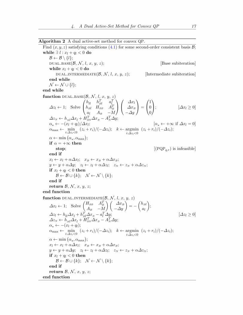
The dual active-set method is summarized in Algorithm 2 below. Its convergenceproperties are given in Theorem 4.1.

Theorem 4.1. Assume that problem (DQPq,r) is nondegenerate. Then, given aninitial point (x, y, z) satisfying conditions (4.1) for some second-order consistentbasis B, Algorithm 2 either solves (DQPq,r) or concludes that (PQPq,r) is infeasiblein a finite number of iterations.

Proof. The proof mirrors that of the primal active-set method of Section 5 (seeTheorem 5.1).

4. A Dual Active-Set Method for Convex QP 17

Algorithm 2 A dual active-set method for convex QP.

Find (x, y, z) satisfying conditions (4.1) for some second-order consistent basis B;while ∃ l : xl + ql < 0 doB ← B \ {l};dual base(B, N , l, x, y, z); [Base subiteration]while xl + ql < 0 do

dual intermediate(B, N , l, x, y, z); [Intermediate subiteration]end whileN ← N ∪ {l};

end while

function dual base(B, N , l, x, y, z)

∆zl ← 1; Solve

hll hTBl aTl


∆xl∆xB

−∆y

=

100

; [∆xl ≥ 0]


BN∆xB −ATN∆y;α∗ ← −(xl + ql)/∆xl; [α∗ ← +∞ if ∆xl = 0]αmax ← min

i:∆zi<0(zi + ri)/(−∆zi); k ← argmin

i:∆zi<0(zi + ri)/(−∆zi);


);

if α = +∞ thenstop; [(PQPq,r) is infeasible]

end ifxl ← xl + α∆xl; xB ← xB + α∆xB;y ← y + α∆y; zl ← zl + α∆zl; zN ← zN + α∆zN ;if xl + ql < 0 thenB ← B ∪ {k}; N ← N \ {k};


end function

function dual intermediate(B, N , l, x, y, z)

∆xl ← 1; Solve

(HBB ATBAB −M

)(∆xB

−∆y

)= −

(hBl

al

);

∆zl ← hll∆xl + hTBl∆xB − aTl ∆y; [∆zl ≥ 0]


BN∆xB −ATN∆y;α∗ ← −(xl + ql);αmax ← min

i:∆zi<0(zi + ri)/(−∆zi); k ← argmin

i:∆zi<0(zi + ri)/(−∆zi);


);

xl ← xl + α∆xl; xB ← xB + α∆xB;y ← y + α∆y; zl ← zl + α∆zl; zN ← zN + α∆zN ;if xl + ql < 0 thenB ← B ∪ {k}; N ← N \ {k};


end function


5. Combining Primal and Dual Active-Set Methods

The primal active-set method proposed in Section 3 may be used to solve (PQPq,r)for a given initial second-order consistent basis satisfying the conditions (3.1). Anappropriate initial point may be found by solving a conventional phase-1 linearprogram. Alternatively, the dual active-set method of Section 4 may be used inconjunction with an appropriate phase-1 procedure to solve the quadratic program(PQPq,r) for a given initial second-order consistent basis satisfying the conditions(4.1). In this section a method is proposed that provides an alternative to theconventional phase-1/phase-2 approach. It is shown that a pair of coupled quadraticprograms may be created from the original by simultaneously shifting the boundconstraints. Any second-order consistent basis can be made optimal for such aprimal-dual pair of shifted problems. The shifts are then updated using the solutionof either the primal or the dual shifted problem. An obvious application of thisapproach is to solve a shifted dual QP to define an initial feasible point for theprimal, or vice-versa. This strategy provides an alternative to the conventionalphase-1/phase-2 approach that utilizes the QP objective function while finding afeasible point.

5.1. Finding an initial second-order-consistent basis

For the methods described in Section 5.2 below, it is possible to define a simpleprocedure for finding the initial second-order consistent basis B. The required basismust define a nonsingular KKT matrix KB such that

KB =

(HBB ATBAB −M

). (5.1)

The initial basis may be obtained by a finding a symmetric permutation Π of the“full” KKT matrix K such that

ΠTKΠ = ΠT

(H AA −M

)Π =

HBB ATB HBN

AB −M AN

HTBN ATN HNN

, (5.2)

where the leading principal block 2× 2 submatrix is of the form (5.1). The full row-rank assumption on

(A −M

)ensures that the partition (5.2) is well defined, see [20,

Section 6]. In practice, the permutation may be determined using any methodfor finding a symmetric indefinite factorization of K, see, e.g., [8, 10, 18]. Suchmethods use symmetric interchanges that implicitly form the nonsingular matrixKB by deferring singular pivots. In this case, KB may be defined as any submatrixof the largest nonsingular principal submatrix obtained by the factorization (Theremay be further permutations within Π that are not relevant to this discussion; forfurther details, see, e.g., [13, 14,20,21].)

The permutation Π defines the initial B-N partition of the columns of A. OnceΠ has been determined, the variables with indices in N are set on their bounds andthe shifts are initialized.

5. Combining Primal and Dual Active-Set Methods 19

5.2. Initializing the shifts

Given a second-order consistent basis, it is straightforward to create a (q(0), r(0))-pair and corresponding (x, y, z) so that q(0) ≥ 0, r(0) ≥ 0 and (x, y, z) are optimal

for (PQPq(0),r(0)) and (DQPq(0),r(0)). First, choose nonnegative vectors q(0)N and r

(0)B .

(Obvious choices are q(0)N = 0 and r

(0)B = 0.) Define zB = −r(0)B , xN = −q(0)N , and

solve the nonsingular KKT-system (2.7) to obtain xB and y, and compute zN from

(2.8). Finally, let q(0)B ≥ max{−xB, 0} and r

(0)N ≥ max{−zN , 0}. Then, it follows

from Proposition 2.1 that x, y and z are optimal for the problems (PQPq(0),r(0)) and

(DQPq(0),r(0)), with q(0) ≥ 0 and r(0) ≥ 0. If q(0) and r(0) are zero, then x, y and zare optimal for the original problem.

5.3. Solving the original problem by removing the shifts

The original problem may now be solved as a pair of shifted quadratic programs.Two alternative strategies are proposed. The first is a “primal first” strategy inwhich a shifted primal quadratic program is solved, followed by a dual. The secondis an analogous “dual first” strategy.

The “primal-first” strategy is summarized as follows.

(0) Find B, N , q(0), r(0), x, y, z, as described in Sections 5.1 and 5.2.

(1) Set q(1) = q(0), r(1) = 0. Solve (PQPq,0) using the primal active-set method.

(2) Set q(2) = 0, r(2) = 0. Solve (DQP0,0) using the dual active-set method.

In steps (1) and (2), the initial B–N partition and initial values of x, y, and z aredefined as the final B–N partition and final values of x, y, and z from the precedingstep.

The “dual-first” strategy is defined in an analogous way.

(0) Find B, N , q(0), r(0), x, y, z, as described in Section 5.1 and 5.2.

(1) Set q(1) = 0, r(1) = r(0). Solve (DQP0,r) using the dual active-set method.

(2) Set q(2) = 0, r(2) = 0. Solve (PQP0,0) using the primal active-set method.

As in the “primal-first” strategy, the initial B–N partition and initial values of x, y,and z for steps (1) and (2), are defined as the final B–N partition and final valuesof x, y, and z from the preceding step.

In order for these approaches to be well-defined, a simple generalization of theprimal and dual active-set methods is needed.

5.4. Relaxed initial conditions for the primal QP method.

For Algorithm 1, the initial values of B, N , q, r, x, y, and z must satisfy conditions(3.1). However, the choice of r = r(1) = 0 in Step (1) of the primal-first strategymay give some negative components in the vector zB + rB. This possibility may be


handled by defining a simple generalization of Algorithm 1 that allows initial pointssatisfying the conditions

Hx+ c−ATy − z = 0, (5.3a)

Ax+My − b = 0, (5.3b)

xB + qB ≥ 0, xN + qN = 0, (5.3c)

zB + rB ≤ 0, (5.3d)

instead of the conditions (3.1). In Algorithm 1, the index l identified at the start ofthe primal base iteration is selected from the nonbasic indices such that zj + rj < 0.In the generalized algorithm, the set of eligible indices for l is extended to includeindices associated with negative values of zB + rB. If the index l is deleted from B,the associated matrix Kl is nonsingular, and intermediate subiterations are executeduntil the updated value satisfies zl + rl = 0. At this point, the index l is returnedB. The method is summarized in Algorithm 3.

Algorithm 3 A primal active-set method for convex QP.

Find (x, y, z) satisfying conditions (5.3) for some second-order consistent basis B;while ∃ l : zl + rl < 0 do

if l ∈ N thenN ← N \ {l};primal base(B, N , l, x, y, z); [returns B, N , x, y, z]

elseB ← B \ {l};

end ifwhile zl + rl < 0 do

primal intermediate(B, N , l, x, y, z); [returns B, N , x, y, z]end whileB ← B ∪ {l};

end while

Theorem 5.1. Assume that problem (PQPq,r) is nondegenerate. Given an initialpoint (x, y, z) satisfying conditions (5.3) for a second-order consistent basis B, thenAlgorithm 3 finds a solution of (PQPq,r) or determines that (DQPq,r) is infeasiblein a finite number of iterations.

Proof. Assume that (x, y, z) satisfies the conditions (5.3) for the second-orderconsistent basis B. Let B< denote the index set B< = {i ∈ B : zi + ri < 0}, andlet r be the vector ri = ri, i 6∈ B<, and ri = −zi, i ∈ B<. These definitions implythat ri = −zi > −zi + zi + ri = ri, for every i ∈ B<. It follows that r ≥ r, and thefeasible region of (DQPq,r) is a subset of the feasible region of (DQPq,r). In addition,if r is replaced by r in (3.1), the only difference is that zB + rB = 0, i.e., the initialpoint for (5.3) is a stationary point with respect to (PQPq,r).

The first step of the proof is to show that after a finite number of iterationsof Algorithm 3, one of three possible events must occur: (i) the cardinality of the

5. Combining Primal and Dual Active-Set Methods 21

set B< is decreased by at least one; (ii) a solution of problem (PQPq,r) is found; or(iii) (DQPq,r) is declared infeasible. The proof will also establish that if (i) does notoccur, then either (ii) or (iii) must hold after a finite number of iterations.

Assume that (i) never occurs. This implies that the index l selected in the baseiteration can never be an index in B< because at the end of such an iteration, it wouldbelong to B with zl + rl = 0, contradicting the assumption that the cardinality ofB< never decreases. For the same reason, it must hold that k 6∈ B< for every index kselected to be moved from B to N in any subiteration, because an index can only bemoved from N to B by being selected in the base iteration. These arguments implythat zi = −ri, with i ∈ B<, throughout the iterations. It follows that the iteratesmay be interpreted as being members of a sequence constructed for solving (PQPq,r)with a fixed r, where the initial stationary point is given, and each iteration givesa new stationary point. The nondegeneracy assumption implies that the objectivevalue of (PQPq,r) is strictly decreasing at each base subiteration, and nonincreasingat each intermediate subiteration. The number of intermediate subiterations isfinite, which implies that a strict improvement of the objective value of (PQPq,r) isobtained at each iteration. As there are only a finite number of stationary points,Algorithm 3 either solves (PQPq,r) or concludes that (DQPq,r) is infeasible after afinite number of iterations. If (PQPq,r) is solved, then zN + rN ≥ 0, because rj = rjfor j ∈ N . Hence, Algorithm 3 can not proceed further by selecting an l ∈ N , andthe only way to reduce the objective is to select an l in B such that zj + rj < 0.Under the assumption that (i) does not occur, it must hold that no eligible indicesexist and B< = ∅. However, in this case (PQPq,r) has been solved with r = r, and(ii) must hold. If Algorithm 3 declares (DQPq,r) to be infeasible, then (DQPq,r) mustalso be infeasible because the feasible region of (DQPq,r) is contained in the feasibleregion of (DQPq,r). In this case (DQPq,r) is infeasible and (iii) occurs.

Finally, if (i) occurs, there is an iteration at which the cardinality of B< decreasesand an index is removed from B<. There may be more than one such index, butthere is at least one l moved from B< to B\B<, or one k moved from B< to N .In either case, the cardinality of B< is decreased by at least one. After such aniteration, the argument given above may be repeated for the new set B< and newshift r. Applying this argument repeatedly gives the result the situation (i) canoccur only a finite number of times.

It follows that, (ii) or (iii) must occur after a finite number of iterations, whichis the required result.

5.5. Relaxed initial conditions for the dual QP method.

Analogous to the primal case, the choice of q = q(1) = 0 in Step (1) of the dual-firststrategy may give some negative components in the vector xN + qN . In the case, the


conditions on the initial values of B, N , q, r, x, y, and z are generalized so that

Hx+ c−ATy − z = 0, (5.4a)

Ax+My − b = 0, (5.4b)

zN + rN ≥ 0, zB + rB = 0, (5.4c)

xN + qN ≤ 0. (5.4d)

Similarly, the set of eligible indices may be extended to include indices associatedwith negative values of xN + qN . If the index l is from N , the associated matrixKB is nonsingular, and intermediate subiterations are executed until the updatedvalue satisfies xl + ql = 0. At this point, the index l is returned N . The method issummarized in Algorithm 4.

The strategies of solving two consecutive quadratic programs may be generalizedto a sequence of more than two quadratic programs, where we alternate betweenprimal and dual active-set methods, and eliminate the shifts in more than two steps.

Algorithm 4 A dual active-set method for convex QP.

Find (x, y, z) satisfying conditions (5.4) for some second-order consistent B;while ∃ l : xl + ql < 0 do

if l ∈ B thenB ← B \ {l};dual base(B, N , l, x, y, z); [Base subiteration]

elseN ← N \ {l};

end ifwhile xl + ql < 0 do

dual intermediate(B, N , l, x, y, z); [Intermediate subiteration]end whileN ← N ∪ {l};

end while

6. Practical Issues

6.1. Quadratic programs with upper and lower bounds

As stated, the primal quadratic program has lower bound zero on the x-variables.This is for notational convenience. This form may be generalized in a straightfor-ward manner to a form where the x-variables has both lower and upper bounds onthe primal variables, i.e., bL ≤ x ≤ bU , where components of bL can be −∞ andcomponents of bU can be +∞. Given primal shifts qL and qU , and dual shifts rL andrU , we have the primal-dual pair

(PQPq,r)minimize

x,y

12x

THx+ 12y

TMy + cTx+ (rL − rU)Tx

subject to Ax+My = b, bL − qL ≤ x ≤ bU + qU ,

6. Practical Issues 23

and

(DQPq,r)maximizex,y,zL,zU

−12x

THx− 12y

TMy + bTy + (bL − qL)TzL − (bU + qU)TzU

subject to −Hx+ATy + zL − zU = c, zL ≥ −rL, zU ≥ −rU .

An infinite bound has neither a shift nor a corresponding dual variable. For example,if xj is a free variable, then the corresponding components of bL and bU are infinite.In the procedure given in Section 5.1 for finding the first second-order consistentbasis B, it is assumed that variables with indices not selected for B are initialized atone of their bounds. As a free variable has no finite bounds, any index j associatedwith a free variable should be selected for B. However, this cannot be guaranteed inpractice, and in the next section it is shown that the primal and dual QP methodsmay be extended to allow a free variable to be fixed temporarily at some value.

6.2. Temporary bounds

If the QP is defined in the general problem format of Section 6.1, then any free vari-able not selected for B has no upper or lower bound and must be temporarily fixedat some value xj = xj (say). The treatment of such “temporary bounds” involvessome additional modifications to the primal and dual methods of Sections 5.4 and5.5.

Each temporary bound xj = xj defines an associated dual variable zj with initialvalue zj . Since the bound is temporary, it is treated as an equality constraint, andthe desired value of zj is zero. Initially, an index j corresponding to a temporarybound is assigned a primal shift qj = 0 and a dual shift rj = −zj , making xj and zjfeasible for the shifted problem. In both the primal-first and dual-first approaches,the idea is to drive the zj-variables associated with temporary bounds to zero in theprimal and leave them unchanged in the dual.

In a primal problem, regardless of whether it is solved before or after the dualproblem, an index j corresponding to a temporary bound for which zj 6= 0 is consid-ered eligible for selection as l in the base subiteration, i.e., the index can be selectedregardless of the sign of zj . Once selected, zj is driven to zero and j belongs toB after such an iteration. In addition, since xj is unbounded, j will remain in Bthroughout the iterations. Hence, at termination of a primal problem, any index jcorresponding to a temporarily bounded variable must have zj = 0. If the maximumstep length at a base subiteration is infinite, the dual problem is infeasible, as in thecase of a regular bound.

In a dual problem, the dual method is modified so that the dual variables as-sociated with temporary bounds remain fixed throughout the iterations. At anysubiteration, if it holds that ∆zj 6= 0 for some temporary bound, then no step istaken and one such index j is moved from N to B. Consequently, a move is madeonly if ∆zj = 0 for every temporary bound j. It follows that the dual variables forthe temporary bounds will remain unaltered throughout the dual iterations. Notethat an index j corresponding to a temporary bound is moved at most once from Nto B, and never moved back since the corresponding xj-variable is unbounded. If the


maximum step length at a base subiteration is infinite, it must hold that ∆zj = 0for all temporary bounds j, and the primal problem is infeasible.

The discussion above implies that a pair of primal and dual problems solvedconsecutively will terminate with zj = 0 for all indices j associated with temporarybounds. This is because zj is unchanged in the dual problem and driven to zero inthe primal problem.

7. Numerical Examples

In this section we describe a particular formulation of the primal-dual shifted methodof Section 5. In addition, some numerical experiments are presented for a simpleMatlab implementation applied to a set of convex problems from the CUTEst testcollection (see Bongartz et al. [7], and Gould, Orban and Toint [33]).

7.1. The coupled primal-dual algorithm PDQP

For illustrative purposes, a primal-dual shifted method is used in which either a“primal-first” or “dual-first” strategy is selected based on the initial point. In par-ticular, if the point is dual feasible, then the “dual-first” strategy. is used. Otherwise,the “primal-first” strategy is selected.

7.2. The implementation

Each CUTEst QP problem may be written in the form

minimizex

cTx+ 12x

THx subject to ` ≤(x

Ax

)≤ u, (7.1)

where ` and u are constant vectors of lower and upper bounds and A has dimensionm×n. In this format, a fixed variable or equality constraint has the same value forits upper and lower bound. Each problem was converted to the equivalent form

minimizex,s

cTx+ 12x

THx subject to Ax− s = 0, ` ≤(xs

)≤ u, (7.2)

where s is a vector of slack variables. With this formulation, the QP problem involvessimple upper and lower bounds instead of nonnegativity constraints. It follows thatthe matrix M is zero, but the full row-rank assumption on the constraint matrix issatisfied because the constraint matrix A takes the form

(A − I

)and has rank m.

In this situation, a nonsingular m ×m submatrix AB of A may be identified usinga so-called “crash” procedure. One algorithm for doing this has been proposed byGill, Murray and Saunders [25], who use a sparse LU factorization of AT to identifya square nonsingular subset of the columns of AB. These factors give a matrix Zwhose columns form a basis for the null space of A as

Z =

(−A−1B AN

I

).

7. Numerical Examples 25

This Z may be used to form ZTHZ, and a partial Cholesky factorization withinterchanges may be used to find an upper-triangular matrix R that is the factor ofthe largest nonsingular leading submatrix of ZTHZ. Let ZR denote the columns ofZ corresponding to R, and let Z be partitioned as Z =

(ZR ZA

). Then, the set

B given by the nonsingular AB may be augmented by the indices corresponding toZR, giving a final B for which the corresponding KKT-matrix KB is nonsingular.

7.3. Numerical results

Numerical results from a simple Matlab implementation of Algorithm PDQP wereobtained for a set of 121 convex QPs in standard interface format (SIF). The prob-lems were selected based on the dimension of the constraint matrix A in (7.2). Inparticular, the test set includes all QP problems for which the smaller of m and nis of the order of 500 or less. This gave 121 QPs ranging in size from BQP1VAR (onevariable and one constraint) to LINCONT (1257 variables and 419 constraints).

In order to judge how the proposed method compares to a conventional two-phaseactive-set method, the same 121 problems were solved using the convex QP solverSQOPT [26], which is a Fortran implementation of a two-phase (primal) reduced-gradient active-set method for large-scale QP. All SQOPT runs were made using thedefault parameter options.

Both PDQP and SQOPT are terminated at a point (x, y, z) that satisfies the equa-tions conditions of (2.6) modified to conform to the constraint format of (7.2). Thefeasibility and optimality tolerances are given by εfea = 10−6 and εopt = 10−6,respectively. For a given εopt, PDQP and SQOPT terminate when

maxi∈B|zi| ≤ εopt‖y‖∞, and

zi ≥ −εopt‖y‖∞ if xi ≥ −`i, i ∈ N ;

zi ≤ εopt‖y‖∞ if xi ≤ ui, i ∈ N .(7.3)

Both PDQP and SQOPT use the EXPAND procedure of Gill et al. [27] to allow thevariables (x, s) to move outside their bounds by as much as εfea.

A summary of the results is given in Table 1. The first four columns give thename of the problem, the number of linear constraints m, the number of variables n,and the optimal objective value Objective. The next two columns summarize theSQOPT result for the given problem, with Phs1 and Itn giving the phase-one itera-tions and iteration total, respectively. The last four columns summarize the resultsfor the PDQP implementation. The first column gives the total number of primal anddual iterations Itn. The second column gives the order in which the primal anddual algorithms were applied, with PD indicating the “primal-first” strategy, and DP

the “dual-first” strategy. The final two columns, headed by p-Itn, and d-Itn, givethe iterations required for the primal method and the dual method, respectively.

Of the 121 problems tested, two (LINCONT and NASH) are known to be infeasible.This infeasibility was identified correctly by both SQOPT and PDQP. In total, SQOPTsolved 117 of the remaining 119 problems, but declared (incorrectly) that problemsRDW2D51U and RDW2D52U are unbounded. PDQP solved the same number of problems,but failed to achieve the required accuracy for the problems RDW2D51B and RDW2D52F.


In these two cases, the final objective values computed by PDQP were 1.0947648E-02and 1.0491239E-02 respectively, instead of the optimal values 1.0947332e-02 and1.0490828e-02. (The five RDW2D5* problems in the test set are known to be difficultto solve, see Gill and Wong [30].)

If the failed and infeasible runs are excluded, Algorithm PDQP required the sameor fewer number of iterations than SQOPT on 73 of the 115 QP problems solved tooptimality by both methods. This constitutes 64% of the problems solved. Of this64%, the “dual-first” strategy made up 44% of the cases and 56% of the improve-ments were associated with the “primal-first” strategy.

Table 1: Results for PDQP and SQOPT on 121 CUTEst QPs.

SQOPT PDQP

Name m n Objective Phs1 Itn Itn Order P-Itn D-Itn

ALLINQP 50 100 -9.1592833E+00 0 45 65 PD 63 2

AUG2DQP 100 220 1.7797215E+02 8 116 440 PD 326 114

AUG3D 27 156 8.3333333E-02 0 45 45 DP 0 45

AVGASA 10 8 -4.6319255E+00 5 8 5 DP 0 5

AVGASB 10 8 -4.4832193E+00 5 8 7 DP 0 7

BIGGSB1 1 100 1.5000000E-02 0 103 101 PD 101 0

BQP1VAR 1 1 0.0000000E+00 0 1 1 DP 0 1

BQPGABIM 1 50 -3.7903432E-05 0 36 7 PD 7 0

BQPGASIM 1 50 -5.5198140E-05 0 40 8 PD 8 0

CHENHARK 1 100 -2.0000000E+00 0 132 32 DP 0 32

CVXBQP1 1 100 2.2725000E+02 0 100 119 DP 2 117

CVXQP1 50 100 1.1590718E+04 5 67 91 DP 1 90

CVXQP2 25 100 8.1209404E+03 2 82 85 DP 2 83

CVXQP3 75 100 1.1943432E+04 17 46 113 DP 2 111

DEGENQP 1005 10 0.0000000E+00 0 6 18 PD 18 0

DTOC3 18 29 2.2459038E+02 1 10 17 DP 0 17

DUAL1 1 85 3.5012967E-02 0 88 88 PD 88 0

DUAL2 1 96 3.3733671E-02 0 99 99 PD 99 0

DUAL3 1 111 1.3575583E-01 0 106 106 PD 106 0

DUAL4 1 75 7.4609064E-01 0 61 61 PD 61 0

DUALC1 215 9 6.1552516E+03 1 9 4 DP 0 4

DUALC2 229 7 3.5513063E+03 2 4 4 DP 0 4

DUALC5 278 8 4.2723256E+02 1 7 6 DP 0 6

DUALC8 503 8 1.8309361E+04 4 6 8 DP 0 8

GENHS28 8 10 9.2717369E-01 0 3 5 DP 0 5

GMNCASE2 1050 175 -9.9444495E-01 18 99 91 DP 0 91

GMNCASE3 1050 175 1.5251466E+00 31 100 86 DP 0 86

GMNCASE4 350 175 5.9468849E+03 74 171 175 DP 0 175

GOULDQP2 199 399 9.0045697E-06 0 213 419 DP 0 419

GOULDQP3 199 399 5.6732908E-02 0 200 406 PD 205 201

GRIDNETA 100 180 9.5242163E+01 5 35 134 PD 81 53

GRIDNETB 100 180 4.7268237E+01 0 81 97 DP 0 97

GRIDNETC 100 180 4.8352347E+01 6 93 153 DP 0 153

HS3 1 2 0.0000000E+00 0 2 1 PD 1 0

HS3MOD 1 2 1.2325951E-32 0 2 1 PD 1 0

HS21 1 2 -9.9960000E+01 0 1 0 PD 0 0

HS28 1 3 1.2325951E-32 0 2 0 PD 0 0

HS35 1 3 1.1111111E-01 0 5 1 DP 0 1

HS35I 1 3 1.1111111E-01 0 5 1 DP 0 1

HS35MOD 1 3 2.5000000E-01 0 1 0 PD 0 0

HS44 6 4 -1.5000000E+01 0 2 4 PD 4 0

HS44NEW 6 4 -1.5000000E+01 0 4 9 PD 9 0

HS51 3 5 -8.8817841E-16 0 2 0 DP 0 0

HS52 3 5 5.3266475E+00 0 2 1 DP 0 1

HS53 3 5 4.0930232E+00 0 2 1 DP 0 1

HS76 3 4 -4.6818181E+00 0 4 4 DP 0 4

7. Numerical Examples 27


(continued)

SQOPT PDQP


HS76I 3 4 -4.6818181E+00 0 4 4 DP 0 4

HS118 17 15 6.6482045E+02 0 21 23 DP 0 23

HS268 5 5 7.2759576E-12 0 8 0 PD 0 0

HUES-MOD 2 100 3.4829823E+07 1 103 7 DP 0 7

HUESTIS 2 100 3.4829823E+09 1 103 7 DP 0 7

JNLBRNG1 1 529 -1.8004556E-01 0 292 82 PD 82 0

JNLBRNG2 1 529 -4.1023852E+00 0 252 42 PD 42 0

JNLBRNGA 1 529 -3.0795806E-01 0 292 292 PD 292 0

JNLBRNGB 1 529 -6.5067871E+00 0 247 247 PD 247 0

KSIP 1001 20 5.7579792E-01 0 2847 36 DP 0 36

LINCONT 419 1257 infeasible 138 138i 304i DP 0 304

LISWET1 100 106 2.6072632E-01 0 52 401 DP 0 401

LISWET2 100 106 2.5876398E-01 0 63 378 DP 0 378

LISWET3 100 106 2.5876398E-01 0 64 378 DP 0 378

LISWET4 100 106 2.5876399E-01 0 61 378 DP 0 378

LISWET5 100 106 2.5876410E-01 0 58 378 DP 0 378

LISWET6 100 106 2.5876390E-01 0 67 378 DP 0 378

LISWET7 100 106 2.5895785E-01 0 68 378 DP 0 378

LISWET8 100 106 2.5747454E-01 0 94 417 DP 0 417

LISWET9 100 103 2.1543892E+01 0 28 263 DP 0 263

LISWET10 100 106 2.5874831E-01 0 68 378 DP 0 378

LISWET11 100 106 2.5704145E-01 0 68 379 DP 0 379

LISWET12 100 106 9.1994948E+00 0 37 460 DP 0 460

LOTSCHD 7 12 2.3984158E+03 4 8 16 DP 0 16

MOSARQP1 10 100 -1.5420010E+02 0 102 52 DP 0 52

MOSARQP2 10 100 -2.0651670E+02 0 100 33 DP 0 33

NASH 24 72 infeasible 5 5i 24i DP 0 24

OBSTCLAE 1 529 1.6780270E+00 0 605 178 DP 0 178

OBSTCLAL 1 529 1.6780270E+00 0 263 263 PD 263 0

OBSTCLBL 1 529 6.5193252E+00 0 469 469 PD 469 0

OBSTCLBM 1 529 6.5193252E+00 0 484 189 DP 0 189

OBSTCLBU 1 529 6.5193252E+00 0 303 303 PD 303 0

OSLBQP 1 8 6.2500000E+00 0 6 0 PD 0 0

PENTDI 1 500 -7.5000000E-01 0 2 2 PD 2 0

POWELL20 100 100 5.2703125E+04 49 52 99 DP 0 99

PRIMAL1 85 325 -3.5012967E-02 0 217 70 PD 70 0

PRIMAL2 96 649 -3.3733671E-02 0 407 97 PD 97 0

PRIMAL3 111 745 -1.3575583E-01 0 1223 102 PD 102 0

PRIMAL4 75 1489 -7.4609064E-01 0 1264 63 PD 63 0

PRIMALC1 9 230 -6.1552516E+03 0 18 5 PD 5 0

PRIMALC2 7 231 -3.5513063E+03 0 3 5 PD 5 0

PRIMALC5 8 287 -4.2723256E+02 0 10 6 PD 6 0

PRIMALC8 8 520 -1.8309432E+04 0 30 6 PD 6 0

QPCBLEND 74 83 -7.8425425E-03 0 111 182 PD 182 0

QPCBOEI1 351 384 1.1503952E+07 415 1055 793 PD 395 398

QPCBOEI2 166 143 8.1719635E+06 142 315 340 PD 163 177

QPCSTAIR 356 467 6.2043917E+06 210 433 970 PD 645 325

QUDLIN 1 420 -8.8290000E+06 0 419 419 PD 419 0

RDW2D51F 225 578 1.1209939E-03 29 29 217 DP 0 217

RDW2D51U 225 578 8.3930032E-04 14 16f 219 DP 0 219

RDW2D52B 225 578 1.0947648E-02 349 488 316f DP 0 314

RDW2D52F 225 578 1.0491239E-02 29 191 414f DP 0 414

RDW2D52U 225 578 1.0455316E-02 15 318f 219 DP 0 219

S268 5 5 7.2759576E-12 0 8 0 PD 0 0

SIM2BQP 1 2 0.0000000E+00 0 1 1 PD 1 0

SIMBQP 1 2 6.0185310E-31 0 2 1 PD 1 0

STCQP1 30 65 4.9452085E+02 8 53 20 DP 0 20

STCQP2 128 257 1.4294017E+03 80 215 73 DP 0 73

STEENBRA 108 432 1.6957674E+04 14 89 177 PD 2 175



(continued)

SQOPT PDQP


TAME 1 2 3.0814879E-33 0 1 1 PD 1 0

TORSION1 1 484 -4.5608771E-01 0 256 256 PD 256 0

TORSION2 1 484 -4.5608771E-01 0 544 144 DP 0 144

TORSION3 1 484 -1.2422498E+00 0 112 112 PD 112 0

TORSION4 1 484 -1.2422498E+00 0 689 288 DP 0 288

TORSION5 1 484 -2.8847068E+00 0 40 40 PD 40 0

TORSION6 1 484 -2.8847068E+00 0 708 360 DP 0 360

TORSIONA 1 484 -4.1611287E-01 0 272 272 PD 272 0

TORSIONB 1 484 -4.1611287E-01 0 529 128 DP 0 128

TORSIONC 1 484 -1.1994864E+00 0 120 120 PD 120 0

TORSIOND 1 484 -1.1994864E+00 0 681 280 DP 0 280

TORSIONE 1 484 -2.8405962E+00 0 40 40 PD 40 0

TORSIONF 1 484 -2.8405962E+00 0 761 360 DP 0 360

UBH1 60 99 1.1473520E+00 11 40 112 DP 0 112

YAO 20 22 2.3988296E+00 0 2 20 DP 0 20

ZECEVIC2 2 2 -4.1250000E+00 0 4 5 PD 5 0

i = infeasible, f = failed

Algorithm PDQP would not be recommended for solving a linear program (LP).Nevertheless, it was applied to 16 LPs from the CUTEst test set. The results aresummarized in Table 2.

Table 2: Results for PDQP and SQOPT on 16 CUTEst LPs.

SQOPT PDQP


AGG 488 163 -3.5991767e+07 84 124 200 PD 156 44

DEGENLPA 15 20 -7.6798369e+01 9 11 52 PD 26 26

DEGENLPB 15 20 -3.0742351e+01 9 10 69 PD 37 32

EXTRASIM 1 2 1.0000000e+00 0 0 0 PD 0 0

GOFFIN 50 51 -1.2612134e-13 3 25 100 PD 100 0

MAKELA4 40 21 0.0000000e+00 0 1 42 PD 42 0

MODEL 38 1542 infeasible 12 12i 44i DP 0 44

OET1 1002 3 5.3824312e-01 1 107 22 DP 0 22

OET3 1002 4 4.5049718e-03 1 319 18 DP 0 18

PT 501 2 1.7839423e-01 1 135 20 DP 0 20

S277-280 4 4 5.0761905e+00 1 6 10 DP 0 10

SIMPLLPA 2 2 1.0000000e+00 1 2 5 DP 1 4

SIMPLLPB 3 2 1.1000000e+00 1 1 6 DP 0 6

SSEBLIN 72 194 1.6170600e+07 26 136 262 DP 8 254

SUPERSIM 2 2 6.6666667e-01 1 1 2 DP 0 2

TFI2 101 3 6.4903111e-01 0 34 48 DP 46 2

i = infeasible

8. Summary and Conclusions

A general framework has been proposed for solving a convex quadratic programwith general equality constraints and simple lower bounds on the variables. Thisframework allows the definition of two methods, one primal and one dual, that gen-erate a sequence of iterates that are feasible with respect to the equality constraintsassociated with the optimality conditions of a general primal-dual form. The primalmethod maintains feasibility of the primal inequalities while driving the infeasibil-

References 29

ities of the dual inequalities to zero. The dual method maintains feasibility of thedual inequalities while moving to satisfy the infeasibilities of the primal inequalities.In each of these methods, the search directions satisfy a KKT system of equationsformed from Hessian and constraint components associated with an appropriate col-umn basis. The composition of the basis is specified by an active-set strategy thatguarantees the nonsingularity of each set of KKT equations.

Each of the proposed methods is a conventional active-set method in the sensethat an initial primal- or dual-feasible point is required. In addition, it has beenshown how the bounds of the primal and dual problems may be shifted so as to givea strategy for solving the original problem by solving a pair of coupled quadraticprograms, one primal and one dual. An application of this approach is to solve ashifted dual QP for a feasible point for the primal (or vice versa), thereby avoidingthe need for a traditional feasibility phase that ignores the properties of the objectivefunction.

The numerical results indicate that the proposed primal, dual, and coupledprimal-dual QP methods can be efficient relative to existing two-phase active-setmethods. Future work will focus on the application of the proposed methods tosituations in which a series of related QPs must be solved, for example, in sequentialquadratic programming methods and methods for mixed-integer nonlinear program-ming.

References

[1] R. A. Bartlett and L. T. Biegler. QPSchur: a dual, active-set, Schur-complement method forlarge-scale and structured convex quadratic programming. Optim. Eng., 7(1):5–32, 2006. 3

[2] E. M. L. Beale. An introduction to Beale’s method of quadratic programming. In J. Abadie,editor, Nonlinear programming, pages 143–153, Amsterdam, the Netherlands, 1967. NorthHolland. 3

[3] E. M. L. Beale and R. Benveniste. Quadratic programming. In H. J. Greenberg, editor,Design and Implementation of Optimization Software, pages 249–258. Sijthoff and Noordhoff,The Netherlands, 1978. 3

[4] M. J. Best. An algorithm for the solution of the parametric quadratic programming prob-lem. CORR 82-14, Department of Combinatorics and Optimization, University of Waterloo,Canada, 1982. 4

[5] M. J. Best. An algorithm for the solution of the parametric quadratic programming problem.In H. Fischer, B. Riedmuller, and S. Schaffler, editors, Applied Mathematics and ParallelComputing: Festschrift for Klaus Ritter, pages 57–76. Physica, Heidelberg, 1996. 4

[6] N. L. Boland. A dual-active-set algorithm for positive semi-definite quadratic programming.Math. Programming, 78(1, Ser. A):1–27, 1997. 3

[7] I. Bongartz, A. R. Conn, N. I. M. Gould, and P. L. Toint. CUTE: Constrained and uncon-strained testing environment. ACM Trans. Math. Software, 21(1):123–160, 1995. 24

[8] J. R. Bunch and L. Kaufman. Some stable methods for calculating inertia and solving sym-metric linear systems. Math. Comput., 31:163–179, 1977. 18

[9] J. R. Bunch and L. Kaufman. A computational method for the indefinite quadratic program-ming problem. Linear Algebra Appl., 34:341–370, 1980. 3

[10] J. R. Bunch and B. N. Parlett. Direct methods for solving symmetric indefinite systems oflinear equations. SIAM J. Numer. Anal., 8:639–655, 1971. 18

30 References

[11] C. C. Cartis and N. I. M. Gould. Finding a point in the relative interior of a polyhedron.Report RAL-TR-2006-016, Rutherford Appleton Laboratory, Oxon, UK, December 2006. 4

[12] F. E. Curtis, Z. Han, and D. P. Robinson. A Globally Convergent Primal-Dual Active-SetFramework for Large-Scale Convex Quadratic Optimization. Computational Optimization andApplications, DOI: 10.1007/s10589-014-9681-9, 2014. 4

[13] I. S. Duff. MA57—a code for the solution of sparse symmetric definite and indefinite systems.ACM Trans. Math. Software, 30(2):118–144, 2004. 18

[14] I. S. Duff and J. K. Reid. The multifrontal solution of indefinite sparse symmetric linearequations. ACM Trans. Math. Software, 9:302–325, 1983. 18

[15] H. Ferreau, C. Kirches, A. Potschka, H. Bock, and M. Diehl. qpOASES: a parametric active-setalgorithm for quadratic programming. Mathematical Programming Computation, pages 1–37,2014. 4

[16] H. J. Ferreau, H. G. Bock, and M. Diehl. An online active set strategy to overcome thelimitations of explicit MPC. Internat. J. Robust Nonlinear Control, 18(8):816–830, 2008. 4

[17] R. Fletcher. A general quadratic programming algorithm. J. Inst. Math. Applics., 7:76–91,1971. 3

[18] R. Fletcher. Factorizing symmetric indefinite matrices. Linear Algebra Appl., 14:257–272,1976. 18

[19] R. Fletcher. Stable reduced Hessian updates for indefinite quadratic programming. Math.Program., 87(2, Ser. B):251–264, 2000. Studies in algorithmic optimization. 3

[20] A. Forsgren. Inertia-controlling factorizations for optimization algorithms. Appl. Num. Math.,43:91–107, 2002. 18

[21] A. Forsgren and W. Murray. Newton methods for large-scale linear equality-constrained min-imization. SIAM J. Matrix Anal. Appl., 14:560–587, 1993. 18

[22] P. E. Gill, N. I. M. Gould, W. Murray, M. A. Saunders, and M. H. Wright. A weighted Gram-Schmidt method for convex quadratic programming. Math. Program., 30:176–195, 1984. 3

[23] P. E. Gill and W. Murray. Numerically stable methods for quadratic programming. Math.Program., 14:349–372, 1978. 3

[24] P. E. Gill, W. Murray, and M. A. Saunders. User’s guide for QPOPT 1.0: a Fortran packagefor quadratic programming. Report SOL 95-4, Department of Operations Research, StanfordUniversity, Stanford, CA, 1995. 3

[25] P. E. Gill, W. Murray, and M. A. Saunders. SNOPT: An SQP algorithm for large-scaleconstrained optimization. SIAM Rev., 47:99–131, 2005. 24

[26] P. E. Gill, W. Murray, and M. A. Saunders. User’s guide for SQOPT Version 7: Software forlarge-scale linear and quadratic programming. Numerical Analysis Report 06-1, Departmentof Mathematics, University of California, San Diego, La Jolla, CA, 2006. 3, 25

[27] P. E. Gill, W. Murray, M. A. Saunders, and M. H. Wright. A practical anti-cycling procedurefor linearly constrained optimization. Math. Program., 45:437–474, 1989. 25

[28] P. E. Gill, W. Murray, M. A. Saunders, and M. H. Wright. A Schur-complement methodfor sparse quadratic programming. In M. G. Cox and S. J. Hammarling, editors, ReliableNumerical Computation, pages 113–138. Oxford University Press, 1990. 3

[29] P. E. Gill, W. Murray, M. A. Saunders, and M. H. Wright. Inertia-controlling methods forgeneral quadratic programming. SIAM Rev., 33(1):1–36, 1991. 3, 7

[30] P. E. Gill and E. Wong. Methods for convex and general quadratic programming. Math. Prog.Comp., 7(1):71–112, 2015. 3, 7, 26

[31] D. Goldfarb and A. Idnani. A numerically stable dual method for solving strictly convexquadratic programs. Math. Programming, 27(1):1–33, 1983. 3

[32] N. I. M. Gould. An algorithm for large-scale quadratic programming. IMA J. Numer. Anal.,11(3):299–324, 1991. 3

References 31

[33] N. I. M. Gould, D. Orban, and P. L. Toint. CUTEr and SifDec: A constrained and uncon-strained testing environment, revisited. ACM Trans. Math. Software, 29(4):373–394, 2003. 3,24

[34] N. I. M. Gould, D. Orban, and P. L. Toint. GALAHAD, a library of thread-safe Fortran 90packages for large-scale nonlinear optimization. ACM Trans. Math. Software, 29(4):353–372,Dec 2003. 3

[35] N. I. M. Gould and P. L. Toint. An iterative working-set method for large-scale nonconvexquadratic programming. Appl. Numer. Math., 43(1-2):109–128, 2002. 19th Dundee BiennialConference on Numerical Analysis (2001). 3

[36] N. I. M. Gould and P. L. Toint. Numerical methods for large-scale non-convex quadraticprogramming. In Trends in industrial and applied mathematics (Amritsar, 2001), volume 72of Appl. Optim., pages 149–179. Kluwer Acad. Publ., Dordrecht, 2002. 3

[37] S. C. Hoyle. A Single-Phase Method for Quadratic Programming. PhD thesis, Report SOL86-9, Department of Operations Research, Stanford University, Stanford, CA, 1986. 3

[38] H. M. Huynh. A Large-Scale Quadratic Programming Solver Based on Block-LU Updates of theKKT System. PhD thesis, Program in Scientific Computing and Computational Mathematics,Stanford University, Stanford, CA, 2008. 3

[39] C. M. Maes. A Regularized Active-Set Method for Sparse Convex Quadratic Programming.PhD thesis, Institute for Computational and Mathematical Engineering, Stanford University,Stanford, CA, August 2010. 3

[40] A. Potschka, C. Kirches, H. Bock, and J. Schloder. Reliable solution of convex quadraticprograms with parametric active set methods. Technical report, Interdisciplinary Center forScientific Computing, Heidelberg University, Im Neuenheimer Feld 368, 69120 Heidelberg,Germany, November 2010. 4

[41] M. J. D. Powell. On the quadratic programming algorithm of Goldfarb and Idnani. Math.Programming Stud., 25:46–61, 1985. 3

[42] K. Ritter. A method for solving nonlinear maximum problems depending on parameters. NavalResearch Logistics Quarterly, 14:147–162, 1967. 4

[43] K. Ritter. On parametric linear and quadratic programming. MRC Technical report 2197,University of Wisconsin at Madison, Wisconsin, USA, 1981. 4

[44] J. Stoer. On the realization of the quadratic programming algorithm of Goldfarb and Idnani.In Vistas in applied mathematics, Transl. Ser. Math. Engrg., pages 167–180. OptimizationSoftware, New York, 1986. 3

[45] E. Wong. Active-Set Methods for Quadratic Programming. PhD thesis, Department of Math-ematics, University of California San Diego, La Jolla, CA, 2011. 3

32 References

A. Appendix

The appendix concerns some basic results used in previous sections. The first resultshows that the nonsingularity of a KKT matrix may be established by checking thatthe two row blocks

(H AT

)and

(A −M

)have full row rank.

Proposition A.1. Assume that H and M are symmetric, positive semidefinite ma-trices. The vectors u and v satisfy(

H AT

A −M

)(u−v

)=

(00

)(A.1)

if and only if (HA

)u =

(00

)and

(AT

−M

)v =

(00

). (A.2)

Proof. If (A.2) holds, then (A.1) holds, which establishes the “if” direction. Nowassume that u and v are vectors such that (A.1) holds. Then,

uTHu− uTATv = 0, and vTAu+ vTMv = 0.

Adding these equations gives the identity uTHu + vTMv = 0. But then, the sym-metry and semidefiniteness of H and M imply uTHu = 0 and vTMv = 0. This canhold only if Hu = 0 and Mv = 0. If Hu = 0 and Mv = 0, (A.1) gives ATv = 0 andAu = 0, which implies that (A.2) holds.

The next result shows that when checking a subset of the columns of a symmetricpositive semidefinite matrix for linear dependence, it is only the diagonal block thatis of importance. The off-diagonal block may be ignored.

Proposition A.2. Let H be a symmetric, positive semidefinite matrix partitionedas

H =

(H11 H12

HT12 H22

).

Then, (H11

HT12

)u =

(00

)if and only if H11u = 0.

Proof. If H is positive semidefinite, then H11 is positive semidefinite, and it holdsthat (

00

)=

(H11

HT12

)u =

(H11 H12

HT12 H22

)(u0

)if and only if

0 =(uT 0

)(H11 H12

HT12 H22

)(u0

)= uTH11u

if and only if H11u = 0, as required.

A. Appendix 33

In the following propositions, the distinct integers k and l, together with integersfrom the index sets B and N define a partition of I = {1, 2, . . . , n}, i.e., I =B ∪ {k} ∪ {l} ∪N . If w is any n-vector, the nB-vector wB and wN -vector wN denotethe vectors of components of w associated with B and N . For the symmetric HessianH, the matrices HBB and HNN denote the subset of rows and columns of H associatedwith the sets B and N respectively. The unsymmetric matrix of components hijwith i ∈ B and j ∈ N will be denoted by HBN . Similarly, AB and AN denote thematrices of columns associated with B and N .

The next result concerns the row rank of the(A −M

)block of the KKT matrix.

Proposition A.3. If the matrix(al ak AB −M

)has full row rank, and there

exist ∆xl, ∆xk, ∆xB, and ∆y such that al∆xl + ak∆xk +AB∆xB +M∆y = 0 with∆xk 6= 0, then

(al AB −M

)has full row rank.

Proof. It must be established that uT(al AB −M

)= 0 implies that u = 0. For

a given u, let γ = −uTak, so that

(uT γ

)(al ak AB −M1

)=(0 0 0 0

).

Then,

0 =(uT γ

)(al ak AB −M1

)∆xl∆xk∆xB

−∆y

= γ ∆xk.

As ∆xk 6= 0, it must hold that γ = 0, in which case

uT(al ak AB −M

)= 0.

As(al ak AB −M

)has full row rank by assumption, it follows that u = 0 and(

al AB −M)

must have full row rank.

An analogous result holds concerning the(H AT

)block of the KKT matrix.

Proposition A.4. If(HBB ATB

)has full row rank, and there exist quantities ∆xN ,

∆xB, ∆y, and ∆zk such that

(hT

Nk hTBk aTk 1

hBN HBB ATB

)∆xN

∆xB

−∆y−∆zk

=

(00

), (A.3)

with ∆zk 6= 0, then the matrix (hkk hT

Bk aTkh

Bk HBB ATB

)has full row rank.

34 References

Proof. Let(µ vT

)be any vector such that

(µ vT

)(hTNk hT

Bk aTkhBN HBB ATB

)=(0 0 0

).

The assumed identity (A.3) gives

0 =(µ vT

)(hTNk hT

Bk aTkhBN HBB ATB

) ∆xN

∆xB

−∆y

= µ∆zk.

As ∆zk 6= 0 by assumption, it must hold that µ = 0. The full row rank of(HBB ATB

)then gives v = 0 and (

hTNk hT

Bk aTkhBN HBB ATB

)must have full row rank. Proposition A.1 implies that this is equivalent to(

hkk hTBk aTk

hBk HBB ATB

)having full row rank.

The next proposition concerns the primal subiterations when the constraint in-dex k is moved from B to N . In particular, it is shown that the Kl matrix isnonsingular after a subiteration.

Proposition A.5. Assume that (∆xl, ∆xk, ∆xB, −∆y, −∆zl) is the unique solu-tion of the equations

hll hkl hTBl aTl 1

hkl hkk hTBk aTk

hBl h

Bk HBB ATBal ak AB −M1 −1

∆xl∆xk∆xB

−∆y−∆zl

=

00001

, (A.4)

and that ∆xk 6= 0. Then, the matrices Kl and Kk are nonsingular, where

Kl =

hll hTBl aTl


and Kk =

hkk hTBk aTk

hBk HBB ATBak AB −M

.

Proof. By assumption, the equations (A.4) have a unique solution with ∆xk 6= 0.This implies that there is no solution of the overdetermined equations

hll hkl hTBl aTl 1

hkl hkk hTBk aTk

hBl h


1

∆xl∆xk∆xB

−∆y−∆zl

=

000010

. (A.5)

A. Appendix 35

Given an arbitrary matrix D and nonzero vector f , the fundamental theorem oflinear algebra implies that if Dw = f has no solution, then there exists a vector vsuch that vTf 6= 0. The application of this result to (A.5) implies the existence of anontrivial vector (∆xl, ∆xk, ∆xB, −∆y, −∆zl, −∆zk) such that

hll hkl hTBl aTl 1

hkl hkk hTBk aTk 1

hBl h


∆xl∆xk∆xB

−∆y−∆zl−∆zk

=

00000

, (A.6)

with ∆zl 6= 0. The last equation of (A.6) gives ∆xl + ∆zl = 0, in which case∆xl∆zl = −∆z2l < 0 because ∆zl 6= 0. Any solution of (A.6) may be viewed asa solution of the equations H∆x − AT∆y − ∆z = 0, A∆x + M∆y = 0, ∆zB = 0,and ∆xi = 0 for i ∈ {1, 2, . . . , n} \ {l} \ {k}. An argument similar to that used toestablish Proposition 2.2 gives

∆xl∆zl +∆xk∆zk ≥ 0,

which implies that ∆xk∆zk > 0, with ∆xk 6= 0 and ∆zk 6= 0.As the search direction is unique, it follows from (A.4) that

(h

Bl HBk HBB ATB

)has full row rank, and Proposition A.2 implies that

(HBB ATB

)has full row rank.

Hence, as ∆zl 6= 0, it follows from (A.6) and Proposition A.4 that the matrix(hll hkl hT

Bl aTlh

Bl hBk HBB ATB

)has full row rank, which is equivalent to the matrix(

hll hTBl aTl

hBl HBB ATB

)having full row rank by Proposition A.2,

Again, the search direction is unique and (A.4) implies that(al ak AB −M

)has full row rank. As ∆xk 6= 0, Proposition A.3 implies that

(al AB −M

)must

have full row rank. Consequently, Proposition A.1 implies that Kl is nonsingular.As ∆xk, ∆xl, ∆zk and ∆zl are all nonzero, the roles of k and l may be reversed

to give the result that Kk is nonsingular.

The next proposition concerns the situation when a constraint index k is movedfrom N to B in a dual subiteration. In particular, it is shown that the resultingmatrix KB defined after a subiteration is nonsingular.

Proposition A.6. Assume that there is a unique solution of the equations

hll hkl hTBl aTl 1

hkl hkk hTBk aTk 1

hBl h


1

∆xl∆xk∆xB


=

000010

, (A.7)

36 References

with ∆zk 6= 0. Then, the matrices Kl and Kk are nonsingular, where

Kl =

hll hTBl aTl


, and Kk =

hkk hTBk aTk

hBk HBB ATBak AB −M

.

Proof. As (A.7) has a unique solution with ∆zk 6= 0, there is no solution of

hll hkl hTBl aTl 1

hkl hkk hTBk aTk

hBl h


1

∆xl∆xk∆xB

−∆y−∆zl

=

000010

. (A.8)

The fundamental theorem of linear algebra applied to (A.8) implies the existence ofa solution of

hll hkl hTBl aTl 1

hkl hkk hTBk aTk 1

hBl h


∆xl∆xk∆xB


=

00000

, (A.9)

with ∆zl 6= 0. It follows from (A.9) that ∆xl + ∆zl = 0. As ∆zl 6= 0, thisimplies ∆xl∆zl < 0. The solution of (A.9) may be regarded as a solution of thehomogeneous equations H∆x − AT∆y −∆z = 0, A∆x + M∆y = 0, with ∆zi = 0,for i ∈ B, and ∆xi = 0, for i ∈ {1, . . . , n} \ {k} \ {l}. Hence, Proposition 2.2 gives

∆xl∆zl +∆xk∆zk ≥ 0,

so that ∆xk∆zk > 0. Hence, it must hold that ∆xk 6= 0 and ∆zk 6= 0.As ∆xk 6= 0, ∆xl 6= 0, ∆zk 6= 0 and ∆zl 6= 0, the remainder of the proof is

analogous to that of Proposition A.5.

The next result gives expressions for the primal and dual objective functions interms of the computed search directions.

Proposition A.7. Assume that (x, y, z) satisfies the primal and dual equality con-straints

Hx+ c−ATy − z = 0, and Ax+My − b = 0.

Consider the partition {1, 2, . . . , n} = B ∪ {l} ∪ N such that xN + qN = 0 andzB + rB = 0. If the components of the direction (∆x, ∆y, ∆z) satisfy (2.10), thenthe primal and dual objective functions for (PQPq,r) and (DQPq,r), i.e.,

fP (x, y) = 12x

THx+ 12y

TMy + cTx+ rTx

fD(x, y, z) = −12x

THx− 12y

TMy + bTy − qTz,

A. Appendix 37

satisfy the identities

fP (x+ α∆x, y + α∆y) = fP (x, y) +∆xl(zl + rl)α+ 12∆xl∆zlα

2,

fD(x+ α∆x, y + α∆y, z + α∆z) = fD(x, y, z)−∆zl(xl + ql)α− 12∆xl∆zlα

2.

Proof. The directional derivative of the primal objective function is given by(∆xT ∆yT

)∇fP (x, y) =

(∆xT ∆yT

)(Hx+ c+ rMy

)=(∆xT ∆yT

)(ATy + z + rMy

)(A.10a)

= (A∆x+M∆y)Ty +∆xT(z + r)

= ∆xl(zl + rl), (A.10b)

where the identity Hx + c = ATy + z has been used in (A.10a) and the identitiesA∆x+M∆y = 0, ∆xN = 0 and zB + rB = 0 have been used in (A.10b).

The curvature in the direction (∆x,∆y) is given by(∆xT ∆yT

)∇2fP (x, y)

(∆x∆y

)=(∆xT ∆yT

)(HM

)(∆x∆y

)=(∆xT ∆yT

)(AT∆y +∆zM∆y

)(A.11a)

= (A∆x+M∆y)T∆y +∆xT∆z

= ∆xl∆zl, (A.11b)

where the identity H∆x−AT∆y−∆z = 0 has been used in (A.11a) and the identitiesA∆x+M∆y = 0, ∆xN = 0 and ∆zB = 0 have been used in (A.11b).

The directional derivative of the dual objective function is given by

(∆xT ∆yT ∆zT

)∇fD(x, y, z) =

(∆xT ∆yT ∆zT

) −Hx−My + b−q

(A.12a)

= −∆xTHx+∆yT(−My + b)−∆zT q (A.12b)

= −(AT∆y +∆z)Tx+∆yT(−My + b)

−∆zT q (A.12c)

= −∆yT(Ax+My − b)−∆zT(x+ q) (A.12d)

= −∆zl(xl + ql), (A.12e)

where the identity H∆x−AT∆y−∆z = 0 has been used in (A.12c) and the identitiesAx+My − b = 0, xN + qN = 0 and ∆zB = 0 have been used in (A.12e).

As z only appears linearly in the dual objective function, it follows from thestructure of the Hessian matrices of fP (x, y) and fD(x, y, z) that

(∆xT ∆yT ∆zT

)∇2fD(x, y, z)

∆x∆y∆z

= −(∆xT ∆yT

)∇2fP (x, y)

(∆x∆y

).

38 References

Consequently, (A.11) gives

(∆xT ∆yT ∆zT

)∇2fD(x, y, z)

∆x∆y∆z

= −∆xl∆zl.

Finally, it is shown that there is no loss of generality in assuming that(A M

)has full row rank in (PQPq,r).

Proposition A.8. There is no loss of generality in assuming that(A M

)has full

row rank in (PQPq,r).

Proof. Let (x, y, z) be any vector satisfying (2.1a) and (2.1b). Assume that(A M

)has linearly dependent rows, and that

(A M

)and b may be partitioned

conformally such that

(A M

)=

(A1 M11 M12

A2 MT12 M22

), and b =

(b1b2

),

with(A1 M11 M12

)of full row rank, and(A2 MT

12 M22

)= N

(A1 M11 M12

), (A.13)

with A1 ∈ Rm1×n and A2 ∈ Rm2×n for some matrix N ∈ Rm2×m1 . From the lineardependence of the rows of

(A M

), it follows that x, y and z satisfy (2.1a) and

(2.1b) if and only if

A1x+M11y1 +M12y2 − b1 = 0 and b2 = Nb1,

Hx+ c−AT1 y1 −AT2 y2 − z = 0.

It follows from (A.13) that M12 = M11NT and AT2 = AT1N

T , so that x, y and zsatisfy (2.1a) and (2.1b) if and only if

A1x+M11(y1 +NTy2)− b1 = 0 and b2 = Nb1,

Hx+ c−AT1 (y1 +NTy2)− z = 0.

We may now define y1 = y1 +NTy2 and replace (2.1a) and (2.1b) by the system

A1x+M11y1 − b1 = 0,

Hx+ c−AT1 y1 − z = 0.

By assumption,(A1 M11 M12

)has full row rank. Proposition A.2 implies that(

A1 M11

)has full row rank. This gives an equivalent problem for which

(A1 M11

)has full row rank.

active-set methods for convex quadratic programming

Documents