ACTIVE VERSUS PASSIVE

INVESTING: AN EMPIRICAL

STUDY ON THE US AND

EUROPEAN MUTUAL FUNDS

AND ETFS

Desmond Pace, Jana Hili and Simon Grima

ABSTRACT

Purpose � In the build-up of an investment decision, the existence ofboth active and passive investment vehicles triggers a puzzle for inves-tors. Indeed the confrontation between active and index replicationequity funds in terms of risk-adjusted performance and alpha generationhas been a bone of contention since the inception of these investmentstructures. Accordingly, the objective of this chapter is to distinctlyunderscore whether an investor should be concerned in choosing betweenactive and diverse passive investment structures.

Methodology/approach � The survivorship bias-free dataset consists of776 equity funds which are domiciled either in America or Europe, andare likewise exposed to the equity markets of the same regions. In addi-tion to geographical segmentation, equity funds are also categorised by

Contemporary Issues in Bank Financial Management

Contemporary Studies in Economic and Financial Analysis, Volume 97, 1�35

Copyright r 2016 by Emerald Group Publishing Limited

All rights of reproduction in any form reserved

ISSN: 1569-3759/doi:10.1108/S1569-375920160000097006

1

Dow

nloa

ded

by U

NIV

ER

SIT

Y O

F M

AL

TA

At 0

0:12

22

Dec

embe

r 20

16 (

PT)

structure and management type, specifically actively managed mutualfunds, index mutual funds and passive exchange traded funds (‘ETFs’).This classification leads to the analysis of monthly net asset values(‘NAV’) of 12 distinct equally weighted portfolios, with a time horizonranging from January 2004 to December 2014. Accordingly, the risk-adjusted performance of the equally weighted equity funds’ portfolios isexamined by the application of mainstream single-factor and multi-factorasset pricing models namely Capital Asset Pricing Model (Fama, 1968;Fama & Macbeth, 1973; Lintner, 1965; Mossin, 1966; Sharpe, 1964;Treynor, 1961), Fama French Three-Factor (1993) and Carhart Four-Factor (1997).

Findings � Solely examination of monthly NAVs for a 10-year horizonsuggests that active management is equivalent to index replication interms of risk-adjusted returns. This prompts investors to be neutral grossof fees, yet when considering all transaction costs it is a distinct story.The relatively heftier fees charged by active management, predominantlyinitial fees, appear to revoke any outperformance in excess of the marketportfolio, ensuing in a Fool’s Errand Hypothesis. Moreover, bothactive and index mutual funds’ performance may indeed be lower if finan-cial advisors or distributors of equity funds charge additional fees overand above the fund houses’ expense ratios, putting the latter investmentvehicles at a significant handicap vis-a-vis passive low-cost ETFs. Thischapter urges investors to concentrate on expense ratios and other trans-action costs rather than solely past returns, by accessing the cheapestavailable vehicle for each investment objective. Put simply, the generalinvestor should retreat from portfolio management and instead accessthe market portfolio using low-cost index replication structures via anexecution-only approach.

Originality/value � The battle among actively managed and index repli-cation equity funds in terms of risk-adjusted performance and alpha gen-eration has been a grey area since the inception of mutual funds. Theinterest in the subject constantly lightens up as fresh instruments infil-trate financial markets. Indeed the mutual fund puzzle (Gruber, 1996)together with the enhanced growth of ETFs has again rejuvenated theactive versus passive debate, making it worth a detailed analysis espe-cially for the benefit of investors who confront a dilemma in choosingbetween the two management styles.

Keywords: Active management; passive management; mutual funds;exchange traded funds; asset pricing models; modern portfolio theory

2 DESMOND PACE ET AL.

Dow

nloa

ded

by U

NIV

ER

SIT

Y O

F M

AL

TA

At 0

0:12

22

Dec

embe

r 20

16 (

PT)

INTRODUCTION

The funds’ industry role has evolved to a central channel where both retailand professional investors can access a wide spectrum of markets, withoutretaining a directional exposure to a single instrument. Perceptibly, thisallows for diversification effects to be augmented through the reduction ofthe specific risk associated with individual securities. Initially the main pur-pose for the formation of funds was to facilitate the pooling of investors’capital into a single structure, thereby exploiting economies of scale andscope by employing a professional portfolio manager and relevant exper-tise, reducing transaction costs vis-a-vis a do-it-yourself portfolio, whilstalso permitting retail investors to access securities with elevated minimuminvestment thresholds which would be otherwise remote and not doable toinvest in.

With regard to indexing prior to the existence of passive funds, it waspractically unviable for investors to replicate effectively the returns of anunderlying index or basket of instruments due to significant transactioncosts and time constraints, owing to ongoing portfolio rebalancing.Moreover, if any physical replication was done by individual investors, thequestion would be that of whether the tracking quality was an adequateone. Subsequently admission to a broad range of securities is nowadaysmore feasible without encountering the aforementioned setbacks, leadingto superior market efficiency, enhanced liquidity and induced financial mar-kets’ growth including market completion.

The establishment of different fund categories with distinct investmentobjectives has pioneered the confrontation involving active and passiveinvestment structures, with the diversity between both ends emanatingfrom the investment management style. More specifically, actively managedmutual funds aim to outperform the market portfolio proxied by majorstock indices, whereas passive funds merely endeavour to replicate an under-lying index, whilst preserving tracking error to a minimum. Undoubtedly,due to various factors including research costs and maintenance of the fund’sobjective, actively managed mutual funds charge higher fees vis-a-vis indexfunds, as the latter’s solely concern is tracking the benchmark index as closeas possible, with no effort exhausted on searching for undervalued and/orovervalued securities.

It is of common knowledge that albeit a percentage of actively mana-ged mutual funds may indeed outperform the market and hence outshinepassive funds, the net returns for active investors may be equivalent toor less than index funds’ net returns, owing to higher management fees

3An Empirical Study on the US and European Mutual Funds and ETFs

Dow

nloa

ded

by U

NIV

ER

SIT

Y O

F M

AL

TA

At 0

0:12

22

Dec

embe

r 20

16 (

PT)

and transaction costs. Indeed, it is worth researching whether theexpenses incurred in attempting to outperform the market do actuallycancel the efforts of the outperformance component over and abovethe market portfolio whilst also considering risk into the equation,thereby resulting in the Fool’s Errand Hypothesis. In such case if risk-adjusted returns, net of fees, transpire to be equivalent, active and pas-sive investors will be indifferent which way to elect. The issue is thatwith passive funds the market portfolio is ‘guaranteed’ as long as thetracking error isn’t abnormal, whereas with actively managed mutualfunds performance may either be better or even worse than the marketindex gross of fees, let alone after costs. This portrays a dilemma as towhether investors should opt for passive or active investment funds.Another concern is that apart from the conventional index funds, inves-tors can nowadays access index replication investments via passiveETFs, therefore the uncertainty of choosing the optimal structure isfurther amplified.

Passive ETFs are akin to index funds, being a basket of instrumentspooled together to replicate the returns of a specific benchmark. Alike toother passive investment vehicles, ETFs also provide a relatively cost-effective exposure to a wide spectrum of securities including equities, fixedincome, commodities, currencies, real estate and major indexes. Apartfrom the initial passive types, active ETFs were gradually introduced inthe market and this trend is expected to augment further. The latterinstruments are a priori deemed as perfect or close substitutes for activelymanaged mutual funds.

Succinctly, ETFs are more liquid as they trade intraday on a stockexchange like any publicly listed security, whereas index and activelymanaged mutual funds are only priced at end of day via the NAV calcula-tion. Being exchange tradable, less liquid ETFs may be inefficientlypriced, at least intraday, and thereby enabling investors to long-sellunder-priced and short-sell over-priced ETFs relative to their intradayindicative values. The characteristic of being exchange tradable makesETFs a crossbreed between a mutual fund and a stock, essentially a pro-duct of financial innovation.

Ultimately the construction of these innovative instruments has pro-vided new horizons for both retail and institutional investors, includingexposure to a diversified index or portfolio through leverage and possiblyarbitrage opportunities, due to the eventuality of ETFs’ intraday pricesdeviating from their underlying portfolio values. Yet such arbitrage maybe short-lived especially during wide mispricings, since ETF structures

4 DESMOND PACE ET AL.

Dow

nloa

ded

by U

NIV

ER

SIT

Y O

F M

AL

TA

At 0

0:12

22

Dec

embe

r 20

16 (

PT)

enable approved parties to create and redeem ETFs at the respectiveNAV at end of trading, hence reducing price inefficiencies by enhancingmarket efficiency.

For the benefit of investors, this chapter aims to provide robust conclu-sions on distinct equity fund structures by tackling the successive researchquestions and hypothesis.

Existing literature suggests that the majority of actively managedmutual funds tend to underperform their underlying benchmarks, grossand net of fees (Blake, Elton, & Gruber, 1993; Gruber, 1996; Harper,Madura, & Schnusenberg, 2006; Malkiel, 1995; Rompotis, 2009; SPIVA,2013, 2014), and hence passive structures including ETFs tend to be thewiser choice for investors. Therefore, is it rational to consider that passivemanagement actually outperforms active? If this is the case, what explainsthe existence of the mutual fund puzzle (Gruber, 1996) along the past twodecades?

Secondly, being close substitutes and index replication structures,ETFs and index funds are expected to mimic their underlying benchmarks,and thus calculated alphas are expected to be inexistent. In particular,existence of high alphas should be solely capturing a high tracking error.Consequently, given that passive ETFs and index funds do not seek tooutperform a relative benchmark but rather track, calculated alphas will benegligible in case both structures have equivalent expense ratios. Hence, isit practical to solely consider passive management structures which actuallycharge the lowest expense ratios vis-a-vis their peers?

AIM OF THE STUDY

The aim of this chapter is to distinctly underscore whether an investorshould be concerned in choosing between active and diverse passive invest-ment structures. It will focus on measuring the generated alphas of activelymanaged mutual funds, index funds and passive ETFs, hence undertakinga risk-adjusted return approach. The researchers aim to grant a recommen-dation to the general investor to successively distribute investment capitaleffectively by procuring the highest alphas and risk-adjusted returns.Ultimately the study pursues to shed light on whether an investor benefitsfrom selecting among active and passive investment funds, amid fierce com-petition between such collective investment structures and the recent explo-sive growth of exchange tradable funds.

5An Empirical Study on the US and European Mutual Funds and ETFs

Dow

nloa

ded

by U

NIV

ER

SIT

Y O

F M

AL

TA

At 0

0:12

22

Dec

embe

r 20

16 (

PT)

LITERATURE REVIEW

Fundamental theories, asset pricing models and evidence on diverse fundstructures are central to this research, all of which are reviewed in this sec-tion. Indeed the foremost reliable literature including research papers fea-ture in this partition.

Theoretical Background

Markovitz’ portfolio theory (1952a, 1952b) and the CAPM (Fama, 1968;Fama & Macbeth, 1973; Lintner, 1965; Mossin, 1966; Sharpe, 1964;Treynor, 1961) are the cornerstones which pioneered the birth and growthof asset pricing models. Indeed the anomalies’ literature and CAPM’s scep-tics notably Roll (1977) indirectly encouraged the development of the basicmodel to extend its structure further. CAPM’s enhancements predominantlyensued into Jensen’s Alpha, the Three-Factor and Four-Factor Modelsas proposed by Fama and French (1993) and Carhart (1997), respectively.Complimenting these asset pricing models are a number of risk-adjustedperformance measures primarily the Treynor ratio (1965), Sharpe ratio(1966) and Jensen’s alpha (1968).

CAPM and Risk-Adjusted Models

Performance evaluation chiefly evolved from the establishment of CAPM,which was introduced as an asset pricing model. The CAPM as a theoreticalmodel follows the mean-variance efficient concept initiated by Markowitz(1952a, 1952b). Put simply this theory entails that an investor will request thehighest return for a given level of risk or the lowest risk for a given level ofreturn, leading to the formation of portfolios on the efficient frontier.Specifically, investors can design the efficient frontier by employing theCAPM formula (Eq. (1)), which exhibits the relationship between risk andreturn via the market or beta risk, hence termed single-factor model.

E R R E R RP f m f( ) = + ( ) −⎡⎣ ⎤⎦β

CAPM (Source: Sharpe, 1964)(1)

where E(Rp) refers to the individual’s portfolio expected return, Rf incorpo-rates the return on risk-free securities, E Rmð Þ−Rf

� �illustrates the excess

6 DESMOND PACE ET AL.

Dow

nloa

ded

by U

NIV

ER

SIT

Y O

F M

AL

TA

At 0

0:12

22

Dec

embe

r 20

16 (

PT)

return of the market portfolio over and above the risk-free rate and theβ coefficient represents the strength of the relationship between theinvestor’s portfolio and the market portfolio.

An important concept of CAPM is that an investor is only compensatedfor systematic or market risk, as it cannot be diversified away. Put differently,no compensation is supplied for firm-specific risk since it can be reduced bydiversification by incorporating more securities in a portfolio. The directionand extent of co-movement with market risk is computed by beta (Eq. (2)).

βσP

P m

m

R R=

( )cov ,2

Beta (Source: Sharpe, 1964)(2)

A beta of 1 connotes a perfectly positively correlation between an inves-tor’s portfolio and market portfolio. Therefore, a specific return generated bythe market should be identically replicated by the investor’s portfolio.Portfolios with a beta of 0 provide return equivalent to the risk-free rate, andhence are uncorrelated with the market returns. Portfolios with a beta of −1inversely replicate the market, thus distribute perfectly opposite returns tothose of the market. As a side note, investors typically expand portfolio betasthroughout economic growth but contract such betas during turbulent times.

The formation of CAPM has long substantiated that computingreturn on its own simply supplies a trivial outcome. This signifies thatportfolio return has to be assessed in tandem with its underlying risk toundertake a correct investment decision. This has led to the creation oftwo distinguished risk-adjusted ratio proposed by Sharpe (1966) (Eq. (3))and Treynor (1965) (Eq. (4)), which concisely underscore the amount ofreturn per each unit of risk.

P

SE R R

PP f=

( ) −σ

Sharpe Ratio (Source: Sharpe, 1966)(3)

TE R R

PP f

P

=( ) −

βTreynor Ratio (Source: Treynor, 1965)

(4)

7An Empirical Study on the US and European Mutual Funds and ETFs

Dow

nloa

ded

by U

NIV

ER

SIT

Y O

F M

AL

TA

At 0

0:12

22

Dec

embe

r 20

16 (

PT)

Though a priori both ratios may appear analogous, this is not the caseas in the denominator a diverse path is employed. The Sharpe ratio is con-cerned with the portfolio’s standard deviation by utilising the capital mar-ket line methodology, whereas the Treynor ratio adopts the portfolio betavia the security market line approach. Pro Roll’s critique will noticeablyfavour the Sharpe ratio, as the latter does not make reference to a specificbenchmark, which is unobservable and inexistent (Roll, 1977).

Single-Factor Regression ModelThe single-factor model as proposed by Jensen (1968) remains to date aprevalent methodology for quantifying managers’ skill and fund perfor-mance via alpha estimation (Eq. (5)). Jensen’s alpha builds on the standardCAPM and hence assumes its empirical validity and robustness, predomi-nantly that portfolio returns are explained by a linear relationship withbeta plus the risk-free rate.

E R R E R Rp f P P M f P( ) − = + ( ) −⎡⎣ ⎤⎦ +β ε

Jensen’s Alpha (Source: Jensen, 1968)

∝(5)

where E Rp

� �−Rf represent the excess return on portfolio p, as a result of

the exposure to the market risk premium βP E Rmð Þ−Rm½ �� �, plus ɛP being

the error term and the notorious Jensen’s alpha (αp). Put simply a positiveαp implies that a portfolio manager has yielded higher risk-adjusted returnthan the underlying index or benchmark signifying skill and/or good luck.Conversely a negative alpha denotes a manager inability to generate theminimum expected return vis-a-vis the market portfolio, hence displayinglack of skill and/or bad luck.

Nevertheless supplementary research depicts that CAPM includingJensen’s alpha is not able to explain returns entirely. Indeed stocks withcertain characteristics tend to generate higher returns than that predictedby CAPM, leading to the introduction of multi-factor regression models.

Multi-Factor Regression ModelsThe first empirical evidence for testing the CAPM for equity portfolios viathe SML demonstrated a robust positive relationship between mean returnsand beta (Black, Jensen, & Scholes, 1972; Fama & Macbeth, 1973). Yet asfurther empirical studies were undertaken, less encouraging support forCAPM was shaping, ensuing in the anomalies’ literature and declaring thatbeta is dead.

8 DESMOND PACE ET AL.

Dow

nloa

ded

by U

NIV

ER

SIT

Y O

F M

AL

TA

At 0

0:12

22

Dec

embe

r 20

16 (

PT)

Basu (1977), Banz (1981), Fama and French (1993) authenticated thatCAPM is mis-specified, since equity portfolios exhibiting large exposures tothe size and/or value effect on average generate higher returns than thatpredicted by the single-factor model. Basu (1977) observed that portfoliosencompassing value stocks outperformed growth stocks. Banz (1981) con-secutively identified the small size effect, where small cap portfolios out-shined larger caps. This evidence has led to consider the rejection of theEfficient Market Hypothesis (‘EMH’) and that securities’ prices could pos-sibly be biased, as an investor could obtain abnormal returns by going longvalue stocks signalled by a low price to earnings ratio, and small capsdenoted by market capitalisation size. Nevertheless a general explanationfor higher returns is that value stocks have a higher exposure to bankruptcyrisk, whereas small caps have a larger exposure to liquidity risk. This meansthat higher returns are merely a compensation for undertaking a higherrisk and hence this does not lead to a breakdown in the EMH. AlthoughBasu (1977) and Banz (1981) evidence may have put some uncertainties onthe EMH, it had geared up the trail for the construction of multi-factormodels and/or improvement of existing ones. Indeed the shortcomings andnaive approach of CAPM has led to notable theoretical and empiricalresearch confirming that expected returns can be described by a number ofvariables via a multi-factor model leading to CAPM enhancement or eventhe creation of other asset pricing models (Carhart, 1997; Fama & French,1993; Jagannathan & Wang, 1996; Ross, 1976).

A case in point was the development of the Arbitrage Pricing Theory byRoss (1976), which is established on the law of one price implying no arbit-rage opportunities. Similarly to CAPM for fully diversified portfolios, themodel assumes that idiosyncratic risk becomes inexistent, and henceexpected returns are only explained by the exposure to risk factors. InArbitrage Pricing Theory (‘APT’), the model is constructed either as asingle-factor or a multi-factor. For this reason, as an asset pricing modelthe APT is more flexible than CAPM, since it can absorb a variety of riskfactors even in the absence of theoretical background. More specifically theAPT assumes that expected returns can be explained by a single or anumber of risk factors, yet it does not visibly sketch out which risk factorsto employ. For instance the utilised risk factors can be stock indexes,fundamental variables, firm characteristics (Fama & French, 1992), macro-economic factors (Chen, Roll, & Ross, 1986) and other generic factors.

Fama and French (1993) utilised previous empirical work predominantlyfrom Basu (1977) and Banz (1981) to develop a Three-Factor model (Eq. (6))for the purpose of explaining asset returns. Fama and French (1993) used firm

9An Empirical Study on the US and European Mutual Funds and ETFs

Dow

nloa

ded

by U

NIV

ER

SIT

Y O

F M

AL

TA

At 0

0:12

22

Dec

embe

r 20

16 (

PT)

characteristics, namely size proxied by market capitalisation (SMB) and bookto market ratio (HML) to gauge systematic risk exposure.

R R R R SMB HMLP f p P M f P P P− = ∝ + −( ) + + +β β β ε0 1 2

Fama French Three-Factor Model (Source: Fama & F rench, 1993)(6)

The SMB (small minus big) risk factor adjusts for the exposure of thegeneral outperformance of small cap portfolios over large ones. The HML(high minus low) variable corrects for the exposure of value stock portfo-lios, measured by a high book to market ratio, which typically outperformgrowth equity portfolios exhibiting low book to market ratios. The SMB isconstructed by grouping small caps (S), being those equities with marketcap below the median, and grouping large caps (B), that is, those firmswith above the median market cap. Once both groups are finalised, then arisk premium is formulated by subtracting (M) the two and obtain anexcess return. For HML a similar procedure is performed as stocks aresorted depending on book to market ratio into three distinct classes. Thetop 33% of stocks with the highest book to market ratio are categorised asH, whilst the bottom 33% of equities with the lowest book to market ratioare grouped as L. Then the risk premium or excess return between the twois calculated by subtracting (M). A high beta for the SMB risk factor wouldillustrate that a portfolio has a large exposure to small caps. Similarly ahigh beta for HML would signify that a fund has a greater exposure tovalue stocks rather than growth equities. In practice the Fama FrenchThree-Factor model aids to illustrate whether a fund manager is generatingreturns given skill, or simply due to a greater risk exposure for small capsand value stocks, therefore reducing noise from alpha.

As an effort for cleaning alpha further, Carhart (1997) added another riskfactor capturing momentum effects (Eq. (7)), which theoretically was intro-duced by Jegadeesh and Titman (1993). The momentum anomaly demon-strates that buying past winners and short selling past losers generatesabnormal returns. Put simply, top performing equities are expected to con-tinue performing well in the future and vice versa. Therefore, the momentumrisk factor corrects for the overexposure to past winning stocks which gener-ally outperform past losing stocks. The MOM risk factor is the risk premiumor excess return of a past winner portfolio over the loser portfolio. It is com-posed by grouping an equally weighted average of last year’s top 30% highperforming equities versus an equally weighted average of last year’s bottom30% lowest performing ones, then taking the difference between the two.

10 DESMOND PACE ET AL.

Dow

nloa

ded

by U

NIV

ER

SIT

Y O

F M

AL

TA

At 0

0:12

22

Dec

embe

r 20

16 (

PT)

R R R RP f P p M f P P p P− = −( ) + + + +β β β β ε0 1 2 3SMB HML MOM

Carhart Four-Facctor Model (Source: Carhart, 1997)(7)

To recapitulate, Carhart’s (1997) Four-Factor model evolved from theFama and French (1993) Three-Factor model, where the latter model wasderived by employing earlier empirical work from Basu (1977), Banz (1981)and Jegadeesh and Titman (1993). Even though such multi-factor modelsmay be criticised for lacking theoretical foundation, numerous empiricalstudies employed these models to assess portfolio performance. Indeed thewidespread usage of these factor models confirms that several researchersendorse their validity.

Evidence on Active and Passive Management

Fund managers’ ability, predominantly securities’ selectivity skills, has had afundamental role in the financial literature. The majority of researchers clinchthat active investment strategies tend to underperform passive ones, prior andpost expenses (Blake et al., 1993; Bogle, 1998; Gruber, 1996; Harper et al.,2006; Malkiel, 1995; Rompotis, 2009; SPIVA, 2013, 2014). Furthermore, dis-tinguished researchers namely Treynor (1965), Sharpe (1966) and Jensen(1968) all confirm that risk-adjusted performance of actively managed mutualfunds underperforms a passive strategy after adjusting for expenses, at leastfor the period studied.

Malkiel (1995) investigated the performance and survivorship bias forequity mutual funds, authenticating that the latter typically underperformtheir underlying index, even gross of fees. Frino and Gallagher (2001)equivalently demonstrated that throughout their period of study, theStandard & Poor’s 500 index fund boasted superior risk-adjusted returnnet of fees. Moreover Bogle (1998) presents a trade-off between fund selec-tion and low expense funds, outlining that it would be prudent to selectlow expense funds at the expense of limiting fund selection.

Malkiel (1995) also suggests that performance persistence was present inthe past and thus an investor could generate excess returns using historicaldata at least for a decade in the 1970s. As markets became efficient andinvestors more informed, such information was gradually reflected ininstruments’ prices, and as a result excess returns along with arbitrageopportunities disappeared. Yet Kuo and Mateus (2006), Rompotis (2007)together with Andreu, Swinkels, and Tjong-A-Tjoe (2012) disagree and

11An Empirical Study on the US and European Mutual Funds and ETFs

Dow

nloa

ded

by U

NIV

ER

SIT

Y O

F M

AL

TA

At 0

0:12

22

Dec

embe

r 20

16 (

PT)

exhibit evidence of performance persistence. More specifically Andreu et al.(2012) highlight country and industry momentum using ETFs and concludethat investors are able to yield an excess return of 5% per annum by buyingprevious winners and shorting previous losers. Rompotis (2007) emphasisesthe existence of a November effect for ETFs, whilst also outliningNovember as the best month for index replicating ETFs in terms of track-ing ability. Indeed Rompotis (2007) states that given the blend of high posi-tive performance, low risk and minimum tracking error in such month, itsignifies an opportunity for investors to obtain excess returns, which onaverage can beat the buy and hold strategies on a five-year horizon.

Harper et al. (2006) contrasted the performance of actively managedclosed ended funds with passive ETFs. Analogous to the mainstream litera-ture, findings depict that passive instruments reveal higher alphas andsuperior Sharpe ratios. More distinctively, on average closed ended fundsexhibited negative alphas. One motivation was that ETFs’ higher alphasand risk-adjusted returns may be driven by diversification effects whenholding positions in globally diversified portfolios.

Rompotis (2009) applied the active versus passive argument to ETFs, byexamining the performance of actively and passively managed ETFs. As acontinuation to the existing literature, Rompotis (2009) authenticated pre-vious research by demonstrating that actively managed ETFs underperformtheir counterparts plus market indexes. Furthermore it was observed thatmarket timing and selection skills of active ETFs are poor. The sameresults in terms of manager skills emerged for passive ETFs, yet since thelatter do not try to beat the market but only replicate a benchmark, it is tri-vial to analyse or search for such skills.

In addition to the available literature, Standard & Poor’s Dow JonesIndices Versus Active (SPIVA) suggest that a large percentage of US activelymanaged equity mutual funds underperform their benchmarks including pas-sive funds. From 2008 to 2013, more than 70% of large-cap funds holdingthe Standard & Poor’s 500 as their benchmark underperformed. During 2013and 2014, above 60% of large cap and around 70% of small cap underper-formed their relative benchmarks net of fees (SPIVA, 2013, 2014). The phe-nomenon that passive funds may indeed outperform actively managedmutual funds is not solely present for equity mutual funds. Blake et al. (1993)employed models for US bond mutual fund samples to determine perfor-mance vis-a-vis their benchmarks. Aggregately it was established that fordiverse bond categories, fixed income funds underperform their relatedbenchmarks net of fees. Moreover a robust regression equation illustratedthat a percentage unit increase in management fees yields a percentage unit

12 DESMOND PACE ET AL.

Dow

nloa

ded

by U

NIV

ER

SIT

Y O

F M

AL

TA

At 0

0:12

22

Dec

embe

r 20

16 (

PT)

decrease in bond fund return. Ultimately the core source for bond fundunderperformance are the higher costs incurred by investors, generating inef-ficiency compared to the underlying index. Also historical performanceadjusted for survivorship bias was found to have no explanatory power forfuture return predictability, and this was also confirmed by Malkiel (1995).

It is evident that existing literature suggests that investors will fare betterby employing a buy and hold approach. Nevertheless even though activelymanaged funds underperform and charge higher fees on average, theirexplosive growth during the last two decades has been remarkable. Gruber(1996) refers to this setting as the actively managed mutual fund puzzle.Still Minor (2001) states that there is potential for actively managed mutualfunds to outperform their peers during certain periods, and hence time hor-izon is a major factor when analysing data. Yet Sharpe (1991) endorsedthat prior transaction costs, the aggregate return of all actively managedportfolios will be equivalent to the market portfolio, and hence equal topassively managed portfolios. But post fees, the aggregate return of allactively managed portfolios will be less than the passive portfolios, givenhigher friction costs.

Since the majority of the literature reckons that passive outperformsactive, this should result in the Grossman�Stiglitz paradox (Grossman &Stiglitz, 1980). If this holds in practice, actively managed mutual funds willcease to exist given their underperformance, ensuing in an increaseddemand for replication structures. This will consecutively trigger marketsto become less efficient as fewer investors and portfolio managers willendeavour to beat the market. Such scenario will eventually lead to inferiormarket efficiency, and hence would be the optimal moment to attempt inoutperforming the market. Consequently a priori, although it may be betterto elect index funds in efficient markets, this may not be the case in less effi-cient markets given the existence of arbitrage opportunities.

Evidence on Index Mutual Funds and Passive ETFs

Dellva (2001) states that small investors may find ETFs less attractive thanindex funds due to higher initial entry costs, even though management feesare relatively cheaper for ETFs. Simultaneously due to the in-kind creationand redemption procedure, ETFs provide considerable tax advantages(Bernstein, 2002; Dellva, 2001; Kostovetsky, 2003; Poterba & Shoven,2002). This is since current ETF investors are only liable for paying capitalgains tax once their position is closed and not at the end of each financial

13An Empirical Study on the US and European Mutual Funds and ETFs

Dow

nloa

ded

by U

NIV

ER

SIT

Y O

F M

AL

TA

At 0

0:12

22

Dec

embe

r 20

16 (

PT)

year. Yet Bernstein (2002) states that regular trading will extinguish ETFs’advantages including taxation benefits, and for this reason recommendsthem for long-term horizons. Indeed Bernstein outlines that in 2001, whilsta mutual fund was being held for three years, SPDR’s ETFs were onlybeing kept for 19 days on average. Such statistic is outdated and hence thescenario may possibly have changed. Also Elton, Gruber, Comer, and Li(2002) argue that a drawback of some ETFs is that investors cannot receiveinterest on their dividends. However this disadvantage can be circum-vented, as ETFs can be structured as open ended investment company orUnit Investment Trusts (Elton et al., 2002).

Kostovetsky (2003) summarised the significant disparities between pas-sive mutual funds and ETFs. The two structures vary in terms of manage-ment fees, shareholder transaction costs, taxation settlement and otherqualitative factors such as the convenience and ease to buy or sell an ETFintraday at a transparent market price as opposed to the end of day NAVof an index mutual fund. As a concept the bid-offer spreads paid on passivemutual funds correspond to the bid-ask spread and brokerage fees onETFs, indicating that both structures charge entry and exit fees apart frommanagement ones. Gastineau (2004) tackled the operating efficiency issue,instead of addressing the lower expense ratios and tax efficiency of ETFs.Gastineau (2004) concluded that index mutual funds possess greater flex-ibility and superior operating efficiency, as these can outperform theirunderlying index and relative ETFs, however at the expense of augmentingtracking error by not undertaking a complete replication.

Engle and Sarkar (2006), Rompotis (2006) and Aber, Li, and Can (2009)closely examined trading patterns for ETFs. Aber et al. (2009) togetherwith Rompotis (2006) observed that ETFs are more likely to be priced at apremium vis-a-vis their actual NAV or intraday indicative value, implyinga higher price to earnings ratio. Engle and Sarkar (2006) further demon-strated that international ETFs have a tendency to significantly deviatefrom the actual NAV, more than local ETFs. Aber et al. (2009) also estab-lished that index mutual funds exhibit lower tracking error than their rela-tive ETFs during their period of study. This is denied by Rompotis (2008),stating that index funds and ETFs exhibit analogous tracking ability onaverage. One motive for such divergence may possibly be the different dataemployed. Interestingly, Johnson (2009) found that a core factorfor explaining tracking error was the difference in trading hours betweennon-US-domiciled ETFs which mimicked US benchmarks.

Guedj and Huang (2008), Rompotis (2008) and Agapova (2009) focusedon the coexistence and substitutability of index mutual funds and ETFs,

14 DESMOND PACE ET AL.

Dow

nloa

ded

by U

NIV

ER

SIT

Y O

F M

AL

TA

At 0

0:12

22

Dec

embe

r 20

16 (

PT)

highlighting market segmentation. Guedj and Huang (2008) observed thatthe mutual fund structure supplies liquidity shocks’ insurance for investors,and therefore it is preferred by risk-averse and short-term horizon inves-tors. Rompotis (2008) states that although both structures deliver similarsolutions, conservative equity and low risk-averse mutual funds investorstogether with professional investors who cannot use derivatives have a pre-ference for ETFs, whilst conventional retail investors usually avoid ETFs.Likewise Agapova (2009) explained that even though ETFs and indexmutual funds are seen as perfect substitutes, they cannot be categorised assuch, owing to structural variations leading to the so-called ‘clientele effect’.Guedj and Huang (2008), Svetina and Wahal (2008) and Agapova (2009)concur that the existence of both vehicles resulted into enhanced marketcompletion. Specifically Svetina and Wahal (2008) remark that approxi-mately only 17% of the ETF universe compete directly with index mutualfunds. With regard to the remaining 83%, they are relatively specific nicheareas where passively managed mutual funds are not usually present, andthis is also evidenced by Guedj and Huang (2008).

METHODOLOGY AND DATA

The applied research and data methodology have been extensively utilisedin research papers as it consents huge volume of data to be examined, pro-viding wider analysis and more robust conclusions (Banz, 1981; Basu,1977; Carhart, 1997; Fama & French, 1993; Jegadeesh & Titman, 1993).

Sample Description

NAV data for all American and European-domiciled actively managedequity mutual funds, index equity mutual funds and equity ETFs, was gath-ered from the Thomson Reuters Eikon Fund Screener. The monthly NAVscover the period from December 2003 to December 2014 for each individualinvestment vehicle, yielding 133 observations for funds surviving the wholeperiod of investigation. Those funds which did not endure the entire periodof study are also included in the dataset to eliminate survivorship bias.

Survivorship bias is a shortcoming that samples are prone to if liqui-dated, merged or dead funds are entirely ignored from a dataset. The reper-cussions will be a bias towards funds which are still alive overstating

15An Empirical Study on the US and European Mutual Funds and ETFs

Dow

nloa

ded

by U

NIV

ER

SIT

Y O

F M

AL

TA

At 0

0:12

22

Dec

embe

r 20

16 (

PT)

the returns of a sample, as on average dead funds typically underperform.The Thomson Reuters Eikon Fund Screener enables data samples to befree of survivorship bias by including Liquidated and Merged funds withActive and Primary Funds in the Funds Status criteria.

An array of criteria was established in the Thomson Reuters EikonFunds Screener to acquire the desired mutual funds and ETFs based on alist of variables. The criteria include Fund Status (Active, Liquidated,Merged, Primary fund), Asset Universe (Mutual Funds or ETFs), AssetType (Equity), Domicile (US or European), Geographical Focus (US orEuropean) and Strategy (Index Replication or otherwise). With regard tothe Strategy variable, any funds which are not passive in nature and do notperform index replication methods are considered to be actively managed.

The selection criteria yielded the NAVs for US- and European-domiciledActive and Passive Equity Mutual Funds and Passive Equity ETFs, with ageographical focus to the United States and Europe (Table 1). The funddataset provided by Thomson Reuters Eikon Funds Screener accumulatedto 776 investment vehicles, representing the research fund universe. NAVdata for all individual funds was subsequently grouped into distinct cate-gories, forming 12 equally weighted portfolios to gauge aggregated resultsfor each subsample (Table 2).

Performance examination of the equally weighted portfolios’ for 10financial years is deemed satisfactory especially given the diverse economiccycles encountered, notably the turmoil of the 2007�2008 global financialcrisis, the subsequent European Sovereign Debt crisis and the 2014 Oil cri-sis inter alia. Such time horizon could not be exceeded given that certainpassively managed funds, specifically ETFs are a ‘recent’ innovation andhence lack historical data. Moreover below a 10-year sample data mightencompass plenty of noise rather than ‘normal’ patterns. Therefore a dec-ade of financial data is seen as the optimal period for the research.

Fund portfolios’ performance are analysed via three major asset pri-cing namely the Capital Asset Pricing Model (Fama, 1968; Fama &Macbeth, 1973; Lintner, 1965; Mossin, 1966; Sharpe, 1964; Treynor,1961), Fama French Three-Factor Model (1993) and Carhart Four-Factor Model (1997), outlined earlier. A crucial aspect for formingportfolios was the extensive presence of heteroscedasticity and serialcorrelation in residuals, when analysing individual funds’ residualdiagnostics. This violated CLRM assumptions, hence a modification inthe methodology to construct equally weighted portfolios was requisite.Indeed undertaking regression analysis for individual securities and/orfunds is susceptible to huge noise generated by idiosyncratic risk, whilstwhen merging into portfolios ‘normal conditions’ are reinstated.

16 DESMOND PACE ET AL.

Dow

nloa

ded

by U

NIV

ER

SIT

Y O

F M

AL

TA

At 0

0:12

22

Dec

embe

r 20

16 (

PT)

Asset Pricing Models, Benchmarks and Proxies

Prior to employing asset pricing models, it is crucial underlining the appliedequity benchmarks and risk-free rate proxies. The Standard & Poor’s 500and the EUROSTOXX are used as equity market portfolios proxies, givenwidespread recognition as mainstream equity benchmarks for their relevantregion. The end-of-month trading price of both benchmarks is acquiredfrom Thomson Reuters Eikon.

Table 1. Funds’ Sample Data and Portfolio.

Origin Style Geographical Focus

USA Europe

US mutual funds Index replication 152 5

Active 184 4

EU mutual funds Index replication 20 88

Active 34 188

US ETFs Index replication 53 3

EU ETFs Index replication 3 42

Table 2. Equally Weighted Portfolios Representation.

Portfolio Code Representation

EU_ETF_GF_EU_IR_PORTFOLIO European passive ETF with European geographical

focus

EU_ETF_GF_US_IR_PORTFOLIO European passive ETF with US geographical focus

EU_MF_GF_EU_ACT_PORTFOLIO European active mutual fund with European

geographical focus

EU_MF_GF_EU_IR_PORTFOLIO European passive mutual fund with European

geographical focus

EU_MF_GF_US_ACT_PORTFOLIO European active mutual fund with US geographical

focus

EU_MF_GF_US_IR_PORTFOLIO European passive mutual fund with US geographical

focus

US_ETF_GF_EU_IR_PORTFOLIO US passive ETF with European geographical focus

US_ETF_GF_US_IR_PORTFOLIO US passive ETF with US geographical focus

US_MF_GF_EU_ACT_PORTFOLIO US active mutual fund with European geographical

focus

US_MF_GF_EU_IR_PORTFOLIO US passive mutual fund with European geographical

focus

US_MF_GF_US_ACT_PORTFOLIO US active mutual fund with US geographical focus

US_MF_GF_US_IR_PORTFOLIO US passive mutual fund with US geographical focus

17An Empirical Study on the US and European Mutual Funds and ETFs

Dow

nloa

ded

by U

NIV

ER

SIT

Y O

F M

AL

TA

At 0

0:12

22

Dec

embe

r 20

16 (

PT)

As for the risk-free rate, the 3-Month US Treasury Bill is generally uti-lised, and likewise is chosen as a proxy. More specifically the 3-Month USTreasury Bill monthly ask yield is selected, as it reflects the actual returnfor retail and institutional investors. The risk-free rate plays an importantrole in asset pricing models, since investors are merely concerned withexcess returns, that is the return over and above the risk-free rate.Nevertheless given late and existing global economic conditions, the risk-free rate has immensely declined across the years to near zero levels.

With regard to Fama French Three-Factor model and Carhart Four-Factor model, the data for the relevant risk factors is accessed from KennethFrench online library. Data for HML being the return-on-value stocks port-folios less growth stocks portfolios’ return; SMB that is, small cap portfoliosminus large cap stocks portfolios’ return; and MOM representing themomentum factor, put simply going long-sell winners’ equity portfolios andshort-sell losers’ equity portfolios. These risk factors are necessary to per-form regression analysis and statistical inferences for capturing alpha if pre-sent, for the equally weighted portfolios. Specifically the SMB, HML andMOM European risk factors are employed for the European exposed equityfund portfolios. Similarly the SMB, HML and MOM US risk factors areapplied for the US-exposed stock fund portfolios. This procedure is neces-sary as application of US research factors for European focused equity port-folio funds and vice versa delivers feeble explanatory power.

Regression Models

The standard CAPM together with the Three and Four-Factor models areimplemented to exhibit any alpha presence for the distinct equally weightedequity fund portfolios, ensuing into 36 regressions.1 The three models canbe represented as follows:

ln ln ln lnΔ Δ Δ ΔR R R Rpi t f t i i mi t f t i t, , ,− = ∝ + − +, ,{ }β ε1

The Market Modeel(8)

whereln ΔRpi;t is the natural logarithm change on the return of portfolio i at time tln ΔRf ;t denotes the natural logarithm change on the risk-free rate at time tln ΔRpi;t − ln ΔRf ;t implying fund excess returns for portfolio i at time t∝i is the alpha for portfolio i

18 DESMOND PACE ET AL.

Dow

nloa

ded

by U

NIV

ER

SIT

Y O

F M

AL

TA

At 0

0:12

22

Dec

embe

r 20

16 (

PT)

βk (for k= 1) stands for the sensitivity of fund portfolios’ excess returns tothe exogenous variable

ln ΔRmi;t is the natural logarithm change on the market portfolio proxy attime t

ln ΔRmi;t − ln ΔRf ;t signifies market excess returns at time tɛi;t embodies the residual for portfolio i assumed to be homoscedastic,

normally distributed and with zero mean.

TheThree-Factor Model

ln ln ln ln SMBΔ Δ Δ ΔR R R Rpi t f t i i mi t f t i t

i

, ,− = ∝ + −{ } + { }+

β β

β21

3 HHML tt i{ }+ ε ,(9)

whereβks (for k= 1�3) stand for the sensitivity of portfolios’ excess returns to

the explanatory variablesSMBtf g indicates the Small Minus Big risk factor for small cap exposure attime t

HMLtf g represents the High Minus Low risk factor for value stockexposure at time t.

The Four-Factor Model

ln ln ln ln SMBΔ Δ Δ ΔR R R Rpi t f t i i mi t f t i t

i

, ,− = ∝ + −{ } + { }+

β β

β

21

3 4HHML MOMt i t{ }+ +t i{ }β ε , (10)

whereβks (for k= 1�4) stand for the sensitivity of portfolios’ excess returns to

the explanatory variablesMOMtf g is the Momentum risk factor for momentum exposure at time t.

OLS and CLRM Assumptions

Application of regression analysis entails routine diagnostic checks to avoidviolation of assumptions under the CLRM (Classical Linear RegressionModel). Such breach will affect the desirable properties of estimators underOLS which will no longer remain BLUE (Best, Linear, Unbiased,Estimator), predominantly influencing hypothesis testing ensuing into type1 and type 2 errors.

19An Empirical Study on the US and European Mutual Funds and ETFs

Dow

nloa

ded

by U

NIV

ER

SIT

Y O

F M

AL

TA

At 0

0:12

22

Dec

embe

r 20

16 (

PT)

There are five CLRM assumptions which need not be violated for OLS towell function (Brooks, 2008). The first assumption is E(ut) = 0, implying thatthe average value of residual terms is zero. This assumption is circumventedand never violated by including a constant term in the regression. Secondly var(ut) = σ2 < ∞ signifying that the variance of the residuals is constant hencehomoscedastic. The White Heteroscedasticity test will verify such data prop-erty. Thirdly cov(ui,uj) = 0 outlining that the covariance of the error term over-time equals zero and hence there is no serial correlation. The Breush Godfreyand Durbin Watson tests will authenticate whether residuals are auto-correlated or otherwise. Fourthly cov(ut,xt) = 0 illustrating that the residualsare not correlated with risk factors, that is the independent variables and henceabsence of multicollinearity. Lastly the normality assumption ut ∼ N(0, σ2)requires data to have the characteristics of a normal distribution, thus skew-ness and excess kurtosis will equal zero. In reality this may not be the case forasset returns, however the Jarque�Bera test will substantiate the matter.

If the first four assumptions are not violated, then the constant coefficientrepresented by α and the beta coefficient/s will be BLUE. B (Best) impliesthat the OLS beta coefficient will have the minimum variance among alllinear unbiased estimators. L (Linear) signifies that the constant and betacoefficient are a linear combination for the dependent variable y. U (Unbiased)means that on average the constant and beta coefficient will be equivalentto their true values. E (Estimator) insinuates that the estimated regressorsfor α and β represent the true values of alpha and beta (Brooks, 2008).

Dataset and Residual Diagnostics Results

This section illustrates the results emanating from the pre- and post-regressiontests namely the ADF unit root test, the KPSS stationarity test, theJarque�Bera normality test, the Durbin Watson serial correlation test,the Breusch�Godfrey autocorrelation test, the White heteroscedasticitytest and the ARCH test.

The ADF and KPSS tests are performed for all the equally weighted port-folios, market proxies, risk-free rate and all the exogenous variables to assesswhether they exhibit stationary or unit root trends. A priori, raw data for allvariables was expected to display random walk characteristics, and this wasunsurprisingly confirmed, supported by large P-values in the ADF test andlikewise by sizeable LM stats in the KPSS. As mentioned earlier, this datacharacteristic is not desirable and requires alteration to stationarity, thusbecoming fit for regression analysis via OLS. For illustration purposes

20 DESMOND PACE ET AL.

Dow

nloa

ded

by U

NIV

ER

SIT

Y O

F M

AL

TA

At 0

0:12

22

Dec

embe

r 20

16 (

PT)

the endogenous variable US_MF_GF_US_IR_PORTFOLIO (Fig. 1) requireddata transformation from raw unit root data till LN(x/x−1) modification tostationarity. The LN(NAV/NAV−1) is subsequently employed as LN(NAV)was not sufficient to induce stationarity.

When applying LN(x/x−1) on the monthly NAVs, the change on previousmonth is calculated hence losing a single observation from the dataset. Afterthe LN(NAV/NAV−1) modification, the data sample now ranges fromJanuary 2004 to December 2014, implying 10 financial years. This adjustmentis crucial as all data was transformed into a stationary time series.

Equally important, due to the non-normality nature of the dataset asconfirmed by the Jarque�Bera, the LN(x/x−1) is employed to approximatenormality. Nevertheless when dealing with asset returns, it is a regular pro-cedure to allow for non-normality by assuming normality (Black &Scholes, 1973; Falzon & Castillo, 2013). The Jarque�Bera normality testjointly with the distribution graphs confirm that on average all data is non-normal distributed except for SMB_EU, SMB, HML_EU, whilst alsodemonstrate negatively skewed data except for the HML_EU and HML inde-pendent variables. Furthermore the data is leptokurtic rather than mesokurtic,given that excess kurtosis is repeatedly exhibiting a positive integer. Summing

2.4

2.8

3.2

3.6

4.0

3 4 5 6 7 8 9 10 11 12 13 14

US_MF_GF_US_IR_Portfolio LN(x)

–0.3

–0.2

–0.1

0.0

0.1

0.2

3 4 5 6 7 8 9 10 11 12 13 14

US_MF_GF_US_IR_Portfolio LN(x/x–1)

10

20

30

40

50

3 4 5 6 7 8 9 10 11 12 13 14

US_MF_GF_US_IR_Portfolio NAV

–10

0

10

20

30

40

50

3 4 5 6 7 8 9 10 11 12 13 14

US_MF_GF_US_IR_Portfolio LN(x)US_MF_GF_US_IR_Portfolio LN(x/x–1)US_MF_GF_US_IR_Portfolio NAV

Fig. 1. US_MF_GF_US_IR_PORTFOLIO.

21An Empirical Study on the US and European Mutual Funds and ETFs

Dow

nloa

ded

by U

NIV

ER

SIT

Y O

F M

AL

TA

At 0

0:12

22

Dec

embe

r 20

16 (

PT)

up, this overall negative skewness implies frequent small gains and few but largeextreme losses, where such downside is further amplified by a positive and largekurtosis, given that extreme observations are more likely vis-a-vis a mesokurtic.Given these results EU_MF_GF_EU_ACT_PORTFOLIO is the most riskyportfolio indicating the largest negative skewness and the highest positivekurtosis, signifying a left skewed leptokurtic distribution.

Moving on to residual diagnostics, auto correlation for the three assetpricing models is practically inexistent, with only minor occurrence. Theresiduals’ auto correlation is examined via the Durbin Watson for lag 1and Breush Godfrey for lag(s) 1, 2, 6 and 12. This was done to investigateany presence of monthly, two months, semi-annually and annual auto cor-relation. The null hypothesis of no serial correlation in residuals for thethree asset pricing models was virtually never rejected and hence noassumption of CLRM was violated. At the 95% confidence interval, auto-correlation was only accepted in 11 instances from 144 cases, mainly forindex replication portfolios at lag 12. This may indicate the existence of aspecific pattern at lag 12 and indeed a seasonality dummy variable may beemployed to capture the presence of such effects.

The White test, another residual diagnostic, confirms that error terms arepredominantly homoscedastic for all employed asset pricing models includ-ing their extensions, signifying no or slight violation of CLRM. Indeed forthe three standard asset pricing models, at the 95% confidence level the nullhypothesis of homoscedasticity is accepted for 30 instances from 36 cases.Furthermore given the nature of financial markets, the frail presence ofnon-constant variances is accepted by notable papers (Falzon & Castillo,2013). This result is further confirmed by the ARCH test, indicating trivialARCH effects among the dataset. The fact that residuals are overall homo-scedastic and no significant ARCH effects are present, GARCH type modeland its variants are not appropriate and hence are overlooked. This ensuedas the error terms exhibited characteristics which are desirable by OLS, andhence orthodox regression analysis methods are exploited.

RESULTS AND ANALYSIS

Recall that central to this chapter is the question of whether investors shouldbe inclined towards any particular investment style between active and pas-sive management, given the examined risk-adjusted performance and alphas.Such examinations are considered robust given that no or trivial violations ofCLRM are encountered as by the pre- and post-regression tests.

22 DESMOND PACE ET AL.

Dow

nloa

ded

by U

NIV

ER

SIT

Y O

F M

AL

TA

At 0

0:12

22

Dec

embe

r 20

16 (

PT)

Orthodox Asset Pricing Models Results

As a starting point the asset pricing models outcomes are based on theassumption that a positive linear relationship subsists between risk and return.This is crucial to highlight as specific research negates that such assumptionholds in theory, thereby underlining no relationship or even the existence of atrade-off between risk and return (Campbell, 1987; Merton, 1973; Whitelaw,1994; Zhang & Jacobsen, 2014). Nonetheless the hypothesis that return can beexplained by various forms of risk, a case in point is via multi-factor models,has been widely analysed and applied in numerous distinguished researchpapers (Black et al., 1972; Carhart, 1997; Chen et al., 1986; Fama, 1968;Fama & French, 1993; Fama & Macbeth, 1973; Jensen, 1968; Lintner, 1965;Mossin, 1966; Sharpe, 1964; Treynor, 1961). Accordingly this researchtogether with the ensuing regression analysis and results examination isdeemed authentic and valid.

For the upcoming regression models (Tables 3�5), the alpha, α, coeffi-cient measures the extent to which portfolio managers given the underlyingrisk are either creating exceptional gains over and above the market portfo-lio or otherwise. Evidently this coefficient is desired to be positive as nega-tive results signify deterioration of value. The market’s β1 measures theconcurrent impact of the changes in the market benchmark on the funds’portfolio returns, where predictably results are found to be highly statisti-cally significant and positively related. The risk factor loadings’ betas, β2(SMB), β3 (HML) and β4 (MOM) evaluate the concurrent exposure to thesmall size effect, value risk factor and momentum variable, respectively.Put simply the higher the beta coefficient, the larger the exposure to theprior mentioned risk factors, which are solely authentic in case of statisticalsignificance.

Moving to the actual research findings, on average it is prevalent thatfund managers’ skill or luck is inexistent, as denoted by the constant coeffi-cient in the regression equations symbolised by alpha (Tables 3�5). Indeedthe solitary presence of positive alpha is exhibited by a class of ETFs speci-fically EU_ETF_GF_EU_IR_PORTFOLIO. This may seem peculiar sinceindex replication structures simply aim to track an underlying benchmarkrather than outperform the market. However an essential reminder is thatEU_ETF_GF_EU_IR_PORTFOLIO’s constituents have dissimilar bench-marks, and hence not necessarily track the EUROSTOXX equity index.The presence of alpha for passively managed funds is therefore not ananomaly but simply a justification that on average the constituents aretracking a superior benchmark in terms of risk-adjusted returns.

23An Empirical Study on the US and European Mutual Funds and ETFs

Dow

nloa

ded

by U

NIV

ER

SIT

Y O

F M

AL

TA

At 0

0:12

22

Dec

embe

r 20

16 (

PT)

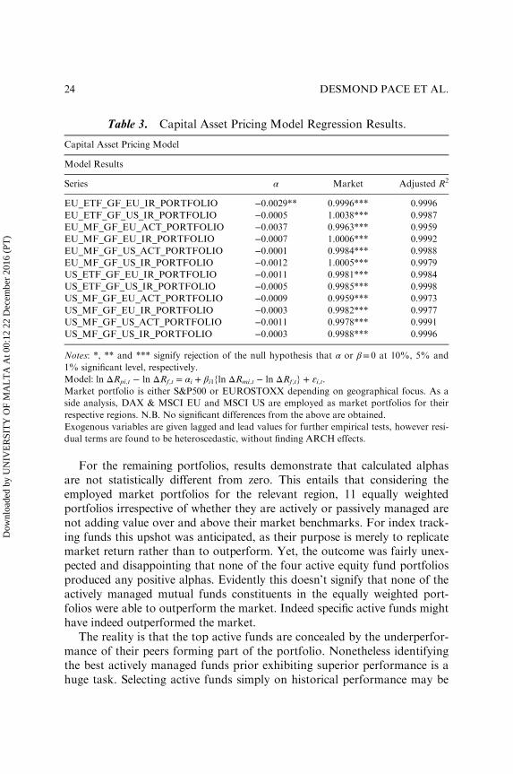
For the remaining portfolios, results demonstrate that calculated alphasare not statistically different from zero. This entails that considering theemployed market portfolios for the relevant region, 11 equally weightedportfolios irrespective of whether they are actively or passively managed arenot adding value over and above their market benchmarks. For index track-ing funds this upshot was anticipated, as their purpose is merely to replicatemarket return rather than to outperform. Yet, the outcome was fairly unex-pected and disappointing that none of the four active equity fund portfoliosproduced any positive alphas. Evidently this doesn’t signify that none of theactively managed mutual funds constituents in the equally weighted port-folios were able to outperform the market. Indeed specific active funds mighthave indeed outperformed the market.

The reality is that the top active funds are concealed by the underperfor-mance of their peers forming part of the portfolio. Nonetheless identifyingthe best actively managed funds prior exhibiting superior performance is ahuge task. Selecting active funds simply on historical performance may be

Table 3. Capital Asset Pricing Model Regression Results.

Capital Asset Pricing Model

Model Results

Series α Market Adjusted R2

EU_ETF_GF_EU_IR_PORTFOLIO −0.0029** 0.9996*** 0.9996

EU_ETF_GF_US_IR_PORTFOLIO −0.0005 1.0038*** 0.9987

EU_MF_GF_EU_ACT_PORTFOLIO −0.0037 0.9963*** 0.9959

EU_MF_GF_EU_IR_PORTFOLIO −0.0007 1.0006*** 0.9992

EU_MF_GF_US_ACT_PORTFOLIO −0.0001 0.9984*** 0.9988

EU_MF_GF_US_IR_PORTFOLIO −0.0012 1.0005*** 0.9979

US_ETF_GF_EU_IR_PORTFOLIO −0.0011 0.9981*** 0.9984

US_ETF_GF_US_IR_PORTFOLIO −0.0005 0.9985*** 0.9998

US_MF_GF_EU_ACT_PORTFOLIO −0.0009 0.9959*** 0.9973

US_MF_GF_EU_IR_PORTFOLIO −0.0003 0.9982*** 0.9977

US_MF_GF_US_ACT_PORTFOLIO −0.0011 0.9978*** 0.9991

US_MF_GF_US_IR_PORTFOLIO −0.0003 0.9988*** 0.9996

Notes: *, ** and *** signify rejection of the null hypothesis that α or β= 0 at 10%, 5% and

1% significant level, respectively.

Model: ln ΔRpi,t � ln ΔRf,t = αi + βi1{ln ΔRmi,t − ln ΔRf,t} + ɛi,t.Market portfolio is either S&P500 or EUROSTOXX depending on geographical focus. As a

side analysis, DAX & MSCI EU and MSCI US are employed as market portfolios for their

respective regions. N.B. No significant differences from the above are obtained.

Exogenous variables are given lagged and lead values for further empirical tests, however resi-

dual terms are found to be heteroscedastic, without finding ARCH effects.

24 DESMOND PACE ET AL.

Dow

nloa

ded

by U

NIV

ER

SIT

Y O

F M

AL

TA

At 0

0:12

22

Dec

embe

r 20

16 (

PT)

an expensive option and undeniably, mutual funds displaying an excellentpast performance don’t guarantee outperformance in the future. Indeed lit-erature suggests that the top performing funds in any one decade tend tobe completely different from the preceding and subsequent period(Greenblatt, 2011), indicating imprudence in choosing mutual funds basedon their past performance. This has a twofold effect, primarily in terms ofunderperformance but may also apparently ensue into higher fees reflectinghigher demand given the mutual fund popularity.

From a risk-adjusted return perspective in view of the 12 equallyweighted portfolios, there is practically no diversity between active and pas-sive management style for the studied decade. Put simply with the excep-tion of a class of European ETFs tracking European indices, an investorwill be indifferent when choosing between the two structures in the absenceof transaction costs. Nevertheless in reality friction costs play a crucial role

Table 4. Fama French Three-Factor Model Regression Results.

Three-Factor Model

Model Results

Series α Market SMB HML Adjusted

R2

EU_ETF_GF_EU_IR_PORTFOLIO −0.0030*** 0.9994*** −0.0007 −0.0004 0.9996

EU_ETF_GF_US_IR_PORTFOLIO −0.0003 1.0030*** −0.0008 −0.0017 0.9987

EU_MF_GF_EU_ACT_PORTFOLIO −0.0035 0.9957*** −0.0010 −0.001 0.9959

EU_MF_GF_EU_IR_PORTFOLIO −0.0007 1.0005*** −0.0004 −0.0001 0.9991

EU_MF_GF_US_ACT_PORTFOLIO −0.0002 0.9981*** −0.0003 −0.0007 0.9988

EU_MF_GF_US_IR_PORTFOLIO −0.0009 0.9998*** −0.0020 −0.0020 0.9979

US_ETF_GF_EU_IR_PORTFOLIO −0.0008 0.9988*** −0.0027** −0.0007 0.9985

US_ETF_GF_US_IR_PORTFOLIO −0.0001 0.9986*** −0.0027*** −0.0008 0.9998

US_MF_GF_EU_ACT_PORTFOLIO −0.0004 0.9971*** −0.0041*** −0.0012 0.9974

US_MF_GF_EU_IR_PORTFOLIO −0.0001 0.9993*** −0.0039*** −0.0013 0.9978

US_MF_GF_US_ACT_PORTFOLIO −0.0018 0.9985*** −0.0044*** −0.0024* 0.9992

US_MF_GF_US_IR_PORTFOLIO −0.0009 0.9989*** −0.0038*** −0.0011 0.9996

Notes: *, ** and *** signify rejection of the null hypothesis that α or β= 0 at 10%, 5% and 1%

significant level, respectively.

Model: ln ΔRpi,t � ln ΔRf,t = αi + βi1{ln ΔRmi,t − ln ΔRf,t} + βi2{SMBt} + βi3{HMLt}+ ɛi,t.Market portfolio is either S&P500 or EUROSTOXX depending on geographical focus. As a side

analysis, DAX & MSCI EU and MSCI US are employed as market portfolios for their respective

regions. N.B. No significant differences from the above are obtained.

Exogenous variables are given lagged and lead values for further empirical tests, however residual

terms are found to be heteroscedastic, without finding ARCH effects.

Fama French US research factors are employed for US equity portfolios and European research fac-

tors are applied for European stock portfolios. When applying US research factors for European

exposed equity portfolio funds and vice versa, weaker explanatory power is found.

25An Empirical Study on the US and European Mutual Funds and ETFs

Dow

nloa

ded

by U

NIV

ER

SIT

Y O

F M

AL

TA

At 0

0:12

22

Dec

embe

r 20

16 (

PT)

when selecting an investment structure particularly in instances where thefinancial instruments yield a similar cash flow or more importantly identicalrisk-adjusted returns. Another consideration which plays an essential roleand is understood to be higher for actively managed funds are agency costs.This indicates that in discretionary management active fund managers maynot always perform their duties in the best interests of investors. A classicscenario is where portfolio managers have incentives to take on more riskswhich may not be desirable from the investors’ point of view. Converselyfor passively managed structures, the actual management is usually muchmore clearly defined and the only hazard is the tracking error.

The revealed alphas emphasise a pivotal role for the cost factor andhence decisive in an investment decision. It is of general knowledge that thecost structure of passively managed funds is more favourable, since the soleobjective of the latter is to track an underlying index. Conversely activefunds engage their efforts in searching for mispriced securities, undertakinga more complex process and eventually more costly.

Table 5. Carhart Four-Factor Model Regression Results.

Four-Factor Model

Model Results

Series α Market SMB HML MOM Adjusted R2

EU_ETF_GF_EU_IR_PORTFOLIO −0.0029** 0.9994*** −0.0007 −0.0003 −0.0002 0.9996

EU_ETF_GF_US_IR_PORTFOLIO −0.0006 1.0041*** −0.0010 −0.0016 −0.0013 0.9987

EU_MF_GF_EU_ACT_PORTFOLIO −0.0041 0.9958*** −0.0010 −0.0004 −0.0007 0.9959

EU_MF_GF_EU_IR_PORTFOLIO −0.0007 1.0006*** −0.0004 −0.0002 −0.0001 0.9991

EU_MF_GF_US_ACT_PORTFOLIO −0.0000 0.9992*** −0.0007 −0.0009 −0.0050** 0.9988

EU_MF_GF_US_IR_PORTFOLIO −0.0011 1.0009*** −0.0022 −0.0018 −0.0006 0.9978

US_ETF_GF_EU_IR_PORTFOLIO −0.0014 0.9987*** −0.0026** −0.0000 −0.0008 0.9985

US_ETF_GF_US_IR_PORTFOLIO −0.0001 0.9986*** −0.0027*** −0.0007 −0.0013 0.9998

US_MF_GF_EU_ACT_PORTFOLIO −0.0016 0.9969*** −0.0040*** −0.0001 −0.0013* 0.9974

US_MF_GF_EU_IR_PORTFOLIO −0.0009 0.9992*** −0.0039*** −0.0002 −0.0013* 0.9979

US_MF_GF_US_ACT_PORTFOLIO −0.0012 0.9962*** −0.0044*** −0.0015 −0.0041** 0.9992

US_MF_GF_US_IR_PORTFOLIO −0.0007 0.9980*** −0.0037*** −0.0008 −0.0019 0.9996

Notes: *, ** and *** signify rejection of the null hypothesis that α or β= 0 at 10%, 5% and 1% significant level,

respectively.

Model: ln ΔRpi,t � ln ΔRf,t = αi + βi1{ln ΔRmi,t − ln ΔRf,t} + βi2{SMBt} + βi3{HMLt} + βi4{MOMt} + ɛi,t.Market portfolio is either S&P500 or EUROSTOXX depending on geographical focus. As a side analysis, DAX &

MSCI EU and MSCI US are employed as equity market portfolios for their respective regions. N.B. No significant

differences from the above are obtained.

Exogenous variables are given lagged and lead values for further empirical tests, however residual terms are found

to be heteroscedastic, without finding ARCH effects.

Fama French US research factors are employed for US equity portfolios and European research factors are applied

for European stock portfolios. When applying US research factors for European exposed equity portfolio funds and

vice versa, weaker explanatory power is found.

26 DESMOND PACE ET AL.

Dow

nloa

ded

by U

NIV

ER

SIT

Y O

F M

AL

TA

At 0

0:12

22

Dec

embe

r 20

16 (

PT)

Given the exposed results, for the typical investor who doesn’t seek regu-lar monitoring, but is more concerned about a longer term horizon andhence growth, it is advisable to opt for a low-cost passive equity fund orETF. However this is easier said than done, as there is a wide spectrum ofindex replication structures for investors to choose from namely rangingfrom cap size, style that is value, growth or blend, sector category, region,etc., and consequently a financial advisor is required for novice investors.For such investors who may also lack financial literacy, it is prudent to electpassive funds which track the general market such as the Standard & Poor’s500 and the EUROSTOXX, or may diversify further by creating a portfolioof passive funds. Passive structures can be chosen depending on the desiredregional exposure, sector and exposure to foreign exchange. Nonethelessinvestors can still be exposed to overseas markets without having a foreignexchange exposure, by choosing funds with the same currency denominationwhich are daily hedged, and hence not capturing currency risk.

Portfolios’ Characteristics Analysis

Examination of the equity fund portfolios’ degree of fluctuation as measuredby market risk depicts an ETF portfolio EU_ETF_GF_US_IR_PORTFOLIO,exhibiting the highest volatility in all three asset pricing models. Hence an indexreplication structure does not necessarily provide a lower standard deviation orinferior beta risk as this is dictated by the behaviour of the underlying bench-mark. Conversely US_MF_GF_EU_ACT_PORTFOLIO, an actively mana-ged mutual fund portfolio displayed the weakest shocks in both CAPM andThree-Factor Model, whilst another actively managed mutual fund portfolio,EU_MF_GF_EU_ACT_PORTFOLIO revealed the lowest market risk in theFour-Factor Model. In fact market betas for active fund portfolios, on averageare lower than their peers. Given regression results, active fund portfolios areless volatile than the employed market benchmarks which could imply thatwhilst active investors are charged higher fees due to identification of underva-lued and overvalued securities, fund managers may be conservative in the pro-cess of stock picking. Conversely it can be viewed that on average active mutualfunds provide more stability given smaller betas, and hence enhanced peace ofmind especially for active risk averse investors, even though this might meanhigher costs. The absence of statistically significant positive alphas could ensuefrom the lack of appetite revealed by active fund managers to detect bargains.The solitary fund portfolio exhibiting a statistically significant positive alpha,EU_ETF_GF_EU_IR_PORTFOLIO, is a relatively cautious index replication

27An Empirical Study on the US and European Mutual Funds and ETFs

Dow

nloa

ded

by U

NIV

ER

SIT

Y O

F M

AL

TA

At 0

0:12

22

Dec

embe

r 20

16 (

PT)

portfolio as illustrated by a beta below one. Another reason could be that fundmanagers try to spot opportunities, yet the identified undervalued or overva-lued equities could endure the mispricing in the long run and hence not return-ing to their intrinsic value, due to model risk.

Investigation of portfolios’ investment styles proves that US equity fundportfolios have a positive exposure to small caps, and the effect is evenstronger for actively managed mutual funds. Put simply, active portfoliomanagers may search for such exposure, since research authenticates thegeneral outperformance of small caps over large ones (Banz, 1981; Fama &French, 1993), however this effect was not statistically significantand thus not present in the case of European equity fund portfolios. Alsofor the HML risk factor, no particular preference or exposure amongvalue or growth stocks was revealed, except for a single portfolioUS_MF_GF_US_ACT_PORTFOLIO, which showed a statistically signifi-cant negative beta in the Three-Factor Model implying an overexposure togrowth equities. As for the momentum risk factor, three out of four activefund portfolios have a statistically significant exposure. More specificallytwo active fund portfolios, EU_MF_GF_US_ACT_PORTFOLIO andUS_MF_GF_US_ACT_PORTFOLIO pursue a momentum strategy, whilstanother actively managed fund portfolio, US_MF_GF_EU_ACT_PORTFOLIOemploys contrarian and reversal strategies. Lastly the adjusted R2 in allregressions for all the three asset pricing models is found to be relativelyhigh, signifying that on average the models are describing an adequate pro-portion of the variation in the equally weighted equity fund portfolios’returns implying adequately explained results.

Hybrid Equity Mutual Funds

The absence of positive alphas indicates that the nightmare for portfoliomanagers continues, as they consistently fail to beat market benchmarks.This downside can be straightforwardly resolved by switching to passivestyles by tracking market benchmarks, also benefiting investors owing tothe lower charges. Nonetheless if the majority of fund managers turn pas-sive, competition for information declines and fewer participants will try tooutperform the market, leading to market inefficiency. At this point, giventhe assumed existence of a trade-off between market efficiency and abnor-mal returns, arbitrage opportunities will become prevalent magnetising theattention of market participants. This will again attract fund managers toperform active management to benefit from such existing and potential

28 DESMOND PACE ET AL.

Dow

nloa

ded

by U

NIV

ER

SIT

Y O

F M

AL

TA

At 0

0:12

22

Dec

embe

r 20

16 (

PT)

opportunities. Theoretically it may be one explanation to Gruber (1996)mutual funds puzzle, apart from the mutual funds’ hard selling and inves-tors’ lack of financial literacy. However as portfolio managers switch backto active management, market efficiency increases again, thereby reducingthe likelihood of abnormal returns and presence of arbitrage.

Understandably investment managers and their fund structures may not beflexible due to a variety of friction costs and barriers halting them from a rapidswitch. Barriers for altering from passive to active and vice versa may includeregulatory constraints, legal costs, non-compliance of prospectus among otherchanging costs that arise in the process. Also funds may not wholly employ adiscretionary investment management policy and thus any transfer of clients’assets may require prior approval, leading to time lag hence defeating thescope of flexibility. Yet an equity fund can avoid these costs by straightawaystressing its intentions in the prospectus to operate as a hybrid, that is, alteringfrom passive to active style depending on changes in market efficiency. Such afund structure may not yield any benefits in consistently highly efficient mar-kets. Yet this fund structure may be valuable for less constantly efficient mar-kets such as emerging markets, where the flow of information may not beuniformly reflected in asset prices. Such vehicle should also promote a cost-effective fee structure including a cheaper expense ratio, given that it does notundertake active management on an ongoing basis.

Active Management Costs as a Subsidy for Market Efficiency

The dilemma remains whether active management provides any benefits atall. From a market structure point of view, active mutual funds are crucialfor keeping high levels of market efficiency. However from the investors’perspective given these results, the benefits sought are questionable espe-cially in the light of higher fees. In general, high levels of market efficiencyare positive for investors as financial instruments’ prices reflect all the avail-able information. But maintaining market efficiency doesn’t come auto-matic but rather the system creates incentives in inefficient markets forparticipants to exploit. Yet when markets are already highly efficient, it isnot clear as to why mutual funds persist in charging high fees when oppor-tunities are practically ‘inexistent’. One possible explanation could be due tomenu costs. Certainly the high fees paid by active investors help in preser-ving market efficiency and indirectly subsidise passive investors’ costs. Putsimply passive investors are the free riders of the fund industry profitingfrom enhanced market efficiency at lower costs due to an intrinsic cost

29An Empirical Study on the US and European Mutual Funds and ETFs

Dow

nloa

ded

by U

NIV

ER

SIT

Y O

F M

AL

TA

At 0

0:12

22

Dec

embe

r 20

16 (

PT)

charged by the ‘market system’ to active investors. Hence part of the feespaid by active investors rather for alpha creation may be deemed as a nat-ural cost imposed by the ‘market structure’ to maintain market efficiency bysupporting and encouraging fund managers to retain market efficiency.

This natural cost for keeping market efficiency is vital from the system’sperspective, yet still a cost for active investors as calculated alphas for activefund portfolios do not appear to compensate for this drawback. Nonethelessthe results confirm that although on average no positive alphas have beengenerated in the last decade, no statistically significant negative alphas wereproduced neither. This finding is important since it clearly indicates the hugeinfluence of the market benchmarks on the distinct equity fund portfolios, asexhibited by the highly statistically significant market beta coefficients proxy-ing market risk in the three asset pricing models. Put simply in booming mar-kets, funds generally enjoy good returns and vice-versa, except in cases wherean inverse strategy is employed. Hence active management for the typicalinvestor is deemed as a caveat emptor, as a passive instrument or index repli-cation structure will perform very well especially given its low cost composi-tion, also considering that the tracking error is well managed.

CONCLUSION

The study provides evidence that neither active nor passive managementstyle is superior in terms of risk-adjusted performance when analysingsolely NAVs for a 10-year timeframe. Nevertheless investors are instinc-tively informed of the higher expenses associated with actively managedmutual funds, such as initial fees which can range from 2% and overincluding higher annual expense ratios, amongst other possible costs.Investors shouldn’t overlook the heftier fees charged by mutual funds, asthese have a massive bearing on portfolio returns. Indeed an investor witha 100,000 worth of investment capital and a 20-year horizon seeking a US-Large Cap Growth equity fund is expected to lose 170,644 due to highercosts, if an actively managed mutual fund such as Morgan Stanley’s withan expense ratio of 1.69% is elected over a Charles Schwab ETF, whichhas a matching objective but is accessible at a hugely cheaper expense ratioof 0.07%. The assumptions for this calculation are a market expectedannual rate of return of 10%, ensuing into a cost-adjusted return rate of8.31% and 9.93% leading to a final balance of 493,595 and 664,239 for theactive and passive structures, respectively. Certainly this calculation is

30 DESMOND PACE ET AL.

Dow

nloa

ded

by U

NIV

ER

SIT

Y O

F M

AL

TA

At 0

0:12

22

Dec

embe

r 20

16 (

PT)

overlooking the initial fees for both cases, where for the actively managedmutual fund it is in the region of 5.75%, whereas for the ETF transactioncosts are equivalent to when purchasing a stock. Again the discrepancy issubstantial, yet this illustration shouldn’t be taken as a blue print as otheractive equity funds might be more cost efficient than demonstrated in thisspecimen and indeed anomalies do exist. For instance if an investor desiresexposure to the US Healthcare sector, iShares US Healthcare ETF is avail-able at an expense ratio of 0.45%, whereas Vanguard’s actively managedHealthcare mutual fund supplies an expense ratio of 0.34%. Using theaforementioned calculation, at a market expected annual rate of return of10%, cost-adjusted return rates are of 9.55% and 9.66% leading to a finalbalance of 619,794 and 632,361 for the ETF and active structure, respec-tively. This demonstrates that the active fund is cheaper than the corre-sponding ETF, and will indeed deliver an added value of 12,567 over itscompetitor. Yet if tax advantages of ETFs are considered in the equation,the balance will easily favour the ETF over the active mutual fund, espe-cially in the case of long horizon and high net worth investors.

This leads to resolve that it is prudent not to generalise about whetheractive or passive management is unquestionably superior to its peer and toanalyse on a case-by-case basis. Simultaneously investors are subliminallyinformed that on average passive vehicles are more cost-effective, whereasETFs provide higher tax advantages. Categorically decisive for investors isthe access to the cheapest available investment structure for their invest-ment objective, regardless of being an active mutual fund, passive mutualfund or index replication ETF.

LIMITATIONS AND RECOMMENDATIONS FOR

FUTURE RESEARCH

The primary shortcoming of this research is the employment of an equitybenchmark as opposed to a well-diversified market portfolio, which intheory (Roll, 1977) would have to encompass the entire asset universeincluding commodities, currencies, real estate, precious metals inter alia.This signifies that alpha generation and risk-adjusted returns are not com-puted on all available investments opportunities and that the true andactual returns are unobservable.

Secondly, the application of an equity benchmark implies that bothactive and passive equity funds are disadvantaged when evaluated with

31An Empirical Study on the US and European Mutual Funds and ETFs

Dow

nloa

ded

by U

NIV

ER

SIT

Y O

F M

AL

TA

At 0

0:12

22

Dec

embe

r 20

16 (

PT)

the former, as it is a purely theoretical concept. Put simply this comparisondoes not have a bearing on investors in practice, as it does not actuallyshow investors’ opportunity set and investment choices. The closest reallife structures to equity indices and thus more realistic benchmarks areindex replication structures such as index mutual funds and ETFs. This issince as opposed to an index mutual fund, pure theoretical equity bench-marks like the Standard & Poor’s 500 do not illustrate the expenses under-taken in replicating an underlying benchmark. The bottom line of thislimitation is that risk-adjusted returns and generated alphas for bothactive and passive equity funds will be lower than they actually are.Nonetheless utilising the aforesaid equity benchmarks for both active andpassive equity funds result in the identical yardstick without favouring amanagement style or investment vehicle over another.

Thirdly, the recently enhanced popularity and growth of ETFs signifieslack of historical data for these investment structures. Indeed adequatedata availability for ETFs can be traced back for a period of 10 years, withdata accessibility reducing exponentially when exceeding such timeframe.

Fourthly, the assessment of active and index replication vehicles via aportfolio approach ensues in findings for fund categories, but conceals out-comes for top performing and worst performing equity funds. Neverthelessas a side analysis, assessment of individual equity funds demonstratedundesirable OLS characteristics and therefore non robust results.

After analysing the empirical work of this study jointly with the presentliterature review relating to active and passive management, a list of newresearch ideas emerge. Principally, the majority of the research is only con-cerned with developed equity mutual funds and equity ETFs, with no refer-ence to any other asset classes and/or emerging/frontier markets. Thispresents a literature gap to analyse active and index replication equityfunds, predominantly ETFs, in emerging and frontier markets, primarilygiven the relative diverse levels of market efficiency. Additionally it presentsan opportunity to undertake a comparison between active and passivemanagement for other asset classes including bonds, commodities, mixedassets and real estate primarily REITs (Real Estate Investment Trusts).

NOTE

1. Twelve equally weighted portfolios require 12 CAPM regressions, 12 Three-Factor model regressions and 12 Four-Factor model regressions.

32 DESMOND PACE ET AL.

Dow

nloa

ded

by U

NIV

ER

SIT

Y O

F M

AL

TA

At 0

0:12

22

Dec

embe

r 20

16 (

PT)

REFERENCES

Aber, J. W., Li, D., & Can, L. (2009). Price volatility and tracking ability of ETFs. Journal of

Asset Management, 10, 210�221.

Agapova, A. (2009). Innovations in financial products: Conventional mutual index funds ver-

sus exchange traded funds. Journal of Financial Markets, 14, 323�343.

Andreu, L., Swinkels, L. A. P., & Tjong-A-Tjoe, L. (2012). Can exchange traded funds be

used to exploit country and industry momentum? Retrieved from http://ssrn.com/

abstract=1150972. Accessed on January 15, 2015.

Banz, R. W. (1981). The relationship between return and market value of common stocks.

Journal of Financial Economics, 9, 3�18.

Basu, S. (1977). Investment performance of common stocks in relation to their price-earnings

ratios: A test of efficient market hypothesis. Journal of Finance, 32(3), 663�682.

Bernstein, J. P. (2002). A primer on exchange-traded funds. Journal of Accountancy, 193(1),

38�41.

Black, F., Jensen, M. C., & Scholes, M. (1972). The capital asset pricing model: Some empiri-

cal tests. In M. Jensen (Ed.), Studies in the theory of capital markets (pp. 79�121).

New York, NY: Praeger Publishers.

Black, F., & Scholes, M. (1973). The pricing of options and corporate liabilities. Journal of

Political Economy, 81(3), 637�654.

Blake, C. R., Elton, E. J., & Gruber, M. J. (1993). The performance of bond mutual funds.

The Journal of Business, 66(3), 371�403.

Bogle, J. C. (1998). The implications of style analysis on mutual fund performance evaluation.

Keynote Speech.

Brooks, C. (2008). Introductory econometrics for finance (2nd ed.). Cambridge: Cambridge

University Press.

Campbell, J. Y. (1987). Stock returns and the term structure. Journal of Financial Economics,

18, 373�399.

Carhart, M. M. (1997). On persistence in mutual fund performance. The Journal of Finance,

52, 57�82.

Chen, N., Roll, R., & Ross, S. (1986). Economic forces and the stock market. Journal of

Business, 59(3), 383�403.

Dellva, W. L. (2001). Exchange-traded funds not for everyone. Journal of Financial Planning,

14, 110�124.

Elton, E. J., Gruber, M. J., Comer, G., & Li, K. (2002). Spiders: Where are the bugs? Journal

of Business, 75, 453�472.

Engle, R. F., & Sarkar, D. (2006). Premiums-discounts and exchange traded funds. Journal of

Derivatives, 13, 27�45.

Falzon, J., & Castillo, D. (2013). A VAR approach to the analysis of the relationship between

oil prices and industry equity returns. In J. Falzon (Ed.), Bank performance, risk and

securitization. Basingstoke: Palgrave Macmillan.

Fama, E. F. (1968). Risk, return and equilibrium: Some clarifying comments. Journal of

Finance, 23(1), 29�40.

Fama, E. F., & French, K. R. (1992). The cross-section of expected stock returns. The Journal

of Finance, 47(2), 427.

Fama, E. F., & French, K. R. (1993). Common risk factors in the returns on stocks and bonds.

Journal of Financial Economics, 33, 3�56.

33An Empirical Study on the US and European Mutual Funds and ETFs

Dow

nloa

ded

by U

NIV

ER

SIT

Y O

F M

AL

TA

At 0

0:12

22

Dec

embe

r 20

16 (

PT)

Fama, E. F., & Macbeth, J. D. (1973). Risk, return, and equilibrium: Empirical tests. The

Journal of Political Economy, 81(3), 607�636.

Frino, A., & Gallagher, D. R. (2001). Tracking S&P 500 index funds. Journal of Portfolio

Management, 28(1), 44�55.

Gastineau, G. L. (2004). The benchmark index ETF performance problem. Journal of

Portfolio Management, 30, 96�103.

Greenblatt, J. (2011). The big secret for the small investor (1st ed.). New York, NY: Crown

Publishing Group.

Grossman, S. J., & Stiglitz, J. E. (1980, June). On the impossibility of informationally efficient

markets. The American Economic Review, 70(3), 393�408.

Gruber, M. J. (1996). Another puzzle: The growth in actively managed mutual funds. Journal

of Finance, 51(3), 783�810.

Guedj, I., & Huang, J. C. (2008). Are ETFs replacing index mutual funds? Retrieved from

http://ssrn.com/abstract=1108728. Accessed on January 15, 2015.

Harper, J. T., Madura, J., & Schnusenberg, O. (2006). Performance comparison between

exchange-traded funds and closed-end country funds. International Financial Markets,

Institutions & Money, 16, 104�122.

Jagannathan, R., & Wang, Z. (1996). The conditional CAPM and the cross-section of expected

returns. Journal of Finance, 51(1), 3�53.

Jegadeesh, N., & Titman, S. (1993, March). Returns to buying winners and selling losers:

Implications for stock market efficiency. Journal of Finance, 48(1), 65�91.

Jensen, M. C. (1968). The performance of mutual funds in the period 1945�1964. Journal of

Finance, 23, 389�416.

Johnson, W. F. (2009). Tracking errors of exchange traded funds. Journal of Asset

Management, 10, 253�262.

Kostovetsky, L. (2003). Index mutual funds and exchange-traded funds. Journal of Portfolio

Management, 29, 80�93.

Kuo, T. W., & Mateus, C. (2006). The performance and persistence of exchange-traded funds:

Evidence for iShares MSCI country-specific ETFs. Paper presented at 2007 FMA

Annual Meeting, Orlando, FL, USA.

Lintner, J. (1965). The valuation of risk assets and the selection of risky investments in stock

portfolios and capital budgets. Review of Economics and Statistics, 47(1), 13�37.

Malkiel, B. G. (1995). Returns from investing in equity mutual funds 1971 to 1991. Journal of

Finance, 50(2), 549�572.

Markowitz, H. M. (1952a). Portfolio selection. The Journal of Finance, 7(1), 77�91.

Markowitz, H. M. (1952b). The utility of wealth. The Journal of Political Economy, 60(2),

151�158.

Merton, R. C. (1973). An intertemporal capital asset pricing model. Econometrica, 41,

867�887.

Minor, D. B. (2001). Beware of index fund fundamentalists. The Journal of Portfolio

Management, 27(4), 45�50.

Mossin, J. (1966). Equilibrium in a capital asset market. Econometrica, 34(4), 768�783.

Poterba, J. M., & Shoven, J. B. (2002). Exchange-traded funds: A new investment option for

taxable investors. American Economic Review, 92, 422�427.

Roll, R. (1977). A critique of the asset pricing theory’s tests part I: On past and potential testa-

bility of the theory. Journal of Financial Economics, 4(2), 129�176.

34 DESMOND PACE ET AL.

Dow

nloa

ded

by U

NIV

ER

SIT

Y O

F M

AL

TA

At 0

0:12

22

Dec

embe

r 20

16 (

PT)

Rompotis, G. G. (2006). Evaluating the performance and the trading characteristics of

iShares. Retrieved from http://ssrn.com/abstract=946732. Accessed on January 15,

2015.

Rompotis, G. G. (2007). Evaluating the seasonality and persistence of ETFs performance and

volatility: Implications for profitable investing. SSRN. Retrieved from http://ssrn.com/

abstract=1022876. Accessed on January 15, 2015.

Rompotis, G. G. (2008). An empirical comparing investigation of exchange traded funds and

index funds performance. European Journal of Economics, Finance and Administrative

Sciences, 13, 7�17.

Rompotis, G. G. (2009). Active vs. passive management: New evidence from exchange traded

funds. Retrieved from http://ssrn.com/abstract=1337708Ross, S. (1976). The arbitrage theory of capital asset pricing. Journal of Economic Theory,

13(3), 341�360.

Sharpe, W. F. (1964). Capital asset prices � A theory of market equilibrium under conditions

of risk. Journal of Finance, 19(3), 425�442.

Sharpe, W. F. (1966). Mutual fund performance. Journal of Business, 39(S1), 119�138.

Sharpe, W. F. (1991). The arithmetic of active management. The Financial Analysts’ Journal,

47(1), 7�9.

Svetina, M., & Wahal, S. (2008). Exchange traded funds: Performance and competition.

Retrieved from http://ssrn.com/abstract=1303643. Accessed on January 10, 2015.

S&P Indices. (2013). (SPIVA®) scorecard � S&P Dow Jones indices. Retrieved from https://

www.google.com.mt/url?url=https://us.spindices.com/documents/spiva/spiva-us-year-

end-2013.pdf%3Fforce_download%3Dtrue&rct=j&frm=1&q=&esrc=s&sa=U&ei=ZaU_VJWdMMXYywP1ioDgCQ&ved=0CBgQFjAB&usg=AFQjCNFZwe_JtuCcrilI

SNK8ORW4czNhOQ. Accessed on January 10, 2015.

S&P Indices. (2014). (SPIVA®) scorecard � S&P Dow Jones indices. Retrieved from http://

www.spindices.com/documents/spiva/spiva-us-mid-year-2014.pdf. Accessed on January

10, 2015.

Treynor, J. L. (1961). Market value, time, and risk. Unpublished manuscript. A final version

was published in 1999. In R. A. Korajczyk (Ed.), Asset pricing and portfolio perfor-

mance: Models, strategy and performance metrics (pp. 15�22). London: Risk Books.

Treynor, J. L. (1965). How to rate management of investment funds. Harvard Business Review,

43, 63�75.

Whitelaw, R. F. (1994). Time variations and covariations in the expectation and volatility of

stock market returns. Journal of Finance, 49, 515�541.

Zhang, C. Y., & Jacobsen, B. (2014). The Halloween indicator, ‘Sell in May and go Away’:

An even bigger puzzle. Retrieved from http://ssrn.com/abstract=2154873. Accessed on

January 10, 2015.

35An Empirical Study on the US and European Mutual Funds and ETFs

Dow

nloa

ded

by U

NIV

ER

SIT

Y O

F M

AL

TA

At 0

0:12

22

Dec

embe

r 20

16 (

PT)